Commercial Demand Module of the National Energy Modeling System: Model Documentation 2013 · 2013-11-05 · Commercial Demand Module of the National Energy Modeling System: Model

Commercial Demand Module of the National Energy Modeling System: Model Documentation 2013

November 2013

Independent Statistics & Analysis

www.eia.gov

U.S. Department of Energy

Washington, DC 20585

U.S. Energy Information Administration | Commercial Demand Module of the National Energy Modeling System: Model Documentation 2013 i

This report was prepared by the U.S. Energy Information Administration (EIA), the statistical and analytical agency within the U.S. Department of Energy. By law, EIA’s data, analyses, and forecasts are independent of approval by any other officer or employee of the United States Government. The views in this report therefore should not be construed as representing those of the Department of Energy or other Federal agencies.

November 2013

U.S. Energy Information Administration | Commercial Demand Module of the National Energy Modeling System: Model Documentation 2013 ii

Contents Update Information ...................................................................................................................................... 1

1. Introduction ............................................................................................................................................. 2

Purpose of the report .............................................................................................................................. 2

Model summary ....................................................................................................................................... 2

Model archival citation ............................................................................................................................ 2

Organization of this report ...................................................................................................................... 2

2. Model Purpose ......................................................................................................................................... 4

Model objectives ..................................................................................................................................... 4

Model input and output .......................................................................................................................... 5

Inputs................................................................................................................................................. 5

Outputs .............................................................................................................................................. 8

Variable classification ........................................................................................................................ 8

Relationship of the Commercial Module to other NEMS Modules ....................................................... 10

3. Model Rationale ..................................................................................................................................... 12

Theoretical approach ............................................................................................................................. 12

Fundamental assumptions .................................................................................................................... 13

Floorspace Submodule .................................................................................................................... 13

Service Demand Submodule ........................................................................................................... 13

Technology Choice Submodule ....................................................................................................... 13

4. Model Structure ..................................................................................................................................... 15

Structural overview................................................................................................................................ 15

Commercial building floorspace projection .................................................................................... 15

Service demand projection ............................................................................................................. 16

Decision to generate or purchase electricity .................................................................................. 17

Equipment choice to meet service needs ....................................................................................... 17

Energy consumption ....................................................................................................................... 18

Flow diagrams ........................................................................................................................................ 19

Key computations and equations .......................................................................................................... 29

Floorspace Submodule .................................................................................................................... 29

Service Demand Submodule ........................................................................................................... 35

November 2013

U.S. Energy Information Administration | Commercial Demand Module of the National Energy Modeling System: Model Documentation 2013 iii

Distributed Generation and Combined Heat and Power (CHP) Submodule ................................... 40

Technology Choice Submodule ....................................................................................................... 44

End-Use Consumption Submodule ................................................................................................. 56

Benchmarking Submodule .............................................................................................................. 59

Appendix A. Input Data and Variable Descriptions .................................................................................... 61

Introduction ........................................................................................................................................... 61

NEMS Commercial Module inputs and outputs .................................................................................... 61

Profiles of input data ........................................................................................................................... 109

Appendix B. Mathematical Description ................................................................................................... 158

Introduction ......................................................................................................................................... 158

Floorspace equations ........................................................................................................................... 160

Service demand equations .................................................................................................................. 161

Technology choice equations .............................................................................................................. 170

End-use fuel consumption equations .................................................................................................. 182

Benchmarking equations ..................................................................................................................... 188

Distributed generation equations ....................................................................................................... 193

Appendix C. References ............................................................................................................................ 206

Introduction ......................................................................................................................................... 206

References ........................................................................................................................................... 206

Appendix D. Model Abstract .................................................................................................................... 211

Introduction ......................................................................................................................................... 211

Appendix E. Data Quality .......................................................................................................................... 216

Introduction ......................................................................................................................................... 216

Quality of input data ............................................................................................................................ 216

Commercial Buildings Energy Consumption Survey (CBECS) ........................................................ 216

CBECS implementation .................................................................................................................. 216

Target population .......................................................................................................................... 217

Response rates .............................................................................................................................. 217

Data collection .............................................................................................................................. 217

The interview process ................................................................................................................... 217

Data quality verification ................................................................................................................ 218

Energy use intensity (EUI) data source ......................................................................................... 218

November 2013

U.S. Energy Information Administration | Commercial Demand Module of the National Energy Modeling System: Model Documentation 2013 iv

Technology characterization data sources .................................................................................... 218

Historical energy consumption data: State Energy Data System (SEDS) ..................................... 218

User-defined parameters .................................................................................................................... 219

Risk-adjusted time preference premium distribution .................................................................. 219

Behavior rule proportions: supporting documentation ..................................................................... 223

References ........................................................................................................................................... 224

November 2013

U.S. Energy Information Administration | Commercial Demand Module of the National Energy Modeling System: Model Documentation 2013 v

Tables Table 1. Categorization of Key variables ....................................................................................................... 9 Table 2. Subscripts for Commercial Module variables ............................................................................... 10 Table 3. Energy consumption calculation example .................................................................................... 18 Table 4. Floorspace survival parameters .................................................................................................... 33 Table 5. Miscellaneous electricity use categories ....................................................................................... 38 Table 6. Distributed generation technology learning function parameters ............................................... 44 Table 7. Array of technology choices and consumer behaviors ................................................................. 47 Table 8. 2003 Floorspace ownership and occupancy ................................................................................. 49 Table 9. Consolidating service demand segments ...................................................................................... 53

Table A-1. NEMS Commercial Module inputs and outputs ....................................................................... 61 Table A.2. Miscellaneous electricity use category equation coefficients ................................................. 135 Table A-3. Range of demand elasticity from the literature ...................................................................... 142

Table E-1. Consumer risk-adjusted time preference premium distribution, 2014-2040 ......................... 221 Table E-2. Commercial customer payback period (PEPCO) ..................................................................... 222 Table E-3. Commercial consumer payback requirement distributions .................................................... 222 Table E-4. Floorspace ownership and occupancy patterns ...................................................................... 223

November 2013

U.S. Energy Information Administration | Commercial Demand Module of the National Energy Modeling System: Model Documentation 2013 vi

Figures Figure 1. Commercial Demand Module's Relationship to Other NEMS Modules ...................................... 11 Figure 2. Commercial Module structure & fundamental process flow ...................................................... 20 Figure 3. COMM calculation process flow .................................................................................................. 21 Figure 4. COMFloorspace calculation process flow .................................................................................... 22 Figure 5. COMServiceDemand calculation process flow ............................................................................ 24 Figure 6. CDistGen calculation process flow ............................................................................................... 25 Figure 7. COMTechnologyChoice calculation process flow ........................................................................ 26 Figure 8. COMConsumption calculation process flow ................................................................................ 27 Figure 9. COMBenchmarking calculation process flow .............................................................................. 28 Figure 10. Floorspace survival function sensitivity to median building lifetimes ....................................... 31 Figure 11. Alternative gamma assumptions and results............................................................................. 32 Figure 12. Distributed generation technology penetration rate curves for new construction for payback times ........................................................................................................................................................... 43

November 2013

U.S. Energy Information Administration | Commercial Demand Module of the National Energy Modeling System: Model Documentation 2013 1

Update Information This edition of the Commercial Demand Module of the National Energy Modeling System: Model Documentation 2013 reflects changes made to the module over the past year for the Annual Energy Outlook 2013. These changes include:

• Updating current and projected cost and performance assumptions for lighting, ventilation, and refrigeration technologies

• Increasing the number of allowed technology vintages in the KTEK input file to accommodate the expanded modeling of solid-state lighting

• Reevaluating long-term weather trends, shifting to a 30-year linear trend • Increasing potential adoption of solar photovoltaic capacity in new construction • Increasing program-based exogenous distributed generation penetration between 2011 and

2016 • Updating data center energy consumption

November 2013


1. Introduction

Purpose of the report This report documents the objectives, analytical approach and development of the National Energy Modeling System (NEMS) Commercial Demand Module (CDM, Commercial Module, or module). The report catalogues and describes the model assumptions, computational methodology, parameter estimation techniques, model source code, and outputs generated through the use of the module.

This document serves three purposes. First, it is a reference document providing a detailed description for model analysts, users, and the public. Second, this report meets the legal requirement of the U.S. Energy Information Administration (EIA) to provide adequate documentation in support of its models (Public Law 93-275, section 57.b.1). Third, it facilitates continuity in model development by providing documentation from which energy analysts can undertake model enhancements, data updates, and parameter refinements as future projects.

Model summary The NEMS Commercial Demand Module is a simulation tool based upon economic and engineering relationships that models commercial sector energy demands at the Census division level of detail for eleven distinct categories of commercial buildings. Commercial equipment selections are performed for the major fuels of electricity, natural gas, and distillate fuel, for the major services of space heating, space cooling, water heating, ventilation, cooking, refrigeration, and lighting. The market segment level of detail is modeled using a constrained life-cycle cost minimization algorithm that considers commercial sector consumer behavior and risk-adjusted time preference premiums. The algorithm also models demand for minor fuels (residual oil, liquefied petroleum gas, steam coal, motor gasoline, and kerosene), renewable fuel sources (wood, municipal solid waste, solar energy, and wind), and the minor services of personal computers, other office equipment, and “other” or miscellaneous end-use loads (MELs) in less detail than the major fuels and services. Commercial decisions regarding the use of distributed generation (DG) and combined heat and power (CHP) technologies are performed using an endogenous cash-flow algorithm. Numerous specialized considerations are incorporated, including the effects of changing building shell efficiencies and consumption to provide district energy services.

As a component of the NEMS integrated projection tool, the Commercial Module generates projections of commercial sector energy demand. The model facilitates policy analysis of energy markets, technological development, environmental issues, and regulatory development as they impact commercial sector energy demand.

Model archival citation This documentation refers to the NEMS Commercial Demand Module as archived for the Annual Energy Outlook 2013 (AEO2013).

Organization of this report Chapter 2 of this report discusses the purpose of the model, detailing its objectives, primary input and output quantities, and the relationship of the Commercial Module to the other modules of the NEMS system. Chapter 3 of the report describes the rationale behind the model design, providing insights into

November 2013


further assumptions utilized in the model development process to this point. Chapter 4 details the model structure, using graphics and text to illustrate model flows and key computations.

The Appendices to this report provide supporting documentation for the input data and parameter files. Appendix A lists and defines the input data used to generate parameter estimates and endogenous projections, along with the parameter estimates and the outputs of most relevance to the NEMS system and the model evaluation process. A table referencing the equation(s) in which each variable appears is also provided in Appendix A. Appendix B contains a mathematical description of the computational algorithms, including the complete set of model equations and variable transformations. Appendix C is a bibliography of reference materials used in the development process. Appendix D provides the model abstract, and Appendix E discusses data quality and estimation methods. Other analyses discussing alternate assumptions, sensitivities, and uncertainties in projections developed using the NEMS Commercial Demand Module are available at EIA’s website.1

1See http://www.eia.gov/analysis/reports.cfm; search by “commercial.”

http://www.eia.gov/analysis/reports.cfm

November 2013


2. Model Purpose

Model objectives The NEMS Commercial Demand Module serves three objectives. First, it develops projections of commercial sector energy demand, currently through 2040,2 as a component of the NEMS integrated projection system. The resulting projections are incorporated into the Annual Energy Outlook, published annually by EIA. Second, it is used as a policy analysis tool to assess the impacts on commercial sector energy consumption of changes in energy markets, building and equipment technologies, environmental considerations and regulatory initiatives. Third, as an integral component of the NEMS system, it provides inputs to the Electricity Market Module (EMM), Coal Market Module (CMM), Natural Gas Transmission and Distribution Module (NGTDM), and Liquid Fuels Market Module (LFMM) of NEMS, contributing to the calculation of the overall energy supply and demand balance of the U.S. energy system.

The CDM projects commercial sector energy demands in five sequential steps. These steps produce projections of new and surviving commercial building floorspace, demands for energy-consuming services in those buildings, generation of electricity by distributed generation technologies, technology choices to meet the end-use service demands, and consumption of electricity, natural gas, and distillate oil by the equipment chosen.3 These projections are based on energy prices and macroeconomic variables from the NEMS system, combined with external data sources.

Projected commercial sector fuel demands generated by the Commercial Demand Module are used by the NEMS system in the calculation of the supply and demand equilibrium for individual fuels. In addition, the NEMS supply modules referenced previously use the commercial sector outputs in conjunction with other projected sectoral demands to determine the patterns of consumption and the resulting amounts and prices of energy delivered to the commercial sector.

Of equal importance, the NEMS Commercial Demand Module is relevant to the analysis of current and proposed legislation, private sector initiatives and technological developments. The flexible model design provides a policy analysis tool able to accommodate a wide range of scenario developments. Both the input file structure and the model source code have been specially developed to facilitate “what if” or scenario analyses of energy markets, technology characterizations, market initiatives, environmental concerns, and regulatory policies such as demand-side management (DSM) programs. Examples of specific policy analyses that can be addressed using this model include assessing the potential impacts of:

2The base year for the Commercial Module is currently 2003, corresponding to the last available energy consumption survey of commercial buildings. Dynamic projections dependent on feedback from the rest of NEMS are made for the years 2004 through 2040. Sector level consumption results reported for 1990 through 2010 are benchmarked to historical estimates from EIA’s State Energy Data System and Annual Energy Review. 3The End-Use Consumption Module accounts for commercial sector consumption of five minor fuels. These fuels do not account for enough commercial sector consumption to justify modeling at the same level of detail as the three major fuels (distillate fuel oil, natural gas, and electricity). The five minor fuels are residual fuel oil, liquefied petroleum gas (LPG), coal, motor gasoline and kerosene.

November 2013


• New end-use technologies (for example, solid-state lighting or ground-source heat pumps) • New energy supply technologies (for example, solar thermal heating or fuel cells) • Federal, state and local government policies, including:

- changes in fuel prices due to tax policies - changes in building shell or equipment energy efficiency standards - financial incentives for energy efficiency or renewable energy investments - information programs - environmental standards

• Utility demand-side management (DSM) programs4

Model input and output

Inputs The primary inputs to the Commercial Demand Module include fuel prices, commercial building floorspace growth, interest rates, and technology cost and performance parameters.5 The technology characteristics used by the model for distributed generation technologies are included in the summary of major inputs that follows. Additional detail on model inputs is provided in Appendix A.

Inputs to Floorspace Submodule • Existing distribution of commercial building floorspace stock in 2003 • Median construction year of existing commercial buildings by type, vintage, and location • Building survival parameters • Commercial building floorspace growth

Inputs to Service Demand Submodule • Energy use intensities (EUIs) in 2003 • Commercial technology characterizations

- market share of equipment existing in 2003 - equipment efficiency - building restrictions - service provided - fuel used

• Building shell efficiency load factors (heating and cooling) for new floorspace • Building shell efficiency improvement through 2040 for existing and new floorspace • Market penetration projections for office equipment and miscellaneous end-use loads (MELs)

categories • Steam EUIs to provide district energy services in 2003

4A recent example of the use of the NEMS Commercial Sector Module in policy analyses can be found on EIA’s website at http://www.eia.gov/todayinenergy/detail.cfm?id=11051. 5End-use technology characteristics are based on reports completed for EIA by Navigant Consulting, Inc. See the detailed description of model inputs in Appendix A for full citation.

http://www.eia.gov/todayinenergy/detail.cfm?id=11051

November 2013


• Efficiencies of district energy systems in 2003 • Fuel shares of district energy service steam production in 2003 • Short-run price elasticities of service demand • Historical and projected heating and cooling degree days • Differences in serviced floorspace proportions between existing and new floorspace

Inputs to Distributed Generation/CHP Submodule • DG and CHP technology characteristics

- fuel used - first and last year of availability for purchase of system - generation capacity - capital cost per kilowatt of capacity - installation cost per kilowatt of capacity - operating and maintenance cost per kilowatt of capacity - inverter replacement cost per kilowatt of capacity (solar photovoltaic and wind systems) - inverter replacement interval (solar photovoltaic and wind systems) - equipment life - tax life and depreciation method - available federal tax credits - generation and thermal heat recovery efficiency - annual operating hours - penetration function parameters - grid interconnection limitation parameters - learning function parameters - capital cost adjustment parameters for peak capacity scale adjustments - renewable portfolio standard credit parameters

• Financing parameters • Building-size category characteristics within building type

- average annual electricity use - average building size in square feet - share of floorspace

• Niche market scaling and price variables

- solar insolation - average wind speed - electricity rates relative to Census division average - natural gas rates relative to Census division average - roof area per unit of floorspace area

November 2013


• Program-driven market penetration projections for distributed generation technologies • Historical CHP generation of electricity data

Inputs to Technology Choice Submodule • Consumer behavior rule segments by building type, service and decision type

- shares of consumers choosing from all technologies, from those using the same fuel, and

from different versions of the same technology

• 10-year Treasury note rate • Consumer risk-adjusted time preference premium segments • Price elasticity of hurdle (implicit discount) rates • Minor service efficiency improvement projections • Building end-use service capacity utilization factors • Commercial technology characterizations

- first and last year of availability for purchase of system - market shares of equipment existing in 2003 - installed capital cost per unit of service demand - operating and maintenance cost per unit of service demand - equipment efficiency - removal/disposal cost factors - building restrictions - service provided - fuel used - expected equipment lifetimes - cost trend parameters - quality factor (lighting only)

• Expected fuel prices

Inputs to End-Use Fuel Consumption Submodule • Short-Term Energy Outlook (STEO) consumption projections • Annual Energy Review (AER) consumption information • State Energy Data System (SEDS) consumption information • Components of SEDS data attributable to other sectors • Minor fuel regression parameters

November 2013


Outputs The primary output of the Commercial Demand Module is projected commercial sector energy consumption by fuel type, end use, building type, Census division, and year. The module also provides annual projections of the following:

• Construction of new commercial floorspace by building type and Census division • Surviving commercial floorspace by building type and Census division • Equipment market shares by technology, end use, fuel, building type, and Census division • Distributed generation and CHP generation of electricity • Quantities of fuel consumed for DG and CHP • Consumption of fuels to provide district energy services • Non-building consumption of fuels in the commercial sector • Average efficiency of equipment mix by end use and fuel type

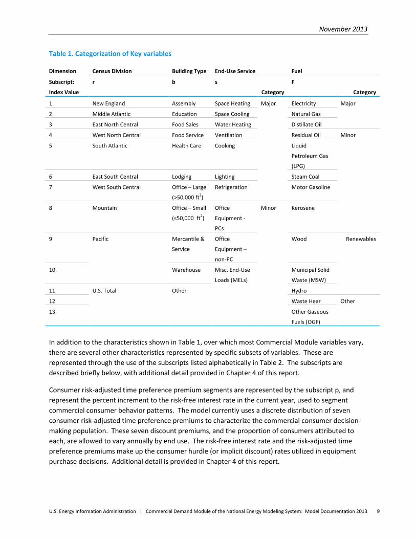
Variable classification The NEMS demand modules exchange information with the supply modules at the Census division level of detail spatially, and average annual level temporally. Information exchanged between the Commercial Demand Module and the Electricity Market Module is also required at the end-use service level of detail. The input data available from EIA’s Commercial Buildings Energy Consumption Survey (CBECS), which forms an important element of the statistical basis for the Commercial Demand Module, and other sources are designed to be statistically significant at various levels (some of which are above the Census division level). Commercial Demand Module variables are resolved at a relatively fine level of detail in order to capture heterogeneous effects that manifest themselves at a high level of aggregation, yet which originate from variations at a disaggregate level. The characteristics represented by key variables are presented in Table 1, which also shows the notation generally used for each characteristic in this report:

November 2013


Table 1. Categorization of Key variables

In addition to the characteristics shown in Table 1, over which most Commercial Module variables vary, there are several other characteristics represented by specific subsets of variables. These are represented through the use of the subscripts listed alphabetically in Table 2. The subscripts are described briefly below, with additional detail provided in Chapter 4 of this report.

Consumer risk-adjusted time preference premium segments are represented by the subscript p, and represent the percent increment to the risk-free interest rate in the current year, used to segment commercial consumer behavior patterns. The model currently uses a discrete distribution of seven consumer risk-adjusted time preference premiums to characterize the commercial consumer decision-making population. These seven discount premiums, and the proportion of consumers attributed to each, are allowed to vary annually by end use. The risk-free interest rate and the risk-adjusted time preference premiums make up the consumer hurdle (or implicit discount) rates utilized in equipment purchase decisions. Additional detail is provided in Chapter 4 of this report.

Dimension Census Division Building Type End-Use Service Fuel

Subscript: r b s F

Index Value Category Category

1 New England Assembly Space Heating Major Electricity Major

2 Middle Atlantic Education Space Cooling Natural Gas

3 East North Central Food Sales Water Heating Distillate Oil

4 West North Central Food Service Ventilation Residual Oil Minor

5 South Atlantic Health Care Cooking Liquid

Petroleum Gas

(LPG)

6 East South Central Lodging Lighting Steam Coal

7 West South Central Office – Large

(>50,000 ft2)

Refrigeration Motor Gasoline

8 Mountain Office – Small

(≤50,000 ft2)

Office

Equipment -

PCs

Minor Kerosene

9 Pacific Mercantile &

Service

Office

Equipment –

non-PC

Wood Renewables

10 Warehouse Misc. End-Use

Loads (MELs)

Municipal Solid

Waste (MSW)

11 U.S. Total Other Hydro

12 Waste Hear Other

13 Other Gaseous

Fuels (OGF)

November 2013


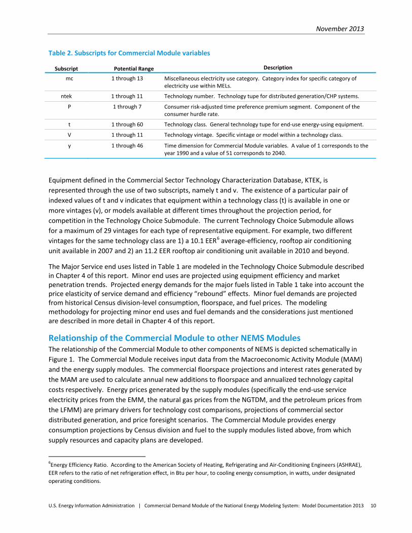
Table 2. Subscripts for Commercial Module variables

Equipment defined in the Commercial Sector Technology Characterization Database, KTEK, is represented through the use of two subscripts, namely t and v. The existence of a particular pair of indexed values of t and v indicates that equipment within a technology class (t) is available in one or more vintages (v), or models available at different times throughout the projection period, for competition in the Technology Choice Submodule. The current Technology Choice Submodule allows for a maximum of 29 vintages for each type of representative equipment. For example, two different vintages for the same technology class are 1) a 10.1 EER6 average-efficiency, rooftop air conditioning unit available in 2007 and 2) an 11.2 EER rooftop air conditioning unit available in 2010 and beyond.

The Major Service end uses listed in Table 1 are modeled in the Technology Choice Submodule described in Chapter 4 of this report. Minor end uses are projected using equipment efficiency and market penetration trends. Projected energy demands for the major fuels listed in Table 1 take into account the price elasticity of service demand and efficiency “rebound” effects. Minor fuel demands are projected from historical Census division-level consumption, floorspace, and fuel prices. The modeling methodology for projecting minor end uses and fuel demands and the considerations just mentioned are described in more detail in Chapter 4 of this report.

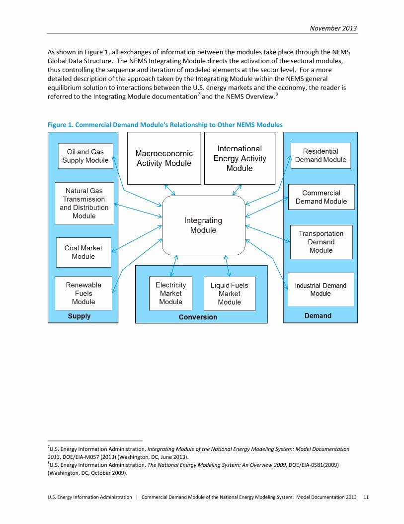
Relationship of the Commercial Module to other NEMS Modules The relationship of the Commercial Module to other components of NEMS is depicted schematically in Figure 1. The Commercial Module receives input data from the Macroeconomic Activity Module (MAM) and the energy supply modules. The commercial floorspace projections and interest rates generated by the MAM are used to calculate annual new additions to floorspace and annualized technology capital costs respectively. Energy prices generated by the supply modules (specifically the end-use service electricity prices from the EMM, the natural gas prices from the NGTDM, and the petroleum prices from the LFMM) are primary drivers for technology cost comparisons, projections of commercial sector distributed generation, and price foresight scenarios. The Commercial Module provides energy consumption projections by Census division and fuel to the supply modules listed above, from which supply resources and capacity plans are developed.

6Energy Efficiency Ratio. According to the American Society of Heating, Refrigerating and Air-Conditioning Engineers (ASHRAE), EER refers to the ratio of net refrigeration effect, in Btu per hour, to cooling energy consumption, in watts, under designated operating conditions.

Subscript Potential Range Description

mc 1 through 13 Miscellaneous electricity use category. Category index for specific category of electricity use within MELs.

ntek 1 through 11 Technology number. Technology tupe for distributed generation/CHP systems.

P 1 through 7 Consumer risk-adjusted time preference premium segment. Component of the consumer hurdle rate.

t 1 through 60 Technology class. General technology tupe for end-use energy-using equipment.

V 1 through 11 Technology vintage. Specific vintage or model within a technology class.

y 1 through 46 Time dimension for Commercial Module variables. A value of 1 corresponds to the year 1990 and a value of 51 corresponds to 2040.

November 2013


As shown in Figure 1, all exchanges of information between the modules take place through the NEMS Global Data Structure. The NEMS Integrating Module directs the activation of the sectoral modules, thus controlling the sequence and iteration of modeled elements at the sector level. For a more detailed description of the approach taken by the Integrating Module within the NEMS general equilibrium solution to interactions between the U.S. energy markets and the economy, the reader is referred to the Integrating Module documentation7 and the NEMS Overview.8

Figure 1. Commercial Demand Module's Relationship to Other NEMS Modules

7U.S. Energy Information Administration, Integrating Module of the National Energy Modeling System: Model Documentation 2013, DOE/EIA-M057 (2013) (Washington, DC, June 2013). 8U.S. Energy Information Administration, The National Energy Modeling System: An Overview 2009, DOE/EIA-0581(2009) (Washington, DC, October 2009).

November 2013


3. Model Rationale

Theoretical approach The Commercial Module utilizes a simulation approach to project energy demands in commercial buildings. The specific approach of the Commercial Module involves explicit economic and engineering-based analysis of the building energy end uses of space heating, space cooling, water heating, ventilation, cooking, lighting, refrigeration, office equipment, and miscellaneous end-use loads (MELs). These end uses are modeled for eleven distinct categories of commercial buildings at the Census division level of detail.

The model is a sequentially structured system of algorithms, with succeeding computations utilizing the outputs of previously executed routines as inputs. For example, the building square footage projections developed in the floorspace routine are used to calculate demands of specific end uses in the Service Demand routine. Calculated service demands provide input to the Technology Choice subroutine, and subsequently contribute to the development of end-use consumption projections.

In the default mode, the Commercial Module assumes myopic foresight with respect to energy prices, using only currently known energy prices in the annualized cost calculations of the technology selection algorithm. The Module is capable of accommodating the alternate scenarios of adaptive foresight and perfect foresight within the NEMS system.

The Commercial Module is able to model equipment efficiency legislation as it continues to evolve. A key assumption is the incorporation of the equipment efficiency standards described in the Energy Policy Act of 1992 (EPACT92), the Energy Policy Act of 2005 (EPACT05), and the Energy Independence and Security Act of 2007 (EISA).9 In addition, residential-type equipment used in commercial buildings, such as room air conditioners, is subject to provisions contained in the National Appliance Energy Conservation Act of 1987 (NAECA). This is modeled in the technology characterization database, by ensuring that all available choices for equipment covered by these laws meet the required efficiency levels. As the Department of Energy continues to promulgate and update efficiency standards under EPACT92, EPACT05, EISA, and NAECA, changes are modeled by the elimination of noncompliant equipment choices and introduction of compliant equipment choices by the year the new standards take effect.

9 For a detailed description of Commercial Module handling of legislative provisions that affect commercial sector energy consumption, including EISA provisions and EPACT05 standards and tax credit provisions, see the Commercial Demand Module section of Assumptions to the Annual Energy Outlook 2013 available at http://www.eia.gov/forecasts/aeo/assumptions/index.cfm.

http://www.eia.gov/forecasts/aeo/assumptions/index.cfm

November 2013


Fundamental assumptions

Floorspace Submodule When the model runs begin, the existing stock, geographic distribution, building usage distribution, and vintaging of floorspace is assumed to be the same as published in the 2003 CBECS.10

Building shell characteristics for new additions to the floorspace stock through the projection period are assumed to at least conform to the American Society of Heating, Refrigerating and Air-Conditioning Engineers (ASHRAE) Standard 90.1-2004.11

Service Demand Submodule The average efficiency of the existing stock of equipment for each service is calculated to produce the 2003 CBECS energy consumption when the energy use intensities (EUIs) derived from the 2003 CBECS data are applied.

The model uses a simplified equipment retirement function under which the proportion of equipment of a specific technology class and model that retires annually is equal to the reciprocal of that equipment's expected lifetime, expressed in years.

Service demand intensity (SDI) is assumed constant over the projection period (for a given service, building type and vintage, and Census division). The primary components of the SDI calculation, EUIs and average equipment efficiencies are assumed to change over time in a manner that preserves the SDI.

The market for the largest major services is assumed to be saturated in all building types in all Census divisions. No increase in market penetration for the services of space conditioning, water heating, ventilation, cooking, refrigeration, and lighting is modeled. However, demand for these services grows as floorspace grows with new additions projected by the Floorspace Submodule.

Technology Choice Submodule The technology selection approach employs explicit assumptions regarding commercial consumer choice behavior. Consumers are assumed to follow one of three behavioral rules: Least Cost, Same Fuel, or Same Technology. The proportion of consumers that follows each behavioral rule is developed based upon quantitative assessment and specific assumptions that are referenced in Appendix A to this report.

The technology selection is performed using a discrete distribution of consumer risk-adjusted time preference premiums. These premiums are developed based on analysis of survey results and additional literature, employing specific assumptions about consumer behavior in order to quantify

10U.S. Energy Information Administration, 2003 CBECS Public Use Files as of December 2006. See http://www.eia.gov/consumption/commercial/index.cfm for the latest CBECS Public Use Files. 11Regional building shell efficiency parameters that reflect current building codes and construction practices, relative to the existing building stock in 2003, were developed from analysis reports prepared for EIA by Science Applications International Corporation. See the detailed description of building shell heating and cooling load factors in Appendix A for full citation.

http://www.eia.gov/consumption/commercial/index.cfm

November 2013


these concepts for inclusion in the model. Myopic foresight is assumed in the default mode of the model operation. In other words, current energy prices are used to develop the annualized fuel costs of technology selections in the default mode. Documentation of these assumptions is referenced in Appendix A to this report.

Energy efficiency and continuing market penetration for minor services (office equipment and MELs) increases over the projection period based on published sources that are further referenced in Appendix A to this report. Office equipment is assumed to consume only electricity, and fuel switching is not addressed.

November 2013


4. Model Structure

Structural overview The commercial sector encompasses establishments that are not engaged in industrial or transportation activities. These may include business such as stores, restaurants, hospitals, and hotels that provide specific services, as well as organizations such as schools, correctional institutions, and places of worship. In the commercial sector, energy is consumed mainly in buildings, while additional energy is consumed by non-building services including street lights and municipal water services.12

Energy consumed in commercial buildings is the sum of energy required to provide specific energy services using selected technologies. New construction, surviving floorspace, and equipment choices projected for previous time periods largely determine the floorspace and equipment in place in future time periods. The model structure carries out a sequence of six basic steps for each projection year. The first step is to project commercial sector floorspace. The second step is to project the energy services (e.g., space heating, lighting, etc.) required by that building space. The third step is to project electricity generation and energy services to be met by distributed generation technologies. The fourth step is to select specific end-use technologies (e.g., gas furnaces, fluorescent lights, etc.) to meet the demand for energy services. The fifth step is to determine the amount of energy consumed by the equipment chosen to meet the demand for energy services. The last step is to benchmark consumption results to published historical data.

General considerations involved in each of these processing steps are examined below. Following this structural overview, flow diagrams are provided illustrating the general model structure and fundamental process flow of the NEMS Commercial Demand Module, the flow within the controlling component, and the process flow for each of the steps carried out in developing fuel demand projections. Finally, the key computations and equations for each of the projection submodules are given.

Commercial building floorspace projection Commercial sector energy consumption patterns depend upon numerous factors, including the composition of commercial building and equipment stocks, regional climate, and building construction variations. The NEMS Commercial Demand Module first develops projections of commercial floorspace construction and retirement by type of building and Census division. Floorspace is projected for the following 11 building types:

• Assembly • Health Care • Mercantile and Service

• Education • Lodging • Warehouse

• Food Sales • Office - large • Other

• Food Services • Office - small

12Energy consumption that is not attributed to buildings is discussed in the End-Use Consumption section.

November 2013


Service demand projection Once the building inventory is defined, the model projects demand for energy-consuming services within buildings. Consumers do not demand energy per se, but the services that energy provides.13 This demand for delivered forms of energy is measured in units of Btu out by the Commercial Module, to distinguish it from the consumption of fuel, measured in Btu in, necessary to produce the useful services. The following ten services, based in part on the level of detail available from published survey work discussed further in this report, are tracked:

• Space Heating • Water Heating • Refrigeration

• Space Cooling • Lighting • Office Equipment - Personal Computers

• Ventilation • Cooking • Office Equipment - Other than PCs

• Miscellaneous End-Use Loads (MELs)

The energy intensity of usage, measured in Btu/square foot, differs across service and building type. For example, health care facilities typically require more space heating per square foot than warehouses. Intensity of usage also varies across Census divisions. Educational buildings in the New England Census division typically require more heating services than educational buildings in the South Atlantic Census division. As a result, total service demand for any service depends on the number, size, type, and location of buildings.

In each projection year, a proportion of energy-consuming equipment wears out in existing floorspace, leaving a gap between the energy services demanded and the equipment available to meet this demand. The efficiency of the replacement equipment, along with the efficiency of equipment chosen for new floorspace, is reflected in the calculated average efficiency of the equipment stock.

Consumers may increase or decrease their usage of a service in response to a change in energy prices. The model accounts for this behavioral impact by adjusting projected service demand using price elasticity of demand estimates for the major fuels of electricity, natural gas, and distillate fuel.14 For electricity, the model uses a weighted-average price for each end-use service and Census division. For the other two major fuels, the model uses a single average annual price for each Census division. In performing this adjustment, the model also takes into account the effects of changing technology efficiencies and building shell efficiencies on the marginal cost of the service to the consumer, resulting in a secondary “take-back” or “rebound” effect modification of the pure price elasticity.

13Lighting is a good example of this concept. It is measured in units that reflect consumers' perception of the level of service received: lumens. 14The calculation described is actually performed on projected fuel consumption by the End-Use Consumption Submodule, making use of the direct proportionality between consumption and service demand. This is necessary because the fuel shares of provided services are not determined until after selection of the equipment mix by the Technology Choice Submodule.

November 2013


Decision to generate or purchase electricity The Distributed Generation and CHP submodule projects electricity generation, fuel consumption, and water and space heating supplied by distributed generation technologies. Historical data are used to derive CHP electricity generation through 2011. In addition, program-driven installation of solar photovoltaic systems, wind turbines, and fuel cells are input based on information from the Department of Energy (DOE) and the Department of Defense (DOD), referenced in Appendix A. After 2011, distributed and CHP electricity generation projections are developed based on economic returns. The module uses a detailed cash-flow approach to estimate the internal rate of return on investment. Penetration of distributed and CHP generation technologies is a function of payback years which are calculated based on the internal rate of return.

Equipment choice to meet service needs Given the level of energy services demanded, the algorithm then projects the class and model of equipment selected to satisfy the demand. Commercial consumers purchase energy-using equipment to meet three types of demand:

• New - service demand in newly-constructed buildings (constructed in the current projection year),

• Replacement - service demand formerly met by retiring equipment (equipment that is at the end of its useful life and must be replaced),

• Retrofit - service demand formerly met by equipment at the end of its economic life (equipment with a remaining useful life that is nevertheless subject to retirement on economic grounds).

Each type of demand is referred to as a “decision type.”

One possible approach to describe consumer choice behavior in the commercial sector would require the consumer to choose the equipment that minimizes the total expected cost over the life of the equipment. However, empirical evidence suggests that traditional cost-minimizing models do not adequately account for the full range of economic factors that influence consumer behavior. The NEMS Commercial Module is coded to allow the use of several possible assumptions about consumer behavior. The consumer behavior assumptions are:

• Buy the equipment with the minimum life-cycle cost. • Buy equipment that uses the same fuel as existing or retiring equipment, but minimizes life-

cycle costs under that constraint. • Buy (or keep) the same technology as the existing or retiring equipment, but choose between

models with different efficiency levels based upon minimum life-cycle costs.

These behavior rules are designed to represent empirically the range of economic factors that influence the consumer's decision. The consumers who minimize life-cycle cost are the most sensitive to energy price changes; thus, the price sensitivity of the model depends in part on the share of consumers using each behavior rule. The proportion of consumers in each behavior rule segment vary by building type,

November 2013


the end-use service under consideration, and decision type, for the three decision types of new construction, replacement, or retrofit.15

The model is designed to choose among a discrete set of technologies exogenously characterized by commercial availability, capital cost, operating and maintenance (O&M) cost, removal/disposal cost, efficiency, and equipment life. The “menuM of equipment cost and performance depends on technological innovation, market development and policy intervention. The design is capable of accommodating a changing menu of technologies, recognizing that changes in energy prices and consumer demand may significantly change the set of relevant technologies the model user wishes to consider. The model includes an option to allow endogenous price-induced technology change in the determination of equipment costs and availability for the menu of equipment. This concept allows future technologies faster diffusion into the marketplace if fuel prices increase markedly for a sustained period of time.

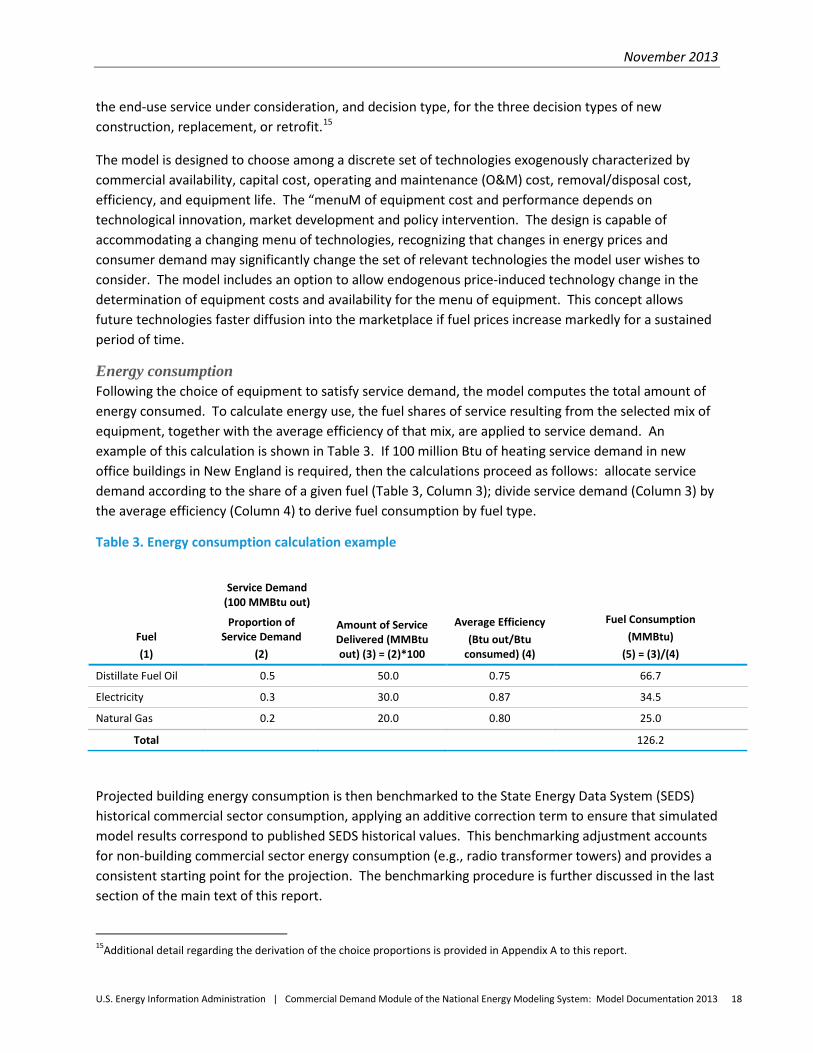
Energy consumption Following the choice of equipment to satisfy service demand, the model computes the total amount of energy consumed. To calculate energy use, the fuel shares of service resulting from the selected mix of equipment, together with the average efficiency of that mix, are applied to service demand. An example of this calculation is shown in Table 3. If 100 million Btu of heating service demand in new office buildings in New England is required, then the calculations proceed as follows: allocate service demand according to the share of a given fuel (Table 3, Column 3); divide service demand (Column 3) by the average efficiency (Column 4) to derive fuel consumption by fuel type.

Table 3. Energy consumption calculation example

Projected building energy consumption is then benchmarked to the State Energy Data System (SEDS) historical commercial sector consumption, applying an additive correction term to ensure that simulated model results correspond to published SEDS historical values. This benchmarking adjustment accounts for non-building commercial sector energy consumption (e.g., radio transformer towers) and provides a consistent starting point for the projection. The benchmarking procedure is further discussed in the last section of the main text of this report.

15Additional detail regarding the derivation of the choice proportions is provided in Appendix A to this report.

Service Demand

(100 MMBtu out)

Fuel (1)

Proportion of Service Demand

(2)

Amount of Service Delivered (MMBtu out) (3) = (2)*100

Average Efficiency (Btu out/Btu

consumed) (4)

Fuel Consumption (MMBtu)

(5) = (3)/(4)

Distillate Fuel Oil 0.5 50.0 0.75 66.7

Electricity 0.3 30.0 0.87 34.5

Natural Gas 0.2 20.0 0.80 25.0

Total 126.2

November 2013


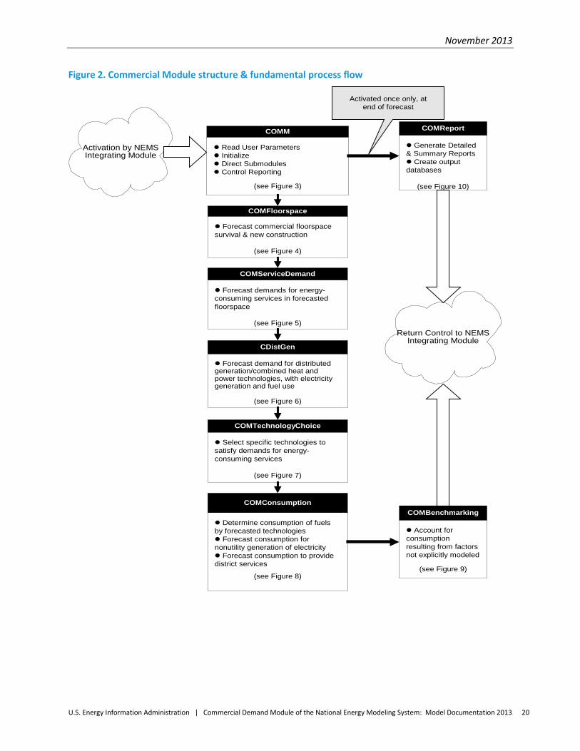
Flow diagrams Figure 2 illustrates the general model flow of the NEMS Commercial Demand Module. The flow proceeds sequentially, with each succeeding submodule utilizing as inputs the outputs of preceding submodules. The basic processing flow used by the Commercial Module to generate its projection of fuel demands consists of six steps:

1. A projection of commercial building floorspace is generated based upon input from the Macroeconomic Activity Module and results from previous years (COMFloorspace Submodule).

2. Demands for services are calculated for that distribution of floorspace (COMServiceDemand Submodule).

3. DG and CHP technologies are chosen to meet electricity demand in place of purchased electricity where economical (CDistGen).

4. Equipment is chosen to satisfy the demands for services (COMTechnologyChoice Submodule). 5. Fuel consumption is calculated based on the chosen equipment mix, and additional commercial

sector consumption components such as those resulting from nonutility generation of electricity and district energy services are accounted for (COMConsumption Submodule).

6. Results by fuel and Census division are adjusted to match the 1990 through 2010 SEDS historical data, 2011 historical estimates from the Annual Energy Review 2011, and optionally the 2012-2013 projections of the Short-Term Energy Outlook (COMBenchmarking Submodule).

The Commercial Module is activated one or more times during each year of the projection period by the NEMS Integrating Module. On each occurrence of module activation, the processing flow follows the outline shown in Figure 2. Details of the processing flow within each of the Commercial Module's submodules, together with the input data sources accessed by each, are shown in Figures 3 through 9, and summarized below. The precise calculations performed at the program subroutine level are described in the next section.

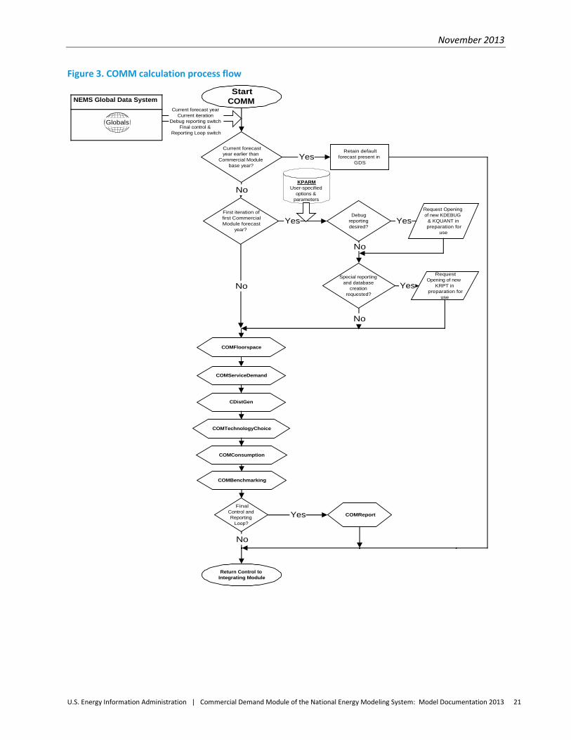
Figure 3 illustrates the flow within the controlling submodule of the Commercial Module, COMM. This is the submodule that retrieves user-specified options and parameters, performs certain initializations, and directs the processing flow through the remaining submodules. It also detects the conclusion of the projection period, and directs the generation of printed reports and output databases to the extent specified by the user.

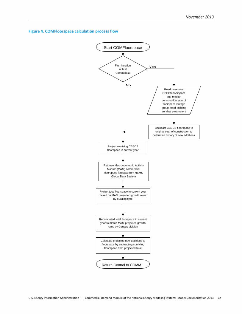
Figure 4 illustrates the processing flow within the Floorspace Submodule of the model, COMFloorspace. The Floorspace Submodule requires the MAM total commercial floorspace projection by Census division, building type, and year. In addition, base year building stock characteristics and building survival parameters (developed based on analysis of CBECS data and additional sources as further referenced in Appendix A to this report) are used by the Floorspace Submodule to evolve the existing stock of floorspace into the future.

November 2013


Figure 2. Commercial Module structure & fundamental process flow

Read User Parameters Initialize Direct Submodules Control Reporting

(see Figure 3)

COMM

Forecast commercial floorspacesurvival & new construction

(see Figure 4)

COMFloorspace

Forecast demands for energy-consuming services in forecastedfloorspace

(see Figure 5)

COMServiceDemand

Select specific technologies tosatisfy demands for energy-consuming services

(see Figure 7)

COMTechnologyChoice

Determine consumption of fuelsby forecasted technologies Forecast consumption fornonutility generation of electricity Forecast consumption to providedistrict services

(see Figure 8)

COMConsumption

Account forconsumptionresulting from factorsnot explicitly modeled

(see Figure 9)

COMBenchmarking

Generate Detailed& Summary Reports Create outputdatabases

(see Figure 10)

COMReport

Activation by NEMSIntegrating Module

Return Control to NEMSIntegrating Module

Activated once only, atend of forecast

Forecast demand for distributedgeneration/combined heat andpower technologies, with electricitygeneration and fuel use

(see Figure 6)

CDistGen

November 2013


Figure 3. COMM calculation process flow

Request Openingof new KDEBUG

& KQUANT inpreparation for

use

Return Control toIntegrating Module

KPARMUser-specified

options &parameters

First iteration offirst CommercialModule forecast

year?

No

Debugreportingdesired?

Yes

Current forecastyear earlier than

Commercial Modulebase year?

No

RequestOpening of new

KRPT inpreparation for

use

FinalControl andReporting

Loop?

YesRetain default

forecast present inGDS

COMReport

Yes

No

Yes

COMFloorspace

COMServiceDemand

COMConsumption

COMTechnologyChoice

COMBenchmarking

Yes

Current forecast yearCurrent iteration

Debug reporting switchFinal control &

Reporting Loop switch

CDistGen

Special reportingand database

creationrequested?

No

No

NEMS Global Data System

Globals

StartCOMM

November 2013


Figure 4. COMFloorspace calculation process flow

Start COMFloorspace

First iteration of first

Commercial

Project surviving CBECS floorspace in current year

Project total floorspace in current year based on MAM projected growth rates

by building type

Recomputed total floorspace in current year to match MAM projected growth

rates by Census division

Calculate projected new additions to floorspace by subtracting surviving

floorspace from projected total

Return Control to COMM

Yes

Backcast CBECS floorspace to original year of construction to

determine history of new additions

No Read base year

CBECS floorspace and median

construction year of floorspace vintage

group, read building survival parameters

Retrieve Macroeconomic Activity Module (MAM) commercial

floorspace forecast from NEMS Global Data System

November 2013


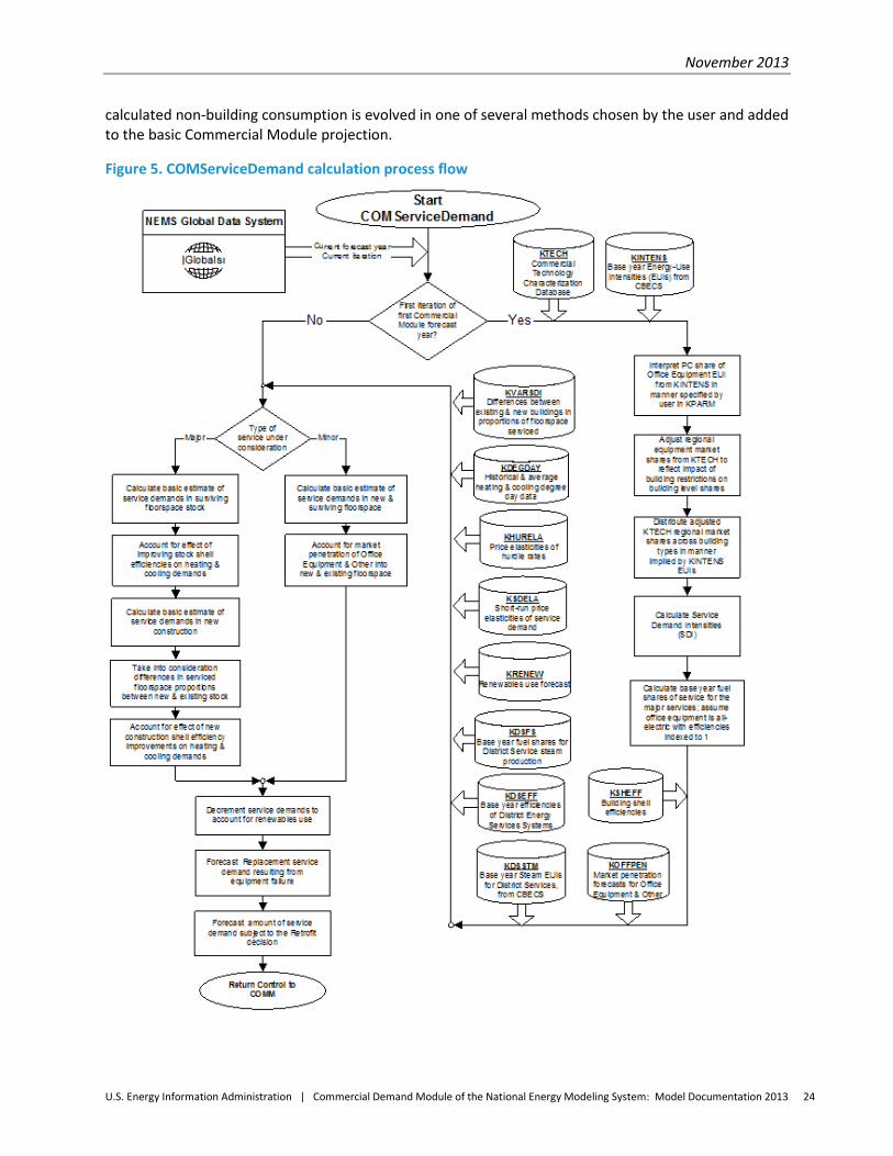
Figure 5 illustrates the processing flow within the Service Demand Submodule of the model, COMServiceDemand. The surviving and new floorspace results generated by the Floorspace Submodule are accepted as inputs by the Service Demand Submodule, along with additional inputs such as base year (2003) EUIs, projected office equipment market penetration, base year equipment market shares and stock efficiencies, equipment survival assumptions, building shell efficiencies, weather data, and district energy services information. The Service Demand Submodule projects demands for the 10 modeled end uses in each of the 11 building types and nine Census divisions separately for newly-constructed commercial floorspace, surviving floorspace with unsatisfied service demands due to equipment failure, and surviving floorspace with currently functioning equipment.

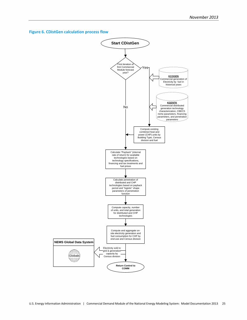
Figure 6 illustrates the processing flow within the Distributed Generation and CHP Submodule of the model, CDistGen. Technology-specific inputs and financing parameters are required by the Distributed Generation and CHP Submodule, along with additional inputs such as historical commercial CHP data, projected program-driven market penetration, and fuel prices. The Distributed Generation and CHP Submodule projects electricity generation, fuel consumption, and water and space heating supplied by DG and CHP technologies. Penetration of these technologies is based on how quickly an investment in a technology is estimated to recoup its flow of costs.

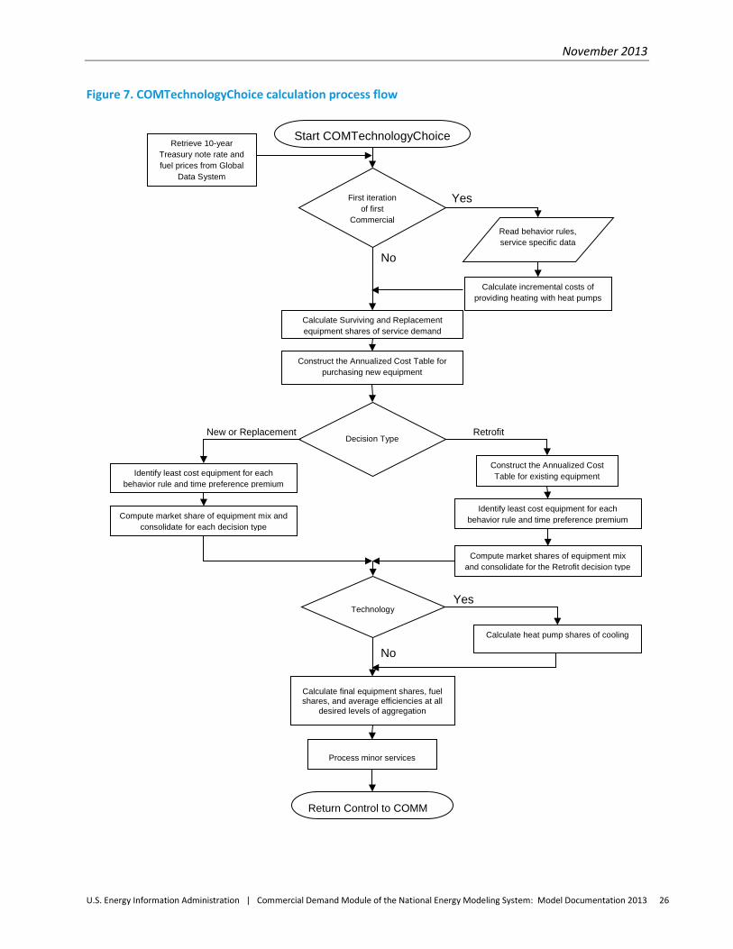
Figure 7 illustrates the processing flow within the Technology Choice Submodule, COMTechnologyChoice. The Technology Choice Submodule requires a variety of inputs, including service demands produced by the Service Demand Submodule; equipment-specific inputs, consumer behavior characterization and risk-adjusted time preference segmentation information specific to the Commercial Module; and NEMS system outputs including Treasury note rates from the MAM and fuel prices from the EMM, NGTDM, and LFMM. The result of processing by this submodule is a projection of equipment market shares of specific technologies retained or purchased for servicing new floorspace, replacing failed equipment, or retrofitting of economically obsolete equipment. This submodule also calculates the corresponding fuel shares and average equipment efficiencies by end-use service, and other characteristics.

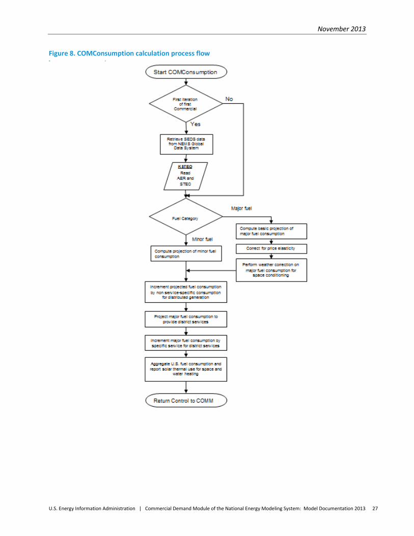
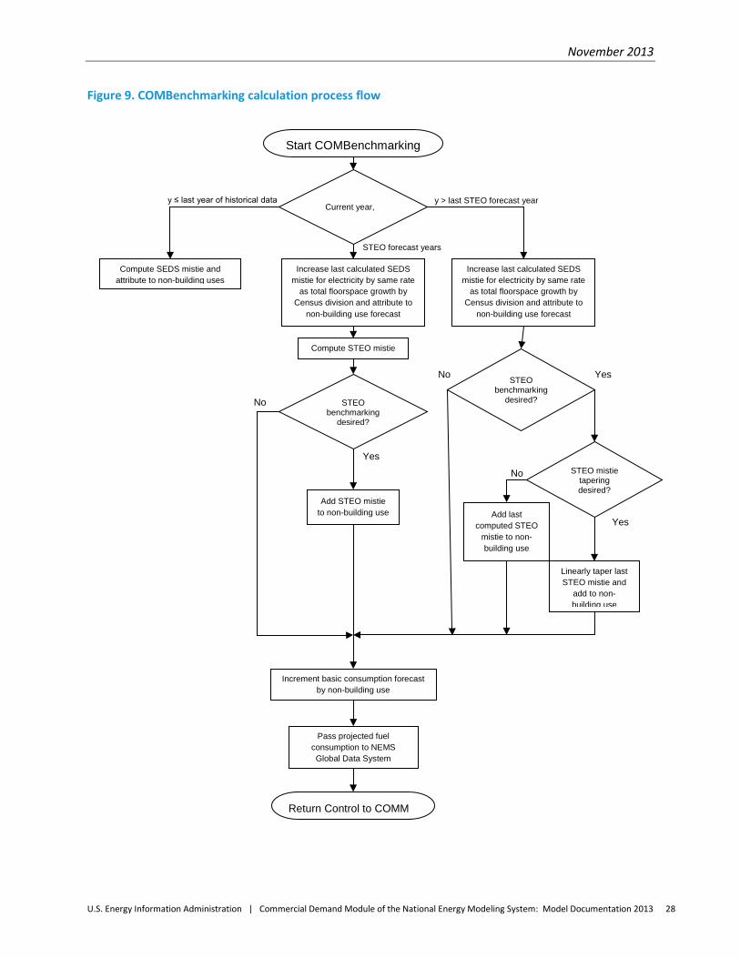
Figure 8 illustrates the processing flow within the Consumption Submodule, COMConsumption. The average equipment efficiency and fuel proportions output by the Technology Choice Submodule are combined with the projected service demands generated by the Service Demand Submodule to produce the projection of major fuel consumption by building type, Census division, and end use. Several additional considerations are incorporated into the final projection, including accounting for the fuel used for electricity generation and CHP in commercial buildings and fuel consumption for the purposes of providing district energy services. Demands for the five minor fuels are also projected by this submodule using double-log regression equations based on historical Census division-level consumption, floorspace, and pricing data. Figure 9 illustrates the Benchmarking Submodule of the fuel consumption projection, COMBenchmarking. Data input from the State Energy Data System (SEDS), and, at the user's option, fuel consumption projections produced for the Short-Term Energy Outlook (STEO), are compared with the basic Commercial Module fuel consumption projection during the period of time over which they overlap, in an attempt to calculate energy consumption in the commercial sector not attributable to the building end uses explicitly modeled in the Commercial Module. The difference between the basic Commercial Module fuel consumption projection and the fuel consumption given by the SEDS or STEO is attributed to non-building energy use and referred to as a “mistie.” If desired, the

November 2013


calculated non-building consumption is evolved in one of several methods chosen by the user and added to the basic Commercial Module projection.

Figure 5. COMServiceDemand calculation process flow

November 2013


Figure 6. CDistGen calculation process flow


Start CDistGen

Electricity sold to grid & generation

capacity by Census division

NEMS Global Data System

Globals

First iteration of first Commercial Module forecast

year?

NoKGENTK

Commercial distributed generation technology

characterization, CBECS niche parameters, financing parameters, and penetration

parameters

Yes

KCOGENCommercial generation of

Electricity by fuel in historical years

Calculate "Payback" (internal rate of return) for available

technologies based on technology specifications,

financing and tax treatments and fuel prices

Calculate penetration of distributed and CHP

technologies based on payback period and "logistic" shape parameters of penetration

function

Compute capacity, number of units, and total generation

for distributed and CHP technologies

Compute and aggregate on-site electricity generation and fuel consumption for CHP by end-use and Census division

Compute existing combined heat and

power (CHP) units by Building Type, Census

division and fuel

November 2013


Figure 7. COMTechnologyChoice calculation process flow

Start COMTechnologyChoice

First iteration of first

Commercial

Construct the Annualized Cost Table for purchasing new equipment

Decision Type

Calculate Surviving and Replacement equipment shares of service demand

Construct the Annualized Cost Table for existing equipment

Identify least cost equipment for each behavior rule and time preference premium

Calculate heat pump shares of cooling

Calculate final equipment shares, fuel shares, and average efficiencies at all

desired levels of aggregation

Process minor services


No

Compute market shares of equipment mix and consolidate for the Retrofit decision type

Yes

New or Replacement Retrofit

Read behavior rules, service specific data

Calculate incremental costs of providing heating with heat pumps

Identify least cost equipment for each behavior rule and time preference premium

Compute market share of equipment mix and consolidate for each decision type

Technology Yes

No

Retrieve 10-year Treasury note rate and fuel prices from Global

Data System

November 2013


Figure 8. COMConsumption calculation process flow

November 2013


Figure 9. COMBenchmarking calculation process flow

Start COMBenchmarking

Current year,

Compute STEO mistie

STEO benchmarking

desired?

Increase last calculated SEDS mistie for electricity by same rate

as total floorspace growth by Census division and attribute to

non-building use forecast

Add STEO mistie to non-building use

Increment basic consumption forecast by non-building use


STEO forecast years

Linearly taper last STEO mistie and

add to non-building use

y > last STEO forecast year

No

Yes

Increase last calculated SEDS mistie for electricity by same rate

as total floorspace growth by Census division and attribute to

non-building use forecast

Compute SEDS mistie and attribute to non-building uses

y ≤ last year of historical data

STEO benchmarking

desired?

STEO mistie tapering desired?

Add last computed STEO

mistie to non-building use

Yes No

Yes

No

Pass projected fuel consumption to NEMS Global Data System

November 2013


A final reporting subroutine, COMReport, generates detailed documentation on the Final Control and Reporting Loop of the last projection year. Numerous subcategories and additional considerations are handled by the model for each of the broad process categories given above. These are described, with references to the appropriate equations in Appendix B, in the Key Computations and Equations section of Chapter 4 under the headings of the applicable subroutines.

Key computations and equations This section provides detailed solution algorithms arranged by sequential submodule as executed in the NEMS Commercial Demand Module. General forms of the fundamental equations involved in the key computations are presented, followed by discussion of the numerous details considered by the full forms of the equations provided in Appendix B.

Floorspace Submodule The Floorspace Submodule utilizes the Census-division-level, building-specific total floorspace projection from the MAM as its primary driver. Many of the parameter estimates used in the Commercial Module, including base year (2003) commercial sector floorspace, are developed from the 2003 CBECS database. Projected total commercial floorspace is provided by the MAM through the MC_COMMFLSP member of the NEMS Global Data Structure (GDS).16 Commercial floorspace from the MAM is specified by the 13 building categories of the database of historical floorspace estimates developed by McGraw-Hill Construction and projected at the Census division level based on population, economic drivers, and historical time trends. To distinguish the Commercial Module floorspace projection ultimately produced within the Commercial Module from that provided by the MAM, the latter is referred to as the MAM floorspace projection in this report.

The Floorspace Submodule first backcasts the 2003 CBECS floorspace stock to its original construction years, and then simulates building retirements by convolving the time series of new construction with a logistic decay function. New floorspace construction during the projection period is calculated in a way that causes total floorspace to grow at the rate indicated by the MAM projection. In the event that the new additions computations produce a negative value for a specific building type, new additions are set to zero.

The building retirement function used in the Floorspace Submodule depends upon the values of two user inputs: average building lifetime, and gamma. The average building lifetime refers to the median expected lifetime of buildings of a certain type; that is, the period of time after construction when half of the buildings have retired, and half still survive. The gamma parameter, γ, corresponds to the rate at which buildings retire near their median expected lifetime. The proportion of buildings of a certain type built at the same time that are surviving after a given period of time has passed is referred to as the survival rate. The survival rate is modeled by assuming a logistic functional form in the Commercial Module, and is given by Equation B-1 in appendix B. This survival function, also referred to as the retirement function, is of the form:

16For the methodology used to develop the MAM floorspace projection, please see U.S. Energy Information Administration, Model Documentation Report: Macroeconomic Activity Module (MAM) of the National Energy Modeling System, DOE/EIA-M065 (2013) (Washington, DC, April 2013).

November 2013


𝑆𝑢𝑟𝑣𝑖𝑣𝑖𝑛𝑔 𝑃𝑟𝑜𝑝𝑜𝑟𝑡𝑖𝑜𝑛 = 1

�1+ 𝐵𝑢𝑖𝑙𝑑𝑖𝑛𝑔 𝐴𝑔𝑒𝑀𝑒𝑑𝑖𝑎𝑛 𝐿𝑖𝑓𝑒𝑡𝑖𝑚𝑒�

𝑦 (1)

Existing floorspace retires over a longer time period if the median building lifetime is increased or over a shorter time as the average lifetime is reduced, as depicted in Figure 10 using a constant gamma value of 3.0. Average building lifetimes are positively related to consumption; the longer the average building lifetime, the more slowly new construction with its associated higher-efficiency equipment enters the market, prolonging the use of the lower-efficiency equipment in the surviving stock. This scenario results in a higher level of energy consumption than in the case of accelerated building retirements and phase-in of new construction.

The user-specified gamma parameter partly determines the shape of the survival rate function that defines the acceleration of the rate of retirement around the average building lifetime. The effects of varying the value of gamma with an assumed median building lifetime of 50 years are illustrated in Figure 11. The larger the value of gamma, the slower the initial rate of retirement and the steeper the survival curve near the median lifetime. This implies greater numbers of buildings retiring at or very near the average lifetime. Large values of gamma should be avoided, as this implies that a vintage of buildings will retire almost entirely at its average lifetime. The converse is true as well. Small gamma values will retire floorspace more evenly over the range of lifetimes.

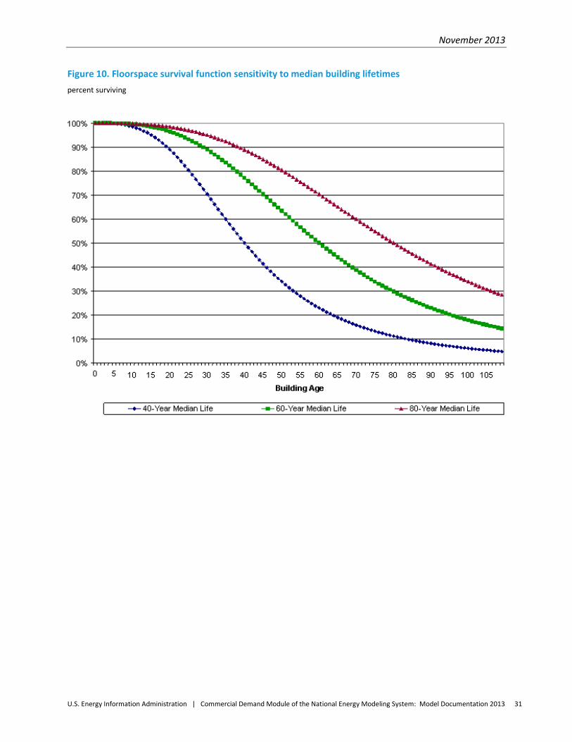
November 2013


Figure 10. Floorspace survival function sensitivity to median building lifetimes percent surviving

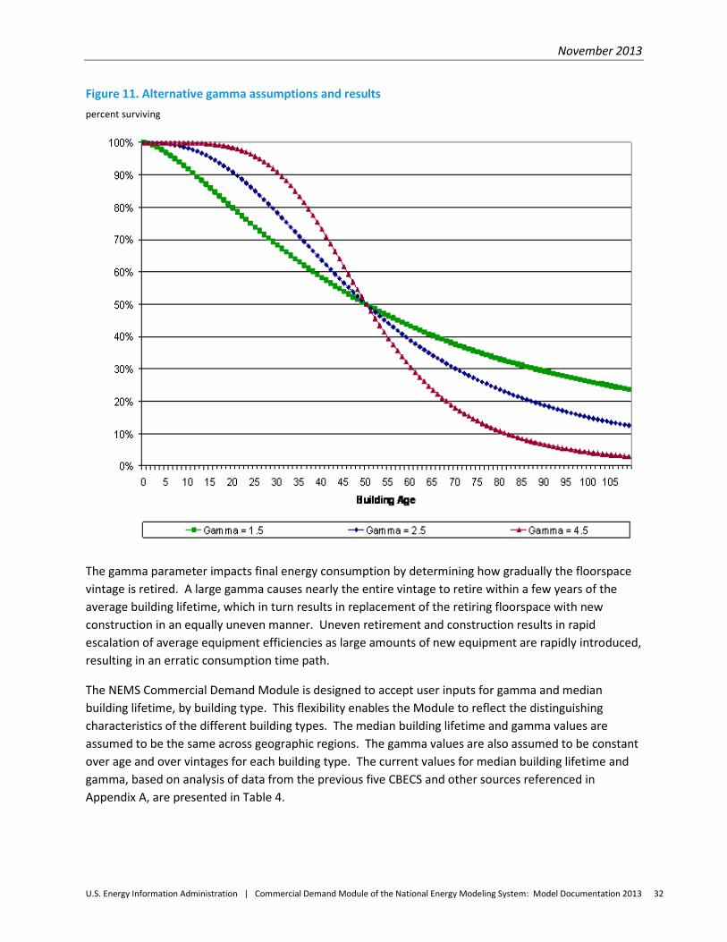
November 2013


Figure 11. Alternative gamma assumptions and results percent surviving

The gamma parameter impacts final energy consumption by determining how gradually the floorspace vintage is retired. A large gamma causes nearly the entire vintage to retire within a few years of the average building lifetime, which in turn results in replacement of the retiring floorspace with new construction in an equally uneven manner. Uneven retirement and construction results in rapid escalation of average equipment efficiencies as large amounts of new equipment are rapidly introduced, resulting in an erratic consumption time path.

The NEMS Commercial Demand Module is designed to accept user inputs for gamma and median building lifetime, by building type. This flexibility enables the Module to reflect the distinguishing characteristics of the different building types. The median building lifetime and gamma values are assumed to be the same across geographic regions. The gamma values are also assumed to be constant over age and over vintages for each building type. The current values for median building lifetime and gamma, based on analysis of data from the previous five CBECS and other sources referenced in Appendix A, are presented in Table 4.

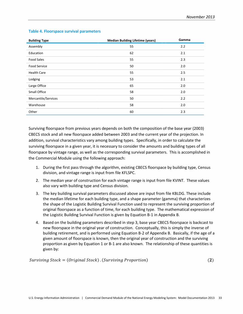
November 2013


Table 4. Floorspace survival parameters

Surviving floorspace from previous years depends on both the composition of the base year (2003) CBECS stock and all new floorspace added between 2003 and the current year of the projection. In addition, survival characteristics vary among building types. Specifically, in order to calculate the surviving floorspace in a given year, it is necessary to consider the amounts and building types of all floorspace by vintage range, as well as the corresponding survival parameters. This is accomplished in the Commercial Module using the following approach:

1. During the first pass through the algorithm, existing CBECS floorspace by building type, Census division, and vintage range is input from file KFLSPC.

2. The median year of construction for each vintage range is input from file KVINT. These values also vary with building type and Census division.

3. The key building survival parameters discussed above are input from file KBLDG. These include the median lifetime for each building type, and a shape parameter (gamma) that characterizes the shape of the Logistic Building Survival Function used to represent the surviving proportion of original floorspace as a function of time, for each building type. The mathematical expression of the Logistic Building Survival Function is given by Equation B-1 in Appendix B.

4. Based on the building parameters described in step 3, base year CBECS floorspace is backcast to new floorspace in the original year of construction. Conceptually, this is simply the inverse of building retirement, and is performed using Equation B-2 of Appendix B. Basically, if the age of a given amount of floorspace is known, then the original year of construction and the surviving proportion as given by Equation 1 or B-1 are also known. The relationship of these quantities is given by:

𝑆𝑢𝑟𝑣𝑖𝑣𝑖𝑛𝑔 𝑆𝑡𝑜𝑐𝑘 = (𝑂𝑟𝑖𝑔𝑖𝑛𝑎𝑙 𝑆𝑡𝑜𝑐𝑘) . (𝑆𝑢𝑟𝑣𝑖𝑣𝑖𝑛𝑔 𝑃𝑟𝑜𝑝𝑜𝑟𝑡𝑖𝑜𝑛) (𝟐)

Building Type Median Building Lifetime (years) Gamma

Assembly 55 2.2

Education 62 2.1

Food Sales 55 2.3

Food Service 50 2.0

Health Care 55 2.5

Lodging 53 2.1

Large Office 65 2.0

Small Office 58 2.0

Mercantile/Services 50 2.2

Warehouse 58 2.0

Other 60 2.3

November 2013


Dividing the surviving stock by the surviving proportion gives the original stock in the year of construction. This time series of new floorspace is concatenated with the new floorspace projected for previous years of the projection (described below) to produce a total history of new additions to floorspace, starting with the original stock of the oldest vintage (currently 1825) in CBECS. Surviving floorspace in any given year is then calculated for each building type by using the appropriate survival parameters to determine the proportion of original stock that survives from each prior year into the current year of the projection. This is accomplished using the calculation shown by Equation B-3 in Appendix B.

In order to calculate new additions to floorspace in the current projection year, the surviving floorspace calculated above is combined with the total floorspace projection provided by MAM as follows:

1. Within each Census division, the total amount of floorspace for each CBECS building type is calculated to be consistent with the growth rate of the corresponding combination of MAM building types. The mapping from the MAM building types to the CBECS building types is represented by a transformation matrix named DRItoCBECS. The twelve commercial building types projected in the MAM are: Amusement, Automotive, Dormitory, Education, Health, Hotel, Miscellaneous, Office, Public Service, Religious, Store, and Warehouse. New additions are obtained by subtracting the surviving floorspace projection from the total CBECS floorspace projection. For reasons described below, this is merely the first estimate of new additions to CBECS floorspace. The calculation is illustrated by Equations B-4 and B-6. Equation B-5 simply prevents negative new additions by replacing such occurrences with zero.

2. Due to differences between the CBECS and MAM data sources, the results obtained in the previous step do not guarantee that the total floorspace growth rate for each entire Census division will be in agreement with the MAM projection. Therefore, the growth rates by building type obtained in the previous step are uniformly modified within each Census division to achieve agreement between the Commercial Module and the MAM Census division level growth rate projections. This is accomplished using Equations B-7 and B-8.

3. New additions to floorspace for each CBECS building type are obtained by subtracting the floorspace projected as surviving into the current year from the total floorspace in the current year calculated in step 2, as shown by Equations B-8 and B-9, completing the projection of new floorspace. The final value obtained for total floorspace is then given by Equation B-10.

This approach is necessary because the floorspace projection read from the MAM is not available as separate projections for new additions and existing floorspace stock.

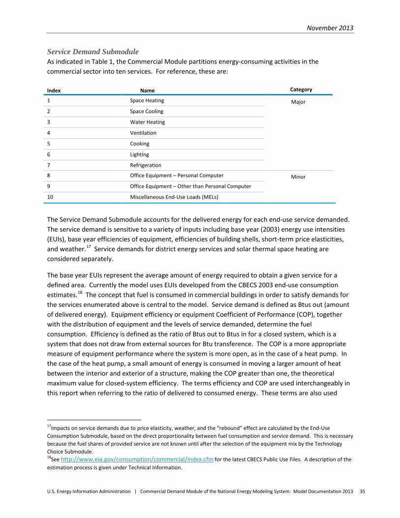
November 2013


Service Demand Submodule As indicated in Table 1, the Commercial Module partitions energy-consuming activities in the commercial sector into ten services. For reference, these are:

The Service Demand Submodule accounts for the delivered energy for each end-use service demanded. The service demand is sensitive to a variety of inputs including base year (2003) energy use intensities (EUIs), base year efficiencies of equipment, efficiencies of building shells, short-term price elasticities, and weather.17 Service demands for district energy services and solar thermal space heating are considered separately.

The base year EUIs represent the average amount of energy required to obtain a given service for a defined area. Currently the model uses EUIs developed from the CBECS 2003 end-use consumption estimates.18 The concept that fuel is consumed in commercial buildings in order to satisfy demands for the services enumerated above is central to the model. Service demand is defined as Btus out (amount of delivered energy). Equipment efficiency or equipment Coefficient of Performance (COP), together with the distribution of equipment and the levels of service demanded, determine the fuel consumption. Efficiency is defined as the ratio of Btus out to Btus in for a closed system, which is a system that does not draw from external sources for Btu transference. The COP is a more appropriate measure of equipment performance where the system is more open, as in the case of a heat pump. In the case of the heat pump, a small amount of energy is consumed in moving a larger amount of heat between the interior and exterior of a structure, making the COP greater than one, the theoretical maximum value for closed-system efficiency. The terms efficiency and COP are used interchangeably in this report when referring to the ratio of delivered to consumed energy. These terms are also used

17Impacts on service demands due to price elasticity, weather, and the “rebound” effect are calculated by the End-Use Consumption Submodule, based on the direct proportionality between fuel consumption and service demand. This is necessary because the fuel shares of provided service are not known until after the selection of the equipment mix by the Technology Choice Submodule. 18See http://www.eia.gov/consumption/commercial/index.cfm for the latest CBECS Public Use Files. A description of the estimation process is given under Technical Information.

Index Name Category

1 Space Heating Major

2 Space Cooling

3 Water Heating

4 Ventilation

5 Cooking

6 Lighting

7 Refrigeration

8 Office Equipment – Personal Computer Minor 9 Office Equipment – Other than Personal Computer

10 Miscellaneous End-Use Loads (MELs)

http://www.eia.gov/consumption/commercial/index.cfm

November 2013


where either ventilation or lighting is the service, although the actual measure used in the model for ventilation is cubic feet per minute of ventilation air delivered to Btus in and that used for lighting is efficacy, defined as lumens delivered per watt of electricity consumed.

Service demand intensity (SDI), defined as the demand for a service per square foot of floorspace, varies with service, building type and location, but is assumed to remain constant for a given service in a given building type and location. The service demand obtained by multiplication of the SDI with the floorspace is, however, subject to modification by various factors such as shell efficiency load factors for heating and cooling, and fuel price elasticity as described below.

The SDI is computed for the major services by applying the composite average equipment efficiency for the service to the EUI. This provides a more realistic picture of the energy needed to provide an end-use service since energy losses occur during conversion to a consumable service. The base year EUI for a given service is related to the SDI and the average efficiency of the base year equipment mix as follows:

𝑆𝐷𝐼 �𝐵𝑡𝑢 𝑜𝑢𝑡𝑓𝑡2

� = 𝐸𝑈𝐼 �𝐵𝑡𝑢 𝑖𝑛𝑓𝑡2

� .𝐶𝑂𝑃𝑎𝑣𝑒𝑟𝑎𝑔𝑒 (𝟑)

The actual calculation of SDI in the model involves several additional considerations, such as buildings from which specific equipment is restricted, base year equipment market shares, and the distribution of Census division level equipment market shares across the different building types. In addition, since the model accommodates fuel switching, the total SDI for the service must be calculated, rather than an SDI corresponding to each fuel used in 2003. The basic calculation illustrated by Equation 3 is carried out by evaluation of Equations B-11 through B-20 in Appendix B for each major service.

Minor services (office equipment and MELs) are modeled in less detail than the major services. In particular, specific discrete minor service technologies are not characterized within the Commercial Module; instead, the efficiency of the composite mix of technologies for a given minor service is modeled as evolving relative to its base year (2003) level. The actual base year average efficiency of the minor service equipment mix is indexed to equal one, resulting in the minor service SDI and EUI values being equal, as indicated by Equation B-21.

The basic computation of service demand for a given service in a given category of floorspace (new or surviving) is the same for major and minor services, namely:

𝑆𝑒𝑟𝑣𝑖𝑐𝑒 𝐷𝑒𝑚𝑎𝑛𝑑(𝐵𝑡𝑢 𝑜𝑢𝑡) = 𝑆𝐷𝐼 �𝐵𝑡𝑢 𝑜𝑢𝑡𝑓𝑡2

� .𝐹𝑙𝑜𝑜𝑟𝑠𝑝𝑎𝑐𝑒 (𝑓𝑡2) (𝟒)

The computation illustrated above is accomplished by evaluating Equations B-22, B-29, B-37, and B-38.

Building shell efficiencies for new construction are user inputs in the form of shell heating and cooling load factors that can be modified to generate scenarios to reflect a variety of technologies and policy options such as increased insulation, weather-stripping, or new highly energy-efficient construction materials. These load factors represent the impacts of building shell efficiency improvements on service

November 2013


demand and are based on a 2010 parametric study completed for EIA by Science Applications International Corporation.19

The present shell efficiencies for existing buildings are indexed to the average 2003 values by building type and Census division. The new shell heating and cooling factors represent the thermal envelope properties of newly constructed buildings relative to the existing 2003 building stock. The shell efficiency factors are modeled as increasing to user-specified values for 2040. Current building practices, rates of adoption for building codes, research, development, and deployment programs focusing on shell improvements, the “green building” movement, and the long-lived nature of commercial buildings are all considered in selecting the level of shell improvement. Additional improvement is assumed for new construction to account for adoption of the ASHRAE 90.1-2007 standard for building shell measures. Based on provisions in the American Recovery and Reinvestment Act of 2009 (ARRA09), states are assumed to adopt and enforce the standard by 2018. For AEO2013, floorspace surviving from the base-year floorstock is assumed to improve a maximum of 6.9 percent over the 2003 stock average by 2040, and new floorspace is assumed to improve 15.0 percent by 2040 relative to the efficiency of new construction in 2003. Changing shell efficiencies impact space heating and space cooling service demands as follows:

𝑆𝑒𝑟𝑣𝑖𝑐𝑒 𝐷𝑒𝑚𝑎𝑛𝑑 = (𝑆𝑒𝑟𝑣𝑖𝑐𝑒 𝐷𝑒𝑚𝑎𝑛𝑑 𝑤𝑖𝑡ℎ 2003 𝑠ℎ𝑒𝑙𝑙) . (𝑆ℎ𝑒𝑙𝑙𝐹𝑎𝑐𝑡𝑜𝑟) (𝟓)

with the appropriate load factor (heating or cooling) used for the given end-use service. The calculations involved in computing the appropriate shell load factors and evaluating the expression illustrated by Equation 5 are accomplished using Equations B-23 through B-28 and Equations B-30 through B-32.

The computation of service demand for space cooling, ventilation, and MELs is adjusted to account for the requirements of data centers that house large numbers of server computers and other internet-related equipment. Data centers are included in the large office category of commercial buildings with their proportion given by Equation B-33. The adjustment to account for increased service requirements is shown in Equations B-34 and B-35. Projections of data center floorspace as a share of large office buildings and estimates of additional consumption for cooling, ventilation, and MELs are developed based on the literature referenced in Appendix A. Projections for the computers and other office equipment used in data centers are included in the office equipment projections discussed below.

The CBECS data indicate that a greater proportion of the floorspace is lit, heated, and cooled in buildings constructed after 1989 than in older buildings. The effect of these service demand differences between newer and older buildings has been estimated and is accounted for using Equation B-36.

While the market for major services is generally assumed to be saturated, additional penetration of the minor services of office equipment (both PC and non-PC) and MELs is modeled. Projections of continuing market penetration are prepared offline for office equipment and the non-specific portion of

19 Science Applications International Corporation, Data Analysis for Enhanced Representation of Commercial Thermal Shell Efficiency in the Commercial Demand Module, prepared for U.S. Department of Energy, U.S. Energy Information Administration, May 2010.

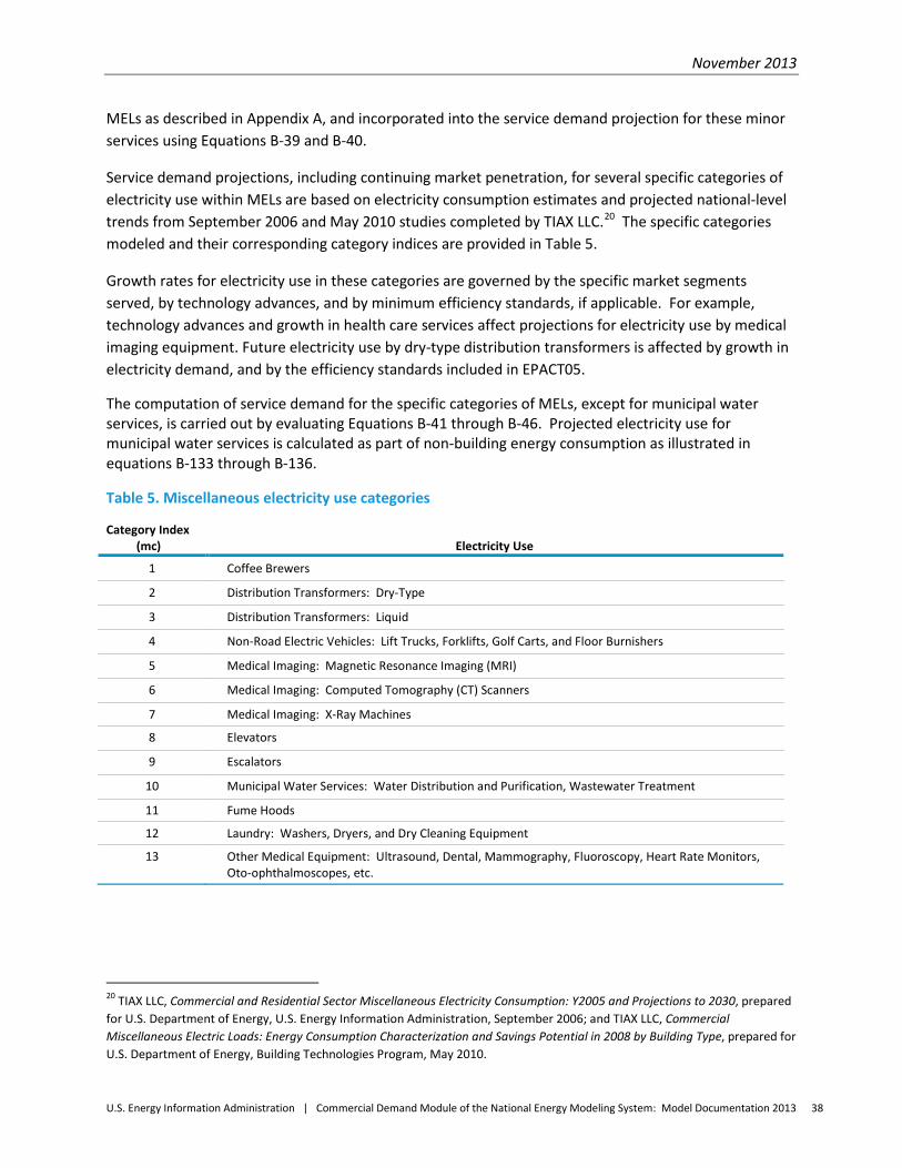
November 2013


MELs as described in Appendix A, and incorporated into the service demand projection for these minor services using Equations B-39 and B-40.

Service demand projections, including continuing market penetration, for several specific categories of electricity use within MELs are based on electricity consumption estimates and projected national-level trends from September 2006 and May 2010 studies completed by TIAX LLC.20 The specific categories modeled and their corresponding category indices are provided in Table 5.

Growth rates for electricity use in these categories are governed by the specific market segments served, by technology advances, and by minimum efficiency standards, if applicable. For example, technology advances and growth in health care services affect projections for electricity use by medical imaging equipment. Future electricity use by dry-type distribution transformers is affected by growth in electricity demand, and by the efficiency standards included in EPACT05.

The computation of service demand for the specific categories of MELs, except for municipal water services, is carried out by evaluating Equations B-41 through B-46. Projected electricity use for municipal water services is calculated as part of non-building energy consumption as illustrated in equations B-133 through B-136.

Table 5. Miscellaneous electricity use categories

20 TIAX LLC, Commercial and Residential Sector Miscellaneous Electricity Consumption: Y2005 and Projections to 2030, prepared for U.S. Department of Energy, U.S. Energy Information Administration, September 2006; and TIAX LLC, Commercial Miscellaneous Electric Loads: Energy Consumption Characterization and Savings Potential in 2008 by Building Type, prepared for U.S. Department of Energy, Building Technologies Program, May 2010.

Category Index (mc) Electricity Use

1 Coffee Brewers

2 Distribution Transformers: Dry-Type

3 Distribution Transformers: Liquid

4 Non-Road Electric Vehicles: Lift Trucks, Forklifts, Golf Carts, and Floor Burnishers

5 Medical Imaging: Magnetic Resonance Imaging (MRI)

6 Medical Imaging: Computed Tomography (CT) Scanners

7 Medical Imaging: X-Ray Machines

8 Elevators

9 Escalators

10 Municipal Water Services: Water Distribution and Purification, Wastewater Treatment

11 Fume Hoods

12 Laundry: Washers, Dryers, and Dry Cleaning Equipment

13 Other Medical Equipment: Ultrasound, Dental, Mammography, Fluoroscopy, Heart Rate Monitors, Oto-ophthalmoscopes, etc.

November 2013


The portion of service demand satisfied by solar water heaters is computed endogenously as solar water heating technologies are included in the Technology Choice Submodule. However, the portion of service demand satisfied by solar space heating and daylighting is computed using exogenous projections for renewable energy for the commercial sector as described in the Appendix A description for the SolarRenewableContrib variable. The penetration of solar energy changes the amount of service demand, affecting the end-use consumption for the major services. The incorporation of solar services in this manner provides a useful method for policy analysis. By varying adoption of these technologies in response to policy mandates or incentive programs, the effects on consumption of conventional fuels can be determined. The calculations involved in modeling the penetration of solar services are performed by Equations B-47 and B-48.

The short-term price elasticity of demand is currently provided for all end-use services. The parameters included in the Commercial Module are currently set to -0.25 for all major services except refrigeration, which is set to -0.10. A value of -0.05 is currently used for all types of office equipment and electric MELs. The parameters for commercial electricity are adjusted to -0.30 for heating, cooling, ventilation, and lighting end-use services in 2010 to represent investment in smart grid technologies, especially smart meters on buildings, which are assumed to make consumers more responsive to electricity price changes. These values are representative of estimates provided in the literature as referenced in Table A-3.

The elasticity parameters represent the short-term price responsiveness of service demands in the model. The values for the elasticities must necessarily be non-positive since the services are assumed to be normal goods, meaning that, as fuel prices increase, the quantity of energy services demanded declines. The full elasticity effect is graduated over a three-year period to allow the degree of consumer response to vary with significant changes in fuel prices. In order to capture the effect of fuel price changes on demands for services satisfied by equipment using the affected fuel, the service demand elasticity calculation is postponed until after the final determination of the current year equipment mix as calculated by the Technology Choice Submodule. Because of the linear relationship between service demand and fuel consumption, as illustrated in Equation 3 above, a proportional change in service demand results in the same proportional change in fuel consumption. The calculation of the service demand elasticity effect for a given year is shown in Equation B-108. The service demand elasticity application is illustrated by Equation B-109. Equation B-109 also illustrates the modification of pure price elasticity to account for the fact that improving equipment and shell efficiencies reduces the actual cost of meeting certain service demands. Incorporation of this “take-back” or “rebound” effect, and weather corrections (described in the End-Use Consumption Submodule section), is also postponed until the calculation of fuel consumption.

By contrast, long-term responses to energy prices are determined endogenously through potentially altered equipment choices. Installed equipment costs, equipment and building shell efficiencies, energy prices, hurdle rates, and annual equipment utilization rates all interact to affect demand and determine long-term energy price responses. The paper “Price Responsiveness in the AEO2003 NEMS Residential

November 2013


and Commercial Buildings Sector Models,” available on EIA’s website, provides a thorough discussion of both short-term and long-term price response in the Commercial Demand Module.21

The final purpose of the Service Demand Submodule is to determine the amount of service demand in surviving floorspace that becomes unsatisfied in the current projection year due to failure of equipment. A simplified equipment vintaging scheme is employed, where each year a proportion of each type of equipment fails, with the proportion given by the reciprocal of the expected equipment lifetime expressed in years. Thus, if the expected lifetime for a particular piece of equipment were 10 years, the Commercial Module would assume that each year one tenth of the total amount of that equipment fails. This relationship is used to split the total amount of service demand in surviving floorspace into the portion in need of equipment replacement and the surviving portion, for satisfaction by appropriate decisions in the Technology Choice Submodule. The calculation of this split is performed by Equations B-49 and B-50.

Distributed Generation and Combined Heat and Power (CHP) Submodule The Distributed Generation and CHP Submodule (subroutine CDistGen) projects electricity generation, fuel consumption and water and space heating supplied by 11 distributed generation technologies. The characterized technologies include: photovoltaics, natural gas (fuel cells, reciprocating engines, turbines and microturbines), diesel engines, coal-fired CHP, municipal solid waste and wood generators, hydroelectric, and distributed wind turbines.22

Estimates of CHP electricity generation for historical years by technology, Census division and building type are developed from data contained in the most recent year’s version of the Form EIA-860 Database, Annual Electric Generator Report. Fuel types are first mapped to appropriate generating technologies. Next an estimate of the number of buildings incorporating each technology is developed based on total generated electricity (from Form 860) divided by the average generation of electricity for the particular technology to which the fuel type was mapped (Equation B-156). The estimated units then form the installed base of CHP equipment that is carried forward into future years and supplemented with any projected additions. Energy consumption and usable waste heat (used first for water heating and then for space heating if sufficient amounts are generated) are computed based on technology characteristics (Equations B-158 and B-159).

For projection years, distributed generation technology penetration rates are estimated by Census division, building type, building size category, and solar/energy price niches and vary depending on floorspace vintage (newly constructed versus existing floorspace). Technology penetration rates for new construction are determined by how quickly an investment in a technology is estimated to recoup its flow of costs based on the internal rate of return (IRR) computed from a cash-flow model. Penetration parameters are allowed to vary by technology and are as high as 30 percent when investment payback is one year. Investments that pay back in less than a year may achieve even greater penetration, up to an

21See http://www.eia.gov/oiaf/analysispaper/elasticity/index.html. 22Assumed technology characterizations for natural gas-fired and oil-fired CHP technologies are based on reports completed for EIA by ICF International, SENTECH, Incorporated and Science Applications International Corporation. See the detailed model inputs in Appendix A for full citation.

http://www.eia.gov/oiaf/analysispaper/elasticity/index.html

November 2013


assumed maximum of 75 percent. That is, up to 75 percent of new construction in any year can potentially include a specific distributed generation technology. Penetration into existing floorspace is limited, by assumption, to a much lower rate due to the added complexities of installing a distributed generation system in an existing building. The limit is the lesser of 0.5 percent or the penetration rate into new construction divided by 10.

For new construction, penetration rates are a direct function of the number of years required to achieve investment “payback.” Payback years are computed based on compounded returns (using the IRR). In addition to the value of energy savings, the NEMS distributed generation submodule includes business tax effects (both timing and magnitude) in the cash flow calculations, thus allowing the modeling of alternative tax policies.

Since the IRR approach captures the impacts of the timing of financial outlays and benefits, it gives greater weight to tax credits and other incentives which are generally received near the beginning of the cash flow horizon. The working assumption is that for new construction, investment in distributed generation technologies is combined with the building costs and financed along with the building. These financing assumptions are supplied in the generation technology input file (kgentk.txt).

For each potential investment decision, a cash flow analysis covering 30 years from the date of investment is made (see Equations B-143 through B-170 for details). The calculations include the costs (down payments, loan payments, maintenance costs and fuel costs) and returns (tax deductions for expenses and depreciation, tax credits and energy cost savings) from the investment. In any particular year, the net of costs and returns can either be positive or negative. The financing assumptions assume that the down payment component of the purchase cost occurs before the investment is fully up and running. Investment returns begin in year 2 as well as any associated tax credits. Once the 30-year analysis is complete, the number of payback years is developed based on the IRR, which in turn drives projected penetration into newly constructed floorspace.

The allowed depreciation treatment for distributed generation technologies can also play an important role in determining penetration rates. Depreciation allowances in NEMS represent initial costs, including material and labor installation costs, divided by the tax life of the equipment. Current tax regulation provides that DG technologies other than solar photovoltaics and distributed wind turbines be depreciated using the straight-line depreciation method. To facilitate the modeling of potential alternate tax depreciation treatments, the Commercial Demand Module allows the user to select a depreciation method via the kgentk.txt file. The user selects between the straight-line depreciation method and the accelerated depreciation method (i.e. declining balance method) by providing an input for each projection year. A value of 100 percent indicates straight-line depreciation while a value of 200 percent indicates the double-declining method (intermediate values are also allowed such as 150 percent declining balances, etc.). Current business tax treatment for building-related investments specifies straight-line depreciation and a tax life of 39.5 years per the Internal Revenue Service. Exceptions have been codified in current tax law for photovoltaic and distributed wind technologies, which are allowed to be depreciated under a Modified Accelerated Cost Recovery System classification using a 5-year tax life and 200 percent declining balance depreciation. The depreciation calculation is provided in Equations B-150 through B-152.

November 2013


The penetration function for new construction is assumed to have a logistic shape that produces slow initial penetration followed by a period of more rapid growth and ending with a tapering-off effect, also known as a sigma or S-curve shape (Equation B-172). The alpha and penparm coefficients control the shape and the maximum penetration allowed, respectively. The coefficients for the shape and maximum penetration vary by assumption depending on whether the technology is considered emerging (e.g., photovoltaics); more mature (e.g., gas turbines); or “non-penetrating” (e.g., coal). Technologies with high emissions profiles like coal and diesel will generally be subject to environmental constraints and as such are not expected to grow significantly over the projection horizon.23 Thus, maximum penetration for these technologies is limited. The maximum penetration for the emerging and mature technologies is limited to 75 percent of new construction when investments pay back in less than one year to reflect the fact that distributed generation will not be appropriate for every new building, no matter how quickly an investment may pay back. The technology-specific penetration function coefficients are supplied in the generation technology input file as described in Appendix A.

The endogenous driver for penetration is the payback time computed based on the IRR. In many cases, the investment may not achieve a positive IRR, so the number of payback years is set to 30. In general, as the economic returns improve, the IRR increases and the payback period is shortened, increasing the projected penetration. Figure 12 represents the penetration function based on various payback times.

Penetration is also affected by consideration of rules, regulations, and policies that affect utility grid interconnection of distributed generation. Based on information from the Database of State Incentives for Renewables & Efficiency (DSIRE)24, state-level scores ranging from zero (closed to interconnection) to one (open to interconnection) are developed to reflect the presence of policies affecting distributed generation. State-level scores are aggregated to the Census division level based on population to produce interconnection limitation factors that reduce the penetration resulting from the cash flow analysis. Interconnection limitations are assumed to decrease over time, ceasing by the end of the projection period. The easing of interconnection limitations over time is presented in Equation B-175 and the effect on penetration is included in Equation B-176.

Economic returns and hence penetration rates are also potentially affected by learning cost effects modeled for the emerging DG technologies and for microturbines, where costs are expected to decline as further experience is gained in developing these scaled-down gas turbines. Learning effects reduce projected installed costs over time as a technology gains “experience” based on higher cumulative shipments. Such effects are often also referred to as stemming from “learning-by-doing.”25 There are

23 As noted in SENTECH’s technology characterization report for EIA, less than 2 percent of new commercial CHP capacity installed between 2006 and 2008 reported oil as a fuel and no new installations reported using coal. See the detailed DG model inputs in Appendix A for a full citation of the SENTECH report. 24 Database of State Incentives for Renewables & Efficiency (DSIRE), http://www.dsireusa.org/, Raleigh, NC, accessed September 2010. 25For a review of the literature on learning costs as well as empirical results for buildings equipment see Richard G. Newell, “Incorporation of Technological Learning into NEMS Buildings Modules,” U.S. Energy Information Administration, Washington, DC, September 29, 2000.

http://www.dsireusa.org/

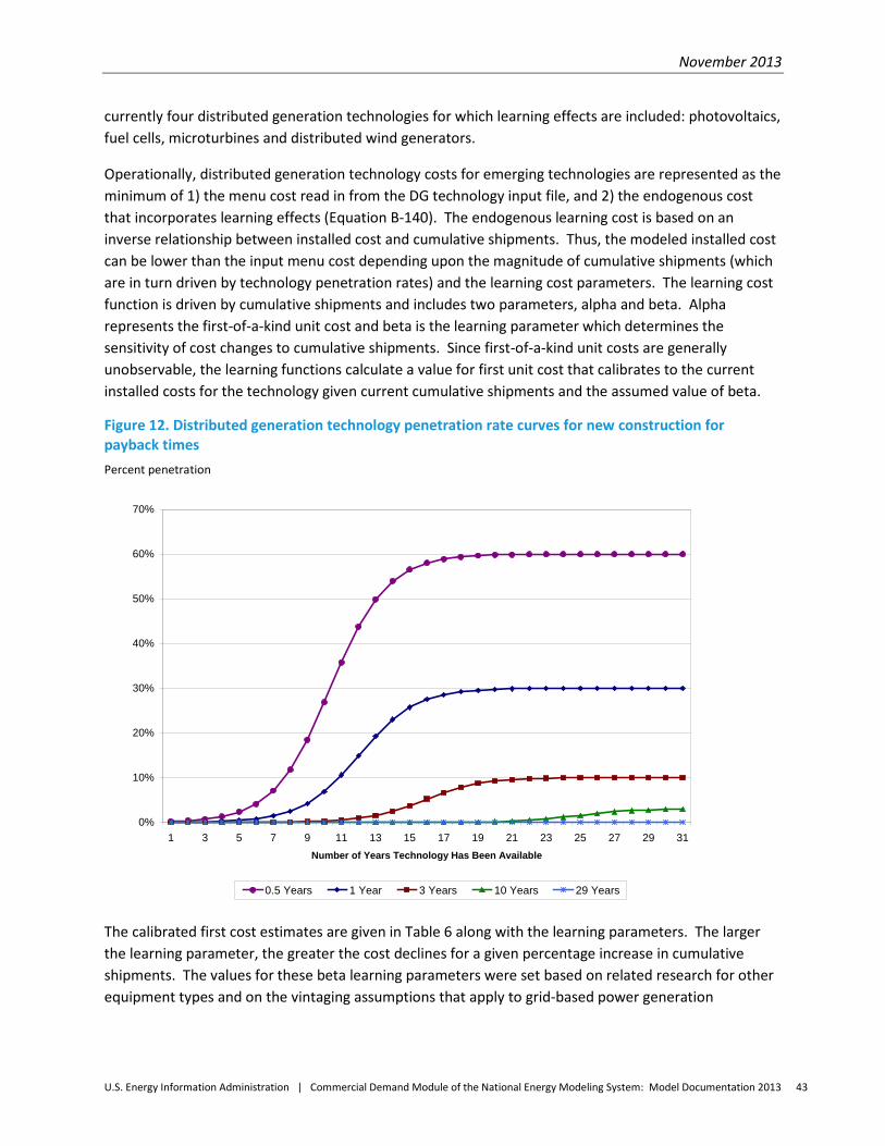
November 2013


currently four distributed generation technologies for which learning effects are included: photovoltaics, fuel cells, microturbines and distributed wind generators.

Operationally, distributed generation technology costs for emerging technologies are represented as the minimum of 1) the menu cost read in from the DG technology input file, and 2) the endogenous cost that incorporates learning effects (Equation B-140). The endogenous learning cost is based on an inverse relationship between installed cost and cumulative shipments. Thus, the modeled installed cost can be lower than the input menu cost depending upon the magnitude of cumulative shipments (which are in turn driven by technology penetration rates) and the learning cost parameters. The learning cost function is driven by cumulative shipments and includes two parameters, alpha and beta. Alpha represents the first-of-a-kind unit cost and beta is the learning parameter which determines the sensitivity of cost changes to cumulative shipments. Since first-of-a-kind unit costs are generally unobservable, the learning functions calculate a value for first unit cost that calibrates to the current installed costs for the technology given current cumulative shipments and the assumed value of beta.

Figure 12. Distributed generation technology penetration rate curves for new construction for payback times Percent penetration

The calibrated first cost estimates are given in Table 6 along with the learning parameters. The larger the learning parameter, the greater the cost declines for a given percentage increase in cumulative shipments. The values for these beta learning parameters were set based on related research for other equipment types and on the vintaging assumptions that apply to grid-based power generation

0%

10%

20%

30%

40%

50%

60%

70%

1 3 5 7 9 11 13 15 17 19 21 23 25 27 29 31Number of Years Technology Has Been Available

0.5 Years 1 Year 3 Years 10 Years 29 Years

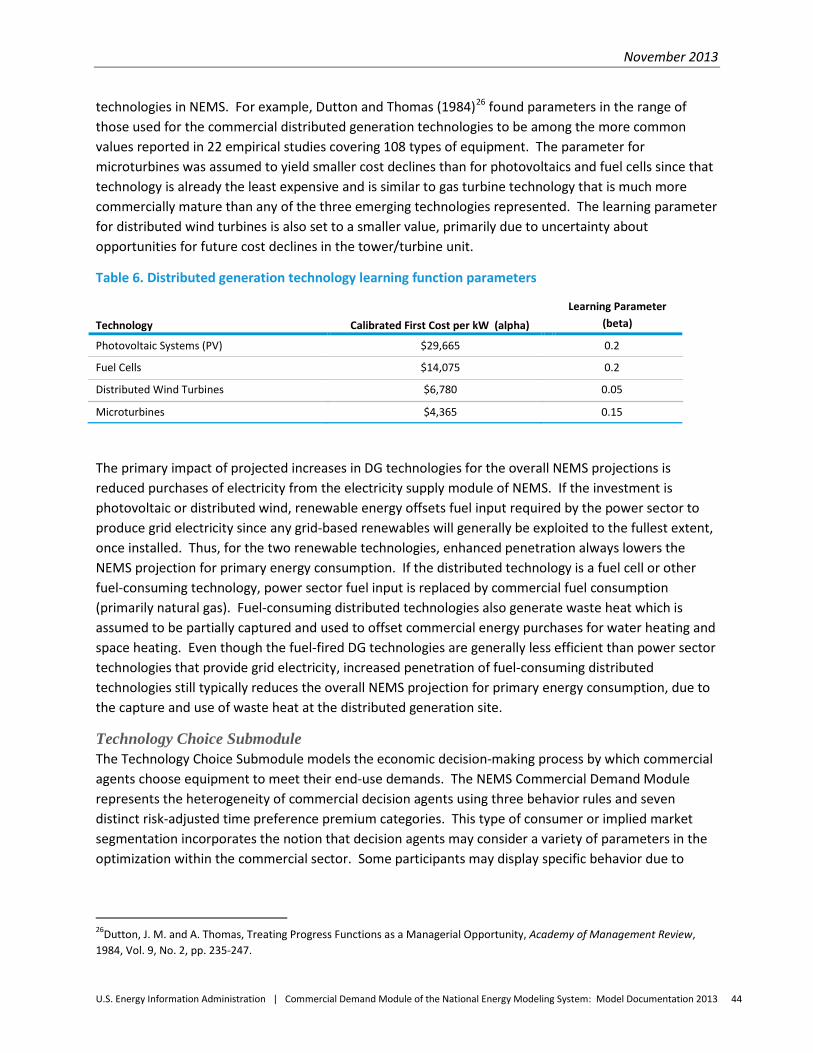
November 2013


technologies in NEMS. For example, Dutton and Thomas (1984)26 found parameters in the range of those used for the commercial distributed generation technologies to be among the more common values reported in 22 empirical studies covering 108 types of equipment. The parameter for microturbines was assumed to yield smaller cost declines than for photovoltaics and fuel cells since that technology is already the least expensive and is similar to gas turbine technology that is much more commercially mature than any of the three emerging technologies represented. The learning parameter for distributed wind turbines is also set to a smaller value, primarily due to uncertainty about opportunities for future cost declines in the tower/turbine unit.

Table 6. Distributed generation technology learning function parameters

The primary impact of projected increases in DG technologies for the overall NEMS projections is reduced purchases of electricity from the electricity supply module of NEMS. If the investment is photovoltaic or distributed wind, renewable energy offsets fuel input required by the power sector to produce grid electricity since any grid-based renewables will generally be exploited to the fullest extent, once installed. Thus, for the two renewable technologies, enhanced penetration always lowers the NEMS projection for primary energy consumption. If the distributed technology is a fuel cell or other fuel-consuming technology, power sector fuel input is replaced by commercial fuel consumption (primarily natural gas). Fuel-consuming distributed technologies also generate waste heat which is assumed to be partially captured and used to offset commercial energy purchases for water heating and space heating. Even though the fuel-fired DG technologies are generally less efficient than power sector technologies that provide grid electricity, increased penetration of fuel-consuming distributed technologies still typically reduces the overall NEMS projection for primary energy consumption, due to the capture and use of waste heat at the distributed generation site.

Technology Choice Submodule The Technology Choice Submodule models the economic decision-making process by which commercial agents choose equipment to meet their end-use demands. The NEMS Commercial Demand Module represents the heterogeneity of commercial decision agents using three behavior rules and seven distinct risk-adjusted time preference premium categories. This type of consumer or implied market segmentation incorporates the notion that decision agents may consider a variety of parameters in the optimization within the commercial sector. Some participants may display specific behavior due to

26Dutton, J. M. and A. Thomas, Treating Progress Functions as a Managerial Opportunity, Academy of Management Review, 1984, Vol. 9, No. 2, pp. 235-247.

Technology Calibrated First Cost per kW (alpha)

Learning Parameter (beta)

Photovoltaic Systems (PV) $29,665 0.2

Fuel Cells $14,075 0.2

Distributed Wind Turbines $6,780 0.05

Microturbines $4,365 0.15

November 2013


existing biases regarding certain equipment types or fuels. In addition, the distribution of risk-adjusted time preference premiums represents a variety of commercial agents' attitudes about the desirability of current versus future expenditures with regard to capital, O&M, and fuel costs. The flexibility of this representational structure allows the module to be calibrated to historic data even if the causal mechanisms determining demand are not fully understood or formally represented within the model structure.

Each one of the above market segments is faced by one of three decisions: 1) to purchase new equipment for new buildings, 2) to purchase replacement equipment for retiring equipment in existing buildings, or 3) to purchase retrofit equipment or retain existing equipment for existing buildings. Within each market segment, the commercial agent will search the available technology menu for the least-cost alternative within the constraints of the applicable behavior rule.

Choosing the least-cost alternative within a market segment involves a tradeoff among capital cost, fuel cost, and operating and maintenance (O&M) cost. In the case of renewable-energy-consuming equipment, costs may also include the cost of backup equipment. The relative importance of each cost component is a function of consumer risk-adjusted time preference. The NEMS Commercial Demand Module sets all other attributes of a technology constant across choices, and these other attributes do not influence the technology choice decision modeled by the algorithm.

Each technology is modeled to preserve a proportional response between capital, fuel and O&M inputs and the service output for these technologies. In addition, the technology costs are represented for comparison in such a way that, for a given total cost, a dollar increase in capital cost must imply more than a dollar decrease in fuel and O&M costs since the dollar spent today for capital is worth more than any future dollar. Therefore, a tradeoff in the form of additional reduction in other costs is necessary in order for the perceived total cost to remain constant. In addition to this tradeoff, this component allows for optional expectations modeling, in that price expectations can be used to determine the acceptable fuel costs over the expected economic lifetime of the equipment.

The algorithm is designed to choose among a discrete set of available technologies for each decision. The Technology Choice Submodule computes an annualized equipment cost per unit of delivered service as the method of weighting the attributes (capital cost, fuel cost, etc.) and developing a composite score for the technology. Technology choice among the alternatives is made based on the minimum annualized cost per unit of service demand (subject to constraints on the set of potential technologies represented by the behavior rules discussed below). The annualized cost represents the discounted flow of all O&M, capital, and fuel costs of the technology over its lifetime. The discount rate is embedded in this annualized cost through a factor that converts the one-time capital and installation costs into an equivalent annuity of equal annual payments over the equipment lifetime. The basic form of the expression for equipment cost used in the Commercial Demand Module is:

𝑎𝑛𝑛𝑢𝑎𝑙𝑖𝑧𝑒𝑑 𝑐𝑜𝑠𝑡𝑢𝑛𝑖𝑡 𝑜𝑓 𝑑𝑒𝑙𝑖𝑣𝑒𝑟𝑒𝑑 𝑠𝑒𝑟𝑣𝑖𝑐𝑒

= (𝑎𝑛𝑛𝑢𝑖𝑡𝑖𝑧𝑒𝑑 𝑝𝑢𝑟𝑐ℎ𝑎𝑠𝑒 & 𝑖𝑛𝑠𝑡𝑎𝑙𝑙𝑎𝑡𝑖𝑜𝑛 𝑜𝑛 𝑐𝑜𝑠𝑡 𝑐𝑜𝑚𝑝𝑜𝑛𝑒𝑛𝑡) (6)

+ (𝑦𝑒𝑎𝑟𝑙𝑦 𝑂 & 𝑀 𝑐𝑜𝑚𝑝𝑜𝑛𝑒𝑛𝑡)

+ (𝑒𝑥𝑝𝑒𝑐𝑡𝑒𝑑 𝑦𝑒𝑎𝑟𝑙𝑦 𝑓𝑢𝑒𝑙 𝑐𝑜𝑠𝑡 𝑐𝑜𝑚𝑝𝑜𝑛𝑒𝑛𝑡)

November 2013


The unit of delivered service referred to above is thousand Btu delivered per hour for all end-use services except lighting and ventilation. The unit of service demand used for lighting is thousand lumens delivered and that used for ventilation is thousand cubic feet per minute of air delivered. Consideration of the building capacity utilization factor is necessary because, unlike the purchase and installation costs, the yearly O&M and fuel costs will vary depending on the intensity of equipment use.

The Commercial Demand Module contains the option to use a cost function to estimate the unit installed capital cost of equipment as a function of time during the interval of equipment availability, rather than limiting technologies to specific models with constant costs during the model years of availability. The choice to enable the cost trend function is specified through the Commercial Module user parameter CostTrendSwitch. Currently, cost trends represented are of logistic functional form and are separated into three categories corresponding to technology maturity: Infant (emerging or future technologies); Adolescent (existing technologies with significant potential for further market penetration and price decline); and Mature (technologies not expected to decline further in cost). The Adolescent and Infant categories require specification of the initial year of price decline, the year of inflection in the price trajectory, the ultimate price reduction as a proportion of initial cost, and a shape parameter, gamma, governing the rate of price decline. The Mature category corresponds to the previous constant-cost representation. The cost trend function specifications are input through the technology characterization file as described in Appendix A. The cost trend function is enabled in the default mode of model operation, although lighting is the only service to use technologies specified as Adolescent or Infant at the current time. The calculation of unit costs using the cost trend function is presented in Equation B-57.

The electricity prices used to develop the annualized fuel costs, in the default mode, are region- and end-use-specific prices developed as weighted averages of time-of-day rates by expected time-of-use patterns. The incorporation of prices relevant to a particular end-use service allows for consideration of varying price and rate structures in the electric power markets, although the regional specification of the EMM and CDM require careful aggregation and weighting in order to represent the complexity of regulatory and business models in today’s markets. Average annual prices by Census division are used to develop the annualized fuel costs for the other major fuels.

In the case of lighting technologies, the yearly fuel cost component includes an adjustment to take lighting output quality into account. The TechCRI factor uses the lighting “color rendering index” (CRI) that characterizes the relative light quality based on the spectrum of natural light output by the particular technology. The adjustment reduces the “effective efficiency” of low-CRI lighting technologies, rendering them less attractive relative to higher CRI options.

The actual calculation of the annualized cost for comparison of candidate technologies is performed using Equation B-62. For decisions regarding space heating and cooling equipment, the calculation includes a shell efficiency load factor, incorporating the effects that building shell improvements have on annual fuel costs for heating and cooling. The shell efficiency factors, illustrated in Equations B-58 and B-59, use the same load factors calculated in the Service Demand Submodule. The effective hurdle (implicit discount) rate used in Equation B-62 is given by Equations B-60 and B-61 and discussed in the section on risk-adjusted time preferences.

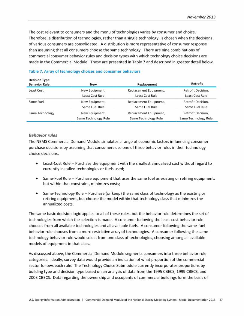
November 2013


The cost relevant to consumers and the menu of technologies varies by consumer and choice. Therefore, a distribution of technologies, rather than a single technology, is chosen when the decisions of various consumers are consolidated. A distribution is more representative of consumer response than assuming that all consumers choose the same technology. There are nine combinations of commercial consumer behavior rules and decision types with which technology choice decisions are made in the Commercial Module. These are presented in Table 7 and described in greater detail below.

Table 7. Array of technology choices and consumer behaviors

Behavior rules The NEMS Commercial Demand Module simulates a range of economic factors influencing consumer purchase decisions by assuming that consumers use one of three behavior rules in their technology choice decisions:

• Least-Cost Rule -- Purchase the equipment with the smallest annualized cost without regard to currently installed technologies or fuels used;

• Same-Fuel Rule -- Purchase equipment that uses the same fuel as existing or retiring equipment, but within that constraint, minimizes costs;

• Same-Technology Rule -- Purchase (or keep) the same class of technology as the existing or retiring equipment, but choose the model within that technology class that minimizes the annualized costs.

The same basic decision logic applies to all of these rules, but the behavior rule determines the set of technologies from which the selection is made. A consumer following the least-cost behavior rule chooses from all available technologies and all available fuels. A consumer following the same-fuel behavior rule chooses from a more restrictive array of technologies. A consumer following the same-technology behavior rule would select from one class of technologies, choosing among all available models of equipment in that class.

As discussed above, the Commercial Demand Module segments consumers into three behavior rule categories. Ideally, survey data would provide an indication of what proportion of the commercial sector follows each rule. The Technology Choice Submodule currently incorporates proportions by building type and decision type based on an analysis of data from the 1995 CBECS, 1999 CBECS, and 2003 CBECS. Data regarding the ownership and occupants of commercial buildings form the basis of

Decision Type: Behavior Rule: New Replacement Retrofit

Least Cost New Equipment, Least Cost Rule

Replacement Equipment, Least Cost Rule

Retrofit Decision, Least Cost Rule

Same Fuel New Equipment, Same Fuel Rule

Replacement Equipment, Same Fuel Rule

Retrofit Decision, Same Fuel Rule

Same Technology New Equipment, Same Technology Rule

Replacement Equipment, Same Technology Rule

Retrofit Decision, Same Technology Rule

November 2013


proportions of the market that act according to each behavior rule for each decision type. Special considerations and interactions between the behavior rules and decision types are described in the section on decision types. The CBECS data are combined with other data characterizing consumer behavior obtained from published literature to develop the behavior rule proportions incorporated in the Module.27 Changing these proportions impacts final consumption estimates.

The supporting data from the 2003 CBECS, including building stock ownership patterns for 2003, are presented in Table 8. The following categories are provided:

• Total Floorspace of All Buildings • Total Floorspace of All Non-government-owned Buildings • Owner Occupied • Non-owner Occupied

Specific ownership categories developed from this data include but are not limited to the following:

• Non-government, Non-owner Occupied, which is the difference between Total Non-government-owned and Non-government Owner Occupied; and

• Government-owned, which is the difference between Total Floorspace and Non-government-owned.

This disaggregation, combined with analysis of consumer behavior literature, results in the behavior rule proportions. The methodology to develop these proportions is described below. The three issues that are examined to determine which behavior rule applies are construction, ownership, and occupancy. Appendix A provides additional documentation and sources for the information in Table 8 and this discussion.

The behavior rule that applies when constructing new buildings is sensitive to the party that is financing the construction. The behavior in selecting equipment in new construction is assumed to differ between those projects that are self-built and those that are built by speculative developers. For each building type, which is the modeled representation of all projects for each region and use, a proportion is assumed to be self-built and developer-built.

The ownership and occupancy of buildings provides some insight into the proportions for the replacement and retrofit decision types. In a replacement decision case, it is assumed that government and owner-occupied buildings will replace most equipment with either the same technology or a technology that uses the same fuel. Owner-occupied floorspace is likely to have similar proportions between same technology and same fuel rules. Renter-occupied floorspace is most likely to simply replace the existing technology with the same technology.

27Further discussion regarding the behavior rule assumptions and specific references for the published literature on consumer behavior is provided in the Appendix E discussion on data quality for user-defined parameters.

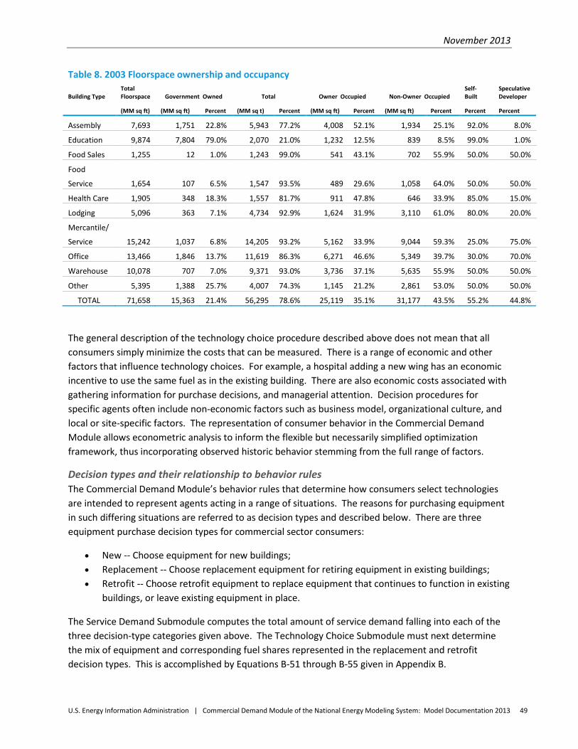
November 2013


Table 8. 2003 Floorspace ownership and occupancy Building Type

Total Floorspace Government Owned Total Owner Occupied Non-Owner Occupied

Self-Built

Speculative Developer

(MM sq ft) (MM sq ft) Percent (MM sq t) Percent (MM sq ft) Percent (MM sq ft) Percent Percent Percent

Assembly 7,693 1,751 22.8% 5,943 77.2% 4,008 52.1% 1,934 25.1% 92.0% 8.0%

Education 9,874 7,804 79.0% 2,070 21.0% 1,232 12.5% 839 8.5% 99.0% 1.0%

Food Sales 1,255 12 1.0% 1,243 99.0% 541 43.1% 702 55.9% 50.0% 50.0%

Food

Service

1,654

107

6.5%

1,547

93.5%

489

29.6%

1,058

64.0%

50.0%

50.0%

Health Care 1,905 348 18.3% 1,557 81.7% 911 47.8% 646 33.9% 85.0% 15.0%

Lodging 5,096 363 7.1% 4,734 92.9% 1,624 31.9% 3,110 61.0% 80.0% 20.0%

Mercantile/

Service

15,242

1,037

6.8%

14,205

93.2%

5,162

33.9%

9,044

59.3%

25.0%

75.0%

Office 13,466 1,846 13.7% 11,619 86.3% 6,271 46.6% 5,349 39.7% 30.0% 70.0%

Warehouse 10,078 707 7.0% 9,371 93.0% 3,736 37.1% 5,635 55.9% 50.0% 50.0%

Other 5,395 1,388 25.7% 4,007 74.3% 1,145 21.2% 2,861 53.0% 50.0% 50.0%

TOTAL 71,658 15,363 21.4% 56,295 78.6% 25,119 35.1% 31,177 43.5% 55.2% 44.8%

The general description of the technology choice procedure described above does not mean that all consumers simply minimize the costs that can be measured. There is a range of economic and other factors that influence technology choices. For example, a hospital adding a new wing has an economic incentive to use the same fuel as in the existing building. There are also economic costs associated with gathering information for purchase decisions, and managerial attention. Decision procedures for specific agents often include non-economic factors such as business model, organizational culture, and local or site-specific factors. The representation of consumer behavior in the Commercial Demand Module allows econometric analysis to inform the flexible but necessarily simplified optimization framework, thus incorporating observed historic behavior stemming from the full range of factors.

Decision types and their relationship to behavior rules The Commercial Demand Module’s behavior rules that determine how consumers select technologies are intended to represent agents acting in a range of situations. The reasons for purchasing equipment in such differing situations are referred to as decision types and described below. There are three equipment purchase decision types for commercial sector consumers:

• New -- Choose equipment for new buildings; • Replacement -- Choose replacement equipment for retiring equipment in existing buildings; • Retrofit -- Choose retrofit equipment to replace equipment that continues to function in existing

buildings, or leave existing equipment in place.

The Service Demand Submodule computes the total amount of service demand falling into each of the three decision-type categories given above. The Technology Choice Submodule must next determine the mix of equipment and corresponding fuel shares represented in the replacement and retrofit decision types. This is accomplished by Equations B-51 through B-55 given in Appendix B.

November 2013


For new buildings, consumers using the least-cost behavior rule choose from among all current technologies and all fuels. Identification of the least-cost equipment from the perspective of each consumer time preference segment is made in two stages. Identification of the least-cost fuel is made in stage 1 using Equation B-65 with the unadjusted distribution of hurdle rates as indicated in Equation B-60. Stage 2 of the least-cost behavior decision evaluates Equation B-66 from among technologies that use the same fuel as chosen in stage 1 with effective hurdle rates that adjust with increasing real energy costs as discussed in the section on risk-adjusted time preferences. Consumers using the same fuel behavior rule choose from among current technologies that use the same fuel as surviving buildings (buildings that do not retire). Identification of the least-cost equipment for each fuel from the perspective of each consumer risk-adjusted time preference segment is made using Equation B-67. Proportions of consumers in this category who choose each fuel are assumed to equal the overall fuel shares that prevailed in existing buildings during the previous year, which is reflected in the individual terms of Equation B-70. Similarly, the identification of least-cost models for each technology for the consumers following the same technology rule is illustrated by Equation B-68. As with the same-fuel rule, the proportions of consumers within this segment that stick with each particular technology class is assumed to equal the overall market share distribution of those technologies within existing buildings during the previous year, as reflected in the individual terms of Equation B-72.

For equipment replacement decisions, consumers using the least-cost behavior rule choose from among all current technologies in two stages, as described for new buildings and illustrated by Equations B-65 and B-66. Consumers using the same-fuel behavior rule choose from among current technologies which use the same fuel as was used by the retiring equipment. The proportions of consumers within the same-fuel rule attempting to preserve the use of each fuel are equal to the fuel shares represented in aggregate by the equipment in need of replacement, as reflected in the individual terms of Equation B-71. Consumers using the same-technology behavior rule choose the least costly vintage of the same technology as the technology in need of replacement. As with the same-fuel rule, the proportions of consumers within the same-technology category attempting to retain equipment within each technology class are equal to the market shares of retiring equipment classes within the aggregate service demand in need of replacement, as reflected in the individual terms of the right side of Equation B-73.

For the retrofit decision, which involves the choice between retaining equipment that continues to function and replacing it with new equipment in order to reduce costs, the costs of purchasing new equipment as described above must be compared against the cost of retaining existing equipment. In order to make this comparison, the existing equipment capital costs are considered sunk costs, meaning that these costs are set to zero. If retrofit equipment is purchased, the decision maker must pay the capital and installation costs of both the existing equipment and the retrofit equipment. If existing equipment is retained, the decision maker continues to pay just the capital and installation costs of the existing equipment. Therefore, the capital and installation costs of existing equipment are netted out, because it is irrelevant to the retrofit decision (this analysis assumes zero salvage value for existing equipment). The cost calculation is similar to that illustrated by Equation 6 above, except without the

November 2013


purchase and installation component. However, the cost of removing and disposing of existing equipment must be considered. This cost is expressed in the Commercial Demand Module technology characterization database as a specified fraction of the original purchase and installation cost, and is annualized over the equipment lifetime. The resulting calculation of the annualized cost of retaining the existing equipment is given by Equation B-76. As in the calculation of the annualized cost of new equipment, the annualized cost of retaining existing space heating or cooling equipment includes the shell efficiency factors illustrated in Equations B-58 and B-59, incorporating the effects that building shell improvements have on fuel costs, and the effective hurdle rate given in Equations B-60 and B-61.

For the equipment retrofit decision, consumers using the least-cost behavior rule choose from among all current technologies in two stages as described for new buildings, comparing the cost of each as expressed by Equations B-62 and B-63 against the cost of retaining the existing equipment as expressed by Equation B-76, and choosing the least-cost result, as illustrated by Equations B-77 and B-78. Consumers using the same-fuel behavior rule choose from among current technologies, which use the same fuel as is currently used by the existing equipment, again comparing the cost of each against the cost of retaining the existing equipment, and choosing the least costly alternative, as indicated by Equation B-79. Two options are available in the Commercial Demand Module to represent the choice behavior of consumers using the same-technology behavior rule for the equipment retrofit decision. One option, used in the AEO2013 reference case, is to allow selection from among available models in the same technology class, comparing the cost of each against the cost of retaining the existing equipment, and choosing the least costly alternative, as illustrated by Equation B-80. Alternatively, all consumers using the same technology behavior rule may be assumed to retain their existing equipment, as indicated by Equation B-83. The choice of methods is specified through the Commercial Module user parameter named STRetBehav.

The equipment selections made for each of the decision types and behavior rules described above will vary according to the risk-adjusted time preference held by the consumer. These risk-adjusted time preferences are discussed below in preparation for the description of consolidation of equipment choices to obtain the final equipment market shares.

Risk-adjusted time preferences This distribution is a function of factors aside from the market interest rate that render current dollars preferable to future dollars. The Commercial Demand Module is designed to accept a distribution of risk-adjusted time preferences as input. This is a discrete distribution; it takes the form of a list of real risk-adjusted time preferences, and a proportion of commercial consumers corresponding to each risk-adjusted time preference.28 The risk-adjusted time preference distribution is modeled independently of

28 There is a substantial literature that attempts to explain why consumers (in the general sense of the word including businesses) choose not to invest in energy-efficient equipment that seems to make economic sense at prevailing market interest rates. Conceptual explanations have included uncertainty about future energy prices, lack of information regarding the performance and cost of particular types of energy-efficient equipment, disruption costs for businesses, energy costs’ typically small share of commercial business expenses, competing investments considered more important than efficiency, and uncertainty about future technologies (buying too soon may “lock in” to a less-efficient technology). For a review of these issues see Chapter 4 of Gillingham K., R. Newell and K. Palmer (2009). "Energy Efficiency Economics and Policy" Annual Review of Resource Economics 2009.1: 597-619.

November 2013


the behavior rules. The risk-adjusted time preference, which appears as an interest rate premium, is intended to reflect differences in consumer preferences between capital costs (paid initially) and fuel and O&M costs (incurred over the lifetime of the equipment). The value of this interest rate premium influences the annualized installed capital cost through an annuity payment financial factor based on the 10-year Treasury note rate, the risk-adjusted time preference premium, and expected physical equipment lifetime. The sum of the 10-year Treasury note rate and the consumer risk-adjusted time preference premium is referred to as the implicit discount rate, i.e., the interest rate required to reflect actual purchases. The implicit discount rate is also known as a hurdle rate to emphasize consideration of all factors, both financial and nonfinancial, that affect an equipment purchase decision. The combination of these factors results in the height of the “hurdle” for the purchase decision.

The model results are sensitive to the distribution of the risk-adjusted time preference premiums. If the distribution is denser at the high premiums, the annualized cost of capital for all new equipment will rise. Higher annualized capital cost implies that fewer buildings will be retrofitted and that equipment that has a higher installed capital cost is less likely to be chosen over a technology with a lower initial cost and higher operating and fuel costs. Typically, those technology and vintage combinations with high installed capital costs are high-efficiency pieces of equipment, so that the indirect effect of this scenario is that fuel consumption is likely to be higher. The values currently used in the Commercial Demand Module have been developed using case studies on the payback period or risk-adjusted time preferences regarding the adoption of a specific technology and recent surveys that examine perceptions of energy efficiency and green building practices.29 The model allows variation in the distribution on an annual basis to accommodate simulation of policy scenarios targeting consumers’ hurdle (or implicit discount) rates. For AEO2013 the distribution of consumer risk-adjusted time preference premiums includes adjustments to reflect recent legislation affecting federal purchasing requirements, to account for funding provided in ARRA09, and to incorporate survey findings. The distribution is assumed constant over the projection horizon after 2013.30 The module currently uses expected physical equipment lifetime as the discount horizon. Appendix A provides additional documentation and sources for the distribution of risk-adjusted time preference premiums.

The distribution of hurdle rates used in the Commercial Module is affected by changes in fuel prices in addition to any annual changes input by the model user. If a fuel price rises relative to its price in the base year (2003), the nonfinancial portion of each hurdle rate in the distribution decreases to reflect an increase in the relative importance of fuel costs, expected in an environment of rising fuel prices. The function representing the fuel price effects on hurdle rates is given by Equations B-60 and B-61. Parameter assumptions for AEO2013 result in a 30-percent reduction in the nonfinancial portion of a

29 Results of surveys conducted by Johnson Controls and Building Design+Construction were considered. See Appendix A for reference information and Appendix E for a more detailed discussion of hurdle rate development. 30EPACT05 and EISA07 update energy intensity reduction goals and performance standards for Federal buildings. EISA07 also mandates use of energy-efficient lighting fixtures and bulbs in Federal buildings to the maximum extent feasible. ARRA09 stimulus funding is assumed to affect purchasing decisions for State and local governments and for Federal agencies. The discussion of the distribution of risk-adjusted time preference premiums in Appendix A addresses the adjustment to the assumed proportion of consumers using specific time preferences to capture the Federal purchasing requirements and effects of stimulus funding due to these provisions.

November 2013


hurdle rate with a doubling of fuel prices, down to a total hurdle rate of 15 percent, the assumed financial discount rate. If the risk-adjusted time preference premium input by the model user results in a hurdle rate below 15 percent with base year fuel prices, no response to increasing fuel prices is assumed.

Consolidate choices from segments Once the technology choices have been made for each segment represented for a given end-use service, these choices must be consolidated in order to obtain equipment market shares by building type, Census division, and decision type for the end use. From these market shares, average efficiencies of the equipment mix and fuel shares may be obtained, which form the basis of the Consumption Submodule calculated fuel consumption.

The first step in consolidation involves combining the results obtained from the perspective of each consumer risk-adjusted time preference segment to calculate market shares of equipment within each behavior rule segment of each decision type. Since a given risk-adjusted time preference segment makes only one equipment selection for a given decision type and behavior rule, the market share of a given equipment type is computed for that decision type and behavior rule segment by simply adding up the proportions of consumers contained in each risk-adjusted time preference segment that selected the equipment. This is the calculation performed by Equations B-69 through B-73 and B-81 through B-83, with the factors associated with same fuel and same technology proportions described previously.

The next step in the consolidation process is to calculate the market shares of equipment within each decision type, consolidated across the behavior rule segments. This is done using Equations B-74, B-75, and B-84 to obtain equipment market shares for the new, replacement, and retrofit decisions, respectively. This and the previously-described consolidation may be viewed as weighted sums, using as weights the quantities described in Table 9.

After this point, all equipment used to provide the major services receives identical treatment, but the calculation of equipment market shares described above differs for the case of heat pumps and deserves separate mention. The purchase decision for heat pumps integrates decisions for providing both space heating and space cooling, because selection of the same heat pump for two services is not realistically accomplished using two independent decisions. Furthermore, if the utility of the heat pump for providing additional services is not considered during the purchase decision, then the total heat pump cost may appear unreasonably high in comparison with other equipment providing the service under consideration. Both of these considerations have been resolved in the current version of the Commercial Module using the following approach:

Table 9. Consolidating service demand segments

Segmenting Variable Weighting Variable for Consolidating Segments

Behavior rule Behavior rule service demand proportions

Consumer’s time value of money preference Consumer risk-adjusted time preference proportions

November 2013


First, heat pumps are assumed to provide both space heating and cooling when purchased, but are considered for purchase during the course of satisfying demands for space heating. Heat pumps compete with other available space heating equipment in the normal fashion during the technology choice process with one notable exception: the installed capital cost of the heat pump for heating is not the total cost of purchasing and installing the heat pump, but rather the incremental cost of doing so over and above the cost of purchasing and installing a standard cooling equipment selection specified by the user. This captures the fact that the heat pump provides both space heating and space cooling, yet has only one purchase and installation cost. This adjustment to the installed capital cost retrieved from the technology characterization database is performed using Equation B-56.

During the technology choice process for satisfying space cooling service demands, heat pumps are excluded from selection due to the assumption that heat pumps will provide both space heating and cooling. Instead, market shares of cooling service demand satisfied by heat pumps are derived from the heat pumps selected to provide space heating. This is accomplished by assuming that the ratio of cooling to heating delivered by a heat pump over the course of the year is equal to the ratio of cooling degree days to heating degree days for the Census division under consideration. From this assumption, the amount of cooling service demand satisfied by heat pumps is calculated, and hence their market shares of cooling service demand. This calculation is performed by Equation B-85. In order to account for the fact that equipment shares of cooling equipment other than heat pumps apply only to that portion of cooling service demand not satisfied by heat pumps, a final correction of the non-heat pump market shares is then performed by Equations B-86 through B-88.

Fuel shares of service demand for the major services and fuels are calculated by summing the equipment market shares of service demand of equipment using a given fuel. This is the calculation performed by Equation B-89 within the decision type segments by end use, fuel type, building type, and Census division, and by Equation B-91 consolidated across decision types. Equations B-97 through B-99 calculate the fuel shares by decision type, end use, fuel type, and Census division consolidated across building type.

Average efficiencies of the equipment mixes within various segments are calculated using the inverse weighted efficiency approach exhibited by Equations B-90, B-93 through B-96, and nationally by end use and fuel using Equation B-100. The particular form of the averaging is necessary because efficiencies possess units of delivered to consumed energy, whereas the equipment market shares used as weights are proportions of delivered energy. Only if the equipment market shares were expressed as proportions of consumed energy would the average efficiency of the equipment mix be obtained using a simple weighted sum of market shares and corresponding efficiencies.

Finally, fuel shares and average efficiencies are determined for the minor services, without consideration of individual equipment choices given to the major services. As described previously, the 2003 average efficiencies for the minor services are indexed to unity. The user may provide an exogenous projection of minor service efficiency improvement for any of the minor services via the EffGrowthRate parameter described in Appendix A. With this option, minor service average efficiency for the current year is calculated from the value for the previous year. The exogenously-specified efficiency growth rate is shown in Equation B-101. Projected changes in PC and other office equipment

November 2013


energy consumption are explicitly included in the PC and other office equipment projections described in Appendix A under Market Penetration, so the EffGrowthRate is set to zero for the both office equipment end-use services. Expected efficiency improvements are also explicitly included in the trend projections for specific categories within miscellaneous end-use loads (MELs). Efficiency improvement for the non-specific portions of MELs is set to zero due to lack of information. However, the option remains available to facilitate analysis of programs aimed at improving efficiency in this area. Minor services are further assumed to possess identical average efficiencies for all decision types and buildings within a given Census division and year, and office equipment services are assumed to use only electricity, as illustrated by Equation B-102.

Technology menu The technology cost and performance assumptions used in the calculations of consumer choice are organized into a “technology menu.” There is a wide range of relevant characteristics that are used in the Commercial Demand Module, many of which are exogenously or user-specified. The following set of parameters is specified exogenously: equipment availability, installed capital costs, removal and disposal cost proportions of installed capital costs, operating and maintenance costs, building restrictions, energy efficiencies, lifetimes, lighting quality factors, and technology cost trends.

Equipment availability pertains to the set of technologies currently in the marketplace during a particular projection year; not all available technologies are economically feasible, and therefore may not be selected. The menu of potential technologies includes technologies that are currently under development to be introduced over the projection period. Equipment supply is assumed to be unlimited for commercially available technologies, with unit costs either fixed or declining according to the appropriate cost trend function. The other equipment characteristics are assumed fixed for a given technology and vintage once it is commercially available.

For the case of certain prototypical or “design-stage” technologies currently not available in the marketplace (or currently not in production), engineering specifications form the basis of the technology characterization. These costs may differ markedly from the actual technology costs when the equipment is introduced to the real-world marketplace.

The 2003 initial historical market shares are based on an analysis of CBECS 2003 data. The years of equipment availability are based on current market conditions and research as well as mandated federal efficiency standards. This window in which each technology vintage is available constrains the technology choice menu for all decision types. For example, a commercial refrigerated vending machine available in 2010 may no longer be available in 2013 due to federally mandated minimum equipment efficiency standards.

An option to allow endogenous price-induced technology change has been included in the determination of equipment costs and availability for the menu of equipment. This concept allows future technology improvements faster diffusion into the marketplace if fuel prices increase markedly for a sustained period of time. The option is activated through the setting of a Commercial Module user parameter named IFMAX which governs the maximum number of years the availability of a technology vintage can potentially be shifted forward. The formulation only works in one direction; i.e., equipment

November 2013


can only be shifted toward earlier availability, and once shifted, a vintage will not be shifted back to its original availability date. In addition, shifts are limited to a lesser number of years for nearer-term technology vintages (e.g., those projected for 2013) to ensure that future improvements cannot become available before the persistent price change is projected to occur. Equations B-103 through B-105 illustrate the calculations needed to move an availability date forward through price-induced technology change. The parameter was set to 0 years for the AEO2013 model runs, effectively assuming there would be no endogenous change.

End-Use Consumption Submodule The End-Use Consumption Submodule models the consumption of fuels to satisfy the demands for end-use services computed in the Service Demand Submodule. Additionally, the End-Use Consumption Submodule projects the consumption of fuels to provide district energy services in the commercial sector, accounts for the net effects of distributed generation and CHP on fuel consumption, and accounts for the use of solar thermal energy to provide space heating and water heating.

The primary inputs to the End-Use Consumption Module are the service demands calculated by the Service Demand Submodule, and the fuel shares and average efficiencies projected by the Technology Choice Submodule. Together, these quantities allow a basic calculation to be made for consumption of the major fuels that has the same form for both the major and minor services. This calculation, given by Equation B-106, makes use of the definition of average efficiency to obtain the projected consumption by fuel, end use, building type, Census division and year, by simply dividing that portion of the end-use service satisfied by a given fuel by the average efficiency of equipment using that fuel. A value of zero for the average efficiency indicates that no equipment consuming the given fuel is used to satisfy the service, and in this case the corresponding consumption projection is explicitly set to zero. Because the units carried for lighting service demand and efficacy differ from those of the other services, a special conversion factor must be applied to the lighting result, as shown by Equation B-107.

The basic estimate of fuel consumption described above is that projected to occur if all conditions other than the amount of floorspace, the building shell efficiency, and the equipment mix were identical to those found in the base year (2003), and consumers were only concerned with fuel prices insofar as they impacted equipment purchase decisions. Since conditions other than those mentioned above vary with time, and because consumers are also concerned with fuel prices when using the equipment they have purchased, the basic estimate is subject to modification by several considerations.

First, a price elasticity of service demand may alter the consumer's demand for a service as a result of a change in the fuel price. As an example, an increase in the price of distillate heating oil may cause the consumer to maintain the floorspace at a somewhat cooler temperature in the winter than would have been the case without a price increase. While this consideration should logically be made where service demands are calculated in the Service Demand Submodule, it is not possible at that point because the mix of equipment using each fuel is not calculated until the Technology Choice Submodule has completed its projection. However, the calculation is easily made by the End-Use Consumption Submodule because of the direct proportionality between service demand and fuel consumption, as can be seen in Equation B-106; that is, a percentage change in service demand corresponds to the same percentage change in fuel consumption. The highly aggregated nature of the service demand as

November 2013


modeled at the regional geographic scale further enables this approach. The actual units of demand are not subject to the strong economies of scale which can induce threshold effects in sectors, such as electric power supply, in which “lumpy capital” can produce a suboptimal investment path when demand changes by a small amount after technology is chosen. The calculation of the short-run price elasticity of demand incorporates a graduated or “lagged” adjustment that allows the degree of consumer response to vary with significant changes in fuel prices. Equation B-108 illustrates the function used to calculate the short-run elasticity adjustment. The first term in Equation B-109 shows the application of the short-run price elasticity of demand to modify the basic consumption estimate obtained by Equation B-106.

Another consideration that affects the consumer's demand for services is known as the “take-back” or “rebound” effect. While fuel price increases can be expected to reduce demand for services, this can be partially offset by other factors that cause a decrease in the marginal cost of providing the service. Two such factors modeled by the End-Use Consumption Submodule are the responses to increased average equipment efficiency and improved building shell efficiency. The proportional change in the marginal cost of service provision due to movement in each of the aforementioned factors relative to their base year values is calculated and combined with a modified price elasticity of service demand parameter to yield the computed effect on fuel consumption, as shown by the second and third terms of Equation B-109. Because these modifications to the basic consumption estimate are each multiplicative, Equation B-109 is capable of accommodating independent changes in each of the underlying driver variables (fuel price, average equipment efficiency, and building shell efficiency) regardless of the directions of movement. While the rebound effect due to equipment efficiency improvement is considered for the end-use services of space heating, space cooling, water heating, ventilation, cooking, and lighting, the effect due to building shell improvement is considered only for space heating and space cooling. The equipment and building shell efficiency rebound elasticity parameters currently included in the Commercial Module are set to -0.15 for these services.31

A final modification to the basic estimate of fuel consumption is made in the form of a weather correction, which accounts for known weather abnormalities during historical years of the projection period, and differences between the base year (2003) weather and weather trends anticipated in future years. The basis for the weather correction is the number of population-weighted heating and cooling degree days by Census division and short-term forecasts available from the National Oceanic and Atmospheric Administration (NOAA), as noted in the KDEGDAY input file. Values through the end of the AEO projection are assumed to exhibit a 30-year linear trend for the number of population-weighted heating and cooling degree days by Census division. The 30-year linear trend is adjusted over the projection period to account for state population shifts. Because 2003 is the base year for the key Commercial Module parameters, the basic projection for consumption in other years to provide space heating and space cooling is modified by considering the heating and cooling requirements in that year relative to those prevailing in 2003. This is accomplished for heating consumption using a multiplicative

31The current parameter values for the rebound effect are within the range of short-run empirical responses found for firms as presented in the literature review by Greening, Greene, and Difiglio in a special issue of the journal Energy Policy. See Greening, L.A., D.L. Greene, and C. Difiglio, Energy efficiency and consumption - the rebound effect - a survey, Energy Policy, Vol. 28, Nos. 6-7 (June 2000), pp. 389-401.

November 2013


factor equal to the ratio of the appropriate degree days, as shown by Equation B-110. Equation B-111 illustrates the weather correction for space cooling requirements, including an exponential term to reflect the non-linear relationship between weather and cooling requirements.

Applying the price elasticity and rebound effect considerations, together with the weather correction, to the basic estimate of fuel consumption by end use provides an enhanced projection of demand for the major fuels of electricity, natural gas, and distillate fuel oil by equipment directly satisfying the 10 basic end-use services. Consumption of the minor fuels of residual oil, liquid petroleum gas, steam coal, motor gasoline, and kerosene is calculated using a different approach, as is consumption for purposes not yet explicitly modeled. These include consumption to provide district energy services and “non-building” consumption (consumption in the commercial sector not attributable to end uses within buildings, such as street lighting and municipal water services).

Consumption of minor fuels is projected from historical Census division-level consumption, floorspace, and pricing data using double-log regression equations. The regression parameters are obtained from the correlation of minor fuel consumption per square foot of commercial floorspace with respect to the corresponding fuel price in constant dollars with time-specific dummy variables (Equation B-125). Two time-specific dummy variables are included to capture the structural shifts from 1970 to 1985 and from 1985 to 1999. For coal, a pooled regression model is estimated. In addition to price and time dummy variables, eight regional dummy variables are also included as explanatory variables. The minor fuel regression parameters were developed using historical Census division-level minor fuel consumption and pricing data from the State Energy Data System, which spans the 38-year period from 1970 to 2008, and the McGraw-Hill Construction (MHC) floorspace database.32 Finally, the estimated parameters are applied to project minor fuel energy use intensity (EUI). The MHC floorspace estimates are benchmarked to floorspace estimates from CBECS by multiplying the EUI by Census division-level floorspace adjustment factors (2003 MHC floorspace/2003 CBECS floorspace). This adjusted EUI is multiplied by projected commercial floorspace to produce projected minor fuel consumption. For coal, floorspace is held at the 2005 level over the projection period (Equation B-125).

The End-Use Consumption Submodule also accounts for nonutility generation of electricity by the commercial sector using distributed generation and CHP technologies, together with the quantities of fuels consumed to accomplish electricity generation and CHP as described in the Distributed Generation and CHP section. End-use consumption of purchased electricity is reduced as given by Equations B-112 through B-114 to reflect the use of self-generated electricity. Equation B-115 calculates reduction in space and water heating consumption through use of heat generated by CHP technologies. Equation B-116 accounts for fuel consumption by distributed generation and CHP technologies.

32An autoregressive error model with one- or two-year lag is estimated to correct for autocorrelation problems. We used the MHC historical floorspace data for estimation of minor fuel parameters since CBECS did not provide enough data to estimate the model. CBECS surveys were conducted triennially between 1979 and 1995, and quadrennially between 1995 and 2007. The MHC database is proprietary.

November 2013


The final component of the End-Use Consumption Submodule is an estimation of the quantities of fuel consumed in order to provide the district energy services of space heating, space cooling, and water heating. District energy services involve the localized production of steam energy that is used to provide distributed end-use services over a wide area, such as a campus environment. Estimates of the steam EUI by Census division, building type, and end-use service for district energy services were prepared separately from those previously described for the standard end-use services. These are used in conjunction with typical efficiencies and Census division-level fuel shares for the systems providing district energy services, together with the floorspace projection, to produce the projection of fuel consumption for district energy services, as shown by Equation B-117. Price elasticity considerations and the weather correction are applied to district energy services fuel consumption in the same manner as they are applied to direct fuel use for end-use services as shown by Equation B-118.

The consumption projection by Census division, fuel, end-use service, and building type is incremented by the district energy service consumption estimate just described, as shown by Equation B-120. Aggregation of this result across end-use services and building types yields the projection of fuel consumption by fuel and year at the Census division level required by the other NEMS modules, as shown by Equation B-127. Another aggregation across fuels and Census divisions is performed to obtain the national-level projection of total energy consumption by building type, to which is added the use of solar thermal energy for space heating and water heating and solar energy for electricity generation by photovoltaic systems, as shown by Equation B-128. Additional results are also aggregated in various ways to satisfy reporting requirements, as illustrated by the End-Use Consumption equations not discussed. One final consumption component, representing non-building consumption, is calculated in the Benchmarking Submodule, described in the next section.

Benchmarking Submodule The Benchmarking Submodule reconciles the fuel consumption projection produced by the End-Use Consumption Submodule with data from the State Energy Data System (SEDS). SEDS contains historical fuel consumption data chosen to serve as a standard for the NEMS system over the historical period of the projection. Additionally, the Benchmarking Submodule provides an option for considering results from EIA’s Annual Energy Review (AER) and Short-Term Energy Outlook (STEO) for the near term immediately beyond the last year of SEDS data availability. Definitional differences between SEDS and CBECS, upon which the Commercial Sector Module is based, are used to construct a projection of commercial sector fuel consumption not attributable to end uses within buildings.

Equation B-129 illustrates the calculation of the “SEDS mistie,” or discrepancy between the End-Use Consumption Submodule results and SEDS data, during years for which SEDS data exist. Because SEDS data are estimates of all consumption by the commercial sector, whereas CBECS applies only to consumption within commercial buildings, the difference between the End-Use Consumption Submodule’s CBECS-based fuel consumption projection and the SEDS data is attributed to fuel consumption for non-building uses, as shown by Equation B-130. This assignment is performed for each year of the projection period for which SEDS data are available. The use of the SEDS data through the year indexed as MSEDYR+1 in these calculations reflects the fact that the AER provides reliable estimates of consumption data for an additional year beyond the latest published SEDS results, and these estimates are used in the same manner as published SEDS data.

November 2013


After the final year of SEDS data availability, electricity consumption for non-building uses is projected to grow at the same rate as commercial floorspace. This expectation follows from the observation that, while not representing fuel consumption within buildings, the non-building uses are generally associated with commercial buildings or activities, as in the case of exterior lighting of parking lots. The projection of SEDS-based consumption of electricity for non-building uses beyond the last year of SEDS data availability is shown by Equation B-132. The projection of electricity use for municipal water services as a component of non-building uses is illustrated in Equations B-133 through B-135. Non-building use of natural gas, distillate and minor fuels is not expected to grow at the same rate as commercial floorspace, but instead to remain at a relatively constant level, as illustrated by Equation B-137.

The Commercial Demand Module includes an option to activate benchmarking to that portion of the STEO projection immediately following the last year of historical data. This is accomplished through the setting of a NEMS system-wide parameter named STEOBM and a Commercial Module user parameter named ComSTEOBM. Both parameters must be set to activate benchmarking to the STEO projection. If selected, the benchmarking is incremental; that is, it is calculated based on the projection produced after benchmarking to SEDS. For years covered by the short-term STEO projection, the calculation of the discrepancy between the SEDS-benchmarked projection and STEO is given by Equation B-131 for electricity. Equation B-136 gives the corresponding calculation for natural gas, distillate and minor fuels. An additional option limits STEO benchmarking adjustments to result in fuel use projections that are within 2 percent of the STEO projections, as illustrated in Equation B-138. Equation B-139 shows the addition of the STEO-based incremental component of non-building consumption to the component based on SEDS.

In the event the STEO benchmarking option is chosen, one of two options for avoiding a discontinuity in the benchmarked projection beyond the last year of STEO data must also be selected. The simplest option is to retain the STEO component of non-building use calculated for the last year of STEO data availability, and apply it to the projections for all future years. Alternatively, the STEO component of non-building use can be ramped down to zero over a specified time period following the last year of STEO data. The choice of methods is specified through the Commercial Module user parameter named DecayBM. Calculation of a time-dependent decay factor based on the selection of the various options is illustrated by Equation B-140. Equation B-141 illustrates the optional addition of a STEO-based component of non-building consumption to that based on SEDS, for projection years after the final year of STEO data availability. For AEO2013, the option to benchmark through year 2012 to the STEO projection was chosen with the STEO component of non-building use ramped down to zero by 2015.

Addition of the projection of fuel consumption for non-building uses to that produced by the End-Use Consumption Submodule for end uses within buildings completes the projection of commercial sector fuel consumption, as shown by Equation B-142.

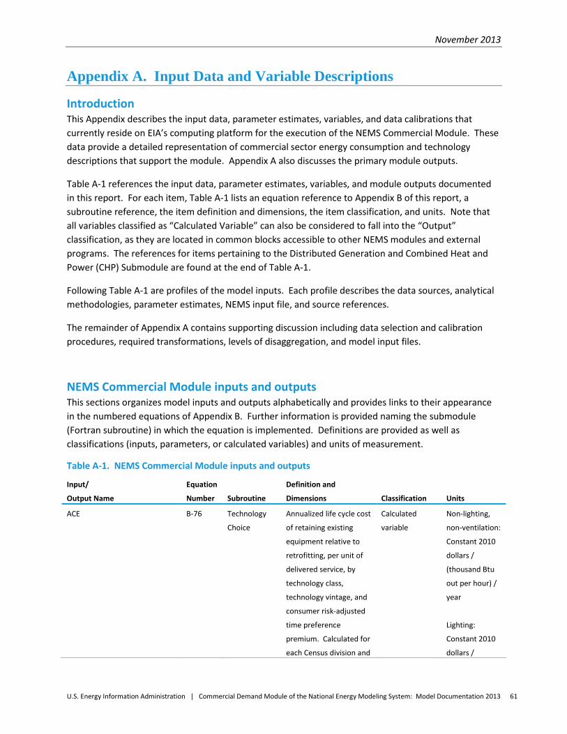
November 2013


Appendix A. Input Data and Variable Descriptions

Introduction This Appendix describes the input data, parameter estimates, variables, and data calibrations that currently reside on EIA’s computing platform for the execution of the NEMS Commercial Module. These data provide a detailed representation of commercial sector energy consumption and technology descriptions that support the module. Appendix A also discusses the primary module outputs.

Table A-1 references the input data, parameter estimates, variables, and module outputs documented in this report. For each item, Table A-1 lists an equation reference to Appendix B of this report, a subroutine reference, the item definition and dimensions, the item classification, and units. Note that all variables classified as “Calculated Variable” can also be considered to fall into the “Output” classification, as they are located in common blocks accessible to other NEMS modules and external programs. The references for items pertaining to the Distributed Generation and Combined Heat and Power (CHP) Submodule are found at the end of Table A-1.

Following Table A-1 are profiles of the model inputs. Each profile describes the data sources, analytical methodologies, parameter estimates, NEMS input file, and source references.

The remainder of Appendix A contains supporting discussion including data selection and calibration procedures, required transformations, levels of disaggregation, and model input files.

NEMS Commercial Module inputs and outputs This sections organizes model inputs and outputs alphabetically and provides links to their appearance in the numbered equations of Appendix B. Further information is provided naming the submodule (Fortran subroutine) in which the equation is implemented. Definitions are provided as well as classifications (inputs, parameters, or calculated variables) and units of measurement.

Table A-1. NEMS Commercial Module inputs and outputs

Input/

Output Name

Equation

Number Subroutine

Definition and

Dimensions Classification Units

ACE B-76 Technology

Choice

Annualized life cycle cost

of retaining existing

equipment relative to

retrofitting, per unit of

delivered service, by

technology class,

technology vintage, and

consumer risk-adjusted

time preference

premium. Calculated for

each Census division and

Calculated

variable

Non-lighting,

non-ventilation:

Constant 2010

dollars /

(thousand Btu

out per hour) /

year

Lighting:

Constant 2010

dollars /

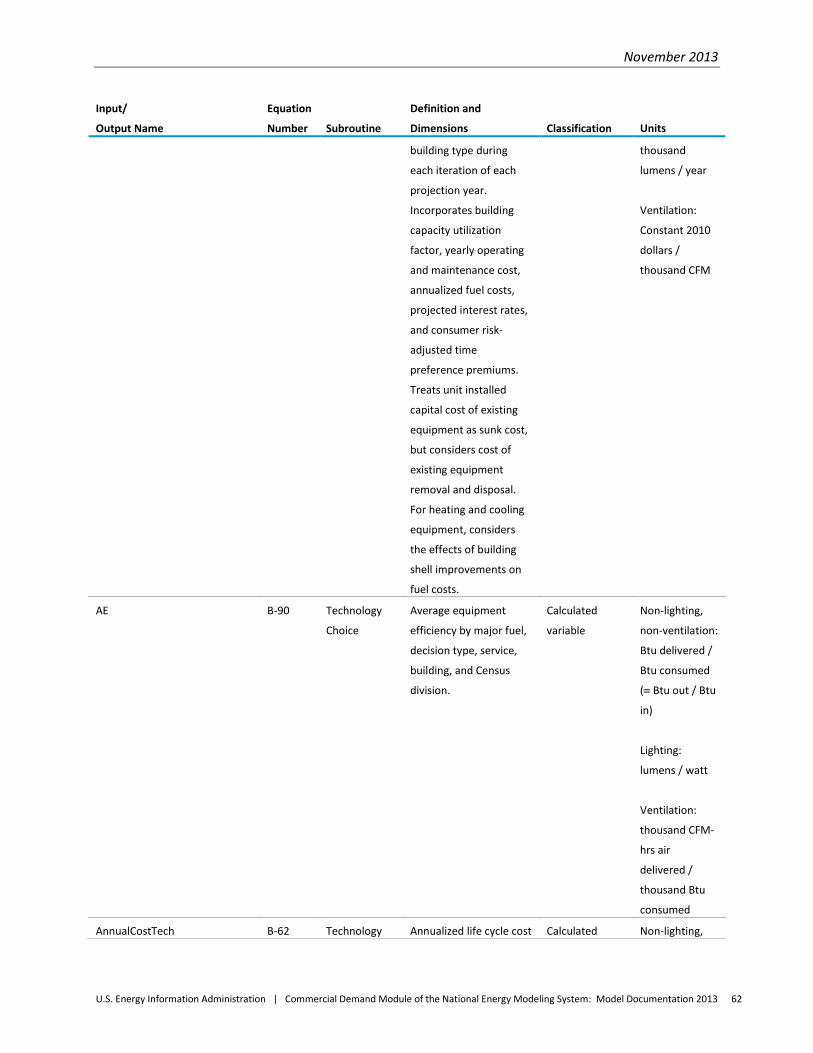
November 2013


Input/

Output Name

Equation

Number Subroutine

Definition and


building type during

each iteration of each

projection year.

Incorporates building

capacity utilization

factor, yearly operating

and maintenance cost,

annualized fuel costs,

projected interest rates,

and consumer risk-

adjusted time

preference premiums.

Treats unit installed

capital cost of existing

equipment as sunk cost,

but considers cost of

existing equipment

removal and disposal.

For heating and cooling

equipment, considers

the effects of building

shell improvements on

fuel costs.

thousand

lumens / year

Ventilation:

Constant 2010

dollars /

thousand CFM

AE B-90 Technology

Choice

Average equipment

efficiency by major fuel,

decision type, service,

building, and Census

division.

Calculated

variable

Non-lighting,

non-ventilation:

Btu delivered /

Btu consumed

(≡ Btu out / Btu

in)

Lighting:

lumens / watt

Ventilation:

thousand CFM-

hrs air

delivered /

thousand Btu

consumed

AnnualCostTech B-62 Technology Annualized life cycle cost Calculated Non-lighting,

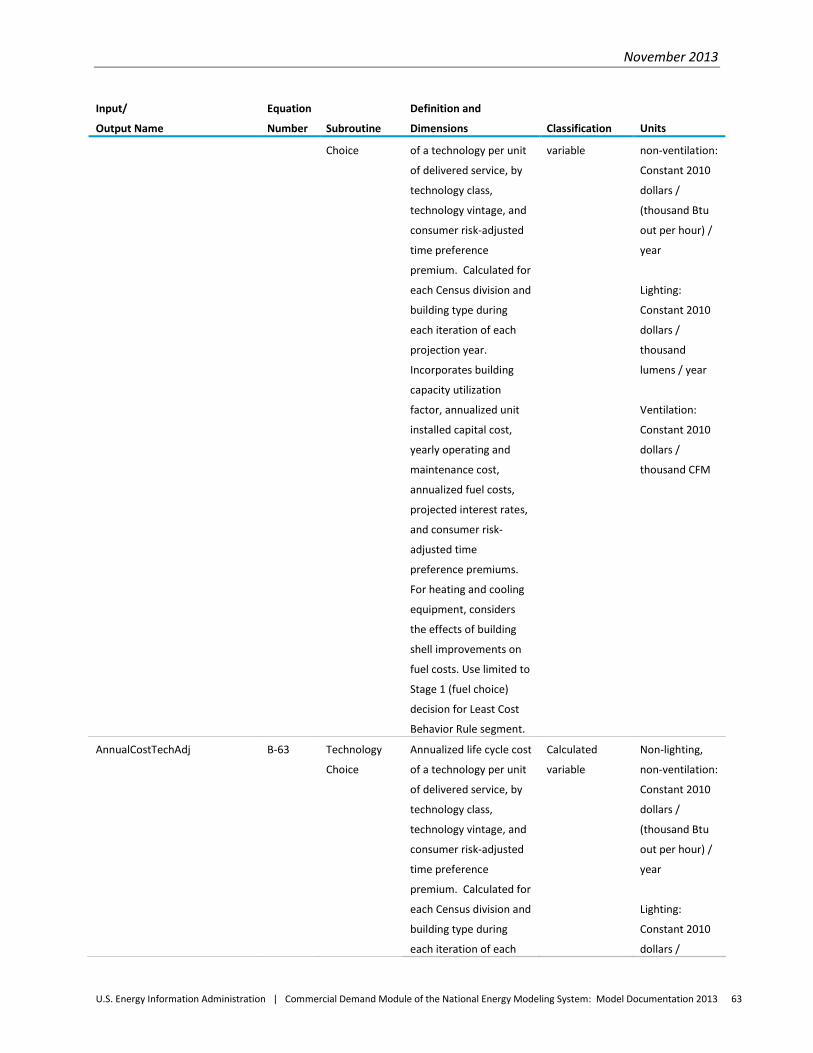
November 2013


Input/

Output Name

Equation

Number Subroutine

Definition and


Choice of a technology per unit

of delivered service, by

technology class,



time preference





projection year.



factor, annualized unit

installed capital cost,

yearly operating and

maintenance cost,



and consumer risk-

adjusted time

preference premiums.





fuel costs. Use limited to

Stage 1 (fuel choice)

decision for Least Cost

Behavior Rule segment.

variable non-ventilation:

Constant 2010

dollars /

(thousand Btu

out per hour) /

year

Lighting:

Constant 2010

dollars /

thousand

lumens / year

Ventilation:

Constant 2010

dollars /

thousand CFM

AnnualCostTechAdj B-63 Technology

Choice

Annualized life cycle cost

of a technology per unit

of delivered service, by

technology class,



time preference





Calculated

variable

Non-lighting,

non-ventilation:

Constant 2010

dollars /

(thousand Btu

out per hour) /

year

Lighting:

Constant 2010

dollars /

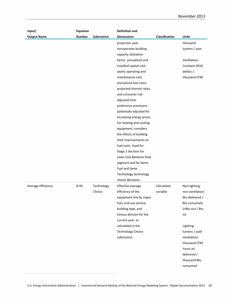
November 2013


Input/

Output Name

Equation

Number Subroutine

Definition and


projection year.



factor, annualized unit

installed capital cost,

yearly operating and

maintenance cost,



and consumer risk-

adjusted time

preference premiums -

potentially adjusted for

increasing energy prices.





fuel costs. Used for

Stage 2 decision for

Least Cost Behavior Rule

segment and for Same

Fuel and Same

Technology technology

choice decisions.

thousand

lumens / year

Ventilation:

Constant 2010

dollars /

thousand CFM

Average Efficiency B-93 Technology

Choice

Effective average

efficiency of the

equipment mix by major

fuel, end-use service,

building type, and

Census division for the

current year, as

calculated in the

Technology Choice

subroutine.

Calculated

variable

Non-lighting,

non-ventilation:

Btu delivered /

Btu consumed

(≡Btu out / Btu

in)

Lighting:

lumens / watt

Ventilation:

thousand CFM

hours air

delivered /

thousand Btu

consumed

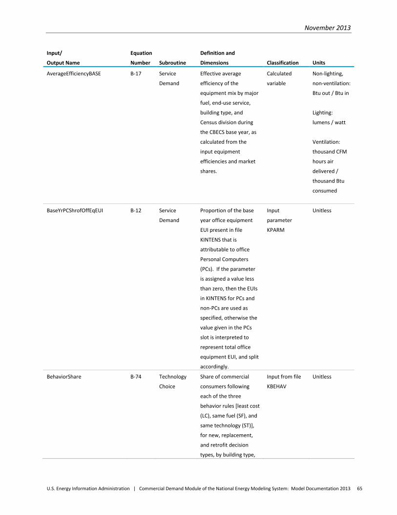
November 2013


Input/

Output Name

Equation

Number Subroutine

Definition and


AverageEfficiencyBASE B-17 Service

Demand

Effective average

efficiency of the

equipment mix by major

fuel, end-use service,

building type, and

Census division during

the CBECS base year, as

calculated from the

input equipment

efficiencies and market

shares.

Calculated

variable

Non-lighting,

non-ventilation:

Btu out / Btu in

Lighting:

lumens / watt

Ventilation:

thousand CFM

hours air

delivered /

thousand Btu

consumed

BaseYrPCShrofOffEqEUI B-12 Service

Demand

Proportion of the base

year office equipment

EUI present in file

KINTENS that is

attributable to office

Personal Computers

(PCs). If the parameter

is assigned a value less

than zero, then the EUIs

in KINTENS for PCs and

non-PCs are used as

specified, otherwise the

value given in the PCs

slot is interpreted to

represent total office

equipment EUI, and split

accordingly.

Input

parameter

KPARM

Unitless

BehaviorShare B-74 Technology

Choice

Share of commercial

consumers following

each of the three

behavior rules [least cost

(LC), same fuel (SF), and

same technology (ST)],

for new, replacement,

and retrofit decision

types, by building type,

Input from file

KBEHAV

Unitless

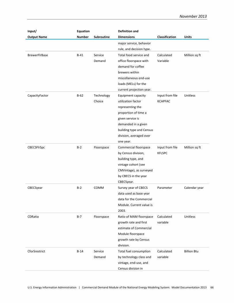
November 2013


Input/

Output Name

Equation

Number Subroutine

Definition and


major service, behavior

rule, and decision type.

BrewerFlrBase B-41 Service

Demand

Total food service and

office floorspace with

demand for coffee

brewers within

miscellaneous end-use

loads (MELs) for the

current projection year.

Calculated

Variable

Million sq ft

CapacityFactor B-62 Technology

Choice

Equipment capacity

utilization factor

representing the

proportion of time a

given service is

demanded in a given

building type and Census

division, averaged over

one year.

Input from file

KCAPFAC

Unitless

CBECSFlrSpc B-2 Floorspace Commercial floorspace

by Census division,

building type, and

vintage cohort (see

CMVintage), as surveyed

by CBECS in the year

CBECSyear.

Input from file

KFLSPC

Million sq ft

CBECSyear B-2 COMM Survey year of CBECS

data used as base year

data for the Commercial

Module. Current value is

2003.

Parameter Calendar year

CDRatio B-7 Floorspace Ratio of MAM floorspace

growth rate and first

estimate of Commercial

Module floorspace

growth rate by Census

division.

Calculated

variable

Unitless

CforSrestrict B-14 Service

Demand

Total fuel consumption

by technology class and

vintage, end-use, and

Census division in

Calculated

variable

Billion Btu

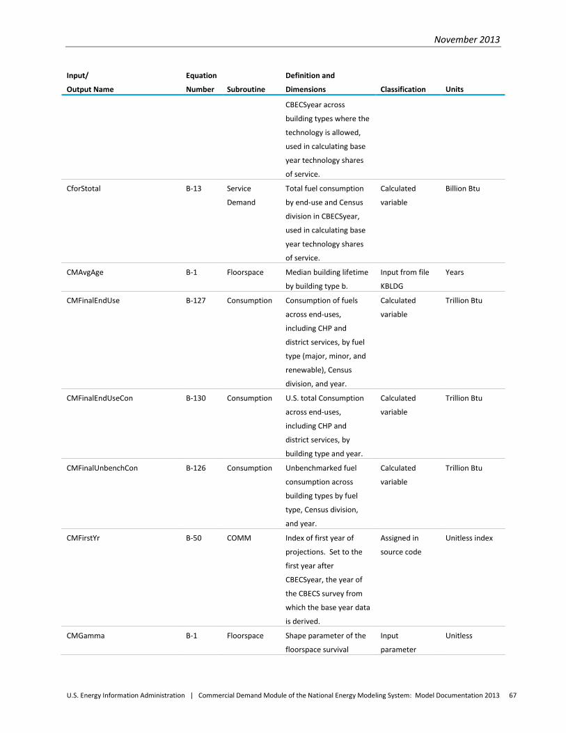
November 2013


Input/

Output Name

Equation

Number Subroutine

Definition and


CBECSyear across

building types where the

technology is allowed,

used in calculating base

year technology shares

of service.

CforStotal B-13 Service

Demand

Total fuel consumption

by end-use and Census

division in CBECSyear,

used in calculating base

year technology shares

of service.

Calculated

variable

Billion Btu

CMAvgAge B-1 Floorspace Median building lifetime

by building type b.

Input from file

KBLDG

Years

CMFinalEndUse B-127 Consumption Consumption of fuels

across end-uses,

including CHP and

district services, by fuel

type (major, minor, and

renewable), Census

division, and year.

Calculated

variable

Trillion Btu

CMFinalEndUseCon B-130 Consumption U.S. total Consumption

across end-uses,

including CHP and

district services, by

building type and year.

Calculated

variable

Trillion Btu

CMFinalUnbenchCon B-126 Consumption Unbenchmarked fuel

consumption across

building types by fuel

type, Census division,

and year.

Calculated

variable

Trillion Btu

CMFirstYr B-50 COMM Index of first year of

projections. Set to the

first year after

CBECSyear, the year of

the CBECS survey from

which the base year data

is derived.

Assigned in

source code

Unitless index

CMGamma B-1 Floorspace Shape parameter of the

floorspace survival

Input

parameter

Unitless

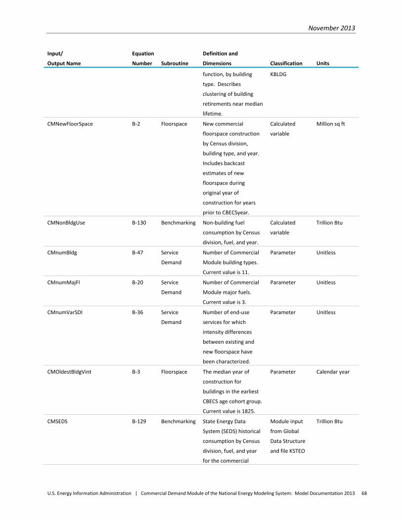
November 2013


Input/

Output Name

Equation

Number Subroutine

Definition and


function, by building

type. Describes

clustering of building

retirements near median

lifetime.

KBLDG

CMNewFloorSpace B-2 Floorspace New commercial

floorspace construction

by Census division,

building type, and year.

Includes backcast

estimates of new

floorspace during

original year of

construction for years

prior to CBECSyear.

Calculated

variable

Million sq ft

CMNonBldgUse B-130 Benchmarking Non-building fuel

consumption by Census

division, fuel, and year.

Calculated

variable

Trillion Btu

CMnumBldg B-47 Service

Demand

Number of Commercial

Module building types.

Current value is 11.

Parameter Unitless

CMnumMajFl B-20 Service

Demand

Number of Commercial

Module major fuels.

Current value is 3.

Parameter Unitless

CMnumVarSDI B-36 Service

Demand

Number of end-use

services for which

intensity differences

between existing and

new floorspace have

been characterized.

Parameter Unitless

CMOldestBldgVint B-3 Floorspace The median year of

construction for

buildings in the earliest

CBECS age cohort group.

Current value is 1825.

Parameter Calendar year

CMSEDS B-129 Benchmarking State Energy Data

System (SEDS) historical

consumption by Census

division, fuel, and year

for the commercial

Module input

from Global

Data Structure

and file KSTEO

Trillion Btu

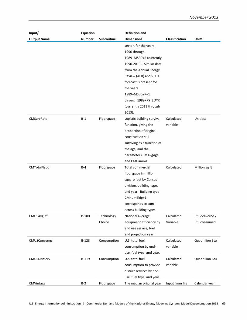
November 2013


Input/

Output Name

Equation

Number Subroutine

Definition and


sector, for the years

1990 through

1989+MSEDYR (currently

1990-2010). Similar data

from the Annual Energy

Review (AER) and STEO

forecast is present for

the years

1989+MSEDYR+1

through 1989+KSTEOYR

(currently 2011 through

2013).

CMSurvRate B-1 Floorspace Logistic building survival

function, giving the

proportion of original

construction still

surviving as a function of

the age, and the

parameters CMAvgAge

and CMGamma.

Calculated

variable

Unitless

CMTotalFlspc B-4 Floorspace Total commercial

floorspace in million

square feet by Census

division, building type,

and year. Building type

CMnumBldg+1

corresponds to sum

across building types.

Calculated Million sq ft

CMUSAvgEff B-100 Technology

Choice

National average

equipment efficiency by

end use service, fuel,

and projection year.

Calculated

Variable

Btu delivered /

Btu consumed

CMUSConsump B-123 Consumption U.S. total fuel

consumption by end-

use, fuel type, and year.

Calculated

variable

Quadrillion Btu

CMUSDistServ B-119 Consumption U.S. total fuel

consumption to provide

district services by end-

use, fuel type, and year.

Calculated

variable

Quadrillion Btu

CMVintage B-2 Floorspace The median original year Input from file Calendar year

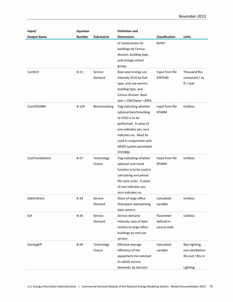
November 2013


Input/

Output Name

Equation

Number Subroutine

Definition and


of construction for

buildings by Census


and vintage cohort

group.

KVINT

ComEUI B-11 Service

Demand

Base year energy use

intensity (EUI) by fuel

type, end-use service,

building type, and

Census division. Base

year = CBECSyear =2003.

Input from file

KINTENS

Thousand Btu

consumed / sq

ft / year

ComSTEOBM B-139 Benchmarking Flag indicating whether

optional benchmarking

to STEO is to be

performed. A value of

one indicates yes; zero

indicates no. Must be

used in conjunction with

NEMS system parameter

STEOBM.

Input from file

KPARM

Unitless

CostTrendSwitch B-57 Technology

Choice

Flag indicating whether

optional cost trend

function is to be used in

calculating annualized

life cycle costs. A value

of one indicates yes;

zero indicates no.

Input from file

KPARM

Unitless

DatCtrShare B-33 Service

Demand

Share of large office

floorspace representing

data centers.

Calculated

variable

Unitless

Dcf B-34 Service

Demand

Service demand

intensity ratio of data

centers to large office

buildings by end-use

service.

Parameter

defined in

source code

Unitless

DecAvgEff B-94 Technology

Choice

Effective average

efficiency of the

equipment mix selected

to satisfy service

demands, by decision

Calculated

variable

Non-lighting,

non-ventilation:

Btu out / Btu in

Lighting:

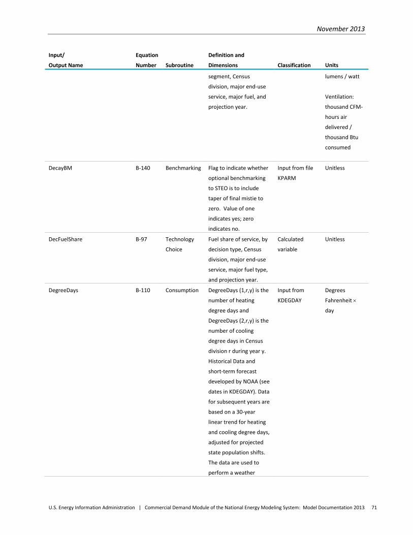
November 2013


Input/

Output Name

Equation

Number Subroutine

Definition and


segment, Census

division, major end-use

service, major fuel, and

projection year.

lumens / watt

Ventilation:

thousand CFM-

hours air

delivered /

thousand Btu

consumed

DecayBM B-140 Benchmarking Flag to indicate whether


to STEO is to include

taper of final mistie to

zero. Value of one

indicates yes; zero

indicates no.

Input from file

KPARM

Unitless

DecFuelShare B-97 Technology

Choice

Fuel share of service, by

decision type, Census

division, major end-use

service, major fuel type,


Calculated

variable

Unitless

DegreeDays B-110 Consumption DegreeDays (1,r,y) is the

number of heating

degree days and

DegreeDays (2,r,y) is the

number of cooling

degree days in Census

division r during year y.

Historical Data and

short-term forecast

developed by NOAA (see

dates in KDEGDAY). Data

for subsequent years are

based on a 30-year

linear trend for heating

and cooling degree days,

adjusted for projected

state population shifts.

The data are used to

perform a weather

Input from

KDEGDAY

Degrees

Fahrenheit ×

day

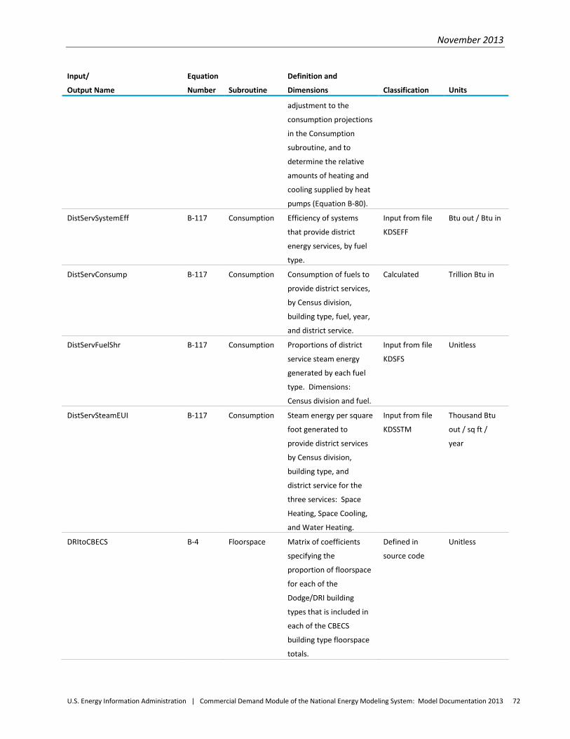
November 2013


Input/

Output Name

Equation

Number Subroutine

Definition and


adjustment to the

consumption projections

in the Consumption

subroutine, and to

determine the relative

amounts of heating and

cooling supplied by heat

pumps (Equation B-80).

DistServSystemEff B-117 Consumption Efficiency of systems

that provide district

energy services, by fuel

type.

Input from file

KDSEFF

Btu out / Btu in

DistServConsump B-117 Consumption Consumption of fuels to

provide district services,

by Census division,

building type, fuel, year,

and district service.

Calculated Trillion Btu in

DistServFuelShr B-117 Consumption Proportions of district

service steam energy

generated by each fuel

type. Dimensions:

Census division and fuel.

Input from file

KDSFS

Unitless

DistServSteamEUI B-117 Consumption Steam energy per square

foot generated to

provide district services

by Census division,

building type, and

district service for the

three services: Space

Heating, Space Cooling,

and Water Heating.

Input from file

KDSSTM

Thousand Btu

out / sq ft /

year

DRItoCBECS B-4 Floorspace Matrix of coefficients

specifying the

proportion of floorspace

for each of the

Dodge/DRI building

types that is included in

each of the CBECS

building type floorspace

totals.

Defined in

source code

Unitless

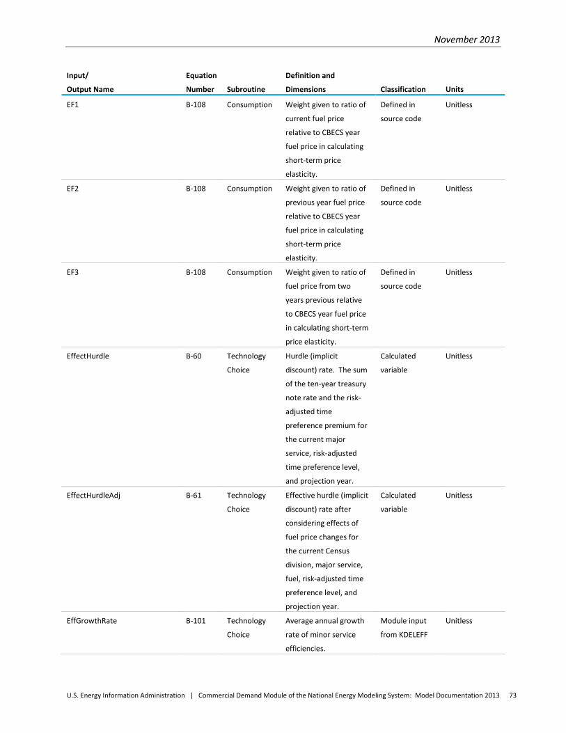
November 2013


Input/

Output Name

Equation

Number Subroutine

Definition and


EF1 B-108 Consumption Weight given to ratio of

current fuel price

relative to CBECS year

fuel price in calculating

short-term price

elasticity.

Defined in

source code

Unitless


previous year fuel price

relative to CBECS year

fuel price in calculating

short-term price

elasticity.

Defined in

source code

Unitless


fuel price from two

years previous relative

to CBECS year fuel price

in calculating short-term

price elasticity.

Defined in

source code

Unitless

EffectHurdle B-60 Technology

Choice

Hurdle (implicit

discount) rate. The sum

of the ten-year treasury

note rate and the risk-

adjusted time

preference premium for

the current major

service, risk-adjusted

time preference level,


Calculated

variable

Unitless

EffectHurdleAdj B-61 Technology

Choice

Effective hurdle (implicit

discount) rate after

considering effects of

fuel price changes for

the current Census

division, major service,

fuel, risk-adjusted time

preference level, and

projection year.

Calculated

variable

Unitless

EffGrowthRate B-101 Technology

Choice

Average annual growth

rate of minor service

efficiencies.

Module input

from KDELEFF

Unitless

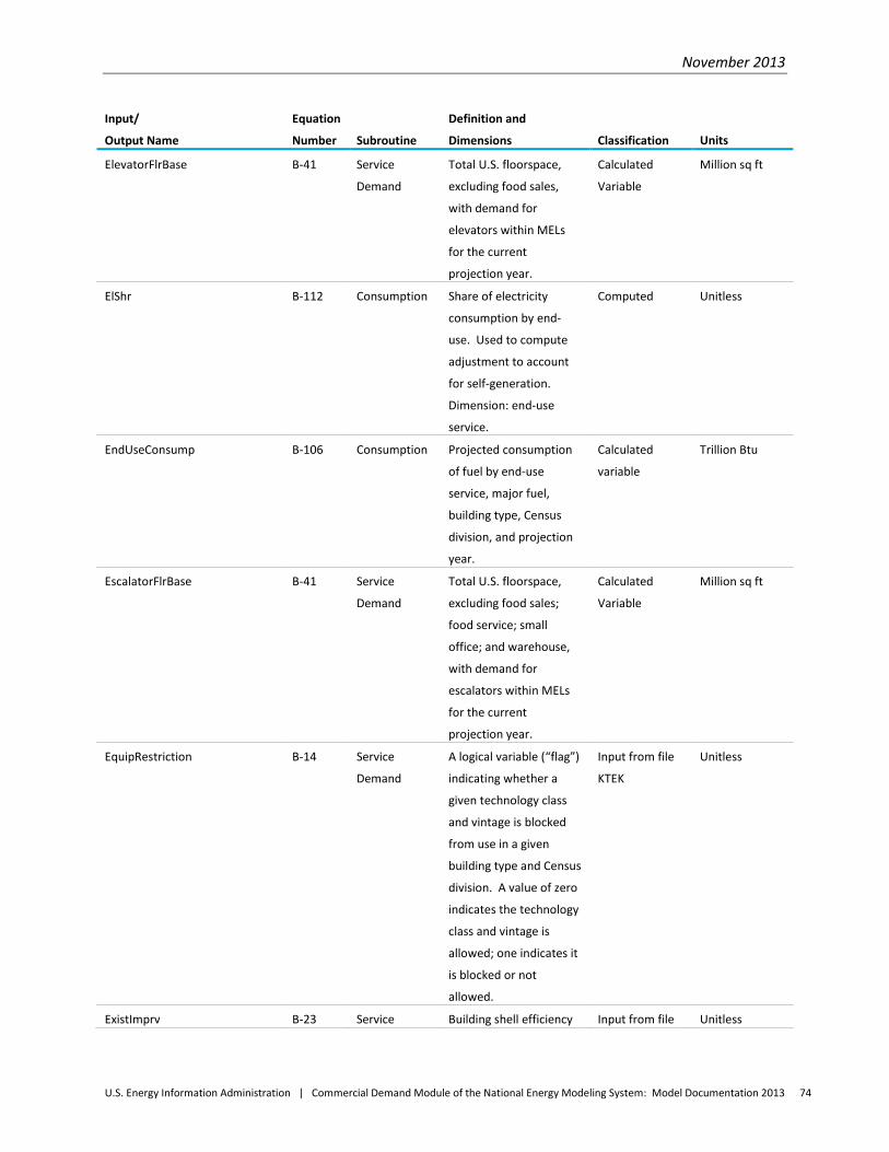
November 2013


Input/

Output Name

Equation

Number Subroutine

Definition and


ElevatorFlrBase B-41 Service

Demand

Total U.S. floorspace,

excluding food sales,

with demand for

elevators within MELs

for the current

projection year.

Calculated

Variable

Million sq ft

ElShr B-112 Consumption Share of electricity

consumption by end-

use. Used to compute

adjustment to account

for self-generation.

Dimension: end-use

service.

Computed Unitless

EndUseConsump B-106 Consumption Projected consumption

of fuel by end-use

service, major fuel,

building type, Census

division, and projection

year.

Calculated

variable

Trillion Btu

EscalatorFlrBase B-41 Service

Demand


excluding food sales;

food service; small

office; and warehouse,

with demand for

escalators within MELs

for the current

projection year.

Calculated

Variable

Million sq ft

EquipRestriction B-14 Service

Demand

A logical variable (“flag”)

indicating whether a

given technology class

and vintage is blocked

from use in a given


division. A value of zero

indicates the technology

class and vintage is

allowed; one indicates it

is blocked or not

allowed.

Input from file

KTEK

Unitless

ExistImprv B-23 Service Building shell efficiency Input from file Unitless

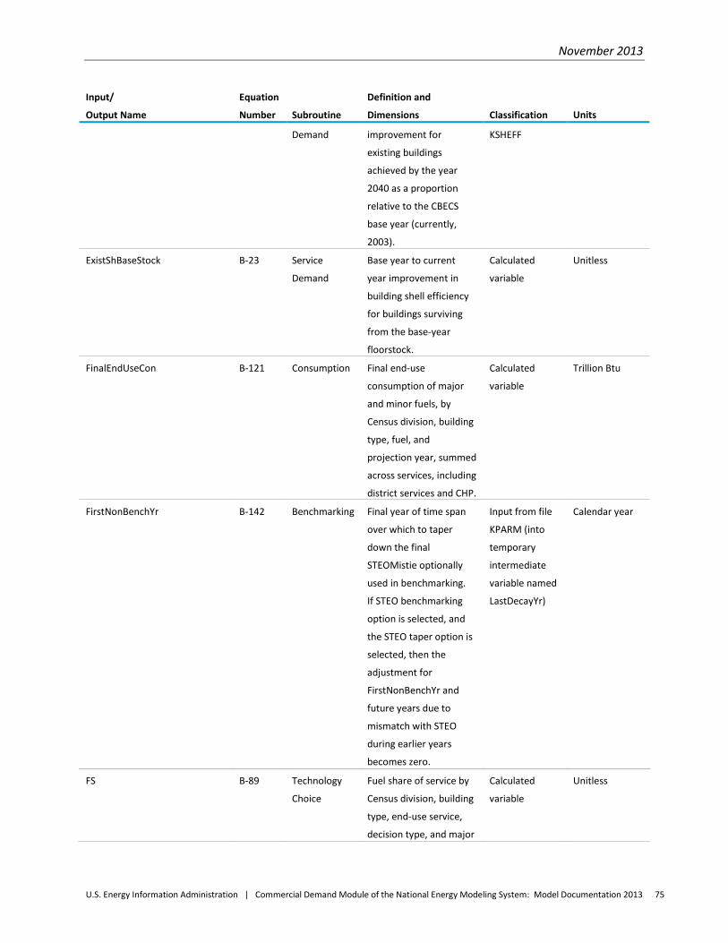
November 2013


Input/

Output Name

Equation

Number Subroutine

Definition and


Demand improvement for

existing buildings

achieved by the year

2040 as a proportion

relative to the CBECS

base year (currently,

2003).

KSHEFF

ExistShBaseStock B-23 Service

Demand

Base year to current

year improvement in

building shell efficiency

for buildings surviving

from the base-year

floorstock.

Calculated

variable

Unitless

FinalEndUseCon B-121 Consumption Final end-use

consumption of major

and minor fuels, by

Census division, building

type, fuel, and

projection year, summed

across services, including

district services and CHP.

Calculated

variable

Trillion Btu

FirstNonBenchYr B-142 Benchmarking Final year of time span

over which to taper

down the final

STEOMistie optionally

used in benchmarking.

If STEO benchmarking

option is selected, and

the STEO taper option is

selected, then the

adjustment for

FirstNonBenchYr and

future years due to

mismatch with STEO

during earlier years

becomes zero.

Input from file

KPARM (into

temporary

intermediate

variable named

LastDecayYr)

Calendar year

FS B-89 Technology

Choice

Fuel share of service by



decision type, and major

Calculated

variable

Unitless

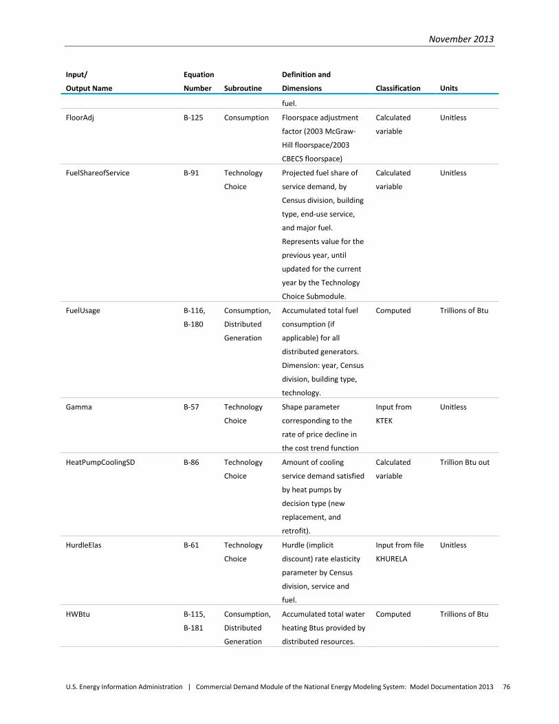
November 2013


Input/

Output Name

Equation

Number Subroutine

Definition and


fuel.

FloorAdj B-125 Consumption Floorspace adjustment

factor (2003 McGraw-

Hill floorspace/2003

CBECS floorspace)

Calculated

variable

Unitless

FuelShareofService B-91 Technology

Choice

Projected fuel share of

service demand, by



and major fuel.

Represents value for the

previous year, until

updated for the current

year by the Technology

Choice Submodule.

Calculated

variable

Unitless

FuelUsage B-116,

B-180

Consumption,

Distributed

Generation

Accumulated total fuel

consumption (if

applicable) for all

distributed generators.

Dimension: year, Census


technology.

Computed Trillions of Btu

Gamma B-57 Technology

Choice

Shape parameter

corresponding to the

rate of price decline in

the cost trend function

Input from

KTEK

Unitless

HeatPumpCoolingSD B-86 Technology

Choice

Amount of cooling

service demand satisfied

by heat pumps by

decision type (new

replacement, and

retrofit).

Calculated

variable

Trillion Btu out

HurdleElas B-61 Technology

Choice

Hurdle (implicit

discount) rate elasticity

parameter by Census

division, service and

fuel.

Input from file

KHURELA

Unitless

HWBtu B-115,

B-181

Consumption,

Distributed

Generation

Accumulated total water

heating Btus provided by

distributed resources.

Computed Trillions of Btu

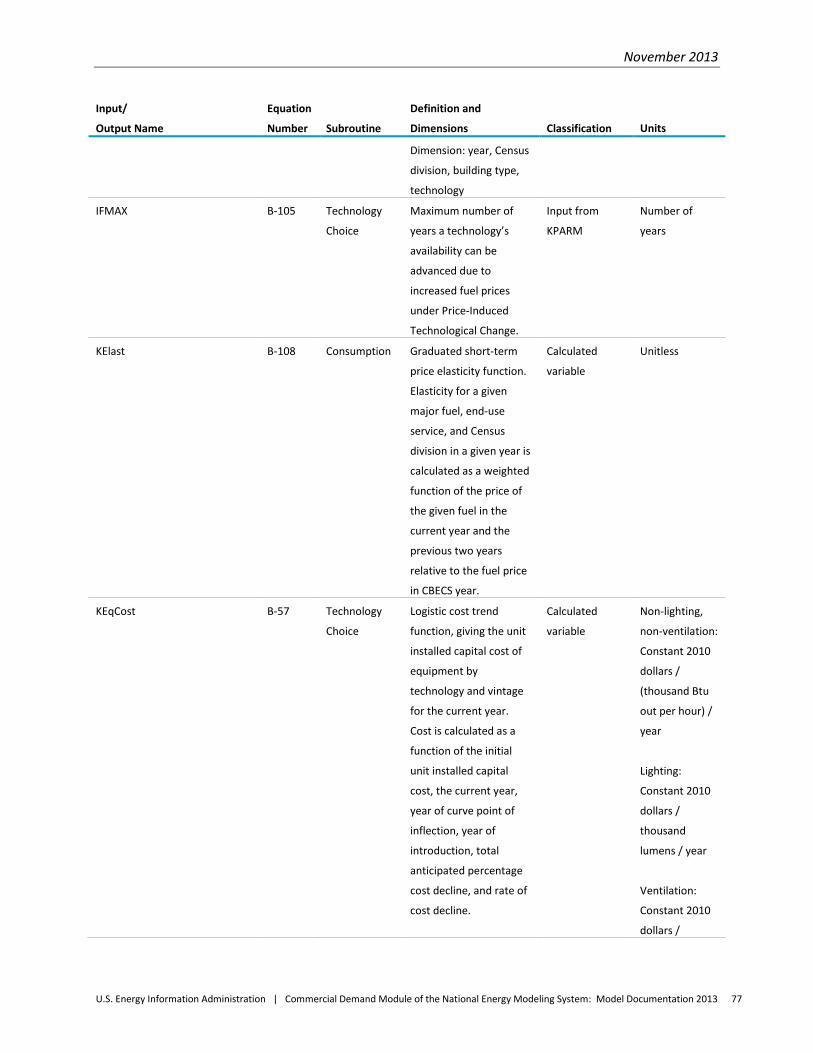
November 2013


Input/

Output Name

Equation

Number Subroutine

Definition and




technology

IFMAX B-105 Technology

Choice

Maximum number of

years a technology’s

availability can be

advanced due to

increased fuel prices

under Price-Induced

Technological Change.

Input from

KPARM

Number of

years

KElast B-108 Consumption Graduated short-term

price elasticity function.

Elasticity for a given

major fuel, end-use

service, and Census

division in a given year is

calculated as a weighted

function of the price of

the given fuel in the

current year and the

previous two years

relative to the fuel price

in CBECS year.

Calculated

variable

Unitless

KEqCost B-57 Technology

Choice

Logistic cost trend

function, giving the unit

installed capital cost of

equipment by

technology and vintage

for the current year.

Cost is calculated as a

function of the initial

unit installed capital

cost, the current year,

year of curve point of

inflection, year of

introduction, total

anticipated percentage

cost decline, and rate of

cost decline.

Calculated

variable

Non-lighting,

non-ventilation:

Constant 2010

dollars /

(thousand Btu

out per hour) /

year

Lighting:

Constant 2010

dollars /

thousand

lumens / year

Ventilation:

Constant 2010

dollars /

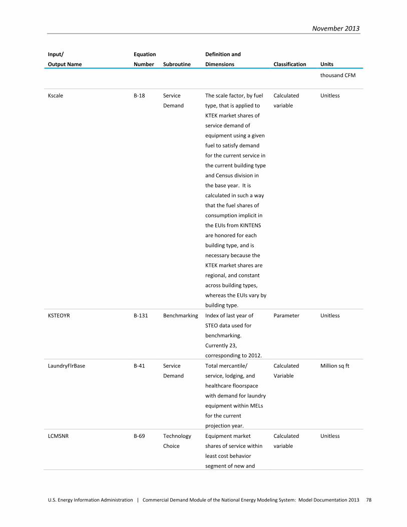
November 2013


Input/

Output Name

Equation

Number Subroutine

Definition and


thousand CFM

Kscale B-18 Service

Demand

The scale factor, by fuel

type, that is applied to

KTEK market shares of

service demand of

equipment using a given

fuel to satisfy demand

for the current service in

the current building type

and Census division in

the base year. It is

calculated in such a way

that the fuel shares of

consumption implicit in

the EUIs from KINTENS

are honored for each

building type, and is

necessary because the

KTEK market shares are

regional, and constant

across building types,

whereas the EUIs vary by

building type.

Calculated

variable

Unitless

KSTEOYR B-131 Benchmarking Index of last year of

STEO data used for

benchmarking.

Currently 23,

corresponding to 2012.

Parameter Unitless

LaundryFlrBase B-41 Service

Demand

Total mercantile/

service, lodging, and

healthcare floorspace

with demand for laundry

equipment within MELs

for the current

projection year.

Calculated

Variable

Million sq ft

LCMSNR B-69 Technology

Choice

Equipment market

shares of service within

least cost behavior

segment of new and

Calculated

variable

Unitless

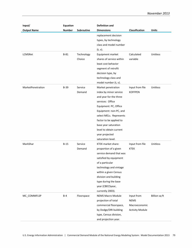
November 2013


Input/

Output Name

Equation

Number Subroutine

Definition and


replacement decision

types, by technology

class and model number

(t, v).

LCMSRet B-81 Technology

Choice

Equipment market

shares of service within

least cost behavior

segment of retrofit

decision type, by

technology class and

model number (t, v).

Calculated

variable

Unitless

MarketPenetration B-39 Service

Demand

Market penetration

index by minor service

and year for the three

services: Office

Equipment: PC, Office

Equipment: non-PC, and

select MELs. Represents

factor to be applied to

base year saturation

level to obtain current

year projected

saturation level.

Input from file

KOFFPEN

Unitless

MarkShar B-15 Service

Demand

KTEK market share:

proportion of a given

service demand that was

satisfied by equipment

of a particular


within a given Census

division and building

type during the base

year (CBECSyear,

currently 2003).

Input from file

KTEK

Unitless

MC_COMMFLSP B-4 Floorspace NEMS Macro Module

projection of total

commercial floorspace,

by Dodge/DRI building



Input from

NEMS

Macroeconomic

Activity Module

Billion sq ft

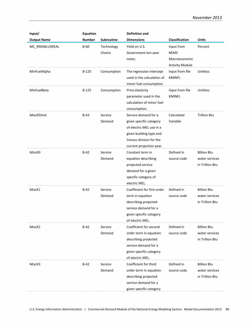
November 2013


Input/

Output Name

Equation

Number Subroutine

Definition and


MC_RMGBLUSREAL B-60 Technology

Choice

Yield on U.S.

Government ten-year

notes.

Input from

NEMS

Macroeconomic

Activity Module

Percent

MinFuelAlpha B-125 Consumption The regression intercept

used in the calculation of

minor fuel consumption.

Input from file

KMINFL

Unitless

MinFuelBeta B-125 Consumption Price elasticity

parameter used in the

calculation of minor fuel

consumption.

Input from file

KMINFL

Unitless

MiscElDmd B-43 Service

Demand

Service demand for a

given specific category

of electric MEL use in a

given building type and

Census division for the

current projection year.

Calculated

Variable

Trillion Btu

MiscK0 B-42 Service

Demand

Constant term in

equation describing

projected service

demand for a given

specific category of

electric MEL.

Defined in

source code

Billion Btu

water services

in Trillion Btu

MiscK1 B-42 Service

Demand

Coefficient for first order

term in equation

describing projected

service demand for a


of electric MEL.

Defined in

source code

Billion Btu

water services

in Trillion Btu

MiscK2 B-42 Service

Demand

Coefficient for second

order term in equation




of electric MEL.

Defined in

source code

Billion Btu

water services

in Trillion Btu

MiscK3 B-42 Service

Demand

Coefficient for third

order term in equation




Defined in

source code

Billion Btu

water services

in Trillion Btu

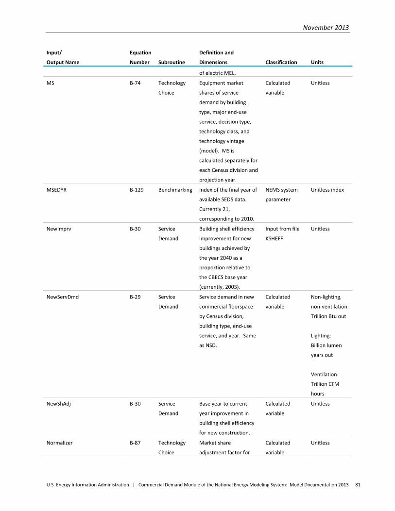
November 2013


Input/

Output Name

Equation

Number Subroutine

Definition and


of electric MEL.

MS B-74 Technology

Choice

Equipment market

shares of service

demand by building

type, major end-use

service, decision type,

technology class, and

technology vintage

(model). MS is

calculated separately for


projection year.

Calculated

variable

Unitless

MSEDYR B-129 Benchmarking Index of the final year of

available SEDS data.

Currently 21,


NEMS system

parameter

Unitless index

NewImprv B-30 Service

Demand

Building shell efficiency

improvement for new

buildings achieved by

the year 2040 as a

proportion relative to

the CBECS base year

(currently, 2003).

Input from file

KSHEFF

Unitless

NewServDmd B-29 Service

Demand

Service demand in new

commercial floorspace

by Census division,

building type, end-use

service, and year. Same

as NSD.

Calculated

variable

Non-lighting,

non-ventilation:

Trillion Btu out

Lighting:

Billion lumen

years out

Ventilation:

Trillion CFM

hours

NewShAdj B-30 Service

Demand

Base year to current

year improvement in


for new construction.

Calculated

variable

Unitless

Normalizer B-87 Technology

Choice

Market share

adjustment factor for

Calculated

variable

Unitless

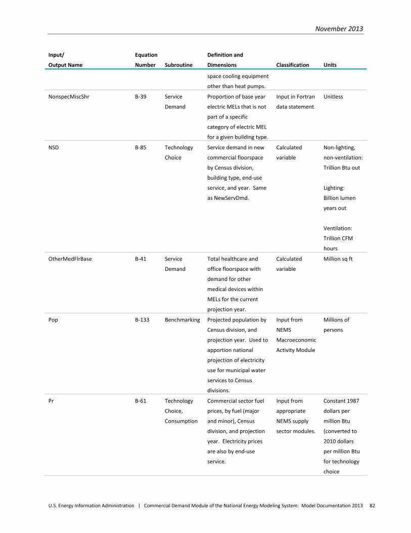
November 2013


Input/

Output Name

Equation

Number Subroutine

Definition and


space cooling equipment

other than heat pumps.

NonspecMiscShr B-39 Service

Demand

Proportion of base year

electric MELs that is not

part of a specific

category of electric MEL

for a given building type.

Input in Fortran

data statement

Unitless

NSD B-85 Technology

Choice

Service demand in new


by Census division,

building type, end-use

service, and year. Same

as NewServDmd.

Calculated

variable

Non-lighting,

non-ventilation:

Trillion Btu out

Lighting:

Billion lumen

years out

Ventilation:

Trillion CFM

hours

OtherMedFlrBase B-41 Service

Demand

Total healthcare and

office floorspace with

demand for other

medical devices within

MELs for the current

projection year.

Calculated

variable

Million sq ft

Pop B-133 Benchmarking Projected population by

Census division, and

projection year. Used to

apportion national

projection of electricity

use for municipal water

services to Census

divisions.

Input from

NEMS

Macroeconomic

Activity Module

Millions of

persons

Pr B-61 Technology

Choice,

Consumption

Commercial sector fuel

prices, by fuel (major

and minor), Census


year. Electricity prices

are also by end-use

service.

Input from

appropriate

NEMS supply

sector modules.

Constant 1987

dollars per

million Btu

(converted to

2010 dollars

per million Btu

for technology

choice

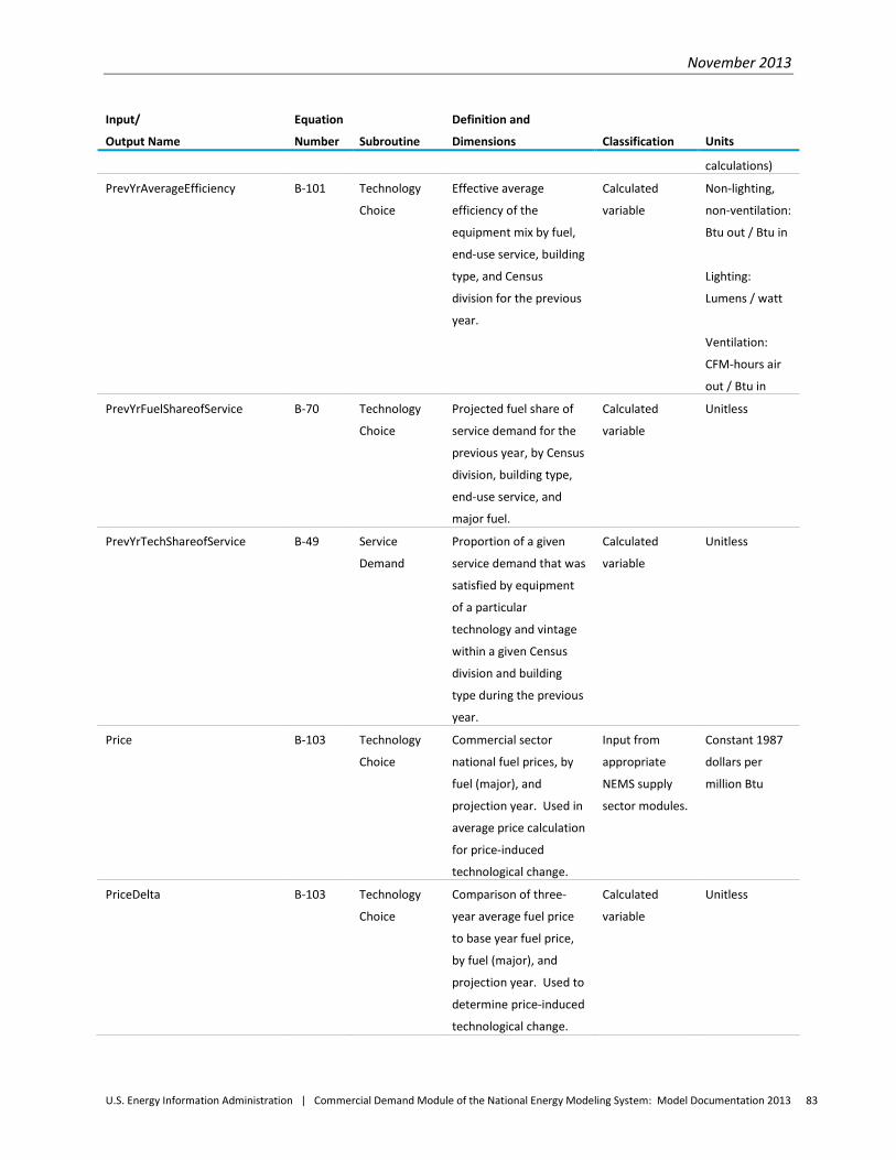
November 2013


Input/

Output Name

Equation

Number Subroutine

Definition and


calculations)

PrevYrAverageEfficiency B-101 Technology

Choice

Effective average

efficiency of the

equipment mix by fuel,

end-use service, building

type, and Census

division for the previous

year.

Calculated

variable

Non-lighting,

non-ventilation:

Btu out / Btu in

Lighting:

Lumens / watt

Ventilation:

CFM-hours air

out / Btu in

PrevYrFuelShareofService B-70 Technology

Choice

Projected fuel share of

service demand for the

previous year, by Census


end-use service, and

major fuel.

Calculated

variable

Unitless

PrevYrTechShareofService B-49 Service

Demand

Proportion of a given



of a particular




type during the previous

year.

Calculated

variable

Unitless

Price B-103 Technology

Choice

Commercial sector

national fuel prices, by

fuel (major), and

projection year. Used in

average price calculation

for price-induced

technological change.

Input from

appropriate

NEMS supply

sector modules.

Constant 1987

dollars per

million Btu

PriceDelta B-103 Technology

Choice

Comparison of three-

year average fuel price

to base year fuel price,

by fuel (major), and

projection year. Used to

determine price-induced

technological change.

Calculated

variable

Unitless

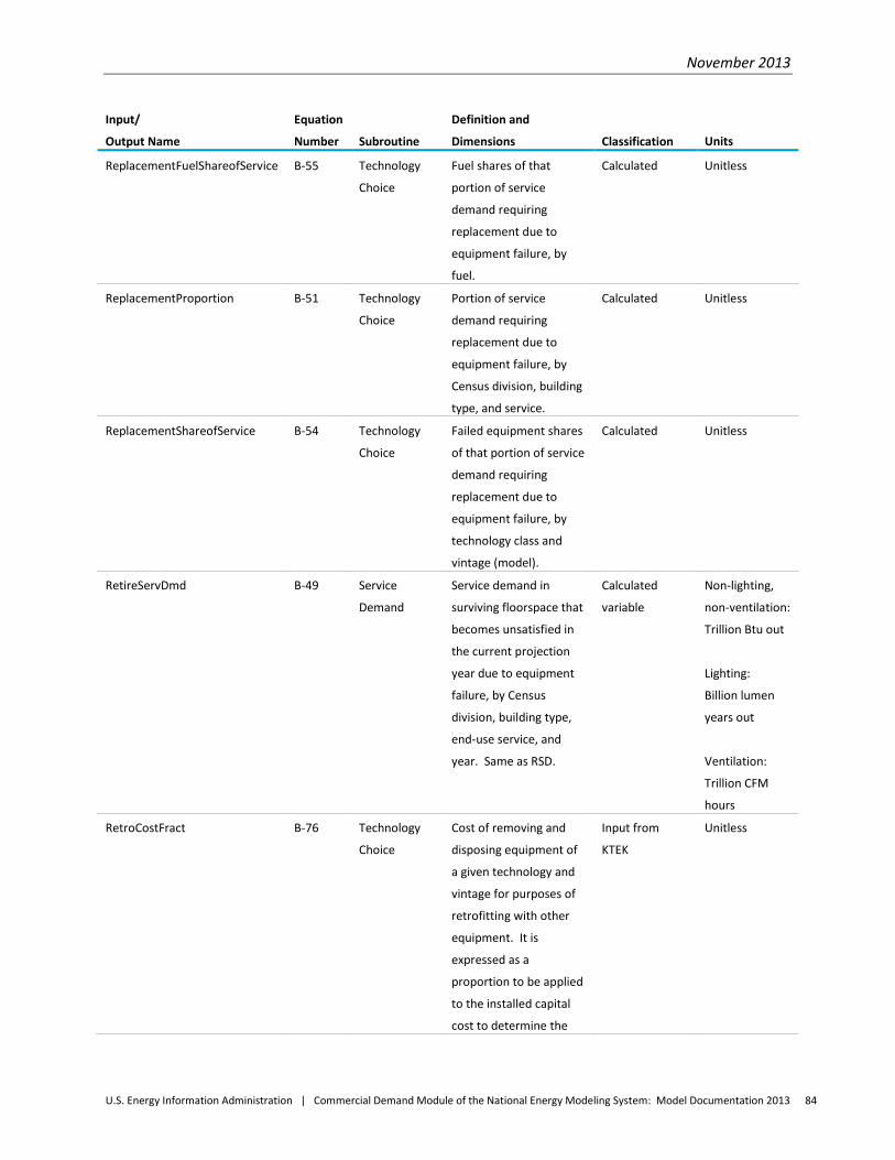
November 2013


Input/

Output Name

Equation

Number Subroutine

Definition and


ReplacementFuelShareofService B-55 Technology

Choice

Fuel shares of that

portion of service

demand requiring

replacement due to

equipment failure, by

fuel.

Calculated Unitless

ReplacementProportion B-51 Technology

Choice

Portion of service

demand requiring

replacement due to



type, and service.

Calculated Unitless

ReplacementShareofService B-54 Technology

Choice

Failed equipment shares

of that portion of service

demand requiring

replacement due to



vintage (model).

Calculated Unitless

RetireServDmd B-49 Service

Demand

Service demand in

surviving floorspace that

becomes unsatisfied in

the current projection

year due to equipment

failure, by Census



year. Same as RSD.

Calculated

variable

Non-lighting,

non-ventilation:

Trillion Btu out

Lighting:

Billion lumen

years out

Ventilation:

Trillion CFM

hours

RetroCostFract B-76 Technology

Choice

Cost of removing and

disposing equipment of

a given technology and

vintage for purposes of

retrofitting with other

equipment. It is

expressed as a

proportion to be applied

to the installed capital

cost to determine the

Input from

KTEK

Unitless

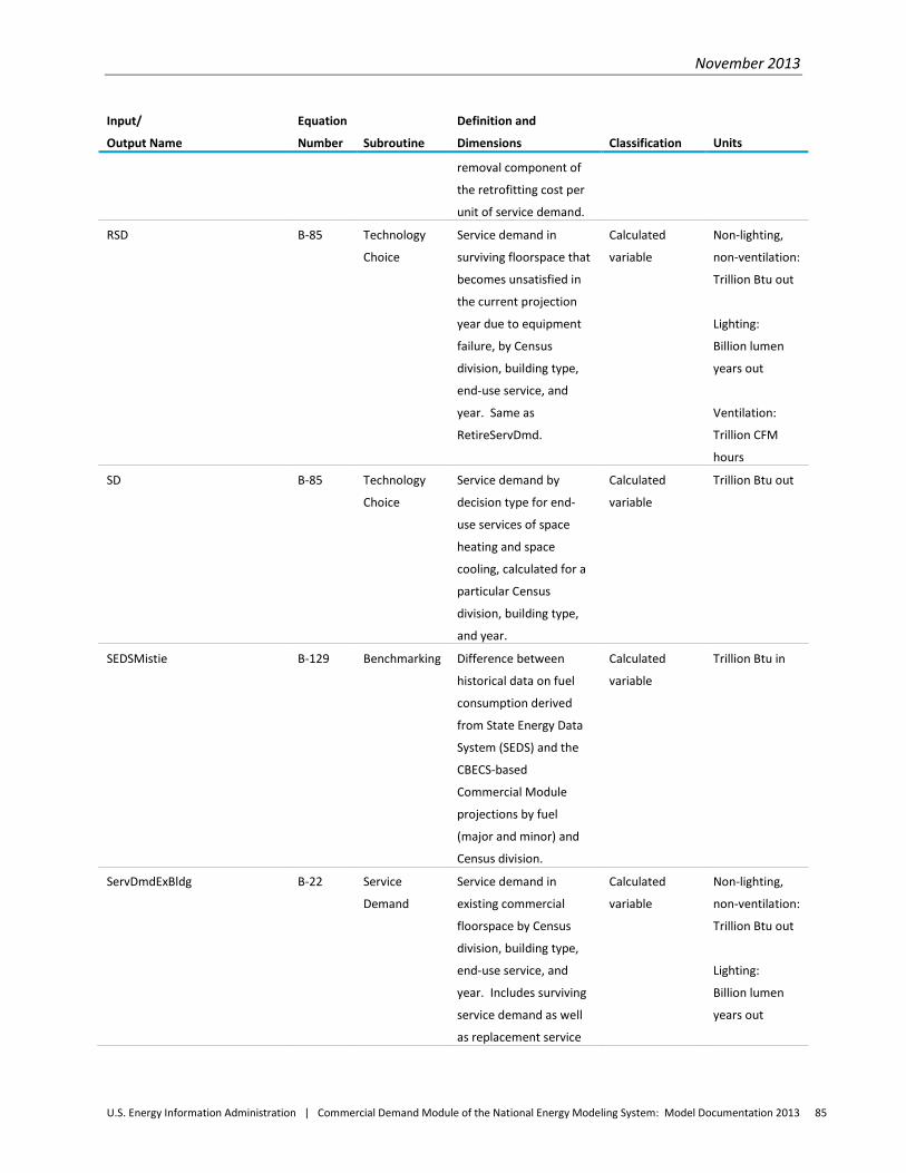
November 2013


Input/

Output Name

Equation

Number Subroutine

Definition and


removal component of

the retrofitting cost per

unit of service demand.

RSD B-85 Technology

Choice

Service demand in

surviving floorspace that

becomes unsatisfied in

the current projection

year due to equipment

failure, by Census



year. Same as

RetireServDmd.

Calculated

variable

Non-lighting,

non-ventilation:

Trillion Btu out

Lighting:

Billion lumen

years out

Ventilation:

Trillion CFM

hours

SD B-85 Technology

Choice

Service demand by

decision type for end-

use services of space

heating and space

cooling, calculated for a

particular Census


and year.

Calculated

variable

Trillion Btu out

SEDSMistie B-129 Benchmarking Difference between

historical data on fuel

consumption derived

from State Energy Data

System (SEDS) and the

CBECS-based

Commercial Module

projections by fuel

(major and minor) and

Census division.

Calculated

variable

Trillion Btu in

ServDmdExBldg B-22 Service

Demand

Service demand in

existing commercial

floorspace by Census



year. Includes surviving

service demand as well

as replacement service

Calculated

variable

Non-lighting,

non-ventilation:

Trillion Btu out

Lighting:

Billion lumen

years out

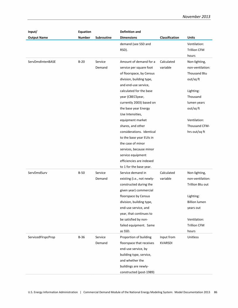
November 2013


Input/

Output Name

Equation

Number Subroutine

Definition and


demand (see SSD and

RSD).

Ventilation:

Trillion CFM

hours

ServDmdIntenBASE B-20 Service

Demand

Amount of demand for a

service per square foot

of floorspace, by Census


and end-use service,

calculated for the base

year (CBECSyear,

currently 2003) based on

the base year Energy

Use Intensities,

equipment market

shares, and other

considerations. Identical

to the base year EUIs in

the case of minor

services, because minor

service equipment

efficiencies are indexed

to 1 for the base year.

Calculated

variable

Non-lighting,

non-ventilation:

Thousand Btu

out/sq ft

Lighting:

Thousand

lumen years

out/sq ft

Ventilation:

Thousand CFM-

hrs out/sq ft

ServDmdSurv B-50 Service

Demand

Service demand in

existing (i.e., not newly-

constructed during the

given year) commercial




year, that continues to

be satisfied by non-

failed equipment. Same

as SSD.

Calculated

variable

Non-lighting,

non-ventilation:

Trillion Btu out

Lighting:

Billion lumen

years out

Ventilation:

Trillion CFM

hours

ServicedFlrspcProp B-36 Service

Demand

Proportion of building

floorspace that receives

end-use service, by

building type, service,

and whether the

buildings are newly-

constructed (post-1989)

Input from

KVARSDI

Unitless

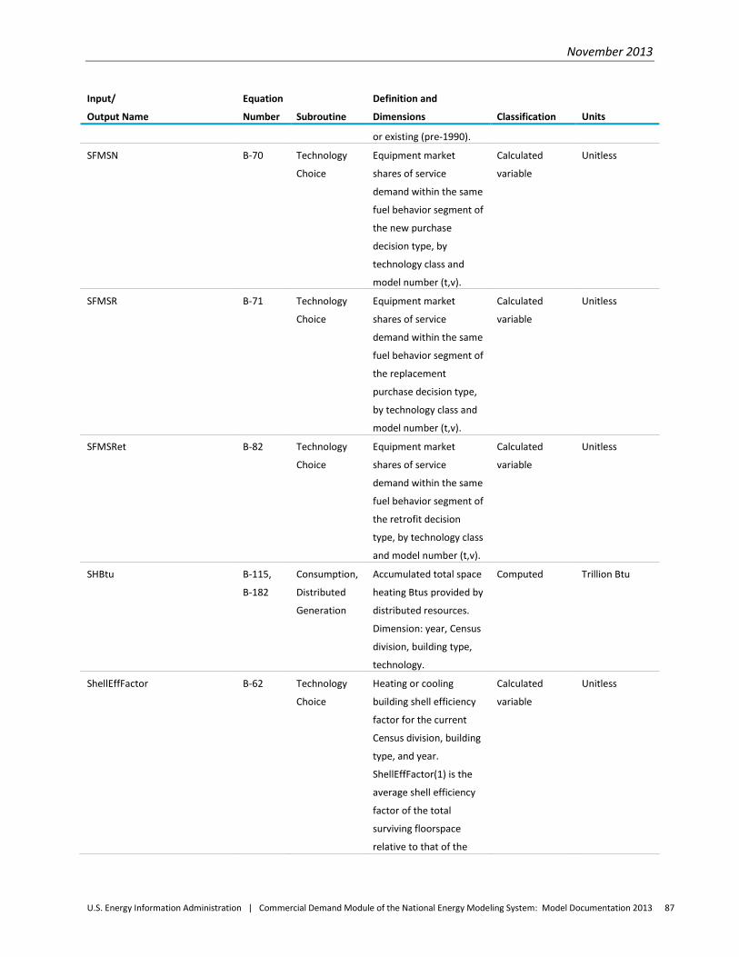
November 2013


Input/

Output Name

Equation

Number Subroutine

Definition and


or existing (pre-1990).

SFMSN B-70 Technology

Choice

Equipment market

shares of service

demand within the same

fuel behavior segment of

the new purchase

decision type, by


model number (t,v).

Calculated

variable

Unitless

SFMSR B-71 Technology

Choice

Equipment market

shares of service



the replacement

purchase decision type,


model number (t,v).

Calculated

variable

Unitless

SFMSRet B-82 Technology

Choice

Equipment market

shares of service



the retrofit decision

type, by technology class

and model number (t,v).

Calculated

variable

Unitless

SHBtu B-115,

B-182

Consumption,

Distributed

Generation

Accumulated total space

heating Btus provided by

distributed resources.



technology.

Computed Trillion Btu

ShellEffFactor B-62 Technology

Choice

Heating or cooling


factor for the current


type, and year.

ShellEffFactor(1) is the

average shell efficiency

factor of the total

surviving floorspace

relative to that of the

Calculated

variable

Unitless

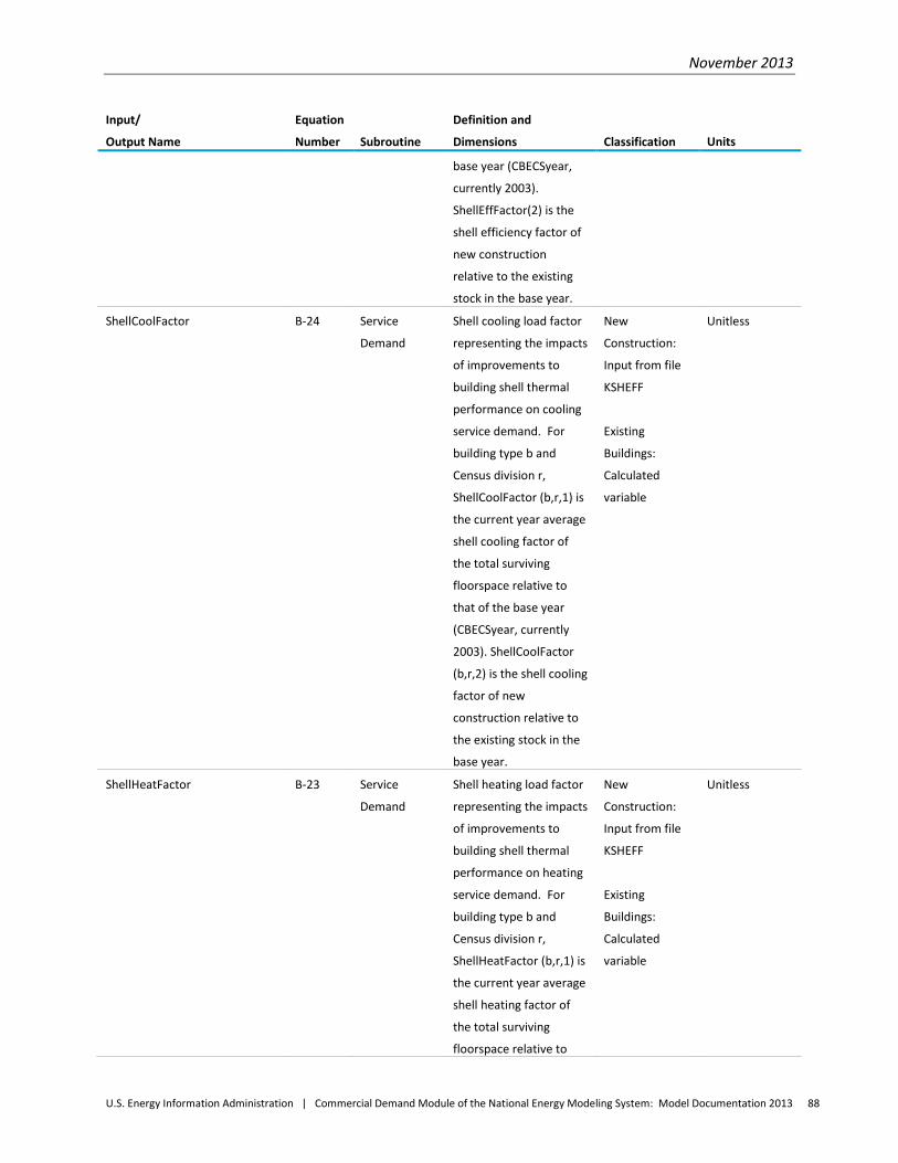
November 2013


Input/

Output Name

Equation

Number Subroutine

Definition and


base year (CBECSyear,

currently 2003).

ShellEffFactor(2) is the

shell efficiency factor of

new construction

relative to the existing

stock in the base year.

ShellCoolFactor B-24 Service

Demand

Shell cooling load factor

representing the impacts

of improvements to

building shell thermal

performance on cooling

service demand. For

building type b and

Census division r,

ShellCoolFactor (b,r,1) is

the current year average

shell cooling factor of

the total surviving

floorspace relative to

that of the base year

(CBECSyear, currently

2003). ShellCoolFactor

(b,r,2) is the shell cooling

factor of new

construction relative to

the existing stock in the

base year.

New

Construction:

Input from file

KSHEFF

Existing

Buildings:

Calculated

variable

Unitless

ShellHeatFactor B-23 Service

Demand

Shell heating load factor

representing the impacts

of improvements to

building shell thermal

performance on heating

service demand. For

building type b and

Census division r,

ShellHeatFactor (b,r,1) is

the current year average

shell heating factor of

the total surviving

floorspace relative to

New

Construction:

Input from file

KSHEFF

Existing

Buildings:

Calculated

variable

Unitless

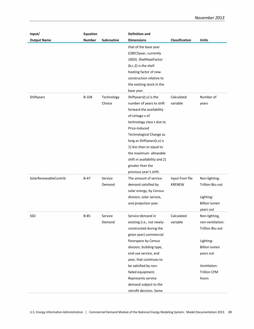
November 2013


Input/

Output Name

Equation

Number Subroutine

Definition and


that of the base year

(CBECSyear, currently

2003). ShellHeatFactor

(b,r,2) is the shell

heating factor of new

construction relative to

the existing stock in the

base year.

Shiftyears B-104 Technology

Choice

Shiftyears(t,v) is the

number of years to shift

forward the availability

of vintage v of

technology class t due to

Price-Induced

Technological Change as

long as Shiftyears(t,v) is

1) less than or equal to

the maximum allowable

shift in availability and 2)

greater than the

previous year’s shift.

Calculated

variable

Number of

years

SolarRenewableContrib B-47 Service

Demand

The amount of service

demand satisfied by

solar energy, by Census

division, solar service,


Input from file

KRENEW

Non-lighting:

Trillion Btu out

Lighting:

Billion lumen

years out

SSD B-85 Service

Demand

Service demand in

existing (i.e., not newly-

constructed during the

given year) commercial




year, that continues to

be satisfied by non-

failed equipment.

Represents service

demand subject to the

retrofit decision. Same

Calculated

variable

Non-lighting,

non-ventilation:

Trillion Btu out

Lighting:

Billion lumen

years out

Ventilation:

Trillion CFM

hours

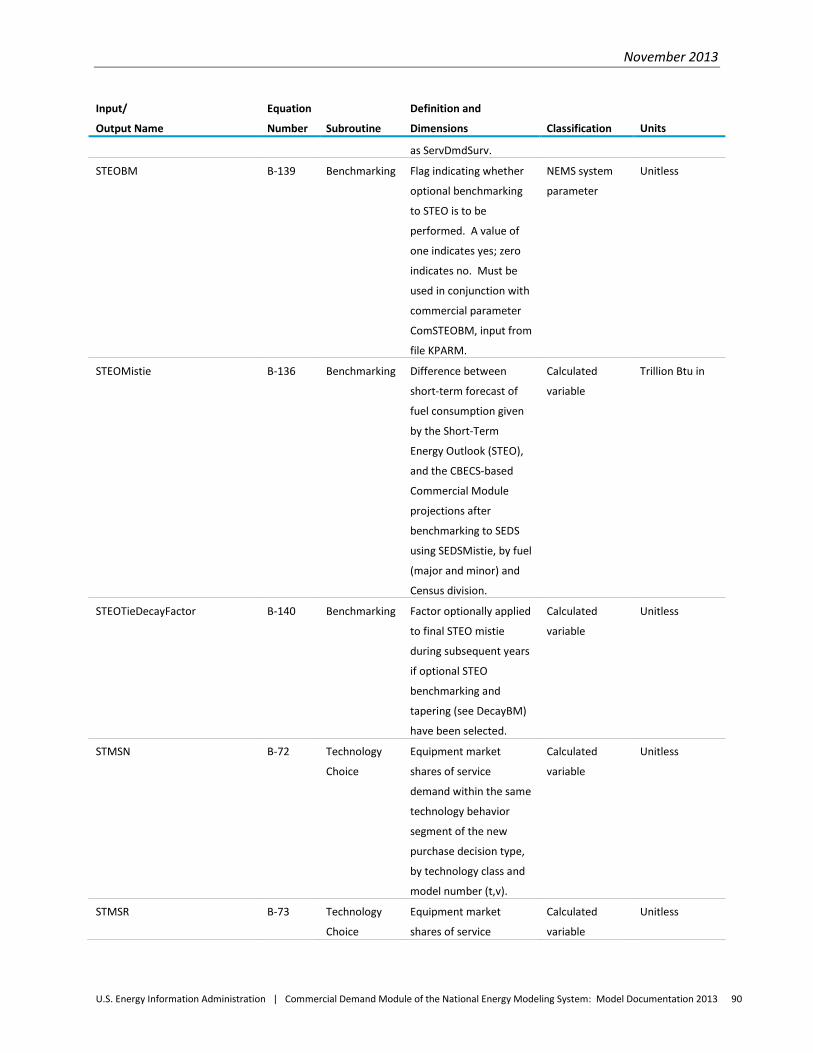
November 2013


Input/

Output Name

Equation

Number Subroutine

Definition and


as ServDmdSurv.

STEOBM B-139 Benchmarking Flag indicating whether


to STEO is to be

performed. A value of


indicates no. Must be

used in conjunction with

commercial parameter

ComSTEOBM, input from

file KPARM.

NEMS system

parameter

Unitless

STEOMistie B-136 Benchmarking Difference between

short-term forecast of

fuel consumption given

by the Short-Term

Energy Outlook (STEO),

and the CBECS-based

Commercial Module

projections after

benchmarking to SEDS

using SEDSMistie, by fuel

(major and minor) and

Census division.

Calculated

variable

Trillion Btu in

STEOTieDecayFactor B-140 Benchmarking Factor optionally applied

to final STEO mistie

during subsequent years

if optional STEO

benchmarking and

tapering (see DecayBM)

have been selected.

Calculated

variable

Unitless

STMSN B-72 Technology

Choice

Equipment market

shares of service


technology behavior

segment of the new

purchase decision type,


model number (t,v).

Calculated

variable

Unitless

STMSR B-73 Technology

Choice

Equipment market

shares of service

Calculated

variable

Unitless

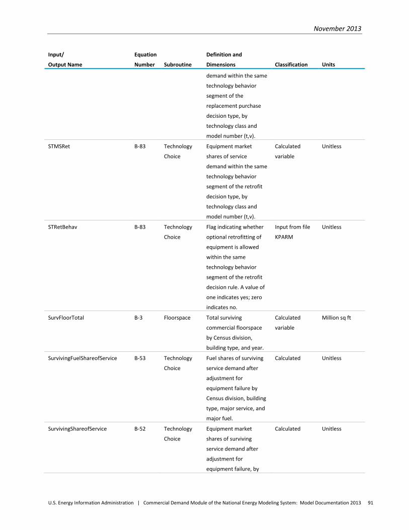
November 2013


Input/

Output Name

Equation

Number Subroutine

Definition and



technology behavior

segment of the

replacement purchase

decision type, by


model number (t,v).

STMSRet B-83 Technology

Choice

Equipment market

shares of service


technology behavior

segment of the retrofit

decision type, by


model number (t,v).

Calculated

variable

Unitless

STRetBehav B-83 Technology

Choice

Flag indicating whether

optional retrofitting of

equipment is allowed

within the same

technology behavior

segment of the retrofit

decision rule. A value of


indicates no.

Input from file

KPARM

Unitless

SurvFloorTotal B-3 Floorspace Total surviving


by Census division,


Calculated

variable

Million sq ft

SurvivingFuelShareofService B-53 Technology

Choice

Fuel shares of surviving

service demand after

adjustment for

equipment failure by


type, major service, and

major fuel.

Calculated Unitless

SurvivingShareofService B-52 Technology

Choice

Equipment market

shares of surviving

service demand after

adjustment for


Calculated Unitless

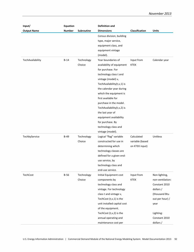
November 2013


Input/

Output Name

Equation

Number Subroutine

Definition and



type, major service,

equipment class, and

equipment vintage

(model).

TechAvailability B-14 Technology

Choice

Year boundaries of

availability of equipment

for purchase. For

technology class t and

vintage (model) v,

TechAvailability(t,v,1) is

the calendar year during

which the equipment is

first available for

purchase in the model.

TechAvailability(t,v,2) is

the last year of

equipment availability

for purchase. By


vintage (model).

Input from

KTEK

Calendar year

TechbyService B-49 Technology

Choice

Logical “flag” variable

constructed for use in

determining which

technology classes are

defined for a given end-

use service, by


end-use service.

Calculated

variable (based

on KTEK input)

Unitless

TechCost B-56 Technology

Choice

Initial Equipment cost

components by


vintage. For technology

class t and vintage v,

TechCost (t,v,1) is the

unit installed capital cost

of the equipment.

TechCost (t,v,2) is the

annual operating and

maintenance cost per

Input from

KTEK

Non-lighting,

non-ventilation:

Constant 2010

dollars /

(thousand Btu

out per hour) /

year

Lighting:

Constant 2010

dollars /

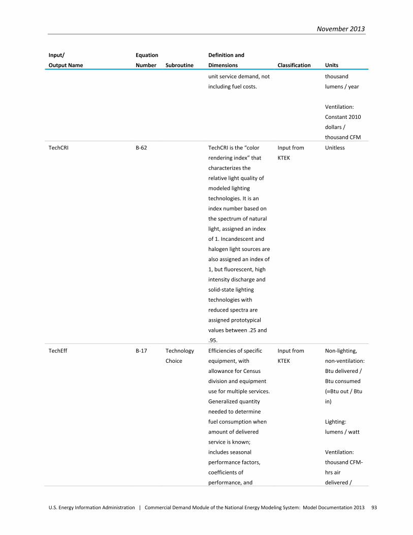
November 2013


Input/

Output Name

Equation

Number Subroutine

Definition and


unit service demand, not

including fuel costs.

thousand

lumens / year

Ventilation:

Constant 2010

dollars /

thousand CFM

TechCRI B-62 TechCRI is the “color

rendering index” that

characterizes the

relative light quality of

modeled lighting

technologies. It is an

index number based on

the spectrum of natural

light, assigned an index

of 1. Incandescent and

halogen light sources are

also assigned an index of

1, but fluorescent, high

intensity discharge and

solid-state lighting

technologies with

reduced spectra are

assigned prototypical

values between .25 and

.95.

Input from

KTEK

Unitless

TechEff B-17 Technology

Choice

Efficiencies of specific

equipment, with

allowance for Census

division and equipment

use for multiple services.

Generalized quantity

needed to determine

fuel consumption when

amount of delivered

service is known;

includes seasonal

performance factors,

coefficients of

performance, and

Input from

KTEK

Non-lighting,

non-ventilation:

Btu delivered /

Btu consumed

(≡Btu out / Btu

in)

Lighting:

lumens / watt

Ventilation:

thousand CFM-

hrs air

delivered /

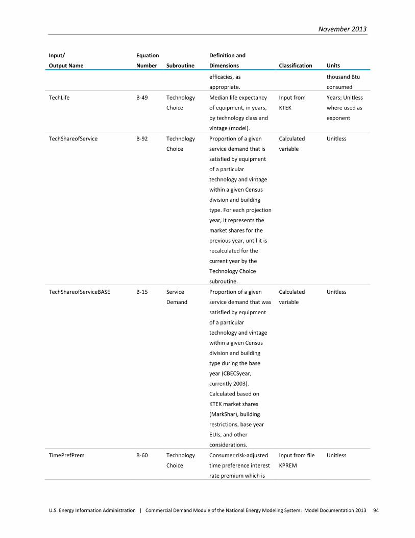
November 2013


Input/

Output Name

Equation

Number Subroutine

Definition and


efficacies, as

appropriate.

thousand Btu

consumed

TechLife B-49 Technology

Choice

Median life expectancy

of equipment, in years,


vintage (model).

Input from

KTEK

Years; Unitless

where used as

exponent

TechShareofService B-92 Technology

Choice


service demand that is


of a particular




type. For each projection

year, it represents the

market shares for the

previous year, until it is

recalculated for the

current year by the

Technology Choice

subroutine.

Calculated

variable

Unitless

TechShareofServiceBASE B-15 Service

Demand




of a particular




type during the base

year (CBECSyear,

currently 2003).

Calculated based on

KTEK market shares

(MarkShar), building

restrictions, base year

EUIs, and other

considerations.

Calculated

variable

Unitless

TimePrefPrem B-60 Technology

Choice

Consumer risk-adjusted

time preference interest

rate premium which is

Input from file

KPREM

Unitless

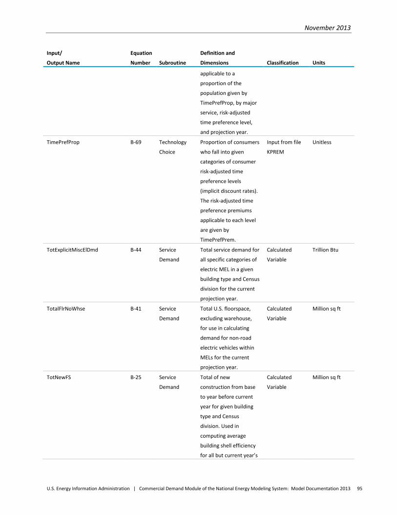
November 2013


Input/

Output Name

Equation

Number Subroutine

Definition and


applicable to a

proportion of the

population given by

TimePrefProp, by major

service, risk-adjusted

time preference level,


TimePrefProp B-69 Technology

Choice

Proportion of consumers

who fall into given

categories of consumer

risk-adjusted time

preference levels

(implicit discount rates).

The risk-adjusted time

preference premiums

applicable to each level

are given by

TimePrefPrem.

Input from file

KPREM

Unitless

TotExplicitMiscElDmd B-44 Service

Demand

Total service demand for

all specific categories of

electric MEL in a given


division for the current

projection year.

Calculated

Variable

Trillion Btu

TotalFlrNoWhse B-41 Service

Demand


excluding warehouse,

for use in calculating

demand for non-road

electric vehicles within

MELs for the current

projection year.

Calculated

Variable

Million sq ft

TotNewFS B-25 Service

Demand

Total of new

construction from base

to year before current

year for given building

type and Census

division. Used in

computing average


for all but current year’s

Calculated

Variable

Million sq ft

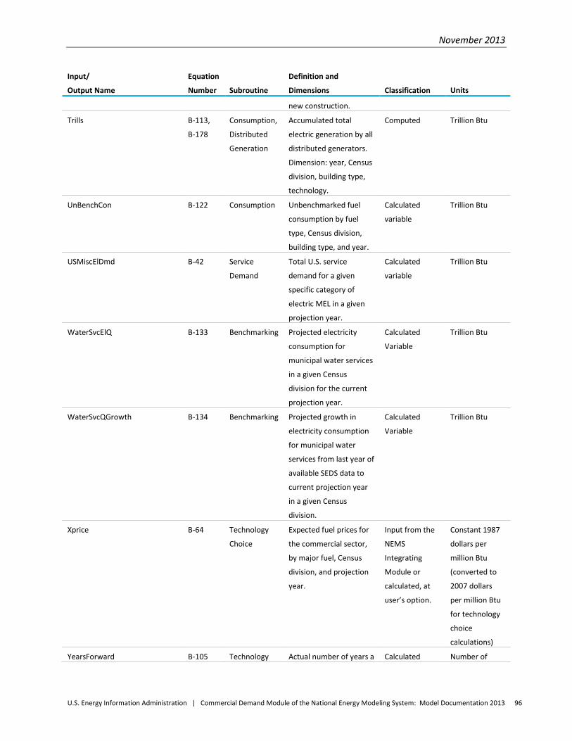
November 2013


Input/

Output Name

Equation

Number Subroutine

Definition and


new construction.

Trills B-113,

B-178

Consumption,

Distributed

Generation

Accumulated total

electric generation by all

distributed generators.



technology.


UnBenchCon B-122 Consumption Unbenchmarked fuel

consumption by fuel



Calculated

variable

Trillion Btu

USMiscElDmd B-42 Service

Demand

Total U.S. service

demand for a given

specific category of

electric MEL in a given

projection year.

Calculated

variable

Trillion Btu

WaterSvcElQ B-133 Benchmarking Projected electricity

consumption for

municipal water services

in a given Census

division for the current

projection year.

Calculated

Variable

Trillion Btu

WaterSvcQGrowth B-134 Benchmarking Projected growth in

electricity consumption

for municipal water

services from last year of

available SEDS data to

current projection year

in a given Census

division.

Calculated

Variable

Trillion Btu

Xprice B-64 Technology

Choice

Expected fuel prices for

the commercial sector,

by major fuel, Census


year.

Input from the

NEMS

Integrating

Module or

calculated, at

user’s option.

Constant 1987

dollars per

million Btu

(converted to

2007 dollars

per million Btu

for technology

choice

calculations)

YearsForward B-105 Technology Actual number of years a Calculated Number of

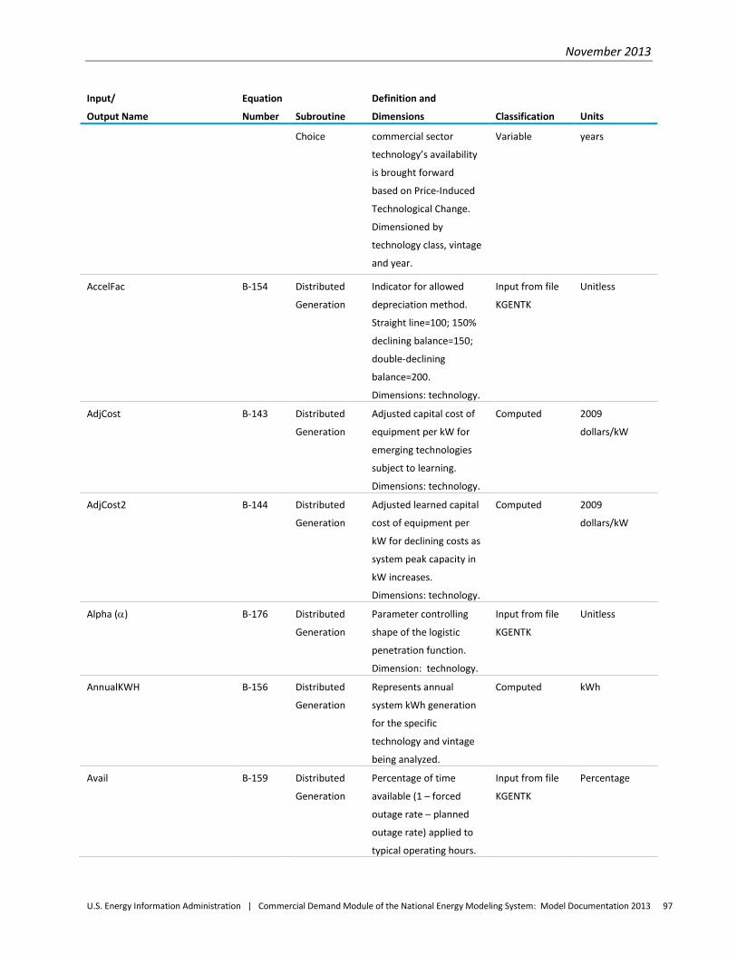
November 2013


Input/

Output Name

Equation

Number Subroutine

Definition and


Choice commercial sector

technology’s availability

is brought forward

based on Price-Induced

Technological Change.

Dimensioned by

technology class, vintage

and year.

Variable years

AccelFac B-154 Distributed

Generation

Indicator for allowed

depreciation method.

Straight line=100; 150%

declining balance=150;

double-declining

balance=200.

Dimensions: technology.

Input from file

KGENTK

Unitless

AdjCost B-143 Distributed

Generation

Adjusted capital cost of

equipment per kW for

emerging technologies

subject to learning.


Computed 2009

dollars/kW

AdjCost2 B-144 Distributed

Generation

Adjusted learned capital

cost of equipment per

kW for declining costs as

system peak capacity in

kW increases.


Computed 2009

dollars/kW

Alpha (α) B-176 Distributed

Generation

Parameter controlling

shape of the logistic

penetration function.

Dimension: technology.

Input from file

KGENTK

Unitless

AnnualKWH B-156 Distributed

Generation

Represents annual

system kWh generation

for the specific


being analyzed.

Computed kWh

Avail B-159 Distributed

Generation

Percentage of time

available (1 – forced

outage rate – planned

outage rate) applied to

typical operating hours.

Input from file

KGENTK

Percentage

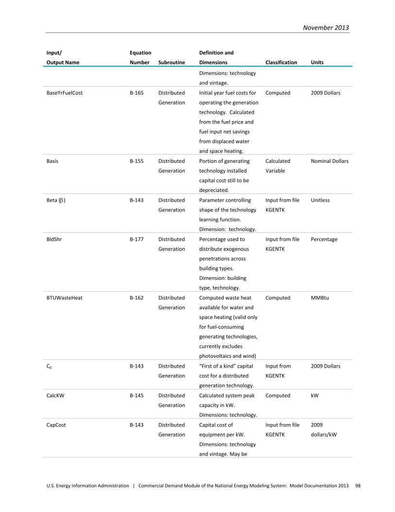
November 2013


Input/

Output Name

Equation

Number Subroutine

Definition and


Dimensions: technology

and vintage.

BaseYrFuelCost B-165 Distributed

Generation

Initial year fuel costs for

operating the generation

technology. Calculated

from the fuel price and

fuel input net savings

from displaced water

and space heating.

Computed 2009 Dollars

Basis B-155 Distributed

Generation

Portion of generating

technology installed

capital cost still to be

depreciated.

Calculated

Variable

Nominal Dollars

Beta (β) B-143 Distributed

Generation


shape of the technology

learning function.


Input from file

KGENTK

Unitless

BldShr B-177 Distributed

Generation

Percentage used to

distribute exogenous

penetrations across

building types.

Dimension: building

type, technology.

Input from file

KGENTK

Percentage

BTUWasteHeat B-162 Distributed

Generation

Computed waste heat

available for water and

space heating (valid only

for fuel-consuming

generating technologies,

currently excludes

photovoltaics and wind)

Computed MMBtu

C0 B-143 Distributed

Generation

“First of a kind” capital

cost for a distributed

generation technology.

Input from

KGENTK

2009 Dollars

CalcKW B-145 Distributed

Generation

Calculated system peak

capacity in kW.


Computed kW

CapCost B-143 Distributed

Generation

Capital cost of

equipment per kW.


and vintage. May be

Input from file

KGENTK

2009

dollars/kW

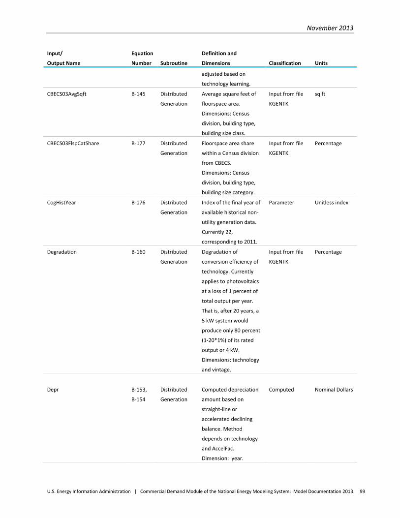
November 2013


Input/

Output Name

Equation

Number Subroutine

Definition and


adjusted based on

technology learning.

CBECS03AvgSqft B-145 Distributed

Generation

Average square feet of

floorspace area.

Dimensions: Census


building size class.

Input from file

KGENTK

sq ft

CBECS03FlspCatShare B-177 Distributed

Generation

Floorspace area share

within a Census division

from CBECS.

Dimensions: Census


building size category.

Input from file

KGENTK

Percentage

CogHistYear B-176 Distributed

Generation

Index of the final year of

available historical non-

utility generation data.

Currently 22,


Parameter Unitless index

Degradation B-160 Distributed

Generation

Degradation of

conversion efficiency of

technology. Currently

applies to photovoltaics

at a loss of 1 percent of

total output per year.

That is, after 20 years, a

5 kW system would

produce only 80 percent

(1-20*1%) of its rated

output or 4 kW.


and vintage.

Input from file

KGENTK

Percentage

Depr

B-153,

B-154

Distributed

Generation

Computed depreciation

amount based on

straight-line or

accelerated declining

balance. Method

depends on technology

and AccelFac.

Dimension: year.

Computed

Nominal Dollars

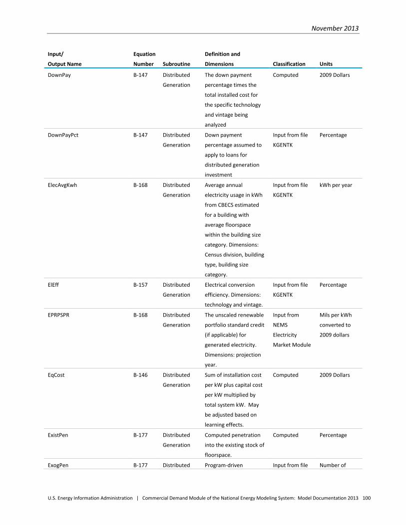
November 2013


Input/

Output Name

Equation

Number Subroutine

Definition and


DownPay B-147 Distributed

Generation

The down payment

percentage times the

total installed cost for

the specific technology

and vintage being

analyzed


DownPayPct B-147 Distributed

Generation

Down payment

percentage assumed to

apply to loans for

distributed generation

investment

Input from file

KGENTK

Percentage

ElecAvgKwh B-168 Distributed

Generation

Average annual

electricity usage in kWh

from CBECS estimated

for a building with

average floorspace

within the building size

category. Dimensions:


type, building size

category.

Input from file

KGENTK

kWh per year

ElEff B-157 Distributed

Generation

Electrical conversion

efficiency. Dimensions:

technology and vintage.

Input from file

KGENTK

Percentage

EPRPSPR B-168 Distributed

Generation

The unscaled renewable

portfolio standard credit

(if applicable) for

generated electricity.

Dimensions: projection

year.

Input from

NEMS

Electricity

Market Module

Mils per kWh

converted to

2009 dollars

EqCost B-146 Distributed

Generation

Sum of installation cost

per kW plus capital cost

per kW multiplied by

total system kW. May

be adjusted based on

learning effects.


ExistPen B-177 Distributed

Generation

Computed penetration

into the existing stock of

floorspace.

Computed Percentage

ExogPen B-177 Distributed Program-driven Input from file Number of

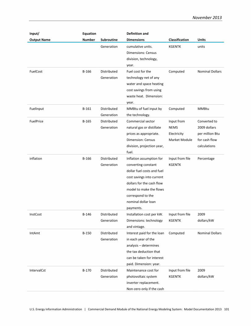
November 2013


Input/

Output Name

Equation

Number Subroutine

Definition and


Generation cumulative units.

Dimensions: Census

division, technology,

year.

KGENTK units

FuelCost B-166 Distributed

Generation

Fuel cost for the

technology net of any

water and space heating

cost savings from using

waste heat. Dimension:

year.

Computed Nominal Dollars

FuelInput B-161 Distributed

Generation

MMBtu of fuel input by

the technology.

Computed MMBtu

FuelPrice B-165 Distributed

Generation

Commercial sector

natural gas or distillate

prices as appropriate.

Dimension: Census

division, projection year,

fuel.

Input from

NEMS

Electricity

Market Module

Converted to

2009 dollars

per million Btu

for cash flow

calculations

inflation B-166 Distributed

Generation

Inflation assumption for

converting constant

dollar fuel costs and fuel

cost savings into current

dollars for the cash flow

model to make the flows

correspond to the

nominal dollar loan

payments.

Input from file

KGENTK

Percentage

InstCost B-146 Distributed

Generation

Installation cost per kW.


and vintage.

Input from file

KGENTK

2009

dollars/kW

IntAmt B-150 Distributed

Generation

Interest paid for the loan

in each year of the

analysis – determines

the tax deduction that

can be taken for interest

paid. Dimension: year.


IntervalCst B-170 Distributed

Generation

Maintenance cost for

photovoltaic system

inverter replacement.

Non-zero only if the cash

Input from file

KGENTK

2009

dollars/kW

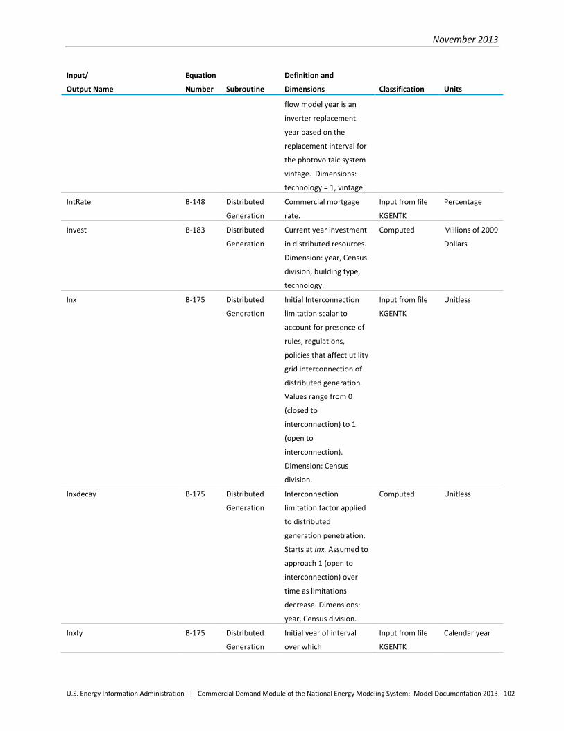
November 2013


Input/

Output Name

Equation

Number Subroutine

Definition and


flow model year is an

inverter replacement

year based on the

replacement interval for

the photovoltaic system

vintage. Dimensions:

technology = 1, vintage.

IntRate B-148 Distributed

Generation

Commercial mortgage

rate.

Input from file

KGENTK

Percentage

Invest B-183 Distributed

Generation

Current year investment

in distributed resources.



technology.

Computed Millions of 2009

Dollars

Inx B-175 Distributed

Generation

Initial Interconnection

limitation scalar to

account for presence of

rules, regulations,

policies that affect utility

grid interconnection of

distributed generation.

Values range from 0

(closed to

interconnection) to 1

(open to

interconnection).

Dimension: Census

division.

Input from file

KGENTK

Unitless

Inxdecay B-175 Distributed

Generation

Interconnection

limitation factor applied

to distributed

generation penetration.

Starts at Inx. Assumed to

approach 1 (open to

interconnection) over

time as limitations

decrease. Dimensions:

year, Census division.

Computed Unitless

Inxfy B-175 Distributed

Generation

Initial year of interval

over which

Input from file

KGENTK

Calendar year

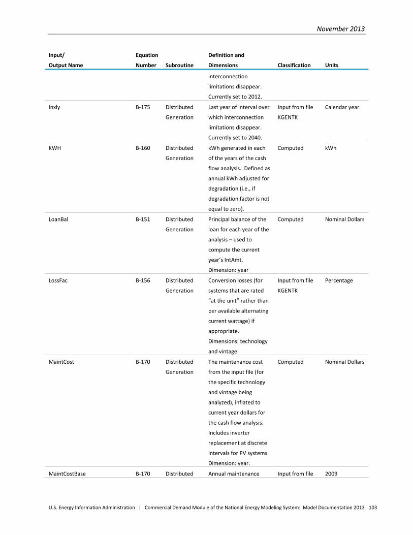
November 2013


Input/

Output Name

Equation

Number Subroutine

Definition and


interconnection

limitations disappear.

Currently set to 2012.

Inxly B-175 Distributed

Generation

Last year of interval over

which interconnection

limitations disappear.

Currently set to 2040.

Input from file

KGENTK

Calendar year

KWH B-160 Distributed

Generation

kWh generated in each

of the years of the cash

flow analysis. Defined as

annual kWh adjusted for

degradation (i.e., if

degradation factor is not

equal to zero).

Computed kWh

LoanBal B-151 Distributed

Generation

Principal balance of the

loan for each year of the

analysis – used to

compute the current

year’s IntAmt.

Dimension: year


LossFac B-156 Distributed

Generation

Conversion losses (for

systems that are rated

“at the unit” rather than

per available alternating

current wattage) if

appropriate.


and vintage.

Input from file

KGENTK

Percentage

MaintCost B-170 Distributed

Generation

The maintenance cost

from the input file (for

the specific technology

and vintage being

analyzed), inflated to

current year dollars for

the cash flow analysis.

Includes inverter

replacement at discrete

intervals for PV systems.

Dimension: year.


MaintCostBase B-170 Distributed Annual maintenance Input from file 2009

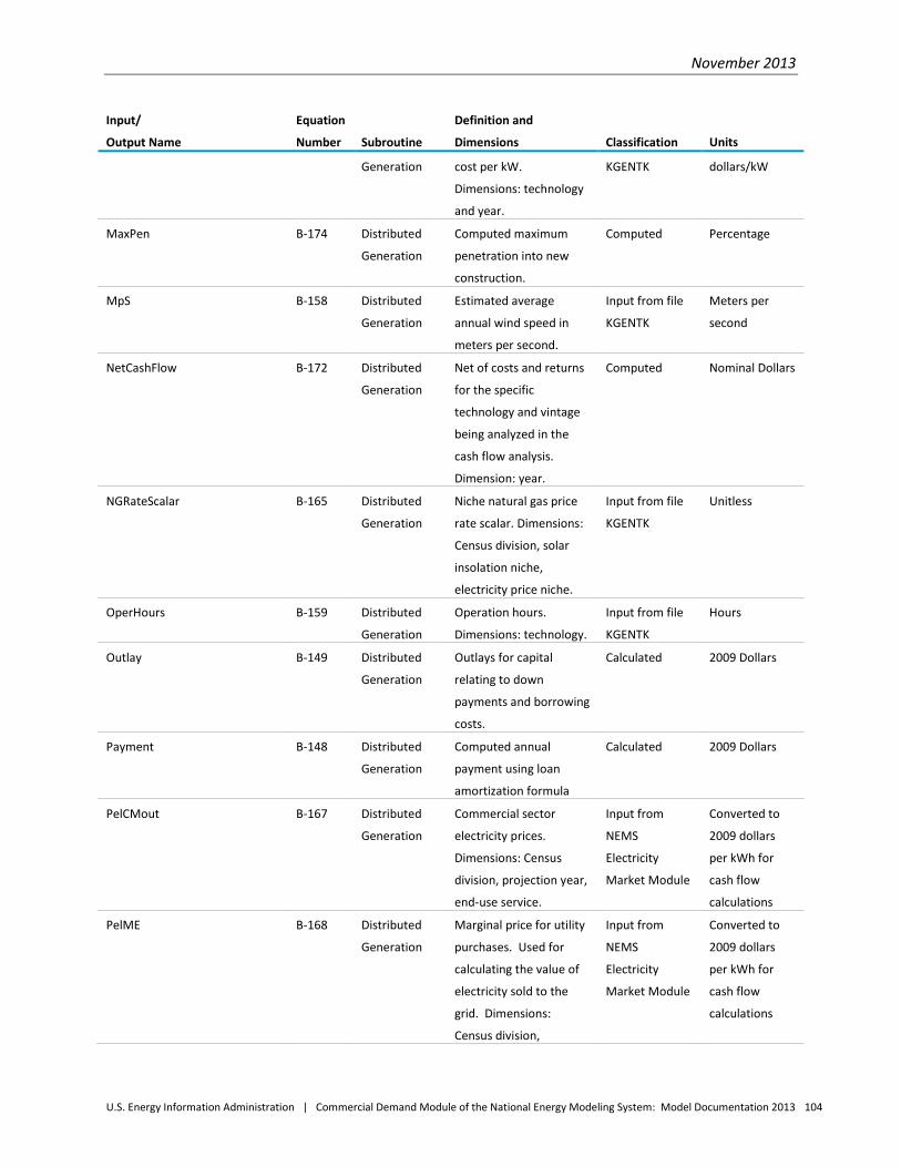
November 2013


Input/

Output Name

Equation

Number Subroutine

Definition and


Generation cost per kW.


and year.

KGENTK dollars/kW

MaxPen B-174 Distributed

Generation

Computed maximum

penetration into new

construction.

Computed Percentage

MpS B-158 Distributed

Generation

Estimated average

annual wind speed in

meters per second.

Input from file

KGENTK

Meters per

second

NetCashFlow B-172 Distributed

Generation

Net of costs and returns

for the specific


being analyzed in the

cash flow analysis.

Dimension: year.


NGRateScalar B-165 Distributed

Generation

Niche natural gas price

rate scalar. Dimensions:

Census division, solar

insolation niche,

electricity price niche.

Input from file

KGENTK

Unitless

OperHours B-159 Distributed

Generation

Operation hours.


Input from file

KGENTK

Hours

Outlay B-149 Distributed

Generation

Outlays for capital

relating to down

payments and borrowing

costs.

Calculated 2009 Dollars

Payment B-148 Distributed

Generation

Computed annual

payment using loan

amortization formula

Calculated 2009 Dollars

PelCMout B-167 Distributed

Generation

Commercial sector

electricity prices.

Dimensions: Census

division, projection year,

end-use service.

Input from

NEMS

Electricity

Market Module

Converted to

2009 dollars

per kWh for

cash flow

calculations

PelME B-168 Distributed

Generation

Marginal price for utility

purchases. Used for

calculating the value of

electricity sold to the

grid. Dimensions:

Census division,

Input from

NEMS

Electricity

Market Module

Converted to

2009 dollars

per kWh for

cash flow

calculations

November 2013


Input/

Output Name

Equation

Number Subroutine

Definition and


projection year.

Pen B-176 Distributed

Generation

Computed penetration

into new construction.

Computed Percentage

PenParm B-174 Distributed

Generation


maximum penetration

into new construction.


Input from file

KGENTK

Unitless

Prin B-151 Distributed

Generation

The amount of principal

paid on the loan in each

year of the analysis –

used to determine the

loan balance for the next

year of the analysis.

Dimension: year.


RateScalar B-167 Distributed

Generation

Niche electricity price

rate scalar. Dimensions:

Census division, solar

insolation niche,


Input from the

file KGENTK

Unitless

RoofAreatoSqftRatio B-145 Distributed

Generation

Roof area per unit of

floorspace area.

Dimensions: Census


solar insolation niche,


Input from the

file KGENTK

Unitless

ScaleFac B-144 Distributed

Generation

Parameter determining

how quickly costs

decline as system peak

capacity in kW increases.


Input from the

file KGENTK

2009

dollars/kW

ScaleRPS B-168 Distributed

Generation

Scalar to adjust the

renewable portfolio

standard credit (if

applicable) for

generated electricity.

Dimension: projection

year.

Input from the

file KGENTK

Unitless

SimplePayback B-173 Distributed

Generation

The equivalent payback

year number computed

from the IRR for use in

Computed Year Index

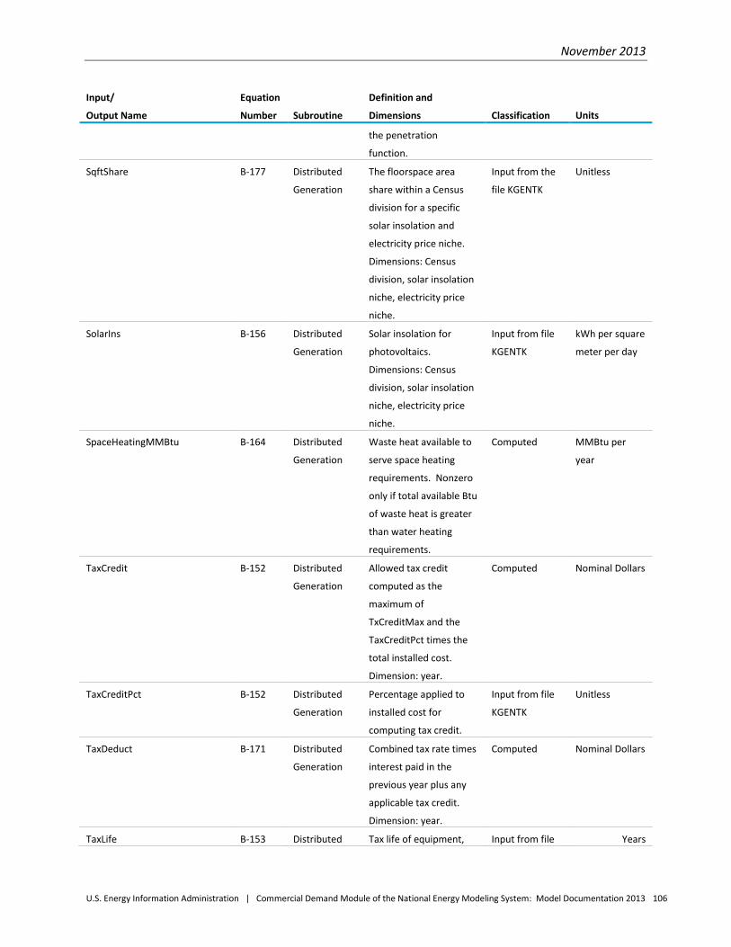
November 2013


Input/

Output Name

Equation

Number Subroutine

Definition and


the penetration

function.

SqftShare B-177 Distributed

Generation

The floorspace area

share within a Census

division for a specific

solar insolation and


Dimensions: Census

division, solar insolation

niche, electricity price

niche.

Input from the

file KGENTK

Unitless

SolarIns B-156 Distributed

Generation

Solar insolation for

photovoltaics.

Dimensions: Census

division, solar insolation

niche, electricity price

niche.

Input from file

KGENTK

kWh per square

meter per day

SpaceHeatingMMBtu B-164 Distributed

Generation

Waste heat available to

serve space heating

requirements. Nonzero

only if total available Btu

of waste heat is greater

than water heating

requirements.

Computed MMBtu per

year

TaxCredit B-152 Distributed

Generation

Allowed tax credit

computed as the

maximum of

TxCreditMax and the

TaxCreditPct times the

total installed cost.

Dimension: year.


TaxCreditPct B-152 Distributed

Generation

Percentage applied to

installed cost for

computing tax credit.

Input from file

KGENTK

Unitless

TaxDeduct B-171 Distributed

Generation

Combined tax rate times

interest paid in the

previous year plus any

applicable tax credit.

Dimension: year.


TaxLife B-153 Distributed Tax life of equipment, Input from file Years

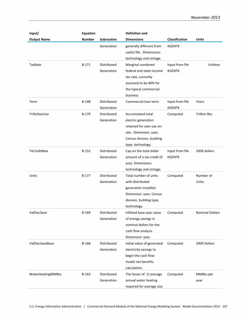
November 2013


Input/

Output Name

Equation

Number Subroutine

Definition and


Generation generally different from

useful life. Dimensions:


KGENTK

TaxRate B-171 Distributed

Generation

Marginal combined

federal and state income

tax rate, currently

assumed to be 40% for

the typical commercial

business

Input from file

KGENTK

Unitless

Term B-148 Distributed

Generation

Commercial loan term Input from file

KGENTK

Years

TrillsOwnUse B-179 Distributed

Generation

Accumulated total

electric generation

retained for own use on-

site. Dimension: year,


type, technology.


TxCreditMax B-152 Distributed

Generation

Cap on the total dollar

amount of a tax credit (if

any). Dimensions:


Input from file

KGENTK

2009 dollars

Units B-177 Distributed

Generation

Total number of units

with distributed

generation installed.



technology.

Computed Number of

Units

ValElecSave B-169 Distributed

Generation

Inflated base year value

of energy savings in

nominal dollars for the

cash flow analysis.

Dimension: year.


ValElecSaveBase B-168 Distributed

Generation

Initial value of generated

electricity savings to

begin the cash flow

model net benefits

calculation.


WaterHeatingMMBtu B-163 Distributed

Generation

The lesser of: 1) average

annual water heating

required for average size

Computed MMBtu per

year

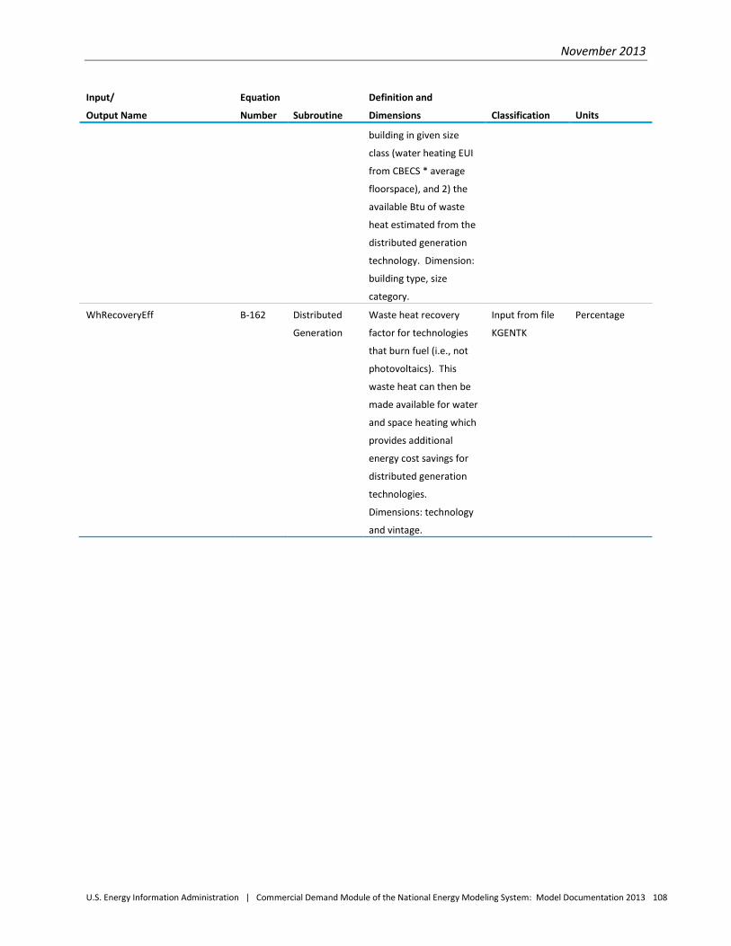
November 2013


Input/

Output Name

Equation

Number Subroutine

Definition and


building in given size

class (water heating EUI

from CBECS * average

floorspace), and 2) the

available Btu of waste

heat estimated from the


technology. Dimension:

building type, size

category.

WhRecoveryEff B-162 Distributed

Generation

Waste heat recovery

factor for technologies

that burn fuel (i.e., not

photovoltaics). This

waste heat can then be

made available for water

and space heating which

provides additional

energy cost savings for


technologies.


and vintage.

Input from file

KGENTK

Percentage

November 2013


Profiles of input data This section provides additional details for the model inputs listed in Table A-1 above. The variable names as they appear in the Fortran code are included along with definitions, classifications, NEMS input file location, longer discussions and source references.

MODEL INPUT: Proportion of base year office equipment EUI attributable to PC use

VARIABLE NAME: BaseYrPCShrofOffEqEUI

MODEL COMPONENT: Service Demand

DEFINITION: PC proportion of base year office equipment EUI

CLASSIFICATION: Input parameter (KPARM)

DISCUSSION:

The 2003 CBECS Public Use Files provide CBECS-derived end-use consumption estimates by building type, fuel type, and Census division for the end-use services modeled by the NEMS Commercial Demand Module, developed using a combination of engineering end-use models and regression approaches. The 2003 estimates include separate breakouts for personal computers (PCs) and other office equipment, eliminating the need for the PC proportion parameter.

The parameter has been given a value of -1.0 in KPARM to automatically disable its use, triggering use of the specific PC EUI in the EUI input file, KINTENS.

SOURCES:

U.S. Energy Information Administration. 2003 Commercial Buildings Energy Consumption Survey, Public Use Files. Washington DC, September 2008, http://www.eia.gov/consumption/commercial/data/2003/

http://www.eia.gov/consumption/commercial/data/2003/

November 2013


MODEL INPUT: Consumer behavior rule proportions

VARIABLE NAME: BehaviorShare

MODEL COMPONENT: Technology Choice

DEFINITION: Proportions of commercial consumers using the least-cost, same-fuel, and same-technology behavior rules for decision type d in building type b

CLASSIFICATION: Input from file KBEHAV

DISCUSSION:

These parameters are designed to facilitate model calibration to historical data, so precise specifications are not expected. Nevertheless, professional judgment is applied to estimate initial values for the proportions by decision type and building type which are consistent with the commercial sector. Building type is used here as a proxy to distinguish different types of commercial sector decision makers, and decision type represents the different economic situations under which technology choice decisions are made.

The judgment estimates are made separately for all government, privately owned, and rented floorspace for the replacement and retrofit decision types. The proportions of floorspace by government, private and rented space from A Look at Commercial Buildings 1995: Characteristics, Energy Consumption, and Energy Expenditures, from the 1999 Commercial Buildings Energy Consumption Survey Public Use Files, and from the 2003 Commercial Buildings Energy Consumption Survey Public Use Files are utilized to weight these estimates by building type to yield replacement and retrofit behavior rule proportions by building type. Similarly, judgment estimates are made for self-built and speculative developer floorspace for the new decision type. These consider estimates of the proportions of self-built and speculative developer floorspace for each by building type to yield new building behavior rule proportions by building type.

SOURCES:

Decision Analysis Corporation of Virginia and Science Applications International Corporation. Alternative Methodologies for NEMS Building Sector Model Development, draft report, prepared under Contract No. DE-AC01-92EI21946, August 3, 1992, p. 14.

Koomey, Jonathan G. Energy Efficiency Choices in New Office Buildings: An Investigation of Market Failures and Corrective Policies, Ph. D. Dissertation, University of California at Berkeley, 1990.

Feldman, S. “Why is it So Hard to Sell ‘Savings’ as a Reason for Energy Conservation?” Energy Efficiency: Perspectives on Individual Behavior, Willett Kempton and Max Neiman eds., American Council for an Energy-Efficient Economy, Washington DC, 1987, pp. 27-40.

Office of Technology Assessment. Building Energy Efficiency. OTA-E-518, U.S. Government Printing Office, Washington DC, May 1992.

November 2013


Komor, P. and L. Wiggins. “Predicting Conservation Choice: Beyond the Cost-Minimization Assumption.” Energy, Vol. 13, No. 8, 1988, pp. 633-645.

Komor, P. and R. Katzev. “Behavioral Determinants of Energy Use in Small Commercial Buildings: Implications for Energy Efficiency.” Energy Systems and Policy, Vol. 12, 1988, pp. 233-242.

Vine, E. and J. Harris. “Implementing Energy Conservation Programs for New Residential and Commercial Buildings.” Energy Systems and Policy, Vol. 13, No. 2, 1989, pp. 115-139.

Lamarre, L. “Lighting the Commercial World” EPRI Journal, December 1989, pp. 4-15.

Lamarre, L. “New Push for Energy Efficiency.” EPRI Journal, April/May 1990, pp. 4-17.

U.S. Energy Information Administration. A Look at Commercial Buildings in 1995: Characteristics, Energy Consumption, and Energy Expenditures. Washington DC, October 1998, DOE/EIA-0625(95), GPO Stock No. 061-003-01046-6

U.S. Energy Information Administration. 1999 Commercial Buildings Energy Consumption Survey, Public Use Files. Washington DC, October 2002, http://www.eia.gov/consumption/commercial/data/1999/ .

U.S. Energy Information Administration. 2003 Commercial Buildings Energy Consumption Survey, Public Use Files. Washington DC, http://www.eia.gov/consumption/commercial/data/2003/.



November 2013


MODEL INPUT: Equipment Capacity Factor

VARIABLE NAME: CapacityFactor


DEFINITION: Capacity factor of equipment to meet service s in Census division r in building type b

CLASSIFICATION: Input from file KCAPFAC

DISCUSSION:

The capacity factor is the ratio of actual annual equipment output to output if equipment were run 100 % of the time at full capacity. Space conditioning capacity factors are developed by Census division, service, and building type from the ratio of average daily load to peak load for space heating and space cooling at 44 selected cities in the EPRI source cited below. The averages for the cities in each Census division are weighted by population to compute the capacity factors used by the NEMS Commercial Demand Module. Lighting capacity factors vary by building type and are based upon the ratio of average hours of operation to total hours from Lighting in Commercial Buildings. Capacity factors for the remaining services are derived by service and building type from the ratio of operating hours to total hours in the building load profiles in the EPRI source.

SOURCES:

Decision Focus, Inc. TAG Technical Assessment Guide, Vol. 2: Electricity End Use; Part 2: Commercial Electricity Use -- 1988. Palo Alto CA, Electric Power Research Institute, October 1988, pp. 4-5 to 4-29, 9-10 to 9-27.

U.S. Energy Information Administration. Energy Consumption Series: Lighting in Commercial Buildings. DOE/EIA-0555(92)/1. Washington DC, March 1992. p. 38.

November 2013


MODEL INPUT: Base year commercial floorspace

VARIABLE NAME: CBECSFlrSpc

MODEL COMPONENT: Floorspace

DEFINITION: Commercial floorspace by building type b in Census division r for 2003

CLASSIFICATION: Input from file KFLSPC

DISCUSSION:

A straightforward aggregation of weighted survey data from the 2003 CBECS was used to compute 2003 levels of commercial floorspace for each of the 11 building categories and nine age ranges (“vintage cohorts” - see CMVintage) in each Census division. The mapping used to transfer from the CBECS building classifications to the building type classification scheme used by the NEMS Commercial Demand Module is shown in the table below:

NEMS Classification Plan for Building Types:

NEMS 2003 CBECS

Assembly Public Assembly Religious Worship

Education Education

Food Sales Food Sales

Food Services Food Services

Health Care Health Care – Inpatient

Lodging Lodging Skilled Nursing Other Residential Care

Office – Large Office (> 50,000 square feet) Health Care - Outpatient (> 50,000 square feet)

Office – Small Office (≤50,000 square feet) Health Care - Outpatient (≤50,000 square feet)

Mercantile and Service Mercantile

November 2013


Service

Warehouse Refrigerated Warehouse Non-refrigerated Warehouse

Other Laboratory Public Order and Safety Vacant Other

SOURCES:


U.S. Energy Information Administration. Description of CBECS Building Types, http://www.eia.gov/consumption/commercial/building-type-definitions.cfm.


http://www.eia.gov/consumption/commercial/building-type-definitions.cfm

November 2013


MODEL INPUT: Expected building lifetimes

VARIABLE NAME: CMAvgAge


DEFINITION: Median building lifetime by building type b

CLASSIFICATION: Input from file KBLDG

DISCUSSION:

The sources cited below contributed to the development of estimates of average building lifetimes for the building types considered by the NEMS Commercial Demand Module. Insufficient data addressing median expected commercial building usage lifetimes were available to enable disaggregation to the Census division level; consequently, a characterization at the national level was developed based on the sources cited below.

SOURCES:

Hazilla, M., and R. Kopp. “Systematic Effects of Capital Service Price Definition on Perceptions of Input Substitution.” Journal of Business and Economic Statistics. April 1986, pp. 209-224.

KEMA-XENERGY Inc. for Northwest Energy Efficiency Alliance, Final Report Assessment of the Commercial Building Stock in the Pacific Northwest, Madison, Wisconsin, March 2004

McGraw-Hill Construction Dodge Annual Starts – non-residential building starts through 2007.

Publicly available information on demolition and construction of sports stadiums.


U.S. Energy Information Administration. 1999 Commercial Buildings Energy Consumption Survey, Public Use Files. Washington DC, October 2002, http://www.eia.gov/consumption/commercial/data/1999/.

U.S. Energy Information Administration. 1995 Commercial Buildings Energy Consumption Survey, Public Use Files. Washington DC, February 1998, http://www.eia.gov/consumption/commercial/data/1995/.

U.S. Energy Information Administration. 1992 Commercial Buildings Energy Consumption Survey, Public Use Files. Washington DC, July 1996, http://www.eia.gov/consumption/commercial/data/1992/.

U.S. Energy Information Administration. 1989 Commercial Buildings Energy Consumption Survey, Public Use Files. Washington DC, April 1992, http://www.eia.gov/consumption/commercial/data/previous/.

U.S. Energy Information Administration. Nonresidential Buildings Energy Consumption Survey: Characteristics of Commercial Buildings 1986, Public Use Files. Washington DC, September 1988, http://www.eia.gov/consumption/commercial/data/previous/.





http://www.eia.gov/consumption/commercial/data/previous/


November 2013


MODEL INPUT: Generation of electricity by commercial sector CHP facilities

VARIABLE NAME: CMCogenEl

MODEL COMPONENT: End-Use Consumption

DEFINITION: Projected commercial sector generation by fuel f to meet service demand s in Census division r

CLASSIFICATION: Calculated variable after 2010; Input from file KCOGEN through 2010

DISCUSSION:

Historical data for commercial sector North American Industry Classification System (NAICS) codes from the EI-860: Annual Electric Generator Report for the years 2004 through 2011 forms the basis for projected power generation by CHP plants by fuel and Census division. The EI-860 surveys generating facilities of 5 MW or more, and with 1 MW or more, at two different levels of detail (less detail is provided for producers smaller than 5 MW). The database covers only those facilities generating 1 MW or greater that sell power to utilities. Commercial buildings with smaller capacity and those that produce electricity for self-consumption are excluded, so this source is not exhaustive.

For years after 2011, the baseline projections of generation by source fuel are developed in the Distributed Generation and CHP Submodule as described in the text of this documentation report.

SOURCES:

U.S. Energy Information Administration. Form EI-860: Annual Electric Generator Report.

November 2013


MODEL INPUT: Floorspace survival function shape parameter

VARIABLE NAME: CMGamma


DEFINITION: Shape parameter for the floorspace survival function

CLASSIFICATION: Input parameter from file KBLDG

DISCUSSION:

CBECS provides data regarding the age distribution of the existing commercial building stock. The NEMS Commercial Demand Module models floorspace retirement using the logistic survival function,

𝑆𝑢𝑟𝑣𝑖𝑣𝑖𝑛𝑔 𝑃𝑟𝑜𝑝𝑜𝑟𝑡𝑖𝑜𝑛 = 1

1 + �𝑐𝑢𝑟𝑟𝑒𝑛𝑡 𝑦𝑒𝑎𝑟 − 𝑏𝑢𝑖𝑙𝑑𝑖𝑛𝑔 𝑣𝑖𝑛𝑡𝑠𝑔𝑒 𝑦𝑒𝑎𝑟𝑚𝑒𝑑𝑖𝑎𝑛 𝑙𝑖𝑓𝑒𝑡𝑖𝑚𝑒 � 𝐶𝑀𝐺𝑎𝑚𝑚𝑎

It can be seen that half the original floorspace constructed during a particular year is modeled as remaining after a period of time equal to the median building lifetime, regardless of the value used for the building survival parameter, CMGamma. As discussed in the text of the Commercial Model Documentation Report, CMGamma describes the variance of building retirement about the median lifetime, and is set for each NEMS building type based on analysis of the building age distributions of the previous five CBECS and the additional sources cited below.

SOURCES:

KEMA-XENERGY Inc. for Northwest Energy Efficiency Alliance, Final Report Assessment of the Commercial Building Stock in the Pacific Northwest, Madison, Wisconsin, March 2004

McGraw-Hill Construction Dodge Annual Starts – non-residential building starts through 2007.

Publicly available information on the construction and demolition of sports stadiums.


U.S. Energy Information Administration. 1999 Commercial Buildings Energy Consumption Survey, Public Use Files. Washington DC, October 2002, http://www.eia.gov/consumption/commercial/data/1999/.

U.S. Energy Information Administration. 1995 Commercial Buildings Energy Consumption Survey, Public Use Files. Washington DC, February 1998, http://www.eia.gov/consumption/commercial/data/1995/

U.S. Energy Information Administration. 1992 Commercial Buildings Energy Consumption Survey, Public Use Files. Washington DC, July 1996, http://www.eia.gov/consumption/commercial/data/1992/.





November 2013


U.S. Energy Information Administration. 1989 Commercial Buildings Energy Consumption Survey, Public Use Files. Washington DC, April 1992, http://www.eia.gov/consumption/commercial/data/previous/.

U.S. Energy Information Administration. Nonresidential Buildings Energy Consumption Survey: Characteristics of Commercial Buildings 1986, Public Use Files. Washington DC, September 1988, http://www.eia.gov/consumption/commercial/data/previous/.



November 2013


MODEL INPUT: Oldest modeled buildings

VARIABLE NAME: CMOldestBldgVint


DEFINITION: Median year of construction for buildings in the earliest CBECS age cohort group

CLASSIFICATION: Input parameter

DISCUSSION:

The 2003 CBECS building characteristics include the year of building construction. Nine age categories, referred to as “vintage cohorts,” are used by CBECS and the NEMS Commercial Demand Module to aggregate average building characteristics. These age cohorts are discussed in the section documenting CMVintage. The median year of construction for the oldest vintage cohort (pre-1900) was determined to be 1825 during processing of the CBECS data set, and is the value currently assigned to the input parameter, CMOldestBldgVint.

SOURCES:



November 2013


MODEL INPUT: Historical fuel consumption

VARIABLE NAME: CMSEDS

MODEL COMPONENT: Consumption

DEFINITION: State Energy Data System (SEDS) historical energy consumption by Census division, fuel, and year for the commercial sector

CLASSIFICATION: Module input from Global Data Structure and file KSTEO

DISCUSSION:

The National Energy Modeling System (NEMS) uses the State Energy Data System (SEDS) historical consumption data as a standard against which the various sectoral module projections are benchmarked during the historical portion of the projection period. The SEDS data are provided to the NEMS Commercial Demand Module by the NEMS Integrating Module, and are more fully described in the Integrating Module Documentation Report. Currently, the latest year for which SEDS data are supplied is 2010. These data are supplemented with data from the Annual Energy Review 2011 (AER) for 2011 and projections from the Short-Term Energy Outlook (STEO) for the commercial sector for the years 2012 – 2013. Data from the AER for 2011 are treated by the Commercial Module as if they were SEDS data, which is very likely to become the actual case. STEO data for 2012 and 2013 are available for optional benchmarking during those years, at the user’s discretion. For AEO2013, the NEMS Commercial Module benchmarks to STEO data through the year 2012.

SOURCES:

U.S. Energy Information Administration. State Energy Consumption, Price, and Expenditure Estimates (SEDS). Washington DC, http://www.eia.gov/state/seds/.

U.S. Energy Information Administration. Annual Energy Review 2011. DOE/EIA-0384(2011). Washington DC, September 2012.

http://www.eia.gov/state/seds/

November 2013


MODEL INPUT: Floorspace vintages

VARIABLE NAME: CMVintage


DEFINITION: Median year of construction of commercial floorspace existing in 2003, by building type, Census division, and vintage cohort group.

CLASSIFICATION: Input from file KVINT

DISCUSSION:

The 2003 CBECS data set provides data on ages and numbers of buildings by building type and Census division. These data were processed to obtain estimates of the median year of construction for buildings constructed in each of the following vintage cohort groups:

pre-1900 1900 - 1919 1920 - 1945 1946 - 1959 1960 - 1969 1970 - 1979 1980 - 1989 1990 - 1999 2000 – 2003 The results vary with building type and Census division, and are organized for input to the Commercial Demand Module in the KVINT file.

SOURCES:



November 2013


MODEL INPUT: Energy-Use Intensity

VARIABLE NAME: ComEUI


DEFINITION: Energy consumed per unit floorspace for service s in building type b in Census division r in year y, 1000 Btu consumed/ft2.

CLASSIFICATION: Input from file KINTENS

DISCUSSION:

The 2003 CBECS Public Use Files provides CBECS-derived end-use consumption estimates by building type, fuel type, and Census division for the end-use services modeled by the NEMS Commercial Demand Module, developed using a combination of engineering end-use models and regression approaches. These end-use consumption estimates are divided by 2003 CBECS floorspace data to obtain end-use energy use intensity (EUI) estimates with adjustments based on issues found during the verification process for the CBECS end-use consumption estimates. The final adjusted EUI estimates are input to the Commercial Module from the KINTENS input file.

SOURCES:



November 2013


MODEL INPUT: Heating and cooling degree days

VARIABLE NAME: DegreeDays


DEFINITION: Heating and cooling degree days by Census division r and year y

CLASSIFICATION: Input from file KDEGDAY

DISCUSSION:

DegreeDays (1,r,y) is the number of heating degree days and DegreeDays (2,r,y) is the number of cooling degree days in Census division r during year y. Historical data are available from 1990 through September 2012. Values for October 2012 through December 2013 are developed from the most recent National Oceanic and Atmospheric Administration (NOAA) forecast for heating and cooling degree days. Data input for subsequent years are based on a 30-year linear trend for heating and cooling degree days, adjusted for projected state population shifts. The data are used to perform a weather adjustment to the consumption projections in the Consumption subroutine to account for historical and “normal” differences from the base year (2003) weather, and to determine the relative amounts of heating and cooling supplied by heat pumps.

SOURCES:

U.S. Department of Commerce, National Oceanic and Atmospheric Administration, Historical Climatology Series 5-1, http://www.ncdc.noaa.gov/oa/documentlibrary/hcs/hcs.html.

U.S. Department of Commerce, National Oceanic and Atmospheric Administration, Historical Climatology Series 5-2, http://www.ncdc.noaa.gov/oa/documentlibrary/hcs/hcs.html.

U.S. Department of Commerce, National Oceanic and Atmospheric Administration, population weighted heating and cooling degree days, http://www.cpc.ncep.noaa.gov/products/analysis_monitoring/cdus/degree_days/ .

http://www.ncdc.noaa.gov/oa/documentlibrary/hcs/hcs.html

http://www.ncdc.noaa.gov/oa/documentlibrary/hcs/hcs.html

http://www.cpc.ncep.noaa.gov/products/analysis_monitoring/cdus/degree_days/

November 2013


MODEL INPUT: Cost Trend Function Parameters

VARIABLE NAMES: Delta, Gamma, y0, y1


DEFINITION: Technology-specific cost trend parameters (see definitions below)

CLASSIFICATION: Input from file KTEK

DISCUSSION:

The cost trend function requires specification of the ultimate price reduction as a proportion of initial cost (delta), a shape parameter governing the rate of cost decline (gamma), the initial year of price decline (y1), and the year of inflection in the price trajectory (y0). The cost trend function is currently only employed for lighting technologies. The assumed values are included in the Technology Characterization Menu of the NEMS Commercial Module. These input parameters are based on the Navigant Consulting, Inc. source cited below.

SOURCES:

Navigant Consulting, Inc., EIA - Technology Forecast Updates – Residential and Commercial Building Technologies – Reference Case Residential and commercial lighting, commercial refrigeration, and commercial ventilation technologies, prepared for U.S. Department of Energy, U.S. Energy Information Administration, December 2012.

Navigant Consulting, Inc., EIA - Technology Forecast Updates – Residential and Commercial Building Technologies – Advanced Case Residential and commercial lighting, commercial refrigeration, and commercial ventilation technologies, prepared for U.S. Department of Energy, U.S. Energy Information Administration, December 2012.

November 2013


MODEL INPUT: District service system efficiencies

VARIABLE NAME: DistServSystemEff


DEFINITION: Efficiency of systems that provide district energy services

CLASSIFICATION: Input from file KDSEFF

DISCUSSION:

National average values for typical boiler efficiencies in converting the fuels of electricity, natural gas, and distillate oil to the intermediate products of steam, hot water, and chilled water plus distribution losses. Values were estimated from data provided in Final Report District Energy Services Commercial Data Analysis for EIA’s National Energy Modeling System.

SOURCES:

Energy and Environmental Analysis, Inc. and International District Energy Association, Final Report District Energy Services Commercial Data Analysis for EIA’s National Energy Modeling System, prepared for U.S. Department of Energy, U.S. Energy Information Administration, Arlington, VA, August 2007.

November 2013


MODEL INPUT: District service fuel shares

VARIABLE NAME: DistServFuelShr


DEFINITION: Proportions of district service steam energy generated by each fuel type

CLASSIFICATION: Input from file KDSFS

DISCUSSION:

These shares are based on fuel consumption of district system plants that generate the intermediate products of steam, hot water, and chilled water. They are estimated from data provided in the Final Report District Energy Services Commercial Data Analysis for EIA’s National Energy Modeling System. The fuel share estimates are input to the NEMS Commercial Demand Module from the file KDSFS, by fuel and Census division.

SOURCES:


November 2013


MODEL INPUT: District service steam EUIs

VARIABLE NAME: DistServSteamEUI


DEFINITION: Steam energy per square foot (MBtu/sq ft) generated to provide district services (space heating, space cooling, water heating), by Census division, building type, and district service

CLASSIFICATION: Input from file KDSSTM

DISCUSSION:

Steam EUI estimates were developed using the 1995 CBECS data set in a manner similar to the development of EUI estimates for other end uses. The steam EUI values are totals by building type and Census division, and are not broken down by generating fuel. EUI estimates for 2003 CBECS are not available; the CBECS 1995 steam EUI estimates will be used until new CBECS steam estimates become available.

SOURCES:

Original work by Eugene Burns of the U.S. Department of Energy, U.S. Energy Information Administration.

U.S. Energy Information Administration. 1995 Commercial Buildings Energy Consumption Survey, Public Use Files. Washington DC, February 1998, http://www.eia.gov/consumption/commercial/data/1995/.



November 2013


MODEL INPUT: Minor service equipment efficiency annual growth rate

VARIABLE NAME: EffGrowthRate


DEFINITION: Annual efficiency improvement factor for the minor services of office equipment: PCs, Office Equipment: non-PC, and miscellaneous end-use loads (MELs).

CLASSIFICATION: Input from file KDELEFF

DISCUSSION:

Optional efficiency improvement factors for any of the minor services may be provided by the user. The annual improvement factor is obtained by calculating the annual percentage improvement in the equipment stock that must be attained in order to reach the target energy efficiency improvement for the entire stock by the end of the projection period. Changes in energy consumption for PCs, non-PC Office Equipment and specific categories within MELs are now explicitly accounted for in the projections described under Market Penetration. Efficiency improvement for the non-specific portions of MELs is set to zero due to lack of information. Thus the entries in KDELEFF are currently set to zero.

SOURCES:

Not applicable.

November 2013


MODEL INPUT: Price elasticity of consumer hurdle (implicit discount) rate

VARIABLE NAME: HurdleElas


DEFINITION: Price elasticity parameter (change in consumer hurdle rate as result of change in energy price) by Census division r, service s, and fuel f for the major fuels of electricity, natural gas, and distillate.

CLASSIFICATION: Input from file KHURELA

DISCUSSION:

This parameter is the exponential term in a logistic function relating the current year fuel price to the base year (2003) fuel price. The parameter is based on user input and allowed to vary by Census division, end-use service and major fuel. Current parameter values are based on analyst judgment.

SOURCES:

Not applicable.

November 2013


MODEL INPUT: Maximum number of years for shift in technology availability

VARIABLE NAME: IFMAX


DEFINITION: Price-Induced Technological Change parameter (change in technology availability as result of change in energy price) governing the maximum number of years a technology’s availability can be shifted forward.

CLASSIFICATION: Input from file KPARM

DISCUSSION:

This parameter is the maximum number of years that a technology’s availability can potentially be advanced based on increasing fuel prices relative to the base year (2003) fuel price. The parameter is based on user input. Current parameter values are based on analyst judgment.

SOURCES:

Not applicable.

November 2013


MODEL INPUT: Office equipment penetration

VARIABLE NAME: MarketPenetration


DEFINITION: Office Equipment (PC, non-PC) and select miscellaneous end-use load (MEL) market penetration index by building type and year

CLASSIFICATION: Input from file KOFFPEN

DISCUSSION:

The energy consumption projections for PC-related equipment (computers, monitors and printers) are based on information from a variety of sources. Base year information on the number of PCs is from EIA’s 2003 CBECS. Current specifications and requirements for ENERGY STAR® and typical office equipment are taken from the EPA ENERGY STAR website (http://www.energystar.gov). Data for energy consumption by PC CPUs and monitors for ENERGY STAR calculators available at the website. Projections of the total number of PCs in service are based on shipments from Appliance Magazine and an assumed further penetration. Adjustments to projected PC energy consumption for the increasing penetration of liquid crystal flat panel monitors are also made. The same sources as well as the additional sources included below provide energy consumption and sales forecast information regarding non-PC office equipment and IT-related equipment. Data for energy consumption by server computers (included in non-PC office equipment) and other data center equipment (included in MELs) are derived from Jonathan Koomey’s 2007 and 2011 reports on estimating power consumption by servers, EPA’s report to Congress on server and data center efficiency, and the Silicon Valley Leadership Group’s energy forecast for data centers. The market penetration index is set to unity in 2003, and increases based on projected consumption. The indexed projections of office equipment market penetration are included in the NEMS Commercial Module calculation of service demand. MarketPenetration for MELs applies only to the non-specific portions of MELs.

SOURCES:

Arthur D. Little, Inc., Energy Consumption by Office and Telecommunications Equipment in Commercial Buildings Volume I: Energy Consumption Baseline, ADL reference 72895-00, prepared for U.S. Department of Energy, Contract No. DE-AC01-96CE23798, January 2002.

Dana Chase Publications, “52nd Annual Statistical Review,” Appliance Magazine, May 2005, page S-4.

Kawamoto, K., J.G. Koomey, B. Nordman, R.E. Brown, M. Piette, M. Ting, A.K. Meier. Electricity Used by Office Equipment and Network Equipment in the U.S.: Detailed Report and Appendices. LBNL-45917. Prepared by Lawrence Berkeley National Laboratory for the U.S. Department of Energy, February, 2001.

Koomey, J.G., Estimating Total Power Consumption by Servers in the U.S. and the World, Stanford University, February, 2007.

Koomey, J.G., Growth in Data Center Electricity Use 2005 to 2010, Stanford University, August, 2011.

http://www.energystar.gov/

November 2013


Navigant Consulting, Inc., EIA - Technology Forecast Updates - Residential and Commercial Building Technologies – Reference Case Second Edition (Revised), Reference No. 20070831.1, prepared for U.S. Department of Energy, U.S. Energy Information Administration, September 2007.

Roberson, J.A., R.E. Brown, B. Nordman, C.A. Webber, G.K. Homan, A. Mahajan, M. McWhinne, J.G. Koomey. Power Levels in Office Equipment: Measurements of New Monitors and Personal Computers, Proceedings of the ACEEE 2002 Summer Study on Energy Efficiency in Buildings, pp. 7.187-7.199, August 2002.

Silicon Valley Leadership Group, Data Center Energy Forecast Final Report, July 2008.

TIAX LLC, Residential Information Technology Energy Consumption in 2005 and 2010, Reference No. D0295, prepared for U.S. Department of Energy, U.S. Energy Information Administration, March 2006.


U.S. Environmental Protection Agency ENERGY STAR Program, Report to Congress on Server and Data Center Energy Efficiency Public Law 109-431, August 2007.


November 2013


MODEL INPUT: Base year equipment market share

VARIABLE NAME: MarkShar


DEFINITION: Market share of technology k of vintage v that meets service demand s in building type b in Census division r.


DISCUSSION:

Initial base year market shares for the representative technologies included in the technology characterization database are computed based primarily upon technology saturation patterns from the 2003 CBECS. The computed shares represent the proportion of demand that is satisfied by the particular technology characterized by building type for ventilation, refrigeration, and lighting services and by Census division for the other major services. Proportions of floorspace serviced by each alternative technology are used as proxies for the market shares of demand where actual market share data is unavailable. These shares are computed for equipment supplying the major services of space heating, space cooling, water heating, ventilation, cooking, lighting, and refrigeration. Additional sources referenced below provided further breakdown of the overall market shares for certain technology classes developed from CBECS.

SOURCES:

Huang et al., 481 Prototypical Commercial Buildings for Twenty Urban Market Areas, Lawrence Berkeley Laboratory, June 1990.


U.S. Energy Information Administration, 2003 Commercial Buildings Energy Consumption Survey, Public Use Files, Washington DC, http://www.eia.gov/consumption/commercial/data/2003/.


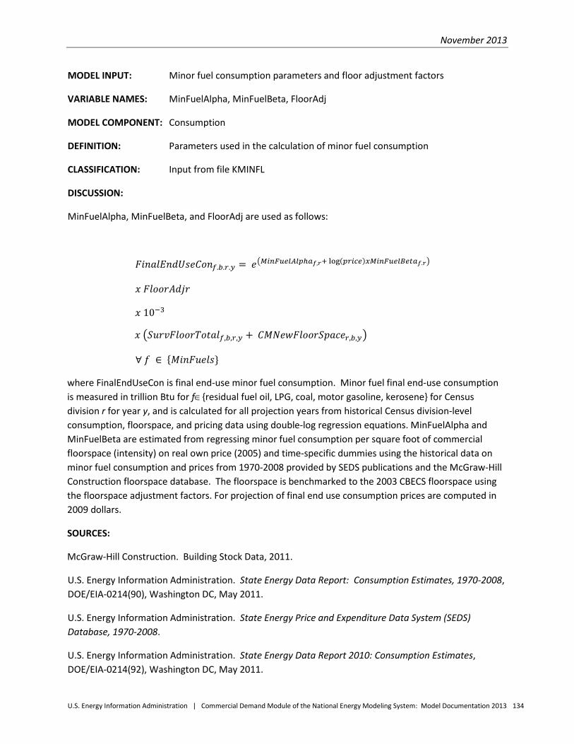
November 2013


MODEL INPUT: Minor fuel consumption parameters and floor adjustment factors

VARIABLE NAMES: MinFuelAlpha, MinFuelBeta, FloorAdj


DEFINITION: Parameters used in the calculation of minor fuel consumption

CLASSIFICATION: Input from file KMINFL

DISCUSSION:

MinFuelAlpha, MinFuelBeta, and FloorAdj are used as follows:

𝐹𝑖𝑛𝑎𝑙𝐸𝑛𝑑𝑈𝑠𝑒𝐶𝑜𝑛𝑓.𝑏.𝑟.𝑦 = 𝑒�𝑀𝑖𝑛𝐹𝑢𝑒𝑙𝐴𝑙𝑝ℎ𝑎𝑓,𝑟+ log(𝑝𝑟𝑖𝑐𝑒)𝑥𝑀𝑖𝑛𝐹𝑢𝑒𝑙𝐵𝑒𝑡𝑎𝑓.𝑟�

𝑥 𝐹𝑙𝑜𝑜𝑟𝐴𝑑𝑗𝑟

𝑥 10−3

𝑥 �𝑆𝑢𝑟𝑣𝐹𝑙𝑜𝑜𝑟𝑇𝑜𝑡𝑎𝑙𝑓,𝑏,𝑟,𝑦 + 𝐶𝑀𝑁𝑒𝑤𝐹𝑙𝑜𝑜𝑟𝑆𝑝𝑎𝑐𝑒𝑟,𝑏,𝑦�

∀ 𝑓 ∈ {𝑀𝑖𝑛𝐹𝑢𝑒𝑙𝑠}

where FinalEndUseCon is final end-use minor fuel consumption. Minor fuel final end-use consumption is measured in trillion Btu for f∈{residual fuel oil, LPG, coal, motor gasoline, kerosene} for Census division r for year y, and is calculated for all projection years from historical Census division-level consumption, floorspace, and pricing data using double-log regression equations. MinFuelAlpha and MinFuelBeta are estimated from regressing minor fuel consumption per square foot of commercial floorspace (intensity) on real own price (2005) and time-specific dummies using the historical data on minor fuel consumption and prices from 1970-2008 provided by SEDS publications and the McGraw-Hill Construction floorspace database. The floorspace is benchmarked to the 2003 CBECS floorspace using the floorspace adjustment factors. For projection of final end use consumption prices are computed in 2009 dollars.

SOURCES:

McGraw-Hill Construction. Building Stock Data, 2011.

U.S. Energy Information Administration. State Energy Data Report: Consumption Estimates, 1970-2008, DOE/EIA-0214(90), Washington DC, May 2011.

U.S. Energy Information Administration. State Energy Price and Expenditure Data System (SEDS) Database, 1970-2008.

U.S. Energy Information Administration. State Energy Data Report 2010: Consumption Estimates, DOE/EIA-0214(92), Washington DC, May 2011.

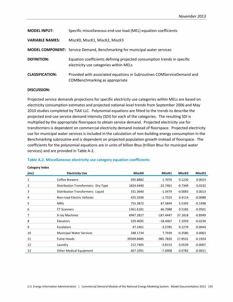
November 2013


MODEL INPUT: Specific miscellaneous end-use load (MEL) equation coefficients

VARIABLE NAMES: MiscK0, MiscK1, MiscK2, MiscK3

MODEL COMPONENT: Service Demand, Benchmarking for municipal water services

DEFINITION: Equation coefficients defining projected consumption trends in specific electricity use categories within MELs

CLASSIFICATION: Provided with associated equations in Subroutines COMServiceDemand and COMBenchmarking as appropriate

DISCUSSION:

Projected service demands projections for specific electricity use categories within MELs are based on electricity consumption estimates and projected national-level trends from September 2006 and May 2010 studies completed by TIAX LLC. Polynomial equations are fitted to the trends to describe the projected end-use service demand intensity (SDI) for each of the categories. The resulting SDI is multiplied by the appropriate floorspace to obtain service demand. Projected electricity use for transformers is dependent on commercial electricity demand instead of floorspace. Projected electricity use for municipal water services is included in the calculation of non-building energy consumption in the Benchmarking subroutine and is dependent on projected population growth instead of floorspace. The coefficients for the polynomial equations are in units of billion Btus (trillion Btus for municipal water services) and are provided in Table A-2.

Table A.2. Miscellaneous electricity use category equation coefficients

Category Index

(mc)

Electricity Use

MiscK0

MiscK1

MiscK2

MiscK3

1 Coffee Brewers 595.8882 1.7076 0.1220 0.0023

2 Distribution Transformers: Dry-Type 1824.4440 -22.7461 -0.7349 0.0232

3 Distribution Transformers: Liquid 331.3640 -1.3479 -0.0083 0.0013

4 Non-road Electric Vehicles 425.3500 -1.7323 0.4114 -0.0088

5 MRIs 755.3872 87.5844 5.5393 -0.1498

6 CT Scanners 1361.6181 66.7088 0.5182 -0.0501

7 X-ray Machines 6947.2827 -187.4447 37.1818 -0.8949

8 Elevators 229.4695 -18.4067 1.1059 -0.0239

9 Escalators 47.2461 -3.5785 0.2279 -0.0044

10 Municipal Water Services 188.1734 7.7939 -0.3580 0.0063

11 Fume Hoods 39509.8485 -985.7820 17.8531 -0.1924

12 Laundry 212.7405 -3.8153 0.0539 -0.0007

13 Other Medical Equipment 667.1091 -7.6908 0.0782 -0.0011

November 2013


SOURCES:

TIAX LLC, Commercial and Residential Sector Miscellaneous Electricity Consumption: Y2005 and Projections to 2030, prepared for U.S. Department of Energy, U.S. Energy Information Administration, September 2006.

TIAX LLC, Commercial Miscellaneous Electric Loads: Energy Consumption Characterization and Savings Potential in 2008 by Building Type, prepared for U.S. Department of Energy, Building Technologies Program, May 2010.

November 2013


MODEL INPUT: Retrofit removal and disposal cost

VARIABLE NAME: RetroCostFract


DEFINITION: Cost of removing and disposing equipment of a given technology and vintage for purposes of retrofitting with other equipment

CLASSIFICATION: Input from KTEK

DISCUSSION:

The cost is expressed as a proportion to be applied to the installed capital cost. Currently, a placeholder value of 1.0 is used throughout the Commercial Demand Module, pending acquisition and analysis of appropriate data.

SOURCES:

U.S. Energy Information Administration. Estimated value.

November 2013


MODEL INPUT: Serviced floorspace variation with building vintage

VARIABLE NAME: ServicedFlspcProp


DEFINITION: Proportion of building floorspace that receives end-use service, by building type, service, and whether the buildings are newly constructed (post-1989) or existing (pre-1990).

CLASSIFICATION: Input from file KVARSDI

DISCUSSION:

An investigation undertaken to determine whether significant variations existed by building age in the proportions of floorspace receiving various end-use services found, for several services, a measurable difference between the two broad classes of “old” and “new.” For this characterization, ‘new’ was defined as floorspace constructed after 1989. The NEMS Commercial Demand Module parameters characterizing service demand patterns are derived by considering the entire floorspace stock as sampled by CBECS 92, and are influenced most heavily by values corresponding to the “old” floorspace category. In order to account for service demand differences in new floorspace construction, the model makes use of the different serviced floorspace proportions, as described in the text of the model documentation. The values were derived by processing the individual CBECS survey records.

SOURCES:

U.S. Department of Energy, U.S. Energy Information Administration, 1992 Commercial Buildings Energy Consumption Survey, Public Use Files, http://www.eia.gov/consumption/commercial/data/1992/.


November 2013


MODEL INPUT: Building shell heating and cooling load factors

VARIABLE NAMES: ShellCoolFactor, ShellHeatFactor


DEFINITION: Shell heating and cooling load factors for buildings constructed in the current year for building type b in Census division r in year y.

CLASSIFICATION: Input from file KSHEFF

DISCUSSION:

The 2003 existing stock shell load factors are indexed to 1.0 for each building type. The building shell load factors for new construction represent the impacts on heating and cooling service demand due to improvements in the thermal performance of the building shell of newly-constructed floorspace that must by law adhere to building codes and the general improvement that results from the continual introduction of more shell-efficient new construction.

Regional heating and cooling load factors that reflect current building codes and construction practices relative to the existing building stock in 2003 were developed from a Science Applications International Corporation (SAIC) study conducted for EIA in 2010. An earlier SAIC study developed overall building U-values for the DOE Building Technology program’s set of benchmark commercial buildings, adjusted those U-values to correspond to the NEMS building categories and climate regions, and developed “stock” and “new” building U-values and thermal indices from the adjusted U-values. The 2010 study used parametric analysis to develop heating and cooling load factors based on the U-values. The shell characteristics of the benchmark buildings are available for three vintages of buildings: Pre-1980, Post-1980, and New Construction, with the New Construction category based on AHRAE 90.1-2004. The “stock” U-values were developed by weighting the Pre-1980 and Post-1980 characteristics using the 2003 CBECS building population.

SOURCES:

Science Applications International Corporation, Thermal Efficiency Indicators Characterizing Existing Commercial Buildings, prepared for U.S. Department of Energy, U.S. Energy Information Administration, December 2008.

Science Applications International Corporation, Data Analysis for Enhanced Representation of Commercial Thermal Shell Efficiency in the Commercial Demand Module, prepared for U.S. Department of Energy, U.S. Energy Information Administration, May 2010.

Science Applications International Corporation, Model Documentation of Enhanced Representation of Commercial Thermal Shell Efficiency in the Commercial Demand Module, prepared for U.S. Department of Energy, U.S. Energy Information Administration, April 2010.

November 2013


MODEL INPUT: Short-term price elasticity of service demand

VARIABLE NAME: ShortRunPriceElasofDmd


DEFINITION: Short run price elasticity (percent change in service demand as result of percent change in energy price), by service demand s, for the major fuels of electricity, natural gas, and distillate. This is a composite factor based on fuel proportions of service demand by Census division and service.

CLASSIFICATION: Input from file KSDELA

DISCUSSION:

Table A-3 summarizes a literature review encompassing price response analyses of major fuel demands. Composite price elasticity of service demand estimates based upon these sources are included. Input values for the fuel and end-use specific elasticity parameters included in the module are Office of Energy Analysis estimates developed from within the range of empirical values in Table A-3.

SOURCES:

Al-Sahlawi, M., “The Demand for Natural Gas: A Survey of Price and Income Elasticities," The Energy Journal, vol. 10, no. 1, January 1989.

Balestra, T. and M. Nerlove, “Pooling Cross-Section and Time-Series Data in the Estimation of a Dynamic Model: The Demand for Natural Gas,” Econometrica, vol. 34, no. 3, July 1966.

Beierlin, J., J. Dunn, and J. McConnor, Jr., "The Demand for Electricity and Natural Gas in the Northeastern United States," Review of Economics and Statistics, vol. 64, 1981.

Berndt, E. and G. Watkins, “Demand for Natural Gas: Residential and Commercial Markets in Ontario and British Columbia,” Canadian Journal of Economics, vol. 10, February 1977.

Chern, W. and R. Just, “Assessing the Need for Power: A Regional Econometric Model,” Energy Economics, vol. 10, no. 3, 1982, pp. 232-239.

Federal Energy Administration, 1976 National Energy Outlook, Washington, DC, 1976.

Griffin, J., Energy Consumption in the OECD: 1880-2000, Cambridge, Mass., Ballinger Publishing Company, 1979.

Halvorsen, R., “Demand for Electric Energy in the United States,” Southern Economic Journal, vol. 42, no. 4, 1975, pp. 610-625.

Joskow, P. and M. Baughman, “The Future of the U.S. Nuclear Energy Industry,” Bell Journal of Economics, vol. 7, Spring 1976.

November 2013


McFadden, D. and C. Puig, Economic Impact of Water Pollution Control on the Steam Electric Industry, Chapter 3, Report EED-12, Teknekron Inc., Berkeley, California, 1975.

Mount, T., L. Chapman & T. Tyrrell, Electricity Demand in the United States: An Econometric Analysis, National Technical Information Service No. ORNL-NSF-EP-49, Springfield, Virginia, 1973.

Murray, M., R. Spann, L. Pulley, & E. Beauvais, “The Demand for Electricity in Virginia,” The Review of Economics and Statistics, vol. 60, no. 4, 1976, pp. 585-660.

Nelson, J., “The Demand for Space Heating Energy,” Review of Economics and Statistics, November 1975, pp.508-512.

Uri, N., A Dynamic Demand Analysis for Electrical Energy by Class of Consumer, Working Paper No. 34, Bureau of Labor Statistics, January 1975.

Westley, G., The Demand for Electricity in Latin America: A Survey and Analysis, Economic and Social Development Department, Country Studies Division, Methodology Unit, Washington, DC, February 1989.

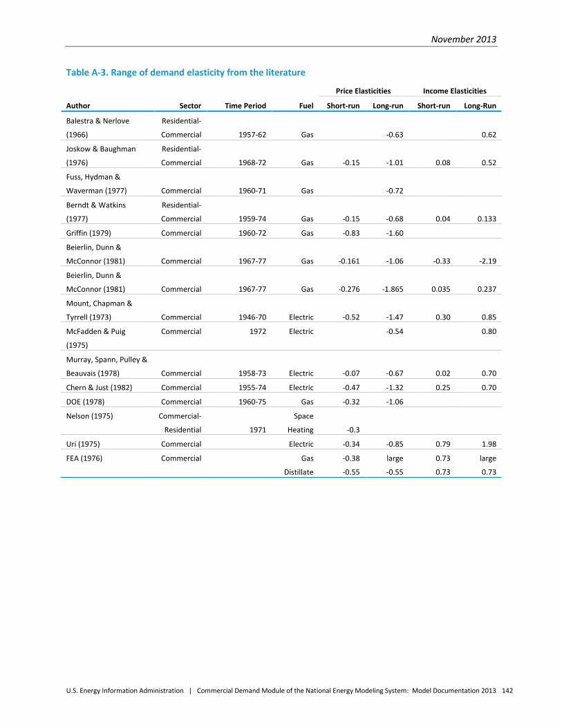
November 2013


Table A-3. Range of demand elasticity from the literature

Price Elasticities Income Elasticities

Author Sector Time Period Fuel Short-run Long-run Short-run Long-Run

Balestra & Nerlove

(1966)

Residential-

Commercial

1957-62

Gas

-0.63

0.62

Joskow & Baughman

(1976)

Residential-

Commercial

1968-72

Gas

-0.15

-1.01

0.08

0.52

Fuss, Hydman &

Waverman (1977)

Commercial

1960-71

Gas

-0.72

Berndt & Watkins

(1977)

Residential-

Commercial

1959-74

Gas

-0.15

-0.68

0.04

0.133

Griffin (1979) Commercial 1960-72 Gas -0.83 -1.60

Beierlin, Dunn &

McConnor (1981)

Commercial

1967-77

Gas

-0.161

-1.06

-0.33

-2.19

Beierlin, Dunn &

McConnor (1981)

Commercial

1967-77

Gas

-0.276

-1.865

0.035

0.237

Mount, Chapman &

Tyrrell (1973)

Commercial

1946-70

Electric

-0.52

-1.47

0.30

0.85

McFadden & Puig

(1975)

Commercial 1972 Electric -0.54 0.80

Murray, Spann, Pulley &

Beauvais (1978)

Commercial

1958-73

Electric

-0.07

-0.67

0.02

0.70

Chern & Just (1982) Commercial 1955-74 Electric -0.47 -1.32 0.25 0.70

DOE (1978) Commercial 1960-75 Gas -0.32 -1.06

Nelson (1975) Commercial-

Residential

1971

Space

Heating

-0.3

Uri (1975) Commercial Electric -0.34 -0.85 0.79 1.98

FEA (1976) Commercial Gas

Distillate

-0.38

-0.55

large

-0.55

0.73

0.73

large

0.73

November 2013


MODEL INPUT: Commercial sector renewable energy consumption projection

VARIABLE NAME: SolarRenewableContrib


DEFINITION: Contribution of solar thermal energy consumed to meet commercial sector service demands by service s

CLASSIFICATION: Input from file KRENEW

DISCUSSION:

Solar water heating technologies are included in the Technology Choice submodule, allowing endogenous computation of solar consumption based on the selection of these technologies. A baseline projection for solar thermal energy consumption for space heating, developed by the National Renewable Energy Laboratory (NREL), is read into the Commercial Module, since projections from the NEMS Renewable Fuels Module are not currently available at the level of disaggregation required by the Commercial Module. The renewable energy projections for active solar space heating are applied, interpolating to fill in the five-year forecast intervals provided in the white paper.

Commercial sector consumption of geothermal technologies is explicitly modeled by including geothermal heat pumps in the technology characterization menu, allowing geothermal technologies to compete in the marketplace. Consumption of the renewable fuels of wood and municipal solid waste (MSW) in the cogeneration of electricity is also modeled explicitly, using data from the EI-860: Annual Electric Generator Report database.

SOURCES:

The Potential of Renewable Energy: An Interlaboratory White Paper, a report prepared for the Office of Policy, Planning and Analysis, U.S. Department of Energy, Golden, Colorado, March 1990.

U.S. Energy Information Administration, EI-860: Annual Electric Generator Report database.

November 2013


MODEL INPUT: Equipment efficiency

VARIABLE NAME: TechEff


DEFINITION: Efficiency, Coefficient of Performance, Seasonal Performance Factor, Efficacy (lighting), of equipment in providing service


DISCUSSION:

Equipment efficiencies for the services of space heating, space cooling, water heating, ventilation, cooking, lighting, and refrigeration are included in the Technology Characterization Menu of the NEMS Commercial Module. These input data are composites of commercial sector equipment efficiencies of existing and prototypical commercial sector technologies provided in the sources cited below.

SOURCES:

Navigant Consulting, Inc. with SAIC, EIA - Technology Forecast Updates - Residential and Commercial Building Technologies – Reference Case, prepared for U.S. Energy Information Administration, September 2011.

Navigant Consulting, Inc. with SAIC, EIA - Technology Forecast Updates - Residential and Commercial Building Technologies – Advanced Case, prepared for U.S. Energy Information Administration, September 2011.



U.S. Congress, House of Representatives. Energy Policy Act of 1992: Conference Report to Accompany H.R. 776, 102nd Cong., 2d sess. October 5, 1992.

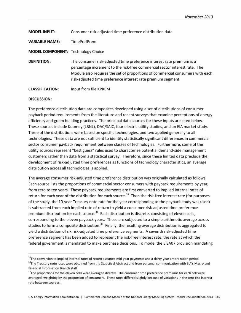
November 2013


MODEL INPUT: Consumer risk-adjusted time preference distribution data

VARIABLE NAME: TimePrefPrem


DEFINITION: The consumer risk-adjusted time preference interest rate premium is a percentage increment to the risk-free commercial sector interest rate. The Module also requires the set of proportions of commercial consumers with each risk-adjusted time preference interest rate premium segment.

CLASSIFICATION: Input from file KPREM

DISCUSSION:

The preference distribution data are composites developed using a set of distributions of consumer payback period requirements from the literature and recent surveys that examine perceptions of energy efficiency and green building practices. The principal data sources for these inputs are cited below. These sources include Koomey (LBNL), DAC/SAIC, four electric utility studies, and an EIA market study. Three of the distributions were based on specific technologies, and two applied generally to all technologies. These data are not sufficient to identify statistically significant differences in commercial sector consumer payback requirement between classes of technologies. Furthermore, some of the utility sources represent “best guess” rules used to characterize potential demand-side management customers rather than data from a statistical survey. Therefore, since these limited data preclude the development of risk-adjusted time preferences as functions of technology characteristics, an average distribution across all technologies is applied.

The average consumer risk-adjusted time preference distribution was originally calculated as follows. Each source lists the proportions of commercial sector consumers with payback requirements by year, from zero to ten years. These payback requirements are first converted to implied internal rates of return for each year of the distribution for each source.33 Then the risk-free interest rate (for purposes of the study, the 10-year Treasury note rate for the year corresponding to the payback study was used) is subtracted from each implied rate of return to yield a consumer risk-adjusted time preference premium distribution for each source.34 Each distribution is discrete, consisting of eleven cells, corresponding to the eleven payback years. These are subjected to a simple arithmetic average across studies to form a composite distribution.35 Finally, the resulting average distribution is aggregated to yield a distribution of six risk-adjusted time preference segments. A seventh risk-adjusted time preference segment has been added to represent the risk-free interest rate, the rate at which the federal government is mandated to make purchase decisions. To model the EISA07 provision mandating

33The conversion to implied internal rates of return assumed mid-year payments and a thirty-year amortization period. 34The Treasury note rates were obtained from the Statistical Abstract and from personal communication with EIA's Macro and Financial Information Branch staff. 35The proportions for the eleven cells were averaged directly. The consumer time preference premiums for each cell were averaged, weighting by the proportion of consumers. These rates differed slightly because of variations in the zero-risk interest rate between sources.

November 2013


energy-efficient lighting in federal buildings to the maximum extent possible, the results of the average distribution have been modified for this end use. Time preference premiums assumed for 2009 and later years were adjusted based on the results of the recent surveys on energy efficiency and green building practices cited below. Further discussion of this and lists of the distributions from each source as well as the resulting values assumed for input into NEMS may be found in Appendix E in the Risk-Adjusted Time Preference Premium Distribution data quality discussion.

The assumed distribution of consumer risk-adjusted time preference premiums is generally assumed constant over the projection period. However, the Commercial Demand Module allows variation in the distribution on an annual basis to accommodate targeted policies that may affect decision-making for specific time periods, such as Recovery Act spending, and for simulation of policy scenarios targeting consumers’ implicit discount rates.

SOURCES:

Building Design + Construction, Green Buildings + Climate Change, Oak Brook IL, November 2008

Johnson Controls, 2011 Energy Efficiency Indicator: IFMA Partner results, October 2011

Koomey, Jonathan G., Energy Efficiency Choices in New Office Buildings: An Investigation of Market Failures and Corrective Policies, Ph.D. Dissertation, University of California at Berkeley, 1990, p. 16.

Decision Analysis Corporation of Virginia and Science Applications International Corporation, Alternative Methodologies for NEMS Building Sector Model Development: Draft Report, prepared for EIA under Contract No. DE-AC01-92EI21946, Task 92-009, Subtask 4, Vienna VA, August 3, 1992, p. 14.

U.S. Department of Commerce, Bureau of the Census, Statistical Abstract of the United States 1990 (110th ed.), Washington DC, 1990, p. 510.

November 2013


MODEL INPUT: Equipment characteristics (see Definition below)

VARIABLE NAMES: TechCost, TechLife


DEFINITION: Installed unit capital cost, annual operating and maintenance cost, and equipment lifetime in years for specific technologies/models


DISCUSSION:

Capital and installation costs are combined to form installed capital costs, based upon available data. The Technology Choice algorithm does not require the separation of capital and installation costs, and currently does not retain information describing absolute equipment capacity. Installed unit capital costs (installed capital cost per thousand Btu/hr output capacity per 1000 lumens in the case of lighting, or per 1000 cfm for ventilation systems) and the annual unit operating and maintenance costs vary by technology and vintage for the services of space heating, space cooling, water heating, ventilation, cooking, lighting and refrigeration. They are developed from a variety of sources, referenced below.

SOURCES:






November 2013


MODEL INPUT: Equipment Availability

VARIABLE NAME: TechAvailability


DEFINITION: Availability of equipment technology/model by year


DISCUSSION:

The first year in which technologies become available corresponds to efficiency and cost data in the sources cited below for space heating, space cooling, water heating and lighting technologies. In addition, the National Energy Policy Act of 1992 Title I, Subtitle C, Sections 122 and 124, provides commercial equipment efficiency standards applicable to units manufactured after January 1, 1994. The Department of Energy has continued to update applicable standards over time and recent legislation has expanded the slate of equipment subject to equipment efficiency standards with standard levels announced and codified in the Federal Register. The companion document, Assumptions to the Annual Energy Outlook 2013, provides more information about the specific commercial equipment subject to standards. This information is combined with the previously cited sources and professional expectations to estimate the first-available and last-available year for each technology that is subject to the standards.

SOURCES:

National Archives and Records Administration, Office of the Federal Register, The Federal Register, Volume 59 through Volume 74.





November 2013



U.S. Department of Energy, Office of Research and Standards, Draft Technical Support Document: Energy Efficiency Program for Commercial and Industrial Equipment: High-Intensity Discharge Lamps, Washington DC, August 2004.

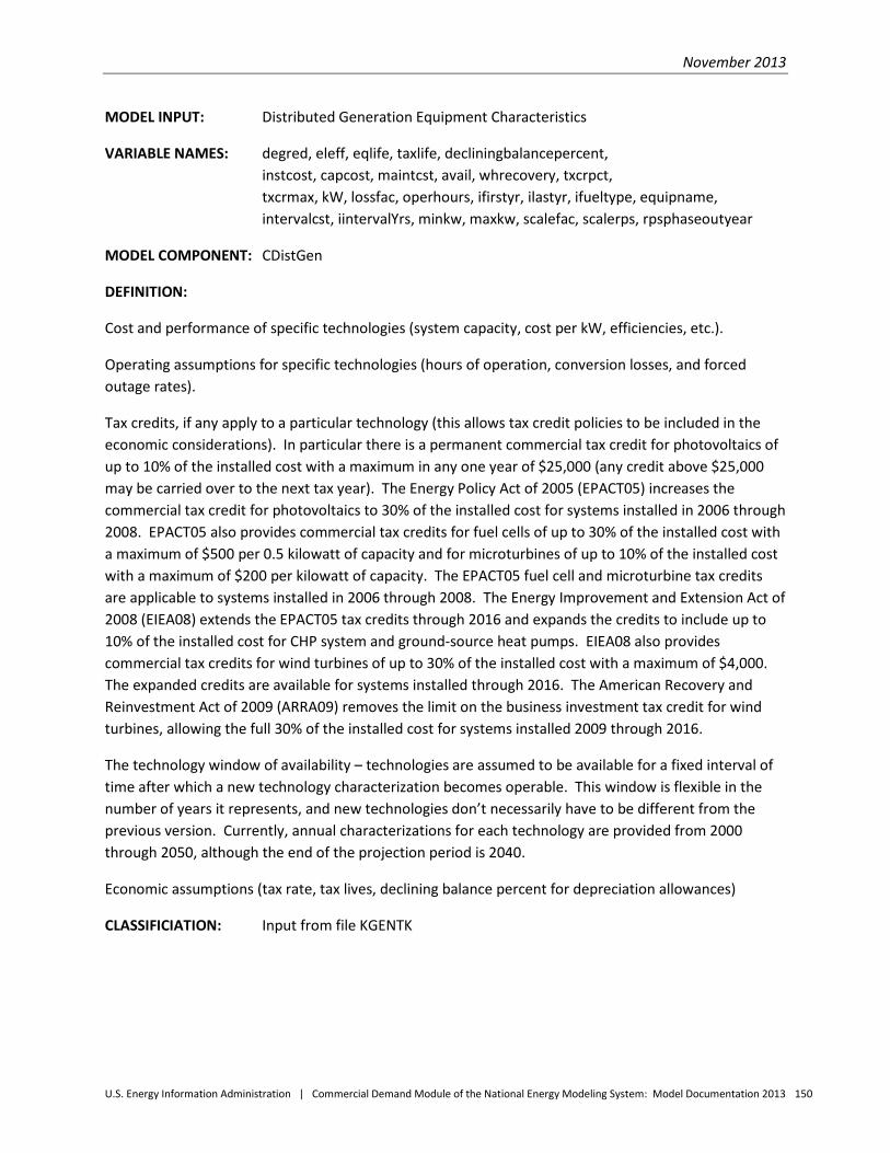
November 2013


MODEL INPUT: Distributed Generation Equipment Characteristics

VARIABLE NAMES: degred, eleff, eqlife, taxlife, decliningbalancepercent, instcost, capcost, maintcst, avail, whrecovery, txcrpct, txcrmax, kW, lossfac, operhours, ifirstyr, ilastyr, ifueltype, equipname, intervalcst, iintervalYrs, minkw, maxkw, scalefac, scalerps, rpsphaseoutyear

MODEL COMPONENT: CDistGen

DEFINITION:

Cost and performance of specific technologies (system capacity, cost per kW, efficiencies, etc.).

Operating assumptions for specific technologies (hours of operation, conversion losses, and forced outage rates).

Tax credits, if any apply to a particular technology (this allows tax credit policies to be included in the economic considerations). In particular there is a permanent commercial tax credit for photovoltaics of up to 10% of the installed cost with a maximum in any one year of $25,000 (any credit above $25,000 may be carried over to the next tax year). The Energy Policy Act of 2005 (EPACT05) increases the commercial tax credit for photovoltaics to 30% of the installed cost for systems installed in 2006 through 2008. EPACT05 also provides commercial tax credits for fuel cells of up to 30% of the installed cost with a maximum of $500 per 0.5 kilowatt of capacity and for microturbines of up to 10% of the installed cost with a maximum of $200 per kilowatt of capacity. The EPACT05 fuel cell and microturbine tax credits are applicable to systems installed in 2006 through 2008. The Energy Improvement and Extension Act of 2008 (EIEA08) extends the EPACT05 tax credits through 2016 and expands the credits to include up to 10% of the installed cost for CHP system and ground-source heat pumps. EIEA08 also provides commercial tax credits for wind turbines of up to 30% of the installed cost with a maximum of $4,000. The expanded credits are available for systems installed through 2016. The American Recovery and Reinvestment Act of 2009 (ARRA09) removes the limit on the business investment tax credit for wind turbines, allowing the full 30% of the installed cost for systems installed 2009 through 2016.

The technology window of availability – technologies are assumed to be available for a fixed interval of time after which a new technology characterization becomes operable. This window is flexible in the number of years it represents, and new technologies don’t necessarily have to be different from the previous version. Currently, annual characterizations for each technology are provided from 2000 through 2050, although the end of the projection period is 2040.

Economic assumptions (tax rate, tax lives, declining balance percent for depreciation allowances)

CLASSIFICIATION: Input from file KGENTK

November 2013


DISCUSSION:

degred (technology, vintage) – degradation of conversion efficiency of technology. Currently applies to photovoltaics (PV) at a loss of 1 percent of total output per year. That is, after 20 years, a 5 kW system would produce only 80 percent (1-20*1%) of its rated output, or 4 kW.

eleff (technology, vintage) – the electrical conversion efficiency of the technology and vintage.

eqlife (technology, vintage) – life of the equipment, specific to the equipment type as well as vintage.

taxlife (technology, vintage) – tax life of building equipment (currently set to 5 years for PV, 39.5 years for all other distributed generation technologies).

decliningbalancepercent (technology, vintage) – percentage to be used for depreciation calculation. A value of 100 percent signifies straight-line depreciation while a value of 150 or 200 results in accelerated declining balance depreciation. Non-PV generation technologies use straight-line depreciation in default operation, PV is automatically set to 200 percent per current tax law.

whrecovery (technology, vintage) – waste heat recovery factor for technologies that burn fuel (i.e., not photovoltaics). This waste heat can then be made available for water heating, which provides additional energy cost savings for distributed generation technologies.

instcost (technology, vintage) – installation cost in 2009 dollars per kW.

capcost (technology, vintage) – capital cost of the investment in 2009 dollars per kW.

maintcost (technology, vintage) – annual maintenance cost in 2009 dollars per kW.

avail (technology, vintage) – percentage of time available (1 – forced outage rate – planned outage rate) applied to typical operating hours.

txcreditpct (technology, vintage) – tax credit percentage that applies to a given technology’s total installed cost (if any).

txcreditmax (technology, vintage) – cap on the total dollar amount of a tax credit (if any).

kW (technology, vintage) – kW of typical system. Note capacity must remain constant across vintages for a given technology.

operhours (technology) – typical operating hours.

lossfac (technology, vintage) – conversion losses (for systems that are rated “at the unit” rather than per available alternating current wattage) if appropriate.

ifirstyr (technology, vintage) – first year that a technology is available.

November 2013


ilastyr (technology, vintage) – last year that a technology is available (Note: the input files are now structured with new vintages for each NEMS model year. Even so, the technology ranges are still operable and the use of “vintage” is maintained even though “year” would also be appropriate.).

ifueltype (technology) – fuel type pointer for generation technologies other than photovoltaics, currently this is 2 for natural gas which is used by fuel cells.

equipname (technology, vintage) – character string variable with equipment type name for report writer.

intervalcst (technology = 1, vintage) – interval maintenance cost for photovoltaic system inverter replacement.

iintervalYrs (technology = 1, vintage) – inverter replacement interval in years for photovoltaic systems.

minkw – varies by technology, smallest unit in terms of peak capacity allowed

maxkw – varies by technology, largest unit in terms of peak capacity allowed

scalefac – cost adjustment parameter for DG technology peak system capacity scale economies

scalerps – renewable portfolio credit scalar (e.g., triple RPS credit would be a user input value of 3.0)

rpsphaseoutyear – last year of renewable portfolio standard credits for cases where the credit is “sunsetted”

SOURCES:

System Capacities and Operating Hours are U.S. Energy Information Administration assumptions.

Solar Insolation - NREL communication to US DOE EE.

Solar Photovoltaic Technology Specifications - ICF International, Photovoltaic (PV) Cost and Performance Characteristics for Residential and Commercial Applications Final Report, prepared for Office of Integrated Analysis and Forecasting, U.S. Energy Information Administration, August 2010.

Wind Turbine Technology Specifications - ICF International, The Cost and Performance of Distributed Wind Turbines, 2010-35 Final Report, prepared for Office of Integrated Analysis and Forecasting, U.S. Energy Information Administration, June 2010.

Fossil-Fired Technology Specifications - SENTECH, Incorporated and Science Applications International Corporation, Commercial and Industrial CHP Technology Cost and Performance Data Analysis for EIA, prepared for U.S. Energy Information Administration, June 2010.

PV, wind accelerated depreciation - Internal Revenue Code, subtitle A, Chapter 1, Subchapter B, Part VI, Section 168 (1994) - accelerated cost recovery. CITE: 26USC168

November 2013


MODEL INPUT: Distributed Generation Financial Inputs

VARIABLE NAMES: term, intrate, downpaypct, taxrate, inflation


DEFINITION: Economic assumptions (loan rate and term, down payment percentage, tax rate, inflation rate for projecting nominal dollar values for the cash flow model).


DISCUSSION:

term – loan term currently set at 15 years

intrate – commercial mortgage rate from the kgentk input file, currently set to 8.5%.

downpaypct – down payment percentage assumed to apply to the distributed generation investment, currently 25% of the installed cost

taxrate – marginal combined federal and state income tax rate, currently assumed to be 40% for the typical commercial business

inflation – inflation assumption for converting constant dollar fuel costs and fuel cost savings into current dollars for the cash flow model in order to make the flows correspond to the nominal dollar loan payments. The current assumption is 3% annually.

SOURCES:

U.S. Energy Information Administration. Estimated values and assumptions.

November 2013


MODEL INPUT: Distributed Generation Program-Driven Penetrations

VARIABLE NAMES: exogpen, bldgshr


DEFINITION: Exogenous, program-driven cumulative installed generation capacity by Census division and technology. These are viewed as non-economic penetrations and supplemental to any economic penetrations determined by the model. Technology-specific allocation shares for the exogenous penetrations for the commercial model building types are also required.


DISCUSSION:

See definition.

SOURCES:

Exogenous penetrations: Developed from news releases – DOE and industry, the Interstate Renewable Energy Council’s annual U.S. Solar Market Trends report, UPVG website, and estimated impacts from California solar initiative and other state programs.

Building shares for exogenous penetrations by technology: EIA Form 860.

November 2013


MODEL INPUT: Distributed Generation Building-Specific Characteristics and Niche Variables

VARIABLE NAMES: cbecs03flspccatshare, cbecs03avgsqft, elecavgkwh, waterhtgmmbtu, spacehtgmmbtu, ratescalar, ngratescalar, roofareatosqft, mps, solarinsolation, sqftshare


DEFINITION: Average electricity usage, average annual water heating energy consumption, average annual space heating energy consumption.

CLASSIFICIATION: Input from data statements in subroutine CDistGen

DISCUSSION:

Note, all of the variables in this group are developed from CBECS 2003.

Size Class and Building Type Inputs – all of the following vary by Census division, building type and building size category:

cbecs03flspcatshare – share of floorspace area within a Census division for a specific building type and size class combination.

cbecs03avgsqft – average floorspace area.

elecavgkwh – average annual electricity usage in kWh (kWh per year).

spacehtgmmbtu – average annual space heating EUI; developed from ComEUI (see energy use intensity model input section above for ComEUI definitions) for space heating and average floorspace area for specific building type and size class combinations, units are MMBtu/year.

waterhtgmmbtu – average annual space heating EUI; developed from ComEUI (see energy use intensity model input section above for ComEUI definitions) for space heating and average floorspace area for specific building type and size class combinations, units are MMBtu/year.

Niche Inputs – All of the following vary by solar and electricity rate combined niches within each Census Division:

ratescalar – niche variable for electricity prices relative to the Census division average price within a niche.

ngratescalar – niche variable for natural gas prices relative to the Census division average price within a niche.

roofareatosqft – average roof area available per unit of floorspace area.

mps – average wind speed for distributed wind turbines in meters per second, developed from NREL wind resource map overlaid with CBECS 2003 niche areas.

November 2013


solarinsolation – solar insolation for photovoltaics in average daily kWh per square meter, developed from NREL insolation map overlaid with CBECS 2003 niche areas.

sqftshare – niche variable representing the floorspace area share of the combined solar and electricity price level niches within each Census division.

SOURCES:

Average annual electricity consumption by building type for Census division and size categories; Average building floorspace area by building type for Census division and size categories; Floorspace shares by building type for Census division and size categories; Floorspace shares, relative electricity cost, relative gas cost, roof area to floorspace area within Census division by solar insolation and electricity price niche – U.S. Energy Information Administration, 2003 Commercial Buildings Energy Consumption Survey, Public Use Files, Washington DC, http://www.eia.gov/consumption/commercial/data/2003/.

Solar insolation levels by Census division, solar insolation niche and electricity price niche – National Renewable Energy Laboratory resource maps at http://www.nrel.gov/gis/solar.html.

Average wind speed maps by Census division, solar insolation niche and electricity price niche – National Renewable Energy Laboratory, Wind Energy Resource Atlas of the United States, 1987, United States Wind Resource Map: Yearly Electricity Production Estimated per Square Meter of Rotor Swept Area for a Small Wind Turbine.


http://www.nrel.gov/gis/solar.html

November 2013


MODEL INPUT: Distributed Generation Penetration Function Parameters

VARIABLE NAMES: alpha, penparm, inx, inxfy, inxly


DEFINITION: Technology-specific penetration function parameters, interconnection limitation parameters.


DISCUSSION:

The values for the technology-specific penetration function parameters alpha and penparm are found in each technology’s characterization data in file KGENTK.txt.

Interconnection potential inx is Census division-specific based on population-weighted aggregation of state scores indicating the presence of rules, regulations, and policies that affect utility grid interconnection of distributed generation. State scores range from zero (closed to interconnection) to one (open to interconnection) and are based on information from the DSIRE Database of State Incentives for Renewables & Efficiency. The parameters Inxfy and Inxly define the interval over which interconnection limitations decrease to 0 and are set to 2012 and 2040, respectively, for AEO2013.

SOURCES:

State-level policy information – Database of State Incentives for Renewables & Efficiency (DSIRE), http://www.dsireusa.org/, September 2011.

U.S. Energy Information Administration. Assumptions.

http://www.dsireusa.org/

November 2013


Appendix B. Mathematical Description

Introduction This section provides the formulae and associated mathematical descriptions which represent the detailed solution algorithms arranged by sequential submodule as executed in the NEMS Commercial Demand Module. The exception to this order is that items pertaining to the Distributed Generation and Combined Heat and Power Submodule are found at the end of Appendix B. Sections are given for the key equations relating to floorspace, service demand, technology choice, end-use fuel consumption, benchmarking and distributed generation. Conventions, nomenclature, and symbols used in the equations found in this appendix are defined below.

In general, the following conventions for subscript usage are observed in this section. Additional subscripts are defined later in this appendix where necessary. Discrete values assumed by the subscripts, and categories of such values, are described in Tables 1 and 2 of Chapter 2:

Subscript Description of Dimension Represented by Subscript

R Census division

B NEMS Commercial Module building type

b' NEMS MAM building type

S end-use service

F fuel

D equipment decision type (values of 1 through 3 correspond, respectively, to the New, Replacement, and

Retrofit decision types)

T technology class

V vintage or model of floorspace or equipment, depending upon usage

t' alternate technology class, for comparison with technology class t

v' alternate vintage of floorspace or model of equipment, depending on usage

P consumer risk-adjusted time preference premium segment

Y year designation (unless otherwise indicated, year ranges from 2004 through 2040, with the year 2004

indexed to the value of 15 in the Fortran code. The equations below treat y as the calendar year.)

Y year designation internal to the 30-year cash flow analysis used in the choice of distributed generation

equipment

X building stock designation (a value of 1 corresponds to existing buildings, a value of 2 corresponds to

new construction)

November 2013


In addition, the following standard mathematical symbols are used in the formulae, primarily to indicate over which values of the subscripts the formula is evaluated:

Symbol Meaning

∀ for all

∈ belonging to the category of

∉ not belonging to the category of

∋ such that

∃ there exists

∃/ there doesn’t exist

⋅ Multiplication

Use is also made of several variables that represent “flags,” indicating conditions observed by the model during input of certain data. These flag variables and their definitions are:

FuelbyTech t, f = 1 if technology t uses fuel f, and is 0 otherwise.

TechbyService s, t = 1 if technology t provides service s, and is 0 otherwise.

Most formulae are evaluated only for the current year of the projections. Subscripts appearing on the left side of the equal sign (=) without explicit restrictions indicate that the formula is evaluated for every combination of applicable values of those subscripts. The variables over which summations are performed are indicated, but often without restriction. In those cases, as with the subscripts, they assume all applicable values. Applicable values are generally all major and minor fuels for the fuel subscript, f; all major services for the end-use subscript, s; and all possible values for the remaining subscripts. In any event, fuels and services involved in calculations where technologies are explicitly referenced are always restricted to the major categories.

The equations follow the logic of the Fortran source code very closely to facilitate an understanding of the code and its structure. In several instances, a variable name will appear on both sides of an equal sign. These statements are assignment statements and cannot be interpreted as mathematical equations. An assignment statement is a computer programming device that allows a previously calculated variable to be updated (for example, multiplied by a factor) and re-stored under the same variable name. The equations and assignment statements are discussed in the text of Chapter 4. The variables appearing in the equations are cross-referenced and fully defined in Appendix A, Table A-1.

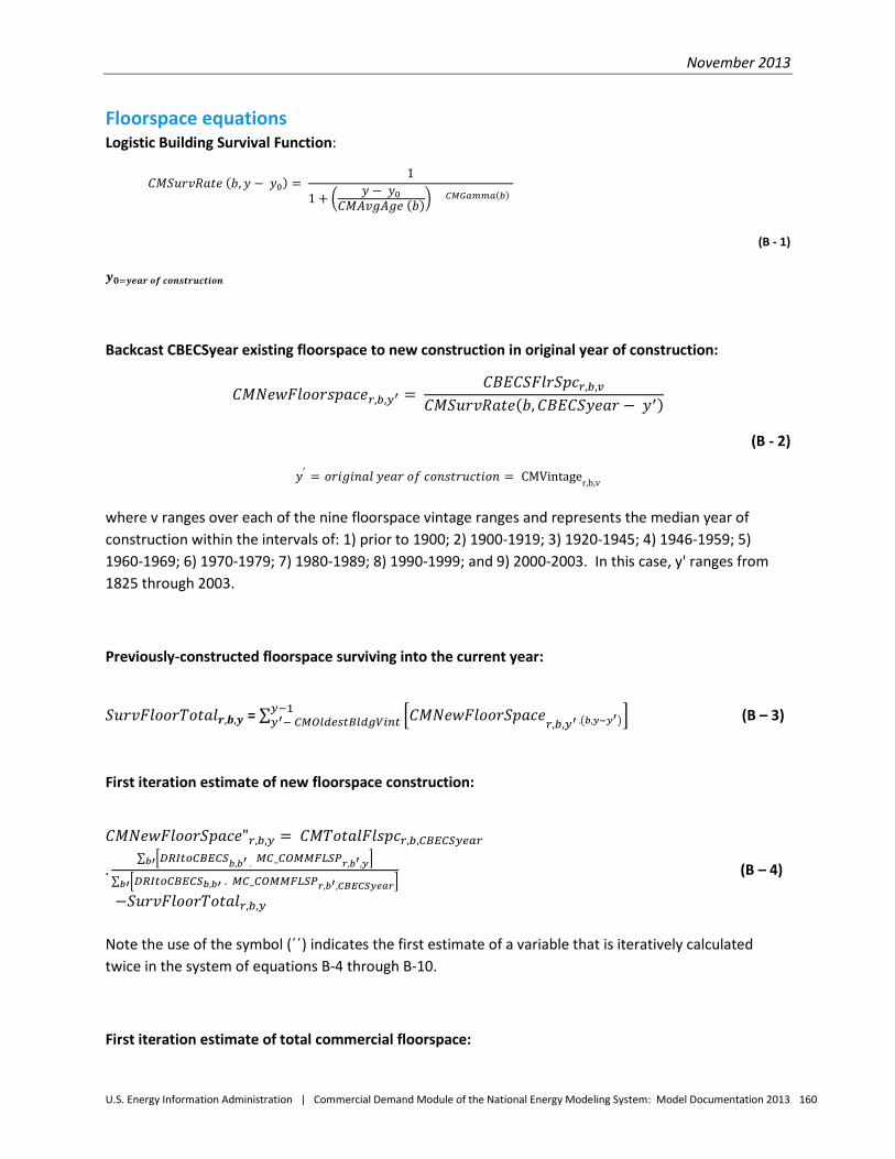
November 2013


Floorspace equations Logistic Building Survival Function:

𝐶𝑀𝑆𝑢𝑟𝑣𝑅𝑎𝑡𝑒 (𝑏,𝑦 − 𝑦0) = 1

1 + � 𝑦 − 𝑦0𝐶𝑀𝐴𝑣𝑔𝐴𝑔𝑒 (𝑏)�

𝐶𝑀𝐺𝑎𝑚𝑚𝑎(𝑏)

(B - 1)

𝒚𝟎=𝒚𝒆𝒂𝒓 𝒐𝒇 𝒄𝒐𝒏𝒔𝒕𝒓𝒖𝒄𝒕𝒊𝒐𝒏

Backcast CBECSyear existing floorspace to new construction in original year of construction:

𝐶𝑀𝑁𝑒𝑤𝐹𝑙𝑜𝑜𝑟𝑠𝑝𝑎𝑐𝑒𝑟,𝑏,𝑦′ = 𝐶𝐵𝐸𝐶𝑆𝐹𝑙𝑟𝑆𝑝𝑐𝑟,𝑏,𝑣

𝐶𝑀𝑆𝑢𝑟𝑣𝑅𝑎𝑡𝑒(𝑏,𝐶𝐵𝐸𝐶𝑆𝑦𝑒𝑎𝑟 − 𝑦′)

(B - 2)

𝑦′ = 𝑜𝑟𝑖𝑔𝑖𝑛𝑎𝑙 𝑦𝑒𝑎𝑟 𝑜𝑓 𝑐𝑜𝑛𝑠𝑡𝑟𝑢𝑐𝑡𝑖𝑜𝑛 = CMVintager,b,v

where v ranges over each of the nine floorspace vintage ranges and represents the median year of construction within the intervals of: 1) prior to 1900; 2) 1900-1919; 3) 1920-1945; 4) 1946-1959; 5) 1960-1969; 6) 1970-1979; 7) 1980-1989; 8) 1990-1999; and 9) 2000-2003. In this case, y' ranges from 1825 through 2003.

Previously-constructed floorspace surviving into the current year:

𝑆𝑢𝑟𝑣𝐹𝑙𝑜𝑜𝑟𝑇𝑜𝑡𝑎𝑙𝒓,𝒃,𝒚 = ∑ �𝐶𝑀𝑁𝑒𝑤𝐹𝑙𝑜𝑜𝑟𝑆𝑝𝑎𝑐𝑒𝑟,𝑏,𝑦′ .�𝑏,𝑦−𝑦′��

𝑦−1𝑦′− 𝐶𝑀𝑂𝑙𝑑𝑒𝑠𝑡𝐵𝑙𝑑𝑔𝑉𝑖𝑛𝑡 (B – 3)

First iteration estimate of new floorspace construction:

𝐶𝑀𝑁𝑒𝑤𝐹𝑙𝑜𝑜𝑟𝑆𝑝𝑎𝑐𝑒"𝑟,𝑏,𝑦 = 𝐶𝑀𝑇𝑜𝑡𝑎𝑙𝐹𝑙𝑠𝑝𝑐𝑟,𝑏,𝐶𝐵𝐸𝐶𝑆𝑦𝑒𝑎𝑟

.∑ �𝐷𝑅𝐼𝑡𝑜𝐶𝐵𝐸𝐶𝑆𝑏,𝑏′ . 𝑀𝐶_𝐶𝑂𝑀𝑀𝐹𝐿𝑆𝑃𝑟,𝑏′,𝑦�𝑏′

∑ �𝐷𝑅𝐼𝑡𝑜𝐶𝐵𝐸𝐶𝑆𝑏,𝑏′ . 𝑀𝐶_𝐶𝑂𝑀𝑀𝐹𝐿𝑆𝑃𝑟,𝑏′,𝐶𝐵𝐸𝐶𝑆𝑦𝑒𝑎𝑟�𝑏′ (B – 4)

−𝑆𝑢𝑟𝑣𝐹𝑙𝑜𝑜𝑟𝑇𝑜𝑡𝑎𝑙𝑟,𝑏,𝑦 Note the use of the symbol (΄΄) indicates the first estimate of a variable that is iteratively calculated twice in the system of equations B-4 through B-10.

First iteration estimate of total commercial floorspace:

November 2013


𝐶𝑀𝑁𝑒𝑤𝐹𝑙𝑜𝑜𝑟𝑆𝑝𝑎𝑐𝑒"𝑟,𝑏,𝑦 = 𝑀𝐴𝑋 �𝐶𝑀𝑁𝑒𝑤𝐹𝑙𝑜𝑜𝑟𝑆𝑝𝑎𝑐𝑒"𝑟,𝑏,𝑦′ 0� (B – 5)

𝐶𝑀𝑇𝑜𝑡𝑎𝑙𝐹𝑙𝑠𝑝𝑐"𝑟,𝑏,𝑦 = 𝑆𝑢𝑟𝑣𝐹𝑙𝑜𝑜𝑟𝑇𝑜𝑡𝑎𝑙𝑟,𝑏,𝑦 + 𝑁𝑒𝑤𝐹𝑙𝑜𝑜𝑟𝑆𝑝𝑎𝑐𝑒"𝑟,𝑏,𝑦 (B – 6)

Ratio between Macro Model and first estimate Commercial Module floorspace growth rates:

𝐶𝐷𝑅𝑎𝑡𝑖𝑜𝑟 = � 𝑀𝐶_𝐶𝑂𝑀𝑀𝐹𝐿𝑆𝑃𝑟,𝑙,𝑦

𝑀𝐶_𝐶𝑂𝑀𝑀𝐹𝐿𝑆𝑃𝑟,𝑙,𝐶𝐵𝐸𝐶𝑆𝑦𝑒𝑎𝑟� ÷ �

∑ 𝐶𝑀𝑇𝑜𝑡𝑎𝑙𝐹𝑙𝑠𝑝𝑐"𝑟,𝑏,𝑦𝑏∑ 𝐶𝑀𝑇𝑜𝑡𝑎𝑙𝐹𝑙𝑠𝑝𝑐𝑟,𝑏,𝐶𝐵𝐸𝐶𝑆𝑦𝑒𝑎𝑟𝑏

� (B - 7)

where the value of 1 for the middle subscript of MC_COMMFLSP denotes the Census division total commercial floorspace, across all NEMS MAM building types.

𝐶𝑀𝑁𝑒𝑤𝐹𝑙𝑜𝑜𝑟𝑆𝑝𝑎𝑐𝑒𝑟,𝑏,𝑦 = 𝐶𝑀𝑇𝑜𝑡𝑎𝑙𝐹𝑙𝑠𝑝𝑐𝑟,𝑏,𝐶𝐵𝐸𝐶𝑆𝑦𝑒𝑎𝑟

.∑ �𝐷𝑅𝐼𝑡𝑜𝐶𝐵𝐸𝐶𝑆𝑏,𝑏′ . 𝑀𝐶_𝐶𝑂𝑀𝑀𝐹𝐿𝑆𝑃𝑟,𝑏′,𝑦�𝑏′

∑ �𝐷𝑅𝐼𝑡𝑜𝐶𝐵𝐸𝐶𝑆𝑏,𝑏′ . 𝑀𝐶_𝐶𝑂𝑀𝑀𝐹𝐿𝑆𝑃𝑟,𝑏′,𝐶𝐵𝐸𝐶𝑆𝑦𝑒𝑎𝑟�𝑏′ (B – 8)

−𝑆𝑢𝑟𝑣𝐹𝑙𝑜𝑜𝑟𝑇𝑜𝑡𝑎𝑙𝑟,𝑏,𝑦

Revised projection of new commercial floorspace construction and total floorspace:

𝐶𝑀𝑁𝑒𝑤𝐹𝑙𝑜𝑜𝑟𝑆𝑝𝑎𝑐𝑒𝑟,𝑏,𝑦 = 𝑀𝐴𝑋 �𝐶𝑀𝑁𝑒𝑤𝐹𝑙𝑜𝑜𝑟𝑆𝑝𝑎𝑐𝑒"𝑟,𝑏,𝑦′ 0� (B – 9)

𝐶𝑀𝑇𝑜𝑡𝑎𝑙𝐹𝑙𝑠𝑝𝑐𝑟,𝑏,𝑦 = 𝑆𝑢𝑟𝑣𝐹𝑙𝑜𝑜𝑟𝑇𝑜𝑡𝑎𝑙𝑟,𝑏,𝑦 + 𝐶𝑀𝑁𝑒𝑤𝐹𝑙𝑜𝑜𝑟𝑆𝑝𝑎𝑐𝑒𝑟,𝑏,𝑦 (B – 10)

Service demand equations

Total Energy Use Intensities:

𝐶𝑜𝑚𝐸𝑈𝐼𝑟,𝑏,𝑠,𝐹 = ∑ 𝐶𝑜𝑚𝐸𝑈𝐼𝑟,𝑏,𝑠,𝐹𝑓 ∈ {𝑀𝑎𝑗𝑜𝑟𝐹𝑢𝑒𝑙𝑠} (B – 11)

where F ≡ CMnumMajF1 + 1, is used to store the total across all major fuels (electricity, natural gas, and distillate fuel oil)

Split Office Equipment EUI into PC and non-PC:

𝐼𝑓 𝐵𝑎𝑠𝑒𝑌𝑟𝑃𝐶𝑆ℎ𝑟𝑜𝑓𝑂𝑓𝑓𝐸𝑞𝐸𝑈𝐼 ≥ 0 𝑇ℎ𝑒𝑛

November 2013


𝐶𝑜𝑚𝐸𝑈𝐼 𝑟,𝑏,𝑠=𝑃𝐶𝑂𝑓𝑓𝐸𝑞 ,𝑓 = 𝐶𝑜𝑚𝐸𝑈𝐼𝑟.𝑏.𝑠=𝑃𝐶𝑂𝑓𝑓𝐸𝑞 ,𝑓 ∙ (1 −𝐵𝑎𝑠𝑒𝑌𝑟𝑃𝐶𝑆ℎ 𝑟𝑜𝑓𝑂𝑓𝑓𝐸𝑞𝐸𝑈 𝐼)

𝐶𝑜𝑚𝐸𝑈𝐼𝑟,𝑏,𝑠=𝑁𝑜𝑛𝑃𝐶𝑂𝑓𝑓𝐸𝑞 ,𝑓 = 𝐶𝑜𝑚𝐸𝑈𝐼𝑟.𝑏.𝑠=𝑃𝐶𝑂𝑓𝑓𝐸𝑞 ,𝑓 ∙ 𝐵𝑎𝑠𝑒𝑌𝑟𝑃𝐶𝑆ℎ 𝑜𝑓𝑂𝑓𝑓𝐸𝑞𝐸𝑈𝐼 (B – 12)

𝑓𝑜𝑟 𝑓 ∈ {𝑀𝑎𝑗𝑜𝑟 𝐹𝑢𝑒𝑙𝑠}

𝑂𝑡ℎ𝑒𝑟𝑤𝑖𝑠𝑒, 𝑢𝑛𝑐ℎ𝑎𝑛𝑔𝑒𝑑

Total consumption by end-use in CBECSyear:

𝐶𝑓𝑜𝑟𝑆𝑡𝑜𝑡𝑎𝑙 [𝑟,𝑠]= ∑ �𝐶𝑜𝑚𝐸𝑈𝐼𝑟,𝑏,𝑠,𝐹� ∙ 𝐶𝑀𝑇𝑜𝑡𝑎𝑙𝐹𝑙𝑠 𝑝𝑐𝑟,𝑏,𝐶𝐵𝐸𝐶𝑆𝑦𝑒𝑎𝑟𝑏 (B – 13)

End-use fuel consumption in CBECSyear in buildings to which particular equipment is restricted:

𝐶𝑓𝑜𝑟𝑆𝑟𝑒𝑠𝑡𝑟 𝑖𝑐𝑡𝑡,𝑣,𝑟,𝑠

= ��𝐶𝑜𝑚𝐸𝑈𝐼𝑟,𝑏,𝑠,𝐹 ∙ 𝐶𝑀𝑇𝑜𝑡𝑎𝑙𝐷𝑙𝑠 𝑝𝑐𝑟,𝑏,𝐶𝐵𝐸𝐶𝑆𝑦𝑒𝑎𝑟 ∙ (1 − 𝐸𝑞𝑢𝑖𝑝𝑅𝑒𝑠𝑡𝑟 𝑖𝑐𝑡𝑖𝑜𝑛𝑣, 𝑏, 𝑟𝑡)�𝑏

𝑖𝑓 𝑇𝑒𝑐ℎ𝑎𝑣𝑎𝑖𝑙𝑎 𝑏𝑖𝑙𝑖𝑡𝑦𝑡,𝑣,𝑙 ≤ 𝐶𝐵𝐸𝐶𝑆𝑦𝑒𝑎𝑟 (B – 14)

Revise initial equipment market shares to reflect building restrictions:

𝑇𝑒𝑐ℎ𝑆ℎ𝑎𝑟𝑒𝑜𝑓𝑆𝑒𝑟𝑣𝑖𝑐𝑒𝐵𝐴𝑆𝐸𝑟,𝑏,𝑠,𝑡,𝑣 = 𝑀𝑎𝑟𝑘𝑆ℎ𝑎𝑟𝑟𝑏,𝑠,𝑡,𝑣 ∙𝐶𝑓𝑜𝑟𝑆𝑡𝑜𝑡𝑎𝑙

𝐶𝑓𝑜𝑟𝑆𝑟𝑒𝑠𝑡𝑟𝑖𝑐𝑡,

𝑖𝑓 𝐸𝑞𝑢𝑖𝑝𝑅𝑒𝑠𝑡𝑟𝑖𝑐𝑡𝑖𝑜𝑛𝑡,𝑣,𝑏,𝑟 = 0 (B -15)

𝑎𝑛𝑑 𝑇𝑒𝑐ℎ𝐴𝑣𝑎𝑖𝑙𝑖𝑏𝑖𝑙𝑖𝑡𝑦𝑡,𝑣,𝑙 ≤ 𝐶𝐵𝐸𝐶𝑆𝑦𝑒𝑎𝑟

𝑇𝑒𝑐ℎ𝑆ℎ𝑎𝑟𝑒𝑜𝑓𝑆𝑒𝑟𝑣𝑖𝑐𝑒𝑟,𝑏,𝑠,𝑡,𝑣 = 𝑇𝑒𝑐ℎ𝑆ℎ𝑎𝑟𝑒𝑜𝑆𝑒𝑟𝑣𝑖𝑐𝑒𝐵𝐴𝑆𝐸𝑟,𝑏,𝑠,𝑡,𝑣∑ ∑ 𝑇𝑒𝑐ℎ𝑆ℎ𝑎𝑒𝑜𝑓𝑆𝑒𝑟𝑣𝑖𝑐𝑒𝐵𝐴𝑆𝐸𝑟,𝑏′,𝑠,𝑡′,𝑣′𝑡′,𝑣′𝑏′

(B-16)

𝑖𝑓 𝑇𝑒𝑐ℎ𝐴𝑣𝑎𝑖𝑙𝑎𝑏𝑖𝑙𝑖𝑡𝑦𝑡′,𝑣′,𝑙 ≤ 𝐶𝐵𝐸𝐶𝑆𝑦𝑒𝑎𝑟

𝑎𝑛𝑑 𝑇𝑒𝑐ℎ𝐴𝑣𝑎𝑖𝑙𝑎𝑏𝑖𝑙𝑖𝑡𝑦𝑡,𝑣,𝑙 ≤ 𝐶𝐵𝐸𝐶𝑆𝑦𝑒𝑎𝑟

Here, b' is used as an alternative NEMS Commercial Module building type index rather than as a NEMS MAM building type index, in order to represent an expression that depends both on a particular building type and a summation over all building types.

November 2013


Average Equipment Efficiency in the CBECS base year by fuel, end-use, building type, and Census division:

𝐴𝑣𝑒𝑟𝑎𝑔𝑒𝐸𝑓𝑓𝑖𝑐𝑖𝑒𝑛𝑐𝑦𝐵𝐴𝑆𝐸𝑟,𝑏,𝑠,𝑓 = ∑ 𝑇𝑒𝑐ℎ𝑆ℎ𝑎𝑟𝑒𝑜𝑓𝑆𝑒𝑟𝑣𝑖𝑐𝑒𝐵𝐴𝑆𝐸𝑟,𝑏,𝑠,𝑡,𝑣∀ 𝑡,𝑣 ∋𝐹𝑢𝑒𝑙𝑏𝑦𝑇𝑒𝑐ℎ( 𝑡,𝑓)−1

∑ �𝑇𝑒𝑐ℎ𝑆ℎ𝑎𝑟𝑒𝑜𝑓𝑆𝑒𝑟𝑣𝑖𝑐𝑒𝐵𝐴𝑆𝐸𝑟,𝑏,𝑠,𝑡,𝑣

𝑇𝑒𝑐ℎ𝐸𝑓𝑓𝑟,𝑓,𝑡,𝑣�∀ 𝑡,𝑣 ∋𝐹𝑢𝑒𝑙𝑏𝑦𝑇𝑒𝑐ℎ( 𝑡,𝑓)−1

(B-17)

Apply fuel-specific factor to bring CBECSyear equipment market shares and EUIs into agreement:

𝐾𝑆𝑐𝑎𝑙𝑒𝑓 =

𝐶𝑜𝑚𝐸𝑈𝐼𝑟,𝑏,𝑠,𝑓𝐶𝑜𝑚𝐸𝑈𝐼𝑟,𝑏,𝑠,𝐹

∙ �𝐴𝑣𝑒𝑟𝑎𝑔𝑒𝐸𝑓𝑓𝑖𝑐𝑖𝑒𝑛𝑐𝑦𝐵𝐴𝑆𝐸𝑟,𝑏,𝑠,𝑓

∑ 𝑇𝑒𝑐ℎ𝑆ℎ𝑎𝑟𝑒𝑜𝑓𝑆𝑒𝑟𝑣𝑖𝑐𝑒𝐵𝐴𝑆𝐸𝑟,𝑏,𝑠,𝑡,𝑣 𝑡,𝑣 ∋𝐹𝑢𝑒𝑙𝑏𝑦𝑇𝑒𝑐ℎ( 𝑡,𝑓)−1�

∑ �𝐶𝑜𝑚𝐸𝑈𝐼𝑟,𝑏,𝑠,𝑓′𝐶𝑜𝑚𝐸𝑈𝐼𝑟,𝑏,𝑠,𝐹

∙𝐴𝑣𝑒𝑟𝑎𝑔𝑒𝐸𝑓𝑓𝑖𝑐𝑖𝑒𝑛𝑐𝑦𝐵𝐴𝑆𝐸𝑟,𝑏,𝑠,𝑓′ �𝑓′∈{𝑀𝑎𝑗𝐹𝑙}

(B - 18)

𝑇𝑒𝑐ℎ𝑆ℎ𝑎𝑟𝑒𝑜𝑓𝑆𝑒𝑟𝑣𝑖𝑐𝑒𝐵𝐴𝑆𝐸𝑟,𝑏,𝑠,𝑡,𝑣 = 𝑇𝑒𝑐ℎ𝑆ℎ𝑎𝑟𝑒𝑜𝑓𝑆𝑒𝑟𝑣𝑖𝑐𝑒𝐵𝐴𝑆𝐸𝑟,𝑏,𝑠,𝑡,𝑣 ∙ 𝐾𝑆𝑐𝑎𝑙𝑒𝑓 (B – 19)

𝑓 ∈ {𝑀𝑎𝑗𝑜𝑟 𝐹𝑢𝑒𝑙𝑠} ; ∀ 𝑡, 𝑣 ∋ 𝐹𝑢𝑒𝑙𝑏𝑦𝑇𝑒𝑐ℎ𝑡,𝑓 = 1

Service demand intensities (SDIs) prevailing in the CBECS Base Year:

𝑆𝑒𝑟𝑣𝐷𝑚𝑑𝐼𝑛𝑡𝑒𝑛𝐵𝐴𝑆𝐸𝑠,𝑏,𝑟 = 𝐶𝑜𝑚𝐸𝑈𝐼𝑟,𝑏,𝑠,𝐹

∑ �𝑇𝑒𝑐ℎ𝑆ℎ𝑎𝑟𝑒𝑜𝑓𝑆𝑒𝑟𝑣𝑖𝑐𝑒𝐵𝐴𝑆𝐸𝑟,𝑏,𝑠,𝑡,𝑣

𝑇𝑒𝑐ℎ𝐸𝑓𝑓𝑟,𝑠,𝑡,𝑣�∀ 𝑡,𝑣 ∋ 𝑇𝑒𝑐ℎ𝐸𝑓𝑓𝑟,𝑠,𝑡,𝑣≠0 (B – 20)

𝑠 ∈ {𝑀𝑎𝑗𝑜𝑟 𝑆𝑒𝑟𝑣𝑖𝑐𝑒𝑠} ;𝐹 = total across fuels" = 𝐶𝑀𝑛𝑢𝑚𝑀𝑎𝑗𝐹𝑙 + 𝑙

𝑆𝑒𝑟𝑣𝐷𝑚𝑑𝐼𝑛𝑡𝑒𝑛𝐵𝐴𝑆𝐸𝑠,𝑏,𝑟 = 𝐶𝑜𝑚𝐸𝑈𝐼𝑟,𝑏,𝑠,𝐹 (B – 21)

𝑠 ∈ {𝑀𝑖𝑛𝑜𝑟 𝑆𝑒𝑟𝑣𝑖𝑐𝑒𝑠};𝐹 = tota;across fuels = 𝐶𝑀𝑛𝑢𝑚𝑀𝑎𝑗𝐹𝑙 + 𝑙

Basic projection of service demands in floorspace surviving into current year:

𝑆𝑒𝑟𝑣𝐷𝑚𝑑𝐸𝑥𝐵𝑙𝑑𝑔𝑠,𝑏,𝑟,𝑦 = 𝑆𝑒𝑟𝑣𝐷𝑚𝑑𝐼𝑛𝑡𝑒𝑛𝐵𝐴𝑆𝐸𝑠,𝑏,𝑟 ∙ 10−3 ∙ 𝑆𝑢𝑟𝑣𝐹𝑙𝑜𝑜𝑟𝑇𝑜𝑡𝑎𝑙𝑟,𝑏,𝑦 (B – 22)

𝑠 ∈ {𝑀𝑎𝑗𝑜𝑟 𝑆𝑒𝑟𝑣𝑖𝑐𝑒𝑠}

The 10-3 in this equation converts units from billion Btu to trillion Btu.

Calculate the current year shell heating and cooling efficiency of surviving base-year floorspace (upper bound is new shell heating or cooling factor):

November 2013


𝐸𝑥𝑖𝑠𝑡𝑆ℎ𝐵𝑎𝑠𝑒𝑆𝑡𝑜𝑐𝑘𝑠,𝑏,𝑟,𝑦 =

�𝑀𝑎𝑥𝑖𝑚𝑢𝑚(𝐸𝑥𝑖𝑠𝑡𝐼𝑚𝑝𝑟𝑜𝑣, 𝑆ℎ𝑒𝑙𝑙𝐶𝑜𝑜𝑙𝐹𝑎𝑐𝑡𝑜𝑟𝑏,𝑟,2) 1(2035−𝐶𝐵𝐸𝐶𝑆𝑦𝑒𝑎𝑟)

( 𝑦−𝐶𝐵𝐸𝐶𝑆𝑦𝑒𝑎𝑟)� (B – 23)

𝑠 ∈ {𝑆𝑝𝐻𝑒𝑎𝑡}

𝐸𝑥𝑖𝑠𝑡𝑆ℎ𝐵𝑎𝑠𝑒𝑆𝑡𝑜𝑐𝑘𝑠,𝑏,𝑟,𝑦 =

�𝑀𝑎𝑥𝑖𝑚𝑢𝑚(𝐸𝑥𝑖𝑠𝑡𝐼𝑚𝑝𝑟𝑜𝑣, 𝑆ℎ𝑒𝑙𝑙𝐶𝑜𝑜𝑙𝐹𝑎𝑐𝑡𝑜𝑟𝑏,𝑟,2) 1(2035−𝐶𝐵𝐸𝐶𝑆𝑦𝑒𝑎𝑟)

( 𝑦−𝐶𝐵𝐸𝐶𝑆𝑦𝑒𝑎𝑟)� (B – 24)

𝑠 ∈ {𝑆𝑝𝐶𝑜𝑜𝑙}

Compute the shell heating and cooling factors of surviving floorspace as weighted averages of surviving base-year stock and post base-year additions:Type equation here.

𝑆ℎ𝑒𝑙𝑙𝐻𝑒𝑎𝑡𝐹𝑎𝑐𝑡𝑜𝑟𝑏,𝑟,𝑙 = 𝐸𝑥𝑖𝑠𝑡𝑆ℎ𝐵𝑎𝑠𝑒𝑆𝑡𝑐𝑘𝑠,𝑏,𝑟,𝑦 �𝑆𝑢𝑟𝑣𝐹𝑙𝑜𝑜𝑟𝑇𝑜𝑡𝑎𝑙𝑟,𝑏,𝑦 − 𝑇𝑜𝑡𝑁𝑒𝑤𝐹𝑆�

+ ∑ �𝐶𝑀𝑁𝑒𝑤𝐹𝑙𝑜𝑜𝑟𝑠𝑝𝑎𝑐𝑒𝑠,𝑏,𝑟,𝑦 ∙ 𝑆ℎ𝑒𝑙𝑙𝐻𝑒𝑎𝑡𝐹𝑎𝑐𝑡𝑜𝑟𝑏,𝑟,2 ∙𝑦−1𝑦′=𝐶𝑀𝐹𝑖𝑟𝑠𝑡𝑌𝑟

�𝑁𝑒𝑤𝐼𝑚𝑝𝑟𝑜𝑣 1(2035−𝐶𝐵𝐸𝐶𝑆𝑦𝑒𝑎𝑟)� ( 𝑦′−𝐶𝐵𝐸𝐶𝑆𝑦𝑒𝑎𝑟)�

𝑠 ∈ {𝑆𝑝𝐻𝑒𝑎𝑡} (B – 25)

𝑆ℎ𝑒𝑙𝑙𝐶𝑜𝑜𝑙𝐹𝑎𝑐𝑡𝑜𝑟𝑏,𝑟,𝑙 = 𝐸𝑥𝑖𝑠𝑡𝑆ℎ𝐵𝑎𝑠𝑒𝑆𝑡𝑐𝑘𝑠,𝑏,𝑟,𝑦 �𝑆𝑢𝑟𝑣𝐹𝑙𝑜𝑜𝑟𝑇𝑜𝑡𝑎𝑙𝑟,𝑏,𝑦 − 𝑇𝑜𝑡𝑁𝑒𝑤𝐹𝑆�

+ ∑ �𝐶𝑀𝑁𝑒𝑤𝐹𝑙𝑜𝑜𝑟𝑠𝑝𝑎𝑐𝑒𝑟,𝑏,𝑦 ∙ 𝑆ℎ𝑒𝑙𝑙𝐶𝑜𝑜𝑙𝐹𝑎𝑐𝑡𝑜𝑟𝑏,𝑟,2 ∙𝑦−1𝑦′=𝐶𝑀𝐹𝑖𝑟𝑠𝑡𝑌𝑟

�𝑁𝑒𝑤𝐼𝑚𝑝𝑟𝑜𝑣 1(2035−𝐶𝐵𝐸𝐶𝑆𝑦𝑒𝑎𝑟)� ( 𝑦′−𝐶𝐵𝐸𝐶𝑆𝑦𝑒𝑎𝑟)�

𝑠 ∈ {𝑆𝑝𝐶𝑜𝑜𝑙} (B – 26)

November 2013


Adjust for the effect of improving shell efficiencies on service demands in surviving floorspace:

𝑆𝑒𝑟𝑣𝐷𝑚𝑑𝐸𝑥𝐵𝑙𝑑𝑔𝑠,𝑏,𝑟,𝑦 = 𝑆𝑒𝑟𝑣𝐷𝑚𝑑𝐸𝑥𝐵𝑙𝑑𝑔𝑠,𝑏,𝑟,𝑦 ∙ 𝑆ℎ𝑒𝑙𝑙𝐻𝑒𝑎𝑡𝐹𝑎𝑐𝑡𝑜𝑟𝑏,𝑟,𝑙

𝑠 ∈ {𝑆𝑝𝐻𝑒𝑎𝑡} (B – 27)

𝑆𝑒𝑟𝑣𝐷𝑚𝑑𝐸𝑥𝐵𝑙𝑑𝑔𝑠,𝑏,𝑟,𝑦 = 𝑆𝑒𝑟𝑣𝐷𝑚𝑑𝐸𝑥𝐵𝑙𝑑𝑔𝑠,𝑏,𝑟,𝑦 ∙ 𝑆ℎ𝑒𝑙𝑙𝐶𝑜𝑜𝑙𝐹𝑎𝑐𝑡𝑜𝑟𝑏,𝑟,𝑙

𝑠 ∈ {𝑆𝑝𝐶𝑜𝑜𝑙} (B – 28)

Basic projection of service demands in new floorspace construction:

𝑁𝑒𝑤𝑆𝑒𝑟𝑣𝐷𝑚𝑑𝑠,𝑏,𝑟,𝑦 = 𝑆𝑒𝑟𝑣𝐷𝑚𝑑𝐼𝑛𝑡𝑒𝑛𝐵𝐴𝑆𝐸𝑠,𝑏,𝑟,𝑦 ∙ 𝐶𝑀𝑁𝑒𝑤𝐹𝑙𝑜𝑜𝑟𝑠𝑝𝑎𝑐𝑒𝑟,𝑏,𝑦

𝑠 ∈ {𝑀𝑎𝑗𝑜𝑟 𝑆𝑒𝑟𝑣𝑖𝑐𝑒𝑠} (B – 29)

The 10-3 in Equation B-27 converts units from billion Btu to trillion Btu.

Calculate the current year improvement to new heating and cooling shell efficiency:

𝑁𝑒𝑤𝑆ℎ𝐴𝑑𝑗 = �𝑁𝑒𝑤𝐼𝑚𝑝𝑟𝑣 1(2035−𝐶𝐵𝐸𝐶𝑆𝑦𝑒𝑎𝑟

� (𝑦−𝐶𝐵𝐸𝐶𝑆𝑦𝑒𝑎𝑟)

𝑠 ∈ {𝑆𝑝𝐻𝑒𝑎𝑡, 𝑆𝑝𝐶𝑜𝑜𝑙} (B – 30)

Adjust for the effect of improving shell efficiencies on service demands in new floorspace:

𝑁𝑒𝑤𝑆𝑒𝑟𝑣𝐷𝑚𝑑𝑠,𝑏,𝑟,𝑦 = 𝑁𝑒𝑤𝑆𝑒𝑟𝑣𝐷𝑚𝑑𝑠,𝑏,𝑟,𝑦 ∙ 𝑆ℎ𝑒𝑙𝑙𝐻𝑒𝑎𝑡𝐹𝑎𝑐𝑡𝑜𝑟𝑏,𝑟,2 ∙ 𝑁𝑒𝑤𝑆ℎ𝐴𝑑𝑗

𝑠 ∈ {𝑆𝑝𝐻𝑒𝑎𝑡} (B – 31)

𝑁𝑒𝑤𝑆𝑒𝑟𝑣𝐷𝑚𝑑𝑠,𝑏,𝑟,𝑦 = 𝑁𝑒𝑤𝑆𝑒𝑟𝑣𝐷𝑚𝑑𝑠,𝑏,𝑟,𝑦 ∙ 𝑆ℎ𝑒𝑙𝑙𝐶𝑜𝑜𝑙𝐹𝑎𝑐𝑡𝑜𝑟𝑏,𝑟,2 ∙ 𝑁𝑒𝑤𝑆ℎ𝐴𝑑𝑗

𝑠 ∈ {𝑆𝑝𝐶𝑜𝑜𝑙} (B – 32)

The value of NewShAdj is adjusted starting in 2010 to account for the phase-in of ASHRAE 90.1-2007 building codes between 2010 and 2018.

Calculation of data center share of large office floorspace:

𝐷𝑎𝑡𝐶𝑡𝑟𝑆ℎ𝑎𝑟𝑒 = 0.000002 ∙ (𝑦 − 𝐶𝑀𝐹𝑖𝑟𝑠𝑡𝑌𝑟) 3

− 0.000002 ∙ (𝑦 − 𝐶𝑀𝐹𝑖𝑟𝑠𝑡𝑌𝑟) 3 + 0.0006 ∙ (𝑦 − 𝐶𝑀𝐹𝑖𝑟𝑠𝑡𝑌𝑟) (B – 33)

November 2013


𝑤ℎ𝑒𝑟𝑒 𝐶𝑀𝐹𝑖𝑟𝑠𝑡𝑌𝑟 = 𝐶𝐵𝐸𝐶𝑆𝑦𝑒𝑎𝑟 + 1

𝑖𝑓 𝑦 > 𝑘𝑠𝑡𝑒𝑜𝑦𝑟

𝑜𝑡ℎ𝑒𝑟𝑤𝑖𝑠𝑒, 0

Equation B-33 expresses the assumed share of large office floorspace attributed to data centers to account for the additional services required by these facilities.36

Effect of data center requirements on demands for certain services, new and existing buildings:

𝑆𝑒𝑟𝑣𝐷𝑚𝑑𝐸𝑥𝐵𝑙𝑑𝑔𝑠,𝑏,𝑟,𝑦 = 𝑆𝑒𝑟𝑣𝐷𝑚𝑑𝐸𝑥𝐵𝑙𝑑𝑔𝑠,𝑏,𝑟,𝑦 ∙ (1 𝐷𝑡𝐶𝑡𝑟𝑆ℎ𝑎𝑟𝑒)

+ 𝑆𝑒𝑟𝑣𝐷𝑚𝑑𝐸𝑥𝐵𝑙𝑑𝑔𝑠,𝑏,𝑟,𝑦 ∙ 𝐷𝑎𝑡𝐶𝑡𝑟𝑆ℎ𝑎𝑟𝑒 ∙ 𝑑𝑐𝑓𝑠 (B – 34)

𝑁𝑒𝑤𝑆𝑒𝑟𝑣𝐷𝑚𝑑𝑠,𝑏,𝑟,𝑦 = 𝑁𝑒𝑤𝑆𝑒𝑟𝑣𝐷𝑚𝑑𝑠,𝑏,𝑟,𝑦 ∙ (1 𝐷𝑡𝐶𝑡𝑟𝑆ℎ𝑎𝑟𝑒)

+ 𝑁𝑒𝑤𝑆𝑒𝑟𝑣𝐷𝑚𝑑𝑠,𝑏,𝑟,𝑦 ∙ 𝐷𝑎𝑡𝐶𝑡𝑟𝑆ℎ𝑎𝑟𝑒 ∙ 𝑑𝑐𝑓𝑠 (B – 35)

𝑠 ∈ {𝑆𝑝𝐶𝑜𝑜𝑙}

𝑠 ∈ {𝐿𝑎𝑟𝑔𝑒 𝑂𝑓𝑓𝑖𝑐𝑒}

where dcfs is the ratio of the service demand intensity in data centers to the service demand intensity of large office buildings for service s.

Effect of serviced floorspace proportion difference between surviving and new construction:

𝑁𝑒𝑤𝑆𝑒𝑟𝑣𝐷𝑚𝑑𝑠,𝑏,𝑟,𝑦 = 𝑁𝑒𝑤𝑆𝑒𝑟𝑣𝐷𝑚𝑑𝑠,𝑏,𝑟,𝑦 ∙ 𝑆𝑒𝑟𝑣𝑖𝑐𝑒𝑑𝐹𝑙𝑠𝑝𝑐𝑃𝑟𝑜𝑝𝑏,𝑠,𝑛𝑒𝑤𝑆𝑒𝑟𝑣𝐹;𝑠𝑝𝑐𝑃𝑟𝑜𝑝𝑏,𝑠,𝑒𝑥𝑖𝑠𝑡𝑖𝑛𝑔

(B – 36)

𝑠 ≤ 𝐶𝑀𝑛𝑢𝑚𝑉𝑎𝑟𝑆𝐷𝐼

Minor service demand projection with CBECSyear average efficiency indexed to one:

𝑆𝑒𝑟𝑣𝐷𝑚𝑑𝐸𝑥𝐵𝑙𝑑𝑔𝑠,𝑏,𝑟,𝑦 = 𝑆𝑒𝑟𝑣𝐷𝑚𝑑𝐼𝑛𝑡𝑒𝑛𝐵𝐴𝑆𝐸𝑠,𝑏,𝑟,𝑦 ∙ 10−3 ∙ 𝑆𝑢𝑟𝑣𝐹𝑙𝑜𝑜𝑟𝑇𝑜𝑡𝑎𝑙𝑟,𝑏,𝑦 (B – 37)

𝑠 ∈ {𝑀𝑖𝑛𝑜𝑟𝑆𝑒𝑟𝑣𝑖𝑐𝑒𝑠}

𝑁𝑒𝑤𝑆𝑒𝑟𝑣𝐷𝑚𝑑𝑠,𝑏,𝑟,𝑦 = 𝑆𝑒𝑟𝑣𝐷𝑚𝑑𝐼𝑛𝑡𝑒𝑛𝐵𝐴𝑆𝐸𝑠,𝑏,𝑟,𝑦 ∙ 10−3 ∙ 𝐶𝑀𝑁𝑒𝑤𝐹𝑙𝑜𝑜𝑟𝑠𝑝𝑎𝑐𝑒𝑟,𝑏,𝑦 (B – 38)

36 Data center floorspace estimates are based on Mitchell-Jackson, Jennifer, “Energy Needs in an Internet Economy: A Closer Look at Data Centers,” Lawrence Berkeley National Laboratory, July 2001 and Stein, Jay, “More Efficient Technology Will Ease the Way for Future Data Centers,” 2002 ACEEE Summer Study on Energy Efficiency in Buildings Proceedings, August 2002.

November 2013


𝑠 ∈ {𝑀𝑖𝑛𝑜𝑟𝑆𝑒𝑟𝑣𝑖𝑐𝑒𝑠}

The 10-3 in these equations converts units from billion Btu to trillion Btu.

Effect of continuing market penetration on demands for certain electricity-based services, new and existing buildings:

𝑆𝑒𝑟𝑣𝐷𝑚𝑑𝐸𝑥𝐵𝑙𝑑𝑔𝑠,𝑏,𝑟,𝑦 = 𝑆𝑒𝑟𝑣𝐷𝑚𝑑𝐸𝑥𝐵𝑙𝑔𝑠,𝑏,𝑟,𝑦

𝑀𝑎𝑟𝑘𝑒𝑡𝑃𝑒𝑛𝑒𝑡𝑟𝑎𝑡𝑖𝑜𝑛𝑠,𝑦 ∙ 𝑁𝑜𝑛𝑠𝑝𝑒𝑐𝑀𝑖𝑠𝑐𝑆ℎ𝑟𝑏 (B – 39)

𝑠 ∈ {𝑂𝑓𝑓𝑖𝑐𝑒𝐸𝑞𝑢𝑖𝑝𝑚𝑒𝑛𝑡 ∶ 𝑃𝐶,𝑂𝑓𝑓𝑖𝑐𝑒 𝐸𝑞𝑢𝑖𝑝𝑚𝑒𝑛𝑡 ∶ 𝑁𝑜𝑛𝑃𝐶,𝑂𝑡ℎ𝑒𝑟 ∶ 𝑁𝑜𝑛 − 𝑠𝑝𝑒𝑐𝑖𝑓𝑖𝑐}

𝑁𝑒𝑤𝑆𝑒𝑟𝑣𝐷𝑚𝑑𝑠,𝑏,𝑟,𝑦 = 𝑁𝑒𝑤𝑆𝑒𝑟𝑣𝐷𝑚𝑑𝑠,𝑏,𝑟,𝑦

𝑀𝑎𝑟𝑘𝑒𝑡𝑃𝑒𝑛𝑒𝑡𝑟𝑎𝑡𝑖𝑜𝑛𝑠,𝑦 ∙ 𝑁𝑜𝑛𝑠𝑝𝑒𝑐𝑀𝑖𝑠𝑐𝑆ℎ𝑟𝑏 (B – 40)

𝑠 ∈ {𝑂𝑓𝑓𝑖𝑐𝑒𝐸𝑞𝑢𝑖𝑝𝑚𝑒𝑛𝑡 ∶ 𝑃𝐶,𝑂𝑓𝑓𝑖𝑐𝑒 𝐸𝑞𝑢𝑖𝑝𝑚𝑒𝑛𝑡 ∶ 𝑁𝑜𝑛𝑃𝐶,𝑂𝑡ℎ𝑒𝑟 ∶ 𝑁𝑜𝑛 − 𝑠𝑝𝑒𝑐𝑖𝑓𝑖𝑐}

The variable NonspecMiscShrb is involved in the calculations only for non-specific uses within miscellaneous end-use loads (MELs).

Service demand projections for specified categories within MELs, including continuing market penetration, are based on electricity consumption estimates and projected national-level trends from September 2006 and May 2010 studies completed by TIAX LLC.37 Polynomial equations are fitted to the trends to describe the projected energy use intensity (EUI) for each of the specified categories. The resulting EUI is multiplied by the floorspace appropriate to the specified category to obtain projected electricity consumption. In this case, service demand is assumed to be the same as electricity consumption because any efficiency improvements and additional market penetration are included in the projected trends.38

Calculation of floorspace of building types with demand for the type of services in a specific category of electricity-based services within MELs:

𝐵𝑟𝑒𝑤𝑒𝑟𝐹𝑙𝑟𝐵𝑎𝑠𝑒 = ∑ (𝐶𝑀𝑆𝑢𝑟𝑣𝐹𝑙𝑜𝑜𝑟𝑇𝑜𝑡 + 𝐶𝑀𝑁𝑒𝑤𝐹𝑙𝑟𝑆𝑝𝑎𝑐𝑒) ∗ 1000𝑟=4,7,8𝑦 (B – 41)

37 TIAX LLC, Commercial and Residential Sector Miscellaneous Electricity Consumption: Y2005 and Projections to 2030, prepared for U.S. Department of Energy, U.S. Energy Information Administration, September, 2006; and TIAX LLC, Commercial Miscellaneous Electric Loads: Energy Consumption Characterization and Savings Potential in 2008 by Building Type, prepared for U.S. Department of Energy, Building Technologies Program, May 2010. 38 The exception to this treatment is municipal water services. Electricity consumption for water services is included in non-building energy consumption with specific equations described in the Benchmarking Equations section.

November 2013


BrewerFlrBase is the sum of floorspace in food service, large office, and small office buildings, or building types 4, 7, and 8 per Table 1, respectively, with demand for coffee brewers. A similar method is used to calculate LaundryFlrBase, OtherMedFlrBase, ElevatorFlrBase, EscalatorFlrBase, and TotFlrNoWhse based on the MELs specific to those building types as outlined in Table A-1.

U.S. service demand projection for specific categories of electricity-based services within MELs:

𝑈𝑆𝑀𝑖𝑠𝑐𝐸𝑙𝐷𝑚𝑑𝑚𝑐,[𝑦] = �𝑀𝑖𝑠𝑐𝐾3𝑚𝑐 ∙ ∆𝑦3 + 𝑀𝑖𝑠𝑐𝐾2𝑚𝑐 ∙ ∆𝑦2 + 𝑀𝑖𝑠𝑐𝐾1𝑚𝑐 ∙ ∆𝑦 + 𝑀𝑖𝑠𝑐𝐾0𝑚𝑐� ∙ 10−3 ∙ 𝑇𝑜𝑡𝑀𝑖𝑠𝑐𝐹𝑙𝑜𝑜𝑟𝑠𝑝𝑎𝑐𝑒𝑚𝑐[𝑦] (B – 42)

𝑚𝑐 ∈ {𝑆𝑝𝑒𝑐𝑒𝑓𝑖𝑐 𝑚𝑖𝑠𝑐𝑒𝑙𝑙𝑎𝑛𝑒𝑜𝑢𝑠 𝑢𝑠𝑒 𝑐𝑎𝑡𝑒𝑔𝑜𝑟𝑖𝑒𝑠 𝑤𝑖𝑡ℎ𝑖𝑛 𝑂𝑡ℎ𝑒𝑟}

where ∆y ≡ y – CBECSyear, the number of years between the current year and the commercial base year. The 10-3 in this equation converts units from billion Btu to trillion Btu. Coefficient values associated with each electric MEL are provided in Appendix A.

Service demand for specific categories of electricity-based MELs services by Census division and building type:

𝑀𝑖𝑠𝑐𝐸𝑙𝐷𝑚𝑑𝑚𝑐,𝑟,𝑏,𝑦 = 𝑈𝑆𝑀𝑖𝑠𝑐𝐸𝑙𝐷𝑚𝑑𝑚𝑐,[𝑦] ∙ 𝑇𝑜𝑡𝑎𝑙𝐹𝑙𝑜𝑜𝑟𝑠𝑝𝑎𝑐𝑒𝑟,𝑏,𝑦

𝑇𝑜𝑡𝑀𝑖𝑠𝑐𝐹𝑙𝑜𝑜𝑟𝑠𝑝𝑎𝑐𝑒𝑚𝑐,[𝑦] ∙ 𝑏 ∈ 𝑚𝑐 (B – 43)

𝑀𝑖𝑠𝑐𝐸𝑙𝐷𝑚𝑑𝑚𝑐,𝑟,𝑏,𝑦 = 0, 𝑜𝑡ℎ𝑒𝑟𝑤𝑖𝑠𝑒

𝑇𝑜𝑡𝐸𝑥𝑝𝑙𝑖𝑐𝑖𝑡𝑀𝑖𝑠𝑐𝐸𝑙𝐷𝑚𝑑𝑟,𝑏,𝑦 = ∑ 𝑀𝑖𝑠𝑚𝐸𝑙𝐷𝑚𝑑𝑚𝑐,𝑟,𝑏,𝑦𝑚𝑐 (B – 44)

𝑚𝑐 ∈ {𝑆𝑝𝑒𝑐𝑖𝑓𝑖𝑐 𝑚𝑖𝑠𝑐𝑒𝑙𝑙𝑎𝑛𝑒𝑜𝑢𝑠 𝑢𝑠𝑒 𝑐𝑎𝑡𝑒𝑟𝑔𝑜𝑟𝑖𝑒𝑠 𝑤𝑖𝑡ℎ𝑖𝑛 𝑂𝑡ℎ𝑒𝑟}

where CMTotalFlspcr,b,y is the sum of SurvfloorTotalr,b,y and CMNewFloorspacer,b,y. In the case of distribution transformers, the previous year’s electricity consumption is substituted for total floorspace in Equation B-43. This substitution is made because transformer losses are more dependent on the electricity load than on the amount of floorspace served.

Add service demand for specific categories to demand for MELs:

𝑆𝑒𝑟𝑣𝐷𝑚𝑑𝐸𝑥𝐵𝑙𝑑𝑔10,𝑏,𝑟,𝑦 = 𝑆𝑒𝑟𝑣𝐷𝑚𝑑𝐸𝑥𝐵𝑙𝑑𝑔10,𝑏,𝑟,𝑦

+ �𝑇𝑜𝑡𝐸𝑥𝑝𝑙𝑖𝑐𝑖𝑡𝑀𝑖𝑠𝑐𝐸𝑙𝐷𝑚𝑑𝑟,𝑏,𝑦 ∙ 𝑆𝑢𝑟𝑣𝐹𝑙𝑜𝑜𝑟𝑇𝑜𝑡𝑎𝑙𝑟,𝑏,𝑦

𝐶𝑀𝑇𝑜𝑡𝑎𝑙𝐹𝑙𝑠𝑝𝑐𝑟,𝑏,𝑦� (B – 45)

November 2013


𝑁𝑒𝑤𝑆𝑒𝑟𝑣𝐷𝑚𝑑10,𝑏,𝑟,𝑦 = 𝑁𝑒𝑤𝑆𝑒𝑟𝑣𝐷𝑚𝑑10,𝑏,𝑟,𝑦

+ �𝑇𝑜𝑡𝐸𝑥𝑝𝑙𝑖𝑐𝑖𝑡𝑀𝑖𝑠𝑐𝐸𝑙𝐷𝑚𝑑𝑟,𝑏,𝑦 ∙ 𝐶𝑀𝑁𝑒𝑤𝐹𝑙𝑜𝑜𝑟𝑠𝑝𝑎𝑐𝑒𝑟,𝑏,𝑦


where CMTotalFlspcr,b,y is the sum of SurvfloorTotalr,b,y and CMNewFloorspacer,b,y.

Reduce demands by amounts satisfied using solar energy directly:

𝑆𝑒𝑟𝑣𝐷𝑚𝑑𝐸𝑥𝐵𝑙𝑑𝑔𝑠,𝑏,𝑟,𝑦 = 𝑆𝑒𝑟𝑣𝐷𝑚𝑑𝐸𝑥𝐵𝑙𝑑𝑔𝑠,𝑏,𝑟,𝑦

− �𝑆𝑜𝑙𝑎𝑟𝑅𝑒𝑛𝑒𝑤𝑎𝑏𝑙𝑒𝐶𝑜𝑛𝑡𝑟𝑖𝑏𝑟,𝑠,𝑦

𝐶𝑀𝑁𝑢𝑚𝐵𝑙𝑑𝑔 ∙ 𝑆𝑢𝑟𝑣𝐹𝑙𝑜𝑜𝑟𝑇𝑜𝑡𝑎𝑙𝑟,𝑏,𝑦


𝑠 ∈ {𝑆𝑜𝑙𝑎𝑟 𝑆𝑒𝑟𝑣𝑖𝑐𝑒𝑠}

𝑁𝑒𝑤𝑆𝑒𝑟𝑣𝐷𝑚𝑑𝑠,𝑏,𝑟,𝑦 = 𝑁𝑒𝑤𝑆𝑒𝑟𝑣𝐷𝑚𝑑𝑠,𝑏,𝑟,𝑦

+ �𝑆𝑜𝑙𝑎𝑟𝑅𝑒𝑛𝑒𝑤𝑎𝑏𝑙𝑒𝐶𝑜𝑛𝑡𝑟𝑖𝑏𝑟,𝑠,𝑦

𝐶𝑀𝑁𝑢𝑚𝐵𝑙𝑑𝑔 ∙ 𝐶𝑀𝑁𝑒𝑤𝐹𝑙𝑜𝑜𝑟𝑠𝑝𝑎𝑐𝑒𝑟,𝑏,𝑦


𝑠 ∈ {𝑆𝑜𝑙𝑎𝑟 𝑆𝑒𝑟𝑣𝑖𝑐𝑒𝑠}

where CMTotalFlspcr,b,y is the sum of SurvfloorTotalr,b,y and CMNewFloorspacer,b,y.

Amount of service demand requiring replacement equipment due to equipment failure:

𝑅𝑒𝑡𝑖𝑟𝑒𝑆𝑒𝑟𝑣𝐷𝑚𝑑𝑠,𝑏,𝑟,𝑦 = 𝑆𝑒𝑟𝑣𝐷𝑚𝑑𝐸𝑥𝐵𝑙𝑑𝑔𝑠,𝑏,𝑟,𝑦 ∙ ∑�𝑃𝑟𝑒𝑣𝑌𝑟𝑇𝑒𝑐ℎ𝑆ℎ𝑎𝑟𝑒𝑜𝑓𝑆𝑒𝑟𝑣𝑖𝑐𝑒𝑟,𝑏,𝑠,𝑡,𝑣𝑇𝑒𝑐ℎ𝐿𝑖𝑓𝑒𝑡,𝑣

� (B – 49)

∀𝑡 ∋ 𝑇𝑒𝑐ℎ𝑏𝑦𝑆𝑒𝑟𝑣𝑖𝑐𝑒𝑠,𝑡 = 1

𝑆𝑒𝑟𝑣𝐷𝑚𝑑𝑆𝑢𝑟𝑣𝑠,𝑏,𝑟,𝑦 = 𝑆𝑒𝑟𝑣𝐷𝑚𝑑𝐸𝑥𝐵𝑙𝑑𝑔𝑠,𝑏,𝑟,𝑦 − 𝑅𝑒𝑡𝑖𝑟𝑒𝑆𝑒𝑟𝑣𝐷𝑚𝑑𝑠,𝑏,𝑟,𝑦 (B - 50)

𝑦 > 𝐶𝑀𝐹𝑖𝑟𝑠𝑡𝑌𝑟

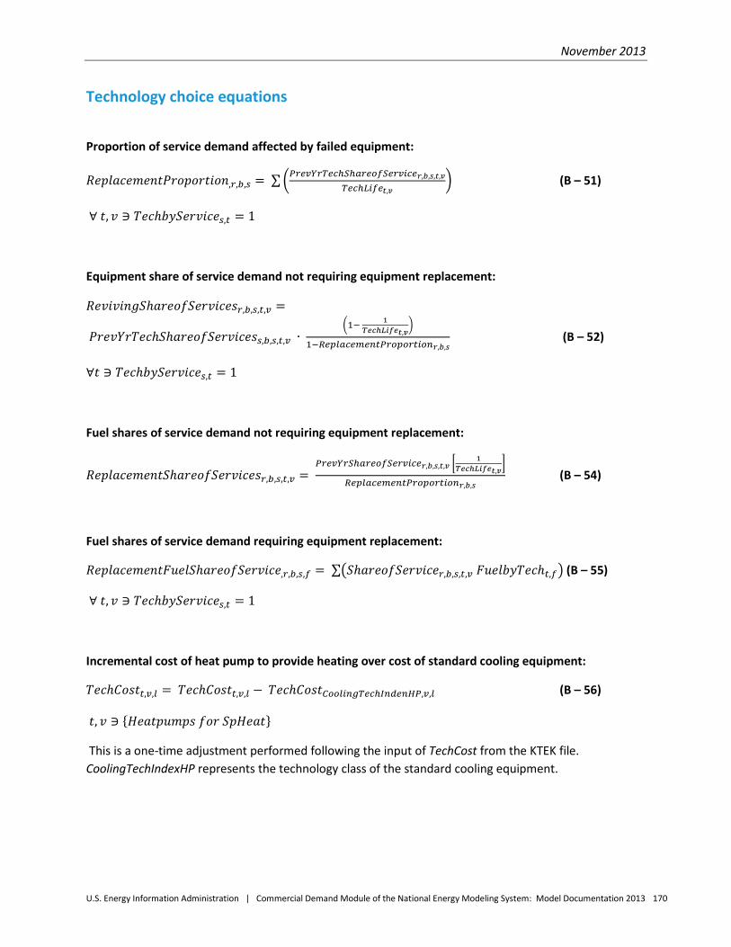
November 2013


Technology choice equations

Proportion of service demand affected by failed equipment:

𝑅𝑒𝑝𝑙𝑎𝑐𝑒𝑚𝑒𝑛𝑡𝑃𝑟𝑜𝑝𝑜𝑟𝑡𝑖𝑜𝑛,𝑟,𝑏,𝑠 = ∑�𝑃𝑟𝑒𝑣𝑌𝑟𝑇𝑒𝑐ℎ𝑆ℎ𝑎𝑟𝑒𝑜𝑓𝑆𝑒𝑟𝑣𝑖𝑐𝑒𝑟,𝑏,𝑠,𝑡,𝑣𝑇𝑒𝑐ℎ𝐿𝑖𝑓𝑒𝑡,𝑣

� (B – 51)

∀ 𝑡, 𝑣 ∋ 𝑇𝑒𝑐ℎ𝑏𝑦𝑆𝑒𝑟𝑣𝑖𝑐𝑒𝑠,𝑡 = 1

Equipment share of service demand not requiring equipment replacement:

𝑅𝑒𝑣𝑖𝑣𝑖𝑛𝑔𝑆ℎ𝑎𝑟𝑒𝑜𝑓𝑆𝑒𝑟𝑣𝑖𝑐𝑒𝑠𝑟,𝑏,𝑠,𝑡,𝑣 =

𝑃𝑟𝑒𝑣𝑌𝑟𝑇𝑒𝑐ℎ𝑆ℎ𝑎𝑟𝑒𝑜𝑓𝑆𝑒𝑟𝑣𝑖𝑐𝑒𝑠𝑠,𝑏,𝑠,𝑡,𝑣 ∙ �1− 1

𝑇𝑒𝑐ℎ𝐿𝑖𝑓𝑒𝑡,𝑣�

1−𝑅𝑒𝑝𝑙𝑎𝑐𝑒𝑚𝑒𝑛𝑡𝑃𝑟𝑜𝑝𝑜𝑟𝑡𝑖𝑜𝑛𝑟,𝑏,𝑠 (B – 52)

∀𝑡 ∋ 𝑇𝑒𝑐ℎ𝑏𝑦𝑆𝑒𝑟𝑣𝑖𝑐𝑒𝑠,𝑡 = 1

Fuel shares of service demand not requiring equipment replacement:

𝑅𝑒𝑝𝑙𝑎𝑐𝑒𝑚𝑒𝑛𝑡𝑆ℎ𝑎𝑟𝑒𝑜𝑓𝑆𝑒𝑟𝑣𝑖𝑐𝑒𝑠𝑟,𝑏,𝑠,𝑡,𝑣 = 𝑃𝑟𝑒𝑣𝑌𝑟𝑆ℎ𝑎𝑟𝑒𝑜𝑓𝑆𝑒𝑟𝑣𝑖𝑐𝑒𝑟,𝑏,𝑠,𝑡,𝑣 � 1

𝑇𝑒𝑐ℎ𝐿𝑖𝑓𝑒𝑡,𝑣�

𝑅𝑒𝑝𝑙𝑎𝑐𝑒𝑚𝑒𝑛𝑡𝑃𝑟𝑜𝑝𝑜𝑟𝑡𝑖𝑜𝑛𝑟,𝑏,𝑠 (B – 54)

Fuel shares of service demand requiring equipment replacement:

𝑅𝑒𝑝𝑙𝑎𝑐𝑒𝑚𝑒𝑛𝑡𝐹𝑢𝑒𝑙𝑆ℎ𝑎𝑟𝑒𝑜𝑓𝑆𝑒𝑟𝑣𝑖𝑐𝑒,𝑟,𝑏,𝑠,𝑓 = ∑�𝑆ℎ𝑎𝑟𝑒𝑜𝑓𝑆𝑒𝑟𝑣𝑖𝑐𝑒𝑟,𝑏,𝑠,𝑡,𝑣 𝐹𝑢𝑒𝑙𝑏𝑦𝑇𝑒𝑐ℎ𝑡,𝑓� (B – 55)

∀ 𝑡, 𝑣 ∋ 𝑇𝑒𝑐ℎ𝑏𝑦𝑆𝑒𝑟𝑣𝑖𝑐𝑒𝑠,𝑡 = 1

Incremental cost of heat pump to provide heating over cost of standard cooling equipment:

𝑇𝑒𝑐ℎ𝐶𝑜𝑠𝑡𝑡,𝑣,𝑙 = 𝑇𝑒𝑐ℎ𝐶𝑜𝑠𝑡𝑡,𝑣,𝑙 − 𝑇𝑒𝑐ℎ𝐶𝑜𝑠𝑡𝐶𝑜𝑜𝑙𝑖𝑛𝑔𝑇𝑒𝑐ℎ𝐼𝑛𝑑𝑒𝑛𝐻𝑃,𝑣,𝑙 (B – 56)

𝑡, 𝑣 ∋ {𝐻𝑒𝑎𝑡𝑝𝑢𝑚𝑝𝑠 𝑓𝑜𝑟 𝑆𝑝𝐻𝑒𝑎𝑡}

This is a one-time adjustment performed following the input of TechCost from the KTEK file. CoolingTechIndexHP represents the technology class of the standard cooling equipment.

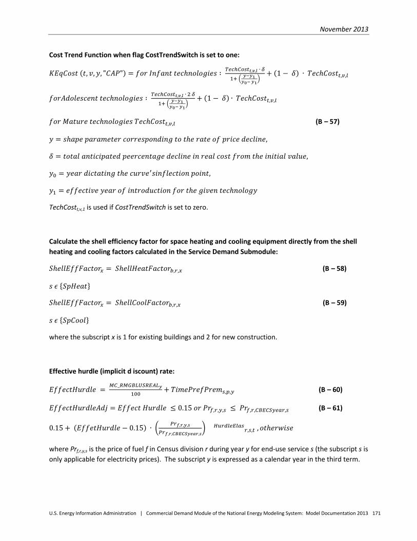
November 2013


Cost Trend Function when flag CostTrendSwitch is set to one:

𝐾𝐸𝑞𝐶𝑜𝑠𝑡 (𝑡, 𝑣,𝑦, "𝐶𝐴𝑃") = 𝑓𝑜𝑟 𝐼𝑛𝑓𝑎𝑛𝑡 𝑡𝑒𝑐ℎ𝑛𝑜𝑙𝑜𝑔𝑖𝑒𝑠 ∶ 𝑇𝑒𝑐ℎ𝐶𝑜𝑠𝑡𝑡,𝑣,𝑙 ∙ 𝛿

1+ � 𝑦−𝑦1𝑦0− 𝑦1

� + (1 − 𝛿) ∙ 𝑇𝑒𝑐ℎ𝐶𝑜𝑠𝑡𝑡,𝑣,𝑙

𝑓𝑜𝑟𝐴𝑑𝑜𝑙𝑒𝑠𝑐𝑒𝑛𝑡 𝑡𝑒𝑐ℎ𝑛𝑜𝑙𝑜𝑔𝑖𝑒𝑠 ∶ 𝑇𝑒𝑐ℎ𝐶𝑜𝑠𝑡𝑡,𝑣,𝑙 ∙ 2 𝛿

1+ � 𝑦−𝑦1𝑦0− 𝑦1

� + (1 − 𝛿) ∙ 𝑇𝑒𝑐ℎ𝐶𝑜𝑠𝑡𝑡,𝑣,𝑙

𝑓𝑜𝑟 𝑀𝑎𝑡𝑢𝑟𝑒 𝑡𝑒𝑐ℎ𝑛𝑜𝑙𝑜𝑔𝑖𝑒𝑠 𝑇𝑒𝑐ℎ𝐶𝑜𝑠𝑡𝑡,𝑣,𝑙 (B – 57)

𝑦 = 𝑠ℎ𝑎𝑝𝑒 𝑝𝑎𝑟𝑎𝑚𝑒𝑡𝑒𝑟 𝑐𝑜𝑟𝑟𝑒𝑠𝑝𝑜𝑛𝑑𝑖𝑛𝑔 𝑡𝑜 𝑡ℎ𝑒 𝑟𝑎𝑡𝑒 𝑜𝑓 𝑝𝑟𝑖𝑐𝑒 𝑑𝑒𝑐𝑙𝑖𝑛𝑒,

𝛿 = 𝑡𝑜𝑡𝑎𝑙 𝑎𝑛𝑡𝑖𝑐𝑖𝑝𝑎𝑡𝑒𝑑 𝑝𝑒𝑒𝑟𝑐𝑒𝑛𝑡𝑎𝑔𝑒 𝑑𝑒𝑐𝑙𝑖𝑛𝑒 𝑖𝑛 𝑟𝑒𝑎𝑙 𝑐𝑜𝑠𝑡 𝑓𝑟𝑜𝑚 𝑡ℎ𝑒 𝑖𝑛𝑖𝑡𝑖𝑎𝑙 𝑣𝑎𝑙𝑢𝑒,

𝑦0 = 𝑦𝑒𝑎𝑟 𝑑𝑖𝑐𝑡𝑎𝑡𝑖𝑛𝑔 𝑡ℎ𝑒 𝑐𝑢𝑟𝑣𝑒′𝑠𝑖𝑛𝑓𝑙𝑒𝑐𝑡𝑖𝑜𝑛 𝑝𝑜𝑖𝑛𝑡,

𝑦1 = 𝑒𝑓𝑓𝑒𝑐𝑡𝑖𝑣𝑒 𝑦𝑒𝑎𝑟 𝑜𝑓 𝑖𝑛𝑡𝑟𝑜𝑑𝑢𝑐𝑡𝑖𝑜𝑛 𝑓𝑜𝑟 𝑡ℎ𝑒 𝑔𝑖𝑣𝑒𝑛 𝑡𝑒𝑐ℎ𝑛𝑜𝑙𝑜𝑔𝑦

TechCostt,v,1 is used if CostTrendSwitch is set to zero.

Calculate the shell efficiency factor for space heating and cooling equipment directly from the shell heating and cooling factors calculated in the Service Demand Submodule:

𝑆ℎ𝑒𝑙𝑙𝐸𝑓𝑓𝐹𝑎𝑐𝑡𝑜𝑟𝑥 = 𝑆ℎ𝑒𝑙𝑙𝐻𝑒𝑎𝑡𝐹𝑎𝑐𝑡𝑜𝑟𝑏,𝑟,𝑥 (B – 58)

𝑠 𝜖 {𝑆𝑝𝐻𝑒𝑎𝑡}

𝑆ℎ𝑒𝑙𝑙𝐸𝑓𝑓𝐹𝑎𝑐𝑡𝑜𝑟𝑥 = 𝑆ℎ𝑒𝑙𝑙𝐶𝑜𝑜𝑙𝐹𝑎𝑐𝑡𝑜𝑟𝑏,𝑟,𝑥 (B – 59)

𝑠 𝜖 {𝑆𝑝𝐶𝑜𝑜𝑙}

where the subscript x is 1 for existing buildings and 2 for new construction.

Effective hurdle (implicit d iscount) rate:

𝐸𝑓𝑓𝑒𝑐𝑡𝐻𝑢𝑟𝑑𝑙𝑒 = 𝑀𝐶_𝑅𝑀𝐺𝐵𝐿𝑈𝑆𝑅𝐸𝐴𝐿𝑦100

+ 𝑇𝑖𝑚𝑒𝑃𝑟𝑒𝑓𝑃𝑟𝑒𝑚𝑠,𝑝,𝑦 (B – 60)

𝐸𝑓𝑓𝑒𝑐𝑡𝐻𝑢𝑟𝑑𝑙𝑒𝐴𝑑𝑗 = 𝐸𝑓𝑓𝑒𝑐𝑡 𝐻𝑢𝑟𝑑𝑙𝑒 ≤ 0.15 𝑜𝑟 𝑃𝑟𝑓,𝑟,𝑦,𝑠 ≤ 𝑃𝑟𝑓,𝑟,𝐶𝐵𝐸𝐶𝑆𝑦𝑒𝑎𝑟,𝑠 (B – 61)

0.15 + (𝐸𝑓𝑓𝑒𝑡𝐻𝑢𝑟𝑑𝑙𝑒 − 0.15) ∙ � 𝑃𝑟𝑓,𝑟,𝑦,𝑠

𝑃𝑟𝑓,𝑟,𝐶𝐵𝐸𝐶𝑆𝑦𝑒𝑎𝑟,𝑠� 𝐻𝑢𝑟𝑑𝑙𝑒𝐸𝑙𝑎𝑠

𝑟,𝑠,𝑡 ,𝑜𝑡ℎ𝑒𝑟𝑤𝑖𝑠𝑒

where Prf,r,y,s is the price of fuel f in Census division r during year y for end-use service s (the subscript s is only applicable for electricity prices). The subscript y is expressed as a calendar year in the third term.

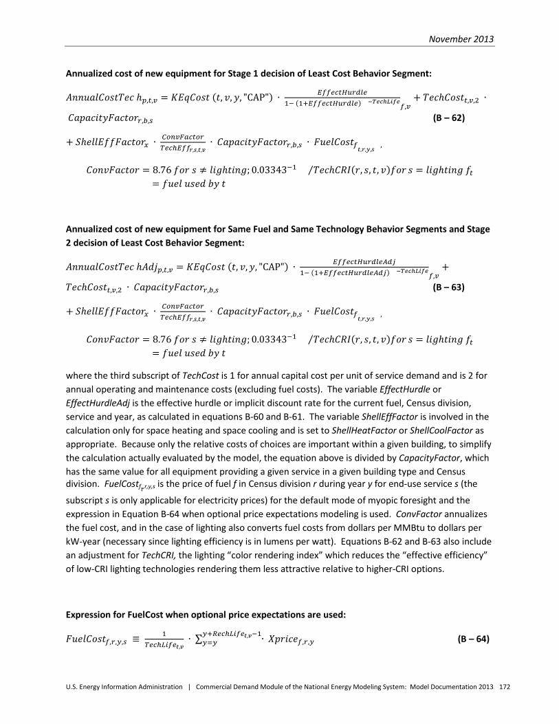
November 2013


Annualized cost of new equipment for Stage 1 decision of Least Cost Behavior Segment:

𝐴𝑛𝑛𝑢𝑎𝑙𝐶𝑜𝑠𝑡𝑇𝑒𝑐 ℎ𝑝,𝑡,𝑣 = 𝐾𝐸𝑞𝐶𝑜𝑠𝑡 (𝑡, 𝑣,𝑦, "CAP") ∙ 𝐸𝑓𝑓𝑒𝑐𝑡𝐻𝑢𝑟𝑑𝑙𝑒1− (1+𝐸𝑓𝑓𝑒𝑐𝑡𝐻𝑢𝑟𝑑𝑙𝑒) −𝑇𝑒𝑐ℎ𝐿𝑖𝑓𝑒

𝑓,𝑣+ 𝑇𝑒𝑐ℎ𝐶𝑜𝑠𝑡𝑡,𝑣,2 ∙

𝐶𝑎𝑝𝑎𝑐𝑖𝑡𝑦𝐹𝑎𝑐𝑡𝑜𝑟𝑟,𝑏,𝑠 (B – 62)

+ 𝑆ℎ𝑒𝑙𝑙𝐸𝑓𝑓𝐹𝑎𝑐𝑡𝑜𝑟𝑥 ∙ 𝐶𝑜𝑛𝑣𝐹𝑎𝑐𝑡𝑜𝑟𝑇𝑒𝑐ℎ𝐸𝑓𝑓𝑟,𝑠,𝑡,𝑣

∙ 𝐶𝑎𝑝𝑎𝑐𝑖𝑡𝑦𝐹𝑎𝑐𝑡𝑜𝑟𝑟,𝑏,𝑠 ∙ 𝐹𝑢𝑒𝑙𝐶𝑜𝑠𝑡𝑓𝑡,𝑟,𝑦,𝑠

,

𝐶𝑜𝑛𝑣𝐹𝑎𝑐𝑡𝑜𝑟 = 8.76 𝑓𝑜𝑟 𝑠 ≠ 𝑙𝑖𝑔ℎ𝑡𝑖𝑛𝑔; 0.03343−1 𝑇𝑒𝑐ℎ𝐶𝑅𝐼(𝑟, 𝑠, 𝑡, 𝑣)𝑓𝑜𝑟⁄ 𝑠 = 𝑙𝑖𝑔ℎ𝑡𝑖𝑛𝑔 𝑓𝑡= 𝑓𝑢𝑒𝑙 𝑢𝑠𝑒𝑑 𝑏𝑦 𝑡

Annualized cost of new equipment for Same Fuel and Same Technology Behavior Segments and Stage 2 decision of Least Cost Behavior Segment:

𝐴𝑛𝑛𝑢𝑎𝑙𝐶𝑜𝑠𝑡𝑇𝑒𝑐 ℎ𝐴𝑑𝑗𝑝,𝑡,𝑣 = 𝐾𝐸𝑞𝐶𝑜𝑠𝑡 (𝑡, 𝑣,𝑦, "CAP") ∙ 𝐸𝑓𝑓𝑒𝑐𝑡𝐻𝑢𝑟𝑑𝑙𝑒𝐴𝑑𝑗1− (1+𝐸𝑓𝑓𝑒𝑐𝑡𝐻𝑢𝑟𝑑𝑙𝑒𝐴𝑑𝑗) −𝑇𝑒𝑐ℎ𝐿𝑖𝑓𝑒

𝑓,𝑣+

𝑇𝑒𝑐ℎ𝐶𝑜𝑠𝑡𝑡,𝑣,2 ∙ 𝐶𝑎𝑝𝑎𝑐𝑖𝑡𝑦𝐹𝑎𝑐𝑡𝑜𝑟𝑟,𝑏,𝑠 (B – 63)

+ 𝑆ℎ𝑒𝑙𝑙𝐸𝑓𝑓𝐹𝑎𝑐𝑡𝑜𝑟𝑥 ∙ 𝐶𝑜𝑛𝑣𝐹𝑎𝑐𝑡𝑜𝑟𝑇𝑒𝑐ℎ𝐸𝑓𝑓𝑟,𝑠,𝑡,𝑣

∙ 𝐶𝑎𝑝𝑎𝑐𝑖𝑡𝑦𝐹𝑎𝑐𝑡𝑜𝑟𝑟,𝑏,𝑠 ∙ 𝐹𝑢𝑒𝑙𝐶𝑜𝑠𝑡𝑓𝑡,𝑟,𝑦,𝑠

,

𝐶𝑜𝑛𝑣𝐹𝑎𝑐𝑡𝑜𝑟 = 8.76 𝑓𝑜𝑟 𝑠 ≠ 𝑙𝑖𝑔ℎ𝑡𝑖𝑛𝑔; 0.03343−1 𝑇𝑒𝑐ℎ𝐶𝑅𝐼(𝑟, 𝑠, 𝑡, 𝑣)𝑓𝑜𝑟⁄ 𝑠 = 𝑙𝑖𝑔ℎ𝑡𝑖𝑛𝑔 𝑓𝑡= 𝑓𝑢𝑒𝑙 𝑢𝑠𝑒𝑑 𝑏𝑦 𝑡

where the third subscript of TechCost is 1 for annual capital cost per unit of service demand and is 2 for annual operating and maintenance costs (excluding fuel costs). The variable EffectHurdle or EffectHurdleAdj is the effective hurdle or implicit discount rate for the current fuel, Census division, service and year, as calculated in equations B-60 and B-61. The variable ShellEffFactor is involved in the calculation only for space heating and space cooling and is set to ShellHeatFactor or ShellCoolFactor as appropriate. Because only the relative costs of choices are important within a given building, to simplify the calculation actually evaluated by the model, the equation above is divided by CapacityFactor, which has the same value for all equipment providing a given service in a given building type and Census division. FuelCostft,r,y,s is the price of fuel f in Census division r during year y for end-use service s (the

subscript s is only applicable for electricity prices) for the default mode of myopic foresight and the expression in Equation B-64 when optional price expectations modeling is used. ConvFactor annualizes the fuel cost, and in the case of lighting also converts fuel costs from dollars per MMBtu to dollars per kW-year (necessary since lighting efficiency is in lumens per watt). Equations B-62 and B-63 also include an adjustment for TechCRI, the lighting “color rendering index” which reduces the “effective efficiency” of low-CRI lighting technologies rendering them less attractive relative to higher-CRI options.

Expression for FuelCost when optional price expectations are used:

𝐹𝑢𝑒𝑙𝐶𝑜𝑠𝑡𝑓,𝑟,𝑦,𝑠 ≡ 1𝑇𝑒𝑐ℎ𝐿𝑖𝑓𝑒𝑡,𝑣

∙ ∑ ∙ 𝑋𝑝𝑟𝑖𝑐𝑒𝑓,𝑟,𝑦𝑦+𝑅𝑒𝑐ℎ𝐿𝑖𝑓𝑒𝑡,𝑣−1𝑦=𝑦 (B – 64)

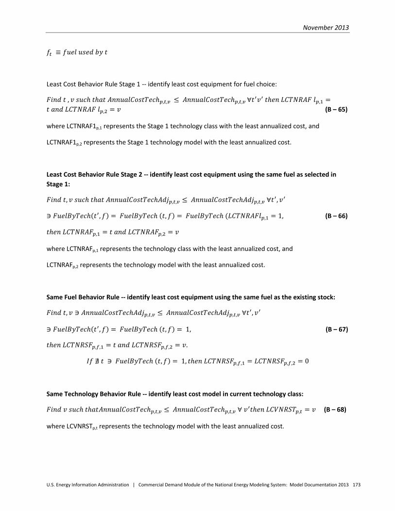
November 2013


𝑓𝑡 ≡ 𝑓𝑢𝑒𝑙 𝑢𝑠𝑒𝑑 𝑏𝑦 𝑡

Least Cost Behavior Rule Stage 1 -- identify least cost equipment for fuel choice:

𝐹𝑖𝑛𝑑 𝑡 , 𝑣 𝑠𝑢𝑐ℎ 𝑡ℎ𝑎𝑡 𝐴𝑛𝑛𝑢𝑎𝑙𝐶𝑜𝑠𝑡𝑇𝑒𝑐ℎ𝑝,𝑡,𝑣 ≤ 𝐴𝑛𝑛𝑢𝑎𝑙𝐶𝑜𝑠𝑡𝑇𝑒𝑐ℎ𝑝,𝑡,𝑣 ∀𝑡′𝑣′ 𝑡ℎ𝑒𝑛 𝐿𝐶𝑇𝑁𝑅𝐴𝐹 𝑙𝑝,1 =𝑡 𝑎𝑛𝑑 𝐿𝐶𝑇𝑁𝑅𝐴𝐹 𝑙𝑝,2 = 𝑣 (B – 65)

where LCTNRAF1p,1 represents the Stage 1 technology class with the least annualized cost, and

LCTNRAF1p,2 represents the Stage 1 technology model with the least annualized cost.

Least Cost Behavior Rule Stage 2 -- identify least cost equipment using the same fuel as selected in Stage 1:

𝐹𝑖𝑛𝑑 𝑡, 𝑣 𝑠𝑢𝑐ℎ 𝑡ℎ𝑎𝑡 𝐴𝑛𝑛𝑢𝑎𝑙𝐶𝑜𝑠𝑡𝑇𝑒𝑐ℎ𝐴𝑑𝑗𝑝,𝑡,𝑣 ≤ 𝐴𝑛𝑛𝑢𝑎𝑙𝐶𝑜𝑠𝑡𝑇𝑒𝑐ℎ𝐴𝑑𝑗𝑝,𝑡,𝑣 ∀𝑡′,𝑣′

∋ 𝐹𝑢𝑒𝑙𝐵𝑦𝑇𝑒𝑐ℎ(𝑡′,𝑓) = 𝐹𝑢𝑒𝑙𝐵𝑦𝑇𝑒𝑐ℎ (𝑡,𝑓) = 𝐹𝑢𝑒𝑙𝐵𝑦𝑇𝑒𝑐ℎ (𝐿𝐶𝑇𝑁𝑅𝐴𝐹𝑙𝑝,1 = 1, (B – 66)

𝑡ℎ𝑒𝑛 𝐿𝐶𝑇𝑁𝑅𝐴𝐹𝑝,1 = 𝑡 𝑎𝑛𝑑 𝐿𝐶𝑇𝑁𝑅𝐴𝐹𝑝,2 = 𝑣

where LCTNRAFp,1 represents the technology class with the least annualized cost, and

LCTNRAFp,2 represents the technology model with the least annualized cost.

Same Fuel Behavior Rule -- identify least cost equipment using the same fuel as the existing stock:

𝐹𝑖𝑛𝑑 𝑡, 𝑣 ∋ 𝐴𝑛𝑛𝑢𝑎𝑙𝐶𝑜𝑠𝑡𝑇𝑒𝑐ℎ𝐴𝑑𝑗𝑝,𝑡,𝑣 ≤ 𝐴𝑛𝑛𝑢𝑎𝑙𝐶𝑜𝑠𝑡𝑇𝑒𝑐ℎ𝐴𝑑𝑗𝑝,𝑡,𝑣 ∀𝑡′,𝑣′

∋ 𝐹𝑢𝑒𝑙𝐵𝑦𝑇𝑒𝑐ℎ(𝑡′,𝑓) = 𝐹𝑢𝑒𝑙𝐵𝑦𝑇𝑒𝑐ℎ (𝑡,𝑓) = 1, (B – 67)

𝑡ℎ𝑒𝑛 𝐿𝐶𝑇𝑁𝑅𝑆𝐹𝑝,𝑓,1 = 𝑡 𝑎𝑛𝑑 𝐿𝐶𝑇𝑁𝑅𝑆𝐹𝑝,𝑓,2 = 𝑣.

𝐼𝑓 ∄ 𝑡 ∋ 𝐹𝑢𝑒𝑙𝐵𝑦𝑇𝑒𝑐ℎ (𝑡,𝑓) = 1, 𝑡ℎ𝑒𝑛 𝐿𝐶𝑇𝑁𝑅𝑆𝐹𝑝,𝑓,1 = 𝐿𝐶𝑇𝑁𝑅𝑆𝐹𝑝,𝑓,2 = 0

Same Technology Behavior Rule -- identify least cost model in current technology class:

𝐹𝑖𝑛𝑑 𝑣 𝑠𝑢𝑐ℎ 𝑡ℎ𝑎𝑡𝐴𝑛𝑛𝑢𝑎𝑙𝐶𝑜𝑠𝑡𝑇𝑒𝑐ℎ𝑝,𝑡,𝑣 ≤ 𝐴𝑛𝑛𝑢𝑎𝑙𝐶𝑜𝑠𝑡𝑇𝑒𝑐ℎ𝑝,𝑡,𝑣 ∀ 𝑣′𝑡ℎ𝑒𝑛 𝐿𝐶𝑉𝑁𝑅𝑆𝑇𝑝,𝑡 = 𝑣 (B – 68)

where LCVNRSTp,t represents the technology model with the least annualized cost.

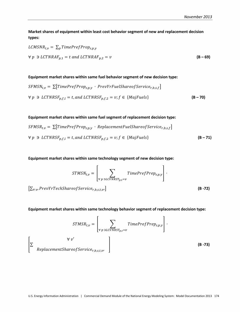
November 2013


Market shares of equipment within least cost behavior segment of new and replacement decision types:

𝐿𝐶𝑀𝑆𝑁𝑅𝑡,𝑣 = ∑ 𝑇𝑖𝑚𝑒𝑃𝑟𝑒𝑓𝑃𝑟𝑜𝑝𝑠,𝑝,𝑦𝑝

∀ 𝑝 ∋ 𝐿𝐶𝑇𝑁𝑅𝐴𝐹𝑝,1 = 𝑡 𝑎𝑛𝑑 𝐿𝐶𝑇𝑁𝑅𝐴𝐹𝑝,2 = 𝑣 (B – 69)

Equipment market shares within same fuel behavior segment of new decision type:

𝑆𝐹𝑀𝑆𝑁𝑡,𝑣 = ∑�𝑇𝑖𝑚𝑒𝑃𝑟𝑒𝑓𝑃𝑟𝑜𝑝𝑠,𝑝,𝑦 ∙ 𝑃𝑟𝑒𝑣𝑌𝑟𝐹𝑢𝑒𝑙𝑆ℎ𝑎𝑟𝑒𝑜𝑓𝑆𝑒𝑟𝑣𝑖𝑐𝑒𝑟,𝑏,𝑠,𝑓�

∀ 𝑝 ∋ 𝐿𝐶𝑇𝑁𝑅𝑆𝐹𝑝,𝑓,𝑙 = 𝑡,𝑎𝑛𝑑 𝐿𝐶𝑇𝑁𝑅𝑆𝐹𝑝,𝑓,2 = 𝑣;𝑓 ∈ {𝑀𝑎𝑗𝐹𝑢𝑒𝑙𝑠} (B – 70)

Equipment market shares within same fuel segment of replacement decision type:

𝑆𝐹𝑀𝑆𝑅𝑡.𝑣 = ∑�𝑇𝑖𝑚𝑒𝑃𝑟𝑒𝑓𝑃𝑟𝑜𝑝𝑠,𝑝,𝑦 ∙ 𝑅𝑒𝑝𝑙𝑎𝑐𝑒𝑚𝑒𝑛𝑡𝐹𝑢𝑒𝑙𝑆ℎ𝑎𝑟𝑒𝑜𝑓𝑆𝑒𝑟𝑣𝑖𝑐𝑒𝑟,𝑏,𝑠,𝑓�

∀ 𝑝 ∋ 𝐿𝐶𝑇𝑁𝑅𝑆𝐹𝑝,𝑓,𝑙 = 𝑡,𝑎𝑛𝑑 𝐿𝐶𝑇𝑁𝑅𝑆𝐹𝑝,𝑓,2 = 𝑣;𝑓 ∈ {𝑀𝑎𝑗𝐹𝑢𝑒𝑙𝑠} (B – 71)

Equipment market shares within same technology segment of new decision type:

𝑆𝑇𝑀𝑆𝑁𝑡,𝑣 = � � 𝑇𝑖𝑚𝑒𝑃𝑟𝑒𝑓𝑃𝑟𝑒𝑝𝑠,𝑝,𝑦∀ 𝑝 ∋𝐿𝐶𝑉𝑁𝑅𝑆𝑇𝑝,𝑡=𝑣

� ∙

�∑ 𝑃𝑟𝑒𝑣𝑌𝑟𝑇𝑒𝑐ℎ𝑆ℎ𝑎𝑟𝑒𝑜𝑓𝑆𝑒𝑟𝑣𝑖𝑐𝑒𝑟,𝑏,𝑠,𝑡,𝑣′∀ 𝑣′ � (B -72)

Equipment market shares within same technology behavior segment of replacement decision type:

𝑆𝑇𝑀𝑆𝑅𝑡,𝑣 = � � 𝑇𝑖𝑚𝑒𝑃𝑟𝑒𝑓𝑃𝑟𝑒𝑝𝑠,𝑝,𝑦∀ 𝑝 ∋𝐿𝐶𝑉𝑁𝑅𝑆𝑇𝑝,𝑡=𝑣

� ∙

�∑∀ 𝑣′

𝑅𝑒𝑝𝑙𝑎𝑐𝑒𝑚𝑒𝑛𝑡𝑆ℎ𝑎𝑟𝑒𝑜𝑓𝑆𝑒𝑟𝑣𝑖𝑐𝑒𝑟,𝑏,𝑠,𝑡,𝑣′

� (B -73)

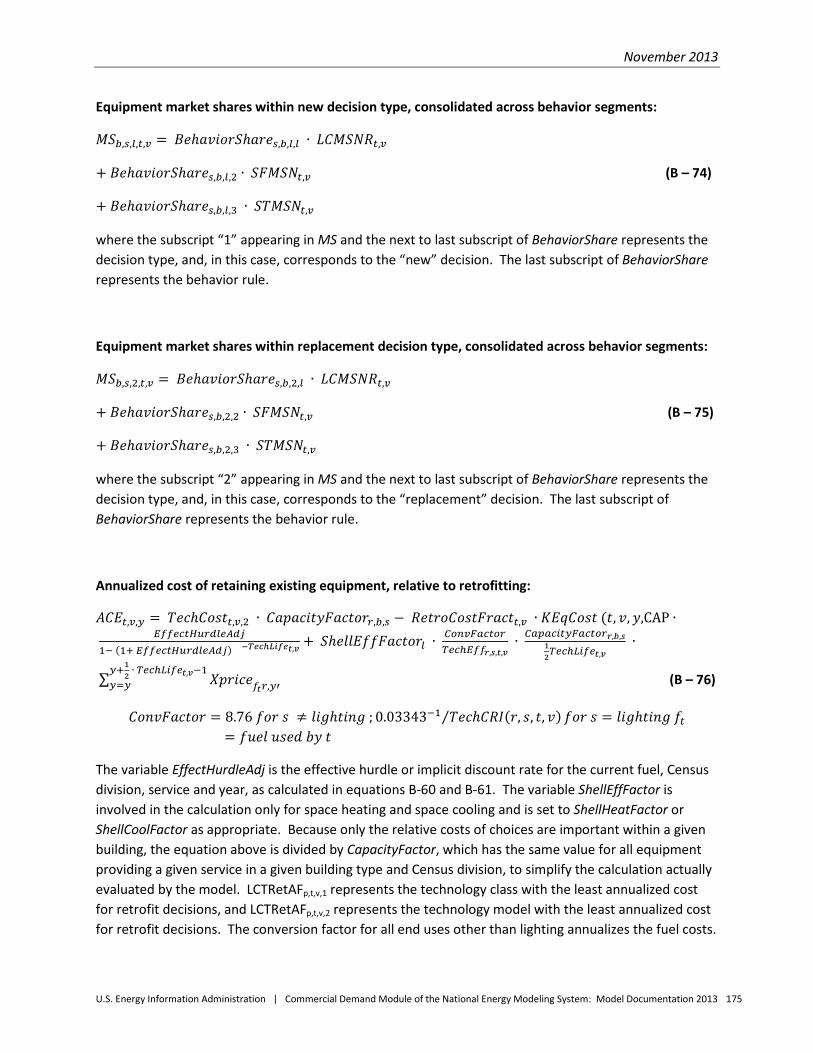
November 2013


Equipment market shares within new decision type, consolidated across behavior segments:

𝑀𝑆𝑏,𝑠,𝑙,𝑡,𝑣 = 𝐵𝑒ℎ𝑎𝑣𝑖𝑜𝑟𝑆ℎ𝑎𝑟𝑒𝑠,𝑏,𝑙,𝑙 ∙ 𝐿𝐶𝑀𝑆𝑁𝑅𝑡,𝑣

+ 𝐵𝑒ℎ𝑎𝑣𝑖𝑜𝑟𝑆ℎ𝑎𝑟𝑒𝑠,𝑏,𝑙,2 ∙ 𝑆𝐹𝑀𝑆𝑁𝑡,𝑣 (B – 74)

+ 𝐵𝑒ℎ𝑎𝑣𝑖𝑜𝑟𝑆ℎ𝑎𝑟𝑒𝑠,𝑏,𝑙,3 ∙ 𝑆𝑇𝑀𝑆𝑁𝑡,𝑣

where the subscript “1” appearing in MS and the next to last subscript of BehaviorShare represents the decision type, and, in this case, corresponds to the “new” decision. The last subscript of BehaviorShare represents the behavior rule.

Equipment market shares within replacement decision type, consolidated across behavior segments:

𝑀𝑆𝑏,𝑠,2,𝑡,𝑣 = 𝐵𝑒ℎ𝑎𝑣𝑖𝑜𝑟𝑆ℎ𝑎𝑟𝑒𝑠,𝑏,2,𝑙 ∙ 𝐿𝐶𝑀𝑆𝑁𝑅𝑡,𝑣

+ 𝐵𝑒ℎ𝑎𝑣𝑖𝑜𝑟𝑆ℎ𝑎𝑟𝑒𝑠,𝑏,2,2 ∙ 𝑆𝐹𝑀𝑆𝑁𝑡,𝑣 (B – 75)

+ 𝐵𝑒ℎ𝑎𝑣𝑖𝑜𝑟𝑆ℎ𝑎𝑟𝑒𝑠,𝑏,2,3 ∙ 𝑆𝑇𝑀𝑆𝑁𝑡,𝑣

where the subscript “2” appearing in MS and the next to last subscript of BehaviorShare represents the decision type, and, in this case, corresponds to the “replacement” decision. The last subscript of BehaviorShare represents the behavior rule.

Annualized cost of retaining existing equipment, relative to retrofitting:

𝐴𝐶𝐸𝑡,𝑣,𝑦 = 𝑇𝑒𝑐ℎ𝐶𝑜𝑠𝑡𝑡,𝑣,2 ∙ 𝐶𝑎𝑝𝑎𝑐𝑖𝑡𝑦𝐹𝑎𝑐𝑡𝑜𝑟𝑟,𝑏,𝑠 − 𝑅𝑒𝑡𝑟𝑜𝐶𝑜𝑠𝑡𝐹𝑟𝑎𝑐𝑡𝑡,𝑣 ∙ 𝐾𝐸𝑞𝐶𝑜𝑠𝑡 (𝑡, 𝑣,𝑦,CAP ∙ 𝐸𝑓𝑓𝑒𝑐𝑡𝐻𝑢𝑟𝑑𝑙𝑒𝐴𝑑𝑗1− (1+ 𝐸𝑓𝑓𝑒𝑐𝑡𝐻𝑢𝑟𝑑𝑙𝑒𝐴𝑑𝑗) −𝑇𝑒𝑐ℎ𝐿𝑖𝑓𝑒𝑡,𝑣 + 𝑆ℎ𝑒𝑙𝑙𝐸𝑓𝑓𝐹𝑎𝑐𝑡𝑜𝑟𝑙 ∙ 𝐶𝑜𝑛𝑣𝐹𝑎𝑐𝑡𝑜𝑟

𝑇𝑒𝑐ℎ𝐸𝑓𝑓𝑟,𝑠,𝑡,𝑣 ∙ 𝐶𝑎𝑝𝑎𝑐𝑖𝑡𝑦𝐹𝑎𝑐𝑡𝑜𝑟𝑟,𝑏,𝑠

12𝑇𝑒𝑐ℎ𝐿𝑖𝑓𝑒𝑡,𝑣

∙

∑ 𝑋𝑝𝑟𝑖𝑐𝑒𝑓𝑡𝑟,𝑦′𝑦+12 ∙ 𝑇𝑒𝑐ℎ𝐿𝑖𝑓𝑒𝑡,𝑣−1𝑦=𝑦 (B – 76)

𝐶𝑜𝑛𝑣𝐹𝑎𝑐𝑡𝑜𝑟 = 8.76 𝑓𝑜𝑟 𝑠 ≠ 𝑙𝑖𝑔ℎ𝑡𝑖𝑛𝑔 ; 0.03343−1 𝑇𝑒𝑐ℎ𝐶𝑅𝐼(𝑟, 𝑠, 𝑡, 𝑣)⁄ 𝑓𝑜𝑟 𝑠 = 𝑙𝑖𝑔ℎ𝑡𝑖𝑛𝑔 𝑓𝑡= 𝑓𝑢𝑒𝑙 𝑢𝑠𝑒𝑑 𝑏𝑦 𝑡

The variable EffectHurdleAdj is the effective hurdle or implicit discount rate for the current fuel, Census division, service and year, as calculated in equations B-60 and B-61. The variable ShellEffFactor is involved in the calculation only for space heating and space cooling and is set to ShellHeatFactor or ShellCoolFactor as appropriate. Because only the relative costs of choices are important within a given building, the equation above is divided by CapacityFactor, which has the same value for all equipment providing a given service in a given building type and Census division, to simplify the calculation actually evaluated by the model. LCTRetAFp,t,v,1 represents the technology class with the least annualized cost for retrofit decisions, and LCTRetAFp,t,v,2 represents the technology model with the least annualized cost for retrofit decisions. The conversion factor for all end uses other than lighting annualizes the fuel costs.

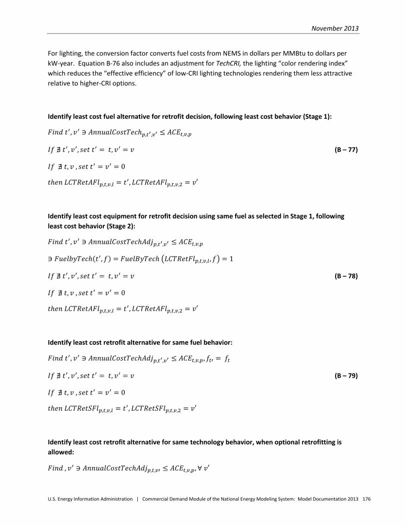
November 2013


For lighting, the conversion factor converts fuel costs from NEMS in dollars per MMBtu to dollars per kW-year. Equation B-76 also includes an adjustment for TechCRI, the lighting “color rendering index” which reduces the “effective efficiency” of low-CRI lighting technologies rendering them less attractive relative to higher-CRI options.

Identify least cost fuel alternative for retrofit decision, following least cost behavior (Stage 1):

𝐹𝑖𝑛𝑑 𝑡′, 𝑣′ ∋ 𝐴𝑛𝑛𝑢𝑎𝑙𝐶𝑜𝑠𝑡𝑇𝑒𝑐ℎ𝑝,𝑡′,𝑣′ ≤ 𝐴𝐶𝐸𝑡,𝑣,𝑝

𝐼𝑓 ∄ 𝑡′, 𝑣′, 𝑠𝑒𝑡 𝑡′ = 𝑡, 𝑣′ = 𝑣 (B – 77)

𝐼𝑓 ∄ 𝑡, 𝑣 , 𝑠𝑒𝑡 𝑡′ = 𝑣′ = 0

𝑡ℎ𝑒𝑛 𝐿𝐶𝑇𝑅𝑒𝑡𝐴𝐹𝑙𝑝,𝑡,𝑣,𝑙 = 𝑡′, 𝐿𝐶𝑇𝑅𝑒𝑡𝐴𝐹𝑙𝑝,𝑡,𝑣,2 = 𝑣′

Identify least cost equipment for retrofit decision using same fuel as selected in Stage 1, following least cost behavior (Stage 2):

𝐹𝑖𝑛𝑑 𝑡′, 𝑣′ ∋ 𝐴𝑛𝑛𝑢𝑎𝑙𝐶𝑜𝑠𝑡𝑇𝑒𝑐ℎ𝐴𝑑𝑗𝑝,𝑡′,𝑣′ ≤ 𝐴𝐶𝐸𝑡,𝑣,𝑝

∋ 𝐹𝑢𝑒𝑙𝑏𝑦𝑇𝑒𝑐ℎ(𝑡′,𝑓) = 𝐹𝑢𝑒𝑙𝐵𝑦𝑇𝑒𝑐ℎ �𝐿𝐶𝑇𝑅𝑒𝑡𝐹𝑙𝑝,𝑡,𝑣,𝑙 ,𝑓� = 1

𝐼𝑓 ∄ 𝑡′, 𝑣′, 𝑠𝑒𝑡 𝑡′ = 𝑡, 𝑣′ = 𝑣 (B – 78)

𝐼𝑓 ∄ 𝑡, 𝑣 , 𝑠𝑒𝑡 𝑡′ = 𝑣′ = 0

𝑡ℎ𝑒𝑛 𝐿𝐶𝑇𝑅𝑒𝑡𝐴𝐹𝑙𝑝,𝑡,𝑣,𝑙 = 𝑡′, 𝐿𝐶𝑇𝑅𝑒𝑡𝐴𝐹𝑙𝑝,𝑡,𝑣,2 = 𝑣′

Identify least cost retrofit alternative for same fuel behavior:

𝐹𝑖𝑛𝑑 𝑡′, 𝑣′ ∋ 𝐴𝑛𝑛𝑢𝑎𝑙𝐶𝑜𝑠𝑡𝑇𝑒𝑐ℎ𝐴𝑑𝑗𝑝,𝑡′,𝑣′ ≤ 𝐴𝐶𝐸𝑡,𝑣,𝑝,𝑓𝑡′ = 𝑓𝑡

𝐼𝑓 ∄ 𝑡′, 𝑣′, 𝑠𝑒𝑡 𝑡′ = 𝑡, 𝑣′ = 𝑣 (B – 79)

𝐼𝑓 ∄ 𝑡, 𝑣 , 𝑠𝑒𝑡 𝑡′ = 𝑣′ = 0

𝑡ℎ𝑒𝑛 𝐿𝐶𝑇𝑅𝑒𝑡𝑆𝐹𝑙𝑝,𝑡,𝑣,𝑙 = 𝑡′, 𝐿𝐶𝑇𝑅𝑒𝑡𝑆𝐹𝑙𝑝,𝑡,𝑣,2 = 𝑣′

Identify least cost retrofit alternative for same technology behavior, when optional retrofitting is allowed:

𝐹𝑖𝑛𝑑 , 𝑣′ ∋ 𝐴𝑛𝑛𝑢𝑎𝑙𝐶𝑜𝑠𝑡𝑇𝑒𝑐ℎ𝐴𝑑𝑗𝑝,𝑡,𝑣′ ≤ 𝐴𝐶𝐸𝑡,𝑣,𝑝,∀ 𝑣′

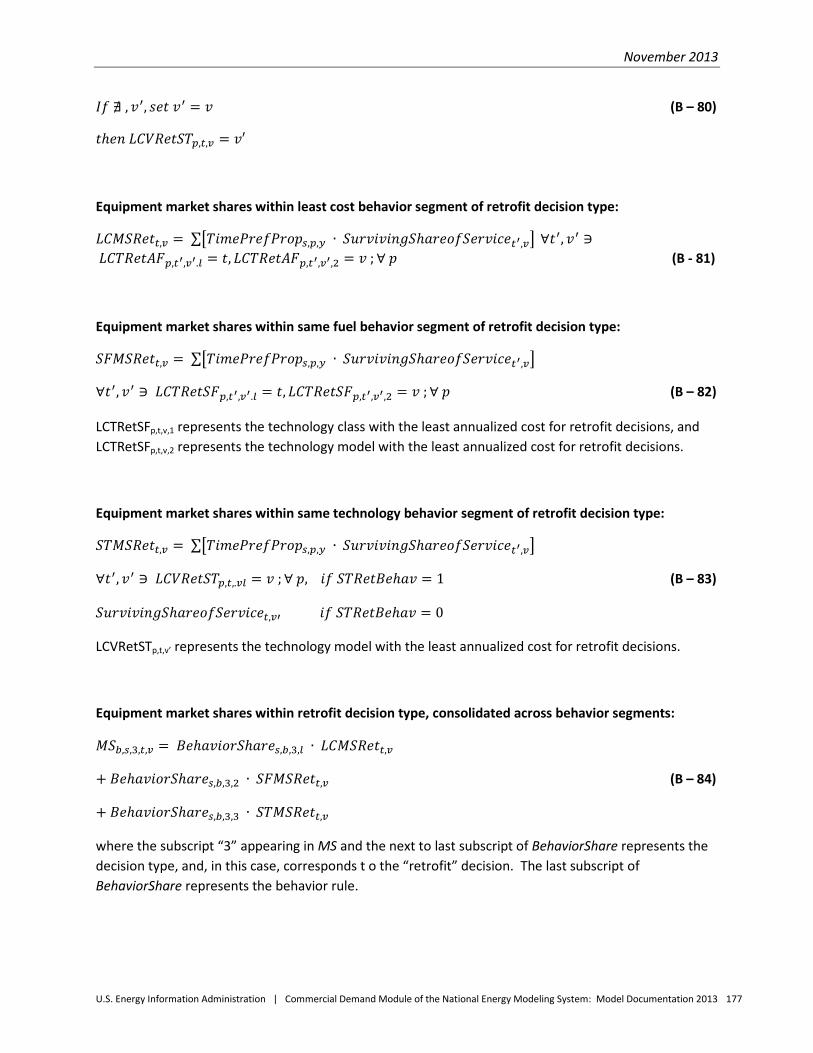
November 2013


𝐼𝑓 ∄ , 𝑣′, 𝑠𝑒𝑡 𝑣′ = 𝑣 (B – 80)

𝑡ℎ𝑒𝑛 𝐿𝐶𝑉𝑅𝑒𝑡𝑆𝑇𝑝,𝑡,𝑣 = 𝑣′

Equipment market shares within least cost behavior segment of retrofit decision type:

𝐿𝐶𝑀𝑆𝑅𝑒𝑡𝑡,𝑣 = ∑�𝑇𝑖𝑚𝑒𝑃𝑟𝑒𝑓𝑃𝑟𝑜𝑝𝑠,𝑝,𝑦 ∙ 𝑆𝑢𝑟𝑣𝑖𝑣𝑖𝑛𝑔𝑆ℎ𝑎𝑟𝑒𝑜𝑓𝑆𝑒𝑟𝑣𝑖𝑐𝑒𝑡′,𝑣� ∀𝑡′, 𝑣′ ∋ 𝐿𝐶𝑇𝑅𝑒𝑡𝐴𝐹𝑝,𝑡′,𝑣′.𝑙 = 𝑡, 𝐿𝐶𝑇𝑅𝑒𝑡𝐴𝐹𝑝,𝑡′,𝑣′,2 = 𝑣 ;∀ 𝑝 (B - 81)

Equipment market shares within same fuel behavior segment of retrofit decision type:

𝑆𝐹𝑀𝑆𝑅𝑒𝑡𝑡,𝑣 = ∑�𝑇𝑖𝑚𝑒𝑃𝑟𝑒𝑓𝑃𝑟𝑜𝑝𝑠,𝑝,𝑦 ∙ 𝑆𝑢𝑟𝑣𝑖𝑣𝑖𝑛𝑔𝑆ℎ𝑎𝑟𝑒𝑜𝑓𝑆𝑒𝑟𝑣𝑖𝑐𝑒𝑡′,𝑣�

∀𝑡′, 𝑣′ ∋ 𝐿𝐶𝑇𝑅𝑒𝑡𝑆𝐹𝑝,𝑡′,𝑣′.𝑙 = 𝑡, 𝐿𝐶𝑇𝑅𝑒𝑡𝑆𝐹𝑝,𝑡′,𝑣′,2 = 𝑣 ;∀ 𝑝 (B – 82)

LCTRetSFp,t,v,1 represents the technology class with the least annualized cost for retrofit decisions, and LCTRetSFp,t,v,2 represents the technology model with the least annualized cost for retrofit decisions.

Equipment market shares within same technology behavior segment of retrofit decision type:

𝑆𝑇𝑀𝑆𝑅𝑒𝑡𝑡,𝑣 = ∑�𝑇𝑖𝑚𝑒𝑃𝑟𝑒𝑓𝑃𝑟𝑜𝑝𝑠,𝑝,𝑦 ∙ 𝑆𝑢𝑟𝑣𝑖𝑣𝑖𝑛𝑔𝑆ℎ𝑎𝑟𝑒𝑜𝑓𝑆𝑒𝑟𝑣𝑖𝑐𝑒𝑡′,𝑣�

∀𝑡′, 𝑣′ ∋ 𝐿𝐶𝑉𝑅𝑒𝑡𝑆𝑇𝑝,𝑡,.𝑣𝑙 = 𝑣 ;∀ 𝑝, 𝑖𝑓 𝑆𝑇𝑅𝑒𝑡𝐵𝑒ℎ𝑎𝑣 = 1 (B – 83)

𝑆𝑢𝑟𝑣𝑖𝑣𝑖𝑛𝑔𝑆ℎ𝑎𝑟𝑒𝑜𝑓𝑆𝑒𝑟𝑣𝑖𝑐𝑒𝑡,𝑣′ 𝑖𝑓 𝑆𝑇𝑅𝑒𝑡𝐵𝑒ℎ𝑎𝑣 = 0

LCVRetSTp,t,v’ represents the technology model with the least annualized cost for retrofit decisions.

Equipment market shares within retrofit decision type, consolidated across behavior segments:

𝑀𝑆𝑏,𝑠,3,𝑡,𝑣 = 𝐵𝑒ℎ𝑎𝑣𝑖𝑜𝑟𝑆ℎ𝑎𝑟𝑒𝑠,𝑏,3,𝑙 ∙ 𝐿𝐶𝑀𝑆𝑅𝑒𝑡𝑡,𝑣

+ 𝐵𝑒ℎ𝑎𝑣𝑖𝑜𝑟𝑆ℎ𝑎𝑟𝑒𝑠,𝑏,3,2 ∙ 𝑆𝐹𝑀𝑆𝑅𝑒𝑡𝑡,𝑣 (B – 84)

+ 𝐵𝑒ℎ𝑎𝑣𝑖𝑜𝑟𝑆ℎ𝑎𝑟𝑒𝑠,𝑏,3,3 ∙ 𝑆𝑇𝑀𝑆𝑅𝑒𝑡𝑡,𝑣

where the subscript “3” appearing in MS and the next to last subscript of BehaviorShare represents the decision type, and, in this case, corresponds t o the “retrofit” decision. The last subscript of BehaviorShare represents the behavior rule.

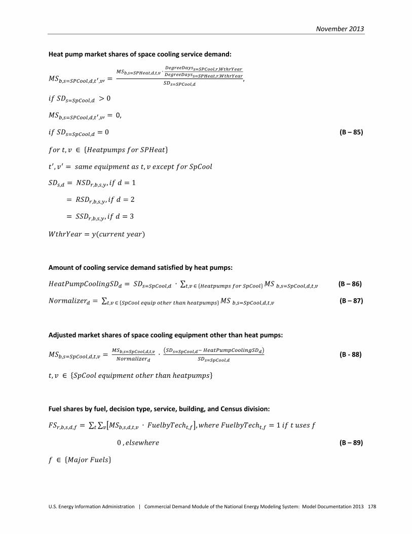
November 2013


Heat pump market shares of space cooling service demand:

𝑀𝑆𝑏,𝑠=𝑆𝑃𝐶𝑜𝑜𝑙,𝑑,𝑡′,𝑣′ = 𝑀𝑆𝑏,𝑠=𝑆𝑃𝐻𝑒𝑎𝑡,𝑑,𝑡,𝑣 ∙

𝐷𝑒𝑔𝑟𝑒𝑒𝐷𝑎𝑦𝑠𝑠=𝑆𝑃𝐶𝑜𝑜𝑙,𝑟,𝑊𝑡ℎ𝑟𝑌𝑒𝑎𝑟𝐷𝑒𝑔𝑟𝑒𝑒𝐷𝑎𝑦𝑠𝑠=𝑆𝑃𝐻𝑒𝑎𝑡,𝑟,𝑊𝑡ℎ𝑟𝑌𝑒𝑎𝑟𝑆𝐷𝑠=𝑆𝑃𝐶𝑜𝑜𝑙,𝑑

,

𝑖𝑓 𝑆𝐷𝑠=𝑆𝑝𝐶𝑜𝑜𝑙,𝑑 > 0

𝑀𝑆𝑏,𝑠=𝑆𝑃𝐶𝑜𝑜𝑙,𝑑,𝑡′,𝑣′ = 0,

𝑖𝑓 𝑆𝐷𝑠=𝑆𝑝𝐶𝑜𝑜𝑙,𝑑 = 0 (B – 85)

𝑓𝑜𝑟 𝑡, 𝑣 ∈ {𝐻𝑒𝑎𝑡𝑝𝑢𝑚𝑝𝑠 𝑓𝑜𝑟 𝑆𝑃𝐻𝑒𝑎𝑡}

𝑡′, 𝑣′ = 𝑠𝑎𝑚𝑒 𝑒𝑞𝑢𝑖𝑝𝑚𝑒𝑛𝑡 𝑎𝑠 𝑡, 𝑣 𝑒𝑥𝑐𝑒𝑝𝑡 𝑓𝑜𝑟 𝑆𝑝𝐶𝑜𝑜𝑙

𝑆𝐷𝑠,𝑑 = 𝑁𝑆𝐷𝑟,𝑏,𝑠,𝑦, 𝑖𝑓 𝑑 = 1

= 𝑅𝑆𝐷𝑟,𝑏,𝑠,𝑦, 𝑖𝑓 𝑑 = 2

= 𝑆𝑆𝐷𝑟,𝑏,𝑠,𝑦, 𝑖𝑓 𝑑 = 3

𝑊𝑡ℎ𝑟𝑌𝑒𝑎𝑟 = 𝑦(𝑐𝑢𝑟𝑟𝑒𝑛𝑡 𝑦𝑒𝑎𝑟)

Amount of cooling service demand satisfied by heat pumps:

𝐻𝑒𝑎𝑡𝑃𝑢𝑚𝑝𝐶𝑜𝑜𝑙𝑖𝑛𝑔𝑆𝐷𝑑 = 𝑆𝐷𝑠=𝑆𝑝𝐶𝑜𝑜𝑙,𝑑 ∙ ∑ 𝑀𝑆 𝑏,𝑠=𝑆𝑝𝐶𝑜𝑜𝑙,𝑑,𝑡,𝑣𝑡,𝑣 ∈ {𝐻𝑒𝑎𝑡𝑝𝑢𝑚𝑝𝑠 𝑓𝑜𝑟 𝑆𝑝𝐶𝑜𝑜𝑙} (B – 86)

𝑁𝑜𝑟𝑚𝑎𝑙𝑖𝑧𝑒𝑟𝑑 = ∑ 𝑀𝑆 𝑏,𝑠=𝑆𝑝𝐶𝑜𝑜𝑙,𝑑,𝑡,𝑣𝑡,𝑣 ∈ {𝑆𝑝𝐶𝑜𝑜𝑙 𝑒𝑞𝑢𝑖𝑝 𝑜𝑡ℎ𝑒𝑟 𝑡ℎ𝑎𝑛 ℎ𝑒𝑎𝑡𝑝𝑢𝑚𝑝𝑠} (B – 87)

Adjusted market shares of space cooling equipment other than heat pumps:

𝑀𝑆𝑏,𝑠=𝑆𝑝𝐶𝑜𝑜𝑙,𝑑,𝑡,𝑣 = 𝑀𝑆𝑏,𝑠=𝑆𝑝𝐶𝑜𝑜𝑙,𝑑,𝑡,𝑣

𝑁𝑜𝑟𝑚𝑎𝑙𝑖𝑧𝑒𝑟𝑑 ∙ �𝑆𝐷𝑠=𝑆𝑝𝐶𝑜𝑜𝑙,𝑑− 𝐻𝑒𝑎𝑡𝑃𝑢𝑚𝑝𝐶𝑜𝑜𝑙𝑖𝑛𝑔𝑆𝐷𝑑�

𝑆𝐷𝑠=𝑆𝑝𝐶𝑜𝑜𝑙,𝑑 (B - 88)

𝑡, 𝑣 ∈ {𝑆𝑝𝐶𝑜𝑜𝑙 𝑒𝑞𝑢𝑖𝑝𝑚𝑒𝑛𝑡 𝑜𝑡ℎ𝑒𝑟 𝑡ℎ𝑎𝑛 ℎ𝑒𝑎𝑡𝑝𝑢𝑚𝑝𝑠}

Fuel shares by fuel, decision type, service, building, and Census division:

𝐹𝑆𝑟,𝑏,𝑠,𝑑,𝑓 = ∑ ∑ �𝑀𝑆𝑏,𝑠,𝑑,𝑡,𝑣 ∙ 𝐹𝑢𝑒𝑙𝑏𝑦𝑇𝑒𝑐ℎ𝑡,𝑓�,𝑤ℎ𝑒𝑟𝑒 𝐹𝑢𝑒𝑙𝑏𝑦𝑇𝑒𝑐ℎ𝑡,𝑓 = 1 𝑖𝑓 𝑡 𝑢𝑠𝑒𝑠 𝑓𝑣𝑡

0 , 𝑒𝑙𝑠𝑒𝑤ℎ𝑒𝑟𝑒 (B – 89)

𝑓 ∈ {𝑀𝑎𝑗𝑜𝑟 𝐹𝑢𝑒𝑙𝑠}

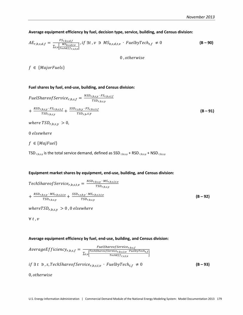
November 2013


Average equipment efficiency by fuel, decision type, service, building, and Census division:

𝐴𝐸𝑟,𝑏,𝑠,𝑑,𝑓 = 𝐹𝑆𝑟,𝑏,𝑠,𝑑,𝑓

∑ �𝑀𝑆𝑏,𝑠,𝑑,𝑡,𝑣

𝑇𝑒𝑐ℎ𝐸𝑓𝑓𝑟,𝑠,𝑡,𝑣�𝑡,𝑣

, 𝑖𝑓 ∃𝑡 , 𝑣 ∋ 𝑀𝑆𝑏,𝑠,𝑑,𝑡,𝑣 ∙ 𝐹𝑢𝑒𝑙𝑏𝑦𝑇𝑒𝑐ℎ𝑡,𝑓 ≠ 0 (B – 90)

0 , 𝑜𝑡ℎ𝑒𝑟𝑤𝑖𝑠𝑒

𝑓 ∈ {𝑀𝑎𝑗𝑜𝑟𝐹𝑢𝑒𝑙𝑠}

Fuel shares by fuel, end-use, building, and Census division:

𝐹𝑢𝑒𝑙𝑆ℎ𝑎𝑟𝑒𝑜𝑓𝑆𝑒𝑟𝑣𝑖𝑐𝑒𝑟,𝑏,𝑠,𝑓 = 𝑁𝑆𝐷𝑟,𝑏,𝑠,𝑦 ∙ 𝐹𝑆𝑟,𝑏,𝑠,𝑙,𝑓

𝑇𝑆𝐷𝑟,𝑏,𝑠,𝑦

+ 𝑅𝑆𝐷𝑟,𝑏,𝑠,𝑦 ∙ 𝐹𝑆𝑟,𝑏,𝑠,2,𝑓

𝑇𝑆𝐷𝑟,𝑏,𝑠,𝑦+ 𝑆𝑆𝐷𝑟,𝑠,𝑏,𝑦 ∙ 𝐹𝑆𝑟,𝑏,𝑠,3,𝑓

𝑇𝑆𝐷𝑟,𝑏,𝑠,𝑦 (B – 91)

𝑤ℎ𝑒𝑟𝑒 𝑇𝑆𝐷𝑟,𝑏,𝑠,𝑦 > 0,

0 𝑒𝑙𝑠𝑒𝑤ℎ𝑒𝑟𝑒

𝑓 ∈ {𝑀𝑎𝑗𝐹𝑢𝑒𝑙}

TSD r,b,s,y is the total service demand, defined as SSD r,b,s,y + RSD r,b,s,y + NSD r,b,s,y

Equipment market shares by equipment, end-use, building, and Census division:

𝑇𝑒𝑐ℎ𝑆ℎ𝑎𝑟𝑒𝑜𝑓𝑆𝑒𝑟𝑣𝑖𝑐𝑒𝑟,𝑏,𝑠,𝑡,𝑣 = 𝑁𝑆𝐷𝑟,𝑏,𝑠,𝑦 ∙ 𝑀𝑆𝑟,𝑏,𝑠,𝑙,𝑡,𝑣

𝑇𝑆𝐷𝑟,𝑏,𝑠,𝑦

+ 𝑅𝑆𝐷𝑟,𝑏,𝑠,𝑦 ∙ 𝑀𝑆𝑟,𝑏,𝑠,2,𝑡,𝑣

𝑇𝑆𝐷𝑟,𝑏,𝑠,𝑦+ 𝑆𝑆𝐷𝑟,𝑠,𝑏,𝑦 ∙ 𝑀𝑆𝑟,𝑏,𝑠,3,𝑡,𝑣

𝑇𝑆𝐷𝑟,𝑏,𝑠,𝑦 (B – 92)

𝑤ℎ𝑒𝑟𝑒𝑇𝑆𝐷𝑟,𝑏,𝑠,𝑦 > 0 , 0 𝑒𝑙𝑠𝑒𝑤ℎ𝑒𝑟𝑒

∀ 𝑡 , 𝑣

Average equipment efficiency by fuel, end-use, building, and Census division:

𝐴𝑣𝑒𝑟𝑎𝑔𝑒𝐸𝑓𝑓𝑖𝑐𝑖𝑒𝑛𝑐𝑦𝑟,𝑏,𝑠,𝑓 = 𝐹𝑢𝑒𝑙𝑆ℎ𝑎𝑟𝑒𝑜𝑓𝑆𝑒𝑟𝑣𝑖𝑐𝑒𝑟,𝑏,𝑠,𝑓

∑ �𝑇𝑒𝑐ℎ𝑆ℎ𝑎𝑟𝑒𝑜𝑓𝑆𝑒𝑟𝑣𝑖𝑐𝑒𝑟,𝑏,𝑠,2,𝑣 ∙ 𝐹𝑢𝑒𝑙𝑏𝑦𝑇𝑒𝑐ℎ𝑡,𝑓

𝑇𝑒𝑐ℎ𝐸𝑓𝑓𝑟,𝑠,𝑡,𝑣�𝑡,𝑣

𝑖𝑓 ∃ 𝑡 ∋ , 𝑠,𝑇𝑒𝑐ℎ𝑆ℎ𝑎𝑟𝑒𝑜𝑓𝑆𝑒𝑟𝑣𝑖𝑐𝑒𝑟,𝑏,𝑠,𝑡,𝑣 ∙ 𝐹𝑢𝑒𝑙𝑏𝑦𝑇𝑒𝑐ℎ𝑡,𝑓 ≠ 0 (B – 93)

0, 𝑜𝑡ℎ𝑒𝑟𝑤𝑖𝑠𝑒

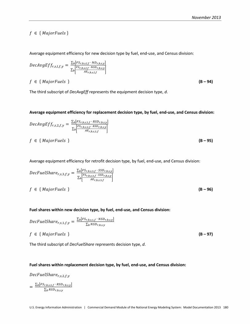
November 2013


𝑓 ∈ { 𝑀𝑎𝑗𝑜𝑟𝐹𝑢𝑒𝑙𝑠 }

Average equipment efficiency for new decision type by fuel, end-use, and Census division:

𝐷𝑒𝑐𝐴𝑣𝑔𝐸𝑓𝑓𝑟,𝑠,𝑙,𝑓,𝑦 = ∑ �𝐹𝑆𝑟,𝑏,𝑠,𝑙,𝑓 ∙ 𝑁𝐷𝑟,𝑏,𝑠,𝑦�𝑏

∑ �𝐹𝑆𝑟,𝑏,𝑠,𝑙,𝑓 ∙ 𝑁𝑆𝐷𝑟,𝑏,𝑠,𝑦

𝐴𝐸𝑟,𝑏,𝑠,𝑙,𝑓�𝑏

𝑓 ∈ { 𝑀𝑎𝑗𝑜𝑟𝐹𝑢𝑒𝑙𝑠 } (B – 94)

The third subscript of DecAvgEff represents the equipment decision type, d.

Average equipment efficiency for replacement decision type, by fuel, end-use, and Census division:

𝐷𝑒𝑐𝐴𝑣𝑔𝐸𝑓𝑓𝑟,𝑠,2,𝑓,𝑦 = ∑ �𝐹𝑆𝑟,𝑏,𝑠,2,𝑓 ∙ 𝑅𝑆𝐷𝑟,𝑏,𝑠,𝑦�𝑏

∑ �𝐹𝑆𝑟,𝑏,𝑠,2,𝑓 ∙ 𝑅𝑆𝐷𝑟,𝑏,𝑠,𝑦

𝐴𝐸𝑟,𝑏,𝑠,2,𝑓�𝑏


Average equipment efficiency for retrofit decision type, by fuel, end-use, and Census division:

𝐷𝑒𝑐𝐹𝑢𝑒𝑙𝑆ℎ𝑎𝑟𝑒𝑟,𝑠,3,𝑓,𝑦 = ∑ �𝐹𝑆𝑟,𝑏,𝑠,3,𝑓 ∙ 𝑆𝑆𝐷𝑟,𝑏,𝑠,𝑦�𝑏

∑ �𝐹𝑆𝑟,𝑏,𝑠,3,𝑓 ∙ 𝑆𝑆𝐷𝑟,𝑏,𝑠,𝑦

𝐴𝐸𝑟,𝑏,𝑠,3,𝑓�𝑏


Fuel shares within new decision type, by fuel, end-use, and Census division:

𝐷𝑒𝑐𝐹𝑢𝑒𝑙𝑆ℎ𝑎𝑟𝑒𝑟,𝑠,1,𝑓,𝑦 = ∑ �𝐹𝑆𝑟,𝑏,𝑠,1,𝑓 ∙ 𝑁𝑆𝐷𝑟,𝑏,𝑠,𝑦�𝑏

∑ 𝑁𝑆𝐷𝑟,𝑏,𝑠,𝑦𝑏


The third subscript of DecFuelShare represents decision type, d.

Fuel shares within replacement decision type, by fuel, end-use, and Census division:

𝐷𝑒𝑐𝐹𝑢𝑒𝑙𝑆ℎ𝑎𝑟𝑒𝑟,𝑠,2,𝑓,𝑦

= ∑ �𝐹𝑆𝑟,𝑏,𝑠,2,𝑓 ∙ 𝑅𝑆𝐷𝑟,𝑏,𝑠,𝑦�𝑏

∑ 𝑅𝑆𝐷𝑟,𝑏,𝑠,𝑦𝑏

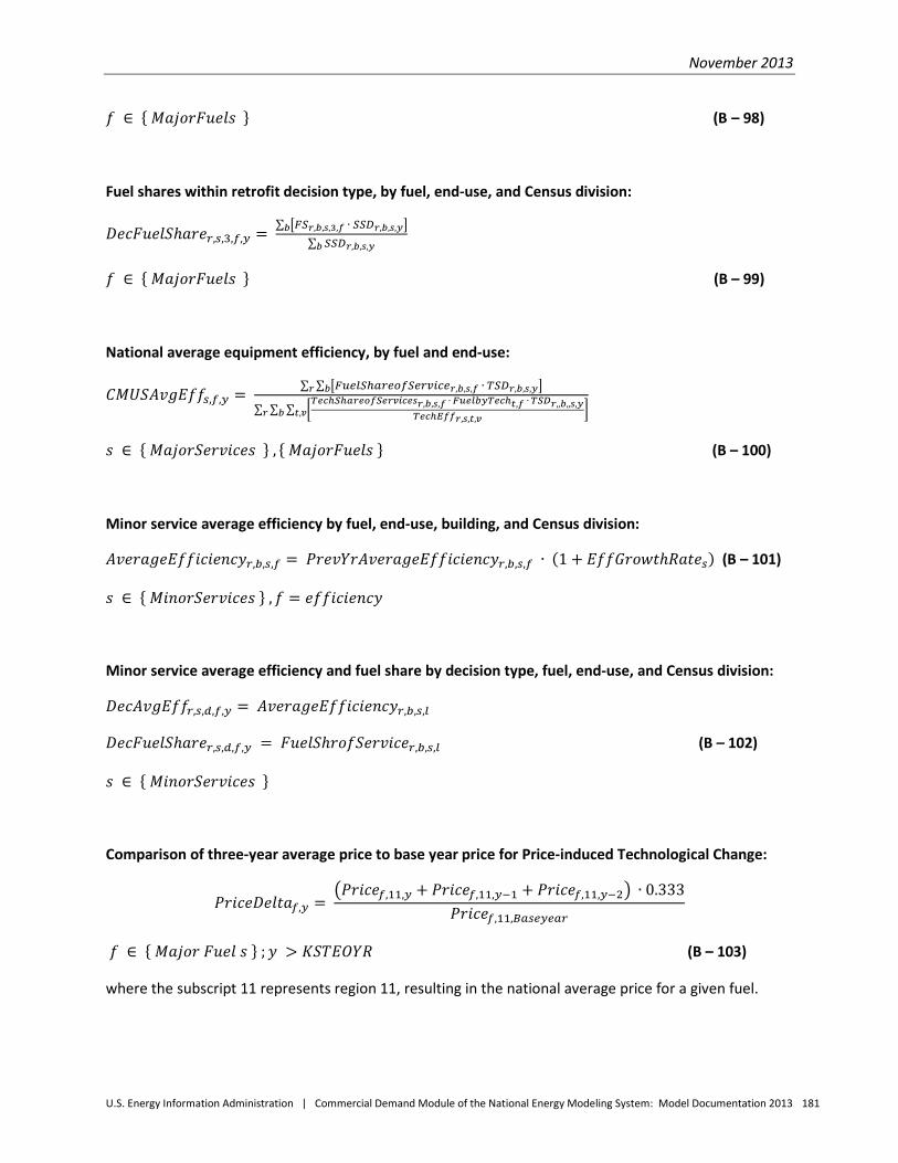
November 2013



Fuel shares within retrofit decision type, by fuel, end-use, and Census division:

𝐷𝑒𝑐𝐹𝑢𝑒𝑙𝑆ℎ𝑎𝑟𝑒𝑟,𝑠,3,𝑓,𝑦 = ∑ �𝐹𝑆𝑟,𝑏,𝑠,3,𝑓 ∙ 𝑆𝑆𝐷𝑟,𝑏,𝑠,𝑦�𝑏

∑ 𝑆𝑆𝐷𝑟,𝑏,𝑠,𝑦𝑏


National average equipment efficiency, by fuel and end-use:

𝐶𝑀𝑈𝑆𝐴𝑣𝑔𝐸𝑓𝑓𝑠,𝑓,𝑦 = ∑ ∑ �𝐹𝑢𝑒𝑙𝑆ℎ𝑎𝑟𝑒𝑜𝑓𝑆𝑒𝑟𝑣𝑖𝑐𝑒𝑟,𝑏,𝑠,𝑓 ∙ 𝑇𝑆𝐷𝑟,𝑏,𝑠,𝑦�𝑏𝑟

∑ ∑ ∑ �𝑇𝑒𝑐ℎ𝑆ℎ𝑎𝑟𝑒𝑜𝑓𝑆𝑒𝑟𝑣𝑖𝑐𝑒𝑠𝑟,𝑏,𝑠,𝑓 ∙ 𝐹𝑢𝑒𝑙𝑏𝑦𝑇𝑒𝑐ℎ𝑡,𝑓 ∙ 𝑇𝑆𝐷𝑟,,𝑏,,𝑠,𝑦

𝑇𝑒𝑐ℎ𝐸𝑓𝑓𝑟,𝑠,𝑡,𝑣�𝑡,𝑣𝑏𝑟

𝑠 ∈ { 𝑀𝑎𝑗𝑜𝑟𝑆𝑒𝑟𝑣𝑖𝑐𝑒𝑠 } , { 𝑀𝑎𝑗𝑜𝑟𝐹𝑢𝑒𝑙𝑠 } (B – 100)

Minor service average efficiency by fuel, end-use, building, and Census division:

𝐴𝑣𝑒𝑟𝑎𝑔𝑒𝐸𝑓𝑓𝑖𝑐𝑖𝑒𝑛𝑐𝑦𝑟,𝑏,𝑠,𝑓 = 𝑃𝑟𝑒𝑣𝑌𝑟𝐴𝑣𝑒𝑟𝑎𝑔𝑒𝐸𝑓𝑓𝑖𝑐𝑖𝑒𝑛𝑐𝑦𝑟,𝑏,𝑠,𝑓 ∙ (1 + 𝐸𝑓𝑓𝐺𝑟𝑜𝑤𝑡ℎ𝑅𝑎𝑡𝑒𝑠) (B – 101)

𝑠 ∈ { 𝑀𝑖𝑛𝑜𝑟𝑆𝑒𝑟𝑣𝑖𝑐𝑒𝑠 } ,𝑓 = 𝑒𝑓𝑓𝑖𝑐𝑖𝑒𝑛𝑐𝑦

Minor service average efficiency and fuel share by decision type, fuel, end-use, and Census division:

𝐷𝑒𝑐𝐴𝑣𝑔𝐸𝑓𝑓𝑟,𝑠,𝑑,𝑓,𝑦 = 𝐴𝑣𝑒𝑟𝑎𝑔𝑒𝐸𝑓𝑓𝑖𝑐𝑖𝑒𝑛𝑐𝑦𝑟,𝑏,𝑠,𝑙

𝐷𝑒𝑐𝐹𝑢𝑒𝑙𝑆ℎ𝑎𝑟𝑒𝑟,𝑠,𝑑,𝑓,𝑦 = 𝐹𝑢𝑒𝑙𝑆ℎ𝑟𝑜𝑓𝑆𝑒𝑟𝑣𝑖𝑐𝑒𝑟,𝑏,𝑠,𝑙 (B – 102)

𝑠 ∈ { 𝑀𝑖𝑛𝑜𝑟𝑆𝑒𝑟𝑣𝑖𝑐𝑒𝑠 }

Comparison of three-year average price to base year price for Price-induced Technological Change:

𝑃𝑟𝑖𝑐𝑒𝐷𝑒𝑙𝑡𝑎𝑓,𝑦 = �𝑃𝑟𝑖𝑐𝑒𝑓,11,𝑦 + 𝑃𝑟𝑖𝑐𝑒𝑓,11,𝑦−1 + 𝑃𝑟𝑖𝑐𝑒𝑓,11,𝑦−2� ∙ 0.333

𝑃𝑟𝑖𝑐𝑒𝑓,11,𝐵𝑎𝑠𝑒𝑦𝑒𝑎𝑟

𝑓 ∈ { 𝑀𝑎𝑗𝑜𝑟 𝐹𝑢𝑒𝑙 𝑠 } ;𝑦 > 𝐾𝑆𝑇𝐸𝑂𝑌𝑅 (B – 103)

where the subscript 11 represents region 11, resulting in the national average price for a given fuel.

November 2013


Calculation of possible shift in technology availability for Price-Induced Technological Change:

𝑆ℎ𝑖𝑓𝑡𝑦𝑒𝑎𝑟𝑠𝑡,𝑣 = �𝑃𝑟𝑖𝑐𝑒𝐷𝑒𝑙𝑡𝑓,𝑦− 1.0�0.10

(B – 104)

𝑓 ∈ { 𝑀𝑎𝑗𝑜𝑟 𝐹𝑢𝑒𝑙𝑠 } ; 𝑦 > 𝐾𝑆𝑇𝐸𝑂𝑌𝑅

Number of years to shift technology availability based on parameter assumptions for Price-Induced Technological Change:

𝑌𝑒𝑎𝑟𝑠𝐹𝑜𝑤𝑎𝑟𝑑𝑡,𝑣,𝑦 =

𝐼𝐹𝑀𝐴𝑋 , 𝑖𝑓 𝐼𝐹𝑀𝐴𝑋 ≤ 𝑆ℎ𝑖𝑓𝑡𝑦𝑒𝑎𝑟𝑠𝑡,𝑣

𝑆ℎ𝑖𝑓𝑡𝑦𝑒𝑎𝑟𝑠𝑡,𝑣 , 𝑖𝑓 𝑌𝑒𝑎𝑟𝑠𝐹𝑜𝑟𝑤𝑎𝑟𝑑𝑡,𝑣,𝑦−1 < 𝑆ℎ𝑖𝑓𝑡𝑌𝑒𝑎𝑟𝑠𝑡,𝑣 < 𝐼𝐹𝑀𝐴𝑋 (B – 105)

𝑌𝑒𝑎𝑟𝑠𝐹𝑜𝑟𝑤𝑎𝑟𝑑𝑡,𝑣,𝑦−1,, 𝑜𝑡ℎ𝑒𝑟𝑤𝑖𝑠𝑒

where IFMAX is the user parameter specifying the maximum number of years a technology can potentially be advanced. YearsForward is adjusted to a smaller number of years if its application causes model v of technology class t to become available before the persistent price increase is projected to occur.

End-use fuel consumption equations

Basic estimate of fuel consumption to meet end-use demands other than lighting:

𝐸𝑛𝑑𝑈𝑠𝑒𝐶𝑜𝑛𝑠𝑢𝑚𝑝𝑓,𝑠,𝑏,𝑟,𝑦 = 𝐹𝑢𝑒𝑙𝑆ℎ𝑎𝑟𝑒𝑜𝑓𝑆𝑒𝑟𝑣𝑖𝑐𝑒𝑟,𝑏,𝑠,𝑓 ∙ 𝑇𝑆𝐷𝑟,𝑏,𝑠,𝑦

𝐴𝑣𝑒𝑟𝑎𝑔𝑒𝐸𝑓𝑓𝑖𝑐𝑖𝑒𝑛𝑐𝑦𝑟,𝑏,𝑠,𝑓 , 𝑖𝑓 𝐴𝑣𝑒𝑟𝑎𝑔𝑒𝐸𝑓𝑓𝑖𝑐𝑖𝑒𝑛𝑐𝑦 > 0

0, 𝑜𝑡ℎ𝑒𝑟𝑤𝑖𝑠𝑒 (B – 106)

𝑠 ≠ 𝑙𝑖𝑔ℎ𝑡𝑖𝑛𝑔 ,𝑓 ∈ { 𝑀𝑎𝑗𝑜𝑟𝐹𝑢𝑒𝑙𝑠 }

Basic estimate of fuel consumption by lighting equipment:

𝐸𝑛𝑑𝑈𝑠𝑒𝐶𝑜𝑛𝑠𝑢𝑚𝑝𝑓,𝑠,𝑏,𝑟,𝑦 = 𝐹𝑢𝑒𝑙𝑆ℎ𝑎𝑟𝑒𝑜𝑓𝑆𝑒𝑟𝑣𝑖𝑐𝑒𝑟,𝑏,𝑠,𝑓 ∙ 𝑇𝑆𝐷𝑟,𝑏,𝑠,𝑦

𝐴𝑣𝑒𝑟𝑎𝑔𝑒𝐸𝑓𝑓𝑖𝑐𝑖𝑒𝑛𝑐𝑦𝑟,𝑏,𝑠,𝑓 ÷ 0.03343

𝑠 = 𝑙𝑖𝑔ℎ𝑡𝑖𝑛𝑔 (B – 107)

𝑤ℎ𝑒𝑟𝑒 0.03343 𝐺𝑊𝑌𝑇𝐵𝑡𝑢

𝑐𝑜𝑛𝑣𝑒𝑟𝑡𝑠 𝑢𝑛𝑖𝑡𝑠 𝑢𝑠𝑒𝑑 𝑖𝑛 𝑙𝑖𝑔ℎ𝑡𝑖𝑛𝑔 𝑡𝑜 𝐵𝑡𝑢 𝑢𝑛𝑖𝑡𝑠

The lighting units GWY refers to electricity use in Gigawatt-Years.

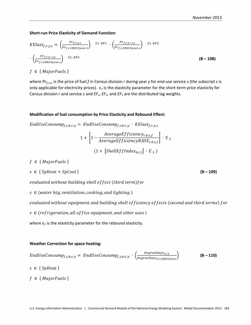
November 2013


Short-run Price Elasticity of Demand Function:

𝐾𝐸𝑙𝑎𝑠𝑡𝑓,𝑟,𝑦,𝑠 = � 𝑃𝑟𝑓,𝑟,𝑦,𝑠

𝑃𝑟𝑓,𝑟,𝐶𝐵𝐸𝐶𝑆𝑦𝑒𝑎𝑟,5� ℇ1 ∙𝐸𝐹1 ∙ � 𝑃𝑟𝑓,𝑟,𝑦−1,𝑠

𝑃𝑟𝑓,𝑟,𝐶𝐵𝐸𝐶𝑆𝑦𝑒𝑎𝑟,𝑠� ℇ1 ∙𝐸𝐹2

∙ � 𝑃𝑟𝑓,𝑟,𝑦−2,𝑠

𝑃𝑟𝑓,𝑟,𝐶𝐵𝐸𝐶𝑆𝑦𝑒𝑎𝑟,𝑠� ℇ1 ∙𝐸𝐹3 (B – 108)


where Prf,r,y,s is the price of fuel f in Census division r during year y for end-use service s (the subscript s is only applicable for electricity prices). ε1 is the elasticity parameter for the short-term price elasticity for Census division r and service s and EF1, EF2, and EF3 are the distributed lag weights.

Modification of fuel consumption by Price Elasticity and Rebound Effect:

𝐸𝑛𝑑𝑈𝑠𝑒𝐶𝑜𝑛𝑠𝑢𝑚𝑝𝑓,𝑠,𝑏,𝑟,𝑦 = 𝐸𝑛𝑑𝑈𝑠𝑒𝐶𝑜𝑛𝑠𝑢𝑚𝑝𝑓,𝑠,𝑏,𝑟,𝑦 ∙ 𝐾𝐸𝑙𝑎𝑠𝑡𝑓,𝑟,𝑦,𝑠

1 + �1 −𝐴𝑣𝑒𝑟𝑎𝑔𝑒𝐸𝑓𝑓𝑖𝑐𝑖𝑒𝑛𝑐𝑦𝑟,𝑏,𝑠,𝑓

𝐴𝑣𝑒𝑟𝑎𝑔𝑒𝐸𝑓𝑓𝑖𝑐𝑖𝑒𝑛𝑐𝑦𝐵𝐴𝑆𝐸𝑟,𝑏,𝑠,𝑓� ∙ ℇ 2

(1 + �𝑆ℎ𝑒𝑙𝑙𝐸𝑓𝑓𝐼𝑛𝑑𝑒𝑥𝑏,𝑟,𝑙� ∙ ℇ 2 )


𝑠 ∈ { 𝑆𝑝𝐻𝑒𝑎𝑡 + 𝑆𝑝𝐶𝑜𝑜𝑙 } (B – 109)

𝑒𝑣𝑎𝑙𝑢𝑎𝑡𝑒𝑑 𝑤𝑖𝑡ℎ𝑜𝑢𝑡 𝑏𝑢𝑖𝑙𝑑𝑖𝑛𝑔 𝑠ℎ𝑒𝑙𝑙 𝑒𝑓𝑓𝑒𝑐𝑡 (𝑡ℎ𝑖𝑟𝑑 𝑡𝑒𝑟𝑚)𝑓𝑜𝑟

𝑠 ∈ (𝑤𝑎𝑡𝑒𝑟 ℎ𝑡𝑔, 𝑣𝑒𝑛𝑡𝑖𝑙𝑎𝑡𝑖𝑜𝑛, 𝑐𝑜𝑜𝑘𝑖𝑛𝑔,𝑎𝑛𝑑 𝑙𝑖𝑔ℎ𝑡𝑖𝑛𝑔 )

𝑒𝑣𝑎𝑙𝑢𝑎𝑡𝑒𝑑 𝑤𝑖𝑡ℎ𝑜𝑢𝑡 𝑒𝑞𝑢𝑖𝑝𝑚𝑒𝑛𝑡 𝑎𝑛𝑑 𝑏𝑢𝑖𝑙𝑑𝑖𝑛𝑔 𝑠ℎ𝑒𝑙𝑙 𝑒𝑓𝑓𝑖𝑐𝑖𝑒𝑛𝑐𝑦 𝑒𝑓𝑓𝑒𝑐𝑡𝑠 (𝑠𝑒𝑐𝑜𝑛𝑑 𝑎𝑛𝑑 𝑡ℎ𝑖𝑟𝑑 𝑡𝑒𝑟𝑚𝑠) 𝑓𝑜𝑟

𝑠 ∈ (𝑟𝑒𝑓𝑟𝑖𝑔𝑒𝑟𝑎𝑡𝑖𝑜𝑛,𝑎𝑙𝑙 𝑜𝑓𝑓𝑖𝑐𝑒 𝑒𝑞𝑢𝑖𝑝𝑚𝑒𝑛𝑡,𝑎𝑛𝑑 𝑜𝑡ℎ𝑒𝑟 𝑢𝑠𝑒𝑠 )

where ε2 is the elasticity parameter for the rebound elasticity.

Weather Correction for space heating:

𝐸𝑛𝑑𝑈𝑠𝑒𝐶𝑜𝑛𝑠𝑢𝑚𝑝𝑓,𝑠,𝑏,𝑟,𝑦 = 𝐸𝑛𝑑𝑈𝑠𝑒𝐶𝑜𝑛𝑠𝑢𝑚𝑝𝑓,𝑠,𝑏,𝑟,𝑦 ∙ � 𝐷𝑒𝑔𝑟𝑒𝑒𝐷𝑎𝑦𝑠𝑠,𝑟,𝑦

𝐷𝑒𝑔𝑟𝑒𝑒𝐷𝑎𝑦𝑠𝑠,𝑟,𝐶𝐵𝐸𝐶𝑆𝑦𝑒𝑎𝑟� (B – 110)

𝑠 ∈ { 𝑆𝑝𝐻𝑒𝑎𝑡 }


November 2013


Weather Correction for space cooling:

𝐸𝑛𝑑𝑈𝑠𝑒𝐶𝑜𝑛𝑠𝑢𝑚𝑝𝑓,𝑠,𝑏,𝑟,𝑦 = 𝐸𝑛𝑑𝑈𝑠𝑒𝐶𝑜𝑛𝑠𝑢𝑚𝑝𝑓,𝑠,𝑏,𝑟,𝑦 ∙ � 𝐷𝑒𝑔𝑟𝑒𝑒𝐷𝑎𝑦𝑠𝑠,𝑟,𝑦

𝐷𝑒𝑔𝑟𝑒𝑒𝐷𝑎𝑦𝑠𝑠,𝑟,𝐶𝐵𝐸𝐶𝑆𝑦𝑒𝑎𝑟� (B – 111)

𝑠 ∈ { 𝑆𝑝𝐶𝑜𝑜𝑙 }


Computation of shares of electricity for end-use adjustment to purchased electricity to account for self-generation:

𝐸𝑙𝑆ℎ𝑟𝑠 = 𝐸𝑛𝑑𝑈𝑠𝑒𝐶𝑜𝑛𝑠𝑢𝑚𝑝𝑙,,𝑠,𝑏,𝑟,𝑦∑ 𝐸𝑛𝑑𝑈𝑠𝑒𝐶𝑜𝑛𝑠𝑢𝑚𝑝𝑙,,𝑠,𝑏,𝑟,𝑦𝑠

(B – 112)

where 1 is the fuel subscript representing electricity.

Deduction of electricity generated by distributed generation technologies other than PV from purchased electricity demand:

𝐸𝑛𝑑𝑈𝑠𝑒𝐶𝑜𝑛𝑠𝑢𝑚𝑝𝑙,𝑠,𝑏,𝑟,𝑦 = 𝐸𝑛𝑑𝑈𝑠𝑒𝐶𝑜𝑛𝑠𝑢𝑚𝑝𝑙,𝑠,𝑏,𝑟,𝑦

−∑ 𝑇𝑟𝑖𝑙𝑙𝑠𝑦,𝑟,𝑏,𝑡𝑡 ∙ 𝐸𝑟𝑙𝑆ℎ𝑠 (B – 113)

where 𝑇𝑟𝑖𝑙𝑙𝑠𝑦,,𝑟,𝑏,𝑡 is the amount of electricity (in trillion Btu) generated during year 𝑦 in Census division 𝑟, building type 𝑏, by distributed technology 𝑡.

Deduction of electricity generated by distributed PV systems from purchased electricity demand:

𝐸𝑛𝑑𝑈𝑠𝑒𝐶𝑜𝑛𝑠𝑢𝑚𝑝1,2,𝑏,𝑟,𝑦 = 𝐸𝑛𝑑𝑈𝑠𝑒𝐶𝑜𝑛𝑠𝑢𝑚𝑝1,2,𝑏,𝑟,𝑦 − 23

∙ 𝑇𝑟𝑖𝑙𝑙𝑠𝑦,𝑟,𝑏,1


∙ 𝑇𝑟𝑖𝑙𝑙𝑠𝑦,𝑟,𝑏,1 (B – 114)


∙ 𝑇𝑟𝑖𝑙𝑙𝑠𝑦,𝑟,𝑏,1

where Trillsy,r,b,1 is the amount of electricity (in trillion Btu) generated during year y in Census division r, building type b, by distributed PV systems (t=1). Electricity generated by PV systems is assumed to primarily affect space cooling loads, with a lesser effect on lighting and miscellaneous end-use loads.

November 2013


Reduction in space and water heating consumption due to combined heat and power (CHP):

𝐸𝑛𝑑𝑈𝑠𝑒𝐶𝑜𝑛𝑠𝑢𝑚𝑝𝑓,𝑙,𝑏,𝑟,𝑦 = 𝐸𝑛𝑑𝑈𝑠𝑒𝐶𝑜𝑛𝑠𝑢𝑚𝑝𝑓,𝑙,𝑏,𝑟,𝑦 − �𝑆𝐻𝐵𝑡𝑢𝑦,𝑟,𝑏,𝑡

𝐸𝑛𝑑𝑈𝑠𝑒𝐶𝑜𝑛𝑠𝑢𝑚𝑝𝑓,3,𝑏,𝑟,𝑦 = 𝐸𝑛𝑑𝑈𝑠𝑒𝐶𝑜𝑛𝑠𝑢𝑚𝑝𝑓,6,𝑏,𝑟,𝑦 − ∑𝐻𝑊𝐵𝑡𝑢𝑦,𝑟,𝑏,𝑡 (B – 115)

∀ 𝑡 𝑢𝑠𝑖𝑛𝑔 𝑓𝑢𝑒𝑙 𝑓

𝑓 ∈ {𝑛𝑎𝑡𝑢𝑟𝑎𝑙 𝑔𝑎𝑠,𝑑𝑖𝑠𝑡𝑖𝑙𝑙𝑎𝑡𝑒}

where SHBtuy,r,b,t and HWBtuy,r,b,t are the amounts of space and water heating (in trillion Btu) provided during year y in Census division r, building type b, by distributed resources (see equations B-180 and 181).

Addition of Consumption of major fuels by distributed generation and CHP technologies:

𝐸𝑛𝑑𝑈𝑠𝑒𝐶𝑜𝑛𝑠𝑢𝑚𝑝𝑓,10,𝑏,𝑟,𝑦 = 𝐸𝑛𝑑𝑈𝑠𝑒𝐶𝑜𝑛𝑠𝑢𝑚𝑝𝑓,10,𝑏,𝑟,𝑦 + ∑ 𝐹𝑢𝑒𝑙𝑈𝑠𝑎𝑔𝑒𝑦,𝑟,𝑏,𝑡∀𝑡 𝑢𝑠𝑖𝑛𝑔 𝑓𝑢𝑒𝑙 𝑓 (B – 116)

𝑓 ∈ {𝑛𝑎𝑡𝑢𝑟𝑎𝑙 𝑔𝑎𝑠,𝑑𝑖𝑠𝑡𝑖𝑙𝑙𝑎𝑡𝑒}

where FuelUsagey,r,b,t is the amount of fuel f used (in trillion Btu) during year y in Census division r, building type b, by distributed resources (see equation B-179).

Consumption of fuels to provide district services, by Census division, building type, fuel, and service:

𝐷𝑖𝑠𝑡𝑆𝑒𝑟𝑣𝐶𝑜𝑛𝑠𝑢𝑚𝑝𝑟,𝑏,𝑠,𝑓,𝑦 = 𝐷𝑖𝑠𝑡𝑆𝑒𝑟𝑣𝑆𝑡𝑒𝑎𝑚𝐸𝑈𝐼𝑟,𝑏,𝑠

�𝑆𝑢𝑟𝑣𝐹𝑙𝑜𝑜𝑟𝑇𝑜𝑡𝑎𝑙𝑟,𝑏,𝑦 + 𝐶𝑀𝑁𝑒𝑤𝐹𝑙𝑜𝑜𝑟𝑆𝑝𝑎𝑐𝑒𝑟,𝑏,𝑦� (B – 117)

� 𝐷𝑖𝑠𝑡𝑆𝑒𝑟𝑣𝐹𝑢𝑒𝑙𝑆ℎ𝑟𝑟,𝑓

𝐷𝑖𝑠𝑡𝑆𝑒𝑟𝑣𝑆𝑦𝑠𝑡𝑒𝑚𝐸𝑓𝑓𝑓� 10−3

𝑠 ∈ {𝐷𝑖𝑠𝑡𝑟𝑖𝑐𝑡𝑆𝑒𝑟𝑣𝑖𝑐𝑒𝑠};𝑓 ∈ {𝑀𝑎𝑗𝑜𝑟𝐹𝑢𝑒𝑙𝑠}

Weather correction and short-term price elasticity for district services consumption:

𝐷𝑖𝑠𝑡𝑆𝑒𝑟𝑣𝐶𝑜𝑛𝑠𝑢𝑚𝑝𝑟,𝑏,𝑠,𝑓,𝑦 = 𝐷𝑖𝑠𝑡𝑆𝑒𝑟𝑣𝐶𝑜𝑛𝑠𝑢𝑚𝑝𝑟,𝑏,𝑠,𝑓,𝑦

𝐾𝐸𝑙𝑎𝑠𝑡𝑓,𝑟,𝑦,𝑠

𝐷𝑒𝑔𝑟𝑒𝑒𝐷𝑎𝑦𝑠𝑠,𝑟,𝑦

𝐷𝑒𝑔𝑟𝑒𝑒𝐷𝑎𝑦𝑠𝑠,𝑟,𝐶𝐵𝐸𝐶𝑆𝑦𝑒𝑎𝑟

(B – 118)

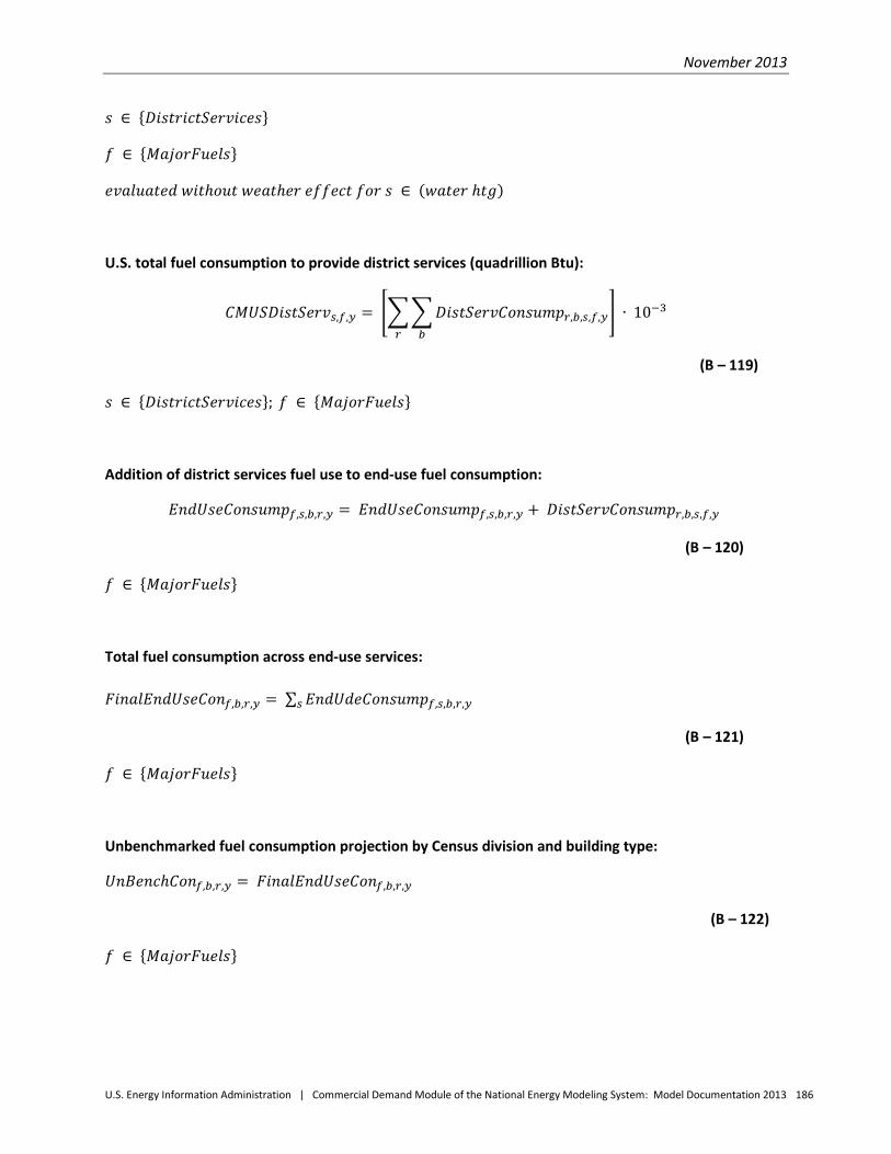
November 2013


𝑠 ∈ {𝐷𝑖𝑠𝑡𝑟𝑖𝑐𝑡𝑆𝑒𝑟𝑣𝑖𝑐𝑒𝑠}


𝑒𝑣𝑎𝑙𝑢𝑎𝑡𝑒𝑑 𝑤𝑖𝑡ℎ𝑜𝑢𝑡 𝑤𝑒𝑎𝑡ℎ𝑒𝑟 𝑒𝑓𝑓𝑒𝑐𝑡 𝑓𝑜𝑟 𝑠 ∈ (𝑤𝑎𝑡𝑒𝑟 ℎ𝑡𝑔)

U.S. total fuel consumption to provide district services (quadrillion Btu):

𝐶𝑀𝑈𝑆𝐷𝑖𝑠𝑡𝑆𝑒𝑟𝑣𝑠,𝑓,𝑦 = ��𝐷𝑖𝑠𝑡𝑆𝑒𝑟𝑣𝐶𝑜𝑛𝑠𝑢𝑚𝑝𝑟,𝑏,𝑠,𝑓,𝑦𝑏𝑟

� ∙ 10−3

(B – 119)

𝑠 ∈ {𝐷𝑖𝑠𝑡𝑟𝑖𝑐𝑡𝑆𝑒𝑟𝑣𝑖𝑐𝑒𝑠}; 𝑓 ∈ {𝑀𝑎𝑗𝑜𝑟𝐹𝑢𝑒𝑙𝑠}

Addition of district services fuel use to end-use fuel consumption:

𝐸𝑛𝑑𝑈𝑠𝑒𝐶𝑜𝑛𝑠𝑢𝑚𝑝𝑓,𝑠,𝑏,𝑟,𝑦 = 𝐸𝑛𝑑𝑈𝑠𝑒𝐶𝑜𝑛𝑠𝑢𝑚𝑝𝑓,𝑠,𝑏,𝑟,𝑦 + 𝐷𝑖𝑠𝑡𝑆𝑒𝑟𝑣𝐶𝑜𝑛𝑠𝑢𝑚𝑝𝑟,𝑏,𝑠,𝑓,𝑦

(B – 120)


Total fuel consumption across end-use services: 𝐹𝑖𝑛𝑎𝑙𝐸𝑛𝑑𝑈𝑠𝑒𝐶𝑜𝑛𝑓,𝑏,𝑟,𝑦 = ∑ 𝐸𝑛𝑑𝑈𝑑𝑒𝐶𝑜𝑛𝑠𝑢𝑚𝑝𝑓,𝑠,𝑏,𝑟,𝑦𝑠

(B – 121)


Unbenchmarked fuel consumption projection by Census division and building type:

𝑈𝑛𝐵𝑒𝑛𝑐ℎ𝐶𝑜𝑛𝑓,𝑏,𝑟,𝑦 = 𝐹𝑖𝑛𝑎𝑙𝐸𝑛𝑑𝑈𝑠𝑒𝐶𝑜𝑛𝑓,𝑏,𝑟,𝑦

(B – 122)


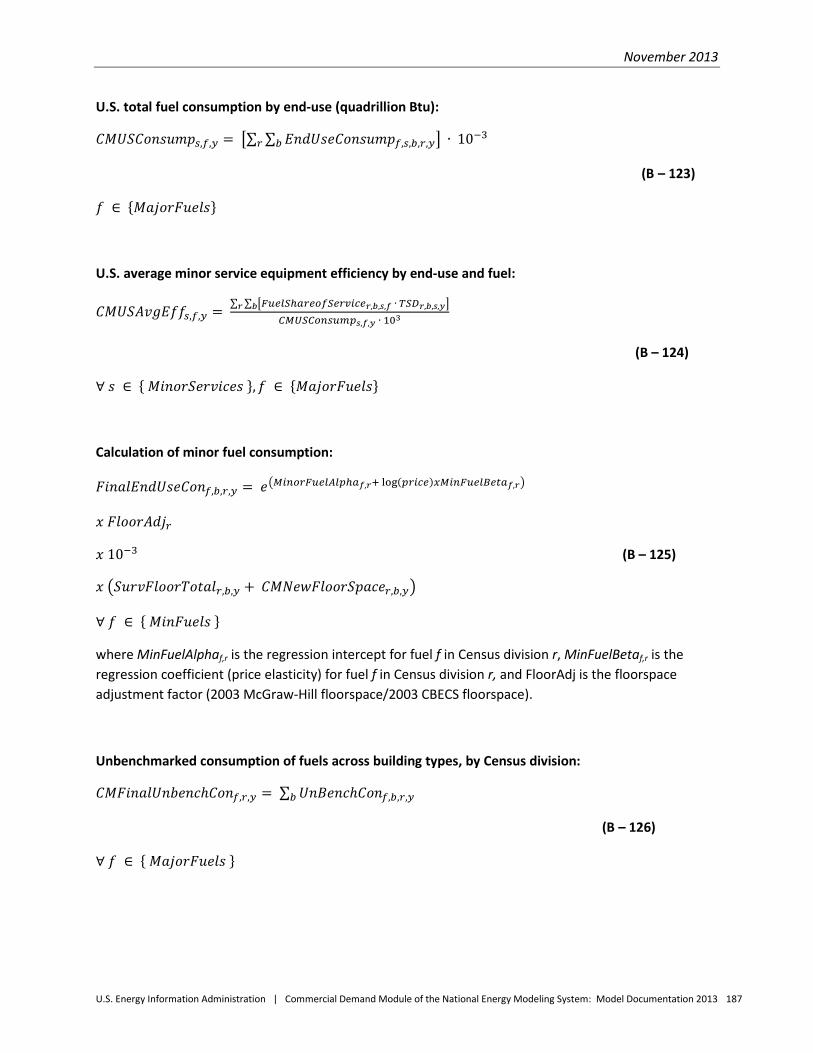
November 2013


U.S. total fuel consumption by end-use (quadrillion Btu):

𝐶𝑀𝑈𝑆𝐶𝑜𝑛𝑠𝑢𝑚𝑝𝑠,𝑓,𝑦 = �∑ ∑ 𝐸𝑛𝑑𝑈𝑠𝑒𝐶𝑜𝑛𝑠𝑢𝑚𝑝𝑓,𝑠,𝑏,𝑟,𝑦𝑏𝑟 � ∙ 10−3

(B – 123)


U.S. average minor service equipment efficiency by end-use and fuel:

𝐶𝑀𝑈𝑆𝐴𝑣𝑔𝐸𝑓𝑓𝑠,𝑓,𝑦 = ∑ ∑ �𝐹𝑢𝑒𝑙𝑆ℎ𝑎𝑟𝑒𝑜𝑓𝑆𝑒𝑟𝑣𝑖𝑐𝑒𝑟,𝑏,𝑠,𝑓 ∙ 𝑇𝑆𝐷𝑟,𝑏,𝑠,𝑦�𝑏𝑟

𝐶𝑀𝑈𝑆𝐶𝑜𝑛𝑠𝑢𝑚𝑝𝑠,𝑓,𝑦 ∙ 103

(B – 124)

∀ 𝑠 ∈ { 𝑀𝑖𝑛𝑜𝑟𝑆𝑒𝑟𝑣𝑖𝑐𝑒𝑠 },𝑓 ∈ {𝑀𝑎𝑗𝑜𝑟𝐹𝑢𝑒𝑙𝑠}

Calculation of minor fuel consumption:

𝐹𝑖𝑛𝑎𝑙𝐸𝑛𝑑𝑈𝑠𝑒𝐶𝑜𝑛𝑓,𝑏,𝑟,𝑦 = 𝑒�𝑀𝑖𝑛𝑜𝑟𝐹𝑢𝑒𝑙𝐴𝑙𝑝ℎ𝑎𝑓,𝑟+ log(𝑝𝑟𝑖𝑐𝑒)𝑥𝑀𝑖𝑛𝐹𝑢𝑒𝑙𝐵𝑒𝑡𝑎𝑓,𝑟�

𝑥 𝐹𝑙𝑜𝑜𝑟𝐴𝑑𝑗𝑟

𝑥 10−3 (B – 125)

𝑥 �𝑆𝑢𝑟𝑣𝐹𝑙𝑜𝑜𝑟𝑇𝑜𝑡𝑎𝑙𝑟,𝑏,𝑦 + 𝐶𝑀𝑁𝑒𝑤𝐹𝑙𝑜𝑜𝑟𝑆𝑝𝑎𝑐𝑒𝑟,𝑏,𝑦�

∀ 𝑓 ∈ { 𝑀𝑖𝑛𝐹𝑢𝑒𝑙𝑠 }

where MinFuelAlphaf,r is the regression intercept for fuel f in Census division r, MinFuelBetaf,r is the regression coefficient (price elasticity) for fuel f in Census division r, and FloorAdj is the floorspace adjustment factor (2003 McGraw-Hill floorspace/2003 CBECS floorspace).

Unbenchmarked consumption of fuels across building types, by Census division:

𝐶𝑀𝐹𝑖𝑛𝑎𝑙𝑈𝑛𝑏𝑒𝑛𝑐ℎ𝐶𝑜𝑛𝑓,𝑟,𝑦 = ∑ 𝑈𝑛𝐵𝑒𝑛𝑐ℎ𝐶𝑜𝑛𝑓,𝑏,𝑟,𝑦𝑏

(B – 126)

∀ 𝑓 ∈ { 𝑀𝑎𝑗𝑜𝑟𝐹𝑢𝑒𝑙𝑠 }

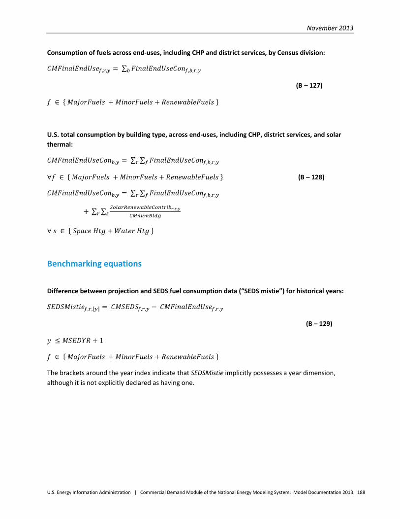
November 2013


Consumption of fuels across end-uses, including CHP and district services, by Census division:

𝐶𝑀𝐹𝑖𝑛𝑎𝑙𝐸𝑛𝑑𝑈𝑠𝑒𝑓,𝑟,𝑦 = ∑ 𝐹𝑖𝑛𝑎𝑙𝐸𝑛𝑑𝑈𝑠𝑒𝐶𝑜𝑛𝑓,𝑏,𝑟,𝑦𝑏

(B – 127)

𝑓 ∈ { 𝑀𝑎𝑗𝑜𝑟𝐹𝑢𝑒𝑙𝑠 + 𝑀𝑖𝑛𝑜𝑟𝐹𝑢𝑒𝑙𝑠 + 𝑅𝑒𝑛𝑒𝑤𝑎𝑏𝑙𝑒𝐹𝑢𝑒𝑙𝑠 }

U.S. total consumption by building type, across end-uses, including CHP, district services, and solar thermal:

𝐶𝑀𝐹𝑖𝑛𝑎𝑙𝐸𝑛𝑑𝑈𝑠𝑒𝐶𝑜𝑛𝑏,𝑦 = ∑ ∑ 𝐹𝑖𝑛𝑎𝑙𝐸𝑛𝑑𝑈𝑠𝑒𝐶𝑜𝑛𝑓,𝑏,𝑟,𝑦𝑓𝑟

∀𝑓 ∈ { 𝑀𝑎𝑗𝑜𝑟𝐹𝑢𝑒𝑙𝑠 + 𝑀𝑖𝑛𝑜𝑟𝐹𝑢𝑒𝑙𝑠 + 𝑅𝑒𝑛𝑒𝑤𝑎𝑏𝑙𝑒𝐹𝑢𝑒𝑙𝑠 } (B – 128)

𝐶𝑀𝐹𝑖𝑛𝑎𝑙𝐸𝑛𝑑𝑈𝑠𝑒𝐶𝑜𝑛𝑏,𝑦 = ∑ ∑ 𝐹𝑖𝑛𝑎𝑙𝐸𝑛𝑑𝑈𝑠𝑒𝐶𝑜𝑛𝑓,𝑏,𝑟,𝑦𝑓𝑟

+ ∑ ∑ 𝑆𝑜𝑙𝑎𝑟𝑅𝑒𝑛𝑒𝑤𝑎𝑏𝑙𝑒𝐶𝑜𝑛𝑡𝑟𝑖𝑏𝑟,𝑠,𝑦

𝐶𝑀𝑛𝑢𝑚𝐵𝑙𝑑𝑔𝑠 𝑟

∀ 𝑠 ∈ { 𝑆𝑝𝑎𝑐𝑒 𝐻𝑡𝑔 +𝑊𝑎𝑡𝑒𝑟 𝐻𝑡𝑔 }

Benchmarking equations

Difference between projection and SEDS fuel consumption data (“SEDS mistie”) for historical years:

𝑆𝐸𝐷𝑆𝑀𝑖𝑠𝑡𝑖𝑒𝑓,𝑟,[𝑦] = 𝐶𝑀𝑆𝐸𝐷𝑆𝑓,𝑟,𝑦 − 𝐶𝑀𝐹𝑖𝑛𝑎𝑙𝐸𝑛𝑑𝑈𝑠𝑒𝑓,𝑟,𝑦

(B – 129)

𝑦 ≤ 𝑀𝑆𝐸𝐷𝑌𝑅 + 1

𝑓 ∈ { 𝑀𝑎𝑗𝑜𝑟𝐹𝑢𝑒𝑙𝑠 + 𝑀𝑖𝑛𝑜𝑟𝐹𝑢𝑒𝑙𝑠 + 𝑅𝑒𝑛𝑒𝑤𝑎𝑏𝑙𝑒𝐹𝑢𝑒𝑙𝑠 }

The brackets around the year index indicate that SEDSMistie implicitly possesses a year dimension, although it is not explicitly declared as having one.

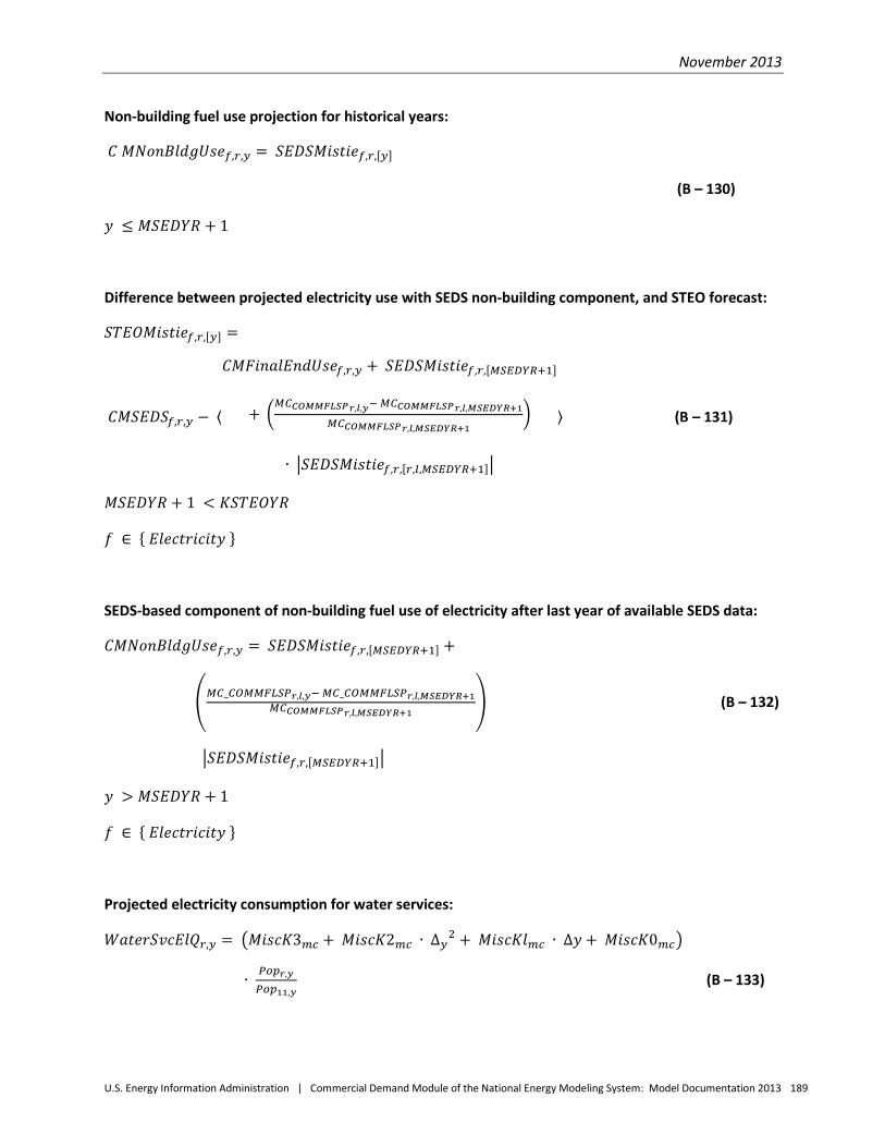
November 2013


Non-building fuel use projection for historical years:

𝐶 𝑀𝑁𝑜𝑛𝐵𝑙𝑑𝑔𝑈𝑠𝑒𝑓,𝑟,𝑦 = 𝑆𝐸𝐷𝑆𝑀𝑖𝑠𝑡𝑖𝑒𝑓,𝑟,[𝑦]

(B – 130)

𝑦 ≤ 𝑀𝑆𝐸𝐷𝑌𝑅 + 1

Difference between projected electricity use with SEDS non-building component, and STEO forecast:

𝑆𝑇𝐸𝑂𝑀𝑖𝑠𝑡𝑖𝑒𝑓,𝑟,[𝑦] =

𝐶𝑀𝑆𝐸𝐷𝑆𝑓,𝑟,𝑦 − ⟨

𝐶𝑀𝐹𝑖𝑛𝑎𝑙𝐸𝑛𝑑𝑈𝑠𝑒𝑓,𝑟,𝑦 + 𝑆𝐸𝐷𝑆𝑀𝑖𝑠𝑡𝑖𝑒𝑓,𝑟,[𝑀𝑆𝐸𝐷𝑌𝑅+1]

+ �𝑀𝐶𝐶𝑂𝑀𝑀𝐹𝐿𝑆𝑃𝑟,𝑙,𝑦− 𝑀𝐶𝐶𝑂𝑀𝑀𝐹𝐿𝑆𝑃𝑟,𝑙,𝑀𝑆𝐸𝐷𝑌𝑅+1

𝑀𝐶𝐶𝑂𝑀𝑀𝐹𝐿𝑆𝑃𝑟,𝑙,𝑀𝑆𝐸𝐷𝑌𝑅+1�

∙ �𝑆𝐸𝐷𝑆𝑀𝑖𝑠𝑡𝑖𝑒𝑓,𝑟,[𝑟,𝑙,𝑀𝑆𝐸𝐷𝑌𝑅+1]�

⟩ (B – 131)

𝑀𝑆𝐸𝐷𝑌𝑅 + 1 < 𝐾𝑆𝑇𝐸𝑂𝑌𝑅

𝑓 ∈ { 𝐸𝑙𝑒𝑐𝑡𝑟𝑖𝑐𝑖𝑡𝑦 }

SEDS-based component of non-building fuel use of electricity after last year of available SEDS data:

𝐶𝑀𝑁𝑜𝑛𝐵𝑙𝑑𝑔𝑈𝑠𝑒𝑓,𝑟,𝑦 = 𝑆𝐸𝐷𝑆𝑀𝑖𝑠𝑡𝑖𝑒𝑓,𝑟,[𝑀𝑆𝐸𝐷𝑌𝑅+1] +

�𝑀𝐶_𝐶𝑂𝑀𝑀𝐹𝐿𝑆𝑃𝑟,𝑙,𝑦− 𝑀𝐶_𝐶𝑂𝑀𝑀𝐹𝐿𝑆𝑃𝑟,𝑙,𝑀𝑆𝐸𝐷𝑌𝑅+1𝑀𝐶𝐶𝑂𝑀𝑀𝐹𝐿𝑆𝑃𝑟,𝑙,𝑀𝑆𝐸𝐷𝑌𝑅+1

� (B – 132)

�𝑆𝐸𝐷𝑆𝑀𝑖𝑠𝑡𝑖𝑒𝑓,𝑟,[𝑀𝑆𝐸𝐷𝑌𝑅+1]�

𝑦 > 𝑀𝑆𝐸𝐷𝑌𝑅 + 1

𝑓 ∈ { 𝐸𝑙𝑒𝑐𝑡𝑟𝑖𝑐𝑖𝑡𝑦 }

Projected electricity consumption for water services:

𝑊𝑎𝑡𝑒𝑟𝑆𝑣𝑐𝐸𝑙𝑄𝑟,𝑦 = �𝑀𝑖𝑠𝑐𝐾3𝑚𝑐 + 𝑀𝑖𝑠𝑐𝐾2𝑚𝑐 ∙ ∆𝑦2 + 𝑀𝑖𝑠𝑐𝐾𝑙𝑚𝑐 ∙ ∆𝑦 + 𝑀𝑖𝑠𝑐𝐾0𝑚𝑐�

∙ 𝑃𝑜𝑝𝑟,𝑦

𝑃𝑜𝑝11,𝑦 (B – 133)

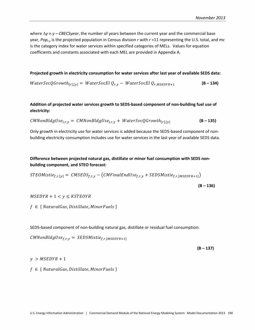
November 2013


where ∆y ≡ y – CBECSyear, the number of years between the current year and the commercial base year, Popr,y is the projected population in Census division r with r =11 representing the U.S. total, and mc is the category index for water services within specified categories of MELs. Values for equation coefficients and constants associated with each MEL are provided in Appendix A.

Projected growth in electricity consumption for water services after last year of available SEDS data:

𝑊𝑎𝑡𝑒𝑟𝑆𝑣𝑐𝑄𝐺𝑟𝑜𝑤𝑡ℎ[𝑟],[𝑦] = 𝑊𝑎𝑡𝑒𝑟𝑆𝑣𝑐𝐸𝑙 𝑄𝑟,𝑦 − 𝑊𝑎𝑡𝑒𝑟𝑆𝑣𝑐𝐸𝑙 𝑄𝑟,𝑀𝑆𝐸𝐷𝑌𝑅+1 (B – 134)

Addition of projected water services growth to SEDS-based component of non-building fuel use of electricity:

𝐶𝑀𝑁𝑜𝑛𝐵𝑙𝑑𝑔𝑈𝑠𝑒𝑙,𝑟,𝑦 = 𝐶𝑀𝑁𝑜𝑛𝐵𝑙𝑑𝑔𝑈𝑠𝑒𝑙,𝑟,𝑦 + 𝑊𝑎𝑡𝑒𝑟𝑆𝑣𝑐𝑄𝐺𝑟𝑜𝑤𝑡ℎ[𝑟],[𝑦] (B – 135)

Only growth in electricity use for water services is added because the SEDS-based component of non-building electricity consumption includes use for water services in the last year of available SEDS data.

Difference between projected natural gas, distillate or minor fuel consumption with SEDS non-building component, and STEO forecast:

𝑆𝑇𝐸𝑂𝑀𝑖𝑠𝑡𝑖𝑒𝑓,𝑟,[𝑦] = 𝐶𝑀𝑆𝐸𝐷𝑆𝑓,𝑟,𝑦 − �𝐶𝑀𝐹𝑖𝑛𝑎𝑙𝐸𝑛𝑑𝑈𝑠𝑒𝑓,𝑟,𝑦 + 𝑆𝐸𝐷𝑆𝑀𝑖𝑠𝑡𝑖𝑒𝑓,𝑟,[𝑀𝑆𝐸𝐷𝑌𝑅+1]�

(B – 136)

𝑀𝑆𝐸𝐷𝑌𝑅 + 1 < 𝑦 ≤ 𝐾𝑆𝑇𝐸𝑂𝑌𝑅

𝑓 ∈ { 𝑁𝑎𝑡𝑢𝑟𝑎𝑙𝐺𝑎𝑠,𝐷𝑖𝑠𝑡𝑖𝑙𝑙𝑎𝑡𝑒,𝑀𝑖𝑛𝑜𝑟𝐹𝑢𝑒𝑙𝑠 }

SEDS-based component of non-building natural gas, distillate or residual fuel consumption:

𝐶𝑀𝑁𝑜𝑛𝐵𝑙𝑑𝑔𝑈𝑠𝑒𝑓,𝑟,𝑦 = 𝑆𝐸𝐷𝑆𝑀𝑖𝑠𝑡𝑖𝑒𝑓,𝑟,[𝑀𝑆𝐸𝐷𝑌𝑅+1]

(B – 137)

𝑦 > 𝑀𝑆𝐸𝐷𝑌𝑅 + 1

𝑓 ∈ { 𝑁𝑎𝑡𝑢𝑟𝑎𝑙𝐺𝑎𝑠,𝐷𝑖𝑠𝑡𝑖𝑙𝑙𝑎𝑡𝑒,𝑀𝑖𝑛𝑜𝑟𝐹𝑢𝑒𝑙𝑠 }

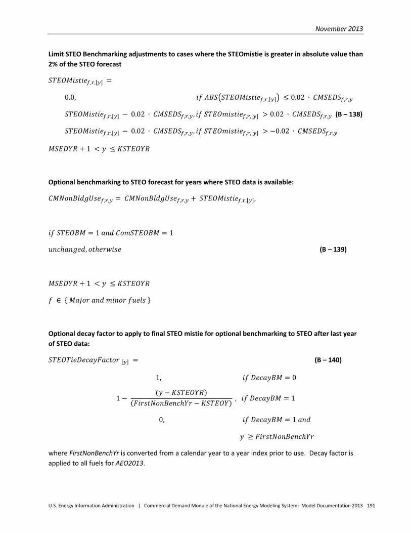
November 2013


Limit STEO Benchmarking adjustments to cases where the STEOmistie is greater in absolute value than 2% of the STEO forecast

𝑆𝑇𝐸𝑂𝑀𝑖𝑠𝑡𝑖𝑒𝑓,𝑟,[𝑦] =

0.0, 𝑖𝑓 𝐴𝐵𝑆�𝑆𝑇𝐸𝑂𝑀𝑖𝑠𝑡𝑖𝑒𝑓,𝑟,[𝑦]� ≤ 0.02 ∙ 𝐶𝑀𝑆𝐸𝐷𝑆𝑓,𝑟,𝑦

𝑆𝑇𝐸𝑂𝑀𝑖𝑠𝑡𝑖𝑒𝑓,𝑟,[𝑦] − 0.02 ∙ 𝐶𝑀𝑆𝐸𝐷𝑆𝑓,𝑟,𝑦, 𝑖𝑓 𝑆𝑇𝐸𝑂𝑚𝑖𝑠𝑡𝑖𝑒𝑓,𝑟,[𝑦] > 0.02 ∙ 𝐶𝑀𝑆𝐸𝐷𝑆𝑓,𝑟,𝑦 (B – 138)

𝑆𝑇𝐸𝑂𝑀𝑖𝑠𝑡𝑖𝑒𝑓,𝑟,[𝑦] − 0.02 ∙ 𝐶𝑀𝑆𝐸𝐷𝑆𝑓,𝑟,𝑦, 𝑖𝑓 𝑆𝑇𝐸𝑂𝑚𝑖𝑠𝑡𝑖𝑒𝑓,𝑟,[𝑦] > −0.02 ∙ 𝐶𝑀𝑆𝐸𝐷𝑆𝑓,𝑟,𝑦


Optional benchmarking to STEO forecast for years where STEO data is available:

𝐶𝑀𝑁𝑜𝑛𝐵𝑙𝑑𝑔𝑈𝑠𝑒𝑓,𝑟,𝑦 = 𝐶𝑀𝑁𝑜𝑛𝐵𝑙𝑑𝑔𝑈𝑠𝑒𝑓,𝑟,𝑦 + 𝑆𝑇𝐸𝑂𝑀𝑖𝑠𝑡𝑖𝑒𝑓,𝑟,[𝑦],

𝑖𝑓 𝑆𝑇𝐸𝑂𝐵𝑀 = 1 𝑎𝑛𝑑 𝐶𝑜𝑚𝑆𝑇𝐸𝑂𝐵𝑀 = 1

𝑢𝑛𝑐ℎ𝑎𝑛𝑔𝑒𝑑, 𝑜𝑡ℎ𝑒𝑟𝑤𝑖𝑠𝑒 (B – 139)


𝑓 ∈ { 𝑀𝑎𝑗𝑜𝑟 𝑎𝑛𝑑 𝑚𝑖𝑛𝑜𝑟 𝑓𝑢𝑒𝑙𝑠 }

Optional decay factor to apply to final STEO mistie for optional benchmarking to STEO after last year of STEO data:

𝑆𝑇𝐸𝑂𝑇𝑖𝑒𝐷𝑒𝑐𝑎𝑦𝐹𝑎𝑐𝑡𝑜𝑟 [𝑦] = (B – 140)

1, 𝑖𝑓 𝐷𝑒𝑐𝑎𝑦𝐵𝑀 = 0

1 − (𝑦 − 𝐾𝑆𝑇𝐸𝑂𝑌𝑅)

(𝐹𝑖𝑟𝑠𝑡𝑁𝑜𝑛𝐵𝑒𝑛𝑐ℎ𝑌𝑟 − 𝐾𝑆𝑇𝐸𝑂𝑌) , 𝑖𝑓 𝐷𝑒𝑐𝑎𝑦𝐵𝑀 = 1

0, 𝑖𝑓 𝐷𝑒𝑐𝑎𝑦𝐵𝑀 = 1 𝑎𝑛𝑑

𝑦 ≥ 𝐹𝑖𝑟𝑠𝑡𝑁𝑜𝑛𝐵𝑒𝑛𝑐ℎ𝑌𝑟

where FirstNonBenchYr is converted from a calendar year to a year index prior to use. Decay factor is applied to all fuels for AEO2013.

November 2013


Optional STEO-based component of non-building fuel consumption projected after last year of available STEO data:

𝐶𝑀𝑁𝑜𝑛𝐵𝑙𝑑𝑔𝑈𝑠𝑒𝑓,𝑟,𝑦 = 𝐶𝑀𝑁𝑜𝑛𝐵𝑙𝑑𝑔𝑈𝑠𝑒𝑓,𝑟,𝑦

+ 𝑆𝑇𝐸𝑂𝑀𝑖𝑠𝑡𝑖𝑒𝑓,𝑟,[𝐾𝑆𝑇𝐸𝑂𝑌𝑅] ∙ 𝑆𝑇𝐸𝑂𝑇𝑖𝑒𝐷𝑒𝑐𝑎𝑦𝐹𝑎𝑐𝑡𝑜𝑟[𝑦],

𝑖𝑓 𝑆𝑇𝐸𝑂𝐵𝑀 = 1; (B -141)

𝑢𝑛𝑐ℎ𝑎𝑛𝑔𝑒𝑑, 𝑜𝑡ℎ𝑒𝑟𝑤𝑖𝑠𝑒

Final benchmarked projected fuel consumption by fuel, Census division, and year:

𝐶𝑀𝐹𝑖𝑛𝑎𝑙𝐸𝑛𝑑𝑈𝑠𝑒𝑓,𝑟,𝑦 = 𝐶𝑀𝐹𝑖𝑛𝑎𝑙𝐸𝑛𝑑𝑈𝑠𝑒𝑓,𝑟,𝑦 + 𝐶𝑀𝑁𝑜𝑛𝐵𝑙𝑑𝑔𝑈𝑠𝑒𝑓,𝑟,𝑦

𝑓 ∈ { 𝑀𝑎𝑗𝑜𝑟 𝑎𝑛𝑑 𝑚𝑖𝑛𝑜𝑟 𝑓𝑢𝑒𝑙𝑠 } (B – 142)

November 2013


Distributed generation equations Projections of distributed generation penetration are based on the results of cash-flow simulations carried out at a finer level of geographic detail, relative to other NEMS commercial model results. The choice of higher-resolution “niches” was made since solar resources as well as electricity prices can vary substantially within a Census division. Penetration estimates based on Census division average insolation and Census division average prices can “ignore” opportunities for niche penetration. The niche concept was extended by including additional variables: one variable relating to solar opportunities (roof area per square foot); another variable to measure average wind speed in the niche for distributed wind turbines; and natural gas prices relative to the Census division average for gas-fired technologies. It is the confluence of renewable resources and energy prices that determines “niche” opportunities for penetration of these types of energy investments.

For each year in a NEMS run, a 30-year cash flow analysis is evaluated for each potential distributed generation investment. Simulations are carried out by Census division, building type, building size category, and niche. The division/building type/size/niche calculations are made separately for each of the modeled distributed generation technologies where additional penetration might be expected.

The niche information is developed from the CBECS Public Use Files, coupled with solar and wind resource maps produced by the National Renewable Energy Laboratory.39 The average solar insolation and average wind speeds are developed by overlaying CBECS climate zones by Census division and either the solar or wind resource maps. The niches are first defined by insolation levels and then average wind speed is developed for each solar niche. There are currently 23 solar niches. The number of niches within a Census division depends on solar insolation variability – generally more niches are required for Census divisions having greater latitudinal dispersion. Within the insolation niches, commercial floorspace area is divided into bins by electricity price relative to the division average price in order to create below-average, average, and above-average price bins. The resulting combined solar resource/electricity price bins define the 69 niches (23 times 3) where either insolation or the electricity price varies.

Even though the niches are defined based on solar resource and electricity rate level, additional information is developed from CBECS for use in the cash flow and penetration calculations for photovoltaics, wind, and gas-fired technologies. For each niche the following variables are included: solar insolation, average wind speed, the floorspace share of Census division floorspace area, average electricity price relative to the Census division average, average natural gas price relative to the Census division average, and roof area as a percentage of floorspace area (since currently only rooftop PV is modeled).

Each distributed generation technology is indexed by an annual “vintage” which aligns with the NEMS model year, and thus allows technical characteristics (like efficiency or cost) or tax incentives to vary annually over the entire NEMS horizon. For ease of notation, subscripts denoting the technology, region, building type, size category and niche are generally suppressed until the interface with NEMS is

39 Sources: solar insolation map – http://www.nrel.gov/gis/solar.html , wind speed map – http://rredc.nrel.gov/wind/pubs/atlas/maps/chap2/2-01m.html.

http://www.nrel.gov/gis/solar.html

http://rredc.nrel.gov/wind/pubs/atlas/maps/chap2/2-01m.html

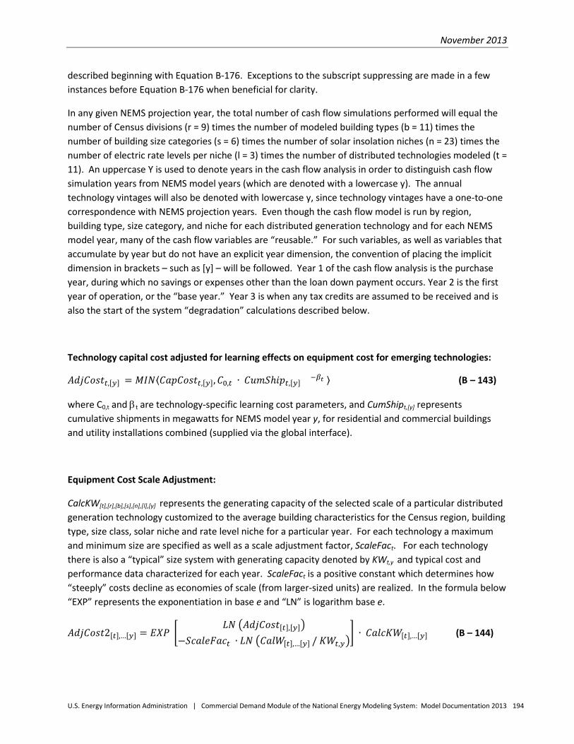
November 2013


described beginning with Equation B-176. Exceptions to the subscript suppressing are made in a few instances before Equation B-176 when beneficial for clarity.

In any given NEMS projection year, the total number of cash flow simulations performed will equal the number of Census divisions (r = 9) times the number of modeled building types (b = 11) times the number of building size categories (s = 6) times the number of solar insolation niches (n = 23) times the number of electric rate levels per niche (l = 3) times the number of distributed technologies modeled (t = 11). An uppercase Y is used to denote years in the cash flow analysis in order to distinguish cash flow simulation years from NEMS model years (which are denoted with a lowercase y). The annual technology vintages will also be denoted with lowercase y, since technology vintages have a one-to-one correspondence with NEMS projection years. Even though the cash flow model is run by region, building type, size category, and niche for each distributed generation technology and for each NEMS model year, many of the cash flow variables are “reusable.” For such variables, as well as variables that accumulate by year but do not have an explicit year dimension, the convention of placing the implicit dimension in brackets – such as [y] – will be followed. Year 1 of the cash flow analysis is the purchase year, during which no savings or expenses other than the loan down payment occurs. Year 2 is the first year of operation, or the “base year.” Year 3 is when any tax credits are assumed to be received and is also the start of the system “degradation” calculations described below.

Technology capital cost adjusted for learning effects on equipment cost for emerging technologies:

𝐴𝑑𝑗𝐶𝑜𝑠𝑡𝑡,[𝑦] = 𝑀𝐼𝑁⟨𝐶𝑎𝑝𝐶𝑜𝑠𝑡𝑡,[𝑦],𝐶0,𝑡 ∙ 𝐶𝑢𝑚𝑆ℎ𝑖𝑝𝑡,[𝑦]−𝛽𝑡 ⟩ (B – 143)

where C0,t and βt are technology-specific learning cost parameters, and CumShipt,[y] represents cumulative shipments in megawatts for NEMS model year y, for residential and commercial buildings and utility installations combined (supplied via the global interface).

Equipment Cost Scale Adjustment:

CalcKW[t],[r],[b],[s],[n],[l],[y] represents the generating capacity of the selected scale of a particular distributed generation technology customized to the average building characteristics for the Census region, building type, size class, solar niche and rate level niche for a particular year. For each technology a maximum and minimum size are specified as well as a scale adjustment factor, ScaleFact. For each technology there is also a “typical” size system with generating capacity denoted by KWt,y and typical cost and performance data characterized for each year. ScaleFact is a positive constant which determines how “steeply” costs decline as economies of scale (from larger-sized units) are realized. In the formula below “EXP” represents the exponentiation in base e and “LN” is logarithm base e.

𝐴𝑑𝑗𝐶𝑜𝑠𝑡2[𝑡],…[𝑦] = 𝐸𝑋𝑃 �𝐿𝑁 �𝐴𝑑𝑗𝐶𝑜𝑠𝑡[𝑡],[𝑦]�

−𝑆𝑐𝑎𝑙𝑒𝐹𝑎𝑐𝑡 ∙ 𝐿𝑁 �𝐶𝑎𝑙𝑊[𝑡],…[𝑦] / 𝐾𝑊𝑡,𝑦�� ∙ 𝐶𝑎𝑙𝑐𝐾𝑊[𝑡],…[𝑦] (B – 144)

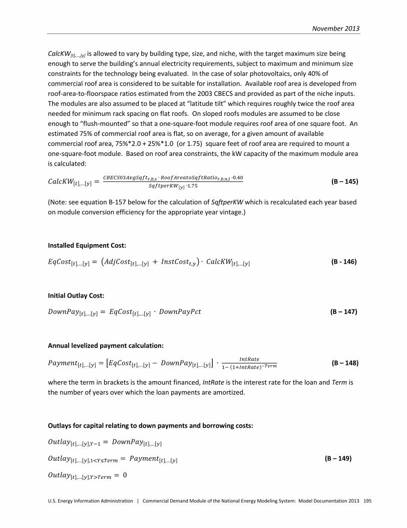
November 2013


CalcKW[t],…,[y] is allowed to vary by building type, size, and niche, with the target maximum size being enough to serve the building’s annual electricity requirements, subject to maximum and minimum size constraints for the technology being evaluated. In the case of solar photovoltaics, only 40% of commercial roof area is considered to be suitable for installation. Available roof area is developed from roof-area-to-floorspace ratios estimated from the 2003 CBECS and provided as part of the niche inputs. The modules are also assumed to be placed at “latitude tilt” which requires roughly twice the roof area needed for minimum rack spacing on flat roofs. On sloped roofs modules are assumed to be close enough to “flush-mounted” so that a one-square-foot module requires roof area of one square foot. An estimated 75% of commercial roof area is flat, so on average, for a given amount of available commercial roof area, 75%*2.0 + 25%*1.0 (or 1.75) square feet of roof area are required to mount a one-square-foot module. Based on roof area constraints, the kW capacity of the maximum module area is calculated:

𝐶𝑎𝑙𝑐𝐾𝑊[𝑡],…[𝑦] = 𝐶𝐵𝐸𝐶𝑆03𝐴𝑣𝑔𝑆𝑞𝑓𝑡𝑟,𝑏,𝑠 ∙ 𝑅𝑜𝑜𝑓𝐴𝑟𝑒𝑎𝑡𝑜𝑆𝑞𝑓𝑡𝑅𝑎𝑡𝑖𝑜𝑟,𝑏,𝑛,𝑙 ∙0.40𝑆𝑞𝑓𝑡𝑝𝑒𝑟𝐾𝑊[𝑦] ∙1.75

(B – 145)

(Note: see equation B-157 below for the calculation of SqftperKW which is recalculated each year based on module conversion efficiency for the appropriate year vintage.)

Installed Equipment Cost:

𝐸𝑞𝐶𝑜𝑠𝑡[𝑡],…[𝑦] = �𝐴𝑑𝑗𝐶𝑜𝑠𝑡[𝑡],…[𝑦] + 𝐼𝑛𝑠𝑡𝐶𝑜𝑠𝑡𝑡,𝑦� ∙ 𝐶𝑎𝑙𝑐𝐾𝑊[𝑡],…[𝑦] (B - 146)

Initial Outlay Cost:

𝐷𝑜𝑤𝑛𝑃𝑎𝑦[𝑡],…[𝑦] = 𝐸𝑞𝐶𝑜𝑠𝑡[𝑡],…[𝑦] ∙ 𝐷𝑜𝑤𝑛𝑃𝑎𝑦𝑃𝑐𝑡 (B – 147)

Annual levelized payment calculation:

𝑃𝑎𝑦𝑚𝑒𝑛𝑡[𝑡],…[𝑦] = �𝐸𝑞𝐶𝑜𝑠𝑡[𝑡],…[𝑦] − 𝐷𝑜𝑤𝑛𝑃𝑎𝑦[𝑡],…[𝑦]� ∙ 𝐼𝑛𝑡𝑅𝑎𝑡𝑒1− (1+𝐼𝑛𝑡𝑅𝑎𝑡𝑒)−𝑇𝑒𝑟𝑚 (B – 148)

where the term in brackets is the amount financed, IntRate is the interest rate for the loan and Term is the number of years over which the loan payments are amortized.

Outlays for capital relating to down payments and borrowing costs:

𝑂𝑢𝑡𝑙𝑎𝑦[𝑡],…[𝑦],𝑌−1 = 𝐷𝑜𝑤𝑛𝑃𝑎𝑦[𝑡],…[𝑦]

𝑂𝑢𝑡𝑙𝑎𝑦[𝑡],…[𝑦],1<𝑌≤𝑇𝑒𝑟𝑚 = 𝑃𝑎𝑦𝑚𝑒𝑛𝑡[𝑡],…[𝑦] (B – 149)

𝑂𝑢𝑡𝑙𝑎𝑦[𝑡],…[𝑦],𝑌>𝑇𝑒𝑟𝑚 = 0

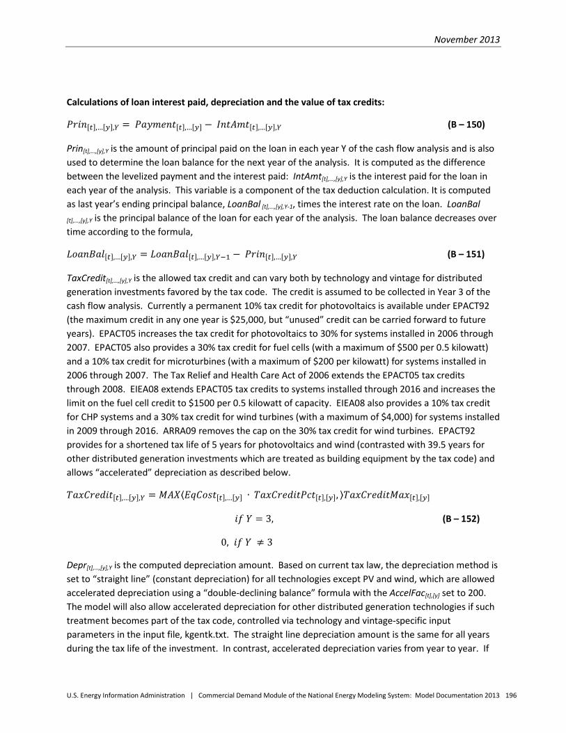
November 2013


Calculations of loan interest paid, depreciation and the value of tax credits:

𝑃𝑟𝑖𝑛[𝑡],…[𝑦],𝑌 = 𝑃𝑎𝑦𝑚𝑒𝑛𝑡[𝑡],…[𝑦] − 𝐼𝑛𝑡𝐴𝑚𝑡[𝑡],…[𝑦],𝑌 (B – 150)

Prin[t],…,[y],Y is the amount of principal paid on the loan in each year Y of the cash flow analysis and is also used to determine the loan balance for the next year of the analysis. It is computed as the difference between the levelized payment and the interest paid: IntAmt[t],…,[y],Y is the interest paid for the loan in each year of the analysis. This variable is a component of the tax deduction calculation. It is computed as last year’s ending principal balance, LoanBal [t],…,[y],Y-1, times the interest rate on the loan. LoanBal [t],…,[y],Y is the principal balance of the loan for each year of the analysis. The loan balance decreases over time according to the formula,

𝐿𝑜𝑎𝑛𝐵𝑎𝑙[𝑡],…[𝑦],𝑌 = 𝐿𝑜𝑎𝑛𝐵𝑎𝑙[𝑡],…[𝑦],𝑌−1 − 𝑃𝑟𝑖𝑛[𝑡],…[𝑦],𝑌 (B – 151)

TaxCredit[t],…,[y],Y is the allowed tax credit and can vary both by technology and vintage for distributed generation investments favored by the tax code. The credit is assumed to be collected in Year 3 of the cash flow analysis. Currently a permanent 10% tax credit for photovoltaics is available under EPACT92 (the maximum credit in any one year is $25,000, but “unused” credit can be carried forward to future years). EPACT05 increases the tax credit for photovoltaics to 30% for systems installed in 2006 through 2007. EPACT05 also provides a 30% tax credit for fuel cells (with a maximum of $500 per 0.5 kilowatt) and a 10% tax credit for microturbines (with a maximum of $200 per kilowatt) for systems installed in 2006 through 2007. The Tax Relief and Health Care Act of 2006 extends the EPACT05 tax credits through 2008. EIEA08 extends EPACT05 tax credits to systems installed through 2016 and increases the limit on the fuel cell credit to $1500 per 0.5 kilowatt of capacity. EIEA08 also provides a 10% tax credit for CHP systems and a 30% tax credit for wind turbines (with a maximum of $4,000) for systems installed in 2009 through 2016. ARRA09 removes the cap on the 30% tax credit for wind turbines. EPACT92 provides for a shortened tax life of 5 years for photovoltaics and wind (contrasted with 39.5 years for other distributed generation investments which are treated as building equipment by the tax code) and allows “accelerated” depreciation as described below.

𝑇𝑎𝑥𝐶𝑟𝑒𝑑𝑖𝑡[𝑡],…[𝑦],𝑌 = 𝑀𝐴𝑋⟨𝐸𝑞𝐶𝑜𝑠𝑡[𝑡],…[𝑦] ∙ 𝑇𝑎𝑥𝐶𝑟𝑒𝑑𝑖𝑡𝑃𝑐𝑡[𝑡],[𝑦], ⟩𝑇𝑎𝑥𝐶𝑟𝑒𝑑𝑖𝑡𝑀𝑎𝑥[𝑡],[𝑦]

𝑖𝑓 𝑌 = 3, (B – 152)

0, 𝑖𝑓 𝑌 ≠ 3

Depr[t],…,[y],Y is the computed depreciation amount. Based on current tax law, the depreciation method is set to “straight line” (constant depreciation) for all technologies except PV and wind, which are allowed accelerated depreciation using a “double-declining balance” formula with the AccelFac[t],[y] set to 200. The model will also allow accelerated depreciation for other distributed generation technologies if such treatment becomes part of the tax code, controlled via technology and vintage-specific input parameters in the input file, kgentk.txt. The straight line depreciation amount is the same for all years during the tax life of the investment. In contrast, accelerated depreciation varies from year to year. If

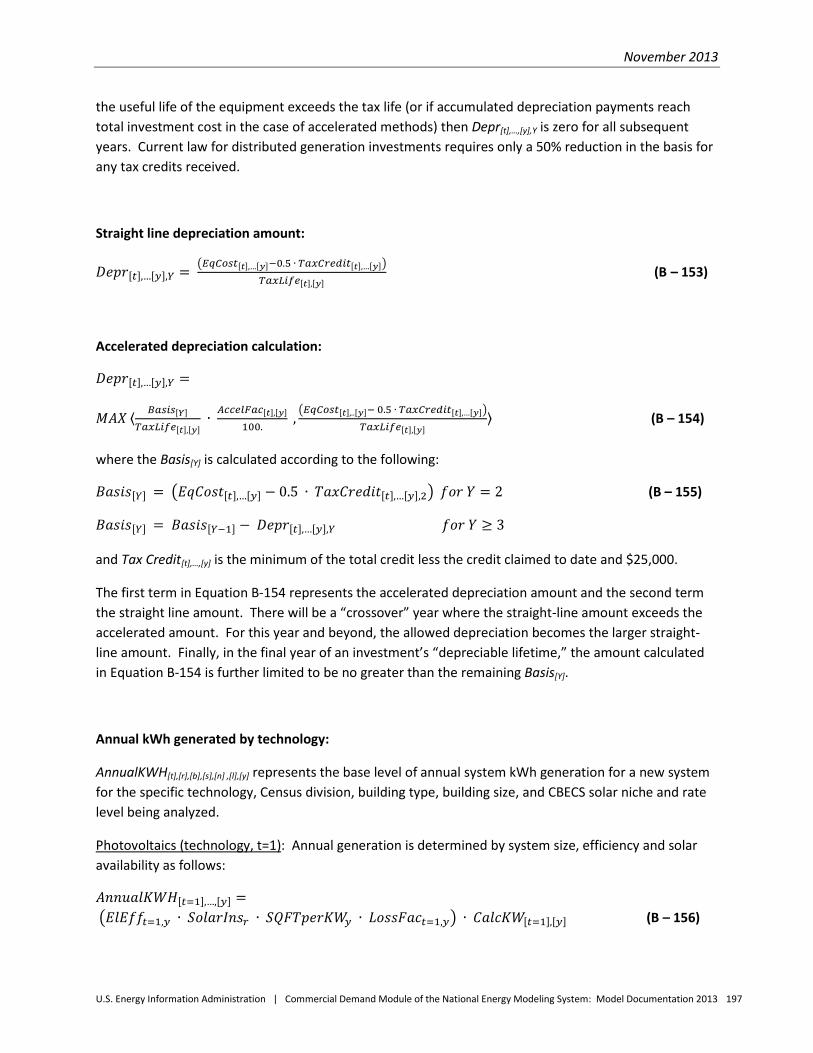
November 2013


the useful life of the equipment exceeds the tax life (or if accumulated depreciation payments reach total investment cost in the case of accelerated methods) then Depr[t],…,[y],Y is zero for all subsequent years. Current law for distributed generation investments requires only a 50% reduction in the basis for any tax credits received.

Straight line depreciation amount:

𝐷𝑒𝑝𝑟[𝑡],…[𝑦],𝑌 = �𝐸𝑞𝐶𝑜𝑠𝑡[𝑡],…[𝑦]−0.5 ∙ 𝑇𝑎𝑥𝐶𝑟𝑒𝑑𝑖𝑡[𝑡],…[𝑦]�

𝑇𝑎𝑥𝐿𝑖𝑓𝑒[𝑡],[𝑦] (B – 153)

Accelerated depreciation calculation:

𝐷𝑒𝑝𝑟[𝑡],…[𝑦],𝑌 =

𝑀𝐴𝑋 ⟨ 𝐵𝑎𝑠𝑖𝑠[𝑌]

𝑇𝑎𝑥𝐿𝑖𝑓𝑒[𝑡],[𝑦] ∙

𝐴𝑐𝑐𝑒𝑙𝐹𝑎𝑐[𝑡],[𝑦]

100. , �

𝐸𝑞𝐶𝑜𝑠𝑡[𝑡],..[𝑦]− 0.5 ∙ 𝑇𝑎𝑥𝐶𝑟𝑒𝑑𝑖𝑡[𝑡],…[𝑦]�𝑇𝑎𝑥𝐿𝑖𝑓𝑒[𝑡],[𝑦]

⟩ (B – 154)

where the Basis[Y] is calculated according to the following:

𝐵𝑎𝑠𝑖𝑠[𝑌] = �𝐸𝑞𝐶𝑜𝑠𝑡[𝑡],…[𝑦] − 0.5 ∙ 𝑇𝑎𝑥𝐶𝑟𝑒𝑑𝑖𝑡[𝑡],…[𝑦],2� 𝑓𝑜𝑟 𝑌 = 2 (B – 155)

𝐵𝑎𝑠𝑖𝑠[𝑌] = 𝐵𝑎𝑠𝑖𝑠[𝑌−1] − 𝐷𝑒𝑝𝑟[𝑡],…[𝑦],𝑌 𝑓𝑜𝑟 𝑌 ≥ 3

and Tax Credit[t],…,[y] is the minimum of the total credit less the credit claimed to date and $25,000.

The first term in Equation B-154 represents the accelerated depreciation amount and the second term the straight line amount. There will be a “crossover” year where the straight-line amount exceeds the accelerated amount. For this year and beyond, the allowed depreciation becomes the larger straight-line amount. Finally, in the final year of an investment’s “depreciable lifetime,” the amount calculated in Equation B-154 is further limited to be no greater than the remaining Basis[Y].

Annual kWh generated by technology:

AnnualKWH[t],[r],[b],[s],[n] ,[l],[y] represents the base level of annual system kWh generation for a new system for the specific technology, Census division, building type, building size, and CBECS solar niche and rate level being analyzed.

Photovoltaics (technology, t=1): Annual generation is determined by system size, efficiency and solar availability as follows:

𝐴𝑛𝑛𝑢𝑎𝑙𝐾𝑊𝐻[𝑡=1],…,[𝑦] = �𝐸𝑙𝐸𝑓𝑓𝑡=1,𝑦 ∙ 𝑆𝑜𝑙𝑎𝑟𝐼𝑛𝑠𝑟 ∙ 𝑆𝑄𝐹𝑇𝑝𝑒𝑟𝐾𝑊𝑦 ∙ 𝐿𝑜𝑠𝑠𝐹𝑎𝑐𝑡=1,𝑦� ∙ 𝐶𝑎𝑙𝑐𝐾𝑊[𝑡=1],[𝑦] (B – 156)

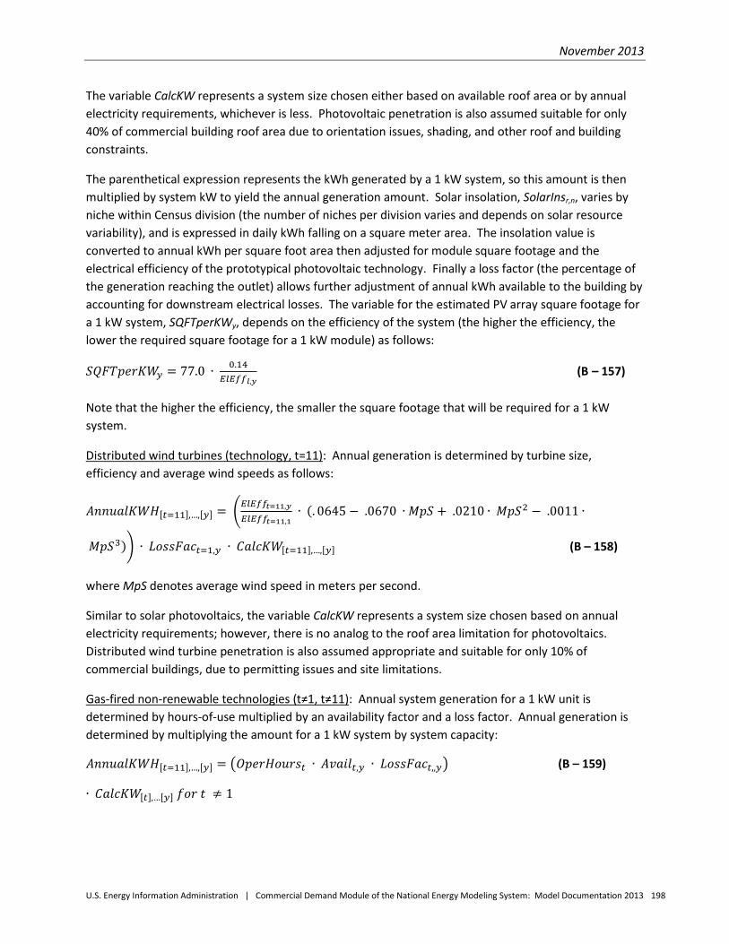
November 2013


The variable CalcKW represents a system size chosen either based on available roof area or by annual electricity requirements, whichever is less. Photovoltaic penetration is also assumed suitable for only 40% of commercial building roof area due to orientation issues, shading, and other roof and building constraints.

The parenthetical expression represents the kWh generated by a 1 kW system, so this amount is then multiplied by system kW to yield the annual generation amount. Solar insolation, SolarInsr,n, varies by niche within Census division (the number of niches per division varies and depends on solar resource variability), and is expressed in daily kWh falling on a square meter area. The insolation value is converted to annual kWh per square foot area then adjusted for module square footage and the electrical efficiency of the prototypical photovoltaic technology. Finally a loss factor (the percentage of the generation reaching the outlet) allows further adjustment of annual kWh available to the building by accounting for downstream electrical losses. The variable for the estimated PV array square footage for a 1 kW system, SQFTperKWy, depends on the efficiency of the system (the higher the efficiency, the lower the required square footage for a 1 kW module) as follows:

𝑆𝑄𝐹𝑇𝑝𝑒𝑟𝐾𝑊𝑦 = 77.0 ∙ 0.14𝐸𝑙𝐸𝑓𝑓𝑙,𝑦

(B – 157)

Note that the higher the efficiency, the smaller the square footage that will be required for a 1 kW system.

Distributed wind turbines (technology, t=11): Annual generation is determined by turbine size, efficiency and average wind speeds as follows:

𝐴𝑛𝑛𝑢𝑎𝑙𝐾𝑊𝐻[𝑡=11],…,[𝑦] = �𝐸𝑙𝐸𝑓𝑓𝑡=11,𝑦

𝐸𝑙𝐸𝑓𝑓𝑡=11,1 ∙ (. 0645 − .0670 ∙ 𝑀𝑝𝑆 + .0210 ∙ 𝑀𝑝𝑆2 − .0011 ∙

𝑀𝑝𝑆3)� ∙ 𝐿𝑜𝑠𝑠𝐹𝑎𝑐𝑡=1,𝑦 ∙ 𝐶𝑎𝑙𝑐𝐾𝑊[𝑡=11],…,[𝑦] (B – 158)

where MpS denotes average wind speed in meters per second.

Similar to solar photovoltaics, the variable CalcKW represents a system size chosen based on annual electricity requirements; however, there is no analog to the roof area limitation for photovoltaics. Distributed wind turbine penetration is also assumed appropriate and suitable for only 10% of commercial buildings, due to permitting issues and site limitations.

Gas-fired non-renewable technologies (t≠1, t≠11): Annual system generation for a 1 kW unit is determined by hours-of-use multiplied by an availability factor and a loss factor. Annual generation is determined by multiplying the amount for a 1 kW system by system capacity:

𝐴𝑛𝑛𝑢𝑎𝑙𝐾𝑊𝐻[𝑡=11],…,[𝑦] = �𝑂𝑝𝑒𝑟𝐻𝑜𝑢𝑟𝑠𝑡 ∙ 𝐴𝑣𝑎𝑖𝑙𝑡,𝑦 ∙ 𝐿𝑜𝑠𝑠𝐹𝑎𝑐𝑡,,𝑦� (B – 159)

∙ 𝐶𝑎𝑙𝑐𝐾𝑊[𝑡],…[𝑦] 𝑓𝑜𝑟 𝑡 ≠ 1

November 2013


KWH[t],…,[y],Y is the actual kWh generated in each of the years of the cash flow analysis. The actual generation is the ideal generation adjusted for degradation as the system ages. Currently, only photovoltaic generation has a non-zero degradation factor. Its value of 0.01 assumes a 1-percent-per-year loss in output as the modules age. Degradation begins in the year after the system is fully in use, which for the cash flow model assumptions is year 3.

𝐾𝑊𝐻[𝑡],…[𝑦],𝑌 = 𝐴𝑛𝑛𝑢𝑎𝑙𝐾𝑊𝐻[𝑡],…,[𝑦] ∙ �1 − 𝐷𝑒𝑔𝑟𝑒𝑑𝑎𝑡𝑖𝑜𝑛[𝑡],[𝑦]� 𝑌−2 (B – 160)

Fuel consumption for distributed generation technologies:

Fuel consumption for “fired” generation technologies is denoted by the variable FuelInput[t],…,[y] and is calculated in MMBtu of the input fuel used by the technology:

𝐹𝑢𝑒𝑙𝐼𝑛𝑝𝑢𝑡[𝑡],…[𝑦] = 0.003412 ∙ 𝑂𝑝𝑒𝑟𝐻𝑜𝑢𝑟𝑠𝑡 ∙ 𝐴𝑣𝑎𝑖𝑙𝑡,𝑦 𝐸𝑙𝐸𝑓𝑓𝑡,𝑦

∙ 𝐶𝑎𝑙𝑐𝐾𝑊[𝑡],…[𝑦] (B – 161)

Calculation of waste heat available for water heating and space heating use:

BTUWasteHeat[t],…,[y] represents the amount of waste heat potentially available for water heating and space heating. It is also computed in MMBtu and is the difference between the fuel input and the energy expended on electricity generation multiplied by the waste heat recovery efficiency specific to this technology and vintage.

𝐵𝑇𝑈𝑊𝑎𝑠𝑡𝑒𝐻𝑒𝑎𝑡[𝑡],… [𝑦] = �𝐹𝑢𝑒𝑙𝐼𝑛𝑝𝑢𝑡[𝑡],…[𝑦] − .003412 ∙ 𝐴𝑛𝑛𝑢𝑎𝑙𝐾𝑊𝐻[𝑡],…[𝑦]� ∙ 𝑊ℎ𝑅𝑒𝑐𝑜𝑣𝑒𝑟𝑦𝐸𝑓𝑓𝑡,𝑦 (B – 162)

The amount of available waste heat is partitioned into water heating and space heating end use services up to the average consumption for those end uses by Census division, building type (b) and size category (s):

𝑊𝑎𝑡𝑒𝑟𝐻𝑒𝑎𝑡𝑖𝑛𝑔𝑀𝑀𝐵𝑡𝑢[𝑡],[𝑟],[𝑏],[𝑠],[𝑦] = 𝑀𝐼𝑁⟨𝐵𝑇𝑈𝑊𝑎𝑠𝑡𝑒𝐻𝑒𝑎𝑡[𝑡],…[𝑦],𝐴𝑣𝑔𝑊𝑎𝑡𝑒𝑟𝐻𝑡𝑔𝑀𝑀𝐵𝑡𝑢[𝑟],[𝑏],[𝑠] ⟩

𝑤ℎ𝑒𝑟𝑒 𝐴𝑣𝑔𝑊𝑎𝑡𝑒𝑟𝐻𝑡𝑔𝑀𝑀𝐵𝑡𝑢[𝑟],[𝑏],[𝑠] = 𝐴𝑣𝑔𝑆𝑞𝑓𝑡𝑏,𝑠 ∙ 𝐶𝑜𝑚𝐸𝑈𝐼𝑟,𝑏,𝐸𝑈=𝑊𝐻 ,𝐹=𝑁𝑎𝑡𝑢𝑟𝑎𝑙𝐺𝑎𝑠 (B – 163)

If the distributed generation equipment provides more waste heat than the average water heating requirements, then any residual is assumed to be provided as space heating up to a maximum of the average space heating requirements. Any amount of waste heat generated beyond the average water and space heating requirements is assumed to be not utilized to offset end-use fuel requirements. Natural gas-fired technologies are expected to be primarily responsible for growth in combined heat and power over the projection horizon, allowing the simplifying assumption that these systems will satisfy water and space heating requirements otherwise met with natural-gas-fired end-use equipment.

𝑆𝑝𝑎𝑐𝑒𝐻𝑒𝑎𝑡𝑖𝑛𝑔𝑀𝑀𝐵𝑡𝑢[𝑡],[𝑟],[𝑏],[𝑠],[𝑦]= 𝑀𝐼𝑁⟨𝐵𝑇𝑈𝑊𝑎𝑠𝑡𝑒𝐻𝑒𝑎𝑡[𝑡],…[𝑦],𝑊𝑎𝑡𝑒𝑟𝐻𝑡𝑔𝑀𝑀𝐵𝑡𝑢[𝑡],…[𝑦],𝐴𝑣𝑔𝑆𝑝𝑎𝑐𝑒𝐻𝑡𝑔𝑀𝑀𝐵𝑡𝑢[𝑟],[𝑏],[𝑠] ⟩

November 2013


𝑤ℎ𝑒𝑟𝑒 𝐴𝑣𝑔𝑆𝑝𝑎𝑐𝑒𝐻𝑡𝑔𝑀𝑀𝐵𝑡𝑢[𝑟],[𝑏],[𝑠] = 𝐴𝑣𝑔𝑆𝑞𝑓𝑡𝑏,𝑠 ∙ 𝐶𝑜𝑚𝐸𝑈𝐼𝑟,𝑏,𝐸𝑈=𝑆𝐻 ,𝐹=𝑁𝑎𝑡𝑢𝑟𝑎𝑙𝐺𝑎𝑠 (B – 164)

Net fuel cost:

BaseYrFuelCost[t],…,[y] is the initial fuel cost for operating the generation technology net of savings stemming from displaced water heating or space heating. It is calculated from the current NEMS fuel price converted into the same year dollars as the technology capital costs (currently 2009 constant dollars). This price is then scaled based on the natural gas price in the solar (n) and electricity rate (l) niches relative to the Census division gas price:

𝐵𝑎𝑠𝑒𝑌𝑟𝐹𝑢𝑒𝑙𝐶𝑜𝑠𝑡[𝑡],…[𝑦],[𝑙],[𝑦] = �𝐹𝑢𝑒𝑙𝐼𝑛𝑝𝑢𝑡[𝑡],…[𝑦] − 𝑊𝑎𝑡𝑒𝑟𝐻𝑡𝑔𝑀𝑀𝐵𝑡𝑢[𝑡],[𝑦],𝑆𝑝𝑎𝑐𝑒𝐻𝑡𝑔𝑀𝑀𝐵𝑡𝑢[𝑡],[𝑦]� ∙ 𝑁𝐺𝑅𝑎𝑡𝑒𝑆𝑐𝑎𝑙𝑎𝑟𝑟,𝑛,𝑙 ∙ 𝐹𝑢𝑒𝑙𝑃𝑟𝑖𝑐𝑒𝑟,𝑦 (B – 165)

FuelCost[t],…,[y],Y is the nominal dollar value fuel cost for the technology net of any water heating and space heating cost savings from using waste heat:

𝐹𝑢𝑒𝑙𝐶𝑜𝑠𝑡[𝑡],…[𝑦],𝑌 = 𝐵𝑎𝑠𝑒𝑌𝑟𝐹𝑢𝑒𝑙𝐶𝑜𝑠𝑡[𝑡],…[𝑦] ∙ (1 + 𝑖𝑛𝑓𝑙𝑎𝑡𝑖𝑜𝑛)(𝑌−2) (B – 166)

The value of electricity savings calculations:

ValElecSaveBase[t],…,[y] represents the calculated value of generated electricity for the initial year of the cash flow simulation. This value is further adjusted to account for inflation and generation efficiency degradation in a later calculation described below.

Case 1: Photovoltaics

If generation is less than average electricity usage for the building type, (i.e., AnnualKWH[t],…,[y] <= ElecAvgKWHb,s), then savings are valued at the air conditioning price (this price is used instead of the average electricity price due to the “coincidence” of air conditioning loads and photovoltaic module generation), scaled based on the electricity price in the rate niche relative to the Census division price:

𝑉𝑎𝑙𝐸𝑙𝑒𝑐𝑆𝑎𝑣𝑒𝐵𝑎𝑠𝑒[𝑡],…,[𝑟],[𝑛],[𝑙],[𝑦] = �𝑃𝑒𝑙𝐶𝑀𝑜𝑢𝑡𝑟,𝑦,𝐴𝐶 ∙ .003412 ∙ 𝑅𝑎𝑡𝑒𝑆𝑐𝑎𝑙𝑎𝑟𝑟,𝑛,𝑙

𝐸𝑃𝑅𝑃𝑆𝑃𝑅𝑦 ∙ .001 ∙ 𝑆𝑐𝑎𝑙𝑒𝑅𝑃𝑆𝑡∙ 𝐴𝑛𝑛𝑢𝑎𝑙𝐾𝑊𝐻[𝑡],…,[𝑦]

� (B – 167)

In the above equation, the factor 0.003412 converts the NEMS commercial electricity price from dollars per MMBtu to dollars per kWh. The factor .001 converts the NEMS “renewable portfolio standard” credit price, EPRPSPRy, from “mills” per kWh to dollars per kWh. ScaleRPSt may vary depending upon legislation. For example, if the credit is received, the scalar is set to a value greater than zero (e.g., for triple credits, the scalar is 3). Since RPS credits often have a last year or “sunset” year, the cash flow simulation also tracks the calendar year of each of the simulated years and zeros out the credit if the calendar year exceeds the sunset year. Finally, the factor RateScalarr,n,l converts the NEMS electricity price for Census division (r) into a price for the solar niche (n) / rate level (l) combination.

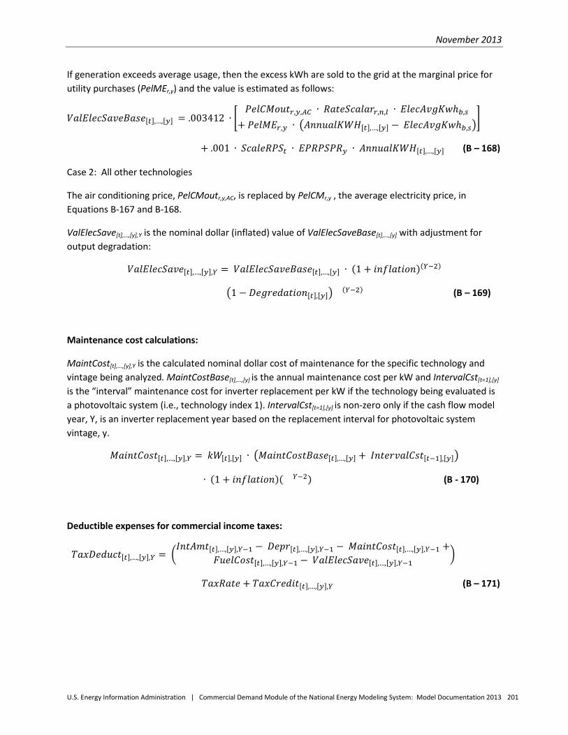
November 2013


If generation exceeds average usage, then the excess kWh are sold to the grid at the marginal price for utility purchases (PelMEr,y) and the value is estimated as follows:

𝑉𝑎𝑙𝐸𝑙𝑒𝑐𝑆𝑎𝑣𝑒𝐵𝑎𝑠𝑒[𝑡],…,[𝑦] = .003412 ∙ �𝑃𝑒𝑙𝐶𝑀𝑜𝑢𝑡𝑟,𝑦,𝐴𝐶 ∙ 𝑅𝑎𝑡𝑒𝑆𝑐𝑎𝑙𝑎𝑟𝑟,𝑛,𝑙 ∙ 𝐸𝑙𝑒𝑐𝐴𝑣𝑔𝐾𝑤ℎ𝑏,𝑠

+ 𝑃𝑒𝑙𝑀𝐸𝑟,𝑦 ∙ �𝐴𝑛𝑛𝑢𝑎𝑙𝐾𝑊𝐻[𝑡],…,[𝑦] − 𝐸𝑙𝑒𝑐𝐴𝑣𝑔𝐾𝑤ℎ𝑏,𝑠��

+ .001 ∙ 𝑆𝑐𝑎𝑙𝑒𝑅𝑃𝑆𝑡 ∙ 𝐸𝑃𝑅𝑃𝑆𝑃𝑅𝑦 ∙ 𝐴𝑛𝑛𝑢𝑎𝑙𝐾𝑊𝐻[𝑡],…,[𝑦] (B – 168)

Case 2: All other technologies

The air conditioning price, PelCMoutr,y,AC, is replaced by PelCMr,y , the average electricity price, in Equations B-167 and B-168.

ValElecSave[t],…,[y],Y is the nominal dollar (inflated) value of ValElecSaveBase[t],…,[y] with adjustment for output degradation:

𝑉𝑎𝑙𝐸𝑙𝑒𝑐𝑆𝑎𝑣𝑒[𝑡],…,[𝑦],𝑌 = 𝑉𝑎𝑙𝐸𝑙𝑒𝑐𝑆𝑎𝑣𝑒𝐵𝑎𝑠𝑒[𝑡],…,[𝑦] ∙ (1 + 𝑖𝑛𝑓𝑙𝑎𝑡𝑖𝑜𝑛)(𝑌−2)

�1 − 𝐷𝑒𝑔𝑟𝑒𝑑𝑎𝑡𝑖𝑜𝑛[𝑡],[𝑦]� (𝑌−2) (B – 169)

Maintenance cost calculations:

MaintCost[t],…,[y],Y is the calculated nominal dollar cost of maintenance for the specific technology and vintage being analyzed. MaintCostBase[t],…,[y] is the annual maintenance cost per kW and IntervalCst[t=1],[y] is the “interval” maintenance cost for inverter replacement per kW if the technology being evaluated is a photovoltaic system (i.e., technology index 1). IntervalCst[t=1],[y] is non-zero only if the cash flow model year, Y, is an inverter replacement year based on the replacement interval for photovoltaic system vintage, y.

𝑀𝑎𝑖𝑛𝑡𝐶𝑜𝑠𝑡[𝑡],…,[𝑦],𝑌 = 𝑘𝑊[𝑡],[𝑦] ∙ �𝑀𝑎𝑖𝑛𝑡𝐶𝑜𝑠𝑡𝐵𝑎𝑠𝑒[𝑡],…,[𝑦] + 𝐼𝑛𝑡𝑒𝑟𝑣𝑎𝑙𝐶𝑠𝑡[𝑡−1],[𝑦]�

∙ (1 + 𝑖𝑛𝑓𝑙𝑎𝑡𝑖𝑜𝑛)( 𝑌−2) (B - 170)

Deductible expenses for commercial income taxes:

𝑇𝑎𝑥𝐷𝑒𝑑𝑢𝑐𝑡[𝑡],…,[𝑦],𝑌 = �𝐼𝑛𝑡𝐴𝑚𝑡[𝑡],…,[𝑦],𝑌−1 − 𝐷𝑒𝑝𝑟[𝑡],…,[𝑦],𝑌−1 − 𝑀𝑎𝑖𝑛𝑡𝐶𝑜𝑠𝑡[𝑡],…,[𝑦],𝑌−1 +

𝐹𝑢𝑒𝑙𝐶𝑜𝑠𝑡[𝑡],…,[𝑦],𝑌−1 − 𝑉𝑎𝑙𝐸𝑙𝑒𝑐𝑆𝑎𝑣𝑒[𝑡],…,[𝑦],𝑌−1�

𝑇𝑎𝑥𝑅𝑎𝑡𝑒 + 𝑇𝑎𝑥𝐶𝑟𝑒𝑑𝑖𝑡[𝑡],…,[𝑦],𝑌 (B – 171)

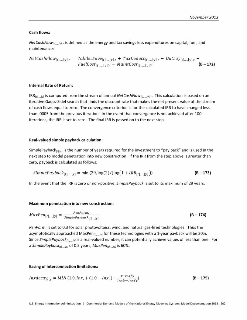
November 2013


Cash flows:

NetCashFlow[t],…,[y],Y is defined as the energy and tax savings less expenditures on capital, fuel, and maintenance:

𝑁𝑒𝑡𝐶𝑎𝑠ℎ𝐹𝑙𝑜𝑤[𝑡],…,[𝑦],𝑌 = 𝑉𝑎𝑙𝐸𝑙𝑒𝑐𝑆𝑎𝑣𝑒[𝑡],…,[𝑦],𝑌 + 𝑇𝑎𝑥𝐷𝑒𝑑𝑢𝑐𝑡[𝑡],…,[𝑦],𝑌 − 𝑂𝑢𝑡𝐿𝑎𝑦[𝑡],…,[𝑦],𝑌 − 𝐹𝑢𝑒𝑙𝐶𝑜𝑠𝑡[𝑡],…,[𝑦],𝑌 − 𝑀𝑎𝑖𝑛𝑡𝐶𝑜𝑠𝑡[𝑡],…,[𝑦],𝑌

(B – 172)

Internal Rate of Return:

IRR[t],…,[y] is computed from the stream of annual NetCashFlow[t],…,[y],Y. This calculation is based on an iterative Gauss-Sidel search that finds the discount rate that makes the net present value of the stream of cash flows equal to zero. The convergence criterion is for the calculated IRR to have changed less than .0005 from the previous iteration. In the event that convergence is not achieved after 100 iterations, the IRR is set to zero. The final IRR is passed on to the next step.

Real-valued simple payback calculation:

SimplePayback[t],[y] is the number of years required for the investment to “pay back” and is used in the next step to model penetration into new construction. If the IRR from the step above is greater than zero, payback is calculated as follows:

𝑆𝑖𝑚𝑝𝑙𝑒𝑃𝑎𝑦𝑏𝑎𝑐𝑘[𝑡],…,[𝑦] = min ⟨29, log(2)/(log �1 + 𝐼𝑅𝑅[𝑡],…,[𝑦] �⟩ (B – 173)

In the event that the IRR is zero or non-positive, SimplePayback is set to its maximum of 29 years.

Maximum penetration into new construction:

𝑀𝑎𝑥𝑃𝑒𝑛[𝑡],…,[𝑦] = 𝑃𝑒𝑛𝑃𝑎𝑟𝑚𝑡𝑆𝑖𝑚𝑝𝑙𝑒𝑃𝑎𝑦𝑏𝑎𝑐𝑘[𝑡],…,[𝑦]

(B – 174)

PenParmt is set to 0.3 for solar photovoltaics, wind, and natural gas-fired technologies. Thus the asymptotically approached MaxPen[t],…,[y] for these technologies with a 1-year payback will be 30%. Since SimplePayback[t],…,[y] is a real-valued number, it can potentially achieve values of less than one. For a SimplePayback[t],…,[y] of 0.5 years, MaxPen[t],…,[y] is 60%.

Easing of interconnection limitations:

𝐼𝑛𝑥𝑑𝑒𝑐𝑎𝑦𝑟,𝑦 = 𝑀𝐼𝑁 ⟨1.0, 𝐼𝑛𝑥, + (1.0− 𝐼𝑛𝑥𝑟) ∙ 𝑦−𝐼𝑛𝑥𝑓𝑦𝐼𝑛𝑥𝑙𝑦−𝐼𝑛𝑥𝑓𝑦

⟩ (B – 175)

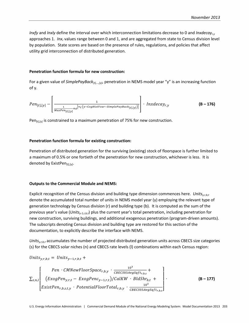
November 2013


Inxfy and Inxly define the interval over which interconnection limitations decrease to 0 and Inxdecayr,y approaches 1. Inxr values range between 0 and 1, and are aggregated from state to Census division level by population. State scores are based on the presence of rules, regulations, and policies that affect utility grid interconnection of distributed generation.

Penetration function formula for new construction:

For a given value of SimplePayBack[t],…,[y], penetration in NEMS model year “y” is an increasing function of y.

𝑃𝑒𝑛[𝑡],[𝑦] − � 11

𝑀𝑎𝑥𝑃𝑒𝑛[𝑡],[𝑦]+𝑒�∝𝑡∙�𝑦−𝐶𝑜𝑔𝐻𝑖𝑠𝑡𝑌𝑒𝑎𝑟−𝑆𝑖𝑚𝑝𝑙𝑒𝑃𝑎𝑦𝐵𝑎𝑐𝑘[𝑡],[𝑦]��

� ∙ 𝐼𝑛𝑥𝑑𝑒𝑐𝑎𝑦𝑟,𝑦 (B – 176)

Pen[t],[y] is constrained to a maximum penetration of 75% for new construction.

Penetration function formula for existing construction:

Penetration of distributed generation for the surviving (existing) stock of floorspace is further limited to a maximum of 0.5% or one fortieth of the penetration for new construction, whichever is less. It is denoted by ExistPen[t],[y].

Outputs to the Commercial Module and NEMS:

Explicit recognition of the Census division and building type dimension commences here. Unitsy,r,b,t denote the accumulated total number of units in NEMS model year (y) employing the relevant type of generation technology by Census division (r) and building type (b). It is computed as the sum of the previous year’s value (Unitsy-1,r,b,t) plus the current year’s total penetration, including penetration for new construction, surviving buildings, and additional exogenous penetration (program-driven amounts). The subscripts denoting Census division and building type are restored for this section of the documentation, to explicitly describe the interface with NEMS.

Unitsy,r,b,t accumulates the number of projected distributed generation units across CBECS size categories (s) for the CBECS solar niches (n) and CBECS rate levels (l) combinations within each Census region:

𝑈𝑛𝑖𝑡𝑠𝑦,𝑟,𝑏,𝑡 = 𝑈𝑛𝑖𝑡𝑠𝑦−1,𝑟,𝑏,𝑡 +

∑

⎣⎢⎢⎢⎡ 𝑃𝑒𝑛 ∙ 𝐶𝑀𝑁𝑒𝑤𝐹𝑙𝑜𝑜𝑟𝑆𝑝𝑎𝑐𝑒𝑟,𝑏,𝑦 ∙ 103

𝐶𝐵𝐸𝐶𝑆03𝐴𝑣𝑔𝑆𝑞𝑓𝑡𝑟,𝑏,𝑠+

�𝐸𝑥𝑜𝑔𝑃𝑒𝑛𝑦,𝑟,𝑡 − 𝐸𝑥𝑜𝑔𝑃𝑒𝑛𝑐𝑦−1,𝑟,𝑡�/𝐶𝑎𝑙𝐾𝑊 ∙ 𝐵𝑙𝑑𝑆ℎ𝑟𝑏,𝑡 +

𝐸𝑥𝑖𝑠𝑡𝑃𝑒𝑛𝑟,𝑏,𝑠,𝑡,𝑦 ∙ 𝑃𝑜𝑡𝑒𝑛𝑡𝑖𝑎𝑙𝐹𝑙𝑜𝑜𝑟𝑇𝑜𝑡𝑎𝑙𝑟,𝑏,𝑦 ∙ 103

𝐶𝐵𝐸𝐶𝑆03𝐴𝑣𝑔𝑆𝑞𝑓𝑡𝑟,𝑏,𝑠⎦⎥⎥⎥⎤

∙𝑠,𝑛,𝑙 (B – 177)

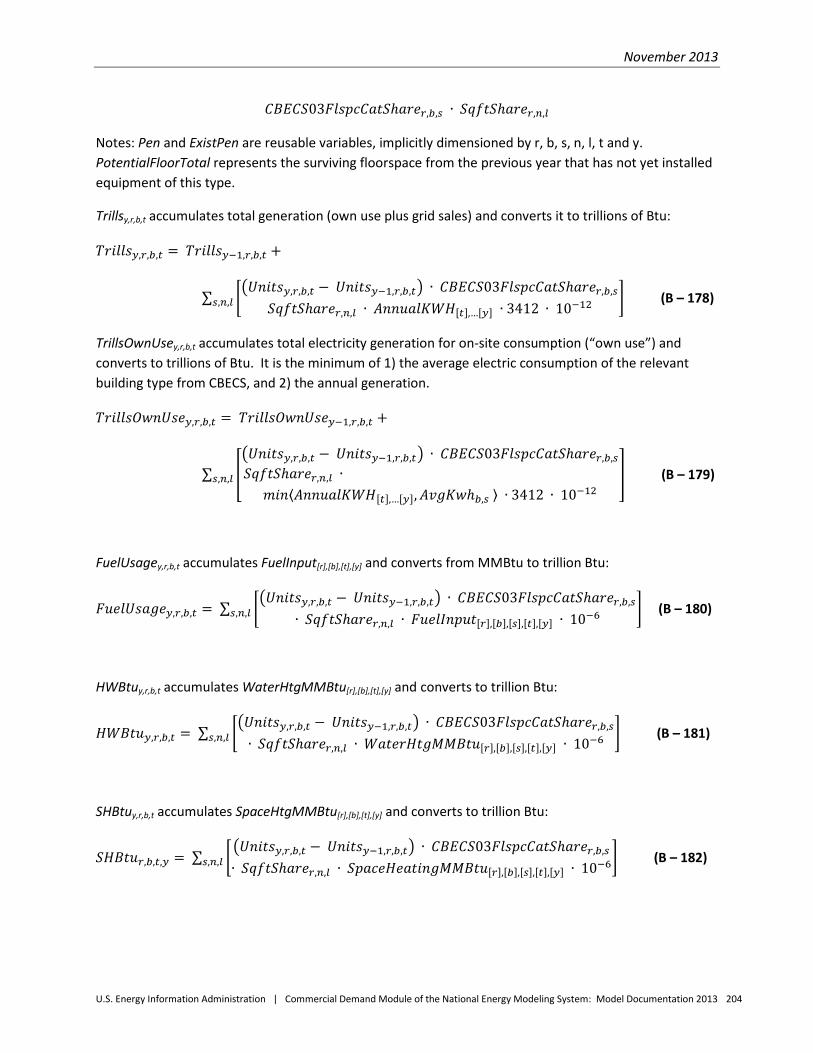
November 2013


𝐶𝐵𝐸𝐶𝑆03𝐹𝑙𝑠𝑝𝑐𝐶𝑎𝑡𝑆ℎ𝑎𝑟𝑒𝑟,𝑏,𝑠 ∙ 𝑆𝑞𝑓𝑡𝑆ℎ𝑎𝑟𝑒𝑟,𝑛,𝑙

Notes: Pen and ExistPen are reusable variables, implicitly dimensioned by r, b, s, n, l, t and y. PotentialFloorTotal represents the surviving floorspace from the previous year that has not yet installed equipment of this type.

Trillsy,r,b,t accumulates total generation (own use plus grid sales) and converts it to trillions of Btu:

𝑇𝑟𝑖𝑙𝑙𝑠𝑦,𝑟,𝑏,𝑡 = 𝑇𝑟𝑖𝑙𝑙𝑠𝑦−1,𝑟,𝑏,𝑡 +

∑ ��𝑈𝑛𝑖𝑡𝑠𝑦,𝑟,𝑏,𝑡 − 𝑈𝑛𝑖𝑡𝑠𝑦−1,𝑟,𝑏,𝑡� ∙ 𝐶𝐵𝐸𝐶𝑆03𝐹𝑙𝑠𝑝𝑐𝐶𝑎𝑡𝑆ℎ𝑎𝑟𝑒𝑟,𝑏,𝑠

𝑆𝑞𝑓𝑡𝑆ℎ𝑎𝑟𝑒𝑟,𝑛,𝑙 ∙ 𝐴𝑛𝑛𝑢𝑎𝑙𝐾𝑊𝐻[𝑡],…[𝑦] ∙ 3412 ∙ 10−12�𝑠,𝑛,𝑙 (B – 178)

TrillsOwnUsey,r,b,t accumulates total electricity generation for on-site consumption (“own use”) and converts to trillions of Btu. It is the minimum of 1) the average electric consumption of the relevant building type from CBECS, and 2) the annual generation.

𝑇𝑟𝑖𝑙𝑙𝑠𝑂𝑤𝑛𝑈𝑠𝑒𝑦,𝑟,𝑏,𝑡 = 𝑇𝑟𝑖𝑙𝑙𝑠𝑂𝑤𝑛𝑈𝑠𝑒𝑦−1,𝑟,𝑏,𝑡 +

∑ ��𝑈𝑛𝑖𝑡𝑠𝑦,𝑟,𝑏,𝑡 − 𝑈𝑛𝑖𝑡𝑠𝑦−1,𝑟,𝑏,𝑡� ∙ 𝐶𝐵𝐸𝐶𝑆03𝐹𝑙𝑠𝑝𝑐𝐶𝑎𝑡𝑆ℎ𝑎𝑟𝑒𝑟,𝑏,𝑠𝑆𝑞𝑓𝑡𝑆ℎ𝑎𝑟𝑒𝑟,𝑛,𝑙 ∙

𝑚𝑖𝑛⟨𝐴𝑛𝑛𝑢𝑎𝑙𝐾𝑊𝐻[𝑡],…[𝑦],𝐴𝑣𝑔𝐾𝑤ℎ𝑏,𝑠 ⟩ ∙ 3412 ∙ 10−12�𝑠,𝑛,𝑙 (B – 179)

FuelUsagey,r,b,t accumulates FuelInput[r],[b],[t],[y] and converts from MMBtu to trillion Btu:

𝐹𝑢𝑒𝑙𝑈𝑠𝑎𝑔𝑒𝑦,𝑟,𝑏,𝑡 = ∑ ��𝑈𝑛𝑖𝑡𝑠𝑦,𝑟,𝑏,𝑡 − 𝑈𝑛𝑖𝑡𝑠𝑦−1,𝑟,𝑏,𝑡� ∙ 𝐶𝐵𝐸𝐶𝑆03𝐹𝑙𝑠𝑝𝑐𝐶𝑎𝑡𝑆ℎ𝑎𝑟𝑒𝑟,𝑏,𝑠

∙ 𝑆𝑞𝑓𝑡𝑆ℎ𝑎𝑟𝑒𝑟,𝑛,𝑙 ∙ 𝐹𝑢𝑒𝑙𝐼𝑛𝑝𝑢𝑡[𝑟],[𝑏],[𝑠],[𝑡],[𝑦] ∙ 10−6�𝑠,𝑛,𝑙 (B – 180)

HWBtuy,r,b,t accumulates WaterHtgMMBtu[r],[b],[t],[y] and converts to trillion Btu:

𝐻𝑊𝐵𝑡𝑢𝑦,𝑟,𝑏,𝑡 = ∑ ��𝑈𝑛𝑖𝑡𝑠𝑦,𝑟,𝑏,𝑡 − 𝑈𝑛𝑖𝑡𝑠𝑦−1,𝑟,𝑏,𝑡� ∙ 𝐶𝐵𝐸𝐶𝑆03𝐹𝑙𝑠𝑝𝑐𝐶𝑎𝑡𝑆ℎ𝑎𝑟𝑒𝑟,𝑏,𝑠

∙ 𝑆𝑞𝑓𝑡𝑆ℎ𝑎𝑟𝑒𝑟,𝑛,𝑙 ∙ 𝑊𝑎𝑡𝑒𝑟𝐻𝑡𝑔𝑀𝑀𝐵𝑡𝑢[𝑟],[𝑏],[𝑠],[𝑡],[𝑦] ∙ 10−6�𝑠,𝑛,𝑙 (B – 181)

SHBtuy,r,b,t accumulates SpaceHtgMMBtu[r],[b],[t],[y] and converts to trillion Btu:

𝑆𝐻𝐵𝑡𝑢𝑟,𝑏,𝑡,𝑦 = ∑ ��𝑈𝑛𝑖𝑡𝑠𝑦,𝑟,𝑏,𝑡 − 𝑈𝑛𝑖𝑡𝑠𝑦−1,𝑟,𝑏,𝑡� ∙ 𝐶𝐵𝐸𝐶𝑆03𝐹𝑙𝑠𝑝𝑐𝐶𝑎𝑡𝑆ℎ𝑎𝑟𝑒𝑟,𝑏,𝑠

∙ 𝑆𝑞𝑓𝑡𝑆ℎ𝑎𝑟𝑒𝑟,𝑛,𝑙 ∙ 𝑆𝑝𝑎𝑐𝑒𝐻𝑒𝑎𝑡𝑖𝑛𝑔𝑀𝑀𝐵𝑡𝑢[𝑟],[𝑏],[𝑠],[𝑡],[𝑦] ∙ 10−6�𝑠,𝑛,𝑙 (B – 182)

November 2013


Investy,r,b,t is the current year investment in distributed generation resources in millions of 2009$:

𝐼𝑛𝑣𝑒𝑠𝑡𝑦,𝑟,𝑏,𝑡 = �𝑈𝑛𝑖𝑡𝑠𝑦,𝑟,𝑏,𝑡 − 𝑈𝑛𝑖𝑡𝑠𝑦−1,𝑟,𝑏,𝑡� ∙ 𝐸𝑞𝐶𝑜𝑠𝑡[𝑡],…[𝑦] ∙ 𝑘𝑤𝑡 ∙ 10−6 (B – 183)

November 2013


Appendix C. References

Introduction This Appendix provides a bibliography citing literature used in the theoretical and analytical design, development, implementation, and evaluation of the NEMS Commercial Module. The references supplied here are supplemented by additional detail regarding page citations, both in the body of this report and in the references provided in Appendix A, starting at Table A-1.

References Al-Sahlawi, M., “The Demand for Natural Gas: A Survey of Price and Income Elasticities,” The Energy Journal, (Jan 1989).

Arthur D. Little, Inc., Energy Consumption by Office and Telecommunications Equipment in Commercial Buildings, ADL reference 72895-00, prepared for U.S. Department of Energy, Office of Building Equipment, January 2002.

Berenyi, E. and R. Gould, 1991 Resource Recovery Yearbook: Directory and Guide, Government Advisory Associates, 1991.

Bloomquist, R. et al, District Heating Development Guide: Legal Institutional, and Marketing Issues, Vol. 1, Washington State Energy Office, October 1988.

Building Design + Construction, Green Buildings + Climate Change, Oak Brook, Illinois, November 2008.

“Citicorp Managers Call Efficiency Key to Tenant Draw,” Energy User News, June 1991, p. 18.

Cowing, T. and D. McFadden, Microeconomic Modeling and Policy Analysis: Studies in Residential Energy Demand, Orlando: Academic Press, Inc. 1984.

Data Resources Inc., Energy Review, Lexington, Massachusetts, Fall-Winter 1992-1993.

Decision Analysis Corporation of Virginia and Science Applications International Corporation, “Alternative Methodologies for NEMS Building Sector Model Development: Draft Report,” prepared for EIA under Contract No. DE-AC01-92EI21946, Task 92-009, Subtask 4, Vienna VA, August 1992.

Electric Power Research Institute, A Compendium of Utility-Sponsored Energy Efficiency Rebate Programs, 1987.


Gordon, F., et al., “Use of Commercial Energy Efficiency Measure Service Life Estimates in Program and Resource Planning,” Proceedings of the 1988 ACEEE Summer Study on Energy Efficiency in Buildings, vol. 3, Commercial and Industrial Building Technologies, Washington DC, American Council for an Energy Efficient Economy, August 1988.

November 2013


Hazilla, M. and R. Kopp, “Systematic Effects of Capital Service Price Definition on Perceptions of Input Substitution,” Journal of Business and Economic Statistics, April 1986.

ICF International, Photovoltaic (PV) Cost and Performance Characteristics for Residential and Commercial Applications Final Report, prepared for Office of Integrated Analysis and Forecasting, U.S. Energy Information Administration, August 2010.

ICF International, The Cost and Performance of Distributed Wind Turbines, 2010-35 Final Report, prepared for Office of Integrated Analysis and Forecasting, U.S. Energy Information Administration, June 2010.

Jackson, J. et al., The Commercial Demand for Energy: A Disaggregated Approach, Oak Ridge National Laboratory, April 1978.

Johnson Controls, 2011 Energy Efficiency Indicator: IFMA Partner results, October 2011.

Kawamoto, K. et al., Electricity Used by Office Equipment and Network Equipment in the U.S.: Detailed Report and Appendices, Lawrence Berkeley National Laboratory, Environmental Energy Technologies Division, Prepared for DOE, Contract No. DE-AC03-76SF00098, Berkeley CA, February 2001.

KEMA-XENERGY Inc., Final Report Assessment of the Commercial Building Stock in the Pacific Northwest, Prepared for Northwest Energy Efficiency Alliance, March 2004.

Komor, P. and R. Katzev, “Behavioral Determinants of Energy Use in Small Commercial Buildings: Implications for Energy Efficiency,” Energy Systems and Policy, vol. 12, 1988.

Koomey, J., “Energy Efficiency Choices in New Office Buildings: An Investigation of Market Failures and Corrective Policies,” Ph.D. dissertation, University of California at Berkeley, 1990.

Koomey, J., et al., The Potential for Electricity Efficiency Improvements in the U.S. Residential Sector, Lawrence Berkeley Laboratory, Applied Science Division, Prepared for DOE, Contract No. DE-AC03-76SF00098, Berkeley CA, July 1991.

Koomey, J.G., Estimating Total Power Consumption by Servers in the U.S. and the World, Stanford University, CA, February 2007.

Koomey, J.G., Growth in Data Center Electricity Use 2005 to 2010, Stanford University, CA, August 2011.

Lamarre, L., “Shaping DSM,” EPRI Journal, October/November 1991.

Lamarre, L., “New Push for Energy Efficiency,” EPRI Journal, April/May 1990.

Lewis, J. and A. Clarke, Easton Consultants, Replacement Market for Selected Commercial Energy Service Equipment: Topical Report, Phase 1B--Commercial, Prepared for Gas Research Institute, June 1990.

Lowe, M., Shaping Cities: The Environmental and Human Dimensions, Worldwatch Paper 105, October 1991.

November 2013


Mitchell-Jackson, J., “Energy Needs in an Internet Economy: A Closer Look at Data Centers,” Master’s Report, University of California at Berkeley, 2001.

National Analysts, Synergic Resources Corp., QEI, Inc., Residential Customer Preference and Behavior: Market Segmentation Using CLASSIFY, EPRI EM-5908, Palo Alto CA: EPRI, March 1989.

Navigant Consulting, Inc., and Science Applications International Corporation, EIA - Technology Forecast Updates - Residential and Commercial Building Technologies – Reference Case, prepared for U.S. Energy Information Administration, October 2011.

Navigant Consulting, Inc., and Science Applications International Corporation, EIA - Technology Forecast Updates - Residential and Commercial Building Technologies – Advanced Case, prepared for U.S. Energy Information Administration, October 2011.

Navigant Consulting, Inc., EIA - Technology Forecast Updates - Residential and Commercial Building Technologies – Reference Case Residential and commercial lighting, commercial refrigeration, and commercial ventilation technologies, prepared for U.S. Energy Information Administration, December 2012.

Navigant Consulting, Inc., EIA - Technology Forecast Updates - Residential and Commercial Building Technologies – Advanced Case Residential and commercial lighting, commercial refrigeration, and commercial ventilation technologies, prepared for U.S. Energy Information Administration, December 2012.

Prete, L., J. Gordon, and L. Bromley, “Electric Utility Demand-Side Management,” Electric Power Monthly, April 1992.

Regional Economic Research, Commercial End-Use Data Development Handbook: COMMEND Market Profiles and Parameters, Vol. 1: COMMEND Market Profiles and Model Structure, EPRI EM-5703, April 1988.

Regional Economic Research, Commercial End-Use Data Development Handbook: COMMEND Market Profiles and Parameters, Vol. 2: COMMEND Data and Parameter Development Techniques, EPRI EM-5703, April 1988.

Science Applications International Corporation, Thermal Efficiency Indicators Characterizing Existing Commercial Buildings, prepared for U.S. Energy Information Administration, December 2008.

Science Applications International Corporation, Data Analysis for Enhanced Representation of Commercial Thermal Shell Efficiency in the Commercial Demand Module, prepared for U.S. Energy Information Administration, May 2010 (rev. February 2011).

Science Applications International Corporation, Model Documentation of Enhanced Representation of Commercial Thermal Shell Efficiency in the Commercial Demand Module, prepared for U.S. Energy Information Administration, April 2010.

November 2013


SENTECH, Incorporated and Science Applications International Corporation, Commercial and Industrial CHP Technology Cost and Performance Data Analysis for EIA, prepared for U.S. Energy Information Administration, June 2010.

Silicon Valley Leadership Group, Data Center Energy Forecast Final Report, July 2008.

TIAX, LLC, Commercial and Residential Sector Miscellaneous Electricity Consumption: Y2005 and Projections to 2030, Reference No. D0366, prepared for U.S. Energy Information Administration, September 2006.

TIAX LLC, Commercial Miscellaneous Electric Loads: Energy Consumption Characterization and Savings Potential in 2008 by Building Type, prepared for Building Technologies Program, May 2010.

U.S. Congress, Office of Technology Assessment, Building Energy Efficiency, OTA-E-518, Washington DC: U.S. Government Printing Office, May 1992.

U.S. Congress, Office of Technology Assessment, Changing by Degrees: Steps to Reduce Greenhouse Gases, OTA-O-482, Washington DC, U.S. Government Printing Office, February 1991.

U.S. Department of Commerce, Bureau of the Census, Statistical Abstract of the United States 1990 (110th ed.), Washington DC, 1990.

U.S. Energy Information Administration, U.S. Department of Energy, 2003 Commercial Buildings Energy Consumption Survey, Public Use Files, Washington DC November 2008, http://www.eia.gov/consumption/commercial/data/2003/.

U.S. Energy Information Administration, U.S. Department of Energy, 1999 Commercial Buildings Energy Consumption Survey, Public Use Files, Washington DC, October 2002, http://www.eia.gov/consumption/commercial/data/1999/.

U.S. Energy Information Administration, U.S. Department of Energy, 1995 Commercial Buildings Energy Consumption Survey, Public Use Files, Washington DC, October 1998, http://www.eia.gov/consumption/commercial/data/1995/.

U.S. Energy Information Administration, U.S. Department of Energy, A Look at Commercial Buildings in 1995: Characteristics, Energy Consumption, and Energy Expenditures, DOE/EIA-0625(95), Washington DC, October 1998.

U.S. Energy Information Administration, U.S. Department of Energy, Commercial Buildings Characteristics 1992, DOE/EIA-0246(92), Washington DC, April 1994.

U.S. Energy Information Administration, U.S. Department of Energy, Commercial Buildings Consumption and Expenditures 1992, DOE/EIA-0318(92), Washington DC, April 1995.

U.S. Energy Information Administration, U.S. Department of Energy, Characteristics of Commercial Buildings 1989, DOE/EIA-0246(89), Washington DC, June 1991.




November 2013


U.S. Energy Information Administration, U.S. Department of Energy, Commercial Buildings Consumption and Expenditures 1986, DOE/EIA-0318(86), Washington DC, May 1989.

U.S. Energy Information Administration, U.S. Department of Energy, “Estimation of Energy End-Use Intensities,” Washington DC, November 2008, http://www.eia.gov/consumption/commercial/estimation-enduse-consumption.cfm.

U.S. Energy Information Administration, U.S. Department of Energy, “Nonutility Power Producers,” Electric Power Monthly, April 1992.

U.S. Energy Information Administration, U.S. Department of Energy, State Energy Consumption, Price, and Expenditure Estimates, Washington DC, http://www.eia.gov/state/seds/.

U.S. Environmental Protection Agency, ENERGY STAR Program, Report to Congress on Server and Data Center Energy Efficiency Public Law 109-431, August 2007.

Vine, E., and J. Harris, “Implementing Energy Conservation Programs for New Residential and Commercial Buildings,” Energy Systems and Policy, vol. 13, no. 2, 1989.

Wharton Economic Forecasting Associates, Energy Analysis Quarterly, Winter 1992.

http://www.eia.gov/consumption/commercial/estimation-enduse-consumption.cfm


November 2013


Appendix D. Model Abstract

Introduction This section gives a brief summary of the Commercial Demand Module and its role within the National Energy Modeling System (NEMS). Specific information on the following topics is provided:

• Model Name • Model Acronym • Description • Purpose of the Model • Most Recent Update • Part of Another Model • Model Interfaces • Official Model Representative • Documentation • Archive Media and Manuals • Energy System Described • Coverage • Modeling Features • Model Inputs • Non-DOE Input Sources • DOE Input Sources • Computing Environment • Independent Expert Review Conducted • Status of Evaluation Efforts by Sponsor

Model name: Commercial Demand Module

Model acronym: CDM

Description: The NEMS Commercial Demand Module is a simulation tool based upon economic and engineering relationships that models commercial sector energy demands at the Census division level of detail for eleven distinct categories of commercial buildings. Commercial equipment selections are performed for the major fuels of electricity, natural gas, and distillate fuel, for the major services of space heating, space cooling, water heating, ventilation, cooking, refrigeration, and lighting. The market segment level of detail is modeled using a constrained life-cycle cost minimization algorithm that considers commercial sector consumer behavior and risk-adjusted time preference premiums. The algorithm also models the minor fuels of residual oil, liquefied petroleum gas, steam coal, motor gasoline, and kerosene, the renewable fuel sources of wood and municipal solid waste, and the minor services of office equipment (with a separate breakout of personal computers), and miscellaneous end-use loads (MELs) in less detail than the major fuels and services. Distributed generation and combined heat and power are

November 2013


represented using a detailed cumulative positive cash-flow approach to model penetration of distributed resources. Numerous specialized considerations are incorporated, including the effects of changing building shell efficiencies, and consumption to provide district services.

Purpose of the model: As a component of NEMS, the Commercial Module generates mid-term projections of commercial sector energy demand. The model facilitates policy analysis of energy markets, technological development, environmental issues, and regulatory development as they impact commercial sector energy demand.

Most recent model update: October 2012

Part of another model? NEMS

Model interfaces: Receives inputs from the Electricity Market Module, Natural Gas Transmission and Distribution Module, Liquid Fuels Market Module, Coal Market Module, and Macroeconomic Activity Module within NEMS. Outputs are provided to the Electricity Market Module, Natural Gas Transmission and Distribution Module, Liquid Fuels Market Module, Coal Market Module, and Integrating Module.

Official model representative: Kevin Jarzomski U.S. Energy Information Administration EI-32/Forrestal Building U. S. Department of Energy 1000 Independence Avenue, SW Washington, D.C. 20585

telephone: (202) 586-3208 fax: (202) 287-1934 e-mail: [email protected]

Documentation: U.S. Energy Information Administration, U.S. Department of Energy, Commercial Demand Module of the National Energy Modeling System: Model Documentation 2013, DOE/EIA-M066 (2013) (Washington, D.C., November 2013).

Archive media and installation manual(s): The Module, as part of the NEMS system, has been archived for the reference case published in the Annual Energy Outlook 2013, DOE/EIA-0383 (2013).

Energy system described: U.S. commercial sector energy consumption.

November 2013


Coverage: • Geographic: Nine Census divisions: New England, Middle Atlantic, East North Central, West

North Central, South Atlantic, East South Central, West South Central, Mountain, Pacific • Time Unit/Frequency: Annual through 2040 • Products: Energy consumption including: electricity, natural gas, distillate, residual oil, liquefied

petroleum gas, coal, motor gasoline, kerosene, wood, municipal solid waste. Commercial floorspace. End-use stock efficiency.

• Economic Sectors: Eleven commercial building categories: assembly, education, food sales, food services, health care, lodging, large office, small office, mercantile & service, warehouse, other.

• Services: Space heating, space cooling, water heating, ventilation, cooking, lighting, refrigeration, PC-related office equipment, non-PC-related office equipment, MELs.

Modeling features: • Model Structure: Sequential calculation of projected commercial floorspace, service demand,

distributed resource penetration, technology choice, and end-use consumption • Modeling Technique: Simulation of technology choice by decision type, within a service, within

a building and Census division, for the current year of the projections. Commercial Buildings Energy Consumption Survey 2003 data are used for initial floorspace, market shares, fuel shares, and district service shares. Engineering analyses used for initial efficiency estimates

• Special Features: Technology choice database and simulation technique is capable of accommodating an extensive range of policy analyses, including but not limited to demand-side management capital incentives, tax credits, and equipment efficiency standards.

Model inputs: • Commercial sector floorspace growth by Census division and building type • Description of floorspace categorization to enable mapping to DOE sources • Commercial sector existing equipment characteristics, including typical equipment capacity,

installed capital cost, operating and maintenance (O&M) cost, expected physical lifetime • Equipment research and development (R&D) advances and projected dates of introduction • Base year floorspace by Census division, building type, building age cohort, energy-consuming

characteristics • Base year district service consumption totals and relative shares • Base year energy use intensity (EUI) by Census division, building type, and energy service • Base year equipment stock characteristics by Census division and energy service • Base year energy consumption for calculation of non-building consumption to benchmark • Historical commercial sector quantities of electricity generated by Census division, generating

fuel, and building type • Annual consumption of fuels for combined heat and power by Census division and building type • Current status of commercial sector generating facilities • Projected commercial sector renewable energy demand, by renewable source and energy

service

November 2013


• Parameter inputs for functional equations, including short-run elasticity parameters, building survival parameters, distributed generation penetration, financing and learning parameters, behavioral parameters.

Non-DOE input sources: McGraw-Hill Construction

• Description of floorspace categorization to enable mapping to DOE sources • Non-residential building construction starts for development of building survival parameters

Science Applications International Corporation (reference provided in Appendix C to this report)

• Shell efficiency indices, heating and cooling factors reflecting current building codes and construction practices, relative to the existing building stock in 2003

Navigant Consulting, Inc. Technical Reports, Arthur D. Little Technical Reports, EPRI Technical Assessment Guide, GRI Baseline Data Book, (references provided in Appendix C to this report)

• Commercial sector existing equipment characteristics, including typical equipment capacity, installed capital cost, operating and maintenance (O&M) cost, expected physical lifetime, based on data from the years 1990-2010

• Equipment research and development (R&D) advances and projected dates of model introduction, projections for technology availability encompassing the years 2010-2040.

ICF International and SENTECH Incorporated Distributed Generation/CHP Technology Characterizations (references provided in Appendix C to this report)

• Commercial sector current distributed generation technology characteristics, including installed capital cost, operating and maintenance (O&M) cost, expected physical lifetime

• Equipment research and development (R&D) advances and projected dates of model introduction, projections for technology availability through 2040.

Energy and Environmental Analysis, Inc. and International District Energy Association District Energy Systems Characterizations (references provided in Appendix C to this report)

• Fuel shares for district services by Census division • System characteristics for district energy systems in the U.S. including system efficiency

(includes both equipment efficiency and distribution losses) and identification of systems providing both district services and CHP.

DOE input sources: Commercial Building Energy Consumption Survey (CBECS), 2003 characteristics, building-level consumption, and end-use energy consumption

• Base year floorspace by Census division, building type, building age cohort, energy-consuming characteristics, size class

• Base year district service consumption totals and relative shares

November 2013


• Base year EUI by Census division, building type, and energy service • Base year equipment stock characteristics by Census division and energy service • Base year electricity and natural gas prices to determine niches for distributed generation

calculations • Base year energy consumption for calculation of non-building consumption to benchmark and

for distributed generation niche calculations

Form EI-860: Annual Electric Generator Report forms for years 2004-2010

• Historical commercial sector quantities of electricity generated by Census division, generating fuel, and building type

• Annual consumption of fuels for combined heat and power by Census division and building type • Current status of commercial sector generating facilities

National Renewable Energy Laboratory (NREL) Interlaboratory Documentation, 1990

• Projected commercial sector renewable energy demand, by renewable source and energy service

Computing Environment: • Hardware Used: HP ProLiant Multiprocessor Server • Operating System: 64-bit Windows 2008 Server, Standard Edition with MKS Toolkit UNIX

emulation • Language/Software Used: Intel Visual Fortran, Version 11.1 • Memory Requirement: 4,000K • Storage Requirement: 221 Megabytes • Estimated Run Time: 65 seconds for a 1990-2040 run in non-iterating NEMS mode • Special Features: None.

Independent expert reviews conducted: Independent Expert Reviews of Commercial Sector Component Design Report, July 31, 1992 conducted by David Belzer, Pacific Northwest Laboratory; Richard E. Jones, Office of Building Technologies, Conservation and Renewable Energy; James E. McMahon, Ph.D., Lawrence Berkeley Laboratory; Robert P. Trost, Ph.D., and Inderjit Kundra, Office of Statistical Standards. Comprehensive reviews of the model documentation were completed by Fred Joutz and Inderjit Kundra, Statistics and Methods Group, in August 2002 and by Robert Trost, Michael Ye, and Inderjit Kundra, Statistics and Methods Group, in September 2006.

Status of evaluation efforts by sponsor: None.

November 2013


Appendix E. Data Quality

Introduction The NEMS Commercial Demand Module develops projections of commercial sector energy consumption based upon the data elements as detailed in Appendix A of this report. The module input data, parameter estimates, and module variables are described in Appendix A, including the transformations, estimation methodologies, and resulting inputs required to implement the model algorithms. The quality of the principal sources of input data is discussed in Appendix E. Information regarding the quality of parameter estimates and user inputs is provided where available.

Quality of input data

Commercial Buildings Energy Consumption Survey (CBECS) EIA's Commercial Buildings Energy Consumption Survey (CBECS) is the principal data source for the NEMS Commercial Module projections of energy consumption. This section discusses the quality of the 2003 CBECS data set as described in Survey Background & Technical Information40 on EIA’s website. Comparable information for the 1999 CBECS is available in the same location.

CBECS implementation EIA conducts the CBECS survey to provide basic statistical information on consumption of, and expenditures for, energy in U.S. commercial buildings, along with data on energy-related characteristics of these buildings. CBECS is based upon a sample of commercial buildings selected according to the sample design for the 2003 CBECS described in Survey Background & Technical Information.41

The CBECS methodology consists of two data-collection stages. In the first stage, information about the selected buildings is collected in the Buildings Characteristics Survey through voluntary personal interviews with the buildings' owners, managers, or tenants. The data are collected using Computer-Assisted Personal Interviewing (CAPI) techniques. Building energy consumption records are provided through the use of an Authorization Form to release these confidential data. In the second stage, the Energy Suppliers Survey, data concerning the actual consumption of energy are obtained through a mail survey conducted by a survey research firm under EIA's mandatory data collection authority. For the 2003 CBECS, the Energy Suppliers Survey was initiated only if the respondents to the Buildings Characteristics Survey could not provide the consumption and expenditures information.

The 2003 CBECS samples 6,955 buildings, selected based upon a multistage area probability sample supplemented by lists of large buildings and special buildings. A subsampling of establishments within strip shopping centers and enclosed malls is included with separate interviews conducted within these establishments. The Technical Information on CBECS source previously cited provides additional detail

40U.S. Energy Information Administration, Survey Background & Technical Information, see the U.S. Energy Information

Administration website at http://www.eia.gov/consumption/commercial/survey-background-technical-information.cfm . 41 Ibid.

http://www.eia.gov/consumption/commercial/survey-background-technical-information.cfm

http://www.eia.gov/consumption/commercial/survey-background-technical-information.cfm

November 2013


regarding the area probability sampling methodology. The 2003 CBECS is the first CBECS since 1986 to be collected under a new sample design.

Target population The target population of the 2003 CBECS is all commercial buildings in the United States that were larger than 1,000 ft2 in area. All buildings in the sample satisfy three criteria: 1) each meets the size criteria described above, 2) each meets the survey definition of a “building,” and 3) each is used primarily for commercial purposes. Building eligibility is evaluated at multiple points throughout the survey purpose to ensure data accuracy and quality.

Response rates The total sample of the 2003 CBECS is 6,955 buildings, comprising 6,120 from the area sample frame and 835 from the special list frames. Of these 6,955 buildings, 6,380 were found eligible for interviewing. For establishments within malls, a sample of 880 was selected, comprising 768 establishments from the area sample and 112 from the list sample. All of these establishments were found eligible for interviewing. Successful interviews for 82% of the eligible buildings (5,215) are contained in the 2003 CBECS, 4,683 from the area sample and 532 from the special list samples. Data for the 2003 CBECS also include successful interviews for 76% of the mall establishments (668).

Data collection As previously described, the Buildings Characteristics Survey consists of personal interviews with buildings' owners, managers, and tenants. Data were collected using Computer-Assisted Personal Interviewing (CAPI) techniques. The six phases of data collection include: (1) designing the questionnaire, (2) pretesting the questionnaire, (3) training supervisors and interviewers, (4) conducting interviews, (5) minimizing nonresponse, and (6) processing the data.

The interview process Each interview includes an initial screening visit to verify building eligibility, list establishments in the case of shopping malls, locate a knowledgeable respondent for the interview, and leave an advance package of survey materials. The interviewer returns to conduct the CBECS interview at a set appointment time, after allowing time for the respondent to complete the advance materials. For buildings that cannot provide the energy consumption and expenditures information, authorization forms are requested to permit the survey contractor to contact the energy supplier for that information. All survey data are collected by contractor field staff trained in data collection, field office procedures, and quality control. This training includes background information on the CBECS, handling of special building types and understanding technical questions, computer use and interviewing and administering the CAPI questionnaire, specific review of the questionnaire, and administrative information. This information is supplemented by general information on interviewing techniques for new interviewers.

Validation is used to ensure that the interviews are conducted as intended, with ten percent of the sample preselected for validation. Conducted by telephone or in person, validation includes verifying that the interview has been conducted, the correct building was visited, and specified procedures have been followed. Additional detail on these procedures is provided in the report previously cited.

November 2013


Data quality verification As a part of the input and editing procedure, an extensive program of edits and verifications was used, including:

• Energy range and skip checks based on previous CBECS responses and on knowledge of utility rates and practices

• Consistency checks • Technical edits to detect and correct errors regarding length of billing periods, extreme

variability, and reporting either consumption or expenditures – but not both

This process ensures the quality of the 2003 CBECS input data, which are the principal source of initial floorspace levels and age cohorts, appliance stock composition, district service shares, and unbenchmarked 2003 end-use consumption.

Energy use intensity (EUI) data source The EUI estimates discussed in Appendix A of this report (referenced in Table A-1) are based upon end-use consumption and floorspace data provided in the 2003 CBECS Public Use Files. The end-use consumption data are developed using a combination of engineering end-use models and regression approaches. The methodology used to obtain the final 2003 end-use estimates and data quality issues are addressed in Estimation of Energy End-Use Consumption42 on EIA’s website within the CBECS Technical Information section.

Technology characterization data sources The Navigant Consulting, ICF International, Science Applications International Corporation, and SENTECH data sources used to develop technology characterization profiles for the NEMS Commercial Module do not provide discussions of data quality.

Historical energy consumption data: State Energy Data System (SEDS) SEDS provides estimated energy consumption for the domestic commercial sector. Much of the SEDS published information is developed from data collected at the state level, and maintaining a reliable time series of consistent consumption data from the state sources is difficult. Some of the consumption estimates provided in SEDS are based on a variety of proxy measures, selected primarily based upon availability, applicability, continuity, and consistency. These general considerations, along with the fuel-specific considerations discussed in the SEDS documentation43 render it impossible to develop meaningful numerical estimates of overall errors associated with the published SEDS data.

42 U.S. Energy Information Administration, Estimation of Energy End-Use Consumption, see the U.S. Energy Information

Administration website at http://www.eia.gov/consumption/commercial/estimation-enduse-consumption.cfm . 43U.S. Department of Energy, U.S. Energy Information Administration, State Energy Consumption, Price, and Expenditure

Estimates, Technical Notes, August 2009, Section 1: Documentation Guide available at http://www.eia.gov/state/seds/.




November 2013


User-defined parameters The principal user-defined parameters in the Commercial Module are the initial proportions of commercial consumers that behave according to each of the seven risk-adjusted time preference premium segments and three behavior rules described in the body of this report. The risk-adjusted time preference premiums are developed based on analysis of survey and utility data as described below. The behavior rules represent the proportion of consumers following the Least Cost, Same Fuel, and Same Technology rules. These parameters are designed to be calibration parameters, and as such are available to align model results with observed historical consumption results and professional expectations.

The initial behavior rule proportions are estimated by building type and decision type in order to utilize relationships between the different types of decision makers and different types of decisions. For existing buildings (replacement and retrofit decision types), the decision makers are divided into government, private sector companies occupying self-owned building space, and private sector companies occupying rented building space. For new buildings, decision makers are divided into organizations building space for their own occupancy and speculative developers building space for sale upon completion. These proportions are developed by building type based on the interpretation of several qualitative descriptions of energy-efficiency-related decisionmaking as described in Appendix A (referenced in Table A-1).

The actual assumptions for the behavior rule proportions associated with government, private sector companies occupying self-owned building space, organizations building space for their own occupancy, and speculative developers are provided in Table E-4 listed by decision type. Data quality analysis was not performed in the data sources providing this information.

Risk-adjusted time preference premium distribution The literature surveyed during the initial development of the premium distribution provides five quantified distributions of commercial sector consumer payback requirements. These show considerable variation, which reflect the uncertainty in this area. These studies have been converted to consumer risk-adjusted time preference interest rate premiums and averaged to yield a risk-adjusted time preference premium distribution that is used in the NEMS Commercial Module. This distribution has been adjusted for 2008 through the projection horizon to reflect recent legislation affecting government purchasing behavior and to incorporate findings from recent surveys that examine perceptions of energy efficiency and green building practices.

Insufficient studies are available to completely disaggregate consumer discount rates by Census division or by end use. As documented in the published data sources, the variance of each estimate was far greater than the difference between the studies by end use or region. Therefore, a single distribution was originally applied to all technologies and all Census divisions.

The distributions from the five studies of commercial sector payback requirements from the literature were first converted to discount rates assuming mid-year cash flows and 30-year equipment lives. Taken as a group, the five studies reported payback periods ranging from 0 through 10 years (see Table E-2 and E-3 below), so initially eleven categories were developed. Next, the zero-risk interest rate for

November 2013


the years in which the five studies were performed were subtracted from the distributions to yield the consumer preference premiums implied by each source. The zero risk interest rate used was the 10-year Treasury note yield (nominal). Finally, the proportions of consumers at each step in the payback distribution were averaged and adjusted, and the associated consumer preference premiums were weighted by proportions of commercial consumers. Each study was given equal weight since they represented, in general, the utilities’ estimates of commercial consumer discount rates, rather than specific statistical studies.

Since each risk-adjusted time preference segment requires computations for all of the relevant technologies as well as consuming memory storage locations, the number of risk-adjusted time preference premium categories has direct effects on both model run time and memory requirements. Initially, for AEO1994 the eleven risk-adjusted time preference premium categories corresponding with payback requirements of 0 through 10 years were modeled. For AEO1995, the number of categories was reduced to six, significantly reducing commercial model runtime as well as its memory requirements. During this category reduction, the input dimensions were extended to have an end-use dimension for the “major” end uses (e.g., having explicitly modeled technologies) as well as by model year to allow potentially different values by end use and over time.44

Each end use and model year originally had the same risk-adjusted time preference premium distributions and values, exceptions having been made in order to simulate programs promoting efficient equipment, such as EPA’s former Green Lights program and the ENERGY STAR Buildings program. A 7th risk-adjusted time preference premium category was added with a zero premium and a small market share appropriate to model federal buildings hurdle rates as required by FEMP and Executive Order 13123, the “Greening of Government” executive order and the federal buildings performance standards of EPACT05 and EISA07. The market share assigned to the zero premium is adjusted further for lighting starting in 2009 to model the effects of the EISA07 provision that all federal buildings be equipped with energy efficient lighting – including when replacing bulbs in existing fixtures. Additional market share is moved to the zero premium for 2010 through 2013 to account for funding provided in ARRA09 for energy efficiency in public buildings.45 The adjustments for ARRA09 funding are limited to heating, cooling, ventilation, and lighting based on results of recent surveys conducted by Johnson Controls and by the publishers of Building Design+Construction.

Johnson Controls has conducted Energy Efficiency Indicator surveys annually since 2007 with responses from over 600 members of the International Facility Management Association. The 2011 Survey also includes responses from nearly 4,000 decision makers around the world with responsibility for managing commercial buildings and their energy use. The vast majority of respondents to the surveys are from the United States. The surveys target energy management decision-makers to measure the impact of rising energy costs on organizations and their expected payback on energy management improvements. The Building Design+Construction survey was conducted in 2008 and targeted architecture, engineering, and construction professionals to determine their “opinions, perceptions, and actions relative to climate 44 Expanding the dimensions of the distributions had virtually no impact on the Commercial Module run time and memory requirements, since each modeled technology choice still involved calculations for only six time preference premiums. 45 Although most stimulus finding authorized in ARRA09 must be obligated by 2011, some funding for new construction is usable through 2013.

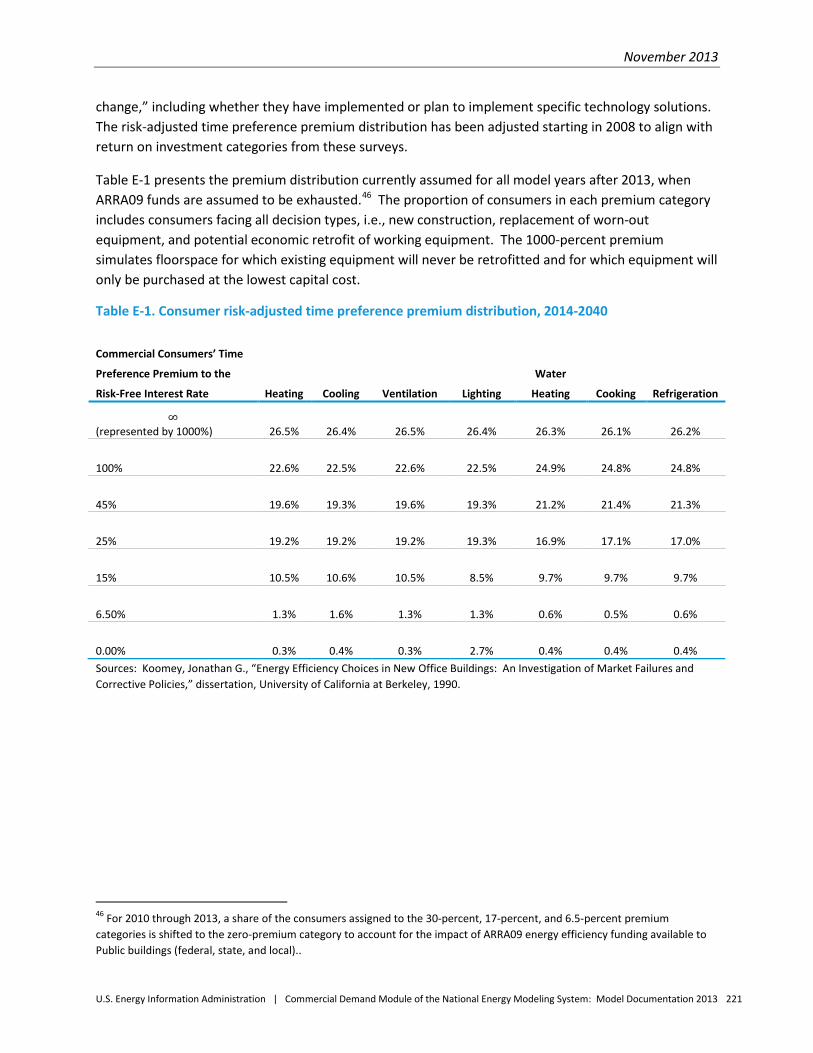
November 2013


change,” including whether they have implemented or plan to implement specific technology solutions. The risk-adjusted time preference premium distribution has been adjusted starting in 2008 to align with return on investment categories from these surveys.

Table E-1 presents the premium distribution currently assumed for all model years after 2013, when ARRA09 funds are assumed to be exhausted.46 The proportion of consumers in each premium category includes consumers facing all decision types, i.e., new construction, replacement of worn-out equipment, and potential economic retrofit of working equipment. The 1000-percent premium simulates floorspace for which existing equipment will never be retrofitted and for which equipment will only be purchased at the lowest capital cost.

Table E-1. Consumer risk-adjusted time preference premium distribution, 2014-2040

Commercial Consumers’ Time

Preference Premium to the

Risk-Free Interest Rate Heating Cooling Ventilation Lighting Water

Heating Cooking Refrigeration

∞ (represented by 1000%) 26.5% 26.4% 26.5% 26.4% 26.3% 26.1% 26.2%

100% 22.6% 22.5% 22.6% 22.5% 24.9% 24.8% 24.8%

45% 19.6% 19.3% 19.6% 19.3% 21.2% 21.4% 21.3%

25% 19.2% 19.2% 19.2% 19.3% 16.9% 17.1% 17.0%

15% 10.5% 10.6% 10.5% 8.5% 9.7% 9.7% 9.7%

6.50% 1.3% 1.6% 1.3% 1.3% 0.6% 0.5% 0.6%

0.00% 0.3% 0.4% 0.3% 2.7% 0.4% 0.4% 0.4% Sources: Koomey, Jonathan G., “Energy Efficiency Choices in New Office Buildings: An Investigation of Market Failures and Corrective Policies,” dissertation, University of California at Berkeley, 1990.

46 For 2010 through 2013, a share of the consumers assigned to the 30-percent, 17-percent, and 6.5-percent premium categories is shifted to the zero-premium category to account for the impact of ARRA09 energy efficiency funding available to Public buildings (federal, state, and local)..

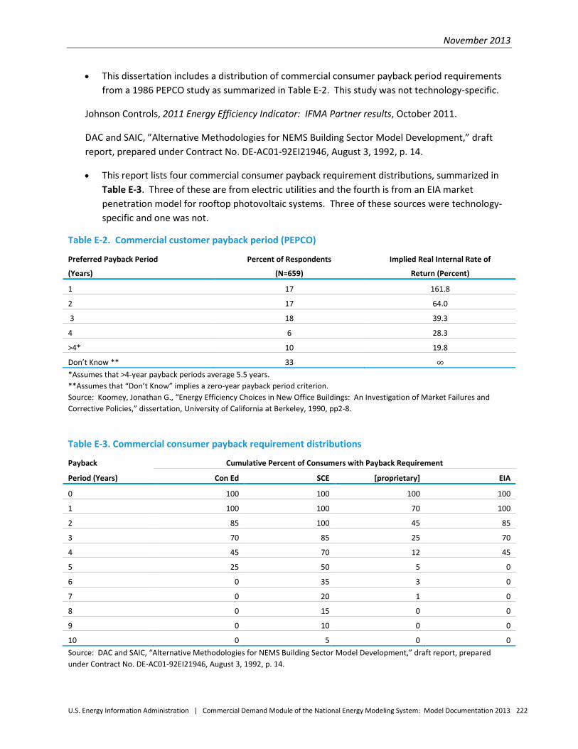
November 2013


• This dissertation includes a distribution of commercial consumer payback period requirements from a 1986 PEPCO study as summarized in Table E-2. This study was not technology-specific.


DAC and SAIC, ”Alternative Methodologies for NEMS Building Sector Model Development,” draft report, prepared under Contract No. DE-AC01-92EI21946, August 3, 1992, p. 14.

• This report lists four commercial consumer payback requirement distributions, summarized in Table E-3. Three of these are from electric utilities and the fourth is from an EIA market penetration model for rooftop photovoltaic systems. Three of these sources were technology-specific and one was not.

Table E-2. Commercial customer payback period (PEPCO)

Preferred Payback Period

(Years)

Percent of Respondents

(N=659)

Implied Real Internal Rate of

Return (Percent)

1 17 161.8

2 17 64.0

3 18 39.3

4 6 28.3

>4* 10 19.8

Don’t Know ** 33 ∞ *Assumes that >4-year payback periods average 5.5 years. **Assumes that “Don’t Know” implies a zero-year payback period criterion. Source: Koomey, Jonathan G., “Energy Efficiency Choices in New Office Buildings: An Investigation of Market Failures and Corrective Policies,” dissertation, University of California at Berkeley, 1990, pp2-8.

Table E-3. Commercial consumer payback requirement distributions

Payback Cumulative Percent of Consumers with Payback Requirement

Period (Years) Con Ed SCE [proprietary] EIA

0 100 100 100 100

1 100 100 70 100

2 85 100 45 85

3 70 85 25 70

4 45 70 12 45

5 25 50 5 0

6 0 35 3 0

7 0 20 1 0

8 0 15 0 0

9 0 10 0 0

10 0 5 0 0 Source: DAC and SAIC, “Alternative Methodologies for NEMS Building Sector Model Development,” draft report, prepared under Contract No. DE-AC01-92EI21946, August 3, 1992, p. 14.

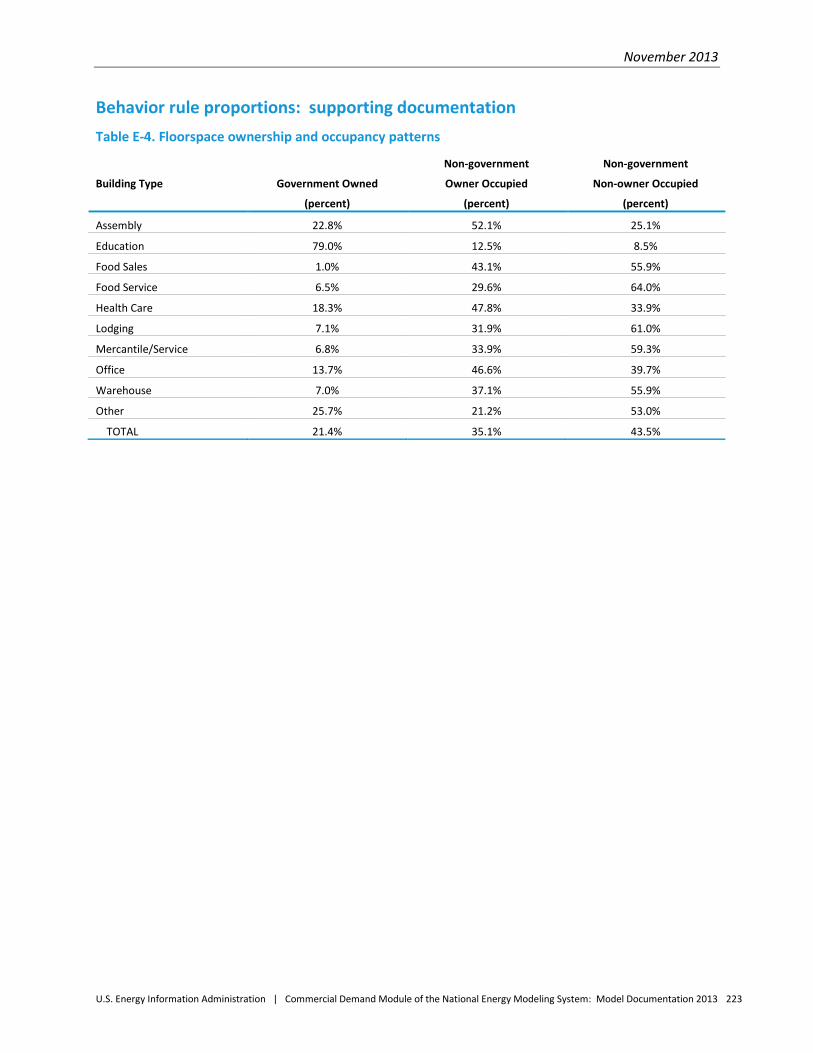
November 2013


Behavior rule proportions: supporting documentation Table E-4. Floorspace ownership and occupancy patterns

Building Type

Government Owned

(percent)

Non-government

Owner Occupied

(percent)

Non-government

Non-owner Occupied

(percent)

Assembly 22.8% 52.1% 25.1%

Education 79.0% 12.5% 8.5%

Food Sales 1.0% 43.1% 55.9%

Food Service 6.5% 29.6% 64.0%

Health Care 18.3% 47.8% 33.9%

Lodging 7.1% 31.9% 61.0%

Mercantile/Service 6.8% 33.9% 59.3%

Office 13.7% 46.6% 39.7%

Warehouse 7.0% 37.1% 55.9%

Other 25.7% 21.2% 53.0%

TOTAL 21.4% 35.1% 43.5%

November 2013


References Building Design + Construction, Green Buildings + Climate Change, Oak Brook, Illinois, November 2008.

Feldman, S., “Why is it So Hard to Sell ‘Savings’ as a Reason for Energy Conservation?” Energy Efficiency: Perspectives on Individual Behavior, Willett Kempton and Max Neiman eds., American Council for an Energy-Efficient Economy, Washington, D.C., 1987.


Komor, P. and R. Katzev, “Behavioral Determinants of Energy Use in Small Commercial Buildings: Implications for Energy Efficiency,” Energy Systems and Policy, Vol. 12, 1988.

Komor, P., and L. Wiggins, “Predicting Conservation Choice: Beyond the Cost-Minimization Assumption,” Energy, Vol. 13, No. 8, 1988.

Koomey, J.. “Energy Efficiency Choices in New Office Buildings: An Investigation of Market Failures and Corrective Policies,” doctoral dissertation, University of California at Berkeley, 1990.

Lamarre, L., “Lighting the Commercial World,” EPRI Journal, December 1989.

Lamarre, L., “New Push for Energy Efficiency,” EPRI Journal, April/May 1990.

Office of Technology Assessment, Building Energy Efficiency, OTS-E-518, U.S. Government Printing Office, Washington, D.C., 1992.

U.S. Department of Energy, U.S. Energy Information Administration, A Look at Commercial Buildings in 1995: Characteristics, Energy Consumption, and Energy Expenditures, DOE/EIA-0625(95), October 1998.

U.S. Department of Energy, U.S. Energy Information Administration, State Energy Data Report 1999, Consumption Estimates, DOE/EIA-0214(99), May 2001.

Vine, E. and J. Harris, “Implementing Energy Conservation Programs for New Residential and Commercial Buildings,” Energy Systems and Policy, Vol. 13, No. 2, 1989.

Documents

Commercial Demand Module of the National Energy Modeling System: Model Documentation 2013 · 2013-11-05 · Commercial Demand Module of the National Energy Modeling System: Model