Combustion and Flame 183 (2017) 88–101

Contents lists available at ScienceDirect

Combustion and Flame

journal homepage: www.elsevier.com/locate/combustflame

A general probabilistic approach for the quantitative assessment of

LES combustion models

Ross Johnson, Hao Wu, Matthias Ihme

∗

Department of Mechanical Engineering, Stanford University, Stanford, CA 94305, United States

a r t i c l e i n f o

Article history:

Received 9 March 2017

Revised 5 April 2017

Accepted 3 May 2017

Available online 23 May 2017

Keywords:

Wasserstein metric

Model validation

Statistical analysis

Quantitative model comparison

Large-eddy simulation

a b s t r a c t

The Wasserstein metric is introduced as a probabilistic method to enable quantitative evaluations of LES

combustion models. The Wasserstein metric can directly be evaluated from scatter data or statistical re-

sults through probabilistic reconstruction. The method is derived and generalized for turbulent reacting

flows, and applied to validation tests involving a piloted turbulent jet flame with inhomogeneous inlets. It

is shown that the Wasserstein metric is an effective validation tool that extends to multiple scalar quan-

tities, providing an objective and quantitative evaluation of model deficiencies and boundary conditions

on the simulation accuracy. Several test cases are considered, beginning with a comparison of mixture-

fraction results, and the subsequent extension to reactive scalars, including temperature and species mass

fractions of CO and CO 2 . To demonstrate the versatility of the proposed method in application to multi-

ple datasets, the Wasserstein metric is applied to a series of different simulations that were contributed

to the TNF-workshop. Analysis of the results allows to identify competing contributions to model devi-

ations, arising from uncertainties in the boundary conditions and model deficiencies. These applications

demonstrate that the Wasserstein metric constitutes an easily applicable mathematical tool that reduce

multiscalar combustion data and large datasets into a scalar-valued quantitative measure.

© 2017 The Combustion Institute. Published by Elsevier Inc. All rights reserved.

s

b

p

fl

fi

t

i

d

t

a

r

c

c

m

i

t

v

m

1. Introduction

A main challenge in the development of models for turbu-

lent reacting flows is the objective and quantitative evaluation of

the agreement between experiments and simulations. This chal-

lenge arises from the complexity of the flow-field data, involv-

ing different thermo-chemical and hydrodynamic quantities that

are typically provided from measurements of temperature, speci-

ation, and velocity. This data is obtained from various diagnos-

tics techniques, including nonintrusive methods such as laser spec-

troscopy and particle image velocimetry, or intrusive techniques

such as exhaust-gas sampling or thermocouple measurements [1–

4] . Instead of directly measuring physical quantities, they are typ-

ically inferred from measured signals, introducing several correc-

tion factors and uncertainties [5] . Depending on the experimen-

tal technique, these measurements are generated from single-point

data, line measurements, line-of-sight absorption, or multidimen-

sional imaging at acquisition rates ranging from single-shot to

high-repetition rate measurements to resolve turbulent dynamics

[6] . This data is commonly processed in the form of statistical re-

∗ Corresponding author.

E-mail addresses: rjohnso2@stanford.edu (R. Johnson), wuhao@stanford.edu (H.

Wu), mihme@stanford.edu (M. Ihme).

c

[

m

i

http://dx.doi.org/10.1016/j.combustflame.2017.05.004

0010-2180/© 2017 The Combustion Institute. Published by Elsevier Inc. All rights reserved

ults from Favre and Reynolds averaging, conditional data, proba-

ility density functions, and scatter data. These data provide im-

ortant information for model evaluation.

Significant progress has been made in simulating turbulent

ows. This progress can largely be attributed to adopting high-

delity large-eddy simulation (LES) for the prediction of unsteady

urbulent flows, and establishing forums for collaborative compar-

sons of benchmark flames that are supported by comprehensive

atabases [7] .

In spite of the increasing popularity of LES, the valida-

ion of combustion models follows previous steady-state RANS-

pproaches, comparing statistical moments (typically mean and

oot-mean-square) and conditional data along axial and radial lo-

ations in the flame. Qualitative comparisons of scatter data are

ommonly employed to examine whether a particular combustion

odel is able to represent certain combustion-physical processes

n composition space that, for instance, are associated with extinc-

ion, equilibrium composition, or mixing conditions. In other in-

estigations, error measures were constructed by weighting mo-

ents and scalar quantities for evaluating the sensitivity of model

oefficients in subgrid models and for uncertainty quantification

8,9] . It is not uncommon that models match particular measure-

ent quantities (such as temperature or major species products)

n certain regions of the flame, while mispredicting the same

.

R. Johnson et al. / Combustion and Flame 183 (2017) 88–101 89

q

fl

d

c

w

c

t

n

m

t

r

p

r

d

t

t

m

p

t

d

m

v

v

t

u

s

s

t

a

m

t

i

S

m

s

m

s

T

m

p

i

s

a

s

r

t

S

2

b

S

t

f

m

s

I

d

r

t

b

s

a

r

o

r

c

[

r

t

p

e

o

e

r

p

W

d

D

d

o

a

m

i

t

t

w

E

m

W

s

d

m

f

f

c

s

W

m

T

v

G

2

t

o

fi

w

m

s

o

uantities in other regions or showing disagreements for other

ow-field data at the same location. Further, the comparison of in-

ividual scalar quantities makes it difficult to consider dependen-

ies and identify correlations between flow-field quantities. Faced

ith this dilemma, such comparisons often only provide an incon-

lusive assessment of the model performance, and limit a quantita-

ive comparison among different modeling approaches. Therefore, a

eed arises to develop a metric that enables a quantitative assess-

ent of combustion models, fulfilling the following requirements:

1. provide a single metric for quantitative model evaluation;

2. combine single and multiple scalar quantities in the validation

metric, including temperature, mixture fraction, species mass

fractions, and velocity;

3. incorporate scatter data from single-shot, high-speed, and si-

multaneous measurements, and enable the utilization of statis-

tical data;

4. enable the consideration of dependencies between measure-

ment quantities; and

5. ensure that the metric satisfies conditions on non-negativity,

identity, symmetry, and triangular inequality.

By addressing these requirements, the objective of this work is

o introduce the probabilistic Wasserstein distance [10] as a met-

ic for the quantitative evaluation of combustion models. Com-

lementing currently employed comparison techniques, this met-

ic possesses the following attractive properties. First, this metric

irectly utilizes the abundance of data from unsteady simulation

echniques and high repetition rate measurement methods. Rather

han considering low-order statistical moments, this metric is for-

ulated in distribution space. As such, it is thereby directly ap-

licable to scatter data that are obtained from transient simula-

ions and high-speed measurements without the need for data re-

uction to low-order statistical moment information. Second, this

etric is able to synthesize multidimensional data into a scalar-

alued quantity, thereby aggregating model discrepancies for indi-

idual quantities. Third, the resulting metric utilizes a normaliza-

ion, thereby enabling the objective comparison of different sim-

lation approaches. Fourth, this method is directly applicable to

ample data that are generated from scatter plots, instantaneous

imulation results or reconstructed from statistical results. Fifth,

he Wasserstein metric enables the consideration of conditional

nd multiscalar data, and is equipped with essential properties of

etric spaces. Finally, this metric can be regarded as a companion

ool to previously established methods for validation of LES and

nstantaneous CFD-simulations.

The remainder of this paper is structured as follows.

ection 2 formally introduces the Wasserstein metric and builds a

athematical foundation for this method. This method is demon-

trated in application to the Sydney piloted jet flame with inho-

ogeneous inlets, and experimental configuration and simulation

etup are described in Section 3 . Results are presented in Section 4 .

o introduce the metric, we first consider a scalar distribution of

ixture fraction and establish a quantitative comparison of ex-

eriments and simulations against presumed closure models. This

s then extended to multiscalar data, involving temperature and

pecies mass fractions. Subsequently, we examine the utility of

pplying the Wasserstein metric to statistical results, rather than

catter data, while Section 5 explores how the Wasserstein met-

ic could add value for directly comparing multiple simulations

o assess different LES modeling approaches. This work finishes in

ection 6 with conclusions.

. Methodology

In this section, the methodology of quantifying the dissimilarity

etween two multivariate distributions (joint PDFs) is discussed.

ince multivariate distributions are commonly used to represent

he thermo-chemical states in turbulent flows, this method is use-

ul for the quantitative assessment of differences between a nu-

erical simulation and experimental data of turbulent flames.

The dissimilarity between two points in the thermo-chemical

tate space can typically be quantified by its Euclidean distance.

n the case of a 1D state space, e.g., temperature, the Euclidean

istance is simply the absolute value of the difference. This met-

ic serves the purpose well for the comparison among two de-

erministic measurements, which can indeed be fully represented

y points in the state space. However, the Euclidean distance falls

hort when measurements are made on random data, e.g., states in

turbulent flow, in which case a single data point can no longer

epresent the measurement and shall be replaced by a distribution

f possible outcomes. Consequently, the dissimilarity between two

andom variables shall be quantified by the “distance” between the

orresponding probability distributions.

Among many definitions of the “distance” between distributions

11,12] , the Wasserstein metric (also known as the Mallows met-

ic) is of interest in this study. Several other methods for quan-

ifying the difference between two distributions have been pro-

osed. However, those methods are either limited to evaluating the

quality of marginal distributions (e.g., Kolmogorov–Smirnov test)

r are incomplete in that they fail to satisfy essential metric prop-

rties (e.g., Kullback–Leibler divergence). The interested reader is

eferred to the survey by Gibbs and Su [11] for a detailed com-

arison between the Wasserstein metric and other candidates. The

asserstein metric represents a natural extension of the Euclidean

istance, which can be recovered as the distribution reduces to a

irac delta function. As such, this metric provides a measure of the

ifference between distributions that resembles the classical idea

f “distance”. The resulting value can be judged and interpreted in

similar fashion as the arithmetic difference between two deter-

inistic quantities.

The Wasserstein metric has been used as a tool for measur-

ng the “distance” between distributions or histograms in the con-

ext of content-based image retrieval [12] , hand-gesture recogni-

ion [13] , and analysis of 3D surfaces [14] , etc. These applications

ere first proposed by Rubner et al. [12] , under the name of the

arth Mover’s Distance (EMD), which is in fact the Wasserstein

etric of order one, W 1 . More recent applications favor the 2nd

asserstein metric by way of Brenier’s theorem [14,15] , which

hows the uniqueness of the optimal solution for the squared-

istance and its connection to differential geometry through which

ore efficient algorithms have been constructed.

This section is primarily concerned with the Wasserstein metric

or discrete distributions in the Euclidean space. This allows us to

ocus on the concepts that are directly related to the practical cal-

ulation and estimation of this metric, and avoid the usage of mea-

ure theory without creating much ambiguity. The definition of the

asserstein metric for general probability measures with more for-

al treatment of the probability theory is discussed in Appendix A .

he interested reader is also referred to books by Villani [16] , sur-

eys by Urbas [17] , and the more recent lectures by McCann and

uillen [18] for further details.

.1. Preliminaries: Monge–Kantorovich transportation problem

The Wasserstein metric is motivated by the classical optimal

ransportation problem first proposed by Monge in 1781 [19] . The

ptimal transportation problem of Monge considers the most ef-

cient transportation of ore from n mines to n factories, each of

hich produces and consumes one unit of ore, respectively. These

ines and factories form two finite point sets in the Euclidean

pace, which are denoted by M and F . The cost of transporting

ne unit of ore from mine x i ∈ M to factory y j ∈ F is denoted by

90 R. Johnson et al. / Combustion and Flame 183 (2017) 88–101

g

c

T

f

s

s

t

t

2

o

t

t

f

e

t

p

p

f

d

r

t

t

w

i

X

m

a

t

S

s

M

i

m

z∣∣

w

d

t

d

b

s

m

r

g

t

c ij , which is chosen by Monge to be the Euclidean distance. The

transport plan can be expressed in the form of an n × n matrix

�, of which the element γ ij represent the amount of ore trans-

ported from x i to y j . The central problem in optimal transporta-

tion is to find the transport plan that minimizes the total cost of

transportation, which is the sum of the costs on n × n available

routes between factories and mines, i.e., ∑ n

i =1

∑ n j=1 γi j c i j . The orig-

inal problem formulated by Monge requires transporting the ore

in its entirety. Therefore, � is constrained to be a permutation ma-

trix, and can only take binary values of 0 or 1. Formally, the Monge

transport problem can be expressed as

min

�

n ∑

i =1

n ∑

j=1

γi j c i j

subject to

n ∑

i =1

γi j =

n ∑

i = j γi j = 1 , γi j ∈ { 0 , 1 } .

(1)

The transport problem in Monge’s formulation can be solved rel-

atively efficient by the Hungarian algorithm proposed by Kuhn

[20] .

In 1942, Kantorovich reformulated Monge’s problem by relaxing

the requirement that all the ore from a given mine goes to a single

factory [21,22] . As a result, the transport plan is modified from be-

ing a permutation matrix to a doubly stochastic matrix. With this,

Monge’s problem is written in the following form:

min

�

n ∑

i =1

n ∑

j=1

γi j c i j

subject to

n ∑

i =1

γi j =

n ∑

i = j γi j = 1 , γi j ≥ 0 .

(2)

This relaxation eliminates the difficulties of Monge’s formulation

in terms of obtaining certain desirable mathematical properties,

such as existence and uniqueness of the optimal transport plan.

The Monge–Kantorovich transportation problem in Eq. (2) can be

solved as the solution to a general linear programming prob-

lem, although more efficient algorithms exists by exploiting special

structures of the problem.

2.2. Wasserstein metric for discrete distributions

The Monge–Kantorovich problem in Eq. (2) not only gives the

solution to the optimal transport problem, but also provides a way

of quantifying the dissimilarity between the distributions of mines

and factories by evaluating the optimal transport cost (normalized

by total mass). The Wasserstein metric [23] follows directly from

this observation.

Consider replacing the mines and factories by two general dis-

crete distributions, whose probability mass functions are:

f (x ) =

n ∑

i =1

f i δ(x − x i ) , g(y ) =

n ′ ∑

j=1

g j δ(y − y i ) , (3)

where ∑ n

i =1 f i =

∑ n ′ j=1 g i = 1 and δ( · ) denotes the Kronecker delta

function:

δ(x ) =

{1 if x = 0 ,

0 if otherwise . (4)

The unit cost of transport between x i and y j is defined to be the

p th power of the Euclidean distance, i.e. c i j = | x i − y j | p . In addition,

the “mass” of probabilities f i and g j is no longer restricted to be

unity and the possible outcomes of the distributions, i.e. x i and y j ,

are points in an Euclidean space whose dimension is not restricted.

The p th Wasserstein metric between discrete distributions f and

is defined to be the p th root of the optimal transport cost for the

orresponding Monge–Kantorovich problem:

W p ( f, g) = min

�

( n ∑

i =1

n ′ ∑

j=1

γi j | x i − y j | p )1 /p

subject to

n ′ ∑

j=1

γi j = f i ,

n ∑

i =1

γi j = g j , γi, j ≥ 0 .

(5)

he constraints in Eq. (5) ensure that the total mass transported

rom x i and the total mass transported to y j match f i and g j , re-

pectively.

The Wasserstein metric for continuous distributions is pre-

ented in Appendix A . The estimation and calculation for the con-

inuous case and for higher-dimensional problems are discussed in

he next section.

.3. Non-parametric estimation of W p through empirical distributions

Two major difficulties arise in obtaining the Wasserstein metric

f two multivariate distributions of thermo-chemical states. One is

hat the multivariate distributions are not readily available from ei-

her experiments or simulations. Instead, a series of samples drawn

rom these distributions is provided. The other is that there is no

asy way of calculating W p for continuous multivariate distribu-

ions, especially for those of high dimensions. To overcome these

roblems, a non-parametric estimation of W p is devised using em-

irical distributions.

An empirical distribution is a random discrete distribution

ormed by a sequence of independent samples drawn from a given

istribution of interest. Let (X 1 , . . . , X n ) b e a set of n independent

andom samples obtained from a continuous multivariate distribu-

ion f . The empirical (or fine-grained [24] ) distribution

f is defined

o be

f n (x ) =

1

n

n ∑

i =1

δ(x − X i ) , (6)

hich is a discrete distribution with equal weights. The empir-

cal distribution is random as it depends on random samples,

i . The samples may be obtained from experimental measure-

ents or generated from a given distribution using, for instance,

n acceptance-rejection method [25] . Calculation of W p between

wo empirical distributions is identical to the method discussed in

ection 2.2 . Its procedure and cost is independent of the dimen-

ionality of the distributions.

The empirical distribution converges to the original distribution.

ost importantly, in the context of this study, is the convergence

n the Wasserstein metric [26] . More specifically, the Wasserstein

etric between empirical and original distributions converges to

ero in probability. Given the metric property of W p :

W p ( f n , g n ′ ) − W p ( f, g) ∣∣ ≤ W p ( f n , f ) + W p ( g n ′ , g) , (7)

hich ensures that the Wasserstein metric between two empirical

istributions also converges in probability to that of the actual dis-

ribution. In addition, the mean rates of convergence for empirical

istributions have also been established [27,28] , giving the upper

ound on the expectation, E (W

p p (

f n , f ) ), as n increases. For the

imilar reason, the convergence rate for the non-parametric esti-

ation follows. The exact rates depend on the dimensionality and

egularity conditions of the distributions. For details on the conver-

ence rate for more general cases, the interested reader is referred

o the work by Fournier and Guillin [28] .

R. Johnson et al. / Combustion and Flame 183 (2017) 88–101 91

m

E

w

d

l

E

w

t

p

f

m

o

t

p

a

2

d

e

r

W

v

v

fi

r

t

p

S

k

t

o

t

g

H

c

f

b

a

m

o

g

n

t

w

f

I

|

I

a

t

c

s

i

r

o

s

d

a

s

2

c

l

P

a

u

o

p

s

m

t

i

c

In the case of d -dimensional distributions that have sufficiently

any moments, we have:

(W

2 2 (

f n , f ) )

≤ C ×

⎧ ⎨

⎩

n

−1 / 2 if d < 4 ,

n

−1 / 2 log (1 + n ) if d = 4 ,

n

−2 /d if d > 4 ,

(8)

here the value of C depends on the distribution f and is indepen-

ent of n . By combining this result with Eq. (7) , we obtain the fol-

owing convergence rate for the non-parametric estimation of W 2 :

(W 2 (

f n , g n ′ ) − W 2 ( f, g) )2 ≤ C ×

⎧ ⎪ ⎨

⎪ ⎩

n

−1 / 2 ∗ if d < 4 ,

n

−1 / 2 ∗ log (1 + n ∗) if d = 4 ,

n

−2 /d ∗ if d > 4 ,

(9)

here n ∗ = min (n, n ′ ) . With this, all necessary results that ensure

he soundness of using W p ( f n , g n ′ ) as an estimator for W p ( f , g ) are

resented.

In addition to the rate of convergence, statistical inference and

urther quantification of uncertainties for the non-parametric esti-

ation of W p can also be performed. For instance, the magnitude

f the uncertainty in Eq. (9) and the corresponding confidence in-

erval can be estimated via the method of bootstrap [29,30] . In

articular, it was shown that the m -out- n bootstrap [31] can be

pplied to the Wasserstein metric [32,33] .

.4. Statistically most likely reconstruction of distributions

So far, the evaluation of the Wasserstein metric using sample

ata as empirical distribution function has been described. How-

ver, the usage of the Wasserstein metric is not limited to results

eported in such fashion. In the following, the computation of the

asserstein metric from statistical results will be discussed. This

ersatility is important to the metric, given the fact that the con-

entional practice of reporting only the statistics, predominantly

rst and second moments, is still the prevailing one.

The procedure of applying the Wasserstein metric to statistical

esults is to first reconstruct the multivariate distribution from sta-

istical results. An empirical distribution is then sampled to com-

ute the Wasserstein metric following the method described in

ection 2.5 . The reconstruction of a continuous PDF from a set of

nown statistical models can be performed using the concept of

he statistically most likely distribution (SMLD) [34,35] . The SMLD

f a d -dimensional random variable is defined to be the distribu-

ion that maximizes the relative entropy, given a prior distribution

( x ), under a given set of constraints:

f SML (x ) = argmax f (·)

∫ R

d

f (x ) ln

(f (x )

g(x )

)dx

subject to

∫ R

d

f (x ) dx = 1 , ∫ R

d

T (x ) f (x ) dx = t . (10)

ere, T ( x ) is the set of statistical moments that are selected as

onstraints, and t is the vector of corresponding values obtained

rom the data. The type of the so obtained distribution is dictated

y the form of the constraints [36] . For instance, if the multivari-

te distribution is constructed using only the first and second mo-

ents with a uniform prior, a multivariate normal distribution is

btained. In addition, if only the marginal second moments are

iven while the cross moments are not, the obtained multivariate

ormal distributions are uncorrelated. More specifically, if

g(x ) ≡ 1 ,

T (x ) = [ x 1 , x 2 , . . . , x d , x

2 1 , x

2 2 , . . . , x

2 d ] ,

(11)

he SMLD becomes

f SML (x ) =

d ∏

k =1

1 √

2 πσ2 k

exp

{− (x k − μk )

2

2 σ2 k

}, (12)

here μk = x k and σ2 k

= x 2 k

− x k 2 .

After obtaining the SMLDs, the sets of samples can be drawn

rom them and the Wasserstein metric can be directly calculated.

n addition, the metric property implies the following inequality

W p ( f SML , g SML ) − W p ( f, g) | ≤ W p ( f SML , f ) + W p (g SML , g) . (13)

n other words, the difference in the Wasserstein metrics of the

ctual distributions, f and g , and that of the reconstructed coun-

erparts, f SML and g SML , are bounded by the error of the SMLD re-

onstruction, which themselves can be quantified by the Wasser-

tein metric. In the current study, the set of constraints are lim-

ted to the marginal first and second moments, which are typically

eported in the literature. More accurate reconstructions can be

btained by including high-order and cross moments. In addition,

tatistics of other forms may also be considered. For instance, β-

istributions can be recovered for constraints in the form of ln (x )

nd ln (1 − x ) , which is potentially more appropriate for conserved

calars such as mixture fraction.

.5. Calculation procedure

In the present study, the 2nd Wasserstein metric is used. The

omputation of the metric can be realized by any general-purpose

inear programming tool. For the present analysis, the program by

ele and Werman [37] is used. It calculates the Wasserstein metric

s a flow-min-cost problem (a special case of linear programming)

sing the successive shortest path algorithm [38] . A pseudo code

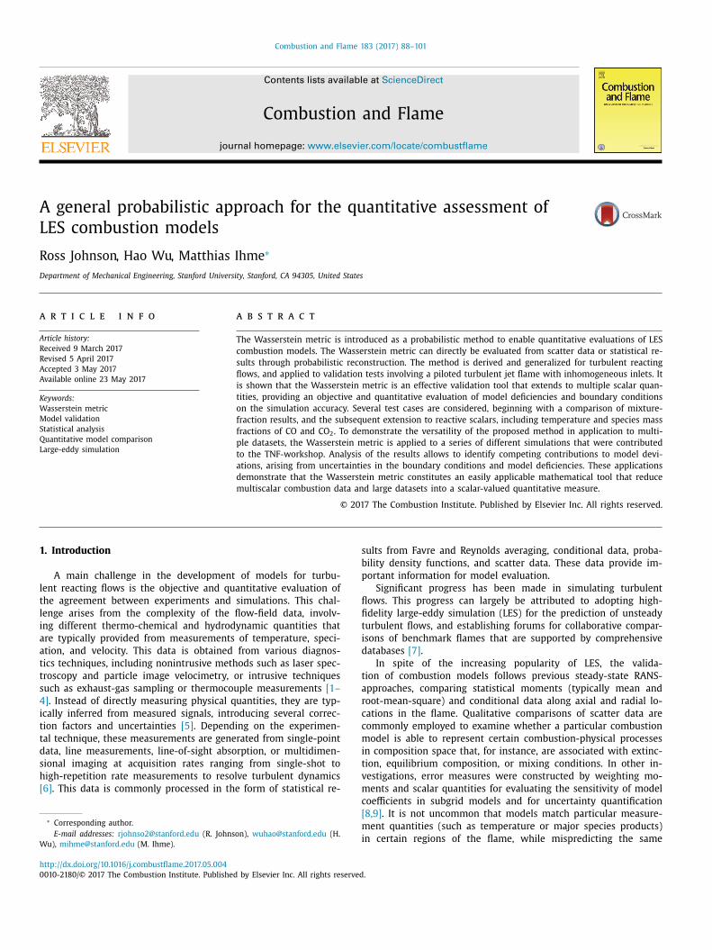
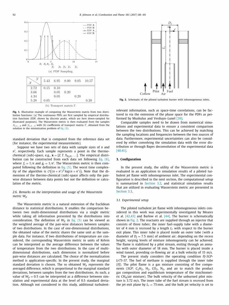
f the corresponding algorithm is given in Algorithm 1 , and Fig. 1

rovides an illustrative example for the evaluation of the Wasser-

tein metric. The source code for the evaluation of the Wasserstein

etric is provided in Appendix B .

Algorithm 1: Pseudo code for evaluating the Wasserstein met-

ric.

Input : Two sets of d-dimensional data representing empirical

distribution functions: X , Y , with lengths n and n ′ from scatter data or sampled from continuous

distribution functions

Preprocessing : Normalize X and Y by standard deviation of

one data set, σx

for i = 1 : n do

for j = 1 : n ′ do

Evaluate pair-wise distance matrix

c i, j =

∑ d k =1

(X k,i − Y k, j

)2 ;

end

end

Compute Wasserstein metric and transport matrix as solution

to minimization problem of Eq. (5) using the shortest path

algorithm by Pele & Werman [37] with input c i, j

Output : Wasserstein metric: W 2

In this context, it is important to note that the input data to

he Wasserstein metric are normalized to enable a direct compar-

son and enable a physical interpretation of the results. A natural

hoice is to normalize each sample-space variable by its respective

92 R. Johnson et al. / Combustion and Flame 183 (2017) 88–101

Fig. 1. Illustrative example of computing the Wasserstein matrix from two distri-

bution functions: (a) The continuous PDFs are first sampled by empirical distribu-

tion functions (EDF, shown by discrete peaks, which are here down-sampled for

illustrated purposes). The Wasserstein metric is then evaluated from the samples

X i =1 , ... , 4 and Y i =1 , ... , 5 with (b) coefficients of transport matrix �, obtained from the

solution to the minimization problem of Eq. (5) .

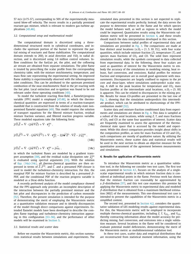
Fig. 2. Schematic of the piloted turbulent burner with inhomogeneous inlets.

r

t

f

l

b

t

d

e

t

[

3

e

b

fi

i

t

S

3

s

e

s

c

t

e

d

h

T

l

w

L

(

n

g

r

t

t

standard deviation that is computed from the reference data set

(for instance, the experimental measurements).

Suppose we have two sets of data with sample sizes of n and

n ′ , respectively. Each sample represents a point in the thermo-

chemical (sub)-space, e.g., x = [ Z, T , Y H 2 O , . . . ] . The empirical distri-

bution can be constructed from each data set following Eq. (6) ,

where f i = 1 /n and g i = 1 / n ′ . The Wasserstein metric is then com-

puted following the definition in Eq. (5) . The worst time complex-

ity of the algorithm is O

((n + n ′ ) 3 log (n + n ′ )

). Note that the di-

mension of the thermo-chemical (sub)-space affects only the pair-

wise distance between data points but not the definition or calcu-

lation of the metric.

2.6. Remarks on the interpretation and usage of the Wasserstein

metric W p

The Wasserstein metric is a natural extension of the Euclidean

distance to statistical distributions. It enables the comparison be-

tween two multi-dimensional distributions via a single metric

while taking all information presented by the distributions into

consideration. The definition of W p in Eq. (5) can be viewed as

the weighted average of the pair-wise distances between samples

of two distributions. In the case of one-dimensional distributions,

the obtained value of the metric shares the same unit as the sam-

ple data. For instance, if two distributions of temperature are con-

sidered, the corresponding Wasserstein metric in units of Kelvin

can be interpreted as the average difference between the values

of temperature from the two distributions. In the case of multi-

dimensional distributions, each dimension is normalized before

pair-wise distances are calculated. The choice of the normalization

method is application-specific. In the present study, the marginal

standard deviation is chosen. The so obtained W p represents the

averaged difference, which is proportional to the marginal standard

deviations, between samples from the two distributions. As such, a

value of W p = 0 . 5 can be interpreted as a difference between sim-

ulation and experimental data at the level of 0.5 standard devia-

tion. Although not considered in this study, additional turbulent-

elevant information, such as space-time correlations, can be fac-

ored in via the extension of the phase space for the PDFs as per-

ormed by Muskulus and Verduyn–Lunel [39] .

Comparable samples need to be drawn from numerical simu-

ations and experimental data to ensure a consistent comparison

etween the two distributions. This can be achieved by matching

he sampling locations and frequencies between the two sources of

ata. Furthermore, experimental uncertainties can also be consid-

red by either convolving the simulation data with the error dis-

ribution or through Bayes deconvolution of the experimental data

40,41] .

. Configuration

In the present study, the utility of the Wasserstein metric is

valuated in an application to simulation results of a piloted tur-

ulent jet flame with inhomogeneous inlet. The experimental con-

guration is described in the next section, the computational setup

s summarized in Section 3.2 , and statistical simulation results

hat are utilized in evaluating Wasserstein metric are presented in

ection 3.3 .

.1. Experimental setup

The piloted turbulent jet flame with inhomogeneous inlets con-

idered in this work was experimentally investigated by Meares

t al. [42,43] and Barlow et al. [44] . The burner is schematically

hown in Fig. 2 . The reactants are supplied through an injector that

onsists of three tubes; the inner fuel-supply tube with a diame-

er of 4 mm is recessed by a length L r with respect to the burner

xit plane. This inner tube is placed inside an outer tube (with a

iameter of D J = 7 . 5 mm) of ambient air; depending on the recess

eight, varying levels of mixture inhomogeneity can be achieved.

he flame is stabilized by a pilot stream, exiting through an annu-

us with outer diameter of 18 mm. The burner is placed inside a

ind tunnel, providing co-flowing air at a bulk velocity of 15 m/s.

The present study considers the operating condition FJ-5GP-

r75-57 . The fuel of methane is supplied through the inner tube

FJ ). The pilot flame is a gas mixture consisting of five compo-

ents ( 5GP : C 2 H 2 , H 2 , CO 2 , N 2 , and air to match the product

as composition and equilibrium temperature of the stoichiomet-

ic CH 4 /air mixture). The bulk velocity of the unburned pilot mix-

ure is 3.72 m/s. The inner tube of the fuel stream is recessed from

he jet exit plane by L r = 75 mm , and the bulk jet velocity is set to

R. Johnson et al. / Combustion and Flame 183 (2017) 88–101 93

5

s

r

p

3

d

c

t

d

r

fl

a

i

c

m

fl

i

c

t

r

v

c

m

p

o

m

T

ρ

ρ

ρ

i

p

i

o

p

u

m

P

m

t

t

h

[

o

a

o

t

p

i

m

3

r

s

c

p

t

c

i

s

s

f

q

s

s

f

u

b

l

f

s

c

i

f

i

fi

F

a

c

m

a

o

a

c

m

t

s

W

b

q

a

4

t

c

s

s

t

a

a

β

t

i

s

t

F

m

t

d

t

e

t

a

7 m/s ( Lr75-57 ), corresponding to 50% of the experimentally mea-

ured blow-off velocity. The recess results in a partially premixed

eactant-gas mixture, which is relevant to modern gas-turbine ap-

lications [45,46] .

.2. Computational setup and mathematical model

The computational domain is discretized using a three-

imensional structured mesh in cylindrical coordinates, and in-

ludes the upstream portion of the burner to represent the par-

ial mixing of reactants and flame stabilization. The computational

omain extends to 20 D J in axial direction and 15 D J in radial di-

ection, and is discretized using 1.6 million control volumes. In-

ow conditions for the fuel/air jet, the pilot, and the coflowing

ir stream are obtained from separate simulations. The pilot flame

s treated by prescribing the scalar profile from the corresponding

hemistry table, with the mixture stoichiometry, temperature, and

ass flow rate representing the experimental setting. An improved

ame stability is experimentally observed with the inhomogeneous

nlet conditions. This can be attributed to the upstream premixed

ombustion of the near-stoichiometric fluid in the jet reacting with

he hot pilot. Local extinction and re-ignition was found to be not

elevant under these operating conditions [43] .

To model the turbulent reacting flow-field, a flamelet/progress

ariable (FPV) model is employed [47,48] , in which the thermo-

hemical quantities are expressed in terms of a reaction-transport

anifold that is constructed from the solution of steady-state non-

remixed flamelet equations [49] . This model requires the solution

f transport equations for the filtered mixture fraction, residual

ixture fraction variance, and filtered reaction progress variable.

hese modeled equations take the following form:

˜ D t Z = ∇ · ( ρ˜ α∇

Z ) + ∇ · τres ˜ Z , (14a)

˜ D t Z ′′ 2 = ∇ · ( ρ˜ α∇

Z ′′ 2 ) + ∇ · τres ˜ Z ′′ 2 − 2 ρ ˜ u

′′ Z ′′ · ∇

Z − ρ˜ χ res Z ,

(14b)

˜ D t C = ∇ · ( ρ˜ α∇

C ) + ∇ · τres ˜ C + ρ˜ ˙ ω C , (14c)

n which the turbulent fluxes are modeled by a gradient trans-

ort assumption [50] , and the residual scalar dissipation rate ˜ χ res Z

s evaluated using spectral arguments [51] . With the solution

f Eqs. (14a)-(14c) , all thermo-chemical quantities are then ex-

ressed in terms of ˜ Z , Z ′′ 2 , and

˜ C , and a presumed PDF-closure is

sed to model the turbulence-chemistry interaction. For this, the

arginal PDF for mixture fraction is described by a presumed β-

DF, and the conditional PDF of the reaction progress variable is

odeled as a Dirac-delta function.

A recently performed analysis of the model compliance showed

hat the FPV-approach only provides an incomplete description of

he interaction between the partially premixed mixture and the

ot pilot and discrepancies in the prediction of carbon monoxide

52] . Therefore, the present simulation is intended for the purpose

f demonstrating the merit of employing the Wasserstein metric

s a quantitative validation measure and to identify discrepancies

f the model through direct comparisons against experiments. Ex-

ended flamelet models have been developed to describe the com-

lex flame topology and turbulence-chemistry interaction appear-

ng in this configuration [53–56] , and the performance of other

odels will be examined in Section 5 .

.3. Statistical results and scatter data

Before we examine the Wasserstein metric, this section summa-

izes statistical results between simulations and experiments. The

imulated data presented in this section is not expected to repli-

ate the experimental results perfectly. Instead, the data serves the

urpose to determine where in the flame and for which species

he model behaves well, as well as regions in which the model

ould be improved. Quantitative results using the Wasserstein val-

dation metric will be presented in Section 4 , and these results

hould match the data interpretation developed in this section.

Comparisons between radial profiles of experimental data and

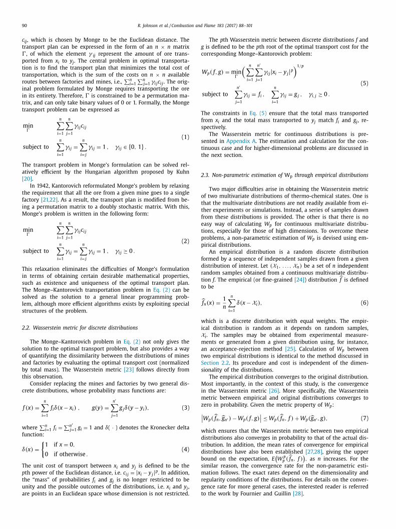
imulations are provided in Fig. 3 . The comparisons are made at

our distinct axial locations ( x/D J = { 1 , 5 , 10 , 15 } ), with four scalar

uantities, which include mixture fraction ( Z ), temperature ( T ), and

pecies mass fractions of CO 2 and CO. The solid lines represent

imulation results, while the symbols correspond to data collected

rom experimental data. In the following, these four scalars are

sed as quantities of interest for the Wasserstein metric to em-

ody the accuracy of the simulations in modeling mixing, heat re-

ease, fuel conversion, and emissions. Radial profiles for mixture

raction and temperature are in overall good agreement with mea-

urements. Discrepancies are largely confined to regions in the jet

ore and shear-layer, where simulations underpredict scalar mix-

ng. A shift in the peak location for temperature and CO 2 mass

raction profiles at the intermediate axial locations, x/D J = { 5 , 10 }s apparent. This can be related to discrepancies in the mixing pro-

le. Results for mean CO-profiles are presented in the last row of

ig. 3 , showing that the simulation underpredicts this intermedi-

te product, which can be attributed to shortcomings of the FPV-

ombustion model [52] .

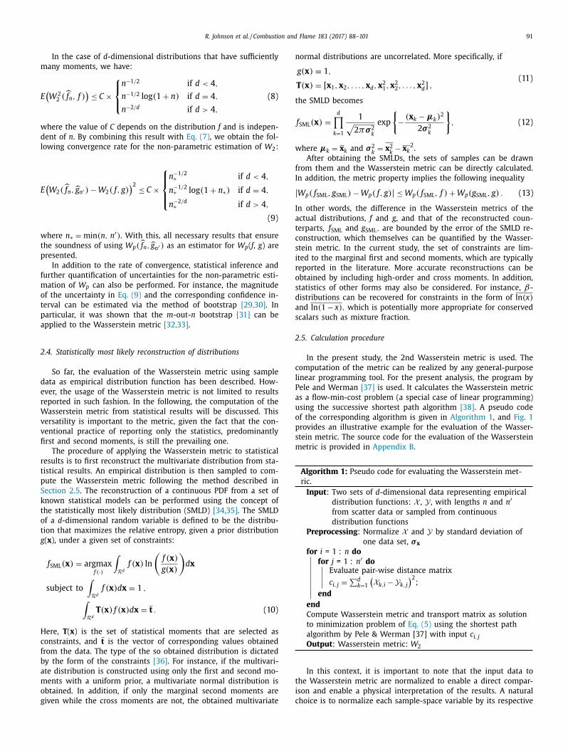
Scatter data and mixture-fraction conditioned data from experi-

ents and simulations are shown in Fig. 4 . This data is sampled at

subset of the axial locations, while using Z , T , and mass fractions

f CO 2 and CO as the same four quantities of interest. Scatter data

re frequently examined to assess the agreement of the thermo-

hemical state space that is accessed by the model and experi-

ent. While this direct comparison provides insight about shifts in

he composition profiles, as seen for mass fractions of CO and CO 2 ,

uch comparisons are mostly of qualitative nature. By utilizing the

asserstein metric, these scatter data and statistical results will

e used in the next section to obtain an objective measure for the

uantitative assessment of the agreement between measurements

nd simulations.

. Results for application of Wasserstein metric

To introduce the Wasserstein metric as a quantitative valida-

ion tool, in the following we consider two test cases. The first test

ase, presented in Section 4.1 , focuses on the analysis of a single-

calar experimental results in which mixture fraction data is con-

idered at individual points in the flame. Previous work has shown

hat the mixture fraction can reasonably be approximated by

β-distribution [57] , and this test case examines this premise by

pplying the Wasserstein metric to experimental data and modeled

-distribution that is obtained from a maximum likelihood estima-

ion (MLE) of the measurements. This one-dimensional test case is

ntended to present the capabilities of the Wasserstein metric in a

implified context.

The second test, presented in Section 4.2 , considers the quanti-

ative validation of LES modeling results against experimental data.

or this, the Wasserstein metric will be employed to incorporate

ultiple thermo-chemical quantities, including Z , T , Y CO 2 , and Y CO ,

hereby contracting information about the model accuracy for pre-

icting mixing, fuel conversion, and emissions into a single valida-

ion measure. Several locations in the flame will be considered to

valuate potential model deficiencies, demonstrating the merit of

he Wasserstein metric as multidimensional validation tool.

In these test cases, scatter data and empirical distributions that

re reconstructed from statistical moment information, using the

94 R. Johnson et al. / Combustion and Flame 183 (2017) 88–101

Fig. 3. Comparison of radial profiles between experimental measurements and simulations at x/D J = { 1 , 5 , 10 , 15 } . Variables considered include mixture fraction, temperature,

and species mass fractions of CO 2 and CO.

o

e

a

w

d

x

p

t

a

A

i

t

t

p

t

t

q

h

a

method presented in Section 2.4 , are considered to examine the

accuracy of both methods.

4.1. Conserved scalar results

Previous investigations have shown that the evolution of con-

served scalars in two-stream systems can be approximated by

a β-distribution [57] , and a Dirichlet-distribution as a multivari-

ate generalization of the β-distribution provides a description of

turbulent scalar mixing in multistream flows [53] . This section ex-

amines the accuracy of representing the conserved scalar by a pre-

sumed PDF using the Wasserstein metric as a quantitative metric.

To simplify the analysis, this study focuses on data collected at

the axial locations introduced previously ( x/D J = { 1 , 5 , 10 , 15 } ) and

a set of four radial positions located at r/D J = { 0 , 0 . 5 , 0 . 85 , 1 . 2 } .The axial positions are spaced uniformly, whereas the radial po-

sitions represent key locations in the burner geometry. Specifically,

these four radial locations correspond approximately to the center

of the fuel stream, the outer edge of the air stream, the midpoint

of the pilot, and the outer edge of the pilot, respectively. Although

these sixteen measurement locations were chosen for the analysis,

it is possible to apply the Wasserstein metric at any location in the

flame and generate similar results.

PDFs for mixture fraction, represented by the histograms in

Fig. 5 , provide the experimental distribution for all of the points

f interest. Superimposed over each plot is a maximum likelihood

stimation of this data using the β-distribution [58] , whose prob-

bility distribution function reads

f (x ; a, b) =

�(a + b)

�(a )�(b) x a −1 (1 − x ) (b−1) , (15)

here �( · ) is the gamma function. Suppose that there are n in-

ependent samples drawn from a β-distribution, whose values are

1 , x 2 , . . . , x n , the method of maximum likelihood estimates the

arameters a and b by finding the arguments of the maxima for

he logarithmic likelihood function,

, b = arg max a,b

n ∑

i =1

log ( f (x i ; a, b)) . (16)

lthough the best-fit β-distribution provides a reasonable approx-

mation for the data, there still are noticeable differences between

he experimental data and the MLE-fit. These differences are quan-

itatively expressed through the Wasserstein metric, and the com-

uted values are reported at the top of each histogram in Fig. 5 .

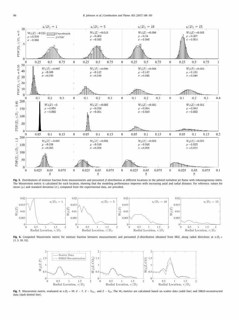
The quantitative evaluation of the Wasserstein metric shows

hat largest deviations between experimental and presumed dis-

ributions occur within the fuel jet near the nozzle exit. These

uantitative results are corroborated with an interpretation of the

istograms. The largest deviations between the MLE β-distribution

nd measurements occur near the nozzle inlet, corresponding to

R. Johnson et al. / Combustion and Flame 183 (2017) 88–101 95

Fig. 4. Qualitative comparison of scatter profiles between measurements and simulations at x/D J = { 1 , 5 } . Variables including temperature, and species mass fractions of CO 2 and CO are plotted against mixture fraction. Conditional mean results are laid over the scatter data.

r

t

o

s

d

t

p

s

A

m

l

s

t

p

c

a

s

n

t

d

t

t

t

t

e

t

s

F

s

a

m

m

i

d

o

t

a

c

4

p

w

t

a

a

r

f

i

W

s

c

m

d

Z

i

a

r

T

a

e

f

egions of high turbulence and strong mixing. Note that the magni-

ude of the Wasserstein metric, W 2 ( Z ), is provided in natural units

f mixture fraction, which is bounded to the interval [0, 1]. As

uch, the metric provides an integral physical interpretation of the

ifferences between both distributions.

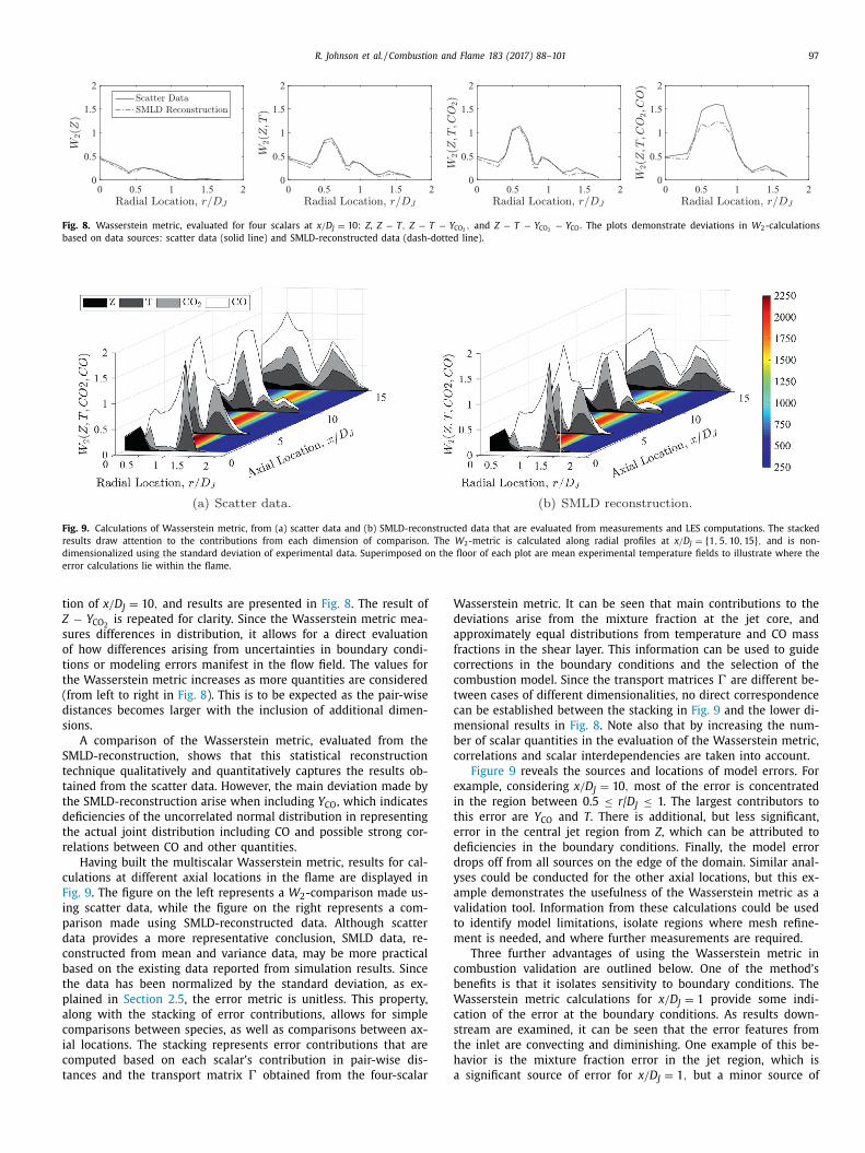
In the next step, we employ the Wasserstein metric to evaluate

he accuracy of the presumed β-distribution along several radial

rofiles. For this, a total of 86 uniformly spaced points are con-

idered along the four axial measurement stations used previously.

t each point, a β-distribution is constructed from the measure-

ents using the maximum likelihood estimate, from which calcu-

ations of the Wasserstein metric are performed subsequently. Re-

ults are presented in Fig. 6 , and they show that the agreement of

he β-distribution with the experimentally determined PDFs im-

roves with increasing axial and radial distance. This observation

orroborates the findings from the point-wise analysis in Fig. 5 ,

nd agrees with physical expectation that with increasing down-

tream distance the mixture composition approaches a homoge-

eous state. The low absolute error values of W 2 < 0.02 compared

o the [0,1] range of mixture fraction shows that, overall, the β-

istribution provides an adequate representation of the experimen-

ally determined mixture fraction data.

While this test case qualitatively affirms that the mixture frac-

ion PDF follows a β-distribution, it also demonstrates three key

raits of the Wasserstein metric. First, the quantitative nature of

he Wasserstein metric allows for direct comparisons between sev-

ral distributions, simultaneously. For example, it is much easier

o compare the four distributions at x/D J = 1 using the Wasser-

tein metric results, as opposed to analyzing their differences in

ig. 5 directly. The Wasserstein metric also provides a compari-

on in distribution space. It therefore contains information about

ll moments, and is not limited to low-order moments such as

ean and root-mean square quantities. Finally, the Wasserstein

etric is applicable to any location in the flow, thereby provid-

e

ng fine-grained information about the simulation accuracy, model

eficiencies in predicting certain scalar quantities, and the impact

f inconsistencies of boundary conditions on the simulation. These

hree fundamental features will be emphasized and built upon

s Section 4.2 considers the multidimensional validation of a LES

ombustion model using experimental data.

.2. Multiscalar results

Having provided a comparison for the Wasserstein metric ap-

lied to mixture fraction as a single scalar, this second test case

ill demonstrate the application of the Wasserstein metric to mul-

iple scalars in the form of joint scalar distributions. This property

llows for multiple, simultaneous error calculations, which provide

multifaceted, quantitative validation. Here, the Wasserstein met-

ic is used to compare simulation results with experimental data

or the piloted jet flame with inhomogeneous inlets as discussed

n Section 3 .

To quantitatively assess a combustion simulation, a multiscalar

asserstein metric can be evaluated that takes into account d

calar quantities. In the present cases, four scalar quantities are

onsidered, namely mixture fraction, temperature, and species

ass fractions of CO 2 and CO, and evaluations are performed at

ifferent axial locations in the jet flame.

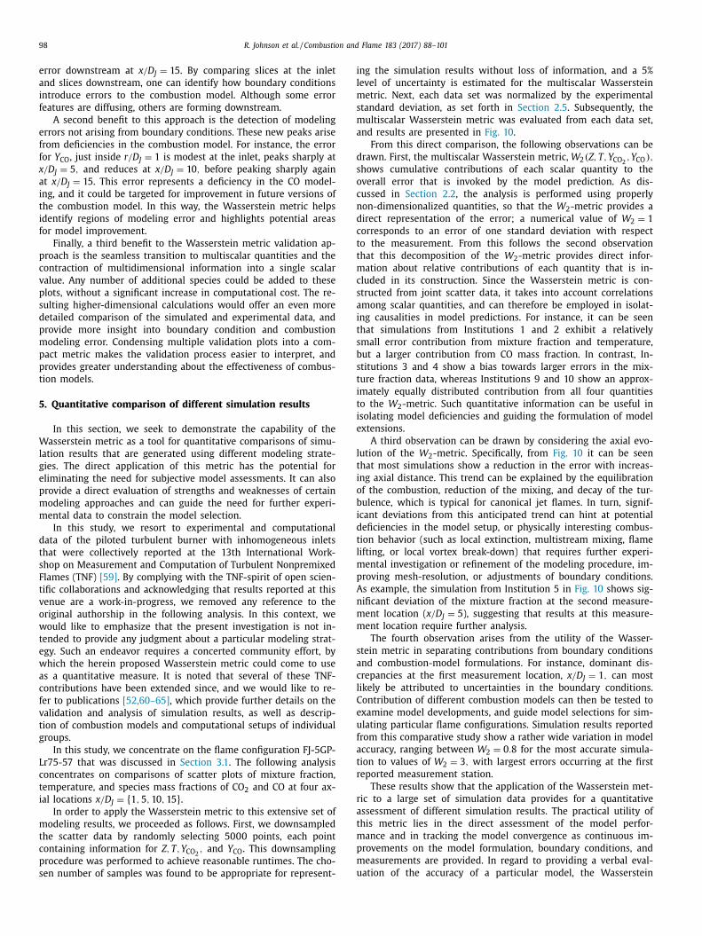
The W 2 -metrics at x/D J = 10 for three two-scalar cases: Z − T ,

− Y CO 2 , and Z − Y CO are shown in Fig. 7 . The W 2 -metric of sim-

lar magnitude and radial profile are found in the cases of Z − T

nd Z − Y CO 2 , in which there is little discrepancy between the

esults obtained from the scatter data and SMLD reconstruction.

he Z − Y CO case exhibits a much higher level of W 2 . There is

lso greater difference between the values from two sources of

xperimental results. We then examine how the W 2 -metric is af-

ected by increasing the number of scalars that is included in its

valuation. For this, we consider results at the same axial loca-

96 R. Johnson et al. / Combustion and Flame 183 (2017) 88–101

Fig. 5. Distributions of mixture fraction from measurements and presumed β-distribution at different locations in the piloted turbulent jet flame with inhomogeneous inlets.

The Wasserstein metric is calculated for each location, showing that the modeling performance improves with increasing axial and radial distance. For reference, values for

mean ( μ) and standard deviation ( σ ), computed from the experimental data, are provided.

Fig. 6. Computed Wasserstein metric for mixture fraction between measurements and presumed β-distribution obtained from MLE, along radial directions at x/D J =

{ 1 , 5 , 10 , 15 } .

Fig. 7. Wasserstein metric, evaluated at x/D J = 10 : Z − T, Z − Y CO 2 , and Z − Y CO . The W 2 -metrics are calculated based on scatter data (solid line) and SMLD-reconstructed

data (dash-dotted line).

R. Johnson et al. / Combustion and Flame 183 (2017) 88–101 97

Fig. 8. Wasserstein metric, evaluated for four scalars at x/D J = 10 : Z , Z − T, Z − T − Y CO 2 , and Z − T − Y CO 2 − Y CO . The plots demonstrate deviations in W 2 -calculations

based on data sources: scatter data (solid line) and SMLD-reconstructed data (dash-dotted line).

(a) Scatter data. (b) SMLD reconstruction.

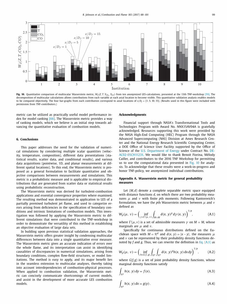
Fig. 9. Calculations of Wasserstein metric, from (a) scatter data and (b) SMLD-reconstructed data that are evaluated from measurements and LES computations. The stacked

results draw attention to the contributions from each dimension of comparison. The W 2 -metric is calculated along radial profiles at x/D J = { 1 , 5 , 10 , 15 } , and is non-

dimensionalized using the standard deviation of experimental data. Superimposed on the floor of each plot are mean experimental temperature fields to illustrate where the

error calculations lie within the flame.

t

Z

s

o

t

t

(

d

s

S

t

t

t

d

t

r

c

F

i

p

d

c

b

t

p

a

c

i

c

t

W

d

a

f

c

c

t

c

m

b

c

e

i

t

e

d

d

y

a

v

t

m

c

b

W

c

s

t

h

a

ion of x/D J = 10 , and results are presented in Fig. 8 . The result of

− Y CO 2 is repeated for clarity. Since the Wasserstein metric mea-

ures differences in distribution, it allows for a direct evaluation

f how differences arising from uncertainties in boundary condi-

ions or modeling errors manifest in the flow field. The values for

he Wasserstein metric increases as more quantities are considered

from left to right in Fig. 8 ). This is to be expected as the pair-wise

istances becomes larger with the inclusion of additional dimen-

ions.

A comparison of the Wasserstein metric, evaluated from the

MLD-reconstruction, shows that this statistical reconstruction

echnique qualitatively and quantitatively captures the results ob-

ained from the scatter data. However, the main deviation made by

he SMLD-reconstruction arise when including Y CO , which indicates

eficiencies of the uncorrelated normal distribution in representing

he actual joint distribution including CO and possible strong cor-

elations between CO and other quantities.

Having built the multiscalar Wasserstein metric, results for cal-

ulations at different axial locations in the flame are displayed in

ig. 9 . The figure on the left represents a W 2 -comparison made us-

ng scatter data, while the figure on the right represents a com-

arison made using SMLD-reconstructed data. Although scatter

ata provides a more representative conclusion, SMLD data, re-

onstructed from mean and variance data, may be more practical

ased on the existing data reported from simulation results. Since

he data has been normalized by the standard deviation, as ex-

lained in Section 2.5 , the error metric is unitless. This property,

long with the stacking of error contributions, allows for simple

omparisons between species, as well as comparisons between ax-

al locations. The stacking represents error contributions that are

omputed based on each scalar’s contribution in pair-wise dis-

ances and the transport matrix � obtained from the four-scalar

asserstein metric. It can be seen that main contributions to the

eviations arise from the mixture fraction at the jet core, and

pproximately equal distributions from temperature and CO mass

ractions in the shear layer. This information can be used to guide

orrections in the boundary conditions and the selection of the

ombustion model. Since the transport matrices � are different be-

ween cases of different dimensionalities, no direct correspondence

an be established between the stacking in Fig. 9 and the lower di-

ensional results in Fig. 8 . Note also that by increasing the num-

er of scalar quantities in the evaluation of the Wasserstein metric,

orrelations and scalar interdependencies are taken into account.

Figure 9 reveals the sources and locations of model errors. For

xample, considering x/D J = 10 , most of the error is concentrated

n the region between 0.5 ≤ r / D J ≤ 1. The largest contributors to

his error are Y CO and T . There is additional, but less significant,

rror in the central jet region from Z , which can be attributed to

eficiencies in the boundary conditions. Finally, the model error

rops off from all sources on the edge of the domain. Similar anal-

ses could be conducted for the other axial locations, but this ex-

mple demonstrates the usefulness of the Wasserstein metric as a

alidation tool. Information from these calculations could be used

o identify model limitations, isolate regions where mesh refine-

ent is needed, and where further measurements are required.

Three further advantages of using the Wasserstein metric in

ombustion validation are outlined below. One of the method’s

enefits is that it isolates sensitivity to boundary conditions. The

asserstein metric calculations for x/D J = 1 provide some indi-

ation of the error at the boundary conditions. As results down-

tream are examined, it can be seen that the error features from

he inlet are convecting and diminishing. One example of this be-

avior is the mixture fraction error in the jet region, which is

significant source of error for x/D J = 1 , but a minor source of

98 R. Johnson et al. / Combustion and Flame 183 (2017) 88–101

i

l

m

s

m

a

d

s

o

c

n

d

c

t

t

m

c

s

a

i

t

s

b

s

t

i

t

i

e

l

t

i

o

b

i

d

t

l

m

p

A

n

m

m

s

a

c

l

C

e

u

f

a

t

r

r

a

t

m

p

m

u

error downstream at x/D J = 15 . By comparing slices at the inlet

and slices downstream, one can identify how boundary conditions

introduce errors to the combustion model. Although some error

features are diffusing, others are forming downstream.

A second benefit to this approach is the detection of modeling

errors not arising from boundary conditions. These new peaks arise

from deficiencies in the combustion model. For instance, the error

for Y CO , just inside r/D J = 1 is modest at the inlet, peaks sharply at

x/D J = 5 , and reduces at x/D J = 10 , before peaking sharply again

at x/D J = 15 . This error represents a deficiency in the CO model-

ing, and it could be targeted for improvement in future versions of

the combustion model. In this way, the Wasserstein metric helps

identify regions of modeling error and highlights potential areas

for model improvement.

Finally, a third benefit to the Wasserstein metric validation ap-

proach is the seamless transition to multiscalar quantities and the

contraction of multidimensional information into a single scalar

value. Any number of additional species could be added to these

plots, without a significant increase in computational cost. The re-

sulting higher-dimensional calculations would offer an even more

detailed comparison of the simulated and experimental data, and

provide more insight into boundary condition and combustion

modeling error. Condensing multiple validation plots into a com-

pact metric makes the validation process easier to interpret, and

provides greater understanding about the effectiveness of combus-

tion models.

5. Quantitative comparison of different simulation results

In this section, we seek to demonstrate the capability of the

Wasserstein metric as a tool for quantitative comparisons of simu-

lation results that are generated using different modeling strate-

gies. The direct application of this metric has the potential for

eliminating the need for subjective model assessments. It can also

provide a direct evaluation of strengths and weaknesses of certain

modeling approaches and can guide the need for further experi-

mental data to constrain the model selection.

In this study, we resort to experimental and computational

data of the piloted turbulent burner with inhomogeneous inlets

that were collectively reported at the 13th International Work-

shop on Measurement and Computation of Turbulent Nonpremixed

Flames (TNF) [59] . By complying with the TNF-spirit of open scien-

tific collaborations and acknowledging that results reported at this

venue are a work-in-progress, we removed any reference to the

original authorship in the following analysis. In this context, we

would like to emphasize that the present investigation is not in-

tended to provide any judgment about a particular modeling strat-

egy. Such an endeavor requires a concerted community effort, by

which the herein proposed Wasserstein metric could come to use

as a quantitative measure. It is noted that several of these TNF-

contributions have been extended since, and we would like to re-

fer to publications [52,60–65] , which provide further details on the

validation and analysis of simulation results, as well as descrip-

tion of combustion models and computational setups of individual

groups.

In this study, we concentrate on the flame configuration FJ-5GP-

Lr75-57 that was discussed in Section 3.1 . The following analysis

concentrates on comparisons of scatter plots of mixture fraction,

temperature, and species mass fractions of CO 2 and CO at four ax-

ial locations x/D J = { 1 , 5 , 10 , 15 } . In order to apply the Wasserstein metric to this extensive set of

modeling results, we proceeded as follows. First, we downsampled

the scatter data by randomly selecting 50 0 0 points, each point

containing information for Z, T , Y CO 2 , and Y CO . This downsampling

procedure was performed to achieve reasonable runtimes. The cho-

sen number of samples was found to be appropriate for represent-

ng the simulation results without loss of information, and a 5%

evel of uncertainty is estimated for the multiscalar Wasserstein

etric. Next, each data set was normalized by the experimental

tandard deviation, as set forth in Section 2.5 . Subsequently, the

ultiscalar Wasserstein metric was evaluated from each data set,

nd results are presented in Fig. 10 .

From this direct comparison, the following observations can be

rawn. First, the multiscalar Wasserstein metric, W 2 (Z, T , Y CO 2 , Y CO ) ,

hows cumulative contributions of each scalar quantity to the

verall error that is invoked by the model prediction. As dis-

ussed in Section 2.2 , the analysis is performed using properly

on-dimensionalized quantities, so that the W 2 -metric provides a

irect representation of the error; a numerical value of W 2 = 1

orresponds to an error of one standard deviation with respect

o the measurement. From this follows the second observation

hat this decomposition of the W 2 -metric provides direct infor-

ation about relative contributions of each quantity that is in-

luded in its construction. Since the Wasserstein metric is con-

tructed from joint scatter data, it takes into account correlations

mong scalar quantities, and can therefore be employed in isolat-

ng causalities in model predictions. For instance, it can be seen

hat simulations from Institutions 1 and 2 exhibit a relatively

mall error contribution from mixture fraction and temperature,

ut a larger contribution from CO mass fraction. In contrast, In-

titutions 3 and 4 show a bias towards larger errors in the mix-

ure fraction data, whereas Institutions 9 and 10 show an approx-

mately equally distributed contribution from all four quantities

o the W 2 -metric. Such quantitative information can be useful in

solating model deficiencies and guiding the formulation of model

xtensions.

A third observation can be drawn by considering the axial evo-

ution of the W 2 -metric. Specifically, from Fig. 10 it can be seen

hat most simulations show a reduction in the error with increas-

ng axial distance. This trend can be explained by the equilibration

f the combustion, reduction of the mixing, and decay of the tur-

ulence, which is typical for canonical jet flames. In turn, signif-

cant deviations from this anticipated trend can hint at potential

eficiencies in the model setup, or physically interesting combus-

ion behavior (such as local extinction, multistream mixing, flame

ifting, or local vortex break-down) that requires further experi-

ental investigation or refinement of the modeling procedure, im-

roving mesh-resolution, or adjustments of boundary conditions.

s example, the simulation from Institution 5 in Fig. 10 shows sig-

ificant deviation of the mixture fraction at the second measure-

ent location ( x/D J = 5 ), suggesting that results at this measure-

ent location require further analysis.

The fourth observation arises from the utility of the Wasser-

tein metric in separating contributions from boundary conditions

nd combustion-model formulations. For instance, dominant dis-

repancies at the first measurement location, x/D J = 1 , can most

ikely be attributed to uncertainties in the boundary conditions.

ontribution of different combustion models can then be tested to

xamine model developments, and guide model selections for sim-

lating particular flame configurations. Simulation results reported

rom this comparative study show a rather wide variation in model

ccuracy, ranging between W 2 = 0 . 8 for the most accurate simula-

ion to values of W 2 = 3 , with largest errors occurring at the first

eported measurement station.

These results show that the application of the Wasserstein met-

ic to a large set of simulation data provides for a quantitative

ssessment of different simulation results. The practical utility of

his metric lies in the direct assessment of the model perfor-

ance and in tracking the model convergence as continuous im-

rovements on the model formulation, boundary conditions, and

easurements are provided. In regard to providing a verbal eval-

ation of the accuracy of a particular model, the Wasserstein

R. Johnson et al. / Combustion and Flame 183 (2017) 88–101 99

Fig. 10. Quantitative comparison of multiscalar Wasserstein metric, W 2 (Z, T, Y CO 2 , Y CO ) from ten anonymized LES-calculations, presented at the 13th TNF-workshop [59] . The

decomposition of multiscalar calculations allows contributions from each variable at each axial location to become visible. This quantitative validation analysis enables models

to be compared objectively. The four bar-graphs from each contribution correspond to axial locations of x/D J = { 1 , 5 , 10 , 15 } . (Results used in this figure were included with

permission from TNF-contributors.)

m

d

o

v

6

c

i

t

d

f

p

j

m

t

u

a

T

p

r

d

t

f

o

a

W

d

T

t

c

b

i

i

i

W

r

a

m

A

T

a

t

A

t

a

S

A

C

u

s

h

A

m

w

s

f

d

W

w

m

c

a

n

W

w

m∫∫

etric can be utilized as practically useful model performance in-

ex for model ranking [66] . The Wasserstein metric provides a way

f ranking models, which we believe is an initial step towards ad-

ancing the quantitative evaluation of combustion models.

. Conclusions

This paper addresses the need for the validation of numeri-

al simulations by considering multiple scalar quantities (veloc-

ty, temperature, composition), different data presentations (sta-

istical results, scatter data, and conditional results), and various

ata acquisitions (pointwise, 1D, and planar measurements at dif-

erent spatial locations). To this end, the Wasserstein metric is pro-

osed as a general formulation to facilitate quantitative and ob-

ective comparisons between measurements and simulations. This

etric is a probabilistic measure and is applicable to empirical dis-

ributions that are generated from scatter data or statistical results

sing probabilistic reconstruction.

The Wasserstein metric was derived for turbulent-combustion

pplications and essential convergence properties where examined.

he resulting method was demonstrated in application to LES of a

artially premixed turbulent jet flame, and used to categorize er-

ors arising from deficiencies in the specification of boundary con-

itions and intrinsic limitations of combustion models. This inves-

igation was followed by applying the Wasserstein metric to dif-

erent simulations that were contributed to the TNF-workshop in

rder to demonstrate the versatility of this method in establishing

n objective evaluation of large data sets.

In building upon previous statistical validation approaches, the

asserstein metric offers greater insight by condensing multiscalar

ifferences between data into a single quantitative error measure.

he Wasserstein metric gives an accurate indication of errors over

he whole flame, and its interpretation can assist in identifying

ausalities of discrepancies in numerical simulations, arising from

oundary conditions, complex flow-field structures, or model lim-

tations. The method is easy to apply, and its major benefit lies

n the seamless extension to multiscalar analyses, thereby taking

nto account interdependencies of combustion-physical processes.

hen applied to combustion validation, the Wasserstein met-

ic can concisely communicate shortcomings of current models,

nd assist in the development of more accurate LES combustion

odels.

cknowledgments

Financial support through NASA’s Transformational Tools and

echnologies Program with Award No. NNX15AV04A is gratefully

cknowledged. Resources supporting this work were provided by

he NASA High-End Computing (HEC) Program through the NASA

dvanced Supercomputing (NAS) Division at Ames Research Cen-

er and the National Energy Research Scientific Computing Center,

DOE Office of Science User Facility supported by the Office of

cience of the U.S. Department of Energy under Contract No. DE-

C02-05CH11231 . We would like to thank Benoit Fiorina, Mélody

ailler, and contributors to the 2016 TNF Workshop for permitting

s to use the computational data presented in Fig. 10 for analy-

is. To acknowledge that these results were a work-in-progress and

onor TNF-policy, we anonymized individual contributions.

ppendix A. Wasserstein metric for general probability

easures

Let ( M , d ) denote a complete separable metric space equipped

ith distance functions d , on which there are two probability mea-

ures μ and ν with finite p th moments. Following Kantorovich’s

ormulation, we have the p th Wasserstein metric between μ and νefined as

p (μ, ν) =

(inf

γ ∈ �(μ, ν)

∫ M×M

d (x, y ) p d γ (x, y ) )1 /p

, (A.1)

here �( μ, ν) is a set of admissible measures γ on M × M , whose

arginals are μ and ν .

Specifically for continuous distributions defined on the Eu-

lidean space with M = R

d and d(x, y ) = | x − y | , the measures μnd ν can be represented by their probability density functions de-

oted by f and g . Thus, we can rewrite the definition in Eq. (A.1) as

p (μ, ν) =

(inf

h ∈ G ( f, g)

∫ R

d

∫ R

d

d(x, y ) p h (x, y ) dx dy

)1 /p

, (A.2)

here G ( f , g ) is a set of joint probability density functions, whose

arginal density functions satisfy

R

d

h (x, y ) dy = f (x ) , (A.3)

R

d

h (x, y ) dx = g(y ) . (A.4)

100 R. Johnson et al. / Combustion and Flame 183 (2017) 88–101

W

W

[

The formulation in Eq. (A.2) of the Wasserstein metric entails

two different interpretations. The first interpretation is very close

to the origin of the optimal transportation problem. If each distri-

bution is viewed as a pile of “dirt” distributed in the Euclidean

space according to the probability, the metric is the minimum

amount of work required to turn one pile into the other. The trans-

port plan h ( x , y ) represents the density of mass to be transported

from x to y . The second interpretation views h ( x , y ) as the joint dis-

tribution of x and y whose marginal distributions match f and g .

The Wasserstein metric is the minimal expectation of the distance

between x and y among all such distributions.

For the special case of one-dimensional distributions on the

real line, the Wasserstein metric possesses many useful properties

[67,68] . Let F and G be the cumulative distribution functions for

one-dimensional distributions μ and ν , while F −1 and G

−1 being

their corresponding inversions. The Wasserstein metric can then be

written in explicit form as

p (μ, ν) =

(∫ 1

0

| F −1 (x ) − G

−1 (x ) | p dx

)1 /p

. (A.5)

Furthermore, when μ and ν are marginal empirical distributions

with the same number of samples, the relationship in Eq. (A.5) can

be further simplified as

p (μ, ν) =

(1

n

n ∑

i

| x ∗i − y ∗i | p )1 /p

, (A.6)

where x ∗i

and y ∗i

are x i and y i in sorted order.

Appendix B. Sample code for the evaluation of the

multidimensional Wasserstein metric

Matlab sample code is provided for three different test-

cases, involving the evaluation of the Wasserstein metric for

a single scalar quantity ( Z ), joint scalars ( Z − T ), and multi

scalars ( Z − T − Y CO 2 − Y CO ). The code, available at: https://

github.com/IhmeGroup/WassersteinMetricSample , is easily adapt-

able to other conditions. The implementation of the sample

code mirrors the procedure laid out in Section 2.5 . The script

sampleWasserstein.m is the main program, while calcW2.mis the function that calculates the Wasserstein metric.

Inputs to calcW2.m , provided as example, include experi-

mental and simulated data samples for the Sydney piloted jet

flame with inhomogeneous inlet, at x/D J = 10 , r/D J = 0 . 6 , as well

as a list of comparison species. Outputs include the calculated

Wasserstein metric ( W 2 ), transport matrix, and data visualiza-

tions (for one-dimensional and two-dimensional cases, only). Addi-

tional cases can be calculated by modifying the species_indexinput, where the available species include Z , T , Y CO 2

, and

Y CO .

References

[1] M.V. Heitor , A.L.N. Moreira , Thermocouples and sample probes for combustionstudies, Progress in Energy and Combustion Science 19 (3) (1993) 259–278 .

[2] A.C. Eckbreth , Laser diagnostics for combustion temperature and species, Gor-

don and Breach, 1996 . [3] K. Kohse-Höinghaus , R.S. Barlow , M. Aldén , J. Wolfrum , Combustion at the fo-

cus: laser diagnostics and control, Proc. Combust. Inst. 30 (1) (2005) 89–123 . [4] R.S. Barlow , Laser diagnostics and their interplay with computations to under-

stand turbulent combustion, Proc. Combust. Inst. 31 (2007) 49–75 . [5] R.S. Barlow , J.H. Frank , A.N. Karpetis , J.-Y. Chen , Piloted methane/air jet flames:

transport effects and aspects of scalar structure, Combust. Flame 143 (2005)433–449 .

[6] M. Aldén , J. Bood , Z. Li , M. Richter , Visualization and understanding of combus-

tion processes using spatially and temporally resolved laser diagnostic tech-niques, Proc. Combust. Inst. 33 (1) (2011) 69–97 .

[7] R.S. Barlow, Web site for the international workshop on measurement andcomputation of turbulent nonpremixed flames (TNF), 1996 . http://www.ca.

sandia.gov/TNF/abstract.html .

[8] A.M. Kempf , B.J. Geurts , J.C. Oefelein , Error analysis of large-eddy simulationof the turbulent non-premixed Sydney bluff-body flame, Combust. Flame 158

(12) (2011) 2408–2419 . [9] M. Khalil , G. Lacaze , J.C. Oefelein , H.N. Najm , Uncertainty quantification in LES

of a turbulent bluff-body stabilized flame, Proc. Combust. Inst. 35 (2) (2015)1147–1156 .

[10] V.I. Bogachev , Measure theory, Springer, 2007 . [11] A.L. Gibbs , F.E. Su , On choosing and bounding probability metrics, Int. Stat. Rev.

70 (3) (2002) 419–435 .

[12] Y. Rubner , C. Tomasi , L.J. Guibas , Earth mover’s distance as a metric for imageretrieval, Int. J. Comput. Vision 40 (2) (20 0 0) 99–121 .

[13] Z. Ren , J. Yuan , Z. Zhang , Robust hand gesture recognition based on fin-ger-earth mover’s distance with a commodity depth camera, 19th ACM Inter-

national Conference on Multimedia (2011), pp. 1093–1096 . [14] Z. Su , Y. Wang , R. Shi , W. Zeng , J. Sun , F. Luo , X. Gu , Optimal mass transport

for shape matching and comparison, IEEE Trans. Pattern. Anal. Mach. Intell. 37

(11) (2015) 2246–2259 . [15] F. deGoes , D. Cohen-Steiner , P. Alliez , M. Desbrun , An optimal transport ap-

proach to robust reconstruction and simplification of 2d shapes, Comput.Graph. Forum 30 (5) (2011) 1593–1602 .

[16] C. Villani , Optimal transport: old and new, A Series of Comprehensive Studiesin Mathematics, 338, Springer, 2008 .

[17] J. Urbas, Mass transfer problems, vol. 41, Sonderforschungsbereich Nichtlineare

Partielle Differentialgleichungen Bonn: Vorlesungsreihe, Sonderforschungs-bereich 256 (1998) http://www.worldcat.org/title/mass-transfer-problems/

oclc/75884472 . [18] R.J. McCann , N. Guillen , Five lectures on optimal transportation: geometry, reg-

ularity and applications, Analysis and Geometry of Metric Measure Spaces,Lecture Notes of The Séminaire de Mathématiques Supérieure (SMS), Montréal,

2012, pp. 145–180 .

[19] G. Monge , Mémoire sur la théorie des déblais et des remblais, De l’ImprimerieRoyale, 1781 .

[20] H.W. Kuhn , The Hungarian method for the assignment problem, Nav. Res. Lo-gist. Q. 2 (1-2) (1955) 83–97 .

[21] L.V. Kantorovich , G.S. Rubinstein , On a space of completely additive functions,Vestnik Leningrad. Univ 13 (7) (1958) 52–59 .

[22] L.V. Kantorovich , On a problem of Monge, J. Math. Sci. 133 (4) (2006) 1383 .

[23] R.M. Dudley , Probabilities and metrics: convergence of laws on metric spaces,with a view to statistical testing, vol. 45, Aarhus Universitet, Matematisk Insti-

tut, 1976 . [24] S.B. Pope , Turbulent flows, Cambridge University Press, Cambridge, 20 0 0 .

[25] R.Y. Rubinstein , D.P. Kroese , Simulation and the Monte Carlo method, John Wi-ley & Sons, Inc., 2008 .

[26] P.J. Bickel , D.A. Freedman , Some asymptotic theory for the bootstrap, Ann. Stat.

(1981) 1196–1217 . [27] J. Horowitz , R.L. Karandikar , Mean rates of convergence of empirical measures

in the Wasserstein metric, J. Comput. Appl. Math. 55 (3) (1994) 261–273 . [28] N. Fournier , A. Guillin , On the rate of convergence in Wasserstein distance of

the empirical measure, Probab. Theory Relat. Fields 162 (3-4) (2015) 707–738 . [29] B. Efron , Bootstrap methods: another look at the jackknife, Ann. Stat. (1979)

1–26 . [30] M.R. Chernick , W. González-Manteiga , R.M. Crujeiras , E.B. Barrios , Bootstrap

methods, Springer, 2011 .

[31] P.J. Bickel , J.J. Ren , The M out of N bootstrap and goodness of fit tests withdouble censored data, Robust Statistics, Data Analysis, and Computer Intensive

Methods, Springer (1996), pp. 35–47 . [32] M. Sommerfeld, A. Munk, Inference for empirical Wasserstein distances on fi-

nite spaces, 2016, arXiv: 1610.03287 . [33] L. Dümbgen , On nondifferentiable functions and the bootstrap, Probab. Theory

Relat. Fields 95 (1) (1993) 125–140 .

[34] S.B. Pope , A rational method of determining probability distributions in turbu-lent reacting flows, J. Non-Equilib. Thermodyn. 4 (1979) 309–320 .

[35] M. Ihme , H. Pitsch , Prediction of extinction and reignition in non-premixedturbulent flames using a flamelet/progress variable model. 1. A priori study

and presumed PDF closure, Combust. Flame 155 (2008) 70–89 . [36] J.H.C. Lisman , M.C.A. VanZuylen , Note on the generation of most probable fre-

quency distributions, Stat. Neerl. 26 (1) (1972) 19–23 .

[37] O. Pele , M. Werman , Fast and robust earth mover’s distances, IEEE Interna-tional Conference on Computer Vision (2009), pp. 460–467 .

[38] R.K. Ahuja , Network flows, Technische Hochschule Darmstadt, 1988 (Ph.D. the-sis) .

[39] M. Muskulus , S. Verduyn-Lunel , Wasserstein distances in the analysis of timeseries and dynamical systems, Phys. D 240 (1) (2011) 45–58 .

[40] B. Efron , Empirical bayes deconvolution estimates, Biometrika 103 (1) (2016)

1 . [41] N. Laird , Nonparametric maximum likelihood estimation of a mixing distribu-

tion, J. Am. Stat. Assoc 73 (364) (1978) 805–811 . [42] S. Meares , A.R. Masri , A modified piloted burner for stabilizing turbulent

flames of inhomogeneous mixtures, Combust. Flame 161 (2) (2014) 4 84–4 95 . [43] S. Meares , V.N. Prasad , G. Magnotti , R.S. Barlow , A.R. Masri , Stabilization of

piloted turbulent flames with inhomogeneous inlets, Proc. Combust. Inst. 35

(2) (2015) 1477–1484 . 44] R.S. Barlow , S. Meares , G. Magnotti , H. Cutcher , A.R. Masri , Local extinction

and near-field structure in piloted turbulent CH 4 /air jet flames with inhomo-geneous inlets, Combust. Flame 162 (10) (2015) 3516–3540 .

R. Johnson et al. / Combustion and Flame 183 (2017) 88–101 101

[

[

[

[

[

[

[

[

[

[

[[

[

[

[

[

[

[

[

45] P. Moin , S.V. Apte , Large-eddy simulation of realistic gas turbine combustors,AIAA J. 44 (4) (2006) 698–708 .

46] L. Esclapez , P.C. Ma , E. Mayhew , R. Xu , S. Stouffer , T. Lee , H. Wang , M. Ihme ,Fuel effects on lean blow-out in a realistic gas turbine combustor, Combust.

Flame 181 (2017) 82–99 . [47] C.D. Pierce , P. Moin , Progress-variable approach for large-eddy simulation of

non-premixed turbulent combustion, J. Fluid Mech. 504 (2004) 73–97 . 48] M. Ihme , C.M. Cha , H. Pitsch , Prediction of local extinction re-ignition effects

in non-premixed turbulent combustion using a flamelet/progress variable ap-

proach, Proc. Combust. Inst. 30 (20 05) 793–80 0 . 49] N. Peters , Laminar diffusion flamelet models in non-premixed turbulent com-

bustion, Prog. Energy Combust. Sci. 10 (3) (1984) 319–339 . 50] T. Poinsot , D. Veynante , Theoretical and numerical combustion, R.T. Edwards,

Inc., Philadelphia, PA, 2001 . [51] M. Ihme , H. Pitsch , Prediction of extinction and reignition in non-premixed

turbulent flames using a flamelet/progress variable model. 2. A posteriori

study with application to Sandia flames D and E, Combust. Flame 155 (2008)90–107 .

52] H. Wu , M. Ihme , Compliance of combustion models for turbulent reacting flowsimulations, Fuel 186 (2016) 853–863 .

53] Y. Chen , M. Ihme , Large-eddy simulation of a piloted premixed jet burner,Combust. Flame 160 (2013) 2896–2910 .

54] M. Ihme , Y.C. See , LES flamelet modeling of a three-stream MILD combustor:

analysis of flame sensitivity to scalar inflow conditions, Proc. Combust. Inst 33(2010) 1309–1317 .

55] H. Wu , Y.C. See , Q. Wang , M. Ihme , A Pareto-efficient combustion frameworkwith submodel assignment for predicting complex flame configurations, Com-

bust. Flame 162 (2015) 4208–4230 . 56] Q. Wang , M. Ihme , Regularized deconvolution method for turbulent combus-

tion modeling, Combust. Flame 176 (2017) 125–142 .

[57] A.W. Cook , J.J. Riley , A subgrid model for equilibrium chemistry in turbulentflows, Phys. Fluids 6 (8) (1994) 2868 .

58] J. Rice , Mathematical statistics and data analysis, Nelson Education, 2006 . 59] R.S. Barlow, 13th International Workshop on Measurement and Computation

of Turbulent Nonpremixed Flames (TNF), 2016 . http://www.sandia.gov/TNF/13thWorkshop/TNF13.html .

60] P. Wang , F. Zieker , R. Schießl , N. Platova , J. Fröhlich , U. Maas , Large eddy sim-ulations and experimental studies of turbulent premixed combustion near ex-

tinction, Proc. Combust. Inst. 34 (1) (2013) 1269–1280 .

[61] F. Proch , A.M. Kempf , Numerical analysis of the Cambridge stratified flame se-ries using artificial thickened flame LES with tabulated premixed flame chem-

istry, Combust. Flame 161 (10) (2014) 2627–2646 . 62] H. Wang , P. Zhang , A unified view of pilot stabilized turbulent jet flames for

model assessment across different combustion regimes, Proc. Combust. Inst.36 (2) (2017) 1693–1703 .

63] K. Kleinheinz , T. Kubis , P. Trisjono , M. Bode , H. Pitsch , Computational study

of flame characteristics of a turbulent piloted jet burner with inhomogeneousinlets, Proc. Combust. Inst. 36 (2) (2017) 1747–1757 .

64] B.A. Perry , M.E. Mueller , A.R. Masri , A two mixture fraction flamelet model forlarge eddy simulation of turbulent flames with inhomogeneous inlets, Proc.

Combust. Inst 36 (2) (2017) 1767–1775 . 65] K. Luo , J. Yang , Y. Bai , J. Fan , Large eddy simulation of turbulent combustion by

a dynamic second-order moment closure model, Fuel 187 (2017) 457–467 .

66] C.J. Willmott , Some comments on the evaluation of model performance, Bull.Am. Meteorol. Soc. 63 (11) (1982) 1309–1313 .

[67] S. Bobkov , M. Ledoux , One-dimensional empirical measures, order statisticsand Kantorovich transport distances, Mem. Amer. Math. Soc. (2016) . preprint

68] S.D. Cohen , L.J. Guibas , The earth mover’s distance: Lower bounds and invari-ance under translation, CS-TR-97-1597, Department of Computer Science, Stan-

ford University, 1997 .