Combining Rules between PIPs and SAX to Identify Patterns in Financial Markets

João Maria Rodrigues Leitão

Thesis to obtain the Master of Science Degree in

Information Systems and Computer Engineering

Supervisors: Prof. Rui Fuentecilla Maia Ferreira Neves Prof. Nuno Cavaco Gomes Horta

Examination Committee

Chairperson: Prof. José Carlos Martins Delgado Supervisor: Prof. Rui Fuentecilla Maia Ferreira Neves

Members of the Committee: Prof. Pável Pereira Calado

May 2016

i

Resumo

Este trabalho apresenta uma nova abordagem de detecção de padrões em mercados financeiros

baseada na combinação de regras com Pontos Perceptualmente Importantes e a representação SAX

associado ao Algoritmo Genético como ferramenta de optimização. As regras e a representação SAX

são utilizadas para representar as séries temporais dos activos financeiros, de forma a identificar

eficientemente padrões nos dados. O Algoritmo Genético é usado para gerar regras de investimento

e consequentemente encontrar soluções óptimas. A abordagem proposta foi testada com dados reais

do índice financeiro S&P500 e todos os resultados obtidos conseguiram superar os resultados da

estratégia Buy&Hold. Esta abordagem obteve, no período 2010-2014, um retorno total de 76.7% que

superou o retorno da estratégia B&H (61.9%).

Palavras-Chave: Detecção de padrões, Regras, Pontos Perceptualmente Importantes,

Representação SAX, Algoritmo Genético, Regras de investimento.

ii

iii

Abstract

This work describes a new pattern discovery approach based on the combination among rules

between Perceptually Important Points (PIPs) and the Symbolic Aggregate approximation (SAX)

representation optimized by Genetic Algorithm (GA). The rules and SAX are used to represent the

financial time series in order to identify efficiently patterns. The GA is used to generate investment

rules and find optimal solutions. We decided to call this new approach Symbolic Important Rules

(SIR). The proposed approach was tested with real data from S&P500 index and all the results

obtained outperform the Buy&Hold strategy. Three different case studies that test SIR/GA approach

are presented. With this approach it was possible to obtain in the period 2011-2014 a total return of

76.7%, which outperformed the Buy&Hold strategy (61.9%).

Keywords: Pattern discovery, Rules, Perceptually Important Points (PIPs), SAX representation,

Genetic Algorithm, Investment rules.

iv

v

List of Contents Resumo ..................................................................................................................................................... i

Abstract ....................................................................................................................................................iii

List of Tables ...........................................................................................................................................vii

List of Figures .......................................................................................................................................... ix

List of Acronyms and Abbreviations ........................................................................................................ xi

Chapter 1 - Introduction......................................................................................................................... 1

1.1 Work’s Purpose ............................................................................................................................... 1

1.2 Main Contributions .......................................................................................................................... 2

1.3 Document Structure ........................................................................................................................ 2

Chapter 2 – Related work ...................................................................................................................... 3

2.1 Market Analysis ............................................................................................................................... 3 2.1.1 Fundamental Analysis ............................................................................................................. 3 2.1.2 Technical Analysis ................................................................................................................... 3

2.1.2.1 Technical Indicators ......................................................................................................... 4 2.1.2.2 Chart Patterns .................................................................................................................. 7

2.2 Optimization Methodologies – Genetic Algorithms ....................................................................... 11

2.3 Pattern Detection Methodologies .................................................................................................. 12 2.3.1 Heuristic Based on Templates ............................................................................................... 12 2.3.2 Perceptually Important Points (PIPs) ..................................................................................... 17 2.3.3 Symbolic Aggregate approXimation (SAX) representation ................................................... 20

Chapter 3 – SIR/GA approach ............................................................................................................. 25

3.1 Time series representation............................................................................................................ 25

3.2 Investment rules ............................................................................................................................ 30

3.4 System’s architecture .................................................................................................................... 36 3.4.1 User Interface ........................................................................................................................ 36 3.4.2 Trading Algorithm................................................................................................................... 37 3.4.3 Financial Data ........................................................................................................................ 39

Chapter 4 – Experiments and results ................................................................................................. 41

4.1 Evaluation metrics ......................................................................................................................... 41

4.2 Case studies .................................................................................................................................. 41 4.2.1 Case study nº1 ....................................................................................................................... 42 4.2.2 Case study nº2 ....................................................................................................................... 52 4.2.3 Case study nº3 ....................................................................................................................... 57

Chapter 5 – Conclusions and future work ......................................................................................... 61

References ............................................................................................................................................. 62

Appendix A ............................................................................................................................................. 64

Appendix B ............................................................................................................................................. 65

vi

vii

List of Tables

Table 1 - Breakpoints for a intervals of the normal distribution curve. – source [23]............................. 22 Table 2 - Results comparison of some studies presented. .................................................................... 24 Table 3 - Results of the average investment strategies in each year. ................................................... 42 Table 4 - Results of the average investment strategies in each year. ................................................... 52 Table 5 - Comparison between results of the two cases studies. ......................................................... 52 Table 6 - Average results of the 5 investment strategies....................................................................... 57 Table 7 - Results of each of the 5 investment strategies. ...................................................................... 58 Table 8 - List of the 422 stocks used in the case studies. ..................................................................... 74

viii

ix

List of Figures

Fig. 1. Apple’s price chart with 10 and 20 days SMA. ............................................................................. 5

Fig. 2. Apple’s price chart and its 14 days RSI. ....................................................................................... 6

Fig. 3. Price chart of Apple with the OBV. ................................................................................................ 7

Fig. 4. Bullish Symmetrical Triangle (left) and Bearish Symmetrical Triangle (right). ............................. 8

Fig. 5. Ascending Triangle. ...................................................................................................................... 8

Fig. 6. Descending Triangle. .................................................................................................................... 9

Fig. 7. Bull Flag (left) and Bear Flag (right). ............................................................................................. 9

Fig. 8. Bull Pennant (left) and Bear Pennant (right). ................................................................................ 9

Fig. 9. Bullish Rectangle (left) and Bearish Rectangle (right). ............................................................... 10

Fig. 10. Head-and-Shoulders (left) and inverse Head-and-Shoulders (right). ....................................... 10

Fig. 11. Triple Top (left) and Triple Bottom (right). ................................................................................. 11

Fig. 12. Double Top (left) and Double Bottom (right). ............................................................................ 11

Fig. 13. Bull Flag matrix pattern template. ............................................................................................. 13

Fig. 14. 60 days time series and its matrix “I” – source [10]. ................................................................. 14

Fig. 15. Matrix with fit value of 6.5 (top) and matrix with fit value .......................................................... 15

Fig. 16. New Bull Flag matrix pattern template. ..................................................................................... 16

Fig. 17. Five typical patterns represented by 7 PIPs. – source [19] ...................................................... 18

Fig. 18. PAA representation. – source [23] ............................................................................................ 21

Fig. 19. SAX representation. – source [23] ............................................................................................ 22

Fig. 20. Chromosome used in GA. – source [23] ................................................................................... 23

Fig. 21. SIR representation process. a) A raw time series. b) Identification of PIPs. c) Creation of rules.

d) Mapping between characters and rules. ............................................................................................ 26

Fig. 22. The five types of rules between 2 PIPs..................................................................................... 27

Fig. 23. Examples of rules definition. ..................................................................................................... 27

Fig. 24. Pseudo code of the rules definition process. ............................................................................ 28

Fig. 25. Mapping between rules and characters. ................................................................................... 29

Fig. 26. Example of a distance calculation. ............................................................................................ 29

Fig. 27. Example with the 3 different exit methods. ............................................................................... 31

Fig. 28. Chromosome used in GA. ......................................................................................................... 31

Fig. 29. Possible genes to swap in the crossover between two chromosomes with different sizes. .... 34

Fig. 30. Possible genes to swap in the crossover between two chromosomes with equal sizes. ......... 34

Fig. 31. Application process. .................................................................................................................. 35

Fig. 32. System’s architecture. ............................................................................................................... 36

Fig. 33. User interface. ........................................................................................................................... 37

Fig. 34. UML class diagram of GA. ........................................................................................................ 38

Fig. 35. Flow chart of Trading Algorithm module. .................................................................................. 39

Fig. 36. Data Structure. .......................................................................................................................... 40

Fig. 37. S&P500 chart for the period 2010-2014. .................................................................................. 42

Fig. 38. S&P500 return of different strategies compared with B&H....................................................... 43

x

Fig. 39. S&P500 index performance in 2011. ........................................................................................ 43

Fig. 40. Buy/sell rules and the pattern of the investment strategy with best result in 2011................... 44

Fig. 41. NBR stock time series identified as a pattern. .......................................................................... 44

Fig. 42. Example of pattern identification and investment rule for NBR stock. ...................................... 45

Fig. 43. S&P500 index performance in 2012. ........................................................................................ 45

Fig. 44. Buy and sell rules of the investment strategy with best result in 2012. .................................... 46

Fig. 45. Pattern of the investment strategy of 2012 ............................................................................... 46

Fig. 46. CBG stock time series identified as a pattern. .......................................................................... 46

Fig. 47. Example of pattern identification and investment rule for CBG stock. ..................................... 47

Fig. 48. S&P500 index performance in 2013. ........................................................................................ 47

Fig. 49. Buy/sell rules and the pattern of the investment strategy with best result in 2013................... 48

Fig. 50. SLM stock time series identified as a pattern. .......................................................................... 48

Fig. 51. Example of pattern identification and investment rule for SLM stock. ...................................... 49

Fig. 52. S&P500 index performance in 2014. ........................................................................................ 49

Fig. 53. Buy and sell rules of the investment strategy with best result in 2014. .................................... 50

Fig. 54. Pattern of the investment strategy of 2014. .............................................................................. 50

Fig. 55. GOOGL stock time series identified as a pattern. .................................................................... 51

Fig. 56. Example of pattern identification and investment rule for GOOGL stock. ................................ 51

Fig. 57. S&P500 return of different strategies compared with B&H....................................................... 53

Fig. 58. Buy/sell rules and the pattern of the investment strategy with best result in 2011................... 53

Fig. 59. JBL stock time series identified as a pattern. ........................................................................... 54

Fig. 60. Buy/sell rules and the pattern of the investment strategy with best result in 2012................... 54

Fig. 61. CME stock time series identified as a pattern. .......................................................................... 55

Fig. 62. Buy/sell rules and the pattern of the investment strategy with best result in 2013................... 55

Fig. 63. ADI stock time series identified as a pattern. ............................................................................ 56

Fig. 64. Buy/sell rules and the pattern of the investment strategy with best result in 2014................... 56

Fig. 65. MTW stock time series identified as a pattern. ......................................................................... 57

Fig. 66. S&P500 return of different strategies compared with B&H strategy. ........................................ 58

Fig. 67. Buy/Sell rules and the pattern of the investment strategy with best result in 2012-2014. ........ 59

Fig. 68. AKS stock time series identified as a pattern. .......................................................................... 59

Fig. 69. Example of pattern identification and investment rule for AKS stock ....................................... 60

Fig. 70. Example of investment evolution with the results in .txt file. ..................................................... 64

xi

List of Acronyms and Abbreviations

x PIP – Perceptually Important Point

x SAX – Symbolic Aggregate approXimation

x GA – Genetic Algorithm

x SIR – Symbolic Important Rules

x SMA – Simple Moving Average

x RSI – Relative Strength Index

x OBV – On-Balance Volume

x NYSE – New York Stock Exchange

x ROI – Return On Investment

x S&P500 – Standard and Poor’s 500 index

x B&H – Buy-and-Hold

x ED – Euclidean distance

x PD – Perpendicular distance

x VD – Vertical distance

x ASCII – American Standard Code for Information Interchange

x PAA – Piecewise Aggregate Approximation

x JGAP – Java Genetic Algorithms Package

xii

1

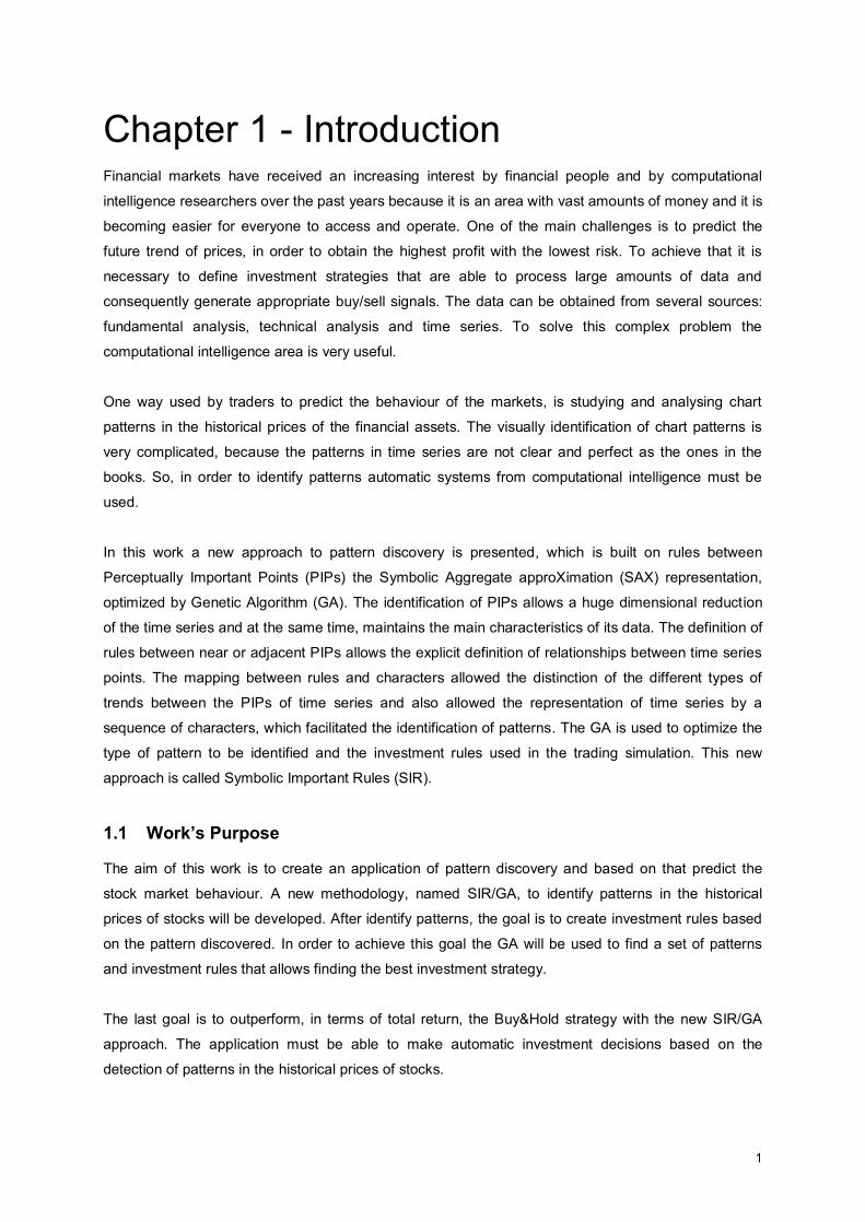
Chapter 1 - Introduction Financial markets have received an increasing interest by financial people and by computational

intelligence researchers over the past years because it is an area with vast amounts of money and it is

becoming easier for everyone to access and operate. One of the main challenges is to predict the

future trend of prices, in order to obtain the highest profit with the lowest risk. To achieve that it is

necessary to define investment strategies that are able to process large amounts of data and

consequently generate appropriate buy/sell signals. The data can be obtained from several sources:

fundamental analysis, technical analysis and time series. To solve this complex problem the

computational intelligence area is very useful.

One way used by traders to predict the behaviour of the markets, is studying and analysing chart

patterns in the historical prices of the financial assets. The visually identification of chart patterns is

very complicated, because the patterns in time series are not clear and perfect as the ones in the

books. So, in order to identify patterns automatic systems from computational intelligence must be

used.

In this work a new approach to pattern discovery is presented, which is built on rules between

Perceptually Important Points (PIPs) the Symbolic Aggregate approXimation (SAX) representation,

optimized by Genetic Algorithm (GA). The identification of PIPs allows a huge dimensional reduction

of the time series and at the same time, maintains the main characteristics of its data. The definition of

rules between near or adjacent PIPs allows the explicit definition of relationships between time series

points. The mapping between rules and characters allowed the distinction of the different types of

trends between the PIPs of time series and also allowed the representation of time series by a

sequence of characters, which facilitated the identification of patterns. The GA is used to optimize the

type of pattern to be identified and the investment rules used in the trading simulation. This new

approach is called Symbolic Important Rules (SIR).

1.1 Work’s Purpose

The aim of this work is to create an application of pattern discovery and based on that predict the

stock market behaviour. A new methodology, named SIR/GA, to identify patterns in the historical

prices of stocks will be developed. After identify patterns, the goal is to create investment rules based

on the pattern discovered. In order to achieve this goal the GA will be used to find a set of patterns

and investment rules that allows finding the best investment strategy.

The last goal is to outperform, in terms of total return, the Buy&Hold strategy with the new SIR/GA

approach. The application must be able to make automatic investment decisions based on the

detection of patterns in the historical prices of stocks.

2

1.2 Main Contributions

The main contributions made in this work are:

x The creation of the new methodology to identify patterns that combines rules between PIPs

with the mapping between those rules and different characters in the SAX representation.

x The combination of multiple exit/sell methods namely time, price and pattern.

x The use of a GA adaptive approach able to automatically identify multiple patterns and

generate trading rules.

1.3 Document Structure

This document is organized as follows:

x Chapter 2 addresses the theory behind the developed work, including technical analysis,

technical indicators and soft computing methodologies. Also, in this chapter, are presented

and analysed several and different methodologies regarding the identification of patterns.

x Chapter 3 describes the new approach SIR/GA methodology for pattern discovery and also

the architecture of the proposed solution.

x Chapter 4 describes first the metrics used to evaluate the developed solution and second

three case studies where the solution was tested.

x Chapter 5 summarizes the provided report and supplies the respective conclusion and future

work.

x Lastly, in references, are described the publications consulted that were used to build this

document, in Appendix A is presented an example with results of SIR/GA approach and in

Appendix B is presented a list of all the stocks used in the case studies.

3

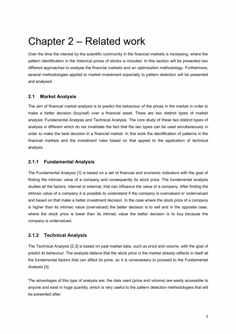
Chapter 2 – Related work Over the time the interest by the scientific community in the financial markets is increasing, where the

pattern identification in the historical prices of stocks is included. In this section will be presented two

different approaches to analyse the financial markets and an optimization methodology. Furthermore,

several methodologies applied to market investment especially to pattern detection will be presented

and analysed.

2.1 Market Analysis

The aim of financial market analysis is to predict the behaviour of the prices in the market in order to

make a better decision (buy/sell) over a financial asset. There are two distinct types of market

analysis: Fundamental Analysis and Technical Analysis. The core study of these two distinct types of

analysis is different which do not invalidate the fact that the two types can be used simultaneously in

order to make the best decision in a financial market. In this work the identification of patterns in the

financial markets and the investment rules based on that appeal to the application of technical

analysis.

2.1.1 Fundamental Analysis

The Fundamental Analysis [1] is based on a set of financial and economic indicators with the goal of

finding the intrinsic value of a company and consequently its stock price. The fundamental analysis

studies all the factors, internal or external, that can influence the value of a company. After finding the

intrinsic value of a company it is possible to understand if the company is overvalued or undervalued

and based on that make a better investment decision. In the case where the stock price of a company

is higher than its intrinsic value (overvalued) the better decision is to sell and in the opposite case,

where the stock price is lower than its intrinsic value the better decision is to buy because the

company is undervalued.

2.1.2 Technical Analysis

The Technical Analysis [2,3] is based on past market data, such as price and volume, with the goal of

predict its behaviour. The analysts believe that the stock price in the market already reflects in itself all

the fundamental factors that can affect its price, so it is unnecessary to proceed to the Fundamental

Analysis [3].

The advantages of this type of analysis are: the data used (price and volume) are easily accessible to

anyone and exist in huge quantity, which is very useful to the pattern detection methodologies that will

be presented after.

4

In technical analysis in order to predict correctly the future movement of the financial markets several

technical indicators are used [2,3], which are built based on the price and volume. In addition to

technical indicators the analysts also study the formation of chart patterns [3,4] in the historical prices

of financial assets. Some of the most well-known and most utilized technical indicators and chart

patterns are presented next.

2.1.2.1 Technical Indicators

A technical indicator is a metric whose value is calculated from the price or the volume of an asset. Its

objective is to help predicting the future price, or simply to indicate a general price trend. Some of the

most popular technical indicators are presented next. Other technical indicators can be found in [2]

and [5].

2.1.2.1.1 Simple Moving Average This indicator is one of the oldest indicators used by the analysts and represents the mean value of

the prices over a certain amount of time (days). Normally it is used the closing price of each day to

calculate the value of this indicator.

The Simple Moving Average (SMA) can be calculated for different lengths of time, where the most

common are 200, 100, 50, 30, 20 and 10 days. Smaller moving averages are usually used to short-

term investments and longer moving averages are used to long-term investments. Naturally, long-term

Simple Moving Averages have fewer fluctuations than long-term Simple Moving Averages.

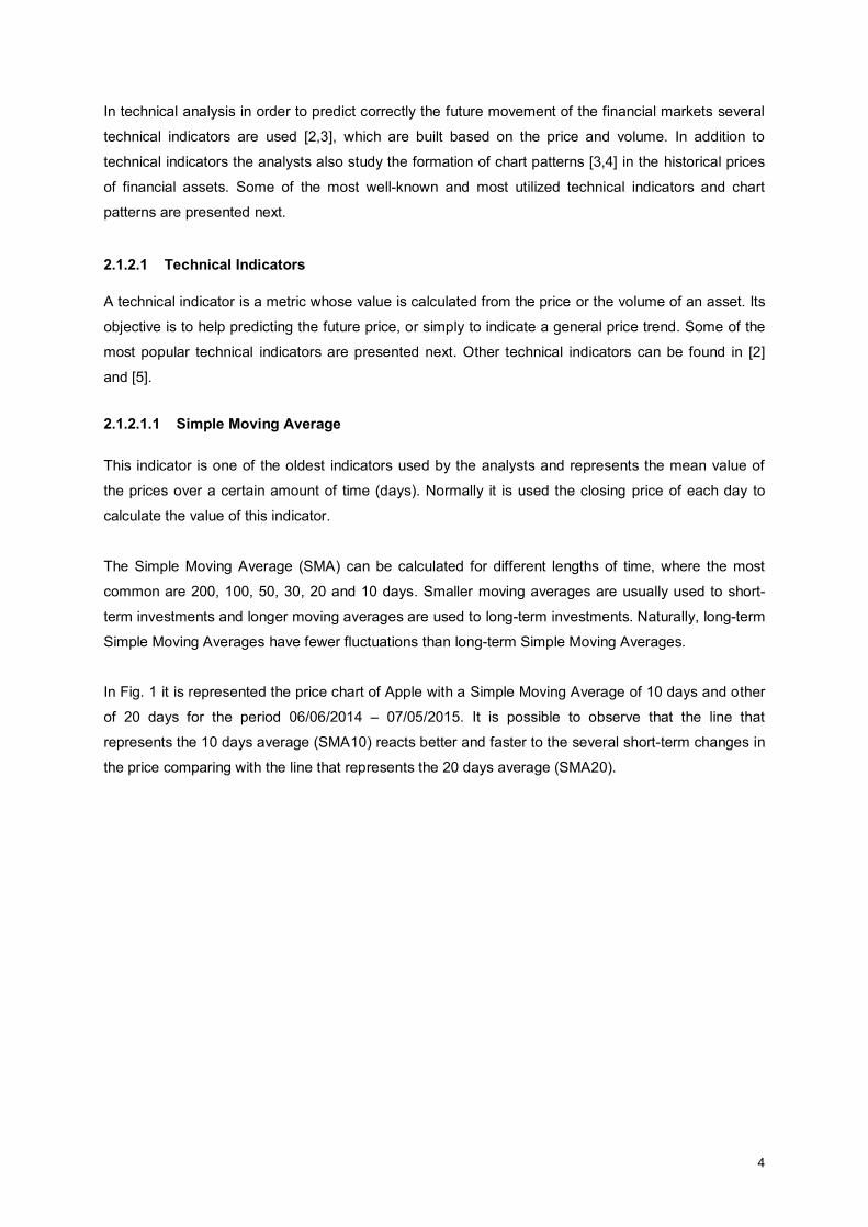
In Fig. 1 it is represented the price chart of Apple with a Simple Moving Average of 10 days and other

of 20 days for the period 06/06/2014 – 07/05/2015. It is possible to observe that the line that

represents the 10 days average (SMA10) reacts better and faster to the several short-term changes in

the price comparing with the line that represents the 20 days average (SMA20).

5

Fig. 1. Apple’s price chart with 10 and 20 days SMA.

This indicator can be used by traders to buy a financial asset when the average is in an upward trend

and to sell a financial asset when the average is in a downward trend. Several and different moving

averages can be used simultaneously to determine intersection points between them which originate

buy or sell signals.

There are other indicators based on the SMA, like the Exponential Moving Average which attributes

more importance (more weight) to the most recent days when calculating the average, in the attempt

to better react to sudden changes of price.

2.1.2.1.2 Relative Strength Index (RSI) This indicator is one of the most used indicators of the category momentum, which compares the

magnitude between the recent profits and losses, with the aim of determine if a financial asset is

overbought or oversold. This indicator oscillates between 0 and 100 and it is often calculated for a

period of 14 days. In equation (1) is described the formula to calculate this indicator.

RSI = 100 – 100/(1 + RS) (1)

RS = Average of x days’ up closes / Average of x days’ down closes

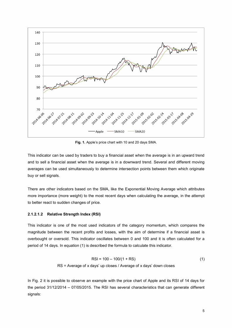
In Fig. 2 it is possible to observe an example with the price chart of Apple and its RSI of 14 days for

the period 31/12/2014 – 07/05/2015. The RSI has several characteristics that can generate different

signals:

6

x If the RSI value of an asset is higher than 50 it means an upward movement of prices and so

the asset should be bought. If the RSI value is lower than 50 it means a downward movement

of prices and consequently the asset should be sold.

x If the RSI value of an asset is higher than 70 it means the asset is overbought and so the

asset should be sold. If the RSI value is lower than 30 it means the asset is oversold and so

the asset should be bought.

Fig. 2. Apple’s price chart and its 14 days RSI.

2.1.2.1.3 On-Balance Volume (OBV) This indicator is the oldest and the most well-known volume indicator. The volume and the price are

used in the calculation of this indicator, which measures buying and selling pressure. The idea behind

this indicator is that using volume to analyse the price chart of an asset, it is possible to predict its

behaviour or simply confirm its trend. The formula to calculate the OBV is represented in equation (2).

OBV(x) = OBV(x-1) + Volume(x) , if Pricex > Pricex-1

OBV(x) = OBV(x-1) - Volume(x) , if Pricex < Pricex-1

OBV(x) = OBV(x-1) , if Pricex < Pricex-1 , if Pricex = Pricex-1

(2)

7

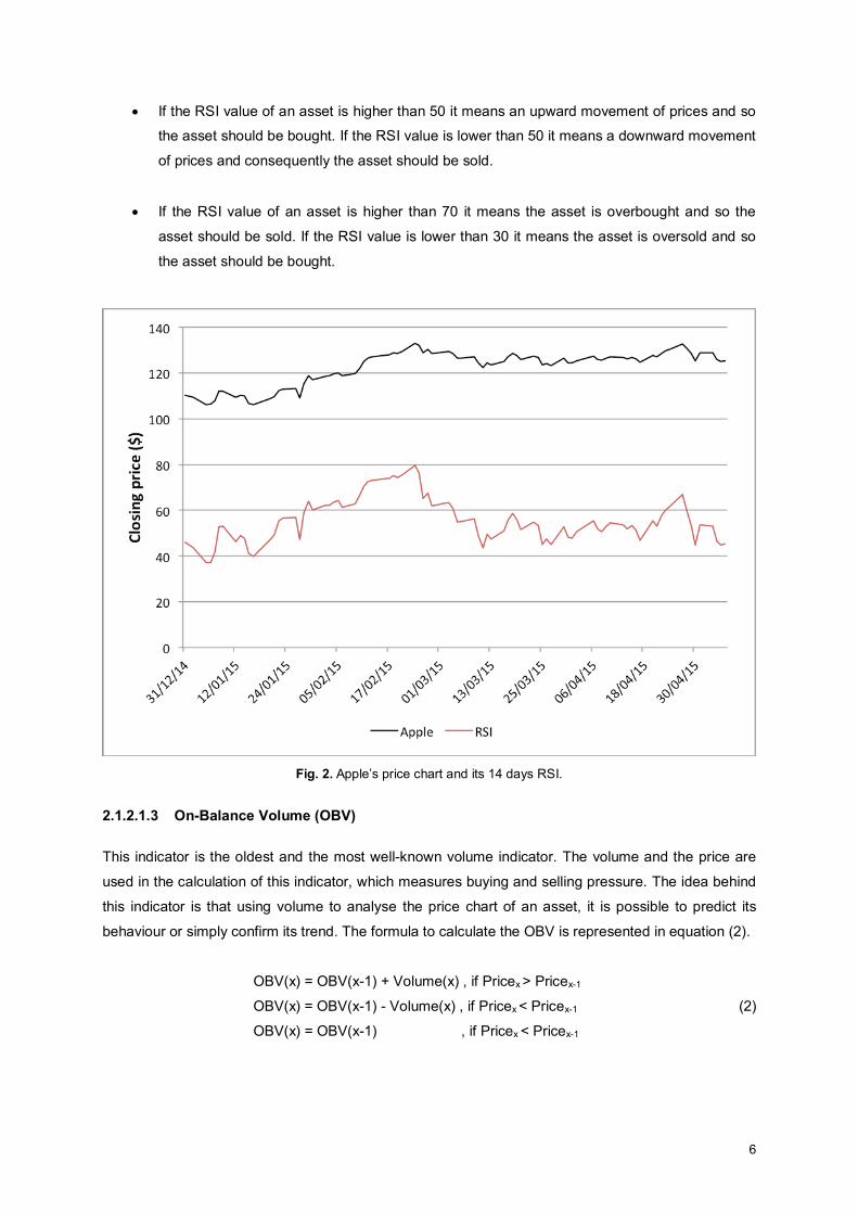
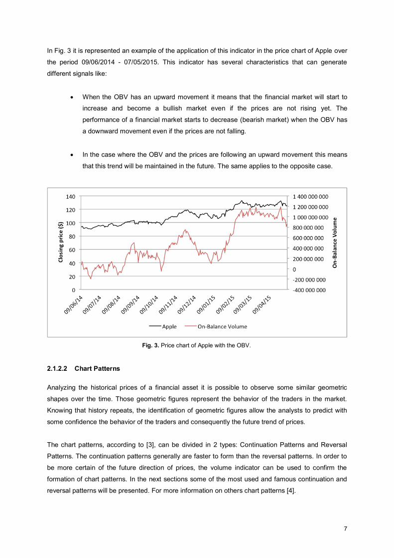
In Fig. 3 it is represented an example of the application of this indicator in the price chart of Apple over

the period 09/06/2014 - 07/05/2015. This indicator has several characteristics that can generate

different signals like:

x When the OBV has an upward movement it means that the financial market will start to

increase and become a bullish market even if the prices are not rising yet. The

performance of a financial market starts to decrease (bearish market) when the OBV has

a downward movement even if the prices are not falling.

x In the case where the OBV and the prices are following an upward movement this means

that this trend will be maintained in the future. The same applies to the opposite case.

Fig. 3. Price chart of Apple with the OBV.

2.1.2.2 Chart Patterns Analyzing the historical prices of a financial asset it is possible to observe some similar geometric

shapes over the time. Those geometric figures represent the behavior of the traders in the market.

Knowing that history repeats, the identification of geometric figures allow the analysts to predict with

some confidence the behavior of the traders and consequently the future trend of prices.

The chart patterns, according to [3], can be divided in 2 types: Continuation Patterns and Reversal

Patterns. The continuation patterns generally are faster to form than the reversal patterns. In order to

be more certain of the future direction of prices, the volume indicator can be used to confirm the

formation of chart patterns. In the next sections some of the most used and famous continuation and

reversal patterns will be presented. For more information on others chart patterns [4].

8

2.1.2.2.1 Continuation Patterns This type of chart patterns is characterized by confirming the uptrend or downtrend of the market,

despite of the trend of prices become a sideways movement temporarily. When this type of pattern

occurs, it can indicate the trend is likely to resume after the pattern completes.

1) Triangles There are three types of Triangles: (a) Symmetrical Triangle, (b) Ascending Triangle and (c)

Descending Triangle. These patterns have a typical duration of 3 months. In case (a) the prices after

breakout the triangle follow the direction of the previous trend. This case applies to bull markets and

bear markets as illustrated in Fig. 4, respectively.

Fig. 4. Bullish Symmetrical Triangle (left) and Bearish Symmetrical Triangle (right).

The case (b) is often a bullish chart pattern, as illustrated in Fig. 5, where the prices breakout the

triangle with an upward direction thereby confirming the previous trend.

Fig. 5. Ascending Triangle.

9

The case (c) is often a bearish chart pattern, where the prices breakout the triangle with a downward

direction that confirms the previous trend. This pattern is illustrated in Fig. 6.

Fig. 6. Descending Triangle.

2) Flags and Pennants

These two types of patterns are very similar due to the fact that they are preceded by a strong

increase or decrease movement that is followed by a consolidation period that marks the reset of the

initial movement (strong increase or decrease). These patters have a typical duration of one to 4

weeks. In Fig. 7 are illustrated the two types of the Flag Pattern: the Bull Flag and the Bear Flag. The

two cases of the Pennant Pattern: the Bull Pennant and the Bear Pennant are illustrated in Fig. 8.

Fig. 7. Bull Flag (left) and Bear Flag (right).

Fig. 8. Bull Pennant (left) and Bear Pennant (right).

10

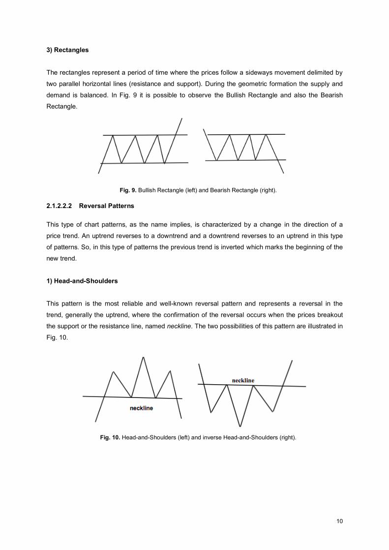
3) Rectangles The rectangles represent a period of time where the prices follow a sideways movement delimited by

two parallel horizontal lines (resistance and support). During the geometric formation the supply and

demand is balanced. In Fig. 9 it is possible to observe the Bullish Rectangle and also the Bearish

Rectangle.

Fig. 9. Bullish Rectangle (left) and Bearish Rectangle (right).

2.1.2.2.2 Reversal Patterns This type of chart patterns, as the name implies, is characterized by a change in the direction of a

price trend. An uptrend reverses to a downtrend and a downtrend reverses to an uptrend in this type

of patterns. So, in this type of patterns the previous trend is inverted which marks the beginning of the

new trend.

1) Head-and-Shoulders This pattern is the most reliable and well-known reversal pattern and represents a reversal in the

trend, generally the uptrend, where the confirmation of the reversal occurs when the prices breakout

the support or the resistance line, named neckline. The two possibilities of this pattern are illustrated in

Fig. 10.

Fig. 10. Head-and-Shoulders (left) and inverse Head-and-Shoulders (right).

11

2) Triple Top and Triple Bottom These patterns, as the name implies, are defined by three peaks (Triple Top) or by three bottoms

(Triple Bottom). These patterns are similar to the Head-and-Shoulders pattern except the fact that the

three peaks or bottoms, in this case are all at the same amplitude as can be seen in Fig. 11.

Fig. 11. Triple Top (left) and Triple Bottom (right).

3) Double Top and Double Bottom These patterns are frequently seen in price charts and are very similar to the two previous patterns

(point 2). The Double Top pattern is represented by 2 peaks with the same amplitude and the Double

Bottom pattern is represented by 2 bottoms at the same amplitude too. As can be seen in Fig. 12, the

Double Top and Double Bottom are often described by the character “M” and the character “W”

respectively.

Fig. 12. Double Top (left) and Double Bottom (right).

2.2 Optimization Methodologies – Genetic Algorithms

A Genetic Algorithm (GA) [6,7] is a search heuristic that mimics the process of natural selection. The

Genetic Algorithms belong to the class of the evolutionary algorithms, which are used to generate

solutions to optimization problems through techniques based on natural evolution. The GA’s are

widely used in financial markets to find the best combination of parameters of an investment strategy

[6][8].

12

In the GA a population of potential solutions is used to find the best solution for a problem. Each

potential solution is represented by a one-dimensional vector, named chromosome that represents the

several parameters to optimize. Each parameter of the chromosome is called gene and for each is

assigned a value. For example, some parameters that can be defined as genes can be the Simple

Moving Average, the RSI, etc.

The process of the GA is an iterative process, where the population in each iteration is named

generation. In each generation the solutions are evaluated according to a fitness function, i.e. an

objective function like maximize profit, and the ones with higher fit value are selected to the next

generation. After that, the genetic operators are used in the solutions to create better solutions and to

create the next generation. These genetic operators are:

x Crossover – this operation is similar to the human reproduction, where a new solution

(children) is created through a combination between the characteristics (parameters) of two

solutions (parents).

x Mutation – this operation represents the biologic mutation and it is used to maintain the

genetic diversity of populations in the next generations by changing some genes of the

chromosomes.

This iterative process is terminated when the stop criteria is reached, that can be defined like: a

solution is found that satisfies the minimum criteria, maximum number of generations is reached, lack

of improvements of solutions in successive generations, etc.

2.3 Pattern Detection Methodologies

In this section several different techniques to reduce the data dimensionality of time series and its

application in the identification of patterns are presented. The first methodology presented is based on

matrixes, the second in relevant points and the last in SAX representation.

2.3.1 Heuristic Based on Templates

As the name implies, this method will recognize patterns based on a template pattern approach,

where the templates are represented in a matrix format. In [9,11] is used a method, based on

templates, to detect the Bull Flag pattern (Fig. 7 left) with the aim of predict a rise in prices in the

future. In this approach the goal is to detect the pattern in the historical prices of financial assets, in

order to obtain more return than the average return of the financial markets. Through this pattern

detection approach were created investment rules that were tested in the NYSE index in [10].

13

This approach aims to detect the Bull Flag pattern based on a template represented by the matrix in

Fig. 13, which comprises a consolidation area (first seven columns), where prices fluctuate within a

channel similar to a parallelogram, which is followed by a strong rise (3 last columns), named

breakout, where prices start to increase.

0.5 -1 -1 -1 -1 -1 -1 -1

1 0.5 -0.5 -1 -1 -1 -1 -0.5

1 1 0.5 -0.5 -0.5 -0.5 -0.5 0.5

0.5 1 1 0.5 -0.5 -0.5 -0.5 1

0.5 1 1 0.5 0.5 1

0.5 1 1 0.5 1 1

-0.5 0.5 1 1 0.5 0.5 1 1

-0.5 -1 0.5 1 1 1 1

-1 -1 -1 -0.5 0.5 1 1 -2

-1 -1 -1 -1 -0.5 0.5 0.5 -2 -2.5

Fig. 13. Bull Flag matrix pattern template.

This template illustrated in Fig. 13 is represented by a 10x10 matrix named “T”, where each cell can have a value between -2.5 and +1.0 and the cells without value are assigned to 0. Also, the sum of all

the values of each column in matrix “T”, is always equal to 0. Then 10x10 matrixes, named “I” are

created to represent each time series of the historical prices. The time series that are represented in

matrixes ”I” have a variable number of days (ex: 120, 60, etc) allowing the identification of patterns

with differents time lengths. This concept is called sliding window.

In each time series the noise of its data is reduced by replacing the closing prices that exceed a

boundary, defined by two standard deviations related to the mean of the time series prices, by its

value (boundary value). Then the time series are divided in 10 identical groups, where each group will

be mapped in a column of matrix “I”. As an example, if the time series has a length of 60 days each

column of its matrix “I” represents 6 days. Using this technique it is possible to represent in matrix “I”

time series of any length.

After that, is calcuated the diference between the highest and the lowest price of each time series,

which defines the maximum amplitude, and divided it by 10 in order to identify the price range of each

row in matrix “I”. As an example if the highest and the lowest price in a time series are 100$ and 50$

repectively, so the first row corresponds to the price range between 95$ and 100$, the second row to

the price range 90$-95$ and so on.

Then, each cell of matrix “I” will have a value between 0.0 and 1.0 dependent on the number of days

that are mapped on it. In Fig. 14 it is possible to observe an example of a 60 days time series without

noise and its matrix “I”.

14

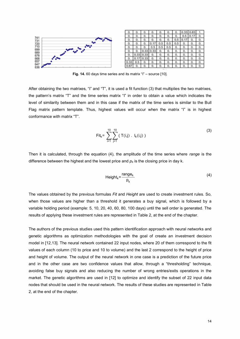
Fig. 14. 60 days time series and its matrix “I” – source [10].

After obtaining the two matrixes, “I” and “T”, it is used a fit function (3) that multiplies the two matrixes,

the pattern’s matrix “T” and the time series matrix “I” in order to obtain a value which indicates the

level of similarity between them and in this case if the matrix of the time series is similar to the Bull

Flag matrix pattern template. Thus, highest values will occur when the matrix “I” is in highest

conformance with matrix “T”.

Fitk= ∑ ∑ ( T(i,j) . Ik(i,j) ) 10

j=1

10

i=1

(3)

Then it is calculated, through the equation (4), the amplitude of the time series where range is the

difference between the highest and the lowest price and pk is the closing price in day k.

Heightk=rangek

pk

(4)

The values obtained by the previous formulas Fit and Height are used to create investment rules. So,

when those values are higher than a threshold it generates a buy signal, which is followed by a

variable holding period (example: 5, 10, 20, 40, 60, 80, 100 days) until the sell order is generated. The

results of applying these investment rules are represented in Table 2, at the end of the chapter.

The authors of the previous studies used this pattern identification approach with neural networks and

genetic algorithms as optimization methodologies with the goal of create an investment decision

model in [12,13]. The neural network contained 22 input nodes, where 20 of them correspond to the fit

values of each column (10 to price and 10 to volume) and the last 2 correspond to the height of price

and height of volume. The output of the neural network in one case is a prediction of the future price

and in the other case are two confidence values that allow, through a “thresholding” technique,

avoiding false buy signals and also reducing the number of wrong entries/exits operations in the

market. The genetic algorithms are used in [12] to optimize and identify the subset of 22 input data

nodes that should be used in the neural network. The results of these studies are represented in Table

2, at the end of the chapter.

15

The advantages of this methodology are the representation of patterns through matrixes templates is

very visually intuitive, also is very efficient to identify simple patterns and the implementation of its

method do not required a great complexity.

A disadvantage of this methodology is that using this method it is not possible to represent complex

patterns like the Head-and-Shoulders (Fig. 10) due to the lack of space in the matrix template. It would

be possible to increase the size of the matrix, but the sliding window would also have to increase

more. Other disadvantage is the lack of explanation about the technique used to build the template of

Fig. 13 therefore the template building is a black box for the users. To solve this problem in [14] is

described a simple technique to build the matrix template for several types of patterns, where the user

only need to put values equal to 1 in each column and the rest of the values of each column are

automatic generated because its sum must be equal to 0.

Other disadvantage of this method is related with the weights assigned to the cells of the matrix

because, as can be seen in Fig. 15, the matrix on top is much more similar to the Bull Flag pattern

than the matrix on the bottom, however its fit value (6.5) is lower than the fit value of the bottom matrix

(7.5), which can cause the wrong identification of the pattern. To resolve this problem a new Bull Flag

template was created in [15] with new weights in each cell of its matrix. The results of this study are

represented in Table 2, at the end of the chapter.

0.5 0 -1 -1 -1 -1 -1 -1 -1 0

1 0.5 0 -0.5 -1 -1 -1 -1 -0.5 0

1 1 0.5 0 -0.5 -0.5 -0.5 -0.5 0 0.5

0.5 1 1 0.5 0 -0.5 -0.5 -0.5 0 1

0 0.5 1 1 0.5 0 0 0 0.5 1

0 0 0.5 1 1 0.5 0 0 1 1

-0.5 0 0 0.5 1 1 0.5 0.5 1 1

-0.5 -1 0 0 0.5 1 1 1 1 0

-1 -1 -1 -0.5 0 0.5 1 1 0 -2

-1 -1 -1 -1 -0.5 0 0.5 0.5 -2 -2.5

0.5 0 -1 -1 -1 -1 -1 -1 -1 0

1 0.5 0 -0.5 -1 -1 -1 -1 -0.5 0

1 1 0.5 0 -0.5 -0.5 -0.5 -0.5 0 0.5

0.5 1 1 0.5 0 -0.5 -0.5 -0.5 0 1

0 0.5 1 1 0.5 0 0 0 0.5 1

0 0 0.5 1 1 0.5 0 0 1 1

-0.5 0 0 0.5 1 1 0.5 0.5 1 1

-0.5 -1 0 0 0.5 1 1 1 1 0

-1 -1 -1 -0.5 0 0.5 1 1 0 -2

-1 -1 -1 -1 -0.5 0 0.5 0.5 -2 -2.5

Fig. 15. Matrix with fit value of 6.5 (top) and matrix with fit value

of 7.5 (bottom).

16

In [16] the authors used the template pattern approach to represent several patterns in order to be

able to identify more and different cases in the historical prices. With the combination of different

patterns it is possible to identify more entry and exit points, which creates more complete and robust

investment strategies. The Genetic Algorithm was used in this study to optimize important parameters

of the process like: sliding window size, noise reduction rate, FitBuy which is the minimum value to

generate a buy signal and FitSell which is the minimum value to generate a sell signal. The results of

this study outperformed the Buy&Hold strategy and are represented in Table 2, at the end of this

chapter.

In a recently approach, described in [17], the creation of the Bull Flag template followed a new

methodology in order to mitigate the problem identified in Fig. 15. Unlike the previous studies [9,11]

and [14,16] that defined the Bull Flag pattern through a consolidation period followed by a strong rise,

this approach defines the Bull Flag pattern as a strong rise (first four columns) followed by a

consolidation period, illustrated in Fig. 16.

0 0 0 0 0 0 0 0 0 0

0 0 0 0 0 0 0 0 0 0

0 0 0 0 0 0 0 0 0 0

0 0 0 0 -1 -1 -1 -1 -1 -1

0 0 0 -1 -2 -2 -2 -2 -2 -2

0 0 -1 -3 -3 -3 -3 -3 -3 -3

0 -1 -3 -5 -5 -5 -5 -5 -5 -5

0 -1 -5 -5 -5 -5 -5 -5 -5 -5

0 -1 -5 -5 -5 -5 -5 -5 -5 -5

5 -1 -5 -5 -5 -5 -5 -5 -5 -5

Fig. 16. New Bull Flag matrix pattern template.

Also the values assignment to the matrix is completely different in this case, because there is only one

cell with a positive value (first column, last row), which ensures that in order to obtain a positive fit

value it is necessary that the prices of a time series pass through this cell. Cells with negative values

are areas where prices should not pass through and cells with value equal to 0 are areas where prices

can pass because do not affect the fit value.

This method is similar to an if-then rule because, as an example, if only the time series with fit value

equal or higher than 4 are considered as Bull Flag pattern then the prices of the time series have to

pass mandatorily through the cell with value 5 and can only pass through one cell with value -1,

thereby constraining the values of the eight remaining columns, that must be 0.

In this study, in order to evaluate the return of each operation in the investment strategies, a different

sell/exit method was adopted instead of defining a holding period of time to generate the sell order.

The sell/exit method is a dynamic method, where the exit point is defined by the evolution of the price

17

and not by time. To do that two variables were defined, take profit and stop loss, which are related

with the maximum amplitude of the time series identified as a pattern that limit the profit and the loss

of each operation, respectively. Thus whenever the price reaches the take profit value or the stop loss

value the operation is closed. The gain at the take profit level is often greater than the loss at the stop

loss level so that the total profit of a strategy depends on the success rate of operations. The results of

this study are represented in Table 2, at the end of the chapter.

2.3.2 Perceptually Important Points (PIPs)

In this approach, as the name implies, the time series are represented by a set of Perceptually

Important Points (PIPs) which are the most relevant points because are the ones who characterize the

time series and the patterns. Patterns are characterized by a set of critical points, as an example the

Head-and-Shoulders pattern can be defined by a head point, two points for the shoulders and two

more points for the neckline. These points are the most relevant points because are the ones that

define the shape of this pattern. So, in order to identify PIPs in time series, a technique based on

distance measures was used in [18]. The algorithm to identify PIPs is described as:

The sequence P is the set of time series data points. The first and the last point of the sequence P are

the first two PIPs identified. The next PIP is the point of sequence P with maximum distance to the first

two PIPs. Then, the fourth PIP will be then the point in P with maximum distance to its two adjacent

PIPs, i.e., in between the first and the second PIPs or the second and the last PIPs. This process ends

when the number of PIPs identified is equal to the number of PIPs of the pattern.

To measure the maximum distance between one point and its two adjacent PIPs, in [18] are presented

3 methods:

1. Euclidean distance (ED)

Calculates the sum of the ED (5) of the test point p3 to its adjacent PIPs p1 e p2

ED(p3,p2,p1)=√(x2-x3)2+ (y2-y3)2 + √(x1-x3)2+ (y1-y3)2

(5)

2. Perpendicular distance (PD)

Calculates the PD (9) between the test point p3 and the line connecting the two adjacent PIPs p1 e

p2.

Slope(p1,p2)= s= y2-y1x2-x1

(6)

18

xc=

x3+ s y3 + s y2- s2 x2

1+s2

(7)

yc= s xc- s x2+ y2

(8)

PD(p3,pc) =√(xc- x3)2 + (yc- y3)2

(9)

3. Vertical distance (VD)

Calculates the VD (10) between the test point p3 and the line connecting the two adjacent PIPs p1

e p2.

VD(p3,pc) = |yc- y3| = |(y1+ (y2- y1)xc- x1

x2- x1) - y3| (10)

These three distance methods were tested in [18], using 2500 points of data from Hang Seng Index

(HSI), and the vertical distance (VD) method proved to be the best in capturing the shapes of patterns

After the identification of PIPs in time series, the next step is to detect pattern based on this

representation. In order to do that two distinct methodologies were used in [19]. The first is based on

templates and the second is based on rules.

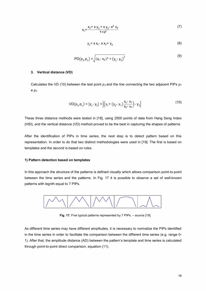
1) Pattern detection based on templates

In this approach the structure of the patterns is defined visually which allows comparison point-to-point

between the time series and the patterns. In Fig. 17 it is possible to observe a set of well-known

patterns with legnth equal to 7 PIPs.

Fig. 17. Five typical patterns represented by 7 PIPs. – source [19]

As different time series may have different amplitudes, it is necessary to normalize the PIPs identified

in the time series in order to facilitate the comparison between the different time series (e.g. range 0-

1). After that, the amplitude distance (AD) between the pattern’s template and time series is calculated

through point-to-point direct comparison, equation (11).

19

AD(SP,Q) = √1n ∑(spk- qk)2

n

k=1

(11)

The variables SP and spk denote the PIPs identified in the time series P and the variables Q and qk

denote the PIPs of the pattern template. It is also necessary to consider the horizontal distortion (time

dimension) of the time series against the pattern templates. The temporal distance (TD) between P

(time series) and Q (pattern template) is defined in equation (12).

TD(SP,Q) = √1

n-1 ∑(spkt - qk

t )2n

k=2

(12)

where spkt and qk

t denote the time coordinate of the sequence points spk and qk , respectively. In order

to take both horizontal and vertical distortion into consideration in the similarity measure, the formula

of this measure is defined as:

D(SP,Q) = w1 × AD(SP,Q) + (1-w1) × TD(SP,Q) (13)

where w1 represents the weight of AD and TD that is specified by the users. The results of this

methodology are represented in Table 2, at the end of the chapter.

2) Pattern detection based on rules

One disadvantage of the template-based methodology is the difficulty of defining the relationship

between the relevant points. In this approach a set of rules between PIPs is created to describe the

shape of the patterns. For example in the Head-and-Shoulders pattern, the two shoulders must be

lower than the point that defines the head and must have a similar degree of amplitude.

Using the patterns from Fig. 17 and assuming that all of them have a length of 7 PIPs, sp1 until sp7, a

set of rules can be defined for each pattern. The set of rules that define the Head-and-Shoulders

pattern are the following:

x sp4 >sp2 e sp6

x sp2 >sp1 e sp3

x sp6 >sp5 e sp7

x sp3 >sp1

x sp5 >sp7

x diff(sp2,sp6) < 15%

x diff(sp3,sp5) < 15%

20

The set of rules that define the other four patterns of Fig. 17 can be found in [19].

After the definition of a set of rules for each pattern, the time series are represented by its PIPs, in this

case by 7 PIPs, and those who comply with all the rules of a pattern are identified as one. The results

of this approach are represented in Table 2, at the end of the chapter and in general, were lower than

the results of the previous approach (template-based). However, this approach obtained excellent

results in the distinction between the Head-and-Shoulders pattern, Triple Top pattern and Double Top

pattern.

The advantages of this new approach, i.e. PIPs representation and detection of patterns based on

templates or rules are:

x High complexity reduction of time series and patterns because only a small set of points is

used to represent time series and identify patterns.

x Possibility to detect complex and detailed patterns.

The main disadvantage of this approach is related with the detection of patterns, where the number of

PIPs that define the patterns and the time series must always be the equal in order to enable the

comparison point-to-point in the template-based methodology or the validation of rules in the rule-

based methodology. For example the Head-and-Shoulders pattern of Fig. 17 is represented by 7 PIPs,

which force the time series to be represented by the same number of PIPs to be possible to compare

them with the pattern. To resolve this problem a DTW (Dynamic time warping) algorithm was used in

[20] to find an optimized alignment between two sequences combined with the three distance

measures described previously (ED, PD and VD). Using this algorithm it is possible to measure the

similarity between a pattern and a time series with different lengths of PIPs

2.3.3 Symbolic Aggregate approXimation (SAX) representation

Traditionally, the representation of time series and its dimensionality reduction was made through

numeric methods like Wavelet Discrete Transform [21]. The SAX representation approach [22] allows

defining metrics between data representation, which is related with the real distance between time

series. The SAX representation solves the problem related with the distance between the real data

and its representation because it is possible to obtain a lower bounding approximation for the distance

measures and also this representation allows a significant reduction of the data dimensionality of time

series.

21

In [23] was used a method based on SAX to represent time series with the aim of identifying patterns,

which begins by dividing larger time series in smaller time series windows. The data of each smaller

time series is then normalized, according to equation (14), to guarantee that the time series can be

compared between each other. In equation (14), xi corresponds to a point of the time series, μx and

σx correspond to the mean and standard deviation of the time series, respectively.

xi'=

xi - μxσx

(14)

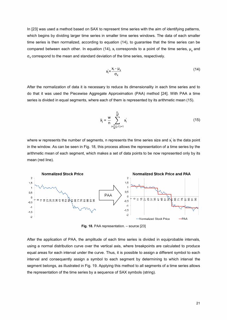
After the normalization of data it is necessary to reduce its dimensionality in each time series and to

do that it was used the Piecewise Aggregate Approximation (PAA) method [24]. With PAA a time

series is divided in equal segments, where each of them is represented by its arithmetic mean (15).

x̅j = wn ∑ xi

'

nwj

i=nw(j-1)+1

(15)

where w represents the number of segments, n represents the time series size and xi' is the data point

in the window. As can be seen in Fig. 18, this process allows the representation of a time series by the

arithmetic mean of each segment, which makes a set of data points to be now represented only by its

mean (red line).

Fig. 18. PAA representation. – source [23]

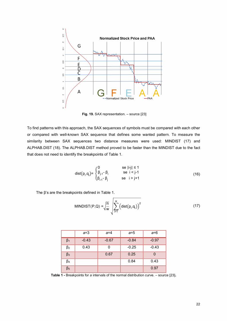
After the application of PAA, the amplitude of each time series is divided in equiprobable intervals,

using a normal distribution curve over the vertical axis, where breakpoints are calculated to produce

equal areas for each interval under the curve. Thus, it is possible to assign a different symbol to each

interval and consequently assign a symbol to each segment by determining to which interval the

segment belongs, as illustrated in Fig. 19. Applying this method to all segments of a time series allows

the representation of the time series by a sequence of SAX symbols (string).

22

Fig. 19. SAX representation. – source [23]

To find patterns with this approach, the SAX sequences of symbols must be compared with each other

or compared with well-known SAX sequence that defines some wanted pattern. To measure the

similarity between SAX sequences two distance measures were used: MINDIST (17) and

ALPHAB.DIST (18). The ALPHAB.DIST method proved to be faster than the MINDIST due to the fact

that does not need to identify the breakpoints of Table 1.

dist(pi,qi)= {0 se |i-j| ≤ 1βj-1- βi se i < j-1βi-1- βj se i > j+1

The β’s are the breakpoints defined in Table 1.

(16)

MINDIST(P,Q) =√nw √∑ (dist(pi,qi))

2w

i=1

(17)

a=3 a=4 a=5 a=6

β1 -0.43 -0.67 -0.84 -0.97

β2 0.43 0 -0.25 -0.43

β3 0.67 0.25 0

β4 0.84 0.43

β5 0.97

Table 1 - Breakpoints for a intervals of the normal distribution curve. – source [23].

23

ALPHAB.DIST(T,P) = √∑(Ti - Pi)2W

i=1

(18)

where Ti e Pi are the symbols i of the sequence T and P, respectively.

An advantage of SAX representation is the simplicity to identify patterns because in this approach the

identification is simply a comparison between two sequences of symbols, i.e. two strings. Other

advantage is the simple implementation of this methodology and also the transformation of time series

in SAX sequences of symbols is fast. The main advantage is that this approach allows a huge

reduction of dimensionality of data and at the same time maintains the main characteristics of time

series and patterns.

The authors of this study [23] also used genetic algorithms to optimize the investment strategies

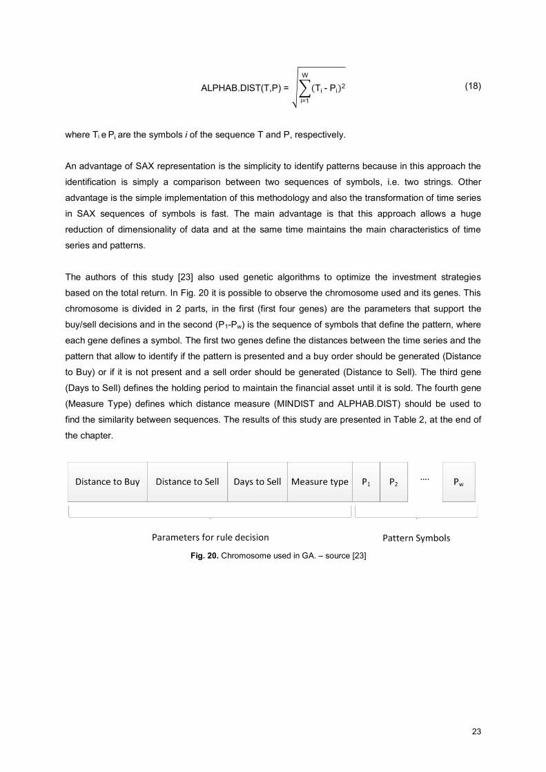
based on the total return. In Fig. 20 it is possible to observe the chromosome used and its genes. This

chromosome is divided in 2 parts, in the first (first four genes) are the parameters that support the

buy/sell decisions and in the second (P1-Pw) is the sequence of symbols that define the pattern, where

each gene defines a symbol. The first two genes define the distances between the time series and the

pattern that allow to identify if the pattern is presented and a buy order should be generated (Distance

to Buy) or if it is not present and a sell order should be generated (Distance to Sell). The third gene

(Days to Sell) defines the holding period to maintain the financial asset until it is sold. The fourth gene

(Measure Type) defines which distance measure (MINDIST and ALPHAB.DIST) should be used to

find the similarity between sequences. The results of this study are presented in Table 2, at the end of

the chapter.

Fig. 20. Chromosome used in GA. – source [23]

24

Ref. Year Method Used Data

Period Financial Market

Algorithm Performance Buy-and-Hold Performance

[10] 2008 Bull Flag w/ Matrix

Template

Stock price

04/08/1967 - 12/05/2003 NYSE Composite

Index

4.59% (Transaction average over the

period)

1.83% (Transaction average over the

period) [15] 2007 Bull Flag w/

Matrix Template

Stock price

NASDAQ TWI NASDAQ & TWI

NASDAQ TWI NASDAQ TWI 03/04/1985

– 20/03/2004

01/06/1971 –

24/03/2004

4.38% (Transaction average over the period)

6.48% (Transaction average over the period)

3.27% (Transaction average over the period)

4.03% (Transaction average over the period)

[13] 2002 Hybrid Neural Network w/

Pattern detection

Stock price and Vol.

24/07/1984 – 11/06/1998 NYSE Composite

Index

66% (Days market goes up after buying

order)

60% (Days market goes up after buying

order)

[17] 2015 Bull Flag w/ Matrix

Template

Stock price

22/05/2000 – 29/11/2013 Dow Jones Industrial Average

Index

13% (Average return)

N/A

[16] 2011 Uptrend pattern w/

Matrix Template +

GA

Stock price

1998 - 2010 S&P500 Index

36.92% (Total return)

-4.69% (Total return)

[19] 2007 Template-Based

Stock price

N/A Several 96% (Hits on pattern identification)

N/A

[19] 2007 Rule-Based Stock price

N/A Several 38% (Hits on pattern identification)

N/A

[19] 2007 PAA Stock price

N/A Several 82% (Hits on pattern identification)

N/A

[23] 2013 SAX + GA Stock price

1998 - 2010 S&P500 Index

16.28% (Average annual return)

7.79% (Average annual return)

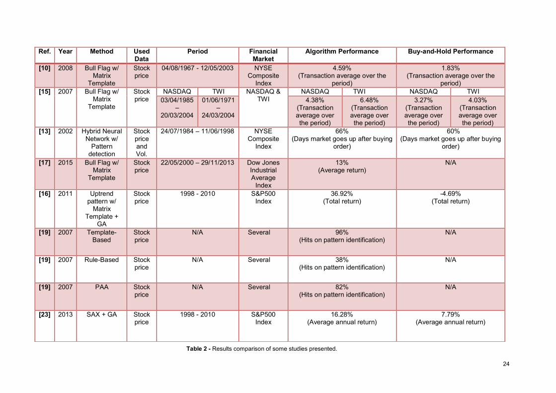
Table 2 - Results comparison of some studies presented.

25

Chapter 3 – SIR/GA approach In this chapter the new approach to pattern discovery will be presented in detail. The objective of this

research is to develop a pattern discovery algorithm that combines ideas from how humans identify

patterns and automatic classification of the patterns. The method uses points that normally a human

would consider important, and then creates rules to describe the relationship between them. Then

using GA and SAX makes a search for the relevant patterns in order to detect opportunities to

enter/exit the market. This new approach, Symbolic Important Rules (SIR), is based on two different

ideas from the related work: PIPs with rules and SAX representation. Also, the system’s architecture

and each of its modules that support this approach will be described later in this chapter.

3.1 Time series representation

The proposed method is divided in 4 steps, represented in Fig. 21. These steps are described here

shortly, and next each one in detail. Firstly, the historical prices of a financial asset are divided into

smaller time series all with the same size in order to identify patterns with the same time length, Fig.

21. a). After this, it is possible to identify patterns in the time series but the dimension of data is too

high, making this process very expensive in time and computational resources. Secondly in order to

reduce the dimension of the data, each time series is represented by its most relevant points,

denominated Perceptually Important Points (PIPs), Fig 21. b). Thirdly, rules are created that identify

the relationship between two PIPs. The two PIPs do not need to be consecutive, it is possible to have

rules between two PIPs that are apart to each other more than one unit. Finally the fourth step where

each different rule created is transformed in a different symbol in order to represent each time series

by a sequence of symbols.

26

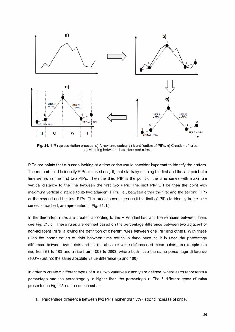
Fig. 21. SIR representation process. a) A raw time series. b) Identification of PIPs. c) Creation of rules.

d) Mapping between characters and rules.

PIPs are points that a human looking at a time series would consider important to identify the pattern.

The method used to identify PIPs is based on [19] that starts by defining the first and the last point of a

time series as the first two PIPs. Then the third PIP is the point of the time series with maximum

vertical distance to the line between the first two PIPs. The next PIP will be then the point with

maximum vertical distance to its two adjacent PIPs, i.e., between either the first and the second PIPs

or the second and the last PIPs. This process continues until the limit of PIPs to identify in the time

series is reached, as represented in Fig. 21. b).

In the third step, rules are created according to the PIPs identified and the relations between them,

see Fig. 21. c). These rules are defined based on the percentage difference between two adjacent or

non-adjacent PIPs, allowing the definition of different rules between one PIP and others. With these

rules the normalization of data between time series is done because it is used the percentage

difference between two points and not the absolute value difference of those points, an example is a

rise from 5$ to 10$ and a rise from 100$ to 200$, where both have the same percentage difference

(100%) but not the same absolute value difference (5 and 100).

In order to create 5 different types of rules, two variables x and y are defined, where each represents a

percentage and the percentage y is higher than the percentage x. The 5 different types of rules

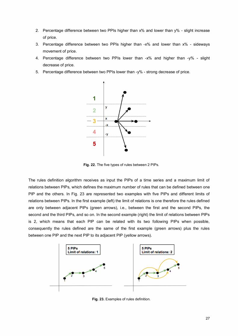
presented in Fig. 22, can be described as:

1. Percentage difference between two PPIs higher than y% - strong increase of price.

27

2. Percentage difference between two PPIs higher than x% and lower than y% - slight increase

of price.

3. Percentage difference between two PPIs higher than -x% and lower than x% - sideways

movement of price.

4. Percentage difference between two PPIs lower than -x% and higher than -y% - slight

decrease of price.

5. Percentage difference between two PPIs lower than -y% - strong decrease of price.

Fig. 22. The five types of rules between 2 PIPs.

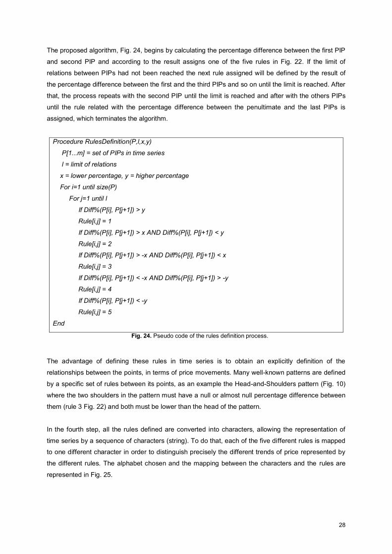
The rules definition algorithm receives as input the PIPs of a time series and a maximum limit of

relations between PIPs, which defines the maximum number of rules that can be defined between one

PIP and the others. In Fig. 23 are represented two examples with five PIPs and different limits of

relations between PIPs. In the first example (left) the limit of relations is one therefore the rules defined

are only between adjacent PIPs (green arrows), i.e., between the first and the second PIPs, the

second and the third PIPs, and so on. In the second example (right) the limit of relations between PIPs

is 2, which means that each PIP can be related with its two following PIPs when possible,

consequently the rules defined are the same of the first example (green arrows) plus the rules

between one PIP and the next PIP to its adjacent PIP (yellow arrows).

Fig. 23. Examples of rules definition.

28

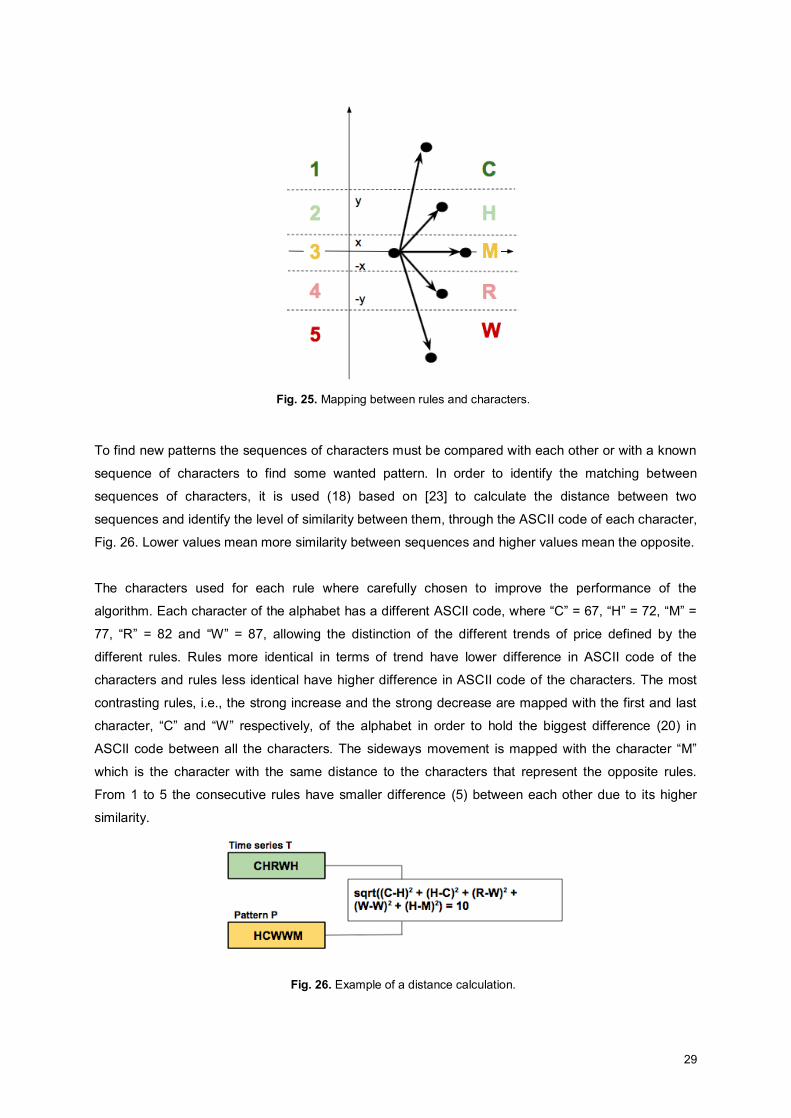
The proposed algorithm, Fig. 24, begins by calculating the percentage difference between the first PIP

and second PIP and according to the result assigns one of the five rules in Fig. 22. If the limit of

relations between PIPs had not been reached the next rule assigned will be defined by the result of

the percentage difference between the first and the third PIPs and so on until the limit is reached. After

that, the process repeats with the second PIP until the limit is reached and after with the others PIPs

until the rule related with the percentage difference between the penultimate and the last PIPs is

assigned, which terminates the algorithm.

Procedure RulesDefinition(P,l,x,y)

P[1...m] = set of PIPs in time series

l = limit of relations

x = lower percentage, y = higher percentage

For i=1 until size(P)

For j=1 until l

If Diff%(P[i], P[j+1]) > y

Rule[i,j] = 1

If Diff%(P[i], P[j+1]) > x AND Diff%(P[i], P[j+1]) < y

Rule[i,j] = 2

If Diff%(P[i], P[j+1]) > -x AND Diff%(P[i], P[j+1]) < x

Rule[i,j] = 3

If Diff%(P[i], P[j+1]) < -x AND Diff%(P[i], P[j+1]) > -y

Rule[i,j] = 4

If Diff%(P[i], P[j+1]) < -y

Rule[i,j] = 5

End

Fig. 24. Pseudo code of the rules definition process.

The advantage of defining these rules in time series is to obtain an explicitly definition of the

relationships between the points, in terms of price movements. Many well-known patterns are defined

by a specific set of rules between its points, as an example the Head-and-Shoulders pattern (Fig. 10)

where the two shoulders in the pattern must have a null or almost null percentage difference between

them (rule 3 Fig. 22) and both must be lower than the head of the pattern.

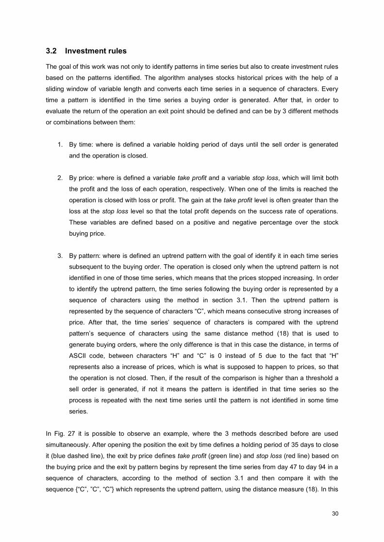
In the fourth step, all the rules defined are converted into characters, allowing the representation of

time series by a sequence of characters (string). To do that, each of the five different rules is mapped

to one different character in order to distinguish precisely the different trends of price represented by

the different rules. The alphabet chosen and the mapping between the characters and the rules are

represented in Fig. 25.

29

Fig. 25. Mapping between rules and characters.

To find new patterns the sequences of characters must be compared with each other or with a known

sequence of characters to find some wanted pattern. In order to identify the matching between

sequences of characters, it is used (18) based on [23] to calculate the distance between two

sequences and identify the level of similarity between them, through the ASCII code of each character,

Fig. 26. Lower values mean more similarity between sequences and higher values mean the opposite.

The characters used for each rule where carefully chosen to improve the performance of the

algorithm. Each character of the alphabet has a different ASCII code, where “C” = 67, “H” = 72, “M” =

77, “R” = 82 and “W” = 87, allowing the distinction of the different trends of price defined by the

different rules. Rules more identical in terms of trend have lower difference in ASCII code of the

characters and rules less identical have higher difference in ASCII code of the characters. The most

contrasting rules, i.e., the strong increase and the strong decrease are mapped with the first and last

character, “C” and “W” respectively, of the alphabet in order to hold the biggest difference (20) in

ASCII code between all the characters. The sideways movement is mapped with the character “M”

which is the character with the same distance to the characters that represent the opposite rules.

From 1 to 5 the consecutive rules have smaller difference (5) between each other due to its higher

similarity.

Fig. 26. Example of a distance calculation.

30

3.2 Investment rules

The goal of this work was not only to identify patterns in time series but also to create investment rules

based on the patterns identified. The algorithm analyses stocks historical prices with the help of a

sliding window of variable length and converts each time series in a sequence of characters. Every

time a pattern is identified in the time series a buying order is generated. After that, in order to

evaluate the return of the operation an exit point should be defined and can be by 3 different methods

or combinations between them:

1. By time: where is defined a variable holding period of days until the sell order is generated

and the operation is closed.

2. By price: where is defined a variable take profit and a variable stop loss, which will limit both

the profit and the loss of each operation, respectively. When one of the limits is reached the

operation is closed with loss or profit. The gain at the take profit level is often greater than the

loss at the stop loss level so that the total profit depends on the success rate of operations.

These variables are defined based on a positive and negative percentage over the stock

buying price.

3. By pattern: where is defined an uptrend pattern with the goal of identify it in each time series

subsequent to the buying order. The operation is closed only when the uptrend pattern is not

identified in one of those time series, which means that the prices stopped increasing. In order

to identify the uptrend pattern, the time series following the buying order is represented by a

sequence of characters using the method in section 3.1. Then the uptrend pattern is

represented by the sequence of characters “C”, which means consecutive strong increases of

price. After that, the time series’ sequence of characters is compared with the uptrend

pattern’s sequence of characters using the same distance method (18) that is used to

generate buying orders, where the only difference is that in this case the distance, in terms of

ASCII code, between characters “H” and “C” is 0 instead of 5 due to the fact that “H”

represents also a increase of prices, which is what is supposed to happen to prices, so that

the operation is not closed. Then, if the result of the comparison is higher than a threshold a

sell order is generated, if not it means the pattern is identified in that time series so the

process is repeated with the next time series until the pattern is not identified in some time

series.

In Fig. 27 it is possible to observe an example, where the 3 methods described before are used

simultaneously. After opening the position the exit by time defines a holding period of 35 days to close

it (blue dashed line), the exit by price defines take profit (green line) and stop loss (red line) based on

the buying price and the exit by pattern begins by represent the time series from day 47 to day 94 in a

sequence of characters, according to the method of section 3.1 and then compare it with the

sequence {“C”, ”C”, “C”} which represents the uptrend pattern, using the distance measure (18). In this

31

example, the position is closed by price because the price reached the take profit level before the

other methods generate sell orders.

Fig. 27. Example with the 3 different exit methods.

3.3 Genetic Algorithms (GA)

To optimize the parameters related to the investment rules is used the Genetic Algorithm (GA). The

chromosome used to create the population is represented in Fig. 28.

Fig. 28. Chromosome used in GA.

The chromosome is divided in 2 major parts. In the first part (first eight genes) are the parameters

related to the buy and sell decisions and in the second part (L1,…,Lx) are the characters that

represent the pattern sequence that will be identified in the time series. The genes of the chromosome

are:

32

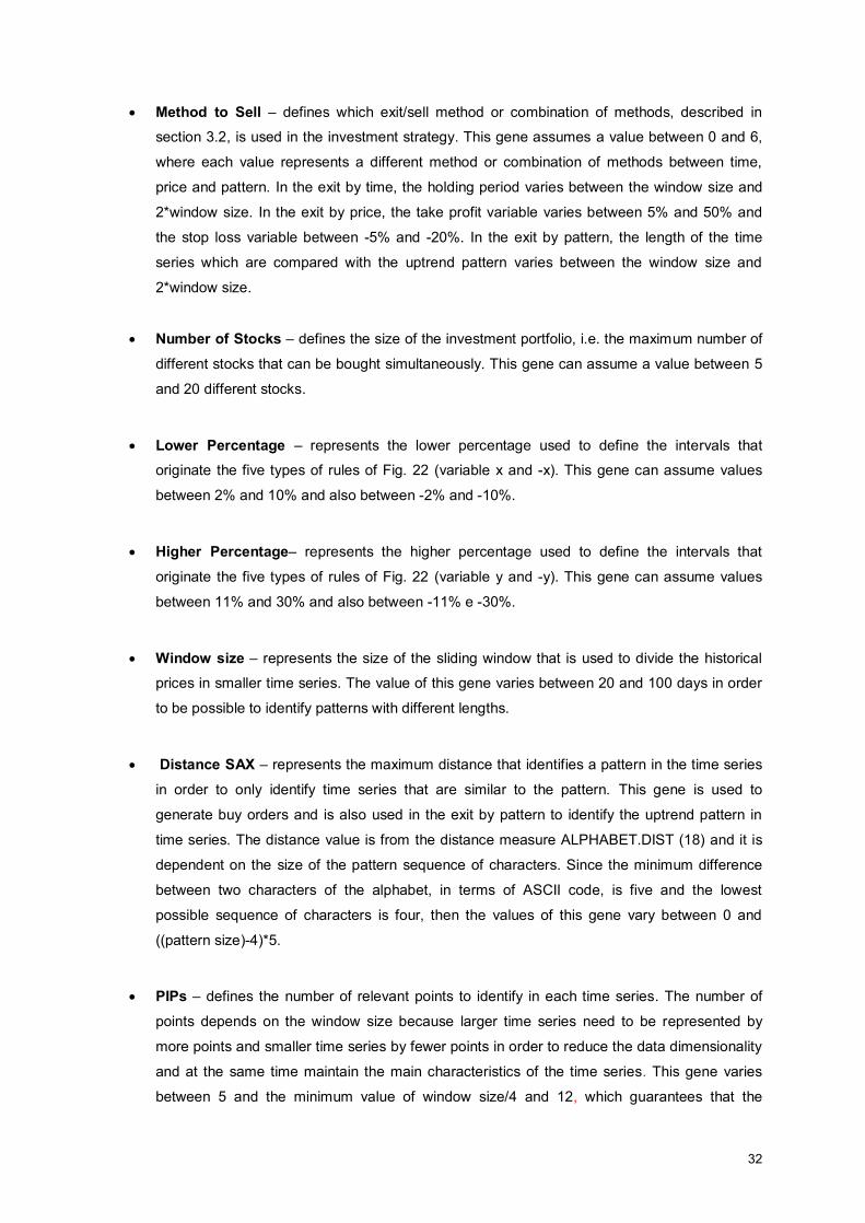
x Method to Sell – defines which exit/sell method or combination of methods, described in

section 3.2, is used in the investment strategy. This gene assumes a value between 0 and 6,

where each value represents a different method or combination of methods between time,

price and pattern. In the exit by time, the holding period varies between the window size and

2*window size. In the exit by price, the take profit variable varies between 5% and 50% and

the stop loss variable between -5% and -20%. In the exit by pattern, the length of the time

series which are compared with the uptrend pattern varies between the window size and

2*window size.

x Number of Stocks – defines the size of the investment portfolio, i.e. the maximum number of

different stocks that can be bought simultaneously. This gene can assume a value between 5

and 20 different stocks.

x Lower Percentage – represents the lower percentage used to define the intervals that

originate the five types of rules of Fig. 22 (variable x and -x). This gene can assume values

between 2% and 10% and also between -2% and -10%.

x Higher Percentage– represents the higher percentage used to define the intervals that

originate the five types of rules of Fig. 22 (variable y and -y). This gene can assume values

between 11% and 30% and also between -11% e -30%.

x Window size – represents the size of the sliding window that is used to divide the historical

prices in smaller time series. The value of this gene varies between 20 and 100 days in order

to be possible to identify patterns with different lengths.

x Distance SAX – represents the maximum distance that identifies a pattern in the time series

in order to only identify time series that are similar to the pattern. This gene is used to

generate buy orders and is also used in the exit by pattern to identify the uptrend pattern in

time series. The distance value is from the distance measure ALPHABET.DIST (18) and it is

dependent on the size of the pattern sequence of characters. Since the minimum difference

between two characters of the alphabet, in terms of ASCII code, is five and the lowest

possible sequence of characters is four, then the values of this gene vary between 0 and

((pattern size)-4)*5.

x PIPs – defines the number of relevant points to identify in each time series. The number of

points depends on the window size because larger time series need to be represented by

more points and smaller time series by fewer points in order to reduce the data dimensionality

and at the same time maintain the main characteristics of the time series. This gene varies

between 5 and the minimum value of window size/4 and 12, which guarantees that the

33

minimum number of points identified in each time series is 5 and the maximum is window

size/4 or 12 in the case where the window size/4 value is greater than 12.

x Limit of relations – indicates the maximum limit of relations between the PIPs that were

identified in each time series and consequently defines the number of rules that will be

created for each PIP with the others PIPs because each relation corresponds to a rule. This

value depends on the number of PIPs because the number of points between the first and the

last PIPs defines the maximum limit of relations, as an example if the number of PIPs is five

then the maximum limit of relations between PIPs is four. Therefore the values of this gene

vary between 1 and total number of PIPs – 1.

x L1,...,Lx – defines the pattern sequence of symbols that will be used to identify in the

historical prices of stocks, where each gene L represents a character of the alphabet {“C”, “H”,

“M”, “R”, “W”}. The size of the sequence of symbols is defined by the number of rules, which is

defined by the number of PIPs and its relations. The definition of each character is restricted

by the previous characters assigned to the rules between the previous PIPs, in order to create

valid sequences of characters. For example in the case where the character assigned to the

rule between the first and second PIPs is “H”, which means that the second point is higher

than the first, and the character assigned to the rule between the first and third PIPs is “R”,

which means that the third point is lower than the first, implies that the third PIP is mandatorily

lower than the second PIP and the character assigned to this rule must be only “R” or “W”.

The chromosomes could have different sizes due to the length of the sequence of characters, which

depends on the number of rules that are defined through the PIPs and its relations, which are also

dependent on the sliding window size. For this reason, the crossover operation between two

chromosomes is done by two different ways, depending on the size of the chromosomes:

1. Chromosomes with different sizes In this case, where the two chromosomes have different sizes the only possible genes that

can be swapped are the ones that are not directly related with the size of the pattern

sequence of characters. The genes that define the size of the sequence of characters of each

time series that will be compared with the pattern sequence of characters cannot be swapped

because the two sequences must have the same size to be possible to compare them. So

only the first four genes or a set of them can be swapped between two chromosomes with

different sizes, as illustrated in Fig. 29.

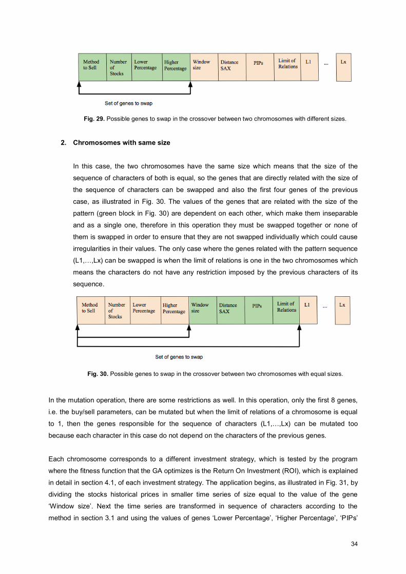
34

Fig. 29. Possible genes to swap in the crossover between two chromosomes with different sizes.

2. Chromosomes with same size

In this case, the two chromosomes have the same size which means that the size of the

sequence of characters of both is equal, so the genes that are directly related with the size of

the sequence of characters can be swapped and also the first four genes of the previous

case, as illustrated in Fig. 30. The values of the genes that are related with the size of the

pattern (green block in Fig. 30) are dependent on each other, which make them inseparable

and as a single one, therefore in this operation they must be swapped together or none of

them is swapped in order to ensure that they are not swapped individually which could cause

irregularities in their values. The only case where the genes related with the pattern sequence

(L1,…,Lx) can be swapped is when the limit of relations is one in the two chromosomes which

means the characters do not have any restriction imposed by the previous characters of its

sequence.

Fig. 30. Possible genes to swap in the crossover between two chromosomes with equal sizes.

In the mutation operation, there are some restrictions as well. In this operation, only the first 8 genes,

i.e. the buy/sell parameters, can be mutated but when the limit of relations of a chromosome is equal

to 1, then the genes responsible for the sequence of characters (L1,…,Lx) can be mutated too

because each character in this case do not depend on the characters of the previous genes.

Each chromosome corresponds to a different investment strategy, which is tested by the program

where the fitness function that the GA optimizes is the Return On Investment (ROI), which is explained

in detail in section 4.1, of each investment strategy. The application begins, as illustrated in Fig. 31, by

dividing the stocks historical prices in smaller time series of size equal to the value of the gene

‘Window size’. Next the time series are transformed in sequence of characters according to the

method in section 3.1 and using the values of genes ‘Lower Percentage’, ‘Higher Percentage’, ‘PIPs’

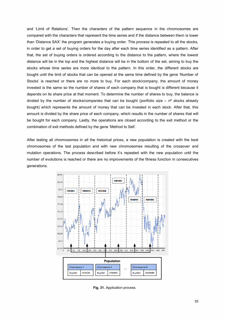
35

and ‘Limit of Relations’. Then the characters of the pattern sequence in the chromosomes are

compared with the characters that represent the time series and if the distance between them is lower

than ‘Distance SAX’ the program generates a buying order. This process is repeated to all the stocks,

in order to get a set of buying orders for the day after each time series identified as a pattern. After

that, the set of buying orders is ordered according to the distance to the pattern, where the lowest

distance will be in the top and the highest distance will be in the bottom of the set, aiming to buy the

stocks whose time series are more identical to the pattern. In this order, the different stocks are

bought until the limit of stocks that can be opened at the same time defined by the gene ‘Number of

Stocks’ is reached or there are no more to buy. For each stock/company, the amount of money

invested is the same so the number of shares of each company that is bought is different because it

depends on its share price at that moment. To determine the number of shares to buy, the balance is

divided by the number of stocks/companies that can be bought (portfolio size – nº stocks already

bought) which represents the amount of money that can be invested in each stock. After that, this

amount is divided by the share price of each company, which results in the number of shares that will

be bought for each company. Lastly, the operations are closed according to the exit method or the

combination of exit methods defined by the gene ‘Method to Sell’.

After testing all chromosomes in all the historical prices, a new population is created with the best

chromosomes of the last population and with new chromosomes resulting of the crossover and

mutation operations. The process described before it’s repeated with the new population until the

number of evolutions is reached or there are no improvements of the fitness function in consecutives

generations.

Fig. 31. Application process.

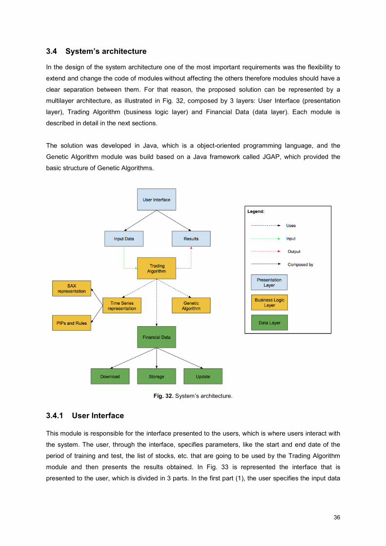
36

3.4 System’s architecture

In the design of the system architecture one of the most important requirements was the flexibility to

extend and change the code of modules without affecting the others therefore modules should have a

clear separation between them. For that reason, the proposed solution can be represented by a

multilayer architecture, as illustrated in Fig. 32, composed by 3 layers: User Interface (presentation

layer), Trading Algorithm (business logic layer) and Financial Data (data layer). Each module is

described in detail in the next sections.

The solution was developed in Java, which is a object-oriented programming language, and the

Genetic Algorithm module was build based on a Java framework called JGAP, which provided the

basic structure of Genetic Algorithms.

Fig. 32. System’s architecture.

3.4.1 User Interface

This module is responsible for the interface presented to the users, which is where users interact with

the system. The user, through the interface, specifies parameters, like the start and end date of the

period of training and test, the list of stocks, etc. that are going to be used by the Trading Algorithm

module and then presents the results obtained. In Fig. 33 is represented the interface that is

presented to the user, which is divided in 3 parts. In the first part (1), the user specifies the input data

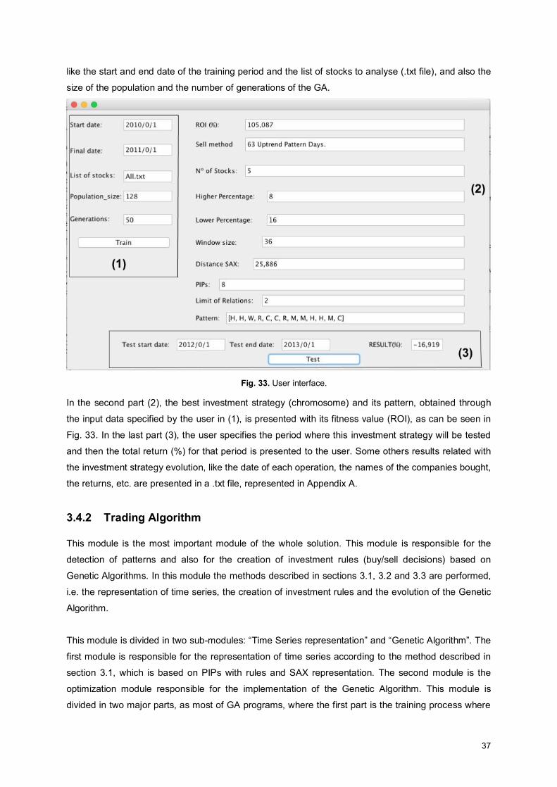
37

like the start and end date of the training period and the list of stocks to analyse (.txt file), and also the

size of the population and the number of generations of the GA.

Fig. 33. User interface.

In the second part (2), the best investment strategy (chromosome) and its pattern, obtained through

the input data specified by the user in (1), is presented with its fitness value (ROI), as can be seen in

Fig. 33. In the last part (3), the user specifies the period where this investment strategy will be tested

and then the total return (%) for that period is presented to the user. Some others results related with

the investment strategy evolution, like the date of each operation, the names of the companies bought,

the returns, etc. are presented in a .txt file, represented in Appendix A.

3.4.2 Trading Algorithm

This module is the most important module of the whole solution. This module is responsible for the

detection of patterns and also for the creation of investment rules (buy/sell decisions) based on

Genetic Algorithms. In this module the methods described in sections 3.1, 3.2 and 3.3 are performed,

i.e. the representation of time series, the creation of investment rules and the evolution of the Genetic

Algorithm.

This module is divided in two sub-modules: “Time Series representation” and “Genetic Algorithm”. The

first module is responsible for the representation of time series according to the method described in

section 3.1, which is based on PIPs with rules and SAX representation. The second module is the

optimization module responsible for the implementation of the Genetic Algorithm. This module is

divided in two major parts, as most of GA programs, where the first part is the training process where

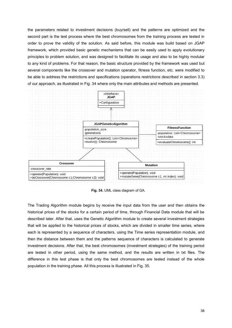
38

the parameters related to investment decisions (buy/sell) and the patterns are optimized and the

second part is the test process where the best chromosomes from the training process are tested in

order to prove the validity of the solution. As said before, this module was build based on JGAP

framework, which provided basic genetic mechanisms that can be easily used to apply evolutionary

principles to problem solution, and was designed to facilitate its usage and also to be highly modular

to any kind of problems. For that reason, the basic structure provided by the framework was used but

several components like the crossover and mutation operator, fitness function, etc. were modified to

be able to address the restrictions and specifications (operations restrictions described in section 3.3)

of our approach, as illustrated in Fig. 34 where only the main attributes and methods are presented.

Fig. 34. UML class diagram of GA.

The Trading Algorithm module begins by receive the input data from the user and then obtains the

historical prices of the stocks for a certain period of time, through Financial Data module that will be

described later. After that, uses the Genetic Algorithm module to create several investment strategies

that will be applied to the historical prices of stocks, which are divided in smaller time series, where

each is represented by a sequence of characters, using the Time series representation module, and

then the distance between them and the patterns sequence of characters is calculated to generate

investment decisions. After that, the best chromosomes (investment strategies) of the training period

are tested in other period, using the same method, and the results are written in txt files. The

difference in this test phase is that only the best chromosomes are tested instead of the whole

population in the training phase. All this process is illustrated in Fig. 35.

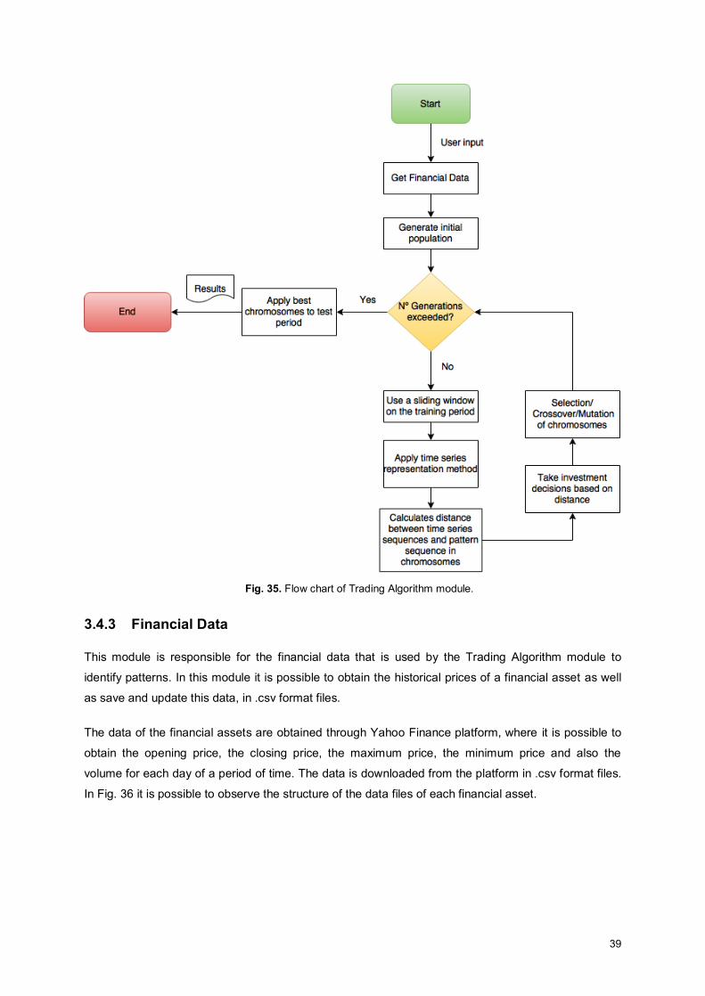
39

Fig. 35. Flow chart of Trading Algorithm module.

3.4.3 Financial Data

This module is responsible for the financial data that is used by the Trading Algorithm module to

identify patterns. In this module it is possible to obtain the historical prices of a financial asset as well

as save and update this data, in .csv format files.

The data of the financial assets are obtained through Yahoo Finance platform, where it is possible to

obtain the opening price, the closing price, the maximum price, the minimum price and also the

volume for each day of a period of time. The data is downloaded from the platform in .csv format files.

In Fig. 36 it is possible to observe the structure of the data files of each financial asset.

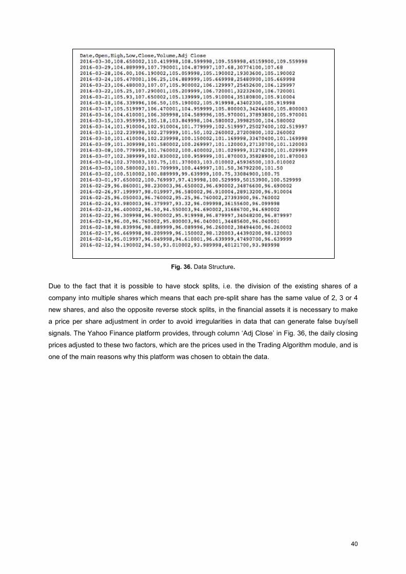
40

Fig. 36. Data Structure.

Due to the fact that it is possible to have stock splits, i.e. the division of the existing shares of a

company into multiple shares which means that each pre-split share has the same value of 2, 3 or 4

new shares, and also the opposite reverse stock splits, in the financial assets it is necessary to make

a price per share adjustment in order to avoid irregularities in data that can generate false buy/sell

signals. The Yahoo Finance platform provides, through column ‘Adj Close’ in Fig. 36, the daily closing

prices adjusted to these two factors, which are the prices used in the Trading Algorithm module, and is

one of the main reasons why this platform was chosen to obtain the data.

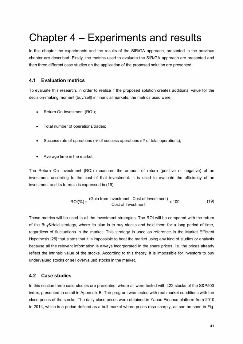
41

Chapter 4 – Experiments and results In this chapter the experiments and the results of the SIR/GA approach, presented in the previous

chapter are described. Firstly, the metrics used to evaluate the SIR/GA approach are presented and

then three different case studies on the application of the proposed solution are presented.

4.1 Evaluation metrics

To evaluate this research, in order to realize if the proposed solution creates additional value for the

decision-making moment (buy/sell) in financial markets, the metrics used were:

x Return On Investment (ROI);

x Total number of operations/trades;

x Success rate of operations (nº of success operations /nº of total operations);

x Average time in the market;

The Return On Investment (ROI) measures the amount of return (positive or negative) of an

investment according to the cost of that investment. It is used to evaluate the efficiency of an

investment and its formula is expressed in (19).

ROI(%) =

(Gain from Investment - Cost of Investment)Cost of Investment x 100 (19)

These metrics will be used in all the investment strategies. The ROI will be compared with the return

of the Buy&Hold strategy, where its plan is to buy stocks and hold them for a long period of time,

regardless of fluctuations in the market. This strategy is used as reference in the Market Efficient

Hypothesis [25] that states that it is impossible to beat the market using any kind of studies or analysis

because all the relevant information is always incorporated in the share prices, i.e. the prices already

reflect the intrinsic value of the stocks. According to this theory, it is impossible for investors to buy

undervalued stocks or sell overvalued stocks in the market.

4.2 Case studies

In this section three case studies are presented, where all were tested with 422 stocks of the S&P500

index, presented in detail in Appendix B. The program was tested with real market conditions with the

close prices of the stocks. The daily close prices were obtained in Yahoo Finance platform from 2010

to 2014, which is a period defined as a bull market where prices rose sharply, as can be seen in Fig.

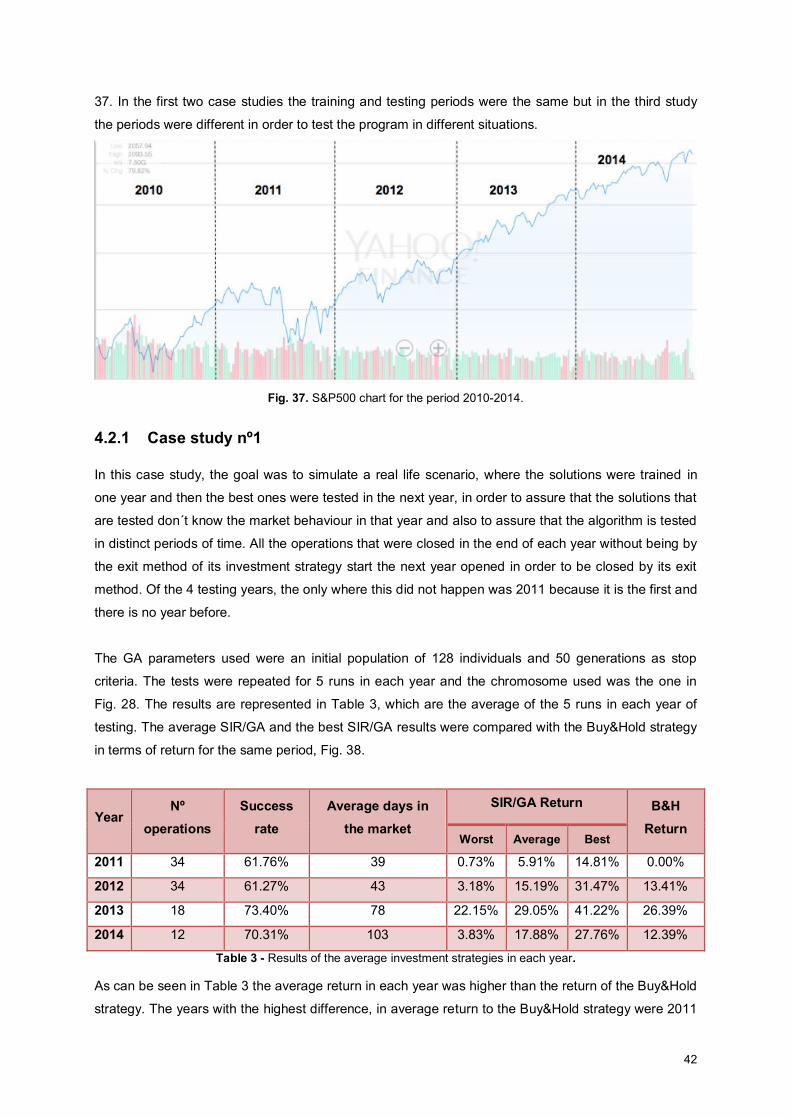
42

37. In the first two case studies the training and testing periods were the same but in the third study

the periods were different in order to test the program in different situations.

Fig. 37. S&P500 chart for the period 2010-2014.

4.2.1 Case study nº1

In this case study, the goal was to simulate a real life scenario, where the solutions were trained in

one year and then the best ones were tested in the next year, in order to assure that the solutions that

are tested don´t know the market behaviour in that year and also to assure that the algorithm is tested

in distinct periods of time. All the operations that were closed in the end of each year without being by

the exit method of its investment strategy start the next year opened in order to be closed by its exit

method. Of the 4 testing years, the only where this did not happen was 2011 because it is the first and

there is no year before.

The GA parameters used were an initial population of 128 individuals and 50 generations as stop

criteria. The tests were repeated for 5 runs in each year and the chromosome used was the one in

Fig. 28. The results are represented in Table 3, which are the average of the 5 runs in each year of

testing. The average SIR/GA and the best SIR/GA results were compared with the Buy&Hold strategy

in terms of return for the same period, Fig. 38.

Year Nº

operations Success

rate Average days in

the market

SIR/GA Return B&H Return

Worst Average Best 2011 34 61.76% 39 0.73% 5.91% 14.81% 0.00%

2012 34 61.27% 43 3.18% 15.19% 31.47% 13.41%

2013 18 73.40% 78 22.15% 29.05% 41.22% 26.39%

2014 12 70.31% 103 3.83% 17.88% 27.76% 12.39%

Table 3 - Results of the average investment strategies in each year.

As can be seen in Table 3 the average return in each year was higher than the return of the Buy&Hold

strategy. The years with the highest difference, in average return to the Buy&Hold strategy were 2011

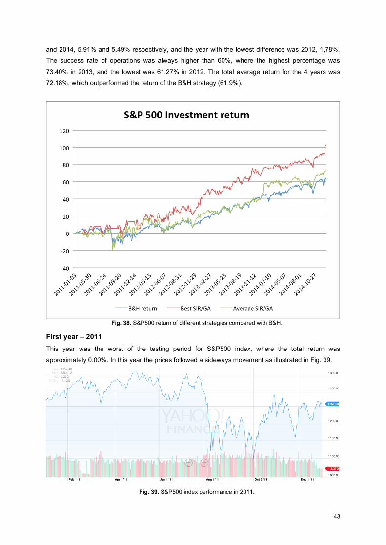
43

and 2014, 5.91% and 5.49% respectively, and the year with the lowest difference was 2012, 1,78%.

The success rate of operations was always higher than 60%, where the highest percentage was

73.40% in 2013, and the lowest was 61.27% in 2012. The total average return for the 4 years was

72.18%, which outperformed the return of the B&H strategy (61.9%).

Fig. 38. S&P500 return of different strategies compared with B&H.

First year – 2011 This year was the worst of the testing period for S&P500 index, where the total return was

approximately 0.00%. In this year the prices followed a sideways movement as illustrated in Fig. 39.

Fig. 39. S&P500 index performance in 2011.

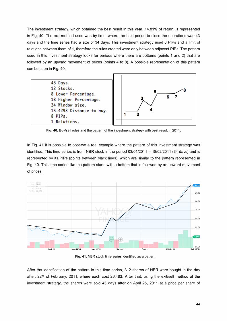
44

The investment strategy, which obtained the best result in this year, 14.81% of return, is represented

in Fig. 40. The exit method used was by time, where the hold period to close the operations was 43

days and the time series had a size of 34 days. This investment strategy used 8 PIPs and a limit of

relations between them of 1, therefore the rules created were only between adjacent PIPs. The pattern

used in this investment strategy looks for periods where there are bottoms (points 1 and 2) that are

followed by an upward movement of prices (points 4 to 8). A possible representation of this pattern

can be seen in Fig. 40.

Fig. 40. Buy/sell rules and the pattern of the investment strategy with best result in 2011.

In Fig. 41 it is possible to observe a real example where the pattern of this investment strategy was

identified. This time series is from NBR stock in the period 03/01/2011 – 18/02/2011 (34 days) and is

represented by its PIPs (points between black lines), which are similar to the pattern represented in

Fig. 40. This time series like the pattern starts with a bottom that is followed by an upward movement

of prices.

Fig. 41. NBR stock time series identified as a pattern.

After the identification of the pattern in this time series, 312 shares of NBR were bought in the day

after, 22nd of February, 2011, where each cost 26.48$. After that, using the exit/sell method of the

investment strategy, the shares were sold 43 days after on April 25, 2011 at a price per share of

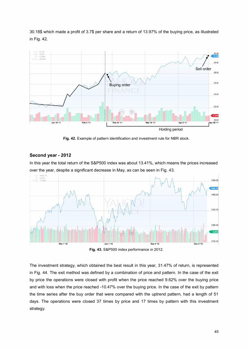
45

30.18$ which made a profit of 3.7$ per share and a return of 13.97% of the buying price, as illustrated

in Fig. 42.

Fig. 42. Example of pattern identification and investment rule for NBR stock.

Second year - 2012 In this year the total return of the S&P500 index was about 13.41%, which means the prices increased

over the year, despite a significant decrease in May, as can be seen in Fig. 43.

Fig. 43. S&P500 index performance in 2012.

The investment strategy, which obtained the best result in this year, 31.47% of return, is represented

in Fig. 44. The exit method was defined by a combination of price and pattern. In the case of the exit

by price the operations were closed with profit when the price reached 9.62% over the buying price

and with loss when the price reached -10.47% over the buying price. In the case of the exit by pattern

the time series after the buy order that were compared with the uptrend pattern, had a length of 51

days. The operations were closed 37 times by price and 17 times by pattern with this investment

strategy.

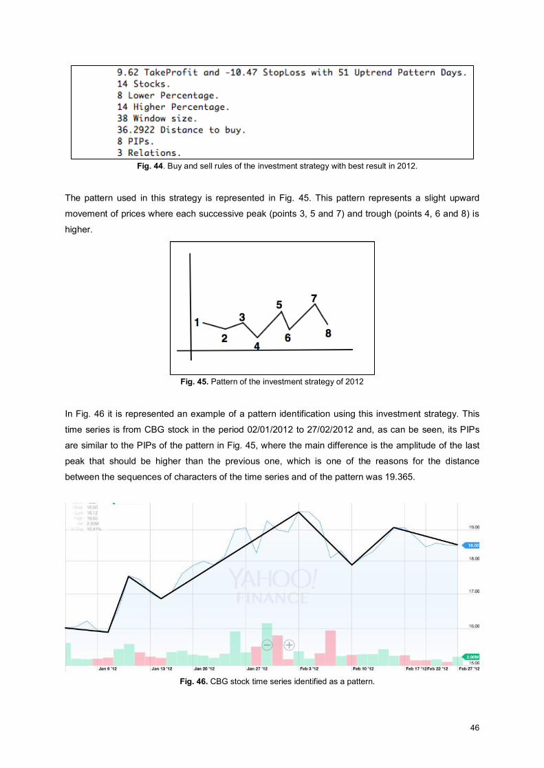
46

Fig. 44. Buy and sell rules of the investment strategy with best result in 2012.

The pattern used in this strategy is represented in Fig. 45. This pattern represents a slight upward

movement of prices where each successive peak (points 3, 5 and 7) and trough (points 4, 6 and 8) is

higher.

Fig. 45. Pattern of the investment strategy of 2012

In Fig. 46 it is represented an example of a pattern identification using this investment strategy. This

time series is from CBG stock in the period 02/01/2012 to 27/02/2012 and, as can be seen, its PIPs

are similar to the PIPs of the pattern in Fig. 45, where the main difference is the amplitude of the last

peak that should be higher than the previous one, which is one of the reasons for the distance

between the sequences of characters of the time series and of the pattern was 19.365.

Fig. 46. CBG stock time series identified as a pattern.

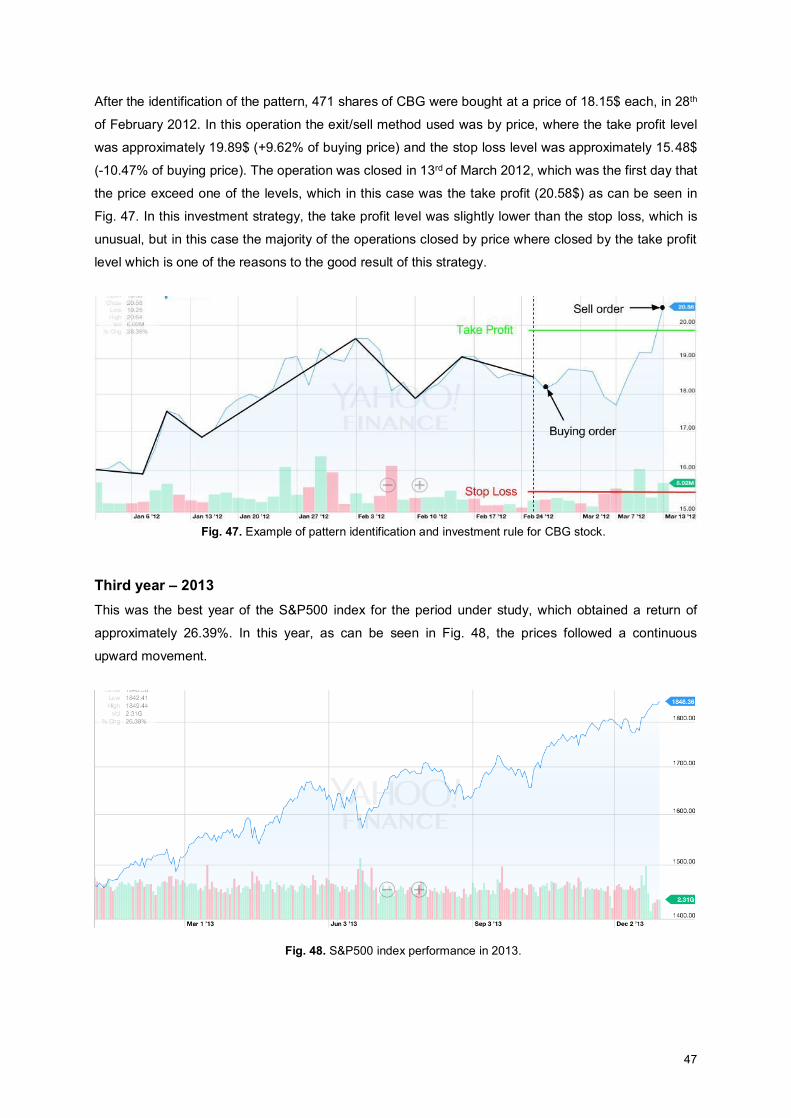
47

After the identification of the pattern, 471 shares of CBG were bought at a price of 18.15$ each, in 28th

of February 2012. In this operation the exit/sell method used was by price, where the take profit level

was approximately 19.89$ (+9.62% of buying price) and the stop loss level was approximately 15.48$

(-10.47% of buying price). The operation was closed in 13rd of March 2012, which was the first day that

the price exceed one of the levels, which in this case was the take profit (20.58$) as can be seen in

Fig. 47. In this investment strategy, the take profit level was slightly lower than the stop loss, which is

unusual, but in this case the majority of the operations closed by price where closed by the take profit

level which is one of the reasons to the good result of this strategy.

Fig. 47. Example of pattern identification and investment rule for CBG stock.

Third year – 2013 This was the best year of the S&P500 index for the period under study, which obtained a return of

approximately 26.39%. In this year, as can be seen in Fig. 48, the prices followed a continuous

upward movement.

Fig. 48. S&P500 index performance in 2013.

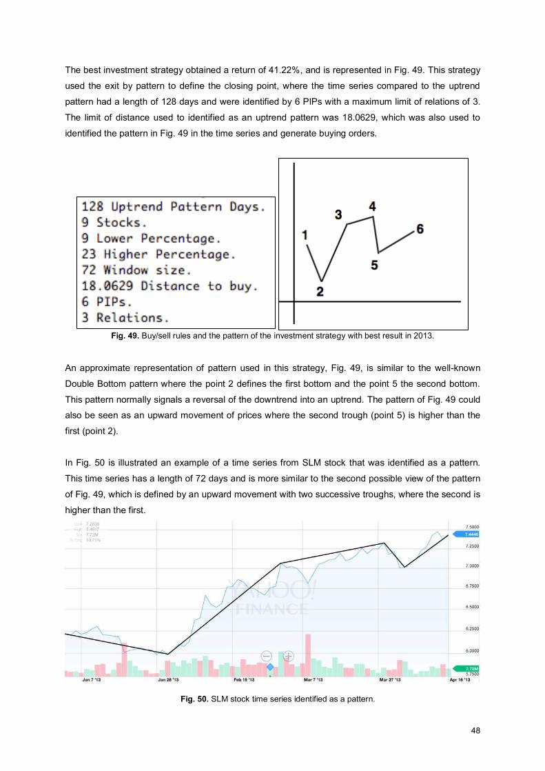
48

The best investment strategy obtained a return of 41.22%, and is represented in Fig. 49. This strategy

used the exit by pattern to define the closing point, where the time series compared to the uptrend

pattern had a length of 128 days and were identified by 6 PIPs with a maximum limit of relations of 3.

The limit of distance used to identified as an uptrend pattern was 18.0629, which was also used to

identified the pattern in Fig. 49 in the time series and generate buying orders.

Fig. 49. Buy/sell rules and the pattern of the investment strategy with best result in 2013.

An approximate representation of pattern used in this strategy, Fig. 49, is similar to the well-known

Double Bottom pattern where the point 2 defines the first bottom and the point 5 the second bottom.

This pattern normally signals a reversal of the downtrend into an uptrend. The pattern of Fig. 49 could

also be seen as an upward movement of prices where the second trough (point 5) is higher than the

first (point 2).

In Fig. 50 is illustrated an example of a time series from SLM stock that was identified as a pattern.

This time series has a length of 72 days and is more similar to the second possible view of the pattern

of Fig. 49, which is defined by an upward movement with two successive troughs, where the second is

higher than the first.

Fig. 50. SLM stock time series identified as a pattern.

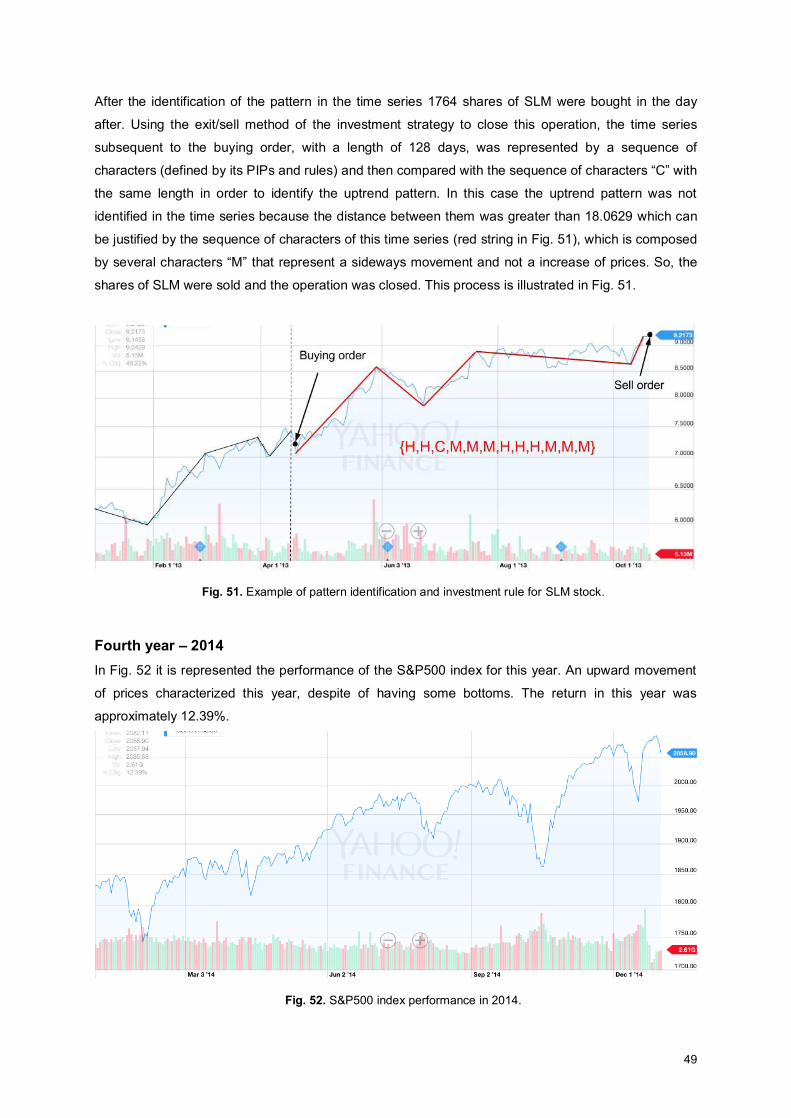
49

After the identification of the pattern in the time series 1764 shares of SLM were bought in the day

after. Using the exit/sell method of the investment strategy to close this operation, the time series

subsequent to the buying order, with a length of 128 days, was represented by a sequence of

characters (defined by its PIPs and rules) and then compared with the sequence of characters “C” with

the same length in order to identify the uptrend pattern. In this case the uptrend pattern was not

identified in the time series because the distance between them was greater than 18.0629 which can

be justified by the sequence of characters of this time series (red string in Fig. 51), which is composed

by several characters “M” that represent a sideways movement and not a increase of prices. So, the

shares of SLM were sold and the operation was closed. This process is illustrated in Fig. 51.

Fig. 51. Example of pattern identification and investment rule for SLM stock.

Fourth year – 2014 In Fig. 52 it is represented the performance of the S&P500 index for this year. An upward movement

of prices characterized this year, despite of having some bottoms. The return in this year was

approximately 12.39%.

Fig. 52. S&P500 index performance in 2014.

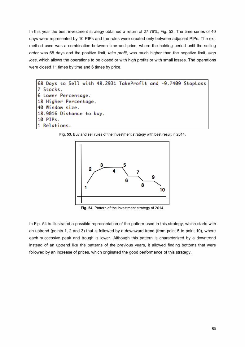
50

In this year the best investment strategy obtained a return of 27.76%, Fig. 53. The time series of 40

days were represented by 10 PIPs and the rules were created only between adjacent PIPs. The exit

method used was a combination between time and price, where the holding period until the selling

order was 68 days and the positive limit, take profit, was much higher than the negative limit, stop

loss, which allows the operations to be closed or with high profits or with small losses. The operations

were closed 11 times by time and 6 times by price.

Fig. 53. Buy and sell rules of the investment strategy with best result in 2014.

Fig. 54. Pattern of the investment strategy of 2014.

In Fig. 54 is illustrated a possible representation of the pattern used in this strategy, which starts with

an uptrend (points 1, 2 and 3) that is followed by a downward trend (from point 5 to point 10), where

each successive peak and trough is lower. Although this pattern is characterized by a downtrend

instead of an uptrend like the patterns of the previous years, it allowed finding bottoms that were

followed by an increase of prices, which originated the good performance of this strategy.

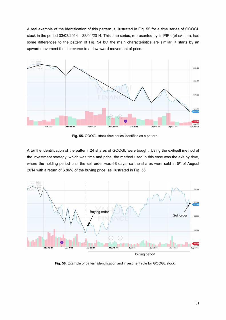
51

A real example of the identification of this pattern is illustrated in Fig. 55 for a time series of GOOGL

stock in the period 03/03/2014 – 28/04/2014. This time series, represented by its PIPs (black line), has

some differences to the pattern of Fig. 54 but the main characteristics are similar, it starts by an

upward movement that is reverse to a downward movement of price.

Fig. 55. GOOGL stock time series identified as a pattern.

After the identification of the pattern, 24 shares of GOOGL were bought. Using the exit/sell method of

the investment strategy, which was time and price, the method used in this case was the exit by time,

where the holding period until the sell order was 68 days, so the shares were sold in 5th of August

2014 with a return of 6.86% of the buying price, as illustrated in Fig. 56.

Fig. 56. Example of pattern identification and investment rule for GOOGL stock.

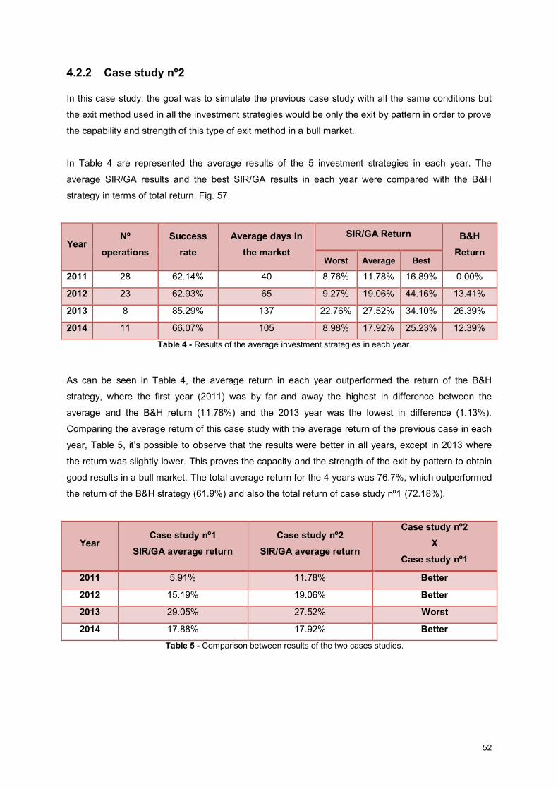
52

4.2.2 Case study nº2

In this case study, the goal was to simulate the previous case study with all the same conditions but

the exit method used in all the investment strategies would be only the exit by pattern in order to prove

the capability and strength of this type of exit method in a bull market.

In Table 4 are represented the average results of the 5 investment strategies in each year. The

average SIR/GA results and the best SIR/GA results in each year were compared with the B&H

strategy in terms of total return, Fig. 57.

Year Nº

operations Success

rate Average days in

the market

SIR/GA Return B&H Return

Worst Average Best 2011 28 62.14% 40 8.76% 11.78% 16.89% 0.00%

2012 23 62.93% 65 9.27% 19.06% 44.16% 13.41%

2013 8 85.29% 137 22.76% 27.52% 34.10% 26.39%

2014 11 66.07% 105 8.98% 17.92% 25.23% 12.39%

Table 4 - Results of the average investment strategies in each year.

As can be seen in Table 4, the average return in each year outperformed the return of the B&H

strategy, where the first year (2011) was by far and away the highest in difference between the

average and the B&H return (11.78%) and the 2013 year was the lowest in difference (1.13%).

Comparing the average return of this case study with the average return of the previous case in each

year, Table 5, it’s possible to observe that the results were better in all years, except in 2013 where

the return was slightly lower. This proves the capacity and the strength of the exit by pattern to obtain

good results in a bull market. The total average return for the 4 years was 76.7%, which outperformed

the return of the B&H strategy (61.9%) and also the total return of case study nº1 (72.18%).

Year Case study nº1

SIR/GA average return Case study nº2

SIR/GA average return

Case study nº2 X

Case study nº1

2011 5.91% 11.78% Better

2012 15.19% 19.06% Better

2013 29.05% 27.52% Worst

2014 17.88% 17.92% Better Table 5 - Comparison between results of the two cases studies.

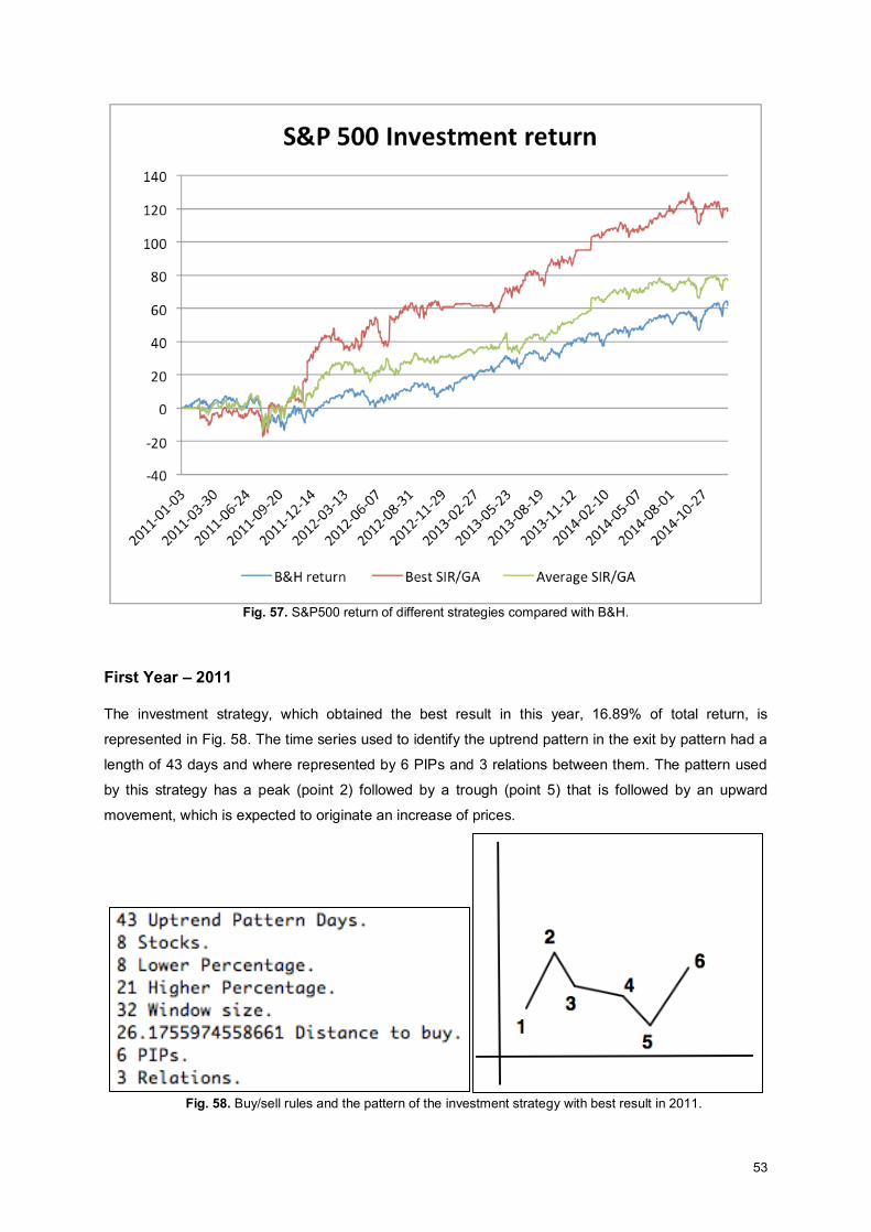
53

Fig. 57. S&P500 return of different strategies compared with B&H.

First Year – 2011

The investment strategy, which obtained the best result in this year, 16.89% of total return, is

represented in Fig. 58. The time series used to identify the uptrend pattern in the exit by pattern had a

length of 43 days and where represented by 6 PIPs and 3 relations between them. The pattern used

by this strategy has a peak (point 2) followed by a trough (point 5) that is followed by an upward

movement, which is expected to originate an increase of prices.

Fig. 58. Buy/sell rules and the pattern of the investment strategy with best result in 2011.

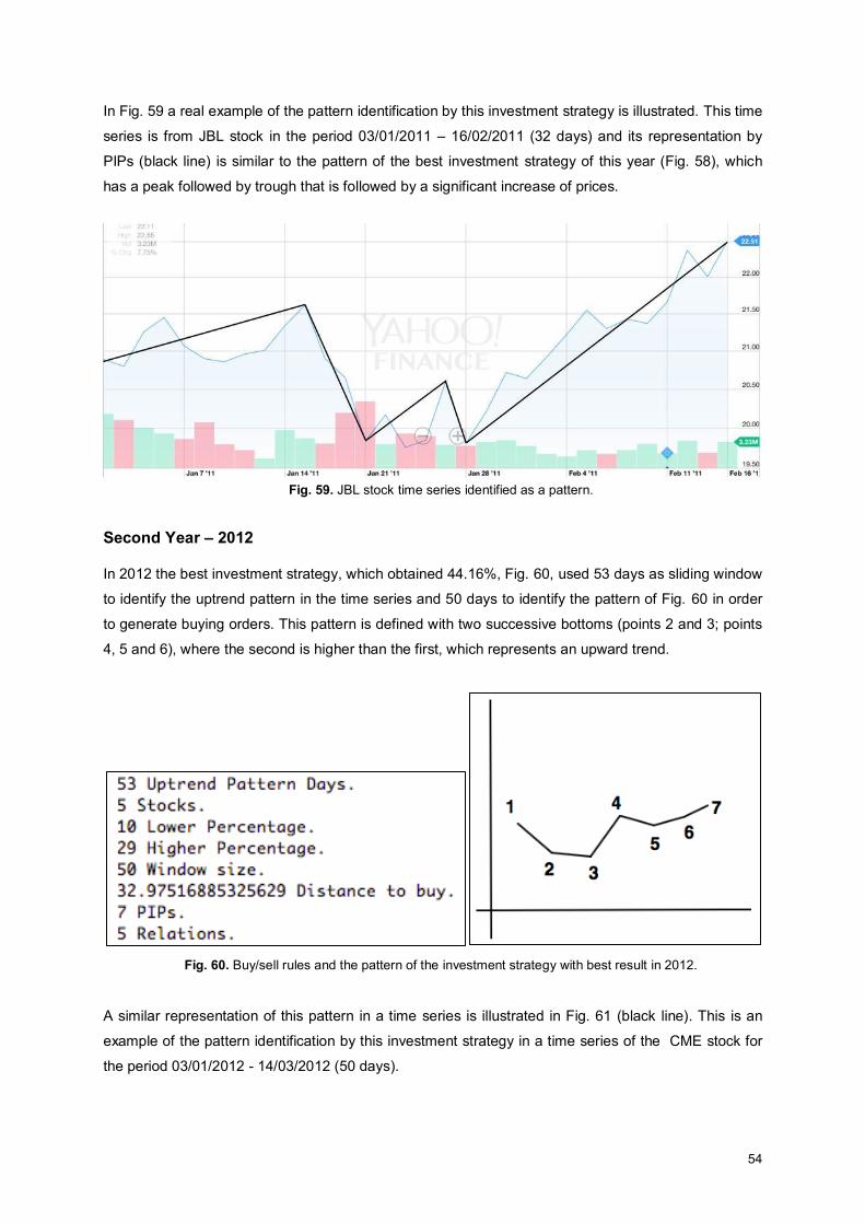
54

In Fig. 59 a real example of the pattern identification by this investment strategy is illustrated. This time

series is from JBL stock in the period 03/01/2011 – 16/02/2011 (32 days) and its representation by

PIPs (black line) is similar to the pattern of the best investment strategy of this year (Fig. 58), which

has a peak followed by trough that is followed by a significant increase of prices.

Fig. 59. JBL stock time series identified as a pattern.

Second Year – 2012

In 2012 the best investment strategy, which obtained 44.16%, Fig. 60, used 53 days as sliding window

to identify the uptrend pattern in the time series and 50 days to identify the pattern of Fig. 60 in order

to generate buying orders. This pattern is defined with two successive bottoms (points 2 and 3; points

4, 5 and 6), where the second is higher than the first, which represents an upward trend.

Fig. 60. Buy/sell rules and the pattern of the investment strategy with best result in 2012.

A similar representation of this pattern in a time series is illustrated in Fig. 61 (black line). This is an

example of the pattern identification by this investment strategy in a time series of the CME stock for

the period 03/01/2012 - 14/03/2012 (50 days).

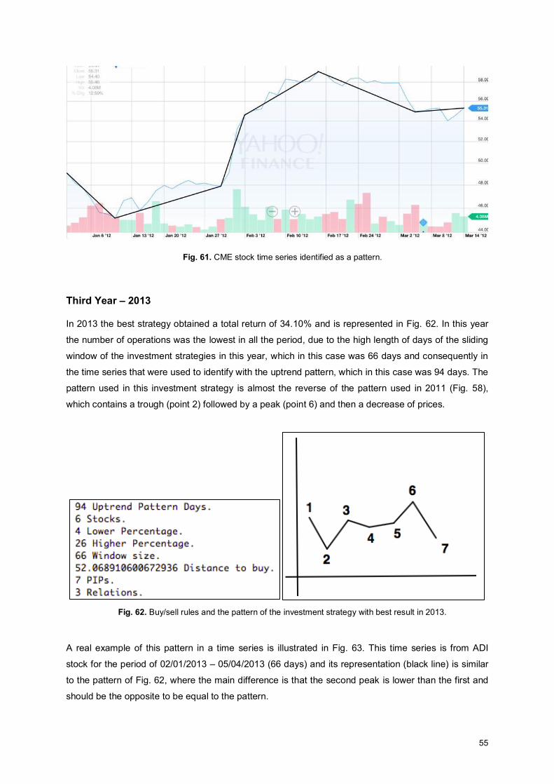
55

Fig. 61. CME stock time series identified as a pattern.

Third Year – 2013

In 2013 the best strategy obtained a total return of 34.10% and is represented in Fig. 62. In this year

the number of operations was the lowest in all the period, due to the high length of days of the sliding

window of the investment strategies in this year, which in this case was 66 days and consequently in

the time series that were used to identify with the uptrend pattern, which in this case was 94 days. The

pattern used in this investment strategy is almost the reverse of the pattern used in 2011 (Fig. 58),

which contains a trough (point 2) followed by a peak (point 6) and then a decrease of prices.

Fig. 62. Buy/sell rules and the pattern of the investment strategy with best result in 2013.

A real example of this pattern in a time series is illustrated in Fig. 63. This time series is from ADI

stock for the period of 02/01/2013 – 05/04/2013 (66 days) and its representation (black line) is similar

to the pattern of Fig. 62, where the main difference is that the second peak is lower than the first and

should be the opposite to be equal to the pattern.

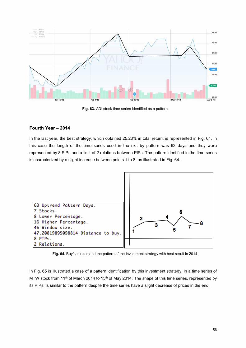
56

Fig. 63. ADI stock time series identified as a pattern.

Fourth Year – 2014

In the last year, the best strategy, which obtained 25.23% in total return, is represented in Fig. 64. In

this case the length of the time series used in the exit by pattern was 63 days and they were

represented by 8 PIPs and a limit of 2 relations between PIPs. The pattern identified in the time series

is characterized by a slight increase between points 1 to 8, as illustrated in Fig. 64.

Fig. 64. Buy/sell rules and the pattern of the investment strategy with best result in 2014.

In Fig. 65 is illustrated a case of a pattern identification by this investment strategy, in a time series of

MTW stock from 11th of March 2014 to 15th of May 2014. The shape of this time series, represented by

its PIPs, is similar to the pattern despite the time series have a slight decrease of prices in the end.

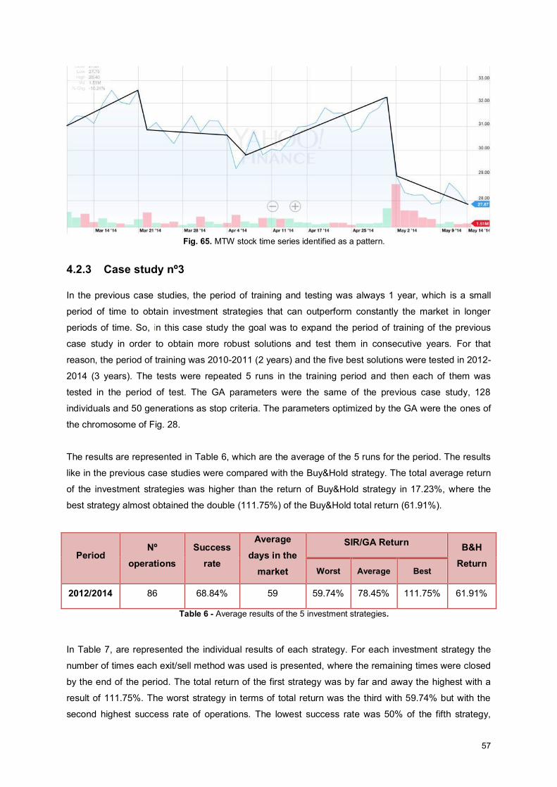
57

Fig. 65. MTW stock time series identified as a pattern.

4.2.3 Case study nº3

In the previous case studies, the period of training and testing was always 1 year, which is a small

period of time to obtain investment strategies that can outperform constantly the market in longer

periods of time. So, in this case study the goal was to expand the period of training of the previous

case study in order to obtain more robust solutions and test them in consecutive years. For that

reason, the period of training was 2010-2011 (2 years) and the five best solutions were tested in 2012-

2014 (3 years). The tests were repeated 5 runs in the training period and then each of them was

tested in the period of test. The GA parameters were the same of the previous case study, 128

individuals and 50 generations as stop criteria. The parameters optimized by the GA were the ones of

the chromosome of Fig. 28.

The results are represented in Table 6, which are the average of the 5 runs for the period. The results

like in the previous case studies were compared with the Buy&Hold strategy. The total average return

of the investment strategies was higher than the return of Buy&Hold strategy in 17.23%, where the

best strategy almost obtained the double (111.75%) of the Buy&Hold total return (61.91%).

Period Nº

operations

Success rate

Average days in the

market

SIR/GA Return B&H Return

Worst Average Best

2012/2014 86 68.84% 59 59.74% 78.45% 111.75% 61.91%

Table 6 - Average results of the 5 investment strategies.

In Table 7, are represented the individual results of each strategy. For each investment strategy the

number of times each exit/sell method was used is presented, where the remaining times were closed

by the end of the period. The total return of the first strategy was by far and away the highest with a

result of 111.75%. The worst strategy in terms of total return was the third with 59.74% but with the

second highest success rate of operations. The lowest success rate was 50% of the fifth strategy,

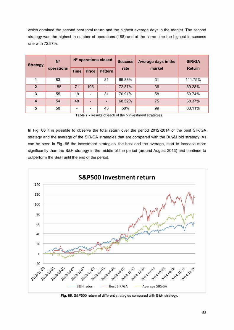
58

which obtained the second best total return and the highest average days in the market. The second

strategy was the highest in number of operations (188) and at the same time the highest in success

rate with 72.87%.

Strategy Nº

operations

Nº operations closed Success rate

Average days in the market

SIR/GA Return

Time Price Pattern

1 83 - - 81 69.88% 31 111.75%

2 188 71 105 - 72.87% 36 69.28%

3 55 19 - 31 70.91% 58 59.74%

4 54 48 - - 68.52% 75 68.37%

5 50 - - 43 50% 99 83.11%

Table 7 - Results of each of the 5 investment strategies.

In Fig. 66 it is possible to observe the total return over the period 2012-2014 of the best SIR/GA

strategy and the average of the SIR/GA strategies that are compared with the Buy&Hold strategy. As

can be seen in Fig. 66 the investment strategies, the best and the average, start to increase more

significantly than the B&H strategy in the middle of the period (around August 2013) and continue to

outperform the B&H until the end of the period.

Fig. 66. S&P500 return of different strategies compared with B&H strategy.

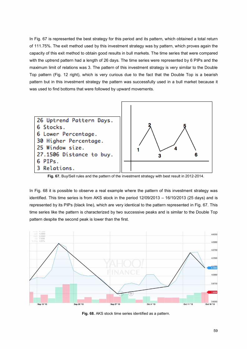
59

In Fig. 67 is represented the best strategy for this period and its pattern, which obtained a total return

of 111.75%. The exit method used by this investment strategy was by pattern, which proves again the

capacity of this exit method to obtain good results in bull markets. The time series that were compared

with the uptrend pattern had a length of 26 days. The time series were represented by 6 PIPs and the

maximum limit of relations was 3. The pattern of this investment strategy is very similar to the Double

Top pattern (Fig. 12 right), which is very curious due to the fact that the Double Top is a bearish

pattern but in this investment strategy the pattern was successfully used in a bull market because it

was used to find bottoms that were followed by upward movements.

Fig. 67. Buy/Sell rules and the pattern of the investment strategy with best result in 2012-2014.

In Fig. 68 it is possible to observe a real example where the pattern of this investment strategy was

identified. This time series is from AKS stock in the period 12/09/2013 – 16/10/2013 (25 days) and is

represented by its PIPs (black line), which are very identical to the pattern represented in Fig. 67. This

time series like the pattern is characterized by two successive peaks and is similar to the Double Top

pattern despite the second peak is lower than the first.

Fig. 68. AKS stock time series identified as a pattern.

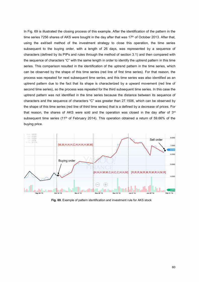
60

In Fig. 69 is illustrated the closing process of this example. After the identification of the pattern in the

time series 7256 shares of AKS were bought in the day after that was 17th of October 2013. After that,

using the exit/sell method of the investment strategy to close this operation, the time series

subsequent to the buying order, with a length of 26 days, was represented by a sequence of

characters (defined by its PIPs and rules through the method of section 3.1) and then compared with

the sequence of characters “C” with the same length in order to identify the uptrend pattern in this time

series. This comparison resulted in the identification of the uptrend pattern in the time series, which

can be observed by the shape of this time series (red line of first time series). For that reason, the

process was repeated for next subsequent time series, and this time series was also identified as an

uptrend pattern due to the fact that its shape is characterized by a upward movement (red line of

second time series), so the process was repeated for the third subsequent time series. In this case the

uptrend pattern was not identified in the time series because the distance between its sequence of

characters and the sequence of characters “C” was greater than 27.1506, which can be observed by

the shape of this time series (red line of third time series) that is a defined by a decrease of prices. For

that reason, the shares of AKS were sold and the operation was closed in the day after of 3rd

subsequent time series (11th of February 2014). This operation obtained a return of 59.66% of the

buying price.

Fig. 69. Example of pattern identification and investment rule for AKS stock

61

Chapter 5 – Conclusions and future work The new approach described and implemented, which was built on the definition of rules based on

PIPs, SAX representation and an optimization algorithm (GA), showed good potential on the stock

market. The identification of PIPs allowed a huge dimensional reduction of the time series and at the

same time, maintains the main characteristics of its data. The creation of rules allowed the specific

definition of relationships between the PIPs identified in time series. The mapping between rules and

characters allowed the distinction of the different types of trends between the PIPs of time series and

also allowed the representation of time series by a sequence of characters, which facilitated the

identification of patterns. The GA allowed a huge flexibility of solutions and also allowed to define and

identify several patterns with different sizes. This optimization algorithm has showed to be an excellent

technique to find good solutions for this kind of problems.

The solution was tested with real data from S&P500 index for the period 2010-2014, which is defined

as a bull market where the prices increase over the time. In order to validate this approach all the test

results were compared with the Buy&Hold strategy, where the results of the SIRG/GA approach

outperformed the B&H strategy in all case studies. The results proved the ability of this approach to

perform well in bull markets. The usage of the exit/sell method by pattern proved to be an excellent

option in this type of markets because this method remains in the market whenever the prices are

increasing which is the common trend of prices in this type of markets.

Some planned ideas to future work on this approach, in order to improve its capability, are:

x Test the solution in other markets like European indexes (Euro Stoxx 50, DAX-30, etc.) to

create a more robust solution.

x Include several technical indicators like OBV, RSI, etc. to support the decision of buy and sell

in the investment strategies.

x Add to the investment strategies the short operation in order to make the program much more

completed for the real life scenarios and to perform in bear markets too.

x Add an option to find some wanted and well-known patterns like the Double Bottom and Top,

Head-and-Shoulders, etc.

62

References

[1] Helfert, E. (2001). Financial Analysis Tools and Techniques: A Guide for Managers. McGraw-Hill

Education.

[2] Kirkpatrick II, C. D., & Dahlquist, J. R. (2010). Technical Analysis: The Complete Resource for

Financial Market Technicians (2nd Edition ed.).

[3] Murphy, J. J. (1999). Technical Analysis of the Financial Markets: A Comprehensive Guide to

Trading Methods and Applications.

[4] Bulkowski, T. N. (2005). Encyclopedia of Chart Patterns (2nd Edition ed.). John Wiley and Sons.

[5] Colby, R. W. (2003). The Encyclopedia of Technical Market Indicators. McGraw-Hill.

[6] Lin, L., Cao, L., Wang, J., & Zhang, C. (2000). The Applications of Genetic Algorithms in Stock

Market Data Mining Optimization.

[7] Chen, S. H. (2002). Genetic Algorithms and Genetic Programming in Cmputational Finance.

Boston: Springer.

[8] Pinto, J., Neves, R., & Horta, N. (2011). Fitness function evaluation for MA trading strategies

based on genetic algorithms. In Proceedings of the 13th annual conference companion on genetic and

evolutionary computation, (pp. 819-820).

[9] Leigh, W., Modani, N., Purvis, R., & Roberts, T. (2002). Stock market trading rule discovery

using technical charting heuristics. Expert Systems with Applications, 23 (2), 155-159.

[10] Leigh, W., Frohlich, C. J., Hornik, S., Purvis, R., & Roberts, T. (2008). Trading With a Stock

Chart Heuristic. Systems, Man and Cybernetics, Part A: Systems and Humans, 38 (1), 93-104.

[11] Leigh, W., Paz, N., & Purvis, R. (2002). Market timing: a test of a charting heuristic. Economics

Letters, 77 (1), 55-63.

[12] Leigh, W., Purvis, R., & Ragusa, J. M. (2002). Forecasting the NYSE composite index with

technical analysis, pattern recognizer, neural network and genetic algorithm: a case study in romantic

decision support. Decision Support Systems, 32 (4), 361-377.

[13] Leigh, W., Paz, M., & Purvis, R. (2002). An analysis of a hybrid neural network and pattern

recognition technique for predicting short-term increases in the NYSE composite index. Omega, 30

(2), 69-76.

63

[14] Wang, J., & Chan, S. (2009). Trading rule discovery in the US stock market: An empirical

study. Expert Systems with Applications , 36 (2), 5450-5455.

[15] Wang, J., & Chan, S. (2007). Stock market trading rule discovery using pattern recognition and

technical analysis. Expert Systems with Applications , 33 (2), 304-315.

[16] Parracho, P., Neves, R., & Horta, N. (2011). Trading with optimized uptrend and downtrend

pattern templates using a genetic algorithm kernel. IEEE Congress on Evolutionary Computation, (pp.

1895–1901).

[17] Cervelló-Royo, R., Guijarro, F., & Michniuk, K. (2015). Stock market trading rule based on

pattern recognition and technical analysis: Forecasting the DJIA index with intraday data. Expert

Systems with Applications, 42 (14), 5963-5975.

[18] Fu, T., Chung, F., Luk, R., & Ng, C. (2008). Representing financial time series based on data

point importance. Engineering Applications of Artificial Intelligence, 21 (2), 277-300.

[19] Fu, T., Chung, F., Luk, R., & Ng, C. (2007). Stock time series pattern matching: Template-

based vs. rule-based approaches. Engineering Applications of Artificial Intelligence, 20 (3), 347-364.

[20] Tsinaslanidis, P. E., & Kugiumtzis, D. (2014). A prediction scheme using perceptually important

points and dynamic time warping. Expert Systems with Applications, 41 (15), 6848-6860.

[21] Ni, H. (2009). Profitability of Technical Chart Pattern Trading on FX Rates: Analyzed by

Wavelet Transform. Third International Symposium on (pp. 138-141). Nanchang: Intelligent

Information Technology Application.

[22] Lin, J., Keogh, E., Wei, L., & Lonardi, S. (2007). Experiencing SAX: a novel symbolic

representation of time series. Data Mining Knowledge Discovery, 15 (2), 107-144.

[23] Canelas, A., Neves, R., & Horta, N. (2013). A SAX-GA approach to evolve investment

strategies on financial markets based on pattern discovery techniques. Expert Systems with

Applications, 40 (5), 1579-1590.

[24] Keogh, E., Chakrabarti, K., Pazzani, M., & Mehrotra, S. (2000). Dimensionality reduction for

fast similarity search in large time series databases. Journal of Knowledge and Information Systems, 3

(3), 263-286.

[25] Bernstein, P. L. (1999). A new look at the efficient market hypothesis. Journal of Porfolio

Management, 25 (2), 1-2.

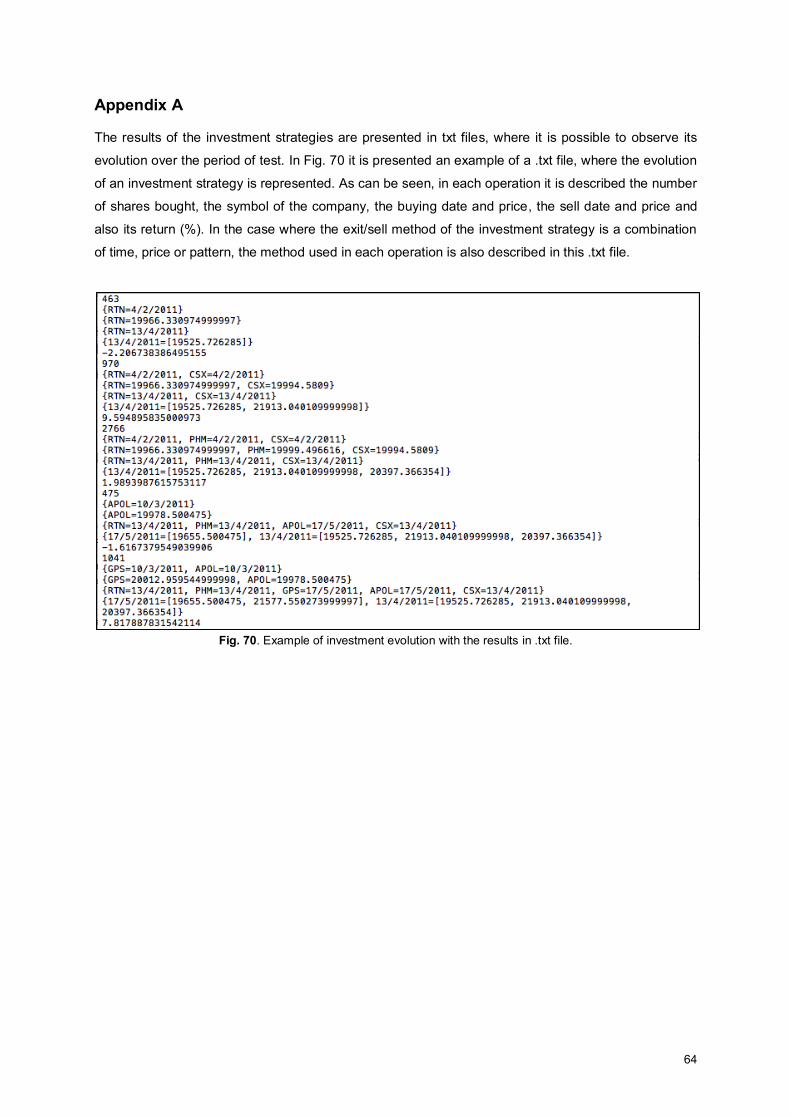
64

Appendix A

The results of the investment strategies are presented in txt files, where it is possible to observe its

evolution over the period of test. In Fig. 70 it is presented an example of a .txt file, where the evolution

of an investment strategy is represented. As can be seen, in each operation it is described the number

of shares bought, the symbol of the company, the buying date and price, the sell date and price and

also its return (%). In the case where the exit/sell method of the investment strategy is a combination

of time, price or pattern, the method used in each operation is also described in this .txt file.

Fig. 70. Example of investment evolution with the results in .txt file.

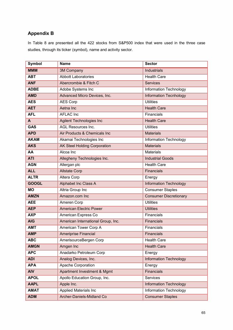
65

Appendix B

In Table 8 are presented all the 422 stocks from S&P500 index that were used in the three case

studies, through its ticker (symbol), name and activity sector.

Symbol Name Sector MMM 3M Company Industrials ABT Abbott Laboratories Health Care ANF Abercrombie & Fitch C Services ADBE Adobe Systems Inc Information Technology AMD Advanced Micro Devices, Inc. Information Tecnhology AES AES Corp Utilities AET Aetna Inc Health Care AFL AFLAC Inc Financials A Agilent Technologies Inc Health Care GAS AGL Resources Inc. Utilities APD Air Products & Chemicals Inc Materials AKAM Akamai Technologies Inc Information Technology AKS AK Steel Holding Corporation Materials AA Alcoa Inc Materials ATI Allegheny Technologies Inc. Industrial Goods AGN Allergan plc Health Care ALL Allstate Corp Financials ALTR Altera Corp Energy GOOGL Alphabet Inc Class A Information Technology MO Altria Group Inc Consumer Staples AMZN Amazon.com Inc Consumer Discretionary AEE Ameren Corp Utilities AEP American Electric Power Utilities AXP American Express Co Financials AIG American International Group, Inc. Financials AMT American Tower Corp A Financials AMP Ameriprise Financial Financials ABC AmerisourceBergen Corp Health Care AMGN Amgen Inc Health Care APC Anadarko Petroleum Corp Energy ADI Analog Devices, Inc. Information Technology APA Apache Corporation Energy AIV Apartment Investment & Mgmt Financials APOL Apollo Education Group, Inc. Services AAPL Apple Inc. Information Technology AMAT Applied Materials Inc Information Technology ADM Archer-Daniels-Midland Co Consumer Staples

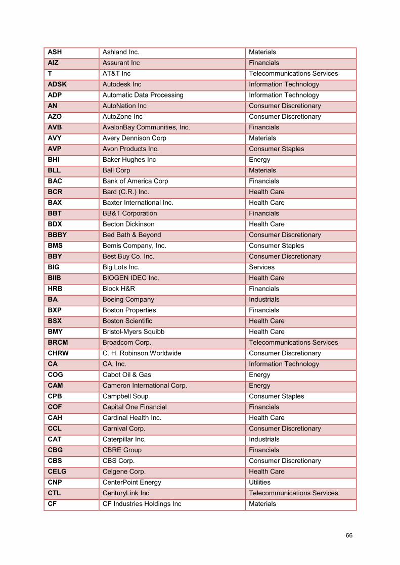
66

ASH Ashland Inc. Materials AIZ Assurant Inc Financials T AT&T Inc Telecommunications Services ADSK Autodesk Inc Information Technology ADP Automatic Data Processing Information Technology AN AutoNation Inc Consumer Discretionary AZO AutoZone Inc Consumer Discretionary AVB AvalonBay Communities, Inc. Financials AVY Avery Dennison Corp Materials AVP Avon Products Inc. Consumer Staples BHI Baker Hughes Inc Energy BLL Ball Corp Materials BAC Bank of America Corp Financials BCR Bard (C.R.) Inc. Health Care BAX Baxter International Inc. Health Care BBT BB&T Corporation Financials BDX Becton Dickinson Health Care BBBY Bed Bath & Beyond Consumer Discretionary BMS Bemis Company, Inc. Consumer Staples BBY Best Buy Co. Inc. Consumer Discretionary BIG Big Lots Inc. Services BIIB BIOGEN IDEC Inc. Health Care HRB Block H&R Financials BA Boeing Company Industrials BXP Boston Properties Financials BSX Boston Scientific Health Care BMY Bristol-Myers Squibb Health Care BRCM Broadcom Corp. Telecommunications Services CHRW C. H. Robinson Worldwide Consumer Discretionary CA CA, Inc. Information Technology COG Cabot Oil & Gas Energy CAM Cameron International Corp. Energy CPB Campbell Soup Consumer Staples COF Capital One Financial Financials CAH Cardinal Health Inc. Health Care CCL Carnival Corp. Consumer Discretionary CAT Caterpillar Inc. Industrials CBG CBRE Group Financials CBS CBS Corp. Consumer Discretionary CELG Celgene Corp. Health Care CNP CenterPoint Energy Utilities CTL CenturyLink Inc Telecommunications Services CF CF Industries Holdings Inc Materials

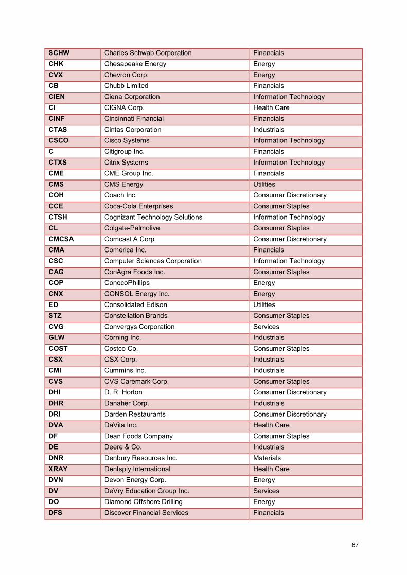
67

SCHW Charles Schwab Corporation Financials CHK Chesapeake Energy Energy CVX Chevron Corp. Energy CB Chubb Limited Financials CIEN Ciena Corporation Information Technology CI CIGNA Corp. Health Care CINF Cincinnati Financial Financials CTAS Cintas Corporation Industrials CSCO Cisco Systems Information Technology C Citigroup Inc. Financials CTXS Citrix Systems Information Technology CME CME Group Inc. Financials CMS CMS Energy Utilities COH Coach Inc. Consumer Discretionary CCE Coca-Cola Enterprises Consumer Staples CTSH Cognizant Technology Solutions Information Technology CL Colgate-Palmolive Consumer Staples CMCSA Comcast A Corp Consumer Discretionary CMA Comerica Inc. Financials CSC Computer Sciences Corporation Information Technology CAG ConAgra Foods Inc. Consumer Staples COP ConocoPhillips Energy CNX CONSOL Energy Inc. Energy ED Consolidated Edison Utilities STZ Constellation Brands Consumer Staples CVG Convergys Corporation Services GLW Corning Inc. Industrials COST Costco Co. Consumer Staples CSX CSX Corp. Industrials CMI Cummins Inc. Industrials CVS CVS Caremark Corp. Consumer Staples DHI D. R. Horton Consumer Discretionary DHR Danaher Corp. Industrials DRI Darden Restaurants Consumer Discretionary DVA DaVita Inc. Health Care DF Dean Foods Company Consumer Staples DE Deere & Co. Industrials DNR Denbury Resources Inc. Materials XRAY Dentsply International Health Care DVN Devon Energy Corp. Energy DV DeVry Education Group Inc. Services DO Diamond Offshore Drilling Energy DFS Discover Financial Services Financials

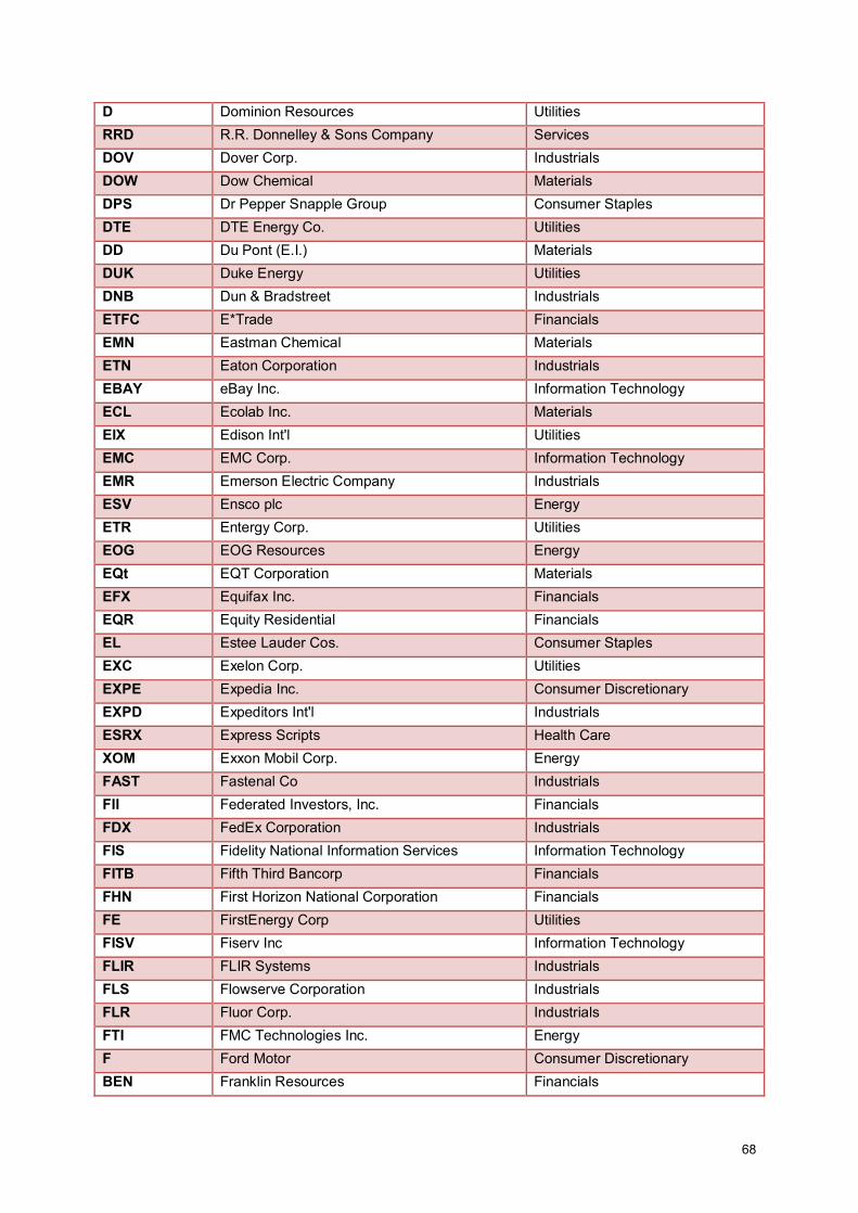
68

D Dominion Resources Utilities RRD R.R. Donnelley & Sons Company Services DOV Dover Corp. Industrials DOW Dow Chemical Materials DPS Dr Pepper Snapple Group Consumer Staples DTE DTE Energy Co. Utilities DD Du Pont (E.I.) Materials DUK Duke Energy Utilities DNB Dun & Bradstreet Industrials ETFC E*Trade Financials EMN Eastman Chemical Materials ETN Eaton Corporation Industrials EBAY eBay Inc. Information Technology ECL Ecolab Inc. Materials EIX Edison Int'l Utilities EMC EMC Corp. Information Technology EMR Emerson Electric Company Industrials ESV Ensco plc Energy ETR Entergy Corp. Utilities EOG EOG Resources Energy EQt EQT Corporation Materials EFX Equifax Inc. Financials EQR Equity Residential Financials EL Estee Lauder Cos. Consumer Staples EXC Exelon Corp. Utilities EXPE Expedia Inc. Consumer Discretionary EXPD Expeditors Int'l Industrials ESRX Express Scripts Health Care XOM Exxon Mobil Corp. Energy FAST Fastenal Co Industrials FII Federated Investors, Inc. Financials FDX FedEx Corporation Industrials FIS Fidelity National Information Services Information Technology FITB Fifth Third Bancorp Financials FHN First Horizon National Corporation Financials FE FirstEnergy Corp Utilities FISV Fiserv Inc Information Technology FLIR FLIR Systems Industrials FLS Flowserve Corporation Industrials FLR Fluor Corp. Industrials FTI FMC Technologies Inc. Energy F Ford Motor Consumer Discretionary BEN Franklin Resources Financials

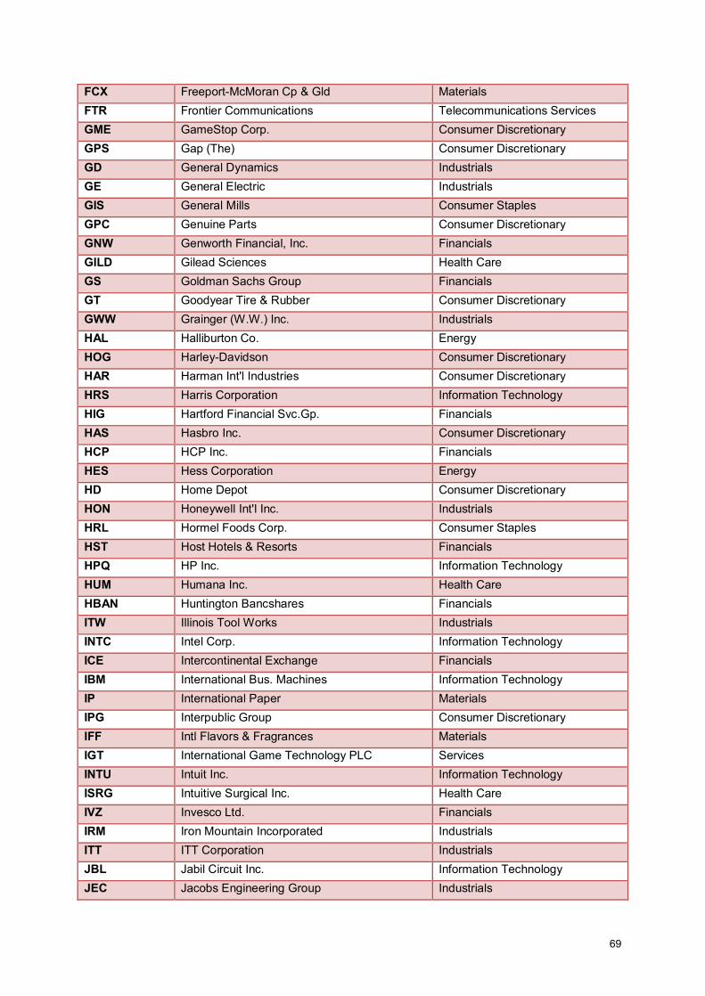
69

FCX Freeport-McMoran Cp & Gld Materials FTR Frontier Communications Telecommunications Services GME GameStop Corp. Consumer Discretionary GPS Gap (The) Consumer Discretionary GD General Dynamics Industrials GE General Electric Industrials GIS General Mills Consumer Staples GPC Genuine Parts Consumer Discretionary GNW Genworth Financial, Inc. Financials GILD Gilead Sciences Health Care GS Goldman Sachs Group Financials GT Goodyear Tire & Rubber Consumer Discretionary GWW Grainger (W.W.) Inc. Industrials HAL Halliburton Co. Energy HOG Harley-Davidson Consumer Discretionary HAR Harman Int'l Industries Consumer Discretionary HRS Harris Corporation Information Technology HIG Hartford Financial Svc.Gp. Financials HAS Hasbro Inc. Consumer Discretionary HCP HCP Inc. Financials HES Hess Corporation Energy HD Home Depot Consumer Discretionary HON Honeywell Int'l Inc. Industrials HRL Hormel Foods Corp. Consumer Staples HST Host Hotels & Resorts Financials HPQ HP Inc. Information Technology HUM Humana Inc. Health Care HBAN Huntington Bancshares Financials ITW Illinois Tool Works Industrials INTC Intel Corp. Information Technology ICE Intercontinental Exchange Financials IBM International Bus. Machines Information Technology IP International Paper Materials IPG Interpublic Group Consumer Discretionary IFF Intl Flavors & Fragrances Materials IGT International Game Technology PLC Services INTU Intuit Inc. Information Technology ISRG Intuitive Surgical Inc. Health Care IVZ Invesco Ltd. Financials IRM Iron Mountain Incorporated Industrials ITT ITT Corporation Industrials JBL Jabil Circuit Inc. Information Technology JEC Jacobs Engineering Group Industrials

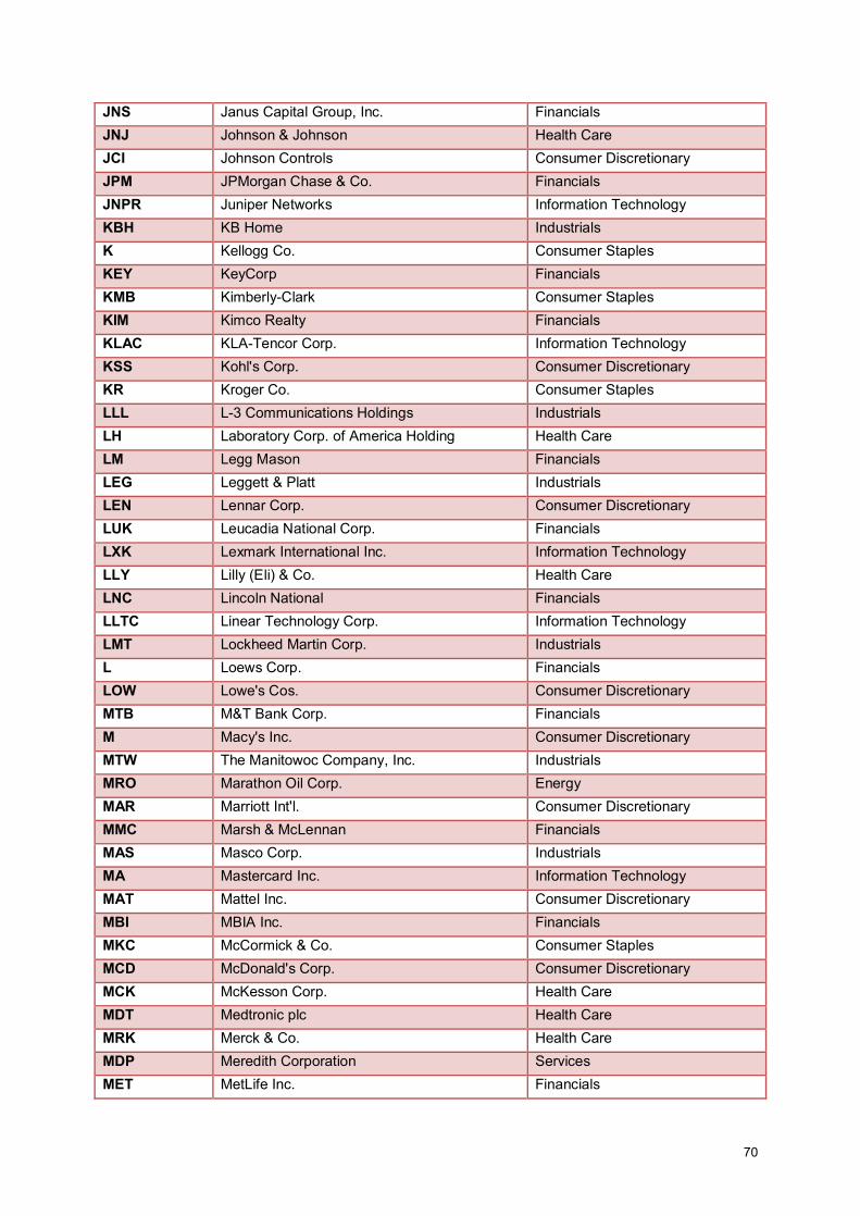
70

JNS Janus Capital Group, Inc. Financials JNJ Johnson & Johnson Health Care JCI Johnson Controls Consumer Discretionary JPM JPMorgan Chase & Co. Financials JNPR Juniper Networks Information Technology KBH KB Home Industrials K Kellogg Co. Consumer Staples KEY KeyCorp Financials KMB Kimberly-Clark Consumer Staples KIM Kimco Realty Financials KLAC KLA-Tencor Corp. Information Technology KSS Kohl's Corp. Consumer Discretionary KR Kroger Co. Consumer Staples LLL L-3 Communications Holdings Industrials LH Laboratory Corp. of America Holding Health Care LM Legg Mason Financials LEG Leggett & Platt Industrials LEN Lennar Corp. Consumer Discretionary LUK Leucadia National Corp. Financials LXK Lexmark International Inc. Information Technology LLY Lilly (Eli) & Co. Health Care LNC Lincoln National Financials LLTC Linear Technology Corp. Information Technology LMT Lockheed Martin Corp. Industrials L Loews Corp. Financials LOW Lowe's Cos. Consumer Discretionary MTB M&T Bank Corp. Financials M Macy's Inc. Consumer Discretionary MTW The Manitowoc Company, Inc. Industrials MRO Marathon Oil Corp. Energy MAR Marriott Int'l. Consumer Discretionary MMC Marsh & McLennan Financials MAS Masco Corp. Industrials MA Mastercard Inc. Information Technology MAT Mattel Inc. Consumer Discretionary MBI MBIA Inc. Financials MKC McCormick & Co. Consumer Staples MCD McDonald's Corp. Consumer Discretionary MCK McKesson Corp. Health Care MDT Medtronic plc Health Care MRK Merck & Co. Health Care MDP Meredith Corporation Services MET MetLife Inc. Financials

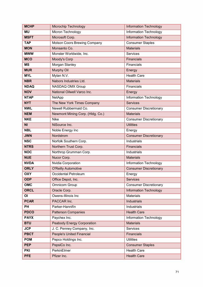
71

MCHP Microchip Technology Information Technology MU Micron Technology Information Technology MSFT Microsoft Corp. Information Technology TAP Molson Coors Brewing Company Consumer Staples MON Monsanto Co. Materials MWW Monster Worldwide, Inc. Services MCO Moody's Corp Financials MS Morgan Stanley Financials MUR Murphy Oil Energy MYL Mylan N.V. Health Care NBR Nabors Industries Ltd. Materials NDAQ NASDAQ OMX Group Financials NOV National Oilwell Varco Inc. Energy NTAP NetApp Information Technology NYT The New York Times Company Services NWL Newell Rubbermaid Co. Consumer Discretionary NEM Newmont Mining Corp. (Hldg. Co.) Materials NKE Nike Consumer Discretionary NI NiSource Inc. Utilities NBL Noble Energy Inc Energy JWN Nordstrom Consumer Discretionary NSC Norfolk Southern Corp. Industrials NTRS Northern Trust Corp. Financials NOC Northrop Grumman Corp. Industrials NUE Nucor Corp. Materials NVDA Nvidia Corporation Information Technology ORLY O'Reilly Automotive Consumer Discretionary OXY Occidental Petroleum Energy ODP Office Depot, Inc. Services OMC Omnicom Group Consumer Discretionary ORCL Oracle Corp. Information Technology OI Owens-Illinois Inc Materials PCAR PACCAR Inc. Industrials PH Parker-Hannifin Industrials PDCO Patterson Companies Health Care PAYX Paychex Inc. Information Technology BTU Peabody Energy Corporation Materials JCP J. C. Penney Company, Inc. Services PBCT People's United Financial Financials POM Pepco Holdings Inc. Utilities PEP PepsiCo Inc. Consumer Staples PKI PerkinElmer Health Care PFE Pfizer Inc. Health Care

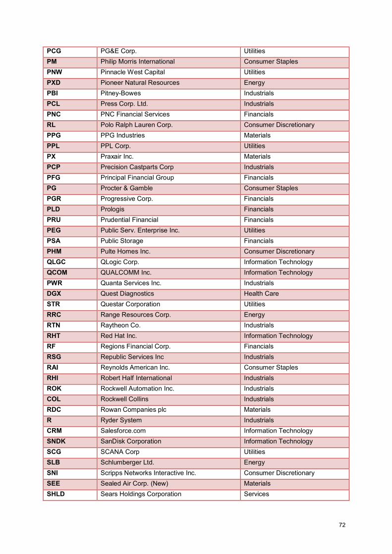
72

PCG PG&E Corp. Utilities PM Philip Morris International Consumer Staples PNW Pinnacle West Capital Utilities PXD Pioneer Natural Resources Energy PBI Pitney-Bowes Industrials PCL Press Corp. Ltd. Industrials PNC PNC Financial Services Financials RL Polo Ralph Lauren Corp. Consumer Discretionary PPG PPG Industries Materials PPL PPL Corp. Utilities PX Praxair Inc. Materials PCP Precision Castparts Corp Industrials PFG Principal Financial Group Financials PG Procter & Gamble Consumer Staples PGR Progressive Corp. Financials PLD Prologis Financials PRU Prudential Financial Financials PEG Public Serv. Enterprise Inc. Utilities PSA Public Storage Financials PHM Pulte Homes Inc. Consumer Discretionary QLGC QLogic Corp. Information Technology QCOM QUALCOMM Inc. Information Technology PWR Quanta Services Inc. Industrials DGX Quest Diagnostics Health Care STR Questar Corporation Utilities RRC Range Resources Corp. Energy RTN Raytheon Co. Industrials RHT Red Hat Inc. Information Technology RF Regions Financial Corp. Financials RSG Republic Services Inc Industrials RAI Reynolds American Inc. Consumer Staples RHI Robert Half International Industrials ROK Rockwell Automation Inc. Industrials COL Rockwell Collins Industrials RDC Rowan Companies plc Materials R Ryder System Industrials CRM Salesforce.com Information Technology SNDK SanDisk Corporation Information Technology SCG SCANA Corp Utilities SLB Schlumberger Ltd. Energy SNI Scripps Networks Interactive Inc. Consumer Discretionary SEE Sealed Air Corp. (New) Materials SHLD Sears Holdings Corporation Services

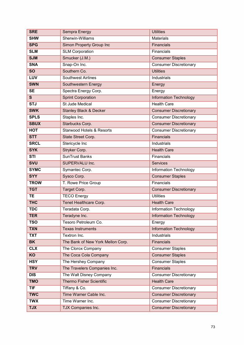
73

SRE Sempra Energy Utilities SHW Sherwin-Williams Materials SPG Simon Property Group Inc Financials SLM SLM Corporation Financials SJM Smucker (J.M.) Consumer Staples SNA Snap-On Inc. Consumer Discretionary SO Southern Co. Utilities LUV Southwest Airlines Industrials SWN Southwestern Energy Energy SE Spectra Energy Corp. Energy S Sprint Corporation Information Technology STJ St Jude Medical Health Care SWK Stanley Black & Decker Consumer Discretionary SPLS Staples Inc. Consumer Discretionary SBUX Starbucks Corp. Consumer Discretionary HOT Starwood Hotels & Resorts Consumer Discretionary STT State Street Corp. Financials SRCL Stericycle Inc Industrials SYK Stryker Corp. Health Care STI SunTrust Banks Financials SVU SUPERVALU Inc. Services SYMC Symantec Corp. Information Technology SYY Sysco Corp. Consumer Staples TROW T. Rowe Price Group Financials TGT Target Corp. Consumer Discretionary TE TECO Energy Utilities THC Tenet Healthcare Corp. Health Care TDC Teradata Corp. Information Technology TER Teradyne Inc. Information Technology TSO Tesoro Petroleum Co. Energy TXN Texas Instruments Information Technology TXT Textron Inc. Industrials BK The Bank of New York Mellon Corp. Financials CLX The Clorox Company Consumer Staples KO The Coca Cola Company Consumer Staples HSY The Hershey Company Consumer Staples TRV The Travelers Companies Inc. Financials DIS The Walt Disney Company Consumer Discretionary TMO Thermo Fisher Scientific Health Care TIF Tiffany & Co. Consumer Discretionary TWC Time Warner Cable Inc. Consumer Discretionary TWX Time Warner Inc. Consumer Discretionary TJX TJX Companies Inc. Consumer Discretionary

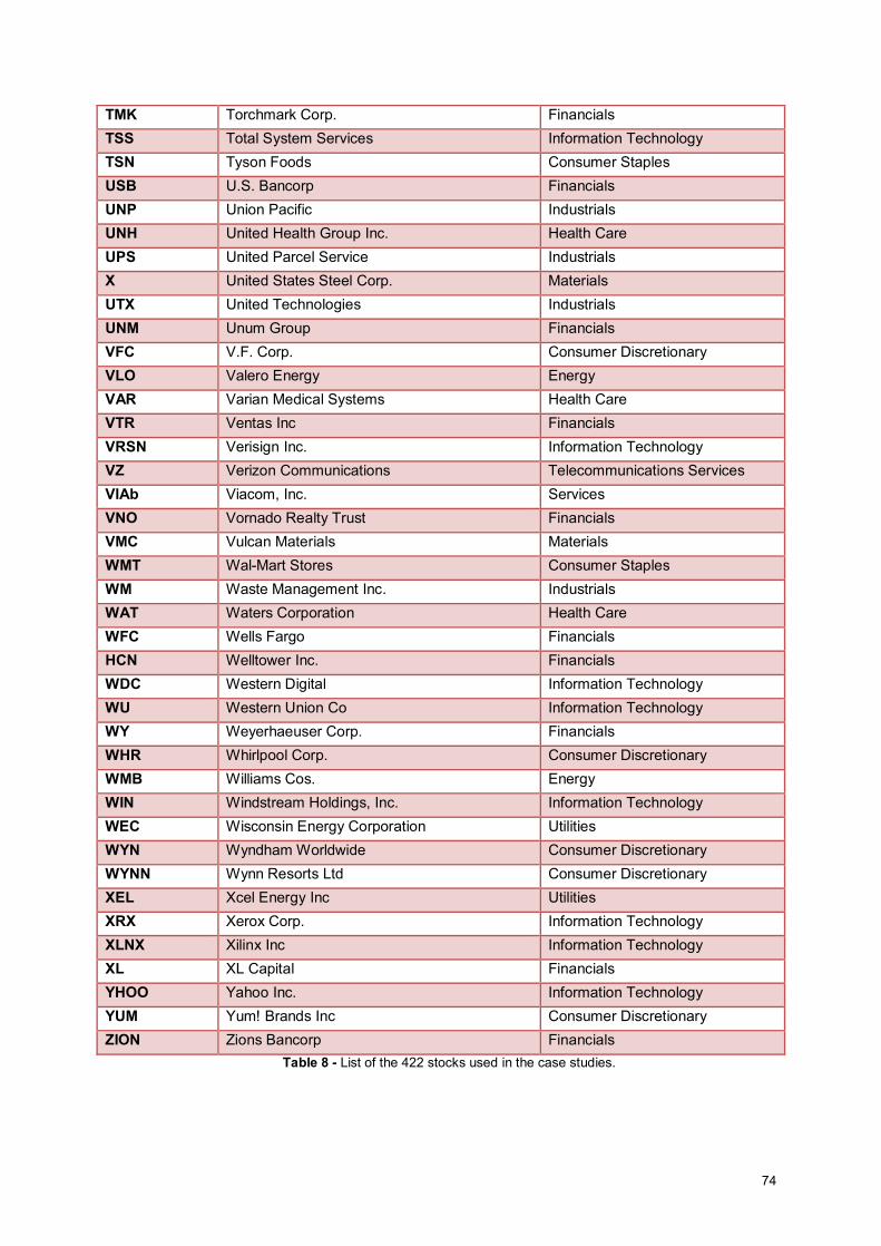
74

TMK Torchmark Corp. Financials TSS Total System Services Information Technology TSN Tyson Foods Consumer Staples USB U.S. Bancorp Financials UNP Union Pacific Industrials UNH United Health Group Inc. Health Care UPS United Parcel Service Industrials X United States Steel Corp. Materials UTX United Technologies Industrials UNM Unum Group Financials VFC V.F. Corp. Consumer Discretionary VLO Valero Energy Energy VAR Varian Medical Systems Health Care VTR Ventas Inc Financials VRSN Verisign Inc. Information Technology VZ Verizon Communications Telecommunications Services VIAb Viacom, Inc. Services VNO Vornado Realty Trust Financials VMC Vulcan Materials Materials WMT Wal-Mart Stores Consumer Staples WM Waste Management Inc. Industrials WAT Waters Corporation Health Care WFC Wells Fargo Financials HCN Welltower Inc. Financials WDC Western Digital Information Technology WU Western Union Co Information Technology WY Weyerhaeuser Corp. Financials WHR Whirlpool Corp. Consumer Discretionary WMB Williams Cos. Energy WIN Windstream Holdings, Inc. Information Technology WEC Wisconsin Energy Corporation Utilities WYN Wyndham Worldwide Consumer Discretionary WYNN Wynn Resorts Ltd Consumer Discretionary XEL Xcel Energy Inc Utilities XRX Xerox Corp. Information Technology XLNX Xilinx Inc Information Technology XL XL Capital Financials YHOO Yahoo Inc. Information Technology YUM Yum! Brands Inc Consumer Discretionary ZION Zions Bancorp Financials

Table 8 - List of the 422 stocks used in the case studies.