Combining a HMM with a Genetic Algorithm for the Fault

1014 Journal of Power Electronics, Vol. 17, No. 4, pp. 1014-1026, July 2017

https://doi.org/10.6113/JPE.2017.17.4.1014

ISSN(Print): 1598-2092 / ISSN(Online): 2093-4718

JPE 17-4-17

Combining a HMM with a Genetic Algorithm for the Fault Diagnosis of Photovoltaic Inverters

Hong Zheng*,**, Ruoyin Wang†, Wencheng Xu*, Yifan Wang*, and Wen Zhu*

*,†School of Electrical and Information Engineering, Jiangsu University, Zhenjiang, China **Key Laboratory of Electric Vehicle Drive and Intelligent Control, Jiangsu University, Zhenjiang, China

Abstract

The traditional fault diagnosis method for photovoltaic (PV) inverters has a difficult time meeting the requirements of the current complex systems. Its main weakness lies in the study of nonlinear systems. In addition, its diagnosis time is long and its accuracy is low. To solve these problems, a hidden Markov model (HMM) is used that has unique advantages in terms of its training model and its recognition for diagnosing faults. However, the initial value of the HMM has a great influence on the model, and it is possible to achieve a local minimum in the training process. Therefore, a genetic algorithm is used to optimize the initial value and to achieve global optimization. In this paper, the HMM is combined with a genetic algorithm (GHMM) for PV inverter fault diagnosis. First Matlab is used to implement the genetic algorithm and to determine the optimal HMM initial value. Then a Baum-Welch algorithm is used for iterative training. Finally, a Viterbi algorithm is used for fault identification. Experimental results show that the correct PV inverter fault recognition rate by the HMM is about 10% higher than that of traditional methods. Using the GHMM, the correct recognition rate is further increased by approximately 13%, and the diagnosis time is greatly reduced. Therefore, the GHMM is faster and more accurate in diagnosing PV inverter faults. Key words: Fault diagnosis, Genetic algorithm, Hidden Markov model (HMM), Photovoltaic (PV) inverter

I. INTRODUCTION

Due to the increasingly serious environmental situation and the growing scarcity of resources, the development and utilization of solar energy has gradually developed into a major focus of the world's energy strategies, and photovoltaic power generation technology is the most common and most valuable of these. The development of photovoltaic power generation control technology is becoming more and more large and complex, and the increasing degree of automation increases the probability of system failure. The control system of photovoltaic power generation systems generally consists of a high power inverter. When the inverter has faults that are not timely diagnosed and repaired, they cause economic losses and security risks which cannot be undone. Thus, research on the fault diagnosis technology of

photovoltaic (PV) inverters is critical. The current diagnostic method is based on a fast sampling circuit that raises an alarm when a fault occurs. The running state of the collected data is processed by a microprocessor to judge whether the system is in trouble, so that it can simultaneously send out the corresponding alarm signal. However, this method requires a long time and cannot accurately generate the alarm. With the increasing demand for reliability and safety of photovoltaic power generation systems, it is an urgent problem to diagnose and locate faults in time. The traditional fault diagnosis method primarily studies linear systems. However, most systems are nonlinear in practical applications.

At present, the common fault diagnosis methods of PV inverters can be roughly divided into the following three categories. (1) Knowledge-based fault diagnosis methods [1], which are based on previously mastered experience and knowledge. These methods include neural networks, SVMs (support vector machines), and expert systems. R. L de Araujo Ribeiro et al. proposed an inverter fault diagnosis method based on a multi neural network structure [2]. H. Keskes and A. Braham used SVM and a pitch synchronous wavelet transform to complete the fault diagnosis of a motor

Manuscript received Feb. 9, 2017; accepted May 8, 2017 Recommended for publication by Associate Editor Hao Ma.

†Corresponding Author: [email protected] Tel: +86-511-88791245, Fax: +86-511-88780088, Jiangsu University

*School of Electrical and Information Eng., Jiangsu University, China **Jiangsu Key Laboratory of Drive and Intelligent Control for Electric

Vehicle, China

© 2017 KIPE

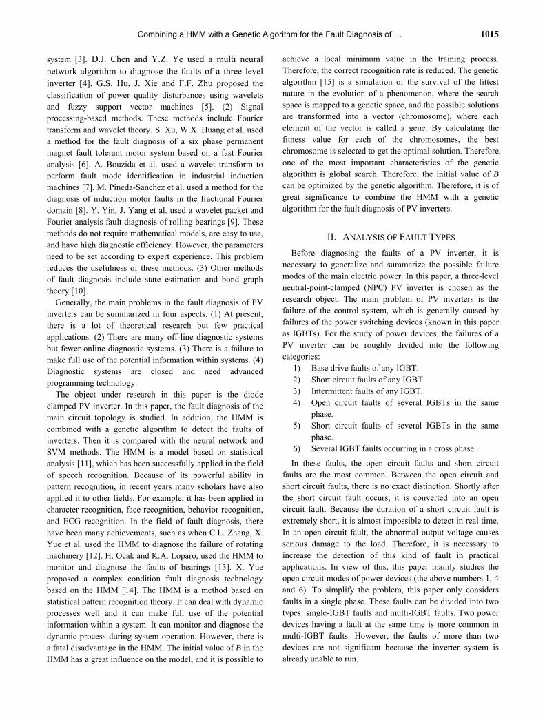
Combining a HMM with a Genetic Algorithm for the Fault Diagnosis of … 1015

system [3]. D.J. Chen and Y.Z. Ye used a multi neural network algorithm to diagnose the faults of a three level inverter [4]. G.S. Hu, J. Xie and F.F. Zhu proposed the classification of power quality disturbances using wavelets and fuzzy support vector machines [5]. (2) Signal processing-based methods. These methods include Fourier transform and wavelet theory. S. Xu, W.X. Huang et al. used a method for the fault diagnosis of a six phase permanent magnet fault tolerant motor system based on a fast Fourier analysis [6]. A. Bouzida et al. used a wavelet transform to perform fault mode identification in industrial induction machines [7]. M. Pineda-Sanchez et al. used a method for the diagnosis of induction motor faults in the fractional Fourier domain [8]. Y. Yin, J. Yang et al. used a wavelet packet and Fourier analysis fault diagnosis of rolling bearings [9]. These methods do not require mathematical models, are easy to use, and have high diagnostic efficiency. However, the parameters need to be set according to expert experience. This problem reduces the usefulness of these methods. (3) Other methods of fault diagnosis include state estimation and bond graph theory [10].

Generally, the main problems in the fault diagnosis of PV inverters can be summarized in four aspects. (1) At present, there is a lot of theoretical research but few practical applications. (2) There are many off-line diagnostic systems but fewer online diagnostic systems. (3) There is a failure to make full use of the potential information within systems. (4) Diagnostic systems are closed and need advanced programming technology.

The object under research in this paper is the diode clamped PV inverter. In this paper, the fault diagnosis of the main circuit topology is studied. In addition, the HMM is combined with a genetic algorithm to detect the faults of inverters. Then it is compared with the neural network and SVM methods. The HMM is a model based on statistical analysis [11], which has been successfully applied in the field of speech recognition. Because of its powerful ability in pattern recognition, in recent years many scholars have also applied it to other fields. For example, it has been applied in character recognition, face recognition, behavior recognition, and ECG recognition. In the field of fault diagnosis, there have been many achievements, such as when C.L. Zhang, X. Yue et al. used the HMM to diagnose the failure of rotating machinery [12]. H. Ocak and K.A. Loparo, used the HMM to monitor and diagnose the faults of bearings [13]. X. Yue proposed a complex condition fault diagnosis technology based on the HMM [14]. The HMM is a method based on statistical pattern recognition theory. It can deal with dynamic processes well and it can make full use of the potential information within a system. It can monitor and diagnose the dynamic process during system operation. However, there is a fatal disadvantage in the HMM. The initial value of B in the HMM has a great influence on the model, and it is possible to

achieve a local minimum value in the training process. Therefore, the correct recognition rate is reduced. The genetic algorithm [15] is a simulation of the survival of the fittest nature in the evolution of a phenomenon, where the search space is mapped to a genetic space, and the possible solutions are transformed into a vector (chromosome), where each element of the vector is called a gene. By calculating the fitness value for each of the chromosomes, the best chromosome is selected to get the optimal solution. Therefore, one of the most important characteristics of the genetic algorithm is global search. Therefore, the initial value of B can be optimized by the genetic algorithm. Therefore, it is of great significance to combine the HMM with a genetic algorithm for the fault diagnosis of PV inverters.

II. ANALYSIS OF FAULT TYPES

Before diagnosing the faults of a PV inverter, it is necessary to generalize and summarize the possible failure modes of the main electric power. In this paper, a three-level neutral-point-clamped (NPC) PV inverter is chosen as the research object. The main problem of PV inverters is the failure of the control system, which is generally caused by failures of the power switching devices (known in this paper as IGBTs). For the study of power devices, the failures of a PV inverter can be roughly divided into the following categories:

1) Base drive faults of any IGBT. 2) Short circuit faults of any IGBT. 3) Intermittent faults of any IGBT. 4) Open circuit faults of several IGBTs in the same

phase. 5) Short circuit faults of several IGBTs in the same

phase. 6) Several IGBT faults occurring in a cross phase.

In these faults, the open circuit faults and short circuit faults are the most common. Between the open circuit and short circuit faults, there is no exact distinction. Shortly after the short circuit fault occurs, it is converted into an open circuit fault. Because the duration of a short circuit fault is extremely short, it is almost impossible to detect in real time. In an open circuit fault, the abnormal output voltage causes serious damage to the load. Therefore, it is necessary to increase the detection of this kind of fault in practical applications. In view of this, this paper mainly studies the open circuit modes of power devices (the above numbers 1, 4 and 6). To simplify the problem, this paper only considers faults in a single phase. These faults can be divided into two types: single-IGBT faults and multi-IGBT faults. Two power devices having a fault at the same time is more common in multi-IGBT faults. However, the faults of more than two devices are not significant because the inverter system is already unable to run.

1016 Journal of Power Electronics, Vol. 17, No. 4, July 2017

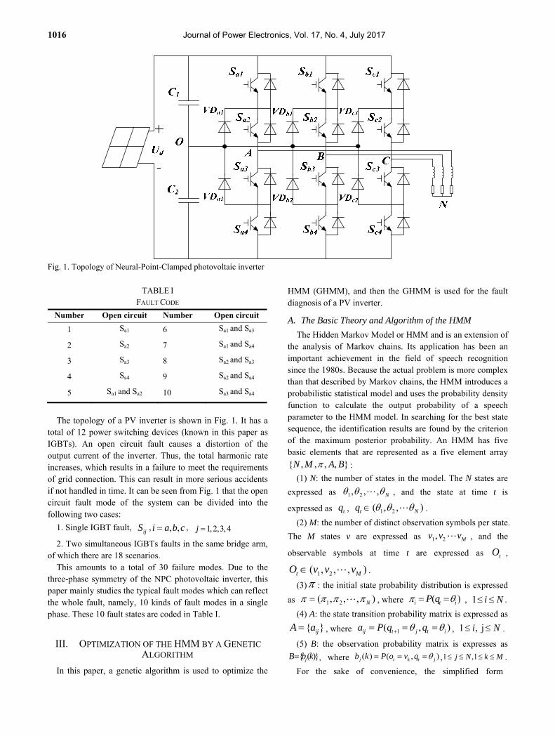
Fig. 1. Topology of Neural-Point-Clamped photovoltaic inverter

TABLE I

FAULT CODE

Number Open circuit Number Open circuit

1 Sa1 6 Sa1 and Sa3

2 Sa2 7 Sa1 and Sa4

3 Sa3 8 Sa2 and Sa3

4 Sa4 9 Sa2 and Sa4

5 Sa1 and Sa2 10 Sa3 and Sa4

The topology of a PV inverter is shown in Fig. 1. It has a

total of 12 power switching devices (known in this paper as IGBTs). An open circuit fault causes a distortion of the output current of the inverter. Thus, the total harmonic rate increases, which results in a failure to meet the requirements of grid connection. This can result in more serious accidents if not handled in time. It can be seen from Fig. 1 that the open circuit fault mode of the system can be divided into the following two cases:

1. Single IGBT fault, ijS , , ,i a b c , 1,2,3,4j

2. Two simultaneous IGBTs faults in the same bridge arm, of which there are 18 scenarios.

This amounts to a total of 30 failure modes. Due to the three-phase symmetry of the NPC photovoltaic inverter, this paper mainly studies the typical fault modes which can reflect the whole fault, namely, 10 kinds of fault modes in a single phase. These 10 fault states are coded in Table I.

III. OPTIMIZATION OF THE HMM BY A GENETIC ALGORITHM

In this paper, a genetic algorithm is used to optimize the

HMM (GHMM), and then the GHMM is used for the fault diagnosis of a PV inverter.

A. The Basic Theory and Algorithm of the HMM

The Hidden Markov Model or HMM and is an extension of the analysis of Markov chains. Its application has been an important achievement in the field of speech recognition since the 1980s. Because the actual problem is more complex than that described by Markov chains, the HMM introduces a probabilistic statistical model and uses the probability density function to calculate the output probability of a speech parameter to the HMM model. In searching for the best state sequence, the identification results are found by the criterion of the maximum posterior probability. An HMM has five basic elements that are represented as a five element array

{ , , , , }N M A B :

(1) N: the number of states in the model. The N states are

expressed as 1 2, , , N , and the state at time t is

expressed as tq , 1 2( , , )t Nq .

(2) M: the number of distinct observation symbols per state.

The M states v are expressed as 1 2, Mv v v , and the

observable symbols at time t are expressed as tO ,

1 2( , , , )t MO v v v .

(3) : the initial state probability distribution is expressed

as 1 2( , , , )N , where ( ) i t iP q , 1 i N .

(4) A: the state transition probability matrix is expressed as

{ }ijA a , where 1( , )ij t j t ia P q q , 1 , ji N .

(5) B: the observation probability matrix is expresses as

{ ( )}jB b k ，where ( ) ( , )j t k t jb k P o v q ,1 ,1j N k M .

For the sake of convenience, the simplified form


1( )t N

1(3)t

1(2)t

1(1)t

1 11

( ) ( )N

t t ij j tt

i a b O

Fig. 2. Procedure of the Backward algorithm.

( , , )A B is used. Thus, the HMM can be expressed as

( , , )A B .

There are three basic algorithms in the HMM. These algorithms are (1) the Forward–Backward algorithm, (2) the Viterbi algorithm, and (3) the Baum–Welch algorithm. The Forward–Backward algorithm is the most basic and it must be used by the other two algorithms. In this paper, the Backward algorithm is introduced, and the Forward algorithm

is similar to it. A backward variable is defined as ( )t i :

1 2( ) ( , , ; | )t t t T t ii P O O O q S (1)

Fig. 2. shows the process. Then it is possible to calculate the backward variables for all of the hidden states at each

time point (shown in the red circle), ( )t i . To calculate the

probability of the observation sequence O at time t, they must all be added:

1

( | ) ( )N

ti

P O i

(2)

B. Genetic Algorithm

As a problem-solving strategy, the genetic algorithm is a programming technique that mimics biological evolution. The main feature of this technique is the information exchange between the group searching strategy and the individuals in the group. The genetic algorithm adaptively controls the search process to obtain an optimal solution. It is a type of global optimization search algorithm that is completely different from the traditional HMM algorithm. First, the genetic algorithm maps the problem space into the space of chromosomes. This process is called coding, and it uses an evaluation function as a basis for genetic manipulation. The evaluation function is also called the fitness function. Its value is closely related to the search problem. The algorithm is initialized to form a group of

Fig. 3. Procedure of the genetic algorithm.

chromosomes that is composed of a number of individuals. Then the group is updated by the appropriate operator. Genetic operators include selection, crossover and mutation. The genetic algorithm is a search method using a randomized technique. However, it is not the same as the general random search algorithm. The genetic algorithm has a clear search direction, which makes it much more efficient. The steps of the genetic algorithm are shown in Fig. 3.

C. Application of a Genetic Algorithm in the HMM

The realization of fault diagnosis consists of two parts: training and recognition. In the HMM, the Baum–Welch algorithm is the basic training algorithm. However, it has a fatal flaw. The final solution depends on the selection of the initial value. As a result, it is easy to fall into a local optimum, which affects the recognition rate of the system. It is necessary to set the initial values of the parameters of each group when the Baum–Welch algorithm is used. If the initial value is not set appropriately, it takes too many iterations to achieve convergence, and the algorithm may converge to a locally optimal solution rather than a globally optimal solution. Therefore, the initial value selection is a very important problem. In particular, the initial value of B. In this paper, a genetic algorithm is used to optimize the initial value. Then the Baum–Welch algorithm is used to find the optimal model. A genetic algorithm is used to improve the HMM, and the procedure is shown in Fig. 4.

The application of a genetic algorithm in the HMM mainly includes coding the parameters, designing the fitness function and operator, and setting the control parameters. The key steps in the GHMM are as follows: 1) Parameter Coding: the general genetic algorithm does not directly address the problem of spatial parameters. However, the mapping of the genetic algorithm space is composed of genes according to a certain structure of the chromosome.


This process is called encoding.

2) Fitness Function: evaluating the genetic algorithm is done exclusively through optimizing the fitness function.

3) Genetic Operations in the GHMM: the genetic operators

are composed of selection, crossover and mutation. Crossover

is the core operator of a genetic algorithm.

4) Setting the Control Parameters: the control parameters of

a general genetic algorithm include setting the population,

crossover probability, mutation probability, etc.

a) Length of the Coding String L: when binary code is used

to represent an individual, the selection of the length L of the

code string is related to the accuracy of the solution.

b) Population Size N: the number of individuals in a group

is called the size of the population. A reasonable value for N

depends on the specific circumstances.

c) Crossover Probability Pc: the crossover probability Pc

controls the frequency of the crossover operation. Generally,

useful crossover probabilities only take values from 0.25 to

0.9.

IV. FAULT DIAGNOSIS TECHNIQUE BASED ON THE GHMM

In actual operation, it is usually not possible to understand all of the fault characteristics. Therefore, to diagnose how a fault occurred in an inverter, it is necessary collect the fault information obtained corresponding to various fault modes. As a result, it is necessary to analyze all of the relevant information in the inverter through a simulation with MATLAB software. In this paper, SIMULINK is used to model a NPC PV inverter, and the various fault models are simulated in the model. The simulation model is shown in Fig. 5. The information obtained is used for the fault diagnosis of the system. Sampling is done to measure the 10 different states and it involves measuring the 2 characteristic variables of each state. These characteristics are the voltage U and current I. Therefore, the output voltage U and current I are collected in the 10 fault states by the simulation. The fault diagnosis of the PV inverter is mainly divided into two parts: the training model and the fault identification.

A. Training Model

(1) Put U and I, which are obtained by sampling, into the model as the observation sequence O. In other words, O = [U, I].

(2) Establish the HMM and the left-right model. Then determine the initial value of the model (the state number), the initial state probability, and the state transition matrix. Based on the circuit model, the implicit state is set to 4. The

initial state probability is set to [1 0 0 0] , and the state

transition matrix A is set to:

Fig. 4. Procedure of the GHMM.

0 .5 0 .5 0 0

0 0 .5 0 .5 0

0 0 .5 0 .5 0

0 0 0 1

A

(3)

(3) Use a genetic algorithm to find the optimal initial value of B. The steps are as follows:

(a) Coded representation: in the hidden Markov model, due to the left-right model, the state transitions can only be transferred from the low state to the high state. Since the initial system can only be in a low state, the initial state probability vector can be launched as follows:

(4)

Because the selection of the initial value of B has the

greatest impact on the model, it is necessary to optimize the initial value of B. First, the initial value of B is coded. The binary coding method is used in this paper. The binary encoding method is one of the most commonly used methods of encoding in a genetic algorithm, using {0,1}. The range of the initial value of B is from [0, 1]. The length of the parameter is 64. Therefore, it can produce 264 different codes in total. The corresponding relationship is as follows:

The accuracy of the binary coding is:

64

1

2 1

(5)

Assume an individual's code:

64 63 62 2 1:X a a a a a (6)

The corresponding decoding formula is:

1 i N 1, 1

0, 1i

i

i


Fig. 5. Simulation model of the Three-Level NPC inverter.

641

641

1( 2 )

2 1i

ii

x a

(7)

The corresponding decoding formula is:

1

1 , 1 ,1m

jkk

b j N k M

(8)

(b) Fitness function: the fitness function can reflect the pros and cons of each chromosome. The traditional algorithm

takes ( | )P O as the optimization target. The chromosome

that has the largest ( | )P O is the best chromosome.

According to the above, it is assumed that Q is a state sequence. The forward and backward algorithms calculate the

sum of all state sequences' ( , | )P Q O . However, the

Viterbi algorithm calculates the ( ', | )P Q O of the optimal

path Q'. In terms of fault treatment, the range of

( , | )P Q O is very large, and the maximum value of

( ', | )P Q O is the only component that has an absolute

advantage in all of ( , | )P Q O . Therefore, ( ', | )P Q O

is often used to replace ( , | )P Q O . The recognition

algorithm in this paper is the Viterbi algorithm. Thus,

( ', | )P Q O is taken as the optimization target.

The fitness of individuals is represented by the log-likelihood of each training sample.

( )( ) ln ( ( | ))kf P O (9)

( )kO refers to the kth observation sequence, and ( )( | )kP O

is obtained by the Viterbi algorithm. (c) Design of genetic operators: the genetic operators

include the crossover operator and the mutation operator. In a certain sense, the crossover operator is equivalent to a local search operation, which produces two offspring near the parent generation. The mutation operator allows an individual to jump out of the current local search area. Therefore, the combination of the two exactly reflects the optimization of the genetic algorithm. In this paper, multi-point crossovers and multi-point mutations are used.

(d) Termination criterion: in this paper, the maximum algorithmic iteration is set to 100.

In the experiment, the performance of the genetic algorithm has a strong relationship with the setting of the control parameters, and the optimal performance of the algorithm often requires an optimal parameter setting. Therefore, it is necessary to have an optimizing search on Pc and Pm. In this paper, the C language is used to implement the above genetic algorithm, from which the optimal initial value of B is obtained.

(4) Use the Baum-Welch algorithm to iterate the initial parameters until the parameters converge to the set range.

First a variable is defined as:

1( , ) ( , | , )t t i t ji j P q q O (10)

This expresses, under the conditions of a given model

and observation sequence O, the probability of state i

at time t, and state j at time t+1.


1 1

1 1

1 11 1

( ) ( ) ( )( , )

( | )

( ) ( ) ( )

( ) ( ) ( )

t ij j t tt

t ij j t t

N N

t ij j t ti j

i a b O ji j

P O

i a b O j

i a b O j

(11)

Define ( )t i as the conditional probability of state i

at time t.

1

( ) ( , )N

t tj

i i j

(12)

Sum ( )t i in t (from 1 to T-1). This yields a quantity

that can be interpreted as the number of transfers from state

i .

The method for estimating parameters of the hidden Markov model includes the following:

The revaluation formula of :

1

1

( ) ( )( )

( ) ( )

t ti N

t ti

i ii

i i

(13)

The revaluation formula of ija :

1

11

1

1

1 11

1

1

( , )

( )

( ) ( ) ( ) / ( | )

( ) ( ) / ( | )

T

ti

ij T

ti

T

t ij j t ti

T

t ti

i jA

i

i a b O j P O

i i P O

(14)

The revaluation formula of ( )jb k :

1

1

1

1

( ) ( )

( )

( ) ( ) / ( | )

( ) ( ) / ( | )

t k

t k

T

t O vt

j T

tt

T

t tt

O v

T

t tt

jB k

j

i i P O

i i P O

(15)

In this study, multiple training samples are used to train the models. During model training, the output may differ under different control models or even under the same control model when the application is not the same. Therefore, the problem of model generalization should be considered when training a model to make the GHMM usable in practical applications. It is necessary to consider the common features of multiple datasets. In other words, it is necessary to use

multiple training samples to train a model for fault diagnosis. For fault diagnosis, the output must be collected under the same fault conditions as that for the training samples.

First, H training samples are defined, that is the

observation sequences (1) (2) (3) ( ), , , , HO O O O . They may be

relevant or statistically independent, therefore:

(1) (2) (1) ( ) ( 1) (1)

(2) (3) (2) (1) ( ) (2)

( ) (1) ( ) ( 1) ( ) (1)

( | ) ( | ) ( | , ) ( | , )

( | ) ( | ) ( | , ) ( | , )

( | ) ( | ) ( | , ) ( | , )

H H

H

H H H H

P O P O P O O P O O O



(16)

Then the weight coefficient is introduced：

(2) (1) ( ) ( 1) (1)1

(3) (2) (1) ( ) (2)2

(1) ( ) ( 1) ( ) (1)

1( | , ) ( | , )

1( | , ) ( | , )

1( | , ) ( | , )

H H

H

H H HH

P O O P O O OH

P O O P O O OH

P O O P O O OH

(17)

In formulas (14) and (15), the following formula is used

to express ( | )P O :

( )

1

( | ) ( | )H

hh

h

P O P O

(18)

The initial model is defined as ( , , )A B , and the

revaluation model is defined as ( , , )A B . The Backward

algorithm is used to calculate ( | )P O , so that

( | ) ( | )P O P O . These calculations are then repeated

using instead of until convergence.

B. Fault Diagnosis

After the training models are completed, the Viterbi algorithm is used to identify the diagnosis. The Viterbi algorithm is a method based on dynamic programming to determine the single optimal state sequence which has the

largest ( | , )P Q O .

First, the variable ( )t i is defined:

1 2 11 2 1 2

, , ,( ) max [ , , , , , , | ]

tt t i t

q q qi P q q q S O O O

(19)

This variable is at time t, along a path to reach the state Si. It generates the maximum probability of the observed {O1, O2 , ..., Ot}.

1) Initialization:

1 1( ) ( ), 1 , ( ) 0t i ii b O i N i (20)

2) Iterative calculation:

11

( ) max[ ( ) ] ( ) , 2 ,1t t ij j ti N

j i a b O t T j N (21)

11

( ) arg max[ ( ) ] , 2 ,1t t iji N

j i a t T j N

(22)

3) Final calculation:


(a)

(b)

(c)

Fig. 6. (a) Fault numbers 1-3; (b) fault numbers 4-7; (c) fault numbers 8-10.

1max[ ( )]T

i NP i

(23)

Then it is possible to identify the diagnosis that has the largest P.

C. Training and Diagnostic Simulation Results:

With the convergence error set to 1×10-5, the training curves for the 10 fault states are shown in Fig. 6.

The number of iterative steps required by the simulation under different fault models is shown in Table II. Each fault corresponds to the GHMM. Therefore, it can be seen that the training of the GHMM requires fewer iteration steps and has a fast convergence rate.

Then the trained GHMM model is used to identify the

measured signal and to calculate ( | , )iP Q O , (1, ,10)i .

The model corresponding to the maximum value of

TABLE II ITERATIVE STEPS

Fault number Iterative steps Fault number Iterative steps

1 20 6 28

2 16 7 22

3 19 8 29

4 16 9 27

5 20 10 8

TABLE III

OUTPUTS OF MODELS Fault

number

Model

number

1 2 3 4 5

Number 1 13.01 -487.66 -86.12 -275.01 -205.51

Number 2 -169.32 4.13 -421.23 -1452.12 -210.12

Number 3 -3620.15 -41.76 -1.55 -542.13 -254.17

Number 4 -4402.29 -660.89 -43.12 -5.42 -3468.75

Number 5 -1542.14 -5015.06 -452.18 -2013.45 -2.74

Number 6 -263.16 -3123.02 -212.09 -2111.71 -2419.89

Number 7 -473.45 -743.11 -311.45 -3710.14 -273.33

Number 8 -907.66 -763.82 -4211.74 -112.43 -172.02

Number 9 -3167.78 -513.69 -76.54 -542.27 -4475.67

Number 10 -616.01 -122.53 -816.01 -101.75 -163.08

Test result NO.1 NO.2 NO.3 NO.4 NO.5

TABLE IV

OUTPUTS OF MODELS Fault

number

Model

number

6 7 8 9 10

Number 1 24.45 -347.12 -86.59 -721.45 -1.79

Number 2 -143.75 -632.12 -711.42 -1010.46 -501.46

Number 3 -2109.34 -444.17 -501.92 -57.63 -1790.84

Number 4 -301.43 -500.58 -1420.46 -427.22 -314.78

Number 5 12.47 -2175.53 -817.62 -2936.34 -3075.44

Number 6 102.01 -142.35 -287.97 -1101.86 -200.13

Number 7 -743.85 -0.18 -2157.42 -340.17 -347.48

Number 8 43.47 -793.19 -5.64 -56.86 -1920.81

Number 9 -1435.02 -1032.75 -267.37 -15.44 -19.09

Number 10 -39.47 -843.52 -142.09 -410.14 27.01

Test result NO.6 NO.7 NO.8 NO.9 NO.10

( | , )iP Q O is the result. Test samples of 10 kinds of faults

are taken into each model to calculate ( | , )iP Q O and to

find the largest one. Table III and Table IV show the outputs of each model. The red number is the largest value in each column. It is found that the model number accurately corresponds to the fault number.

The test result is the model corresponding to the maximum

( | , )iP Q O , (1, ,10)i . Therefore, the model trained

by the GHMM can accurately identify the fault.


TABLE V DIAGNOSTIC RESULTS IN SIMULATION

Fault

number

Times of

diagnosis

GHMM HMM

Correct

times

Correct

rate

Correct

times

Correct

rate

1 100 100 100% 84 84%

2 100 100 100% 91 91%

3 100 100 100% 83 83%

4 100 96 96% 93 93%

5 100 94 94% 91 91%

6 100 100 100% 89 89%

7 100 100 100% 75 75%

8 100 95 95% 88 88%

9 100 95 95% 84 84%

10 100 100 100% 85 85%

To verify the validity of the circuit state identification

using the GHMM, many experiments have been carried out in this paper and test samples have been selected in different states, for a total of 1000 groups (there are 100 test samples in each fault state).

Table V shows diagnostic simulation results. The overall recognition has 98% accuracy, which is a good recognition performance.

In this paper, the HMM is also used without a genetic algorithm to diagnose PV inverter faults. The diagnostic results are shown in Table V. The overall recognition of this algorithm has 86.3% accuracy. Therefore, it can be seen that the GHMM can realize the optimization of the initial value of B and effectively improve the recognition rate.

To verify the advantages of using the GHMM in diagnosing PV inverter faults, it is compared with other traditional pattern recognition methods. In previous studies, traditional pattern recognition methods have been based on neural networks and SVMs (support vector machines). A neural network is an information processing system for simulating the biological nervous system. It can imitate the human brain in terms of learning, memory, recognition and many other functions. Since the development of neural networks, there have been many structural models and algorithms, of which the back propagation (BP) neural network is the most widely used. The BP neural network is a feed-forward network. The parameters of the BP neural network are shown in Table VI.

A BP neural network is used to identify the 10 kinds of faults in the NPC PV inverter model. The results of the simulation are shown in Table VII. In this method, the choice of the number of hidden layer nodes considerably affects the results. In theory, the higher the number of hidden layer nodes, the higher the correct recognition rate becomes. Fault diagnosis using the BP neural network method has the following disadvantages [16]. First, the method often falls into a local minimum, possesses a slow convergence rate, and produces oscillation. Second, no explicit formulas or theories

TABLE VI BP NEURAL NETWORK PARAMETERS

Parameter Value

Learning rate 0.02

Maximum number of iterations 1000

Target error of training 0.0001

Neuron transfer function in the hidden layer logsig

Neuron transfer function in the output layer trainlm

TABLE VII

BP NEURAL NETWORK RESULTS

TABLE VIII

SVM PARAMETERS

Parameter Value

Kernel function radial basis

Parameter 0.0082334

Error cost coefficient C 128

Promotion strategy one to one vote

TABLE IX

SVM RESULTS

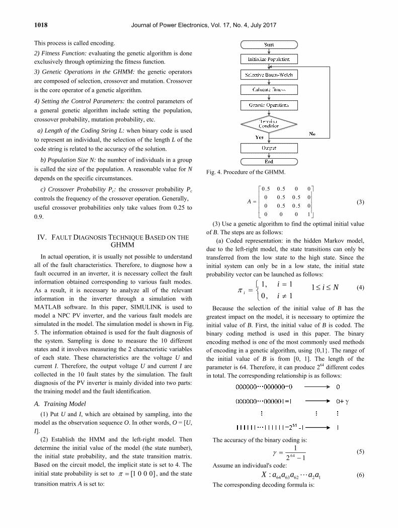
Average number of iterations 657 Average training time 75.46s Correct recognition rate 75.66%

are available as a guide to determine the numbers of hidden layers and nodes. These are usually calculated based on experience. Therefore, this algorithm is flawed. This is why the BP method used in this study has a long training time and a very low correct rate.

SVM is a new generation of learning algorithms based on the statistical learning theory. SVM is based on the principle of structural risk minimization. There are 3 problems in using SVM: (1) the selection of the kernel function; (2) the selection of the kernel function parameter and error cost coefficient C; (3) generalization for multi class problem identification. In this paper, a radial basis function has been

chosen: 2( , ) exp( || || )K x y x y , 0.0082334 , and

the error cost coefficient C=128. Then, a one-to-one voting strategy is used. The parameters are shown in Table VIII.

The results of the simulation are shown in Table IX. In this method, the selection of the kernel function and error cost coefficient C significantly influences the fault identification. The selection of these two parameters differs in different systems. When using SVM for fault diagnosis, satisfactory accuracy cannot be obtained if the method is not optimized [17], [18].

Therefore, this method is also flawed. It is unstable and has poor robustness. This method has a lower recognition accuracy than the GHMM.

Average number of iterations 422 Average training time 30.01s Correct recognition rate 71.02%


(a)

(b)

Fig. 7. (a) Average iterative steps; (b) average training times; (c) correct recognition rate.

To study the advantages and feasibility of applying the

GHMM to the fault diagnosis of PV inverters, the above four different methods are compared and analyzed. Fig. 7 shows simulation data obtained by the different methods.

The following conclusions can be obtained from the experimental data shown in Fig. 7. From Fig 7(a), the average number of steps of the GHMM and the HMM iterations are much lower than those of the other two methods. The neural network and SVM models need to be iterated several times to converge to set values. From Fig. 7(b), in terms of the training time, the SVM takes the longest time, followed by the neural network. While the GHMM and HMM require almost the same time, the training time of the HMM is the shortest. From Fig. 7(c), the correct recognition rate of the GHMM is significantly better than those of the other three methods.

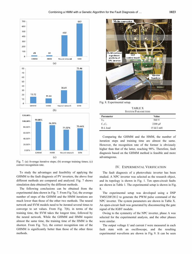
Fig. 8. Experimental setup.

TABLE X SYSTEM PARAMETERS

Parameter Value

Ud 560 V

C1,C2 2200 μF

R-L load 15 Ω/2 mH

Comparing the GHMM and the HMM, the number of

iteration steps and training time are almost the same. However, the recognition rate of the former is obviously higher than that of the latter, reaching 98%. Therefore, fault diagnosis based on the GHMM method is feasible and more advantageous.

IV. EXPERIMENTAL VERIFICATION

The fault diagnosis of a photovoltaic inverter has been studied. A NPC inverter was selected as the research object, and its topology is shown in Fig. 1. Ten open-circuit faults are shown in Table 1. The experimental setup is shown in Fig. 8. The experimental setup was developed using a DSP TMS320F2812 to generate the PWM pulse command of the NPC inverter. The system parameters are shown in Table X. An open-circuit fault was generated by disconnecting the gate signal of the IGBT module.

Owing to the symmetry of the NPC inverter, phase A was selected for the experimental analysis, and the other phases were similar.

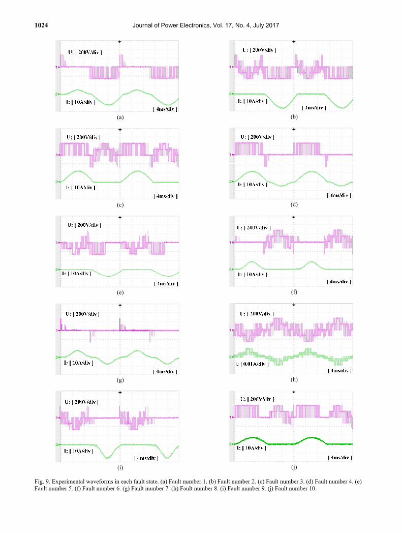
The output voltage U and current I were measured in each fault state with an oscilloscope, and the resulting experimental waveform are shown in Fig. 9. It can be seen

(c)


(a)

(c)

(e)

(g)

(i)

(b)

(d)

(f)

(h)

(j)

Fig. 9. Experimental waveforms in each fault state. (a) Fault number 1. (b) Fault number 2. (c) Fault number 3. (d) Fault number 4. (e) Fault number 5. (f) Fault number 6. (g) Fault number 7. (h) Fault number 8. (i) Fault number 9. (j) Fault number 10.


195208

415

648

120.4 115.1

311.2

760.4

0

100

200

300

400

500

600

700

800

0

100

200

300

400

500

600

700

GHMM HMM Neural�network SVM

Total�steps�of�iterations Total�training�time

Fig. 10. Iteration steps and training time.

TABLE XI DIAGNOSTIC EXPERIMENTAL RESULTS

Diagnosis method

Fault number

GHMM HMM Neural

network SVM

1 100% 84% 69% 79%

2 100% 91% 80% 76%

3 100% 84% 58% 65%

4 96% 92% 75% 80%

5 95% 90% 81% 83%

6 100% 89% 65% 70%

7 100% 83% 71% 73%

8 96% 85% 80% 71%

9 96% 85% 72% 84%

10 100% 86% 76% 80%

that the output voltage U and current I differed in each fault state. Because of this difference, the output voltage U and current I can be used as the characteristic value, and each model can be independently trained by the GHMM. The output voltage and current data for each of the fault states were received by the PC and DSP control board and subsequently read and displayed by MATLAB. Observation sequence O, which consisted of the sampled U and I, was the input of the model training with the GHMM. MATLAB software was used to read and process the sampled data for the model training and fault diagnosis. In the experiments, the algorithms were realized with MATLAB. First, a genetic algorithm was used to obtain the optimal initial value of B. Second, the Baum–Welch algorithm was used for the iterative training of the fault models. Finally, the Viterbi algorithm was used to identify faults.

Model training and fault diagnosis were completed on a PC. The two traditional methods, namely, BP neural network and SVM, were also implemented with the MATLAB software.

The number of iteration steps and training time for each of the methods are shown in Fig. 10.

After training all of the models, the diagnostic experiment was conducted. Multiple diagnoses were performed for each fault to verify the effectiveness of inverter fault diagnosis by using the GHMM and to eliminate contingency. 100 samples

Fig. 11. Correct recognition rate in the experiment.

were selected in each fault condition, and a total of 10 × 100 = 1000 test samples were used to carry out the fault diagnosis. The experimental results are shown in Table XI.

Fig. 11 shows a comparison of the total correct recognition rates of the four methods in the experiment. The experimental results indicated that the simulation results were correct. It was faster and more accurate to use the GHMM in diagnosing inverter faults.

Thus, the feasibility and advantages of the GHMM have been proven.

V. CONCLUSIONS

As a method based on the statistical pattern recognition theory, the HMM can handle the dynamic process well. Compared with traditional fault diagnosis methods, the HMM can monitor and diagnose faults in the dynamic process of a system, and determine the faults in time. The classical training algorithm (Baum-Welch) in the HMM has a fatal flaw, since the final solution depends on the initial value. Therefore, it is often only a local optimum. Due to the genetic algorithm’s use of a global search based on population, the chance of obtaining the globally optimal solution is much greater.

In this paper, the GHMM is introduced for the fault diagnosis of PV inverters. First a genetic algorithm is used to search for the optimal initial value of B. Then the Baum-Welch algorithm is used to train the model. Finally, the Viterbi algorithm is used to identify faults, and the improved fault recognition rate is obtained. The simulation and experimental results show that it is feasible and effective to use the GHMM to diagnose the faults of PV inverters. Compared with the traditional HMM, the recognition rate of the GHMM is much higher. At the same time, in terms of the number of iterations, the training time and the correct recognition rate, the GHMM is significantly better than the neural network and SVM models. As a global optimization method, the GHMM can deal with dynamic processes very well. This is especially useful because the working mode of the PV inverter circuit is nonlinear. Therefore, it is of great theoretical and practical value to combine a genetic algorithm with the HMM for PV inverter fault diagnosis.


ACKNOWLEDGMENT This work is supported in part by the Priority Academic

Program Development of Jiangsu Higher Education Institutions (PAPD).

REFERENCES [1] S. Peuget, S. Courtine, and J. P. Rognon, “Fault detection

and isolation on a PWM inverter by knowledge-based model,” IEEE Trans. Ind. Appl., Vol. 34, No. 6, pp. 1318-1326, Nov. 1997.

[2] R. L. de Araujo Ribeiro, C. B. Jacobina, E. R. C. da Silva, and A. M. N. Limam “Fault detection of open-switch damage in voltage-fed PWM motor drive systems,” IEEE Trans. Power Electron., Vol. 18, No. 2, pp. 587-593, Mar. 2003.

[3] H. Keskes and A. Braham, “DAG SVM and pitch synchronous wavelet transform for induction motor diagnosis,” in Proc. Iet International Conference on Power Electronics, Machines and Drives , pp. 0166-0166, Apr. 2014.

[4] D. J. Chen and Y. Z. Ye, “Open circuit fault diagnosis method for three level inverter based on multi neural network,” Transactions of China Electrotechnical Society, Vol. 28, No. 6, pp. 120-126, Jun. 2013.

[5] G. S. Hu，J. Xie, and F. F. Zhu, “Classification of power quality disturbances using wavelet and fuzzy support vector machines,” in Proc. International Conference on Machine Learning and Cybernetics IEEE, pp. 3981-3984, Vol. 7, Aug. 2005.

[6] S. Xu, W.X. Huang, Y.W. Hu, W.T. Yu, and Z.Y. Hao, “A novel six phase permanent magnet fault tolerant motor system and its fault diagnosis method,” in Proc. Annual meeting of China Power Supply Society, May 2009.

[7] A. Bouzida, O. Touhami, R. Ibtiouen, A. Belouchrani, M. Fadel, and A. Rezzoug, “Fault diagnosis in industrial induction machines through discrete wavelet transform,” IEEE Trans. Ind. Electron., Vol. 58, No. 9, pp. 4385-4395, Sep. 2011.

[8] M. Pineda-Sanchez, M. Riear-Guasp, J.A. Antonino-Daviu, J. Roger-Folch, J. Perez-Cruz, and R. Puche-Panadero, “Diagnosis of induction motor faults in the fractional fourier domain,” IEEE Trans. Instrum. Meas. Vol. 59, No, 8, pp. 2065-2075, Aug. 2010.

[9] Y. F. Yin, J.W. Yang, G.Q. Cai, and D.C. Yao, “Fault Diagnosis of Rolling Bearing Based on Wavelet Packet and Fourier Analysis,” in Proc. Computational Aspects of Social Networks, pp. 703-706, Sep. 2010.

[10] Z. M. Wu, “Analog circuit fault diagnosis based on information fusion and extreme learning machine,” M.S. Thesis, Hunan University, China, 2011.

[11] Y. P. Bao, J. Zheng, and X.G. Wu, “Speech recognition system based on HMM and genetic neural network,” Computer engineering and Science, Vol. 33, No. 4, pp. 139-144, Apr. 2011.

[12] C. L. Zhang, and X. Yue, “Fault Diagnosis of Rotating Machinery Based on Energy Moment and HMM,” Key Engineering Materials, Vol. 455, pp. 558-564, Dec. 2010.

[13] H. Ocak, and K.A. Loparo, “A new bearing fault detection and diagnosis scheme based on hidden Markov modeling of vibration signals.” in Proc. Acoustics, Speech, and Signal Processing, Vol. 5, pp. 3141-3144, May. 2001.

[14] X. Yue, “Research on fault diagnosis of complex condition based on HMM,” M.S. Thesis, South China University of

Technology, China, 2012. [15] R.F. Han, Principle and application of genetic algorithm,

Weapon Industry Press, 2010. [16] J. J. Fu, “Study on the Fault Diagnosis System of Active

Neutral Point Clamped Three Level Inverter Based on Neural Network,” M.S. Thesis, China Mining University, China, 2016.

[17] F, F. Xie, “Fault Diagnosis Method Based on Support Vector Machine,” M.S. Thesis, Hunan University, China, 2006.

[18] A. Widodo, B.S. Yang, “Support vector machine in machine condition monitoring and fault diagnosis,” Mechanical Systems & Signal Processing, Vol. 21, pp. 2560-2574, Aug. 2007.

Hong Zheng was born in Anhui, China, in 1965. He received his B.S. and Ph.D. degrees in Power Electronics and Drives Engineering from Jiangsu University, Zhenjiang, China, in 1987 and 2011, respectively. From 1987 to 2001, he was a Design Engineer working in the Xi’an Power Electronics Research Institute (PERI), Xi’an, China. Since 2009, he has been

working as a Professor in the School of Electrical and Information Engineering, Jiangsu University. His current research interests include power electronic converters, custom power technology and power quality control technology for smartgrids, distributed generation and energy storage technology.

Ruoyin Wang was born in China, in 1991. He received his B.S. degree from the Jiangsu University of Science and Technology, Zhenjiang, China, in 2013. He is presently working towards his M.S. degree in Electrical Engineering from Jiangsu University, Zhenjiang, China. His current research interests include power electronics,

photovoltaic inverters and electric drives.

Wencheng Xu was born in China, in 1990. He received his B.S. degree from the Applied Technology College of Soochow University, Suzhou, China, in 2014. He is presently working towards his M.S. degree in Electrical Engineering from Jiangsu University, Zhenjiang, China. His current research interests include power electronics

and power quality control.

Yifan Wang was born in China, in 1991. He received his B.S. degree from Jiangsu University, Zhenjiang, China, in 2015, where he is presently working towards his M.S. degree in Electrical Engineering. His current research interests include power electronics and DC-DC converters.

Wen Zhu was born in China, in 1992. He received his B.S. degree from the Jingjiang College of Jiangsu University, Zhenjiang, China, in 2015, where he is presently working toward his M.S. degree in Electrical Engineering. His current research interests include power electronics and AC-DC converters.

Documents

Combining a HMM with a Genetic Algorithm for the Fault