Embed Size (px)
Citation preview
École Normale Superieure de LyonLaboratoire de l’Informatique du Parallélisme
Master 2 – Informatique Fondamentale
Academic Year 2013/2014
Combining Algorithm-Based Fault Toleranceand Checkpointing for Iterative Solvers
Massimiliano FasiAdvisors: Yves Robert & Bora Uçar
Project-Team ROMA
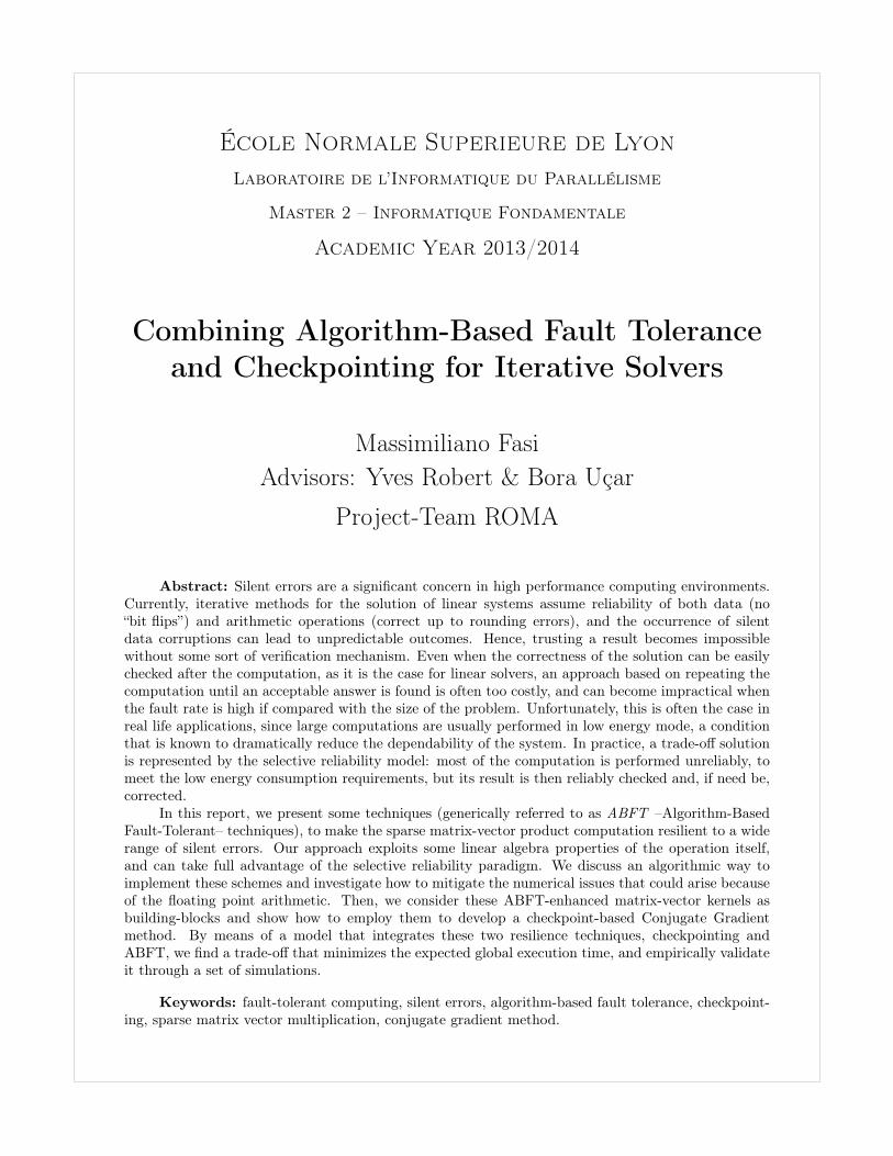
Abstract: Silent errors are a significant concern in high performance computing environments.Currently, iterative methods for the solution of linear systems assume reliability of both data (no“bit flips”) and arithmetic operations (correct up to rounding errors), and the occurrence of silentdata corruptions can lead to unpredictable outcomes. Hence, trusting a result becomes impossiblewithout some sort of verification mechanism. Even when the correctness of the solution can be easilychecked after the computation, as it is the case for linear solvers, an approach based on repeating thecomputation until an acceptable answer is found is often too costly, and can become impractical whenthe fault rate is high if compared with the size of the problem. Unfortunately, this is often the case inreal life applications, since large computations are usually performed in low energy mode, a conditionthat is known to dramatically reduce the dependability of the system. In practice, a trade-off solutionis represented by the selective reliability model: most of the computation is performed unreliably, tomeet the low energy consumption requirements, but its result is then reliably checked and, if need be,corrected.
In this report, we present some techniques (generically referred to as ABFT –Algorithm-BasedFault-Tolerant– techniques), to make the sparse matrix-vector product computation resilient to a widerange of silent errors. Our approach exploits some linear algebra properties of the operation itself,and can take full advantage of the selective reliability paradigm. We discuss an algorithmic way toimplement these schemes and investigate how to mitigate the numerical issues that could arise becauseof the floating point arithmetic. Then, we consider these ABFT-enhanced matrix-vector kernels asbuilding-blocks and show how to employ them to develop a checkpoint-based Conjugate Gradientmethod. By means of a model that integrates these two resilience techniques, checkpointing andABFT, we find a trade-off that minimizes the expected global execution time, and empirically validateit through a set of simulations.
Keywords: fault-tolerant computing, silent errors, algorithm-based fault tolerance, checkpoint-ing, sparse matrix vector multiplication, conjugate gradient method.
2 Massimiliano Fasi
1 IntroductionThough CPUs are usually trusted and considered as units that can quickly perform reliable computa-tions, such a thought is quite far from being true [15]. In fact, the growing size of High-PerformanceComputing (HPC) systems increases the probability of having faults even when each single componenthas a relatively high Mean Time Between Failure (MTBF). Moreover, energy consumption constrainsmodern computer hardware. While executing at a lower energy level decreases the power consumptionof a supercomputer, it also strongly increases the probability of faulty executions. Thus, especially ifthe computation involves a great amount of data, and hence of computational operations, the risk offailing cannot be neglected.
In this work, we focus our attention on the so-called silent errors, that are especially treacherous asthey alter the result of a computation without producing any visible failure. In particular, we examinethe issues related to the Conjugate Gradient method [1], a well-known and widely-used Krylov iterativesolver for linear systems of the form
Ax = b
where A ∈ Rn×n is positive definite and x,b ∈ Rn. Since the material presented in the followingsections addresses computational problems that arise when the coefficient matrixA is huge, we considerA to be sparse, unless specified otherwise. Nevertheless, most of the results are valid for dense matricesas well.
Algorithm 1 The Conjugate Gradient algorithm for a sparse positive definite matrix.Require: A ∈ Rn×n,b,x0 ∈ Rn, ε ∈ REnsure: x ∈ Rn : | Ax− b |≤ ε1: r0 ← b−Ax0;2: p0 ← r0;3: i← 0;4: while ‖ri‖ > ε (‖A‖ · ‖r0‖+ ‖b‖) do5: qi ← Api;6: αi ← ‖ri‖2
pᵀi qi
;7: xi+1 ← xi + αpi;8: ri+1 ← ri − αq;9: β ← ‖ri+1‖2
‖ri‖2;
10: pi+1 ← ri+1 + β pi;11: i← i+ 1;12: end while13: return xi;
Our Conjugate Gradient implementation is based on the analysis of Saad [13] and the advices ofBarret et al. [8, Section 2.3.1, Section 4.2], and is given in Algorithm 1. As the cost of an iteration isdominated by the matrix-vector product at line 5, we are interested in developing methods to protectthis matrix operation, detecting and correcting errors striking both the computation itself and thememory locations containing the input data structures. Our final goal is the development of a modelto couple two well known resilience techniques, namely checkpointing [5] and Algorithm-Based FaultTolerance (ABFT) [3].
The remainder of the report is organized as follows. Section 2 introduces the subject matter, re-viewing an essential bibliography of related work and recalling some basic concepts. In Sections 3 wepropose an ABFT method to correct multiple errors in dense matrix-matrix multiplications. Section 4discusses the problem of detection and correction of silent errors in sparse matrix-vector multipli-cation (SpMxV), examining several ways to develop fault-tolerant algorithms. A theoretical modelto optimally combine these ABFT schemes and checkpointing is the subject of Section 5. Section 6presents an experimental validation of our model and an empirical evaluation of the performances of
Combining ABFT and Checkpointing for Iterative Solvers 3
our resilience techniques. Section 7 concludes with a summary and a discussion of future researchdirections.
2 Background
Related work The very first idea of algorithm-based fault tolerance for linear algebra kernels is tobe found in the work of Huang and Abraham [3]. They describe an algorithm capable of detecting andcorrecting a single silent error striking a matrix-matrix multiplication by means of row and columnchecksums. This germinal idea is then elaborated by Anfinson and Luk [6], who devise a methodto detect and correct up to two errors in a matrix representation using just four column checksums.Despite its theoretical merit, the idea presented in their paper is actually applicable only with relativelysmall matrices, and is hence out of our scope.
The problem of algorithm-based fault-tolerance for sparse matrices is investigated by Shantharamet al. [21], who suggest a way to detect a single error in a SpMxV at the cost of a few additionaldot products. Sloan et al. [22] suggest that this approach can be relaxed using randomization schemes,and propose several checksumming techniques for sparse matrices. These techniques are less effectivethan the previous ones, not being able to protect the computation from faults striking the memory,but provide an interesting theoretical insight.
Error classification As the range of issues that can strike a large scale computation is quite broad,classifying and precisely identifying which kind of errors one wants to deal with is mandatory. We retaina simplified version of the multilevel classification of software reliability issues devised by Parhami [9].On the one hand, we adopt the term failure to denote the state of a system that has computed awrong result, failing its calculation. On the other hand, we employ the term fault to indicate, moregenerally, any kind of abnormal behaviour of the system, whether or not it is likely to lead to a failure.It is clear that at least one fault is necessary to have a failure, but the vice-versa does not hold, sincea faulty condition could possibly be recovered before actually reaching a failure state.
Among the faults, we further distinguish between hard and silent ones. A hard fault can arisebecause of severe data corruption (e.g. data loss) or hardware malfunction (e.g. arithmetic unit thatcomputes incorrect results). Since these errors cause a fail-stop behavior, i.e., an immediate failure,they are outside of the scope of this work. Silent errors, instead, occur usually as bit flips in the memoryor during the computation, and cannot be detected without some introspection mechanism [17]. Theyare the object of our investigation.
Resilience techniques As already pointed out, we focus on a selective reliability setting [17, 18,20, 24]. It essentially means that we can choose to perform any operation in reliable or unreliablemode, assuming the former to be error-free but energy consuming and the latter to be error-prone butpreferable from an energetic point of view.
We deal with two widely-used resilience techniques, namely checkpointing and ABFT. The firstapproach consists in periodically saving program data into a safe location, called reliable storage (suchas the hard disk), in order to make it possible to rollback and restart when a fault is detected. On theother hand, the algorithm-based approach relies on modifying the source code by inserting additionaloperations, so that eventual errors can be fixed by the algorithm itself.
3 ABFT for Dense Matrix-Matrix Product
In general terms, a fault tolerant algorithm for linear algebra requires to focus on two tasks, namelydevising an encoding scheme for the input and redesigning the original algorithm to operate on theencoded data. On the one hand, we would like the encoding to be as light as possible, i.e., fast tobe computed and small to be stored. On the other hand, we would desire the modified version of thealgorithm to be as similar as possible to the original one, so to take advantage of any already existingoptimized subroutine.
4 Massimiliano Fasi
A good example of all these ideas is represented by the ABFT scheme for single error detectionand correction in matrix-matrix products devised by Huang and Abraham [3], that we briefly revisein Section A of the Appendix. There we recall the essential definitions of checksum matrix, explainthe original matrix-matrix product algorithm proposed by Huang and Abraham and suggest a newdecoding algorithm (Algorithm 4) whose correctness we prove in Theorem 5.
To the best of our knowledge, the problem of detecting or correcting more than one error in amatrix-matrix or matrix-vector product has not been addressed anywhere. According to the reviewon ABFT methods by Vijay and Mittal [10], the approach devised by Jou and Abraham [4] should beable to correct up to k errors in a matrix representation using 2k column weighted checksums, for a“suitable choice of the weight vectors”. Nevertheless, Anfinson and Luk [6] show that such an approachis not general, and propose a specific algorithm for k = 2 and a particular set of weights. An extensionof this algorithm to larger k, however, does not seem trivial at all.
In fact, in this section we face the problem in a different way, i.e., using multiple row and columnchecksums. As already anticipated, we consider a selective reliability model and hence assume that noerror can occur in a checksum vector or during checksum computations [3, 6, 21]. Let us also remarkthat we here describe our algorithm just for square matrices, but the result holds for rectangularmatrices as well, using different sets of weight vectors. However, such a generalization would have onlymade the notation more complicated without giving any particular insight.
Let us consider a matrix A ∈ Rn×n and k weight vectors w(1), . . . ,w(k) ∈ Rn such that any squaresub-matrix of
W =[w(1)w(2) . . .w(k)
]is non-singular [12]. We can use W to compute the full weighted checksum matrix of A
Af =
[A AW
WᵀA WᵀAW
]=
A Aw(1) · · · Aw(k)
w(1)ᵀA w(1)ᵀAw(1) · · · w(1)ᵀAw(k)
......
. . ....
w(k)ᵀA w(k)ᵀAw(1) · · · w(k)ᵀAw(k)
,that is a straightforward generalization of the full checksum matrix proposed by Huang and Abraham.Let us assume that k′ ≤ k errors have struck A and let us denote the faulty representation by A. Tocorrect such errors, let us suppose that during the verification step, the row and column checksumshave shown that
• I = {ı1, . . . , ınr} is the set of the indices of the rows where an error has occurred;
• J = {1, . . . , nc} is the set of the indices of the columns where an error has occurred.
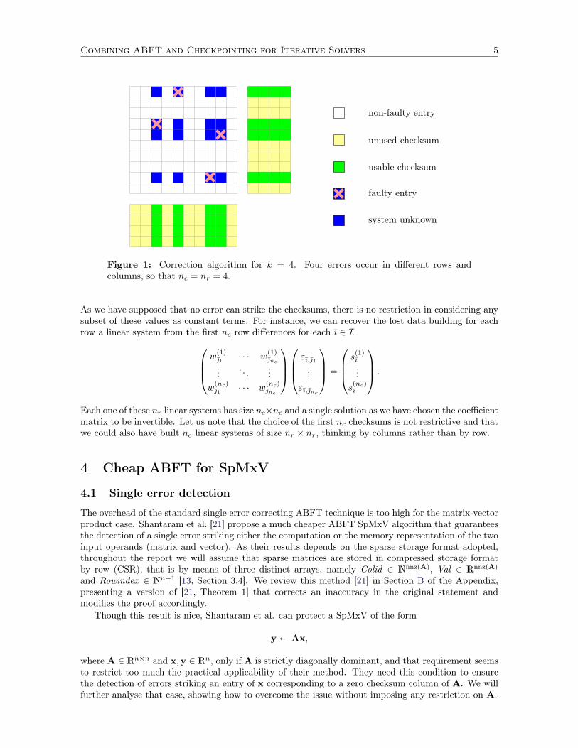
Clearly, neither nc nor nr are greater than k. The set of all the possible position where an error canhave struck is indeed a grid, of size nr × nc, as shown in Figure 1. As we have a lot of redundancy,we can just imagine to put an error at each node of the grid and then solve a linear system in nr × ncvariable, one for each grid point. Most of these errors will turn out to be zero, unless we are dealingwith pathological cases where the positions of the errors form a grid themselves.
Hence, we have nr × nc unknowns, denoted by εi,j with i ∈ I and j ∈ J . As constant terms, wehave to choose nr × nc values out of the union of:
• the k nr row differences, defined, for 1 ≤ ` ≤ k and for any ı ∈ I, as
s(`)ı =
n∑j=1
w(`)j aı,j −
(Aw(`)
)ı,
• the k nc column differences, defined, for 1 ≤ ` ≤ k and for any ∈ I, as
s(`) =
n∑i=1
w(`)i ai, −
(w(`)ᵀA
)ı.
Combining ABFT and Checkpointing for Iterative Solvers 5
non-faulty entry
unused checksum
usable checksum
faulty entry
system unknown
Figure 1: Correction algorithm for k = 4. Four errors occur in different rows andcolumns, so that nc = nr = 4.
As we have supposed that no error can strike the checksums, there is no restriction in considering anysubset of these values as constant terms. For instance, we can recover the lost data building for eachrow a linear system from the first nc row differences for each ı ∈ I
w(1)1 · · · w
(1)nc
.... . .
...w
(nc)1 · · · w
(nc)nc
εı,1...
εı,nc
=
s
(1)ı...
s(nc)ı
.
Each one of these nr linear systems has size nc×nc and a single solution as we have chosen the coefficientmatrix to be invertible. Let us note that the choice of the first nc checksums is not restrictive and thatwe could also have built nc linear systems of size nr × nr, thinking by columns rather than by row.
4 Cheap ABFT for SpMxV
4.1 Single error detection
The overhead of the standard single error correcting ABFT technique is too high for the matrix-vectorproduct case. Shantaram et al. [21] propose a much cheaper ABFT SpMxV algorithm that guaranteesthe detection of a single error striking either the computation or the memory representation of the twoinput operands (matrix and vector). As their results depends on the sparse storage format adopted,throughout the report we will assume that sparse matrices are stored in compressed storage formatby row (CSR), that is by means of three distinct arrays, namely Colid ∈ Nnnz(A), Val ∈ Rnnz(A)
and Rowindex ∈ Nn+1 [13, Section 3.4]. We review this method [21] in Section B of the Appendix,presenting a version of [21, Theorem 1] that corrects an inaccuracy in the original statement andmodifies the proof accordingly.
Though this result is nice, Shantaram et al. can protect a SpMxV of the form
y← Ax,
where A ∈ Rn×n and x,y ∈ Rn, only if A is strictly diagonally dominant, and that requirement seemsto restrict too much the practical applicability of their method. They need this condition to ensurethe detection of errors striking an entry of x corresponding to a zero checksum column of A. We willfurther analyse that case, showing how to overcome the issue without imposing any restriction on A.
6 Massimiliano Fasi
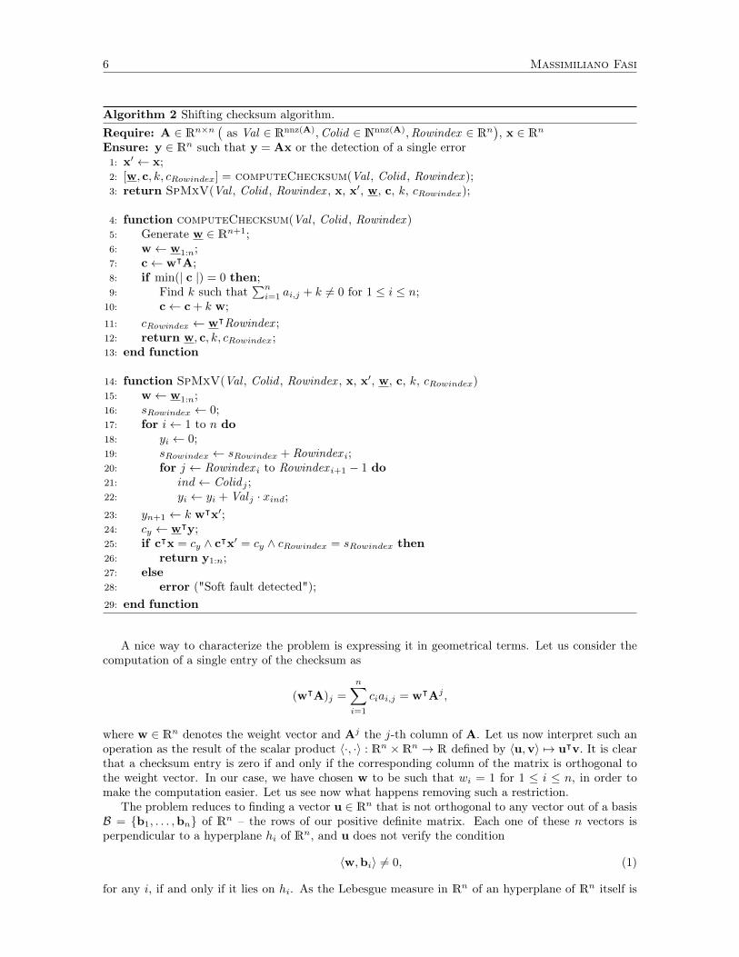
Algorithm 2 Shifting checksum algorithm.Require: A ∈ Rn×n
(as Val ∈ Rnnz(A),Colid ∈ Nnnz(A),Rowindex ∈ Rn
), x ∈ Rn
Ensure: y ∈ Rn such that y = Ax or the detection of a single error1: x′ ← x;2: [w, c, k, cRowindex] = computeChecksum(Val , Colid , Rowindex );3: return SpMxV(Val , Colid , Rowindex , x, x′, w, c, k, cRowindex);
4: function computeChecksum(Val , Colid , Rowindex )5: Generate w ∈ Rn+1;6: w← w1:n;7: c← wᵀA;8: if min(| c |) = 0 then;9: Find k such that
∑ni=1 ai,j + k 6= 0 for 1 ≤ i ≤ n;
10: c← c + k w;11: cRowindex ← wᵀRowindex ;12: return w, c, k, cRowindex;13: end function
14: function SpMxV(Val , Colid , Rowindex , x, x′, w, c, k, cRowindex)15: w← w1:n;16: sRowindex ← 0;17: for i← 1 to n do18: yi ← 0;19: sRowindex ← sRowindex + Rowindex i;20: for j ← Rowindex i to Rowindex i+1 − 1 do21: ind← Colid j ;22: yi ← yi + Val j · xind;23: yn+1 ← k wᵀx′;24: cy ← wᵀy;25: if cᵀx = cy ∧ cᵀx′ = cy ∧ cRowindex = sRowindex then26: return y1:n;27: else28: error ("Soft fault detected");29: end function
A nice way to characterize the problem is expressing it in geometrical terms. Let us consider thecomputation of a single entry of the checksum as
(wᵀA)j =
n∑i=1
ciai,j = wᵀAj ,
where w ∈ Rn denotes the weight vector and Aj the j-th column of A. Let us now interpret such anoperation as the result of the scalar product 〈·, ·〉 : Rn ×Rn → R defined by 〈u,v〉 7→ uᵀv. It is clearthat a checksum entry is zero if and only if the corresponding column of the matrix is orthogonal tothe weight vector. In our case, we have chosen w to be such that wi = 1 for 1 ≤ i ≤ n, in order tomake the computation easier. Let us see now what happens removing such a restriction.
The problem reduces to finding a vector u ∈ Rn that is not orthogonal to any vector out of a basisB = {b1, . . . ,bn} of Rn – the rows of our positive definite matrix. Each one of these n vectors isperpendicular to a hyperplane hi of Rn, and u does not verify the condition
〈w,bi〉 6= 0, (1)
for any i, if and only if it lies on hi. As the Lebesgue measure in Rn of an hyperplane of Rn itself is
Combining ABFT and Checkpointing for Iterative Solvers 7
zero, the union of these hyperplanes is measurable with
mn
(n⋃i=1
hi
)= 0,
where mn denotes the Lebesgue measure of Rn. Therefore, the probability that a vector randomlypicked in Rn does not satisfy condition (1) for any i is zero.
Nevertheless, there are many reasons to consider zero checksum columns. First of all, when workingwith finite precision the number of elements in Rn we can consider is finite, and the probability ofrandomly picking a vector that is orthogonal to a given one could be bigger than zero. Moreover, acoefficient matrix usually comes from the discretization of a physical problem, and the distributionof its columns cannot be considered as random. Finally, using a randomly chosen vector instead of(1, . . . , 1)ᵀ increases the number of required floating point operations, causing a growth of both theexecution time and the number of rounding errors (see Section 4.4).
In Algorithm 2 we propose an ABFT SpMxV method that uses weighted checksums and does notrequire the matrix to be strictly diagonally dominant. The idea is to compute the checksum vectorand then shift it by adding to all of its entries a constant value chosen so that all of the elements ofthe new vector are different from zero. We give the generalized result in Theorem 1.
Theorem 1. [Correctness of Algorithm 2] Let A ∈ Rn×n be a square matrix, let x,y ∈ Rn be theinput and output vector respectively, and let x′ = x. Let us assume that the algorithm performs thecomputation
y← Ax, (2)
where A ∈ Rn×n and x ∈ Rn are the possibly faulty representations of A and x respectively, whiley ∈ Rn is the possibly erroneous result of the sparse matrix-vector product. Let us also assume thatthe encoding scheme relies on
1. an auxiliary checksum vector c = [∑ni=1 ai,1 + k, . . . ,
∑ni=1 ai,n + k], where k is such that∑n
i=1 ai,j + k 6= 0 for 1 ≤ i ≤ n,
2. an auxiliary checksum yn+1 = k∑ni=i xi,
3. an auxiliary counter sRowindex initialized to 0 and updated at runtime by adding the value ofthe hit element each time the Rowindex array is accessed (line 20 of Algorithm 2),
4. an auxiliary checksum cRowindex =∑ni=1 Rowindex i ∈ N.
Then, a single error in the computation of the SpMxV causes one of the following conditions to fail:
i. cᵀx =∑n+1i=1 yi,
ii. cᵀx′ =∑n+1i=1 yi,
iii. sRowindex = cRowindex.
Proof. We will consider three possible cases, namely
a. a faulty arithmetic operation during the computation of y,
b. a bit flip in the sparse representation of A,
c. a bit flip in an element of of x.
Case a. Let us assume, without loss of generality, that the error has struck at the p− th positionof y, that implies yi = yi for 1 ≤ i ≤ n with i 6= p and yp = yp + ε, where ε ∈ R \ {0} represents the
8 Massimiliano Fasi
value of the error that has occurred. Summing up the elements of y gives
n+1∑i=1
yi =
n+1∑i=1
yi + ε
=
n∑i=1
n∑j=1
ai,j xj + k
n∑j=1
xj + ε
=
n∑j=1
(n∑i=1
ai,j + k
)xj + ε
=
n∑j=1
cj xj + ε
= cᵀx + ε,
that violates condition (i).Case b. A single error in the A matrix can strike one of the three vectors that constitute its sparse
representation:
• a fault in Val that alters the value of an element ai,j implies an error in the computation of yi,which leads to the violation of the safety condition (i) because of (a),
• a variation in Colid can zero out an element in position ai,j shifting its value in position ai,j′ ,leading again to an erroneous computation of yi,
• a transient fault in Rowindex entails an incorrect value of sRowindex and hence a violation ofcondition (iii).
Case c. Let us assume, without loss of generality, an error in position p of x. Hence we have thatxi = xi for 1 ≤ i ≤ n with i 6= p and xp = xp + ε, for some ε ∈ R \ {0}. Noting that x = x′, the sumof the elements of y gives
n+1∑i=1
yi =
n∑i=1
n∑j=1
ai,j xj + k
n∑j=1
xj
=
n∑i=1
n∑j=1
ai,jxj + k
n∑j=1
xj + ε
n∑i=1
ai,p + εk
=
n∑j=1
(n∑i=1
ai,j + k
)xj + ε
(n∑i=1
ai,p + k
)
=
n∑j=1
cjxj + ε
(n∑i=1
ai,p + k
)
= cᵀx′ + ε
(n∑i=1
ai,p + k
),
that violates (ii) since∑ni=1 ai,p + k 6= 0 by definition of k.
Let us remark that the function computeChecksum in Algorithm 2 requires just the knowledgeof the matrix, hence in the common scenario of many SpMxV with a same matrix, it is enough toinvoke it once to protect several matrix-vector multiplications. This observation will be crucial whentalking about the performances of the checksumming techniques.
This approach is probably the simplest one to relax the strictly diagonal dominance hypothesis,but it is not the only one. An alternative method, based on a completely different idea, is presentedin Section C of the Appendix. It has the merit of being faster than Algorithm 2 when the number ofcolumns with zero checksum is smaller than n
5 .
Combining ABFT and Checkpointing for Iterative Solvers 9
4.2 Multiple error detection
With some effort, this shifting idea can be extended to multiple errors detection. Let us consider theproblem of detecting up to k errors in the computation of y = Ax introducing an overhead of O (kn).Let k weight vectors w(1), . . . ,w(k) ∈ Rn be such that any sub-matrix of
W =[w(1) w(2) . . . w(k)
]is full rank. To build our ABFT scheme let us note that, if no error occurs, for each weight vector w(`)
it holds that
w(`)ᵀA =
[n∑i=1
w(`)i ai,1, . . . ,
n∑i=1
w(`)i ai,n
],
and hence that
w(`)ᵀAx =
n∑i=1
w(`)i ai,1x1 + · · ·+
n∑i=1
w(`)i ai,nxn =
n∑i=1
n∑j=1
w(`)i ai,jxj .
Similarly, the sum of the entries of y weighted with the same w(`) is
n∑i=1
w(`)i yi = w
(`)1 y1 + · · ·+ w(`)
n yn
= w(`)1
n∑j=1
a1,jxj + · · ·+ w(`)n
n∑j=1
an,jxj
=
n∑i=1
n∑j=1
w(`)i ai,jxj ,
and we can conclude thatn∑i=1
w(`)i yi =
(w(`)ᵀA
)x,
for any w(`) with 1 ≤ ` ≤ k.To convince ourself that with these checksums it is actually possible to detect up to k errors, let
us suppose that k′ errors, with k′ ≤ k, occur in positions p1, . . . , pk′ , and let us denote by y the faultyvector where ypi = ypi + εpi for εpi ∈ R \ {0} and 1 ≤ i ≤ k′ and yi = yi otherwise. Then for each oneof the weight vectors we have
n∑i=1
w(`)i yi −
n∑i=1
w(`)i yi =
k′∑j=1
w(`)pj εpj .
Said otherwise, the occurrence of the k′ errors is not detected if and only if, for 1 ≤ ` ≤ k, all the εpirespect
k′∑j=1
w(`)pj εpj = 0 . (3)
We claim that there cannot exist a vector (εp1 , . . . , εp′k)ᵀ ∈ Rk′ \ {0} such that all of the conditionsin (3) are simoultaneously verified. Indeed, let us consider the following linear system that representsthe conditions in (3)
w(1)p1 · · · w
(1)pk′
.... . .
...w
(k)p1 · · · w
(k)pk′
εp1...
εpk′
=
0...0
.
10 Massimiliano Fasi
Denoting by W∗ the coefficient matrix of this system, it is clear that the errors cannot be detectedif only if (εp1 , . . . εpk′ )
ᵀ ∈ ker(W∗) \ {0}. Because of the properties of W, we have that rk(W∗) = k.It is also clear that the rank of the augmented matrix
w(1)p1 · · · w
(1)pk′ 0
.... . .
......
w(k)p1 · · · w
(k)pk′ 0
is k. Hence, by means of Rouché-Capelli theorem, the solution of the system is unique and the nullspace of W∗ is trivial. Therefore, this construction can detect the occurrence of k′ errors duringthe computation of y by comparing the values of the weighted sums yᵀw(`) with the result of thedot product (w(`)ᵀA)x, for 1 ≤ ` ≤ k.
However, to get a true extension of the algorithm described in the previous section, we also needto make it able to detect errors that strike the sparse representation of A and the full representationof x. The first case is simple, as the k errors can strike the Val or Colid arrays, leading to at most kerrors in y, or in Rowindex , where they can be caught using k weighted checksums of the Rowindexvector.
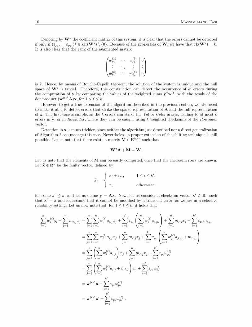
Detection in x is much trickier, since neither the algorithm just described nor a direct generalizationof Algorithm 2 can manage this case. Nevertheless, a proper extension of the shifting technique is stillpossible. Let us note that there exists a matrix M ∈ Rk×n such that
WᵀA + M = W.
Let us note that the elements of M can be easily computed, once that the checksum rows are known.Let x ∈ Rn be the faulty vector, defined by
xi =
xi + εpi , 1 ≤ i ≤ k′,
xi otherwise.
for some k′ ≤ k, and let us define y = Ax. Now, let us consider a checksum vector x′ ∈ Rn suchthat x′ = x and let assume that it cannot be modified by a transient error, as we are in a selectivereliability setting. Let us now note that, for 1 ≤ ` ≤ k, it holds that
n∑i=1
w(`)i yi +
n∑j=1
m`,j xj =
n∑i=1
n∑j=1
w(`)i ai,jxj +
k′∑i=1
εpi
n∑j=1
w(`)j aj,pi
+
n∑j=1
m`,jxj +
k′∑i=1
εpiml,pi
=
n∑j=1
n∑i=1
w(`)i ai,jxj +
n∑j=1
m`,jxj +
k′∑i=1
εpi
n∑j=1
w(`)j aj,pi +ml,pi
=
n∑j=1
(n∑i=1
w(`)i ai,j
)xj +
n∑j=1
m`,jxj +
k′∑i=1
εpiw(`)pi
=
n∑j=1
(n∑i=1
w(`)i ai,j +m`,j
)xj +
k′∑i=1
εpiw(`)pi
= w(`)ᵀx +
k′∑i=1
εpiw(`)pi
= w(`)ᵀx′ +
k′∑i=1
εpiw(`)pi .
Combining ABFT and Checkpointing for Iterative Solvers 11
Therefore, an error is not detected if and only if the linear systemw
(1)p1 · · · w
(1)pk′
.... . .
...w
(k)p1 · · · w
(k)pk′
εp1...
εpk′
=
0...0
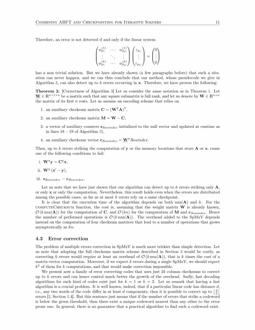
has a non trivial solution. But we have already shown (a few paragraphs before) that such a situ-ation can never happen, and we can thus conclude that our method, whose pseudocode we give inAlgorithm 3, can also detect up to k errors occurring in x. Therefore, we have proven the following:
Theorem 2. [Correctness of Algorithm 3] Let us consider the same notation as in Theorem 1. LetW ∈ Rn+1×n be a matrix such that any square submatrix is full rank, and let us denote by W ∈ Rn×nthe matrix of its first n rows. Let us assume an encoding scheme that relies on
1. an auxiliary checksum matrix C = (WᵀA)ᵀ,
2. an auxiliary checksum matrix M = W −C,
3. a vector of auxiliary counters sRowindex initialized to the null vector and updated at runtime asin lines 18 – 19 of Algorithm 3),
4. an auxiliary checksum vector cRowindex = WᵀRowindex .
Then, up to k errors striking the computation of y or the memory locations that store A or x, causeone of the following conditions to fail:
i. Wᵀy = Cᵀx,
ii. Wᵀ (x′ − y),
iii. sRowindex = cRowindex.
Let us note that we have just shown that our algorithm can detect up to k errors striking only A,or only x or only the computation. Nevertheless, this result holds even when the errors are distributedamong the possible cases, as far as at most k errors rely on a same checkpoint.
It is clear that the execution time of the algorithm depends on both nnz(A) and k. For thecomputeChecksum function, the cost is, assuming that the weight matrix W is already known,O (k nnz(A)) for the computation of C, and O (kn) for the computation of M and cRowindex . Hencethe number of performed operations is O (k nnz(A)). The overhead added to the SpMxV dependsinstead on the computation of four checksum matrices that lead to a number of operations that growsasymptotically as kn.
4.3 Error correction
The problem of multiple errors correction in SpMxV is much more trickier than simple detection. Letus note that adopting the full checksum matrix scheme described in Section 3 would be costly, ascorrecting k errors would require at least an overhead of O (k nnz(A)), that is k times the cost of amatrix-vector computation. Moreover, if we expect k errors during a single SpMxV, we should expectk2 of them for k computations, and that would make correction impossible.
We present now a family of error correcting codes that uses just 2k column checksums to correctup to k errors and can hence control much better the growth of the overhead. Sadly, fast decodingalgorithms for such kind of codes exist just for k = 1 or k = 2. Let us remark that having a fastalgorithm is a crucial problem. It is well known, indeed, that if a particular linear code has distance d,i.e., any two words of the code differ in at least d components, then it is possible to correct up to
⌊d2
⌋errors [2, Section 1.4]. But this sentence just means that if the number of errors that strike a codewordis below the given threshold, then there exist a unique codeword nearest than any other to the errorprone one. In general, there is no guarantee that a practical algorithm to find such a codeword exist.
12 Massimiliano Fasi
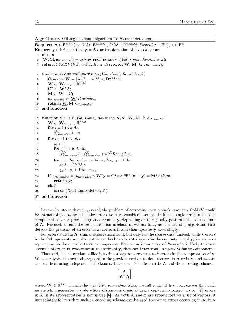
Algorithm 3 Shifting checksum algorithm for k errors detection.Require: A ∈ Rn×n
(as Val ∈ Rnnz(A),Colid ∈ Nnnz(A),Rowindex ∈ Rn
), x ∈ Rn
Ensure: y ∈ Rn such that y = Ax or the detection of up to k errors1: x′ ← x2: [W,M, cRowindex] = computeChecksums(Val , Colid , Rowindex , k);3: return SpMxV(Val , Colid , Rowindex , x, x′, W, M, k, cRowindex);
4: function computeChecksums(Val , Colid , Rowindex , k)5: Generate W =
[w(1) . . .w(k)
]∈ Rn+1×n;
6: W←W1:n,∗ ∈ Rn×k7: Cᵀ ←WᵀA;8: M←W −C;9: cRowindex ←WᵀRowindex ;
10: return W,M, cRowindex;11: end function
12: function SpMxV(Val , Colid , Rowindex , x, x′, W, M, k, cRowindex)13: W←W1:n,∗ ∈ Rn×k14: for i = 1 to k do15: s
(i)Rowindex ← 0;
16: for i← 1 to n do17: yi ← 0;18: for j = 1 to k do19: s
(j)Rowindex ← s
(j)Rowindex + w
(j)i Rowindex i;
20: for j ← Rowindex i to Rowindex i+1 − 1 do21: ind← Colid j ;22: yi ← yi + Val j · xind;23: if cRowindex = sRowindex ∧Wᵀy = Cᵀx ∧Wᵀ (x′ − y) = Mᵀx then24: return y;25: else26: error ("Soft faults detected");27: end function
Let us also stress that, in general, the problem of correcting even a single error in a SpMxV wouldbe intractable, allowing all of the errors we have considered so far. Indeed a single error in the i-thcomponent of x can produce up to n errors in y, depending on the sparsity pattern of the i-th columnof A. For such a case, the best correction mechanism we can imagine is a two step algorithm, thatdetects the presence of an error in x, corrects it and then updates y accordingly.
For errors striking A, similar observations hold, but only for the sparse case. Indeed, while k errorsin the full representation of a matrix can lead to at most k errors in the computation of y, for a sparserepresentation they can be twice as dangerous. Each error in an entry of Rowindex is likely to causea couple of errors in two consecutive entries of y, that can hence contain up to 2k faulty components.
That said, it is clear that suffice it to find a way to correct up to k errors in the computation of y.We can rely on the method proposed in the previous section to detect errors in A or in x, and we cancorrect them using independent checksums. Let us consider the matrix A and the encoding scheme[
AWᵀA
],
where W ∈ Rk×n is such that all of its row submatrices are full rank. It has been shown that suchan encoding generates a code whose distance is k and is hence capable to correct up to
⌊k2
⌋errors
in A, if its representation is not sparse [6]. As both A and x are represented by a set of vectors, itimmediately follows that such an encoding scheme can be used to correct errors occurring in A, in x
Combining ABFT and Checkpointing for Iterative Solvers 13
and during the computation of y.Therefore, to perform the actual computation, we execute the encoded multiplication[
AWᵀA
]x =
[Ax
WᵀAx
],
for a given k. For what has been said so far, we know that, using also the k independent checksums ofthe Rowindex vector, this scheme is capable to correct up to
⌊k2
⌋errors in the computation of y or in
the sparse representation of A. To correct up to⌊k2
⌋errors in x, we need to detect them in the first
place. To do this, we can use Algorithm 3, on the first⌊k2
⌋rows of W. It will hence be possible to
correct the faulty entries of x and then the ones of y consequently.
4.4 Numerical issues
Implementing Algorithm 2, Algorithm 3, Algorithm 5 and Algorithm 6 poses a challenge when dealingwith the equality test between ABFT checksums. Let us consider, to fix the ideas, the bunch of tests atline 19 of Algorithm 5. The last comparison, cRowindex = sRowindex, is between two integers, and canbe correctly evaluated by any programming language using the equality sign, even in case of overflow.
However, it is well known that checking the equality of two floating point numbers requires aparticular care. Even though the computations of c, p and cy perform the same operations on thesame floating point numbers (if no error occurs), these operations are arranged in different ways.Hence, since floating point operations are not associative and the distributive property does not hold,we need a tolerance parameter that takes into account the rounding operations that are performed byeach floating point operation.
In the remainder of this section, we will define a false positive a computation without any errorthat is considered as faulty by the algorithm and, conversely, a false negative an iteration during whichan error occurs without being detected by the ABFT mechanism. Let us remark that, in our setting,false positives are much worse that false negatives, as they could lead to a non-terminating executionor to very inaccurate results even if no error has occurred. For that reason, we are mainly interestedin avoiding false positives, allowing false negatives when the relative error they produce in the solutionis “small enough”.
Let F = 〈β, p, emin, emax〉 denote a floating-point family where β is the radix, p the precision andemin and emax are the minimum and maximum allowed exponent respectively. Let us denote byfl : R → F a rounding to nearest, that is the function that associates to any x ∈ R, a value fl(x) ∈ Fsuch that | fl(x) − x |= min {| f − x |: f ∈ F} where the ties are broken arbitrarily. Let the machineepsilon1, i.e., the distance from 1.0 to the next bigger floating point number, be denoted by u.
Restricting again ourselves to Algorithm 5, we give an upper bound on the difference between thetwo floating point checksums, using the standard model [11, Section 2.2].
Theorem 3. [Accuracy of the floating point checksums] Let A ∈ Rn×n, x ∈ Rn and let c ∈ Nn bean auxiliary vector such that ci = 1 for 1 ≤ i ≤ n. Then, if all of the sums involved into the matrixoperations are performed using some flavour of recursive summation [11, Chapter 4], it holds that
| fl ((cᵀA)x)− fl (cᵀ (Ax)) |≤ 2 γ2n−1 cᵀ | A | | x |, (4)
where γn =nu
1− nuand the absolute value of matrices and vectors hold componentwise.
Proof. See Section E.1 of the Appendix.
This bound can be directly used in Algorithm 2, and along the lines of the proof of Theorem 3,similar bounds can be derived for Algorithm 3 and Algorithm 6. In particular, it should be noted thatconsidering a generic c vector does not increase much the absolute value of the bound, as we show inthe following theorem.
1Called sometimes relative rounding error or unit round-off.
14 Massimiliano Fasi
Theorem 4. [Accuracy of the floating point weighted checksums] Let A ∈ Rn×n, x ∈ Rn, c ∈ Rn.Then, if all of the sums involved into the matrix operations are performed using some flavour ofrecursive summation, it holds that
| fl ((cᵀA)x)− fl (cᵀ (Ax)) |≤ 2 γ2n | cᵀ | | A | | x | . (5)
Proof. See Section E.2 of the Appendix.
Let us note that if all of the entries of c are positive, as it is often the case in our setting, theabsolute value of c in (5) can be safely replaced with c itself. It is also clear that these bounds arenot computable, since cᵀ | A | | x | is not, in general, a floating point number. This problem can bealleviated by overestimating the bound by means of matrix and vector norms.
Recalling that it can be shown [14, Section B.7] that
‖A‖1 = max1≤j≤n
n∑i=1
| ai,j |, (6)
it is possible to upperbound the right hand side in (4) so to get that
| fl ((cᵀA)x)− fl (cᵀ (Ax)) |≤ 2 γ2n n ‖cᵀ‖∞ ‖A‖1 ‖x‖∞ . (7)
Though the right hand side of (7) is not exactly computable in floating point arithmetic, it requiresan amount of operations dramatically smaller than the one in (5), just a few sums for the norm of A.As this norm is usually computed using the identity in (6), any kind of summation yields a relativeerror of at most n′u [11, Section 4.6], where n′ is the maximum column degree of A. Since we aredealing with sparse matrices, we expect n′ to be very small, and hence the computation of the normto be accurate. Moreover, as in (7) the quantity 2 γ2n n ‖cᵀ‖∞ ‖A‖1 does not depend on x, it canbe computed just once for a given matrix and weight vector. Thus, we could even imagine to performsuch a computation in higher precision and use the rounded result afterwards. However, we will notexamine this solution in depth here, as it would require a careful analysis of double rounding issuesthat is outside of the scope of our work.
Clearly, using (7) as tolerance parameter guarantees no false positive, but allows false negativewhen these perturbations of the result are small. Nonetheless, this solution works almost perfectly inpractice, meaning that though the convergence rate can be slowed down, the algorithms still convergestowards the “correct” answer. Though such an outcome could be surprising at first, Elliott et al. [23,25] showed that bit flips that strike the less significant digits of the floating point representation ofvector elements during a dot product create small perturbations of the results and that the magnitudeof this perturbation gets smaller as the size of the vectors increases. Hence, we expect errors that arenot detected by our tolerance threshold to be too small to impact the solution of the linear solver.
5 Model to trade-off ABFT and checkpointingLet us now examine the problem of combining ABFT methods with a checkpoint-based approach inorder to develop a reliable algorithm for Conjugate Gradient computations. On the one hand, ABFTadds a small overhead to each step of the iterative method, while, on the other hand, checkpointingeach s steps the application state entails an overhead that decreases proportionally to the growth of sitself. In general, for s large enough, a checkpoint-based approach could be cheaper than a correctionscheme that relies on the ABFT techniques that we have presented so far. However, s can be largeonly when errors are unfrequent, and it is natural to expect that adding some intrinsic correctioncapability to a Conjugate Gradient algorithm will increase on the one hand the reliability, on the otherthe execution time of each step. An increased resilience also reduces the number of checkpoints, hencethe checkpointing overhead, so looking for a trade-off solution seems a worthy endeavor.
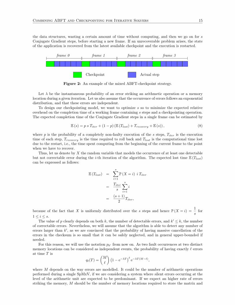
Let us suppose that a computation without any critical fault happens as depicted in Figure 2,that is, as a sequence of multi-step frames. At the beginning of each frame, we save a snapshot of
Combining ABFT and Checkpointing for Iterative Solvers 15
the data structures, wasting a certain amount of time without computing, and then we go on for sConjugate Gradient steps, before starting a new frame. If an unrecoverable problem arises, the stateof the application is recovered from the latest available checkpoint and the execution is restarted.
frame 0 frame 1 frame 2 frame 3
Checkpoint Actual step
Figure 2: An example of the mixed ABFT-checkpoint strategy.
Let λ be the instantaneous probability of an error striking an arithmetic operation or a memorylocation during a given iteration. Let us also assume that the occurrence of errors follows an exponentialdistribution, and that these errors are independent.
To design our checkpointing model, we want to optimize s so to minimize the expected relativeoverhead on the completion time of a working frame containing s steps and a checkpointing operation.The expected completion time of the Conjugate Gradient steps in a single frame can be estimated by
E (s) = p s Titer + (1− p) (E (Tlost) + Trecovery + E (s)) , (8)
where p is the probability of a completely non-faulty execution of the s steps, Titer is the executiontime of each step, Trecovery is the time required to roll back and Tlost is the computational time lostdue to the restart, i.e., the time spent computing from the beginning of the current frame to the pointwhen we have to recover.
Thus, let us denote by X the random variable that models the occurrence of at least one detectablebut not correctable error during the i-th iteration of the algorithm. The expected lost time E (Tlost)can be expressed as follows:
E (Tlost) =
s∑i=1
P (X = i) i Titer
=Titers
s∑i=1
i
=(s+ 1)
2Titer,
because of the fact that X is uniformly distributed over the s steps and hence P (X = i) =1
sfor
1 ≤ i ≤ s.The value of p clearly depends on both k, the number of detectable errors, and k′ ≤ k, the number
of correctable errors. Nevertheless, we will assume that the algorithm is able to detect any number oferrors larger than k′, as we are convinced that the probability of having massive cancellation of theerrors in the checksum is so small that it can be safely neglected, and in general upper-bounded ifneeded.
For this reason, we will use the notation pk′ from now on. As two fault occurrences at two distinctmemory locations can be considered as independent events, the probability of having exactly ` errorsat time T is
q`(T ) =
(M
`
)(1− e−λT
)`e−λT (M−`),
where M depends on the way errors are modelled. It could be the number of arithmetic operationsperformed during a single SpMxV, if we are considering a system where silent errors occurring at thelevel of the arithmetic unit are expected to be predominant. If we expect an higher rate of errorsstriking the memory, M should be the number of memory locations required to store the matrix and
16 Massimiliano Fasi
the vector. Finally, if we are dealing with a system where the two kinds of fault rates are similar, weshould consider the (possibly weighted) sum of both.
Then, the probability of having at most k′ errors per iteration for s iterations is
pk′ =
k′∑i=0
qi
(T
(k′)iter
)s
,
where we use the notation T (k′)iter , since the duration of an iteration depends on the overhead introduced
by a particular ABFT method and hence on k′.Our main objective is to compare what happens for k′ = 0 and k′ = 1. When k′ = 0, we have to
rollback and recover each time we detect an error. In that case, we get
p0 = e−λsT(0)iterM . (9)
When k′ = 1, we can correct an error upon detection and rollback only when two errors are detected,that gives
p1 =(
e−λT(1)iterM +Me−λT
(1)iter(M−1)
(1− e−λT
(1)iter
))s. (10)
Therefore, given k′ equation (8) can be rewritten as
E (s) = pk′ s T(k′)iter + (1− pk′)
((s+ 1)
2T
(k′)iter + Trecovery + E (s)
), (11)
that represents the expected time to successfully execute s steps of the Conjugate Gradient methodwith ABFT detection and/or correction. We want to find an s that minimizes the expected overheadratio of a single frame, that is
E (fs) =E (s)− s T (k′)
iter + Tcheckpoint
s T(k′)iter
,
where Tcheckpoint is the checkpointing time. Hence the optimal number of steps for a single frame is
s = argmins∈N
(E (s)− s Titer + Tcheckpoint
s Titer
), (12)
that substituting (11) and simplifying leads to
s = argmins∈N
(
1
pk′− 1
)(s+ 1
2T
(k′)iter + Trecovery
)+ Tcheckpoint
s T(k′)iter
. (13)
6 EvaluationWe conduce a series of numerical experiments using C implementations of the algorithms describedin Section 5, organized by means of Matlab scripts. Intuitively, there are two different sources ofadvantages in combining ABFT and checkpointing. On the one hand, the error detection capabilitylet us perform a cheap validation of the partial result of each Conjugate Gradient step, recovering assoon as an error strikes. On the other hand, being able to correct a single error makes each step moreresilient and thus let us increase the expected number of consecutive valid steps. Here a valid step iseither non-faulty, or suffers from a single error that is corrected via ABFT.
For our experiments, we use three positive definite test matrices, as detailed in Table 1. The firstmatrix, P3D, comes from the finite difference discretization of the 3D Poisson equation on a cubicdomain of size 30 × 30 × 30. The second, BCSSTK09, is a K matrix from a generalized eigenvalue
Combining ABFT and Checkpointing for Iterative Solvers 17
Name N NNZ κ(A) ‖A‖2 Convergence
BCSSTK09 1083 18437 3.10173e+04 6.72182e+07 linearP3D 27000 183600 6.45723e+02 1.18112e+01 quadratic
THERMAL1 82654 574458 4.96250e+05 7.59160e+00 sublinear
Table 1: Synoptic table of test matrices.
problem Kx = λMx and can be found in the Harwell-Boeing Sparse Matrix Collection [7]. The thirdmatrix, THERMAL1, comes from a steady state thermal problem. Both BCSSTK09 and THERMAL1belong to the University of Florida Sparse Matrix Collection [16], where they are indexed with #31and #1402, respectively. When the Conjugate Gradient method is used on these three matrices,the sequences of their residuals exhibit three different convergence rate: P3D converges superlinearly,BCSSTK09 linearly and THERMAL1 sublinearly. These matrices were used in similar studies [19, 24].
As we are assuming a selective reliability setting, faults are injected, at each step, only during theSpMxV. These faults are modelled as bit flips occurring at each step in an independent way, undera uniform distribution of parameter λ, as detailed in Section 5. A silent error can occur as a bit flipduring an arithmetic operation or in the binary representation of the numbers involved in the SpMxV,i.e., the entries of A2 and p in Algorithm 1. To simplify the injection mechanism, Titer in (9) and (10)is normalized to be one, meaning that each memory location or operation is given the chance to failjust once per iteration [24]. To get homogeneous results, the fault rate λ is chosen to be inverselyproportional to M with a proportionality constant α ∈ (0, 1). It follows that the expected number ofConjugate Gradient steps between two distinct fault occurrences does not depend either on the size oron the sparsity ratio of the matrix.
We evaluate two algorithms, CG-1D, that performs single detection and rolls back as soon as anerror is detected, and CG-2D1C, that is capable of correcting a single error during a given step androlls back only if two errors occur3.
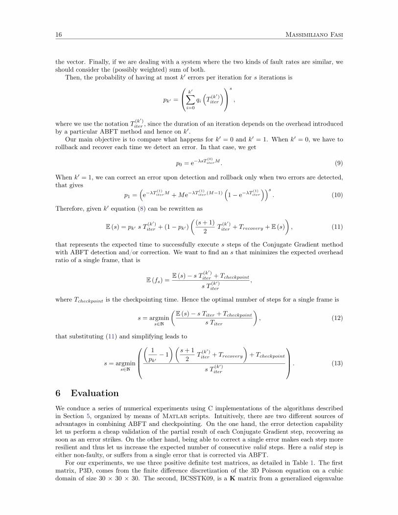
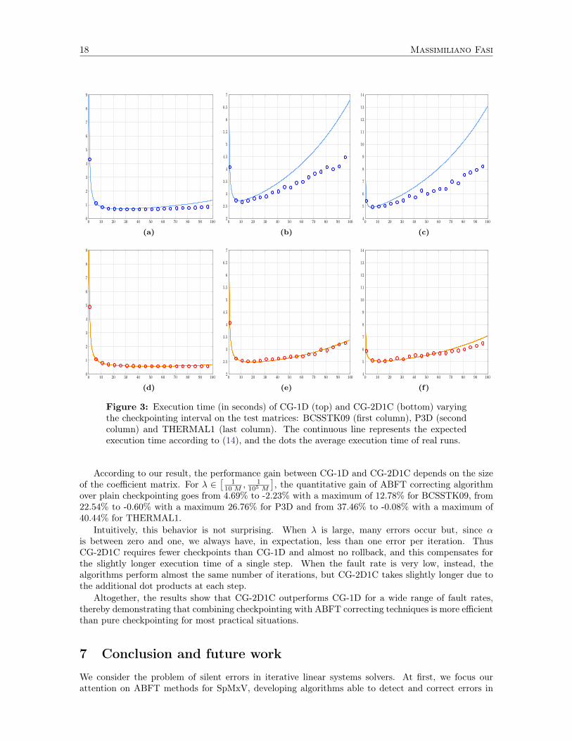
To validate the model, we perform the simulation whose results are depicted in Figure 3. For eachmatrix, we set λ = 1
64 M and consider the execution time of both CG-1D (first row) and CG-2D1C(second row), gradually increasing the checkpointing interval. The continuous line represents theexpected execution time predicted by
f(s) = (E (s) + Tcheckpoint)(niter
s
)(14)
where E (s) is defined in (11) and niter is the number of iterations of a fault-free execution of themethod. Indeed, f(s) makes a prediction based on the average execution time of a single step andthe expected number of frames that the algorithm should perform before reaching the stopping cri-terion. The isolated points represent the average duration of 1000 actual runs of both CG-1D (toprow) and CG-2D1C (bottom row). The graphs show that the model is very accurate for CG-2D1C,whereas the actual execution time is shorter than expected for CG-1D when the checkpoint intervalgrows. Nevertheless, in both cases the local minimizer of the predicting function represents an accurateapproximation of the optimal checkpointing interval. Similar results hold for different values of λ.
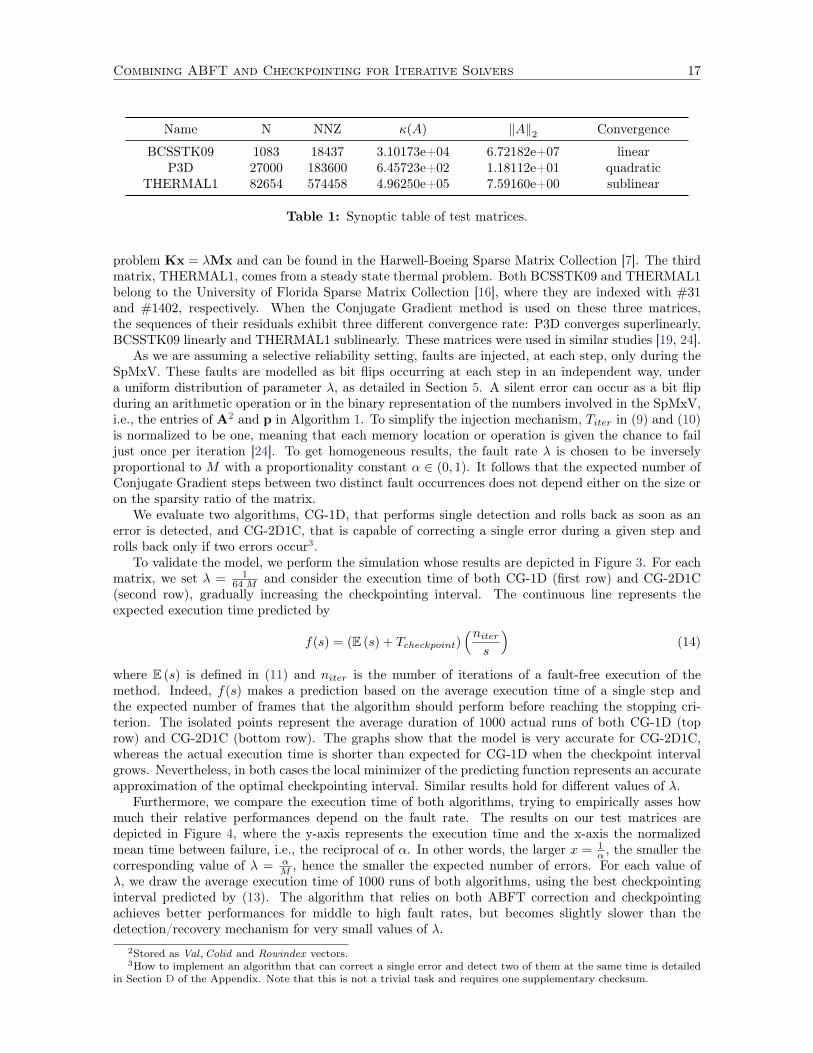
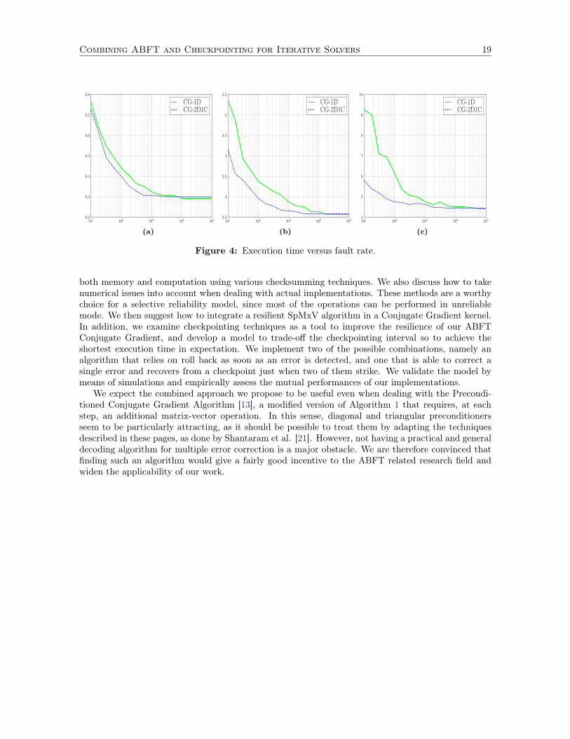
Furthermore, we compare the execution time of both algorithms, trying to empirically asses howmuch their relative performances depend on the fault rate. The results on our test matrices aredepicted in Figure 4, where the y-axis represents the execution time and the x-axis the normalizedmean time between failure, i.e., the reciprocal of α. In other words, the larger x = 1
α , the smaller thecorresponding value of λ = α
M , hence the smaller the expected number of errors. For each value ofλ, we draw the average execution time of 1000 runs of both algorithms, using the best checkpointinginterval predicted by (13). The algorithm that relies on both ABFT correction and checkpointingachieves better performances for middle to high fault rates, but becomes slightly slower than thedetection/recovery mechanism for very small values of λ.
2Stored as Val ,Colid and Rowindex vectors.3How to implement an algorithm that can correct a single error and detect two of them at the same time is detailed
in Section D of the Appendix. Note that this is not a trivial task and requires one supplementary checksum.
18 Massimiliano Fasi
0 10 20 30 40 50 60 70 80 90 1000
1
2
3
4
5
6
7
8
9
(a)0 10 20 30 40 50 60 70 80 90 100
2
2.5
3
3.5
4
4.5
5
5.5
6
6.5
7
(b)0 10 20 30 40 50 60 70 80 90 100
4
5
6
7
8
9
10
11
12
13
14
(c)
0 10 20 30 40 50 60 70 80 90 1000
1
2
3
4
5
6
7
8
9
(d)0 10 20 30 40 50 60 70 80 90 100
2
2.5
3
3.5
4
4.5
5
5.5
6
6.5
7
(e)0 10 20 30 40 50 60 70 80 90 100
4
5
6
7
8
9
10
11
12
13
14
(f)
Figure 3: Execution time (in seconds) of CG-1D (top) and CG-2D1C (bottom) varyingthe checkpointing interval on the test matrices: BCSSTK09 (first column), P3D (secondcolumn) and THERMAL1 (last column). The continuous line represents the expectedexecution time according to (14), and the dots the average execution time of real runs.
According to our result, the performance gain between CG-1D and CG-2D1C depends on the sizeof the coefficient matrix. For λ ∈
[1
10 M , 1105 M
], the quantitative gain of ABFT correcting algorithm
over plain checkpointing goes from 4.69% to -2.23% with a maximum of 12.78% for BCSSTK09, from22.54% to -0.60% with a maximum 26.76% for P3D and from 37.46% to -0.08% with a maximum of40.44% for THERMAL1.
Intuitively, this behavior is not surprising. When λ is large, many errors occur but, since αis between zero and one, we always have, in expectation, less than one error per iteration. ThusCG-2D1C requires fewer checkpoints than CG-1D and almost no rollback, and this compensates forthe slightly longer execution time of a single step. When the fault rate is very low, instead, thealgorithms perform almost the same number of iterations, but CG-2D1C takes slightly longer due tothe additional dot products at each step.
Altogether, the results show that CG-2D1C outperforms CG-1D for a wide range of fault rates,thereby demonstrating that combining checkpointing with ABFT correcting techniques is more efficientthan pure checkpointing for most practical situations.
7 Conclusion and future work
We consider the problem of silent errors in iterative linear systems solvers. At first, we focus ourattention on ABFT methods for SpMxV, developing algorithms able to detect and correct errors in
Combining ABFT and Checkpointing for Iterative Solvers 19
101 102 103 104 1050.2
0.3
0.4
0.5
0.6
0.7
0.8
CG-1DCG-2D1C
(a)101 102 103 104 105
2.5
3
3.5
4
4.5
5
5.5
CG-1DCG-2D1C
(b)101 102 103 104 1054
5
6
7
8
9
10
CG-1DCG-2D1C
(c)
Figure 4: Execution time versus fault rate.
both memory and computation using various checksumming techniques. We also discuss how to takenumerical issues into account when dealing with actual implementations. These methods are a worthychoice for a selective reliability model, since most of the operations can be performed in unreliablemode. We then suggest how to integrate a resilient SpMxV algorithm in a Conjugate Gradient kernel.In addition, we examine checkpointing techniques as a tool to improve the resilience of our ABFTConjugate Gradient, and develop a model to trade-off the checkpointing interval so to achieve theshortest execution time in expectation. We implement two of the possible combinations, namely analgorithm that relies on roll back as soon as an error is detected, and one that is able to correct asingle error and recovers from a checkpoint just when two of them strike. We validate the model bymeans of simulations and empirically assess the mutual performances of our implementations.
We expect the combined approach we propose to be useful even when dealing with the Precondi-tioned Conjugate Gradient Algorithm [13], a modified version of Algorithm 1 that requires, at eachstep, an additional matrix-vector operation. In this sense, diagonal and triangular preconditionersseem to be particularly attracting, as it should be possible to treat them by adapting the techniquesdescribed in these pages, as done by Shantaram et al. [21]. However, not having a practical and generaldecoding algorithm for multiple error correction is a major obstacle. We are therefore convinced thatfinding such an algorithm would give a fairly good incentive to the ABFT related research field andwiden the applicability of our work.
20 Massimiliano Fasi
References[1] Magnus R. Hestenes and Eduard Stiefel. “Methods of Conjugate Gradients for Solving Linear
Systems”. In: Journal of Research of the National Bureau of Standards 49.6 (1952), pp. 409–436.
[2] W. W. Peterson and Jr. E.J. Weldon. Error-Correcting Codes. 2nd. MIT press, 1972.
[3] K.-H. Huang and J. A. Abraham. “Algorithm-Based Fault Tolerance for Matrix Operations”. In:Computers, IEEE Transactions on C–33.6 (1984), pp. 518–528.
[4] J.-Y. Jou and J. A. Abraham. “Fault-Tolerant Matrix Operations On Multiple Processor SystemsUsing Weighted Checksums”. In: Proc. SPIE. Vol. 0495. 1984, pp. 94–101.
[5] R. Koo and S. Toueg. “Checkpointing and Rollback-Recovery for Distributed Systems”. In: Soft-ware Engineering, IEEE Transactions on SE-13.1 (1987), pp. 23–31.
[6] C.J. Anfinson and F.T. Luk. “A Linear Algebraic Model of Algorithm-Based Fault Tolerance”.In: Computers, IEEE Transactions on 37.12 (1988), pp. 1599–1604.
[7] I. S. Duff, R. G. Grimes, and J. G. Lewis. “Sparse Matrix Test Problems”. In: ACM Trans. Math.Softw. 15.1 (1989), pp. 1–14.
[8] R. Barrett et al. Templates for the Solution of Linear Systems: Building Blocks for IterativeMethods. 2nd. SIAM Press, 1994.
[9] B. Parhami. “Defect, Fault, Error,..., or Failure?” In: IEEE Transactions on Reliability 46.4(1997), pp. 450–451.
[10] M. Vijay and R. Mittal. “Algorithm-Based Fault Tolerance: a Review”. In: Microprocessors andMicrosystems 21.3 (1997), pp. 151 –161.
[11] N. J. Higham. Accuracy and Stability of Numerical Algorithms. 2nd. SIAM Press, 2002.
[12] J. Lacan and J. Fimes. “A Construction of Matrices with No Singular Square Submatrices”. In:International Conference on Finite Fields and Applications. Ed. by G. L. Mullen, A. Poli, andH. Stichtenoth. Vol. 2948. Lecture Notes in Computer Science. Springer, 2003, pp. 145–147.
[13] Y. Saad. Iterative Methods for Sparse Linear Systems. 2nd. SIAM Press, 2003.
[14] N. J. Higham. Functions of Matrices: Theory and Computation. SIAM Press, 2008.
[15] F. Cappello et al. “Toward exascale resilience”. In: International Journal of High PerformanceComputing Applications 23.4 (2009), pp. 374–388.
[16] T. A. Davis and Y. Hu. “The University of Florida Sparse Matrix Collection”. In: ACM Trans.Math. Softw. 38.1 (2011), 1:1–1:25.
[17] M. Hoemmen and M. A. Heroux. Fault-tolerant iterative methods via selective reliability. Tech.rep. Sandia Corporation, 2011.
[18] M. Hoemmen and M. A Heroux. “Fault-Tolerant Iterative Methods via Selective Reliability”. In:Proceedings of the 2011 International Conference for High Performance Computing, Networking,Storage and Analysis (SC). IEEE Computer Society. Vol. 3. 2011, p. 9.
[19] M. Shantharam, S. Srinivasmurthy, and P. Raghavan. “Characterizing the Impact of Soft Errorson Iterative Methods in Scientific Computing”. In: ICS ’11. ACM, 2011, pp. 152–161.
[20] P. G Bridges et al. Fault-tolerant linear solvers via selective reliability. preprint. 2012.
[21] M. Shantharam, S. Srinivasmurthy, and P. Raghavan. “Fault Tolerant Preconditioned ConjugateGradient for Sparse Linear System Solution”. In: ICS ’12. ACM, 2012, pp. 69–78.
[22] J. Sloan, R. Kumar, and G. Bronevetsky. “Algorithmic Approaches to Low Overhead FaultDetection for Sparse Linear Algebra”. In: Dependable Systems and Networks (DSN), 2012 42ndAnnual IEEE/IFIP International Conference on. 2012, pp. 1–12.
[23] J. Elliott et al. Quantifying the impact of single bit flips on floating point arithmetic. preprint.2013.
[24] P. Sao and R. Vuduc. “Self-Stabilizing Iterative Solvers”. In: ScalA ’13. ACM, 2013, 4:1–4:8.
Combining ABFT and Checkpointing for Iterative Solvers 21
[25] Miroslav Stoyanov and Clayton Webster. Quantifying the impact of single bit flips on floatingpoint arithmetic. Tech. rep. Oak Ridge National Laboratory, 2013.
22 Massimiliano Fasi
Appendix
A Single error detection in dense matrix-matrix product
A.1 Matrix encoding
The encoding technique developed in [3] for matrix-matrix product is based on row and column check-sums of the matrices involved in the computation, and relies on the concept of checksum matricesdetailed in Definitions 1, 2 and 3 below.
Definition 1 (Row checksum matrix). Let M ∈ Rp×q. The row checksum matrix of M is the matrixMr ∈ Rp×q+1 whose elements are defined by the rule
mri,j =
mi,j , 1 ≤ i ≤ p, 1 ≤ j ≤ q,
q∑k=1
mi,k, 1 ≤ i ≤ p, j = q + 1.
We use also the block notation Mr = [M |Mu], where u ∈ Rq is such that ui = 1 for 1 ≤ i ≤ q.
Definition 2 (Column checksum matrix). Let M ∈ Rp×q. The column checksum matrix of M is thematrix Mc ∈ Rp+1×q whose elements are defined by the rule
mci,j =
mi,j , 1 ≤ i ≤ p, 1 ≤ j ≤ q,
p∑k=1
mk,j , i = p+ 1, 1 ≤ j ≤ q.
We will often use the block notation Mc =
[M
vᵀM
]where v ∈ Rp is such that vi = 1 for 1 ≤ i ≤ p.
Definition 3 (Full checksum matrix). Let M ∈ Rp×q. The full checksum matrix of M is the matrixMf ∈ Rp+1×q+1 that is the column checksum matrix of the row checksum matrix of the matrix M.
Let use note that in the last definition, the order of the checksumming operations can be invertedwithout affecting the result, as can be easily proven by means of some arithmetic calculations. More-over, we will often use the block notation
Mf =
[M Mu
vᵀM vᵀMu
],
to denote the full checksum matrix of M.
A.2 Matrix product algorithm
With the encoding scheme just defined, the relationship between checksum matrices can be easilycharacterized [3, Theorem 4.1]. Here we give in Theorem 5 a slightly more modified version of theclaim.
Theorem 5. [Huang and Abraham, [3]] Let us consider the matrix-matrix product C = A ·B whereA ∈ Rm×n, B ∈ Rn×p and C ∈ Rm×p. Then it holds that
Ac ·Br = Cf . (15)
Proof. The proof is straightforward using the block representation of the checksum matrices. Wereproduce it here, since it is a very clear way to exactly understand how ABFT algorithms work. It
Combining ABFT and Checkpointing for Iterative Solvers 23
runs as follows:
Ac ·Br =
[A
vᵀA
]· [B | Bu]
=
[A ·B A ·Bu
vᵀA ·B vᵀA ·Bu
]=
[C Cu
vᵀC vᵀCu
]= Cf .
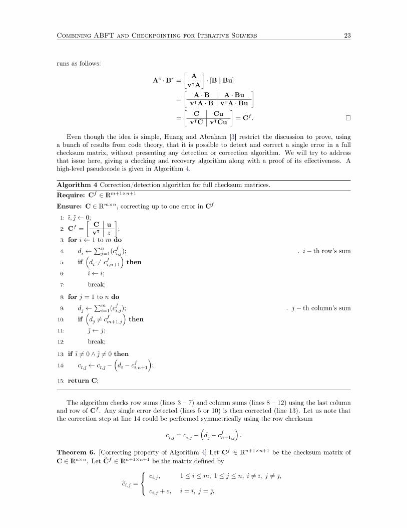
Even though the idea is simple, Huang and Abraham [3] restrict the discussion to prove, usinga bunch of results from code theory, that it is possible to detect and correct a single error in a fullchecksum matrix, without presenting any detection or correction algorithm. We will try to addressthat issue here, giving a checking and recovery algorithm along with a proof of its effectiveness. Ahigh-level pseudocode is given in Algorithm 4.
Algorithm 4 Correction/detection algorithm for full checksum matrices.Require: Cf ∈ Rm+1×n+1
Ensure: C ∈ Rm×n, correcting up to one error in Cf
1: ı, ← 0;
2: Cf =
[C uvᵀ z
];
3: for i← 1 to m do
4: dı ←∑nj=1(cfi,j); . i− th row’s sum
5: if(dı 6= cfi,n+1
)then
6: ı← i;
7: break;
8: for j = 1 to n do
9: d ←∑mi=1(cfi,j); . j − th column’s sum
10: if(d 6= cfm+1,j
)then
11: ← j;
12: break;
13: if ı 6= 0 ∧ 6= 0 then
14: cı, ← cı, −(dı − c
fı,n+1
);
15: return C;
The algorithm checks row sums (lines 3 – 7) and column sums (lines 8 – 12) using the last columnand row of Cf . Any single error detected (lines 5 or 10) is then corrected (line 13). Let us note thatthe correction step at line 14 could be performed symmetrically using the row checksum
cı, = cı, −(d − c
fn+1,
).
Theorem 6. [Correcting property of Algorithm 4] Let Cf ∈ Rn+1×n+1 be the checksum matrix ofC ∈ Rn×n. Let Cf ∈ Rn+1×n+1 be the matrix defined by
ci,j =
ci,j , 1 ≤ i ≤ m, 1 ≤ j ≤ n, i 6= ı, j 6= ,
ci,j + ε, i = ı, j = ,
24 Massimiliano Fasi
where ε ∈ R denotes a fault occurred at position (ı, ), 1 ≤ ı ≤ m, and 1 ≤ ≤ n. Then Algorithm 4will compute C from Cf .
Proof. To simplify the discussion let us introduce the following block decomposition of the input matrixwhere an error has struck
Cf =
[C uvᵀ z
]. (16)
Let us note that since the error can strike at most one block, Cf and Cf differ in at most one of them.We will use such property later on.
To prove the claim, we consider four different scenarios depending on the two indices ı, such thatcfı, 6= cfı,, namely
a. 1 ≤ ı ≤ m, 1 ≤ ≤ n that is an error in C,
b. 1 ≤ ı ≤ m and = n+ 1, that is an error in u,
c. 1 ≤ ≤ n and ı = m+ 1, that is an error in v,
d. ı = m+ 1, = n+ 1, that is an erroneous computation of z.
Case a. (An error in C) Let us consider the state after the execution of the first two for loops ofthe algorithm on Cf . After the first for, for i < ı we have
dı =
n∑j=1
ci,j =
n∑j=1
ci,j = ci,n+1
while for i = ı we have
dı =
n∑j=1
cı,j =
n∑j=1
cı,j + e 6=n∑j=1
cı,j = cı,n+1.
So at line 8 we have ı = ı and
dı =
n∑j=1
cı,j + ε.
Analogously, it can be shown that the execution of the second loop yield = and
d =
m∑i=1
ci, + ε.
Hence, the value of the element at row ı and column of Cf is
cfı, −(dı − c
fı,n+1
)= cfı, + ε−
n∑j=1
cfı,j − cfı,n+1
= cfı, + ε−
n∑j=1
cfı,j + e−n∑j=1
cfı,j
= cfı,
that is cı, by Definition 3.Case b. (An error in u) Reasoning as in the previous case, it is easy to show that after the
execution of the second for loop, one has that ı = ı and = 0. Thus, the correction step is notexecuted. Moreover, since the error has struck v, we have that C = C. This suffices to prove theclaim.
Case c. (An error in v) This case is much like the previous one. The same observations hold, infact, for = and ı = 0.
Case d. (An error in z) As the algorithm do not consider neither the m+ 1-st row nor the n+ 1-stcolumn, the values of ı and is not modified by its execution. So no element of Cf is changed, andthe claim can be proved again noting that C = C.
Combining ABFT and Checkpointing for Iterative Solvers 25
Let us note that Algorithm 4 could be easily extended to correct errors in the last row and column,but that would have made the proof longer. Such kind of extension can be easily made along the samelines.
A.3 Computational aspects
The computation of the matrix productA·B, whereA ∈ Rm×n andB ∈ Rn×p has complexityO (mnp)using the naive algorithm, and the overhead of Algorithm 4 is quite straightforward to compute. Indeed,on the left hand side of (15) we just have to compute the checksums of the two matrices A and B,which require O (mn) and O (np) time, respectively, while for the right hand side, the overhead isclearly dominated by the computation of the sum of all the rows and columns, which requires O (pm)time. Therefore the total number of operations is O (pm+mn+ np).
Let us note that whenm = n = p, that is the two matrices are square, the asymptotic complexity ofthe checksum overhead grows as O
(n2)for dense matrices. On the other hand, to get the complexity
of a matrix vector product suffice it to put m = n and p = 1. With this observation in mind, thechecking overhead can be easily seen to be O
(n2), since the row-checksum matrix of the input vector
is just an n× 2 matrix. This computational overhead is excessively high, as it represents roughly onehalf of the overall amount of time used to perform the computation. The same remark holds true forthe sparse case, remembering that the complexity of the matrix-vector product is O (nnz(A)) in thatcase.
26 Massimiliano Fasi
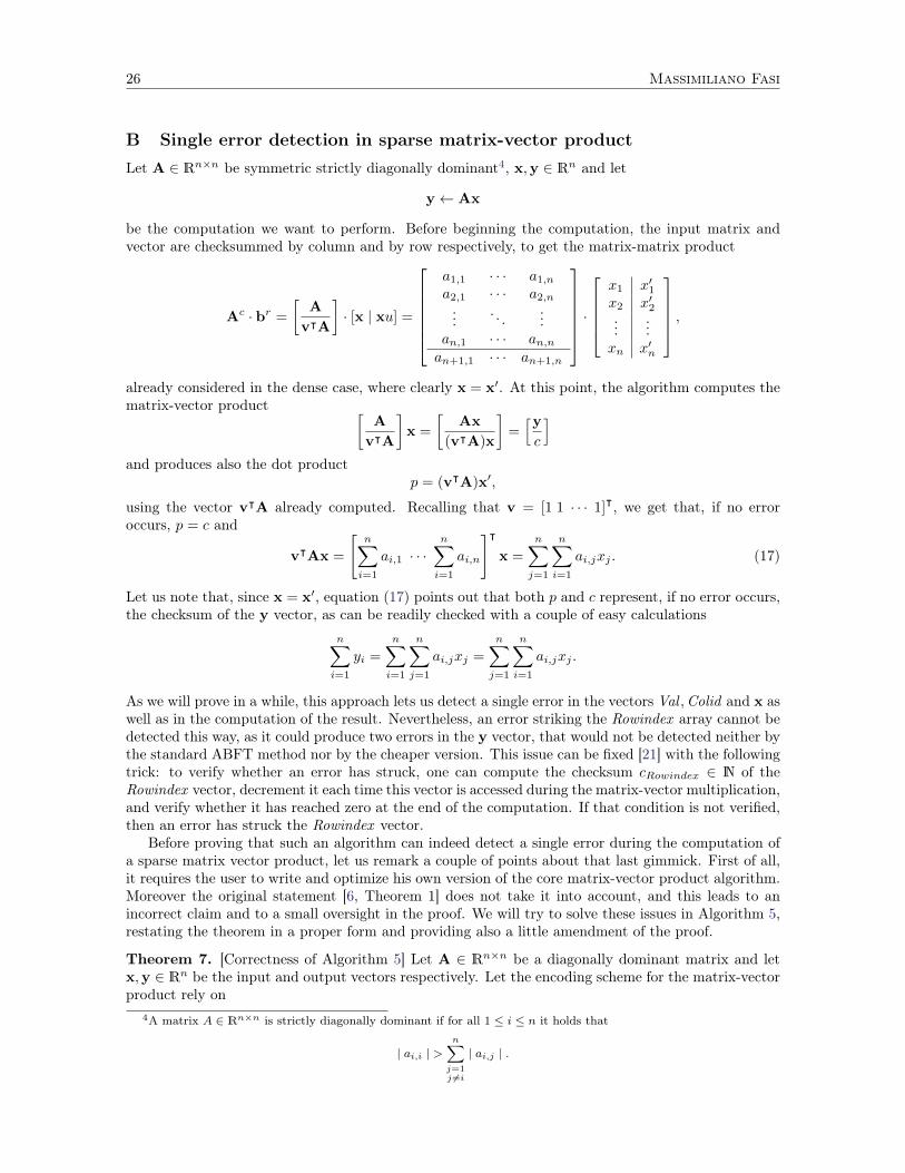
B Single error detection in sparse matrix-vector productLet A ∈ Rn×n be symmetric strictly diagonally dominant4, x,y ∈ Rn and let
y← Ax
be the computation we want to perform. Before beginning the computation, the input matrix andvector are checksummed by column and by row respectively, to get the matrix-matrix product
Ac · br =
[A
vᵀA
]· [x | xu] =
a1,1 · · · a1,n
a2,1 · · · a2,n
.... . .
...an,1 · · · an,nan+1,1 · · · an+1,n
·x1 x′1x2 x′2...
...xn x′n
,
already considered in the dense case, where clearly x = x′. At this point, the algorithm computes thematrix-vector product [
A
vᵀA
]x =
[Ax
(vᵀA)x
]=[yc
]and produces also the dot product
p = (vᵀA)x′,
using the vector vᵀA already computed. Recalling that v = [1 1 · · · 1]ᵀ, we get that, if no error
occurs, p = c and
vᵀAx =
[n∑i=1
ai,1 · · ·n∑i=1
ai,n
]ᵀx =
n∑j=1
n∑i=1
ai,jxj . (17)
Let us note that, since x = x′, equation (17) points out that both p and c represent, if no error occurs,the checksum of the y vector, as can be readily checked with a couple of easy calculations
n∑i=1
yi =
n∑i=1
n∑j=1
ai,jxj =
n∑j=1
n∑i=1
ai,jxj .
As we will prove in a while, this approach lets us detect a single error in the vectors Val ,Colid and x aswell as in the computation of the result. Nevertheless, an error striking the Rowindex array cannot bedetected this way, as it could produce two errors in the y vector, that would not be detected neither bythe standard ABFT method nor by the cheaper version. This issue can be fixed [21] with the followingtrick: to verify whether an error has struck, one can compute the checksum cRowindex ∈ N of theRowindex vector, decrement it each time this vector is accessed during the matrix-vector multiplication,and verify whether it has reached zero at the end of the computation. If that condition is not verified,then an error has struck the Rowindex vector.
Before proving that such an algorithm can indeed detect a single error during the computation ofa sparse matrix vector product, let us remark a couple of points about that last gimmick. First of all,it requires the user to write and optimize his own version of the core matrix-vector product algorithm.Moreover the original statement [6, Theorem 1] does not take it into account, and this leads to anincorrect claim and to a small oversight in the proof. We will try to solve these issues in Algorithm 5,restating the theorem in a proper form and providing also a little amendment of the proof.
Theorem 7. [Correctness of Algorithm 5] Let A ∈ Rn×n be a diagonally dominant matrix and letx,y ∈ Rn be the input and output vectors respectively. Let the encoding scheme for the matrix-vectorproduct rely on
4A matrix A ∈ Rn×n is strictly diagonally dominant if for all 1 ≤ i ≤ n it holds that
| ai,i | >n∑
j=1j 6=i
| ai,j | .
Combining ABFT and Checkpointing for Iterative Solvers 27
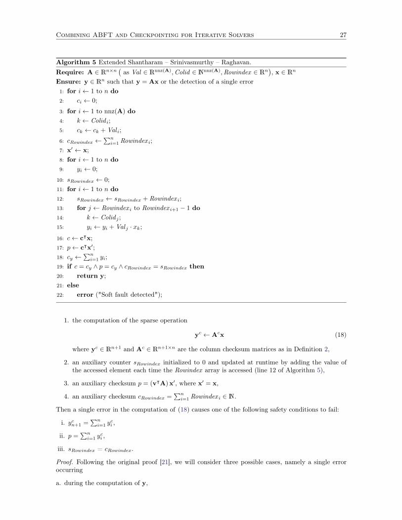
Algorithm 5 Extended Shantharam – Srinivasmurthy – Raghavan.Require: A ∈ Rn×n
(as Val ∈ Rnnz(A),Colid ∈ Nnnz(A),Rowindex ∈ Rn
), x ∈ Rn
Ensure: y ∈ Rn such that y = Ax or the detection of a single error1: for i← 1 to n do2: ci ← 0;
3: for i← 1 to nnz(A) do4: k ← Colid i;5: ck ← ck + Val i;
6: cRowindex ←∑ni=1 Rowindex i;
7: x′ ← x;8: for i← 1 to n do9: yi ← 0;
10: sRowindex ← 0;11: for i← 1 to n do12: sRowindex ← sRowindex + Rowindex i;13: for j ← Rowindex i to Rowindex i+1 − 1 do14: k ← Colid j ;15: yi ← yi + Val j · xk;
16: c← cᵀx;17: p← cᵀx′;18: cy ←
∑ni=1 yi;
19: if c = cy ∧ p = cy ∧ cRowindex = sRowindex then20: return y;21: else22: error ("Soft fault detected");
1. the computation of the sparse operation
yc ← Acx (18)
where yc ∈ Rn+1 and Ac ∈ Rn+1×n are the column checksum matrices as in Definition 2,
2. an auxiliary counter sRowindex initialized to 0 and updated at runtime by adding the value ofthe accessed element each time the Rowindex array is accessed (line 12 of Algorithm 5),
3. an auxiliary checksum p = (vᵀA)x′, where x′ = x,
4. an auxiliary checksum cRowindex =∑ni=1 Rowindex i ∈ N.
Then a single error in the computation of (18) causes one of the following safety conditions to fail:
i. ycn+1 =∑ni=1 y
ci ,
ii. p =∑ni=1 y
ci ,
iii. sRowindex = cRowindex.
Proof. Following the original proof [21], we will consider three possible cases, namely a single erroroccurring
a. during the computation of y,
28 Massimiliano Fasi
b. in the representation of A,
c. in the representation of x.
Since (a) and (c) lead to a violation of the first and last safety condition respectively, they werecorrectly addressed in the original paper. Hence we will focus our attention on the proof of (b).
A single error in the A matrix can occur in one of the three vectors that constitute its sparserepresentation:
• a fault in Val that alters the value of an element ai,j implies an error in the computation of ycithat leads condition (i) to fail because of (a),
• a variation in Colid can zero out an element in position ai,j shifting its value in position ai,j′
and leading again to an erroneous computation of yci ,
• a transient fault in Rowindex entails an incorrect value of sRowindex and hence a violation ofcondition (iii).
That proves (b).
It is easy to note that this method can even detect more than one error, provided that they affectdata protected by different checksums. For example, an error striking Val can be detected whileanother one strikes Rowind , but not with one striking Colid .
Combining ABFT and Checkpointing for Iterative Solvers 29
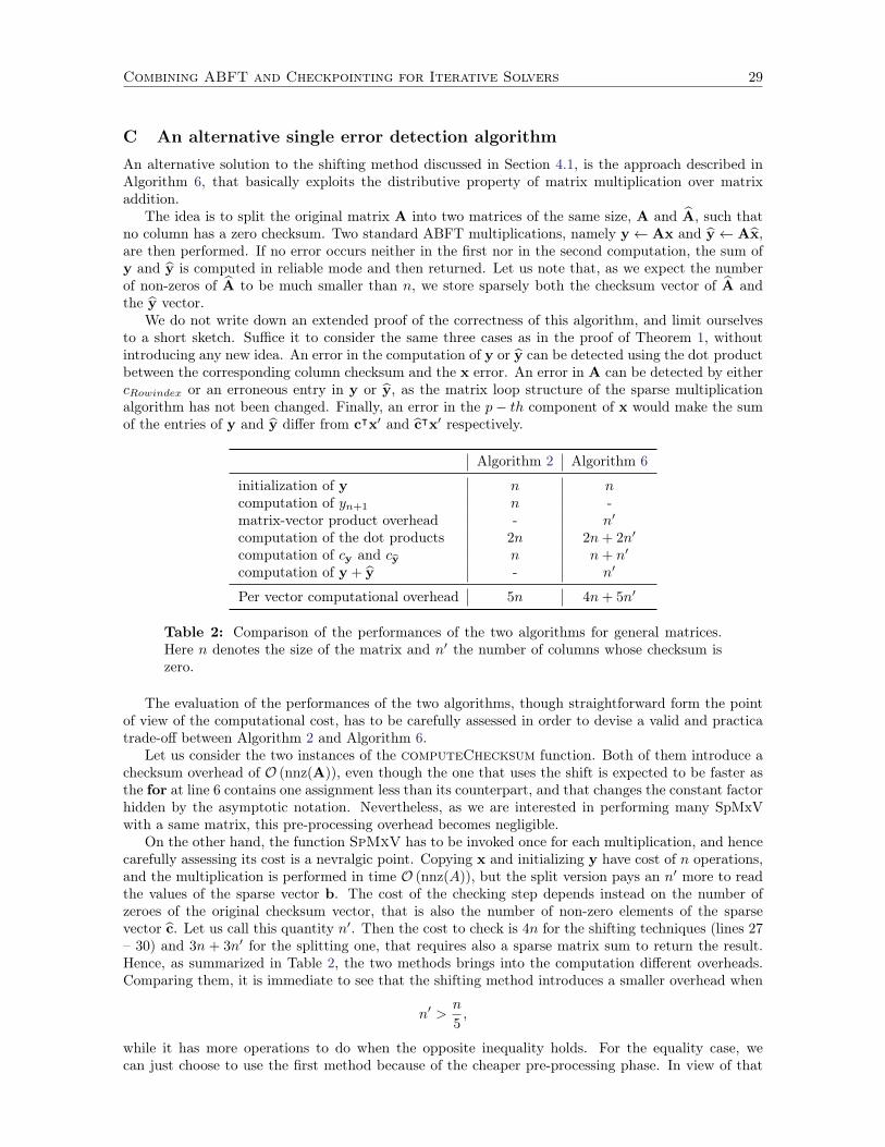
C An alternative single error detection algorithmAn alternative solution to the shifting method discussed in Section 4.1, is the approach described inAlgorithm 6, that basically exploits the distributive property of matrix multiplication over matrixaddition.
The idea is to split the original matrix A into two matrices of the same size, A and A, such thatno column has a zero checksum. Two standard ABFT multiplications, namely y← Ax and y← Ax,are then performed. If no error occurs neither in the first nor in the second computation, the sum ofy and y is computed in reliable mode and then returned. Let us note that, as we expect the numberof non-zeros of A to be much smaller than n, we store sparsely both the checksum vector of A andthe y vector.
We do not write down an extended proof of the correctness of this algorithm, and limit ourselvesto a short sketch. Suffice it to consider the same three cases as in the proof of Theorem 1, withoutintroducing any new idea. An error in the computation of y or y can be detected using the dot productbetween the corresponding column checksum and the x error. An error in A can be detected by eithercRowindex or an erroneous entry in y or y, as the matrix loop structure of the sparse multiplicationalgorithm has not been changed. Finally, an error in the p− th component of x would make the sumof the entries of y and y differ from cᵀx′ and cᵀx′ respectively.
Algorithm 2 Algorithm 6
initialization of y n ncomputation of yn+1 n -matrix-vector product overhead - n′
computation of the dot products 2n 2n+ 2n′
computation of cy and cy n n+ n′
computation of y + y - n′
Per vector computational overhead 5n 4n+ 5n′
Table 2: Comparison of the performances of the two algorithms for general matrices.Here n denotes the size of the matrix and n′ the number of columns whose checksum iszero.
The evaluation of the performances of the two algorithms, though straightforward form the pointof view of the computational cost, has to be carefully assessed in order to devise a valid and practicatrade-off between Algorithm 2 and Algorithm 6.
Let us consider the two instances of the computeChecksum function. Both of them introduce achecksum overhead of O (nnz(A)), even though the one that uses the shift is expected to be faster asthe for at line 6 contains one assignment less than its counterpart, and that changes the constant factorhidden by the asymptotic notation. Nevertheless, as we are interested in performing many SpMxVwith a same matrix, this pre-processing overhead becomes negligible.
On the other hand, the function SpMxV has to be invoked once for each multiplication, and hencecarefully assessing its cost is a nevralgic point. Copying x and initializing y have cost of n operations,and the multiplication is performed in time O (nnz(A)), but the split version pays an n′ more to readthe values of the sparse vector b. The cost of the checking step depends instead on the number ofzeroes of the original checksum vector, that is also the number of non-zero elements of the sparsevector c. Let us call this quantity n′. Then the cost to check is 4n for the shifting techniques (lines 27– 30) and 3n + 3n′ for the splitting one, that requires also a sparse matrix sum to return the result.Hence, as summarized in Table 2, the two methods brings into the computation different overheads.Comparing them, it is immediate to see that the shifting method introduces a smaller overhead when
n′ >n
5,
while it has more operations to do when the opposite inequality holds. For the equality case, wecan just choose to use the first method because of the cheaper pre-processing phase. In view of that
30 Massimiliano Fasi
observation, it is possible to devise a simple algorithm that exploits this trade-off to achieve betterperformances. It suffices to compute the checksum vector of the input matrix, count the number ofnon-zeros and choose which detection method to use accordingly.
Combining ABFT and Checkpointing for Iterative Solvers 31
D Case study: a 1-correcting 2-detecting encodingThough we have considered so far detection and correction as two completely different problems, andhave presented separate algorithms for the two cases, we actually need a way to combine them. Sincethere is no general algorithm for error correction, we analyse the single error correcting code presentedin Section 4.3 and discuss how to integrate it with a two error detecting method.
Let us note that using as the weight matrix
W =
1 11 21 3...
...1 n
is enough to guarantee on the one hand single error correction and, on the other, two errors correction,but not to achieve both correction and detection at the same time. Indeed, let us restrict ourselves toan easy case, without considering errors in x. As usual, we compute the column checksums matrix
C = (WᵀA)ᵀ,
and then compare the two entries of d = Cᵀx ∈ R2 with the weighted sums
yc1 =
n∑i=1
yi
and
yc2 =
n∑i=1
iyi
where y is the possibly faulty vector computed by the algorithm. It is clear that if no error occurs, thecomputation verifies the condition δ = yc− c = 0. Furthermore, if exactly one error occurs, clearly wehave that δ1, δ2 6= 0 and δ2
δ1∈ N, and if two errors strike the vectors protected by the checksum c, the
algorithm is able to detect them by verifying that δ 6= 0.At this point it is natural to ask whether this information is enough to build a working algorithm
or some border cases can bias its behaviour. In particular when δ2δ1
= p ∈ N it is not clear how todiscern whether there have been one or two errors.
Let ε1, ε2 ∈ R \ {0} be the value of two errors occurring at position p1 and p2 respectively, and lety ∈ Rn be such that
yi =
yi, 1 ≤ i ≤ n, i 6= p1, p2
yi + ε1, i = p1
yi + ε2, i = p2
.
Then the following conditions
δ1 = ε1 + ε2, (19)δ2 = p1ε1 + p2ε2, (20)
hold. Therefore, it is clear that if ε1 and ε2 are such that
p (ε1 + ε2) = p1ε1 + p2ε2, (21)
it is not possible to distinguish these two errors from a single error of value ε1 + ε2 occurring inposition p. This issue can be solved by introducing a new set of weights and hence a new row ofcolumn checksums. Indeed, let us consider a weight matrix W ∈ Rn×3 that includes a quadraticweight vector
W =
1 1 11 2 41 3 9...
...1 n n2
.
32 Massimiliano Fasi
Then let us consider the vectorδ =
(WᵀA
)x− Wᵀy,
whose components can be expressed as
δ1 = ε1 + ε2 (22)δ2 = p1ε1 + p2ε2 (23)δ2 = p2
1ε1 + p22ε2. (24)
To be confused with a single error in position p, ε1 and ε2 have to be such that
p (ε1 + ε2) = p1ε1 + p2ε2
andp2 (ε1 + ε2) = p2
1ε1 + p22ε2
hold simultaneously for some p ∈ N. In other words, possible values of the errors are the solution ofthe linear system (
(p− p1) (p− p2)(p2 − p2
1) (p2 − p22)
)(ε1
ε2
)=
(00
).
It can be easily computed that the determinant of the coefficient matrix is
(p− p1) (p− p2) (p2 − p1) ,
that always differs from zero, as long as p, p1 and ps differ pairwise. Thus, the matrix is invertible andthe solution space of the linear system is the trivial kernel (ε1, ε2) = (0, 0). Thus using W as weightmatrix guarantees that it is always possible to distinguish single from double errors.
Combining ABFT and Checkpointing for Iterative Solvers 33
E Proof of theorems in Section 4.4
E.1 Proof of Theorem 3
To prove the result in (4) we bound the left hand side of the inequality with the sum of two classicalfloating point bounds in the form | x− fl(x) | and then bound them independently. For the first step,let us note that the absolute value is a norm on the real numbers and hence
| fl ((cᵀA)x)− fl (cᵀ (Ax)) | = | fl ((cᵀA)x)− fl (cᵀ (Ax)) + cᵀAx− cᵀAx |≤ | fl ((cᵀA)x)− (cᵀA)x | + | fl (cᵀ (Ax))− cᵀ (Ax) | . (25)
To bound the absolute value of the dot product of the checksum of A and x, we proceed by levels.First of all, we can upper-bound the value of a single entry of cᵀA with
fl (cᵀA)j ≤ a1,j(1 + δ1)n−1 + a2,j(1 + δ2)n−1 + a3,j(1 + δ2)n−2 + · · ·+ an,j(1 + δn), (26)
where | δi |≤ u for 1 ≤ i ≤ n. As it is standard in classical error analysis, we drop the subscriptand simplify the expression by writing 1 + δi = 1 ± δ. Now, multiplying the j-th entry of the matrixchecksum with the corresponding x entry, gives that
fl(
(cᵀA)j xj
)≤
(a1,j(1± δ)n−1 + a2,j(1± δ)n−1 + a3,j(1± δ)n−2 + · · ·+ an,j(1± δ)
)xj(1± δ)
= a1,jxj(1± δ)n + a2,jxj(1± δ)n + a3,jxj(1± δ)n−1 + · · ·+ an,jxj(1± δ)2.
Finally, we can upper-bound the whole dot product with a sum
fl ((cᵀA)x) ≤(a1,1x1 (1± δ)n + a2,1x1 (1± δ)n + a3,1x1 (1± δ)n−1
+ · · ·+ an,1x1 (1± δ)2)
(1± δ)n−1
+(a1,2x2 (1± δ)n + a2,2x2 (1± δ)n + a3,2x2 (1± δ)n−1
+ · · ·+ an,2x2 (1± δ)2)
(1± δ)n−1
+(a1,3x3 (1± δ)n + a2,3x3 (1± δ)n + a3,3x3 (1± δ)n−1
+ · · ·+ an,3x3 (1± δ)2)
(1± δ)n−2
+(
(1± δ)n−2)
. . .(
(1± δ)n−2)
+(a1,nxn (1± δ)n + a2,nxn (1± δ)n + a3,nxn (1± δ)n−1
+ · · ·+ an,nxn (1± δ)2)
(1± δ) ,
that distributing becomes
fl ((cᵀA)x) ≤ a1,1x1 (1± δ)2n−1+ a2,1x1 (1± δ)2n−1
+ a3,1x1 (1± δ)2n−2+ · · ·+ an,1x1 (1± δ)n+1
+ a1,2x2 (1± δ)2n−1+ a2,2x2 (1± δ)2n−1
+ a3,2x2 (1± δ)2n−2+ · · ·+ an,2x2 (1± δ)n+1
+ a1,3x3 (1± δ)2n−2+ a2,3x3 (1± δ)2n−2
+ a3,3x3 (1± δ)2n−3+ · · ·+ an,3x3 (1± δ)n
+(
(1± δ)n−2)
. . .(
(1± δ)n−2)
+ a1,nxn (1± δ)n+1+ a2,nxn (1± δ)n+1
+ a3,nxn (1± δ)n + · · ·+ an,nxn (1± δ)3.
This long expression can be simplified [11, Lemma 3.1] to get
fl ((cᵀA)x) ≤ a1,1x1
(1 + θ
(1,1)2n−1
)+ a2,1x1
(1 + θ
(2,1)2n−1
)+ a3,1x1
(1 + θ
(3,1)2n−2
)+ · · ·+ an,1x1
(1 + θ
(n,1)n+1
)+ a1,2x2
(1 + θ
(1,2)2n−1
)+ a2,2x2
(1 + θ
(2,2)2n−1
)+ a3,2x2
(1 + θ
(3,2)2n−2
)+ · · ·+ an,2x2
(1 + θ
(n,2)n+1
)+ a1,3x3
(1 + θ
(1,3)2n−2
)+ a2,3x3
(1 + θ
(2,3)2n−2
)+ a3,3x3
(1 + θ
(3,3)2n−3
)+ · · ·+ an,3x3
(1 + θ(n,3)
n
)+
((1± δ)n−2
). . .
((1± δ)n−2
)+ a1,nxn
(1 + θ
(1,4)n+1
)+ a2,nxn
(1 + θ
(2,4)n+1
)+ a3,nxn
(1 + θ(3,4)
n
)+ · · ·+ an,nxn
(1 + θ
(n,4)3
),
34 Massimiliano Fasi
where | θi,jn |≤ γn, for 1 ≤ i, j ≤ n. This formulation can be interpreted as a backward error result,i.e.,
fl ((cᵀA)x) = cᵀ (A + ∆A)x, | ∆A |≤ γ2n−1 | A |,
where both the matrix absolute value and the inequality between matrices hold componentwise. Toget a forward error bound, we proceed as follows:
| fl ((cᵀA)x)− (cᵀA)x | = | cᵀ (A + ∆A)x− (cᵀA)x |≤ | cᵀ | | ∆A | | x |≤ γ2n−1 cᵀ | A | | x | . (27)
Along the same lines, it can also be shown that
| fl (cᵀ (Ax))− cᵀ (Ax) |≤ γ2n−1 cᵀ | A | | x |, (28)
and thus substituting (27) and (28) into (25) concludes the proof.
E.2 Proof of Theorem 4
It can be shown by proceeding as in the proof of Theorem 3. Suffices it to start from
fl (cᵀA)j ≤ c1a1,j(1 + δ1)n + c2a2,j(1 + δ2)n + c3a3,j(1 + δ2)n−1 + · · ·+ cnan,j(1 + δn)2
instead of (26) and to develop accordingly.
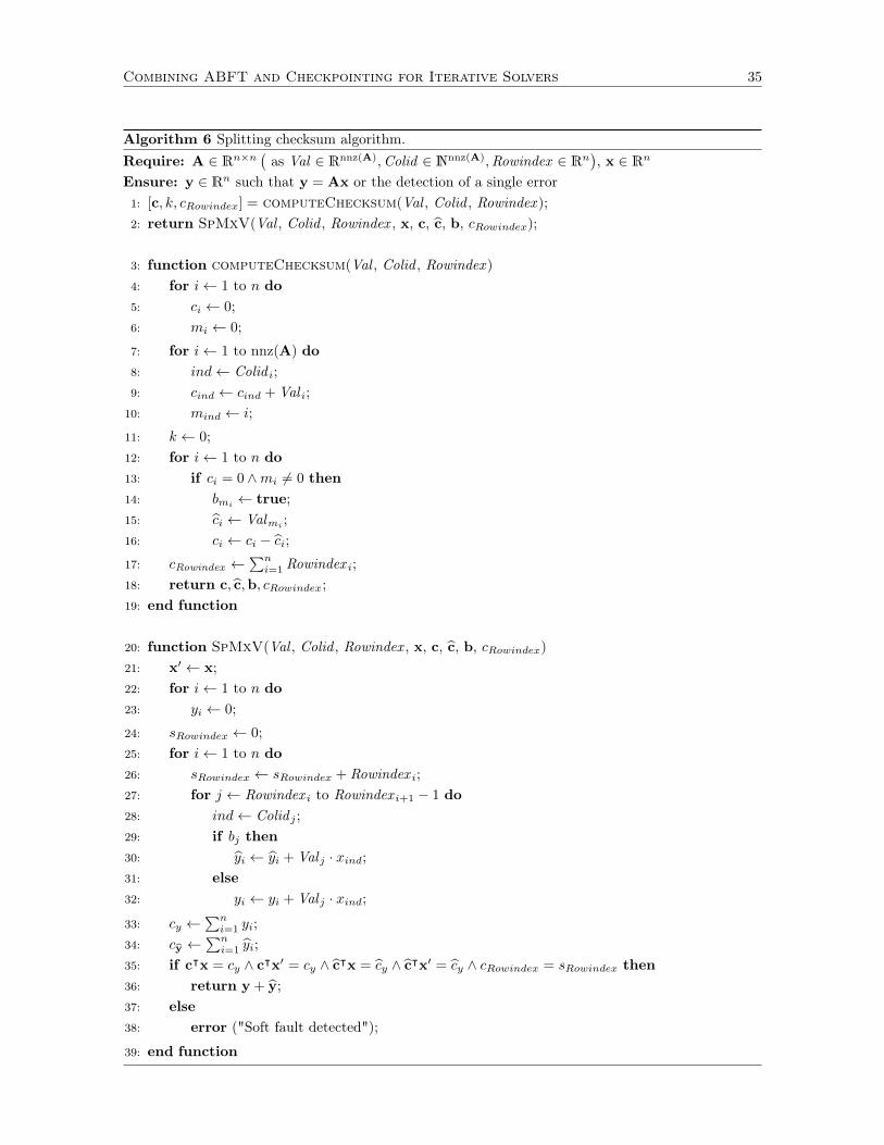
Combining ABFT and Checkpointing for Iterative Solvers 35
Algorithm 6 Splitting checksum algorithm.Require: A ∈ Rn×n
(as Val ∈ Rnnz(A),Colid ∈ Nnnz(A),Rowindex ∈ Rn
), x ∈ Rn
Ensure: y ∈ Rn such that y = Ax or the detection of a single error1: [c, k, cRowindex] = computeChecksum(Val , Colid , Rowindex );2: return SpMxV(Val , Colid , Rowindex , x, c, c, b, cRowindex);
3: function computeChecksum(Val , Colid , Rowindex )4: for i← 1 to n do5: ci ← 0;6: mi ← 0;
7: for i← 1 to nnz(A) do8: ind← Colid i;9: cind ← cind + Val i;
10: mind ← i;
11: k ← 0;12: for i← 1 to n do13: if ci = 0 ∧mi 6= 0 then14: bmi
← true;15: ci ← Valmi
;16: ci ← ci − ci;17: cRowindex ←
∑ni=1 Rowindex i;
18: return c, c,b, cRowindex;19: end function
20: function SpMxV(Val , Colid , Rowindex , x, c, c, b, cRowindex)21: x′ ← x;22: for i← 1 to n do23: yi ← 0;
24: sRowindex ← 0;25: for i← 1 to n do26: sRowindex ← sRowindex + Rowindex i;27: for j ← Rowindex i to Rowindex i+1 − 1 do28: ind← Colid j ;29: if bj then30: yi ← yi + Val j · xind;31: else32: yi ← yi + Val j · xind;
33: cy ←∑ni=1 yi;
34: cy ←∑ni=1 yi;
35: if cᵀx = cy ∧ cᵀx′ = cy ∧ cᵀx = cy ∧ cᵀx′ = cy ∧ cRowindex = sRowindex then36: return y + y;37: else38: error ("Soft fault detected");
39: end function