Embed Size (px)
Citation preview
College Education, Occupational Sorting, and International Trade
Saiah LeeUniv of Wisconsin
Soo Hyun OhKorea Research Institute forInternational Economic Policy
June 16, 2017
We study how education system impacts endogenous formation of human capital,trade patterns and income inequality. We construct the model of education choice withmodifying three-sector occupation choice model by Grossman and Maggi (2000). Overthe countries, education systems are characterized by education cost and efficiency ofeducation. We presume universal education system lowers unit education cost to makeit evenly accessible to the public, while elite education system effectively reinforceshuman capital increase. Upon trade liberalization from autarky state, country withhigher human capital has comparative advantage in the innovative sector while theother country specializes in the routine sector, with obtaining xed and lower returns.This specialization pattern promotes more education acquisition in the former countryin expense of higher income inequality.We also provide empirical evidence supporting our theory that countries with elite ed-ucation system heavily specialize on high-tech industry while countries with universaleducation system specialize on non-high-tech industries such as agricultural & raw ma-terial production, food production, or manufactures. We construct education measuresand industry specialization measures for 270 countries using publicly available univer-sity ranking data and World Development Indicators provided by World Bank. Weconduct cross-country regression analysis to examine the theory, and the results con-firm that elite education system and high-tech industries specialization are positivelyrelated and that higher returns to education, which is delivered by elite education sys-tem, leads to higher wage inequality controlling population, real GDP per capita, andtrade openness. The empirical results are consistent and robust across specifications.
JEL Classification: F16; F66; I23; I24; I26; J31
1
1 Introduction
Education system reform has been a central issue that both economists and policymakers are facing. Since education is an important public-sector service that deter-mines individual human capital accumulation, the debate over ‘universal education’versus ‘elite education’ has become increasingly controversial and required extensiveeconomic analysis. In this paper, focusing on tertiary education which directly affectsindividual occupation choice, we study how education system contribute endogenousformation of Ricardian comparative advantage, trade patterns and income inequality.
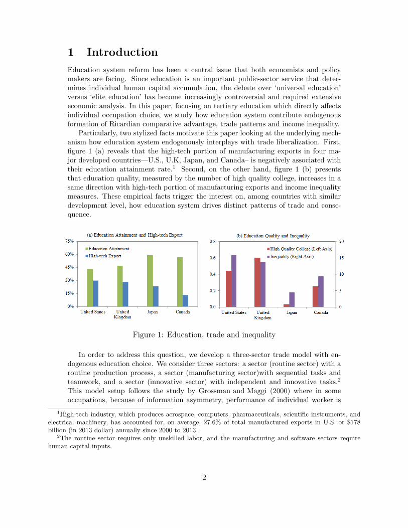
Particularly, two stylized facts motivate this paper looking at the underlying mech-anism how education system endogenously interplays with trade liberalization. First,figure 1 (a) reveals that the high-tech portion of manufacturing exports in four ma-jor developed countries—U.S., U.K, Japan, and Canada– is negatively associated withtheir education attainment rate.1 Second, on the other hand, figure 1 (b) presentsthat education quality, measured by the number of high quality college, increases in asame direction with high-tech portion of manufacturing exports and income inequalitymeasures. These empirical facts trigger the interest on, among countries with similardevelopment level, how education system drives distinct patterns of trade and conse-quence.
Figure 1: Education, trade and inequality
In order to address this question, we develop a three-sector trade model with en-dogenous education choice. We consider three sectors: a sector (routine sector) with aroutine production process, a sector (manufacturing sector)with sequential tasks andteamwork, and a sector (innovative sector) with independent and innovative tasks.2
This model setup follows the study by Grossman and Maggi (2000) where in someoccupations, because of information asymmetry, performance of individual worker is
1High-tech industry, which produces aerospace, computers, pharmaceuticals, scientific instruments, andelectrical machinery, has accounted for, on average, 27.6% of total manufactured exports in U.S. or $178billion (in 2013 dollar) annually since 2000 to 2013.
2The routine sector requires only unskilled labor, and the manufacturing and software sectors requirehuman capital inputs.
2
difficult to measure separately.3 This imperfect contracting varies over industries, andthus, workers productivity is more measurable in some industries than others. Thiswill induce more talented workers to choose a sector where they can be compensatedmore based on their own talent than average productivity of team.4 The newly-bornworkers can enhance their human capital through college education before they enterthe labor market based on their lifetime value change. One can think that enhancingthe universal education system is associated with lowering unit education cost to makeit evenly accessible to the public, while encouraging the elite education system is asso-ciated with reinforcing human capital increase from education. Then, we study whichcountry specialize which sectors in response to the trade liberalization. (small openworld and two country bilateral trade)
Under autarky, we demonstrate that both cheaper education cost and higher skillacquisition drive more workers to take education and raise product price in routinesector.5 On the other hand, they induce more workers to choose the innovative sectorwhere the workers can be compensated based on their human capital.6 After tradeliberalization, country with higher education has comparative advantage in the inno-vative sector while the counterpart country will specialize in the routine sector. Thisway of specialization promotes more education acquisition in the former country, andthereby reinforcing their comparative advantages.
We also show that country with higher education experiences higher income inequal-ity in response to the trade liberalization due to higher dispersion of human capitaldistribution from education choice (and wage). Therefore, this result suggests thatcountries aiming to concentrate in high-tech industries or service industries needs topromote selective education for high quality in the expense of higher income inequality.It is unclear whether quality-focused education increases the total welfare. The highereducation strengthens the comparative advantage of service- and high-tech industriesover other countries, however, simultaneously increases the income inequality over time.In particular, this paper suggests that education system significantly determines thehuman capital distribution combining with the formation of comparative advantage infree trade.
This paper has to several important implications on growing literature. First, thereare growing interests on the underlying link between the distribution of human capitaland the pattern of international trade. However, previous literature assumes the ex-ogenous distribution of human capital. Furthermore, in spite of the important role ofhigh-tech industry separating from manufacturing sector, previous trade literature con-sider them as a same sector and overlooks the variation in trade patterns between man-ufacturing and high-tech sector. We endogenize the education choice into trade modeland demonstrate the underlying channel. Since the education system is more persis-
3It is often hard to distinguish from other inputs, particularly, from their peers. Therefore, the contractsare likely to be tied to team performance and heterogeneous workers will receive similar compensationregardless of their skill/human capital.
4The workers with poor talent choose the routine sector and receive fixed wages. Since the workers havingenough human capital prefer to do innovative tasks by herself, they choose the hi-tech industry. The workersin the middle choose the manufacturing sector.
5It increases total income but reduces the supply in the routine sector.6It increases both supply and product price.
3
tent than other government policy (Glaeser, La Porta, Lopez-de Silanes, and Shleifer,2004), the in-depth analysis on the link between education system and trade outcomemay provide significant implications.
The rest of the paper proceeds as follows. Section 2 presents the environmentand equilibrium configuration. Section 3 characterizes the steady state equilibrium ofautarky and open economies. Section 4 provides numerical experiments to examine theeffects of different education systems on the pattern of international trade and Section5 concludes.
2 The Model
2.1 Environment
We consider a small open economy populated by a unit measure of workers, who areworking in three different sectors, ‘traditional’, ‘manufacturing’, and ‘high-tech’ sectorsdenoted by i = x, y and z, respectively. Workers enter the labor market with different‘ability’ a ∈ [a, a], where ability a represents the units of human capital that she canutilize. We call the worker with a-units of human capital ‘a-type worker’. All agentsdiscount future at discount factor β ∈ [0, 1]. In what follows, we restrict our attentionto the steady state equilibrium.
The traditional sector is characterized by a routine production process as in agricul-ture and routine service, which does not require human capital inputs, i.e. knowledgeor knowhow acquired through advanced education. The high-tech sector such as fash-ion design, finance, and computer software industries asks each individual worker toperform an independent and innovative task by fully utilizing their human capital.Bougheas and Riezman (2007) label the former as a primary commodity sector andthe latter as a high-tech product sector. In addition to the two sectors, we introducethe manufacturing sector, which produces manufactured products such as ‘automobiles’through a sequence of sophisticated tasks. The manufacturing sector requires cooper-ative human capital inputs by n number of workers as in Grossman and Maggi (2000),Grossman (2004), and Buera, Kaboski, and Shin (2011). The production technologyof each sector is given by
yi(h) =
{αx if i = x
αzh if i = z, and yy(h1, h2, · · · , hn) = αy(
n∑k=1
hµk)1µ , (1)
where µ < 0. The final goods are sold in perfectly competitive markets. The productiontechnologies reveal that the human capital inputs by individual workers are not requiredin the traditional sector, whereas they are cooperatively and independently utilized inthe manufacturing and high-tech sectors, respectively.
An individual worker with income flow w consumes each products (qx, qy, qz) tomaximize her per period utility, (qσx + qσy + qσz )
1/σ, subject to the budget constraintpxqx + pyqy + pzqz = w, where (px, py, pz) are the prices of each sectoral products inthe world market. The individual demand for each sectoral products is given by
qi = wp1
σ−1
i Pσ
1−σ , where P =(p
σσ−1x + p
σσ−1y + p
σσ−1z
)σ−1σ. (2)
4
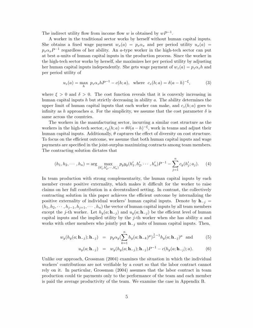
The indirect utility flow from income flow w is obtained by wP−1.A worker in the traditional sector works by herself without human capital inputs.
She obtains a fixed wage payment wx(a) = pxαx and per period utility ux(a) =pxαxP
−1 regardless of her ability. An a-type worker in the high-tech sector can putat best a-units of human capital inputs in the production process. Since the worker inthe high-tech sector works by herself, she maximizes her per period utility by adjustingher human capital inputs independently. She gets wage payment of wz(a) = pzαzh andper period utility of
uz(a) = maxh
pzαzhP−1 − c(h; a), where cz(h; a) = δ(a− h)−ξ, (3)
where ξ > 0 and δ > 0. The cost function reveals that it is convexly increasing inhuman capital inputs h but strictly decreasing in ability a. The ability determines theupper limit of human capital inputs that each worker can make, and cz(h; a) goes toinfinity as h approaches a. For the simplicity, we assume that the cost parameter δ issame across the countries.
The workers in the manufacturing sector, incurring a similar cost structure as theworkers in the high-tech sector, cy(h; a) = θδ(a− h)−ξ, work in teams and adjust theirhuman capital inputs. Additionally, θ captures the effect of diversity on cost structure.To focus on the efficient outcome, we assume that both human capital inputs and wagepayments are specified in the joint-surplus maximizing contracts among team members.The contracting solution dictates that
(h1, h2, · · · , hn) = arg max(h′
1,h′2,··· ,h′
n)pyyy(h
′1, h
′2, · · · , h′n)P−1 −
n∑j=1
cy(h′j ; aj). (4)
In team production with strong complementarity, the human capital inputs by eachmember create positive externality, which makes it difficult for the worker to raiseclaims on her full contribution in a decentralized setting. In contrast, the collectivelycontracting solution in this paper achieves the efficient outcome by internalizing thepositive externality of individual workers’ human capital inputs. Denote by h−j =(h1, h2, · · · , hj−1, hj+1, · · · , hn) the vector of human capital inputs by all team membersexcept the j-th worker. Let hy(a;h−j) and uy(a;h−j) be the efficient level of humancapital inputs and the implied utility by the j-th worker when she has ability a andworks with other members who jointly put h−j units of human capital inputs. Then,
wy(hy(a;h−j);h−j) = pyαy(n∑
k=1
hy(a;h−k)µ)
1µ−1
hy(a;h−j)µ and (5)
uy(a;h−j) = wy(hy(a;h−j);h−j)P−1 − c(hy(a;h−j); a). (6)
Unlike our approach, Grossman (2004) examines the situation in which the individualworkers’ contributions are not verifiable by a court so that the labor contract cannotrely on it. In particular, Grossman (2004) assumes that the labor contract in teamproduction could tie payments only to the performance of the team and each memberis paid the average productivity of the team. We examine the case in Appendix B.
5
Taking the expected human capital inputs by all workers as given, workers choosein which sector they work. The Bellman equation for the worker having a is given by
E(a) = max{ux, uy(a;h−j), uz(a)}+ β(1− ρ)E(a). (7)
At each period, workers retire (or die) with probability ρ and all retirees are replacedby newly-born workers. The newly-born workers draw their innate ability a from thebounded Pareto distribution with shape parameter η(> 0) and support [a, a]. Thecumulative distribution function is given by F (a) = (1 − (a/a)η)/(1 − (a/a)η) fora ∈ [a, a]. The newly-born workers can acquire additional human capital throughcollege education before they enter the labor market. They make their own decisionsuch that
e(a) ∈ argmax E(a+ e)− E(a)− ce(e) (8)
where E(a) represents the lifetime value of the workers having a-units of human capital.and ce(e) = κ−1eκ.
Let G(a) be the proportion of workers who have human capital less than equalto a-unit in the labor market at each period. It evolves as follows on a steady stateequilibrium.
G(a) =
∫ a−e(a)
adF (a′) (9)
Definition An steady state equilibrium consists of the distribution of human capitalG(·), price vectors {pi, wi}i∈{x,y,z}, allocation of workers ϕi(·), consumption schedule{qi}i∈{x,y,z}, and value equations E(a) at each period such that given expectation on{pi, wi}i={x,y,z} and G(·),(i) forward-looking newly-born workers make their schooling decisions,
(ii) each worker chooses her optimal consumption, human capital inputs (under thecollective labor contract), and sector,
(iii) the human capital distribution governed by (9) is consistent with G(·).
3 Steady State Analysis
In this section, we characterize the steady state equilibrium. All proofs are postponedto Appendix.
Lemma 1 Given h−j, both hy(·;h−j) and uy(·;h−j) are strictly increasing in a.
The workers in the manufacturing sector form a team without friction. Ifan a-type worker applies to a particular team made up of (a1, a2, · · · , an) andmin{a1, a2, · · · , an} < a, she will be welcomed by all members except the least ableworker with min{a1, a2, · · · , an}. Lemma 1 says that the a-type worker will not put
6
less inputs than the worker having min{a1, a2, · · · , an} and also all other membersput more human capitals in the new formation, which again accelerates the humancapital inputs by the new member. Hence as long as a > min{a1, a2, · · · , an}, allmembers except the least able worker prefer substitution. The equilibrium formationrequires that each worker has no profitable deviation from her status quo team in themanufacturing sector.
Definition A team composed of (a1, a2, · · · , an) is feasible to a-type workers ifa > min{a1, a2, · · · , an}. A team having a vector of h = (h1, h2, · · · , hn) is stable ifno worker can get more than uy(h(a;h−j);h−j) from any other feasible teams.
The stable formation requires that each team should pay to its members theirmaximum wages from all feasible team formation and all workers of a same typeshould be paid the exactly same wages. It makes positive assortative matching occur.
Lemma 2 Only homogenous teams composed of the same types survive on equilibrium.
Lemma 2 says that on equilibrium all teams should be made up of n-number ofhomogenous workers. It is consistent with Kremer (1993) and Grossman and Maggi(2000) in the sense that complementarity and super-modularity drives positive assor-tative matching. In particular, Kremer (1993) argues that a small mistake or failurein a sequence of complementary tasks may destroy the entire value of the product inmany production processes, which drives positive assortative matching. We reflect hisinsight by embodying complementarity among human capital inputs of individual teammembers. By invoking Lemma 2, we drop h−j from hy(a;h−j) and uy(a;h−j) and usehy(a) and uy(a) respectively in what follows. The a-type workers in sector y and z willchoose the level of their human capital inputs such that
hy(a) = a−( θδξP
pyαyn1−µµ
) 1ξ+1
, and (10)
hz(a) = a−(θδξPpyαy
) 1ξ+1
, (11)
on equilibrium. In equation (10), as n increases, hy(a) declines. Plugging (10) and(11) into (3) and (6) yields that
uy(a) = pyαyn1−µµ
{a−
( θδξP
pyαyn1−µµ
) 1ξ+1
}P−1 − θδ
( θδξP
pyαyn1−µµ
) 1ξ+1
, and (12)
uz(a) = pzαz
{a−
( δξP
pzαz
) 1ξ+1
}P−1 − δ
( δξP
pzαz
) 1ξ+1
(13)
on equilibrium.
Lemma 3 On any equilibrium, it should be the case that pz/py > n−1(αy/αz).
7
Lemma 3 implies that the most able worker always works in the high-tech sec-tor. From equations (12) and (13), it is true that (duz(a)/da) > (duy(a)/da) > 0and uz(0) < uy(0). It implies that the per period utility of working in sectorz should cross the utility of working in sector y from the below just once. Inother words, for sufficiently large a, there exists a unique az ∈ (a, a) such thatuz(az) = max{ux(az), uy(az)}. Lemma 4 and 5 tell us that the threshold for eachindustry is well-defined.
Lemma 4 Suppose that Equilibrium Restriction 1 holds.
(i) For any a > az, uz(a) > max{ux(a), uy(a)}.(ii) For any a < az, uz(a) < max{ux(a), uy(a)}.
Moreover, suppose to the contrary that ux(az) ≥ uy(az). Since uy(·) is strictlyincreasing in a and ux is constant, uy(a) < ux for any a < az. Then, no worker worksin sector y and py is not well defined. Thus, we obtain that ux < uy(az) and thereexists an ax ∈ [a, az) such that ux(ax) = uy(ax) on equilibrium. Putting these togetheryields that
ax =
pxαxP−1 + pyαyn
1−µµ
(θδξP
pyαyn1−µµ
) 1ξ+1
P−1 + θδ(
θδξP
pyαyn1−µµ
) 1ξ+1
pyαyn1−µµ P−1
and (14)
ay =
pyαyn1−µµ
(θδξP
pyαyn1−µµ
) 1ξ+1
P−1 − pzαz
(δξPpzαz
) 1ξ+1
P−1 + θδ(
θδξP
pyαyn1−µµ
) 1ξ+1 − δ
(δξPpzαz
) 1ξ+1
pyαyn1−µµ P−1 − pzαzP−1
.(15)
Lemma 5 Suppose that ax satisfies (14).
(i) For any a < ax, ux(a) > uy(a).
(ii) For any a > ax, ux(a) < uy(a).
By combining the market clearing conditions together and normalizing px to beone, we get
p1
σ−1y =
[αy
n
∫ az
ax
hy(a)dG(a)][αxG(ax)− q
]−1, and (16)
p1
σ−1z = αz
[ ∫ a+λ
az
hz(a)dG(a)][αxG(ax)− q
]−1, (17)
where G(·), αx, and αz are respectively given in (9), (14), and (15). Since the righthand side of (16) cannot be negative, αxG(ax) > q. Otherwise, there is no equilibrium.The condition says that the aggregate supply in sector x should be greater than thesubsistence level of the sectoral products.
8
-
6
-
6
a
E(a)
a
e(a)
(a) Lifetime Values (b) Education Choice
ax az
������
���������
ax − λ ax az − λ az
-
6
-
6
a
h(a)
a
w(a)
(c) Human Capital Inputs (d) Wages
####
#####
az
#####
ax ax
���������
###
##
az
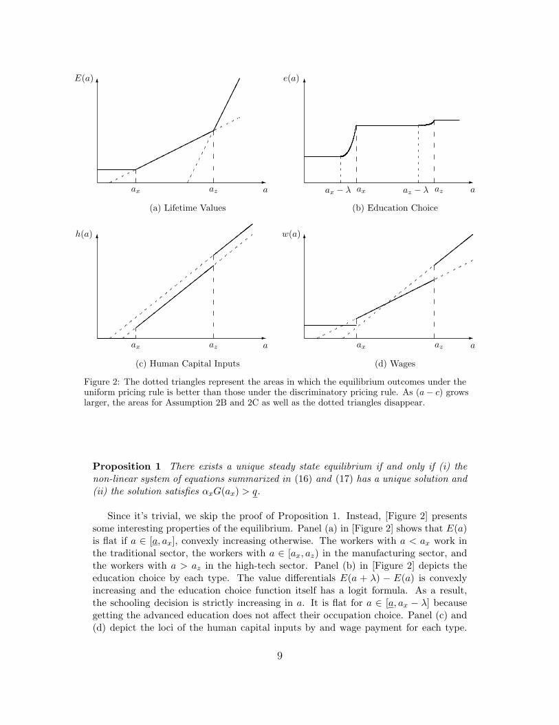
Figure 2: The dotted triangles represent the areas in which the equilibrium outcomes under theuniform pricing rule is better than those under the discriminatory pricing rule. As (a− c) growslarger, the areas for Assumption 2B and 2C as well as the dotted triangles disappear.
Proposition 1 There exists a unique steady state equilibrium if and only if (i) thenon-linear system of equations summarized in (16) and (17) has a unique solution and(ii) the solution satisfies αxG(ax) > q.
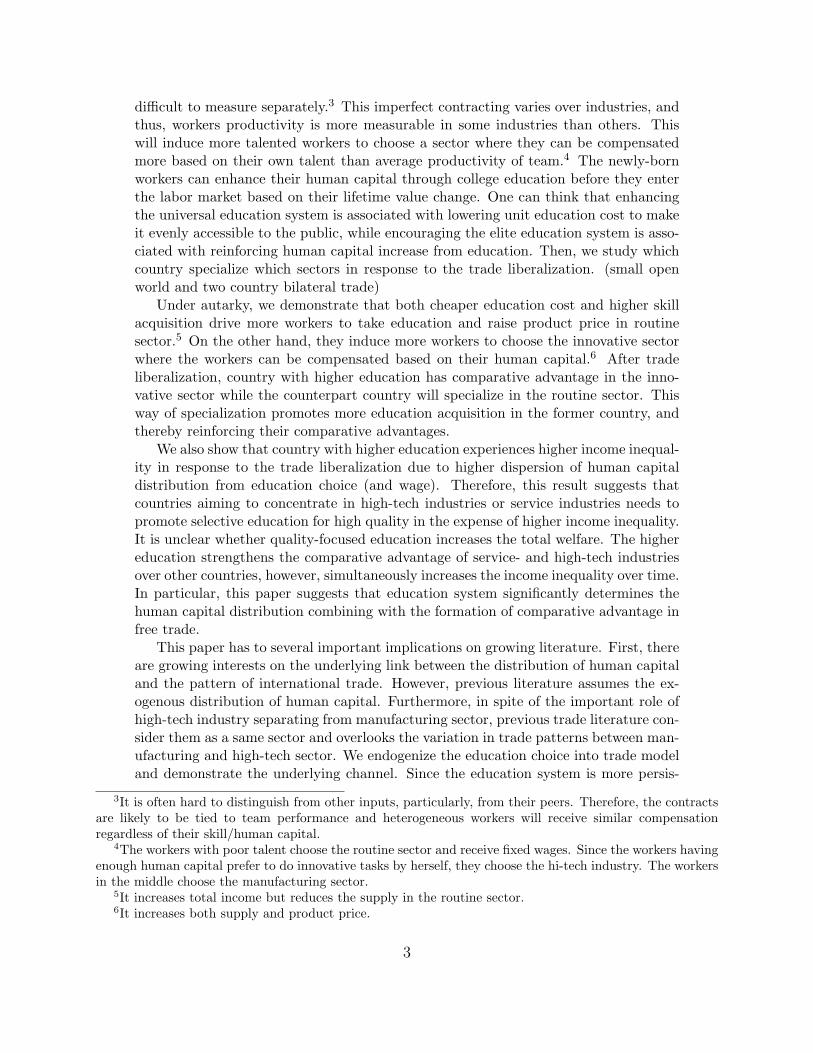
Since it’s trivial, we skip the proof of Proposition 1. Instead, [Figure 2] presentssome interesting properties of the equilibrium. Panel (a) in [Figure 2] shows that E(a)is flat if a ∈ [a, ax], convexly increasing otherwise. The workers with a < ax work inthe traditional sector, the workers with a ∈ [ax, az) in the manufacturing sector, andthe workers with a > az in the high-tech sector. Panel (b) in [Figure 2] depicts theeducation choice by each type. The value differentials E(a + λ) − E(a) is convexlyincreasing and the education choice function itself has a logit formula. As a result,the schooling decision is strictly increasing in a. It is flat for a ∈ [a, ax − λ] becausegetting the advanced education does not affect their occupation choice. Panel (c) and(d) depict the loci of the human capital inputs by and wage payment for each type.
9
The fact that the wages convexly rise accounts for the emergence of ‘superstars’ as inRosen (1981) in the high-tech sector.
Proposition 2 e(·) is strictly increasing in a, as long as a > ax − λ.
Proposition 2 points out ‘self-selection’ in schooling decision as in Roy (1951)and Willis and Rosen (1979). It implies that the workers with higher innate abilitiesare more likely to get the advanced education. It is caused by the convexity of thelifetime value and human capital inputs. As a result, the income inequality worsen.In particular, the country with a well-developed elite education system characterizedby a high λ may suffer from ‘polarization’.
We consider a shock that alter the country-specific ethnical composition such aschanges in immigration policy or trade policy. A positive shock on ethnical diversitymay increase δ the coefficient for the cost function in the manufacturing sector. Thediversity can reduce the team work due to barriers as such in language and culture.
4 Empirical Evidences
4.1 Data Sources
4.1.1 Education Measures
The Times Higher Education World University Ranking is founded in the UnitedKingdom in 2010 and widely regarded as one of the most influential and frequentlyobserved university measures. We extract the list of top universities in 2011-2017 fromthe website and use it for constructing variables, timesnum, the number of universitiesin each country among the top 400, averaged in 2012 and 2013.7
The Center for World University Rankings (CWUR) is founded in Saudi Arabia in2012 and publishes the global university ranking that measures the quality of educationand training of students as well as the prestige of the faculty members and the qualityof their research without relying on surveys and university data submissions. Weextract the list of top universities in 2012-2016 and use it for constructing a variable,cwurnum, the number of universities in each country among the top 100, averaged in2012 and 2013.8
We also construct dummy variables, timesdum and cuwrdum, which equal 1 if thecountry has any university listed among top 400 and top 100, respectively. Table 2shows the list of countries with university rankings in the data.
7http://www.cwur.org/8https://www.timeshighereducation.com/world-university-rankings/2017/world-
ranking#!/page/0/length/25/sort by/rank/sort order/asc/cols/stats/
10
4.1.2 World Development Indicators
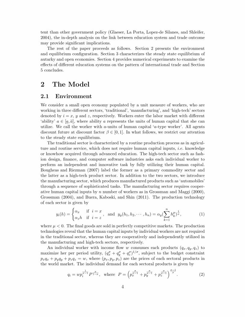
World Development Indicators (WDI) is the primary World Bank collection of develop-ment indicators, compiled from officially recognized international sources. It presentsthe most current and accurate global development data available, and includes na-tional, regional and global estimates. We extract imports and exports data in variouscategories and use them as dependent variables. We take agricultural & raw ma-terials exports (Agri&Raw), food exports (Food), manufacture exports (Manu), andhigh-technology exports (Hi-Tech) from this dataset, all in current US$, and constructhigh-tech industry specialization measures, Hi/Agri, Hi/Food, and Hi/Manu, each de-fined as the ratio of high-technology exports to agricultural & raw materials exports,the ratio of high-technology exports to food exports, and the ratio of high-technologyexports to manufacture exports, respectively. The size of the economy is controlledusing goods and services exports for all export variables. Figure 3 shows the countries’high-tech exports, agricultural raw material exports, and food exports. We can seethat there is a negative tendency between high-technology exports and non-high-techexports, especially agricultural & raw materials exports and food exports. Figure 4shows positive relationship between high-technology exports and high-tech industryspecialization measures.
4.1.3 Penn World Table 9.0
Population, real GDP per capita, and trade openness are drawn from a single source,Penn World Table version 9.0, which is constructed by Robert Summers and AlanHeston of the University of Pennsylvania, together with Irving Kravis and currentlymaintaied by scholars at the University of California, Davis and the Groningen GrowthDevelopment Centre of the University of Groningen. In addition to this dataset, weadded oecd dummy variable and regional dummy variables.
From the above data soures we construct a noble dataset, and its summary statisticsare reported in Table 1, and the list of countries with university rankings in the datais reported in Table 2.
4.2 Empirical Results
4.2.1 Education System and High-Tech Specialization
Our theory suggests that elite education system and high-tech industries specializationare positively related. We conduct cross-country analysis using the noble datasetto see this relationship. We run regressions using high-technology exports (Hi-Tech)and high-tech industry specialization measures, Hi/Agri, Hi/Food, and Hi/Manu, asdependent variables, and the regression results are reported in Table 3. Each country’seconomy size is controlled using goods and services exports for all export variables.We take education measures, real GDP per capita, population, and trade openness asexplanatory variables. OECD dummy is included in odd-number columns, and regionaldummies are included in even-number columns. We consider two education measures:
11
Top100 Dummy and Top400 Number. We take Top100 Dummy as an indicator of eliteeducation system. If a country has at least one university in the top 100 university list,then we assume that this country has an elite education system. On the contrary, ifa country does not have any university in the top 100 university list, then we assumethat this country does not have an elite education system. We take Top400 Number asa measure of universal education system. If a country has many universities in the top400 university list, then we assume that this country’s universal education is strong.Our measures allow a country to have both strong elite education (positive coefficientson Top100 Dummy) and strong universal education (positive coefficients on Top400Number) or to have both weak elite education (negative coefficients on Top100 Dummy)and weak universal education (negative coefficients on Top400 Number). However, inour theory, countries specialize on either elite education or universal education, and weexpect that countries would show either a combination of positive coefficients on Top100Dummy and negative coefficients on Top400 Number or a combination of negativecoefficients on Top100 Dummy and positive coefficients on Top400 Number. Especially,if a country specializes on high-technology industries, then this country is expectedto have high high-technology exports, positive coefficients on Top100 Dummy, andnegative coefficients on Top400 Number, and this is supported by our results in Table 3.All coefficients on Top100 Dummy are positive and very significant, and all coefficientson Top400 Number are negative. In addition, our results show that coefficients on realGDP per capita are all positive across specifications, that coefficients on populationare all negative across specifications, and that coefficients on trade openness are allpositive and significant across specifications. Note that coefficients on Top400 Numberin colomn (3) and (4) are less significant than those in the other specifications. Weexplain that a country’s climate environment and natural resources play a big role inexplaining agriculture & raw material exports, along with its education system. Inother words, even if a country specializes on high-technology industry, this country’sagriculture & raw material exports would be high if this country has a good climateenvironment for farming and rich natural resources. Also, note that coefficients onTop400 Number in colomn (7) and (8) are less significant than those in the otherspecifications. This can be explained by the fact that high-tech industries tend to haveconnections with manufactural industries in most countries.
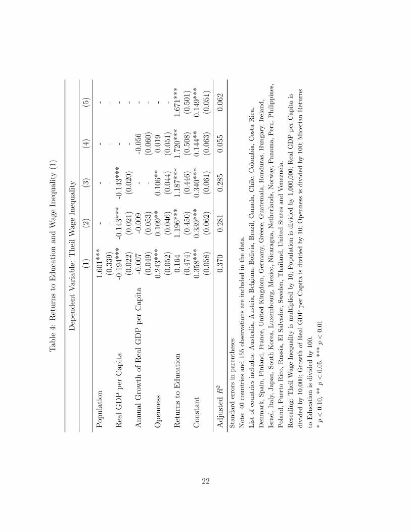
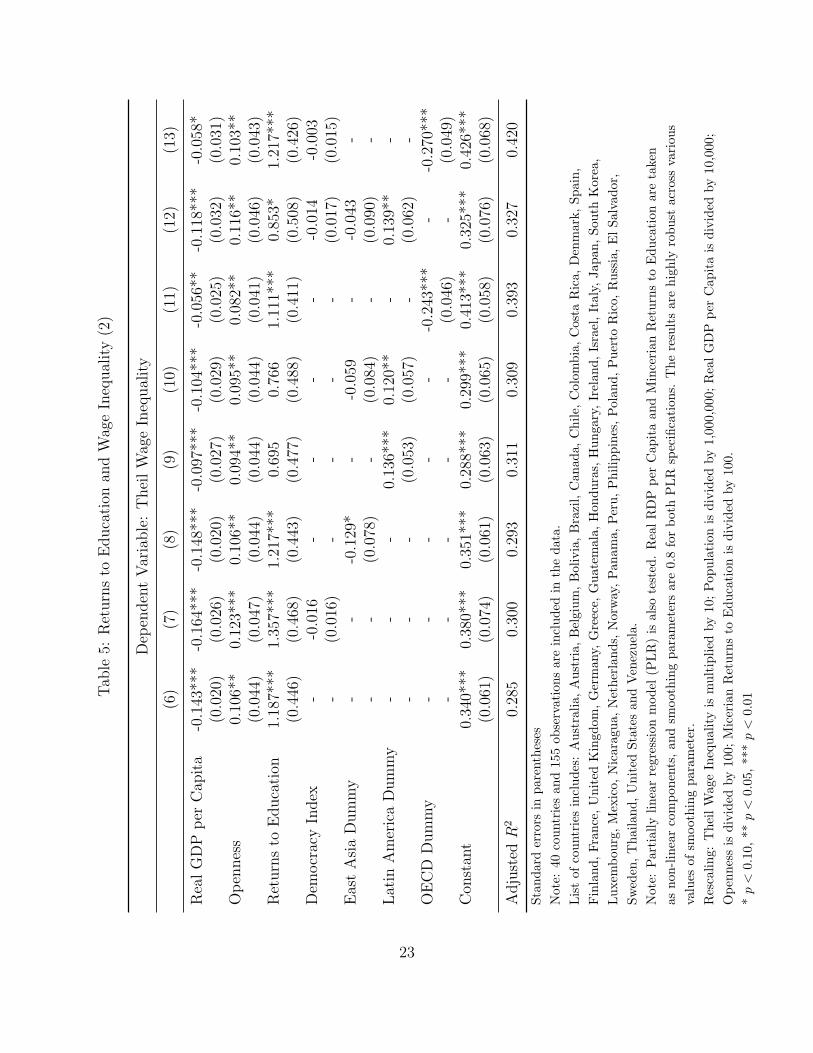
4.2.2 Returns to Education and Wage Inequality
Our theory suggests that, as a country adopts elite education system, returns toeducation increses, and it causes higher wage inequality. We study this relationshipwith cross-country panel regressions. Table 4 and Table 5 are drawn from Lee (2017),and they show strong and positive relationship between returns to education and wageinequality.9 Also, note that coefficients on trade openness are positive and significantin both tables. The empirical results are robust across specifications, and they supportour theoretical outcome that country with higher education experiences higher wage
9The Theil measure of wage inequality is used in the regressions, and it is given by the following formula:
T = 1n
∑ni=1
(Yi
Y
)ln(
Yi
Y
), where n is the number of all earners in the country, Yi is the wage of individual
i, is the mean wage of the population in the country.
12
inequality in response to the trade liberalization due to higher dispersion of humancapital distribution from education choice and wage.
5 Conclusion
We study how education system impacts endogenous formation of human capital, tradepatterns and income inequality. We construct the model of education choice withmodifying three-sector occupation choice model by Grossman and Maggi (2000). Overthe countries, education systems are characterized by education cost and eciency ofeducation. We presume universal education system lowers unit education cost to makeit evenly accessible to the public, while elite education system eectively reinforceshuman capital increase. Upon trade liberalization from autarky state, country withhigher human capital has comparative advantage in the innovative sector while theother country specializes in the routine sector, with obtaining xed and lower returns.This specialization pattern promotes more education acquisition in the former countryin expense of higher income inequality.
We also provide empirical evidence supporting our theory that countries with eliteeducation system heavily specialize on high-tech industry while countries with uni-versal education system specialize on non-high-tech industries such as agricultural &raw material production, food production, or manufactures. We construct educationmeasures and industry specialization measures for 270 countries using publically avail-able university ranking data and World Development Indicators provided by WorldBank. We conduct cross-country regression analysis to examine the theory, and theresults confirm that elite education system and high-tech industries specialization arepositively related and that higher reterns to education, which is delivered by elite ed-ucation system, leads to higher wage inequality controlling population, real GDP percapita, and trade openness. The empirical results are consistent and robust acrossspecifications.
13
References
Bougheas, S., and R. Riezman (2007): “Trade and the distribution of humancapital,” Journal of International Economics, 73(2), 421–433. 4
Buera, F. J., J. P. Kaboski, and Y. Shin (2011): “Finance and Development: ATale of Two Sectors,” The American Economic Review, 101(5), 1964–2002. 4
Glaeser, E. L., R. La Porta, F. Lopez-de Silanes, and A. Shleifer (2004):“Do Institutions Cause Growth?,” Journal of Economic Growth, 9(3), 271–303. 4
Grossman, G. M. (2004): “The Distribution of Talent and the Pattern and Conse-quences of International Trade,” Journal of Political Economy, 112(1), pp. 209–239.4, 5
Grossman, G. M., and G. Maggi (2000): “Diversity and Trade,” The AmericanEconomic Review, 90(5), 1255–1275. 2, 4, 7
Kremer, M. (1993): “The O-Ring Theory of Economic Development,” The QuarterlyJournal of Economics, 108(3), 551–575. 7
Lee, S. (2017): “Macroeconomic Conditions and Wage Inequality: Expanding andAnalyzing the Worldwide Dataset,” Working Paper. 12
Rosen, S. (1981): “The Economics of Superstars,” The American Economic Review,71(5), pp. 845–858. 10
Roy, A. D. (1951): “Some Thoughts on the Distribution of Earnings,” Oxford Eco-nomic Papers, 3(2), 135–146. 10
Willis, R. J., and S. Rosen (1979): “Education and Self-Selection,” Journal ofPolitical Economy, 87(5), S7–36. 10
14

Appendices
A Mathematical Appendix
Proof of Lemma 1 The first order condition of the contracting solution implies that
n−1pyαy(n∑
k=1
n−1hµk)1µ−1
(hy(a;h−j))µ−1P−1 = (hy(a;h−j))
ξ−1a−ξ
Suppose to the contrary that there exist a pair of (a, a′) such that a > a′ buthy(a;h−j) ≤ hy(a
′;h−j). Since µ < 0 and
n−1pyαy
((hy(a;h−j))µ∑n
k=1 n−1hµk
)1− 1µP−1 ≥ n−1pyαy
((hy(a′;h−j))µ∑n
k=1 n−1hµk
)1− 1µP−1
= (hy(a′;h−j))
ξ−1(a′)−ξ > (hy(a;h−j))ξ−1a−ξ,
hy(a;h−j) cannot be the solution of the first order condition. Therefore, if a > a′ thenhy(a;h−j) > hy(a
′;h−j). Again, let a > a′. Then,
uy(a′;h−j) = wj
y(h(a′);h−j)− c(h(a′); a′) < wj
y(h(a′);h−j)− c(h(a′); a)
≤ wjy(h(a);h−j)− c(h(a); a) = uy(a;h−j).
The second strict inequality follows from the property of the cost function and thethird inequality follows from the optimality. It completes the proof.
Proof of Lemma 2 Suppose to the contrary that there exists a team composedof (a1, a2, · · · , an) with max{a1, a2, · · · , an} > min{a1, a2, · · · , an}. Without loss ofgenerality, let a1 = max{a1, a2, · · · , an} and an = min{a1, a2, · · · , an}. Also denote byh′
−j the vector of the human capital inputs by the members of the team except the j-the worker. The stability condition dictates that no a1-type workers can receive strictlymore than uy(hy(a1;h
′−1);h
′−1) on the equilibrium. Since it is feasible to a1-type, an-
other a1-type worker from the outside can substitute the n-th worker. Then, given h′−n,
hy(a1;h′−n) > hy(an;h
′−n) and also all other members put more human capital in the
new formation, which increases further the human capital inputs by the new member.Denote by h′′
−j the new input vector by all other members except the j-th workerin the new team. Apparently, 0 < wy(hy(a1;h
′−1);h
′−1) < wy(hy(a1;h
′′−n);h
′′−n),
which contradicts the stability of other teams with a1-type workers. Therefore, onequilibrium, max{a1, a2, · · · , an} = min{a1, a2, · · · , an} in any teams of the manufac-turing industry.
Proof of Lemma 3 Suppose to the contrary that pz/py ≤ n−1(αy/αz). It impliesthat for any a ∈ [a, a],
uz(a)− uy(a) = (1− ξ−1)(a/P )ξ
ξ−1[(pzαz)
ξξ−1 − (n−1pyαy)
ξξ−1
]− pzαzh/P
= (1− ξ−1)(pyαza/P )ξ
ξ−1[(pz/py)
ξξ−1 − (n−1αy/αz)
ξξ−1
]− pzαzh/P
15
< 0.
The last strict inequality always holds as ξ > 1. Thus, no worker works in sector z,which is contradiction.
Proof of Lemma 4
(i) If a > az, uz(a)−max{ux(a), uy(a)} > uz(az)−max{ux(az), uy(az)} = 0.
(ii) First, suppose that max{ux(az), uy(az)} = ux(az). When a < az, ux(a) =ux(az) = max{ux(az), uy(az)} = uz(az) > uz(a). Suppose that max{ux(az), uy(az)} =uy(az). Then, uy(a) − uz(a) > uy(az) − uz(az) = 0. In any case, uz(a) <max{ux(a), uy(a)}.
Proof of Lemma 5
(i) Pick an arbitrary a(< ax). No matter which one is larger, max{uy(a), uz(a)}can be expressed as A(a)a − B(a), where A(a) > 0 and B(a) > 0. Then,ax ≤ A−1(a)(pxαx + B(a)). a < ax ≤ A−1(a)(pxαx + B(a)), which impliesthat ux(a) = pxαx > A(a)a−B(a) = max{uy(a), uz(a)}.
(ii) Pick an arbitrary a(> ax). Let max{uy(ax), uz(ax)} = A(ax)ax − B(ax), whereA(ax) > 0 and B(ax) > 0. Then, ax = A−1(ax)(pxαx + B(ax)). Since a > axand ux(a) = ux(ax) = pxαx, we get ux(a) = pxαx = A(ax)ax − B(ax) <A(ax)a−B(ax) ≤ max{uy(a), uz(a)}.
Proof of Proposition 2
E(a+ λ)− E(a) = (1− β(1− ρ))−1×
0 if a ∈ [a, ax − λ)
(1− ξ−1)(pyαy(a+ λ)/(nP ))ξ
ξ−1 − pxαx/P if a ∈ [ax − λ, ax)
(1− ξ−1)(pyαy/(nP ))ξ
ξ−1[(a+ λ)
ξξ−1 − a
ξξ−1
]if a ∈ [ax, az − λ)
(1− ξ−1)[(pzαz(a+ λ)/P )
ξξ−1 − (pyαya/(nP ))
ξξ−1
]− pzαz/P if a ∈ [az − λ, az)
(1− ξ−1)(pzαz/P )ξ
ξ−1[(a+ λ)
ξξ−1 − a
ξξ−1
]otherwise
Together with the definition of (ax, az), it implies that E(a+ λ)− E(a) is strictly in-creasing in a as long as a > ax−λ. Therefore e(·) is also strictly increasing in a. Q.E.D.
16
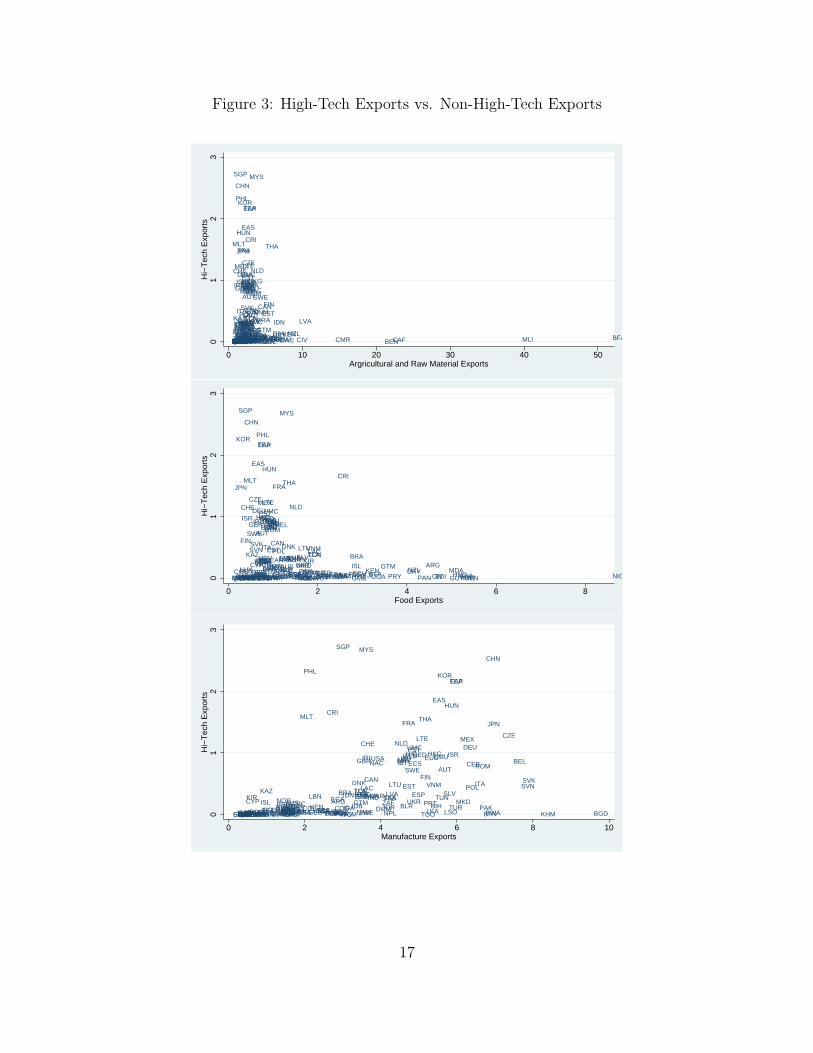
Figure 3: High-Tech Exports vs. Non-High-Tech Exports
ABWALB
ARG
ARMATG
AUS
AUT
AZE BDI
BEL
BENBFABGD
BGR
BHRBHSBIHBLR
BOL
BRA
BRBBTNBWA CAF
CAN
CEB
CHE
CHL
CHN
CIV CMRCOGCOL
COMCPV
CRI
CSS
CYP
CZE
DEU
DMA
DNK
DOMDZA
EAP
EAR
EAS
ECA
ECS
ECUEGY
EMU
ESPEST
EUU
FIN
FJI
FRA
GBR
GEO GHAGMB
GRC GTM
GUY
HICHKG
HND HPC
HRV
HUN
IBDIBT
IDAIDB
IDN
IDX
IND
IRL
IRNISL
ISR
ITA
JAMJOR
JPN
KAZ
KENKGZKHM
KIR
KNA
KOR
LACLBN
LCN
LKA
LMC
LMY
LSO
LTE
LTU
LUX
LVA
MAC
MAR
MDAMDG
MEX
MIC
MKD
MLI
MLT
MNA MOZMUSMWI
MYS
NAC
NAMNERNGANIC
NLD
NOR
NPLNZL
OED
OMNOSSPAK
PANPER
PHL
POL
PRT
PRYPSS
PST
QAT
ROM
RUSRWA
SAS
SAUSDNSEN
SGP
SLV
SSASSFSSTSUR
SVKSVN
SWE
TEA
TEC
TGO
THA
TLA
TMNTON
TSA
TSSTTO
TUN
TUR TZAUGA
UKR
UMC
URY
USA
VCTVEN
VNM
VUT
WLD
WSM
ZAF
ZMB ZWE01
23
Hi−
Tec
h E
xpor
ts
0 10 20 30 40 50Argricultural and Raw Material Exports
ABWALB
ARG
ARMATG
AUS
AUT
AZE BDI
BEL
BENBFABGD
BGR
BHR BHSBIH BLR
BOL
BRA
BRBBTNBWACAF
CAN
CEB
CHE
CHL
CHN
CIVCMRCOG COL
COMCPV
CRI
CSS
CYP
CZE
DEU
DMA
DNK
DOMDZA
EAP
EAR
EAS
ECA
ECS
ECUEGY
EMU
ESPEST
EUU
FIN
FJI
FRA
GBR
GEO GHAGMB
GRC GTM
GUY
HICHKG
HNDHPC
HRV
HUN
IBDIBT
IDAIDB
IDN
IDX
IND
IRL
IRNISL
ISR
ITA
JAMJOR
JPN
KAZ
KENKGZKHM
KIR
KNA
KOR
LACLBN
LCN
LKA
LMC
LMY
LSO
LTE
LTU
LUX
LVA
MAC
MAR
MDAMDG
MEX
MIC
MKD
MLI
MLT
MNA MOZMUS MWI
MYS
NAC
NAMNERNGA NIC
NLD
NOR
NPLNZL
OED
OMNOSS PAK
PANPER
PHL
POL
PRT
PRYPSS
PST
QAT
ROM
RUSRWA
SAS
SAUSDN SEN
SGP
SLV
SSASSFSSTSUR
SVKSVN
SWE
TEA
TEC
TGO
THA
TLA
TMN TON
TSA
TSSTTO
TUN
TUR TZA UGA
UKR
UMC
URY
USA
VCTVEN
VNM
VUT
WLD
WSM
ZAF
ZMB ZWE01
23
Hi−
Tec
h E
xpor
ts
0 2 4 6 8Food Exports
ABW ALB
ARG
ARMATG
AUS
AUT
AZEBDI
BEL
BENBFA BGD
BGR
BHR BHSBIHBLR
BOL
BRA
BRBBTNBWACAF
CAN
CEB
CHE
CHL
CHN
CIVCMRCOGCOL
COMCPV
CRI
CSS
CYP
CZE
DEU
DMA
DNK
DOMDZA
EAP
EAR
EAS
ECA
ECS
ECU EGY
EMU
ESPEST
EUU
FIN
FJI
FRA
GBR
GEOGHAGMB
GRC GTM
GUY
HIC HKG
HNDHPC
HRV
HUN
IBDIBT
IDAIDB
IDN
IDX
IND
IRL
IRNISL
ISR
ITA
JAMJOR
JPN
KAZ
KENKGZ KHM
KIR
KNA
KOR
LACLBN
LCN
LKA
LMC
LMY
LSO
LTE
LTU
LUX
LVA
MAC
MAR
MDAMDG
MEX
MIC
MKD
MLI
MLT
MNAMOZ MUSMWI
MYS
NAC
NAMNERNGANIC
NLD
NOR
NPLNZL
OED
OMNOSS PAK
PANPER
PHL
POL
PRT
PRY PSS
PST
QAT
ROM
RUSRWA
SAS
SAUSDN SEN
SGP
SLV
SSASSFSSTSUR
SVKSVN
SWE
TEA
TEC
TGO
THA
TLA
TMNTON
TSA
TSS TTO
TUN
TURTZAUGA
UKR
UMC
URY
USA
VCTVEN
VNM
VUT
WLD
WSM
ZAF
ZMB ZWE01
23
Hi−
Tec
h E
xpor
ts
0 2 4 6 8 10Manufacture Exports
17
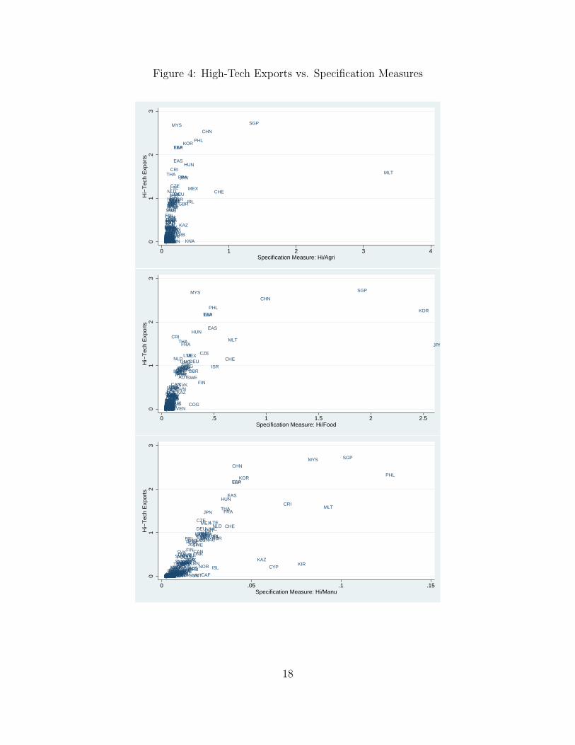
Figure 4: High-Tech Exports vs. Specification Measures
ABWALB
ARG
ARM
AUS
AUT
AZEBDI
BEL
BENBFABGD
BGR
BHRBHSBIHBLRBOL
BRA
BRBBTNBWACAF
CAN
CEB
CHE
CHL
CHN
CIVCMRCOGCOLCOM
CRI
CSS
CYP
CZE
DEU
DMA
DNK
DOMDZA
EAP
EAR
EAS
ECA
ECS
ECUEGY
EMU
ESPEST
EUU
FIN
FJI
FRA
GBR
GEOGHAGMB
GRCGTM
GUY
HICHKG
HNDHPC
HRV
HUN
IBDIBT
IDAIDB
IDN
IDX
IND
IRL
IRNISL
ISR
ITA
JAMJOR
JPN
KAZ
KENKGZKHM
KIR
KNA
KOR
LACLBN
LCN
LKA
LMC
LMY
LSO
LTE
LTU
LUX
LVAMAR
MDAMDG
MEX
MIC
MKD
MLI
MLT
MNAMOZMUSMWI
MYS
NAC
NAMNERNGANIC
NLD
NOR
NPLNZL
OED
OMNOSSPAK
PANPER
PHL
POL
PRT
PRYPSS
PST
QAT
ROM
RUSRWA
SAS
SAUSDNSEN
SGP
SLV
SSASSFSSTSUR
SVKSVN
SWE
TEA
TEC
TGO
THA
TLA
TMNTON
TSA
TSSTTO
TUN
TURTZAUGA
UKR
UMC
URY
USA
VCTVEN
VNM
VUT
WLD
WSM
ZAF
ZMBZWE01
23
Hi−
Tec
h E
xpor
ts
0 1 2 3 4Specification Measure: Hi/Agri
ABWALB
ARG
ARMATG
AUS
AUT
AZEBDI
BEL
BENBFABGD
BGR
BHRBHSBIHBLR
BOL
BRA
BRBBTNBWACAF
CAN
CEB
CHE
CHL
CHN
CIVCMRCOGCOL
COMCPV
CRI
CSS
CYP
CZE
DEU
DMA
DNK
DOMDZA
EAP
EAR
EAS
ECA
ECS
ECUEGY
EMU
ESPEST
EUU
FIN
FJI
FRA
GBR
GEOGHAGMB
GRCGTM
GUY
HICHKG
HNDHPC
HRV
HUN
IBDIBT
IDAIDB
IDN
IDX
IND
IRL
IRNISL
ISR
ITA
JAMJOR
JPN
KAZ
KENKGZKHM
KIR
KNA
KOR
LACLBN
LCN
LKA
LMC
LMY
LSO
LTE
LTU
LUX
LVA
MAC
MAR
MDAMDG
MEX
MIC
MKD
MLI
MLT
MNAMOZMUSMWI
MYS
NAC
NAMNERNGANIC
NLD
NOR
NPLNZL
OED
OMNOSSPAK
PANPER
PHL
POL
PRT
PRYPSS
PST
QAT
ROM
RUSRWA
SAS
SAUSDNSEN
SGP
SLV
SSASSFSSTSUR
SVKSVN
SWE
TEA
TEC
TGO
THA
TLA
TMNTON
TSA
TSSTTO
TUN
TURTZAUGA
UKR
UMC
URY
USA
VCT VEN
VNM
VUT
WLD
WSM
ZAF
ZMBZWE01
23
Hi−
Tec
h E
xpor
ts
0 .5 1 1.5 2 2.5Specification Measure: Hi/Food
ABWALB
ARG
ARMATG
AUS
AUT
AZE BDI
BEL
BENBFABGD
BGR
BHRBHSBIHBLR
BOL
BRA
BRBBTNBWA CAF
CAN
CEB
CHE
CHL
CHN
CIVCMRCOGCOL
COMCPV
CRI
CSS
CYP
CZE
DEU
DMA
DNK
DOMDZA
EAP
EAR
EAS
ECA
ECS
ECUEGY
EMU
ESPEST
EUU
FIN
FJI
FRA
GBR
GEOGHAGMB
GRCGTM
GUY
HICHKG
HNDHPC
HRV
HUN
IBDIBT
IDAIDB
IDN
IDX
IND
IRL
IRNISL
ISR
ITA
JAMJOR
JPN
KAZ
KENKGZKHM
KIR
KNA
KOR
LACLBN
LCN
LKA
LMC
LMY
LSO
LTE
LTU
LUX
LVA
MAC
MAR
MDAMDG
MEX
MIC
MKD
MLI
MLT
MNAMOZMUSMWI
MYS
NAC
NAMNERNGANIC
NLD
NOR
NPLNZL
OED
OMNOSSPAK
PANPER
PHL
POL
PRT
PRYPSS
PST
QAT
ROM
RUSRWA
SAS
SAUSDNSEN
SGP
SLV
SSASSFSSTSUR
SVKSVN
SWE
TEA
TEC
TGO
THA
TLA
TMNTON
TSA
TSSTTO
TUN
TURTZAUGA
UKR
UMC
URY
USA
VCTVEN
VNM
VUT
WLD
WSM
ZAF
ZMBZWE01
23
Hi−
Tec
h E
xpor
ts
0 .05 .1 .15Specification Measure: Hi/Manu
18
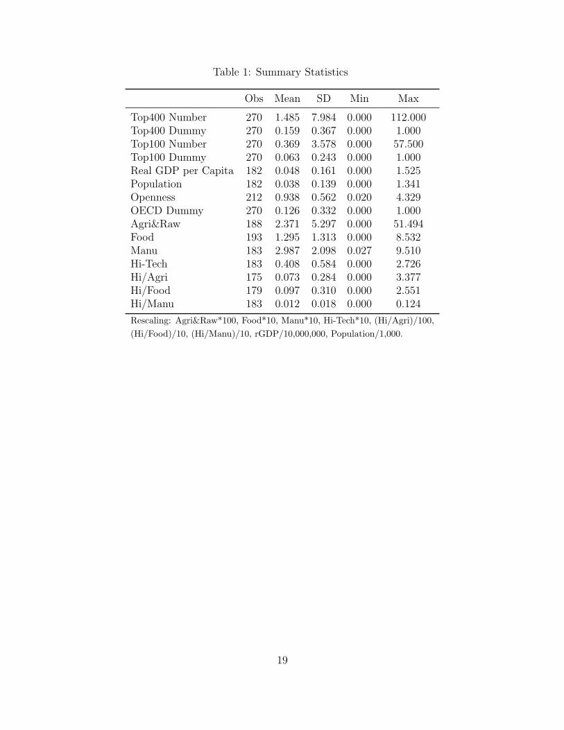
Table 1: Summary Statistics
Obs Mean SD Min Max
Top400 Number 270 1.485 7.984 0.000 112.000Top400 Dummy 270 0.159 0.367 0.000 1.000Top100 Number 270 0.369 3.578 0.000 57.500Top100 Dummy 270 0.063 0.243 0.000 1.000Real GDP per Capita 182 0.048 0.161 0.000 1.525Population 182 0.038 0.139 0.000 1.341Openness 212 0.938 0.562 0.020 4.329OECD Dummy 270 0.126 0.332 0.000 1.000Agri&Raw 188 2.371 5.297 0.000 51.494Food 193 1.295 1.313 0.000 8.532Manu 183 2.987 2.098 0.027 9.510Hi-Tech 183 0.408 0.584 0.000 2.726Hi/Agri 175 0.073 0.284 0.000 3.377Hi/Food 179 0.097 0.310 0.000 2.551Hi/Manu 183 0.012 0.018 0.000 0.124
Rescaling: Agri&Raw*100, Food*10, Manu*10, Hi-Tech*10, (Hi/Agri)/100,
(Hi/Food)/10, (Hi/Manu)/10, rGDP/10,000,000, Population/1,000.
19
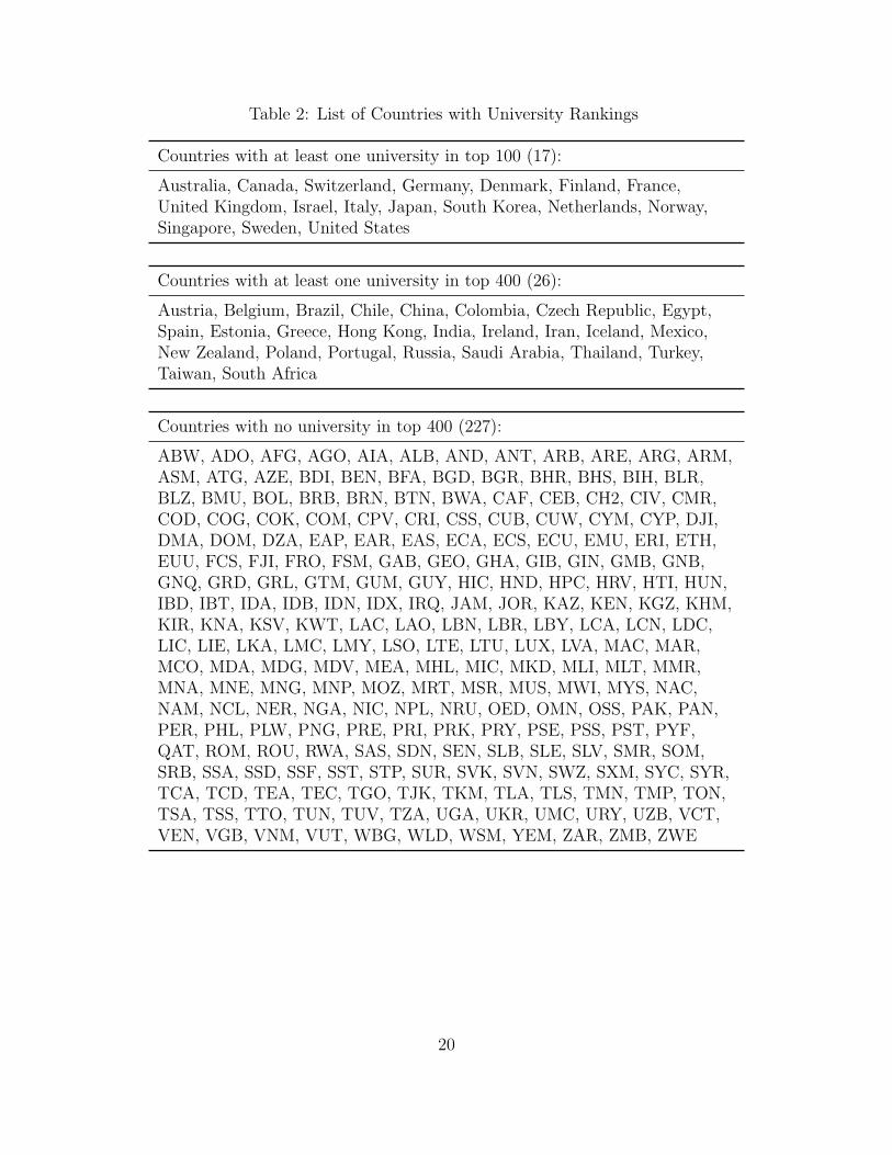
Table 2: List of Countries with University Rankings
Countries with at least one university in top 100 (17):
Australia, Canada, Switzerland, Germany, Denmark, Finland, France,United Kingdom, Israel, Italy, Japan, South Korea, Netherlands, Norway,Singapore, Sweden, United States
Countries with at least one university in top 400 (26):
Austria, Belgium, Brazil, Chile, China, Colombia, Czech Republic, Egypt,Spain, Estonia, Greece, Hong Kong, India, Ireland, Iran, Iceland, Mexico,New Zealand, Poland, Portugal, Russia, Saudi Arabia, Thailand, Turkey,Taiwan, South Africa
Countries with no university in top 400 (227):
ABW, ADO, AFG, AGO, AIA, ALB, AND, ANT, ARB, ARE, ARG, ARM,ASM, ATG, AZE, BDI, BEN, BFA, BGD, BGR, BHR, BHS, BIH, BLR,BLZ, BMU, BOL, BRB, BRN, BTN, BWA, CAF, CEB, CH2, CIV, CMR,COD, COG, COK, COM, CPV, CRI, CSS, CUB, CUW, CYM, CYP, DJI,DMA, DOM, DZA, EAP, EAR, EAS, ECA, ECS, ECU, EMU, ERI, ETH,EUU, FCS, FJI, FRO, FSM, GAB, GEO, GHA, GIB, GIN, GMB, GNB,GNQ, GRD, GRL, GTM, GUM, GUY, HIC, HND, HPC, HRV, HTI, HUN,IBD, IBT, IDA, IDB, IDN, IDX, IRQ, JAM, JOR, KAZ, KEN, KGZ, KHM,KIR, KNA, KSV, KWT, LAC, LAO, LBN, LBR, LBY, LCA, LCN, LDC,LIC, LIE, LKA, LMC, LMY, LSO, LTE, LTU, LUX, LVA, MAC, MAR,MCO, MDA, MDG, MDV, MEA, MHL, MIC, MKD, MLI, MLT, MMR,MNA, MNE, MNG, MNP, MOZ, MRT, MSR, MUS, MWI, MYS, NAC,NAM, NCL, NER, NGA, NIC, NPL, NRU, OED, OMN, OSS, PAK, PAN,PER, PHL, PLW, PNG, PRE, PRI, PRK, PRY, PSE, PSS, PST, PYF,QAT, ROM, ROU, RWA, SAS, SDN, SEN, SLB, SLE, SLV, SMR, SOM,SRB, SSA, SSD, SSF, SST, STP, SUR, SVK, SVN, SWZ, SXM, SYC, SYR,TCA, TCD, TEA, TEC, TGO, TJK, TKM, TLA, TLS, TMN, TMP, TON,TSA, TSS, TTO, TUN, TUV, TZA, UGA, UKR, UMC, URY, UZB, VCT,VEN, VGB, VNM, VUT, WBG, WLD, WSM, YEM, ZAR, ZMB, ZWE
20
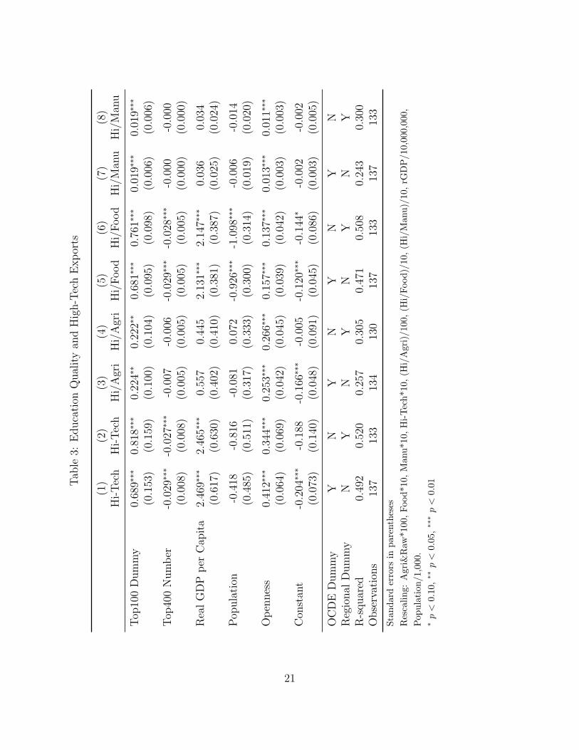
Tab
le3:
Education
Qualityan
dHigh-TechExports
(1)
(2)
(3)
(4)
(5)
(6)
(7)
(8)
Hi-Tech
Hi-Tech
Hi/Agri
Hi/Agri
Hi/Food
Hi/Food
Hi/Man
uHi/Man
u
Top
100Dummy
0.689∗
∗∗0.818∗
∗∗0.224∗
∗0.222∗
∗0.681∗
∗∗0.761∗
∗∗0.019∗
∗∗0.019∗
∗∗
(0.153)
(0.159)
(0.100)
(0.104)
(0.095)
(0.098)
(0.006)
(0.006)
Top
400Number
-0.029
∗∗∗
-0.027
∗∗∗
-0.007
-0.006
-0.029
∗∗∗
-0.028
∗∗∗
-0.000
-0.000
(0.008)
(0.008)
(0.005)
(0.005)
(0.005)
(0.005)
(0.000)
(0.000)
RealGDPper
Cap
ita
2.469∗
∗∗2.465∗
∗∗0.557
0.445
2.131∗
∗∗2.147∗
∗∗0.036
0.034
(0.617)
(0.630)
(0.402)
(0.410)
(0.381)
(0.387)
(0.025)
(0.024)
Pop
ulation
-0.418
-0.816
-0.081
0.072
-0.926
∗∗∗
-1.098
∗∗∗
-0.006
-0.014
(0.485)
(0.511)
(0.317)
(0.333)
(0.300)
(0.314)
(0.019)
(0.020)
Openness
0.412∗
∗∗0.344∗
∗∗0.253∗
∗∗0.266∗
∗∗0.157∗
∗∗0.137∗
∗∗0.013∗
∗∗0.011∗
∗∗
(0.064)
(0.069)
(0.042)
(0.045)
(0.039)
(0.042)
(0.003)
(0.003)
Con
stan
t-0.204
∗∗∗
-0.188
-0.166
∗∗∗
-0.005
-0.120
∗∗∗
-0.144
∗-0.002
-0.002
(0.073)
(0.140)
(0.048)
(0.091)
(0.045)
(0.086)
(0.003)
(0.005)
OCDEDummy
YN
YN
YN
YN
Regional
Dummy
NY
NY
NY
NY
R-squared
0.492
0.520
0.257
0.305
0.471
0.508
0.243
0.300
Observations
137
133
134
130
137
133
137
133
Standarderrors
inparentheses
Rescaling:
Agri&
Raw
*100
,Food*1
0,Man
u*1
0,Hi-Tech*1
0,(H
i/Agri)/1
00,(H
i/Food)/10
,(H
i/Man
u)/10
,rG
DP/1
0,00
0,000,
Pop
ulation
/1,000
.∗p<
0.10
,∗∗
p<
0.05,
∗∗∗p<
0.01
21
Tab
le4:
Returnsto
Education
andWageInequality(1)
Dep
endentVariable:TheilWageInequality
(1)
(2)
(3)
(4)
(5)
Pop
ulation
1.601***
--
--
(0.339)
--
--
RealGDPper
Cap
ita
-0.194***
-0.143***
-0.143***
--
(0.022)
(0.021)
(0.020)
--
Annual
Growth
ofRealGDPper
Cap
ita
-0.007
-0.009
--0.056
-(0.049)
(0.053)
-(0.060)
-Openness
0.243***
0.109**
0.106**
0.019
-(0.052)
(0.046)
(0.044)
(0.051)
-Returnsto
Education
0.164
1.196***
1.187***
1.720***
1.671***
(0.474)
(0.450)
(0.446)
(0.508)
(0.501)
Con
stan
t0.358***
0.339***
0.340***
0.144**
0.149***
(0.058)
(0.062)
(0.061)
(0.063)
(0.051)
Adjusted
R2
0.370
0.281
0.285
0.055
0.062
Standarderrors
inparentheses
Note:
40countriesan
d15
5ob
servationsareincluded
inthedata.
Listof
countriesincludes:Australia,
Austria,
Belgium,Bolivia,Brazil,Can
ada,
Chile,
Colom
bia,Costa
Rica,
Den
mark,Spain,Finland,France,United
Kingd
om,German
y,Greece,
Guatem
ala,
Hon
duras,
Hunga
ry,Irelan
d,
Israel,Italy,
Jap
an,Sou
thKorea,Luxem
bou
rg,Mexico,
Nicarag
ua,
Netherlands,
Norway,Pan
ama,
Peru,Philippines,
Polan
d,Puerto
Rico,
Russia,ElSalvador,Swed
en,Thailand,United
Statesan
dVen
ezuela.
Rescaling:
TheilWag
eInequalityis
multiplied
by10
;Pop
ulation
isdivided
by1,00
0,00
0;RealGDP
per
Cap
itais
divided
by10
,000
;Growth
ofRealGDP
per
Cap
itais
divided
by10
;Open
nessis
divided
by10
0;MicerianReturns
toEducation
isdivided
by10
0.
*p<
0.10
,**
p<
0.05
,**
*p<
0.01
22
Tab
le5:
Returnsto
Education
andWageInequality(2)
Dep
endentVariable:TheilWageInequality
(6)
(7)
(8)
(9)
(10)
(11)
(12)
(13)
RealGDPper
Cap
ita
-0.143***
-0.164***
-0.148***
-0.097***
-0.104***
-0.056**
-0.118***
-0.058*
(0.020)
(0.026)
(0.020)
(0.027)
(0.029)
(0.025)
(0.032)
(0.031)
Openness
0.106**
0.123***
0.106**
0.094**
0.095**
0.082**
0.116**
0.103**
(0.044)
(0.047)
(0.044)
(0.044)
(0.044)
(0.041)
(0.046)
(0.043)
Returnsto
Education
1.187***
1.357***
1.217***
0.695
0.766
1.111***
0.853*
1.217***
(0.446)
(0.468)
(0.443)
(0.477)
(0.488)
(0.411)
(0.508)
(0.426)
Dem
ocracyIndex
--0.016
--
--
-0.014
-0.003
-(0.016)
--
--
(0.017)
(0.015)
EastAsiaDummy
--
-0.129*
--0.059
--0.043
--
-(0.078)
-(0.084)
-(0.090)
-Latin
AmericaDummy
--
-0.136***
0.120**
-0.139**
--
--
(0.053)
(0.057)
-(0.062)
-OECD
Dummy
--
--
--0.243***
--0.270***
--
--
-(0.046)
-(0.049)
Con
stan
t0.340***
0.380***
0.351***
0.288***
0.299***
0.413***
0.325***
0.426***
(0.061)
(0.074)
(0.061)
(0.063)
(0.065)
(0.058)
(0.076)
(0.068)
Adjusted
R2
0.285
0.300
0.293
0.311
0.309
0.393
0.327
0.420
Standarderrors
inparentheses
Note:
40countriesan
d15
5ob
servationsareincluded
inthedata.
Listof
countriesincludes:Australia,
Austria,
Belgium,Bolivia,Brazil,Can
ada,
Chile,
Colom
bia,Costa
Rica,
Den
mark,Spain,
Finland,France,United
Kingd
om,German
y,Greece,
Guatem
ala,
Hon
duras,
Hunga
ry,Irelan
d,Israel,Italy,
Jap
an,Sou
thKorea,
Luxem
bou
rg,Mexico,
Nicarag
ua,
Netherlands,
Norway,Pan
ama,
Peru,Philippines,Polan
d,Puerto
Rico,
Russia,ElSalvador,
Sweden,Thailand,United
Statesan
dVen
ezuela.
Note:
Partially
linearregression
model
(PLR)is
also
tested
.RealRDP
per
Cap
itaan
dMincerian
Returnsto
Education
aretaken
asnon
-linearcompon
ents,an
dsm
oothingparam
etersare0.8forbothPLR
specification
s.Theresultsarehighly
robust
across
variou
s
values
ofsm
oothingparam
eter.
Rescaling:
TheilWag
eInequalityis
multiplied
by10
;Pop
ulation
isdivided
by1,00
0,00
0;RealGDP
per
Cap
itais
divided
by10,000;
Opennessis
divided
by10
0;MicerianReturnsto
Education
isdivided
by10
0.
*p<
0.10,**
p<
0.05
,**
*p<
0.01
23