Embed Size (px)
Citation preview
NBER WORKING PAPER SERIES
COLLEGE AS COUNTRY CLUB:DO COLLEGES CATER TO STUDENTS’ PREFERENCES FOR CONSUMPTION?
Brian JacobBrian McCall
Kevin M. Stange
Working Paper 18745http://www.nber.org/papers/w18745
NATIONAL BUREAU OF ECONOMIC RESEARCH1050 Massachusetts Avenue
Cambridge, MA 02138January 2013
We would like to thank Jon Bartik, Michael Gelman, Jonathan Hershaff, Max Kapustin, Geoff Perrin,Nathan Schwartz, Elias Walsh, and Tamara Wilder for their research assistance. We would also liketo recognize the valuable comments and suggestions provided by various seminar and conference participants.We also thank Bridget Terry Long for sharing her data. The views expressed herein are those of theauthors and do not necessarily reflect the views of the National Bureau of Economic Research.
NBER working papers are circulated for discussion and comment purposes. They have not been peer-reviewed or been subject to the review by the NBER Board of Directors that accompanies officialNBER publications.
© 2013 by Brian Jacob, Brian McCall, and Kevin M. Stange. All rights reserved. Short sections oftext, not to exceed two paragraphs, may be quoted without explicit permission provided that full credit,including © notice, is given to the source.
College as Country Club: Do Colleges Cater to Students’ Preferences for Consumption?Brian Jacob, Brian McCall, and Kevin M. StangeNBER Working Paper No. 18745January 2013JEL No. I20,I21,I23,J01,J18
ABSTRACT
This paper investigates whether demand-side market pressure explains colleges’ decisions to provideconsumption amenities to their students. We estimate a discrete choice model of college demand usingmicro data from the high school classes of 1992 and 2004, matched to extensive information on allfour-year colleges in the U.S. We find that most students do appear to value college consumption amenities,including spending on student activities, sports, and dormitories. While this taste for amenities is broad-based,the taste for academic quality is confined to high-achieving students. The heterogeneity in studentpreferences implies that colleges face very different incentives depending on their current student bodyand the students who the institution hopes to attract. We estimate that the elasticities implied by ourdemand model can account for 16 percent of the total variation across colleges in the ratio of amenityto academic spending, and including them on top of key observable characteristics (sector, state, size,selectivity) increases the explained variation by twenty percent.
Brian JacobGerald R. Ford School of Public PolicyUniversity of Michigan735 South State StreetAnn Arbor, MI 48109and [email protected]
Brian McCall2108B School of EducationUniversity of Michigan610 East University Ave.Ann Arbor MI [email protected]
Kevin M. StangeUniversity of MichiganFord School of Public Policy5236 Weill Hall735 S. State StreetAnn Arbor, MI 48109-3091 [email protected]
“Share of College Spending for Recreation is Rising” (New York Times 2010). “Colleges’ new rec centers lure students.” (Columbus Dispatch 2011)
“Resort Living Comes to College.” (Wall Street Journal 2012).
I. Introduction
In line with the human capital framework developed by Becker (1964), economists
typically model education as an investment wherein individuals forgo current labor market
earnings and incur direct costs in return for higher future wages. While this framework does not
rule out that education may also provide immediate consumption, such consumption aspects
have received little attention in the literature.1 Recently, however, there has been increasing
attention devoted to the recreation that accompanies investment in higher education, as
illustrated by the newspaper headlines above.2 The media attention coincides with an
accumulation of evidence on limited student learning (Arum and Roksa, 2011), diminished study
effort (Babcock and Marks, 2011), and declining graduation rates (Bound, Lovenhiem, and
Turner, 2010).
While the evidence on whether colleges today devote a greater share of resources to
consumption and recreational amenities than they have in the past is inconclusive, it is clear that
there is substantial heterogeneity in the emphasis that institutions place on amenities (Jacob,
McCall and Stange 2013a).3 In 2007, for example, the average ratio of amenity to academic
spending was 0.51 across the roughly 1,300 four-year public and private non-profit
1 Exceptions include Schultz (1963) and Oreopoulos and Salvanes (2011). Some related literature describes the benefits that education confers on subsequent household production as a “consumption aspect” of education in the sense that it increases the efficiency of future consumption (see Michaels 1973). These benefits of education would not count as consumption value in our framework as they accrue post-schooling. 2 The focus on recreation is not new, as suggested by Tunis (1939, p.7): “Boys and girls and their parents too often choose an educational institution for strange reasons: because it has lots of outdoor life; a good football team; a lovely campus; because the president or the dean or some professor is such a nice man.” 3 Throughout this paper, we use institutional spending in areas such as instruction, academic support, student services and auxiliary services as proxies for the academic and consumption amenities offered by institutions. While it is not obvious ex-ante that the spending measures we use are good proxies for “consumption” vs. “academic” amenities, Section V presents several different pieces of evidence to support this assumption.
2
postsecondary institutions in the United States. The ratio varied tremendously, from .26 at the
10th percentile to .80 at the 90th percentile. Thus different institutions make very different choices
about the optimal level of consumption amenities to offer their students. While there are several
systematic patterns to this heterogeneity – for instance, public institutions spend relatively less
on consumption amenities– the sources of these patterns have not been previously explored.
This paper investigates whether this spending variation is attributable to heterogeneity in
the demand-side pressure institutions face. Some observers have argued that increased market
pressure has compelled some colleges to cater to students’ desires for leisure (Kirp 2005),
possibly distracting students from college’s primary mission of education. To investigate this,
we estimate the demand consequences of each institution’s spending decisions and examine how
this demand-side pressure correlates with colleges’ provision of consumption amenities. Do
institutions that face a greater enrollment response to changes in consumption amenities devote
more of their resources to this attribute, as a simple revenue-maximizing model would predict?
Institution-specific demand elasticities come from simulations of an estimated discrete
choice model of student demand where students care about net price, academic quality,
consumption amenities, proximity, and peer composition. This approach is in the spirit of the
standard differentiated product demand models used to study product demand (e.g. Berry,
Levinsohn, Pakes, 1995), residential choice (e.g. Bayer, Ferreira, McMillan, 2007), and school
choice (e.g. Hastings, Kane, and Staiger, 2009), among others. Student preference parameters are
inferred from observed college choices, where each college is a bundle of observed and
unobserved characteristics.
We find that many students do appear to value college consumption amenities. More
importantly, we find significant heterogeneity of preferences across students, with higher
3
achieving students having a greater willingness-to-pay for academic quality than their less
academically-oriented peers and wealthier students much more willing to pay for consumption
amenities. This demand pattern holds after accounting for several shortcomings in much of the
prior work on college choice. Specifically, our estimation accounts for (i) unobserved choice set
variability created by selective admissions, (ii) fixed unobserved differences between schools,
(iii) price discounting, and (iv) preference heterogeneity, which permits more flexible
substitution patterns across institutions.
Preference heterogeneity has important implications for the postsecondary market since it
results in different colleges facing very different resource allocation incentives depending on the
characteristics of students on their enrollment margin. More selective schools have a much
greater incentive to improve academic quality since this is the dimension most valued by their
marginal students. Less selective (but expensive) schools, by comparison, have a greater
incentive to focus on consumption amenities. The elasticities implied by our demand model can
account for sixteen percent of the total variation in the ratio of amenity to instructional spending
between colleges, and including them on top of key observable characteristics (sector, state, size,
selectivity) increases the explained variation by twenty percent. While the development and
estimation of a full general equilibrium model of postsecondary supply and demand is beyond
the scope of this paper, we conclude that higher education institutions do respond to the demand
pressure they face along this important non-price dimension.
The importance of market pressure to the behavior of higher education institutions has
not been thoroughly examined. Our analysis is in the spirit of Hoxby (1997), who shows that
changes in the level of competition in the U.S. higher education market explain changes in
tuition and quality. This analysis, along with most of the rest of the literature, focuses on the role
4
of academic quality and cost, while we examine another dimension on which colleges compete.
Our demand model also expands the range of college characteristics examined in college choice
models, demonstrating that consumption amenities are an empirically important factor
determining the sorting of students to colleges and thus deserve more attention.
Characterizing the incentive differences across colleges is a first step towards
understanding how student preferences may influence the functioning of the postsecondary
market. One important implication is that for many institutions, demand-side market pressure
may not compel investment in academic quality, but rather in consumption amenities. This is an
important finding given that quality assurance is primarily provided by demand-side pressure:
the fear of losing students is believed to compel colleges to provide high levels of academic
quality. Our findings call this accountability mechanism into question. A parallel finding has
started to emerge in the hospital market, where patient amenities are a much stronger driver of
hospital demand than clinical quality (Goldman and Romley, 2008, Goldman, Vaiana, Romley,
2010). However, our findings do not speak to the normative issue of whether consumption
amenities are good or bad for students and taxpayers.4
The remainder of the paper proceeds as follows. The next section reviews prior work on
the higher education market and on the consumption value of education. Section III presents a
simple model of college’s amenity decisions as related to demand pressure and describes how
differences in demand pressure across institutions stems from student preference heterogeneity.
Section IV introduces our empirical strategy and elaborates on the identification challenges. Our
data sources are discussed in Section V. The estimates of our choice model are presented in
4 Spending on consumption amenities could actually have a positive impact on student outcomes (Webber and Ehrenberg, 2010). There is also a vast literature that finds substantial returns to academic quality (Black and Smith, 2004; Hoekstra 2009), though none of these studies have attempted to separate the returns to academic quality from the returns to consumption amenities, though these college attributes are positively correlated.
5
Section VI. Section VII uses the choice model to characterize the demand-side pressure faced by
colleges and its relation to colleges’ spending priorities. Section VIII concludes.
II. Prior literature
Despite the vast literature on the returns to education and college choice, there has been
relatively little analysis of the market for higher education. In the seminal model of the higher
education market, Rothschild and White (1993, 1995) stress complementarities between
students’ academic aptitude and colleges’ academic resources. Their key finding is that
complementarity results in vertical differentiation and efficient sorting of students to colleges.
Hoxby (1997, 2009) describes several important changes in the market structure and shows how
they have affected college price and quality. She demonstrates that the declining cost of air
travel and telecommunications along with the rise of standardized college admissions testing and
subsequent decline in colleges’ informational costs have made the undergraduate market more
competitive. Students are increasingly willing to consider schools outside of their immediate
geographic area or even state. As predicted by economic theory, this has increased the tuition,
subsidies and prices of colleges on average and led to greater between-college variation in
tuition, subsidies and student quality. Epple, Romano and Sieg (2006) develop an equilibrium
model of the market for higher education that incorporates student admissions, financial aid and
educational outcomes. Consistent with Hoxby, their model generates substantial between college
heterogeneity in student outcomes.
While this existing literature demonstrates that colleges do respond to market incentives,
it has primarily focused on price, geographic location, and academic aspects of colleges. The
role of consumption amenities as a competitive dimension in the market has not been previously
6
investigated. We extend the existing models by allowing colleges to attract students with the
choice of different levels of academic versus amenity spending.
The relative lack of attention to the market for higher education stands in contrast to the
larger literature on college choice. Since the seminal work of Manski and Wise (1983), many
empirical models of college choice have focused on estimating the importance of price, academic
quality and distance. For example, Long (2004) estimates a conditional logit model using data
on high school graduates in 1972, 1982 and 1992. She finds that the role of college costs and
distance became less important over this period while proxies for college academic quality such
as instructional expenditures per student became more important over time.5
Only a few studies have explored consumption aspects of college quantitatively. Using a
panel of NCAA Division 1 sports schools, Pope and Pope (2008, 2009) find that football and
basketball success increases the quantity of applications colleges receive and the number of
students sending SAT scores. Since the additional applications come from both high and low
SAT scoring students, colleges are able to increase both the number and quality of incoming
students following sports success. Alter and Reback (2012) find that changes in both academic
and quality-of-life reputations listed in two popular college guidebooks affect the number of
applicants received and the quality and geographic diversity of incoming students.
Another literature attempts to quantify the consumption (and other non-pecuniary) value
of education. This research typically compares observed schooling to the financially optimal
amount or type, concluding that schooling itself must contribute directly to utility if individuals
consume a level or type of schooling that is not financially optimal (Lazear, 1977; Schaafsma,
1976; Kodde and Ritzen, 1984; Oosterbeek and Ophem, 2000; see also a related approach taken
5 Other papers that estimate the willingness to pay for academic quality include McDuff (2007), Monks and Ehrenberg (1999) and Griffith and Rask (2007).
7
by Heckman et al. 1999, Carniero et al. 2003 and Brand and Xie 2010, Alstadsæte, 2011,
Arcidiacono, 2004). Unfortunately, these approaches are not able to separate an individual’s
preference for a particular type of work from consumption value during schooling. The choice to
attend college or pursue a specific major implies a particular career path, which incorporates not
only monetary rewards, but different working conditions and, indeed, a different “type” of work
that may provide different direct utility to individuals. In this way, these studies differ
substantially from this paper in focus and approach.6
III. A Simple Model of College Expenditures by Type
To illustrate how demand pressure may influence institutions’ amenity decisions, we
develop a simple model of college resource allocation. Let there be j =1 ,…, J colleges and i =
1,2, …, N college students. For simplicity we will assume that there are two (non-price) college
attributes: academic quality A and consumption amenities C. Colleges have a price equal to T.
For simplicity we will also assume that students are characterized by two characteristics
(preferences) for colleges denoted by α and γ along with their income I where α is a student’s
preference for academic quality and γ their preference for consumption amenities. Also denote
the preference parameter for income as β. We denote the distribution of these characteristics
across the population of college students by G, so
( , , , )N dG Iβ α γ= ∫ .
Assume that colleges maximize net revenues πj and for simplicity that the only revenues
that they receive are tuition revenues. Also assume for now that everybody pays the same
tuition. Finally assume, perhaps for historical reasons, that colleges have different technologies
(costs) in producing academic quality and consumption amenities. Denote this per student cost
6 Our approach is somewhat related to the approach of Jacob and Lefgren (2007). They find that wealthy parents want teachers that both teach and increase student satisfaction. This latter aspect could be considered “consumption value” in our framework.
8
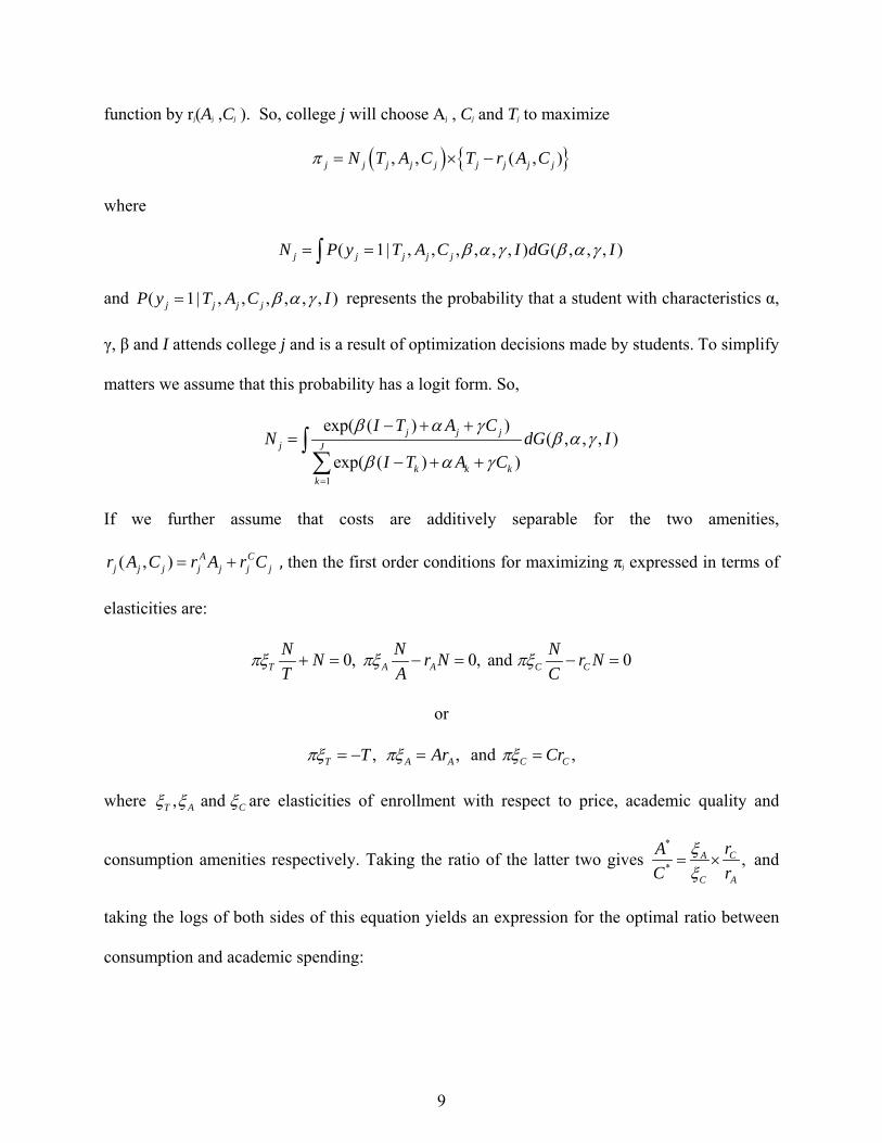
function by rj(Aj ,Cj ). So, college j will choose Aj , Cj and Tj to maximize
( ) { }, , ( , )j j j j j j j j jN T A C T r A Cπ = × −
where
( 1| , , , , , , ) ( , , , )j j j j jN P y T A C I dG Iβ α γ β α γ= =∫
and ( 1| , , , , , , )j j j jP y T A C Iβ α γ= represents the probability that a student with characteristics α,
γ, β and I attends college j and is a result of optimization decisions made by students. To simplify
matters we assume that this probability has a logit form. So,
1
exp( ( ) )( , , , )
exp( ( ) )
j j jj J
k k kk
I T A CN dG I
I T A C
β α γβ α γ
β α γ=
− + +=
− + +∫∑
If we further assume that costs are additively separable for the two amenities,
( , ) A Cj j j j j j jr A C r A r C= + , then the first order conditions for maximizing πj expressed in terms of
elasticities are:
0, 0, and 0T A A C CN N NN r N r NT A C
πξ πξ πξ+ = − = − =
or
,T Tπξ = − ,A AArπξ = and ,C CCrπξ =
where , and T A Cξ ξ ξ are elasticities of enrollment with respect to price, academic quality and
consumption amenities respectively. Taking the ratio of the latter two gives *
* ,CA
C A
rAC r
ξξ
= × and
taking the logs of both sides of this equation yields an expression for the optimal ratio between
consumption and academic spending:
9
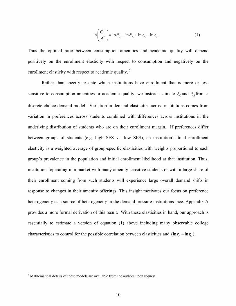
*
*ln ln ln ln lnC A A CC r rA
ξ ξ
= − + −
. (1)
Thus the optimal ratio between consumption amenities and academic quality will depend
positively on the enrollment elasticity with respect to consumption and negatively on the
enrollment elasticity with respect to academic quality. 7
Rather than specify ex-ante which institutions have enrollment that is more or less
sensitive to consumption amenities or academic quality, we instead estimate Cξ and Aξ from a
discrete choice demand model. Variation in demand elasticities across institutions comes from
variation in preferences across students combined with differences across institutions in the
underlying distribution of students who are on their enrollment margin. If preferences differ
between groups of students (e.g. high SES vs. low SES), an institution’s total enrollment
elasticity is a weighted average of group-specific elasticities with weights proportional to each
group’s prevalence in the population and initial enrollment likelihood at that institution. Thus,
institutions operating in a market with many amenity-sensitive students or with a large share of
their enrollment coming from such students will experience large overall demand shifts in
response to changes in their amenity offerings. This insight motivates our focus on preference
heterogeneity as a source of heterogeneity in the demand pressure institutions face. Appendix A
provides a more formal derivation of this result. With these elasticities in hand, our approach is
essentially to estimate a version of equation (1) above including many observable college
characteristics to control for the possible correlation between elasticities and (ln ln )A Cr r− .
7 Mathematical details of these models are available from the authors upon request.
10
IV. Empirical Strategy for Estimating Demand
Our objective is to estimate student willingness to pay for various attributes of college in
order to calculate the demand elasticities that individual colleges face. To do so, we estimate a
discrete choice model of college choice, building on the approach taken by Manski and Wise
(1983) and Long (2004). We extend the prior work in four important ways, accounting for: (i)
choice set variability created by selective admissions, (ii) fixed unobserved differences between
schools, (iii) individual-specific price discounting, and (iv) preference heterogeneity. In this
section, we describe the basic setup, the innovations in our approach and the remaining
limitations.
A. Basic Setup
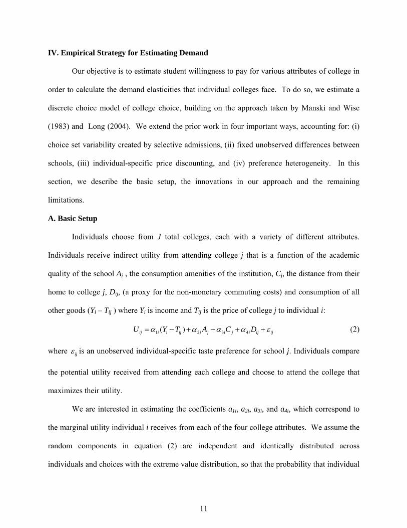
Individuals choose from J total colleges, each with a variety of different attributes.
Individuals receive indirect utility from attending college j that is a function of the academic
quality of the school Aj , the consumption amenities of the institution, Cj, the distance from their
home to college j, Dij, (a proxy for the non-monetary commuting costs) and consumption of all
other goods (Yi – Tij ) where Yi is income and Tij is the price of college j to individual i:
1 2 3 4( )ij i i ij i j i j i ij ijU Y T A C Dα α α α ε= − + + + + (2)
where ijε is an unobserved individual-specific taste preference for school j. Individuals compare
the potential utility received from attending each college and choose to attend the college that
maximizes their utility.
We are interested in estimating the coefficients a1i, a2i, a3i, and a4i, which correspond to
the marginal utility individual i receives from each of the four college attributes. We assume the
random components in equation (2) are independent and identically distributed across
individuals and choices with the extreme value distribution, so that the probability that individual
11
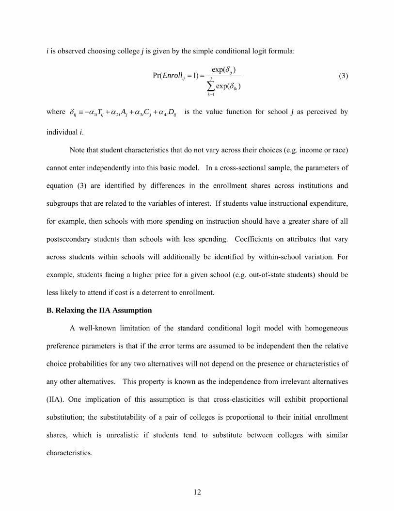
i is observed choosing college j is given by the simple conditional logit formula:
1
exp( )Pr( 1)
exp( )
ijij J
ikk
Enrollδ
δ=
= =
∑ (3)
where 1 2 3 4ij i ij i j i j i ijT A C Dδ α α α α≡ − + + + is the value function for school j as perceived by
individual i.
Note that student characteristics that do not vary across their choices (e.g. income or race)
cannot enter independently into this basic model. In a cross-sectional sample, the parameters of
equation (3) are identified by differences in the enrollment shares across institutions and
subgroups that are related to the variables of interest. If students value instructional expenditure,
for example, then schools with more spending on instruction should have a greater share of all
postsecondary students than schools with less spending. Coefficients on attributes that vary
across students within schools will additionally be identified by within-school variation. For
example, students facing a higher price for a given school (e.g. out-of-state students) should be
less likely to attend if cost is a deterrent to enrollment.
B. Relaxing the IIA Assumption
A well-known limitation of the standard conditional logit model with homogeneous
preference parameters is that if the error terms are assumed to be independent then the relative
choice probabilities for any two alternatives will not depend on the presence or characteristics of
any other alternatives. This property is known as the independence from irrelevant alternatives
(IIA). One implication of this assumption is that cross-elasticities will exhibit proportional
substitution; the substitutability of a pair of colleges is proportional to their initial enrollment
shares, which is unrealistic if students tend to substitute between colleges with similar
characteristics.
12
To address this concern, we allow preference parameters to vary with student gender,
ability (as measured by 12th grade test scores) and socioeconomic status. In addition, we
estimate several specifications that allow for unobserved heterogeneity using a mixed (random
coefficients) logit model (Train 2009). We demonstrate that this additional flexibility of the
mixed logit does not qualitatively change the results of our estimated willingness-to-pay. Hence,
for the sake of computational ease, our preferred specification allows for interactions with
observable student characteristics but does not allow preferences to vary randomly across
individuals.
C. Addressing Omitted Variable Bias
A second concern is omitted variable bias. If observed college characteristics are related
to unobserved college characteristics that also influence demand, then simple estimates of (3)
may suffer from omitted variable bias. Much of the existing college-choice literature does not
address this fundamental identification concern.8 Importantly, this is not the case for college
characteristics that vary across students within an institution such as price or distance. The
coefficients on these variables are identified from differences in the likelihood of attendance
among students with different values of the characteristic.9 Coefficients on interactions between
student and school characteristics are identified in a similar manner.
In order to identify the importance of student-invariant college attributes, we stack data
from multiple cohorts and include institution fixed effects for the roughly 1,300 colleges in our
8 Structural equilibrium models of the college market (Epple, Romano, and Sieg, 2006) potentially address this issue, but at a cost of stronger assumptions about the objective functions of colleges. 9 For example, the coefficient on distance is identified by differences in enrollment shares among individuals living closer to or farther away from a given institution. Similarly, the in-state versus out-state tuition difference helps identify the coefficient on price by a comparison of the likelihood of in-state versus out-state students attending a particular college. One limitation is that many public universities place a cap on the number of out-of-states students they enroll, which may be correlated with in-/out-of-state tuition differentials.
13
analysis sample.10 This approach exploits variation in attributes and enrollment within schools
across cohorts. If students are willing to pay for an attribute, schools with increasing levels of
this attribute should see their enrollment increasing over time and one should observe schools
with high values of this attribute entering the market. We estimate this model through an
iterative procedure in the spirit of Berry (1994) and Guimarães and Portugal (2009).11
In this model, our identifying assumption is that changes in college attributes are
uncorrelated with changes in unobserved tastes for individual colleges. For instance, if colleges
that increase spending on consumption amenities also strengthen other favorable attributes (e.g.,
desirable alumni network), then our estimates will overstate the causal effect of amenities on
colleges’ ability to attract students. Similarly, this model assumes that changes in college
characteristics are exogenous from the perspective of school administrators. While colleges
clearly have some discretion over characteristics such as amenities and tuition and could alter
them in anticipation of (or in response to) demand changes, we believe that the potential bias
introduced is minimal.12
Price discounting is another possible time-varying confounder. Our preferred
specifications use estimated net price rather than college sticker price to account for price
discounting across students, schools, and time. To implement this, we estimate a model with the
net price ratio (price minus grants over price) as the dependent variable using the 1996 and 2004
10 To our knowledge, the only other papers to take this fixed effects approach are Avery, Glickman, Hoxby, and Metrick (2005) and Griffith and Rask (2007). 11 Briefly, the approach iterates between estimating the main model parameters assuming a given set of fixed effects, then updating the fixed effects to equate predicted and sample probabilities. Standard errors are found by inverting the numerical Hessian for the entire coefficient vector (including the fixed effects). 12 It should be noted that if the market responds to a demand for college amenities with the creation of new amenity rich schools, then the inclusion of school fixed effects would tend to understate the value students place on amenities. In practice, the entry and exit of colleges seems unlikely to be important in our analysis. Of the 2,853 college-years in our sample of “regular” four-year colleges, 46 were open only in 1992, 97 were open only in 2004 and the remaining 2,710 were open in both years. When we limit our sample to the 2,458 college-years that were ever selected by individuals in our student-level data, 13 were only open in 1992 and 51 were only open in 2004.
14
National Postsecondary Student Aid Study. The model was estimated separately for six groups
(defined by race X sector X in-state) separately by year and with many interactions and estimates
were used to predict net price for all student-school pairs in our analysis sample.13
In some specifications we also control for other time-varying characteristics associated
with each college. For example, we control for the unemployment rate in the state in which a
college is located in the year in which the cohort would have been applying to college in order to
account for the fact that students may be reluctant to attend college in an economically depressed
area if they intend to reside in the area after graduation. In some specifications, we control for
binary indicators of whether the college is located in the same state and/or region in which the
student attended high school. This is meant to control for hard-to-observe factors such as family
connections that will influence a student’s college choice beyond the distance and cost variables
that we already have in the model.
There are several other limitations to the panel model described above. While colleges
have some flexibility to adjust enrollment and tuition, neither of these factors is perfectly elastic
(in the short-run). For example, an individual college could not quadruple the size of its
incoming class to accommodate increased demand due to short-run constraints in physical
capital. Similarly, there are probably at least some barriers to entry in the college market. These
frictions will lead us to understate student preferences for college characteristics in the model.
D. Admissions Selectivity and Unobservable Choice Set Variation
A third concern with the basic conditional logit model is that selective admissions
necessarily prevent some people from attending certain schools, even if they desire to do so. This
is a specific form of omitted variable bias caused by a misspecification of some students’ choice
set; we do not observe the actual full set of schools that a student could feasibly attend. The
13 Results are described in Appendix E.
15

consequence is that estimates will cofound school selectivity with student preferences, causing
us to overstate (understate) student WTP for attributes of less (more) selective schools.14
There are a number of ways that have been proposed to address this issue. First, one can
specify the choice set for each individual ex-ante. This approach inevitably causes errors: some
alternatives that are excluded from the choice set may be chosen. Conditioning on the set of
schools accepted to (Arcidiacono, 2004) addresses this problem, but loses all information
contained in students’ application decisions. This may bias preference parameter estimates since
some attributes that are important at the application stage may not important at the enrollment
stage. A second approach is to control for characteristics that determine choice set variation. In
this vein, Long (2004) includes flexible interactions between a college’s academic quality and
student ability (measured by test scores) to control for the likelihood that an individual would
have been admitted to the school. A limitation of this approach is that it cannot separately
identify admissions constraints from heterogeneity in preferences by student ability.
A third possibility is to estimate a model of choice set determination explicitly. This is
the approach taken by Arcidiacono (2005) and advocated by Horowitz (1990), which is easiest to
implement when the choice set is actually observed. This is not feasible in our setting because,
like in many others, the choice set is partially unobserved since we do not know the full set of
schools applied and admitted to and do not know admissions outcomes for schools to which the
student did not apply.15
14 Such unobserved choice set variability is pervasive in many situations beyond education, including choice of residence, job or occupation, and products that experience supply constraints and stock-outs. While the IO demand estimation literature has primarily focused on settings where all products are available to all consumers, some authors have addressed the issue of unobserved choice set variation (e.g., Conlon and Mortimer 2010). 15 Arcidiacano (2005) also observed a partial application set (3 schools) and for computational tractability restricted the full set (from which the application set is drawn) to eight. This approach seemed undesirable in our context given the considerable geographic integration of the higher education market between the time of his study (1972) and ours and computationally infeasible with the inclusion of institution fixed effects.
16
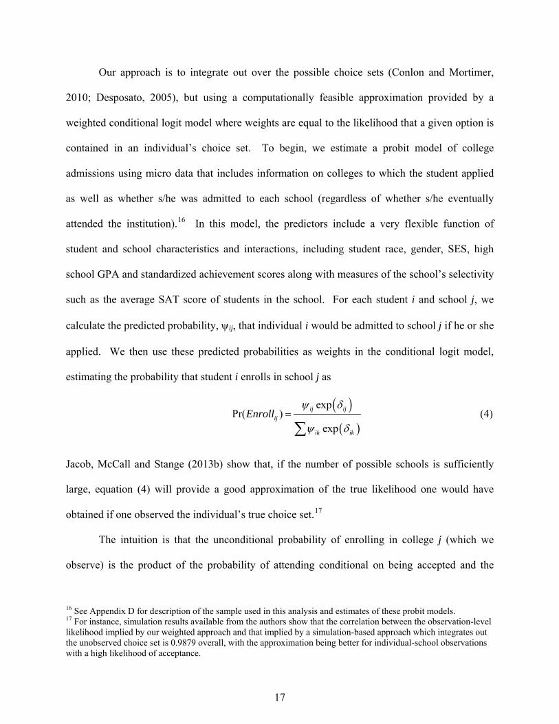
Our approach is to integrate out over the possible choice sets (Conlon and Mortimer,
2010; Desposato, 2005), but using a computationally feasible approximation provided by a
weighted conditional logit model where weights are equal to the likelihood that a given option is
contained in an individual’s choice set. To begin, we estimate a probit model of college
admissions using micro data that includes information on colleges to which the student applied
as well as whether s/he was admitted to each school (regardless of whether s/he eventually
attended the institution).16 In this model, the predictors include a very flexible function of
student and school characteristics and interactions, including student race, gender, SES, high
school GPA and standardized achievement scores along with measures of the school’s selectivity
such as the average SAT score of students in the school. For each student i and school j, we
calculate the predicted probability, ψij, that individual i would be admitted to school j if he or she
applied. We then use these predicted probabilities as weights in the conditional logit model,
estimating the probability that student i enrolls in school j as
( )
( )
expPr( )
exp
ij ijij
ik ik
Enrollψ δ
ψ δ=
∑ (4)
Jacob, McCall and Stange (2013b) show that, if the number of possible schools is sufficiently
large, equation (4) will provide a good approximation of the true likelihood one would have
obtained if one observed the individual’s true choice set.17
The intuition is that the unconditional probability of enrolling in college j (which we
observe) is the product of the probability of attending conditional on being accepted and the
16 See Appendix D for description of the sample used in this analysis and estimates of these probit models. 17 For instance, simulation results available from the authors show that the correlation between the observation-level likelihood implied by our weighted approach and that implied by a simulation-based approach which integrates out the unobserved choice set is 0.9879 overall, with the approximation being better for individual-school observations with a high likelihood of acceptance.
17
probability of being accepted. For the large number of nonselective institutions where the
probability of admissions is near one, the probability of enrollment is simply that estimated by
the standard conditional logit. For schools that the students has little chance of being
admitted, ψij is very low, which means the probability of enrollment is also low. A key benefit
of this approach is that it allows preferences for a given school to be high at the same time the
empirical likelihood of observing a student at this school is extremely low.
The identifying assumption in our approach is that, conditional on the detailed set of
student and school characteristics we include in the admission and enrollment models, there are
no unobservable factors that are simultaneously correlated with the likelihood of admissions and
enrollment. For example, if extraordinary unobserved talent in violin were correlated with the
probability of admissions and enrollment at Julliard, it would lead to an upward bias in the WTP
for fine arts programs. We recognize that such biases likely still exist, but as we show below, it
appears that this approach does account for many of the first-order concerns associated with
students not being able to gain admissions to selective schools with high levels of spending in
various areas.
E. Interpretation Issues
It is worth noting several things when interpreting our estimates of student demand for
particular college attributes. First, our interpretation of demand responses as preferences
necessarily assumes that students are informed about college characteristics. If information is
incomplete, we might misinterpret a lack of demand for an attribute with a lack of information
about the attribute. Second, variables we interpret as “consumption” may actually measure
something that provide labor market returns, and thus be properly categorized as “investment.”
For example, Webber and Ehrenberg (2010) find some evidence that student service
18
expenditures are positively associated with graduation rates at an institution. Moreover, it is
entirely possible that certain attributes have aspects of both consumption and investment.
Regardless of the interpretation, our estimates can still accurately reflect the effect of these
college attributes on students’ college choice.
V. Data
In our analysis, we combine student-level data from two nationally representative cohorts
of high school seniors with college-level data on approximately all four-year colleges in the U.S.
This section briefly describes the key features of the data used, including the sample
construction. For additional detail, see Appendix B.
A. College-Level Data
We combine data from a number of different sources to construct an unbalanced panel
dataset of postsecondary institutions for 1992 and 2004. We limit our sample in several ways to
facilitate our focus on amenities arguably related to direct, immediate consumption value. First,
we limit our sample to public and non-profit private undergraduate four-year schools only,
excluding all two-year (or less) schools, all for-profit schools, and schools offering professional
degrees only. Second, we drop specialized divinity, law, medical, specialized health (e.g.
nursing), and art colleges, though we keep engineering, teaching, military, and business colleges.
Finally, we drop schools with an average of fewer than 50 freshmen or 300 FTEs during our
analysis years in an effort to eliminate remaining specialized schools that are arguably not in
many students’ consideration set.
We use institutional spending in various categories as our primary measures of academic
quality and consumption amenities. We use expenditures on instruction and academic support
per FTE as a measure of the institution’s academic quality. The expenditure data comes from the
19
IPEDS Finance survey assembled by the Delta Cost Project.18 These categories include
expenses for all forms of instruction (i.e., academic, occupational, vocational, adult basic
education and extension sessions, credit and non-credit) as well as spending on libraries,
museums, galleries, etc. Following the prior literature, in most specifications we also use the
average SAT score of students in the college as a second measure of academic quality. We
obtained the average SAT percentile score (or ACT equivalent) of the incoming student body
from Cass Barron’s Profiles of American Colleges (1992).19 For 2004, we used the average of
the 25th and 75th SAT percentile, which we obtained from IPEDS.
Our primary measure of consumption amenities is current spending on student services
and auxiliary enterprises. Spending on student services includes spending on admissions,
registrar, student records, student activities, cultural events, student newspapers, intramural
athletics, and student organizations. Auxiliary expenditures include operating expenditures for
residence halls, food services, student health services, intercollegiate athletics, college unions
and college stores. None of these categories includes interest payments or other capital
expenses, so this is likely to be a noisy measure of the full extent of amenities experienced by
students. All spending measures have been deflated by the CPI-U and are in 2009 dollars.
Table 1 presents summary statistics of the college data, separately by sector for 1992 and
2004. Real tuition costs and spending on instruction and student services increased considerably
during the 1990s, though there are differences across sectors. Public institutions saw a greater
proportionate increase in tuition prices, while private institutions saw larger relative increases in
spending. Although spending increased in both categories, the average ratio of amenity (i.e.,
18 This survey was changed considerably in 2000, but the spending categories are mostly comparable across years. 19 We thank Bridget Terry Long for providing us this data, which was used in Long 2004.
20
student service + auxiliary) to academic (i.e., instruction + academic support) remained constant
over this period.
Many of these measures are highly positively correlated (see Appendix Table B3). Log
per-student spending on instruction/academic support is correlated 0.55 with student
services/auxiliary spending. Tuition, expenditures and SAT percentile are all correlated at 0.49
or higher with each other. Schools that have high SAT-scoring students tend to spend more on
both instruction and amenities and also charge higher tuition. Because changes in college
attributes within institution over time (as opposed to levels) will identify the preference
parameters in our model, it is useful to also consider the correlation of changes. These
correlations are substantially smaller than the correlations in levels, which suggests we will have
sufficient independent variation to identify preferences for multiple attributes.
B. Student-Level Data
We combine two nationally representative samples of the high school classes of 1992
(National Educational Longitudinal Study, NELS) and 2004 (Educational Longitudinal Survey,
ELS).20 These longitudinal surveys follow students from high school into college. We limit our
sample to individuals who graduated from high school, attended a four-year institution within
two years of expected high school graduation, attended a college in our sample, and were not
missing key covariates (test scores, race, gender, family SES, college choice, etc).
We assign out-of-state tuition levels to individuals residing in all states other than the one
in which the institution is located, so we do not take into account tuition reciprocity agreements
between neighboring states. Tuition does not vary by in-state status for private institutions. As a
20 Prior work by Long (2004) has utilized data from two earlier cohorts, the high school classes of 1972 (National Longitudinal Survey, NLS72) and 1980/82 (High School and Beyond, HSB82). We exclude these from our analysis because they do not have sufficient information on college applications/admissions to properly account for the limited choice set that many students will face.
21
proxy for the distance between a student’s home and a college, we calculate the distance between
the centroid of the zip code in which the student’s high school is located and the centroid of the
zip code in which each institution is located.
Table 2 presents summary statistics for our analysis sample. The middle panel presents
statistics on the colleges attended by our sample. Over our analysis period, the real cost
(including tuition, fees, room & board) increased more than forty percent, from $14,801 in 1992
to $20,859 in 2004, while the average distance traveled to college increased from 196 to 219
miles. Schools attended by our sample increased spending on instruction 19 percent over the
period and spending on consumption amenities by roughly 14 percent.
Each of these surveys asked high school seniors what factors they viewed as most
important in selecting a college, including courses, academic reputation, low cost, availability of
financial aid, athletics and social life. These self-reported preferences allow us to validate some
of our more objective college characteristics. We first standardize each item using the 1972
mean and standard deviation (students reported importance on a 4-point scale), and then
calculate a simple average of two items for each composite: academics (courses and reputation),
costs (low cost, financial aid), and social amenities (athletics, social life).21 The summary
statistics for these composites shown in Table 2 are for the analysis sample, and show an
increasing value placed on all three factors. However, in the analysis below, we rely primarily
on the across-student variation in these measures rather than the across-cohort variation.
VI. Estimates of Demand Model
A. Preference Estimates: No Heterogeneity
Table 3 presents estimates (odds ratios and standard errors) of the choice model pooling
21 This normalization reflects our use of the 1972 cohort in earlier analysis. The normalization base will not have any effect on our results.
22
the 1992 and 2004 cohorts and imposing homogeneity in student preferences.22 Columns (1) and
(2) do not include college fixed effects and demonstrate patterns found in much of the previous
literature. Cost and distance are major predictors of where students choose to enroll, as is
spending on academics and peer quality. Conditional on these college attributes, we also find that
spending on consumption amenities is a significant predictor of college choice. As expected,
controlling for selective admissions in column (3) increases the estimated willingness-to-pay for
measures of academic quality such as instructional spending and school mean SAT. Better
accounting for the actual price faced by each student in column (4) reduces the importance of
school spending on consumption amenities as expected, but does not change estimated
importance of price or instructional quality.
To control for unobserved characteristics that are correlated with size and the desirability
of the college, specification (5) includes college fixed effects, meaning that identification comes
from within-college changes over time in attributes that are associated with chances in
enrollment. The inclusion of college fixed effects changes the results in several important ways.
First, the importance of cost increases noticeably, with the odds ratio going from 0.158 in
column (4) to 0.05 in column (5). This suggests that expensive colleges also possess
unobservable qualities that are attractive to students. Not accounting for these fixed
unobservable attributes may cause cost to appear to be a less important consideration than it truly
is.23 The coefficients on the other college attributes decline substantially and the coefficient on
instructional spending actually becomes negative. The coefficient on our measure of
22 To provide a direct comparison with previous work, we also replicated and extended the analysis of Long (2004) by including measures of college consumption amenities into her conditional logit specifications. These results are reported in Appendix C. We find that several different types of “consumption amenities” are significant predictors of student choice above and beyond the academic measures studied by Long (2004). Furthermore, the inclusion of these measures diminishes the estimated importance of instructional expenditure. Comparable models estimated separately by cohort, but using a specification that mirrors that used in our subsequent analysis are similar. 23 This is a finding that is common in the differentiated products literature: accounting for unobserved product characteristics typically makes the effect of price more negative.
23

consumption amenities declines as well (odds ratio = 1.24), but remains statistically significant.
Columns (6) and (7) include controls for other regional and geographic characteristics
that may be correlated with college amenities. Interestingly, the indicators for whether a college
is in the student’s home state and region in column (7) are large and significant predictors of
student choice, suggesting important non-linearities in preferences for proximity coupled with
changes in the geographic distribution of students over time. These controls reduce the estimated
importance of price considerably, perhaps because of out-of-state tuition differentials are no
longer used to identify price responsiveness. However, the inclusion of these controls does not
qualitatively change the estimated importance of the other college amenities, although the
estimated odds ratio for consumption spending is no longer statistically significant at
conventional levels.
In order to help interpret the magnitude of these results and to quantify the relative
tradeoffs that students are making, the bottom panel of the table reports measures of
“willingness-to-pay” (WTP) for each college attribute. WTP is given by the (negative) ratio of
the estimated coefficient on that attribute to the estimated coefficient on log(total cost). For
example, the WTP of .162 for consumption amenities in the bottom panel of column (7)
indicates that students are willing to pay roughly 0.16 percent more to attend a school that spends
1 percent more on consumption amenities. The WTP of .009 on school mean SAT indicates that
a student would pay 0.9 percent more to attend a school whose mean SAT score is 1 percentage
point higher on the national distribution. In order to attend a top quartile school (in terms of
mean SAT measure) instead of a bottom quartile school, a student would be willing to pay 40
percent more (i.e., .009 x (79-34) ~ .40).24
24 We also estimated specifications that included controls for the cost of living (normalized within year) in each college’s city, to absorb variation in spending due to higher prices which may not reflect differences in real
24
B. Preference Estimates: Heterogeneity by Observable Characteristics
The results presented above suggest that, on average, students marginally value
institutions’ spending on consumption attributes and the academic ability of their peers, but do
not value spending on instruction. However, preferences are likely to differ between students for
many reasons and this preference heterogeneity will impact the elasticies that colleges face in
response to changes in their characteristics.
To examine how preferences for college attributes vary with observable student
characteristics, we permit student preferences for college attributes to vary with sex, student
ability and family income. Table 4 reports coefficient estimates for models that include
interactions between these three student characteristics and the five college attributes (odds ratios
are difficult to interpret with many interactions, so raw coefficients are presented). The first
specification accounts for selective admissions, net price, state unemployment rate, high school
cohort size, and dummies for in-state and in-region, but does not include college fixed effects.
Column (2) includes college fixed effects. Across both specifications, heterogeneity is
considerable. Wealthier students (higher SES) are substantially less sensitive to price and
distance and higher achieving students are less sensitive to distance. Male students are more
price sensitive than female students.25
High-ability students have a much greater preference for academic quality, both in the
form of instructional spending and mean SAT. Interestingly, this pattern changes little when
school fixed effects are included. Recall that these models account for the predicted probability
amenities. Estimates of students’ willingness to pay for college amenities are unaffected by this control. To address multicolinearity concerns with including two distinct measures of academic quality (instructional spending per student and average SAT scores), we also estimated specifications that exclude average SAT score. This has virtually no impact on the other estimates and instructional expenditure remains insignificant. These results are available from the authors upon request. 25 One often cannot interpret the coefficients on interactions in non-linear choice models directly. The patterns described here are confirmed through simulations.
25
of acceptance that incorporate the 12th grade test scores along with other measures of academic
aptitude so this finding is not simply an indication of the greater likelihood of acceptance to elite
institutions among such students. Interestingly, differences in valuation for consumption
amenities by student ability and income is less pronounced, though higher income students have
a greater preference for consumption amenities while higher achieving students place less value
on this.
Figures 1 and 2 summarize the variation in predicted WTP across our sample, where
WTP is predicted using our preferred model that includes all controls and college fixed effects.
Figure 1 plots the overall distribution of WTP for each college attribute, demonstrating that there
is substantial predicted heterogeneity in students’ willingness to pay for all college
characteristics.26 The WTP for consumption amenities is positive for most members of the
sample and positive for SAT for the majority of the sample, yet the same is only true for
instruction for a limited number of individuals. In fact, our estimates suggest that relatively few
students actually place a positive value on instructional spending.27 Figure 2 presents comparable
distributions for certain sub-populations to better quantify the importance of preference
heterogeneity by observed student characteristics. These graphs demonstrate a strong variation in
preference for academic quality associated with academic preparation. Very high achieving
students tend to derive greater value from high academic quality. In fact, the distribution of
estimated preferences for instructional spending does not overlap between students in the top and
26 The distribution of estimated willingness-to-pay is continuous because two of the variables used to estimate each preference parameter (math score and SES) are continuous. 27 Figure F1 in the appendix presents the distribution of WTP from the model without college fixed effects. In this model, the qualitative finding that the WTP for marginal changes in consumption amenities is greater (more positive) than that for instruction still holds: all students have a positive WTP for consumption amenities, but only about half do for instructional spending, though the scale differs. Since the coefficient on cost is smaller (less negative) in the model without fixed effects, the estimated willingness-to-pay for other college characteristics (calculated with the cost coefficient as the denominator) are greater in magnitude. Thus the scale of the WTP distribution is much larger without fixed effects (Figure F1) than with (Figure 1).
26
lowest test score terciles. SES does contribute to heterogeneity, particularly on the WTP for
consumption amenities.28 Our estimates suggest that students with the greatest willingness-to-
pay for consumption amenities are low-ability, high-income students and that instructional
spending only has a positive WTP for high-ability, high-SES students. 29
C. Robustness and Unobserved Heterogeneity
In Table 5, we explore the robustness of our demand model to a different measure of academic
resources and to greater flexibility across institutional type. One concern is that instructional
spending is an imperfect (or not salient) measure of the resources institutions devote to academic
quality. Column (2) uses the log of number of full-time faculty per student as our measure of
academic resources, which is also common in the literature (e.g. Bound, Lovenheim, and Turner,
2010). This model produces results that are qualitatively identical (and for some coefficients,
quantitatively similar) to that using instructional and academic support. Given that four-year
colleges are quite heterogeneous, a second concern is that marginal spending at different types of
institutions may be used for very different purposes. For instance, PhD-granting institutions may
devote marginal increases in student services or instructional spending to very different activities
than small BA-granting institutions. Column (3) lets the marginal effect of the two spending
categories differ by the highest level of degree offered. We find no significant differences
between institutions offering different degrees, though estimates are not very precise.
Furthermore, estimates of the heterogeneity across individuals are not impacted nor is model fit
improved much by this added flexibility. Though we continue to rely on our main specification
28 Preference variation by sex is minimal, as demonstrated in Appendix Figure F2. 29 Appendix Figure F3 shows median WTP for nine subgroups defined by test scores and SES. Models without college fixed effects demonstrate a very similar pattern of heterogeneity, though the non-fixed effects models suggest more students respond favorably to instructional spending. In results not reported here and not included in these specifications, we also find that students are substantially more likely to attend institutions that match their background (e.g., Black students attending historically Black colleges, Catholic students attending Catholic colleges, etc.), suggesting that campus life is an important factor in students’ enrollment decisions.
27
(Table 4, column 2) throughout the rest of our analysis, later we also report results using these
two alternative specifications to estimate the demand elasticities faced by institutions.
A natural question is whether the few student characteristics we have interacted with
college characteristics capture a sufficient amount of the preference variation. To explore this,
we also estimated models that permit the coefficients on college attributes to vary randomly.
Table 6 presents results from random coefficient models that do not include school fixed
effects.30 Specification (1) includes only the five college characteristics and permits the
coefficients on these attributes to vary in the population according to a normal distribution with
mean and variance to be estimated. The table reports the maximum simulated likelihood
estimates of the mean and standard deviation of this preference distribution. The coefficient
means are very consistent with those from the fixed coefficient specification (column 3 in Table
3, though coefficient estimates are not reported in that table), but the variance terms indicate
quite a bit of preference heterogeneity.
Column (2) additionally controls for interactions between college attributes and male,
math score, and SES, and is the random coefficient analog of specification (1) from Table 4.
These observable student characteristics control for a substantial amount of preference
heterogeneity, reducing the residual preference variation quite a bit. Further controlling for
students’ stated reasons for choosing a college (column (3)) reduces this residual variation only
marginally more. Throughout all three specifications, our estimates suggest that preference for
consumption amenities is fairly broad-based across all students, while taste for academic quality
exhibits substantial heterogeneity across the population. Furthermore, our observed
30 Estimation of random coefficients models that also control for school fixed effects is computationally infeasible given the number of colleges (1300) and our fixed effects estimation algorithm. However, given that the inclusion of fixed effects did not impact the patterns of preference heterogeneity documented in Table 4, we expect that the inclusion of fixed effects in the random coefficients model would not impact our conclusions about the importance of unobserved preference heterogeneity.
28
characteristics (male, math score, and SES) do a good job characterizing this heterogeneity.
D. Interpretation as Consumption Amenities
We have documented a substantial enrollment response to spending on student services
and auxiliary enterprises, which we interpret as reflective of the importance of consumption
considerations in students’ decisions. Evidence in favor of this interpretation is presented in
Table 7. Column (1) presents estimates from a model that includes interactions between our five
college attributes and the three self-reported student “preference” measures described earlier.
Recall that these measures are standardized composite variables that reflect how the students, as
12th graders, reported the importance of different college characteristics in their college
enrollment decision. We view this specification as a useful check on the validity of our college
attribute measures. For example, if spending on student services was really capturing something
about the consumption value of an institution, we would expect students who report that a
school’s social life is important to be more likely to attend these institutions. Similarly, if
instructional spending were a good proxy for academic quality, students who report academics to
be very important to them should be more likely to attend schools with higher spending on
instruction.
Indeed, we find exactly these patterns. Additionally, students that report expenses to be
an important consideration in college choice are much more responsive (negatively) to cost and
distance and much less responsive (less positive) to other college characteristics. These estimates
account for selective admissions and financial aid so these patterns do not simply reflect
differences in acceptance or financial aid generosity at schools with different characteristics
between students reporting “social” vs. “academic” factors as being important to their decisions.
Further evidence of this conclusion is found in column (2), which includes interactions
29
between our five college attributes and these “preference” measures and interactions with the
three observable characteristics examined earlier (male, math score, and SES). The point
estimates of the preference interactions change very little. Students seeking a college with a
strong social life respond favorably to spending on student services but negatively to spending on
academics. Students choosing colleges based on academics are attracted to colleges that spend
more on instruction, but are unresponsive to spending on student services. These patterns hold
even when the stronger preference that high achieving students (i.e. high math test scores) have
for colleges that spend more on instruction is held constant. Comparing specification (2) in Table
4 with specification (2) in Table 7, it is interesting to note that the pattern of interactions between
our college characteristics and sex, test scores, and SES are very similar with and without
controlling for these self-reported aspects of preferences.
We further explore the consumption amenities interpretation of our main findings by
interacting our spending measures with other institution- and student-level characteristics.31 For
instance, we’d expect campus spending on consumption amenities to be less important in areas
that have locational amenities that act as substitutes (e.g. vibrant urban life or access to beaches
and ski resorts). We tested this by interacting spending with an index of the “quality of life” of
the campus location, developed in Albouy (2012). While the negative point estimate on the
interaction between consumption amenity spending and QOL is consistent with this
interpretation, the estimate is sufficiently imprecise to rule out no effect. We also interact
spending by category with an index for whether the student plans to live at home during college.
Since amenities spending is directed primarily towards students spending significant amount of
time on campus, we’d expect it to be most important for students planning to live on or near
campus. We do find that students planning to live at home are less sensitive to spending on
31 These results are reported in Table F1 in the Appendix.
30
consumption amenities than those planning to live on campus or on their own. Third, we interact
spending by category with the fraction of students living on campus in 1992, again testing
whether spending on consumption amenities is more important at institutions that already have a
large share of students residing on campus. We do not find evidence for this interpretation,
though again estimates are imprecise.
Finally, in other work, we show that our college spending measures are correlated with
the subjective assessments of college “quality of life” and “quality of academics” presented in
the Princeton Review guidebooks (Jacob, McCall and Stange 2013a). Students attending
colleges with more spending on student services and auxiliary enterprises rate the quality of life
of the institution much higher, whereas instructional spending has little correlation with
subjective quality of life. By contrast, students rate colleges with high instructional expenditure
or higher student services expenditure as having a better academic environment.
VII. Implications for the Postsecondary Market
A. Variation in Demand-side Pressure
We now use our estimated college demand model to characterize the consequences of
heterogeneous student preferences for institutions by simulating changes in patterns of demand if
colleges were to alter their characteristics. We took each individual college and altered a single
characteristic one at a time, holding all other characteristics of it and of all other colleges
constant. Then we recorded how the entire pattern of enrollment across all colleges changed.
These marginal responses are expected to vary across colleges due to variation in the preferences
of their marginal students and differences in the proximity of colleges with similar attributes (i.e.
competitors). For instance, colleges whose marginal students are wealthy but with low academic
aptitude will see particularly large enrollment responses to changes in consumption amenities
31
spending, though the opposite is true for colleges attracting many high-achieving, low-income
students.
Figure 3 plots the distribution of predicted own total enrollment elasticities with respect
to each of the four college characteristics. These estimates come from the model that permits
preference parameters to vary by sex, math scores, and SES (specification (2) from Table 4).32
Consider first the distribution of price elasticties shown in the top-left panel. The entire
distribution of elasticities falls to the left of zero, indicating that all schools experience a
downward sloping demand curve (i.e., a negative enrollment response to higher tuition). Overall
demand is price-elastic: the mean price elasticity among colleges is -1.6, indicating that a 1%
increase in tuition is associated with a 1.6% decrease in total enrollment. The panel in the top-
right corner shows that all colleges are estimated to have a positive total enrollment response to
marginal increases in consumption amenities spending. While most colleges are estimated to
have a positive total enrollment response to marginal improvements in average SAT score, some
institutions in our sample are estimated to have a negative elasticity of enrollment with respect to
improvements in mean SAT score. Consistent with the results presented in Table 4, the vast
majority of colleges appear to have a negative total enrollment response to increases in
instructional spending.
Figure 4 plots the implied own-elasticities for enrollment of high SES (above the 75th
percentile, solid line) and of high achieving (above the 75th percentile of math test score, dashed
line) students. The total enrollment elasticity (bold line) is included for reference. High achieving
students are particularly responsive to improvements in academic quality, both in the form of
average SAT and instructional spending. In fact, high achieving students are the only subgroup
32 Simulations confirm that using the demand model with no preference heterogeneity generates limited variation in responsiveness across colleges, with this variation due only to differences in the distribution of distances and costs across students.
32
that responds positively to instructional spending; almost all colleges can attract more high
achieving students by increasing instructional spending, though this usually comes at a cost to
their ability to attract other students. On the other hand, marginal increases in consumption
amenities spending will have a greater impact on colleges’ enrollment of high SES students.
Most institutions can increase total or high SES enrollment by increasing consumption amenities,
though the response of high-achieving students is smaller. The implication is that most colleges
face a trade-off: increases in instructional spending will attract high achieving students, but may
deter enrollment from a broader student body. Increases in amenities spending, however, will
attract all types of students (though disproportionately lower-achieving and high income
students). 33
Figure 5 depicts how demand-side pressure varies with one important observable college
characteristic: selectivity. The graph depicts the own-demand elasticity with respect to college
characteristics, by average student SAT score percentile at baseline. Though the own-price
elasticity is similar across institutions with very different levels of selectivity, there are clear
differences in responsiveness to other characteristics. The demand response to academic quality
is more positive at more selective schools. Students on the margin of attending more selective
schools tend to place greater value on academic quality and thus changes in academic quality
have a greater impact on overall enrollment. The pattern for consumption amenities spending is
less clear. Very low selectivity schools (i.e., schools with low average student SAT scores)
experience a slightly greater enrollment response to an increase in amenities spending than
moderately more selective schools, but responsiveness then increases with selectivity at higher
levels of selectivity. Appendix Figure F7 plots the elasticities for certain student groups by
33 This same pattern is apparent in models that do not include fixed effects, use faculty-student ratio as the measure of academic quality, or let the marginal effect of spending differ by type of institution. These are reported in Appendix Figures F4-F6.
33
selectivity level. One finding is that institutions of very different selectivity face relatively
similar incentives for attracting the most high-achieving students, but very different incentives
when trying to attract students overall. 34 Figure 5 also demonstrates that there is substantial
variation in demand response to consumption amenities even among institutions with similar
levels of selectivity.
B. Can Variation in Demand-side Pressure Explain Resource Allocation?
The previous section demonstrated that colleges face different enrollment consequences from
their spending decisions due to differences in the preferences of students at their enrollment
margin. But do colleges that face greater pressure to provide consumption amenities respond
accordingly? Figure 6 plots the ratio of consumption amenities spending to instructional
spending from 1992 to 2007 for four groups of colleges, categorized by their enrollment
elasticity with respect to these two categories of spending.35 Colleges that face the highest
demand elasticity for consumption amenities and the lowest elasticity for instructional spending
(solid line) provide the highest level of spending on the latter, relative to the former. These
schools spend nearly $.90 on consumption amenities for every dollar spent on instruction. In
contrast, colleges that face the greatest pressure to spend resources on instruction only spend
$0.45 on consumption amenities for every dollar spent on instruction. These ratios have not
changed appreciably over time at the group level. It should be noted that this cross-institutional
variation is not used to estimate the parameters of our student demand model since our preferred
specifications include college fixed effects, which control for any time-invariant characteristics
34 This result is qualitatively very similar with or without college fixed effects, but does depend strongly on the inclusion of preference heterogeneity (Appendix Figure F7). Without it, the response to all characteristics appears to be similar across institutions and student groups. This pattern can be quantitatively and even directionally incorrect since some colleges may face negative enrollment responses when they increase academic quality, while other colleges may see a positive response overall or for certain subgroups. Heterogeneity in institution-specific demand pressure is masked without allowing for individual preference heterogeneity. 35 In this figure, colleges were divided into terciles for each of the spending elasticities, but only four of the nine resulting groups are displayed for clarity of presentation.
34
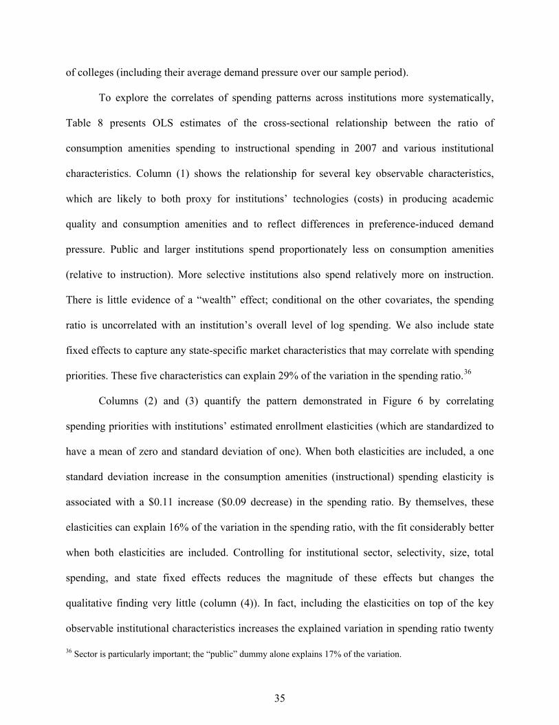
of colleges (including their average demand pressure over our sample period).
To explore the correlates of spending patterns across institutions more systematically,
Table 8 presents OLS estimates of the cross-sectional relationship between the ratio of
consumption amenities spending to instructional spending in 2007 and various institutional
characteristics. Column (1) shows the relationship for several key observable characteristics,
which are likely to both proxy for institutions’ technologies (costs) in producing academic
quality and consumption amenities and to reflect differences in preference-induced demand
pressure. Public and larger institutions spend proportionately less on consumption amenities
(relative to instruction). More selective institutions also spend relatively more on instruction.
There is little evidence of a “wealth” effect; conditional on the other covariates, the spending
ratio is uncorrelated with an institution’s overall level of log spending. We also include state
fixed effects to capture any state-specific market characteristics that may correlate with spending
priorities. These five characteristics can explain 29% of the variation in the spending ratio.36
Columns (2) and (3) quantify the pattern demonstrated in Figure 6 by correlating
spending priorities with institutions’ estimated enrollment elasticities (which are standardized to
have a mean of zero and standard deviation of one). When both elasticities are included, a one
standard deviation increase in the consumption amenities (instructional) spending elasticity is
associated with a $0.11 increase ($0.09 decrease) in the spending ratio. By themselves, these
elasticities can explain 16% of the variation in the spending ratio, with the fit considerably better
when both elasticities are included. Controlling for institutional sector, selectivity, size, total
spending, and state fixed effects reduces the magnitude of these effects but changes the
qualitative finding very little (column (4)). In fact, including the elasticities on top of the key
observable institutional characteristics increases the explained variation in spending ratio twenty
36 Sector is particularly important; the “public” dummy alone explains 17% of the variation.
35
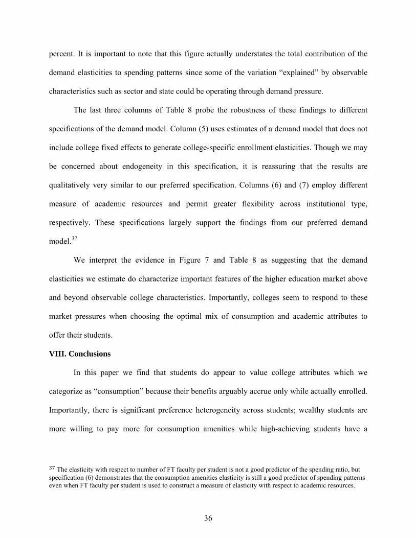
percent. It is important to note that this figure actually understates the total contribution of the
demand elasticities to spending patterns since some of the variation “explained” by observable
characteristics such as sector and state could be operating through demand pressure.
The last three columns of Table 8 probe the robustness of these findings to different
specifications of the demand model. Column (5) uses estimates of a demand model that does not
include college fixed effects to generate college-specific enrollment elasticities. Though we may
be concerned about endogeneity in this specification, it is reassuring that the results are
qualitatively very similar to our preferred specification. Columns (6) and (7) employ different
measure of academic resources and permit greater flexibility across institutional type,
respectively. These specifications largely support the findings from our preferred demand
model.37
We interpret the evidence in Figure 7 and Table 8 as suggesting that the demand
elasticities we estimate do characterize important features of the higher education market above
and beyond observable college characteristics. Importantly, colleges seem to respond to these
market pressures when choosing the optimal mix of consumption and academic attributes to
offer their students.
VIII. Conclusions
In this paper we find that students do appear to value college attributes which we
categorize as “consumption” because their benefits arguably accrue only while actually enrolled.
Importantly, there is significant preference heterogeneity across students; wealthy students are
more willing to pay more for consumption amenities while high-achieving students have a
37 The elasticity with respect to number of FT faculty per student is not a good predictor of the spending ratio, but specification (6) demonstrates that the consumption amenities elasticity is still a good predictor of spending patterns even when FT faculty per student is used to construct a measure of elasticity with respect to academic resources.
36
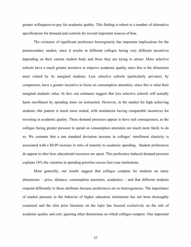
greater willingness-to-pay for academic quality. This finding is robust to a number of alternative
specifications for demand and controls for several important sources of bias.
The existence of significant preference heterogeneity has important implications for the
postsecondary market, since it results in different colleges facing very different incentives
depending on their current student body and those they are trying to attract. More selective
schools have a much greater incentive to improve academic quality since this is the dimension
most valued by its marginal students. Less selective schools (particularly privates), by
comparison, have a greater incentive to focus on consumption amenities, since this is what their
marginal students value. In fact, our estimates suggest that less selective schools will actually
harm enrollment by spending more on instruction. However, in the market for high achieving
students, this pattern is much more muted, with institutions having comparable incentives for
investing in academic quality. These demand pressures appear to have real consequences, as the
colleges facing greater pressure to spend on consumption amenities are much more likely to do
so. We estimate that a one standard deviation increase in colleges’ enrollment elasticity is
associated with a $0.09 increase in ratio of amenity to academic spending. Student preferences
do appear to alter how educational resources are spent. This preference-induced demand pressure
explains 16% the variation in spending priorities across four-year institutions.
More generally, our results suggest that colleges compete for students on many
dimensions – price, distance, consumption amenities, academics – and that different students
respond differently to these attributes because preferences are so heterogeneous. The importance
of market pressure to the behavior of higher education institutions has not been thoroughly
examined and the slim prior literature on the topic has focused exclusively on the role of
academic quality and cost, ignoring other dimensions on which colleges compete. One important
37
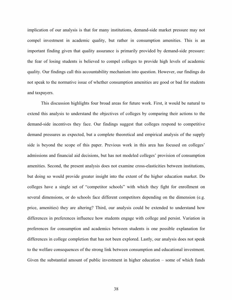
implication of our analysis is that for many institutions, demand-side market pressure may not
compel investment in academic quality, but rather in consumption amenities. This is an
important finding given that quality assurance is primarily provided by demand-side pressure:
the fear of losing students is believed to compel colleges to provide high levels of academic
quality. Our findings call this accountability mechanism into question. However, our findings do
not speak to the normative issue of whether consumption amenities are good or bad for students
and taxpayers.
This discussion highlights four broad areas for future work. First, it would be natural to
extend this analysis to understand the objectives of colleges by comparing their actions to the
demand-side incentives they face. Our findings suggest that colleges respond to competitive
demand pressures as expected, but a complete theoretical and empirical analysis of the supply
side is beyond the scope of this paper. Previous work in this area has focused on colleges’
admissions and financial aid decisions, but has not modeled colleges’ provision of consumption
amenities. Second, the present analysis does not examine cross-elasticities between institutions,
but doing so would provide greater insight into the extent of the higher education market. Do
colleges have a single set of “competitor schools” with which they fight for enrollment on
several dimensions, or do schools face different competitors depending on the dimension (e.g.
price, amenities) they are altering? Third, our analysis could be extended to understand how
differences in preferences influence how students engage with college and persist. Variation in
preferences for consumption and academics between students is one possible explanation for
differences in college completion that has not been explored. Lastly, our analysis does not speak
to the welfare consequences of the strong link between consumption and educational investment.
Given the substantial amount of public investment in higher education – some of which funds
38
consumption amenities – it is natural to ask whether this investment is sound. We leave these
questions for future researchers to answer.
39
References Albouy, David, 2012. “Are Big Cities Bad Places to Live? Estimating Quality of Life across Metropolitan Areas.” University of Michigan. Mimeo.
Alstadsæter, A. (2011). “Measuring the Consumption Value of Higher Education, CESifo Economic Studies, 57(3): 458-479.
Alter, Molly and Randal Reback. (2012). “True for Your School? How Changing Reputations Alter Demand for Selective U.S. Colleges.” Barnard College, Columbia University. Mimeo.
Arcidiacono, Peter (2004). ”Ability sorting and the returns to college major.”Journal of Econometrics 121, 343-375.
Arcidiacano, Peter (2005). "Affirmative Action in Higher Education: How Do Admission and Financial Aid Rules Affect Future Earnings?" Econometrica, 73(5): 1477-1524.
Arum, Richard and Josipa Roksa (2011). Academically Adrift: Limited Learning on College Campuses. University of Chicago Press: Chicago, IL.
Avery, Chris, Mark Glickman, Caroline Hoxby, and Andrew Metrick (2005). “A Revealed Preference Ranking of U.S. Colleges and Universities.” NBER WP 10803.
Babcock, Philip and Minday Marks (forthcoming) The Falling Time Cost of College: Evidence from Half a Century of Time Use Data , Review of Economics and Statistics.
Bayer, Patrick, Fernando Ferreira, and Robert McMillan (2007). “A Unified Framework for Measuring Preferences for Schools and Neighborhoods.” Journal of Political Economy, August.
Becker, Gary (1964). Human Capital. New York: Columbia University Press.
Berry, Steven T. (1994). "Estimating Discrete-Choice Models of Product Differentiation," RAND Journal of Economics, 25(2): 242-262.
Berry, Steven, James Levinsohn, and Ariel Pakes (1995). "Automobile Prices in Market Equilibrium," Econometrica, 63(4), pages 841-90, July.
Black, Dan, and Jeff Smith (2004). “How Robust Is the Evidence on the Effects of College Quality? Evidence from Matching,” Journal of Econometrics, 121, 99–124.
Bound, John, Michael Lovenheim, and Sarah E. Turner (2010) "Why Have College Completion Rates Declined? An Analysis of Changing Student Preparation and Collegiate Resources." American Economic Journal: Applied Economics, 2(3): 1-31.
Brand, Jennie, and Yu Xie (2010). "Who benefits Most From College? Evidence for Negative Selection in Heterogeneous Economic Returns to Higher Education." American Sociological Review Carneiro, P., K.T. Hansen, and J.J. Heckman (2003). ”Estimating distributions of treatment
40
effects with and application to the returns to schooling and measurement of the effects of uncertainty of college choice”, International Economic Review 44(2), 361-422.
Conlon, Christopher T. and Julie Holland Mortimer (2010). “Demand Estimation Under Incomplete Product Availability.” NBER Working Paper No. 14315,September 2008, Revised May 2010.
Desposato, Scott (2005). “A Model of Unordered Multiple Choice with Unobserved Choice Set Selection” University of California San Diego, mimeo.
Epple, Dennis, Richard Romano, and Holger Sieg (2006). “Admission, Tuition, and Financial Aid Policies in the Market for Higher Education.” Econometrica 74 (4): 885-928.
Goldman, Dana and John Romley (2008). “Hospitals as Hotels: The Role of Patient Amenities in Hospital Demand.” NBER Working Paper 14619.
Goldman, Dana, Mary Vaiana, and John Romley (2010). “The Emerging Importance of Patient Amenities in Hospital Care.” New England Journal of Medicine 363: 2185-2187.
Guimaraes, Paulo and Pedro Portugal (2009). "A Simple Feasible Alternative Procedure to Estimate Models with High-Dimensional Fixed Effects," IZA Discussion Paper 3935.
Griffith, Amanda and Kevin Rask (2007). “The influence of the US News and World Report collegiate rankings on the matriculation decision of high-ability students: 1995-2004. Economics of Education Review, 26: 244-255.
Hastings, Justine S., Thomas J. Kane, and Doug O. Staiger, 2009. “Heterogeneous Preferences and the Efficacy of Public School Choice.” Mimeo..
Heckman, J.J., L. Lochner, and C. Taber (1999). ”General-equilibrium cost-benefit analysis of education and tax policies”, In: Ranis, G., L.K. Raut (Eds.): Trade, Growth, and Development. Elsevier, Amsterdam, 291-349.
Hoekstra, Mark (2009). “The Effect of Attending the Flagship State University: A Regression Discontinuity Approach.” The Review of Economics and Statistics, 91(4): 717–724.
Horowitz, J L (1991). “Modeling the choice of choice set in discrete-choice random-utility models.” Environment and Planning A, 23: 1237-1246.
Hoxby, Caroline (1997). “How the Changing Market Structure of U.S. Higher Education Explains College Tuition.” NBER Working Paper 6323.
Hoxby, Caroline (2009). “The Changing Selectivity of American Colleges. “Journal of Economic Perspectives. 23(4): 95-118.
Jacob, Brian and Lars Lefgren (2007). "What Do Parents Value in Education? An Empirical Investigation of Parents' Revealed Preferences for Teachers," The Quarterly Journal of Economics, 122(4): 1603-1637.
41
Jacob, Brian, Brian McCall, and Kevin Stange (2013a). “The Growth of Amenities in Postsecondary Education.” Mimeo, University of Michigan.
Jacob, Brian, Brian McCall, and Kevin Stange (2013b). “Conditional Logit Estimation with Unobserved Choice Sets.” Mimeo, University of Michigan.
Kirp, David L. (2005). “This little student goes to market.” In Declining by degrees of mediocrity : higher education at risk / edited by Richard H. Hersch and John Merrow. New York : Palgrave Macmillan, 2005. Kodde, D.A. and J.M.M. Ritzen (1984), ”Integrating consumption and investment motives in a neoclassical model of demand for education”, Kyklos 37(4), 598-605.
Lazear, Edward (1977). “Education: consumption or production?” Journal of Political Economy 85(3).
Long, Bridget Terry (2004). “How have college decisions changed over time? An application of the conditional logistic choice model.” Journal of Econometrics 121:271-296.
Manski, Charles F. and David A. Wise (1983). College choice in America. Cambridge, MA: Harvard University Press, 1983.
McDuff, DeForest (2007). “Quality, tuition, and applications to in-state public colleges.” Economics of Education Review. Vol. 26: 433-449.
Michael,R.T, (1973). “Education in nonmarket production,” Journal of Political Economy, Vol. 80.
Monks, James and Ronald G. Ehrenberg (1999). “The Impact of U.S News & World Report College Rankings On Admission Outcomes and Pricing Decisions at Selective Private Institutions.” NBER Working Paper No. 7227 July 1999
Oreopoulos, Philip and Kjell Salvanes (2011). “How large are returns to schooling? Hint: Money isn’t everything.” Journal of Economic Perspectives 25(1): 159-184.
Oosterbeek, H. and H.V. Ophem (2000), ”Schooling choices: Preferences, discount rates, and rates of return”, Empirical Economics 25, 15-34.
Pope, Devin G. and Jaren C. Pope (2008). “Understanding College Application Decisions: Why College Sports Success Matters.” mimeo.
Pope, Devin G. and Jaren C. Pope (2009). “The Impact of College Sports Success on the Quantity and Quality of Student Applications.” Southern Economic Journal 75(3): 750-780.
Rothschild, Michael, and Lawrence J. White (1993). “The University in the Marketplace: Some Insights and Some Puzzles.” In Studies of Supply and Demand in Higher Education, ed. Charles Clotfelter, 11–37. Chicago: University of Chicago Press.
42
Rothschild, Michael, and Lawrence J. White (1995). “The Analytics of the Pricing of Higher Education and Other Services in Which the Customers Are Inputs.” The Journal of Political Economy, 10(3): 573–86
Schaafsma, J. (1976). “The consumption and investment aspects of the demand for education”, Journal of Human Resources 11(2), 233-42.
Schultz, T. (1963) The Economic Value of Education. New York: Columbia Univ. Press.
Train, Kenneth E. (2003). Discrete Choice Methods with Simulation. New York: Cambridge University Press.
Tunis, J.R. (1939). Choosing a college. New York: Harcourt, Brace and Company.
Webber, Douglas A. and Ronald G. Ehrenberg (2010). "Do expenditures other than instructional expenditures affect graduation and persistence rates in American higher education?," Economics of Education Review, 29(6): 947-958.
43
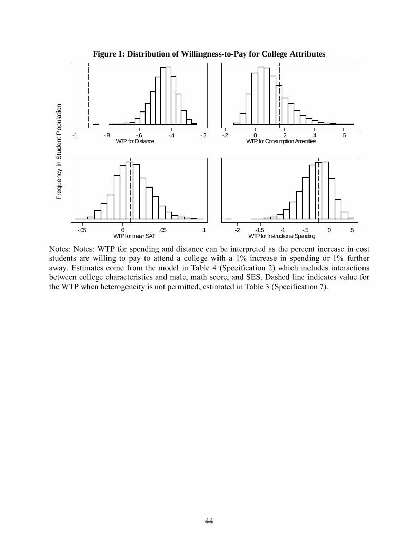
Figure 1: Distribution of Willingness-to-Pay for College Attributes
Notes: Notes: WTP for spending and distance can be interpreted as the percent increase in cost students are willing to pay to attend a college with a 1% increase in spending or 1% further away. Estimates come from the model in Table 4 (Specification 2) which includes interactions between college characteristics and male, math score, and SES. Dashed line indicates value for the WTP when heterogeneity is not permitted, estimated in Table 3 (Specification 7).
-1 -.8 -.6 -.4 -.2WTP for Distance
-.2 0 .2 .4 .6WTP for Consumption Amenities
-.05 0 .05 .1WTP for mean SAT
-2 -1.5 -1 -.5 0 .5WTP for Instructional Spending
Freq
uenc
y in
Stu
dent
Pop
ulat
ion
44
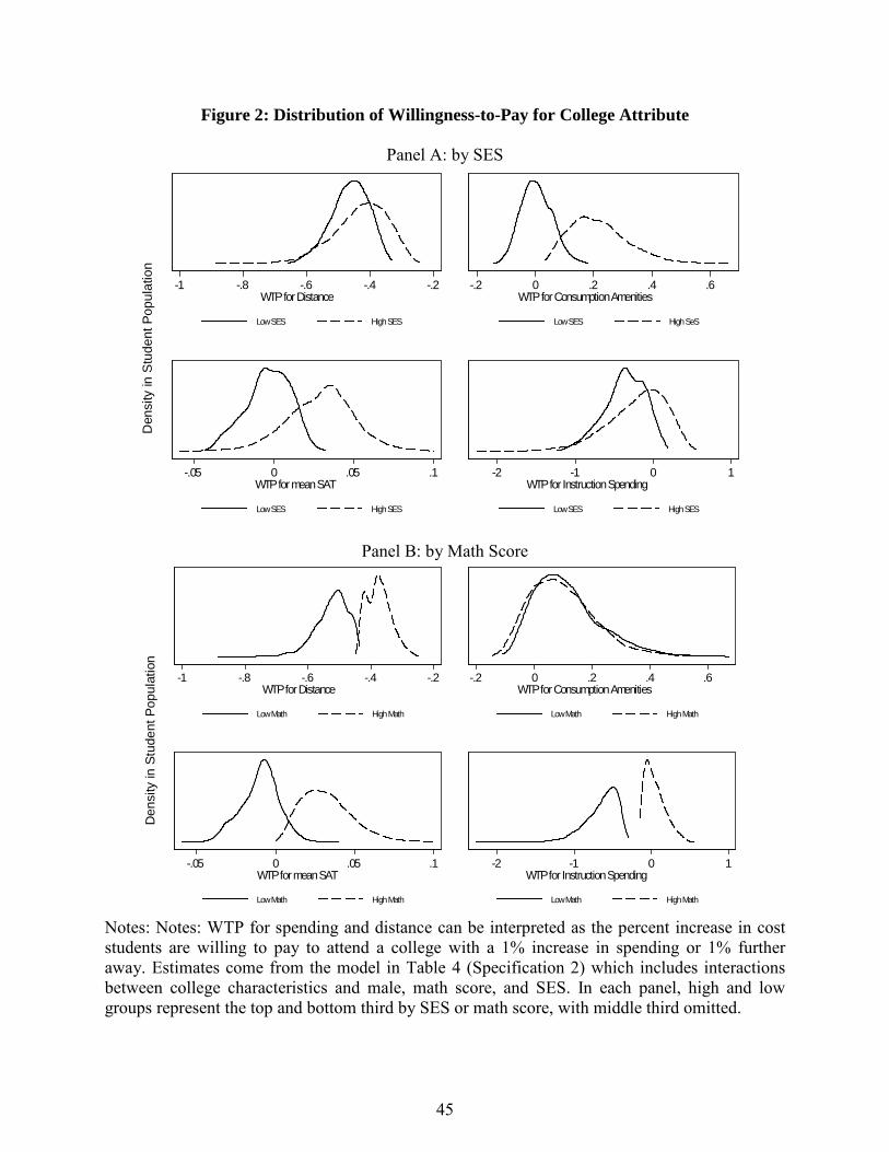
Figure 2: Distribution of Willingness-to-Pay for College Attribute
Panel A: by SES
Panel B: by Math Score
Notes: Notes: WTP for spending and distance can be interpreted as the percent increase in cost students are willing to pay to attend a college with a 1% increase in spending or 1% further away. Estimates come from the model in Table 4 (Specification 2) which includes interactions between college characteristics and male, math score, and SES. In each panel, high and low groups represent the top and bottom third by SES or math score, with middle third omitted.
-1 -.8 -.6 -.4 -.2WTP for Distance
Low SES High SES
-.2 0 .2 .4 .6WTP for Consumption Amenities
Low SES High SeS
-.05 0 .05 .1WTP for mean SAT
Low SES High SES
-2 -1 0 1WTP for Instruction Spending
Low SES High SES
Den
sity
in S
tude
nt P
opul
atio
n
-1 -.8 -.6 -.4 -.2WTP for Distance
Low Math High Math
-.2 0 .2 .4 .6WTP for Consumption Amenities
Low Math High Math
-.05 0 .05 .1WTP for mean SAT
Low Math High Math
-2 -1 0 1WTP for Instruction Spending
Low Math High Math
Den
sity
in S
tude
nt P
opul
atio
n
45
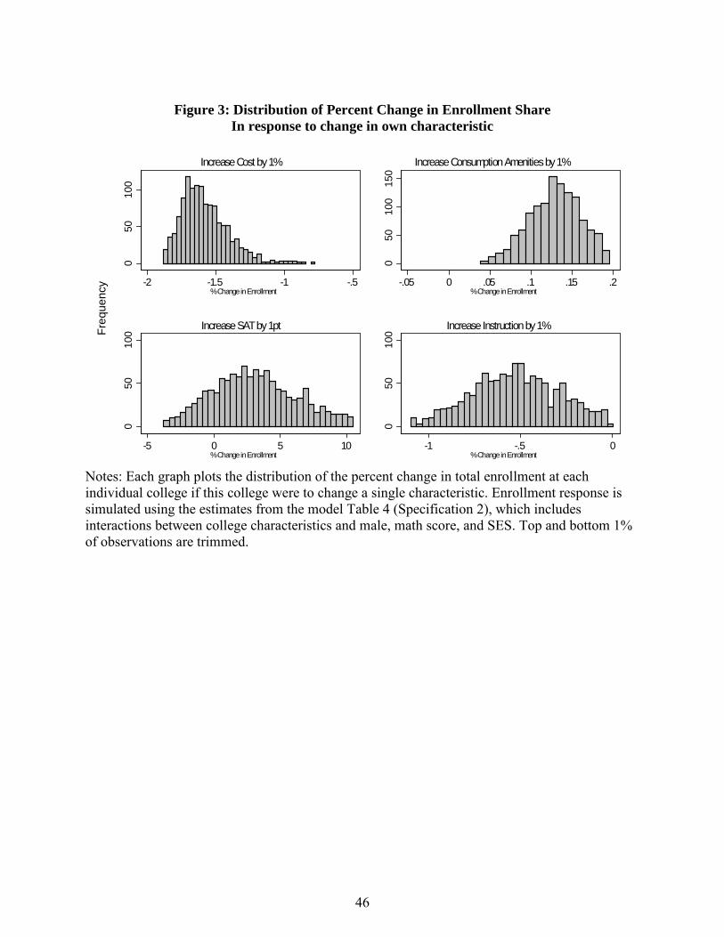
Figure 3: Distribution of Percent Change in Enrollment Share
In response to change in own characteristic
Notes: Each graph plots the distribution of the percent change in total enrollment at each individual college if this college were to change a single characteristic. Enrollment response is simulated using the estimates from the model Table 4 (Specification 2), which includes interactions between college characteristics and male, math score, and SES. Top and bottom 1% of observations are trimmed.
050
100
-2 -1.5 -1 -.5% Change in Enrollment
Increase Cost by 1%
050
100
-5 0 5 10% Change in Enrollment
Increase SAT by 1pt
050
100
150
-.05 0 .05 .1 .15 .2% Change in Enrollment
Increase Consumption Amenities by 1%
050
100
-1 -.5 0% Change in Enrollment
Increase Instruction by 1%Freq
uenc
y
46
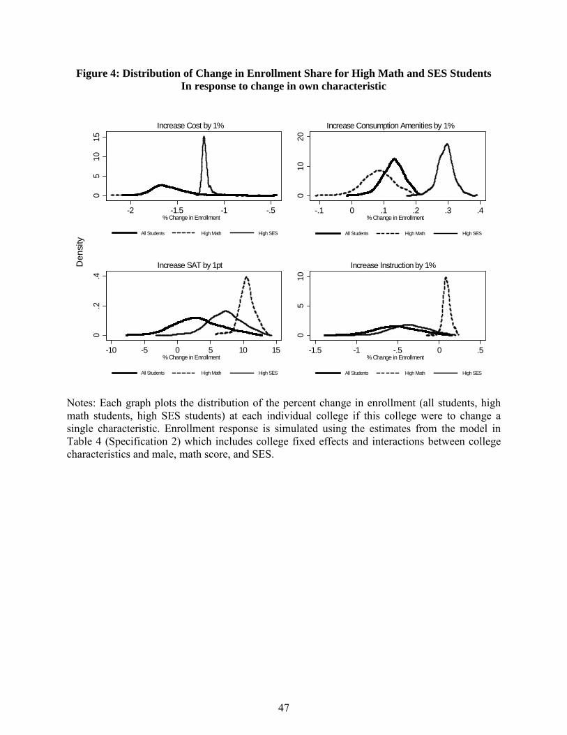
Figure 4: Distribution of Change in Enrollment Share for High Math and SES Students In response to change in own characteristic
Notes: Each graph plots the distribution of the percent change in enrollment (all students, high math students, high SES students) at each individual college if this college were to change a single characteristic. Enrollment response is simulated using the estimates from the model in Table 4 (Specification 2) which includes college fixed effects and interactions between college characteristics and male, math score, and SES.
05
1015
-2 -1.5 -1 -.5% Change in Enrollment
All Students High Math High SES
Increase Cost by 1%
0.2
.4
-10 -5 0 5 10 15% Change in Enrollment
All Students High Math High SES
Increase SAT by 1pt
010
20
-.1 0 .1 .2 .3 .4% Change in Enrollment
All Students High Math High SES
Increase Consumption Amenities by 1%
05
10
-1.5 -1 -.5 0 .5% Change in Enrollment
All Students High Math High SES
Increase Instruction by 1%Den
sity
47
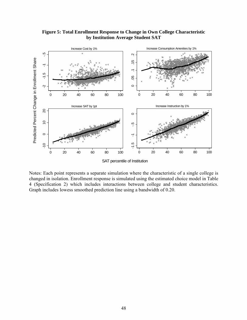
Figure 5: Total Enrollment Response to Change in Own College Characteristic by Institution Average Student SAT
Notes: Each point represents a separate simulation where the characteristic of a single college is changed in isolation. Enrollment response is simulated using the estimated choice model in Table 4 (Specification 2) which includes interactions between college and student characteristics. Graph includes lowess smoothed prediction line using a bandwidth of 0.20.
-2-1
.5-1
-.5
0 20 40 60 80 100
Increase Cost by 1%
0.0
5.1
.15
.2
0 20 40 60 80 100
Increase Consumption Amenities by 1%-1
00
1020
0 20 40 60 80 100
Increase SAT by 1pt
-1.5
-1-.5
0
0 20 40 60 80 100
Increase Instruction by 1%
Pre
dict
ed P
erce
nt C
hang
e in
Enr
ollm
ent S
hare
SAT percentile of Institution
48
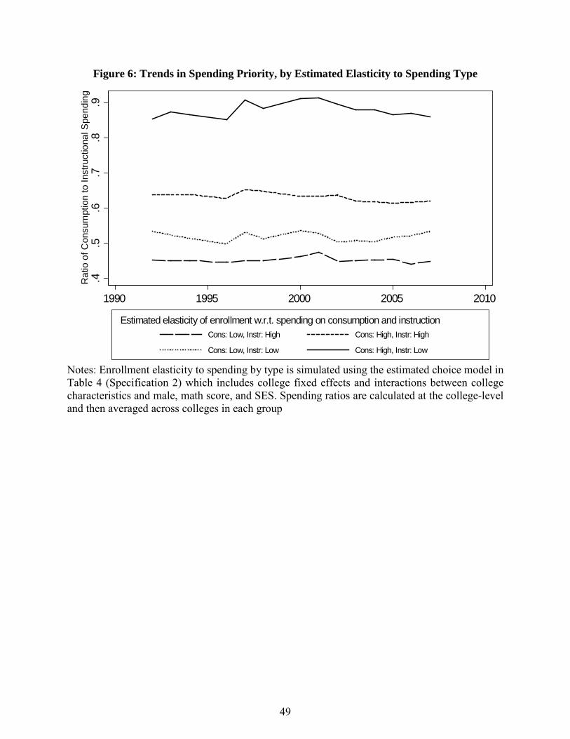
Figure 6: Trends in Spending Priority, by Estimated Elasticity to Spending Type
Notes: Enrollment elasticity to spending by type is simulated using the estimated choice model in Table 4 (Specification 2) which includes college fixed effects and interactions between college characteristics and male, math score, and SES. Spending ratios are calculated at the college-level and then averaged across colleges in each group
.4.5
.6.7
.8.9
Rat
io o
f Con
sum
ptio
n to
Inst
ruct
iona
l Spe
ndin
g
1990 1995 2000 2005 2010
Cons: Low, Instr: High Cons: High, Instr: High
Cons: Low, Instr: Low Cons: High, Instr: Low
Estimated elasticity of enrollment w.r.t. spending on consumption and instruction
49
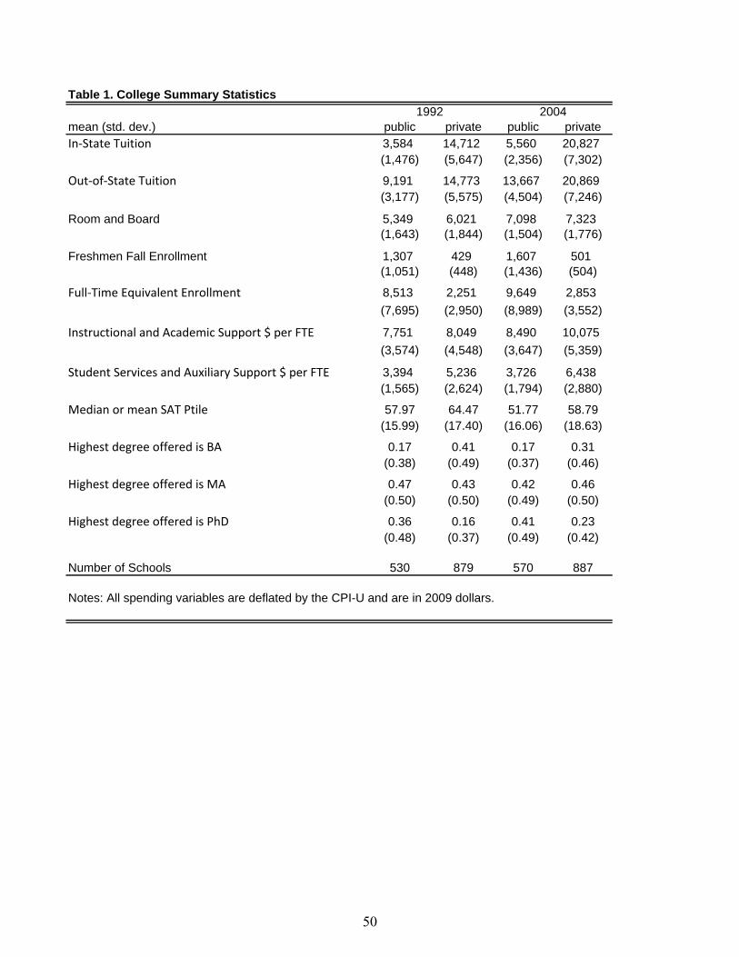
Table 1. College Summary Statistics
mean (std. dev.) public private public privateIn‐State Tuition 3,584 14,712 5,560 20,827
(1,476) (5,647) (2,356) (7,302)
Out‐of‐State Tuition 9,191 14,773 13,667 20,869(3,177) (5,575) (4,504) (7,246)
Room and Board 5,349 6,021 7,098 7,323(1,643) (1,844) (1,504) (1,776)
Freshmen Fall Enrollment 1,307 429 1,607 501(1,051) (448) (1,436) (504)
Full‐Time Equivalent Enrollment 8,513 2,251 9,649 2,853(7,695) (2,950) (8,989) (3,552)
Instructional and Academic Support $ per FTE 7,751 8,049 8,490 10,075(3,574) (4,548) (3,647) (5,359)
Student Services and Auxiliary Support $ per FTE 3,394 5,236 3,726 6,438(1,565) (2,624) (1,794) (2,880)
Median or mean SAT Ptile 57.97 64.47 51.77 58.79(15.99) (17.40) (16.06) (18.63)
Highest degree offered is BA 0.17 0.41 0.17 0.31(0.38) (0.49) (0.37) (0.46)
Highest degree offered is MA 0.47 0.43 0.42 0.46(0.50) (0.50) (0.49) (0.50)
Highest degree offered is PhD 0.36 0.16 0.41 0.23(0.48) (0.37) (0.49) (0.42)
Number of Schools 530 879 570 887
1992 2004
Notes: All spending variables are deflated by the CPI-U and are in 2009 dollars.
50
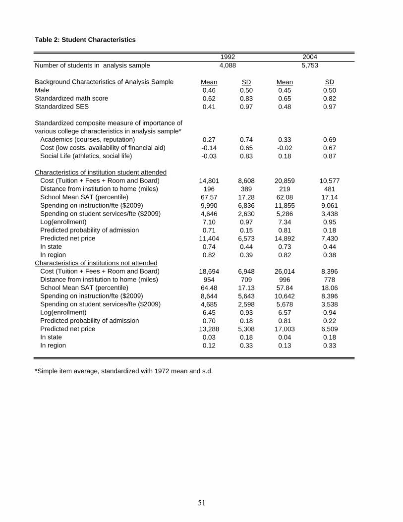
Table 2: Student Characteristics
Number of students in analysis sample
Background Characteristics of Analysis Sample Mean SD Mean SDMale 0.46 0.50 0.45 0.50Standardized math score 0.62 0.83 0.65 0.82Standardized SES 0.41 0.97 0.48 0.97
Standardized composite measure of importance of various college characteristics in analysis sample*
Academics (courses, reputation) 0.27 0.74 0.33 0.69Cost (low costs, availability of financial aid) -0.14 0.65 -0.02 0.67Social Life (athletics, social life) -0.03 0.83 0.18 0.87
Characteristics of institution student attendedCost (Tuition + Fees + Room and Board) 14,801 8,608 20,859 10,577Distance from institution to home (miles) 196 389 219 481School Mean SAT (percentile) 67.57 17.28 62.08 17.14Spending on instruction/fte ($2009) 9,990 6,836 11,855 9,061Spending on student services/fte ($2009) 4,646 2,630 5,286 3,438Log(enrollment) 7.10 0.97 7.34 0.95Predicted probability of admission 0.71 0.15 0.81 0.18Predicted net price 11,404 6,573 14,892 7,430In state 0.74 0.44 0.73 0.44In region 0.82 0.39 0.82 0.38
Characteristics of institutions not attendedCost (Tuition + Fees + Room and Board) 18,694 6,948 26,014 8,396Distance from institution to home (miles) 954 709 996 778School Mean SAT (percentile) 64.48 17.13 57.84 18.06Spending on instruction/fte ($2009) 8,644 5,643 10,642 8,396Spending on student services/fte ($2009) 4,685 2,598 5,678 3,538Log(enrollment) 6.45 0.93 6.57 0.94Predicted probability of admission 0.70 0.18 0.81 0.22Predicted net price 13,288 5,308 17,003 6,509In state 0.03 0.18 0.04 0.18In region 0.12 0.33 0.13 0.33
1992 20044,088 5,753
*Simple item average, standardized with 1972 mean and s.d.
51
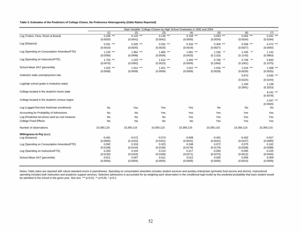
Table 3: Estimates of the Predictors of College Choice, No Preference Heterogeneity (Odds Ratios Reported)
(1) (2) (3) (4) (5) (6) (7)Log (Tuition, Fees, Room & Board) 0.106 *** 0.143 *** 0.145 *** 0.158 *** 0.053 *** 0.054 *** 0.441 ***
(0.0025) (0.0041) (0.0042) (0.0055) (0.0034) (0.0034) (0.0294)Log (Distance) 0.331 *** 0.329 *** 0.331 *** 0.326 *** 0.309 *** 0.308 *** 0.472 ***
(0.0019) (0.0020) (0.0020) (0.0019) (0.0027) (0.0027) (0.0050)Log (Spending on Consumption Amenities/FTE) 1.229 *** 1.854 *** 1.865 *** 1.581 *** 1.236 ** 1.245 ** 1.142
(0.0269) (0.0499) (0.0509) (0.0433) (0.1133) (0.1143) (0.0963)Log (Spending on Instruction/FTE) 1.753 *** 1.223 *** 1.512 *** 1.493 *** 0.760 ** 0.758 ** 0.832
(0.0476) (0.0392) (0.0515) (0.0509) (0.1064) (0.1061) (0.1075)School Mean SAT (percentile) 1.025 *** 1.014 *** 1.021 *** 1.022 *** 1.016 *** 1.016 *** 1.008 ***
(0.0008) (0.0009) (0.0009) (0.0009) (0.0028) (0.0029) (0.0025)Institution state unemployment rate 0.970 0.935 ***
(0.0224) (0.0244)Log(high school grads in institution state) 1.165 1.138
(0.2841) (0.3253)College located in the student's home state 8.242 ***
(0.4078)College located in the student's census region 2.047 ***
(0.0920)Log (Lagged first time freshman enrollment) No Yes Yes Yes No No No
Accounting for Probability of Admissions No No Yes Yes Yes Yes YesLog (Predicted net price) used as cost measure No No No Yes Yes Yes YesCollege Fixed Effects No No No No Yes Yes Yes
Number of observations 10,350,115 10,350,115 10,350,115 10,350,115 10,350,115 10,350,115 10,350,115
Willingness-to-Pay (s.e.)Log (Distance) -0.491 -0.572 -0.573 -0.608 -0.401 -0.402 -0.917
(0.0065) (0.1010) (0.0101) (0.0041) (0.0041) (0.0107) (0.0089)Log (Spending on Consumption Amenities/FTE) 0.092 0.318 0.323 0.248 0.072 0.075 0.162
(0.0108) (0.0144) (0.0146) (0.0179) (0.0179) (0.0338) (0.0288)Log (Spending on Instruction/FTE) 0.250 0.104 0.214 0.217 -0.094 -0.095 -0.225
(0.0130) (0.0163) (0.0169) (0.0271) (0.0270) (0.0512) (0.0440)School Mean SAT (percentile) 0.011 0.007 0.011 0.012 0.005 0.006 0.009
(0.0004) (0.0004) (0.0005) (0.0005) (0.0005) (0.0010) (0.0009)
Dept Variable: College Chosen by High School Graduates in 1992 and 2004
Notes: Odds ratios are reported with robust standard errors in parentheses. Spending on consumption amenities includes student services and auxilary enterprises (primarily food service and dorms). Instructional spending includes both instruction and academic support services. Selective admissions is accounded for by weighing each observation in the conditional logit model by the predicted probability that each student would be admitted to the school in the given year. See text. *** p<0.01, ** p<0.05, * p<0.1
52
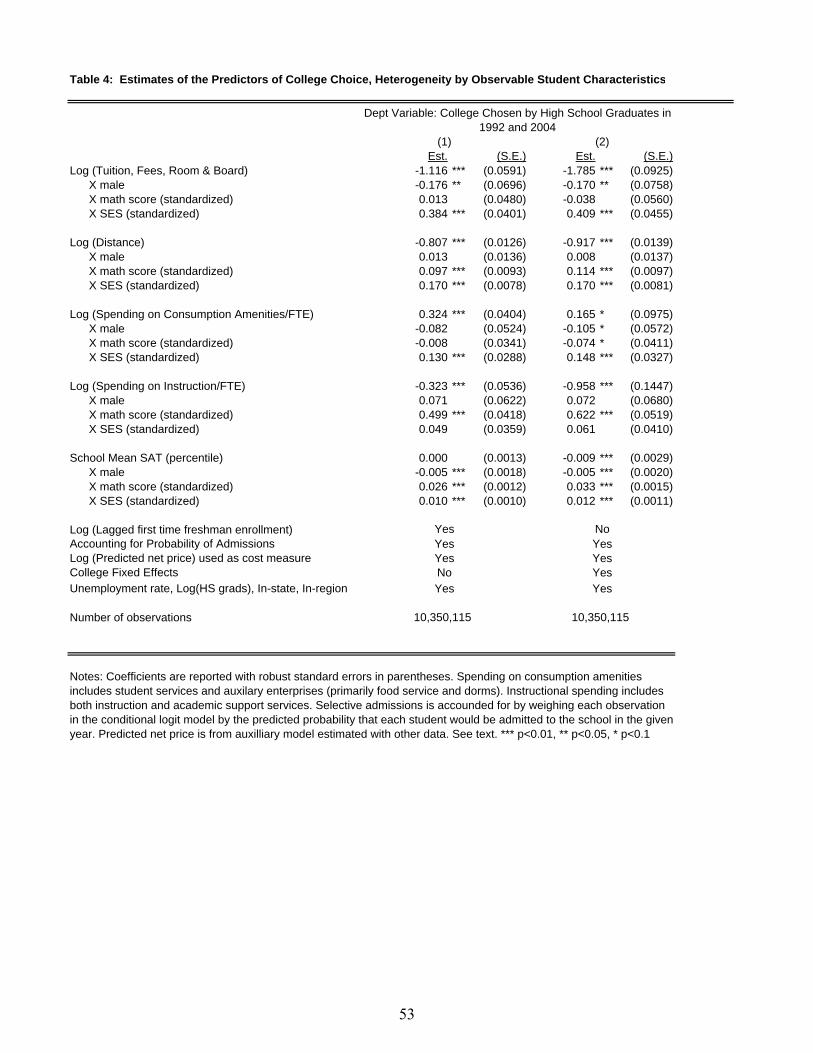
Table 4: Estimates of the Predictors of College Choice, Heterogeneity by Observable Student Characteristics
Est. (S.E.) Est. (S.E.)Log (Tuition, Fees, Room & Board) -1.116 *** (0.0591) -1.785 *** (0.0925)
X male -0.176 ** (0.0696) -0.170 ** (0.0758)X math score (standardized) 0.013 (0.0480) -0.038 (0.0560)X SES (standardized) 0.384 *** (0.0401) 0.409 *** (0.0455)
Log (Distance) -0.807 *** (0.0126) -0.917 *** (0.0139)X male 0.013 (0.0136) 0.008 (0.0137)X math score (standardized) 0.097 *** (0.0093) 0.114 *** (0.0097)X SES (standardized) 0.170 *** (0.0078) 0.170 *** (0.0081)
Log (Spending on Consumption Amenities/FTE) 0.324 *** (0.0404) 0.165 * (0.0975)X male -0.082 (0.0524) -0.105 * (0.0572)X math score (standardized) -0.008 (0.0341) -0.074 * (0.0411)X SES (standardized) 0.130 *** (0.0288) 0.148 *** (0.0327)
Log (Spending on Instruction/FTE) -0.323 *** (0.0536) -0.958 *** (0.1447)X male 0.071 (0.0622) 0.072 (0.0680)X math score (standardized) 0.499 *** (0.0418) 0.622 *** (0.0519)X SES (standardized) 0.049 (0.0359) 0.061 (0.0410)
School Mean SAT (percentile) 0.000 (0.0013) -0.009 *** (0.0029)X male -0.005 *** (0.0018) -0.005 *** (0.0020)X math score (standardized) 0.026 *** (0.0012) 0.033 *** (0.0015)X SES (standardized) 0.010 *** (0.0010) 0.012 *** (0.0011)
Log (Lagged first time freshman enrollment)Accounting for Probability of AdmissionsLog (Predicted net price) used as cost measureCollege Fixed EffectsUnemployment rate, Log(HS grads), In-state, In-region
Number of observations 10,350,115 10,350,115
Notes: Coefficients are reported with robust standard errors in parentheses. Spending on consumption amenities includes student services and auxilary enterprises (primarily food service and dorms). Instructional spending includes both instruction and academic support services. Selective admissions is accounded for by weighing each observation in the conditional logit model by the predicted probability that each student would be admitted to the school in the given year. Predicted net price is from auxilliary model estimated with other data. See text. *** p<0.01, ** p<0.05, * p<0.1
No Yes
Dept Variable: College Chosen by High School Graduates in 1992 and 2004
Yes Yes
Yes Yes
(1) (2)
Yes NoYes Yes
53
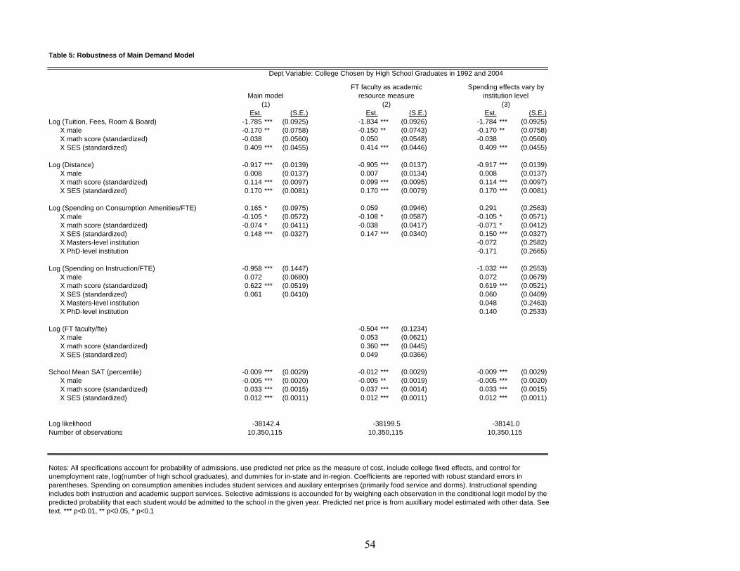
Table 5: Robustness of Main Demand Model
Est. (S.E.) Est. (S.E.) Est. (S.E.)Log (Tuition, Fees, Room & Board) -1.785 *** (0.0925) -1.834 *** (0.0926) -1.784 *** (0.0925)
X male -0.170 ** (0.0758) -0.150 ** (0.0743) -0.170 ** (0.0758)X math score (standardized) -0.038 (0.0560) 0.050 (0.0548) -0.038 (0.0560)X SES (standardized) 0.409 *** (0.0455) 0.414 *** (0.0446) 0.409 *** (0.0455)
Log (Distance) -0.917 *** (0.0139) -0.905 *** (0.0137) -0.917 *** (0.0139)X male 0.008 (0.0137) 0.007 (0.0134) 0.008 (0.0137)X math score (standardized) 0.114 *** (0.0097) 0.099 *** (0.0095) 0.114 *** (0.0097)X SES (standardized) 0.170 *** (0.0081) 0.170 *** (0.0079) 0.170 *** (0.0081)
Log (Spending on Consumption Amenities/FTE) 0.165 * (0.0975) 0.059 (0.0946) 0.291 (0.2563)X male -0.105 * (0.0572) -0.108 * (0.0587) -0.105 * (0.0571)X math score (standardized) -0.074 * (0.0411) -0.038 (0.0417) -0.071 * (0.0412)X SES (standardized) 0.148 *** (0.0327) 0.147 *** (0.0340) 0.150 *** (0.0327)X Masters-level institution -0.072 (0.2582)X PhD-level institution -0.171 (0.2665)
Log (Spending on Instruction/FTE) -0.958 *** (0.1447) -1.032 *** (0.2553)X male 0.072 (0.0680) 0.072 (0.0679)X math score (standardized) 0.622 *** (0.0519) 0.619 *** (0.0521)X SES (standardized) 0.061 (0.0410) 0.060 (0.0409)X Masters-level institution 0.048 (0.2463)X PhD-level institution 0.140 (0.2533)
Log (FT faculty/fte) -0.504 *** (0.1234)X male 0.053 (0.0621)X math score (standardized) 0.360 *** (0.0445)X SES (standardized) 0.049 (0.0366)
School Mean SAT (percentile) -0.009 *** (0.0029) -0.012 *** (0.0029) -0.009 *** (0.0029)X male -0.005 *** (0.0020) -0.005 ** (0.0019) -0.005 *** (0.0020)X math score (standardized) 0.033 *** (0.0015) 0.037 *** (0.0014) 0.033 *** (0.0015)X SES (standardized) 0.012 *** (0.0011) 0.012 *** (0.0011) 0.012 *** (0.0011)
Log likelihoodNumber of observations
Dept Variable: College Chosen by High School Graduates in 1992 and 2004
10,350,115
Notes: All specifications account for probability of admissions, use predicted net price as the measure of cost, include college fixed effects, and control for unemployment rate, log(number of high school graduates), and dummies for in-state and in-region. Coefficients are reported with robust standard errors in parentheses. Spending on consumption amenities includes student services and auxilary enterprises (primarily food service and dorms). Instructional spending includes both instruction and academic support services. Selective admissions is accounded for by weighing each observation in the conditional logit model by the predicted probability that each student would be admitted to the school in the given year. Predicted net price is from auxilliary model estimated with other data. See text. *** p<0.01, ** p<0.05, * p<0.1
-38142.4
Main model(1)
FT faculty as academic resource measure
Spending effects vary by institution level
(2) (3)
10,350,115 10,350,115-38199.5 -38141.0
54
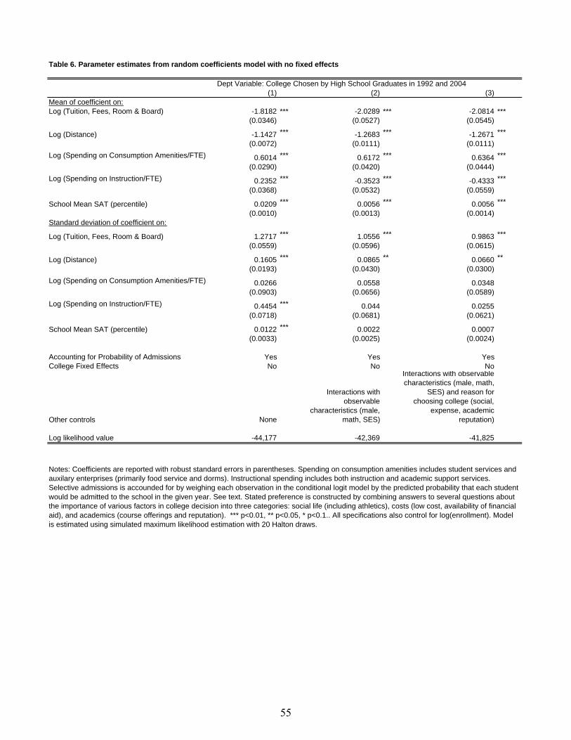
Table 6. Parameter estimates from random coefficients model with no fixed effects
Dept Variable: College Chosen by High School Graduates in 1992 and 2004(1) (2) (3)
Mean of coefficient on:Log (Tuition, Fees, Room & Board) -1.8182 *** -2.0289 *** -2.0814 ***
(0.0346) (0.0527) (0.0545)
Log (Distance) -1.1427 *** -1.2683 *** -1.2671 ***(0.0072) (0.0111) (0.0111)
Log (Spending on Consumption Amenities/FTE) 0.6014 *** 0.6172 *** 0.6364 ***(0.0290) (0.0420) (0.0444)
Log (Spending on Instruction/FTE) 0.2352 *** -0.3523 *** -0.4333 ***(0.0368) (0.0532) (0.0559)
School Mean SAT (percentile) 0.0209 *** 0.0056 *** 0.0056 ***(0.0010) (0.0013) (0.0014)
Standard deviation of coefficient on:
Log (Tuition, Fees, Room & Board) 1.2717 *** 1.0556 *** 0.9863 ***(0.0559) (0.0596) (0.0615)
Log (Distance) 0.1605 *** 0.0865 ** 0.0660 **(0.0193) (0.0430) (0.0300)
Log (Spending on Consumption Amenities/FTE) 0.0266 0.0558 0.0348(0.0903) (0.0656) (0.0589)
Log (Spending on Instruction/FTE) 0.4454 *** 0.044 0.0255(0.0718) (0.0681) (0.0621)
School Mean SAT (percentile) 0.0122 *** 0.0022 0.0007(0.0033) (0.0025) (0.0024)
Accounting for Probability of Admissions Yes Yes YesCollege Fixed Effects No No No
Other controls None
Interactions with observable
characteristics (male, math, SES)
Interactions with observable characteristics (male, math,
SES) and reason for choosing college (social,
expense, academic reputation)
Log likelihood value -44,177 -42,369 -41,825
Notes: Coefficients are reported with robust standard errors in parentheses. Spending on consumption amenities includes student services and auxilary enterprises (primarily food service and dorms). Instructional spending includes both instruction and academic support services. Selective admissions is accounded for by weighing each observation in the conditional logit model by the predicted probability that each student would be admitted to the school in the given year. See text. Stated preference is constructed by combining answers to several questions about the importance of various factors in college decision into three categories: social life (including athletics), costs (low cost, availability of financial aid), and academics (course offerings and reputation). *** p<0.01, ** p<0.05, * p<0.1.. All specifications also control for log(enrollment). Model is estimated using simulated maximum likelihood estimation with 20 Halton draws.
55
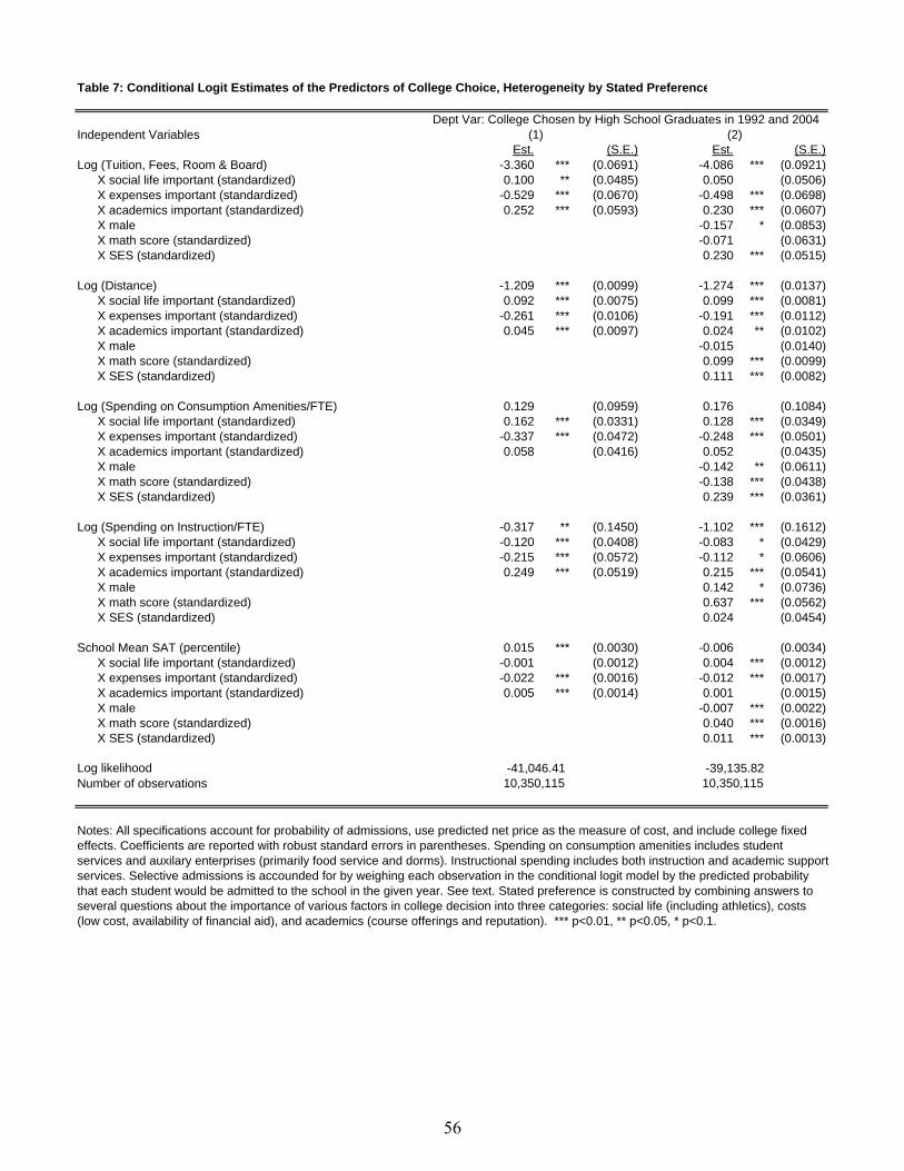
Table 7: Conditional Logit Estimates of the Predictors of College Choice, Heterogeneity by Stated Preference
Dept Var: College Chosen by High School Graduates in 1992 and 2004Independent Variables
Est. (S.E.) Est. (S.E.)Log (Tuition, Fees, Room & Board) -3.360 *** (0.0691) -4.086 *** (0.0921)
X social life important (standardized) 0.100 ** (0.0485) 0.050 (0.0506)X expenses important (standardized) -0.529 *** (0.0670) -0.498 *** (0.0698)X academics important (standardized) 0.252 *** (0.0593) 0.230 *** (0.0607)X male -0.157 * (0.0853)X math score (standardized) -0.071 (0.0631)X SES (standardized) 0.230 *** (0.0515)
Log (Distance) -1.209 *** (0.0099) -1.274 *** (0.0137)X social life important (standardized) 0.092 *** (0.0075) 0.099 *** (0.0081)X expenses important (standardized) -0.261 *** (0.0106) -0.191 *** (0.0112)X academics important (standardized) 0.045 *** (0.0097) 0.024 ** (0.0102)X male -0.015 (0.0140)X math score (standardized) 0.099 *** (0.0099)X SES (standardized) 0.111 *** (0.0082)
Log (Spending on Consumption Amenities/FTE) 0.129 (0.0959) 0.176 (0.1084)X social life important (standardized) 0.162 *** (0.0331) 0.128 *** (0.0349)X expenses important (standardized) -0.337 *** (0.0472) -0.248 *** (0.0501)X academics important (standardized) 0.058 (0.0416) 0.052 (0.0435)X male -0.142 ** (0.0611)X math score (standardized) -0.138 *** (0.0438)X SES (standardized) 0.239 *** (0.0361)
Log (Spending on Instruction/FTE) -0.317 ** (0.1450) -1.102 *** (0.1612)X social life important (standardized) -0.120 *** (0.0408) -0.083 * (0.0429)X expenses important (standardized) -0.215 *** (0.0572) -0.112 * (0.0606)X academics important (standardized) 0.249 *** (0.0519) 0.215 *** (0.0541)X male 0.142 * (0.0736)X math score (standardized) 0.637 *** (0.0562)X SES (standardized) 0.024 (0.0454)
School Mean SAT (percentile) 0.015 *** (0.0030) -0.006 (0.0034)X social life important (standardized) -0.001 (0.0012) 0.004 *** (0.0012)X expenses important (standardized) -0.022 *** (0.0016) -0.012 *** (0.0017)X academics important (standardized) 0.005 *** (0.0014) 0.001 (0.0015)X male -0.007 *** (0.0022)X math score (standardized) 0.040 *** (0.0016)X SES (standardized) 0.011 *** (0.0013)
Log likelihoodNumber of observations
(1)
Notes: All specifications account for probability of admissions, use predicted net price as the measure of cost, and include college fixed effects. Coefficients are reported with robust standard errors in parentheses. Spending on consumption amenities includes student services and auxilary enterprises (primarily food service and dorms). Instructional spending includes both instruction and academic support services. Selective admissions is accounded for by weighing each observation in the conditional logit model by the predicted probability that each student would be admitted to the school in the given year. See text. Stated preference is constructed by combining answers to several questions about the importance of various factors in college decision into three categories: social life (including athletics), costs (low cost, availability of financial aid), and academics (course offerings and reputation). *** p<0.01, ** p<0.05, * p<0.1.
(2)
10,350,115 10,350,115-41,046.41 -39,135.82
56
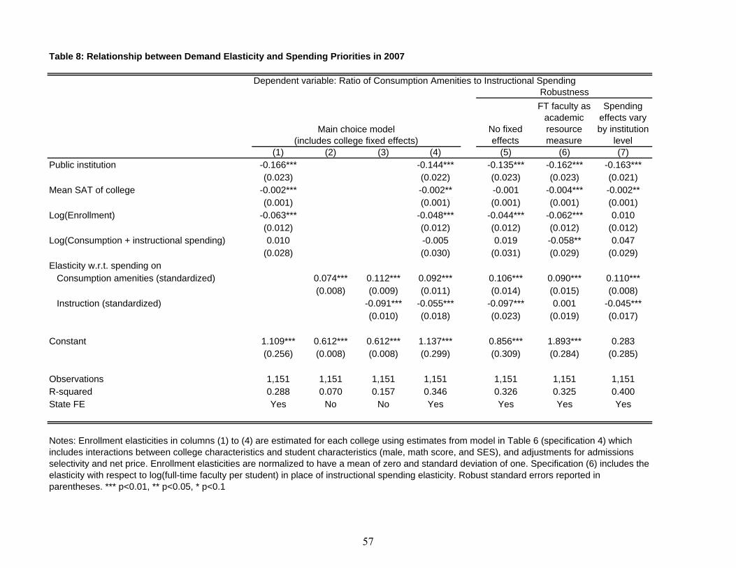
Table 8: Relationship between Demand Elasticity and Spending Priorities in 2007
Dependent variable: Ratio of Consumption Amenities to Instructional Spending
No fixed effects
FT faculty as academic resource measure
Spending effects vary by institution
level(1) (2) (3) (4) (5) (6) (7)
Public institution -0.166*** -0.144*** -0.135*** -0.162*** -0.163***(0.023) (0.022) (0.023) (0.023) (0.021)
Mean SAT of college -0.002*** -0.002** -0.001 -0.004*** -0.002**(0.001) (0.001) (0.001) (0.001) (0.001)
Log(Enrollment) -0.063*** -0.048*** -0.044*** -0.062*** 0.010(0.012) (0.012) (0.012) (0.012) (0.012)
Log(Consumption + instructional spending) 0.010 -0.005 0.019 -0.058** 0.047(0.028) (0.030) (0.031) (0.029) (0.029)
Elasticity w.r.t. spending onConsumption amenities (standardized) 0.074*** 0.112*** 0.092*** 0.106*** 0.090*** 0.110***
(0.008) (0.009) (0.011) (0.014) (0.015) (0.008)Instruction (standardized) -0.091*** -0.055*** -0.097*** 0.001 -0.045***
(0.010) (0.018) (0.023) (0.019) (0.017)
Constant 1.109*** 0.612*** 0.612*** 1.137*** 0.856*** 1.893*** 0.283(0.256) (0.008) (0.008) (0.299) (0.309) (0.284) (0.285)
Observations 1,151 1,151 1,151 1,151 1,151 1,151 1,151R-squared 0.288 0.070 0.157 0.346 0.326 0.325 0.400State FE Yes No No Yes Yes Yes Yes
Notes: Enrollment elasticities in columns (1) to (4) are estimated for each college using estimates from model in Table 6 (specification 4) which includes interactions between college characteristics and student characteristics (male, math score, and SES), and adjustments for admissions selectivity and net price. Enrollment elasticities are normalized to have a mean of zero and standard deviation of one. Specification (6) includes the elasticity with respect to log(full-time faculty per student) in place of instructional spending elasticity. Robust standard errors reported in parentheses. *** p<0.01, ** p<0.05, * p<0.1
Main choice model (includes college fixed effects)
Robustness
57
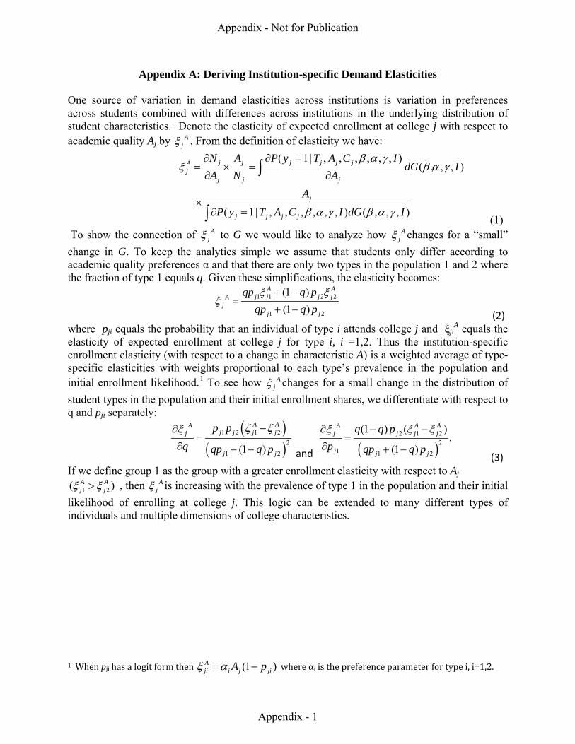
Appendix A: Deriving Institution-specific Demand Elasticities One source of variation in demand elasticities across institutions is variation in preferences across students combined with differences across institutions in the underlying distribution of student characteristics. Denote the elasticity of expected enrollment at college j with respect to academic quality Aj by A
jξ . From the definition of elasticity we have:
( 1| , , , , , , )( , , , )
( 1| , , , , , , ) ( , , , )
j j j j j jAj
j j j
j
j j j j
N A P y T A C IdG I
A N AA
P y T A C I dG I
β α γξ β α γ
β α γ β α γ
∂ ∂ == × =∂ ∂
×∂ =
∫
∫ (1)
To show the connection of Ajξ to G we would like to analyze how A
jξ changes for a “small” change in G. To keep the analytics simple we assume that students only differ according to academic quality preferences α and that there are only two types in the population 1 and 2 where the fraction of type 1 equals q. Given these simplifications, the elasticity becomes:
1 1 2 2
1 2
(1 )(1 )
A Aj j j jA
jj j
qp q pqp q pξ ξ
ξ+ −
=+ − (2)
where pji equals the probability that an individual of type i attends college j and ξjiA equals the
elasticity of expected enrollment at college j for type i, i =1,2. Thus the institution-specific enrollment elasticity (with respect to a change in characteristic A) is a weighted average of type-specific elasticities with weights proportional to each type’s prevalence in the population and initial enrollment likelihood.1 To see how A
jξ changes for a small change in the distribution of student types in the population and their initial enrollment shares, we differentiate with respect to q and pji separately:
( )( )
1 2 1 22
1 2(1 )
A AAj j j jj
j j
p pq qp q p
ξ ξξ −∂=
∂ − − and ( )2 1 2
21 1 2
(1 ) ( ).
(1 )
A A Aj j j j
j j j
q q pp qp q p
ξ ξ ξ∂ − −=
∂ + − (3)
If we define group 1 as the group with a greater enrollment elasticity with respect to Aj 1 2( )A A
j jξ ξ> , then Ajξ is increasing with the prevalence of type 1 in the population and their initial
likelihood of enrolling at college j. This logic can be extended to many different types of individuals and multiple dimensions of college characteristics.
1 When pji has a logit form then (1 )Aji i j jiA pξ α= − where αi is the preference parameter for type i, i=1,2.
Appendix - Not for Publication
Appendix - 1
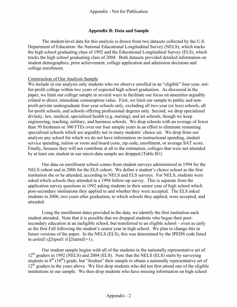
Appendix B: Data and Sample
The student-level data for this analysis is drawn from two datasets collected by the U.S. Department of Education: the National Educational Longitudinal Survey (NELS), which tracks the high school graduating class of 1992 and the Educational Longitudinal Survey (ELS), which tracks the high school graduating class of 2004. Both datasets provided detailed information on student demographics, prior achievement, college application and admission decisions and college enrollment.
Construction of Our Analysis Sample We include in our analysis only students who we observe enrolled in an “eligible” four-year, not-for-profit college within two years of expected high school graduation. As discussed in the paper, we limit our college sample in several ways to facilitate our focus on amenities arguably related to direct, immediate consumption value. First, we limit our sample to public and non-profit private undergraduate four-year schools only, excluding all two-year (or less) schools, all for-profit schools, and schools offering professional degrees only. Second, we drop specialized divinity, law, medical, specialized health (e.g. nursing), and art schools, though we keep engineering, teaching, military, and business schools. We drop schools with an average of fewer than 50 freshmen or 300 FTEs over our four sample years in an effort to eliminate remaining specialized schools which are arguably not in many students’ choice set. We drop from our analysis any school for which we do not have information on instructional spending, student service spending, tuition or room and board costs, zip code, enrollment, or average SAT score. Finally, because they will not contribute at all to the estimation, colleges that were not attended by at least one student in our micro-data sample are dropped (Table B1).
Our data on enrollment school comes from student surveys administered in 1994 for the
NELS cohort and in 2006 for the ELS cohort. We define a student’s choice school as the first institution she or he attended, according to NELS and ELS surveys. For NELS, students were asked which schools they attended in a 1994 follow-up survey. This is separate from the application survey questions in 1992 asking students in their senior year of high school which post-secondary institutions they applied to and whether they were accepted. The ELS asked students in 2006, two years after graduation, to which schools they applied, were accepted, and attended.
Using the enrollment dates provided in the data, we identify the first institution each
student attended. Note that it is possible that we dropped students who began their post-secondary education at an ineligible school, but transferred to an eligible school – even as early as the first Fall following the student’s senior year in high school. We plan to change this in future versions of the paper. In the NELS (ELS), this was determined by the IPEDS code listed in unitid1 (f2iiped1 if f2iattnd1=1).
Our student sample begins with all of the students in the nationally representative set of
12th graders in 1992 (NELS) and 2004 (ELS). Note that the NELS (ELS) starts by surveying students in 8th (10th) grade, but “freshen” their sample to obtain a nationally representative set of 12th graders in the years above. We first drop students who did not first attend one of the eligible institutions in our sample. We then drop students who have missing information on high school
Appendix - Not for Publication
Appendix - 2
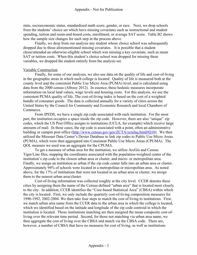
state, socioeconomic status, standardized math score, gender, or race. Next, we drop schools from the students’ choice set which have missing covariates such as instructional and student spending, tuition and room-and-board costs, enrollment, or average SAT score. Table B2 shows how the sample size changes for each step in the process above.
Finally, we drop from our analysis any student whose choice school was subsequently dropped due to those aforementioned missing covariates. It is possible that a student chose/attended an otherwise-eligible school which was missing a key covariate, such as mean SAT or tuition costs. When this student’s choice school was dropped for missing these variables, we dropped the student entirely from the analysis set. Variable Construction Finally, for some of our analyses, we also use data on the quality of life and cost-of-living in the geographic areas in which each college is located. Quality of life is measured both at the county level and the consistent Public Use Micro Area (PUMA) level, and is calculated using data from the 2000 census (Albouy 2012). In essence, these hedonic measures incorporate information on local land values, wage levels and housing costs. For this analysis, we use the consistent PUMA quality of life. The cost-of-living index is based on the cost of a weighted bundle of consumer goods. The data is collected annually for a variety of cities across the United States by the Council for Community and Economic Research and local Chambers of Commerce.
From IPEDS, we have a single zip code associated with each institution. For the most part, the institution occupies a space inside the zip code. However, there are also “unique” zip codes, which the US Post Office assigns to institutions (UCLA, for example) which receive large amounts of mail. In these cases, the zip code is associated with a point, often an administrative building or campus post office (http://www.census.gov/geo/ZCTA/zctafaq.html#Q10). We then utilized the Missouri Data Center’s Dexter Database to link zip codes to Public Use Micro Areas (PUMA), which were then aggregated into Consistent Public Use Micro Areas (CPUMA). The QOL measure we used was an aggregate for the CPUMA.
To get a measure of urban area for the institution, we utilize ArcGis and Census Tiger/Line files, mapping the coordinates associated with the population-weighted center of the institution’s zip code to the closest urban area or cluster, and micro- or metropolitan area. Finally, we assign an institution as urban if the zip code center falls into an urban area or cluster. Approximately 94% of schools were located in a metropolitan or micropolitan area. As noted above, for the 17% of institutions that were not located in an urban area or cluster, we assign them to the nearest urban area/cluster.
Cost-of-living information was collected roughly at the city level. CCER denotes these cities by assigning them the name of the Census-defined “urban area” that is located most closely to the city. In addition, CCER identifies the “Core-based Statistical Area” (CBSA) within which the city is located. First, we only include the quarterly cost-of-living composition measures for 1990-1992, 2002-2004. We then take four steps to match the cost of living to institutions. First, we match urban area name from the CCER data to the urban area in which the college is located, which we identified based on the latitude and longitude of the zip code centroid in which the institution is located. Those institutions matching are then assigned the mean composite cost-of-living over the relevant time period. Second, for those not matching via urban area name, we then aggregate the cost of living over the CBSA and match via the CBSA code. There are, however, a number of CBSA that have no measures for cost of living, as well as institutions
Appendix - Not for Publication
Appendix - 3

which are not located in a CBSA. Third, for those not matching via CBSA code, we match to the mean composite cost of living over the state. Finally, there are no cost-of-living measures for Maine (1992 and 2004) or Rhode Island (1992). Institutions in these states are assigned the mean composite over all New England states.
Appendix - Not for Publication
Appendix - 4
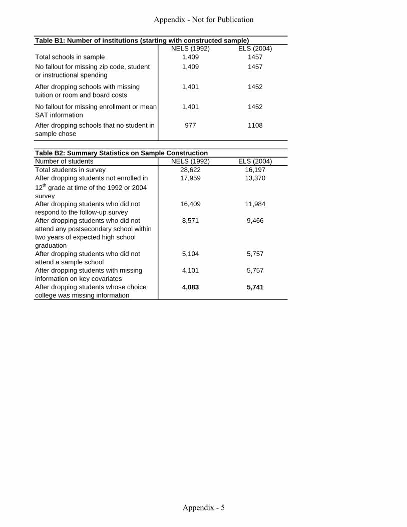
NELS (1992) ELS (2004)Total schools in sample 1,409 1457No fallout for missing zip code, student or instructional spending
1,409 1457
After dropping schools with missing tuition or room and board costs
1,401 1452
No fallout for missing enrollment or mean SAT information
1,401 1452
After dropping schools that no student in sample chose
977 1108
Table B2: Summary Statistics on Sample ConstructionNumber of students NELS (1992) ELS (2004)Total students in survey 28,622 16,197After dropping students not enrolled in 12th grade at time of the 1992 or 2004 survey
17,959 13,370
After dropping students who did not respond to the follow-up survey
16,409 11,984
After dropping students who did not attend any postsecondary school within two years of expected high school graduation
8,571 9,466
After dropping students who did not attend a sample school
5,104 5,757
After dropping students with missing information on key covariates
4,101 5,757
After dropping students whose choice college was missing information
4,083 5,741
Table B1: Number of institutions (starting with constructed sample)
Appendix - Not for Publication
Appendix - 5
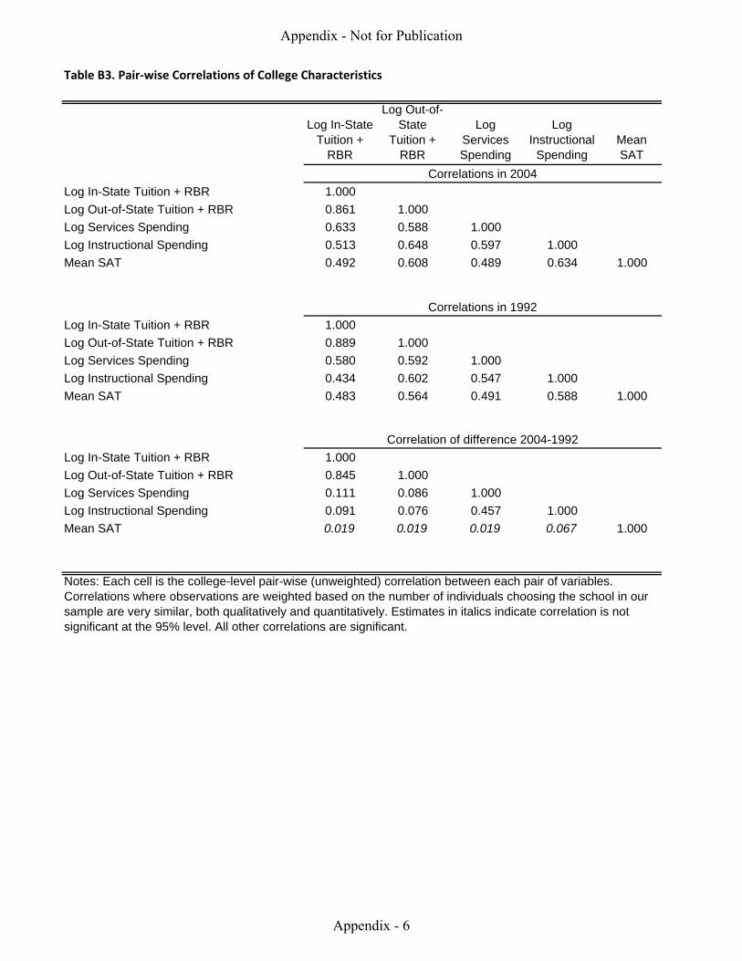
Table B3. Pair‐wise Correlations of College Characteristics
Log In-State Tuition +
RBR
Log Out-of-State
Tuition + RBR
Log Services Spending
Log Instructional
SpendingMean SAT
Log In-State Tuition + RBR 1.000Log Out-of-State Tuition + RBR 0.861 1.000Log Services Spending 0.633 0.588 1.000Log Instructional Spending 0.513 0.648 0.597 1.000Mean SAT 0.492 0.608 0.489 0.634 1.000
Log In-State Tuition + RBR 1.000Log Out-of-State Tuition + RBR 0.889 1.000Log Services Spending 0.580 0.592 1.000Log Instructional Spending 0.434 0.602 0.547 1.000Mean SAT 0.483 0.564 0.491 0.588 1.000
Log In-State Tuition + RBR 1.000Log Out-of-State Tuition + RBR 0.845 1.000Log Services Spending 0.111 0.086 1.000Log Instructional Spending 0.091 0.076 0.457 1.000Mean SAT 0.019 0.019 0.019 0.067 1.000
Correlations in 2004
Correlations in 1992
Correlation of difference 2004-1992
Notes: Each cell is the college-level pair-wise (unweighted) correlation between each pair of variables. Correlations where observations are weighted based on the number of individuals choosing the school in our sample are very similar, both qualitatively and quantitatively. Estimates in italics indicate correlation is not significant at the 95% level. All other correlations are significant.
Appendix - Not for Publication
Appendix - 6
Appendix C: Extension of Long (2004) and Cohort-Specific Estimates
To provide a direct comparison with previous work, we first extend the analysis of Long (2004) by including measures of college consumption amenities into her conditional logit specifications. In Table C1, the first two columns for each cohort year show her results (BTL) and our results (JMS) for a comparable specification side by side, indicating that we are able to successfully replicate her findings. It should be noted that our results should not be exactly comparable to hers since her estimation includes two-year colleges and students (which we exclude) and not all variables are interacted with sector in her model. The third column for each cohort adds three measures of consumption amenities to this basic model. We find that spending on student services and auxiliary enterprises have a large and statistically significant relationship with the likelihood of choosing a particular college, as does the presence of a division 1 basketball or football team and the fraction of students who join fraternities or sororities. The inclusion of these measures diminished the estimated importance of instructional expenditure.
Table C2 presents results from comparable models estimated separately by cohort, but using a specification that mirrors that used in main analysis. Table B2 shows the odds ratios and standard errors from our conditional logit model described above, separately for the 1992 and 2004 cohort. Following the prior literature, we include log enrollment to control for school size. Given the cross-sectional identification concerns raised in the previous section, we do not interpret these specifications as providing good estimates of preference parameters for student-invariant characteristics. Rather, this analysis provides a benchmark for subsequent analysis and illustrates the importance of including consumption amenities and accounting for selective admissions when estimating college choice models.
In columns 1 and 5, we see that tuition and distance are negatively associated with student choice while enrollment, instructional spending and mean SAT score are positively associated with choice. In columns 2 and 6, we add the log of per pupil spending on student services and auxiliary enterprises, which we argue measures the level of consumption amenities at the college. Conditional on the measures of cost, distance and academic quality, we see that spending on student services is a significant predictor of enrollment. Specifically, the odds ratio of 2.45 in column (2) indicates that a doubling of spending on student services is associated with a 145 percent increase in the likelihood a student will attend a given school in 1992. Note that the magnitude of this effect is even larger than the effect of instructional spending. Because school mean SAT and instructional spending are arguably closely related proxies for academic quality, in columns 3 and 7 we show results for a model that excludes school mean SAT. The odds ratio on instructional spending does increase, but spending on student services still remains a stronger predictor of enrollment than instructional spending.
As noted earlier, however, failing to account for whether a student would be accepted to a given school may bias estimates of the importance of college attributes. To account for selective admissions, the models shown in columns 4 and 8 weight each student-college observation by the predicted probability that the student would have been accepted to the college. As expected, the coefficients on both measures of academic quality – instructional spending and mean SAT – increase considerably. Failing to adequately account for selective admissions may bias estimates of students’ preferences for college attributes that are also related to admissions difficulty.
Appendix - Not for Publication
Appendix - 7
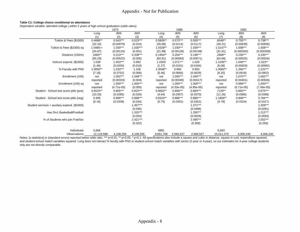
Table C1: College choice conditional on attendanceDependent variable: attended college j within 2 years of high school graduation (odds ratios)
Long JMS JMS Long JMS JMS Long JMS JMS(1) (2) (3) (4) (5) (6) (7) (8) (9)
Tuition & Fees ($1000) 0.4686** 0.543*** 0.523*** 0.5809** 0.573*** 0.555*** .6548** 0.755*** 0.738***[32.32] (0.00979) (0.010) [26.68] (0.0114) (0.0117) [39.21] (0.00639) (0.00656)
Tuition & Fees ($1000) sq 1.0485∗∗ 1.030*** 1.030*** 1.0328** 1.030*** 1.030*** 1.0147** 1.008*** 1.008***[24.87] (0.00116) (0.001) [21.98] (0.00128) (0.00138) [31.91] (0.000292) (0.000308)
Distance (100mi) .1665** 0.213*** 0.208*** 0.1954** 0.204*** 0.196*** .2668** 0.235*** 0.235***[65.29] (0.00522) (0.005) [60.91] (0.00583) (0.00571) [64.66] (0.00525) (0.00526)
Instruct expend. ($1000) 1.038 1.053*** 0.992 1.0303 1.071*** 1.029 1.1035** 1.040*** 1.023**[1.46] (0.0200) (0.019) [1.27] (0.0191) (0.0184) [6.08] (0.00929) (0.00992)
% Faculty with PhD 1.0050** 1.233*** 1.106 1.0048** 0.950 0.903 1.0060** 1.266*** 1.222***[7.18] (0.0752) (0.068) [5.46] (0.0656) (0.0629) [6.20] (0.0918) (0.0902)
Enrollment (100) not 1.052*** 1.048*** not 1.045*** 1.040*** not 1.070*** 1.062***reported (0.00333) (0.004) reported (0.00349) (0.00417) reported (0.00401) (0.00506)
Enrollment (100) sq not 1.000*** 1.000*** not 1.000*** 1.000*** not 0.999*** 1.000***reported (4.71e-05) (0.000) reported (4.33e-05) (4.95e-05) reported (6.71e-05) (7.56e-05)
Student - School test score ptile (pos) 0.6525** 0.805*** 0.815*** 0.8662** 0.858*** 0.883*** .7129** 0.850*** 0.875***[10.26] (0.0285) (0.029) [4.64] (0.0357) (0.0370) [11.26] (0.0385) (0.0398)
Student - School test score ptile (neg) 0.995 0.899*** 0.898*** 0.8324** 0.886*** 0.885*** 1.1809** 0.808*** 0.784***[0.16] (0.0338) (0.034) [5.75] (0.0352) (0.0352) [4.78] (0.0324) (0.0317)
Student services + auxilary expend. ($1000) 1.457*** 1.371*** 1.209***(0.045) (0.0496) (0.0281)
Has Div1 Basketball/Football 1.202*** 1.200*** 1.212***(0.054) (0.0629) (0.0593)
% of Students who join Frat/Sor 2.421*** 2.095*** 2.052***(0.322) (0.358) (0.293)
Individuals 5,666 4881 5,693Observations 12,118,588 4,108,256 4,108,256 9,651,768 2,566,527 2,566,527 15,011,370 4,006,240 4,006,240
1972 1980 1992
Notes: [z-statistics] or (standard errors) reported below odds ratio. *** p<0.01, ** p<0.05, * p<0.1. All specifications also include a square and cubic in distance, square in cost, expenditure squared, and student-school match variables squared. Long does not interact % faculty with PhD or student-school match variables with sector (2-year or 4-year), so our estimates for 4-year college students only are not directly comparable.
Appendix - Not for Publication
Appendix - 8
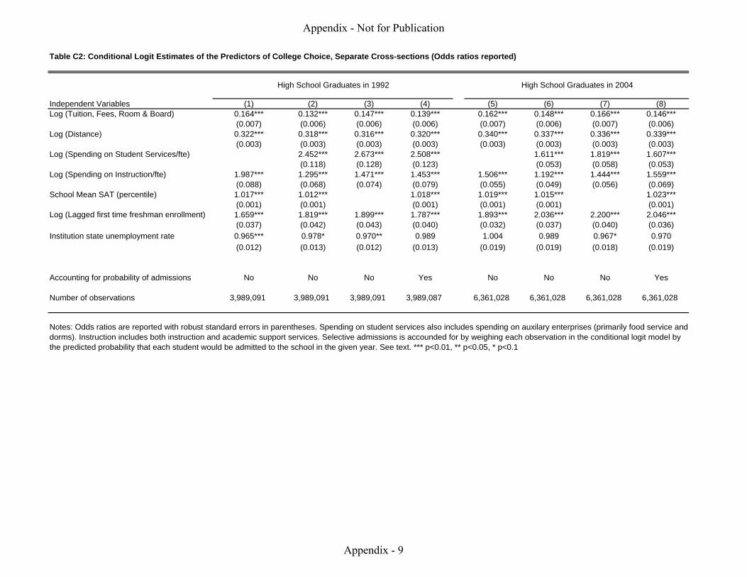
Table C2: Conditional Logit Estimates of the Predictors of College Choice, Separate Cross-sections (Odds ratios reported)
Independent Variables (1) (2) (3) (4) (5) (6) (7) (8)Log (Tuition, Fees, Room & Board) 0.164*** 0.132*** 0.147*** 0.139*** 0.162*** 0.148*** 0.166*** 0.146***
(0.007) (0.006) (0.006) (0.006) (0.007) (0.006) (0.007) (0.006)Log (Distance) 0.322*** 0.318*** 0.316*** 0.320*** 0.340*** 0.337*** 0.336*** 0.339***
(0.003) (0.003) (0.003) (0.003) (0.003) (0.003) (0.003) (0.003)Log (Spending on Student Services/fte) 2.452*** 2.673*** 2.508*** 1.611*** 1.819*** 1.607***
(0.118) (0.128) (0.123) (0.053) (0.058) (0.053)Log (Spending on Instruction/fte) 1.987*** 1.295*** 1.471*** 1.453*** 1.506*** 1.192*** 1.444*** 1.559***
(0.088) (0.068) (0.074) (0.079) (0.055) (0.049) (0.056) (0.069)School Mean SAT (percentile) 1.017*** 1.012*** 1.018*** 1.019*** 1.015*** 1.023***
(0.001) (0.001) (0.001) (0.001) (0.001) (0.001)Log (Lagged first time freshman enrollment) 1.659*** 1.819*** 1.899*** 1.787*** 1.893*** 2.036*** 2.200*** 2.046***
(0.037) (0.042) (0.043) (0.040) (0.032) (0.037) (0.040) (0.036)Institution state unemployment rate 0.965*** 0.978* 0.970** 0.989 1.004 0.989 0.967* 0.970
(0.012) (0.013) (0.012) (0.013) (0.019) (0.019) (0.018) (0.019)
Accounting for probability of admissions No No No Yes No No No Yes
Number of observations 3,989,091 3,989,091 3,989,091 3,989,087 6,361,028 6,361,028 6,361,028 6,361,028
High School Graduates in 1992 High School Graduates in 2004
Notes: Odds ratios are reported with robust standard errors in parentheses. Spending on student services also includes spending on auxilary enterprises (primarily food service and dorms). Instruction includes both instruction and academic support services. Selective admissions is accounded for by weighing each observation in the conditional logit model by the predicted probability that each student would be admitted to the school in the given year. See text. *** p<0.01, ** p<0.05, * p<0.1
Appendix - Not for Publication
Appendix - 9
Appendix D: Estimating the Probability of College Admissions
Both the NELS and ELS ask students to list colleges to which they applied and whether they were admitted to each college. We restrict our attention to student applications to the set of “regular” four-year colleges or universities in our main analysis sample. The resulting data set contains 22,934 (12,155) student-college observations from 2004 (1992). To determine the probability that individual i would be admitted to school j, we estimate probit models where the dependent variable is a binary indicator for admitted and the independent variables include student and school characteristics (and student x school interactions), including student race, gender, SES, high school GPA and standardized achievement scores along with measures of the school’s selectivity such as the average SAT score of students in the school. Admissions models are estimated separately by the triple interaction of race, sector, and in-state status. Using the coefficient estimates from these models, we predict the likelihood that student i would be admitted to each of the college in our sample (regardless of whether or not the student actually applied to the college).
In order to separate admissions from enrollment decisions, we must first estimate the probability that student i would have been admitted to college j (conditional on applying).
NELS and ELS both ask students to report which colleges they applied to and, among these, to which colleges they were admitted. In the NELS, students were asked in 1992 (when they were high school seniors) to list up to 2 schools to which they had applied and to indicate whether or not they had been accepted to each school. In the 1994 follow-up survey, students were asked to list up to 5 schools they had attended since the 1992 survey. In order to capture a more complete set of schools to which the student may have applied, we combine information from both of these surveys. Specifically, we include all schools the student listed in the 1992 survey as well as the first two schools we observe the students attending based on the information reported in the 1994 survey (this survey provides enrollment dates which allow us to identify the first two schools). In this way, we observe a maximum of four application schools for each student. Also note that, by construction, a student will have been accepted to any school we observe him or her attending by 1994. Table D1 (D2) shows the distribution of applications and acceptances for the NELS (ELS) sample. Note that for this analysis we are incorporating information on all schools to which a student applied, including many two-year colleges that are not included in our analysis sample of colleges.
In the ELS, students were asked in 2006 (two years after expected high school graduation) to list up to 20 schools to which they applied, and whether they were accepted and/or attended. It also allows them to list the start and end dates of attendance.
Note that less than 0.1% of students listed the maximum possible number of schools in ELS, suggesting that we are capturing the full set of application schools for most students. In NELS, by contrast, over half of the students listed two different application schools in the 1992 survey, suggesting that even by including the extra information from the 1994 survey, we are likely missing at least some information on student application behavior.
We then estimate Probit models of the probability that student i was admitted to school j. In order to allow the admission function to vary across groups, we estimate separate models for each cohort year, and then within cohort year, we estimate separate models for six mutually exclusive set of student-school observations: 1) White or Asian students applying to in-state public colleges, 2) White or Asian students applying to out-state public colleges, 3) White or Asian students applying to private colleges, 4) other students applying to in-state public
Appendix - Not for Publication
Appendix - 10
colleges, 5) other students applying to out-state public colleges, 6) other students applying to private colleges. We estimate separate models for racial minorities to allow for affirmative action policies. We estimate separate models for different school types to allow for admission preferences for in-state students in public universities and different admissions procedures in private colleges.
As predictors, we include several different measures of student academic ability, including high school GPA, 12th grade math score and the interaction between GPA and math score, a measure of student socioeconomic status, several measures of college selectivity, including the average SAT/ACT score of students in the college, the fraction of students admitted to the college and the log(enrollment). We also include a series of interactions between student ability and college selectivity. Finally, in order to allow for college preferences with regard to the geographic diversity of their students, we include a series of fixed effects for the region of the country in which the student went to high school (i.e., Northeast, South, Midwest, West) x the region in which the college is located.
Tables D3 and D4 show the results of these regressions. Because of the large number of higher-order terms and interactions, it is not productive to examine coefficients on specific predictors to assess the fit of the model. Instead, Tables C5 and C6 present summary statistics on the resulting predicted probabilities, broken out by various subgroups. The results all go in the expected direction and suggest that our predicted probabilities will provide good estimates.
Appendix - Not for Publication
Appendix - 11
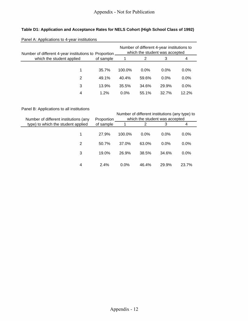
Table D1: Application and Acceptance Rates for NELS Cohort (High School Class of 1992)
Panel A: Applications to 4-year institutions
1 2 3 4
1 35.7% 100.0% 0.0% 0.0% 0.0%
2 49.1% 40.4% 59.6% 0.0% 0.0%
3 13.9% 35.5% 34.6% 29.9% 0.0%
4 1.2% 0.0% 55.1% 32.7% 12.2%
Panel B: Applications to all institutions
1 2 3 4
1 27.9% 100.0% 0.0% 0.0% 0.0%
2 50.7% 37.0% 63.0% 0.0% 0.0%
3 19.0% 26.9% 38.5% 34.6% 0.0%
4 2.4% 0.0% 46.4% 29.9% 23.7%
Proportion of sample
Number of different institutions (any type) to which the student applied
Proportion of sample
Number of different 4-year institutions to which the student applied
Number of different 4-year institutions to which the student was accepted
Number of different institutions (any type) to which the student was accepted
Appendix - Not for Publication
Appendix - 12
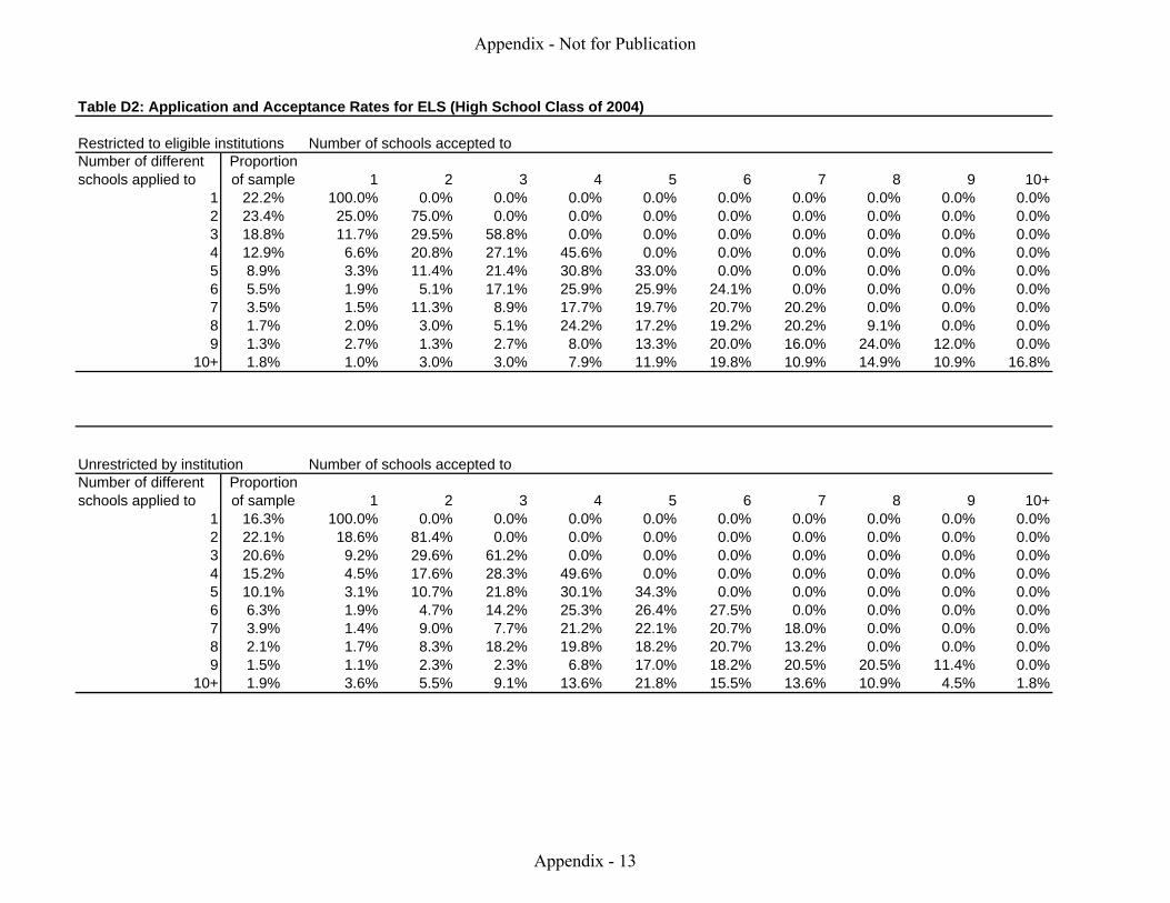
Table D2: Application and Acceptance Rates for ELS (High School Class of 2004)
Number of different schools applied to
Proportion of sample 1 2 3 4 5 6 7 8 9 10+
1 22.2% 100.0% 0.0% 0.0% 0.0% 0.0% 0.0% 0.0% 0.0% 0.0% 0.0%2 23.4% 25.0% 75.0% 0.0% 0.0% 0.0% 0.0% 0.0% 0.0% 0.0% 0.0%3 18.8% 11.7% 29.5% 58.8% 0.0% 0.0% 0.0% 0.0% 0.0% 0.0% 0.0%4 12.9% 6.6% 20.8% 27.1% 45.6% 0.0% 0.0% 0.0% 0.0% 0.0% 0.0%5 8.9% 3.3% 11.4% 21.4% 30.8% 33.0% 0.0% 0.0% 0.0% 0.0% 0.0%6 5.5% 1.9% 5.1% 17.1% 25.9% 25.9% 24.1% 0.0% 0.0% 0.0% 0.0%7 3.5% 1.5% 11.3% 8.9% 17.7% 19.7% 20.7% 20.2% 0.0% 0.0% 0.0%8 1.7% 2.0% 3.0% 5.1% 24.2% 17.2% 19.2% 20.2% 9.1% 0.0% 0.0%9 1.3% 2.7% 1.3% 2.7% 8.0% 13.3% 20.0% 16.0% 24.0% 12.0% 0.0%
10+ 1.8% 1.0% 3.0% 3.0% 7.9% 11.9% 19.8% 10.9% 14.9% 10.9% 16.8%
Number of different schools applied to
Proportion of sample 1 2 3 4 5 6 7 8 9 10+
1 16.3% 100.0% 0.0% 0.0% 0.0% 0.0% 0.0% 0.0% 0.0% 0.0% 0.0%2 22.1% 18.6% 81.4% 0.0% 0.0% 0.0% 0.0% 0.0% 0.0% 0.0% 0.0%3 20.6% 9.2% 29.6% 61.2% 0.0% 0.0% 0.0% 0.0% 0.0% 0.0% 0.0%4 15.2% 4.5% 17.6% 28.3% 49.6% 0.0% 0.0% 0.0% 0.0% 0.0% 0.0%5 10.1% 3.1% 10.7% 21.8% 30.1% 34.3% 0.0% 0.0% 0.0% 0.0% 0.0%6 6.3% 1.9% 4.7% 14.2% 25.3% 26.4% 27.5% 0.0% 0.0% 0.0% 0.0%7 3.9% 1.4% 9.0% 7.7% 21.2% 22.1% 20.7% 18.0% 0.0% 0.0% 0.0%8 2.1% 1.7% 8.3% 18.2% 19.8% 18.2% 20.7% 13.2% 0.0% 0.0% 0.0%9 1.5% 1.1% 2.3% 2.3% 6.8% 17.0% 18.2% 20.5% 20.5% 11.4% 0.0%
10+ 1.9% 3.6% 5.5% 9.1% 13.6% 21.8% 15.5% 13.6% 10.9% 4.5% 1.8%
Restricted to eligible institutions Number of schools accepted to
Unrestricted by institution Number of schools accepted to
Appendix - Not for Publication
Appendix - 13

Table D3: Probit Estimation for Predicted Probabilities of Admission - NELS 1992
Private PrivateIn State Out of State Both In State Out of State Both
(1) (2) (3) (4) (5) (6)VARIABLES accepted accepted accepted accepted accepted accepted
Student Grade Point Average -0.391 4.473 -4.173 8.982** 5.948 -5.321 (2.294) (5.531) (2.840) (3.802) (11.612) (3.728)
Missing GPA 0.241** 0.579*** 0.291*** 0.012 -0.554 0.209 (0.106) (0.211) (0.102) (0.188) (0.849) (0.233)
Student Standardized Math Score 1.841** 0.964 0.613 1.061 -3.143 1.249 (0.735) (1.723) (0.873) (1.191) (3.498) (1.046)
Student Math Score * Student GPA 0.132 1.527** -0.413 0.369 -0.473 0.428 (0.248) (0.600) (0.277) (0.615) (2.229) (0.522)
Student Socioeconomic Status 0.229 -0.133 0.026 -0.145 -0.643 0.173 (0.211) (0.452) (0.227) (0.333) (0.993) (0.398)
Log Enrollment -0.060* -0.051 0.018 -0.153** 0.036 -0.085 (0.036) (0.068) (0.030) (0.063) (0.174) (0.075)
Mean College SAT Score -0.001 -0.054* -0.024* -0.022 -0.064 -0.012 (0.014) (0.031) (0.014) (0.024) (0.092) (0.022)
College Admission Rate 1.515 -2.562 -0.147 -1.035 1.174 1.758 (1.325) (3.195) (1.559) (2.159) (6.538) (2.256)
School Mean SAT * Student GPA -0.011 -0.061 0.048 -0.124** -0.257 0.044 (0.030) (0.063) (0.031) (0.052) (0.213) (0.047)
School Mean SAT * Student Math Score -0.015 -0.005 -0.012 -0.009 0.059 -0.014 (0.011) (0.024) (0.011) (0.016) (0.046) (0.013)
School Mean SAT * Student Math * StudentGPA -0.002 -0.009** 0.001 0.001 -0.018 -0.009* (0.002) (0.005) (0.002) (0.004) (0.021) (0.004)
School Mean SAT * Student SES -0.003 0.001 -0.000 -0.001 0.000 -0.001 (0.002) (0.004) (0.002) (0.003) (0.007) (0.003)
College Admission Rate * Student GPA -0.861 -6.093 3.781 -11.391** -15.309 6.204 (2.885) (6.749) (3.589) (4.628) (14.996) (4.823)
College Admission Rate * Student Math Score -1.977** -0.682 -0.113 -1.502 6.633 -1.472 (0.870) (2.093) (1.101) (1.485) (4.779) (1.372)
College Admission Rate * Student Math Score * Student GPA -0.091 -1.146** 0.271 -0.486 2.232 0.166 (0.205) (0.505) (0.236) (0.588) (1.599) (0.550)
College Admission Rate * Student SES -0.013 0.074 0.046 0.394 1.216 -0.021 (0.164) (0.330) (0.154) (0.307) (0.946) (0.348)
Squared Student GPA 0.663 -1.798 1.508 -3.911** -2.412 2.326 (1.006) (2.641) (1.294) (1.722) (5.596) (1.677)
Squared Student Math Score 0.064 0.684 -0.363 -1.028 -0.444 -1.469 (0.606) (1.275) (0.763) (1.024) (2.747) (0.994)
School Mean SAT * College Admission Rate -0.001 0.045 0.017 0.025 0.138 -0.005 (0.018) (0.039) (0.019) (0.030) (0.127) (0.030)
School Mean SAT * College Admission Rate * Student Math Score 0.021* 0.006 0.013 0.023 -0.111* 0.021 (0.013) (0.030) (0.015) (0.020) (0.065) (0.018)
School Mean SAT * College Admission Rate * Student GPA 0.028 0.062 -0.046 0.153** 0.486* -0.047 (0.039) (0.078) (0.040) (0.067) (0.291) (0.064)
School Mean SAT * College Admission Rate * Squared Student GPA -0.003 -0.017 0.011 -0.073** -0.240* 0.023 (0.017) (0.037) (0.018) (0.030) (0.143) (0.028)
School Mean SAT * College Admission Rate * Squared Student Math Score 0.004 0.010 -0.010 -0.009 0.015 -0.017 (0.010) (0.019) (0.011) (0.017) (0.056) (0.016)
School Mean SAT * Squared Student GPA -0.002 0.021 -0.015 0.057** 0.124 -0.019 (0.013) (0.029) (0.014) (0.024) (0.104) (0.021)
College Admission Rate * Squared Student GPA -0.253 2.330 -1.092 5.125** 6.982 -2.749 (1.252) (3.226) (1.629) (2.088) (7.283) (2.173)
School Mean SAT * Squared Student Math Score -0.001 -0.007 0.008 0.011 -0.006 0.019 (0.008) (0.016) (0.009) (0.013) (0.040) (0.012)
College Admission Rate * Squared Student Math Score -0.271 -0.927 0.358 0.965 0.568 1.389 (0.721) (1.524) (0.968) (1.260) (3.739) (1.277)
Constant -0.394 3.544 0.952 2.657 -2.507 0.412(1.077) (2.657) (1.243) (1.798) (5.187) (1.815)
Observations 4990 1335 3873 1124 212 621Coefficient Estimates, Standard errors in parentheses*** p<0.01, ** p<0.05, * p<0.1Variables included but not presented: Interactions between Student and Institution Census (4) Region. Out-of-State specification (2,3,5,6), combine non-Northeast Institution region to account for relatively few students traveling to out-of-state public schools
White or Asian All OthersPublic Public
Appendix - Not for Publication
Appendix - 14
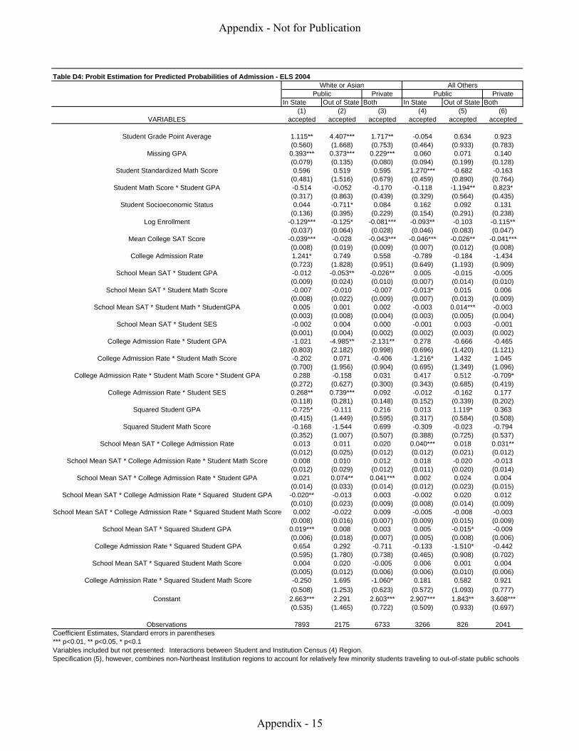
Private PrivateIn State Out of State Both In State Out of State Both
(1) (2) (3) (4) (5) (6)VARIABLES accepted accepted accepted accepted accepted accepted
Student Grade Point Average 1.115** 4.407*** 1.717** -0.054 0.634 0.923 (0.560) (1.668) (0.753) (0.464) (0.933) (0.783)
Missing GPA 0.393*** 0.373*** 0.229*** 0.060 0.071 0.140 (0.079) (0.135) (0.080) (0.094) (0.199) (0.128)
Student Standardized Math Score 0.596 0.519 0.595 1.270*** -0.682 -0.163 (0.481) (1.516) (0.679) (0.459) (0.890) (0.764)
Student Math Score * Student GPA -0.514 -0.052 -0.170 -0.118 -1.194** 0.823* (0.317) (0.863) (0.439) (0.329) (0.564) (0.435)
Student Socioeconomic Status 0.044 -0.711* 0.084 0.162 0.092 0.131 (0.136) (0.395) (0.229) (0.154) (0.291) (0.238)
Log Enrollment -0.129*** -0.125* -0.081*** -0.093** -0.103 -0.115** (0.037) (0.064) (0.028) (0.046) (0.083) (0.047)
Mean College SAT Score -0.039*** -0.028 -0.043*** -0.046*** -0.026** -0.041*** (0.008) (0.019) (0.009) (0.007) (0.012) (0.008)
College Admission Rate 1.241* 0.749 0.558 -0.789 -0.184 -1.434 (0.723) (1.828) (0.951) (0.649) (1.193) (0.909)
School Mean SAT * Student GPA -0.012 -0.053** -0.026** 0.005 -0.015 -0.005 (0.009) (0.024) (0.010) (0.007) (0.014) (0.010)
School Mean SAT * Student Math Score -0.007 -0.010 -0.007 -0.013* 0.015 0.006 (0.008) (0.022) (0.009) (0.007) (0.013) (0.009)
School Mean SAT * Student Math * StudentGPA 0.005 0.001 0.002 -0.003 0.014*** -0.003 (0.003) (0.008) (0.004) (0.003) (0.005) (0.004)
School Mean SAT * Student SES -0.002 0.004 0.000 -0.001 0.003 -0.001 (0.001) (0.004) (0.002) (0.002) (0.003) (0.002)
College Admission Rate * Student GPA -1.021 -4.985** -2.131** 0.278 -0.666 -0.465 (0.803) (2.182) (0.998) (0.696) (1.420) (1.121)
College Admission Rate * Student Math Score -0.202 0.071 -0.406 -1.216* 1.432 1.045 (0.700) (1.956) (0.904) (0.695) (1.349) (1.096)
College Admission Rate * Student Math Score * Student GPA 0.288 -0.158 0.031 0.417 0.512 -0.709* (0.272) (0.627) (0.300) (0.343) (0.685) (0.419)
College Admission Rate * Student SES 0.268** 0.739*** 0.092 -0.012 -0.162 0.177 (0.118) (0.281) (0.148) (0.152) (0.339) (0.202)
Squared Student GPA -0.725* -0.111 0.216 0.013 1.119* 0.363 (0.415) (1.449) (0.595) (0.317) (0.584) (0.508)
Squared Student Math Score -0.168 -1.544 0.699 -0.309 -0.023 -0.794 (0.352) (1.007) (0.507) (0.388) (0.725) (0.537)
School Mean SAT * College Admission Rate 0.013 0.011 0.020 0.040*** 0.018 0.031** (0.012) (0.025) (0.012) (0.012) (0.021) (0.012)
School Mean SAT * College Admission Rate * Student Math Score 0.008 0.010 0.012 0.018 -0.020 -0.013 (0.012) (0.029) (0.012) (0.011) (0.020) (0.014)
School Mean SAT * College Admission Rate * Student GPA 0.021 0.074** 0.041*** 0.002 0.024 0.004 (0.014) (0.033) (0.014) (0.012) (0.023) (0.015)
School Mean SAT * College Admission Rate * Squared Student GPA -0.020** -0.013 0.003 -0.002 0.020 0.012 (0.010) (0.023) (0.009) (0.008) (0.014) (0.009)
School Mean SAT * College Admission Rate * Squared Student Math Score 0.002 -0.022 0.009 -0.005 -0.008 -0.003 (0.008) (0.016) (0.007) (0.009) (0.015) (0.009)
School Mean SAT * Squared Student GPA 0.019*** 0.008 0.003 0.005 -0.015* -0.009 (0.006) (0.018) (0.007) (0.005) (0.008) (0.006)
College Admission Rate * Squared Student GPA 0.654 0.292 -0.711 -0.133 -1.510* -0.442 (0.595) (1.780) (0.738) (0.465) (0.908) (0.702)
School Mean SAT * Squared Student Math Score 0.004 0.020 -0.005 0.006 0.001 0.004 (0.005) (0.012) (0.006) (0.006) (0.010) (0.006)
College Admission Rate * Squared Student Math Score -0.250 1.695 -1.060* 0.181 0.582 0.921 (0.508) (1.253) (0.623) (0.572) (1.093) (0.777)
Constant 2.663*** 2.291 2.603*** 2.907*** 1.843** 3.608***(0.535) (1.465) (0.722) (0.509) (0.933) (0.697)
Observations 7893 2175 6733 3266 826 2041Coefficient Estimates, Standard errors in parentheses*** p<0.01, ** p<0.05, * p<0.1Variables included but not presented: Interactions between Student and Institution Census (4) Region. Specification (5), however, combines non-Northeast Institution regions to account for relatively few minority students traveling to out-of-state public schools
Table D4: Probit Estimation for Predicted Probabilities of Admission - ELS 2004White or Asian All Others
Public Public
Appendix - Not for Publication
Appendix - 15
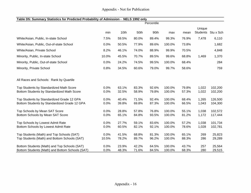
Table D5: Summary Statistics for Predicted Probability of Admission - NELS 1992 only
min 10th 50th 90th max meanUnique
Students Stu x Sch
White/Asian, Public, In-state School 7.5% 59.5% 80.0% 89.4% 99.3% 76.9% 7,478 6,110
White/Asian, Public, Out-of-state School 0.0% 50.5% 77.9% 89.6% 100.0% 73.8% 1,682
White/Asian, Private School 8.2% 46.1% 74.0% 88.9% 99.9% 70.5% 4,848
Minority, Public, In-state School 10.0% 45.5% 70.7% 89.5% 99.6% 68.8% 1,469 1,370
Minority, Public, Out-of-state School 0.0% 24.2% 74.5% 99.5% 100.0% 68.4% 284
Minority, Private School 0.8% 34.5% 60.6% 79.0% 99.7% 58.6% 759
All Races and Schools: Rank by Quartile
Top Students by Standardized Math Score 0.0% 63.1% 83.3% 92.6% 100.0% 79.8% 1,022 102,200 Bottom Students by Standardized Math Score 0.0% 32.5% 58.9% 79.8% 100.0% 57.3% 1,022 102,200
Top Students by Standardized Grade 12 GPA 0.0% 40.4% 71.5% 92.4% 100.0% 68.4% 1,265 126,500 Bottom Students by Standardized Grade 12 GPA 0.0% 39.8% 69.8% 87.3% 100.0% 66.5% 1,043 104,300
Top Schools by Mean SAT Score 0.0% 28.8% 57.8% 76.8% 100.0% 55.1% 1,038 102,572 Bottom Schools by Mean SAT Score 0.0% 65.1% 84.8% 93.5% 100.0% 81.2% 1,172 117,444
Top Schools by Lowest Admit Rate 0.0% 27.7% 59.1% 83.6% 100.0% 57.2% 1,038 101,734 Bottom Schools by Lowest Admit Rate 0.0% 60.5% 82.1% 92.1% 100.0% 78.6% 1,028 102,781
Top Students (Math) and Top Schools (SAT) 0.0% 41.5% 68.8% 81.3% 100.0% 65.1% 269 25,823 Top Students (Math) and Bottom Schools (SAT) 10.5% 78.2% 89.7% 96.2% 100.0% 88.3% 286 29,289
Bottom Students (Math) and Top Schools (SAT) 0.0% 23.9% 42.2% 64.5% 100.0% 43.7% 257 25,564 Bottom Students (Math) and Bottom Schools (SAT) 0.0% 48.3% 71.6% 84.5% 100.0% 68.3% 280 29,515
Percentile
Appendix - Not for Publication
Appendix - 16
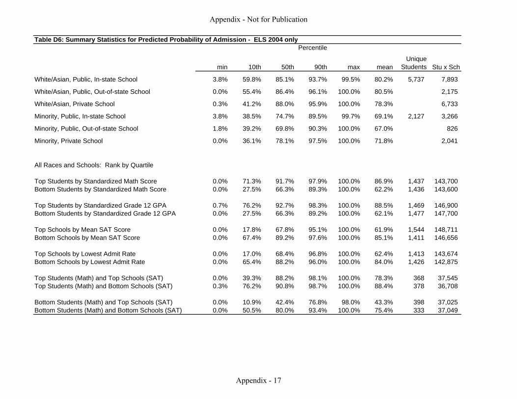
Table D6: Summary Statistics for Predicted Probability of Admission - ELS 2004 only
min 10th 50th 90th max meanUnique
Students Stu x Sch
White/Asian, Public, In-state School 3.8% 59.8% 85.1% 93.7% 99.5% 80.2% 5,737 7,893
White/Asian, Public, Out-of-state School 0.0% 55.4% 86.4% 96.1% 100.0% 80.5% 2,175
White/Asian, Private School 0.3% 41.2% 88.0% 95.9% 100.0% 78.3% 6,733
Minority, Public, In-state School 3.8% 38.5% 74.7% 89.5% 99.7% 69.1% 2,127 3,266
Minority, Public, Out-of-state School 1.8% 39.2% 69.8% 90.3% 100.0% 67.0% 826
Minority, Private School 0.0% 36.1% 78.1% 97.5% 100.0% 71.8% 2,041
All Races and Schools: Rank by Quartile
Top Students by Standardized Math Score 0.0% 71.3% 91.7% 97.9% 100.0% 86.9% 1,437 143,700 Bottom Students by Standardized Math Score 0.0% 27.5% 66.3% 89.3% 100.0% 62.2% 1,436 143,600
Top Students by Standardized Grade 12 GPA 0.7% 76.2% 92.7% 98.3% 100.0% 88.5% 1,469 146,900 Bottom Students by Standardized Grade 12 GPA 0.0% 27.5% 66.3% 89.2% 100.0% 62.1% 1,477 147,700
Top Schools by Mean SAT Score 0.0% 17.8% 67.8% 95.1% 100.0% 61.9% 1,544 148,711 Bottom Schools by Mean SAT Score 0.0% 67.4% 89.2% 97.6% 100.0% 85.1% 1,411 146,656
Top Schools by Lowest Admit Rate 0.0% 17.0% 68.4% 96.8% 100.0% 62.4% 1,413 143,674 Bottom Schools by Lowest Admit Rate 0.0% 65.4% 88.2% 96.0% 100.0% 84.0% 1,426 142,875
Top Students (Math) and Top Schools (SAT) 0.0% 39.3% 88.2% 98.1% 100.0% 78.3% 368 37,545 Top Students (Math) and Bottom Schools (SAT) 0.3% 76.2% 90.8% 98.7% 100.0% 88.4% 378 36,708
Bottom Students (Math) and Top Schools (SAT) 0.0% 10.9% 42.4% 76.8% 98.0% 43.3% 398 37,025 Bottom Students (Math) and Bottom Schools (SAT) 0.0% 50.5% 80.0% 93.4% 100.0% 75.4% 333 37,049
Percentile
Appendix - Not for Publication
Appendix - 17

Appendix E. Estimates of Predicted Net Price
Appendix - Not for Publication
Appendix - 18
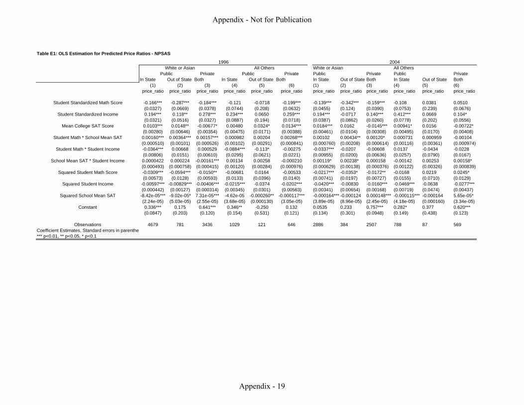
Table E1: OLS Estimation for Predicted Price Ratios - NPSAS
White or Asian All OthersPrivate Private Public Private Public Private
In State Out of State Both In State Out of State Both In State Out of State Both In State Out of State Both(1) (2) (3) (4) (5) (6) (1) (2) (3) (4) (5) (6)
price_ratio price_ratio price_ratio price_ratio price_ratio price_ratio price_ratio price_ratio price_ratio price_ratio price_ratio price_ratio
Student Standardized Math Score -0.166*** -0.287*** -0.184*** -0.121 -0.0718 -0.199*** -0.139*** -0.342*** -0.159*** -0.108 0.0381 0.0510 (0.0327) (0.0669) (0.0378) (0.0744) (0.208) (0.0632) (0.0455) (0.124) (0.0390) (0.0753) (0.239) (0.0676)
Student Standardized Income 0.194*** 0.118** 0.278*** 0.234*** 0.0650 0.259*** 0.194*** -0.0717 0.140*** 0.412*** 0.0669 0.104* (0.0321) (0.0516) (0.0327) (0.0887) (0.194) (0.0718) (0.0387) (0.0862) (0.0260) (0.0778) (0.202) (0.0556)
Mean College SAT Score 0.0103*** 0.0148** -0.00677* 0.00480 0.0324* 0.0134*** 0.0184*** 0.0162 -0.0145*** 0.00941* 0.0156 -0.00722* (0.00280) (0.00646) (0.00354) (0.00475) (0.0171) (0.00388) (0.00461) (0.0104) (0.00308) (0.00495) (0.0170) (0.00408)
Student Math * School Mean SAT 0.00160*** 0.00364*** 0.00157*** 0.000982 0.00204 0.00268*** 0.00102 0.00434** 0.00120* 0.000731 0.000959 -0.00104 (0.000510) (0.00101) (0.000526) (0.00102) (0.00291) (0.000841) (0.000760) (0.00208) (0.000614) (0.00116) (0.00361) (0.000974)
Student Math * Student Income -0.0364*** 0.00668 0.000529 -0.0884*** -0.113* -0.00275 -0.0337*** -0.0207 -0.00608 0.0137 -0.0434 -0.0228 (0.00806) (0.0151) (0.00610) (0.0295) (0.0621) (0.0221) (0.00955) (0.0200) (0.00636) (0.0257) (0.0790) (0.0167)
School Mean SAT * Student Income 0.0000422 0.000224 -0.00161*** 0.00134 0.00258 -0.000210 0.00119* 0.00238* 0.000158 -0.00142 0.00253 0.00158* (0.000493) (0.000758) (0.000415) (0.00120) (0.00284) (0.000976) (0.000629) (0.00138) (0.000376) (0.00122) (0.00326) (0.000839)
Squared Student Math Score -0.0309*** -0.0594*** -0.0150** -0.00681 0.0164 -0.00533 -0.0217*** -0.0353* -0.0172** -0.0168 0.0219 0.0245* (0.00573) (0.0128) (0.00593) (0.0133) (0.0396) (0.0140) (0.00741) (0.0197) (0.00727) (0.0155) (0.0710) (0.0129)
Squared Student Income -0.00597*** -0.00829*** -0.00406*** -0.0215*** -0.0374 -0.0202*** -0.0420*** -0.00830 -0.0160*** -0.0469*** -0.0638 -0.0277*** (0.000442) (0.00127) (0.000314) (0.00345) (0.0301) (0.00563) (0.00341) (0.00654) (0.00168) (0.00719) (0.0474) (0.00437)
Squared School Mean SAT -8.42e-05*** -9.02e-05* 7.31e-05*** -4.62e-05 -0.000260** -0.000117*** -0.000164*** -0.000124 0.000148*** -0.000115*** -0.000164 5.65e-05* (2.24e-05) (5.03e-05) (2.55e-05) (3.68e-05) (0.000130) (3.05e-05) (3.89e-05) (8.96e-05) (2.45e-05) (4.18e-05) (0.000160) (3.34e-05)
Constant 0.336*** 0.175 0.641*** 0.346** -0.250 0.132 0.0535 0.233 0.757*** 0.282* 0.377 0.620***(0.0847) (0.203) (0.120) (0.154) (0.531) (0.121) (0.134) (0.301) (0.0948) (0.149) (0.438) (0.123)
Observations 4679 781 3436 1029 121 646 2886 384 2507 788 87 569Coefficient Estimates, Standard errors in parenthe*** p<0.01, ** p<0.05, * p<0.1
1996 2004White or Asian All Others
Public Public
Appendix - Not for Publication
Appendix - 19
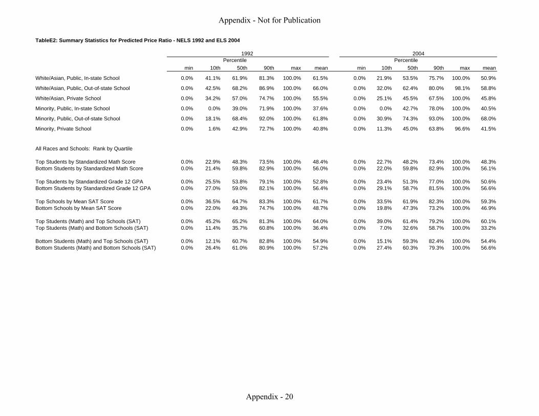
TableE2: Summary Statistics for Predicted Price Ratio - NELS 1992 and ELS 2004
min 10th 50th 90th max mean min 10th 50th 90th max mean
White/Asian, Public, In-state School 0.0% 41.1% 61.9% 81.3% 100.0% 61.5% 0.0% 21.9% 53.5% 75.7% 100.0% 50.9%
White/Asian, Public, Out-of-state School 0.0% 42.5% 68.2% 86.9% 100.0% 66.0% 0.0% 32.0% 62.4% 80.0% 98.1% 58.8%
White/Asian, Private School 0.0% 34.2% 57.0% 74.7% 100.0% 55.5% 0.0% 25.1% 45.5% 67.5% 100.0% 45.8%
Minority, Public, In-state School 0.0% 0.0% 39.0% 71.9% 100.0% 37.6% 0.0% 0.0% 42.7% 78.0% 100.0% 40.5%
Minority, Public, Out-of-state School 0.0% 18.1% 68.4% 92.0% 100.0% 61.8% 0.0% 30.9% 74.3% 93.0% 100.0% 68.0%
Minority, Private School 0.0% 1.6% 42.9% 72.7% 100.0% 40.8% 0.0% 11.3% 45.0% 63.8% 96.6% 41.5%
All Races and Schools: Rank by Quartile
Top Students by Standardized Math Score 0.0% 22.9% 48.3% 73.5% 100.0% 48.4% 0.0% 22.7% 48.2% 73.4% 100.0% 48.3%Bottom Students by Standardized Math Score 0.0% 21.4% 59.8% 82.9% 100.0% 56.0% 0.0% 22.0% 59.8% 82.9% 100.0% 56.1%
Top Students by Standardized Grade 12 GPA 0.0% 25.5% 53.8% 79.1% 100.0% 52.8% 0.0% 23.4% 51.3% 77.0% 100.0% 50.6%Bottom Students by Standardized Grade 12 GPA 0.0% 27.0% 59.0% 82.1% 100.0% 56.4% 0.0% 29.1% 58.7% 81.5% 100.0% 56.6%
Top Schools by Mean SAT Score 0.0% 36.5% 64.7% 83.3% 100.0% 61.7% 0.0% 33.5% 61.9% 82.3% 100.0% 59.3%Bottom Schools by Mean SAT Score 0.0% 22.0% 49.3% 74.7% 100.0% 48.7% 0.0% 19.8% 47.3% 73.2% 100.0% 46.9%
Top Students (Math) and Top Schools (SAT) 0.0% 45.2% 65.2% 81.3% 100.0% 64.0% 0.0% 39.0% 61.4% 79.2% 100.0% 60.1%Top Students (Math) and Bottom Schools (SAT) 0.0% 11.4% 35.7% 60.8% 100.0% 36.4% 0.0% 7.0% 32.6% 58.7% 100.0% 33.2%
Bottom Students (Math) and Top Schools (SAT) 0.0% 12.1% 60.7% 82.8% 100.0% 54.9% 0.0% 15.1% 59.3% 82.4% 100.0% 54.4%Bottom Students (Math) and Bottom Schools (SAT) 0.0% 26.4% 61.0% 80.9% 100.0% 57.2% 0.0% 27.4% 60.3% 79.3% 100.0% 56.6%
Percentile1992
Percentile2004
Appendix - Not for Publication
Appendix - 20

Appendix F. Additional Tables and Figures
Appendix - Not for Publication
Appendix - 21
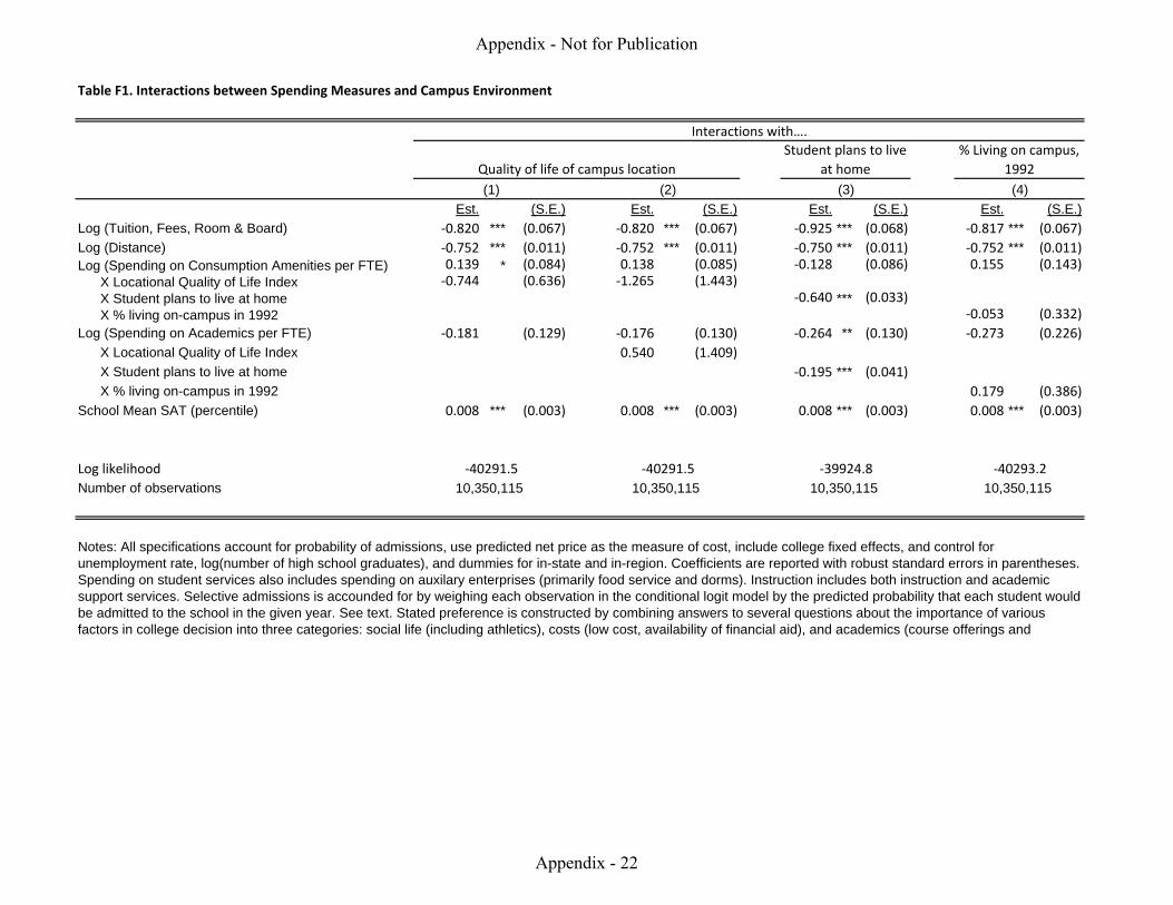
Table F1. Interactions between Spending Measures and Campus Environment
Est. (S.E.) Est. (S.E.) Est. (S.E.) Est. (S.E.)Log (Tuition, Fees, Room & Board) ‐0.820 *** (0.067) ‐0.820 *** (0.067) ‐0.925 *** (0.068) ‐0.817 *** (0.067)
Log (Distance) ‐0.752 *** (0.011) ‐0.752 *** (0.011) ‐0.750 *** (0.011) ‐0.752 *** (0.011)Log (Spending on Consumption Amenities per FTE) 0.139 * (0.084) 0.138 (0.085) ‐0.128 (0.086) 0.155 (0.143)
X Locational Quality of Life Index ‐0.744 (0.636) ‐1.265 (1.443)X Student plans to live at home ‐0.640 *** (0.033)X % living on-campus in 1992 ‐0.053 (0.332)
Log (Spending on Academics per FTE) ‐0.181 (0.129) ‐0.176 (0.130) ‐0.264 ** (0.130) ‐0.273 (0.226)
X Locational Quality of Life Index 0.540 (1.409)
X Student plans to live at home ‐0.195 *** (0.041)
X % living on-campus in 1992 0.179 (0.386)
School Mean SAT (percentile) 0.008 *** (0.003) 0.008 *** (0.003) 0.008 *** (0.003) 0.008 *** (0.003)
Log likelihood
Number of observations
Notes: All specifications account for probability of admissions, use predicted net price as the measure of cost, include college fixed effects, and control for unemployment rate, log(number of high school graduates), and dummies for in-state and in-region. Coefficients are reported with robust standard errors in parentheses. Spending on student services also includes spending on auxilary enterprises (primarily food service and dorms). Instruction includes both instruction and academic support services. Selective admissions is accounded for by weighing each observation in the conditional logit model by the predicted probability that each student would be admitted to the school in the given year. See text. Stated preference is constructed by combining answers to several questions about the importance of various factors in college decision into three categories: social life (including athletics), costs (low cost, availability of financial aid), and academics (course offerings and
10,350,115 10,350,115 10,350,11510,350,115‐40291.5 ‐40291.5 ‐40293.2‐39924.8
Quality of life of campus location
% Living on campus,
1992
Student plans to live
at home
Interactions with….
(4)(1) (2) (3)
Appendix - Not for Publication
Appendix - 22
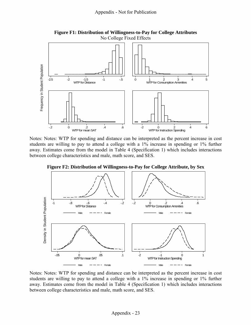
Figure F1: Distribution of Willingness-to-Pay for College Attributes No College Fixed Effects
Notes: Notes: WTP for spending and distance can be interpreted as the percent increase in cost students are willing to pay to attend a college with a 1% increase in spending or 1% further away. Estimates come from the model in Table 4 (Specification 1) which includes interactions between college characteristics and male, math score, and SES.
Figure F2: Distribution of Willingness-to-Pay for College Attribute, by Sex
Notes: Notes: WTP for spending and distance can be interpreted as the percent increase in cost students are willing to pay to attend a college with a 1% increase in spending or 1% further away. Estimates come from the model in Table 4 (Specification 1) which includes interactions between college characteristics and male, math score, and SES.
-2.5 -2 -1.5 -1 -.5WTP for Distance
0 1 2 3 4 5WTP for Consumption Amenities
-.2 0 .2 .4 .6WTP for mean SAT
-2 0 2 4 6WTP for Instruction Spending
Freq
uenc
y in
Stu
dent
Pop
ulat
ion
-1 -.8 -.6 -.4 -.2WTP for Distance
Male Female
-.2 0 .2 .4 .6WTP for Consumption Amenities
Male Female
-.05 0 .05 .1WTP for mean SAT
Male Female
-2 -1 0 1WTP for Instruction Spending
Male Female
Den
sity
in S
tude
nt P
opul
atio
n
Appendix - Not for Publication
Appendix - 23
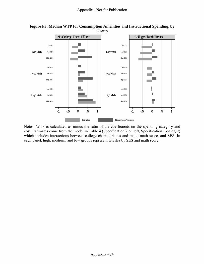
Figure F3: Median WTP for Consumption Amenities and Instructional Spending, by Group
Notes: WTP is calculated as minus the ratio of the coefficients on the spending category and cost. Estimates come from the model in Table 4 (Specification 2 on left, Specification 1 on right) which includes interactions between college characteristics and male, math score, and SES. In each panel, high, medium, and low groups represent terciles by SES and math score.
-1 -.5 0 .5 1 -1 -.5 0 .5 1
High Math
Med Math
Low Math
High Math
Med Math
Low Math
High SES
Med SES
Low SES
High SES
Med SES
Low SES
High SES
Med SES
Low SES
High SES
Med SES
Low SES
High SES
Med SES
Low SES
High SES
Med SES
Low SES
No College Fixed Effects College Fixed Effects
Instruction Consumption Amenities
Appendix - Not for Publication
Appendix - 24
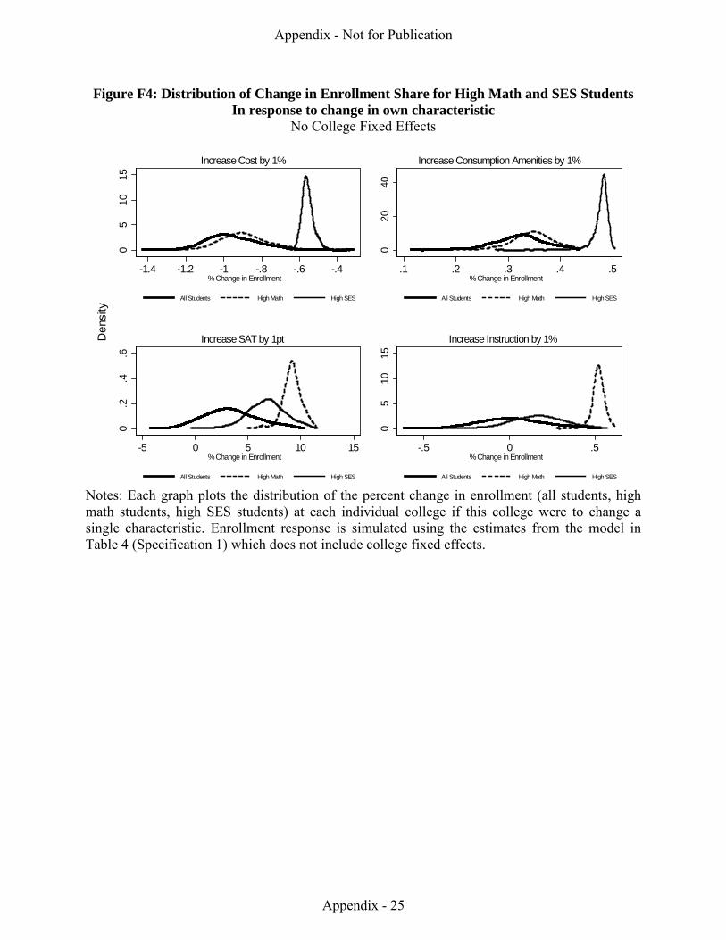
Figure F4: Distribution of Change in Enrollment Share for High Math and SES Students In response to change in own characteristic
No College Fixed Effects
Notes: Each graph plots the distribution of the percent change in enrollment (all students, high math students, high SES students) at each individual college if this college were to change a single characteristic. Enrollment response is simulated using the estimates from the model in Table 4 (Specification 1) which does not include college fixed effects.
05
1015
-1.4 -1.2 -1 -.8 -.6 -.4% Change in Enrollment
All Students High Math High SES
Increase Cost by 1%
0.2
.4.6
-5 0 5 10 15% Change in Enrollment
All Students High Math High SES
Increase SAT by 1pt
020
40
.1 .2 .3 .4 .5% Change in Enrollment
All Students High Math High SES
Increase Consumption Amenities by 1%
05
1015
-.5 0 .5% Change in Enrollment
All Students High Math High SES
Increase Instruction by 1%Den
sity
Appendix - Not for Publication
Appendix - 25
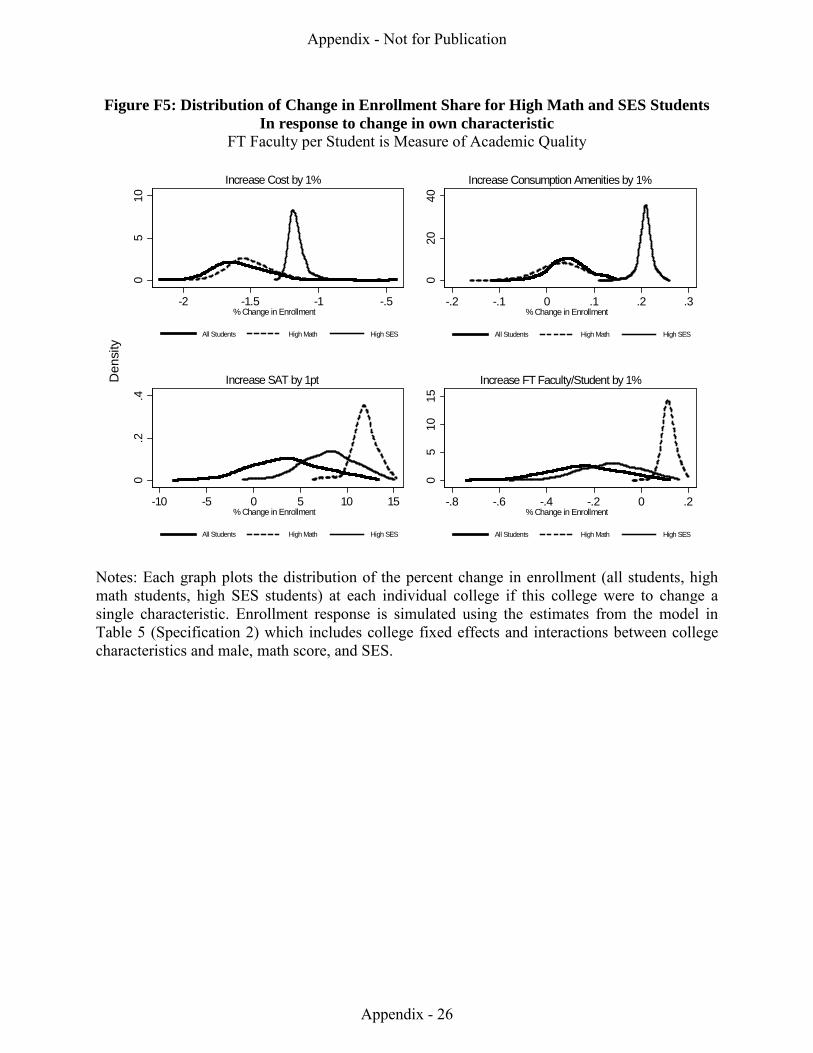
Figure F5: Distribution of Change in Enrollment Share for High Math and SES Students In response to change in own characteristic
FT Faculty per Student is Measure of Academic Quality
Notes: Each graph plots the distribution of the percent change in enrollment (all students, high math students, high SES students) at each individual college if this college were to change a single characteristic. Enrollment response is simulated using the estimates from the model in Table 5 (Specification 2) which includes college fixed effects and interactions between college characteristics and male, math score, and SES.
05
10
-2 -1.5 -1 -.5% Change in Enrollment
All Students High Math High SES
Increase Cost by 1%
0.2
.4
-10 -5 0 5 10 15% Change in Enrollment
All Students High Math High SES
Increase SAT by 1pt
020
40
-.2 -.1 0 .1 .2 .3% Change in Enrollment
All Students High Math High SES
Increase Consumption Amenities by 1%
05
1015
-.8 -.6 -.4 -.2 0 .2% Change in Enrollment
All Students High Math High SES
Increase FT Faculty/Student by 1%Den
sity
Appendix - Not for Publication
Appendix - 26
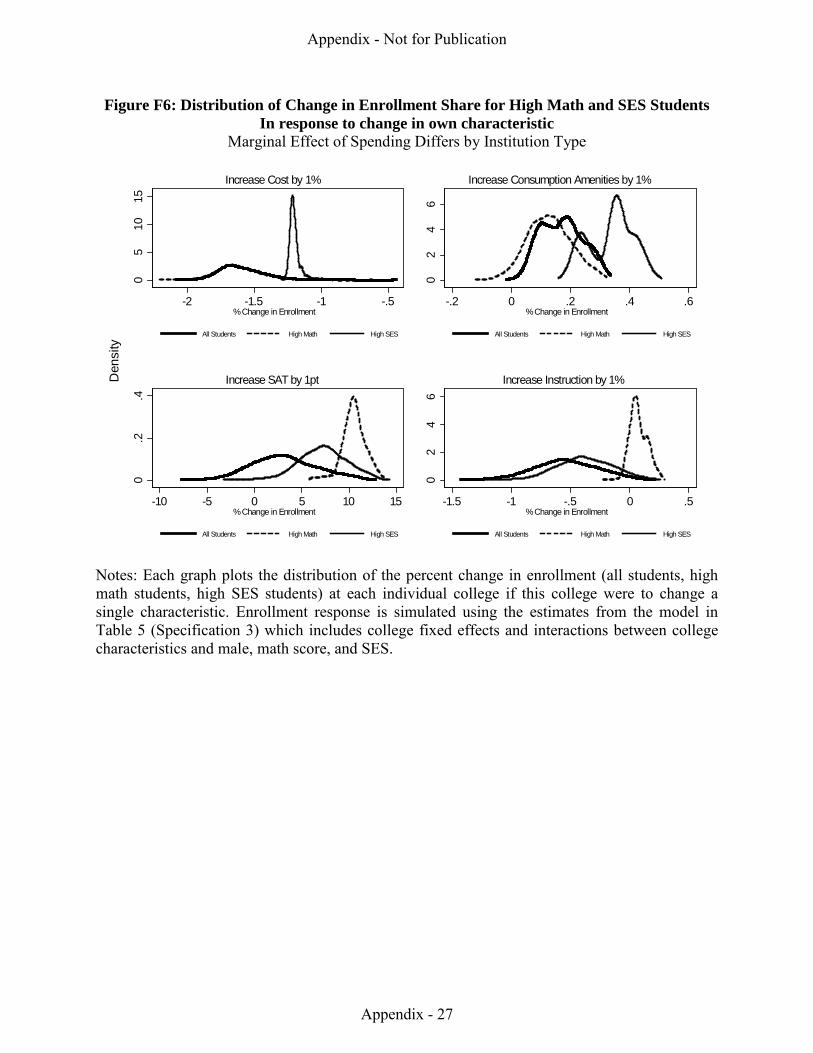
Figure F6: Distribution of Change in Enrollment Share for High Math and SES Students In response to change in own characteristic
Marginal Effect of Spending Differs by Institution Type
Notes: Each graph plots the distribution of the percent change in enrollment (all students, high math students, high SES students) at each individual college if this college were to change a single characteristic. Enrollment response is simulated using the estimates from the model in Table 5 (Specification 3) which includes college fixed effects and interactions between college characteristics and male, math score, and SES.
05
1015
-2 -1.5 -1 -.5% Change in Enrollment
All Students High Math High SES
Increase Cost by 1%
0.2
.4
-10 -5 0 5 10 15% Change in Enrollment
All Students High Math High SES
Increase SAT by 1pt
02
46
-.2 0 .2 .4 .6% Change in Enrollment
All Students High Math High SES
Increase Consumption Amenities by 1%
02
46
-1.5 -1 -.5 0 .5% Change in Enrollment
All Students High Math High SES
Increase Instruction by 1%Den
sity
Appendix - Not for Publication
Appendix - 27
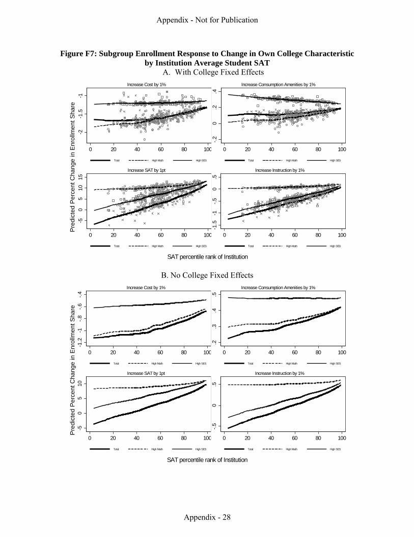
Figure F7: Subgroup Enrollment Response to Change in Own College Characteristic by Institution Average Student SAT
A. With College Fixed Effects
B. No College Fixed Effects
-2-1
.5-1
0 20 40 60 80 100
Total High Math High SES
Increase Cost by 1%
-.20
.2.4
0 20 40 60 80 100
Total High Math High SES
Increase Consumption Amenities by 1%-5
05
1015
0 20 40 60 80 100
Total High Math High SES
Increase SAT by 1pt
-1.5
-1-.5
0.5
0 20 40 60 80 100
Total High Math High SES
Increase Instruction by 1%
Pre
dict
ed P
erce
nt C
hang
e in
Enr
ollm
ent S
hare
SAT percentile rank of Institution
-1.2
-1-.8
-.6-.4
0 20 40 60 80 100
Total High Math High SES
Increase Cost by 1%
.2.3
.4.5
0 20 40 60 80 100
Total High Math High SES
Increase Consumption Amenities by 1%
-50
510
0 20 40 60 80 100
Total High Math High SES
Increase SAT by 1pt
-.50
.5
0 20 40 60 80 100
Total High Math High SES
Increase Instruction by 1%
Pre
dict
ed P
erce
nt C
hang
e in
Enr
ollm
ent S
hare
SAT percentile rank of Institution
Appendix - Not for Publication
Appendix - 28
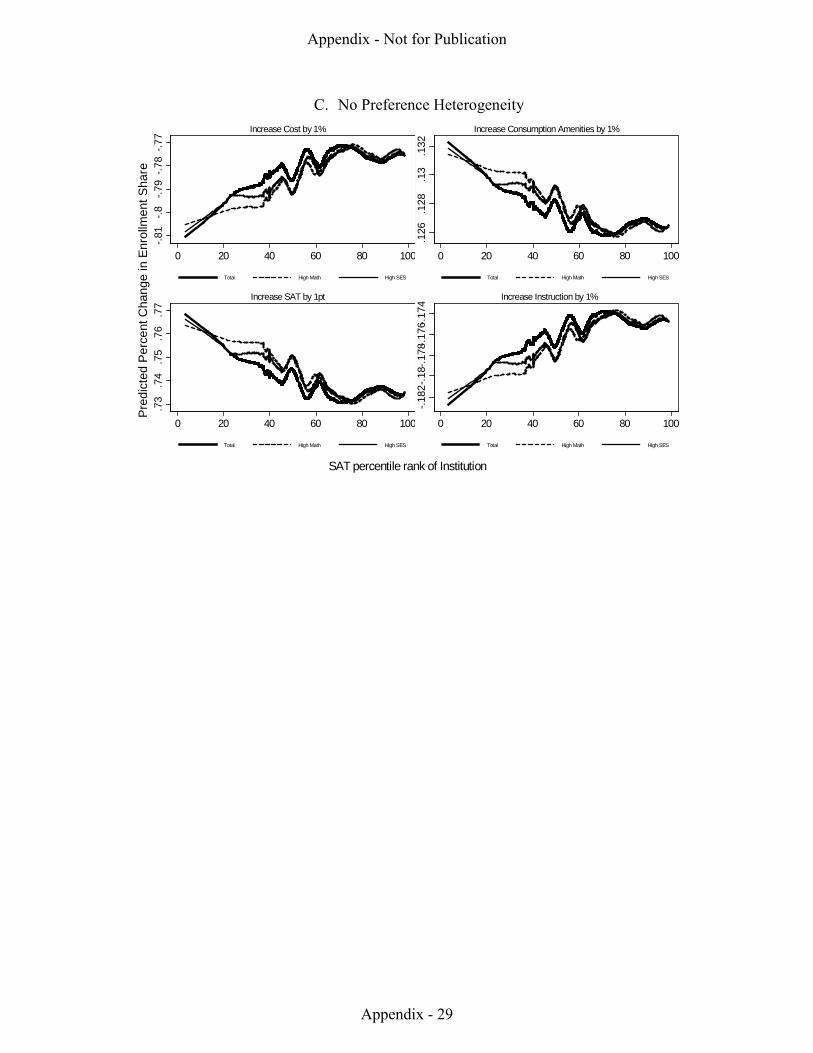
C. No Preference Heterogeneity
-.81
-.8-.7
9-.7
8-.7
7
0 20 40 60 80 100
Total High Math High SES
Increase Cost by 1%
.126
.128
.13
.132
0 20 40 60 80 100
Total High Math High SES
Increase Consumption Amenities by 1%
.73
.74
.75
.76
.77
0 20 40 60 80 100
Total High Math High SES
Increase SAT by 1pt
-.182
-.18-
.178
-.176
-.174
0 20 40 60 80 100
Total High Math High SES
Increase Instruction by 1%
Pre
dict
ed P
erce
nt C
hang
e in
Enr
ollm
ent S
hare
SAT percentile rank of Institution
Appendix - Not for Publication
Appendix - 29