ÉCOLE DE TECHNOLOGIE SUPÉRIEURE UNIVERSITÉ ...espace.etsmtl.ca/658/1/RIVARD_Dominique.pdfBOARD OF EXAMINERS THIS THESIS HAS BEEN EVALUATED BY THE FOLLOWING BOARD OF EXAMINERS M

ÉCOLE DE TECHNOLOGIE SUPÉRIEUREUNIVERSITÉ DU QUÉBEC

THESIS PRESENTED TOÉCOLE DE TECHNOLOGIE SUPÉRIEURE

IN PARTIAL FULFILLMENT OF THE REQUIREMENTS FORA MASTER’S DEGREE IN ELECTRICAL ENGINEERING

M. Eng.

BYDominique RIVARD

MULTI-FEATURE APPROACH FOR WRITER-INDEPENDENT OFFLINE SIGNATUREVERIFICATION

MONTREAL, OCTOBER 20, 2010

c© Copyright 2010 reserved by Dominique Rivard

BOARD OF EXAMINERS

THIS THESIS HAS BEEN EVALUATED

BY THE FOLLOWING BOARD OF EXAMINERS

M. Robert Sabourin, Thesis SupervisorDépartement de génie de la production automatisée à l’École de technologie supérieure

M. Eric Granger, Thesis Co-supervisorDépartement de génie de la production automatisée à l’École de technologie supérieure

M. Jean-Marc Robert, President of the Board of ExaminersDépartement de génie logiciel et des TI à l’École de technologie supérieure

M. Richard LepageDépartement de génie de la production automatisée à l’École de technologie supérieure

THIS THESIS HAS BEEN PRESENTED AND DEFENDED

BEFORE A BOARD OF EXAMINERS AND PUBLIC

OCTOBER 6, 2010

AT ÉCOLE DE TECHNOLOGIE SUPÉRIEURE

ACKNOWLEDGMENTS

I would like to extend my sincere gratitude to Dr. Robert Sabourin and Dr. Eric Granger for

supervising my work over these last years.

My thanks go to all the friends at LIVIA for their help and friendship that enriched my study

these years.

I would like to thank the members of my examining committee: Dr. Jean-Marc Robert and

Dr. Richard Lepage. Their comments helped to improve the quality of the final version of this

thesis.

Special thanks to my parents, Jacqueline and Pierre Rivard, for their love and guidance.

Most of all, thanks to my wife, Audrée Gagné, for her unfailing support that gave me peace

and strength all the way through. This work is dedicated to her and to our son Luca.

This research has been financially supported by Banctec Canada and by research grants from

Fonds de recherche sur la nature et les technologies and École de technologie supérieure.

FUSION AU NIVEAU DES CARACTÉRISTIQUES POUR LA VÉRIFICATION DESSIGNATURES MANUSCRITES DANS UN CONTEXTE INDÉPENDANT DU

SCRIPTEUR

Dominique RIVARD

RÉSUMÉ

Les principales difficultés rencontrées en vérification des signatures manuscrites statiques sontla grande quantité d’utilisateurs, la grande quantité de caractéristiques, le nombre limité designatures de référence disponibles pour l’apprentissage, la grande variabilité naturelle des sig-natures et l’absence de faux en guise de contre-exemples d’apprentissage. Cette rechercheprésente premièrement une revue de littérature des techniques utilisées pour la vérification dessignatures manuscrites statiques, en portant une attention particulière à l’extraction de carac-téristiques et aux stratégies de vérification. L’objectif est de présenter les progrès les plusimportants, ainsi que les défis de ce domaine. Un intérêt particulier est porté aux techniquesqui permettent de concevoir un système de vérification de signatures avec un nombre limité dedonnées. Ensuite est présenté un nouveau système de vérification des signatures statiques basésur plusieurs techniques d’extraction de caractéristiques, la transformation dichotomique et lasélection de caractéristiques par boosting. L’utilisation de plusieurs techniques d’extractionde caractéristiques augmente la diversité de l’information extraite des signatures, produisantainsi des caractéristiques pouvant atténuer la variabilité naturelle des signatures alors que latransformation dichotomique permet une classification indépendante du scripteur, ce qui in-sensibilise le système de vérification par rapport à l’impact du nombre très grand de scripteurs.Finalement, la sélection de caractéristiques par boosting permet la construction d’un systèmede vérification rapide en sélectionnant les caractéristiques lors de son apprentissage. Ainsi,le système proposé offre un contexte pratique pour l’exploration et l’apprentissage de prob-lèmes composés de nombre important de caractéristiques potentielles. Une étude comparativeavec les résultats publiés dans la littérature confirme la viabilité du système proposé, mêmelorsqu’une seule signature de référence est disponible. Le système proposé offre une solutionefficace à un grand nombre de problèmes (par exemple, en vérification biométrique) où le nom-bre d’exemples est limité lors de l’apprentissage, où de nouveaux exemples peuvent surveniren cours d’utilisation, où les classes sont nombreuses et où peu, sinon aucun, contre-exemplen’est disponible.

Mots-clés : vérification des signatures statiques, extraction de caractéristiques multi-échelles,sélection de caractéristiques par boosting, vérification indépendante du scripteur

MULTI-FEATURE APPROACH FORWRITER-INDEPENDENT OFFLINESIGNATURE VERIFICATION

Dominique RIVARD

ABSTRACT

Some of the fundamental problems facing handwritten signature verification are the large num-ber of users, the large number of features, the limited number of reference signatures for train-ing, the high intra-personal variability of the signatures and the unavailability of forgeries ascounterexamples. This research first presents a survey of offline signature verification tech-niques, focusing on the feature extraction and verification strategies. The goal is to presentthe most important advances, as well as the current challenges in this field. Of particular in-terest are the techniques that allow for designing a signature verification system based on alimited amount of data. Next is presented a novel offline signature verification system basedon multiple feature extraction techniques, dichotomy transformation and boosting feature se-lection. Using multiple feature extraction techniques increases the diversity of informationextracted from the signature, thereby producing features that mitigate intra-personal variabil-ity, while dichotomy transformation ensures writer-independent classification, thus relievingthe verification system from the burden of a large number of users. Finally, using boosting fea-ture selection allows for a low cost writer-independent verification system that selects featureswhile learning. As such, the proposed system provides a practical framework to explore andlearn from problems with numerous potential features. Comparison of simulation results fromsystems found in literature confirms the viability of the proposed system, even when only asingle reference signature is available. The proposed system provides an efficient solution to awide range problems (eg. biometric authentication) with limited training samples, new trainingsamples emerging during operations, numerous classes, and few or no counterexamples.

Keywords: offline signature verification, multi-scale feature extraction, boosting feature se-lection, writer-independent verification

TABLE OF CONTENT

Page

INTRODUCTION................................................................................................ 1

CHAPTER 1 STATE OF THE ART IN OFFLINE SIGNATURE VERIFICATION .......... 51.1 Signatures and Forgeries Types .................................................................... 61.2 Feature Extraction Techniques ..................................................................... 8

1.2.1 Signature Representations ............................................................. 101.2.2 Geometrical Features.................................................................... 121.2.3 Statistical Features....................................................................... 141.2.4 Similarity Features....................................................................... 141.2.5 Fixed Zoning .............................................................................. 161.2.6 Signal Dependent Zoning .............................................................. 171.2.7 Pseudo-dynamic Features .............................................................. 20

1.3 Verification Strategies and Experimental Results............................................ 201.3.1 Performance Evaluation Measures................................................... 221.3.2 Distance Classifiers...................................................................... 221.3.3 Artificial Neural Networks............................................................. 241.3.4 Hidden Markov Models ................................................................ 271.3.5 Dynamic Time Warping ................................................................ 291.3.6 Support Vector Machines .............................................................. 301.3.7 Structural Techniques ................................................................... 31

1.4 Dealing With A Limited Amount Of Data .................................................... 321.5 Discussion............................................................................................. 34

CHAPTER 2 WRITER-INDEPENDENT SIGNATURE VERIFICATION ................... 392.1 Dichotomy Transformation ....................................................................... 40

2.1.1 Illustrative Example ..................................................................... 402.1.2 Mathematical Formulation............................................................. 41

2.2 Verification and Writer-Independence.......................................................... 422.2.1 Writer-Independence versus Accuracy Trade-off ................................ 432.2.2 Questioned Document Expert Approach ........................................... 462.2.3 Ensemble of writer-independent Dichotomizers ................................. 48

2.3 Discussion............................................................................................. 50

CHAPTER 3 WRITER-INDEPENDENT OFFLINE SIGNATURE VERIFICA-TION FRAMEWORK ..................................................................... 52

3.1 Multiscale Feature Extraction .................................................................... 523.1.1 Fast Extended Shadow Code .......................................................... 533.1.2 Local Directional Probability Density Functions................................. 60

VII

3.2 Boosting Feature Selection........................................................................ 663.2.1 Gentle AdaBoost ......................................................................... 673.2.2 Decision Stumps ......................................................................... 693.2.3 Complexity analysis ..................................................................... 703.2.4 Receiver Operating Characteristics .................................................. 74

CHAPTER 4 EXPERIMENTAL METHODOLOGY............................................... 764.1 Signature Database.................................................................................. 774.2 Feature Sets ........................................................................................... 794.3 Protocols............................................................................................... 79

4.3.1 Single Scale Representations.......................................................... 794.3.2 Information Fusion at the Feature Level ........................................... 814.3.3 Information Fusion at the Confidence Score Level .............................. 82

4.3.3.1 Overproduce and Choose ................................................... 824.3.4 Incremental Selection of Representations.......................................... 83

CHAPTER 5 RESULTS AND DISCUSSION ........................................................ 865.1 Single Scale Representations ..................................................................... 865.2 Information Fusion at Feature Level............................................................ 885.3 Information Fusion at the Confidence Score Level.......................................... 92

5.3.1 Overproduce and Choose .............................................................. 925.3.2 Incremental Selection of Representations.......................................... 94

5.4 Discussion............................................................................................. 94

CONCLUSION ................................................................................................. 99

APPENDIX I BOOSTING DECISION STUMPS .................................................. 101

APPENDIX II SINGLE SCALE EXTENDED SHADOW CODE SELECTEDFEATURES.................................................................................. 104

APPENDIX III SINGLE SCALE DIRECTIONAL PDF SELECTED FEATURES ....... 109

APPENDIX IV MULTISCALE EXTENDEDSHADOWCODE SELECTED FEA-TURES........................................................................................ 114

APPENDIX V MULTISCALE DIRECTIONAL PDF SELECTED FEATURES........... 119

APPENDIX VI MULTISCALE EXTENDED SHADOW CODE AND DIREC-TIONAL PDF SELECTED FEATURES............................................. 124

LIST OF TABLES

Page

Table 1.1 Signature verification databases (I = Individual; G = Genuine; F =Forgeries; S = Samples). . . . . . . . . . . . . . . . . . . . . . . . . . . . . . . . . . . . . . . . . . . . . . . . . . . . . . . 35

Table 2.1 Gaussian distribution parameters N (μμμ,ΣΣΣ) for writers {ω1, ω2, ω3} . . . . . . . . . . . 45

Table 2.2 Bayesian error (%) in both feature and distance spaces in functionof parameterΣΣΣ. . . . . . . . . . . . . . . . . . . . . . . . . . . . . . . . . . . . . . . . . . . . . . . . . . . . . . . . . . . . . . . . . . . . 48

Table 4.1 Signature Databases. . . . . . . . . . . . . . . . . . . . . . . . . . . . . . . . . . . . . . . . . . . . . . . . . . . . . . . . . . . . . . 77

Table 4.2 Details of the Resolutions . . . . . . . . . . . . . . . . . . . . . . . . . . . . . . . . . . . . . . . . . . . . . . . . . . . . . . . 80

Table 5.1 Committee size (number of stumps) for single scale ExtendedShadow Code representation committees . . . . . . . . . . . . . . . . . . . . . . . . . . . . . . . . . . . . . . . 86

Table 5.2 Selected feature ratio for single scale Extended Shadow Coderepresentation committees . . . . . . . . . . . . . . . . . . . . . . . . . . . . . . . . . . . . . . . . . . . . . . . . . . . . . . . 87

Table 5.3 Error Rate (%) for the committee of Extended Shadow Coderepresentation at scale 2 × 3 . . . . . . . . . . . . . . . . . . . . . . . . . . . . . . . . . . . . . . . . . . . . . . . . . . . . . 87

Table 5.4 Committee size (number of stumps) for single scale DirectionalPDF representation committees . . . . . . . . . . . . . . . . . . . . . . . . . . . . . . . . . . . . . . . . . . . . . . . . . 88

Table 5.5 Selected feature ratio for single scale Directional PDFrepresentation committees . . . . . . . . . . . . . . . . . . . . . . . . . . . . . . . . . . . . . . . . . . . . . . . . . . . . . . . 88

Table 5.6 Error Rate (%) for the committee of Directional PDF representationat scale 20 × 6 . . . . . . . . . . . . . . . . . . . . . . . . . . . . . . . . . . . . . . . . . . . . . . . . . . . . . . . . . . . . . . . . . . . . 88

Table 5.7 Selected feature ratios for the Extended Shadow Code multiscalerepresentation committee . . . . . . . . . . . . . . . . . . . . . . . . . . . . . . . . . . . . . . . . . . . . . . . . . . . . . . . . 89

Table 5.8 Error Rate (%) for the committee of Extended Shadow Codemultiscale representation . . . . . . . . . . . . . . . . . . . . . . . . . . . . . . . . . . . . . . . . . . . . . . . . . . . . . . . . 89

Table 5.9 Selected feature ratios for the Directional PDF multiscalerepresentation committee . . . . . . . . . . . . . . . . . . . . . . . . . . . . . . . . . . . . . . . . . . . . . . . . . . . . . . . . 90

IX

Table 5.10 Error Rate for the committee of Directional PDF multiscalerepresentation (%) . . . . . . . . . . . . . . . . . . . . . . . . . . . . . . . . . . . . . . . . . . . . . . . . . . . . . . . . . . . . . . . 91

Table 5.11 Selected feature ratios for the Extended Shadow Code/DirectionalPDF multiscale representation committee . . . . . . . . . . . . . . . . . . . . . . . . . . . . . . . . . . . . . . 91

Table 5.12 Error Rate for the Extended Shadow Code/Directional PDFmultiscale representation committee (%) . . . . . . . . . . . . . . . . . . . . . . . . . . . . . . . . . . . . . . . 92

Table 5.13 Selection ratio of each single Extended Shadow Code/DirectionalPDF representation from the overproduce and choose approach . . . . . . . . . . . . . . 93

Table 5.14 Error rate (%) from the overproduce and choose approach . . . . . . . . . . . . . . . . . . . . 94

Table 5.15 Error rates (%) comparison with other systems . . . . . . . . . . . . . . . . . . . . . . . . . . . . . . . . 95

LIST OF FIGURES

Page

Figure 1.1 Block diagram of a generic signature verification system. . . . . . . . . . . . . . . . . . . . . . 6

Figure 1.2 Examples of (a) (b) cursive and (c) graphical signatures. . . . . . . . . . . . . . . . . . . . . . . 7

Figure 1.3 Examples of (a) genuine signature, (b) random forgery, (c) simpleforgery and (d) skilled forgery. . . . . . . . . . . . . . . . . . . . . . . . . . . . . . . . . . . . . . . . . . . . . . . . . . . 8

Figure 1.4 A taxonomy of feature types used in signature verification. Thedynamic features are represented but are only used in online approaches. . . . 9

Figure 1.5 (a) Example of a handwritten signature and (b) its upper and lowerenvelopes (Bertolini et al., 2010). . . . . . . . . . . . . . . . . . . . . . . . . . . . . . . . . . . . . . . . . . . . . . . 11

Figure 1.6 Examples of handwritten signatures with two different calibers: (a)large, and (b) medium (Oliveira et al., 2005). . . . . . . . . . . . . . . . . . . . . . . . . . . . . . . . . . 12

Figure 1.7 Examples of handwritten signatures with threedifferent proportions: (a) proportional, (b) disproportionate, and(c) mixed (Oliveira et al., 2005). . . . . . . . . . . . . . . . . . . . . . . . . . . . . . . . . . . . . . . . . . . . . . . . 13

Figure 1.8 Examples of handwritten signatures (a) with spaces and (b) nospace (Oliveira et al., 2005).. . . . . . . . . . . . . . . . . . . . . . . . . . . . . . . . . . . . . . . . . . . . . . . . . . . . 13

Figure 1.9 Examples of handwritten signatures with an alignment to baselineof (a) 22◦, and (b) 0◦ (Oliveira et al., 2005). . . . . . . . . . . . . . . . . . . . . . . . . . . . . . . . . . . . 13

Figure 1.10 Example of a directional PDF extracted from the handwrittensignature shown in the upper part of the figure (Drouhard et al.,1996). The peaks around 0◦, 90◦ and 180◦ indicates thepredominance of horizontal and vertical strokes. . . . . . . . . . . . . . . . . . . . . . . . . . . . . . 15

Figure 1.11 (a) Example of a grid-like fixed zoning and of two featureextraction techniques applied to a given cell: (b) pixel density and(c) gravity center distance (Justino et al., 2005). . . . . . . . . . . . . . . . . . . . . . . . . . . . . . . 16

Figure 1.12 Example of feature extraction on a looping stroke by the ExtendedShadow Code technique (Sabourin et al., 1993). Pixel projectionson the bars are shown in black. . . . . . . . . . . . . . . . . . . . . . . . . . . . . . . . . . . . . . . . . . . . . . . . . . 18

XI

Figure 1.13 Example of polar sampling on an handwritten signature. Thecoordinate system is centered on the centroid of the signature toachieve translation invariance and the signature is sampled using asampling length α and an angular step β (Sabourin et al., 1997a). . . . . . . . . . . . 19

Figure 1.14 Examples of stroke progression: (a) few changes in directionindicates a tense stroke, and (b) a limp stroke changes directionmany times (Oliveira et al., 2005). . . . . . . . . . . . . . . . . . . . . . . . . . . . . . . . . . . . . . . . . . . . . . 21

Figure 1.15 Example of stroke form extracted from retinas using concavityanalysis (Oliveira et al., 2005). . . . . . . . . . . . . . . . . . . . . . . . . . . . . . . . . . . . . . . . . . . . . . . . . . 21

Figure 2.1 Generic writer-independent signature verificationsystem. Enrollment process is indicated by dotted arrows whilesolid arrows illustrate the authentication process. . . . . . . . . . . . . . . . . . . . . . . . . . . . . . 39

Figure 2.2 Vectors from three different writers {ω1, ω2, ω3} in feature space(left) projected into distance space (right) by the dichotomytransformation to form two classes {ω⊕, ω�}. Decision boundariesin both spaces are inferred by the nearest-neighbor algorithm. .. . . . . . . . . . . . . . 41

Figure 2.3 Writer-independent signature verification process using thedichotomy transformation. . . . . . . . . . . . . . . . . . . . . . . . . . . . . . . . . . . . . . . . . . . . . . . . . . . . . . 43

Figure 2.4 The dichotomizer from the previous example is asked toauthenticate the questioned signature xq with respect to thereference signature xr. The distance vector u resulting from theircomparison is assigned to thewithin class, meaning both signaturescome from the same writer.. . . . . . . . . . . . . . . . . . . . . . . . . . . . . . . . . . . . . . . . . . . . . . . . . . . . . 44

Figure 2.5 Distributions in feature space (left) projected into distance spaceby the dichotomy transformation (right). . . . . . . . . . . . . . . . . . . . . . . . . . . . . . . . . . . . . . . 46

Figure 2.6 Distributions in feature space (left) projected into distance spaceby the dichotomy transformation (right) with a larger gaussiandistribution parameterΣΣΣ. . . . . . . . . . . . . . . . . . . . . . . . . . . . . . . . . . . . . . . . . . . . . . . . . . . . . . . . 47

Figure 3.1 Overview of the proposed writer-independent offline signatureverification system with multiscale Extended Shadow Code andDirectional Probability Density Functions at the feature extractionand a committee of stumps built by Boosting Feature Selection atthe classifier level. . . . . . . . . . . . . . . . . . . . . . . . . . . . . . . . . . . . . . . . . . . . . . . . . . . . . . . . . . . . . . . 52

Figure 3.2 Example of the Extended Shadow Code technique applied to theextraction of features from a binary signature image. . . . . . . . . . . . . . . . . . . . . . . . . . 54

XII

Figure 3.3 Details of each shadow projection for a given grid cell: (a)horizontal, (b) vertical, (c) main diagonal and (d) secondary diagonal. . . . . . . 54

Figure 3.4 Disposition of the light detectorsBvert,Bhorz,Bmain andBseco inside

a grid cell along with the indices of their bits. . . . . . . . . . . . . . . . . . . . . . . . . . . . . . . . . . 57

Figure 3.5 Values of b∗ at every position (m, n) obtained for the foursimultaneous shadow projections, according to the cell illustratedin Figure 3.4 . . . . . . . . . . . . . . . . . . . . . . . . . . . . . . . . . . . . . . . . . . . . . . . . . . . . . . . . . . . . . . . . . . . . 59

Figure 3.6 (a) For a given cell (i, j) and its eight neighbors, the informationexchange takes place at the two boundaries represented bycontinuous lines. (b) Location of the four features extracted fromeach grid cell. . . . . . . . . . . . . . . . . . . . . . . . . . . . . . . . . . . . . . . . . . . . . . . . . . . . . . . . . . . . . . . . . . . . 60

Figure 3.7 Sobel operator masks used for convolution: (a) vertical component,and (b) horizontal component. . . . . . . . . . . . . . . . . . . . . . . . . . . . . . . . . . . . . . . . . . . . . . . . . . 62

Figure 3.8 Example of a gradient representation. Arrows indicates directionand magnitude of the gradient at each pixel location. . . . . . . . . . . . . . . . . . . . . . . . . . 63

Figure 3.9 Example of quantized values over a full circle for a quantizationprocess with Φ = 8. . . . . . . . . . . . . . . . . . . . . . . . . . . . . . . . . . . . . . . . . . . . . . . . . . . . . . . . . . . . . . 64

Figure 3.10 Example of signature where the gradiant angle has been quantizedaccording to the process depicted in Figure 3.9 . . . . . . . . . . . . . . . . . . . . . . . . . . . . . . 65

Figure 3.11 Illustration of a decision stump. . . . . . . . . . . . . . . . . . . . . . . . . . . . . . . . . . . . . . . . . . . . . . . . . 70

Figure 3.12 Example of an ROC curve. . . . . . . . . . . . . . . . . . . . . . . . . . . . . . . . . . . . . . . . . . . . . . . . . . . . . . 75

Figure 4.1 Independence between the training or development phase and thetesting or exploitation phase. . . . . . . . . . . . . . . . . . . . . . . . . . . . . . . . . . . . . . . . . . . . . . . . . . . . 76

Figure 5.1 Mean error rate in function of both the number of references perwriter and the number of representations presented to the system. . . . . . . . . . . 93

Figure 5.2 Mean error rate in function of both the number of references perwriter and the number of representations presented to the system. . . . . . . . . . . 95

Figure 5.3 Mean (solid line) and standard deviation (dotted lines) of thenumber of features used by the system in function of the number ofrepresentations that has been presented. The dashed line representsthe number of feature that would be used by the system, shouldit select all representations presented to it. The dashed line

XIII

continues outside the graphic to reach 30201 features when the 60representations have been presented. . . . . . . . . . . . . . . . . . . . . . . . . . . . . . . . . . . . . . . . . . . 96

Figure 5.4 Comparison of the error rates of the different approaches presentedin this research using boxes and whiskers. Error rates are obtainedwith reference sets of 5 signatures. . . . . . . . . . . . . . . . . . . . . . . . . . . . . . . . . . . . . . . . . . . . . 97

Figure 5.5 Mean error rate in function of number of signature representationsusing 5 references. . . . . . . . . . . . . . . . . . . . . . . . . . . . . . . . . . . . . . . . . . . . . . . . . . . . . . . . . . . . . . . 98

Figure I.1 Building of a decision stump based on a toy problem. Left panelillustrates the two dimensional problem. Center and right panelsdescribe how the parameters of the stump are determined. . . . . . . . . . . . . . . . . . .102

Figure I.2 Three firsts and last iterations of Gentle AdaBoost (a to d,respectively). At each iteration, the left panel shows theclassification result from the committee of stumps while the rightpanel illustrates the current decision stump and the weights to beused for the next iteration. . . . . . . . . . . . . . . . . . . . . . . . . . . . . . . . . . . . . . . . . . . . . . . . . . . . . .103

Figure II.1 Extended Shadow Code selected features and their correspondingregion of the image for the “20 rows” single scale representations. . . . . . . . . .104

Figure II.2 Extended Shadow Code selected features and their correspondingregion of the image for the “10 rows” single scale representations. . . . . . . . . .105

Figure II.3 Extended Shadow Code selected features and their correspondingregion of the image for the “5 rows” single scale representations. . . . . . . . . . .106

Figure II.4 Extended Shadow Code selected features and their correspondingregion of the image for the “2 rows” single scale representations. . . . . . . . . . .107

Figure II.5 Extended Shadow Code selected features and their correspondingregion of the image for the “1 row” single scale representations. . . . . . . . . . . .108

Figure III.1 Directional PDF selected features for the “20 rows” single scalerepresentations. . . . . . . . . . . . . . . . . . . . . . . . . . . . . . . . . . . . . . . . . . . . . . . . . . . . . . . . . . . . . . . . .109




XIV

Figure III.5 Directional PDF selected features for the “1 row” single scalerepresentations. . . . . . . . . . . . . . . . . . . . . . . . . . . . . . . . . . . . . . . . . . . . . . . . . . . . . . . . . . . . . . . . .113

Figure IV.1 Extended Shadow Code selected features and their correspondingregion of the image for the “20 rows” aspect of the multiscalerepresentation. . . . . . . . . . . . . . . . . . . . . . . . . . . . . . . . . . . . . . . . . . . . . . . . . . . . . . . . . . . . . . . . . .114

Figure IV.2 Extended Shadow Code selected features and their correspondingregion of the image for the “10 rows” aspect of the multiscalerepresentation. . . . . . . . . . . . . . . . . . . . . . . . . . . . . . . . . . . . . . . . . . . . . . . . . . . . . . . . . . . . . . . . . .115

Figure IV.3 Extended Shadow Code selected features and their correspondingregion of the image for the “5 rows” aspect of the multiscale representation.116

Figure IV.4 Extended Shadow Code selected features and their correspondingregion of the image for the “2 rows” aspect of the multiscale representation.117

Figure IV.5 Extended Shadow Code selected features and their correspondingregion of the image for the “1 row” aspect of the multiscale representation.118

Figure V.1 Directional PDF selected features for the “20 rows” aspect of themultiscale representation. . . . . . . . . . . . . . . . . . . . . . . . . . . . . . . . . . . . . . . . . . . . . . . . . . . . . .119




Figure V.5 Directional PDF selected features for the “1 row” aspect of themultiscale representation. . . . . . . . . . . . . . . . . . . . . . . . . . . . . . . . . . . . . . . . . . . . . . . . . . . . . .123

Figure VI.1 Extended Shadow Code selected features and their correspondingregion of the image for the “20 rows” aspect of the ExtendedShadow Code and Directional PDF multiscale representation. . . . . . . . . . . . . . .125



XV


Figure VI.5 Extended Shadow Code selected features and their correspondingregion of the image for the “1 row” aspect of the Extended ShadowCode and Directional PDF multiscale representation. . . . . . . . . . . . . . . . . . . . . . . .129

Figure VI.6 Directional PDF selected features for the “20 rows” aspect of themultiscale representation. . . . . . . . . . . . . . . . . . . . . . . . . . . . . . . . . . . . . . . . . . . . . . . . . . . . . .130




Figure VI.10 Directional PDF selected features for the “1 row” aspect of themultiscale representation. . . . . . . . . . . . . . . . . . . . . . . . . . . . . . . . . . . . . . . . . . . . . . . . . . . . . .134

LIST OF SYMBOLS

δ (m, n) Euclidian distance from the center of the filter

ωk Class k

ω⊕ Within class

ω� Between class

Φ Number of quantization ranges

μμμ Mean parameter of gaussian distribution

ΣΣΣ Variance parameter of gaussian distribution

ρleftt Weighted mean of the response for the left leave of decision stump t

ρrightt Weighted mean of the response for the right leave of decision stump t

τt Splitting threshold of decision stump t

AER Average Error Rate

AUC Arear Under and ROC Curve

ang(m, n) Direction of the gradient vector at pixel (m, n)

Bhorz Set of bits on the Extended Shadow Code horizontal bars

Bmain Set of bits on the Extended Shadow Code main diagonal bar

Bseco Set of bits on the Extended Shadow Code secondary diagonal bar

Bvert Set of bits on the Extended Shadow Code vertical bars

Ci,j Individual cell of an image segmentation grid

DPDF Directional PDF (Probability Density Function)

XVII

D Number of dimensions

D Development database of signatures

dt Splitting dimension of decision stump t

EER Equal Error Rate

ESC Extended Shadow Code

E Exploitation database of signatures

FAR False Acceptation Rate

FRR False Rejection Rate

F (u) Confidence score of the committee for sample u

ft(u) Confidence score of a decision stump for sample u

g(·) Fusion function

Gm Vertical component of a Sobel filter

Gn Horizontal component of a Sobel filter

GLPF Gaussian lowpass filter

H Hold-out set

H Number of samples in the hold-out set

I Set of horizontal scales

J Set of vertical scales

K Number of classes (writers)

L Learning set

XVIII

L Number of samples in the learning set

M ′ Height of a grid cell in pixels

M Height of an image in pixels

mag(m, n) Magnitude of the gradient vector at pixel (m, n)

N ′ Width of a cell in pixels

N Width of an image in pixels

Ns Number of support vectors

O Number of bits on the Extended Shadow Code diagonals

Q Set of questioned signatures

Q Number of samples in the questioned set

qnt(m, n) Quantization of the direction of the gradient vector at pixel (m, n)

R set of reference signatures

ROC Receiver Operating Characteristics

R Number of samples in the reference set

S (m, n) Pixel (m, n) of a signature image

Sq Questioned signature

Sr Reference signature

T Number of decision stumps in a committee

TH Early stopping criterion

TL Maximum iteration stopping criterion

XIX

twctest Worst case time to classify an input vector

twcsort Worst case time to perform a quick sort

tavesort Average case time to perform a quick sort

twcstump Worst case time to train a decision stump

twcAUC Worst case time to compute the AUC

twcGAB Worst case time to train a committee

t1 Time taken for a simple operation

t2 Time taken for a complex operation

ui Distance vector of sample i

vi Distance label of sample i

xi Feature vector of sample i

xESC Extended Shadow Code feature vector

xhorz Horizontal feature extracted from an Extended Shadow Code cell

xmain Main diagonal feature extracted from an Extended Shadow Code cell

xseco Secondary diagonal feature extracted from an Extended Shadow Code cell

xvert Vertical feature extracted from an Extended Shadow Code cell

yi Feature label of sample i

INTRODUCTION

Although biometrics has emerged from its extensive use in law enforcement and forensic sci-

ences, it is increasingly being adopted in a wide variety of civilian applications to ensure se-

curity and privacy (Prabhakar et al., 2007). Biometric systems perform the recognition of

individuals based on their physiological or behavioral characteristics. Physiological character-

istics consist of biological traits such as face and fingerprint, while behavioral traits consider

behavioral patterns like voice print and handwritten signature. Further, biometric traits are in-

trinsic to a person, and as such cannot be lost, stolen or forgotten as with security tokens and

secret knowledge (Jain et al., 2004).

Biometric systems provide three recognition functions: identification, screening and verifi-

cation. Identification seeks to establish a person’s identity by matching his biometric sample

against all user templates in the system database. Screening discreetly determines if the biomet-

ric sample of an individual, whose enrollment procedure is not typically well-defined, matches

the system’s watchlist of identities. Finally, verification authenticates the claimed identity of

an individual by comparing his biometric sample to his template stored in the system database

(Jain et al., 2006). Further, a biometric system should also address practical issues such as

performance, acceptability and circumvention. In other words, its design has to maximize

recognition accuracy and speed while minimizing the use of resources. Also, it has to rely on a

biometric trait accepted by the users and it must be resistant to fraudulent methods (Jain et al.,

2004).

Among the numerous biometric traits considered so far, handwritten signatures have long been

established as one of the most widespread means for authenticating a person’s identity by ad-

ministrative and financial institutions. Furthermore, the procedure for acquisition of signature

samples is familiar and non-invasive (Fairhurst, 1997).

Features extracted from handwritten signatures are broadly divided into two categories, static

and dynamic, according to the basis of the acquisition method. Static features are extracted by

offline acquisition device after the writing process has been completed, while dynamic features

2

are extracted by online acquisition device during the writing process. By extension, automatic

signature verification systems are either referred to as offline or online.

Problem Statement

Some of the fundamental problems facing handwritten signature verification are the large num-

ber of users, the large number of features, the limited number of reference signatures for train-

ing, the high intra-personal variability of the signatures and the unavailability of forgeries as

counterexamples.

A forgery occurs when a forger attempts to reproduce signatures to bypass the verification sys-

tem. Forgeries are usually divided into three types, namely random, simple and skilled. The

random forgery occurs when the forger does not know both the writer’s name and the signa-

ture’s morphology. It can also happen when a genuine signature presented to the system is

mislabeled to another user. When the forger knows the writer’s name but not the signature’s

morphology, the forger can only produce a simple forgery using a style of writing of his liking.

The skilled forgery occurs when the forger has access to a sample to produce a reasonable im-

itation of the genuine signature. Clearly, when enrolling a new writer, only genuine signatures

and no forgeries are provided, hence the unavailability of forgeries as counterexamples to train

the verification system.

Since no single biometric trait, sensor or sampling can guarantee perfect authentication by it-

self, some authors advocate the use of multiple feature extraction techniques (Jain et al., 2004).

Verification systems based on multiple feature extraction techniques can be used to diversify

the information extracted from a given biometric trait and thus lead to improvement in recog-

nition rate. In this respect, handwritten signature is a promising candidate since diverse feature

extraction techniques have been proposed in literature (Batista et al., 2008), (Impedovo and

Pirlo, 2008). In addition, extracting different feature types at multiple scales from a signa-

ture sample may uncover information that might go undetected using a single scale, thereby

producing features that mitigate intra-personal variability, and thus improve accuracy.

3

Authors have described two approaches for offline signature verification: writer-dependent and

writer-independent. The former models the signature of a specific individual from his samples,

thus a specialized classifier is built for each writer. The latter uses a classifier to match the input

questioned signature to one (or more) reference signatures, and therefore a single classifier is

needed for all writers (Srihari et al., 2004b). Automatic signature verification systems proposed

in the literature are mainly writer-dependent. However, as with most biometric applications,

the performance of signature verification systems degrades due to the large number of users

and limited number of reference signatures per person. For instance, in verification of bank

check signatures, the number of bank customers can easily reach the tens of thousands. In

most cases, sampling a sufficient number of samples from each writer is not practical and is

limited to 4-6 signatures in general (Oliveira et al., 2007).

In contrast, the writer-independent approach alleviates both these problems. Input feature vec-

tors are transformed into a distance space to construct one single classifier. Thus the number

of users is of little consequence to a writer-independent approach since only a single, two-class

classifier is needed to authenticate the signature of all writers. To tackle the lack of genuine

signatures, the writer-independent classifier can be built from a sufficient set of signatures col-

lected beforehand. The writers composing this learning set do not need to be the system users

since the classifier is writer-independent. However, the underlying hypothesis is that their sig-

natures are representative of those of the legitimate users of the signature verification system.

Proposed approach

This research presents a novel writer-independent offline signature verification system based

on multiple feature extraction techniques, dichotomy transformation and Boosting Feature Se-

lection. The multiscale approach implies that the representation and analysis of signature im-

ages is performed on more than one scale, and is achieved by extracting features at multiple

grid scales using two well-known and complementary grid-based feature extraction techniques,

namely Extended Shadow Code (Sabourin and Genest, 1994) and Directional Probability Den-

sity Functions (Drouhard et al., 1996). While the Extended Shadow Code extracts information

4

about the spatial distribution of the signature, Directional Probability Density Functions ex-

tracts information about the orientation of the strokes. In this research, both feature extraction

techniques are shown to be complementary, and once combined into a single feature set, they

provide a powerful spatio-directional representation of the signature.

Using multiple scales and features results in a large number of features per sample per writer,

and therefore requires the classifier to provide a high level of performance in very high dimen-

sional spaces. The Boosting Feature Selection algorithm is employed in this research because

it is known to efficiently select a small subset of discriminant features from the very large set of

potential features while building the classifier (Tieu and Viola, 2004). In this research, signature

verification is performed in a writer-independent framework derived from a forensic document

examination approach (Santos et al., 2004) and compared to the performance of state-of-the-art

results on a database composed of 168 writers. Writer-independence is achieved by the veri-

fication system by using the dissimilarity between the questioned signatures and the reference

signatures.

Organization of the thesis

The thesis is organized as follows. Chapter 1 presents a survey of the most important tech-

niques used for feature extraction and verification in the field of offline signature verification.

A survey of related writer-independent signature verification systems is provided in Chapter

2 before presenting the proposed framework in Chapter 3. In Chapter 4, the experimental

methodology, including data and performance metrics are defined. In Chapter 5, simulation

results are presented and discussed.

CHAPTER 1

STATE OF THE ART IN OFFLINE SIGNATURE VERIFICATION

The handwritten signature has always been one of the most simple and accepted way to au-

thenticate an official document. It is easy to obtain, results from a spontaneous gesture and it

is unique to each individual (Abdelghani and Amara, 2006). Automatic signature verification

can, therefore, be applied in all situations where handwritten signatures are currently used, such

as cashing a check, signing a credit card transaction and authenticating a document (Griess and

Jain, 2002).

The goal of a signature verification system is to verify the identity of an individual based on

an analysis of his or her signature through a process that discriminates a genuine signature

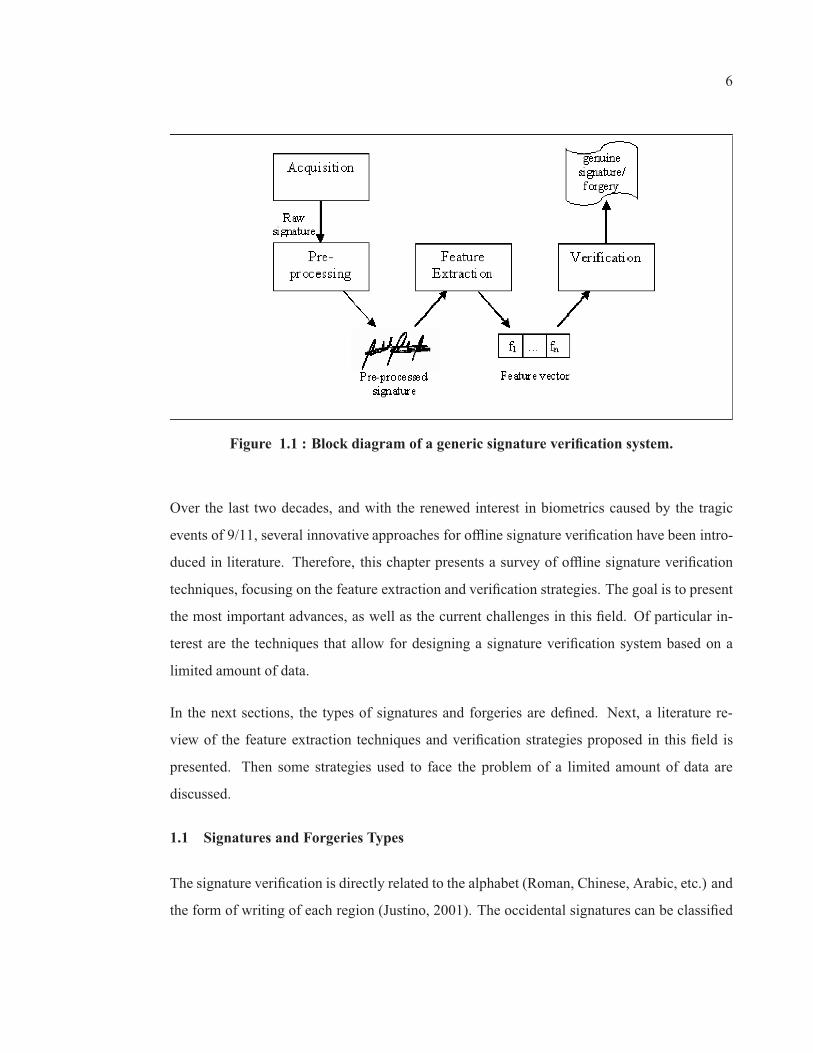
from a forgery (Plamondon, 1994). Figure 1.1 shows an example of a generic signature

verification system. The process follows the classical pattern recognition model steps, that

is, data acquisition, preprocessing, feature extraction, classification (which is generally called

“verification” in the signature verification field) and decision.

Depending on the data acquisition mechanism, the process of signature verification can be

classified as online or offline. In the online (or dynamic) approach, specialized hardware (such

as a digitizing tablet or a pressure sensitive pen) is used in order to capture the pen movements

over the paper at the time of the writing. In this case, a signature can be viewed as a space-

time variant curve that can be analyzed in terms of its curvilinear displacement, its angular

displacement and the torsion of its trajectory (Plamondon and Lorette, 1989). On the other

hand, in the offline (or static) approach, the signature is available on a sheet of paper, which is

later scanned in order to obtain a digital representation composed ofM ×N pixels. Hence, the

signature image is considered as a discrete 2D function f(x, y), where x = 0, 1, 2, . . . , M and

y = 0, 1, 2, . . . , N denote the spatial coordinates. The value of f in any (x, y) corresponds to

the grey level (generally a value from 0 to 255) in that point (Gonzalez and Woods, 2002).

6

Figure 1.1 : Block diagram of a generic signature verification system.

Over the last two decades, and with the renewed interest in biometrics caused by the tragic

events of 9/11, several innovative approaches for offline signature verification have been intro-

duced in literature. Therefore, this chapter presents a survey of offline signature verification

techniques, focusing on the feature extraction and verification strategies. The goal is to present

the most important advances, as well as the current challenges in this field. Of particular in-

terest are the techniques that allow for designing a signature verification system based on a

limited amount of data.

In the next sections, the types of signatures and forgeries are defined. Next, a literature re-

view of the feature extraction techniques and verification strategies proposed in this field is

presented. Then some strategies used to face the problem of a limited amount of data are

discussed.

1.1 Signatures and Forgeries Types

The signature verification is directly related to the alphabet (Roman, Chinese, Arabic, etc.) and

the form of writing of each region (Justino, 2001). The occidental signatures can be classified

7

in two main styles: cursive or graphical, as shown in Figure 1.2 . With cursive signatures, the

author writes his or her name in a legible way, while the graphical signatures contain complex

patterns which are very difficult to interpret as a set of characters.

Figure 1.2 : Examples of (a) (b) cursive and (c) graphical signatures.

According to Coetzer et al. (Coetzer et al., 2004), the forged signatures can be classified in

three basic types:

1) Random forgery, the forger has no access to the genuine signature (not even the author’s

name) and reproduces a random one. A random forgery may also include the forger’s own

signature;

2) Simple forgery, the forger knows the author’s name, but has no access to a sample of the

signature. Thus, the forger reproduces the signature in his own style;

3) Skilled forgery, the forger has access to one or more samples of the genuine signature and is

able to reproduce it. Skilled forgeries can be even subdivided according to the level of the

forger’s skill. Figure 1.3 presents examples of the mentioned types of forgeries.

8

Figure 1.3 : Examples of (a) genuine signature, (b) random forgery, (c) simple forgeryand (d) skilled forgery.

Generally, only random forgeries are used to train the classification module of a signature

verification system. The reason is that, in practice, it is rarely possible to obtain samples of

forgeries; and for example, when dealing with banking applications, it becomes impracticable

(Oliveira et al., 2007). On the other hand, all the types of forgeries are used to evaluate the

system’s performance.

1.2 Feature Extraction Techniques

Feature extraction is essential to the success of a signature verification system. In an offline

environment, the signatures are acquired from a medium, usually paper, and preprocessed be-

fore the feature extraction begins. Offline feature extraction is a fundamental problem because

of handwritten signatures variability and the lack of dynamic information about the signing

process. An ideal feature extraction technique extracts a minimal feature set that maximizes

interpersonal distance between signature examples of different persons, while minimizing in-

trapersonal distance for those belonging to the same person.

There are two classes of features used in offline signature verification:

9

1) Static, related to the signature shape;

2) Pseudo-dynamic, related to the dynamics of the writing.

These features can be extracted locally, if the signature is viewed as a set of segmented regions,

or globally, if the signature is viewed as a whole. It is important to note that techniques used

to extract global features can also be applied to specific regions of the signature in order to

produce local features. In the same way, a local technique can be applied to the whole image

to produce global features. Figure 1.4 presents a taxonomy of the categories of features used

signature verification.

Figure 1.4 : A taxonomy of feature types used in signature verification. The dynamicfeatures are represented but are only used in online approaches.

Moreover, the local features can be described as contextual and non-contextual. If the signature

segmentation is performed in order to interpret the text (for example, bars of "t" and dots of

"i"), the analysis is considered contextual (Chuang, 1977). This type of analysis is not popular

for two reasons:

1) It requires a complex segmentation process;

2) It is not suitable to deal with graphical signatures.

10

On the other hand, if the signature is viewed as a drawing composed of line segments (as it

occurs in the majority of the literature), the analysis is considered non-contextual.

Before describing the most important features extraction techniques in the field of offline sig-

nature verification, signature representation is discussed.

1.2.1 Signature Representations

Some techniques transform the signature image into another representation before extracting

the features. Offline signature verification literature is quite extensive about signature repre-

sentations.

Box and convex hull representations have been used to represent signatures (Frias-Martinez

et al., 2006). The box representation is composed of the smallest rectangle fitting the sig-

nature. Its perimeter, area and perimeter/area ratio can be used as features. The convex hull

representation is composed of the smallest convex hull fitting the signature. Its area, roundness,

compactness and also the length and orientation of its maximum axis can be used as features.

The skeleton of the signature, its outline, directional frontiers and ink distributions have also

been used has signature representations (Huang and Yan, 1997). The skeleton (or core) rep-

resentation is the pixel wide strokes resulting from the application of a thinning algorithm to

a signature image. The skeleton can be used to identify the signature edge points (1-neighbor

pixels) that mark the beginning and ending of strokes (Ozgunduz et al., 2005). Further, pseudo-

Zernike moments have also been extracted from this kind of representation (Wen-Ming et al.,

2004).

The outline representation is composed of every black pixel adjacent to at least one white

pixel. Directional frontiers (also called shadow images) are obtained when keeping only the

black pixels touching a white pixel in a given direction (and there are 8 possible directions). To

perform ink distribution representations, a virtual grid is superposed over the signature image.

The cells containing more than 50% of black pixels are completely filled while the others are

emptied. Depending on the grid scale, the ink distributions can be coarser or more detailed.

11

The number of filled cells can also be used as a global feature. Upper and lower envelopes (or

profiles) are also found in the literature. The upper envelope is obtained by selecting column-

wise the upper pixels of a signature image, while the lower envelope is achieved by selecting

the lower pixels, as illustrated by Figure 1.5 . As global features, the numbers of turns and

gaps in these representations have been extracted (Ramesh and Murty, 1999).

(a) (b)

Figure 1.5 : (a) Example of a handwritten signature and (b) its upper and lowerenvelopes (Bertolini et al., 2010).

Mathematic transforms have been used to represent signature images. Nemcek and Lin (Nem-

cek and Lin, 1974) chose the fast Hadamard transform in their feature extraction process as

a tradeoff between computational complexity and representation accuracy, when compared to

other transforms. Discrete Radon transform is used to extract an observation sequence of the

signature, which is used as a feature set (Coetzer et al., 2004).

Finally, signature images can also undergo a series of transformations before feature extraction.

For example, Tang et al. (Tang et al., 2002) used a central projection to reduce the signature im-

age to a 1-D signal that is in turn transformed by a wavelet before fractal features are extracted

from its fractal dimension.

12

1.2.2 Geometrical Features

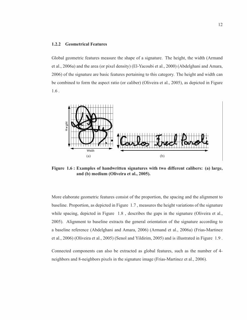
Global geometric features measure the shape of a signature. The height, the width (Armand

et al., 2006a) and the area (or pixel density) (El-Yacoubi et al., 2000) (Abdelghani and Amara,

2006) of the signature are basic features pertaining to this category. The height and width can

be combined to form the aspect ratio (or caliber) (Oliveira et al., 2005), as depicted in Figure

1.6 .

(a) (b)

Figure 1.6 : Examples of handwritten signatures with two different calibers: (a) large,and (b) medium (Oliveira et al., 2005).

More elaborate geometric features consist of the proportion, the spacing and the alignment to

baseline. Proportion, as depicted in Figure 1.7 , measures the height variations of the signature

while spacing, depicted in Figure 1.8 , describes the gaps in the signature (Oliveira et al.,

2005). Alignment to baseline extracts the general orientation of the signature according to

a baseline reference (Abdelghani and Amara, 2006) (Armand et al., 2006a) (Frias-Martinez

et al., 2006) (Oliveira et al., 2005) (Senol and Yildirim, 2005) and is illustrated in Figure 1.9 .

Connected components can also be extracted as global features, such as the number of 4-

neighbors and 8-neighbors pixels in the signature image (Frias-Martinez et al., 2006).

13

(a) (b)

(c)

Figure 1.7 : Examples of handwritten signatures with three different proportions: (a)proportional, (b) disproportionate, and (c) mixed (Oliveira et al., 2005).

(a) (b)

Figure 1.8 : Examples of handwritten signatures (a) with spaces and (b) no space(Oliveira et al., 2005).

(a) (b)

Figure 1.9 : Examples of handwritten signatures with an alignment to baseline of (a) 22◦,and (b) 0◦ (Oliveira et al., 2005).

14

1.2.3 Statistical Features

Many authors use projection representation. It consists in projecting every pixel on a given axis

(usually horizontal or vertical), resulting in a pixel density distribution. Statistical features,

such as the mean (or center of gravity), global and local maximums can be extracted from this

distribution (Frias-Martinez et al., 2006) (Ozgunduz et al., 2005) (Senol and Yildirim, 2005).

Moments - which can include central moments (i.e. skewness and kurtosis) (Frias-Martinez

et al., 2006) (Bajaj and Chaudhury, 1997) and moment invariants (Al-Shoshan, 2006) (Lv

et al., 2005) (Oz, 2005) - are also extracted from the pixel distributions.

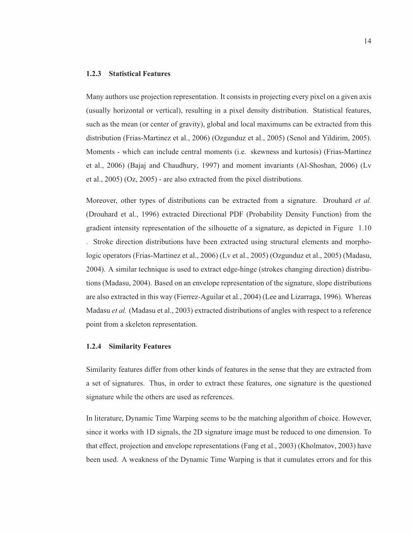
Moreover, other types of distributions can be extracted from a signature. Drouhard et al.

(Drouhard et al., 1996) extracted Directional PDF (Probability Density Function) from the

gradient intensity representation of the silhouette of a signature, as depicted in Figure 1.10

. Stroke direction distributions have been extracted using structural elements and morpho-

logic operators (Frias-Martinez et al., 2006) (Lv et al., 2005) (Ozgunduz et al., 2005) (Madasu,

2004). A similar technique is used to extract edge-hinge (strokes changing direction) distribu-

tions (Madasu, 2004). Based on an envelope representation of the signature, slope distributions

are also extracted in this way (Fierrez-Aguilar et al., 2004) (Lee and Lizarraga, 1996). Whereas

Madasu et al. (Madasu et al., 2003) extracted distributions of angles with respect to a reference

point from a skeleton representation.

1.2.4 Similarity Features

Similarity features differ from other kinds of features in the sense that they are extracted from

a set of signatures. Thus, in order to extract these features, one signature is the questioned

signature while the others are used as references.

In literature, Dynamic Time Warping seems to be the matching algorithm of choice. However,

since it works with 1D signals, the 2D signature image must be reduced to one dimension. To

that effect, projection and envelope representations (Fang et al., 2003) (Kholmatov, 2003) have

been used. A weakness of the Dynamic Time Warping is that it cumulates errors and for this

15

Figure 1.10 : Example of a directional PDF extracted from the handwritten signatureshown in the upper part of the figure (Drouhard et al., 1996). The peaksaround 0◦, 90◦ and 180◦ indicates the predominance of horizontal andvertical strokes.

reason the sequences to match must be the shortest possible. To solve this problem, a wavelet

transform can be used to extract inflection points from the 1D signal. Then, Dynamic Time

Warping matches this shorter sequence of points (Deng et al., 2003). The inflection points

can also be used to segment the wavelet signal into shorter sequences to be matched by the

Dynamic Time Warping algorithm (Ye et al., 2005).

Among other methods, a local elastic algorithm has been used to match the skeleton represen-

tations of two signatures (You et al., 2005) (Fang et al., 2003) and cross-correlation has been

16

used the extract correlation peak features frommultiple signature representations obtained from

identity filters and Gabor filters (Fasquel and Bruynooghe, 2004).

1.2.5 Fixed Zoning

Fixed zoning defines arbitrary regions and uses them for all signatures. To perform fixed zon-

ing based on pixels, all the pixels of a signature are sent to the classifier after the signature

image has been normalized to a given size (Frias-Martinez et al., 2006) (Martinez et al., 2004)

(Mighell et al., 1989). Otherwise, numerous fixed zoning methods are described in the litera-

ture. Usually, the signature is divided into strips (vertical or horizontal) or using a layout like

a grid or angular partitioning. Then, geometric features (Abdelghani and Amara, 2006) (Ar-

mand et al., 2006b) (Ferrer et al., 2005) (Justino et al., 2005) (Ozgunduz et al., 2005) (Senol

and Yildirim, 2005) (Martinez et al., 2004) (Santos et al., 2004) (Huang and Yan, 1997) (Qi and

Hunt, 1994), wavelet transform features (Abdelghani and Amara, 2006) and statistical features

(Frias-Martinez et al., 2006) (Hanmandlu et al., 2005) (Justino et al., 2005) (Fierrez-Aguilar

et al., 2004) (Madasu, 2004) can be extracted. Figure 1.11 illustrate an example of feature

extraction from a grid cell of a handwritten signature.

(a) (b) (c)

Figure 1.11 : (a) Example of a grid-like fixed zoning and of two feature extractiontechniques applied to a given cell: (b) pixel density and (c) gravity centerdistance (Justino et al., 2005).

17

Other techniques are specially designed for extracting local features. Strips based methods

include peripheral features extraction from horizontal and vertical strips of a signature edge

representation. Peripheral features measure the distance between two edges and the area be-

tween the virtual frame of the strip and the first edge of the signature (Fang and Tang, 2005)

(Fang et al., 2002).

Most fixed zoning techniques use a grid layout. For example, the Modified Direction Fea-

ture (MDF) technique (Armand et al., 2006b) extracts the location of the transitions from the

background to the signature and their corresponding direction values for each cell of grid super-

posed on the signature image. The Gradient, Structural and Concavity (GSC) technique (Kalera

et al., 2004a) (Srihari et al., 2004a) extracts gradient features from edge curvature, structural

features from short strokes and concavity features from certain hole types independently for

each cell a grid covering the signature image. The Extended Shadow Code technique, proposed

by Sabourin and colleagues (Sabourin et al., 1993) (Sabourin and Genest, 1994) (Sabourin and

Genest, 1995) centers the signature image on a grid layout where each rectangular cell of the

grid is composed of six bars: one bar for each side of the cell plus two diagonal bars stretching

from a corner of the cell to the other in an ‘X’ fashion. The pixels of the signature are projected

perpendicularly on the nearest horizontal bar, the nearest vertical bar, and also on both diagonal

bars. The features are extracted from the normalized area of each bar that is covered by the

projected pixels. The envelope-based technique (Ramesh and Murty, 1999) (Bajaj and Chaud-

hury, 1997) describes, for each grid cell, the comportment of the upper and lower envelope of

the signature. The pecstrum technique (Sabourin et al., 1997b) (Sabourin et al., 1996) centers

the signature image on a grid of overlapping retinas and then uses successive morphological

openings to extract local granulometric size distributions.

1.2.6 Signal Dependent Zoning

Signal dependent zoning generates different regions adapted to individual signature. When

signal dependent zoning is performed using the pixels of the signature as local regions, posi-

tion features are extracted from each pixel with respect to a coordinate system. Martinez et

18

Figure 1.12 : Example of feature extraction on a looping stroke by the Extended ShadowCode technique (Sabourin et al., 1993). Pixel projections on the bars areshown in black.

al. (Martinez et al., 2004), followed by Ferrer et al. (Ferrer et al., 2005), extracted position

features from a contour representation in polar coordinates. Still using the polar coordinate

system, signal dependent angular-radial partitioning techniques have been developed. These

techniques adjust themselves to the circumscribing circle of the signature to achieve scale in-

variance and they achieve rotation invariance by synchronizing the sampling with the baseline

of the signature, as depicted in Figure 1.13 . Shape matrices have been defined this way to

sample the silhouette of two signatures and extract similarity features (Sabourin et al., 1997a).

A similar method is used by Chalechale et al. (Chalechale et al., 2004), though edge pixel area

features are extracted from each sector and rotation invariance is obtained by applying a 1-D

discrete Fourier transform to the extracted feature vector.

In Cartesian coordinate system, signal dependent retinas have been used to define local regions

best capturing the intrapersonal similarities from the reference signatures of individual writers

(Ando and Nakajima, 2003). A genetic algorithm is used to optimize the location and size

19

Figure 1.13 : Example of polar sampling on an handwritten signature. The coordinatesystem is centered on the centroid of the signature to achieve translationinvariance and the signature is sampled using a sampling length α and anangular step β (Sabourin et al., 1997a).

of these retinas before similarity features are extracted from the questioned signature and its

reference set.

Connectivity analysis has been performed on a signature image to generate local regions before

extracting geometric and position features from each region (Igarza et al., 2005). Even more

localized, signal dependent regions are achieved using stroke segmentation. Perez-Hernandez

et al. (Perez-Hernandez et al., 2004) achieved stroke segmentation by first finding the direction

of each pixel of the skeleton of the signature and then using a pixel tracking process. Then,

the orientation and endpoints of the strokes are extracted as features. Another technique is

to erode the stroke segments into bloated regions before extracting similarity features (Franke

et al., 2002).

Instead of focusing on the strokes, the segmentation can be done in other signature represen-

tations. Chen and Srihari (Chen and Srihari, 2006) matched two signature contours using Dy-

namic Time Warping before segmenting and extracting Zernike moments from the segments.

Xiao and Leedham (Xiao and Leedham, 2002) segmented upper and lower envelopes where

their orientation changes sharply. After that, they extracted length, orientation, position and

pointers to the left and right neighbors of each segment.

20

1.2.7 Pseudo-dynamic Features

The lack of dynamic information is a serious constrain for offline signature verification sys-

tems. The knowledge of the pen trajectory, along with speed and pressure, gives an edge to

online systems. To overcome this difficulty, some approaches use dynamic signature refer-

ences to develop individual stroke models that can be applied to offline questioned signatures.

For instance, Guo et al. (Guo et al., 2000) used stroke-level models and heuristic methods to

locally compare dynamic and static pen positions and stroke directions. Lau et al. (Lau et al.,

2005) developed the Universal Writing Model (UWM), which consists of a set of distribution

functions constructed using the attributes extracted from online signature samples. Whereas

Nel et al. (Nel et al., 2005) used a probabilistic model of the static signatures based on Hidden

Markov Models (HMM) where the HMMs restrict the choice of possible pen trajectories de-

scribing the morphology of the signature. Then, the optimal pen trajectory is calculated using

a dynamic sample of the signature.

However, without resorting to online examples, it is possible to extract pseudo-dynamic fea-

tures from static signature images. Pressure features can be extracted from pixel intensity (i.e.

grey levels) (Lv et al., 2005) (Santos et al., 2004) (Wen-Ming et al., 2004) (Huang and Yan,

1997) and stroke width (Lv et al., 2005) (Oliveira et al., 2005). Whereas speed information can

be extrapolated from stroke curvature (Santos et al., 2004) (Justino et al., 2005), stroke slant

(Justino et al., 2005) (Oliveira et al., 2005) (Senol and Yildirim, 2005), progression (Oliveira

et al., 2005) (Santos et al., 2004) and form (Oliveira et al., 2005). Figure 1.14 and 1.15

illustrates stroke progression and form, respectively.

1.3 Verification Strategies and Experimental Results

This section categorizes some research in offline signature verification according to the tech-

nique used to perform verification, that is, Distance Classifiers, Artificial Neural Networks,

Hidden Markov Models, Dynamic Time Warping, Support Vector Machines, Structural Tech-

niques and Bayesian Networks.

21

(a) (b)

Figure 1.14 : Examples of stroke progression: (a) few changes in direction indicates atense stroke, and (b) a limp stroke changes direction many times (Oliveiraet al., 2005).

Figure 1.15 : Example of stroke form extracted from retinas using concavity analysis(Oliveira et al., 2005).

In signature verification, the verification strategy can either be categorized as writer-indepen-

dent or writer-dependent (Srihari et al., 2004a). With writer-independent verification, a single

22

classifier deals with the whole population of writers. In contrast, the writer-dependent verifica-

tion necessitates a different classifier for each writer. As the majority of the research presented

in literature is designed to perform writer-dependent verification, this aspect is mentioned only

when writer-independent verification is considered.

Before describing the verification strategies, a word on the measures used to evaluate the per-

formance of signature verification systems.

1.3.1 Performance Evaluation Measures

The simplest way to report the performance of signature verification systems is in terms of

error rates. The False Rejection Rate (FRR) is related to the number of genuine signatures

erroneously classified by the system as forgeries. Whereas the False Acceptance Rate (FAR)

is related to the number of forgeries misclassified as genuine signatures. FRR and FAR are

also known as type 1 and type 2 errors, respectively. Finally, the Average Error Rate (AER) is

related to the total error of the system, that is, the type 1 and type 2 errors together.

On the other hand, if the decision threshold of a system is set to have the FRR approximately

equal to the FAR, the Equal Error Rate (EER) is being calculated.

1.3.2 Distance Classifiers

A simple Distance Classifier is a statistical technique which usually represents a pattern class

with a Gaussian probability density function (PDF). Each PDF is uniquely defined by the mean

vector and covariance matrix of the feature vectors belonging to a particular class. When the

full covariance matrix is estimated for each class, the classification is based on Mahalanobis

distance. On the other hand, when only the mean vector is estimated, classification is based on

Euclidean distance (Coetzer, 2005).

Approaches based on Distance Classifiers are traditionally writer-dependent. The reference

samples of a given author are used to compose the class of genuine signatures and a subset of

samples from each other writer is chosen randomly to compose the class of (random) forgeries.

23

The questioned signature is classified according to the label of its nearest reference signature

in the feature space. Further, if the classifier is designed to find a number of k nearest reference

signatures, a voting scheme is used to take the final decision.

Distance Classifiers were one of the first classification techniques to be used in offline signa-

ture verification. One of the earliest reported research was by Nemcek and Lin (Nemcek and

Lin, 1974). By using a fast Hadamard transform as feature extraction technique on genuine

signatures and simple forgeries, and Maximum Likelihood Classifiers, they obtained an FRR

of 11% and an FAR of 41%.

Then, Nagel and Rosenfeld (Nagel and Rosenfeld, 1977) proposed a system to discriminate

between genuine signatures and simple forgeries using images obtained from real bank checks.

A number of global and local features were extracted considering only the North American’s

signature style. Using Weighted Distance Classifiers, they obtained FRRs ranging from 8% to

12% and an FAR of 0%.

It is only years later that skilled forgeries began to be considered in offline signature verifica-

tion. Besides proposing a method to separate the signatures from noisy backgrounds and to

extract pseudo-dynamic features from static images, Ammar and colleagues were the first to

try to detect skilled forgeries using an offline signature verification system. In their research

(Ammar et al., 1985) (Ammar et al., 1988) (Ammar, 1991), distance classifiers were used com-

bined with the leave-one-out cross validation method, since the number of signatures samples

was small.

Qi and Hunt (Qi and Hunt, 1994) presented a signature verification system based on global

geometric features and local grid-based features. Different types of similarity measures, such

as Euclidean distance, were used to discriminate between genuine signatures and forgeries

(including simple and skilled). They achieved an FRR ranging from 3% to 11.3% and an FAR

ranging from 0% to 15%.

24

Sabourin and colleagues have done extensive research in offline signature verification since

middle 80’s (Sabourin and Plamondon, 1986). In one of their research (Sabourin et al., 1993),

the Extended Shadow Code was used in order to extract local features from genuine signatures

and random forgeries. The first experiment used a k-Nearest Neighbors classifier (k-NN) with

a voting scheme, obtaining an AER of 0.01% when k = 1. The second experiment used a Min-

imum Distance Classifier, obtaining an AER of 0.77% when 10 training signatures were used

for each writer. In another relevant research (Sabourin et al., 1997b), they used granulometric

size distributions as local features, also in order to eliminate random forgeries. By using k-

Nearest Neighbors and Threshold Classifiers, they obtained an AER around 0.02% and 1.0%,

respectively.

Fang et al. (Fang et al., 2001) developed a system based on the assumption that the cursive seg-

ments of skilled forgeries are generally less smooth than those of genuine signatures. Besides

the utilization of global shape features, a crossing and a fractal dimension methods were pro-

posed to extract the smoothness features from the signature segments. Using a simple Distance

Classifier and the leave-one-out cross-validation method, an FRR of 18.1% and an FAR of

16.4% were obtained. More recently (Fang et al., 2002), they extracted a set of peripheral fea-

tures in order to describe internal and the external structures of the signatures. To discriminate

between genuine signatures and skilled forgeries, they used a Mahalanobis distance classi-

fier together with the leave-one-out cross-validation method. The obtained AERs were in the

range of 15.6% (without artificially generated samples) and 11.4% (with artificially generated

samples).

1.3.3 Artificial Neural Networks

An Artificial Neural Network (ANN) is a massively parallel distributed system composed of

processing units capable of storing knowledge learned from experience (samples) and using

it to solve complex problems (Haykin, 1998). Multilayer Perceptron (MLP) trained with the

error Back Propagation algorithm (Rumelhart et al., 1986) has been so far the most frequently

ANN architecture used in pattern recognition.

25

Mighell et al. (Mighell et al., 1989) were the first to apply ANNs to offline signature verifi-

cation. In order to eliminate simple forgeries, they used the raw images as input to an MLP.

In the experiments, by using a training set composed of genuine signatures and forgeries, they

achieved an EER of 2%.

Sabourin and Drouhard (Sabourin and Drouhard, 1992) used directional PDFs as global feature

vectors and MLP as classifier in order to eliminate random forgeries. Since their database

was composed of few data, some signature samples were artificially generated by rotating the

directional PDFs. In the experiments, they obtained an FRR of 1.75% and an FAR of 9%.

Cardot et al. (Cardot et al., 1994) used the outline of the signature images and geometric

features to compose two types of feature vectors. The most important contribution of their

research was the proposal of a multi-stage architecture to eliminate random forgeries. The first

level is composed of two Kohonen maps (one for each set of features), in order to perform

an initial classification and to choose the random forgeries to train the networks of the second

level. As the number of writers was very large (over 300), they had to limit the number of

classes to less than 50. In the second level, two MLPs for each writer are used to perform

writer-dependent verification. Finally, in the last level, an MLP accepts or rejects the signature.

By using a dataset of signatures extracted from real postal checks, they achieved an FRR of

4% and an FAR of 2%.

Murshed et al. (Murshed et al., 1995) proposed a verification strategy based on Fuzzy ARTMAPs

in the context of random forgeries. Differently from other neural networks types, the Fuzzy

ARTMAPs allows training by using examples of only one class. Therefore, in this approach,

the genuine signatures are used for training and the random forgeries (as well as some un-

seen genuine signatures samples), for testing. In order to simulate different experts examining

different regions of the signature, the image is divided in a number of overlapping squares, ac-

cording to the writer signature shape. After that, each signature region is reduced, by applying

a MLP network, and verified by a specialized Fuzzy ARTMAP. Finally, based on the results

26

given by each Fuzzy ARTMAP, the final decision is taken. In the experiments, they obtained

an AER of 9.14%.

Bajaj and Chaudhary (Bajaj and Chaudhury, 1997) used an ensemble of MLPs to perform

writer identification. In order to discriminate between genuine signatures and random forg-

eries, one MLP was trained per signature representation: moments, upper envelope and lower

envelope. Moreover, each MLP was composed of 10 outputs (one for each writer). In the

verification phase, the output of the three classifiers was combined to obtain a final decision.

In the experiments, a substantial reduction of the error rate was obtained when using the three

classifiers together (FRR=1%; FAR = 3%).

Fadhel and Bhattacharya (Fadhel and Bhattacharyya, 1999) proposed a signature verification

system based on Steerable Wavelets as feature extraction technique and MLP as classifier. In

the first experiment, by selecting only the first 2 of the 16 coefficients which represent each

signature image, they obtained a classification rate of 85.4%. Whereas in a second experiment,

by using all the 16 coefficients, the classification rate was improved to 93.8%.

Sansone and Vento (Sansone and Vento, 2000) proposed a three-stage multi-expert system in

order to deal with all the types of forgeries. The first stage was designed to eliminate random

and simple forgeries by using only the signature’s outline as feature. The second stage receives

the signatures accepted by the previous stage, which can be classified as genuine or as skilled

forgery. The features used in this stage are the high pressure regions. Finally, a third stage

takes the final decision. Using MLP as classifiers, they obtained an FRR of 2.04% and FARs

of 0.01%, 4.29% and 19.80% on random, simple and skilled forgeries, respectively.

Baltzakis and Papamarkos (Baltzakis and Papamarkos, 2001) used global geometric features,

grid features and texture features to represent the signatures. They proposed a two-stage system

in order to eliminate random forgeries. In the first stage, three MLPs (one for each feature set)

and the Euclidean distance metric perform a coarse classification. After that, a RBF (Radial

Basis Function) neural network, trained with samples which were not used in the first stage,

takes the final decision. An FRR of 3% and an FAR of 9.8% were obtained in the experiments.

27

Quek and Zhou (Quek and Zhou, 2002) proposed a system based on Fuzzy Neural Networks,

in order to eliminate skilled forgeries. To represent the signatures, they used reference pattern-

based features, global baseline features, pressure features and slant features. In the first set

of experiments, using both genuine signatures and skilled forgeries to train the network, an

average EER of 22.4% was obtained. Comparable results were obtained in the second set of

experiments, in which only genuine signatures were used as training data.

Vélez et al. (Vélez et al., 2003) performed signature verification by comparing sub-images

or positional cuttings of a test signature to the representations stored in Compression Neural

Networks. In this approach, neither image preprocessing nor feature extraction is performed.

By using one signature per writer, together with a set of artificially generated samples, they

obtained a classification rate of 97.8%.

Armand et al. (Armand et al., 2006b) proposed the combination of the Modified Direction

Feature (MDF) extracted from the signature’s contour with a set of geometric features. In

the experiments, they compared RBF and Resilient Backpropagation (RBP) neural network

performances. Both networks performed writer identification and contained 40 classes: 39

corresponding to each writer and one corresponding to the forgeries. In this case, skilled forg-

eries were used in the training phase. The best classification rates obtained were 91.21% and

88.0%, using RBF and RBP, respectively.

1.3.4 Hidden Markov Models

HiddenMarkovModels (Rabiner, 1989) are finite stochastic automata used to model sequences

of observations. Although this technique is more suitable to model dynamic data (such as

speech and online signatures) it has also been applied to offline signatures. Generally, HMMs

are used to perform writer-dependent verification, by modeling only the genuine signatures of

a writer. In this case, the forgeries are detected by thresholding.

Rigoll and Kosmala (Rigoll and Kosmala, 1998) presented a comparison between online and

offline signature verification using discrete HMMs. To represent the signatures in the online

28

model, they used both static and pseudo-dynamic features. In the first set of experiments, in

which each feature was investigated separately, surprising results were obtained. The bitmap

feature was the most important one, achieving a classification rate of 92.2%. The Fourier fea-

ture also supplied a high classification rate. Finally, another surprise was the low importance

of the acceleration. As expected, good results were obtained using the velocity feature. Other

experiments, using several features together, were performed in order to obtain high classifica-

tion rates. The best result (99%) was obtained when only 4 features (bitmap, velocity, pressure

and Fourier feature) where combined.

To represent the signatures in the offline model, they subdivided the signature image into sev-

eral squares of 10 × 10 pixels. After that, the grey value of each square was computed and

used as feature. In the experiments, a classification rate of 98.1% was achieved. The small

difference between the online and offline classification rates is an important practical result,

since offline verification is simpler to implement.

El-Yacoubi et al. (El-Yacoubi et al., 2000) proposed an approach based on HMM and pixel

density feature in order to eliminate random forgeries. To perform training while choosing the

optimal HMM parameters, the Baum-Welch algorithm and the cross-validation method were

used. In the experiments, each signature was analyzed under three resolutions (100 × 100,

40 × 40 and 16 × 16 pixels) by applying the Forward algorithm. Finally, a majority-vote rule

took the final decision. An AER of 0.46% was obtained when both genuine and impostor

spaces were modeled, and AER of 0.91% was obtained when only the genuine signatures were

modeled.

Justino (Justino, 2001) used HMMs to detect random, simple and skilled forgeries. Also using

a grid-segmentation scheme, three features were extracted from the signatures: pixel density

feature, Extended Shadow Code and axial slant feature. They applied the cross-validation

method in order to define the number of states for each HMM writer model. Using the Bakis

model topology and the Forward algorithm, they obtained an FRR of 2.83% and FARs of

1.44%, 2.50% and 22.67%, for random, simple and skilled forgeries, respectively.

29

Coetzer et al. (Coetzer et al., 2004) used HMMs and Discrete Radon Transform to detect

simple and skilled forgeries. In this research, some strategies were proposed in order to obtain

noise, shift, rotation and scale invariances. By using a left-to-right ring model and the Viterbi

algorithm, EERs of 4.5% and 18% were achieved for simple and skilled forgeries, respectively.

1.3.5 Dynamic Time Warping

Widely applied in Speech Recognition, Dynamic Time Warping is a Template Matching tech-

nique used for measuring similarity between two sequences of observations. The primary

objective of Dynamic TimeWarping is to nonlinearly align the sequences before they are com-

pared (or matched) (Coetzer, 2005). Despite being more suitable to model data which may vary

in time or speed, Dynamic Time Warping has been used in offline signature verification. As

it usually occurs with similarity-based approaches, a test signature is compared to the genuine

ones of a writer and a forgery is detected by thresholding.

Wilkinson and Goodman (Wilkinson and Goodman, 1990) used Dynamic Time Warping to

discriminate between genuine signatures and simple forgeries. Assuming that curvature, total

length and slant angle are constant among different signatures of a same writer, they used a

slope histogram to represent each sample. In the experiments, they obtained an EER of 7%.

Increases in the error rates were observed when the forgers had some a priori knowledge about

the signatures.

Deng et al. (Deng et al., 1999) proposed a Wavelet-based approach to eliminate simple and

skilled forgeries. After applying a Closed-Contour Tracing algorithm to the signatures, the

curvature data obtained were decomposed into multi-resolution signals using Wavelets. Then,

Dynamic Time Warping were used to match the corresponding zero-crossings. Experiments

were performed using English and Chinese signature datasets. For the English dataset, an FRR

of 5.6% and FARs of 21.2% on skilled forgeries and 0% on simple forgeries were obtained.

Whereas using the Chinese dataset, an FRR of 6.0% and FARs of 13.5% and 0% were achieved

on skilled and simple forgeries, respectively.

30

Fang et al. (Fang et al., 2003) proposed a method based on Dynamic Time Warping and one-

dimensional projection profiles in order to deal with intra-personal signature variations. To

achieve discrimination between genuine signatures and skilled forgeries, nonlinear Dynamic

Time Warping was used in a different way. Instead of using the distance between a test sig-

nature and a reference sample to take a decision, the positional distortion at each point of the

projection profile was incorporated into a distance measure. Using the leave-one-out cross-

validation method and the Mahalanobis distance, they obtained AERs of 20.8% and 18.1%,

when binary and grey level signatures were considered, respectively.

1.3.6 Support Vector Machines

Support Vector Machines (SVM) (Vapnik, 1999) use a kernel-based learning technique which

has shown successful results in various domains such as pattern recognition, regression esti-

mation, density estimation, novelty detection and others.

Signature verification systems that use SVM as classifier are designed in a similar way to those

that use neural networks. That is, in a writer-dependent approach, there is one class for the

genuine signatures and other class for the forgeries. In addition, by using one-class SVMs

(Scholkopf et al., 2001), it is possible to perform training by using only genuine signatures.

In the research of Srihari et al. (Srihari et al., 2004a) they tried to use it in the context of

skilled forgeries. However, by using the traditional two-class approach, the AER decreased

from 46.0% to 9.3%.

Martinez et al. (Martinez et al., 2004) used SVM with RBF kernel in order to detect skilled

forgeries. In the experiments, different types of geometrical features, as well as raw signatures

were tested. The best result, an FAR of 18.85%, was obtained when raw images with a scale

of 0.4 were used.

Justino et al. (Justino et al., 2005) performed a comparison between SVM and HMM classifiers

in the detection of random, simple and skilled forgeries. By using a grid-segmentation scheme,

they extracted a set of static and pseudo-dynamic features. Under different experimental con-

31

ditions, that is, varying the size of the training set and the types of forgeries, the SVM with a

linear kernel outperformed the HMM.

Ozgunduz et al. (Ozgunduz et al., 2005) used Support Vector Machines in order to detect

random and skilled forgeries. To represent the signatures, they extracted global geometric

features, direction features and grid features. In the experiments, a comparison between SVM

and ANN was performed. Using a SVM with RBF kernel, an FRR of 0.02% and an FAR

of 0.11% were obtained. Whereas the ANN, trained with the Backpropagation algorithm,

provided an FRR of 0.22% and an FAR of %0.16. In both experiments, skilled forgeries were

used to train the classifier.

1.3.7 Structural Techniques

In Structural Techniques, the patterns are organized hierarchically in a way that, at each level,

they are viewed as being composed of simpler subpatterns. By using a small number of primi-

tives (the most elementary subpatterns) and grammatical rules, it is possible to describe a large

collection of complex patterns (Coetzer, 2005). Therefore, it is possible to interpret the scene

both globally and locally.

Sabourin et al. (Sabourin et al., 1994) were the first ones to propose a structural representation

of handwritten signatures images. In their approach, a segmentation process breaks up the sig-

nature into a set of primitives. From these shape primitives, both static and pseudo-dynamic

features are extracted. The comparison process is composed of two stages: Local Interpre-

tation of Primitives (LIP) and Global Interpretation of the Scene (GIS). In the LIP stage, a

template match process is performed, in which each primitive of the test signature image is

labeled taking into account the reference set. Finally, the GIS stage takes the final decision by

computing a similarity measure between the test primitive set and the reference primitive set.

The experiments were performed in order to eliminate random forgeries. By using a minimum

distance classifier with two reference signatures, they obtained an AER of 1.43%.

32

Bastos et al. (Bastos et al., 1997) proposed a mathematical signature representation in terms

of ellipses, parabolas and hyperbolas. The goal of this approach is to allow a simplification of

the signature tracing when detecting random forgeries. After performing a thinning process,

junction and end points are found in the signatures. Next, an algorithm is applied in each

part of the signature tracing (between an end point and a junction point) in order to obtain all

necessary points for modeling a mathematical equation. Finally, the Least Square Method of

curve adjusting is applied to each set of tracing points, resulting in number of equations of

ellipses, parabolas and hyperboles. Performing superpositions between the found equations

and the respective signatures, they obtained similarity indices ranged from 86.3% and 97.3%,

with respect to different writers.

Huang and Yan (Huang and Yan, 2002) proposed a two-stage signature verification system

based on ANN and a structural approach. To represent the signatures, they used geometric

and directional frontier features. In the first stage of the system, a neural network attributes

to the signature three possible labels: pass (genuine signature), fail (random or less skilled

forgery) and questionable (skilled forgery). For the questionable signatures, the second stage

uses a Structural Feature Verification algorithm to compare the detailed structural correlation

between the test signature and the reference samples. In the experiments, the first classifier

rejected 2.2% of the genuine signatures, accepted 3.6% of the forgeries and was undecided

on 32.7% of the signatures. The second classifier rejected 31.2% of the questionable genuine

signatures and accepted 23.2% of the questionable forgeries. Therefore, for the combined

classifier, an FRR of 6.3% and an FAR of 8.2% were obtained.

1.4 Dealing With A Limited Amount Of Data

Mainly for practical reasons, a limited number of signatures per writer is available to train

a classifier for signature verification. For example, a bank client is asked to supply from 3

to 5 signature samples at the time of her subscription. On the other hand, a high number of

features are generally extracted from handwritten signature images. This combination - few

samples and a high dimensionality representation space - is likely to result into unsatisfactory

33

verification performance since class statistics estimation errors may be significant (Fang and

Tang, 2005). However, this crucial issue has received little attention in literature. Possible

solutions are:

1) Selecting the most discriminating features. In the research of Xuhua et al. (Xuhua et al.,

1996), for example, Genetic Algorithms were used in order to select the optimal set of

partial curves from an online signature and the best features of each partial curve;

2) Using regularization techniques, in order to obtain a stable estimation of the covariance

matrix (Fang and Tang, 2005);

3) Generating synthetic samples. This can be done by adding noise or applying transforma-

tions to the real signatures (Huang and Yan, 1997) (Vélez et al., 2003) (Fang et al., 2002)

(Fang and Tang, 2005);

4) Using Dissimilarity Representation. This technique, used to design writer-independent ver-

ification systems, allows to reduce the number of classes, as well as to increase the quantity

of feature vectors (Santos et al., 2004) (Srihari et al., 2004a) (Kalera et al., 2004a).

The rest of this section describes approaches generating synthetic samples as a solution. Writer-

independent approaches based on dissimilarity representation are covered in details in Chapter

2.

Huang and Yan (Huang and Yan, 1997) applied slight transformations to the genuine signa-

tures, in order to generate additional training samples; and heavy transformations, also to the

genuine signatures, in order to generate forgeries. In the two cases, the transformations were:

slant distortions, scalings in horizontal and vertical directions, rotations and perspective view

distortions.

Whereas Vélez et al. (Vélez et al., 2003) tried to reproduce intrapersonal variability while using

only one signature per writer. To generate additional training samples, they applied rotations

34

(in the range of ±15◦), scalings (in the range of ±20%), horizontal and vertical displacements

(in the range of ±20%) and different types of noise for each original signature.

By using a different approach, Fang and Tang (Fang and Tang, 2005) proposed the generation

of additional samples in the following way:

1) Two samples are selected from the set of genuine signatures;

2) An Elastic Matching Algorithm is applied to the pair of signatures in order to establish

correspondences between individual strokes;

3) Corresponding stroke segments are linked up by displacement vectors;

4) These displacement vectors are used to perform an interpolation between the two signatures

and, thus, to produce a new training sample.

1.5 Discussion

This chapter presented a survey of techniques developed in the field of offline signature verifi-

cation over the last twenty years. Even if error rates are reported, it is very difficult to compare

performances between verification strategies since each research uses different experimenta-

tion protocols, and signature databases (see Table 1.1).

Moreover, for security reasons, it is not easy to make a signature dataset available to the sig-

nature verification community, especially if the signatures come from a real application, as

banking documents, for example. However, the availability of datasets could make possible

to define a common experimentation protocol in order to perform comparative studies in this

field.

As we could observe, despite the vast amount of research performed in order to solve this

problem, there are still fundamental problems facing signature verification: the large number

of users, the large number of features, the limited number of reference signatures for train-

35

Table 1.1: Signature verification databases (I = Individual; G = Genuine; F = Forgeries;

S = Samples)

References Images Signatures Forgery Types

(Nemcek and Lin, 1974)128x256 pixels 600G / 15I

Simplebinary 120F / 4I

(Nagel and Rosenfeld, 1977)500 ppi 11G / 2I

Simple64 grey levels 14F / 2I

(Ammar et al., 1985)256x1024 pixels 200G / 10I

Simple256 grey levels 200F / 10I

(Qi and Hunt, 1994)300 dpi 300G / 15I Simple

256 grey levels 150F / 10I Skilled

(Sabourin and Drouhard, 1992)

800G / 20I Random(Sabourin et al., 1993) 128x512 pixels

(Sabourin and Genest, 1994) 256 grey levels

(Sabourin et al., 1997b)

(Fang et al., 2002) 300 dpi 1320G / 55ISkilled

(Fang et al., 2003) 256 grey levels 1320F / 12I

(Mighell et al., 1989)128x64 pixels 80G / 1I

Skilledbinary 66F

(Cardot et al., 1994)1024x512 pixels

6000G/ 300I Random256 grey levels

(Murshed et al., 1995)128x512 pixels

200G / 5I Random256 grey levels

(Bajaj and Chaudhury, 1997)200 dpi

150G / 10I Randombinary

(Fadhel and Bhattacharyya, 1999)340 dpi

300S / 30I Skilled256 grey levels

Continued on Next Page. . .

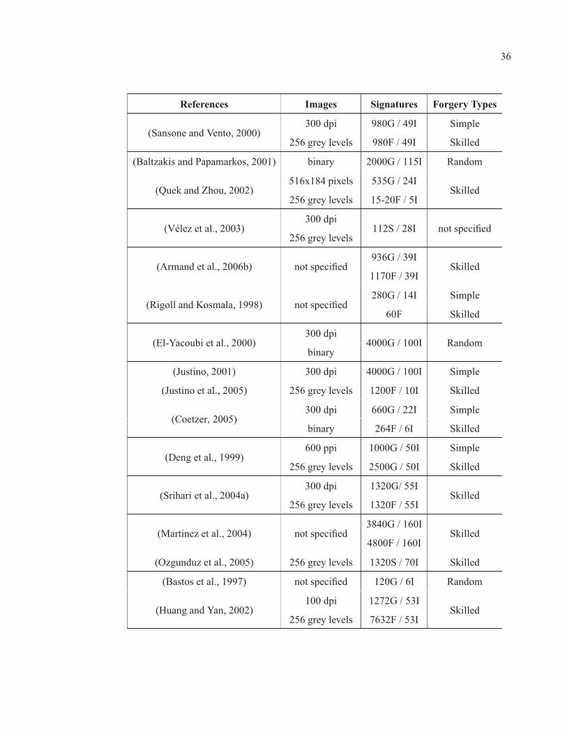
36

References Images Signatures Forgery Types

(Sansone and Vento, 2000)300 dpi 980G / 49I Simple

256 grey levels 980F / 49I Skilled

(Baltzakis and Papamarkos, 2001) binary 2000G / 115I Random

(Quek and Zhou, 2002)516x184 pixels 535G / 24I

Skilled256 grey levels 15-20F / 5I

(Vélez et al., 2003)300 dpi

112S / 28I not specified256 grey levels

(Armand et al., 2006b) not specified936G / 39I

Skilled1170F / 39I

(Rigoll and Kosmala, 1998) not specified280G / 14I Simple

60F Skilled

(El-Yacoubi et al., 2000)300 dpi

4000G / 100I Randombinary

(Justino, 2001) 300 dpi 4000G / 100I Simple

(Justino et al., 2005) 256 grey levels 1200F / 10I Skilled

(Coetzer, 2005)300 dpi 660G / 22I Simple

binary 264F / 6I Skilled

(Deng et al., 1999)600 ppi 1000G / 50I Simple

256 grey levels 2500G / 50I Skilled

(Srihari et al., 2004a)300 dpi 1320G/ 55I

Skilled256 grey levels 1320F / 55I

(Martinez et al., 2004) not specified3840G / 160I

Skilled4800F / 160I

(Ozgunduz et al., 2005) 256 grey levels 1320S / 70I Skilled

(Bastos et al., 1997) not specified 120G / 6I Random

(Huang and Yan, 2002)100 dpi 1272G / 53I

Skilled256 grey levels 7632F / 53I

37

ing, the high intra-personal variability of the signatures and the unavailability of forgeries as

counterexamples.

Some important feature extraction techniques used to extract global and local information from

signatures were presented. The choice of using global or local features depends, mainly, on

the types of forgeries to be detected by the system. The global features are extracted at a

low computational cost and they have good noise resilience. However, they have less capacity

to discriminate between genuine signatures and skilled forgeries. On the other hand, local

features are more suitable to identify skilled forgeries, despite their dependence on a zoning

process. Thus, a verification system designed to eliminate random, simple and skilled forgery

could benefit from using both global and local features. In this respect, Extended Shadow Code

(Sabourin and Genest, 1994) appears to be a good trade-off between global and local features;

since it permits the projection of the handwritten at several resolutions. On the other hand,

such an approach is likely to generate a very high number of potential features. Consequently,

a feature selection process could improve the system performances by disregarding irrelevant

or redundant features.

Despite the great recognition rates obtained by using classifiers learning from examples (as

ANNs, HMMs, and SVMs), there are some difficulties to be faced. The first one, which occurs

mainly with ANNs and SVMs, is the necessity of using forgery counterexamples in the training

set in order to allow class separation by the classifier. However, some authors have already been

dealing with this problem by using one-class classifiers (Murshed et al., 1995) (Srihari et al.,

2004a), computer generated forgeries (Mighell et al., 1989) and a subset of genuine signatures

from other writers as random forgeries.

Another difficulty is the large number of examples required to ensure that the classifier will

be able to generalize on unseen data (Leclerc and Plamondon, 1994). On the other hand,

classifiers without explicit training phase, such as Distance Classifiers, while not requiring

many reference samples tend to have a low generalization capability. In that respect, writer-

independent approaches, described in the next chapter, are very interesting since they cope

38

with the problem of having a reduced training set and they also tackle the problem of having

to design a single classifier for each user of the signature verification system.

CHAPTER 2

WRITER-INDEPENDENT SIGNATURE VERIFICATION

As with most biometric applications, the performance of offline signature verification systems

degrades due to the large numbers of users and limited number of available references per per-

son. Writer-independent signature verification systems based on a dissimilarity representation

approach alleviates both these problems (Santos et al., 2004) (Srihari et al., 2004a) (Kalera

et al., 2004a). This chapter reviews writer-independent systems for offline signature verifica-

tion. First, dichotomy transformation (Cha and Srihari, 2000) is described, followed by its

application to signature verification (Santos et al., 2004). Finally, an ensemble of dichotomiz-

ers approach to writer-independent signature verification (Bertolini et al., 2010) is presented.

As with the standard writer-dependent case, writer-independent systems input handwritten sig-

natures and output verification results. However, as depicted by Figure 2.1 , when enrolling

Figure 2.1 : Generic writer-independent signature verification system. Enrollmentprocess is indicated by dotted arrows while solid arrows illustrate theauthentication process.

(dotted arrows in the Figure) a new reference signature Sr, the feature vector xr is extracted

from the image of the signature and is stored for later use as a user template in the knowledge-

base of the system. In verification mode (solid arrows in the Figure), the image of the ques-

40

tioned signature Sq is presented to the system and its feature vector xq is extracted from the

image. Along with the user’s reference set {xr}R1 previously stored in the knowledge-base, the

questioned feature vector is sent to the dichotomy transformation module, described in Sec-

tion 2.1. Then, as described in Section 2.2, the set of distance vectors {ur}R1 produced by

the dichotomy transformation module is sent to a 2-class classifier, called a dichotomizer, to

reproduce the document expert approach by making a set of partial decision {f(ur)}R1 , before

a fusion strategy is applied to provide a final decision g(xq) about the nature of the questioned

signature.

2.1 Dichotomy Transformation

The objective of the dichotomy transformation is to transform a seemingly insurmountable

pattern recognition problem where the number of classes is very large or unspecified into a

2-class problem (Cha and Srihari, 2000). Automatic signature verification on bank checks is

an example of such a problem; the number of bank customers (i.e. classes or more accurately,

writers) can easily reach the tens of thousands. Another difficulty encountered by such a real

application is a limited number of signatures per writer. In most cases, sampling a sufficiently

large sample from each writer is intractable.

2.1.1 Illustrative Example

Figure 2.2 illustrates a dichotomy transformation. Suppose there are three writers, {ω1, ω2, ω3}

and each writer provides three signatures. The feature extraction process extracts a vector of

two features (x1 x2)T from each signatures. The left panel of Fig. 2.2 plots the vectors of

the signatures into the feature space. The dichotomy transformation calculates the distance

between the features of each pair of signatures to form vectors (u1 u2)T in the distance space,

as depicted in the right panel. When both signatures come from the same writer, the distance

vector is associated to the within class denoted ω⊕ and when the signatures are from different

writers, the distance vector is associated to the between class denoted ω�.

41

−6 −4 −2 0 2 4

−6

−4

−2

0

2

4

ω1ω1

ω1

ω2

ω2ω2

ω3

ω3ω3

x1

x 2

0 5 100

2

4

6

8

10

12

ω⊕

ω⊕ω⊕ω⊕

ω⊕ω⊕ω⊕ω⊕ω⊕ ω−

ω− ω−

ω−

ω− ω−

ω−

ω− ω−

ω−

ω−

ω−

ω−

ω−

ω−ω−

ω−

ω−

ω−

ω−

ω−

ω−

ω−

ω−ω−

ω−

ω−

u1

u 2

Figure 2.2 : Vectors from three different writers {ω1, ω2, ω3} in feature space (left)projected into distance space (right) by the dichotomy transformation toform two classes {ω⊕, ω�}. Decision boundaries in both spaces are inferredby the nearest-neighbor algorithm.

The dichotomy transformation affects the geometry of the distributions. In this example, mul-

tiple boundaries are needed to separate the three writers in the feature space as opposed to only

one in the distance space. Also, the vectors in the distance space are always non-negative since

they are made up of distances. Finally, the dichotomy transformation augments the number of

samples in the distance space because they are made up of every pairs of signatures.

2.1.2 Mathematical Formulation

Let xq, xr be two feature vectors from the feature domain labeled yq, yr, respectively and ur

be the distance vector in the distance domain resulting from the dichotomy transformation:

ur = |xq − xr| (2.1)

where |·| is the absolute value. It is important to emphasize that each element of vector ur

equals the distance between the corresponding elements of vectors xq and xr, thus distance

42

vector and feature vectors have the same dimensionality. In the distance domain, indifferently

of the number of writers, there are only two classes: the within class ω⊕ and the between class

ω�. The distance vector ur is assigned the label vr according to:

vr =

⎧⎪⎨⎪⎩

ω⊕ if yq = yr

ω� otherwise.(2.2)

Intuitively, signatures from the same writer should be near one to each other in the feature

space, thus clustering near the origin in distance space whereas signatures from different writ-

ers should be distant from each other in the feature space and thus be scattered away from the

origin in the distance space. This is illustrated in the example of Fig. 2.2 .

As for the number of distance vectors generated by the dichotomy transformation, ifK writers

provide a set of R references each, (2.1) generates up to(

KR2

)different distance vectors. Of

these, K(

R2

)are of the within class and

(K2

)R2 are of the between class. Thus, using a small

sample of references from each writer, the dichotomy transformation generates an appreciable

quantity of samples in the distance domain.

2.2 Verification and Writer-Independence

Based in the context of the dichotomy transformation, the handwritten signature verification

problem is formulated as follow; given a signature of reference and a questioned signature,

the handwritten signature verification problem is to determine wether the two signatures were

written by the same writer. Figure 2.3 presents the process of the signature verification using

the dichotomy transformation. Let Sq and Sr be the questioned signature and the signature of

reference, respectively. First, features are extracted from both handwritten signatures, giving

feature vectors xq and xr. Then the dichotomy transformation (2.1) computes the distance

vector ur which is in turn presented to the dichotomizer. Finally, the dichotomizer outputs the

confidence rate f (ur) of the distance vector ur being part of the within class. In other words,

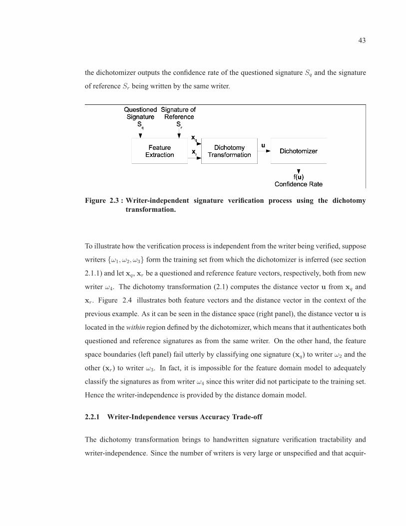
43

the dichotomizer outputs the confidence rate of the questioned signature Sq and the signature

of reference Sr being written by the same writer.

Figure 2.3 : Writer-independent signature verification process using the dichotomytransformation.

To illustrate how the verification process is independent from the writer being verified, suppose

writers {ω1, ω2, ω3} form the training set from which the dichotomizer is inferred (see section

2.1.1) and let xq, xr be a questioned and reference feature vectors, respectively, both from new

writer ω4. The dichotomy transformation (2.1) computes the distance vector u from xq and

xr. Figure 2.4 illustrates both feature vectors and the distance vector in the context of the

previous example. As it can be seen in the distance space (right panel), the distance vector u is

located in the within region defined by the dichotomizer, which means that it authenticates both

questioned and reference signatures as from the same writer. On the other hand, the feature

space boundaries (left panel) fail utterly by classifying one signature (xq) to writer ω2 and the

other (xr) to writer ω3. In fact, it is impossible for the feature domain model to adequately

classify the signatures as from writer ω4 since this writer did not participate to the training set.

Hence the writer-independence is provided by the distance domain model.

2.2.1 Writer-Independence versus Accuracy Trade-off

The dichotomy transformation brings to handwritten signature verification tractability and

writer-independence. Since the number of writers is very large or unspecified and that acquir-

44

−6 −4 −2 0 2 4

−6

−4

−2

0

2

4

ω1ω1

ω1

ω2

ω2ω2

ω3

ω3ω3

x q

x r

x1

x 2

0 5 100

2

4

6

8

10

12

ω⊕

ω⊕ω⊕ω⊕

ω⊕ω⊕ω⊕ω⊕ω⊕ ω−

ω− ω−

ω−

ω− ω−

ω−

ω− ω−

ω−

ω−

ω−

ω−

ω−

ω−ω−

ω−

ω−

ω−

ω−

ω−

ω−

ω−

ω−ω−

ω−

ω−

u

u1

u 2

Both signatures arefrom the same writer

Figure 2.4 : The dichotomizer from the previous example is asked to authenticate thequestioned signature xq with respect to the reference signature xr. Thedistance vector u resulting from their comparison is assigned to the withinclass, meaning both signatures come from the same writer.

ing a sufficiently large sample from each of them is intractable, the dichotomy transformation

makes the problem tractable by reducing it to a 2-class problem and by increasing the quantity

of samples available to build the dichotomizer.

However, there is a drawback to the dichotomy transformation; perfectly clustered writers in

feature domain may not be perfectly dichotomized in distance domain (Cha and Srihari, 2000).

To illustrate this, suppose the distributions of each writer {ω1, ω2, ω3} are known, so that the

Bayesian error can be evaluated both in feature and distance domains. Table 2.1 presents the

gaussian distribution parameters of the three writers.

The center of each distribution is located at 6.92 units from the others, that is more than six

standard deviations, which imply negligible overlap between the distributions. As such, the

Bayesian error in the feature domain is evaluated numerically to 0.05%. Once projected into

distance domain, the Bayesian error between the within and between classes is evaluated nu-

merically to 1.76%. Figure 2.5 depicts the probability function for each distribution both in

45

Table 2.1: Gaussiandistribution parametersN (μμμ,ΣΣΣ) for writers{ω1, ω2, ω3}

Writers Mean μμμ VarianceΣΣΣ

ω1

(2.83

2.83

) (1 0

0 1

)

ω2

(−3.86

1.04

) (1 0

0 1

)

ω3

(1.04

−3.86

) (1 0

0 1

)

the feature space and the distance space. In the distance space, it can be observed that thewithin

class is clustered near the origin whereas the between class is distributed into three modes away

from the origin. These three modes are the result of the comparison between writers ω1 and

ω2, writers ω1 and ω3 and writers ω2 and ω3.

By increasing the variance of the distributions, as depicted by Figure 2.6 where the gaussian

distribution parameterΣΣΣ =(

5 00 5

), the Bayesian error is increased in both domains but the effect

is more apparent in the distance domain. Table 2.2 presents the Bayesian error in both spaces

in function of the gaussian distribution parameter ΣΣΣ while the parameter μμμ of each writer is

fixed.

When comparing the Bayesian error in both spaces it is obvious that a model in the distance

domain is less robust to the overlap between the writers. In other words, the broader the spread

of the feature distributions among the writers, the less the dichotomizer is able to detect real

differences between signatures who do not differ greatly (Cha and Srihari, 2000). Thus, the

performance of the dichotomizer is crucially affected by the choice of the feature set extracted

from the handwritten signatures. Moreover, because the dichotomy transformation affects the

spatial geometry of the distributions, the best feature set may not be the same in feature domain

and in distance domain. The solution proposed in this research to tackle this drawback is to

46

Figure 2.5 : Distributions in feature space (left) projected into distance space by thedichotomy transformation (right).

extract a very large set of potential features to efficiently select a small set of discriminant

features in the distance domain.

2.2.2 Questioned Document Expert Approach

The Questioned Document Expert’s approach (Santos et al., 2004) is an extension to the di-

chotomy transformation that applies when users have more than one template stored in the

knowledge-base. The idea is to emulate the expert’s approach, which consists of comparing

the input questioned signature to a set of genuine signatures. Each comparison leads to a partial

decision from the expert, his/her final decision being based on all partial decisions. Intuitively,

47

Figure 2.6 : Distributions in feature space (left) projected into distance space bythe dichotomy transformation (right) with a larger gaussian distributionparameterΣΣΣ.

the more reference signatures available for comparison with the questioned signature, the more

accurate the final decision will be.

Formally, the dichotomy transformation is applied between the questioned signature’s feature

vector xq and the user’s reference set {xr}R1 from the knowledge-base, giving the set of dis-

tance vectors {ur}R1 . The dichotomizer evaluates individually each distance vector and outputs

a set of confidence values {f (ur)}R1 representing the partial decisions from the expert. The

final decision of the system about the questioned signature is based on the fusion of all confi-

dence values by a function g(·). The choice of fusion function is dependent on the nature of the

48

Table 2.2: Bayesian error (%) in both featureand distance spaces in function ofparameterΣΣΣ.

VarianceΣΣΣ Feature space (%) Distance space (%)(1 0

0 1

)0.05 1.76(

2 0

0 2

)1.35 10.51(

3 0

0 3

)4.15 19.16(

4 0

0 4

)7.39 25.92(

5 0

0 5

)10.54 31.48

dichotomizer’s output. For instance, if the output of the dichotomizer is a label, then the major-

ity vote is an appropriate fusion strategy. On the other hand, if the output of the dichotomizer

is a probability, then a wider range of fusion strategies are available such as the sum, mean,

median, max and min functions, to name a few.

Specifically in (Santos et al., 2004), four grid-based feature extraction techniques, namely,

pixel distribution, pixel density, stroke curvature and stroke slant are used to extract a feature

set of 640 features at a single grid scale. Then a multilayer perceptron as a dichotomizer on

distance vectors generated from a learning set of 180 writers, using a subset of 40 writers for

hold-out validation. Finally, the system is tested on an independent test set of 60 writers. The

results demonstrate the validity of the writer-independent approach. However, the recognition

rate could benefit from extracting features at different scales.

2.2.3 Ensemble of writer-independent Dichotomizers

In (Bertolini et al., 2010), the original writer-independent offline signature verification frame-

work is improved on by replacing the single dichotomizer by an ensemble of dichotomizers.

To achieve ensemble diversity, Support Vector Machines are trained on a learning set of 40

49

writers using 16 different scales of segmentation grid during feature extraction. The same four

grid-based feature extraction techniques of (Santos et al., 2004) are used except for stroke cur-

vature information which is extracted based on cubic Bezier curves. Thus, a pool of 64 Support

Vector Machines is overproduced, from which a genetic algorithm chooses a subset to form the

final ensemble of dichotomizers. These dichotomizers are combined with the Sum rule fusion

strategy.

Different objective functions were tried on the genetic algorithm and the authors conclude that

maximization of the Area Under the Receiver Operating Characteristic Curve (AUC) is the

more suitable. In all simulations, the fitness of the objective function is evaluated on an inde-

pendent validation set of 20 writers. The influence of the number of reference signatures in

the validation set is evaluated by increasing their numbers from 3 to 15, repeating the ensem-

ble optimization every time. The authors conclude that the authentication rate depends on a

tradeoff between the number of references and the intra-class variability of the reference set.

Overall, authentication by ensembles of dichotomizers show an improvement over classifica-

tion by a single dichotomizer. However, this approach complicates the verification system,

specifically in (Bertolini et al., 2010), ensembles count an average of 13 SVMs, using a total

of 2300 features and thus increasing the use of resources while reducing recognition speed.

Moreover, the ensemble optimization process being stochastic in nature, each run may lead to

a different ensemble, as demonstrated by their results.

The gain in authentication is, first and foremost, a result of extracting different features at

different scales. However, the features are integrated at the confidence score level and it is

generally believed that it is more effective to integrate combined information as early as pos-

sible in the verification system (Jain et al., 2004). Integrating combined information at feature

level should result in better improvement since at this level information about the signatures is

richer.

50

2.3 Discussion

This chapter reviewed writer-independent signature verification systems based on the dissimi-

larity representation. To achieve writer-independence, a dissimilarity representation technique

known as the dichotomy transformation is used. This technique allows the reduction of a K-

class problem into a 2-class problem that is used to train the system’s classifier. Then, given

a reference signature and a questioned signature, the classifier determines if both signatures

were written by the same person. The main advantage of the writer-independent approach is

that it tackles two fundamental problems of signature verification:

1) Large number of users. By applying the dichotomy transform to a given questioned signa-

ture and the reference signatures of the user stored in the knowledge-base, writer-independent

distance vectors are obtained. These distance vectors are presented to a writer-independent

classifier that have associated small distances to genuine signatures and large distances to

forgeries. As such, the references of any writer can be used, even from writers that are

not part of the training set. Hence, writer-independence implies independence from the

number of writers using the verification system, provided at least one reference signature is

available for each of these writers.

2) Limited number of reference signatures for training. Since dichotomy transform reduces

any K-class problem into a 2-class problem learned by the system’s classifier, the training

set may be composed of signatures collected beforehand from K writers that do not need

to be the system users since the classifier is writer-independent. However, the underlying

hypothesis is that their signatures are representative of those of the legitimate users of the

signature verification system.

However, there is a drawback to the dichotomy transformation; perfectly clustered writers in

feature domain may not be perfectly dichotomized in distance domain. This occurs when

feature distributions are broadly spread among the writers, with the negative effect that the

classifier is able to detect forgeries from genuine signatures (Cha and Srihari, 2000). Thus, the

51

performance of the classifier is crucially affected by the choice of the feature set extracted from

the handwritten signatures. Moreover, because the dichotomy transformation affects the spatial

geometry of the distributions, the best feature set may not be the same in feature domain and

in distance domain. The solution proposed in this research and presented in the next chapter is

to extract a very large set of potential features to efficiently select a small set of discriminant

features in the distance domain.

CHAPTER 3

WRITER-INDEPENDENT OFFLINE SIGNATURE VERIFICATION FRAMEWORK

This chapter presents an efficient writer-independent offline signature verification system based

on multiple feature extraction techniques. As described in this section, this novel system uses

an ensemble of dichotomizers to combine features from across several scales and feature ex-

traction techniques, leading to lighter and more accurate verification systems. As depicted by

Figure 3.1 , the proposed system respects the architecture of generic writer-independent sig-

nature verification systems. However, as described in the following sections, it uses (i) the

Extended Shadow Code and Directional Probability Density Functions techniques at the multi-

scale feature extraction level, and (ii) the Boosting Feature Selection technique at the classifier

level.

Figure 3.1 : Overview of the proposed writer-independent offline signature verificationsystem with multiscale Extended Shadow Code and Directional ProbabilityDensity Functions at the feature extraction and a committee of stumps builtby Boosting Feature Selection at the classifier level.

3.1 Multiscale Feature Extraction

Regarding handwritten signatures, it is important for the feature extraction process to be text

insensitive. In other words, the measurements taken on signature must not rely on the segmen-

53

tation of specific letters, a very difficult task especially if the signature is highly personalized

(Sabourin and Genest, 1994). A practical alternative is to partition the signatures using a virtual

grid and to take local measurements in each of the grid cells. By varying the scale of the virtual

grid, nearly global to very local features are extracted. In the literature, grid based approaches

generally tend to find a grid scale suitable to their signature database. Here the proposed ap-

proach is to extract features at multiple scales and let the classifier select the features most

adapted to its needs.

When a new signature is enrolled or questioned, it is presented to the system as a gray-level

image. From there, two preprocessing steps are necessary in order to prepare the signature

for feature extraction. First, the signature is automatically segmented from its background

using Otsu’s threshold selection method from gray-level histograms (Otsu, 1979). According

to questioned document experts, the proportion and orientation of handwritten signatures are

intrinsic characteristics of the writer when guided by a form (Harrison, 1981). Consequently,

the second preprocessing step corrects the binary signature images in translation by aligning

their centroid with the center of the feature extraction grid.

3.1.1 Fast Extended Shadow Code

The Extended Shadow Code (Sabourin and Genest, 1994), (Sabourin and Genest, 1995) con-

sists in the superposition of bar mask array over the binary image of a handwritten signature

as depicted by Figure 3.2 . Each bar is assumed to be a light detector related to a spatially

constrained area of the 2D signal. A shadow projection is defined as the simultaneous pro-

jection of each black pixel into its closest horizontal, vertical and diagonal bars. Figure 3.3

illustrates each projection in details for a given grid cell. A projected shadow turns on a set of

bits distributed uniformly along the bar. After all the pixels on a signature are projected, the

number of on bits in each bar is counted and normalized to the range of [0, 1].

This section presents the a formal description of the Extended Shadow Code and shows how the

technique can be improved with look-up tables to achieve real-time speed. Formally, a binary

signature of heightM and width N is defined as {S(m, n)}1≤m≤M1≤n≤N where S(m, n) = 0 if the

54

Figure 3.2 : Example of the Extended Shadow Code technique applied to the extractionof features from a binary signature image.

(a) (b)

(c) (d)

Figure 3.3 : Details of each shadow projection for a given grid cell: (a) horizontal, (b)vertical, (c) main diagonal and (d) secondary diagonal.

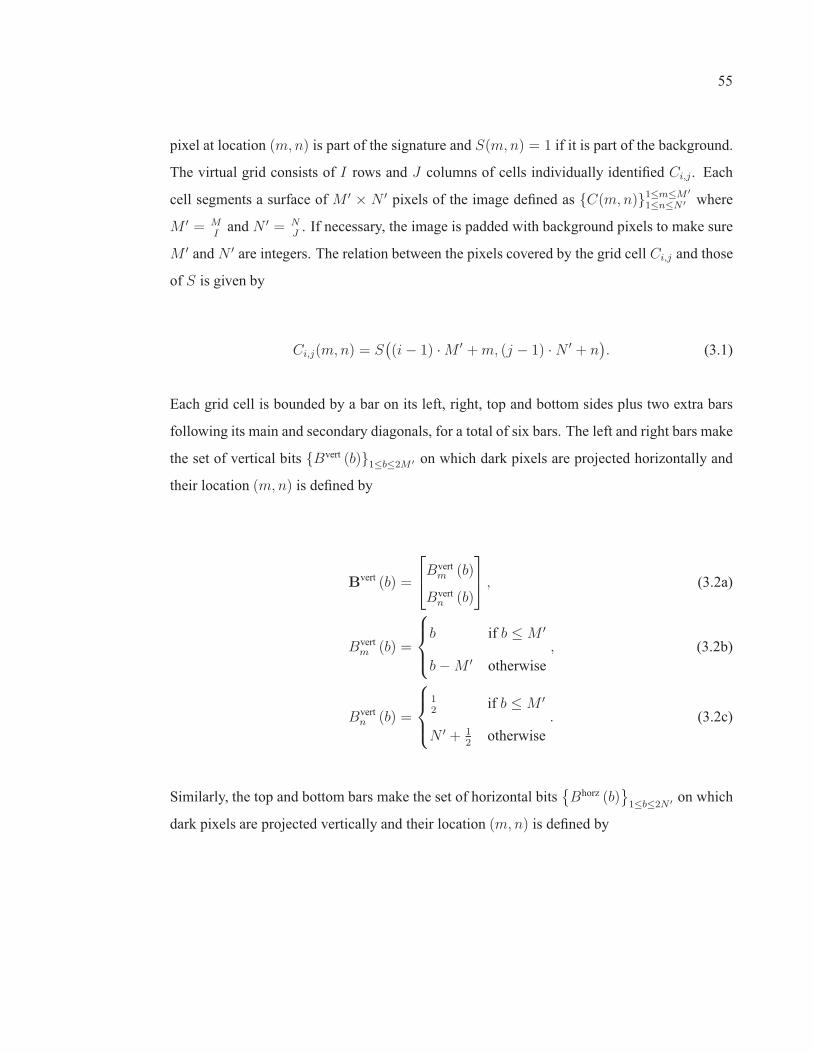
55

pixel at location (m, n) is part of the signature and S(m, n) = 1 if it is part of the background.

The virtual grid consists of I rows and J columns of cells individually identified Ci,j. Each

cell segments a surface of M ′ × N ′ pixels of the image defined as {C(m, n)}1≤m≤M ′

1≤n≤N ′ where

M ′ = MIand N ′ = N

J. If necessary, the image is padded with background pixels to make sure

M ′ and N ′ are integers. The relation between the pixels covered by the grid cell Ci,j and those

of S is given by

Ci,j(m, n) = S((i − 1) · M ′ + m, (j − 1) · N ′ + n

). (3.1)

Each grid cell is bounded by a bar on its left, right, top and bottom sides plus two extra bars

following its main and secondary diagonals, for a total of six bars. The left and right bars make

the set of vertical bits {Bvert (b)}1≤b≤2M ′ on which dark pixels are projected horizontally and

their location (m, n) is defined by

Bvert (b) =

⎡⎣Bvert

m (b)

Bvertn (b)

⎤⎦ , (3.2a)

Bvertm (b) =

⎧⎪⎨⎪⎩

b if b ≤ M ′

b − M ′ otherwise, (3.2b)

Bvertn (b) =

⎧⎪⎨⎪⎩

12

if b ≤ M ′

N ′ + 12otherwise

. (3.2c)

Similarly, the top and bottom bars make the set of horizontal bits{Bhorz (b)

}1≤b≤2N ′

on which

dark pixels are projected vertically and their location (m, n) is defined by

56

Bhorz (b) =

⎡⎣Bhorz

m (b)

Bhorzn (b)

⎤⎦ , (3.3a)

Bhorzm (b) =

⎧⎪⎨⎪⎩

12

if b ≤ N ′

M ′ + 12otherwise

, (3.3b)

Bhorzn (b) =

⎧⎪⎨⎪⎩

b if b ≤ N ′

b − N ′ otherwise. (3.3c)

In contrast, shadow projection occurs simultaneously on both diagonal bars. The set of bits of

the main diagonal (from upper left to lower right) is defined by{Bmain (b)

}1≤b≤O

where the

number of bits O =

⌊√(M ′)2 + (N ′)2

⌉, the symbol �·� being the nearest integer function,

and their location (m, n) is defined by

Bmain (b) =

⎡⎣Bmain

m (b)

Bmainn (b)

⎤⎦ , (3.4a)

Bmainm (b) =

M ′

Ob −

M ′

2O, (3.4b)

Bmainn (b) =

N ′

Ob −

N ′

2O. (3.4c)

Similarly, the set of bits of the secondary diagonal (from lower left to upper right) is defined

by {Bseco (b)}1≤b≤O and their location (m, n) is defined by

57

Bseco (b) =

⎡⎣Bseco

m (b)

Bsecon (b)

⎤⎦ , (3.5a)

Bsecom (b) =

M ′

O(O − b + 1) −

M ′

2O, (3.5b)

Bsecon (b) =

N ′

O(O − b + 1) −

N ′

2O. (3.5c)

Figure 3.4 illustrates the disposition of the light detectors inside a grid cell along with the

indices of their bits.

Figure 3.4 : Disposition of the light detectors Bvert, Bhorz, Bmain and B

seco inside a gridcell along with the indices of their bits.

The shadow projection occurs simultaneously into the four sets of bits previously defined. In

their normal state, the bits are turned off B (b) = 0 and a dark pixel C (m, n) = 0 at location

(m, n) defined as the vectorC turns on the closest bit b∗ of each set such as

58

b∗ = arg minb

‖C − B (b)‖ , (3.6a)

B (b∗) = 1, (3.6b)

where the operator ‖·‖ is the Euclidean distance. Figure 3.5 shows, for the four simultaneous

shadow projections, the value of b∗ at every position (m, n) according to the cell previously

illustrated in Figure 3.4 .

Traditional Extended Shadow Code is computationaly expensive since the distances from each

dark pixel to all bits of the bar mask have to be computed to determine which is the nearest bit.

By noting that for any given pixel the nearest bits of the bar mask are always the same, Figure

3.5 can be used as look-up tables of the nearest bits whenever a dark pixel is encountered, thus

greatly reducing the computational burden of the feature extraction technique.

Since light detectors on the boundary of two grid cells detect dark pixels in both cells, juxta-

posed cells must share turned on bits such as

Bverti,j (b) ← Bvert

i,j (b) ∨ Bverti,j−1 (b + M ′) , 1 ≤ b ≤ M ′, 1 ≤ i ≤ I, 2 ≤ j ≤ J, (3.7a)

Bhorzi,j (b) ← Bhorz

i,j (b) ∨ Bhorzi−1,j (b + N ′) , 1 ≤ b ≤ N ′, 2 ≤ i ≤ I, 1 ≤ j ≤ J, (3.7b)

where the operator ∨ is a logical disjunction. For a given cell (i, j) and its eight neighbors, Fig-

ure 3.6 (a) illustrates with continuous lines the two boundaries where the information exchange

takes place.

Once shadow projection is completed, features are extracted from the light detectors. Each grid

cell yields four features such as

59

(a) Bvert (b) B

horz

(c) Bmain (d) B

seco

Figure 3.5 : Values of b∗ at every position (m, n) obtained for the four simultaneousshadow projections, according to the cell illustrated in Figure 3.4 .

xvert =1

M ′

M ′∑b=1

Bvert (b), (3.8a)

xhorz =1

N ′

N ′∑b=1

Bhorz (b), (3.8b)

xmain =1

O

O∑b=1

Bmain (b), (3.8c)

xseco =1

O

O∑b=1

Bseco (b) (3.8d)

60

(a) (b)

Figure 3.6 : (a) For a given cell (i, j) and its eight neighbors, the information exchangetakes place at the two boundaries represented by continuous lines. (b)Location of the four features extracted from each grid cell.

and illustrated by Figure 3.6 (b). The feature vector extracted from the whole signature image

consists of the concatenation of the feature extracted from each cell (i, j) such as

xESC =

I⋃i=1

J⋃j=1

{xverti,j , xhorzi,j , xmaini,j , xsecoi,j

} I⋃i=1

{xverti,J+1

} J⋃j=1

{xhorzI+1,j

}(3.9)

Notice that in the case of xvert, the extraction process goes up to column J + 1 to account for

the last vertical bar at the extreme right of the grid. Similarly, the extraction process goes up

to row I + 1 to account for the last xhorz at the bottom of the grid. Thus, the cardinality of the

Extended Shadow Code feature vector is equal to

∣∣xESC∣∣ = 4IJ + I + J. (3.10)

3.1.2 Local Directional Probability Density Functions

Directional Probability Density Functions (Drouhard et al., 1996) have been used as a global

shape factor for automatic offline handwritten signature verification. The rationale of this ap-

61

proach is that the stroke orientation of handwritten signatures is stable enough to properly

discriminate writers. Thus this technique extracts features based on the frequency distribution

of the orientation of the gradient at the edge of the signature. Gradient features are used by

other signature verification systems, for instance (Kalera et al., 2004b).

The approach described therein innovates by extracting local Directional Probability Density

Functions from within each cell of a virtual grid placed over the handwritten signature image.

This way, local information is extracted from different parts of the signature, consequently

increasing its discriminating power. Moreover, the information extracted from the signature

is complementary to that extracted using the Extended Shadow Code technique. While the

Extended Shadow Code extracts information about the spatial distribution of the signature,

Directional Probability Density Functions extracts information about the orientation of the

strokes. Since the same grid scale is used for both techniques, this leads to a powerful spatio-

directional representation of handwritten signatures.

The gradient is computed from the binarized version of the signature image after it has been

smoothed using a 3× 3 normalized, rotationally symmetric, Gaussian lowpass filter with stan-

dard deviation σ = 0.5 defined by

GLPF (m, n) = e−δ2(m,n)/2σ2 (3.11)

where δ (m, n) is the Euclidean distance from the center of the filter. The Gaussian lowpass fil-

ter reduces the impact that residual noise can have on the two key derivatives used for gradient

computation. It may seems counter-intuitive to compute the gradient on a smoothed binary im-

age when its gray-level version is available but this approach has the definitive advantage that

the intensity of the image is already normalized, consequently there is no need of a threshold

to detect the edges of the image. In fact, the binary segmentation process has already managed

to detect the edges of the signature and the remaining task is to determine their orientation.

62

The gradient measures the first derivatives of an image within a small neighborhood of each

pixel. This research uses Sobel operators, illustrated in Figure 3.7 , to compute the gradient

vertical and horizontal components.

(a) (b)

Figure 3.7 : Sobel operator masks used for convolution: (a) vertical component, and (b)horizontal component.

Formally, for an image S (m, n) of size M × N , each pixel neighborhood is convolved with

both masks to determine vertical and horizontal components Gm and Gn, respectively

Gm (m, n) = S (m + 1, n + 1) + 2S (m + 1, n) + S (m + 1, n − 1)

− S (m − 1, n + 1) − 2S (m − 1, n) − S (m − 1, n − 1) , (3.12a)

Gn (m, n) = S (m + 1, n + 1) + 2S (m + 1, n) + S (m + 1, n − 1)

− S (m − 1, n + 1) − 2S (m − 1, n) − S (m − 1, n − 1) . (3.12b)

Then the magnitude of the gradient vector is equal to

63

mag (m, n) =√

G2m (m, n) + G2

n (m, n) (3.13)

and its direction is calculated as

ang (m, n) = tan−1 Gm (m, n)

Gn (m, n). (3.14)

Figure 3.8 illustrates the gradient of a handwritten signature image using arrows to indicate its

direction and magnitude at each pixel location. Since the signature consists of a binary image,

gradient is null in the background of the image and within the strokes of the signature where

intensity is constant. Gradient is non-null along the edges of the signature and its direction

varies perpendicularly to the contour of the signature.

Figure 3.8 : Example of a gradient representation. Arrows indicates direction andmagnitude of the gradient at each pixel location.

64

In order to obtain a fixed number of features, gradient directions are quantized into an even Φ

number of ranges by the quantization function:

qnt (m, n) =

⌊ang (m, n) + π/Φ

Φ

⌋+ 1 (3.15)

where �·� is the floor function. A greater Φ results into a more exact representation of the

gradient of the signature, thus increasing between-writers discrimination. However, the more

exact the representation, the more sensitive it is to intra-personal variance, thus lowering gen-

eralization capabilities. As a tradeoff, this research uses Φ = 8 as depicted by Figure 3.9

.

Figure 3.9 : Example of quantized values over a full circle for a quantization process withΦ = 8.

Since the objective of this feature extraction technique is to extract the orientation of the strokes

composing the signature, it is important to realize that for any stroke orientation there are two

admissible quantized values. For example, in Figure 3.9 both values 1 and 5 refer to an

horizontal gradient, thus a vertical stroke; the whole quantization process is depicted in Figure

3.10 for a given signature.

65

Figure 3.10 : Example of signature where the gradiant angle has been quantizedaccording to the process depicted in Figure 3.9 .

Generally speaking, given an even Φ number of ranges and a quantized value φ comprised

between[1, Φ

2

], both φ and φ + Φ

2indicate the same stroke orientation. Consequently, each

cell (i, j) of the virtual grid partitioning the signature image yields a Φ2elements feature vector

xDPDFi,j where element xDPDFi,j (φ) is the sum of the gradient magnitude at all location (m, n)

where the quantized gradient direction is either φ or φ + Φ2. Formally,

xDPDFi,j (φ) =∑

qnt(m,n)∈{φ,φ+Φ

2 }

mag (m, n) (3.16)

where 1 ≤ φ ≤ Φ2. The feature vector extracted from the whole image is given by

xDPDF =

I⋃i=1

J⋃j=1

Φ/2⋃φ=1

{xDPDFi,j (φ)

}(3.17)

and has a cardinality of

∣∣xDPDF∣∣ =1

2IJΦ. (3.18)

66

3.2 Boosting Feature Selection

Boosting is a machine-learning procedure which combines the performance of many weak

classifiers into a powerful committee. The rationale behind boosting is that finding many mod-

erately inaccurate rules of thumb using many simple classifiers can be easier than finding a

single highly accurate prediction rule using a more elaborate learning algorithm. Boosting

methods have proved to be very competitive in terms of generalization in a variety of applica-

tions (Schapire, 2003). The general idea of boosting is to form a committee of weak classifiers

iteratively by adding one weak classifier at a time. At the beginning of the training proce-

dure, a uniform weighting is assigned to the patterns of the training data set. Each time a new

classifier is added to the committee, the samples in the training data are reweighted to reflect

the performance of this weak classifier, assigning more importance to misclassified samples.

Thus, the next weak classifier focuses on more difficult samples and the procedure ends after a

predefined number of weak classifiers have been trained.

The problem of feature selection is defined as follows: given a set of potential features, the ob-

jective is to select the best subset under some classification objectives. This procedure has three

goals: (i) to reduce the cost of extracting features, (ii) to improve the classification accuracy,

and (iii) to improve the reliability of the estimate of performance (Kudo, 2000). The Boost-

ing Feature Selection algorithm (Tieu and Viola, 2004) (and further studied in (Redpath and

Lebart, 2005)) explicitly incorporates feature selection into AdaBoost (Freund and Schapire,

1996), the most commonly used variant of boosting. Boosting Feature Selection is performed

by designing a weak classifier that selects the single most discriminant feature of a set of po-

tential features and finds a threshold to separate the two classes to learn, effectively a decision

stump. Consequently, features are selected in a greedy fashion according to the weighting

while learning is conducted by the boosting algorithm. Given a very large set of features, the

result is a committee built on the best subset of features representing the training data.

The next sections describe the boosting algorithm and the weak classifier used in this research

and are followed by a complexity study of the resulting committee.

67

3.2.1 Gentle AdaBoost

The problem of handwritten signature verification can have a significant class overlap, espe-

cially between genuine signatures and simulated forgeries, and as mentioned previously the

dichotomy transformation can exacerbate this phenomenon. Also, it has been observed by sev-

eral authors that AdaBoost is not an optimal method on very noisy problems (Dietterich, 2000),

(Rätsch et al., 2001), (Servedio, 2003). By design, Adaboost focuses on misclassified samples

and this may result in fitting the noise.

Several boosting methods address the overfitting problem, mostly by adjusting the weighting

scheme. For instances, MadaBoost (Domingo and Watanabe, 1999) bounds the weight as-

signed to each sample by its initial probability, Gentle AdaBoost (Friedman et al., 2000) takes

adaptive Newton steps to update the weights more slowly, BrownBoost (Freund, 2001) uses

a non-monotone weighting function decreasing the weight of samples far from the margin,

AdaBoostτ (Rätsch et al., 2001) and AdaBoost∗ν (Rätsch and Warmuth, 2005) both uses the

concept of soft margin to regularize by allowing for misclassification, SmoothBoost (Servedio,

2003) constructs smooth distributions which do not put too much weight on any single sample

and NadaBoost (Nakamura et al., 2004) prevents too high weight values by thresholding.

Moreover, validation sets have long been used in machine learning to limit overfitting, and,

as noted by the authors of AdaBoost (Freund and Schapire, 1997), a validation set could be

used for early stopping. This research makes use of Gentle AdaBoost and early stopping to

address the significant class overlap problem. Early stopping is implemented using a hold-out

validation set. The early stopping criterion is based on the maximization of area under the

receiver operating characteristics curve (AUC, see Section 3.2.4) on the hold-out validation

set.

Algorithm 3.1 describes Gentle AdaBoost with early stopping. Let L = {ul, vl, wl}L1 be a

learning set of L feature vectors ul ∈ RD labelled to vl ∈ {−1, 1} and weighted by the distri-

bution wl ∈ [0, 1],∑L

l=1 wl = 1. Similarly, let H = {uh, vh}H1 be a hold-out validation set of

H non-weighted samples. Let also TL, TH ∈ N be the maximum iteration stopping criterion

68

and the early stopping criterion, respectively. The first half of the algorithm implements the

four steps of the Gentle AdaBoost algorithm: (i) train a new decision stump ft (u) based on L,

(ii) add ft (u) to the committee F (u), (iii) update the weights wl according to the response of

ft (ul), and (iv) renormalize the weights to ensure a distribution. The second half implements

a hold-out validation scheme using the AUC for criterion. The AUC is computed using Algo-

rithm 2 described in (Fawcett, 2006). If the algorithm reaches TH iterations without increase

of the AUC, it early stops. The Gentle AdaBoost with early stopping procedure outputs the

committee F (u) composed of T decision stumps.

1: Inputs: Learning set L = {ul, vl}L1 , hold-out validation setH = {uh, vh}

H1 , early

stopping criterion TH, maximum iteration stopping criterion TL.2: Output: Classifier sign [F (u)] = sign

[∑Tt=1 ft (u)

].

3: Initialize: wl = 1/L, F = 0, Amax = −∞.4: for t = 1 to TL do5: /* Gentle AdaBoost algorithm */6: Train ft (L, w).7: Update F ← F + ft.8: Update wl ← wl exp (−vlft (ul)).9: Renormalize wl ← wl/wtot, where wtot =

∑l wl.

10: /* Early stopping check */11: if AUC (H, F ) > Amax then12: Update Amax = AUC (H, F ).13: Update T = t.14: Reset counter = 0.15: else16: Increment counter ← counter + 1.17: if counter = TH then18: Exit by early stopping.19: end if20: end if21: end for

Algorithm 3.1: Gentle AdaBoost algorithm with early stopping.

69

3.2.2 Decision Stumps

Decision trees classify a pattern through a sequence of questions (Duda et al., 2001). Each

question tests a single feature of the data and is represented by a tree node, the first question

being the root of the tree and each possible decision spanning a branch to new node (i.e. the

next question) and so on until a terminal node, called a leaf, is reached and the pattern is

classified. Each decision outcome is called a split since it effectively splits the data into subsets,

binary decisions being referred to as single-splits and higher number of decisions as multi-

splits. Decision stumps are one-level, single-split trees (Iba and Langley, 1992).

Formally, a decision stump ft (u) is composed of four parameters: dt the dimension to split, τt

the splitting threshold in that dimension, and ρleftt , ρright

t the weighted means of the response

for the left and right leaves, respectively. Figure 3.11 illustrates these parameters and algo-

rithm 3.2 describes the decision stump learning algorithm. The first step in the algorithm is

to computeW⊕, W� the positive and negative weight totals, respectively. Then the algorithm

independently searches each problem dimension to find the best split-point (dt, τt). For a given

dimension, the samples are first sorted by increasing feature values, then the algorithm com-

putes w⊕, w� the positive and negative weight cumulative distribution functions, respectively.

Based on the CDFs and the weight totals, the splitting threshold is selected to minimize the

probability that a training sample would be misclassified. Once the split-point is optimized,

the algorithm computes the weighted means of the response for both leaves.

When presented a sample u to classify, the decision stump ft(u) thresholds the feature dt of u

at τt and assigns the sample to the corresponding leave. Formally:

ft(u) =

⎧⎪⎨⎪⎩

ρleftt if udt

< τt

ρrightt otherwise.

(3.19)

Decision stumps typically have high bias and low variance. However, boosting algorithms are

capable of both bias and variance reduction, hence the increase in performance from committee

70

Figure 3.11 : Illustration of a decision stump.

of stumps (Friedman et al., 2000). Moreover, when boosting implements a reweighting strategy

(as opposed to resampling), like it is the case for Gentle AdaBoost, decision stumps cause

boosting to become deterministic in the sense that multiple runs on the same learning set will

result in identical committees. Also, the order of presentation of the samples and of the features

of the learning set does not affect the resulting committees. Finally, following (3.19), a decision

stump classifies a pattern using a single feature. This means that boosting decision stumps

will greedily select informative features while building the committee, ignoring redundant and

irrelevant features. It is worth noting that the committee may learn several stumps based on the

same feature, each with a different decision threshold and response. Appendix I contains an

illustrative example of the boosting decision stumps process.

3.2.3 Complexity analysis

Suppose a committee composed of T decision stumps built from a two-class D-dimensional

problem with training and validation datasets of L = |L| and H = |H| patterns, respectively.

Let t1 be the time taken to perform an addition, substraction or comparison, and t2 the time for

a multiplication, division or exponentiation. For the purpose of this analysis, suppose that later

operations are an order of magnitude greater than the former such as t2 = 10t1.

71

1: Inputs: Pre-sorted weighted learning set L = {ul, vl, wl}L1 .

2: Output: Decision stump ft(u) with parameters dt, τt, ρleftt and ρright

t .3: Initialize: ρleft

t , ρrightt ← 0, and local variables εtot ← ∞,W⊕,W�,Wleft,Wright ← 0.

4: /* Compute total positive and negative weights */5: W⊕ =

∑l wl where vl = 1

6: W� = 1 − W⊕

7: /* Find the best split point for this learning set */8: for d = 1 toD do9: Sort L by increasing ud values10: w⊕ ← 0, w� ← 011: for l = 1 to L − 1 do12: if vl is a positive sample then13: w⊕ ← w⊕ + wl

14: else15: w� ← w� + wl

16: end if17: if ul,d �= ul+1,d then18: εleft ← 1 − max{w⊕, w�}19: εright ← 1 − max{W⊕ − w⊕, W� − w�}20: if εleft + εright < εtot then21: εtot ← εleft + εright

22: dt ← d23: τt ←

ul,d+ul+1,d

2.

24: end if25: end if26: end for27: end for28: /* Compute weighted means of the response in the left and right leaves of the stump */29: ρleft

t =∑

l wl · vl/∑

l wl where ul,dt< τt

30: ρrightt =

∑l wl · vl/

∑l wl where ul,dt

≥ τt

31: end

Algorithm 3.2: Decision stump learning algorithm.

During testing, a decision stump classifies (3.19) an input distance vector regardless of the

number of features, and thus has a constant time complexity of t1. A committee of stumps

repeats this operation T times and then sums the T − 1 responses from the stumps. Thus, the

total worst-case time required to classify an input vector using the committee in a normalized

format is twctest

t1= (2T − 1). The corresponding growing rate, valid when T 1, is O(T ),

72

making for very fast classification during the operation phase. By comparison, Radial Basis

Function kernel Support Vector Machine (RBF-SVM) classification time complexity scales to

O(DNs) (Burges, 1998), where Ns is the number of support vectors. For noisy problems such

as writer-independent signature verification, the set Ns increases dramatically and causes a

major slowdown for SVM during operation. On the other hand, the boosting approach does

not suffer from this inconvenience. Moreover, when working with high-dimensional databases

such as in this research, D T , which makes the boosting approach an attractive alternative

to SVMs.

During training, the total worst case time required to learn with Gentle AdaBoost and early

stopping includes the time for quicksort, training decision stumps, and computing the AUC.

Using quicksort algorithm (Hoare, 1989), the worst case time to sort the values of one feature

is

twcsort =

(L2

2+

L

2

)t1 (3.20)

Once values are sorted, training a decision stump (see Algorithm 3.2) has a worst case time of

twcstump = (13D(L − 1) + 5L) t1 + (D(L − 1) + L + 2) t2

= (23DL − 23D + 15L + 20) t1

(3.21)

The algorithm to compute the area under an ROC curve (Fawcett, 2006) has a worst case time

of

73

twcAUC = twc

sort + (5H + 3)t1 + (2H + 4)t2

=

(H2

2+

51H

2+ 43

)t1

(3.22)

Thus the total worse case time required to perform the Gentle AdaBoost with early stopping in

a normalized format (see Algorithm 3.1) is expressed by:

twcGAB = Dtsort + Ttstump + TtAUC + (TL + 2L + T )t1 + 4Lt2

twcGAB

t1=

DL2

2+

H2T

2+

DL

2+

51HT

2+ 23DLT − 23DT + 16LT + 42L + 64T

(3.23)

and the corresponding growth rate, when D, L, T 1, is:

O(DL2 + TH2 + DTL). (3.24)

By comparison, the time complexity of computing a RBF kernel matrix for a SVM scales to

O(DL2) (Burges, 1998), not including the time spent on parameters selection.

It is worth noting that quicksort does much better in the average case with tavesort ≈ L log L.

Thus, the growth rate of the average case time complexity of the Gentle AdaBoost with early

stopping is O(DLT ). In computer simulations, the authors have observed the average case

analysis to be more representative of the reality than the worst case analysis. Considering this,

when working with large databases such as in this research, L T , which makes the boosting

approach a method of choice since O(DLT ) grows significantly slower than O(DL2) making

the Gentle AdaBoost with early stopping a fast learning algorithm that scales linearly. Our

simulations with SVMs were executed on the same machine as for Boosting Feature Selec-

tion, a dual-core Opteron 875 running at 2.2GHz with 32GB of memory, using the small and

74

medium single scale resolution datasets presented in this research at Chapter 4. By comparing

execution durations, the SVM approach increased the time complexity by two and three orders

of magnitude for learning and testing, respectively, thus confirming the theoretical complexity

analysis presented herein. Given that the Boosting Feature Selection approach took 2 days to

learn the largest of the multiscale datasets used in this research, the learning time of the SMV

approach can be estimated to require up to 6 months, a prohibitive duration for most applica-

tions. Finally, the committee resulting from the Boosting Feature Selection approach classifies

up to 4800 samples per second while the SVM classifier would classify only 5 samples per

second. These numbers clearly point out the value of the Boosting Feature Selection approach

when working with large databases such as in this research.

3.2.4 Receiver Operating Characteristics

Receiver operating characteristics (ROC) curves are graphs plotting the true positive rate of a

classifier in function of its false positive rate. The points composing the curve are obtained

by varying the decision threshold of the classifier (see Algorithm 1 of (Fawcett, 2006) for an

efficient method for generation of ROC points). In the case of Gentle AdaBoost, this treshold

needs to be added to the classifier equation such as

sign [F (u) + Δ] = sign

[T∑

t=1

ft (u) + Δ

](3.25)

where Δ is a real number representing the desired threshold. To fall back to the original

classifier formulation, simply set Δ = 0. Figure 3.12 gives an example of an ROC curve.

Each point of the curve represents an operating point, the default operating point of Gentle

AdaBoost (i.e. Δ = 0) is indicated by an asterisk and all other points are obtained by varying

Δ from −∞ to∞.

ROC curves have an attractive property: they are insensitive to change in class distribution

(Fawcett, 2006). If the proportion of genuine signatures and forgeries changes between the

design of a system and its exploitation, the ROC curves will not change. It is the case with

75

Figure 3.12 : Example of an ROC curve.

signature verification applications, as the proportions of fraud for real applications are likely to

vary in time and from place to place.

The area under an ROC curve (AUC) can be computed using Algorithm 2 of (Fawcett, 2006).

The AUC has an important statistical property: it is equivalent to the probability that the clas-

sifier will rank a randomly chosen positive instance higher than a randomly chosen negative

instance (Fawcett, 2006). As such, the AUC is invariant to the decision threshold optimized by

Gentle AdaBoost (i.e. Δ = 0), which is a significant advantage in the context of this research

since the decision threshold is learned using random forgeries as counterexamples when in fact

the committee is tested against random, simple and simulated forgeries. Moreover, the decision

threshold is function of the priors and the classification cost, both of which are likely to vary

in a signature verification application.

CHAPTER 4

EXPERIMENTAL METHODOLOGY

The objective of this chapter is to describe the experimental protocols meant to assess the

performance of offline signature verification systems based on multiple type of features and

multiscale representations of handwritten signatures. Writer-independent verification implies

that there is only one verification system for all writers. Therefore, the protocol makes use of

two disjoint set of writers for system design (during development phase) and system testing

(during exploitation phase), as depicted by Figure 4.1 . The underlying hypothesis is that

the set of writers used for training is representative of the set of writers encountered during

exploitation.

Figure 4.1 : Independence between the training or development phase and the testing orexploitation phase.

77

In most real-world applications, very few genuine signatures, and no forgeries, are available per

writer. Consequently, random forgeries are usually the only kind of counterexamples available

for designing a system. For this reason, only random forgeries were included in the training

database, yet the system is tested against random, simple and simulated forgeries.

The following sections describe both signature databases, the feature sets extracted from the

signatures, and the experimental protocols.

4.1 Signature Database

The signature database used in this research is composed of 168 writers divided into a 108 writ-

ers development databaseD and a 60 writers exploitation database E as presented in Table 4.1.

As described in (Bertolini et al., 2010), the signatures were provided by 168 under-graduated

students in four different sessions, ten samples at a time, once a week during one month, for a

total of 40 genuine signatures per writer. The signatures were collected on an A4 white sheet

of paper with no overlap and then scanned in gray level at 300 dpi. Regarding the forgeries, ten

people with no experience in making forgeries were selected as forgers to produce one simple

and one simulated forgery for the 60 first writers. Simple forgeries were produced by supplying

only the name of the writer to the forger. Simulated forgeries were produced by showing the

forger four genuine signatures of the writer.

Table 4.1: Signature Databases

Development database D Exploitation database EWriters 108 60Genuine Signatures 40 40Simple Forgeries - 10Simulated Forgeries - 10

To build a writer-independent classifier, distance vectors must be computed from the feature

vectors using the dichotomy transformation as explained in Section 2.1. The learning set L

78

and hold-out validation set H are both generated from the development database D. To do so,

the 40 genuine signatures of each writers of D are partitionned into a 30 and a 10 signatures

subsets denoted D1 and D2, respectively.

The learning set L is generated using exclusively the genuine signatures of subset D1. The

within class samples are computed using all genuine signatures from every writers, giving

108 · 30·292

= 46980 distance vectors. To generate an equivalent number of counterexamples,

the dichotomy transformation is applied, for each writer, to 29 genuine signatures used as

signatures of references against 15 random forgeries selected from the genuine signatures of

15 other writers. The result is 108 · 29 · 15 = 46980 between class distance vectors. Thus, the

learning set is defined as L = {ul, vl}93960l=1 .

The hold-out validation set H is generated using the genuine signatures of subset D1 as refer-

ence signatures against the genuine signatures of subsetD2. Since each writer has 30 references

signatures in D1 and 10 genuine signatures in D2, the number of within class samples is equal

to 108 · 30 · 10 = 32400. To generate an equivalent number of counterexamples, for each

writer, 10 random forgeries are selected from 10 different writers in D2. The random forgeries

are compared to the 30 references fromD1, giving 108 ·30 ·10 = 32400 between class distance

vectors. Thus, the hold-out validation set is defined as H = {uh, vh}64800h=1 .

To perform a writer-independent evaluation of the system, both reference R and questioned

Q sets are generated from the exploitation database E whose writers are unknown to the ver-

ification system. The reference set R is composed of 30 randomly selected genuine signa-

tures from each writer of the exploitation database E . Thus, the reference set is defined as

R = {xr, yr}1800r=1 . The questioned set Q is composed of the 10 remaining genuine signa-

tures and simple and simulated forgeries from each writer plus 10 random forgeries selected

from the genuine signatures of 10 different writers. Thus, the questioned set is defined as

Q = {xq, yq}2400q=1 .

79

4.2 Feature Sets

Extended Shadow Code and Directional PDF feature vectors are extracted from both signature

databases D and E . Feature resolution depends on the size of the extraction grid; the smaller

the grid cells, the higher the resolution. The highest resolution used in this research is a cell of

20×20 pixels. Since the width of a stroke measures an average of 10 pixels, higher resolutions

would results mostly in saturated cells and empty cells. On the other hand, the lowest resolution

is limited by the size of the image. Since the signature images are 400 pixels high by 1000

pixels wide, the lowest resolution consists of a single cell of that size. Let I = {1, 2, 5, 10, 20}

be a set of 5 horizontal scales defined by their number of grid rows and J = {1, 3, 6, 12, 25, 50}

be a set of 6 vertical scales defined by their number of grid columns. The Cartesian product

I × J results in the 30 single scales used in this research. Finally, multiscale is achieved by

combining feature sets from every scales, for a total of 15457 and 14744 features for Extended

Shadow Code and Directional PDF, respectively, and a grand total of 30201 features when both

techniques are combined, as detailled in Table 4.2.

4.3 Protocols

This section describes the experimental protocols used in this research. Firstly, individual eval-

uations of each single scale representation extracted from both Extended Shadow Code and

Directional PDF is performed. This evaluation is followed by a comparison between informa-

tion fusion applied at feature level and information fusion applied at score level.

4.3.1 Single Scale Representations

In order to independently characterize both Extended Shadow Code and Directional PDF fea-

ture extraction techniques, single scale committees are built using the following protocol. For

each available feature set, the Gentle Adaboost algorithm with early stopping (see Algorithm

3.1) builds a committee of decision stumps on the learning set L using the hold-out validation

set H to prevent overfitting. The early stopping criterion is set to TH = 100 and the maximum

iteration stopping criterion to TL = 100000.

80

Table 4.2: Details of the Resolutions

Pixels FeaturesRows × Columns Height Width Extended Shadow Code Directional PDF

20 × 50 20 20 4070 400020 × 25 20 40 2045 200020 × 12 20 84 992 96020 × 6 20 167 506 48020 × 3 20 334 263 24020 × 1 20 1000 101 8010 × 50 40 20 2060 200010 × 25 40 40 1035 100010 × 12 40 84 502 48010 × 6 40 167 256 24010 × 3 40 334 133 12010 × 1 40 1000 51 405 × 50 80 20 1055 10005 × 25 80 40 530 5005 × 12 80 84 257 2405 × 6 80 167 131 1205 × 3 80 334 68 605 × 1 80 1000 26 202 × 50 200 20 452 4002 × 25 200 40 227 2002 × 12 200 84 110 962 × 6 200 167 56 482 × 3 200 334 29 242 × 1 200 1000 11 81 × 50 400 20 251 2001 × 25 400 40 126 1001 × 12 400 84 61 481 × 6 400 167 31 241 × 3 400 334 16 121 × 1 400 1000 6 4

Total: 15457 14744Grand Total: 30201

The performance of each writer-independent committee is evaluated using reference signatures

from new writers in the set R to authenticate the questioned signatures of set Q. To measure

the impact of the cardinality of the reference set, reference subsets containing 1, 3, 5, 7, 9, 11,

81

13 and 15 randomly selected signatures are used for authentication. To simulate the effect of

enrolling new signatures over time, previously selected signatures are kept and new signatures

are added to increase the size of the reference subsets. This procedure is repeated 100 times for

variance estimation. Algorithm 4.1 presents the evaluation protocol in an algorithmic format.

1: for all committees do2: for replication 1 to 100 do3: R = {x1,x2, . . . ,xR}4: R = {∅}5: repeat6: /* randomly select signatures i and j fromR */7: R′ = {xi,xj | xi,xj ∈ R}8: R = {R \ R′}9: R =

{R∪R′

}10: evaluate the committee on Q usingR11: until

∣∣R∣∣ = 1512: end for13: end for

Algorithm 4.1: Committee Evaluation Protocol

ROC analysis is used to select the optimal threshold for each committee while testing the

questioned set; this must be done to ensure that the results presented herein can be compared

with those published in the litterature (i.e. references (Bertolini et al., 2010) and (Santos et al.,

2004)). Additionally, the committees are evaluated using their error rates on the questioned

set. To do so, the decision threshold minimizing the zero-one loss is used to characterize the

questioned set and also to allow for a straightforward comparison with previous systems.

4.3.2 Information Fusion at the Feature Level

Contrary to previous writer-independent system (Bertolini et al., 2010) which implements in-

formation fusion at the confidence score level, the proposed system implements information

fusion at the feature extraction level. Three multiscale committees are compared:

82

1) Using a multiscale feature set only from the Extended Shadow Code technique;

2) Using a multiscale feature set only from the Directional PDF technique;

3) Using a multiscale feature set from both Extended Shadow Code and Directional PDF tech-

niques.

Multiscale feature sets are achieved by concatenating appropriate single scale feature sets. To

permit result comparison, training and evaluation protocols are the same as for single scale

feature set, as described previously.

To complete this aspect of the study, the experimental protocol presented at Algorithm 4.2 is

designed to evaluate the impact of the quantity of signature representations on the Boosting

Feature Selection algorithm with early stopping. Let L, H, Q, R be the learning, hold-out,

questioned and references sets, respectively. They are all initialized as empty sets. Then,

the 60 signature representations are randomly selected one at a time and added to the sets.

When the sets contain 1, 5, 10, 15, 20, 25, 30, 40, 50 and 60 representations, the committee

of stumps Fp is built from sets L and H using the Boosting Feature Selection algorithm with

early stopping and then tested on set Q using 1, 3, 5, 7, 9, 11, 13, 15 references from set R.

This protocol is repeated 10 times to show replicability.

4.3.3 Information Fusion at the Confidence Score Level

In this section two protocols based on information fusion at the confidence score level are

presented. The first reproduces the overproduce and choose approach used in (Bertolini et al.,

2010) and the second evaluates the modularity of the proposed system.

4.3.3.1 Overproduce and Choose

The overproduce and choose approach used in (Bertolini et al., 2010) is reproduced here us-

ing our feature extraction techniques and database partitions in order to compare the two ap-

proaches. To perform information fusion at the confidence score level, committees built on

83

1: for replication 1 to 10 do2: Initialize L = H = Q = R = {∅}3: for p = 1 to 60 do4: Acquire new handwritten signature representation datasetsHp,Lp,Qp,Rp from

feature extraction expert5: Add L ← L∪ Lp

6: AddH ← H∪Hp

7: Add Q ← Q∪Qp

8: AddR ← R∪Rp

9: if p ∈ {1, 5, 10, 15, 20, 25, 30, 40, 50, 60} then10: Build committee of stumps Fp ← GentleAdaBoost(L,H)11: Evaluate Fp onQ using 1, 3, . . . , 15 references fromR12: end if13: end for14: end for

Algorithm 4.2: Protocol to evaluate the impact of the quantity of representations.

single scale feature sets are combined together into an ensemble of committees by summating

their individual confidence level output. Ensembles of committees are optimized with a ge-

netic algorithm based on bit representation, one-point crossover, bit-flip mutation and roulette

wheel selection with elitism. The parameter setting is the same as in (Bertolini et al., 2010):

population = 100, number of generations = 300, probability of crossover = 0.7, and probability

of mutation = 0.03. The chromosomes are composed of 60 bits, that is, one bit per single scale

committee and for a given chromosome, turned on bits identify the selected committees. The

fitness function is the maximization of the AUC on the hold-out validation set H. Once an

ensemble of committees is optimized, it is evaluated on the questioned set using the evaluation

protocol described in Section 4.3.1. This procedure is also repeated 100 times for variance

estimation to allow for direct comparison with the other approaches explored in this research.

4.3.4 Incremental Selection of Representations

In order to demonstrate the modularity of the proposed system, an experimental protocol is de-

signed to implement an incremental selection of the handwritten signature representations. For

instance, suppose that domain experts extract new representations from the design database.

84

As new signature representations become available, they are added incrementally to the verifi-

cation system in order to increase its recognition rate.

A greedy incremental selection scheme is implemented to demonstrate the modularity of the

proposed system. Single scale signature representations are presented to the system one at

a time. For each representation, a committee of stumps is built and combined with previous

committees to form an ensemble of committees. Then the AUC of the ensemble of commit-

tees is evaluated on the hold-out validation set H and the newly added committee is kept if it

improves the AUC of the ensemble or dismissed otherwise. The 60 single scale representa-

tions are presented in random order and this procedure is replicated 100 times to evaluate the

replicability.

1: for replication 1 to 100 do2: InitializeH = {∅}3: Initialize Feoc = 04: Initialize Amax = −∞5: for p = 1 to 60 do6: Acquire new handwritten signature representation datasetsHp,Lp,Qp,Rp from

feature extraction expert7: Build committee of stumps Fp ← GentleAdaBoost(Lp,Hp)8: Add Feoc ← Feoc + Fp

9: AddH ← H∪Hp

10: if AUC(H, Feoc) > Amax then11: Update Amax ← AUC(H, Feoc)12: AddQ ← Q∪Qp

13: AddR ← R∪Rp

14: Evaluate Feoc on Q using 1, 3, . . . , 15 references from R15: else16: DismissH ← H \Hp

17: Dismiss Feoc ← Feoc − Fp

18: end if19: end for20: end for

Algorithm 4.3: Forward selection of representions protocol.

85

Algorithm 4.3 details this experimental protocol. Given a signature representation p, the learn-

ing set Lp and hold-out validation set Hp are both generated from the design database D and

the reference set Rp and questioned set Qp are generated from the exploitation database E

whose writers are unknown to the verification system. Committees of stumps are the result of

the Gentle Adaboost algorithm with early stopping, described at Algorithm 3.1, and they are

evaluated according to the evaluation protocol described in Section 4.3.1.

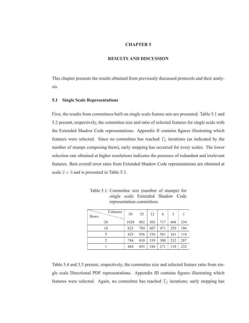
CHAPTER 5

RESULTS AND DISCUSSION

This chapter presents the results obtained from previously discussed protocols and their analy-

sis.

5.1 Single Scale Representations

First, the results from committees built on single scale feature sets are presented. Table 5.1 and

5.2 present, respectively, the committee size and ratio of selected features for single scale with

the Extended Shadow Code representations. Appendix II contains figures illustrating which

features were selected. Since no committee has reached TL iterations (as indicated by the

number of stumps composing them), early stopping has occurred for every scales. The lower

selection rate obtained at higher resolutions indicates the presence of redundant and irrelevant

features. Best overall error rates from Extended Shadow Code representations are obtained at

scale 2 × 3 and is presented in Table 5.3.

Table 5.1: Committee size (number of stumps) forsingle scale Extended Shadow Coderepresentation committees

��

��

��

��

��

RowsColumns 50 25 12 6 3 1

20 1028 802 303 717 468 23410 623 784 607 471 259 1865 425 956 536 561 161 1182 784 810 539 300 232 2871 484 493 344 271 110 232

Table 5.4 and 5.5 present, respectively, the committee size and selected feature ratio from sin-

gle scale Directional PDF representations. Appendix III contains figures illustrating which

features were selected. Again, no committee has reached TL iterations; early stopping has

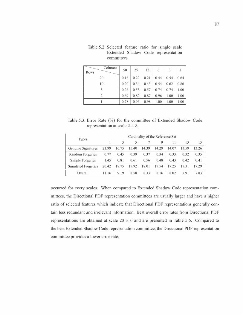
87

Table 5.2: Selected feature ratio for single scaleExtended Shadow Code representationcommittees

��

��

��

��

��


20 0.16 0.22 0.21 0.44 0.54 0.6410 0.20 0.34 0.43 0.54 0.62 0.865 0.26 0.53 0.57 0.74 0.74 1.002 0.69 0.82 0.87 0.96 1.00 1.001 0.78 0.96 0.98 1.00 1.00 1.00

Table 5.3: Error Rate (%) for the committee of Extended Shadow Coderepresentation at scale 2 × 3

TypesCardinality of the Reference Set

1 3 5 7 9 11 13 15Genuine Signatures 21.99 16.75 15.40 14.39 14.29 14.07 13.59 13.26Random Forgeries 0.77 0.45 0.39 0.37 0.34 0.33 0.32 0.35Simple Forgeries 1.45 0.81 0.61 0.56 0.48 0.43 0.42 0.41Simulated Forgeries 20.42 18.75 17.92 18.01 17.54 17.25 17.31 17.29

Overall 11.16 9.19 8.58 8.33 8.16 8.02 7.91 7.83

occurred for every scales. When compared to Extended Shadow Code representation com-

mittees, the Directional PDF representation committees are usually larger and have a higher

ratio of selected features which indicate that Directional PDF representations generally con-

tain less redundant and irrelevant information. Best overall error rates from Directional PDF

representations are obtained at scale 20 × 6 and are presented in Table 5.6. Compared to

the best Extended Shadow Code representation committee, the Directional PDF representation

committee provides a lower error rate.

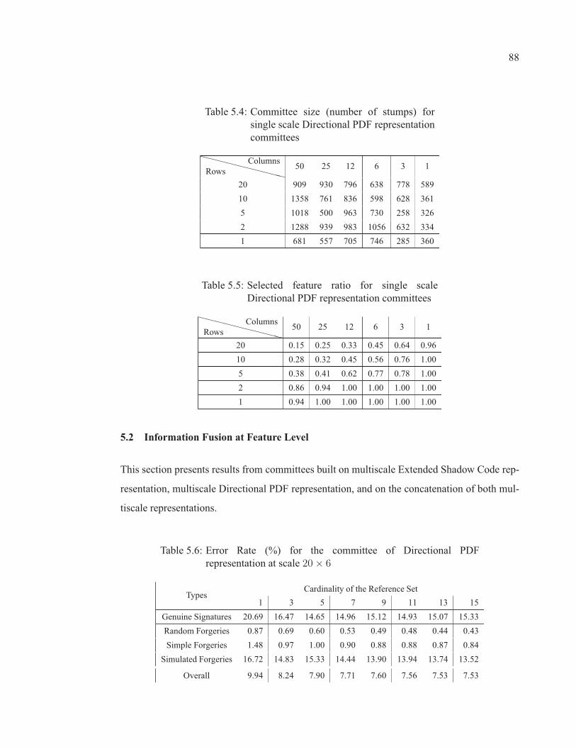
88

Table 5.4: Committee size (number of stumps) forsingle scale Directional PDF representationcommittees

��

��

��

��

��


20 909 930 796 638 778 58910 1358 761 836 598 628 3615 1018 500 963 730 258 3262 1288 939 983 1056 632 3341 681 557 705 746 285 360

Table 5.5: Selected feature ratio for single scaleDirectional PDF representation committees

��

��

��

��

��


20 0.15 0.25 0.33 0.45 0.64 0.9610 0.28 0.32 0.45 0.56 0.76 1.005 0.38 0.41 0.62 0.77 0.78 1.002 0.86 0.94 1.00 1.00 1.00 1.001 0.94 1.00 1.00 1.00 1.00 1.00

5.2 Information Fusion at Feature Level

This section presents results from committees built on multiscale Extended Shadow Code rep-

resentation, multiscale Directional PDF representation, and on the concatenation of both mul-

tiscale representations.

Table 5.6: Error Rate (%) for the committee of Directional PDFrepresentation at scale 20 × 6

TypesCardinality of the Reference Set


Overall 9.94 8.24 7.90 7.71 7.60 7.56 7.53 7.53

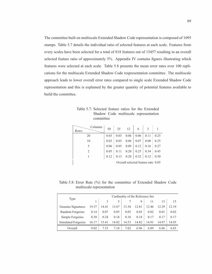
89

The committee built on multiscale Extended Shadow Code representation is composed of 1095

stumps. Table 5.7 details the individual ratio of selected features at each scale. Features from

every scales have been selected for a total of 818 features out of 15457 resulting in an overall

selected feature ratio of approximately 5%. Appendix IV contains figures illustrating which

features were selected at each scale. Table 5.8 presents the mean error rates over 100 repli-

cations for the multiscale Extended Shadow Code respresentation committee. The multiscale

approach leads to lower overall error rates compared to single scale Extended Shadow Code

representation and this is explained by the greater quantity of potential features available to

build the committee.

Table 5.7: Selected feature ratios for the ExtendedShadow Code multiscale representationcommittee

��

��

��

��

��


20 0.03 0.03 0.06 0.06 0.11 0.2510 0.03 0.03 0.06 0.07 0.08 0.255 0.06 0.05 0.09 0.12 0.16 0.272 0.05 0.11 0.20 0.25 0.34 0.451 0.12 0.13 0.20 0.32 0.12 0.50

Overall selected feature rate: 0.05

Table 5.8: Error Rate (%) for the committee of Extended Shadow Codemultiscale representation

TypeCardinality of the Reference Set


Overall 9.02 7.53 7.18 7.02 6.96 6.89 6.86 6.83

90

The committee built on Directional PDFmultiscale representation is composed of 1288 stumps.

Table 5.9 details the individual selected feature ratio for each scale. Features from every scales

have been selected for a total of 888 features out of 14744 resulting in an overall selected

feature ratio of approximately 6%; a result similar to the one obtained with multiscale Extended

Shadow Code respresentation. Appendix V contains figures illustrating which features were

selected at each scale.

Table 5.9: Selected feature ratios for the Directional PDFmultiscale representation committee

��

��

��

��

��


20 0.04 0.04 0.06 0.08 0.11 0.4110 0.03 0.04 0.04 0.06 0.12 0.305 0.06 0.07 0.09 0.11 0.22 0.352 0.14 0.11 0.19 0.25 0.21 0.381 0.18 0.18 0.31 0.54 0.25 0.75

Overall selected feature ratio: 0.06

Table 5.10 presents the mean error rates (in %) of the 100 replications for the multiscale

Directional PDF respresentation committee. Similarly to the Extended Shadow Code multi-

scale respresentation, the multiscale approach leads to lower error rates compared to the single

scale Directional PDF representation. However, the multiscale Directional PDF respresentation

committee provides lower error rates than the multiscale Extended Shadow Code respresenta-

tion committee.

The committee built on both Extended Shadow Code and Directional PDF multiscale represen-

tations is composed of 679 terms. Table 5.11 details the selected feature ratio for both feature

extraction techniques at each scale. Features from every scales have been selected for a total of

555 features out of 30201 resulting in an overall selected feature ratio of less than 2%. Thus,

providing a more diversified information to the Boosting Feature Selection method results in a

91

Table 5.10: Error Rate for the committee of Directional PDF multiscalerepresentation (%)



Overall 8.04 6.57 6.28 6.13 6.05 6.00 5.95 5.94

lighter committee using less features. Appendix VI contains figures illustrating which features

were selected at each scale.

Table 5.11: Selected feature ratios for the Extended Shadow Code/Directional PDFmultiscale representation committee

��

��

��

��

��


20 0.01/0.01 0.01/0.01 0.02/0.02 0.02/0.03 0.03/0.05 0.11/0.2310 0.01/0.01 0.01/0.01 0.02/0.02 0.04/0.03 0.02/0.06 0.10/0.175 0.01/0.01 0.02/0.03 0.04/0.02 0.06/0.05 0.10/0.12 0.23/0.252 0.02/0.03 0.04/0.04 0.05/0.07 0.09/0.12 0.07/0.12 0.27/0.251 0.02/0.03 0.06/0.05 0.13/0.08 0.13/0.12 0.12/0.08 0.50/0.25

Overall selected features rate: 0.02/0.02

Table 5.12 presents the mean error rates (in %) of the 100 replications for the committee built on

both Extended Shadow Code and Directional PDF multiscale representations. The error rates

are better than those obtained from the committees based only on one of the two multiscale

representations. This confirms that both multiscale representations are complementary and

that together, they provide a more diversified information to the Boosting Feature Selection

method.

92

Table 5.12: Error Rate for the Extended Shadow Code/Directional PDFmultiscale representation committee (%)



Overall 7.26 5.89 5.52 5.37 5.32 5.29 5.23 5.19

Figure 5.1 presents the mean error rate in function of both the number of references per

writer and the number of representations used by the verification system. The mean error rate

decreases monotonically for both the number of representations and the number of references.

In both cases, their seems to be a limit to the improvement provided by adding new references

and new representations since the improvement lessens as more references or representation

are added. However, the figure clearly shows that adding new representations (the “∗”) has a

greater impact on accuracy than by adding new references (the “◦”).

5.3 Information Fusion at the Confidence Score Level

This section presents the results obtained from the protocols dealing with information fusion

at the confidence score level.

5.3.1 Overproduce and Choose

The overproduce and choose approach selected a mean of 19.81 committees per replication.

Each committee uses a mean of 1736.93 Extended Shadow Code features and 2004.12 Direc-

tional PDF features for a total of 3741.05 features. Table 5.13 details the individual selection

ratio of each representation. Of the 30 resolutions, 4 are systematically selected for both types

of representation and 11 are systematically discarded. Interestingly, the remaining fifteen (that

is, half of the resolutions available) are equally shared between both types of representation

which is an indication of the complementarity of the two feature extraction techniques.

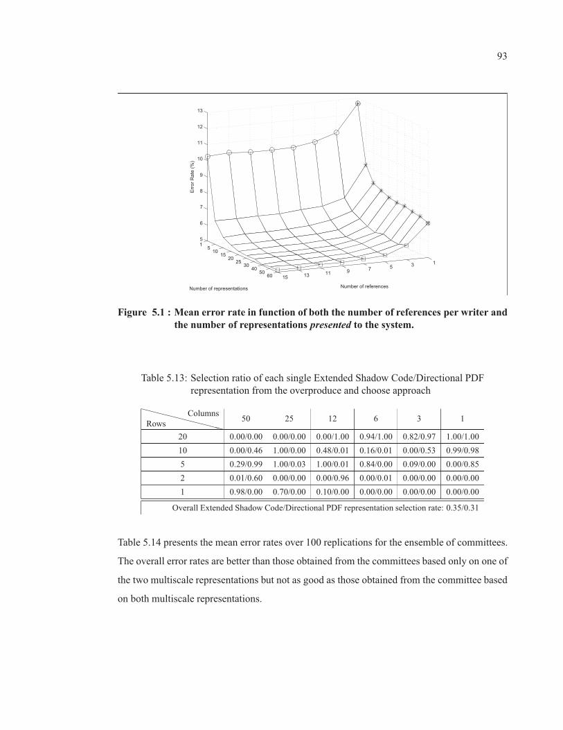
93

13579111315

15

1015

2025

3040

5060

5

6

7

8

9

10

11

12

13

Number of referencesNumber of representations

Err

or R

ate

(%)

Figure 5.1 : Mean error rate in function of both the number of references per writer andthe number of representations presented to the system.

Table 5.13: Selection ratio of each single Extended Shadow Code/Directional PDFrepresentation from the overproduce and choose approach

��

��

��

��

��


20 0.00/0.00 0.00/0.00 0.00/1.00 0.94/1.00 0.82/0.97 1.00/1.0010 0.00/0.46 1.00/0.00 0.48/0.01 0.16/0.01 0.00/0.53 0.99/0.985 0.29/0.99 1.00/0.03 1.00/0.01 0.84/0.00 0.09/0.00 0.00/0.852 0.01/0.60 0.00/0.00 0.00/0.96 0.00/0.01 0.00/0.00 0.00/0.001 0.98/0.00 0.70/0.00 0.10/0.00 0.00/0.00 0.00/0.00 0.00/0.00

Overall Extended Shadow Code/Directional PDF representation selection rate: 0.35/0.31

Table 5.14 presents the mean error rates over 100 replications for the ensemble of committees.

The overall error rates are better than those obtained from the committees based only on one of

the two multiscale representations but not as good as those obtained from the committee based

on both multiscale representations.

94

Table 5.14: Error rate (%) from the overproduce and choose approach



Overall 7.24 6.16 5.88 5.78 5.71 5.65 5.61 5.59

5.3.2 Incremental Selection of Representations

This section presents results from the incremental selection of representations scheme. Figure

5.2 presents the mean error rate in function of both the number of references per writer and

the number of representations presented to the system. The actual number of selected repre-

sentations is indicated on Figure 5.3 using the mean number of used features in function of

the number of representations that has been presented to the system.

The mean error rate decreases monotonically for both the number of representations and the

number of references. In both cases, their seems to be a limit to the improvement provided

by adding new references and new representations since the improvement lessens as more

references or representation are added. However, the graphic clearly shows that adding new

representations has a greater impact on accuracy than by adding new references.

5.4 Discussion

Tables 5.15 sums up the results presented so far. Regarding both best single scale representa-

tions, Directional PDF are significantly more discriminant than Extended Shadow Code rep-

resentations. However, an interesting fact is that Extended Shadow Code performs better at

low resolution while Directional PDF provides better performance at higher resolution; in this

respect, the two feature extraction techniques are complementary.

95

Figure 5.2 : Mean error rate in function of both the number of references per writer andthe number of representations presented to the system.

Table 5.15: Error rates (%) comparison with other systems

Approach FeaturesCardinality of the Reference Set

1 3 5 7 9 11 13 15ESC scale 2 × 3 29 11.16 9.19 8.58 8.33 8.16 8.02 7.91 7.83DPDF scale 20 × 6 216 9.94 8.24 7.90 7.71 7.60 7.56 7.53 7.53Multiscale ESC 818 9.02 7.53 7.18 7.02 6.96 6.89 6.86 6.83Multiscale DPDF 888 8.04 6.57 6.28 6.13 6.05 6.00 5.95 5.94Multiscale ESC/DPDF 555 7.26 5.89 5.52 5.37 5.32 5.29 5.23 5.19Using All Representations 10137 7.54 6.59 6.34 6.27 6.24 6.20 6.20 6.17Incremental Selection of Represent. 5178 7.31 6.25 6.01 5.87 5.81 5.76 5.74 5.73Overproduce & Choose (herein) 3741 7.24 6.16 5.88 5.78 5.71 5.65 5.61 5.59Over. & Choo. (Bertolini et al., 2010) - - 7.86 7.32 6.32 7.04 7.19 6.73 6.48MLP (Santos et al., 2004) - - - 8.02 - - - - -

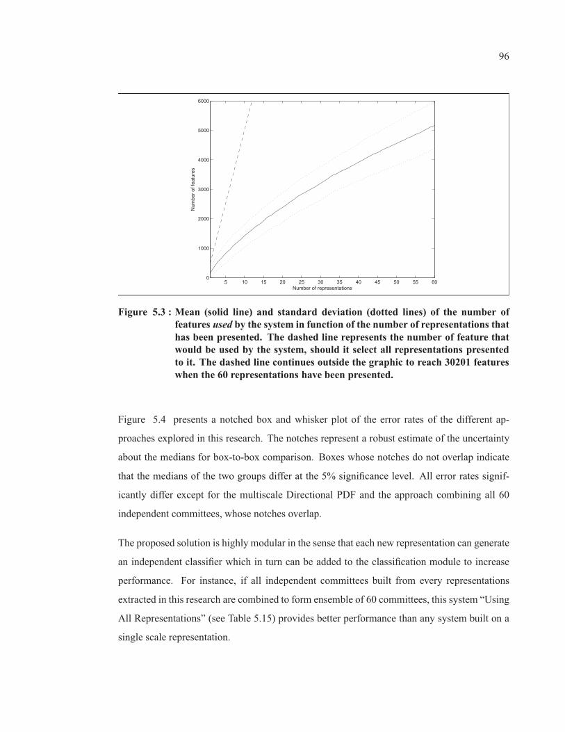
96

5 10 15 20 25 30 35 40 45 50 55 600

1000

2000

3000

4000

5000

6000

Num

ber o

f fea

ture

s

Number of representations

Figure 5.3 : Mean (solid line) and standard deviation (dotted lines) of the number offeatures used by the system in function of the number of representations thathas been presented. The dashed line represents the number of feature thatwould be used by the system, should it select all representations presentedto it. The dashed line continues outside the graphic to reach 30201 featureswhen the 60 representations have been presented.

Figure 5.4 presents a notched box and whisker plot of the error rates of the different ap-

proaches explored in this research. The notches represent a robust estimate of the uncertainty

about the medians for box-to-box comparison. Boxes whose notches do not overlap indicate

that the medians of the two groups differ at the 5% significance level. All error rates signif-

icantly differ except for the multiscale Directional PDF and the approach combining all 60

independent committees, whose notches overlap.

The proposed solution is highly modular in the sense that each new representation can generate

an independent classifier which in turn can be added to the classification module to increase

performance. For instance, if all independent committees built from every representations

extracted in this research are combined to form ensemble of 60 committees, this system “Using

All Representations” (see Table 5.15) provides better performance than any system built on a

single scale representation.

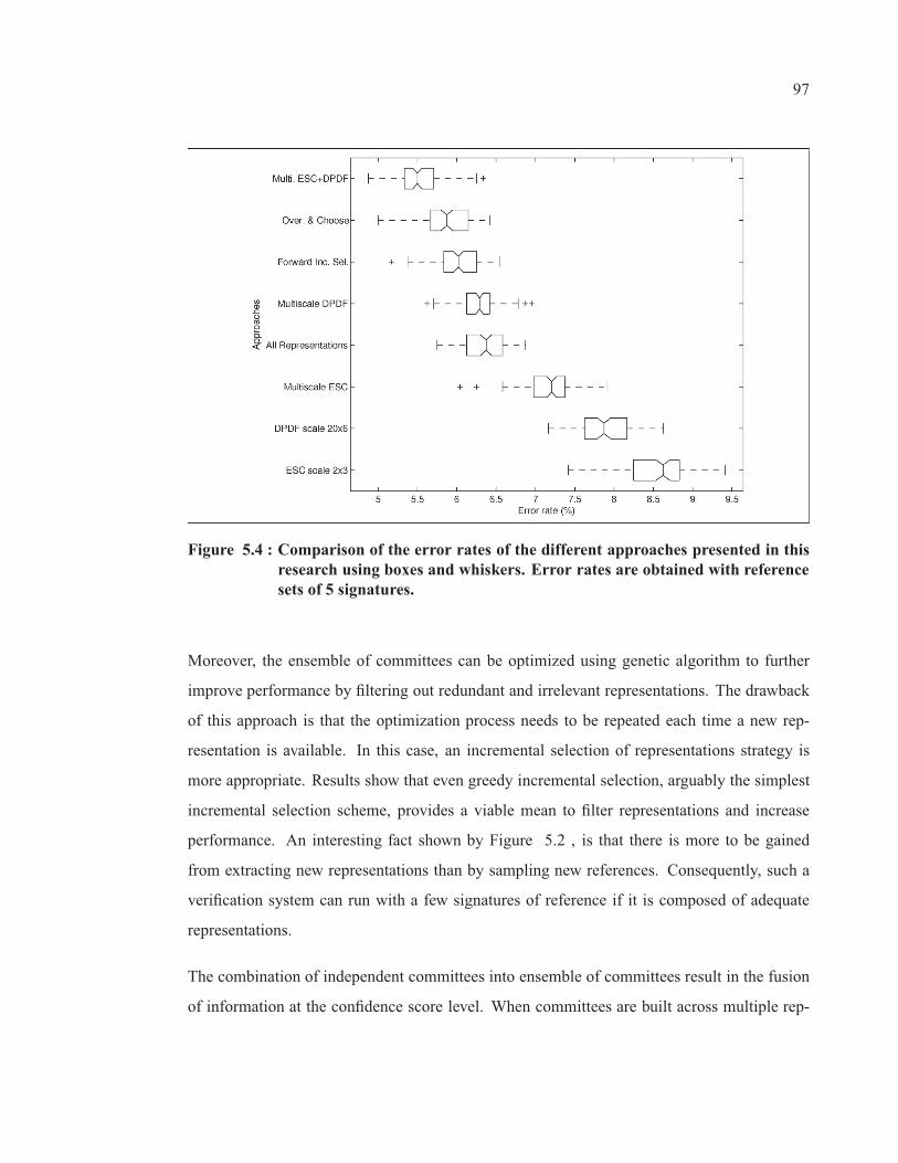
97

Figure 5.4 : Comparison of the error rates of the different approaches presented in thisresearch using boxes and whiskers. Error rates are obtained with referencesets of 5 signatures.

Moreover, the ensemble of committees can be optimized using genetic algorithm to further

improve performance by filtering out redundant and irrelevant representations. The drawback

of this approach is that the optimization process needs to be repeated each time a new rep-

resentation is available. In this case, an incremental selection of representations strategy is

more appropriate. Results show that even greedy incremental selection, arguably the simplest

incremental selection scheme, provides a viable mean to filter representations and increase

performance. An interesting fact shown by Figure 5.2 , is that there is more to be gained

from extracting new representations than by sampling new references. Consequently, such a

verification system can run with a few signatures of reference if it is composed of adequate

representations.

The combination of independent committees into ensemble of committees result in the fusion

of information at the confidence score level. When committees are built across multiple rep-

98

1 5 10 15 20 25 30 40 50 605

6

7

8

9

10

11

Number of representations

Err

or ra

te (%

)

Information fusion at score levelInformation fusion at feature level

Figure 5.5 : Mean error rate in function of number of signature representations using 5references.

resentations the information fusion occurs at the feature level and result in smaller committees

with better generalization performances. Both multiscale Extended Shadow Code and mul-

tiscale Directional PDF committees outrank their single representation counterparts and use

only 5% and 6% of all available features, respectively. This result is even more convincing

for a multiscale committee built across all 60 representations; the committee uses even less

features (2%) and provides a lower error rate. Figure 5.5 compares the mean error rates when

applying information fusion at the feature level compared to the confidence score level for an

growing number of representations, using 5 reference signatures. Error rates are similar when

a single representation is available; an expected result since the learning context, at this point,

is identical for both fusion strategy, that is one representation and one classifier. However, as

more representation are made available to the verification system, information fusion at the

feature level clearly performs better then information fusion at the score level. An expected re-

sult which is explained by the richer information conveyed by features rather then scores (Jain

et al., 2004).

CONCLUSION

This research presented a practical solution to the fundamental problems encountered with

signature verification: a large number of users, a large number of features, a limited number of

reference signatures, a high intra-personal variability of the signatures and the unavailability

of forgeries as counterexamples. The solution consists of a writer-independent framework,

based on the dichotomy transformation, that palliates the large number of users and reduced

number of reference signatures. Experimental methodology and results clearly demonstrated

the writer-independence by training and testing the system on two disjoint sets of writers and

even indicate the possibility of signature verification using a single reference signature for

each writer. Further, results demonstrate the viability of using random forgeries to train a

classifier in the distance space of the dichotomy transformation, thus tackling the unavailability

of forgeries.

The high intra-personal variability of handwritten signatures is dealt with by extracting multi-

scale features using Extended Shadow Code and Directional PDF, two complementary feature

extraction techniques, resulting in a powerful multiscale spatio-directional representation of

the signatures. The large number of extracted features is dealt with using Boosting Feature Se-

lection, a feature selection while learning technique originally proposed for traditional feature

vectors, which proves also effective with distance vectors resulting from the dichotomy trans-

formation. Further, this approach result in light-weight, efficient classifiers viable for real-time

applications.

Another significant advantage of the proposed framework resides in the modularity of its clas-

sification module. Using the properties inherited from the writer-independent approach, new

samples as well as new signature representations can be added to the system during the ex-

ploitation phase. From there, a single classifier may be built over all available signature repre-

sentations, thus implementing a fusion of the information at the feature level. Or one classifier

may be built per representation and then grouped into an ensemble of classifiers, thus imple-

menting in a fusion of the information at the confidence score level. The former approach

100

results into more efficient classifiers, however it requires all representations to be available

during the design phase. On the other hand, the latter allows the system to be designed using

a single representation and then incrementally updated when a new representation is avail-

able. Interestingly, results show that starting with a single representation and a single reference

signature, the accuracy of the system is better improved by adding more representations than

references, making the proposed framework ideally suited to applications where few samples

are available.

Further research will focus on dynamically adapting the classification module to the writer, or

even to the signature to authenticate, thus combining the advantages of both writer-independent

and writer-dependent approaches. Other feature extraction techniques are also to be considered

to increase information diversity and thus the system accuracy. Finally, significant improve-

ment in learning time are expected from a distributed implementation of the Boosting Feature

Selection algorithm.

APPENDIX I

BOOSTING DECISION STUMPS

This section presents the process of boosting decision stumps based on a toy problem composed

of 20 examples from two classes (“X” and “O”) as illustrated in the left panel of Figure I.1.

The horizontal and vertical lines represent the two split points considered by the first decision

stump built by the Gentle AdaBoost algorithm (see Algorithm 3.1).

The center panel of Figure I.1 represents the search made by the decision stump algorithm (see

Algorithm 3.2) for the best split point in the x1 dimension. This search imply to test all split

points admissible by the data; since there are 20 examples, 19 split points are tested. Doing

so, the errors on both distributions (represented by the curves marked by “X” and “O”) are

computed as well as the total error from both distributions (represented by the top curve). The

best split point in x1 is the point minimizing the total error (represented by an asterisk) which in

this case equals 1.3 and is obtained by splitting the data between the fourth and fifth examples.

The right panel of Figure I.1 represents the same search process but in the x2 dimension. It

gives a minimal total error of 1.2 when splitting the data between the 14th and 15th examples.

Since 1.2 < 1.3, this is the split point selected by the decision stump.

The left panel of Figure I.2a illustrates the current classification result from the decision stump;

the top region is labelled “O” and contains no misclassifications while the bottom region is la-

belled “X” and contains four misclassified examples. The right panel shows the weight update

by the Gentle AdaBoost algorithm in function of the result of the first decision stump (t = 1);

the font size of each example being proportional to its new weight. The four “Os” below the

decision stump threshold are misclassified, hence their weight is increased accordingly. The

next decision stump will have to take these new weights into account when optimizing its split

point.

102

−5 0 5−2

−1.5

−1

−0.5

0

0.5

1

1.5

x1

x 2

0 10 200.5

0.6

0.7

0.8

0.9

1

1.1

1.2

1.3

1.4

1.5

x1

i(x1)

0 10 200.5

0.6

0.7

0.8

0.9

1

1.1

1.2

1.3

1.4

1.5

x2

i(x2)

Figure I.1: Building of a decision stump based on a toy problem. Left panel illustratesthe two dimensional problem. Center and right panels describe how theparameters of the stump are determined.

The right panel of Figure I.2b shows the split point of the second decision stump (t = 2) and

the subsequent weight update. The left panel illustrates the frontier drawn by the committee of

stumps (EoC). The top-right region is closely fitting the six “Os” in that region but still there

are four “Os” misclassified.

The right panel of Figure I.2c shows the result of the third decision stump (t = 3) and the

subsequent weight update. The left panel illustrates the new frontier drawn by the committee

of stumps. A second region, at the bottom-right of the feature space is now labelled “O”,

leaving a single “O” example misclassified. This last example is more difficult to classify and

its weight is increased accordingly. In fact, Gentle AdaBoost focuses on these difficult cases.

Forwarding to the tenth iteration, the right panel of Figure I.2d shows the result of the tenth

decision stump (t = 10) and the subsequent weight update. The left panel illustrates the

frontier drawn by the committee of ten stumps. A notch has been added to the bottom-right

103

“O” region to acheive a perfect classification of the data. However, the complexity of the

frontier illustrates how Gentle AdaBoost can overfit when learning from noisy data. Using

an early stopping criterion based on a validation dataset could have, for instance, stopped the

learning process at the third iteration, thus preventing Gentle AdaBoost from overfitting the

data.

−4 −2 0 2 4−2

−1.5

−1

−0.5

0

0.5

1

1.5

x1

x 2

t = 1

−4 −2 0 2 4−2

−1.5

−1

−0.5

0

0.5

1

1.5

x1

x 2

EoC

(a) first iteration

−4 −2 0 2 4−2

−1.5

−1

−0.5

0

0.5

1

1.5

x1

x 2

t = 2

−4 −2 0 2 4−2

−1.5

−1

−0.5

0

0.5

1

1.5

x1

x 2

EoC

(b) second iteration

−4 −2 0 2 4−2

−1.5

−1

−0.5

0

0.5

1

1.5

x1

x 2

t = 3

−4 −2 0 2 4−2

−1.5

−1

−0.5

0

0.5

1

1.5

x1

x 2

EoC

(c) third iteration

−4 −2 0 2 4−2

−1.5

−1

−0.5

0

0.5

1

1.5

x1

x 2

t = 10

−4 −2 0 2 4−2

−1.5

−1

−0.5

0

0.5

1

1.5

x1

x 2

EoC

(d) tenth iteration

Figure I.2: Three firsts and last iterations of Gentle AdaBoost (a to d, respectively). Ateach iteration, the left panel shows the classification result from the committeeof stumps while the right panel illustrates the current decision stump and theweights to be used for the next iteration.

APPENDIX II

SINGLE SCALE EXTENDED SHADOW CODE SELECTED FEATURES

For each Extended Shadow Code representation (Figures II.1 to II.5), the selected features are

shown with continous lines while the others are made up of dotted lines. The regions of the

signature image where information is extracted are colored in grey.

(a) 20 × 50 (b) 20 × 25

(c) 20 × 12 (d) 20 × 6

(e) 20 × 3 (f) 20 × 1

Figure II.1: Extended Shadow Code selected features and their corresponding region ofthe image for the “20 rows” single scale representations.

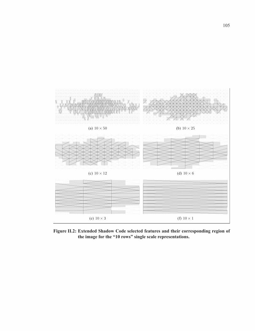
105

(a) 10 × 50 (b) 10 × 25

(c) 10 × 12 (d) 10 × 6

(e) 10 × 3 (f) 10 × 1


106

(a) 5 × 50 (b) 5 × 25

(c) 5 × 12 (d) 5 × 6

(e) 5 × 3 (f) 5 × 1


107

(a) 2 × 50 (b) 2 × 25

(c) 2 × 12 (d) 2 × 6

(e) 2 × 3 (f) 2 × 1


108

(a) 1 × 50 (b) 1 × 25

(c) 1 × 12 (d) 1 × 6

(e) 1 × 3 (f) 1 × 1

Figure II.5: Extended Shadow Code selected features and their corresponding region ofthe image for the “1 row” single scale representations.

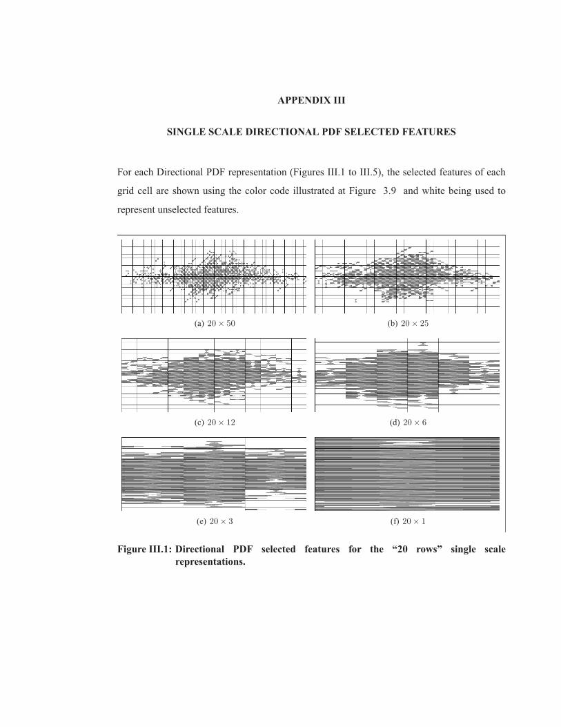
APPENDIX III

SINGLE SCALE DIRECTIONAL PDF SELECTED FEATURES

For each Directional PDF representation (Figures III.1 to III.5), the selected features of each

grid cell are shown using the color code illustrated at Figure 3.9 and white being used to

represent unselected features.

(a) 20 × 50 (b) 20 × 25

(c) 20 × 12 (d) 20 × 6

(e) 20 × 3 (f) 20 × 1

Figure III.1: Directional PDF selected features for the “20 rows” single scalerepresentations.

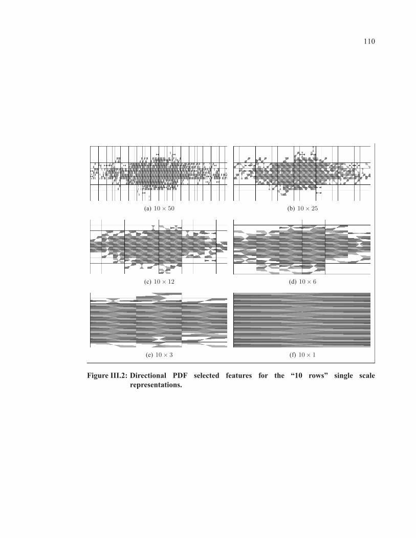
110

(a) 10 × 50 (b) 10 × 25

(c) 10 × 12 (d) 10 × 6

(e) 10 × 3 (f) 10 × 1


111

(a) 5 × 50 (b) 5 × 25

(c) 5 × 12 (d) 5 × 6

(e) 5 × 3 (f) 5 × 1


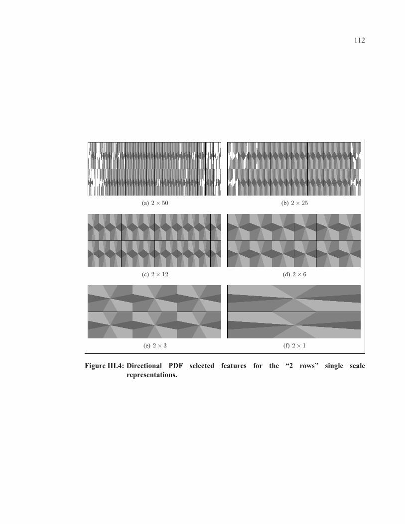
112

(a) 2 × 50 (b) 2 × 25

(c) 2 × 12 (d) 2 × 6

(e) 2 × 3 (f) 2 × 1


113

(a) 1 × 50 (b) 1 × 25

(c) 1 × 12 (d) 1 × 6

(e) 1 × 3 (f) 1 × 1

Figure III.5: Directional PDF selected features for the “1 row” single scalerepresentations.

APPENDIX IV

MULTISCALE EXTENDED SHADOWCODE SELECTED FEATURES

For the Extended Shadow Code multiscale representation (Figures IV.1 to IV.5), the features

selected at each scale are shown with continous lines while the others are made up of dotted

lines. The regions of the signature image where information is extracted are colored in grey.

(a) 20 × 50 (b) 20 × 25

(c) 20 × 12 (d) 20 × 6

(e) 20 × 3 (f) 20 × 1

Figure IV.1: Extended Shadow Code selected features and their corresponding region ofthe image for the “20 rows” aspect of the multiscale representation.

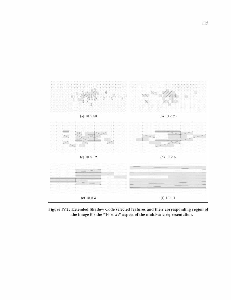
115

(a) 10 × 50 (b) 10 × 25

(c) 10 × 12 (d) 10 × 6

(e) 10 × 3 (f) 10 × 1


116

(a) 5 × 50 (b) 5 × 25

(c) 5 × 12 (d) 5 × 6

(e) 5 × 3 (f) 5 × 1


117

(a) 2 × 50 (b) 2 × 25

(c) 2 × 12 (d) 2 × 6

(e) 2 × 3 (f) 2 × 1


118

(a) 1 × 50 (b) 1 × 25

(c) 1 × 12 (d) 1 × 6

(e) 1 × 3 (f) 1 × 1

Figure IV.5: Extended Shadow Code selected features and their corresponding region ofthe image for the “1 row” aspect of the multiscale representation.

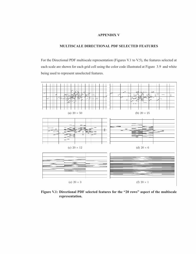
APPENDIX V

MULTISCALE DIRECTIONAL PDF SELECTED FEATURES

For the Directional PDF multiscale representation (Figures V.1 to V.5), the features selected at

each scale are shown for each grid cell using the color code illustrated at Figure 3.9 and white

being used to represent unselected features.

(a) 20 × 50 (b) 20 × 25

(c) 20 × 12 (d) 20 × 6

(e) 20 × 3 (f) 20 × 1

Figure V.1: Directional PDF selected features for the “20 rows” aspect of the multiscalerepresentation.

120

(a) 10 × 50 (b) 10 × 25

(c) 10 × 12 (d) 10 × 6

(e) 10 × 3 (f) 10 × 1


121

(a) 5 × 50 (b) 5 × 25

(c) 5 × 12 (d) 5 × 6

(e) 5 × 3 (f) 5 × 1


122

(a) 2 × 50 (b) 2 × 25

(c) 2 × 12 (d) 2 × 6

(e) 2 × 3 (f) 2 × 1


123

(a) 1 × 50 (b) 1 × 25

(c) 1 × 12 (d) 1 × 6

(e) 1 × 3 (f) 1 × 1

Figure V.5: Directional PDF selected features for the “1 row” aspect of the multiscalerepresentation.

APPENDIX VI

MULTISCALE EXTENDED SHADOW CODE AND DIRECTIONAL PDF

SELECTED FEATURES

For the Extended Shadow Code and Directional PDF multiscale representation, the Extended

Shadow Code features (Figures VI.1 to VI.5) selected at each scale are shown with continous

lines while the others are made up of dotted lines. The regions of the signature image where

information is extracted are colored in grey.

Regarding the Directional PDF (Figures VI.6 to VI.10), the features selected at each scale are

shown for each grid cell using the color code illustrated at Figure 3.9 and white being used to

represent unselected features.

125

(a) 20 × 50 (b) 20 × 25

(c) 20 × 12 (d) 20 × 6

(e) 20 × 3 (f) 20 × 1

Figure VI.1: Extended Shadow Code selected features and their corresponding regionof the image for the “20 rows” aspect of the Extended Shadow Code andDirectional PDF multiscale representation.

126

(a) 10 × 50 (b) 10 × 25

(c) 10 × 12 (d) 10 × 6

(e) 10 × 3 (f) 10 × 1


127

(a) 5 × 50 (b) 5 × 25

(c) 5 × 12 (d) 5 × 6

(e) 5 × 3 (f) 5 × 1


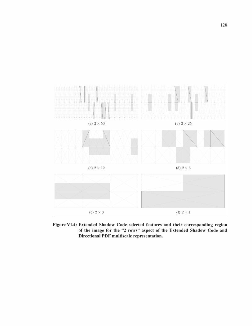
128

(a) 2 × 50 (b) 2 × 25

(c) 2 × 12 (d) 2 × 6

(e) 2 × 3 (f) 2 × 1


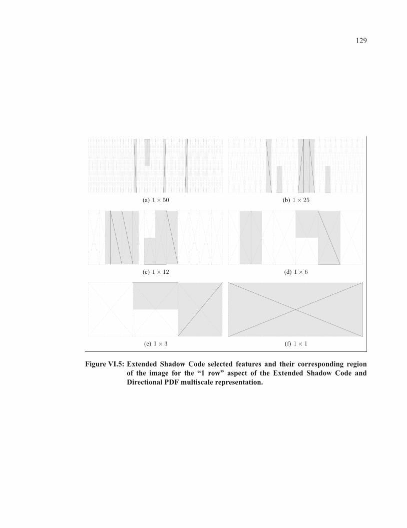
129

(a) 1 × 50 (b) 1 × 25

(c) 1 × 12 (d) 1 × 6

(e) 1 × 3 (f) 1 × 1

Figure VI.5: Extended Shadow Code selected features and their corresponding regionof the image for the “1 row” aspect of the Extended Shadow Code andDirectional PDF multiscale representation.

130

(a) 20 × 50 (b) 20 × 25

(c) 20 × 12 (d) 20 × 6

(e) 20 × 3 (f) 20 × 1

Figure VI.6: Directional PDF selected features for the “20 rows” aspect of the multiscalerepresentation.

131

(a) 10 × 50 (b) 10 × 25

(c) 10 × 12 (d) 10 × 6

(e) 10 × 3 (f) 10 × 1


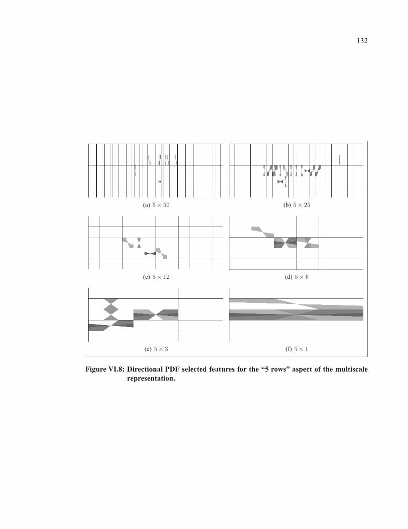
132

(a) 5 × 50 (b) 5 × 25

(c) 5 × 12 (d) 5 × 6

(e) 5 × 3 (f) 5 × 1


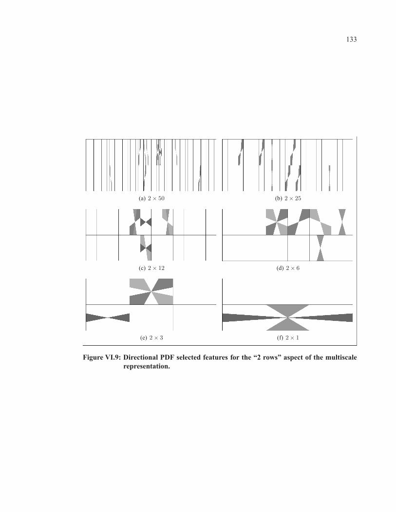
133

(a) 2 × 50 (b) 2 × 25

(c) 2 × 12 (d) 2 × 6

(e) 2 × 3 (f) 2 × 1


134

(a) 1 × 50 (b) 1 × 25

(c) 1 × 12 (d) 1 × 6

(e) 1 × 3 (f) 1 × 1

Figure VI.10: Directional PDF selected features for the “1 row” aspect of the multiscalerepresentation.

BIBLIOGRAPHY

Imen A. Abdelghani and Najoua E. Amara. 2006. “Deux approches neuronales pour la véri-

fication hors-ligne de la signature manuscrite”. In 15ième congrès francophone sur la

reconnaissance de forme et l’intelligence artificielle (RFIA2006).

A. I. Al-Shoshan. 2006. “Handwritten signature verification using image invariants and dy-

namic features”. In 2006 International Conference on Computer Graphics, Imaging and

Visualisation, p. 173–176.

M. Ammar. 1991. “Progress in verification of skillfully simulated handwritten signatures”.

International Journal of Pattern Recognition and Artificial Intelligence, vol. 5 no. 1-2,

p. 337–351.

M. Ammar, Y. Yoshida, and T. Fukumura. 1985. “Off-line verification of signature based on

pressure features”. In Tech. Group Meeting of Pattern Recognition Learn, p. 134–144.

M. Ammar, Y. Yoshida, and T. Fukumura. 1988. “Off-line pre-processing and verification

of signatures”. International Journal of Pattern Recognition and Artificial Intelligence,

vol. 2 no. 4, p. 589–602.

Shingo Ando and Masato Nakajima. 2003. “An active search method for local individual

features in off-line signature verification”. Systems and Computers in Japan, vol. 34 no.

12, p. 64–76.

S. Armand, M. Blumenstein, and V. Muthukkumarasamy. 2006a. “Off-line signature verifi-

cation based on the modified direction feature”. In 18th International Conference on

Pattern Recognition (ICPR 2006), vol. 4, p. 509–512.

Stephane Armand, Michael Blumenstein, and Vallipuram Muthukkumarasamy. 2006b. “Off-

line signature verification using the enhanced modified direction feature and neural-

based classification”. In International Joint Conference on Neural Networks.

136

Reena Bajaj and Santanu Chaudhury. January 1997. “Signature verification using multiple

neural classifiers”. Pattern Recognition, vol. 30 no. 1, p. 1–7.

H. Baltzakis and N. Papamarkos. 2001. “A new signature verification technique based on a

two-stage neural network classifier”. Engineering Applications of Artificial Intelligence,

vol. 14, p. 95–103.

L. Bastos, F. Bortolozzi, R. Sabourin, and C. Kaestner. 1997. “Mathematical modelation of

handwritten signatures by conics”. Revista da Sociedade Paranaese de Matemática, vol.

18, p. 135–146.

L. Batista, D. Rivard, R. Sabourin, E. Granger, and P. Maupin. 2008. “State of the art in off-

line signature verification”. B. Verma and M. Blumenstein, editors, Pattern Recognition

Technologies and Applications: Recent Advances, p. 39–62.

D. Bertolini, L. S. Oliveira, E. Justino, and R. Sabourin. January 2010. “Reducing forgeries

in writer-independent off-line signature verification through ensemble of classifiers”.

Pattern Recognition, vol. 43 no. 1, p. 387–396.

Christopher J. C. Burges. June 1998. “A tutorial on support vector machines for pattern

recognition”. Data Min. Knowl. Discov., vol. 2 no. 2, p. 121–167.

H. Cardot, M. Revenu, B. Victorri, and M. Revillet. 1994. “A static signature verification

system based on a cooperating neural network architecture”. International Journal on

Pattern Recognition and Artificial Intelligence, vol. 8 no. 3, p. 679–692.

Sung-Hyuk Cha and Sargur Srihari. 2000. “Writer identification: Statistical analysis and

dichotomizer”. Advances in Pattern Recognition, p. 123–132.

A. Chalechale, G. Naghdy, P. Premaratne, and A. Mertins. 2004. “Document image analysis

and verification using cursive signature”. In 2004 IEEE International Conference on

Multimedia and Expo (ICME’04), vol. 2, p. 887–890.

137

Siyuan Chen and Sargur Srihari. 2006. “Combining one- and two-dimensional signal recog-

nition approaches to off-line signature verification”. In Kazem Taghva and Xiaofan Lin,

editors, Document Recognition and Retrieval XIII, vol. 6067. SPIE.

P.C. Chuang. 1977. “Machine verification of handwritten signature image”. In 1977 Interna-

tional Conference on Crime Countermeasures–Science and Engineering, p. 105–109.

J. Coetzer. 2005. “Off-line signature verification”. PhD thesis, University of Stellenbosch.

J. Coetzer, B. M. Herbst, and J. A. du Preez. 2004. “Offline signature verification using the

discrete radon transform and a hidden markov model”. EURASIP Journal on Applied

Signal Processing, vol. 2004 no. 4, p. 559–571.

Peter S. Deng, Hong-Yuan M. Liao, Chin W. Ho, and Hsiao-Rong Tyan. December 1999.

“Wavelet-based off-line handwritten signature verification”. Computer Vision and Image

Understanding, vol. 76 no. 3, p. 173–190.

Peter S. Deng, Li-Jing Jaw, Jau-Hwang Wang, and Cheng-Tan Tung. 2003. “Trace copy

forgery detection for handwritten signature verification”. In IEEE 37th Annual 2003

International Carnahan Conference on Security Technology, p. 450–455.

T. G. Dietterich. June 2000. “Ensemble methods in machine learning”. In First Interna-

tional Workshop on Multiple Classifier Systems, p. 1–15, Berlin, Germany, June 2000.

Springer-Verlag.

C. Domingo and O. Watanabe. December 1999. “Madaboost: a modification of adaboost”. Re-

search Reports on Mathematical and Computing Sciences Series C (Computer Science),

vol. no. C-138, p. 1–26.

J. Drouhard, R. Sabourin, and M. Godbout. March 1996. “A neural network approach to off-

line signature verification using directional pdf”. Pattern Recognition, vol. 29 no. 3, p.

415–424.

Richard O. Duda, Peter E. Hart, and David G. Stork, 2001. Pattern Classification. John Wiley

& Sons, Inc.

138

A. El-Yacoubi, E. J. R. Justino, R. Sabourin, and F. Bortolozzi. 2000. “Off-line signature

verification using hmms and cross-validation”. In Proceedings of the 2000 IEEE Signal

Processing Society Workshop Neural Networks for Signal Processing X, vol. 2, p. 859–

868 vol.2.

E. Fadhel and P. Bhattacharyya. 1999. “Application of a steerable wavelet transform using

neural network for signature verification”. Pattern Analysis and Applications, vol. 2, p.

184–195.

M. C. Fairhurst. 1997. “Signature verification revisited: promoting practical exploitation of

biometric technology”. Electronics & Communication Engineering Journal, vol. 9 no.

6, p. 273–280.

B. Fang, Y. Wang, C. Leung, and K. Tse. 2001. “Off-line signature verification by the analysis

of cursive strokes”. International Journal of Pattern Recognition and Artificial Intelli-

gence, vol. 15 no. 4, p. 659–673.

B. Fang, C. H. Leung, Y. Y. Tang, P. C. K. Kwok, K. W. Tse, and Y. K. Wong. 2002. “Of-

fline signature verification with generated training samples”. IEE Proceedings of Vision,

Image and Signal Processing, vol. 149 no. 2, p. 85–90.

B. Fang, C. Leung, Y. Tang, K. Tse, P. Kwok, and Y. Wong. January 2003. “Off-line signature

verification by the tracking of feature and stroke positions”. Pattern Recognition, vol.

36 no. 1, p. 91–101.

Bin Fang and Yuan Y. Tang. 2005. “Improved class statistics estimation for sparse data prob-

lems in offline signature verification”. IEEE Transactions on Systems, Man and Cyber-

netics, Part C, vol. 35 no. 3, p. 276–286.

J. B. Fasquel and M. Bruynooghe. March 2004. “A hybrid opto-electronic method for fast off-

line handwritten signature verification”. International Journal on Document Analysis

and Recognition (IJDAR), vol. 7 no. 1, p. 56–68.

139

Tom Fawcett. June 2006. “An introduction to roc analysis”. Pattern Recognition Letters, vol.

27 no. 8, p. 861–874.

M. Ferrer, J. Alonso, and C. Travieso. 2005. “Offline geometric parameters for automatic sig-

nature verification using fixed-point arithmetic”. IEEE Transactions on Pattern Analysis

and Machine Intelligence, vol. 27 no. 6, p. 993–997.

J. Fierrez-Aguilar, N. Alonso-Hermira, G. Moreno-Marquez, and J. Ortega-Garcia. 2004. “An

off-line signature verification system based on fusion of local and global information”.

In D. Maltoni and A. K. Jain, editors, Biometric Authentication, Proceedings Lecture

Notes In Computer Science 3087: 295-306 2004, p. 295–306. Springer-Verlag Berlin,

Heidelberger Platz 3, D-14197 Berlin, Germany.

Katrin Franke, Yu-Nong Zhang, and Mario Koppen. 2002. “Static signature verification

employing a kosko-neuro-fuzzy approach”. In Proceedings International Conference

on Fuzzy Systems - Advances in Soft Computing (AFSS 2002), vol. 2275, p. 185–190.

Springer Berlin / Heidelberg.

Y. Freund and R. E. Schapire. July 1996. “Experiments with a new boosting algorithm”. In

Proceedings of Thirteenth International Conference on Machine Learning, San Fran-

cisco, CA, USA, July 1996. Eur. Coordinating Committee for Artificial Intelligence;

Italian Assoc. Artificial Intelligence, Morgan Kaufmann Publishers.

Yoav Freund. June 2001. “An adaptive version of the boost by majority algorithm”. Machine

Learning, vol. 43 no. 3, p. 293–318.

Yoav Freund and Robert E. Schapire. August 1997. “A decision-theoretic generalization of on-

line learning and an application to boosting,”. Journal of Computer and System Sciences,

vol. 55 no. 1, p. 119–139.

E. Frias-Martinez, A. Sanchez, and J. Velez. September 2006. “Support vector machines

versus multi-layer perceptrons for efficient off-line signature recognition”. Engineering

Applications of Artificial Intelligence, vol. 19 no. 6, p. 693–704.

140

Jerome Friedman, Trevor Hastie, and Robert Tibshirani. 2000. “Additive logistic regression: a

statistical view of boosting (with discussion and a rejoinder by the authors)”. Annals of

Statistics, vol. 28 no. 2, p. 337–407.

R. Gonzalez and R. Woods, editors, 2002. Digital Image Processing. Prentice Hall, 2nd

edition.

F. Griess and A. Jain. 2002. “On-line signature verification”. Pattern Recognition, vol. 35, p.

2963–2972.

J. K. Guo, D. Doermann, and A. Rosenfeld. 2000. “Off-line skilled forgery detection using

stroke and sub-stroke properties”. In 15th International Conference on Pattern Recog-

nition, vol. 2, p. 355–358 vol.2.

Madasu Hanmandlu, Mohd Yusof, and Vamsi K. Madasu. March 2005. “Off-line signature

verification and forgery detection using fuzzy modeling”. Pattern Recognition, vol. 38

no. 3, p. 341–356.

W. R. Harrison, 1981. Suspect Documents, Their Scientific Examination. Nelso-Hall publish-

ers, Chicago.

S. Haykin, 1998. Neural Networks: A Comprehensive Foundation. Prentice Hall, 2 edition.

C. A. R. Hoare, 1989. Essays in computing science. Prentice-Hall, Inc., Upper Saddle River,

NJ, USA. ISBN 0-13-284027-8.

K. Huang and H. Yan. 2002. “Off-line signature verification using structural feature corre-

spondence”. Pattern Recognition, vol. 35, p. 2467–2477.

Kai Huang and Hong Yan. January 1997. “Off-line signature verification based on geometric

feature extraction and neural network classification”. Pattern Recognition, vol. 30 no. 1,

p. 9–17.

W. Iba and P. Langley. 1992. “Induction of one-level decision trees”. In Proceedings of the

Ninth International Machine Learning Conference. Morgan Kaufmann.

141

Juan J. Igarza, Inmaculada Hernaez, and Inaki Goirizelaia. 2005. “Static signature recognition

based on left-to-right hidden markov models”. Journal of Electronic Imaging, vol. 14

no. 4.

D. Impedovo and G. Pirlo. 2008. “Automatic signature verification: The state of the art”. IEEE

Transactions on Systems, Man, and Cybernetics, Part C: Applications and Reviews, vol.

38 no. 5, p. 609–635.

A. K. Jain, A. Ross, and S. Prabhakar. 2004. “An introduction to biometric recognition”. IEEE

Transactions on Circuits and Systems for Video Technology, vol. 14 no. 1, p. 4–20.

A. K. Jain, A. Ross, and S. Pankanti. 2006. “Biometrics: a tool for information security”.

IEEE Transactions on Information Forensics and Security, vol. 1 no. 2, p. 125–143.

E. Justino. 2001. “O grafismo e os modelos escondidos de markov na verificação automática

de assinaturas”. PhD thesis, PUC-PR, Brasil.

Edson Justino, Flavio Bortolozzi, and Robert Sabourin. July 2005. “A comparison of svm and

hmm classifiers in the off-line signature verification”. Pattern Recognition Letters, vol.

26 no. 9, p. 1377–1385.

Meenakshi K. Kalera, Sargur Srihari, and Aihua Xu. 2004a. “Offline signature verification and

identification using distance statistics”. International Journal of Pattern Recognition and

Artificial Intelligence, vol. 18 no. 7, p. 1339–1360.

Meenakshi K. Kalera, Sargur Srihari, and Aihua Xu. 2004b. “Offline signature verification and

identification using distance statistics”. International Journal of Pattern Recognition and

Artificial Intelligence, vol. 18 no. 7, p. 1339–1360.

Alisher A. Kholmatov, 2003. “Biometric identity verification using on-line and off-line signa-

ture verification”. Master’s thesis, Sabanci University, Istanbul, Turkey.

M. Kudo. January 2000. “Comparison of algorithms that select features for pattern classifiers”.

Pattern Recognition, vol. 33 no. 1, p. 25–41.

142

Kai K. Lau, Pong C. Yuen, and Yuan Y. Tang. 2005. “Universal writing model for recovery

of writing sequence of static handwriting images”. International Journal of Pattern

Recognition and Artificial Intelligence, vol. 19 no. 5, p. 603–630.

F. Leclerc and R. Plamondon. 1994. “Automatic signature verification: the state of the art

- 1989-1993”. International Journal of Pattern Recognition and Artificial Intelligence,

vol. 8 no. 3, p. 643–660.

Luan L. Lee and M. G. Lizarraga. 1996. “An off-line method for human signature verification”.

In 13th International Conference on Pattern Recognition, vol. 3, p. 195–198 vol.3.

Hairong Lv, WenyuanWang, ChongWang, and Qing Zhuo. November 2005. “Off-line chinese

signature verification based on support vector machines”. Pattern Recognition Letters,

vol. 26 no. 15, p. 2390–2399.

V. K. Madasu. April 2004. “Off-line signature verification and bank cheque processing”. PhD

thesis, University of Queensland.

Vamsi K. Madasu, Madasu Hanmandlu, and Shweta Madasu. 2003. “Neuro-fuzzy approaches

to signature verification”. In 2nd National Conference on Document Analysis and

Recognition (NCDAR-2003).

L. E. Martinez, C. M. Travieso, J. B. Alonso, and M. A. Ferrer. 2004. “Parameterization of a

forgery handwritten signature verification system using svm”. In Security Technology,

2004. 38th Annual 2004 International Carnahan Conference on, p. 193–196.

D. Mighell, T. Wilkinson, and J. Goodman, 1989. Advances in Neural Information Processing

Systems I. Morgan Kaufmann, San Mateo, CA.

N. Murshed, F. Bortolozzi, and R. Sabourin. 1995. “Off-line signature verification using fuzzy

artmap neural networks”. In IEEE International Conference on Neural Networks, p.

2179–2184.

R. Nagel and A. Rosenfeld. 1977. “Computer detection of freehand forgeries”. IEEE Trans-

actions on Computers, vol. 26, p. 895–905.

143

Masayuki Nakamura, Hiroki Nomiya, and Kuniaki Uehara. May 2004. “Improvement of

boosting algorithm by modifying the weighting rule”. Annals of Mathematics and Arti-

ficial Intelligence, vol. 41 no. 1, p. 95–109.

E. M. Nel, J. A. du Preez, and B. M. Herbst. 2005. “Estimating the pen trajectories of static

signatures using hidden markov models”. IEEE Transactions on Pattern Analysis and

Machine Intelligence, vol. 27 no. 11, p. 1733–1746.

W. Nemcek and W. Lin. 1974. “Experimental investigation of automatic signature verifi-

cation”. IEEE Transactions on Pattern Analysis and Machine Intelligence, vol. 4, p.

121–126.

L. Oliveira, E. J. R. Justino, C. O. A. Freitas, and R. Sabourin. 2005. “The graphology applied

to signature verification”. In 12th Conference of the International Graphonomics Society

(IGS2005), p. 178–182.

Luiz S. Oliveira, Edson Justino, and Robert Sabourin. 2007. “Off-line signature verification

using writer-independent approach”. In International Joint Conference on Neural Net-

works.

N. Otsu. January 1979. “A threshold selection method from gray-level histograms”. IEEE

Transactions on Systems, Man and Cybernetics, vol. 9 no. 1, p. 62–66.

Cemil Oz. 2005. “Signature recognition and verification with artificial neural network using

moment invariant method”. In Advances in Neural Networks - ISNN 2005. Second In-

ternational Symposium on Neural Networks. Proceedings, Part II, vol. 3497 of Lecture

Notes in Computer Science, p. 195–202. Springer Berlin / Heidelberg.

E. Ozgunduz, T. Senturk, and M. E. Karsligil. September 2005. “Off-line signature verifica-

tion and recognition by support vector machine”. In 13th European Signal Processing

Conference (EUSIPCO 2005).

A. Perez-Hernandez, A. Sanchez, and J. F. Velez. 2004. “Simplified stroke-based approach for

off-line signature recognition”. In 2nd COST Workshop on Biometrics on the Internet:

144

Fundamentals, Advances and Applications, p. 89–94, Ed. Univ. Vigo, 2004. C. Garcia

et al.

R. Plamondon, 1994. Progress in Automatic Signature Verification. Word Scientific, Singapore.

R. Plamondon and G. Lorette. 1989. “Automatic signature verification and writer identification

- the state of the art”. Pattern Recognition, vol. 22, p. 107–131.

Salil Prabhakar, Josef Kittler, Davide Maltoni, Lawrence O’Gorman, and Tieniu Tan. 2007.

“Introduction to the special issue on biometrics: Progress and directions”. IEEE Trans-

actions on Pattern Analysis and Machine Intelligence, vol. 29 no. 4, p. 513–516.

Y. Qi and B. Hunt. 1994. “Signature verification using global and grid features”. Pattern

Recognition, vol. 27 no. 12, p. 1621–1629.

C. Quek and R. Zhou. 2002. “Antiforgery: A novel pseudo product based fuzzy neural network

driven signature verification system”. Pattern Recognition Letters, vol. 23, p. 1795–

1816.

L. Rabiner. 1989. “A tutorial on hidden markov models and selected applications in speech

recognition”. IEEE, vol. 77 no. 2, p. 257–286.

V. Ramesh and M. Murty. February 1999. “Off-line signature verification using genetically

optimized weighted features”. Pattern Recognition, vol. 32 no. 2, p. 217–233.

G. Rätsch, T. Onoda, and K. R. Müller. March 2001. “Soft margins for adaboost”. Machine

Learning, vol. 42 no. 3, p. 287–320.

Gunnar Rätsch and Manfred K. Warmuth. December 2005. “Efficient margin maximizing with

boosting”. Journal of Machine Learning Research, vol. 6, p. 2131–2152.

D. B. Redpath and K. Lebart. 2005. “Observations on boosting feature selection”. In 6th

International Workshop on Multiple Classifier Systems, MCS 2005, p. 32–41.

145

G. Rigoll and A. Kosmala. 1998. “A systematic comparison between on-line and off-line meth-

ods for signature verification with hidden markov models”. In International Conference

on Pattern Recognition, vol. 2, p. 1755–1757.

D. Rumelhart, G. Hinton, and R. William, 1986. Learning Internal Representations by Error

Propagation, vol. 1. MIT Press.

R. Sabourin and J. Drouhard. 1992. “Off-line signature verification using directional pdf and

neural networks”. In International Conference on Pattern Recognition, p. 321–325.

R. Sabourin and G. Genest. 1994. “An extended-shadow-code based approach for off-line sig-

nature verification. i. evaluation of the bar mask definition”. In 12th IAPR International

Conference on Pattern Recognition, vol. 2, p. 450–453 vol.2.

R. Sabourin and G. Genest. 1995. “An extended-shadow-code based approach for off-line

signature verification. ii. evaluation of several multi-classifier combination strategies”.

In Third International Conference on Document Analysis and Recognition, vol. 1, p.

197–201 vol.1.

R. Sabourin and R. Plamondon. 1986. “Preprocessing of handwritten signatures form image

gradient analysis”. In 8th International Conference on Pattern Recognition, p. 576–579.

R. Sabourin, M. Cheriet, and G. Genest. 1993. “An extended-shadow-code based approach

for off-line signature verification”. In Second International Conference on Document

Analysis and Recognition, p. 1–5.

R. Sabourin, R. Plamondon, and L. Beaumier. 1994. “Structural interpretation of handwritten

signature images”. International Journal of Pattern Recognition and Artificial Intelli-

gence, vol. 8 no. 3, p. 709–748.

R. Sabourin, G. Genest, and F. Preteux. 1996. “Pattern spectrum as a local shape factor for

off-line signature verification”. In Pattern Recognition, 1996., Proceedings of the 13th

International Conference on, vol. 3, p. 43–48 vol.3.

146

R. Sabourin, J. P. Drouhard, and E. S. Wah. 1997a. “Shape matrices as a mixed shape factor

for off-line signature verification”. In Fourth International Conference on Document

Analysis and Recognition, vol. 2, p. 661–665 vol.2.

R. Sabourin, G. Genest, and F. J. Preteux. 1997b. “Off-line signature verification by local

granulometric size distributions”. IEEE Transactions on Pattern Analysis and Machine

Intelligence, vol. 19 no. 9, p. 976–988.

C. Sansone and M. Vento. 2000. “Signature verification: Increasing performance by a multi-

stage system”. Pattern Analysis and Applications, vol. 3, p. 169–181.

C. Santos, E. J. R. Justino, F. Bortolozzi, and R. Sabourin. 2004. “An off-line signature verifica-

tion method based on the questioned document expert’s approach and a neural network

classifier”. In Ninth International Workshop on Frontiers in Handwriting Recognition,

p. 498–502.

Robert E. Schapire. 2003. “The boosting approach to machine learning: An overview.”, chap-

ter 8. Springer.

B. Scholkopf, J. Platt, J. Taylor, A. Smola, and R. Williamson. 2001. “Estimating the support

of a high dimensional distribution”. Neural Computation, vol. 13, p. 1443–1471.

Canan Senol and Tulay Yildirim. 2005. “Signature verification using conic section function

neural network”. In 20th International Symposium on Computer and Information Sci-

ences (ISCIS 2005), p. 524–532.

Rocco A. Servedio. September 2003. “Smooth boosting and learning with malicious noise”.

Journal of Machine Learning Research, vol. 4, p. 633–648.

S. N. Srihari, Aihua Xu, andM. K. Kalera. 2004a. “Learning strategies and classification meth-

ods for off-line signature verification”. In Ninth International Workshop on Frontiers in

Handwriting Recognition, p. 161–166.

147

S. N. Srihari, Aihua Xu, andM. K. Kalera. 2004b. “Learning strategies and classification meth-

ods for off-line signature verification”. In Ninth International Workshop on Frontiers in

Handwriting Recognition, p. 161–166.

Yuan Y. Tang, Yu Tao, and Ernest C. Lam. May 2002. “New method for feature extraction

based on fractal behavior”. Pattern Recognition, vol. 35 no. 5, p. 1071–1081.

Kinh Tieu and Paul Viola. January 2004. “Boosting image retrieval”. International Journal of

Computer Vision, vol. 56 no. 1, p. 17–36.

V. Vapnik, editor, 1999. The Nature of Statistical Learning Theory. Springer-Verlag, New

York, 2nd edition.

J. Vélez, Á. Sánchez, and A. Moreno. 2003. “Robust off-line signature verification using

compression networks and positional cuttings”. In IEEE Workshop on Neural Networks

for Signal Processing, p. 627–636.

Zuo Wen-Ming, Li Shao-Fa, and Zeng Xian-Gui. 2004. “A hybrid scheme for off-line chinese

signature verification”. In Cybernetics and Intelligent Systems, 2004 IEEE Conference

on, vol. 2, p. 1402–1405.

T. Wilkinson and J. Goodman. 1990. “Slope histogram detection of forged handwritten signa-

tures”. In SPIE - International Society for Optical Engineering, p. 293–304.

Xuhong Xiao and Graham Leedham. May 2002. “Signature verification using a modified

bayesian network”. Pattern Recognition, vol. 35 no. 5, p. 983–995.

Y. Xuhua, T. Furuhashi, K. Obata, and Y. Uchikawa. 1996. “Selection of features for signature

verification using the genetic algorithm”. Computers & Industrial Engineering, vol. 30

no. 4, p. 1037–1045.

Xiufen Ye, Weiping Hou, and Weixing Feng. 2005. “Off-line handwritten signature verifica-

tion with inflections feature”. In IEEE International Conference on Mechatronics and

Automation, vol. 2, p. 787–792.

148

Xinge You, Bin Fang, Zhenyu He, and Yuanyan Tang. 2005. “Similarity measurement for

off-line signature verification”. In International Conference on Intelligent Computing,

ICIC 2005, p. 272–281.