Embed Size (px)
Citation preview
Coexistence of GMO production, labeling
policies, and strategic firm interaction
Thomas Johann Venus

ii
Thesis Committee
Promotor
Prof. Dr J.H.H. Wesseler
Professor of Agricultural Economics and Rural Policy
Wageningen University & Research
Co-promotors
Dr D. Drabik
Assistant Professor, Agricultural Economics and Rural Policy Group
Wageningen University & Research
Dr M.J. Punt
Assistant Professor, Management and Economics of Resources and the Environment Group
University of Southern Denmark, Odense
Other members
Prof. Dr B. Brümmer, Georg-August Universität Göttingen, Germany
Dr C. Soregaroli, Universitá Cattolica del Sacro Cuore, Italy
Prof. Dr J. Trienekens, Wageningen University & Research
Dr H-P. Weikard, Wageningen University & Research
This research was conducted under the auspices of the Wageningen School of Social Sciences (WASS)
iii
Coexistence of GMO production, labeling policies, and
strategic firm interaction
Thomas Johann Venus
Thesis
submitted in fulfilment of the requirements for the degree of doctor
at Wageningen University
by the authority of the Rector Magnificus,
Prof. Dr A.P.J. Mol,
in the presence of the
Thesis Committee appointed by the Academic Board
to be defended in public
on Tuesday 19 September 2017
at 4 p.m. in the Aula.

iv
Thomas Johann Venus
Coexistence of GMO production, labeling policies, and strategic firm interaction
157 pages.
PhD thesis, Wageningen University, Wageningen, the Netherlands (2017)
With references, with summary in English
ISBN: 978-94-6343-667-0
DOI: 10.18174/421131

v
Dedicated to my parents

vi
ACKNOWLEDGEMENTS
During the years of my Ph.D. studies, I have immensely benefited from the guidance and support of
many people. I would like to express my gratitude to all of them and mention a few in particular.
First and foremost, I thank my three supervisors, Justus Wesseler, Dušan Drabik, and Maarten Punt.
Justus Wesseler has put all his trust in me from the very beginning when he accepted me as a Ph.D.
student and has continued to do so until today. He gave me the opportunity to participate in an exciting
EU project, introduced me to a large network of researchers, and gave me the freedom to work on the
topics in which I was most interested. Dušan Drabik has been my driving force of progress and
motivation since the time I moved to Wageningen. His enthusiasm about research became my role
model of how to be a scientist, his guidance created a feeling of comfort at all times, and his teaching
by example coached me how important endurance is to achieve my goals in life. He taught me to take
the things how they come, but to make sure that things come the way I would like to take them. Maarten
Punt supported me from the very start of my Ph.D. studies to ensure a smooth transition into the world
of science and constant progress in my scientific career, he greatly involved me in the organization of a
large project, and introduced me to some of the most important concepts of economics and game theory
in particular. Without his effort, it would have been undoubtedly a much more difficult path to succeed
in my work.
Many of my research ideas have their origin in fruitful discussions with Nicholas Kalaitzandonakes
during my stay at the University of Missouri-Columbia and with David Zilberman during my stay at the
University of California, Berkeley. I thank both for their fantastic hospitality.
During the beginning of my PhD studies, I greatly benefited from discussions with colleagues at
the Technical University of Munich. I like to thank Gertrud Buchenrieder for her support as chair of our
group and Luisa Menapace for her immense effort to discuss some of my work even on the weekends.
I also like to thank Emanuel Benjamin, Jaqueline Garcia-Yi, Kim Anh Bui, Matthias Blum, Oliver Etzel,
Philipp Wree, Qianqian Shao, and Richard Smart.
After moving to Wageningen University, my colleagues and friends at the Agricultural Economics
and Policy Group soon became indispensable for a successful work. I thank my office colleagues Evert
Loss and Hoyga Myagmar for sharing and creating a creative and enjoyable working environment. After
being the best office men, I am more than pleased that they will also be my best (defense) men as
paranymphs during my Ph.D. defense. Special thanks also to Karen van der Heide, who has been the
single point of contact for important organizational issues and creativity breaks. All AEP colleagues
and friends were crucial for a creative group atmosphere: Afroditi Karapliafi, Anouschka Groeneveld,
Betty de Haan, Dadan Wardhana, Dineke Wemmenhove, Eko Nugroho, Isaac Ansah, Jack Peerlings,
Jinghui Hao, Koos Gardebroek, Liesbeth Dries, Marian Jonker-Mooi, Min Liu, Mohammed Degnet,

vii
Oriana Gava, Praxedis Dube, Rico Ihle, Roel Jongeneel, Sabrina Samson, Shanshan Miao, Valentina
Materia, Wim Heijman, and Yan P. Jin.
The two people who welcomed me as the very first ones after moving to The Netherlands were
Hans and Rinske Schiere. People who immensly contributed to a high quality of life in Wageningen are
Julia Assis, Riccardo Cabral, Rodrigo Godinho, Annelin and David Molotsi, Jasmin Riedweg, and
Dogan Yuksel. I also thank all friends for being who they are: friends. I thank Verena Poxleitner who
has always been supporting me.
And last but not least, I would like to thank my family—my grandmother Katharina, my brother
Alex, my sister Steffi with Jörn, Jonas, Julius, and Marlene and my parents Angela and Hans for all
their seemingly infinite love and support during all the years.

viii
TABLE OF CONTENTS
1. INTRODUCTION ............................................................................................................................... 3
1.1 Problem Statement ........................................................................................................................ 3
1.2 Objectives, Research Questions, and Basic Methods ................................................................... 8
2. BACKGROUND ............................................................................................................................... 13
2.1 Cultivation of GM Crops Worldwide ......................................................................................... 13
2.2 EU Regulation on GMOs ............................................................................................................ 14
2.3 Stakeholders’ Objectives of Non-GMO Labeling and Optimal Stringency ............................... 18
2.4 Coexistence Measures in the European Union ............................................................................ 23
3. THE COSTS OF COEXISTENCE MEASURES FOR GENETICALLY MODIFIED MAIZE IN
GERMANY ....................................................................................................................................... 25
3.1 Introduction ................................................................................................................................. 26
3.2 Material and Methods ................................................................................................................. 28
3.3 Results ......................................................................................................................................... 35
3.4 Discussion ................................................................................................................................... 42
3.5 Conclusions ................................................................................................................................. 44
3.6 Appendix ..................................................................................................................................... 46
4. NON-GMO FOOD LABELING IN GERMANY – FROM A NICHE TO MAINSTREAM? ........ 49
4.1 Introduction ................................................................................................................................. 50
4.2 The EU Regulation on GMOs and the German Legislation on Non-GMO Labeling ................ 52
4.3 The Private Voluntary Non-GMO Production Standard ............................................................. 54
4.4 Market Structure and Non-GMO Labeling Evolution in Germany ............................................ 57
4.5 Discussion ................................................................................................................................... 63
4.6 Conclusions ................................................................................................................................. 65
5. THE INTERACTIONS AMONG THE REGULATION OF NEW PLANT BREEDING
TECHNIQUES, GMO LABELING, AND COEXISTENCE AND SEGREGATION COSTS: THE
CASE OF RAPESEED IN THE EU ................................................................................................. 69
5.1 Introduction ................................................................................................................................. 70
5.2 Background: Labeling and Coexistence ...................................................................................... 71

ix
5.3 The Model ................................................................................................................................... 74
5.4 Rapeseed Supply ......................................................................................................................... 77
5.5 Scenarios Description and Market Equilibriums ........................................................................ 79
5.6 Calibration of the Baseline .......................................................................................................... 83
5.7 Simulation and Results ................................................................................................................ 86
5.8 Sensitivity Analysis and Discussion ........................................................................................... 95
5.9 Conclusions ................................................................................................................................. 96
5.10 Appendix ................................................................................................................................... 98
6. INVESTING IN EMERGING VERTICALLY DIFFERENTIATED PRODUCTS ...................... 103
6.1 Introduction ............................................................................................................................... 104
6.2 The Model ................................................................................................................................. 106
6.3 Investment Decision when One or Both Firms Have a Second-Mover Advantage .................. 110
6.4 Preemption ................................................................................................................................ 113
6.5 Effects of Exogenous Parameters – An Illustration .................................................................. 116
6.6 Conclusions ............................................................................................................................... 118
6.7 Appendix ................................................................................................................................... 119
7. DISCUSSION AND CONCLUSIONS ........................................................................................... 122
7.1 Synthesis of the Answers to the Research Questions ................................................................ 122
7.2 Limitations and Recommendations for Future Research .......................................................... 126
7.3 Policy Implications .................................................................................................................... 128
REFERENCES .................................................................................................................................... 133
SUMMARY ......................................................................................................................................... 144


2
Chapter 1
Introduction
3
1. INTRODUCTION
1.1 Problem Statement1
Genes are part of cells in all living organisms and carry information that define organisms’
physical traits. Scientists have developed genetic engineering tools that can isolate a gene from
one organism and insert it into the genome of another organism to change the physical traits of
the organism. In agriculture, genetic engineering can be a valuable tool to create transgenic
plants with traits that would otherwise not exist or be very costly to create. An example is a
maize plant that produces its own toxins to defend itself against insects (i.e., insect-resistant
maize) or a soybean plant that is resistant to a broad-spectrum herbicide (i.e., herbicide-resistant
soybeans). Other traits make plants more resistant to, for example, droughts and viruses (Tait
and Barker, 2011).
Worldwide Cultivation of Genetically Modified Crops
In spring 1996, farmers in the United States first commercially cultivated genetically
engineered crops. These crops are widely referred to as GMOs (genetically modified organisms)
or GM (genetically modified) crops. The GM crops that occupy the largest area worldwide are
soybeans, maize, cotton, and rapeseed (James, 2016). The genetically modified traits that seed
companies apply to these crops and that farmers commercially grow are, so far, almost entirely
those that generate first-generation GM crops (Tait and Barker, 2011). First-generation GM
crops are modified to increase crop productivity.2 The two most relevant traits are insect
resistance and herbicide resistance or a combination of those traits, which is referred to as
stacked traits.
In 2016, twenty years after the first GM crop cultivation in the United States, farmers in
the European Union still commercially cultivated only one GM crop—Bt maize MON810,
which is resistant to the European Corn Borer (Ostrinia nubilalis). More than 94 percent of Bt
maize cultivation in the European Union occurs in Spain (James, 2016). Farmers use the
harvested Bt maize mainly as a feed for livestock production. Other GM crops have no EU-
authorization for commercial cultivation. However, several GM crops have the approval for
import into the European Union. Soybeans and soybean meal from Brazil, Argentina, and other
countries in the Americas are the most imported GM commodities to the European Union
1 Parts of this problem statement are based on Venus, T.J. and Wesseler, J., 2015. Evolution of European GM-free
Standards: Reasoning of Consumers and Strategic Adoption by Companies, Review of Agricultural and Applied
Economics 2, pp. 20-27. 2 Whereas first-generation GM crops impact production efficiency, second-generation GM crops, also referred to
as value-enhanced crops, include plant varieties that have “modified output characteristics adding end-user value
to the commodity” (Jefferson-Moore and Traxler, 2005).

4
(James, 2016). Like Bt maize, GM soybean finds its use almost entirely in feed production as a
protein source.
GM Regulation in the European Union
The EU definition of a GMO is technology-based, and hence, the GMO regulatory framework
regulates a novel organism based on the technique used to create it (Breyer et al., 2009). Safety
evaluations assess whether GMOs are safe for human and animal consumption and the
environment. When seed companies submit their documents, they must often wait for several
years to receive a decision (Smart et al., 2017). Long and expensive approval processes
including safety assessments deterred many institutions such as seed companies from
submitting new GM crops in the European Union to obtain approval for cultivation. However,
many GM crops received authorization for import into the European Union. As in other
countries, the EU GMO regulation prohibits the use of non-approved GMOs in food or feed,
but manufacturers can use GMOs that received authorization as a GM food or GM feed,
respectively.
Opponents’ and Proponents’ Views on GM Crops
The use of GMOs is controversial. The proponents point to effects such as increased crop
productivity, longer shelf life, lower use of environmentally harmful pesticides, and lower
levels of fungal toxins (e.g., mycotoxins) (e.g., Uzogara, 2000). Through these direct effects,
GM crops should lower food prices and reduce hunger in developing countries, reduce
greenhouse gas emissions, improve food and feed safety, allow more biofuel production, or
decrease soil erosion (Federici, 2010; Kimbrell and Paulsen, 2014). Additionally, they note that
the strict regulations on GMOs increase the authorization costs, which only larger companies
can afford (Kalaitzandonakes et al., 2007). The opponents often point to long-term uncertainties
related to the safety of GMOs with respect to human health and the environment (Herring and
Paarlberg, 2016). Concerns about the effects on human health include unexpected allergenic
reactions, antibiotic resistance, and increased toxicity levels in food products (Herring, 2008).
Some concerns about the environment have been found to be real, but they are not a direct cause
of GMOs, as these effects can equally apply to conventional agriculture (Gilbert, 2013). These
concerns are, for example, that GM crops indirectly facilitate monoculture and hence, lower
plant diversity, that target insects and weeds get resistant over time, leading to long-term
increases in pesticide applications (Perry et al., 2016), or that GM crops outcross with non-
target plants and create (super-)weeds that are difficult to control once these weeds are resistant
to some broad-spectrum herbicides (Gilbert, 2013). Other concerns are that patents on these

5
GM crops are concentrated within a few seed companies, allowing them to control the
worldwide food supply. Other reasons are based on ethics or religion (Finucane and Holup,
2005).
Labeling of GM Food Products
So far, none of the GMOs that farmers commercially cultivate has been demonstrated to be
more unsafe for human consumption or the environment than their non-GM counterparts
(National Academies of Sciences and Medicine, 2016). Nevertheless, many consumers are
concerned for various reasons. As with most safety and process attributes, consumers cannot
distinguish GM from non-GM products before or after consumption, which makes the GMO
attribute a credence attribute (Caswell, 1998; Darby and Karni, 1973). For example, consumers
cannot reliably judge whether the maize chips they are buying were produced from GM or non-
GM maize, or whether the sugar in their soda comes from GM or non-GM sugar beet. Inspection
tests can identify the GMO attribute in the first example if the chips were produced from GM
maize, but these tests cannot identify the GM attribute in sugar because sugar from GM sugar
beet does not contain (or contains very small amounts of) DNA. First-generation GM and non-
GM products are often considered to be vertically differentiated, as consumers are either
indifferent or prefer the non-GM product if offered at the same price as the GM product (e.g.,
Fulton and Giannakas, 2004; Lapan and Moschini, 2007).
Independent of whether the product contains the GMO or not, the EU GMO regulation
requires that manufacturers label all products from GM crops (European Commission,
2003a, ,b). The EU GMO regulation on positive mandatory labeling has been in place since the
early 2000s. Shortly after the import of the first GMOs into the European Union, some retailers
began to exclude GM store brands from their shelves (Kalaitzandonakes and Bijman, 2003).
Already in the early 2000s, most EU retailers and manufacturers excluded most GM products
to avoid protests by anti-GMO activist groups and the risk of boycotts (Gruère, 2006). The
United Kingdom is one of the EU Member States with a few GM-labeled products (GM Freeze
Online, 2017).
Labeling of Non-GMO Food Products
Even though retailers hardly offer any GM-labeled products in Europe, GM crops are widely
used in food production. These GM crops are mostly used for feeding animals. Feeding GM
crops to animals does not require labeling of the final livestock product because the GMO
regulation exempts products that are derived with (the help of) GMOs (i.e., products in which
manufacturers use GMOs in the production process only) from positive mandatory labeling

6
(European Commission, 2003b). For example, fresh milk derived from cows that consumed
GM soybean meal is not required to be labeled as a GM product. The exemption also concerns
the use of GM enzymes or other GM additives. However, some EU Member States have
developed voluntary non-GMO certification standards to label products that limit the use of
GMOs in the production process. In the European Union, the current GMO regulation can result
in three possible product labeling categories (Venus et al., 2016): products labeled GMO,
following the EU mandatory labeling regulation; products labeled non-GMO, following a
national or private voluntary labeling standard; and non-labeled food products.
In Austria, the Austrian Ministry of Health implemented a Directive in 1998 for defining
non-GMO production (Federal Ministry of Austria, 2010) shortly after 1.2 million people
signed a referendum against the use of GMOs in food and feed (Seifert, 2002). The non-GMO
production standard allows a manufacturer in Austria to indicate that a product is neither from
a GMO nor that it was derived with the use of GMOs. The Austrian non-GMO scheme allows
a GMO presence to some extent, as the absolute absence of GMOs is often difficult to achieve.
Also, Germany implemented its first national non-GMO labeling standard as part of its
regulation on novel foods in 1998 (Federal Ministry of Germany, 1998). While the Austrian
standard facilitates non-GMO labeling, the German standard was very strict, expensive, and
legally uncertain for manufacturers to implement. In 2008, non-GMO labeling in Germany
became part of the federal law on genetic engineering, and since then, similar to the Austrian
regulatory framework, it has been facilitating non-GMO labeling (Federal Ministry of Germany,
2004). In 2015, for example, 3.5 percent of new food products launched in Germany had a non-
GMO claim (Michail, 2015). In France, non-GMO labeling is regulated in the Decree of the
Ministry of Economics, Finance, and Industry (2012-128), and has been in force since July
2012. Additionally, South Tyrol and Hungary cover non-GMO labeling by law (Castellari et
al., forthcoming).
Strategic Choice of Vertical Product Differentiation
Downstream suppliers with market power such as processors and retailers decide whether to
offer products derived from or with (the help of) GMOs or not. Because some consumers are
willing to pay a premium for products that comply with a non-GMO certification standard,
suppliers can use labeling to differentiate their products from competitors. Vertical product
differentiation allows firms to reduce price competition and to raise profits (e.g., Mussa and
Rosen, 1978; Spence, 1976; Tirole, 1988). In the case of GM products, a small retail chain in
the UK announced that it had removed all GM ingredients from its store brand products in 1998.

7
Within two years, major retail chains and major food manufacturers in Europe followed suit,
and announced the removal of all GM ingredients from their store brand or branded products,
respectively (Kalaitzandonakes and Bijman, 2003).
Coexistence of GM and non-GM crops
Positive mandatory labeling for products from GMOs and negative voluntary labeling for
products derived without GMOs necessitate the coexistence of various systems. Even if GM
crops are evaluated to be safe for human and animal health and the environment, the opinion of
the European Commission is that the production systems should guarantee consumers, farmers,
and businesses the freedom of choice between GM and non-GM products (European
Commission, 2010). Coexistence then refers to the conditions under which GMO and non-
GMO agricultural products can be grown in the same territory and transported and marketed
side-by-side, preserving the identity in accordance with the relevant labeling rules and purity
standards (Schenkelaars and Wesseler, 2016). In addition to the distinction of GMO and non-
GMO products, coexistence is relevant to subgroups, such as EU-approved and unapproved
GMOs, or products that do or do not comply with the non-GMO certification standard.
Coexistence is a concept that occupies the whole supply chain from the seed company to
the final consumer. At the farm level, the European Commission recommends that each EU
Member State implements measures to ensure the coexistence of GM crops with conventional
and organic farming (European Commission, 2010). In general, for the European Union at the
farm level, non-GMO farmers can be considered to have the property right to non-GMO
production (Soregaroli and Wesseler, 2005). The property right assignment has implications for
coexistence policies and measures and the distribution of benefits and costs (Beckmann et al.,
2014). Hence, farmers who want to grow GM crops must ensure that their neighboring farmers
can grow conventional or organic crops (e.g., the coexistence measures should prevent pollen
drift from a GM crop field to a neighboring organic field). In the European Union, farm-level
coexistence measures play, so far, a role for Bt maize only, as it is the only commercially grown
GM crop in the region. Some EU Member States have developed specific ex-ante measures,
such as a minimum distance between a GM and a non-GM crop field, and ex-post liability rules,
such as joint and strict liability (e.g., Beckmann et al., 2010).
In addition to the issues that arise at the farm level, there exist a number of issues for the
supply chain. Farmers may either sell the crop or may use it in livestock production as feed. If
a farmer sells a GM crop, he may receive a lower price than is the price for a non-GMO crop.
If he avoids GM crops as feed, then he may get a premium for the livestock product for feeding

8
it non-GMO crops if he participates in a voluntary non-GMO production program. Hence,
traders and processors who want to avoid GMOs need to segregate their products from the
GMO supply chain and set up a system to preserve the identity of non-GMO products
(Kalaitzandonakes et al., 2016).
Regulation of New Plant Breeding Techniques
The coexistence, segregation, and identity preservation system works well if physical product
tests can identify genetic modifications in crops. Identification of the GM trait is possible with
PCR-based methods3 in transgenic crops and products that contain their DNA. However,
identification is usually not possible in crops that were derived by a variety of additional
genomic modification techniques that have been recently developed. These techniques are often
referred to as new plant breeding techniques (NPBTs) (Lusser and Davies, 2013).4 Over the last
several years, the regulation of NPBTs has been discussed by regulators and the scientific
community (Andersson et al., 2012; Breyer et al., 2009; Hartung and Schiemann, 2014; Lusser
and Davies, 2013; Lusser et al., 2011; Pauwels et al., 2014; Podevin et al., 2013; Podevin et al.,
2012; Sprink et al., 2016; Wolt et al., 2016). It is the European Court of Justice that will render
a final and binding opinion on the interpretation of the EU law on how to regulate NPBTs
(Laaninen, 2016). The current regulatory system is binary: GMO or not. If a crop derived by
NPBTs is regulated as a GMO, then it must comply with the EU GMO regulation, which implies
an expensive and time-consuming GMO authorization process and the requirement of GMO
labeling (Kalaitzandonakes et al., 2007; McDougall, 2011; Smart et al., 2017). This
categorization has wide-ranging implications for the welfare of consumers and producers as
well as for the coexistence and identity preservation systems along the supply chain
(Kalaitzandonakes et al., 2016).
1.2 Objectives, Research Questions, and Basic Methods
The EU regulatory framework allows firms to vertically differentiate products through either
the adoption of a non-GMO label or the production of goods that do not require GMO labeling.
Furthermore, for the cultivation of GMO and non-GMO products side by side, some EU
Member States have defined a number of specific coexistence measures. From this line of
argumentation follows the overall underlying question that I investigate in this thesis:
3 PCR stands for polymerase chain reaction and is a technique to amplify specific DNA sequences to identify, for
example, transgenic material in organisms. 4 The major NPBT categories are site-specific mutagenesis, cisgenesis and intragenesis, breeding with transgenic
inducer line, grafting techniques, and agro-infiltration techniques.

9
What does the system that regulates GMOs in the European Union imply for coexistence,
product labeling, and firms’ strategic decision making related to vertical product
differentiation?
The body of the thesis is based on four articles. In these articles, I address four research
questions related to the topics introduced in the problem statement of this thesis.
Question 1: What are the costs of coexistence measures for genetically modified maize in
Germany?
Many EU Member States introduced coexistence policies that require GM crops cultivating
farmers to comply with a set of agricultural practices. The policies are diverse and farmers in
many cases can choose between different policies. The benefits and costs of the different
policies from a farmers’ perspective are not well known. In Germany, commercial Bt-maize
cultivation was allowed from 2005 to 2008. Germany is one of the EU Member States that
defined ex-ante coexistence measures and ex-post liability rules that farmers who wanted to
cultivate Bt-maize had to follow. Applying these measures creates costs to Bt-maize farmers,
which has implications for farmers’ decisions whether to cultivate Bt-maize or not. Farmers
have to make a trade-off between the adoption of coexistence measures and their expected
incremental gross margin from cultivating Bt-maize versus conventional maize. The costs of a
number of coexistence measures are estimated with the help of a choice experiment in which
farmers make a trade-off between an incremental gross margin as the monetary attribute and a
set of coexistence measures with different levels as non-monetary attributes.
Question 2: What drivers and institutional set-up are leading the German non-GMO market
from niche to mainstream?
Germany is one of a few EU Member States that have embedded non-GMO labeling into
national law and in which the market share of these products has increased rapidly in recent
years. A multi-stakeholder nonprofit organization that includes various supply chain
participants, as well as other institutions such as consumer and environmental NGOs, was
founded in 2010. The different stakeholders have some common and some diverging objectives
that are combined by the multi-stakeholder organization. The organization has set a voluntary
production and certification standard that operationalizes non-GMO labeling. This
operationalization and its relation to stakeholder objectives form the basis of a framework that
is used to systematically discuss the development of the growing non-GMO market in Germany.

10
Question 3: What are the market and welfare effects of regulating New Plant Breeding
Techniques as a GMO technology under the present coexistence, segregation, and
labeling regulations?
Crops that enter different food supply chains are an interesting case for evaluating the market
and welfare effects of GMO regulations. Rapeseed is a crop that can be crushed and separated
into oil and meal. Oil can be used as food for human consumption or as feedstock for processing
into biodiesel. Whereas oil from GM rapeseed requires labeling if it is used as food, it does not
require labeling if it is converted into biodiesel, and neither is labeling required for livestock
products derived from GM rapeseed meal. Since most EU retailers have decided to exclude
GM-labeled products from their shelves, GM rapeseed is not a feasible option for food oil
production. GM rapeseed can, however, be used in biodiesel and livestock products. However,
a livestock product firm can vertically differentiate its products by complying with the
voluntary non-GMO labeling scheme. Consumers that are willing to pay a sufficiently high
premium for the exclusion of GMOs in the production process may choose to buy the non-
GMO product whereas other consumers may choose the unlabeled counterpart. If farmers can
use a more cost-efficient rapeseed variety that is based on NPBTs, then the decision whether
NPBTs are categorized as a GMO or not has major implications for the market and welfare
effects. A partial-equilibrium model can capture the different labeling systems to evaluate these
effects. To consider the parallel existence of GMO and non-GMO supply chains, the model
incorporates coexistence costs at the farm level and segregation and identity preservation costs
at the downstream level of food and feed processors.
Question 4: How do different demand and cost variables influence the time to invest in high-
quality production?
There is no simple answer to the question of whether GMOs or non-GMOs are of higher quality.
Even though vertical product differentiation is a property of the supplied goods, it is the
difference in the quality as perceived by consumers that drives differentiation. Non-GMO
labeled products are usually considered to be weakly superior to GM products as suggested by
many consumer studies. Downstream processors and retailers are often considered to be firms
with market power. These firms can decide to use product differentiation by offering higher-
quality products than their competitors to increase profits. If market barriers to new entry exist,
and the demand for the high-quality product increases over time, then all firms will offer the
high-quality product if the demand is sufficiently large. An industrial organization model with

11
vertical product differentiation and increasing demand for the high-quality product allows the
study of quality updating and the effects of different cost and demand factors on the investment
decision.
Each of the research questions is addressed in one of the chapters of the main body of the
thesis (Chapters 3 to 6). Before the main body, the thesis contains a background chapter
(Chapter 2). The background chapter provides further information about the cultivation of GM
crops worldwide and in the European Union, in particular. It also lays down a brief history and
the current state of the framework that regulates the authorization, cultivation, trade, and
labeling of GMOs. Since the standard for non-GMO labeling is governed by a private voluntary
production standard set by multiple stakeholders, the background section discusses the
objectives of these stakeholders. After the main body of the thesis, Chapter 7 discusses policy
implications that go beyond the discussions in the individual chapters by drawing on the
findings presented in the thesis.

12
Chapter 2
Background

13
2. BACKGROUND
2.1 Cultivation of GM Crops Worldwide
Since the first cultivation of GM crops, the area on which farmers cultivated them increased
each year, except in 2015, in many countries worldwide, reaching 185 million hectares in 2016
(James, 2016). The United States remained the biggest GM crop producer, followed by Brazil,
Argentina, Canada, and India. Table 1 shows all countries that planted more than 0.1 million
hectares of GM crops in 2016 as well as the respective genetically modified crops that farmers
used in those countries.
Table 1. Cultivation area and crops in countries that cultivated at least 0.1 million hectares
Country Cultivation area
(million hectares) Crops
USA 70.9 maize, soybean, cotton, rapeseed, sugar beet, alfalfa,
papaya, squash, potato
Brazil 44.2 soybean, maize, cotton
Argentina 24.5 soybean, maize, cotton
India 11.6 cotton
Canada 11.0 canola, maize, soybean, sugar beet
China 3.7 cotton, papaya, poplar
Paraguay 3.6 soybean, maize, cotton
Pakistan 2.9 cotton
South Africa 2.3 maize, soybean, cotton
Uruguay 1.4 soybean, maize
Bolivia 1.1 soybean
Philippines 0.7 maize
Australia 0.7 cotton, rapeseed
Burkina Faso 0.4 cotton
Myanmar 0.3 cotton
Mexico 0.1 cotton, soybean
EU (4 countries) 0.1 maize
Columbia 0.1 cotton, maize
Sudan 0.1 cotton
Source: Based on James (2016)
The most widely planted GM crops (soybean, maize, and cotton) are mainly used as feed
for livestock production or as feedstock for industry rather than as food. For example, 94
percent of soybean and 92 percent of corn in the United States were genetically modified in
2015, and approximately 98 percent of soybean meal goes to animal feed, and 88 percent of

14
corn is used either for animal feed or as industrial feedstock (mainly for ethanol production)
(Herring and Paarlberg, 2016). Table 2 shows that the four principal GM crops worldwide are
soybean, maize, cotton, and rapeseed. In the United States, the country with the largest GM
crop area, the share of GM exceeds 90 percent for these crops.
Table 2. Area and share of the most important GM crops worldwide, in the United States, and
Europe
Worldwide United States Europe
Million ha Share Million ha Share Million ha Share
Soybean 91.4 78% 31.8 94% -
Maize 60.6 26% 35.0 92% 0.1 1.55%
Cotton 22.3 64% 3.76 93%
Rapeseed 8.6 24% 0.64 93%
Source: Based on James (2016)
While GM crop cultivation worldwide has steadily increased, cultivation in the European
Union has remained very low. The only EU-authorized GM crop that farmers commercially
cultivated in four EU Member States (Spain, Portugal, the Czech Republic, and Slovakia) in
2016 is insect-resistant Bt maize MON810. Of the 137,000 hectares of GM cultivation in the
European Union, 94.2 percent occur in Spain and another 5.1 percent in Portugal. However, the
European Union imports approximately 65 percent of the consumed soybean meal mostly from
Brazil and Argentina. Approximately 91 percent of Brazil’s soybean production is GMO, and
the share amounts to 99 percent in Argentina (James, 2016).
2.2 EU Regulation on GMOs
After the European Commission had approved Bt maize for placement on the market, some
Member States decided to restrict marketing of this crop on their territories. Several EU
Member States opposed the Commission’s initial proposal to approve the GM crop with one of
the concerns being that the marketed product would not need to be labeled (Begley, 2017). In
1997, the Commission tried to solve the Member States’ concerns by amending the then
Deliberate Release Directive with required labeling of GMOs. However, the amendment could
not prevent a de facto moratorium as no new GMOs were authorized or placed on the market
in the European Union until 2004, when the European Union reformed its GMO regulatory
system (Begley, 2017).
After the de facto moratorium on GMOs, the European Union reformed GMO regulation
into a three-part system (Begley, 2017). The system consists of the 2001 Deliberate Release

15
Directive (Directive 2001/18/EC), the Genetically Modified Food and Feed Regulation
(Regulation (EC) 1829/2003), and the Traceability and Labeling Regulation (Regulation (EC)
1830/2003). According to the 2001 Deliberate Release Directive, each new GM trait submitted
for marketing in the European Union requires a case-by-case environmental risk assessment.
This assessment applies to the cultivation as well as imports of GM products. The Directive
allowed Member States to apply the safeguard clause (Article 23 of Directive 2001/18/EC) to
provisionally ban or restrict the use and sale of a GMO on their territory based on new or
additional scientific knowledge regarding a risk to human health or the environment. By 2015,
nine of the 28 EU Member States applied the safeguard clause (Boccaletti et al., 2017). After
13 Member States had requested the Commission to also base their decisions on other reasons
than food and environmental safety, the EU Commission adopted a new Directive in March
2015 (USDA FAS, 2016). The Directive allows Member States to demand that part or all of its
territory be exempt from the applications of GM crop cultivation without any justification prior
to approval, or to opt out by restricting or banning GM cultivation based on duly justified
grounds (e.g., land use, socio-economic reasons, and public policy) after approval. The
Directive only applies to cultivation, not the import of GMOs. By October 2015, 19 EU Member
States opted out of GM crop cultivation (Figure 1).
The Genetically Modified Food and Feed Regulation concerns GMOs for food use, food
containing or consisting of GMOs, and food produced from or containing ingredients produced
from GMOs. The Regulation specifies the GMO authorization process for cultivation and
import. The applicant submits the application to a national competent authority, which forwards
the application to the European Food Safety Authority (EFSA). The EFSA publishes its opinion
to the public and sends it to the Commission, which drafts and submits a proposal for granting
or refusing an authorization to the Standing Committee. The Commission adopts the decision
if the Standing Committee reaches a qualified majority in favor of EFSA’s opinion. If the
Committee’s decision is different from the EFSA’s opinion, it must provide a detailed
description of the differences. If the Committee does not reach a favorable opinion, then the
Council of Ministers votes. If the Council does not reach a qualified majority, the Commission
must adopt the decision within three months. A market authorization is valid for ten years
(Begley, 2017).

16
Source: Castellari et al. (forthcoming) based on USDA FAS (2015a)
Figure 1. Member States that opted out of GM crop cultivation
The idea of the Traceability and Labeling Regulation is to facilitate the withdrawal of
products once unforeseen adverse effects on human health, the environment, or animal health
become apparent (European Union, 2004). It should also ensure accurate information to
operators and consumers to enable them to use their freedom of choice. The Regulation
specifies a 0.9 percent “de minimis” threshold of adventitious presence of EU-approved GMOs
(by weight of the individual ingredient). Products beyond this threshold need to be treated as
GMOs.
The EU Genetically Modified Food and Feed Regulation does not require GMO labeling
of livestock food products when animals are fed with GM feed. The reason for the exemption
is that the livestock products were derived with GM feed; the product is derived with a GMO,
but it is neither derived from a GM crop nor does it contain GMOs. The use of GM feed in
livestock products can be considered a process attribute. Because consumers are unable to
distinguish livestock products derived from GM and non-GM feed, several consumer and

17
environmental groups actively lobbied for labeling these products as well to give consumers
the freedom of choice. Some EU Member States implemented national non-GMO production
standards. Non-GMO labeling options allow producers to use a label to show that the product
is neither derived from GM crops nor were GMOs used in the production process.
In Europe, a harmonized legislation defining “non-GMO,” “GMO-free,” or similar
labeling terms does not (yet) exist. Instead, several EU Member States and Switzerland have
defined different rules and guidelines for labeling non-GM products (European Commission,
2015). Furthermore, the non-profit organization “Donau Soja” created a non-GMO standard,
which it handed over to the agricultural ministers of 15 countries along the Danube River in
October 2016.5 The standard is based on the labeling guidelines established by the Austrian
organization for non-GMO food products and only applies in the respective country once it is
transposed into national law. The standard is meant as the first step toward harmonization of
non-GMO labeling and can guide countries that do not have their own national approaches to
non-GMO labeling.
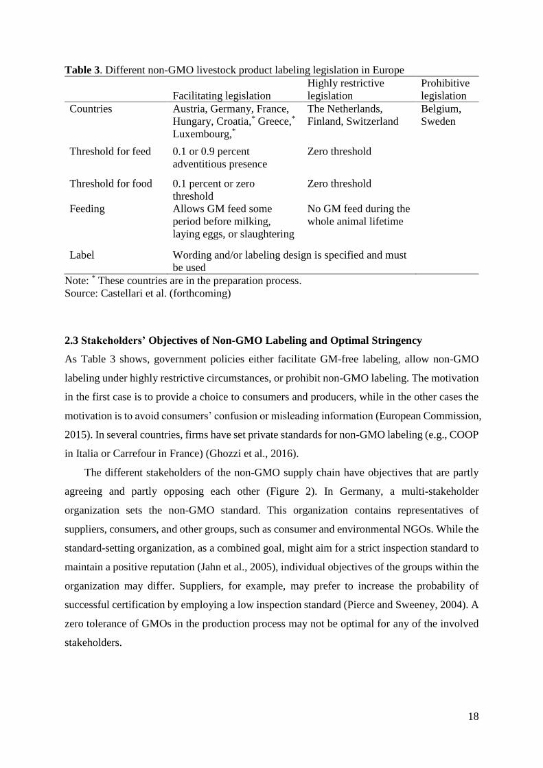
The current Member State schemes of countries that have national non-GMO standards
range from legislations that facilitate non-GMO labeling to legislations that ban labeling
altogether and everything in between (Table 3). Facilitating legislations in Austria, Germany,
France, and recently Hungary define threshold values for the adventitious presence of GMOs
for non-GMO labeling. These legislations also allow feeding of GMO feed for a period prior to
deriving the livestock product. The periods differ by country and animal. Additional countries
(Croatia, Greece, and Luxembourg) are preparing similar regulatory frameworks.
By 2015, 18 EU Member States were not directly involved in non-GMO labeling schemes.
For example, the Italian government does not have an official position on non-GMO labeling,
leaving Italian regions free to develop their own positions. In Italy, the national accreditation
body, Accredia, developed a technical document (RT-11) defining the minimum requirements
for the certification of products commonly referred to as “non-GMO” (Boccaletti et al., 2012).
According to this document, non-GMO food must not contain random traces of genetically
modified DNA above 0.1 percent of an ingredient’s weight for food compared to the species-
specific total DNA; these values go down to 0.01 percent for seeds and up to 0.9 percent for
feed use.
5 These countries are: Austria, Bosnia and Herzegovina, Bulgaria, Croatia, the Czech Republic, Germany (Bavaria,
Baden Wuerttemberg), Hungary, Italy (Trentino Alto Adige, Friuli Venezia Giulia, Veneto, Emilia-Romana,
Lombardia, Piemont, Vallée d'Aoste), Moldova, Poland (Dolnoslaskie, Opolskie, Slaskie, Swietokrzyskie,
Podkarpackie, Malopolske), Romania, Serbia, the Slovak Republic, Slovenia, Switzerland, Ukraine (Uschgorod,
Tschernowzy, Winniza, Odessa, Lwow, Ternopol, Chmelnizkij, Iwano-Frankovsm).
18
Table 3. Different non-GMO livestock product labeling legislation in Europe
Facilitating legislation
Highly restrictive
legislation
Prohibitive
legislation
Countries Austria, Germany, France,
Hungary, Croatia,* Greece,*
Luxembourg,*
The Netherlands,
Finland, Switzerland
Belgium,
Sweden
Threshold for feed 0.1 or 0.9 percent
adventitious presence
Zero threshold
Threshold for food 0.1 percent or zero
threshold
Zero threshold
Feeding Allows GM feed some
period before milking,
laying eggs, or slaughtering
No GM feed during the
whole animal lifetime
Label Wording and/or labeling design is specified and must
be used
Note: * These countries are in the preparation process.
Source: Castellari et al. (forthcoming)
2.3 Stakeholders’ Objectives of Non-GMO Labeling and Optimal Stringency
As Table 3 shows, government policies either facilitate GM-free labeling, allow non-GMO
labeling under highly restrictive circumstances, or prohibit non-GMO labeling. The motivation
in the first case is to provide a choice to consumers and producers, while in the other cases the
motivation is to avoid consumers’ confusion or misleading information (European Commission,
2015). In several countries, firms have set private standards for non-GMO labeling (e.g., COOP
in Italia or Carrefour in France) (Ghozzi et al., 2016).
The different stakeholders of the non-GMO supply chain have objectives that are partly
agreeing and partly opposing each other (Figure 2). In Germany, a multi-stakeholder
organization sets the non-GMO standard. This organization contains representatives of
suppliers, consumers, and other groups, such as consumer and environmental NGOs. While the
standard-setting organization, as a combined goal, might aim for a strict inspection standard to
maintain a positive reputation (Jahn et al., 2005), individual objectives of the groups within the
organization may differ. Suppliers, for example, may prefer to increase the probability of
successful certification by employing a low inspection standard (Pierce and Sweeney, 2004). A
zero tolerance of GMOs in the production process may not be optimal for any of the involved
stakeholders.

19
Figure 2. Possible objectives of stakeholders of non-GMO labeling
Consumers’ Objectives
Consumers buy non-GMO products if their utility of these products exceeds the utility of GMO
products. For example, the results of choice experiments reveal that some consumers are willing
to pay more for some non-GMO-labeled products (Roosen et al., 2003). From an economic
point of view, the predictions from a utility framework are not straightforward, as the non-GMO
attribute may not only yield direct personal benefits but also indirect benefits to consumers.
Indirect benefits may be altruistic reasons or a perceived contribution to some public good
(Kirchhoff, 2000; Mason, 2013).
Furthermore, there are several interacting effects between the information provision of the
label and preferences of consumers that complicate the evaluation of utility derived from non-
GMO labeling. Consider, for example, a case in which consumers are perfectly informed about
the use of GMOs in livestock feed production, and they also know that GM feed can be
produced at a lower marginal cost. Then, in the absence of a signaling opportunity for firms,
consumers can infer that firms default to the less expensive (GM) feed variety (in accordance
with the Akerlof (1970)’s lemons problem). However, if GM-averse consumers are unaware of
the use of GMOs in food production, then those consumers prefer the GM products over the
same physical product when it is offered in cases in which they are aware that the product is
derived from GMOs. However, due to the difference in preferences, consumer surpluses with
and without information are incomparable (Bagwell, 2007; Braithwaite, 1928; Dixit and
Norman, 1978; Teisl et al., 2002) if treated as the same good. Hence, to measure the effect of
information, the awareness needs to be considered in the utility evaluation (Teisl et al., 2002).
However, additional information about a product does not only create awareness; it can also
Consumers
Suppliers Anti-GMO
activist groups
Maximize utility
- Improve information
- Stringency-price trade-off
Maximize profits
- Product differentiation
- Transaction cost and
uncertainty reduction
- Long-run reputation gain
Minimize the amount of GMOs
- Increase consumers’ GMO
aversion
- Pressure GMO-using firms

20
distract consumers from other (potentially more) important information (Teisl and Caswell,
2003).
Another challenge of measuring the consumer welfare of labeling is that awareness itself
can be endogenously determined through labeling. This endogeneity has been shown in
experiments where consumers’ willingness to pay to avoid an undesired attribute (e.g., GMOs)
was significantly higher if the GM product is labeled (e.g., “contains GMOs”) than if the
product without the undesired product is labeled (e.g., “does not contain GMOs”) (Costanigro
and Lusk, 2014; Liaukonyte et al., 2013). Furthermore, the label itself may signal to consumers
that GMOs are unsafe because if they were safe, a label would be irrelevant (Costanigro and
Lusk, 2014). As discussed by Caswell (1998), consumers may consider the label to be an
indicator of a safety concern regarding the GMO attribute, even though regulators evaluate it
as safe. This endogeneity questions how far a non-GMO label can reduce imperfect information
(i.e., informing consumers that products are GM or not) or can potentially cause new
information imperfections (i.e., signaling safety concerns of GMOs).
Not all consumers are equally averse to GMOs. Consumers who are indifferent between a
GM and non-GM product are unaffected by the label if the price of the lower-priced GM
product remains the same after labeling. These consumers are better off if the price of the GM
product decreases (e.g., due to an inward shift in demand when some consumers switch to non-
GMO products). GM-averse consumers, however, are only better off and will buy the labeled
product if the incremental utility from the non-GMO attribute minus the price premium that
firms ask for non-GMO products exceeds the utility of consuming the GM product. In the
absence of other imperfections, there exists an equilibrium stringency and a market clearing
price (Caswell, 1998).6
Suppliers’ Objectives
For suppliers to maximize their profits, not only the direct effect on the labeled product, but
also the indirect (external) effect on unlabeled products must be considered. The key variables
are a firm’s reputation as well as non-GMO production and certification costs (e.g., incremental
production costs for more expensive raw material or segregation from other GMO sources).
Further costs arise for the implementation of the production standard (e.g., separating
production lines) and transaction costs (e.g., loss of flexibility to source raw materials).
6 The equilibrium only exists if the marginal production costs of zero-tolerance are increasing and are initially
below the consumers’ choke price.

21
Firms have several incentives to adopt policies for labeling attributes that are perceived by
consumers as higher quality. These incentives are, for example, to soften price competition
through vertical product differentiation (e.g., Arora and Gangopadhyay, 1995) or to increase
bargaining power over upstream suppliers (von Schlippenbach and Teichmann, 2012).
Additionally, historical factors, communication infrastructure, or sectoral conditions play a role
such that not all firms equally benefit from labeling (Vigani and Olper, 2014). However,
Fulponi (2006) finds that reputation is the largest incentive for the implementation of private
standards by the majority of OECD food retailers. Reputation also plays a major role for dairy
companies to switch to non-GMO production (Punt et al., 2016).
Non-GMO suppliers benefit from an increased attribute awareness of consumers due to
labeling. However, the non-GMO attribute may have both a negative and positive information
externality. The negative externality is that the label not only increases awareness that a product
is non-GMO, but also increases awareness that the unlabeled products do not comply with the
non-GMO standard, which signals a product’s GM attribute. Firms that offer both labeled and
unlabeled products may face a trade-off between the direct benefits of non-GMO product
supply and the indirect effects of making consumers aware that unlabeled products may not
comply with the non-GMO standard.
The positive externality relates to the halo (positive spill-over) effect of a non-GMO label
on a firm’s reputation. Consumers may prefer the unlabeled products of a firm that offers non-
GMO labeled products to other unlabeled products of firms that do not offer any non-GMO
products in their assortment. For example, most retailers communicate their non-GMO supply
as part of their sustainability strategy (Vigani and Olper, 2014; Wesseler, 2014). This strategy
extends the positive effect of a few non-GMO labeled products as a quality attribute to the
overall brand or whole firm image (Gruère and Sengupta, 2009). It is not clear a priori which
externality is stronger.
Furthermore, while consumer activist groups advocate transparency of the production
standard, it may not be in the firms’ interest to provide full information to consumers if
consumers perceive the non-GMO label to be stricter than it is. As Henseleit and Kubitzki (2009)
show in their survey, consumers’ expectations of the non-GMO label are higher than the current
non-GMO standard requirements. Hence, most processors (17 out of 18) and some of the other
stakeholders (e.g., consumers associations, food industry associations, NGOs, retailers) in a
survey on non-GMO labeling agreed that the non-GMO label potentially misleads consumers
(European Commission, 2015, , p.60).

22
Anti-GMO Activist Groups
The main concern of anti-GMO activist groups refers to the usage of GMOs in agriculture,
aquaculture, and forestry. Because GM animals are not approved for consumption or production
in the European Union, in the view of anti-GMO activist groups, the non-GMO label may be
considered mainly as a tool to minimize the total area of GM plant cultivation. Through the
promotion of non-GMO labeling and pressure against GMO-using firms, these groups try to
minimize the total amount of the GMO content (mainly GM crops) used in food production.
Fulponi (2006) found in her survey that the strength of NGOs is to determine retailers’ adoption
of a higher private production standard for animal welfare.
Activist groups have different strategies to achieve their goals. The greater the consumers’
aversion towards GMOs, combined with the consumers’ awareness of GMO use by firms, the
more successful the activist groups are in achieving their goals. These groups use consumer and
public pressure to cause financial and reputational harm to firms that use GM crops in their
food production (Winston, 2002). Targeted firms are firms that are highly visible, well-
recognized and highly susceptible to public pressure (Spar and La Mure, 2003). Examples are
Greenpeace’s protests at the dairy companies Landliebe (a subsidiary of FrieslandCampina)
and Weihenstephan (a subsidiary of Müller), or protests at Wiesenhof (a subsidiary of the
largest German poultry producer, PHW Group). Landliebe became the first (large) dairy
company to use non-GMO labeling. Greenpeace also claims that Wiesenhof switched to non-
GMO production because of Greenpeace’s pressure (Greenpeace, 2014). Similar cases were
reported in France, where Greenpeace groups placed large posters in front of supermarkets
calling them “contaminated with GM food,” because these supermarkets listed some products
with GM-labeled ingredients (Gruère, 2006). In addition, the NGO publishes shopping guides
to help consumers distinguish between firms that adopt non-GMO strategies and other firms.
Regarding the optimal standard stringency from the activist groups’ viewpoint, we need to
distinguish between options that concern the GMO attribute and options that concern the non-
GMO attribute. In the first case, activist groups’ optimal stringency is stricter than the social
planner’s or the firm’s optimum (Bonroy and Constantatos, 2015). For example, the activist
group’s preferred option is a ban on GM food. However, in terms of labeling the non-GMO
attribute, the activist groups’ optimal stringency may be even weaker than a social planner’s or
a firm’s optimal stringency. This order reversion occurs, because a stricter non-GMO labeling
standard increases the firms’ compliance costs, deterring some firms from adopting the standard
(Bernstein and Cashore, 2007). A non-GMO standard stringency that is optimal for anti-GMO
activist groups minimizes the total usage of GM crops in food production.

23
2.4 Coexistence Measures in the European Union
The provision of non-GM products in the presence of GM cultivation requires coexistence of
the systems. In the European Union, the national authorities of individual Member States set
coexistence rules for GM crops to guarantee coexistence with conventional and organic crops.
The European Commission published Recommendation 2003/556/EC on 23 July 2003 on
guidelines for the development of national strategies and best practices to ensure coexistence
(European Commission, 2003). In 2010, the Commission replaced the recommendations with
the recommendation on guidelines for the development of national measures to avoid the
unintended presence of GMOs in conventional and organic crops (European Commission,
2010).
This recommendation to set up coexistence measures also holds for the EU Member States
without GM crop cultivation, because these countries need to be prepared if they allow GM
cultivation. At the EU level, the European Coexistence Bureau organizes the exchange of
technical and scientific information on the best agricultural management practices for
coexistence. On this basis, it develops crop-specific guidelines for coexistence measures.
Most EU Member States have adopted coexistence rules or are preparing them. All
countries that cultivate GM crops, except Spain, have enacted coexistence legislation. Spain
manages coexistence based on the good agricultural practices defined by the National
Association of Seed Breeders. Some EU Member States or regions (e.g., Southern Belgium and
Hungary) enacted very restrictive coexistence rules that strongly limit the cultivation of GM
crops (USDA FAS, 2016).
Germany is one of the Member States with well-defined coexistence measures; however,
these measures are restrictive and according to the U.S. Department of Agriculture (USDA),
they are biased against the use of GM crops (USDA FAS, 2016). Commercial GM crop
cultivation was allowed from 2005 to 2008, until Germany applied the safeguard clause. Several
of the coexistence measures that the European Commission recommends, are discussed in
Chapter 3 of this thesis.

24
Chapter 3
The Costs of Coexistence Measures for
Genetically Modified Maize in Germany

25
3. THE COSTS OF COEXISTENCE MEASURES FOR GENETICALLY
MODIFIED MAIZE IN GERMANY7
ABSTRACT: We estimate the perceived costs of legal requirements (‘coexistence measures’)
for growing genetically modified Bt maize in Germany using a choice experiment. The costs
of the evaluated ex-ante and ex-post coexistence measures range from zero to more than 300
euros per measure and most of them are greater than the extra revenue the farmers in our survey
expect from growing Bt maize or than estimates in the literature. The cost estimates for temporal
separation, the highest in our evaluation, imply that the exclusion of this measure in Germany
is justified. The costliest measures of the ones that are currently applied in Germany are joint
and strict liability for all damages. Our results further show that neighbors do not cause a
problem and opportunities for reducing costs through agreements with them exist. Finally, we
find that farmers’ attitudes toward genetically modified crops affect the probability of adoption
of Bt maize. Our results imply that strict liability will deter the cultivation of Bt maize in
Germany unless liability issues can be addressed through other means, for example, through
neighbors agreements.
KEYWORDS: Coexistence measure cost, genetically modified crops, Bt maize
7 This chapter is based on the article: Venus, T.J., Dillen, K., Punt, M.J., and Wesseler, J.H.H., 2017. The Costs of
Coexistence Measures for Genetically Modified Maize in Germany. Journal of Agricultural Economics. pp. 407-
426.
26
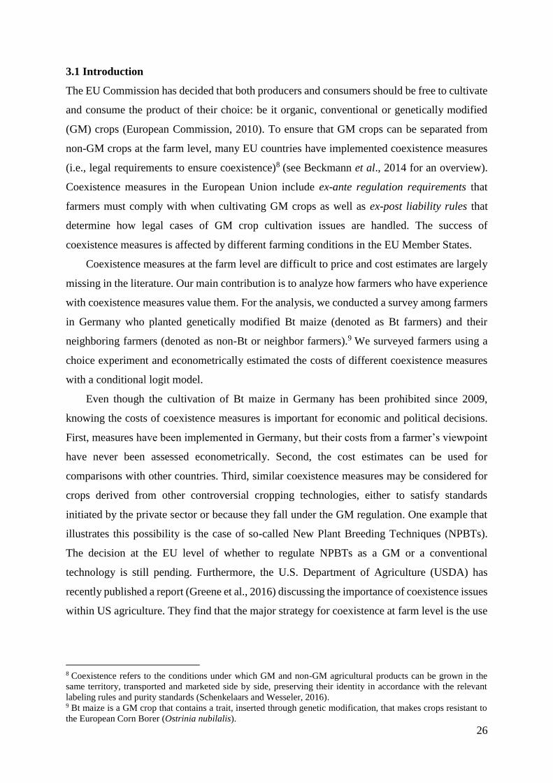
3.1 Introduction
The EU Commission has decided that both producers and consumers should be free to cultivate
and consume the product of their choice: be it organic, conventional or genetically modified
(GM) crops (European Commission, 2010). To ensure that GM crops can be separated from
non-GM crops at the farm level, many EU countries have implemented coexistence measures
(i.e., legal requirements to ensure coexistence)8 (see Beckmann et al., 2014 for an overview).
Coexistence measures in the European Union include ex-ante regulation requirements that
farmers must comply with when cultivating GM crops as well as ex-post liability rules that
determine how legal cases of GM crop cultivation issues are handled. The success of
coexistence measures is affected by different farming conditions in the EU Member States.
Coexistence measures at the farm level are difficult to price and cost estimates are largely
missing in the literature. Our main contribution is to analyze how farmers who have experience
with coexistence measures value them. For the analysis, we conducted a survey among farmers
in Germany who planted genetically modified Bt maize (denoted as Bt farmers) and their
neighboring farmers (denoted as non-Bt or neighbor farmers).9 We surveyed farmers using a
choice experiment and econometrically estimated the costs of different coexistence measures
with a conditional logit model.
Even though the cultivation of Bt maize in Germany has been prohibited since 2009,
knowing the costs of coexistence measures is important for economic and political decisions.
First, measures have been implemented in Germany, but their costs from a farmer’s viewpoint
have never been assessed econometrically. Second, the cost estimates can be used for
comparisons with other countries. Third, similar coexistence measures may be considered for
crops derived from other controversial cropping technologies, either to satisfy standards
initiated by the private sector or because they fall under the GM regulation. One example that
illustrates this possibility is the case of so-called New Plant Breeding Techniques (NPBTs).
The decision at the EU level of whether to regulate NPBTs as a GM or a conventional
technology is still pending. Furthermore, the U.S. Department of Agriculture (USDA) has
recently published a report (Greene et al., 2016) discussing the importance of coexistence issues
within US agriculture. They find that the major strategy for coexistence at farm level is the use
8 Coexistence refers to the conditions under which GM and non-GM agricultural products can be grown in the
same territory, transported and marketed side by side, preserving their identity in accordance with the relevant
labeling rules and purity standards (Schenkelaars and Wesseler, 2016). 9 Bt maize is a GM crop that contains a trait, inserted through genetic modification, that makes crops resistant to
the European Corn Borer (Ostrinia nubilalis).
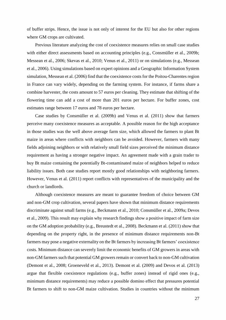
27
of buffer strips. Hence, the issue is not only of interest for the EU but also for other regions
where GM crops are cultivated.
Previous literature analyzing the cost of coexistence measures relies on small case studies
with either direct assessments based on accounting principles (e.g., Consmüller et al., 2009b;
Messean et al., 2006; Skevas et al., 2010; Venus et al., 2011) or on simulations (e.g., Messean
et al., 2006). Using simulations based on expert opinions and a Geographic Information System
simulation, Messean et al. (2006) find that the coexistence costs for the Poitou-Charentes region
in France can vary widely, depending on the farming system. For instance, if farms share a
combine harvester, the costs amount to 57 euros per cleaning. They estimate that shifting of the
flowering time can add a cost of more than 201 euros per hectare. For buffer zones, cost
estimates range between 17 euros and 78 euros per hectare.
Case studies by Consmüller et al. (2009b) and Venus et al. (2011) show that farmers
perceive many coexistence measures as acceptable. A possible reason for the high acceptance
in those studies was the well above average farm size, which allowed the farmers to plant Bt
maize in areas where conflicts with neighbors can be avoided. However, farmers with many
fields adjoining neighbors or with relatively small field sizes perceived the minimum distance
requirement as having a stronger negative impact. An agreement made with a grain trader to
buy Bt maize containing the potentially Bt-contaminated maize of neighbors helped to reduce
liability issues. Both case studies report mostly good relationships with neighboring farmers.
However, Venus et al. (2011) report conflicts with representatives of the municipality and the
church or landlords.
Although coexistence measures are meant to guarantee freedom of choice between GM
and non-GM crop cultivation, several papers have shown that minimum distance requirements
discriminate against small farms (e.g., Beckmann et al., 2010; Consmüller et al., 2009a; Devos
et al., 2009). This result may explain why research findings show a positive impact of farm size
on the GM adoption probability (e.g., Breustedt et al., 2008). Beckmann et al. (2011) show that
depending on the property right, in the presence of minimum distance requirements non-Bt
farmers may pose a negative externality on the Bt farmers by increasing Bt farmers’ coexistence
costs. Minimum distance can severely limit the economic benefits of GM growers in areas with
non-GM farmers such that potential GM growers remain or convert back to non-GM cultivation
(Demont et al., 2008; Groeneveld et al., 2013). Demont et al. (2009) and Devos et al. (2013)
argue that flexible coexistence regulations (e.g., buffer zones) instead of rigid ones (e.g.,
minimum distance requirements) may reduce a possible domino effect that pressures potential
Bt farmers to shift to non-GM maize cultivation. Studies in countries without the minimum

28
distance requirement, however, also document a size effect (i.e., that larger farms are more
likely to adopt GM crops) (e.g., Fernandez-Cornejo et al., 2002; Hubbell et al., 2000) without
explicitly identifying the reasons.
For farmers to adopt Bt maize, coexistence costs have to be outweighed by the extra
revenue of Bt maize compared to conventional maize. This profitability depends on several
agronomic and economic factors such as the European Corn Borer infestation rate, farm
structure, pest control management or maize acreage per farm (e.g., Breustedt et al., 2008;
Consmüller et al., 2010). Areal et al. (2011) find that the major reasons for farmers to adopt
herbicide-resistant maize and oilseed rape in six European countries are a guaranteed higher
income and the reduction in weed control costs. However, the social environment, farmer’s
knowledge about and attitudes towards GMOs, age and education have also been identified to
affect potential adoption (e.g., Areal et al., 2011; Gyau et al., 2009; Skevas et al., 2012). Several
studies have used choice experiments to analyze factors influencing farmers’ choice of adopting
GM-crops (see Breustedt et al., 2008, , for an overview). However, these studies do not
explicitly calculate the costs of coexistence measures.
As shown earlier, arguments on the choice and impact of coexistence measures are often
based on theoretical models, simulations, or narratives. To judge the importance of the impact
on farmers, econometric cost estimates are missing in the literature. We provide these estimates
derived from choice experiments with former Bt maize farmers and their neighbors in
Germany—one of the few countries besides the Czech Republic, Portugal and Slovakia, where
farmers have experience in complying with a complete national coexistence regulation regime.
The estimates form a basis for further discussion on this issue for researchers and policymakers
and constitute a validation of previous theoretical work.
3.2 Material and Methods
3.2.1. Coexistence Measures in Germany
Germany is one of the EU Member States that allowed farmers to grow genetically modified
Bt maize after the EU approved its cultivation. The German government approved Bt maize
cultivation in 2005, but banned it again in early 2009. During the period of 2005 to 2008, 91
farmers from 12 out of 16 German federal states registered Bt maize cultivation areas. The total
area increased each year and reached a total of 3,171 hectares (0.15 percent) of the total German
maize production in the last year before the ban (BVL, 2013). More than 92 percent of the Bt

29
maize area was located in three federal states: Brandenburg (39 percent), Saxony (30 percent),
and Mecklenburg-Western Pomerania (24 percent).
In 2008, coexistence measures for Germany were formulated in the German Genetic
Engineering Act (GenTG), complemented by the Genetic Engineering Plant Act (GenTPflEV),
and by the Regulation on the implementation of the EU regulation on labeling and application
of genetically modified organisms (GMOs) (Federal Ministry of Germany, 1990, 2004, 2008).
The ex-ante and ex-post coexistence measures for the cultivation of Bt maize include:
(1) Compulsory registration. A farmer who plants a GM crop has to inform the Federal Office
of Consumer Protection and Food Safety (BVL) 3 months before the intended GM plant
seeding.
(2) Spatial isolation minimum distance. Genetically modified maize must keep a distance of
150 m from conventional and 300 m from organic maize fields. The Federal States have
the right to implement additional minimum distance requirements to nature conservation
areas. The Federal States of Brandenburg and Baden-Wuerttemberg, for example, require
a minimum distance of 800 m and 3,000 m, respectively, between a Bt maize field and a
nature conservation area.
(3) Obligation to notify the BVL and neighbors about the intention to cultivate genetically
modified plants. Neighbors are owners of a field within 300 m from the GM field.
(4) Private arrangements. The Bt farmer can agree with the neighbor to reduce the obligatory
minimum distance up to 3 months before seeding. The neighbor has to sign an admonition.
If the neighbor does not answer the request within one month, it is considered as consent
to the Bt farmer’s request. The Bt farmer has to inform the BVL about the agreement.
(5) Obligation to inquire information from the lower nature conservation authority. The Bt
farmer has to ask for information about nature protected areas three months before seeding
if all conditions for the environmental protection are pertinent.
(6) Obligation to document. The Bt farmer has to document the seed used and the location of
the genetically modified plants. Additionally, the document must contain the cultivation
technique and potential growth of unintended GM maize in the following year (i.e.,
volunteers). The farmer has to destroy volunteer GM plants.
(7) Avoidance of commingling. The farmer has to prevent GM seeding and GM harvest
material from commingling with the conventional material; the farmer must, for instance,
clean all machinery that could potentially lead to an admixture.
(8) Crop rotation. Farmers must wait for at least one year before cultivating conventional
maize in a field if GM maize grew on that field before.

30
Prior to these regulations, a 20-meter pollen barrier was recommended as a best practice
measure at the farm level (Consmüller et al., 2009a; Weber et al., 2007).
3.2.2. Selection of Farms and Study Design
A total of 91 farmers planted Bt maize in the period of 2005–2008 in Germany. We approached
those farmers as they have experience with coexistence measures. We also included their
neighbor farmers because Bt maize producers need to inform neighboring farmers about their
intention to cultivate GM crops. Although the size of our sample does not allow inference about
German farms in general, it does allow comparison of the estimated coexistence costs with the
expected Bt maize benefits. Moreover, because the farmers in our sample cultivated Bt maize,
our results are based on past experience rather than on expectations.
In June 2012, the Federal Office of Consumer Protection and Food Safety sent out a letter
to all 91 farmers. The letter asked them to provide their names and addresses to the project
institution (Technische Universität München). Two out of the 91 letters were returned because
the address was wrong or the recipient was unknown. Initially, 35 farmers replied to the letter.
Of those who replied, 24 agreed to participate in the survey. The reasons of those who declined
included: ‘… cultivation and coexistence are currently not relevant to agriculture,’ ‘… fed up
with the ban by the politicians,’ ‘… had trouble in the first year. The yield was 20 percent extra,
though,’ ‘… was criminalized by neighbors’ and ‘… was forbidden by the landowner to grow
GM.’ The 24 farmers who agreed received a personal phone call, in which four changed their
mind about participating.
InnoPlanta e.V.,10 an organization at which all Bt farmers are registered, contacted five
additional Bt farmers who had not replied to the BVL letter. Four of them agreed to participate
in the survey.11 The surveyed Bt farmers identified seven additional Bt neighbor farmers who
initially had not replied to the BVL letter. Three of the Bt neighbors agreed to participate,
resulting in a sample size of 27 Bt-farmers.
The 27 Bt farmers in the survey provided a contact for 53 non-Bt neighbors. All of the
neighbors received a request by phone to participate in the survey. 20 non-Bt neighbor farmers
agreed to participate. The main reasons for refusal were ‘… no time,’ ‘… no interest in the
topic,’ ‘… do not plant maize,’ ‘…area is leased out,’ ‘… the responsible person is retired, sick,
or passed away.’ In summary, 27 Bt and 20 non-Bt farmers participated in the survey.
10 InnoPlanta e.V. is an association whose objective is to promote agro-biotechnological and modern plant breeding
activities of farmers, companies, scientific institutions, and others and to connect them in a network. 11 The one who disagreed had problems with his landowners and did not want to be further connected with GMO
activities.

31
Our sample farms are in six out of the 16 German federal states (Table 1). Most sample
farms are in Brandenburg, which was the state with the largest Bt maize production. Farms in
Saxony, the second largest Bt maize cultivating state in Germany, are also well-represented.
Farmers were mostly evenly spread within the states except for Bavaria where all farmers were
in the northern part that has the highest application of insecticides against the European Corn
Borer (Zellner et al., 2009).
All respondents are highly involved in the arable production decision of the farm either as
farm owners or managers (39 cases) or as plant department managers (8 cases). They were all
employed when Bt maize was planted and hence were well-informed; they were either involved
in the decision in favor of or against Bt maize or, in the case of non-Bt farmers, knew about
their Bt neighbors’ decision.
Table 1. A summary of farmers’ characteristics
All Bt Non-Bt
n = 47 n = 27 n = 20
Gender Male 45 27 18
Education University (of applied
sciences) degree 37 22 15
Juristic person Yes 37 24 13
Federal state Bavaria 10 3 7
Brandenburg 14 11 3
Mecklenburg-W. Pom. 5 1 4
Saxony-Anhalt 3 2 1
Saxony 14 9 5
Thuringia 1 1 0
Source: Authors’ survey
3.2.3. The Survey Questionnaire
The questionnaire included general questions on farm and farmers’ characteristics. Farm
characteristics included general farm type (arable, mixed, livestock, or other), specific farm
type (e.g., cereal, dairy, or hog), farm-utilized agricultural area (UAA) (in hectares), and farm
land leased. We also included questions on maize production, such as the cultivated maize;
ranking of limits that prevented the farmer from receiving the maximum maize yield; as well
as a 10-point scale ranking of the European Corn Borer damage and weed damage, if not or
only insufficiently controled.
The questionnaire also included socio-demographic characteristics such as the job position
of the respondent within the farm, his or her farming experience, age, gender, and level of
education. Questions on the private farm household addressed the number of employees and

32
farm income. Furthermore, we asked about the 2008 conventional and Bt grain and silage maize
production. We gathered information on the planted area, number of fields, and yield of the
crops. In most cases, the exact yield, especially for silage maize, was not available, so the
information was rather farmers’ best estimate. Further information included the percentage of
on-farm usage of maize, and if sold, the selling strategy and price per metric ton. To examine
farmers’ attitudes, we used a Likert scale with 15 items about their perception of GM foods,
food health and environmental issues, and the role of the government.
To examine the costs of coexistence, the survey included a discrete choice experiment
requiring farmers to make a trade-off between a set of four coexistence measures and one
monetary attribute—the extra gross margin from planting GM crops. The coexistence measures
were some of those recommended by the European Commission (European Commission,
2003). We chose measures for which we expected a low correlation with one another. We
excluded, for example, buffer zones because of a large correlation with minimum distance.
Table 2 presents the five attributes.
Each attribute varies within three available levels. A full factorial design comprises 35 =
243 possible combinations of attributes. Statistical design methods were then used to structure
the presentation of the attribute levels within the choice sets. A D-optimal experimental design
was constructed with only the main effects (Johnson et al., 2006). A fraction of the full factorial
design was employed to construct an efficient design with 12 choice sets, in which each level
occurred once in each attribute and choice set. During the survey, each farmer was presented
with those 12 choice sets, each containing two options to grow Bt maize and an option to ‘opt
out’ by planting conventional maize with the information that this option could not lead to an
additional gross margin but also does not require coexistence measures. This design results in
a total of 47 x 12 = 564 responses.
Table 2. Attributes and levels of the choice experiment
Attributes Level 0 Level 1 Level 2
(1) Liability Not liable Only if non-compliant with
coexistence rules (negligence)
Joint and
strict
(2) Minimum distance None 50 m 100 m
(3) Information provision None Neighbor Location
register
(4) Temporal isolation None 2 weeks 4 weeks
(5) Extra gross margin €25 €75 €150
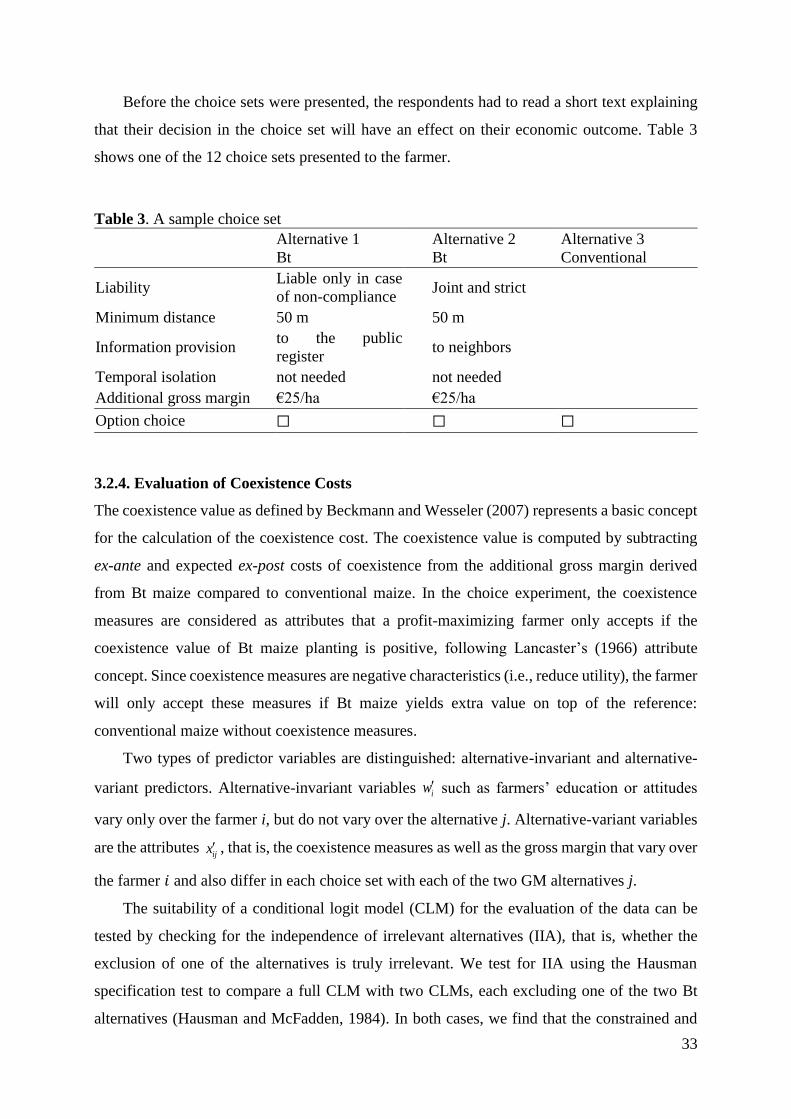
33
Before the choice sets were presented, the respondents had to read a short text explaining
that their decision in the choice set will have an effect on their economic outcome. Table 3
shows one of the 12 choice sets presented to the farmer.
Table 3. A sample choice set
Alternative 1
Bt
Alternative 2
Bt
Alternative 3
Conventional
Liability Liable only in case
of non-compliance Joint and strict
Minimum distance 50 m 50 m
Information provision to the public
register to neighbors
Temporal isolation not needed not needed
Additional gross margin €25/ha €25/ha
Option choice ☐ ☐ ☐
3.2.4. Evaluation of Coexistence Costs
The coexistence value as defined by Beckmann and Wesseler (2007) represents a basic concept
for the calculation of the coexistence cost. The coexistence value is computed by subtracting
ex-ante and expected ex-post costs of coexistence from the additional gross margin derived
from Bt maize compared to conventional maize. In the choice experiment, the coexistence
measures are considered as attributes that a profit-maximizing farmer only accepts if the
coexistence value of Bt maize planting is positive, following Lancaster’s (1966) attribute
concept. Since coexistence measures are negative characteristics (i.e., reduce utility), the farmer
will only accept these measures if Bt maize yields extra value on top of the reference:
conventional maize without coexistence measures.
Two types of predictor variables are distinguished: alternative-invariant and alternative-
variant predictors. Alternative-invariant variables iw such as farmers’ education or attitudes
vary only over the farmer i, but do not vary over the alternative j. Alternative-variant variables
are the attributes ijx , that is, the coexistence measures as well as the gross margin that vary over
the farmer 𝑖 and also differ in each choice set with each of the two GM alternatives j.
The suitability of a conditional logit model (CLM) for the evaluation of the data can be
tested by checking for the independence of irrelevant alternatives (IIA), that is, whether the
exclusion of one of the alternatives is truly irrelevant. We test for IIA using the Hausman
specification test to compare a full CLM with two CLMs, each excluding one of the two Bt
alternatives (Hausman and McFadden, 1984). In both cases, we find that the constrained and

34
unconstrained estimated coefficients on the remaining categories are not significantly different,
implying no rejection of the IIA, thus indicating the suitability of the CLM model.
The three alternatives a farmer can choose are 1, 2,Bt Bt conv , where Bt1 and Bt2 are the
first two Bt choice options and 𝑐𝑜𝑛𝑣 is the third conventional option. Based on McFadden’s
(1974) random utility theory, the utility, ijU , for the ith farmer to choose the jth maize
alternative that maximizes his or her utility is
(1) ' 'ij ij i j ijU x w
The coefficient 𝛾𝑐𝑜𝑛𝑣 of the conventional alternative, which serves as the reference, is
normalised to zero. There are two sets of coefficients, j , however. Following Breustedt et al.
(2008), we restrict the alternative-invariant coefficients not to vary between the two Bt
alternatives, that is, 𝛾𝐵𝑡1 = 𝛾𝐵𝑡2 = 𝛾. For the alternative-variant coefficient, the conventional
alternative serves as the reference, such that the predictor * *
ij ij iconvx x x and the error terms
become * *
ij ij iconv . The probability that the observed outcome, jy j , that is, that the ith
farmer chooses alternative 1, 2Btj Bt is
(2)
3
1
exp
exp
j
ij i
kij ik
ij ix wp Prob y j
x w
.
Interaction terms between some of the alternative-variant and alternative-invariant
variables depend on i and j and are considered inijx . Taking the derivative of the probability
with respect to the alternative-variant variables yields the marginal effect of an increase in a
regressor on the probability of selecting alternative j, that is
(3) Indij ik ij ikp x p j k p ,
where Ind (.) is an indicator function, equalling one if j = k, and zero otherwise.
The alternative-variant variable coefficients resulting from the CLM are used to estimate
the coexistence costs, that is, the marginal rate of substitution of the coexistence measure
attribute and the monetary gross margin attribute, which is given by
(4) coexistence measure
gross margin
W
.
In this study, the interpretation of the non-monetary and monetary attribute parameter ratio
is the willingness-to-accept rather than willingness-to-pay as farmers only accept coexistence
measures if they get additional gross margin. Independently of this interpretation, however, W
represents the cost of an attribute and hence the cost of coexistence measures.

35
3.2.5. Principal Component Analysis
Farmers were asked to rank several items on a Likert scale to measure their attitudes towards
GMOs. To include the attitudes in the choice experiment, we use a Principal Component
Analysis (PCA).12 The PCA explores if the variance of responses to an item overlaps with the
variance of other items to form some common construct (component) (Costello and Osborne,
2005).
Even though explanatory factor analysis is more reliable in explaining an underlying
construct, we use PCA as it is more robust because it assumes that all variance—the variance
shared with other items and a part that is unique to the item—can be analyzed compared to
factor analysis, which explains the shared variance only (Costello and Osborne, 2005).13
The Kaiser-Meyer-Okin (KMO) (Kaiser, 1970) measure of sampling adequacy is used to
test whether the sample is large enough and the Cronbach’s alpha analysis to test the reliability
of the component (see Appendix 3.6.2). Finally, the farmers’ perception is measured by their
score on each construct. This score is the weighted average of all item values that comprise a
component.
3.3 Results
3.3.1. Statistics of Sample Farms
Our sample farms cover 0.03 percent of UAA in Germany and produce 9,174 hectares of maize
(see online Appendix S1).14 The sample covers 30 percent of the Bt maize farms that planted
37 percent of the 2008 Bt maize area. The sample contains farms that planted a somewhat larger
area than the average Bt maize producer. The size of Bt maize parcels, however, is similar to
the average of the 2008 registered parcels, as the share of the number of parcels to the total
number of parcels (63/200 = 31.5 percent) almost equals the share of Bt maize farmers to the
total number of Bt maize farmers (30 percent). Of the 1,182 hectares, 77 percent specialized in
silage maize and 23 percent in grain maize.
Table 4 reports the mean socio-demographic and farm descriptive variables of all sample
farms. For comparison, the fourth column represents data from Germany. The farms can be
considered average maize producers at least in relative terms where maize occupies about 19.8
percent of their area, compared to 16 percent on average for Germany.
12 A more detailed explanation of the procedure is outlined in Appendix 3.6.2. 13 We use Varimax rotation—an ‘orthogonal rotation’ that forces the factors to be uncorrelated with each other. 14 Note that we asked farmers about their farm size in the year before the survey, that is, in 2012.
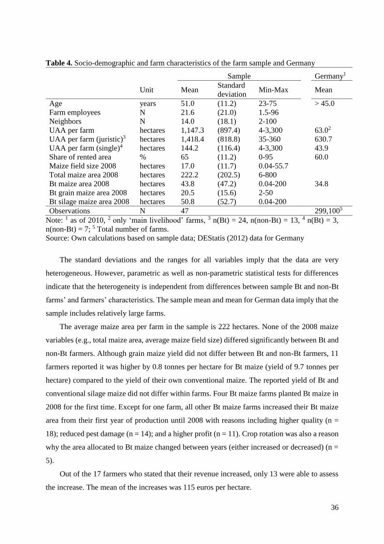
36
Table 4. Socio-demographic and farm characteristics of the farm sample and Germany
Sample Germany1
Unit Mean
Standard
deviation Min-Max
Mean
Age years 51.0 (11.2) 23-75 > 45.0
Farm employees N 21.6 (21.0) 1.5-96
Neighbors N 14.0 (18.1) 2-100
UAA per farm hectares 1,147.3 (897.4) 4-3,300 63.02
UAA per farm (juristic)3 hectares 1,418.4 (818.8) 35-360 630.7
UAA per farm (single)4 hectares 144.2 (116.4) 4-3,300 43.9
Share of rented area % 65 (11.2) 0-95 60.0
Maize field size 2008 hectares 17.0 (11.7) 0.04-55.7
Total maize area 2008 hectares 222.2 (202.5) 6-800
Bt maize area 2008 hectares 43.8 (47.2) 0.04-200 34.8
Bt grain maize area 2008 hectares 20.5 (15.6) 2-50
Bt silage maize area 2008 hectares 50.8 (52.7) 0.04-200
Observations N 47 299,1005
Note: 1 as of 2010, 2 only ‘main livelihood’ farms, 3 n(Bt) = 24, n(non-Bt) = 13, 4 n(Bt) = 3,
n(non-Bt) = 7; 5 Total number of farms.
Source: Own calculations based on sample data; DEStatis (2012) data for Germany
The standard deviations and the ranges for all variables imply that the data are very
heterogeneous. However, parametric as well as non-parametric statistical tests for differences
indicate that the heterogeneity is independent from differences between sample Bt and non-Bt
farms’ and farmers’ characteristics. The sample mean and mean for German data imply that the
sample includes relatively large farms.
The average maize area per farm in the sample is 222 hectares. None of the 2008 maize
variables (e.g., total maize area, average maize field size) differed significantly between Bt and
non-Bt farmers. Although grain maize yield did not differ between Bt and non-Bt farmers, 11
farmers reported it was higher by 0.8 tonnes per hectare for Bt maize (yield of 9.7 tonnes per
hectare) compared to the yield of their own conventional maize. The reported yield of Bt and
conventional silage maize did not differ within farms. Four Bt maize farms planted Bt maize in
2008 for the first time. Except for one farm, all other Bt maize farms increased their Bt maize
area from their first year of production until 2008 with reasons including higher quality (n =
18); reduced pest damage (n = 14); and a higher profit (n = 11). Crop rotation was also a reason
why the area allocated to Bt maize changed between years (either increased or decreased) (n =
5).
Out of the 17 farmers who stated that their revenue increased, only 13 were able to assess
the increase. The mean of the increases was 115 euros per hectare.

37
Most non-Bt maize farmers expected no price difference between Bt and non-Bt maize,
probably (as indicated by some interviewees) due to the use of maize as feed. However, on
average they expected a yield increase of 9.3 percent (about 0.9 tonnes) and additional gross
margin of 34.4 euros (median value of 5 euros) per hectare. The expected yield increase does
not differ much from the one tonne yield increase found in the meta-analysis by Areal et al.
(2013).
3.3.2. Farmers’ Attitudes toward Bt Maize Cultivation
A Likert scale consisting of 15 items was included in the questionnaire to survey farmers’
attitudes towards GM crops and their perception of related benefits and risks of GM
technologies and the role of the government.
Figure 1 shows the mean results of Bt and non-Bt farmers. We tested whether the
distribution of given answers differs significantly using Fisher’s exact test. Eight of 15 item
response distributions differed significantly between Bt and non-Bt farmers. Bt and non-Bt
sample farmers agreed on average that GM crops should be approved if the majority of
consumers is in favor of them (question 1). They also agree that GM crops should be approved
if farmers find them useful (question 2). This result confirms the results by Skevas et al. (2012)
who asked similar questions in their survey of Greek farmers.
Our results, however, differ from Skevas et al. (2012) for question 11, 12, and 13 on the
potential environmental and health risks and the unnaturalness of GM crops, where our farmers
disagree on average. On the other hand, farmers tended to agree that food safety risks are among
the most important ones (question 8); that GM crops can eradicate diseases and pests (question
10); and that the rejection of GM crops makes EU farmers less competitive. Farmers were rather
neutral about trust in food labels (question 3), harmfulness of food additives, and the ability of
the government to manage potential health and environmental damages (questions 4 and 5). Bt
farmers disagreed more strongly than non-Bt farmers that human interference in nature would
have disastrous consequences.

38
Note: Items for which Fisher’s exact test for differences between the distribution of Bt and non-
Bt farmers is statistically significant are: 1,4,7,10,11,12,13,14,15.
Figure 1. Mean values of Likert scale values for Bt and non-Bt farmers (n = 47). The scale
rages from strongly disagree (1) to strongly agree (5)
3.3.3 Estimation of Coexistence Costs
Costs of coexistence measures were estimated from the choice experiment data. Each farmer’s
principal component score (PCS) on a single construct derived from the PCA (Table S1 in the
online Appendix) was used as an alternative-invariant variable in the conditional logit model.
The higher the score of farmers on the component, the more they agree with items opposing
GM crops.
1. If the majority of European consumers are infavour of GM crops they should be approved
2. If farmers think that a GM crop is useful tothem they should be allowed to grow it
3. Food labels can be trusted
4. I think additives in food are not harmful to myhealth
5. The health risks surrounding GM crops canbe managed by the government
6. The environmental risks surrounding GMcrops can be managed by the government
7. When humans interfere with naturedisastrous consequences result
8. Among the risks we face in our lives, thoseimpacting food safety are very important
9. Pesticides and fertilizers are dangerous tothe environment
10. We can eradicate the diseases and peststhat attack crops by using GM crops
11. GM crops are against nature
12. Harmful environmental effects of GM foodsare likely to appear in the future
13. Harmful human health effects of GM foodsare likely to appear in the future
14. GM crops are the future of agriculture
15. Rejecting GM crops will make EU farmersuncompetitive on the world market
1 2 3 4 5
non-Bt Bt
Increasing agreement

39
We estimated two variations of the conditional logit model of 47 farmers who filled out 12
choice sets each (Table 5). The first estimation is unrestricted while the second estimation is
the parsimonious model excluding all insignificant variables that do not improve the model’s
goodness of fit when compared with a likelihood ratio test.
The reference level for the coefficient estimates of the alternative-invariant variables is
conventional production. Therefore, a positive value implies that a larger value of the respective
variable relates to a higher likelihood of choosing Bt maize. The reference level for the
alternative variant variables (i.e., the coexistence measures) is the zero level of each attribute
(i.e., not liable, no isolation distance, no information provision, and no temporal isolation
distance). On average, 56.2 percent farmers chose the conventional alternative (i.e., the
reference category), 22.3 percent the first Bt alternative (Bt1), and 21.5 percent the second Bt
alternative (Bt2).
Only two alternative-invariant coefficient estimates were significant: the principal
component score (PCS) and the number of neighbors. Unlike previous studies, which found a
positive impact of farm size measured by UAA on the adoption (Breustedt et al., 2008; Hubbell
et al., 2000; Qaim and de Janvry, 2003), we found no effect. It is, however, important to stress
that the Bt maize farms in our sample were much larger than the average German farm. This
size effect is probably due to self-selection of larger farms cultivating Bt maize. If this is the
case, farm size positively affects the adoption, and we cannot identify a size-effect due to a self-
selection bias. Two further insignificant coefficients were found for farmer’s age and education.
Previous studies show either a positive or a negative impact of education on the adoption of
GM crops (Breustedt et al., 2008). We also did not find any effect of the dummy for arable
farming, which is one if the farm is a pure arable farm and zero if the farm also has livestock.
We expected a negative effect assuming that Bt maize can be used as feed without affecting the
outcome of animal production, whereas marketing Bt maize could be more problematic.
However, agreements of grain traders to buy Bt and conventional maize at equal prices may
weaken or refute the marketing problem argument.
All statistically significant non-monetary attribute coefficients (i.e., coexistence measure)
are negative, meaning that when the respective attribute is present, the Bt alternative containing
this attribute is less likely to be chosen. For example, the 4-week temporal isolation coefficient
of -3.43 in the parsimonious model indicates that if farmers had to implement this measure,
they would be less likely to adopt Bt maize. Furthermore, farmers value the lower level of each
attribute as less demanding. For example, the absolute value of the 2-week temporal isolation
distance of -0.98 is lower than the value for 4-week isolation.

40
Table 5. Determinants of Bt maize adoption of Bt and non-Bt farmers
Variable/Attribute Attribute level Unrestricted model Parsimonious model
Constant 1.87** (0.86) 1.64*** (0.44)
PCS 0.74*** (0.15) 0.71*** (0.14)
Number of neighbors -0.02*** (0.01) -0.02*** (0.01)
Education -0.03 (0.09)
Farmer’s age -0.01 (0.01)
Farm size -0.00 (0.00)
Arable farm -0.28 (0.45)
Liability Negligence -1.06*** (0.31) -0.63*** (0.19)
Joint and strict -1.86*** (0.39) -1.98*** (0.25)
Isolation distance 50 m -1.26 (0.34) -0.80** (0.31)
100 m -2.22*** (0.61) -1.82*** (0.42)
Information provision Neighbor 0.02 (0.35)
Public register 0.39 (0.44)
Temporal isolation 2 weeks -1.10*** (0.36) -0.98*** (0.23)
4 weeks -3.93*** (0.56) -3.43*** (0.33)
Negligence x Bt 0.53 (0.34)
Joint and strict x Bt -0.29 (0.46)
50 meter x Bt 1.36** (0.52) 0.76** (0.32)
100 meter x Bt 1.44* (0.80) 0.75** (0.35)
Neighbor x Bt -0.30 (0.37)
Public register x Bt -0.65 (0.52)
2 weeks x Bt) -0.26 (0.40)
4 weeks x Bt 0.60 (0.63)
Gross Margin x Bt -0.004 (0.005)
Gross Margin 0.012*** (0.003) 0.010*** (0.002)
Log-likelihood -420 -428
Akaike Information Criterion (AIC) 905 885
Notes: *** 0.01, ** 0.05, * 0.1 significance level. Standard errors in parentheses. Dependent
variable = ‘Probability of choosing Bt maize instead of conventional maize’. x: interaction;
PCS: Principal Component Score on farmer’s attitudes towards GMOs.
The sign of the coefficient of the monetary attribute, that is, the extra gross margin from
growing Bt maize is, as expected, positive.15 The only insignificant coexistence measure is
information provision for both attribute levels: the neighbors and the public register. The model
also includes the alternative-invariant Bt variable as an interaction term to the alternative-
variant coexistence measures. This variable equals one when the individual is a Bt farmer, and
zero otherwise, and is used to check whether cost estimates differ between Bt and non-Bt
farmers. Significant differences are only observed for isolation distances.
The PCS estimate is positive, indicating that farmers with a high PCS (i.e., with positive
responses toward GMOs) are more likely to choose one of the Bt options. The more positive
15 Note that we tested also for non-linearity of the gross margin as was suggested by an anonymous referee. The
coefficient for the squared gross margin was insignificant.

41
perception relationship with higher adoption likelihood is consistent with a survey on Bt maize
adoption in Spain (Gómez-Barbero et al., 2008).
Table 6 presents the marginal effects in the third column and the coexistence costs in the
fourth column. Both estimates are derived from the parsimonious model. The marginal effects,
calculated at the mean, refer in percentage points to the effect of an increase in the respective
variable by one unit on the probability of choosing Bt maize instead of conventional maize. The
interpretation of the marginal effects of the coexistence measures—those are included as
dummy variables in the choice set—is that if the respective coexistence measure is present, the
probability of choosing Bt maize changes by the marginal effect’s percentage points. The
coexistence costs are computed by dividing coexistence measure coefficients (e.g., -3.43 in the
case of 4-week isolation) by the gross margin coefficient (e.g., 0.010). The ordering of
magnitudes of coexistence costs follows the ordering of magnitudes of the estimated
coefficients.
If a farmer has one additional neighbor, the farmer’s probability of choosing Bt maize
decreases by 0.2 percentage points. This may have several reasons. The more neighbors a
farmer has, the more coordination is necessary. Even though the estimated costs are zero for
informing the neighbors about Bt maize cultivation, Breustedt et al. (2008) show a GM-hostile
neighbor can negatively affect the adoption probability, while a GM-friendly neighbor can
positively affect adoption.
Table 6. Marginal effects and coexistence costs of coexistence attributes
Attribute Attribute level
Marginal effect
(percentage points)
Coexistence costs
(euros per hectare)
Liability Negligence -9.5 60.6
Joint and strict -29.8 189.1
Isolation distance 50 m (non-Bt) -5.4 76.1
50 m (Bt) -0.2 4.0
100 m (non-Bt) -20.9 174.1
100 m (Bt) -16.2 100.4
Information provision Neighbor 0.0
Public register 0.0
Temporal isolation 2 weeks -14.8 93.9
4 weeks -51.6 328.0
PCS 8.6
Number of neighbors -0.2
Our results show that the highest coexistence costs of about 328 euros for farmers are
related to the temporal isolation distance of 4 weeks. This result is consistent with estimates of
about 201 euros for France showing that temporal isolation can be one of the most expensive

42
measures (Messean et al., 2006). The high cost reflects the need to switch between very late
and late varieties.16 Our results also support the arguments of Devos et al. (2009), Messeguer
et al. (2006) and Weber et al. (2007) that temporal scheduling to isolate Bt maize flowering
from non-Bt maize flowering is not an effective measure if the seeding window is very short as
in non-Mediterranean regions like Germany. This may explain the exclusion of temporal
isolation distance from the obligatory coexistence measures in Germany, as is the case at
present.
Of the obligatory measures, joint and strict liability has the highest cost of 189 euros per
hectare. If liability is restricted to negligence, the cost is lower at 61 euros per hectare. Isolation
distance of 100 m is the third costliest measure at 174 euros for non-Bt farmers, and 100 euros
for Bt farmers. Similarly, Bt farmers valued the 50-meter isolation distance lower than their
non-Bt neighbors. Since we control for attitudes towards Bt (with the PCS variable), and since
the Bt versus non-Bt differences exhibit solely on the costs of isolation, this implies that the
actual costs of isolation are lower than those expected ex-ante. Alternatively, Bt farmers have
other unobserved differences which account for these lower costs.
3.4 Discussion
Coexistence measures such as joint and strict liability rules and the public register were put in
place in Germany for Bt maize between 2005 and 2008. Isolation distance and information
provision to neighbors were introduced in 2008. Our high cost estimates of joint and strict
liability (189 euros per hectare) appear to contradict the idea of profit-maximizing farmers since
the average additional revenue for Bt farmers was estimated at only 115 euros per hectare and
the additional gross margin found by Areal et al. (2013) was 65 euros. However, farmers may
have planted Bt maize in the presence of joint and strict liability because, as some farmers
mentioned, one of the grain traders paid the same price for conventional and Bt maize while the
GM seed supplying company safeguarded potential economic damage given farmer compliance
with the laws. In the absence of such private insurance by grain traders and seed suppliers,
compensation funds are a potential way to reduce liability costs. These funds cover accidental
cross pollination as long as the farmer follows ex-ante regulations. Since the fund would only
be paid if farmers complied with the ex-ante measures, it would reduce the coexistence costs
from 189 euros to 61 euros in our estimates. The funds can be financed through a small tariff,
for example, on the price of the GM seed bag by private stakeholders, as is the case for measures
16 These costs are smaller if farmers have to switch from a late to a mid-early variety, and larger if they must switch
from a very late to a mid-early variety (Messean et al., 2006).

43
in The Netherlands, Portugal, and Ireland or paid by the GM farmer and the government as in
Denmark (Beckmann et al., 2006).
An alternative solution to compensation funds is the grouping of Bt maize farmers in clubs
as implemented for Bt maize in Portugal (Skevas et al., 2009) but also reported for identity
preservation of organic mustard in Canada (Furtan et al., 2007). Punt and Wesseler (2015) show
that farmers form clubs depending on the property rights as well as the liability regime. The
perceived high costs related to liability in our study supports the results of Punt and Wesseler
(2015) that clubs will be large and stable but may not always completely solve the problem.
The presence of minimum distance requirements might have been one of the reasons why
Bt farmers decided to plant Bt maize while their neighbors did not, as Bt farmers valued
minimum distance as less costly. However, we cannot exclude potential reverse causation:
farmers valued the distance requirement attribute less because they already had a positive
experience from Bt maize cultivation and found it unproblematic to keep the minimum distance.
Nevertheless, minimum distance costs for 100-meter distance may restrict Bt maize adoption
as those costs are greater than the average gross margin. The 50-meter isolation distance,
however, was estimated to be much lower. This lower distance would be sufficient to maintain
cross-fertilization levels below 0.5 percent at the border of the recipient maize field (Sanvido
et al., 2008). A further reduction in coexistence costs to more efficiently reduce the extent of
cross-fertilization might be achieved through a negotiability or replacement of isolation
distance by pollen barriers (Demont et al., 2009). A 10- to 20-m pollen barrier may be
comparable to a 50-m isolation distance of bare ground (Devos et al., 2005).
Our estimates for information provision to the neighbor and the public register were
insignificant, implying zero ex-ante coexistence costs of information provision. An explanation
for the insignificant result might be that the information provision process per se is inexpensive.
However, information provision may have some potential negative externalities ignored by
farmers. Negative externalities can be field destruction by anti-GMO activists, since the
information enables or facilitates finding out the exact place of the Bt maize fields. For example,
environmental non-governmental organizations ‘… linked the location register with [their] own
geographical maps and internet information on how to reach GM fields’ (Vaasen et al., 2006).
Field destruction was of concern to Bt maize farmers in our sample as well as in previous case
studies. However, this externality may be of less concern to farmers when the GM seed provider
agrees to compensate farmers for damage due to vandalism as is, for example, the case in
Portugal (Skevas et al., 2009). Furthermore, the primary aim of the register is to monitor adverse

44
environmental effects. This monitoring would be possible without public access. The register
is only publicly available to increase transparency.
That informing neighbors has been assessed by farmers as inexpensive is further supported
by the low negative affect of an additional neighbor on the decision to adopt Bt maize. This is
an important result. Even so, GM crops are controversial, perhaps also among farmers, though
they do not appear to increase conflicts between farmers in our sample.
3.5 Conclusions
Former Bt farmers and their non-Bt neighbors in Germany present a unique case for evaluating
the practicality and cost of coexistence measures. Our sample contains about 30 percent of the
former Bt maize farmers and some of their neighbors. Descriptive statistics of Bt farm
characteristics reveal that mainly above average size farms chose to plant Bt maize.
Farm size as well as other farm characteristics of the sample Bt farmers were not found to
differ statistically significantly from their non-Bt neighbors, but their attitudes toward GM crop
cultivation do. On the one hand, the above average farm size character due to a self-selection
bias allows us to draw only limited conclusions for a larger population with different
characteristics. On the other hand, the similarity between Bt farms and non-Bt neighbor farms
in our sample indicate that farmers’ attitudes play a key role in the Bt maize adoption decision
in common with other studies.
We find that farmers value temporal isolation as the costliest coexistence measure,
confirming its unsuitability in non-Mediterranean countries and explaining its exclusion from
the set of coexistence measures in Germany. Strict liability is the costliest obligatory
coexistence measure in Germany followed by large minimum distance requirements.
Compensation funds may help reduce liability costs. The effect of information provision to
neighbors or the public register on the adoption probability was insignificant. Further, an
increase in the number of neighbors had only a negligible negative effect on the adoption
decision. Hence, we conclude, agreements between neighbors can be a suitable and cost-
efficient strategy to reduce the costs of minimum distance requirements. In this sense, voluntary
solutions by farmers seem to be very suitable for achieving coexistence. This should come as
no surprise since cooperation between neighboring farmers for many different reasons is more
common than conflict.

45
ACKNOWLEDGEMENTS:
The research leading to these results has received funding from the European Union’s Seventh
Framework Programme (FP7/2007-2013) under grant agreement no. KBBE-2011-5-289157.
The information and views set out in this article are those of the authors and do not necessarily
reflect the official opinion of the European Union. Neither the European Union institutions and
bodies nor any person acting on their behalf may be held responsible for the use which may be
made of the information contained herein. The authors thank Dušan Drabik as well as two
anonymous referees and the Editor, David Harvey, for constructive comments.

46
3.6 Appendix
3.6.1 Utilized Agricultural Area (UUA), Bt Silage and Bt Maize Grain Area
Table A.3.6.1 shows the UAA and maize area of the total sample farms in comparison to the
UAA and maize area in Germany of the year 2012. Also shown is the cumulative Bt maize area
split up into the grain and silage maize, and the number of Bt maize parcels in 2008.
Table A.3.6.1. Descriptive statistics of the total sample and Germany
Unit Sample Germany
UAA 2012 hectares 53,923 16,427,868
Maize area 2012 hectares 9,174 2,600,000
Bt maize area 2008 hectares 1,182 3,171
Bt maize parcels 2008 63 200
Bt grain maize 2008 hectares 267 -
Bt silage maize 2008 hectares 915 -
Source: Own calculations based on sample data; DEStatis (2012) and BVL (2013) data
estimates for Germany
Note: “-“ Data not available.
3.6.2 Principal Component Analysis Results
For using the principal component analysis (PCA), the construct of the Likert scale itself is
assumed to be reliable, as the Cronbach’s alpha is 0.8517 and the Kaiser-Meyer-Olkin (KMO)
measure of Sampling Adequacy is 0.74.18 Using Horn (1965)’s parallel analysis, we obtain that
five variable constructs can explain more than one unit of variance and the first construct has
an eigenvalue above the expected eigenvalue from Monte-Carlo simulation.19 Based on the
parallel analysis, we use a single component. Table A.3.2 shows the component loadings on
this component.
For robust results, many authors (e.g., Comrey and Lee, 1992; Field, 2012; Guadagnoli and
Velicer, 1988) suggest choosing cut-off values dependent on the sample size, higher ones for
small samples. Hence, we included only the items with loadings with an absolute value of 0.6
and above as suggested by Stevens (2009) for PCA with less than 150 observations.
17 Field (2012, 799f) argues that, even though a Cronbach’s alpha value between 0.7 and 0.8 is by many
publications considered to be acceptable for reliable scales, the value depends on the number of items and on the
scale (i.e., the more items, the larger the alpha). For the calculation of Cronbach’s alpha, reversed phrased questions
were re-reversed. 18 The closer the KMO measure is to one, the more “compact” are the patterns of correlations and hence, the more
reliable it is to extract reliable factors, whereby Hutcheson and Sofroniou (1999) consider values between 0.7 and
0.8 as “good” and between the range of “mediocre” values (ranging from 0.5 and 0.7), “great” (ranging between
0.8 and 0.9), or “superb” values (above 0.9). 19 The ‘expected’ values are obtained from “…simulating [uncorrelated] normal random samples that parallel the
observed data in terms of sample size and number of variables’ (Ledesma and Valero-Mora, 2007).

47
Table A.3.6.2. Component loadings of Principal components analysis (PCA) with orthogonal
“varimax” rotation.
Item
No.
Principal
component
h² u² Item
No.
Principal
component
h² u²
1 0.60 0.36 0.64 9 (-0.39) 0.15 0.85
2 0.49 0.24 0.76 10 0.60 0.35 0.65
3 0.22 0.05 0.95 11 (-0.81) 0.66 0.34
4 0.46 0.21 0.79 12 (-0.77) 0.59 0.41
5 0.48 0.23 0.77 13 (-0.80) 0.64 0.36
6 0.65 0.43 0.57 14 0.66 0.43 0.57
7 (-0.68) 0.46 0.54 15 0.60 0.37 0.63
8 (-0.33) 0.11 0.89
Note: h² = proportion of total variance explained by the component, u² = remaining variance,
which is not common to other items; it is unique. Bolt font means component loading above
±0.6.
Farmers who score higher on the component agreed more with the items that are in favor
of GM crops and vice versa. We obtain one component that has factor loadings of 0.6 and higher
for ten variables.

48
Chapter 4
Non-GMO Food Labeling in Germany –
From a Niche to Mainstream?

49
4. NON-GMO FOOD LABELING IN GERMANY – FROM A NICHE TO
MAINSTREAM?20
ABSTRACT: We discuss and illustrate the complexity of product labeling whereby
manufacturers and retailers show that genetically modified organisms (GMO), were not used
in the production process. We show how a multi-stakeholder organization that sets a voluntary
private production and certification standard can combine the opposing and agreeing interests
of its members. This cohesion reduces the fears of retailers to come under fire of non-
governmental organizations in the case of mislabeling. While non-GMO labeling started as a
niche for farmer-to-consumer direct marketing and small processors, it was further driven by
anti-GMO organizations. Today, retail chains label some of their store brands and are now the
drivers. We also discuss how informing consumers through non-GMO labeling regulates
externalities of imperfect information, but at the same time can create new information
imperfections if consumers are not well informed about the labeling system itself.
KEYWORDS: Labeling, credence good, voluntary private standards, certification, process
attribute
20 This chapter is based on the article: Venus, T.J., Drabik, D., and Wesseler, J.H.H., Non-GMO Food Labeling in
Germany – From a Niche to Mainstream?, submitted to Food Policy.

50
4.1 Introduction
The use of genetically modified organisms (GMOs) in agriculture is controversial. The public
discordance about genetically modified (GM) food has increased consumers’ anxiety over food
safety and quality, even though product safety has increased over time (Goodman and DuPuis,
2002; Trienekens and Zuurbier, 2008). In the European Union, the GMO regulation, in place
since the early 2000s, requires suppliers to label a product as GMO if the food or feed contains
ingredients with a GM content above some threshold (mandatory labeling). GM-labeled food
products are, with a few exceptions, absent in the EU Member States. In Germany, for example,
retailers have decided to exclude all GM-labeled products from their assortment (transGEN
online, 2017). However, retailers offer products, for which GMOs were used in the production
process (e.g., livestock products that are derived from animals fed with GM feed). These
products are not within the scope of the EU GMO regulation and hence, are excluded from the
mandatory labeling. To allow consumers to choose products for which GMOs were not directly
used in the production process (e.g., cheese from milk from cows fed without GM feed), some
EU Member States have developed rules and guidelines for labeling these products as non-
GMO (voluntary labeling).
Labeling the absence of a specific product attribute (such as genetic modification) is termed
“clean labeling” in marketing. This practice usually concerns attributes that consumers judge
as unhealthy or reject for other reasons (e.g., preservatives, color additives, genetically modified
organisms). However, the concerns are often about credence attributes, which consumers
cannot objectively verify through inspection or consumption of the good (Darby and Karni,
1973). To allow consumers to choose or avoid a credence attribute, products are labeled. Hence,
the label’s objective is to regulate the externality of imperfect information caused by this
specific attribute (Mason, 2013). Some of these labels are controversial because by trying to
resolve imperfect information on one dimension, they can create other market imperfections
that may even cause a negative net effect on social welfare (Bonroy and Constantatos, 2015).
In this article, we discuss and illustrate the complexity of GMO product labeling in
Germany and point to potential consequences for stakeholders in the supply chain. We embed
our discussion in the recent literature on product labeling and private voluntary certification
standards. We show how non-GMO labeling initially developed as a niche market for small
producers and in farmer-to-consumer direct marketing, and how retailers have become the
drivers of the non-GMO production.
We focus on Germany for at least three reasons. First, Germany is one of two countries

51
(together with France) with a national legislation that facilitates non-GMO labeling.21 Second,
Germany has become one of the largest non-GM feed importing EU Member States. Third, all
major retail chains in Germany that operate in a highly-concentrated market have started or
announced to use non-GMO labeling for their store brands.
In Germany, a national production standard specifies the minimum requirements for non-
GMO labeling of food products since 2008. This standard is voluntary in that firms are not
obliged to produce non-GMO products; however, firms must comply with the standard if they
want to label their products as non-GMO. To operationalize the national production standard,
a multi-stakeholder non-governmental organization (NGO) sets a private voluntary standard.
Although products labeled as non-GMO were estimated to constitute only 0.4 percent of
the total food revenue in Germany in 2015, the impact of non-GMO labeling on feed imports
and domestic production can be significant. For example, two-thirds of dairy cows in the biggest
German federal state, Bavaria, consumed only non-GM feed in 2015 (Peter and Krug, 2016).
Imports of protein sources (mainly from South America) for livestock in Germany are double
of the domestic production (transGEN online, 2017). Soybean meal constitutes around one-
quarter of the total protein source for livestock production and around three-quarters of the total
raw protein imports. In 2014-2015, 20 to 22 percent of consumed soybean meal was non-GMO
(Peter and Krug, 2016).
Because more than 95 percent of soybeans produced in South and North America are
genetically modified, and because the use of GM feed is prohibited in non-GMO livestock
products (at least for most of the animals’ lifetime), non-GMO labeling necessarily affects
production and trade in protein sources. The coexisting GM and non-GM production processes
require segregation and identity preservation systems for feed handling and quality assurance
systems for the supply chain between feed traders and final consumers.
In this paper, we describe how the EU GMO regulation and a national non-GMO labeling
legislation build the basis for a private voluntary non-GMO standard. We next explain the
private voluntary standard and how it creates a new form of cooperation, and how the non-
GMO market developed since the introduction of the national standard. We discuss the
implications of non-GMO labeling for different stakeholders and conclude with an outlook on
the future development of the market.
21 Austria developed guidelines that facilitate non-GMO labeling as well. Other countries have either very strict
legislation that makes labeling very expensive or prohibits non-GMO labeling altogether. In some countries
without national legislation, private firms developed private non-GMO standards.

52
4.2 The EU Regulation on GMOs and the German Legislation on Non-GMO Labeling
Since April 2004, the EU GMO regulation requires that food and feed products containing
GMO ingredients be labeled with the words “This product contains genetically modified
organisms” or “This product contains genetically modified [name of organism(s)]” (European
Commission, 2003a).
Traceability is required at all stages that concern products that fall under the mandatory
labeling regulation (e.g., GM feed and other GM raw materials). The EU regulation on
traceability requires each supplier of GM products to inform his customers about the GM
quality, and the supplier has to keep a list of the customers for identification purposes (European
Union, 2004). Risk-oriented third-party certification for the GM credence attributes to test
whether products are correctly labeled according to the EU labeling law takes place at the
respective stage of the supply chain without being requested by the concerned party (Crespi,
2001; Roe and Sheldon, 2007; Schlicht and Felsner, 2015). In Germany, the federal states are
responsible for performing random GMO monitoring of the final food and feed products.
Table 1 provides a list of products with examples and a note whether the products fall
within the scope of the EU GMO regulation and mandatory labeling.
Table 1. Examples of products that fall within the scope of the EU regulation on mandatory
labeling
Product Example
Mandatory
GM label
GM plants, seeds, food Maize, cotton seed, tomato Yes
Food produced from GM crops Maize flour, soybean oil, rapeseed oil Yes
Food additive/flavoring from GMOs Lecithin from GM soybean Yes
Feed produced from GM crops Soybean meal Yes
Feed additives from GMOs Vitamin B2 Yes
Livestock products from animals fed
with GM feed
Eggs, meat, milk No
Food produced with the help of GM
enzymes
Bakery products produced with amylase No
Source: Based on European Commission (2003a,b)
Table 1 contains examples of some products that do not have to be labeled; the Regulation
1829/2003 (recital 16) states:
“This Regulation should cover food and feed produced ‘from’ a GMO but not food and
feed ‘with’ a GMO. […] Thus, products obtained from animals fed with genetically
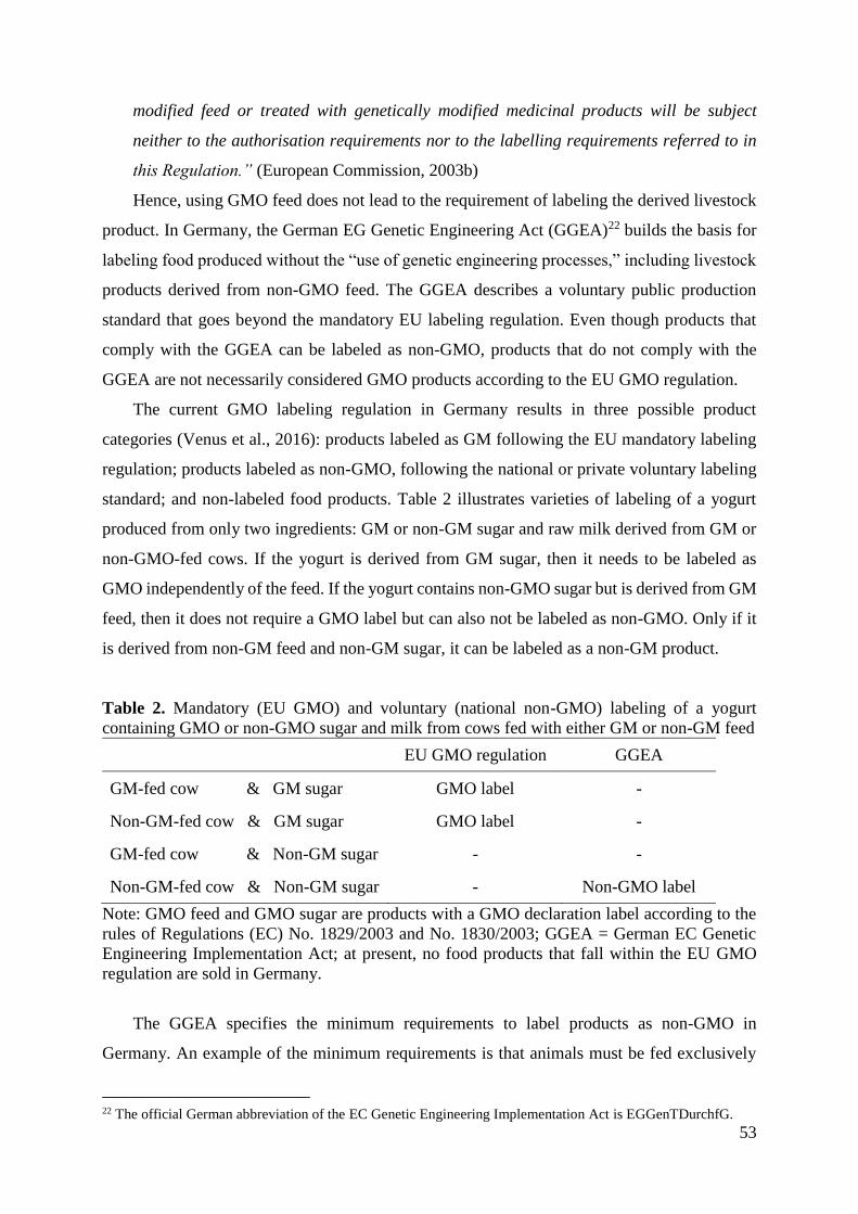
53
modified feed or treated with genetically modified medicinal products will be subject
neither to the authorisation requirements nor to the labelling requirements referred to in
this Regulation.” (European Commission, 2003b)
Hence, using GMO feed does not lead to the requirement of labeling the derived livestock
product. In Germany, the German EG Genetic Engineering Act (GGEA)22 builds the basis for
labeling food produced without the “use of genetic engineering processes,” including livestock
products derived from non-GMO feed. The GGEA describes a voluntary public production
standard that goes beyond the mandatory EU labeling regulation. Even though products that
comply with the GGEA can be labeled as non-GMO, products that do not comply with the
GGEA are not necessarily considered GMO products according to the EU GMO regulation.
The current GMO labeling regulation in Germany results in three possible product
categories (Venus et al., 2016): products labeled as GM following the EU mandatory labeling
regulation; products labeled as non-GMO, following the national or private voluntary labeling
standard; and non-labeled food products. Table 2 illustrates varieties of labeling of a yogurt
produced from only two ingredients: GM or non-GM sugar and raw milk derived from GM or
non-GMO-fed cows. If the yogurt is derived from GM sugar, then it needs to be labeled as
GMO independently of the feed. If the yogurt contains non-GMO sugar but is derived from GM
feed, then it does not require a GMO label but can also not be labeled as non-GMO. Only if it
is derived from non-GM feed and non-GM sugar, it can be labeled as a non-GM product.
Table 2. Mandatory (EU GMO) and voluntary (national non-GMO) labeling of a yogurt
containing GMO or non-GMO sugar and milk from cows fed with either GM or non-GM feed
EU GMO regulation GGEA
GM-fed cow & GM sugar GMO label -
Non-GM-fed cow & GM sugar GMO label -
GM-fed cow & Non-GM sugar - -
Non-GM-fed cow & Non-GM sugar - Non-GMO label
Note: GMO feed and GMO sugar are products with a GMO declaration label according to the
rules of Regulations (EC) No. 1829/2003 and No. 1830/2003; GGEA = German EC Genetic
Engineering Implementation Act; at present, no food products that fall within the EU GMO
regulation are sold in Germany.
The GGEA specifies the minimum requirements to label products as non-GMO in
Germany. An example of the minimum requirements is that animals must be fed exclusively
22 The official German abbreviation of the EC Genetic Engineering Implementation Act is EGGenTDurchfG.

54
non-GM feed for a defined period before milking, laying eggs, or slaughtering. The GGEA
specifies that companies that want to place non-GMO products on the market must use the
wording “ohne Gentechnik” (i.e., without GMO). In August 2009, the former Minister of Food,
Agriculture, and Consumer Production, Ilse Aigner, introduced a uniform non-GMO label,
which firms can adopt. A firm can also use its own label, but it must comply with the GGEA.
4.3 The Private Voluntary Non-GMO Production Standard
In March 2010, the German Association of Food without Genetic Engineering (VLOG) was
founded. 23 It is a multi-stakeholder association whose members are retailers, processors,
farmers, traders, consumers, and consumer and environmental NGOs. The Ministry of
Agriculture exclusively commissioned the VLOG to issue and administer licenses for the use
of the uniform non-GMO label. The VLOG operationalizes the GGEA. In March 2013, VLOG
set the first version of its non-GMO production and certification standard.
Figure 1 shows how the EU regulations on GMOs and labeling and traceability build the
basis for the GGEA, which further sets minimum requirements for a private non-GMO
production and certification standard. The challenge for non-GMO certification is that the GMO
attribute that falls under the mandatory labeling scheme can mostly be detected through
objective inspection tests24 whereas the attribute cannot typically be detected in livestock
products derived from GM feed.25 To distinguish the detectable and undetectable attribute, Jahn
et al. (2005) refer to the first one as a credence attribute and the latter as a Potemkin attribute.
Labeling a Potemkin attribute requires moving from an end-of-line inspection to a quality
assurance systems (QAS) of the whole supply chain (e.g., to distinguish livestock products
derived from GM feed from products derived from non-GMO feed). QAS rely on
documentation of production processes and practices at all stages of the supply chain, and often
on third-party auditing and certification (Holleran et al., 1999).
Figure 2 shows how the credence attribute can be transformed into a Potemkin attribute
along the supply chain. The transformation takes place at the farm level, where GM or non-GM
feed is used. Other raw materials used by processors can either be credence or Potemkin
23 www.ohnegentechnik.org 24 Exceptions are, for example, sugar and oil, which fall under the mandatory labeling regulation if they are derived
from GM sugar beet or GM soybean, respectively, even though the derived product does not contain GMOs. 25 The European Food Safety Authority stated in 2007 that “… no technique is currently available to enable a valid
and reliable tracing of animals products (meat, milk, eggs) when the producer animals have been fed a diet
incorporating GM plants.” (EFSA, 2007).

55
attributes. For example, the GM attribute in maize flour is detectable and hence a credence
attribute, but it is undetectable in sugar and hence a Potemkin attribute.
Figure 1. Different levels of the GMO/non-GMO production standards (based on
Trienekens and Zuurbier (2008)); VLOG = multi-stakeholder non-governmental
organization
In addition to the licenses for the final product suppliers (here: food processors), the VLOG
licenses feed suppliers (e.g., feed traders, feed processors). Through the certification of feed
suppliers, food processors can get direct information about farmers’ feed purchases, which
lowers processors’ search, negotiation, and monitoring costs as compared to evaluating the
purchase information of many farmers. Farmers, too, benefit from the direct certification of
feed suppliers as a means of reliable feed monitoring without interference with their
entrepreneurial autonomy. This interference, farmers stated in a survey, would be one of their
main reasons to restraining them from non-GMO production (Schreiner and Latacz-Lohmann,
2015). Like other private standards (e.g., for vegetable markets in Kenya as described by Jaffee
(2003)), the non-GMO private standard creates new forms of cooperation vertically (e.g., feed
suppliers and food processors) and horizontally (e.g., competing retailers cooperate in standard
setting).
Private
production
and certification
standard by
VLOG
German EC Genetic
Engineering Implementation
Act (GGEA)
EU regulations concerning GMO food and feed
production, traceability, and labeling
(No. 1829/2003 and No. 1830/2003)

56
Figure 2. Transformation of a credence attribute into a Potemkin attribute in the livestock
product supply chain
The dashed lines in figure 3 show the linkages among members of the VLOG: stakeholders
in the supply chain, third-party certifiers, and consumer and environmental NGOs. VLOG
grants licenses to producers of the final product (e.g., processors) and to feed suppliers, and
monitors third-party certifiers. Third-party certifiers must sign a contract with the VLOG (e.g.,
to regularly participate in training courses) for obtaining the allowance to audit and certify the
label licensees.
Figure 3. VLOG membership of various stakeholders, licensing of non-GMO label, and
third-party auditing and certification (Note: some members are not licensees, and some
licensees are not members)
Retailer
Processor (e.g.,
dairy company)
Livestock
farmer
Feed
trader/processor
Feed producer
(crop farmer)
Potemkin attribute
Credence attribute
Other raw materials
(e.g., sugar)
Credence or
Potemkin attribute
Potemkin (and
potentially credence)
attribute
Retailer
Processor (e.g.,
dairy company)
Livestock
farmer
Feed
trader/processor
Feed producer
(crop farmer)
VLOG
Consumer &
environmental
NGOs
Third-party
certifier
Membership

57
In the presence of a public regulation (such as the GGEA), the private non-GMO standard
is not required for labeling but reduces producers’ uncertainty through clarification of aspects
of monitoring, control, and certification. To guarantee, that the quality of the non-GMO
Potemkin attribute (i.e., an attribute that cannot be detected through tracing) has been met, the
use of the non-GMO label is permitted only after prior prima facie evidence to the VLOG that
all legal requirements are fulfilled.
Prima facie evidence is based on documentation. In addition, third-party certification is
mandatory for prima facie evidence, depending on:
(1) the complexity of the production process (e.g., are GM varieties approved for cultivation
in the country of origin of the raw materials? Do the animal raw materials originate from
contract farmers or not? Does the company also buy raw material from the spot market?)
(2) the raw materials used that could cause commingling with GMO material (e.g., does the
raw material producer also produce similar food that is not suitable for non-GMO
production? Does the product contain more than five ingredients?)
(3) the size of the licensee’s company (e.g., if the total turnover is more than 50 million euros
per year)
The non-GMO standard requires lower certification costs for smaller firms (e.g., measured
by turnover), because these firms are not required to use third-party certification, unless some
of the other criteria mentioned above apply.
4.4 Market Structure and Non-GMO Labeling Evolution in Germany
The non-GMO market evolved very differently to the organic market in Germany. The organic
market development was initially (in the 1920s) driven by farmers. Only later it was induced
by consumers (in the 1970s) and agricultural policies (the late 1980s) (Latacz-Lohmann and
Foster, 1997). Well-established organic producer organizations and their private standards with
a high reputation remained in place after the implementation of the EU Eco-regulation in 1992,
even though these private standards go beyond the minimum requirements of the EU Eco-
regulation. Together with the EU regulation, an EU-wide label was introduced that has been
mandatory for labeling organic products in the European Union since 2012.
Unlike organic production, the GGEA has been in force only since 2008. Before that time,
non-GMO labeling was regulated under the novel food regulation, which did not specify any
thresholds for feeding (see table 3).

58
Table 3. Comparison of non-GMO labeling regulated under the novel food regulation and under
the German Genetic Engineering Implementation Act (GGEA)
Novel Food Regulation
(before 2008)
GGEA
(after 2008)
GM enzymes and
additives in feed
No Yes
GM medical products for
animals
No* Yes
Periods in which GM
feed is allowed
No Egg: 6 weeks
Poultry: 10 weeks
Dairy: 3 months
Pork: 4 months
Beef: 12 months (and at least
¾ of animal life)
GM threshold for
adventitious presence
No thresholds defined 0.9% for feed
0.1% for food
GM enzymes and
additives in food product
No No
Source: Based on Federal Ministry of Germany (1998, , 2004; 2004)
Note: GM medicine for animals was allowed if no alternative non-GM version was available.
The absence of a threshold implied a zero tolerance GMO policy (i.e., neither GM medicine
nor GM enzymes were allowed), which made labeling very expensive and legally uncertain.
This uncertainty was confirmed in an interview with the CEO of the first dairy company in
Germany, the Upländer dairy, that offered non-GMO labeled dairy products under the novel
food regulation (Gen-ethisches-Netzwerk, 2006). The dairy stated that the major challenge was
to find suppliers of feed (mainly soybean, rapeseed, and maize) that complies with the zero-
tolerance requirement. Since the specification of minimum requirements in the GGEA, the
compliance to label products as non-GMO has become less costly and less legally uncertain.
The GM threshold in feed and the periods in which GM feed is allowed are based on the organic
regulation.
In the initial phase after non-GMO labeling became part of the GGEA, non-GMO products
were supplied in a niche market by farmer-to-consumer direct marketing and other smaller
producers (Venus et al., 2016). Greenpeace claims that the first (large) dairy company
(Landliebe) after the GGEA came into force switched to non-GMO production and labeling
because of Greenpeace’s pressure (Greenpeace, 2008). Anti-GMO groups have also been
demonstrated to play a significant role in other cases of adopting voluntary standards. For

59
example, Fulponi (2006) finds in her survey that the strength of NGOs is determining retailers’
adoption of a higher private production standard for animal welfare.
After the introduction of the uniform label in 2009 and the establishment of the VLOG, the
number of non-GMO labeled products and firms steadily increased (Figure 4). At the end of
2016, the VLOG had 328 members and 290 licensees (266 food label licensees and 24
feedstuffs label licensees).
Figure 4. Development of members and licensees of the German Association of Food
without Genetic Engineering (VLOG) (Note: The total does not correspond to the sum of
members and licensees, because some members are not licensees and some licensees are
not members)
In 2014, the number of new licensees was very low (as compared to other years). The low
growth rate was due to the public announcement of the German Association of Poultry
Producers not to relinquish GM feed anymore (ZDG, 2014). The association had relinquished
GM feed since the year 2000 without labeling. The announcement created uncertainty in the
non-GMO market and was followed by heavy debates among retailers, poultry producers, and
the VLOG for several months, and by a judicial advisory opinion letter as well as NGO-pressure
on the German brand leader for chicken and poultry (Wiesenhof). Within this period, very few
new firms entered the non-GMO market. At the end of 2014, Wiesenhof decided to enter the
non-GMO market, and many other poultry and egg producers followed suit in 2015. This switch
0
50
100
150
200
250
300
350
400
450
500
2010 2011 2012 2013 2014 2015 2016
Num
ber
of
mem
bers
/lic
encees
Year (in December)
Total (Members & Lincencees) Members Licencees

60
was a tipping point and basis for the announcement of the major German retailer chains to use
non-GMO labeling for some of their store brands.26
Before 2015, retailers’ decisions to implement the non-GMO labeling standard were
tentative. This initial restraint had several reasons. According to the public statement of the
VLOG (2011), the major fears of retailers to label their retail brands as non-GMO were: (1)
potential product recalls due to violation of the standard in the upstream production; (2) fear of
coming under fire of environmental and consumer associations in case of small mistakes; and
(3) discrimination against other products without a non-GMO label.
Potential causes of mislabeling exist at several stages along the supply chain. The key
determinants that affect the probability of detection are the amount of monitoring and the
recognition value of the company brand to generate interest to newspaper reports (Jahn et al.,
2005). Both points put more pressure on larger and highly-visible firms. Food monitoring
frequently detects traces of GMOs. However, these are usually below the labeling threshold.
For example, in 2014, five percent of non-GMO products in Bavaria (23 percent in Baden-
Württemberg), contained some GMO traces below 0.1 percent by weight. In very few cases,
monitoring agencies found non-approved GMOs, for which zero tolerance applies, or EU-
approved GMOs above the legal advantageous presence threshold of 0.9 percent. However,
mislabeling of feed products is often found in risk-oriented sampling where samples are taken
due to suspicion (Table 4).27
Table 4. Number of risk-oriented feed samples taken due to objections in Bavaria
Year Number of
feed samples Violations (%)
2007 58 3.0
2008 114 6.1
2009 75 28.0*
2010 52 3.9
2011 41 2.4
2012 59 3.4
2013 55 5.5
2014 41 7.0
Note: *High violation rate due to samples after rapid alert notification for traces of EU
non-approved maize event MON88017 and flaxseed event FP-9678.
Source: Schlicht and Felsner (2015)
26 Alexander Hissing, CEO of the VLOG (personal communication, April 6, 2017) 27 See Wree and Wesseler (2016) for a discussion of two cases, where unapproved GM crops (a potato and a maize
variety) accidentally entered the German market.

61
In 2010, the German discounter LIDL signed agreements with their store brand suppliers
to only use non-GMO feed for raw milk production without labeling the final product (Spiegel
Online, 2010). Similar cases to this supply chain initiative have been observed for some retailers
that have adopted production methods that go beyond minimum requirement specifications of
safety or quality regulations without mentioning it explicitly through labeling (Codron et al.,
2005). Through this non-labeling strategy, retailers can reduce expenses on monitoring, avoid
reputation losses in case of standard violations, and prevent progressive escalation of
competitive advertising (Codron et al., 2005). Venus and Wesseler (2015) argue that the non-
labeling non-GMO production can be viewed as a two-stage investment, where the supplier
agreement reduces the vulnerability to anti-GMO group pressure and the risk of liability issues,
but allows firms to implement the label quickly if uncertainty decreases or demand for labeled
products increases. Furthermore, a LIDL representative stated the fear of a negative externality
of labeled products on the unlabeled products (European Commission, 2015). By the end of
2015, LIDL decided to implement the non-GMO label for some of their store brand dairy
products in combination with a large marketing initiative.
Since the major retailers in Germany have decided to enter the non-GMO market, they
have been taking the role of the “driving” sector and moving non-GMO production from a niche
to a mainstream market. The four biggest retailing groups in Germany (Edeka, Rewe, Schwarz-
Gruppe, and Aldi) have a total market share of more than 80 percent. Their market power allows
them to determine the production decisions of the less powerful firms that produce store brands
for the big four (Klooster, 2005). Store brands play a particularly vital role for the products (e.g.,
livestock products) most amenable to non-GMO labeling. In 2014, around 38 percent of food
retailers’ revenue in Germany was generated with retail brands, and the share was more than
70 percent for fresh milk.28 Retailers demand from their suppliers to comply with the non-GMO
standard and exclude suppliers who do not comply. As often argued, regulatory systems or
private standards can become de facto mandatory for suppliers, even if these standards are not
legally binding (Trienekens and Zuurbier, 2008). One cannot rule out a situation in which
retailers not only exclude all mandatorily GM-labeled products from their assortment (as is the
case at presence) but also livestock products derived from GM feed.
In April 2017, the food label licensees offered a total number of 6,170 non-GMO labeled
products and the VLOG estimated a revenue of 4,415 million euros generated with non-GMO
labeled products for 2017. Figure 5(A) shows that 76 percent are livestock products and each
28 www.moproweb.de

62
of the three main non-GMO labeled livestock products (dairy, poultry, eggs) takes about one-
fourth of the share of total non-GMO labeled products. Other products (also about one-fourth
of the total products) are pasta and cereal products, beverages, honey, and others. Figure 5(B)
shows that dairy products generate with 55 percent the largest revenue of non-GMO products.
This percentage corresponds to 2,440 million euros. To put this value into perspective, we
mention that in 2013-2014, around 9,586 million euros were generated with basic dairy
products (e.g., fresh milk, butter, yogurt, cream). The second largest revenue is generated with
poultry (24 percent) followed by eggs (16 percent).
To ensure the availability of protein feed supply, European retailers signed the Brussels
soybean declaration. This declaration should make soybean producers in South American
countries—with Brazil being the only non-GM soybean exporter—aware of the growing
relevance to European retailers to allow the establishment of non-GM soybean supply chains.
The German retail organization complements the declaration with a position paper. National
non-GMO protein feed supply is furthered by a national protein strategy together with legume
breeding support as well as an agreement to foster soybean production along the Danube River
in several European countries. In expert interviews, Peter and Krug (2016) see no technical
limitations to increasing non-GM soybean production in Brazil. A growing demand for non-
GM soybean can increase prices, but it may also lower segregation costs due to economies of
scales. This demand also depends on other EU Member States.
(A) Number of non-GMO products (B) Revenue from non-GMO products
Figure 5. Number (A) and revenue (B) of non-GMO labeled products certified by the
VLOG
Source: Based on VLOG (2017)
Dairy
products
26%
Poultry
23%
Eggs
27%
Other
24%
Dairy
products
55%
Poultry
24%
Eggs
16%
Other
5%
Number
6,170
Revenue
4,415
million
euros

63
Because Brazil is the main non-GM soybean supplier, there is little flexibility for protein feed
substitution, and so supply shortage can create strong price fluctuations. Currently, 4.5 million
metric tons of soybean meal is used in German livestock production (Peter and Krug, 2016).
Given a price premium of approximately 100 euros per metric ton, livestock producers would,
under current conditions, need to generate an additional 450 million euros of revenue to cover
the incremental soybean costs. Further costs arise for quality assurance from the farmers until
the final product.
4.5 Discussion
Complying with the national GGEA standard would be sufficient for non-GMO labeling.
However, firms have several incentives to comply with the VLOG standard. Private voluntary
standards reduce uncertainty through providing assurance that rules and regulations are adhered
to (Henson and Humphrey, 2010). Internal motives such as cost and uncertainty reductions play
a greater role for larger firms for the adoption of the voluntary private standard, whereas smaller
firms tend to adopt quality assurance for external, customer-driven reasons (e.g., see Holleran
et al. (1999) for the ISO 9000 quality assurance system). Furthermore, the exemption of smaller
firms from third-party auditing facilitates smaller firms to participate in the certification scheme
instead of forcing them out. Avoiding the exit of small- and medium-sized suppliers is a
common challenge when implementing third-party certification schemes (Hatanaka et al.,
2005).
Another incentive for firms to comply with the voluntary private standard is that consumers
can easily recognize the uniform label that signals compliance with the VLOG standard due to
its familiarity if widely used by many firms. In the long run, this familiarity and recognition
value, as well as the transparency of the certification process, may increase consumers’ trust in
the certification and the label and change their long-term preferences for non-GMO products
(Roe and Teisl, 2007; Teisl and Roe, 2005).
Regarding the strictness of the labeling standard, the interests of firms can be very different
to the ones by anti-GMO groups or consumers. However, the multi-stakeholder organization
VLOG combines the interests of consumers, firms, and anti-GMO groups. Their combined
interest is to create and maintain a positive reputation of the non-GMO label. This collective
interest limits the potential scope of action of anti-GMO activist groups. All relevant
environmental and consumer associations in Germany indicated in a public statement29 to
support non-GMO labeling (VLOG, 2011). Non-compliance with the non-GMO labeling
29 http://bit.ly/Verbaendeposition
64
standard would deceive consumers, and if consumers become aware of misleading labeling, the
effects for the acceptance of genuinely certified products can be strong (Giannakas, 2002).
Hence, it is not in the interest of a non-GMO labeling supporter to increase the awareness of
consumers of potential deceptions through mislabeling. Hence, anti-GMO groups may actually
prefer a standard that is not too strict, because a stricter non-GMO labeling standard increases
firms’ compliance costs, deterring some firms from adopting the standard (Bernstein and
Cashore, 2007). A non-GMO standard stringency that is optimal for anti-GMO activist groups
minimizes the total usage of GM crops in food production.
One of the retailer’s concerns was the negative externality of non-GMO labeled products
on the unlabeled products. This concern is problematic if consumers are poorly informed about
which products can be labeled and which not. If a consumer has full knowledge about which
products can be produced with GMOs, and they also know that GM products can be produced
at a lower marginal cost, then, in the absence of a signaling opportunity for firms, a consumer
can infer that a firm defaults to the less expensive (GM) feed variety (in accordance with
Akerlof’s (1970) lemons problem). If, however, consumers know that some products—but not
which products—are potentially produced with GMOs, they may hold prior expectations about
the probability of receiving GMOs. And because non-GMO labeling is a dichotomous choice,
it signals its non-GMO quality, and at the same time, it signals that a non-labeled product may
not comply with the non-GMO standard. Hence, consumers can update their prior (i.e., initial
probability of buying a GM product) and hence attribute a higher probability to receive a GM
product when buying the unlabeled products (Roe et al., 2014).
The update of the prior works well if consumers are well informed about the specifications
on which products can or cannot be labeled. However, consumers are not always well informed
about these specifications (Henseleit and Kubitzki, 2009; Weinrich et al., 2015). As Henseleit
and Kubitzki (2009) show in their survey, consumers’ expectations of the non-GMO label are
higher than the current non-GMO standard requirements. Furthermore, products for which there
exists no GM version (e.g., cucumbers) cannot be labeled as non-GMO, even though these
products are not genetically modified. The reason why these products cannot be labeled is that
labeling must comply with the regulation on self-evident advertising (European Commission,
2011). Error-free updating of the prior works only if consumers are informed, which products
are “naturally” non-GMO. If, however, consumers are unaware of the rule on self-evident
advertising and which products it concerns, then they may expect unlabeled products to be
derived with GMOs.

65
Another reason why only some of the products but not all are labeled is that labeling of
products made of various raw materials (e.g., fruit yogurt) exhibit large production and
transaction, and hence labeling costs. The reason for these higher costs is that the national
regulation requires processors to use also, for example, non-GMO certified sugar or enzymes
produced without the help of GMOs. These costs may exceed consumers’ incremental
willingness to pay. Hence, most non-GMO labeled products are the ones with few raw materials
only, such as fresh milk, plain yogurt, some cheeses, eggs, and poultry, for which production
and certification are relatively inexpensive. Labeling of these products may send the correct
signal to consumers, but it is not in the interest of firms to make them aware that unlabeled
products may not comply with the non-GMO standard.
Because of imperfect information of consumers about the labeling system itself, most
processors (17 out of 18) and also some of other stakeholders (e.g., consumers associations,
food industry associations, NGOs, retailers) in a survey on non-GMO labeling agreed that the
non-GMO label potentially misleads consumers (European Commission, 2015, , p.60). The
potential consumer confusion may also arise from the parallel existence of a voluntary and a
mandatory labeling scheme, which can result in uncertainties for consumers that are similar to
the absence of labeling (Dannenberg et al., 2011).
Besides the negative externality of labeling on unlabeled products, there also exists a
positive externality. This positive externality relates to the halo (positive spill-over) effect of a
non-GMO label on a firm’s reputation. Consumers may prefer unlabeled products of a firm that
offers non-GMO labeled products to other unlabeled products of firms that do not offer any
non-GMO products in their assortment. For example, most retailers communicate their non-
GMO supply as part of their sustainability strategy (Vigani and Olper, 2014; Wesseler, 2014).
This strategy extends the positive effect of a few non-GMO labeled products as a quality
attribute to the overall brand or whole firm image (Gruère and Sengupta, 2009).
A general issue of non-GMO labeling is that the label itself may signal to consumers that
GMOs are unsafe (Costanigro and Lusk, 2014). As discussed by Caswell (1998), consumers
may take the label as an indicator of a safety concern of the GMO attribute, even though
regulators evaluate it a safe. This endogeneity questions how far a non-GMO label can reduce
imperfect information (i.e., informing consumers that products are GM or not) or potentially
cause new information imperfections (i.e., signaling safety concerns of GMOs).
4.6 Conclusions
In this article, we showed how the different interests of non-GMO labeling stakeholders are
combined in the VLOG, a multi-stakeholder organization that developed a private production

66
and certification standard in Germany. Through the combination of the organization members’
interests, the probability of one of the main fears of retailers to being pressured by NGOs in the
case of mislabeling could be substantially lowered. We show how a non-GMO label that is
supposed to solve the externality of imperfect information can create new information
imperfections if consumers are not well informed about the labeling system itself. Even with
perfect information, some consumers gain from choosing non-GM products whereas others
may lose from increased prices through firms’ product differentiation.
The government may achieve a reduction in the externalities and therefore a more aligned
freedom of choice through science-based information campaigns. It is the Ministry of
Agriculture that commissioned the VLOG for the issuance and administration of the non-GMO
label licenses. However, the VLOG’s interest is to increase its market impact and hence, the
organization may benefit from providing one-sided information to consumers. The VLOG
website (www.ohnegentechnik.org) mentions the existence of evidence of negative
environmental effects of GMOs, farmers’ dependence on a few global seed companies due to
GM seed usage, and the non-excludability of negative human health effects of GM food. The
website neglects all positive effects of GMOs. If the government’s aim is to provide consumers
with a true freedom of choice, it might be necessary, but it is not sufficient, to facilitate non-
GMO labeling if it does not ensure that consumers have more unbiased information.
Finally, within the European Union, there are many differences regarding the non-GMO
legislations. So far, producers who comply with the non-GMO rules of Austria and Switzerland
can also use the German label. For other countries, trade may be more complicated.
Harmonization of non-GMO labeling would reduce these problems within the European Union.
For all other countries that export to the European Union, the non-GMO requirements of
retailers may have similar effects as other private standards. These effects have been extensively
discussed, in particular, for developing countries (see Henson and Humphrey, 2010, for an
overview). Whether an increase in non-GMO labeling to reduce GMO crop production is useful
from an economic, social, and environmental perspective is another question.

67

68
Chapter 5
The Interactions among the Regulation
of New Plant Breeding Techniques,
GMO Labeling, and Coexistence and
Segregation Costs: The Case of
Rapeseed in the EU
69
5. THE INTERACTIONS AMONG THE REGULATION OF NEW PLANT
BREEDING TECHNIQUES, GMO LABELING, AND COEXISTENCE
AND SEGREGATION COSTS: THE CASE OF RAPESEED IN THE EU30
ABSTRACT: We analyze the market and welfare effects of regulating crops derived by New
Plant Breeding Techniques (NPBTs) as genetically modified (GM) or conventional products.
We consider the EU mandatory scheme for labeling GM products and a voluntary non-GM
scheme for labeling livestock products derived from non-GM feed. We develop a partial
equilibrium model that explicitly takes into account both the coexistence costs at the farm level
and the segregation and identity preservation costs at downstream level. By applying the model
to EU rapeseed, we find that regulating NPBTs as GM (as compared to non-GM) in
combination with mandatory and voluntary labeling increases prices and makes producers
better off. We also show that higher coexistence costs make the price increasing effect even
stronger. Voluntary non-GM labeling applied to feed makes consumers in this sector overall
worse off, but benefits farmers and rapeseed oil consumers overall as long as segregation costs
are low. Consumers of biodiesel and industrial products such as lubricants produced from GM
rapeseed benefit from high segregation costs. We show that the effects of farm-level
coexistence costs largely differ from the effects of downstream market segregation costs.
KEYWORDS: New plant breeding techniques, GMO, labeling, coexistence, identity
preservation, regulation, vertical product differentiation
30 This chapter is based on the article: Venus, T.J., Drabik, D., and Wesseler, J.H.H., 2017. The Interaction among
the Regulation of New Plant Breeding Techniques, GMO Labeling, and Coexistence and Segregation Costs: The
Case of Rapeseed in the EU. LICOS Discussion Paper 389/2017, submitted to a peer-reviewed journal.

70
5.1 Introduction
Since the adoption of the official definition of genetically modified organisms (GMOs) in the
European Union in 1990, a number of new techniques have been developed to genetically
modify plants.31 Currently, regulators in different countries, including the European Union and
the United States, assess whether these biotechnology-driven “New Plant Breeding Techniques”
(NPBTs) should fall within the scope of the GMO regulation (Lusser and Davies, 2013).32
Because plants derived by NPBTs do not necessarily contain an inserted transgene, they are
often indistinguishable from crops derived through conventional breeding (Lusser et al., 2011).
Therefore, one of the main questions in determining how NPBTs should be regulated in the
European Union is whether the technique itself or the organism produced by such a technique
must be regulated by the current GMO legislation (Hartung and Schiemann, 2014). A similar
debate may arise in the United States in the context of labeling food products.
The decision on whether crops derived by NPBTs are classified as GM or non-GM has
important economic implications for the product registration, research and development, trade,
cultivation, and marketing of NPBTs. The registration costs are low for non-GM crops, while
the cost of the approval procedure for GMOs in the European Union ranges between 7-15
million euros and is very time-consuming (Kalaitzandonakes et al., 2007; McDougall, 2011;
Smart et al., 2017; Tait and Barker, 2011). High approval costs may disincentivize firms to
invest in the innovation of NPBTs. Furthermore, if an NPBT-derived crop is considered a GMO
in one country, but not in another, asynchronous approval and low-level presence can lead to
trade disruptions (Stein and Rodríguez-Cerezo, 2010). GM products must be labeled as such,
and if GM and non-GM products are marketed side-by-side, segregation and identity
preservation of the non-GM product are required (European Commission, 2003b).
In this chapter, we analyze the market and welfare effects of alternative NPBT regulations
and focus on herbicide-resistant rapeseed to study these effects. There are at least three reasons
why we focus on rapeseed. First, rapeseed accounts for more than 50 percent of both the total
supply and use of oilseeds in the European Union (European Commission, 2016). Second, in a
survey conducted by the Joint Research Center of the European Commission, plant breeding
companies identified herbicide-resistant rapeseed as one of the first potential commercial
31 The Directive 2001/18/EC on the deliberate release into the environment of GMOs defines GMOs as an
“organism, with the exception of human beings, in which the genetic material has been altered in a way that does
not occur naturally by mating and/or natural recombination” (European Commission, 2001). 32 In 2007, the EU Commission and different National Component Authorities named eight NPBTs for which the
regulation is unclear: zinc finger nuclease (ZFN) technology; oligonucleotide-directed mutagenesis; cisgenesis and
intragenesis; RNA-dependent DNA methylation; grafting on GM rootstock; reverse breeding; agro-infiltration;
and synthetic genomics (Hartung and Schiemann, 2014).

71
products derived by NPBTs (Lusser et al., 2011).33 Third, rapeseed oil and its joint product
meal are used in the food supply chain as food (e.g., cooking oil) and feed (e.g., protein source
in compound feed for cattle, pigs, and poultry) as well as in the industrial supply chain, for
example, as a feedstock for lubricants and biodiesel. Whereas GM labeling applies to food and
feed products, it usually does not apply to industrial products. Hence, the segmentation of
markets implies that regulation and labeling do not affect all consumers and producers equally.
We look at how different labeling schemes affect the welfare of different market agents. In
addition, we analyze the effects of farm-level coexistence and processing/marketing
segregation and identity preservation costs. We show that regulating NPBT-derived crops like
GMOs, in combination with GMO labeling regulation, increases market prices and decreases
consumer welfare but increases producer welfare relative to regulating NPBT as non-GM. We
also show that higher coexistence costs make the price increase effect even stronger. When
coexistence costs are high enough, no NPBTs are used. Downstream market segregation costs
affect the market differently than coexistence costs by increasing the price of non-GM oil and
meal but reducing the price of non-GM rapeseed.
We find that voluntary non-GM labeling, whereby producers can label livestock products
derived from non-GM meal, benefits all farmers and oil consumers but makes meal consumers
overall worse off (as compared to a situation in which voluntary labeling is not allowed). If,
however, segregation costs are high, only industrial and biodiesel consumer gain from voluntary
non-GM labeling.
5.2 Background: Labeling and Coexistence
The discussion of regulating NPBTs brings back much of the debate of the last two decades on
the economic effects of introducing GMOs in general, and GM labeling and coexistence in
particular. Labeling in the European Union is mandatory for food and feed that contains GMOs
(e.g., oil derived from GM rapeseed). However, the mandatory labeling scheme does not require
livestock products derived from animals fed by GM feed (e.g., fed by GM rapeseed meal) to be
labeled, although a voluntary labeling scheme for these products has emerged.
In the case of rapeseed, the mandatory labeling scheme directly affects only the oil market,
whereas the voluntary non-GM labeling scheme directly affects only the meal market. In
particular, oil can be used as food or can be converted into biodiesel and other industrial goods.
33 In their survey of plant breeding companies, Lusser et al. (2011) identified the following products as likely to
be among the first commercial products derived from NPBTs: herbicide-resistant rapeseed and maize; fungal-
resistant potatoes; drought-tolerant maize; and scab-resistant apples and potatoes with reduced amylose content.

72
Food, and hence oil for human consumption, must be labeled if it is derived from GM crops but
industrial products do not require labeling. Retailers in Europe removed or announced the
removal of all GM products in 1998, shortly after the first commercial cultivation of GM crops
(Kalaitzandonakes and Bijman, 2003). This exclusion of GM-labeled products has been
adopted by almost all EU retailers and food manufacturers and is still in place today. Therefore,
human consumption of oil is covered by non-GM oil, whereas both GM and non-GM oils can
be used industrially.
Rapeseed meal, the joint product of oil production, is mainly used as protein feed for milk,
egg, and meat production. If firms want to offer products derived from non-GM feed, they have
to comply with a voluntary non-GM labeling standard. 34 Some countries (e.g., Austria,
Germany, and France) have implemented national non-GM labeling standards that vary in their
requirements across countries (European Commission, 2015). In Germany, for example, the
non-GMO standard allows farmers to use GM feed over some period. All major retail chains in
Germany have started to offer or have announced offering of some of their retail brand livestock
products (e.g., dairy products and eggs) with a non-GM label. Other voluntary labeling schemes,
such as the scheme in The Netherlands, allow non-GM labeling only under highly restrictive
circumstances, while the schemes in Belgium and Sweden prohibit non-GM labeling altogether
(European Commission, 2015).
Retailers’ and industries’ removal of GM food products has led to the absence of
mandatorily labeled GM food oil whereas the voluntary labeling scheme has led to product
differentiation of meal-derived products. Providing non-GM oil and meal in the presence of
GM cultivation requires the coexistence of GM and non-GM supply chains. Coexistence at the
farm level mainly concerns the avoidance of potential economic losses that non-GM farmers
can face, such as losses through admixture due to cross-pollination if the adventitious (i.e.,
accidental or technically unavoidable) presence greater than the 0.9-percent threshold if a
separate market exists for GM and non-GM products. To ensure coexistence, several EU
Member States have implemented coexistence measures (see Beckmann et al., 2014, for an
overview of coexistence measures in different EU Member States).35
In the European Union, GM farmers have to implement the coexistence measures and bear
the costs of implementation (i.e., coexistence costs). These coexistence measures often result
34 The non-GM labeling standard considers feed without a mandatory GM label as non-GM feed. Most non-GM
labeling standards tolerate some adventitious (i.e., unintended or technically unavoidable) presence of GMOs.
Most standards also define some time before slaughtering, milking, or laying eggs in which GM feed is tolerated. 35 Following the subsidiarity-based approach to coexistence, each EU Member State shall specify national
measures.

73
in costs that are greater than the benefits of GM cultivation, potentially preventing some farmers
from adopting GM crops (Venus et al., 2017). Moschini (2015) shows that putting the burden
of mandatory minimum distance requirements to achieve coexistence at the farm level entirely
on GM producers, creates a bias against GM crop adoption, and to restore efficient allocation,
coexistence costs must be shared equally between adjacent GM and non-GM farmers. Moschini
(2015) does not, however, explicitly consider the effects of segregation and identity
preservation costs (henceforth referred to as segregation costs) on downstream markets.
Downstream market participants, such as agricultural traders, grain processors, and food
producers, have to avoid commingling of GM and non-GM commodities if they want to
preserve the non-GM identity. Therefore, in the downstream market, the non-GM firms are
usually assumed to bear the direct costs of segregation and identity preservation (Fulton and
Giannakas, 2004; Lapan and Moschini, 2007; Lapan and Moschini, 2004; Lence and Hayes,
2005; Mayer and Furtan, 1999; Moschini et al., 2005; Saak and Hennessy, 2002; Sobolevsky
et al., 2005).36 For example, dairy companies that voluntarily offer non-GM labeled products
must ensure through contracting, testing, documentation, third-party auditing, and certification
that farmers feed only non-GM feed to their cows (Punt et al., 2016).
Several authors model the effects of segregation costs on product prices, consumer and
producer welfare, but do not separately consider the coexistence costs of GM farmers (e.g.,
Fulton and Giannakas, 2004; Lapan and Moschini, 2007; Lapan and Moschini, 2004; Moschini
et al., 2005; Sobolevsky et al., 2005). The effect of positive segregation costs on downstream
markets in combination with farm-level ex-ante and ex-post regulation is discussed by
Desquilbet and Poret (2014). They argue that segregation costs increase the non-GM price and
hence, decrease non-GM consumers’ utility, making a welfare increase through coexistence
costs less likely. However, they do not explicitly incorporate segregation costs in their model.
The work by Sobolevsky et al. (2005) is closest to ours as they use a partial equilibrium
model of differentiated consumers to analyze the market and welfare effects of segregation
costs on GM soybean trade. Unlike Sobolevsky et al. (2005), however, our focus is on the
distribution of market and welfare effects within an economy rather than on trade. We consider
the different effects of coexistence and segregation costs and allow for different labeling
schemes.
Whereas most theoretical approaches in the previous literature assume that both GM and
non-GM products are supplied and demanded once the technology is approved, we show that
36 Desquilbet and Bullock (2009) argue that non-GM production results in a loss of flexibility and therefore also
creates indirect costs for the GM producers.

74
the market outcome depends on labeling as well as coexistence and segregation schemes. Our
model serves as a means to analyze the market and welfare effects of regulating rapeseed
derived from NPBTs under mandatory and/or voluntary labeling schemes compared to
regulating NPBTs as a conventional technique. Furthermore, we analyze the effects of
coexistence costs at the farm level and segregation costs at the level of downstream processors.
5.3 The Model
We model different regulatory systems for oilseed crops derived from NPBTs in the European
Union. The model is used for an ex-ante analysis since NPBT oilseed crops have not been
commercially cultivated in the European Union yet. We assume that GM and non-GM food
products are vertically differentiated. Consumers perceive a GM product as a (weakly) inferior
substitute for a non-GM product, that is, consumers are indifferent to or prefer non-GM
products to GM products if offered at equal prices.
Although we do not model net trade of the included commodities explicitly, we consider
its possible effects on market prices in a sensitivity analysis by varying the domestic
supply/demand elasticities. For commodities in which the European Union is a net exporter, a
modeled demand curve can be thought of as the horizontal sum of the domestic demand and
the EU export demand curve. So by construction, the aggregated curve is more elastic (a similar
argument holds for the supply curve and a commodity for which the country is a net importer).
By varying the elasticities in the sensitivity analysis (in a later section), we can then test how
sensitive our results are with respect to the inclusion of trade in commodities. The sensitivity
analysis shows robust results.
We assume that the total rapeseed quantity that farmers supply is processed into oil and
meal, such that rapeseed is only indirectly demanded through its processed products. Rapeseed
derived from NPBTs as well as its products, oil and meal, can either be of non-GM quality N
or of GM quality G . The quality type depends on how an NPBT is regulated (i.e., GM vs non-
GM) as well as on the relevant labeling scheme (i.e., mandatory vs voluntary labeling).
Processors crush rapeseed, indexed by R, to obtain oil and meal, indexed by O and M,
respectively. Oil is used for human consumption, industrial use (e.g., lubricants), or biodiesel
production.
We assume that consumers judge the technology used for rapeseed production only by its
characterization (i.e., consumers consider only how NPBTs are categorized and regulated).
Hence, consumers are indifferent between crops derived by NPBTs and crops derived by
conventional breeding techniques, as long as NPBT-derived crops are officially categorized and

75
regulated as non-GM. This assumption together with vertical product differentiation imply that
if NPBTs are regulated as a GM technique, NPBT-derived products must be labeled as GM and
therefore some consumers are willing to pay a premium for food products produced without the
GM-categorized NPBTs.37
5.3.1 The Meal Demand
Rapeseed meal is a crucial component of livestock feed. It is, therefore, closely related to most
livestock food products. In what follows, we assume that the demand for meal by livestock feed
processors reflects consumers’ preferences over the GM/non-GM characteristic. This
assumption makes it possible to focus on a representative consumer’s demand for meal.
The representative consumer has a quasi-linear utility ( , , )G N
M MU q q y , where G
Mq and N
Mq
denote quantities of GM and non-GM products, respectively, and y denotes the consumption of
the numeraire good. The quasi-linear form allows to add up the utilities for a continuum of
consumers of the same type without altering the properties of preferences for the GM or non-
GM good. The consumption of GM and non-GM products depends on the relative price and the
degree of substitutability, [0,1] . The closer is to zero, the more the products are
differentiated.
The consumer seeks to maximize the total surplus from consuming G
Mq and N
Mq
(1) ,
max , ,G NM M
G N G G N N
M M M M M Mq q
U q q y P q P q ,
and the utility function takes the form as in Singh and Vives (1984)
2 21, , 2
2
G N G N G N N
M M G M N M G M N M M
G
MU q q y q q q q q yq ,
where G
MP and N
MP denote the price of GM and non-GM meal, respectively, and the quality
parameters satisfy 0N G and 2 0G N . The parameters N and G represent the
intrinsic quality of each product that increases the marginal utility of consuming that product.
The parameters N and G measure the rate at which the marginal utility of consumption for a
product declines with higher consumption of that product (Choi and Coughlan, 2006).
Solving the consumer maximization problem (1), we obtain linear GM and non-GM
demand functions
(2) ,G G N G G G
M M M M M M M
N
MD P P a b P c P
37 A reason why consumers treat NPBTs as a genetic modification if they fall within the scope of the EU regulation
of GMOs is that consumers cannot distinguish GM-classified crops derived by NPBTs from other GM crops (e.g.,
transgenic crops).

76
and
(3) ,N G N N N G
M M M M M
N
M M MD P cP P a b P
with parameters2
G G N NM
G N
a
,
2
G NM
G N
b
,
2
N N G GM
G N
a
,
2
N GM
G N
b
, and
2M
G N
c
. Since both products are substitutes, the GM meal demand depends on its own
price and on the non-GM meal price. Likewise for the non-GM demand.
If NPBTs are considered GM but no voluntary non-GM labeling option exists, consumers
cannot distinguish (NPBT-derived) GM from non-GM products. So if GM and non-GM
products are indistinguishable, we assume that consumers perceive all meal products to be of
GM quality independently of the share of GM and non-GM content. As in Sobolevsky et al.
(2005), we model the situation in which only GM(-perceived) meal is available by setting the
non-GM price above its “choke” price, N N G N
M M M M MP a c P b , making the non-GM meal price
prohibitively high (i.e., non-GM meal demand is zero). After substituting the choke price into
equation (2) and denoting the single meal price as MP , the demand for GM meal (in the absence
of non-GM meal) becomes
(4) 2
| 0N
G N G GM MM M M M M MN N
M
M M
a cD P q a b P
b
c
b
.
For future reference, we also quantify the total demand for meal when all consumers
perceive the meal to be of non-GM quality. This situation can have two causes: (i) NPBTs are
regulated as non-GM, and (ii) NPBTs are unavailable to consumers either because the technique
is prohibitively expensive to use (e.g., if the approval process is too expensive) or because
NPBT-derived crops are banned. We provide details when this can happen in a later section
describing different scenarios. The total meal demand curve in this case is obtained by summing
the right-hand sides of equations (2) and (3), and recognizing that in this situation G N
M M MP P P ,
because there is only a single meal market price. As a result, the demand of non-GM meal (in
the absence of GM meal) is
(5) | 0 2N G G N G N
M M M M M M M M MD P q a a b b c P .
5.3.2 The Oil Demand
Due to retailers’ and food manufacturers’ removal of GM food products, oil demand for human
consumption can only be derived from non-GM rapeseed. We assume that retailers’ and food
manufacturers’ GM food exclusion stays in place (e.g., by assuming that the costs of changing

77
their policy is infinitely high). The mandatorily labeled and less expensive GM oil can thus only
be used for industrial and biodiesel purposes; this does, however, not preclude industrial and
biodiesel users from demanding non-GM oil if it is less or equally expensive than the GM
counterpart. The prices of GM and non-GM oil, denoted by G
OP and N
OP , respectively, are
determined in two separate markets as long as in the equilibrium G N
O OP P . On the one hand,
food oil consumers can only consume non-GM oil and hence their demand H N
O OD P , where H
denotes human consumption, depends only on the price of non-GM oil. On the other hand,
industrial and biodiesel users always demand the less expensive alternative, which in most cases
is the GM oil. 38 This implies that the industrial (I) demand function I
OD depends on
min ,G N
O OP P . To be consistent with the functional form of the demand functions for meal
given by equations (2)-(5), we also use linear demands for food and industrial use of oil39,40
(6) H N H H N
O O O O OD P a b P
and
(7) min , min ,I G N I I G N
O O O O O O OD P P a b P P .
The quantity of biodiesel (B) to be produced is assumed to be fixed. Because one metric
ton of oil yields B liters of biodiesel, the oil demand for biodiesel is given by BB and is
therefore perfectly price-inelastic.
5.4 Rapeseed Supply
There are Z homogeneous competitive farmers in our model, similar to Sobolevsky et al. (2005),
who can choose from two production technologies: GM and non-GM. Because consumers
demand both GM and non-GM products in our baseline, a farmer can decide whether to produce
GM or non-GM rapeseed. However, we assume a farmer does not produce both at the same
time because of on-farm costs related to dual production. These costs relate, for example, to the
time and money spent cleaning machinery after seeding, harvesting, transporting; or potential
hurdles a farmer might face when selling non-GM rapeseed to a non-GM processor because of
38 Under certain conditions and under two separate oil demands it is possible that the hypothetical price of GM oil
exceeds the price of non-GM oil. However, because industrial and biodiesel users are flexible in their choice of
oil and decide solely based on its price, the GM oil price has to equal the non-GM price. 39 One can think of equations (6) and (7) as linear approximations of the optimal demand functions derived from
profit maximization for a production technology and given prices of the output and other inputs. 40 It should be noted that the effective GM food removal of retailers leaves food oil consumers with only one
choice, that is, non-GM oil, which means that oil demand only depends on its own price.

78
a higher probability of commingling of seeds. Punt and Wesseler (2015) also argue that farmers
have incentives to form GM and non-GM clubs, 41 which supports our full specialization
assumption. Moreover, many voluntary labels prohibit the use of any GM feed on mixed farms
that are registered as non-GM producers for parts of their animal products.
If both types of rapeseed are produced, then k farmers produce GM and the rest, (Z – k),
produce non-GM rapeseed. The distribution of farmers (i.e., k) is endogenous and depends on
the relative price of GM and non-GM rapeseed in equilibrium. Each farmer using the GM
technology produces according to the supply function G G
R RS P , where G
RP denotes the market
price of GM rapeseed. Likewise, supply of each farmer producing non-GM rapeseed is
N N
R RS P , where N
RP is the market price of non-GM rapeseed.
We assume lower marginal costs for GM rapeseed production, which is the main feature
of first-generation GM crops (e.g., Klümper and Qaim, 2014; Smyth et al., 2011b). Associated
with GM production, however, are coexistence costs (e.g., isolation distance, crop rotation,
potential liability costs) that the GM farmer has to bear (Venus et al., 2017). Additional costs
to GM farmers are technology fees that a seed company charges to (partially) recoup the costs
of the costly approval process. For reference convenience, we subsume the technological fees
under the coexistence costs, noting that this aggregation does not have any qualitative
implications for our results.
The coexistence costs affect the farm input prices and hence pivot the GM seed supply
curve.42 We, therefore, model the coexistence costs as a percentage ( ) of the potential
producer surplus (at a given GM rapeseed market price) that GM farmers forgo because of the
presence of these costs. Given the functional form of the rapeseed supply we use, the
coexistence costs can be implemented in our model via impacting the production of rapeseed
of each GM farmer: 1 G G
R RS P . Therefore, can alternatively be thought of as a
reduction in the potential GM rapeseed production (at a given price).
The technology a farmer adopts depends on the producer surplus earned per crop. In an
equilibrium in which both GM and non-GM crops are adopted, each farmer must be indifferent
41 Although the formation of a GM club would reduce the coexistence costs (e.g., keeping a minimum distance
from a non-GM farmer), the costs would not be eliminated completely because the formation of a club leads to
other coexistence costs, for instance, the costs the incumbent GM farmers would need to spend to convince non-
GM farmers to switch to GM production.
42 One can also think of coexistence costs as an additional input cost to GM rapeseed production.

79
between the two technologies; this requires that the producer surplus be equal for each crop and
farmer
(8) 0 0
1
G NR RP P
G N
R RS P dP S P dP .
Finally, the total supply of GM rapeseed is 1 G G
R Rk S P and the total supply of non-
GM rapeseed is N N
R RZ k S P .
5.5 Scenarios Description and Market Equilibriums
We consider four scenarios summarized in table 1. Scenario 1 is the baseline scenario reflecting
the current labeling policies and practices in the EU. In both scenario 1 and scenario 2, NPBTs
are regulated as a GM technique and mandatory labeling of food oil applies. The two scenarios
differ in the treatment of meal. In scenario 1, a voluntary non-GM labeling scheme is available,
which gives rise to separate GM and non-GM meal markets. In scenario 2, a voluntary labeling
option is absent and hence only a single market for GM meal exists. In scenario 3, NPBTs are
regulated as a non-GM technique and hence all farmers default to this less costly technology
whereas consumers perceive all products as non-GM. Scenario 4 assumes that NPBTs are
banned (or coexistence costs are prohibitively high), so that all farmers use the conventional
technology, which consumers, of course, perceive as non-GM.
Table 1. Overview of the Four Scenarios of NPBT Regulation and Labeling
Scenario 1 Scenario 2 Scenario 3 Scenario 4
Categorization of NPBTs G G N banned
Food oil labeling mandatory mandatory - -
Meal-derived product labeling voluntary - - -
Technology used by farmers NPBT & conv NPBT & conv NPBT conv
Coexistence costs - -
Oil segregation cost - -
Meal segregation cost - - -
Consumers perceive … as
…Food oil N N N N
…Industrial oil G G N N
…Meal-derived food G & N G N N
Note: “G” = GM, “N” = non-GM, “conv” = conventional, ““ = applies, “-“ = does not apply.

80
5.5.1 Scenario 1: NPBTs Regulated as GM & Mandatory Oil Labeling & Voluntary Meal
Labeling
The processor buys GM or non-GM rapeseed at price G
RP or N
RP , respectively. After the
crushing, one metric ton of rapeseed yields O metric tons of oil and M metric tons of meal
( 1M O ). We assume no differences in the oil and meal content per ton between GM and
non-GM rapeseed. We also assume constant processing cost per ton of rapeseed (other than the
feedstock price) and denote it by Rc ; the processing cost is the same for both types of rapeseed.
The GM (or non-GM) rapeseed processing yields revenues from selling oil and meal at market
prices G
OP (or N
OP ) and G
MP (or N
MP ), respectively. The constant returns to scale technology
implies zero marginal profits for the crusher and enables to express the GM rapeseed price as
(9) G G
R R
G
O O MMP P P c .
The price relationship for the non-GM branch of the supply chain is very similar, but
includes additional segregation costs for oil ( Os ) and meal ( Ms )
(10) M
N N N
R O O O M M RP P s P s c .
The segregation costs represent, for example, non-GM processors’ increased collection and
transport costs as well as auditing, inspection, and certification costs to guarantee the non-GM
quality (e.g., Gabriel and Menrad, 2015). We model the segregation costs as a production tax
in a given final product market, and therefore subtract them from the market price of oil and
meal the crusher receives.
The GM market clearing condition equilibrates the total supply of GM oil with its total
demand. The GM oil supply is given by the total GM rapeseed supply multiplied by the share
of oil, O , in rapeseed. The demand consists of the oil needed to produce B liters of biodiesel
(where one ton of oil yields B liters of biodiesel) and the industrial use of oil (e.g., oil used for
lubricants), yielding
(11) 1 min ,B
G G I G N
O R R O O O
Bk S P D P P
.
Because for industrial users, GM and non-GM oils are perfect substitutes, it is possible that
some non-GM oil is used in the industry if non-GM oil prices happen to equal the GM oil prices.
Due to retailers’ exclusion of GM food products, only non-GM oil is used for human
consumption. The non-GM oil market clearing condition is
(12) N N H N
O R R O OZ k S P D P .

81
The market clearing conditions for GM and non-GM meal are represented by
(13) 1 ,G G G G N
M R R M M Mk S P D P P
and
(14) ,N N N G N
M R R M M MZ k S P D P P ,
respectively. It should be noted that the farm-level coexistence costs are included in the GM
rapeseed supply function, whereas the segregation costs are part of the zero-profit condition of
the non-GM rapeseed processor. Hence, the segregation costs are not explicit in the market
equilibrium conditions. The market equilibrium for scenario 1 is determined by solving the
system of equations (8)-(14) for prices , , , , ,G N G N G N
R R O O M MP P P P P P , and the number of GM farmers
k.
5.5.2 Scenario 2: NPBT Regulated as GM & Mandatory Oil Labeling & No Voluntary
Meal Labeling
In the second scenario, we model the effects of regulating NPBTs as GM in the absence of a
voluntary non-GM labeling option for meal-derived livestock products. Without non-GM
labeling, consumers cannot distinguish GM or non-GM meal-derived products and so we
assume that consumers perceive meal-derived products as GM regardless of the share of GM
and non-GM meal the products contain. Therefore, there is only one market price of meal
denoted by MP . The meal market clearing condition in this case is
(15) 1 | 0G G N N G N
M R M R M M Mk S P Z k S P D P q ,
where the left-hand side represents the sum of GM and non-GM meal supply, and the right-
hand side represents the total meal demand (for which in the empirical part of the article we use
equation (4)). The absence of the voluntary labeling option further affects the zero-profit
condition of the processors since meal needs not be segregated, such that sM = 0, and there is
only a single meal price; hence we have
(16) G G
R M RO O MP P P c
and
(17) N N
R O MO MO RP P s cP .
The market-clearing condition for oil is unaffected by the absence of the non-GM labeling
scheme, and hence the system of equations (8), (11), and (15)-(17) in unknowns
, , , ,G N G N
R R O O MP P P P P , and k constitutes the equilibrium for scenario 2.
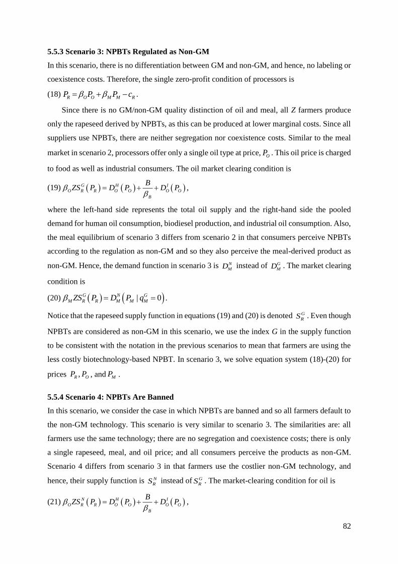
82
5.5.3 Scenario 3: NPBTs Regulated as Non-GM
In this scenario, there is no differentiation between GM and non-GM, and hence, no labeling or
coexistence costs. Therefore, the single zero-profit condition of processors is
(18) R O O M M RP P P c .
Since there is no GM/non-GM quality distinction of oil and meal, all Z farmers produce
only the rapeseed derived by NPBTs, as this can be produced at lower marginal costs. Since all
suppliers use NPBTs, there are neither segregation nor coexistence costs. Similar to the meal
market in scenario 2, processors offer only a single oil type at price,OP . This oil price is charged
to food as well as industrial consumers. The oil market clearing condition is
(19) G H I
O R R O O O O
B
BZS P D P D P
,
where the left-hand side represents the total oil supply and the right-hand side the pooled
demand for human oil consumption, biodiesel production, and industrial oil consumption. Also,
the meal equilibrium of scenario 3 differs from scenario 2 in that consumers perceive NPBTs
according to the regulation as non-GM and so they also perceive the meal-derived product as
non-GM. Hence, the demand function in scenario 3 is N
MD instead of G
MD . The market clearing
condition is
(20) | 0G N G
M R R M M MZS P D P q .
Notice that the rapeseed supply function in equations (19) and (20) is denoted G
RS . Even though
NPBTs are considered as non-GM in this scenario, we use the index G in the supply function
to be consistent with the notation in the previous scenarios to mean that farmers are using the
less costly biotechnology-based NPBT. In scenario 3, we solve equation system (18)-(20) for
prices ,R OP P , and MP .
5.5.4 Scenario 4: NPBTs Are Banned
In this scenario, we consider the case in which NPBTs are banned and so all farmers default to
the non-GM technology. This scenario is very similar to scenario 3. The similarities are: all
farmers use the same technology; there are no segregation and coexistence costs; there is only
a single rapeseed, meal, and oil price; and all consumers perceive the products as non-GM.
Scenario 4 differs from scenario 3 in that farmers use the costlier non-GM technology, and
hence, their supply function is N
RS instead of G
RS . The market-clearing condition for oil is
(21) N H I
O R R O O O O
B
BZS P D P D P
,

83
and the market-clearing condition for meal is
(22) | 0N N G
M R R M M MZS P D P q .
The system of equations (21) and (22), together with the zero-profit condition, equation (18),
in unknowns ,R OP P , and MP constitutes the equilibrium for scenario 4.
5.6 Calibration of the Baseline
We calibrate our model to scenario 1 in the absence of segregation and coexistence costs, which
then constitutes the model baseline. We use the observed and derived prices and quantities for
the European Union in the year 2013. We calibrate to scenario 1 as this is the most general
scenario, in which NPBTs are regulated as GM and both mandatory GM and voluntary non-
GM labeling schemes are in place. The calibration to the most general scenario makes it
possible to use the calibrated parameters later in simulating the other scenarios.
In scenario 1, NPBT-derived crops are categorized GM and conventionally produced crops
are considered non-GM. But since up to now, all rapeseed in Europe is conventional (and
therefore non-GM), we assume for the calibration that the observed prices are non-GM
commodity prices ( N
RP , N
OP , and N
MP ) but that the observed quantities are GM and non-GM
quantities. From this assumption, we calculate the equilibrium GM-categorized NPBT prices
G
RP , G
OP , and N
OP .
We assume that the price for rapeseed derived by NPBTs is lower than the conventional
rapeseed price, because NPBT crops are produced at lower marginal costs. Estimates of the
variable cost differences, for example, for GM and non-GM canola in Canada show mixed
results; benefits, such as easier weed control and better time management, are often difficult to
quantify (Qaim, 2009; Smyth et al., 2011a). Yield increases and cost reductions through
reduced expenditures on herbicides, fuel, and labor have been reported for herbicide-resistant
canola in Canada, the United States, and Australia to be higher for the more recent years as
compared to the early years after the introduction (Brookes and Barfoot, 2016). We assume a
10-percent cost advantage for GM rapeseed, which represents an average estimate for GM
canola for the years 2004 to 2014 as reported by Brookes and Barfoot (2016). The cost
advantage implies /1.10G N
R RP P and is assumed to be a result of differences in production
costs for competitive farmers, whereas coexistence and segregation costs are assumed to be
zero in the calibration.
We assume an equal percentage price advantage for GM oil and meal as compared to their
non-GM counterparts. The estimated price advantage must be such, that the crushing costs of

84
GM and non-GM crops are equal. Denoting the relative price premium by x, GM oil and meal
prices in the absence of segregation costs (i.e., 0O Ms s ) satisfy / (1 )G N
O OP P x and
/ (1 )G N
M MP P x , respectively. To meet the non-GM zero-profit condition of rapeseed
processors in equation (10), the premium is found by rewriting the GM zero-profit condition in
equation (9) into / 1G N N
R O O M M RP P P x c . Using the observed prices N
OP and N
MP
and recalling that /1.10G N
R RP P , we obtain, 8.8x percent. We assume that the price a
processor pays for rapeseed equals the price a farmer receives.
Table 2. Values of Technical Coefficients, Prices, Crushing Costs, and Number of Farmers for
the Model Calibration
Description Symbol Value Source/explanation
Oil yield from crushing one metric ton of
rapeseed (metric tons) O 0.38a Ferchau (2000) and
FEDIOL (2013)
Meal yield from crushing one metric ton of
rapeseed (metric tons) M 0.62a 1 O
Liters of biodiesel from a metric ton of
rapeseed oil B 1,098.08 CARD (2016)
Price of GM rapeseed (€/metric ton) G
RP 386.59 /1.10G N
R RP P
Price of non-GM rapeseed (€/metric ton) N
RP 425.25 Average price for
2013, UFOP
(2013)
Price of GM oil (€/metric ton) G
OP 755.46 /1.088G N
O OP P
Price of non-GM oil (€/metric ton) N
OP 822.17 Average price for
2013, UFOP
(2013)
Price of GM meal (€/metric ton) G
MP 243.12 /1.088G N
M MP P
Price of non-GM meal (€/metric ton) N
MP 264.58 Average price for
2013, UFOP
(2013)
Crushing cost (€/metric ton) Rc 51.20
N N N
R O O MM Rc P P P
Total number of farmers Z 100.00 Assumed
Number of GM farmers k 67.80 Calculated
Note: a The amount of oil and meal from crushing rapeseed can vary, depending on the type of
rapeseed crushing/pressing.
Table 2 summarizes the values of technical coefficients, prices, crushing costs, and the
number of GM farmers used to calibrate the model to scenario 1. The number of GM farmers,
k, can be thought of as a percentage of the total number of rapeseed farmers, Z, when 100Z .

85
The number of GM farmers is endogenously determined in the calibration (Appendix 5.10.1).
Changing the total number of farmers would affect k but not the share of GM farmers, /k Z .
Rapeseed contains about 43 to 46 percent oil. However, not all oil is extracted during
crushing. The extracted oil amount varies between 30 and 43 percent, depending on the type of
crushing and pressing of the rapeseed (Ferchau, 2000; Grau et al., 2010). We set the technical
oil and meal coefficients to 0.38O and 1 0.38 0.62M , respectively. Using the
observed non-GM prices as well as the technical oil and meal coefficients, we derive the
crushing costs from the zero-profit condition in equation (10). These derived crushing costs are
51.20 euros per metric ton, which is in line with estimates by Ferchau (2000).
The total rapeseed net-supply in 2013 was 25.09 million metric tons (European
Commission, 2014). After rapeseed crushing, 2.80 million tons of oil were demanded as food
for human consumption. The oil used for biodiesel consumption is calculated by multiplying
the share of rapeseed oil in total biodiesel feedstock of 55.67 percent (USDA FAS, 2015b) by
the total amount of vegetable oil, 8.51 million tons (FEDIOL, 2013) that was used as feedstock
for biodiesel. This calculation yields a biodiesel quantity of 5,202 million liters derived from
4.74 million tons of rapeseed oil. To meet the total rapeseed net-supply we categorize the
remaining rapeseed oil of 1.99 million tons as demand for industrial use.
Table 3. Supply and Demand Quantities for Equilibrium Model Calibration Description Symbol Value Source/explanation a
Total supply of GM rapeseed (metric tons) G
RkS 17.72 Calculated b
Total supply of non-GM rapeseed (metric tons) N
RZ k S 7.37 Calculated b
Demand for oil for human consumption
(metric tons)
H
OD 2.80 FEDIOL (2013)
Demand for oil for industrial consumption
(metric tons)
I
OD 1.99 Calculated
Oil for biodiesel demand (metric tons) / BB 4.74 USDA FAS
(2015b) and
FEDIOL (2013)
Demand for meal GM (metric tons) G
MD 10.98 Calculated
Demand for meal non-GM (metric tons) N
MD 4.57 Calculated
Note: a See text for further explanation on the calculations, b The sum of calculated GM and
non-GM rapeseed supply equals 2013 rapeseed supply (USDA FAS, 2015b).
By applying the technical coefficients, crushing and pressing of the total rapeseed net-
supply yields 15.55 million tons of meal of which 10.98 million tons are calculated (using the
model equations) to be GM and the remainder, 4.57 million tons, is non-GM meal. Given the

86
different demands, the division of rapeseed into GM and non-GM can be derived from the
baseline (scenario 1) equation system to be 17.52 and 7.57 million tons, respectively. Table 3
summarizes the supply and demand quantities used in the calibration.
Supply and demand elasticities are taken from the FAPRI elasticity database.43 We use
constant price elasticity supply curves for GM and non-GM rapeseed. For a sensitivity analysis,
we take these elasticities as the mean values of a beta distribution (Davis, 2008) from which
random values are drawn in 10,000 simulations.Table 4 shows the supply and demand elasticity
parameters as well as the mean, minimum, and maximum value of the beta distribution. One of
the restrictions in our sensitivity analysis is that the own-price elasticity of GM rapeseed supply
must be greater than the own-price elasticity of non-GM rapeseed supply. This requirement
reflects the effect of the NPBT in lowering the marginal production costs. Furthermore, own-
and cross-price elasticities for meal demand are chosen to satisfy the restrictions imposed on
the parameters of the underlying utility function.
Table 4. Parameters and Baseline Elasticity Values for Model Calibration
Description Parameter Mean Min Max
Own-price elasticity of GM rapeseed supply G
R 0.35b 0.10 0.80
Own-price elasticity of non-GM rapeseed supply N
R 0.30a 0.10 0.80
Own-price elasticity of GM oil demand for
industrial use
I
O -0.38a -1.00 -0.10
Own-price elasticity non-GM rapeseed oil demand
for human consumption
H
O -0.25a -1.00 -0.10
Own-price elasticity of GM meal demand G
M -4.50b -5.00 -0.80
Own-price elasticity of non-GM meal demand N
M -4.50b -5.00 -0.80
Cross-price elasticity of demand crossNG
M 0.35b 0.01 1.00
Source: a FAPRI (2013), b assumed to satisfy the conditions of the quasi-linear utility function
for vertical product differentiation.
5.7 Simulation and Results
We start by investigating the welfare implications of individual scenarios (1 to 4) in the absence
of segregation and coexistence cost effects as presented in block A of tables 5 and 6. To that
end, we first simulate the market and welfare effects of removing the voluntary non-GM
labeling option for meal in case NPBT-derived rapeseed is regulated as GM; that is, we compare
scenario 2a with the calibrated scenario 1a (=baseline). Second, we analyze the effect of
regulating NPBTs as a non-GM technique by comparing scenario 3a with the baseline. Finally,
43 http://www.fapri.iastate.edu/tools/elasticity.aspx
87
we analyze the effects of banning NPBTs by comparing scenario 4a with the baseline. Table 1
above summarizes the details of individual scenarios. Blocks B, C, and D of tables 5 and 6 show
the effects of oil segregation costs, meal segregation costs, and coexistence costs, respectively.
Following the estimates by Tillie and Rodriguez-Cerezo (2015) for soybean meal, we set
the segregation costs of meal to 20 percent of the non-GM meal price. For oil, we assume
segregation costs of 10 percent. In a study of the German rapeseed oil industry, these costs were
found to vary widely, depending on factors like storage, elevation systems, processing strategies,
and monitoring arrangements (Gabriel and Menrad, 2015). We set the coexistence costs
(including the technology fee) to 5 percent (θ = 0.05) to show their qualitative effects. The 5
percent coexistence costs correspond to 50.5 euros per ha assuming an average rapeseed yield
of 3.1 metric tons per ha.44 However, the coexistence costs (incl. the technology fee) for
rapeseed under current coexistence policies are likely to be higher (e.g., Gabriel and Menrad,
2015), and may even outweigh farmers’ marginal cost benefits of growing NPBT rapeseed; this
case would enforce scenario 4a, in which farmers do not grow NPBTs. Since there are no
qualitative insights into the effects of coexistence costs if we set them too high, we show the
effects of 5 percent in block D of tables 5 and 6 and analyze the effects of increasing these costs
to find the maximum coexistence costs in a sensitivity analysis.
Table 5 shows the market effects of different scenarios and table 6 shows the changes in
the welfare components. The changes are in comparison to baseline scenario 1a.
44The average rapeseed yield in the European Union in 2012
(http://ec.europa.eu/agriculture/statistics/agricultural/2013/pdf/d04-1-44_en.pdf). We show the details of
calculating the coexistence costs per metric ton of rapeseed in the section on the welfare effects of coexistence
costs.
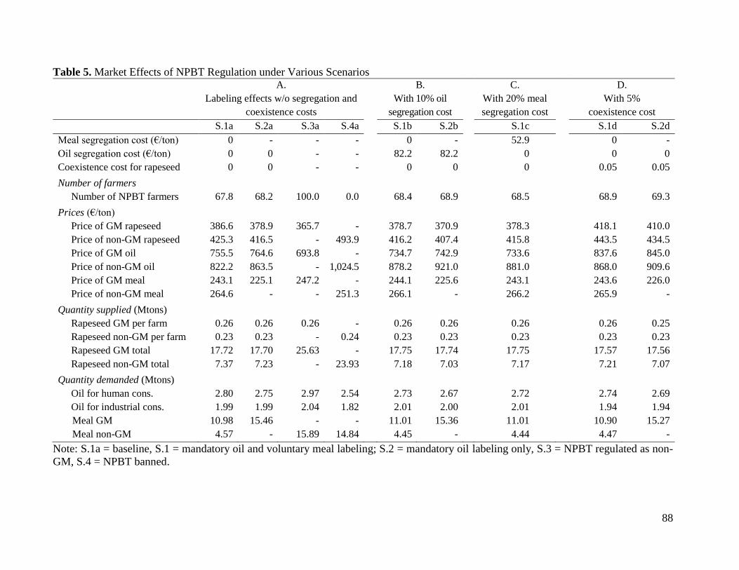
88
Table 5. Market Effects of NPBT Regulation under Various Scenarios
A.
Labeling effects w/o segregation and
coexistence costs
B.
With 10% oil
segregation cost
C.
With 20% meal
segregation cost
D.
With 5%
coexistence cost
S.1a S.2a S.3a S.4a S.1b S.2b S.1c S.1d S.2d
Meal segregation cost (€/ton) 0 - - - 0 - 52.9 0 -
Oil segregation cost (€/ton) 0 0 - - 82.2 82.2 0 0 0
Coexistence cost for rapeseed 0 0 - - 0 0 0 0.05 0.05
Number of farmers
Number of NPBT farmers 67.8 68.2 100.0 0.0 68.4 68.9 68.5 68.9 69.3
Prices (€/ton)
Price of GM rapeseed 386.6 378.9 365.7 - 378.7 370.9 378.3 418.1 410.0
Price of non-GM rapeseed 425.3 416.5 - 493.9 416.2 407.4 415.8 443.5 434.5
Price of GM oil 755.5 764.6 693.8 - 734.7 742.9 733.6 837.6 845.0
Price of non-GM oil 822.2 863.5 - 1,024.5 878.2 921.0 881.0 868.0 909.6
Price of GM meal 243.1 225.1 247.2 - 244.1 225.6 243.1 243.6 226.0
Price of non-GM meal 264.6 - - 251.3 266.1 - 266.2 265.9 -
Quantity supplied (Mtons)
Rapeseed GM per farm 0.26 0.26 0.26 - 0.26 0.26 0.26 0.26 0.25
Rapeseed non-GM per farm 0.23 0.23 - 0.24 0.23 0.23 0.23 0.23 0.23
Rapeseed GM total 17.72 17.70 25.63 - 17.75 17.74 17.75 17.57 17.56
Rapeseed non-GM total 7.37 7.23 - 23.93 7.18 7.03 7.17 7.21 7.07
Quantity demanded (Mtons)
Oil for human cons. 2.80 2.75 2.97 2.54 2.73 2.67 2.72 2.74 2.69
Oil for industrial cons. 1.99 1.99 2.04 1.82 2.01 2.00 2.01 1.94 1.94
Meal GM 10.98 15.46 - - 11.01 15.36 11.01 10.90 15.27
Meal non-GM 4.57 - 15.89 14.84 4.45 - 4.44 4.47 -
Note: S.1a = baseline, S.1 = mandatory oil and voluntary meal labeling; S.2 = mandatory oil labeling only, S.3 = NPBT regulated as non-
GM, S.4 = NPBT banned.
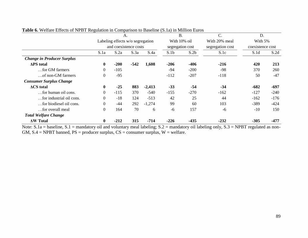
89
Table 6. Welfare Effects of NPBT Regulation in Comparison to Baseline (S.1a) in Million Euros
A.
Labeling effects w/o segregation
and coexistence costs
B.
With 10% oil
segregation cost
C.
With 20% meal
segregation cost
D.
With 5%
coexistence cost
S.1a S.2a S.3a S.4a S.1b S.2b S.1c S.1d S.2d
Change in Producer Surplus
ΔPS total 0 -200 -542 1,608 -206 -406 -216 420 213
…for GM farmers 0 -105 -94 -200 -98 370 260
…of non-GM farmers 0 -95 -112 -207 -118 50 -47
Consumer Surplus Change
ΔCS total 0 -25 883 -2,413 -33 -54 -34 -682 -697
…for human oil cons. 0 -115 370 -540 -155 -270 -162 -127 -240
…for industrial oil cons. 0 -18 124 -513 42 25 44 -162 -176
…for biodiesel oil cons. 0 -44 292 -1,274 99 60 103 -389 -424
…for overall meal 0 164 70 6 -6 157 -6 -10 150
Total Welfare Change
ΔW Total 0 -212 315 -714 -226 -435 -232 -305 -477
Note: S.1a = baseline, S.1 = mandatory oil and voluntary meal labeling; S.2 = mandatory oil labeling only, S.3 = NPBT regulated as non-
GM, S.4 = NPBT banned, PS = producer surplus, CS = consumer surplus, W = welfare.
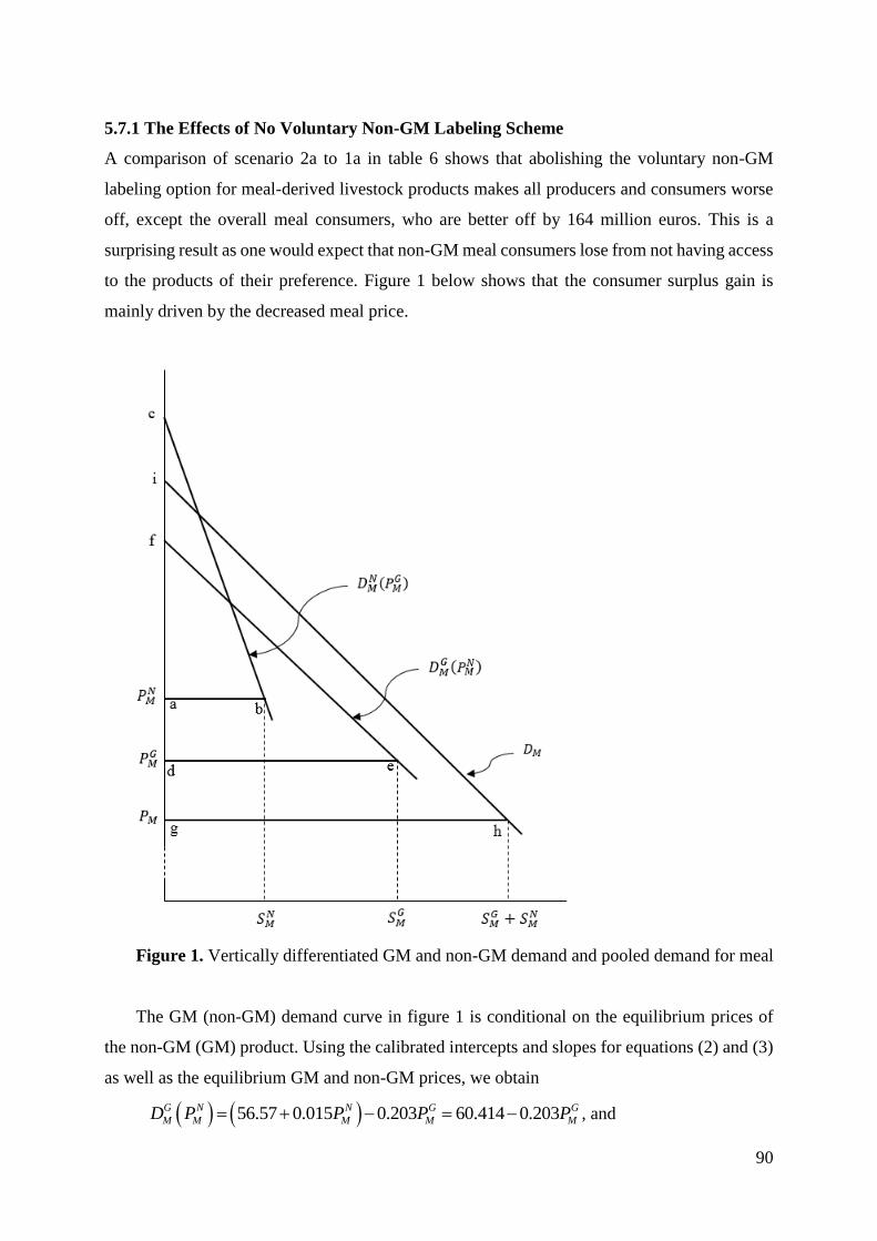
90
5.7.1 The Effects of No Voluntary Non-GM Labeling Scheme
A comparison of scenario 2a to 1a in table 6 shows that abolishing the voluntary non-GM
labeling option for meal-derived livestock products makes all producers and consumers worse
off, except the overall meal consumers, who are better off by 164 million euros. This is a
surprising result as one would expect that non-GM meal consumers lose from not having access
to the products of their preference. Figure 1 below shows that the consumer surplus gain is
mainly driven by the decreased meal price.
Figure 1. Vertically differentiated GM and non-GM demand and pooled demand for meal
The GM (non-GM) demand curve in figure 1 is conditional on the equilibrium prices of
the non-GM (GM) product. Using the calibrated intercepts and slopes for equations (2) and (3)
as well as the equilibrium GM and non-GM prices, we obtain
56.57 0.015 0.203 60.414 0.203G N N G G
M M M M MD P P P P , and

91
21.594 0.015 0.078 25.126 0.078N G G N N
M M M M MD P P P P .
The equation for the pooled meal demand curve (corresponding to equation (4)) turns out to be
60.607 0.201G
M MD P . Notice that, because the substitution parameter [0,1] , the intercept
of the inverse pooled demand curve is between the GM and non-GM inverse demand intercepts.
The prices G
MP , N
MP , and MP correspond to equilibriums related to the three demand curves
above.
The total meal consumer surplus in scenario 2a is represented by area ghi, which is greater
than the sum of areas abc and def, corresponding to the consumer surpluses of non-GM and
GM meal in scenario 1a.
Everything else held constant, the immediate effect of a lower meal price is to reduce the
rapeseed price and hence the rapeseed supply. A reduced rapeseed supply yields a lower oil
supply, which drives oil prices up. The decreased rapeseed price and increased oil price cause
a loss in producer and oil consumer welfare in comparison to scenario 1a. The sum of these
losses outweighs the meal consumer surplus gain, so that the abolition of a voluntary non-GM
label reduces overall welfare by 212 million euros (Table 6).
5.7.2 The Effects of Regulating NPBTs as Non-GM
Regulating NPBT-derived crops as non-GM is the only scenario that increases total welfare as
compared to baseline. In scenario 3a (third column in block A of tables 5 and 6) all farmers use
NPBTs for two reasons: first, rapeseed derived by NPBTs is treated as non-GM, and, second,
the marginal cost of production is lower for NPBTs. This implies that farmers have no incentive
to use the costlier conventional technology for which they would get no price premium. Since
all farmers are using the marginal cost-reducing technology, the rapeseed supply increases,
driving down rapeseed, oil, and meal prices. Producers lose and consumers gain from the lower
prices as compared to scenario 1a. The gain in oil and meal consumer surplus outweighs the
loss in producer surplus, such that regulating NPBTs as non-GM leads to an overall welfare
gain of 315 million euros.
5.7.3 The Effects of Oil Segregation Costs
Scenarios 1b and 2b in table 5, show that oil segregation costs increase the non-GM oil
consumer price, which reduces the quantity of oil demanded for human consumption. A lower
non-GM oil consumption drives down the non-GM rapeseed price and hence also the supplied
non-GM rapeseed quantity. Furthermore, a lower supply of non-GM rapeseed reduces the non-
GM meal supply, leading to an increase in the non-GM meal price. This result is in line with

92
Sobolevsky et al. (2005) who show that food consumers and producers benefit from low
segregation costs. However, our results (1b and 2b) show that not all consumers benefit from
low segregation costs.
When segregation costs increase, more farmers produce GM rapeseed. A larger GM
rapeseed supply drives down GM rapeseed prices, which leads to a lower GM oil price and
hence more oil for industrial and biodiesel use. Because the GM oil price with segregation costs
(734.7 euros per metric ton) in scenario 1b in table 5 is lower than the GM oil prices without
segregation costs in the baseline (755.5 euros per metric ton), GM oil consumers benefit from
segregation costs. But the total welfare change with segregation costs in scenarios 1b and 2b is
negative.
By further comparing scenario 1b with 1a and scenario 2b with 2a, we see that the market
and welfare effects of oil segregation costs are similar for partial labeling (no non-GM labeling)
and full labeling (with non-GM labeling), respectively. Producers and non-GM consumers lose
and GM consumers gain. In scenario 2b, the producer and non-GM oil consumer losses due to
segregation costs are added to the losses due to the non-GM label abolishment. The GM
consumers’ gains due to oil segregation costs, on the other hand, outweigh their losses due to
the non-GM label abolishment. Finally, the gain meal consumers get due to the abolishment of
the non-GM label (scenario 2a) is slightly lower with oil segregation costs (scenario 2b).
5.7.4 The Effects of Meal Segregation Costs
Table 5 and 6 show that in scenario 1, meal segregation costs of 20 percent of the non-GM meal
price have very similar effects than oil segregation costs of 10 percent of the non-GM oil price.
This similarity is due to the similarity between the levels of the segregation costs for oil and
meal: 0.1 31.2O
N
OP and 0.2 32.8M
N
MP . The welfare effects of segregation costs
are that non-GM consumers and producers lose and GM oil and meal consumers gain. However,
meal segregation costs apply only in scenario 1 because in scenario 2 the total meal supply is
pooled. This pooling effect when abolishing the non-GM meal labeling option has important
implications.
Comparing scenario 1c with 1a and 2a in table 5, we find that if meal segregation costs are
sufficiently high, producers and some consumers would benefit from the abolishment of the
non-GM label (i.e., their surplus in 1c exceeds their surplus in 1a). For example, oil consumers’
surplus loss from not having the voluntary labeling scheme (i.e., scenario 2a) is 115 million
euros. But their surplus loss from having the scheme in the presence of meal segregation costs
(i.e., scenario 1c) is even higher, that is, 162 million euros. Similarly, producers’ loss from not

93
having the label is 200 million euros whereas their loss from having the label in the presence
of meal segregation costs is 216 million euros. As shown above, meal consumers clearly gain
(164 million euros in scenario 2a) from not having the voluntary label. This effect is even
stronger with meal segregation costs.
In summary, our comparison implies that producers and non-GM oil consumers benefit
from a voluntary non-GM label, as long as meal segregation costs are sufficiently small. This
result is consistent with the one by Fulton and Giannakas (2004). However, when high
segregation costs are added to the baseline, these consumers and producer are better off without
voluntary labeling. GM oil consumers (i.e., industrial use and biodiesel) are worse off (by 18
and 44 million euros, respectively) from not having the voluntary label so they benefit from the
label. Their benefit is even higher, when meal segregation costs are high.
5.7.5 The Effects of Coexistence Costs
Coexistence costs decrease GM rapeseed, oil, and meal supply, which leads to price increases
in the GM commodities (cf. scenarios 1d and 2d in table 5). The increase in the GM rapeseed
price drives up the non-GM rapeseed price because each farmer is assumed to be indifferent
between producing the GM or non-GM rapeseed variety. The increased non-GM rapeseed
prices increase non-GM oil and meal prices, which decreases non-GM quantities demanded.
All consumers in scenario 1d and 2d are worse off due to the increased prices caused by
coexistence costs as compared to the situation without coexistence costs. Comparing scenario
1d with the baseline, GM rapeseed farmers benefit from coexistence costs because the GM price
increase of 31.5 euros (from 386.6 to 418.1) causes a surplus gain that exceeds the surplus loss
due to coexistence costs. Since a farmer is indifferent between GM and non-GM rapeseed
production, the non-GM rapeseed price also increases by 18.2 euros (from 425.3 to 443.3) such
that the non-GM surplus gain equals the GM net-surplus gain (i.e., the difference between the
GM surplus and the coexistence cost).
Notice that the GM price increase is greater than the non-GM price increase. Similarly, the
GM oil price also increases faster than the non-GM oil price with higher coexistence costs. This
effect is shown in figure 2, where the percentage coexistence costs are translated into costs per
hectare. This can be done by first computing GM farmers total surplus and multiplying by .
The 5 percent, as used in tables 5 and 6, correspond to total coexistence costs of 287 million
euros (not presented in the tables). Dividing the coexistence costs by the total GM rapeseed
quantity of 17.57 million tons (cf. column 1d in table 6), we get 16.30 euros per ton or 50.53
euros per hectare (assuming a rapeseed yield of 3.1 ton per hectare). Similarly, we can translate,

94
for example, an 1-percent coexistence cost into 9.11 euros per hectare and an 10 percent cost
into 115.79 euros per hectare.
Figure 2. Effects of increasing coexistence costs (in percent of farmers’ surplus and in euros
per hectare) on GM and non-GM commodity prices
The GM oil price approaches the non-GM oil price faster than does the GM rapeseed price
the non-GM rapeseed price. Once the coexistence costs reach 8.6 percent (95.80 euros per
hectare) in the absence of segregation costs, the GM and non-GM oil prices would intersect,
which cannot happen because the condition, G N
O OP P , of vertical product differentiation must
hold. This condition is always satisfied, since the value of our industrial oil demand function is
95
min ,I G N
O O OD P P . Whenever the GM oil price would exceed the non-GM oil price, biofuel
and industrial oil consumers would buy non-GM oil until its price equalizes with the GM price.
Hence, for the case in which coexistence costs exceed 8.6 percent, we have G N
O OP P .
Once coexistence costs reach a threshold of 12.6 percent (157.01 euros per ton), also the
rapeseed prices equalize. This point constitutes the maximum coexistence costs (for our
baseline values) under which both GM and non-GM crops are cultivated. Increasing the
coexistence costs beyond this maximum would cause GM rapeseed and meal prices to exceed
non-GM prices—a price relation that would contradict the conditions of vertical production
differentiation. Hence all farmers switch to non-GM crops, that is, they switch to scenario 4a.
This switch explains the discontinuity in figure 2 at the 12.6 percent coexistence cost.
Scenario 4a is identical to scenario 3a, except now farmers are only using the conventional
technology instead of NPBT. The conventional technology yields a lower total rapeseed supply,
which increases commodity prices. Farmers benefit from these higher prices while all
consumers lose. This is in line with Fulton and Giannakas (2004) who show that consumers
benefit from a situation without labeling (i.e., regulating NPBTs as conventional in our case)
when consumer aversion is low.
5.8 Sensitivity Analysis and Discussion
The simulation shows that increased productivity through NPBTs has a price decreasing effect
that makes farmers worse off and consumers better off. For testing the robustness of our results,
we ran a Monte Carlo simulation with 10,000 random draws of elasticities from a beta
distribution. The mean, minimum, and maximum values of the distribution are reported in table
4. In each simulation, we calculate the market and welfare changes. Table A5.2 in the Appendix
5.10.2 shows the 10 and 90 percent range of the resulting welfare changes distribution. None
of the signs change within the ranges. This sign consistency indicates robust results.
A decrease in the producer surplus from technological improvement may seem counter-
intuitive. However, for inelastic demands, the surplus loss due to a price decrease when
switching from non-GM to GM production (e.g., switching from scenario 4a to scenario 3a)
outweighs the surplus gain due to lower marginal costs. On the other hand, elastic demand leads
to a greater surplus gain due to reduced marginal costs (from the GM technology) than the
surplus loss due to a price decrease. Hence, an elastic demand can reverse the producer surplus
effect (e.g., Duncan and Tisdell, 1971; Martin and Alston, 1997). This reverse effect is shown

96
in table A.3 in the Appendix, where we report welfare changes of table 6 for a price elasticity
of demand for human oil consumption of -3.0.
An elastic demand also reduces the positive effect of coexistence costs. Whereas under the
elastic oil demand the producer welfare effect of coexistence costs is lower but still positive in
scenario 1, it is negative is scenario 2. Segregation costs, on the other hand, have a much
stronger negative effect on producer welfare under an elastic oil demand. This negative effect,
caused by segregation costs, is compensated for by higher consumer surpluses as compared to
inelastic oil demand.
Finally, it may also seem counter-intuitive that a voluntary non-GM label for meal-derived
products reduces overall surplus of meal consumers. However, the model only allows to make
a point about the overall meal consumers and does not allow to distinguish by how much GM
and non-GM meal consumers benefit or lose separately. What we can say with the model is that
all consumers who consume GM meal in the baseline are better off in without the non-GM
labeling option (scenario 2a) due to the lower meal price. Furthermore, some of the initial non-
GM consumers also benefit in scenario 2a from the reduced price, so that they do not mind
consuming GM instead of non-GM meal. However, some of the initial non-GM consumers may
leave the rapeseed meal market and switch to a substitute market. These consumers are the ones
that are worse off by abolishing the voluntary labeling scheme. We estimate only the overall
meal consumer surplus change, which is positive when abolishing voluntary labeling.
5.9 Conclusions
We develop a partial equilibrium model to analyze the market and welfare effects of regulating
new plant breeding techniques (NPBTs) as GM or non-GM technologies. We apply the model
to the EU market of rapeseed and commodities derived thereof: meal and oil. The market and
welfare effects are analyzed under a mandatory label for GM food products and a voluntary
label for meal-derived livestock products. Both labels apply in the baseline. A key feature of
our model is that it allows us to separate the effects of farm-level coexistence cost and
marketing-level segregation and identity preservation costs.
In general, the model shows that regulating NPBTs as GM generates an overall welfare
loss as compared to regulating them as non-GM. This is because when NPBT crops are
regulated as GM (as compared to non-GM), prices are higher and consumers’ welfare loss
outweighs producers’ gains. Increasing coexistence costs intensifies this effect and may even
lead to the absence of NPBTs if the costs pass a certain threshold. Unlike coexistence costs,
segregation costs, do not increase all prices but actually lower the price of GM rapeseed oil

97
(benefiting industrial and biodiesel consumers) as well as the rapeseed prices received by
farmers. The prices of food oil and meal increase due to segregation costs, however.
We show that vertical product differentiation of meal-derived livestock products through a
voluntary non-GM labeling scheme, which some EU Member States have developed,
substantially increases the meal price and hence makes overall meal consumers worse off. But
industrial oil and biodiesel consumers benefit from voluntary meal labeling. Also, farmers and
food oil consumers benefit from the voluntary labeling scheme. However, we show that these
farmers and food oil consumers are only better off if meal segregation costs do not exceed a
threshold level. When meal segregation costs exceed that threshold, only industrial and
biodiesel consumers benefit from voluntary meal labeling.
Coexistence costs have an overall welfare decreasing effect. We show that even if the use
of NPBTs lowers farmers’ marginal rapeseed production costs by 10 percent, they would not
cultivate these crops if the coexistence costs (including the technology fees in the form of higher
seed costs for the NPBT seeds) exceed a threshold of around 157 euros per hectare. Under
current coexistence policies in most EU Member States, coexistence costs are likely to exceed
this level (Venus et al., 2017). These results imply that if NPBTs are regulated as GM in the
European Union, the cultivation of such crops is likely to be unprofitable under the current
labeling and coexistence policies.
An important assumption of our model is that consumers only care about the regulation of
NPBTs but not about NPBTs per se. However, very little is known about how consumers would
behave if NPBTs were actually marketed. If consumers do care about NPBTs per se, they might
be willing to pay a premium to avoid NPBT-derived products even if these products are
regulated as non-GM. If this is the case, the industry may develop voluntary labeling schemes
to avoid NPBTs (similar to the non-GM labeling schemes for livestock products). This,
however, requires to set up a segregation system including coexistence measures at the farm
level. Our model actually covers this case in the scenario 1 except that food oil, in this case,
may also be vertically differentiated into an NPBT and a non-NPBT food oil market. While
segregation and coexistence costs would still be necessary to segregate NPBT from non-NPBT
products, the approval costs would be much lower than if NPBT-derived rapeseed is categorized
as GM product.
Overall, the results show that a ban on NPBTs is the most costly strategy in which
consumers lose and farmers gain the most. This illustrates that farmers may not lobby for
NPBTs. On the consumer side, the biodiesel industry complex would be the one losing most
and have a strong incentive to lobby for NPBTs (even in the presence of labeling policies).
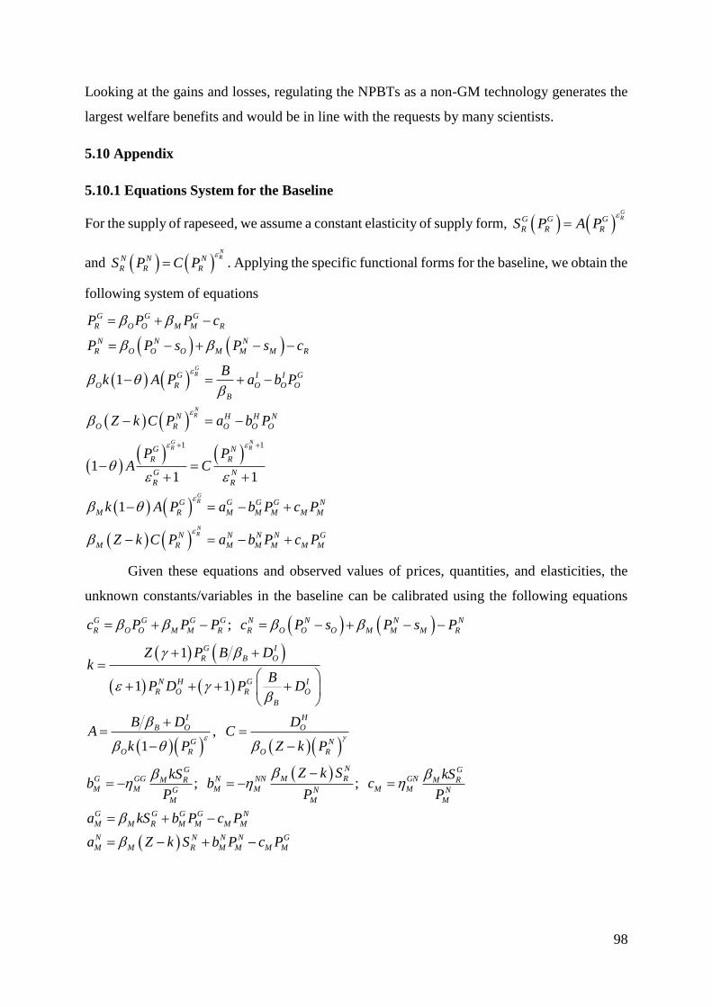
98
Looking at the gains and losses, regulating the NPBTs as a non-GM technology generates the
largest welfare benefits and would be in line with the requests by many scientists.
5.10 Appendix
5.10.1 Equations System for the Baseline
For the supply of rapeseed, we assume a constant elasticity of supply form, GRG G G
R R RS P A P
and NRN N N
R R RS P C P
. Applying the specific functional forms for the baseline, we obtain the
following system of equations
1 1
1
11 1
1
GR
NR
G NR R
GR
NR
G G G
R O O M M R
N N N
R O O O M M M R
G I I G
O R O O O
B
N H H N
O R O O O
G N
R R
G N
R R
G G G G
M R M M M M
N N N N
M R M M M
N
M
G
MM
P P P c
P P s P s c
Bk A P a b P
Z k C P a b P
P PA C
k A P a b P c
Z k C PP a b P c
P
Given these equations and observed values of prices, quantities, and elasticities, the
unknown constants/variables in the baseline can be calibrated using the following equations
;
1
1 1
, 1
; ;
G G G G N N N N
R O O M M R R O O O M M M R
G I
R B O
N H G I
R O R O
B
I H
B O O
G N
O R O R
NG GM RG GG N NN GNM R M R
M M M M M MG N N
M M M
G G
M M R
c P P P c P s P s P
Z P B Dk
BP D P D
B D DA C
k P Z k P
Z k SkS kSb b c
P P P
a kS b
G G
M M M
N N N N
M M
N
M
G
MR M M M
P c
a Z k S b P c
P
P

99
5.10.2 Sensitivity Analysis
Table A.5.2. 10 and 90 Percent Range of Welfare Changes through a Sensitivity Analysis of Supply and Demand Elasticities
A.
Labeling effects w/o segregation and coexistence
costs
B.
With 10% oil
segregation cost
C.
With 20%
meal seg. c.
D.
With 5%
coexistence cost
S.1a S.2a S.3a S.4a S.1b S.2b S.1c S.1d S.2d
Change in Producer Surplus
ΔPS total 0 [-211,-185] [-640,-441] [1329,1905] [-218,-194] [-426,-381] [-237,-203] [398,443] [189,243]
…for GM farmers 0 [-112,-97] [-100,-97] [-210,-186] [-112,-99] [351,390] [243,281]
…of non-GM farm. 0 [-100,-88] [-118,-106] [-217,-194] [-125,-106] [45,56] [-56,-35]
Consumer Surplus Change
ΔCS total 0 [-31,3] [754,948] [-2648,-2027] [-32,-8] [-56,-6] [-34,-9] [-715,-663] [-724,-662]
…for human oil c. 0 [-119,-109] [342,399] [-628,-458] [-159,-151] [-278,-262] [-161,-153] [-134,-121] [-248,-230]
…for industrial oil 0 [-21,-14] [105,144] [-576,-454] [39,44] [20,31] [40,45] [-168,-156] [-183,-169]
…for biodiesel oil 0 [-51,-33] [246,339] [-1440,-1123] [93,104] [48,74] [94,106] [-403,-376] [-440,-407]
…for overall meal 0 [135,188] [56,73] [-6,10] [-6,-5] [128,181] [-6,-5] [-11,-9] [122,-174]
Total Welfare Change
ΔW Total 0 [-222,-204] [296,326] [-747,-694] [-226,-226] [-444,-426] [-232,-232] [-272,-265] [-487,-467]
Note: S.1a = baseline, S.1 = mandatory oil and voluntary meal labeling; S.2 = mandatory oil labeling only, S.3 = NPBT regulated as non-
GM, S.4 = NPBT banned, PS = producer surplus, CS = consumer surplus, W = welfare.

100
Table A.5.3. Welfare Changes with Elastic Oil Demand ( H
O = -3.0)
A.
Labeling effects w/o segregation
and coexistence costs
B.
With 10% oil
segregation cost
C.
With 20% meal
segregation cost
D.
With 5%
coexistence cost
S.1a S.2a S.3a S.4a S.1b S.2b S.1c S.1d S.2d
Change in Producer Surplus
ΔPS total 0 -433 226 394 -504 -951 -529 169 -282
…for GM farmers 0 -212 -231 -454 -243 255 30
…of non-GM farmers 0 -221 -273 -497 -286 -86 -313
Consumer Surplus Change
ΔCS total 0 223 116 -1,051 284 531 298 -39 -75
…for human oil cons. 0 -36 145 -157 -48 -86 -50
…for industrial oil cons. 0 31 -38 -254 103 143 108 -111 -71
…for biodiesel oil cons. 0 73 -90 -617 243 337 255 -266 -169
…for overall meal 0 156 98 -22 -14 136 -14 -17 133
Total Welfare Change
ΔW Total 0 -210 342 -657 -220 -421 -231 -264 -465
Note: S.1a = baseline, S.1 = mandatory oil and voluntary meal labeling; S.2 = mandatory oil labeling only, S.3 = NPBT regulated as non-
GM, S.4 = NPBT banned, PS = producer surplus, CS = consumer surplus, W = welfare.

101

102
Chapter 6
Investing in Emerging Vertically
Differentiated Products

103
6. INVESTING IN EMERGING VERTICALLY DIFFERENTIATED
PRODUCTS45
ABSTRACT: We model a decision of a duopoly that initially offers a low-quality product to
invest in an emerging high-quality product. We investigate whether the smaller or the larger
firm invests first. Preemption or a war of attrition can result, depending on demand and cost
factors. For each case, we derive the unique Nash equilibrium. If both firms have a second-
mover advantage, the larger firm invests first independently of demand-side factors. Only
higher costs for the larger firm can reverse this result. If both firms have a first-mover advantage,
one firm invests before its optimal leader time to preempt its rival.
KEYWORDS: Entry, exit, emerging market, firm size, investment analysis, preemption,
vertical product differentiation
45 This chapter is based on the article: Venus, T.J., Drabik, D., and Wesseler, J.H.H. Investing in Emerging
Vertically Differentiated Products. Paper submitted to a peer-reviewed journal.
104
6.1 Introduction
Firms can follow different strategies to differentiate themselves from competition. They can
invest in quality-improving technologies (e.g., a waterproof mobile phone), make products safer
(e.g., by complying with a certain hygienic standard in food production), produce more
environmentally friendly (e.g., by using renewable energy sources), or exclude genetically
modified organisms (GMOs) from the food production process (e.g., by complying with a non-
GMO standard in food production). If all consumers choose a product with some of these
attributes (perceived as higher quality) over a product lacking them (viewed as lower quality)
when both qualities are offered at the same prices, the products are said to be vertically
differentiated (Shaked and Sutton, 1982). This preference, of course, requires that firms can
signal the higher quality. In this article, we consider investments in vertically differentiated,
high-quality products in a duopoly when the choice is dichotomous (i.e., either low or high
quality).
Dichotomous choices are common, for example, for credence good labeling. In this case,
consumers cannot distinguish between high- and low-quality products in the absence of any
credible indication of the quality, even after lengthy inspection. In Germany, for instance, firms
can adopt a non-GMO label by complying with the labeling standard specified by the
government. This kind of labeling creates two quality levels because firms can either meet the
standard and label the products to signal a high quality or not comply and signal low quality.
The variable costs of producing the high quality usually exceed the variable costs of producing
the low quality. In addition, the adoption of the label requires firms, among other things, to
make sunk investments in new production technologies, certification systems, training of
employees, and negotiations with suppliers.
The set-up of our investment problem is as follows. Initially, both firms offer the low
quality assuming that the demand and hence the incremental profits for the high-quality
products are sufficiently low. As the demand for the high-quality product increases, one of the
firms eventually invests, and the other firm follows. We assume that large product segregation
costs make a firm switch completely. Therefore, once a firm invests, it becomes a monopoly
supplier of high quality while its opponent becomes a monopoly supplier of low quality until
the demand for a high-quality good is large enough to yield positive profits for both firms. We
show that investment in high quality can result in a war of attrition or preemption.
The model shows that due to vertical product differentiation (VPD), it is not clear a priori
whether the smaller or the larger firm leads. This result is important as the order of investment
through vertical product differentiation affects the welfare distribution of consumers differently.
In addition, we show both demand-side and cost factors determine which firm enters the high-

105
quality market first. A production standard, for example, that affects the level of product
differentiation or the firms’ cost structure may affect the order of investment given other
exogenous variables, such as firm size, interest and growth rate, investment costs, and the slope
of the demand curves.
The study of high-quality investments is closely related to the investigation of investments
in new technology. Reinganum (1981) shows that if all firms have a first-mover advantage,
then identical firms adopt the technology sequentially, earning different profits. Fudenberg and
Tirole (1985) relax Reinganum’s (1981) assumption of pre-commitment and allow a firm to
preempt their rival firm. Their revised setup using continuous-time mixed strategies allows
determining firm rules endogenously instead of exogenously. If a first-mover advantage exists,
a firm preempts its rival until the preempting firm is indifferent between following and leading.
Fudenberg and Tirole (1985) refer to this phenomenon as “rent equalization.” In the case of
firms of different size, mixed strategies are not necessary. Because we consider different firm
sizes, rent equalization can be ruled out, and so the framework by Reinganum (1981) works
without the pre-commitment assumption.
Investing in high-quality production implies entering the high-quality market and exiting
the low-quality market if the segregation costs of producing both products simultaneously are
sufficiently high. If one firm benefits more when its opponent leads than when it leads itself,
then switching to high-quality represents a second-mover advantage because the opportunity
costs of exit exceed the benefit of entry. Ghemawat and Nalebuff (1985, 1990) and Fudenberg
and Tirole (1986) analyze exit of firms with asymmetric market shares from markets with
shrinking demand in a deterministic framework. They show that a smaller firm can sustain
losses of a decreasing product demand over a longer period and therefore the larger firm exits
first. Only large scale economies for the large firm’s production costs can reverse this result.
Whinston (1988) shows that the results stated by Ghemawat and Nalebuff (1985) do not
generalize for the multi-plant setting; hence, firm size alone may not be a good predictor for
determining firm exit when firms possess more than one production facility. Esteve-Pérez (2005)
shows that also demand-side effects must be considered when analyzing market exit in the case
of vertically differentiated products. Due to product differentiation, the larger firm may outlast
the smaller firm, when the firms produce different qualities.
Product differentiation, for example, through labeling, affects competition by creating two
markets. Following the imperfect information framework by Gabszewicz and Thisse (1979)
and Shaked and Sutton (1982), Bonroy and Constantatos (2015) apply this idea to a duopoly
market with firms of different exogenously given qualities. Bonroy and Constantatos (2015)
show that both firms benefit, whereas only consumers with high willingness to pay for the high-

106
quality product gain and the remaining consumers lose compared to no product differentiation.
In our model, both firms are already active in the low-quality market. As in Fudenberg et
al. (1983) and Ghemawat and Nalebuff (1985, 1990), we assume that the demand structure, as
well as capacities and production costs, are common knowledge and that each firm eventually
earns a positive profit in a duopoly, which allows us to study a finite-horizon game. Firms
decide only whether to invest in high-quality production and when to make this choice. Whereas
the previous literature analyzes either investment in or exit from markets with a first-mover or
second-mover advantage, we show that investment in exogenously determined, high-quality
products requires a combination of entry and exit models. We model investment in high-quality
production in a duopoly market where the demand for high-quality increases deterministically
over time. Our model merges the theory of investment in new technology and exit from
declining markets with the theory of product differentiation.
6.2 The Model
6.2.1 Static Demand for Vertically Differentiated Products and Fixed Capacities
We assume two firms, indexed by i and j, where both indexes can denote either firm 1 or 2, that
is, , 1,2i j with i j . We assume that each firm produces either low quality (l) or high
quality (h), but not both. We study entry as in Gabszewicz and Thisse (1979), due to, for
example, the credence good characteristic of the product, assuming that l and h are exogenously
given.
Vertical product differentiation (VPD) implies that the price of the low-quality product is
smaller than the price of the high-quality product. Therefore, firms only choose the low-quality
if they can produce it at a sufficiently lower marginal cost than the high-quality product or if
the investment in the high-quality production exceeds the firm’s net present value.
We assume that a firm’s capacity,iK , is fixed and firm 1’s capacity is smaller than firm
2’s, that is, 1 2K K . The justification for the fixed capacity comes from the idea that firms
maximize their profits by choosing multiple product characteristics and the high- and low-
quality dimension is only one of them. For example, before the government introduces a
labeling standard, firms may set their capacities through Cournot competition, choosing various
levels in different quality dimensions (e.g., taste, geographical indication, fat content,
appearance). Consumers in our model are price and quality takers.
We assume that both firms face a constant per-unit cost of capacity for low- and high-
quality products, denoted by lc and hc , respectively. Beyond capacity, the costs are

107
prohibitively high. We normalize the low-quality production costs to zero, such that 0hc
denotes a firm’s incremental per-unit costs of producing high instead of low quality. We further
assume the input supply is perfectly elastic. We assume that the marginal profit is always
positive and hence, firms always fully use their available capacity instead of making short-run
adjustments (Ghemawat and Nalebuff, 1985). Once a firm offers high-quality products, it
cannot return to low-quality. High set-up costs prevent entry of other firms.
Given the capacity constraints, firms set the prices at each point in time corresponding to
the demand schedules (e.g., Boccard and Wauthy, 2010). Let us denote firm i’s decision byiD ,
where
(1) i
lD
h
if firm has not invested in high-quality production,
if firm has invested in high-quality production.
i
i
Similarly, we denote firm j’s decision by { , }jD l h . Then we can write the downward-
sloping inverse demand function that firm i faces by ,i j
i
D DP . For example, if firm 1 produces
high quality (i.e., 1D h ) and firm 2 produces low quality (i.e., 2D l ), then firm 1 sets price
1
,h lP and firm 2 sets price 2
,l hP . We normalize the duopoly low-quality price to zero (, 0 l lP ).
If firms produce different product types, each firm is a monopolist in its market.
6.2.2 Utility Function and Demand Structure
A representative consumer has a quasi-linear utility function, and consumes low- and high-
quality products in quantities, lq and hq , respectively, and a numeraire good, y . Following
Singh and Vives (1984), we assume the consumer maximizes ( , , )h l l h hlU q q y p q p q , where
(2) 2 21
( , , ) ( ) ( 2 )2
h h l ll h l l hhl hU q q y t q q q s q yq q ,
where 0h lt . The utility function depends on the degree of substitutability, [0,1]s ,
of the l and h quality, the intrinsic qualities ( l and ( )h t ), and the rate of utility saturation ( l
and h ). The intrinsic quality of the high-quality product, h t , grows smoothly over time (t),
whereas the intrinsic low quality is constant. Furthermore, for the total demand we assume that
own-price effects dominate cross-price effects, that is, 0l s and 0h s .46 This set-up
leads to time-dependent inverse demand functions ( , j
i
h DP t ) for high-quality products and
46 The condition that own-price effects exceed cross-price effects “maintains a notion of generalized
substitutability among goods” (Lapan and Moschini, 2004) but is more restrictive than requiring a negative
semidefinite Slutsky matrix (i.e., 2 0l h s ).

108
time-invariant inverse demand functions ( , j
i
l DP ) for low-quality products (see Appendix for
particular functional forms).
Because the inverse demand curve in each market is downward-sloping and 1 2K K , and
own-price effects dominate cross-price effects, firm 1 sets a higher monopoly price than firm 2
in the same market, 1 2
, ,h l h lP P and1 2
, ,l h l hP P . The downward-sloping demand curves imply that
prices for producing the low-quality product type as a monopolist are always larger than prices
from producing the same type in a duopoly , , 0 i
l h l lP P . Furthermore, because VPD implies
that all consumers would buy the high-quality product if offered at the same price as the low-
quality product, hence, , ,
i i
h l l hP P .
Because capacities are fixed, we use unit profits (henceforth profits) to determine the order
of firm’s entry in high-quality production. Firm i’s profits depend on firm j’s decision, jD , such
that firm i’s monopoly low-quality profit is , ,j j
i
D
i
l Dl P (recalling that the unit cost of low-
quality production is zero) and its monopoly and duopoly high-quality profit is
,,
i
h l
i
h l hct P t and , ,hh hh ht P t c , respectively. Note that duopoly profits for both
firms are equal at each unit costs (therefore we omit the subscript). The demand structure and
costs are common knowledge for the firms.
At each 0t , firm’s available actions are to remain in the low-quality market or invest in
high-quality production. Firms are assumed not to reverse their investment decisions. Under
growing high-quality demand and the assumption that monopoly profits of high-quality
production at 0t are negative (i.e., ,0
0j
i
h Dt
), there exist three stages: 1) both firms
produce low-quality in a duopoly and earn zero profits; 2) one firm invests and becomes a high-
quality monopolist while the second firm becomes a low-quality monopolist; and 3) both firms
produce high quality in a duopoly. For the second stage, we are interested in which firm invests
first to become the high-quality leader.
6.2.3 Leader’s and Follower’s Time
To determine the leader and the follower, we first define the net-present value of leading (i.e.,
leader’s value) and the net present value of following (i.e., follower’s value). Denote firm i ’s
leader value function as ,i i j
L FL T T when firm i invests as a leader at i
LT and firm j invests as
a follower at j
FT . As soon as firm i leads, it becomes a monopoly supplier of the h product, and
its profits increase from ,l l to , ( )i
h l t . Firm i will earn monopoly profits until the rival firm j

109
follows at j
FT . When firm j follows, firm i’s profits change to , ( )h h t .
The leader values of firm 1 and 2 are
(3) 2
1
1 2 ,
1 1 2 1
,, ( ) ( )F
L
L F
TrTrt rt
L F h lT T
h hL T T t e dt t e dt Ie
and
(4) 1
2
2 1 ,
2 2 1 2
,, ( ) ( )F
L
L F
TrTrt rt
L F h lT T
h hL T T t e dt t e dt Ie
,
where r denotes the discount rate and I denotes the unit investment cost, which is assumed to
be the same for both firms.
Furthermore, denote ,i j i
L FF T T as firm i ’s follower value function, when firm j invests
as the leader at j
LT and firm i invests as the follower at i
FT . The follower values of firm 1 and 2
are
(5) 1
1
2 1
1 2 1
, ,
1, ( )F
F
L F
TrTrt rt
L F l hT T
h hF T T e dt t e dt Ie
and
(6) 2
2
1 2
2 1 2
, ,
2, ( )F
F
L F
TrTrt rt
L F l hT T
h hF T T e dt t e dt Ie
.
The optimal investment time for the leader solves the first-order condition corresponding
to equations (3) and (5), that is, *, 0( ) /i i j i
L F LL T T T , which can also be expressed as
(7)
*
, ( )i i
h l Lr
T
I
.
Because , 0i
h l t and 1 2
, ,( ) ( )h l h lt t , we have 1* 2*
L LT T . Equation (7) corresponds to
the Jorgensonian rule, which states to invest when the profit level equals the Jorgensonian user
cost of capital ( rI ) (Dixit and Pindyck, 1994, 148; Jorgenson, 1963). Similarly, the optimal
follower time solves *( , ) / 0i j i i
L F FF T T T , or
(8)
*
, ,( )i i
h h F l hTr
I
.
Because , 0h h t and
1 2
, ,l h l h , we have 2* 1*
F FT T . Firm i’s leader/follower value
dependents on firm j’s choice but its optimal leader time is independent of firm j’s choice. In
deciding whether to become a leader or a follower, the firm has to take into account the
opportunity cost of its action. To that end, we define the net leader value ( iV ) as the difference
between leading at *i
LT and following at *,i
FT conditional on firm j’s optimal choice, that is,
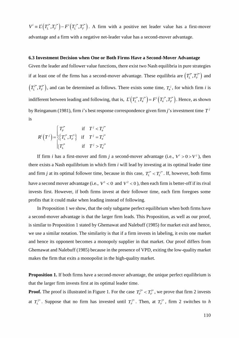
110
* * * *, ,i i i j i j i
L F L FV L T T F T T . A firm with a positive net leader value has a first-mover
advantage and a firm with a negative net-leader value has a second-mover advantage.
6.3 Investment Decision when One or Both Firms Have a Second-Mover Advantage
Given the leader and follower value functions, there exist two Nash equilibria in pure strategies
if at least one of the firms has a second-mover advantage. These equilibria are 1* 2*,L FT T and
2* 1*,L FT T , and can be determined as follows. There exists some time, #
jT , for which firm i is
indifferent between leading and following, that is, * * * *
# #, ,i j j i
L
i i
FL T T F T T . Hence, as shown
by Reinganum (1981), firm i’s best response correspondence given firm j’s investment time jT
is
* *
#
* * *
#
* *
#
if
, if
if
i j j
F
j i i j j
L F
i j j
L
i
T T T
R T T T T T
T T T
If firm i has a first-mover and firm j a second-mover advantage (i.e., 0i jV V ), then
there exists a Nash equilibrium in which firm i will lead by investing at its optimal leader time
and firm j at its optimal follower time, because in this case, * *i j
L LT T . If, however, both firms
have a second mover advantage (i.e., 1 0V and 2 0V ), then each firm is better-off if its rival
invests first. However, if both firms invest at their follower time, each firm foregoes some
profits that it could make when leading instead of following.
In Proposition 1 we show, that the only subgame perfect equilibrium when both firms have
a second-mover advantage is that the larger firm leads. This Proposition, as well as our proof,
is similar to Proposition 1 stated by Ghemawat and Nalebuff (1985) for market exit and hence,
we use a similar notation. The similarity is that if a firm invests in labeling, it exits one market
and hence its opponent becomes a monopoly supplier in that market. Our proof differs from
Ghemawat and Nalebuff (1985) because in the presence of VPD, exiting the low-quality market
makes the firm that exits a monopolist in the high-quality market.
Proposition 1. If both firms have a second-mover advantage, the unique perfect equilibrium is
that the larger firm invests first at its optimal leader time.
Proof. The proof is illustrated in Figure 1. For the case 2* 1*
F FT T , we prove that firm 2 invests
at 2*
LT . Suppose that no firm has invested until 2*
FT . Then, at 2*
FT , firm 2 switches to h

111
independently of firm 1’s decision at this point. If firm 1 is of type h at 2*
FT , its profits fall from
monopoly to duopoly h profits. It earns duopoly h profits over the period 2* 1*[ , )F FT T . However,
if firm 1 is of type l at 2*
FT , it earns monopoly l profits over the period 2* 1*[ , )F FT T . Define area
a to be firm 1’s gain from producing l in monopoly instead of h in duopoly over the period
2* 1*[ , )F FT T .
Suppose Ax is the first time such that firm 1 is willing to remain of type l and earn zero
profits over the period 2*[ , )A Fx T to avoid losing area a. Remaining of type l requires to give up
monopoly h profits. Taking into account a positive interest rate as well as investment costs, Ax
is implicitly defined by
2* 1*
1*
2*
1 1
, , ,( ) ( ) 0F F
A F
A F
T Trx rTrt rt
h l l h h hx T
t e dt I e e t e dt ,
where the right-hand side corresponds to area a and the left-hand side to area b c d . This
area takes into account the negative effects of investing earlier at a time Ax instead of 1*
FT , as
defined by the second term of the left-hand side.
Regarding area, Ax is the first time that firm 1 is willing to give up area b c d to avoid
losing area a. Hence, if firm 1 has not invested until Ax , it will remain of type l until 1*
FT with
probability one. Because the continued production of l in duopoly leads to zero profits, firm 2’s
optimal decision at the time Ax is to invest at this point with probability one.
Figure 1. Backward induction when both firms have a second-mover advantage
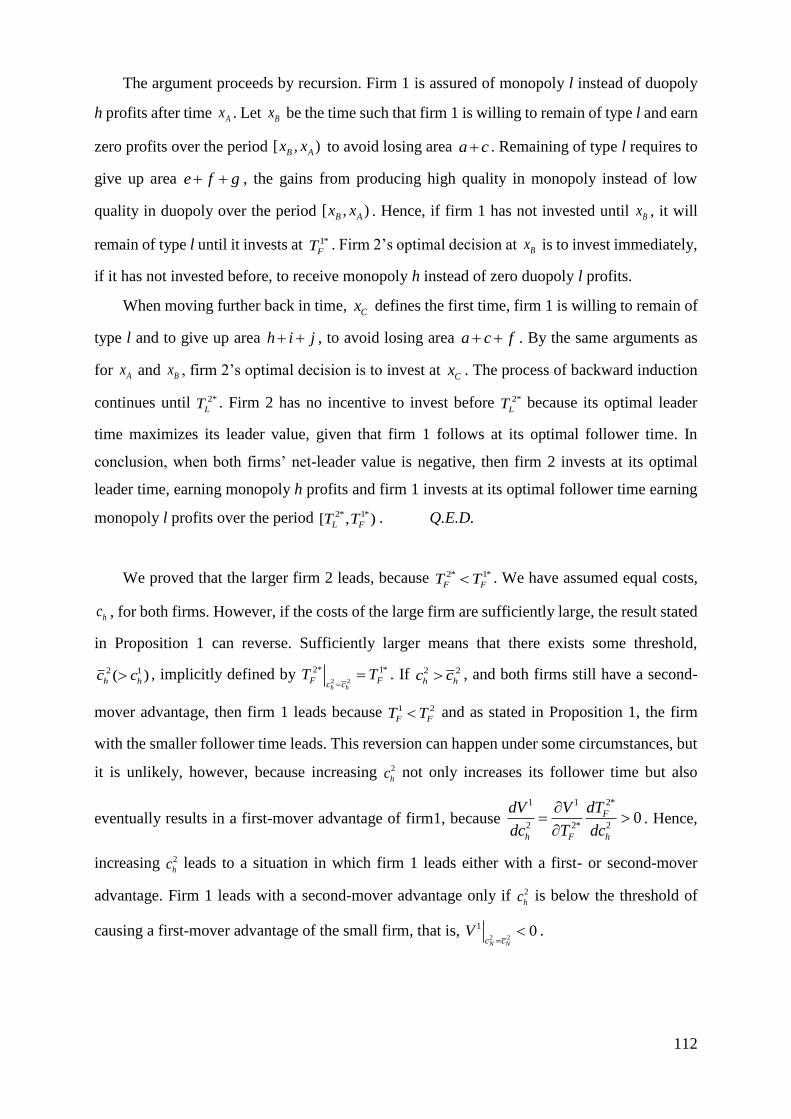
112
The argument proceeds by recursion. Firm 1 is assured of monopoly l instead of duopoly
h profits after time Ax . Let Bx be the time such that firm 1 is willing to remain of type l and earn
zero profits over the period [ , )B Ax x to avoid losing area a c . Remaining of type l requires to
give up area e f g , the gains from producing high quality in monopoly instead of low
quality in duopoly over the period [ , )B Ax x . Hence, if firm 1 has not invested until Bx , it will
remain of type l until it invests at 1*
FT . Firm 2’s optimal decision at Bx is to invest immediately,
if it has not invested before, to receive monopoly h instead of zero duopoly l profits.
When moving further back in time, Cx defines the first time, firm 1 is willing to remain of
type l and to give up area h i j , to avoid losing area a c f . By the same arguments as
for Ax and Bx , firm 2’s optimal decision is to invest at Cx . The process of backward induction
continues until 2*
LT . Firm 2 has no incentive to invest before 2*
LT because its optimal leader
time maximizes its leader value, given that firm 1 follows at its optimal follower time. In
conclusion, when both firms’ net-leader value is negative, then firm 2 invests at its optimal
leader time, earning monopoly h profits and firm 1 invests at its optimal follower time earning
monopoly l profits over the period 2* 1*[ , )L FT T . Q.E.D.
We proved that the larger firm 2 leads, because 2* 1*
F FT T . We have assumed equal costs,
hc , for both firms. However, if the costs of the large firm are sufficiently large, the result stated
in Proposition 1 can reverse. Sufficiently larger means that there exists some threshold,
2 1( )h hc c , implicitly defined by 2 2
2* 1*
h hF Fc c
T T
. If 2 2
h hc c , and both firms still have a second-
mover advantage, then firm 1 leads because 1 2
F FT T and as stated in Proposition 1, the firm
with the smaller follower time leads. This reversion can happen under some circumstances, but
it is unlikely, however, because increasing 2
hc not only increases its follower time but also
eventually results in a first-mover advantage of firm1, because 2*1
2 2
1
* 20F
h F h
dTVdV
dc T dc
. Hence,
increasing 2
hc leads to a situation in which firm 1 leads either with a first- or second-mover
advantage. Firm 1 leads with a second-mover advantage only if 2
hc is below the threshold of
causing a first-mover advantage of the small firm, that is, 2 2
1 0N Nc c
V
.
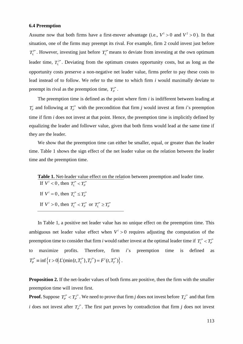
113
6.4 Preemption
Assume now that both firms have a first-mover advantage (i.e., 1 0V and 2 0V ). In that
situation, one of the firms may preempt its rival. For example, firm 2 could invest just before
1*
LT . However, investing just before 1*
LT means to deviate from investing at the own optimum
leader time, 2*
LT . Deviating from the optimum creates opportunity costs, but as long as the
opportunity costs preserve a non-negative net leader value, firms prefer to pay these costs to
lead instead of to follow. We refer to the time to which firm i would maximally deviate to
preempt its rival as the preemption time, *i
PT .
The preemption time is defined as the point where firm i is indifferent between leading at
i
PT and following at *i
FT with the precondition that firm j would invest at firm i’s preemption
time if firm i does not invest at that point. Hence, the preemption time is implicitly defined by
equalizing the leader and follower value, given that both firms would lead at the same time if
they are the leader.
We show that the preemption time can either be smaller, equal, or greater than the leader
time. Table 1 shows the sign effect of the net leader value on the relation between the leader
time and the preemption time.
Table 1. Net-leader value effect on the relation between preemption and leader time.
If 0iV , then * *i i
L PT T
If 0iV , then * *i i
L PT T
If 0iV , then * *i i
L PT T or * *i i
L PT T
In Table 1, a positive net leader value has no unique effect on the preemption time. This
ambiguous net leader value effect when 0iV requires adjusting the computation of the
preemption time to consider that firm i would rather invest at the optimal leader time if * *i i
L PT T
to maximize profits. Therefore, firm i’s preemption time is defined as
* * ** inf 0 (min{ , }, ) ( , )i i j i i
LP F F
i t L Ft T tT TT .
Proposition 2. If the net-leader values of both firms are positive, then the firm with the smaller
preemption time will invest first.
Proof. Suppose * *i j
P PT T . We need to prove that firm j does not invest before *j
PT and that firm
i does not invest after *j
PT . The first part proves by contradiction that firm j does not invest

114
before *j
PT . Preemption time *j
PT is defined as the first time at which firm j’s net leader value is
zero. If firm j invests at the time *j
PT , its leader value decreases to * *, ) ,( ( )j j j j
P PL T L T
while its follower value increases to * *, ) ,( ( )j j j j
P PF T F T . Hence, firm j’s net-leader value
before its preemption time is negative, * *, ) , )( 0(j j j j
P PL T F T , such that firm j has a
second-mover advantage. With a second-mover advantage, firm j prefers to invest as a follower.
Hence, if firm i invests at *j
PT to become a leader, it contradicts maximization of the leader
value.
The second part proves by contradiction that firm i does not invest after *j
PT . Suppose firm
i does not invest in the period *( , ]j
Pt T . Then firm j will invest at *j
PT and firm i becomes a
follower. Because firm i can decide to invest at any time in the period *( , ]j
Pt T to lead without
needing to fear preemption, deciding to be a follower contradicts profit-maximization.
Q.E.D.
Proposition 2 leaves open the question when the firms invest. Proposition 3 shows that
there is a unique time.
Proposition 3. If the net leader values of both firms are positive, each firm invests either at its
optimal leader time or at its opponent’s preemption time. In particular, firm 1 leads at 1
LT , where
1* 1* 1* 2*
1
1* 2* 1* 1* 2*
if max ,
min , if min ,
L L P P
L
L P P L P
T T T TT
T T T T T
,
or firm 2 leads at 2
LT , where
2* 1* 1* 2* 2* 1*
2
1* 2* 1*
min , if min ,
if
L P L P L P
L
P P P
T T T T T TT
T T T
.
Proof. Suppose that each firm leads either at its optimal leader time or at its opponent’s
preemption time. Define the set iS to be the period before firm i’s preemption time, that
is, *( | 0 )i i
PS t t T . From Proposition 3, firm i can make no credible threat to preempt firm
j at any it S .
First, suppose 1* 2*
P PT T . This situation is illustrated in Figure 2. Firm 1 invests first. Firm
1 can choose to invest at any 2t S without fear of preemption by firm 2. If 21*
LT S , firm 1
chooses to invest at 1*
LT to maximize its leader value. If 1* 2
LT S , then firm 1 will try to get as

115
close as possible to 1*
LT , to maximize its leader value, because the leader value function is
strictly concave in 2S .
Figure 2. Possible relations of preemption and optimal leader times, for which firm 1
invests first at the shaded times
The closest firm 1 can get to its optimal leader value is the least upper bound of 2S , that
is, 2 2*sup PS T . This proves that firm 1 invests at 1*
LT if 1* 1* 2*max{ , }L P PT T T or 1* 1* 2*
P L PT T T
and it invests at 2*
PT if 1* 2* 1*
P P LT T T .
Now suppose that 2* 1*
P PT T . This second part is illustrated in Figure 3. Firm 2 invests first.
Firm 2 can choose to invest at any 1t S without fear of preemption by firm 1.
Figure 3. Possible relations of preemption and optimal leader times, for which firm 2
invests first at the shaded times
If 12*
LT S , firm 2 chooses to invest at its optimal leader time to maximize its leader value.
If 12*
LT S , then firm 2 will try to get as close as possible to its optimal leader value. The closest
firm 2 can get to its optimal leader value is 1 1*sup PS T . This proves that firm 2 invests at 2*
LT
if 2* 2* 1*
P L PT T T and at 1*
PT if 2* 1* 2*
P P LT T T . Q.E.D.
If the small firm’s production costs are sufficiently higher than the ones of the large firm,
such that 2* 1*
L LT T , then the results stated in the proof reverse.

116
6.5 Effects of Exogenous Parameters – An Illustration
We have shown above that firms’ decision when to invest depends on several exogenous
parameters. Varying these parameters can result into different situations: (A) one of the firms
has a first-mover advantage; (B) both firms have a second-mover advantage; or (C) both firms
have a first-mover advantage.

117
Table 2. Example Combinations of Variables and the Different Resulting Investment Cases
A. One firm has a first-
mover, one a second-
mover advantage
B. Both firms have a
second-mover
advantage
C. Both firms have a
first-mover
advantage A.1
Firm 1 leads
A.2 Firm 2 leads
B.1 Firm 1 leads
B.2 Firm 2 leads
C.1 Firm 1 leads
C.2 Firm 2 leads
Market share of firm 1 1K 40 48 48 48 40 40
Market share of firm 2 2K 60 52 52 52 60 60
Substitutability parameter s 0.50 0.50 0.50 0.50 0.50 0.30
Growth rate g 0.12 0.12 0.12 0.12 0.10 0.10
Cost per unit of firm 1 1
hc 100 100 100 100 150 150
Cost per unit of firm 2 2
hc 100 100 103 100 150 150
High-quality saturation par. h 0.60 0.70 0.60 0.60 1.20 1.20
Opt. leader time of firm 1 1*
LT 4.51 4.58 4.58 4.58 12.81 11.61
Opt. leader time of firm 2 2*
LT 4.68 5.03 4.86 4.61 14.21 13.41
Opt. follower time of firm 1 1*
FT 8.84 8.44 8.44 8.44 38.22 36.91
Opt. follower time of firm 2 2*
FT 7.84 8.74 8.54 8.24 35.82 33.71
Opt. preemption time of firm 1 1*
PT - - - - 7.60 7.95
Opt. preemption time of firm 2 2*
PT - - - - 7.73 7.91
Net-leader value of firm 1 1V -19.10 1.18 -3.22 -9.90 121.54 106.75
Net-leader value of firm 2 2V 2.76 -15.03 -11.26 -5.53 115.60 96.68

118
Table 2 illustrates the three investment cases by assuming specific parameter values. For each
case, we show how changes in some parameters result in leadership of the smaller firm 1 or the
larger firm 2. In all examples, the values of the following parameters are held constant:
investment cost, I = 1, low-quality saturation parameter, 1l , low-quality inverse demand
intercept, 100l , high-quality inverse demand intercept, 100h , and discount rate, 0.1r .
Using column A.1 as a reference (i.e., firm 1 is the only firm with a first-mover advantage),
a higher market share of firm 1 (i.e., more similar firm sizes) results in case B.2, where both
firms have a second-mover advantage and firm 2 leads. However, if at the same time h , or
firm 2’s cost increase, then the result is A.2 or B.1, respectively. The latter case shows that firm
1 leading with a second-mover advantage can be the result of only a small unit cost increase of
firm 2. Examples of parameters for which both firms have a first-mover advantage are presented
in column C.1 and C.2. Lowering the substitutability between low- and high-quality products
can, for instance, change C.1 to C.2.
6.6 Conclusions
We show that firm’s investment in high-quality production with fixed capacity can be a strategic
substitute or a strategic complement, depending on several factors such as the difference in firm
size and the level of vertical differentiation, growth and discount rate, demand parameters, and
per-unit production costs. The distinctive feature of our model of high-quality investment and
vertical product differentiation is that it models entry in the high-quality and exit from the low-
quality market in a single framework. We state propositions that determine the unique
equilibrium under various conditions for the small or the large firm to invest first and derive
the respective optimal investment times.
The model allows to show, for example, how the stringency of a private or public quality
standard (e.g., the farm certification scheme GlobalGAP), which affects the production and
compliance costs as well as the level of product differentiation, affects the market structure of
differentiated products. Hence, our model implies that through the setting of these standards,
private and governmental institutions can impact the market structre.
A limitation of our study is that we consider only single-plant firms. If considering a
multiplant setting, a complex model of multiple equilibria would result, where other factors that
are difficult to assess, influence the order of investment (Whinston, 1988). Furhermore, because
we asume fixed production quantities, our model does not consider capacity investment
dynamics. For example, small firm’s growth is higher and more variable than large firm’s

119
growth (e.g., Chi and Choi, 2017). A combintion of capacity investment in a setting of vertically
differentiated products is left for future research.
6.7 Appendix
A Specific Demand Function for Vertically Differentiated Products
A representative consumer solves the following problem
2 21max ( , , ) max ( ) ( 2 )
2hl h l l h h l l h l h l lh h hl l hU q q y p q p q t qq q q s q y p q p qq .
Parameters h t , l , s , l , and h are defined in the text. First-order conditions
corresponding to the objective function above with respect to lq and hq , yield the inverse
demand functions
, ( , )h lll hh l lP q sqq q
, ( )( , , )h l l h h h h ltP t q qq sq ,
where ,l hP denotes the inverse demand function for low-quality products for a given quantity
of the high-quality product; similarly, ,h lP denotes the inverse demand function for the high-
quality product given the quantity of the low-quality product. Given the utility maximization
problem and the respective assumptions about parameter, the inferiority of the low-quality
product limits its price to be below the price of the high-quality product, that is,
, ,( , ) ( , )h hh l ll h lP q q P q q . If only low-quality products are produced and the consumer does not
have a choice, we obtain
, ( )l l ll l lP q a q .
On the other hand, if duopoly high-quality profits are greater than either firm’s monopoly
low-quality profits, firms will only offer high-quality products. Given the parameters of the
utility function above, we solve for the duopoly price by adding up the low- and high-quality
demand curves and then solving for the inverse demand to obtain
2
,2 2
h l l h l h
l
h h
l
h h
h h
t sP q
s s
sq
s
.
If, for example, the intercept of the high-quality demand curve grows linearly at rate g,
such that, (1( ))h ht gt , the corresponding profits conditional on firm 1’s and 2’s capacities,
are
, ( )l i j
l l l l i jK K lqq a K K
,

120
,, ,
l i h jjq K q
i
l h l h l l iKsKq q K
,
,, , ,
h i l j
i i
h l q K ql h h h h i j hKt q q gt K sK c
,
2
, (2 2 2
, )h i j
l l h il hi j hq K K
l l l
h h li
h h h
h h h
s st K K
g s
st
s s
sq c
Given the functional forms of the profit functions, the leader and follower times, implicitly
defined by equations (7) and (8), are
(9) ,*
,i
h l l h
h
i
L
rI qT
g
q
and
(10)
, ,*
2
,i i
l h l h h h hi
F
h
h
l
l
rI q q q
s
Tg s
.
To test whether firm i has a first- or second-mover advantage, we substitute the optimal
leader and follower times into the leader and follower value equations (3) to (6) to obtain
(11) 2* 1* 1*
1* 1*
1* 2* 2*
1 1* 2* 1
,
1 1
, ,, ( ) ( )F F F
L F
L L F
T T TrT rTrt rt rt
L F h l l hT T T
h hV T T e t dt e dt e t dt I e e
and
(12) 1* 2*
22
* 2*
2* 1*
*
1*
2 2* 1* 2 2
, ,,
2, ( ) ( )F F
L F
L L F
FT TrT rTrt rt rt
L F
T
h hh l l hT T T
V T T e t dt e dt e t dt I e e .
In total, we get three cases and for each case two subcases. The subcases are that either
firm 1 or firm 2 leads. If both firms have a first-mover advantage (i.e., right-hand sides of both
(11) and (12) are positive), the lower preemption time * *min ,i i i
L L PT T T determines the leader.
In this case, firm 1’s preemption time, 1*
PT , solves
(13)
2* 1* 1* 1* 1* 1*
1* 1* 1* 2*
min ,1 1
, , ,min ,
( ) ( ) 0F F F P L
F
P L P F
T T T r T T rTrt rt rt
h l l h h hT T T T
e t dt e dt e t dt I e Ie
,
and firm 2’s preemption time, 2*
PT , solves
(14)
1* 2* 2* 2* 2* 2*
2* 2* 2* 1*
min ,2 2
, ,m
2
,in ,
( ) ( ) 0F F F P L
F
P L P F
T T T r T T rTrt rt rt
h l l hT T
hT
hT
e t dt e dt e t dt I e Ie
.

121
Chapter 7
Discussion and Conclusions
122
7. DISCUSSION AND CONCLUSIONS
In this thesis, I address the overall question: “What does the system that regulates GMOs in the
European Union imply for coexistence, product labeling, and firms’ strategic decision-making
related to vertical product differentiation?”
In the thesis, I present some of the wide-ranging implications of the EU GMO regulatory
system for agricultural supply chains. Firms can use a GM crop for food production once the
crop has been authorized for human consumption. If a food ingredient contains more than 0.9
percent EU-authorized GMOs (by weight), suppliers of that product must label the product.
Products that only use GMOs in the production process do not require labeling. Firms,
particularly in concentrated markets, can use labeling for vertical product differentiation.
Labeling leads to a separation into GM and non-GM supply chains if firms offer both product
types. To guarantee the parallel existence of these supply chain systems, some EU Member
States implemented specific farm-level coexistence measures. Furthermore, firms have
developed systems to preserve the identity of non-GM products along the supply chain. The
regulatory system, combined with labeling, coexistence, and identity preservation systems,
affects the market and welfare effects of the introduction of several new plant breeding
techniques, which may or may not fall within the scope of the GMO regulation.
7.1 Synthesis of the Answers to the Research Questions
In this thesis, I stated four research questions related to the system that regulates GMOs in the
European Union. Each of these questions is addressed in a chapter of this thesis. To synthesize
the thesis, a summary of the answers from the four chapters is presented in the following text.
What are the costs of coexistence measures for genetically modified maize in Germany?
Coexistence measures at the farm level are difficult to price and cost estimates are largely
missing in the literature. The previous literature relies on small case studies with either direct
assessments based on accounting principles (e.g., Consmüller et al., 2009b; Messean et al., 2006;
Skevas et al., 2010; Venus et al., 2011) or on simulations (e.g., Messean et al., 2006). The
evaluation of a choice experiment with farmers in Germany enables an estimation of the
farmer’s perceived coexistence costs. Chapter 3 shows that these costs highly depend on the
defined coexistence requirements, and that some of the strict measures can significantly
increase the cost of cultivating GMO crops up to and beyond the point where GM crops are no
longer profitable. In Germany, farmers rated temporal isolation as the costliest coexistence
measure, confirming its unsuitability in non-Mediterranean countries and explaining its

123
exclusion from the set of coexistence measures in Germany. Our results support the arguments
of Devos et al. (2009), Messeguer et al. (2006), and Weber et al. (2007), who state that temporal
scheduling to isolate Bt maize flowering from non-Bt maize flowering is not an effective
measure if the seeding window is very short.
Strict liability is the costliest obligatory coexistence measure that is also used in Germany
followed, by large minimum distance requirements. Even though strict liability costs exceed
the expected benefit of Bt maize cultivation, farmers may have planted Bt maize in the presence
of joint and strict liability because as some farmers mentioned, one of the grain traders paid the
same price for conventional and Bt maize, while the GM seed supplying company safeguarded
potential economic damage as long as farmers comply with the laws.
As Bt farmers valued minimum distance as less costly, minimum distance requirements
might have been one of the reasons why Bt farmers in our sample decided to plant Bt maize in
2008 even though their neighbors did not. This finding confirms that minimum distance can
severely limit the economic benefits of GM growers in areas with non-GM farmers (Demont et
al., 2008; Groeneveld et al., 2013). The findings further indicate that an increase in the number
of neighbors had a negligible negative effect on the adoption decision.
What drivers and institutional set-up is leading the German non-GMO market from niche to
mainstream?
Complying with a public voluntary labeling standard would be sufficient for labeling a
particular product attribute. However, firms have several incentives to adopt a private voluntary
standard that operationalizes the public standard. In the case of Germany, the Ministry of
Agriculture commissioned a multi-stakeholder organization to issue and administer the licenses
of a national non-GMO label. The organization sets a private voluntary non-GMO production
and certification standard with which firms must comply to use the label. In line with Henson
and Humphrey (2010), Chapter 4 discusses how the private non-GMO standard reduces
uncertainty by providing assurance that the rules and regulations are adhered to. Furthermore,
the exemption of smaller firms from third-party auditing facilitates the participation of smaller
firms in the certification scheme instead of forcing them out, which has been the case for other
third-party certification schemes (Hatanaka et al., 2005).
Chapter 4 shows that initially, only small producers used non-GMO labeling and formed a
niche market. Around the same time, anti-GMO activist groups were pressuring larger firms to
convert to non-GMO. The decision of large egg producers in 2015 to use non-GMO labeling
created a tipping point, and this decision was the basis for the announcement of major German
retailer chains to use non-GMO labeling for some of their store brands. The chapter discusses

124
how the initial concerns of retailers were resolved through the multi-stakeholder organization.
The organization combines the interests of all its stakeholders, which lowers the probability of
one of the main fears of retailers, which is being pressured by NGOs should mislabeling occur.
Since the major retailers in Germany have decided to enter the non-GMO market, they have
been taking the role of the “driving” sector and moving non-GMO production from a niche to
a mainstream market. Their market power allows them to determine the production decisions
of the less powerful firms that produce their store brands (Klooster, 2005). Store brands play a
particularly vital role for the products (e.g., livestock products) that are most amenable to non-
GMO labeling.
What are the market and welfare effects of regulating New Plant Breeding Techniques as a
GMO technology under the present coexistence, segregation, and labeling regulations?
The current EU GMO regulatory system is binary: GMO or not. The decision on how to regulate
a number of new plant breeding techniques (NPBTs) is still open. The chapter presents a partial
equilibrium model to analyze the market and welfare effects of regulating NPBT-derived crops
as a GMO or not. The model is applied to the EU market of rapeseed and its derived
commodities: meal and oil. The market and welfare effects are analyzed under a mandatory
label for GM food products and a voluntary label for meal-derived livestock products. Both
labels apply in the baseline. A key feature of the model is that it allows a separation of the
effects of farm-level coexistence cost and marketing-level segregation and identity preservation
costs.
Several authors model the effects of segregation costs on product prices and consumer and
producer welfare, but they do not separately consider the coexistence costs of GM farmers (e.g.,
Fulton and Giannakas, 2004; Lapan and Moschini, 2007; Lapan and Moschini, 2004; Moschini
et al., 2005; Sobolevsky et al., 2005). The work by Sobolevsky et al. (2005) is the closest to
Chapter 5, as they use a partial equilibrium model of differentiated consumers to analyze the
market and welfare effects of costly segregation costs on GM soybean trade. Unlike Sobolevsky
et al. (2005), however, the focus of Chapter 5 is on the distribution of market and welfare effects
within an economy rather than on trade. We furthermore consider the different effects of
coexistence and segregation costs and allow for different labeling schemes.
As shown in Chapter 5, the vertical product differentiation of meal-derived livestock
products substantially increases the meal price and hence makes the consumers of these
products worse off overall. At the same time, Chapter 5 shows that industrial oil and biodiesel
consumers benefit from voluntary labeling of meal-derived livestock products. Additionally,
farmers and food oil consumers benefit from the voluntary labeling scheme. However, these

125
farmers and food oil consumers are only better off if meal segregation costs do not exceed a
threshold level. When meal segregation costs exceed that threshold, only industrial and
biodiesel consumers benefit from the voluntary non-GMO labeling of livestock products.
In Chapter 5, farm-level coexistence costs in the case where NPBTs are characterized as
GM technology are modeled as an increase of the marginal production costs of farmers; hence,
high farm-level coexistence costs can lead to the absence of NPBTs if the costs pass a certain
threshold. Unlike coexistence costs, segregation costs in downstream markets, do not increase
all prices (i.e., rapeseed, meal, oil); instead, they actually lower the price of oil, a derived
commodity from NPBT rapeseed (benefiting industrial and biodiesel consumers), and the
rapeseed prices received by farmers. However, the prices of food oil and meal increase due to
segregation costs, which is in line with the findings by Desquilbet and Poret (2014).
Furthermore, coexistence costs have an overall welfare decreasing effect. Even if the use of
GMOs lowers the farmers’ marginal rapeseed production costs by 10 percent, they would not
cultivate these crops if the coexistence costs (including the technology fees in the form of higher
seed costs for the NPBT seeds) exceed a threshold of approximately 157 euros per hectare.
Under current coexistence policies in most EU Member States, coexistence costs are likely to
exceed this level as shown for maize in Chapter 3. These results imply that the current GMO
regulation in the European Union, is likely to make the cultivation of such crops unprofitable
under the current labeling and coexistence policies in some EU Member States.
How do different demand and cost variables influence the time to invest in high-quality
production?
The timing of the adoption of voluntary production standards can be a strategic choice of
companies (e.g., retailers) in highly concentrated markets to vertically differentiate their
products. In the case of GMOs, models presented in the literature consider GM and non-GM
products as vertically differentiated such that all consumers would either buy the non-GMO
product or are indifferent if both products are offered at equal prices (e.g., Fulton and Giannakas,
2004; Giannakas, 2002; Lapan and Moschini, 2007; Lapan and Moschini, 2004). Product
differentiation, for example, through labeling, affects competition by creating two markets.
Following the imperfect information framework by Gabszewicz and Thisse (1979) and Shaked
and Sutton (1982), Bonroy and Constantatos (2015) apply this idea to a duopoly market with
firms of different exogenously given qualities. Bonroy and Constantatos (2015) show that both
firms benefit, whereas only consumers with a high willingness to pay for the high-quality
product gain and the remaining consumers lose. In the model presented in Chapter 6, both firms
are already active in the low-quality market. As in Fudenberg et al. (1983) and Ghemawat and

126
Nalebuff (1985, 1990), the assumption in Chapter 6 is that the demand structure, as well as the
capacities and production costs are common knowledge, and that each firm eventually earns a
positive profit in a duopoly from quality-updating, which allows us to study a finite-horizon
game. Firms decide only whether to invest in higher-quality production and when to make this
choice. Whereas the previous literature analyzes either investment in or exit from markets with
a first-mover or second-mover advantage, our results show that investment in exogenously
determined, high-quality products requires a combination of entry and exit models. Quality-
updating in a duopoly market is modeled, where the demand for higher-quality increases
deterministically over time. The model merges the theory of investment in new technology and
exit from declining markets with the theory of product differentiation.
Chapter 6 shows that a firm’s timing to invest in high-quality production depends on
several factors, such as the difference in firm size between competing firms and the level of
vertical differentiation, growth and discount rate, demand parameters, and per-unit production
costs. The results also imply that the stringency of a private or public quality standard affects
the market structure of differentiated products, because stringency affects the production and
compliance costs as well as the level of product differentiation.
7.2 Limitations and Recommendations for Future Research
Before I discuss several implications of the research presented in this thesis, I would like to
note some limitations and point to challenges for future research.
Limitations of Chapter 3
The above-average farm size characteristics, due to a self-selection bias, allow us to draw only
limited conclusions for a larger population with different characteristics. However, the
similarity between Bt farms and non-Bt neighbor farms in our sample allows some comparison
to explain why some farmers planted Bt maize while their neighbors with similar characteristics
did not. Furthermore, since GM crops are not grown in Germany (or in many other EU Member
States) and since there is not much reason to believe in substantial increases of GM crop
cultivation in the European Union anytime soon, one may question the practical relevance of
the results. However, the main contribution of Chapter 3 is the estimation of costs of several
coexistence measures to inform the ongoing debate on coexistence measures in the literature
and policy arena. Even though Germany and several other European Member States do
currently not grow GM crops, additional GMOs can be approved any time in the future. The
lack of available experience with coexistence measures in other EU Member States also

127
prevents assessments with farmers that have experience with such measures. Hence, if a country
with a large GMO cultivation, such as Spain, adopts coexistence measues, the proposed
evaluation methods can be used. In the case of further GM crop approvals, the study design of
Chapter 3 can build a valuable basis for estimating coexistence costs on a larger scale. For
future research, a random selection of farmers can yield more robust and representative results
if the number of farmers is relatively large.
Limitations of Chapter 4
One of the main limitations of Chapter 4 is its focus on a single EU Member State, that is,
Germany. The evolution of the institutional construct of the non-GMO labeling sector may take
very different paths in other countries. A further comparison between the non-GMO labeling
scheme of Germany with other countries could yield a further understanding of the non-GMO
labeling and its drivers. Castellari et al. (forthcoming) make a start by comparing various EU
Member States’ initiatives with one another and by comparing the EU labeling system as a
whole with the US labeling system. In case voluntary labeling schemes in the European Union
further harmonize, future research can address the convergence of several regulatory systems
in the case of non-GMO voluntary certification schemes.
Limitations of Chapter 5
An important assumption of our partial equilibrium model in Chapter 5 is that consumers only
care about the regulation of NPBTs but not about NPBTs per se. However, very little is known
about how consumers would behave if NPBTs were marketed. If consumers do care about
NPBTs per se, they might be willing to pay a premium to avoid NPBT-derived products even
if these products are regulated as non-GM. If this is the case, the industry may develop voluntary
labeling schemes to avoid NPBTs (similar to the non-GM labeling schemes for livestock
products). This, however, requires the establishment of a segregation system that includes
coexistence measures at the farm level. Our model covers a similar case, except that food oil
would also be vertically differentiated into an NPBT and a non-NPBT food oil market if
retailers do not systematically exclude NPBT products. Because the model is calibrated to a
case where no supply of GMO oil exists, the parameters for such a scenario are not available
for simulation. This lack of available data also requires several assumptions or the use of data
for close enough substitutes, such as soybean. The values for coexistence and identity
preservation costs are different in many ways for the substitute. For example, soybean, unlike
rapeseed, is self-pollinating. Future development in the sector and potential data from field trials
will bring more certainty and will allow us to recalibrate the model once some of the crops are
cultivated.

128
Furthermore, the change in producer surplus is sensitive to the specification of the supply
curve shift caused by the introduction of an innovation; economic theory is not informative
about this specification, as discussed by Alston et al. (1995, pp. 63-64). In the paper, producers
lose from the introduction of cost-reducing NBPTs because the modeling framework implies a
pivotal supply shift; but as discussed in the chapter, producers would gain if a parallel supply
shift was used instead. As described in Chapter 5, a pivotal shift was used because of the
assumption that the new technology reduces the marginal production costs of conventional
production.
Limitations of Chapter 6
A limitation of Chapter 6 is, as with most research in the field of industrial organization, the
results’ dependence on several strong assumptions that are noted in the chapter. The
exploitation of empirical predictions derived from the model with capacity constraints can yield
valuable insights for future research. Another limitation is the consideration of single-plant
firms only. If considering a multi-plant setting, a complex model of multiple equilibria would
result, where other factors that are difficult to assess, influence the order of investment
(Whinston, 1988). Furthermore, because we assume fixed production quantities, our model
does not consider capacity investment dynamics. For example, small firms’ growth is higher
and more variable than large firms’ growth (e.g., Chi and Choi, 2017). A combination of
capacity investment in a setting of vertically differentiated products is left for future research.
7.3 Policy Implications
The EU regulatory framework on GMOs has implications for many parts of agriculture and its
supply chains. The combination of a positive mandatory and a negative voluntary labeling
scheme together with nationally defined coexistence measures is unique to the European Union.
Nevertheless, lessons learned from the EU case can yield valuable insights for other regulatory
systems. One example is the United States, which has already had a non-GMO labeling system
in place since the early 2000s, and recently a bill was signed that will require the disclosure of
GMO food in the United States. The bill was signed to avoid a patchwork system in which each
state has its own labeling laws (Begley, 2017). In both the European Union and the United
States, private standards for non-GMO labeling have emerged. From about the mid-2000s, food
producers, retailers, and chain restaurants started to advertise non-GMO products. A
recognizable market for these products emerged from approximately 2010 onward in both
regions (European Commission, 2015).

129
The provision of non-GMO products is voluntary, and hence, it seems to be a market-based
approach. However, governments of EU Member States decide whether or not to allow non-
GMO labeling, and if allowed, they decide on the minimum stringency to label a product as
non-GMO. If the government intends to provide the freedom to choose products produced with
or (to some extent) without GMOs to consumers, it might be necessary, but it is not sufficient,
to facilitate non-GMO labeling. In Germany, the multi-stakeholder organization, commissioned
by the Ministry of Agriculture, provides one-sided information to consumers. Hence, the non-
GMO label that is supposed to solve the externality of imperfect information can create new
information imperfections. The government may achieve a reduction in the externalities and
therefore a more aligned freedom of choice through science-based information campaigns.
Because the stringency of labeling legislation affects production and compliance costs, it
also affects the market structure of differentiated products. Hence, by setting these standards,
private and governmental institutions can impact the market structure and the growth of the
market, and through this impact, they can affect the distribution of welfare effects. Because of
the impact on the timing of a firm’s adoption of voluntary production standards, standard-setters
should be aware of the various influential factors.
There are many producers that avoid GMOs in their production process or even comply
with the non-GMO standards, but do not explicitly signal non-GMO quality through labeling.
Examples in the European Union are products produced under three EU-wide quality logos:
protected designation of origin, protected geographical indication, and traditional specialty
guaranteed. The economic advantage of using non-GMO labeling for these products is that the
production process is already well documented and certified, and hence, the additional costs for
a non-GMO label are relatively low. Hence, the non-GMO market has the potential for further
growth in the coming years.
Within the European Union, a harmonized legislation defining “non-GMO,” “GMO-free,”
or similar labeling terms does not (yet) exist; hence, there are many differences regarding the
non-GMO legislations ranging from facilitating legislations to bans. For the facilitating
legislations, EU Member States started to harmonize their standards. So far, producers who
comply with the non-GMO rules of Austria and Switzerland can also use the German label.
Furthermore, the non-profit organization “Donau Soja” created a non-GMO standard, which it
handed over to the agricultural ministers of 15 countries along the Danube River in October
2016. The standard is based on the labeling guidelines established by the Austrian organization
for non-GMO food products and only applies to adopters in a respective country, once it gets
transposed into national law. The standard is meant to be a first step toward harmonizing non-

130
GMO labeling and guiding countries that do not have their own national approaches to non-
GMO labeling.
Harmonization of non-GMO labeling would reduce trade problems within the European
Union. For all other countries that export to the European Union, the non-GMO requirements
of retailers may have similar effects to other private standards. These effects have been
extensively discussed, in particular, for developing countries (for an overview, see Henson and
Humphrey, 2010). Aside from the impacts on the direct trade of labeled final products,
harmonization and growing non-GMO production has potential impacts on international trade
in agricultural commodities. If the market for non-GMO labeled products increases, the demand
for non-GMO feed will also increase. A growing demand for non-GM soybean can increase
prices, but it may also lower segregation costs due to economies of scale. Because Brazil is the
main non-GM soybean supplier, there is little flexibility in protein feed substitution, and thus
supply shortage can create strong price fluctuations. Currently, 4.5 million metric tons of
soybean meal are used in German livestock production (Peter and Krug, 2016). Given a price
premium of approximately 100 euros per metric ton, livestock producers would, under current
conditions, need to generate an additional 450 million euros of revenue to cover the incremental
soybean costs. Further costs arise for quality assurance from the farmers toward the final
product.
An increasing non-GMO market will also have implications for coexistence between GMO
and non-GMO products. Because non-GMO livestock products do not allow the use of GM
feed, a larger non-GMO market may increase the economies of scale of non-GMO supply
chains and certification systems, and hence, it may lower the costs of segregating non-GMO
from GMO products. Hence, identity preservation costs may decrease. Since the non-GMO
attribute cannot be identified with tests based on the PCR-method (EFSA, 2007), a certification
system must cover the whole supply chain and must be mainly based on documentation (cf.
Chapter 4). However, a growing market may also lead to further challenges for coexistence at
the farm level in the United States and the European Union, if the later authorizes further GMO
crops for cultivation.
The choice of coexistence measures can significantly impact farmers’ choice of adopting
GM crops. The estimates in Chapter 3 suggest that coexistence costs can be significantly
reduced through measures that reduce expected liability costs. In the absence of private
insurance by grain traders and seed suppliers, compensation funds are a potential way to reduce
liability costs. These funds cover accidental cross pollination as long as the farmer follows ex-
ante regulations (Skevas et al., 2009). Alternative private solutions include the formation of Bt
maize production clubs (Punt and Wesseler, 2015). Also, minimum distance requirements can

131
significantly increase production costs. Demont et al. (2009) and Devos et al. (2013) argue that
flexible coexistence regulations (e.g., buffer zones) instead of rigid ones (e.g., minimum
distance requirements) may reduce a possible domino effect that pressures potential Bt farmers
to shift to non-GM maize cultivation. Furthermore, agreements between neighbors can be a
suitable and cost-efficient strategy to reduce the costs of minimum distance requirements. In
this sense, voluntary solutions by farmers seem to be very suitable to achieve coexistence.
The larger market implications will depend on the regulation of crops derived by various
new genetic modification techniques. As discussed in Chapter 5, the market and welfare effects
are very different if NPBTs fall within the scope of the GMO regulation compared to treating
them as conventional products. Overall, the results in Chapter 5 indicate that a ban on NPBTs
may benefit farmers. This effect illustrates that farmers may not lobby for NPBTs. On the
consumer side, the biodiesel industry complex would be the one losing the most from an NPBT
ban and therefore, it has a strong incentive to lobby for NPBTs (even in the presence of labeling
policies).
Because a range of NPBTs exists, one could think of several categories of regulation
instead of the binary system. However, it is likely that there will be a whole continuum of
NPBTs in the future, and many categories would make the regulatory system complex.
Furthermore, if the United States regulated NPBTs differently than the European Union, then
the trade implications could be substantial. Some environmental organizations claim that
NPBTs are a strategy that the industry uses to avoid GMO regulation (Pollack, 2015). These
organizations have positioned themselves against the use of NPBTs and favor regulating them
as GMOs (Sprink et al., 2016). Hence, even if NPBTs will not fall within the scope of GMO
regulation, it is possible that consumer and environmental organizations will advocate labeling
of non-GMO products, including products derived from NPBTs. Such a labeling system would
require careful documentation because the NPBT attribute (similar to the GMO attribute after
GM feed is processed into a livestock product) is a Potemkin attribute that cannot be traced
through identification tests (cf. Chapter 4). A growing number of NPBTs would make non-
GMO food production relatively more expensive. This imposes additional limits on the market
size for non-GMO labeled foods. Furthermore, NPBTs will challenge the identity preservation
systems, including coexistence issues at the farm level, because some NPBTs only introduce
minimal changes to the genome of the plant, and currently available tests cannot distinguish
these changes from naturally occurring mutations. Identification would require the use of
specific markers and would require costly monitoring of firms’ application of these markers.
Nevertheless, experiences with other credence goods, such as organic food products, seem to

132
make the supply of non-GMO products under these growing challenges possible only if the
demand is sufficiently high to cover the potentially increasing costs of non-GMO certification.
Finally, besides the possibility of regulating NPBTs as a GMO or not, regulators in the
European Union can change the complete regulatory system from a process-based system to a
strictly product-based system, such as in Canada.47 Under this alternative framework, which is
often considered more scientifically-based and effective (Marchant and Stevens, 2015), a
product trait needs approval only if it differs from what already exists on the market, that is, if
it is novel. This evaluation is independent of the technique. Hence, if the new traits were
achieved through conventional breeding, the authorization process would be the same as if the
trait were achieved through, for example, mutagenesis, transgenesis, or cross-breeding
(Marchant and Stevens, 2015). In the presence of product-based GMO regulation, traceability
measures would not be required, and hence, it would probably not be possible for firms to
exclude crops derived by NPBTs at reasonable costs if the technology could not be identified
through product testing. In that case, mandatory GMO labeling and private, voluntary non-
GMO labeling for product differentiation with respect to the GMO attribute and the related
coexistence, segregation, and identity preservation requirements would become a part of the
past.
47 Note that even though the EU regulatory system for GMOs has often been considered a purely process-based
system (Marchant and Stevens, 2015), several research institutions have recently taken a stand for interpreting the
2001 Deliberate Release Directive as process- as well as product-based (Sprink et al., 2016).

133
REFERENCES
Akerlof, G., 1970. The market for lemons; qualitative uncertainty and the market mechanism.
Quarterly Journal of Economics 84 (1), 488-500.
Alston, J.M., Norton, G.W., Pardey, P.G., 1995. Science under scarcity: principles and practice
for agricultural research evaluation and priority setting. Cornell University Press, Ithaca,
USA.
Andersson, H., Arpaia, S., Bartsch, D., Casacuberta, J., Davies, H., Jardin, P., Flachowsky, G.,
Herman, L., Jones, H., Kärenlampi, S., 2012. Scientific opinion addressing the safety
assessment of plants developed through cisgenesis and intragenesis. EFSA Journal 10
(2), 2561.
Areal, F.J., Riesgo, L., Rodríguez-Cerezo, E., 2011. Attitudes of European farmers towards GM
crop adoption. Plant Biotechnology Journal 9 (9), 945-957.
Areal, F.J., Riesgo, L., Rodríguez-Cerezo, E., 2013. Economic and agronomic impact of
commercialized GM crops: a meta-analysis. Journal of Agricultural Science 151 (1), 7-
33.
Arora, S., Gangopadhyay, S., 1995. Toward a theoretical model of voluntary overcompliance.
Journal of Economic Behavior & Organization 28 (3), 289-309.
Bagwell, K., 2007. The economic analysis of advertising. Handbook of Industrial Organization
3, 1701-1844.
Beckmann, V., Soregaroli, C., Wesseler, J., 2006. Coexistence Rules and Regulations in the
European Union. American Jounal of Agricultural Economics 88 (5), 1193-1199.
Beckmann, V., Soregaroli, C., Wesseler, J., 2010. Ex-Ante Regulation and Ex-Post Liability
under Uncertainty and Irreversibility: Governing the Coexistence of GM Crops.
Economics The Open-Access, Open-Assessment E-Journal 4 (9), 1-33.
Beckmann, V., Soregaroli, C., Wesseler, J., 2011. Coexistence of Genetically Modified (GM)
and Non-Modified (non-GM) crops: Are the Two Main Property Rights Regimes
Equivalent with Respect to the Coexistence Value?, in: Carter, C.A., Moschini, G.,
Sheldon, I. (Eds.), Frontiers of Economics and Globalization, pp. 201-224.
Beckmann, V., Soregaroli, C., Wesseler, J., 2014. Coexistence, in: Castle, D., Phillips, P.,
Smyth, S. (Eds.), Handbook on Agriculture, Biotechnology and Development, Chapter
25. Edward Elgar, pp. 372-391.
Beckmann, V., Wesseler, J., 2007. Spatial dimension of externalities and the Coase theorem:
Implications for co-existence of transgenic crops, in: Heijman, W. (Ed.), Regional
externalities. Springer, Heidelberg, pp. 223-242.
Begley, C., 2017. So Close, Yet So Far: The United States Follows the Lead of the European
Union in Mandating GMO Labeling: But Did It Go Far Enough. Fordham International
Law Journal 40 (2), 625.
Bernstein, S., Cashore, B., 2007. Can nonstate global governance be legitimate? An analytical
framework. Regulation & Governance 1 (4), 347-371.
Boccaletti, S., Passuello, F., Soregaroli, C., 2017. Segregation between GM and non-GM Inputs
in EU Feed and Food Supply Chains: Future Scenarios. AgBioForum 20 (1), 1-13.
Boccard, N., Wauthy, X.Y., 2010. Equilibrium vertical differentiation in a Bertrand model with
capacity precommitment. International Journal of Industrial Organization 28 (3), 288-
297.
Bonroy, O., Constantatos, C., 2015. On the economics of labels: how their introduction affects
the functioning of markets and the welfare of all participants. American Journal of
Agricultural Economics 97 (1), 239-259.
Braithwaite, D., 1928. The economic effects of advertisement. The Economic Journal 38 (149),
16-37.

134
Breustedt, G., Müller-Scheeßel, J., Latacz-Lohmann, U., 2008. Forecasting the Adoption of
GM Oilseed Rape: Evidence from a Discrete Choice Experiment in Germany. Journal
of Agricultural Economics 59 (2), 237-256.
Breyer, D., Herman, P., Brandenburger, A., Gheysen, G., Remaut, E., Soumillion, P., Van
Doorsselaere, J., Custers, R., Pauwels, K., Sneyers, M., 2009. Commentary: Genetic
modification through oligonucleotide-mediated mutagenesis. A GMO regulatory
challenge? Environmental Biosafety Research 8 (2), 57-64.
Brookes, G., Barfoot, P., 2016. GM crops: global socio-economic and environmental impacts
1996–2014. PG Econ, Dorchester.
BVL, 2013. "German GMO location register."
<http://apps2.bvl.bund.de/stareg_visual_web/localeSwitch.do?language=en&page=/da
ta.do?> (accessed April 15, 2017)
CARD, 2016. "Historical Biodiesel Operating Margins."
<https://www.card.iastate.edu/research/biorenewables/tools/hist_bio_gm.aspx >
(accessed August 30, 2016)
Castellari, E., Soregaroli, C., Venus, T.J., Wesseler, J., forthcoming. Food Processor and
Retailer non-GMO Standards in the US and EU and the Driving Role of Regulations.
Food Policy.
Caswell, J., 1998. How labeling of safety and process attributes affects markets for food.
Agricultural and Resource Economics Review 27 (2), 151-158.
Chi, C.K., Choi, K.J., 2017. The Impact of Firm Size on Dynamic Incentives and Investment.
RAND Journal of Economics 48 (1), 147-177.
Choi, S.C., Coughlan, A.T., 2006. Private label positioning: Quality versus feature
differentiation from the national brand. Journal of retailing 82 (2), 79-93.
Codron, J.-M., Giraud-Héraud, E., Soler, L.-G., 2005. Minimum quality standards, premium
private labels, and European meat and fresh produce retailing. Food Policy 30 (3), 270-
283.
Comrey, A.L., Lee, H.B., 1992. A first course in factor analysis. Lawrence Erlbaum Associates,
Hillsdale, NJ.
Consmüller, N., Beckmann, V., Petrick, M., 2009a. The Adoption of Bt-maize in Germany. An
Econometric Analysis, GEWISOLA "Agrar- und Ernährungsmärkte nach dem Boom",
Kiel.
Consmüller, N., Beckmann, V., Petrick, M., 2010. An econometric analysis of regional
adoption patterns of Bt maize in Germany. Agricultural Economics 41 (3-4), 275-284.
Consmüller, N., Beckmann, V., Schleyer, C., 2009b. The Role of Coordination and Cooperation
in the Early Adoption of GM-crops: The Case of Bt-maize in Brandenburg, Germany.
AgBioForum 12 (1), 47-59.
Costanigro, M., Lusk, J.L., 2014. The signaling effect of mandatory labels on genetically
engineered food. Food Policy 49 (1), 259-267.
Costello, A.B., Osborne, J.W., 2005. Best Practices in Exploratory Factor Analysis: Four
Recommendations for Getting the Most From Your Analysis. Practical Assessment,
Research & Evaluation 10 (7), 1-9.
Crespi, J.M., 2001. How should food safety certification be financed? American Journal of
Agricultural Economics 83 (4), 852-861.
Dannenberg, A., Scatasta, S., Sturm, B., 2011. Mandatory versus voluntary labelling of
genetically modified food: evidence from an economic experiment. Agricultural
Economics 42 (3), 373-386.
Darby, M., Karni, E., 1973. Free competition and the optimal amount of fraud. Journal of Law
and Economics 16 (1), 67-88.
Davis, R., 2008. Teaching project simulation in excel using PERT-beta distributions.
INFORMS Transactions on Education 8 (3), 139-148.

135
Demont, M., Daems, W., Dillen, K., Mathijs, E., Sausse, C., Tollens, E., 2008. Regulating
coexistence in Europe: Beware of the domino-effect! Ecological Economics 64 (4), 683-
689.
Demont, M., Dillen, K., Daems, W., Sausse, C., Tollens, E., Mathijs, E., 2009. On the
proportionality of EU spatial ex ante coexistence regulations. Food Policy 34 (6), 508-
518.
Desquilbet, M., Bullock, D.S., 2009. Who Pays the Costs of Non-GMO Segregation and
Identity Preservation? American Journal of Agricultural Economics 91 (3), 656-672.
Desquilbet, M., Poret, S., 2014. How do GM/non GM coexistence regulations affect markets
and welfare? European Journal of Law and Economics 37 (1), 51-82.
DEStatis, 2012. Ausgewählte Zahlen der Landwirtschaftszählung/Agrarstrukturerhebung 2010,
Land- und Forstwirtschaft, Fischerei - Fachserie 3 Reihe 1. Statistisches Bundesamt,
Wiesbaden.
Devos, Y., Demont, M., Dillen, K., Reheul, D., Kaiser, M., Sanvido, O., 2009. Coexistence of
genetically modified (GM) and non-GM crops in the European Union. A review.
Agronomy for Sustainable Development 29 (1), 11-30.
Devos, Y., Dillen, K., Demont, M., 2013. How can flexibility be integrated into coexistence
regulations? A review. Journal of the Science of Food and Agriculture 94 (3), 381-387.
Devos, Y., Reheul, D., Schrijver, A.d., 2005. The co-existence between transgenic and non-
transgenic maize in the European Union: a focus on pollen flow and cross-fertilization.
Environmental Biosafety Research 4 (2), 71-87.
Dixit, A., Norman, V., 1978. Advertising and welfare. The Bell Journal of Economics 9 (1), 1-
17.
Dixit, A., Pindyck, R.S., 1994. Investment Under Uncertainty. Princeton University Press,
Princeton, New Jersey.
Duncan, R., Tisdell, C., 1971. Research and technical progress: the returns to producers.
Economic Record 47 (1), 124-129.
EFSA, 2007. Statement on the fate of recombinant DNA or proteins in the meat, milk or eggs
of animals fed with GM feed EFSA Journal 5 (7), 1-8.
Esteve-Pérez, S., 2005. Exit with vertical product differentiation. International Journal of
Industrial Organization 23 (3), 227-247.
European Commission, 2001. DIRECTIVE 2001/18/EC of 12 March 2001 on the deliberate
release into the environment of genetically modified organisms and repealing Council
Directive 90/220/EEC. Official Journal of the European Communities L106/1.
European Commission, 2003. COMMISSION RECOMMENDATION of 23 July 2003 on
guidelines for the development of national strategies and best practices to ensure the co-
existence of genetically modified crops with conventional and organic farming. Official
Journal of the European Communities L189, 36-47.
European Commission, 2003a. Regulation (EC) No 1830/2003 of 22 September 2003
concerning the traceability and labeling of GMO and the traceability of food and feed
products produced from GMO and amending Directive 2001/18/EC. Official Journal of
the European Communities L268/24.
European Commission, 2003b. Regulation (EC) No 1829/2003 of 22 September 2003 on
genetically modified food and feed. Official Journal of the European Communities
L268/1, 1-23.
European Commission, 2010. Commission recommendation of 13 July 2010 on guidelines for
the development of national co-existence measures to avoid the unintended presence of
GMOs in conventional and organic crops (2010/C 200/01). Official Journal of the
European Union.
European Commission, 2011. Regulation No. 1169/2011 on the provision of food information
to consumers. Official Journal of the European Union L304/18, 18-46.

136
European Commission, 2014. "Balance Sheets - EU Markets. Oilseeds, Oilseed Meals &
Vegetable Oils - Supply & Demand." <http://ec.europa.eu/agriculture/cereals/balance-
sheets/oilseeds/overview_en.pdf > (accessed August 30, 2016)
European Commission, 2015. State of play in the EU on GM-free food labelling schemes and
assessment of the need for possible harmonisation, Final report. DG SANCO. Written
by ICF GHK in association with ADAS, Luxembourg.
European Commission, 2016. "Balance Sheets for Oilseeds, Oilseed Meals & Vegetable Oils
Supply & Demand." <http://ec.europa.eu/agriculture/cereals/balance-
sheets/oilseeds/overview_en.pdf> (accessed Oct 17, 2016)
European Union, 2004. Questions and Answers on the Regulation of GMOs in the EU.
MEMO/04/85, Brussels.
FAPRI, 2013. "Elasticity Database." <http://www.fapri.iastate.edu/tools/elasticity.aspx >
(accessed August 30, 2016)
Federal Ministry of Austria, 2010. Richtlinie zur Definition der "Gentechnikfreien Produktion"
von Lebensmitteln und deren Kennzeichnung. Österreichs Lebensmittelbuch, IV.
Auflage.
Federal Ministry of Germany, 1990. Gesetz zur Regelung der Gentechnik (Gentechnikgesetz -
GenTG).
Federal Ministry of Germany, 1998. Neuartige Lebensumittel- und Lebensmittelzutaten-
Verordnung - NLV. German Federal Ministry of Justice and Consumer Protection.
Federal Ministry of Germany, 2004. EG-Gentechnik-Durchführungsgesetz vom 22. Juni 2004
(BGBl.|S.1244), das zuletzt durch Artikel 2 des Gesetzes vom 9. Dezember 2010
(BGBl.|S.1934) geändert worden ist (EGGenTDurchfG). German Federal Ministry of
Justice and Consumer Protection.
Federal Ministry of Germany, 2008. Verordnung über die gute fachliche Praxis bei der
Erzeugung gentechnisch veränderter Pflanzen (Gentechnik-
Pflanzenerzeugungsverordnung - GenTPflEV). German Federal Ministry of Justice and
Consumer Protection.
Federici, V., 2010. Genetically Modified Food and Informed Consumer Choice: Comparing US
and EU Labeling Laws. Brooklin Journal of International Law 35, 515.
FEDIOL, 2013. "Comparison FEDIOL split of end-use (consumption) of all EU-27 vegetable
oils in 2012 vs 2013."
<http://www.fediol.be/data/1433929911Summary%20FEDIOL%20Split%20end-
use%20of%20all%20EU27%20vegetable%20oils%20in%202012%20vs%202013.pdf>
(accessed April 15, 2017)
Ferchau, E., 2000. Equipment for decentralised cold pressing of oil seeds. Nordvestjysk
Folkecenter for Vedvarende Energi.
Fernandez-Cornejo, J., Daberkow, S., McBride, W.D., 2002. Decomposing the size effect on
the adoption of innovations. AgBioForum 4 (2), 124-136.
Field, A.P., 2012. Discovering statistics using R. SAGE Publications Ltd, London.
Finucane, M.L., Holup, J.L., 2005. Psychosocial and cultural factors affecting the perceived
risk of genetically modified food: an overview of the literature. Social Science &
Medicine 60 (7), 1603-1612.
Fudenberg, D., Gilbert, R., Stiglitz, J., Tirole, J., 1983. Preemption, leapfrogging and
competition in patent races. European Economic Review 22 (1), 3-31.
Fudenberg, D., Tirole, J., 1985. Preemption and rent equalization in the adoption of new
technology. The Review of Economic Studies 52 (3), 383-401.
Fudenberg, D., Tirole, J., 1986. A theory of exit in duopoly. Econometrica: Journal of the
Econometric Society 54 (4), 943-960.
Fulponi, L., 2006. Private voluntary standards in the food system: The perspective of major
food retailers in OECD countries. Food Policy 31 (1), 1-13.

137
Fulton, M., Giannakas, K., 2004. Inserting GM Products into the Food Chain: The Market and
Welfare Effects of Different Labeling and Regulatory Regimes. American Journal of
Agricultural Economics 86 (1), 42-60.
Gabriel, A., Menrad, K., 2015. Cost of Coexistence of GM and Non‐GM Products in the Food
Supply Chains of Rapeseed Oil and Maize Starch in Germany. Agribusiness 31 (4), 472-
490.
Gabszewicz, J.J., Thisse, J.-F., 1979. Price competition, quality and income disparities. Journal
of Economic Theory 20 (3), 340-359.
Gen-ethisches-Netzwerk, 2006. "Milch ohne Gentechnik - geht das? Interview von Christof
Potthof." <http://www.gen-ethisches-netzwerk.de/gid/176/milch-ohne-gentechnik-geht>
(accessed April 15, 2017)
Ghemawat, P., Nalebuff, B., 1985. Exit. The RAND Journal of Economics 16 (2), 184-194.
Ghozzi, H., Ghozzi, H., Soregaroli, C., Soregaroli, C., Boccaletti, S., Boccaletti, S., Sauvée, L.,
Sauvée, L., 2016. Impacts of non-GMO standards on poultry supply chain governance:
transaction cost approach vs resource-based view. Supply Chain Management: An
International Journal 21 (6), 743-758.
Giannakas, K., 2002. Information Asymmetries and Consumption Decisions in Organic Food
Product Markets. Canadian Journal of Agricultural Economics 50 (1), 35-50.
Gilbert, N., 2013. A hard look at GM crops. Nature 497 (7447), 24.
GM Freeze Online, 2017. "GM products are creeping into our shops."
<http://www.gmfreeze.org/actions/5/> (accessed May 26, 2017)
Gómez-Barbero, M., Berbel, J., Rodríguez-Cerezo, E., 2008. Adoption and performance of the
first GM crop introduced in EU agriculture: Bt maize in Spain, JRC Scientific and
Technical Reports.
Goodman, D., DuPuis, E.M., 2002. Knowing food and growing food: beyond the production–
consumption debate in the sociology of agriculture. Sociologia Ruralis 42 (1), 5-22.
Grau, B., Bernat, E., Antoni, R., Jordi-Roger, R., Rita, P., 2010. Small-scale production of
straight vegetable oil from rapeseed and its use as biofuel in the Spanish territory.
Energy Policy 38 (1), 189-196.
Greene, C., Wechsler, S.J., Adalja, A., Hanson, J., 2016. Economic Issues in the Coexistence
of Organic, Genetically Engineered (GE), and Non-GE Crops. U.S. Department of
Agriculture, Economic Research Service EIB-149.
Greenpeace, 2008. "Greenpeace-Erfolg: Landliebe ohne Gentechnik."
<https://www.greenpeace.de/themen/gentechnik/greenpeace-erfolg-landliebe-ohne-
gentechnik> (accessed April 15, 2017)
Greenpeace, 2014. Press release: "Wiesenhof verzichtet auf Gentechnik. Erfolg für die
Greenpeace-Kampagne gegen Gen-Soja in Tierfutter," 7 Dec 2014. Hamburg, Germany
Groeneveld, R.A., Wesseler, J., Berentsen, P., 2013. Dominos in the dairy: An analysis of
transgenic maize in Dutch dairy farming. Ecological Economics 86, 107-116.
Gruère, G., Sengupta, D., 2009. GM-free private standards and their effects on biosafety
decision-making in developing countries. Food Policy 34 (5), 399-406.
Gruère, G.P., 2006. A preliminary comparison of the retail level effects of genetically modified
food labelling policies in Canada and France. Food Policy 31 (2), 148-161.
Guadagnoli, E., Velicer, W., 1988. Relation of sample size to the stability of component
patterns Psychological Bulletin 103 (2), 265-275.
Gyau, A., Voss, J., Spiller, A., Enneking, U., 2009. Farmer Acceptance of Genetically Modified
seeds in Germany: Results of a Cluster Analysis. International Food and Agribusiness
Management Review 12 (4), 61-80.
Hartung, F., Schiemann, J., 2014. Precise plant breeding using new genome editing techniques:
opportunities, safety and regulation in the EU. The Plant Journal 78 (5), 742-752.
Hatanaka, M., Bain, C., Busch, L., 2005. Third-party certification in the global agrifood system.
Food Policy 30 (3), 354-369.

138
Hausman, J.A., McFadden, D., 1984. Specification Tests for the Multinomial Logit Model.
Econometrica: Journal of the Econometric Society 52 (5), 1219-1240.
Henseleit, M., Kubitzki, S., 2009. Are consumers’ expectations of ‘GMO-free’labels answered
by production qualities?, Ethical Futures: Bioscience and Food Horizons: EurSafe 2009,
Nottingham, United Kingdom, 2-4 July 2009, p. 322.
Henson, S., Humphrey, J., 2010. Understanding the complexities of private standards in global
agri-food chains as they impact developing countries. The Journal of Development
Studies 46 (9), 1628-1646.
Herring, R., Paarlberg, R., 2016. The political economy of biotechnology. Annual Review of
Resource Economics 8, 397-416.
Herring, R.J., 2008. Opposition to transgenic technologies: ideology, interests and collective
action frames. Nature Reviews Genetics (Perspectives) 9 (6), 458-463.
Holleran, E., Bredahl, M.E., Zaibet, L., 1999. Private incentives for adopting food safety and
quality assurance. Food Policy 24 (6), 669-683.
Horn, J.L., 1965. A rational and test for the number of factors in factor analysis. Psychometrica
30 (2), 179-185.
Hubbell, B.J., Marra, M.C., Carlson, G.A., 2000. Estimating the demand for a new technology:
Bt cotton and insecticide policies. American Journal of Agricultural Economics 82 (1),
118-132.
Hutcheson, G.D., Sofroniou, N., 1999. The Multivariate Social Scientist. SAGE Publications
Ltd, London.
Jaffee, S., 2003. From challenge to opportunity: Transforming Kenya's fresh vegetable trade in
the context of emerging food safety and other standards in Europe. World Bank.
Jahn, G., Schramm, M., Spiller, A., 2005. The reliability of certification: Quality labels as a
consumer policy tool. Journal of Consumer Policy 28 (1), 53-73.
James, C., 2016. Brief 52: Global status of commercialized biotech/GM crops: 2016. ISAAA
Brief. Ithaca, NY: International Service for the Acquisition of Agri-biotech
Applications 290.
Jefferson-Moore, K.Y., Traxler, G., 2005. Second-generation GMOs: where to from here?
AgBioForum 8 (2&3), 143-150.
Johnson, F.R., Kanninen, B., Bingham, M., Özdemir, S., 2006. Experimental design for stated-
choice studies, Valuing environmental amenities using stated choice studies. Springer,
Dortrecht, pp. 159-202.
Jorgenson, D.W., 1963. Capital theory and investment behavior. The American Economic
Review 53 (2), 247-259.
Kaiser, H.F., 1970. A second generation little jiffy. Psychometrika 35 (4), 401-415.
Kalaitzandonakes, N., Alston, J.M., Bradford, K.J., 2007. Compliance costs for regulatory
approval of new biotech crops. Nature Biotechnology 25 (5), 509-511.
Kalaitzandonakes, N., Bijman, J., 2003. Who is driving biotechnology acceptance? Nature
Biotechnology 21 (4), 366-369.
Kalaitzandonakes, N., Phillips, P.W., Wesseler, J., Smyth, S.J., 2016. The coexistence of
genetically modified, organic and conventional foods: government policies and market
practices. Springer.
Kimbrell, G.A., Paulsen, A.L., 2014. The Constitutionality of State-Mandated Labeling for
Genetically Engineered Foods: A Definitive Defense. Vermont Law Review 39, 341.
Kirchhoff, S., 2000. Green business and blue angels. Environmental and Resource Economics
15 (4), 403-420.
Klooster, D., 2005. Environmental certification of forests: The evolution of environmental
governance in a commodity network. Journal of Rural Studies 21 (4), 403-417.
Klümper, W., Qaim, M., 2014. A meta-analysis of the impacts of genetically modified crops.
PloS one 9 (11), e111629.

139
Laaninen, T., 2016. Briefing: New plant-breeding techniques. Applicability of GM rules,
Briefing European Parliamentary Research Service.
Lancaster, K.J., 1966. A new approach to consumer theory. Journal of Political Economy 74
(2), 132-157.
Lapan, H., Moschini, G., 2007. Grading, Minimum Quality Standards, and the Labeling of
Genetically Modified Products. American Jounal of Agricultural Economics 89 (3),
769-783.
Lapan, H.E., Moschini, G., 2004. Innovation and trade with endogenous market failure: The
case of genetically modified products. American Journal of Agricultural Economics 86
(3), 634-648.
Latacz-Lohmann, U., Foster, C., 1997. From “niche” to “mainstream”-strategies for marketing
organic food in Germany and the UK. British Food Journal 99 (8), 275-282.
Ledesma, R.D., Valero-Mora, P., 2007. Determining the Number of Factors to Retain in EFA:
an easy-to-use computer program for carrying out Parallel Analysis. Practical
Assessment, Research & Evaluation 12 (2), 1-11.
Lence, S.H., Hayes, D.J., 2005. Genetically Modified Crops: Their Market and Welfare Impacts.
American Jounal of Agricultural Economics 87 (4), 931-950.
Liaukonyte, J., Streletskaya, N.A., Kaiser, H.M., Rickard, B.J., 2013. Consumer response to
“contains” and “free of” labeling: Evidence from lab experiments. Applied Economic
Perspectives and Policy 35 (3), 476-507.
Lusser, M., Davies, H.V., 2013. Comparative regulatory approaches for groups of new plant
breeding techniques. New biotechnology 30 (5), 437-446.
Lusser, M., Parisi, C., Plan, D., Rodríguez-Cerezo, E., 2011. New plant breeding techniques,
State-of-the-art and prospects for commercial development. (JRC Scientific and
Technical Reports/EUR 24760 EN).
Marchant, G.E., Stevens, Y.A., 2015. A new window of opportunity to reject process-based
biotechnology regulation. GM crops & food 6 (4), 233-242.
Martin, W., Alston, J.M., 1997. Producer Surplus without Apology? Evaluating Investments in
RD. Economic Record 73 (221), 146-158.
Mason, C.F., 2013. The economics of eco-labeling: Theory and empirical implications.
International Review of Environmental and Resource Economics 6 (4), 1-32.
Mayer, H., Furtan, W.H., 1999. Economics of transgenic herbicide-tolerant canola: The case of
western Canada. Food Policy 24 (4), 431-442.
McDougall, P., 2011. Getting a biotech crop to market, CropLife International, Brussels,
Belgium.
McFadden, D., 1974. Conditional logit analysis of qualitative choice bahavior (Chapter four),
Academic Press, New York.
Messean, A., Angevin, F., Gómez-Barbero, M., Menrad, K., Rodríguez-Cerezo, E., 2006. New
case studies on the coexistence of GM and non-GM crops in European agriculture.
European Commission, Joint Research Centre (DG JRC), Institute for Prospective
Technological Studies, Spain.
Messeguer, J., Penas, G., Ballenster, J., Bas, M., Serra, J., Salvia, J., Palaudelmás, M., Melé,
E., 2006. Pollen-mediated gene flow in maize in real situations of coexistence. Plant
Biotechnology Journal 4 (6), 633-645.
Michail, N., 2015. "Non-GMO labels are on the rise in Europe - but why?"
<http://www.foodnavigator.com/Market-Trends/Non-GMO-labels-are-on-the-rise-in-
Europe-but-why> (accessed June 3, 2017)
Moschini, G., 2015. In medio stat virtus: coexistence policies for GM and non-GM production
in spatial equilibrium. European Review of Agricultural Economics 42 (5), 851-874.
Moschini, G., Bulut, H., Cembalo, L., 2005. On the segregation of genetically modified,
conventional and organic products in European agriculture: a multi ‐ market
equilibrium analysis. Journal of Agricultural Economics 56 (3), 347-372.

140
Mussa, M., Rosen, S., 1978. Monopoly and product quality. Journal of Economic Theory 18
(2), 301-337.
National Academies of Sciences, E., Medicine, 2016. Genetically Engineered Crops:
Experiences and Prospects. The National Academies Press, Washington, DC.
Pauwels, K., Podevin, N., Breyer, D., Carroll, D., Herman, P., 2014. Engineering nucleases for
gene targeting: safety and regulatory considerations. New Biotechnology 31 (1), 18-27.
Perry, E.D., Ciliberto, F., Hennessy, D.A., Moschini, G., 2016. Genetically engineered crops
and pesticide use in US maize and soybeans. Science Advances 2 (8), e1600850.
Peter, G., Krug, O., 2016. "Die Verfügbarkeit von nicht-getechnisch verändertem Soja aus
Brasilien."
<https://www.bmel.de/SharedDocs/Downloads/Landwirtschaft/Pflanze/GrueneGentec
hnik/TInichtgentSojaBrasilien.pdf?__blob=publicationFile> (accessed 24 April 2017)
Pierce, B., Sweeney, B., 2004. Cost–quality conflict in audit firms: an empirical investigation.
European Accounting Review 13 (3), 415-441.
Podevin, N., Davies, H.V., Hartung, F., Nogue, F., Casacuberta, J.M., 2013. Site-directed
nucleases: a paradigm shift in predictable, knowledge-based plant breeding. Trends in
Biotechnology 31 (6), 375-383.
Podevin, N., Devos, Y., Davies, H.V., Nielsen, K.M., 2012. Transgenic or not? No simple
answer! EMBO reports 13 (12), 1057-1061.
Pollack, A., 2015. By “editing” plant genes, companies avoid regulation. The New York Times.
Punt, M., Venus, T., Wesseler, J., 2016. Labelling GM-free Products - A Case Study of Dairy
Companies in Germany. EuroChoices 15 (1), 45-51.
Punt, M., Wesseler, J., 2015. The Formation of GM-free and GM Coasean clubs, International
Conference of Agricultural Economics (ICAE), Milano, Italy.
Qaim, M., 2009. The Economics of Genetically Modified Crops. Annual Review of Resource
Economics 1 (3), 1-3.29.
Qaim, M., de Janvry, A., 2003. Genetically modified crops, corporate pricing strategies, and
farmers' adoption: the case of Bt cotton in Argentina. American Journal of Agricultural
Economics 85 (4), 814-828.
Reinganum, J.F., 1981. On the diffusion of new technology: A game theoretic approach. The
Review of Economic Studies 48 (3), 395-405.
Roe, B., Sheldon, I., 2007. Credence good labeling: The efficiency and distributional
implications of several policy approaches. American Journal of Agricultural Economics
89 (4), 1020-1033.
Roe, B., Teisl, M.F., 2007. Genetically modified food labeling: The impacts of message and
messenger on consumer perceptions of labels and products. Food Policy 32 (1), 49-66.
Roe, B.E., Teisl, M.F., Deans, C.R., 2014. The economics of voluntary versus mandatory labels.
Annuual Review of Resource Economics 6 (1), 407-427.
Roosen, J., Lusk, J.L., John, A.F., 2003. Consumer Demand for and Attitudes Toward
Alternative Beef Labeling Strategies in France, Germany, and the UK. Agribusiness 19
(1), 77-99.
Saak, A.E., Hennessy, D.A., 2002. Planting decisions and uncertain consumer acceptance of
genetically modified crop varieties. American Journal of Agricultural Economics 84 (2),
308-319.
Sanvido, O., Widmer, F., Winzeler, M., Streit, B., Szerencsits, E., Bigler, F., 2008. Definition
and feasibility of isolation distances for transgenic maize cultivation. Transgenic
Research 17 (3), 317-335.
Schenkelaars, P., Wesseler, J., 2016. Farm Level GM Coexistence Policies in the European
Union: Context, Concpts, and Developments. EuroChoices 15 (Special Issue on GMO
Coexistence).
Schlicht, C., Felsner, M., 2015. "Untersuchung von Futtermitteln auf gentechnisch veränderte
Organismen (GVO)." Lebensmittelsicherheit, B.L.f.G.u.

141
<http://www.lgl.bayern.de/tiergesundheit/futtermittel/gentechnik/> (accessed April 10,
2017)
Schreiner, J., Latacz-Lohmann, U., 2015. Farmers’ valuation of incentives to produce
genetically modified organism-free milk: Insights from a discrete choice experiment in
Germany. Journal of Dairy Science 98 (11), 7498-7509.
Seifert, F., 2002. Gentechnik - Öffentlichkeit - Demokratie: Der österreichische Gentechnik-
Konflikt im internationalen Kontext. Profil Verlag, Munich, Vienna.
Shaked, A., Sutton, J., 1982. Relaxing price competition through product differentiation. The
Review of Economic Studies 49 (1), 3-13.
Singh, N., Vives, X., 1984. Price and quantity competition in a differentiated duopoly. The
RAND Journal of Economics 15 (4), 546-554.
Skevas, T., Feveiro, P., Wesseler, J., 2010. Coexistence regulations and agriculture production:
A case study of five Bt maize producers in Portugal. Ecological Economics 69, 2402-
2408.
Skevas, T., Kikulwe, E., Papadopoulou, H., Skevas, I., Wesseler, J., 2012. Do European Union
Farmers Reject Genetically Modified Maize? Farmer Preferences for Genetically
Modified Maize in Greece. AgBioForum 15 (3), 242-256.
Skevas, T., Wesseler, J., Fevereiro, P., 2009. Coping with ex-ante regulations for planting Bt
maize: the Portuguese experience. AgBioForum 12 (1).
Smart, R.D., Blum, M., Wesseler, J., 2017. Trends in approval times for genetically engineered
crops in the United States and the European Union. Journal of Agricultural Economics.
Smyth, S., Gusta, M., Belcher, K., Phillips, P., Castle, D., 2011a. Changes in herbicide use after
adoption of HR canola in Western Canada. Weed Technology 25 (3), 492-500.
Smyth, S.J., Gusta, M., Belcher, K., Phillips, P.W., Castle, D., 2011b. Environmental impacts
from herbicide tolerant canola production in Western Canada. Agricultural Systems 104
(5), 403-410.
Sobolevsky, A., Moschini, G., Lapan, H., 2005. Genetically modified crops and product
differentiation: Trade and welfare effects in the soybean complex. American Journal of
Agricultural Economics 87 (3), 621-644.
Soregaroli, C., Wesseler, J., 2005. Chapter 11a. Minimum distance requirements and liability:
implications for co-existence. Springer, Dordrecht, NL.
Spar, D.L., La Mure, L.T., 2003. The power of activism: Assessing the impact of NGOs on
global business. California Management Review 45 (3), 78-101.
Spence, M., 1976. Product differentiation and welfare. The American Economic Review, 407-
414.
Spiegel Online, 2010. "Lidl verkauft Milch ohne Gentechnik."
<http://www.spiegel.de/wirtschaft/unternehmen/neue-regionalprodukte-lidl-verkauft-
milch-ohne-gentechnik-a-670912.html> (accessed May 8, 2017)
Sprink, T., Eriksson, D., Schiemann, J., Hartung, F., 2016. Regulatory hurdles for genome
editing: process-vs. product-based approaches in different regulatory contexts. Plant
Cell Reports 35 (7), 1493-1506.
Stein, A.J., Rodríguez-Cerezo, E., 2010. International trade and the global pipeline of new GM
crops. Nature Biotechnology 28 (1), 23-25.
Stevens, J., 2009. Applied multivariate statistics for the social sciences. Taylor & Francis US,
New York, USA.
Tait, J., Barker, G., 2011. Global food security and the governance of modern biotechnologies.
EMBO reports 12 (8), 763-768.
Teisl, M.F., Caswell, J.A., 2003. Information policy and genetically modified food: Weighing
the benefits and costs. Department of Resource Economics Working Paper 2003-1.
Teisl, M.F., Roe, B., 2005. Evaluating the factors that impact the effectiveness of eco-labelling
programmes, in: Krarup, S., Russel, C.S. (Eds.), Environment, Information and
Consumer Behaviour. Edward Elgar, pp. 65-90.

142
Teisl, M.F., Roe, B., Hicks, R.L., 2002. Can eco-labels tune a market? Evidence from dolphin-
safe labeling. Journal of Environmental Economics and Management 43 (3), 339-359.
Tillie, P., Rodriguez-Cerezo, E., 2015. Markets for non Genetically Modified Identity
Preserved crops and derived products, in: Joint Research Centre, Institute for
Prospective Technological Studies (Eds.). Institute for Prospective and Technological
Studies, Joint Research Centre.
Tirole, J., 1988. The theory of industrial organization. MIT press.
transGEN online, 2017. "Ohne Gentechnik! Und wo kommt das ganze Futter her?" e.V., F.B.-
u.G. <http://www.transgen.de/lebensmittel/2622.futter-soja-ohne-gentechnik.html>
(accessed April 18, 2017)
Trienekens, J., Zuurbier, P., 2008. Quality and safety standards in the food industry,
developments and challenges. International Journal of Production Economics 113 (1),
107-122.
UFOP, 2013. "UFOP - Marktinformation. Ölsaaten und Biokraftstoffe." Arnes, S.U., Bockey,
D.U., von Schenck, W.A.
<http://www.ufop.de/files/1313/5755/5165/RZ_MI_0113.pdf> (accessed August 30,
2016)
USDA FAS, 2015a. 19 European countries restrict the cultivation of GE crops, Biotechnology
- GE Plants and Animals. U.S. Department of Agriculture - Foreign Agricultural Service,
Paris.
USDA FAS, 2015b. EU-28 Biofuels Annual 2015, Biofuels Annual. U.S. Department of
Agriculture - Foreign Agricultural Service, The Hague.
USDA FAS, 2016. EU-28 Agricultural Biotechnology Annual. U.S. Department of Agriculture
- Foreign Agricultural Service.
Uzogara, S.G., 2000. The impact of genetic modification of human foods in the 21st century:
A review. Biotechnology Advances 18 (3), 179-206.
Vaasen, A., Gathmann, A., Bartsch, D., 2006. Public GMO location register in Germany for
supporting national surveillance measures. Journal für Verbraucherschutz und
Lebensmittelsicherheit 1 (1), 60-63.
Venus, T.J., Casadamon, R., Soregaroli, C., Wesseler, J., 2011. Comparison of Bt and Non-Bt
Maize Cultivation Gross Margin: A Case Study of Maize Producers from Italy, Spain
and Germany, in: Futuragra (Ed.), Rome.
Venus, T.J., Dillen, K., Punt, M.J., Wesseler, J.H.H., 2017. The Costs of Coexistence Measures
for Genetically Modified Maize in Germany. Journal of Agricultural Economics 68 (2),
407-426.
Venus, T.J., Kalaitzandonakes, N., Wesseler, J., 2016. Lessons from EU voluntary labeling
schemes for GM-free processed animal food products, in: Kalaitzandonakes, N.,
Phillips, P., Smith, S., Wesseler, J. (Eds.), The Coexistence of Genetically Modified,
Organic and Conventional Foods. Springer New York, pp. 379-386.
Venus, T.J., Wesseler, J., 2015. Evolution of European GM-free Standards: Reasoning of
Consumers and Strategic Adoption by Companies. Review of Agricultural and Applied
Economics 18 (2), 3-56.
Vigani, M., Olper, A., 2014. GM-free private standards, public regulation of GM products and
mass media. Environment and Development Economics 19 (6), 743-768.
VLOG, 2011. Stellungnahme vom 07. Dezember 2011, Argumente für eine "Ohne
GenTechnik" Kennzeichung.
VLOG, 2017. Press release: "4,4 Millionen Euro Umsatz mit "Ohne GenTechnik"-
Lebensmitteln. May 3, 2017. Berlin
von Schlippenbach, V., Teichmann, I., 2012. The strategic use of private quality standards in
food supply chains. American Journal of Agricultural Economics 94 (5), 1189-1201.

143
Weber, W.E., Bringezu, T., Broer, I., Eder, J., Holz, F., 2007. Coexistence Between GM and
Non-GM Maize Crops - Tested in 2004 at the Field Scale Level (Erprobungsanbau
2004). Journal of Agronomy and Crop Science 193 (2), 79-92.
Weinrich, R., Nitzko, S., Spiller, A., Zühlsdorf, A., 2015. Verbraucherverständnis von
Verkehrsbezeichnungen. Journal für Verbraucherschutz und Lebensmittelsicherheit 10
(1), 13-22.
Wesseler, J., 2014. Biotechnologies and agrifood strategies: opportunities, threats and
economic implications. Bio-based and Applied Economics 3 (3), 187-204.
Whinston, M.D., 1988. Exit with multiplant firms. The RAND Journal of Economics 19 (4),
568-588.
Winston, M., 2002. NGO strategies for promoting corporate social responsibility. Ethics &
International Affairs 16 (1), 71-87.
Wolt, J.D., Wang, K., Yang, B., 2016. The Regulatory Status of Genome‐edited Crops. Plant
Biotechnology Journal 14 (2), 510-518.
Wree, P., Wesseler, J., 2016. Consequences of Adventitious Presence of Non-approved GMOS
in Seeds: The Case of Maize Seeds in Germany, in: Kalaitzandonakes, N., Phillips, P.,
Smith, S., Wesseler, J. (Eds.), The Coexistence of Genetically Modified, Organic and
Conventional Foods. Springer, pp. 177-183.
ZDG, 2014. Press release: "Deutsche Geflügelwirtschaft sucht neue Alternativen in der
Futtermittelproduktion: Versorgung mit GMO-freiem Soja nicht mehr sichergestellt.
Zentralverband der Deutschen Geflügelwirtschaft e.V., Berlin, Germany
Zellner, M., Wagner, S., Weber, B., Hofbauer, J., 2009. "Control of the European Corn Borer -
What Possibilities are there and What is to be paid Attention to?"
<http://www.lfl.bayern.de/ips/landwirtschaft/13469/ > (accessed June 20, 2013)

144
SUMMARY
This dissertation analyzes the market effects of the coexistence of genetically modified
organism (GMO) and conventional production, labeling policies, and strategic firm interactions
through vertical product differentiation. Although we focus on GMOs, the applied frameworks
can be adopted and extended to other differentiated products where similar concepts apply.
The main body of the dissertation consists of four chapters. In the first chapter, we
estimate the perceived costs of legal requirements (‘coexistence measures’) for growing
genetically modified (GM) Bt maize in Germany using a choice experiment. The costs of the
evaluated ex-ante and ex-post coexistence measures range from zero to more than 300 euros
per hectare per measure, and most of them are greater than the extra revenue the farmers in our
survey expect from growing Bt maize or than the estimates in the literature. The cost estimates
for temporal separation, which were the highest in our evaluation, imply that the exclusion of
this measure in Germany is justified. The costliest measures that are currently applied in
Germany are joint and strict liability for all damages. Our results further show that neighbors
do not cause a problem and that opportunities for reducing costs through agreements with them
exist. Finally, we find that farmers’ attitudes toward genetically modified crops affect the
probability of adoption of Bt maize. Our results imply that strict liability will deter the
cultivation of Bt maize in Germany unless liability issues can be addressed through other means,
for example, through neighbor agreements.
The coexistence costs have implications for the supply of products in which GMOs are
excluded from the production process (i.e., non-GM labeling). This is the topic of the second
chapter. In that chapter, we discuss and illustrate the complexity of non-GM food labeling in
Germany. We show how a multi-stakeholder organization that sets a voluntary private
production and certification standard can combine the opposing and agreeing interests of its
members. This cohesion reduces the fears of retailers of NGO pressure in the case of
mislabeling. Whereas non-GM labeling in Germany started as a niche for farmer-to-consumer
direct marketing and small processors, it was further driven by anti-GMO organizations. Today,
retail chains label some of their store brands and are now the drivers. We also discuss how
informing consumers through non-GM labeling addresses imperfect information, but at the
same time, can create new information imperfections if consumers are not well informed about
the labeling system itself.
Non-GM labeling, together with the EU-wide mandatory labeling of GMOs and their
requirements on coexistence, have implications for the potential regulation of crops derived by
new plant breeding techniques (NPBTs). In the third chapter, we analyze the market and welfare
effects of regulating crops derived by NPBTs as genetically modified or conventional products.

145
We consider the mandatory scheme for labeling GM products and a voluntary non-GM scheme
for labeling livestock products derived from non-GM feed. We develop a partial equilibrium
model that explicitly takes into account both the coexistence costs at the farm level and the
segregation and identity preservation costs at the downstream level. By applying the model to
EU rapeseed, we find that regulating NPBTs as GM (as compared to non-GM) in combination
with mandatory and voluntary labeling increases prices and therefore makes producers better
off. We also show that higher coexistence costs make the price increasing effect even stronger.
Voluntary non-GM labeling applied to feed makes consumers in this sector overall worse off,
but it benefits farmers and rapeseed oil consumers overall as long as segregation costs are low.
Consumers of biodiesel and industrial products, such as lubricants produced from GM rapeseed,
benefit from high segregation costs. We show that the effects of farm-level coexistence costs
largely differ from the effects of downstream market segregation costs.
In the last of the four chapters, we consider the effects of market power and analyze the
decision of investing in quality updating when high-quality product demand is growing. We
model a decision of a duopoly that initially offers a product perceived as lower quality (e.g.,
GM product) to invest in an emerging high-quality (e.g., labeled non-GM) product. We
investigate whether the smaller or the larger firm invests first. Either preemption or a war of
attrition can result, depending on demand and cost factors. For each case, we derive the unique
Nash equilibrium. We show that a firm’s timing to invest in high-quality production (e.g.,
implement a voluntary production standard) depends on several factors, such as the difference
in firm size between competing firms and the level of vertical differentiation, growth and
discount rate, demand parameters, and per-unit production costs. We show that institutions,
which set private or public certification standards, can affect firms’ investment in differentiated
products because the standard stringency affects the production and compliance costs as well
as the level of product differentiation. Hence, through the setting of these standards, private and
governmental institutions can impact the market structure as well as the growth of an emerging
market. Finally, we discuss policy implications and how an adjustment of the EU-regulatory
framework from a process- to a product-based system can make several issues discussed in this
thesis problems of the past.

146
Biography
Thomas Johann Venus was born on May 20, 1987 in Rotthalmünster, Germany. He studied
Agricultural Marketing and Management at the University of Applied Sciences
Weihenstephan-Triesdorf from 2005 to 2010 and received his Diploma in Engineering
Management. Before, during, and after his Diploma studies, he completed several internships
and research projects in private companies. He was part of a consulting team to implement the
value-added management control system in a leading agricultural trading company, BayWa AG.
He was also part of the restructuring of the management control system of a dairy company that
now belongs to ARLA Foods. From 2010 to 2013, Thomas studied Agricultural Economics at
the Technical University Munich and graduated with an M.Sc. degree. During his Master
studies, he spent six months at the University of Missouri-Columbia to work with Prof. Dr.
Nicholas Kalaitzandonakes.
In October 2013, Thomas started his Ph.D. studies at the Technical University Munich, partly
funded by the EU FP7 project PRICE. In May 2015, he continued his Ph.D. studies in the
Agricultural Economics and Rural Policy Group at Wageningen University under the
supervision of Prof. Dr. Justus Wesseler, Dr. Dušan Drabik, and Dr. Maarten Punt. During his
PhD studies, he spent three months at the University of California, Berkeley, to work with Prof.
Dr. David Zilberman. After finishing his contract in Wageningen, Thomas started as a Post-
Doc at the Technical University Munich. His current research interests focus on the impact of
regulating the cultivation and marketing of crops derived from GMOs on the supply chain
including farmers, processors, retailers, and consumers. His latest work focuses on the market
and welfare effects of regulating plants derived from New Plant Breeding Techniques.
147
Thomas Johann Venus
Wageningen School of Social Sciences (WASS)
Completed Training and Supervision Plan
*One credit according to ECTS is on average equivalent to 28 hours of study load
Name of the learning activity Department/Institute Year ECTS*
A) Project related competences
Econometric and Mathematical Programming Models for Policy Analysis under FADN Data
WASS 2013 1.5
Welfare Economics Analysis TUM 2014 6
Economic Models, AEP 30806 WUR 2015 6
Advanced Microeconomics, ECH 32306 WUR 2015 6
Advanced Econometrics, AEP 50806 WUR 2016 6
Hands on modelling course, Ravello WUR/Cornell University 2015 2
Scientific Writing WGS 2016 1.8
Agricultural Economics and Policy WASS 2016 2
B) General research related competences
Research Proposal writing WUR 2015 6
‘The interaction of Biofuel Production and Labeling of New Plant Breeding Techniques’
AAEA annual meeting, Boston, USA
2016 1
‘Market and Welfare Effects of First and Second generation Biodiesel Policies in the EU’
15th EAAE congress, Parma, Italy
2017 1
‘Farm-Level Decision to Cultivate Genetically Modified Crops: An Analysis of Former Bt Maize Farmers and Their Neighbors in Germany’
6th GMCC Conference, Lisbon, Portugal
2013 1
‘Dairies Investment Decision in Voluntary GM-free Labeling Standards in Germany’
7th GMCC conference, Amsterdam, The Netherlands
2015 1
‘Voluntary Labels for GMO-Free Animal Products in Germany: Market Development and Market Structure’
ICABR-EAAE Conference, Ravello, Italy
2012 1
‘Regulation of New Plant Breeding Techniques: The case of Rapeseed in the EU’
iPlanta Conference, Rome, Italy
2017 1
‘The Economics of Regulating New Plant Breeding Techniques and the Effects of GMO Labeling in the EU
20th ICABR Conference, Ravello, Italy
2016 1
‘Investing in Emerging Vertically Differentiated Products. The Case of Voluntary GM-free Labeling’
C) Career related competences/personal development
Teaching: Mathematics for Economists TUM 2014 1
Teaching: Life Science Economics and Policy TUM 2013 1
Teaching: Production and Marketing TUM 2015 1
Teaching Assistant: Economics of Agribusiness WUR 2015 1
Total 49.3

148
Part of the research described in this thesis was financially supported by the European Union’s
Seventh Framework Programme (FP7/2007-2013) under grant agreement no. KBBE-2011-5-
289157.
Financial support from Wageningen University, the G. Schieter Foundation and Biomoney
for printing this thesis is gratefully acknowledged.
Cover design by Thomas Johann Venus
Printed by Digiforce Print & Logistics