arX

iv:q

uant

-ph/

9907

077v

1 2

4 Ju

l 199

9

Coding Theorems ofQuantum Information Theory

Andreas Winter

Dissertation zur Erlangung des Doktorgrades,vorgelegt der Fakultat fur Mathematik,

Universitat Bielefeld

13. April 1999

Abstract

Coding theorems and (strong) converses for memoryless quantum communicationchannels and quantum sources are proved: for the quantum source the coding theo-rem is reviewed, and the strong converse proven. For classical information transmissionvia quantum channels we give a new proof of the coding theorem, and prove the strongconverse, even under the extended model of nonstationary channels. As a by–product weobtain a new proof of the famous Holevo bound. Then multi–user systems are inves-tigated, and the capacity region for the quantum multiple access channel is determined.The last chapter contains a preliminary discussion of some models of compression of cor-related quantum sources, and a proposal for a program to obtain operational meaning forquantum conditional entropy. An appendix features the introduction of a notation andcalculus of entropy in quantum systems.

Acknowledgements

This work grew out of an attempt to learn about quantum mechanics and informationtheory at the same time. My innocence in the one field and almost–ignorance in the otherenabled me to proceed in both in the kind of naıve way that is necessary for success.

Thanks are due to Prof. Rudolf Ahlswede, who became my Doktorvater out of hisdesire to explore quantum information theory, and thus I was his student: I am indebted tohim for his teaching and constant support. To Prof. Martin Aigner (FU Berlin) who, afterbeing my Diplom advisor, obtained for me the opportunity to study with Prof. Ahlswede.Also to Prof. Volker Strassen (Uni Konstanz) whom I regard as a teacher, though henever was in a formal sense, for widening my mathematical interests, and for educatingme in combinatorics and information theory, without which preparation I would havebeen lost at Bielefeld. Not least I want to thank my collegue Peter Lober for manydiscussions during the last one and a half years, and sparing me the ill fate of isolationby working in close neighbourhood: mathematically (as one also pursuing problems ofquantum communication), and physically (by sharing the bureau room). Finally, thejustification of the present work’s pages was done by hand based on explanations byProf. Eberhard Konig (FU Berlin), which hereby I acknowledge.

iii

Contents

Introduction 1

I Quantum Source Coding 3

Models of quantum data compression . . . . . . . . . . . . . . . . . . . . . . . . 3

Typical subspaces and shadows . . . . . . . . . . . . . . . . . . . . . . . . . . . 7

Schumacher’s quantum coding . . . . . . . . . . . . . . . . . . . . . . . . . . 12

Strong converse . . . . . . . . . . . . . . . . . . . . . . . . . . . . . . . . . . . . 13

Relation to classical source coding . . . . . . . . . . . . . . . . . . . . . . . . . . 16

Open questions . . . . . . . . . . . . . . . . . . . . . . . . . . . . . . . . . . . . 17

II Quantum Channel Coding 19

Quantum channels and codes . . . . . . . . . . . . . . . . . . . . . . . . . . . . 19

Maximal code construction . . . . . . . . . . . . . . . . . . . . . . . . . . . . . . 20

Strong converse . . . . . . . . . . . . . . . . . . . . . . . . . . . . . . . . . . . . 22

Refined analysis for stationary channels . . . . . . . . . . . . . . . . . . . . . . . 24

Holevo bound . . . . . . . . . . . . . . . . . . . . . . . . . . . . . . . . . . . . 33

Open questions . . . . . . . . . . . . . . . . . . . . . . . . . . . . . . . . . . . . 33

IIIQuantum Multiple Access Channels 36

Quantum multiway channels and capacity region . . . . . . . . . . . . . . . . . 36

Outer bounds . . . . . . . . . . . . . . . . . . . . . . . . . . . . . . . . . . . . . 37

Coding theorem for multiple access channels . . . . . . . . . . . . . . . . . . . . 38

Open questions . . . . . . . . . . . . . . . . . . . . . . . . . . . . . . . . . . . . 40

IV Quantum Multiple Source Coding 41

Correlated quantum sources . . . . . . . . . . . . . . . . . . . . . . . . . . . . . 41

Classical source with quantum side information . . . . . . . . . . . . . . . . . . 49

Quantum source with classical side information . . . . . . . . . . . . . . . . . . 52

The c0q2–source: coding vs. side information . . . . . . . . . . . . . . . . . . . . 53

Extreme points of rate regions . . . . . . . . . . . . . . . . . . . . . . . . . . . . 53

Open questions . . . . . . . . . . . . . . . . . . . . . . . . . . . . . . . . . . . . 54

iv

A Quantum Probability and Information 56Quantum systems . . . . . . . . . . . . . . . . . . . . . . . . . . . . . . . . . . . 56Entropy and divergence . . . . . . . . . . . . . . . . . . . . . . . . . . . . . . . 60Observable language . . . . . . . . . . . . . . . . . . . . . . . . . . . . . . . . . 60Subalgebra language . . . . . . . . . . . . . . . . . . . . . . . . . . . . . . . . . 61Common tongue . . . . . . . . . . . . . . . . . . . . . . . . . . . . . . . . . . . 64Inequalities . . . . . . . . . . . . . . . . . . . . . . . . . . . . . . . . . . . . . . 66

References 73

1

Introduction

In the present thesis problems of information in quantum systems are discussed, mainly inthe context of coding problems of various kind. Thus we follow a line of research initiatedby Shannon (1948), where informational–operational meaning was lent to terms likeentropy, information, capacity, building on models of a stochastic nature. This is wherequantum theory enters, which is generally understood to be a stochastic theory (startingwith Born (1926), now in any modern textbook, e.g. Peres (1995)). A stochastic theoryhowever of a novel type: it was soon understood that the statistical predictions of quan-tum theory cannot be described in ordinary (“classical”) stochastic theories (Einstein

et al. (1935), Bell (1964)), and this is formally mirrored in the necessity to introduce a“noncommutative probability”.

These observations led physicists during the 1960s to speculate about the role ofquantum probabilism in information theory: cf. the works of Gordon (1964), Levitin

(1969), and Forney (1963). Holevo (1973) however is to be credited with foundingan appropriate mathematical theory (after a first step by Stratonovich (1966)) andproving the justly named Holevo bound on quantum channel capacities. This work wasextended subsequently by Holevo (1979). Apart from this and formulating the definitemodel (Holevo (1977), relying on earlier clarifying work on quantum stochastics byLudwig (1954), Holevo, and Davies & Lewis) efforts concentrated on the analysis ofspecific restrictive or highly symmetric situations.

Then progress in foundations ceased, until the stormy revival and extension of thesubject in 1994, which year saw two important contributions: the quantum algorithm ofShor (1994) for factoring integers, proving the power of quantum information processing,and by Schumacher (1995) the successful interpretation of von Neumann entropy asasymptotic source coding rate for quantum information (at the same time establishingquantum information at all as a quantity, distinguished from what is now called “classicalinformation”. The reader should be aware however that it was known from the early daysof quantum theory on that operationally quantum states are “more” than the knowlegdewe can acquire about them. A true expression of this qualitative distinction is the no–cloning theorem of Wootters & Zurek (1982), stating that quantum states cannot beduplicated, i.e. “copied”, whereas classical data obviously can).

Both works continue to exert a tremendous influence on the new thinking about quan-tum information theory. After that soon the coding theorem complementing the Holevo

bound was proved (Hausladen et al. (1997), Holevo (1998a), Schumacher & West-

2

moreland (1997)), and today we face a variety of classical, quantum, or mixed informa-tion models, some of which at least we understand.

The present work opens and closes with quantum information: beginning with a reviewof Schumacher’s quantum source coding, to which we contribute the strong converse,ending with some speculations about multiple quantum source coding. In between wedeal with transmission of classical information via quantum channels. Here our achieve-ments include new proofs of the channel coding theorem (which is new for nonstationarychannels), and the completely new strong converse (independently Ogawa & Nagaoka

(1998) have proved the strong converse for stationary and finite alphabet channels by adifferent method), estimates on the reliability function, and — as a by–product a newproof of the Holevo bound. In the third chapter we determine the capacity region ofquantum multiple access channels, using our results on multiple quantum source codingwith side information from the fourth chapter, where also a number of simple estimateson the rate region and some examples are discussed. Among the positive results of thispart are the weak subadditivity for the so–called coherent information (while the ordi-nary subadditivity one would expect fails), and the determination of the rate region formultiple classical source coding with quantum side information at the decoder. Thus wecompletely skirt all questions of channel coding of quantum information and noise protec-tion of quantum information by quantum error correcting codes, these issues only enteringimplicitely in the discussion of multiple quantum source coding. Also we choose to staywith discrete (i.e. finite, or, in the quantum case, finite–dimensional) and memorylesssystems: this is not an essential restriction for our results, but allows to work consis-tently with techniques of a combinatorial flavor and to skip technicalities (such as finitevariance conditions etc.) which, at the present state of techniques, could not have beenavoided. The restriction is further justified by the ignorance on many questions even inthis somewhat narrow setting. An appendix contains the necessary elements of quantumprobabilistic theory and a calculus of entropy and information in quantum systems. Itwill be referred to for any concept of that field needed in the main text.

Parts of this work have been pre–published in the author’s work: appendix A is dis-tilled from its (very inadequate) predecessor Winter (1998c), chapter I is from Winter

(1999c), and the results of chapters II and III were reported by Winter (1998b), Winter

(1999a), Winter (1999b), and Winter (1998a).

I have tried to give due credit (or else a reasonable reference) to any result of someimportance, especially in the main text. If there is no credit it is implicit that I amthe inventor. However this does not apply to a number of propositions of less weight,especially in the appendix, which I found on my own but which I regard as “folklore”,and thus never tried to trace them back to an original inventor.

3

Chapter I

Quantum Source Coding

In this chapter quantum information and the notion of its compression are introduced.To prove the corresponding coding theorem and strong converse basic techniques aredeveloped: a relation between fidelity and trace norm distance, different notions of typicalsubspace, and an estimate on general η–shadows. Finally we comment on the relation toclassical source coding.

Models of quantum data compression

Fix the complex Hilbert space H, d = dimH <∞. L(H) denotes the algebra of (bounded)linear operators of H, L(H)∗ its predual under the trace pairing.1

A (discrete memoryless) quantum source (q–DMS) is a pair (P, P ) with a finite setP ⊂ L(H)∗ of pure states on L(H) and a p.d. P on P. The average state of the source isPP =

∑π∈P

P (π)π.

An n–block code for the q–DMS (P, P ) is a pair (ε∗, δ∗) where ε∗ : Pn → L(K)∗ maps

Pn into the states on L(K) (with some Hilbert space K), and δ∗ : L(K)∗ → L(H)⊗n∗ is

trace preserving and completely positive (i.e. it is a physical state transformation, seeappendix A).

We say that (ε∗, δ∗) is quantum encoding if ε∗ is the restriction to Pn of a trace

preserving and completely positive map ε∗ : L(H)⊗n∗ → L(K)∗. If there is no conditionon ε∗ we say that (ε∗, δ∗) is arbitrary encoding.

For an n–block code (ε∗, δ∗) define

1. the (average) fidelity

F = F (ε∗, δ∗) =∑

πn∈Pn

P n(πn)·Tr ((δ∗ε∗πn)πn),

1For these notions (algebras, states, operations, trace pairing, trace norm, etc.) see appendix A,section Quantum systems.

4

2. the (average) distortion

D = D(ε∗, δ∗) =∑

πn∈Pn

P n(πn)· 12‖δ∗ε∗πn − πn‖1 ,

3. the entanglement fidelity (see Schumacher (1996))

Fe = Fe(ε∗, δ∗) = Tr(((δ∗ε∗ ⊗ id)Ψ⊗n

PP)Ψ⊗n

PP

),

where ΨPP is a purification of PP, i.e. it is a pure state on an extended system(by tensor product with some space H0), and PP = ΨPP|L(H) (cf. Schumacher

(1996) who proves that Fe does not depend on the purification chosen). Note thatthis makes sense only if (ε∗, δ∗) is quantum encoding.

Observe that generally ρn = ρ1 ⊗ · · · ⊗ ρn denotes a product state of n factors, whileρ⊗n = ρ⊗ · · · ⊗ ρ is the n–fold tensor power of ρ.

Theorem I.1D2 ≤ 1 − F ≤ D and 1 − F ≤ 1 − Fe .

Proof. For the last inequality see Schumacher (1996). The first double inequality followsfrom lemma I.3 below by linearity, and by convexity of the square function. 2

A digression on fidelity First note that both D(ρ, σ) =1

2‖ρ− σ‖1 and 1−F (ρ, σ) =

1 − Tr (ρσ) obey a triangle inequality:

‖ρ1 ⊗ ρ2 − σ1 ⊗ σ2‖1 ≤ ‖ρ1 − σ1‖1 + ‖ρ2 − σ2‖1

and1 − F (ρ1 ⊗ ρ2, σ1 ⊗ σ2) ≤ 1 − F (ρ1, σ1) + 1 − F (ρ2, σ2).

Lemma I.2 (Pure state) Let ρ = |ψ〉〈ψ| and σ = |φ〉〈φ| pure states. Then

1 − F (ρ, σ) = D(ρ, σ)2 .

Proof. W.l.o.g. we may assume |ψ〉 = α|0〉+ β|1〉 and |φ〉 = α|0〉 − β|1〉 (|α|2 + |β|2 = 1).A straightforward calculation shows F = (|α|2 − |β|2)2, and D = 2|αβ|. Now

1 − F = 1 − (|α|2 − |β|2)2

= (1 + |α|2 − |β|2)(1 − |α|2 + |β|2)= 4|αβ|2 = D2 .

2

5

Lemma I.3 (Mixed state) Let σ an arbitrary mixed state (and ρ pure as above). Then

D ≥ 1 − F ≥ D2 .

Proof. Write σ =∑

j qjπj with pure states πj . Then

1 − F (ρ, σ) =∑

j

qj (1 − F (ρ, πj)) =∑

j

qjD(ρ, πj)2

≥(∑

j

qjD(ρ, πj)

)2

≥ D(ρ, σ)2 .

Conversely: extend ρ to the observable (ρ,1− ρ) and consider the quantum operation

κ∗ : σ 7−→ ρσρ+ (1− ρ)σ(1− ρ).

Then (with monotonicity of ‖ · ‖1 under quantum operations, see appendix A, sectionQuantum systems)

2D = ‖ρ− σ‖1 ≥ ‖κ∗ρ− κ∗σ‖1 = ‖ρ− κ∗σ‖1

(since ρ = κ∗ρ). Hence with F = Tr (σρ)

2D ≥∥∥(1 − F )ρ− Tr (σ(1− ρ))π

∥∥1

= (1 − F ) + (1 − F ) = 2(1 − F )

for a state π supported in 1− ρ. 2

Observe that the inequalities of this lemma still hold if only∑

j qj ≤ 1. To close ourdigression we want to note two useful lemmata concerning “good” measurements:

Lemma I.4 (Tender operator) Let ρ be a state, and X a positive operator with X ≤ 1and 1 − Tr (ρX) ≤ λ ≤ 1. Then

∥∥∥ρ−√Xρ

√X∥∥∥

1≤

√8λ .

Proof. Let Y =√X and write ρ =

∑k pkπk with one–dimensional projectors πk and

weights pk ≥ 0. Now

‖ρ− Y ρY ‖21 ≤

(∑

k

pk‖πk − Y πkY ‖1

)2

≤∑

k

pk‖πk − Y πkY ‖21

≤ 4∑

k

pk(1 − Tr (πkY πkY ))

≤ 8∑

k

pk(1 − Tr (πkY ))

= 8(1 − Tr (ρY ))

≤ 8(1 − Tr (ρX)) ≤ 8λ

6

by triangle inequality, convexity of x 7→ x2, lemma I.3, 1− x2 ≤ 2(1− x), and X ≤ Y . 2

Lemma I.5 (Tender measurement) Let ρa (a ∈ A) a family of states on H, and Dan observable indexed by B. Let ϕ : A −→ B a map and λ > 0 such that

∀a ∈ A 1 − Tr (ρaDϕ(a)) ≤ λ

(i.e. the observable identifies ϕ(a) from ρa with maximal error probability λ). Then thecanonically corresponding quantum operation

Dint∗ : ρ 7−→∑

b∈B

√Dbρ

√Db

disturbes the states ρa only a little:

∀a ∈ A ‖ρa −Dint∗ρa‖1 ≤√

8λ+ λ.

Furthermore the total observable operation2

Dtot∗ : ρ 7−→∑

b∈B[b] ⊗

√Dbρ

√Db

satisfies

∀a ∈ A ‖[ϕ(a)] ⊗ ρa −Dtot∗ρa‖1 ≤√

8λ+ λ.

Proof. An easy calculation:

‖ρa −Dint∗ρa‖1 ≤ ‖ρa −√Dϕ(a)ρa

√Dϕ(a)‖1 +

∑

b6=ϕ(a)

‖√Dbρa

√Db‖1

= ‖ρa −√Dϕ(a)ρa

√Dϕ(a)‖1 +

∑

b6=ϕ(a)

Tr (ρaDb)

≤√

8(1 − Tr (ρaDϕ(a))) + 1 − Tr (ρaDϕ(a))

≤√

8λ+ λ,

using triangle inequality and lemma I.4. The second part (which actually implies thefirst) is similar. 2

Remark I.6 If we modify the statement of the lemma to that the average error in iden-tifying ϕ(a) from ρa should be at most λ (relative a distribution on A), then also thedistortion bound of the lemma holds — on average.

2See also appendix A, section Common tongue, for Dint and Dtot.

7

Let us return to the source coding schemes: The n–block code (ε∗, δ∗) is called an(n, λ)F–code if 1− F (ε∗, δ∗) ≤ λ. Similarly an (n, λ)Fe–code is defined. The n–block code(ε∗, δ∗) is called an (n, λ)D–code if D(ε∗, δ∗) ≤ λ.

The rate of an n–block code (ε∗, δ∗) is defined as R(ε∗, δ∗) = 1n

log dimK.3

From the previous theorem it is clear that the most restrictive model is where wehave to find an (n, λ)Fe–code with quantum encoding, whereas the most powerful modelis where we have to find an (n, λ)F–code with arbitrary encoding (equivalently we mayuse D). Now we define for a q–DMS (P, P )

1. the λ–(quantum,Fe)–rate as

Rq,Fe(λ) = lim supn→∞

minR(ε∗, δ∗) : (ε∗, δ∗) an (n, λ)Fe–code with qu. encoding,

2. the λ–(quantum,F )–rate as

Rq,F (λ) = lim supn→∞

minR(ε∗, δ∗) : (ε∗, δ∗) an (n, λ)F–code with qu. encoding,

3. the λ–(arbitrary,F )–rate as

Ra,F (λ) = lim supn→∞

minR(ε∗, δ∗) : (ε∗, δ∗) an (n, λ)F–code with arb. encoding.

Despite our lot of definitions the situation turns out to be quite simple:

Theorem I.7 For all λ ∈ (0, 1) the three λ–rates of the q–DMS (P, P ) are equal to thevon Neumann entropy of the ensemble (P, P ):

Rq,Fe(λ) = Rq,F (λ) = Ra,F (λ) = H(PP),

where H(ρ) = −Tr (ρ log ρ) (see appendix A, section Entropy and divergence).

Proof. Between the first two members of the chain we have “≥” by theorem I.1, betweenthe second and the third “≥” is obvious. Rq,Fe(λ) ≤ H(PP) follows from the codingtheorem I.16. Finally Ra,F (λ) ≥ H(PP) follows from the strong converse theorem I.19. 2

Typical subspaces and shadows

Let P a p.d. on the set X , with |X | = a <∞. Define for α > 0 the set

T nV,P,α = xn ∈ X n : ∀x ∈ X |N(x|xn) − nP (x)| ≤ α

√P (x)(1 − P (x))

√n

of variance–typical sequences with constant α (in the sense of Wolfowitz (1964)), whereN(x|xn) = |i : xi = x|. For a sequence xn the empirical distribution Pxn on X (i.e.Pxn(x) = 1

nN(x|xn)) is called type of xn.

It is easily seen that there are at most (n+1)a types; this kind of reasoning is generallycalled type counting.

3Here and in the sequel log is always understood to base 2, as well as exp. The unit of this rate isusually called qubit (short for quantum bit: the states of a two–level quantum system L(C2)).

8

Lemma I.8 (cf. Wolfowitz (1964)) For every p.d. P on X and α > 0

P⊗n(T nV,P,α) ≥ 1 − a

α2

|T nV,P,α| ≤ exp

(nH(P ) +Kdα

√n).

Proof. T nV,P,α is the intersection of a events, namely for each x ∈ X that the mean of

the independent Bernoulli variables Xi with value 1 iff xi = x has a deviation from itsexpectation P (x) at most α

√P (x)(1 − P (x))/

√n. By Chebyshev’s inequality each of

these has probability at least 1 − 1/α2.The cardinality estimate is like in the proof of the following lemma I.9. 2

Now construct variance–typical projectors ΠnV,ρ,α using typical sequences: for a diagonal-

ization ρ =∑

j qjπj let sj =√qj(1 − qj) and

T nV,ρ,α = (j1, . . . , jn) : ∀j |N(j|jn) − nqj | ≤ sjα

√n,

and defineΠnV,ρ,α =

∑

(j1,... ,jn)∈T nV,ρ,α

πj1 ⊗ · · · ⊗ πjn .

For a state ρ define µ(ρ) as the minimal nonzero eigenvalue of√ρ(1− ρ) and N(ρ) =

dim supp√ρ(1− ρ), finally K = 2 log e

e. Then one has

Lemma I.9 For every state ρ and n > 0

Tr (ρ⊗nΠnV,ρ,α) ≥ 1 − d

α2

Tr (ρ⊗nΠnV,ρ,α) ≥ 1 − 2N(ρ)e−2µ(ρ)2α2

,

and with Πn = ΠnV,ρ,α

Πn exp(−nH(ρ) −Kdα

√n)≤ Πnρ⊗nΠn ≤ Πn exp

(−nH(ρ) +Kdα

√n)

Tr ΠnV,ρ,α ≤ exp

(nH(ρ) +Kdα

√n).

Every η–shadow B of ρ⊗n (this means 0 ≤ B ≤ 1 and Tr (ρ⊗nB) ≥ η) satifies

TrB ≥(η − 2N(ρ)e−2µ(ρ)2α2

)exp

(nH(ρ) −Kdα

√n).

Proof. The first estimate is the Chebyshev inequality, as before: the trace is the prob-ability of a set of variance–typical sequences of eigenvectors of the ρ′i in the product ofthe measures given by the eigenvalue lists. Similarly the second estimate is the wellknown inequality of Hoeffding (1963). The third estimate is the key: to prove it letπn = πj1 ⊗ · · · ⊗ πjn one of the eigenprojections of ρ⊗n which contributes to Πn

V,ρ,α. Then

Tr (ρ⊗nπn) = qj1 · · · qjn =∏

j

qN(j|jn)j .

9

Taking logs and using the defining relation for the N(j|jn) we find∣∣∣∣∣∑

j

−N(j|jn) log qj−nH(ρ)

∣∣∣∣∣ ≤∑

j

− log qj |N(j|jn) − nqj |

≤∑

j

−α√n√qj log qj

= 2α√n∑

j

−√qj log

√qj

≤ 2dlog e

eα√n .

The rest follows from the following lemma I.10. 2

Lemma I.10 (Shadow bound) Let 0 ≤ Λ ≤ 1 and ρ a state such that for someλ, µ1, µ2 > 0

Tr (ρΛ) ≥ 1 − λ and µ1Λ ≤√

Λρ√

Λ ≤ µ2Λ.

Then (1 − λ)µ−12 ≤ Tr Λ ≤ µ−1

1 and for 0 ≤ B ≤ 1 with Tr (ρB) ≥ η one has TrB ≥(η −

√8λ)µ−1

2 . If ρ and Λ commute this can be improved to TrB ≥ (η − λ)µ−12 .

Proof. The bounds on Tr Λ follow by taking traces in the inequalities in√

Λρ√

Λ andusing 1 − λ ≤ Tr (ρΛ) ≤ 1. For the η–shadow B observe

µ2TrB ≥ Tr (µ2ΛB) ≥ Tr(√

Λρ√

ΛB)

= Tr (ρB) − Tr((ρ−

√Λρ

√Λ)B)≥ η −

∥∥∥ρ−√

Λρ√

Λ∥∥∥

1.

If ρ and Λ commute the trace norm can obviously be estimated by λ, else we have toinvoke the tender operator lemma I.4 to bound it by

√8λ. 2

For the benefit of discussions in later chapters let us mention here two other notions oftypical projector:

Entropy typical projectors Let ρ1, . . . , ρn states on L(H), with diagonalizations ρi =∑j qj|iπij with one–dimensional projectors πij . Let δ > 0, and define

T nH,ρn,δ = (j1, . . . , jn) :

∣∣∣∣∣

n∑

i=1

− log qiji−n∑

i=1

H(ρi)

∣∣∣∣∣ ≤ δ√n.

Define the entropy–typical projector 4 of ρn with constant δ as

ΠnH,ρn,δ =

∑

(j1,... ,jn)∈T nH,ρn,δ

π1j1 ⊗ · · · ⊗ πnjn .

Then we have the following4This is essentially what Schumacher (1995) calls typical subspace.

10

Lemma I.11 There is a constant K depending only on d (in fact one may choose K ≤max(log 3)2, (log d)2) such that for arbitrary states ρ1, . . . ρn

Tr (ρnΠnH,ρn,δ) ≥ 1 − K

δ2.

Proof. This is just Chebyshev’s inequality applied to the random variables Xi = − log q·|ifor the diagonalizations ρi =

∑j qj|iπij . Observe that K may be any bound for the

variance of the Xi. 2

Concerning its size we have

Lemma I.12 For the entropy–typical projector

(1 − K

δ2

)exp

(n∑

i=1

H(ρi) − δ√n

)≤ Tr Πn

H,ρn,δ ≤ exp

(n∑

i=1

H(ρi) + δ√n

).

Conversely, if B is an η–shadow of ρn then

TrB ≥(η − K

δ2

)exp

(n∑

i=1

H(ρi) − δ√n

).

Proof. Observe that by definition of Πn = ΠnH,ρn,δ

Πn exp

(−

n∑

i=1

H(ρi) − δ√n

)≤ ΠnρnΠn ≤ Πn exp

(−

n∑

i=1

H(ρi) + δ√n

).

Now the lemma follows by the shadow bound lemma I.10. 2

Constant typical projectors Let ρ a state with diagonalization ρ =∑

j qjπj , andδ > 0, then define

T nC,ρ,δ = (j1, . . . , jn) : ∀j

∣∣N(j|jn) − nqj∣∣ ≤ δ

√n,

and the constant–typical projector

ΠnC,ρ,δ =

∑

jn∈T nC,ρn,δ

πj1 ⊗ · · · ⊗ πjn

=∑

jn with ‖∑n

i=1πji

−nρ‖∞≤δ√n

πj1 ⊗ · · · ⊗ πjn .

Then one has

11

Lemma I.13 (Weak law) Let ρ, ρ1, . . . , ρn states of a system and δ, ǫ > 0 such that∥∥∥∥∥

1

n

n∑

i=1

ρi − ρ

∥∥∥∥∥∞

≤ ǫ.

Then

Tr (ρnΠnC,ρ,δ+ǫ

√n) ≥ 1 − 1

δ2.

Proof. Consider the diagonalization ρ =∑

j qjπj , and the conditional expectation map

κ∗ : σ 7−→∑

j

πjσπj .

Defining ρ′i = κ∗(ρi) we claim that

ΠnC, 1

n

∑ni=1

ρ′i,δ≤ Πn

C,ρ,δ+ǫ√n .

Indeed observe that we have∥∥∥∥∥

1

n

n∑

i=1

ρ′i − ρ

∥∥∥∥∥∞

≤∥∥∥∥∥

1

n

n∑

i=1

ρi − ρ

∥∥∥∥∥∞

≤ ǫ.

Thus for jn = (j1, . . . , jn) with∥∥∥∥∥

n∑

i=1

πji −n∑

i=1

ρ′i

∥∥∥∥∥∞

≤ δ√n

we have by triangle inequality∥∥∥∥∥

n∑

i=1

πji − nρ

∥∥∥∥∥∞

≤ (δ + ǫ√n)√n .

So we can estimate

Tr (ρnΠnC,ρ,δ+ǫ

√n) ≥ Tr (ρnΠn

C, 1n

∑ni=1

ρ′i,δ)

= Tr (ρ′nΠnC, 1

n

∑ni=1

ρ′i,δ)

≥ 1 − 1

δ2,

the last line by d uses of Chebyshev’s inequality, as in the proof of lemma I.9. 2

Concerning the size of this projector we have

Lemma I.14 For every state ρ and 0 < δ ≤ 12d

√n

Tr ΠnC,ρ,δ ≤ (n + 1)d exp

(nH(ρ) + ndη

(δ√n

)).

12

Proof. The whole question reduces obviously to counting sequences of eigenvectors of ρwith type close to the p.d. given by the eigenvalue list of ρ. Each sequence of type Phas P⊗n–probability exp(−nH(P )). Thus there are at most exp(nH(P )) of these. Sincethere at most (n + 1)d many types, and by the continuity of entropy (lemma A.4) thestatement follows. 2

The constant typical projectors will be used as shadows of whole sets (namely of stateswhich satisfy the “average” condition of the weak law lemma I.13).

Schumacher’s quantum coding

Let α > 0. The Schumacher scheme with constant α for the q–DMS (P, P ) is thefollowing family of n–block codes (ε∗, δ∗) with quantum encoding: define Πn = Πn

V,PP,α

and the Hilbert space K = imΠn, and

ε∗ : L(H)⊗n∗ −→ L(K)∗

σ 7−→ ΠnσΠn +1 − Tr (σΠn)

dimK 1δ∗ : L(K)∗ −→ L(H)⊗n∗

σ 7−→ σ .

Remark I.15 Essentially the above scheme was first defined by Schumacher (1995),with a slightly different definition of Πn. The great contribution of Schumacher (1995)was to notice the possibility and importance of having a typical subspace, and the followingtheorem is just a variation of the original argument. Subsequently there appeared minormodifications and refinements (Jozsa & Schumacher (1994) and Jozsa et al. (1998)),but all rely on one or another notion of typical subspace of H⊗n.

Theorem I.16 The Schumacher scheme has rate

R(ε∗, δ∗) ≤ H(PP) +Kdα√n

and entanglement fidelity

Fe(ε∗, δ∗) ≥ 1 − 4N(PP)e−2µ(PP)2α2

.

Proof. The rate estimate is immediate from lemma I.9. For the fidelity consider a purifi-cation of PP =

∑j qj |ϕj〉〈ϕj|, e.g. the projector of |ψ〉 =

∑j

√qj|ϕj〉 ⊗ |ϕj〉 on L(H⊗2).

With that the fidelity estimate follows easily from the shadow lemma I.9. 2

13

By slightly changing the definition of the subspace used we arrive at the JHHH–schemeof Jozsa et al. (1998): just take for Πn the projector

ΠnH(·)≤R = l. c. suppH(ν)≤RΠn

V,ν,0

(the least common support) with some rate R ≥ 0. Then in Jozsa et al. (1998) it isproved that this gives universally good compression of all sources (P, P ) with H(PP) < R.For one thing (see Jozsa et al. (1998))

Tr ΠnH(·)≤R ≤ (n+ 1)d

2+d exp(nR),

and for the fidelity one has

Theorem I.17 Let (ε∗, δ∗) the JHHH–scheme with rate R and block length n. Then forevery q–DMS (P, P )

Fe(ε∗, δ∗) ≥ 1 − 2(n+ 1)d exp

(−n · min

H(ν)≥RD(ν‖PP)

).

Proof. First note that by direct calculation for ν codiagonal with a state ρ we have

ΠnV,ν,0ρ

⊗nΠnV,ν,0 = Πn

V,ν,0 exp (−nD(ν‖ρ) − nH(ν))

(see lemma II.12). Fix a diagonalization PP =∑

j qjπj and observe

ΠnH(·)≤R ≥

∑

ν∈C[π1,... ,πd],H(ν)≤RΠnV,ν,0 .

Using the simple facts that ΠV,ν,0 6= 0 only if ν ∈ 1nN[πj |j], and Tr Πn

V,ν,0 ≤ exp(nH(ν)),we find as in the previous theorem

1 − F (ε∗, δ∗) ≤ 2∑

ν∈ 1

nN[πj |j],H(ν)>R

exp(−nD(ν‖PP))

≤ 2(n+ 1)d exp

(−n · min

H(ν)≥RD(ν‖PP)

),

where the last estimate is by type counting: there are at most (n+1)d different ν diagonalin the basis πj|j and Πn

V,ν,0 6= 0. 2

Strong converse

The first proofs by Schumacher (1995) and Jozsa & Schumacher (1994) for theoptimality of the Schumacher scheme where valid only under the additional assumptionthat δ∗ is of the form δ∗(σ) = UσU∗ for a unitary embedding U of K into H⊗n. Alsothey achieved the bound H(PP) only in the limit of λ → 0 (so they proved a weak

14

converse). The proof of Barnum et al. (1996) removed the restriction on δ∗, but stillyields only a weak converse. Also it works with some surprising and difficult fidelityestimates, involving even mixed state fidelity, see Jozsa (1994) (We may note that theyseem to be related to our inequalities of theorem I.1). We should also mention the workof Allahverdyan & Saakian (1997a) where a weak converse was proved for quantumencodings and using entanglement fidelity (compare our theorem IV.7 with s = 1). Thecriticism of the authors on Barnum et al. (1996) however is unjustified: by the abovediscussion (proof of theorem I.7) their result is weaker than that of Barnum et al. (1996).Then Horodecki (1998) noticed that considering D instead of F drastically simplifiesthe proof. His argument is as follows:

Assume that we are given a code (ε∗, δ∗) with arbitrary encoding in the states on ak–dimensional Hilbert space and

D =1

2

∑

πn∈Pn

P n(πn)‖πn − δ∗ε∗πn‖1 ≤ λ ≤ 1

4.

So by Markov’s inequality there is a subset C ⊂ Pn with P n(C) ≥ 1 − 2

√λ and

∀πn ∈ C ‖πn − δ∗ε∗πn‖1 ≤

√λ .

Now form the state σ =∑

πn∈Pn P n(πn)ε∗πn, then by Uhlmann’s monotonicity of the

quantum I–divergence (theorem A.5)

∀πn ∈ Pn D(ε∗π

n‖σ) ≥ D(δ∗ε∗πn‖δ∗σ).

Averaging we obtain

∑

πn∈Pn

P n(πn)D(ε∗πn‖σ) ≥

∑

πn∈Pn

P n(πn)D(δ∗ε∗πn‖δ∗σ).

Now it is straightforward to calculate the l.h.s. of this to H(σ)−∑πn∈Pn P n(πn)H(ε∗πn),

whereas the r.h.s. evaluates similarly to H(δ∗σ) −∑πn∈Pn P n(πn)H(δ∗ε∗πn). Since 2λ ≤

1/2 and√λ ≤ 1/2 we can use a continuity property of H (see lemma A.4):

‖δ∗σ − (PP)⊗n‖1 ≤ 2λ implies

|H(δ∗σ) − nH(PP)| ≤ −2λ log2λ

dn,

and (for πn ∈ C) ‖δ∗ε∗πn − πn‖1 ≤√λ implies

|H(δ∗ε∗πn) −H(πn)| ≤ −

√λ log

√λ

dn.

15

Combining we get the chain of inequalities

log k ≥ H(σ)

≥ H(σ) −∑

πn∈Pn

P n(πn)H(ε∗πn)

≥ H(δ∗σ) −∑

πn∈Pn

P n(πn)H(δ∗ε∗πn)

≥ nH(PP) −∑

πn∈Pn

P n(πn)H(πn) − 2√λ log dn + 2λ log

2λ

dn+√λ log

√λ

dn

= nH(PP) − n(2λ+ 3√λ) log d+ 2λ log 2λ+

√λ log

√λ .

Thus we proved

Theorem I.18 (Weak converse) For every q–DMS (P, P )

lim infλ→0

Ra,F (λ) = lim infλ→0

Ra,D(λ) ≥ H(PP).

2

But in fact much more is true:

Theorem I.19 (Strong converse) Let (P, P ) a q–DMS and (ε∗, δ∗) an (n, λ)F–codewith arbitrary encoding, and α > 0. Then

dimK ≥(1 − λ− 4

√N(PP)e−µ(PP)2α2

)· exp

(nH(PP) −Kdα

√n).

Proof. Let B = δ∗(1K) and Πn = ΠnV,PP,α. Since ε∗π

n ≤ 1K for every πn ∈ Pn it is clear

that δ∗ε∗πn ≤ B. Thus

Tr (B · ΠnπnΠn) ≥ Tr ((δ∗ε∗πn)ΠnπnΠn)

= Tr ((δ∗ε∗πn)πn) − Tr (δ∗ε∗π

n(πn − ΠnπnΠn))

≥ Tr ((δ∗ε∗πn)πn) − ‖πn − ΠnπnΠn‖1

≥ Tr ((δ∗ε∗πn)πn) −

√8(1 − Tr πnΠn)

(the last estimate by lemma I.4). Averaging over P⊗n we find, with the shadow lemma I.9and concavity of the square root:

Tr(Πn(PP)⊗nΠnB

)≥ F −

√8 (1 − Tr (PP)⊗nΠn)

≥ 1 − λ− 4√N(PP)e−µ(PP)2α2

.

Since by lemma I.9

Πn(PP)⊗nΠn ≤ Πn exp(−nH(PP) +Kdα

√n)

16

we conclude

TrB ≥ Tr (BΠn) ≥(1 − λ− 4

√N(PP)e−µ(PP)2α2

)· exp

(nH(PP) −Kdα

√n),

and with dimK = Tr1K = TrB the proof is complete. 2

Corollary I.20 Let En = o(n) and λn ≤ 1 − e−En. Then for every sequence (εn∗, δn∗) of(n, λn)F–codes with arbitrary encoding for the q–DMS (P, P )

lim infn→∞

R(εn∗, δn∗) ≥ H(PP).

2

Remark I.21 The proof of the above theorem is remarkable in that it employs a positiveoperator which is not necessarily bounded by 1 (this is why we could not directly apply theshadow). Even though it has consequently no interpretation as a physical measurement(maybe it has one as a quantity), it can be analyzed to give information about the codingscheme.

Relation to classical source coding

Consider a slight variation of our initial model: P is now a set of pure states on a finitedimensional C∗–algebra A (which is a direct sum of full matrix algebras L(H)), andconsider only F as a fidelity measure. A major (and extremal) example is a classicalsource, i.e. A = CX is commutative, with a finite set X , and w.l.o.g. P = X (all possiblepure states). The general case may be seen as an interpolation between this and thequantum case A = L(H).

Observe that since PP ∈ A∗ we find the typical projectors Πn in A⊗n (note that forA = CX such a projector is given just by a set of typical sequences from X n). This meansthat the Schumacher and JHHH–schemes make sense by just replacing L(H) in thedefinitions by A, without changing the fidelity values (note again that for A = CX theaverage fidelity is just the classical success probability). The strong converse need notbe modified at all as L(H) is already the most “spacious” algebra imaginable. Thus wearrive (with obvious definitions) at

Theorem I.22 For all λ ∈ (0, 1) the arbitary and quantum encoding rates of the discretememoryless source (P, P ) on the C∗–algebra A are equal to the von Neumann entropyof the ensemble (P, P ):

Rq,F (λ) = Ra,F (λ) = H(PP).

2

17

Open questions

Dimension Why stay with finite dimensional spaces? In fact there is no obstructionto defining sensibly a Schumacher scheme, indeed the original paper of Schumacher

(1995) had no dimension restriction, instead (implicitly) requiring bounded variance ofthe information density, i.e. in the present setting the condition Tr (ρ(log ρ)2) <∞. Thenthe typical projector of choice is the entropy typical one, and in fact the reader may asan exercise translate the coding theorem and our strong converse to this situation.

Memory It appears that no one has formalized the concept of coding a “quantumMarkov chain”.

Lossless coding It might be worthwhile to try and to convert the techniques of Huff-

man coding, and especially of arithmetic coding of the source to quantum sources. SeeBraunstein et al. (1998) for a discussion.

Rate distortion theory Develop further a rate distortion theory: the start to this wasmade by Bendjaballah et al. (1998), and a short note of Barnum (1998).

Refined resource analysis A not yet investigated (and perhaps most interesting)problem is, how much “quantum” one actually needs to compress the source (P, P ):whereas dimK is shown by theorem I.22 to be a good resource measure, it is oblivious tothe difference between an orthogonal ensemble (for whose coding a commutative algebra,i.e. a classical system, suffices), and a highly non–orthogonal one (which presumably needsall the quantum resources, i.e. possibilities of superpositions, of k degrees of freedom).As a measure of this “quantum” resource I propose the following:

A coding scheme is a pair (ε∗, δ∗) with

ε∗ :Pn −→ K∗ a mapping,

δ∗ :K∗ −→ A⊗n∗ a quantum operation,

where K is a finite dimensional C∗–algebra. Quantum and arbitrary encoding schemes areas before. Observe that Tr1K takes now the place of the previous dimK. Define the, say,rate of superposition as

r(ε∗, δ∗) =1

n(log dimC K − log Tr1K) .

Observe that 0 ≤ r(ε∗, δ∗) ≤ 1n

log Tr1K, with r(ε∗, δ∗) = 0 iff K is commutative.

Now define for λ ∈ (0, 1), R ≥ 0 the λ–rates of superposition with arbitrary and

18

quantum encoding:

ra,F (λ,R) = lim supn→∞

minr(ε∗, δ∗) : (ε∗, δ∗) an (n, λ)F–code (arb. enc.), R(ε∗, δ∗) ≤ R,

rq,F (λ,R) = lim supn→∞

minr(ε∗, δ∗) : (ε∗, δ∗) an (n, λ)F–code (qu. enc.), R(ε∗, δ∗) ≤ R.

It is obvious that ra,F and rq,F are nonincreasing functions of R, and that both are upperbounded by H(PP). The problem is now to analyze ra,F and rq,F depending on λ and R.

• It is clear that ra,F (λ,R) = 0 if R is large enough (R = H(P ) suffices). It wouldbe interesting to determine the exact threshold, the value at R = H(PP) and thebehavior between these points. In any case, I conjecture that ra,F (λ,R) does notdepend on λ ∈ (0, 1).

• I conjecture further that rq,F depends neither on λ ∈ (0, 1) nor on R > H(PP). Ifthis is true rq,F is an interesting ensemble property of (P, P ).

19

Chapter II

Quantum Channel Coding

In this chapter we introduce the notion of a quantum channel. From the beginning wefocus on the product state capacity for transmission of classical information, and provecoding theorem and strong converse, even for nonstationary channels. In the finite sta-tionary case we can sharpen our rate estimates and derive some bounds for the reliabilityfunction. As a corollary to our strong converse we obtain another proof of the Holevo

bound.

Quantum channels and codes

The following definition is after Holevo (1977): a (discrete memoryless) quantum channel(q–DMC) is a completely positive, trace preserving mapping ϕ∗ from the states on a C∗–algebra A into the states on L(H), where d = dimH is assumed to be finite.

A nonstationary q–DMC is a sequence (ϕn∗)n∈N of q–DMCs, with a global Hilbertspace H. This extends the concept of q–DMCs which are contained as constant sequences.

An n–block code for a nonstationary quantum channel (ϕn∗)n is a pair (f,D), wheref is a mapping from a finite set M into S(A1)× · · · ×S(An), and D is an observable onL(H)⊗n indexed by M′ ⊃ M, i.e. a partition of 1 into positive operators Dm, m ∈ M′.The (maximum) error probability of the code is defined as

e(f,D) = max1 − Tr (ϕ⊗n∗ (f(m))Dm) : m ∈ M.

We call (f,D) an (n, λ)–code, if e(f,D) ≤ λ. The rate of an n–block code is defined as1n

log |M|. Finally define N(n, λ) as the maximal size (i.e. |M|) of an (n, λ)–code.

Remark II.1 Observe that we did not allow all joint states of the system A1 ⊗ · · · ⊗ An

as code words, but only product states. This is the restriction under which the currenttheory was done. It is unknown if the following theorem II.2 is still true in the more generalmodel: maybe higher capacities can be achieved there, see the discussion of Schumacher

& Westmoreland (1997).

20

With our restriction we may without harm identify a channel mapping ϕ∗ with its imageWϕ = ϕ∗(S(A)) in the set of states on L(H) (for then the image of an input state underϕn∗ is a product state on L(H)⊗n).

Generalizing, a nonstationary quantum channel is now a sequence (Wn)n of arbitrary(measureable) subsets of states on a fixed L(H). In this spirit we reformulate the definitionof an n–block code as a pair (f,D) with a mapping f : M → W1 × · · · × Wn

1 and D asbefore. The main result of the present chapter (to be proved in the following sections) is

Theorem II.2 Let (W1,W2, . . . ) a nonstationary q–DMC, and

C(Wi) = supP p.d. on Wi

I(P ; Wi)

(with I(P ; W) = H(PW) −H(W|P ), see remark A.15). Then for every λ ∈ (0, 1)

∣∣∣∣∣1

nlogN(n, λ) − 1

n

n∑

i=1

C(Wi)

∣∣∣∣∣→ 0 as n→ ∞.

Proof. Combine the coding theorem II.4 and the strong converse theorem II.7. 2

This theorem justifies the name capacity (of the channel W) for the quantity C(W), evenin the strong sense of Wolfowitz (1964). Observe that this theorem is a quantumgeneralization of a theorem by Ahlswede (1968).

Remark II.3 It should be clear that the same (including proofs) applies if the outputsystem L(H) is replaced by a ∗–subalgebra A.

Maximal code construction

Theorem II.4 (Maximal codes) For 0 < τ, λ < 1 there is a constant K ′ and δ > 0such that for every nonstationary q–DMC (Wi)i, distributions Pi on Wi and A ⊂ Wn

with P n(A) ≥ τ there exists an (n, λ)–code (f,D) with the properties

∀m ∈ M f(m) ∈ A and TrDm ≤ Tr ΠnH,f(m),δ ,

log |M| ≥ H(P nWn) −H(Wn|P n) −K ′√n

=

n∑

i=1

(H(PiWi) −H(Wi|Pi)) −K ′√n .

1Where we identify (ρ1, . . . , ρn) with ρn = ρ1 ⊗ · · · ⊗ ρn.

21

Proof. On every Wi the entropy H is a random variable with expectation H(Wi|Pi) andvariance bounded by (log d)2. Define δ = max

√2/λ,

√2/τ log d, then by Chebyshev’s

inequality the set

A′= ρn∈A :

∣∣∣∣∣H(ρn) −n∑

i=1

H(Wi|Pi)∣∣∣∣∣≤δ

√n

has probability P n(A′) ≥ τ/2. Now let (f,D) a maximal (n, λ)–code with

∀m ∈ M f(m) ∈ A′ and TrDm ≤ Tr ΠnH,f(m),δ .

Define B =∑

m∈MDm. We claim that with η = min1 − λ, λ2/32

∀ρn ∈ A′ Tr (ρnB) ≥ η.

This is clear for codewords, and true for the other states because otherwise we couldextend our code by the codeword ρn with corresponding observable operator

D =√1−BΠn

H,ρn,δ

√1− B

which clearly satisfies the trace bound (note that B+D ≤ 1): to see this apply lemma I.4to obtain

‖ρn −√1− Bρn

√1−B‖1 ≤√

8η ≤ λ

2.

Thus

Tr (ρn√1− BΠn

H,ρn,δ

√1− B) = Tr(ρnΠn

H,ρn,δ

)− Tr

((ρn −

√1− Bρn√1−B)Πn

H,ρn,δ

)

≥(

1 − λ

2

)− λ

2= 1 − λ.

So B is an η–shadow of A′, and consequently

Tr (P nWnB) ≥ ητ/2 .

By lemma I.12 there is K with

TrB ≥ exp

(n∑

i=1

H(PiWi) −K√n

).

On the other hand

TrB =∑

m∈MTrDm ≤

∑

m∈MTr Πn

H,f(m),δ ≤ |M| exp

(n∑

i=1

H(Wi|Pi) + 2δ√n

),

the last inequality again by lemma I.12, and we are done. 2

22

Remark II.5 We can strengthen the theorem to that all the Dm are projectors. The proofgoes through unchanged but for the construction of the code extension: there we take thesupport of the above D. The trace estimate holds because the trace of a projector is thedimension of its range.

Remark II.6 The above coding theorem — for stationary channels and with slightlyweaker bounds — was first proved by Holevo (1998a) (and independently by Schu-

macher & Westmoreland (1997)), building on ideas of Hausladen et al. (1997)for the pure state channel.

Strong converse

Theorem II.7 (Strong Converse) For every λ ∈ (0, 1) and ǫ > 0 there is n0 = n0(λ, ǫ)such that for every n ≥ n0 and every nonstationary q–DMC (Wi)i

logN(n, λ) ≤n∑

i=1

C(Wi) + nǫ.

Before proving this we need to follow a short technical digression:

Approximation of channels We have continuum many states on L(H) to deal with,and even more channels, so we introduce a simple approximation scheme: a partition Z

of S(L(H)) into t sections Z1, . . . ,Zt each having ‖ · ‖1–diameter at most θ > 0 is calledθ–fine. The relation of the parameters t and θ is:

Lemma II.8 For any θ > 0 there is a θ–fine partition of S(L(H)) into t ≤ Cθ−d2

sections, with a constant C depending only on d.

Proof. The set of states is ‖ · ‖1–isometric to the set of positive d× d–matrices with traceone. This is obviously a compact set of real dimension d2 −1. It is contained in the set ofall selfadjoint matrices with the real and imaginary parts of all its entries in the interval[−1, 1] which is geometrically a d2–dimensional cube. Now obviously we may decomposethis cube into (2

√2d3)d

2

θ−d2

cubes of edge length θ/(d3√

2). We claim that for two statesρ, ρ′ in the same small cube ‖ρ − ρ′‖1 ≤ θ. But this follows from the fact that a matrixwith all entries absolutely bounded by ǫ has all its eigenvalues bounded by d2ǫ, which isstraightforward (and rather crude). 2

We close the digression with two definitions: the Z–type of a state ρn is the empiricaldistribution on sections in which Zj has weight proportional to the number of ρi ∈ Zj.The Z–class of a channel Wi is the set of sections Zj which have nonempty intersectionwith Wi.

Obviously the number of Z–types is bounded by (n + 1)t, the number of Z–classes isbounded by 2t.

23

Proof of theorem II.7. Let (f,D) an (n, λ)–code. Consider a θ–fine partition Z ofS(L(H)) into t sections and choose representatives σj ∈ Zj . For every (Z–)class γ letIγ the set of indices i ∈ [n] with Wi of class γ. Consider the (Z–)types of the restrictionsf(m)Iγ of the codewords to the positions Iγ . For each γ with Iγ 6= ∅ there is a typePγ occuring in a fraction of at least (|Iγ| + 1)−t of the codewords. Successively choosingsubcodes we arrive at a code M′ with at least |M| · (n+ 1)−t2

t

codewords and f(m)Iγ oftype Pγ for all m ∈ M′, whenever Iγ 6= ∅.

For each i, i ∈ Iγ choose states ρij ∈ Wi ∩ Zj and define a distribution Pi on Wi byPi(ρij) = Pγ(j). Finally let ρiγ = PiWi =

∑j Pγ(j)ρij and σγ =

∑j Pγ(j)σj .

For classes γ with |Iγ| ≥ n2−2t (which we call good) define (with some δ > 0)

Πγ = ΠIγ

C,σγ ,δ+θ√

|Iγ |in L(H)⊗Iγ .

For bad γ define Πγ = 1 in L(H)⊗Iγ . Then by the weak law lemma I.13 for every γ

∀m ∈ M′ Tr (f(m)IγΠγ) ≥ 1 − 1

δ2

and thus defining Π0 =⊗

γ Πγ we obtain

∀m ∈ M′ Tr (f(m)Π0) ≥ 1 − 2t

δ2.

Now assume that n2−2t is large enough and θ is small enough so that according to lem-mata I.14 and A.4 we have for good γ

Tr Πγ ≤ exp (|Iγ|(H(σγ) + ǫ)) ≤ exp

∑

i∈IγH(ρiγ) + 2|Iγ|ǫ

.

Hence we get (collecting the contributions of good and bad classes)

TrΠ0 ≤ exp

(n∑

i=1

H(ρiγ) + 2nǫ+ n2−t log d

).

Now consider the code (f ′, D′) with f ′ = f |M′ and D′m = Π0DmΠ0 for m ∈ M′. By

the above considerations and lemma I.4 it is an (n, λ +√

82t/2δ−1)–code. Assuming√82t/2δ−1 ≤ 1−λ

2, by lemma I.12 we get

TrD′m ≥ exp

(n∑

i=1

H(Wi|Pi) − nǫ

)

if n is large enough. So we arrive at

Tr Π0 ≥∑

m∈M′

D′m ≥ |M′| exp

(n∑

i=1

H(Wi|Pi) − nǫ

),

24

and thus

|M| ≤ (n+ 1)t2t

exp

(n∑

i=1

H(PiWi) −H(Wi|Pi)) + 3nǫ+ n2−t log d

)

≤ exp

(n∑

i=1

(H(PiWi) −H(Wi|Pi)) + 5nǫ

)

≤ exp

(n∑

i=1

C(Wi) + 5nǫ

)

if we can adjust our parameters accordingly: choose for example t = ⌈13log n⌉ with

θ ≤(

3Clogn

)d−2

(which is possible by lemma II.8), δ = n1/3, and let n large enough. 2

Remark II.9 The weak converse is already a consequence of the information bound ofHolevo (1973), see theorem A.16, together with subadditivity of quantum mutual infor-mation (corollary A.18) and the classical Fano inequality (see theorem A.24).

Refined analysis for stationary channels

From this point on we restrict ourselves to the finite and stationary case.Let W : X → S(L(H)) a finite q–DMC, mapping x ∈ X to the state Wx, with a set X ,

say of cardinality |X | = a <∞, for a fixed complex Hilbert space H of finite dimension d(i.e., in slight variation to the previous sections, we label the set of channel states by X ).We will have occasion to consider other channels, say V , implicitely all with the same X .Note that we drop here the subscript ∗ for state maps, to be closer to the notation in usein the literature.

For an n–block code (f,D) for W we will here interpret f as a mapping from the finiteset M into X n. The (maximum) error probability of the code then reads as

e(f,D) = max1 − Tr (Wf(m)Dm) : m ∈ M.

(For f(m) = xn ∈ X n we adopt the convention Wf(m) = Wxn = Wx1⊗ · · · ⊗Wxn). The

rate of an n–block code is defined as 1n

log |M|. Recall that N(n, λ) is the maximal size(i.e. |M|) of an (n, λ)–code, and define

emin(n,R) = mine(f,D) : (f,D) is n–block code, |M| ≥ exp(nR).

Finally for states ρ and ν, and another channel V and p.d. P on X let

D(ν‖ρ) = Tr(ν(log ν − log ρ)

)

D(V ‖W |P ) =∑

x∈XP (x)D(Vx‖Wx),

25

the (conditional) quantum I–divergence, see appendix A, section Entropy and divergence.

The rewards of our restriction are stronger estimates on N(n, λ), and — more interest-ingly — upper and lower bounds on emin(n,R), which lead to nontrivial lower and upperbounds on the reliability function of the channel. This extends results of Burnashev &

Holevo (1997) from pure state to general channels, and thus gives (partial) answers totwo problems posed by Holevo (1998b).

Some more typicalities We begin with an extension of lemma I.9: define the condi-tional variance–typical projectors Πn

V,W,δ(xn) with xn ∈ X n to be

ΠnV,W,δ(x

n) =⊗

x∈XΠIxV,Wx,δ

,

where Ix = i ∈ [n] : xi = x.

Lemma II.10 For every xn ∈ X n of type P , and with Πn = ΠnV,W,δ(x

n)

TrWxnΠn ≥ 1 − ad

δ2

Πn exp(−nH(W |P ) −Kd

√aδ√n)≤ ΠnWxnΠn ≤ Πn exp

(−nH(W |P ) +Kd

√aδ√n)

Tr ΠnV,W,δ(x

n) ≤ exp(nH(W |P ) +Kd

√aδ√n)

Tr ΠnV,W,δ(x

n) ≥(

1 − ad

δ2

)exp

(nH(W |P ) −Kd

√aδ√n).

Every η–shadow B of Wxn satifies

TrB ≥(η − ad

δ2

)exp

(nH(W |P ) −Kd

√aδ√n).

Proof. The first inequality is just a times the estimate from lemma I.9. The estimate forΠnV,W,δ(x

n)WxnΠnV,W,δ(x

n) follows from piecing together the estimates for the ΠIxV,Wx,δ

in

the same lemma (using∑

x∈X√P (x) ≤ √

a). The rest follows from the shadow boundlemma I.10. 2

From this we get the following

Lemma II.11 Let δ > 0 and xn ∈ X n of type P . Then

Tr (WxnΠnV,PW,δ

√a) ≥ 1 − ad

δ2.

26

Proof. Diagonalize PW =∑

j qjπj , and let κ∗ : L(H)∗ → L(H)∗ the conditional expecta-tion be defined by κ∗(σ) =

∑j πjσπj . We claim that

ΠnV,PW,δ

√a ≥ Πn

V,κ∗W,δ(xn).

Indeed let πj1 ⊗· · ·⊗πjn one of the product states constituting⊗

x∈X ΠIxV,κ∗(Wx),δ, i.e. with

κ∗(Wx) =∑

j qj|xπj

∀x∈X ∀j∣∣N(j|jIx) − qj|x|Ix|

∣∣ ≤ δ√|Ix|√qj|x(1 − qj|x).

Hence (with |Ix| = P (x)n)

|N(j|jn) − qjn| ≤∑

x∈X

∣∣N(j|jIx) − qj|x|Ix|∣∣

≤∑

x∈Xδ√n√P (x)

√qj|x(1 − qj|x)

≤ δ√a√n

√∑

x∈XP (x)qj|x(1 − qj|x)

≤ δ√a√n√qj(1 − qj),

the last inequality by concavity of the map x 7→ x(1 − x), and qj =∑

x∈X P (x)qj|x.Thus we can estimate

Tr (WxnΠnV,PW,δ

√a) = Tr

((κ⊗n∗ Wxn)Πn

V,PW,δ√a

)

≥ Tr((κ⊗n∗ Wxn)Πn

V,κ∗W,δ(xn))

≥ 1 − ad

δ2,

the last line by lemma II.10. 2

Of particular interest are the variance–typical projectors with δ = 0, i.e. the Πnρ =

ΠnV,ρ,0 and Πn

W (xn) = ΠnV,W,0(x

n), which we call exact types.For the following fix diagonalizations ρ =

∑j qjπj and Wx =

∑j qj|xπxj . The commu-

tative algebras C[πj |j] and C[πxj |j] (which are maximal commutative subalgebras of thecommutants C[ρ]′ and C[Wx]

′) will be important below.

Lemma II.12 For ν ∈ C[ρ]′ we have

Πnνρ

⊗nΠnν = Πn

ν exp (−nD(ν‖ρ) − nH(ν))

(n+ 1)−d exp(nH(ν)) ≤ Tr Πnν ≤ exp(nH(ν)).

For Vx ∈ C[Wx]′ and xn ∈ X n of type P

ΠnV (xn)WxnΠn

V (xn) = ΠnV (xn) exp (−nD(V ‖W |P )− nH(V |P ))

(n+ 1)−ad exp(nH(V |P )) ≤ Tr ΠnV (xn) ≤ exp(nH(V |P )).

27

Proof. The first equation is straightforward. To estimate Tr Πnν let ρ = ν and note that

(n+ 1)−d ≤ Tr (ν⊗nΠnν ) ≤ 1.

There the upper bound is trivial, whereas the lower bound is by type counting, i.e. observ-ing that in the decomposition 1 =

∑ν∈C[πj |j] Π

nν there appear at most (n + 1)d nonzero

terms, and the fact that for such ν the quantity Tr (ν⊗nΠnν ) is maximized with ν = ν

(Compare Csiszar & Korner (1981), lemma 1.2.3). The second part of the lemmafollows from the first by collecting positions of equal letters in xn. 2

Corollary II.13 If ν ∈ C[ρ]′ and Πnν 6= 0 then

(n+ 1)−d exp(−nD(ν‖ρ)) ≤ Tr (ρ⊗nΠnν ) ≤ exp(−nD(ν‖ρ)).

2

Define for a state ρ, channel W , xn ∈ X n of type P , and a real number L:

Πnρ,H(·)≤L =

∑

ν∈C[πj |j],H(ν)≤LΠnν

Πnρ,H(·)≥L =

∑

ν∈C[πj |j],H(ν)≥LΠnν

ΠnW,H(·|P )≤L(x

n) =∑

Vx∈C[πxj |j],H(V |P )≤LΠnV (xn)

ΠnW,H(·|P )≥L(x

n) =∑

Vx∈C[πxj |j],H(V |P )≥LΠnV (xn).

Lemma II.14 For ρ, W , xn ∈ X n of type P , and L as above

Tr(ΠnW,H(·|P )≤L(x

n))≤ (n+ 1)ad exp(nL)

Tr(WxnΠn

W,H(·|P )≤L(xn))≥ 1 − (n+ 1)ad exp

(−n · inf

H(V |P )>LD(V ‖W |P )

)

Tr(ρ⊗nΠn

ρ,H(·)≥L)≥ 1 − (n+ 1)d exp

(−n · min

H(ν)≤LD(ν‖ρ)

).

Proof. The inequalities all follow from lemma II.12 and corollary II.13 together with typecounting. 2

28

Lemma II.15 For ρ and L as above

Πnρ,H(·)≥Lρ

⊗nΠnρ,H(·)≥L ≤ Πn

ρ,H(·)≥L exp

(−n · min

H(ν)≥L(H(ν) +D(ν‖ρ))

)

= Πnρ,H(·)≥L exp

(−nL − n · min

H(ν)=LD(ν‖ρ)

)

≤ Πnρ,H(·)≥L exp

(−nL− n · min

H(ν)≤LD(ν‖ρ)

).

For an η–shadow B of ρ⊗n

TrB ≥(η − (n+ 1)d exp(−n · min

H(ν)≤LD(ν‖ρ))

)· exp

(nL+ n · min

H(ν)≤LD(ν‖ρ)

).

Proof. The first estimate is directly from lemma II.12. To see that the required minis assumed at the boundary of the (convex) region where H(ν) ≥ L observe that theminimized quantity is linear in ν.

For the η–shadow B: note that by lemma II.14 with Πn = Πnρ,H(·)≥L

Tr(ρ⊗nΠnBΠn

)≥ η − (n + 1)d exp

(−n · min

H(ν)≤LD(ν‖ρ)

)

and the rest follows by the estimate on Πnρ⊗nΠn. 2

Code bounds up to O(√

n) terms Our first result is a variation of theorem II.4:

Theorem II.16 For every λ ∈ (0, 1) there is a constant K(a, d, λ) such that for everyq–DMC W

N(n, λ) ≥ exp(nC(W ) −K(a, d, λ)

√n).

Proof. Let P a p.d. on X with C(W ) = H(PW ) − H(W |P ). Let (f,D) a maximal(n, λ)–code with the property

∀m ∈ M f(m) ∈ T nV,P,

√2a, TrDm ≤ Tr Πn

V,W,δ(f(m)),

with δ =√

2adλ

. In particular (by lemma II.10)

TrDm ≤ exp(nH(W |P ) + (Kd

√aδ +Ka

√2a log d)

√n).

Let B =∑

m∈MDm, we claim that for all xn ∈ T nV,P,

√2a

Tr (WxnB) ≥ η = min1 − λ, λ2/32.

29

This is clear if xn is a code word, and true else, for otherwise we could extend our codewith the word xn and decoding operator

D′ =√1−BΠn

V,W,δ(xn)√1−B .

This is exactly as in the proof of theorem II.4. Thus we arrive at

Tr((PW )⊗nB

)≥ η/2

which by lemma I.9 implies the estimate

TrB ≥(η

2− d

δ20

)exp

(nH(PW ) −Kdδ0

√n).

Choosing δ0 =√

4dη

the proof is complete. 2

The next theorem improves upon our previous converse, theorem II.7:

Theorem II.17 For every λ ∈ (0, 1) there is a constant K(a, d, λ) such that for everyq–DMC W and every (n, λ)–code (f,D)

|M| ≤ (n+ 1)a exp(nC(W ) +K(a, d, λ)

√n).

Proof. We will prove even more: under the additional assumption that all code words areof the same type P (such codes are called constant composition) one has

|M| ≤ exp(nI(P ;W ) +K(a, d, λ)

√n)

(from which the theorem clearly follows). To see this modify the decoder as follows: let

D′m = Πn

V,PW,δDmΠnV,PW,δ

with δ =√

32ad1−λ . Then (f,D′) is an (n, 1+λ

2)–code:

Tr (Wf(m)D′m) = Tr (Wf(m)Π

nV,PW,δDmΠn

V,PW,δ)

= Tr (Wf(m)Dm) − Tr((Wf(m) − Πn

V,PW,δWf(m)ΠnV,PW,δ)Dm

)

≥ 1 − λ− 1 − λ

2

(the last line by lemma II.11 and the tender operator lemma I.4). Now from lemma II.10

TrD′m ≥

(1 − λ

2− ad

δ2

)exp

(nH(W |P )−Kd

√aδ√n)

≥ 1 − λ

4exp

(nH(W |P ) −Kd

√aδ√n).

On the other hand∑

m∈MD′m ≤ Πn

V,PW,δ, hence by lemma I.9∑

m∈MTrD′

m ≤ exp(nH(PW ) +Kdδ

√n)

and we are done. 2

30

Reliability function For the finite q–DMC W with capacity C(W ) the reliability func-tion E(R) is defined by

E(R) = lim infn→∞, δ→0

−1

nlog emin(n,R− δ).

From the previous section we see that E(R) = 0 for R > C(W ). On the other hand definethe greedy bound

Eg(R,P ) = maxminµi(L, P ),1

2µc(L

′, P ) : R ≤ L′ − L,

with the individual exponent (which may be +∞)

µi(L, P ) = infD(V ‖W |P ) : H(V |P ) > L,

and the collective exponent (which is finite)

µc(L′, P ) = minD(ρ‖PW ) : H(ρ) ≤ L′.

Then we have

Theorem II.18 For n > 0, a type P , and R < I(P,W ) there exist constant compositionn–block codes (f,D) of type P with

|M| ≥ (n+ 1)d−ad exp(nR)

and error probabilitye(f,D) ≤ 8(n+ 1)ad exp(−nEg(R,P ))

if n ≥ n0(a, d, P ).

Proof. Let L,L′ a pair of numbers with R ≤ L′ − L and

Eg(R,P ) = minµi(L, P ),1

2µc(L

′, P ).

It is easily seen that we may assume µi(L, P ) ≥ 12µc(L

′, P ). Also that in this caseL′ < H(PW ) and L ≥ H(W |P ), in particular Eg(R,P ) > 0.

Define λ = 8(n + 1)ad exp(−nEg(R,P )) and assume n to be large enough such that

η = λ2

32≤ 1 − λ. Let (f,D) a maximal (n, λ)–code with the additional requirement

∀m ∈ M TrDm ≤ (n+ 1)ad exp(nL).

We claim that with B =∑

m∈MDm

∀xn of type P Tr (WxnB) ≥ η.

31

For else we could extend our code by an exceptional xn and corresponding decodingoperator

D′ =√1− BΠn

W,H(·|P )≤L(xn)√1− B .

The argument is as in the proof of theorem II.4: observe that ΠnW,H(·|P )≤L(x

n), and henceD′, satisfies the trace requirement, and

Tr(WxnΠn

W,H(·|P )≤L(xn))≥ 1 − (n + 1)ad exp(−nµi(L, P )).

ConsequentlyTr((PW )⊗nB

)≥ η(n+ 1)−a

and by lemma II.15

TrB ≥(η(n+ 1)−a − (n+ 1)d exp(−nµc(L

′, P )))· exp(nL′ + nµc(L

′, P ))

≥ (n+ 1)d exp(nL′),

from which the estimate on |M| follows immediately. 2

Corollary II.19 For 0 ≤ R ≤ C(W )

E(R) ≥ Eg(R) = maxP p.d.: R≤I(P ;W )

Eg(R,P ).

2

Conversely, defining the sphere packing bound

Esp(R,P ) = minV channel: I(P ;V )≤R

D(V ‖W |P )

we have

Theorem II.20 For R ≥ 0 and n > 0 let (f,D) a constant composition n–block code (oftype P ) with

|M| ≥ exp(n(R + δ)).

Then for the error probability

e(f,D) ≥ 1

2exp(−nEsp(R,P )(1 + δ))

if n ≥ n0(a, d, δ).

Proof. We can directly apply the original idea of Haroutunian (1968): consider a chan-nel V : X → S(L(H)) with I(P ;V ) ≤ R. From the proof of the strong converse theo-rem II.17 we see that e(f,D) ≥ 1 − δ

2if n is large enough (we assume δ < 1). I.e. for

some message m ∈ M and Sm = 1−Dm

Tr (Vf(m)Sm) ≥ 1 − δ

2

32

Now generally for two states ρ, σ and complementary positive operators S,D (i.e. S+D =1) one has

Tr (ρS) logTr (ρS)

Tr (σS)+ Tr (ρD) log

Tr (ρD)

Tr (σD)≤ D(ρ‖σ).

This follows immediately from the monotonicity of quantum I–divergence, theorem A.5,applied to the completely positive, trace preserving map

L(H)∗ −→ C2

α 7−→ Tr (αS)e1 + Tr (αD)e2 .

From this we get by elementary operations

Tr (σS) ≥ exp

(−D(ρ‖σ) + h(Tr (ρS))

Tr (ρS)

).

Applying this to ρ = Vf(m), σ = Wf(m) and S = Sm, D = Dm we find

Tr (Wf(m)Sm) ≥ exp

(−nD(V ‖W |P ) + h

(1 − δ

2

)

1 − δ2

)

≥ 1

2exp(−nD(V ‖W |P )(1 + δ))

if only δ is small enough (which is no real restriction). Now we choose V such thatD(V ‖W |P ) is minimal. 2

Corollary II.21 For 0 ≤ R ≤ C(W ) (with the possible exception of the leftmost finitevalue of Esp)

E(R) ≤ Esp(R) = maxP p.d.

Esp(R,P ).

Proof. To apply the theorem we have just to note the continuity of Esp in R, which followsfrom its convexity. 2

Remark II.22 The proof obviously also works for infinite input alphabet, if only we havea strong converse which indeed we have, by the previous section.

Remark II.23 The reader may wish to apply the techniques of the previous proofs to showthat e(f,D) tends to 1 exponentially for rates above the capacity. The results however yieldnothing of interest beyond the analysis of Ogawa & Nagaoka (1998).

33

Holevo bound

An interesting application of our converse theorem II.17 is in a new, and completelyelementary, proof of the Holevo bound (theorem A.16):

For a q–DMC W : X → S(L(H)), a p.d. P on X and D an observable on L(H), sayindexed by Y , the composition D∗ W : X → Y is a classical channel.

Holevo (1973) considered C1 = maxP,D I(P ;D∗W ) (the capacity if one is restrictedto tensor product observables!) and proved C1 ≤ C(W ). For us this is now clear, sinceall codes for the classical channel D∗ W (whose maximal rates are asymptotically justC1) can be interpreted as special channel codes for W .

But we can show even a little more, namely Holevo’s original information boundI(P ;D∗ W ) ≤ I(P ;W ) (from which the capacity estimate clearly follows).

Proof. Assume the opposite, I(P ;D∗ W ) > I(P ;W ). Then by the well known classicalcoding theorem (Shannon (1948) — alternatively theorem II.4 which by remark II.3generalizes the classical case) there is to every δ > 0 an infinite sequence of (n, 1/2)–codes with codewords chosen from T n

V,P,√

2afor the channel D∗ W with rates exceeding

I(P ;D∗ W )− δ. Restricting to a single type of codewords we find constant compositioncodes (of type Pn) with rate exceeding I(P ;D∗ W ) − 2δ (if n is large enough).

As already explained these are special channel codes forW , so by theorem II.17 (proof)their rates are bounded by I(Pn;W ) + δ (again, n large enough), hence

I(P ;D∗ W ) − 2δ ≤ I(Pn;W ) + δ.

Collecting inequalities we find

I(P ;W ) < I(P ;D∗ W ) ≤ I(Pn;W ) + 3δ.

But since Pn → P by assumption and by the continuity of I in P (see lemma A.4), sincefurthermore δ is arbitrarily small, we end up with

I(P ;W ) < I(P ;D∗ W ) ≤ I(P ;W ),

a contradiction. 2

Open questions

We left open a number of problems:

Entangled input Is it possible to exceed the rate C(1) = C(ϕ∗) = maxP I(P ;ϕ∗)by using block codes where not only product states but arbitrary (entangled) states areallowed as “codewords”? We conjecture that the “ultimate” classical information capacityof ϕ∗,

C = lim supn→∞

1

nmaxP

I(P ;ϕ⊗n∗ )

equals C(1) (compare Schumacher & Westmoreland (1997)).

34

Computations Closely related is the issue of constructing a feasible algorithm to nu-merically compute the quantity C(1), maybe by an adaption of Arimoto’s algorithm forcomputing the capacity of a classical channel (cf. ideas of Nagaoka (1998)). This couldbe used for experimental tests of whether C(n) = 1

nmaxP I(P ;ϕ⊗n

∗ ) exceeds C(1).

Abstract approach In the proofs so far we relied heavily on the product structure ofthe n–fold channel. For reasons of better understanding of the foundations, as well as forhaving a unified framework for proof, it is desireable to have “abstract” coding theoremsand converses at ones disposal. What this means is that time structure (blocks, in ourcase even products) is not used: after all the n–fold use of a channel is just a channelwith larger alphabet. This is e.g. how Fano’s inequality is used in weak converses. Forsomething closer to our present setting compare Wolfowitz (1964), chapter 7.

• Prove an abstract coding theorem in this spirit!

• Prove the abstract converse, by exhibiting a usable “packing lemma”, as is knownin the classical theory.

Blowing up Prove a blowing up lemma as in the classical theory (commutative A), dueto Ahlswede et al. (1976)! I suggest the following definition:

Let A = L(H) a C∗–algebra with q = dimC A, and Π ∈ A⊗n a projector. Define theblow–up of Π as

ΓΠ = l. c. suppA(i)ΠA∗(i) : 1 ≤ i ≤ n, A ∈ A, A∗A ≤ 1

where A(i) = 1⊗(i−1) ⊗A⊗ 1⊗(n−i). The lth blow–up of Π is ΓlΠ, defined as

ΓlΠ = l. c. suppA(I)ΠA∗(I) : I ⊂ [n], |I| = l, A ∈ A⊗l, A∗A ≤ 1

where A(I) = 1⊗([n]\I) ⊗ A (in the right order).

In loose words: ΓlΠ is the least common support of all images of Π under all quantumoperations confined to l positions (factors in the tensor product).

Lemma II.24 The blowing up operation has the following properties:

1. ΓlΠ is a projector.

2. Γl is the l–fold iteration of Γ.

3. For 0 ≤ l ≤ l′ one has Π ≤ ΓlΠ ≤ Γl′

Π.

4. Tr ΓlΠ ≤ (qn)l · Tr Π.

35

Proof. Points (1) and (3) are obvious. For (2) and (4) write Π =∑

π∈Pπ for a set P of

(necessarily orthogonal) minimal idempotents. Clearly Tr Π = |P|. Then

ΓlΠ = l. c. suppA(I)πA∗(I) : π ∈ P, I ⊂ [n], |I| = l, A ∈ A⊗l, A∗A ≤ 1

and the supporting subspace2 of this is

∑

π=|ψ〉〈ψ|∈P

spanA(I)|ψ〉 : I ⊂ [n], |I| = l, A ∈ A⊗l, A∗A ≤ 1.But A has a linear basis (A1, . . . , Aq) which produces by tensor products a basis of lengthql of A⊗l. This shows (2), and since there are at most nl many I ⊂ [n] of cardinality l weget (4). 2

Conjecture II.25 Let W a fixed q–DMC, mW the smallest non–zero eigenvalue of theWx, x

n ∈ X n, and B a projector. Then

Tr (WxnΓlB) ≥ Φ

(Φ−1(Tr (WxnB)) + a

l − 1√n

),

with a = cmW√

− lnmW

, where c > 0 is a universal constant and Φ : R → [0, 1] is the

Gaussian distribution function: Φ(x) = 1√2π

∫ x−∞ e−t

2/2dt.

Among the possible applications would be the transition from weak to strong converses(after Ahlswede & Dueck, cf. Csiszar & Korner (1981), chapter 2.1).

Reliability function We proved the sphere packing bound and a lower bound on thereliability function which at least shows its positivity for rates below the capacity. Forthe pure state channel this is matched by random coding and expurgated lower boundsof Burnashev & Holevo (1997). Unfortunately in this case our sphere packing boundis trivial!

We leave as open problems: the proof of a random coding lower bound in the generalcase (which should enable us to determine the reliability function above a critical rate),and (at least in the pure state case) to find a suitable modification of the sphere packingbound (as the present formulation does not take into account possible noncommutativity).

2In H1 ⊕ · · · ⊕ Hm, which we think of A =⊕

m

i=1L(Hi) to live on!

36

Chapter III

Quantum Multiple Access Channels

The multiway channel with s senders and r receivers in classical information theory wasalready studied by Shannon (1961). Ahlswede (1971) and Ahlswede (1974a) firstdetermined its capacity region. For a good overview on multiuser communication theoryone should consult El Gamal & Cover (1980). In the present chapter we will definethe corresponding quantum channel (after recent work by Allahverdyan & Saakian

(1997b)), extending the results of the previous chapter: we bound the capacity region (inthe limit of vanishing error probability), and — for the multiple access channel, i.e. onereceiver — we are able to prove the corresponding coding theorem.

Quantum multiway channels and capacity region

This is the simplest situation of multi–user communication in general: consider s indepen-dent senders, sender i using an alphabet Xi, say with an a priori probability distributionPi. We describe this by the quantum state σi =

∑xi∈Xi

Pi(xi)xi on the commuative C∗–algebra Xi = CXi generated by the xi which are mutually orthogonal idempotents (todistinguish these as generators of this algebra we will sometimes write [xi]). The channelis then a map

W : X1 × · · · × Xs → S(Y)

with a (finite dimensional) C∗–algebra Y, which connects the input (x1, . . . , xs) with theoutput Wx1...xs. By linear extension we may view W as a completely positive, tracepreserving map from X1∗ ⊗ · · · ⊗ Xs∗ to Y∗. The receivers are modelled by compatible∗–subalgebras Yj (see appendix A, section Quantum systems).

If all the Wx1...xs commute with each other (hence have a common diagonalization)the channel is called classical.

For fixed a priori distributions we have the channel state

γ =∑

∀i xi∈Xi

P1(x1) · · ·Ps(xs)[x1] ⊗ · · · ⊗ [xs] ⊗Wx1...xs

on X1 ⊗ · · · ⊗ Xs ⊗ Y.

37

For a subset J ⊂ [s] denote PJ =⊗

i∈J Pi, i.e. PJ(xi|i ∈ J) =∏

i∈J Pi(xi), andX (J) =

∏i∈J Xi (similarly X(J) =

⊗i∈J Xi).

Further define a reduced channel PJcW : X (J) → S(Y) by

PJcW : (xi|i ∈ J) 7−→∑

∀i∈Jc: xi∈Xi

PJc(xi|i ∈ Jc)Wx1...xs .

Note that

Tr X(Jc)γ =∑

∀i∈J : xi∈Xi

PJ(xi|i ∈ J)[xi|i ∈ J ] ⊗ (PJcW )(xi|i∈J) .

An n–block code is a collection (f1, . . . , fs, D1, . . . , Dr) of maps fi : Mi → X ni and

decoding observables Dj ⊂ Y⊗nj , indexed by M′

1 × · · · ×M′s ⊃ M1 × · · · ×Ms. There

are r (average) error probabilities of the code, the probability that the receiver j guesseswrongly any one of the sent words, taken over the uniform distribution on the codebooks:

ej(f1, . . . , fs, Dj) = 1 − 1

|M1| · · · |Ms|∑

∀i:mi∈Mi

Tr(W⊗n(f(m1), . . . , f(ms))Dj,m1...ms

).

We call (f1, . . . , fs, D1, . . . , Dr) an (n, λ)–code if all ej(f1, . . . , fs, Dj) are at most λ.The rates of the code are the Ri = 1

nlog |Mi|. A tuple (R1, . . . , Rs) is said to be

achievable, if for any λ, δ > 0 there exists for any large enough n an (n, λ)–code with i–thrate at least Ri − δ. The set of all achievable tuples (which is clearly closed, and convexby the time sharing principle, cf. Csiszar & Korner (1981), lemma 2.2.2) is called thecapacity region of the channel.

Outer bounds

In the case r = 1, s = 2 the following theorem was already stated by Allahverdyan &

Saakian (1997b), who also gave hints on the proof.

Theorem III.1 (Outer bounds) The capacity region of the quantum multiway channelis contained in the closure of all nonnegative (R1, . . . , Rs) satisfying

∀J ⊂ [s], j ∈ [r] R(J) =∑

i∈JRi ≤

∑

u

quIγu (X(J) ∧ Yj |X(Jc))

for some channel states γu (belonging to appropriate input distributions) and qu ≥ 0,∑u qu = 1.

Proof. Consider any (n, λ)–code (f1, . . . , fs, D1, . . . , Dr) with rate tuple (R1, . . . , Rs).Then the uniform distribution on the codewords induces a channel state γ on the block(X1 · · ·XsY)⊗n. Its restriction to the u–th copy in this tensor power will be denoted γu.Let j ∈ [r], J ⊂ [s]. By Fano inequality in the form of corollary A.25 we have

H(X⊗n(J)|Y⊗nj X⊗n(Jc)) ≤ 1 + λ · nR(J).

38

With

H(X⊗n(J)|Y⊗nj X⊗n(Jc)) = H(X⊗n(J)) − I(X⊗n(J) ∧ Y⊗n

j X⊗n(Jc))

= nR(J) − I(X⊗n(J) ∧ Y⊗nj X⊗n(Jc))

we conclude (with subadditivity of mutual information, corollary A.18) that

(1 − λ)R(J) ≤ 1

n+

1

nIγ(X

⊗n(J) ∧ Y⊗nj X⊗n(Jc))

≤ 1

n+

1

n

n∑

u=1

Iγu(X(J) ∧ YjX(Jc)).

2

Remark III.2 In the case of classical channels the region described in the theorem isthe exact capacity region (i.e. all the rates there are achievable), as was first proved byAhlswede (1971) and Ahlswede (1974a).

Remark III.3 The numeric computation of the above regions is not yet possible fromthe given description: we need a bound on the number of different single–letter channelstates one has to consider in the convex combinations. For the multiple access channel(r = 1) this is easy: by Caratheodory’s theorem s will suffice. For general r there arealso classical bounds, which carry over unchanged to the quantum case (since the quantummutual information has properties similar to those of classical mutual information): r(2s−1) always suffice, as was observed by Ahlswede (1974b).

Coding theorem for multiple access channels

With the notation as before for a quantum multiway channel W with one receiver wehave

Theorem III.4 An s–tuple (R1, . . . , Rs) is achievable (i.e. there is an infinite sequenceof (n, λn)–codes with λn → 0 and rate tuple tending to (R1, . . . , Rs)), if and only if it is inthe convex hull of the pairs satifying (for some input distributions which induce a channelstate γ)

∀J ⊂ [s] R(J) =∑

i∈JRi ≤ Iγ (X(J) ∧ Y|X(Jc)) .

We shall prove this only in the case s = 2, the reader should have no difficulty to see theextension to larger numbers. In this case the conditions reduce to

R1 +R2 ≤ I(Y ∧ X1X2),

39

R1 ≤ I(Y ∧ X1|X2), R2 ≤ I(Y ∧ X2|X1).

That these are necessary is of course theorem III.1. For proof of the achievability it is (bythe time sharing principle) sufficient to consider an extreme point of the region describedby the above inequalities for a particular channel state. It is easily seen that w.l.o.g.R1 = I(X1 ∧ Y), R2 = I(X2 ∧ YX1). That this point is achievable follows immediatelyfrom theorem IV.14 and the following theorem, applied with R1 = I(X1 ∧ Y) + δ andR2 = I(X2 ∧ X1Y) + δ.

Theorem III.5 (Cf. Csiszar & Korner (1981), proof of theorem 3.2.3) Let λ, δ > 0,W a quantum multiple access channel with two senders, and Pi probability distributionson the sender alphabets Xi. Define the c2h1–source (see chapter IV, section Correlatedquantum sources) (X1,X2,Y,X1 × X2 × P, P ) on X1 ⊗ X2 ⊗ Y by P (x1 ⊗ x2 ⊗ π) =P1(x1)P2(x2)qπ|x1x2

, where P is a set of pure states on Y and the qπ|x1x2≥ 0 are such

that Wx1x2=∑

π∈Pqπ|x1x2

π (e.g. diagonalize all Wx1x2and take P to be the set of all

eigenstates occuring.Then from any (n, λ)–coding scheme (g1, g2, D

(0)) with quantum side information atthe decoder for this source, with rates R1, R2, one can construct an (n, 4λ)–code (f1, f2, D)for W with rates Ri ≥ H(Pi) − Ri − δ, provided n ≥ n0(|X1|, |X2|, δ).

Proof. Let g1 : X n1 → M1 and g2 : X n

2 → M2 the encodings, D(0) the observable onCM1 ⊗ CM2 ⊗ Y indexed by X n

1 × X n2 . Observe that it is of the form

D(0)xn1xn2

=∑

m1∈M1,m2∈M2

m1 ⊗m2 ⊗D′m1m2,xn

1xn2

.

Define for every (m1, m2) ∈ M1 ×M2

Am1= g−1

1 m1, Bm2= g−1

2 m2.

Assume that the Am1, Bm2

consist of words of single type (otherwise one modifies thecoding by also encoding the type of the sequences, increasing the rate negligibly, in theasymptotics).

Construct now codes (f(m1m2)1 , f

(m1m2)2 , D(m1m2)) for W as follows:

f(m1m2)1 = idAm1

, f(m1m2)2 = idBm2

and D(m1m2) an observable on Y indexed by Am1×Bm2

with D(m1m2)xn1xn2

≥ D′m1m2,xn

1xn2

.

As in Csiszar & Korner (1981), pp.272 we can see that for the error probabilities

∑

m1∈M1

∑

m2∈M2

P n1 (Am1

)P n2 (Bm2

)e(f(m1m2)1 , f

(m1m2)2 , D(m1m2)) ≤ e(g1, g2, D

(0))

and again copying from Csiszar & Korner (1981) we find that there is one of them

having e(f(m1m2)1 , f

(m1m2)2 , D(m1m2)) ≤ 4λ and rates Ri ≥ H(Pi) − Ri − δ, if n is large

enough. 2

40

Open questions

Random coding The major drawback of the above method of proof is that it allowsno direct code construction for every point in the capacity region, as does the proof ofAhlswede (1974a) (we needed to invoke the time sharing principle). It seems that thisapproach is no longer possible if there are two or more receivers present. The above outerbounds however we conjecture to be the correct ones (by formal analogy with the classicalcase). A proof of the corresponding coding theorem would be highly desireable, possiblyby a cleverly adapted random coding argument (see the proofs of the quantum channelcoding theorem by Holevo (1998a) and Schumacher & Westmoreland (1997)). Itshould be clear that such a proof is far more natural than the one we presented here.For a proof of the quantum multiple access channel coding theorem which does not relyon code partitions and reduction to a source coding problem but instead uses iterated“slicing” of the rate with random code selection, see Winter (1998a).

41

Chapter IV

Quantum Multiple Source Coding

Having investigated in chapter I the problem of quantum source coding we now turn to theproblem of (independent) source coding of possibly dependent sources. In the first sectionwe will introduce the mathematical model, and venture then to analyze this model as faras possible (which, as it will turn out, is not very much): we will restrict ourselves mostlyto double sources, proving some general bounds and presenting characteristic examples.Then we study the particular case that only one of the sources is quantum, the othersbeing classical. We are thus led to consider the problem of coding with side information,which for this kind of source we can in part solve. In general however there is to bedistinguished between multiple source coding and coding with side information.

Correlated quantum sources

A multiple (s–fold) quantum source is a tuple (A1, . . . ,As,P, P ) of C∗–algebras Ai (withus: finite dimensional), a finite set P of pure states on A = A1 ⊗ · · · ⊗ As and a p.d. Pon P.

The average state of the source is the state PP on A, its marginal restricted to A⊗I =⊗i∈I Ai is denoted PP|I .We call the source classically correlated if all the states π ∈ P are product states

with respect to A1, . . . ,As: π = π1 ⊗ · · · ⊗ πs, πi ∈ S(Ai). In this case we obtain foreach J ⊂ [n] a multiple source ((Aj|j ∈ J),P|J , P ) by restricting the π ∈ P to A⊗J , i.e.replacing π by π|J . Always in this situation we assume w.l.o.g. P = P1 × · · · × Ps

If in particular k of the Ai are classical (i.e. commutative), l are fully quantum (i.e.full matrix algebras) and the remaining m are arbitrary (“hybrid”), we speak of a ckqlhm–source.

An n–block coding scheme with quantum encoding for a multiple quantum source(A1, . . . ,As,P, P ) is a tuple (ε1∗, . . . , εs∗, δ∗) with quantum operations

εi∗ :A⊗ni∗ −→ L(Ki)∗

δ∗ :L(K1 ⊗ · · · ⊗ Ks)∗ −→ A⊗n1∗ ⊗ · · · ⊗ A⊗n

s∗ .

42

An n–block coding scheme with arbitrary encoding for a classically correlated (!) mul-tiple quantum source (A1, . . . ,As,P, P ) is a tuple (ε1∗, . . . , εs∗, δ∗) with

εi∗ :Pni −→ S(L(Ki)) mappings and

δ∗ :L(K1 ⊗ · · · ⊗ Ks)∗ −→ A⊗n1∗ ⊗ · · · ⊗ A⊗n

s∗ a quantum operation.

Writing ε∗ = ε1∗ ⊗ · · · ⊗ εs∗ we define the average fidelity and average distortion ofthe scheme (ε1∗, . . . , εs∗, δ∗) as expected:

F (ε1∗, . . . , εs∗, δ∗) =∑

πn∈Pn

P n(πn)·Tr ((δ∗ε∗πn)πn),

D(ε1∗, . . . , εs∗, δ∗) =∑

πn∈Pn

P n(πn)· 12‖δ∗ε∗πn − πn‖1 .

If all Ai are fully quantum, say Ai = L(Hi), we can define the entanglement fidelity by

Fe(ε1∗, . . . , εs∗, δ∗) = Tr(((δ∗ε∗ ⊗ id)Ψ⊗n

PP)Ψ⊗n

PP

).

Quite obviously theorem I.1 for these quality measures is still valid. It should be clearalso what we mean by (n, λ)F–, (n, λ)D–, and (n, λ)Fe–coding schemes.

The rate tuple (R1, . . . , Rs) of the coding scheme is defined by Ri = 1n

log dimKi. Atuple (R1, . . . , Rs) is called (quantum, F )–achievable if there is a sequence of (n, λn)F–coding schemes with rate tuples converging to (R1, . . . , Rs) and λ → 0 as n → ∞. Theset Rq,F of all (quantum, F )–achievable rate tuples is called (quantum, F )–rate region.

Analogously (arbitrary, F )–, the same with D, and (quantum, Fe)–achievability aredefined, with their respective rate regions Ra,F , Rq,D, Ra,D and Rq,Fe.

It is clear from the definition that the rate regions are closed, convex (by the timesharing principle) and right upper closed (increasing some of the Ri does not leave therate region). Also we have the following quite obvious inclusions:

Rq,Fe ⊂ Rq,F ⊂ Ra,F

‖ ‖Rq,D Ra,D

Note that the different rate regions depend on the ensemble (P, P ), only Rq,Fe is obviousto depend only on the average state PP. For the others we will present evidence thatthey do in fact depend on further properties of (P, P ) besides PP.

43

Some general bounds Consider first a double source, quantum encoding with averagefidelity:

Theorem IV.1 Let (A1,A2,P, P ) a double quantum source and (R1, R2) a (quantum, D)–achievable pair. Then with the average state PP on A = A1 ⊗ A2

R1 +R2 ≥ H(A1A2), R1 ≥ H(A1|A2), R2 ≥ H(A2|A1).

Proof. The first inequality follows from the converse to source coding, in the generalizedform of theorem I.22. For the second, consider an (n, λ)D–coding scheme (ε1∗, ε2∗, δ∗)with quantum encoding which has rate pair (R1 + ǫ, R2 + ǫ). Modify the coding schemeas follows (for n large enough):

A1 encodes just as before, but A2 uses Schumacher’s data compression to encodehis part in H(A2) + ǫ qubits per symbol and with D ≤ 1−λ

2. The decoder first ”unpacks”

the signal from A2 and then applies A2’s previous encoding ε2∗. After that she appliesher previous decoding δ∗. Let us estimate the average trace norm distortion of the newscheme: by the non–increasing of ‖ · ‖1 under quantum operations and triangle inequalityit is at most 1+λ

2. Thus from theorem I.22 it follows that R1 + H(A2) + 2ǫ ≥ H(A),

and since ǫ is arbitrarily small we get the second inequality. The third one is exactlysymmetrical. 2

Example IV.2 (Cloned wheel) Consider the c0q2–source (A1,A2,P, P ) given by A1 =A2 = L(C2), and P is equidistributed on

P = |00〉〈00|, |11〉〈11|, |++〉〈++|, |−−〉〈−−| ,

where |0〉, |1〉 is an orthonormal basis of C2, and |+〉 = 1√2(|0〉+|1〉), |−〉 = 1√

2(|0〉−|1〉).

So the average state of the source is

PP =1

4(|00〉〈00| + |11〉〈11| + |++〉〈++| + |−−〉〈−−|)

and clearly the marginals are

PP|A1= PP|A2

=1

21.

Since each of the sent pairs is clearly invariant under exchange of A1 and A2 we see thatso is PP, i.e. PP is supported on the three–dimensional symmetrical subspace Sym2(C

2)of C2 ⊗C2. In fact, an orthonormal basis of Sym2(C

2) is given by the triplet Bell states

|Φ+〉 =1√2

(|00〉 + |11〉)

|Φ−〉 =1√2

(|00〉 − |11〉)

|Ψ+〉 =1√2

(|01〉 + |10〉)

44

and it is readily checked that

PP =1

2|Φ+〉〈Φ+| + 1

4|Φ−〉〈Φ−| + 1

4|Ψ+〉〈Ψ+|.

Thus H(PP) = 3/2 and it is clear from the previous theorem IV.1 that with quantumencoding one gets R1 +R2 ≥ 3/2, R1, R2 ≥ 1/2:

Rq,F ⊂ (R1, R2) : R1, R2 ≥ 1/2, R1 +R2 ≥ 3/2.This might appear strange: naıvely, in the coding A2 (say) is unnecessary, since its

state is identical to that of A1 (which would mean that the uncertainty of the state of A2

given that of A1 is zero). So let’s try the following coding scheme: A2 transmits nothing,whereas A1 transmits his state π faithfully using one qubit. But the task of the decoderis to reconstruct the total state, i.e. π ⊗ π, which is clearly impossible by the no–cloningtheorem. So we see that there is indeed a sense in the above inequalities.

However, in the model with arbitrary encoding, the first encoder can replace his stateπ by π⊗π and code it into (asymptotically) 3/2 qubits per symbol using Schumacher’squantum coding. Hence

Ra,F = (R1, R2) : R1, R2 ≥ 0, R1 +R2 ≥ 3/2,and thus we learn:

In general Ra,F and Rq,F are different.

Remark IV.3 In the proof of theorem IV.1 a coding theorem (Schumacher’s) was used.Thus, to prove lower bounds for more than two sources, we need some coding theorem forcorrelated quantum sources.

Interestingly we can prove directly lower bounds on the resources needed for schemes withquantum encoding having high entanglement fidelity. We employ for this the followingconcepts from Schumacher (1996), Schumacher & Nielsen (1996):

For a quantum operation ϕ∗ : L(H)∗ = A∗ → A∗ and a state ρ on A choose apurification Ψρ of ρ on the extended system A ⊗ R (for reference system). The entropyexchange1 is defined as

Se(ρ;ϕ∗) = H ((ϕ∗ ⊗ idR∗)Ψρ)

and Schumacher (1996) shows that it does not depend on the purification chosen. Itcan be seen as a measure for the quantum information exchange between system andenvironment.

Thus it is natural to define the coherent information (after Schumacher & Nielsen

(1996)) asIe(ρ;ϕ∗) = H(ϕ∗ρ) − Se(ρ;ϕ∗).

From Barnum et al. (1998) we take the following lemma, which is a direct consequenceof the quantum Fano inequality from Schumacher (1996).

1We adopt the name Se for this following Schumacher (1996) and general physical fashion.

45

Lemma IV.4 Let ϕ∗, ψ∗ quantum operations on the system A, ρ a state on A and denoted2 = dimC A. Then

H(ρ) ≤ Ie(ρ;ϕ∗) + 2 + 4(1 − Fe(ψ∗ ϕ∗)) log d.

2

We are now ready to prove

Lemma IV.5 (Weak subadditivity of coherent information) Let ρ a state on A1⊗A2 with marginals ρ1, ρ2, and ϕ1∗, ϕ2∗ quantum operations on A1,A2, respectively. Then

Ie(ρ;ϕ1∗ ⊗ ϕ2∗) ≤ Ie(ρ1;ϕ1∗) +H(ρ2).

Proof. Introducing environment systems E1, E2, pure “null” states τ1 on E1, τ2 on E2 andunitaries on the underlying Hilbert space of A1 ⊗ E1, A2 ⊗ E2, respectively, such that

ϕ1∗(σ) = Tr E1(U1(σ ⊗ τ1)U

∗1 ))

ϕ2∗(σ) = Tr E2(U2(σ ⊗ τ2)U

∗2 ))

(which is possible by Stinespring’s theorem A.1). Now what we have to prove (withR = R1 ⊗ R2) is

H((ϕ1∗⊗ϕ2∗)ρ)−H((ϕ1∗⊗ϕ2∗⊗ idR∗)Ψρ) ≤H(ϕ∗ρ1)−H((ϕ1∗⊗ idA2∗⊗ idR∗)Ψρ)+H(ρ2).

Defining operations

E1∗ = (U1 · ⊔ ·U∗1 ) ⊗ idE2∗ ⊗ idA2∗ ⊗ idR∗

E2∗ = idE1∗ ⊗ idA1∗ ⊗ (U2 · ⊔ ·U∗2 ) ⊗ idR∗

on E1 ⊗ A1 ⊗ E2 ⊗ A2 ⊗ R, and the state σ = τ1 ⊗ τ2 ⊗ Ψρ we can write this as

HE1∗E2∗σ(A1A2) +HE1∗σ(A1A2R) ≤ HE1∗E2∗σ(A1A2R) +HE1∗σ(A1) +Hσ(A2).

Notice that all the states here are pure! Thus by theorem A.12

HE1∗E2∗σ(A1A2) = HE1∗E2∗σ(E1E2R)

HE1∗E2∗σ(A1A2R) = HE1∗E2∗σ(E1E2)

HE1∗σ(A1A2R) = HE1∗σ(E1E2)

= HE1∗σ(E1) = HE1∗E2∗σ(E1)

(the last step since E1∗σ|E2is pure and E2∗ acts trivially on E1∗), and our inequality

transforms to

HE1∗E2∗σ(E1E2R) +HE1∗E2∗σ(E1) ≤ HE1∗E2∗σ(E1E2) +HE1∗σ(A1) +HE1∗σ(A2).

46

Here with strong subadditivity of entropy (theorem A.9) the left hand side can be esti-mated by

HE1∗E2∗σ(E1E2) +HE1∗E2∗σ(E1R)

and we are done if we can prove that

HE1∗E2∗σ(E1R) ≤ HE1∗σ(A1) +HE1∗σ(A2).

But E1∗σ|A1A2E1R is pure, so again by theorem A.12

HE1∗σ(A1) = HE1∗σ(A2E1R).

And since E2∗ acts trivially on E1∗R∗ we have

HE1∗E2∗σ(E1R) = HE1∗σ(E1R)

which renders our last inequality equivalent to

HE1∗σ(E1R) −HE1∗σ(A2) ≤ HE1∗σ(A2E1R),

and this is the triangle inequality, theorem A.13. 2

Remark IV.6 Subadditivity

Ie(ρ;ϕ1∗ ⊗ ϕ2∗) ≤ Ie(ρ1;ϕ1∗) + Ie(ρ2;ϕ2∗)

which is by Ie(ρ2;ϕ2∗) ≤ H(ρ2) stronger than our lemma, and which one would expect ofan information, actually fails: see Barnum et al. (1998).

Theorem IV.7 Let (A1, . . . ,As,P, P ) a multiple quantum source with Ai = L(Hi) and(R1, . . . , Rs) a (quantum, Fe)–achievable tuple. Then

∀I ⊂ [s]∑

i∈IRi ≥ H(A(I)|A(Ic)) = H(PP) −H(PP|Ic).

Proof. Let an (n, λ)Fe–coding scheme (ε1∗, . . . , εs∗, δ∗) with rate tuple (R1, . . . , Rs) begiven. Denote d =

∑si=1 dimHi.

We may think of εi∗ as acting on A⊗ni∗ by embedding the coding space L(Ki)∗. Thus we

can apply for I ⊂ [s] lemma IV.4 to ϕ∗ = ϕ1∗⊗ϕ2∗ (with ϕ1∗ =⊗

i∈I εi∗, ϕ2∗ =⊗

i∈Ic εi∗)and ψ∗ = δ∗, and obtain

nH(PP) ≤ Ie((PP)⊗n;ϕ1∗ ⊗ ϕ2∗) + 2 + 4nλ log d

≤ Ie((PP|I)⊗n;ϕ1∗) + nH(PP|Ic) + 2 + 4nλ log d

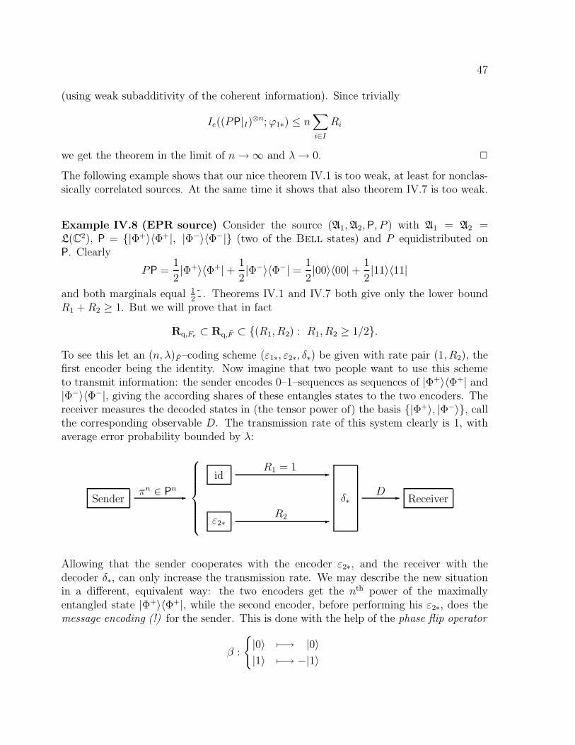
47

(using weak subadditivity of the coherent information). Since trivially

Ie((PP|I)⊗n;ϕ1∗) ≤ n∑

i∈IRi

we get the theorem in the limit of n→ ∞ and λ→ 0. 2

The following example shows that our nice theorem IV.1 is too weak, at least for nonclas-sically correlated sources. At the same time it shows that also theorem IV.7 is too weak.

Example IV.8 (EPR source) Consider the source (A1,A2,P, P ) with A1 = A2 =L(C2), P = |Φ+〉〈Φ+|, |Φ−〉〈Φ−| (two of the Bell states) and P equidistributed onP. Clearly

PP =1

2|Φ+〉〈Φ+| + 1

2|Φ−〉〈Φ−| =

1

2|00〉〈00| + 1

2|11〉〈11|

and both marginals equal 121. Theorems IV.1 and IV.7 both give only the lower bound

R1 +R2 ≥ 1. But we will prove that in fact

Rq,Fe ⊂ Rq,F ⊂ (R1, R2) : R1, R2 ≥ 1/2.

To see this let an (n, λ)F–coding scheme (ε1∗, ε2∗, δ∗) be given with rate pair (1, R2), thefirst encoder being the identity. Now imagine that two people want to use this schemeto transmit information: the sender encodes 0–1–sequences as sequences of |Φ+〉〈Φ+| and|Φ−〉〈Φ−|, giving the according shares of these entangles states to the two encoders. Thereceiver measures the decoded states in (the tensor power of) the basis |Φ+〉, |Φ−〉, callthe corresponding observable D. The transmission rate of this system clearly is 1, withaverage error probability bounded by λ:

Sender -

πn ∈ Pn

id -

R1 = 1

ε2∗ -

R2

δ∗ -

DReceiver

Allowing that the sender cooperates with the encoder ε2∗, and the receiver with thedecoder δ∗, can only increase the transmission rate. We may describe the new situationin a different, equivalent way: the two encoders get the nth power of the maximallyentangled state |Φ+〉〈Φ+|, while the second encoder, before performing his ε2∗, does themessage encoding (!) for the sender. This is done with the help of the phase flip operator

β :

|0〉 7−→ |0〉|1〉 7−→ −|1〉

48

on C2, as it is readily checked that (id⊗β)|Φ+〉 = |Φ−〉. But here the first encoder becomes

superfluous: thus we can assume that initially sender and receiver share n maximallyentangled pairs |Φ+〉〈Φ+|, and the second encoder (viz., the sender!) transmits nR2

qubits to the receiver. This is exactly the situation of superdense coding, invented byBennett & Wiesner (1992): and it is well known that the maximal transmission ratein this situation is 2R2, forcing R2 ≥ 1/2 in the limit of n → ∞, λ → 0. Of coursesymmetrically for R1.

We can note the two lessons we learned:

Theorem IV.1 is too weak.

Theorem IV.7 is too weak.

The last example shows the difference between average and entanglement fidelity:

Example IV.9 (Cloned cross) Consider the source (A1,A2,P, P ) with A1 = A2 =L(C2) and P equidistributed on P = |00〉〈00|, |11〉〈11|. Clearly

PP =1

2|00〉〈00| + 1

2|11〉〈11|

with both marginals equal to 121. A natural purification of this source would be by the

GHZ–state 1√2(|000〉 + |111〉), invented by Greenberger et al. (1990) to extend Bell’s

theorem to multi–party entanglement.Since the average state is the same as in the EPR source we have

Rq,Fe ⊂ (R1, R2) : R1, R2 ≥ 1/2.

On the other hand it is obvious that

Rq,F = (R1, R2) : R1, R2 ≥ 0, R1 +R2 ≥ 1.

It is clear from theorem IV.1 that R1+R2 ≥ 1 is necessary (even with arbitrary encoding).And also one sees easily that R1 = 1, R2 = 0 is (quantum, F )–achievable: A2 sendsnothing, whereas A1 transmits his qubit faithfully, the decoder has just to copy it toobtain the initial joint state (this is only possible because the two alternative states sentby A1 are orthogonal!).

Again collecting our lessons:

Rq,F depends not just on PP.

In general Rq,F and Rq,Fe are different.

Concluding this section we may state that the pleasing situation of chapter I hascompletely dissolved: all three rate concepts differ, and (except for entanglement fidelity)the rate region depends not only on the average state.

49

Classical source with quantum side information

In this and the following section we will turn to the study of a restricted kind of multiplesource, namely csh1–sources, and we will be able to complement the above bewilderingpicture by some positive results (coding theorems).

Theorem IV.10 (Code partition) (Cf. Csiszar & Korner (1981), proof of theorem3.1.2) Let W : X → S(Y) a q–DMC, P a probability distribution on X , λ, δ, η > 0. Thenfor n ≥ n0(|X |, dimH, λ, δ, η) there exist m − 1 ≤ exp(n(H(P ) − I(P ;W ) + 3δ)) many(n, λ)–codes with pairwise disjoint “large” codebooks Ci:

|Ci| ≥ exp(n(I(P ;W ) − 2δ)),

such that P n(X n \⋃m−1i=1 Ci) < η.

Proof. Choose α > 0 such that P n(T nV,P,α) ≥ 1 − η/2 and n large enough such that for

every A ⊂ T nV,P,α with P n(A) ≥ η/2 there is a (n, λ)–code with codebook C ⊂ A and

|C| ≥ exp(n(I(P ;W ) − 2δ)) (by the coding theorem II.4). Now choose such a codebookC1 ⊂ A1 = T n

V,P,α and inductively Ci ⊂ Ai = Ai−1\Ci−1 until P n(Ai) < η/2, say for i = m.Obviously the codebooks are disjoint, and the rest has weight less than η. It remains toestimate m:

(m− 1) · exp(n(I(P ;W ) − 2δ)) ≤m−1∑

i=1

|Ci| ≤ |T nV,P,α| ,

and since by lemma I.8 |T nV,P,α| ≤ exp(n(H(P ) + δ)) for large enough n we get the state-

ment. 2

Consider the problem to encode the classical part of a c1h1–source (X = CX ,Y,X×P, P ),using the quantum source as side information at the decoder:

An n–block coding scheme with quantum side information at the decoder is a pair(f,D), with a mapping f : X n −→ M and an observable D on CM⊗ Y indexed by X .Its error probability (averaged over P ) is

e(f,D) = 1 −∑

xn∈Xn,πn∈Pn

P n(xn, πn)Tr ((f(xn) ⊗ πn)Dxn).

The proof of the following theorem goes back to an idea of Ahlswede (1974b):

Theorem IV.11 (Rate slicing) (Cf. Csiszar & Korner (1981), theorem 3.1.2) Forevery λ, δ > 0 and c1h1–source (X = CX ,Y,X ×P, P ) there exists an n–block code (f,D)with quantum side information at the decoder such that

1

nlog |M| ≤ H(X|Y) + 3δ, and e(f,D) ≤ λ

whenever n ≥ n0(|X |, dimH, ǫ, δ). Furthermore, the observable may be modified to theoperation D′

∗ = Tr CM Dtot∗ from (CM)∗ ⊗ Y∗ to (CX n)∗ ⊗ Y∗ which satisfies∑

xn∈Xn,πn∈Pn

P n(xn, πn) ‖xn ⊗ πn −D′∗(f(xn) ⊗ πn)‖1 ≤

√8λ+ λ.

50

Proof. Define the q–DMC W : X → Y∗ by

Wx =1

PX (x)

∑

π∈P

P (x, π)π

(with the marginal distribution PX of P on X ). Choose η ≤ λ in theorem IV.10, and naccordingly large such that codes (gi, Di), i ∈ [m− 1] like in that theorem exist. Assumethat their message sets coincide with their codebooks and that gi is the identity.

Define now

f(xn) =

i if xn ∈ Ci ,m else.

The decoder reads i = f(xn) and if i 6= m uses Di to recover xn from the side information:formally, D consists of the operators [i] ⊗Dic for i ∈ [m− 1], c ∈ C′

i, and [m] ⊗ 1. Thatthis has the desired properties is easily checked. Now for the second part: observe that

D′∗ : [j] ⊗ ρ 7−→

∑c∈Cj

[c] ⊗√Djcρ

√Djc if j < m,

[m] ⊗ ρ if j = m.

By the tender measurement lemma I.5 and note I.6 the assertion follows. 2

Remark IV.12 The decoder either says “don’t know” (with probability at most λ overthe source distribution P n), or decodes correctly with maximal error probability λ.

Corollary IV.13 For the c1h1–source (X = CX ,Y,X × P, P ) the pair (H(X|Y), H(Y))is (quantum, F )–achievable.

Proof. Combine theorem IV.11 with Schumacher’s quantum coding. 2

Consider now the csh1–source

((Xi = CXi|i ∈ [s]),Y,X1 × · · · × Xs × P, P ).

An n–block coding scheme with quantum side information at the decoder for this isa (s + 1)–tuple (f1, . . . , fs, D) of mappings fi : X n

i → Mi and an observable D onX1 ⊗ · · · ⊗ Xs ⊗ Y, indexed by X n

1 × · · · × X ns . Its error probability (averaged over P ) is

e(f1, . . . , fs, D) = 1 −∑

xni ∈Xn

i ,ρ∈Pn

P (xn1 , . . . , xns , ρ)Tr ((f1(x

n1 ) ⊗ · · · ⊗ fs(x

ns ) ⊗ ρ)Dxn

1...xn

s).

Theorem IV.14 With the notation above and λ, δ > 0 there exists an n–block codingscheme with quantum side information at the decoder with

∀J ⊂ [s]1

n

∑

j∈Jlog |Mj| ≤ H(X(J)|X(Jc)Y) + |J | · 3δ

51

and error probability at most λ, whenever n ≥ n0(|Xi|, dimH, λ, δ).Moreover for the operation D′

∗ = Tr C(M1×···×Ms) Dtot∗,

D′∗ : C(M1 × · · · ×Ms)∗ ⊗ Y⊗n

∗ → C(X n1 × · · · × X n

s )∗ ⊗ Y⊗n∗ ,

it holds that∑

xni∈Xn

i ,ρ∈Pn

P (xn1 , . . . , xns , ρ)‖[xn1 . . . xns ] ⊗ ρ−D′

∗([f1(xn1 ) . . . fs(x

ns )] ⊗ ρ)‖1 ≤ λ.

Proof. Only the second statement is to be proved. We use induction on s, the number ofsources: s = 1 is clear by direct application of the rate slicing theorem IV.11. For s > 1 itis sufficient (by the time sharing principle) to consider only extreme points of the region:thus w.l.o.g.

1

nlog |M1| ≤ H(X1|Y) + 3δ

1

nlog |M2| ≤ H(X2|X1Y) + 3δ

. . .

1

nlog |Ms| ≤ H(Xs|X1 · · ·Xs−1Y) + 3δ.

The proof that these are indeed the extreme points is in the section Extreme points ofrate regions below.

Now by induction we have an (n, λ/2)–coding scheme for the source

((Xi = CXi|i ∈ [s− 1]),Xs ⊗ Y,X1 × · · · × Xs−1 × (Xs × P), P ),

call its decoding operation D′1∗. By rate slicing we also have an (n, λ/2)–coding scheme

for the source (Xs,Y,Xs × P, P ) with side information at the decoder, call its decodingoperation D′

2∗. Then the concatenation D′∗ = D′

1∗ (id ⊗ D′2∗) of the two processes

obviously has the desired error properties, and it is readily checked that it has the statedform. By tracing out Y⊗n we recover the observable D. 2

Remark IV.15 The theorem shows that not only we can use quantum side information“just like” classical information to improve compression but also that we can do so withalmost not disturbing the quantum information.

Corollary IV.16 For the above source all tuples (R1, . . . , Rs, H(Y)) satisfying

∀J ⊂ [s]∑

j∈JRj ≥ H(X(J)|X(Jc)Y)

are (quantum, F )–achievable.

52

Proof. Combine theorem IV.14 with Schumacher’s quantum coding. 2

We close this section with a converse to these coding theorems:

Theorem IV.17 Still with the above source all (quantum, F )–achievable rate tuples ofthe form (R1, . . . , Rs, H(Y)) satisfy

∀J ⊂ [s]∑

j∈JRj ≥ H(X(J)|X(Jc)Y).

Proof. Otherwise we could by theorem III.5 construct an infinite sequence of transmissionn–block codes for the quantum multiple access channel

W : X1 × · · · × Xs −→ S(Y)

(x1, . . . , xs) 7−→1

PX1×···×Xs(x1 . . . xs)

∑

π∈P

P (x1 . . . xs, π)

which violate the outer bounds of theorem III.1. 2

Quantum source with classical side information

The simplest instance of the problem considered in the previous section is the case ofthe c1q1–source. There we solved the problem of compressing the classical source withthe quantum information as side information at the decoder, which gave us one extremepoint of the rate region of the multiple source coding problem. It is natural, therefore,to consider the complementary problem of compressing the quantum source, using theclassical information as side information, preferably only at the decoder: this would giveus another extreme point, presumably completing the determination of the rate region ofthe c1q1–source (if the bounds of theorem IV.1 are already the correct ones).

An n–block quantum source coding scheme with side information at the decoder forthe c1q1–source (X = CX ,Y = L(H),X × P, P ) is a pair (ε∗, δ∗) with a mapping

ε∗ : Pn −→ S(L(K))

and a family of quantum operations

δ∗ : X n × L(K)∗ −→ Y⊗n∗ .

Quantum and arbitrary encoding are as before, also rate, and the average fidelity is

F = F (ε∗, δ∗) =∑

(xn,πn)∈Xn×Pn

P n(xn, πn)·Tr ((δ∗(xn)ε∗π

n)πn)

(average distortion D(ε∗, δ∗) similarly).

53

The limiting rates Rq,F (λ) and Ra,F (λ) are defined obviously. What can we say aboutthem? From theorem IV.1 we get at least

lim infλ→0

Rq,F (λ) ≥ H(Y|X) =∑

x∈XPX (x)H

(∑

π∈P

P (x, π)

PX (x)π

).

In fact even Ra,F (λ) ≥ H(Y|X) for λ ∈ (0, 1): otherwise we could (with compressingX classically, e.g. by ignoring all non–typical sequences) compress the total source XY

with asymptotically at most Ra,F (λ) + H(X) < H(Y|X) + H(X) = H(XY) qubits persymbol, contradicting theorem I.22.

At present we do not know if one can approach this bound. But let us make anexperiment! Assume that also the encoder has the side information, i.e. now

ε∗ : X n × Pn −→ S(Y).

Since we are interested only in average performance it suffices that the scheme workswell for typical xn ∈ X n, say xn ∈ T n

V,PX ,α. To encode this the encoder has just to

collect the positions of equal x ∈ X and do Schumacher quantum coding on blocks oflength nPX (x)±α

√PX (x)(1 − PX (x))

√n. This scheme — with side information both at

the encoder and the decoder — obviously achieves the rate H(Y|X) asymptotically witharbitary high fidelity.

The c0q2–source: coding vs. side information

With the c1q1–source the idea to consider extreme points in a certain convex region proveduseful, and in connection with this the idea to encode only part of the source while usingthe rest as side information at the decoder.

Whereas this paradigm is of undoubted worth in the classical theory, where we took itfrom (and which gave us some insights already for quantum communication problems, notjust in the two previous sections but also in chapter III), in general one must be cautiouswith it: using quantum information often means using it up. As an illustration consideronce more the cloned wheel example IV.2:

Obviously we can encode A1 with rate zero, with side information from A2 at thedecoder, because the state π on A2 is a faithful copy of the lost state π on A1. This is ofcourse in contrast to theorem IV.1, and we can note our last lesson:

Coding independent sources is not reducible to coding with side information.

Extreme points of rate regions

Here we prove the claim in the proof of theorem IV.14 that every extremal point of theregion of all (R1, . . . , Rs) which satisfy for all J ⊂ [s]

R(J) =∑

i∈JRi ≥ H(X(J)|YX(Jc)) (J)

54

is of the form

Rπ(i) = H(Xπ(i)|YXπ(1) · · ·Xπ(i−1))

for a permutation π of the set [s], and that these points all belong to the above region.

Assume that we have an extremal point: it follows that s of the inequalities (J) aremet with equality. Choose one, say K:

R(K) = H(X(K)|YX(Kc)).

We claim that we can find the remaining inequalities (J) met with equality among theJ ⊂ K or J ⊃ K. This follows from the following

Lemma IV.18 From R(K) = H(X(K)|YX(Kc)) the validity of (J) for all J followsfrom the validity for those which contain K or are contained in K.

Proof. First consider J ⊃ K: there we have

R(J \K) ≥ H(X(J)|YX(Jc)) −H(X(K)|YX(Kc)).

Thus for arbitrary J , setting J1 = J ∩K, J2 = J ∩Kc, one obtains

R(J) ≥ H(X(J1)|YX(Jc1)) +H(X(J2 ∪K)|YX(Jc2 ∩Kc)) −H(X(K)|YX(Kc))

= H(YX1 · · ·Xs) −H(YX(Jc1)) −H(YX(Jc2 ∩Kc)) +H(YX(Kc))

≥ H(YX1 · · ·Xs) −H(X(Jc1 ∩ Jc2))= H(X(J)|YX(Jc))

by strong subadditivity (theorem A.9), applied to A1 = X(J2), A2 = YX(Kc \ J2) andA3 = X(K \ J1). 2

If K is not a singleton there must be equalities below K, if K 6= [s] there must besome above: otherwise it is easily seen that we are not in an extremal point. So byinduction we arrive at a chain ∅ 6= K1 ⊂ K2 ⊂ . . . ⊂ Ks = [s] of equalities, w.l.o.g.Ki = s, s− 1, . . . , s+ 1 − i, which produces

Ri = H(Xi|YX1 · · ·Xi−1).

To see that this is indeed a point of the region apply again the lemma, iteratively.

Open questions

The reader will have noticed that the past chapter consisted mainly of open questions,skilfully disguised as half theorems, examples and suggestions. For convenience we collecthere some of the more important problems:

55

Examples Clarify example IV.2: are there coding schemes with R1 = 1, R2 = 1/2?Clarify the examples IV.8 and IV.9: can one improve the bounds? or can one actually

construct coding schemes with R1 = R2 = 1/2, or at least R1 = 1, R2 = 1/2 for one orboth of them?

The c1q1–source Solve the c1q1–source completely! From the above it is enough toconsider quantum source coding with classical side information, since we conjecture thattheorem IV.1 gives (at least in this case) already the right bounds.

More complicated sources Solve the c0q2–source: it seems that it is easier if we insiston no entanglement, but this might be a deception.

Consider entanglement fidelity This seems to be the only right choice if dealingwith arbitrary kinds of correlation. Also it simplifies things a bit: namely at least theresult will depend only on the average state of the source.

Techniques The only technique for code construction was the “code partition” trick.This is not satisfactory, as it destroys artificially the symmetry of the situation; also wehave to resort to a channel coding theorem.

A promising direct approach that may be converted to work for the quantum problemsis the hypergraph coloring paradigm (see Ahlswede (1979) and Ahlswede (1980)). Sucha program would involve to elaborate further on techniques describable maybe by the termnoncommutative combinatorics.

Guiding ideas? One of the initial motivations of the work in this chapter was theidea that the classical Slepian–Wolf theorem is one possibility to give operationalmeaning to conditional entropies. As such a thing is completely lacking in quantuminformation theory, and on the other hand only formal definitions of quantum conditionalentropy exist (derived from analogies, say with classical quantities), without consistentoperational meaning, one sees that solving the above coding theorems would clarify thispoint dramatically.

It is interesting to note that already at this stage we can foresee (from the lessonswe learned from our examples) that there must be necessarily several natural notions ofconditional entropy.

Also we observe that the theory around Schumacher’s coherent information fails togive the right answers even to simple problems. I suspect that this comes from the factthat this theory builds on pair entanglement, whereas our situations involved multi–partyentanglement.

56

Appendix A

Quantum Probability andInformation

In this appendix the basic mathematical machinery of quantum probability with specialattention to information theory is collected. Alongside we introduce a calculus of en-tropy and information quantities in quantum systems. Whenever possible we refer to theliterature instead of giving full proofs.

Quantum systems

In classical probability theory one has generally two ways of seeing things: either throughdistributions (and the relation of their images, mostly marginals), or through randomvariables (with a joint distribution). Both ways have their merits (though random vari-ables are considered more elegant), but basically they are equivalent, in particular nonelacks anything without the other. Things are different in quantum probability, and wewill take the following view: the analog of a distribution is a density operator on somecomplex Hilbert space, whereas the analog of random variables are observables, definedbelow. With density operators alone we can study physical processes transforming them,but every experiment involves some observable. Studying observables one usually fixesthe underlying density operator (as the statistics of the experiments depend on the latter),but this falls short of not appropriately reflecting our manipulating quantum states, orhaving several alternative states.

For the following we refer to textbooks on C∗–algebras like Arveson (1976), andstandard references on basic mathematics of quantum mechanics: Davies (1976), Kraus

(1983), and the more advanced Holevo (1982).A C∗–algebra with unit is a complex Banach space A which is also a C–algebra with

unit 1 and a C–antilinear involution ∗, such that

‖AB‖ ≤ ‖A‖‖B‖, ‖A∗‖2 = ‖A‖2 = ‖AA∗‖

These algebras will be the mathematical models for quantum systems, and subsystems

57

are simply ∗–subalgebras (which are always assumed to be closed).The set A+ of A ∈ A that can be written as A = BB∗ is called the positive cone of A

which is norm closed, and induces a partial order ≤. By the famous Gelfand–Naimark–

Segal representation theorem (see e.g. Arveson (1976)) every C∗–algebra is isomorphicto a closed ∗–subalgebra of some L(H), the algebra of bounded linear operators on theHilbert space H. With us all C∗–algebras will be of finite dimension. It is known thatthose algebras are isomorphic to a direct sum of L(Hi) (see e.g. Arveson (1976)). Thisincludes as extremal cases the algebras L(H), and the commutative algebras CX over afinite set X , with the generators x ∈ X as idempotents. In particular we have on everysuch algebra a well defined and unique trace functional, denoted Tr , that assigns traceone to all minimal positive idempotents.

States A state on a C∗–algebra A is a positive C–linear functional ρ with ρ(1) = 1.Positivity here means that its values on the positive cone are nonnegative. Clearly thestates form a convex set S(A) whose extreme points are called pure states, all others aremixed. For A = L(H) the pure states are exactly the one–dimensional projectors, i.e.using Dirac’s bra–ket–notation, the |ψ〉〈ψ| with unit vector |ψ〉 ∈ H.

One can easily see that every state ρ can be represented uniquely in the form ρ(X) =Tr (ρX) for a positive, selfadjoint element ρ of A with trace one (such elements are calleddensity operators). In the sequel we will therefore make no distinction between ρ and itsdensity operator ρ. The set of operators with finite trace will be denoted A∗, the traceclass in A which contains the states and is a two–sided ideal in A, the Schatten–ideal(in our — finite dimensional — case this is of course just A). Then Tr (ρA) defines areal bilinear and positive definite pairing of A∗s and As, the selfadjoint parts of A∗ andA, which makes As the dual of A∗s. Notice that in this sense pure states are equivalentlydescribed as minimal selfadjoint idempotents of A.

Observables Let F be a σ–algebra on some set Ω, X a C∗–algebra. A map X : F −→ X

is called a positive operator valued measure (POVM), or an observable, with values in X

(or on X), if:

1. X(∅) = 0, X(Ω) = 1.

2. E ⊂ F implies X(E) ≤ X(F ).

3. If (En)n is a countable family of pairwise disjoint sets in F then X(⋃nEn) =∑

nX(En) (in general the convergence is to be understood in the weak topology:for every state its value at the left equals the limit value at the right hand side).

If the values of the observable are all projection operators and Ω is the real line one speaksof a spectral measure or a von Neumann observable.1 An observable X together with a

1Strictly speaking this term only applies to the expectation of the measure (in general an unboundedoperator), but this in turn by the spectral theorem determines the measure.

58

state ρ yields a probability measure PX on Ω via the formula

PX(E) = Tr (ρX(E)).

In this way we may view X as a random variable with values in X, its distribution wedenote PX (note that PX may not be isomorphic to PX : if X takes the same value ondisjoint events, which means that X introduces randomness by itself).

Two observables X, Y are said to be compatible, if they have values in the same algebraand XY = Y X elementwise, i.e. for all E ∈ FX , F ∈ FY : X(E)Y (F ) = Y (F )X(E)(Note that it is possible for an observable not to be compatible with itself). By the way,the term compatible may be defined in obvious manner for arbitrary sets or collections ofoperators, in which meaning we will use it in the sequel. If X, Y are compatible we maydefine their joint observable XY : FX × FY −→ X mapping E × F to X(E)Y (F ) (thisdefines the product mapping uniquely just as in the classical case of product measures). Infact we can analogously define the joint observable for any collection of pairwise compatibleobservables.2 As the random variable of a product XY we will take X × Y , rather thanXY itself, with values in X × X (because the same product operator may be generatedin two different ways which we want to distinguish). To indicate this difference we willsometimes write X · Y for the product.

Note that here we can see the reason why we cannot just consider all observables asrandom variables (and forget about the state): they will not have a joint distribution, atfirst of course only by our definition. But Bell’s theorem (Bell (1964)) shows that onecomes into trouble if one tries to allow a joint distribution for noncompatible observables.Conversely we see why we cannot do without observables, even though ρ contains all pos-sible information: the crux is that we cannot access it due to the forbidden noncompatibelobservables (a good account of this aspect of quantum theory is by Peres (1995)).

From now on all observables will be countable, i.e. w.l.o.g. are they defined on acountable Ω with σ–algebra 2Ω. This means that we may view an observable X as aresolution of 1 into a countable sum 1 =

∑j∈ΩXj of positive operators Xj .

If A1,A2 are subalgebras of A, they are compatible if they commute elementwise(again note, that a subalgebra need not not be compatible with itself: in fact it is iff itis commutative). In this case the closed subalgebra generated (in fact: spanned) by theproducts A1A2, Ai ∈ Ai is denoted A1A2.

Operations Now we describe the transformations between quantum systems: a C–linear map ϕ : A2 → A1 is called a quantum operation if it is completely positive (i.e.positive, so that positive elements have positive images, and also the ϕ⊗ idn are positive,where idn is the identity on the algebra of n × n–matrices), and unit preserving. Thesemaps are in 1–1 correspondence with their (pre–)adjoints ϕ∗ by the trace form, mapping

2Observe however that in general a joint observable might exist for non–compatible (i.e. non–commuting) observables. The operational meaning of this is that there is a common refinement of theinvolved observables. If they commute then this certainly is possible as demonstrated, but commutativityis not necessary.

59

states to states, and being completely positive and trace preserving.3 Since here we restrictourselves to finite dimensional algebras the adjoint map simply goes from A1 to A2, butto keep things well separated (which they actually are in the infinite case) we write theadjoint as ϕ∗ : A1∗ → A2∗, the dual map (in fact we consider this as the primary objectand the operator maps as their adjoint, which is the reason for writing subscript ∗). Noticethat ϕ∗ is sometimes considered as restricted to ϕ∗ : S(A1) → S(A2). A characterizationof quantum operations is by the Stinespring dilation theorem (Stinespring (1955)):

Theorem A.1 (Dilation) Let ϕ : A → L(H) a linear map of C∗–algebras. Then ϕ iscompletely positive if and only if there exist a representation α : A → L(K), with Hilbertspace K, and a bounded linear map V : H → K such that

∀A ∈ A ϕ(A) = V ∗α(A)V.

For proof see e.g. Davies (1976). A commonly used corollary of this is

Corollary A.2 (cf. Kraus (1983)) Let ϕ : L(H2) → L(H1) a linear map of C∗–algebras.Then ϕ is completely positive and unit preserving if and only if there exist linear mapsBi : H1 → H2 with

∑iB

∗iBi = 1H1

and

∀A ∈ L(H2) ϕ(A) =∑

i

B∗iABi .

Norms and norm inequalities For the C∗–algebra L(H) of linear operators on thecomplex Hilbert space H (of dimension d) the norm is the supremum norm ‖ · ‖∞, i.e.‖A‖∞ is the largest absolute value of an eigenvalue of A. The other important norm weuse is the trace norm ‖ · ‖1: ‖α‖1 is the sum of the absolute values of all eigenvalues of α.Note the important formula

‖α‖1 = sup|Tr (αB)| : ‖B‖∞ ≤ 1,which explains the name “trace norm”. Its proof is by the polar decomposition of α,see e.g. Arveson (1976). Also it implies immediately that ‖ · ‖1 is nonincreasing underquantum operations. Obviously

‖α‖∞ ≤ ‖α‖1 ≤ d‖α‖∞ .

If α is self–adjoint we have the unique decomposition (via diagonalization) α = α+ − α−into the positive and negative part of α, where α+, α− ≥ 0 and α+α− = 0. Then note

‖α‖1 = Trα+ + Trα− = supTr (αB) : −1 ≤ B ≤ 1and

Trα+ = supTr (αB) : 0 ≤ B ≤ 1.It should be clear that all the above suprema are in fact maxima.

Finally note that these observations still hold for any direct sum of L(Hi), d beingreplaced by the sum of the dimHi.

3In general this is only true if we restrict ϕ to be a normal map, cf. Davies (1976).

60

Entropy and divergence

The von Neumann entropy of a state ρ (introduced by von Neumann (1927)4) isdefined as H(ρ) = −Tr (ρ log ρ), which reduces to the usual Shannon entropy for acommutative algebra because then a state is nothing but a probability distribution. Forstates ρ, σ also introduce the I–divergence, or simply divergence (first defined by Umegaki

(1962)) as D(ρ‖σ) = Tr (ρ(log ρ − log σ)) with the convention that this is ∞ if supp ρ 6≤supp σ (supp ρ being the support of ρ, the minimal selfadjoint idempotent p with pρp = ρ).For properties of these quantities we will often refer to Ohya & Petz (1993), and toWehrl (1978). Three important facts we will use are

Theorem A.3 (Klein inequality) For positive operators ρ, σ (not necessarily states)

D(ρ‖σ) ≥ 1

2Tr (ρ− σ)2 + Tr (ρ− σ).

In particular for states the divergence is nonnegative, and zero if and only if they areequal.

Proof. See Ohya & Petz (1993). 2

Lemma A.4 (Continuity) Let ρ, σ states with ‖ρ− σ‖1 ≤ θ ≤ 1

2. Then

|H(ρ) −H(σ)| ≤ −θ logθ

d= dη

(θ

d

).

Proof. See Ohya & Petz (1993). 2

Theorem A.5 (Monotonicity) Let ρ, σ be states on a C∗–algebra A, and ϕ∗ a tracepreserving, completely positive linear map from states on A to states on B. Then

D(ϕ∗ρ‖ϕ∗σ) ≤ D(ρ‖σ).

Proof. See Uhlmann (1977); the situation we are in was already solved by Lindblad

(1975). For a textbook account see Ohya & Petz (1993). 2

Observable language

This and the following two sections will introduce language (or formalism) to talk aboutentropy and information in the context of quantum systems in a transparent fashion.

Fix a state on a C∗–algebra, say ρ on A and let X, Y, Z compatible observables onA. These are then random variables with a joint distribution, and one defines entropy

4It was in fact introduced independently in the same year by Landau and Weyl.

61

H(X), conditional entropy H(X|Y ), mutual information I(X ∧ Y ), and conditional mu-tual information I(X ∧ Y |Z) for these observables as the respective quantities for theminterpreted as random variables. Note however that these depend on the underlying stateρ. In case of need we will thus add the state as an index, like Hρ(X) = H(X), etc.

As things are there is not much to say about that part of the theory. We only notesome useful formulas:

H(X|Y ) =∑

j

Tr (ρYj)Hρj(X), with ρj =

1

Tr (ρYj)

√Yjρ√Yj

(which is an easy calculation using the compatibility of X and Y ), and

I(X ∧ Y ) = H(X) +H(Y ) −H(XY )

= D(PXY ‖PX ⊗ P Y ) = D(PX·Y ‖PX ⊗ PY )

(whose analogue is known from classical information theory).

Subalgebra language

Let X,X1,X2,Y compatible ∗–subalgebras of the C∗–algebra A, and ρ a fixed state on A.First consider the inclusion map ı : X → A (which is certainly completely positive)

and its adjoint ı∗ : A∗ → X∗. Define

H(X) = H(ı∗ρ)

(where at the right hand appears the von Neumann entropy). For example for X = A

we obtain just the von Neumann entropy of ρ. For the trivial subalgebra C = C1(which obviously commutes with every subalgebra) we obtain, as expected, H(C) = 0.The general philosophy behind this definition is that H(X) is the von Neumann entropyof the global state viewed through (or restricted to) the subsystem X. To reflect this inthe notation we define ρ|X = ı∗ρ.

Now conditional entropy, mutual information, and conditional mutual information aredefined by reducing them to entropy quantities:

H(X|Y) = H(XY) −H(Y)

I(X1 ∧ X2) = H(X1) +H(X2) −H(X1X2)

= H(X2) −H(X2|X1)

I(X1 ∧ X2|Y) = H(X1|Y) +H(X2|Y) −H(X1X2|Y)

= H(X1Y) +H(X2Y) −H(X1X2Y) −H(Y).

62

It is not at all clear a priori that these definitions are all well behaved: while it is ob-vious from the definition that the entropy is always nonnegative, this is not true for theconditional entropy (as was observed by several authors before): if A = X⊗Y and ρ is apure entangled state then H(X|Y) = −H(Y) < 0. This might raise pessimism whetherthe other two quantities also are (at least sometimes) pathological. This they are not (atleast not in this way), as will be shown in a moment:

We have the following commutative diagram of inclusions, and the natural multiplica-tion map µ (which is in fact a ∗–algebra homomorphism, and thus completely positive!):

X1 X1 X1yϕ1

yı1y1

X1 ⊗ X2µ−−−→ X1X2

−−−→ Axϕ2

xı2x2

X2 X2 X2

And hence the corresponding commutative diagram of adjoint maps (note that ϕ1∗ andϕ2∗ are just partial traces). With this we find

I(X1 ∧ X2) = H(X1) +H(X2) −H(X1X2)

= H(1∗ρ) +H(2∗ρ) −H(∗ρ)

= H(ϕ1∗µ∗∗ρ) +H(ϕ2∗µ∗∗ρ) −H(µ∗∗ρ)

= D(µ∗∗ρ‖ϕ1∗µ∗∗ρ⊗ ϕ2∗µ∗∗ρ)

by definition, then by commutativity of the diagram and the fact that µ∗ preserves eigen-values of density operators (because µ is a surjective ∗–homomorphism, see lemma A.6below), the last by direct calculation on the tensor product (just as for the classical for-mula). From the last line we see that the mutual information is nonnegative becausethe divergence is, by theorem A.3 (we could also have seen this already from the defi-nition by applying subadditivity of von Neumann entropy to the second last line, seetheorem A.9).

Lemma A.6 Let µ : A → B a surjective ∗–algebra homomorphism. Then

1. For all pure states p ∈ S(A): µ(p) is pure or 0.

2. For all A ∈ A, A ≥ 0: TrA ≥ Trµ(A).

3. For pure p ∈ S(A), q ∈ S(B):

µ∗(µ(p)) = p or µ(p) = 0, µ(µ∗(µ(p))) = µ(p), µ(µ∗(q)) = q.

4. For ρ ∈ S(B), µ∗(ρ) =∑

i αipi diagonalization with the αi > 0, then ρ =∑

i αiµ(pi)is a diagonalization.

63

5. Conversely every diagonalization of a state on B is by µ∗ translated into a diago-nalization of its µ∗–image.

Proof.

1. We have only to show that µ(p) is minimal if it is not 0: let q′ any pure state withq′ ≤ µ(p). Then

1 = Tr (q′µ(p)) = Tr (µ∗(q′)p) ≤ Tr (p) = 1.

So we must have equality which implies p ≤ µ∗(q′), but both operators are states,

so p = µ∗(q′). Because µ∗ is injective this means that there is only one pure state

q′ ≤ µ(p), i.e. µ(p) is pure.

2. We may write A =∑

i aipi with pure states pi and ai ≥ 0. Then µ(A) =∑

i aiµ(pi)and since pure states have trace 1 the assertion follows from (1).

3. Let A ∈ A, A ≥ 0. Then

Tr (µ∗(µ(p))A) = Tr (µ(p)µ(A)) = Tr (µ(p)µ(A)µ(p))

= Tr (µ(pAp)) ≤ Tr (pAp) = Tr (pA).

Thus µ∗(µ(p)) ≤ p. If µ(p) 6= 0 it is a pure state, hence µ∗(µ(p)) a state whichforces µ∗(µ(p)) = p. This proves the left formula, the middle follows immediately,and for the right observe that we may choose a pure pre–image p of q (in fact thatwill be µ∗(q), as one can see from (4)).

4.∑

i αiµ(pi) is certainly the diagonalization of some positive operator since the µ(pi)which are not 0 are by the homomorphism property and by (1) pairwise orthogonalpure states. Now observe µ(µ∗(ρ)) =

∑i αiµ(pi) and

µ∗(ρ) = µ∗(µ(µ∗(ρ))) =∑

i

αiµ∗(µ(pi)) ≤∑

i

αipi = µ∗(ρ),

hence equality, i.e. all µ(pi) are pure. From

µ∗(ρ) =∑

i

αiµ∗(µ(pi)) = µ∗(∑

i

αiµ(pi))

and injectivity of µ∗ the assertion follows.

5. This is a direct consequence of (3) and (4).

2

For the conditional mutual information we have to do somewhat more (yet from thedefinition we see that its positivity will have something to do with the strong subadditivityof von Neumann entropy, see theorem A.9):

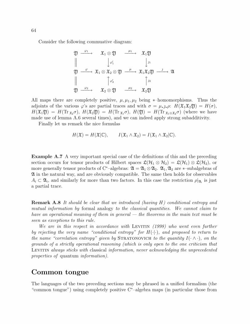
64

Consider the following commuative diagram:

Yϕ1−−−→ X1 ⊗ Y

µ1−−−→ X1Y∥∥∥yϕ′

1

y1

Yϕ−−−→ X1 ⊗ X2 ⊗ Y

µ−−−→ X1X2Y−−−→ A∥∥∥

xϕ′

2

x2

Yϕ2−−−→ X2 ⊗ Y

µ2−−−→ X2Y

All maps there are completely positive, µ, µ1, µ2 being ∗–homomorphisms. Thus theadjoints of the various ϕ’s are partial traces and with σ = µ∗∗ρ: H(X1X2Y) = H(σ),H(X1Y) = H(Tr X2

σ), H(X2Y) = H(Tr X1σ), H(Y) = H(Tr X1⊗X2

σ) (where we havemade use of lemma A.6 several times), and we can indeed apply strong subadditivity.

Finally let us remark the nice formulas

H(X) = H(X|C), I(X1 ∧ X2) = I(X1 ∧ X2|C).

Example A.7 A very important special case of the definitions of this and the precedingsection occurs for tensor products of Hilbert spaces L(H1 ⊗ H2) = L(H1) ⊗ L(H2), ormore generally tensor products of C∗–algebras: A = A1 ⊗A2. A1,A2 are ∗–subalgebras ofA in the natural way, and are obviously compatible. The same then holds for observablesAi ⊂ Ai, and similarly for more than two factors. In this case the restriction ρ|Ai

is justa partial trace.

Remark A.8 It should be clear that we introduced (having H) conditional entropy andmutual information by formal analogy to the classical quantities. We cannot claim tohave an operational meaning of them in general — the theorems in the main text must beseen as exceptions to this rule.

We are in this respect in accordance with Levitin (1998) who went even furtherby rejecting the very name “conditional entropy” for H(·|·), and proposed to return tothe name “correlation entropy” given by Stratonovich to the quantity I(· ∧ ·), on thegrounds of a strictly operational reasoning (which is only open to the one criticism thatLevitin always sticks with classical information, never acknowledging the unprecedentedproperties of quantum information).

Common tongue

The languages of the two preceding sections may be phrased in a unified formalism (the“common tongue”) using completely positive C∗–algebra maps (in particular those from

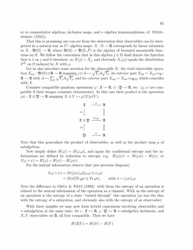
65

or to commutative algebras, inclusion maps, and ∗–algebra homomorphisms, cf. Stine-

spring (1955)).That this is promising one can see from the observation that observables can be inter-

preted in a natural way as C∗–algebra maps: X : Ω → A corresponds by linear extensionto X : B(Ω) → A, where B(Ω) = B(Ω,F) is the algebra of bounded measurable func-tions on Ω. We follow the convention that in this algebra j ∈ Ω shall denote the functionthat is 1 on j and 0 elsewhere, so X(j) = Xj , and obviously X∗(ρ) equals the distributionPX on Ω induced by X with ρ.

Let us also introduce some notation for the observable X: the total observable opera-tion Xtot : B(Ω)⊗A → A mapping j⊗A 7→

√YjA

√Yj, its interior part Xint = Xtot ıA :

A → A with A 7→∑j

√YjA

√Yj, and its exterior part Xext = Xtot ıB(Ω) which coincides

with X.Consider compatible quantum operations ϕ : X → A, ψ : Y → A, etc. (ϕ, ψ are com-

patible if their images commute elementwise). In this case their product is the operationϕψ : X ⊗ Y → A mapping X ⊗ Y 7→ ϕ(X)ψ(Y ):

Xϕ−−−→ A

ϕ1

y∥∥∥

X ⊗ Y∃!ϕψ−−−→ A

ϕ2

x∥∥∥

Yψ−−−→ A

Note that this generalizes the product of observables, as well as the product map µ ofsubalgebras.

Now simply define H(ϕ) = H(ϕ∗ρ), and again the conditional entropy and the in-formations are defined by reduction to entropy, e.g. H(ϕ|ψ) = H(ϕψ) − H(ψ), orI(ϕ ∧ ψ) = H(ϕ) +H(ψ) −H(ϕψ).

For the mutual information observe that (see previous diagram)

I(ϕ ∧ ψ) = D((ϕψ)∗ρ‖ϕ∗ρ⊗ ψ∗ρ)

= D(σ‖Tr Yσ ⊗ Tr Xσ), with σ = (ϕψ)∗ρ.

Note the difference to Ohya & Petz (1993): with them the entropy of an operation isrelated to the mutual information of the operation as a channel. With us the entropy ofan operation is the entropy of a state “viewed through” this operation (as was the ideawith the entropy of a subsystem, and obviously also with the entropy of an observable).

With these insights we may now form hybrid expressions involving observables and∗–subalgebras at the same time: let ı : X → A, : Y → A ∗–subalgebra inclusions, andX, Y observables on A, all four compatible. Then we have

H(X|Y ) = H(ıY ) −H(Y )

66

I(X ∧ Y ) = H(ı) +H(Y ) −H(ıY ),

and lots of others. From the previous section we know that the information quantitiesare nonnegative, but also the entropy conditional on an observable, from the formula

H(X|Y ) =∑

j

Tr (ρYj)Hρj(X), with ρj =

1

Tr (ρYj)

√Yjρ√Yj .

But again there are some expressions which seem suspicious, like

H(X|Y) = H(X) −H(Y).

However, due to the inequality of theorem A.20 in fact it behaves nicely.

Inequalities

Entropy Let us first note the basic

Theorem A.9 For compatible ∗–subalgebras A1,A2,A3 one has:

1. Subadditivity: H(A1A2) ≤ H(A1) +H(A2).

2. Strong subadditivity: H(A1A2A3) +H(A2) ≤ H(A1A2) +H(A2A3).

(In our language this is equivalent to the more natural form

H(A1A3|A2) ≤ H(A1|A2) +H(A3|A2)).

Proof. Subadditivity is a special case of strong subadditivity: A2 = C. The latter canbe reduced to the familiar form, proved first by Lieb & Ruskai (see the references inUhlmann (1977)), by the same type of argument as we used in the section Subalgebralanguage for the nonnegativity of conditional mutual information. 2

Another kind of inequality may serve as an operational justification of the definitionof von Neumann entropy. Call a quantum operation ϕ : A1 → A2 doubly stochastic ifit preserves the trace, i.e. for all A ∈ A1: Trϕ(A) = TrA (see Ohya & Petz (1993)).We will consider the less restrictive condition Trϕ(A) ≤ TrA, and for an observableX, a ∗–subalgebra X let us say it is maximal in A if X, the inclusion map has thisproperty, respectively (obviously for the ∗–subalgebra this implies doubly stochastic).Main examples are: an observable whose atoms are minimal in the target algebra, i.e.have only trivial decompositions into positive operators, and a maximal commutative∗–subalgebra.

Theorem A.10 (Entropy increase) Let ϕ : Y → X with Trϕ(A) ≤ TrA, and ψ :X → A quantum operations. Then H(ψ ϕ) ≥ H(ψ). (Notice that in the physical sensethe operation ϕ∗ is applied after ψ∗).

67

Before we prove this let us note two important case of equality: Let ρ =∑

i λipi withmutually orthogonal pure states pi, λi ≥ 0,

∑i pi = 1. Then equality holds for the ∗–

subalgebra generated by the pi (in fact for any ∗–subalgebra which contains them), andfor the observable that corresponds to the pi’s resolution of 1.Proof of theorem A.10. Let σ = ψ∗ρ, we have to prove H(ϕ∗σ) ≥ H(σ). From theprevious discussion we see that we may assume Y to be commutative, without changingthe trace relation. Let σ =

∑i αipi a diagonalization with pure states pi on X, and qj the

family of minimal idempotents of Y (which by commutativity are othogonal). Then wehave decompositions ϕ∗pi =

∑j βijqj , hence

ϕ∗σ =∑

i

αiϕ∗pi =∑

j

(∑

i

αiβij

)qj .

Now observe that for all j

∑

i

βij = Tr

(qj∑

i

ϕ∗pi

)= Tr

((ϕqj)

∑

i

pi

)= Tr (ϕqj) ≤ Tr (qj) = 1,

and the result follows from the formulas H(σ) = H(αi|i), H(ϕ∗σ) = H(∑

i βijαi|j). 2

Let us formulate the special cases of maximal observables and maximal ∗–subalgebrasas a corollary:

Corollary A.11 Let X an observable maximal in X, then H(X) ≥ H(X). Let X′ a∗–subalgebra maximal in X, then H(X′) ≥ H(X). 2

An application of this is in the proof of

Theorem A.12 Let X,Y compatible, ρ|XY pure. Then H(X) = H(Y).

Proof. By retracting the state ρ to X ⊗ Y by the multiplication map µ : X ⊗ Y → XY

(see lemma A.6) and embedding X and Y into full matrix algebras (see the proof of thenext theorem) we may assume that we have a pure state ρ on L(H1) ⊗ L(H2) (entropiesdo not change as the ∗–subalgebras are maximal). Then the assertion of the theorem isH(Tr Xρ) = H(Tr Yρ) which is well known (proof via the Schmidt decomposition of |ψ〉,where ρ = |ψ〉〈ψ|: cf. Peres (1995)). 2

Theorem A.13 Let X,Y compatible, ρ any state. Then |H(X) −H(Y)| ≤ H(XY).

Proof. Like in the previous theorem we may assume that ρ is a state on X ⊗ Y, and bysymmetry we have to prove that

H(X) −H(Y) ≤ H(XY).

If we think of X and Y as sums of full operator algebras, say X =⊕

i L(Hi), Y =⊕j L(Kj), then embedding them into L(

⊕iHi), L(

⊕j Kj), respectively, does not change

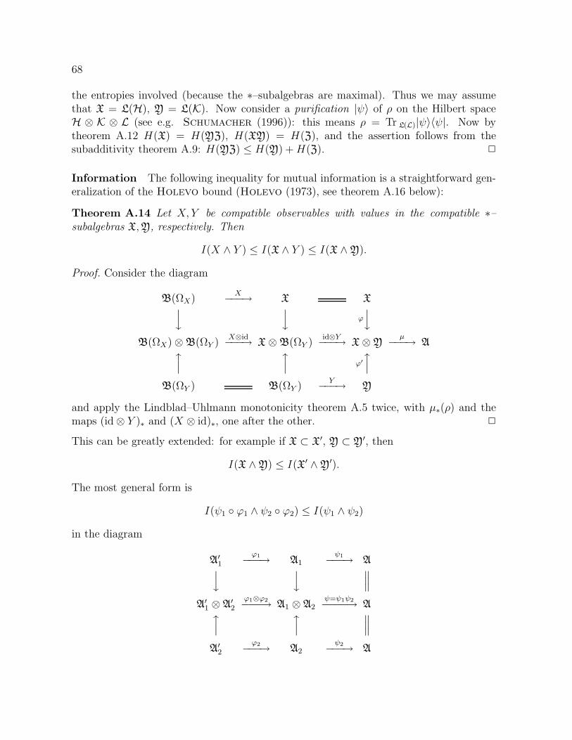
68

the entropies involved (because the ∗–subalgebras are maximal). Thus we may assumethat X = L(H), Y = L(K). Now consider a purification |ψ〉 of ρ on the Hilbert spaceH ⊗ K ⊗ L (see e.g. Schumacher (1996)): this means ρ = Tr L(L)|ψ〉〈ψ|. Now bytheorem A.12 H(X) = H(YZ), H(XY) = H(Z), and the assertion follows from thesubadditivity theorem A.9: H(YZ) ≤ H(Y) +H(Z). 2

Information The following inequality for mutual information is a straightforward gen-eralization of the Holevo bound (Holevo (1973), see theorem A.16 below):

Theorem A.14 Let X, Y be compatible observables with values in the compatible ∗–subalgebras X,Y, respectively. Then

I(X ∧ Y ) ≤ I(X ∧ Y ) ≤ I(X ∧ Y).

Proof. Consider the diagram

B(ΩX)X−−−→ X Xy

y ϕ

y

B(ΩX) ⊗ B(ΩY )X⊗id−−−→ X ⊗ B(ΩY )

id⊗Y−−−→ X ⊗ Yµ−−−→ Ax

x ϕ′

x

B(ΩY ) B(ΩY )Y−−−→ Y

and apply the Lindblad–Uhlmann monotonicity theorem A.5 twice, with µ∗(ρ) and themaps (id ⊗ Y )∗ and (X ⊗ id)∗, one after the other. 2

This can be greatly extended: for example if X ⊂ X′, Y ⊂ Y′, then

I(X ∧ Y) ≤ I(X′ ∧ Y′).

The most general form is

I(ψ1 ϕ1 ∧ ψ2 ϕ2) ≤ I(ψ1 ∧ ψ2)

in the diagram

A′1

ϕ1−−−→ A1ψ1−−−→ Ay

y∥∥∥

A′1 ⊗ A′

2

ϕ1⊗ϕ2−−−→ A1 ⊗ A2ψ=ψ1ψ2−−−−→ Ax

x∥∥∥

A′2

ϕ2−−−→ A2ψ2−−−→ A

69

Remark A.15 It is worth noting that the above formulation of the information bound hasthe nice form of a data processing inequality. To dwell on this point a little more, and atthe same time link our discussion with the traditional view and the language employed inthe chapters I and II of the main text let us define for a (measureable) map ϕ∗ : X → S(Y)(which we identify with its linear extension to CX and regard as a quantum channel, seechapter II) and a p.d. P on X

I(P ;ϕ∗) = Iγ(CX ∧ Y)

with the channel state γ =∑

x∈X P (x)[x] ⊗ ϕ∗(x). It is easily verified that

I(P ;ϕ∗) = H(Pϕ∗) −H(ϕ∗|P ) where

Pϕ∗ = Tr CXγ =

∑x∈X P (x)ϕ∗(x),

H(ϕ∗|P ) =∑

x∈X P (x)H(ϕ∗(x)).

Now with a quantum operation ψ∗ : Y∗ → Z∗ the data processing inequality specializes to

I(P ;ψ∗ ϕ∗) ≤ I(P ;ϕ∗).

In particular if Z is commutative, i.e. the operation, now denoted D∗, is a measurement,we recover the

Theorem A.16 (Holevo bound) I(P ;D∗ ϕ∗) ≤ I(P ;ϕ∗). 2

In chapter II an elementary proof of this inequality is presented.

Theorem A.17 Let X1,X2,Y1,Y2 compatible ∗–subalgebras of A, ρ a state on A. Then

I(X1X2 ∧ Y1Y2) ≤ I(X1 ∧ Y1) + I(X2 ∧ Y2)

if I(Y1 ∧X2Y2|X1) = 0 and I(Y2 ∧X1Y1|X2) = 0 (i.e. Yk is independent from the other∗–subalgebras conditional on Xk).

Proof. First observe that the conditional independence mentioned, I(Y1 ∧ X2Y2|X1) =0, is equivalent to H(Y1|X1X2Y2) = H(Y1|X1). By theorem A.23 we then have alsoH(Y1|X1X2) = H(Y1|X1). Now observe (with the obvious chain rule)

H(Y1Y2|X1X2) = H(Y1|X1X2Y2) +H(Y2|X1X2)

= H(Y1|X1) +H(Y2|X2)

and hence

I(X1X2 ∧ Y1Y2) = H(Y1Y2) −H(Y1Y2|X1X2)

≤ H(Y1) +H(Y2) −H(Y1|X1) −H(Y2|X2)

= I(X1 ∧ Y1) + I(X2 ∧ Y2)

70

where we have used the subadditivity of von Neumann entropy, theorem A.9. 2

The same obviously applies if we have n ∗–subalgebras Xk, and n Yk, all compatible, andif Yk is independent from the others given Xk, i.e. for all k

H(Yk|X1 · · ·XnY1 · · · Yk · · ·Yn) = H(Yk|Xk).

Corollary A.18 Let X1, . . . ,Xn, Y1, . . . ,Yn C∗–algebras, Xi = CXi commutative, andA = X1 ⊗ · · · ⊗ Xn ⊗ Y1 ⊗ · · · ⊗ Yn. Then with the state

γ =∑

xi∈Xi

P (x1, . . . , xn)[x1] ⊗ · · · ⊗ [xn] ⊗Wx1⊗ · · · ⊗Wxn

on A (where P is a p.d. on X1 × · · · × Xn and W maps the Xi to states on Yi):

I(X1 · · ·Xn ∧ Y1 · · ·Yn) ≤n∑

k=1

I(Xk ∧ Yk).

Proof. We only have to check the conditional independence, which is left to the reader. 2

We note another estimate for the mutual information:

Theorem A.19 For compatible ∗–subalgebras X,Y: I(X ∧ Y) ≤ 2 minH(X), H(Y).Proof. Put together the formula I(X ∧ Y) = H(X) − H(X|Y) and the simple estimateH(X|Y) ≥ −H(X) from theorem A.13. 2

Conditional entropy We start with a simple positivity condition:

Theorem A.20 Let ϕ : X → A, ψ : Y → A compatible quantum operations with X or Y

commutative. Then H(ϕ|ψ) ≥ 0.

Proof. Let σ = (ϕψ)∗ρ, then by definition and lemma A.6

H(ϕ|ψ) = H(σ) −H(Tr Yσ).

First case: X is commutative, so we can write σ =∑

xQ(x)[x]⊗τ∗(x) with a distribu-tion Q on X , and states τ∗(x) on Y. Obviously H(σ) = H(Q) +

∑xQ(x)H(τ∗(x)), and

Tr Yσ =∑

xQ(x)[x] = Q, and hence H(ϕ|ψ) =∑

xQ(x)H(τ∗(x)) ≥ 0.Second case: Y is commutative, so we can write σ =

∑xQ(x)[x]τ∗(x) ⊗ [x], like in

the first case. H(σ) is calculated as before, but now Tr Yσ =∑

xQ(x)τ∗(x) = Qτ∗, and

H(ϕ|ψ) = H(Q) −(H(Qτ∗) −

∑

x

Q(x)H(τ∗(x))

)

= H(Q) − I(Q; τ∗) ≥ 0,

the last step by an application of the Holevo bound, theorem A.16. 2

71

Remark A.21 From the proof we see that the commutativity of X or Y enters in therepresentation of σ as a particular separable state with respect to the ∗–subalgebras X, Y

(see definition below), namely with one party admitting common diagonalization of herstates. We formulate as a conjecture the more general:

H(X|Y) ≥ 0 if ρ is separable with respect to X and Y.

From this it would follow that in this case I(X ∧Y) ≤ minH(X), H(Y) (compare theo-rem A.19), which we now only get from the commutativity assumption.

Definition A.22 Call ρ separable with respect to compatible ∗–subalgebras X1, . . . ,Xm

of A, if, for the natural multiplication map µ : X1⊗· · ·⊗Xm → A, µ∗ρ is a separable stateon X1 ⊗ · · · ⊗Xm, i.e. a convex combination of product states σ1 ⊗ · · · ⊗ σm, σi ∈ S(Xi).If µ∗ρ is a product state, we call also ρ a product state with respect to X1, . . . ,Xm.

Theorem A.23 (Knowledge decreases uncertainty) Let ϕ : X → A, ψ : Y → A

compatible quantum operations, and ϕ′ : X′ → X any quantum operation.

Then H(ψ|ϕ) ≤ H(ψ|ϕ ϕ′), and in particular H(ψ|ϕ) ≤ H(ψ).

Proof. The inequality is obviously equivalent to I(ψ ∧ ϕ) ≥ I(ψ ∧ ϕ ϕ′), i.e. to theo-rem A.14. 2

Defining h(x) = −x log x− (1 − x) log(1 − x) for x ∈ [0, 1] we have the famous

Theorem A.24 (Fano inequality) Let ρ a state on A, and Y be a ∗–subalgebra of A,compatible with the observable X (indexed by X ). Then for any observable Y with valuesin Y the probability that “X 6= Y ”, i.e. Pe = 1 −∑j Tr (ρXjYj), satisfies

H(X|Y) ≤ h(Pe) + Pe log(|X | − 1).

Proof. By the previous theorem A.23 it suffices to prove the inequality with H(X|Y )instead of H(X|Y). But then we have the classical Fano inequality: the uncertainty onX given Y may be estimated by the uncertainty of the event that they are equal plus theuncertainty on the value of X if they are not. 2

Corollary A.25 Let X a commutative ∗–subalgebra compatible with Y, and X the —uniquely determined — maximal observable on X, Pe as in the theorem, then

H(X|Y) ≤ h(Pe) + Pe log(Tr supp (ρ|X) − 1).

72

Proof. First observe that H(X|Y) = H(X|Y). To apply the theorem we only have torestrict the range of X to those values that are actually assumed. 2

Some philosophical remarks may be in order: quantum theory stipulates the channel asa process, an asymmetric notion, and this brings about the formula I(P ;ϕ∗) = H(Pϕ∗)−H(ϕ∗|P ): input, average and conditional output entropy. In classical information theoryhowever we like to see things more symmetric, namely the channel as a stochastic two–end system, with some underlying joint distribution. Following this idea produces ourchannel states γ, and a symmetric “information” expression I(X ∧ Y). Even thoughthere are questions in quantum information where these two pictures can be brought torelation, for example in the above results (a connection that was noticed before by Hall

(1997) in his investigation of what he calls context mappings), they are not reducible toeach other: the “dynamic” picture is asymmetric (there may not even exist a backwardchannel producing the same channel state), whereas the “static” picture is obviouslysymmetric. Even worse, for a joint state it is not obvious that a channel and inputdistribution generating it exist at all. And if it exists, there is no uniqueness in its choice.On the other hand, modelling a situation of quantum evolutions statically may produceunphysical effects, see the example from Winter (1998c), VIII.B.2, pp.24: the channelstate incorporates parts of a system which can never be simultaneously accessible.

73

References

Ahlswede, R. (1968), Beitrage zur Shannonschen Informationstheorie im Falle nicht-stationarer Kanale. Z. Wahrscheinlichkeitstheorie und verw. Gebiete, 10, 1–42.

Ahlswede, R. (1971), Multi–way communication channels. In Second InternationalSymposium on Information Theory , 23–52, Hungarian Academy of Sciences.

Ahlswede, R. (1974a), The capacity region of a channel with two senders and tworeceivers. Ann. Prob., 2(5), 805–814.

Ahlswede, R. (1974b), Paper presented at 7th Hawaii International Conference onSystem Sciences, Jan. 1974. Published in Ahlswede, R. & Korner, J. (1975),Source coding with side information at the decoder and a converse for degradedbroadcast channels. IEEE Trans. Inf. Theory, 21, 629–637.

Ahlswede, R. (1979), Coloring Hypergraphs: A New Approach to Multi–user SourceCoding — I. J. Combinatorics, Information & System Sciences, 4(1), 76–115.

Ahlswede, R. (1980), Coloring Hypergraphs: A New Approach to Multi–user SourceCoding — II. J. Combinatorics, Information & System Sciences, 5(3), 220–268.

Ahlswede, R., Gacs, P. & Korner, J. (1976), Bounds on Conditional Probabilitieswith Applications to Multi–User Communication. Z. Wahrscheinlichkeitstheorie undverw. Geb., 34, 157–177.

Allahverdyan, A. E. & Saakian, D. B. (1997a), Converse coding theoremsfor quantum source and noisy channels. LANL eprint quant-ph/9702034, http:

//xxx.lanl.gov/.

Allahverdyan, A. E. & Saakian, D. B. (1997b), Multi–access channels in quantuminformation theory. LANL eprint quant-ph/9712034, http://xxx.lanl.gov/.

Arveson, W. (1976), An Invitation to C∗–Algebras. Springer, New York.

Barnum, H. (1998), Quantum Rate–Distortion Coding. LANL eprint quant-ph/

9806065, http://xxx.lanl.gov/.

74

Barnum, H., Fuchs, C. A., Jozsa, R. & Schumacher, B. (1996), General FidelityLimit for Quantum Channels. Phys. Rev. A, 54, 4707–4711.

Barnum, H., Nielsen, M. A. & Schumacher, B. (1998), Information transmissionthrough a noisy quantum channel. Phys. Rev. A, 57(6), 4153–4175.

Bell, J. (1964), On the Einstein Podolsky Rosen paradox. Physics , 1(3), 195–200.

Bendjaballah, C., Leroy, J. M. & Vourdas, A. (1998), Rate Distortion andDetection in Quantum Communication. IEEE Trans. Inf. Theory , 44(4), 1658–1665.

Bennett, C. H. & Wiesner, S. J. (1992), Communication via one– and two–particleoperators on Einstein–Podolsky–Rosen states. Phys. Rev. Letters , 69(20), 2881–2884.

Born, M. (1926), Zur Quantenmechanik der Stoßvorgange. Zeitschrift fur Physik , 37,863–867.

Braunstein, S. L., Fuchs, C. A., Gottesman, D. & Lo, H.-K. (1998),A quantum analog of Huffman coding. LANL eprint quant-ph/9805080, http:

//xxx.lanl.gov/, presented at the IEEE International Symposium on InformationTheory, Boston, 1998.

Burnashev, M. V. & Holevo, A. (1997), On Reliability Function of Quantum Com-munication Channel. LANL eprint quant-ph/9703013, http://xxx.lanl.gov/.

Csiszar, I. & Korner, J. (1981), Information Theory: Coding Theorems for DiscreteMemoryless Systems. Academic Press, New York.

Davies, E. B. (1976), Quantum Theory of Open Systems. Academic Press, London.

Einstein, A., Podolsky, B. & Rosen, N. (1935), Can Quantum–Mechanical Descrip-tion of Physical Reality be Considered Complete? Physical Review , 47, 777–780.

El Gamal, A. & Cover, T. (1980), Multiple User Information Theory. Proc. IEEE ,68, 1466–1483.

Forney, jr., G. D. (1963), (unpublished). Master’s thesis, MIT, Boston.

Gordon, J. P. (1964), Noise at optical frequencies: information theory. In Proc. Int.School Phys. “Enrico Fermi” ( P. A. Miles, ed.), 156–181, Academic Press, NewYork.

Greenberger, D. M., Horne, M. A., Shimony, A. & Zeilinger, A. (1990), Bell’stheorem without inequalities. Am. J. Phys., 58(12), 1131–1143.

Hall, M. J. W. (1997), Quantum information and correlation bounds. Phys. Rev. A,55(1), 100–113.

75

Haroutunian, A. E. (1968), Estimates on the error exponent for the semicontinuousmemoryless quantum channel. Probl. Peredachi Inform., 4(4), 37–48, in Russian.

Hausladen, P., Jozsa, R., Schumacher, B., Westmoreland, M. & Wootters,

W. K. (1997), Classical information capacity of a quantum channel. Phys. Rev. A,54(3), 1869–1876.

Hoeffding, W. (1963), Probability Inequalities for Sums of Bounded Random Variables.J. Amer. Statist. Assoc., 58, 13–30.

Holevo, A. S. (1973), Bounds for the quantity of information transmitted by a quantumchannel. Probl. Inf. Transm., 9(3), 177–183.

Holevo, A. S. (1977), Problems in the mathematical theory of quantum communicationchannels. Rep. Math. Phys., 12(2), 273–278.

Holevo, A. S. (1979), Capacity of a Quantum Communication Channel. Probl. Inf.Transm., 15(4), 247–253.

Holevo, A. S. (1982), Probabilistic and Statistical Aspects of Quantum Theory . North–Holland, Amsterdam.

Holevo, A. S. (1998a), The Capacity of the Quantum Channel with General SignalStates. IEEE Trans. Inf. Theory , 44(1), 269–273.

Holevo, A. S. (1998b), Coding Theorems for Quantum Channels. Research Review 4,Tamagawa University, extended version as LANL eprint quant-ph/9809023.

Horodecki, M. (1998), Limits for compression of quantum information carried by en-sembles of mixed states. Phys. Rev. A, 57, 3364–3369.

Jozsa, R. (1994), Fidelity for mixed states. J. Mod. Optics , 41(12), 2315–2323.

Jozsa, R., Horodecki, M., Horodecki, P. & Horodecki, R. (1998), UniversalQuantum Information Compression. Phys. Rev. Letters , 81, 1714–1717.

Jozsa, R. & Schumacher, B. (1994), A new proof of the quantum noiseless codingtheorem. J. Mod. Optics , 41(12), 2343–2349.

Kraus, K. (1983), States, Effects and Operations . Number 190 in Lecture Notes inPhysics, Springer, Berlin.

Levitin, L. B. (1969), On quantum measure of information. In Proc. IV All–UnionConference on Information Transmission and Coding Theory , 111–115, Tashkent.

Levitin, L. B. (1998), Conditional Entropy and Information in Quantum Systems. InProc. IEEE International Symposium on Information Theory, Boston, 88.

76

Lindblad, G. (1975), Completely positive maps and entropy inequalities. Comm. Math.Phys., 40, 147–151.

Ludwig, G. (1954), Die Grundlagen der Quantenmechanik . Springer, Berlin.

Nagaoka, H. (1998), Algorithms of Arimoto–Blahut Type for Computing QuantumChannel Capacity. In Proc. IEEE International Symposium on Information Theory,Boston.

Ogawa, T. & Nagaoka, H. (1998), Strong Converse to the Quantum Channel CodingTheorem. LANL eprint quant-ph/9808063, http://xxx.lanl.gov/.

Ohya, M. & Petz, D. (1993), Quantum Entropy and Its Use. Springer, Berlin.

Peres, A. (1995), Quantum Theory: Concepts and Methods. Kluwer, Dordrecht.

Schumacher, B. (1995), Quantum Coding. Phys. Rev. A, 51(4), 2738–2747.

Schumacher, B. (1996), Sending entanglement through noisy quantum channels. Phys.Rev. A, 54(4), 2614–2628.

Schumacher, B. & Nielsen, M. A. (1996), Quantum data processing and error cor-rection. Phys. Rev. A, 54(4), 2629–2635.

Schumacher, B. & Westmoreland, M. (1997), Sending classical information vianoisy quantum channels. Phys. Rev. A, 56(1), 131–138.

Shannon, C. E. (1948), A Mathematical Theory of Communication. Bell System Thech-nical Journal , 27, 379–423.

Shannon, C. E. (1961), Two–way communication channels. In Proc. Fourth BerkeleySymposium Probability and Statistics ( J. Neyman, ed.), 611–644, Berkeley.

Shor, P. W. (1994), Algorithms for Quantum Computation: Discrete Logarithm andFactoring. In Proc. 35th Ann. Symp. Foundations of Computer Science ( S. Gold-wasser, ed.), 124–134, IEEE Press, Santa Fe, full paper: Polynomial–Time Algo-rithms for Prime Factorization and Discrete Logarithms on a Quantum Computer,SIAM J. Computing, 26(5), 1484–1509 (1997).

Stinespring, W. F. (1955), Positive Functions on C∗–Algebras. Proc. Amer. Math.Soc., 6, 211–216.

Stratonovich, R. L. (1966), Information transmission rate in certain quantum com-munication channels. Probl. Peredachi Inform., 2(2), 45–57, in Russian.

Uhlmann, A. (1977), Relative entropy and the Wigner–Yanase–Dyson–Lieb concavityin an interpolation theory. Comm. Math. Phys., 54, 21–32.

77

Umegaki, H. (1962), Conditional expectations in an operator algebra, IV (entropy andinformation). Kodai Math. Sem. Rep., 14, 59–85.

von Neumann, J. (1927), Thermodynamik quantenmechanischer Gesamtheiten. Nachr.der Gesellschaft der Wiss. Gott., 273–291.

Wehrl, A. (1978), General properties of entropy. Rev. Mod. Phys., 50(2), 221–260.

Winter, A. (1998a), The Capacity of the Quantum Multiple Access Channel. LANLeprint quant-ph/9807019, http://xxx.lanl.gov/.

Winter, A. (1998b), Coding Theorem and Strong Converse for Quantum Channels.Preprint 98–074, Sonderforschungsbereich 343 “Diskrete Strukturen in der Mathe-matik”, Universitat Bielefeld, to appear in IEEE Trans. Inf. Theory, Nov. 1999.

Winter, A. (1998c), Languages of Quantum Information Theory. Preprint E98–009,Sonderforschungsbereich 343 “Diskrete Strukturen in der Mathematik”, UniversitatBielefeld, also as LANL eprint quant-ph/9807008.

Winter, A. (1999a), Coding Theorem and Strong Converse for Nonstationary QuantumChannels. Preprint 99–033, Sonderforschungsbereich 343 “Diskrete Strukturen in derMathematik”, Universitat Bielefeld.

Winter, A. (1999b), Rate and Error Estimates for Quantum Channels. Preprint 99–032,Sonderforschungsbereich 343 “Diskrete Strukturen in der Mathematik”, UniversitatBielefeld.

Winter, A. (1999c), Schumacher’s Quantum Coding Revisited. Preprint 99–034, Sonder-forschungsbereich 343 “Diskrete Strukturen in der Mathematik”, Universitat Biele-feld.

Wolfowitz, J. (1964), Coding Theorems of Information Theory . Springer, Berlin, sec-ond edition.

Wootters, W. K. & Zurek, W. H. (1982), A single quantum cannot be cloned.Nature, 299, 802–803.