1

Geoderma 1

2

Title: Integration of mid-infrared spectroscopy and geostatistics in the assessment of soil 3

spatial variability at landscape level 4

5

Article Type: Research Paper 6

7

Section/Category: Soil Fertility, Soil Quality and Tropical Soils 8

9

Keywords: Autocorrelation; chemometrics; DRIFT; sampling designs; soil fertility; spatial 10

patterns; variography; Zimbabwe. 11

12

Corresponding Author: Dr. G. Cadisch, 13

14

Corresponding Author's Institution: Uni Hohenheim 15

16

First Author: Juan Guillermo Cobo 17

18

Order of Authors: Juan Guillermo Cobo; Gerd Dercon; Tsitsi Yekeye; Lazarus Chapungu; 19

Chengetai Kadzere; Amon Murwira; Robert Delve; G. Cadisch 20

21

Abstract: Knowledge of soil spatial variability is important in natural resource management, 22

interpolation and soil sampling design, but requires a considerable amount of geo-referenced 23

data. In this study, mid-infrared spectroscopy in combination with spatial analyses tools is 24

being proposed to facilitate landscape evaluation and monitoring. Mid-infrared spectroscopy 25

2

(MIRS) and geostatistics were integrated for evaluating soil spatial structures of three land 26

settlement schemes in Zimbabwe (i.e. communal area, old resettlement and new resettlement; 27

on loamy-sand, sandy-loam and clay soils, respectively). A nested non-aligned design with 28

hierarchical grids of 750, 150 and 30 m resulted in 432 sampling points across all three 29

villages (730-1360 ha). At each point, a composite topsoil sample was taken and analyzed by 30

MIRS. Conventional laboratory analyses on 25-38% of the samples were used for the 31

prediction of concentration values on the remaining samples through the application of MIRS 32

- partial least squares regression models. These models were successful (R2>89) for sand, 33

clay, pH, total C and N, exchangeable Ca, Mg and effective CEC; but not for silt, available P 34

and exchangeable K and Al (R2<82). Minimum sample sizes required to accurately estimate 35

the mean of each soil property in each village were calculated. With regard to locations, 36

fewer samples were needed in the new resettlement area than in the other two areas (e.g. 66 37

versus 133-473 samples for estimating soil C at 10% error, respectively); regarding 38

parameters, less samples were needed for estimating pH and sand (i.e. 3-52 versus 27-504 39

samples for the remaining properties, at same error margin). Spatial analyses of soil 40

properties in each village were assessed by constructing standardized isotropic 41

semivariograms, which were usually well described by spherical models. Spatial 42

autocorrelation of most variables was displayed over ranges of 250-695 m. Nugget-to-sill 43

ratios showed that, in general, spatial dependence of soil properties was: new resettlement > 44

old resettlement > communal area; which was potentially attributed to both intrinsic (e.g. 45

texture) and extrinsic (e.g. management) factors. As a new approach, geostatistical analysis 46

was performed using MIRS data directly, after principal component analyses, where the first 47

three components explained 70% of the overall variability. Semivariograms based on these 48

components showed that spatial dependence per village was similar to overall dependence 49

identified from individual soil properties in each area. In fact, the first component (explaining 50

3

49% of variation) related well with all soil properties of reference samples (absolute 51

correlation values of 0.55-0.96). This suggested that MIRS data could be directly linked to 52

geostatistics for a broad and quick evaluation of soil spatial variability. It is concluded that 53

integrating MIRS with geostatistical analyses is a cost-effective promising approach, i.e. for 54

soil fertility and carbon sequestration assessments, mapping and monitoring at landscape 55

level. 56

4

Integration of mid-infrared spectroscopy and geostatistics in the assessment of soil 57

spatial variability at landscape level 58

59

Juan Guillermo Cobo1,2, Gerd Dercon1,3, Tsitsi Yekeye4, Lazarus Chapungu4, Chengetai 60

Kadzere2, Amon Murwira4, Robert Delve2,5, Georg Cadisch1,* 61

1 University of Hohenheim, Institute of Plant Production and Agroecology in the Tropics and 62

Subtropics, 70593 Stuttgart, Germany 63

2 Tropical Soil Biology and Fertility Institute of the International Center for Tropical 64

Agriculture (TSBF-CIAT), MP 228, Harare, Zimbabwe 65

3 Present address: Soil and Water Management and Crop Nutrition Subprogramme, Joint 66

FAO/IAEA Division of Nuclear Techniques in Food and Agriculture, Department of Nuclear 67

Sciences and Applications, International Atomic Energy Agency – IAEA, Wagramerstrasse 5 68

A-1400, Vienna, Austria 69

4 University of Zimbabwe, Dept. of Geography and Environmental Science, MP 167 70

Harare, Zimbabwe 71

5 Present address: Catholic Relief Services, P.O. Box 49675-00100, Nairobi, Kenya 72

73

74

Pages: 27 75

Figures: 10 76

Tables: 4 77

78

79

* Corresponding author: E-mail address: georg.cadisch@uni-hohenheim.de; Tel.: +49 711 80

459 22438; Fax: +49 711 459 22304.81

5

Abstract 82

Knowledge of soil spatial variability is important in natural resource management, 83

interpolation and soil sampling design, but requires a considerable amount of geo-referenced 84

data. In this study, mid-infrared spectroscopy in combination with spatial analyses tools is 85

being proposed to facilitate landscape evaluation and monitoring. Mid-infrared spectroscopy 86

(MIRS) and geostatistics were integrated for evaluating soil spatial structures of three land 87

settlement schemes in Zimbabwe (i.e. communal area, old resettlement and new resettlement; 88

on loamy-sand, sandy-loam and clay soils, respectively). A nested non-aligned design with 89

hierarchical grids of 750, 150 and 30 m resulted in 432 sampling points across all three 90

villages (730-1360 ha). At each point, a composite topsoil sample was taken and analyzed by 91

MIRS. Conventional laboratory analyses on 25-38% of the samples were used for the 92

prediction of concentration values on the remaining samples through the application of MIRS 93

- partial least squares regression models. These models were successful (R2>0.89) for sand, 94

clay, pH, total C and N, exchangeable Ca, Mg and effective CEC; but not for silt, available P 95

and exchangeable K and Al (R2<0.82). Minimum sample sizes required to accurately estimate 96

the mean of each soil property in each village were calculated. With regard to locations, 97

fewer samples were needed in the new resettlement area than in the other two areas (e.g. 66 98

versus 133-473 samples for estimating soil C at 10% error, respectively); regarding 99

parameters, less samples were needed for estimating pH and sand (i.e. 3-52 versus 27-504 100

samples for the remaining properties, at same error margin). Spatial analyses of soil 101

properties in each village were assessed by constructing standardized isotropic 102

semivariograms, which were usually well described by spherical models. Spatial 103

autocorrelation of most variables was displayed over ranges of 250-695 m. Nugget-to-sill 104

ratios showed that, in general, spatial dependence of soil properties was: new resettlement > 105

old resettlement > communal area; which was potentially attributed to both intrinsic (e.g. 106

6

texture) and extrinsic (e.g. management) factors. As a new approach, geostatistical analysis 107

was performed using MIRS data directly, after principal component analyses, where the first 108

three components explained 70% of the overall variability. Semivariograms based on these 109

components showed that spatial dependence per village was similar to overall dependence 110

identified from individual soil properties in each area. In fact, the first component (explaining 111

49% of variation) related well with all soil properties of reference samples (absolute 112

correlation values of 0.55-0.96). This showed that MIRS data could be directly linked to 113

geostatistics for a broad and quick evaluation of soil spatial variability. It is concluded that 114

integrating MIRS with geostatistical analyses is a cost-effective promising approach, i.e. for 115

soil fertility and carbon sequestration assessments, mapping and monitoring at landscape 116

level. 117

118

Key words 119

Autocorrelation; chemometrics; DRIFT; sampling designs; soil fertility; spatial patterns; 120

variography; Zimbabwe. 121

122

1. Introduction 123

Soil properties are inherently variable in nature mainly due to pedogenetical factors (e.g. 124

parental material, vegetation, climate), but heterogeneity can be also induced by farmers’ 125

management (Dercon et al., 2003; Giller et al., 2006; Samake et al., 2005; Wei et al., 2008; 126

Yemefack et al., 2005). Soil spatial variability can occur over multiple spatial scales, ranging 127

from micro-level (millimeters), to plot level (meters), up to the landscape (kilometers) 128

(Garten Jr. et al., 2007). Thus, soil spatial variability is a function of the different driving 129

factors and spatial scale (in terms of size and resolution), but also of the specific soil property 130

(or process) under evaluation and the spatial domain (location), among others factors (Lin et 131

7

al., 2005). Recognizing spatial patterns in soils is important as this knowledge can be used for 132

enhancing natural resource management (e.g. Borůvka et al., 2007; Liu et al., 2004; Wang et 133

al., 2009), predicting soil properties at unsampled locations (e.g. Liu et al., 2009; Wei et al., 134

2008) and improving sampling designs in future agro-ecological studies (e.g. Rossi et al., 135

2009; Yan and Cai, 2008). In fact, the identification of spatial patterns is the first step to 136

understanding processes in natural and/or managed systems, which are usually characterized 137

by spatial structures due to spatial autocorrelation: i.e. where closer observations are more 138

likely to be similar than by random chance (Fortin et al., 2002). Conventional statistical 139

analyses are not appropriate to identify spatial patterns, as these analyses require the 140

assumption of independence among samples, which is violated when auto-correlated 141

(spatially dependent) data are present (Fortin et al., 2002; Liebhold and Gurevitch, 2002). 142

Thus, since 1950s, alternative methods, so-called spatial statistics, have been developed for 143

dealing with spatial autocorrelation (Fortin et al., 2002). Today several methods for spatial 144

analyses exist (e.g. Geostatistics, Mantel tests, Moran’s I, Fractal analyses), while the reasons 145

for the different studies carried out to date on spatial assessments are also diverse (e.g. 146

hypotheses testing, spatial estimation, uncertainty assessment, stochastic simulation, 147

modeling) (Goovaerts, 1999; Liebhold and Gurevitch, 2002). However, a common 148

characteristic is that all methods intent to capture and quantify in one way or another 149

underlying spatial patterns of a specific spatial domain (Liebhold and Gurevitch, 2002; Olea, 150

2006). 151

152

Geostatistics is one of the most used and powerful approaches for evaluating spatial 153

variability of natural resources such as soils (Sauer et al., 2006). However, construction of 154

stable semivariograms (the main tool on which geostatistics is based) requires considerable 155

amount of geo-referenced data (Davidson and Csillag, 2003). Infrared spectroscopy (IRS) has 156

8

been suggested as a viable option to facilitate access to the extensive soil data required 157

(Cécillon et al., 2009; Shepherd and Walsh, 2007). IRS is able to detect the different 158

molecular vibrations due to the stretching and binding of the different compounds of a sample 159

when illuminated by an infrared beam in the near, NIRS (0.7-2.5 m), or mid, MIRS (2.5-25 160

m) ranges. The result of the measurements is summarized in one spectrum (e.g. wavelength 161

versus absorbance), which is later related by multivariate calibration to known concentration 162

values of the properties of interest (e.g. carbon content, texture) from reference samples. 163

Thus, a mathematical model is created and used later for the prediction of concentration 164

values of these properties in other samples from which IRS data is also available (Conzen, 165

2003). IRS measurements are therefore not destructive, take few minutes, and one spectra can 166

be related to multiple physical, chemical and biological soil properties (Janik et al., 1998; 167

McBratney et al., 2006). Hence the technique is more rapid and cheaper than conventional 168

laboratory analysis, especially when a large number of samples must be analyzed (Viscarra-169

Rossel et al., 2006). IRS has the additional advantage that spectral information can be used as 170

an integrative measure of soil quality, and therefore employed as a screening tool of soil 171

conditions (Shepherd and Walsh, 2007). The few existing initiatives in this regard are, 172

however, limited to NIRS. For example, a visible-NIRS (VNIRS) soil fertility index based on 173

ten common soil properties has been developed and applied in Madagascar (Vågen et al., 174

2006); ordinal logistic regression and classification trees were used to discriminate soil 175

ecological conditions by using biogeochemical data and VNIRS in the USA (Cohen et al., 176

2006); and in Kenya, Awiti et al. (2008) developed an odds logistic model based on principal 177

components from NIRS for soil fertility classification. Nevertheless, despite its multiple 178

applications, to date IRS has not been widely used, especially for wide-scale purposes and in 179

developing countries (Shepherd and Walsh, 2007). 180

181

9

African regions are usually characterized by food insecurity and poverty, which have been 182

extensively attributed to low soil fertility and soil mining (Sanchez and Leakey, 1997; 183

Vitousek et al., 2009). Therefore, to boost land productivity in the continent, there is an 184

increasing need to develop and apply reliable indicators of land quality at different spatial 185

scales (Cobo et al., 2010). In fact, Shepherd and Walsh (2007) proposed that the successful 186

“combination of infrared spectroscopy and geographic positioning systems will provide one 187

of the most powerful modern tools for agricultural and environmental monitoring and 188

analysis” in the next decade. The present study aims to contribute to this goal, and follows up 189

a study from Cobo et al. (2009), in which three villages as typical cases of three settlement 190

schemes in north-east Zimbabwe (communal area, old resettlement and new resettlement) 191

were evaluated to determine specific cropping strategies, soil fertility investments and land 192

management practices at each site. The assessment, however, was done at plot and farm level, 193

and did not take into account spatial structures of soil properties. Hence, the same three 194

villages of Cobo et al. (2009) were systematically sampled, soils characterized by MIRS, and 195

data subsequently analyzed using conventional statistics and geostatistics tools. The main 196

objectives of this study were: i) to evaluate advantages and disadvantages of using MIRS and 197

geostatistics in the assessment of spatial variability of soils, ii) to test if MIRS can be directly 198

integrated with geostatistics for landscape analyses, and iii) to present recommendations for 199

guiding future sampling designs. 200

201

2. Materials and methods 202

2.1 Description of study sites 203

The study sites consisted of three villages, selected as typical cases of three small-holder 204

settlement schemes, in the districts of Bindura and Shamva, north-east Zimbabwe (Table 1). 205

The first village, Kanyera, is located in a communal area, covers 730 ha, and is mainly 206

10

characterized with loamy sand soils of low fertility. The second village, Chomutomora, is 207

located in an old resettlement area (from 1987), covers 780 ha and mostly presents sandy 208

loam soils of low quality. The third village, Hereford farm, is located in a new resettlement 209

area (from 2002), covers 1360 ha and is predominantly characterized by clay soils of 210

relatively higher fertility. All villages are located in natural region II, which covers a region 211

with altitudes of 1000 to 1800 m a.s.l. and unimodal rainfall (April to October) with 750–212

1000 mm per annum (FAO, 2006). Maize (Zea maiz L.) is the main crop planted in the three 213

areas, and farmers have free access to communal grazing areas and woodlands. A full 214

description of the sites’ selection and characteristics is provided in Cobo et al. (2009). 215

216

2.2. Soil sampling design 217

A non-aligned block sampling design was used in the three villages to capture both small and 218

large variation over large areas (Urban, 2002). It started with the delineation of the villages’ 219

boundaries by using a hand-held GPS. Coordinates were later overlaid in ArcView 220

(www.esri.com) to a Landsat TM image of the zone acquired on 12 June 2006. A buffer of 30 221

m inside each village boundary was created and later a grid of 750 x 750 m was drawn for 222

each village in ILWIS (www.ilwis.org) (Figure 1a). Next, each main cell of 750 x 750 m was 223

divided in 25 sub-cells of 150 x 150 m, which were subsequently divided once again in 25 224

micro-cells of 30 x 30 m. All grids were later transferred to ArcView, where 3 sub-cells from 225

each main cell and 3 micro-cells from each sub-cell were randomly selected. This yielded a 226

cluster of 9 micro-cells per main cell (Figure 1b). Finally, the centroids of each selected 227

micro-cells were estimated and included into the GPS to locate these points in the field 228

(Figure 1c). However, as some points were found in unsuitable places for sampling (e.g. road, 229

water way, household) they were re-located (if possible) to alternate locations within 230

cropping fields, grasslands or woodlands, mostly inside a radius of 30 m. In the same way, in 231

11

cropping fields maize was preferentially chosen for future comparison purposes. At Hereford 232

farm, a part of the woodlands in the southern border was considered to be sacred by the 233

villagers, hence this sector was excluded. 432 points were successfully sampled in the three 234

villages: 159 points in cropping fields (105 in maize, 32 in fallow and 22 in other crops), 163 235

in woodlands and 110 in grasslands. Maximum sampling distance between points was 5.2 236

(communal area), 3.8 (old resettlement) and 4.6 km (new resettlement); while minimum 237

sampling distance was 30 m (for all three villages). Sample collection was carried out at the 238

end of the 2006-7 cropping season. 239

240

Each sampling point consisted of a radial-arm containing four sampling plots: one central and 241

other three located at 12.2 m in directions north, south-west and south-east (Figure 1d), which 242

were designed to represent the internal characteristics and variations in each 30 x 30 m 243

micro-cell (K. Shepherd & T. Vågen, personal communication, 2006). Once plots were 244

established, they were fully characterized by using the FAO land cover classification system 245

(FAO, 2005). Soils were sampled (0-20 cm depth) in each plot and all soil samples per point 246

(4 plots) were thoroughly mixed to account for short-range (<30 m) spatial variability, and a 247

composite sub-sample (~250 g) was taken from the field. Composite soil sub-samples were 248

air-dried, sieved (<2 mm) and a sub-sub-sample sent to Germany for laboratory analyses. 249

250

2.3. Conventional and MIRS analyses of soil samples 251

Soil texture, pH, total carbon (C) and nitrogen (N), available phosphorus (Pav), exchangeable 252

potassium (K), calcium (Ca), magnesium (Mg) and aluminum (Al), and effective cation 253

exchange capacity (CEC) were analyzed on 25% (texture) to 38% (other soil properties) of all 254

collected samples (referred in this study as “reference samples”) for the calibration and 255

validation of the MIRS models. Soil texture was determined by Bouyucos (Anderson and 256

12

Ingram, 1993), pH by CaCl2 (Anderson and Ingram, 1993), total C and N by combustion 257

using an auto-analyzer (EL, Elementar Analysensysteme, Germany), Pav by the molybdenum 258

blue complex reaction method of Bray and Kurtz (1945) and exchangeable cations and 259

effective CEC by extraction with ammonium chloride (Schöning and Brümmer, 2008). 260

261

All 432 soil samples were analyzed by Diffuse Reflectance Infrared Fourier Transform 262

(DRIFT) -MIRS. Five grams of ball-milled soil samples were scanned in a TENSOR-27 FT-263

IR spectrometer (Bruker Optik GmbH, Germany) coupled to a DRIFT-Praying Mantis 264

chamber (Harrick Scientific Products Inc., New York, US). Spectra were obtained at least in 265

triplicate, from 600 to 4,000 wavenumber cm-1, with a resolution of 4 cm-1 and 16 266

scans/sample, and expressed in absorbance units [log(1/Reflectance)]. Potassium bromide 267

(KBr) for IR spectroscopy (assay ≥99.5%), kept always dry in a desiccator, was used as a 268

background. All spectral replicates per sample were averaged and later subjected to 269

multivariate calibration by using partial least square (PLS) regression, which relates the 270

processed spectra (e.g. Figure 2) to the related concentration values from the reference 271

samples. Through a random split selection of the reference samples, half of the samples were 272

used for calibration, while the other half left for validation. Chemometric models were 273

constructed with the “Optimization” function of the OPUS-QUANT2 package (Bruker Optik 274

GmbH, Germany). Calibration regions were set to exclude the background CO2 region (2300-275

2400 cm-1) and the edge of the detection limits of the spectrometer (<700 and >3900 cm-1) to 276

reduce noise. Prediction accuracy of selected MIRS models was evaluated by the residual 277

prediction deviation (RPD) value, the coefficient of determination (R2) and the root mean 278

square error of the prediction (RMSEP). Once suitable chemometric models were selected, 279

models were applied to every spectrum replicate of non reference samples for the prediction 280

of unknown concentration values for each possible soil property; and results of all replicates 281

13

per sample were finally averaged. All spectral manipulation and development of chemometric 282

models were carried out in OPUS, version 6.5 (Bruker Optik GmbH, Germany). 283

284

2.4. Conventional statistical analyses 285

Descriptive statistics were calculated to explore the distribution of each soil property under 286

evaluation and as a critical step before geostatistical analyses (Olea, 2006). This comprised 287

the calculation of univariate statistical moments (e.g. mean, median, range), construction of 288

scatter plots, box plots, frequency tables and normality tests, as well as the identification of 289

true outliers and their exclusion if necessary, as even a few outliers can produce very unstable 290

results (Makkawi, 2004). We usually considered as outliers those points with values higher or 291

lower than three standard deviations from the mean (Liu et al., 2009). The coefficient of 292

variation (CV) was calculated as an index for assessing overall variability (Gallardo and 293

Paramá, 2007). The non-parametric tests of Kruskal-Wallis and Mann-Whitney (a Kruskall-294

Wallis version for only two levels) were chosen for testing the equality of medians among 295

villages following the method of Bekele and Hudnall (2006). All classical statistical analyses 296

were performed in SAS version 9.2 (SAS Institute Inc). 297

298

2.5. Minimum sample size estimations 299

The minimum number of samples required for estimating the mean of the different evaluated 300

soil properties in each village, at different probabilities of its true value (error), with a 95% of 301

confidence, was estimated by using equation 1: 302

303

n = [(tα * s)/d]2 (equation 1) 304

305

14

where n is the sample size, t is the value of t Student (at α=0.05 and n-1 degrees of freedom, 306

i.e. 1.96), s is the standard deviation, and d is the margin of error (Garten Jr. et al., 2007; 307

Rossi et al., 2009; Yan and Cai, 2008). 308

309

2.6. Geo-statistical analyses of estimated soil properties 310

The spatial dependence of soil properties, as determined by the combination of conventional 311

laboratory analyses and MIRS, was assessed in each area by using geostatistical analyses, via 312

the semivariogram, which measures the average dissimilarity of data as a function of distance 313

(Goovaerts, 1999) as illustrated in equation 2: 314

315

γ(h) = 1/2N(h) i i+h [z(i)-z(i+h)]2 (equation 2) 316

317

where γ is the semivariance for N data pairs separated by a distance lag h; and z the variable 318

under consideration at positions i and i+h. As construction of semivariograms assumes a 319

Gaussian distribution (Olea, 2006; Reimann and Filzmoser, 2000), variables were 320

transformed if necessary to approximate normality and to stabilize variance (Goovaerts, 321

1999). Data were also detrended by fitting low-order polynomials according to the exhibited 322

trend (if existent) to accounting for any systematic variation (i.e. global trend) and hence 323

fulfilling the assumption of stationarity (Bekele and Hudnall, 2006; Sauer et al., 2006). Thus, 324

after detrending, respective residuals were used to construct standardized isotropic 325

semivariograms for each soil property in each village. Hence, anisotropy (effect of direction 326

in the intensity of spatial dependence) was not taken into account, as this analysis required a 327

higher number of samples for the construction of stable semivariograms in each direction. 328

When number of samples is limited an ommnidirectional (isotropic) characterization of 329

spatial dependence is more recommendable (Davidson and Csillag, 2003). The 330

15

standardization was achieved by dividing the semivariance data by the sample variance, and 331

this allowed a fair comparison among variables and sites (Pozdnyakova et al., 2005). The half 332

of the maximum sampling distance in each village was chosen as the active lag distance for 333

the construction of all semivariograms, and more than 100 pairs per each lag distance class 334

interval were included in the calculations. 335

336

Once semivariograms were constructed, theoretical semivariogram models were fitted to the 337

data. This was done by selecting the model with the lowest residual sum of squares and 338

highest R2 (e.g. Liu et al., 2009; Wang et al., 2009; Wei et al., 2008). As the spherical model 339

characterized well most of the cases, this model was selected to fit all data (with the 340

exception when a linear trend was found). Having the same model further facilitates 341

comparisons among variables and villages (Cambardella et al., 1994; Davidson and Csillag, 342

2003; Gallardo and Paramá, 2007). The spherical model is defined in equation 3 (Liu et al., 343

2004; Pozdnyakova et al., 2005) as: 344

345

γ(h) = { Co + C [ 1.5 (h/a) – 0.5(h/a)3 ] 0 < h a (equation 3) 346

= {Co + C h > a 347

348

where γ is the semivariance, h the distance, Co is the nugget, Co+C is the sill, and a is the 349

range. These parameters were used to describe and compare spatial structures of soil 350

properties in each village. ArcGIS version 9 (ESRI) and procedures Univariate, Means and 351

Variogram of SAS version 9.2 were used for exploratory data and trend analyses; while Proc 352

GLM of SAS was used for data detrending. Construction of semivariograms and model 353

fitting were performed in GS+ version 9 (Gamma Design Software, USA). 354

355

16

2.7. Geo-statistical analyses of MIRS data 356

To determine the feasibility of using MIRS data as direct input for the determination of 357

spatial variation of soils, all spectra were baseline corrected (Rubberband correction method, 358

64 baseline points) and derived (1st order derivative, Savitzky-Golay algorithm, 9 smoothing 359

points) in OPUS. Data were later exported to SAS, where the CO2 regions and the edges of 360

the spectra were excluded, as explained for the multivariate calibration. Next, spectral data 361

were reduced by re-sampling at 12 cm-1 and selected wavenumbers (i.e. variables) subjected 362

to Spearman correlation analyses among each other, where highly autocorrelated variables 363

(i.e. r > 0.99) were manually excluded, to reduce computational demands. Data were later 364

standardized to zero mean and unit variance, and analyzed by principal component analyses 365

(Borůvka et al., 2007; Yemefack et al., 2005). The three first components were retained, 366

rotated (varimax option) and respective scores assigned to each soil sample. Score 367

components were thus used as input variables for the constructions of semivariograms per 368

each village, by following the same methodology previously explained for the conventional 369

soil parameters. Spearman correlation analyses were finally performed between the principal 370

components and chemical data from reference samples. 371

372

3. Results 373

3.1. MIRS models and prediction 374

A good representation across the different concentration ranges for most of the soil properties 375

was obtained by the selection of the samples, as shown in Figure 3. Calibration and validation 376

models also showed that predictability potential of MIRS varied with the specific soil 377

property under evaluation and location, as indicated by the different model fit and 378

performance indicators (Figure 3, Table 2). For example, in agricultural applications RPD 379

values higher than 5 indicate that predictions models are excellent; RPD values greater than 3 380

17

are considered acceptable; while values less than 3 indicate poor prediction power (Pirie et 381

al., 2005). Besides, R2 values near 1 typically indicate good models (Conzen, 2003), in 382

particular when bias is minimal and regression line follows the 1:1 line. Hence, excellent 383

models (5<RPD6.8, 0.96R20.98) were obtained for sand, clay, C, N, Ca and CEC; 384

acceptable models (3<RPD<5, 0.89<R2<0.92) were obtained for pH and Mg; while 385

unsuitable models (RPD<3, R2≤0.82) were obtained for silt, Pav, K and Al. Poor validation for 386

these last variables (especially Pav, K and Al) was the result of a deficient calibration, as 387

indicated by their model fit (Figure 3) and parameters (Table 2). Mid-infrared spectroscopy 388

models for these variables were thus not used for prediction, and hence these data were 389

dropped from any further analyses. Silt fraction, however, could be calculated from the other 390

two fractions (silt = 100 – sand - clay). Therefore, by using the selected MIRS models shown 391

in Table 2 for the prediction of soil parameters in non-reference samples, the entire dataset of 392

sand, silt, clay, pH, C, N, Ca, Mg and CEC could be completed. 393

394

3.2. Exploratory data analysis and differences among villages 395

Exploratory data analyses in the entire dataset indicated that most soil properties presented 396

skewed and kurtic distributions (data not shown). For example, texture fractions showed 397

clearly a bimodal distribution, which suggested the presence of different populations, as it 398

was in fact the case (i.e. different villages presenting different textural classes). Descriptive 399

statistics and histograms were therefore also obtained by village. In this case, although 400

texture fractions often approximated normality, the other soil properties still exhibited non-401

normal distributions (data not shown). Non-normality is usually the rule and not the 402

exception when dealing with geostatistical and environmental data (Reimann and Filzmoser, 403

2000). This is why the median (instead of the mean) and non-parametric approaches were 404

18

preferably used for classical statistical analyses, in spite of data transformation of skewed 405

variables usually helped to approximate normality. 406

407

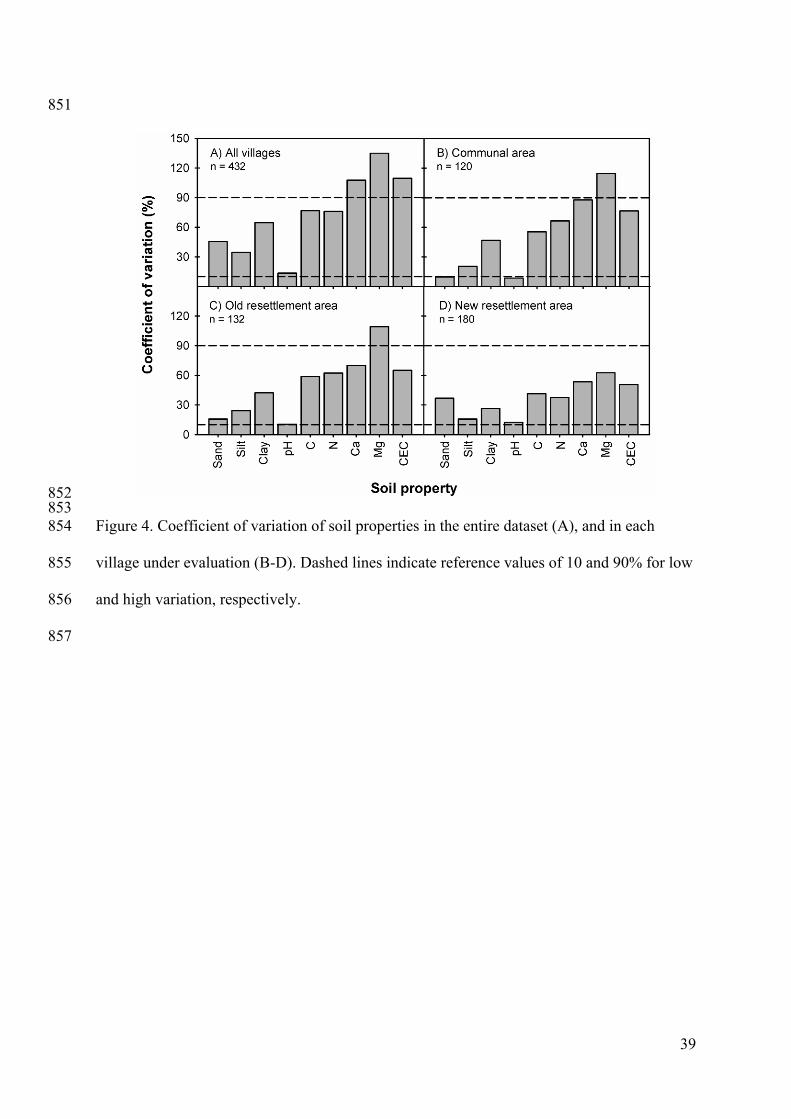
Overall variability of soil properties in each area was evaluated by its coefficient of variation. 408

According to Wei et al. (2008), a CV less than 10% indicates that variability of a considered 409

property is low; while a CV higher than 90% indicates high variation. Thus, calculated CVs 410

in the entire dataset (Figure 4A) showed that Ca, Mg and CEC were the properties with the 411

highest overall variability (>90%); while only pH presented a relative low variation (~10%). 412

Other evaluated soil properties showed intermediate variability (CV=10-90%). When 413

calculations were performed by village (Figure 4B-D), CVs of all soil properties reduced 414

considerably, as expected. Data showed that Mg varied the most in the three villages, while 415

pH (in all villages) and sand (in the communal and old resettlement area) presented the 416

lowest variation. With the particular exception of sand and pH, variability of all soil 417

properties in the new resettlement was lower than in the other two areas. 418

419

Differences in medians among villages for all soil properties were significant at p<0.001 420

(Figure 5). Differences were especially evident when the communal and old resettlement 421

areas were compared to the new resettlement area, mainly due to divergent soil textural types 422

(Table 1). In fact, the new resettlement area presented the lowest values for sand and the 423

highest for the remaining properties. This is why a Mann-Whitney test was also performed to 424

compare only between the communal and old resettlement area. This analysis showed highly 425

significant differences (p<0.001) in medians between these two villages for all evaluated soil 426

properties (Figure 5). 427

428

3.3. Minimum sample size requirements 429

19

Estimated minimum sample sizes, for all evaluated parameters, exhibited a negative 430

exponential trend by increasing the margin of error (Figure 6). Taking soil C as an example, a 431

minimum of 473 samples would be required in the communal area to estimate the mean at 432

5% of its true value; while a minimum of 118, 53, 30 and 19 samples would be necessary at 433

margins errors of 10, 15, 20 and 25%, respectively. With the exception of sand and pH, the 434

required number of samples was found to be lower in the new resettlement area than in the 435

other villages. In general, a higher number of samples would be required for Mg, CEC and 436

Ca, while relatively fewer samples would be necessary for pH, silt and sand. 437

438

3.4. Geostatistical analyses of generated soil data 439

Geostatistical analyses require data following Gaussian distribution. Thus, transformation of 440

variables was necessary in most of the cases (see Table 3) and this generally allowed to 441

approximate normality. However, for Mg in the communal and old resettlement areas any 442

transformations used could shift the highly skewed distribution of this variable. This was 443

attributed to the low concentrations measured (Figure 5), where a high proportion of samples 444

had null values as they were below analytical detection limits. Approximations to normality 445

in a situation like this is simply not possibly by any mean (Reimann and Filzmoser, 2000); 446

therefore data for Mg must be interpreted with caution for these two areas. 447

448

To determine the grade of spatial dependence of each soil property, the nugget-to-sill ratio 449

from all semivariograms was calculated. According to Cambardella et al. (1994), and since 450

then further applied by many others (e.g. Huang et al., 2006; Rossi et al., 2009; Wang et al., 451

2009), if this ratio is lower than 25% the spatial dependence is considered strong; if the ratio 452

is between 25-75% the dependence is considered moderate; and if this ratio is higher than 453

75% the dependence is considered weak. A similar approach was used here, but their 454

20

moderate range of spatial dependence (25-75%), that in our opinion is quite wide, was 455

subdivided, and the following classes of spatial dependency used: class I (very strong) <25%, 456

class II (moderately strong) = 25-50%, class III (moderately weak) = 50-75%, class IIII (very 457

weak) >75%, and class O (null) = 100%. Hence, spatial dependence of evaluated soil 458

properties was mostly moderately strong to very strong in the new resettlement area; 459

moderately weak to moderately strong in the old resettlement area; and null to moderately 460

weak in the communal area (Figure 7, Table 3). In fact, in the communal area N and CEC 461

showed null spatial dependency, while sand, clay and Mg exhibited a linear trend with an 462

undefined spatial autocorrelation at the considered lag distance. From the other two areas 463

only N in the old resettlement area exhibited lack of spatial dependence. All the rest of the 464

cases could be very well represented by spherical models with variable parameters depending 465

on the soil property and area under evaluation. For example, while the nugget-to-sill ratio for 466

Ca was 74% in the communal area (moderately weak dependency), in the old and new 467

resettlement areas this ratio reduced to 42 and 28% (moderately strong dependency), 468

respectively. This contrasted with silt, as the nugget-to-sill ratio increased from 30 and 34% 469

in the communal and old resettlement area, respectively, up to 67% in the new resettlement 470

area. Ranges of the semivariograms for all soil properties and sites ranged from 250 m (silt in 471

the communal area) to 695 m (clay in the new resettlement). With the exception of Ca, 472

estimated ranges were lowest in the communal area and highest in the new resettlement. 473

474

3.5. Principal components and geo-statistical analyses of MIRS data 475

Forty nine percent (49%) of overall variability of MIRS data could be explained by the first 476

principal component (PC1), while 11, 10, 6, 4 and 4% could be explained by PC2, PC3, PC4, 477

PC5 and PC6 respectively. Therefore, only the first three components, accounting for 70% of 478

overall variability, were retained. Scores of the first three components were next correlated to 479

21

concentration values of reference samples. In general, PC1 related very well to texture 480

fractions, C, N, Ca and Mg (absolute Spearman coefficient values of 0.55-0.96, Figure 8); 481

while relationships between PC2 or PC3 with analyzed soil properties were weaker (0.39-482

0.69) or mostly non significant (0.01-0.27), respectively (data not shown). 483

484

Standardized semivariograms based on the principal components were usually represented 485

very well by spherical models, with variable parameters according to the component and 486

village. PC1, however, showed a linear trend in the communal area, indicating an undefined 487

spatial dependence at the considered lag distance. In fact, semivariograms showed mainly 488

that spatial dependence was usually moderately strong to very strong in the new resettlement 489

area; moderate weak to moderately strong in the old resettlement area; and very weak to 490

moderately weak in the communal area (Figure 9, Table 4). Ranges of these semivariograms 491

were 399 m (in the communal area), 161-481 m in the old resettlement area, and 604-744 m 492

in the new resettlement. 493

494

4. Discussion 495

4.1. MIRS and Geostatistics: a viable combination? 496

This study clearly illustrated that MIRS can be successfully used for complementing large 497

soil datasets required for spatial assessments at landscape level. Furthermore, it suggested 498

that spectral information from MIRS, after principal component analyses, could be directly 499

integrated in geostatistical analyses without the need of a calibration/validation step. 500

Effectively, MIRS proved its potential in predicting most of the soil properties under 501

evaluation; although the technique was not effective for all properties. This was evident for 502

silt, Pav, K and Al which presented inadequate MIRS models and therefore, predictions for 503

these variables could not be carried out. Hence, semivariograms for silt, Pav, K and Al were 504

22

not constructed due to insufficient data. Working with different soils in Vietnam, and by 505

using the same MIRS methodology and equipment, Schmitter et al. (2010) found, conversely, 506

acceptable models for silt and K; while their models for clay and CEC were inadequate (P. 507

Schmitter, personal communication). Hence, applicability and efficacy of MIRS depends on 508

the soil type and/or location, and illustrates why regional calibrations are still required for a 509

successful prediction of soil properties (McBratney et al., 2006; Shepherd and Walsh, 2004). 510

These issues limit a generic applicability of MIRS in the prediction of soil variables for agro-511

ecological assessments. Some advances in the development of global calibrations, however, 512

have been achieved in the last few years (Brown et al., 2005; Cécillon et al., 2009), which 513

should help to overcome this limitation in the near future. Alternative solutions could be the 514

use of MIRS-based predictions models to estimate through pedotransfer functions those soil 515

properties that cannot be predicted accurately by sole MIRS (McBratney et al., 2006), or the 516

utilization of auxiliary predictors (i.e. simple and inexpensive conventional soil parameters, 517

like pH and sand; or from complementary sensors, like NIRS) that can improve the prediction 518

of other soil properties (Brown et al., 2005). Thus, all data could be later used in spatial 519

analyses without restriction. 520

521

Semivariograms based on the soil dataset clearly showed that spatial autocorrelation of most 522

soil properties in the villages followed the order: communal area < old resettlement < new 523

resettlement. Variography analyses based on the principal components from MIRS data 524

showed comparable spatial patterns (i.e., nugget to sill ratios and ranges of semivariograms, 525

Figure 10). This implies important savings in terms of analytical costs and time, as it creates 526

the possibility of a broad and quick assessment of soil spatial variability at landscape scale 527

based only on MIRS, confirming previous suggestions by Shepherd and Walsh (2007) and 528

complementing studies based on NIRS (i.e. by Awiti et al., 2008; Cohen et al., 2006; Vågen 529

23

et al., 2006). A related approach to our study, but at plot level and by using NIRS, was 530

carried out by Odlare et al. (2005). However, they found out that spatial dependence from 531

principal components (based on spectral information) was not related to the spatial 532

dependence from considered soil properties (i.e. C, clay and pH). Hence, although spatial 533

variation based on NIRS could be identified, the authors did not know what the variation 534

represented. Thus, to properly understand the meaning of the spatial structures from the 535

principal components it is necessary to link the component scores to soil parameters of 536

reference samples. In our case, this was possible for the first principal component (PC1), 537

which was well related to textural fractions, C, N, Ca, Mg and CEC. Therefore, PC1 was 538

clearly associated to soil fertility, and thus, derived spatial results could be used for 539

distinguishing areas of different soil quality. However, for PC2 and PC3 simple relationships 540

with measured variables were not evident. A reason for this may be related to the explained 541

variance in each component, where PC1 accounted for 49% of the overall variability, while 542

the other two components each explained a lower proportion (10-11%). The unexplained 543

variance and lack of relationships for the other components would indicate that MIRS could 544

be either generating noise or capturing additional characteristics of soils that this study did 545

not take into account (e.g. carbonates, lime requirements, dissolved organic C, phosphatase 546

and urease activity, among others). In fact, MIRS can be related to a wide range of physical, 547

chemical and biological soil characteristics (for further details please refer to Shepherd and 548

Walsh, 2007; and Viscarra-Rossel et al., 2006). All this would further suggest that MIRS may 549

present great potential as an integrative measurement of soil status and, hence, could be a 550

valuable tool for characterizing spatial variation of soils. 551

552

4.2 Analyses of spatial patterns 553

24

Nearly all experimental semivariograms of soil properties were very well described by the 554

spherical model, with a reachable sill, which clearly indicates the presence of spatial 555

autocorrelation. However, some of the semivariograms in the communal area (for sand, clay, 556

Mg and PC1), could only be described by a linear model with an undefined spatial 557

dependence. If there is no reachable sill this could indicate that spatial dependence may exist 558

beyond the considered lag distance (Huang et al., 2006). Semivariograms for N and CEC in 559

the communal area, and N in the old resettlement showed instead pure nugget effect. Pure 560

nugget effect can represent either extreme homogeneity (all points have similar values) or 561

extreme heterogeneity (values are very different, in a random way). However, pure nugget 562

effect do not compulsory reveal spatial independence, as spatial structure may be present but 563

at lower resolution than our minimum sample distance (that in our case was 30 m) (Davidson 564

and Csillag, 2003). In any case, a high nugget effect would imply higher uncertainty when 565

further interpolation is necessary (e.g. by using Kriging). In such circumstances, calculating 566

the mean value from sampled locations would be sufficient for interpolation, as no spatial 567

structure could be detected at the scale of observation. Finding no spatial dependence for 568

some soil parameters is not an unusual result, as its magnitude (from strong to null 569

dependency) can vary as a function of the soil property and location, among others factors 570

(Garten Jr. et al., 2007). 571

572

As indicated before, spatial dependence (either based on soil properties or just on MIR 573

spectral data) was in general lowest in the communal area and highest in the new 574

resettlement. Although the reasons for these differences can not be completely determined, 575

since our experimental design did not allow a proper separation of causal factors, direct and 576

indirect evidence would suggest some potential drivers that nevertheless need to be 577

investigated in future studies. For example, it is generally accepted (Cambardella et al., 1994; 578

25

Liu et al., 2004; Liu et al., 2009; Rüth and Lennartz, 2008) that a strong spatial dependency 579

of soil properties is controlled by intrinsic factors, like texture and mineralogy; while a weak 580

dependence is attributed to extrinsic factors, like farmers’ management (e.g. fertilizer 581

applications). Thus, in terms of intrinsic factors, spatial dependence seems to follow the 582

particular textural classes and inherent soil quality of each area. In terms of extrinsic factors, 583

findings from Cobo et al. (2009) would support this as investment in soil fertility and land 584

management of cropping fields was higher in the communal area than in the two resettlement 585

areas. Moreover, according to the history of each settlement (Cobo et al., 2009) the grade of 586

disturbance of natural resources is in the order: communal area > old resettlement > new 587

resettlement, which would also affect correspondingly the spatial variability of soil 588

properties. The coefficient of variation of evaluated soil properties seems to support this, as 589

(with the exception of pH and sand) usually the highest CVs were obtained in the communal 590

area, while the lowest values were found in the new resettlement. However, despite this 591

global trend, no clear relationships were found between the CVs and their respective spatial 592

variability parameters, which indicates once more that only part of the variation could be 593

explained. Similar observations between CVs and spatial variability parameters have been 594

also reported by Gallardo and Paramá (2007). 595

596

4.3. Relevance of findings for future sampling designs 597

Knowledge of sample sizes for each soil property and village presented in this study could be 598

used as guide for better planning sampling designs at landscape scale in areas of similar 599

conditions, as it helps to estimate approximate minimum number of samples that must be 600

taken in each location for achieving a predetermined level of precision. These data, however, 601

do not indicate how samples should be distributed in space. Derived ranges from variography 602

analyses complement very well this information. They indicate the adequate sample distances 603

26

among points for obtaining spatially-independent samples (i.e. that distance that exceeds the 604

ranges of the semivariograms), as better results are obtained when samples are not 605

autocorrelated (Rossi et al., 2009). However, when a high level of precision is required, 606

collection of spatially-independent samples may be problematic, especially for those 607

properties exhibiting high ranges, due to the potential difficulty of arranging a high number 608

of samples at the required (i.e. long) separation distances. For example, for C assessments, if 609

a 5% of error is selected, a minimum of 264 samples should be distributed at >577 m of 610

separation among each other in the new resettlement, which is simply not possible if we 611

consider the same spatial domain. However, at 10% of error, only 66 samples are needed, 612

thus their distribution in the same area is feasible. In the case of sand, clay, N, Mg and CEC 613

for the communal area, and N for the old resettlement, samples could be placed at random 614

instead, as these properties showed pure nugget effect. Data for pH, on the other hand, should 615

be cautiously interpreted, as it is already in a logarithmic scale; hence, not surprisingly it 616

showed the lowest CVs and minimum sample sizes. If the intention of the sampling is to 617

characterize again the spatial variability within villages, results indicated that a sampling 618

distance of 30 m is acceptable for the new resettlement; but lower distances may be necessary 619

for the communal and old resettlement to be able to capture shorter-range variability which 620

this study was not be able to detect. In any case, care is required if direct extrapolation of 621

sampling sizes and ranges to other scales is carried out (e.g. at plot or national levels), as 622

spatial dependence usually differ with the scale (Cambardella et al., 1994). 623

624

5. Conclusions 625

Results from this study clearly showed that required large soil datasets can be built by using 626

MIRS for the prediction of several soil properties, and later successfully used in geostatistical 627

analyses. However, it was also illustrated that not all soil properties exhibit a MIR spectral 628

27

response, and those ones who were well predicted (i.e. sand, clay, pH, C, N, Ca, Mg and 629

CEC) usually depend on the success of regional calibrations. As a new approach, results 630

showed that MIRS data could be directly integrated, after principal component analyses, in 631

geostatistic assessments without the necessity of calibration/validation steps. This approach is 632

very useful when time and funds are limited, and when a coarse measure of soil spatial 633

variability is required. However, principal components must be associated to soil functional 634

characteristics to be able to explain the results, as was demonstrated with the soil properties 635

considered in this study. Understanding variability of soils and its spatial patterns in these 636

three contrasting areas brought out also important recommendations for future sampling 637

designs and mapping. By combining information about minimum sample sizes, with 638

corresponding reported ranges from the semivariograms, a better efficiency (in terms of time, 639

costs and accuracy) during sampling exercises could be obtained. Hence, it is concluded that 640

MIRS and geostatistics can be successfully integrated for spatial landscape analyses and 641

monitoring. A similar approach would be very valuable in regional and global soil fertility 642

assessments and mapping (e.g. Sanchez et al., 2009) and carbon sequestration campaigns 643

(e.g. Goidts et al., 2009), where large soil sample sizes are required and uncertainty about 644

sampling designs prevail. 645

646

6. Acknowledgments 647

The authors are grateful to all farmers in the three villages who supported this study. Many 648

thanks also go to: the extension officers in the region for their collaboration; to Stefan 649

Becker, Cheryl Batistel and the staff of Landesanstalt für Landwirtschaftliche Chemie in the 650

University of Hohenheim for laboratory analyses; to Irene Chukwumah for her support 651

during MIRS readings; and to Hans-Peter Piepho for assistance during statistical analyses. 652

Thanks also to Andrea Schmidt (Bruker Optik GmbH) for her useful help during the analyses 653

28

of MIRS data. The methodology development of this study is linked to the DFG-funded 654

project PAK 346 (“Structure and functions of agricultural landscapes under global climate 655

change”), subproject P3. 656

657

7. References 658

Anderson, J.M. and Ingram, J.S.I., 1993. Tropical Soil Biology and Fertility: A Handbook of 659 Methods. CAB International, Wallingford, Oxon, 221 pp. 660

Awiti, A.O., Walsh, M.G., Shepherd, K.D. and Kinyamario, J., 2008. Soil condition 661 classification using infrared spectroscopy: A proposition for assessment of soil 662 condition along a tropical forest-cropland chronosequence. Geoderma, 143: 73-84. 663

Bekele, A. and Hudnall, W.H., 2006. Spatial variability of soil chemical properties of a 664 prairie–forest transition in Louisiana. Plant and Soil, 280: 7-21. 665

Borůvka, L., Mládková, L., Penížek, V., Drábek, O. and Vašát, R., 2007. Forest soil 666 acidification assessment using principal component analysis and geostatistics. 667 Geoderma, 140: 374-382. 668

Bray, R.H. and Kurtz, L.T., 1945. Determination of total, organic, and available forms of 669 phosphorus in soils. Soil Science, 59: 39-45. 670

Brown, D.J., Shepherd, K.D., Walsh, M.G., Mays, M.D. and Reinsch, T.G., 2005. Global soil 671 characterization with VNIR diffuse reflectance spectroscopy. Geoderma, 132(3-4): 672 273-290. 673

Cambardella, C.A., Moorman, T.B., Novak, J.M., Parkin, T.B., Karlen, D.L., Turco, R.F. and 674 Konopka, A.E., 1994. Field-Scale Variability of Soil Properties in Central Iowa Soils. 675 Soil Science Society of America Journal, 58: 1501-1511. 676

Cécillon, L., Barthès, B.G., Gomez, C., Ertlen, D., Genot, V., Hedde, M., Stevens, A. and 677 Brun, J.J., 2009. Assessment and monitoring of soil quality using near-infrared 678 reflectance spectroscopy (NIRS). European Journal of Soil Science, 60: 770-784. 679

Cobo, J.G., Dercon, G. and Cadisch, G., 2010. Nutrient balances in African land use systems 680 across different spatial scales: a review of approaches, challenges and progress. 681 Agriculture, Ecosystem and Environment, 136(1-2): 1-15. 682

Cobo, J.G., Dercon, G., Monje, C., Mahembe, P., Gotosa, T., Nyamangara, J., Delve, R. and 683 Cadisch, G., 2009. Cropping strategies, soil fertility investment and land management 684 practices by smallholder farmers in communal and resettlement areas in Zimbabwe. 685 Land Degradation & Development, 20(5): 492-508. 686

Cohen, M., Dabral, S., Graham, W., Prenger, J. and Debusk, W., 2006. Evaluating Ecological 687 Condition Using Soil Biogeochemical Parameters and Near Infrared Reflectance 688 Spectra. Environmental Monitoring and Assessment, 116: 427-457. 689

Conzen, J.-P., 2003. Multivariate Calibration: A Practical Guide for the Method Development 690 in the Analytical Chemistry. Bruker Optik GmbH, 92 pp. 691

Davidson, A. and Csillag, F., 2003. A comparison of nested analysis of variance (ANOVA) 692 and variograms for characterizing grassland spatial structure under a limited sampling 693 budget. Canadian Journal of Remote Sensing, 29: 43-56. 694

Dercon, G., Deckers, J., Govers, G., Poesen, J., Sanchez, H., Vanegas, R., Ramirez , M. and 695 Loaiz, G., 2003. Spatial variability in soil properties on slow-forming terraces in the 696 Andes region of Ecuador. Soil and Tillage Research, 72: 31-41. 697

29

FAO, 2005. Land Cover Classification System. Classification concepts and user manual, 698 Software version 2. Environment and natural resources series 8. FAO, Rome, Italy. 699

Fortin, M.-J., Dale, M.R.T. and Hoef, J.v., 2002. Spatial analysis in ecology. In: A.H. El-700 Shaarawi and W.W. Piegorsch (Editors), Encyclopedia of Environmetrics. John Wiley 701 & Sons, Ltd, Chichester, pp. 2051-2058. 702

Gallardo, A. and Paramá, R., 2007. Spatial variability of soil elements in two plant 703 communities of NW Spain. Geoderma, 139: 199-208. 704

Garten Jr., C.T., Kanga, S., Bricea, D.J., Schadta, C.W. and Zho, J., 2007. Variability in soil 705 properties at different spatial scales (1 m–1 km) in a deciduous forest ecosystem. Soil 706 Biology & Biochemistry, 39: 2621-2627. 707

Giller, K.E., Rowe, E.C., De Ridder, N. and Van Keulen, H., 2006. Resource use dynamics 708 and interactions in the tropics: Scaling up in space and time. Agricultural Systems, 88: 709 8-27. 710

Goidts, E., Wesemael, B.V. and Crucifix, M., 2009. Magnitude and sources of uncertainties 711 in soil organic carbon (SOC) stock assessments at various scales. European Journal of 712 Soil Science, 60: 723-739. 713

Goovaerts, P., 1999. Geostatistics in soil science: state-of-the-art and perspectives. 714 Geoderma, 89: 1-45. 715

Huang, S.-W., Jin, J.-Y., Yang, L.-P. and Bai, Y.-L., 2006. Spatial variability of soil nutrients 716 and influencing factors in a vegetable production area of Hebei Province in China. 717 Nutrient Cycling in Agroecosystems, 75: 201-212. 718

Janik, L.J., Merry, R.H. and Skjemstad, J.O., 1998. Can mid infrared diffuse reflectance 719 analysis replace soil extractions? Australian Journal of Experimental Agriculture, 38: 720 681-196. 721

Liebhold, A.M. and Gurevitch, J., 2002. Integrating the statistical analysis of spatial data in 722 ecology. Ecography, 25: 553–557. 723

Lin, H., Wheeler, D., Bell, J. and Wilding, L., 2005. Assessment of soil spatial variability at 724 multiple scales. Ecological Modelling, 182: 271-272. 725

Liu, X., Xu, J., Zhang, M. and Zhou, B., 2004. Effects of Land Management Change on 726 Spatial Variability of Organic Matter and Nutrients in Paddy Field: A Case Study of 727 Pinghu, China. Environmental Management, 34: 691-700. 728

Liu, X., Zhang, W., Zhang, M., Ficklin, D.L. and Wang, F., 2009. Spatio-temporal variations 729 of soil nutrients influenced by an altered land tenure system in China. Geoderma, 152: 730 23-34. 731

Makkawi, M.H., 2004. Integrating GPR and geostatistical techniques to map the spatial 732 extent of a shallow groundwater system. Journal of Geophysics and Engineering, 1: 733 56-62. 734

McBratney, A.B., Minasny, B. and Rossel, R.V., 2006. Spectral soil analysis and inference 735 systems: A powerful combination for solving the soil data crisis. Geoderma, 136: 272-736 278. 737

Odlare, M., Svensson, K. and Pell, M., 2005. Near infrared reflectance spectroscopy for 738 assessment of spatial soil variation in an agricultural field. Geoderma, 126: 193-202. 739

Olea, R.A., 2006. A six-step practical approach to semivariogram modeling. Stochastic 740 Environmental Research and Risk Assessment, 20: 307-318. 741

Pirie, A., Singh, B. and Islam, K., 2005. Ultra-violet, visible, near-infrared, and mid-infrared 742 diffuse reflectance spectroscopic techniques to predict several soil properties. 743 Australian journal of soil research, 43: 713-721. 744

Pozdnyakova, L., Gimenez, D. and Oudemans, P.V., 2005. Spatial Analysis of Cranberry 745 Yield at Three Scales. Agronomy Journal, 97: 49-57. 746

30

Reimann, C. and Filzmoser, P., 2000. Normal and lognormal data distribution in 747 geochemistry : death of a myth. Consequences for the statistical treatment of 748 geochemical and environmental data. Environmental geology, 39: 1001-1014. 749

Rossi, J., Govaerts, A., Vos, B.D., Verbist, B., Vervoort, A., Poesen, J., Muys, B. and 750 Deckers, J., 2009. Spatial structures of soil organic carbon in tropical forests - A case 751 study of Southeastern Tanzania. Catena, 77: 19-27. 752

Rüth, B. and Lennartz, B., 2008. Spatial Variability of Soil Properties and Rice Yield Along 753 Two Catenas in Southeast China. Pedosphere, 18: 409-420. 754

Samake, O., Smaling, E.M.A., Kropff, M.J., Stomph, T.J. and Kodio, A., 2005. Effects of 755 cultivation practices on spatial variation of soil fertility and millet yields in the Sahel 756 of Mali. Agriculture, Ecosystems and Environment 109: 335-345. 757

Sanchez, P.A. et al., 2009. Digital Soil Map of the World. Science, 325: 680-681. 758 Sanchez, P.A. and Leakey, R.R.B., 1997. Land use transformation in Africa: three 759

determinants for balancing food security with natural resource utilization. European 760 Journal of Agronomy, 7: 15-23. 761

Sauer, T.J., Cambardella, C.A. and Meek, D.W., 2006. Spatial variation of soil properties 762 relating to vegetation changes. Plant and Soil, 280: 1-5. 763

Schmitter, P., Dercon, G., Hilger, T., Le Ha, T., Thanh, N.H., Vien, T.D., Lam, N.T. and 764 Cadisch, G., 2010. Sediment induced soil spatial variation in paddy fields of 765 Northwest Vietnam. Geoderma, 155(3-4): 298-307. 766

Schöning, A. and Brümmer, G.W., 2008. Extraction of mobile element fractions in forest 767 soils using ammonium nitrate and ammonium chloride. Journal of Plant Nutrition and 768 Soil Science 171: 392-398. 769

Shepherd, K.D. and Walsh, M.G., 2004. Diffuse Reflectance Spectroscopy for Rapid Soil 770 Analysis. In: R. Lal (Editor), Encyclopedia of Soil Science. Marcel Dekker, Inc. 771

Shepherd, K.D. and Walsh, M.G., 2007. Infrared spectroscopy - enabling an evidence-based 772 diagnostic surveillance approach to agricultural and environmental management in 773 developing countries. Journal of Near Infrared Spectroscopy, 15: 1-20. 774

Urban, D.L., 2002. Tactical monitoring of landscapes. In: J. Liu and W.W. Taylor (Editors), 775 Integrating Landscape Ecology into Natural Resource Management. Cambridge 776 University Press, Cambridge, pp. 294-311. 777

Vågen, T.-G., Shepherd, K.D. and Walsh, M.G., 2006. Sensing landscape level change in soil 778 fertility following deforestation and conversion in the highlands of Madagascar using 779 Vis-NIR spectroscopy. Geoderma, 133: 281-294. 780

Viscarra-Rossel, R.A., T, D.J.J.W., McBratney, A.B., Janik, L.J. and Skjemstad, J.O., 2006. 781 Visible, near infrared, mid infrared or combined diffuse reflectance spectroscopy for 782 simultaneous assessment of various soil properties. Geoderma, 131: 59-75. 783

Vitousek, P.M. et al., 2009. Nutrient Imbalances in Agricultural Development. Science, 324: 784 1519-1520. 785

Wang, Y., Zhang, X. and Huang, C., 2009. Spatial variability of soil total nitrogen and soil 786 total phosphorus under different land uses in a small watershed on the Loess Plateau, 787 China. Geoderma, 150: 141-149. 788

Wei, J.-B., Xiao, D.-N., Zeng, H. and Fu, Y.-K., 2008. Spatial variability of soil properties in 789 relation to land use and topography in a typical small watershed of the black soil 790 region, northeastern China. Environmental Geology, 53: 1663-1672. 791

Yan, X. and Cai, Z., 2008. Number of soil profiles needed to give a reliable overall estimate 792 of soil organic carbon storage using profile carbon density data. Soil Science and 793 Plant Nutrition, 54: 819-825. 794

31

Yemefack, M., Rossiter, D.G. and Njomgang, R., 2005. Multi-scale characterization of soil 795 variability within an agricultural landscape mosaic system in southern Cameroon. 796 Geoderma, 125: 117-143. 797

798 799

32

Table 1. Main characteristics of the villages under study 800

801

Village name

Settlement type

Settlement time

Location (District, Ward)

Dominant soil type&

Mean soil textural class

Village area (ha)

Kanyera Communal area 1948 Shamva, 6 Chromic Luvisols Loamy sand 730 Chomutomora Old resettlement 1987 Shamva, 15 Chromic Luvisols Sandy Loam 780 Hereford Farm New resettlement 2002 Bindura, 8 Rhodic Ferrasols Clay 1360

802

& According to FAO soil classification 803

33

Table 2. Optimization parameters and performance indicators of best MIRS models for each soil property under evaluation. 804

805

Outliers Preprocessing Calibration Validation Property n removed method& Rank R2 RMSEE RPD R2 RMSEP RPD Prediction

Sand 110 1 1stDer+VN 7 0.98 3.7 6.7 0.98 3.3 6.8 Yes Silt 110 1 1stDer+VN 6 0.85 3.1 2.6 0.82 3.6 2.4 No# Clay 110 1 1stDer+SLS 3 0.97 3.0 6.1 0.97 2.6 6.2 Yes pH 165 2 1stDer+SLS 9 0.93 0.20 3.8 0.89 0.24 3.1 Yes C 165 1 1stDer+VN 14 0.99 0.14 10.1 0.98 0.19 6.4 Yes N 165 2 1stDer+VN 9 0.98 0.01 6.6 0.96 0.02 5.2 Yes Pav 165 0 SLS 6 0.47 5.5 1.4 0.49 6.2 1.4 No K 165 0 None 5 0.48 1.9 1.4 0.56 1.4 1.5 No Ca 165 1 COE 8 0.94 25.2 4.1 0.96 18.7 5.1 Yes Mg 165 0 1stDer+MSC 8 0.96 14.8 5.2 0.92 18.0 3.4 Yes Al 165 0 1stDer+SLS 12 0.69 0.70 1.8 0.66 0.61 1.8 No

CEC 165 0 1stDer+VN 9 0.98 22.8 7.6 0.98 24.4 6.6 Yes 806

& 1stDer: 1st derivative, COE: constant offset elimination, SLS: straight line subtraction, MSC: multiplicative scatter correction, VN: vector 807

normalization. Considered spectral regions from the optimization process are not shown. 808

n: number of observations; Rank: number of factors used in the PLS regression; RMSEE: Root Mean Square Error of Estimation, RMSEP: 809

Root Mean Square Error of the Prediction, RPD: Residual Prediction Deviation 810

# But could be calculated from the other two textural fractions811

34

Table 3. Model parameters of standardized theoretical semivariograms of evaluated soil 812

properties in the three villages under study. See Figure 7 for a visualization of respective 813

experimental and theoretical semivariograms. 814

815

Outliers Type of Nugget Sill Range Co Property$ removed Model R2 RSS@ Co Co+C a (in m) (Co+C)# Class& Communal area (n=120) Sand 0 Linear 0.26 6.79E-00 0.86 1.05 82.1 IIII Silt 0 Spherical 0.49 9.35E-01 0.30 1.01 250 29.7 II Clay L 0 Linear 0.25 2.33E-02 0.89 1.09 81.1 IIII pH L 0 Spherical 0.21 5.64E-04 0.62 0.97 451 63.6 III C A 0 Spherical 0.14 5.53E-05 0.56 1.01 400 56.0 III N A 2 - - - 1.0 1.0 100 O Ca S 0 Spherical 0.29 1.08E-02 0.72 0.98 527 73.6 III Mg A 0 Linear 0.25 1.67E-04 0.86 1.04 82.8 IIII CEC L 0 - - - 1.0 1.0 100 O Old resettlement area (n=132) Sand 0 Spherical 0.63 8.58E-00 0.49 0.94 441 51.6 III Silt L 0 Spherical 0.67 5.34E-03 0.36 1.06 426 34.2 II Clay L 0 Spherical 0.59 1.01E-02 0.48 0.95 415 50.4 III pH S 0 Spherical 0.64 1.34E-03 0.51 1.07 484 48.1 II C L 0 Spherical 0.52 7.20E-03 0.69 1.06 532 65.2 III N A 1 - - - 1.0 1.0 100 O Ca S 0 Spherical 0.72 3.39E-02 0.45 1.08 483 41.6 II Mg A 0 Spherical 0.56 3.18E-04 0.54 1.09 459 49.8 II CEC L 0 Spherical 0.63 1.31E-02 0.61 1.02 386 60.0 III New resettlement area (n=180) Sand S 0 Spherical 0.71 5.11E-02 0.42 1.06 506 39.4 II Silt 0 Spherical 0.60 8.60E-01 0.69 1.03 671 67.3 III Clay 0 Spherical 0.76 6.80E-00 0.46 1.05 695 43.7 II pH L 0 Spherical 0.65 1.57E-03 0.39 1.08 638 36.2 II C L 0 Spherical 0.75 1.11E-02 0.23 1.05 577 21.4 I N A 0 Spherical 0.77 6.70E-06 0.23 1.04 517 22.1 I Ca S 0 Spherical 0.64 2.51E-01 0.31 1.10 649 28.1 II Mg S 0 Spherical 0.71 1.98E-01 0.17 1.05 522 15.8 I CEC A 0 Spherical 0.70 4.91E-03 0.25 1.08 604 23.3 I

816 $: If carried out, the type of transformation is indicated (L = logarithm, S = square root, A = 817

arcsin, n: number of observations; @: Residual Sum of Squares, #: Nugget-to-sill ratio (%), 818 &: Spatial dependency class: I = very strong, II = moderately strong, III = moderately weak, 819

IIII = very weak, O = null. 820

821

35

Table 4. Model parameters of standardized theoretical semivariograms of the three first 822

principal components from MIRS data of the three areas under study. See Figure 8 for a 823

visualization of respective experimental and theoretical semivariograms. 824

825

Outliers Type of Nugget Sill Range Co Property$ removed Model R2 RSS@ Co Co+C a (in m) (Co+C)# Class& Communal area (n=120) PC1 L 0 Linear 0.09 4.41E-03 0.94 1.03 90.9 IIII PC2 0 Spherical 0.15 3.93E-03 0.59 1.01 399 58.7 III PC3 L 0 Spherical 0.41 6.41E-03 0.60 1.03 399 58.0 III Old resettlement area (n=132) PC1 1 Spherical 0.62 4.44E-03 0.54 1.05 481 51.0 III PC2 L 4 Spherical 0.60 1.60E-03 0.59 1.15 479 51.1 II PC3 L 2 Spherical 0.40 3.73E-03 0.41 0.99 161 41.0 II New resettlement area (n=180) PC1 A 1 Spherical 0.69 9.74E-06 0.20 1.10 606 18.3 I PC2 10 Spherical 0.80 4.66E-05 0.45 1.10 744 41.0 II PC3 0 Spherical 0.78 2.13E-01 0.05 1.11 604 4.6 I

826

$: If carried out, the type of transformation is indicated (L = logarithm, A = arcsin), n: number 827

of observations; @: Residual Sum of Squares, #: Nugget-to-sill ratio (%), &: Spatial 828

dependency class: I = very strong, II = moderately strong, III = moderately weak, IIII = very 829

weak. 830

831

36

832 833 Figure 1. Soil sampling design. Hereford farm is used here as illustration: A) Representation 834 of the overlay of a village boundary with main grid of 750 x 750 m; B) Zooming into a cell of 835 750 x 750 m where grids of 150 x 150 and 30 x 30 m, and selected sub-cells and micro-cells 836 (with respective centroids), are shown; C) Final distribution of sampling points in the 837 village; D) Schematic representation of the radial arm for each sampling point, where central 838 circle indicates the centroid of each micro-cell (N: north, SW: south west; SE: south east). 839

840

37

841 842 Figure 2. Examples of mid infrared spectra of soil samples from the three villages under 843

study: i.e. the baseline-corrected spectrum of one sample per village having an average C 844

content of 7, 11 and 29 g kg-1 for the communal area, and the old and new resettlement areas, 845

respectively.846

38

847

848

Figure 3. Calibration (triangles) and validation (circles) scatter plots of MIRS models from evaluated soil properties. For respective performance 849

indicators refer to Table 2.850

39

851

852 853 Figure 4. Coefficient of variation of soil properties in the entire dataset (A), and in each 854

village under evaluation (B-D). Dashed lines indicate reference values of 10 and 90% for low 855

and high variation, respectively. 856

857

40

858 859 Figure 5. Box and whisker plots of soil properties in each village under evaluation, and associated 860

statistical differences (*** : p<0.001) according to the [Kruskall-Wallis | Mann-Whitney] tests. 861

Kruskall-Wallis compared medians (horizontal line inside boxes) of the three villages, while 862

Mann-Whitney compared only the communal and old resettlement areas. Number of data as 863

shown in Figure 4. 864

865

41

866 867 Figure 6. Minimum sample sizes required for estimating the mean of different evaluated soil 868 properties at different probabilities of its true value (margin of error), with a 95% of 869 confidence in: communal area (closed triangles), old resettlement (closed circles) and new 870 resettlement (open circles). Notice that Y-axes are in logarithmic scale. Number of data for 871 calculations and units as shown in Figure 4. 872

873

42

874 875 Figure 7. Standardized experimental (circles) and theoretical (line) semivariograms for 876 evaluated soil properties in the three areas under study. For model parameters please refer to 877 Table 3. 878

879

43

880 881 Figure 7. Continuation 882

883

44

884 885 Figure 8. Scatter plots and Spearman correlation coefficients for the relationships between 886 soil properties from reference samples (i.e. analyzed by conventional laboratory procedures) 887 and respective component scores of the first principal component (PC1) based on MIRS data. 888 ***: p<0.001. 889 890

891

45

892 893 Figure 9. Standardized experimental (circles) and theoretical (line) semivariograms for the 894 three first principal components based on MIRS data from all soil samples collected in the 895 three areas under study. For model parameters please refer to Table 4. 896

897

46

898

899

Figure 10. Comparison of A) nugget-to-sill ratios (and spatial dependency classes as defined 900

in the text), and B) ranges, from semivariograms of the three studied settlement schemes 901

based on MIRS-derived principal components (PC1-PC3) and evaluated soil properties. 902

Circles exclude variables that deviate from the behavior of the main group. Variables with 903

undefined ranges (see Tables 3 and 4) were not plotted. 904