COBEM-2017-2703 MODELLING, SIMULATION AND CONTROL OF …

24th ABCM International Congress of Mechanical EngineeringDecember 3-8, 2017, Curitiba, PR, Brazil

COBEM-2017-2703MODELLING, SIMULATION AND CONTROL OF FIXED-WING

UNMANNED AERIAL VEHICLE (UAV)Willian Rigon SilvaAndré Luís da SilvaUFSM - Grupo de Sistemas Aeroespaciais e Controle (GSAC) - RS, [email protected]@gmail.com

Hilton Abílio GründlingUFSM - Grupo de Eletrônica de Potência e Controle (GEPOC) - RS, [email protected]

Abstract. The work presents a methodology for mathematical modelling, simulation and control design for the longitu-dinal dynamics of a fixed-wing Unmanned Aerial Vehicle (UAV). The methodology used is well known in aeronauticalliterature for manned airplane design, so its adaptation to UAV was investigated. Due to the non-linear coupled dynamicspresent in this type of plant, some assumptions were made during the modelling and control design. Two models of theUAV were obtained: one purely analytic (by stability and control derivatives given by USAF DATCOM), and the otherby X-Plane Flight Simulator (which uses Blade Element Theory to calculate the flight model). The analytical model waslinearized for a chosen equilibrium point (cruise flight at chosen altitude and speed). The longitudinal flight dynamicmodes were analysed: Short Period and Phugoid Mode. The chosen plant is the University of Toronto Explorer (UT-X)UAV, designed and built by the University of Toronto Aerospace Team (UTAT). Using classical automatic flight controltheory, an Altitude and Mach Hold Autopilot was designed. A Software In The Loop (SITL) simulation was developed,using MATLAB/Simulink communicating with X-Plane through UDP protocol. The SITL simulation setup was used toperform virtual flight tests, in order to assess the performance of the designed autopilots. Wind, Gust and Turbulence testswere also presented.

Keywords: Flight Dynamics, Simulation, Autopilot, Control, UAV

1. INTRODUCTION

The paper presents a methodology to model the longitudinal dynamics of an UAV by two methods: stability andcontrol derivatives (given by USAF DATCOM), and virtual flight tests using X-Plane flight simulator.

The analytical model is composed by fixed-wing airplane equations of motion derived with Newtonian Mechanics,using Flat-Earth model, with dimensionless aerodynamic coefficients calculated by stability and control derivatives givenby USAF DATCOM, (Siddiqui and Khushnood, 2009). The longitudinal dynamics modes, phugoid and short-period,given by the analytical simulation were compared with the results of virtual flight tests in the X-Plane simulator. If thelongitudinal dynamics for both models are similar, then it is possible to use the analytical model to design the autopilotusing control theory, and test its performance in a Software In The Loop (SITL) simulation with the X-Plane model. Inorder to refine the analytical model, wind tunnel data and real flight test data should be used. This methodology is wellknown in aeronautical industry and it is used for manned airplanes (Stevens and Lewis, 1992).

The study main objectives are to answer the two following problems: First, given an UAV with already definedairframe and physical characteristics (weight, moments of inertia, surface deflections, engine), how to obtain a longitudinaldynamics mathematical model; Second, knowing an UAV mathematical model, how to design an autopilot (Altitude Holdand Mach Hold) that can be implemented in low performance hardware (microcontrollers).

Nowadays, UAVs are ubiquitous aircraft which are used in several applications, such as: hobby, aerial photography,topography, Search And Rescue (SAR), and military (Austin, 2010). Quad-rotors and fixed-wing are the most commontypes of UAVs, flying under direct control of an operator or autonomously (assisted flight). The use of these flying robotsin civilian and military roles is increasing, justified by the advantages that they present.

A more recent name definition for UAVs is Remotely Piloted Aircraft (RPA). Aeronautical legislation discussions(internationally and in Brazil) stated that these types of aircraft cannot fly unassisted. In other words, a fully autonomous

W.R. Silva, A.L. da Silva and H.A. GründlingModelling, Simulation, and Control of Fixed-Wing UAV

flight can only occur if exists an operator with direct communication with the vehicle, that can take control immediatelyif necessary. The term RPA is more precise, describing this legislation requirement. In this paper the term UAV will beused along the text, but RPA is a synonym.

UAVs exists in several different weights and sizes, designed for a specific purpose and sometimes referred as drones.For professional applications (civilian or military), the increasing use of this type of aircraft is justified by its advantagesover the manned aircraft. The main advantages are the low flight-hour and maintenance cost. For instance, UAV aerialreconnaissance missions can be of high risk and demanding, taking long time on air, even more than one day withoutlanding. Using UAVs in this type of mission can minimize the risk to occur human error, since the operators are com-fortable, safe, and can be changed while the aircraft is on flight (Austin, 2010). The use of UAVs also present advantagesin radioactive environments, precision agriculture, and wildfires identification/combat. Therefore, it is important to fullyunderstand the UAVs technology (design and operation) in order to develop optimized designs to specific applications(Beard and McLain, 2012).

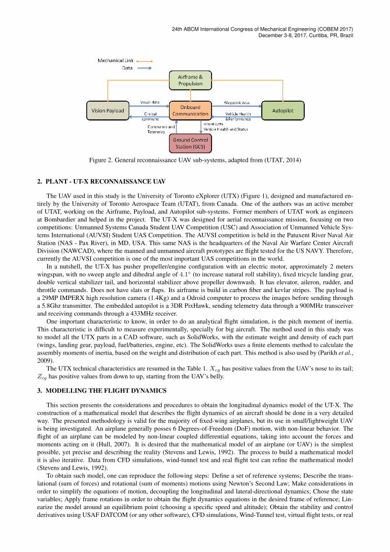
An usual reconnaissance UAV (Figure 1) can be viewed as a system composed of several smaller sub-systems (Figure2): Airframe, Engine, Electrical, Payload, Communications, Sensors and Actuators, Autopilot, and Ground Control Sta-tion (GCS). The detailing about each system is beyond the scope of this paper. The UAV and the GCS together forms anUnmanned Aerial System (UAS).

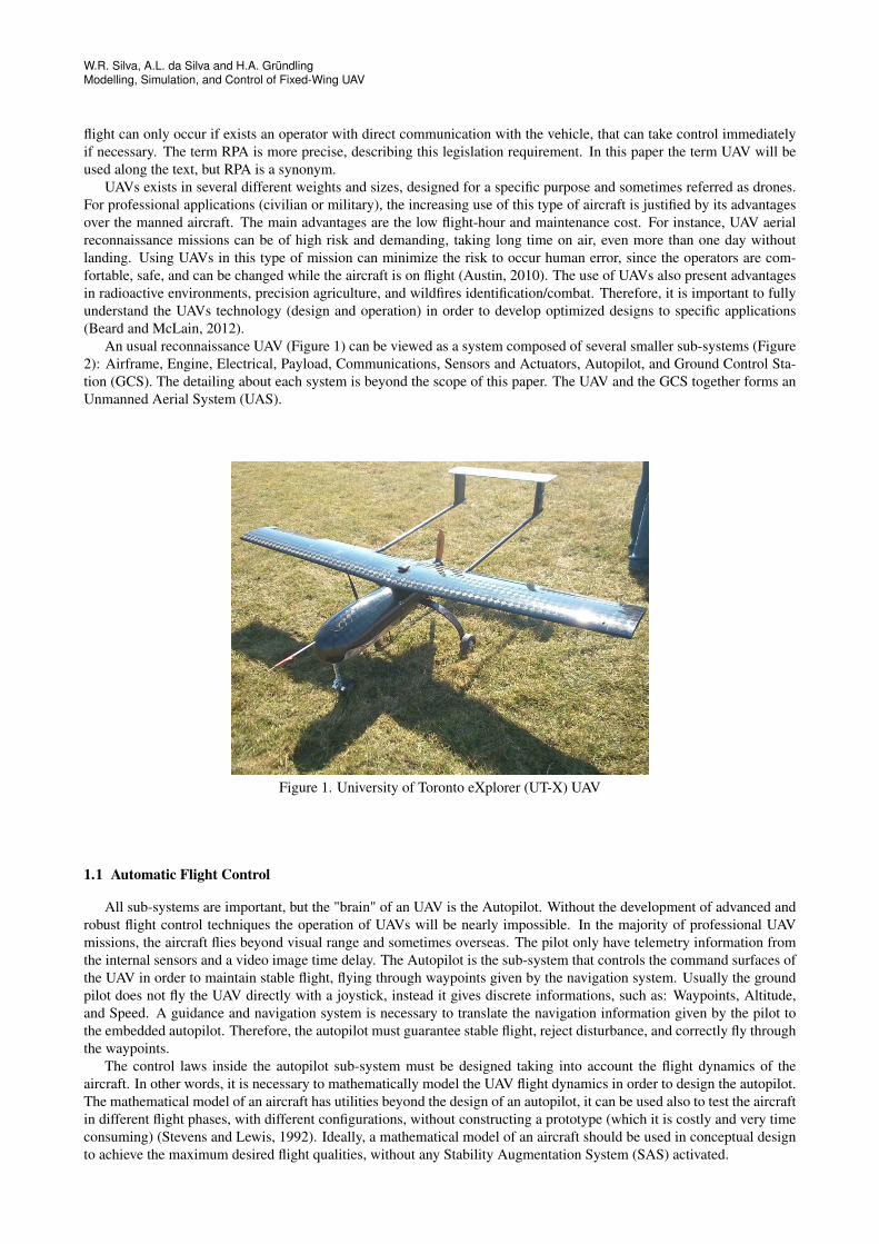
Figure 1. University of Toronto eXplorer (UT-X) UAV

1.1 Automatic Flight Control

All sub-systems are important, but the "brain" of an UAV is the Autopilot. Without the development of advanced androbust flight control techniques the operation of UAVs will be nearly impossible. In the majority of professional UAVmissions, the aircraft flies beyond visual range and sometimes overseas. The pilot only have telemetry information fromthe internal sensors and a video image time delay. The Autopilot is the sub-system that controls the command surfaces ofthe UAV in order to maintain stable flight, flying through waypoints given by the navigation system. Usually the groundpilot does not fly the UAV directly with a joystick, instead it gives discrete informations, such as: Waypoints, Altitude,and Speed. A guidance and navigation system is necessary to translate the navigation information given by the pilot tothe embedded autopilot. Therefore, the autopilot must guarantee stable flight, reject disturbance, and correctly fly throughthe waypoints.

The control laws inside the autopilot sub-system must be designed taking into account the flight dynamics of theaircraft. In other words, it is necessary to mathematically model the UAV flight dynamics in order to design the autopilot.The mathematical model of an aircraft has utilities beyond the design of an autopilot, it can be used also to test the aircraftin different flight phases, with different configurations, without constructing a prototype (which it is costly and very timeconsuming) (Stevens and Lewis, 1992). Ideally, a mathematical model of an aircraft should be used in conceptual designto achieve the maximum desired flight qualities, without any Stability Augmentation System (SAS) activated.

24th ABCM International Congress of Mechanical Engineering (COBEM 2017)December 3-8, 2017, Curitiba, PR, Brazil

Figure 2. General reconnaissance UAV sub-systems, adapted from (UTAT, 2014)

2. PLANT - UT-X RECONNAISSANCE UAV

The UAV used in this study is the University of Toronto eXplorer (UTX) (Figure 1), designed and manufactured en-tirely by the University of Toronto Aerospace Team (UTAT), from Canada. One of the authors was an active memberof UTAT, working on the Airframe, Payload, and Autopilot sub-systems. Former members of UTAT work as engineersat Bombardier and helped in the project. The UT-X was designed for aerial reconnaissance mission, focusing on twocompetitions: Unmanned Systems Canada Student UAV Competition (USC) and Association of Unmanned Vehicle Sys-tems International (AUVSI) Student UAS Competition. The AUVSI competition is held in the Patuxent River Naval AirStation (NAS - Pax River), in MD, USA. This same NAS is the headquarters of the Naval Air Warfare Center AircraftDivision (NAWCAD), where the manned and unmanned aircraft prototypes are flight tested for the US NAVY. Therefore,currently the AUVSI competition is one of the most important UAS competitions in the world.

In a nutshell, the UT-X has pusher propeller/engine configuration with an electric motor, approximately 2 meterswingspan, with no sweep angle and dihedral angle of 4.1◦ (to increase natural roll stability), fixed tricycle landing gear,double vertical stabilizer tail, and horizontal stabilizer above propeller downwash. It has elevator, aileron, rudder, andthrottle commands. Does not have slats or flaps. Its airframe is build in carbon fiber and kevlar stripes. The payload isa 29MP IMPERX high resolution camera (1.4Kg) and a Odroid computer to process the images before sending througha 5.8Ghz transmitter. The embedded autopilot is a 3DR PixHawk, sending telemetry data through a 900MHz transceiverand receiving commands through a 433MHz receiver.

One important characteristic to know, in order to do an analytical flight simulation, is the pitch moment of inertia.This characteristic is difficult to measure experimentally, specially for big aircraft. The method used in this study wasto model all the UTX parts in a CAD software, such as SolidWorks, with the estimate weight and density of each part(wings, landing gear, payload, fuel/batteries, engine, etc). The SolidWorks uses a finite elements method to calculate theassembly moments of inertia, based on the weight and distribution of each part. This method is also used by (Parikh et al.,2009).

The UTX technical characteristics are resumed in the Table 1. Xcg has positive values from the UAV’s nose to its tail;Zcg has positive values from down to up, starting from the UAV’s belly.

3. MODELLING THE FLIGHT DYNAMICS

This section presents the considerations and procedures to obtain the longitudinal dynamics model of the UT-X. Theconstruction of a mathematical model that describes the flight dynamics of an aircraft should be done in a very detailedway. The presented methodology is valid for the majority of fixed-wing airplanes, but its use in small/lightweight UAVis being investigated. An airplane generally posses 6 Degrees-of-Freedom (DoF) motion, with non-linear behavior. Theflight of an airplane can be modeled by non-linear coupled differential equations, taking into account the forces andmoments acting on it (Hull, 2007). It is desired that the mathematical model of an airplane (or UAV) is the simplestpossible, yet precise and describing the reality (Stevens and Lewis, 1992). The process to build a mathematical modelit is also iterative. Data from CFD simulations, wind-tunnel test and real flight test can refine the mathematical model(Stevens and Lewis, 1992).

To obtain such model, one can reproduce the following steps: Define a set of reference systems; Describe the trans-lational (sum of forces) and rotational (sum of moments) motions using Newton’s Second Law; Make considerations inorder to simplify the equations of motion, decoupling the longitudinal and lateral-directional dynamics; Chose the statevariables; Apply frame rotations in order to obtain the flight dynamics equations in the desired frame of reference; Lin-earize the model around an equilibrium point (choosing a specific speed and altitude); Obtain the stability and controlderivatives using USAF DATCOM (or any other software), CFD simulations, Wind-Tunnel test, virtual flight tests, or real


Table 1. Physical Parameters of the UT-X UAV

Symbol Parameter Valuem Total Mass with Payload and Batteries 9.57 kg− Approximate Flight Autonomy 45 min

VTmax Approximate Maximum True Airspeed (TAS) 25 m/sb Wingspan 1.978 md Body Length 1.34 mS Wing Reference Area 0.485 m2

Λ Wing Sweep Angle 0.0 ◦

Γ Wing Dihedral Angle 4.1 ◦

Iyy Pitch Moment of Inertia 3.33 kg.m2

c Aerodynamic Mean Chord 0.2449 mXcg Gravity Center Position at X axis 0.477 mZcg Gravity Center Position at Z axis 0.109 m

Wairfoil Wing Airfoil NACA− 6412HVairfoil Horizontal and Vertical Stabilizers Airfoils NACA− 0012

flight tests; Calculate the aerodynamic forces using the stability and control derivatives.

3.1 Considerations and Definition of Reference Frames

In order to simplify the model, some considerations should be done. By doing assumptions, we are allowing someerrors that will be translated into limitations of this mathematical model. The errors of the model should be minimized, butwe can incorporate the residual errors into the control system design. It is important to understand the model limitations,neglecting these limitations can lead to design error (that could be fatal).

The considerations done in order to obtain the longitudinal dynamics mathematical model, balancing simplicity andprecision, are the following: The aircraft is in cruise flight phase; The atmosphere is stationary. The atmospheric propertiesonly depends on altitude (i.e. they are independent of temperature variations and wind); The Earth surface is consideredflat (Flat Earth Model), with no acceleration, no rotation, no translation, and with constant gravity intensity and direction(perpendicular to the Earth’s surface); The aircraft body is considered rigid (rigid-body model) and with constant mass(mass is not a time function); The Sideslip angle (β) is zero; The perturbations around the equilibrium point are small(small pitch angles θ around trim point); The elevator deflection does not change forces, only the pitch moment; Allaerodynamic forces (Lift,Drag,Thrust) act in the aircraft center of gravity (CG); The aircraft presents airframe symmetryin the x and z planes.

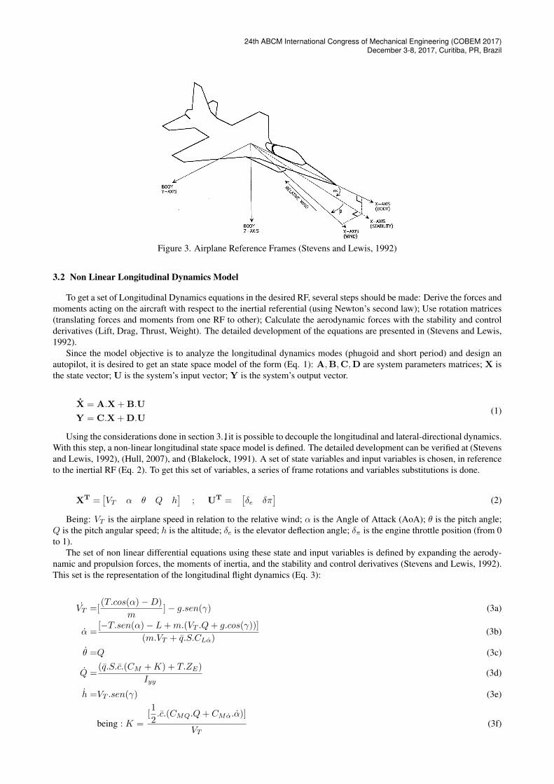
The forces and moments that act on an aircraft are produced by the relative wind passing through the aerodynamicsurfaces (wings, body, command surfaces, and propulsive force). To determine the orientation and direction of theseforces, it is necessary to define a system of reference. The equations of motion should be derived in relation to an inertialreference frame (RF) (Stevens and Lewis, 1992). Three reference frames (RFs) are defined (Figure 3):

(a) Body Axes - RF with 3 orthogonal axes, fixed on the aircraft CG. By convention, starting at the airplane CG, theX axis is pointing to airplane’s nose, Y axis pointing to airplane’s right wing, and Z axis pointing to airplane’sbottom;

(b) Stability Axes - This RF is also known as North-East-Down(NED) frame. It has 3 orthogonal axes located at theairplane CG, with theX axis pointing North, Y axis pointing East, and Z axis pointing down (to the Earth’s center);

(c) Wind Axes - RF with 3 orthogonal axes, fixed on the aircraft CG. These axes always follow the relative winddirection, with respect to the airplane. The X axis points in the reverse direction of the relative wind. The Z axis isperpendicular with the relative wind and it points down. The Y axis completes the system.

The inertial referential is chosen to be a fixed point in the Earth’s surface. Even if the Earth has rotation and acceler-ation, they can be neglected since the time constants are different. The Earth acceleration is considerably slower than theacceleration of an aircraft maneuvering in its surface (Stevens and Lewis, 1992). Therefore, an inertial referential frameis fixed in the ground:

• Ground Axes System - RF with 3 orthogonal axes, fixed on the ground. The X and Y axes are parallel to the Earth’shorizon (Flat Earth Model). It uses the NED convention.


Figure 3. Airplane Reference Frames (Stevens and Lewis, 1992)

3.2 Non Linear Longitudinal Dynamics Model

To get a set of Longitudinal Dynamics equations in the desired RF, several steps should be made: Derive the forces andmoments acting on the aircraft with respect to the inertial referential (using Newton’s second law); Use rotation matrices(translating forces and moments from one RF to other); Calculate the aerodynamic forces with the stability and controlderivatives (Lift, Drag, Thrust, Weight). The detailed development of the equations are presented in (Stevens and Lewis,1992).

Since the model objective is to analyze the longitudinal dynamics modes (phugoid and short period) and design anautopilot, it is desired to get an state space model of the form (Eq. 1): A,B,C,D are system parameters matrices; X isthe state vector; U is the system’s input vector; Y is the system’s output vector.

X = A.X + B.U

Y = C.X + D.U(1)

Using the considerations done in section 3.1, it is possible to decouple the longitudinal and lateral-directional dynamics.With this step, a non-linear longitudinal state space model is defined. The detailed development can be verified at (Stevensand Lewis, 1992), (Hull, 2007), and (Blakelock, 1991). A set of state variables and input variables is chosen, in referenceto the inertial RF (Eq. 2). To get this set of variables, a series of frame rotations and variables substitutions is done.

XT =[VT α θ Q h

]; UT =

[δe δπ

](2)

Being: VT is the airplane speed in relation to the relative wind; α is the Angle of Attack (AoA); θ is the pitch angle;Q is the pitch angular speed; h is the altitude; δe is the elevator deflection angle; δπ is the engine throttle position (from 0to 1).

The set of non linear differential equations using these state and input variables is defined by expanding the aerody-namic and propulsion forces, the moments of inertia, and the stability and control derivatives (Stevens and Lewis, 1992).This set is the representation of the longitudinal flight dynamics (Eq. 3):

VT =[(T.cos(α) −D)

m] − g.sen(γ) (3a)

α =[−T.sen(α) − L+m.(VT .Q+ g.cos(γ))]

(m.VT + q.S.CLα)(3b)

θ =Q (3c)

Q =(q.S.c.(CM +K) + T.ZE)

Iyy(3d)

h =VT .sen(γ) (3e)

being : K =[1

2.c.(CMQ.Q+ CMα.α)]

VT(3f)


Where: γ = θ − α; g the acceleration due to gravity; m the mass of the airplane; L and D the aerodynamic forcesof Lift and Drag respectively; T the propulsion force (Thrust); ZE the offset of the propulsion axis z in relation to theairplane CG, in the UT-X case it is supposed to be zero; q = (1/2)ρV 2

T the dynamic pressure (ρ is the air density); S thewing reference area; c the mean aerodynamic chord of the wing; CLα, CMQ, CMα are stability derivatives and CM thepitch moment coefficient.

3.3 Aerodynamic Forces, Propulsion, and Stability and Control Derivatives

In order to calculate the aerodynamic forces (Eq. 4), it is needed to define the dimensionless aerodynamic coefficients.These coefficients are formed by stability and control derivatives, as a sum of one main influential part (usually dependingon α and β angles) and several others of less influence (Stevens and Lewis, 1992) (Eq. 4). The stability derivatives arethose considering the command surfaces in neutral position, the control derivatives are those referred to the changes inthe command surfaces (e.g. δe).

L = q.S.CL, (4a)D = q.S.CD, (4b)CL = CL0 + CLαα (4c)

CD = CD0 + CDCLC2L (4d)

CM = CM0 + CMαα+ CMδeδe; (4e)

Being: TC = Tq.SD

- Is the normalized dimensionless propulsive coefficient, being the part that considerate the airpushed from the propeller to the wings; SD is the propeller disc area. The other terms are defined in table 2.

The propulsive force (Eq. 5) is modelled depending on the engine type (electric, piston, turbo-prop, jet, turbo-fan,etc.). It was considered a propeller efficiency of 70%, more engine parameters are shown at Table 2.

T = (TS + VT .dT

dV).δπ (5)

TS is the static thrust, at zero altitude and zero speed;dT

dV= − TS

VTmax- Thrust decrease rate in relation to speed.

The stability and control derivatives for the UTX UAV were obtained using USAF DATCOM (Siddiqui and Khush-nood, 2009), which uses semi-empirical methods, wind-tunnel data, and real flight test data to calculate the derivatives.The input for DATCOM was a FORTRAN language program describing the UTX (geometry and physical characteristics),accordingly to DATCOM rules. The dimensionless derivatives given by DATCOM are shown in Table 2.

4. SIMULATION

The state model has 7 variables (Eq. 2), but only 5 equations (Eq. 3). Therefore, it is needed to chose the values for 2variables in order to solve this set of non linear longitudinal equations (for derivatives equal zero). Since it is consideredonly the cruise flight phase, the speed (VT ) and altitude (h) are chosen. An equilibrium point (trim point) is calculatedusing MATLAB/Simulink software, finding the elevator deflection (δe) and throttle percentage (δπ) necessary to fly in thedesired speed and altitude. The δeE is a negative value, indicating the trailing edge going up (accordingly to (Stevens andLewis, 1992) convention). The trim values are shown at Table 2.

Table 2. Simulation variables definition:

Symbol Parameter Value Symbol Parameter ValueVTE True airspeed (trim) 20.58 m/s hE Altitude (trim) 200 mαE AoA (trim) 3.5385 ◦ θE Pitch angle (trim) 3.5385 ◦

δeE Elevator deflection (trim) −3.7721 ◦ δπE Throttle (trim) 80.43 %CL0 Lift coefficient at zero AoA 0.423 CLα Lift curve slope 0.0910CD0 Drag coefficient at zero lift 0.0342 CDCL

Induced drag derivative 0.0473CM0 Pitch moment coef. at zero AoA 0.0032 CMQ Pitch moment stability derivative −13.5275CMα Pitch moment stability derivative −0.0202 CMα Pitch moment stability derivative −5.8614CMδe Pitch moment control derivative −0.0181 QE Pitch rate (trim) 0 ◦/sdT/dV Thrust decrease rate over speed −2.1353 TS Static Thrust 5.44.g N


4.1 Longitudinal Modes and Simulation Results

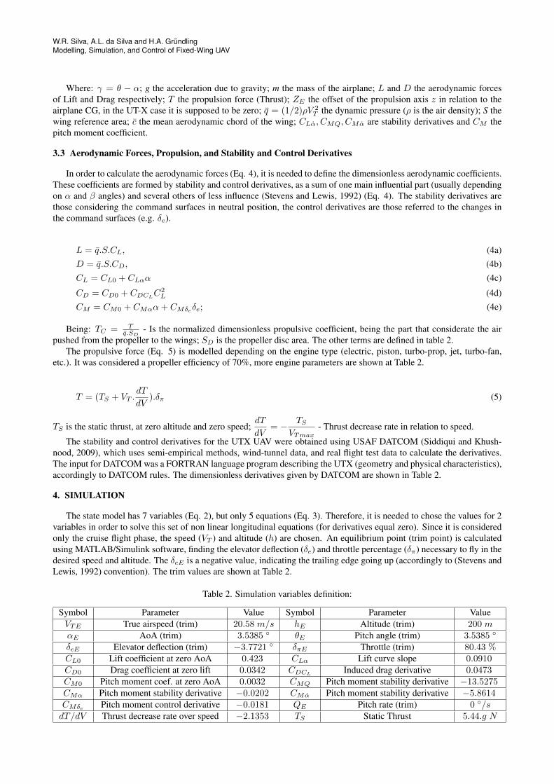
The analytical flight simulation of the UTX was done in MATLAB/Simulink, starting from the trim point. Consideringthat the UTX project presents a stable flight characteristics, it should present two longitudinal dynamics oscillationsmodes: short period and phugoid (Stevens and Lewis, 1992)(Blakelock, 1991)(Cook, 2011). The simulation objective isto identify the modes characteristics, such as: oscillation damping factor and frequency. In order to measure these values,the command inputs are the following: Maintain δπE at fixed trim value; Apply a doublet signal in the δe. Blue linesin figure 4 present the results of MATLAB/Simulink simulation, the short period mode happens as soon as the doubletsignal is applied, it showed a fast and strongly dampened oscillation (lasting 3 seconds), making the UTX AoA oscillatefrom −10◦ to 15◦. The phugoid mode starts to happen together with the short period mode, it showed a low frequencyand weak dampened oscillation, lasting about 60 seconds. It is related with the change of energy between speed (VT ) andaltitude (h). The phugoid mode result confirmed that the UTX has a stable aerodynamic project.

Figure 4. Comparison of analytical flight simulation and virtual flight simulation results

In order to compare the results of the analytical simulation, it is needed to get flight data of the same airplane with adifferent method (virtual test flight, wind-tunnel data or real test flight). Since at the time of this study a real test flightwas not possible, a virtual flight test was performed at X-Plane flight simulator. The X-Plane was chosen because itcalculates the aircraft model by using a different method of the stability and control derivatives. It uses a finite elementsmethod to calculate the aerodynamic forces (Lift, Drag, Thurst) of each small part of the aircraft, at each time step ofthe simulation, this method is known as Blade Element Theory. X-Plane is also used for certified flight simulations(FAA-regulations), and have been used in several other flight dynamics and control studies (Figueiredo and Saotome,2012)(Bittar et al., 2013)(Thong, 2010). Therefore, a UTX model was designed inside X-Plane’s Plane Maker software,the airfoils aerodynamic coefficients where obtained in JavaFoil software. With the UTX model built inside X-Planeenvironment, a virtual test flight was performed, flying the UTX to the desired trim altitude and applying the same typeof doublet signal in δe manually, using a joystick. In other words, the virtual test flight repeated the same procedures ofthe analytical test flight. The results are shown in the red line of figure 4. It can be seen that the MATLAB/Simulinkand X-Plane results are coherent. The best compatibility happens with the short period response. The X-Plane curveshave a poorer behaviour, mainly because the manual command. Other major cause of incoherence is the engine model inX-Plane, that is most related to the long period response. In X-Plane, the engine model is more suitable for large airplanes.

In general, both modelling methods are approximated, but, the similar results indicate that both are reasonable for apreliminary analysis and design.


5. AUTOPILOT DESIGN

The controllers were designed using classical control techniques, also used in the aeronautical industry for mannedairplanes (Stevens and Lewis, 1992). In order to design the flight control, the analytical model was linearized around thetrim point (using the Jacobian matrix). The eigenvalues of the UTX UAV are shown in Eq. 6. Although the eigenvaluesshow that the UTX is an asymptotically stable system, it has a pole almost at the origin (turning into a marginally stablesystem). Analyzing the eigenvalues, it can be concluded that the short period mode dampening factor is 0.616 withfrequency of 3.67rad/s. The phugoid mode dampening factor is 0.130 with frequency of 0.595rad/s. The controllersare designed in layers, with the most internal layer being the Stability Augmentation System (SAS), and the outermostlayer being the Mach Hold Autopilot. The inner layers form an augmented state space system for the outer layers. Thistechnique works because the the internal feedback variables have faster dynamics than the outer ones (different timeconstants).

−2.2614 ± 2.8899i−0.0772 ± 0.5898i−0.0004 + 0.0000i

(6)

5.1 Stability Augmentation System (SAS)

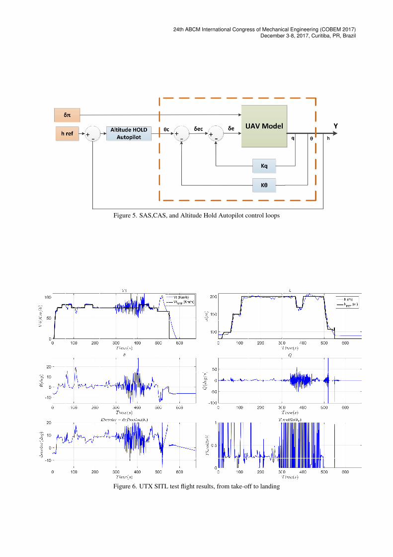
The first control loop is the SAS, done with the feedback of the pitch rate (Q) (Figure 5). The main objective of SASis to satisfy a frequency or dampening requirement for the short-period mode (Stevens and Lewis, 1992). It helps theairplane to become more stable, rejecting fast changes in pitch rate (e.g. that can be caused by wind-gust). The SAScontroller gain is Kq = −0.2.

5.2 Controllability Augmentation System (CAS)

The second control loop is the CAS, with feedback of pitch angle (θ) (Figure 5). The main objective is to follow areference for θ, this can be viewed as a Fly-By-Wire layer since the reference can be given by the pilot (in the joystick)or by the autopilot (numerically). However, a CAS can take different forms accordingly to its objectives (follow an AoAreference for instance). The CAS controller gain is Kθ = −0.8.

5.3 Altitude Hold Autopilot

The third control layer is an Altitude HOLD Autopilot, which takes the feedback of altitude (h) (Figure 5). As thename says, the main objective is to follow an altitude reference, giving pitch angle reference input to the CAS controller.The altitude hold autopilot is a Proportional-Integrative (PI) type of controller: PIh(s) = −0.0002.(1 + 100.s)/s

5.4 Mach Hold Autopilot (AutoThrottle)

The last control layer is an Mach Hold Autopilot, also known as AutoThrottle. This controller is not indicated inthe figure 5. Its main objective is to maintain a desired speed by measuring it (feedback) and acting on the throttlepercentage. The main difficulty to design such controller together with an altitude autopilot is because it is needed totake into account the augmented system created by closing the SAS, CAS and Altitude autopilot loops. To calculatethe augmented system it was used state space model and matrix algebra. The Mach Hold autopilot is also of PI type:PIVT

(s) = −0.04.(1 + 50.s)/s

5.5 Software In The Loop (SITL) Simulation Flight Test Results

To refine and assess the autopilot, a SITL simulation was performed using MATLAB/Simulink communicating viaUDP protocol with X-Plane flight simulator. This SITL is possible because the analytical model is with accordance withthe X-Plane model (as showed in previous section). In the SITL virtual test flight, the UTX altitude and speed were entirelycontrolled by the autopilot since take-off until landing. Even though the autopilot was designed only to the desired trimpoint, it also performs well out of this scope. Several tests were performed with constant wind, wind-gust, and turbulence,showing that the autopilot performed well in these conditions. A 10 minutes flight result can be viewed in Figure 6, from300 to 430s of simulation there is wind-gusts, and from 380 to 430s there is presence of turbulence. A video showing theentire SITL can be viewed at Youtube’s platform, on the internet (can be found searching for "uav willian" keywords ordirectly at www.youtube.com/watch?v=blhMO1KRQMU ).


Figure 5. SAS,CAS, and Altitude Hold Autopilot control loops

Figure 6. UTX SITL test flight results, from take-off to landing


6. CONCLUSION

The comparison of analytical (DATCOM-MATLAB/Simulink) with finite elements (X-Plane) models showed thatboth techniques presented similar responses for the UTX UAV. This result shows that this analysis methodology is inter-esting for simulating conceptual and real airplanes. The final data comparison should be made with real test flight data, torefine both analytical and X-Plane models. A refined analytical model can be used for control design, determining severallayers of control (Stability Augmentation System (SAS), Controllability Augmentation System (CAS), Fly-By-Wire andAutopilot). With a X-Plane refined model, the flight control laws can be evaluated in a flight simulation environment,where pilots can fly and assess the control modes, serving also as a pilot training platform. For autopilot assess, the X-Plane can be used for Software in the Loop (SITL) and Hardware in the Loop (HITL) simulations. HITL can test the realflight computers that will be embedded in the real aircraft afterwards, considerably cutting the costs and risks to developand test new flight computers. These techniques can also improve the training of pilots and operators.

7. ACKNOWLEDGEMENTS

The authors want to thanks the CAPES for the financial support to present this paper.The author Willian Rigon Silva was an active member of University of Toronto Aerospace Team (UTAT), while

studying in the University of Toronto (UofT), participating in a scholarship program called Science Without Borders(SwB).

8. REFERENCES

Austin, R., 2010. Unmanned Aircraft Systems: UAVS Design, Development and Deployment. John Wiley and Sons Ltd.Aerospace Series. ISBN 9780470058190.

Beard, R. and McLain, T., 2012. Small Unmanned Aircraft: Theory and Practice. Princeton University Press. ISBN9780691149219.

Bittar, A., de Oliveira, N.M.F. and Figueiredo, H.V., 2013. “Hardware-in-the-loop simulation with x-plane of attitudecontrol of a suav exploring atmospheric conditions”. J Intell Robot Syst (2014) 73:271–287.

Blakelock, J., 1991. Automatic Control of Aircraft and Missiles. A Wiley-Interscience publication. ISBN 9780471506515.Cook, M., 2011. Flight Dynamics Principles: A Linear Systems Approach to Aircraft Stability and Control. Elsevier

aerospace engineering series. ISBN 9780080550367.Figueiredo, H.V. and Saotome, O., 2012. “Modelagem e simulação de veículo aéreo não tripulado (vant) do tipo

quadricóptero usando o simulador x-plane e simulink”. Anais do XIX Congresso Brasileiro de Automática, CBA2012.

Hull, D.G., 2007. Fundamentals of Airplane Flight Mechanics. Springer. ISBN 103540465715.Parikh, K.K., Dogan, A., Subbarao, K., Reyes, A. and Huff, B., 2009. “Cae tools for modeling inertia and aerodynamic

properties of an r/c airplane”. AIAA Atmospheric Flight Mechanics Conference 10 - 13 August 2009, Chicago, Illinois.Siddiqui, B.A. and Khushnood, A., 2009. “Improving usaf datcom predictions of aircraft nonlinear aerodynamics”.

Canadian Aeronautics and Space Institute AERO’09 Conference Aerodynamics Symposium.Stevens, B.L. and Lewis, F.L., 1992. Aircraft Control and Simulation. John Wiley and Sons Ltd. ISBN 0471613975.Thong, C.W.S., 2010. “Modeling aircraft performance and stability on x-plane”. Final Thesis Report 2010, SEIT,

[email protected], 2014. “University of toronto explorer design report”.

9. RESPONSIBILITY NOTICE

The authors are the only responsible for the printed material included in this paper.

Documents

COBEM-2017-2703 MODELLING, SIMULATION AND CONTROL OF …