Embed Size (px)
Citation preview
Graduate Theses, Dissertations, and Problem Reports
2001
Coating studies and video imaging of the flow patterns of tablets Coating studies and video imaging of the flow patterns of tablets
in a semi-circular fluidized bed in a semi-circular fluidized bed
Ganeshkumar A. Subramanian West Virginia University
Follow this and additional works at: https://researchrepository.wvu.edu/etd
Recommended Citation Recommended Citation Subramanian, Ganeshkumar A., "Coating studies and video imaging of the flow patterns of tablets in a semi-circular fluidized bed" (2001). Graduate Theses, Dissertations, and Problem Reports. 1175. https://researchrepository.wvu.edu/etd/1175
This Thesis is protected by copyright and/or related rights. It has been brought to you by the The Research Repository @ WVU with permission from the rights-holder(s). You are free to use this Thesis in any way that is permitted by the copyright and related rights legislation that applies to your use. For other uses you must obtain permission from the rights-holder(s) directly, unless additional rights are indicated by a Creative Commons license in the record and/ or on the work itself. This Thesis has been accepted for inclusion in WVU Graduate Theses, Dissertations, and Problem Reports collection by an authorized administrator of The Research Repository @ WVU. For more information, please contact [email protected].
Coating Studies and Video Imaging of the Flow Patterns ofTablets in a Semi-Circular Fluidized Bed
Ganeshkumar A. Subramanian
THESISSubmitted to the College of Engineering and Mineral Resources
at West Virginia University
In partial fulfillment of the requirementsfor the degree of
Master of Sciencein
Chemical Engineering
Richard Turton, Ph.D., ChairEugene V. Cilento, Ph.D.Aubrey L. Miller, Ph.D.
Department of Chemical Engineering
Morgantown, West Virginia2001
Keywords: Particle Coating, Wurster bed, Fluidization, Velocity and Voidage Profile,Video Imaging, Inserts, Coating Variation.
ABSTRACT
Coating Studies and Video Imaging of the Flow Patterns of Tablets in a Semi-Circular Fluidized Bed
Ganeshkumar A. Subramanian
Particle coating is of increasing interest in the Pharmaceutical Industry, with moreand more manufacturers moving towards production of tablets with layers of coating.When a tablet is coated with a drug, the amount of coating that each tablet possessesbecomes very critical, as it constitutes the total dosage. The amount and consistency ofdrug coated on the tablet depends on the dynamics of the tablet in the vicinity of thespray zone.
The objective of this work was to study the dynamics of particle motion (largeplacebo tablets, 8mm diameter and sphericity factor, φ ≠ 1) in the vicinity of the sprayzone of a semi-circular Wurster bed coater. A novel method of computer based videoimaging was used to measure the velocity and voidage profiles in the draft tube region ofthe semi-circular fluidized bed coater. Continuous and pulse coating runs were performedto study the variation in coating consistency. This variation was explained in-terms ofcoating-per-pass variation and the cycle time variation. Inserts were used to alter thevoidage profile around the spray nozzle and the coating runs were used to study theireffect on the coating consistency.
The experimental set-up consists of two cameras connected to separate frame-grabbing boards that are in turn connected to a computer. Software written in VisualBasic 6.0 controls the triggering of the cameras and retrieving of images from the framegrabber to the computer screen. For velocity measurements, the time lag between thecameras was set to a known value and the relative distance moved by the particle, in boththe x and y directions, was measured with the help of computer-generated crosshair.Using this technique, the velocity vector was determined, in both the vertical andhorizontal plane. For voidage measurements, the number of tablets in the area of focuswas determined, and the depth of field obtained from previously calibrated values. Byusing these values, with the known tablet volume in a given volume of bed, void volumein the bed was calculated. By repeating this process across the bed, the voidage profilewas obtained.
Velocity and voidage profiles were found to be consistent with visualobservations. The parameters that were investigated included air velocity, gap height(height between the draft tube and the distributor), distributor plate design, and the use ofguides or inserts to direct particle movement from the annulus into the draft tube. Therationale behind the use of these inserts (deflectors) was to provide a smooth path that
iii
would guide the radially inward moving particles away from the spray nozzle. Thisprevents the tablets from flowing directly over the spray nozzle and thus prevents thelocal wetting of a small portion of the particles. For the coating runs, FD&C Blue DyeNo.1 dissolved in aqueous-based polymeric dispersion was used. After the coatingexperiment, 100 tablets picked at random were analyzed for their blue dye content andthe data analyzed statistically.
The experimental data show that video-imaging techniques can be used toestimate velocity and voidage profiles in a semi-circular fluidized bed. These profiles arepresented as maps in the draft tube region. The results showed that the major cause forvariation in coating consistency was due to variation in the amount of coating received bytablets during each pass and that by reducing this variation, by reducing the shelteringphenomena, the overall coating consistency was improved.
iv
ACKNOWLEDGEMENTS
I wish to express my sincerest gratitude to my advisor Dr. Richard Turton for his
guidance, advice and encouragement during the course of this work. It has been a great
pleasure and honor to work with such a gifted researcher and wonderful person.
I would like to express my gratitude to the members of my advisory committee,
Dr Eugene V. Cilento and Dr. Aubrey Miller for their useful comments and suggestions
on the work. I would like to specially thank Dr. Cilento for spending some of his valuable
time helping me with statistical analysis of experimental data. I am also thankful to all the
faculty and graduate student in the Department of Chemical Engineering, especially
Aashish Bhattia, for his valuable discussions while sharing the same laboratory and some
equipment with me. I would also like to make a special mention of Neeraj Pugalia,
Balakrishnan. A , Jarod Macormick and Sandeepa Sandadi for their valuable inputs and
help.
My sincere thanks to Mr. Jim Hall, without whose help and support this work
would not have been possible. He fabricated the fluidized bed and the various
modifications/inserts used during this work. I also thank Ms. Linda Rogers and Ms.
Bonita Helmick for all the help in handling the paper work and being great friends. I wish
to thank Mr. Luke Flemmer of Peltec Inc., for providing the software and also helping me
getting started with using the same.

v
I wish to thank Merck and Co., Inc for sponsoring this project and extending the
financial support to finish the final experimental runs.
I wish to thank my parents Mr. Subramanian and Mrs. Anasuya Subramanian, my
brother and sister for their unconditional love and support. Words cannot describe the
love, patience, support and encouragement they have give me throughout this work and
my life.
I finally like to thank God almighty, and dedicate this work to the people who
have had a profound impact on my life, my advisor Dr. Richard Turton, and my parents.
vi
Table of Contents
CHAPTER I: INTRODUCTION 1
1-1 An overview of fluidization technology 1
1-2 Fluidization applied to pharmaceutical coatings 2
1-3 Objective of this work 5
CHAPTER II: LITERATURE REVIEW 8
2-1 An overview of spouted fluidized bed 8
2-2 Techniques used to study particle motion within a bed 8
2-3 An overview of draft-tube equipped bed 11
2-4 The hydrodynamics within the spray zone of a fluidized bed coating device 13
2-5 Application of fluidized bed coating to obtain controlled/sustained and sequential release drugs 14
CHAPTER III: EXPERIMENTAL METHOD 18
3-1 Description of the experimental set-up and equipment 18
3-2 Design of Deflectors 29
3-3 Measurement techniques and equipment used 34
3-4 Calibration of video imaging system 38
3-5 Principles of velocity measurement 40
3-6 Principle of voidage measurement 42
3-7 Objective of Coating experiments 47
3-8 Determining the coating formula 48
3-9 Coating experiments 49
3-9.1 Continuous coating Experiments 49
vii
3-9.2 Method of coating for continuous tests 50
3-9.3 Pulse coating test 51
3-9.4 Method of coating for pulse tests 51
3-10 Analysis of coated tablets 52
3-10.1 Analysis of continuous coating runs 52
3-10.2 Analysis for pulse test runs 53
CHAPTER IV: RESULTS AND DISCUSSION 54
4-1. Velocity measurement in the draft-tube region 54
4-1.1 Velocity profiles in the draft-tube 54
4-1.2 Velocity measurements in the annulus 70
4-2. Voidage Measurement 72
4-2.1 Voidage measurement in draft-tube 72
4-2.2 Voidage measurement in the annulus 84
4-3 Mass balance between solid mass flow rate in the spout and annulus 84
4-4 Sheltering effect and Coating Variation 87
4.5 Results of the Coating Experimental runs 92
4-5.1 Continuous coating runs 92
4-5.2 Pulse Coating runs 98
4-5.3 Statistical analysis of the pulse coating runs 100
CHAPTER V: CONCLUSION 109
CHAPTER VI: RECOMMENDATION FOR FUTURE WORK 113
NOMENCLATURE 116
BIBILOGRAPHY 118
viii
APPENDICES
Appendix I. Orifice plate calibration and flow measurement. 123
Appendix II. Measurement of annulus voidage. 125
Appendix III. Calibration of velocity measurement technique using disk rotating at know velocity and strobe. 130
Appendix IV. Apparent Depth of field calibration (ADOF). 133
Appendix V. Alignment of cameras and calibration of pixel size. 136
Appendix VI. Velocity vector and voidage calculation. 139
Appendix VII Scanning spectra of Blue Dye # 1 in Water. 141
Appendix VIII Data for calibration of the Spectrometer and thecalibration curve higher concentrations. 142
Appendix IX Data for calibration of the spectrophotometer and thecalibration curve for very low concentrations. 143
Appendix X Determination of Coating Formula. 145
Appendix XI Coating efficiency calculation 146
Appendix XII Calibration of the peristaltic pump used for pumpingthe coating solution. 147
Appendix XIII Calculation of amount of blue dye coated during thepulse test. 149
Appendix XIV Obtaining values for voidage by linear interpolation. 150
Appendix XV Solids Mass flow calculations in the draft-tubeand annulus. 152
Appendix XVI Photographs of the Fluidized Bed 156
Appendix XVII Photographs of the Distributor plates 159
ix
LIST OF TABLES
Table Page
3-1. Experimental matrix for the velocity and voidage profile study. 19
3-2. Experimental matrix for coating consistency study. 20
3-3. Operating parameters for the continuous coating runs. 49
3-4. Operating parameters for the pulse test runs. 51
4-1. STD, Mean, RSD and % Efficiency on the amount of coatingtablets received with the use of different deflectors. 95
4-2. STD, Mean and RSD on the amount of coating tablets receivedper-pass with no deflector and with the optimum deflector. 98
4-3. Average RSDper-pass values of the 10 groups formed form the total sample population of 100 optimum deflector. 101
4-4. Average RSDtotal values of the 10 groups formed form the totalsample population of 100 for optimum deflector. 102
4-5. Average RSDper-pass values of the 10 groups formed form the total sample population of 100 for no deflector. 105
4-6. Average RSDper-pass values of the 10 groups formed form thetotal sample population of 100 no deflector. 106
4-7. Consolidated results of coating experiments. 108
x
LIST OF FIGURES
Figures Page
1-1. Bottom-spray Wurster coater (Glatt Air Techniques) Mehta etal 1986. 4
3-1. Schematic diagram of the semi-circular spouted bed coating device. 21
3-2. Diagram showing the dimensions of the semi-circular column of the bed. 22
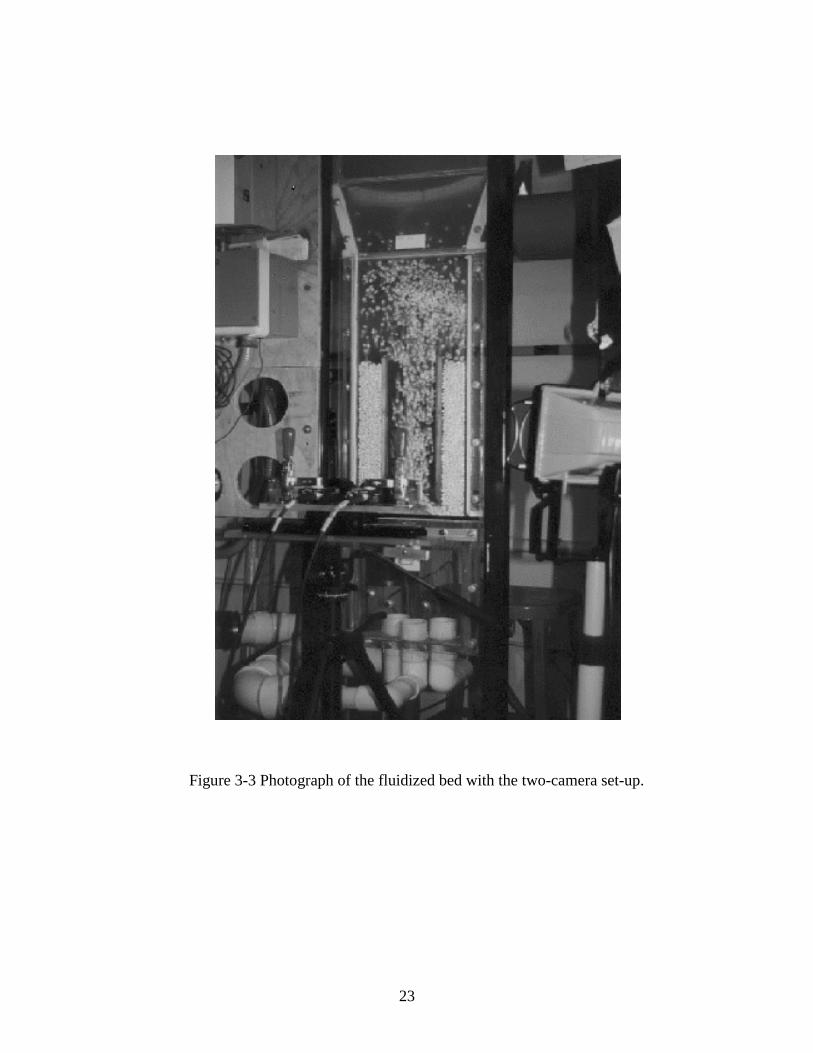
3-3. Photograph of the fluidized bed with the two-camera set-up. 23
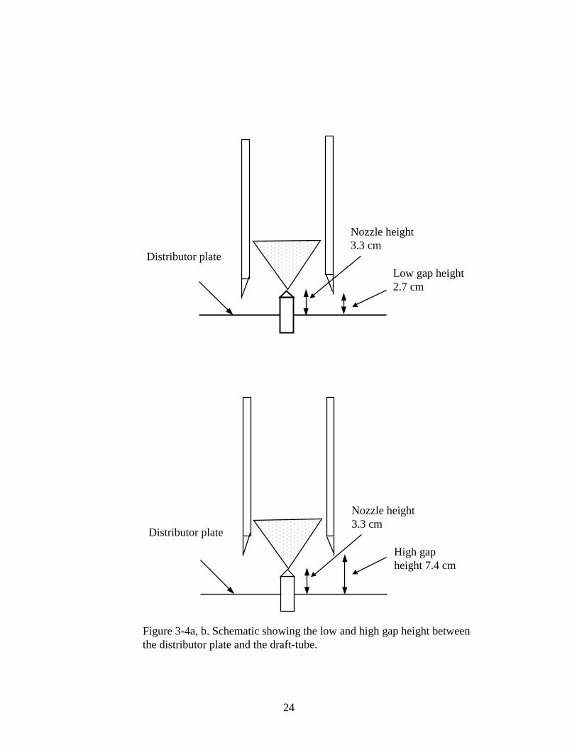
3-4a,b. Schematic showing the low and high gap height between the
distributor plate and the draft-tube, respectively. 24
3-5. Flow diagram of the experimental setup 26
3-6. Schematic diagram of the fluidized bed video imaging system 27
3-7. Photograph of the tablet used in the study. 28
3-8a. Schematic diagram of deflector 1. The arrows show the directionof deflection of the tablets. 30
3-8b. Photograph of deflector 1 mounted on distributor plate. 30
3-9a. Schematic diagram of modified deflector 1. The arrows show thedirection of deflection of the tablets. 31
3-9b. Photograph of modified deflector 1. 31
3-10. Schematic diagram of modified deflector 2. The arrows show thedirection of deflection of the tablets. 32
3-11. Schematic diagram of modified deflector 3. The arrows show thedirection of deflection of the tablets. 32
3-12a. Schematic diagram of optimum deflector. The arrows show thedirection of deflection of the tablets. 32
3-12b. Photograph of optimum deflector mounted on the distributor plate. 33
3-12c. Photograph of optimum deflector mounted on the distributor plate. 33
xi
3-13. Schematic diagram showing an image/frame formed by two fields takenwith a standard RS-170 interlaced video format (time lag of 16.67 ms)and spliced together to form the image. 35
3-14. Schematic diagram showing an image/frame formed by two fields takenwith a standard RS-170 interlaced video format (time lag of 16.67 ms)being split into two fields odd and even. 35
3-15. Illustration of Stereoscopic Imaging using Two Identical camerasand Imaging Boards. 37
3-16. Two cameras set-up on the steep sides of an isosceles triangle. 37
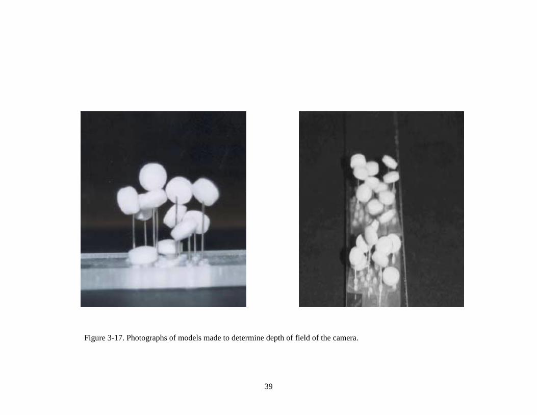
3-17. Photographs of models made to determine depth of field of the camera. 39
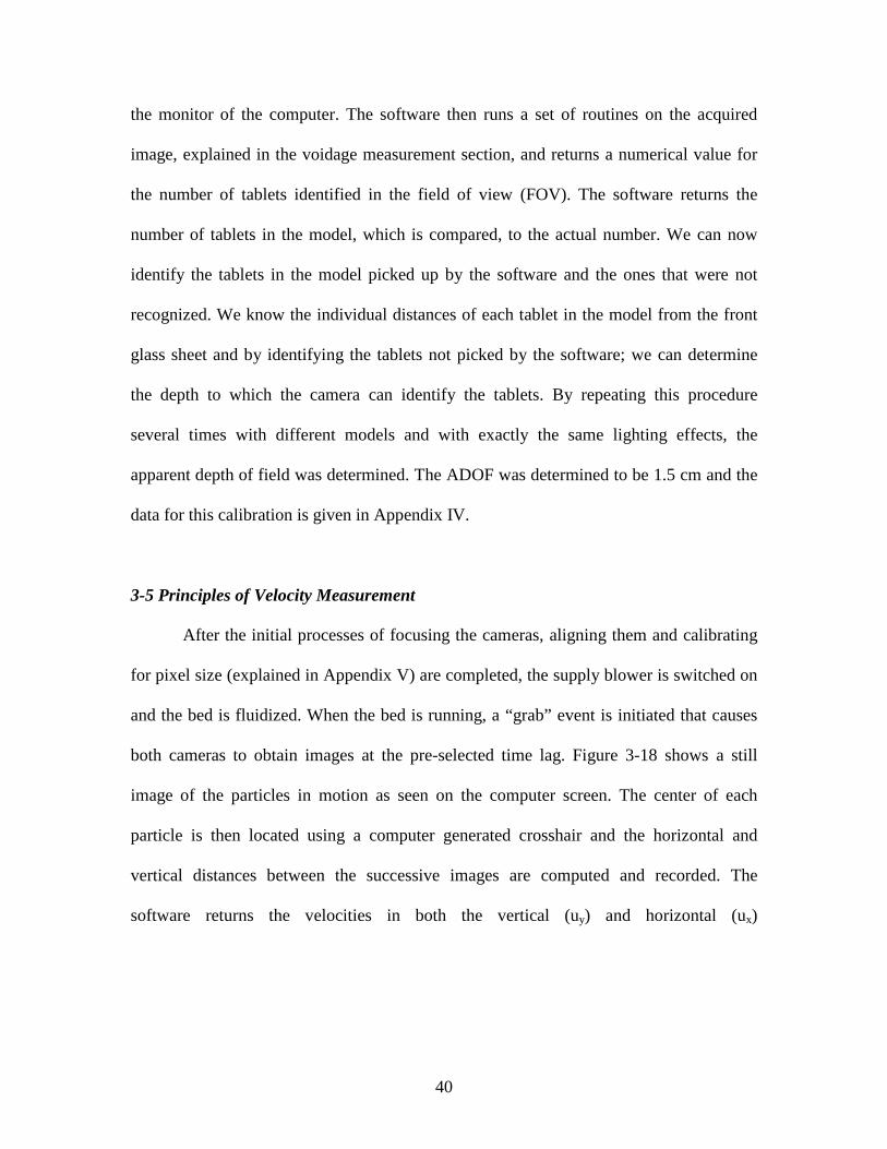
3-18. Photographs of still images of particles in motion as seen on the computermonitor. The hairlines shows the distance moved by the center of theparticle. 41
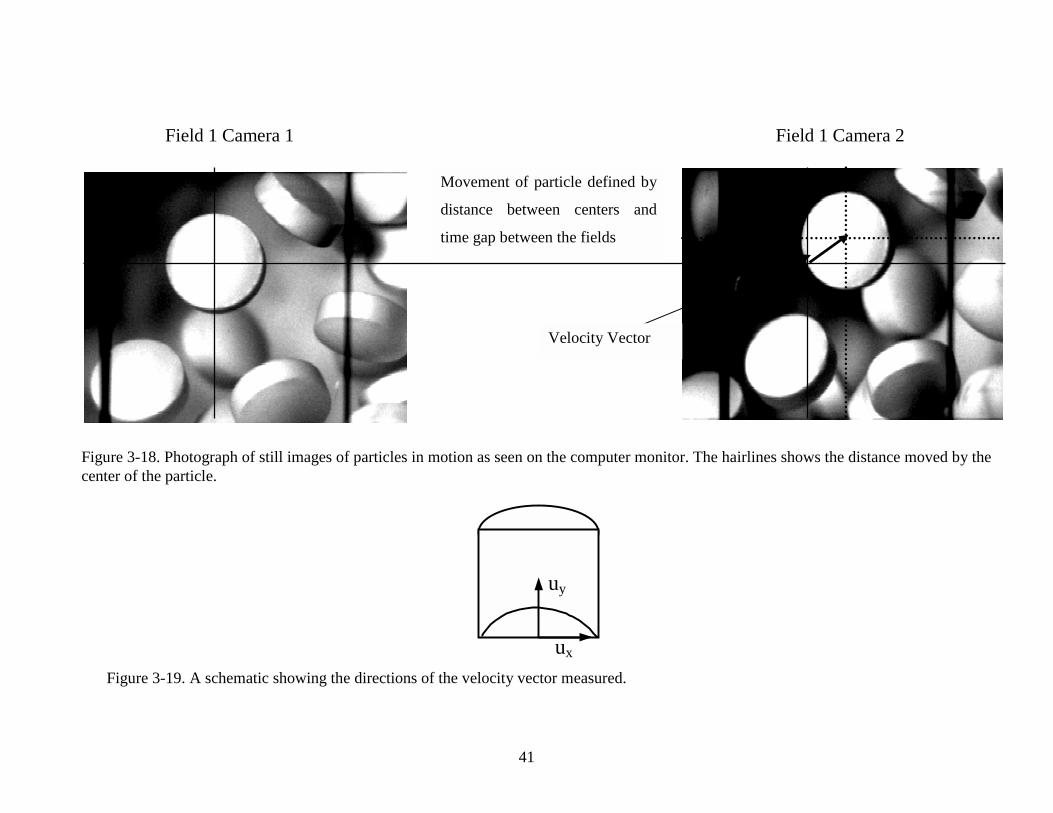
3-19. A schematic showing the directions of the velocity vector measured. 41
3-20. Arrangement of light and cameras for the experimental runs. 43
3-21. Sequence of events before the particles are picked up for voidagemeasurement. 46
4-1. Diagram showing the relative position of the distributor plate, deflector,nozzle and the imaginary grid for the case with deflector 1 and lowergap height (2.5 cm) 55
4-2a,b. Radial particle velocity profile along the height in the draft-tube with no deflector and gap heights of 2.5 cm and 6.8 cm, respectively. 56
4-3a,b. Radial particle velocity profile along the height in the draft-tube with deflector 1 and gap heights of 2.5 cm and 6.8 cm, respectively. 56
4-4a,b. Radial particle velocity profile along the height in the draft-tube with deflector 1 and gap heights of 2.5 cm and 6.8 cm, respectively. 57
4-5a,b. Radial particle velocity profile along the height in the draft-tube with modified deflector 1 and gap heights of 2.5 cm and 6.8 cm, respectively. 57
4-6. Particle velocity map in the draft-tube at different axial location for thebed with distributor1, no deflector and gap height 2.5 cm. 61
4-7. Particle velocity map in the draft-tube at different axial location for the
xii
bed with distributor1, no deflector and gap height 6.8 cm. 62
4-8. Particle velocity map in the draft-tube at different axial location for thebed with distributor 1, deflector 1 and gap height 2.5 cm. 63
4-9. Particle velocity map in the draft-tube at different axial location for thebed with distributor 1, deflector 1 and gap height 6.8 cm. 64
4-10. Particle velocity map in the draft-tube at different axial location for thebed with distributor 1, modified deflector 1 and gap height 2.5 cm. 65
4-11. Particle velocity map in the draft-tube at different axial location for thebed with distributor 1, modified deflector 1 and gap height 6.8 cm. 66
4-12a,b. Radial particle velocity profile along the height in the draft-tube with modified deflector 1and gap heights 2.5 cm and 6.8 cm respectively. 67
4-13a,b. Radial particle velocity profile along the height in the draft-tube with modified deflector 1and gap heights 2.5 cm and 6.8 cm respectively. 67
4-14. Particle velocity map in the draft-tube at different axial location for the
bed with distributor 2, no deflector and gap height 6.8 cm. 68
4-15. Particle velocity map in the draft-tube at different axial location for the
bed with distributor 1, modified deflector 1, gap height 6.8 cm and high
airflow rate. 69
4-16. Graph showing a plot of annular velocity at different gap heights
above distributor plate for the three cases of with/without deflector
and modified deflector 1. . 71
4-17a,b. Radial particle voidage profile along the height in the draft-tube with
no deflector and gap heights 2.5 cm and 6.8 cm respectively. 73
4-18a,b. Radial particle voidage profile along the height in the draft-tube with
deflector 1 and gap heights 2.5 cm and 6.8 cm respectively. 73
4-19a,b. Radial particle voidage profile along the height in the draft-tube with

xiii
deflector 1 and gap heights 2.5 cm and 6.8 cm respectively. 75
4-20a,b. Radial particle voidage profile along the height in the draft-tube with
modified deflector 1and gap heights 2.5 cm and 6.8 cm respectively. 75
4-21. Voidage map in the draft-tube at different axial location for the bed
with distributor 1, no deflector and gap height 2.5 cm. 78
4-22. Voidage map in the draft-tube at different axial location for the bed
with distributor 1, deflector 1 and gap height 2.5 cm. 79
4-23. Voidage map in the draft-tube at different axial location for the bed
with distributor 1, modified deflector 1 and gap height 2.5 cm. 80
4-24. Voidage map in the draft-tube at different axial location for the bed
with distributor 1, no deflector and gap height 6.8 cm. 81
4-25. Voidage map in the draft-tube at different axial location for the bed
with distributor 1, deflector 1 and gap height 6.8 cm. 82
4-26. Voidage map in the draft-tube at different axial location for the bed
with distributor 1, modified deflector 1 and gap height 6.8 cm. 83
4-27. Plot of mass-flux in the annulus vs. mass-flux in the draft-tube for
the eight different experimental variations. 86
4-28. The basic process involved during particle coating in a fluidizedbed coater. 88
4-29. A schematic diagram showing the sheltering effect. The tablet closerto the nozzle blocks the coating solution from reaching the tablets thatare away from the nozzle. 89
4-30. Schematic representation of the sources of variation in a fluidized
xiv
bed coating process and the type of variation obtained for eachindividual source. 90
4-31. Frequency plot of amount of blue dye coated on tablets during thecontinuous coating runs, with the different deflector designs. 94
4-32a,b. Frequency plot for the pulse test, with optimum deflector and no deflector, respectively. 99
4-33. Frequency plot of ( x /Sx) for the pulse test, with optimum deflector. 100
4-34. Frequency plot of ( x /Sx) for the continuous coating experiments,with optimum deflector. 102
4-35. Frequency plot of ( x /Sx) for the pulse test, with no deflector. 104
4-36. Frequency plot of ( x /Sx) for the continuous coating run, with no deflector.106
6-1. Diagram showing alterations made to the draft-tube. 114
1
CHAPTER IINTRODUCTION
1-1 An overview of Fluidization Technology
Fluidization is an operation in which a bed of solid particles is suspended by the
fluidizing medium, which may be a gas or liquid, passing through the column containing
the particles. These particles begin to fluidize when the weight of the particles are
balanced by the drag force of the fluid flowing through them and at this state the bed of
solids behaves in some ways like a fluid. Gas-solid systems are more common than
liquid-solid systems and are widely used in many commercial processes such as
gasification of coal, drying of food grains, mixing of powdery material, granulating fine
solids, coating in the pharmaceutical industry.
The first large scale, commercially significant use of fluidized beds was by Fritz
Winkler (Kunii and Levenspiel, 1969) for the gasification of powdered coal in 1926.
Fluid Catalytic Cracking (FCC) in the 1940’s was a major breakthrough in the
manufacture of high-octane aviation gasoline, which played a very critical role in World
War II (Kunii and Levenspiel, 1969). Since then fluidized bed technology has made vast
strides and has been used in a variety of industries from mineral processing to the
manufacture of coated tablets in the pharmaceutical industry.
In this work, we have concentrated on the use of fluidized bed coating techniques
in the pharmaceutical industry. This technique has been widely used not only for
functional coating and drug applications (Wurster, 1959; Singiser and Lowenbthal, 1961;
Caldwell and Rosen, 1964; Robinson et al., 1968), but also for granulation (Rankell, et
al., 1964; Scott et al., 1964; Davies and Gloor, 1971, 1972) and drying (Scott et al., 1963;
and Zoglio et al., 1975). For example, tablets may be coated in a fluidized bed to alter the
2
drug release rate (controlled-release dosage forms) or the drug release site (enteric coated
tablets) and both these coatings can be applied in a fluidized bed coater.
1-2. Fluidization Applied to Pharmaceutical Coatings
The coating of tablets is a critical, as well as costly step in the manufacturing
process of solid dosage forms. Tablets may be coated for the following reasons:
- to mask any unpleasant taste or objectionable odor of the drug
- to improve pharmaceutical elegance by coating to give special colors or
textures
- to control the release rate of drug by coating a layer of polymer on the drug
- to protect the drug through first pass metabolism thus controlling the site of
drug release
- to incorporate another drug or excipient in the coating to avoid chemical
incompatibility , or provide sequential release of drugs
- to mark for product identification (Lehmann and Dreher, 1981; Cheng, 1993;
and Rocha, et al., 1995)
In 1989, more than two-thirds of the $20-billion annual U.S. drug market consists
of orally administered drugs, more than 85% of which are delivered as solid dosage
forms (Rekhi et al.1989). Currently, solid drug dosage forms can be classified into four
different forms namely tablets, capsules, pills, lozengers and suppositories. In the case of
a capsule, the drug is in the form of small particles that may be individually coated and
housed in a capsule of gelatin or similar material. Here the amount of drug coating that a
single particle possesses is not very critical, since the dosage will be an integral of the
3
amount of drug on all particles. In the case of a single tablet coated with a drug, the
amount of coating that each tablet possesses becomes very crucial, as it constitutes the
total dosage.
Traditionally, tablets were coated in pan coaters and these rotating devices have
been used in the pharmaceutical industry since the mid-1800’s. However, this equipment
has some inherent problems such as lengthy processing time, the need for skilled operator
supervision, and high energy for operation. Moreover, there is considerable variation in
product quality because of the inherent dead zones in the pan coater. With the above-
mentioned disadvantages of pan coating processes, newer processes for coating were
developed. Some of the commonly used commercial devices are coacervation tanks,
compression coating machines, and fluidized and spouted bed coaters.
Wurster, in 1950, was the first to introduce the process of coating drug
formulations using fluidized beds. Since then, there have been significant improvements
in this method of dosage form manufacture. The fluidized bed coating method has several
advantages over other conventional coating methods. The process provides intimate
contact between the fluidizing medium and the fluidized particles, resulting in high rates
of heat and mass transfer and reduced processing time. In a Wurster bed coater, shown in
Figure 1-1 (Wurster, 1953) a bed of tablets is fluidized by a stream of air, supplied by a
blower, passing through a distributor plate at the bottom of the bed. The distributor plate
is designed such that the airflow at the center of the bed is much higher than that in the
annular region. This design, along with the presence of an insert, causes the particles to
flow upwards in the form of a spout in the center of the bed and move down slowly in the
annular region. The nozzle is located in the center of the bed, just above the distributor
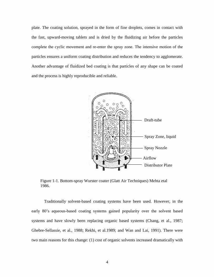
4
plate. The coating solution, sprayed in the form of fine droplets, comes in contact with
the fast, upward-moving tablets and is dried by the fluidizing air before the particles
complete the cyclic movement and re-enter the spray zone. The intensive motion of the
particles ensures a uniform coating distribution and reduces the tendency to agglomerate.
Another advantage of fluidized bed coating is that particles of any shape can be coated
and the process is highly reproducible and reliable.
Traditionally solvent-based coating systems have been used. However, in the
early 80’s aqueous-based coating systems gained popularity over the solvent based
systems and have slowly been replacing organic based systems (Chang, et al., 1987;
Ghebre-Sellassie, et al., 1988; Rekhi, et al.1989; and Wan and Lai, 1991). There were
two main reasons for this change: (1) cost of organic solvents increased dramatically with
Figure 1-1. Bottom-spray Wurster coater (Glatt Air Techniques) Mehta etal1986.
Airflow
Distributor Plate
Spray Nozzle
Spray Zone, liquid
Draft-tube
5
the government introducing new regulations concerning these solvents, and (2)
Environmental Protection Agency (EPA) became increasingly stringent on solvent and
solvent-vapor discharge to the environment. Aqueous polymeric coating has several
advantages over solvent-based coating. Aqueous based coating systems are less
expensive, hazard of explosion is negligible, potential for toxicity and problems
controlling vapor emissions into the atmosphere is very low. Aqueous based coating
systems also have some inherent disadvantages: (1) tablet appearance is usually inferior,
(2) selection of coating material is limited to those which are water soluble or water
dispersible, (3) water has an adverse effect on many active ingredients and (4) water is
less volatile and hence requires more energy to evaporate and dry. However, the
advantages out-weigh the disadvantages and many solvent-based coating systems have
given way to aqueous polymeric coating systems. With aqueous based systems gaining
popularity, fluidized bed coating is the preferred process, as it provides excellent drying
efficiency and product uniformity.
1-3. Objective of this work
Several researchers have worked in the area of fluidized bed coating for
pharmaceutical applications. Different techniques have been used to study the
hydrodynamics of a semi-circular fluidized bed Wurster coater. Still there has not been
much work done addressing the particle velocity and voidage profiles across the entire
draft-tube region. Saadevandi and Turton (1996) used video imaging techniques to study
the hydrodynamics of particle motion in the spray zone of a fluidized bed and the effect
of liquid spray on the voidage and velocity profiles in the spray region. They used smaller
6
spherical particles (1mm diameter) with lower bed loadings and were able to measure the
velocity and voidage profiles in the draft-tube region of a semi-circular draft-tube
equipped fluidized bed coater.
Cheng and Turton (1993) observed that the variation in coating in a Wurster bed
coater can be attributed to two factors: (1) coating variation per pass through the spray
zone, and (2) variation in the number of times the particle passes through the spray zone.
They developed a phenomenological model to determine the variation in the coating
received based on the above two factors. Cheng (1993) also talks about the sheltering
effect that a particle close to the spray source or nozzle has on a particle further away
from the nozzle. Shelukar et al. (2000), conducted experiments to determine the variation
in coating-per-pass and variation in total coating received based on the above observation
of the sheltering effect and have quantified this variation. The above-mentioned work
emphasizes the importance of reducing the variation in per pass coating received and
reducing the variation in cycle time distribution. The video imaging technique used also
showed that the particles moved close to the nozzle causing the sheltering effect to have a
pronounced effect on the coating consistency. The above results and the interest to
minimize the variation in the coating consistency is the driving force behind this research.
This work can be considered as an extension of the work done by Saadevandi and Turton
(1996) and Cheng and Turton (1993).
The objective of this research was to investigate the hydrodynamics of fluidized
particles (large placebo tablets, 8mm diameter and 5 mm thick) passing through the spray
zone in a semicircular fluidized bed coating device. In addition, the factors that affect the
flow pattern, circulation rate, coating consistency and variation were to be evaluated.
7
Factors such as distributor design, fluidizing air velocity, gap height (height between
distributor and insert), and particle size have been investigated. Since the particles were
not spherical, the task of making velocity and voidage measurements was complex as the
orientation of the particle was an important factor to be considered. A databank of
particle velocity and voidage measurements, for a variety of operating conditions in the
bed, was obtained and profiles plotted using custom-written software in Microsoft Visual
Basic. Computer based video imaging techniques were used to measure the velocity and
voidage profiles in the draft-tube region of the fluidized bed. Some of the parameters
investigated were fluidizing air velocity, gap height (height between the draft-tube and
the distributor), distributor plate design, and the use of guides or inserts to direct particles
from entering the spray zone directly above the nozzle. The use of deflectors was
expected to improve the coating consistency, as it would reduce the effect of particle
sheltering in the spray zone. The study of the use of guides\deflectors to alter the voidage
in the immediate vicinity of the spray zone and thereby reduce the sheltering effect was
the first of its kind.
Actual coating experiments were conducted with and without the use of deflectors
to quantify the effect of these devices on coating consistency. Efforts were also made to
quantify the variation in coating received by particles in a single pass through the spray
zone with the help of pulse tests.
8
CHAPTER II
Literature Review
2.1 An Overview of Spouted Fluidized Beds
Spouted beds have been widely employed in a variety of industrial processes. In
these processes, gas is introduced at high velocities into the bottom of the bed and forms
a spout of gas and solid particles in the center of the bed. The solid particles move up
rapidly in the center, while the particles in the sides form an annular dense bed, which
moves downward. The solids are entrained from the annular bed into the spout causing
the circulation of particles within the bed. The upward movement of the spout stabilizes
the bed. These types of beds are known as conventional spouted beds. Mathur and
Gishler (1955) first developed the spouted bed technique and showed the existence of a
maximum spoutable bed depth, Hm, and a minimum superficial velocity for spouting, Us.
They also showed that both these quantities were complex functions of fluid properties,
particle size and bed geometry.
2.2 Techniques used to study particle motion within a bed
Several techniques have been used in the past to study the particle motion and
voidage profiles in a fluidized bed. A brief review is given here. High-speed photography
can be used to study the particle motion within a bed, though it is restricted to the region
near the wall. Toomey and Johnstone (1955) were the first to use this technique to study
the particle motion in a metal column fitted with a window. Todd et al. (1957) used the
same technique to study the flow dynamics in a two dimensional bed. Massimilla and
Westwater (1960) used motion pictures at 2000 frames/sec to measure the movement of
9
individual particles and gas bubbles in a fluidized bed. Air was the fluidizing medium
and the particles studied were 0.028 in. glass spheres and 200-mesh alumina particles in a
3.75 in. semi-cylindrical glass column. They observed that aggregates were very common
and particles and aggregates showed pronounced alternations of fast and slow movement
in the upward and downward direction near the wall. They also studied the effect of
baffles and observed that baffles increased bed density and reduced particle velocity.
Small bubbles rose rapidly with little change while large cavities were slow and tended to
collapse and reform elsewhere.
Lefroy and Davidson (1969) measured maximum spoutable bed depth; Hm and
overall pressure drop with bed dimensions ranging from 7.6 cm to 61 cm in diameter.
They observed that a spouted bed in a half cylinder behaved similarly to a fully
cylindrical bed of the same diameter, and they were able to measure the spout diameter
Ds. Van Velzen et al. (1974) investigated solids movement in a spouted bed by means of
a radioactively marked particle technique, using a scintillation counter as a detector.
Their results showed that the average particle velocity in the spout depended on the gas
flow rate, gas inlet geometry, axial elevation, bed height, and column diameter. The solid
circulation rate was found to be proportional to the gas flow rate, and further, a function
of column and gas inlet geometry, density of fluidizing gas and particle diameter. They
gave empirical correlations for both the particle velocities in the spout and the solids
circulation rate as a function of axial elevation. Suciu and Maximillan (1977 and 1978),
conducted experiments on particle circulation in a spouted bed produced by introducing
air in a 100-mm diameter semicircular, conical-bottom column with a transparent front
wall. The results they obtained, by using pictures captured using a high-speed camera,
10
showed that the average bulk-velocity of particles in the annulus, at a distance of 0.7 –
0.8 R (R- radius of the cylindrical bed) from the wall, were significantly different from
particles which were in contact with the wall.
Boulos and Waldie (1986) used Laser-Doppler Anemometry (LDA) to obtain
high-resolution measurements of particle velocities in a spouted bed and were able to find
answers to previously unresolved aspects of particle motion, including wall effects in
half-section beds. Laser-Doppler Anemometry (LDA) is a non-intrusive technique and is
capable of providing particle velocity data of high resolution in the spout and fountain
regions. The basic principle of LDA is that the difference in frequency between the
incident laser light beam and the light scattered by the moving particles is proportional to
the velocity of the particle. By measuring the frequency difference (Doppler shift) and the
optical geometry, the velocity was calculated.
He et al. (1994a, 1994b) used fiber optic probes to measure voidage and velocity
profiles in the fountain, spout and annulus of semi-circular and circular spouted beds.
They observed that the voidage in the annulus was somewhat greater than the voidage in
a loosely packed bed and increased with gas flow rate, this was contrary to earlier
assumptions. The results also showed that overall voidage profiles were very similar in
both the 2-dimensional and 3-dimensional beds. The particle velocity measurement in the
spout region showed that although the overall profile for both columns are similar in
shape, the local particle velocities in the half column are approximately 30% lower than
the full column, under identical operating conditions. In the half column, particle
velocities in the spout adjacent to the front plate were approximately 24% lower than
11
particles a few millimeters away. In the annulus region, the difference between particle
velocities adjacent to the column wall and those 2mm away was 28%.
Roy et al. (1994) conducted experiments using a 3-D radioactive particle tracking
technique in cylindrical beds. This method was used to overcome the distortion caused by
the curtain effect associated with a semi-cylindrical bed. A non-invasive γ-ray emission
system, employing eight NaI detectors was used to follow the motion of a single
radioactive particle. The count-rates measured simultaneously by the detectors were
converted into tracer coordinates (x, y, z) using a pre-established calibration model that
accounted for the physical and geometrical aspect involved in the spouting facility. They
were able to extract a number of hydrodynamic parameters, which included the complete
particle velocity field, the spout shape, the cycle time distribution and the solid exchange
distribution at the spout-annulus interface.
2.3 An overview of Draft-Tube-Equipped beds
Various modifications have been proposed to improve the operability of spouted
beds. One of these is the addition of a tubular insert known as a draft-tube. The draft-tube
functions as a partition, separating the bed into two regions, an inner fast-moving lean-
bed in the upward direction and an annular slow-moving dense-bed region in the
downward direction. This design has several advantages over the conventional spouted
bed. Notably, for beds with draft-tubes, there are no bed height limitations contrary to
conventional spouted beds. The minimum spouting velocity will also be less because the
gas does not leak through the spouted core, as in the case in a conventional spouted bed.
Also, all types of powders can be spouted easily, while only large particles (Geldart type
12
D) can be spouted using conventional beds. The draft-tube forces all the particles to
travel through the entire annular section surrounding the draft-tube before reentering the
spout, thereby reducing the residence time distribution in the annulus. With independent
gas supply to the annulus and central regions, the solid circulation rate can be controlled.
A schematic diagram of a draft-tube-equipped spouted bed, with the arrows indicating the
direction of solids movement is shown in Figure 1-1.
Draft-tube-equipped spouted beds have found wide application as equipment for
chemical reactors, coal devolaitizers, dryers, mixing and blending units, and coating
devices. Hattori and Takeda (1978) showed that the side-outlet spouted bed with a draft-
tube could be used as a chemical reactor. Klaflin et al. (1983) and Khoe et al. (1983) used
a draft-tube spouted bed for drying and thermal treatment of grains. Yang and Keairns
(1974, 1978 and 1983) successfully demonstrated a single-stage coal devolatilizer for
cracking coal in a pilot-scale process development unit. Another important commercial
application of this system is the spray coating of pharmaceutical and agricultural products
(Wurster, 1957; Wurster et al. 1966; Singiser et al. 1966; Brudney and Toupin, 1961 and
Liu and Liter 1993) and as a granulating device for preparing agglomerates (Wurster et
al., 1965).
In the past, both 2-dimensional and 3-dimensional columns, with a variety of
different designs have been used for the study of hydrodynamics in gas-solid fluidized
beds. A 2-dimensional bed can be readily viewed with the aid of good lighting and an
image capturing setup and quantitative information on the fluidization characteristics of
such a gas-solid system has been reported by Grace and Baeyens (1986).

13
Although the 2-dimensional column is useful for qualitative purposes, there are
quantitative differences between 2-dimensional and 3-dimensional beds. A column
geometry that is intermediate between the 2 and 3-dimensional geometry is the semi-
cylindrical column with a flat transparent surface. The particle dynamics across the
diameter can be viewed through the flat face. The semi-cylindrical column has been very
popular with many researchers and a number of experiments have been conducted to
understand the dynamics of such a bed.
2.4 The Hydrodynamics within the Spray Zone of a Fluidized Bed Coating Device
Mann et al. (1972, 1983) studied the coating of particles in a fluidized bed with a
draft-tube insert. They considered coating to be renewal type process in which a particle
receives a random amount of coating material each time it passes through the spray zone.
In addition, although the circulation of the particle around the bed is quite regular, the
time between successive passes varies, causing additional variation in the total amount of
material coated on the particle. Cheng and Turton (1994) used a magnetic tracer
technique to address this variation using a phenomenological model of the coating
process based on the sheltering effect of particles in the spray zone. However the model
was based on the following assumptions: (a) the particles were assumed to pass through
the spray zone at a uniform velocity, (b) the voidage in the spray zone was assumed to be
constant, (c) the particles were assumed to be distributed evenly throughout the spray
from a distance, ro, from the centerline of the bed to the inside diameter of the draft-tube
insert R, and (d) the shape of the spray was assumed to be a hollow or solid cone. Cheng
(1993) performed an analysis of the variance (ANOVA) on the variables involved in the
14
coating operation, using a 25 factorial design. Spherical particles of approximately 1-mm
diameter were used. The results indicated that the spacing between the distributor plate
and the draft-tube, as well as the draft-tube diameter, were key factors in controlling the
circulation rate.
Xu (1994) verified these results and concluded that the two gas feed rates, to the
inner and outer regions, had a relatively small affect on the circulation rate and that the
vertical gap between the distributor and the draft-tube was the dominant factor in
determining the solid circulation rate. Recently Saadevandi (1996) used a computer-
based video imaging technique to investigate the hydrodynamics of fluidized particles
(glass beads, dp = 1.086 mm, ρ = 2500 kg/m3, and sphericity φ =1) passing through the
liquid spray in a semi-circular spouted fluidized bed. He studied the particle velocity and
voidage profile in the draft-tube region with dilute and concentrated particle flow
conditions. This study showed that the particle velocity decreases and voidage increases
with radial distance from the center of the draft-tube and with increasing distance from
the distributor, except at the bottom of the bed where the velocities of the particles
increase. This was attributed to the inward and upward motion of particles at the bottom
of the draft-tube, causing a region of low solid density and velocity at the bottom and
center of the draft-tube.
2-5 Application of fluidized bed coating to obtain controlled/sustained and sequential
release drugs
During the past few decades, significant advances have been made in the area of
controlled release drugs. By improving the way in which drugs are delivered to the target
15
organ, a controlled-release drug delivery system is capable of achieving the following
benefits: (1) maintain optimum therapeutic drug concentration in the blood with
minimum fluctuation: (2) predictable and reproducible release rates for extended duration
(3) enhance activity duration for short half-life drugs (4) eliminate side effects due to
toxic levels and frequent dosing (5) reduce drug wastage, and (6) optimize therapy and
help better patient compliance (Lee and Robinson, 1987 and Good and Lee, 1987).
The idea of Compression Coated tablets were conceived by P.J Noyes of New
Hampshire as early as 1896, but the first compression-coating machines were not
available commercially until the 1950s. The Layer-Tablet process was first patented by
F.J Stokes in 1917. In this process, the granules of drugs were first compressed separately
before the deposition of the next granulated layer and pressed to form the complete tablet.
A totally new technique for manufacture of solid dosage forms was started by Hoffmann-
La Roche Inc., in the 1980s called the web delivery system. In this process, the dosage
units are formed by laminating a multitude of layers, some of which are drug coated
(Goldberg, H. 1986). Wurster in 1953 was the first to introduce fluidized bed for coating
of drug formulations. Since then, several developments have been made in this field and
some of this will be reviewed next.
The amount of coating a particle receives in a fluidized bed Wurster coater can be
determined by two factors: (1) the amount of coating received by the individual particles
during each pass through the spray zone, and (2) the number of times the particle passes
the spray zone. A quantitative measure of the variation of these two factors will give the
variation in coating consistency of the final product. Mann 1974 and Mann et al., 1984
proposed that the total amount of coating deposited on a single particle depends on the
16
number of cycles distribution of particles and the coating amount deposited on particles
in each cycle. They derived a theoretical model to determine the total amount of coating
based on arbitrary values assigned to the two above-mentioned variables.
Sherony (1981) applied the concept of random surface renewal to describe the
exchange of particles between the active feed-zone and the inactive bulk of the bed. He
also proposed a model to determine the coated weight distribution on the particle as a
function of the coating time and size of the active feed zone. Similar work was done by
Wnukowski and Setterwall (1989) for coating mono-sized seed particles in a fluidized
bed focusing on the effect of feed supply on the coating mass distribution. They
concluded that the coating mass distribution depended on the size of the feed zone, the
rate of coating mass supply, and the circulation of the solid in the bed.
Uniformity of the final coated product depended on the fluidizing air and this
should be maintained high enough to provide a good solid circulation rate (Chang, et al.,
1987). However, this factor is limited by the shape, size and fragility of the particles
being coated and the characteristics of the coating material (Mann, 1972). Ragnarsson
and Johansson; 1988, observed that regardless of the size of the particles being coated,
the coating layer seems to be built up in a similar manner. Choi and Meisen (1996)
developed models to describe the operation of shallow spouted beds in which droplets of
coating materials (sulfur) were injected coaxially with the spouting gas (air) under
steady-state, transient, batch wise and/or continuous condition. The models predict the
distribution of the coating material on the bed particles (urea) and the product quality.
Weiss and Meisen (1983) identified the principle operating variables affecting the
product quality for batch process as the bed temperature, sulfur injection rate, atomizing
17
air flow rate through the pneumatic nozzle, bed depth, spouting air flow rate and
chemical additives to the sulfur.
Sudsakorn and Turton 1999 conducted experiments to study the effect of particle
size on the amount of coating received by the particles in a batch-fluidized bed Wurster
coater. They observed that the coating mass (m), received by the particle was related to
the particle diameter (dp) and could be expressed as m = kdp3.40, where k is a constant.
Iley 1991, reported a similar correlation between the mass coated and the particle
diameter, but reported a lower-order of dependence (m = kdp2.2).
Li and Peck (1990) found that the processing conditions in an air suspension
column were critical in producing controlled release polyethylene glycol-silicone
elastomer film coating on tablets. The coating equipment used was shown to play a major
role in determining the permeability of the resultant tablet coating. Li and Peck (1990)
also discuss in detail the effects of various operating conditions on controlled release film
coating applied on tablets, using a fluidized bed. They observed that the temperature of
the fluidizing air must be suitably high to evaporate the moisture, but not too high as to
cause spray drying of the coating fluid. They also made the following observations about
the coated film: (1) coating at a faster spraying rate tended to produce a less compact and
more porous coating with fewer film layers and enhanced drug permeability, and (2)
coating with high solid-content dispersions provides fewer layers but thicker films with
the same coating weight, essentially resulting in more porous films and faster drug
release rate.
18
CHAPTER III
EXPERIMENTAL METHOD
The experimental program in this research can be divided into four main sections,
details of the experiments conducted for each section will be explained along with the
parameters, the equipment, and the operating techniques as they arise.
As a review, the objective of this research was to obtain the velocity and voidage
profiles of tablets in a semicircular fluidized bed coater for various operating conditions.
The experimental program involved changing the parameters that affect the flow pattern
of the tablets such as distributor plate design, gap height, gas velocity and particle
deflectors and study their effect on the hydrodynamics of the bed. Work was also done to
determine the variability of the amount of dye coated on batches of tablets with and
without the use of the particle deflectors. These deflectors changed the velocity and
voidage profiles of the particles near the spray nozzle. Efforts were also made to quantify
the variability in amount of coating received by particles after a complete coating run and
the percentage of this variation caused by the variability in the amount coated per pass
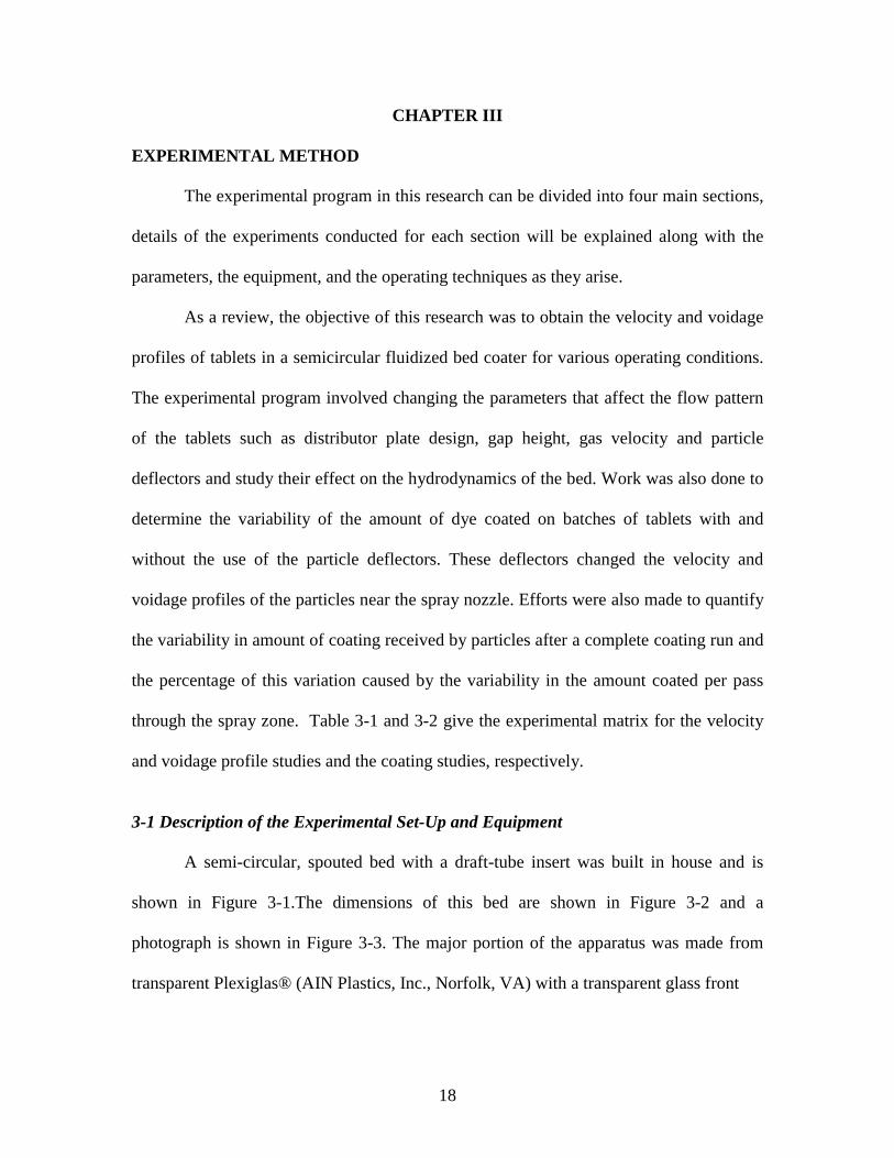
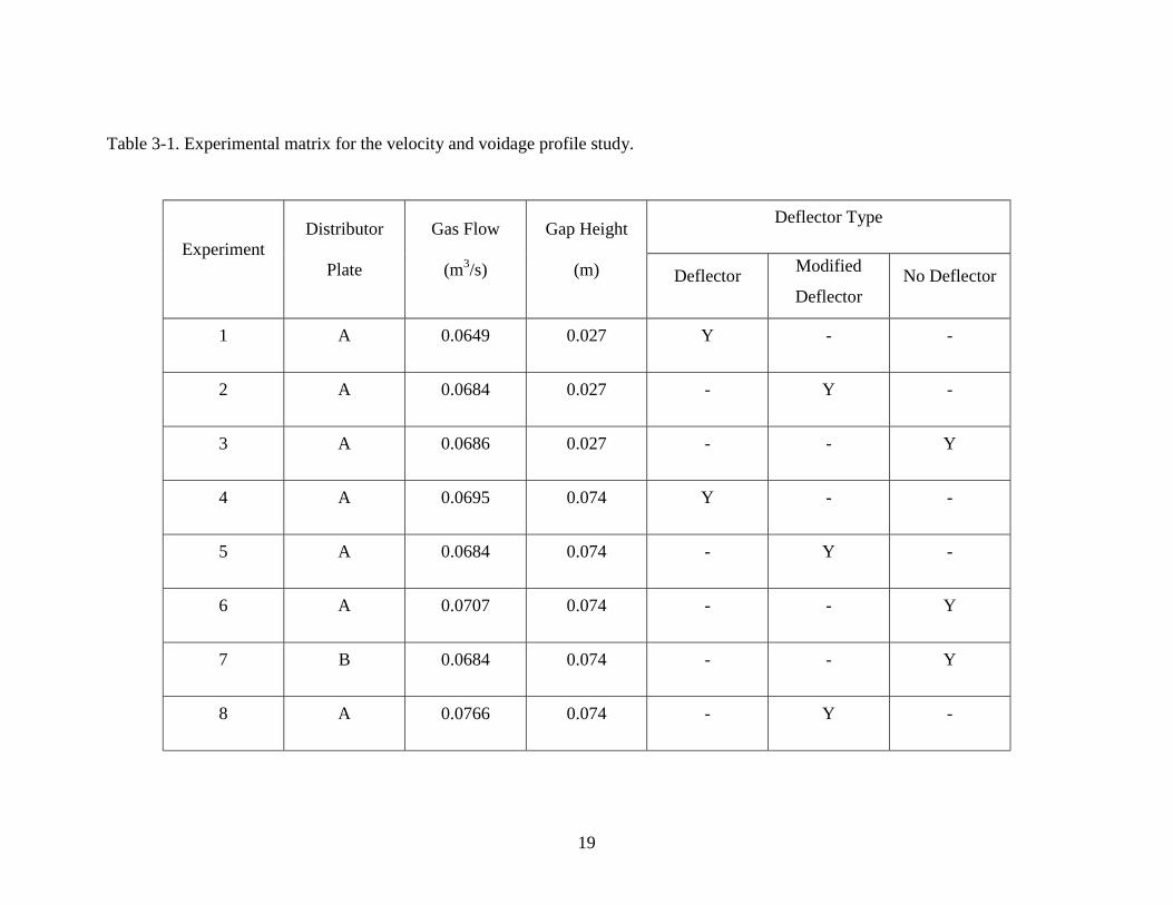
through the spray zone. Table 3-1 and 3-2 give the experimental matrix for the velocity
and voidage profile studies and the coating studies, respectively.
3-1 Description of the Experimental Set-Up and Equipment
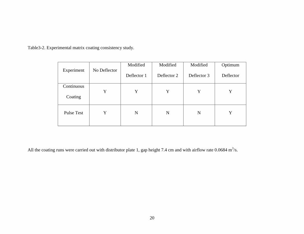
A semi-circular, spouted bed with a draft-tube insert was built in house and is
shown in Figure 3-1.The dimensions of this bed are shown in Figure 3-2 and a
photograph is shown in Figure 3-3. The major portion of the apparatus was made from
transparent Plexiglas® (AIN Plastics, Inc., Norfolk, VA) with a transparent glass front
19
Table 3-1. Experimental matrix for the velocity and voidage profile study.
Deflector Type
ExperimentDistributor
Plate
Gas Flow
(m3/s)
Gap Height
(m) DeflectorModified
DeflectorNo Deflector
1 A 0.0649 0.027 Y - -
2 A 0.0684 0.027 - Y -
3 A 0.0686 0.027 - - Y
4 A 0.0695 0.074 Y - -
5 A 0.0684 0.074 - Y -
6 A 0.0707 0.074 - - Y
7 B 0.0684 0.074 - - Y
8 A 0.0766 0.074 - Y -
20
Table3-2. Experimental matrix coating consistency study.
All the coating runs were carried out with distributor plate 1, gap height 7.4 cm and with airflow rate 0.0684 m3/s.
Experiment No DeflectorModified
Deflector 1
Modified
Deflector 2
Modified
Deflector 3
Optimum
Deflector
Continuous
CoatingY Y Y Y Y
Pulse Test Y N N N Y
21
Figure 3-1: Schematic diagram of the semi-circular spouted bed coating device. Arrowsindicate direction of solids movement.
Draft Tube
Spray Region
Draft Tube(ID = 10.2 cm)
Column(ID = 22.9 cm)
Expanded Region
Fountain Region
Atomizing Air
Spray Nozzle
Air Inlet
Insert ‘A’
Coating Solution
Distributor Plate
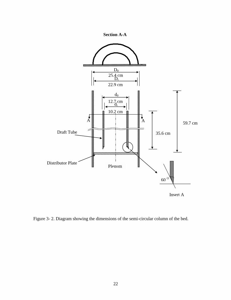
22
10.2 cm
12.7 cm
22.9 cm
25.4 cm
35.6 cm
59.7 cm
Draft Tube
Distributor PlatePlenum
A A
Section A-A
Figure 3- 2. Diagram showing the dimensions of the semi-circular column of the bed.
60 O
Insert A
di
d0
D0
Di
23
Figure 3-3 Photograph of the fluidized bed with the two-camera set-up.
24
Low gap height2.7 cm
Nozzle height3.3 cm
Distributor plate
Nozzle height3.3 cm
High gapheight 7.4 cm
Distributor plate
Figure 3-4a, b. Schematic showing the low and high gap height betweenthe distributor plate and the draft-tube.
25
face. Through the transparent glass sheet it was possible to observe the flow pattern of the
tablets. This enabled the use of a computer-based video imaging system to study the
particle dynamics and obtain velocity and voidage data. The bottom of the draft-tube is
angled at 600 from the horizontal as shown in Figure 3-2, insert ‘A’. This modification
reduces the flow of particles towards the spray nozzle and assists the particle movement
upward through the spray zone as shown in Figure 3-1 (the arrows indicate the direction
of particle motion). The draft-tube is anchored in the center of the column using two sets
of tension bars, springs and o-rings. The draft-tube is pressed against the front transparent
glass plate by the springs that seals the draft-tube with the front surface. The o-rings
facilitate the upward and downward movement of the draft-tube relative to the distributor
plate. The position of the draft-tube relative to the distributor plate can be used to control
solids flow from the annular region to the draft-tube region. The higher the position of the
draft-tube (bigger gap between the draft-tube and distributor plate) the greater the solids
flow, and hence the denser is the bed. Figure 3-4 a, b show the two gap heights
investigated and the relative position of the distributor plate and nozzle.
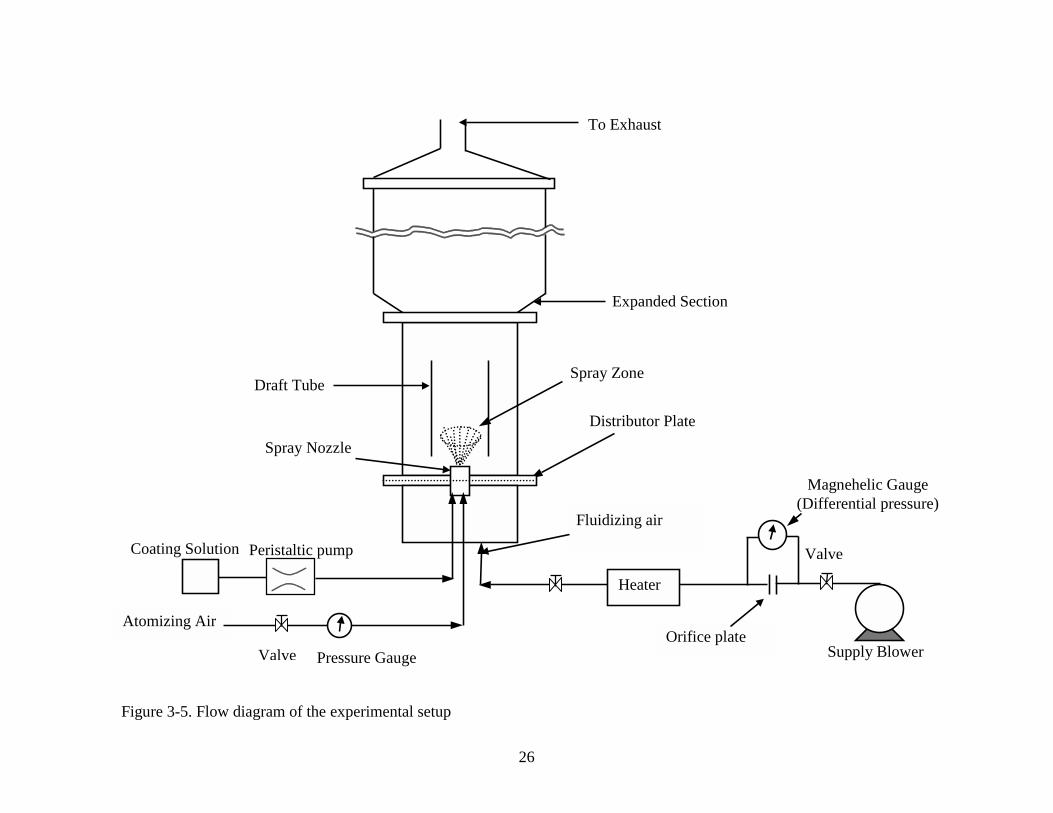
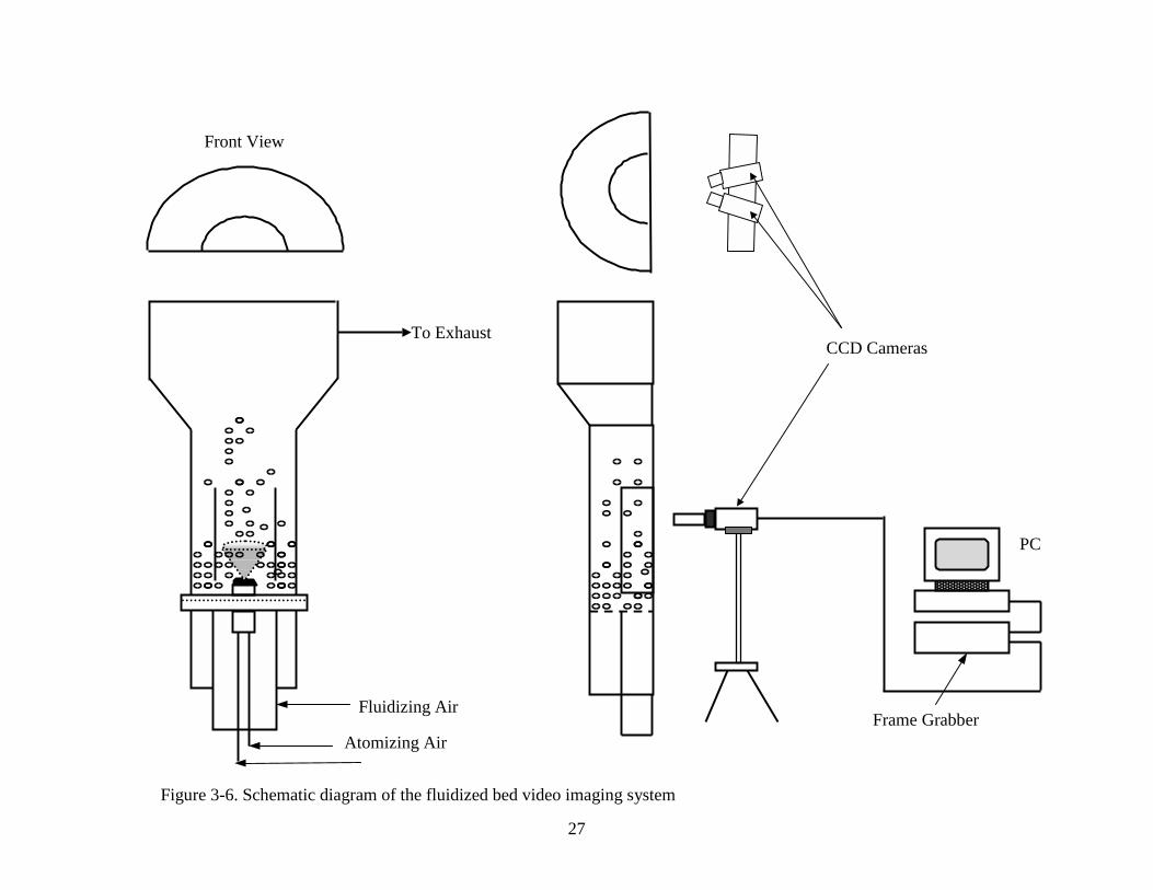
The flow diagram of the experimental system used in this work is shown in Figure
3-5 and the schematic diagram of the video imaging system is shown in Figure 3-6. Air is
supplied by a centrifugal blower and is regulated through valves before in enters the
plenum chamber located beneath the distributor plate. The airflow rate to the bed is
controlled using the valves up-stream of the bed. The airflow rate is inferred from the
pressure drop across a calibrated orifice plate upstream of the valves. Calibration details
of the orifice plate are given in Appendix I. During the experimental runs to obtain
26
Figure 3-5. Flow diagram of the experimental setup
Magnehelic Gauge(Differential pressure)
Coating Solution
Orifice plateAtomizing Air
Draft Tube
Distributor Plate
Expanded Section
Spray Nozzle
Fluidizing air
Heater
Supply Blower
ValvePeristaltic pump
To Exhaust
Valve Pressure Gauge
Spray Zone
27
Front View
CCD Cameras
Frame Grabber
PC
Fluidizing Air
Atomizing Air
To Exhaust
Figure 3-6. Schematic diagram of the fluidized bed video imaging system
28
velocity and voidage profiles, the spray nozzle though present was plugged and no air or
liquid was allowed to flow through it into the bed.
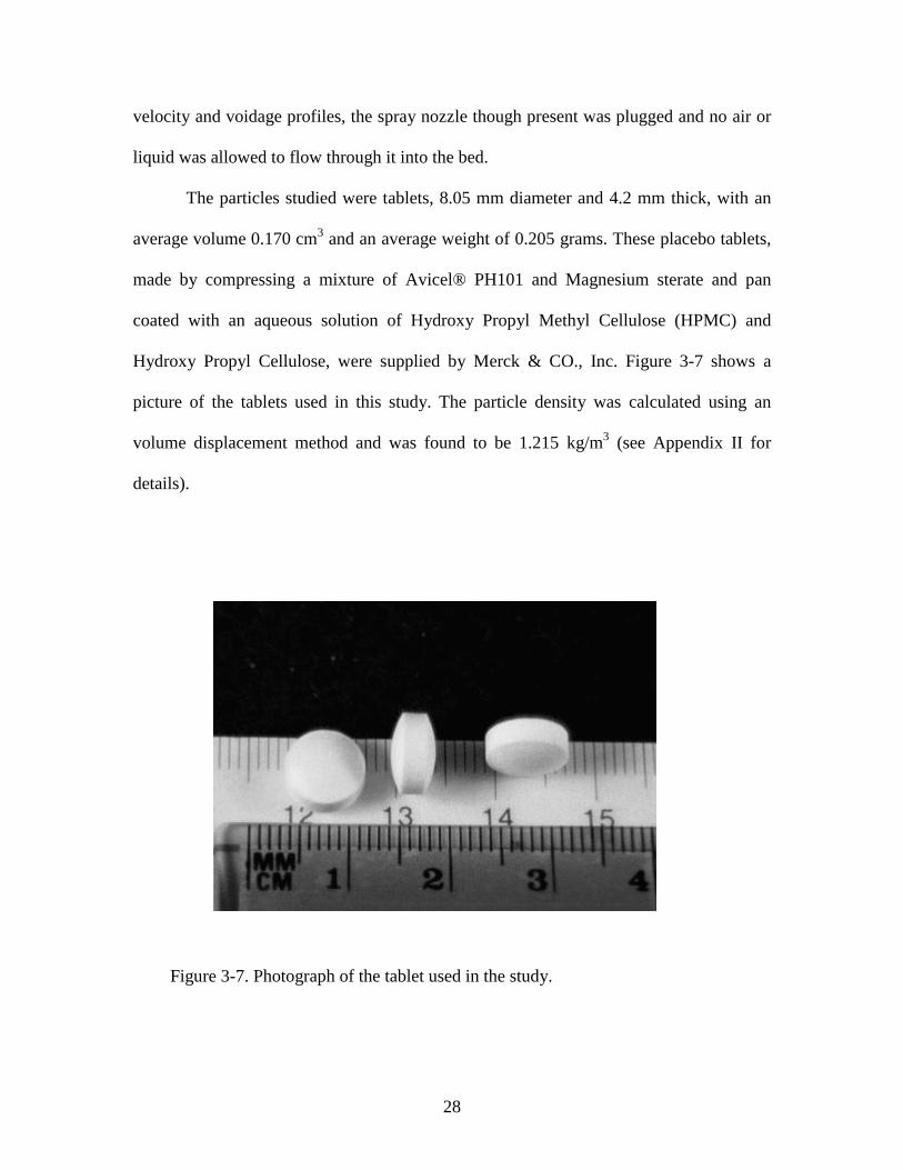
The particles studied were tablets, 8.05 mm diameter and 4.2 mm thick, with an
average volume 0.170 cm3 and an average weight of 0.205 grams. These placebo tablets,
made by compressing a mixture of Avicel® PH101 and Magnesium sterate and pan
coated with an aqueous solution of Hydroxy Propyl Methyl Cellulose (HPMC) and
Hydroxy Propyl Cellulose, were supplied by Merck & CO., Inc. Figure 3-7 shows a
picture of the tablets used in this study. The particle density was calculated using an
volume displacement method and was found to be 1.215 kg/m3 (see Appendix II for
details).
Figure 3-7. Photograph of the tablet used in the study.
29
3-2 Design of Deflector
The work done by Cheng and Turton (1993) and Shelukar et al.(2000) has shown
that major cause of the variation in the amount of coating received can be attributed to the
variation in the coating-per-pass received by the particles in the spray zone. A major
factor for this variation is due to the sheltering effect caused by the particles near the
nozzle on particles farther from the spray source, Cheng (1993). This sheltering effect
can be reduced by guiding the particles away from the spray source, and this reduces the
variation in the coating-per-pass distribution. A more detailed explanation of this
phenomena is given in section 4-4. The desired characteristics of the deflector are: (1) to
prevent the particles entering the draft-tube from passing close to and directly over the
spray nozzle, (2) to give a uniform voidage pattern in the spray zone, (3) does not reduce
the particle flow into the draft-tube, and (4) and does not increase the attrition of the
tablets. Four different deflector designs were tried before the final optimum deflector was
designed.
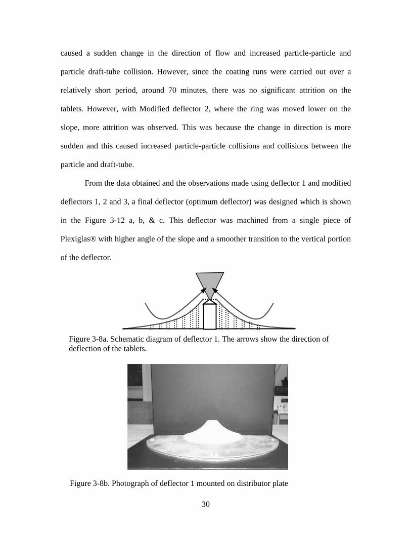
Figure 3-8a and b show the first deflector design. Though this deflector was
effective in some ways (explained in section 4-2.1), it did not give any substantial
improvement in the coating consistency compared to the case without a deflector. The
particles still moved close to the spray zone and the desired effect of moving the particles
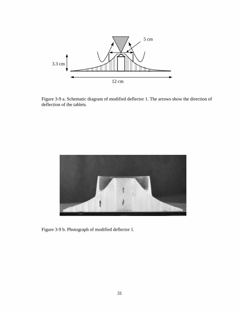
away from the spray nozzle was not obtained. This deflector was further modified by
adding a ring around the nozzle as shown in Figure 3-9 a and b. This ring was moved to
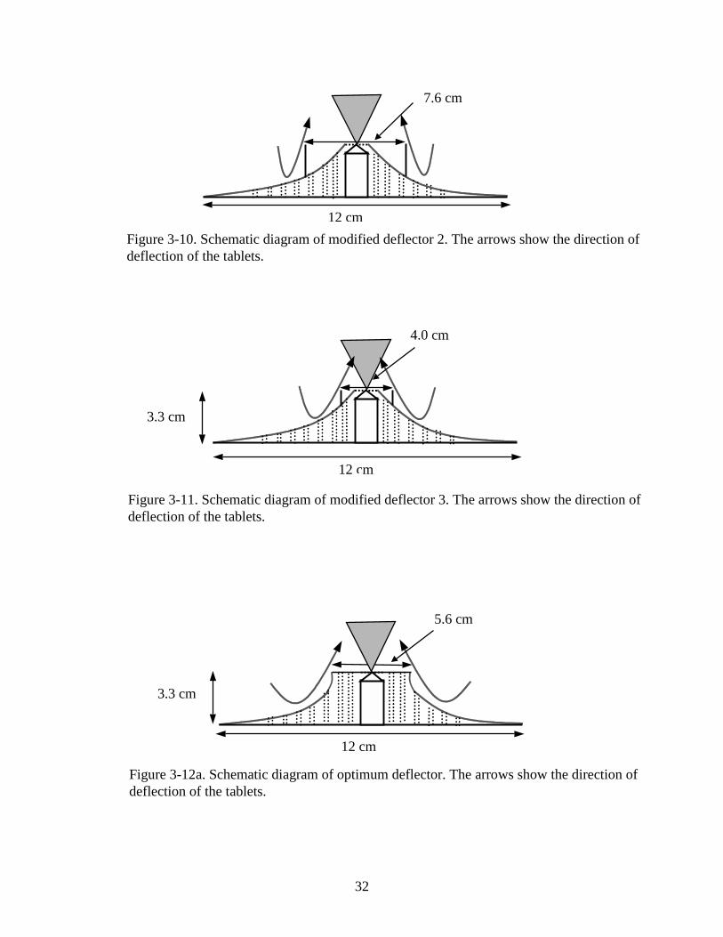
different positions along the slope of the deflector (Figures 3-10 and Figure 3-11) in an
attempt to optimize its effect in deflecting the particles away from the spray nozzle. The
use of these deflectors resulted in increased particle attrition. The ring on the deflectors
30
caused a sudden change in the direction of flow and increased particle-particle and
particle draft-tube collision. However, since the coating runs were carried out over a
relatively short period, around 70 minutes, there was no significant attrition on the
tablets. However, with Modified deflector 2, where the ring was moved lower on the
slope, more attrition was observed. This was because the change in direction is more
sudden and this caused increased particle-particle collisions and collisions between the
particle and draft-tube.
From the data obtained and the observations made using deflector 1 and modified
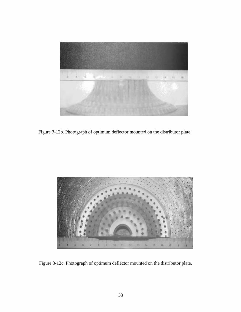
deflectors 1, 2 and 3, a final deflector (optimum deflector) was designed which is shown
in the Figure 3-12 a, b, & c. This deflector was machined from a single piece of
Plexiglas® with higher angle of the slope and a smoother transition to the vertical portion
of the deflector.
Figure 3-8a. Schematic diagram of deflector 1. The arrows show the direction ofdeflection of the tablets.
Figure 3-8b. Photograph of deflector 1 mounted on distributor plate
31
Figure 3-9 b. Photograph of modified deflector 1.
Figure 3-9 a. Schematic diagram of modified deflector 1. The arrows show the direction ofdeflection of the tablets.
12 cm
3.3 cm
5 cm
32
Figure 3-11. Schematic diagram of modified deflector 3. The arrows show the direction ofdeflection of the tablets.
Figure 3-10. Schematic diagram of modified deflector 2. The arrows show the direction ofdeflection of the tablets.
7.6 cm
4.0 cm
5.6 cm
3.3 cm
3.3 cm
12 cm
12 cm
12 cm
Figure 3-12a. Schematic diagram of optimum deflector. The arrows show the direction ofdeflection of the tablets.
33
Figure 3-12b. Photograph of optimum deflector mounted on the distributor plate.
Figure 3-12c. Photograph of optimum deflector mounted on the distributor plate.
34
3-3 Measurement Techniques and Equipment Used
Computer-based video imaging techniques were used with customized imaging
software to measure particle velocity and voidage profiles in the semi-circular fluidized
bed. The set-up consisted of two CCD cameras (Sony XC – 75 CE CCD, Sony Inc.,),
connected to two frame grabbers (PX610 Precision Frame Grabber, Imagenation
Corporation, Beaverton, Oregon), which in-turn were connected to a computer (486DX,
33 MHZ, Keydata International Inc., S. Plainfield, NJ). The standard RS-170 interlaced
signal (30 frames/sec) from the cameras are captured by the frame grabbers and viewed
on the monitor of the computer with the help of custom software written in Microsoft
Visual Basic 6.0.
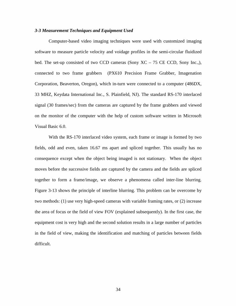
With the RS-170 interlaced video system, each frame or image is formed by two
fields, odd and even, taken 16.67 ms apart and spliced together. This usually has no
consequence except when the object being imaged is not stationary. When the object
moves before the successive fields are captured by the camera and the fields are spliced
together to form a frame/image, we observe a phenomena called inter-line blurring.
Figure 3-13 shows the principle of interline blurring. This problem can be overcome by
two methods: (1) use very high-speed cameras with variable framing rates, or (2) increase
the area of focus or the field of view FOV (explained subsequently). In the first case, the
equipment cost is very high and the second solution results in a large number of particles
in the field of view, making the identification and matching of particles between fields
difficult.
35
Field 1 Field 2 Frame 1
+ =
Figure 3-13. Schematic diagram showing an image/frame formed by two fields taken with astandard RS-170 interlaced video format (time lag of 16.67 ms) and spliced together to form theimage.
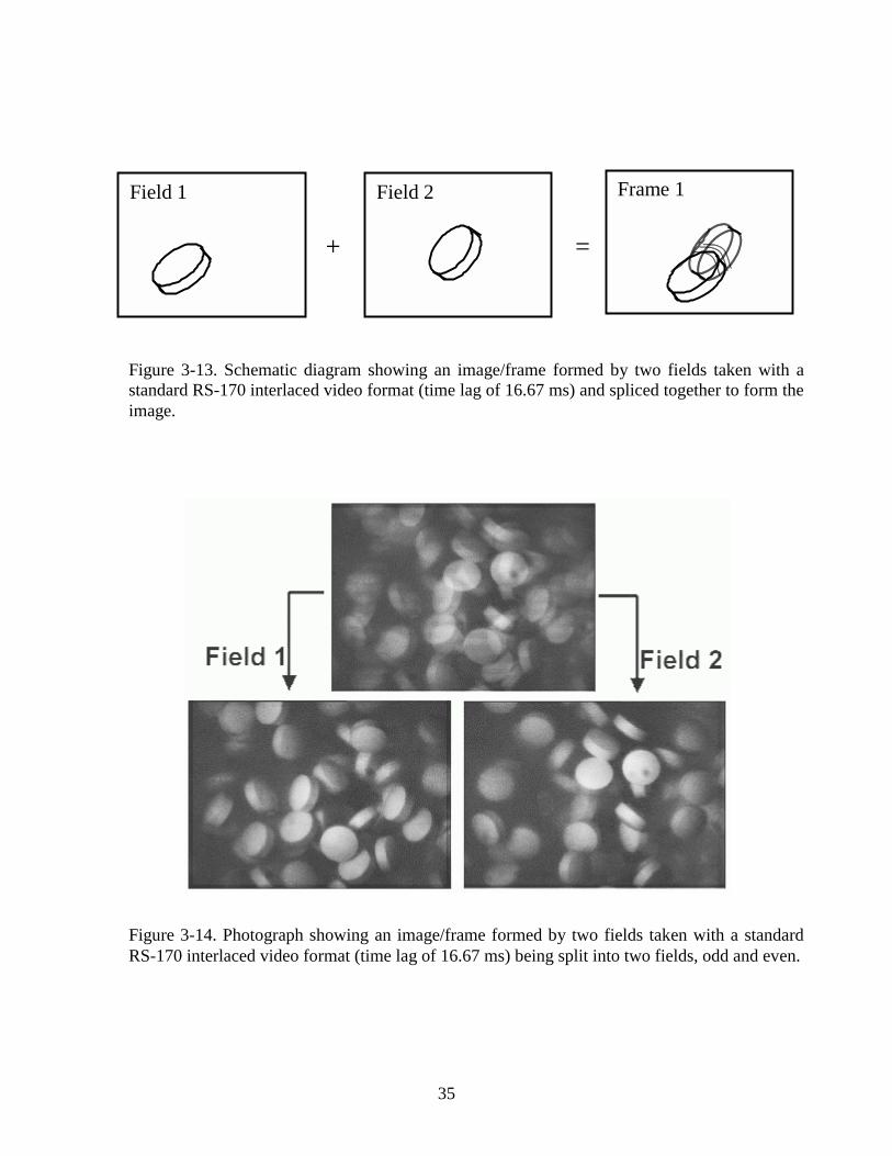
Figure 3-14. Photograph showing an image/frame formed by two fields taken with a standardRS-170 interlaced video format (time lag of 16.67 ms) being split into two fields, odd and even.
36
In our case, the tablets move with high velocities of 1 to 3 m/s and when imaged
with a RS-170 format, the particles move a significant distance (16 to 40 mm) before the
successive fields are captured. Thus, the particles may move out of the field of view and
hence cannot be tracked by normal cameras. The solution utilized here is a low cost one
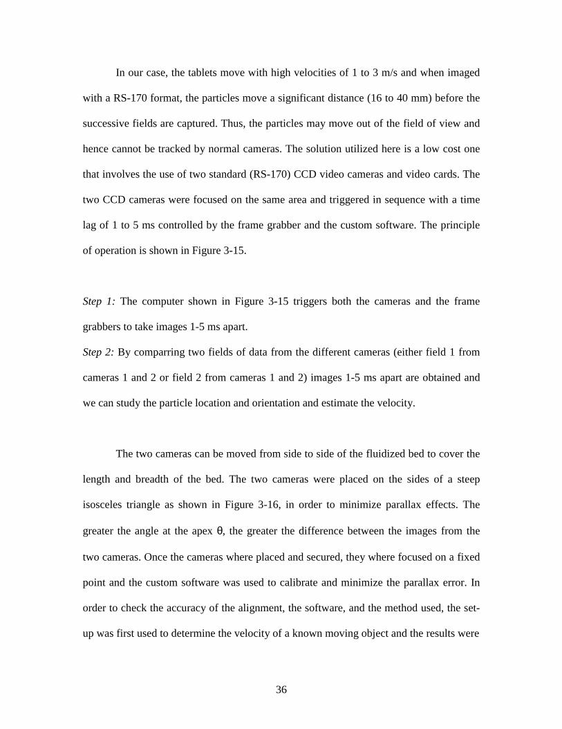
that involves the use of two standard (RS-170) CCD video cameras and video cards. The
two CCD cameras were focused on the same area and triggered in sequence with a time
lag of 1 to 5 ms controlled by the frame grabber and the custom software. The principle
of operation is shown in Figure 3-15.
Step 1: The computer shown in Figure 3-15 triggers both the cameras and the frame
grabbers to take images 1-5 ms apart.
Step 2: By comparring two fields of data from the different cameras (either field 1 from
cameras 1 and 2 or field 2 from cameras 1 and 2) images 1-5 ms apart are obtained and
we can study the particle location and orientation and estimate the velocity.
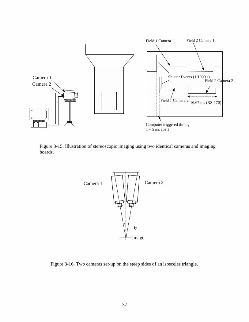
The two cameras can be moved from side to side of the fluidized bed to cover the
length and breadth of the bed. The two cameras were placed on the sides of a steep
isosceles triangle as shown in Figure 3-16, in order to minimize parallax effects. The
greater the angle at the apex θ, the greater the difference between the images from the
two cameras. Once the cameras where placed and secured, they where focused on a fixed
point and the custom software was used to calibrate and minimize the parallax error. In
order to check the accuracy of the alignment, the software, and the method used, the set-
up was first used to determine the velocity of a known moving object and the results were
37
θ
Camera 2Camera 1
Image
Figure 3-16. Two cameras set-up on the steep sides of an isosceles triangle.
Computer triggered timing1 – 5 ms apart
Figure 3-15. Illustration of stereoscopic imaging using two identical cameras and imagingboards.
Camera 1Camera 2
Field 1 Camera 1 Field 2 Camera 1
Field 1 Camera 2
Shutter Events (1/1000 s)
16.67 ms (RS-170)
Field 2 Camera 2

38
compared. A hand held drill (DeWalt DW 998, 0 to 650 rpm) fixed with aflat disk
marked with points was used for this purpose. The speed of rotation or the RPM of the
disk was measured with a stroboscope (Sticht Nova-strobe® DA Model, Bluefield, VA)
and the linear velocity of the point on the disk was calculated using the formula v = r ω
(where r is the distance between the center of the disk and the point in focus and � is the
angular velocity). The resulting comparison is shown in Appendix III. This check
validated the method used and gave an estimation of the accuracy possible.
3-4 Calibration of Video Imaging System
The draft-tube region where the particle velocities were measured was divided
into boxes of dimensions 20mm by 20mm. This size, 20 x 20 mm, was found to be
appropriate, because it was large enough to track a particle within the same box and was
not too big to cause confusion with a large number of tablets in the field of view. This
square box formed the Field of View (FOV) of the cameras. The positions of the cameras
were adjusted and extension rings (7.5 mm) were used to obtain a clear, focused image.
The depth from the front transparent glass sheet into the bed, over which the
camera could pick up clear image of tablets, is the Apparent Depth of Field (ADOF). To
determine the ADOF the following procedure was used. Models shown in Figure 3-17
were made. The tablets were mounted on pins, held on a sheet of Plexiglas to give the
effect of being suspended in air, as shown in the picture. These models where then placed
in the empty fluidized bed with the tablets on the front face just touching the front glass
sheet of the bed. The camera was then focused on the inner surface of the glass sheet or
the permanent marks made in the draft-tube, so as to get a clear image of the models on
39
Figure 3-17. Photographs of models made to determine depth of field of the camera.
40
the monitor of the computer. The software then runs a set of routines on the acquired
image, explained in the voidage measurement section, and returns a numerical value for
the number of tablets identified in the field of view (FOV). The software returns the
number of tablets in the model, which is compared, to the actual number. We can now
identify the tablets in the model picked up by the software and the ones that were not
recognized. We know the individual distances of each tablet in the model from the front
glass sheet and by identifying the tablets not picked by the software; we can determine
the depth to which the camera can identify the tablets. By repeating this procedure
several times with different models and with exactly the same lighting effects, the
apparent depth of field was determined. The ADOF was determined to be 1.5 cm and the
data for this calibration is given in Appendix IV.
3-5 Principles of Velocity Measurement
After the initial processes of focusing the cameras, aligning them and calibrating
for pixel size (explained in Appendix V) are completed, the supply blower is switched on
and the bed is fluidized. When the bed is running, a “grab” event is initiated that causes
both cameras to obtain images at the pre-selected time lag. Figure 3-18 shows a still
image of the particles in motion as seen on the computer screen. The center of each
particle is then located using a computer generated crosshair and the horizontal and
vertical distances between the successive images are computed and recorded. The
software returns the velocities in both the vertical (uy) and horizontal (ux)
41
ux
uy
Field 1 Camera 1 Field 1 Camera 2
Velocity Vector
Movement of particle defined by
distance between centers and
time gap between the fields
Figure 3-18. Photograph of still images of particles in motion as seen on the computer monitor. The hairlines shows the distance moved by thecenter of the particle.
Figure 3-19. A schematic showing the directions of the velocity vector measured.
42
direction in meters/second (Figure 3-19). The magnitude and angle of the velocity vector
can be calculated as shown in Appendix VI.
The process of obtaining velocities in the horizontal and vertical direction is
repeated nearly 80 times for each box/FOV. The cameras are then moved on the sliding
stand to focus on the next box. This process is repeated across the entire width and height
of the draft-tube so as to obtain the velocity profile of the moving particles across the
draft-tube region. The 70 to 100 velocity measurements obtained for each of the boxes
are then averaged to get an average velocity vector for the respective boxes.
3-6 Principle of Voidage Measurement
For the voidage measurement, only one of the cameras was used. The amount of
light on the bed during the voidage measurement was very critical. A variation in light
intensity changes the depth of field resulting in variation in the number of particles
identified by the software. Several trials were done with different light positions,
intensities, and tablet models, until the software returned consistent values for voidage for
the same model. The final position of the light and its intensity were maintained constant
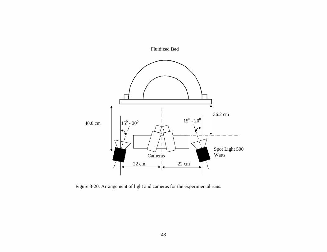
for the entire experimental run. Figure 3-20 shows the final positions of the lights. In
order to fine-tune the software, several standard samples of known voidage where made
from the same tablets used in the runs. The voidage values from the software, were
compared to the actual voidage.
After a field is acquired using the camera for voidage measurement, the software
carries out the following tests and operation on the image to obtain a value for the
43
Figure 3-20. Arrangement of light and cameras for the experimental runs.
36.2 cm
40.0 cm
Cameras
Fluidized Bed
Spot Light 500Watts
22 cm22 cm
150 - 200 150 - 200
44
voidage in that field. First, the software enhances the acquired image (increases the
contrast between the bright and dark areas of the image). Then the software binarized the
image into two groups, one as an area that is above the set gray scale value and the other
below the set gray scale value. The software allows the user to set the value of the gray
scale used in the program. Since the tablets overlap, this binarized image is a contiguous
image of a single tablet or a group of tablets. The software then determines the number of
tablets in each contiguous area using the algorithm explained below.
The software first calculates the contiguous area of the image above the threshold
gray scale value. Two values are set initially, the minimum and maximum area a tablet
can occupy. Since the tablets are not spherical and can take any orientation, these values
were determined by trial and error. When the software scans a binarized image, it checks
each contiguous area and compares it with the pre-set values. If the area is less than the
minimum area, then it is rejected and the software jumps to the next contiguous area. If
the area is above the maximum area a tablet can occupy, then the software subtracts the
area in question with the value of the pre-set maximum area for a tablet and continues to
repeat this process with the area left, until the area left is less than the minimum pre-set
value. Each time a tablet area is subtracted from a contiguous area, the tablet count is
increased by one and the software gives the final number of tablets obtained in that
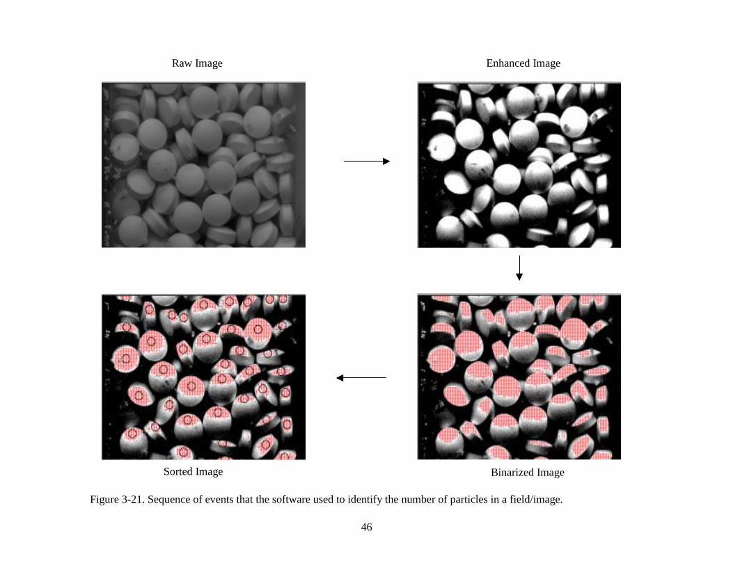
frame. Figure 3-21 shows the sequence of the camera grabbing an image, enhancing it,
then binarizing it into two areas (shaded area is above the pre-set value, the remainder is
below the pre-set value) and finally the number of tablets are counted based on the
algorithm written in the program. Each small black circle in the image represents a
particle.
45
The number of fields over which the average value is to be determined can be set
and this whole process is automated. Hence, when the user gives the number of fields
over which he wants to determine the average number of particles in the area of focus,
the software captures the number of fields given and determines the number of tablets in
each field and returns an average value of the number of tablets in that area of focus or
field of view (FOV) for the given number of fields.
To measure the dynamic bed voidage, the process explained above was carried
out with the dynamic bed for the various conditions in the experimental matrix. The
number of fields over which the voidage value was averaged was fixed at 50. By
increasing the number of fields that are analyzed, the error is reduced. However, it was
observed that there was no significant difference between the voidage values obtained by
averaging over 50 fields and those using 75 fields. Hence, the number of frames for the
voidage determination was set to be 50.
46
Raw Image Enhanced Image
Binarized ImageSorted Image
Figure 3-21. Sequence of events that the software used to identify the number of particles in a field/image.
47
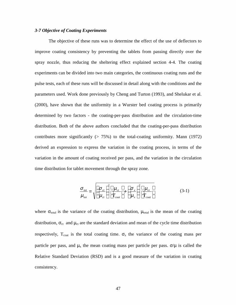
3-7 Objective of Coating Experiments
The objective of these runs was to determine the effect of the use of deflectors to
improve coating consistency by preventing the tablets from passing directly over the
spray nozzle, thus reducing the sheltering effect explained section 4-4. The coating
experiments can be divided into two main categories, the continuous coating runs and the
pulse tests, each of these runs will be discussed in detail along with the conditions and the
parameters used. Work done previously by Cheng and Turton (1993), and Shelukar et al.
(2000), have shown that the uniformity in a Wurster bed coating process is primarily
determined by two factors - the coating-per-pass distribution and the circulation-time
distribution. Both of the above authors concluded that the coating-per-pass distribution
contributes more significantly (> 75%) to the total-coating uniformity. Mann (1972)
derived an expression to express the variation in the coating process, in terms of the
variation in the amount of coating received per pass, and the variation in the circulation
time distribution for tablet movement through the spray zone.
where σtotal is the variance of the coating distribution, µtotal is the mean of the coating
distribution, σct and µct are the standard deviation and mean of the cycle time distribution
respectively, Tcoat is the total coating time. σx the variance of the coating mass per
particle per pass, and µx the mean coating mass per particle per pass. σ/µ is called the
Relative Standard Deviation (RSD) and is a good measure of the variation in coating
consistency.
+
=
coat
ct
x
x
coat
ct
ct
ct
tot
tot
TT
µµσµ
µσ
µσ
22
(3-1)

48
The first term on the right hand side of equation (3-1) is the variation caused by
the non-uniformity of particle circulation, while the second term represents the variation
due to different amounts of coating being received by a particle per pass through the
spray zone. It is the second source of variance that is the more important one for coating
operations over reasonably long (>20 minutes) coating runs. The coating experiments
were designed to investigate quantitatively the effect of deflectors in reducing the
variance caused by the second term and hence its effect on the coating quality.
3-8 Determining the coating formulation
The total amount of coating material used was determined by the time of the
coating run and the rate at which the coating material was sprayed. A mixture of
Aquacoat® (Ethyl cellulose aqueous dispersion with 30% solids, supplied by FMC Corp.,
Newark, DE) and water with blue dye (FD&C approved blue dye # 1, supplied by
Warner-Jenkinson Company, St. Louis, MO) was used as the coating mixture. The
coating mixture distributes evenly on the tablet surface indicating that this mixture is
representative of the actual coating process. The coating solution spreads evenly on the
tablet surface indicating that the blue dye is representative of the actual coating process.
The coating for the continuous coating runs was formulated such that the amount of blue
dye coated on each tablet, at the end of a run, would be high enough to be analyzed by
the spectrophotometer. The amount of blue dye used was estimated by back-calculating
the amount of blue dye that would be coated if all the coating material pumped were to
deposit on the tablets. The weight of the tablets to be coated was very large compared to
the amount of coating material and hence the increase in the weight of

49
individual tablets was insignificant. The details of calculations for determining the
coating formulation are given in Appendix X.
3.9 Coating Experiments
3-9.1 Continuous coating Experiments
The objective of these runs was to determine the overall coating consistency after
a complete coating run and hence obtain a value for σtotal/µtotal (RSDtotal), the LHS of
equation 3-1 . The operating parameters for the coating runs are given in Table 3-3.
Table 3-3 Operating parameters for the continuous coating runs
Air Flow Rate 0.066 m3/s
Coating liquid flow rate 10 ml/min
Volume of Coating liquid 600 ml
Temperature of Air 115 F or 45 C
Time of Coating 70 min
Weight of Bed Material 3.675 kg
Weight of Blue Dye used 2.7 gm
Bed air temperature 114 F
Liquid spray air pressure 35 psi
These coating runs were repeated for the different deflector designs, keeping all
the parameters constant except the design of the deflector. After each coating run, 100
tablets were picked randomly and were analyzed for blue dye content. A histogram plot
of blue dye concentration per tablet vs. frequency shows the spread of the amount of

50
coating each tablet receives. The change in the spread or variance with the use of
different deflectors was then studied.
3-9.2 Method of coating for continuous tests
The fluidized bed is first cleaned and assembled. A pre-weighed quantity (3.675
kg) of tablets is then charged into the equipment through the charge point at the top of the
bed. The supply blower is then started and the valves adjusted to obtain the desired
airflow rate. The coil heater for heating the supply air is then switched on and the
temperature set to the desired value. The spray nozzle airflow is adjusted to the desired
value, the peristaltic spray pump is switched on, and the flow rate set to 10 ml/min.
Calibration details of the peristaltic pump are given in Appendix XII. A detailed flow
diagram of the experimental setup is shown in the Figure 3-5.
The fluidized bed is run under these conditions for 70 minutes, and all the coating
solution is pumped into the bed over this period. The peristaltic pump and the heater are
then turned off and the bed is run for 10 minutes to dry any moisture remaining on the
tablets. The supply air is then lowered and the coated tablets are collected through the
discharge port at the bottom of the bed above the distributor plate. Finally, the air supply
to the spray nozzle is shut-off.
The coating solution is made just before the run by adding blue dye to Aquacoat®
in a beaker and stirred by a Magnetic stirrer. The solubility of the blue dye in Aquacoat®
is excellent and the concentration of blue dye (0.5 %) was far less than the saturation
concentration of 10%.

51
3-9.3 Pulse coating test
The pulse tests were conducted to determine the variation in coating quality due
to the variation in the amounts of coating received by a particle-per-pass through the
spray zone. This will quantify the second term (σx/µx) on the RHS of Equation (3-1).
3-9.4 Method of coating for Pulse tests
The coating process for the pulse test is similar to that of the continuous coating
runs. The parameters are given in Table 3-4 below. After the bed is cleaned and the bed
charged with the measured quantity of tablets, the supply blower is switched on and the
bed is fluidized with the same conditions as that of the continuous run, except that the
coating material does not contain blue dye. After the supply-air has reached the required
temperature (usually a couple of minutes), a pulse of highly concentrated blue dye is
injected into the coating fluid line close to the spray nozzle. The pulse of blue dye is
sprayed over a period of 8 to 10 seconds, which is equal to one circulation time. The
fluidized bed is stopped and emptied as in the case of continuous coating runs.
Table 3-4 Operating parameters for the pulse test runs
Air Flow Rate 0.066 m3/s
Coating liquid flow rate 10 ml/min
Volume of Coating liquid 100 ml
Temperature of Air 115 F or 45 C
Time of Coating 25 minutes
Weight of Bed Material 3.675 kg
Weight of Blue Dye used 2.7 gm
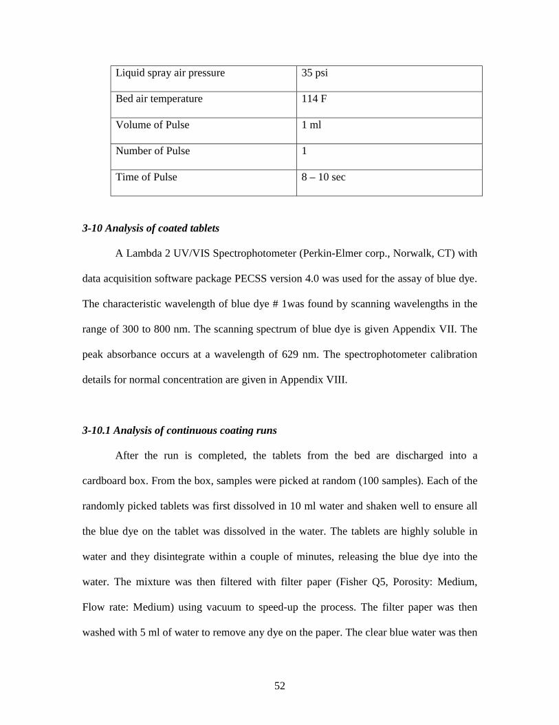
52
Liquid spray air pressure 35 psi
Bed air temperature 114 F
Volume of Pulse 1 ml
Number of Pulse 1
Time of Pulse 8 – 10 sec
3-10 Analysis of coated tablets
A Lambda 2 UV/VIS Spectrophotometer (Perkin-Elmer corp., Norwalk, CT) with
data acquisition software package PECSS version 4.0 was used for the assay of blue dye.
The characteristic wavelength of blue dye # 1was found by scanning wavelengths in the
range of 300 to 800 nm. The scanning spectrum of blue dye is given Appendix VII. The
peak absorbance occurs at a wavelength of 629 nm. The spectrophotometer calibration
details for normal concentration are given in Appendix VIII.
3-10.1 Analysis of continuous coating runs
After the run is completed, the tablets from the bed are discharged into a
cardboard box. From the box, samples were picked at random (100 samples). Each of the
randomly picked tablets was first dissolved in 10 ml water and shaken well to ensure all
the blue dye on the tablet was dissolved in the water. The tablets are highly soluble in
water and they disintegrate within a couple of minutes, releasing the blue dye into the
water. The mixture was then filtered with filter paper (Fisher Q5, Porosity: Medium,
Flow rate: Medium) using vacuum to speed-up the process. The filter paper was then
washed with 5 ml of water to remove any dye on the paper. The clear blue water was then
53
analyzed for blue dye content using the spectrophotometer. This gives the blue dye
content per tablet. The process was repeated for 100 tablets to get an average blue dye
content, spread, and variation for each batch. Similarly, samples were analyzed for the
other coating runs with the deflector, modified deflector 1, modified deflector2, modified
deflector3 and optimum deflector.
3-10.2 Analysis for Pulse test runs
The analysis of blue dye content for the pulse test runs was similar to that of the
continuous runs. However, for the pulse test, a tablet was dissolved in 2 ml water and
then washed with 1 ml water. The amount of blue dye received by tablets during a pulse
test was very low and hence the amount of water used to dissolve the tablet was kept as
low as possible, so that the blue dye concentration can be deduced by the spectrometer.
The blue dye content fell in the lower part of the detectable range of the
spectrophotometer and a low concentration calibration curve shown in Appendix IX was
used. The software, PECSS version 4.0, used with the spectrometer could calculate
values only up to the fourth decimal place and hence when values less than that were
calculated, they were rounded off to 0. Hence, even though the spectrometer detected
different values of absorbance for the samples, the software sometimes gave the same
concentration values. Therefore, for the pulse tests the value of blue dye concentration
was calculated by substituting the value of absorbance into a linear equation that related
absorbance to blue dye concentration shown in Appendix XIII, rather than using the
results from the PECCS software.
54
CHAPTER IV
RESULTS AND DISCUSSION
4-1. Velocity Measurement in the Draft-tube region
4-1.1 Velocity Profiles in the draft-tube
The draft-tube region in the semi-circular bed was divided into an imaginary grid
of square boxes with sides equal to 2.0 cm. The draft-tube, 10.2 cm wide and 35.2 cm in
height, was divided into five boxes in the horizontal direction and 17 boxes in the vertical
direction. Velocity and voidage measurements were taken up to the 13th box in the
vertical direction. It was observed that the particles at this point already showed a steady
profile, and were out of the spray zone and hence the reminder of the velocity data in the
draft-tube was of less significance. The first row of the imaginary boxes was directly
above the nozzle, where the particles entered the spray zone. The imaginary grid is
illustrated in Figure 4-1.
The particle velocity profiles in the draft-tube were measured for a variety of
operating conditions shown in the experimental matrix in Table 3-1. For each operating
condition, the velocity profile has been mapped and is pictorially represented using a
software program written in Microsoft Visual Basic 6.0. The grid corresponds to that
shown in Figure 4-1 and the lines inside these boxes represent the magnitude and
direction of the average velocity vector of the particle motion in that region of the draft-
tube. The velocities shown in these figures were the average value of between 70 to 100
sets of velocity data obtained at each position in the bed.
The major variations in the operating conditions were the gap height between the
distributor plate and draft-tube and the presence or absence of different types of
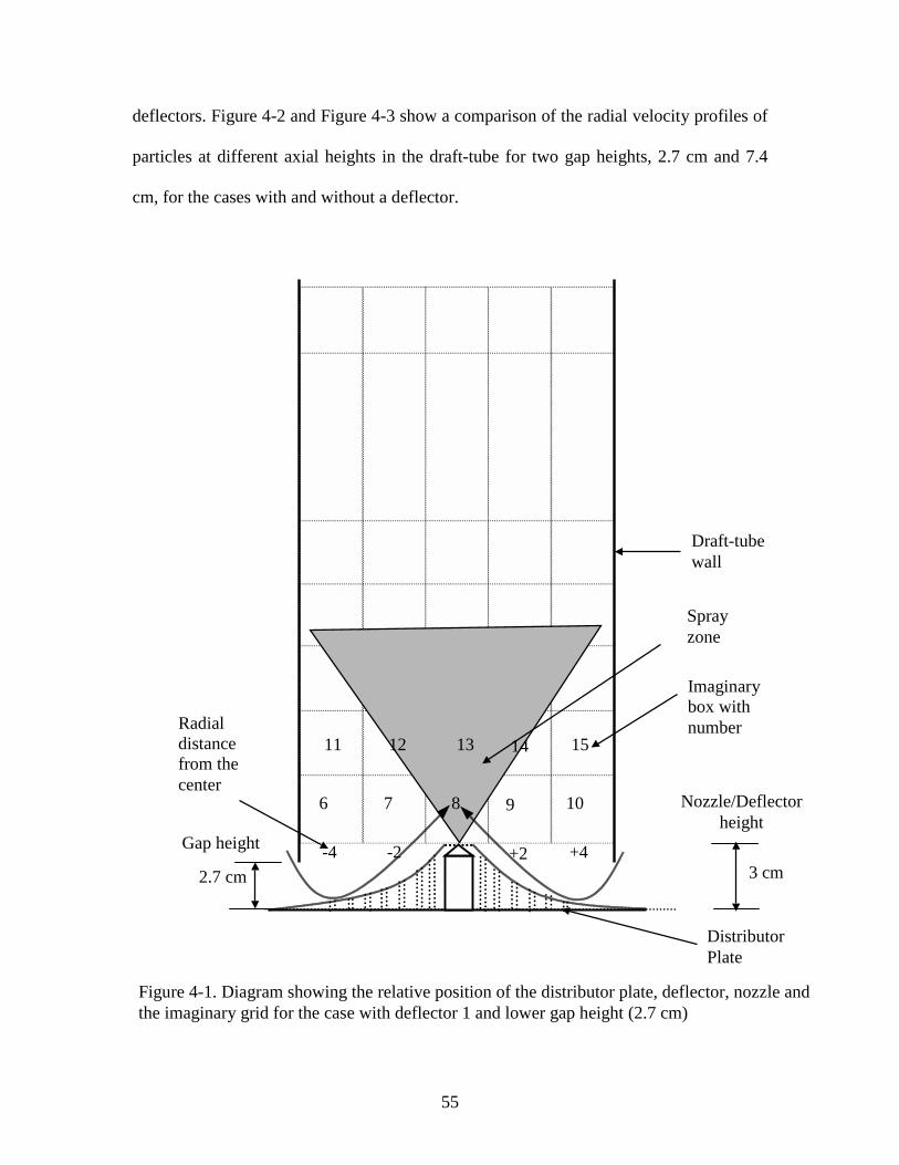
55
deflectors. Figure 4-2 and Figure 4-3 show a comparison of the radial velocity profiles of
particles at different axial heights in the draft-tube for two gap heights, 2.7 cm and 7.4
cm, for the cases with and without a deflector.
Figure 4-1. Diagram showing the relative position of the distributor plate, deflector, nozzle andthe imaginary grid for the case with deflector 1 and lower gap height (2.7 cm)
� �
3 cm2.7 cm
Gap height
Nozzle/Deflectorheight
Imaginarybox withnumber
Sprayzone
Draft-tubewall
DistributorPlate
-4 -2 +2 +4
6 7 9 108
11 12 14 1513Radialdistancefrom thecenter
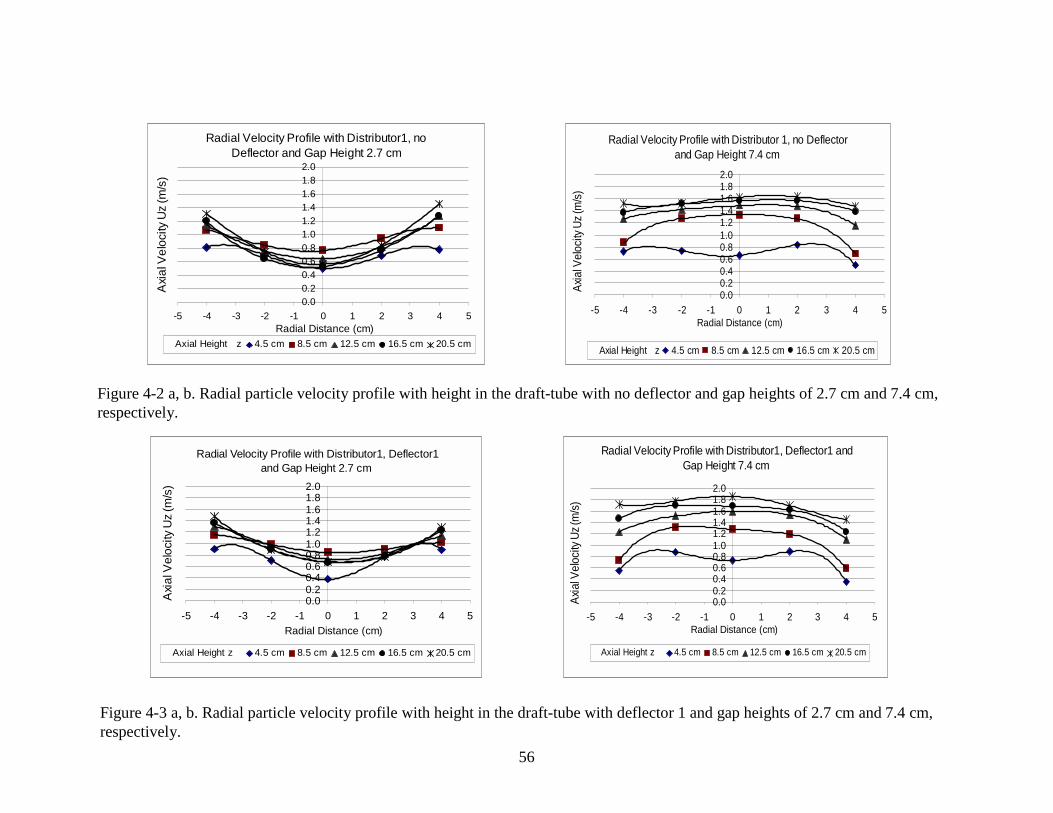
56
Figure 4-2 a, b. Radial particle velocity profile with height in the draft-tube with no deflector and gap heights of 2.7 cm and 7.4 cm,respectively.
Figure 4-3 a, b. Radial particle velocity profile with height in the draft-tube with deflector 1 and gap heights of 2.7 cm and 7.4 cm,respectively.
Radial Velocity Profile with Distributor 1, no Deflector and Gap Height 7.4 cm
0.00.20.40.60.81.01.21.41.61.82.0
-5 -4 -3 -2 -1 0 1 2 3 4 5Radial Distance (cm)
Axi
al V
eloc
ity U
z (m
/s)
Axial Height z 4.5 cm 8.5 cm 12.5 cm 16.5 cm 20.5 cm
Radial Velocity Profile with Distributor1, no Deflector and Gap Height 2.7 cm
0.00.2
0.4
0.60.8
1.01.2
1.41.6
1.8
2.0
-5 -4 -3 -2 -1 0 1 2 3 4 5Radial Distance (cm)
Axi
al V
elo
city
Uz
(m/s
)
Axial Height z 4.5 cm 8.5 cm 12.5 cm 16.5 cm 20.5 cm
Radial Velocity Profile with Distributor1, Deflector1 and Gap Height 2.7 cm
0.00.20.40.60.81.01.21.41.61.82.0
-5 -4 -3 -2 -1 0 1 2 3 4 5
Radial Distance (cm)
Axi
al V
elo
city
Uz
(m/s
)
Axial Height z 4.5 cm 8.5 cm 12.5 cm 16.5 cm 20.5 cm
Radial Velocity Profile with Distributor1, Deflector1 and Gap Height 7.4 cm
0.00.20.40.60.81.01.21.41.61.82.0
-5 -4 -3 -2 -1 0 1 2 3 4 5Radial Distance (cm)
Axi
al V
eloc
ity U
z (m
/s)
Axial Height z 4.5 cm 8.5 cm 12.5 cm 16.5 cm 20.5 cm
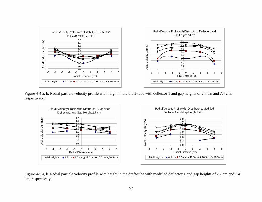
57
Figure 4-4 a, b. Radial particle velocity profile with height in the draft-tube with deflector 1 and gap heights of 2.7 cm and 7.4 cm,respectively.
Figure 4-5 a, b. Radial particle velocity profile with height in the draft-tube with modified deflector 1 and gap heights of 2.7 cm and 7.4cm, respectively.
Radial Velocity Profile with Distributor1, Deflector1 and Gap Height 2.7 cm
0.00.20.40.60.81.01.21.41.61.82.0
-5 -4 -3 -2 -1 0 1 2 3 4 5
Radial Distance (cm)
Axi
al V
elo
city
Uz
(m/s
)
Axial Height z 4.5 cm 8.5 cm 12.5 cm 16.5 cm 20.5 cm
Radial Velocity Profile with Distributor1, Deflector1 and Gap Height 7.4 cm
0.00.20.40.60.81.01.21.41.61.82.0
-5 -4 -3 -2 -1 0 1 2 3 4 5Radial Distance (cm)
Axi
al V
eloc
ity U
z (m
/s)
Axial Height z 4.5 cm 8.5 cm 12.5 cm 16.5 cm 20.5 cm
Radial Velocity Profile with Distributor1, Modified Deflector1 and Gap Height 2.7 cm
0.00.20.40.60.81.01.21.41.61.82.0
-5 -4 -3 -2 -1 0 1 2 3 4 5Radial Distance (cm)
Axi
al V
elo
city
Uz
(m
/s)
Axial Height z 4.5 cm 8.5 cm 12.5 cm 16.5 cm 20.5 cm
Radial Velocity Profile with Distributor1, Modified Deflector1 and Gap Height 7.4 cm
0.00.20.40.60.81.01.21.41.61.82.0
-5 -4 -3 -2 -1 0 1 2 3 4 5Radial Distance (cm)
Axi
al V
eloc
ity U
z (m
/s)
Axial Height z 4.5 cm 8.5 cm 12.5 cm 16.5 cm 20.5 cm
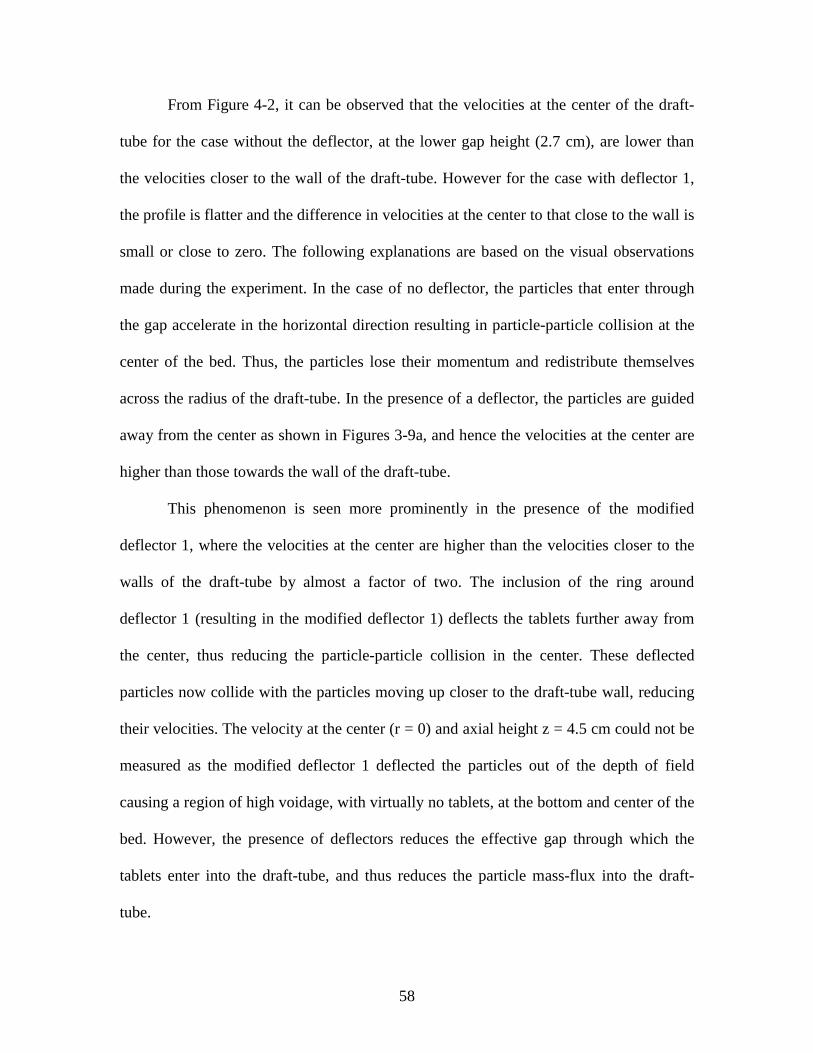
58
From Figure 4-2, it can be observed that the velocities at the center of the draft-
tube for the case without the deflector, at the lower gap height (2.7 cm), are lower than
the velocities closer to the wall of the draft-tube. However for the case with deflector 1,
the profile is flatter and the difference in velocities at the center to that close to the wall is
small or close to zero. The following explanations are based on the visual observations
made during the experiment. In the case of no deflector, the particles that enter through
the gap accelerate in the horizontal direction resulting in particle-particle collision at the
center of the bed. Thus, the particles lose their momentum and redistribute themselves
across the radius of the draft-tube. In the presence of a deflector, the particles are guided
away from the center as shown in Figures 3-9a, and hence the velocities at the center are
higher than those towards the wall of the draft-tube.
This phenomenon is seen more prominently in the presence of the modified
deflector 1, where the velocities at the center are higher than the velocities closer to the
walls of the draft-tube by almost a factor of two. The inclusion of the ring around
deflector 1 (resulting in the modified deflector 1) deflects the tablets further away from
the center, thus reducing the particle-particle collision in the center. These deflected
particles now collide with the particles moving up closer to the draft-tube wall, reducing
their velocities. The velocity at the center (r = 0) and axial height z = 4.5 cm could not be
measured as the modified deflector 1 deflected the particles out of the depth of field
causing a region of high voidage, with virtually no tablets, at the bottom and center of the
bed. However, the presence of deflectors reduces the effective gap through which the
tablets enter into the draft-tube, and thus reduces the particle mass-flux into the draft-
tube.
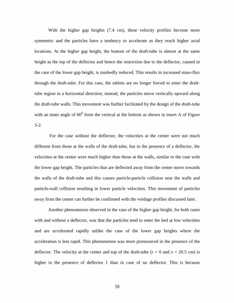
59
With the higher gap heights (7.4 cm), these velocity profiles become more
symmetric and the particles have a tendency to accelerate as they reach higher axial
locations. At the higher gap height, the bottom of the draft-tube is almost at the same
height as the top of the deflector and hence the restriction due to the deflector, caused in
the case of the lower gap height, is markedly reduced. This results in increased mass-flux
through the draft-tube. For this case, the tablets are no longer forced to enter the draft-
tube region in a horizontal direction; instead, the particles move vertically upward along
the draft-tube walls. This movement was further facilitated by the design of the draft-tube
with an inner angle of 600 from the vertical at the bottom as shown in insert A of Figure
3-2.
For the case without the deflector, the velocities at the center were not much
different from those at the walls of the draft-tube, but in the presence of a deflector, the
velocities at the center were much higher than those at the walls, similar to the case with
the lower gap height. The particles that are deflected away from the center move towards
the walls of the draft-tube and this causes particle-particle collision near the walls and
particle-wall collision resulting in lower particle velocities. This movement of particles
away from the center can further be confirmed with the voidage profiles discussed later.
Another phenomenon observed in the case of the higher gap height, for both cases
with and without a deflector, was that the particles tend to enter the bed at low velocities
and are accelerated rapidly unlike the case of the lower gap heights where the
acceleration is less rapid. This phenomenon was more pronounced in the presence of the
deflector. The velocity at the center and top of the draft-tube (r = 0 and z = 20.5 cm) is
higher in the presence of deflector 1 than in case of no deflector. This is because
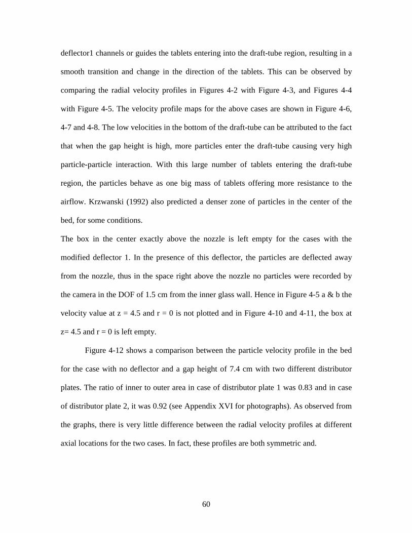
60
deflector1 channels or guides the tablets entering into the draft-tube region, resulting in a
smooth transition and change in the direction of the tablets. This can be observed by
comparing the radial velocity profiles in Figures 4-2 with Figure 4-3, and Figures 4-4
with Figure 4-5. The velocity profile maps for the above cases are shown in Figure 4-6,
4-7 and 4-8. The low velocities in the bottom of the draft-tube can be attributed to the fact
that when the gap height is high, more particles enter the draft-tube causing very high
particle-particle interaction. With this large number of tablets entering the draft-tube
region, the particles behave as one big mass of tablets offering more resistance to the
airflow. Krzwanski (1992) also predicted a denser zone of particles in the center of the
bed, for some conditions.
The box in the center exactly above the nozzle is left empty for the cases with the
modified deflector 1. In the presence of this deflector, the particles are deflected away
from the nozzle, thus in the space right above the nozzle no particles were recorded by
the camera in the DOF of 1.5 cm from the inner glass wall. Hence in Figure 4-5 a & b the
velocity value at z = 4.5 and r = 0 is not plotted and in Figure 4-10 and 4-11, the box at
z= 4.5 and r = 0 is left empty.
Figure 4-12 shows a comparison between the particle velocity profile in the bed
for the case with no deflector and a gap height of 7.4 cm with two different distributor
plates. The ratio of inner to outer area in case of distributor plate 1 was 0.83 and in case
of distributor plate 2, it was 0.92 (see Appendix XVI for photographs). As observed from
the graphs, there is very little difference between the radial velocity profiles at different
axial locations for the two cases. In fact, these profiles are both symmetric and.
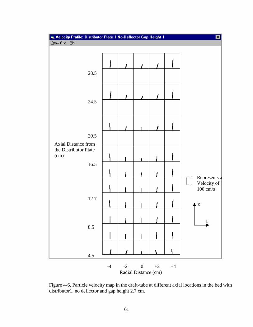
61
-4 -2 0 +2 +4 Radial Distance (cm)
28.5
24.5
20.5
16.5
12.7
8.5
4.5
Axial Distance fromthe Distributor Plate(cm)
Represents aVelocity of100 cm/s
Figure 4-6. Particle velocity map in the draft-tube at different axial locations in the bed withdistributor1, no deflector and gap height 2.7 cm.
z
r
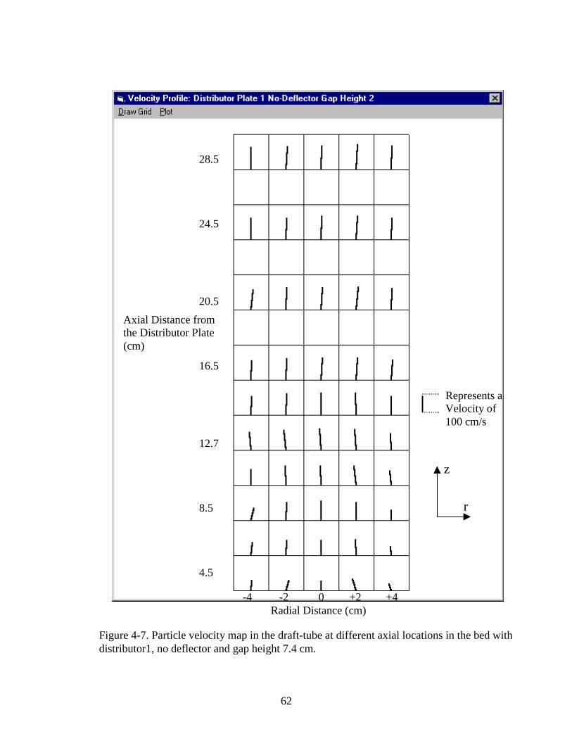
62
-4 -2 0 +2 +4 Radial Distance (cm)
28.5
24.5
20.5
16.5
12.7
8.5
4.5
Axial Distance fromthe Distributor Plate(cm)
Represents aVelocity of100 cm/s
Figure 4-7. Particle velocity map in the draft-tube at different axial locations in the bed withdistributor1, no deflector and gap height 7.4 cm.
z
r
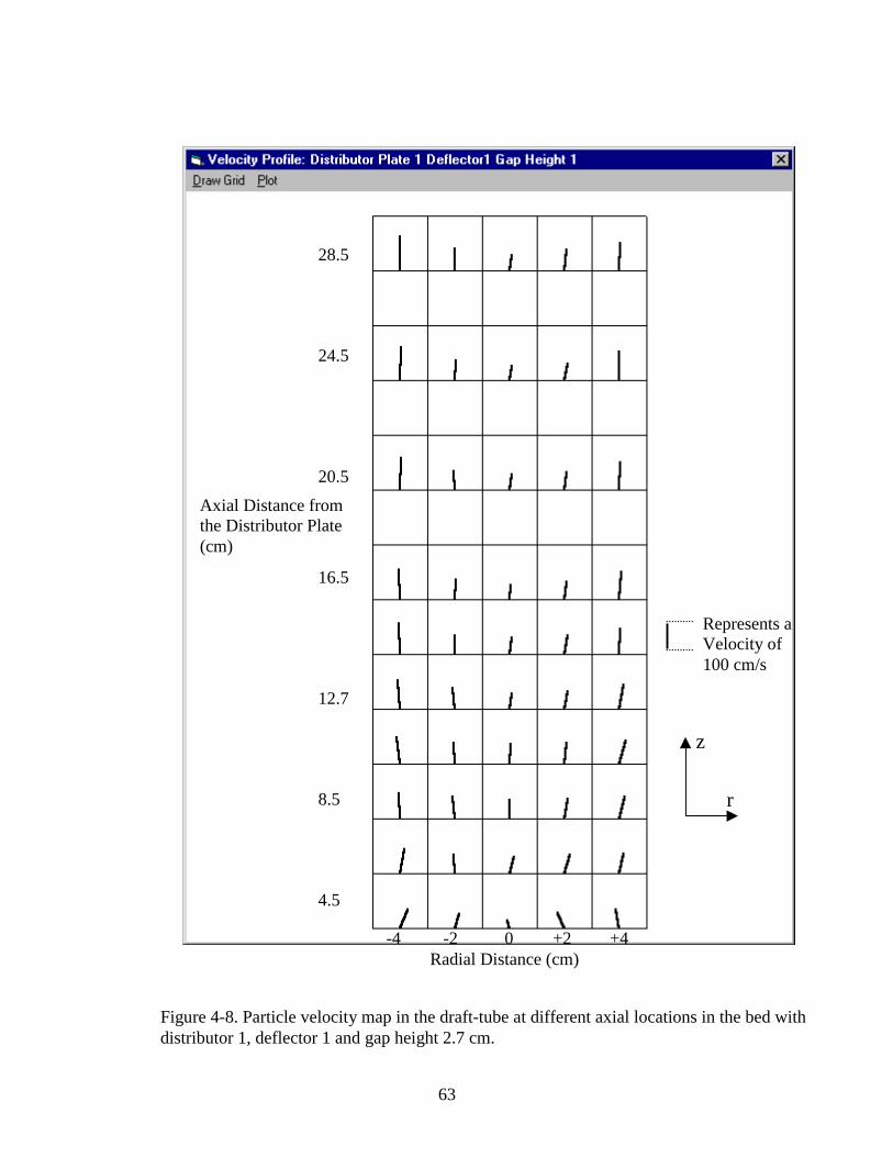
63
-4 -2 0 +2 +4 Radial Distance (cm)
28.5
24.5
20.5
16.5
12.7
8.5
4.5
Axial Distance fromthe Distributor Plate(cm)
Represents aVelocity of100 cm/s
Figure 4-8. Particle velocity map in the draft-tube at different axial locations in the bed withdistributor 1, deflector 1 and gap height 2.7 cm.
z
r
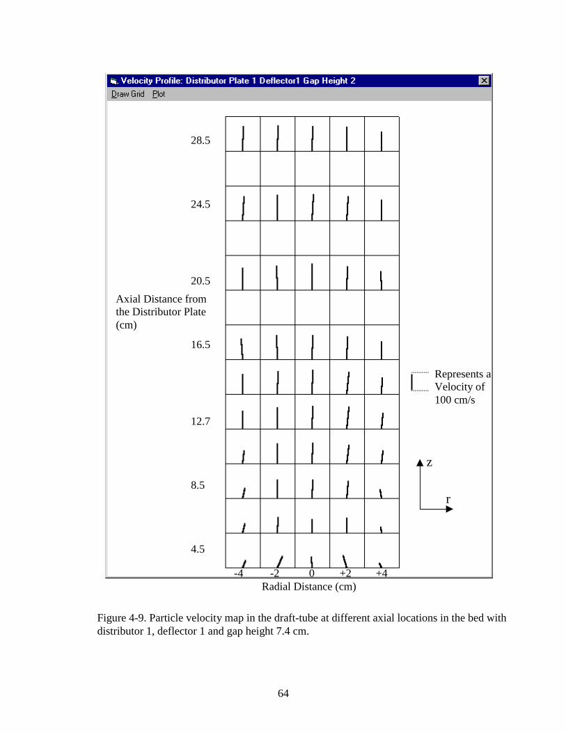
64
-4 -2 0 +2 +4 Radial Distance (cm)
28.5
24.5
20.5
16.5
12.7
8.5
4.5
Axial Distance fromthe Distributor Plate(cm)
Represents aVelocity of100 cm/s
Figure 4-9. Particle velocity map in the draft-tube at different axial locations in the bed withdistributor 1, deflector 1 and gap height 7.4 cm.
z
r
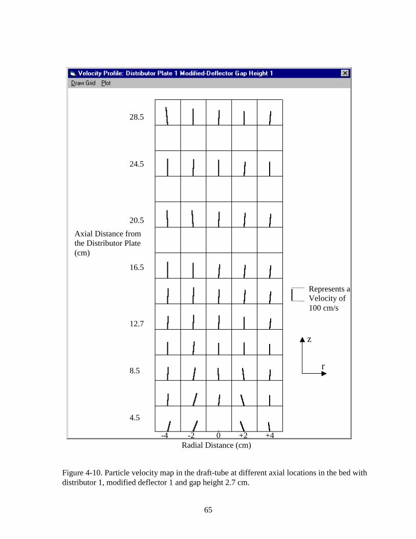
65
-4 -2 0 +2 +4 Radial Distance (cm)
28.5
24.5
20.5
16.5
12.7
8.5
4.5
Axial Distance fromthe Distributor Plate(cm)
Represents aVelocity of100 cm/s
Figure 4-10. Particle velocity map in the draft-tube at different axial locations in the bed withdistributor 1, modified deflector 1 and gap height 2.7 cm.
z
r
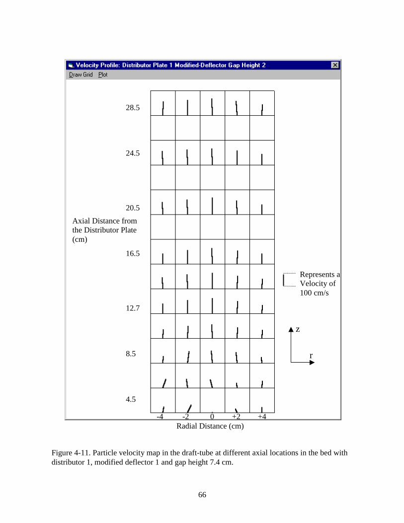
66
-4 -2 0 +2 +4 Radial Distance (cm)
28.5
24.5
20.5
16.5
12.7
8.5
4.5
Axial Distance fromthe Distributor Plate(cm)
Represents aVelocity of100 cm/s
Figure 4-11. Particle velocity map in the draft-tube at different axial locations in the bed withdistributor 1, modified deflector 1 and gap height 7.4 cm.
z
r
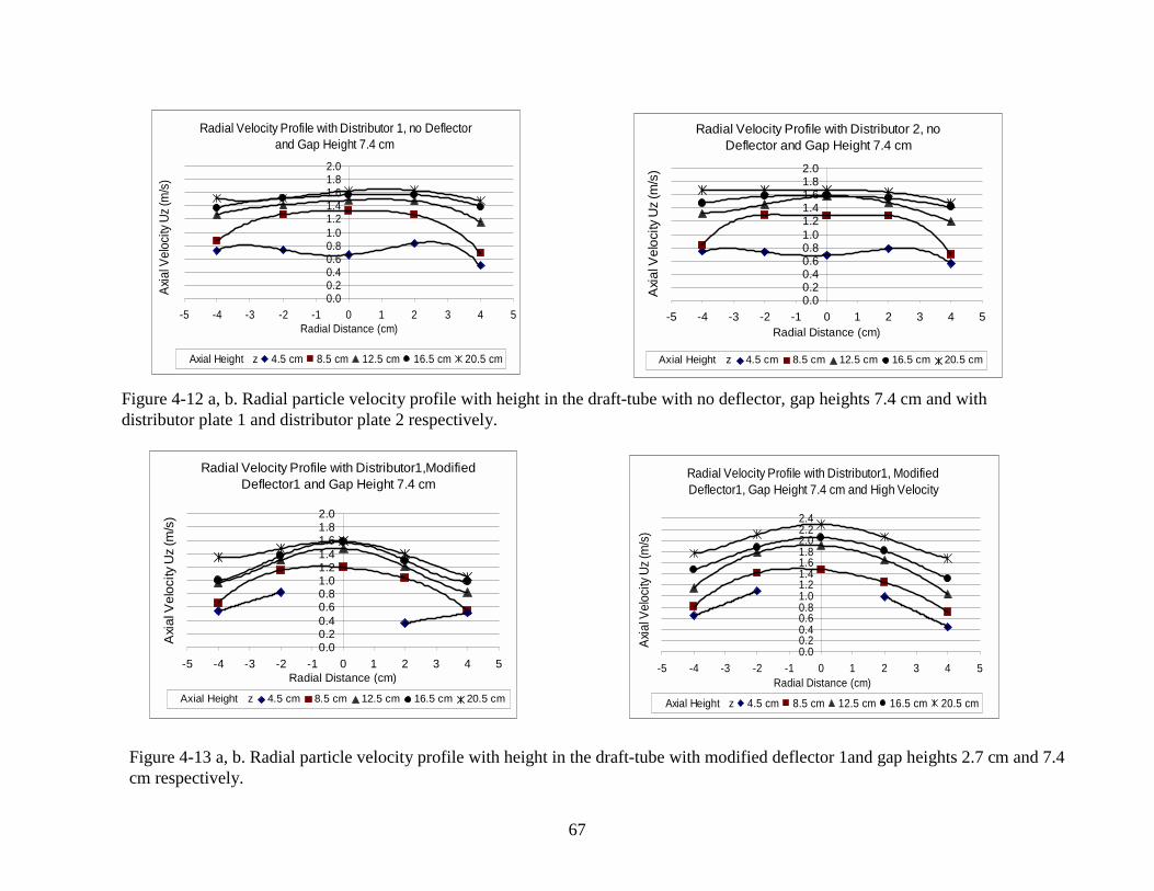
67
Figure 4-12 a, b. Radial particle velocity profile with height in the draft-tube with no deflector, gap heights 7.4 cm and withdistributor plate 1 and distributor plate 2 respectively.
Figure 4-13 a, b. Radial particle velocity profile with height in the draft-tube with modified deflector 1and gap heights 2.7 cm and 7.4cm respectively.
Radial Velocity Profile with Distributor 2, no Deflector and Gap Height 7.4 cm
0.00.20.40.60.81.01.21.41.61.82.0
-5 -4 -3 -2 -1 0 1 2 3 4 5Radial Distance (cm)
Axi
al V
elo
city
Uz
(m/s
)
Axial Height z 4.5 cm 8.5 cm 12.5 cm 16.5 cm 20.5 cm
Radial Velocity Profile with Distributor 1, no Deflector and Gap Height 7.4 cm
0.00.20.40.60.81.01.21.41.61.82.0
-5 -4 -3 -2 -1 0 1 2 3 4 5Radial Distance (cm)
Axi
al V
eloc
ity U
z (m
/s)
Axial Height z 4.5 cm 8.5 cm 12.5 cm 16.5 cm 20.5 cm
Radial Velocity Profile with Distributor1,Modified Deflector1 and Gap Height 7.4 cm
0.00.20.40.60.81.01.21.41.61.82.0
-5 -4 -3 -2 -1 0 1 2 3 4 5Radial Distance (cm)
Axi
al V
elo
city
Uz
(m/s
)
Axial Height z 4.5 cm 8.5 cm 12.5 cm 16.5 cm 20.5 cm
Radial Velocity Profile with Distributor1, Modified Deflector1, Gap Height 7.4 cm and High Velocity
0.00.20.40.60.81.01.21.41.61.82.02.22.4
-5 -4 -3 -2 -1 0 1 2 3 4 5Radial Distance (cm)
Axi
al V
eloc
ity U
z (m
/s)
Axial Height z 4.5 cm 8.5 cm 12.5 cm 16.5 cm 20.5 cm
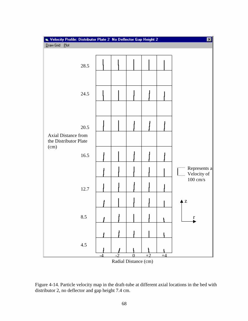
68
-4 -2 0 +2 +4 Radial Distance (cm)
28.5
24.5
20.5
16.5
12.7
8.5
4.5
Axial Distance fromthe Distributor Plate(cm)
Represents aVelocity of100 cm/s
Figure 4-14. Particle velocity map in the draft-tube at different axial locations in the bed withdistributor 2, no deflector and gap height 7.4 cm.
z
r
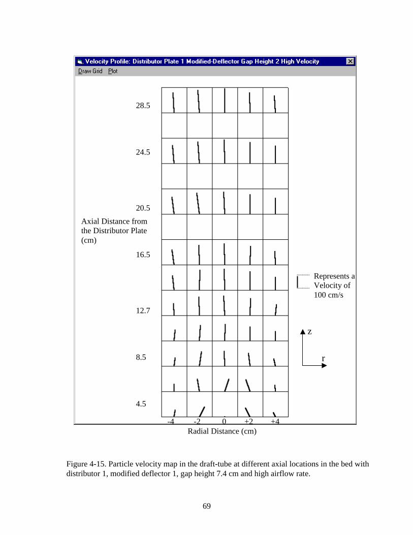
69
-4 -2 0 +2 +4 Radial Distance (cm)
28.5
24.5
20.5
16.5
12.7
8.5
4.5
Axial Distance fromthe Distributor Plate(cm)
Represents aVelocity of100 cm/s
Figure 4-15. Particle velocity map in the draft-tube at different axial locations in the bed withdistributor 1, modified deflector 1, gap height 7.4 cm and high airflow rate.
z
r
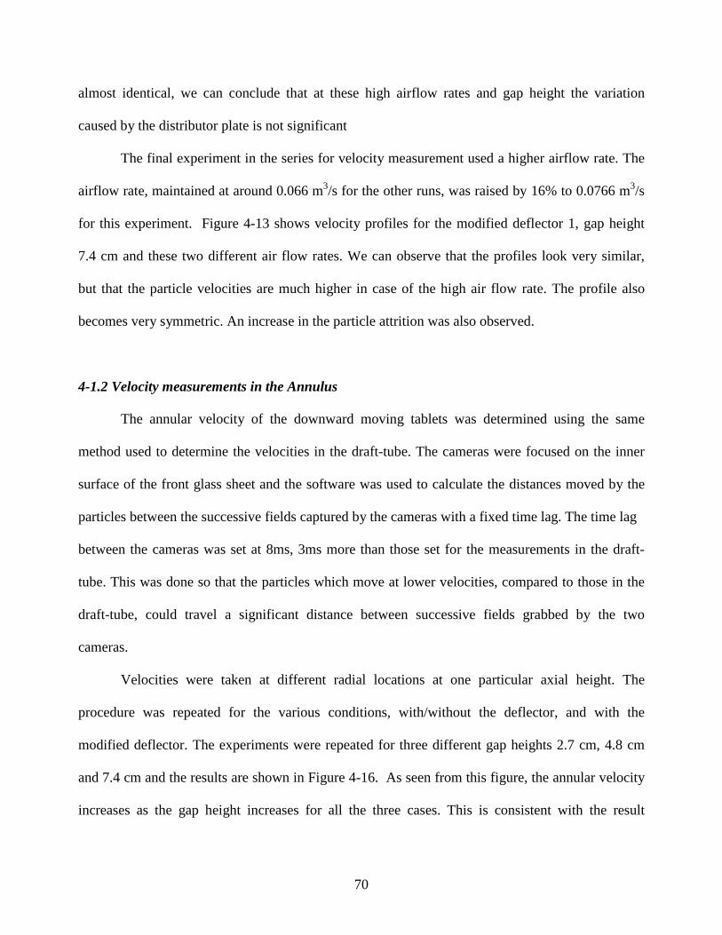
70
almost identical, we can conclude that at these high airflow rates and gap height the variation
caused by the distributor plate is not significant
The final experiment in the series for velocity measurement used a higher airflow rate. The
airflow rate, maintained at around 0.066 m3/s for the other runs, was raised by 16% to 0.0766 m3/s
for this experiment. Figure 4-13 shows velocity profiles for the modified deflector 1, gap height
7.4 cm and these two different air flow rates. We can observe that the profiles look very similar,
but that the particle velocities are much higher in case of the high air flow rate. The profile also
becomes very symmetric. An increase in the particle attrition was also observed.
4-1.2 Velocity measurements in the Annulus
The annular velocity of the downward moving tablets was determined using the same
method used to determine the velocities in the draft-tube. The cameras were focused on the inner
surface of the front glass sheet and the software was used to calculate the distances moved by the
particles between the successive fields captured by the cameras with a fixed time lag. The time lag
between the cameras was set at 8ms, 3ms more than those set for the measurements in the draft-
tube. This was done so that the particles which move at lower velocities, compared to those in the
draft-tube, could travel a significant distance between successive fields grabbed by the two
cameras.
Velocities were taken at different radial locations at one particular axial height. The
procedure was repeated for the various conditions, with/without the deflector, and with the
modified deflector. The experiments were repeated for three different gap heights 2.7 cm, 4.8 cm
and 7.4 cm and the results are shown in Figure 4-16. As seen from this figure, the annular velocity
increases as the gap height increases for all the three cases. This is consistent with the result
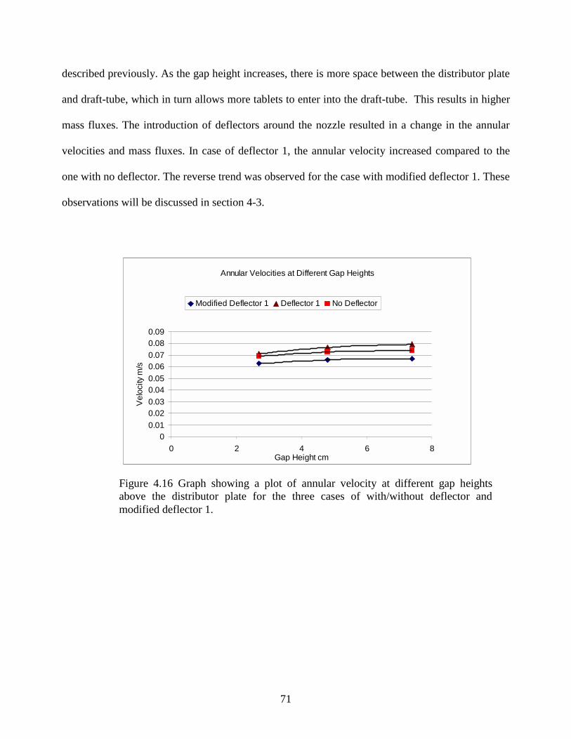
71
Annular Velocities at Different Gap Heights
00.01
0.020.03
0.040.05
0.060.07
0.080.09
0 2 4 6 8Gap Height cm
Ve
loci
ty m
/s
Modified Deflector 1 Deflector 1 No Deflector
described previously. As the gap height increases, there is more space between the distributor plate
and draft-tube, which in turn allows more tablets to enter into the draft-tube. This results in higher
mass fluxes. The introduction of deflectors around the nozzle resulted in a change in the annular
velocities and mass fluxes. In case of deflector 1, the annular velocity increased compared to the
one with no deflector. The reverse trend was observed for the case with modified deflector 1. These
observations will be discussed in section 4-3.
Figure 4.16 Graph showing a plot of annular velocity at different gap heightsabove the distributor plate for the three cases of with/without deflector andmodified deflector 1.
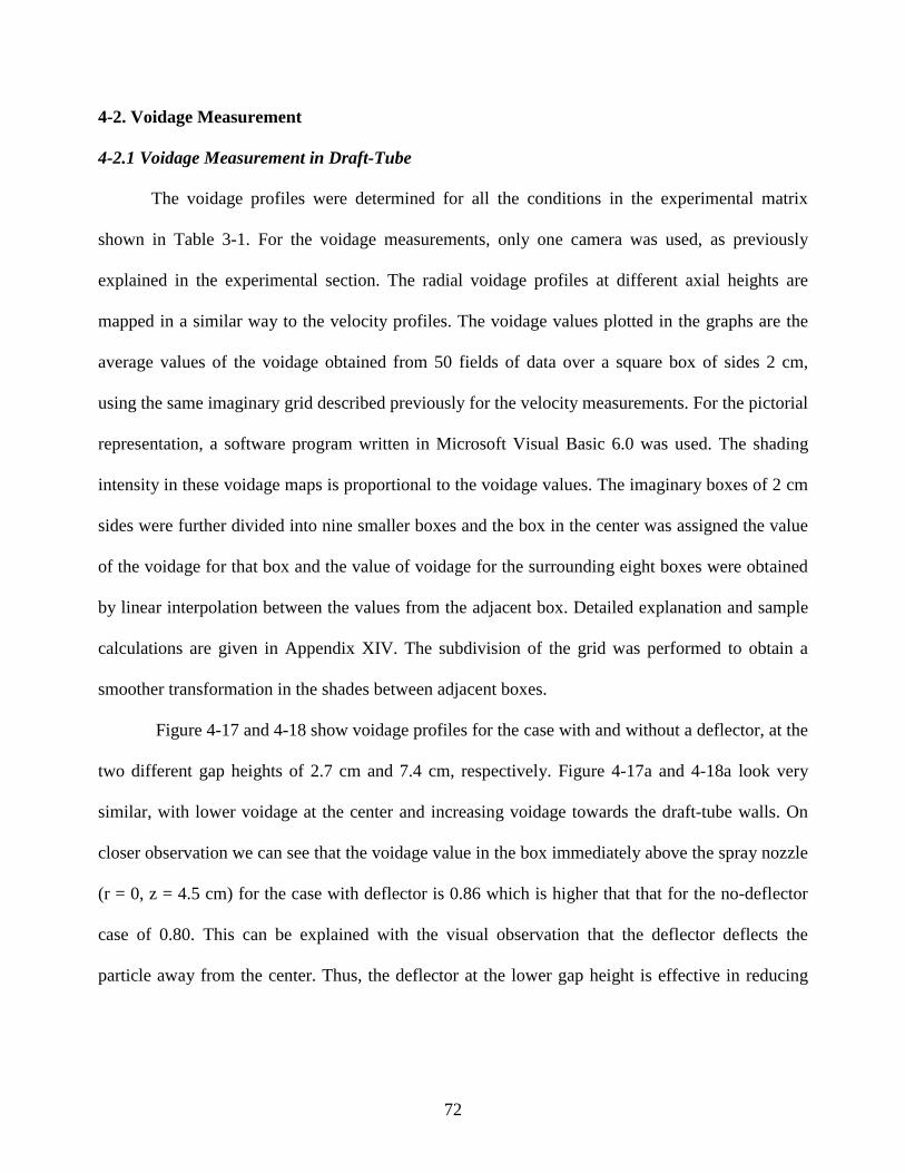
72
4-2. Voidage Measurement
4-2.1 Voidage Measurement in Draft-Tube
The voidage profiles were determined for all the conditions in the experimental matrix
shown in Table 3-1. For the voidage measurements, only one camera was used, as previously
explained in the experimental section. The radial voidage profiles at different axial heights are
mapped in a similar way to the velocity profiles. The voidage values plotted in the graphs are the
average values of the voidage obtained from 50 fields of data over a square box of sides 2 cm,
using the same imaginary grid described previously for the velocity measurements. For the pictorial
representation, a software program written in Microsoft Visual Basic 6.0 was used. The shading
intensity in these voidage maps is proportional to the voidage values. The imaginary boxes of 2 cm
sides were further divided into nine smaller boxes and the box in the center was assigned the value
of the voidage for that box and the value of voidage for the surrounding eight boxes were obtained
by linear interpolation between the values from the adjacent box. Detailed explanation and sample
calculations are given in Appendix XIV. The subdivision of the grid was performed to obtain a
smoother transformation in the shades between adjacent boxes.
Figure 4-17 and 4-18 show voidage profiles for the case with and without a deflector, at the
two different gap heights of 2.7 cm and 7.4 cm, respectively. Figure 4-17a and 4-18a look very
similar, with lower voidage at the center and increasing voidage towards the draft-tube walls. On
closer observation we can see that the voidage value in the box immediately above the spray nozzle
(r = 0, z = 4.5 cm) for the case with deflector is 0.86 which is higher that that for the no-deflector
case of 0.80. This can be explained with the visual observation that the deflector deflects the
particle away from the center. Thus, the deflector at the lower gap height is effective in reducing
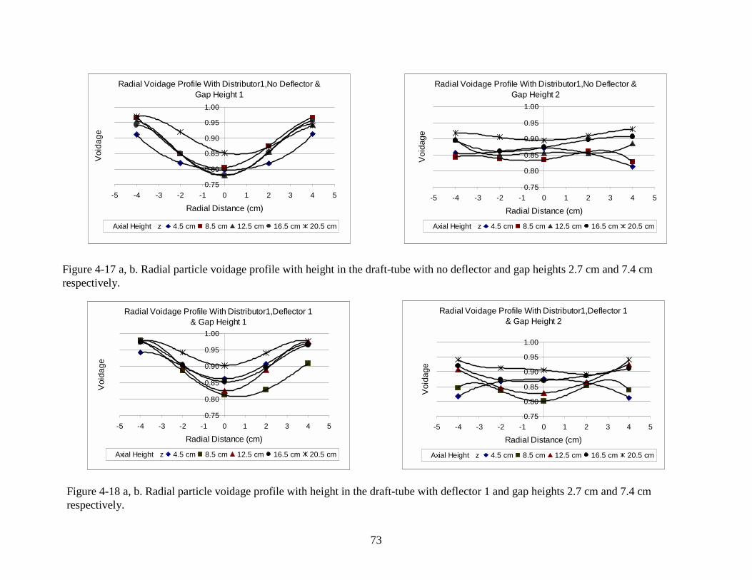
73
Figure 4-17 a, b. Radial particle voidage profile with height in the draft-tube with no deflector and gap heights 2.7 cm and 7.4 cmrespectively.
Figure 4-18 a, b. Radial particle voidage profile with height in the draft-tube with deflector 1 and gap heights 2.7 cm and 7.4 cmrespectively.
Radial Voidage Profile With Distributor1,No Deflector & Gap Height 1
0.75
0.80
0.85
0.90
0.95
1.00
-5 -4 -3 -2 -1 0 1 2 3 4 5
Radial Distance (cm)
Void
ag
e
Axial Height z 4.5 cm 8.5 cm 12.5 cm 16.5 cm 20.5 cm
Radial Voidage Profile With Distributor1,No Deflector & Gap Height 2
0.75
0.80
0.85
0.90
0.95
1.00
-5 -4 -3 -2 -1 0 1 2 3 4 5
Radial Distance (cm)
Void
ag
e
Axial Height z 4.5 cm 8.5 cm 12.5 cm 16.5 cm 20.5 cm
Radial Voidage Profile With Distributor1,Deflector 1 & Gap Height 1
0.75
0.80
0.85
0.90
0.95
1.00
-5 -4 -3 -2 -1 0 1 2 3 4 5
Radial Distance (cm)
Void
age
Axial Height z 4.5 cm 8.5 cm 12.5 cm 16.5 cm 20.5 cm
Radial Voidage Profile With Distributor1,Deflector 1 & Gap Height 2
0.75
0.80
0.85
0.90
0.95
1.00
-5 -4 -3 -2 -1 0 1 2 3 4 5
Radial Distance (cm)
Void
age
Axial Height z 4.5 cm 8.5 cm 12.5 cm 16.5 cm 20.5 cm
74
the particle density around the nozzle. The voidage across the bed is also marginally
higher for the case with the deflector in comparison with the no-deflector case.
For the case of the higher gap height (7.4 cm), Figures 4-17b and 4-18b, the
voidage profiles still look similar. However, the voidage across the draft-tube varies over
a wide range in the presence of deflector 1 (0.8 to 0.91) whereas the profile is flat with
very little variation (0.85 to 0.91) in case of no-deflector. It is very interesting to note that
the voidage profile at z = 4.5 is almost the same for both these cases. This can explain the
similar coating consistency obtained in the above cases detailed in section 4-5. Thus, at
the higher gap height deflector 1 is not effective, as it does not increase the voidage
significantly around the nozzle and thus does not reduce the sheltering effect in the spray
zone.
At the lower gap height, the voidage values at different axial heights are less than
the corresponding voidage values for higher gap height for the case with no deflector.
This is in contrast to what we might expect. At the lower gap height, the number of
particles entering the draft-tube region is low because of the low clearance between the
distributor plate and the draft-tube. We might expect this to cause a higher voidage or
fewer particles in the draft-tube region. The possible reason for this behavior can be
explained as follows. With the lower gap height, the particles face higher resistance to
enter the draft-tube region resulting in a very low entry velocity at the bottom of the bed.
The air stream in the draft-tube then accelerates the particles, but the acceleration
achieved is low resulting in a build-up in the draft-tube and hence higher particle density
in the draft-tube. These observations can be confirmed with the velocity profiles, which
show that the velocities in case of the lower gap height and no deflector are almost half
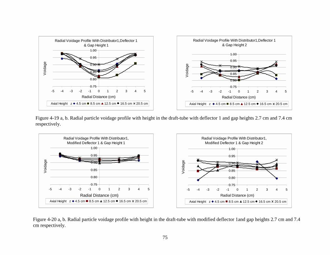
75
Figure 4-20 a, b. Radial particle voidage profile with height in the draft-tube with modified deflector 1and gap heights 2.7 cm and 7.4cm respectively.
Figure 4-19 a, b. Radial particle voidage profile with height in the draft-tube with deflector 1 and gap heights 2.7 cm and 7.4 cmrespectively.
Radial Voidage Profile With Distributor1,Deflector 1 & Gap Height 1
0.75
0.80
0.85
0.90
0.95
1.00
-5 -4 -3 -2 -1 0 1 2 3 4 5
Radial Distance (cm)
Void
age
Axial Height z 4.5 cm 8.5 cm 12.5 cm 16.5 cm 20.5 cm
Radial Voidage Profile With Distributor1,Deflector 1 & Gap Height 2
0.75
0.80
0.85
0.90
0.95
1.00
-5 -4 -3 -2 -1 0 1 2 3 4 5
Radial Distance (cm)
Void
age
Axial Height z 4.5 cm 8.5 cm 12.5 cm 16.5 cm 20.5 cm
Radial Voidage Profile With Distributor1, Modified Deflector 1 & Gap Height 1
0.75
0.80
0.85
0.90
0.95
1.00
-5 -4 -3 -2 -1 0 1 2 3 4 5
Radial Distance (cm)
Void
age
Axial Height z 4.5 cm 8.5 cm 12.5 cm 16.5 cm 20.5 cm
Radial Voidage Profile With Distributor1, Modified Deflector 1 & Gap Height 2
0.75
0.80
0.85
0.90
0.95
1.00
-5 -4 -3 -2 -1 0 1 2 3 4 5
Radial Distance (cm)
Void
age
Axial Height z 4.5 cm 8.5 cm 12.5 cm 16.5 cm 20.5 cm
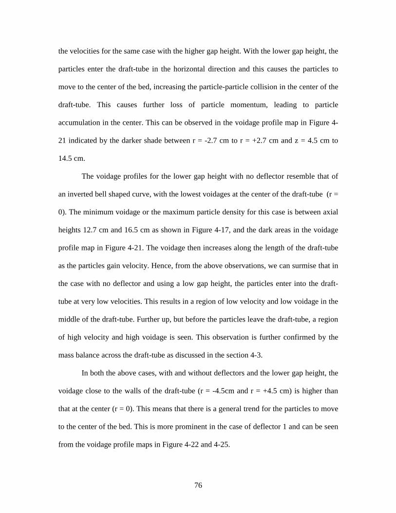
76
the velocities for the same case with the higher gap height. With the lower gap height, the
particles enter the draft-tube in the horizontal direction and this causes the particles to
move to the center of the bed, increasing the particle-particle collision in the center of the
draft-tube. This causes further loss of particle momentum, leading to particle
accumulation in the center. This can be observed in the voidage profile map in Figure 4-
21 indicated by the darker shade between r = -2.7 cm to r = +2.7 cm and z = 4.5 cm to
14.5 cm.
The voidage profiles for the lower gap height with no deflector resemble that of
an inverted bell shaped curve, with the lowest voidages at the center of the draft-tube (r =
0). The minimum voidage or the maximum particle density for this case is between axial
heights 12.7 cm and 16.5 cm as shown in Figure 4-17, and the dark areas in the voidage
profile map in Figure 4-21. The voidage then increases along the length of the draft-tube
as the particles gain velocity. Hence, from the above observations, we can surmise that in
the case with no deflector and using a low gap height, the particles enter into the draft-
tube at very low velocities. This results in a region of low velocity and low voidage in the
middle of the draft-tube. Further up, but before the particles leave the draft-tube, a region
of high velocity and high voidage is seen. This observation is further confirmed by the
mass balance across the draft-tube as discussed in the section 4-3.
In both the above cases, with and without deflectors and the lower gap height, the
voidage close to the walls of the draft-tube (r = -4.5cm and r = +4.5 cm) is higher than
that at the center (r = 0). This means that there is a general trend for the particles to move
to the center of the bed. This is more prominent in the case of deflector 1 and can be seen
from the voidage profile maps in Figure 4-22 and 4-25.
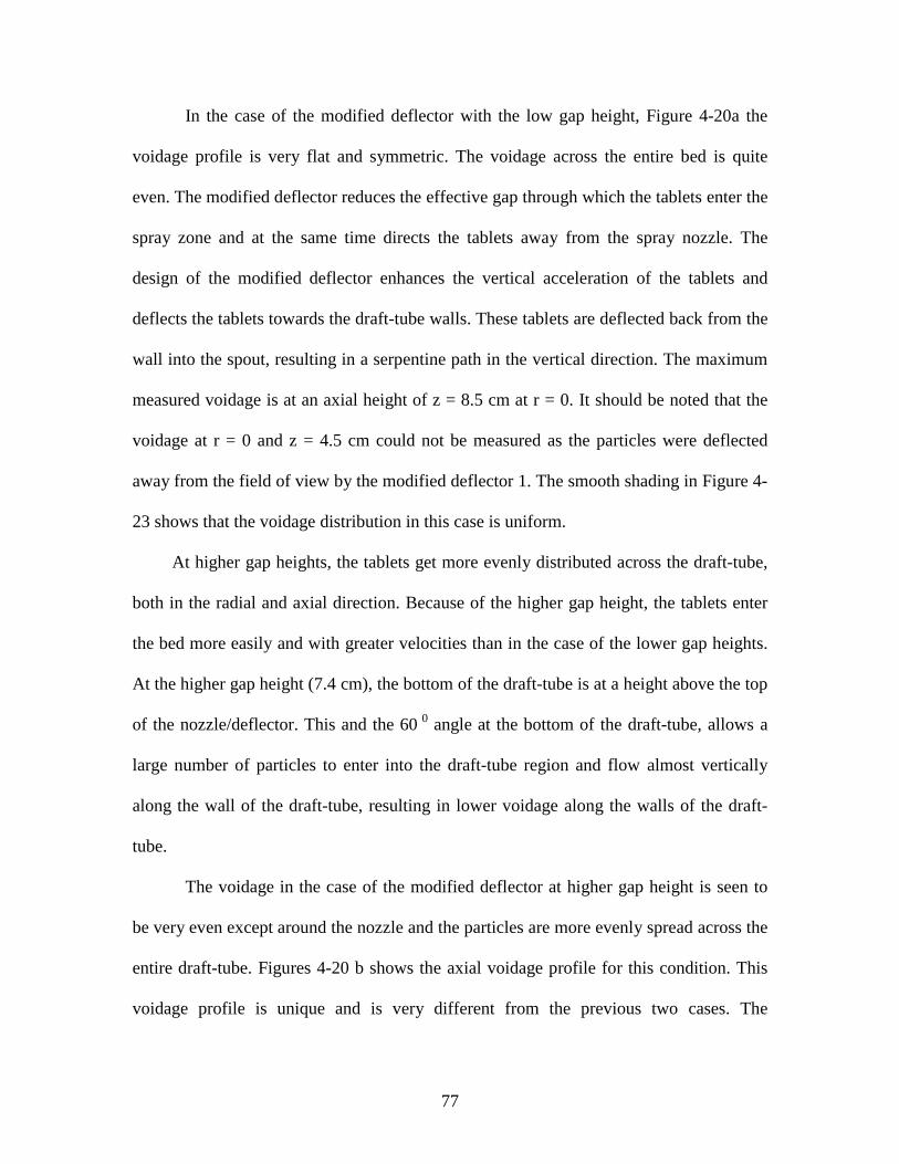
77
In the case of the modified deflector with the low gap height, Figure 4-20a the
voidage profile is very flat and symmetric. The voidage across the entire bed is quite
even. The modified deflector reduces the effective gap through which the tablets enter the
spray zone and at the same time directs the tablets away from the spray nozzle. The
design of the modified deflector enhances the vertical acceleration of the tablets and
deflects the tablets towards the draft-tube walls. These tablets are deflected back from the
wall into the spout, resulting in a serpentine path in the vertical direction. The maximum
measured voidage is at an axial height of z = 8.5 cm at r = 0. It should be noted that the
voidage at r = 0 and z = 4.5 cm could not be measured as the particles were deflected
away from the field of view by the modified deflector 1. The smooth shading in Figure 4-
23 shows that the voidage distribution in this case is uniform.
At higher gap heights, the tablets get more evenly distributed across the draft-tube,
both in the radial and axial direction. Because of the higher gap height, the tablets enter
the bed more easily and with greater velocities than in the case of the lower gap heights.
At the higher gap height (7.4 cm), the bottom of the draft-tube is at a height above the top
of the nozzle/deflector. This and the 60 0 angle at the bottom of the draft-tube, allows a
large number of particles to enter into the draft-tube region and flow almost vertically
along the wall of the draft-tube, resulting in lower voidage along the walls of the draft-
tube.
The voidage in the case of the modified deflector at higher gap height is seen to
be very even except around the nozzle and the particles are more evenly spread across the
entire draft-tube. Figures 4-20 b shows the axial voidage profile for this condition. This
voidage profile is unique and is very different from the previous two cases. The
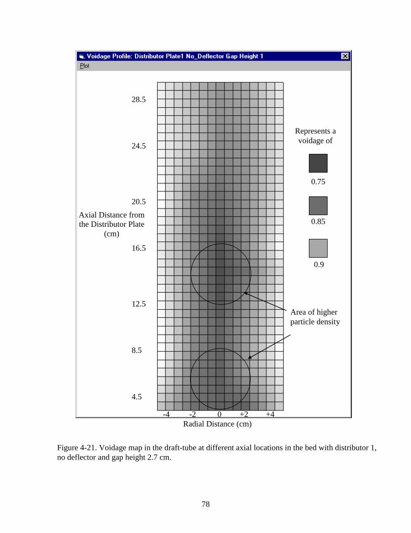
78
Figure 4-21. Voidage map in the draft-tube at different axial locations in the bed with distributor 1,no deflector and gap height 2.7 cm.
-4 -2 0 +2 +4 Radial Distance (cm)
28.5
24.5
20.5
16.5
12.5
8.5
4.5
Axial Distance fromthe Distributor Plate
(cm)
Area of higherparticle density
Represents avoidage of
0.75
0.85
0.9

79
Figure 4-22. Voidage map in the draft-tube at different axial locations in the bed with distributor 1,deflector 1 and gap height 2.7 cm.
-4 -2 0 +2 +4 Radial Distances (cm)
28.5
24.5
20.5
16.5
12.5
8.5
4.5
Axial Distance fromthe Distributor Plate
(cm)
Area of higherparticle density
Represents avoidage of
0.75
0.85
0.9
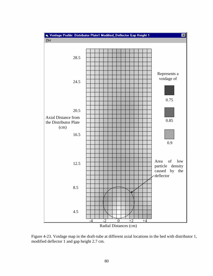
80
Figure 4-23. Voidage map in the draft-tube at different axial locations in the bed with distributor 1,modified deflector 1 and gap height 2.7 cm.
-4 -2 0 +2 +4 Radial Distances (cm)
28.5
24.5
20.5
16.5
12.5
8.5
4.5
Axial Distance fromthe Distributor Plate
(cm)
Area of lowparticle densitycaused by thedeflector
Represents avoidage of
0.75
0.85
0.9
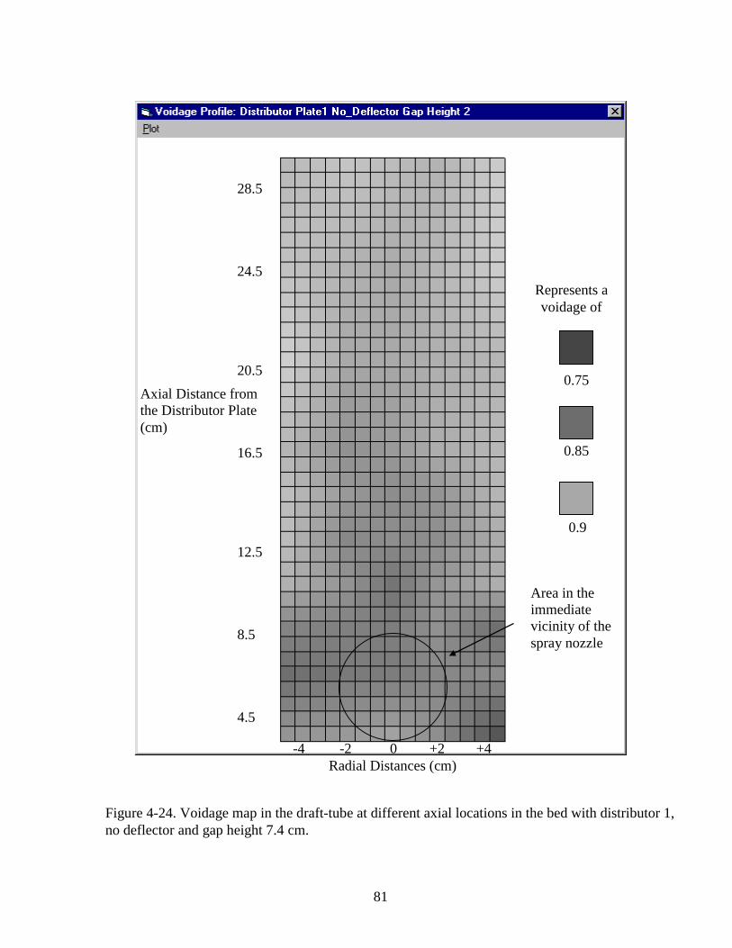
81
Figure 4-24. Voidage map in the draft-tube at different axial locations in the bed with distributor 1,no deflector and gap height 7.4 cm.
-4 -2 0 +2 +4 Radial Distances (cm)
28.5
24.5
20.5
16.5
12.5
8.5
4.5
Axial Distance fromthe Distributor Plate(cm)
Area in theimmediatevicinity of thespray nozzle
Represents avoidage of
0.75
0.85
0.9
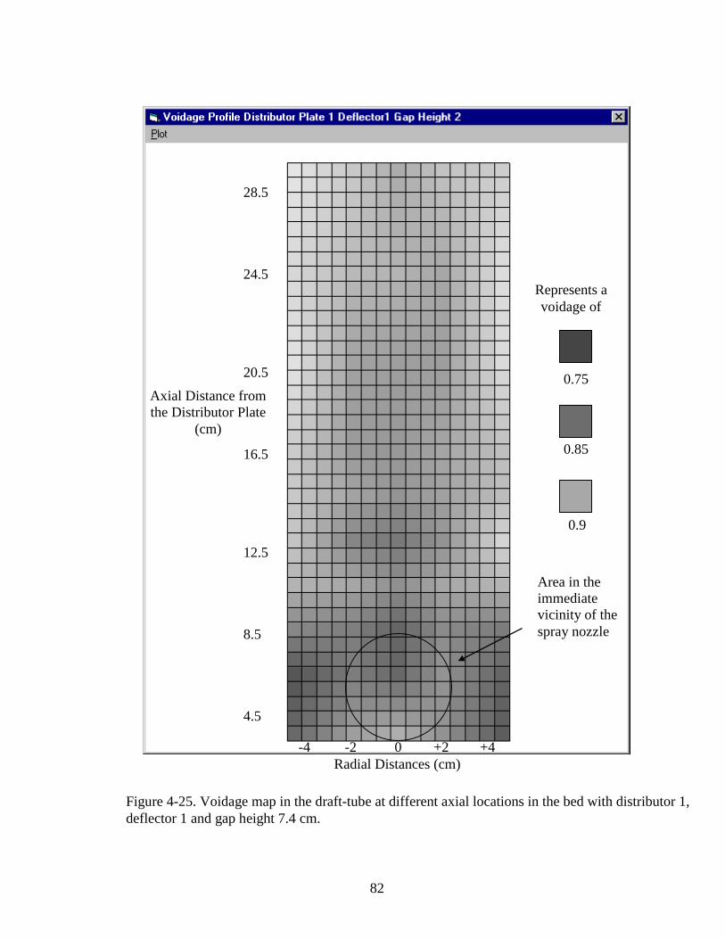
82
Figure 4-25. Voidage map in the draft-tube at different axial locations in the bed with distributor 1,deflector 1 and gap height 7.4 cm.
-4 -2 0 +2 +4 Radial Distances (cm)
28.5
24.5
20.5
16.5
12.5
8.5
4.5
Axial Distance fromthe Distributor Plate
(cm)
Area in theimmediatevicinity of thespray nozzle
Represents avoidage of
0.75
0.85
0.9
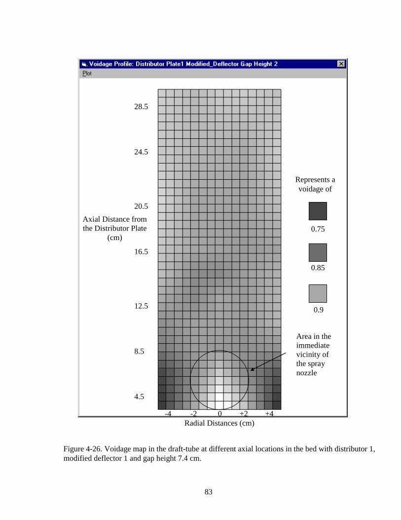
83
Figure 4-26. Voidage map in the draft-tube at different axial locations in the bed with distributor 1,modified deflector 1 and gap height 7.4 cm.
-4 -2 0 +2 +4 Radial Distances (cm)
28.5
24.5
20.5
16.5
12.5
8.5
4.5
Axial Distance fromthe Distributor Plate
(cm)
Area in theimmediatevicinity ofthe spraynozzle
Represents avoidage of
0.75
0.85
0.9
84
voidage values are very low at the points where the particles enter the draft-tube (r = -4.0
cm and r = +4.0 cm at z = 4.5 cm) and increase drastically at (r = -2.0 cm and r = +2.0 cm
at z = 4.5 ). The inclusion of a ring to the deflector 1 (the modified deflector 1), further
reduces the gap available for particle entry into the draft-tube. This causes the particles to
enter the bed along the wall of the draft-tube. The particles that enter the bed closer to the
deflector are deflected away towards the wall of the draft-tube resulting in very high
voidage around nozzle area. The modified deflector 1 thus served its purpose of
increasing the voidage around the nozzle and giving a very even voidage distribution
across the draft-tube, though the inclusion of the modified deflector resulted in reduced
mass-flux (reduces particle flow into the draft-tube). However, this difference is small
(15.6% less than no deflector). There was no observed increase in the attrition of the
tablets with the use of modified deflector 1.
4 -2.2 Voidage measurement in the annulus
The voidage in the annulus was assumed to be that of a loosely packed bed. The voidage
� was calculated to be 0.576 from the measured bulk and absolute density. Since there was no
separate air supply to the annulus, and the bed was never fluidized, the assumption of packed
bed conditions is acceptable. See Appendix II for calculation of bulk and absolute density and
voidage calculations in the annulus from these values.
4 -3 Mass balance between solid mass flow rate in the spout and annulus
A mass balance can be made between the mass-flux in the draft-tube and the mass-flux
in the downward moving annulus. This serves two purposes: (1) it validates the velocity and

85
voidage measurements in the draft-tube, and (2) it acts as a crosscheck for the observed
apparent depth of field (ADOF) which is calculated by using the models explained in the
experimental section.
Based on the law of conservation of mass, at steady state conditions, the upward solids
mass flow at a given cross-section in the spout must equal the downward solids mass flow in
the annulus. Figure 4-27 shows the mass-flux plots in the draft-tube and in the annulus, for the
eight different sets of conditions shown in the experimental matrix in Table 3-1. The results
show that there is agreement between the solid mass flow rate in the draft-tube and annulus.
The solids mass flow rate in the draft-tube and the annulus were calculated using numerical
integration of Equations (4-1) and (4-2) respectively, See Appendix XV for details of the
calculation.
Draft-tube
Annulus
where mdft and manul are the solids mass flow in the draft-tube and annulus, udft and uanul are the
axial particle velocity in the spout and annulus, εdft and εanul are the voidage in the draft-tube
and annulus, and rdi is the radius of the draft-tube to its inner wall, rdo is the radius of the draft-
tube plus draft-tube wall thickness, and R the column radius, respectively. The annular
velocities measured were those of the particles in contact with the front glass sheet. However,
rdrdft
r
zdftuz
dftm
id
p )1(0
,2)( ερπ −∫=
rdranul
R
rzanul
uzanul
m
od
p )1(,2
)( ερπ −∫=
(4-1)
(4-2)
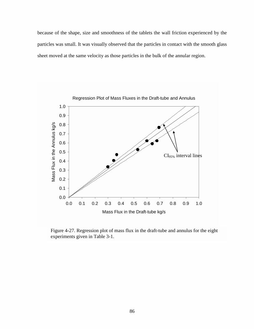
86
Figure 4-27. Regression plot of mass flux in the draft-tube and annulus for the eightexperiments given in Table 3-1.
because of the shape, size and smoothness of the tablets the wall friction experienced by the
particles was small. It was visually observed that the particles in contact with the smooth glass
sheet moved at the same velocity as those particles in the bulk of the annular region.
Regression Plot of Mass Fluxes in the Draft-tube and Annulus
Mass Flux in the Draft-tube kg/s
0.0 0.1 0.2 0.3 0.4 0.5 0.6 0.7 0.8 0.9 1.0
Mass
Flu
x in
the A
nnulu
s kg
/s
0.0
0.1
0.2
0.3
0.4
0.5
0.6
0.7
0.8
0.9
1.0
CI95% interval lines
87
4-4.Sheltering effect and Coating Variation
The total variation in the amount of coating received by a particle in a fluidized bed
coating equipment can be explained or accounted for by two factors: (1) variation in
cycle time distribution, and (2) variation in coating received by a particle each time it
passes through the spray zone, Cheng and Turton (1993). Cheng (1993) in her
dissertation talks extensively about these two factors. She used a phenomenological
model to explain the experimental results that she obtained. But the phenomenological
model assumed that: (1) the spray pattern was in the form of a hollow cone, (2) all the
spray is not coated on the tablets, (3) the spray not captured by the particles is carried
upwards by the fluidizing gas, (4) the spray droplets are assumed to follow straight
radially directed stream tubes, and (5) most importantly that the particles are distributed
uniformly throughout the spray zone with uniform voidage and move vertically upward
with a constant velocity.
Figures 4-28 and 4-29 explains the basic process involved in coating and the
sheltering effect explained by Cheng. Figure 4-28 explains the continuous renewal
theory. The total amount of coating a particle receives at the end of the coating run is an
integral amount of the coating the particle receives during each pass through the spray
zone. Sheltering effect is explained by Figure 4-29. Particles closer to the spray nozzle
receive more coating, and block the spray from reaching the tablets that are away from
the nozzle, resulting in those particles getting less coating. The particles closer to the
nozzle shelter the particles that are away from the spray nozzle. Mann (1972) derived an
expression for the variation in the coating process in terms of the variation in the amount
of coating received per pass and the variation in the number of times the tablet passes
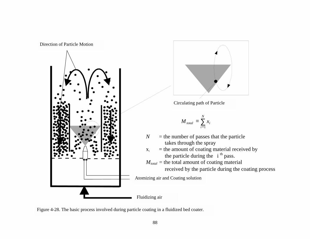
88
∑=
=N
iitotal xM
1
N = the number of passes that the particletakes through the spray
xi = the amount of coating material received bythe particle during the i th pass.
Mtotal = the total amount of coating materialreceived by the particle during the coating process
Atomizing air and Coating solution
Fluidizing air
Circulating path of Particle
Direction of Particle Motion
Figure 4-28. The basic process involved during particle coating in a fluidized bed coater.
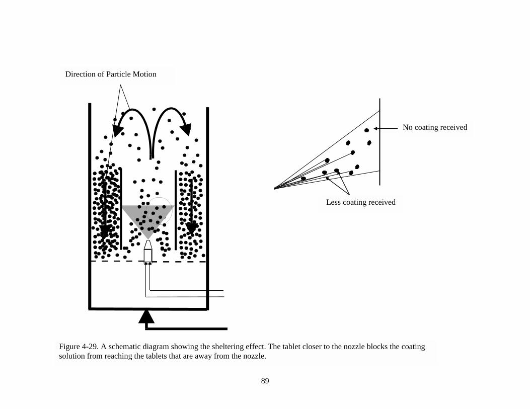
89
No coating received
Less coating received
Direction of Particle Motion
Figure 4-29. A schematic diagram showing the sheltering effect. The tablet closer to the nozzle blocks the coatingsolution from reaching the tablets that are away from the nozzle.
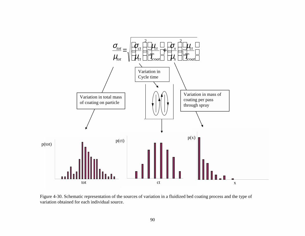
90
+
=
coat
ct
x
x
coat
ct
ct
ct
tot
tot
TT
µµσµ
µσ
µσ
22
Variation in total massof coating on particle
Variation in mass ofcoating per passthrough spray
Variation inCycle time
p(tot)
tot
p(ct)
ct
p(x)
x
Figure 4-30. Schematic representation of the sources of variation in a fluidized bed coating process and the type ofvariation obtained for each individual source.
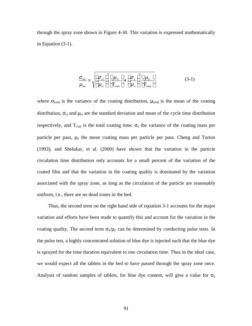
91
through the spray zone shown in Figure 4-30. This variation is expressed mathematically
in Equation (3-1).
where σtotal is the variance of the coating distribution, µtotal is the mean of the coating
distribution, σct and µct are the standard deviation and mean of the cycle time distribution
respectively, and Tcoat is the total coating time. σx the variance of the coating mass per
particle per pass, µx the mean coating mass per particle per pass. Cheng and Turton
(1993), and Shelukar, et al. (2000) have shown that the variation in the particle
circulation time distribution only accounts for a small percent of the variation of the
coated film and that the variation in the coating quality is dominated by the variation
associated with the spray zone, as long as the circulation of the particle are reasonably
uniform, i.e., there are no dead zones in the bed.
Thus, the second term on the right hand side of equation 3-1 accounts for the major
variation and efforts have been made to quantify this and account for the variation in the
coating quality. The second term σx/µx can be determined by conducting pulse tests. In
the pulse test, a highly concentrated solution of blue dye is injected such that the blue dye
is sprayed for the time duration equivalent to one circulation time. Thus in the ideal case,
we would expect all the tablets in the bed to have passed through the spray zone once.
Analysis of random samples of tablets, for blue dye content, will give a value for σx
(3-1)
+
=
coat
ct
x
x
coat
ct
ct
ct
tot
tot
TT
µµσµ
µσ
µσ
22
92
(standard deviation of amount of blue dye coated) and µx (mean amount of blue dye
coated).
4.5 Results of the Coating Experimental runs
As a review, the coating runs can be divided into two categories: (1) the continuous
coating runs, and (2) the pulse tests. The continuous coating runs were carried out to
determine the total variation in a batch of coated tablets for a given set of experimental
conditions. The pulse test were to help determine the variation in coating per-pass and
thus verify if this variation accounts for > 70 % of the total variation as observed by
earlier researchers. These two sources of variation and the combined variance are shown
schematically in Figure 4-30. The continuous coating runs were also used to determine
the effectiveness of the various deflectors on the overall coating quality, by reducing the
sheltering effect. From the velocity and voidage profiles obtained from the eight different
experimental conditions, three conditions were selected for the continuous coating runs:
(1) no deflector, (2) deflector 1, and (3) modified deflector 1. Based on the results
obtained, three more deflector designs were tried, modified deflector 2, modified
deflector 3, and optimum deflector. The experimental matrix for the coating runs is
described in Table 3-2.
4-5.1 Continuous coating runs
For all the continuous coating runs, the process variables such as, fluidizing air
velocity and temperature, liquid flow rate and viscosity, gap height, air pressure for
atomizing the liquid spray, were held constant. The only variation was the use of different
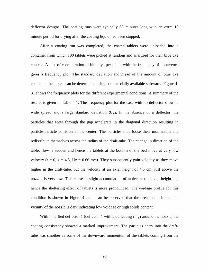
93
deflector designs. The coating runs were typically 60 minutes long with an extra 10
minute period for drying after the coating liquid had been stopped.
After a coating run was completed, the coated tablets were unloaded into a
container from which 100 tablets were picked at random and analyzed for their blue dye
content. A plot of concentration of blue dye per tablet with the frequency of occurrence
gives a frequency plot. The standard deviation and mean of the amount of blue dye
coated on the tablets can be determined using commercially available software. Figure 4-
31 shows the frequency plots for the different experimental conditions. A summary of the
results is given in Table 4-1. The frequency plot for the case with no deflector shows a
wide spread and a large standard deviation σtotal. In the absence of a deflector, the
particles that enter through the gap accelerate in the diagonal direction resulting in
particle-particle collision at the center. The particles thus loose their momentum and
redistribute themselves across the radius of the draft-tube. The change in direction of the
tablet flow is sudden and hence the tablets at the bottom of the bed move at very low
velocity (r = 0, z = 4.5, Uz = 0.66 m/s). They subsequently gain velocity as they move
higher in the draft-tube, but the velocity at an axial height of 4.5 cm, just above the
nozzle, is very low. This causes a slight accumulation of tablets at this axial height and
hence the sheltering effect of tablets is more pronounced. The voidage profile for this
condition is shown in Figure 4-24, it can be observed that the area in the immediate
vicinity of the nozzle is dark indicating low voidage or high solids content.
With modified deflector 1 (deflector 1 with a deflecting ring) around the nozzle, the
coating consistency showed a marked improvement. The particles entry into the draft-
tube was smother as some of the downward momentum of the tablets coming from the
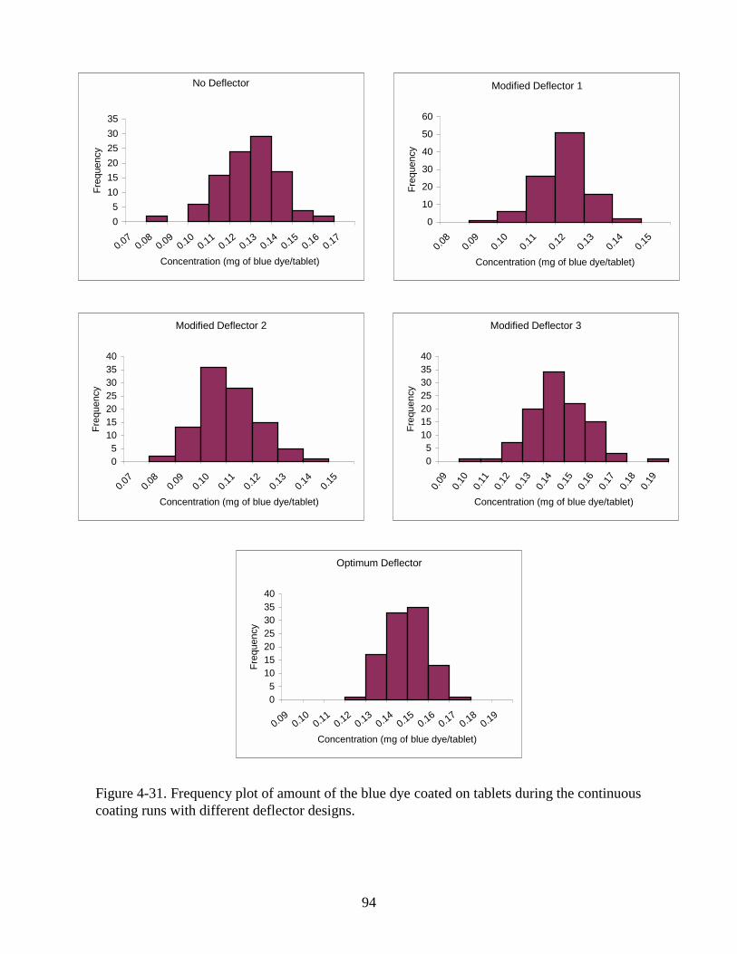
94
Figure 4-31. Frequency plot of amount of the blue dye coated on tablets during the continuouscoating runs with different deflector designs.
No Deflector
0
5
10
15
20
25
30
35
0.070.08
0.090.10
0.110.12
0.130.14
0.150.16
0.17
Concentration (mg of blue dye/tablet)
Fre
quency
Modified Deflector 1
0
10
20
30
40
50
60
0.08
0.09
0.10
0.11
0.12
0.13
0.14
0.15
Concentration (mg of blue dye/tablet)
Fre
quency
Modified Deflector 2
05
10152025303540
0.07
0.08
0.09
0.10
0.11
0.12
0.13
0.14
0.15
Concentration (mg of blue dye/tablet)
Fre
quency
Modified Deflector 3
05
10152025303540
0.09
0.10
0.11
0.12
0.13
0.14
0.15
0.16
0.17
0.18
0.19
Concentration (mg of blue dye/tablet)
Fre
quency
Optimum Deflector
05
10152025303540
0.090.10
0.110.12
0.130.14
0.150.16
0.170.18
0.19
Concentration (mg of blue dye/tablet)
Fre
quency
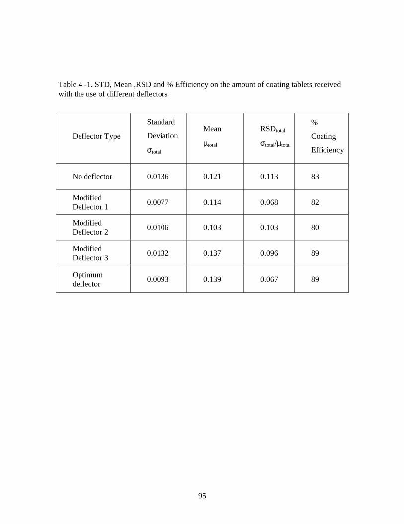
95
Deflector Type
Standard
Deviation
σtotal
Mean
µtotal
RSDtotal
σtotal/µtotal
%
Coating
Efficiency
No deflector 0.0136 0.121 0.113 83
ModifiedDeflector 1
0.0077 0.114 0.068 82
ModifiedDeflector 2
0.0106 0.103 0.103 80
ModifiedDeflector 3
0.0132 0.137 0.096 89
Optimumdeflector
0.0093 0.139 0.067 89
Table 4 -1. STD, Mean ,RSD and % Efficiency on the amount of coating tablets receivedwith the use of different deflectors
96
annulus, was transferred smoothly into upward momentum. The deflector also reduced
the effective gap between the distributor plate and draft-tube, hence causing a leaner bed.
The voidage in the bed is very uniform and the voidage in the immediate vicinity of the
nozzle is very high (shown by the circle in the voidage profile map, Figure 4-26).
Modified deflector 1 thus reduces the sheltering effect and the particles are coated
more evenly, resulting in improvement in the overall coating consistency. Based on the
results obtained with modified deflector 1, it was decided to try a few other modifications
to the deflector. The ring around modified deflector 1 was moved to two different
positions as shown in Figure 3-7 and Figure 3-8.
With modified deflector 2, where the ring is moved away from the nozzle, the
effective gap for the particles to enter is very low, resulting in the particles entering into
the draft-tube at very low velocity. The particles are also deflected away from the nozzle,
but since the change in direction of the particles is so drastic, the particles tend to move
towards the draft-tube walls and in the process collide with the particles that are entering
into the draft-tube. This causes further reduction in velocity resulting in some vortex
formation at slightly higher axial heights (z = 15 cm to 20 cm). Thus, moving the ring
away from the nozzle was counter productive and the coating consistency was worse. The
efficiency of coating also went down, as the chances of the liquid spray escaping in the
upward draft of air, without coming in contact with the particles, increased. The attrition
of tablets was also observed to increase, though no quantitative measurement of this was
made. It is believed that the increase in attrition was caused by the increased particle-
particle collision and the collision of the particles with the draft-tube walls.
97
For modified deflector 3, the ring was moved higher up the deflecting slope. This
caused the deflector to behave more like deflector 1,which did not have a deflecting ring.
This resulted in particles being deflected towards the center resulting in increased particle
density above the spray nozzle. Thus this modification of the deflector was not effective
in reducing the sheltering effect and the coating consistency obtained was poor compared
to that obtained with modified deflector 1, but was better than that obtained without a
deflector.
The optimum deflector was designed based on the observation and results obtained
from the previous deflector designs. The best coating consistency obtained with the
preliminary designs was with modified deflector 1 and hence the optimum deflector was
designed with dimensions very close to this deflector. This deflector was very similar to
modified deflector 1, the only difference being that the former was made of a single piece
of Plexiglas® and the slope of the deflector was slightly steeper and the transformation
into the vertical section was smother. Hence, the voidage profile obtained for the
optimum deflector should be close to that obtained with the modified deflector 1.
Referring back to Figure 4-26, the voidage in the immediate vicinity of the spray nozzle
is very high, as seen by the very light shaded region in the circle. This increased voidage
in results in reducing the sheltering effect and thus particles acquire a more even amount
of spray each time they pass through the spray zone.
The coating efficiencies of the continuous coating runs were calculated based on
the average increase in weight of the tablets due to the coating acquired, to that of an
ideal case where all the coating solution pumped is coated on the tablets. See Appendix
XI for sample calculations.
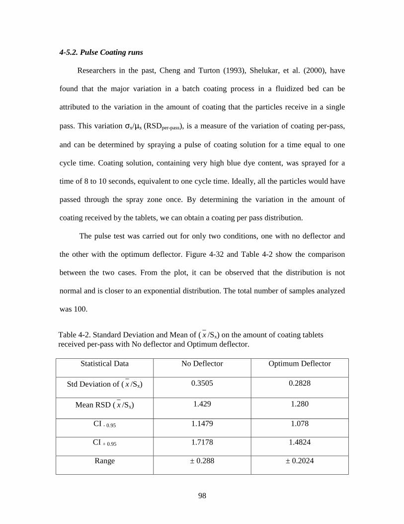
98
4-5.2. Pulse Coating runs
Researchers in the past, Cheng and Turton (1993), Shelukar, et al. (2000), have
found that the major variation in a batch coating process in a fluidized bed can be
attributed to the variation in the amount of coating that the particles receive in a single
pass. This variation σx/µx (RSDper-pass), is a measure of the variation of coating per-pass,
and can be determined by spraying a pulse of coating solution for a time equal to one
cycle time. Coating solution, containing very high blue dye content, was sprayed for a
time of 8 to 10 seconds, equivalent to one cycle time. Ideally, all the particles would have
passed through the spray zone once. By determining the variation in the amount of
coating received by the tablets, we can obtain a coating per pass distribution.
The pulse test was carried out for only two conditions, one with no deflector and
the other with the optimum deflector. Figure 4-32 and Table 4-2 show the comparison
between the two cases. From the plot, it can be observed that the distribution is not
normal and is closer to an exponential distribution. The total number of samples analyzed
was 100.
Statistical Data No Deflector Optimum Deflector
Std Deviation of ( x /Sx) 0.3505 0.2828
Mean RSD ( x /Sx) 1.429 1.280
CI - 0.95 1.1479 1.078
CI + 0.95 1.7178 1.4824
Range ± 0.288 ± 0.2024
Table 4-2. Standard Deviation and Mean of ( x /Sx) on the amount of coating tabletsreceived per-pass with No deflector and Optimum deflector.

99
Figure 4-32a, b. Frequency plot for the pulse test, with no deflector andoptimum deflector, respectively.
Frequency Plot for Pulse Test with Optimum Deflector
0
5
10
15
20
25
30
35
0.0E
+00
1.2E
-04
2.4E
-04
3.6E
-04
4.8E
-04
5.9E
-04
7.1E
-04
8.3E
-04
9.5E
-04
1.1E
-03
1.2E
-03
Concentration mg/tablet
Fre
qu
en
cy
Frequency Plot for Pulse Test with No Deflector
0
5
10
15
20
25
30
35
40
45
50
0.0E
+00
1.2E
-04
2.4E
-04
3.6E
-04
4.8E
-04
5.9E
-04
7.1E
-04
8.3E
-04
9.5E
-04
1.1E
-03
1.2E
-03
Concentration blue dye mg/tablet
Fre
qu
en
cy
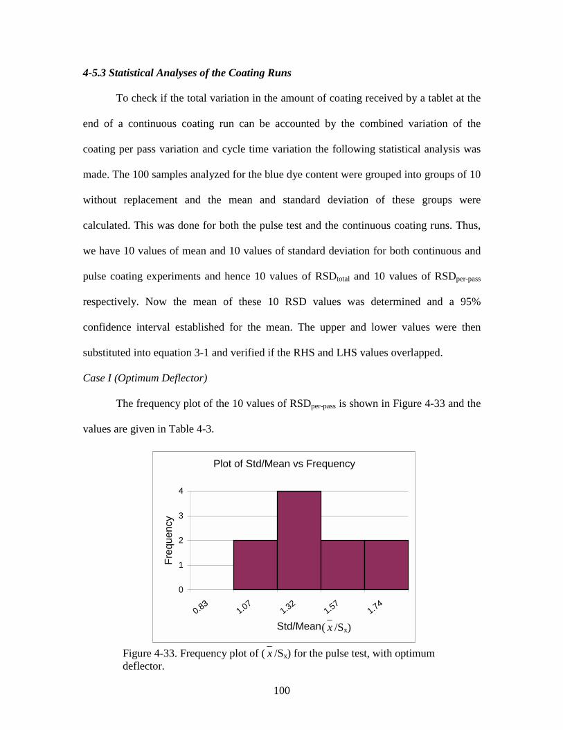
100
4-5.3 Statistical Analyses of the Coating Runs
To check if the total variation in the amount of coating received by a tablet at the
end of a continuous coating run can be accounted by the combined variation of the
coating per pass variation and cycle time variation the following statistical analysis was
made. The 100 samples analyzed for the blue dye content were grouped into groups of 10
without replacement and the mean and standard deviation of these groups were
calculated. This was done for both the pulse test and the continuous coating runs. Thus,
we have 10 values of mean and 10 values of standard deviation for both continuous and
pulse coating experiments and hence 10 values of RSDtotal and 10 values of RSDper-pass
respectively. Now the mean of these 10 RSD values was determined and a 95%
confidence interval established for the mean. The upper and lower values were then
substituted into equation 3-1 and verified if the RHS and LHS values overlapped.
Case I (Optimum Deflector)
The frequency plot of the 10 values of RSDper-pass is shown in Figure 4-33 and the
values are given in Table 4-3.
Figure 4-33. Frequency plot of ( x /Sx) for the pulse test, with optimumdeflector.
Plot of Std/Mean vs Frequency
0
1
2
3
4
0.831.07
1.321.57
1.74
Std/Mean
Fre
quen
cy
( x /Sx)
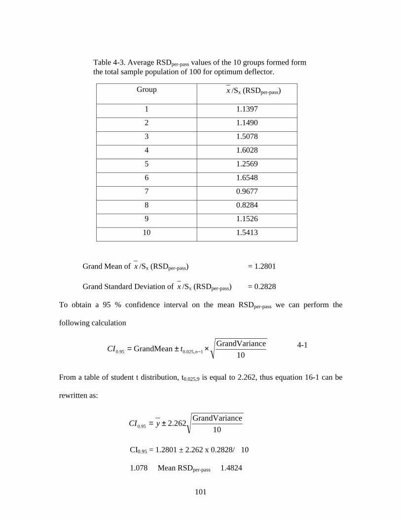
101
Group x /Sx (RSDper-pass)
1 1.1397
2 1.1490
3 1.5078
4 1.6028
5 1.2569
6 1.6548
7 0.9677
8 0.8284
9 1.1526
10 1.5413
Grand Mean of x /Sx (RSDper-pass) = 1.2801
Grand Standard Deviation of x /Sx (RSDper-pass) = 0.2828
To obtain a 95 % confidence interval on the mean RSDper-pass we can perform the
following calculation
From a table of student t distribution, t0.025,9 is equal to 2.262, thus equation 16-1 can be
rewritten as:
CI0.95 = 1.2801 ± 2.262 x 0.2828/�10
1.078 � Mean RSDper-pass � 1.4824
10
nceGrandVariaGrandMean 1,025.095.0 ×±= −ntCI 4-1
Table 4-3. Average RSDper-pass values of the 10 groups formed formthe total sample population of 100 for optimum deflector.
10
nceGrandVaria262.295.0 ±= yCI

102
The frequency plot of the 10 values of RSDtotal (continuous coating runs) is shown in
Figure 4-34 and the values are given in Table 4-4.
Group x /Sx (RSDtotal)
1 0.055
2 0.079
3 0.064
4 0.090
5 0.047
6 0.057
7 0.069
8 0.072
9 0.043
10 0.067
Table 4-4. Average RSDtotal values of the 10 groups formed form thetotal sample population of 100 for optimum deflector.
Figure 4-34. Frequency plot of ( x /Sx) for the continuous coating experiments,with optimum deflector.
Grand Mean of x /Sx (RSDtotal) = 0.064
Grand Standard Deviation of x /Sx (RSDtotal) = 0.014
Plot of Std/Mean vs Frequency
0
1
2
3
4
0.05
0.06
0.08
0.09
0.10
Std/Mean
Fre
quency
( x /Sx)
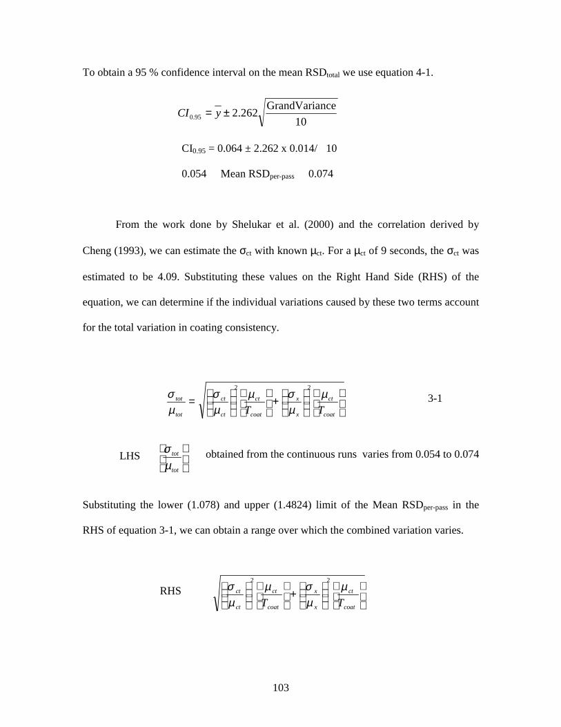
103
To obtain a 95 % confidence interval on the mean RSDtotal we use equation 4-1.
CI0.95 = 0.064 ± 2.262 x 0.014/�10
0.054 � Mean RSDper-pass � 0.074
From the work done by Shelukar et al. (2000) and the correlation derived by
Cheng (1993), we can estimate the σct with known µct. For a µct of 9 seconds, the σct was
estimated to be 4.09. Substituting these values on the Right Hand Side (RHS) of the
equation, we can determine if the individual variations caused by these two terms account
for the total variation in coating consistency.
obtained from the continuous runs varies from 0.054 to 0.074
Substituting the lower (1.078) and upper (1.4824) limit of the Mean RSDper-pass in the
RHS of equation 3-1, we can obtain a range over which the combined variation varies.
+
=
coat
ct
x
x
coat
ct
ct
ct
tot
tot
TT
µµσµ
µσ
µσ
22
3-1
tot
tot
µσ
+
coat
ct
x
x
coat
ct
ct
ct
TT
µµσµ
µσ
22
10
nceGrandVaria262.295.0 ±= yCI
RHS
LHS
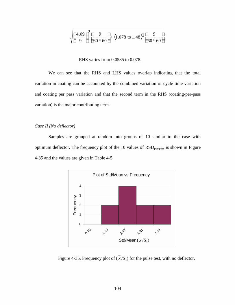
104
We can see that the RHS and LHS values overlap indicating that the total
variation in coating can be accounted by the combined variation of cycle time variation
and coating per pass variation and that the second term in the RHS (coating-per-pass
variation) is the major contributing term.
Case II (No deflector)
Samples are grouped at random into groups of 10 similar to the case with
optimum deflector. The frequency plot of the 10 values of RSDper-pass is shown in Figure
4-35 and the values are given in Table 4-5.
Figure 4-35. Frequency plot of ( x /Sx) for the pulse test, with no deflector.
( )
+
60*60
9248.1to078.160*60
92
9
09.4
RHS varies from 0.0585 to 0.078.
Plot of Std/Mean vs Frequency
0
1
2
3
4
0.79
1.13
1.47
1.81
2.15
Std/Mean
Fre
quen
cy
( x /Sx)
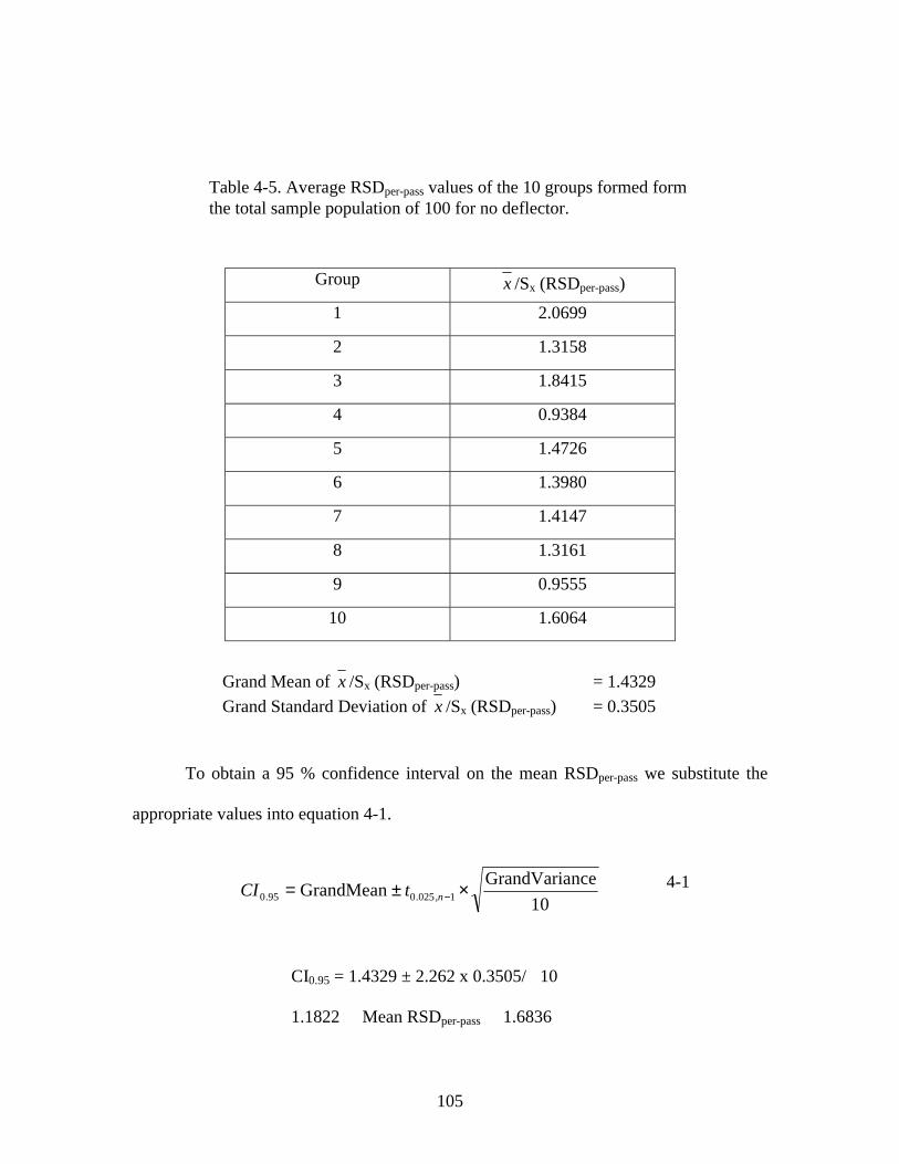
105
Group x /Sx (RSDper-pass)
1 2.0699
2 1.3158
3 1.8415
4 0.9384
5 1.4726
6 1.3980
7 1.4147
8 1.3161
9 0.9555
10 1.6064
To obtain a 95 % confidence interval on the mean RSDper-pass we substitute the
appropriate values into equation 4-1.
CI0.95 = 1.4329 ± 2.262 x 0.3505/�10
1.1822 � Mean RSDper-pass � 1.6836
Table 4-5. Average RSDper-pass values of the 10 groups formed formthe total sample population of 100 for no deflector.
Grand Mean of x /Sx (RSDper-pass) = 1.4329
Grand Standard Deviation of x /Sx (RSDper-pass) = 0.3505
10
nceGrandVariaGrandMean 10250950 ×±= −,n.. tCI 4-1

106
The frequency plot of the 10 values of RSDtotal is shown in Figure 4-36 and the values are
shown in Table 4-6.
Group x /Sx (RSDper-pass)
1 0.078
2 0.118
3 0.112
4 0.083
5 0.168
6 0.112
7 0.177
8 0.097
9 0.075
10 0.084
Plot of Std/Mean vs Frequency
0
1
2
3
4
0.06
0.08
0.10
0.14
0.18
0.22
Std/Mean
Fre
qu
en
cy
Figure 4-36. Frequency plot of ( x /Sx) for the continuous coating run, withno deflector.
Table 4-6. Average RSDper-pass values of the 10 groups formed formthe total sample population of 100 no deflector.
Grand Mean of x /Sx (RSDtotal) = 0.11
Grand Standard Deviation x /Sx (RSDtotal) = 0.036
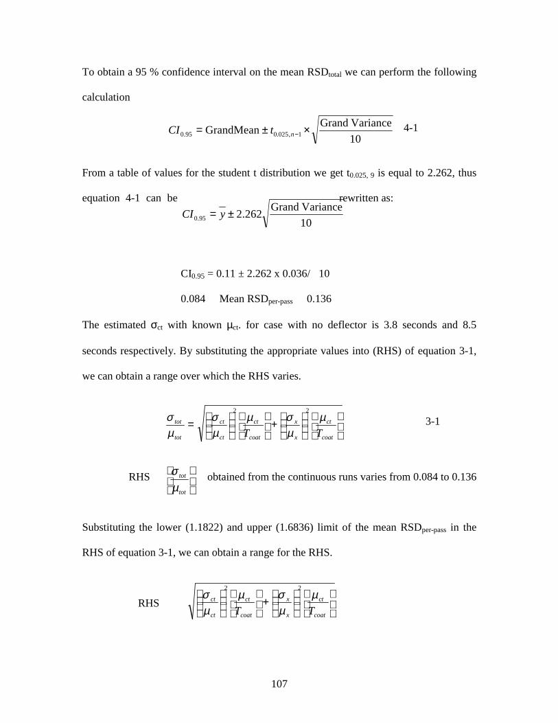
107
To obtain a 95 % confidence interval on the mean RSDtotal we can perform the following
calculation
From a table of values for the student t distribution we get t0.025, 9 is equal to 2.262, thus
equation 4-1 can be rewritten as:
CI0.95 = 0.11 ± 2.262 x 0.036/�10
0.084 � Mean RSDper-pass � 0.136
The estimated σct with known µct. for case with no deflector is 3.8 seconds and 8.5
seconds respectively. By substituting the appropriate values into (RHS) of equation 3-1,
we can obtain a range over which the RHS varies.
RHS obtained from the continuous runs varies from 0.084 to 0.136
Substituting the lower (1.1822) and upper (1.6836) limit of the mean RSDper-pass in the
RHS of equation 3-1, we can obtain a range for the RHS.
10
Variance Grand262.295.0 ±= yCI
+
=
coat
ct
x
x
coat
ct
ct
ct
tot
tot
TT
µµσµ
µσ
µσ
22
3-1
tot
tot
µσ
10
Variance GrandGrandMean 1,025.095.0 ×±= −ntCI 4-1
+
coat
ct
x
x
coat
ct
ct
ct
TT
µµσµ
µσ
22
RHS
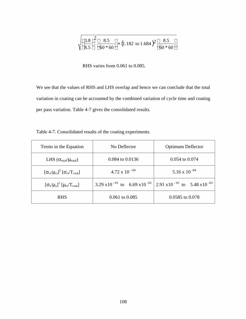
108
We see that the values of RHS and LHS overlap and hence we can conclude that the total
variation in coating can be accounted by the combined variation of cycle time and coating
per pass variation. Table 4-7 gives the consolidated results.
Table 4-7. Consolidated results of the coating experiments.
Terms in the Equation No Deflector Optimum Deflector
LHS (σtotal/µtotal) 0.084 to 0.0136 0.054 to 0.074
[σct/µct]2 [σct/Tcoat] 4.72 x 10 - 04 5.16 x 10 -04
[σx/µx]2 [µct/Tcoat] 3.29 x10 - 03 to 6.69 x10 -03 2.91 x10 - 03 to 5.48 x10 -03
RHS 0.061 to 0.085 0.0585 to 0.078
( )
+
60*60
8.521.684 to1.18260*60
8.52
8.5
3.8
RHS varies from 0.061 to 0.085.
109
CHAPTER V
CONCLUSIONS
The hydrodynamics of large particles in the vicinity of the spray zone and in the
draft-tube of a semi-circular Wurster fluidized bed coater were investigated using a
computer-based video imaging system. The particle velocity profiles and the bed voidage
profiles thus obtained were mapped using custom written programs in Microsoft© Visual
Basic. A large database of velocity and voidage profiles with different operating
parameters was also obtained. For the first time, a device for altering the voidage profile
in the draft-tube (deflectors) was used and its effect on the hydrodynamics of the bed
investigated. Coating studies were carried out to study the variation in the amount of
coating received by the particles and to determine the factors that affect the coating
consistency. Single-pass coating studies were carried out in an effort to estimate variation
in the amount of coating that particles receive per pass and the effect this plays in the
total coating variation.
The observations and conclusions that can be made from these experimental
investigations are summarized below.
• At the lower gap height, (2.7 cm between the distributor plate and draft-tube) the
particle velocities at the center were lower than particle velocities closer to the
wall of the draft-tube when no deflector was present or deflector 1 was present.
This was observed because at the lower gap height, the particles entry is restricted
by the low gap height and the particles enter the bed in the horizontal direction.
This causes particle-particle interaction at the center resulting in the loss of
vertical momentum. In the presence of modified deflector 1, the velocity at the
110
center was marginally less or equal to the velocities near the draft-tube walls. This
is because the modified deflector 1 deflects the particles away from the center and
thus reduces particle-particle interaction at the center.
• At the higher gap height, (7.4 cm between the distributor plate and draft-tube), the
particles entered the draft-tube with less restriction, resulting in a denser bed. The
particles also showed a tendency to accelerate at higher axial heights and more
symmetric velocity profiles were observed. With the higher gap height, deflector
1 became less effective and the profile around the nozzle was not much different.
The presence of modified deflector 1 resulted in a very symmetric velocity profile
and the velocities at the center were significantly higher than velocities closer to
the wall.
• Increasing the fluidizing air velocity did not alter the velocity profile significantly.
However, the profile became more symmetric and the particles moved with higher
velocities.
• The use of distributor plate 2 with a higher ratio of inner to outer area (11% more
than distributor plate 1) did not result in any significant change in the velocity
profile.
• The voidage profiles with the lower gap height are similar for the both the cases
of with/without deflector 1. However, the voidage profile changed significantly in
the presence of modified deflector 1. The voidage across the entire bed became
very uniform and the voidage varied over a very narrow range (0.90 to 0.95).
• At the higher gap height, deflector 1 was not effective in increasing the voidage
around the spray zone, and the voidage at axial height z = 4.5 and r = 0 was the
111
same for the case with no deflector. With the modified deflector 1, the voidage in
the spray zone increased considerably, and the voidage distribution was even
across the draft-tube.
• The continuous coating runs showed that the use of deflectors to alter the voidage
around the nozzle resulted in variation in the coating quality. This showed that
reducing the sheltering effect results in improved coating consistency. Deflector 1
was not effective in altering the voidage profile around the nozzle and gave a
coating consistency close to the no deflector case. However, with modified
deflector 1, a marked improvement in coating consistency was achieved.
• An Optimum deflector was designed based on the results obtained with deflector
1, and modified deflectors 1, 2 and 3. The use of this optimum deflector, gave the
best coating consistency although not much improvement was seen from that
obtained from modified deflector 1. The dimensions of the optimum deflector
were very close to those of modified deflector 1.
• The pulse test or the single-pass coat test showed that variation in coating per pass
accounted for nearly 80% of the total coating variation. Hence, the use of these
deflectors, which increase the voidage in the spray zone and reduce sheltering
effect, resulted in less variation in coating per-pass and a better overall coating
consistency.
• The mass balance on flow rate of particles in the draft-tube and annulus, at both
dilute (lower gap height), and concentrated (higher gap height) flow conditions,
showed good agreement. This favorable agreement is an indication of the
112
reliability of the particle velocity and voidage data obtained and the use of
computer based video imaging to obtain such data.
The above results indicate that the non-invasive computer-based video imaging
technique with custom software can be used effectively to measure particle velocity and
voidage profiles in the draft-tube region of a semi-circular Wurster fluidized bed coater.
The use of a deflector to guide the particles away from directly passing over the spray
nozzle, thus reducing the sheltering effect, resulted in an improvement of the coating
consistency of the tablets. As a final check for consistency of data, the particle velocity
and voidage data in the draft-tube and annular regions were used to compute a solids
mass flow balance using numerical integration. The results show good agreement
between the solid mass flow rates in the draft-tube and annulus.
113
CHAPTER VI
RECOMMENDATION FOR FUTURE WORK
Recommendations and scope for future work:
• Studies in conventional spouted beds (cylindrical), using optical probes and other
methods have shown that there are quantitative differences in the velocity and
voidage measurements between the semi-cylindrical and cylindrical geometries
(this difference is more pronounced with the velocity measurements). Thus
obtaining the velocity and voidage measurements in a three-dimensional bed and
comparing it with the data obtained in the case of a two dimensional bed of the
same dimensions can further validate the data obtained in this study.
• Based on the extensive database of velocity and voidage profiles obtained in this
study, simulation and modeling can be done to predict the path that the particles
take after entering into the draft-tube region.
• The use of deflectors has shown measurable improvement in the coating
consistency in a semi-circular bed. From the observations made, it is clear that
these deflectors will be more effective in the case of a three dimensional bed. This
can be verified by conducting actual coating runs in a three dimensional bed.
• The optimum deflector design obtained here, proved very effective in improving
the coating consistency. However, this deflector’s design parameters can be
studied further and optimized and can be compared with existing (commercial)
designs to give a basis for comparison.
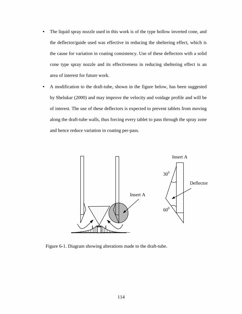
114
• The liquid spray nozzle used in this work is of the type hollow inverted cone, and
the deflector/guide used was effective in reducing the sheltering effect, which is
the cause for variation in coating consistency. Use of these deflectors with a solid
cone type spray nozzle and its effectiveness in reducing sheltering effect is an
area of interest for future work.
• A modification to the draft-tube, shown in the figure below, has been suggested
by Shelukar (2000) and may improve the velocity and voidage profile and will be
of interest. The use of these deflectors is expected to prevent tablets from moving
along the draft-tube walls, thus forcing every tablet to pass through the spray zone
and hence reduce variation in coating per-pass.
300
600
Deflector
Figure 6-1. Diagram showing alterations made to the draft-tube.
Insert A
Insert A
115
• The use of the modified/optimum deflector not only showed improvement in the
coating consistency but also showed difference in the dissolution rate of the
coated blue dye. This observation though not investigated further in this study, is
an area of interest for future studies and may hold important answers relating to
the morphology of the coating.
• Computer based video imaging technique is limited to measurements at the wall
and shallow depths from the wall. As one attempts to penetrate further into the
bed, the computer images become more susceptible to the masking effect of
foreground particles and changes in the light intensity. Hence, other measurement
techniques such as optical probes or γ-ray emission methods can be used to study
particle behavior in these areas of the bed.
116
NOMENCLATURE
dp diameter of the particle, m
ρp absolute density of particles, kg/m3
ρb bulk density, kg/m3
rdo inside diameter of draft-tube, m
rdi outside diameter of draft-tube, m
Do inside diameter of fluidized bed, m
Di outside diameter of fluidized bed, m
uanul 2-D particle velocity in annulus, m/s
udft 2-D particle velocity in the draft-tube, m/s
mdft mass flow rate in draft-tube, kg/s
manul mass flow rate in the annulus, kg/s
εdft voidage in the draft-tube
εanul voidage in the annulus
θ angle of the resultant 2-D velocity vector, relative tothe positive r direction
σ standard deviation
µ mean
RSD relative standard deviation (σ/µ) also calledcoefficient of variation
ADOF apparent depth of field
FOV field of view
CI0.95 95% confidence interval
117
x sample standard deviation
Sx sample mean
Std standard deviation
Tcoat Total time of coating experiment
118
BIBLIOGRAPHY
Boulos, M.I., and B. Waldie, “High Resolution of Particle Velocities in a Spouted Bedusing Laser-Doppler Anemometry,” The Canadian Journal of Chemical Engineering, 64,pp. 939-943 (1986).
Brudney, N. and P.Y. Toupin, “Air Suspension Coating,” Can.Pharm. J., 94(7), pp. 18-19 (1961).
Caldwell, H. C., and E. Rosen, “New Air Suspension Apparatus for Coating DiscreteSolids,” Journal of Pharm. Sci., 53, pp. 1387-1391 (1964).
Chang, R. K., E. Hsiao, and J. R. Robinson, “ A Review of Aqueous coating Techniquesand Prelimenary data on Release from a Theophylline Product,” Pharm. Tech., 11(3),pp.56-68 (1987).
Cheng, X.X, “The Study of Uniformity of Particle Coating,” Ph.D. Dissertation, WestVirginia University (1993).
Cheng, X.X. and R. Turton, “The Uniformity of Coating Occurring in Fluidized Bed,”AIChE Symp. Sep. 90 (301), pp. 142-151 (1994).
Choi, M.S. Michael and Meisen Axel “Sulfur Coating of Urea in Shallow Spouted Beds,”Chemical engineering Science, 52,pp.1073 (1996).
Davies, W.L., and W.T., Jr., Gloor, “Batch Production of Pharmaceutical Granulations ina Fluidized Bed I: Effects of Process Variables on Physical Properties of FinalGranulation,” J. Pharm. Sci., 61, pp. 1869-1874 (1971).
Davies, W.L., and W.T., Jr., Gloor, “Batch Production of Pharmaceutical Granulations ina Fluidized Bed II: Effects of Various Binders and their Concentrations on theGranulations and Compressed Tablets,” J. Pharm. Sci., 60, pp. 618-622 (1972).
Ghebre-Sellassie, I., U. Iyer, D. Kubert, and M. B. Fawzi, “Characterization of a NewWater-Based Coating for Modified-Release Preparations,” Pharm. Tech., 12(9), pp.96-106 (1988).
Goldberg, H. and W. J. Joseph, “Using the Web Delivery System to Produce SolidDosage forms,” Pharmaceutical Manufacturing, pp. 21-29, April (1986).
Good, R. W. and Lee, P. I, “Controlle-Release Technology – PharmaceuticalApplications,” ACS Sym. Series348, (1987).
Grace, J.R and J. Baeyens, “Gas Fluidization Technology,” Chapter 13, ed. D. Geldart,John Wily & Sons Inc., New York (1986).
119
Hattori, H. and K. Takeda, “Slide-outlet Spouted Bed with Inner Draft Tube for Small-sized Solids Particles,” J. Chem. Eng. Japan, 11, pp. 125-129 (1978).
He, Y.L., C.J. Lim, J.R. Grace, J.X.Zhu and S.Z. Qin, “Measurement of Voidage Profilesin Spouted Beds,” Can. J. Chem. Eng., 72, pp. 229-234 (1994a).
He, Y.L., C.J. Lim, J.R. Grace, J.X.Zhu and S.Z. Qin, “Particle Velocity Profiles andSolids Flow Patterns in Spouted Beds,” Can. J. Chem. Eng., 72, pp. 561- 568 (1994b).
Khoe, G.K. and J. Van Brakel, “Drying Charecteristics of s Draft Tube Spouted Bed,”Can. J. Chem. Eng., 61, pp. 411-418 (1983).
Klaflin, J. K. and A. G. Fane, “Spouting with a Porous Draft Tube,” Can. J. Chem. Eng.,61, pp. 346-363 (1983).
Kunii, D., O. Levenspiel, “Fluidization Engineering,” First Edition, Robert E. KriegerPublishing Company, Inc., Chapter-2, pp. 16 (1969).
Kunii, D., O. Levenspiel, “Fluidization Engineering,” Industrial Application of FluidizedFlow, 8 (2), pp. 125-146 (1982).
Kandis Sudsakron, “The Effect of Particle Size on the Amount of coating Receivedduring a Batch Fluidized Bed Coating Operation,” Masters Thesis, West VirginaUniversity (1999).
Lee, V. L. and J. R. Robinson, “Controlled Drug Delivery: Fundamentals andApplications,” 2nd Ed., Marcel Dekker Inc., (1987).
Lefroy G.A. and J.F. Davidson, “The Mechanics of Spouted Beds,” Trans. Instn. Chem.Engrs., 47, pp. T120-T128 (1969).
Lehmann, K. and D. Dreher, “Coating of Tablets and Small Particles with acrylic resinsby Fluid bed technology,” J. Pharm. Tech & Prod. Mrf., 2(4) 31-43, (1981).
Li, L. C. and E. G. Peck, “Water Based Silicone Elastomer Controlled Release TabletFilm coating in Process Evaluation,” Drug Development and Industrial Pharmacy, 16(3),pp. 415-435 (1990).
Liu, L. X. and J. D. Liter, “Spouted Bed Seed Coating: the Effect of Process Variables onMaximum Coating Rate and Elutration,” Powder Tech., 74, pp. 215-230 (1993).
Mann, U., “Coating of Particulate Solids by Air Suspension,” Ph.D. Dissertation,University of Wisconsin, Madison (1972).
120
Mann, U., E.J. Crosby and M. Rubinovitch, “Number of Cycles Distribution inCirculating Systems,” Chem. Eng. Sci., 29, pp. 761-765 (1974).
Massimilla, L., J.W. Westwater, “Photographic Study of Solids-Gas Fluidization,”AIChE J., 6(1) pp. 132-138 (1959).
Mathur, K.B., and P.E. Gishler, “A Technique for Contacting Gases with Coarse SolidParticles,” AIChE. J., 1, pp. 157-164 (1955).
Rekhi, S.G., W. R. Mendes, S. C. Porter, and S.S. Jamhekar, “Aqueous PolymericDispersions for Controlled Drug Delivery – Wurster Process,” PharmaceuticalTechnology, pp. 112-125, March (1989).
Robinson, M. J., G. M. Grass, and R. J. Lantz, “An Apparatus and Method for theCoating of Solid Particles,” J. Pharm. Sci., 57, pp. 1983-1988, (1968).
Robinson, M. J., “Coating of Pharmaceutical Dosage,” Remingtons PharmaceuticalScinece, 16th, pp. 1585-1593 (1980).
Rankell, A. S., M. W. Scott, A. Lieberman, F. S. Chow, and J. V. Battista, “ContinuousProduction of Tablet Granulations in a Fluidized Bed II. Operation and Performance ofEeuipment,” J. Pharm Sci., 53, pp. 320-324 (1964).
Roy, D., F. Larachi, L. Robert, and C. Jamal, “A Study of Solid Behaviour in SpoutedBeds Using 3-D Particle Tracking,” Can. J. Chem. Eng., 72, pp. 945-952 (1994).
Saadevandi, B. A., and R. Turton, “The Application of Computer-Based Imaging to theMeasurements of Particle Velocity and Voidage Profiles in a Fluidized Bed,” PowderTechnology, 98, pp. 183-189 (1998).
Saadevandi, B. A, “The Use of Imaging Techniques to Study the Hydrodynamics ofParticle Motion in a Fluidized Bed Coating Device in the Region of the Liquid Spray,”Ph.D Dessertation, West Virginia University (1996).
Shernoy, D. F., “Amodel of Surface Renewal with Application to Fluid Bed Coating ofParticles,” Chem. Eng. Sci., 36, pp. 845-848 (1981).
Shelukar, S., Jennifer Ho, James Zega, Ed Roland, Norman Yeh, David Quiram, AntonyNole, Ashok Katdare and Scott Reynolds, “ Identification and Characterization of FactorsControlling Tables Coating Uniformity in a Wurster Coating Process,” PowderTechnology, 110, pp. 29-36 (2000).
Singiser, R.E., A.L. Heiser, and E.B. Prilling, “Air-Suspension Tablets Coating,” Chem.Eng. Progress, 72 (6), pp. 107-111 (1966).
121
Suciu G.C., and M. Patrascu, “Particle Circulation in a Spouted Bed,” PowderTechnology, 19, pp. 109-114 (1978).
Suciu G.C., and M. Patrascu, “Prediction of Solids Circulation Patterns in a SpoutedBed,” Powder Technology, 53, pp. 257-271 (1977).
Todd, D. B., R. H. Overcashier, and D. B. Olney, Motion Picture, “FluidizationCharacteristics in a Two-Dimensional Fluid Bed,” Shell Development Company,Emeryville, California (1957)
Toomey, R. D., and H.F. Johnstone, Chem. Eng. Progr. Symposium Ser. No 5, 49, 51(1953).
Van Velzen, D., H.J. Flamm, H. Langenkamp and A. Casile, “Motion of Solids inSpouted Beds,” Can. J. Chem. Eng., 52, pp. 156- 161 (1974).
Wan, L. S. C and W. F. Lai, “Factors Affecting Drug Release from Drug-CoatedGranules Prepared by Fluidized-Bed Coating,” Intl. J. of Pharmaceutics, 72, pp. 1499-1501 (1980).
Wnukowski, P. and F. Setterwall, “The Coating of Particles in a Fluidized Bed(Residence Time Distribution in a system of Two Coupled Perfect Mixers),” Chem. Eng.Sci., 44(3), pp. 493-505 (1989).
Weiss, P. J. and A. Meisen, “Laboratory Studies on Sulphur-Coating Urea by the SpoutedBed Process,” Can. J. of Chem. Eng., 61, pp. 440-447, (1983).
Wurster, D.E., “Means for Applying coating to Tablets or Like,” US Patent 2,799,241(1957).
Wurster, D. E., “U.S. Patent, 2,648,609,” (1953).
Wurster, D.E., Lindlof, and J.Y. Battisita, “Process for Preparing Agglomerates,” USPatent 3,207,824 (1965).
Yang, W. C. and D. L. Keairns, “Recirculating Fluidized Bed Reactor Data Utilizing aTwo-Dimensional Cold Model,” AIChE Symp. Ser., 70 (141), pp. 27-40 (1974).
Yang, W. C. and D. L. Keairns, “Design of Recirculating Fluidized Bed for CommercialApplications,” AIChE Symp. Ser., 74(176), pp. 218-227 (1978).
Yang, W. C. and D. L. Keairns, “Studies on the Solid Circulation Rate and GasBypassing in a Spouted Fluid-Bed with a Draft Tube,” Can. J. Chem. Eng., 61, pp. 349-355 (1983).
122
Xu M., “A Theoretical and Experimental Investigation of Spouted Beds With DraftTube,” Ph.D. Dissertation, West Virginia University, (1994).
Zogilo, M. A., W. H. Streng, and J. T. Carstensen, “Diffusion Model for Fluidized BedDrying,” J. Pharm. Sci., 64 pp. 1869-`873 (1975).
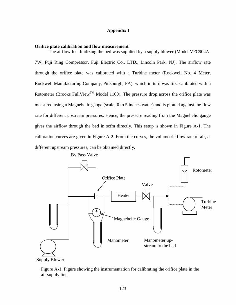
123
Appendix I
Orifice plate calibration and flow measurementThe airflow for fluidizing the bed was supplied by a supply blower (Model VFC904A-
7W, Fuji Ring Compressor, Fuji Electric Co., LTD., Lincoln Park, NJ). The airflow rate
through the orifice plate was calibrated with a Turbine meter (Rockwell No. 4 Meter,
Rockwell Manufacturing Company, Pittsburgh, PA), which in turn was first calibrated with a
Rotometer (Brooks FullViewTM Model 1100). The pressure drop across the orifice plate was
measured using a Magnehelic gauge (scale; 0 to 5 inches water) and is plotted against the flow
rate for different upstream pressures. Hence, the pressure reading from the Magnehelic gauge
gives the airflow through the bed in scfm directly. This setup is shown in Figure A-1. The
calibration curves are given in Figure A-2. From the curves, the volumetric flow rate of air, at
different upstream pressures, can be obtained directly.
Supply Blower
Figure A-1. Figure showing the instrumentation for calibrating the orifice plate in theair supply line.
Heater
By Pass Valve
Magnehelic Gauge
Manometer up-stream to the bed
Orifice Plate
Valve
Manometer
Rotometer
TurbineMeter
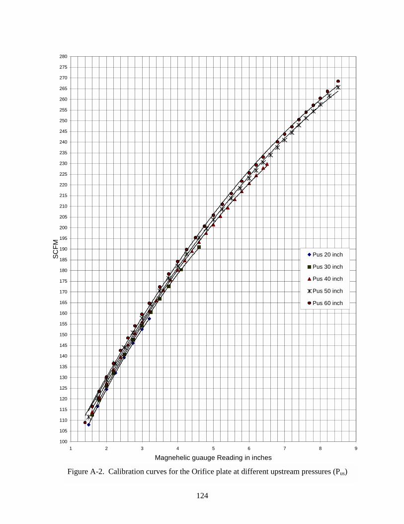
124
Figure A-2. Calibration curves for the Orifice plate at different upstream pressures (Pus)
100
105
110
115
120
125
130
135
140
145
150
155
160
165
170
175
180
185
190
195
200
205
210
215
220
225
230
235
240
245
250
255
260
265
270
275
280
1 2 3 4 5 6 7 8 9
Magnehelic guauge Reading in inches
SC
FM
Pus 20 inch
Pus 30 inch
Pus 40 inch
Pus 50 inch
Pus 60 inch
125
Appendix II
Measurement of voidage in the annulus
The voidage in the annulus was calculated from the measured absolute and bulk
densities. The particles were weighed (electronic balance, model XE-100A, Denver
Instruments Company, Arvado, Colorado), in groups of 10 and an average weight of an
individual tablet was obtained (0.205 gm). The weight of the tablet, thus determined, confirms
that specified by the supplier. The bulk density (0.70813 kg/m3) of the tablets was determined
by the un-tapped volume occupied by tablets poured in a graduated beaker and the absolute
density (1.215 kg/m3) was measured by the actual volume occupied by a known weight of
tablets, the voids being filled by a non-penetrating vegetable oil. The details of the result are
given in Table A-1, Table A-2 and Table A-3.
The packed bed voidage was calculated to be 0.42 or 42% using the following relationship.
ε = 1 – (ρbulk/ ρparticle)
ε = 1 – (0.708/1.215)
ε = 0.42
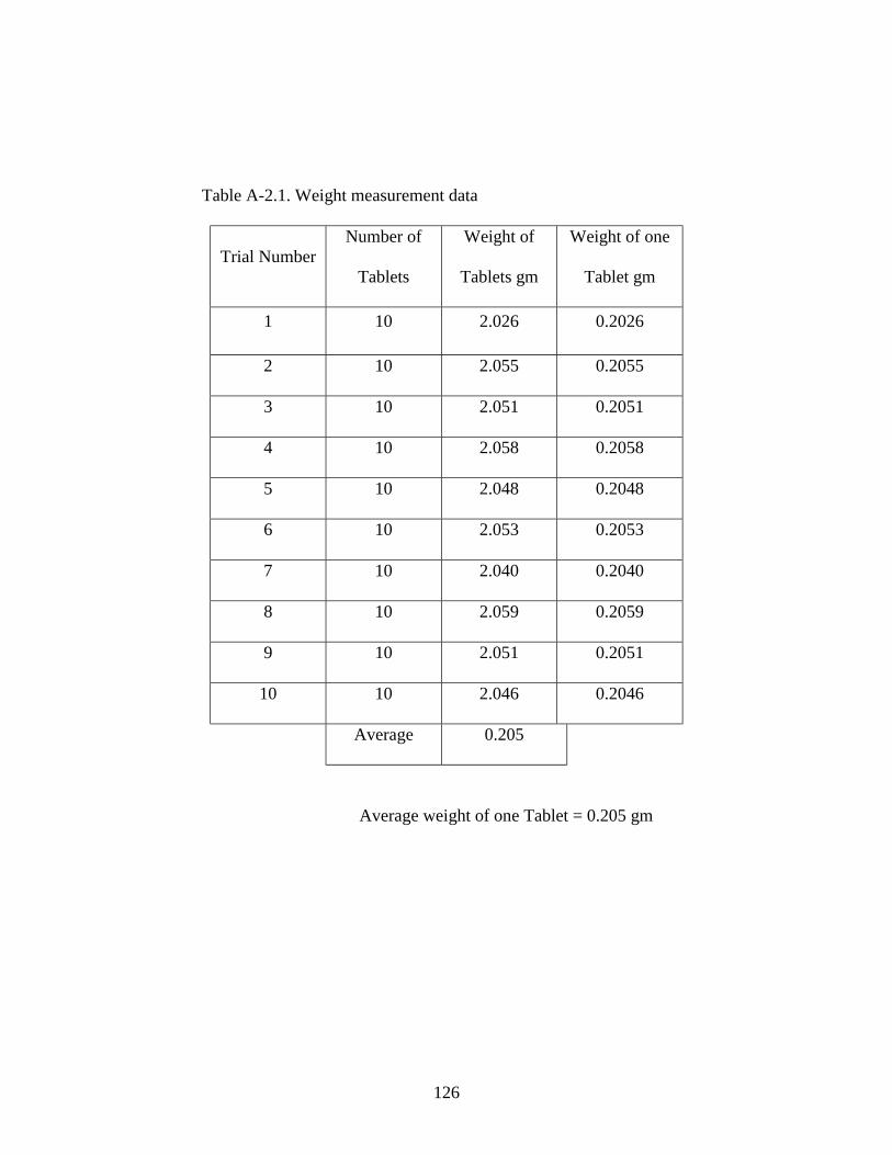
126
Table A-2.1. Weight measurement data
Trial NumberNumber of
Tablets
Weight of
Tablets gm
Weight of one
Tablet gm
1 10 2.026 0.2026
2 10 2.055 0.2055
3 10 2.051 0.2051
4 10 2.058 0.2058
5 10 2.048 0.2048
6 10 2.053 0.2053
7 10 2.040 0.2040
8 10 2.059 0.2059
9 10 2.051 0.2051
10 10 2.046 0.2046
Average 0.205
Average weight of one Tablet = 0.205 gm
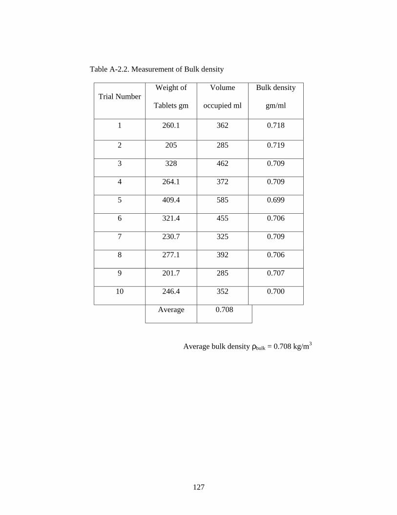
127
Table A-2.2. Measurement of Bulk density
Trial NumberWeight of
Tablets gm
Volume
occupied ml
Bulk density
gm/ml
1 260.1 362 0.718
2 205 285 0.719
3 328 462 0.709
4 264.1 372 0.709
5 409.4 585 0.699
6 321.4 455 0.706
7 230.7 325 0.709
8 277.1 392 0.706
9 201.7 285 0.707
10 246.4 352 0.700
Average 0.708
Average bulk density ρbulk = 0.708 kg/m3
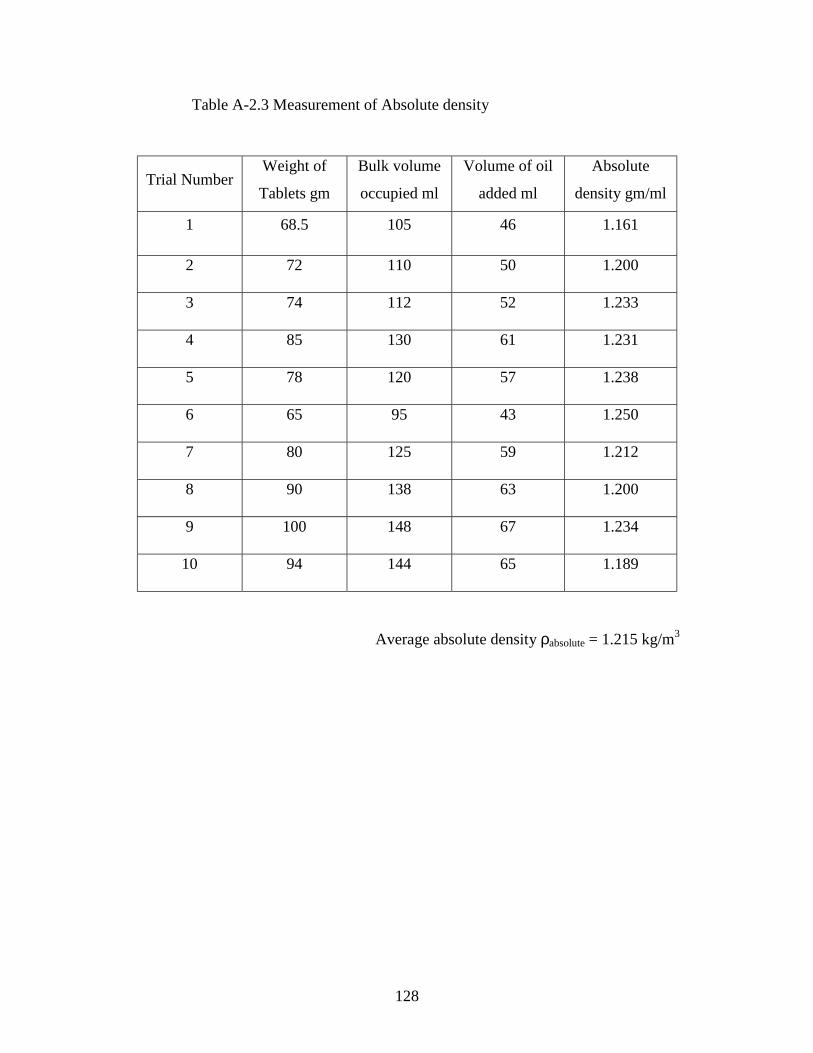
128
Table A-2.3 Measurement of Absolute density
Average absolute density ρabsolute = 1.215 kg/m3
Trial NumberWeight of
Tablets gm
Bulk volume
occupied ml
Volume of oil
added ml
Absolute
density gm/ml
1 68.5 105 46 1.161
2 72 110 50 1.200
3 74 112 52 1.233
4 85 130 61 1.231
5 78 120 57 1.238
6 65 95 43 1.250
7 80 125 59 1.212
8 90 138 63 1.200
9 100 148 67 1.234
10 94 144 65 1.189
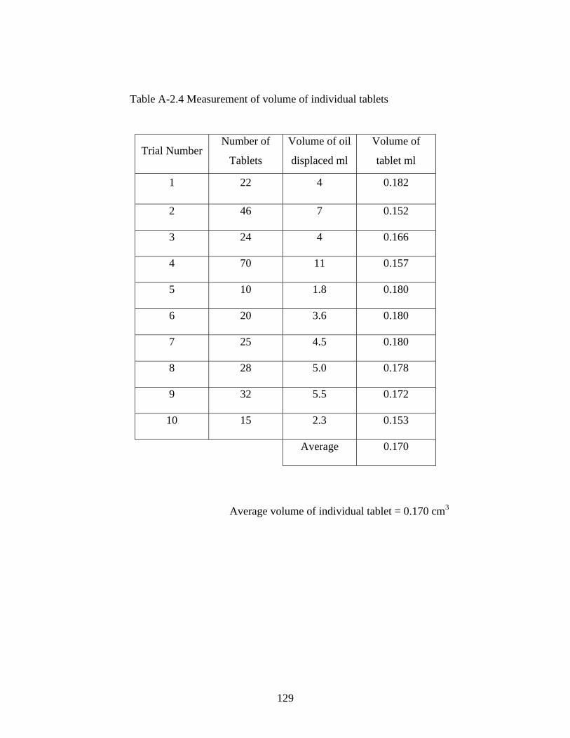
129
Table A-2.4 Measurement of volume of individual tablets
Average volume of individual tablet = 0.170 cm3
Trial NumberNumber of
Tablets
Volume of oil
displaced ml
Volume of
tablet ml
1 22 4 0.182
2 46 7 0.152
3 24 4 0.166
4 70 11 0.157
5 10 1.8 0.180
6 20 3.6 0.180
7 25 4.5 0.180
8 28 5.0 0.178
9 32 5.5 0.172
10 15 2.3 0.153
Average 0.170
130
Appendix III
Calibration of the velocity measurement technique using a rotating disk of knownvelocity and stroboscope
The accuracy of the imaging system and software used, to determine the velocity
of moving tablets in the fluidized bed, was tested by measuring the velocity of a known
source with the imaging system and comparing the results.
The known source was a marked disk mounted on a battery-powered drill as
shown in Figure A-3. The cameras were mounted on the stand and the distance between
the disk and the cameras were set to be 36.2mm, the same distance between the cameras
and the front glass face of the fluidized bed. The drill was started and the rate of rotation
was measured with a stroboscope (Nova-Strobe® DA Digital, AC, Monarch Instrument,
Amherst, NH).
The actual velocity of a point on the disk was calculated using the formula, v = rω
where v is the velocity, r is the radial distance from the center and ω = 2πN (N is the rps)
and compared to the values obtained by using the software. Figure A-3.1 shows a setup
of the drill with a graduated disk and the imaging system. The distance between the
cameras and the drill was measured to be the same as the distance between the cameras
and the inside surface of the glass sheet. The results are shown in Table A-3.1 and Figure
A-3.2. Based on the results, the software captures the true velocity within a 95%
confidence interval.

131
Figure A-3.1. Graduated disk mounted on a battery-powered drill
Cameras
Graduated Disk
Drill
DrillGraduated Disk
CamerasComputer

132
Velocity as determined by Software Velocity as determined by Strobe
Mean = 2.61 Mean = 2.57
CI- 0.95 = 2.67 m/s
CI+ 0.95 = 2.54 m/s
CI- 0.95 = 2.64 m/s
CI+ 0.95 = 2.51 m/s
Figure A-3.2. Plot shows the CI0.95 bars associated with the velocity measurementsusing the software and the calculated values using the strobe overlap.
Method of velocity measurement
B - CI+0.95 bars obtained by softwareC - CI-0.95 bars obtained by strobe
Velocity m/s
Table A-3.1. Velocity measurement values as measured by software and bystroboscope
133
Appendix IV
Apparent Depth of Field (ADOF) Calibration
The apparent depth of field is the range of distance over which the camera can
record images from the point of focus. The greater the ADOF, the greater is the distance
over which the camera can record clear focused images and vice versa. It was necessary
to obtain an accurate value of the ADOF, in order that the volume element over which the
voidage is to be calculated could be determined. The camera is focused on permanent
marks made on the draft-tube so that a fixed reference is always maintained.
The models shown in Figure 3-16, were placed inside the draft tube as shown in
Figure A-4.1. The camera was focused on the permanent marks on the draft-tube shown
in the figure. The cameras were then moved on the sliding stand to obtain the image of a
single model. Each of these models had a different number of tablets with different
orientations. The farthest particle recorded by the camera and identified by the software
in each of these models was noted and the distance from the front glass sheet was
measured. This distance is the calculated ADOF and the average distance was determined
to be 1.5 cm. To verify this value of ADOF, the following procedure was carried out.
With each model in focus, the routine for determining the voidage, explained in Section
3-5, was carried out. By correlating the number of particles picked up by the camera, and
the actual number of particles present within the ADOF (1.5 cm) from the front glass
sheet, we can determine the actual voidage and the voidage obtained using the software.
A graph of the actual number of particles vs. the number picked by the software is shown
in Figure A- 4.2.
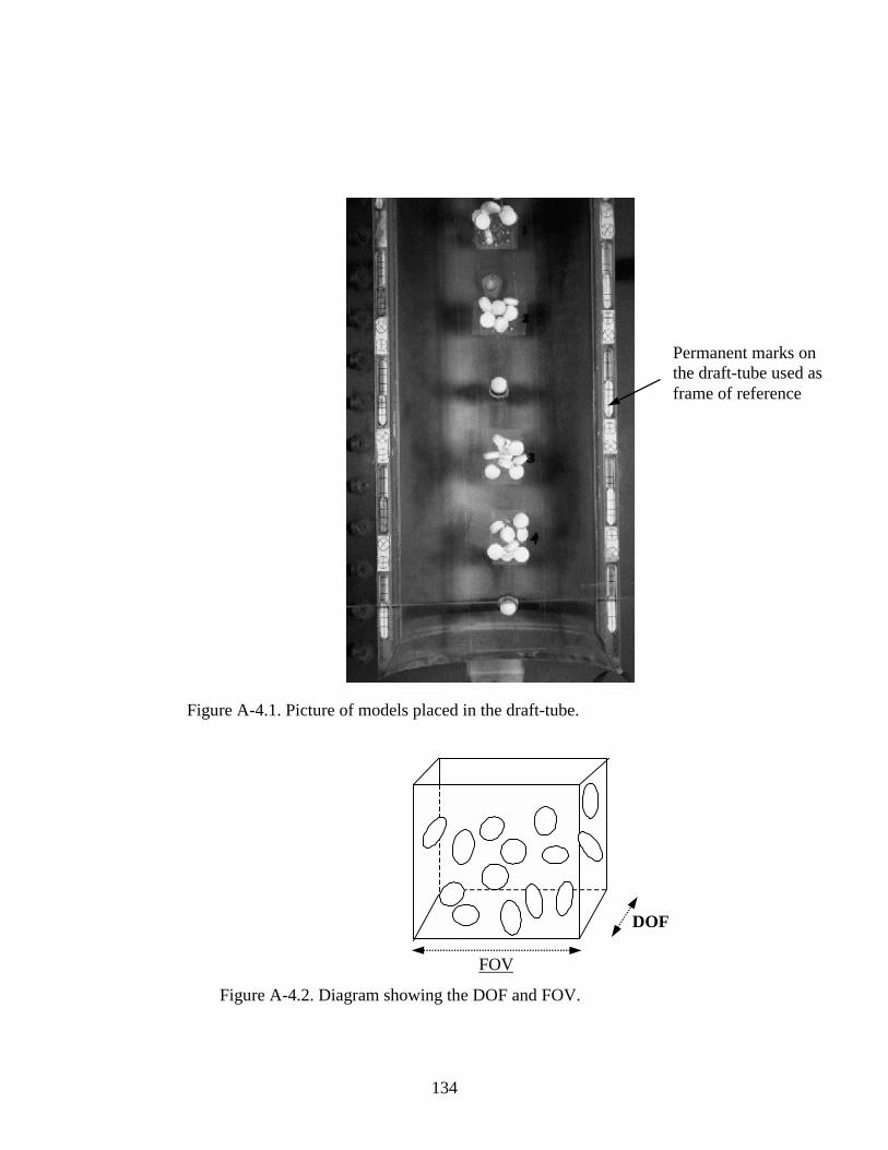
134
DOF
FOV
Permanent marks onthe draft-tube used asframe of reference
Figure A-4.1. Picture of models placed in the draft-tube.
Figure A-4.2. Diagram showing the DOF and FOV.
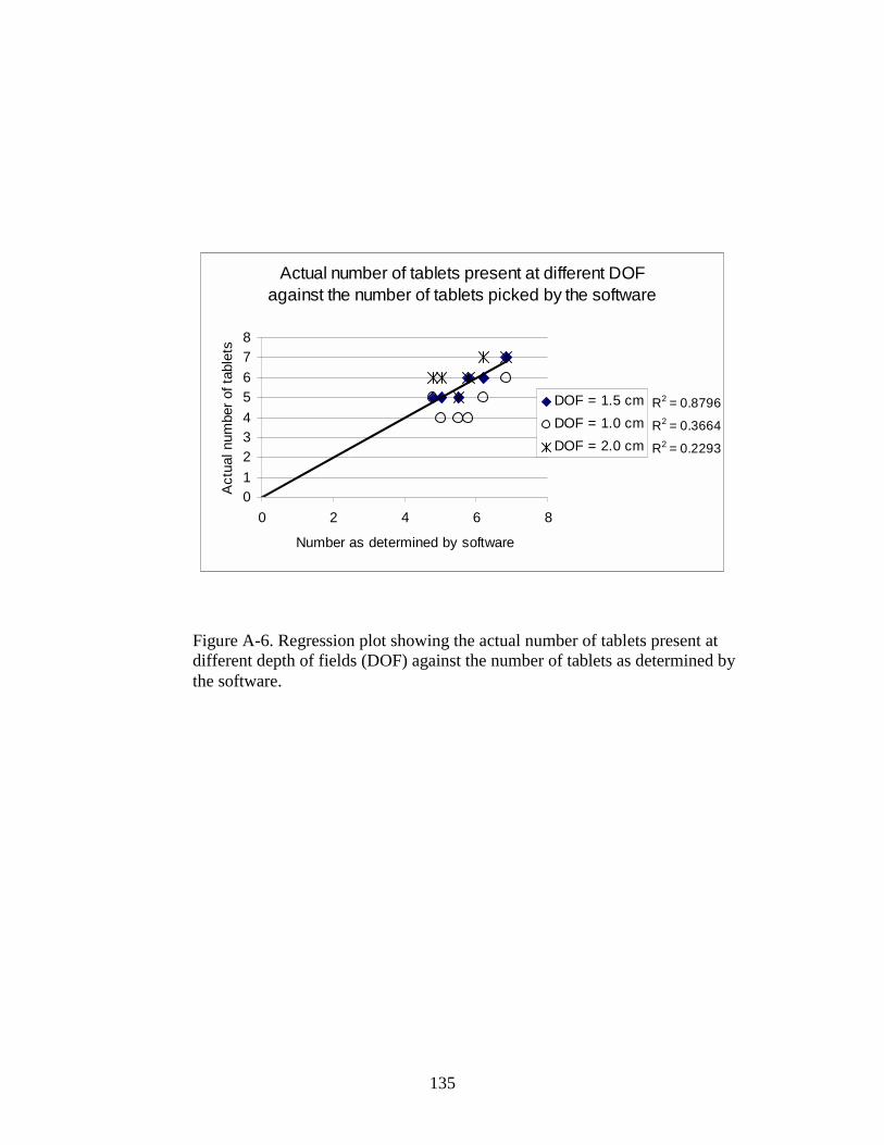
135
Figure A-6. Regression plot showing the actual number of tablets present atdifferent depth of fields (DOF) against the number of tablets as determined bythe software.
Actual number of tablets present at different DOF against the number of tablets picked by the software
R2 = 0.3664
R2 = 0.8796
R2 = 0.2293
0
1
2
3
4
5
6
7
8
0 2 4 6 8
Number as determined by software
Act
ual n
umbe
r of
tab
lets
DOF = 1.5 cm
DOF = 1.0 cm
DOF = 2.0 cm
136
Appendix V
Alignment of Cameras and Calibration of Pixel Size
Calibration of Pixel Size
The imaging system consisted of two CCD cameras (Sony XC – 75 CE CCD
Video camera, Sony Inc.,), equipped with Ultrak TV lensess (50 mm and aperture f 1.3)
with 8 mm extension rings, connected to separate frame grabbers (PX610 Precision
Frame Grabber, Imagenation Corporation, Beaverton, Oregon). The images acquired by
these cameras are viewed on the screen of a computer (486DX, 33 MHZ, Keydata
International Inc., S. Plainfield, NJ). The custom software written in Microsoft® Visual
Basic used to trigger the frame grabbers and the camera also calibrates the pixel size to
actual distance measured by the following routine.
Camera 1 is used as a reference for both pixel calibration and alignment. Camera
1 is focused on an object of known dimensions (a circle with cross hair of known
diameter) was used. The dimension of the focused object is entered into the program.
After obtaining a focused image, the calibrate pixel command is invoked. The software
asks the user to click on the left and right edges of the object. The software now counts
the number of pixels between the two edges. With these two values, the actual distance
between the two edges and the number of pixels required to measure the distance, the
software directly gives the actual distance one pixel represents. This value was
determined to be one pixel = 5.825 x 10⁻² m, which was maintained constant for all the
runs.
137
Alignment of cameras
The alignment of the cameras was a lengthy process and the following sequence
of events occurs before the final alignment is made and corrected for parallax error.
1) Positioning the Camera Stand
The optimum distance between the camera and the front glass sheet of the fluidized bed
was first determined. With variation in focusing caused by the camera lens and the
extension rings, several distances were tried before the distance between the cameras and
the fluidized bed was set. The criteria for this was to obtain a clear focused image and
obtain a field of view equal to the imaginary grid boxes of dimension 20 x 20 mm. After
finalizing the distance between the cameras and the fluidized bed, permanent marks were
made on the floor where the camera stand was placed and this position was used for all
the experimental runs.
2) Placing the Cameras on the Sliding Stand Mounted on the Camera Stand
The two cameras were placed on the sides of a steep isosceles triangle as shown in Figure
3-15, in order to minimize parallax effects. The greater the angle at the apex,θ, the greater
is the difference between the images from the two cameras. Both the cameras were
focused on the same object and effort was made to obtain the same FOV in both the
cameras. Camera 1 was used as the reference camera. At this point, the calibrate
alignment command is invoked in the software. The software prompts the user to click
on any particular fixed point (permanent marks made on the draft-tube shown in Figure
A-4.1 were used) on the image obtained from camera 1, and then the software prompts
the user to click on the same fixed point on the image obtained from camera 2. The
138
software determines the relative position of the two points clicked in the two images and
offsets the image obtained by camera 2 to match exactly the image obtained from camera
1. After this step, the accuracy of the alignment was verified by focusing the cameras on
stationary objects (a packed bed filled with the tablets) and running routines for the
velocity measurement. Random tablets are picked and the distance moved by these
particles in the time lag between the cameras determined. This value should be zero as
the tablets are not in motion. This process of alignment and verifying is repeated until the
software returns a value of 0 or close to 0 (maximum error allowed was a value equal to
two pixel sizes).
Once these processes of pixel size calibration and camera alignment were
completed, the cameras were secured and these positions were marked. The position and
alignment of the cameras were closely reproduced for all the experimental runs.
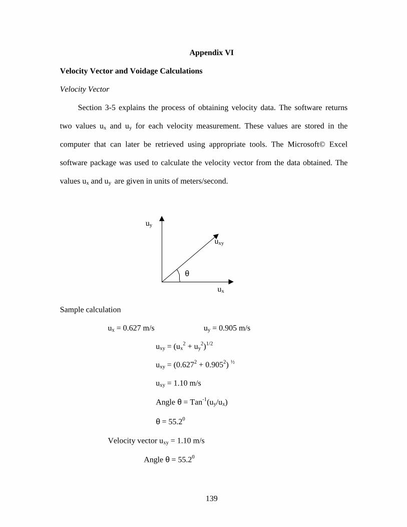
139
Appendix VI
Velocity Vector and Voidage Calculations
Velocity Vector
Section 3-5 explains the process of obtaining velocity data. The software returns
two values ux and uy for each velocity measurement. These values are stored in the
computer that can later be retrieved using appropriate tools. The Microsoft© Excel
software package was used to calculate the velocity vector from the data obtained. The
values ux and uy are given in units of meters/second.
Sample calculation
ux = 0.627 m/s uy = 0.905 m/s
uxy = (ux2 + uy
2)1/2
uxy = (0.6272 + 0.9052) ½
uxy = 1.10 m/s
Angle θ = Tan-1(uy/ux)
θ = 55.20
Velocity vector uxy = 1.10 m/s
Angle θ = 55.20
uy
ux
uxy
θ
140
Voidage Calculations
Principles of voidage measurement are explained in section 3-6. For each box in the imaginary
grid, the software returns an average number of particles in the FOV and DOF. Thus, we know
the volume element of the box over which the camera and software record particles and the
number of particles in that volume. Thus, we can obtain a value for voidage, a sample
calculation is shown below.
Average number of particles in the volume considered = 7.8
Volume of the box in which the particles were recorded = 2 cm x 2 cm x 1.5 cm
Volume of one tablet = 0.170 cm3 (from Appendix II, Table A-4)
ε = 1 – volume of particles/volume considered
ε = 1 – 7.8 * 0.170/ 2*2*1.5
ε = 0.78
ε = 78 %
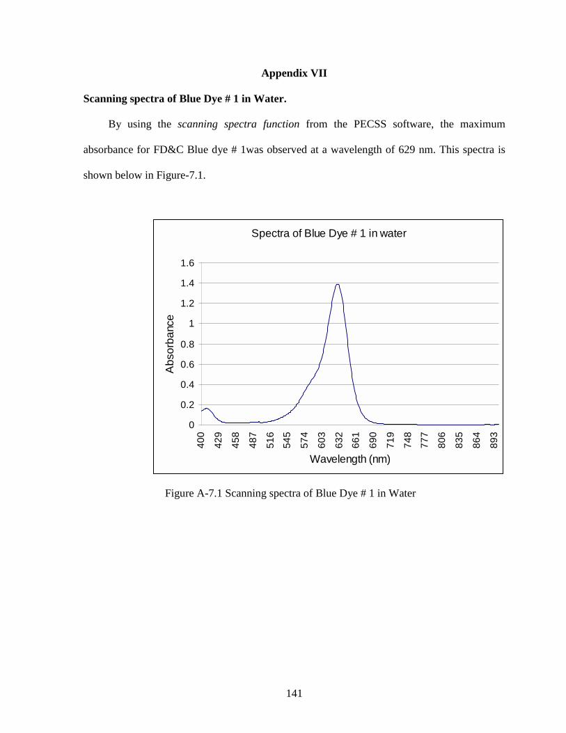
141
Appendix VII
Scanning spectra of Blue Dye # 1 in Water.
By using the scanning spectra function from the PECSS software, the maximum
absorbance for FD&C Blue dye # 1was observed at a wavelength of 629 nm. This spectra is
shown below in Figure-7.1.
Spectra of Blue Dye # 1 in water
0
0.2
0.4
0.6
0.8
1
1.2
1.4
1.6
40
0
42
9
45
8
48
7
51
6
54
5
57
4
60
3
63
2
66
1
69
0
71
9
74
8
77
7
80
6
83
5
86
4
89
3
Wavelength (nm)
Ab
sorb
anc
e
Figure A-7.1 Scanning spectra of Blue Dye # 1 in Water
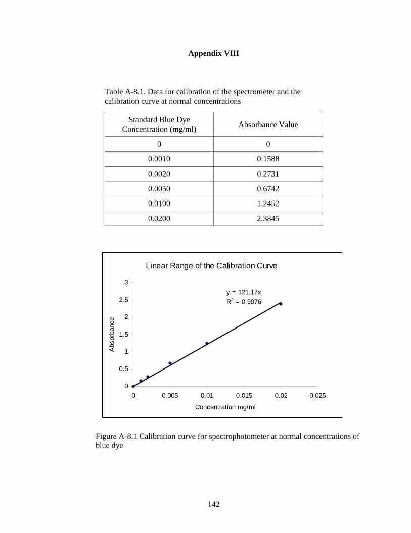
142
Appendix VIII
Standard Blue DyeConcentration (mg/ml)
Absorbance Value
0 0
0.0010 0.1588
0.0020 0.2731
0.0050 0.6742
0.0100 1.2452
0.0200 2.3845
Table A-8.1. Data for calibration of the spectrometer and thecalibration curve at normal concentrations
Linear Range of the Calibration Curve
y = 121.17x
R2 = 0.9976
0
0.5
1
1.5
2
2.5
3
0 0.005 0.01 0.015 0.02 0.025
Concentration mg/ml
Abs
orba
nce
Figure A-8.1 Calibration curve for spectrophotometer at normal concentrations ofblue dye
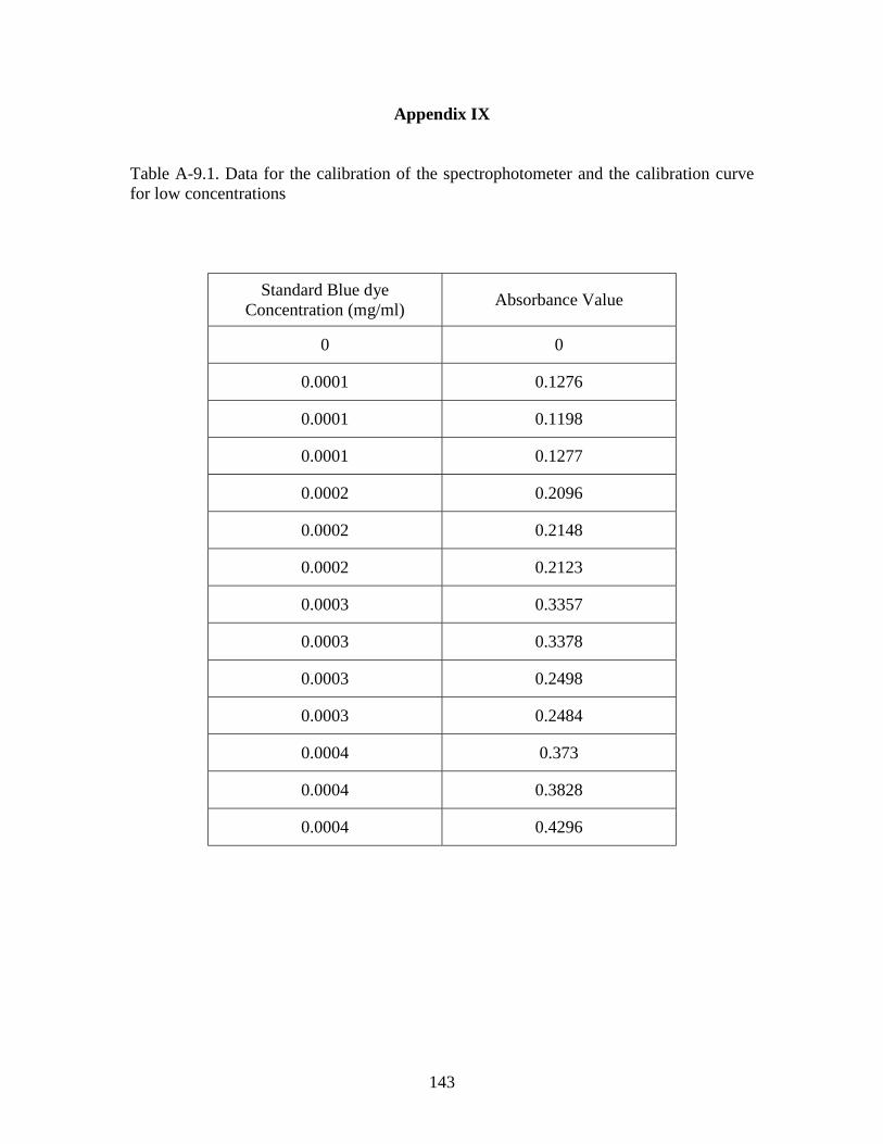
143
Appendix IX
Table A-9.1. Data for the calibration of the spectrophotometer and the calibration curvefor low concentrations
Standard Blue dyeConcentration (mg/ml)
Absorbance Value
0 0
0.0001 0.1276
0.0001 0.1198
0.0001 0.1277
0.0002 0.2096
0.0002 0.2148
0.0002 0.2123
0.0003 0.3357
0.0003 0.3378
0.0003 0.2498
0.0003 0.2484
0.0004 0.373
0.0004 0.3828
0.0004 0.4296
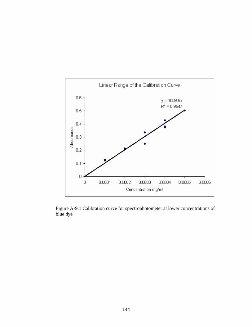
144
Figure A-9.1 Calibration curve for spectrophotometer at lower concentrations ofblue dye
145
Appendix X
Determination of Coating Formula
The flow rate of the coating solution = 10 ml/min.
Time to coat = 60 min.
Volume of Coating to be used = 600 ml
Density of the coating media = 1.00 g/ml, Surelease
Mass of the coating material = 1 * 550 = 550 gm
Amount of water added = 50 ml
Amount of Blue dye added = 2.5 gm
Total weight of coating mixture = 552.5 gm
Total weight of the particles to be coated = 3.675 kg
Average weight of each particle = 0.205 gm
Average number of particle in the bed = 17.93 *10 3
Average wt of blue dye/particle = 2.5/17.93 * 10 3 = 1.4 * 10 – 4 gm
15 ml of water was used to dissolve the blue dye from the tablet, thus the blue
dye concentration will be = 0.14 mg/15 ml
= 0.009 mg/ml
The calculations above are based on 100% efficiency. Considering an efficiency rage of
70% to 80%, the concentration of blue dye/tablet will fall in the range of 0.0063mg/ml to
0.0072 mg/ml. The optimum concentration required to obtain a good absorbance value was
in the rage of 0.006 mg/ml to 0.009 mg/ml.
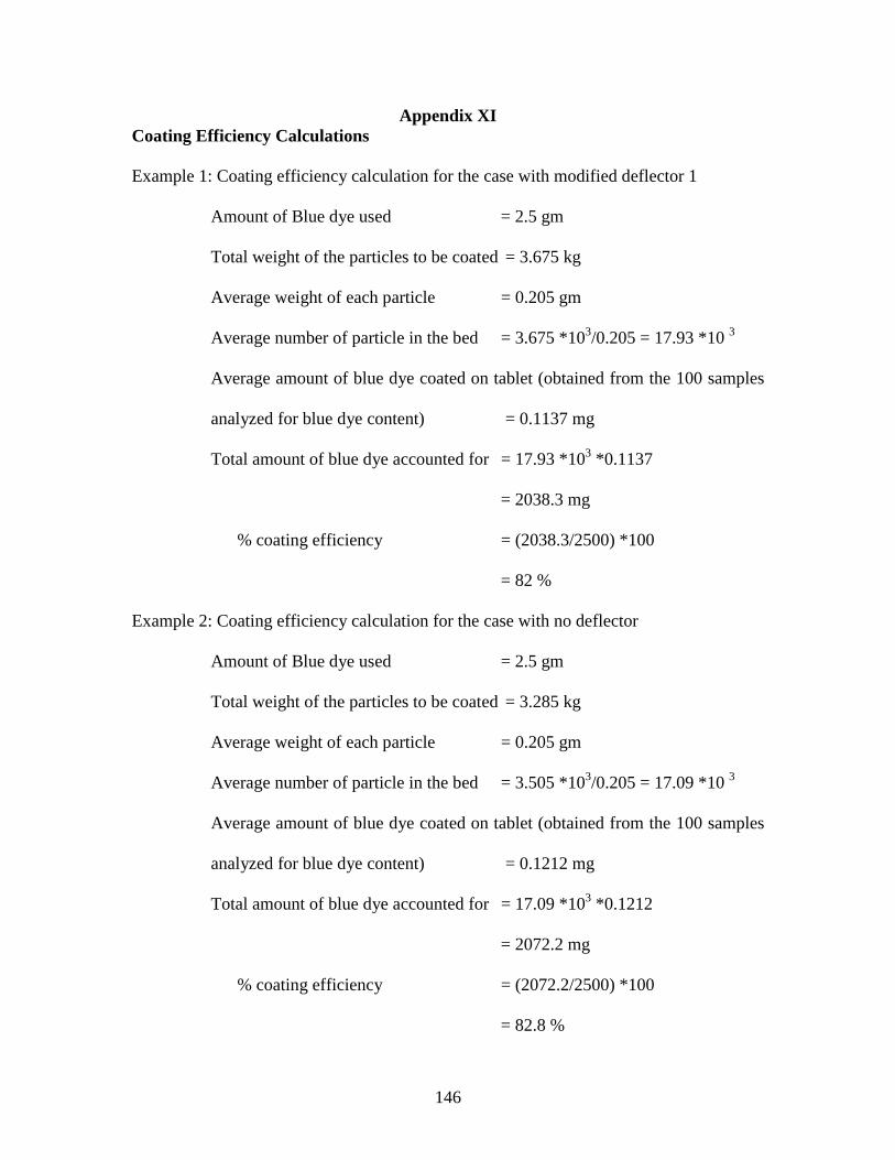
146
Appendix XICoating Efficiency Calculations
Example 1: Coating efficiency calculation for the case with modified deflector 1
Amount of Blue dye used = 2.5 gm
Total weight of the particles to be coated = 3.675 kg
Average weight of each particle = 0.205 gm
Average number of particle in the bed = 3.675 *103/0.205 = 17.93 *10 3
Average amount of blue dye coated on tablet (obtained from the 100 samples
analyzed for blue dye content) = 0.1137 mg
Total amount of blue dye accounted for = 17.93 *103 *0.1137
= 2038.3 mg
% coating efficiency = (2038.3/2500) *100
= 82 %
Example 2: Coating efficiency calculation for the case with no deflector
Amount of Blue dye used = 2.5 gm
Total weight of the particles to be coated = 3.285 kg
Average weight of each particle = 0.205 gm
Average number of particle in the bed = 3.505 *103/0.205 = 17.09 *10 3
Average amount of blue dye coated on tablet (obtained from the 100 samples
analyzed for blue dye content) = 0.1212 mg
Total amount of blue dye accounted for = 17.09 *103 *0.1212
= 2072.2 mg
% coating efficiency = (2072.2/2500) *100
= 82.8 %
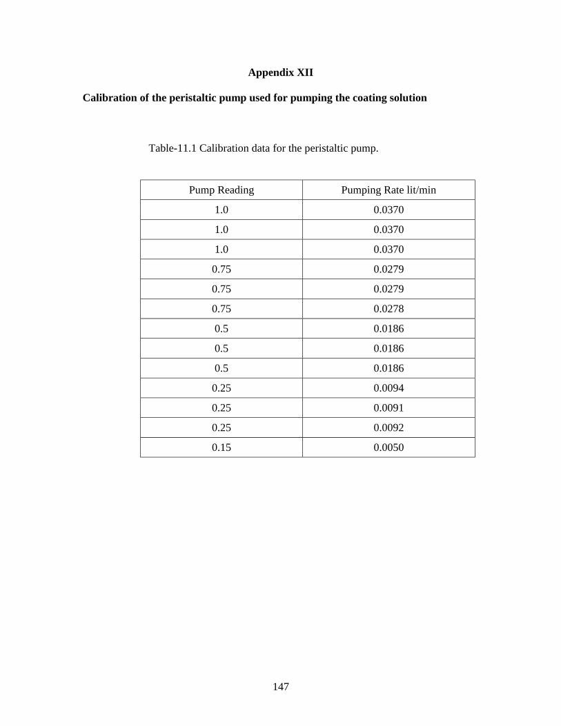
147
Appendix XII
Calibration of the peristaltic pump used for pumping the coating solution
Table-11.1 Calibration data for the peristaltic pump.
Pump Reading Pumping Rate lit/min
1.0 0.0370
1.0 0.0370
1.0 0.0370
0.75 0.0279
0.75 0.0279
0.75 0.0278
0.5 0.0186
0.5 0.0186
0.5 0.0186
0.25 0.0094
0.25 0.0091
0.25 0.0092
0.15 0.0050
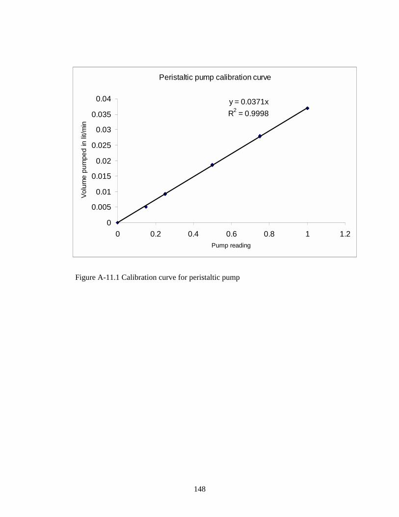
148
Peristaltic pump calibration curve
y = 0.0371x
R2 = 0.9998
0
0.005
0.01
0.015
0.02
0.025
0.03
0.035
0.04
0 0.2 0.4 0.6 0.8 1 1.2
Pump reading
Vo
lum
e p
um
pe
d in
lit/
min
Figure A-11.1 Calibration curve for peristaltic pump
149
Appendix XIII
Calculation of Amount of Blue Dye Coated during the Pulse Test
During the pulse test, the tablets pass through the spray zone only once and the
amount of blue dye coated on them is very small, making it difficult to measure. To
obtain blue dye concentrations in the detectable range the solution used for pulse tests
was saturated with blue dye and the amount of water used to dissolve the blue off the
tablets was kept at the lowest possible amount. Even so, the blue dye content fell in the
lower part of the detectable range of the spectrophotometer and a low concentration
calibration curve shown in Appendix IX had to be used. The software, PECSS version
4.0, used with the spectrometer could calculate values only up to the fourth decimal value
and hence when values less than that were calculated, they were rounded off to 0. Hence,
even though the spectrometer detected different values of absorbance for the samples, the
software sometimes gave the same (zero) concentration values. Therefore, for the pulse
tests the value of blue dye concentration was calculated by substituting the value of
absorbance in a linear equation that related absorbance to blue dye concentration shown
in the Appendix IX rather than using the results from the PECCS software.
Equation relating the absorbance to concentration obtained from the graph is
Concentration mg/ml = Absorbance /1009.5 ………From Graph A-9.1
For example:
If the absorbance value obtained was = 0.0015
Concentration = 0.0015/1009.5 = 1.48588E-06 mg/ml
Amount of blue dye mg/tablet (when dissolved in ml of water) = (3)* 1.48588E-06
= 4.45765E-06 mg/tablet
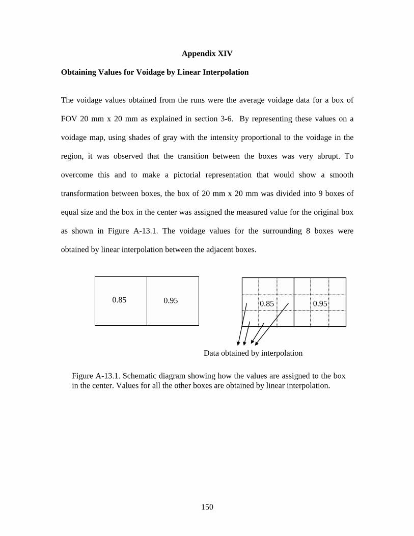
150
Appendix XIV
Obtaining Values for Voidage by Linear Interpolation
The voidage values obtained from the runs were the average voidage data for a box of
FOV 20 mm x 20 mm as explained in section 3-6. By representing these values on a
voidage map, using shades of gray with the intensity proportional to the voidage in the
region, it was observed that the transition between the boxes was very abrupt. To
overcome this and to make a pictorial representation that would show a smooth
transformation between boxes, the box of 20 mm x 20 mm was divided into 9 boxes of
equal size and the box in the center was assigned the measured value for the original box
as shown in Figure A-13.1. The voidage values for the surrounding 8 boxes were
obtained by linear interpolation between the adjacent boxes.
0.85 0.95 0.85 0.95
Data obtained by interpolation
Figure A-13.1. Schematic diagram showing how the values are assigned to the boxin the center. Values for all the other boxes are obtained by linear interpolation.

151
As an example, the calculation to determine the voidage value for the shaded box, from
the values in the adjacent boxes, is shown below.
The equation used for this interpolation is shown below
A similar form of this equation is used to interpolate in the vertical direction. For boxes
lying around the edge of the bed, linear extrapolation is used.
0.85 0.95
ini
i
xx
xx
ini
i
xx
xx
εεεε
−−
=−
−
++
xi x xi+n
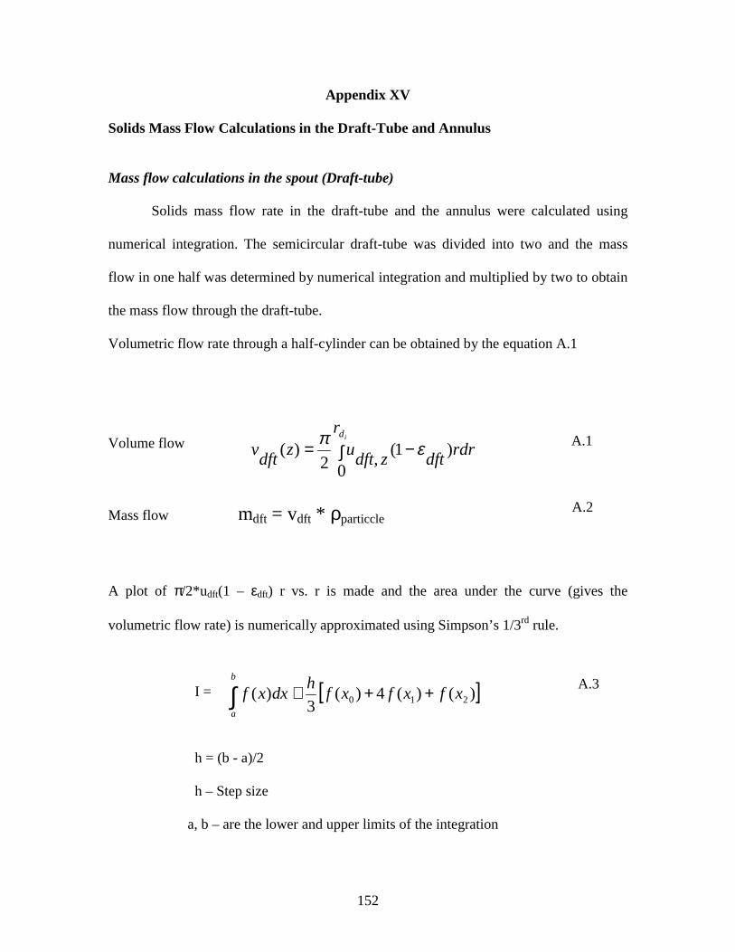
152
Appendix XV
Solids Mass Flow Calculations in the Draft-Tube and Annulus
Mass flow calculations in the spout (Draft-tube)
Solids mass flow rate in the draft-tube and the annulus were calculated using
numerical integration. The semicircular draft-tube was divided into two and the mass
flow in one half was determined by numerical integration and multiplied by two to obtain
the mass flow through the draft-tube.
Volumetric flow rate through a half-cylinder can be obtained by the equation A.1
Volume flow
Mass flow mdft = vdft * ρparticcle
A plot of π/2*udft(1 – εdft) r vs. r is made and the area under the curve (gives the
volumetric flow rate) is numerically approximated using Simpson’s 1/3rd rule.
I =
h = (b - a)/2
h – Step size
a, b – are the lower and upper limits of the integration
rdrdft
r
zdftuz
dftv
id
)1(0
,2)( επ −∫= A.1
[ ]∫ ++≅b
a
xfxfxfh
dxxf )()(4)(3
)( 210
A.2
A.3
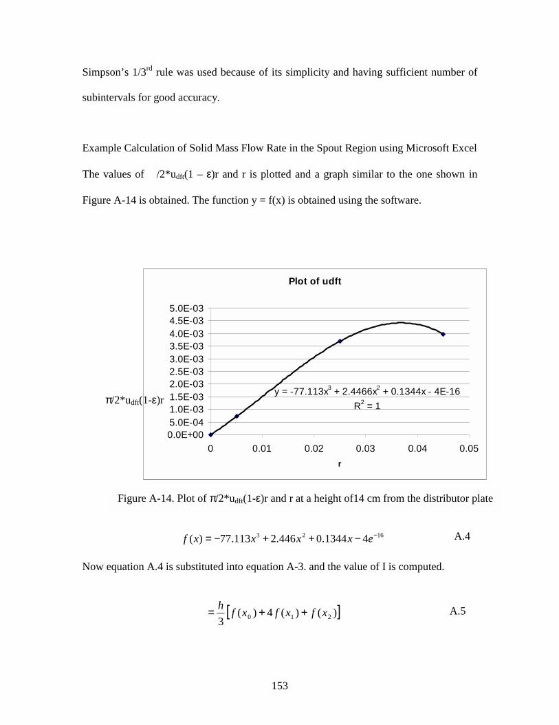
153
Simpson’s 1/3rd rule was used because of its simplicity and having sufficient number of
subintervals for good accuracy.
Example Calculation of Solid Mass Flow Rate in the Spout Region using Microsoft Excel
The values of �/2*udft(1 – ε)r and r is plotted and a graph similar to the one shown in
Figure A-14 is obtained. The function y = f(x) is obtained using the software.
Now equation A.4 is substituted into equation A-3. and the value of I is computed.
Plot of udft
y = -77.113x3 + 2.4466x2 + 0.1344x - 4E-16
R2 = 1
0.0E+005.0E-041.0E-031.5E-032.0E-032.5E-033.0E-033.5E-034.0E-034.5E-035.0E-03
0 0.01 0.02 0.03 0.04 0.05
r
π/2*udft(1-ε)r
1623 41344.0446.2113.77)( −−++−= exxxxf A.4
[ ])()(4)(3 210 xfxfxfh ++= A.5
Figure A-14. Plot of π/2*udft(1-ε)r and r at a height of14 cm from the distributor plate
154
x0 = 0.005 x1 = 0.025 x2 = 0.045
h = (0.045 – 0.005)/2 = 0.02
Substituting the values into equation A.5 the value of I is determined.
I = 0.000129573
vdft = 2*( 0.000129573) = 2.59 x 10⁻⁴ m3/s
Mass flow = vdft * ρparticle
Mass flow = 2.59 x 10-4 * 1.215 *103 (m3/s)(kg/m3)
Mass flow = 0.32 kg/s
The mass flux at different heights from the distributor plate is calculated in a similar
fashion and then they are averaged to obtain the average mass flux in the draft-tube.
Mass flow calculations in the annulus.
The voidage in the annulus was assumed to be equal to the packed bed voidage was also
assumed a constant. The downward velocity of the particles in the annulus was assumed
the same across the annulus and assumed a constant. With the above assumptions of
constant voidage and velocity across the annulus the equation A.1 can be written as
Volume flow
This equation can now be integrated directly and the mass flow rate can be determined by
multiplying the value obtained with the particle density.
rdrR
ranulzanul
uzanul
v
od
∫−= )1(,2
)( επ A.6
155
Mass flow manul = vanul * ρparticcle
Substituting values into equation A.6
vanul = π/2 (0.054 m/s)* (1- 0.42) ∫45.11
35.6
rdr
vanul = π/2 (0.054 m/s)* (1- 0.42) * {[ (0.1145)^2 – (0.0635)^2]/2}
Mass flow = 2.23 x10⁻⁴ m3/s * 1.215x10³ kg/m3
Mass Flow = 0.273 kg/s
A.7
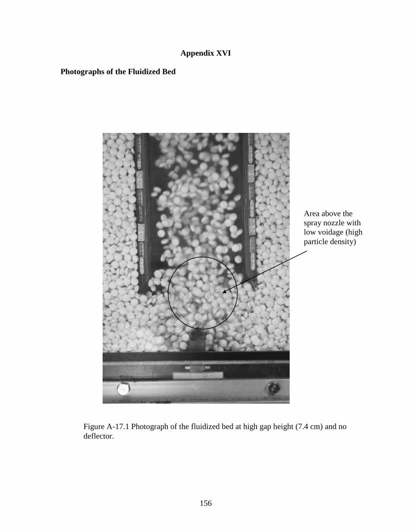
156
Appendix XVI
Photographs of the Fluidized Bed
Figure A-17.1 Photograph of the fluidized bed at high gap height (7.4 cm) and nodeflector.
Area above thespray nozzle withlow voidage (highparticle density)
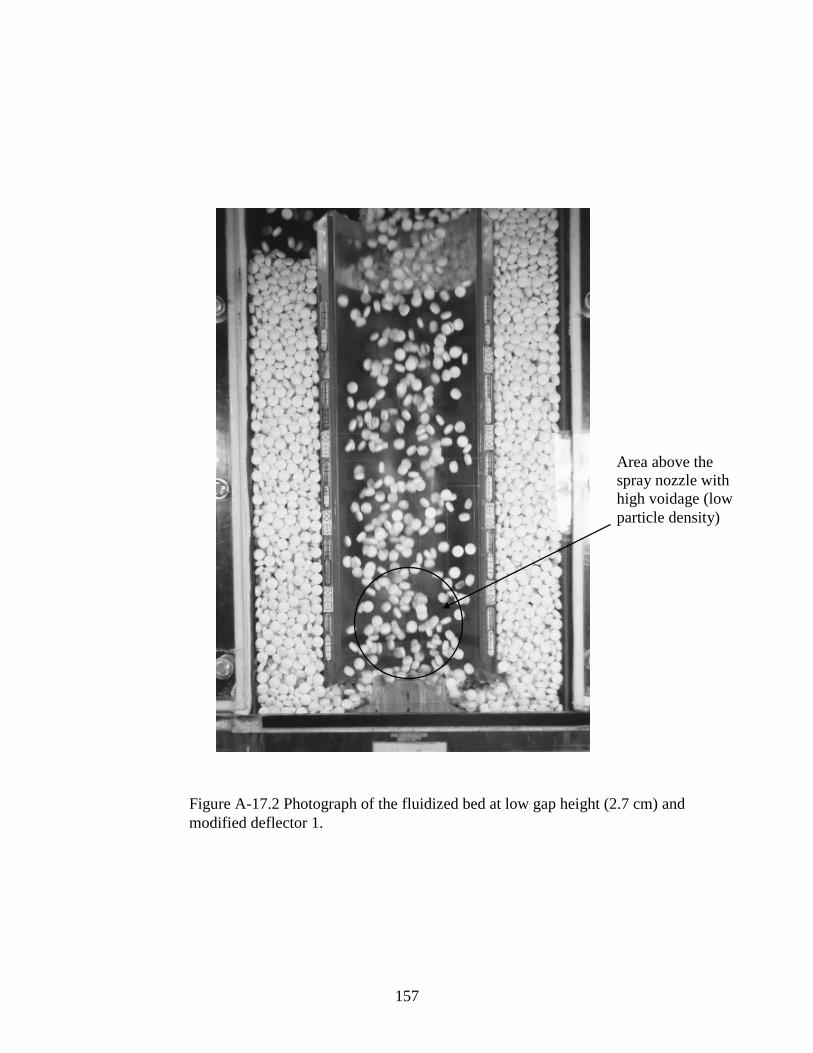
157
Area above thespray nozzle withhigh voidage (lowparticle density)
Figure A-17.2 Photograph of the fluidized bed at low gap height (2.7 cm) andmodified deflector 1.

158
Area above thespray nozzle withhigh voidage (lowparticle density)
Figure A-17.3 Photograph of the fluidized bed at high gap height (7.4 cm) andmodified deflector 1.
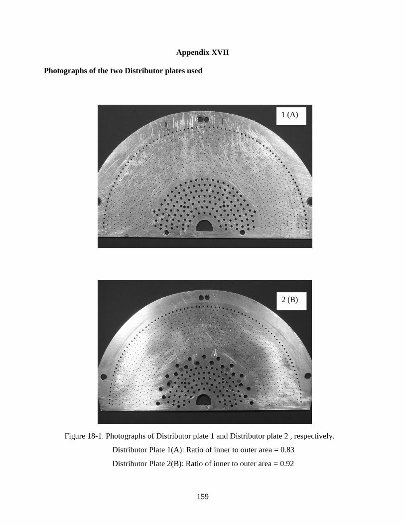
159
Appendix XVII
Photographs of the two Distributor plates used
Figure 18-1. Photographs of Distributor plate 1 and Distributor plate 2 , respectively.
Distributor Plate 1(A): Ratio of inner to outer area = 0.83
Distributor Plate 2(B): Ratio of inner to outer area = 0.92
1 (A)
2 (B)


![Cleaning Before Coating - SMTA · Deposition Me Men+ + ne* ne* + Men+ Me ... PU-coating AY-coating , Wax coating ed m 2] ... Cleaning Before Coating](https://img.pdfslide.us/doc/110x75/5ad9e7b37f8b9a53618bdbed/cleaning-before-coating-smta-me-men-ne-ne-men-me-pu-coating-ay-coating.jpg)