Coastal-ocean uptake of anthropogenic carbon · to observation-based estimates. Simulated global uptake of anthropogenic carbon results averaged 2.3PgCyr1 during the years 1993–2012,

Biogeosciences, 13, 4167–4185, 2016www.biogeosciences.net/13/4167/2016/doi:10.5194/bg-13-4167-2016© Author(s) 2016. CC Attribution 3.0 License.

Coastal-ocean uptake of anthropogenic carbonTimothée Bourgeois1, James C. Orr1, Laure Resplandy2, Jens Terhaar1, Christian Ethé3, Marion Gehlen1, andLaurent Bopp1

1Laboratoire des Sciences du Climat et de l’Environnement, LSCE/IPSL, CEA-CNRS-UVSQ, Université Paris-Saclay,91191 Gif-sur-Yvette, France2Scripps Institution of Oceanography, University of California San Diego, La Jolla, CA, USA3Institut Pierre Simon Laplace, 4 Place Jussieu, 75005 Paris, France

Correspondence to: Timothée Bourgeois ([email protected])

Received: 18 February 2016 – Published in Biogeosciences Discuss.: 22 February 2016Revised: 15 June 2016 – Accepted: 17 June 2016 – Published: 22 July 2016

Abstract. Anthropogenic changes in atmosphere–ocean andatmosphere–land CO2 fluxes have been quantified exten-sively, but few studies have addressed the connection be-tween land and ocean. In this transition zone, the coastalocean, spatial and temporal data coverage is inadequate toassess its global budget. Thus we use a global ocean biogeo-chemical model to assess the coastal ocean’s global inven-tory of anthropogenic CO2 and its spatial variability. We usedan intermediate resolution, eddying version of the NEMO-PISCES model (ORCA05), varying from 20 to 50 km hor-izontally, i.e. coarse enough to allow multiple century-scale simulations but finer than coarse-resolution models(∼ 200 km) to better resolve coastal bathymetry and complexcoastal currents. Here we define the coastal zone as the con-tinental shelf area, excluding the proximal zone. Evaluationof the simulated air–sea fluxes of total CO2 for 45 coastal re-gions gave a correlation coefficient R of 0.8 when comparedto observation-based estimates. Simulated global uptake ofanthropogenic carbon results averaged 2.3 PgCyr−1 duringthe years 1993–2012, consistent with previous estimates. Yetonly 0.1 PgCyr−1 of that is absorbed by the global coastalocean. That represents 4.5 % of the anthropogenic carbonuptake of the global ocean, less than the 7.5 % proportionof coastal-to-global-ocean surface areas. Coastal uptake isweakened due to a bottleneck in offshore transport, whichis inadequate to reduce the mean anthropogenic carbon con-centration of coastal waters to the mean level found in theopen-ocean mixed layer.

1 Introduction

The ocean mitigates climate change by absorbing atmo-spheric CO2 produced by combustion of fossil fuels, land-use change, and cement production. During the 2005–2014period, the global ocean absorbed 2.6± 0.5 PgCyr−1 of an-thropogenic carbon, an estimated 26 % of the total anthro-pogenic CO2 emissions (Le Quéré et al., 2015). The globalanthropogenic carbon budget relies on separate estimates foratmosphere, land, and ocean reservoirs. Yet it neglects whathappens in the aquatic continuum between land and ocean(Cai, 2011; Regnier et al., 2013), for which there is no con-sensus on anthropogenic carbon uptake (Wanninkhof et al.,2013; Mackenzie et al., 2004; Bauer et al., 2013; Regnieret al., 2013; Le Quéré et al., 2015; Ciais et al., 2013).

The land–ocean aquatic continuum includes inland waters,estuaries, and the coastal ocean, i.e. the succession of activephysical–biogeochemical systems that connect upland terres-trial soils to the open ocean (Regnier et al., 2013). Our fo-cus here is on the coastal ocean, which plays an inordinatelylarge role relative to the open ocean in terms of primary pro-ductivity, export production, and carbon burial. Although thecoastal ocean covers only 7–10 % of the global ocean sur-face area, it accounts for up to 30 % of oceanic primary pro-duction, 30–50 % of oceanic inorganic carbon burial, and80 % of oceanic organic carbon burial (Gattuso et al., 1998;Longhurst et al., 1995; Walsh, 1991); moreover, the coastal-ocean supplies about half of the organic carbon that is deliv-ered to the deep open ocean (Liu et al., 2010). All these esti-mates suffer from high uncertainties as do those for coastal-ocean air–sea CO2 exchange (Laruelle et al., 2014), particu-

Published by Copernicus Publications on behalf of the European Geosciences Union.

4168 T. Bourgeois et al.: Air–sea flux of anthropogenic CO2 in the global coastal ocean

larly its anthropogenic component. Indeed, in addition to theeffect of increasing atmospheric CO2, potential changes incoastal-ocean physics (e.g. temperature) and biology (e.g. netecosystem production) as well as changes in riverine input,and interactions with the sediment may be of primary im-portance (Mackenzie et al., 2004; Hu and Cai, 2011). Thesechanges would modify the distribution of carbon and alkalin-ity, hence change the potential of the coastal ocean to absorbanthropogenic carbon.

To date, few studies have distinguished anthropogenic car-bon uptake by the global coastal ocean. Estimating air–seafluxes of anthropogenic CO2 in the coastal ocean would re-quire multi-decadal time series of coastal CO2 observationsin order to extract an anthropogenic signal from the strongcoastal natural variability. Such time series are still rare andprobably not long enough. To our knowledge, the only avail-able equivalent time series are the Ishii et al. (2011) 1994–2008 time series along 137◦ E on Japanese coasts and theAstor et al. (2013) 1996–2008 time series at the CARIACOstation on Venezuelan coasts. Therefore, estimates of anthro-pogenic carbon uptake by the global coastal ocean have beenbased on modelling studies, extrapolating data and modeloutput from the open-ocean, and estimating residuals withbudget calculations. An early modelling approach was pro-posed by Andersson and Mackenzie (2004) and Mackenzieet al. (2004). They used a 2-box model (Shallow-water OceanCarbonate Model, SOCM) that separated the coastal oceaninto surface waters and sediment pore waters. They estimatedthat the preindustrial coastal ocean was a source of CO2 tothe atmosphere and had recently switched to a CO2 sink.This source-to-sink switch is mainly caused by a shift in netecosystem production (NEP) due to increased anthropogenicnutrient inputs (Andersson and Mackenzie, 2004; Mackenzieet al., 2004). Another proposed mechanism is simply linkedto the anthropogenic increase in atmospheric CO2, consider-ing constant NEP (Bauer et al., 2013). The difference be-tween the simulated air–sea CO2 fluxes from the SOCMmodel for the years 1700 and 2000 suggests that in 2000 thecoastal ocean absorbed 0.17 PgCyr−1 of anthropogenic car-bon from the atmosphere (Borges, 2005). As for extrapola-tion, Wanninkhof et al. (2013) used coarse-resolution global-ocean models and observations and estimated a similar up-take of 0.18 PgCyr−1 by extrapolating open-ocean air–seafluxes of anthropogenic CO2 into the coastal zone. Finally,Liu et al. (2010) combined estimates from the same SOCMmodel for the preindustrial coastal zone with observationalestimates of the contemporary flux to deduce a correspondinganthropogenic carbon uptake of 0.5 PgCyr−1 for the 1990s.

In addition, there exist 3-D regional-circulation–biogeochemistry–ecosystem models that have been used tostudy other aspects of coastal-ocean carbon cycling as sum-marized by Hofmann et al. (2011). Typically, such modelshave been implemented in regions where sufficient measure-ments are available for model validation, e.g. the MiddleAtlantic Bight (eastern US coast) (Fennel et al., 2008;

Fennel, 2010), the California current system (Fiechter et al.,2014; Turi et al., 2014; Lachkar and Gruber, 2013), and theEuropean shelf seas (Artioli et al., 2014; Phelps et al., 2014;Wakelin et al., 2012; Allen et al., 2001; Cossarini et al.,2015; Prowe et al., 2009). Because of their limited regionaldomains, such models are typically able to make simulationswith horizontal resolutions of 10 km or less, which remainsa challenge for global-circulation–biogeochemical models.The reduced computational requirements of regional modelsalso allow biogeochemistry and ecosystem components tobe more complex. Unfortunately, joining together a networkof regional models to allow efficient simulations that coverall parts of the global coastal ocean remains a technicalchallenge (Holt et al., 2009).

The alternative to using a global model is computa-tionally more challenging because few of them have ade-quate resolution to properly simulate many critical coastal-ocean processes (Griffies et al., 2010; Holt et al., 2009).Coarse-resolution global models fail to adequately resolvethe coastal bathymetry, which substantially alters coastal-ocean circulation (Fiechter et al., 2014) as well as mesoscaledynamics, upwelling, and coastal currents, all of which arethought to strongly affect the variability of air–sea CO2fluxes along ocean margins (Borges, 2005; Lachkar et al.,2007; Kelley et al., 1971). Global models also typically lack abenthic component, i.e. early diagenesis in sediments, whichin some regions is likely to affect simulated coastal-oceanbiogeochemistry of overlying waters. Moreover, input of car-bon and nutrients from rivers and groundwater is usuallylacking. Even in models such as ours, where that input isimposed as boundary conditions (Aumont et al., 2015), tem-poral variability and trends are neglected (Bauer et al., 2013;Cotrim da Cunha et al., 2007).

Nonetheless, coarse-resolution models are no longer stateof the art. Recently, there have been improvements in spatialresolution of global ocean models and the spatio-temporalresolution of surface forcing fields (Brodeau et al., 2010),thereby improving the representation of bathymetry andocean processes in the highly variable coastal zone (Capet,2004; Hofmann et al., 2011; McKiver et al., 2014). In anycase, models currently provide the only means to estimatecoastal uptake of anthropogenic carbon due to the lack ofdata-based estimates.

Here our aim is to estimate the air-to-sea flux of anthro-pogenic CO2 into the coastal ocean and how it varies fromregion to region across the globe. We focus solely on thegeochemical effect of anthropogenic CO2 addition from theatmosphere to the ocean and neglect the role of varying riverinput and interactions with the sediment, as well as feedbackfrom a changing climate. To do so, we rely on an eddying ver-sion of the global NEMO circulation model (Madec, 2008),which also includes the LIM2 sea ice model and is coupledto the PISCES biogeochemical model (Aumont and Bopp,2006). More precisely, we use the ORCA05 eddy-admittingresolution, which ranges from 0.2 to 0.5◦ (i.e. 20 to 50 km).

Biogeosciences, 13, 4167–4185, 2016 www.biogeosciences.net/13/4167/2016/

T. Bourgeois et al.: Air–sea flux of anthropogenic CO2 in the global coastal ocean 4169

Although this resolution does not fully resolve coastal-oceanbathymetry and dynamics, it does provide a first step into theeddying regime and a starting point upon which to comparefuture studies that will model the coastal ocean, globally, athigher resolution.

2 Methods

2.1 Coupled physical–biogeochemical model

For this study, we use version 3.2 of the ocean modelknown as NEMO (Nucleus for European Modelling of theOcean), which includes (1) the primitive equation modelOcéan Parallélisé (OPA, Madec, 2008), (2) the dynamic-thermodynamic Louvain-La-Neuve sea ice model (LIM,Fichefet and Morales Maqueda, 1997), and (3) the Tracer inthe Ocean Paradigm (TOP), a passive tracer module. Herethe latter is connected to version 1 of the ocean biogeo-chemical model PISCES (Pelagic Interaction Scheme forCarbon and Ecosystem Studies) (Aumont and Bopp, 2006).For the NEMO model, we use a global-scale configurationfrom the DRAKKAR community (see Barnier et al., 2006;Timmermann et al., 2005). Namely, we use the ORCA05global configuration, which possesses a curvilinear, tripolargrid with a horizontal resolution that ranges between 0.2◦

near the North Pole to 0.5◦ at the Equator (Fig. 1). Verti-cally, ORCA05 is discretized into 46 levels with thicknessesthat range from 6 m at the surface to 250 m for the deepestocean level (centred at 5625 m). Model bathymetry is com-puted from the 2 min bathymetry file ETOPO2 from the Na-tional Geophysical Data Center. The numerical characteris-tics of our ORCA05 configuration follow the lead of Barnieret al. (2006) for the ORCA025 configuration with resolution-dependent modifications for the horizontal eddy diffusivityfor tracers modified to 600 m2 s−1 and horizontal eddy vis-cosity fixed to −4× 1011 m2 s−1. To simulate the advectivetransport driven by geostrophic eddies, our ORCA05 simu-lation uses the eddy parameterization scheme of Gent andMcWilliams (1990) applied with an eddy diffusion coeffi-cient of 1000 m2s−1.

The biogeochemical model PISCES includes four plank-ton functional types: two phytoplankton (nanophytoplank-ton and diatoms) and two zooplankton (micro- and mesozoo-plankton). PISCES also uses a mixed-quota Monod approachwhere (1) phytoplankton growth is limited by five nutrients(nitrate, ammonium, phosphate iron, and silicate), followingMonod (1949) and (2) elemental ratios of Fe, Si, and Chl to Care prognostic variables based on the external concentrationsof the limiting nutrients. In addition PISCES assumes a fixedC : N : P Redfield ratio set to 122 : 16 : 1 from Takahashi et al.(1985) for both living and non-living pools. Similar to Gei-der et al. (1998), the phytoplankton Chl:C ratio in PISCESvaries with photoadaptation. Furthermore, PISCES includesnon-living pools, namely a pool of semilabile dissolved or-

ganic matter and two size classes of particulate organic mat-ter. PISCES also explicitly accounts for biogenic silica andcalcite particles. In PISCES, the sediment–water interface istreated as a reflective boundary condition where mass fluxesfrom particles are remineralized instantaneously, except thatsmall proportions of particle fluxes of organic matter, calcite,and biogenic silica escape the system through burial. Thoseburial rates are hence dependent on the local sinking fluxes,but are set to balance inputs from rivers and atmospheric de-position at the global scale. Thus global budgets of alkalinityand nutrients are balanced. For further details, we refer read-ers to Aumont and Bopp (2006).

To simulate carbon chemistry and air–sea CO2 fluxes,the model follows the protocol from phase 2 of the OceanCarbon-Cycle Model Intercomparison Project (OCMIP, Na-jjar and Orr, 1999) protocol. The sea-to-air CO2 flux FCO2 iscomputed using the following equation:

FCO2 = α k1pCO2, (1)

where α is the solubility of CO2 computed from Weiss(1974) and1pCO2 is the difference between the partial pres-sures of sea surface and atmospheric CO2. Thus FCO2 is pos-itive when CO2 is transferred from the ocean to the atmo-sphere. The piston velocity k is based on Eq. (3) of Wan-ninkhof (1992):

k = 0.30 u2w

√660Sc(1− fice), (2)

where uw is the wind speed at 10 m, Sc is the CO2 Schmidtnumber, and fice is the ice fraction.

2.2 Simulations

The dynamic model was started from rest and spun up for50 years. Initial conditions for temperature and salinity areas described by Barnier et al. (2006). Initial biogeochemicalfields of nitrate, phosphate, oxygen, and silicate are from the2001 World Ocean Atlas (Conkright et al., 2002), whereaspreindustrial dissolved inorganic carbon (DIC) and total al-kalinity (Alk) come from the GLODAP gridded product (Keyet al., 2004). Conversely, because data for iron and dissolvedorganic carbon (DOC) are more limited, both those fieldswere initialized with model output from a 3000-year spin upsimulation of a global 2◦ configuration of the same NEMO-PISCES model (Aumont and Bopp, 2006). All other biogeo-chemical tracers have much shorter timescales; hence, theywere initialized to globally uniform constants.

After the 50-year spin-up, we launched two parallel simu-lations: the first was a historical simulation run from 1870to 2012 (143 years), and forced with a spatially uniformand temporally increasing atmospheric mole fraction of CO2(from which PISCES computes atmospheric pCOatm

2 follow-ing OCMIP2) reconstructed from ice core and atmosphericrecords (Le Quéré et al., 2014); the second simulation is a

www.biogeosciences.net/13/4167/2016/ Biogeosciences, 13, 4167–4185, 2016


Figure 1. (a) Global segmentation of the coastal ocean following Laruelle et al. (2013) as regridded on the ORCA05 model grid. Coloursdistinguish limits between the MARCATS regions, numbers indicate regions defined in LA13. To perceive the spatial resolution of theORCA05 configuration in the MARCATS context, we show zoomed-in images of bathymetry in four regions: (b) the Arctic polar margins,(c) the North Sea, (d) the Sea of Japan, the China Sea, and Kuroshio, and (e) south-western Africa and the Agulhas current. In the latter threepanels, grid resolution is indicated by thin black lines.

parallel control run, where the 143-year simulation is identi-cal except that it is forced with the preindustrial level of at-mospheric mole fraction of CO2 (287 ppm, constant in time).The preindustrial reference year is defined as 1870, thusneglecting changes in anthropogenic carbon storage in theocean from 1750 to 1870. The FCO2 computed with the his-torical simulation is for total carbon (total FCO2 ), whereas the

FCO2 from the control simulation is for natural carbon (nat-ural FCO2 ). The corresponding anthropogenic FCO2 is com-puted as the total minus natural FCO2 .

All simulations were forced identically with atmosphericfields from the DRAKKAR Forcing Set (DFS, Brodeau et al.,2010). These fields include zonal and meridional compo-nents of 10 m winds, 2 m air humidity, 2 m air tempera-



ture, downward shortwave and longwave radiation at thesea surface, and precipitation. More specifically the NEMO-PISCES model is forced with version 4.2 of this forcing(DFS4.2, based on the ERA40 reanalysis) over 1958–2001,and that is followed by forcing from version 4.4 (DFS4.4)over 2002–2012. For the 1870–1957 period, where atmo-spheric reanalyses are unavailable, we repeatedly cycled the1958–2007 DFS4.2 forcing.

Boundary conditions are also needed for biogeochemicaltracers, i.e. besides the atmospheric CO2 connection men-tioned already. The model’s lateral input from river dischargeof DIC and DOC are taken from the annual estimates ofthe Global Erosion Model (Ludwig et al., 1996), constant intime. The DOC from river discharge is assumed to be la-bile and is directly converted to DIC upon its delivery to theocean. Inputs of dissolved iron (Fe), nitrate (NO2−

3 ), phos-phate (PO3−

4 ), and silicate (SiO2) are computed from the sumof DIC and DOC river input using a constant set of ratios forC : N : P : Si : Fe, namely 320 : 16 : 1 : 53.3 : 3.64× 10−3, ascomputed from Meybeck (1982) for C : N, from Takahashiet al. (1985) for N : P, from de Baar and de Jong (2001) forFe : C, and from Treguer et al. (1995) for Si : C. River dis-charge assumes no seasonal variation. Atmospheric deposi-tion of iron comes from Tegen and Fung (1995).

Here, we use the conventional definition of anthropogeniccarbon in the ocean used by previous global-ocean modelstudies (OCMIP, http://ocmip5.ipsl.jussieu.fr/OCMIP/ ande.g. Bopp et al., 2015), namely that anthropogenic carboncomes only from the direct geochemical effect of increasingatmospheric CO2 and its subsequent invasion into the ocean.By definition, this anthropogenic FCO2 does not include anyeffect from potential changes in ocean physics or biology. Inthe model, there are no changes nor variability in riverine de-livery of carbon and nutrients, and anthropogenic carbon isnot buried in sediments.

Following the 50-year spin-up and 143-year control simu-lation, the simulation remains far from equilibrium. Its globalnatural carbon flux is −0.33± 0.3 PgCyr−1 (correspondingto CO2 uptake by the ocean) during the last 10 years of thecontrol simulation (2003–2012), compared to the estimateof natural carbon outgassing of 0.45 PgCyr−1 by Jacobsonet al. (2007). That difference is partly due to the strategy forour simulations, which were initialized with data and spunup for only 50 years because of the computational constraintsto make higher-resolution simulations (ORCA05). At lowerresolution (ORCA2), after a spin-up of 3000 years, there is0.26 PgCyr−1 greater globally integrated sea-to-air flux, rel-ative to results after only a 50-year spin-up. Nearly all ofthat enhanced sea-to-air CO2 flux due to the longer spin-upcomes from the Southern Ocean. Anthropogenic FCO2 esti-mates are expected to be influenced very little by model driftbecause of the way anthropogenic carbon is defined (i.e. driftaffects both natural carbon and total carbon in the same way).

2.3 Defining the global coastal ocean

To sample the global coastal-ocean area, the model grid cellswere selected following the MARgins and CATchments Seg-mentation (MARCATS) of Laruelle et al. (2013), hereafterLA13. The outer limit of the coastal ocean is defined as themaximum slope at the shelf break, while the inner limit istaken as the coastline, thus excluding the proximal zone ofthe coastal ocean (Fig. 1). Hence, only the continental shelfarea is taken into account. The MARCATS segmentation di-vides the global coastal ocean into 45 regional units (Ta-ble 2). The limits of each of these units delineate areas thatpresent roughly homogenous oceanic features such as coastalcurrents or the boundaries of marginal seas. Following theLiu et al. (2010) classification of the continental shelf seas,LA13 aggregated the 45 units into seven classes with similarphysical and oceanographic large-scale characteristics suchas the eastern boundary currents and the polar margins. Thehigh-resolution geographical information system (GIS) filedescribing the MARCATS segmentation from LA13 was re-gridded using the QGIS software (QGIS Development Team,2015) on the ORCA05 model grid in order to sample themodel results on its own grid. This regridding technique im-plies some modifications to the regions initially described inLA13. In the model, the global coastal ocean has a total sur-face area of 27.0×106 km2, which is 8 % less than the origi-nal value from Laruelle et al. (2014). Here, the model’s totalcoastal-ocean surface area represents 7.5 % of the total areaof the global ocean. Subsequently we refer to the individualMARCATS regions using the terminology of LA13.

2.4 Evaluation dataset

To evaluate the total FCO2 simulated by the model (his-torical simulation), we compare it to the database fromLaruelle et al. (2014), hereafter LA14, which providesobservation-based estimates for the flux over the MAR-CATS regions. This database was constructed by aggregating3× 106 coastal-sea surface pCO2 measurements collectedover 1990 to 2011 and included in the Surface Ocean CO2Atlas version 2.0 (SOCAT v2.0, Pfeil et al., 2013; Bakkeret al., 2014). These measurements represent about 30 % ofthe SOCAT v2.0 dataset. To compute the flux, LA14 alsorelied on wind speeds from the multiplatform CCMP windspeed database (Atlas et al., 2011), atmospheric CO2 fromGLOBALVIEW-CO2 (2012), and the flux parameterizationfrom Wanninkhof (1992) as modified by Takahashi et al.(2009). As sensitivity tests, LA14 also used the flux parame-terizations from Ho et al. (2006) as well as the original for-mulation from Wanninkhof (1992).

Thus LA14 computed mean annual FCO2 estimates for 42of the 45 MARCATS regions defined in LA13. The remain-ing MARCATS areas (12: Hudson Bay, 21: Black Sea and29: Persian Gulf) are devoid of observations in the SOCATdatabase and were neglected. For the remaining regions, be-


http://ocmip5.ipsl.jussieu.fr/OCMIP/


cause of the large heterogeneity in both the spatial and tem-poral coverage of ocean pCO2 observations, the uncertain-ties for each of the MARCATS FCO2 estimates from LA14vary greatly. For example, only 28 % of the sub-units ofMARCATS regions used in LA14 have an estimate for FCO2

uncertainty of less than 0.25 molCm−2 yr−1. The data-basedFCO2 estimate for the Sea of Okhotsk is not taken into ac-count due to the extremely poor data coverage of this regionand its strong divergence with the local literature (LA14).Here, we do not evaluate the simulated annual cycle of fluxof total carbon because few MARCATS regions provide ad-equate temporal coverage. Finally, LA14 is the first and onlystudy to provide coastal-ocean observation-based FCO2 es-timates at global scale taking into account the reduction inFCO2 due to sea ice cover along coasts; hence it is directlycomparable to our model results.

Besides the coastal data-based estimates of FCO2 fromLA14, we also compare our model results to those for theopen ocean from Takahashi et al. (2009) and Landschützeret al. (2014). Both the global and coastal observational es-timates are compared to the average modelled FCO2 overthe last 20 years (1993–2012) of the historical simulation.For the coastal comparison, simulated total FCO2 are spa-tially averaged over each MARCATS regions. In addition,the model’s uncertainty, computed as the interannual vari-ability over 1993–2012, is compared to uncertainties in theobservational estimates, computed as the standard deviationbetween flux parameterizations from Wanninkhof (1992) asmodified by Takahashi et al. (2009), Ho et al. (2006) andWanninkhof (1992).

2.5 Revelle factor calculation

To assess how the capacity of the coastal ocean to absorb an-thropogenic carbon differs from open-ocean surface waters,we computed the Revelle factor (Rf, Sundquist et al., 1979)using the CO2SYS MATLAB software (Van Heuven et al.,2011(@). CO2SYS was used with the simulated sea surfacetemperature, salinity, alkalinity, and DIC for model years1993–2012 while choosing the total pH scale, theK1 andK2constants from Lueker et al. (2000), the KSO4 constant fromDickson (1990), and the formulation of the borate-to-salinityratio from Uppström (1974).

2.6 Residence time

To compute water residence time in each MARCATS region,we divided the volume of each region by the integrated out-flow of water from 5-day mean current velocities at coastalboundaries from 2011.

3 Results

3.1 Global ocean fluxes

The simulated global-ocean uptake of anthropogenic carbonincreases roughly linearly from 1950 to 2012, reaching an av-erage of 2.3 PgCyr−1 during the period 1993–2012. That iscomparable to the estimate from the fifth assessment reportof the Intergovernmental Panel on Climate Change (IPCC)(Ciais et al., 2013) of 2.3± 0.7 PgCyr−1 for 2000–2009(Fig. 2).

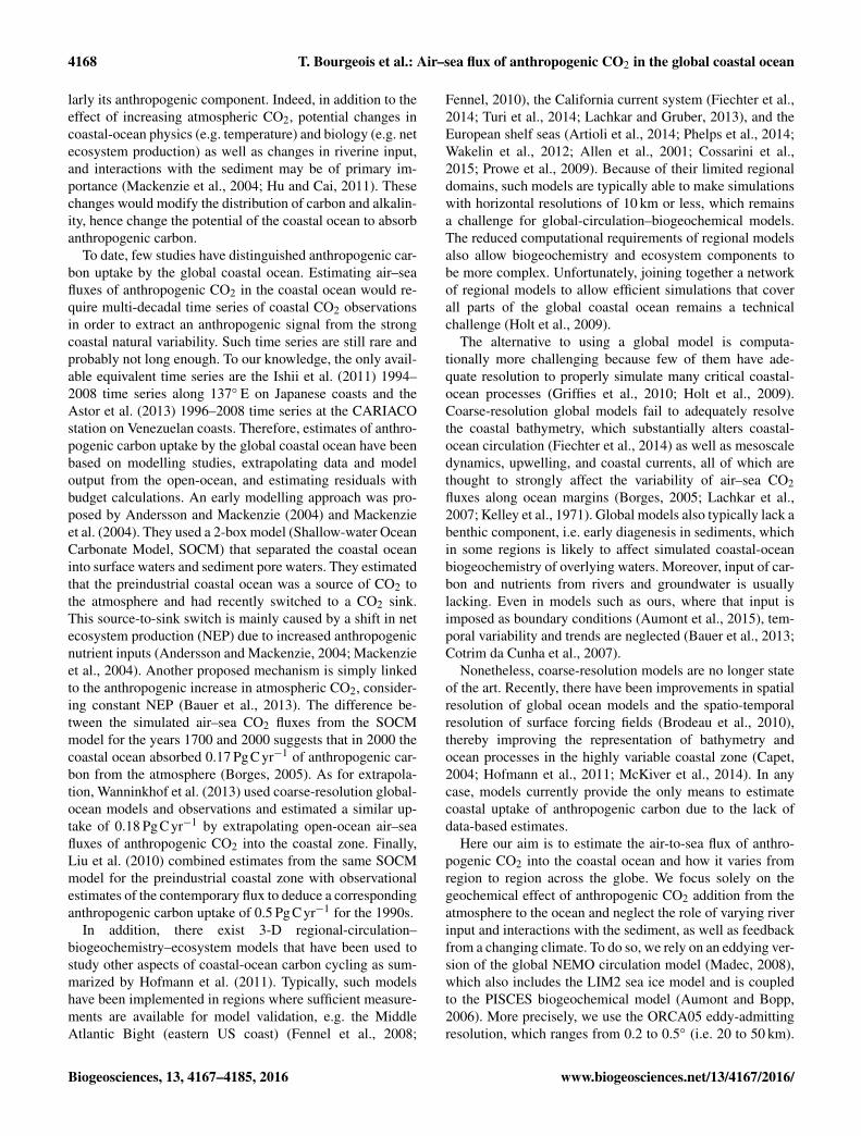
Regionally, overall patterns in the total FCO2 are simi-lar between the model and data-based estimates from Land-schützer et al. (2014) and Takahashi et al. (2009) (Fig. 3).Carbon is lost from the ocean in the equatorial band and incoastal upwelling regions, while it is gained by the ocean inthe northern high latitudes. Quantitative comparison of theannual-mean map from the model with that from the Taka-hashi et al. (2009) observation-based database gives a rootmean square error (RMSE) of 0.73 molCm−2 yr−1 and acorrelation coefficient R of 0.80; likewise, comparison withthe Landschützer et al. (2014) observational-based databasegives a similar RMSE (0.70 molCm−2 yr−1) and R (0.81).Integrating over latitudinal bands, (Table 1), the model over-estimates carbon uptake for the 90–30◦ S region, where it ab-sorbs 1.50 PgCyr−1 of total carbon vs. 0.73–0.77 PgCyr−1

from Takahashi et al. (2009) and Landschützer et al. (2014)observational databases. This overestimate may result fromthe model simulation still being far from equilibrium (seeSect. 2.2 paragraph 5 for details). The model also under-estimates outgassing in the tropical band, where it releases0.13 PgCyr−1 vs. 0.13–0.20 PgCyr−1 for the two data-basedestimates. Further north in the 30–90◦ N band, the modeltakes up 0.93 PgCyr−1 vs. 1.53–1.59 PgCyr−1 for Taka-hashi et al. (2009) and Landschützer et al. (2014).

3.2 Coastal-ocean fluxes

3.2.1 Total CO2

The simulated uptake of total carbon by the coastal-oceanaverages 267 TgCyr−1 during the 1993–2012 period. Mostof the 45 MARCATS regions act as carbon sinks; to-gether, they absorb 283 TgCyr−1. The largest uptake is3.4 molCm−2 yr−1 in the South Greenland region. FewMARCATS regions act as carbon sources to the atmosphere(Table 2 and Fig. 4.a), i.e. only 14 % of the global coastal-ocean surface area, together losing 16 TgC of carbon to theatmosphere every year. The mean annual carbon loss persquare metre in these MARCATS regions is usually rela-tively weak, less than 1.5 molCm−2 yr−1). When groupedinto MARCATS classes (see Table 3), all classes are carbonsinks, absorbing from 0.06 to 1.65 molCm−2 yr−1. By class,the largest specific fluxes occur in the western boundary cur-rent regions and the subpolar margins, which absorb 1.65



Figure 2. Simulated temporal evolution of area-integrated anthropogenic carbon uptake for (a) the open ocean and (b) the coastal ocean.(c) Analogous evolution of anthropogenic carbon uptake for the open ocean, the coastal ocean, the Southern Ocean, and the tropical oceans,but given as the average flux per unit area.

Table 1. Sea-to-air total CO2 fluxes (PgCyr−1) given as zonal means from Takahashi et al. (2009) for the reference year 2000, fromLandschützer et al. (2014) for 1998–2011 and the ORCA05 model for 1993–2012.

Latitudinal Observation-based climatologies This studybands Takahashi et al. (2009) Landschützer et al. (2014) ORCA05

90–30◦ S −0.77 −0.73 −1.5030◦ S–30◦ N 0.20 0.13 0.1330–90◦ N −1.59 −1.53 −0.93

and 1.61 molCm−2 yr−1 respectively. More generally, thetropical MARCATS regions act as weak carbon sources andthe mid-to-high-latitude regions act as strong carbon sinks(Fig. 4a). The same trend is also apparent in the zonal-meandistribution (Fig. 5).

A comparison of the simulated vs. observed FCO2 esti-mates for each MARCATS region is reported in Table 2 andFig. 6. The Pearson correlation coefficient R is 0.8 for spe-cific fluxes. In the model, 79 % of the MARCATS regions actas carbon sinks, whereas that proportion is 64 % for LA14.



Table2.M

AR

CA

TS

regionsas

describedby

Laruelle

etal.(2013,2014),alongw

ithm

eansfor

data-basedfluxes

oftotalC

O2

fromL

A14

duringthe

period1990–2011

asw

ellassim

ulatedanthropogenic

andtotalC

O2

fluxes,andresidence

time

duringthe

period1993–2012.U

ncertaintiesare

theinterannualvariability

overtheaveraged

period.Abbreviations

areincluded

fornorth(N

),south(S),east(E

),west(W

),easternboundary

current(EB

C),w

esternboundary

current(WB

C),sea-to-airflux

oftotalcarbon(F

CO

tot2

),anthropogeniccarbon

(FC

Oant2

).Surfaceareas

indicatedas

“fromL

A14”

actuallydifferslightly

fromthose

publishedin

LA

13as

theyhave

beenm

odifiedforsubsequentcom

putations(G

oulvenG

.Laruelle,

personalcomm

unication,January2015).

N◦

SystemN

ame

Class

Surface(10 3

km2)

FC

Otot2

(molC

m−

2yr−

1)F

CO

tot2

(Tg

Cyr−

1)F

CO

ant2

Residence

Model

LA

14Sim

ulatedL

A14

Simulated

LA

14m

olCm−

2yr−

1T

gC

yr−

1tim

e(m

onth)

1N

-EPacific

Subpolar397

350−

2.29±

0.17−

1.61−

10.935±

0.823−

6.775−

0.45±

0.05−

2.16±

0.230.83±

0.232

Californian

currentE

BC

118208

−0.34±

0.10−

0.05−

0.477±

0.148−

0.135−

0.35±

0.09−

0.50±

0.131.00±

0.233

TropicalEPacific

Tropical152

183−

0.12±

0.050.09

−0.222

±0.095

0.192−

0.36±

0.05−

0.65±

0.100.51±

0.094

Peruvianupw

ellingcurrent

EB

C138

1431.44±

0.800.65

2.386±

1.3251.073

−0.39±

0.09−

0.64±

0.150.72±

0.155

SouthernA

merica

Subpolar1126

1190−

1.51±

0.13−

1.31−

20.460±

1.705−

18.715−

0.46±

0.05−

6.28±

0.740.65±

0.056

Brazilian

currentW

BC

475484

−0.33±

0.080.10

−1.872

±0.479

0.567−

0.34±

0.05−

1.95±

0.290.26±

0.067

TropicalWA

tlanticTropical

479488

0.86±

0.100.07

4.934±

0.5510.394

−0.26±

0.05−

1.50±

0.310.20±

0.028

Caribbean

SeaTropical

303358

0.10±

0.100.81

0.366±

0.3483.460

−0.31±

0.04−

1.12±

0.140.32±

0.039

GulfofM

exicoM

arginalsea469

532−

0.79±

0.11−

0.33−

4.478±

0.633−

2.100−

0.32±

0.03−

1.81±

0.161.01±

0.1510

Floridaupw

ellingW

BC

545591

−2.25±

0.21−

0.38−

14.692±

1.351−

2.723−

0.66±

0.05−

4.29±

0.360.39±

0.0211

SeaofL

abradorSubpolar

576638

−1.27±

0.18−

1.72−

8.808±

1.244−

13.172−

0.32±

0.03−

2.19±

0.211.20±

0.3512

Hudson

Bay

Marginalsea

9981064

0.31±

0.29n.d

3.757±

3.423n.d.

−0.08±

0.04−

0.99±

0.4651.22

±22.75

13C

anadianA

rchipelagoPolar

10011145

−0.52±

0.06−

1.02−

6.234±

0.748−

13.986−

0.09±

0.02−

1.03±

0.212.82±

0.4614

NG

reenlandPolar

544602

−0.97±

0.15−

0.61−

6.333±

1.000−

4.400−

0.26±

0.05−

1.67±

0.332.38±

0.4415

SG

reenlandPolar

238262

−3.35±

0.44−

3.81−

9.564±

1.259−

11.972−

0.86±

0.19−

2.45±

0.530.48±

0.0916

Norw

egianB

asinPolar

141162

−2.87±

0.23−

1.72−

4.855±

0.396−

3.342−

0.60±

0.09−

1.02±

0.150.31±

0.1017

NE

Atlantic

Subpolar1020

1073−

2.16±

0.12−

1.33−

26.501±

1.419−

17.165−

0.53±

0.05−

6.52±

0.590.93±

0.1118

Baltic

SeaM

arginalsea324

3640.30±

0.070.51

1.184±

0.2882.245

−0.01±

0.01−

0.05±

0.0317.37

±9.52

19Iberian

upwelling

EB

C251

267−

1.13±

0.120.04

−3.393

±0.352

0.122−

0.27±

0.03−

0.82±

0.102.31±

0.5420

Mediterranean

SeaM

arginalsea423

529−

0.24±

0.060.62

−1.196

±0.327

3.925−

0.30±

0.02−

1.52±

0.120.72±

0.0921

Black

SeaM

arginalsea131

172−

0.24±

0.11n.d.

−0.375

±0.174

n.d.−

0.18±

0.02−

0.28±

0.031.60±

0.4822

Moroccan

upwelling

EB

C177

2060.18±

0.122.92

0.385±

0.2637.220

−0.33±

0.03−

0.71±

0.070.67±

0.1423

TropicalEA

tlanticTropical

225259

0.09±

0.08−

0.060.239

±0.208

−0.174

−0.19±

0.02−

0.52±

0.050.59±

0.0924

SWA

fricaE

BC

300298

0.43±

0.40−

1.431.544

±1.448

−5.103

−0.59±

0.08−

2.14±

0.282.17±

0.5525

Agulhas

currentW

BC

189239

−1.20±

0.09−

0.58−

2.730±

0.206−

1.664−

0.53±

0.05−

1.21±

0.120.13±

0.0126

TropicalWIndian

Tropical46

68−

0.06±

0.081.00

−0.031

±0.044

0.815−

0.16±

0.04−

0.09±

0.030.20±

0.0427

WA

rabianSea

Indianm

argins82

920.35±

0.041.14

0.342±

0.0431.257

−0.31±

0.04−

0.31±

0.040.12±

0.0428

Red

SeaM

arginalsea158

1740.24±

0.030.16

0.460±

0.0650.330

−0.15±

0.01−

0.28±

0.020.57±

0.1529

PersianG

ulfM

arginalsea208

2330.04±

0.08n.d.

0.092±

0.203n.d.

−0.12±

0.02−

0.31±

0.0424.67

±12.09

30E

Arabian

SeaIndian

margins

298317

0.21±

0.120.67

0.749±

0.4272.555

−0.30±

0.04−

1.07±

0.150.67±

0.1531

Bay

ofBengal

Indianm

argins197

203−

0.69±

0.12−

0.22−

1.641±

0.276−

0.530−

0.31±

0.04−

0.74±

0.090.43±

0.1132

TropicalEIndian

Indianm

argins727

763−

0.06±

0.07−

0.02−

0.482±

0.569−

0.170−

0.20±

0.02−

1.78±

0.170.50±

0.0433

Leeuw

incurrent

EB

C81

117−

2.05±

0.15−

0.98−

2.010±

0.148−

1.379−

0.60±

0.07−

0.58±

0.070.56±

0.1634

SA

ustraliaSubpolar

392436

−1.37±

0.18−

1.14−

6.438±

0.859−

5.983−

0.27±

0.03−

1.29±

0.140.74±

0.2535

EA

ustraliancurrent

WB

C98

130−

1.74±

0.18−

1.09−

2.036±

0.205−

1.695−

0.50±

0.07−

0.58±

0.080.37±

0.0436

New

Zealand

Subpolar263

286−

1.23±

0.16−

1.25−

3.882±

0.498−

4.274−

0.52±

0.07−

1.64±

0.230.49±

0.0437

NA

ustraliaTropical

22782292

−0.29±

0.110.44

−7.872

±3.114

12.120−

0.23±

0.04−

6.19±

1.000.38±

0.0338

SEA

siaTropical

21302160

−0.29±

0.07−

0.91−

7.344±

1.908−

23.609−

0.20±

0.03−

5.01±

0.720.49±

0.0539

China

Seaand

Kuroshio

WB

C1132

1129−

1.99±

0.15−

1.41−

27.046±

1.991−

19.100−

0.45±

0.05−

6.13±

0.720.32±

0.0140

SeaofJapan

Marginalsea

233147

−3.07±

0.17−

3.47−

8.613±

0.475−

6.113−

0.51±

0.06−

1.44±

0.181.64±

0.2441

SeaofO

khotskM

arginalsea933

952−

1.66±

0.071.31

−18.623

±0.761

14.955−

0.36±

0.03−

4.00±

0.343.52±

1.3842

NW

PacificSubpolar

10251000

−1.85±

0.14−

0.70−

22.760±

1.726−

8.419−

0.24±

0.04−

2.99±

0.521.48±

0.5943

SiberianShelves

Polar1848

1889−

0.47±

0.10−

0.90−

10.499±

2.117−

20.322−

0.05±

0.01−

1.09±

0.284.10±

0.6444

Barents

andK

araseas

Polar1559

1680−

0.75±

0.14−

1.60−

14.176±

2.585−

32.225−

0.11±

0.02−

2.05±

0.431.58±

0.4645

Antarctic

ShelvesPolar

24522936

−0.90±

0.14−

0.15−

26.630±

3.989−

5.381−

0.69±

0.07−

20.30±

2.182.08±

0.29



Figure 3. Climatological mean of sea-to-air flux of total carbon fluxes in molCm−2 y−1 for (a) the model average during the 1993–2012period, (b) the data-based estimate from Landschützer et al. (2014) for 1998–2011, and (c) the data-based estimate from Takahashi et al.(2009) for 2000–2009. Panels (d) and (f) present differences between simulated and observed sea-to-air total carbon fluxes (molCm−2 yr−1)relative to (b) and (c) respectively. Panel (d) presents the latitudinal distribution of the simulated and the observed mean sea-to-air totalcarbon fluxes.

Table 3. Weighted mean of simulated and data-based sea-to-air CO2 fluxes and simulated residence time for each MARCATS class, excludingthe Sea of Okhotsk (see text). Abbreviations are included for eastern boundary current (EBC) and western boundary current (WBC).

Class Sea-to-air CO2 flux (molCm−2 yr−1) Residence

Total (LA14) Total (model) Anthropogenic (model) time (month)

EBC 0.12 −0.12 ± 0.16 −0.42 ± 0.03 1.52 ± 0.22Indian margins 0.19 −0.06 ± 0.05 −0.24 ± 0.02 0.49 ± 0.04Marginal Seas −0.56 −0.92 ± 0.07 −0.29 ± 0.01 10.34 ± 3.50Polar margins −0.88 −0.83 ± 0.06 −0.32 ± 0.03 2.18 ± 0.20Subpolar margins −1.23 −1.61 ± 0.07 −0.36 ± 0.02 0.92 ± 0.16Tropical margins −0.10 −0.15 ± 0.06 −0.22 ± 0.02 0.42 ± 0.03WBC −0.80 −1.65 ± 0.08 −0.48 ± 0.03 0.31 ± 0.01

After aggregating the specific flux estimates into the differ-ent MARCATS classes (Table 3 and Fig. 7), the correlationcoefficient R increases to 0.9. Generally, our model resultstend to simulate larger sinks and weaker sources than ob-served (i.e. 76 % of the specific simulated fluxes of totalcarbon have lower relative values than the data-based esti-

mates). For some MARCATS classes, even the sign of thesimulated flux differs from the data-based estimates, e.g. forthe Indian margins and the eastern boundary currents. Thelatter class contains two regions (Moroccan and SW Africaupwelling) having the worst overall agreement. Otherwise, in



Figure 4. Global mean distribution of the simulated sea-to-air flux of (a) total carbon and (b) anthropogenic carbon over 1993–2012 asmol Cm−2 yr−1 in the global coastal ocean segmented following MARCATS from LA13. (c) Bar chart of the anthropogenic carbon uptake inTg Cyr−1 according to the MARCATS classification. Abbreviations are included for eastern boundary current (EBC) and western boundarycurrent (WBC). Links between numbers and regions are reported in Table 2. Interactive illustrations can be found at http://lsce-datavisgroup.github.io/CoastalCO2Flux/.

the Arctic polar regions, the simulated uptake is too low, with52 TgCyr−1 from the model vs. 86 TgCyr−1 from LA14.

3.2.2 Anthropogenic CO2

The anthropogenic FCO2 is computed as the difference be-tween the total flux (historical simulation) and natural flux(control simulation). When integrated over the global coastalocean, the mean anthropogenic flux from 1993 to 2012 is0.10 ± 0.01 PgCyr−1. That amounts to 4.5 % of the simu-lated global anthropogenic carbon uptake, substantially lessthan the 7.5 % proportion of the coastal-to-global ocean sur-

face areas. During the period 1950–2000, the uptake of an-thropogenic carbon by the coastal ocean essentially growslinearly as it does for the global ocean. That is, it grows ata nearly constant rate of 0.0015 PgCyr−2, which is 4.4 % ofthe rate for the global ocean increase in anthropogenic car-bon uptake over the same period (Fig. 2).

All MARCATS regions absorb anthropogenic carbon atrates ranging from 0.01 molCm−2 yr−1 for the Baltic Seato 0.86 molCm−2 yr−1 for the South Greenland region (Ta-ble 2 and Fig. 4.b). By class, the strongest specific fluxes ofanthropogenic carbon into the ocean occur in the boundary


http://lsce-datavisgroup.github.io/CoastalCO2Flux/

http://lsce-datavisgroup.github.io/CoastalCO2Flux/


(a)

(b)

TotalAnthropogenicNatural

TotalAnthropogenicNatural

Figure 5. Zonal-mean, sea-to-air fluxes of total, anthropogenic, andnatural CO2 (molCm−2 yr−1) given as the average over 1993–2012for (a) the coastal ocean and (b) the global ocean. Shaded areasindicate the standard deviation of environmental variability of allocean grid cells within each latitudinal band. Interannual variationsare not shown.

current regions, namely the EBC and WBC, with 0.42 and0.48 molCm−2 yr−1 respectively. Conversely, the weakestanthropogenic carbon uptake occurs in the tropical marginsand the Indian margins with 0.22 and 0.24 molCm−2 yr−1

respectively. But specific fluxes can be misleading. Althoughthe polar and subpolar margins do not have the highest spe-cific fluxes, their integrated uptake of anthropogenic carbonis large because of their large surface areas (Fig. 4b and c).Together they absorb 46 TgCyr−1, which is 45 % of total up-take of anthropogenic carbon by the global coastal ocean.

These results emphasize that there is no link between an-thropogenic and total carbon fluxes when comparing patternsbetween regions. For example, even though the EBC andWBC regions are the most efficient regions in anthropogeniccarbon uptake (both above 0.4 molCm−2 yr−1), their be-haviour differs greatly in terms of the flux of total carbon,i.e. −1.65 vs. −0.12 molCm−2 yr−1 respectively (Fig. 7).The same lack of correlation between anthropogenic and to-

−4 −3 −2 −1 0 1 2 3

−4

−3

−2

−1

0

1

2

3

Observed CO2 flux (mol C m−2 y−1)

Sim

ulat

ed C

O2 f

lux

(mol

C m

−2 y−1

)

EBCWBCPolarSubpolarTropicalIndianMarginal

Figure 6. Simulated vs. observed MARCATS sea-to-air flux of totalcarbon in (a) molCm−2 yr−1 and (b) TgCyr−1. Vertical error barsshow the standard deviation from the 1993–2012 interannual vari-ability for model results and the horizontal bars correspond to the1990–2011 variability from computational methods used in LA14for observation-based estimates. Here, regression line (grey dotted)have y intercepts forced to 0. All MARCATS regions have beenused except the Black Sea, the Persian Gulf (no data estimate), andthe Sea of Okhotsk (see text).

-25

-20

-15

-10

-5

0

5

EBC WBC Indian Marginal Tropical Subpolar Polar

MARCATS classes

Sea−

to−a

ir C

O2

flux

(Tg

C y−1

)

Figure 7. Box plots of the simulated sea-to-air CO2 fluxes(TgCyr−1) grouped into the MARCATS classes of the coastalocean. Black boxes indicate total fluxes, and red boxes indicate an-thropogenic fluxes. Shown are the lowest estimate, the first quar-tile, the median, the third quartile, and the highest estimate for eachclass.

tal flux patterns is even clearer in the zonal mean distributions(Fig. 5). For instance, the specific fluxes of anthropogeniccarbon into the coastal ocean between 55◦ S and 90◦ N arenearly uniform, remaining near −0.5 molCm−2 yr−1; con-versely, the total carbon fluxes vary greatly between −2



and +0.5 molCm−2 yr−1. These variations in the total car-bon flux are dictated by variations in the natural carbon flux(Fig. 5).

4 Discussion

4.1 Comparison with previous coastal estimates

4.1.1 Total flux

Our mean simulated uptake of total carbon by the globalcoastal ocean over 1993 to 2012 is 0.27± 0.07 PgCyr−1,which falls within the range of previous data-based esti-mates of 0.2–0.4 PgCyr−1 (Borges et al., 2005; Cai et al.,2006; Chen and Borges, 2009; Laruelle et al., 2010; Cai,2011; Chen et al., 2013; Laruelle et al., 2014). Out of those,estimates provided since 2011 gather closer to the lowerlimit, e.g. the estimate of 0.2 PgCyr−1 from LA14, as isalso the case for our model-based estimate. Some aspectsof the LA14 data-based approach are shared by our model-based approach, i.e. the same reference period, essentiallythe same definition of the coastal ocean, and the same cor-rection for the effect of sea ice cover on FCO2 . LA14 is thefirst observation-based study to take into account this sea iceeffect for coastal-ocean FCO2 estimates at the global scale.

Using a box model, Andersson and Mackenzie (2004) andMackenzie et al. (2004) estimated that the global coastalocean acted as a carbon source to the atmosphere prior toindustrialization; however, they also estimate that industrial-ization has recently led to a reversal in the sign of this flux(the global coastal ocean became a carbon sink) mainly dueto the enhancement of NEP from increased riverine inputs.In contrast, our model simulations indicate that the preindus-trial coastal ocean was already a carbon sink, and that thissink has strengthened over the industrial period. This dis-crepancy appears to be explained by different definitions ofthe coastal ocean. Both the box model and our 3-D modelinclude the distal coastal zone, but only the box model in-cludes the proximal coastal zone (bays, estuaries, deltas, la-goons, salt marshes, mangroves, and banks). That proximalzone is known generally as a strong source of carbon to theatmosphere (Rabouille et al., 2001).

The model representation of riverine DOC input and itsinstantaneous remineralization has potential implications forour estimates of total FCO2 . In the Amazon plume for in-stance, we underestimate CO2 absorption because of this in-stantaneous addition of DIC without input of alkalinity. How-ever this assumption has no direct implication on our anthro-pogenic FCO2 estimates.

Furthermore, our simplified representation of sedimentaryprocesses affects simulated total CO2 fluxes (Krumins et al.,2013; Soetaert et al., 2000). First, the model lacks an ex-plicit representation of sedimentary processes. Thus it can-not reproduce the temporal dynamics of interactions between

sediments and the overlying water column, e.g. resulting inpotential delays between sediment burial and remineraliza-tion. Second, our model neglects any alkalinity source fromsediment anaerobic degradation, such as denitrification andsulfate reduction of deposited organic matter. Even if notwell constrained (Chen, 2002; Thomas et al., 2009; Hu andCai, 2011; Krumins et al., 2013), this source of alkalinitycould partially balance the total CO2 uptake of the coastalocean. However, the simplified representation of these sed-iment processes has no direct effect on our anthropogenicFCO2 estimates.

4.1.2 Anthropogenic flux

The strongest specific fluxes of anthropogenic carbon intothe ocean occur in the boundary current regions, namely theEBC and WBC. Indeed, these regions show significant verti-cal and lateral mixing features such as filaments and eddiesfrom the strong adjacent western boundary currents and up-welling from Eastern boundary upwelling systems (EBUS).Those physical processes lead to the deepening of the mixedlayer depth, export of the absorbed anthropogenic carbonfrom shallow water to deeper water layers, and its transferto the adjacent open ocean.

Our estimate of the simulated anthropogenic carbon up-take of 0.10 PgCyr−1 for the global coastal ocean (Fig. 9) isabout half that found by Wanninkhof et al. (2013) for a sim-ilar period. The latter study estimates coastal anthropogenicCO2 uptake by extrapolating specific FCO2 from the adjacentopen ocean into coastal areas, exploiting coarse-resolutionmodels and data. To compare approaches, we applied theWanninkhof et al. (2013) extrapolation method to our modeloutput; we found the same result as theirs for global coastal-ocean uptake of anthropogenic CO2 (0.18 PgCyr−1). Thusthe extrapolation technique leads to an overestimate of an-thropogenic CO2 uptake in the model’s global coastal ocean.

Nonetheless, the Wanninkhof et al. (2013) estimate for theanthropogenic carbon uptake by the coastal ocean was usedby Regnier et al. (2013) for their coastal carbon budget. Thatbudget also accounts for the increase in river discharge ofcarbon (0.1 PgCyr−1) and nutrients during the industrial era,which promotes organic carbon production, some of whichis buried in the coastal zone (up to 0.15 PgCyr−1). Unfor-tunately, these numbers remain particularly uncertain. Hencewe have chosen to ignore them, adopting the conventionaldefinition of anthropogenic carbon in the ocean used by pre-vious global-ocean model studies, namely that anthropogeniccarbon comes only from the direct geochemical effect of theanthropogenic increase in atmospheric CO2 and its subse-quent invasion into the ocean. The future challenge of im-proving estimates of changes and variability in riverine de-livery of carbon and nutrient and sediment burial is criticalto refine land contributions to the coastal-ocean carbon bud-get.



Our estimate of 0.10 PgCyr−1 for the anthropogenic FCO2

into the coastal ocean is 40 % less than the 0.17 PgCyr−1 es-timated by Borges (2005) from Andersson and Mackenzie(2004) and Mackenzie et al. (2004). Causes for this differ-ence may stem from (1) the different definitions of the coastalocean (proximal coastal zone included in the box model butnot the 3-D model), (2) the different approaches (uniformcoastal ocean in the box model but not in the 3-D model),and (3) the role of sediments (pore waters included in thebox model but neglected in the 3-D model).

4.2 Coastal vs. open ocean

Patterns in our simulated total FCO2 in the coastal oceangenerally follow those for the open ocean, with net carbonsources in the low latitudes and carbon sinks in the middle tohigh latitudes (Fig. 5). The same tendency was pointed out byGruber (2014) when discussing the LA14 data-based fluxes.The patterns in our simulated total CO2 flux are mainlydriven by patterns in the natural CO2 flux both in the coastaland open oceans (Fig. 5). Yet the pattern for anthropogenicCO2 flux differs greatly from that of natural CO2, having itsstrongest uptake in the Southern Ocean in both the open andcoastal oceans, i.e. where zonally averaged specific uptakereaches up to 1.5 molCm−2 yr−1. The bathymetry of MAR-CATS regions around the Antarctic continent is much deeperthan in the other coastal regions (500 m vs. 160 m for theglobal coastal ocean); this probably reduces the contrast be-tween the coastal and open ocean in the Southern Ocean andexplains the similarities of anthropogenic carbon uptake ratesthere.

Despite large-scale similarities between coastal- and open-ocean fluxes of total carbon, some coastal regions differsubstantially from those in the adjacent open-ocean waters(Fig. 3a). These local differences are particularly apparentaround coastal upwelling systems, i.e. in the western Ara-bian Sea and in eastern boundary upwelling systems (EBUS),such as the Peruvian upwelling current, the Moroccan up-welling, and the south-western Africa upwelling. Some ofthese coastal regions act as strong total carbon sources, withmean carbon fluxes of up to 1.44 molCm−2 yr−1, whereassurrounding open-ocean waters exhibit little FCO2 (fluxesclose to 0 molCm−2 yr−1). Other regions also exhibit largecontrast between their coastal waters and the adjacent openocean, including the tropical western Atlantic where thereis a massive loss of carbon at the location of the Amazonriver discharge. However the carbon sink in the Amazonriver plume reported in Lefèvre et al. (2010) is not repro-duced in our model. This discrepancy may be due to the mod-elled instantaneous remineralization of land-derived DOC orto shortcomings in the model representation of sedimentaryprocesses.

A key finding of our model study is that the flux of an-thropogenic CO2 into the coastal ocean (0.10 PgCyr−1) ishalf the previous estimate (Wanninkhof et al., 2013). Un-

like in that study, our specific flux of anthropogenic CO2 issubstantially lower for the global coastal ocean than for theglobal open ocean (i.e. −0.31 vs. −0.54 molCm−2 yr−1 forthe 1993–2012 average). Although the coastal-ocean surfacearea is 7.5 % of the global ocean, it absorbs only 4.5 % ofthe globally integrated flux of anthropogenic carbon into theocean.

Our estimate for coastal-ocean uptake of anthropogeniccarbon is 10 times smaller than the 1 PgCyr−1 estimate byTsunogai et al. (1999) associated with their proposed conti-nental shelf pump (CSP). However, Tsunogai’s CSP is basedon contemporary measurements and thus concerns total car-bon, not the anthropogenic change. That nuance is critical be-cause contemporary estimates of fluxes are not directly com-parable to anthropogenic fluxes nor global budgets of car-bon from the IPCC and the Global Carbon Project, both fo-cused on the anthropogenic change. Unfortunately Tsunogaiet al. (1999) prompted confusion by stating that their totalcarbon flux into the coastal ocean was equivalent to half ofthe global-ocean uptake of anthropogenic carbon. The sameconfusion prompted Thomas et al. (2004) to emphasize thatthe coastal ocean contributes more to the global carbon bud-get than expected from its surface area.

The lower specific flux of anthropogenic CO2 into theglobal coastal ocean relative to the average for the openocean could have two causes: (1) physical factors (e.g. ifvertical mixing in the coastal ocean is relatively weak or ifthere is a bottleneck in the offshore transport carbon) and(2) chemical factors, if coastal waters have a lower chemi-cal capacity to absorb anthropogenic carbon (lower carbon-ate ion concentration, higher Revelle factor Rf).

To assess how Rf differs between coastal- and open-oceansurface waters, we computed it using CO2SYS from sim-ulated sea surface temperature, salinity, alkalinity, and DICfor the model years 1993–2012. Thus we computed meanRevelle factors of 12.5 for the global coastal ocean, 10.9 forthe global ocean, 9.2 for the tropical oceans (30◦ S–30◦ N),and 12.8 for the Southern Ocean (90–30◦ S). These tenden-cies are persistent. During the period 1910–2012, the aver-age coastal-ocean Revelle factor remains 15 % larger than forthe open ocean. Hence average surface waters in the model’scoastal ocean have a lower chemical capacity to take up an-thropogenic carbon relative to average surface waters of theglobal ocean. That finding is consistent with the lower simu-lated specific fluxes of anthropogenic carbon into the coastalocean. Yet it is not only the chemical capacity that matters.For example, despite similar chemical capacities, the specificflux of anthropogenic carbon into Southern Ocean is morethan twice that of the global coastal ocean. Thus, we mustturn to physical factors to help explain the lower efficiencyof the coastal ocean to take up anthropogenic carbon.

Out of the 0.10 PgCyr−1 absorbed by the coastal ocean,we find that only 70 % (i.e. 0.07 PgCyr−1) is transferredto the open ocean (Fig. 9). Thus 0.03 PgCyr−1 of anthro-pogenic carbon accumulates in the coastal-ocean water col-



Long

itude

Latitude

Residence time (m

onth)

Figure 8. Global distribution of simulated residence time (month) for the global coastal ocean segmented following Laruelle et al. (2013).

0.07

0.10

0.03 0.05 COASTAL OCEAN

ATMOSPHERE

OPEN OCEAN

2.16

2.23 2.4

2.26 2.5

0.2

Simulated and data-‐based anthropogenic carbon flux and accumula>on rate on 1993-‐2012 (Pg C yr-‐1)

0 Rivers

0.1

2.3

0 0.15 0 0

Sediments

0.1

Figure 9. Transfer of anthropogenic carbon between the atmo-sphere, coastal ocean, and open ocean along with increases in thecorresponding inventory in each reservoir, given as the average ofsimulated values over 1993–2012. All results are in PgCyr−1. Sim-ulated results are shown as dark numbers in boxes and adjacentnumbers (grey italic) indicate data-based estimates for the 2000–2010 average (Regnier et al., 2013).

umn during the 1993–2012 period. That simulated accu-mulation is not significantly different from the estimate of0.05± 0.05 PgCyr−1 from Regnier et al. (2013). The ac-cumulation in the coastal ocean is effective over the entireperiod (1910–2012) as the uptake of anthropogenic carbonby the global coastal ocean is always inferior to its cross-shelf export (Fig. 10). To gain insight into this cross-shelfexchange, we computed the simulated mean water residencetimes for each MARCATS region (Fig. 8). Residence timesfor most coastal regions are of the order of a few months orless, except for Hudson Bay, the Baltic Sea, and the PersianGulf. The latter three regions are generally more confined

and we expect longer residence times, although our modelsimulations were never designed to simulate these regions ac-curately. Generally, our simulated residence times are shorterthan what has been published for similarly defined coastal re-gions, although methods differ substantially (Jickells, 1998;Men and Liu, 2014; Delhez et al., 2004). Despite these shortresidence times, the cross-shelf export of anthropogenic car-bon is unable to keep up with the increasing air–sea flux ofanthropogenic carbon (Fig. 10). This may be explained bythe open-ocean waters that are imported to the coastal oceanbeing already charged with anthropogenic carbon, thus limit-ing further uptake in the coastal zone. This accumulation rateof anthropogenic carbon in the coastal ocean contrasts withthe lower simulated proportion that remains in the mixedlayer of the global ocean. Using a coarse-resolution globalmodel, Bopp et al. (2015) showed that on average for theglobal ocean, only ∼10 % of the anthropogenic carbon thatcrosses the air–sea interface accumulates in the seasonally-varying mixed layer. The CSP hypothesis from Tsunogaiet al. (1999) assumes that much of the 1 PgCyr−1 of totalcarbon absorbed by the coastal ocean is exported to the deepocean. Also assuming that the CSP operates equally in allshelf regions across the world, Yool and Fasham (2001) useda coarse- resolution global model to estimate that 53 % ofthe coastal uptake is exported to the open ocean. Yet theyconsidered only natural carbon. Conversely, we focus purelyon anthropogenic carbon. Our simulations suggest that 70 %of the anthropogenic carbon absorbed by the coastal oceanover 1993 to 2012 is transported offshore to the deeper openocean.



1920 1940 1960 1980 20000

0.5

1

1.5

2

Time (year)

Anth

ropo

geni

c ca

rbon

inve

ntor

y (P

g C

)

1920 1940 1960 1980 20000

0.02

0.04

0.06

0.08

0.1

0.12

Time (year)

Anth

ropo

geni

c ca

rbon

flux

(Pg

C y

r−1)

Cross−shelf DICant export

Coastal Cant uptake

Figure 10. Simulated temporal evolution of (a) coastal-ocean inventory of anthropogenic carbon given in PgC and (b) anthropogenic CO2(Cant) uptake by the global coastal ocean and global cross-shelf export of anthropogenic carbon (DICant) given in PgCyr−1.

5 Conclusions

The goal of this study was to estimate the anthropogenic CO2flux from the atmosphere to the coastal ocean, both glob-ally and regionally, using an eddying global-ocean model,making 143-year simulations forced by atmospheric reanal-ysis data and atmospheric CO2. We first evaluated the sim-ulated air–sea fluxes of total CO2 for 45 coastal regions andfound a correlation coefficient R of 0.8 when compared toobservation-based estimates. Then we estimated the averagesimulated anthropogenic carbon uptake by the global coastalocean over 1993–2012 to be 0.10± 0.01 PgCyr−1, equiva-lent to 4.5 % of global-ocean uptake of anthropogenic CO2,an amount less than expected based on the surface area ofthe global coastal ocean (7.5 % of the global ocean). Fur-thermore, our estimate is only about half of that estimatedby Wanninkhof et al. (2013), whose budget was based onextrapolating adjacent open-ocean data-based estimates ofthe specific flux into the coastal ocean. We attribute ourlower specific flux of anthropogenic carbon into the globalcoastal ocean mainly to the model’s associated offshore car-bon transport, which is not strong enough to reduce surfacelevels of anthropogenic DIC (and thus anthropogenic pCO2)to levels that are as low as those in the open ocean (on aver-age). Whether or not our model provides a realistic estimateof offshore transport at the global scale is a critical questionthat demands further investigation.

Clearly, our approach is limited by the extent to whichthe coastal ocean is resolved. Our model’s horizontal resolu-tion does not allow it to fully resolve some fine-scale coastalprocesses such as tides, which affect FCO2 at tidal fronts(Bianchi et al., 2005). Model resolution is also inadequate tofully resolve mesoscale and submesoscale eddies and asso-ciated upwelling. Moreover, in the midlatitudes with a waterdepth of 80 m, the first baroclinic Rossby radius (the domi-nant scale affecting coastal processes) is around 200 km, but

the latter falls below 10 km on Arctic shelves (Holt et al.,2014; Nurser and Bacon, 2014). Thus the higher latitudesneed much finer resolution (Holt et al., 2009).

Yet all model studies must weigh the costs and bene-fits of pushing the limits toward improved realism. Our ap-proach has been to use a model that takes only a first stepinto the eddying regime in order to be able to achieve longphysical-biogeochemical simulations with atmospheric CO2increasing from preindustrial levels to today. It represents astep forward relative to previous studies with typical coarse-resolution ocean models (around 2◦ horizontal resolution),which may be considered to be designed exclusively for theopen ocean. In the coming years, increasing computationalresources will allow further increases in spatial resolutionand a better representation of the coastal ocean in globalocean carbon cycle models.

Improvements will also be needed in terms of the mod-elled biogeochemistry of the coastal zone. Most global-scalebiogeochemical models neglect river input of nutrients andcarbon. Although that is taken into account in our simula-tions, the river input forcing is constant in time (Aumontet al., 2015). Seasonal and higher frequency variability in car-bon and nutrient river input (e.g. from floods and droughts)is substantial as are typical anthropogenic trends. For sim-plicity, virtually all global-scale models neglect sediment re-suspension and early diagenesis in the coastal zone. Thoseprocesses in some coastal areas may well alter nutrient avail-ability, surface DIC, and total alkalinity, which would affectFCO2 . In addition, in the coastal zone, one must eventuallygo beyond the classic definition of anthropogenic carbon, i.e.the change due only to the direct influence of the anthro-pogenic increase in atmospheric CO2 on the FCO2 and oceancarbonate chemistry. Changes in other human-induced per-turbations may be substantial. For example, future researchshould better assess potential changes in sediment burial ofcarbon in the coastal zone during the industrial era, estimated



at up to 0.15 PgC yr−1 but with large uncertainty (Regnieret al., 2013).

To improve understanding of the critical land–ocean con-nection and its role in carbon and nutrient exchange, we callfor a long-term effort to exploit the latest, global-scale, high-resolution, ocean general circulation models, adding oceanbiogeochemistry, and improving them to better represent thecoastal and open oceans together as one seamless system.

6 Code availability

The code of the NEMO ocean model version 3.2 is availableunder CeCILL license at http://www.nemo-ocean.eu.

7 Data availability

As a supplementary material, we provide the simulated air-sea total and natural CO2 fluxes over the 1993–2012 period(bg-2016-57-Cflux.nc), model grid parameters (bg-2016-57-grid.nc), and times series for area-integrated CO2 fluxes (bg-2016-57-timeseries.txt).

Acknowledgements. We are grateful to the associate editorJ. Middelburg for managing the peer-reviewing process and to tworeferees, N. Gruber and P. Regnier, for their helpful comments.We thank G. G. Laruelle for providing the raw data versionof the Laruelle et al. (2014) database, and we are grateful toC. Nangini and P. Brockmann for their help with the GIS analysis,data treatment, and data visualization. We also thank J. Simeonfor the first implementation of the ORCA05-PISCES model.The research leading to these results was supported throughthe EU FP7 project CARBOCHANGE (grant 264879), the EUH2020 project CRESCENDO (grant 641816), and the EU H2020project C-CASCADES (Marie Sklodowska-Curie grant 643052).Simulations were made using HPC resources from GENCI-IDRIS(grant x2015010040). Timothée Bourgeois was funded through ascholarship cosupported by DGA-MRIS and CEA scholarship.

Edited by: J. MiddelburgReviewed by: N. Gruber and P. Regnier

References

Allen, J. I., Blackford, J., Holt, J., Proctor, R., Ashworth, M., andSiddorn, J.: A highly spatially resolved ecosystem model for theNorth West European Continental Shelf, Sarsia, 86, 423–440,2001.

Andersson, A. J. and Mackenzie, F. T.: Shallow-water oceans: asource or sink of atmospheric CO2?, Front. Ecol. Environ., 2,348–353, 2004.

Artioli, Y., Blackford, J. C., Nondal, G., Bellerby, R. G. J., Wake-lin, S. L., Holt, J. T., Butenschön, M., and Allen, J. I.: Het-erogeneity of impacts of high CO2 on the North Western Eu-ropean Shelf, Biogeosciences, 11, 601–612, doi:10.5194/bg-11-601-2014, 2014.

Astor, Y. M., Lorenzoni, L., Thunell, R., Varela, R., Muller-Karger,F., Troccoli, L., Taylor, G. T., Scranton, M. I., Tappa, E., andRueda, D.: Interannual variability in sea surface temperature andFCO2 changes in the Cariaco Basin, Deep-Sea Res. Pt. II, 93,33–43, 2013.

Atlas, R., Hoffman, R. N., Ardizzone, J., Leidner, S. M., Jusem,J. C., Smith, D. K., and Gombos, D.: A Cross-calibrated, Multi-platform Ocean Surface Wind Velocity Product for Meteorolog-ical and Oceanographic Applications, Bull. Am. Meteorol. Soc.,92, 157–174, 2011.

Aumont, O. and Bopp, L.: Globalizing results from ocean in situiron fertilization studies, Global Biogeochem. Cy., 20, GB2017,doi:10.1029/2005GB002591, 2006.

Aumont, O., Ethé, C., Tagliabue, A., Bopp, L., and Gehlen,M.: PISCES-v2: an ocean biogeochemical model for carbonand ecosystem studies, Geosci. Model Dev., 8, 2465–2513,doi:10.5194/gmd-8-2465-2015, 2015.

Bakker, D. C. E., Pfeil, B., Smith, K., Hankin, S., Olsen, A., Alin,S. R., Cosca, C., Harasawa, S., Kozyr, A., Nojiri, Y., O’Brien,K. M., Schuster, U., Telszewski, M., Tilbrook, B., Wada, C.,Akl, J., Barbero, L., Bates, N. R., Boutin, J., Bozec, Y., Cai,W.-J., Castle, R. D., Chavez, F. P., Chen, L., Chierici, M., Cur-rie, K., de Baar, H. J. W., Evans, W., Feely, R. A., Fransson,A., Gao, Z., Hales, B., Hardman-Mountford, N. J., Hoppema,M., Huang, W.-J., Hunt, C. W., Huss, B., Ichikawa, T., Johan-nessen, T., Jones, E. M., Jones, S. D., Jutterström, S., Kitidis,V., Körtzinger, A., Landschützer, P., Lauvset, S. K., Lefèvre, N.,Manke, A. B., Mathis, J. T., Merlivat, L., Metzl, N., Murata,A., Newberger, T., Omar, A. M., Ono, T., Park, G.-H., Pater-son, K., Pierrot, D., Ríos, A. F., Sabine, C. L., Saito, S., Salis-bury, J., Sarma, V. V. S. S., Schlitzer, R., Sieger, R., Skjelvan,I., Steinhoff, T., Sullivan, K. F., Sun, H., Sutton, A. J., Suzuki,T., Sweeney, C., Takahashi, T., Tjiputra, J., Tsurushima, N., vanHeuven, S. M. A. C., Vandemark, D., Vlahos, P., Wallace, D.W. R., Wanninkhof, R., and Watson, A. J.: An update to the Sur-face Ocean CO2 Atlas (SOCAT version 2), Earth Syst. Sci. Data,6, 69–90, doi:10.5194/essd-6-69-2014, 2014.

Barnier, B., Madec, G., Penduff, T., Molines, J. M., Treguier, A. M.,Le Sommer, J., Beckmann, A., Biastoch, A., Böning, C., Dengg,J., Derval, C., Durand, E., Gulev, S., Remy, E., Talandier, C.,Theetten, S., Maltrud, M., McClean, J., and De Cuevas, B.:Impact of partial steps and momentum advection schemes ina global ocean circulation model at eddy-permitting resolution,Ocean Dynam., 56, 543–567, 2006.

Bauer, J. E., Cai, W.-J., Raymond, P. A., Bianchi, T. S., Hopkinson,C. S., and Regnier, P.: The changing carbon cycle of the coastalocean, Nature, 504, 61–70, 2013.

Bianchi, A. A., Bianucci, L., Piola, A. R., Pino, D. R., Schloss, I.,Poisson, A., and Balestrini, C. F.: Vertical stratification and air-sea CO2 fluxes in the Patagonian shelf, J. Geophys. Res.-Ocean.,110, 1–10, 2005.

Bopp, L., Lévy, M., Resplandy, L., and Sallée, J. B.: Pathways ofanthropogenic carbon subduction in the global ocean, Geophys.Res. Lett., 42, 6416–6423, 2015.

Borges, A. V.: Do we have enough pieces of the jigsaw to integrateCO2 fluxes in the coastal ocean?, Estuaries, 28, 3–27, 2005.

Borges, A. V., Delille, B., and Frankignoulle, M.: Budget-ing sinks and sources of CO2 in the coastal ocean: Diver-


http://www.nemo-ocean.eu

http://dx.doi.org/10.5194/bg-11-601-2014

http://dx.doi.org/10.5194/bg-11-601-2014

http://dx.doi.org/10.1029/2005GB002591

http://dx.doi.org/10.5194/gmd-8-2465-2015

http://dx.doi.org/10.5194/essd-6-69-2014


sity of ecosystems counts, Geophys. Res. Lett., 32, L14601,doi:10.1029/2005GL023053, 2005.

Brodeau, L., Barnier, B., Treguier, A.-M., Penduff, T., and Gulev,S.: An ERA40-based atmospheric forcing for global ocean cir-culation models, Ocean Model., 31, 88–104, 2010.

Cai, W.-J.: Estuarine and coastal ocean carbon paradox: CO2 sinksor sites of terrestrial carbon incineration?, Ann. Rev. Mar. Sci.,3, 123–45, 2011.

Cai, W.-J., Dai, M., and Wang, Y.: Air-sea exchange of carbon diox-ide in ocean margins: A province-based synthesis, Geophys. Res.Lett., 33, L12603, doi:10.1029/2006GL026219, 2006.

Capet, X. J.: Upwelling response to coastal wind profiles, Geophys.Res. Lett., 31, L13311, doi:10.1029/2004GL020123, 2004.

Chen, C.-T. A.: Shelf-vs. dissolution-generated alkalinity above thechemical lysocline, Deep-Sea Res. Pt. II, 49, 5365–5375, 2002.

Chen, C.-T. A. and Borges, A. V.: Reconciling opposing viewson carbon cycling in the coastal ocean: Continental shelves assinks and near-shore ecosystems as sources of atmospheric CO2,Deep-Sea Res. Pt. II, 56, 578–590, 2009.

Chen, C.-T. A., Huang, T. H., Chen, Y. C., Bai, Y., He, X., andKang, Y.: Air-sea exchanges of CO2 in the world’s coastal seas,Biogeosciences, 10, 6509–6544, doi:10.5194/bg-10-6509-2013,2013.

Ciais, P., Sabine, C., Bala, G., Bopp, L., Brovkin, V., Canadell, J.,Chhabra, a., DeFries, R., Galloway, J., Heimann, M., Jones, C.,Quéré, C. L., Myneni, R., Piao, S., Thornton, P., France, P. C.,Willem, J., Friedlingstein, P., and Munhoven, G.: 2013: Carbonand Other Biogeochemical Cycles, Climate Change 2013: ThePhysical Science Basis. Contribution of Working Group I to theFifth Assessment Report of the Intergovernmental Panel on Cli-mate Change, 465–570, doi:10.1017/CBO9781107415324.015,2013.

Conkright, M. E., Locarnini, R. A., Garcia, H. E., O’Brien, T. D.,Boyer, T. P., Stephens, C., and Antonov, J. I.: World OceanDatabase 2001: Objective analyses, data statistics and figures,2002.

Cossarini, G., Querin, S., and Solidoro, C.: The continental shelfcarbon pump in the northern Adriatic Sea (Mediterranean Sea):Influence of wintertime variability, Ecol. Model., 314, 118–134,2015.

Cotrim da Cunha, L., Buitenhuis, E. T., Le Quéré, C., Giraud, X.,and Ludwig, W.: Potential impact of changes in river nutrientsupply on global ocean biogeochemistry, Global Biogeochem.Cy., 21, GB4007, doi:10.1029/2006GB002718, 2007.

de Baar, H. J. W. and de Jong, J. T. M.: Distributions, sources andsinks of iron in seawater, The Biogeochemistry of Iron in Sea-water, IUPAC Series on Analytical and Physical Chemistry ofEnvironmental Systems, 123–253, 2001.

Delhez, É. J., Heemink, A. W., and Deleersnijder, É.: Residencetime in a semi-enclosed domain from the solution of an adjointproblem, Estuarine, Coast. Shelf Sci., 61, 691–702, 2004.

Dickson, A. G.: Standard potential of the reaction:AgCl(s)+ 12H2(g)=Ag(s)+HCl(aq), and the standardacidity constant of the ion HSO−4 in synthetic sea water from273.15 to 318.15 K, The Journal of Chemical Thermodynamics,22, 113–127, 1990.

Fennel, K.: The role of continental shelves in nitrogen and carboncycling: Northwestern North Atlantic case study, Ocean Sci., 6,539–548, doi:10.5194/os-6-539-2010, 2010.

Fennel, K., Wilkin, J., Previdi, M., and Najjar, R.: Denitrificationeffects on air-sea CO2 flux in the coastal ocean: Simulations forthe northwest North Atlantic, Geophys. Res. Lett., 35, L24608,doi:10.1029/2008GL036147, 2008.

Fichefet, T. and Morales Maqueda, M. A. M.: Sensitivity of a globalsea ice model to the treatment of ice thermodynamics and dy-namics, J. Geophys. Res., 102, 12609, doi:10.1029/97JC00480,1997.

Fiechter, J., Curchitser, E. N., Edwards, C. A., Chai, F., Goebel,N. L., and Chavez, F. P.: Air-sea CO2 fluxes in the California Cur-rent: Impacts of model resolution and coastal topography, GlobalBiogeochem. Cy., 28, 371–385, 2014.

Gattuso, J. P., Frankignoulle, M., and Wollast, R.: Carbon andcarbonate metabolism in coastal aquatic ecosystems, Ann. Rev.Ecol. Syst., 29, 405–434, 1998.

Geider, R. J., MacIntyre, H. L., and Kana, T. M.: A dynamic reg-ulatory model of phytoplanktonic acclimation to light, nutrients,and temperature, Limnol. Oceanogr., 43, 679–694, 1998.

Gent, P. R. and McWilliams, J. C.: Isopycnal Mixing in Ocean Cir-culation Models, J. Phys. Oceanogr., 20, 150–155, 1990.

GLOBALVIEW-CO2: Cooperative Global Atmospheric Data Inte-gration Project Carbon Dioxide, Multi-laboratory compilation ofsynchronized and gap-filled atmospheric carbon dioxide recordsfor the period 1979–2012, Compiled by NOAA Global Monitor-ing Division, Boulder, Colorado, doi:10.3334/OBSPACK/1002,2012.

Griffies, S.: Problems and Prospects in Large-Scale Ocean Circula-tion Models, in: Proceedings of OceanObs’09, Sustained OceanObservations and Information for Society, 1, European SpaceAgency, Venice, Italy, 410–431, 2010.

Gruber, N.: Ocean biogeochemistry: Carbon at the coastal interface,Nature, 517, 148–149, 2014.

Ho, D. T., Law, C. S., Smith, M. J., Schlosser, P., Harvey, M.,and Hill, P.: Measurements of air-sea gas exchange at high windspeeds in the Southern Ocean: Implications for global parame-terizations, Geophys. Res. Lett., 33, 1–6, 2006.

Hofmann, E. E., Cahill, B., Fennel, K., Friedrichs, M. A. M., Hyde,K., Lee, C., Mannino, A., Najjar, R. G., O’Reilly, J. E., Wilkin, J.,and Xue, J.: Modeling the dynamics of continental shelf carbon,Ann. Rev. Mar. Sci., 3, 93–122, 2011.

Holt, J., Harle, J., Proctor, R., Michel, S., Ashworth, M., Batstone,C., Allen, I., Holmes, R., Smyth, T., Haines, K., Bretherton, D.,and Smith, G.: Modelling the global coastal ocean, Philos. Trans.Ser. A, 367, 939–51, 2009.

Holt, J., Icarus Allen, J., Anderson, T. R., Brewin, R., Butenschön,M., Harle, J., Huse, G., Lehodey, P., Lindemann, C., Memery, L.,Salihoglu, B., Senina, I., and Yool, A.: Challenges in integrativeapproaches to modelling the marine ecosystems of the North At-lantic: Physics to fish and coasts to ocean, Prog. Oceanogr., 129,285–313, 2014.

Hu, X. and Cai, W.-J.: An assessment of ocean margin anaerobicprocesses on oceanic alkalinity budget, Global Biogeochem. Cy.,25, GB3003, doi:10.1029/2010GB003859, 2011.

Ishii, M., Kosugi, N., Sasano, D., Saito, S., Midorikawa, T., andInoue, H. Y.: Ocean acidification off the south coast of Japan:A result from time series observations of CO2 parameters from1994 to 2008, J. Geophys. Res.-Ocean., 116, 1–9, 2011.

Jacobson, A. R., Fletcher, S. E. M., Gruber, N., Sarmiento, J. L., andGloor, M.: A joint atmosphere-ocean inversion for surface fluxes


http://dx.doi.org/10.1029/2005GL023053

http://dx.doi.org/10.1029/2006GL026219

http://dx.doi.org/10.1029/2004GL020123

http://dx.doi.org/10.5194/bg-10-6509-2013

http://dx.doi.org/10.1017/CBO9781107415324.015

http://dx.doi.org/10.1029/2006GB002718

http://dx.doi.org/10.5194/os-6-539-2010

http://dx.doi.org/10.1029/2008GL036147

http://dx.doi.org/10.1029/97JC00480

http://dx.doi.org/10.3334/OBSPACK/1002

http://dx.doi.org/10.1029/2010GB003859


of carbon dioxide: 1. Methods and global-scale fluxes, GlobalBiogeochem. Cy., 21, GB1019, doi:10.1029/2005GB002556,2007.

Jickells, T. D.: Nutrient Biogeochemistry of the Coastal Zone, Sci-ence, 281, 217–222, 1998.

Kelley, J. J., Longerich, L. L., and Hood, D. W.: Effect of upwelling,mixing, and high primary productivity on CO2 concentrations insurface waters of the Bering Sea, J. Geophys. Res., 76, 8687–8693, 1971.

Key, R. M., Kozyr, A., Sabine, C. L., Lee, K., Wanninkhof, R.,Bullister, J. L., Feely, R. A., Millero, F. J., Mordy, C., and Peng,T.-H.: A global ocean carbon climatology: Results from GlobalData Analysis Project (GLODAP), Global Biogeochem. Cy., 18,GB4031, doi:10.1029/2004GB002247, 2004.

Krumins, V., Gehlen, M., Arndt, S., Van Cappellen, P., and Reg-nier, P.: Dissolved inorganic carbon and alkalinity fluxes fromcoastal marine sediments: model estimates for different shelf en-vironments and sensitivity to global change, Biogeosciences, 10,371–398, doi:10.5194/bg-10-371-2013, 2013.

Lachkar, Z. and Gruber, N.: Response of biological production andair-sea CO2 fluxes to upwelling intensification in the Californiaand Canary Current Systems, J. Mar. Syst., 109/110, 149–160,2013.

Lachkar, Z., Orr, J. C., Dutay, J. C., and Delecluse, P.: Effects ofmesoscale eddies on global ocean distributions of CFC-11, CO2,and 114C, Ocean Sci., 3, 461–482, doi:10.5194/os-3-461-2007,2007.

Landschützer, P., Gruber, N., Bakker, D. C. E., and Schuster, U.:Recent variability of the global ocean carbon sink, Global Bio-geochem. Cy., 28, 927–949, 2014.

Laruelle, G. G., Dürr, H. H., Slomp, C. P., and Borges,A. V.: Evaluation of sinks and sources of CO2 in the globalcoastal ocean using a spatially-explicit typology of estuar-ies and continental shelves, Geophys. Res. Lett., 37, L15607,doi:10.1029/2010GL043691, 2010.

Laruelle, G. G., Dürr, H. H., Lauerwald, R., Hartmann, J., Slomp,C. P., Goossens, N., and Regnier, P.: Global multi-scale segmen-tation of continental and coastal waters from the watersheds tothe continental margins, Hydrol. Earth Syst. Sci., 17, 2029–2051,doi:10.5194/hess-17-2029-2013, 2013.

Laruelle, G. G., Lauerwald, R., Pfeil, B., and Regnier, P.: Region-alized global budget of the CO2 exchange at the air-water in-terface in continental shelf seas, Global Biogeochem. Cy., 28,1199–1214, doi:10.1002/2014GB004832, 2014.

Le Quéré, C., Peters, G. P., Andres, R. J., Andrew, R. M., Boden,T. A., Ciais, P., Friedlingstein, P., Houghton, R. A., Marland, G.,Moriarty, R., Sitch, S., Tans, P., Arneth, A., Arvanitis, A., Bakker,D. C. E., Bopp, L., Canadell, J. G., Chini, L. P., Doney, S. C.,Harper, A., Harris, I., House, J. I., Jain, A. K., Jones, S. D., Kato,E., Keeling, R. F., Klein Goldewijk, K., Körtzinger, A., Koven,C., Lefèvre, N., Maignan, F., Omar, A., Ono, T., Park, G.-H.,Pfeil, B., Poulter, B., Raupach, M. R., Regnier, P., Rödenbeck, C.,Saito, S., Schwinger, J., Segschneider, J., Stocker, B. D., Taka-hashi, T., Tilbrook, B., van Heuven, S., Viovy, N., Wanninkhof,R., Wiltshire, A., and Zaehle, S.: Global carbon budget 2013,Earth Syst. Sci. Data, 6, 235–263, doi:10.5194/essd-6-235-2014,2014.

Le Quéré, C., Moriarty, R., Andrew, R. M., Peters, G. P., Ciais, P.,Friedlingstein, P., Jones, S. D., Sitch, S., Tans, P., Arneth, A.,

Boden, T. A., Bopp, L., Bozec, Y., Canadell, J. G., Chini, L. P.,Chevallier, F., Cosca, C. E., Harris, I., Hoppema, M., Houghton,R. A., House, J. I., Jain, A. K., Johannessen, T., Kato, E., Keel-ing, R. F., Kitidis, V., Klein Goldewijk, K., Koven, C., Landa,C. S., Landschützer, P., Lenton, A., Lima, I. D., Marland, G.,Mathis, J. T., Metzl, N., Nojiri, Y., Olsen, A., Ono, T., Peng, S.,Peters, W., Pfeil, B., Poulter, B., Raupach, M. R., Regnier, P., Rö-denbeck, C., Saito, S., Salisbury, J. E., Schuster, U., Schwinger,J., Séférian, R., Segschneider, J., Steinhoff, T., Stocker, B. D.,Sutton, A. J., Takahashi, T., Tilbrook, B., van der Werf, G. R.,Viovy, N., Wang, Y.-P., Wanninkhof, R., Wiltshire, A., and Zeng,N.: Global carbon budget 2014, Earth Syst. Sci. Data, 7, 47–85,doi:10.5194/essd-7-47-2015, 2015.

Lefèvre, N., Diverrès, D., and Gallois, F.: Origin of CO2 undersat-uration in the western tropical Atlantic, Tellus B, 62, 595–607,2010.

Liu, K.-K., Atkinson, L., Quiñones, R., and Talaue-McManus, L.,(Eds.): Carbon and Nutrient Fluxes in Continental Margins,Global Change – The IGBP Series, Springer Berlin Heidelberg,Berlin, Heidelberg, doi:10.1007/978-3-540-92735-8, 2010.

Longhurst, A., Sathyendranath, S., Platt, T., and Caverhill, C.: Anestimate of global primary production in the ocean from satelliteradiometer data, J. Plank. Res., 17, 1245–1271, 1995.

Ludwig, W., Probst, J.-L., and Kempe, S.: Predicting the oceanicinput of organic carbon by continental erosion, Global Bio-geochem. Cy., 10, 23, doi:10.1029/95GB02925, 1996.

Lueker, T. J., Dickson, A. G., and Keeling, C. D.: Ocean pCO2calculated from dissolved inorganic carbon, alkalinity, and equa-tions for K1 and K2: validation based on laboratory measure-ments of CO2 in gas and seawater at equilibrium, Mar. Chem.,70, 105–119, 2000.

Mackenzie, F. T., Lerman, A., and Andersson, A. J.: Past andpresent of sediment and carbon biogeochemical cycling models,Biogeosciences, 1, 11–32, doi:10.5194/bg-1-11-2004, 2004.

Madec, G.: NEMO ocean engine, Note du Pole de modélisation del’Institut Pierre-Simon Laplace, 27, 250 pp., 2008.

McKiver, W. J., Vichi, M., Lovato, T., Storto, A., andMasina, S.: Impact of increased grid resolution on globalmarine biogeochemistry, J. Mar. Syst., 147, 153–158,doi:10.1016/j.jmarsys.2014.10.003, 2015.

Men, W. and Liu, G.: Distribution of 226Ra and the residence timeof the shelf water in the Yellow Sea and the East China Sea, J.Radioanal. Nucl. Chem., 303, 2333–2344, 2014.

Meybeck, M.: Carbon, nitrogen, and phosphorus transport by worldrivers, Am. J. Sci., 282, 401–450, 1982.

Monod, J.: The Growth of Bacterial Cultures, Annu. Rev. Micro-biol., 3, 371–394, 1949.

Najjar, R. G. and Orr, J. C.: Biotic-HOWTO, Internal OCMIP Re-port, LSCE/CEA Saclay, Gif-sur-Yvette, France, 1–15, 1999.

Nurser, A. J. G. and Bacon, S.: The Rossby radius in the ArcticOcean, Ocean Sci., 10, 967–975, doi:10.5194/os-10-967-2014,2014.

Pfeil, B., Olsen, A., Bakker, D. C. E., Hankin, S., Koyuk, H., Kozyr,A., Malczyk, J., Manke, A., Metzl, N., Sabine, C. L., Akl, J.,Alin, S. R., Bates, N., Bellerby, R. G. J., Borges, A., Boutin,J., Brown, P. J., Cai, W. J., Chavez, F. P., Chen, A., Cosca, C.,Fassbender, A. J., Feely, R. A., González-Dávila, M., Goyet,C., Hales, B., Hardman-Mountford, N., Heinze, C., Hood, M.,Hoppema, M., Hunt, C. W., Hydes, D., Ishii, M., Johannessen,


http://dx.doi.org/10.1029/2005GB002556

http://dx.doi.org/10.1029/2004GB002247

http://dx.doi.org/10.5194/bg-10-371-2013

http://dx.doi.org/10.5194/os-3-461-2007

http://dx.doi.org/10.1029/2010GL043691

http://dx.doi.org/10.5194/hess-17-2029-2013

http://dx.doi.org/10.1002/2014GB004832



http://dx.doi.org/10.1007/978-3-540-92735-8

http://dx.doi.org/10.1029/95GB02925

http://dx.doi.org/10.5194/bg-1-11-2004

http://dx.doi.org/10.1016/j.jmarsys.2014.10.003

http://dx.doi.org/10.5194/os-10-967-2014


T., Jones, S. D., Key, R. M., Körtzinger, A., Landschützer, P.,Lauvset, S. K., Lefèvre, N., Lenton, A., Lourantou, A., Merlivat,L., Midorikawa, T., Mintrop, L., Miyazaki, C., Murata, A., Naka-date, A., Nakano, Y., Nakaoka, S., Nojiri, Y., Omar, A. M., Padin,X. A., Park, G. H., Paterson, K., Perez, F. F., Pierrot, D., Poisson,A., Ríos, A. F., Santana-Casiano, J. M., Salisbury, J., Sarma, V. V.S. S., Schlitzer, R., Schneider, B., Schuster, U., Sieger, R., Skjel-van, I., Steinhoff, T., Suzuki, T., Takahashi, T., Tedesco, K., Tel-szewski, M., Thomas, H., Tilbrook, B., Tjiputra, J., Vandemark,D., Veness, T., Wanninkhof, R., Watson, A. J., Weiss, R., Wong,C. S., and Yoshikawa-Inoue, H.: A uniform, quality controlledSurface Ocean CO2 Atlas (SOCAT), Earth Syst. Sci. Data, 5,125–143, doi:10.5194/essd-5-125-2013, 2013.

Phelps, J. J. C., Blackford, J. C., Holt, J. T., and Polton, J. A.: Mod-elling large-scale CO2 leakages in the North Sea, Int. J. Greenh.Gas Con., 38, 210–220, doi:10.1016/j.ijggc.2014.10.013, 2014.

Prowe, A. E. F., Thomas, H., Pätsch, J., Kühn, W., Bozec, Y., Schi-ettecatte, L.-S., Borges, A. V., and de Baar, H. J. W.: Mechanismscontrolling the air-sea flux in the North Sea, Cont. Shelf Res., 29,1801–1808, 2009.

QGIS Development Team: QGIS Geographic Information System,2015.

Rabouille, C., Mackenzie, F. T., and Ver, L. M.: Influence of the hu-man perturbation on carbon, nitrogen, and oxygen biogeochem-ical cycles in the global coastal ocean, Geochim. Cosmochim.Ac., 65, 3615–3641, 2001.

Regnier, P., Friedlingstein, P., Ciais, P., Mackenzie, F. T., Gruber,N., Janssens, I. A., Laruelle, G. G., Lauerwald, R., Luyssaert,S., Andersson, A. J., Arndt, S., Arnosti, C., Borges, A. V., Dale,A. W., Gallego-Sala, A., Goddéris, Y., Goossens, N., Hartmann,J., Heinze, C., Ilyina, T., Joos, F., LaRowe, D. E., Leifeld, J.,Meysman, F. J. R., Munhoven, G., Raymond, P. A., Spahni, R.,Suntharalingam, P., and Thullner, M.: Anthropogenic perturba-tion of the carbon fluxes from land to ocean, Nat. Geosci., 6,597–607, doi:10.1038/ngeo1830, 2013.

Soetaert, K., Middelburg, J. J., Herman, P. M., and Buis, K.: On thecoupling of benthic and pelagic biogeochemical models, Earth-Sci. Rev., 51, 173–201, 2000.

Sundquist, E. T., Plummer, L. N., and Wigley, T. M. L.: CarbonDioxide in the Ocean Surface: The Homogeneous Buffer Factor,Science, 204, 1203–1205, 1979.

Takahashi, T., Broecker, W. S., and Langer, S.: Redfield ratio basedon chemical data from isopycnal surfaces, J. Geophys. Res., 90,6907, doi:10.1029/JC090iC04p06907, 1985.

Takahashi, T., Sutherland, S. C., Wanninkhof, R., Sweeney, C.,Feely, R. A., Chipman, D. W., Hales, B., Friederich, G., Chavez,F., Sabine, C., Watson, A., Bakker, D. C. E., Schuster, U., Metzl,N., Yoshikawa-Inoue, H., Ishii, M., Midorikawa, T., Nojiri, Y.,Körtzinger, A., Steinhoff, T., Hoppema, M., Olafsson, J., Arnar-son, T. S., Tilbrook, B., Johannessen, T., Olsen, A., Bellerby, R.,Wong, C. S., Delille, B., Bates, N. R., and de Baar, H. J. W.: Cli-matological mean and decadal change in surface ocean pCO2,and net sea-air CO2 flux over the global oceans, Deep-Sea Res.Pt. II, 56, 554–577, 2009.

Tegen, I. and Fung, I.: Contribution to the atmospheric mineralaerosol load from land surface modification, J. Geophys. Res.,100, 18707, doi:10.1029/95JD02051, 1995.

Thomas, H., Bozec, Y., Elkalay, K., and de Baar, H. J. W.:Enhanced open ocean storage of CO2 from shelf sea

pumping, Science (New York, NY), 304, 1005–1008,doi:10.1126/science.1103193, 2004.

Thomas, H., Schiettecatte, L.-S., Suykens, K., Koné, Y. J. M., Shad-wick, E. H., Prowe, A. E. F., Bozec, Y., de Baar, H. J. W., andBorges, A. V.: Enhanced ocean carbon storage from anaerobic al-kalinity generation in coastal sediments, Biogeosciences, 6, 267–274, doi:10.5194/bg-6-267-2009, 2009.

Timmermann, R., Goosse, H., Madec, G., Fichefet, T., Ethe, C.,and Dulière, V.: On the representation of high latitude processesin the ORCA-LIM global coupled sea ice-ocean model, OceanModel., 8, 175–201, 2005.

Treguer, P., Nelson, D. M., Van Bennekom, A. J., DeMaster, D. J.,Leynaert, A., and Queguiner, B.: The Silica Balance in the WorldOcean: A Reestimate, Science, 268, 375–379, 1995.

Tsunogai, S., Watanabe, S., and Sato, T.: Is there a “continental shelfpump” for the absorption of atmospheric CO2?, Tellus B, 51,701–712, 1999.

Turi, G., Lachkar, Z., and Gruber, N.: Spatiotemporal variability anddrivers of pCO2 and air-sea CO2 fluxes in the California CurrentSystem: an eddy-resolving modeling study, Biogeosciences, 11,671–690, doi:10.5194/bg-11-671-2014, 2014.

Uppström, L. R.: The boron/chlorinity ratio of deep-sea water fromthe Pacific Ocean, Deep-Sea Res. Oceanogr. Abstracts, 21, 161–162, 1974.

Van Heuven, S., Pierrot, D., Rae, J., Lewis, E., and Wal-lace, D.: CO2SYS v1.1, MATLAB program devel-oped for CO2 system calculations., in: ORNL/CDIAC-105b. Carbon Dioxide Information Analysis Center, OakRidge National Laboratory, US DoE, Oak Ridge, TN.,doi:10.3334/CDIAC/otg.CO2SYS_MATLAB_v1.1, 2011.

Wakelin, S. L., Holt, J. T., Blackford, J. C., Allen, J. I., Butenschön,M., and Artioli, Y.: Modeling the carbon fluxes of the northwestEuropean continental shelf: Validation and budgets, J. Geophys.Res., 117, C05020, doi:10.1029/2011JC007402, 2012.

Walsh, J. J.: Importance of continental margins in the marine bio-geochemical cycling of carbon and nitrogen, Nature, 350, 53–55,1991.

Wanninkhof, R.: Relationship between wind speed and gasexchange over the ocean, J. Geophys. Res., 97, 7373,doi:10.1029/92JC00188, 1992.

Wanninkhof, R., Park, G. H., Takahashi, T., Sweeney, C., Feely, R.,Nojiri, Y., Gruber, N., Doney, S. C., McKinley, G. A., Lenton,A., Le Quéré, C., Heinze, C., Schwinger, J., Graven, H., andKhatiwala, S.: Global ocean carbon uptake: magnitude, variabil-ity and trends, Biogeosciences, 10, 1983–2000, doi:10.5194/bg-10-1983-2013, 2013.

Weiss, R.: Carbon dioxide in water and seawater: the solubility of anon-ideal gas, Mar. Chem., 2, 203–215, 1974.

Yool, A. and Fasham, M. J. R.: An Examination of the “Continentalshelf pump” in an open ocean general circulation model, GlobalBiogeochem. Cy., 15, 831–844, 2001.



http://dx.doi.org/10.1016/j.ijggc.2014.10.013

http://dx.doi.org/10.1038/ngeo1830

http://dx.doi.org/10.1029/JC090iC04p06907

http://dx.doi.org/10.1029/95JD02051

http://dx.doi.org/10.1126/science.1103193

http://dx.doi.org/10.5194/bg-6-267-2009

http://dx.doi.org/10.5194/bg-11-671-2014

http://dx.doi.org/10.3334/CDIAC/otg.CO2SYS_MATLAB_v1.1

http://dx.doi.org/10.1029/2011JC007402

http://dx.doi.org/10.1029/92JC00188

http://dx.doi.org/10.5194/bg-10-1983-2013

http://dx.doi.org/10.5194/bg-10-1983-2013

Documents

Coastal-ocean uptake of anthropogenic carbon · to observation-based estimates. Simulated global uptake of anthropogenic carbon results averaged 2.3PgCyr1 during the years 1993–2012,