Coareaintegrationinmetricspaces - DML · Coareaintegrationinmetricspaces In:BohumírOpicandJiříRákosník ... the Frostman lemma and of the Muckenhoupt-Wheeden inequali ty appear

NAFSA 7

Jan MalýCoarea integration in metric spaces

In: Bohumír Opic and Jiří Rákosník (eds.): Nonlinear Analysis, Function Spaces andApplications, Proceedings of the Spring School held in Prague, July 17-22, 2002, Vol. 7.Czech Academy of Sciences, Mathematical Institute, Praha, 2003. pp. 149--192.

Persistent URL: http://dml.cz/dmlcz/702476

Terms of use:© Institute of Mathematics AS CR, 2003

Institute of Mathematics of the Academy of Sciences of the Czech Republic providesaccess to digitized documents strictly for personal use. Each copy of any part of thisdocument must contain these Terms of use.

This paper has been digitized, optimized for electronic delivery andstamped with digital signature within the project DML-CZ: The CzechDigital Mathematics Library http://project.dml.cz

http://dml.cz/dmlcz/702476

http://project.dml.cz

COAREA INTEGRATION IN METRIC SPACES

Jan Maly

Abstract. Let X be a metric space with a doubling measure, Y be a bound-

edly compact metric space and u : X → Y be a Lebesgue precise mappingwhose upper gradient g belongs to the Lorentz space Lm,1, m ≥ 1. Let

E ⊂ X be a set of measure zero. Then bHm(E ∩ u−1(y)) = 0 for Hm-a.e.

y ∈ Y , where Hm is the m-dimensional Hausdorff measure and bHm is them-codimensional Hausdorff measure. This property is closely related to thecoarea formula and implies a version of the Eilenberg inequality. The resultrelies on estimates of Hausdorff content of level sets of mappings betweenmetric spaces and analysis of their Lebesgue points. Adapted versions ofthe Frostman lemma and of the Muckenhoupt-Wheeden inequality appearas essential tools.

Contents1. Introduction2. Results in the Euclidean setting3. Setting in metric spaces: preliminaries4. Lorentz spaces5. Riesz potentials6. Frostman measure7. Hausdorff content of level sets8. Upper gradients9. Consequences of the Poincare inequality

10. Hausdorff content of level sets continued11. Lebesgue points12. Coarea property13. Eilenberg inequality

1991 Mathematics Subject Classification. Primary 28A75, secondary 28A78, 31C15,42B25, 43A85, 46E35, 54E99.

Key words and phrases. coarea formula, Eilenberg inequality, Hausdorff content, Haus-dorff measure, Lebesgue points, Riesz potentials, Lorentz space, upper gradient, Poincareinequality, space of homogenous type, metric space, doubling measure.

The research is supported in part by the Research Project MSM 113200007 from theCzech Ministry of Education, and by Grant no. 201/03/0931 from the Grant Agency of

the Czech Republic (GA CR).

149

150 JAN MALY

1. Introduction

The Federer’s coarea formula is a common generalization of the formula onchange of variables in integral and of the Fubini theorem. Suppose thatwe integrate a non-negative measurable function ω on an open set Ω ⊂ Rn

through a transformation of variables represented by a mapping u : Ω → Rd.The formula gives us a chance to integrate first over the level sets u−1(y),y ∈ Rd, and then conclude the operation by integration over y. If eithern = d or the range of u is m-dimensional, then under some assumptions onthe quality of u we can expect the coarea formula in the form

∫

Rd

(∫

u−1(y)

ω(x) dHn−m(x))dHm(y) =

∫

Ω

ω(x)|Jmu(x)| dx. (1.1)

Here Jmu is the[(

nm

)(dm

)]-tuple of all m ×m minors of the Jacobi matrix

of u and Hs is the s-dimensional Hausdorff measure.Recently, some new results on coarea formula for Sobolev transformations

and fine properties of Sobolev functions have been obtained by J. Maly,D. Swanson and W. P. Ziemer in [MSZ1], [MSZ2] and [M3]. The maingoal of this article is to present these results and to show a generalization tometric spaces.

In Section 2, we discuss the coarea formula and the Eilenberg inequalityfor mappings between Euclidean spaces. The main result there, Theorem 2.6,is reduced to verification of the so-called coarea property. This is done in theremaining sections. Starting from Section 3, all is done in the generality ofmetric spaces equipped with a doubling measure. With the aid of a versionof the Frostman lemma (Section 6), we estimate the Hausdorff content oflevel sets of potentials of Riesz type (Section 7). This is, in fact, a versionof the relationship between Hausdorff content and Sobolev-Lorentz capacity.In Sections 8–13, properties of functions with integrable upper gradients arestudied. We prove a kind of the inequality between the Hausdorff contentand W 1,1-capacity (Section 10), existence of Lebesgue points outside a setof null Hausdorff measure (Section 11), and the coarea property needed inthe proof of the coarea formula (Section 12). Although the statement (1.1)of the coarea formula does not seem to give a sense in the very generality ofmetric spaces, the Eilenberg-type inequality in Section 13 shows that also inthis abstract setting some interesting results can be achieved.

2. Results in the Euclidean setting

In this section we review some results on area and coarea for mappingsbetween Euclidean spaces. Some notions used already here (like Hausdorff

COAREA INTEGRATION IN METRIC SPACES 151

measure, Lorentz spaces) are explained in Section 3 in the setting of metricspaces. The n-dimensional Lebesgue measure is denoted by Ln.

First, we list H. Federer’s result for Lipschitz transformations. Thecase m = n of (1.1) is known as the area formula [F, 3.2.3]:

Theorem 2.1. Let Ω ⊂ Rn be an open set, E ⊂ Ω be a measurable set andu : Ω → Rd be a Lipschitz function. Let ω : Ω → R be a measurable function.Then ∫

Rd

( ∑

E∩u−1(y)

ω(x))dHn(y) =

∫

E

ω(x)|Jnu(x)| dx,

provided the integral on the right makes sense.

Another important case, namely the coarea formula in the narrow sense,is m = d, see [F, 3.2.12].

Theorem 2.2. Let Ω ⊂ Rn be an open set, E ⊂ Ω be a measurable set andu : Ω → Rd be a Lipschitz function. Let ω : Ω → R be a measurable function.Then

∫

Rd

(∫

E∩u−1(y)

ω(x) dHn−d(x))dy =

∫

E

ω(x)|Jdu(x)| dx,

provided the integral on the right makes sense.

If m < minn, d, then the formula (1.1) breaks down. If, for example,n = d and u is the identity mapping, then the point preimages are singlepoints, so that the integral on the left-hand side is zero. On the right-handside we integrate

(nm

)ω(x). One might think that the effect is due to the fact

that the rank of the Jacobi matrix is bigger than m. Therefore we presenta bit more sophisticated example.Example 2.3. There exists a C1 function u : R2 → R2 and a measurableset E ⊂ R2 of positive measure such that J2u = 0 on E, J1u = 1 on E andu is one-to-one on E. Hence

∫

R2H1

(E ∩ u−1(y)

)dy = 0 < L2(E) =

∫

E

|J1u(x)| dx.Constru tion. Let D be a discontinuum of positive measure in [0, 1],E = D × [0, 1] and g : R → R be a continuous function which is strictlypositive on (0, 1) \D and vanishing elsewhere. Let

v(t) =∫ t

−∞g(s) ds, u(x) =

(v(x1), x2

).

152 JAN MALY

Then u is one-to-one on E and thus the point preimages are points, whichmakes the left-hand side to be 0. For the right-hand side, we notice thatJ1u = 1 on E.

The coarea formula (1.1) remains valid if the range of u is, in some suitablesense, m-dimensional, e.g. if u(Ω) is Hm-rectifiable, see [F, 3.2.22]. We shallnot pursue this direction. We shall concentrate on the inequality which ispreserved even in the case when any of m-dimensionality on the image fails.If we replace |Jmu| by |∇u|m, we even do not need m to be an integer. Thenext theorem is a version of Eilenberg’s inequality [E]. The general case isdue to H. Federer, [F, 2.10.25, 2.10.26]. We write

α(s) =πs/2

Γ( s2 + 1)

.

Theorem 2.4. Let Ω ⊂ Rn be an open set, E ⊂ Ω be a measurable setand u : Ω → Rd be a Lipschitz function. Let ω : Ω → R be a non-negativemeasurable function. Suppose that 1 ≤ m ≤ n is a real number. Then

∫

Rd

(∫

E∩u−1(y)

ω(x)Hn−m(x))dHm(y)

≤ α(n−m)α(m)α(n)

∫

E

ω(x)|∇u(x)|m dx.

(2.1)

In this lecture we are interested in validity of (1.1) or (2.1) for Sobolevtransformations of variables. It is well known that the problem can be re-duced to analysis of Lebesgue null sets E.

For m = n this leads to the so-called Lusin N-property: if Ln(E) = 0,then Hn(u(E)) = 0. We shall consider a more general version, which fitsalso to m < n.

Let m be a real number, 1 ≤ m ≤ n. We say that a Sobolev mappingu : Ω → Rd satisfies the m-coarea property in Ω if for every Lebesgue nullset E ⊂ Ω and Hm-almost every y ∈ Rd we have Hn−m(E ∩ u−1(y)) = 0.

The following theorem is still an easy consequence of results in [F] al-though it is not explicitly written there. See also [Ha].

Theorem 2.5. Let Ω ⊂ Rn be an open set, E ⊂ Ω be a measurable setand u : Ω → Rd be a Sobolev function satisfying the m-coarea property. Let1 ≤ m ≤ n. Let ω : Ω → R be a non-negative measurable function. Thenthe following assertions are true.

(a) The Eilenberg-type inequality (2.1) is valid.(b) If m = minn, d, then the area or coarea (respectively) formula (1.1)

is valid.

COAREA INTEGRATION IN METRIC SPACES 153Proof. It is enough to investigate the case when ω is a characteristicfunction. By [F, Thm. 3.1.8], there is a sequence uj of Lipschitz mappingsof Rn to Rd such that uj = u and ∇uj = ∇u a.e. in Ω. Since each formulaholds for Lipschitz mappings, it remains to consider sets of measure zero.However, the claim for ω = χE with Lebesgue null set E is exactly them-coarea property.

Theorem 2.5, though very general, does not give the final answer to thequestion of validity of coarea formula and other results on change of variablesfor Sobolev functions. It only converts the problem to verification of the mostdelicate case, namely that of null sets. Now, let us discuss the final question,namely, if u is a well represented Sobolev function and ∇u is in a functionspace in consideration, when this implies that the formulas on change ofvariables hold.

We really need a restriction on representatives, since even very regularSobolev functions may loose their good properties for change of variables ifwe modify them on a null set. Therefore we assume that they are as wellrepresented as possible. We say that a measurable function u : Ω → Rd

is Lebesgue represented if it does not have “removable singularities” of thetype that a point would become Lebesgue when correcting the value at it.In the following discussion we tacitly assume that functions are Lebesguerepresented; this, for example, implies that elements of W 1,p are continuousfor p > n.

The area formula for Sobolev spaces W 1,p, p > n, was established byM. Marcus and V. J. Mizel [MMi]. We cannot pass to the borderlinecase p = n. The counterexample is due to L. Cesari [Ce], his examplewas further adapted and generalized by O. Martio and J. Maly [MM],J. Kauhanen, P. Koskela and J. Maly [KKM] and P. Haj lasz [Ha]to demonstrate sharpness of all further discussed results on area and coareaformulas. It is shown in [KKM] that the area formula holds for Sobolevmappings with gradient in the Lorentz space Ln,1. This result is the bestpossible in the class of rearrangement invariant spaces, see also [M1].

The coarea formula for scalar W 1,1-functions is due to H. Federer [F,4.5.9 (14)]. In W 1,p spaces, p > n, it was obtained by R. Van der Putten[VP]. The correct borderline exponent is, however, m. The range p > m hasbeen reached by P. Haj lasz [Ha] for measuring level sets by the integralgeometric measure, and the final statement with the Hausdorff measure andthe Lorentz space Lm,1 (for the gradient) has been established by J. Maly,D. Swanson and W. P. Ziemer [MSZ1]. The “Eilenberg part” has beenadded in [M3]. The presentation of the following theorem in this paperis self-contained in the sense that the proof, based on the results of later

154 JAN MALY

sections (namely on the m-coarea property in Section 12), is given here. Thedevelopment here is not the mere translation of previous proofs to metricspaces, the methods used now are essentially different.

Theorem 2.6. Let 1 ≤ m ≤ n. Let Ω ⊂ Rn be an open set, E ⊂ Ω bea measurable set and u : Ω → Rd be a Lebesgue represented Sobolev functionwith ∇u ∈ Lm,1. Let ω : Ω → R be a non-negative measurable function.Then the following assertions are true.

(a) The Eilenberg-type inequality (2.1) is valid.(b) If m = minn, d, then the area or coarea (respectively) formula (1.1)

is valid.Proof. From Theorem 2.5 we see that it is enough to verify the m-coareaproperty. This is done below in Theorem 12.3.

We can prove the m-coarea property with all consequences for a mappingu ∈ W 1,m if u is Holder continuous. Such a result was first proved inthe area case by J. Maly and O. Martio [MM], the coarea case based onestimates by S. Hencl and J. Maly [HM] has been established by J. Maly,D. Swanson and W. P. Ziemer [MSZ1]. See also [M3].

Finally, let us note that another approach to the coarea formula is basedon the BV theory. A classical version is due to W. H. Fleming and R. Ri-shel [FR], for new developments see R. L. Jerrard and H. M. Soner[JS]. Following this direction, we obtain a weak formulation of the result fora very general class of transformations.

3. Setting in metric spaces: preliminaries

The main goal of the rest of this paper is to establish estimates of levelsets and coarea properties in the setting of metric spaces. This enablesapplications to weighted spaces, manifolds, Carnot-Caratheodory spaces etc.and simultaneously demonstrates that the structure of metric spaces withdoubling measures is the only requirement for this type of results.

We refer to [HaK], [GGKK], [He], [AT] for introduction to the analysison metric spaces and historical remarks.

We consider a metric space (X, dX) with a doubling measure m, i.e., weassume that m is a Borel measure and there is a constant D such that

m(B(x, 2r)) ≤ Dm(B(x, r)) (3.1)

for every ball B(x, r) in X. A measure here means an outer Borel-regularmeasure, if it is in addition locally finite, we call it a Borel measure.


Notice that any doubling measure is sigma-finite and forces the space tobe separable.

We shall work with Riesz potentials of measures,

IRα µ(x) =

∫ R

0

µ(B(x, r))m(B(x, r))

drα.

The Riesz potential of a measure with density g with respect to m (i.e.dµ = g dm) is labeled as Iαg.

We also consider the fractional maximal operator

MRα µ(x) = sup

0<r<R

rαµ(B(x, r))m(B(x, r))

.

The m-dimensional Hausdorff measure Hm on a metric space Y is definedby

Hm(E) = limδ→0

Hδm(E),

where

Hδm(E) = 2−mαm inf

∑diamm(Ej) : diam(Ej) ≤ δ, E ⊂

⋃

j

Ej

,

αm =π1/2

Γ(m2 + 1)

.

We shall also use the spherical Hausdorff measure of codimension q on X:

Hδq(E) = inf

∑r−qj m(B(xj , rj)) : rj ≤ δ, E ⊂

⋃

j

B(xj , rj).

Again, the limiting process δ → 0 gives a Borel measure labeled as Hq.Note that a Vitali-type covering theorem in metric spaces is available,

namely, from a given family of balls with an upper bound for radii coveringa set E ⊂ X we can select a pairwise disjoint subfamily B(xj , rj) suchthat

E ⊂⋃

j

B(xj , 5rj),

see e.g. [F], [He], [HaK], [Z]. Since we work in separable spaces, the selectedsubfamily is always countable ( = finite or countably infinite).

In what follows, C will denote a generic constant which can change fromexpression to expression; the dependence of C on various entries will beindicated in statements.

156 JAN MALY

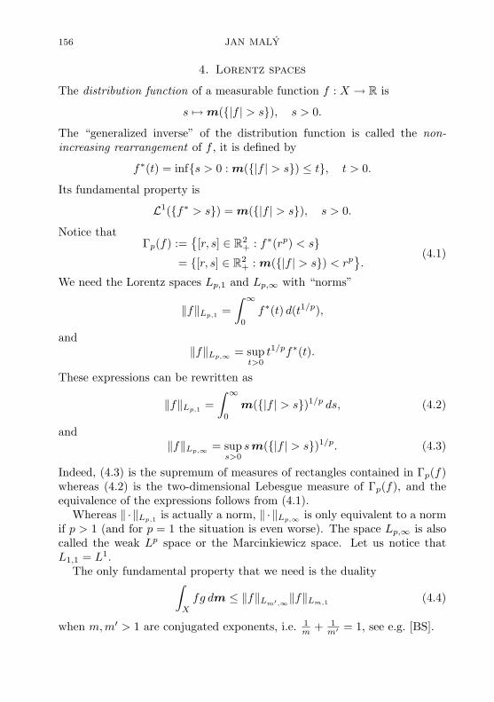
4. Lorentz spaces

The distribution function of a measurable function f : X → R is

s 7→ m(|f | > s), s > 0.

The “generalized inverse” of the distribution function is called the non-increasing rearrangement of f , it is defined by

f∗(t) = infs > 0 : m(|f | > s) ≤ t, t > 0.

Its fundamental property is

L1(f∗ > s) = m(|f | > s), s > 0.

Notice thatΓp(f) :=

[r, s] ∈ R2

+ : f∗(rp) < s= [r, s] ∈ R2

+ : m(|f | > s) < rp.

(4.1)

We need the Lorentz spaces Lp,1 and Lp,∞ with “norms”

‖f‖Lp,1 =∫ ∞

0

f∗(t) d(t1/p),

and‖f‖Lp,∞ = sup

t>0t1/pf∗(t).

These expressions can be rewritten as

‖f‖Lp,1 =∫ ∞

0

m(|f | > s)1/p ds, (4.2)

and‖f‖Lp,∞ = sup

s>0sm(|f | > s)1/p. (4.3)

Indeed, (4.3) is the supremum of measures of rectangles contained in Γp(f)whereas (4.2) is the two-dimensional Lebesgue measure of Γp(f), and theequivalence of the expressions follows from (4.1).

Whereas ‖ · ‖Lp,1 is actually a norm, ‖ · ‖Lp,∞ is only equivalent to a normif p > 1 (and for p = 1 the situation is even worse). The space Lp,∞ is alsocalled the weak Lp space or the Marcinkiewicz space. Let us notice thatL1,1 = L1.

The only fundamental property that we need is the duality∫

X

fg dm ≤ ‖f‖Lm′,∞‖f‖Lm,1 (4.4)

when m,m′ > 1 are conjugated exponents, i.e. 1m + 1

m′ = 1, see e.g. [BS].


Lemma 4.1. Suppose that Ej are pairwise disjoint Borel subsets of X andf ∈ Lm,1(X). Then ∑

j

‖fχEj‖m

Lm,1≤ ‖f‖m

Lm,1.Proof. Let η be the distribution function of f and ηj be the distribution

functions of fχj . Then ∑

j

ηj ≤ η.

Let S = infs > 0 : η(s) = 0. (S = ∞ if η is strictly positive everywhere.)Holder’s inequality yields

(∫ S

0

η1mj (s) ds

)m

≤(∫ S

0

ηj(s)η1m−1(s) ds

)(∫ S

0

η1m (s) ds

)m−1

for every j ∈ N. Summing over j, we obtain

∑

j

‖fχEj‖m

Lm,1=

∑

j

(∫ S

0

η1mj (s) ds

)m

≤(∫ S

0

η1m (s) ds

)m−1 ∑

j

(∫ S

0

ηj(s)η1m−1(s) ds

)

≤(∫ S

0

η1m (s) ds

)m

= ‖f‖mLm,1

.

5. Riesz potentials

The Riesz potentials studied here are a version of Riesz potentials from[HaK], see also [MMo], [MP].

Definition 5.1 (Whitney ball, Whitney covering). Let R > 0 be fixed.Let G ⊂ X be an open set. We say that B = B(z, r) is a Whitney ball forG constrained by R if

r = min1

2dist(z,X \G), R

.

A Whitney covering of G constrained by R is such a covering W of G byWhitney balls for G constrained by R that the balls B(z,r/5) :B(z, r)∈W

158 JAN MALY

are pairwise disjoint. The existence of a Whitney covering follows fromthe Vitali-type covering theorem. Every Whitney covering has its overlapmultiplicity bounded by a constant depending only on the doubling constantof m.

Whitney balls are a powerful replacement of Whitney cubes; evidentlythe latter ones are not available in metric spaces. The idea comes fromR. R. Coifman and G. Weiss [CW].

The Riesz kernels in Euclidean spaces are symmetric. In our generalitywe have the following.

Lemma 5.2. Suppose that µ and ν are measures on X. Then∫

X

IRα µ(x) dν(x) ≤ D

∫

X

IRα ν(y) dµ(y),

where D is the doubling constant of m.Proof. For y ∈ B(x, r) we have

m(B(y, r)) ≤ m(B(x, 2r)) ≤ Dm(B(x, r)).

Hence we have∫

X

(∫ R

0

µ(B(x, r))m(B(x, r))

drα

)dν(x)

=∫ R

0

(∫

X

(∫

B(x,r)

dµ(y)m(B(x, r))

)dν(x)

)drα

≤ D

∫ R

0

(∫

X

(∫

B(y,r)

dν(x)m(B(y, r))

)dµ(y)

)drα

= D

∫

X

(∫ R

0

(∫

B(y,r)

dν(x)m(B(y, r))

drα

)dµ(y)

)

= D

∫

X

IRα ν(y) dµ(y).

The main result of this section is the following “good lambda inequality”.

In the Euclidean setting, it is due to Muckenhoupt and Wheeden [MW]; inthis generality it is done in [Ho]. The method of good lambda inequalitieshas been invented by D. L. Burkholder and R. F. Gundy [BG].


Theorem 5.3. Let α > 0 and ε > 0. Then there exist a = a(D,α) > 0 andσ = σ(ε,D, α) > 0, where D is the doubling constant from (3.1), such that,for every measure µ on X,

m(IRα µ ≥ aλ

)≤ εm

(IRα µ ≥ λ

)+ m

(MR

α µ ≥ σ λ).Proof. Set

a = 22−αD2. (5.1)

DenoteG = IR

α µ > λ, Ga = IRα µ > aλ.

Obviously, G, Ga are open sets. Let B = B(z, r) be a Whitney ball for Gconstrained by R/3. We claim that

m(B ∩Ga

)≤ εm(B) + m

(B ∩

MR

α µ ≥ σ(ε)λ). (5.2)

The claim clearly holds if MRα µ ≥ λ on B. Hence we assume that there is

z′ ∈ B such thatMR

α µ(z′) ≤ λ.

Now we choose δ = δ(ε,D, α) ∈ (0, 1) to be determined later and denote

E = B ∩Iδrα µ >

aλ

2

.

Let ν be m restricted to B. Since B(x, δr) ⊂ B(z′, 3r) for every x ∈ B, wehave

Iδrα ν(y) = 0, y /∈ B(z′, 3r).

For y ∈ B(z′, 3r) we have

Iδrα ν(y) =

∫ δr

0

m(B(y, t) ∩B(z, r))m(B(y, t))

dtα ≤ δαrα.

Thus, using Lemma 5.2, we obtain

aλ

2m(E) ≤

∫

B

Iδrα µ(x) dx ≤ D

∫

X

Iδrα ν(y) dµ(y)

≤ D

∫

B(z′,3r)

δαrα dµ(y) = Dδαrαµ(B(z′, 3r))

≤ DδαMRα µ(z′)m(B(z′, 3r)) ≤ D3δαλm(B(z, r)).

160 JAN MALY

This showsm(E) ≤ εm(B) (5.3)

if δ = δ(ε,D, α) is chosen small enough. Choose x ∈ B ∩Ga \ E. Then

aλ

2≤

∫ 3r

δr

µ(B(x, t))m(B(x, t))

dtα +∫ R/2

3r


dtα

+∫ R

R/2


dtα.

(5.4)

We have∫ 3r

δr


dtα ≤ αMRα µ(x)

∫ 3r

δr

dt

t≤ αMR

α µ(x) ln(3/δ) (5.5)

and similarly ∫ R

R/2


dtα ≤ α ln 2MRα µ(x). (5.6)

Finally, we consider the integral from 3r to R/2. In the non-trivial case wehave 3r < R and thus from the definition of the Whitney ball there existsz′′ ∈ B(z, 3r) \G. Since

IRα µ(z′′) ≤ λ

andB(x, t) ⊂ B(z′′, 2t) ⊂ B(x, 3t), 3r < t,

using (3.1) and (5.1), we obtain

∫ R/2

3r


dtα ≤ D2

∫ R/2

3r

µ(B(z′′, 2t))m(B(z′′, 2t))

dtα

= 2−αD2

∫ R

6r

µ(B(z′′, s))m(B(z′′, s))

dsα

≤ 2−αD2IRα µ(z′′) ≤ 2−αD2λ =

aλ

4.

(5.7)

From (5.4)–(5.7) and (5.1) we infer that

λ ≤ C ln(3/δ)MRα µ(x), x ∈ B ∩Ga \ E. (5.8)

A combination of (5.3) and (5.8) yields (5.2). Summing over B in a Whitneycovering, we obtain the assertion of the theorem.


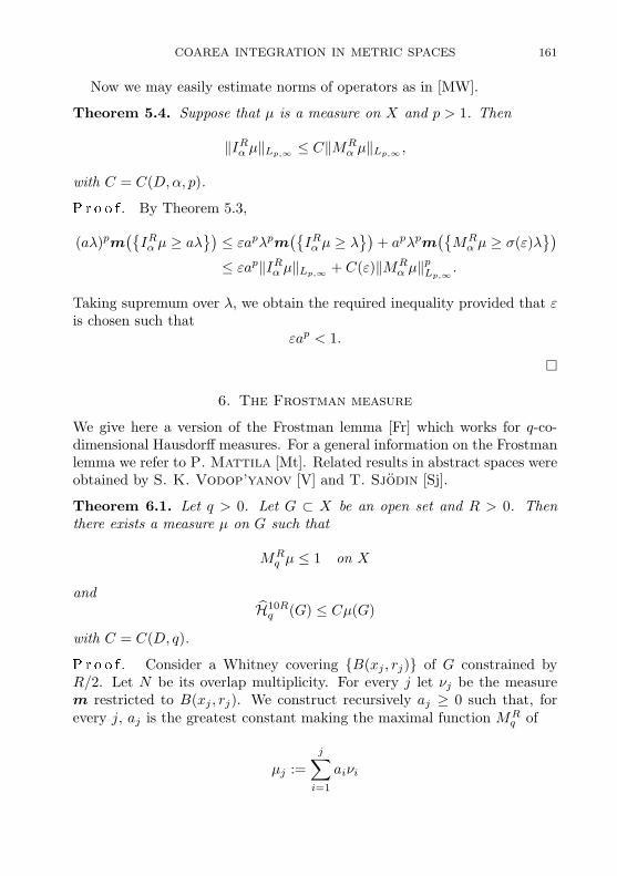
Now we may easily estimate norms of operators as in [MW].

Theorem 5.4. Suppose that µ is a measure on X and p > 1. Then

‖IRα µ‖Lp,∞ ≤ C‖MR

α µ‖Lp,∞ ,

with C = C(D,α, p).Proof. By Theorem 5.3,

(aλ)pm(IRα µ ≥ aλ

)≤ εapλpm

(IRα µ ≥ λ

)+ apλpm

(MR

α µ ≥ σ(ε)λ)

≤ εap‖IRα µ‖Lp,∞ + C(ε)‖MR

α µ‖pLp,∞ .

Taking supremum over λ, we obtain the required inequality provided that εis chosen such that

εap < 1.

6. The Frostman measure

We give here a version of the Frostman lemma [Fr] which works for q-co-dimensional Hausdorff measures. For a general information on the Frostmanlemma we refer to P. Mattila [Mt]. Related results in abstract spaces wereobtained by S. K. Vodop’yanov [V] and T. Sjodin [Sj].

Theorem 6.1. Let q > 0. Let G ⊂ X be an open set and R > 0. Thenthere exists a measure µ on G such that

MRq µ ≤ 1 on X

andH10R

q (G) ≤ Cµ(G)

with C = C(D, q).Proof. Consider a Whitney covering B(xj , rj) of G constrained byR/2. Let N be its overlap multiplicity. For every j let νj be the measurem restricted to B(xj , rj). We construct recursively aj ≥ 0 such that, forevery j, aj is the greatest constant making the maximal function MR

q of

µj :=j∑

i=1

aiνi

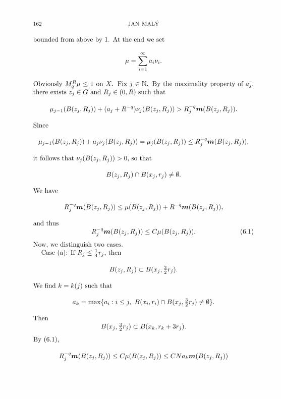
162 JAN MALY

bounded from above by 1. At the end we set

µ =∞∑

i=1

aiνi.

Obviously MRq µ ≤ 1 on X. Fix j ∈ N. By the maximality property of aj ,

there exists zj ∈ G and Rj ∈ (0, R) such that

µj−1(B(zj , Rj)) + (aj +R−q)νj(B(zj , Rj)) > R−qj m(B(zj , Rj)).

Since

µj−1(B(zj , Rj)) + ajνj(B(zj , Rj)) = µj(B(zj , Rj)) ≤ R−qj m(B(zj , Rj)),

it follows that νj(B(zj , Rj)) > 0, so that

B(zj , Rj) ∩B(xj , rj) 6= ∅.

We have

R−qj m(B(zj , Rj)) ≤ µ(B(zj , Rj)) +R−qm(B(zj , Rj)),

and thusR−q

j m(B(zj , Rj)) ≤ Cµ(B(zj , Rj)). (6.1)

Now, we distinguish two cases.Case (a): If Rj ≤ 1

4rj , then

B(zj , Rj) ⊂ B(xj ,32rj).

We find k = k(j) such that

ak = maxai : i ≤ j, B(xi, ri) ∩B(xj ,32rj) 6= ∅.

ThenB(xj ,

32rj) ⊂ B(xk, rk + 3rj).

By (6.1),

R−qj m(B(zj , Rj)) ≤ Cµ(B(zj , Rj)) ≤ CNakm(B(zj , Rj))


and thusR−q

j ≤ Cak. (6.2)

Setyj = xk, tj = rk + 3rj ≤ 2R.

Then B(xj , rj) ⊂ B(yj , tj). Suppose that 2rk = dist(xk,X \G). Then

2rj ≤ dist(xj ,X \G) ≤ dX(xj , xk) + dist(xk,X \G) ≤ 32rj + rk + 2rk,

and thusrj ≤ 6rk. (6.3)

If rk = R/2, we have trivially rj ≤ rk and thus (6.3) holds as well. We inferthat

m(B(yj , tj)) = m(B(xk, rk + 3rj)) ≤ D5m(B(xk, rk)).

SinceRj ≤

14rj ≤ tj ,

by (6.2),

t−qj m(B(yj , tj)) ≤ D5R−q

j m(B(xk, rk)) ≤ C akm(B(xk, rk))

≤ C µ(B(xk, rk)) ≤ C µ(B(yj , tj)).

Case (b): Suppose that Rj >14rj . We set

yj = zj , tj = Rj + 2rj ≤ 2R.

Then againB(xj , rj) ⊂ B(zj , Rj + 2rj) = B(yj , tj).

We havetj ≤ 9Rj .

By (6.1) and (3.1),

t−qj m(B(yj , tj)) ≤ D4R−q

j m(B(zj , Rj)) ≤ Cµ(B(zj , Rj)) ≤ Cµ(B(yj , tj)).

In any case, with each j we have associated yj ∈ X and tj ∈ (0, 2R) suchthat

B(xj , rj) ⊂ B(yj , tj) and t−qj m(B(yj , tj)) ≤ Cµ(yj , tj).

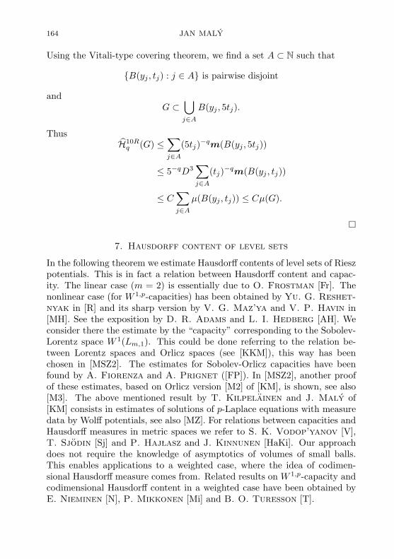
164 JAN MALY

Using the Vitali-type covering theorem, we find a set A ⊂ N such that

B(yj , tj) : j ∈ A is pairwise disjoint

andG ⊂

⋃

j∈A

B(yj , 5tj).

ThusH10R

q (G) ≤∑

j∈A

(5tj)−qm(B(yj , 5tj))

≤ 5−qD3∑

j∈A

(tj)−qm(B(yj , tj))

≤ C∑

j∈A

µ(B(yj , tj)) ≤ Cµ(G).

7. Hausdorff content of level sets

In the following theorem we estimate Hausdorff contents of level sets of Rieszpotentials. This is in fact a relation between Hausdorff content and capac-ity. The linear case (m = 2) is essentially due to O. Frostman [Fr]. Thenonlinear case (for W 1,p-capacities) has been obtained by Yu. G. Reshet-nyak in [R] and its sharp version by V. G. Maz’ya and V. P. Havin in[MH]. See the exposition by D. R. Adams and L. I. Hedberg [AH]. Weconsider there the estimate by the “capacity” corresponding to the Sobolev-Lorentz space W 1(Lm,1). This could be done referring to the relation be-tween Lorentz spaces and Orlicz spaces (see [KKM]), this way has beenchosen in [MSZ2]. The estimates for Sobolev-Orlicz capacities have beenfound by A. Fiorenza and A. Prignet ([FP]). In [MSZ2], another proofof these estimates, based on Orlicz version [M2] of [KM], is shown, see also[M3]. The above mentioned result by T. Kilpelainen and J. Maly of[KM] consists in estimates of solutions of p-Laplace equations with measuredata by Wolff potentials, see also [MZ]. For relations between capacities andHausdorff measures in metric spaces we refer to S. K. Vodop’yanov [V],T. Sjodin [Sj] and P. Haj lasz and J. Kinnunen [HaKi]. Our approachdoes not require the knowledge of asymptotics of volumes of small balls.This enables applications to a weighted case, where the idea of codimen-sional Hausdorff measure comes from. Related results on W 1,p-capacity andcodimensional Hausdorff content in a weighted case have been obtained byE. Nieminen [N], P. Mikkonen [Mi] and B. O. Turesson [T].


Here we present a direct proof of the estimate of the m-codimensionalHausdorff content by the “W 1(Lm,1)-capacity”, not passing through Orliczspaces.

Theorem 7.1. Let m > 1. Suppose that IRα g ≥ b > 0 on G. Then

bmH10Rαm (G) ≤ C‖g‖m

Lm,1, (7.1)

with C = C(D,α,m).Proof. Let µ be the Frostman measure for H10Rαm (G), see Theorem 6.1.

Let λ > 0 and x ∈ MRα µ > λ. Then, for every t ∈ (0, R),

µ(B(x, t)) ≤ t−αmm(B(x, t)), (7.2)

and there exists tx ∈ (0, R) such that

λt−αx m(B(x, tx)) ≤ µ(B(x, tx)). (7.3)

Multiplying (7.2) with the m-th power of (7.3), we obtain

λm(m(B(x, tx))

)m−1 ≤(µ(B(x, tx))

)m−1.

By the Vitali-type theorem, there exists a sequence B(xj , rj) of pairwisedisjoint balls such that xj ∈ MR

α µ > λ, rj = txjand

MRα µ > λ ⊂

⋃

j

B(xj , 5rj).

Using (3.1), we obtain

λm′m

(MR

α µ > λ)≤ Cλm′ ∑

j

m(B(xj , 5rj))

≤ Cλm′ ∑

j

m(B(xj , rj))

≤ C∑

j

µ(B(xj , rj))

≤ Cµ(X).

It follows that‖MR

α µ‖m′Lm′,∞

≤ Cµ(X).

166 JAN MALY

By Theorem 5.4, we have also

‖IRα µ‖m′

Lm′,∞≤ Cµ(X).

Using the duality (4.4) between Lm,1 and Lm′,∞ and Lemma 5.2, we obtain

bµ(X) ≤ C

∫

X

IRα g dµ ≤ C

∫

X

gIRα µdx

≤ C‖g‖Lm,1‖IRα µ‖Lm′,∞

≤ C‖g‖Lm,1

(µ(X)

)1/m′.

Hence, by the properties of the Frostman measure,

bmH10rαm ≤ Cbmµ(X) ≤ C‖g‖m

Lm,1.

Example 7.2. The estimate (7.1) does not hold for m = 1. Indeed, if µ isthe (n−1)-dimensional Hausdorff measure in Rn restricted to

F := x ∈ Rn : xn = 0, |x| ≤ 1

and R > 0, then IR1 µ ≡ +∞ on F , but HR

1 > 0. In this example µ is notabsolutely continuous with respect to the Lebesgue measure. However, if gj

are mollifications of µ with radii δj → 0, then (7.1) cannot hold with m = 1and C independent of j.

In fact, the only estimate that we can have for m = 1 is the followingCartan lemma. It can be obtained by the method of proving the Hardy-Littlewood maximal theorem, see [BZ] (for the Euclidean case) and [HaK]or [He] (for the maximal theorem in metric spaces).

Lemma 7.3. Let R > 0. Suppose that g ∈ L1(X). Then

bH5R1 (MR

1 g > b) ≤ C

∫

X

g(x) dx.

We shall need also the following modification.

Lemma 7.4. Suppose that g ∈ L1(X). Then

limr→0+

Mr1 g(x) = 0 Hm-a.e.

COAREA INTEGRATION IN METRIC SPACES 167Proof. Choose ε > 0 and R > 0. Let

Eε = x ∈ X : lim supr→0

Mr1 g(x) > ε.

It is clear that MRg(x) = +∞ at every x ∈ Eε. By the maximal theorem,cf. [HaK, Thm. 14.13], m(Eε) = 0. Let G ⊂ X be any open set containingEε. For every x ∈ G we can find rx > 0 such that 5rx < R, B(x, rx) ⊂ Gand ∫

B(x,rx)

g(x′) dx′ > εr−1x m(B(x, rx)).

Using the Vitali-type covering theorem, we observe that

HR1 (Eε) ≤ C

∫

G

g(x′) dx′.

Since G was arbitrary, we obtain

HR1 (Eε) = 0, R > 0, ε > 0,

which is enough to prove the conclusion.

8. Upper gradients

There are many non-equivalent ways how to define “Sobolev spaces” onmetric spaces, depending on what is considered to serve as a substituteto gradients. We shall use upper gradients introduced by J. Heinonenand P. Koskela in [HeK]. See [Sh], [Ch], [HaK] for various definitions ofsuch spaces. Spaces based on an upper gradient are well fitting not onlyto abstract domains, but also to abstract targets, see [HKST]. The mainreason for our choice is that once assumed Poincare inequalities, they arestable under truncation, an observation due to S. Semmes [Se].

Definitions. Let Ω ⊂ X be an open set. Given points x, x′ ∈ Ω, we denoteby Γx,x′,Ω the set of all 1-Lipschitz paths γ : [a, b] → Ω with γ(a) = x andγ(b) = y. The interval [a, b] depends on γ. Let g be a non-negative Borelmeasurable function on Ω. We define the weighted geodetic distance of pointsx, x′ ∈ Ω by

dg(x, x′; Ω) = infγ∈Γx,y,Ω

∫ b

a

g(γ(t)) dt.

The function dg has all properties of distance except that dg(x, x′; Ω) can be0 or ∞ for distinct points x, x′. Let (Y, dY ) be a metric space and u : Ω → Y

168 JAN MALY

be an m-measurable function. We say that g : Ω → [0,+∞] is an uppergradient to u if

dY (u(x), u(x′)) ≤ dg(x, x′; Ω), x, x′ ∈ Ω.

Throughout this section we suppose that X supports pre-Poincare inequali-ties

−∫

B(z,r)

−∫

B(z,r)

dg(x, x′) dx dx′ ≤ Pr −∫

B(z,τr)

g(x) dx (8.1)

for every z ∈ X, r > 0, and g ∈ L1(B(z, τt))+, here the constant P and thescaling parameter τ ≥ 1 are fixed parameters of the space X.

Let u : Ω → Y be an m-measurable function and g be its upper gradient.Then (8.1) easily implies the Poincare inequalities

−∫

B(z,r)

−∫

B(z,r)

dY (u(x), u(x′)) dx dx′ ≤ Pr −∫

B(z,τr)

g(x) dx (8.2)

for all balls B(z, r) with B(z, τr) ⊂ Ω.Remarks. (a) If X = Rn, then X supports (8.1) and if u is a Sobolevfunction, |∇u| is a limit of upper gradients to u. More precisely, if ∇u =∑

j gj , where the sum converges in L1, then for every k,∑

j≤k gj +∑

j>k |gj |is an upper gradient to u.

(b) There are many examples of spaces supporting Poincare inequalitiesin the literature, see eg. [HaK]. A usual assumption is that inequalities equiv-alent to (8.2) are satisfied for all scalar functions u : X → R and their uppergradients. Our assumption is probably a bit stronger but realistic, becausestandard proofs of Poincare inequalities implicitly show (8.1).

In fact, (8.1) is equivalent to validity of (8.2) for all spaces Y with theconstant independent of Y , as the following example shows: Let Yg be thequotient space X/∼ where

x ∼ x′ means dg(x, x′) = 0,

and u : X → Yg be the quotient mapping. We define the distance dk on Yg

bydk(u(x), u(x′)) = mindg(x, x′), k, k > 0.

Assuming (8.2) for (Yg, dk), we obtain

−∫

B(z,r)

−∫

B(z,r)

dk(u(x), u(x′)) dx dx′ ≤ Pr

∫

B(z,τr)

g(x) dx

which, letting k →∞, yields (8.1).The following lemma is essentially due to Semmes [Se], see also [Sh,

Lemma 4.3].


Lemma 8.1. Suppose that u : Ω → R is an m-measurable function and g isan upper gradient to u. If G ⊃ u 6= 0 is an open set, then gχG is also anupper gradient to u.Proof. Let x, x′ ∈ Ω and γ : [a, b] → Ω is a path, γ ∈ Γx,x′ . We want toshow

|u(x)− u(x′)| ≤∫ b

a

g(γ(t))χG(γ(t)) dt.

This is evident if γ([a, b]) ⊂ G. Otherwise there is s ∈ [a, b] such thatγ(s) /∈ G and thus u(γ(s)) = 0. Set

a′ = inft ∈ [a, s] : γ(t) /∈ G

,

b′ = supt ∈ [s, b] : γ(t) /∈ G

.

Then a ≤ a′ ≤ s ≤ b′ ≤ b and u(γ(a′)) = u(γ(b′)) = 0. If a′ > a, thenγ([a, a′]) ⊂ G and thus

|u(x)| = |u(γ(a′))− u(γ(a))| ≤∫ a′

a

g(γ(t)) dt =∫ a′

a

g(γ(t))χG(γ(t)) dt.

Similarly,

|u(x′)| ≤∫ b

b′g(γ(t))χG(γ(t)) dt.

It follows that

|u(x)− u(x′)| ≤ |u(x)|+ |u(x′)| ≤∫ b

a

g(γ(t))χG(γ(t)) dt

if γ([a, b]) 6⊂ G. In any case the assertion is valid. Lemma 8.2. Let κ > 0. Suppose that u : Ω → R is an m-measurablefunction and g is an upper gradient to u. Suppose that B(z, τr) ⊂ Ω. Ifa < b are real levels such that

m(B(z, r) ∩ u ≥ b

)≥ κm(B(z, r)),

m(B(z, r) ∩ u ≤ a

)≥ κm(B(z, r)),

then(b− a)m(B(z, τr)) ≤ Cr

∫

B(z,τr)∩a<u<bg(x) dx,

where C = C(κ, τ, P ).

170 JAN MALYProof. Let

w =

a on u ≤ ab on u ≥ bu elsewhere.

Then g is an upper gradient to w. Let Ga be an open set containing u > aand Gb be an open set containing u < b. Then by Lemma 8.1, gχGa

is an upper gradient to w − a. Hence it is also a weak upper gradient tow−b. Using Lemma 8.1 once more, we obtain that gχGa∩Gb

is a weak uppergradient to w − b and hence also to w. By (8.2),

(b− a)m(B(z, r)) ≤ Cm(B(z, r))−∫

B(z,r)

−∫

B(z,r)

|w(x)− w(x′)| dx dx′

≤ Cr

∫

B(z,τr)∩Ga∩Gb

g(x) dx.

Passing to infimum over all open sets Ga ⊃ u > a and Gb ⊃ u < b, weobtain the assertion.

9. Consequences of the Poincare inequality

In this chapter we recall some standard estimates modified to the form thatwe need.

Lemma 9.1. Suppose that Y is a metric space, u : Ω → Y is an m-measurable function and g ∈ L1(Ω) is an upper gradient to u. Suppose thatB(z, 2τr) ⊂ Ω. Let 0 < s ≤ t ≤ r. Then

−∫

B(z,s)

−∫

B(z,t)

dY (u(x), u(x′)) dx dx′ ≤ CI2τt1 g(z)

with C = C(D,P, τ).Proof. Suppose that 0 < s ≤ t ≤ r. Let k be such that 2−k−1t < s ≤ 2−kt.


Then by (8.2),

−∫

B(z,s)

−∫

B(z,t)

dY (u(x), u(x′)) dx dx′

≤ −∫

B(z,s)

−∫

B(z,2−kt)


+k−1∑

j=0

−∫

B(z,2−j−1t)

−∫

B(z,2−jt)


≤ C

k∑

j=0

−∫

B(z,2−jt)

−∫

B(z,2−jt)


≤ C

k∑

j=0

2−jt−∫

B(z,τ2−jt)

g(x) dx

≤ C

∫ 2τt

0

(−∫

B(z,s)

g(x) dx)ds

= CI2τt1 g(z)

as required. Lemma 9.2. Suppose that Y is a metric space, u : Ω → Y is an m-measur-able function and g ∈ L1(Ω) is an upper gradient to u. Suppose that

limr→0+

Mr1 g(z) = 0.

Then there exists yr : r > 0 ⊂ Y such that

limr→0

−∫

B(z,r)

dY (u(x), yr) dx = 0.Proof. We find rk ց 0 such that

Pr −∫

B(z,τr)

g(x) dx < 2−k−1, 0 < r < rk.

Set xr = z for r ≥ r1. Let rk+1 ≤ r < rk. By (8.2), we obtain

−∫

B(z,r)

−∫

B(z,r)

dY (u(x), u(x′)) dx dx′ ≤ 2−k−1.

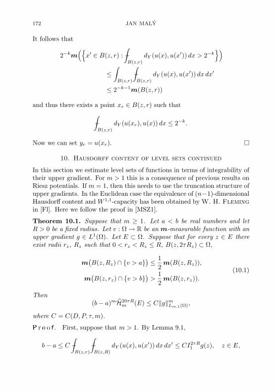
172 JAN MALY

It follows that

2−km(x′ ∈ B(z, r) : −

∫

B(z,r)

dY (u(x), u(x′)) dx > 2−k)

≤∫

B(z,r)

−∫

B(z,r)


≤ 2−k−1m(B(z, r))

and thus there exists a point xr ∈ B(z, r) such that

−∫

B(z,r)

dY (u(xr), u(x)) dx ≤ 2−k.

Now we can set yr = u(xr).

10. Hausdorff content of level sets continued

In this section we estimate level sets of functions in terms of integrability oftheir upper gradient. For m > 1 this is a consequence of previous results onRiesz potentials. If m = 1, then this needs to use the truncation structure ofupper gradients. In the Euclidean case the equivalence of (n−1)-dimensionalHausdorff content and W 1,1-capacity has been obtained by W. H. Flemingin [Fl]. Here we follow the proof in [MSZ1].

Theorem 10.1. Suppose that m ≥ 1. Let a < b be real numbers and letR > 0 be a fixed radius. Let v : Ω → R be an m-measurable function with anupper gradient g ∈ L1(Ω). Let E ⊂ Ω. Suppose that for every z ∈ E thereexist radii rz, Rz such that 0 < rz < Rz ≤ R, B(z, 2τRz) ⊂ Ω,

m(B(z,Rz) ∩ v > a

)≤ 1

2m(B(z,Rz)),

m(B(z, rz) ∩ v > b

)>

12

m(B(z, rz)).(10.1)

Then(b− a)mH20τR

m (E) ≤ C‖g‖mLm,1(Ω),

where C = C(D,P, τ,m).Proof. First, suppose that m > 1. By Lemma 9.1,

b− a ≤ C −∫

B(z,r)

−∫

B(z,R)

dY (u(x), u(x′)) dx dx′ ≤ CI2τR1 g(z), z ∈ E,


and the same certainly holds with g replaced by gχΩ. Using Theorem 7.1,we obtain

(b− a)mH20τRm (E) ≤ C‖g‖m

Lm,1(Ω).

Now, suppose that m = 1. Let us consider the monotone real function

ψ(s) =∫

a<v<sg(x) dx.

Then ψ is a.e. differentiable and

∫ b

a

ψ′(s) ds ≤ ψ(b)− ψ(a) = ψ(b).

Hence there exists s0 ∈ (a, b) such that (b−a)ψ′(s0) < 2ψ(b). We find δ > 0such that

ψ(s)− ψ(s0)s− s0

≤ 2ψ(b)b− a

for every s ∈ (s0, s0 + δ). (10.2)

Choose z ∈ E. By (10.1), the set

Sz =t > 0 :

m(B(z, t) ∩ v > s0)m(B(z, t))

>12

contains rz but does not contain Rz. Then, with every z ∈ E we canassociate tz ∈ (0, Rz] by

t′z = sup (0, Rz] ∩ Sz, tz = minRz, 2t′z.

Obviously, we have

m(B(z, t′x) ∩ v > s0) ≥12

m(B(z, t′x)),

m(B(z, tx) ∩ v > s0) ≤12

m(B(z, tx)),

and thusm(B(z, tx) ∩ v > s0) ≥

12D

m(B(z, tx)),

m(B(z, tx) ∩ v ≤ s0) ≥12

m(B(z, tx)).(10.3)

174 JAN MALY

We use the Vitali-type covering theorem to extract a (finite or infinite) se-quence Bjj∈I of pairwise disjoint balls Bj = B(zj , tj) from B(z, τtx):x ∈ E such that

E ⊂⋃

j∈I

B(zj , 5tj).

Here I = N or I = 1, 2, . . . , imax. Fix i ∈ I. Using (10.3), we find a levelsi ∈ (s0, s0 + δ) such that

m(B(zj , tj/τ) ∩ v > si

)≥ 1

4Dm

(B(zj , tj/τ)

), j = 1, . . . , i. (10.4)

From Lemma 8.2, (10.3) and (10.4) we infer that

t−1j (si − s0)m(B(zj , tj)) ≤ C

∫

B(zj ,tj)∩s0<g<sig(x) dx.

Summing over j = 1, . . . , i and using (10.2), we obtain

(si − s0)i∑

j=1

t−1j m(B(zj , tj)) ≤

i∑

j=1

∫

B(zj ,tj)∩s0<g<sig(x) dx

≤∫

s0<g<sig(x) dx

≤ ψ(si)− ψ(s0)

≤ (si − s0)2ψ(b)b− a

.

Passing i to imax or ∞, we obtain

H5τR1 (E) ≤

∑

j

(5tj)−1m(B(zj , 5tj)) ≤ C∑

j

t−1j m(B(zj , tj))

≤ Cψ(b)b− a

=2Cb− a

∫

Ω

g(x) dx,

as required. Remark. We cannot prove the m = 1 part of Theorem 10.1 similarly tothe m > 1 part because of the lack of H1-estimates of level sets of Rieszpotentials, see Example 7.2. Also the estimate of Lemma 7.3 is not enough.Indeed, the inequality

v(x) ≤ CM1g(x), x ∈ E,does not hold under the assumptions of Theorem 10.1; consider the functions

vε(x) = ε log(1/|x|)+, ε→ 0+,

as an example in Rn, n > 1.


11. Lebesgue points

H. Federer and W. P. Ziemer [FZ] showed that Sobolev functions haveLebesgue points q.e. in the sense of the Sobolev capacity. The case Sobolev-Orlicz and Sobolev-Lorentz spaces was treated by P. Maly, D. Swansonand W. P. Ziemer in [MSZ2]. The results concerning Sobolev-Orlicz spacesalso follow from Aissaoui’s work [A] on Lebesgue points of potentials.

In metric spaces, a W 1,p result for p > 1 has been obtained by J. Kin-nunen and V. Latvala [KL].

Definitions. Let Ω ⊂ X be an open set, z ∈ Ω and u : X → Y be an m-measurable mapping. A point y ∈ Y is said to be a Lebesgue limit of u at zand denoted by L-limx→z u(x) if

limr→0

−∫

B(z,r)

dY (u(x), y) dx = 0.

We say that an m-measurable function u : Ω → Y is Lebesgue precise if

L-limx→z

u(x) = u(z)

whenever the Lebesgue limit of u at z exists.

Lemma 11.1. Suppose that Y is a complete metric space, u : Ω → Y isan m-measurable function and g ∈ L1(Ω) is an upper gradient to u. Supposethat B(z, 2τR) ⊂ Ω and

I2τR1 g(z) <∞. (11.1)

Then u has a Lebesgue limit y at z and

−∫

B(z,r)

dY (u(x), y) dx ≤ CI2τr1 g(z) (11.2)

for every r ∈ (0, R], with C = C(D,P, τ).Proof. By (11.1), we have

limr→0+

Ir1g(z) = 0, (11.3)

and thus also

limr→0+

Mr1 g(z) ≤ C lim

r→0+

∫ 2r

r

(−∫

B(z,t)

g(x) dx)dt = 0.

176 JAN MALY

By Lemma 9.2 and (11.3), there exist rk ց 0 and yk ∈ Y such that

−∫

B(z,rk)

dY (u(x), yk) dx < 2−k, I2τrk1 (z) < 2−k. (11.4)

For k < j ∈ N we estimate

dY (yk, yj) ≤ dY (yk, u(x)) + dY (u(x), u(x′)) + dY (u(x′), yj),

x ∈ B(z, rk), x′ ∈ B(z, rj).

Integrating with respect to x and x′ and using (11.4) and Lemma 9.1, weobtain

dY (yk, yj) ≤ −∫

B(z,rk)

dY (yk, u(x)) dx

+−∫

B(z,rk)

−∫

B(z,rj)

dY (u(x), u(x′)) dx′ dx

+−∫

B(z,rj)

dY (yj , u(x′)) dx′

≤ 2−k+1 + CI2τrk1 g(z) ≤ C2−k.

(11.5)

Hence ykk is a Cauchy sequence and, since Y is complete, there existsy ∈ Y such that

y = limkyk.

Now, for 0 < rk < r ≤ R, by Lemma 9.1, (11.4) and (11.5) we have

−∫

B(z,r)

dY (u(x), y) dx ≤ −∫

B(z,r)

−∫

B(z,rk)

dY (u(x), u(x′)) dx′ dx

+−∫

B(z,rk)

dY (u(x′), yk) dx′ + dY (yk, y)

≤ C(I2τr1 g(z) + 2−k

).

Letting k →∞, we obtain (11.2). Theorem 11.2. Let m > 1. Suppose that Y is a complete metric space,u : Ω → Y is an m-measurable function and g ∈ Lm,1(Ω) is an uppergradient to u. Then for Hm-a.e. x ∈ Ω there exists a Lebesgue limit of uat x. In particular, if u is Lebesgue precise, then Hm-a.e. points of Ω areLebesgue points for u.Proof. This is a combination of Lemma 11.1 and Theorem 7.1.


Theorem 11.3. Suppose that Y is boundedly compact. Let Ω ⊂ X be anopen set and u : Ω → Y be an m-measurable function with an upper gradientg ∈ L1(Ω). Then for H1-a.e. x ∈ Ω there exists a Lebesgue limit of u at x.In particular, if u is Lebesgue precise, then H1-a.e. points of Ω are Lebesguepoints for u.Proof. The scalar case.Set

Z =z ∈ Ω : lim sup

r→0+Mr

1 g(z) > 0.

By Lemma 7.4,H1(Z) = 0.

Hence we may consider only z ∈ Ω \ Z. Then by Lemma 9.2, there existsa sequence yk, yk = yk(z) ∈ R, such that

limk→∞

−∫

B(z,rk)

|u(x)− yk| dx = 0, rk = 2−k.

Using the doubling property of m and the special choice of rk, we easilyobserve that the values

ϕ(z) = lim supk→∞

yk(z), ψ(z) = lim infk→∞

yk(z)

do not depend on the choice of yk, and that L-limx→z u(x) ∈ R exists if andonly if ϕ(z) = ψ(z) ∈ R. Therefore, it remains to prove that

ϕ(z) = ψ(z) ∈ R for H1-a.e. x ∈ Ω \ Z. (11.6)

Suppose that ϕ(z) = ∞. Then we consider a ball B(z0, R) containing z andsuch that B(z0, 3τR) ⊂ Ω. There exists a number a ∈ R satisfying

m(B(z0, 2R) ∩ u > a

)≤ 1

2D2m(B(z0, 2R)).

Then, since B(z,R) ⊂ B(z0, 2R) ⊂ B(z, 4R),

m(B(z,R) ∩ u > a

)≤ m

(B(z0, R) ∩ u > a

)

≤ 12D2

m(B(z0, 2R))

≤ 12

m(B(z, 2R)).

178 JAN MALY

Suppose that b > a and yk > b+ 1. Then

m(B(z, rk) ∩ u ≤ b)m(B(z, rk))

≤ −∫

B(z,rk)

|u− yk| dx→ 0,

which implies that there exists rz ∈ (0, R) such that

m(B(z, rz) ∩ u > b) > 12

m(B(z, rz)).

By Theorem 10.1, we have

(b− a) H20τR1 (B(z0, R) ∩ ϕ(z) = ∞) ≤ C

∫

Ω

g(x) dx.

On letting b→∞, we obtain that

H1(z : ϕ(z) = ∞) = 0, (11.7)

and similarlyH1(z : ψ(z) = −∞) = 0. (11.8)

Now, given rational numbers a < b, consider the set

E := z : ψ(z) < a < b < ϕ(z).

Since m-a.e. point z ∈ Ω is a Lebesgue point for u, it follows that m(E) = 0.Let G ⊂ Ω be an arbitrary open set containing E and a′ ∈ (ψ(z), a). Thenfor big k, yk < a′ and thus

(a− a′)m(B(z, rk) ∩ u > a)

m(B(z, rk))≤ −

∫

B(z,rk)

|u− yk| dx→ 0.

Hence there exists Rz > 0 such that B(z, 2τRz) ⊂ G and

m(B(z,Rz) ∩ u > a) ≤ 12

m(B(z,Rz)).

Similarly, there exists rz ∈ (0, Rz) such that

m(B(z, rz) ∩ u > b) > 12

m(B(z, rz)).


By Theorem 10.1,

H20τR1 (E) ≤ C

∫

G

g(x) dx.

Since G containing E was arbitrary, we have

H20τR1 (E) = 0.

Letting R→ 0 and passing to union over all rational couples (a, b), we obtainthat

H1(z : ψ(z) < ϕ(z)) = 0. (11.9)

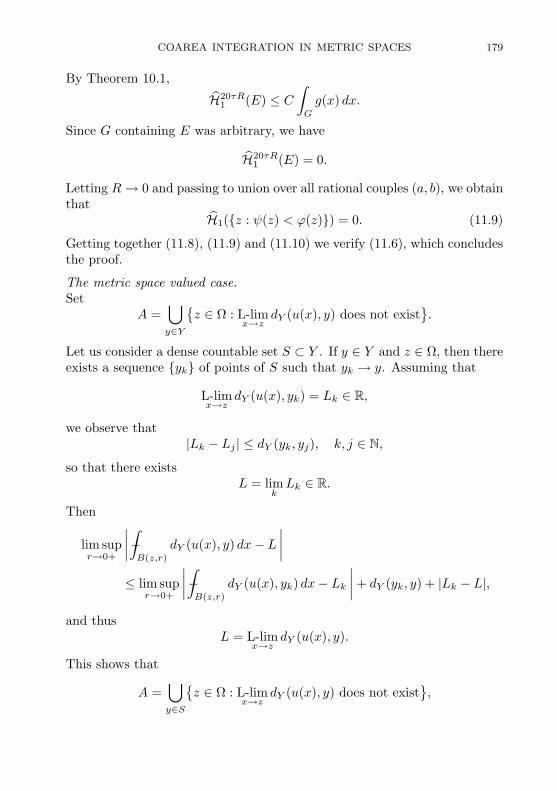
Getting together (11.8), (11.9) and (11.10) we verify (11.6), which concludesthe proof.

The metric space valued case.Set

A =⋃

y∈Y

z ∈ Ω : L-lim

x→zdY (u(x), y) does not exist

.

Let us consider a dense countable set S ⊂ Y . If y ∈ Y and z ∈ Ω, then thereexists a sequence yk of points of S such that yk → y. Assuming that

L-limx→z

dY (u(x), yk) = Lk ∈ R,

we observe that|Lk − Lj | ≤ dY (yk, yj), k, j ∈ N,

so that there existsL = lim

kLk ∈ R.

Then

lim supr→0+

∣∣∣∣−∫

B(z,r)

dY (u(x), y) dx− L

∣∣∣∣

≤ lim supr→0+

∣∣∣∣−∫

B(z,r)

dY (u(x), yk) dx− Lk

∣∣∣∣ + dY (yk, y) + |Lk − L|,

and thusL = L-lim

x→zdY (u(x), y).

This shows that

A =⋃

y∈S

z ∈ Ω : L-lim

x→zdY (u(x), y) does not exist

,

180 JAN MALY

and since S is countable, by the scalar part of the proof applied to thefunctions

y 7→ dY (u(x), y), y ∈ S,we infer that

H1(A) = 0. (11.10)

Fix z ∈ Ω \A and set

f(y) = L-limx→z

dY (u(x), y), y ∈ Y.

Then clearly

|f(y)− f(y′)| ≤ dY (y, y′) ≤ f(y) + f(y′), y, y′ ∈ Y.

Hence f is a 1-Lipschitz function and

limdY (y,y′)→∞

f(y) = ∞, y′ ∈ Y.

Since Y is boundedly compact, these observations imply that f attains itsminimum at some point y0 ∈ Y . Set

L0 = f(y0) = miny∈Y

f(y).

Assume that L0 > 0. The set

K = y ∈ Y : |dY (y, y0)− L0| ≤ L0/2

is compact and thus there exists a finite set

yk : k = 1, . . . , q ⊂ K

such that the balls B(yk, L0/4) cover K. For every ε > 0 we find δ > 0 suchthat ∣∣∣∣−

∫

B(z,r)

dY (u(x), yk)− f(yk)∣∣∣∣ < ε, 0 < r < δ.

Fix r ∈ (0, δ). Then

B(z, r) =q⋃

k=0

Ek,


where

E0 =x ∈ B(z, r) : |dY (u(x), y0)− L0| > L0/2

,

Ek =x ∈ B(z, r) : |dY (u(x), yk)− f(yk)| < L0/4

, k = 1, . . . , q.

If x ∈ E0, then

dY (u(x), y0) ≤ |dY (u(x), y0)− L0|+ L0 ≤ L0/2 + 2|dY (u(x), y0)− L0|.

If x ∈ Ek, k ∈ 1, . . . , q, then by the minimum property of L0,

dY (u(x), y0) ≤ 2L0 ≤ 2f(yk) ≤ 2|dY (u(x), yk)− f(yk)|+ 2dY (u(x), yk)

≤ 2|dY (u(x), yk)− f(yk)|+ L0/2.

Integrating these inequalities, we obtain

−∫

B(z,r)

dY (u(x), y0) dx ≤L0

2+−

∫

B(z,r)

(dY (u(x), y0)−

L0

2

)+

dx

≤ L0

2+

1m(B(z,R))

q∑

k=0

∫

Ek

(dY (u(x), y0)−

L0

2

)+

dx

≤ L0

2+ 2

q∑

k=0

−∫

B(z,r)

∣∣dY (u(x), yk)− f(yk)∣∣ dx

≤ L0

2+ 2(q + 1)ε.

For sufficiently small ε this implies that

−∫

B(z,r)

dY (u(x), y0) dx <34L0, 0 < r < δ,

and thus f(y0) < L0. This contradiction yields

f(y0) = L0 = 0,

so that y0 is the Lebesgue limit of f at z. We have shown that the Lebesguelimit at z exists for every z ∈ Ω \A. By (11.11), this concludes the proof.

182 JAN MALY

12. Coarea property

Now we are ready to establish metric space versions of results already dis-cussed in Section 2.

Definition. We say that a function u : Ω → Y satisfies the m-coareaproperty in Ω if for every Lebesgue null set E ⊂ Ω and Hm-almost everyy ∈ Y we have Hm(E ∩ u−1(y)) = 0.

Notation. Consider a mapping u : X → Y . We denote by Lu the set of allLebesgue points of u. For any z ∈ X and r > 0, we denote

Gu(z, r) =x ∈ B(z, r) : u(x) ∈ B(u(z), r)

.

Lemma 12.1. Suppose that m ≥ 1. Let u : Ω → Y be a mapping withan upper gradient g ∈ L1(X). Let z ∈ Ω, y ∈ Y and let R > 0 be a radiussuch that B(z, 3τR) ⊂ Ω. Then

RmH20τRm (Gu(z,R) ∩ Lu) ≤ C‖(1 + g)χGu(z,3τR)‖m

Lm,1, (12.1)

with C = C(D,P, τ,m).Proof. Setv(x) =

(2R− dY (u(x), u(z))

)+

and consider an open set G containing v > 0. Then g is an upper gradientto v and, by Lemma 8.1, gχG is an upper gradient to v.

Suppose first that

m(B(x,R) ∩Gu(z, 2R)

)≤ 1

2m(B(x,R)) for every x ∈ B(z,R). (12.2)

Then, taking into account the definition of Lebesgue points, there existsrx ∈ (0, R) such that

m(B(x, rx) ∩ |u− u(x)| < R

)>

12

m(B(x, rx)).

Hencem

(B(x,R) ∩ v > 0

)≤ 1

2m(B(z,R)),

m(B(x, rx) ∩ v > R

)>

12

m(B(z, rx)).


By Theorem 10.1,

RmH20τRm (Gu(z,R) ∩ Lu) ≤ C‖gχGu(z,3τR)‖m

Lm,1.

Suppose now that (12.2) is violated. Then there exists x ∈ B(z,R) suchthat

m(B(x,R) ∩Gu(z, 2R)) >12

m(B(x,R)).

We estimate the Hausdorff measure via the trivial covering of the set by theball B(z,R). Thus

RmHRm((Gu(z,R) ∩ Lu)) ≤ m(B(z,R))

≤ Dm(B(x,R))

≤ 2Dm(Gu(z, 2R))

≤ 2D‖χGu(z,2R)‖mLm,1

.

In any case we have (12.1).

Definition 12.2. For integration with respect to the Hausdorff measure, itis useful to consider the functionals

Λδm : f 7→ inf

∑j

γj(diamAj)m : γj ≥ 0, diamAj ≤ δ, f ≤ ∑j

γjχAj

, δ > 0,

defined on non-negative functions f on Y . By [F, 2.10.24],

∫ ∗

Y

f dHm = limδ→0

Λδm(f)

for any such an f provided that Y is boundedly compact. Recall that∫ ∗

stands for the upper integral.

The following theorem is our final statement on the m-coarea property.

Theorem 12.3. Suppose that m ≥ 1 and that Y is boundedly compact. LetΩ ⊂ X be an open set and u : Ω → Y be a Lebesgue precise m-measurablemapping with an upper gradient g ∈ Lm,1(Ω). Then u satisfies the m-coareaproperty in Ω.Proof. Let E ⊂ Ω be a set of m-measure 0. By Theorems 11.2, 11.3, wemay assume that E consists only of Lebesgue points for u. In the Cartesian

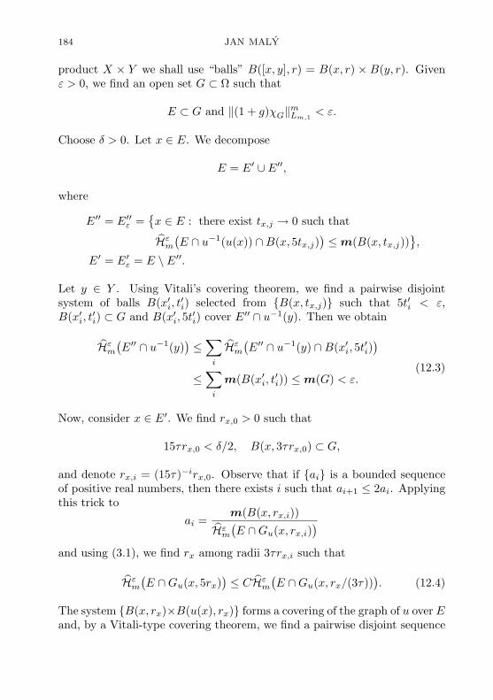
184 JAN MALY

product X × Y we shall use “balls” B([x, y], r) = B(x, r) × B(y, r). Givenε > 0, we find an open set G ⊂ Ω such that

E ⊂ G and ‖(1 + g)χG‖mLm,1

< ε.

Choose δ > 0. Let x ∈ E. We decompose

E = E′ ∪ E′′,

where

E′′ = E′′ε =x ∈ E : there exist tx,j → 0 such that

Hεm

(E ∩ u−1(u(x)) ∩B(x, 5tx,j)

)≤ m(B(x, tx,j))

,

E′ = E′ε = E \ E′′.

Let y ∈ Y . Using Vitali’s covering theorem, we find a pairwise disjointsystem of balls B(x′i, t

′i) selected from B(x, tx,j) such that 5t′i < ε,

B(x′i, t′i) ⊂ G and B(x′i, 5t

′i) cover E′′ ∩ u−1(y). Then we obtain

Hεm

(E′′ ∩ u−1(y)

)≤

∑

i

Hεm

(E′′ ∩ u−1(y) ∩B(x′i, 5t

′i)

)

≤∑

i

m(B(x′i, t′i)) ≤ m(G) < ε.

(12.3)

Now, consider x ∈ E′. We find rx,0 > 0 such that

15τrx,0 < δ/2, B(x, 3τrx,0) ⊂ G,

and denote rx,i = (15τ)−irx,0. Observe that if ai is a bounded sequenceof positive real numbers, then there exists i such that ai+1 ≤ 2ai. Applyingthis trick to

ai =m(B(x, rx,i))

Hεm

(E ∩Gu(x, rx,i)

)

and using (3.1), we find rx among radii 3τrx,i such that

Hεm

(E ∩Gu(x, 5rx)

)≤ CHε

m

(E ∩Gu(x, rx/(3τ))

). (12.4)

The system B(x, rx)×B(u(x), rx) forms a covering of the graph of u over Eand, by a Vitali-type covering theorem, we find a pairwise disjoint sequence


Bj of “balls” Bj = B(xj , rj) × B(u(xj), rj) such that xj ∈ E, rj = rxj,

and [x, u(x)] : x ∈ E′

⊂

⋃

j

B(xj , 5rj)×B(u(xj), 5rj

). (12.5)

We denote

Aj = B(u(xj), 5rj),

γj = Hεm

(E ∩B(xj , 5rj) ∩ u−1(Aj)

)= Hε

m

(E ∩Gu(xj , 5rj)

).

Then for every y ∈ Y , we have by (12.5),

Hεm

(E′ ∩ u−1(y)

)≤

∑

j

Hεm

(E ∩B(xj , 5rj) ∩ u−1(Aj)

)χ

Aj(y)

=∑

j

γjχAj(y),

so that for the functional introduced in Definition 12.2 and

fε(y) = Hεm

(E′ε ∩ u−1(y)

)

we haveΛδ

m(fε) ≤∑

j

γj diam(Aj)m

≤ C∑

j

Hεm

(E ∩Gu(xj , 5rj)

)diam(Aj)m.

(12.6)

By Lemma 12.1 and (12.4),

Hεm

(E ∩Gu(xj , 5rj)

)diam(Aj)m ≤ Crm

j Hεm

(E ∩Gu(xj , rj/(3τ))

)

≤ C‖(1 + g)χGu(xj ,rj)‖m

Lm,1.

(12.7)

Since the sets Gu(xj , rj) are pairwise disjoint and contained in G, by Lemma4.1, (12.7) and (12.6), we obtain

Λδm(fε) ≤ C‖(1 + g)χG‖m

Lm,1≤ Cε.

Letting δ → 0, we obtain∫ ∗

Y

Hεm(E′ε ∩ u−1(y)) dHm(y) = 0,

so that, by (12.3), for Hm-almost every y ∈ Y we have

Hεm(E ∩ u−1(y)) ≤ Hε

m(E′ε ∩ u−1(y)) + Hεm(E′′ε ∩ u−1(y)) ≤ ε.

Since ε > 0 was arbitratily small, it concludes the proof.

186 JAN MALY

13. The Eilenberg inequality

In this section we generalize the part (a) of Theorem 2.5 to metric spaces.A combination with Theorem 12.3 verifies that the Eilenberg inequality inour metric space setting is valid for mappings with upper gradients in theLorentz space Lm,1.

Lemma 13.1. There is a constant ℓ = ℓ(D,P, τ) with the following prop-erty: Suppose that Y is a metric space and u : Ω → Y is an m-measurablefunction with a strictly positive upper gradient g ∈ L1(Ω). Then for everyBorel set E ⊂ Ω and ε > 0 there is a pairwise disjoint decomposition

E = N ∪⋃

j

Ej

such that m(N) = 0 and

dY (u(z), u(z′)) ≤ (1 + ε)ℓdX(z, z′) infx∈Ej

g(x)

for every z, z′ ∈ Ej.Proof. Let ε > 0 be fixed. First, we decompose X into the sets

Xk = x : (1 + ε)k−1 ≤ g(x) < (1 + ε)k, k ∈ Z.

We may assume that E ⊂ Xk for some k. By the Lebesgue differentiationtheorem [HaK], almost every point x of E is a Lebesgue point for g. Thismeans that for every ε > 0 there exists a radius Rx such that B(x,Rx) ⊂ Ω,

−∫

B(x,t)

|g| dx′ ≤ (1 + ε)k, 0 < t < Rx.

We can decompose E into countably many pieces on which Rx is boundedaway from zero, so that we may assume that Rx ≥ δ > 0 on E. Supposethat z, z′ ∈ E are Lebesgue points for u, dX(z, z′) = r < δ/(4τ). ThenB(z, r) ⊂ B(z′, 2r) and, by the Poincare inequality (8.2),

−∫

B(z,r)

−∫

B(z′,2r)

dY (u(x), u(x′)) dx′ dx ≤ Cr −∫

B(z′,2τr)

g(x′) dx′

≤ Cr(1 + ε)k.

(13.1)


By Lemma 11.1,

−∫

B(z,r)

dY (u(x), u(z)) dx ≤ CI2τr1 g(z),

−∫

B(z′,2r)

dY (u(x′), u(z′)) dx′ ≤ CI4τr1 g(z′).

Since

I2τr1 g(z) =

∫ 2τr

0

(−∫

B(z,t)

g(x) dx)dt ≤ Cr(1 + ε)k

and similarlyI4τr1 g(z′) ≤ Cr(1 + ε)k,

together with (13.1) we obtain

dY (u(z), u(z′)) ≤ Cr(1 + ε)k ≤ (1 + ε) ℓ dX(z, z′) infx∈Ej

g(x)

for an appropriate constant ℓ. Remark. The proof of Lemma 13.1 is fairly general, but it hardly leadsto the optimal constant. In some situations, e.g. in Euclidean spaces, oneobtains Lemma 13.1 with ℓ = 1. Indeed, we have ℓ = 1 if u is smooth.For Sobolev functions, a theorem of Lusin-type (see e.g. [Z]) enables us toapproximate u by a smooth function v such that the set where u differsfrom v is small.

Now, we are ready to establish the Eilenberg-type inequality.

Theorem 13.2. Suppose that Y is boundedly compact and m ≥ 1. Letu : Ω → Y be an m-measurable function satisfying the m-coarea propertyand let g ∈ Lm(Ω) be an upper gradient to u. Let ω be a non-negativem-measurable function on Ω. Then

∫ ∗

Y

(∫

u−1(y)

ω(x) dHm(x))dHm(y) ≤ (2ℓ)mαk

∫

Ω

ω gm dx, (13.2)

where ℓ is the constant from Lemma 13.1.Proof. We may assume that ω is a characteristic function of a measurableset E. Also, we may neglect sets of m-measure zero, because for (character-istic functions of) such sets (13.2) holds by the m-coarea property. An easy

188 JAN MALY

approximation argument shows that we may assume that g is strictly posi-tive. Given ε > 0, by Lemma 13.1, we may decompose E into Borel sets Ek

such that

dY (u(x), u(x′)) ≤ (1 + ε) ℓ dX(x, x′) infEk

g, x, x′ ∈ Ek.

Taking away a set of m-measure zero, we may assume that every point of Ek

is a Lebesgue density point of Ek. Fix k ∈ N and choose δ > 0. Let Gk ⊂ Ωbe an open set such that

∫

Gk

gm(x) dx ≤∫

Ek

(gm(x) + εm) dx.

By the fine Vitali covering theorem [He, Thm. 1.6.], we find a sequence ofpairwise disjoint balls B(xj , rj) ⊂ G such that rj < ε,

diamu(B(xj , rj)) ≤ 2(1 + ε) ℓrj infEk

g < δ,

m(B(xj , rj)) ≤ (1 + ε)m(B(xj , rj) ∩ Ek),(13.3)

andm

(Ek \

⋃

j

B(xj , rj))

= 0.

For each j, by (13.3),

m(B(xj , rj))(diamu(B(xj , rj))

)m

≤ (1 + ε)m(Ek ∩B(xj , rj))(diamu(B(xj , rj))

)m

≤ (1 + ε)m+1 ℓm rmj

∫

B(xj ,rj)

gm(x) dx.

(13.4)

We denoteAj = u(B(xj , rj)).

Then for every y ∈ Y we have by (12.5)

Hεm

(Ek ∩ u−1(y)

)≤

∑

j

r−mj m(B(xj , rj))χAj

(y),

so that for the functional introduced at Definition 12.2 and

fk,ε(y) = Hεm

(Ek ∩ u−1(y)

),


appealing to (13.4), we have

Λδm(fk,ε) ≤

∑

j

r−mj m(B(xj , rj))αk(diamAj)m

≤ (2ℓ)m(1 + ε)m+1αk

∑

j

∫

B(xj ,rj)

gm(x) dx

≤ (2ℓ)m(1 + ε)m+1αk

∫

Gk

gm(x) dx

≤ (2ℓ)m(1 + ε)m+1αk

∫

Ek

(gm(x) + εm) dx.

Letting δ → 0, we obtain∫ ∗

Y

Hεm

(Ek ∩ u−1(y)

)dHm(y) ≤ (2ℓ)m(1 + ε)m+1αk

∫

Ek

(gm + εm) dx.

Summing over k and then letting ε→ 0, we obtain the required estimate.

References

[AH] D. R. Adams and L. I. Hedberg: Function spaces and potential theory. Grund-lehren der Mathematischen Wissenschaften 314, Springer-Verlag, Berlin, 1995.

Zbl 0834.46021.

[A] N. Aıssaoui: Maximal operators, Lebesgue points and quasicontinuity in stronglynonlinear potential theory. Acta Math. Univ. Comenian. 71 (2002), 35–50. MR1 943 014.

[AT] L. Ambrosio and P. Tilli: Selected topics on analysis on metric spaces. ScuolaNormale Superiore Pisa, 2000.

[BZ] T. Bagby and W. P. Ziemer: Pointwise differentiability and absolute continuity.

Trans. Amer. Math. Soc. 191 (1974), 129–148. Zbl 0295.26013, MR 49#9129.

[BS] C. Bennett and R. Sharpley: Interpolation of operators. Pure and AppliedMathematics 129, Academic Press, Inc., Boston, MA, 1988. Zbl 0647.46057, MR89e:46001.

[BG] D. L. Burkholder and R. F. Gundy: Extrapolation and interpolation of quasi-linear operators on martingales. Acta Math. 124 (1970), 249–304. Zbl 0223.60021,

MR 55 #13567.

[Ce] L. Cesari: Sulle funzioni assolutamente continue in due variabili. Ann. ScuolaNorm. Sup. Pisa, II. Ser. 10 (1941), 91–101. Zbl 0025.31301, MR 3,230e.

[Ch] J. Cheeger: Differentiability of Lipschitz functions on metric measure spaces.Geom. Funct. Anal. 9 (1999), 428–517. Zbl 0942.58018, MR 2000g:53043.

[CW] R. R. Coifman and G. Weiss: Analyse harmonique non-commutative sur certainespaces homogenes. Lecture Notes in Math. 242. Springer-Verlag, Berlin, 1971.

Zbl 0224.43006, MR 58 #17690.

190 JAN MALY

[E] S. Eilenberg: On ϕ measures. Ann. Soc. Pol. Math. 17 (1938), 251–252.

[F] H. Federer: Geometric measure theory. Die Grundlehren der mathematischenWissenschaften in Einzeldarstellungen 153. Springer-Verlag, New York, 1969.Zbl 0176.00801, MR 41 #1976.

[FZ] H. Federer and W. P. Ziemer: The Lebesgue set of a function whose partial

derivatives are p-th power summable. Indiana Univ. Math. J. 22 (1972), 139–158.Zbl 0238.28015, MR 55 #8321.

[FP] A. Fiorenza and A. Prignet: Orlicz capacities and applications to someexistence questions for elliptic PDEs having measure data. ESAIM: Control,Optim. and Calc. Var. 9 (2003), 317–341.

[Fl] W. H. Fleming: Functions whose partial derivatives are measures. Illinois J.Math. 4 (1960), 452–478. Zbl 0151.05402, MR 24 #A202.

[FR] W. H. Fleming and R. Rishel: An integral formula for the total variation.Arch. Math. 111 (1960), 218–222. Zbl 0094.26301, MR 22 #5710.

[Fr] O. Frostman: Potentiel d’equilibre et capacite des ensembles avec quelques

applications a la theorie des fonctions. Medd. Lunds Univ. Mat. Sem. 3 (1935),1–118. Zbl 0013.06302.

[GGKK] I. Genebashvili, A. Gogatishvili, V. Kokilashvili and M. Krbec: Weighttheory for integral transforms on spaces of homogeneous type. Pitman Mono-

graphs and Surveys in Pure and Applied Mathematics 92. Longman, Harlow,1998. Zbl 0955.42001, MR 2003b:42002.

[Ha] P. Haj lasz: Sobolev mappings, co-area formula and related topics. In: Pro-ceedings on analysis and geometry. International conference in honor of the

70th birthday of Professor Yu. G. Reshetnyak, Novosibirsk, Russia, August 30–September 3, 1999 (S. K. Vodop’yanov, ed.). Izdatel’stvo Instituta MatematikiIm. S. L. Soboleva SO RAN, Novosibirsk, 2000, pp. 227–254. Zbl 0988.28002,MR 2002h:28005.

[HaKi] P. Haj lasz and J. Kinnunen: Holder quasicontinuity of Sobolev functions onmetric spaces. Rev. Mat. Iberoamericana 14 (1998), 601–622. Zbl pre01275454,MR 2000e:46046.

[HaK] P. Haj lasz and P. Koskela: Sobolev met Poincare. Memoirs Amer. Math.Soc. 688. Zbl 0954.46022, MR 2000j:46063.

[He] J. Heinonen: Lectures on analysis on metric spaces. Universitext. Springer-Verlag, New York, 2001. Zbl 0985.46008, MR 2002c:30028.

[HeK] J. Heinonen and P. Koskela: Quasiconformal maps in metric spaces withcontrolled geometry. Acta Math. 181 (1998), 1–61. Zbl 0915.30018, MR 99j:30025.

[HKST] J. Heinonen, P. Koskela, N. Shanmugalingam and J. Tyson: Sobolev

classes of Banach space-valued functions and quasiconformal mappings. J. Anal.Math. 85 (2001), 87–139. Zbl pre01765855, MR 2002k:46090.

[HM] S. Hencl and J. Maly: Mapping of bounded distortion: Hausdorff measure ofzero sets. Math. Ann. 324 (2002), 451–464. MR 1 938 454.

[Ho] P. Honzık: Estimates of norms of operators in weighted spaces (Czech). Di-

ploma Thesis, Charles University, Prague, 2001.


[JS] R. L. Jerrard and H. M. Soner: Functions of bounded higher variation.

Indiana Univ. Math. J. 51 (2002), 645–677. MR 2003e:49069.

[KKM] J. Kauhanen, P. Koskela and J. Maly: On functions with derivativesin a Lorentz space. Manuscripta Math. 100 (1999), 87–101. Zbl 0976.26004,MR 2000j:46064.

[KM] T. Kilpelainen and J. Maly: The Wiener test and potential estimates for

quasilinear elliptic equations. Acta Math. 172 (1994), 137–161. Zbl 0820.35063,MR 95a:35050.

[KL] J. Kinnunen and V. Latvala: Lebesgue points for Sobolev functions on metricspaces. Rev. Mat. Iberoamericana 18 (2002), 685–700. MR 1 954 868.

[M1] J. Maly: Sufficient conditions for change of variables in integral. In: Pro-

ceedings on analysis and geometry. International conference in honor of the70th birthday of Professor Yu. G. Reshetnyak, Novosibirsk, Russia, August 30–September 3, 1999 (S. K. Vodop’yanov, ed.). Izdatel’stvo Instituta Matematiki

Im. S. L. Soboleva SO RAN, Novosibirsk, 2000, pp. 370–386. Zbl 0988.26011,MR 2002m:26013.

[M2] J. Maly: Wolff potential estimates of superminimizers of Orlicz type Dirichletintegrals. Manuscripta Math. 110 (2003), 513–525.

[M3] J. Maly: Coarea properties of Sobolev functions. In: Function Spaces, Dif-

ferential Operators, Nonlinear Analysis. The Hans Triebel Anniversary Volume(D. Haroske, T. Runst, H.-J. Schmeisser, eds.). Birkhauser, Basel, 2003, pp. 371–381.

[MM] J. Maly and O. Martio: Lusin’s condition (N) and of the class W 1,n. J. ReineAngew. Math. 458 (1995), 19–36. Zbl 0812.30007, MR 95m:26024.

[MMo] J. Maly and U. Mosco: Remarks on measure-valued Lagrangians on homo-geneous spaces (Italian). Papers in memory of Ennio De Giorgi. Ricerche Mat.47 suppl. (1999), 217–231. Zbl 0957.46027, MR 2002e:31005.

[MP] J. Maly and L. Pick: The sharp Riesz potential estimates in metric spaces.

Indiana Univ. Math. J. 51 (2002), 251–268. Zbl pre01780940,MR 2003d:46045.

[MSZ1] J. Maly, D. Swanson and W. P. Ziemer: The co-area formula for Sobolevmappings. Trans. Amer. Math. Soc. 355 (2003), 477–492. Zbl pre01821246,MR 1 932 709.

[MSZ2] J. Maly, D. Swanson and W. P. Ziemer: Fine behavior of functions withgradients in a Lorentz space. In preparation.

[MZ] J. Maly and W..P. Ziemer: Fine regularity of solutions of elliptic differen-tial equations. Mathematical Surveys and Monographs 51. Amer. Math. Soc.,Providence, R.I., 1997. Zbl 0882.35001, MR 98h:35080.

[MMi] M. Marcus and V. J. Mizel: Transformations by functions in Sobolev spacesand lower semicontinuity for parametric variational problems. Bull. Amer. Math.Soc. 79 (1973), 790–795. Zbl 0275.49041, MR 48 #1013.

[Mt] P. Mattila: Geometry of sets and measures in Euclidean spaces. Fractals andrectifiability. Cambridge Studies in Advanced Mathematics 44. Cambridge Uni-

versity Press, Cambridge, 1995. Zbl 0819.28004, MR 96h:28006.

192 JAN MALY

[MH] V. G. Maz’ya and V. P. Havin: Nonlinear potential theory. Uspekhi Mat.

Nauk 27 (1972), 67–138. English transl. in Russian Math. Surveys, 27 (1972),71–148. MR 53 #13610.

[Mi] P. Mikkonen: On the Wolff potential and quasilinear elliptic equations involv-ing measures. Ann. Acad. Sci. Fenn. Math. Diss. 104 (1996). Zbl 0860.35041,MR 97e:35069.

[MW] B. Muckenhoupt and R. L. Wheeden: Weighted norm inequalities for frac-tional integrals. Trans. Amer. Math. Soc. 192 (1974), 261–274. Zbl 0289.26010,MR 49 #5275.

[N] E. Nieminen: Hausdorff measures, capacities and Sobolev spaces with weights.Ann. Acad. Sci. Fenn. Math. Diss. 81 (1991). Zbl 0723.46024, MR 92i:46039.

[R] Yu. G. Reshetnyak: On the concept of capacity in the theory of functionswith generalized derivatives (Russian). Sibirsk. Mat. Zh. 10 (1969), 1109–1138.English transl. Siberian Math. J. 10 (1969), 818–842. Zbl 0199.20701.

[VP] R. Van der Putten: On the critical-values lemma and the coarea formula(Italian). Boll. Un. Mat. Ital., VII. Ser. B 6 (1992), 561–578. Zbl 0762.46019.

[Se] S. Semmes: Finding curves on general spaces through quantitative topology, withapplication to Sobolev and Poincare inequalities. Selecta Math. (N. S.) 2 (1996),155–295. Zbl 0870.54031, MR 97j:46033.

[Sh] N. Shanmugalingam: Newtonian spaces: An extension of Sobolev spaces tometric spaces. Rev. Mat. Iberoamericana 16 (2000), 243–279. Zbl 0974.46038,MR 2002b:46059.

[Sj] T. Sjodin: A note on capacity and Hausdorff measure in homogeneous spaces.Potential Anal. 6 (1997), 87–97. Zbl 0873.31013, MR 98e:31007.

[T] B. O. Turesson: Nonlinear potential theory and weighted Sobolev spaces. Lec-ture Notes Math. 1736. Springer-Verlag, Berlin, 2000. Zbl 0949.31006,MR 2002f:31027.

[V] S. K. Vodop’yanov: Lp-theory of potential for generalized kernels and itsapplications (Russian). Akad. Nauk SSSR Sibirsk. Otdel., Inst. Mat. Novosibirsk,1990.

[Z] W. P. Ziemer: Weakly differentiable functions. Sobolev spaces and function ofbounded variation. Graduate Texts in Mathematics 120. Springer-Verlag, NewYork, 1989. Zbl 0692.46022, MR 91e:46046.

Documents

Coareaintegrationinmetricspaces - DML · Coareaintegrationinmetricspaces In:BohumírOpicandJiříRákosník ... the Frostman lemma and of the Muckenhoupt-Wheeden inequali ty appear