Embed Size (px)
Citation preview

COALESCING SYSTEMS OFNON-BROWNIAN PARTICLES
STEVEN N. EVANS, BEN MORRIS, AND ARNAB SEN
Abstract. A well-known result of Arratia shows that one can make rigorous
the notion of starting an independent Brownian motion at every point of anarbitrary closed subset of the real line and then building a set-valued process by
requiring particles to coalesce when they collide. Arratia noted that the value
of this process will be almost surely a locally finite set at all positive times,and a finite set almost surely if the initial value is compact: the key to both
of these facts is the observation that, because of the topology of the real line
and the continuity of Brownian sample paths, at the time when two particlescollide one or the other of them must have already collided with each particle
that was initially between them. We investigate whether such instantaneous
coalescence still occurs for coalescing systems of particles where either the statespace of the individual particles is not locally homeomorphic to an interval or
the sample paths of the individual particles are discontinuous. We give a quitegeneral criterion for a coalescing system of particles on a compact state space
to coalesce to a finite set at all positive times almost surely and show that there
is almost sure instantaneous coalescence to a locally finite set for systems ofBrownian motions on the Sierpinski gasket and stable processes on the real
line with stable index greater than one.
1. Introduction
A construction due to Richard Arratia [Arr79, Arr81] shows that it is possibleto make rigorous sense of the informal notion of starting an independent Brownianmotion at each point of the real line and letting particles coalesce when they collide.
Arratia proved that the set of particles remaining at any positive time is locallyfinite almost surely. Arratia’s argument is based on the simple observation thatat the time two particles collide, one or the other must have already collided witheach particle that was initially between them. The same argument shows that ifwe start an independent circular Brownian motion at each point of the circle andlet particles coalesce when they collide, then, almost surely, there are only finitelymany particles remaining at any positive time.
Arratia established something even stronger: it is possible to construct a flowof random maps (Fs,t)s<t from the real line to itself in such a way that for eachfixed s the process (Fs,s+u)u≥0 is given by the above particle system. Arratia’s flowhas since been studied by several authors such as [TW98, STW00, SW02, LJR04,Tsi04, FINR04, HW09] for purposes as diverse as giving a rigorous definition of
Date: March 17, 2012.
1991 Mathematics Subject Classification. 60G17, 60G52, 60J60, 60K35.Key words and phrases. stepping stone model, Brownian web, fractal, hitting time, coalescing
particle system.SNE supported in part by NSF grants DMS-0405778 and DMS-0907630.
BM supported in part by NSF grant DMS-0707144.
1
2 STEVEN N. EVANS, BEN MORRIS, AND ARNAB SEN
a one-dimensional self-repelling Brownian motion to providing examples of noisesthat are, in some sense, completely “orthogonal” to those produced by Poissonprocesses or Brownian motions.
Coalescing systems of more general Markov processes have been investigatedbecause of their appearance as the duals of models in genetics of the steppingstone type, see, for example, [Kle96, EF96, Eva97, DEF+00, Zho03, XZ05, HT05,MRTZ06, Zho08].
We show in Section 2 that if E is a locally compact, second-countable, Hausdorff(and hence metrizable) space and X is a Feller process on E, then it is possibleto define a process ζ taking values in EN with the property that the coordinateprocesses evolve as independent copies of X until two such processes collide, afterwhich those two coordinate processes evolve as a common copy of X. Write Ξt forthe closure of the random countable set {ζi(t) : i ∈ N}. We demonstrate that if x′
and x′′ are two elements of EN with the same closure, then the distribution of Ξwhen ζ starts from x′ is the same as that when ζ starts from x′′, and it follows thatΞ is a strong Markov process. Taking the entries in the sequence ζ0 ∈ EN to be acountable dense subset of E gives Ξ0 = E and corresponds to the intuitive idea ofconstructing a coalescing particle system with an initial condition consisting of aparticle at each point of E.
Arratia’s “topological” argument for the instantaneous coalescence of such asystem to a locally finite set fails when one considers Markov processes on the lineor circle with discontinuous sample paths or Markov processes with state spaces thatare not locally like the real line. We show, however, that analogous conclusions holdsfor coalescing Brownian motions on the “finite” and “infinite” (that is, compactand non-compact) Sierpinski gaskets and stable processes on the circle and line –provided, of course, that the stable index is greater than 1, so that an independentpair of such motions collides with positive probability.
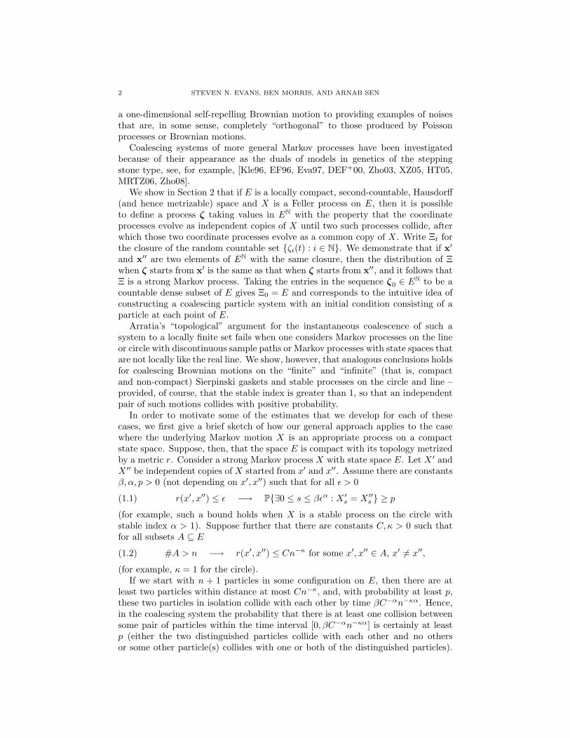
In order to motivate some of the estimates that we develop for each of thesecases, we first give a brief sketch of how our general approach applies to the casewhere the underlying Markov motion X is an appropriate process on a compactstate space. Suppose, then, that the space E is compact with its topology metrizedby a metric r. Consider a strong Markov process X with state space E. Let X ′ andX ′′ be independent copies of X started from x′ and x′′. Assume there are constantsβ, α, p > 0 (not depending on x′, x′′) such that for all ε > 0
(1.1) r(x′, x′′) ≤ ε −→ P{∃0 ≤ s ≤ βεα : X ′s = X ′′s } ≥ p
(for example, such a bound holds when X is a stable process on the circle withstable index α > 1). Suppose further that there are constants C, κ > 0 such thatfor all subsets A ⊆ E
(1.2) #A > n −→ r(x′, x′′) ≤ Cn−κ for some x′, x′′ ∈ A, x′ 6= x′′,
(for example, κ = 1 for the circle).If we start with n + 1 particles in some configuration on E, then there are at
least two particles within distance at most Cn−κ, and, with probability at least p,these two particles in isolation collide with each other by time βC−αn−κα. Hence,in the coalescing system the probability that there is at least one collision betweensome pair of particles within the time interval [0, βC−αn−κα] is certainly at leastp (either the two distinguished particles collide with each other and no othersor some other particle(s) collides with one or both of the distinguished particles).

COALESCING PARTICLE SYSTEMS 3
Moreover, if there is no collision between any pair of particles after time βC−αn−κα,then we can again find at time βC−αn−κα a possibly different pair of particles thatare within distance Cn−κ from each other, and the probability that this pair ofparticles will collide within the time interval [βC−αn−κα, 2βC−αn−κα] is again atleast p. By repeating this argument and using the Markov property, we see that ifwe let τn+1
n be the first time there are n or fewer surviving particles starting from(n+ 1) particles, then, regardless of the particular initial configuration of the n+ 1particles,
P{τn+1n ≥ kβC−αn−κα
}≤ (1− p)k.
In particular, the expected time needed to reduce the number of particles from n+1to n or fewer is bounded above by cn−κα for a suitable constant c.
Suppose now that κα > 1. If we start with N particles somewhere on E, thenthe probability that after some positive time t the number of particles remaining isgreater than m is, by Markov’s inequality, bounded above by
1t
N−1∑n=m
E[τn+1n
]≤ c
t
N−1∑n=m
n−κα ≤ c′
tm1−κα
for some constant c′. The probability in question therefore converges to zero asN →∞ and then m→∞. It follows that, even if we start with a coalescing particleat each point of E, by time t there are only finitely many particles almost surely(see the last part of the proof of Theorem 5.1 for the proof that the convergence tozero of the given probability implies that an infinite coalescing system coalesces tofinitely many points instantaneously).
The above argument required three ingredients, the collision probability bound(1.1), the estimate (1.2) that provides quantitative information on the extent towhich E is totally bounded, and the assumption ακ > 1. We show in Section 3 that(1.1) follows from suitable upper and lower bounds on the transition densities of theprocess with respect to some reference probability measure µ, whereas (1.2) followsfrom the assumption that the µ mass of any ball of radius ε is bounded below by aconstant multiple of ε1/κ. Informally, both of these conditions hold when the statespace and the process have suitable approximate local self-similarity properties.
The compactness, and hence total boundedness, of the state space was crucialfor the “pigeonhole principle” reasoning that we used above. The same methodcannot be applied as it stands to deal with, say, coalescing stable processes on thereal line to show a result of the Arratia type that the set of particles remainingat some positive time is locally finite. The primary difficulty is that the proofbounds the time to coalesce from some number of particles to a smaller numberby considering a particular sequence of coalescent events, and while waiting forone of these events to occur the particles might spread out to such an extent thatthe pigeonhole argument can no longer be used. We overcome this problem bydeveloping a more sophisticated pigeonhole argument that assigns the bulk of theparticles to a collection of suitable disjoint pairs (rather than just selecting a singlesuitable pair) and then employing a simple large deviation bound to ensure thatwith high probability at least a certain fixed proportion of the pairs will havecollided over an appropriate time interval.
We are able to carry this general approach through for stable processes withindex α > 1 and Brownian motions on the infinite (that is, unbounded) Sierpinskigasket. Elements of our argument seem rather specific to these two special cases

4 STEVEN N. EVANS, BEN MORRIS, AND ARNAB SEN
and differ between the two cases, and we don’t have a general method that appliesto a broad class of processes with non-compact state spaces. It is an interestingand challenging open problem to develop techniques for non-compact state spacesthat have wider applicability.
We note that, as well as providing an interesting test case of a process withcontinuous sample paths on a state space that is not locally one-dimensional butis such that two independent copies of the process will collide with positive prob-ability, the Brownian motion on the Sierpinski gasket was introduced as a modelfor diffusion in disordered media and it has since attracted a considerable amountof attention. The reader can get a feeling for this literature by consulting someof the earlier works such as [BP88, Lin90, Bar98] and more recent papers such as[HK03, KS05] and the references therein.
2. Countable systems of coalescing Feller processes
In this section we develop some general properties of coalescing systems ofMarkov processes that we will apply later to Brownian motions on the Sierpin-ski gasket and stable processes on the line or circle.
2.1. Vector-valued coalescing process. Fix N ∈ N ∪ {∞}, where, as usual, Nis the set of positive integers. Write [N ] for the set {1, 2, . . . , N} when N is finiteand for the set N when N =∞.
Fix a locally compact, second-countable, Hausdorff space E. Note that E ismetrizable. Let d be a metric giving the topology on E. Denote by D := D(R+, E)the usual Skorokhod space of E-valued cadlag paths. Fix a bijection σ : [N ]→ [N ].We will call σ a ranking of [N ]. Define a mapping Λσ : DN → DN by settingΛσξ = ζ for ξ = (ξ1, ξ2, . . .) ∈ DN , where ζ is defined inductively as follows. Setζσ(1) ≡ ξσ(1). For i > 1, set
τi := inf{t ≥ 0 : ξσ(i)(t) ∈ {ζσ(1)(t), ζσ(2)(t), . . . , ζσ(i−1)(t)}
},
with the usual convention that inf ∅ =∞. Put
Ji := min{j ∈ {1, 2, . . . , i− 1} : ξσ(i)(τi) = ζσ(j)(τi)
}if τi <∞.
For t ≥ 0, define
ζσ(i)(t) :=
{ξσ(i)(t), if t < τi,
ζσ(Ji)(t), if t ≥ τi.We call the map Λσ a collision rule. It produces a vector of “coalescing” pathsfrom of a vector of “free” paths: after the free paths labeled i and j collide, thecorresponding coalescing paths both subsequently follow either the path labeled ior the path labeled j, according to whether σ(i) < σ(j) or σ(i) > σ(j). Note foreach n < N that the value of (ζσ(i))1≤i≤n is unaffected by the value of (ξσ(j))j>n.
Suppose from now on that the paths ξ1, ξ2, . . . are realizations of independentcopies of a Feller Markov process X with state space E.
A priori, the distribution of the finite or countable coalescing system ζ = Λσξdepends on the ranking σ. However, we have the following result, which is aconsequence of the strong Markov property of ξ and the observation that if we aregiven a bijection π : [N ]→ [N ] and define a map Σπ : DN → DN by (Σπξ)i = ξπ(i),i ∈ [N ], then ΣπΛσ = Λσπ−1Σπ.
COALESCING PARTICLE SYSTEMS 5
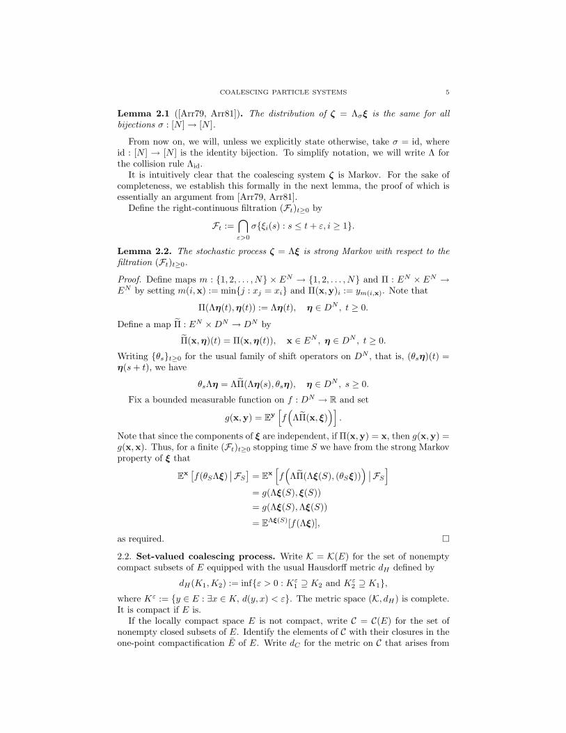
Lemma 2.1 ([Arr79, Arr81]). The distribution of ζ = Λσξ is the same for allbijections σ : [N ]→ [N ].
From now on, we will, unless we explicitly state otherwise, take σ = id, whereid : [N ] → [N ] is the identity bijection. To simplify notation, we will write Λ forthe collision rule Λid.
It is intuitively clear that the coalescing system ζ is Markov. For the sake ofcompleteness, we establish this formally in the next lemma, the proof of which isessentially an argument from [Arr79, Arr81].
Define the right-continuous filtration (Ft)t≥0 by
Ft :=⋂ε>0
σ{ξi(s) : s ≤ t+ ε, i ≥ 1}.
Lemma 2.2. The stochastic process ζ = Λξ is strong Markov with respect to thefiltration (Ft)t≥0.
Proof. Define maps m : {1, 2, . . . , N} × EN → {1, 2, . . . , N} and Π : EN × EN →EN by setting m(i,x) := min{j : xj = xi} and Π(x,y)i := ym(i,x). Note that
Π(Λη(t),η(t)) := Λη(t), η ∈ DN , t ≥ 0.
Define a map Π : EN ×DN → DN by
Π(x,η)(t) = Π(x,η(t)), x ∈ EN , η ∈ DN , t ≥ 0.
Writing {θs}t≥0 for the usual family of shift operators on DN , that is, (θsη)(t) =η(s+ t), we have
θsΛη = ΛΠ(Λη(s), θsη), η ∈ DN , s ≥ 0.
Fix a bounded measurable function on f : DN → R and set
g(x,y) = Ey[f(
ΛΠ(x, ξ))].
Note that since the components of ξ are independent, if Π(x,y) = x, then g(x,y) =g(x,x). Thus, for a finite (Ft)t≥0 stopping time S we have from the strong Markovproperty of ξ that
Ex[f(θSΛξ)
∣∣FS] = Ex[f(
ΛΠ(Λξ(S), (θSξ))) ∣∣FS]
= g(Λξ(S), ξ(S))
= g(Λξ(S),Λξ(S))
= EΛξ(S)[f(Λξ)],
as required. �
2.2. Set-valued coalescing process. Write K = K(E) for the set of nonemptycompact subsets of E equipped with the usual Hausdorff metric dH defined by
dH(K1,K2) := inf{ε > 0 : Kε1 ⊇ K2 and Kε
2 ⊇ K1},where Kε := {y ∈ E : ∃x ∈ K, d(y, x) < ε}. The metric space (K, dH) is complete.It is compact if E is.
If the locally compact space E is not compact, write C = C(E) for the set ofnonempty closed subsets of E. Identify the elements of C with their closures in theone-point compactification E of E. Write dC for the metric on C that arises from

6 STEVEN N. EVANS, BEN MORRIS, AND ARNAB SEN
the Hausdorff metric on the compact subsets of E corresponding to some metric onE that induces the topology of E.
Let Ξt ⊆ E denote the closure of the set {ζi(t) : i = 1, 2, . . .} in E, where ζ = Λξ.The following result is an almost immediate consequence of Lemma 2.1.
Lemma 2.3. If x′,x′′ ∈ EN are such that the sets {x′i : i ∈ [N ]} and {x′′i : i ∈ [N ]}are equal, then the distributions of the process Ξ under Px′ and Px′′ are also equal.
For the remainder of this section, we will make the following assumption.
Assumption 2.4. The Feller process X is such that if X ′ and X ′′ are two inde-pendent copies of X, then, for all t0 > 0 and x′ ∈ E,
limx′′→x′
Px′,x′′{X ′t = X ′′t for some t ∈ [0, t0]
}= 1.
Proposition 2.5. Let x′,x′′ ∈ EN be such that the sets {x′i : i ∈ [N ]} and {x′′i : i ∈[N ]} have the same closure. Then, the process Ξ has the same distribution underPx′ and Px′′ .
Proof. We will consider the case where E is compact. The non-compact case isessentially the same, and we leave the details to the reader.
We need to show for any finite set of times 0 < t1 < . . . < tk that the distributionof (Ξt1 , . . . ,Ξtk) is the same under Px′ and Px′′ .
We may suppose without loss of generality that x′1, x′2, . . . (resp. x′′1 , x
′′2 , . . .) are
distinct.Fix n ∈ [N ] and δ > 0. Given ε > 0 that will be specified later, choose
y′′1 , y′′2 , . . . , y
′′n ∈ {x′′i : i ∈ [N ]} such that d(x′i, y
′′i ) ≤ ε for 1 ≤ i ≤ n. Let η′
(resp. η′′) be an En-valued process with coordinates that are independent copiesof X started at (x′1, . . . , x
′n) (resp. (y′′1 , y
′′2 , . . . , y
′′n)).
By the Feller property, there is a time 0 < t0 ≤ t1 that depends on x′1, . . . , x′n
such that for all ε sufficiently small
P{η′′i (t) = η′′j (t) for some 1 ≤ i 6= j ≤ n and 0 < t ≤ t0} ≤δ
2.
By our standing Assumption 2.4, if we take ε sufficiently small, then
P{η′i(t) 6= η′′i (t) for all 0 < t ≤ t0} ≤δ
2n, 1 ≤ i ≤ n.
Write Ξ′ (resp. Ξ′′, Ξ, Ξ) for the set-valued processes constructed from η′ (resp.η′′, (η′,η′′), (η′′,η′)) in the same manner that Ξ is constructed from ξ. We have
P{Ξt = Ξ′′t for all t ≥ t0} ≥ 1− δ,
Ξ′t ⊆ Ξt, for all t ≥ 0,
and, by Lemma 2.3,
Ξ d= Ξ.
For each z ∈ E, define a continuous function φz : K → R+ by
φz(K) := inf{d(z, w) : w ∈ K}.
COALESCING PARTICLE SYSTEMS 7
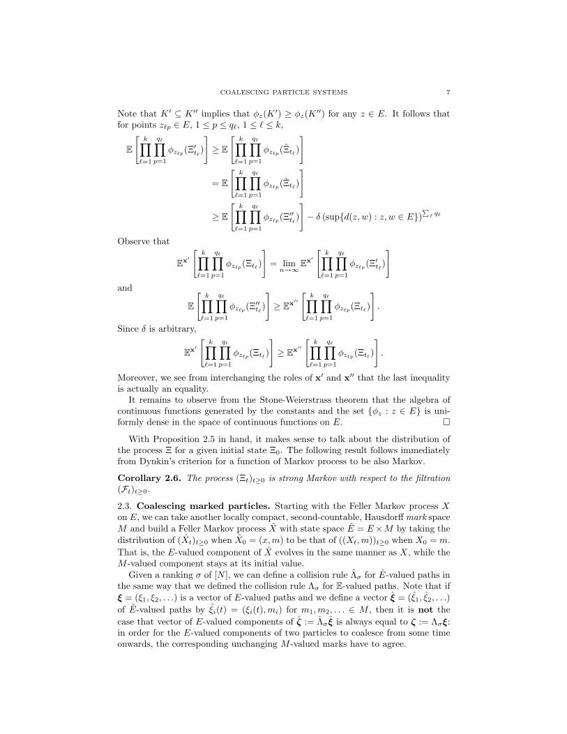
Note that K ′ ⊆ K ′′ implies that φz(K ′) ≥ φz(K ′′) for any z ∈ E. It follows thatfor points z`p ∈ E, 1 ≤ p ≤ q`, 1 ≤ ` ≤ k,
E
[k∏`=1
q∏p=1
φz`p(Ξ′t`)
]≥ E
[k∏`=1
q∏p=1
φz`p(Ξt`)
]
= E
[k∏`=1
q∏p=1
φz`p(Ξt`)
]
≥ E
[k∏`=1
q∏p=1
φz`p(Ξ′′t`)
]− δ (sup{d(z, w) : z, w ∈ E})
∑` q`
Observe that
Ex′
[k∏`=1
q∏p=1
φz`p(Ξt`)
]= limn→∞
Ex′
[k∏`=1
q∏p=1
φz`p(Ξ′t`)
]and
E
[k∏`=1
q∏p=1
φz`p(Ξ′′t`)
]≥ Ex′′
[k∏`=1
q∏p=1
φz`p(Ξt`)
].
Since δ is arbitrary,
Ex′
[k∏`=1
q∏p=1
φz`p(Ξt`)
]≥ Ex′′
[k∏`=1
q∏p=1
φz`p(Ξt`)
].
Moreover, we see from interchanging the roles of x′ and x′′ that the last inequalityis actually an equality.
It remains to observe from the Stone-Weierstrass theorem that the algebra ofcontinuous functions generated by the constants and the set {φz : z ∈ E} is uni-formly dense in the space of continuous functions on E. �
With Proposition 2.5 in hand, it makes sense to talk about the distribution ofthe process Ξ for a given initial state Ξ0. The following result follows immediatelyfrom Dynkin’s criterion for a function of Markov process to be also Markov.
Corollary 2.6. The process (Ξt)t≥0 is strong Markov with respect to the filtration(Ft)t≥0.
2.3. Coalescing marked particles. Starting with the Feller Markov process Xon E, we can take another locally compact, second-countable, Hausdorff mark spaceM and build a Feller Markov process X with state space E = E×M by taking thedistribution of (Xt)t≥0 when X0 = (x,m) to be that of ((Xt,m))t≥0 when X0 = m.That is, the E-valued component of X evolves in the same manner as X, while theM -valued component stays at its initial value.
Given a ranking σ of [N ], we can define a collision rule Λσ for E-valued paths inthe same way that we defined the collision rule Λσ for E-valued paths. Note that ifξ = (ξ1, ξ2, . . .) is a vector of E-valued paths and we define a vector ξ = (ξ1, ξ2, . . .)of E-valued paths by ξi(t) = (ξi(t),mi) for m1,m2, . . . ∈ M , then it is not thecase that vector of E-valued components of ζ := Λσξ is always equal to ζ := Λσξ:in order for the E-valued components of two particles to coalesce from some timeonwards, the corresponding unchanging M -valued marks have to agree.
8 STEVEN N. EVANS, BEN MORRIS, AND ARNAB SEN
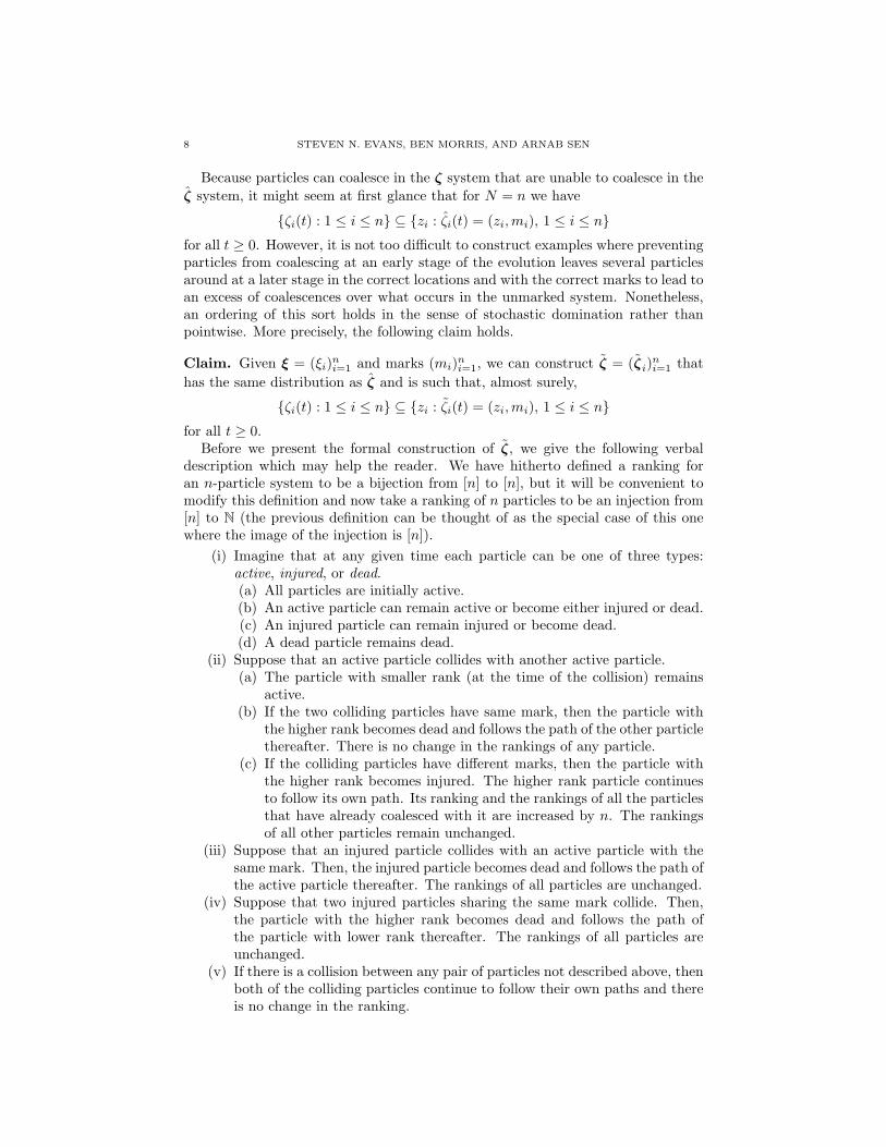
Because particles can coalesce in the ζ system that are unable to coalesce in theζ system, it might seem at first glance that for N = n we have
{ζi(t) : 1 ≤ i ≤ n} ⊆ {zi : ζi(t) = (zi,mi), 1 ≤ i ≤ n}for all t ≥ 0. However, it is not too difficult to construct examples where preventingparticles from coalescing at an early stage of the evolution leaves several particlesaround at a later stage in the correct locations and with the correct marks to lead toan excess of coalescences over what occurs in the unmarked system. Nonetheless,an ordering of this sort holds in the sense of stochastic domination rather thanpointwise. More precisely, the following claim holds.
Claim. Given ξ = (ξi)ni=1 and marks (mi)ni=1, we can construct ζ = (ζi)ni=1 thathas the same distribution as ζ and is such that, almost surely,
{ζi(t) : 1 ≤ i ≤ n} ⊆ {zi : ζi(t) = (zi,mi), 1 ≤ i ≤ n}for all t ≥ 0.
Before we present the formal construction of ζ, we give the following verbaldescription which may help the reader. We have hitherto defined a ranking foran n-particle system to be a bijection from [n] to [n], but it will be convenient tomodify this definition and now take a ranking of n particles to be an injection from[n] to N (the previous definition can be thought of as the special case of this onewhere the image of the injection is [n]).
(i) Imagine that at any given time each particle can be one of three types:active, injured, or dead.(a) All particles are initially active.(b) An active particle can remain active or become either injured or dead.(c) An injured particle can remain injured or become dead.(d) A dead particle remains dead.
(ii) Suppose that an active particle collides with another active particle.(a) The particle with smaller rank (at the time of the collision) remains
active.(b) If the two colliding particles have same mark, then the particle with
the higher rank becomes dead and follows the path of the other particlethereafter. There is no change in the rankings of any particle.
(c) If the colliding particles have different marks, then the particle withthe higher rank becomes injured. The higher rank particle continuesto follow its own path. Its ranking and the rankings of all the particlesthat have already coalesced with it are increased by n. The rankingsof all other particles remain unchanged.
(iii) Suppose that an injured particle collides with an active particle with thesame mark. Then, the injured particle becomes dead and follows the path ofthe active particle thereafter. The rankings of all particles are unchanged.
(iv) Suppose that two injured particles sharing the same mark collide. Then,the particle with the higher rank becomes dead and follows the path ofthe particle with lower rank thereafter. The rankings of all particles areunchanged.
(v) If there is a collision between any pair of particles not described above, thenboth of the colliding particles continue to follow their own paths and thereis no change in the ranking.
COALESCING PARTICLE SYSTEMS 9
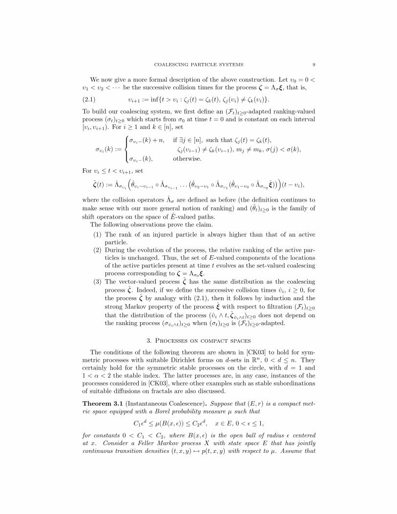
We now give a more formal description of the above construction. Let υ0 = 0 <υ1 < υ2 < · · · be the successive collision times for the process ζ = Λσξ, that is,
(2.1) υi+1 := inf{t > υi : ζj(t) = ζk(t), ζj(υi) 6= ζk(υi)}.
To build our coalescing system, we first define an (Ft)t≥0-adapted ranking-valuedprocess (σt)t≥0 which starts from σ0 at time t = 0 and is constant on each interval[υi, υi+1). For i ≥ 1 and k ∈ [n], set
συi(k) :=
συi−(k) + n, if ∃j ∈ [n], such that ζj(t) = ζk(t),
ζj(υi−1) 6= ζk(υi−1), mj 6= mk, σ(j) < σ(k),συi−(k), otherwise.
For υi ≤ t < υi+1, set
ζ(t) := Λσυi(θυi−υi−1 ◦ Λσυi−1
. . .(θυ2−υ1 ◦ Λσυ1 (θυ1−υ0 ◦ Λσυ0 ξ)
))(t− υi),
where the collision operators Λσ are defined as before (the definition continues tomake sense with our more general notion of ranking) and (θt)t≥0 is the family ofshift operators on the space of E-valued paths.
The following observations prove the claim.
(1) The rank of an injured particle is always higher than that of an activeparticle.
(2) During the evolution of the process, the relative ranking of the active par-ticles is unchanged. Thus, the set of E-valued components of the locationsof the active particles present at time t evolves as the set-valued coalescingprocess corresponding to ζ = Λσ0ξ.
(3) The vector-valued process ζ has the same distribution as the coalescingprocess ζ. Indeed, if we define the successive collision times υi, i ≥ 0, forthe process ζ by analogy with (2.1), then it follows by induction and thestrong Markov property of the process ξ with respect to filtration (Ft)t≥0
that the distribution of the process (υi ∧ t, ζυi∧t)t≥0 does not depend onthe ranking process (συi∧t)t≥0 when (σt)t≥0 is (Ft)t≥0-adapted.
3. Processes on compact spaces
The conditions of the following theorem are shown in [CK03] to hold for sym-metric processes with suitable Dirichlet forms on d-sets in Rn, 0 < d ≤ n. Theycertainly hold for the symmetric stable processes on the circle, with d = 1 and1 < α < 2 the stable index. The latter processes are, in any case, instances of theprocesses considered in [CK03], where other examples such as stable subordinationsof suitable diffusions on fractals are also discussed.
Theorem 3.1 (Instantaneous Coalescence). Suppose that (E, r) is a compact met-ric space equipped with a Borel probability measure µ such that
C1εd ≤ µ(B(x, ε)) ≤ C2ε
d, x ∈ E, 0 < ε ≤ 1,
for constants 0 < C1 < C2, where B(x, ε) is the open ball of radius ε centeredat x. Consider a Feller Markov process X with state space E that has jointlycontinuous transition densities (t, x, y) 7→ p(t, x, y) with respect to µ. Assume that
10 STEVEN N. EVANS, BEN MORRIS, AND ARNAB SEN
X is symmetric with respect to µ, so that p(t, x, y) = p(t, y, x). Assume further thatfor some α > d we have bounds of the form
c1
{t−d/α ∧ t
r(x, y)d+α
}≤ p(t, x, y) ≤ c2
{t−d/α ∧ t
r(x, y)d+α
}, 0 < t ≤ 1,
for suitable constants 0 < c1 < c2. Let Ξ be the corresponding set-valued coalescingsystem. Then, almost surely, Ξt is a finite set for all t > 0.
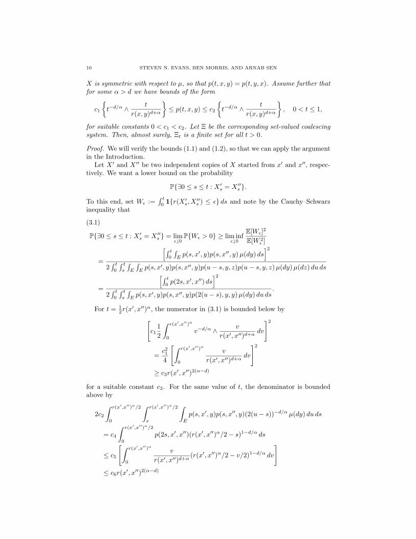
Proof. We will verify the bounds (1.1) and (1.2), so that we can apply the argumentin the Introduction.
Let X ′ and X ′′ be two independent copies of X started from x′ and x′′, respec-tively. We want a lower bound on the probability
P{∃0 ≤ s ≤ t : X ′s = X ′′s }.
To this end, set Wε :=∫ t
01{r(X ′s, X ′′s ) ≤ ε} ds and note by the Cauchy–Schwarz
inequality that
P{∃0 ≤ s ≤ t : X ′s = X ′′s } = limε↓0
P{Wε > 0} ≥ lim infε↓0
E[Wε]2
E[W 2ε ]
=
[∫ t0
∫Ep(s, x′, y)p(s, x′′, y)µ(dy) ds
]22∫ t
0
∫ ts
∫E
∫Ep(s, x′, y)p(s, x′′, y)p(u− s, y, z)p(u− s, y, z)µ(dy)µ(dz) du ds
=
[∫ t0p(2s, x′, x′′) ds
]22∫ t
0
∫ ts
∫Ep(s, x′, y)p(s, x′′, y)p(2(u− s), y, y)µ(dy) du ds
.
(3.1)
For t = 12r(x
′, x′′)α, the numerator in (3.1) is bounded below by[c1
12
∫ r(x′,x′′)α
0
v−d/α ∧ v
r(x′, x′′)d+αdv
]2
=c214
[∫ r(x′,x′′)α
0
v
r(x′, x′′)d+αdv
]2
≥ c3r(x′, x′′)2(α−d)
for a suitable constant c3. For the same value of t, the denominator is boundedabove by
2c2∫ r(x′,x′′)α/2
0
∫ r(x′,x′′)α/2
s
∫E
p(s, x′, y)p(s, x′′, y)(2(u− s))−d/α µ(dy) du ds
= c4
∫ r(x′,x′′)α/2
0
p(2s, x′, x′′)(r(x′, x′′)α/2− s)1−d/α ds
≤ c5
[∫ r(x′,x′′)α
0
v
r(x′, x′′)d+α(r(x′, x′′)α/2− v/2)1−d/α dv
]≤ c6r(x′, x′′)2(α−d)
COALESCING PARTICLE SYSTEMS 11
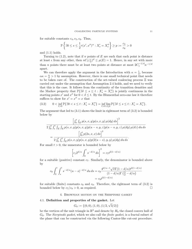
for suitable constants c4, c5, c6. Thus,
P{∃0 ≤ s ≤ 1
2r(x′, x′′)α : X ′s = X ′′s
}≥ p :=
c3c6> 0
and (1.1) holds.Turning to (1.2), note that if n points of E are such that each point is distance
at least ε from any other, then nC1( ε2 )d ≤ µ(E) = 1. Hence, in any set with morethan n points there must be at least two points at distance at most 2C−1/d
1 n−1/d
apart.We can therefore apply the argument in the Introduction with κ = 1
d , becauseακ = α
d > 1 by assumption. However, there is one small technical point that needsto be taken care of. The construction of the set-valued coalescing process Ξ wascarried out under the assumption that Assumption 2.4 holds, and we need to verifythat this is the case. It follows from the continuity of the transition densities andthe Markov property that P{∃δ ≤ s ≤ t : X ′s = X ′′s } is jointly continuous in thestarting points x′ and x′′ for 0 < δ ≤ t. By the Blumenthal zero-one law it thereforesuffices to show for x′ = x′′ = x that
(3.2) 0 < inft>0
P{∃0 < s ≤ t : X ′s = X ′′s } = inft>0
limδ↓0
P{∃δ ≤ s ≤ t : X ′s = X ′′s }.
The argument that led to (3.1) shows the limit in rightmost term of (3.2) is boundedbelow by [∫ t
0
∫Ep(s, x, y)p(s, x, y)µ(dy) ds
]22∫ t
0
∫ ts
∫E
∫Ep(s, x, y)p(s, x, y)p(u− s, y, z)p(u− s, y, z)µ(dy)µ(dz) du ds
=
[∫ t0p(2s, x, x) ds
]22∫ t
0
∫ ts
∫Ep(s, x, y)p(s, x, y)p(2(u− s), y, y)µ(dy) du ds
.
For small t > 0, the numerator is bounded below by[c12d/α
∫ t
0
s−d/α ds
]2
= c7t2(1−d/α)
for a suitable (positive) constant c7. Similarly, the denominator is bounded aboveby
c8
∫ t
0
∫ t
s
s−d/α(u− s)−d/α du ds = c84d/α−1
√πΓ(1− d/α)t2(1−d/α)
(1− d/α)Γ(
32 − d/α
)= c9t
2(1−d/α)
for suitable (finite) constants c8 and c9. Therefore, the rightmost term of (3.2) isbounded below by c7/c9 > 0, as required. �
4. Brownian motion on the Sierpinski gasket
4.1. Definition and properties of the gasket. Let
G0 := {(0, 0), (1, 0), (1/2,√
3/2)}be the vertices of the unit triangle in R2 and denote by H0 the closed convex hull ofG0. The Sierpinski gasket, which we also call the finite gasket, is a fractal subset ofthe plane that can be constructed via the following Cantor-like cut-out procedure.
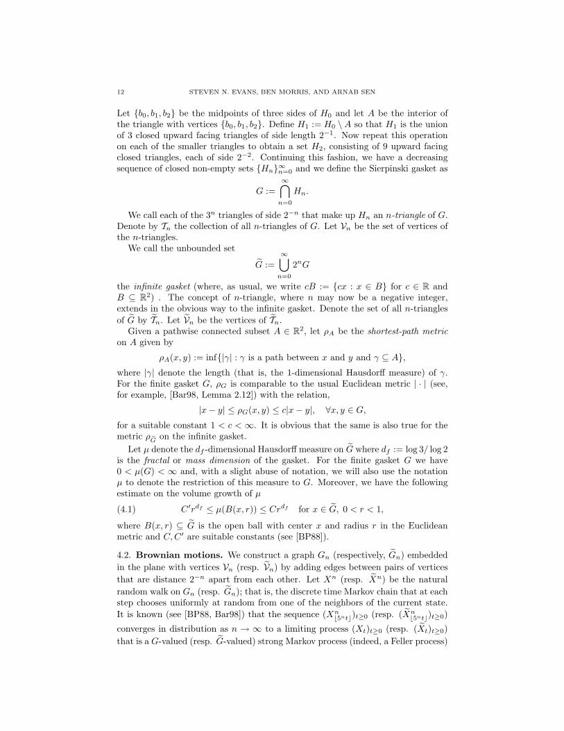
12 STEVEN N. EVANS, BEN MORRIS, AND ARNAB SEN
Let {b0, b1, b2} be the midpoints of three sides of H0 and let A be the interior ofthe triangle with vertices {b0, b1, b2}. Define H1 := H0 \A so that H1 is the unionof 3 closed upward facing triangles of side length 2−1. Now repeat this operationon each of the smaller triangles to obtain a set H2, consisting of 9 upward facingclosed triangles, each of side 2−2. Continuing this fashion, we have a decreasingsequence of closed non-empty sets {Hn}∞n=0 and we define the Sierpinski gasket as
G :=∞⋂n=0
Hn.
We call each of the 3n triangles of side 2−n that make up Hn an n-triangle of G.Denote by Tn the collection of all n-triangles of G. Let Vn be the set of vertices ofthe n-triangles.
We call the unbounded set
G :=∞⋃n=0
2nG
the infinite gasket (where, as usual, we write cB := {cx : x ∈ B} for c ∈ R andB ⊆ R2) . The concept of n-triangle, where n may now be a negative integer,extends in the obvious way to the infinite gasket. Denote the set of all n-trianglesof G by Tn. Let Vn be the vertices of Tn.
Given a pathwise connected subset A ∈ R2, let ρA be the shortest-path metricon A given by
ρA(x, y) := inf{|γ| : γ is a path between x and y and γ ⊆ A},where |γ| denote the length (that is, the 1-dimensional Hausdorff measure) of γ.For the finite gasket G, ρG is comparable to the usual Euclidean metric | · | (see,for example, [Bar98, Lemma 2.12]) with the relation,
|x− y| ≤ ρG(x, y) ≤ c|x− y|, ∀x, y ∈ G,for a suitable constant 1 < c < ∞. It is obvious that the same is also true for themetric ρG on the infinite gasket.
Let µ denote the df -dimensional Hausdorff measure on G where df := log 3/ log 2is the fractal or mass dimension of the gasket. For the finite gasket G we have0 < µ(G) < ∞ and, with a slight abuse of notation, we will also use the notationµ to denote the restriction of this measure to G. Moreover, we have the followingestimate on the volume growth of µ
(4.1) C ′rdf ≤ µ(B(x, r)) ≤ Crdf for x ∈ G, 0 < r < 1,
where B(x, r) ⊆ G is the open ball with center x and radius r in the Euclideanmetric and C,C ′ are suitable constants (see [BP88]).
4.2. Brownian motions. We construct a graph Gn (respectively, Gn) embeddedin the plane with vertices Vn (resp. Vn) by adding edges between pairs of verticesthat are distance 2−n apart from each other. Let Xn (resp. Xn) be the naturalrandom walk on Gn (resp. Gn); that is, the discrete time Markov chain that at eachstep chooses uniformly at random from one of the neighbors of the current state.It is known (see [BP88, Bar98]) that the sequence (Xn
b5ntc)t≥0 (resp. (Xnb5ntc)t≥0)
converges in distribution as n → ∞ to a limiting process (Xt)t≥0 (resp. (Xt)t≥0)that is a G-valued (resp. G-valued) strong Markov process (indeed, a Feller process)

COALESCING PARTICLE SYSTEMS 13
with continuous sample paths. The processes X and X are called, for obviousreasons, the Brownian motion on the finite and infinite gaskets, respectively. TheBrownian motion on the infinite gasket has the following scaling property:
(4.2) (2Xt)t≥0 under Px has same law as (X5t)t≥0 under P2x.
The process X has a family p(t, x, y), x, y ∈ G, t > 0, of transition densities withrespect to the measure µ that is jointly continuous on (0,∞) × G × G. Moreover,p(t, x, y) = p(t, y, x) for all x, y ∈ G and t > 0, so that the process X is symmetricwith respect to µ.
Let dw := log 5/ log 2 denote the walk dimension of the gasket. The followingcrucial “heat kernel bound” is established in [BP88]
c′1t−df/dw exp
(−c′2
(|x− y|dw
t
)1/(dw−1))
≤ p(t, x, y)
≤ c1t−df/dw exp
(−c2
(|x− y|dw
t
)1/(dw−1)), ∀x, y ∈ G, t > 0.
(4.3)
Because the infinite gasket G and the associated Brownian motion X both havere-scaling invariances that G and X do not, it will be convenient to work with Xand then use the following observation to transfer our results to X.
Lemma 4.1 (Folding lemma). There exists a continuous mapping ψ : G→ G suchthat ψ restricted to G is the identity, ψ restricted to any 0-triangle is an isometry,and |ψ(x)−ψ(y)| ≤ |x−y| for arbitrary x, y ∈ G. Moreover, if the G-valued processX is started at an arbitrary x ∈ G, then the G-valued process ψ ◦ X has the samedistribution the process X started at ψ(x).
Proof. Let L be the subset of the plane formed by the set of points of the formn1(1, 0) + n2(1/2,
√3/2), where n1, n2 are non-negative integers, and the line seg-
ments that join such points that are distance 1 apart. It is easy to see that there isa unique labeling of the vertices of L by {1, ω, ω2} that has the following properties.
• Label (0, 0) with 1.• If vertex v is labeled a ∈ {1, ω, ω2}, then the vertex v + (1, 0) are labeled
with aω.• If we think of the labels as referring to elements of the cyclic group of order
3, then if vertex v is labeled a ∈ {1, ω, ω2}, then vertex v + (1/2,√
3/2) islabeled with aω2.
Indeed, the label of the vertex n1(1, 0) + n2(1/2,√
3/2) is ωn1+2n2 .Given a vertex v ∈ L, let ι(v) be the unique vertex in {(0, 0), (1, 0), (1/2,
√3/2)}
that has the same label as v. If the vertices v1, v2, v3 ∈ L are the vertices of atriangle with side length 1, then ι(v1), ι(v2), ι(v3) are all distinct.
With the above preparation, let us now define the map ψ. Given x ∈ G, let∆ ∈ T0 be a triangle with vertices v1, v2, v3 that contains x (if x belongs to Vn,then there may be more than one such triangle, but the choice will not matter).

14 STEVEN N. EVANS, BEN MORRIS, AND ARNAB SEN
We may write x as a unique convex combination of the vertices v1, v2, v3,
x = λ1v1 + λ2v2 + λ3v3,
3∑i=1
λi = 1, λi ≥ 0.
The triple (λ1, λ2, λ3) is the vector of barycentric coordinates of x. We define ψ(x)by
ψ(x) := λ1ι(v1) + λ2ι(v2) + λ3ι(v3).
It is clear that ψ : G→ G is well-defined and has the stated properties.Recall that X(n) be the natural random walk on Gn. It can be verified easily
that the projected process ψ ◦ X(n) is the natural random walk on Gn. The resultfollows by taking the limit as n→∞ and using the continuity of ψ. �
Lemma 4.2 (Maximal inequality). (a) Let Xi, 1 ≤ i ≤ n, be n independentBrownian motions on the infinite gasket G starting from the initial states xi, 1 ≤i ≤ n. For any t > 0,
P{
sup0≤s≤t
|Xis − xi| > r, for some 1 ≤ i ≤ n
}≤ 2nc1 exp
(− c2(rdw/t)1/(dw−1)
),
where c1, c2 > 0 are constants and dw = log 5/ log 2 is the walk dimension of thegasket.(b) The same estimate holds for the case of n independent Brownian motions Xi,1 ≤ i ≤ n, on the finite gasket G starting from the initial states xi, 1 ≤ i ≤ n.
Proof. (a) Let X = (Xt)t≥0 be a Brownian motion on G. Then for x ∈ G, t > 0,and r > 0,
Px{
sup0≤s≤t
|Xs − x| > r
}≤ Px{|Xt − x| > r/2}
+ Px{|Xt − x| ≤ r/2, sup
0≤s≤t|Xs − x| > r
}.
Writing S := inf{s > 0 : |Xs − x| > r}, the second term above equals
Ex[1{S<t}PXS{|Xt−S − x| ≤ r/2}
]≤ supy∈∂B(x,r)
sups≤t
Py{|Xt−s − y| > r/2},
where ∂B(x, r) is the boundary of B(x, r) so that
Px{
sup0≤s≤t
|Xs − x| > r
}≤ 2 sup
y∈Gsups≤t
Py{|Xs − y| > r/2}
≤ 2c1 exp(− c2(rdw/t)1/(dw−1)
),
where the last estimate is taken from [Bar98, Theorem 2.23(e)]. The lemma nowfollows by a union bound.
(b) This is immediate from part (a) and Lemma 4.1. �
COALESCING PARTICLE SYSTEMS 15
4.3. Collision time estimates. We first show that two independent copies of Xcollide with positive probability.
Proposition 4.3. Let X ′ and X ′′ be two independent copies of X. Then,
P(x′,x′′){∃t > 0 : X ′t = X ′′t } > 0
for all (x′, x′′) ∈ G× G.
Proof. Note that X = (X ′, X ′′) is a Feller process on the locally compact separablemetric space G × G that is symmetric with respect to the Radon measure µ ⊗ µand has transition densities p(t, x′, y′)× p(t, x′′, y′′). The corresponding α-potentialdensity is
uα(x,y) :=∫ ∞
0
e−αtp(t, x1, y1)× p(t, x2, y2) dt for α > 0,
where x = (x1, x2) and y = (y1, y2). A standard potential theoretic result says thata compact set B ⊆ G × G is non-polar if there exists a non-zero finite measure νthat is supported on B and has finite energy, that is,∫ ∫
uα(x,y) ν(dx) ν(dy) <∞.
Take B = {(x′, x′′) ∈ G×G : x′ = x′′} and ν to be the ‘lifting’ of the Hausdorffmeasure µ on the finite gasket onto B. We want to show that∫
G
∫G
∫ ∞0
e−αtp2(t, x, y) dt µ(dx)µ(dy) <∞.
It will be enough to show that∫G
∫G
∫ ∞0
p2(t, x, y) dt µ(dx)µ(dy) <∞.
It follows from the transition density estimate (4.3) and a straightforward inte-gration that ∫ ∞
0
p2(t, x, y) dt ≤ C|x− y|−γ
for some constant C, where γ := 2df − dw. Thus,∫G
∫G
∫ ∞0
p2(t, x, y) dt µ(dx)µ(dy)
≤ C∫G
∫G
|x− y|−γ µ(dx)µ(dy)
≤ C∫G
∫ ∞0
µ{x ∈ G : |x− y|−γ > s} ds µ(dy)
≤ C∫G
∫ ∞0
µ{x ∈ G : |x− y| < s−1/γ} ds µ(dy)
≤ C + C
∫G
∫ ∞1
µ{x ∈ G : |x− y| < s−1/γ} ds µ(dy)
≤ C + C1
∫G
∫ ∞1
s−df/γ ds µ(dy) [ By (4.1)]
≤ C + C2
∫ ∞1
s−df/γ ds.

16 STEVEN N. EVANS, BEN MORRIS, AND ARNAB SEN
It remains to note that γ − df = (2 log 3/ log 2 − log 5/ log 2) − (log 3/ log 2) =(log 3− log 5)/ log 2 < 0, and so df/γ < 1.
This shows that P(x′,x′′){X hits the diagonal} > 0 for some (x′, x′′) ∈ G ×G. Because p2(t, x, y) > 0 for all x, y ∈ G and t > 0, we even haveP(x′,x′′){X hits the diagonal} > 0 for all (x′, x′′) ∈ G× G. �
We next establish a uniform lower bound on the collision probability of a pairof independent Brownian motions on the infinite gasket as long as the distancebetween their starting points remains bounded.
Theorem 4.4. There exist constants β > 0 and p > 0 such that if X ′ and X ′′ aretwo independent Brownian motions on G starting from any two points x, y belongingto the same n-triangle of G, then
P(x,y){X ′t = X ′′t for some t ∈ (0, β5−n)} ≥ p.
This result will require a certain amount of work, so we first note that it leadseasily to an analogous result for the finite gasket.
Corollary 4.5. If X ′ and X ′′ are two independent Brownian motions on G startingfrom any two points x, y belonging to the same n-triangle of G, then
P(x,y){X ′t = X ′′t for some t ∈ (0, β5−n)} ≥ p,
where β > 0 and p > 0 are the constants given in Theorem 4.4.
Proof. The proof follows immediately from Lemma 4.1, because if X ′t = X ′′t forsome t, then it is certainly the case that ψ ◦ X ′t = ψ ◦ X ′′t . �
Definition 4.6 (Extended triangles for the infinite gasket). Recall that Tn is theset of all n-triangles of G. Given ∆ ∈ T0 such that ∆ does not have the origin as oneits vertices, we define the corresponding extended triangle ∆e ⊂ G as the interiorof the union of the original 0-triangle ∆ with the three neighboring 1-triangles inG which share one vertex with ∆ and are not contained in ∆. Note that for the(unique) triangle ∆ in Tn having the origin as one of its vertices, there are twoneighboring 1-triangles in G that share one vertex with it which are not containedin ∆. In this case, by ∆e, we mean the interior of the union of ∆ and these twotriangles.
Fix some ∆ ∈ T0. Let Z be the Brownian motion on ∆e killed when it exits∆e. It follows from arguments similar to those on [Doo01, page 590], that Z hastransition densities pK(t, x, y), t > 0, x, y ∈ ∆e, with respect to the restriction of µto ∆e, and these densities have the following properties:
• pK(t, x, y) = pK(t, y, x) for all t > 0, x, y ∈ ∆e.• pK(t, x, y) ≤ p(t, x, y), for all t > 0, x, y ∈ ∆e.• y 7→ pK(t, x, y) is continuous for all t > 0, x ∈ ∆e, and x 7→ pK(t, x, y) is
continuous for all t > 0, y ∈ ∆e.
It follows that the process Z is Feller and symmetric with respect to the measureµ.

COALESCING PARTICLE SYSTEMS 17
Lemma 4.7. Let Z ′, Z ′′ be two independent copies of the killed Brownian motionZ. Given any ε > 0, there exists 0 < δ < ε such that the set of (x, y) ∈ ∆e ×∆e
for whichP(x,y){Z ′t = Z ′′t for some t ∈ (δ, ε)} > 0
has positive µ⊗ µ mass.
Proof. An argument similar to that in the proof of Proposition 4.3 shows that
P(x0,y0){Z ′t = Z ′′t for some t > 0} > 0
for some (x0, y0) ∈ ∆e ×∆e.Thus, for any ε > 0, we can partition the interval (0,∞) into the subintervals
(0, ε), [iε, (i+ 1)ε), i ≥ 0 and use the Markov property to deduce that there existsa point (x1, y1) ∈ ∆e ×∆e such that
(4.4) P(x1,y1){Z ′t = Z ′′t for some t ∈ (0, ε)} > 0.
By continuity of probability, we can find 0 < η < ε <∞ such that
P(x1,y1){Z ′t = Z ′′t for some t ∈ (η, ε)} > 0.
By the Markov property,
0 < P(x1,y1){Z ′t = Z ′′t for some t ∈ (η, ε)}
=∫
∆e
∫∆e
pK(η/2, x1, x)pK(η/2, y1, y)
× P(x,y){Z ′t = Z ′′t , for some t ∈ (η/2, ε− η/2)}µ(dx)µ(dy).
Therefore, the initial points (x, y) ∈ ∆e ×∆e for which the probability
P(x,y){Z ′t = Z ′′t for some t ∈ (η/2, ε− η/2)}
is positive form a set with positive µ⊗µ measure. The proof now follows by takingδ = η/2. �
We record the following result for the reader’s ease of reference.
Lemma 4.8 (Lemma 3.35 of [Bar98]). There exists a constant c1 > 1 such that ifx, y ∈ ∆e, r = |x− y|, then
Px{Xt = y for some t ∈ (0, rdw) and |Xt − x| ≤ c1r for all t ≤ rdw} > 0.
Lemma 4.9. There exists a constant c > 0 such that for each point x ∈ ∆e, eachopen subset U ⊂ ∆e, and each time 0 < t ≤ c
Px{Zt ∈ U} > 0.
In particular, pK(t, x, y) > 0 for all x, y ∈ ∆e and 0 < t ≤ c.
Proof. The following three steps combined with the strong Markov property estab-lish the lemma.Step 1. There exists a constant c > 0 such that starting from x ∈ ∆e, the unkilledBrownian motion on the infinite gasket X will stay within ∆e up to time c withpositive probability.Step 2. Fix y ∈ U . For all sufficiently small η > 0,
Py{X does not exit U before time η} > 0.

18 STEVEN N. EVANS, BEN MORRIS, AND ARNAB SEN
Step 3. For any δ > 0, z, y ∈ ∆e
Pz{Z hits y before δ} > 0.
Consider Step 1. Note that if x ∈ G, then (see [Bar98, Equation 3.11]) thereexists a constant c > 0 such that for the unkilled process X, we have,
Px{|Xt − x| ≤ 1/4 for t ∈ [0, c]} > 0.
But if x ∈ ∆e, then
Px{Xt ∈ ∆e for t ∈ [0, c]} ≥ Px{|Xt − x| ≤ 1/4 for t ∈ [0, c]},and the claim follows.
Step 2 is obvious from the right continuity of the paths of the killed Brownianmotion Z at time 0.
Consider Step 3. Fix z, y ∈ ∆e and 0 < δ ≤ |z − y|. Let Sn be the n-thapproximating graph of G with the set of vertices Vn. Choose n large enough sothat we can find points z0 and y0 in Vn close to z and y respectively so that
|z − z0| ≤δ
3, |y − y0| ≤
δ
3and
B(z, c1|z − z0|) ⊆ ∆e, B(y0, c1|y − y0|) ⊆ ∆e
where c1 is as in Lemma 4.8 and the notation B(u, r) denotes the intersection withthe infinite gasket G of the closed ball in the plane of radius r around the point u.
The length of a shortest path γ lying Sn between z0 and y0 is the same as theirdistance in the original metric ρG(z0, y0). Moreover, for any two points p and p′ onγ, the length of the segment of γ between p and p′ is the same as their distance inthe original metric ρG(p, p′).
Thus, we can choose m + 1 equally spaced points z0, z1, . . . , zm = y0 on γ suchthat
ρG(zi+1, zi) =1mρG(z0, y0) for each i.
Since γ is compact, dist(γ, ∂∆e) > 0. Thus we can choose m large so that
B(zi, c1|zi+1 − zi|) ⊆ ∆e for each i.
By repeated application of Lemma 4.8 and the strong Markov property, weconclude that the probability that Z hits y starting from z before the time
Tm := |z − z0|dw + |y − y0|dw +m−1∑i=0
|zi+1 − zi|dw
is strictly positive. Step 3 follows immediately since
Tm ≤(δ
3
)dw+(δ
3
)dw+ constant×m× 1
mdw|z0 − y0|dw ≤ δ
for m sufficiently large, because dw > 1. �
Lemma 4.10. Let Z ′ and Z ′′ be two independent copies of the killed Brownianmotion Z. For any 0 < δ < β, the map
(x, y) 7→ P(x,y){Z ′t = Z ′′t for some t ∈ (δ, β)}is continuous on ∆e ×∆e.

COALESCING PARTICLE SYSTEMS 19
Proof. We have
P(x,y){Z ′t = Z ′′t for some t ∈ (δ, β)}
=∫
∆e
∫∆e
pK(δ, x, x′) pK(δ, y, y′)
× P(x′,y′){Z ′t = Z ′′t for some t ∈ (0, β − δ)}µ(dx′)µ(dy′),
and the result follows from the continuity of z 7→ pK(δ, z, z′) for each z′ ∈ ∆e. �
Proof of Theorem 4.4. For any x, y ∈ ∆,
P(x,y){Z ′t = Z ′′t for some t ∈ (δ, β)}
=∫
∆e
∫∆e
pK(δ/2, x, x′)pK(δ/2, y, y′)
× P(x′,y′){Z ′t = Z ′′t for some t ∈ (δ/2, β − δ/2)}µ(dx′)µ(dy′) > 0,
(4.5)
by Lemmas 4.7, 4.9 and 4.10.Applying Lemma 4.10 and equation (4.5) and the fact that a continuous function
achieves its minimum on a compact set, we have for any ∆ ∈ T0 that
q(∆) := infx,y∈∆
P(x,y){Z ′t = Z ′′t for some t ∈ (0, β)} > 0.
Note that for any two ∆1,∆2 ∈ T0 which do not contain the origin, there existsa local isometry between the corresponding extended triangles ∆e
1,∆e2. Since the
unkilled Brownian motion X in G is invariant with respect to local isometries,
q(∆1) = q(∆2).
Given two independent copies X ′ and X ′′ of X, set
p := inf∆∈T0
infx,y∈∆
P(x,y){X ′t = X ′′t for some t ∈ (0, β)}.
The above observations enable us to conclude that p > 0.For the infinite gasket, if ∆ ∈ Tn, then 2n∆ ∈ T0 and the scaling property of
Brownian motion on the infinite gasket gives us that for any ∆ ∈ Tninf
x,y∈∆P(x,y){X ′t = X ′′t for some t ∈ (0, 5−nβ)}
= infx,y∈2n∆
P(x,y){X ′t = X ′′t for some t ∈ (0, β)}.
Therefore, for any ∆ ∈ Tn and any x, y ∈ ∆,
(4.6) P(x,y){X ′t = X ′′t for some t ∈ (0, 5−nβ)} ≥ p.�
Corollary 4.11. The Brownian motions X and X on the infinite and finite gasketsboth satisfy Assumption 2.4.
Proof. By Theorem 4.4 and the Blumenthal zero-one law, we have for two indepen-dent Brownian motions X ′ and X ′′ on G and any point (x, x) ∈ G× G that
P(x,x){for all ε > 0, ∃ 0 < t < ε such that X ′t = X ′′t } = 1.
Lemma 4.10 then gives the claim for X. The proof for X is similar. �

20 STEVEN N. EVANS, BEN MORRIS, AND ARNAB SEN
5. Instantaneous coalescence on the gasket
We will establish the following three results in this section after obtaining somepreliminary estimates.
Theorem 5.1 (Instantaneous Coalescence). (a) Let Ξ be the set-valued coalescingBrownian motion process on G with Ξ0 compact. Almost surely, Ξt is a finite setfor all t > 0.(b) The conclusion of part (a) also holds for the set-valued coalescing Brownianmotion process on G
Theorem 5.2 (Continuity at time zero). (a) Let Ξ be the set-valued coalescingBrownian motion process on G with Ξ0 compact. Almost surely, Ξt converges toΞ0 as t ↓ 0.(b) The conclusion of part (a) also holds for the set-valued coalescing Brownianmotion process on G.
Theorem 5.3 (Instantaneous local finiteness). Let Ξ be the set-valued coalescingBrownian motion process on G with Ξ0 a possibly unbounded closed set. Almostsurely, Ξt is a locally finite set for all t > 0.
Lemma 5.4 (Pigeon hole principle). Place M balls in m boxes and allow any twoballs to be paired off together if they belong to the same box. Then, the maximumnumber of disjoint pairs of balls possible is at least (M −m)/2.
Proof. Note that in an optimal pairing there can be at most one unpaired ball perbox. It follows that the number of paired balls is at least M −m and hence thenumber of pairs is at least (M −m)/2. �
Define the ε-fattening of a set A ⊆ G to be the set Aε := {y ∈ G : ∃x ∈A, |y − x| < ε}. Define the ε-fattening of a set A ⊆ G in G similarly. Recall theconstants p and β from Theorem 4.4. Set γ := 1/(1 − p/5) > 1. Given a finitesubset A of G or G and a time-interval I ⊆ R+, define the random variable R(A; I)to be the range of the set-valued coalescing process Ξ in the finite or the infinitegasket during time I with initial state A; that is,
R(A; I) :=⋃s∈I
Ξs.
Define a stopping time for the same process Ξ by τAm := inf{t : #Ξt ≤ m}.
Lemma 5.5. (a) Let Ξ be the set-valued coalescing Brownian motion process in theinfinite gasket with Ξ0 = A, where A ⊂ G of cardinality n such that Aε for someε > 0 is contained in an extended triangle ∆e of G. Then, there exist constants C1
and C2 which may depend on ε but are independent of A such that
P{τAdnγ−1e > 25βn− log3 5or R(A, [0, τdnγ−1e]) 6⊆ Aεn
−(1/6) log3 5}
≤ C1 exp(−C2n1/3).
(5.1)
(b) The same inequality holds for the set-valued coalescing coalescing Brownianmotion process in the finite gasket.

COALESCING PARTICLE SYSTEMS 21
Proof. (a) For any integer b ≥ 1, the set A can be covered by at most 2 × 3b
b-triangles. Putbn := max{b : 2× 3b ≤ n/2},
or, equivalently,bn = blog3(n/4)c.
By Lemma 5.4, at time t = 0 it is possible to form at least n/2 − n/4 = n/4disjoint pairs of particles, where two particles are deemed eligible to form a pair ifthey belong to the same bn-triangle. Fix such an (incomplete) pairing of particles.Define a new “partial” coalescing system involving n particles, where a particle isonly allowed to coalesce with the one it has been paired up with and after such acoalescence occurs the two partners in the pair both follow the path of the particlehaving the lower rank among the two. Evidently this new system is same as thecoalescing system in the marked space where two particles have the same mark ifand only if they have been paired up. From the discussion in Subsection 2.3 thenumber of surviving distinct particles in this partial coalescing system stochasticallydominates the number of surviving particles in the original coalescing system.
By Theorem 4.4, the probability that a pair in the partial coalescing system coa-lesces before time tn := β5−bn is at least p, independently of the other pairs. Thus,the number of coalescence by time tn in the partial coalescing system stochasticallydominates a random variable that is distributed as the number of successes in n/4independent Bernoulli trials with common success probability p. By Hoeffding’sinequality, the probability that a random variable with the latter distribution takesa value np/5 or greater is at least 1− e−C′1n for some constant C ′1 > 0. Thus, theprobability that the number of surviving particles in the original coalescing systemdrops below d(1− p/5)ne = dnγ−1e by time tn ≤ 25βn− log3 5 is at least 1− e−C′1n.
From Corollary 4.2(a) and the fact that during a fixed time interval the maxi-mum displacement of particles in the coalescing system is always bounded by themaximum displacement of independent particles starting from the same initial con-figuration, the probability that over a time interval of length 25βn− log3 5 one of thecoalescing particles has moved more than a distance εn−(1/6) log3 5 from its originalposition is bounded by
2nc1 exp(− c2((εn−(1/6) log3 5)dw(25βn− log3 5)−1)1/(dw−1)
)≤ 2 exp
(log n− C ′2(n(1/2) log3 5)1/(dw−1)
)≤ C1 exp(−C2n
(1/4) log3 5)
≤ C1 exp(−C2n1/3).
(b) The proof is identical to part (a). It uses Corollary 4.5 in place of Theorem 4.4and Lemma 4.2(b) in place of Lemma 4.2(a). �
Lemma 5.6. (a) Let Ξ be the set-valued coalescing Brownian motion process inthe infinite gasket with Ξ0 = A. Fix ε > 0. Set νi := εγ−(1/6) log3 5×i and ηi =25βγ−i log3 5 for i ≥ 1. There are positive constants C1 = C1(ε) and C2 = C2(ε)such that
P
{τAdγke >
m∑i=k+1
ηi or R(A; [0, τAdγke]) 6⊆ (A)∑mi=k+1 νi
}≤
m∑i=k+1
C1 exp(−C2γi/3),

22 STEVEN N. EVANS, BEN MORRIS, AND ARNAB SEN
uniformly for all sets A of cardinality dγme such that the fattening A∑mi=k+1 νi is
contained in some extended triangle ∆e of G.(b) The analogous inequality holds for the set-valued coalescing Brownian motionprocess in the finite gasket.
Proof. Fix an extended triangle ∆e of the infinite gasket and a set A such that#A = dγme and A
∑mi=k+1 νi ⊆ ∆e. We will prove the bound by induction on
m. By the strong Markov property and Lemma 5.5, we have, using the notationAτ,m−1 := ΞτA
dγm−1e,
P{τAdγke >
m∑i=k+1
ηi or R(A; [0, τAdγke]) 6⊆ (A)∑mi=k+1 νi
}≤ P
{τAdγm−1e > ηm or R(A; [0, τAdγm−1e]) 6⊆ A
νm}
+ E[1{Aτ,m−1 ⊆ Aνm
}× P
{τAτ,m−1
dγke >
m−1∑i=k+1
ηi or R(Aτ,m−1; [0, τAτ,m−1
dγke ]) 6⊆ A∑m−1i=k+1 νi
}]≤ C1 exp(−C2γ
m/3)
+ supA1:|A1|=bγm−1c,
A1⊆Aνm
P
{τA1dγke >
m−1∑i=k+1
ηi or R(A1; [0, τA1dγke]) 6⊆ A
∑m−1i=k+1 νi
1
}.
Since (Aνm)νm−1 ⊆ Aνm+νm−1 ⊆ ∆e, the second term on the last expression can bebounded similarly as
supA1:|A1|=bγm−1c,
A1⊆Aνm
P
{τA1dγke >
m−1∑i=k+1
ηi or R(A1; [0, τA1dγke]) 6⊆ A
∑m−1i=k+1 νi
1
}
≤ C1 exp(−C2γ(m−1)/3)
+ supA2:|A2|=bγm−2c,A2⊆Aνm+νm−1
P
{τA2dγke >
m−2∑i=k+1
ηi or R(A2; [0, τA2dγke]) 6⊆ A
∑m−2i=k+1 νi
2
}.
Iterating the above argument, the assertion follows.(b) Same as part (a). �
Proof of Theorem 5.1. (a) We may assume that Q := Ξ0 is infinite, since otherwisethere is nothing to prove. By scaling, it is enough to prove the theorem when Qis contained in G. Let Q1 ⊆ Q2 ⊆ . . . ⊆ Q be a sequence of finite sets such that#Qm = dγme and Q is the closure
⋃∞m=1Qm. By assigning suitable rankings to
a system of independent particles starting from each point in⋃∞m=1Qm, we can
obtain coupled set-valued coalescing processes Ξ1,Ξ2, . . . and Ξ with the propertythat Ξm0 = Qm, Ξ0 = Q, and for each t > 0,
Ξ1t ⊆ Ξ2
t ⊆ . . . ⊆ Ξt
and Ξt is the closure of⋃∞m=1 Ξmt .

COALESCING PARTICLE SYSTEMS 23
Fix ε > 0 so that Qε∑∞i=0 γ
−(1/6) log3 5×iis contained in the extended triangle
corresponding to G. Set νi := εγ−(1/6) log3 5×i and ηi := 25βγ−i log3 5. Fix t > 0.Choose k0 so that
∑∞i=k0+1 ηi ≤ t. By Lemma 5.6 and the fact that s 7→ #Ξms is
non-increasing, we have, for each k ≥ k0,
P{
#Ξmt ≤ dγke}≥ 1−
m∑i=k+1
C1 exp(−C2γi/3).
By the coupling, the sequence of events {#Ξmt ≤ dγke} decreases to the event{#Ξt ≤ dγke}. Consequently, letting m→∞, we have, for each k ≥ k0,
P{
#Ξt ≤ dγke}≥ 1−
∞∑i=k+1
C1 exp(−C2γi/3).
Finally letting k →∞, we conclude that
P {#Ξt <∞} = 1.
(b) Same as part (a). �
Proof of Theorem 5.2. (a) Assume without loss of generality thatQ := Ξ0 is infiniteand contained in the 1-triangle that contains the origin. By Theorem 5.1, Ξt isalmost surely finite and hence it can be considered as a random element in (K, dH).It is enough to prove that limt↓0 dH(Ξt,Ξ0) = 0 almost surely.
Let Q1 ⊆ Q2 ⊆ · · · be a nested sequence of finite approximating sets of Q chosenas in the proof of Theorem 5.1, and let Ξm be the corresponding coupled sequenceof set-valued processes.
Fix δ > 0. Choose m sufficiently large that Q ⊆ Qδ/2m . By the right-continuity
of the finite coalescing process, we have
limt↓0
dH(Ξmt , Qm)→ 0 a.s.
Thus, with probability one, (Ξmt )δ/2 ⊇ Qm when t is sufficiently close to 0. But,by the choice of Qm, with probability one,
(5.2) (Ξmt )δ ⊇ (Qm)δ/2 ⊇ Q
for t sufficiently close to 0.Conversely, choose ε > 0 sufficiently small so that
∑∞i= νi < δ/2 where νi is
defined as in Lemma 5.6. Set sk :=∑∞i=k+1 ηi ∼ Cγ−k log3 5. From Lemma 5.6, we
have
P{R(Qm; [0, sk]) 6⊆ (Q)δ
}≤ P
{τQmdγke >
m∑i=k+1
ηi or R(Qm; [0, τQmdγke]) 6⊆ (Q)δ/2}
+ P{
max displacement of dγke independent particles in [0, sk−1] > δ/2}
≤m∑
i=k+1
C1 exp(−C2γi/3) + C ′1dγke exp(−C ′2γk)
≤ C3 exp(−C2γk/3).(5.3)

24 STEVEN N. EVANS, BEN MORRIS, AND ARNAB SEN
By Theorem 5.1 #Ξs <∞ almost surely, and hence Ξms = Ξs for all m sufficientlylarge almost surely. Therefore, by letting m→∞ in (5.3), we obtain
P{R(Q; [0, sk]) 6⊆ (Q)δ
}≤ C3 exp(−C2γ
k/3).
Letting k →∞, we deduce that, with probability one,
Ξt ⊆ Qδ
for t sufficiently close to 0. Combined with (5.2), this gives the desired claim. �
Proof of Theorem 5.3. By scaling, it suffices to show that almost surely, the setΞt ∩G is finite for all t > 0. Fix any 0 < t1 < t2. We will show that almost surely,the set Ξt ∩G is finite for all t ∈ [t1, t2].
Set J0,1 := G. Now for r ≥ 1, the set 2rG \ 2r−1G can be covered by exactly2 × 3r−1 many 0-triangles that we will denote by Jr,` for 1 ≤ ` ≤ 2 × 3r−1. Thecollection {Jr,`} forms a covering of the infinite gasket.
Put Q := Ξ0 and let D be a countable dense subset of Q. Associate each pointof D with one of the (at most two) 0-triangles to which it belongs. Denote by Dr,`
the subset of D consisting of particles associated with Jr,`. Construct a partialcoalescing system starting from D such that two particles coalesce if and only ifthey collide and both of their initial positions belonged to the same set Dr,`. Let(Ξr,`t )t≥0 denote the set-valued coalescing process consisting of the (possibly empty)subset of the particles associated with Jr,`.
Note that (⋃
(r,`) Ξr,`t )t≥0 is the set-valued coalescing process in the marked spacewhere two particles have same mark if and only if both of them originate fromthe same Dr,`. Approximate the set D by a sequence of increasing finite sets.By appealing to the same kind of reasoning as in Theorem 5.1, we can find anincreasing sequence of set-valued coalescing processes in the original (resp. marked)space starting from this sequence of increasing finite sets which ‘approximates’the process (Ξt)t≥0 ( resp. (
⋃(r,`) Ξr,`t )t≥0) in the limit. Now using the coupling
involving finitely many particles given in Subsection 2.3 and then passing to thelimit, it follows that
P{#Ξt ∩G <∞ ∀t ∈ [t1, t2]} ≥ P{#⋃(r,`)
Ξr,`t ∩G <∞ ∀t ∈ [t1, t2]}.
It thus suffices to prove that almost surely, the set G ∩⋃
(r,`) Ξr,`t is finite for allt ∈ [t1, t2].
Fix ∆ = Jr,` ∈ T0. Recall the notation of Lemma 5.6. Find ε > 0 such that∆∑∞i=0 νi ⊂ ∆e. Let A1 ⊆ A2 ⊆ . . . be an increasing sequence of sets such that⋃
mAm = Dr,`. Construct coupled set-valued coalescing processes Ξ1 ⊆ Ξ2 ⊆ . . . ⊆

COALESCING PARTICLE SYSTEMS 25
Ξr,` such that Ξm0 = Am. Note that by Lemma 5.6
P{
Ξr,`t ∩G 6= ∅ for some t ∈ [t1, t2]}
= limm→∞
P{
Ξmt ∩G 6= ∅ for some t ∈ [t1, t2]}
≤ lim supm→∞
P{τAmdγre >
∞∑i=r+1
ηi or ΞmτAmdγre
6⊆ ∆e or max displacement
of the remaining dγre coalescing particles in [τAmdγre, t2] > (r − 3/2)}
≤ lim supm→∞
P{τAmdγre >
∞∑i=r+1
ηi or ΞmτAmdγre
6⊆ ∆e}
+ P{
max displacement of dγre independent particles in [0, t2] > (r − 3/2)}
≤ C ′1 exp(−C2γr/3) + 2c1dγre exp
(− c2((r − 3/2)dw/t2)1/(dw−1)
)≤ C3 exp(−C4γ
r/3)
for some constants C3, C4 > 0 that may depend on t2 but are independent of r and`. The first of the above inequalities follows from the fact that
infx∈Jr,`, y∈G
|x− y| ≥ 2r−1 − 1 ≥ r − 1,
which implies that ∆e is at least at a distance (r − 3/2) away from G.Now by a union bound,
P{
Ξr,`t ∩G 6= ∅ for some t ∈ [t1, t2] and for some `}≤ 2× 3r−1C3 exp(−C4γ
r/3).
By the Borel-Cantelli lemma, the events Ξr,`t ∩G 6= ∅ for some t ∈ [t1, t2] happen foronly finitely many (r, `) almost surely. This combined with the fact that #Ξr,`t <∞for all t > 0 almost surely gives that
#⋃(r,`)
(G ∩ Ξr,`t ) <∞ for all t ∈ [t1, t2]
almost surely. �
6. Instantaneous coalescence of stable particles
6.1. Stable processes on the real line and unit circle. Let X = (Xt)t≥0 be a(strictly) stable process with index α > 1 on R. The characteristic function of Xt
can be expressed as exp(−Ψ(λ)t) where Ψ(·) is called the characteristic exponentand has the form
Ψ(λ) = c|λ|α(1− iυsgn(λ) tan(πα/2)
), λ ∈ (−∞,∞), i =
√−1.
where c > 0 and υ ∈ [−1, 1]. The Levy measure of Π is absolutely continuous withrespect to Lebesgue measure, with density
Π(dx) ={c+x−α−1dx if x > 0,c−|x|−α−1dx if x < 0,

26 STEVEN N. EVANS, BEN MORRIS, AND ARNAB SEN
where c+, c− are two nonnegative real numbers such that υ = (c+− c−)/(c+ + c−).The process is symmetric if c+ = c− or equivalently υ = 0. The stable process hasthe scaling property
Xd= (c−1/αXct)t≥0
for any c > 0. If we put Yt := e2πiXt , then the process (Yt)t≥0 is the stable processwith index α > 1 on the unit circle T.
We define the distance between two points on T as the length of the shortestpath between them and continue to use the same notation | · | as for the Euclideanmetric on the real line.
Theorem 6.1 (Instantaneous Coalescence). (a) Let Ξ be the set-valued coalescingstable process on R with Ξ0 compact. Almost surely, Ξt is a finite set for all t > 0.(b) The conclusion of part (a) holds for the set-valued coalescing stable process onT.
Theorem 6.2 (Continuity at time zero). (a) Let Ξ be the set-valued coalescingstable process on R with Ξ0 compact. Almost surely, Ξt converges to Ξ0 as t ↓ 0.(b) The conclusion of part (a) holds for the set-valued coalescing stable process onT.
Theorem 6.3 (Instantaneous local finiteness). Let Ξ be the set-valued coalescingstable process on R with Ξ0 a possibly unbounded closed set. Almost surely, Ξt is alocally finite set for all t ≥ 0.
We now proceed to establish hitting time estimates and maximal inequalitiesfor stable processes that are analogous to those established for Brownian motionson the finite and infinite gaskets in Section 4. With these in hand, the proofs ofTheorem 6.1 and Theorem 6.2 follow along similar, but simpler, lines to those in theproofs of the corresponding results for the gasket (Theorem 5.1 and Theorem 5.2),and so we omit them. However, the proof of Theorem 6.3 is rather different fromthat of its gasket counterpart (Theorem 5.3), and so we provide the details at theend of this section.
Lemma 6.4. Let Z = X ′ − X ′′ where X ′ and X ′′ are two independent copies ofX, so that Z is a symmetric stable process with index α. For any 0 < δ < β,
Pz{Zt = 0 for some t ∈ (δ, β)} > 0.
Proof. The proof follows from [Ber96, Theorem 16] which says that the single pointsare not essentially polar for the process Z, the fact that Z has a continuous symmet-ric transition density with respect to Lebesgue measure, and the Markov propertyof the Z. �
It is well-known that symmetric stable process Z on R with index greater thanone hit points (see, for example, [Ber96, Chapter VIII, Lemma 13]). Thus thereexists a 0 < β <∞ so that
0 < P1{Zt = 0 for some t ∈ (0, β)} =: p (say).
By scaling,Pε{Zt = 0 for some t ∈ (0, βεα)} = p.

COALESCING PARTICLE SYSTEMS 27
Lemma 6.5. Suppose that X ′ and X ′′ are two independent stable processes on Rstarting at x′ and x′′. For any ε > 0,
inf|x′−x′′|≤ε
P{X ′t = X ′′t for some t ∈ (0, βεα)} = p.
Since X ′t = X ′′t always implies that exp(2πiX ′t) = exp(2πiX ′′t ) (but converse isnot true), we have the following corollary of the above lemma.
Corollary 6.6. If Y ′ and Y ′′ are two independent stable processes on T startingat y′ and y′′, then for any ε > 0
inf|y′−y′′|≤2πε
P{Y ′t = Y ′′t for some t ∈ (0, βεα)} ≥ p.
Lemma 6.7 ([Ber96]). Suppose that X is an α-stable process on the real line.There exists a constant C > 0 such that
P0
{sup
0≤s≤1|Xs| > u
}≤ Cu−α, u ∈ R+.
Corollary 6.8. (a) Let X1, X2, . . . , Xn be independent stable processes of indexα > 1 on R starting from x1, x2, . . . , xn respectively. Then for each x ∈ R+ andt > 0,
P{
sup0≤s≤t
|Xis − xi| > u for some 1 ≤ i ≤ n
}≤ Cntu−α.
(b) The same bound holds for n independent stable processes on T when u < π.
Again we set γ := 1/(1 − p/5) > 1. Fix (α − 1)/2 < η < α − 1 and defineh := 1− (1 + η)/α > 0. Recall the definitions of τAm and R(A; I).
Lemma 6.9. Fix 0 < ε ≤ 1/2.(a) There is a constant C1 = C1(ε) such that Ξ be a set-valued coalescing stableprocess in R with Ξ0 = A, then
P{τAdnγ−1e > β(2`/n)α or R(A, [0, τdnγ−1e]) 6⊆ Aε`n
−h}≤ C1n
−η,(6.1)
where n = #A and `/2 is the diameter of A.(b) Let Ξ be the set-valued coalescing process in T with Ξ0 = A, where A hascardinality n. Then there exists constant C1 = C1(ε), independent of A, such that
P{τAdnγ−1e > β(2/n)α or R(A, [0, τdnγ−1e]) 6⊆ Aεn
−h}≤ C1n
−η.
Proof. (a) Note that Aε` ⊆ [a − `/2, a + `/2] for some a ∈ R, and this intervalcan be divided into n/2 subintervals of length 2`/n. We follow closely the proof ofLemma 5.5. By considering a suitable partial coalescing particle system consistingof at least n/4 pairs of particles where a pair can only coalesce if they have startedfrom the same subinterval, we have that the number of surviving particles in theoriginal coalescing system is at most dγ−1ne within time tn := β(2`/n)α with errorprobability bounded by exp(−C ′1n).
By Corollary 6.8, the maximum displacement of n independent stable particleson R within time tn is at most
ε(tn)1/αn(1+η)/α = 2β1/αε`n−1+(1+η)/α = 2β1/αε`n−h
with error probability at most c2n−η.(b) The proof for part (b) is similar. �
28 STEVEN N. EVANS, BEN MORRIS, AND ARNAB SEN
Using strong Markov property and Lemma 6.9 repetitively as we did in the proofof Lemma 5.6, we can obtain the following lemma. We omit the details.
Lemma 6.10. Let 0 < ε ≤ 1/2, ` > 0 be given. Let νi := εγ−hi and ηi := β2αγ−αi.(a) Given a finite set A ⊂ R, let Ξ denote the set-valued coalescing stable processin R with Ξ0 = A . Then, there exist constants C2 = C2(ε) such that
P{τAdγke > `α
m∑i=k+1
ηi or R(A; [0, τAdγke]) 6⊆ (A)`∑mi=k+1 νi
}≤ C2γ
−ηk,
uniformly over all sets A such that A ⊆ [a − `/4, a + `/4] for some a ∈ R and#A = dγme.(b) Given a finite set A ⊂ T, let Ξ denote the set-valued coalescing stable processin T with Ξ0 = A . Then, there exist constants C2 = C2(ε) such that
P{τAdγke >
m∑i=k+1
ηi or ΞτAdγke6⊆ (A)
∑mi=k+1 νi
}≤ C2γ
−ηk,
uniformly over all sets A ⊆ T such that #A = dγme.
Proof of Theorem 6.3. By scaling, it is enough to show that for each 0 < t1 < t2 <∞, almost surely, the set Ξt ∩ [−1, 1] is finite for each t ∈ [t1, t2]. Set d := 2/η. Forr ≥ 1, define
Jr,1 :=[−
r∑j=1
jd,−r−1∑j=1
jd)
and Jr,2 :=[ r−1∑j=1
jd,
r∑j=1
jd).
Then the collection {Jr,i}r≥1,i=1,2 forms a partition of the real line into boundedsets. Note that infx∈[−1,1],y∈Jr,i |x− y| � rd+1 as r →∞.
Let D be a countable dense subset of Q. Run a partial coalescing system startingfrom D such that two particles coalesce if and only if they collide and both belongedinitially to the same Jr,i. Let (Ξr,it )t≥0 denote the set-valued coalescing processconsisting of the (possibly empty) subset of the particles starting from D∩Jr,i. Byarguing similarly as in the proof of Theorem 5.3, it suffices to prove that the set[−1, 1] ∩ Ξr,it is empty for all t ∈ [t1, t2] for all but finitely many pairs (r, i) almostsurely.
Fix a pair (r, i). Find ε > 0 such that∑∞i=0 νi ≤ 1/2 which implies that
(Jr,i)∑∞i=0 νi ⊆ (Jr,i)r
d
. Let A1 ⊆ A2 ⊆ . . . be an increasing sequence of finitesets such that for
⋃mAm = D ∩ Jr,i. Let Ξm be a coalescing set-valued sta-
ble processes such that Ξm0 = Am and couple these processes together so thatΞ1t ⊆ Ξ2
t ⊆ . . . ⊆ Ξr,it . Set b = b(r) := (2/η)dlogγ re. Note that by Lemma 6.10,Corollary 6.8, and the fact that there exists c1 > 0 such that for all r sufficientlylarge
infx∈[−1,1],y∈Jr,i
|x− y| − rd ≥ crd+1,

COALESCING PARTICLE SYSTEMS 29
we can write
P{
Ξr,it ∩ [−1, 1] 6= ∅ for some t ∈ [t1, t2]}
= limm→∞
P{
Ξmt ∩ [−1, 1] 6= ∅ for some t ∈ [t1, t2]}
≤ lim supm→∞
P{τAmdγbe >
∞∑i=b+1
ηi or ΞmτAmdγbe6⊆ (Jr,i)r
d
or max displacement
of the remaining dγbe coalescing particles in [τAmdγbe, t2] > crd+1}
≤ lim supm→∞
P{τAmdγbe >
∞∑i=r+1
ηi or ΞmτAmdγbe6⊆ (Jr,i)r
d}
+ P{
max displacement of dγbe independent particles in [0, t2] > crd+1}
≤ C2γ−ηb + C3dγbecr−α(d+1) ≤ C ′2r−2 + C ′3r
−α
for suitable constants C ′2, C′3 > 0. The proof now follows from the Borel-Cantelli
lemma. �
References
[Arr79] R. Arratia, Coalescing brownian motions on the line, Ph.D. Thesis, 1979.
[Arr81] , Coalescing brownian motions and the voter model on Z, Unpublished partialmanuscript. Available from [email protected]., 1981.
[Bar98] Martin T. Barlow, Diffusions on fractals, Lectures on probability theory and statistics
(Saint-Flour, 1995), Lecture Notes in Math., vol. 1690, Springer, Berlin, 1998, pp. 1–121. MR MR1668115 (2000a:60148)
[Ber96] Jean Bertoin, Levy processes, Cambridge Tracts in Mathematics, vol. 121, Cambridge
University Press, Cambridge, 1996. MR MR1406564 (98e:60117)[BP88] M.T. Barlow and E.A. Perkins, Brownian motion on the Sierpinski gasket, Probability
Theory and Related Fields 79 (1988), no. 4, 543–623.
[CK03] Zhen-Qing Chen and Takashi Kumagai, Heat kernel estimates for stable-like pro-cesses on d-sets, Stochastic Process. Appl. 108 (2003), no. 1, 27–62. MR 2008600
(2005d:60135)
[DEF+00] Peter Donnelly, Steven N. Evans, Klaus Fleischmann, Thomas G. Kurtz, and Xi-aowen Zhou, Continuum-sites stepping-stone models, coalescing exchangeable parti-tions and random trees, Ann. Probab. 28 (2000), no. 3, 1063–1110. MR MR1797304(2001j:60183)
[Doo01] Joseph L. Doob, Classical potential theory and its probabilistic counterpart, Clas-
sics in Mathematics, Springer-Verlag, Berlin, 2001, Reprint of the 1984 edition.MR MR1814344 (2001j:31002)
[EF96] Steven N. Evans and Klaus Fleischmann, Cluster formation in a stepping-stone modelwith continuous, hierarchically structured sites, Ann. Probab. 24 (1996), no. 4, 1926–1952. MR MR1415234 (98g:60179)
[Eva97] Steven N. Evans, Coalescing Markov labelled partitions and a continuous sites genetics
model with infinitely many types, Ann. Inst. H. Poincare Probab. Statist. 33 (1997),no. 3, 339–358. MR MR1457055 (98m:60126)
[FINR04] L. R. G. Fontes, M. Isopi, C. M. Newman, and K. Ravishankar, The Brownianweb: characterization and convergence, Ann. Probab. 32 (2004), no. 4, 2857–2883.MR MR2094432 (2006i:60128)
[HK03] B. M. Hambly and T. Kumagai, Diffusion processes on fractal fields: heat kernelestimates and large deviations, Probab. Theory Related Fields 127 (2003), no. 3, 305–
352. MR MR2018919 (2004k:60219)

30 STEVEN N. EVANS, BEN MORRIS, AND ARNAB SEN
[HT05] Tim Hobson and Roger Tribe, On the duality between coalescing Brownian particles
and the heat equation driven by Fisher-Wright noise, Electron. Comm. Probab. 10
(2005), 136–145 (electronic). MR MR2162813 (2006h:60146)[HW09] Chris Howitt and Jon Warren, Dynamics for the Brownian web and the erosion flow,
Stochastic Process. Appl. 119 (2009), no. 6, 2028–2051. MR MR2519355
[Kle96] Achim Klenke, Different clustering regimes in systems of hierarchically interactingdiffusions, Ann. Probab. 24 (1996), no. 2, 660–697. MR MR1404524 (97h:60125)
[KS05] Takashi Kumagai and Karl-Theodor Sturm, Construction of diffusion processes on
fractals, d-sets, and general metric measure spaces, J. Math. Kyoto Univ. 45 (2005),no. 2, 307–327. MR MR2161694 (2006i:60113)
[Lin90] Tom Lindstrøm, Brownian motion on nested fractals, Mem. Amer. Math. Soc. 83
(1990), no. 420, iv+128. MR MR988082 (90k:60157)[LJR04] Yves Le Jan and Olivier Raimond, Flows, coalescence and noise, Ann. Probab. 32
(2004), no. 2, 1247–1315. MR MR2060298 (2005c:60075)[MRTZ06] Ranjiva Munasinghe, R. Rajesh, Roger Tribe, and Oleg Zaboronski, Multi-scaling of
the n-point density function for coalescing Brownian motions, Comm. Math. Phys.
268 (2006), no. 3, 717–725. MR MR2259212 (2007i:60132)[STW00] Florin Soucaliuc, Balint Toth, and Wendelin Werner, Reflection and coalescence be-
tween independent one-dimensional Brownian paths, Ann. Inst. H. Poincare Probab.
Statist. 36 (2000), no. 4, 509–545. MR MR1785393 (2002a:60139)[SW02] Florin Soucaliuc and Wendelin Werner, A note on reflecting Brownian motions, Elec-
tron. Comm. Probab. 7 (2002), 117–122 (electronic). MR MR1917545 (2003j:60115)
[Tsi04] Boris Tsirelson, Scaling limit, noise, stability, Lectures on probability theory andstatistics, Lecture Notes in Math., vol. 1840, Springer, Berlin, 2004, pp. 1–106.
MR MR2079671 (2005g:60066)
[TW98] Balint Toth and Wendelin Werner, The true self-repelling motion, Probab. TheoryRelated Fields 111 (1998), no. 3, 375–452. MR MR1640799 (99i:60092)
[XZ05] Jie Xiong and Xiaowen Zhou, On the duality between coalescing Brownian motions,Canad. J. Math. 57 (2005), no. 1, 204–224. MR MR2113855 (2005m:60187)
[Zho03] Xiaowen Zhou, Clustering behavior of a continuous-sites stepping-stone model with
Brownian migration, Electron. J. Probab. 8 (2003), no. 11, 15 pp. (electronic).MR MR1986843 (2004e:60067)
[Zho08] , Stepping-stone model with circular Brownian migration, Canad. Math. Bull.
51 (2008), no. 1, 146–160. MR MR2384748 (2009b:60154)
E-mail address: [email protected]
Department of Statistics #3860, University of California at Berkeley, 367 Evans
Hall, Berkeley, CA 94720-3860, U.S.A.
E-mail address: [email protected]
Department of Mathematics, University of California at Davis, Mathematical Sci-ences Building, One Shields Avenue, Davis, CA 95616, U.S.A.
E-mail address: [email protected]
Department of Statistics #3860, University of California at Berkeley, 367 Evans
Hall, Berkeley, CA 94720-3860, U.S.A.