Co-ordinated Port Scans: A Model, A Detector and An Evaluation

Methodology

by

Carrie Gates

Submitted in partial fulfillment of the

requirements for the degree of

Doctor of Philosophy

at

Dalhousie University

Halifax, Nova Scotia

February, 2006

c© Copyright by Carrie Gates, 2006

DALHOUSIE UNIVERSITY

FACULTY OF COMPUTER SCIENCE

The undersigned hereby certify that they have read and recommend to

the Faculty of Graduate Studies for acceptance a thesis entitled “Co-ordinated

Port Scans: A Model, A Detector and An Evaluation Methodology”

by Carrie Gates in partial fulfillment of the requirements for the degree of

Doctor of Philosophy.

Dated: February 22, 2006

External Examiner:Dr. Vern Paxson

Research Supervisor:Dr. Jacob Slonim

Examining Committee:Dr. Gordon B. Agnew

Dr. Michael McAllister

Dr. John McHugh

ii

DALHOUSIE UNIVERSITY

Date: February 22, 2006

Author: Carrie Gates

Title: Co-ordinated Port Scans: A Model, A Detector and An

Evaluation Methodology

Department: Computer Science

Degree: Ph.D. Convocation: May Year: 2006

Permission is herewith granted to Dalhousie University to circulate and tohave copied for non-commercial purposes, at its discretion, the above title upon therequest of individuals or institutions.

Signature of Author

The author reserves other publication rights, and neither the thesis norextensive extracts from it may be printed or otherwise reproduced without theauthor’s written permission.

The author attests that permission has been obtained for the use of anycopyrighted material appearing in the thesis (other than brief excerpts requiringonly proper acknowledgement in scholarly writing) and that all such use is clearlyacknowledged.

iii

Table of Contents

List of Tables . . . . . . . . . . . . . . . . . . . . . . . . . . . . . . . . . . . vii

List of Figures . . . . . . . . . . . . . . . . . . . . . . . . . . . . . . . . . . ix

Abstract . . . . . . . . . . . . . . . . . . . . . . . . . . . . . . . . . . . . . . xi

Acknowledgements . . . . . . . . . . . . . . . . . . . . . . . . . . . . . . . xii

List of Abbreviations Used . . . . . . . . . . . . . . . . . . . . . . . . . . xiv

Glossary . . . . . . . . . . . . . . . . . . . . . . . . . . . . . . . . . . . . . . xvi

Chapter 1 Introduction . . . . . . . . . . . . . . . . . . . . . . . . . . 1

1.1 Motivation . . . . . . . . . . . . . . . . . . . . . . . . . . . . . . . . . 1

1.2 Hypotheses . . . . . . . . . . . . . . . . . . . . . . . . . . . . . . . . 6

1.3 Research Objective and Approach . . . . . . . . . . . . . . . . . . . . 8

1.4 Overview of the Thesis . . . . . . . . . . . . . . . . . . . . . . . . . . 9

Chapter 2 Relevant Background . . . . . . . . . . . . . . . . . . . . . 10

2.1 Port Scan Terminology . . . . . . . . . . . . . . . . . . . . . . . . . . 10

2.1.1 Single-Source Port Scans . . . . . . . . . . . . . . . . . . . . . 10

2.1.2 Distributed Scans . . . . . . . . . . . . . . . . . . . . . . . . . 12

2.2 Port Scan Detection . . . . . . . . . . . . . . . . . . . . . . . . . . . 14

2.2.1 Single-Source Port Scan Detection . . . . . . . . . . . . . . . . 14

2.2.2 Distributed Port Scan Detection . . . . . . . . . . . . . . . . . 22

2.3 Evaluation Methodologies . . . . . . . . . . . . . . . . . . . . . . . . 26

2.3.1 Metrics . . . . . . . . . . . . . . . . . . . . . . . . . . . . . . 26

2.3.2 Lincoln Labs . . . . . . . . . . . . . . . . . . . . . . . . . . . 28

2.3.3 Network Traces . . . . . . . . . . . . . . . . . . . . . . . . . . 30

2.4 Summary . . . . . . . . . . . . . . . . . . . . . . . . . . . . . . . . . 33

iv

Chapter 3 Model . . . . . . . . . . . . . . . . . . . . . . . . . . . . . . 35

3.1 Scan Definitions . . . . . . . . . . . . . . . . . . . . . . . . . . . . . . 36

3.1.1 Effects of Address Aliasing . . . . . . . . . . . . . . . . . . . . 40

3.2 Scan Characteristics . . . . . . . . . . . . . . . . . . . . . . . . . . . 41

3.2.1 IP/Port Pairs . . . . . . . . . . . . . . . . . . . . . . . . . . . 43

3.2.2 Selection Algorithm and Camouflage . . . . . . . . . . . . . . 43

3.2.3 Coverage and Hit Rate . . . . . . . . . . . . . . . . . . . . . . 44

3.3 Co-ordinated Scan Characteristics . . . . . . . . . . . . . . . . . . . . 45

3.3.1 Overlap . . . . . . . . . . . . . . . . . . . . . . . . . . . . . . 47

3.3.2 Scanning Algorithm . . . . . . . . . . . . . . . . . . . . . . . . 48

3.4 Footprint Representation . . . . . . . . . . . . . . . . . . . . . . . . . 48

3.4.1 Limitations and Future Directions . . . . . . . . . . . . . . . . 50

3.5 Adversary Model . . . . . . . . . . . . . . . . . . . . . . . . . . . . . 51

3.6 Co-ordinated Scan Detector . . . . . . . . . . . . . . . . . . . . . . . 55

3.6.1 Set Covering Problem . . . . . . . . . . . . . . . . . . . . . . 56

3.6.2 Algorithm for Detecting Co-ordinated Port Scans . . . . . . . 59

3.6.3 Variables . . . . . . . . . . . . . . . . . . . . . . . . . . . . . . 64

3.6.4 Limitations . . . . . . . . . . . . . . . . . . . . . . . . . . . . 67

3.6.5 Extension to Other Adversary Types . . . . . . . . . . . . . . 68

3.7 Summary . . . . . . . . . . . . . . . . . . . . . . . . . . . . . . . . . 70

Chapter 4 Experimental Design and Results . . . . . . . . . . . . . 71

4.1 Experimental Design . . . . . . . . . . . . . . . . . . . . . . . . . . . 73

4.1.1 Scan Data Acquisition . . . . . . . . . . . . . . . . . . . . . . 74

4.1.2 Variable Ranges . . . . . . . . . . . . . . . . . . . . . . . . . . 76

4.1.3 Noise Datasets . . . . . . . . . . . . . . . . . . . . . . . . . . 77

4.1.4 DETER Network . . . . . . . . . . . . . . . . . . . . . . . . . 84

4.1.5 Co-ordinated Scan Data . . . . . . . . . . . . . . . . . . . . . 87

4.2 Metrics . . . . . . . . . . . . . . . . . . . . . . . . . . . . . . . . . . . 99

4.3 Evaluation Models . . . . . . . . . . . . . . . . . . . . . . . . . . . . 102

4.3.1 Detection Rate . . . . . . . . . . . . . . . . . . . . . . . . . . 103

v

4.3.2 False Positive Rate . . . . . . . . . . . . . . . . . . . . . . . . 108

4.3.3 Predictive Model Validation . . . . . . . . . . . . . . . . . . . 111

4.3.4 Effect of Scanning Algorithm . . . . . . . . . . . . . . . . . . 117

4.4 Detector Performance . . . . . . . . . . . . . . . . . . . . . . . . . . . 119

4.5 Model Performance . . . . . . . . . . . . . . . . . . . . . . . . . . . . 124

4.6 Comparison to Related Work . . . . . . . . . . . . . . . . . . . . . . 130

4.6.1 Models . . . . . . . . . . . . . . . . . . . . . . . . . . . . . . . 131

4.6.2 Model Comparison . . . . . . . . . . . . . . . . . . . . . . . . 138

4.6.3 Detection Comparison . . . . . . . . . . . . . . . . . . . . . . 140

4.7 Deployment Issues . . . . . . . . . . . . . . . . . . . . . . . . . . . . 142

4.7.1 Detector . . . . . . . . . . . . . . . . . . . . . . . . . . . . . . 142

4.7.2 Testing Methodology . . . . . . . . . . . . . . . . . . . . . . . 144

4.8 Summary . . . . . . . . . . . . . . . . . . . . . . . . . . . . . . . . . 145

Chapter 5 Conclusion . . . . . . . . . . . . . . . . . . . . . . . . . . . . 147

5.1 Research Contributions . . . . . . . . . . . . . . . . . . . . . . . . . . 147

5.1.1 Adversary Model . . . . . . . . . . . . . . . . . . . . . . . . . 147

5.1.2 Detection Algorithm . . . . . . . . . . . . . . . . . . . . . . . 148

5.1.3 Experimental Design . . . . . . . . . . . . . . . . . . . . . . . 149

5.1.4 Metrics . . . . . . . . . . . . . . . . . . . . . . . . . . . . . . 150

5.1.5 Evaluation Models . . . . . . . . . . . . . . . . . . . . . . . . 151

5.1.6 Model Comparisons . . . . . . . . . . . . . . . . . . . . . . . . 152

5.2 Conclusions . . . . . . . . . . . . . . . . . . . . . . . . . . . . . . . . 153

5.3 Future Directions . . . . . . . . . . . . . . . . . . . . . . . . . . . . . 154

Appendix A Port Scans . . . . . . . . . . . . . . . . . . . . . . . . . . . . 158

Appendix B Logistic Regression . . . . . . . . . . . . . . . . . . . . . . 161

B.1 Estimating the Parameter Values . . . . . . . . . . . . . . . . . . . . 163

Bibliography . . . . . . . . . . . . . . . . . . . . . . . . . . . . . . . . . . . 165

vi

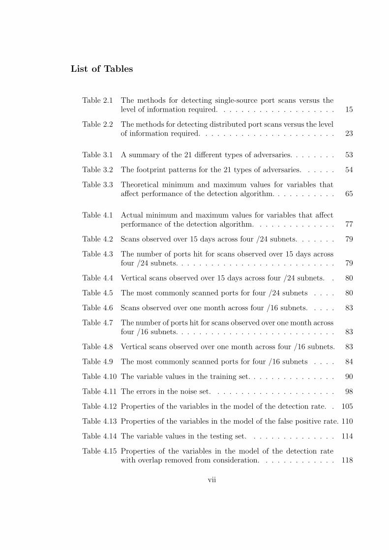
List of Tables

Table 2.1 The methods for detecting single-source port scans versus thelevel of information required. . . . . . . . . . . . . . . . . . . . 15

Table 2.2 The methods for detecting distributed port scans versus the levelof information required. . . . . . . . . . . . . . . . . . . . . . . 23

Table 3.1 A summary of the 21 different types of adversaries. . . . . . . . 53

Table 3.2 The footprint patterns for the 21 types of adversaries. . . . . . 54

Table 3.3 Theoretical minimum and maximum values for variables thataffect performance of the detection algorithm. . . . . . . . . . . 65

Table 4.1 Actual minimum and maximum values for variables that affectperformance of the detection algorithm. . . . . . . . . . . . . . 77

Table 4.2 Scans observed over 15 days across four /24 subnets. . . . . . . 79

Table 4.3 The number of ports hit for scans observed over 15 days acrossfour /24 subnets. . . . . . . . . . . . . . . . . . . . . . . . . . . 79

Table 4.4 Vertical scans observed over 15 days across four /24 subnets. . 80

Table 4.5 The most commonly scanned ports for four /24 subnets . . . . 80

Table 4.6 Scans observed over one month across four /16 subnets. . . . . 83

Table 4.7 The number of ports hit for scans observed over one month acrossfour /16 subnets. . . . . . . . . . . . . . . . . . . . . . . . . . . 83

Table 4.8 Vertical scans observed over one month across four /16 subnets. 83

Table 4.9 The most commonly scanned ports for four /16 subnets . . . . 84

Table 4.10 The variable values in the training set. . . . . . . . . . . . . . . 90

Table 4.11 The errors in the noise set. . . . . . . . . . . . . . . . . . . . . 98

Table 4.12 Properties of the variables in the model of the detection rate. . 105

Table 4.13 Properties of the variables in the model of the false positive rate. 110

Table 4.14 The variable values in the testing set. . . . . . . . . . . . . . . 114

Table 4.15 Properties of the variables in the model of the detection ratewith overlap removed from consideration. . . . . . . . . . . . . 118

vii

Table 4.16 The detection rates for 65536 IP addresses (/16 subnet) giventhat most variables have optimal values. . . . . . . . . . . . . . 120

Table 4.17 The detection rates for 65536 IP addresses (/16 subnet) giventhat most variables have the least optimal values. . . . . . . . . 120

Table 4.18 The variable values required to achieve 90% detection rates with65536 IP addresses (/16 subnet) and one port. . . . . . . . . . 121

Table 4.19 The detection rates using NSAT on 65536 IP addresses (/16subnet) given that most variables have optimal values. . . . . . 121

Table 4.20 The detection and false positive rates for NSAT and DScan givendifferent network sizes when all other variables have mediumvalues. . . . . . . . . . . . . . . . . . . . . . . . . . . . . . . . 122

Table 4.21 The variable values in the validation set. . . . . . . . . . . . . . 126

Table 4.22 The most commonly scanned ports for one /17 subnet. . . . . . 127

Table 4.23 The variable values in the training set for Yegneswaran et al. [85].134

Table 4.24 The detection and false positive rates for the DScan scanningalgorithm with 100 sources and 20% overlap against a /24 subnet(256 IP addresses). . . . . . . . . . . . . . . . . . . . . . . . . . 141

Table 4.25 The detection and false positive rates for the DScan scanningalgorithm with 100 sources and 20% overlap against a /16 subnet(65536 IP addresses). . . . . . . . . . . . . . . . . . . . . . . . 141

viii

List of Figures

Figure 3.1 An illustration of port scanning . . . . . . . . . . . . . . . . . 37

Figure 3.2 An example set covering problem using 9 points and 4 sets. . . 57

Figure 3.3 AltGreedy [22] portion of algorithm. . . . . . . . . . . . . . . 60

Figure 3.4 Rejection algorithm. . . . . . . . . . . . . . . . . . . . . . . . 61

Figure 3.5 Detection Algorithm . . . . . . . . . . . . . . . . . . . . . . . 62

Figure 3.6 Strobe Algorithm . . . . . . . . . . . . . . . . . . . . . . . . . 64

Figure 4.1 The distribution of activity for the top five most often scannedports: data set 1 (/24 subnet) . . . . . . . . . . . . . . . . . . 81

Figure 4.2 The distribution of activity for the top five most often scannedports: data set 2 (/24 subnet) . . . . . . . . . . . . . . . . . . 81

Figure 4.3 The distribution of activity for the top five most often scannedports: data set 3 (/24 subnet) . . . . . . . . . . . . . . . . . . 82

Figure 4.4 The distribution of activity for the top five most often scannedports: data set 4 (/24 subnet) . . . . . . . . . . . . . . . . . . 82

Figure 4.5 The distribution of activity for the top five most often scannedports: data set 1 (/16 subnet). . . . . . . . . . . . . . . . . . . 84

Figure 4.6 The distribution of activity for the top five most often scannedports: data set 2 (/16 subnet). . . . . . . . . . . . . . . . . . . 85

Figure 4.7 The distribution of activity for the top five most often scannedports: data set 3 (/16 subnet). . . . . . . . . . . . . . . . . . . 85

Figure 4.8 The distribution of activity for the top five most often scannedports: data set 4 (/16 subnet). . . . . . . . . . . . . . . . . . . 86

Figure 4.9 Co-ordinated port scan DETER set up with 5 agents, 1 handlerand a /16 subnet. . . . . . . . . . . . . . . . . . . . . . . . . . 87

Figure 4.10 DScan Algorithm . . . . . . . . . . . . . . . . . . . . . . . . . 94

Figure 4.11 Comparison between the difference in errors and the averageerror for false positive rates. . . . . . . . . . . . . . . . . . . . 100

Figure 4.12 Comparison between the difference in errors and the averageerror for false negative rates. . . . . . . . . . . . . . . . . . . . 100

ix

Figure 4.13 Effect of the fraction of network covered by the scan on thedetection rate. . . . . . . . . . . . . . . . . . . . . . . . . . . . 107

Figure 4.14 Effect of the number of scanning sources on the detection rate. 107

Figure 4.15 Effect of the number of scanned ports on the detection rate. . 108

Figure 4.16 Effect of the number of noise scans on the detection rate. . . . 109

Figure 4.17 Effect of the fraction of the network covered on the false positiverate. . . . . . . . . . . . . . . . . . . . . . . . . . . . . . . . . 111

Figure 4.18 Effect of the percentage of overlap on the false positive rate. . 112

Figure 4.19 The observed detection rate versus the predicted detection ratefor 50 experiments (testing set). . . . . . . . . . . . . . . . . . 115

Figure 4.20 The predicted false positive rate versus the residuals for 50 ex-periments (testing set). . . . . . . . . . . . . . . . . . . . . . . 117

Figure 4.21 The distribution of activity for the top five most often scannedports for one /17 subnet. . . . . . . . . . . . . . . . . . . . . . 127

Figure 4.22 The observed detection rate versus the predicted detection ratefor 50 experiments (validation set). . . . . . . . . . . . . . . . 129

Figure 4.23 The ROC curve for the training, testing and validation sets. . 130

Figure 4.24 The predicted false positive rate versus the residuals for 50 ex-periments (validation set). . . . . . . . . . . . . . . . . . . . . 131

Figure 4.25 The effect of the number of seconds between scan start timesand subnet size on the false positive rate for Yegneswaran etal.’s algorithm [85]. . . . . . . . . . . . . . . . . . . . . . . . . 137

Figure 4.26 The effect of the number of scanning sources and the subnetsize on the false positive rate, using Yegneswaran et al.’s algo-rithm [85]. . . . . . . . . . . . . . . . . . . . . . . . . . . . . . 138

Figure 4.27 The predicted false positive rate versus the residuals for 48 ex-periments (testing set) for Yegneswaran et al.’s algorithm [85]. 139

Figure B.1 An illustration of a single predictor variable P (x). . . . . . . . 163

x

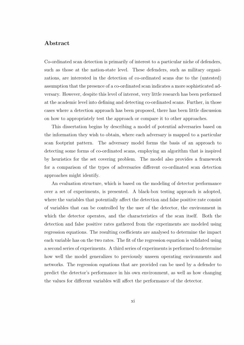
Abstract

Co-ordinated scan detection is primarily of interest to a particular niche of defenders,

such as those at the nation-state level. These defenders, such as military organi-

zations, are interested in the detection of co-ordinated scans due to the (untested)

assumption that the presence of a co-ordinated scan indicates a more sophisticated ad-

versary. However, despite this level of interest, very little research has been performed

at the academic level into defining and detecting co-ordinated scans. Further, in those

cases where a detection approach has been proposed, there has been little discussion

on how to appropriately test the approach or compare it to other approaches.

This dissertation begins by describing a model of potential adversaries based on

the information they wish to obtain, where each adversary is mapped to a particular

scan footprint pattern. The adversary model forms the basis of an approach to

detecting some forms of co-ordinated scans, employing an algorithm that is inspired

by heuristics for the set covering problem. The model also provides a framework

for a comparison of the types of adversaries different co-ordinated scan detection

approaches might identify.

An evaluation structure, which is based on the modeling of detector performance

over a set of experiments, is presented. A black-box testing approach is adopted,

where the variables that potentially affect the detection and false positive rate consist

of variables that can be controlled by the user of the detector, the environment in

which the detector operates, and the characteristics of the scan itself. Both the

detection and false positive rates gathered from the experiments are modeled using

regression equations. The resulting coefficients are analysed to determine the impact

each variable has on the two rates. The fit of the regression equation is validated using

a second series of experiments. A third series of experiments is performed to determine

how well the model generalizes to previously unseen operating environments and

networks. The regression equations that are provided can be used by a defender to

predict the detector’s performance in his own environment, as well as how changing

the values for different variables will affect the performance of the detector.

xi

Acknowledgements

The process of obtaining a PhD is often considered to be very lonely. It is only when

you reflect back on the experience when near the end that you recognize just how

many people actually helped and supported you throughout the years. First on my

list, I would like to thank Marc Kellner, who provided guidance near the beginning

of the dissertation. I hope that he is cheered by my completing the dissertation.

Of course, I would like to thank my supervisor, Jacob Slonim, for not giving up

on me, even when I decided that I wanted to do research on security rather than

databases! And I want to thank my committee: Mike McAllister, who exhibited

tremendous patience when helping me with the theory portion of the adversary model,

John McHugh, who ensured that I explored all possible explanations for any behaviour

I observed, and Gord Agnew, who always provided useful comments, often on very

short notice! Vern Paxson also deserves thanks for agreeing to serve as my external

and for providing very useful comments on how the dissertation could be improved.

I want to thank the IBM Centre for Advanced Studies in Toronto for funding my

PhD studies. I especially want to thank Kelly Lyons for supporting my fellowship

applications and Anthony Tjong for supporting my internships at IBM Toronto.

CERT at Carnegie Mellon University also supported my PhD by allowing me to

work with them as a Visiting Scientist and have access to their data. Within CERT I

am especially grateful to the late Suresh Konda, for fighting to allow a student foreign

national access to perform research at CERT. I am also grateful to Tom Longstaff

for helpful discussions, and to Roman Danyliw for allowing me to take a two month

leave of absence to finish my first draft. Finally, I want to thank Sean McAllister for

giving me data access and Captain Jeff Jaime for allowing me to keep that access.

I want to thank Symantec for performing some experiments and providing some

data in support of my thesis topic. Within Symantec I especially want to acknowledge

John Schwartz, Alfred Huger, Elias Levy and Scott Shannon.

The DETER community also deserves a great deal of thanks. In particular, I

would like to thank Terry Benzel for supporting my application to use the DETER

xii

testbed and allowing me the opportunity to present on my thesis at a DETER project

meeting. I would also like to thank Jeff Rowe for providing some of his scripts.

There are a number of individuals that contributed to my thoughts during my

research. Jeanette Jannsen pointed me towards the set covering literature when I

described the set operations I wanted to perform. Jay Kadane and Josh McNutt

provided a great deal of statistical support, and were very patient at explaining some

of the subtleties of the statistical tests I use in my evaluation methodology. I want

to thank Roy Maxion for reviewing my experimental design and commenting on it,

and also Kymie Tan for helpful conversations on modeling and testing methodologies.

Finally, I would like to thank Bob Blakley for allowing me to bounce ideas off him,

which helped me refine my thoughts on adversary modeling.

I received tremendous technical support throughout my research. Thanks go to

Dave Green and Jeff Allen for putting up with my constant technical requests, as well

as Mike Murphy and Jeff Uebele from UCIS for responding to networking requests

in support of the experiments performed with Symantec. Additionally, Mike Smit

deserves thanks for serving as my remote OS installer and power recycler!

On a more personal level, I want to thank Kirstie Hawkey and Tara Whalen for

their peer support throughout the entire PhD process, as well as Richard Nowakowski,

who patiently listened to my complaints on a number of occasions. I also want to

thank Brian Trammel, Amanda Cook, Drew Kompanek, Sven Dietrich, Stephanie

Rogers, Caesy Dunlevy and Ginny Trapino for being supportive and understanding

all the times that I had to pass on going out for supper.

I would like to thank Sam Scully, who not only understood why I would want my

parchment written in latin, but who went above and beyond the call of duty so that

it would be. And, of course, Dr. Keast, for not only believing in me back when I was

an undergrad with a C average, but for allowing me to wear his birretum at every

graduation ceremony! I am also grateful to Mike Shepherd for convincing me to do

my PhD in the first place.

Finally, and perhaps most importantly, I want to thank Jason Rouse for unfailingly

believing in me for the past six years.

xiii

List of Abbreviations Used

CIDR Classless InterDomain Routing

CPU Central Processing Unit

DDOS Distributed Denial-of-Service

DHCP Dynamic Host Configuration Protocol

DNS Domain Name Service

FTP File Transfer Provider

HTTP HyperText Transfer Protocol

ICMP Internet Control Message Protocol

IDS Intrusion Detection System

IIS Internet Information Services

IP Internet Protocol

IRC Internet Relay Chat

ISP Internet Service Provider

NAT Network Address Translation

NSAT Network Security Analysis Tool

NSM Network Security Monitor

ROC Relative Operating Characteristic

RPC Remote Procedure Call

SMB Server Message Block

SMTP Simple Mail Transfer Protocol

SSH Secure Shell

xiv

TCP Transmission Control Protocol

TRW Threshold Random Walk

UDP User Datagram Protocol

UPnP Universal Plug and Play

xv

Glossary

A A set of IP addresses

C A scan, represented by the tuple (s, T,∆t), is a set

of connection attempts from source s in time inter-

val ∆t to the set of targets T

F The footprint of a scan, which is the targets of a

scan that appear in a monitored network.

P A set of ports

S A set of source IP addresses

T A set of target IP/port pairs of interest in the net-

work space

∆t A time interval

δ(S) A co-ordinated scan, represented by the tuple

(S, T,∆t), is a collection of scans from a set of

sources S where there is a single instigator behind

the set of sources

F A footprint pattern, represented by the tuple

(|A|, |P |, ζ(C),H(C), ς, κ).

H(C) The hit rate, or number of targeted IP addresses

within the scanned range, of a scan C.

ρ A probe, which is represented by the tuple (s, τ,∆t)

τ A target, or a single port at a single IP address

θ(Ci, Cj) The overlap between scans Ci and Cj.

ζ(C) The percentage of contiguous network IP space cov-

ered by scan C.

a An IP address

p A port on a computer system, assumed to use the

TCP protocol in this dissertation

s A source IP address

xvi

Chapter 1

Introduction

1.1 Motivation

The tactics of traditional warfare are applied to the electronic realm. One such tac-

tic is the use of reconnaissance missions before a military attack to determine the

vulnerabilities and resources of the enemy. This is described as “a precursor to ma-

neuver and fire” in the United States Army’s Field Manual 100-5 (cited from [41])

and, in fact, the success of an attack has a high correlation with the thoroughness of

the reconnaissance [41, 61]. Similarly, before an adversary makes an attack against

a target computer or network, he will usually perform some form of information

gathering in an effort to determine potential vulnerabilities on a target computer or

network [36]. As stated by the HoneyNet Project [58, p. 77], “Most attacks involve

some type of information gathering before the attack is launched.” While this par-

ticular project concentrated primarily on those attackers with low skill levels, it is

believed that information gathering techniques are also used by more sophisticated

attackers. Supporting this assumption are the results from a study by Ning et al. [49],

who correlated the intrusion alerts from a Capture the Flag event at DEF CON 8 (an

underground hacking conference). This study showed that many attacks contained

a prerequisite stage employing various types of port scanning. Further, according to

the Annual Report to Congress on Foreign Economic Collection and Industrial Espi-

onage 2001 [51], the “majority of Internet endeavors are foreign probes searching for

potential weaknesses in systems for exploitation.”

Reconnaissance can take several forms, not all of which are technical. For ex-

ample, adversaries will often use social engineering approaches, where an adversary

manipulates an employee into revealing sensitive information [54]. Other information

gathering techniques include “dumpster diving” [68], where an adversary searches

through a target’s physical garbage for items such as computer listings, CDs and

DVDs.

1

2

One of the technical information gathering techniques is a scan. A port scan is

a method of determining whether particular services are available on a computer or

network by observing the responses to connection attempts or other carefully crafted

packets [39, 12]. A vulnerability scan is similar, except that a positive response from

the target results in further communication to determine whether the target is vulner-

able to a particular exploit. Panjwani et al. [53] have found that approximately 50%

of attacks are preceded by some form of scanning activity, particularly vulnerability

scanning. They used a honeypot-like deployment of two machines on a campus net-

work. The machines were configured to respond to connection requests, thus eliciting

enough traffic from the scanning source to determine if the scan was a port scan or if

it tested for the presence of particular vulnerabilities.

Given that a scan consists of packets that traverse the target’s network, the scan

information can be logged by network applications, such as intrusion detection sys-

tems. As a result, attackers have developed various methods for eluding monitoring

systems [18]. One such approach that has been used by adversaries to avoid detection

is to insert a time delay between the probing of each scan target which defeats many

threshold-based detection approaches [25]; however, this slows down the rate of in-

formation gathering for the adversary. As a result, other methods to elude detection

systems have evolved, such as distributed or co-ordinated port scans [21, 25]. In this

case, the adversary will divide the target space amongst multiple source IP addresses,

so that each source scans a portion of the target. The result is that an intrusion

detection system might not detect any of the sources. If the sources are detected, the

system will not recognize that the various sources are collaborating.

There are several types of adversaries that an organization can face. While, his-

torically, computer attacks were viewed as a game (see Landreth [33] for a discussion

of hacker motivations in 1985), motivations for computer attacks have since evolved

to include attackers who are interested in financial profit or advancing their political

agendas [24, 54, 64, 66]. For example, Rogers [64] developed a taxonomy of seven

hacker types based on motivations. He identified the two groups with the greatest level

of technical sophistication as professional criminals and cyber-terrorists. CERT has

also noted in a presentation on incident and vulnerability trends that “intruders are

prepared and organized” and that “intruder tools are increasingly sophisticated” [8].

3

Schneier [66] notes that “we expect to see ever-more-complex worms and viruses in

the wild”, and goes on to comment that “Hacking has moved from a hobbyist pursuit

with a goal of notoriety to a criminal pursuit with a goal of money.”

In this research we assume a sophisticated adversary, such as a professional crim-

inal, and an assumption is also made that the adversary will attempt to hide his

scanning activity using some of the methods described above. This assumption has

been made by others, such as Lowry [37], who stated “All sophisticated adversaries

are assumed to be risk averse during all phases leading up to an attack. This is

because detection prior to attack execution may cause the defender to respond.”

Braynov and Jadliwala provide a formal model for detecting co-ordinated or co-

operative activity [7]. They define two types of co-operation: action correlation and

task correlation. Action correlation refers to how the actions of one user can interfere

with the actions of another. For example, a coordinated attack may require that one

user perform a particular action so that another can perform the actual attack; this

is the form of co-ordination on which their model focuses. Task correlation, however,

refers to the division of tasks amongst multiple users where a parallel (or distributed)

port scan is provided as an example. The authors go on to state that “cooperation

through task correlation is difficult to discover. It is often the case that sensor data is

insufficient to find correlation between agents’ tasks. User intentions are, in general,

not directly observable and a system trace could be intentionally ambiguous. The

problem is further complicated by the presence of a strategic adversary who is aware

that he has been monitored.”

The detection of co-ordinated port scans is of particular interest to larger orga-

nizations, such as nation-states or military operations. However, it is not solely of

interest at the nation-state level, but also to those organizations who desire a greater

level of network situational awareness [84] and who might be interested in having in-

formation regarding the sudden appearance of, or an increase in, co-ordinated scans

against the monitored network. At the nation-state level, this interest tends to be

based on the untested assumption that an adversary who uses a co-ordinated port

scan poses a greater threat than one who does not. This is because the use of a

sophisticated technique, such as a co-ordinated port scan, implies that the adversary

4

is technically sophisticated. It also implies that the adversary desires to remain un-

detected while gathering information. However, these assumptions do not take into

account the likelihood that toolkits have been developed that automate co-ordinated

scanning, nor do they take into account the possible use of botnets as co-ordinated

stealthy attackers.

Co-ordinated (or distributed) scans have been mentioned in several papers [7,

21, 27, 62, 72, 73, 74, 85]; however, not all of these papers have provided potential

solutions to the detection of such scans. Yegneswaran et al. [85] and Robertson et

al. [62] both describe how they detect distributed port scans; however, they both

use different definitions for what constitutes a distributed port scan. Staniford et

al. [70, 71] have developed a generic approach to the detection of distributed port scans

based on the assumption that there will be enough common elements between the

scans from the multiple sources that they will form a cluster; however, their method

was not intended to solely detect distributed port scans, but also to cluster other

network events, such as single-source port scans, denial of service attacks, and software

misconfigurations [69]. The clusters are not labeled, so it is left to an administrator

to determine the event represented by each cluster. In addition to the lack of papers

that discuss solutions for the detection of co-ordinated port scans, even fewer provide

a detection or false positive rate indicating how well their algorithm performs, nor

are there any discussions on the circumstances under which the algorithm performs

either well or poorly.

The detection of port scans, and in particular stealthy or co-ordinated port scans,

allows for the early detection of and reaction to potential intruders. Cohen [10] has

used simulations of computer attacks and defences to determine optimal defender

strategies. He reports that the most successful strategy a defender can employ is to

respond quickly to an attack, and that this strategy is even better than that of having

a larger number of defences in place (such as firewalls, intrusion detection systems,

etc.) but a slower response time to an attack. By providing an administrator with

tools for detecting co-ordinated port scans, the administrator can use this information

to prioritize any response to the scan. Given that the scan targets indicate the likely

target of the adversary, the administrator can use this information to determine the

5

machines and services that are most likely to be attacked and to ensure that they are

secure.

Ideally, the defender would know a priori how well the co-ordinated scan detector

will perform on his network, including what forms of scans it is mostly likely to

detect and the probability of detection given different criteria. However, testing in

the intrusion detection field has focused primarily on the use of the Lincoln Labs data

set and network traces [4]. The Lincoln Labs data set consists of a combination of

simulated background traffic and actual attack traffic that was generated and injected

in a controlled fashion [36]; however, there are known flaws with this data set [38, 42].

Network traces, in comparison, contain actual background traffic but the attacks are

not injected in a controlled fashion, nor are the attacks labeled. The result is that

reports on the performance of intrusion detection systems consist of, at best, a true

and false positive rate based on a single network. This result is not necessarily

transferable to other networks. That is, the results obtained on one network do not

necessarily indicate the results that will be obtained on a different network, as the

detector might be affected by issues such as the size of the network, the amount of

traffic observed, the type of traffic observed, and general usage patterns.

Given that a defender will want to know how well a detector will work given his

particular environment, a better approach to presenting results for a detector is to

provide a model that represents the detector’s performance under different operating

conditions. Such a model could be used by a defender to determine how well the

detector will work in his particular environment. Additionally, it could be used to

determine the probability that particular activities will be detected based on the

salient characteristics of that activity.

In the case of co-ordinated scan detection, a model that indicates the expected

detection rate and false positive rate can be used by the defender to estimate the

number of co-ordinated scans he might not be detecting, the characteristics of scans

that he might not be detecting, and the number of suspected co-ordinated scans that

are actually false positives. If the false positive rate is considered to be high, he can

use this information to determine whether the benefit of detecting some co-ordinated

scans is worth the cost of investigating the false positives.

6

1.2 Hypotheses

A co-ordinated TCP port scan is represented by the tuple (S, T,∆t), consisting of a

collection of scans from a set of sources S aimed at a set of targets T during some

time interval ∆t. The entire set of sources behave in a co-ordinated manner that is

controlled by a single adversary. The set of destinations is T = {τ1, τ2, ...τn}, where

τi = (a, p), consisting of the destination IP address a and the destination port p, where

we assume the TCP protocol in this dissertation. These definitions are explained in

greater detail in Section 3.1.

Chapter 3 defines various classes of adversaries that might employ co-ordinated

scans. This set of adversaries is based on the information they wish to obtain, and

they can be recognized by a defender based on the scan footprint pattern, where a

scan footprint is “the set of port/IP combinations which the attacker is interested in

characterizing” [70]. From this set of adversaries the focus is narrowed to those whose

goals result in one of two footprint patterns: horizontal scans and strobe scans. A

horizontal scan is a port scan of a single port across multiple IP addresses, while a

strobe scan is a port scan that targets multiple ports across multiple IP addresses [70].

We provide more precise definitions for horizontal and strobe scans in Section 3.4,

where we define the minimum number of IP addresses and/or ports to be targeted

to meet the definitions as user-specified variables. Yegneswaran et al. [85] found that

60%-70% of all scans were horizontal, where all scanning activity performed by worms

had already been filtered out. This is consistent with empirical evidence presented

in Section 4.1.3 which shows that, on average, 73% of TCP scans were horizontal

when scans against eight different subnets were analysed. Yegneswaran et al. did not

perform an analysis for strobe scans specifically; however, the empirical investigation

presented in Section 4.1.3 indicates that an average of 24% of scans are strobe scans.

The focus in this dissertation is on horizontal and strobe scans because they occur

more commonly than other scan footprint patterns.

Two commonly found network sizes are /24 and /16 subnets, consisting of 256

and 65536 IP addresses respectively. Any detector for co-ordinated port scans should,

at a minimum, work on both of these network sizes. In the ideal case, a detector will

perform correctly regardless of the size of the network.

A common measurement used in intrusion detection system (IDS) literature is that

7

of true and false positives and negatives [5]. A true positive (or detection) is defined

as correctly classifying that a single-source scan belongs to a co-ordinated scan. A

false positive is defined as incorrectly classifying a single-source scan as belonging to

a co-ordinated scan. Given these definitions, the detector is expected to achieve a

detection rate (true positive) of greater than 99% and a false positive rate of less

than 1%. The two rates used here are taken from Jung et al. [28], who used 1% as

the maximum desirable false positive rate for their single source scan detector. The

ideal detection rate was set in this paper at 99%, where they achieved a rate of 96.0%

or better. The best detection rate achieved on the same data set by Bro was 15.0%

while Snort achieved 12.6%.

While the performance of a detector can be measured both in terms of the de-

tection rate and the false positive rate, Maxion and Tan [40] demonstrated that

the performance of a detector can be impacted by the environment, and that the

performance obtained from one environment does not necessarily indicate the same

performance given a different environment. It should be possible to identify the key

properties of a detector’s input and environment that contribute to the true and false

positive rates. It should be further possible to model both the detection rate and

false positive rate of a given detector if the significant properties of the operating

environment can be identified and used as variables (e.g., size of the network, number

of events). These models should be able to predict how well the detector will perform

given conditions under which the detector has not previously been tested. This will

allow the network administrator to determine the trade-offs between the detection or

false positive rates and the values for the different variables in the model based on

their detection requirements and available resources. The administrator should also

be informed of the expected accuracy of the model to further inform his decisions.

In particular, we would expect a model to have a minimum accuracy of 75% when

predicting if a scan would be detected. We would also expect that the predicted false

positive rate would be within ±0.03 of the actual false positive rate at least 75% of the

time. The values of 75% and 0.03 were chosen arbitrarily as representing satisfactory

performance.

Given this background information, there are two hypotheses that the research

presented in this dissertation sets out to address:

8

Hypothesis 1.1 A detector can be designed to detect co-ordinated TCP port scans

against a target network where the scan footprint is either horizontal or strobe with a

detection rate of greater than 99% and a false positive rate of less than 1% on both

/24 and /16 networks.

Hypothesis 1.2 Evaluation models that can predict the performance of a detector

in terms of detection rates and false positive rates, given previously unseen operating

environments, can be developed, where the the model of the detection rate should have

an accuracy of at least 75% and the model of the false positive rate should be accurate

to within ±0.03 of the actual false positive rate in 75% of the cases.

1.3 Research Objective and Approach

The objectives of this research are two-fold: (1) to develop and evaluate a detector

that recognizes co-ordinated port scans, and (2) to develop a model of the true and

false positive rates for the detector given new environments.

The approach taken in this study to address the first objective involves devel-

oping an adversary model of co-ordinated port scans, where the model is based on

an identification and classification of various types of adversaries based on the infor-

mation they wish to obtain. This approach builds on comments made by Braynov

and Jadliwala [7] when describing task correlation, who state that “in order to detect

such cooperation, one needs a clear understanding of agents’ incentives, benefits, and

criteria of efficiency.” Each adversary has a particular goal, and the defender can

use the scan footprint pattern generated by the adversary to infer the goal of the

adversary.

Each adversary is represented by a footprint pattern, which indicates the informa-

tion that the adversary wishes to obtain. We observe that an adversary performing a

co-ordinated scan will still have the same footprint pattern when each of the single-

source scans are combined. This observation is used as the basis of an algorithm

for detecting co-ordinated scans. We focus specifically on adversaries that perform

horizontal and strobe scans, and attempt to detect whether such scanning patterns

are present in some subset of scans when we are given a larger set of scans. This

problem is related to the set covering problem, with the resulting detection algorithm

9

inspired by the AltGreedy heuristic of Grossman and Wool [22]. The capability of

the algorithm is tested through a set of controlled experiments that combine isolated

co-ordinated scans using the DETER network testbed [79] with scans detected given

live network traffic.

Our second objective is addressed by first identifying the variables that are sus-

pected of contributing to the detection rate and the false positive rate. Regression

equations are used to model these two rates, and an analysis of the variables that

contribute most to each rate is provided. These equations are tested using scans

with characteristics that were not part of the training set to determine how well the

models predicted the detection and false positive rates of the detector. The equations

were further tested using background noise from a network that was not used in the

training phase to determine how well both the detector and the regression models

generalized to networks with different characteristics. The result is two equations

that allow a user of the detection algorithm to predict how well the algorithm will

perform in his own operating environment.

1.4 Overview of the Thesis

This thesis is composed of five chapters. The first introduces the problem and states

the hypotheses of the dissertation; the research objectives and approach to proving

the hypotheses are also provided. Chapter 2 provides a review of detection algorithms

for both single-source and co-ordinated port scans, as well as discusses the common

evaluation methodologies employed in the intrusion detection literature. Chapter 3

provides an adversary model of co-ordinated scans, based on the footprint patterns

that different adversaries will generate; this model provides a framework for a de-

tection algorithm, presented at the end of the chapter. The detection algorithm is

evaluated through a series of controlled experiments, described in Chapter 4. Regres-

sion equations are provided that model the performance of the detection algorithm

given different operating environments (such as network size and the size of the input

set). Chapter 5 provides a summary of the research contributions and the conclusions

of the thesis, and finishes with a discussion of future research directions.

Chapter 2

Relevant Background

While port scanning is a common occurrence, there is very little literature surround-

ing the subject (as noted by both Stanford et al. [70] and Jung et al. [28]). As a

result, different terms are often used to represent the same activity. Conversely, the

same term might be used by multiple people with slightly different meanings or as-

sumptions. Section 2.1 provides a sampling of some of the definitions found in the

literature.

Section 2.2 discusses the different approaches that have been developed to detect

both single-source and distributed scans. Some approaches for single-source scans

are discussed in the context of larger intrusion detection systems, while others have

been discussed in terms of just the port scan detection algorithm. We note in our

discussion of each of the detector approaches where the algorithm provided was part

of a larger system.

Section 2.3 describes the different evaluation approaches that are commonly used

in the intrusion detection literature, describing those which were used for the detectors

presented in the previous section. It should be noted that not all the detectors

described in Section 2.2 were evaluated, so not all the detectors appear in Section

2.3.

2.1 Port Scan Terminology

2.1.1 Single-Source Port Scans

While scans have been discussed in both the academic and hacker literature, no

consistent definitions of scans have been developed. An early article on scanning, ap-

pearing in the hacker magazine Phrack, defined portscanning as a solution to knowing

“the services a certain host offers.” [39]. A later article in the same magazine used

10

11

scanning and port scanning interchangeably, and defined them as “a method for dis-

covering exploitable communication channels” [18]. Two years later, hybrid [25] used

the term information gathering instead, defining it as “the process of determining the

characteristics of one or more remote hosts (and/or networks).” This article goes on

to state that “Information gathering can be used to construct a model of a target

host, and to facilitate future penetration attempts.” [25]

Some security institutes have provided glossaries of common security terms. SANS,

which provides training, certification and research in the computer security field, has

defined a port scan as: [65]

A port scan is a series of messages sent by someone attempting to break

into a computer to learn which computer network services, each associated

with a ”well-known” port number, the computer provides. Port scanning,

a favorite approach of computer cracker, gives the assailant an idea where

to probe for weaknesses. Essentially, a port scan consists of sending a mes-

sage to each port, one at a time. The kind of response received indicates

whether the port is used and can therefore be probed for weakness.

In the academic literature, a review of port scanning techniques defined port scan-

ners as “specialized programs used to determine what TCP ports of a host have pro-

cesses listening on them for possible connections” [12]. Jung et al. [28] describe port

scanning as “the attacker probes a set of addresses at a site looking for vulnerable

servers.” Staniford et al. [70] described portscanning based on why it was used, with

the assumption that the readers already knew what the activity itself was. They said

that portscanning was used “by computer attackers to characterize hosts or networks”

and by network administrators to “find vulnerabilities in their own networks”. Sim-

ilarly, Leckie and Kotagiri [34] describe network scans as “an exercise in intelligence

gathering by an attacker.” They go on to say that they are used “to systematically

explore the topology or the configuration of a victim’s network.” A port scan is then

defined as a scan that is specifically targeted at TCP or UDP services. Muelder

et al. [47], however, defined a network scan as “a connection is attempted to every

possible destination in a network” while a port scan was defined as “a connection is

attempted to each port on a given destination.” In contrast, Robertson et al. [62]

used the more general term surveillance, defining it as “the scanning of target IPs and

12

ports for vulnerabilities.” Meanwhile, Basu et al. [6] and Streilein et al. [74] used the

more specific term probe, stating that “Probe attacks automatically scan a network

of computers or a DNS server to find valid IP addresses (ipsweep, lsdomain, mscan),

active ports (portsweep, mscan), host operating system types (queso, mscan), and

known vulnerabilities (satan).” [6] Finally, an early article in the intrusion detection

field called port scans sweeps, which it defined as “when a single host systematically

contacts many others in succession.” [73]

These definitions largely have two threads in common. The first is that there are

multiple targets — either multiple ports on a single computer, multiple IP addresses,

or even networks. The second commonality is the intent behind performing the scan,

which is to determine some characteristics of a particular computer or network (e.g.,

the services available, or whether an address is occupied, etc.). Some definitions are

even more specific than this, stating that the reason for determining what services

are running is to locate potential vulnerabilities.

Staniford et al. [71, 70] provided further definitions for scans, which are now in

common use. In particular, they defined a scan footprint as “the set of port/IP com-

binations which the attacker is interested in characterizing.” They further classified

port scans into four types based on their footprint geometry: vertical, horizontal,

strobe and block. A vertical scan consists of a port scan of some or all ports on a

single computer. Port scans across multiple IP addresses break down into three basic

types, based on the number of ports in the scan. A horizontal scan is a port scan of

a single port across multiple IP addresses. If the port scan is of multiple ports across

multiple IP addresses, then it is called a strobe scan. A block scan is a port scan

against all ports on multiple IP addresses. Yegneswaran et al. [85] quantified vertical

and horizontal scans, defining six or more ports on a single computer as a vertical

scan, and five or more IP addresses within a subnet (of undefined size) as a horizontal

scan.

2.1.2 Distributed Scans

As with single-source port scans, there are many definitions for distributed scans. In

the hacker literature, Phrack magazine states that “distributed information gathering

13

is performed using a ‘many-to-one’ or ‘many-to-many’ model” for gathering infor-

mation about a target computer or network [25]. In this case the “attacker utilizes

multiple hosts to execute information gathering techniques in a random, rate-limited,

non-linear way.” The non-linear portion of a scan appears to refer to randomizing

the destination IP/port pairs amongst the various sources and within the sources, as

well as randomizing the time delay between each probe packet.

In the academic literature, the more generic form of a distributed scan, called

co-ordinated attacks, was first described in a paper by Staniford-Chen et al. [73].

They defined co-ordinated attacks as “multi-step exploitations using parallel sessions

where the distribution of steps between sessions is designed to obscure the unified

nature of the attack or to allow the attack to proceed more quickly (e.g. several

simultaneous sweep attacks from multiple sources).” Distributed scans specifically

were first addressed three years later by Green et al. [21], who defined the term

co-ordinated attack to describe the behaviour they were observing. They defined a

co-ordinated attack as “multiple IP addresses working together toward a common

goal.” (Note that this is in contrast to the definition by Staniford-Chen et al. [73],

who used an attack in the more generic sense, to include items such as intrusion

attempts.) Green et al. continue on to state that “a coordinated attack can also look

as though multiple attackers are working together to execute a distributed scan on

many internal addresses or services.” Staniford et al. [70] later defined distributed

scanning as scans that are launched “from a number of different real IP addresses”,

so that the scanner can “investigate different parts of the footprint from different

places.” In a later paper, Staniford et al. [72] state:

An attacker could scan the Internet using a few dozen to a few thousand

already-compromised “zombies,” similar to what DDOS attackers assem-

ble in a fairly routine fashion. Such distributed scanning has already

been seen in the wild—Lawrence Berkeley National Laboratory received

10 during the past year.

Yegneswaran et al. [85] defined co-ordinated scans as being “scans from multiple

sources (5 or more) aimed at a particular port of destinations in the same /24 subnet

within a one hour window.” They go on to state “These scans usually come from

the more aggressive/active sources that comprise several collaborative peers working

14

in tandem.” Finally, while not defining distributed port scans, Robertson et al. [62]

grouped source addresses together as forming a potential distributed port scan if they

were sufficiently close (e.g., within the same /24), where the scanner simply obtained

multiple IP addresses from his ISP. It should be noted that all of these definitions

imply some level of co-ordination between the single sources used in the scan.

2.2 Port Scan Detection

2.2.1 Single-Source Port Scan Detection

Detection methods for single-source port scans have been part of intrusion detection

systems since 1990, with the release of Network Security Monitor (NSM) [23]. In gen-

eral, these systems can be divided into three categories: threshold-based, algorithmic

and visual. Threshold-based detection consists of “testing for X events of interest

across a Y -sized time window.” [50, p. 125] One example of an event in this context is

the number of unique IP addresses contacted (e.g., as is the case in Snort[63]). Algo-

rithmic approaches, however, consist of other detection methods, such as sequential

hypothesis testing, probability calculations, or neural networks. The algorithmic ap-

proaches employed to date are discussed in more detail below. Visual approaches

focus on presenting the data to the user in some visual manner so that they can

recognize the scan by the pattern it generates.

Categories of port scan detection techniques can be further divided based on

the type of network data processed. For example, some approaches require packet-

level information to be provided. This level of detail provides not just connection

information, but also allows for an analysis of the packet payload. This, in turn,

allows signatures of known attacks to be used on the data to determine whether the

packet payload contains an attack. Other approaches use flow-level information rather

than packet-level. Flow-level information (such as is provided by Cisco NetFlow [75]

and Argus [60]), is a summarized form of connection information. A single flow

summarizes all the traffic for a single session providing information, such as the source

IP and port, destination IP and port, protocol, start time and end time of the session,

and the number of bytes and packets transferred. As flows represent aggregated

information, detection methods that use them have less information available from

15

Packet-Level Flow-Level

Thresholds NSM [23] OSU Flow-dscan [17]Bro [55] Navarro et al. [48]

Snort [63]Algorithmic NSM [23] MINDS [14]

GrIDS [73] Gates et al. [20]Kato et al. [30]

Lincoln Labs [6, 74]Leckie and Kotagiri [34]

Robertson et al. [62]Threshold Random Walk [28]

Kim et al. [31]Visual Conti and Abdullah [11] NVisionIP [32]

PortVis [43][47]

Table 2.1: The methods for detecting single-source port scans versus the level ofinformation required.

which to make a decision. Table 2.1 provides a summary of the scan detection tools

that are available in each of the four categories for both single-source and distributed

port scans.

There are three intrusion detection systems (IDSs) in the public domain that

use threshold methods and require packet level information: Snort, Bro and NSM.

Snort [63] is a signature-based intrusion detection system having a preprocessor that

extracts port scans, which is based on either invalid flag combinations (e.g., NULL

scans, Xmas scans, SYN-FIN scans) or on exceeding a threshold. Snort uses a pre-

processor, called portscan2, that watches connections to determine whether a scan

is occurring. By default, Snort is configured to generate an alarm only if it has de-

tected SYN packets sent to at least five different IP addresses within 60 seconds or

20 different ports within 60 seconds, although this can be adjusted manually. By

having such a high threshold, the number of false positives are reduced. However,

an adversary can easily go undetected by scanning at a rate just slow enough that it

does not exceed the threshold and, hence, does not generate any alarms.

Bro [55] is also an intrusion detection system that detects scans using a thresh-

olding approach. Network scans are detected by a single source contacting more than

some threshold of destination IP addresses. Similarly, vertical scans are indicated by

16

a single source contacting too many different ports (it appears that this is indepen-

dent of the destination IP address). In both of these cases, the external site must

have initiated the conversation (that is, sent the starting SYN packet), otherwise the

connection was initiated internally and so is not considered to be (potentially) part

of a scan. Paxson notes that false positives are also generated by this method, such

as by a single-source client contacting multiple internal web servers, or by an FTP

server being located on a non-standard port. Bro also uses payload information, as

well as packet information, so provides analysis for specific applications. (It should

be noted that more recent versions of Bro incorporates a threshold random walk as

developed by Jung et al. [28] and described below.)

The first threshold method, Network Security Monitor (NSM), was published in

1990 by Heberlein et al. [23]. It is also the first paper to address network intrusion de-

tection and, hence, port scan detection [28]. In NSM, a source is flagged as anomalous

(and potentially malicious) if it contacted more than 15 other IP addresses, where the

time period analysed was not specified. In addition to thresholding, NSM employed

an algorithmic approach, where a source was also considered anomalous if it tried to

contact an IP address that did not contain a responding computer on the monitored

network. The implicit assumption with this last approach is that an external source

would only ever contact an internal IP address for a reason (e.g. ftp server, mail

server) and, hence, would know a priori of the existence of the internal computer at

that IP address.

The next single-source algorithmic approach to scan detection using packet-level

information was released in 1996, as part of the Graph-based Intrusion Detection

System, GrIDS [73]. The approach used by GrIDS is to generate graphs that represent

the communication patterns observed on a network, where the traffic added to a

particular graph is determined based on similarity in time and network geography.

Events can be identified based on the topography of the graphs. For example, a

tree-like structure is often indicative of a worm. A fan structure, representing one IP

connecting to multiple IPs, indicates a scan.

Kato et al. [30] published a scan detection method aimed at detecting scans on

large-scale networks in 1999. This method was similar to GrIDS [73] in that it identi-

fied scans based on a single IP address connecting to multiple IP addresses. However,

17

Kato et al. further refined this approach to only evaluate those connection attempts

that resulted in a RST-ACK packet from the destination, indicating that the TCP

service did not exist on the target IP address. They performed experiments using

this method where they identified a scan as consisting of four or more destinations

returning RST-ACK packets to a single source in a 15-minute window. Given that a

RST-ACK packet is only returned if the destination IP address has an active host, it

is possible that scans of sparse networks were missed, since at best ICMP responses

would be returned rather than RST-ACKs. Additionally, scans that were not TCP-

based would also be missed.

Researchers from MIT’s Lincoln Labs have published on an architecture for an

intrusion detection system, which includes an algorithm to detect “low-profile probes”

and denial of service (DoS) attacks [6, 74], where a low-profile probe was defined to

consist of ten or fewer connections, or whether there were more than 59 seconds

between connection attempts. The system reads packets in real time and maintains

connection state on the sessions that it observes, through monitoring a bi-directional

network link. Anomaly scores are generated for connections based on the likelihood

of seeing a particular connection — with the assumption that legitimate connections

will be more common and, hence, more “normal”, than scans or denial of service

attacks. The connections are then classified using neural networks.

Leckie and Kotagiri [34], in 2002, presented an algorithm for port scan detection

that was based on probabilistic modeling. For each IP address in the monitored

network a probability is generated that represents how likely it is that a source will

contact that particular destination IP, P (d|s) where d is the destination IP and s is

the source, based on how commonly that destination IP is contacted by other sources,

P (d). A similar approach is used for each port, where a probability is calculated that

represents how likely it is that a source will contact that particular destination port,

P (p|s) where p is the destination port. The probability P (d) is based on the prior

distribution of sources that have accessed that IP address, which implies that if the

probabilities for this approach are generated based on a sample of network data, and if

the monitored network is scanned regularly or heavily then the resulting distributions

will include scans as being normal traffic; this will likely make the approach less

accurate in practice. The second flaw in this approach is the assumption that an

18

attacker will access destinations at random. This is not necessarily true. For example,

an analysis of a data set provided by the Cooperative Association for Internet Data

Analysis (CAIDA) found that 91% of horizontal scans accessed the destination IP

addresses sequentially [35]. While this figure may no longer be as high as 91%, it

indicates that we can not make assumptions about the randomness with which an

attacker will scan.

Kim et al. [31] also took a statistical analysis approach to the detection of port

scanning activity. They generated a model of normal network traffic, and then

searched for traffic that departed from their model of normal based on statistical

techniques. They use four different statistical tests for anomalies, focusing on detect-

ing anomalies in the distribution of destination ports and destination IP addresses,

to detect the presence of a port scan.

Robertson et al. [62] developed a method based on return traffic. They reconstruct

sessions (generating approximate sessions, rather than dedicating the CPU cycles

necessary to complete reconstructions) and flag any source IP that has contacted a

destination for which there was no response as performing a port scan. A score is

assigned to each source IP based on the number of destinations contacted where no

response was observed. This system requires, however, that the sensor is located

such that it can view all traffic in both directions, which may not be possible on

large networks due to asymmetric routing policies. To address this issue, Robertson

et al. [62] presented a second method, called PSD (for peering center surveillance

detection), which has additional heuristics for analysing traffic where there is the

possibility that traffic for one direction only is available (and, hence, no response

does not necessarily indicate a scan).

Jung et al. [28] have developed a method of detecting port scans based on an “or-

acle”, such as a database that contains the assigned IP addresses and ports inside a

network, or an analysis of the return traffic similar to that performed by Robertson et

al. [62]. This method performs a threshold random walk (TRW) based on sequential

hypothesis testing. As each connection request is received, the source IP is entered

into a list, along with each destination to which this source has attempted a connec-

tion. If the current connection is to a destination which is already in this list, the

connection is ignored; if it is to a new destination, then this is added to the list, and

19

the measure that the connection is scanning or not is updated based on the success

of the connection. Once this measure has reached a particular threshold, the entire

source is flagged as either scanning or not-scanning, depending on whether the mea-

sure has exceeded the maximum threshold or dropped below the minimum threshold.

This approach is based on the observation that benign activity rarely results in con-

nections to hosts or services which are not available, whereas scanning activity often

makes such connections, with the probability of connecting to a legitimate service

based on the density of the target network. One advantage is that, due to TRW’s

basis in statistics, it is possible to calculate the number of packets required for detec-

tion based on the desired thresholds for false positives and detection (true positives).

This fast detection can also be deployed to detect scanning worms quickly and, when

combined with limiting the rate at which a host can make connect attempts to other

IP addresses or by completely blocking additional connection attempts, can be an

effective method to restrict the spread of a worm [29][81].

One of the key motivating factors for the threshold random walk (TRW) method is

the fast detection of a scan; however, the use of certain security methods based on this

detection must be used with care. For example, while this method can be used to then

block further connections from that source at the router, this can in turn be used by

an adversary as a denial of service by performing scanning behaviour using a spoofed

source, thus denying that legitimate source connectivity. Additionally, there may

be issues of performance when deployed on actively-used or popular networks (e.g.,

Google, eBay), not in terms of the algorithm itself, but rather due to the requirement

that a table of all sources and their destinations be maintained. On networks that see

a large number of unique sources connect to them the size of a table that maintains

all the unique destinations per unique source may be prohibitive. While one approach

to addressing this would be to remove older entries to keep the table small, this opens

up the possibility for a scanner to scan slowly enough not to be detected.

While the above algorithms depend either on payload information or having in-

formation available for both directions of a session, other papers have discussed rec-

ognizing port scans using only uni-directional flow information. Two of these papers

use thresholding approaches, while three use algorithmic techniques. Fullmer and

Romig [17] have developed a suite of flow analysis tools which include a tool called

20

“flow-dscan”. This tool examines flows for floods and port scans. Floods are identi-

fied by excessive packets per flow. Port scans are identified by a source IP address

contacting more than a certain threshold of destination IP addresses, or destination

ports (where only ports less than 1024 are examined) on a single IP address. Fullmer

and Romig make use of a “suppress list” consisting of IP addresses, such as multi-

user games and web-based ad servers, that often appear as port scans. Similarly,

port scans are identified by Navarro et al. [48] as part of their suite of flow analysis

tools by extracting the source IP addresses that have contacted more than a certain

threshold of targets within a particular time frame. In the example used in the paper,

the threshold was 64 destination IP addresses within three days.

Ertoz et al. [14] have developed an algorithmic anomaly-based intrusion detection

system that analyses network traffic. Among other types of anomalous behaviour

(e.g., policy breaches), their system, called MINDS (Minnesota INtrusion Detection

System), also detects port scans. This system reads NetFlow data, generating 16

characteristics from this data, including flow-level information (e.g., source IP, source

port, number of bytes, etc.) and derived information, such as the number of con-

nections from a single source, the number of connections to a single destination, the

number of connections from a single source to the same port, and the number of

connections from a single destination to the same source port. These four features

are counted over a time window and over a connection window, where a connection

window consists of the past N connections instead of time.

An anomaly score is generated based on the flow data and derived data. This

score is calculated based on how much of an outlier the current piece of data is

from the overall data. Unlike most outlier calculations, however, MINDS uses a local

outlier factor, the Mahalanobis distance, which takes into consideration the density

of the nearest cluster when calculating whether an event is an outlier. This value is

used to determine how anomalous a particular event is. The report that is generated

presents all the events, ordered by this anomaly score. Ertoz et al. [14] claim that this

method can detect both fast and slow scanning (without defining what slow scanning

is, other than to say that it is slower than what can be detected by Snort); however,

no validation of this claim is presented. MINDS is compared to Snort and SPADE;

21

however, this is done without any measurements against network traffic performed to

determine how well each approach works.

The most recent scan detection algorithm based on flow-level data was developed

by Gates et al. [20]. This approach analyses Cisco NetFlow version 5 data in a retro-

spective fashion for port scans. Given a set of flow data, events are extracted for each

source, where an event is a burst of network activity surrounded by quiescent periods.

The flows in each event are then sorted by destination IP and destination port. Six

characteristics are calculated for each event (e.g., the percentage of flows that appear

to have a payload, the percentage of flows with fewer than three packets, the ratio of

flag combinations with the ACK flag set to all flows, the average number of source

ports per destination IP address, the ratio of the number of unique destination IP

addresses to the number of flows, and the ratio of flows with a backscatter-related flag

combination such as SYN-ACK or RST-ACK to all flows), where the six characteris-

tics were chosen from a larger set of 21 characteristics based on a statistical analysis

of the contribution of each of the characteristics to the detection of a port scan. A

probability that the event contains a scan is calculated using a logistic regression (see

Appendix B for a description of logistic regressions) with these six characteristics as

input variables. A Bayesian approach was used to determine the variable coefficients

in the equation, which uses a combination of elicitation of expert opinion (using a data

set containing 100 events) and a training set containing 200 events. The event data

was manually extracted and labeled as containing a scan or not. The disadvantage of

this approach is that it cannot be performed in real time. This is a limitation due, in

part, by the use of flow-level data, which is not available until either the connection

has been completed or the monitoring system has expunged the flow from its cache.

Additionally, the flows need to be further aggregated into events for analysis, which

requires waiting until enough flows from a single source have been observed to create

an event.

Visualization approaches to detecting port scans have also been investigated, us-

ing packet-level information, flow-level information, and summarized flow-level in-

formation. Conti and Abdullah [11] examined visualization approaches to detecting

various network events, including scans, using packet-level information. They show

how parallel coordinate plots illustrate relationships between ports and IP numbers,

22

and demonstrate how different attack tools (e.g., nmap, SuperScan) exhibit different

fingerprint patterns. However, while they conclude that scans demonstrate identifi-

able patterns in visual data, they do not examine the limitations on such detection.

For example, they do not examine how much traffic can be visualized at once before

any scan traffic is obscured by normal traffic, and how this in turn affects how slowly

an adversary would need to scan to remain undetected.

NVisionIP [32] is a visualization system based on bi-directional flow-level data.

Lakkaraju et al. [32] discuss the detection of various security-related activities using

NVisionIP, including port scans. They comment that horizontal scans are easily

detected using the “galaxy view”, which allows a user to quickly view all connection

activity on a /16 network, as they appear as horizontal stripes. They also comment

that in reality, /16 networks are often sparsely populated enough that such horizontal

stripes are generally horizontal scans and not caused by legitimate traffic.

Still other algorithms have used summarized information to model network con-

nectivity to search for port scans. Muelder et al. [47] and McPherson et al. [43] both

report on PortVis, a tool that uses summarized network traffic for each protocol and

port for a user-specified time period for scan detection. The summaries include the

number of unique source addresses, the number of unique destination addresses, and

the number of unique source/destination address pairs. A series of visualization ap-

proaches and drill-downs are used to determine whether the monitored traffic contains

horizontal scans, called “network scans” [47], or vertical scans (“port scans” [47]). It

is unclear how well this algorithm will scale to larger networks. Additionally, this

approach requires a manual analysis of the visualizations, rather than an automated

recognition of scans.

2.2.2 Distributed Port Scan Detection

Carver et al. [27] describe an intrusion response architecture based on “intelligent

agents”, where it is suggested that distributed port scans can be detected by their

system. They suggest using a “master analysis agent” that takes as input alerts from

other intrusion detection systems (IDSs) along with a confidence measure for that

IDS based on observed false positive rates. The master analysis agent can combine

the various alerts using a two-level fuzzy rule set to determine whether a current

23

Packet Level Scan or Alert Level

Clustering Spice [71, 70] Streilein et al. [74]Robertson et al. [62]

Yegneswaran et al. [85]AI Carver et al. [27]Visual Conti and Abdullah [11]

Table 2.2: The methods for detecting distributed port scans versus the level of infor-mation required.

attack is a continuation of a previous attack, or a new attack. The agent would

consider characteristics of the attack, such as the time between the incident reports,

IP addresses, the user name, and the program name. The details of the fuzzy logic

employed were not provided in the article, nor were the results of any experiments

indicating how well this algorithm performs.

A 2001 paper by Streilein et al. [74] claimed that distributed probes can be de-

tected. This paper builds on an approach originally published by Basu et al. [6].

The new approach uses a series of tables that maintain connection information about

current sessions. One of the tables maintains all the alerts generated by probes. This

table is analysed based on the type of probe, source IP network, time and duration

of the probes, to cluster probes to see whether any of them form a distributed at-

tack; however, as their test data set (the data provided by Lincoln Labs in 1998 and

1999 [36]) does not include any distributed port scans, this function was untested.

Robertson et al. [62] also contend that their method detects distributed port scans.

However, they have defined “distributed port scans” as port scans that originate from

source IP addresses that are located close together (e.g., as part of the same /24

subnet). Thus, they assume that a scanner will likely take the approach of using

several IP addresses on the same subnet (e.g., by disconnecting from their ISP, and

then reconnecting to obtain a different address, assuming that their ISP uses DHCP).

Based on this assumption, their results show that the most effective method to reduce

the number of scans (generating clusters of distributed scans) is based on using small

group sizes. This implies that if a particular IP address scans a network, then IP

addresses nearer to this IP address, rather than farther away, are more likely to have

also scanned the network.

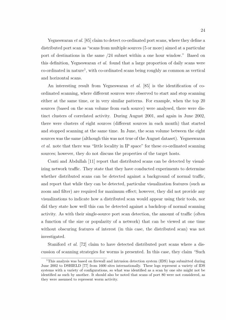
24

Yegneswaran et al. [85] claim to detect co-ordinated port scans, where they define a

distributed port scan as “scans from multiple sources (5 or more) aimed at a particular

port of destinations in the same /24 subnet within a one hour window.” Based on

this definition, Yegneswaran et al. found that a large proportion of daily scans were

co-ordinated in nature1, with co-ordinated scans being roughly as common as vertical

and horizontal scans.

An interesting result from Yegneswaran et al. [85] is the identification of co-

ordinated scanning, where different sources were observed to start and stop scanning

either at the same time, or in very similar patterns. For example, when the top 20

sources (based on the scan volume from each source) were analysed, there were dis-

tinct clusters of correlated activity. During August 2001, and again in June 2002,

there were clusters of eight sources (different sources in each month) that started

and stopped scanning at the same time. In June, the scan volume between the eight

sources was the same (although this was not true of the August dataset). Yegneswaran

et al. note that there was “little locality in IP space” for these co-ordinated scanning

sources; however, they do not discuss the properties of the target hosts.

Conti and Abdullah [11] report that distributed scans can be detected by visual-

izing network traffic. They state that they have conducted experiments to determine

whether distributed scans can be detected against a background of normal traffic,

and report that while they can be detected, particular visualization features (such as

zoom and filter) are required for maximum effect; however, they did not provide any

visualizations to indicate how a distributed scan would appear using their tools, nor

did they state how well this can be detected against a backdrop of normal scanning

activity. As with their single-source port scan detection, the amount of traffic (often

a function of the size or popularity of a network) that can be viewed at one time

without obscuring features of interest (in this case, the distributed scan) was not

investigated.

Staniford et al. [72] claim to have detected distributed port scans where a dis-

cussion of scanning strategies for worms is presented. In this case, they claim “Such

1This analysis was based on firewall and intrusion detection system (IDS) logs submitted duringJune 2002 to DSHIELD [77] from 1600 sites internationally. These logs represent a variety of IDSsystems with a variety of configurations, so what was identified as a scan by one site might not beidentified as such by another. It should also be noted that scans of port 80 were not considered, asthey were assumed to represent worm activity.

25

distributed scanning has already been seen in the wild—Lawrence Berkeley National

Laboratory received 10 during the past year.” These scans were identified by security

analysts due to both the sudden onset of activity from dozens of sources and the small

amount of overlap between the scans [56].

Distributed port scans have also been seen in the network data collected by

CAIDA [67, 45]. Moore described a distributed port scan using RST packets that

were sent to a dark /8 subnet, where each source only scanned a /27 (128 IP ad-

dresses) with no overlap between scans [45]. This scan was discovered accidentally

when analysing backscatter behaviour on the monitored network. Other distributed

scans have also been seen in the data [67]. In these cases, ping sweeps (ICMP scans)

were performed, with little to no overlap between sources, and where each source

began scanning at the same time.

Staniford et al. [71, 70] present a method for the detection of stealthy port scans,

where stealthy port scans are defined as port scans with properties that would elude

traditional IDS systems. Examples of properties that elude traditional IDS systems

are long delays between scans, and using numerous source IPs in a distributed port

scan.

The method employed by Staniford et al. can be divided into two distinct sec-

tions: the network anomaly detector (called Spade) and the correlation engine (called

Spice). The network anomaly detector estimates the current probability distribution

of normal traffic and, based on the entropy in this measurement, assigns an anomaly

score to an incoming packet. The more unlikely it is that a particular packet will occur

(e.g. based on source and destination port/IP combinations), the higher its anomaly

score. If a packet is considered to be sufficiently anomalous, then it is passed to the

correlation engine, Spice. Thus, Spade is not required for distributed port scan de-

tection, but could be replaced by any method that indicates whether a packet should

be further considered as being part of a larger, possibly malicious, event.

Any packet flagged as anomalous is passed to the correlation engine, Spice, where

it is inserted into a graph in which the nodes represent packets and the connections

between nodes contain weights indicating the strength of the relationship between

the two nodes (packets). The weights are based on a combination of the relationships

between features, such as their having the same value or similar values, or exhibiting a

26

well-known separation (e.g., five minutes). In the final graph, all edges with weights

less than a certain threshold are dropped, and the remaining subgraphs represent

network events, such as port scans, distributed port scans, denial-of-service attacks,

and server misconfigurations [69].

2.3 Evaluation Methodologies

Evaluation methodologies have not been a focus of intrusion detection systems. This

was noted by Athanasiades et al. [4], who stated the “ad-hoc methodology that is

prevalent in today’s testing and evaluation of network intrusion detection algorithms

and systems makes it difficult to compare different algorithms and approaches.” There

are two approaches to intrusion detection system evaluation that are in common use:

the Lincoln Labs data set and network traces [4]. The Lincoln Labs data set consists

of a combination of simulated background data and actual attacks, created by MIT’s

Lincoln Labs in 1998 and 1999 [36]. This data set is described in more detail in Section

2.3.2. Network traces consist of traffic gathered from actual networks, which is then

provided to intrusion detectors for evaluation. This approach is discussed in more

detail in Section 2.3.3. Before discussing either of these approaches, we first provide

some information in Section 2.3.1 on the different metrics used to evaluate intrusion

detection systems, regardless of the whether the Lincoln Labs data or network traces

are used.

For those port scan detection algorithms described in Section 2.2 where an eval-

uation of the algorithm was provided, all used either the Lincoln Labs data set or

network traces with one exception: Kim et al. [31] have only tested their approach

using a simulation of network traffic. While their results on simulated traffic indicated

that these approaches were promising, no validation was performed to determine how

closely the simulated data mimicked actual network traffic. In addition, they assume

that network traffic follows a Poisson distribution, while it is now widely believed

that network traffic is self-similar [57].

2.3.1 Metrics

Four measurements are commonly used in the intrusion detection community. The

first two are the detection rate and false positive rate (and, conversely, the true and

27

false negative rates) [5]. The detection rate is the conditional probability that an

alert A was generated given that there was intrusive behaviour I, P (A|I). The false

positive rate is the conditional probability of an alert A given that intrusive behaviour

is not present ¬I, P (A|¬I). Similarly, a true negative is the conditional probability

that no alert was generated and there was no intrusive behaviour, P (¬A|¬I) and a

false negative is the conditional probability that no alert was generated but there was

intrusive activity, P (¬A|I).

The use of these two metrics is affected by what is known as the base rate fal-

lacy [5]. In brief, the base rate fallacy for intrusion detection purposes is related to

the volume of normal traffic compared to the volume of attack traffic. Given that

attacks are fairly rare when compared to the volume of normal traffic, even when the

false positive rate is quite low (e.g., 1% or less), the result is that the analyst might

still be overwhelmed by the number of false positives. Generally, when values such

as detection rates and false positive rates are provided, the context of the number of

possible false positives that an analyst might need to investigate is often not provided.

Two other metrics — effectiveness and efficiency — were defined by Staniford et

al. [71]. Effectiveness was defined as the ratio of detected scans (true positives) to all

scans (true positives plus false negatives). Efficiency was defined as the ratio of the

number of identified scans (true positives) to all cases flagged as a scan (true positives

plus false positives), and is the same as the detection rate defined previously. These

two metrics have been used by Jung et al. [28] to compare the performance of Bro [55],

Snort [63], and threshold random walk (TRW) [28], the results of which are discussed

in Section 2.3.3.

Another technique often used to evaluate the performance of a particular detector

is a Relative Operating Characteristic (ROC) curve. This approach was used in the

Lincoln Labs evaluation of anomaly-based detection systems [36] and discussed in

detail by John McHugh [42]. A ROC curve has the false positive rate on its x-axis

and the true positive rate on its y-axis, thus moving from (0,0) at the origin to (1,1).

The detection system must return a likelihood score, or some value between 0 and

1, when it detects an intrusion in order for the ROC curve to provide meaningful

results [42]. This is because different thresholds can then be applied to the score

in order to determine how the false positive and true positive rates are affected by

28

threshold choice. The ideal curve is a vertical line to (0,1), followed by a horizontal line

to (1,1), representing the case where we have perfect detection with no false positives.

The ROC curve can be used to determine how well the overall system performs, the

most appropriate threshold values given acceptable true and false positive rates, and

to compare different detection systems.

2.3.2 Lincoln Labs

In 1998 MIT’s Lincoln Lab performed an evaluation of anomaly-based intrusion de-

tection systems [36]. To perform this evaluation, they generated both training and

testing data sets; both data sets contained attacks and background traffic.

A statistical analysis of network traffic from an Air Force base was performed.

Based on this analysis, automatons were created to represent different types of users

(such as secretaries, programmers and managers). These automatons performed dif-

ferent actions (such as sending email, editing files and browsing the web) that were

commonly performed by the users. Complete network traffic, including payload, was

generated for each of these activities. Email traffic consisted of a combination of

simulated email (generated based on statistical analysis) and actual email gathered

from public-domain list servers. Web traffic was gathered by a crawler that visited

various web sites.

A taxonomy of attack types was created to determine what types of attacks should

be performed. Four main types were identified: denial of service, remote-to-local,

user-to-root, and surveillance/probing. Attacks were identified for each of these types,

and were then generated by a human actor who performed the attacks.

Given that the background traffic was simulated and the attacks were all known,

the result was a set of labeled data. The training set, consisting of seven weeks of

labeled data, was provided to the developers of intrusion detection systems so that

they could train their systems. The testing set also consisted of simulated background

traffic and known attacks, including some attacks that were not present in the training

set. This data, without the labels, was provided to the developers as well, who

returned the results from processing this data with their detectors.

After the analysis was performed, the data was made available to the research

29

community so that others could train and test their detectors. A similar data set was

generated for 1999 and also made available to the research community.

This was the first large-scale evaluation of intrusion detection systems ever per-

formed, and the results in terms of performing such an evaluation are a valuable

addition to the research corpus; however, there are still flaws in the approach.

McHugh published a critique of the Lincoln Labs data set in 2000 [42]. One of the

flaws noted by McHugh was that no validation had been performed on background

data to determine how well it represented actual background traffic. One suggested

method for validation was to compare the false positive alarm behaviour for the

different systems being tested on both the simulated background traffic and actual

network traces. Related to the background data, it was noted that “Real data on

the internet is not well behaved.” This is represented in both legitimate traffic,

where anomalies might occur due to various types of misconfigurations, as well as

in malicious traffic such as Internet background radiation [52]. However, there was

no indication that Lincoln Labs included either non-malicious spurious traffic, nor

malicious background traffic such as background radiation. In addition, McHugh

questioned the actual data rates present in the background traffic, suggesting that

the amount of traffic might be much lower than is typically observed on the Internet.

In terms of the attack traffic, in addition to questioning whether the taxonomy used

was appropriate, there were questions concerning whether the number of attacks of

each type was representative of actual network attacks. It was noted, for example,

that probe/surveillance activity was by far the most common form of attack reported,

but that it represented less than 25% of the attacks performed. (In fact, the number

of probe/surveillance attacks was 64, spread across ten weeks of data.)

In 2003, Mahoney and Chan [38] presented a paper in which they had performed

a comparison of the simulated background data from the Lincoln Labs data set and

real traffic collected from a university department. One difference they found was the

regularity in TCP SYN packets. For example, in the simulated data, SYN packets

always had exactly four option bytes, whereas in the network traces, SYN packets had

anywhere from zero to 28 option bytes. The number of remote source addresses ob-

served in the simulated data was only 29, whereas the actual traffic exhibited 24,924

different source addresses. In particular, the statistics for source address distribution

30

in the network traces followed a power law distribution. Other differences were found

in the TCP window sizes, checksum errors, and TTL (time to live) and TOS (type

of service) values. In terms of payload analysis, Mahoney and Chan also found dif-

ferences in the characteristics of HTTP requests, SMTP requests and SSH requests.

They concluded that these differences would be important in the training and testing

of anomaly detection systems, as such systems might use characteristics of the sim-

ulated background traffic in determining whether something is an attack when that

characteristic cannot be used reliably given actual network traffic.

Despite these shortcomings, this data set is still in widespread use for testing

intrusion detection systems, especially those that use an anomaly-based detection

approach. In terms of the port scan detection algorithms presented in Section 2.2,

the neural network approaches developed by Basu et al. [6] and Streilein et al. [74]

were tested using the Lincoln Labs dataset. Based on these datasets, they found that

their system had a false positive rate of less than one per day and a true positive rate

fluctuating between 85% (probes) and 100% (stealthy attacks).

2.3.3 Network Traces

Network traces captured from live networks are often used for testing intrusion detec-

tion systems. The main advantage in using network traces is that the results will not

demonstrate any bias due to artifacts from simulated data that are not representative

of actual data.

Even when network traces are available, they are often limited. For example, the

traces might only contain packet header data, or be summarized even further into

flow-level information. Obtaining payload is often difficult because of privacy issues.

While a detector can be deployed in real time so that the payload does not need to be

captured, no validation can be performed based on the payload, nor can the results

be repeated with the deployed detector or compared to other detectors.

The greatest disadvantage in using network traces is that the data is not labeled.

This means that if an attack is detected, a manual analysis is usually required to

confirm whether the detector made an accurate detection or whether the alarm rep-

resented a false positive. Of even greater concern is the amount of data where no

alarms were generated is so voluminous that it is not possible to determine whether

31

attacks were missed. Given that the data is not labeled, at best it can be used

for evaluation; however, it is much more difficult to train anomaly-based detection

systems unless they use an unsupervised learning approach.

Finally, when detectors are tested in a given environment or on a particular set of

network traces, it is often not possible to determine how well the detector will perform

given a different environment or network traces captured from a different network. In

fact, Maxion and Tan [40] noted that, in the context of anomaly detectors, the same

detector cannot be used in different environments and achieve the same performance,

even when the anomaly detector is retrained for the new environment. Maxion and

Tan go on to state that “This is in absolute contrast to current practice.”

Given the port scan detectors presented in Section 2.2, four algorithms were tested

using network traces. Kato et al. [30] reported the results from running their algo-

rithm (which used an approach similar to GrIDS but focused on only those connection

requests that resulted in a RST-ACK packet) on live network traces. However, they

did not perform any verification as to whether the algorithm was indeed detecting

scans, nor did they examine how many scans this approach missed.

Robertson et al. [62] also tested their algorithms using network traces gathered

from a large enclave at a multinational client. They ran their scan detection algo-

rithms for both enclave surveillance detection (ESD) and peering center surveillance

detection (PSD) against these network traces. To determine how well their algorithm

performed, they used a manual analysis of the results, analysing only those scans

that were detected to determine whether the activity actually contained scanning

activity; therefore no insight is available as to the false negative rate. The man-

ual review used 1000 alerts and concluded that ESD achieved a false positive rate

of 0.6%. When asymmetric traffic was used (PSD), there was a significant increase

in the false positive rate, going from 0.6% to 14.6%, based on a manual analysis of

652 alerts. This increase was experienced even though the available traffic was not

entirely unidirectional (30% of the traffic analysed did not have both sides of the

communication available, implying that bi-directional information was available for

70% of the traffic).

Gates et al. [20] also used network traces gathered from a live network; more

specifically, they used NetFlow traffic gathered from an ISP. They converted the

32

NetFlow traffic into “events”, which were all the traffic from a single source and

bounded by periods of inactivity from that source. Their approach required three sets

of data: elicitation, training and testing. The elicitation set consisted of 100 events,

the training set 200, and the testing set 300. Each event was manually analysed

to determine whether it contained a scan; this process was performed for each of

TCP, UDP and ICMP scans. For TCP scans, the algorithm was demonstrated to

have a detection rate of 95.5% and a false positive rate of 0.4%, based on the results

from using a test set; however, it has not been shown that the approach performs

consistently across other networks.

Jung et al. [28] perform “trace-driven simulation” where network traces are used to

determine how well their algorithm will perform. They use network traces gathered

from two different sites, both of which run the Bro Network Intrusion Detection

System [55]. Thus, ground truth is considered to be those scans, worms and other bad

behaviour that are detected by Bro. Scan alerts are considered to be false positives

if any subsequent activity from the same source makes a “useful” connection, where

the connection is properly established and data is transferred. For those sources that

are not flagged by Bro as being malicious, the connection attempts are considered to

be scans if they demonstrate the same properties as other malicious sources, namely

that a large number of connection attempts were made to IP addresses that do not

contain responding hosts.

Jung et al. [28] analysed the results from Bro [55], Snort [63] and threshold random

walk (TRW) [28] using two sets of network traces. One network trace consisted of

15,614,500 inbound connections from 190,928 unique remote sources, while the second

consisted of 161,122 inbound connections from 29,528 unique remote sources. They

found that Snort’s efficiency was only 0.615 and its effectiveness was only 0.126 on

one dataset. On the second dataset they found Snort’s efficiency to have increased to

1.0, while its effectiveness dropped to 0.029. By comparison, Bro had an efficiency of

1.0; however, its effectiveness was 0.15 on one network trace and 0.029 on the other.

The threshold random walk (TRW) method, however, had both a high effectiveness

and a high efficiency, while requiring very few packets to make a determination. The

efficiency for this approach was 96.3% with an effectiveness of 96.0% on one data

set, and 100% and 99.2% respectively on a second data set. In addition, it made

33

a determination of whether a source was performing a scan or was benign after an

average of 5.2 destinations were contacted.

The visual methods, such as PortVis [43][47] and the approach of Conti and Ab-

dullah [11], also used network traces; however, the traces were used in the context of

determining whether particular scanning activity could be identified by visual pat-

terns. No evaluations were performed to determine how well the approaches worked,

such as by performing user studies to determine how quickly or accurately a person

could recognize a scan buried amongst normal network traffic.

2.4 Summary

In this chapter we presented a survey of the terms and terminology typically used to

describe port scanning activity, highlighting the classification of scans by the footprint

geometries into one of four types: vertical, horizontal, strobe and block. It was noted

that while some terms tend to be used frequently (such as terms like “horizontal

scans”), they are not used consistently; people might use different terms to represent

the same activity or, conversely, use the same term to represent slightly different

activity.

Several algorithms for detecting port scans were identified in the literature, and

these were classified into three general approaches: threshold-based, algorithmic and

visual. A summary of which algorithms are grouped into which approaches is pro-

vided in Table 2.1. It was noted when some of the algorithms were described as part

of a larger intrusion detection system, and when the algorithms for port scan detec-

tion were the focus of the research. The detection of co-ordinated port scans was

also discussed, where only algorithmic and visual approaches exist. Four detection

algorithms were presented. Two of the algorithms were presented in passing when

discussing scanning activity in general. One of the algorithms consisted of a visualiza-

tion approach. The final algorithm consisted of a machine learning approach to the

detection of stealthy scans, where co-ordinated scans were considered to be a form of

stealthy scan.

We note that some of the background work will be presented (or repeated) in

other chapters. This has been done to ensure coherence for the reader so that each

section can be read and understood in isolation.

34

The chapter concluded with a discussion on the most-common approaches to the

evaluation of intrusion detection systems. The metrics most-often used were de-

scribed, followed by a description of each of the two most-common approaches: the

use of the Lincoln Labs data set and the use of network traces. Both of these ap-

proaches have advantages and disadvantages. Where evaluations were available for

the port scan detectors described in the previous section, the approaches to that

evaluation were highlighted with the results of the evaluation.

Chapter 3

Model

The approach we take to the problem of detecting co-ordinated port scans is based

on adversary modeling. While adversary motives and targets will vary across orga-

nizations, we can build a more generic model in the case of port scanning because it

can be based on the information that the adversary is trying to gain. We describe

such a model where we have abstracted the details of the target information for the

adversary, forming a more generic set of information. This model forms the basis

of an algorithm that detects co-ordinated scans, where we can specify exactly which

adversaries this algorithm can detect. (We use the term “co-ordinated port scans”

because this term more closely resembles the type of scans in which we are interested.

Much of the literature uses the term “distributed port scan”, and we use that term

when we refer to the approaches of others where they have themselves used this term.)

Previous approaches to detecting co-ordinated (or distributed) port scans have

focused on one of three strategies:

1. defining a distributed port scan as having very specific characteristics so that

scans can easily be clustered (e.g., see Yegneswaran et al. [85] and Robertson

et al. [62]),

2. clustering packets or alerts based on feature similarity using a machine learning

approach (e.g., simulated annealing [71] [70], neural networks [74]), and

3. visualizing network traffic to determine whether there are any patterns repre-

sentative of distributed scans (e.g., see Conti and Abdullah [11]).

In the first instance, it becomes easy for an adversary to “game” the system if he

knows how the defender has defined a distributed scan. The second case assumes

that distributed scans will cluster together based on similarities between scans or

packets; this assumption has not been verified. In fact, Staniford [69] identified the

approach used in [70] clustered events, which included distributed scans but also

35

36

denial-of-service attacks, single-source port scans and server misconfigurations. The

third case requires a human analyst to view network traffic, rather than using an

automated alerting mechanism.

Unlike these, our approach is based on detecting patterns in the information that

adversaries are gathering. We expect that these patterns will indicate those areas

where multiple adversaries (or scan sources) are co-operating. This follows from

comments made by Braynov and Jadliwala [7], who stated that “in order to detect

such cooperation, one needs a clear understanding of agents’ incentives, benefits, and

criteria of efficiency.”

Given that we are attempting to detect co-ordinated scans, this chapter begins

by providing a set of definitions for scans and co-ordinated scans. Based on these

definitions, we identify the characteristics of scans. We then discuss two approaches

to developing a model of co-ordinated scans, settling on an adversary based approach.

We develop an adversary model, which maps the characteristics of scans to particular

adversary types, identifying each adversary by their scan “footprint” pattern. This

culminates in an algorithm inspired by a modified Greedy approach to the set covering

problem developed by Grossman and Wool [22], that can aggregate scan information

to form particular footprint patterns, using these patterns to recognize particular

adversaries.

3.1 Scan Definitions

The activity of a port scan can be viewed from two different perspectives: that of

the adversary performing the attack (attacker) and that of the network administrator

defending the network (defender). While we are most interested in the perspective

of the defender, we sometimes need to examine the perspective of the attacker as

this is related to the information that can be viewed by the defender. The defender

can only monitor his own network, so information about the entire attack is not

necessarily available to him. In the definitions presented below, an omniscient view

of the network is taken, and where this perspective makes a difference is specified.

To define scanning activity, a target must first be defined, as scanning activity

is always directed at some target. A target is a particular port on a particular IP

address. A set of targets is represented by T , where T consists of a set of IP addresses

37

p

MonitoredNetwork

a (S)δ

S3

2

1

C

C

C

τ

ρ

s0

2 s

1 s

P

A

T

Figure 3.1: An illustration of port scanning

A and ports P 1. The entire set of target IP addresses A are not necessarily aimed

entirely at the defender’s network, so the defender will only see traffic directed at his

monitored space. These concepts are illustrated in Figure 3.1.

Definition 3.1 A target τ consists of a port p on IP address a. A set of targets

T is a set of network space elements of interest, T ⊆ A × P where A is a set of IP

addresses and P is a set of ports.

In contrast, a source is a computer system from which some activity (e.g., a scan,

an attack) originates. It should be noted that this definition specifies the physical

origin of an activity and not the IP number; therefore, if the source changes its

IP address in the middle of the activity, it is still a single source. However, as

IP addresses are commonly used to represent a source, and as it is often difficult

to determine whether two different IP addresses represent the same source, in this

dissertation we will use IP addresses to indicate the source, recognizing that we may

do so erroneously in some cases.

Given a definition of a source and target, we can now define a probe. A probe is a

reconnaissance technique aimed at a single target. It consists of one or more packets

1We assume the TCP protocol throughout our discussions; however, the concepts presented inthis model are equally applicable to other network protocols.

38

from a single source with the packets crafted so as to elicit a response of a particular

target under certain conditions. Types of reconnaissance include such activities as

crafting TCP packets with particular flag combinations [12][18].

Definition 3.2 A probe, ρ = (s, τ,∆t), consists of one or more packets from a

single source address s to a single target τ during time interval ∆t, where the purpose

of the communication is reconnaissance.

Definition 3.3 A scan, denoted C = (s, T,∆t), is a set of connection attempts from

source address s during time interval ∆t where T is the set of targets (address, port)

and whose purpose is reconnaissance. We further define a scan of order c to be a

scan where c is the number of targets.

The degenerative case of Definition 3.3 is a scan of order 1, which is a probe. A

scan may also consist of multiple probes, where a probe is against a single target.

This is consistent with the term “probe” as used by Staniford et al. [70]. While they

do not define a probe, they make statements such as “Turning now to the individual

scan probes, ....” which implies that a scan consists of multiple probes.

A scan uses the generic form of a target, T ⊆ A× P . This can be related to the

notation provided by Leckie and Kotagiri [34], where they represent traffic as a tuple

< si, dj, pk > where si is the source i, dj is the destination IP address j, and pk is

the destination port k. This is represented in our scan notation as (si, {(dj, pk)},∆t)

where {(dj, pk)} contains the single tuple (dj, pk). The requirement of the time stamp

was added to the tuple, which is not present in Leckie and Kotagiri’s definition, to

ensure that it is possible to distinguish between different probes over time.

The targets of a scan form the scan’s “footprint”. A footprint pattern was de-

fined by Staniford et al. [70] as “the set of port/IP combinations which the attacker

is interested in characterizing.” The footprint pattern that the scan leaves on the

defender network is the main observable for a port scan and is related to the infor-

mation the adversary wishes to obtain. We define a footprint from the perspective of

some monitored network, µ. Therefore, while the target, T , of a scan might have been

several administratively unrelated networks, the observed footprint is that subset of

the target that intersects with the monitored space, F = T ∩ µ. We formally define

a footprint as:

39

Definition 3.4 A footprint of a scan (h, T,∆t) relative to a monitored network µ

is the set of scan targets that appear in the monitored network, that is F = T ∩µ and

|F | > 0.

Given that scans are initiated by some adversary, they can, therefore, be cate-

gorized by intent. Given an omniscient viewpoint, whether the source of a scan is

a human intelligence intent on learning particular information or whether it is an

automated process, such as a worm, that is searching for more machines to infect,

can be determined. We call the first case a directed scan, while the second is a non-

directed scan, where in the first case the information gathering activity is directed at

a particular target. From the viewpoint of a monitored network space, it is some-

times difficult to distinguish the two types of scans, particularly depending on the

scan patterns adopted by each; rather, the type of scan must be inferred from the

patterns observed.

Definition 3.5 A directed scan is a scan that is performed with the intent to gather

information about a particular target.

As a directed scan is focused, one of its characteristics is that of coverage. We

define coverage as the ratio of contiguous space that is targeted to the size of the

monitored space, where the definition of a target is based on the type of scan. For

example, a scan against a network might target a particular port on each IP address

in the network, so the coverage is the number of IP addresses on the network that

were probed. Coverage in the case of a scan against a single IP address would be

the contiguous space of ports on that IP address that were probed. The larger the

coverage of a particular target, the greater the focus on that target, where a target

here is considered to be some subset of the entire space. For example, an adversary

might have particular interest in a given /24 subnet that is part of a larger /16

network. Thus his coverage of the /24 subnet would be large, while his coverage of

the entire /16 network would be correspondingly small, indicating that he is focused

on that particular target.

The coverage of a scan also implies something about the intent behind the scan.

It is generally assumed that the more focused the scan, the more interested a scanner

is in that particular target network or IP address. If a scanner’s intent is that of

40

gaining specific information, the coverage of a target network tends to be contiguous

and complete. (This is not necessarily true of a single target IP address, where a

scanner might focus more on a specific set of service ports.) This does not imply

anything about the order in which the IP addresses on the network are scanned, but

rather the pattern that remains once the scan has been completed. Scans performed

by humans (as opposed to automated service discovery) tend to fall into this category.

Scans can be even more focused (e.g., targeting solely those IP addresses known

to be assigned to client desktops). For example, an early (directed) scan (e.g., a ping

sweep) might have identified all of the computers on a network. Some time later,

a scanner might follow up with a directed scan of just those IP addresses known to

contain computers that responded to the earlier ping sweep. In this case, the coverage

characteristic must be more narrowly defined. Rather than looking at the coverage in

relation to the entire subnet, we might instead look at the coverage in relation to the

number of assigned IP addresses on a given subnet. Other types of foci are possible

as well, such as examining the coverage of a scan across the web servers in a network,

or across the FTP servers.

A non-directed scan refers to all those scans that are not directed, an example

of which is the type performed by some worms, such as a random constant spread

scan (see Staniford et al. [72]). In this case, the intent is to attack or infect other

computers without targeting a specific network. As a result, the scanning patterns

often appear to be spread randomly across some IP address space (such as the entire

Internet).

3.1.1 Effects of Address Aliasing

The use of IP addresses figure prominently in the scanning definitions, both for rep-

resenting sources and targets. It is important to note that IP addresses do not

necessarily represent a direct mapping to a particular computer. For example, the

actual IP address observed at a border router or in the core of the network could be

the result of an aliasing mechanism such as Network Address Translation (NAT). In

this case, the actual scanning source, for example, is on a private network. When

establishing a connection outside of the private network, an intermediate networking

device will “translate” the private IP address into a routable address and will thus

41

act as an intermediary, forwarding any responses to the routable address back to the

originating source on the private network. In this case, the source address of a scan

will reflect the originating network, but not the originating source, potentially leading

to issues of attribution.

A single scanning source can also erroneously appear as multiple sources perform-

ing a co-ordinated scan. Two potential causes of this are DHCP and multihoming.

DHCP is a method for dynamically assigning an IP address to a particular computer,

removing the need to perform this task manually. As a result, if a single source starts

a scan, disconnects from the network, reconnects, and then continues the scan, there

is a possibility that it will be assigned a different IP address upon reconnecting to

the network. The result from the defender’s perspective is that the scan will appear

as a co-ordinated scan from two different sources. That a co-ordinated scan is caused

by a DHCP issue such as this might be recognized by the defender because the scans

would not overlap in time. Similarly, a single source can be multihomed, meaning

that there are multiple IP addresses assigned to the same physical computer. If the

different IP addresses are used during the scan, then from the defender’s perspective

it will again appear as a co-ordinated scan from multiple sources.

3.2 Scan Characteristics

Given that we are classifying adversaries based on the information they are trying to

gather, we use the following four dimensions as part of this classification: (i) number

of ports targeted, (ii) number of IP addresses targeted, (iii) the selection algorithm

for how the target IP addresses were selected, and (iv) whether camouflage is used to

hide the adversary’s intended target. The number of ports can be divided into a single

port or multiple ports. The number of IP addresses can be classified as one, some

and all (from a defender’s perspective, where “all” means that all the IP addresses in

the defender’s network have been targeted). When some IP addresses are targeted,

the number of IP addresses can further be subdivided into one or more subnets,

randomly-chosen IP addresses and “some” IP addresses (where “some” can represent

a selection algorithm such as only IP addresses known to be assigned to responding

servers or only web servers, for example). Finally, the adversary can attempt to

camouflage his intended target by scanning other IP addresses that do not contribute

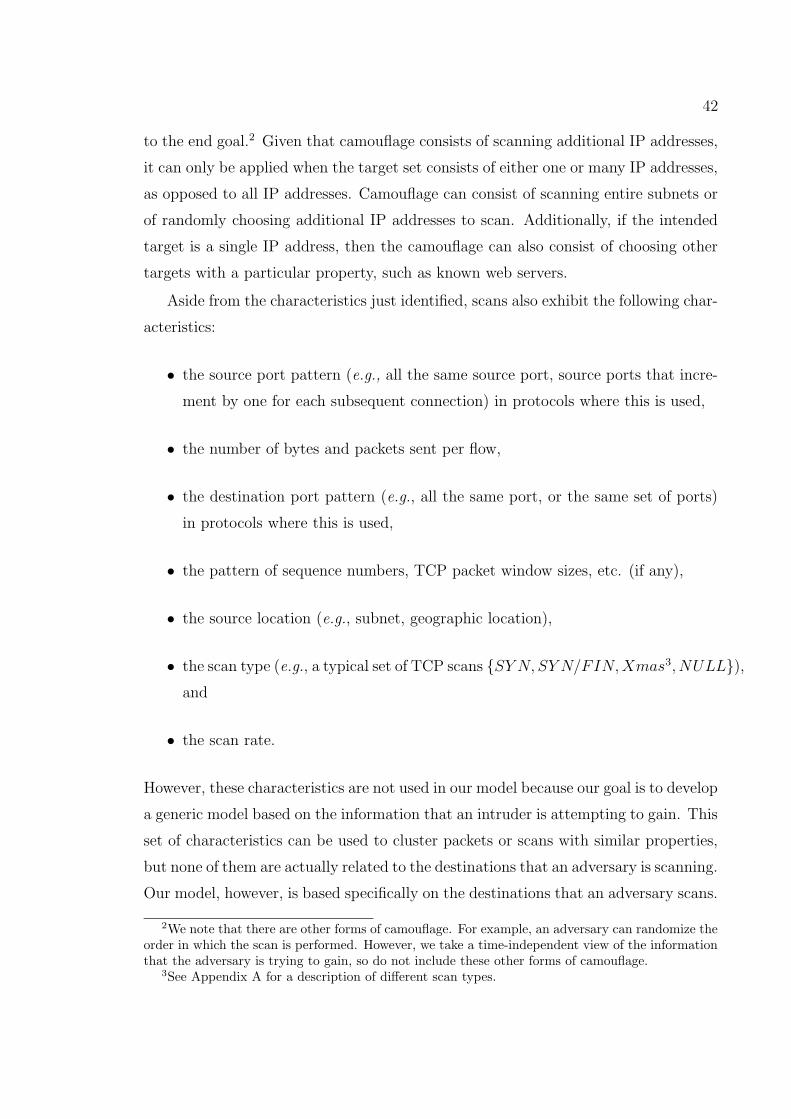
42

to the end goal.2 Given that camouflage consists of scanning additional IP addresses,

it can only be applied when the target set consists of either one or many IP addresses,

as opposed to all IP addresses. Camouflage can consist of scanning entire subnets or

of randomly choosing additional IP addresses to scan. Additionally, if the intended

target is a single IP address, then the camouflage can also consist of choosing other

targets with a particular property, such as known web servers.

Aside from the characteristics just identified, scans also exhibit the following char-

acteristics:

• the source port pattern (e.g., all the same source port, source ports that incre-

ment by one for each subsequent connection) in protocols where this is used,

• the number of bytes and packets sent per flow,

• the destination port pattern (e.g., all the same port, or the same set of ports)

in protocols where this is used,

• the pattern of sequence numbers, TCP packet window sizes, etc. (if any),

• the source location (e.g., subnet, geographic location),

• the scan type (e.g., a typical set of TCP scans {SY N, SY N/FIN,Xmas3, NULL}),

and

• the scan rate.

However, these characteristics are not used in our model because our goal is to develop

a generic model based on the information that an intruder is attempting to gain. This

set of characteristics can be used to cluster packets or scans with similar properties,

but none of them are actually related to the destinations that an adversary is scanning.

Our model, however, is based specifically on the destinations that an adversary scans.

2We note that there are other forms of camouflage. For example, an adversary can randomize theorder in which the scan is performed. However, we take a time-independent view of the informationthat the adversary is trying to gain, so do not include these other forms of camouflage.

3See Appendix A for a description of different scan types.

43

3.2.1 IP/Port Pairs

By definition, a scan must have a set of targets T . We, therefore, use in part the set

of targets to define a scan. This is consistent with a footprint pattern as defined by

Staniford et al. [70]: “the set of port/IP combinations which the attacker is interested

in characterizing.” The footprint pattern that the scan leaves on the defender network

is the main observable for a port scan and is related to the information the adversary

wishes to obtain.

As provided in Definition 3.1, a target consists of a single port on a single IP

address, and a set of targets consists of a set of ports P on a set of IP addresses A.

We classify scans based on these sets. In particular, two of the characteristics we use

for characterizing scans are the number of ports of interest, |P |, and the number of

IP addresses of interest, |A|. The number of ports can be summarized as being either

one or multiple, while the number of IP addresses can be summarized as being one,

some or all.

3.2.2 Selection Algorithm and Camouflage

In addition to categorizing a scan based on the number of target IP addresses, we can

also use any relationships between the addresses. These relationships can be classified

into the following categories:

• randomly selected IP addresses Ψ, where Ψ ⊆ A,

• only IP addresses with a particular property Φ (e.g., only IP addresses known

to be assigned to client desktops, only known web servers, only IP addresses

with 0 for the last octet), where Φ ⊆ A, or

• one or more subnets Σ within the target organization, where Σ ⊆ A.

In this classification, subnets are considered separately from “IP addresses with a

particular property” due to the ease with which the property can be recognized.

Subnet scanning involves a scan against a large number of contiguous IP addresses,

which is more obvious than, for example, scanning only web servers, which might be

a number of seemingly unrelated IP addresses.

44

Different types of scans are available to an adversary (described in Appendix A),

and a number of variables, such as the time delay between individual probes and

the values of different TCP fields, can be controlled to avoid detection; however, we

focus here on camouflage aimed at obscuring the true target of a scan. For example,

an adversary can add IP addresses to his target set so that the true target is less

obvious. If additional IP addresses are added, they can be added in one of the

following fashions:

• randomly chosen IP addresses, Ψ,

• additional IP addresses that meet some property (e.g., IP addresses known to

be assigned to client desktops, known web servers), Φ, or

• additional subnets, Σ.

3.2.3 Coverage and Hit Rate

Another port scan characteristic is coverage, which is the percentage of contiguous

space in the defender network that is targeted by a port scan. More specifically,

coverage is defined from the viewpoint of a defender of some monitored network

space and refers to the percentage of the monitored network covered by the range of

IP addresses that are both in the monitored network space and targets in the scan,

ζ(C)% =an − a1 + 1

|A|(3.1)

where A is the set of IP addresses in the defender network, a1 is the first IP address

in the range of addresses scanned on the monitored network, and an is the last IP

address in that range.

Another characteristic is hit rate. Given the first and last IP addresses in a scan,

the hit rate is the percentage of IP addresses within this range that were targeted by

the scan. This is represented as:

H(C)% =|AC |

an − a1 + 1(3.2)

where a1 is the first IP address in the scanned range on the monitored network space,

an is the last IP address in the scanned range on the monitored network space, and

AC is the set of target IP addresses on the monitored network for scan C.

45

For example, assume that we have the network 10.2.0.0/24, and that a source

sends probes to 64 of the IP addresses ranging from 10.2.0.5 through 10.2.0.104. In

this example, the coverage is 100

256= 39% while the hit rate is 64

100= 64%.

3.3 Co-ordinated Scan Characteristics

A co-ordinated scan is a directed scan where portions of the scan have been distributed

amongst multiple sources, but which are ultimately controlled by a single instigator

who co-ordinates which sources will scan which targets. Co-ordinated scans consist

of multiple sources, each of which are scanning a portion of the desired target space.

Thus, a co-ordinated scan can be thought of as consisting of multiple single-source

scans or probes. By distributing a scan amongst multiple sources, these types of

scans provide the advantage of speed, as various portions of the target network can

be scanned in parallel and discreteness, as the scan will appear to the target as

multiple small scans rather than one large scan. Co-ordinated scans also provide the

ability to examine a target network from different viewpoints, which might help to

reveal firewall and access rules [21]. Thus, an adversary can use a co-ordinated scan

to obscure his scan.

Definition 3.6 A co-ordinated scan, δ(S), is a collection of scans from a set of

sources S, δ(S) = {C1, ..., Ck}, consisting of k scans C1 through Ck. The scan is

represented by the tuple (S, T,∆t), where S is the union of the sources from each of

the scans C1 through Ck, T is the union of targets from each of the scans C1 through

Ck, and ∆t is the minimum time interval [tm, tn] that still contains all scans. The

co-ordinated scans have a single instigator, k > 1, |S| ≥ 2 and |T | ≥ 2.

In this dissertation, we distinguish between “co-ordinated” scans and “dispersed”

scans. A co-ordinated scan is directed, as defined in Definition 3.5, and implies co-

ordination between the single-source scans. In contrast, a dispersed scan is a scan

performed by multiple sources, but is non-directed. The term “dispersed” is used to

indicate sources that are scattered haphazardly with no co-ordination between them,

whereas “co-ordinated” implies a more purposeful act. An example of an activity that

might appear as a dispersed scan is that of a random-spread scanning worm. A second

example is Stumbler, which has been characterized by Intrusec [26] as being a passive,

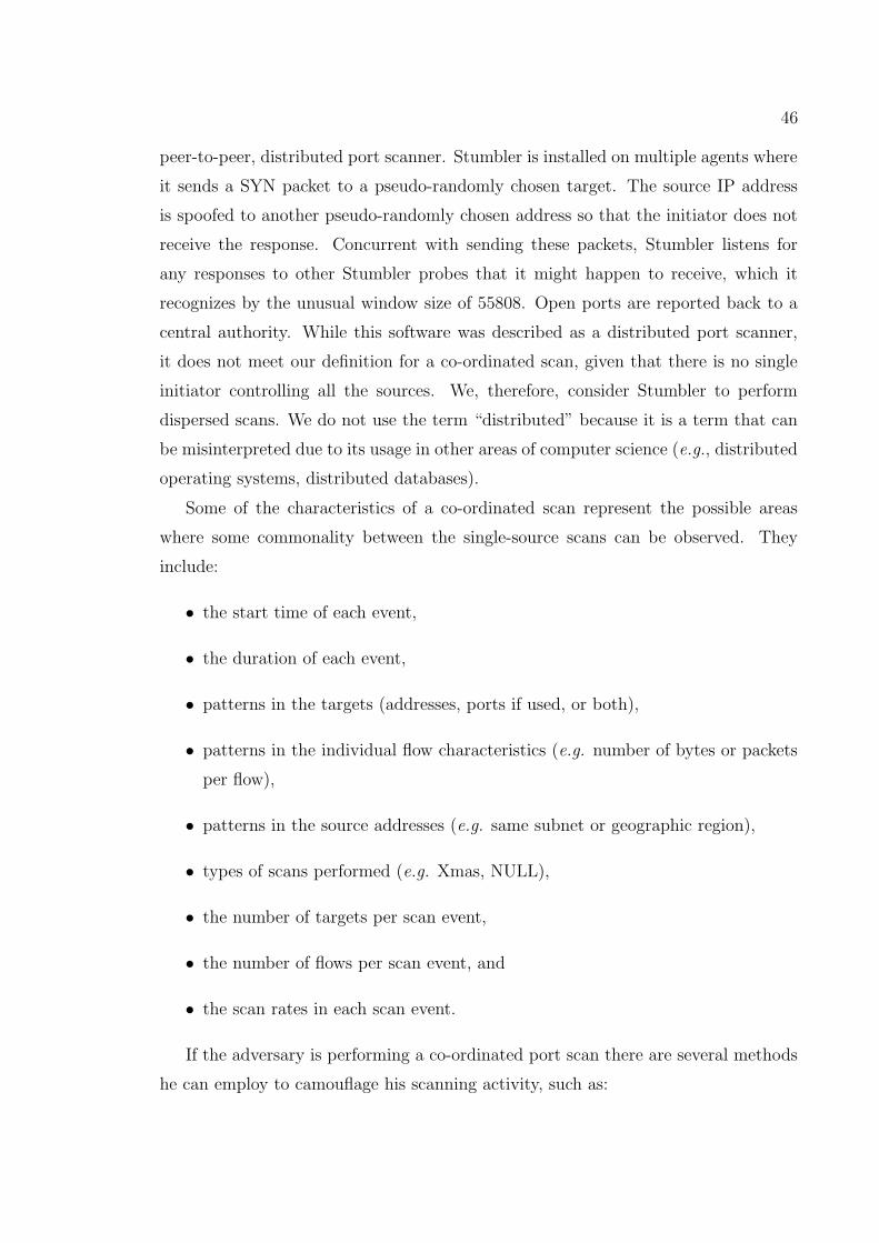
46

peer-to-peer, distributed port scanner. Stumbler is installed on multiple agents where

it sends a SYN packet to a pseudo-randomly chosen target. The source IP address

is spoofed to another pseudo-randomly chosen address so that the initiator does not

receive the response. Concurrent with sending these packets, Stumbler listens for

any responses to other Stumbler probes that it might happen to receive, which it

recognizes by the unusual window size of 55808. Open ports are reported back to a

central authority. While this software was described as a distributed port scanner,

it does not meet our definition for a co-ordinated scan, given that there is no single

initiator controlling all the sources. We, therefore, consider Stumbler to perform

dispersed scans. We do not use the term “distributed” because it is a term that can

be misinterpreted due to its usage in other areas of computer science (e.g., distributed

operating systems, distributed databases).

Some of the characteristics of a co-ordinated scan represent the possible areas

where some commonality between the single-source scans can be observed. They

include:

• the start time of each event,

• the duration of each event,

• patterns in the targets (addresses, ports if used, or both),

• patterns in the individual flow characteristics (e.g. number of bytes or packets

per flow),

• patterns in the source addresses (e.g. same subnet or geographic region),

• types of scans performed (e.g. Xmas, NULL),

• the number of targets per scan event,

• the number of flows per scan event, and

• the scan rates in each scan event.

If the adversary is performing a co-ordinated port scan there are several methods

he can employ to camouflage his scanning activity, such as:

47

1. The adversary can overlap the targets between each of the scan sources (as

defined in Subsection 3.3.1).

2. The adversary can vary the start times of each scan so that they do not all start

at the same time, nor do they each start at regular intervals, nor do they scan

sequentially so that scan b starts once scan a finishes. The adversary can also

vary the rate at which each source scans.

3. The adversary can vary the types of scans used by each client (see Appendix A

for some of the scan types that could be used).

4. The adversary can vary the sources so that there is no obvious relation between

the different sources (e.g., not in the same network, not in the same geographic

location).

5. The adversary can distribute the targets amongst the sources in various ways,

including randomly at one extreme, or in contiguous blocks at the other. In

addition, the adversary can distribute random numbers of targets to each source.

The second, third and fourth methods in the list for hiding scanning activity do not

affect the footprint pattern that the scan generates. Thus, they are not used in the

model, as the model is based specifically on the destinations that an adversary scans.

3.3.1 Overlap

The first of the five methods listed above suggests that an adversary might use overlap

to hide his scanning activity. Overlap is defined as the number of targets in common

between two sources. Given scans C0 = (s0, T0,∆t0) and C1 = (s1, T1,∆t1), as given

in Definition 3.3, and taken from the perspective of the monitored network, the target

addresses are the sets A0 and A1 respectively. Assume that the ports are the same

for both T0 and T1. The overlap in addresses can be defined as:

θ(C0, C1)% =|A0 ∩ A1|

|A0 ∪ A1|(3.3)

for the set of destination IP addresses Ai for each single-source scan Ci in the co-

ordinated scan δ(S). This characteristic is added to the footprint patterns for a

co-ordinated scan.

48

3.3.2 Scanning Algorithm

The last of the five methods listed above for hiding scanning activity is based on the

distribution algorithm used, A. There are several distribution patterns available to

the adversary, including

• interleaved series of length x,

• randomly distributed, and

• sequential blocks.

Given that the scanning algorithm used by the adversary, while not affecting the

overall co-ordinated scan footprint, does affect the footprint patterns of each of the

single-source scans, it is included in the tuple that represents the footprint pattern for

a co-ordinated scan. For example, if the scanning algorithm distributes the targets

randomly between the sources, then the footprint of any one source will be different

than if the scanning algorithm distributes the targets using an interleaved series.

3.4 Footprint Representation

We defined a scan footprint in Definition 3.4 as being a set of scan targets (port/IP

pairs) on some monitored network. We went on to define six characteristics of scans:

the number of IP addresses, the number of ports, the coverage of the network, the hit

rate within the scanned space, the target selection algorithm and camouflage. We use

these six characteristics of a scan to develop a representation of the footprint pattern:

F =< |A|, |P |, ζ(C),H(C), ς, κ > (3.4)

where |A| is the number of IP addresses scanned, |P | is the number of ports scanned,

ζ(C) is the coverage of the network, H(C) is the hit rate of the scanned space (see

Subsection 3.2.3), ς is the selection algorithm and κ is the camouflage approach. The

values for ς are selected from the set {Ψ,Σ,Φ}, and the values for κ are selected from

the set {∅,Ψ,Σ,Φ}, where ∅ is the empty set, Ψ is randomly chosen, Σ is a subnet,

and Φ refers to IP addresses chosen based on some criteria.

The tuple that represents footprints can also be used to represent the different

footprint geometries defined by Staniford et al. [71]: vertical, horizontal, strobe and

49

block. A vertical scan consists of a port scan of some or all ports on a single IP

address. Port scans across multiple IP addresses break down into three basic types,

based on the number of ports in the scan. A horizontal scan is a port scan of a single

port across multiple IP addresses. If the port scan is of multiple ports across multiple

IP addresses, then it is called a strobe scan. A block scan is a port scan against

all ports on multiple IP addresses. Yegneswaran et al. [85] quantified vertical and

horizontal scans, defining six or more ports on a single IP address as a vertical scan,

and five or more IP addresses within a subnet (of undefined size) as a horizontal scan.

A generic footprint pattern is represented by F =< x, y, x|A|

, ∗, ∗, ∅ >, where a

∗ represents an unknown value, x ≥ 1 is the number of IP addresses, y ≥ 1 is the

number of ports, and |A| is the number of IP addresses in the monitored network.

This represents a strobe scan when both x > 1 and y > 1. When y = 1, the footprint

pattern represents a horizontal scan, while a value of x = 1 represents a vertical

scan. When both x = 1 and y = 1, the footprint pattern actually represents a probe.

Changing the value for the camouflage type κ to something other than ∅ when x = 1

and y = 1 will also result in a horizontal scan, and in a strobe scan when y > 1. We

use m and n to represent user-defined thresholds for the number of IP addresses and

ports respectively, and |A| as the number of IP addresses in the monitored network.

For example, we can represent the definitions used by Yegneswaran et al. [85] by

setting m = 5 and n = 6 in the following formal definitions for each of the scan types:

Definition 3.7 A horizontal scan targets a single port across multiple IP addresses.

It is represented by the tuple < x, 1, ζ(C), ∗, ς, κ > where x ≥ m and ζ(c) ≥ n|A|.

Definition 3.8 A vertical scan targets multiple ports on a single IP address. It is

represented by the tuple < 1, y, ζ(C), 1.0, ς, κ > where y ≥ n, ζ(C) = 1

|A|.

Definition 3.9 A strobe scan targets multiple ports across multiple IP addresses.

It is represented by the tuple < x, y, ζ(C), ∗, ς, κ > where x ≥ m, y ≥ 2, ζ(C) ≥ 2

|A|.

Definition 3.10 A probe targets a single port on a single IP address. It is repre-

sented by the tuple < 1, 1, ζ(C), 1.0, ς, κ > where ζ(C) = 1

|A|.

We can further define the boundary cases that were not represented by the four

definitions above. In particular, < |A|, |P |, ζ(C), ∗, ς, κ >, where |A| < m, |P | < n

50

and ζ(C) < n|A|

is not represented. We consider this case to consist of multiple probes.

Similarly, < |A|, |P |, ζ(C), ∗, ς, κ >, where |A| < m, |P | ≥ n and ζ(C) < n|A|

is not

represented. We consider this case to be multiple vertical scans.

The tuple representing the footprint of the adversary goals can represent co-

ordinated port scans as well as single-source port scans. This is because the entire

co-ordinated scan has its own footprint pattern which consists of a union of the foot-

print patterns from each of the single-source ports scans of which it is comprised;

however, due to having multiple sources, there are also additional characteristics

found in a co-ordinated scan that are not represented by the tuple for single-source

scans.

The tuple that represents the characteristics of a co-ordinated scan is, therefore,

< F , |S|, θ,A > where F taken from Equation 3.4, is the overall footprint pattern of

the co-ordinated scan, |S| is the number of sources used in the co-ordinated scan, θ is

the amount of overlap between the sources, and A is the algorithm used to distribute

targets amongst the sources.

The footprint pattern defined in Equation 3.4 represents the footprint pattern

covered by the entire scan and is, therefore, time independent. The footprint pattern

was defined in this manner to remove any complexities associated with the partial

detection of scans. In practice, however, a defender might be monitoring network

activity during a particular time period and capture only the portion of the scan that

occurred during the monitored time. The footprint pattern that the defender sees

will, therefore, only be a portion of the actual footprint pattern.

3.4.1 Limitations and Future Directions

The generic footprint representation provided in Equation 3.4 can represent any form

of scan. However, the three variables hit rate, coverage and camouflage are defined

based on the IP address space. By ignoring the space of all possible ports, the resulting

tuple provides information focused on horizontal scans, rather than vertical or strobe

scans.

The coverage for a scan was defined in Section 3.2.3 as representing the percentage

of the network that a scan covers in terms of contiguous IP addresses. For a vertical

scan, the coverage is only one over the number of IP addresses in the monitored

51

space. It can be argued, however, that for vertical scans the important characteristic

is not the IP space coverage, but rather the coverage of ports on the IP address being

scanned. One approach to removing this limitation is to modify coverage to represent

the values in the 2-dimensional space representing (IP, port) pairs. Coverage might

then be measured along either a single coordinate axis or across the whole space

depending on the type of scan.

Similarly, hit rate, as defined in Section 3.2.3, is based on an examination of IP

addresses and is defined as the percentage of IP addresses within the covered range

that were targeted. It does not take into account any port information. Therefore, if

an adversary performs a strobe scan where his targets are chosen randomly from some

set of addresses and ports, the tuple with the current definition of hit rate does not

provide enough information for this to be recognized. While adding the notion of port

coverage, as described in the previous paragraph, serves to provide more information

about the scan, it is still limited. One approach to addressing this limitation is to

modify the definition of hit rate to cover both IP addresses and ports, so that the hit

rate encompasses the two dimensional space defined by the network coverage and the

number of ports, rather than just by the network coverage.

Camouflage, defined in Section 3.2.2, focuses on how the true target of the scan

can be obscured by scanning additional IP addresses. It goes on to define how those

additional IP addresses might be chosen, such as randomly, or by scanning a full

subnet when the true target is a subset of that subnet. However, other tactics for

avoiding detection may not be covered by the current definition of camouflage. For

example, an adversary can scan additional ports instead of, or in addition to, scanning

additional IP addresses in order to mask his intended targets. The definition of

camouflage could be extended to take into account the scanning of additional ports.

Alternatively, an additional camouflage variable could be added to the tuple that

would define how additional ports might be chosen to obscure the true scan target.

3.5 Adversary Model

Adversary modeling has traditionally fallen into two arenas in the area of information

security. The first is found most commonly in the area of cryptography, where adver-

saries are used to determine whether cryptographic protocols are safe given that the

52

adversary has certain powers. For example, the adversary might have both the plain-

text and ciphertext from a particular key, with the goal to then break that key. Ad-

versary modeling is also beginning to be included in security systems engineering. For

example, Tinnel et al. [76] advocate the development of a “cyberwar playbook” which

lists various adversary goals and strategies, along with defender counter-strategies.

Evans et al. [15] describe a process called risk-based systems security engineering,

where they develop attack trees, beginning with an adversary objective. In short,

adversary modeling starts from the premise of defining the potential goals of the ad-

versary. From these goals, a model can be developed that represents the different

activities of an adversary.

Four dimensions were identified in Section 3.2 as contributing to the information

that an adversary would try to gain: the number of ports (one or multiple), the

number of IP addresses (one, some, all), the selection algorithm used to choose the

IP addresses (entire subnet, randomly chosen, chosen based on some criteria) and

the camouflage used (none, scanning a subnet, randomly choosing additional IP ad-

dresses, choosing additional IP addresses based on some criteria). Given these four

dimensions, and some of the restrictions on particular combinations, there are 72 po-

tential adversary types. Of these, we identify 21 adversary types, presented in Table

3.1. These adversary types are generated by removing those types from the set of 72

that are not relevant. In addition to specifying the values for each of the dimensions,

Table 3.1 also provides the footprint geometry that will result from a scan meeting

those criteria.

Some combinations have been omitted from Table 3.1. First, some combinations

are not possible. For example, when there is only one target IP address, there can

be no selection algorithm for how the set of targets was chosen. (This removes 8

adversaries.) This is similarly the case for when all IP addresses are scanned (thus

removing a further 8 adversaries). When all IP addresses are targeted, there is no

selection algorithm used nor is there any camouflage (this removes a further 22 ad-

versaries). Additionally, no forms of camouflage are applied in the case where there

is one port and one IP address. While it is possible for an adversary to do this, it

seems unlikely given that a single probe is often considered to be difficult to detect,

53

Adversary Ports Addresses Selection Camouflage Scan Type1 One One — None Probe2 One Some Subnet None Horizontal3 Subnet Horizontal4 Some None Horizontal5 Some Horizontal6 Subnet Horizontal7 Random Horizontal8 Random None Horizontal9 One All — None Horizontal10 Multiple One — None Vertical11 — Some Strobe12 — Subnet Strobe13 — Random Strobe14 Multiple Some Subnet None Strobe15 Subnet Strobe16 Some None Strobe17 Some Horizontal18 Subnet Strobe19 Random Strobe20 Random None Strobe21 Multiple All — None Strobe

Table 3.1: A summary of the 21 different types of adversaries.

whereas targeting additional IP addresses would increase the likelihood of being de-

tected. (This removed 3 adversaries.) In the cases where there are some IP addresses

and where those IP addresses have been chosen randomly, no camouflage is applied

because there is no specific target to conceal (6 adversaries). In the cases where a

particular subnet is the target, the only form of camouflage applied was that of scan-

ning additional subnets (4 adversaries). Using IP addresses either chosen randomly

or based on some criteria for camouflage was not provided as an option because the

complete coverage of a single subnet within a set of random IP addresses would be

too obvious.

In Section 3.4 we demonstrated how we can represent various footprint patterns

using the tuple provided in Equation 3.4, including how this tuple can represent the

four footprint geometries identified by Staniford et al. [71]. We have also shown in

Table 3.1 how the 21 different adversaries map to different footprint geometries. We

54

can therefore represent the adversaries using the footprint tuple. The results from

mapping the adversaries in Table 3.1 onto different footprint tuples are provided in

Table 3.2.

Adversary Ports Addresses Selection Camouflage Footprint Pattern1 One One — None < 1, 1, 1/|A|, 1.0,Φ, ∅ >2 One Some Subnet None < x, 1, x/|A|, ∗,Σ, ∅ >3 Subnet < x, 1, x/|A|, ∗,Σ,Σ >4 Some None < x, 1, x/|A|, ∗,Φ, ∅ >5 Some < x, 1, x/|A|, ∗,Φ,Φ >6 Subnet < x, 1, x/|A|, ∗,Φ,Σ >7 Random < x, 1, x/|A|, ∗,Φ,Ψ >8 Random None < x, 1, x/|A|, ∗,Ψ, ∅ >9 One All — None < |A|, 1, 1.0, 1.0,Σ, ∅ >10 Multiple One — None < 1, y, 1/|A|, 1.0,Φ, ∅ >11 — Some < 1, y, 1/|A|, 1.0,Φ,Φ >12 — Subnet < 1, y, 1/|A|, 1.0,Φ,Σ >13 — Random < 1, y, 1/|A|, 1.0,Φ,Ψ >14 Multiple Some Subnet None < x, y, x/|A|, ∗,Σ, ∅ >15 Subnet < x, y, x/|A|, ∗,Σ,Σ >16 Some None < x, y, x/|A|, ∗,Φ, ∅ >17 Some < x, y, x/|A|, ∗,Φ,Φ >18 Subnet < x, y, x/|A|, ∗,Φ,Σ >19 Random < x, y, x/|A|, ∗,Φ,Ψ >20 Random None < x, y, x/|A|, ∗,Ψ, ∅ >21 Multiple All — None < |A|, y, 1.0, 1.0,Σ, ∅ >

Table 3.2: The footprint patterns for the 21 types of adversaries, where x representssome number of IP addresses, y represents some number of ports, |A| represents thenumber of IP addresses (IP addresses) in the monitored network, and ∗ represents anunknown value.

Given that the footprint pattern describes the adversary, if we can recognize the

footprint pattern of a scan, we can then determine the type of adversary and hypoth-

esize his potential goals. Further, the footprint tuple can be extended to represent

the salient features of a co-ordinated port scan, as discussed in Section 3.4. We use

the information inherent in the footprint tuple to design a co-ordinated port scan

detector.

55

3.6 Co-ordinated Scan Detector

We develop a detector that is based on the footprint patterns that adversaries will

necessarily generate in performing scans of a target network. In particular, an adver-

sary that performs a co-ordinated scan is still trying to gain the same information;

however, the mechanism for gathering that information is co-ordinated amongst mul-

tiple sources rather than using a single-source scan. We use this observation to detect

co-ordinated scans by trying to combine single-source scans into particular footprint

patterns.

The algorithm discussed below takes advantage of the fact that a particular adver-

sary will generate a footprint with a particular pattern by trying to combine various

smaller footprints to form a larger footprint with a recognizable pattern. In partic-

ular, this algorithm focuses on the ability to detect nine of the 21 adversary types

identified in Table 3.1 — all those that perform horizontal scans against either a

subnet or the entire network space, whether as the intended target or as camouflage.

Of the remaining twelve adversary types, the first adversary can not perform a co-

ordinated scan as there is only a single target. There are four adversary types that

perform horizontal scans that potentially do not target enough contiguous addresses

for its footprint pattern to be recognized. Similarly, there are another four adversary

types that perform strobe scans with this same limitation. Finally, there are three

types of vertical scans, which are not addressed by the specific implementation of

this algorithm. (The one type of vertical scan that can be detected by this algorithm

scans an entire subnet as camouflage.) We return to these twelve adversary types in

Section 3.6.5, discussing how this algorithm could be modified to detect them.

The footprint patterns the algorithm will detect are F =< x, ∗, x|A|

, ∗,Σ, ∗ > and

F =< x, ∗, x|A|

, ∗, ∗,Σ >, where the co-ordinated scan itself has the characteristics

< F , |S|, θ,A > where |S| ≥ 2. The footprint patterns F can be recognized by

combining the footprint patterns of each of the single-source scans that contribute

to the co-ordinated scan. Given the set of all single-source scans performed against

some target network over some time period as input, the detection of a co-ordinated

port scan can then be thought of as detecting the subset of these single-source scans

56

that, together, provide all the information the adversary seeks to gather, while si-

multaneously weeding out any incidental collisions of scans that are not part of the

co-ordinated scan.

The algorithm in this dissertation is similar in approach to that of Robertson et

al. [62] and Yegneswaran et al. [85] in that it requires detecting the presence of single-

source scans first, and then grouping these scans based on characteristics that imply

co-ordinated activity. However, these other two approaches apply basic thresholding

to the characteristics of the scans (e.g. distance between two source IP addresses [62],

or number of scans in a particular time period against a particular target size [85])

to determine the presence of co-ordinated activity, without defining an underlying

model or explanation as to why these thresholds define groups of scans that represent

co-ordinated activity.

3.6.1 Set Covering Problem

Recognizing a co-ordinated port scan within a set of single-source port scans can

be compared to the set covering problem. The set covering problem is defined as,

given all the sets that are available in some space, choose the minimum number

of sets such that the entire space is covered. Figure 3.2 provides an example set

covering problem where there are four sets covering nine different points. There are

two possible solutions to the set covering problem in this example: sets A, B and C

cover the entire space, as do sets B, C and D.

The set covering problem was more formally defined by Grossman and Wool [22]

as:

SCP : minn

∑

j=1

xj s.t.

{

Ax ≥ 1

x ∈ {0, 1}n(3.5)

where A is an m× n matrix, ai,j ∈ {0, 1}, m represents the number of points in the

space and n represents the number of sets. Each column in the matrix A represents a

set and each row represents a point. A value of 1 for element ai,j indicates that point

i is included in set j. The goal is to choose the vector x whose sum (of the elements

of x) is minimal, where a value of one for element xj indicates that set j (column

j of array A) is chosen. That is, vector x contains one element for each set, and a

value of 1 for position j indicates that set j is part of the solution set. The vector x

57

0

1

0

1

1

0

1

1

1

1

0

0

1

0

1

0

j

i

C

D

A

B 987

65

432

1

0

8

7

6

5

4

1

2

3

0

9 0

1

1

1

1

0

0

0

01

1

1

0

1

0

0

0

0

DCBA

Figure 3.2: An example set covering problem using nine points and four sets. Thematrix represents the matrix A, containing m = 9 points and n = 4 sets.

needs to be chosen such that there are as few elements with value 1 as possible while

still ensuring that each point is included in at least one of the scans in the solution

set. That is, for each point i there must be at least one value for j where xj = 1 and

Ai,j = 1. Referring to Figure 3.2, m = 9 and n = 4, the two possible solutions are

represented by x as xT = [ 1 1 1 0 ] and xT = [ 0 1 1 1 ].

Mapping the problem of detecting a co-ordinated scan directly to the set covering

problem, detecting a co-ordinated port scan, assuming that one is present in the data

set, would be equivalent to finding the minimum set of scans out of all scans observed

such that the set of scans covers the entire network. Each IP address is equivalent

to a point i in the set covering problem, while each scan is equivalent to a set j;

however, the co-ordinated port scans of interest will not necessarily consist of the

minimum set of scans such that the entire space is covered. Rather, given that we are

detecting horizontal scans as provided in the adversary model, the co-ordinated scan

is more likely to consist of a set of scans such that some contiguous portion of the total

space is covered. Using the notation defined earlier in this chapter, this is represented

by the variable for coverage, ζ(C) where C is a scan, which was defined in Section

3.2.3. The goal is to maximize this variable, indicating that a large portion of the

network is covered (although not necessarily the entire network, as is the case with

58

the set covering problem). This set of scans can be further constrained by minimizing

the amount of overlap, θ(C1, C2), between two scans C1 and C2, where overlap was

defined formally in Section 3.3.1. Grossman and Wool [22] provide some heuristics

for solving the set covering problem which inspire our approach to the problem of

detecting co-ordinated scans.

Grossman and Wool [22] surveyed eight approaches to solving the set covering

problem, implementing them and testing them on a series of problems, the largest of

which consisted of a 28160 × 11264 matrix, A, representing 28160 points and 11264

sets. The algorithm that performed the best on the combinatorial problems4 (and

second best on all those problems that were generated using a random process) was

“Altgreedy”, which is a variation on the Greedy algorithm.

Altgreedy [22] works by first choosing the set with the largest number of unsatisfied

inequalities where variable j appears, ∆j, and adding it to the solution set. That is,

Altgreedy chooses the set that covers the largest number of points (i) that are still

not covered by some other set in the solution. Ties in sets are arbitrarily broken

by choosing the set with the smallest index given the array of sets. At this point,

Altgreedy diverges from the traditional Greedy algorithm to reject sets from the

solution set. It chooses the set that is the “most redundant” (covers the most points

(i) that are also covered by other sets (j)) in the solution set. This set is then removed

from the solution set as long as the number of unsatisfied inequalities in the solution

set does not exceed ∆j − 1. This process of removing sets repeats until the number

of unsatisfied inequalities in the solution set is either equal to ∆j − 1, or is as close

to this value as possible while not exceeding it, resulting in a guaranteed stopping

condition, avoiding an infinite loop.

The problem of detecting co-ordinated port scans is not the set covering problem,

although it has some similarity. We are not interested in the minimum number of

sets (scans) that cover an entire space (which might well be only one), but rather in

detecting that multiple sets (scans) fit together such that some large portion of the en-

tire space is covered and the amount of overlap between each of the sets is minimized.

The entire space is defined here as the entire defender (monitored) network, so a set

4Grossman and Wool tested the algorithms on two different types of combinatorial problems todetermine how well they performed, as well as on problems that were generated using a randomprocess.

59

(scan) consists of (target) IP addresses that cover some portion of the entire space

(monitored network). Our detection method is thus based on combining single-source

scans to develop a set that maximizes the amount of coverage ζ(C) (see equation 3.1)

and minimizes the amount of overlap θ(C1, C2) (see equation 3.3). To determine

whether the resulting set forms a co-ordinated scan, it must meet the conditions that

ζ(C) > X and θ(C1, C2) < Y where X is a user-defined threshold representing the

minimum acceptable network coverage and Y is a user-defined threshold representing

the maximum acceptable overlap. The algorithms for solving the set covering prob-

lem, and in particular the Altgreedy approach, influence our algorithm for detecting

co-ordinated port scans.

3.6.2 Algorithm for Detecting Co-ordinated Port Scans

Given that the approach to detecting a co-ordinated scan is inspired by the set cov-

ering problem approach Altgreedy, where a scan represents a set (j) and the points

(i) in the set are the IP addresses (see the previous section), the data input must

consist of single-source scans (sets). In particular, the algorithm requires the source

IP address for the scan (which is used to identify the single-source scan) and all the

unique destination IP/port pairs targeted by the scan. Using scans as the input data

set implies that the detection approach is limited by the performance of the associated

single-source scan detector. If the single-source scans within the co-ordinated scan

are too small to be detected by the single-source port scan detector5, then they will

not be detected by the co-ordinated scan detector as it will not have the necessary

input data set. This approach is consistent with those of Yegneswaran et al. [85] and

Robertson et al. [62], both of whom define a co-ordinated scan based on a combination

of single-source scans that were detected first.

Figure 3.3 provides the pseudo-code for the Altgreedy-inspired portion of our

algorithm to detecting co-ordinated scans. Like Altgreedy, our algorithm slowly builds

a subset through the addition of new scans and the removal of scans that are the most

redundant within the solution set. Unlike Altgreedy, which chooses the set that covers

the largest number of points, we choose the scan that covers the least number of points

5For example, one of the results from Jung et al. [28] was that an average of 5.2 targets wererequired in order to determine if the source was performing a scan. Thus scans that are smaller thanthis would not be detected by their method.

60

Input: A set of scans AInput: Maximum percent of overlap MAXOVERLAPInput: Minimum percent of network covered MINCOVERAGEOutput: Set S of scans forming a co-ordinated scan

S ← smallestScan(A)rejected← ∅rejectedOnce← ∅repeat

i← smallestOverlap(A− rejected, S) {get scan with smallest amount of overlap}if newlyCoveredIPs(S,i) > 0 then

S ← S ∪ {i} {add scan to solution set if it covers at least 1 new IP}else

Run rejection algorithm(rejected, rejectedOnce, i) {possibly reject scan from fur-

ther consideration }end if

if overlap(S) > MAXOVERLAP then

i← greatestOverlap(S) {get scan with most overlap with other scans }S ← S − {i} {reject scan from solution set}Run rejection algorithm(rejected, rejectedOnce, i) {possibly reject scan from fur-

ther consideration }end if

until S ∪ rejected == A

Figure 3.3: AltGreedy [22] portion of algorithm.

(i), or destination IP addresses. Thus, rather than building our set by continually

adding in the largest sets, we add in the smallest sets first. We make this change

because we hypothesize that small scans are more likely to be part of a co-ordinated

scan because even with only two sources the scan size will be approximately half the

network size (assuming little overlap between the scans). Thus, as more sources are

added, the smaller each scan will be; we, therefore, start by adding in the smaller

scans first.

We choose all subsequent scans based on two contrasting goals: maximizing cov-

erage (see Subsection 3.2.3) while minimizing overlap (see Subsection 3.3.1). Thus,

we add to the solution set (x) the scan that has the smallest overlap with any other

scans in the solution set, breaking ties by choosing the scan that is smallest. We

choose to minimize the overlap based on the assumption that an adversary will not

want to scan the same target multiple times as it provides no additional information;

however, we recognize that an adversary might use overlap to camouflage his activity.

61

Input: A set of scans rejectedInput: A set of scans rejectedOnceInput: A scan iOutput: Set of scans rejected (possibly modified)Output: Set of scans rejectedOnce (possibly modified)

if i ∈ rejectedOnce then

rejected ← rejected ∪ {i} {reject scan so it can no longer be used }else

rejectedOnce ← rejectedOnce ∪ {i} {mark scan as rejected, but allow further use }end if

Figure 3.4: Rejection algorithm.

If the scan chosen to be added to the solution set covers at least one IP address that

is not covered by the others in the solution set, then it is added to the solution set

(x); otherwise, we flag the scan as being rejected. However, when we reject a scan,

we do not immediately remove it from further consideration; instead, we “remember”

that it has been rejected and, if it is added to the set again later and then rejected a

second time, we reject it permanently. This latter step is represented in Figure 3.4.

We check the entire solution set (x) to determine whether the amount of over-

lap has exceeded a user-defined threshold value (Y ), which indicates the maximum

acceptable overlap as a percentage value. If the overlap has exceeded this thresh-

old, then we remove the scan with the largest overlap with other scans in the set,

regardless of the number of additional IP addresses that only this scan covers.

We continue to add and remove scans until all (j) have been examined and either

added to, or permanently rejected from, the solution set (x). Thus, the condition

where a scan is permanently rejected after having been considered is used to ensure

a stopping condition. An alternative would be to continue adding and removing

scans, ensuring that at least one more IP address (or some number of additional IP

addresses) is covered with each iteration, similar to the stopping condition used in

the Altgreedy set covering approach. However, the method of adding or rejecting all

scans (j) has the advantage that a large scan (that is, a scan covering a large number

of IP addresses that are not covered by some other scan) can be removed so that other

alternatives can be examined; this would not be possible using a stopping condition

similar to Altgreedy.

Once all scans have been examined, the resulting solution set (x) is examined for

62

Input: A set of scans AInput: Maximum percent of overlap MAXOVERLAP { user-defined value between 0 and

100% }Input: Minimum percent of network covered MINCOVERAGE { user-defined value be-

tween 0 and 100% }Output: Set results containing a co-ordinated scan

results← ∅S ← AltGreedy Portion of Algorithm( A, MAXOVERLAP, MINCOVERAGE )while overlap(S) > MAXOVERLAP do

i← greatestOverlap(S) {remove scans with too much overlap }S ← S − i

end while

{ while we have not found a co-ordinated scan, and the coverage is still large enough

that there might be one, keep looking }while ( ! isDPS(S) ) && ( coverage(S) > MINCOVERAGE ) do

gap ← largest set of contiguous IP addresses not covered in SS ← scans in largest subset of S when split into two sets separated by gap

end while

if isDPS(S) then

results← Send if

Figure 3.5: Detection Algorithm

the presence of a co-ordinated port scan. This means that the set meets the following

four conditions:

1. there is more than one scan (i) in the set,

2. the overlap in the set, θ, is less than the maximum acceptable overlap Y%,

3. the contiguous coverage of the network, ζ(C), is greater than the minimum

acceptable network coverage X%, and

4. the hit rate within the covered area, H(C) is at least Z%,

where X and Y are percentage values that have been defined by the defender using

the detector. The hit rate has been arbitrarily set at Z = 95%, and is included to

account for missing data due to, for example, dropped packets.

If the set does not form a co-ordinated scan, then we check to see whether it

is because the amount of overlap is too great. If it is, we loop until the overlap is

acceptable, removing the scan with the greatest overlap during each loop. Once the

63

amount of overlap has reached an acceptable level, we check again for the presence

of a co-ordinated scan. If there is none, then we check to see whether it might be

due to the influence of noise (single-source scans that are not actually part of the

co-ordinated scan) on a co-ordinated scan that does not span the entire monitored

network. To address this, the largest gap in the monitored network space (largest

contiguous space of IP addresses not covered by a scan in the set) is found, and the

set split in two. All those scans in the smallest half are removed from the set, and

the remainder are checked for the presence of a co-ordinated port scan. This process

continues until either there are not enough IP addresses covered to form a co-ordinated

scan (item three in the list above, where the coverage ζ(C) is less than the minimum

required threshold of X%) or a co-ordinated scan is found. If a co-ordinated scan is

found, then we save the results. The pseudo-code for this is presented in Figure 3.5.

We have extended the basic algorithm presented in Figure 3.3 to detect the pres-

ence of strobe scans in addition to horizontal scans (and, hence, detect more of the

different types of adversaries provided in Tables 3.1 and 3.2). We do this by first

checking for the presence of any co-ordinated scans on each port in isolation, and

then seeing whether the scans across two or more ports can be combined. The scans

for two different ports are combined into one possible co-ordinated scan if they meet

one of two conditions:

1. the two solution sets (x) cover nearly the same target IP addresses (with an

agreement of 95% or better, again allowing for the possibility of missing data),

or

2. the two solution sets (x) consist of scans from the same source IP addresses

(with an agreement of 95% or better),

where the value of 95% has been arbitrarily chosen as representing a high level of

agreement between the two sets. This process is repeated for each pair of ports that

have solution sets x, so that a strobe scan can be recognized. The resulting aggregated

sets are then examined for the presence of a co-ordinated scan using the same four

criteria defined on the previous page.

If a co-ordinated scan is found, we provide the co-ordinated scan sources to the

user and then remove those scans from the set of all scans. We repeat the algorithm to

64

Input: A set of scans AInput: Maximum percent of overlap MAXOVERLAPInput: Minimum percent of network covered MINCOVERAGEOutput: A set S of co-ordinated scans

S ← ∅P ← all unique ports in Arepeat

for every p ∈ P do

resultsp ← Detection Algorithm( A, MAXOVERLAP, MINCOVERAGE )end for

{Check for strobe scan — 2 ports mostly cover same IPs or have same sources}for every {i, j} ∈ P, i 6= j do

if (coverage(i, resultsi) ≈ coverage(j, resultsj)) || (resultsi ≈ resultsj) then

resultsi ← resultsi + resultsjresultsj ← ∅

end if

end for

for every p ∈ P do

S ← S∪ { resultsp }A← A - resultsp

end for

until resultsp = ∅ ∀ p ∈ P

Figure 3.6: Strobe Algorithm

determine whether there is a second co-ordinated scan in the set. The algorithm exits

when no more co-ordinated scans are found. The pseudocode for this is presented in

Figure 3.6.

The co-ordinated scan footprint patterns that this specific algorithm can recognize

are F =< x, ∗, x|A|

, 0.95,Σ, ∗ > and F =< x, ∗, x|A|

, 0.95, ∗,Σ > (which will both

appear as the same to the defender) where x ≥ X × |A| and |A| is the number of IP

addresses in the monitored networks (see Table 3.2). Both X and Y are percentage

values as defined above and provided by the user of the system. The co-ordinated

scan itself has the characteristics < F , |S|, θ,A > where |S| ≥ 2 and θ ≤M .

3.6.3 Variables

There are seven variables that potentially impact the performance of the detection

algorithm, which are presented in Table 3.3 with their theoretical minimum and

maximum values. They are (i) the network coverage, (ii) overlap, (iii) size of the

65

dataset, (iv) number of sources, (v) number of scanned ports, (vi) size of the subnet,

and (vii) scan algorithm. Three of these variables are directly controlled by the

defender, three are directly controlled by the adversary, and one is a function of the

defender environment.

Variables Minimum Value Maximum ValueNetwork Coverage 0% 100%Overlap 0% 100%Size of the Dataset 2 100,000Number of Sources 2 400,000Number of Scanned Ports 1 65,536Size of the Subnet /28 /8Scan Algorithm DScan, NSAT, others

Table 3.3: Theoretical minimum and maximum values for variables that affect per-formance of the detection algorithm.

The three that are controlled by the defender when running the co-ordinated scan

detection program are network coverage (the threshold X in Subsection 3.6.2), overlap

(the threshold Y in Subsection 3.6.2) and the size of the dataset. Network coverage

refers to the minimum amount of contiguous network IP address space (in terms of a

percentage of the entire defender network) that must be targeted by a set of single-

source scans for them to be considered a co-ordinated scan (the third condition in

the list of conditions for a co-ordinated scan, provided in the Subsection 3.6.2). The

formal definition for this term is provided in Equation 3.1. Its value ranges from 0%

to 100%. Overlap refers to the percentage of targets (of all the targets) in common

between two scanning sources, and was defined more formally in Equation 3.3. This

value also ranges from 0% to 100%, and represents the maximum amount of overlap

allowed in a co-ordinated scan (the second condition in the previous list of four).

The size of the dataset is the number of scans that are to be processed to determine

whether there is a co-ordinated scan among them. This measure is used rather than a

time frame (e.g. one day, one week) because the number of scans seen in any particular

time frame will vary across different networks. This ambiguity is removed by stating

the number of scans in the input data set, recognizing that the volume of scans

observed will vary across different organizations and networks. (For example, the

network at Dalhousie University will demonstrate different characteristics from the

66

network for NASA). Additionally, this allows the defender to determine how well the

algorithm will work on his network over varying amounts of time, assuming he knows

the average number of scans observed over different time intervals on his network.

The minimum number of scans in the size of the dataset is two, because at least two

are needed to recognize a co-ordinated scan. The maximum value was arbitrarily set

to 100,000, which represents a large number of scans. (In Section 4.1.3, the eight

sample networks demonstrate far fewer scans, even over a one month period.)

The fourth variable, the size of the monitored network, is considered to be under

the control of the defender because it relates to the size of the subnet that is monitored

by the defender (which might only be a subset of his entire network). This value can

range in the extreme from /32 (a single target) to /1 (the entire Internet), given IPv4

addressing. A more realistic range is from /28 (128 IP addresses) to /8 (approximately

16 million IP addresses), which refers to the Internet address space assigned to the

defender’s organization as observed at a border router.

Three variables are controlled by the adversary performing the scan and can affect

detection: the algorithm used for scanning, the number of sources used, and the

number of ports scanned. The adversary also controls the target IP addresses to

be scanned; however, this variable is ignored for now as the focus of this detection

approach is on horizontal and strobe scans. The algorithm used for scanning refers to

how scan targets are distributed amongst the scan sources. For example, the targets

could be randomly distributed or they could be sequentially distributed so that each

source scans a contiguous section of IP address space.

The number of sources used by the adversary can affect detection. It is expected

that this value will be based on the resources available to the adversary, and may also

be based on the number of targets. The minimum number of sources required to be

considered a co-ordinated scan is two. The maximum number of sources can be as

high as the total number of IP addresses on the Internet. However, more realistically,

botnets as large as 400,000 [78] are known to exist, so this provides a reasonable upper

limit for this value.

The number of ports scanned by the adversary will be based on the type of in-

formation the adversary is interested in gaining. If, for example, the adversary has

an exploit for a particular service, then he might perform a horizontal scan against a

67

single port (where the port chosen is the one most likely, by convention, to host the

service of interest). At the opposite extreme, an adversary might be interested in de-

termining all the services available on one or more IP addresses and, thus, perform a

scan against all ports on the protocol of interest. For example, the maximum number

of ports for the TCP protocol is 65,536.

3.6.4 Limitations

The detector described in Section 3.6.2 has some limitations. A motivated adversary

who desires to perform a horizontal scan can avoid detection using one of the following

approaches:

1. The adversary can exploit the weakness in the detector that occurs due to the

requirement for an underlying single-source scan detector. If an adversary can

avoid having the individual sources detected, then the co-ordinated scan will

not be detected. One way to achieve this is to have enough sources that each

source can scan below the threshold of the single-source detector (e.g., each

source scans fewer than five targets).

2. The adversary can exploit the weakness caused by the minimum required hit

rate. In the description of the algorithm, this rate was arbitrarily set at 95%.

Thus an adversary can sacrifice a small portion of his target space (e.g., 6%) in

order to avoid detection.

3. The adversary can combine the two weaknesses identified above, requiring fewer

resources than is required to exploit the first weakness alone and without fore-

going scanning any of the target space as in the second weakness alone. To

achieve this, the adversary dedicates some of his resources to performing very

small scans, while the remainder can scan the remaining target space. The

small scans need to be small enough to not be detected by the single-source

scan detector, and taken together need to cover enough of the target space that

the remaining (larger) scans do not satisfy the hit rate requirement.

There is an additional limitation that exists when an adversary is interested in

performing a strobe scan, where he can take advantage of the method by which scans

68

against different ports are combined. In order for scans against two different ports to

be combined into a single co-ordinated scan, one of two conditions need to be met:

the scan sources for the two ports need to be substantially (95%) identical, or the IP

addresses that were targeted on both ports need to be substantially (95%) identical.

An adversary can avoid detection by ensuring that these conditions are not met. This

is possible by having some of the sources scan all ports, while others scan only one

port, thus ensuring that the overlap in sources between the two ports is less than 95%.

At the same time, care must be taken to ensure that there is enough disagreement

in the target IP addresses between the ports; this can be achieved by sacrificing a

small portion of the target space (e.g., 3% of the entire space for each port in the

case of two ports) or by employing the third strategy identified previously for hiding

co-ordinated horizontal scans.

There are also timing issues that an adversary can use to avoid detection, partic-

ularly if he is aware of how many scans the monitored site tends to observe in a given

period of time. The adversary can distribute his scans such that each source scans

at a different time, where there is enough of a gap between the scans that not all

of his scanning sources will be analysed together by the defender. That is, for a co-

ordinated scan to be detected, all of the scanning sources must be present in the time

window being analysed. If the adversary can perform the single-source scans with

enough time between each single-source scan that they will not be grouped together

in the input data set, then the algorithm will not be able to detect the presence of

the co-ordinated scan.

3.6.5 Extension to Other Adversary Types

As was mentioned in Section 3.6, this algorithm has been designed primarily to detect

nine of the 21 adversary types from Table 3.1. More specifically, this algorithm can

detect horizontal and strobe scans that target at least some minimum (contiguous)

percentage of the network, either as the intended target or as camouflage. This

leaves twelve adversary types that can not be detected. In the case of the first

adversary, this is because the target is a single port on a single IP address, which can

not be distributed across multiple sources. The ability to detect the four remaining

horizontal scans and four remaining strobe scans is limited by their coverage, hit rate

69

and selection algorithm. That is, those scans that cover a large enough contiguous

space of the network will be detected. Thus the coverage must be large enough, and

the hit rate within this covered space must be at least 95%, using the values given in

Section 3.6.2.

If the selection and camouflage algorithms employed by the adversary can be

determined, then it might be possible to detect the co-ordinated scan, even when it

at first does not meet the coverage and hit rate requirements. For example, if the

adversary scanned only those IP addresses known to be assigned to client desktops,

then this could be detected by running the algorithm with all scans as input and a

target space consisting only of IP addresses assigned to client desktops. The effect

would be to remove all those IP addresses that were not assigned, compressing the

IP space to form a contiguous space. The algorithm could then be used to determine

if there was some set of scans that met the criteria for a co-ordinated scan against

this IP space.

The general approach developed in Sections 3.6.1 and 3.6.2 can also be applied

to the vertical scans that comprise the remaining three adversary types. This would

require searching for a set of scans that target different ports on the same small

number of IP addresses. The concepts of hit rate and coverage can still be used,

however they would be applied to ports on a single IP address rather than to IP

addresses on a single port. The detection of vertical scans, however, is much more

difficult because an attacker will not necessarily scan a set of contiguous ports but will

likely focus on ports for which he knows of vulnerabilities. Additionally, given that

there is likely to be fewer target IP/port pairs for a vertical scan than for a horizontal

or strobe scan, the likelihood of the adversary having enough sources that the scans

will be too small to be detected by the single-source scanning method increases. It

might be the case that using all incoming connection requests as the input data

set, rather than all single-source scans, will result in a vertical scan being detected.

However, in general, this last set of adversaries is less likely to be detected using the

approach developed in Sections 3.6.1 and 3.6.2.

70

3.7 Summary

In this chapter we presented the definitions for scanning activity that we use through-

out the dissertation. We discussed the characteristics that scans possess, with a focus

on those that are related to the information that an adversary gains by performing

the scan.

We discussed the traditional concept of a scan footprint [71], which is based on IP

address/port pairs. We went on to define a tuple that represents a summary of a scan

footprint. The tuple includes the algorithm used to select the target IP addresses,

the types of camouflage used, the coverage of the target network, and the hit rate

within the scanned area, all of which are variables whose values are derived from the

address/port pairs that are targeted by a scan. We commented on the limitations of

this representation and provide suggestions for extending it.

We developed an adversary model, where adversaries are classified by the types of

information they wish to gain. Four dimensions — number of IP addresses, number

of ports, selection algorithm and types of camouflage — were used to generate the list

of possible adversaries. After removing the pathological cases (for example, when all

the IP addresses in a network are targeted, there is no particular selection algorithm

used to choose the target addresses), the result was a list of 21 adversary types. We

then associated each adversary with a footprint tuple.

Recognizing that particular adversaries will necessarily have particular footprint

patterns, we used this observation in designing a co-ordinated scan detector. In

particular, when each of the targets from each of the sources in a co-ordinated scan

are combined, they will form one of the 21 footprint patterns representing one of the

21 adversaries. Thus, we developed a co-ordinated scan detector that takes single-

source scans and combines them to determine whether some subset of them forms a

particular footprint pattern. We developed the algorithm for this, which is able to

recognize nine of the 21 adversary types (those adversaries that perform horizontal

and strobe scans). We discuss how this algorithm might be extended to detecting the

remaining twelve adversary types, as well as some of the limitations of the current

algorithm.

Chapter 4

Experimental Design and Results

The adversary model presented in the previous chapter forms the basis for a co-

ordinated port scan detector. In particular, the detector focuses on those adversaries

who perform either horizontal or strobe scans, based on the observation that the

majority of single-source scans are either horizontal or strobe in nature, where Sec-

tion 4.1.3 provides an experimental validation of this claim. Section 3.6 describes

the implementation of an algorithm developed to detect co-ordinated scans, based

on a modification to the set covering problem [22]. Previous approaches to solv-

ing this problem have focused on thresholds (which can be easy for an adversary

to game) [62][85] and on machine learning approaches (where precise performance

bounds are difficult to predict) [71][74].

To determine how well the detection algorithm performs, metrics are defined and

presented in Section 4.2. The metrics that are commonly used in the intrusion de-

tection literature are those of detection rates and false positive rates [5], where it

is assumed that the measurement is based on how well something is categorized as

belonging to one group or another (e.g. an intrusion or not an intrusion). In this

case, the unit of analysis chosen is the scan, which is classified as either being part

of a co-ordinated scan or not. However, these two measurements are not sufficient

given that the underlying result is actually a grouping of scans. An additional met-

ric is, therefore, provided, called the effective false positive rate, which measures the

workload placed on the defender from having multiple “groups” (co-ordinated scans)

versus a single co-ordinated scan, even when the false positive rate remains the same.

Given the detector and a set of metrics for measuring its performance, Section 4.1

describes the design of the experiment used to evaluate the performance of the detec-

tor. Previous experiments designed to compare the performance of different detectors

have either focused on performance in terms of computational requirements [59] or

have provided a single test set that was used to test multiple detectors [36]. The

71

72

experimental design described in Section 4.1 is a new approach to determining the

performance of detection systems. It uses the DETER network [83] to perform at-

tacks in an isolated, controlled environment where the attack traffic can be captured.

This is combined with network traffic that has been captured from a live network,

using the assumption that none of the traffic captured contains any of the attack

of interest. The combined traffic can then be analysed for the presence of a known

attack. Any false positives can be manually analysed to determine whether they are

truly a false positive, or whether there was an attack present in the network data

that was then found by the detector. While this approach might not give the exact

false positive rate (as it will not be known that a given attack was present in the data

but not observed) it, at least, provides a lower bound on the false positive rate and

potentially provides evidence of when an attack will not be detected.

An additional weakness of current testing methodologies is that results tend to

be provided in terms of detection and false positive rates, with no associated analysis

indicating the conditions under which those rates are maintained, or how those rates

would change as a function of the environment. This short-coming is addressed in

Section 4.3 through the use of models of the detection rate and false positive rate

for the detector. These models are based on two sets of data: one for training the

model and one for testing the model. The results from running the detector on the

training data form the basis of a regression analysis. These models are then analysed

to determine the effect different variables have on the detection capability of the co-

ordinated scan detector, indicating the influence that different environment variables

might have on the detector. The test set is then used to determine the accuracy of

the predictive models.

Section 4.6 describes an implementation of the co-ordinated scan detection ap-

proach described by Yegneswaran et al. [85], where the experimental data generated

in Section 4.1 is used to form evaluation models of the detection rate and false positive

rate, using the regression approach described in Section 4.3. The evaluation models

of this approach are compared to the evaluation models of the detector described in

Section 3.6 to determine the relative capabilities and the conditions under which one

detector would be favoured over another. Section 4.6 compares the two detectors,

73

based on a description of the operating environments in which each performs well,

rather than a comparison of detection rates across a single dataset.

4.1 Experimental Design

The detection algorithm was tested through a controlled experiment designed to de-

termine the conditions under which the detection rate was acceptably high while the

false positive rate was acceptably low, where the user of the detector could determine

what he considered to be acceptable for both measurements. The detection and false

positive rates as defined in Section 4.2 were used to measure the performance of the

detection algorithm. The approach taken to test the detection algorithm was to de-

velop two models of its performance: a model of the detection rate and a model of

the false positive rate (both described in Section 4.3). These models were based on

a training set consisting of 116 experiments (shown to be a sufficiently large number

of experiments to generate the model by a Relative Operating Characteristic (ROC)

curve in Figure 4.23) and validated through a testing set consisting of 50 experiments

(chosen arbitrarily but considered to be sufficiently large to validate the performance

of the model).

The experiments used in the training and testing sets consisted of a combination of

a co-ordinated scan and noise data. Each training and testing observation specified

the values for each of the seven variables identified in Section 3.6.3, using values

described in Section 4.1.2. A co-ordinated scan meeting all of these variables was

performed on the DETER network [79], which is an isolated network testbed. Thus,

the network traffic captured contained only the scan traffic and no extraneous traffic.

A single-source scan detection algorithm (Gates et al. [20]) was deployed against this

traffic, and the results added to a dataset. Noise scans were also added to the dataset,

where the noise consisted of single-source port scans gathered from eight different

subnets. Section 4.1.1 compares our approach, which is based on emulation, to an

alternative approach based on simulation. Section 4.1.3 describes the characteristics

of the background noise scans in detail, while Section 4.1.5 details the co-ordinated

scan generation process.

Models of the detection rate and false positive rate were generated based on the

seven variables identified in Section 3.6.3 and on using the training set. The models

74

were analysed for the impact each of the seven variables had on the detection rate

and false positive rate, resulting in identifying the changes in different conditions

that were required to improve either rate. The models and analysis are presented

in Section 4.3. The performance of these models was then validated using 50 test

experiments, with the results provided in Section 4.3.3.

4.1.1 Scan Data Acquisition

Scan data is required for testing the detector’s capabilities. In the ideal case, scan

data collected from live networks would be available, this data would include co-

ordinated port scans, and it would be labeled to indicate which scans were part of

which co-ordinated scans. However, labeled data of this kind is unavailable for several

reasons. First, there is the issue of labeling data captured from a live network — this

must be performed manually and, for a network that is large or in active use, there

is too much data for a manual labeling process. Second, there is no guarantee that

the data being labeled will contain a co-ordinated scan. Third, the labels assigned

to the data can not be confirmed to be correct. Finally, there is no control over

the characteristics of the scans performed in this situation, and so it is difficult to

determine the conditions under which a detector will perform well.

One approach to addressing some of these issues is to have a third party perform

co-ordinated scans against a particular network while that network is being monitored,

saving the resulting data. For example, a red team could perform an exercise such

as this. However, a different set of issues arises with this approach; these issues are

primarily legal in nature. The target network needs to agree to having co-ordinated

scans performed against it by the third party. If the third party is actually from the

same organization as the targeted network, then this party needs access to a set of

hosts outside the targeted network to use for the scan. Finally, the third party needs

to agree to perform the scan.

A third option, which removes the legal issues surrounding scanning a monitored

network, is an emulation approach. In this instance, the scans are performed on

an isolated testbed, with the resulting data injected into traffic captured from the

monitored network. Thus, all of the background traffic has still been collected from a

live network and so represents actual traffic. The scans, however, have been performed

75

in an isolated testbed and so have not impacted on any live networks, removing the

legal issues surrounding performing scans against a live network. The scan traffic

can be collected and the target IP addresses modified to fit within the monitored

network; this data can then be combined with the data captured from the monitored

network for processing by the detector. One advantage of using a testbed for scanning

is that the scan results have still been generated by actual network tools. Thus, any

idiosyncrasies of the tools will be captured, and it will more closely reflect what

might actually be observed on a network. It should be noted, however, that the data

captured will not exactly reflect what would be observed on the network as there might

be artefacts generated by the testbed itself. A second advantage to this approach is

the ability to control the characteristics of the scans that are performed so that the

conditions under which the detector performs well or poorly can be determined.

The final approach that can be used to gather data is simulation, where the co-

ordinated scan is simulated and the results injected into background traffic collected

from a live network. In this instance, code is written to simulate the traffic that would

be generated by a co-ordinated port scan. The advantage of this approach is that

many different configurations can be tested, regardless of whether tools are known

to perform those particular configurations. This allows testing of configurations that

might not yet exist in the wild to determine how well the detector will perform. The

disadvantage, however, of doing simulations is that there is no guarantee that the

simulated data is representative of actual data.

The approach used in this thesis is emulation. The ideal approach was to use

labeled data generated through the use of a third party who performs various scans;

however, this approach was not available. Emulation was chosen in order to limit

author bias in the results through the use of tools that are publicly available. It should

be noted that emulation and simulation could provide complementary approaches, as

initial simulation models can be tested against the results obtained from emulation.

Properties that are not found in the set of known, publicly-available, tools can be

further explored through simulation once the simulator was verified against known

tools.

76

4.1.2 Variable Ranges

The performance of the detection algorithm is modeled using a regression model. The

seven variables identified in Section 3.6.3 are used as the variables in the regression

model, with two modifications. The first is that we use the number of noise scans

rather than the size of the dataset in the regression model; this was done to allow

us to guarantee the presence of noise. For example, if we used a dataset containing

100 scans, and there were 100 scanning sources, then the dataset would contain only

the co-ordinated scan. Thus, we control the amount of noise in order to guarantee

its presence. The second modification is that we use the number of IP (Internet

Protocol) addresses in a subnet, rather than using the subnet size in terms of its

CIDR notation.

The minimum and maximum values for each variable are provided in Table 4.1,

with the theoretical minimum and maximum values from Table 3.3 provided in paren-

theses for those variables where a different value was used. In some experiments, the

theoretical maximum value is not used, but rather some other large value, often based

on limitations of the DETER testing environment. In particular, network coverage

starts at 10%, rather than 0%, to ensure that the co-ordinated scan has covered

enough of the network that it might be detected. (For example, using 1% of a /24

subnet results in only three IP addresses being targeted. By using 10% of the net-

work there will be 26 IP addresses that were scanned, which might be detected by the

detector.) Overlap is defined as having a maximum value of 20%, when the actual

maximum is 100%; however, it is expected that an adversary will only use overlap

to camouflage his activity, especially as the greater the overlap the greater the re-

dundancy in the scan. The value of 20% was chosen arbitrarily as the maximum

value for overlap. While the number of noise scans could be set as low as zero (thus

setting the minimum dataset size to two), 100 was arbitrarily chosen as a minimum

value that could be used for the number of noise scans to include with the data.

This represents a relatively small number of scans, yet a large enough number that

it might have an impact on the performance of the detector. The maximum value

was arbitrarily set at 1000 scans because this represented approximately one month

of data for the /16 subnets used for noise data (with the theoretical maximum set to

the theoretical maximum for the dataset size). The maximum value for the number

77

of sources was set at 100 due to limits in the testing environment. That is, one of

the algorithms would not run on a subinterface (where a subinterface allows a single

network interface to respond as multiple IP addresses), so a separate computer was

required for each source. Thus, to have 100 sources required 100 computers. Due to

both the size of the network testbed and its use as a shared resource, more than 100

computers were not often available. The number of target ports used ranged up to

five. The number of ports was not increased beyond this value because the majority

of scans (approximately 90%) identified in the noise sets targeted five or fewer ports.

Finally, the number of IP addresses in the subnet were 256 (for the /24 subnet) and

65536 (for the /16 subnet). These sizes were used because they represent the two

most commonly deployed CIDR block sizes. This is in contrast to the minimum and

maximum possible subnet sizes provided in Table 3.3, which were set at /28 (16 IP

addresses) and /8 (16,777,216 IP addresses).

Variables Minimum Value Maximum Valuex1 Network Coverage 10% (0%) 100%x2 Overlap 0% 20% (100%)x4 Number of Noise Scans 100 (0) 1000 (100,000)x5 Number of Sources 2 100 (400,000)x6 Number of Scanned Ports 1 5 (65,536)x3 Scan Algorithm DScan, NSATx7 IPs in Subnet 256, 65536

Table 4.1: Actual minimum and maximum values for variables that affect performanceof the detection algorithm.

4.1.3 Noise Datasets

Eight noise sets were gathered for use in testing the scan detector: four from a /24

subnet and four from a /16 subnet. The characteristics of each of these noise sets are

discussed in more detail below.

The noise sets that are used to test the detector are specified based on two char-

acteristics: the number of noise scans in the data set and the size of the subnet. The

size of the subnet determines which group of four noise sets are used. A data set is

then randomly drawn from this set of four. The specific number of noise scans de-

sired, X, is taken as a sequential block from this set. That is, a starting point within

78

the data file is randomly chosen from within the first Y − X scans, where the data

file contains Y scans. The first X scans from that starting point are then chosen as a

representative sample of noise. This approach is used instead of randomly sampling

each of the X scans to maintain any temporal relationships between the scans.

Characteristics

Flow-level network data was collected from four /24 subnets and four /16 subnets

and analysed for the presence of single-source scans. In particular, the scan detection

algorithm by Gates et al. [20] was used for scan detection with its default settings: the

minimum number of flows required for analysis is 32 with a five minute period with

no activity required to signal the completion of any one event. This indicates that a

minimum of 32 flows were required from a single source to determine whether a single-

source scan was present. Additionally, if there were two groups of flows separated

by five minutes or more, then the two groups were analysed separately rather than

combining them into a single event to analyse for the presence of a single-source scan.

It should be noted that, were a different detection algorithm used, that the collected

data set would likely be different. For example, had Threshold Random Walk [28]

been used, then it is likely that there would be a larger number of scans in the data

set, and that these extra scans would consist of fewer destinations.

Data was collected for the /24 subnets from May 20 to June 5, 2005. All four

subnets were part of the .gov domain, and were further collected from the same

/8 network. All four networks were sparsely populated, with less than 10% of the

subnet allocated. The entire period of time was processed for the presence of scanning

activity, where the scans observed ranged from a few seconds in duration to nearly

ten hours. The average number of SYN scans per data set was 1178, with a large

variability between the data sets (ranging from 561 SYN scans in one data set to

2644 in another data set). More specifically, one of the four data sets was particularly

popular among scanners. Table 4.2 provides the details for each unique data set, such

as the number of unique source IP addresses performing the SYN scans, the number

of unique destination ports observed across all scans, and the total number of probes

observed across all scans.

The majority of scans in these data sets were horizontal, where a horizontal scan is

79

/24 Subnet SYN Scans Unique Source IPs Probes Unique Dest Ports1 561 298 27,481 302 2644 889 51,969 26003 796 456 41,295 264 712 436 44,551 313

Table 4.2: Scans observed over 15 days across four /24 subnets.

defined as any scan that targets only one port. The overall percentage of horizontal

scans across these four data sets was 72.5%. Strobe scans include any scan that

targeted between two and five ports inclusive, as well as any scans that target more

than five ports on more than ten IP addresses; the percentage of such scans was 22.5%.

The horizontal scan definition used here is similar to the definition of horizontal scans

used by Yegneswaran et al. [85]; however, it does not include the same time component

(within one hour). Yegneswaran et al. [85] do not define strobe scans, but rather lump

them in with vertical scans. For us, a vertical scan is any scan that targeted more

than five ports (similar to [85]), but ten or fewer unique IP addresses. The percentage

of vertical scans was only 5.0%. There were no scans that targeted both more than

five ports and more than ten IP addresses (which are also considered strobe scans).

Tables 4.3 and 4.4 provide details on the number of horizontal, strobe and vertical

scans for each of the data sets.

/24 Subnet 1 port <=2 ports <= 5 ports <= 100 ports all ports1 341 355 561 561 5612 2058 2164 2433 2639 26443 557 566 796 796 7964 459 471 687 711 712

Table 4.3: The number of ports hit for scans observed over 15 days across four /24subnets. The column for 1 port represents horizontal scans, while the columns for 2or more ports are either strobe or vertical scans.

Table 4.5 provides the five most commonly targeted ports taken across all four

data sets and counted by the number of scans. The activity of these ports over time

for each data set is shown in Figures 4.1 to 4.4. These figures show the total number

of scans that started on each day over the time period of the data. The top two ports

(80 and 25) show a large variability both within each data set and between data

80

/24 scans > scans <= 10 avg. #Subnet 5 ports IP addresses of ports

1 0 0 02 211 211 3653 0 0 04 25 25 51

Table 4.4: Vertical scans observed over 15 days across four /24 subnets.

Port Service # of Scans # of Sources80 Web (HTTP) 1666 43125 Mail (SMTP) 1618 386

1025 MS remote procedure calls (RPC) protocol 1152 3145000 MS Windows universal plug and play (UPnP) 693 1733410 Optix Pro trojan 669 175

Table 4.5: The most commonly scanned ports for four /24 subnets

sets. In particular, traffic for port 80 starts to spike around June 1, 2005, increasing

to two or three times the number of scans per day that were previously observed.

This might be due to a modification to Win32.Rbot, an IRC controlled backdoor,

that allowed it to exploit SMB over the IIS web server. Port 25, by comparison, is

consistently heavily scanned on two of the subnets, but shows limited activity on the

other two subnets. The next three ports (1025, 5000 and 3410) show a relatively

constant amount of activity over time. The amount of scanning observed for ports

5000 and 3410 track together closely, implying that this traffic might be the result of

a single tool that scans both ports. This conclusion is supported by the observation

that in each data set, at least 85% of the sources that scanned port 5000 also scanned

port 3410. It is interesting to note the variability between the scans in each of these

figures, despite the fact that the four subnets are reasonably similar, being from the

same /8 network and sparsely populated.

Data was also collected for four /16 subnets over the period of March 1 to March

29, 2005. These networks were also part of the .gov domain and also all gathered

from the same /8 network (although this is a different /8 network than the one from

which the /24 subnet data was collected). As with the previous set of subnets, these

subnets are also very sparsely populated, with less than 10% of the network space

81

0

50

100

150

200

20/05 22/05 24/05 26/05 28/05 30/05 01/06 03/06 05/06

Num

ber

of S

cans

Date (2005)

/24 Subnet Set 1

Port 80Port 25

Port 1025Port 5000Port 3410

Figure 4.1: The distribution of activity for the top five most often scanned ports:data set 1 (/24 subnet)

0

50

100

150

200

20/05 22/05 24/05 26/05 28/05 30/05 01/06 03/06 05/06

Num

ber

of S

cans

Date (2005)

/24 Subnet Set 2

Port 80Port 25

Port 1025Port 5000Port 3410

Figure 4.2: The distribution of activity for the top five most often scanned ports:data set 2 (/24 subnet)

82

0

50

100

150

200

20/05 22/05 24/05 26/05 28/05 30/05 01/06 03/06 05/06

Num

ber

of S

cans

Date (2005)

/24 Subnet Set 3

Port 80Port 25

Port 1025Port 5000Port 3410

Figure 4.3: The distribution of activity for the top five most often scanned ports:data set 3 (/24 subnet)

0

50

100

150

200

20/05 22/05 24/05 26/05 28/05 30/05 01/06 03/06 05/06

Num

ber

of S

cans

Date (2005)

/24 Subnet Set 4

Port 80Port 25

Port 1025Port 5000Port 3410

Figure 4.4: The distribution of activity for the top five most often scanned ports:data set 4 (/24 subnet)

83

allocated. The shortest scans during this time period covered only a few seconds,

while the longest scan was over seven days in duration. The details for each unique

data set are provided in Table 4.6. The average number of SYN scans was 1114.

Of these, 74.1% were horizontal scans, while vertical scans comprised only 0.9% of

the total number of scans. Strobe scans comprised the remaining 25.0% of the scans.

Details on the number of ports targeted per scan is provided in Table 4.7, while detail

on vertical scans is provided in Table 4.8.

Data Set SYN Scans Unique Source IPs Probes Unique Dest Ports1 1253 837 661,688 19682 1101 763 567,481 21433 1032 714 564,005 19254 1069 752 781,650 2018

Table 4.6: Scans observed over one month across four /16 subnets.

Data Set 1 port <=2 ports <= 5 ports <= 100 ports all ports1 917 1080 1080 1136 12532 819 933 933 998 11013 772 880 880 929 10324 794 897 898 965 1069

Table 4.7: The number of ports hit for scans observed over one month across four/16 subnets. The column for 1 port represents horizontal scans, while the columnsfor 2 or more ports are either strobe or vertical scans.

Data scans > scans <= 10 avg. #Set 5 ports IP addresses of ports1 173 12 1062 168 7 1313 152 3 1104 171 17 87

Table 4.8: Vertical scans observed over one month across four /16 subnets.

The five most commonly targeted ports, by number of scans, are provided in

Table 4.9. Figures 4.5 to 4.8 show the number of scans to these four ports per day

over time for each of the four /16 subnets. The number of scans for each subnet is

84

Port Service # of Scans # of Sources1025 MS remote procedure calls (RPC) 2946 72680 Web (HTTP) 1461 92622 SSH 419 18

1080 web services and W32.Mydoom.F@mm worm 56 138080 web services 31 11

Table 4.9: The most commonly scanned ports for four /16 subnets

relatively similar to each over time, demonstrating the same overall features; however,

the activity per port over time for ports 1025 and 80 shows some variability within

each dataset. In particular, the number of scans per day against port 1025 drops to

less than half its previous level of activity on March 9, 2005, and then slowly ramps

up again. The cause of the sudden drop is unknown.

0

10

20

30

40

50

60

70

05/03 12/03 19/03 26/03

Num

ber

of S

cans

Date (2005)

/16 Subnet Set 1

Port 1025Port 80Port 22

Port 1080Port 8080

Figure 4.5: The distribution of activity for the top five most often scanned ports:data set 1 (/16 subnet).

4.1.4 DETER Network

One experiment was performed for each of the variable combinations (described be-

low in Section 4.1.5) using the DETER network testbed, which is a testbed that has

85

0

10

20

30

40

50

60

70

05/03 12/03 19/03 26/03

Num

ber

of S

cans

Date (2005)

/16 Subnet Set 2

Port 1025Port 80Port 22

Port 1080Port 8080

Figure 4.6: The distribution of activity for the top five most often scanned ports:data set 2 (/16 subnet).

0

10

20

30

40

50

60

70

05/03 12/03 19/03 26/03

Num

ber

of S

cans

Date (2005)

/16 Subnet Set 3

Port 1025Port 80Port 22

Port 1080Port 8080

Figure 4.7: The distribution of activity for the top five most often scanned ports:data set 3 (/16 subnet).

86

0

10

20

30

40

50

60

70

05/03 12/03 19/03 26/03

Num

ber

of S

cans

Date (2005)

/16 Subnet Set 4

Port 1025Port 80Port 22

Port 1080Port 8080

Figure 4.8: The distribution of activity for the top five most often scanned ports:data set 4 (/16 subnet).

been specifically designed for testing security applications and related simulations.

The DETER testbed [79] is based on the Emulab software from the University of

Utah [83], which provides a framework where the operating systems and networking

characteristics of each host in the testbed can be controlled through a single con-

figuration script. A user reserves the number of nodes needed for the experiment,

with the nodes forming a private network, so that multiple experiments can be run

simultaneously. Each node can be contacted through a single “boss” server, where

the boss server can be accessed remotely. There are an additional four network cards

per testbed host, which allows the host to have up to four IP addresses on the private

network.

Using this testbed provided the advantage of a controlled environment where the

network traffic generated by the scans could be captured in isolation from any other

network traffic. Figure 4.9 illustrates an example network configuration for a typical

scanning experiment. The scanning agents are installed on each node labeled “agent”,

and the scanning handler is installed on the node labeled “handler”. The computers

labeled “target1” and “target2” emulate the target subnet by configuring the host

87

Figure 4.9: Co-ordinated port scan DETER set up with 5 agents, 1 handler and a/16 subnet.

labeled “monitor” to route any traffic to anything in the target subnet to one of those

two hosts. Two hosts were used due to a limit on the address resolution protocol

(arp) table on the monitor that prevented a single host from having 65536 entries.

4.1.5 Co-ordinated Scan Data

The training set for the logistic regression model1 consisted of 116 experiments. For

96 of the experiments the parameters were drawn from all possible combinations of

minimum and maximum values of the variable ranges as defined in Table 4.1. Only the

minimum and maximum values were used, as opposed to values chosen within these

ranges, because the extremes tend to provide the most information when creating

statistical models [13]. The variance in the estimated value for y (see Equation 4.3

on page 104) is proportional to the variance for each of the coefficients, βi, in the

regression equation, where the coefficients modify the seven variables xi identified in

Table 4.1. The variance for a coefficient βi can be reduced by increasing the value for

the sum of squares for xi because there is an inverse relationship between these two

1Logistic regression is described in more detail in Appendix B.

88

values. The value for the sum of squares for xi is maximized when the chosen values

for xi are furthest from the mean, x [82, p. 13-15]. Thus, the model that best fits the

data (has the least variance) comes from choosing the xi values that represent the

extremes.

Using only the two extremes for values for each of the seven variables resulted

in 128 (27) combinations. However, the NSAT scanning algorithm, which distributes

the scan targets amongst the sources using an interleaving pattern, did not provide

any method for overlap; therefore, all of the variable combinations that had both the

NSAT scanning algorithm and 20% overlap had to be removed from consideration.

(Note that overlap was also not available in DScan, which distributes targets ran-

domly amongst the scanning sources; however, this algorithm was modified to allow

for overlap so that this aspect of the detection algorithm could be tested. This mod-

ification is described in more detail in Section 4.10.) Holding the scanning algorithm

and overlap constant left five variables, or 25 = 32 possible combinations. The final

number of possible combinations was, therefore, 27 − 25 = 96.

In addition to these 96 experiments, a further 20 were performed where the values

for each of the variables were chosen randomly from the range of possible values.

That is, the network coverage was chosen from the range 10 - 100%, the scanning

algorithm was chosen randomly to be either DScan or NSAT, the percentage of overlap

was chosen from the range 0 - 20% when the scanning algorithm is DScan, the number

of noise scans was chosen from the set { 100, 200, 300, 400, 500, 600, 700, 800, 900,

1000 }, the number of scanning sources was chosen from the range 2 - 100, the number

of scanned ports was chosen from the range 1 - 5, and the subnet size was randomly

chosen to be either a /16 or a /24. The variable values for this set of 116 experiments

are provided in Table 4.10, where the results have been grouped by the detection and

prediction rates.

Each variable was then instantiated. In the case where the network coverage

for the experiment was 10%, the first IP address in the range was randomly chosen

from the first 0.9X IP addresses in the subnet. The next 0.1X IP addresses were

then used as the target addresses. The target ports were based on the top five ports

identified in Section 4.1.3 for that particular subnet size. It should be noted that

both scanning algorithms (NSAT and DScan) were designed with scanning ranges of

89

IP addresses in mind, as both algorithms expect as input the start and end of an

IP range. Additionally, the detector developed in Section 3.6 was designed to detect

co-ordinated scans against a contiguous set of IP addresses, and so we have designed

our tests around this requirement, recognizing a priori that scans that do not cover

some contiguous space will not be detected.

The co-ordinated scans were performed against the top five ports for that subnet

size. That is, if there was a co-ordinated scan against a single port on a /24 subnet,

then the port that was scanned was port 80 (the top port across the four /24 subnets

analysed). This approach was chosen based on the assumption that the adversary is

likely to be interested in the same port in which other scanners are interested. This

approach also provides the most noise to interfere with the detection algorithm.

Network traffic was collected at the network monitor node using tcpdump. This

traffic was converted into a modified version of NetFlow data using the SiLK toolset [19]

and then processed into scans using the scan detection algorithm by Gates et al. [20],

which uses a logistic regression approach to determine the probability that a set of

flow records (an event) represents a single-source scan. The minimum number of flows

required to determine whether a single-source scan was present was set to one. The

minimum period required between any two sets of flows for the two sets to be treated

as separate events was set to 24 hours. This change from the default values was made

to ensure that all events would be turned into scans for later analysis, regardless of

whether that scan would have been detected “in the wild” by any particular scan de-

tection algorithm. Thus, all the sources for the co-ordinated scan are guaranteed to

be present for analysis by the co-ordinated scan detector. It should be noted that this

approach was used to guarantee that the co-ordinated scan detector would be tested,

regardless of the capability of the underlying single-source scan detector; however,

in a deployment situation, there would be some co-ordinated scans that might not

be detected because the underlying single-source scans might not be detected. This

would be particularly true in those cases where the number of sources was close to

the number of targets.2

2For example, one result from Jung et al. [28] was that their approach required on average 5.2targets per source to detect a scanner. If an adversary used enough sources to reduce the numberof targets per source to below such a threshold, then the co-ordinated scan would not be detectedbecause the single-source scans would not be detected.

90

Table 4.10: The variable values in the training set. Each table is sorted by thepredicted detection rate. (Cov = Coverage, Ov = Overlap, DR = Detection Rate,FP = False Positive, P = Predicted Detection Rate)

(a) Not Detected and Predicted

Cov. Ov. Algo Scan # of IPs

% % 0 − NSAT1 − DScan Window Source Port in Subnet DR FP P

10 0 1 1000 2 5 65536 0.00 0.000 0.48010 20 1 1000 2 5 65536 0.00 0.002 0.48010 20 1 100 100 1 65536 0.00 0.000 0.475

100 0 1 1000 2 1 65536 0.00 0.002 0.46845 0 0 800 4 4 65536 0.00 0.005 0.46648 13 1 700 5 4 256 0.00 0.073 0.40610 0 1 1000 100 5 256 0.00 0.000 0.398

100 0 1 1000 100 1 256 0.00 0.013 0.38610 0 0 100 2 5 256 0.00 0.110 0.370

100 0 0 100 2 1 256 0.00 0.150 0.35949 18 1 1000 100 3 256 0.00 0.047 0.35428 0 0 700 29 5 256 0.00 0.034 0.30510 0 0 1000 2 5 65536 0.00 0.002 0.30510 0 0 100 100 1 65536 0.00 0.000 0.301

100 0 0 1000 2 1 65536 0.00 0.004 0.29518 17 1 500 64 1 65536 0.00 0.000 0.28810 20 1 100 2 1 65536 0.00 0.000 0.26610 0 1 100 100 1 256 0.00 0.000 0.20610 20 1 100 100 1 256 0.00 0.040 0.206

100 0 1 1000 2 1 256 0.00 0.014 0.201100 20 1 1000 2 1 256 0.00 0.032 0.20110 0 1 1000 100 1 65536 0.00 0.002 0.16310 20 1 1000 100 1 65536 0.00 0.004 0.16310 0 0 100 2 1 65536 0.00 0.000 0.147

100 0 0 1000 2 1 256 0.00 0.010 0.10710 0 1 100 2 1 256 0.00 0.050 0.09410 20 1 100 2 1 256 0.00 0.030 0.09410 0 0 1000 100 1 65536 0.00 0.002 0.08410 0 1 1000 100 1 256 0.00 0.016 0.05310 0 1 1000 2 1 65536 0.00 0.002 0.07210 20 1 1000 2 1 65536 0.00 0.000 0.07210 0 0 100 2 1 256 0.00 0.090 0.04710 0 0 1000 100 1 256 0.00 0.009 0.02610 0 1 1000 2 1 256 0.00 0.000 0.02210 20 1 1000 2 1 256 0.00 0.052 0.02210 0 0 1000 2 1 256 0.00 0.000 0.010

91

Table 4.10: The variable values in the training set (continued).

(b) Detected and Predicted

Cov. Ov. Algo Scan # of IPs

% % 0 − NSAT1 − DScan Window Source Port in Subnet DR FP P

100 0 1 100 100 5 65536 1.00 0.010 0.992100 20 1 100 100 5 65536 1.00 0.080 0.992100 0 0 100 100 5 65536 1.00 0.000 0.983100 0 1 100 2 5 65536 1.00 0.000 0.980100 20 1 100 2 5 65536 1.00 0.010 0.980100 0 1 100 100 5 256 1.00 0.020 0.972100 20 1 100 100 5 256 1.00 0.000 0.972100 0 1 1000 100 5 65536 1.00 0.002 0.963100 20 1 1000 100 5 65536 1.00 0.063 0.963100 0 0 100 2 5 65536 1.00 0.010 0.959100 20 1 100 2 5 256 1.00 0.040 0.93387 0 0 300 61 4 65536 1.00 0.010 0.91610 0 1 100 100 5 65536 1.00 0.010 0.91510 20 1 100 100 5 65536 1.00 0.000 0.915

100 20 1 1000 2 5 65536 1.00 0.007 0.913100 0 1 100 100 1 65536 1.00 0.000 0.911100 20 1 100 100 1 65536 1.00 0.000 0.91177 11 1 900 36 5 65536 1.00 0.006 0.90275 14 1 900 34 5 65536 1.00 0.014 0.895

100 0 0 100 2 5 256 1.00 0.100 0.86910 0 0 100 100 5 65536 1.00 0.000 0.83787 4 1 700 28 5 256 1.00 0.016 0.81885 7 1 200 5 2 65536 1.00 0.000 0.81510 0 1 100 2 5 65536 1.00 0.000 0.81210 20 1 100 2 5 65536 1.00 0.000 0.812

100 20 1 100 2 1 65536 1.00 0.000 0.80447 0 0 300 4 5 65536 1.00 0.000 0.80164 3 1 200 48 2 65536 1.00 0.000 0.78979 13 1 800 41 3 65536 1.00 0.004 0.778

100 0 1 1000 2 5 256 1.00 0.011 0.750100 20 1 1000 2 5 256 1.00 0.011 0.750100 0 1 100 100 1 256 1.00 0.010 0.74684 4 1 1000 90 2 65536 1.00 0.014 0.70810 0 1 1000 100 5 65536 1.00 0.004 0.698

100 20 1 1000 100 1 65536 1.00 0.004 0.688100 0 1 1000 100 1 65536 1.00 0.002 0.68810 0 0 100 2 5 65536 1.00 0.000 0.67210 0 1 100 2 5 256 1.00 0.000 0.55310 20 1 100 2 5 256 1.00 0.020 0.55373 0 0 200 39 3 256 1.00 0.110 0.52662 0 0 700 24 3 65536 1.00 0.006 0.515

92

Table 4.10: The variable values in the training set (continued).

(c) Partial Detections

Cov. Ov. Algo Scan # of IPs

% % 0 − NSAT1 − DScan Window Source Port in Subnet DR FP P

100 0 0 100 100 5 256 0.97 0.030 0.943100 0 0 1000 100 5 65536 0.97 0.004 0.92695 0 0 700 84 4 65536 0.96 0.007 0.894

100 0 1 1000 100 5 256 0.93 0.013 0.882100 20 1 1000 100 5 256 0.99 0.185 0.882100 0 0 100 100 1 65536 0.97 0.000 0.83010 0 1 100 100 5 256 0.95 0.000 0.755

100 20 1 100 100 1 256 0.94 0.160 0.746100 0 0 100 100 1 256 0.98 0.020 0.583100 0 0 1000 100 1 65536 0.97 0.002 0.51110 0 1 100 100 1 65536 0.99 0.000 0.475

100 20 1 1000 100 1 256 0.69 0.137 0.386100 0 0 1000 100 1 256 0.89 0.007 0.23015 0 0 1000 64 3 256 0.53 0.018 0.06910 20 1 100 100 5 256 0.17 0.020 0.75510 0 0 100 100 5 256 0.25 0.040 0.59510 20 1 1000 100 5 256 0.14 0.016 0.398

100 20 1 1000 100 1 256 0.38 0.146 0.38610 0 0 1000 100 5 256 0.24 0.013 0.23910 0 0 100 100 1 256 0.22 0.030 0.110

(d) Detected But Not Predicted

Cov. Ov. Algo Scan # of IPs

% % 0 − NSAT1 − DScan Window Source Port in Subnet DR FP P

22 16 1 500 13 3 65536 1.00 0.000 0.491100 20 1 1000 2 1 65536 1.00 0.002 0.46886 0 0 800 39 1 65536 1.00 0.003 0.36310 0 0 1000 2 5 65536 1.00 0.002 0.30510 0 1 100 2 1 65536 1.00 0.000 0.26610 0 1 1000 2 5 256 1.00 0.013 0.20910 20 1 1000 2 5 256 1.00 0.060 0.20910 0 0 1000 2 5 256 1.00 0.009 0.112

93

Table 4.10: The variable values in the training set (continued).

(e) Not Detected And Not Predicted

Cov. Ov. Algo Scan # of IPs

% % 0 − NSAT1 − DScan Window Source Port in Subnet DR FP P

100 0 1 1000 2 5 65536 0.00 0.002 0.913100 0 0 1000 2 5 65536 0.00 0.002 0.833100 0 1 100 2 1 65536 0.00 0.000 0.804100 0 0 1000 100 5 256 0.00 0.000 0.78110 20 1 1000 100 5 65536 0.00 0.002 0.698

100 0 0 100 2 1 65536 0.00 0.000 0.662100 0 0 1000 2 5 256 0.00 0.014 0.588100 0 1 100 2 1 256 0.00 0.040 0.540100 20 1 100 2 1 256 0.00 0.020 0.54010 0 0 1000 100 5 65536 0.00 0.004 0.524

Scanning Algorithm Modifications

Experiments to test the performance of the co-ordinated scan detector use scanning

tools that are publicly available via the World Wide Web. Specifically, DScan [3] and

NSAT [44] (Network Security Analysis Tool) are used. DScan scans by distributing

its set of target IP/port pairs randomly amongst its sources. In contrast, NSAT

distributes its target IP addresses sequentially among the sources, forming an inter-

leaving series. That is, if there are N sources, then the first source gets IP address

1, 1 + N , 1 + 2N , ..., while the second source gets IP address 2, 2 + N , 2 + 2N , ...,

and so on. Each source scans all the target ports on the IP addresses to which it is

assigned.

The scanning algorithms required modification for practical purposes. Neither

DScan nor NSAT provide the capability of having overlap between scanning sources,

so DScan was modified to provide this to test this aspect of the detection algorithm.

Additionally, both algorithms took a very long time to scan the target subnet. This is-

sue was addressed in both algorithms so that scanning a single subnet would complete

in hours rather than days.

DScan: The original DScan algorithm accepts a list of targets where the targets can

be provided as a single IP address, a range of IP addresses, or in CIDR-block

notation. Additionally, single or multiple ports can be specified for scanning. A

94

Input: A list of servers SInput: A set of target IP/port pairs T

for every s ∈ S do

portsPerServer ← |T |/|S|while portsPerServer > 0 do

t← T0

repeat

n← rand()/1000000until n < |T | && n > 0i← 0while n ≥ 1 do

t← Ti

i← i+ 1n← n− 1

end while

if status(t) 6= SENT then

send target t to server sstatus(t) ← SENTportsPerServer ← portsPerServer - 1

end if

end while

end for

(a) Original

Input: A list of servers SInput: A set of target IP/port pairs TInput: Percentage of overlap overlap

o← overlap100

× |T |for every i ∈ o do

n← rand() % |T |T ← T + Tn

end for

for every s ∈ S do

portsPerServer ← |T |/|S|while portsPerServer > 0 do

n ← rand()%|T |if status(Tn) = SENT then

while status(Tn) = SENT do

n← n+ 1if n = |T | then

n← 0end if

end while

end if

send target Tn to server sstatus(Tn) ← SENTportsPerServer ← portsPerServer - 1

end while

end for

(b) Modified

Figure 4.10: DScan Algorithm

linked list is generated where each element contains a target IP/port pair and

status information. The handler loops through each agent, randomly choosing

targets from this list to send to the agent for scanning, changing the status of

the target to indicate that this has been done.

An element in the linked list is chosen at random during each iteration of the

loop over all the targets. If that element contains a target that has not already

been sent to an agent, then it is sent and the loop counter is decremented;

otherwise the loop continues. The result is that the scanning rate decreases as

more elements are scanned, as the probability of randomly choosing a target

that has not already been scanned decreases. If the target network consists of

a /16 subnet and one port, then the last target to be scanned will be chosen

95

during each iteration with a probability of 1/65536. The result is that scanning

a /16 subnet can take up to 24 hours due to this unusual behaviour. Figure

4.10(a) provides the original pseudo-code for this process.

To decrease the amount of time required to scan a subnet so that the exper-

iments could be completed in a reasonable amount of time (e.g., so that a

single experiment would take approximately two hours instead of 24 hours),

the algorithm for choosing the next target was modified. The target is initially

randomly chosen, as before; however, if it has already been scanned, then the

list is traversed from that point forward (continuing at the beginning of the list

once the end is reached) until an unscanned target is found. The pseudo-code

for this modification is provided in Figure 4.10(b).

The effect of this modification can be observed by the single-source scan de-

tector. If the single-source scan detector is sensitive to time, then it might not

include all the targets in the recorded scan. For example, the detector by Gates

et al. [20] considers by default a single event to have a gap of less than five

minutes between flows. Thus, it would likely detect only a small number of

the targets scanned by the last source (but have less issue with earlier sources).

In contrast, an approach such as sequential hypothesis testing, as proposed by

Jung et al. [28], would detect all the targets scanned by each source, as it is

not sensitive to time; this effect is carried forward to the co-ordinated scan

detection.

A second modification was made to the DScan algorithm to allow for camouflage

in the form of overlap. This was done because the only co-ordinated scanning

algorithm available that has the ability to generate overlap was Rivat, which is

an algorithm that is not used for testing because it uses connect() scans and,

therefore, takes too long to scan a /16 subnet (on the order of days rather than

hours). Overlap was added to DScan to test the capability of the co-ordinated

scan detector to detect scans in the presence of overlap, with the pseudo-code

provided at the top of Figure 4.10(b).

The percentage of overlap to be used is provided at the command line. This

value is multiplied by the number of targets to determine the number of overlap

96

targets to use, and the overlap targets are appended to the list of targets.

The overlap targets are chosen randomly from the total list of targets. The

result is that, for the same number of targets and percentage of overlap, the

number of overlap targets will always be the same while the actual overlap

targets themselves will be different. In addition, each source will scan the same

number of targets, where these targets are chosen randomly from the entire list

of original targets plus overlap targets.

NSAT: NSAT requires a long time to scan, particularly when scanning a large sub-

net such as a /16. The length of time required to scan was determined by a

number of sleep()’s and long socket time-outs that appear to have been added to

ensure that scanning completed when searching for vulnerabilities on a set of IP

addresses. As only SYN scans were required for this set of experiments, many

of the timing constraints could be removed. In particular, the socket time-outs

were reduced from 60 seconds to two seconds, the sleep() on the handler after

each target was sent was removed, and all other sleep()’s were reduced by a

factor of 1000 (e.g., from 500000 microseconds to 500 microseconds).

Noise Exemplar

The noise sets used in these experiments are based on the assumption that the data

for each subnet size (/24 and /16) are representative of other subnets of comparable

sizes; this is an untested assumption. In fact, it is expected that other subnets of

comparable size are likely to see very different scanning behaviour, and this has been

observed in some of the data samples selected for the noise sets. For example, if

the co-ordinated scan was performed against port 25 on a /24 subnet, and the noise

sample was drawn from Subnet 1 (which saw very little activity on port 25), then the

results might be very different from a noise sample drawn from Subnet 2 (where the

most often scanned port was port 25).

In addition to differences between subnets, scan distributions within the same data

set or chosen sample can also vary. For example, if a small noise set is chosen from

near the beginning of Subnet 3, then the results might be different than if the noise

was chosen from near the end of Subnet 3, since the number of scans against port 80

tripled between the two time periods.

97

To determine whether the particular noise sample has a significant impact on the

results, the results obtained using different sets of noise are compared. In particular,

the error rates (false positive rate and false negative rate) are calculated for two sets

of experiments. A set of 40 experiments was randomly chosen from the training

set (set A). The experiments from this set were rerun using different noise sets

(set B). That is, for a given experiment x chosen from set A, a second experiment

was performed using the same values for the seven variables, but randomly choosing

different background noise. The false positive and negative rates from these two sets

of experiments are provided in Table 4.11, where each line represents one experiment

(and so the same seven values for the variables). The difference between the two

experiments for each error rate is also provided. The average difference in the false

positive rates is -0.0035 with a standard deviation of 0.0307. The average difference in

the false negative rate is -0.03925 with a standard deviation of 0.2139. These results

indicate that the difference in the error rates due to noise is, on average, quite low;

however, there are some outliers that cause large standard deviations.

False Positives False Negatives

Set A Set B Difference Set A Set B Difference

0.146 0.146 0.000 0.62 0.62 0.00

0.000 0.000 0.000 0.00 0.00 0.00

0.000 0.020 -0.020 0.00 0.00 0.00

0.002 0.004 -0.002 1.00 1.00 0.00

0.014 0.011 0.003 1.00 1.00 0.00

0.000 0.100 -0.100 0.05 0.77 -0.72

0.011 0.000 0.011 0.00 1.00 -1.00

0.000 0.000 0.000 0.00 0.00 0.00

0.150 0.050 0.100 1.00 1.00 0.00

0.000 0.000 0.000 0.01 0.01 0.00

0.000 0.000 0.000 0.00 0.00 0.00

0.014 0.000 0.014 1.00 1.00 0.00

0.016 0.013 0.003 0.86 1.00 -0.14

0.000 0.069 -0.069 1.00 0.49 0.51

Continued on next page

98

Continued from previous page

False Positives False Negatives

Set A Set B Difference Set A Set B Difference

0.002 0.002 0.000 1.00 1.00 0.00

0.007 0.002 0.005 0.00 0.00 0.00

0.060 0.032 0.028 0.00 0.00 0.00

0.080 0.090 -0.010 0.00 0.00 0.00

0.010 0.020 -0.010 0.00 0.00 0.00

0.000 0.000 0.000 0.00 0.00 0.00

0.040 0.080 -0.040 0.00 0.00 0.00

0.002 0.002 0.000 1.00 1.00 0.00

0.110 0.050 0.060 1.00 1.00 0.00

0.020 0.040 -0.020 0.02 0.02 0.00

0.004 0.007 -0.003 0.00 0.00 0.00

0.032 0.009 0.023 1.00 1.00 0.00

0.010 0.000 0.010 0.00 0.00 0.00

0.000 0.000 0.000 1.00 1.00 0.00

0.063 0.050 0.013 0.00 0.00 0.00

0.030 0.000 0.030 1.00 1.00 0.00

0.000 0.050 -0.050 1.00 1.00 0.00

0.002 0.004 -0.002 1.00 1.00 0.00

0.000 0.000 0.000 0.00 0.00 0.00

0.010 0.012 -0.002 1.00 1.00 0.00

0.052 0.032 0.020 1.00 1.00 0.00

0.016 0.010 0.006 1.00 1.00 0.00

0.002 0.004 -0.002 0.00 0.00 0.00

0.004 0.004 0.000 1.00 1.00 0.00

0.010 0.010 0.000 0.00 0.00 0.00

0.030 0.040 -0.010 0.78 1.00 -0.22

Table 4.11: The errors in the noise set. (Cov = Coverage, Ov = Overlap, DR =

Detection Rate, FP = False Positive, P = Predicted Detection Rate)

99

A different approach to determining if the key factor causing the differences be-

tween any two experiments is due to the background noise or to the values of the

seven variables is to compare two rates. Given the error rates for an experiment i in

sets A and B, EAi and EB

i , we compare the difference of the two errors, EAi −EB

i , with

the average error rate, (EAi +EB

i )/2. If the background noise is a primary contributor

to the error rates, then we should observe a great deal of variation in the differences.

If, however, the characteristics of the scan itself is the primary contributor to the

error rate, then we would expect to see a large amount of variation in the average

error. We graph these results in Figures 4.11 and 4.12. The short dashed blue lines

in both figures represent the lines at 0.0. In Figure 4.11, the long dashed red lines

represent the values at ±0.05, while in Figure 4.12 the long dashed red lines represent

the values at ±0.2. For the false positive errors, there are six outliers for the average

error versus four outliers for the difference in errors. For the false negative errors,

there are 22 outliers for the average error (where the average error for 16 outliers was

1.0 with an error difference of 0.0) versus four outliers for the difference in errors,

using 0.2 as the threshold. These results indicate that noise is not the primary cause

of errors, but rather that the characteristics of the scan itself (the values for the seven

variables) are the primary cause.

4.2 Metrics

When analysing intrusion detection systems, measurements can be obtained by in-

jecting known attacks into a set of benign activity and then measuring the percent-

age of known attacks that were correctly identified, and the number of false alarms

(see, for example, the intrusion detection system performance analysis performed by

Lippmann et al. [36]); however, this approach does not provide a rate for the false

alarms. This is because such approaches tend to ignore the unit of analysis problem

as identified by McHugh [42]. The unit of analysis problem refers to determining an

appropriate unit of analysis, which is the smallest unit on which measurement pre-

dictions are based. The number of false alarms can be expected to be proportional

to the unit of analysis, providing a rate as the desired measurement.

In the case of detecting co-ordinated scans, there is a set of items (scans) which

have either been correctly or incorrectly grouped. The unit of analysis is, therefore,

100

−0.10 −0.05 0.00 0.05 0.10

0.00

0.05

0.10

0.15

False Positive Rates

Difference

Ave

rage

Err

or

Figure 4.11: Comparison between the difference in errors and the average error forfalse positive rates.

−1.0 −0.5 0.0 0.5

0.0

0.2

0.4

0.6

0.8

1.0

False Negative Rates

Difference

Ave

rage

Err

or

Figure 4.12: Comparison between the difference in errors and the average error forfalse negative rates.

101

set at the level of a single-source scan. As the detection algorithm returns sets of

scans, where each set represents a co-ordinated scan, the measurements are based on

the correct classification of a single-source scan as belonging to a co-ordinated scan.

Therefore, the detection rate is the percentage of scans that were identified as being

a member of a co-ordinated scan and that actually are members of a co-ordinated

scan. Similarly, the false positive rate is defined as the percentage of scans that were

incorrectly identified as being a member of a co-ordinated scan.

As the detection of co-ordinated scans consists of grouping scans into sets, a second

measure can be defined that is based on the number of groups (co-ordinated scans)

that have been identified. This measure, called the effective false positive rate, refers

to the average number of co-ordinated scans that are identified in a given amount of

data. This measure is considered to be the “effective” rate because it directly relates

to the workload of a security or network administrator who must examine any such

alerts. For example, the false positive rate might be 1%, due to ten scans out of 1000

being falsely determined to be part of a co-ordinated scan; however, the workload for

the administrator is actually based on the number of distinct events that he must

investigate. So, while the false positive rate might be 1%, there is still a difference

between an effective false positive rate of one (all ten scans were incorrectly part of a

single co-ordinated scan) and five (the ten scans represented five co-ordinated scans

of two sources each), as one represents a smaller workload for the administrator than

five. An incorrect grouping is defined as a set of scans where fewer than 50% belong

to a known co-ordinated scan. The value of 50% was chosen arbitrarily but represents

a common threshold value.

A third measure that can indicate how well the detector performs can be based

on the targets of the scan, rather than the sources. This measure, called the target

measure, consists of determining for any given co-ordinated scan a measure for the

targets that were correctly identified. Thus a scan where, for example, only five

of the ten sources were recognized might still have a large number of the targets

recognized because the five detected sources actually covered more than only 50%

of the scanned space. However, sources can be added to the co-ordinated scan that

are actually not part of the co-ordinated scan. In this case, we rely on the detection

and false positive rates defined above. For the target measure, if these sources target

102

addresses that were part of the actual co-ordinated scan then the addresses count

towards the measure. However, if the sources target addresses that are not part of

the actual co-ordinated scan, then there is a penalty measure applied, where for each

additional target address the number of detected addresses is reduced by one. (Note

that this can result in a negative value for this measure.) In order to provide some

indication of the proportion of the target space that this value represents, the number

the counted target addresses is divided by the number of target addresses in the actual

co-ordinated scan. Therefore the metric is:

|Td ∩ Ta| − |Td − Ta|

|Ta|(4.1)

where Td is the target set for the detected co-ordinated scan and Ta is the target

set for the actual co-ordinated scan. Thus credit is given for all targets in common

between the actual and detected co-ordinated scans, and all targets that are detected

but not part of the actual scan result in a penalty.

While the target measure is introduced here, we concentrate on the detection and

false positive rates in the dissertation, developing models in order to predict these

rates given new environments. We also provide some examples of the effective false

positive rate.

4.3 Evaluation Models

The first step taken to test the performance of the detection algorithm was to define

several different environments. Two evaluation models were developed — one for

the detection rate and one for the false positive rate — which indicate how well the

detector performs given these different environments. These models were developed

using a training set consisting of 116 experiments (provided in Table 4.10). The

models were then tested using a testing set consisting of 50 experiments (described in

Section 4.3.3), where this was an arbitrarily chosen value that was considered large

enough to determine how well the model represented the data. The test set consisted

of noise data selected from the same set of noise that was used for the training set. To

determine how well the model predicted performance given noise data and a subnet

size on which the model had not been trained, a validation set was developed and the

model tested against this set (described in Section 4.5).

103

The 116 experiments outlined in Table 4.10 resulted in 116 co-ordinated scans.

The detection algorithm was deployed against each scan to determine whether the

scan could be detected when no noise was present. Appropriately sized noise sets

were then generated for each scan using the method described in Section 4.1.3. The

resulting data sets were analysed for the detection and false positive rates, which are

also provided in Table 4.10. This data was then used to train two generalized linear

models: one that models detection rates and one that models false positive rates.

4.3.1 Detection Rate

The 116 experiments demonstrated a nearly bimodal distribution, with 46 experi-

ments having a value 0.000 for the dependent variable, 50 having a value of 1.000,

and only 20 having a value between the two extremes. The 20 experiments with a

value between 0.0 and 1.0 represent a partial detection where some, but not all, of the

scanning sources of the co-ordinated scan were recognized. For example, if there were

100 scanning sources, but the detector only identified 85, then the result is a partial

detection of 0.85. As there were only 20 partial detections, this indicates that the

detector tends to either recognize the co-ordinated scan in its entirety or not at all. It

should be noted that the detection rates described here do not include any penalties

for including additional scans that were not part of the actual co-ordinated scan. Due

to this bimodal distribution, the detection rate for the detector is modeled using a

logistic regression [1, p. 85-91]. The experiments with dependent values between 0.5

and 1.0 inclusive were considered to be detections, and their dependent value was

set to 1.0. The experiments with dependent values less than 0.5 were considered to

not have been detected, and their dependent values were set to 0.0. The model was

developed using the seven independent variables identified in Table 4.1, where the

output represents the probability that a co-ordinated scan would be detected given

specific values for the independent variables.

The Akaike Information Criterion (AIC) [2][1, p. 251] was used on the regression

model to determine whether removing any of the variables resulted in a model with

a better fit to the data. The model with the best fit contained six variables: the

variable for overlap (x2) was removed. The resulting model for the detection rate is:

P (co-ordinated scan is detected) =ey

1 + ey(4.2)

104

where

y = −3.752+0.02699x1+0.7437x3−0.001713x4+0.009355x5+0.6195x6+0.00001918x7

(4.3)

where x1 is the fraction of the network covered, x3 is the algorithm used (0 for NSAT

and 1 for DScan), x4 is the number of noise scans, x5 is the number of (co-ordinated)

scanning sources, x6 is the number of ports, x7 is the number of IP addresses in the

subnet, e is the base of the natural log (2.718282), P is the predicted probability that

a co-ordinated scan is detected, and -3.752 is the y-intercept. This model represents

the detection rate for the detection algorithm from Section 3.6.2. It can be analysed

to determine how each variable affects the detection rate, and can also be used to

predict the detection rate given previously unseen values for each of the variables.

(This process is performed in Section 4.3.3 to validate that this model does correctly

predict the detection rate given experiments that are outside the training set.) The

values for P for each of the 116 experiments in the training set are provided in Table

4.10. The model correctly fits 79.3% of the training data (92 of the 116 experiments).

The average difference between the actual detection rate and the predicted rate for

the training set was 0.3061834; this is considered to be acceptable because the actual

values tend to be bimodal. This means, for example, that a detection often has an

actual value of 1.0, so has a predicted value near 0.7, which would still be considered

a detection. Conversely, a non-detection often has a value of 0.0, so has a predicted

value near 0.3, which would still be considered a non-detection.

Examining the cases were the model did not correctly predict the result more

carefully, we find that there are eight cases that were detected perfectly where the

model gave a low probability of detection, with the probability ranging from 11.2%

to 49.1%. These cases consisted largely of small coverages (10%) and/or a small

number of ports combined with a large number of noise scans. There were six cases

where there was a partial detection of the co-ordinated scan, but the model did

not predict correctly if more than 50% of the sources were detected. There are no

obvious indicators as to what is causing the errors in this case. However, in the cases

where there was disagreement, the model generally gave probabilities near 0.5; more

specifically, the probabilities provided by the model were 0.755, 0.595, 0.475, 0.386,

0.230, and 0.069. There were also ten cases where the scan was not detected at all,

105

but the model gave a probability of detection ranging from 52.4% to 91.3%. There are

no obvious indicators in this group as to why they were not detected. One possible

explanation centers around the fact that the model returns a probability that a scan

will be detected, rather than a certainty. In order to determine the full accuracy of

the model, it may be the case that multiple experiments should be performed using

the same variable values to determine if there are some scans that are never detected

even when the probability is high, or vice versa, and examine specifically those cases.

Four of the six variables in the model are significant at p < 0.053. The statistical

precision of the coefficients comes from the standard errors and is related to the unit

size of the variables. Similarly, the size of the coefficient is related to the range of the

variables. Thus scaling the variables to a different range results in a similar scaling

in the co-efficient. Scaling the variables non-linearly (for example, using the CIDR-

block notation for a subnet size rather than the number of IP addresses in a subnet)

results in both the co-efficient and the y-intercept being changed. Details on each of

the coefficients are provided in Table 4.12.

p-value b coefficient eb

x1 0.0000324 0.02699 1.027358x3 0.140 0.7437 2.103705x4 0.00473 -0.001713 0.9982885x5 0.0798 0.009355 1.009399x6 0.0000272 0.6195 1.857999x7 0.0116 0.00001918 1.000019

Table 4.12: Properties of the variables in the model of the detection rate.

The coefficient for the scanning algorithm (x3) is positive, but not significant.

Given that DScan was assigned value 1 and NSAT was assigned value 0, this implies

that the detection algorithm is more likely to detect the presence of DScan than

NSAT. More specifically, the detection rate for DScan is 2.103705 times greater than

it is for NSAT. Thus, it is easier to detect the presence of a co-ordinated scan where

the targets were chosen randomly (DScan) rather than using an interleaving series

(NSAT); this effect is demonstrated in Figures 4.13, 4.14 and 4.15 (along with the

effect of other variables, described below). It is expected that the cause of this

3We use the convention of a p-value of 0.05 or less indicating significance as first proposed byFisher [16, p. 41-45].

106

difference is the potential amount of overlap between an NSAT source and the noise

scans. If there are only two sources, then each source targets every second IP address;

however, due to their size, these sources would be added to the solution set after a

number of smaller scans had already been added. Due to the consistency of the

targets for each source, they are likely to have a large amount of overlap with sources

that are already present in the solution set, so are likely to be removed.

The positive coefficients for the variables fraction of the network covered (x1),

number of scanning sources (x5), number of ports (x6) and the number of IP addresses

in the subnet (x7) indicate that as the values for these variables increase, so does the

detection rate. It is not surprising that an increase in the number of ports (x6)

causes an increase in the detection rate given that the detector analyses each port

individually for co-ordinated scans, and only later combines the scans across ports.

Thus, the co-ordinated scan might not be found on one port due to the effect of noise

(other scans against that port), but could be identified on a second port. Similarly,

it is not surprising that an increase in the detection rate is caused by an increase in

the number of scanning sources (x5), as a larger number of sources results in each

source scanning a smaller portion of the network. This increases the likelihood that

the sources will be added to the solution set early as the detection algorithm operates

by adding the smallest scans first. An increase in the fraction of the network covered

(x1) also results in an increase in the detection rate; this is because the greater

the coverage, the more data there is from which to recognize a co-ordinated scan.

Similarly, an increase in the number of IP addresses in the scanned subnet (x7) also

increases the detection rate because there is more data from which to recognize a

co-ordinated scan.

The increases in detection rates for these four independent variables are provided

in Figures 4.13, 4.14, and 4.15, where all other variables are held constant, and only

the one independent variable is varied per graph.

The one negative coefficient is the number of noise scans (x4). The negative

coefficient indicates that as the value for the independent variable increases, the

detection rate decreases. With each additional noise scan there is a small decrease in

the detection rate. This result is expected, as it is expected that the more noise scans

there are, the more difficult it will be to detect the co-ordinated scan. The effect of

107

20 40 60 80 100

0.0

0.2

0.4

0.6

0.8

1.0

500 Noise Scans, 50 Sources, 2 Ports

Percentage of Network Covered

Tru

e P

ositi

ve R

ate

20 40 60 80 100

0.0

0.2

0.4

0.6

0.8

1.0

xxxxxxxxxxxxxxxxxxxxxxxxxxxxxxxxxxxxxxxxxxxxxxxxxxxxxxxxxxxxxxxxxxxxxxxxxxxxxxxxxxxxxxxxxxx

20 40 60 80 100

0.0

0.2

0.4

0.6

0.8

1.0

xxxxxxxxxxxxxxxxxxxxxxxxxxxxxxxxxxxxxxxxxxxxxxxxxxxxxxxxxxxxxxxxxxxxxxxxxxxxxxxxxxxxxxxxxxx

20 40 60 80 100

0.0

0.2

0.4

0.6

0.8

1.0

oxox

DScan, 65536 IP addressesNSAT, 65536 IP addressesDScan, 256 IP addressesNSAT, 256 IP addresses

Figure 4.13: Effect of the fraction of network covered by the scan on the detectionrate.

0 20 40 60 80 100

0.0

0.2

0.4

0.6

0.8

1.0

50% Network Coverage, 500 Noise Scans, 2 Ports

Number of Scanning Sources

Tru

e P

ositi

ve R

ate

0 20 40 60 80 100

0.0

0.2

0.4

0.6

0.8

1.0

xxxxxxxxxxxxxxxxxxxxxxxxxxxxxxxxxxxxxxxxxxxxxxxxxxxxxxxxxxxxxxxxxxxxxxxxxxxxxxxxxxxxxxxxxxxxxxxxxxx

0 20 40 60 80 100

0.0

0.2

0.4

0.6

0.8

1.0

xxxxxxxxxxxxxxxxxxxxxxxxxxxxxxxxxxxxxxxxxxxxxxxxxxxxxxxxxxxxxxxxxxxxxxxxxxxxxxxxxxxxxxxxxxxxxxxxxxx

0 20 40 60 80 100

0.0

0.2

0.4

0.6

0.8

1.0

oxox

DScan, 65536 IP addressesNSAT, 65536 IP addressesDScan, 256 IP addressesNSAT, 256 IP addresses

Figure 4.14: Effect of the number of scanning sources on the detection rate.

108

1 2 3 4 5

0.0

0.2

0.4

0.6

0.8

1.0

50% Network Coverage, 500 Noise Scans, 50 Sources

Number of Ports Scanned

Tru

e P

ositi

ve R

ate

1 2 3 4 5

0.0

0.2

0.4

0.6

0.8

1.0

x

x

x

x

x

1 2 3 4 5

0.0

0.2

0.4

0.6

0.8

1.0

x

x

x

x

x

1 2 3 4 5

0.0

0.2

0.4

0.6

0.8

1.0

oxox

DScan, 65536 IP addressesNSAT, 65536 IP addressesDScan, 256 IP addressesNSAT, 256 IP addresses

Figure 4.15: Effect of the number of scanned ports on the detection rate.

this variable on the detection rate, combined with the effect from the number of IP

addresses in the subnet, is shown in Figure 4.16.

While Figures 4.13 through 4.16 demonstrate the increase or decrease in detection

rates that are associated with each of the variables, they also demonstrate the overall

capability of the detector to detect co-ordinated scans. In particular, modest values

for each of the constant variables were chosen (for example, when network coverage

was held constant, a value of 50% was used). The resulting detection rates are cor-

respondingly modest, ranging from 10% to 90% depending on the particular variable

values. This indicates that the detector performs best given ideal conditions, but

that the detection rate is considerably lower given a combination of values that fall

between most and least optimal. The detector’s performance is examined in more

detail in Section 4.4.

4.3.2 False Positive Rate

A linear model was used for modeling the false positive rate of the detection algorithm

because its dependent variable demonstrated a more normal distribution than the

109

200 400 600 800 1000

0.0

0.2

0.4

0.6

0.8

1.0

50% Network Coverage, 50 Sources, 2 Ports

Number of Noise Scans

Tru

e P

ositi

ve R

ate

200 400 600 800 1000

0.0

0.2

0.4

0.6

0.8

1.0

x x x x x x x x x x x x x x x x x x x x x x x x x x x x x x x x x x x x x

200 400 600 800 1000

0.0

0.2

0.4

0.6

0.8

1.0

x x x x x x x x x x x x x x x x x x x x x x x x x x x x x x x x x x x x x

200 400 600 800 1000

0.0

0.2

0.4

0.6

0.8

1.0

oxox

DScan, 65536 IP addressesNSAT, 65536 IP addressesDScan, 256 IP addressesNSAT, 256 IP addresses

Figure 4.16: Effect of the number of noise scans on the detection rate.

bimodal distribution observed in the detection rate. A linear model was created based

on the seven variables identified in Table 4.1, which had an adjusted R2 value (which

takes into account the number of variables as well as the experiments) of 0.2886, with

an F-statistic that was significant at p < 0.001, indicating that we can reject the

null hypothesis that this model performs no better than by just using the mean of

the training set. That is, our model more accurately predicts the false positive rate

for a given set of variables than taking the mean of the false positive rates from the

training set and using that as our predicted false positive rate.

The Akaike Information Criterion (AIC) was used to determine whether any of the

variables could be removed from the model. The result was a reduced model with four

variables: fraction of the network covered (x1), amount of overlap (x2), the scanning

algorithm (x3), and the number of IP addresses in the subnet (x7). This model had

an adjusted R2 value [1, p. 110-112] of 0.2968, indicating that it was a better fit to the

data than the seven-variable model. The F-statistic remained significant at p < 0.001.

The resulting model is:

z = 0.03076 + 0.0001529x1 + 0.001389x2 − 0.01454x3 − 0.0000005224x7 (4.4)

where x1 is the fraction of the network covered by the scan, x2 is the amount of overlap,

110

x3 is a dummy variable representing the scanning algorithm, x7 is the number of IP

addresses in the subnet, 0.03076 is the y-intercept, and z is the expected false positive

rate. Details on each of the coefficients are provided in Table 4.13.

p-value b coefficientx1 0.027481 0.0001529x2 0.000398 0.001389x3 0.044993 -0.01454x7 0.0000000437 -0.0000005224

Table 4.13: Properties of the variables in the model of the false positive rate.

The fraction of the network covered (x1) and the amount of overlap (x2) both

have positive coefficients, implying that an increase in their value corresponds to an

increase in the false positive rate. For x1, a single unit increase in the fraction of the

network to be covered corresponds to an increase of 0.0001529 in the false positive

rate. This indicates that increasing the fraction of the network covered from 10%

to 100% results in an increase in the false positive rate of 1.3761%. This is likely

because specifying that a larger fraction of the network needs to be covered increases

the likelihood that noise scans will be added to ensure that enough of the network

is covered. For x2, a single unit increase in the amount of overlap in the model

corresponds to an increase of 0.001389 in the false positive rate. This is expected

given that allowing an increase in the amount of overlap increases the likelihood that

two random scans can be combined, whereas allowing no overlap, for example, would

prevent any scans from being combined that had even one IP address in common

between them.

The number of IP addresses in the scanned subnet (x7) has a very significant

negative coefficient. A single unit increase in the number of IP addresses results in

a decrease of 0.0000005224 in the false positive rate. Thus the false positive rate

for a /24 subnet is approximately 3.4% more than for a /16 subnet. This result is

not surprising given that a smaller number of IP addresses means that there is less

information (in terms of number of IP addresses) on which to base decisions. The

scanning algorithm (x3) also has a negative coefficient with a value of -0.01454. This

indicates that the false positive rate for DScan (represented by the value 1) is nearly

1.5% less than that for NSAT (represented by the value 0). The effect of both the

111

variables with both positive and negative coefficients on the false positive rate is

shown in Figures 4.17 and 4.18. Recall from Section 4.2 that the false positive rate is,

given all single-source scans that are not part of a co-ordinated scan, the percentage

of such scans that are flagged as being part of a co-ordinated scan.

20 40 60 80 100

0.00

0.05

0.10

0.15

0.20

No Overlap

Percentage of Network Covered

Fal

se P

ositi

ve R

ate

20 40 60 80 100

0.00

0.05

0.10

0.15

0.20

xxxxxxxxxxxxxxxxxxxxxxxxxxxxxxxxxxxxxxxxxxxxxxxxxxxxxxxxxxxxxxxxxxxxxxxxxxxxxxxxxxxxxxxxxxx

20 40 60 80 100

0.00

0.05

0.10

0.15

0.20

xxxxxxxxxxxxxxxxxxxxxxxxxxxxxxxxxxxxxxxxxxxxxxxxxxxxxxxxxxxxxxxxxxxxxxxxxxxxxxxxxxxxxxxxxxx

20 40 60 80 100

0.00

0.05

0.10

0.15

0.20

oxox

DScan, 65536 IP addressesNSAT, 65536 IP addressesDScan, 256 IP addressesNSAT, 256 IP addresses

Figure 4.17: Effect of the fraction of the network covered on the false positive rate.

4.3.3 Predictive Model Validation

The predictive capabilities of the models for the detection rate and the false positive

rate were validated experimentally. Fifty experiments were performed. Values for five

of the seven variables — fraction of network coverage (x1), amount of overlap (x2),

number of noise scans (x4), number of scanning sources (x5) and number of ports (x6)

— were chosen randomly from within the ranges defined in Table 4.1. Additionally,

the scanning algorithm (x3) used was randomly chosen from one of DScan or NSAT,

and the subnet size (x7) was randomly chosen to be either a /24 subnet (256 IP

addresses) or a /16 subnet (65536 IP addresses). The details for each of the 50

experiments are provided in Table 4.14.

112

0 5 10 15 20

0.00

0.05

0.10

0.15

0.20

50% Network Coverage

Percentage of Overlap

Fal

se P

ositi

ve R

ate

0 5 10 15 20

0.00

0.05

0.10

0.15

0.20

x x x x x x x x x x x x x x x x x x x x x

0 5 10 15 20

0.00

0.05

0.10

0.15

0.20

x x x x x x x x x x x x x x x x x x x x x

0 5 10 15 20

0.00

0.05

0.10

0.15

0.20

oxox

DScan, 65536 IP addressesNSAT, 65536 IP addressesDScan, 256 IP addressesNSAT, 256 IP addresses

Figure 4.18: Effect of the percentage of overlap on the false positive rate.

Cov. Ov. Algo Scan # of IPs

% % 0 − NSAT1 − DScan Window Source Port in Subnet DR FP P

55 4 1 500 33 5 65536 1.000 0.008 0.907

97 3 1 800 82 3 65536 1.000 0.010 0.893

95 0 0 200 42 5 256 1.000 0.020 0.877

23 5 1 200 36 5 65536 1.000 0.005 0.877

21 0 0 400 91 5 65536 1.000 0.005 0.792

91 10 1 100 16 3 256 1.000 0.130 0.784

23 18 1 700 36 5 65536 1.000 0.007 0.751

97 15 1 400 26 3 256 1.000 0.033 0.737

42 4 1 100 53 2 65536 1.000 0.020 0.720

90 0 0 900 72 5 256 1.000 0.014 0.713

50 16 1 200 59 1 65536 1.000 0.030 0.605

20 0 0 800 18 5 65536 1.000 0.003 0.485

39 0 0 900 99 5 256 1.000 0.000 0.447

31 4 1 1000 54 3 65536 1.000 0.012 0.434

Continued on next page

113

Continued from previous page

Cov. Ov. Algo Scan # of IPs

% % 0 − NSAT1 − DScan Window Source Port in Subnet DR FP P

28 19 1 900 36 3 65536 1.000 0.010 0.415

73 0 0 900 29 2 65536 1.000 0.002 0.364

74 1 1 900 2 3 256 1.000 0.000 0.338

19 18 1 300 24 3 256 1.000 0.000 0.285

61 7 1 1000 24 3 256 1.000 0.050 0.271

34 0 0 700 36 2 65536 1.000 0.003 0.231

14 0 0 400 85 3 65536 0.988 0.000 0.463

92 0 0 400 72 3 256 0.986 0.023 0.642

42 0 0 200 61 4 65536 0.984 0.000 0.793

62 2 1 700 81 3 65536 0.975 0.016 0.792

82 0 0 300 87 1 65536 0.966 0.007 0.654

62 0 0 400 85 1 65536 0.965 0.005 0.477

100 6 1 500 35 4 65536 0.943 0.002 0.948

71 6 1 1000 74 2 256 0.932 0.000 0.295

71 0 0 1000 83 3 65536 0.923 0.004 0.585

33 9 1 500 39 5 65536 0.923 0.006 0.851

16 0 1 400 22 2 65536 0.864 0.005 0.363

87 5 1 1000 36 5 256 0.833 0.000 0.744

74 0 0 200 59 2 256 0.763 0.055 0.425

22 7 1 400 73 3 256 0.740 0.020 0.365

88 0 0 1000 73 2 256 0.466 0.000 0.238

30 0 0 500 9 5 256 0.444 0.016 0.351

82 12 1 700 11 5 256 0.000 0.010 0.770

20 11 1 800 22 5 65536 0.000 0.075 0.673

97 0 0 300 66 2 256 0.000 0.087 0.553

35 10 1 700 17 5 256 0.000 0.057 0.499

15 0 0 700 5 5 65536 0.000 0.003 0.464

98 12 1 400 25 1 256 0.000 0.038 0.452

Continued on next page

114

Continued from previous page

Cov. Ov. Algo Scan # of IPs

% % 0 − NSAT1 − DScan Window Source Port in Subnet DR FP P

61 0 0 800 6 4 256 0.000 0.080 0.281

19 12 1 800 89 1 65536 0.000 0.005 0.239

29 0 0 600 30 4 256 0.000 0.018 0.226

12 0 0 200 2 2 65536 0.000 0.000 0.221

18 10 1 500 72 2 256 0.000 0.026 0.188

38 15 1 400 57 1 256 0.000 0.015 0.181

50 5 1 600 25 1 256 0.000 0.020 0.138

59 0 0 1000 96 1 256 0.000 0.000 0.088

Table 4.14: The variable values in the testing set. The first group of values represent

perfect detection and correct prediction, while the second group is perfect detection

but incorrect prediction. The third group represents partial detection rates. The

fourth group represents no detection and incorrect prediction, while the fifth group

represents no detection and correct prediction. Each group is sorted by the predicted

detection rate except for the partial detections, which are sorted by the actual de-

tection rate. (Cov = Coverage, Ov = Overlap, DR = Detection Rate, FP = False

Positive, P = Predicted Detection Rate)

For each of the 50 experiments, the predicted value for the detection rate was

calculated using the logistic regression model provided in Equations 4.2 and 4.3, with

the results provided in Tables 4.14. That is, the value for each of the seven variables

was used in the logistic regression equation, resulting in the probability that the co-

ordinated scan with those characteristics and environment would be detected. It was

assumed that any predicted value ≥ 0.5 indicated that the co-ordinated scan would

have been detected, while any value < 0.5 indicated that the scan would not have been

detected. Of the 50 experiments, there were 16 where the co-ordinated scan was not

detected and 34 where it was, where a partial detection is considered to be a detection

for those cases where 50% or more of the co-ordinated scan sources are identified. The

validation rate that was calculated using the logistic regression equation across these

50 tests was 64%, where the model erred on the side of expecting a scan not to

115

be detected. That is, for the 34 scans that were actually detected, the model only

detected 19 (56%). In comparison, for the 16 scans that were not detected, the model

correctly predicted that 13 (81%) would not be detected. Reducing the cut-off from

0.5 to 0.35 results in 29 of the 34 detections being correctly classified (85%), while

the detection rate for the non-detections dropped to 9/16 (56%), changing the overall

validation rate to 76%. This result is shown in Figure 4.19, which shows the relation

between the predicted and observed detection rates. The solid black line indicates a

threshold of 0.5, while the dashed blue line indicates a threshold of 0.35.

Examining more closely the 15 instances where the model incorrectly determined

that the scan would not be detected, we find that in eight of the nine cases where the

detector detected the scan perfectly there was a large number of noise scans, reducing

the probability of the scan being detected to between 23.1% and 48.5%. For the six

cases where there was a partial detection, three of the cases appear to be due to the

small amount of coverage, two of the cases due to a large amount of noise, and one

due to a combination of factors where each variable had only modest values. For

these six cases the probabilities ranged from 29.5% to 47.7%.

0.0 0.2 0.4 0.6 0.8 1.0

0.0

0.2

0.4

0.6

0.8

1.0

Observed Versus Predicted Detection Rates

Observed Detection Rate

Pre

dict

ed D

etec

tion

Rat

e

False Positives

True Negatives False Negatives

True Positives

Figure 4.19: The observed detection rate versus the predicted detection rate for 50experiments (testing set).

116

The predicted false positive rate was also calculated for the 50 experiments, using

the model from equation 4.4. The results are provided in Figure 4.20, which shows

the predicted false positive rate for each of the 50 experiments with their associated

residuals. The majority of the predictions (74%) were within ± 0.03 of the observed

values (shown by the dashed blue lines on the graph), and 94% of the predictions

were within ± 0.05 of the observed values (shown by the dashed green lines on the

graph). The three outliers had unusually large observed false positive rates — 0.075,

0.106 and 0.13 — which were underestimated by the model.

The experiment with a false rate of 0.13 was due to three co-ordinated scans being

detected. The first scan consisted of the 16 sources that were part of the actual co-

ordinated scan, along with an additional seven (incorrect) sources. The 16 sources

scanned three ports on 91% of the /24 subnet, where the scans were recognized on

two of the ports. The seven erroneous sources each scanned a different port across the

entire subnet, so that the net effect was that the 23 sources appeared to perform a

co-ordinated strobe scan of nine ports. The second and third scans detected were due

to similar reasons — sources that scanned a single port across the entire subnet were

combined as co-ordinated scans — resulting in an additional four and two sources

respectively being flagged as performing co-ordinated scans. Given that the entire

data set contained only 100 noise scans, the resulting false positive rate was 13

100= 0.13.

The experiment with a false positive rate of 0.075 had a high false positive rate due

to similar reasons — many single-source scans of one port across an entire /24 subnet

being combined into strobe scans.

The experiment with the false positive rate of 0.106 had different characteristics.

The co-ordinated scan itself consisted of 73 sources scanning two ports on 88% of a

/24 subnet. The scan against port 1025 was detected with 34 of the sources, plus

an additional 73 sources that were not part of the co-ordinated scan. A scan against

port 80 was also detected, however none of the actual co-ordinated scan sources were

included, but rather 66 other scans were combined instead.

There are two limitations to this testing of the predictive models. The first is

that the background noise used for testing was gathered from the same data sets

that were used for training. While the noise was gathered by choosing a random start

position from within a randomly chosen data set, it is still the case that the tests only

117

0.00 0.01 0.02 0.03 0.04 0.05

−0.

08−

0.06

−0.

04−

0.02

0.00

0.02

0.04

Residuals for Predicted False Positive Rates

Predicted False Positive Rate

Res

idua

l

Figure 4.20: The predicted false positive rate versus the residuals for 50 experiments(testing set).

demonstrate that the model holds for this particular set of background noise, and not

that it can predict the detection or false positive rates given any other network or

set of scans. Related to this is that the network sizes tested were still only 256 or

65536 IP addresses. The second limitation is that the entire testing strategy uses

the same emulation environment that was developed for training. Thus any artefacts

that result from this environment will not be detected, and no indication of how well

this model performs given a different testing environment is provided.

4.3.4 Effect of Scanning Algorithm

One result from Section 4.3.1 that is surprising is that the variable x3 for the scanning

algorithm, while not significant (p = 0.140), is not removed when using the Akaike

Information Criterion [2]. This implies that this variable still has an impact on the

detection rate. This is surprising because the detector’s algorithm should not show

any bias for detecting one particular method of distributing targets amongst sources

over another.

However, there are other differences between the scanning algorithms DScan and

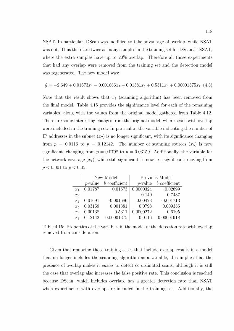
118

NSAT. In particular, DScan was modified to take advantage of overlap, while NSAT

was not. Thus there are twice as many samples in the training set for DScan as NSAT,

where the extra samples have up to 20% overlap. Therefore all those experiments

that had any overlap were removed from the training set and the detection model

was regenerated. The new model was:

y = −2.649 + 0.01673x1 − 0.001686x4 + 0.01381x5 + 0.5311x6 + 0.00001375x7 (4.5)

Note that the result shows that x3 (scanning algorithm) has been removed from

the final model. Table 4.15 provides the significance level for each of the remaining

variables, along with the values from the original model gathered from Table 4.12.

There are some interesting changes from the original model, where scans with overlap

were included in the training set. In particular, the variable indicating the number of

IP addresses in the subnet (x7) is no longer significant, with its significance changing

from p = 0.0116 to p = 0.12142. The number of scanning sources (x5) is now

significant, changing from p = 0.0798 to p = 0.03159. Additionally, the variable for

the network coverage (x1), while still significant, is now less significant, moving from

p < 0.001 to p < 0.05.

New Model Previous Modelp-value b coefficient p-value b coefficient

x1 0.01787 0.01673 0.0000324 0.02699x3 — — 0.140 0.7437x4 0.01691 -0.001686 0.00473 -0.001713x5 0.03159 0.001381 0.0798 0.009355x6 0.00138 0.5311 0.0000272 0.6195x7 0.12142 0.00001375 0.0116 0.00001918

Table 4.15: Properties of the variables in the model of the detection rate with overlapremoved from consideration.

Given that removing those training cases that include overlap results in a model

that no longer includes the scanning algorithm as a variable, this implies that the

presence of overlap makes it easier to detect co-ordinated scans, although it is still

the case that overlap also increases the false positive rate. This conclusion is reached

because DScan, which includes overlap, has a greater detection rate than NSAT

when experiments with overlap are included in the training set. Additionally, the

119

best detection rate achieved when overlap is included is 99.2% (discussed below in

Section 4.4), yet without overlap the same variable values result in a detection rate of

97.8%. The effect of overlap can be examined in more detail by modifying NSAT to

include overlap, running the 32 experiments that would include overlap, regenerating

the 20 random training cases and running those, and recalculating all of the models.

This exercise is described in Section 5.3 on future work.

4.4 Detector Performance

The hypothesis of this research was that a detector can be designed to accurately

detect co-ordinated TCP port scans against a target network, where the scan footprint

is either horizontal or strobe in nature. The details of this hypothesis, set out in

Section 1.2, included that the detector would be considered accurate if it obtained

a detection rate of 99% or better, and a false positive rate of less than 1%. This

detection rate was met under certain conditions on the scan and environment. These

conditions are examined using the model of the detection rate provided in Section

4.3.

If the five variables identified by the model of the detection rate are set to their

optimum values (e.g., 100% network coverage, 0% overlap, DScan as the scanning

algorithm, 100 noise scans, 100 scanning sources and five scanned ports against a /16

subnet), then the detection rate is 99.2% with a 0.0% false positive rate (see Table

4.16); this meets our requirements as set out in the hypothesis. However, changing

any of these values away from the optimum, with the exception of the amount of

overlap (x2), results in a detection rate that is too low to meet our requirements. The

amount of overlap (x2) can be increased to as much as 9% before the false positive

rate becomes too large to meet our requirements.

If we reduce the minimum required detection rate to 90%, then we can start to

adjust some of the variables to different values. Table 4.16 presents the detection

rates and false positive rates for a /16 subnet (65536 IP addresses) given various

combinations for each of the variables. The first row indicates the rates given optimum

values. Each subsequent row provides the rates given optimum values for all variables

but one, where the one variable is given the least optimal value. The detection rate

under these values (with at least one least optimal value) ranges from 91.1% to 98.3%.

120

The false positive rate ranges as high as 4.0% and as low as 0.0%. Assuming the least

optimal values for each of the variables, however, results in a detection rate of only

3.6%. This is shown in Table 4.17, where the first line contains the least optimal

values for all variables and each subsequent line changes one variable to the optimal

value leaving all others at their least optimal values. Under these circumstances, the

highest detection rate is 30.5% (which occurs when the number of ports is five).

% % Algorithm Detection FalseCoverage Overlap 0 − NSAT

1 − DScan Noise Sources Ports Rate Positives100 0 DScan 100 100 5 0.992 0.00010 0 DScan 100 100 5 0.915 0.000

100 0 NSAT 100 100 5 0.983 0.012100 0 DScan 1000 100 5 0.963 0.000100 0 DScan 100 2 5 0.980 0.000100 0 DScan 100 100 1 0.911 0.00010 20 DScan 100 100 5 0.915 0.011

100 20 NSAT 100 100 5 0.983 0.040100 20 DScan 1000 100 5 0.963 0.025100 20 DScan 100 2 5 0.980 0.025100 20 DScan 100 100 1 0.911 0.025

Table 4.16: The detection rates for 65536 IP addresses (/16 subnet) given that mostvariables have optimal values. Highlighted values indicate the variables with the leastoptimal values.

% % Algorithm Detection FalseCoverage Overlap 0 − NSAT

1 − DScan Noise Sources Ports Rate Positives10 20 NSAT 1000 2 1 0.036 0.010

100 20 NSAT 1000 2 1 0.295 0.04010 20 DScan 1000 2 1 0.072 0.01110 20 NSAT 100 2 1 0.147 0.02610 20 NSAT 1000 100 1 0.084 0.02610 20 NSAT 1000 2 5 0.305 0.026

Table 4.17: The detection rates for 65536 IP addresses (/16 subnet) given that mostvariables have the least optimal values. Highlighted values indicate the variables withthe most optimal values.

The lowest detection rate in Table 4.16 is 91.1%, which occurs when the number

of ports is 1. Table 4.18 assumes a co-ordinated scan against one port on a /16

121

% % Algorithm Detection FalseCoverage Overlap 0 − NSAT

1 − DScan Noise Sources Rate Positives100 9 DScan 100 100 0.911 0.010100 9 DScan 181 100 0.900 0.01095 9 DScan 100 100 0.900 0.009

100 9 DScan 100 86 0.900 0.010

Table 4.18: The variable values required to achieve 90% detection rates with 65536IP addresses (/16 subnet) and one port.

subnet, and shows the effect that modifying different variables can have while still

maintaining an acceptably high detection rate (90%) and acceptably low false positive

rate (1%). For example, the number of noise scans can be increased to 181 before the

detection rate is too low. Similarly, the coverage can be reduced to 95%. It should

be noted that under these circumstances (one port on a /16 subnet), any scans where

the scanning algorithm is NSAT will not have an acceptably high detection rate (the

highest possible value is 83.0%). To maintain an acceptably low false positive rate,

the maximum possible value for the amount of overlap is 9%. Changing the subnet

size for Table 4.18 to /24 from /16 reduces the detection rate to only 74.6% in the

best case, along with increasing the false positive rate to 3.1% even when the amount

of overlap is reduced to 0%.

% % Detection FalseCoverage Overlap Noise Sources Ports Rate Positives

100 0 100 100 5 0.983 0.01210 0 100 100 5 0.834 0.000

100 0 1000 100 5 0.926 0.012100 0 100 2 5 0.959 0.012100 0 100 100 1 0.830 0.012100 20 100 100 5 0.983 0.04010 20 100 100 5 0.834 0.026

100 20 1000 100 5 0.926 0.040100 20 100 2 5 0.959 0.040100 20 100 100 1 0.830 0.040

Table 4.19: The detection rates using NSAT on 65536 IP addresses (/16 subnet) giventhat most variables have optimal values. Highlighted values indicate the variableswith the least optimal values.

122

Table 4.19 provides the detection and false positive rates when the scanning algo-

rithm is NSAT against 65536 IP addresses (a /16 subnet). The false positive rate is

affected by the algorithm, increasing from 0.0% to 1.2% when there is no overlap, and

from 2.5% to 4.0% when the amount of overlap is 20%. Additionally, the detection

rate is lower for NSAT than for DScan, with a 10% coverage rate and a scanned port

of one both reducing the detection rate to below 90%.

As was mentioned in Section 4.3.1, modest values for the variables also results in

only a modest detection rate. For example, the values for each of the variables can

be set to a mid-range value. That is, network coverage can be set to 50%, percentage

of overlap to 10%, number of noise scans to 500, number of sources to 50 and number

of ports to two. The resulting detection and false positive rates for both DScan

and NSAT at varying network sizes are provided in Table 4.20. The results indicate

that the detector performs modestly at best, and generally quite poorly, given a

combination of modest (medium) values for each of the variables. For example, the

best detection rate achieved is only 61.0%, with the lowest detection rate being 17.5%.

Similarly there is a high false positive rate, ranging from 5.2% in the worst case to

0.4% in the best case.

Scanning # of IPs Detection FalseAlgorithm in Subnet Rate Positives

DScan 65536 0.610 0.004DScan 32640 0.454 0.021DScan 256 0.309 0.038NSAT 65536 0.427 0.018NSAT 32640 0.284 0.035NSAT 256 0.175 0.052

Table 4.20: The detection and false positive rates for NSAT and DScan given differentnetwork sizes when all other variables have medium values.

At runtime, the variables that the defender can control are the minimum amount

of network coverage required to detect the scan, the maximum amount of overlap,

and the number of scans processed at any one time. Setting the minimum amount

of network coverage to a small number (say, 10%) does not impact the false positive

rate. The effect on the detection rate is that large scans (approximately 100% network

coverage) will still be detected with a high probability, while still allowing for the

123

possible detection (albeit with a lower probability) of scans that cover less of the

target network. This effect is because the algorithm tries to maximize the network

coverage when searching for a co-ordinated scan. Thus, larger scans will more likely

still be detected, even when a small value is used for this variable. Setting the amount

of overlap at a large value (say, 20%) also does not affect the detection rate, and will

allow the defender to detect scans that have overlap; however, it does impact the

false positive rate, which the defender might find high enough to reduce the amount

of overlap to a smaller value. Finally, the number of scans processed at any one time

impacts the detection rate. The smaller the number of scans processed, the greater

the likelihood of detecting a co-ordinated scan. This must be balanced, however, with

the amount of scanning activity generally observed by the defender network and with

the expected size of any co-ordinated scan (in terms of the number of sources). The

general guideline here is that the number of scans processed at any time should be

kept in the hundreds rather than the thousands.

We can also evaluate the detector based on the effective false positive rate, which

consists of the number of co-ordinated scans that were detected where more than

50% of the single-source scans in the co-ordinated scan are false positives. Examining

the training set first, we find the number of effective false positives ranges from 0 to

18, with an average of 1.6875 effective false positives per data set and a median of

one. This means that, in general, given a data set a defender will have to examine

only one additional co-ordinated scan that is actually not a co-ordinated scan. The

number of days in each of the data sets ranged from one to 27. The worst case, where

there were 18 effective false positives, covered 15 days, resulting in slightly more than

one effective false positive per day. Examining the number of effective false positives

per day, the largest number was three, which occurred only once. There were twelve

instances ranging from one to two false positives per day inclusive. In 49 of the 116

cases (42%), there were no false positives, with 54 cases having > 1.0 but greater

than < 0.0 effective false positives per day.

Performing a similar examination of the testing set provides similar results. The

number of effective false positives ranged from zero to 14, with an average of 1.34

false positives per data set and a median of one.

124

4.5 Model Performance

It was shown in Section 4.3.3 that the model would generalize to scan combinations

on which it had not been trained; however, in this validation, the size of the subnets

was not changed from those sizes on which it had been trained (/24 and /16 subnets

containing 256 and 65536 IP addresses respectively). In addition, the noise used was

chosen in the same manner from the same sets that had been used for training. Thus,

we cannot state with certainty that the model presented here will generalize to other

environments. To test whether the model can, indeed, generalize to previously unseen

environments, we present a further 50 validation cases using a different set of noise

on a /17 subnet (32768 IP addresses).

In these 50 experiments, we chose values for six of the variables using the same

approach as in Section 4.3.3. That is, we randomly chose values from within the

ranges defined in Table 4.1 for variables fraction of network coverage (x1), amount of

overlap (x2), number of noise scans (x4), number of scanning sources (x5) and number

of ports (x6). The scanning algorithm (x3) was chosen randomly to be one of either

DScan or NSAT; however, rather than randomly choosing the subnet size to be either

/24 (256 IP addresses) or /16 (65536 IP addresses), we used a /17 subnet (32768 IP

addresses). The details for each of the 50 experiments are provided in Table 4.21.

Cov. Ov. Algo Scan # of IPs

% % 0 − NSAT1 − DScan Window Source Port in Subnet DR FP P

83 11 1 500 99 4 32768 1.000 0.006 0.917

67 16 1 500 56 5 32768 1.000 0.006 0.900

86 0 0 500 66 5 32768 1.000 0.008 0.886

83 8 1 200 69 3 32768 1.000 0.020 0.883

78 10 1 800 39 5 32768 1.000 0.009 0.860

83 0 0 200 38 4 32768 1.000 0.020 0.833

95 1 1 800 77 3 32768 1.000 0.000 0.801

72 9 1 400 69 3 32768 1.000 0.005 0.799

40 20 1 400 11 5 32768 1.000 0.005 0.771

42 0 0 100 89 4 32768 1.000 0.010 0.759

38 11 1 600 31 5 32768 1.000 0.007 0.732

Continued on next page

125

Continued from previous page

Cov. Ov. Algo Scan # of IPs

% % 0 − NSAT1 − DScan Window Source Port in Subnet DR FP P

100 7 1 500 97 1 32768 1.000 0.008 0.729

34 20 1 300 36 4 32768 1.000 0.000 0.698

26 18 1 400 8 5 32768 1.000 0.005 0.691

42 7 1 100 90 2 32768 1.000 0.000 0.660

99 0 0 1000 86 3 32768 1.000 0.007 0.622

48 17 1 800 47 4 32768 1.000 0.005 0.614

72 0 0 900 9 5 32768 1.000 0.008 0.613

68 0 0 100 2 3 32768 1.000 0.010 0.603

86 20 1 200 15 1 32768 1.000 0.000 0.589

96 0 0 400 31 2 32768 1.000 0.008 0.577

26 0 0 600 59 5 32768 1.000 0.003 0.549

98 0 0 900 37 3 32768 1.000 0.009 0.546

37 0 0 200 72 3 32768 1.000 0.000 0.516

48 0 0 500 87 3 32768 1.000 0.008 0.497

71 0 0 300 49 2 32768 1.000 0.017 0.494

57 15 1 800 13 3 32768 1.000 0.008 0.442

18 10 1 300 12 3 32768 1.000 0.007 0.392

50 1 1 300 46 1 32768 1.000 0.007 0.379

99 0 0 500 13 1 32768 1.000 0.004 0.362

100 0 0 500 9 1 32768 1.000 0.000 0.359

18 17 1 100 5 2 32768 1.000 0.000 0.314

16 0 0 1000 21 5 32768 1.000 0.007 0.248

51 0 0 700 38 2 32768 1.000 0.010 0.206

38 3 1 1000 92 1 32768 1.000 0.007 0.170

68 0 0 200 65 3 32768 0.969 0.020 0.697

11 14 1 600 91 2 32768 0.967 0.003 0.265

76 0 0 800 45 3 32768 0.956 0.006 0.459

37 0 0 900 36 4 32768 0.944 0.008 0.299

Continued on next page

126

Continued from previous page

Cov. Ov. Algo Scan # of IPs

% % 0 − NSAT1 − DScan Window Source Port in Subnet DR FP P

75 0 0 1000 78 1 32768 0.923 0.005 0.188

80 0 0 200 60 2 32768 0.917 0.010 0.621

17 0 0 800 81 3 32768 0.914 0.010 0.195

62 8 1 200 80 4 32768 0.000 0.010 0.898

11 1 1 600 41 5 32768 0.000 0.000 0.591

61 10 1 900 21 3 32768 0.000 0.003 0.445

31 9 1 600 49 3 32768 0.000 0.000 0.437

13 18 1 400 48 3 32768 0.000 0.010 0.400

95 0 0 900 92 1 32768 0.000 0.003 0.349

56 0 0 300 17 1 32768 0.000 0.010 0.206

32 0 0 900 78 2 32768 0.000 0.006 0.138

Table 4.21: The variable values in the validation set. The first group of values

represent perfect detection and correct prediction, while the second group is perfect

detection but incorrect prediction. The third group represents partial detection rates.

The fourth group represents no detection and incorrect prediction, while the fifth

group represents no detection and correct prediction. Each group is sorted by the

predicted detection rate except for the partial detections, which are sorted by the

actual detection rate. (Cov = Coverage, Ov = Overlap, DR = Detection Rate, FP

= False Positive, P = Predicted Detection Rate)

The noise set used consisted of flow-level network data which was collected from

a /17 subnet over a period of one month, from September 1 to September 30, 2005.

(More specifically, the data was collected from the first half of a /16 subnet, which

we then treated as a /17 subnet.) This data was analysed for the presence of single-

source scans using the scan detection algorithm by Gates et al. [20], using the default

values: a minimum of 32 flows per event were required before the event could be

analysed for the presence of a scan, and an event consisted of network activity that

had a five minute period with no activity both before and after the event.

127

In this data set there were 4426 scans with 1,709,549 targets. Of the 4426 scans,

4260 were SYN scans. The majority of the scans (4345) were horizontal (targeting

only one port), with only 76 strobe scans and five vertical scans. There were 1835

different ports scanned in this data set, with the five most popular ports provided in

Table 4.22. Figure 4.21 provides a graph showing the distribution of scans over time

for each of the top five ports, with the number of scans shown on a log scale.

Port Service # of Scans # of Sources80 Web (HTTP) 4211 1885

4899 Remote admin (radmin) trojan backdoor 85 815900 Virtual Network Computing (VNC) service 63 6122 SSH 37 32

1080 web services and W32.Mydoom.F@mm worm 31 25

Table 4.22: The most commonly scanned ports for one /17 subnet.

1

10

100

1000

08/27 09/03 09/10 09/17 09/24 10/01

Num

ber

of S

cans

Per

Day

(LO

G S

cale

)

Date (2005)

/17 Subnet

Port 80Port 4899Port 5900

Port 22Port 1080

Figure 4.21: The distribution of activity for the top five most often scanned ports forone /17 subnet.

For each of the 50 experiments provided in Table 4.21, the predicted value for

the detection rate was calculated using the logistic regression model from Equations

128

4.2 and 4.3. The results from the regression model are also provided in Table 4.21.

Assuming that any predicted value ≥ 0.5 indicates that the co-ordinated scan would

have been detected, the prediction rate was 64%. There were 42 instances where

the detector did detect the co-ordinated scan, of which the logistic regression model

correctly predicted 26 (62%). In contrast, the model correctly predicted 6 of the

8 experiments where the co-ordinated scan was not detected (75%). Reducing the

threshold from 0.5 to 0.35, as was done in Section 4.3.3, the prediction rate increases

from 64% to 86%. This is demonstrated in Figure 4.22, which shows the observed

versus the predicted detection rates for this set of data.

It should be noted that the detector detects 42 of the 50 scans (84%), missing only

eight (16%); this imbalance is reflected in the performance of the model. That is, there

are only eight points against which the true or false negative rates can be calculated,

versus 42 points for the true/false positives. As a result, setting the threshold to zero

will result in the model having an accuracy of 84%, as it will correctly identify all

42 experiments where the co-ordinated scan was detected; however, its false positive

rate will be 100%. Thus a receiver operator characteristic (ROC) curve is perhaps a

better representation of how well the model performs.

The ROC curve for the training, testing and validation sets is provided in Figure

4.23. The curves were generated by increasing the threshold in steps of 0.05 from 0.00

to 1.00. The point that was circled on each of the three curves represents a threshold

of 0.35. This ROC curve demonstrates that the curves for the testing and validation

sets both closely follow the curve of the training set. This indicates that the model

created by using the training set generalizes well to both the testing and validation

sets. Given how close the fit is for the validation set to the training set, this indicates

that our model generalizes well even to those cases where the detector has been used

against different noise sets.

The predicted false positive rates for the 50 experiments are provided in Figure

4.24. As can be seen from the figure, all of the predicted false positive rates were

greater than the actual false positive rate, and all but two of these rates (96%) were

within ±0.03 (the dashed blue line on the graph) of the actual false positive rate.

Both outliers were within ±0.04 of the actual rates. This shows that our model of

the false positive rate tends to overestimate rather than underestimate the rate.

129

0.0 0.2 0.4 0.6 0.8 1.0

0.0

0.2

0.4

0.6

0.8

1.0

Observed Versus Predicted Detection Rates

Observed Detection Rate

Pre

dict

ed D

etec

tion

Rat

e

False Positives

True Negatives False Negatives

True Positives

Figure 4.22: The observed detection rate versus the predicted detection rate for 50experiments (validation set).

While this experiment addresses one of the limitations of the testing performed

in Section 4.3.3, it does not address them completely. These experiments indicate

that the model can predict the performance of the detector given a new environment,

however this environment consisted of only a single network. Further tests using

other networks need to be performed. In particular, this network was chosen from

the same set of networks (government networks) as the training set, and therefore

might not exhibit as large a variation as could otherwise be expected. Additionally,

the network size chosen was a /17 network (32768 IP addresses), which represents

the number of IP addresses directly between a /24 network (256 IP addresses) and a

/16 network (65536 IP addresses). Other network sizes need to be tested, including

those that lie between a /24 and a /16, and possibly even larger networks, scaling

up to a /8 network. A further limitation of the validation performed here is that the

same emulation environment that was used for training and testing is used in this

validation. Thus it might be accurately representing some artefact of the emulation

environment and not correctly predict detector performance given either a simulated

or a real environment. Further testing in such environments needs to be performed.

130

0.0 0.2 0.4 0.6 0.8 1.0

0.0

0.2

0.4

0.6

0.8

1.0

ROC Curve

False Positive Rate

Tru

e P

ositi

ve R

ate

xxxxxx

xx

x

x

xx

xx

x

x

xx

x

xx

0.0 0.2 0.4 0.6 0.8 1.0

0.0

0.2

0.4

0.6

0.8

1.0

*****

***

****

*

*

****

***0.0 0.2 0.4 0.6 0.8 1.0

0.0

0.2

0.4

0.6

0.8

1.0

ox

*

Training SetTesting SetValidation Set

Figure 4.23: The ROC curve for the training, testing and validation sets.

4.6 Comparison to Related Work

An algorithm based on the definition for a co-ordinated port scan used by Yeg-

neswaran et al. [85] was implemented. This co-ordinated scan detector was chosen

because the description of it in the public record was sufficient for it to be repro-

duced. The purpose for implementing this approach is to demonstrate that the re-

gression modeling presented in Section 4.3 is applicable to other detectors and that

these models can be used to compare the circumstances under which each detector

performs best. This is demonstrated by developing models of Yegneswaran et al.’s

approach and analysing them. These models are then used to compare the influences

on the detection and false positive rates of Yegneswaran et al.’s approach and the

adversary model based approach developed in this dissertation.

Yegneswaran et al.’s approach [85] consisted of labeling any group of five or more

sources that scanned a single /24 subnet during a one hour period as being a co-

ordinated scan. The implementation used here modified this approach to be any set

of scans that started within the same one hour period, rather than scanned during

the same one hour period. This results in a more conservative approach than that

131

0.01 0.02 0.03 0.04

0.00

0.01

0.02

0.03

0.04

Residuals for Predicted False Positive Rates

Predicted False Positive Rate

Res

idua

l

Figure 4.24: The predicted false positive rate versus the residuals for 50 experiments(validation set).

defined by Yegneswaran et al., as a scan might span multiple hours, but only be

counted during the first hour. This is particularly true when the scan has targeted a

larger subnet (e.g. a /16 subnet). The result is that the detection rate is potentially

lower than what it might have otherwise been; however, the false positive rate is

also potentially lower. The implementation used a sliding window with ten-minute

increments.

4.6.1 Models

The approach taken to generate a model of the detection and false positive rates

in Section 4.3 is used to generate models for the performance of the approach by

Yegneswaran et al. [85]. However, given that Yegneswaran et al. do not consider a

scan with only two sources to be a co-ordinated scan, but rather require there to be

five sources, the 50 experiments where the number of sources was less than five are

removed from the set of 116 training experiments. The result is 66 experiments, where

there are 24 cases where the co-ordinated scan was not detected, 20 cases where all of

the single-source scans within the co-ordinated scan are detected, and 22 cases where

132

there is partial detection. Similar to Section 4.3, the cases where there is partial

detection are put into the detection group if the detection rate was ≥ 0.5, bringing

the total to 35 experiments where the co-ordinated scan is detected and 31 where it

was not. The actual detection and false positive rates for the 66 experiments in the

training set are provided in Table 4.23.

Cov Ov Algo Scan # of IPs Scan

% % 0 − NSAT1 − DScan Window Source Port in Subnet Times DR FR

100 0 0 100 100 1 256 1484 1.000 0.810

100 0 1 100 100 5 256 496 1.000 0.680

100 0 1 100 100 1 256 617 1.000 0.660

10 20 1 100 100 5 256 573 1.000 0.610

100 20 1 100 100 5 256 491 1.000 0.590

100 20 1 1000 100 5 256 19751 1.000 0.356

100 0 1 1000 100 1 256 20871 1.000 0.328

87 4 1 700 28 5 256 14646 1.000 0.327

10 20 1 1000 100 5 256 14165 1.000 0.326

100 0 1 1000 100 5 256 21288 1.000 0.316

10 0 1 1000 100 5 256 24458 1.000 0.242

100 20 1 1000 100 1 256 24458 1.000 0.240

100 20 1 1000 100 1 256 17475 1.000 0.234

100 0 0 1000 100 5 256 17771 1.000 0.211

48 13 1 700 5 4 256 17589 1.000 0.137

28 0 0 700 29 5 256 19715 1.000 0.140

100 20 1 100 100 1 256 2893 1.000 0.130

73 0 0 200 39 3 256 6870 1.000 0.055

100 0 0 100 100 5 65536 4506 1.000 0.000

100 0 1 1000 100 5 65536 41606 1.000 0.000

10 0 1 100 100 5 256 681 0.990 0.760

100 0 0 1000 100 1 256 8076 0.970 0.433

49 18 1 1000 100 3 256 21536 0.970 0.307

100 0 0 100 100 5 256 2636 0.970 0.080

Continued on next page

133

Continued from previous page

Cov Ov Algo Scan # of IPs Scan

% % 0 − NSAT1 − DScan Window Source Port in Subnet Times DR FR

100 20 1 100 100 5 65536 3589 0.970 0.040

100 20 1 1000 100 5 65536 40158 0.970 0.008

100 0 0 1000 100 5 65536 40495 0.970 0.001

100 0 0 1000 100 1 65536 40431 0.970 0.000

100 0 0 100 100 1 65536 5175 0.970 0.000

100 20 1 1000 100 1 65536 40414 0.960 0.004

100 0 1 100 100 5 65536 3544 0.950 0.010

100 20 1 100 100 1 65536 4718 0.950 0.000

100 0 1 1000 100 1 65536 41606 0.880 0.000

100 0 1 100 100 1 65536 4385 0.840 0.000

15 0 0 1000 64 3 256 5628 0.594 0.578

10 0 1 100 100 1 256 2918 0.270 0.030

10 0 1 1000 100 1 256 22258 0.270 0.250

10 20 1 100 100 1 256 1882 0.270 0.230

10 0 0 1000 100 1 256 5466 0.260 0.734

10 0 0 100 100 5 256 1940 0.260 0.290

10 0 0 1000 100 5 256 21771 0.260 0.283

10 0 0 100 100 1 256 654 0.250 0.460

10 0 0 100 100 5 65536 2906 0.000 0.000

10 0 1 100 100 1 65536 4579 0.000 0.000

10 20 1 1000 100 5 65536 41555 0.000 0.000

10 0 1 1000 100 1 65536 39994 0.000 0.000

10 0 1 100 100 5 65536 3808 0.000 0.000

10 20 1 100 100 5 65536 4231 0.000 0.000

10 0 0 1000 100 5 65536 40231 0.000 0.000

10 20 1 100 100 1 65536 3703 0.000 0.000

10 20 1 1000 100 1 65536 39529 0.000 0.000

10 0 0 100 100 1 65536 3165 0.000 0.000

Continued on next page

134

Continued from previous page

Cov Ov Algo Scan # of IPs Scan

% % 0 − NSAT1 − DScan Window Source Port in Subnet Times DR FR

10 0 1 1000 100 5 65536 39490 0.000 0.000

10 0 0 1000 100 1 65536 36638 0.000 0.000

22 16 1 500 13 3 65536 22074 0.000 0.000

95 0 0 700 81 4 65536 31432 0.000 0.000

86 0 0 800 39 1 65536 30559 0.000 0.000

77 11 1 900 36 5 65536 36961 0.000 0.000

64 3 1 200 48 2 65536 8080 0.000 0.000

18 17 1 500 64 1 65536 18687 0.000 0.000

79 13 1 800 41 3 65536 28159 0.000 0.000

75 14 1 900 34 5 65536 37551 0.000 0.000

62 0 0 700 24 3 65536 26072 0.000 0.000

85 7 1 200 5 2 65536 9256 0.000 0.000

84 4 1 1000 90 2 65536 40231 0.000 0.000

87 0 0 300 61 4 65536 12196 0.000 0.000

Table 4.23: The variable values in the training set for Yegneswaran et al. [85]. The

first group represents all those scans that were detected perfectly by decreasing false

positive rate. The second group contains all partial detections ordered by the de-

tection rate, while the third group contains all experiments where none of the scan

sources were detected. (Cov = Coverage, Ov = Overlap, DR = Detection Rate, FP

= False Positive)

A second change was made to the experiments. For the models of the adversary

model based detector, the time for a scan was irrelevant; however, it is relevant to

Yegneswaran et al.’s approach. This was not an issue for the noise scans, which were

taken as a sequential block from some random starting point in one of the noise sets,

thus preserving any temporal relationships between the scans in the data. However,

the co-ordinated scan that was injected in the set of noise scans did not necessarily

occur at the same time. This issue was addressed by taking the start and end times

for the noise sample to be used in the experiment and randomly choosing a time

135

inside this interval. This time was then used as the start time for the first scan in the

co-ordinated scan. All other scans in the co-ordinated scan had their times adjusted

such that they maintained their temporal relationship relative to the new start time.

Seven variables were used for the models in Section 4.3: fraction of the network

covered (x1), amount of overlap (x2), scanning algorithm (x3), number of noise scans

(x4), number of scanning sources (x5), number of scanned ports (x6) and subnet

size (x7). Of the seven variables, the first three are not relevant to this detection

algorithm, so are excluded from the following models.

In the previous models, time-related information was not included as a variable

because it was not relevant to the detector; however, in the approach by Yegneswaran

et al. [85], time is part of the definition of a co-ordinated scan. To capture this, a

variable representing the average number of seconds between the start times of noise

scans was added to the model. The values in the training set for this variable are

provided in Table 4.23, in the column labeled “Scan Times”.

A logistic regression approach was used to generate a model based on the five

variables number of noise scans (x4), number of scanning sources (x5), number of

scanned ports (x6), number of IP addresses in the subnet(x7), and the average number

of seconds between scans (x8). An AIC was applied to the model to reduce the number

of variables to those that contributed significantly to the detection rate. The resulting

model was:

P (co-ordinated scan is detected) =ey

1 + ey(4.6)

where

y = 1.197− 0.00002884x7 (4.7)

where x7 is the number of IP addresses in the subnet, e is the natural log and P is the

predicted detection rate. Thus, the only variable required to predict the detection

rate is the number of IP addresses in the scanned subnet. This makes intuitive sense

in that the algorithm is designed around scans against /24 subnets. Further, as the

experiments did not control for time between scans, all scans against /24 subnets

took less than one hour, which is the threshold used for this algorithm. Due to

this association between the two variables, only the size of the subnet is required to

determine the probability that a scan will be detected.

An increase in the number of IP addresses in the subnet (x7) causes the decrease

136

the detection rate, indicating that scans are more likely to be detected on a /24

subnet than on a /16 subnet. More specifically, the detection rate given a /24 subnet

(256 IP addresses) is 0.767, while the detection rate given a /16 subnet (65536 IP

addresses) is 0.333. This is due to the detection algorithm operating on /24 subnets.

If a co-ordinated scan is performed against a /16 subnet, then there is less chance that

at least five of the sources will target the same port on the same /24 subnet within

the same hour. This will be true for two reasons: the scan will be targeting 256 /24

subnets instead of just one and, if the sources scan sequentially in time (that is, one

source scans, followed by the second, etc.), then given the increase in the size of the

network being scanned, it is less likely that five different sources will scan within a

one hour period.

The false positive rate was modeled using a linear regression. The same variables

that were used above were used in the linear regression, followed by using an AIC

approach to reducing the number of variables. The resulting model is:

z = 0.3043 + 0.0009177x5 − 0.000004981x7 − 0.000002206x8 (4.8)

where x5 is the number of scanning sources, x7 is the size of the scanned subnet,

which is significant at p < 0.001, and x8 is the average number of seconds between

scans. The adjusted R2 value for the model is 0.610, and the F-statistic is significant

at p < 0.001, which indicates that this model performs significantly better than by

just using the mean. The negative coefficients for x7 and x8 indicate that as the

subnet size increases, or as the average number of seconds between scans increases,

the false positive rate decreases. The positive coefficient for x5 indicates that as the

number of scanning sources increases, so does the false positive rate.

The results for x7 and x8 are related to how Yegneswaran et al. [85] define co-

ordinated scans, where at least five scans must have targeted the same port on the

same /24 subnet within the same hour. The smaller the average number of seconds

between scans, the more scans there will be in a given hour and, therefore, the higher

the likelihood that five scans will target the same port on the same /24 subnet.

Similarly, for x7 a smaller subnet indicates more false positives because the algorithm

of Yegneswaran et al. operates on /24 subnets. For example, if there are five scans in

one hour on a /24 subnet, then they will form a co-ordinated scan. However, if there

are five scans in one hour on a /16 subnet, then they likely did not all target the same

137

/24 subnet within the /16 subnet, so will not form a co-ordinated scan. This effect

is demonstrated in Figure 4.25.

0 10000 20000 30000 40000

0.0

0.1

0.2

0.3

0.4

0.5

Effect of Scan Rate on False Positive Rate

Average Number of Seconds Between Scans

Fal

se P

ositi

ve R

ate

x x x x x x x x x x x x x x x x x x x x x x x x x x x x x x x x x x x x x x x x x x x x x x x x x x x x x x x x x x x x x x x x x x x x x x x x x x x x x x x x x x x

0 10000 20000 30000 40000

0.0

0.1

0.2

0.3

0.4

0.5

xo

/24 Subnet (256 IP addresses)/16 Subnet (65536 IP addresses)

Figure 4.25: The effect of the number of seconds between scan start times and subnetsize on the false positive rate for Yegneswaran et al.’s algorithm [85].

The result for x5 — that the false positive rate increases as the number of scanning

sources increase — is due to the likelihood that, with more sources, there will be

enough scans on any given /24 subnet to meet the threshold increases. For example,

with 100 sources there is an increased likelihood that one of those scans will target

a particular /24 subnet. If there were already four other scans against that subnet,

then the combination will be flagged as a co-ordinated scan, resulting in four false

positives. This effect is demonstrated in Figure 4.26.

The testing set used in Section 4.3 was used here to test the predictive capabil-

ities of the model, given unknown data. There were two experiments in the testing

set where the number of scan sources was less than five, so these experiments were

removed. The detector based on the adversary model had correctly identified 36 of

the remaining 48 co-ordinated scans; Yegneswaran et al.’s model [85] detected 26 of

the co-ordinated scans. The logistic regression model of this detection rate had a

96% accuracy, correctly predicting the detection (or non-detection) of 46 of the 48

138

20 40 60 80 100

0.0

0.1

0.2

0.3

0.4

0.5

Effect of Number of Scanning Sources on False Positive Rate

Number of Scanning Sources

Fal

se P

ositi

ve R

ate xxxxxxxxxxxxxxxxxxxxxxxxxxxxxxxxxxxxxxxxxxxxxxxxxxxxxxxxxxxxxxxxxxxxxxxxxxxxxxxxxxxxxxxxxxxxxxxx

20 40 60 80 100

0.0

0.1

0.2

0.3

0.4

0.5

xo

/24 Subnet (256 IP addresses)/16 Subnet (65536 IP addresses)

Figure 4.26: The effect of the number of scanning sources and the subnet size on thefalse positive rate, using Yegneswaran et al.’s algorithm [85].

scans. Specifically, all the co-ordinated scans against a /24 subnet were detected

(as predicted by the model), while only two of the 24 scans against a /16 subnet

were detected (and the model expected none of the scans against a /16 subnet to be

detected).

A comparison of the residuals to the predicted false positive rate for each of the

experiments in the test set is provided in Figure 4.27. This graph shows that the

predicted false positive rates are within ±0.1 of the actual false positive rates in the

majority of cases (shown by the dashed blue lines in Figure 4.27), with seven outliers.

The average predicted false positive rate was 0.162, while the actual average false

positive rate was 0.165. The median predicted false positive rate was 0.146 (versus

0.097 actual), while the maximum predicted value was 0.356 (versus 0.779 actual).

The largest residual was 0.473.

4.6.2 Model Comparison

There is one variable in common between the evaluation model of the detection rate for

Yegneswaran et al.’s detector [85] and the evaluation model developed in Section 4.3

139

0.00 0.05 0.10 0.15 0.20 0.25 0.30 0.35

−0.

5−

0.4

−0.

3−

0.2

−0.

10.

00.

10.

2

Residuals for Predicted False Positive Rates

Predicted False Positive Rate

Res

idua

l

Figure 4.27: The predicted false positive rate versus the residuals for 48 experiments(testing set) for Yegneswaran et al.’s algorithm [85].

of the adversary model-based detector. This indicates that the detection capabilities

of the two detectors are based mostly on different characteristics of the co-ordinated

scans and associated environment. In particular, the adversary model-based detector

used four characteristics of the scan itself in its evaluation model of the detection

rate: the fraction of the network covered by the scan (x1), the scanning algorithm

used (x3), the number of scanning sources (x5) and the number of ports scanned (x6).

In comparison, Yegneswaran et al.’s detector did not use any of the characteristics

of the scan itself. This indicates that the adversary model-based detector is sensitive

to characteristics of the scan, whereas Yegneswaran et al.’s detector is not. The

adversary detector also used two environment variables — the number of noise scans

(x4) and the size of the scanned subnet (x7) — as an indicator of the detector’s

performance. Only the size of the scanned subnet (x7) was a factor in the model of

Yegneswaran’s et al.’s approach. In the adversary detector, an increase in the number

of noise scans resulted in the co-ordinated scan being more difficult to detect; this

is not the case with Yegneswaran’s et al.’s detector as it is based on a thresholding

approach that is not hidden by noise scans. The only variable required to model

140

the approach of Yegneswaran et al. is the number of IP addresses in the subnet

(x7). In their detector an increase in the size of the subnet decreased the detection

rate because it defines co-ordinated scans based on /24 subnets. By comparison, the

adversary model-based detector performed better on larger subnets (e.g., /16 subnets)

than on smaller subnets (e.g., /24 subnets) because more information was available

on the larger subnets.

The models of the false positive rates for the two detectors also indicates differences

in the characteristics of the detectors. The false positive rate of the adversary-based

detector is affected by several scan characteristics: the fraction of the network covered

by the scan (x1), the amount of overlap (x2) allowed by the detector, and the scanning

algorithm (x3); however, none of these impacts the false positive rate for Yegneswaran

et al.’s detector, but it is affected by the number of scanning sources used. Two

environment characteristics — the size of the scanned subnet (x7) and the average

number of seconds between scan start times (x8) — both affect the false positive

rate for the detector by Yegneswaran et al. but only the subnet size (x7) affects the

adversary model-based detector. In both cases a larger subnet indicates a lower false

positive rate.

The quality of the models of the detection rate for each of the detectors also

varies. The model of Yegneswaran et al.’s detector correctly classifies 96% of the test

set with a threshold of 0.5, whereas the model of the adversary detector correctly

classified only 76% of the test set with a threshold of 0.35; however, the model of the

false positive rate for the adversary model has a better fit than Yegneswaran et al.’s

approach, with the majority of experiments falling within ± 0.03 of the actual value

versus within ± 0.1.

4.6.3 Detection Comparison

Table 4.24 provides the detection rate and false positive rate for the adversary model

based detector given 20% overlap and the DScan scanning algorithm with 100 sources

against a /24 subnet (256 IP addresses), using some of the cases provided earlier in

Table 4.16. The value for overlap was chosen in order to maximize the false positive

rate. The values for the scanning algorithm and number of sources serve to maximize

the detection rate. The table also provides the detection and false positive rates for

141

Yegneswaran et al.’s model for comparison. Table 4.25 provides similar comparisons

for a /16 subnet (65536 IP addresses) instead of a /24 subnet.

Adversary Model Yegneswaran et al.Scan Detection False Detection False

Coverage Noise Ports Times Rate Positives Rate Positives100 100 5 500 0.972 0.059 0.777 0.39410 100 5 500 0.755 0.045 0.777 0.394

100 1000 5 500 0.882 0.059 0.777 0.394100 100 1 500 0.746 0.059 0.777 0.394100 100 5 2500 0.972 0.059 0.777 0.38910 100 5 2500 0.755 0.045 0.777 0.389

100 1000 5 2500 0.882 0.059 0.777 0.389100 100 1 2500 0.746 0.059 0.777 0.389

Table 4.24: The detection and false positive rates for the DScan scanning algorithmwith 100 sources and 20% overlap against a /24 subnet (256 IP addresses).

Adversary Model Yegneswaran et al.Scan Detection False Detection False

Coverage Noise Ports Times Rate Positives Rate Positives100 100 5 500 0.992 0.025 0.333 0.06910 100 5 500 0.915 0.011 0.333 0.069

100 1000 5 500 0.963 0.025 0.333 0.069100 100 1 500 0.911 0.025 0.333 0.069100 100 5 2500 0.992 0.025 0.333 0.06410 100 5 2500 0.915 0.011 0.333 0.064

100 1000 5 2500 0.963 0.025 0.333 0.064100 100 1 2500 0.911 0.025 0.333 0.064

Table 4.25: The detection and false positive rates for the DScan scanning algorithmwith 100 sources and 20% overlap against a /16 subnet (65536 IP addresses).

Yegneswaran et al.’s [85] approach, when used on a /24 subnet (256 IP addresses),

has a 78% detection rate. While it would be possible to evade this system (by having

each source scan during a different hour, for example), the model presented here used

the co-ordinated scanners with their default settings. In comparison, the adversary-

based model had a detection rate that ranged from 0.746 to 0.972, depending on

the scan characteristics. This detection rate was premised on having mostly optimal

values. Changing the variables to less optimal values decreased the detection rate to

142

below 78%, and going as low as 3.6% (see Table 4.17 for more examples); however,

the cost from using Yegneswaran et al.’s approach comes as a (potentially) high false

positive rate — as high as 0.394 when the average number of seconds between two

scans starting is 500. In comparison, the adversary model had a false positive rate

ranging from 0.045 to 0.059, based largely on the high amount of overlap (20%).

While the detection rate for the adversary model is affected positively by an increase

in the number of IP addresses in the subnet, it negatively affects the detection rate

for Yegneswaran et al.’s approach, reducing it to 0.333; however, it also has the effect

of significantly reducing the false positive rate, to 0.069 from 0.394.

4.7 Deployment Issues

4.7.1 Detector

While the detection algorithm has been shown to work reasonably well in the con-

trolled testing scenarios discussed in Section 4.4, there are still several issues that

would arise in the deployment of this detection approach. In particular, the defender

will need to chose which values to use for each of the variables under his control. As

discussed in Section 4.4, the minimum percentage of the network covered can be set

as low as 10% and the maximum allowed overlap can be set as high as 20% without

affecting performance, given that the algorithm attempts to maximum the coverage

while minimizing the overlap, and so these values provide lower and upper bounds

respectively. However, the higher overlap rate may result in more false positives, and

so the defender might want to set this to a lower value.

While suggested coverage and overlap values are provided, the number of scans

to use as input to the algorithm is not addressed well. Rather, the suggestion is

made to keep this value as low as possible. However, this might allow an attacker

to provide enough time between the scans of each individual source that not all the

sources in the co-ordinated scan will be included in the input set. Thus a defender

will also want to have the number of scans being analysed be large enough to detect

any co-ordinated scans. Any given defender will need to choose this value recognizing

the need to balance the number of false negatives, the number of scans observed per

unit time on his particular network, the size of his network (as this will also affect the

143

number of false negatives), and the desire to make the amount of time great enough

that the adversary finds spreading his scans over time prohibitive.

The tests performed on this detector also assume a retrospective analysis. How-

ever, in a deployment situation, this requires that a defender maintain a database

of scan sources and all of their associated scan targets. It might be the case that a

defender wants to examine his data for the presence of a co-ordinated scan before

the scans have necessarily finished running. This issue has not been addressed in this

dissertation. Another issue is the choice of the underlying single-source scan detec-

tor. The better this detector is at detecting scans, the greater the likelihood that

any co-ordinated scans will also be detected. A third consideration is the decision

of what particular set of scans to analyse. That is, if discrete time periods are used

(e.g., each set of 1000 scans), then a co-ordinated scan that spans multiple analysis

periods (e.g., half of the scanning sources occur in the first set of 1000 scans, while

the other half occur in the second set) will not be detected by the defender. It is

recommended in this case that the defender use a sliding window approach, where

the size of each slide is determined by the defender based on resource issues such as

the amount of processing power and time required to analyse the input set of scans

versus the number of scans he typically observes during some unit of time.

Additionally, the defender will not be able to verify the results he obtains from

running this detector. There is no guarantee that the true and false positive rates

found in this dissertation will apply to the defender’s network despite the tests to

confirm the detector’s performance using networks that were not part of the training

set. Nor are there any methods to test how well the detector is performing other than

to perform co-ordinated scans against the defender’s network or to inject co-ordinated

scans into the database of scanning activity. It may be possible, however, to estimate

if a particular co-ordinated scan is a true or false positive based on other information

about the sources, such as if they are all performing the same type of scan or if they

all originate from the same domain or country. Without this additional verification,

and given only scan traffic collected from the monitored network, the defender will

not be able to ascertain if any scans found by the detector are actually co-ordinated

scans, nor will he be able to ascertain the number of co-ordinated scans that he is

not detecting.

144

4.7.2 Testing Methodology

The testing methodology developed in this dissertation has been shown to be effective

at predicting the detection and false positive rates for a co-ordinated scan detector

given new environments on which the detector and model have not previously been

trained or tested; however, there are several issues which need to be addressed before

the testing methodology can be deployed more generally.

In order for a model to be developed, the appropriate independent variables must

first be determined. Unfortunately, there are no guidelines for how to determine

which variables are most likely to affect the performance of a detector. Rather the

experimenter must give thought to what factors might affect a detector, such as the

inputs to the detector, the qualities of the activity that the detector purports to

detect, and the characteristics of the operating environment.

A second limitation to the deployment of this testing methodology is the require-

ment for clean background noise. In this dissertation, an assumption was made that

the scan data collected for background noise did not contain any co-ordinated scans.

This was considered a reasonable assumption in this case; however, if the detector

was designed to detect a more common activity, such as the presence of worm activity

on a network, then the generation of background data that is free of this activity is

more difficult.

A third deployment issue is the experiment-intensive nature of the approach.

While the use of regression modeling reduces considerably the number of experi-

ments required to explore a multi-dimensional space, there is still a large number of

experiments required. For example, in this dissertation, 216 experiments were per-

formed, where some experiments took many hours. Thus, this approach can be very

slow, which makes it less likely to be deployed.

Finally, the testing methodology described here was aimed at testing a detector

that was developed to recognize a single type of activity. Deploying this approach

for the testing of larger systems, such as generic intrusion detection systems, will

likely require separating the system into the different activities it detects and testing

each activity separately. This will be time consuming, as experiments will need to be

developed to test each aspect of the detector.

145

4.8 Summary

In this chapter we evaluated an implementation of the detector that was described

in Chapter 3. Previous approaches to testing have tended to use either the Lincoln

Labs data set (which provides a labeled data set) or network traces [4]. Similar to

the approach used by Lincoln Labs [36], we generate a labeled data set consisting of

a combination of manually created attacks and network traces. Unlike the Lincoln

Labs data set, we use actual network traces rather than simulating the network traces.

This requires the assumption that no co-ordinated scans are present in our network

traces. If scans are present, and if they are detected, then our false positive rates will

be too high. Conversely, if such scans are present and they are not detected, then the

true positive rate will be too high.

Co-ordinated scans were performed on the DETER network [83], where the vari-

ables of the scans — fraction of the network scanned, amount of overlap, scanning

algorithm used, number of scanning sources and number of scanned ports — were

controlled. Additionally, two environmental conditions were controlled: the size of

the scanned subnet and the number of noise scans used in the background. A training

set consisting of 116 experiments was created, ensuring that the extreme cases were

part of the training set. The result was that the detector only found 64 (55%) of the

scans.

The training set was used to generate two models — one of the detection rate

and another of the false positive rate — using regression modeling. The detection

rate used a logistic regression model, finding that six of the seven variables were

important to the detection rate, with only the amount of overlap not contributing to

the detection rate. The false positive rate used a linear regression model, finding that

four of the variables contributed to the false positive rate: the fraction of the network

covered by the scan, the amount of overlap, the scanning algorithm and the size of

the subnet. While overlap does not contribute to the detection rate and also increases

the false positive rate, we do not suggest restructuring the algorithm to remove this

variable. This is because an adversary would then be able to avoid detection by

adding overlap in their scanning behaviour. The algorithm is structured to allow the

user to specify the maximum acceptable overlap, allowing him to therefore control

the false positive rate.

146

Two other data sets were generated, a testing set and a validation set, both

consisting of 50 experiments. For the testing set, the value for each variable was

randomly chosen; however, the testing set used the same sets of network traces that

had been used in the training set. In contrast, the validation set used both randomly-

chosen values for the variables and a /17 subnet instead of either a /24 or a /16 subnet.

In addition, the scan data was gathered from a different network at a different time

from the training data. These two data sets were used to test the detector and model.

The detector correctly identified 36 of the 50 co-ordinated scans (72%) in the

testing set, and 42 of the 50 co-ordinated scans (84%) in the validation set. The

model correctly predicted how the detector would perform in 76% of the cases when

the threshold was set at 0.35 (up from 64% with a threshold of 0.5) on the testing set.

For the validation set, the model correctly predicted the detector’s performance in

86% of cases with a threshold of 0.35 (up from 64% with a threshold of 0.5). In terms

of the false positive rates, we correctly predicted the rate to within ±0.03 for the

majority (74% of the testing set and 96% of the validation set) of the experiments. In

addition, we examined the “effective” false positive rate — the number of co-ordinated

scans detected where the majority of the single-source scans in the co-ordinated scan

were false positives — where we found that the average number of effective false

positives per data set was fewer than two for both the training and testing sets.

Thus, we have demonstrated how regression models can be used to model the

detection and false positive rates for a detector. We have shown that these models

can be used to predict the performance of a detector given conditions that have pre-

viously not been observed, including having deployed the detector against a different

network using traces that had not been used in the training of the model. In addition

to demonstrating this model of our detector, we also implemented a detector by Yeg-

neswaran et al. and demonstrated how our modeling approach can be used on their

detector. We further used the results to compare the two approaches to discuss the

conditions under which one would perform better than the other. We concluded the

chapter with a discussion on the deployment issues surrounding both the deployment

of the detector and the use of the testing methodology.

Chapter 5

Conclusion

This chapter highlights the research contributions and conclusions of this dissertation.

A summary of each research contribution is provided in Section 5.1, including any

limitations to the contribution. The two hypotheses introduced in Chapter 1 are

discussed, stating the conditions under which we accept each hypothesis. The chapter

then concludes with a discussion of future work.

5.1 Research Contributions

The research contributions contained in this dissertation fall into two broad categories,

each related to the two main hypotheses: the proving of the hypothesis that a co-

ordinated scan detector can be developed, and the use of evaluation methodologies

that are not typically applied to the field of intrusion detection system. Subsections

5.1.1 and 5.1.2 both discuss contributions that are related to the development of a co-

ordinated scan detector that achieves a 99% detection rate and a 1% false positive rate.

The remaining four subsections each describe contributions to the area of evaluating

intrusion detectors.

5.1.1 Adversary Model

We provided an adversary model in Section 3.5 that represents scanning activity. We

observed that adversaries can be classified based on the information they wish to ob-

tain, identifying four dimensions in Section 3.2 that characterize this information: (i)

the number of ports scanned, (ii) the number of IP addresses scanned, (iii) the criteria

used to select the IP addresses to be scanned, and (iv) the form of camouflage used (if

any). While there are 72 possible combinations for the four dimensions, we focused on

21 specific adversary types and discarded the remainder as being pathological cases

(such as those cases that combine an address selection criteria with scanning all IP

147

148

addresses — if all IP addresses are being scanned, then they cannot also be randomly

selected, for example).

We relate the 21 adversary types to the generic footprint pattern of a scan meeting

the same criteria as the adversary, where a footprint is the set of target IP/port

pairs [71]. We extend the traditional concept of a footprint to be a tuple that is

based on the four dimensions identified on the previous page, with an additional two

characteristics — coverage and hit rate. Coverage is the percentage of the defender

network that the scan covers, while hit rate is the percentage of IP addresses targeted

in the range that the scan itself covers. Thus, we have a representation for each type

of scan and can relate it to one of the adversary types.

5.1.2 Detection Algorithm

We developed an algorithm that detects co-ordinated port scans in Section 3.6. While

previous approaches to detecting co-ordinated port scans were either threshold-based

(e.g., [85], [62]), used a machine learning approach (e.g., [74], [71]), or used visualiza-

tions for a manual analysis of network traffic patterns (e.g., [11]), our approach took

advantage of the adversary model that we developed and implemented.

We noted that a co-ordinated scan has a footprint pattern, which is the union of

the footprints for each of the single-source scans. We, therefore, use this information

to develop a detector for co-ordinated scans. The detector combines sets of scans to

determine whether the overall footprint forms a pattern that is representative of one

of the adversary types. Simultaneously, we try to minimize the overlap between the

scans, based on the assumption that someone performing a co-ordinated scan to gather

particular information will not want to have a large amount of repetition between

scans as it will make the single-source scans larger and will take longer to run; however,

we allow for some overlap as an adversary might use this as a form of camouflage.

We developed a detector that was designed to detect nine of the 21 adversary types,

where these nine types are identifiable because they perform either a horizontal or

strobe scan that covers a large amount of contiguous IP space. We discussed in

Section 3.6.5 how the algorithm could be modified to detect the other adversary

types. The detection approach was verified in Chapter 4 through an implementation

149

where the detection algorithm was inspired by a Greedy-like heuristic [22] for solving

the set-covering problem (described in Section 3.6.1).

The co-ordinated scan detector is limited by the underlying scan detector. If

the adversary has obtained enough sources to ensure that the number of targets per

source is small enough that the single-source scan detector will not detect them, then

the co-ordinated scan detector will not have the granularity required to detect the

scan. For example, Jung et al. [28] found that their scan detection algorithm made a

decision based on an average of 5.2 unique destinations being contacted. Thus, if each

source that is part of a co-ordinated port scan scans only three targets, for example,

then they are not likely to be detected as performing a scan. Thus, these sources will

not be input to the co-ordinated scan detector, and our detector will not detect this

scan.

5.1.3 Experimental Design

We presented a new approach to the evaluation of intrusion detectors based on a

controlled experiment using a combination of an isolated testbed and network traffic

captured at the border of a live network (described in Section 4.1). Intrusion de-

tection testing has largely focused on two different approaches: the use of a known

testing set and deployment on a live network [4]. In the first case, there is one testing

set in wide-spread use; developed by Lincoln Labs in 1998 [36], this set contains la-

beled data, including attacks that were actually performed and simulated background

(benign) traffic. While this dataset has been shown to be flawed [42][38], it is the

only comprehensive labeled dataset that is publicly available to researchers. In the

second case, experiments are performed by deploying systems on live networks —

this allows a defender to determine what is detected by a system; however, the false

negative rate cannot be determined. Two other approaches that have also been used

include simulation and analysis. In the first case, the detector is tested using data

that has been simulated. This approach has the advantage of being able to control

all aspects of the testing data, however there is no guarantee that it will accurately

reflect performance on network data. The analysis approach consists of providing

bounds on the detector’s performance based on an understanding of the algorithm,

which in turn specifies the conditions under which the detector will perform well.

150

However, the expected true and false positive rates can not be determined without

knowing the characteristics of the network traffic. In contrast, this thesis has pre-

sented and employed an approach to determining detection rates for a detector based

on a controlled experiment performed using the DETER testbed [83], in conjunction

with traffic captured from a live network. Unlike other uses of the DETER network,

which have focused on simulating Internet-scale events (e.g., see [80]), the testbed

was used as an attack platform where attacks could be performed in an isolated en-

vironment and the network traffic captured. This was combined with network traffic

captured from a live network, with the subsequent analysis assuming that the network

traffic contained no co-ordinated port scans. This dissertation has shown that this is

a viable method for determining the performance capabilities of a detector.

We used this experimental design to test the detection capability of our algorithm.

Single-source scan data were recorded from eight different subnets (four /24 subnets

and four /16 subnets) and used as background noise. Co-ordinated scans, using two

publicly available co-ordinated scanning algorithms, were performed on the DETER

network [83]. The network traffic captured from the DETER testbed was processed

with the resulting scans injected into the background traffic.

5.1.4 Metrics

We defined two metrics to evaluate the performance of a co-ordinated scan detector in

Section 4.2. While other work has examined the issue of how to detect co-ordinated

scans, none have identified methods for measuring how well different detectors have

performed. This issue is complicated by the fact that the measurement is focused on

group membership rather than a strict classification of each observation. That is, most

metrics are based on determining whether the classification of a single observation is

correct, rather than determining the correctness of a group of observations. The first

of our two metrics follows this approach of evaluating single observations — which is

achieved by identifying a scan as the appropriate unit of analysis. Thus, for example,

a true positive was a scan categorized as part of a co-ordinated scan that was, in

fact, part of a co-ordinated scan. The second metric, which we called the effective

false positive rate, was created to measure the number of co-ordinated scans that

a defender would need to investigate. Thus, while there might be 10 false positive

151

scans out of 1000, resulting in a false positive rate of 0.01, there was also a measure

to indicate that these false positives forming five co-ordinated port scans was worse

than forming one co-ordinated port scan, as it results in an increased workload for

the defender to examine multiple events.

5.1.5 Evaluation Models

We developed regression models in Section 4.3 to predict the detection and false

positive rates for our detector given deployment operating environments. The usual

method for reporting the performance capabilities for intrusion detection systems is in

terms of the detection rate and false positive rate [5]; however, these rates are generally

provided based on a single test environment, assuming that the detection and false

positive rates will be consistent across other test environments. This assumption

was shown to be false by Maxion and Tan [40]. This dissertation has presented

an alternative approach where the detector performance is modeled based on the

characteristics of the attack, the defender’s choice of detector input variables, and

the deployment environment.

Seven variables, enumerated in Table 3.3, were identified to contribute to the

detector’s performance: (i) the percentage of the network covered by the scan, (ii)

the amount of overlap between the sources of the co-ordinated scan, (iii) the scanning

algorithm used, (iv) the number of noise scans, (v) the number of scan sources, (vi) the

number of ports scanned and (vii) the size of the target subnet. A logistic regression

model, based on these seven variables, was developed in Section 4.3.1 to represent the

detection rate for the algorithm, based on 116 observations using the above-mentioned

experimental design. A statistical analysis of the logistic regression equation for the

detection rate, using the Akaike Information Criterion (AIC) [2], found that six of

the seven variables had a significant effect on the detection capability of the detector,

with only the amount of overlap (ii) not contributing to the detection rate (see Table

4.12). A similar model was developed in Section 4.3.2 of the false positive rate, using

a linear regression approach and the AIC. This model found that the percentage of

the network covered (i), the amount of overlap between any two scanning sources (ii),

the scanning algorithm (iii) and the size of the network being monitored (vii) had a

significant effect on the false positive rate (see Table 4.13).

152

The use of regression modeling provides the advantage of allowing a network

administrator to determine the expected performance of the detector given his own

operating environment (e.g., subnet size, number of noise scans). It allows the user

to determine the detection rate given various forms of the attack itself within his

operating environment. We developed evaluation models for both the detection and

false positive rates, testing the model using the same noise sets but different scan

characteristics. As described in Section 4.4, the model of the detection rate was

found to be 76% accurate given a threshold of 0.35. The majority of the predictions

for the false positive rate (86%) were within ±0.03 of the actual false positive rate.

We further tested the model in Section 4.5 using a previously unseen background

noise set on a network size that had not been used for training. In this case the

detection model was found to be 86% accurate given a threshold of 0.35, and 96% of

the predicted false positives were within ±0.03 of the actual false positive rate.

One limitation involves how the noise data was chosen. We specified the number of

noise scans to be used as background and then determined whether the co-ordinated

scan could be detected given this background, where the co-ordinated scan targeted

the most popular ports. For example, if the most commonly scanned port was port

80, then the co-ordinated scan was performed against port 80. The argument for this

approach is that this provided the best reflection of a realistic scenario; however, it

can be argued that a better testing strategy would be to specify the number of scans

against a particular port, rather than the number of scans against all ports.

5.1.6 Model Comparisons

We provided a method to compare two different detectors in terms of the conditions

under which each will perform well (see Section 4.6.2). When intrusion detection

systems have been compared to each other, the approach has been to run the systems

against the same data and compare the true positive and false positive rates (for

examples, see Lippmann et al. [36] and Jung et al. [28]). We demonstrated in Section

4.6.3 how comparing the regression models generated for each detector can be used

to determine which variables have the greatest influence on the detection and false

positive rates for each detector. From this, the circumstances under which each

detector should be deployed can be determined.

153

5.2 Conclusions

Hypothesis 1.1 stated “A detector can be designed to detect co-ordinated TCP port

scans against a target network where the scan footprint is either horizontal or strobe

with a detection rate of greater than 99% and a false positive rate of less than 1% on

both /24 and /16 networks.”

We accept this hypothesis under the conditions that (i) 100% of the target network

is scanned, (ii) the overlap does not exceed 9%, (iii) the scanning algorithm is DScan

(which randomly distributes the targets amongst its sources), (iv) the number of noise

scans is no greater than 100, (v) the number of scanning sources is at least 100, (vi)

the number of scanned ports is at least five, and (vii) the scanned subnet contains

at least 65536 IP addresses (/16 subnet). Given these conditions, the detection rate,

as calculated from the evaluation models described in Subsection 4.3, was 99.2% and

the false positive rate was 1.0% (see the first row of Table 4.16 for the detection rate

and the first row of Table 4.18 for the false positive rate); however, as discussed in

Section 4.4, all other conditions result in either a detection rate of less than 99% or

a false positive rate of greater than 1%.

Hypothesis 1.2 stated “Evaluation models that can predict the performance of a

detector in terms of detection rates and false positive rates, given previously unseen

operating environments, can be developed, where the the model of the detection rate

should have an accuracy of at least 75% and the model of the false positive rate should

be accurate to within ±0.03 of the actual false positive rate in 75% of the cases.”

We accept this hypothesis. We developed two evaluation models, one for the de-

tection rate and one for the false positive rate, to predict the performance of the

co-ordinated scan detector. We demonstrated in Sections 4.3.1 and 4.3.2 how these

models can be used to determine the characteristics of a detector that have the great-

est impact on either the detection or the false positive rate. The model was tested in

Section 4.3.3 using a set of 50 experiments performed under new conditions on which

the model had not be trained. We found that the ideal threshold for the model of the

detection rate was 0.35, which resulted in an accuracy of 76%. We also found that

the false positive rate was predicted to within ±0.03 of the actual false positive rate

in 86% of the cases. The model was tested further in Section 4.5 using a data set that

not only contained scans with characteristics that had not been observed previously,

154

but also using background noise gathered from a different subnet during a different

time period. The model of the detection rate demonstrated an accuracy of 86% with

a threshold of 0.35, while the model of the false positive rate predicted a value within

±0.03 of the actual value in 96% of the cases. We note, however, that the threshold

for the model of the detection rate needs to be set to 0.35 in order to achieve these

results — using the traditional threshold of 0.5 results in a 64% accuracy for both

data sets, which would result in the hypothesis being rejected.

5.3 Future Directions

One of the weaknesses in the literature surrounding port scans is the lack of consistent

definitions. As a result, we needed to specify definitions in this thesis to ensure that

there was a common framework for discussion; however, these definitions lack a formal

framework, which should be developed. If this is developed properly, it would not only

provide the ability to specify precisely how, for example, a scan is defined, but would

also allow for comparisons of different detection methods based on the characteristics

of the scans they detect.

The adversary model does not explicitly include time as a component, but rather

assumes that the entire scan is available; this model could be extended to include time

as a component. This would allow a user to specify a footprint based on only partially

detecting the scan. This could potentially be extended to allow for comparisons

between different detection techniques based on the minimum amount of footprint

information required to detect the presence of a scan.

The detector is currently limited to detecting horizontal and strobe scans with a

very high (95%) hit rate.1 The reasoning behind having a hit rate of less than 100%

was to allow for missing data. The effect of varying the hit rate needs to be examined

to determine whether other footprint patterns can be recognized, such as a pattern

where the adversary scans one or more ports on a set of randomly chosen IP addresses.

It is hypothesized that the scan will become undetectable once the hit rate becomes

too small; however, “too small” remains undefined. It is further hypothesized that

1Given the first and last IP address in a set of targets, the hit rate is the percentage of theintervening IP addresses that were targeted.

155

the minimum hit rate that still allows for reasonable detection rates will be related

to the characteristics of the scans against the monitored network.

The detection and false positive rates of the detector are currently affected by the

scanning algorithm used by the adversary. We specifically examined two scanning

tools: DScan and NSAT. We identified in Section 4.3.4 that the different detection

rates for the two algorithms is caused by an artefact due to only DScan having the

ability to use overlap to obscure scans. Additionally, we have found that overlap

appears to increase the probability that a co-ordinated scan will be detected. This

needs to be further investigated by modifying the NSAT scanning algorithm to use

overlap. A new series of experiments will need to be performed, with an accompanying

analysis of the regression models. Additionally, the detection algorithm has only been

tested against two methods of distributing targets — other distribution patterns,

such as sequential blocks of targets, should be investigated to determine how well the

algorithm performs.

At present, this algorithm does not consider information beyond the footprint

pattern for each scan. One extension that can be made is to cluster similar scans

together first, and then use this algorithm on each cluster. An adversary who performs

a co-ordinated scan is likely to use the same tool on each of the sources, which will

then demonstrate similar scan characteristics (e.g. timing information, type of scan).

By clustering scans with similar characteristics, it is likely that the entirety of the

co-ordinated scan will be in the same cluster and the number of noise scans will be

reduced, as it is unlikely that all the remaining scans will be part of the same cluster.

The detector was tested using scans that were identified by the algorithm of Gates

et al. [20]; however, when this algorithm was deployed on the live networks to generate

the background noise data sets, it was used in its default settings. As a result, scans

were only detected if they consisted of at least 32 flows. A different scan detection

algorithm that potentially detects scanners with fewer flows, such as the Threshold

Random Walk method [28], should be used for testing the co-ordinated scan detection

algorithm. The results could also be tested using not only all known scanners (those

identified by a given scan detection algorithm), but also all possible scanners, where

a possible scanner is identified as a source that has sent only SYN packets, regardless

of the number of flows generated. While this has the effect of potentially removing

156

scanners that have established connections with machines that have responded to

their probes, it would also have the effect of considering those sources that have sent

only a single SYN packet as a potential scanner. The detector should be tested using

these more extreme cases where much smaller scans are included in the noise sets.

While the detector presented in this dissertation is specific to the detection of co-

ordinated port scans, it might be the case that the general approach can be applied

to the detection of other forms of co-ordinated activity. For example, one case that is

potentially of interest to various government organizations is based on the keywords

used during web searches to locate information on their site. The organization might

be interested to know whether someone appears to be searching on different, but

related, terms from different IP addresses and then collating the information; in

this case, the space consists of words rather than IP addresses. Each port could

represent a different set of related terms. A modified version of this detector could

then be applied to determining whether different sources are searching a set of related

terms. One interesting aspect to this problem is that the notion of ordering no longer

exists. When detecting co-ordinated port scans, the IP addresses had an order (in

IP space) and so the detection was performed assuming that some contiguous space

was covered; however, if the space to be searched consists of terms, then there is no

implicit ordering in the set and so no notion of a contiguous space.

The evaluation methodology used in this dissertation warrants further attention.

In particular, the methodology of combining experiments on an isolated network

testbed with traffic captured from a network needs to be investigated to determine

how well it extends to other, more generic, testing of intrusion detection systems.

In particular, this dissertation focused on data that consisted solely of summarized

scan information. It is not known how well this approach would perform if flow-level

or packet-level information was required. Additionally, we examined a very specific

detector. The ability for this method to generalize to a generic intrusion detection

system needs to be examined. It is suspected that a taxonomy of attacks will be

required, and that each type of attack (e.g., worms, web server buffer overflows) will

need to be tested separately.

Further exploration of how well the logistic regression modeling approach repre-

sents operating environments outside those used in generating the model needs to be

157

performed. While initial results from a test using one previously unseen environment

are promising, experiments need to be performed using several different noise sets

that were gathered from different subnets during different time periods. The results

from using the regression equations to model the detection and false positive rates

would then be compared against the actual detection and false positive rates.

Appendix A

Port Scans

Port scans have been classified by the TCP flag settings they use. Commonly em-

ployed scans include: [18]

• TCP connect() scanning,

• TCP SYN (half open) scanning,

• TCP FIN (stealth) scanning,

• SYN/FIN scanning using IP fragments,

• UDP raw ICMP port unreachable scanning,

• Xmas scans, Null scans

• ACK scans and Window scans

• RST scans

A TCP connect() scan can be performed by anyone on any machine. A standard

connection is made to a port which indicates that the port is open by establishing a

connection, or closed if a connection cannot be established. Thus, a complete TCP

handshake is performed. The disadvantage to this method is that sites often log the

connections made to various services offered. A number of packets are sent in this

case — a SYN packet to initiate the connection, a SYN-ACK to to acknowledge the

connection, an ACK to establish the connection, some data from the scanned site

to the scanner, and a FIN to end the connection. At least three packets are sent

from the scanner, and at least three packets are received by the scanner; however,

despite the logging performed, this type of scan is sometimes performed, for example

to determine the particular version of the service being offered at the port of interest.

158

159

A TCP SYN scan begins a connection, but never completes it and is, therefore, also

known as a half-open scan. The scanner sends a SYN packet to initiate a connection.

If the port is open, a SYN-ACK is received, else a RST-ACK is received indicating

that the port is not accepting connections. If a SYN-ACK is received, the scanner

might send a RST packet to close the connection without completing the handshake.

The advantage to this method is that the service probed does not log the access as

the connection was never completed. Only two packets are sent from the scanner,

and only one received.

In some cases, firewalls are configured to block SYN packets to closed ports, thus,

preventing the SYN-ACK from being returned to the scanner. In these cases, a TCP

FIN scan, also known as a stealth scan, can be used, as firewalls are often configured

to allow these to pass unconditionally. When a FIN packet is sent to a port that

is closed, it will result in a RST packet; however, if the port is open, no response

will be made at all. This attack is unreliable in that it is based upon an incorrect

implementation of the TCP protocol, which is operating system dependent. In these

instances, only one packet is sent from the scanner, and at most one is received.

Several variations on the FIN scan exist, the most common of which are Xmas

scans and Null scans. In the case of Xmas scans, the URG, PSH and FIN flags are

set, with a sequence number of zero. In the case of Null scans, none of the flags

are set, and the sequence number is zero. In all these cases, the aim is to create a

packet that will not be stopped by a firewall. Again, only one packet is sent from the

scanner, and at most one is received [9].

It is also possible to by-pass firewalls by using IP fragmentation. In this case, the

TCP packet is spread across multiple IP packets, resulting in very small packets, on

the order of 24 or 36 bytes. Firewalls are often not configured to reassemble the TCP

packets due to performance considerations.

To determine whether a port is filtered by a firewall, ACK scans can be used where

a packet with only the ACK flag set is sent to a port. If a RST response is received,

then the port is unfiltered, so can be accessed remotely. If no response is received, or

if an ICMP unreachable response is received, then the port is filtered by the firewall.

Another form of scanning is RST scanning, where a RST packet is sent to a target.

If there is no response, or if there is an ICMP port unreachable message returned,

160

then the target IP likely contains a host that is up and running. If no host exists at

that IP address, then an ICMP host unreachable message will be returned instead. If

outgoing ICMP port or host unreachable messages are blocked by a firewall or router,

however, the adversary will not be able to gain any information using this form of

scanning.

In some situations, it may be preferable to use UDP packets over TCP packets

(although this is rare) as the service of interest might be UDP-based rather than

TCP-based. In these cases, a UDP packet is sent to a destination. If the destination

port is closed, a ICMP port unreachable message will be returned. If the destination

port is open, there will either be no response or a UDP packet will be returned. This

is not a reliable scanning method, as UDP transport is unreliable and packets can

be dropped from the network. In these cases, the result may look like an open port

when, in fact, the packet never reached the destination. In addition, such a scan can

be slow, as some kernels (such as some variants of Linux) place limits on the number

of responses to UDP packets made within a certain period of time.

Other traffic that might appear as scan traffic is backscatter. Backscatter consists

of response traffic to connection requests sent by other hosts who have spoofed their

IP addresses [46]. That is, a source sends a TCP connection request to a destination,

but spoofs its IP address, and the destination sends a response packet to the spoofed

IP. If the spoofed IP address is in a monitored network, then the defender will observe

the response. The responses generally consist of either SYN-ACK, RST-ACK or RST

packets. If a large number of spoofed IP addresses are found in the monitored network,

then this might appear as, for example, a RST scan to the defender.

Appendix B

Logistic Regression

Logistic regression was first developed for use in cases where an outcome (dependent)

variable is dichotomous (i.e. Boolean). In the case at hand, “This traffic event does

or does not contain scanning activity.” According to Agresti, “Logistic regression ...

is the most important model for categorical response data.” [1, p. 165] Early uses of

the technique were in biomedical studies but, in the past 20 years or so, it has been

applied in diverse fields such as social science research, marketing, and genetics.

In general, a logistic regression model estimates the probability, P , that the out-

come variable will be true in any given case, based on the value(s) of one or more

predictor (independent) variable(s) for that case. Unfortunately, the probability can-

not be measured directly; however, if we were to observe a number, N , of independent

cases (all with the same probability P ), the number of cases where the outcome vari-

able is true would follow the binomial distribution with index N and parameter P .

Any model is a simplification of reality. Linear models are very widely used as

simplifications while still offering considerable flexibility and generality. Suppose then

that we want to develop a model of the form

P (outcome is true) = f(β0 + β1x1 + β2x2 + ...+ βnxn) (B.1)

where

x1, x2, ..., xnrepresent the values of the n predictor variables for this case (B.2)

It can be shown that using f -inverse as

f−1(x) = ln(x

1− x) (B.3)

provides a model which is linear in the predictor variables and whose random com-

ponent is reflected by the binomial distribution noted above. [1, p. 121-123] Applying

this transformation to equation B.1 yields

ln(P

1− P) = β0 + β1x1 + β2x2 + ...+ βnxn (B.4)

161

162

“In 1944, the physician and statistician Joseph Berkson introduced the term logit

for this transformation [i.e., ln(P / (1 - P))]. ... [H]is subsequent work did much to

popularize logistic regression.” [1, p. 624]

The quantity P/(1− P ) is called the odds ratio; it is the ratio of the probability

the outcome is true to the probability the outcome is not true. For example, when

the odds of an outcome are 3:1 (i.e., 3) the probability of that outcome is 0.75. When

the odds of an outcome are 3:5 (i.e., 0.6) the probability of that outcome is 0.375.

The log of the odds ratio, ln[P/(1− P )], is called the “logit”.

Finally, solving equation B.4 for the probability P yields

P (outcome is true) =ey

1 + ey(B.5)

where

y = β0 + β1x1 + β2x2 + ...+ βnxn (B.6)

On a more intuitive level, P is a probability and must, therefore, fall in the range

[0,1]. If P was a direct linear function of the predictor variables (i.e., if the function

f in equation B.1 was the identity function) it would be very difficult to constrain

its values to the [0,1] interval. Moreover, we anticipate that a fixed change in one of

the predictor variables will have less impact on the probability when the probability

is already close to 0 or 1, than it will have when the probability is in the mid-range

(closer to 0.5). As an example, consider the case of a single predictor variable — say,

the address coverage indicator (maximum number of individual addresses targeted

within any class C subnet) which takes on integer values where 1 <= x <= 256.

When x = 251, intuitively we would already assign a fairly high probability that the

event contains scanning activity. If x increased by 5 (meaning all 256 addresses in a

/24 space were targeted) we do not expect the probability to rise much more; it was

already very close to 1. On the other hand, if x was 7 and went up to 12 (increase of

5 again) we would expect a more noticeable increase in the probability that the event

contains scanning activity.

Accordingly, we hypothesize that for a single predictor variable P (x) has an S-

shaped curve, as illustrated in Figure B.1. Of course, the curve may be shifted left

or right, ascend more steeply or more gradually, and/or be flipped across the vertical

axis (so the probability would decrease as x increases). A widely used function with

163

this distinctive S-shape is

g(x) =ex

1 + ex(B.7)

Thus, we are led to model P (x) as this function. Generalizing to an arbitrary linear

combination of n predictor variables leads directly to equations B.5 and B.6 above.

0

0.25

0.5

0.75

1

-10 -5 0 5 10

Figure B.1: An illustration of a single predictor variable P (x).

B.1 Estimating the Parameter Values

β0, β1, β2, ... , βn in equation B.6 represent the parameters of the model for the prob-

ability that a traffic event contains scanning activity, when x1, x2, ... , xn represent

the values of the n predictor variables for this event. The most appropriate β values

can be determined for a set of traffic events where (1) the values of the n predictor

variables are available for each event, and (2) an independent determination has been

made for whether or not each event contains scanning activity. Maximum likelihood

estimates are generally used for the model parameter (β) values. The maximum like-

lihood estimates are the parameter values which give the observed data the highest

probability of occurrence, based on the model. The mechanics of the calculations

are described in various texts (e.g., see [1]), and are implemented in many statistical

software packages.

164

Once these parameter values are available, equations B.5 and B.6 can be applied

to predict the probability for any other case, based on the values of the predictor

variables for that case.

Bibliography

[1] Alan Agresti. Categorical Data Analysis. John Wiley and Sons, 2002. ISBN1-471-36093-7.

[2] H. Akaike. Information theory as an extension of the maximum likelihood princi-ple. In B. N. Petrov and F. Csaksi, editors, Proceedings of the 2nd InternationalSymposium on Information Theory, pages 267 – 281, Budapest, Hungary, 1973.

[3] Dobin Rutishauser (Anthraxx) and Bjorn Paetzel (Kolrabi). DScan software.http://www.u-n-f.com/dscan.html, 2002. Last visited: 2 July 2002.

[4] Nicholas Athanasiades, Randal Abler, John Levine, Henry Own, and George Ri-ley. Intrusion detection testing and benchmarking methodologies. In Proceedingsof First IEEE International Workshop on Information Assurance, pages 63 – 72,Darmstadt, Germany, March 2003.

[5] Stefan Axelsson. The base-rate fallacy and the difficulty of intrusion detection.ACM Transactions on Information and System Security, 3(3):186 – 205, 2000.

[6] Raj Basu, Robert K. Cunningham, Seth E. Webster, and Richard P. Lippmann.Detecting low-profile probes and novel denial-of-service attacks. In Proceedingsof the 2001 IEEE Workshop on Information Assurance and Security, pages 5 –10, United States Military Academy, West Point, New York, USA, June 2001.

[7] Sviatoslav Braynov and Murtuza Jadliwala. Detecting malicious groups ofagents. In Proceedings of the First IEEE Symposium on Multi-Agent Securityand Survivability, Drexel University, Philadelphia, PA, USA, August 2004.

[8] CERT. CERT/CC overview: Incident and vulnerability trends. http://www.

cert.org/present/cert-overview-trends/module-2.pdf, 2003. Last Vis-ited: 29 December 2005.

[9] Laura Chappell. You’re being watched: Cyber-crime scans. Novell Connection:The Magazine for Networking Professionals, 2001. Last visited: 18 February2002.

[10] Fred Cohen. Simulating cyber attacks, defenses, and consequences. http://www.all.net/journal/ntb/simulate/simulate.html, 1999. Last visited: 5 April2002.

[11] Gregory Conti and Kulsoom Abdullah. Passive visual fingerprinting of networkattack tools. In Proceedings of 2004 CCS Workshop on Visualization and DataMining for Computer Security, pages 45 – 54, Washington, DC, USA, October2004.

165

166

[12] Marco de Vivo, Eddy Carrasco, Germinal Isern, and Gabriela O. de Vivo. Areview of port scanning techniques. ACM SIGCOMM Computer CommunicationReview, 29(2):41 – 48, 1999.

[13] G. Elfving. Optimum allocation in linear regression theory. The Annals ofMathematical Statistics, 23(2):255 – 262, 1952.

[14] Levent Ertoz, Eric Eilertson, Aleksandar Lazarevic, Pang-Ning Tan, Paul Dokas,Vipin Kumar, and Jaideep Srivastava. Detection of novel network attacks usingdata mining. In Proceedings of the 2003 ICDM Workshop on Data Mining forComputer Security, Melbourne, Florida, USA, November 2003.

[15] Shelby Evans, David Heinbuch, Elizabeth Kyle, John Piorkowski, and JamesWallner. Risk-based systems security engineering: Stopping attacks with inten-tion. IEEE Security and Privacy, 2(6):59 – 62, 2004.

[16] Ronald A. Fisher. Statistical Methods for Research Workers. Hafner PublishingCompany, 14 edition, 1970.

[17] Mark Fullmer and Steve Romig. The OSU flow-tools package and Cisco Netflowlogs. In Proceedings of the 14th Systems Administration Conference (LISA 2000),pages 291 – 303, New Orleans, LA, USA, December 2000. Usenix Organization.

[18] Fyodor. The art of port scanning. Phrack Magazine, 7(51), 1997. Article 11.

[19] Carrie Gates, Michael Collins, Michael Duggan, Andrew Kompanek, and MarkThomas. More NetFlow tools: For performance and security. In Proceedingsof the 18th Large Installation Systems Administration Conference (LISA 2004),pages 121–132, Atlanta, Georgia, USA, November 2004.

[20] Carrie Gates, Joshua J. McNutt, Joseph B. Kadane, and Marc Kellner. Scandetection on very large networks using logistic regression modeling. In Proceed-ings of the IEEE Symposium on Computers and Communications, Pula-Cagliari,Sardinia, Italy, June 2006. To Appear.

[21] John Green, David Marchette, Stephen Northcutt, and Bill Ralph. Analysistechniques for detecting coordinated attacks and probes. In Proceedings of theWorkshop on Intrusion Detection and Network Monitoring, Santa Clara, Cali-fornia, USA, April 1999. Usenix Association.

[22] Tal Grossman and Avishai Wool. Computational experience with approxima-tion algorithms for the set covering problem. European Journal of OperationalResearch, 101(1):81 – 92, 1997.

[23] Todd Heberlein, Gihan Dias, Karl Levitt, Biswanath Mukherjee, Jeff Wood, andDavid Wolber. A network security monitor. In Proceedings of the 1990 IEEESymposium on Research in Security and Privacy, pages 296 – 304, Oakland,California, USA, May 1990.

167

[24] Richard O. Hundley and Robert H. Anderson. Emerging challenge: security andsafety in cyberspace. IEEE Technology and Society Magazine, 14(4):19 – 28,1995.

[25] hybrid. Distributed information gathering. Phrack Magazine, 9(55), 1999. Article9.

[26] Intrusec. Intrusec alert: 55808 trojan analysis. http://www.intrusec.com/

55808.html, 2003. Last visited: 1 July 2003.

[27] Curtis A. Carver Jr., John M.D. Hill, John R. Surdu, and Udo W. Pooch. Amethodology for using intelligent agents to provide automated intrusion response.In Proceedings of the 2000 IEEE Workshop on Information Assurance and Se-curity, pages 110 – 116, United States Military Academy, West Point, NY, June2000.

[28] Jaeyeon Jung, Vern Paxson, Arthur W. Berger, and Hari Balakrishnan. Fastportscan detection using sequential hypothesis testing. In Proceedings of the2004 IEEE Symposium on Security and Privacy, pages 211 – 225, Oakland,California, USA, May 2004. IEEE Computer Society.

[29] Jaeyeon Jung, Stuart E. Schechter, and Arthur W. Berger. Fast detection ofscanning worm infections. In Proceedings of the Seventh International Symposiumon Recent Advances in Intrusion Detection, Sophia Antipolis, French Riviera,France, September 2004.

[30] Nei Kato, Hiroaki Nitou, Kohei Ohta, Glenn Mansfield, and Yoshiaki Nemoto.A real-time intrusion detection system (IDS) for large scale networks and itsevaluations. IEICE Transactions on Communications, E82-B(11):1817 – 1825,1999.

[31] Hyukjoon Kim, Surrey Kim, Michael A. Kouritzin, and Wei Sun. Detecting net-work portscans through anomaly detection. In Proceedings of SPIE, volume 5429,pages 254 – 263, 2004. Signal Processing, Sensor Fusion, and Target RecognitionXIII.

[32] Kiran Lakkaraju, William Yurcik, and Adam J. Lee. NVisionIP: NetFlow visu-alizations of system state for security situational awareness. In Proceedings of2004 CCS Workshop on Visualization and Data Mining for Computer Security,pages 65 – 72, Washington, DC, USA, October 2004.

[33] Bill Landreth. Out of the Inner Circle: A Hacker’s Guide to Computer Security.Microsoft Press, 1985.

[34] C. Leckie and R. Kotagiri. A probabilistic approach to detecting network scans.In Proceedings of the 2002 IEEE Network Operations and Management Sympo-sium, pages 359 – 372, Florence, Italy, April 2002.

168

[35] Cynthia Bailey Lee, Chris Roedel, and Elena Silenok. Detection and charac-terization of port scan attacks. http://www.cs.ucsd.edu/users/clbailey/

PortScans.pdf, 2003. Last visited: 31 December 2005.

[36] Richard P. Lippmann, David J. Fried, Isaac Graf, Joshua W. Haines, Kristo-pher R. Kendall, David McClung, Dan Weber, Seth E. Webster, DanWyschogrod, Robert K. Cunningham, and Marc A. Zissman. Evaluating in-trusion detection systems: The 1998 DARPA off-line intrusion detection evalua-tion. In DARPA Information Survivability Conference and Exposition, volume 2,pages 12 – 26, 2000.

[37] John Lowry, Rico Valdez, and Brad Wood. Adversary modeling to develop foren-sic observables. In Proceedings of the Air Force Research Lab’s Digital ForensicResearch Workshop, Baltimore, Maryland, 2004. August 11-13, 2004.

[38] Matthew V. Mahoney and Philip K. Chan. An analysis of the 1999DARPA/Lincoln Laboratory evaluation data for network anomaly detection. InProceedings of the Sixth International Symposium on Recent Advances in Intru-sion Detection, pages 220 – 237, Pittsburgh, PA, USA, September 2003.

[39] Uriel Maimon. Port scanning without the SYN flag. Phrack Magazine, 7(49),1996. Article 15.

[40] Roy A. Maxion and Kymie M.C. Tan. Benchmarking anomaly-based detectionsystems. In Proceedings of 2000 International Conference on Dependable Systemsand Networks, pages 623 – 630, June 2000.

[41] Lieutenant Colonel Thomas C. McCarthy. U.S. Army Heavy Brigade Recon-naissance During Offensive Operations. United States Army Command AndGeneral Staff College, Fort Leavenworth, Kansas, 12 1994. Monograph. ReportNo. 8589003. 64 Pages.

[42] John McHugh. Testing intrusion detection systems: a critique of the 1998 and1999 DARPA intrusion detection system evaluations as performed by LincolnLaboratory. ACM Transactions on Information and System Security, 3(4):262 –294, 2000.

[43] Jonathan McPherson, Kwan-Liu Ma, Paul Krystosk, Tony Bartoletti, and Mar-vin Christensen. PortVis: A tool for port-based detection of security events.In Proceedings of 2004 CCS Workshop on Visualization and Data Mining forComputer Security, pages 73 – 81, Washington, DC, USA, October 2004.

[44] Mixter. Network security analysis tools. http://nsat.sourceforge.net/, 2003.Last Visited: 9 November 2004.

[45] David Moore. Network telescopes. Presentation on 21 July 2004 at FloCon,2004.

169

[46] David Moore, Geoffrey M. Voelker, and Stefan Savage. Inferring internet denial-of-service activity. In Proceedings of the 10th USENIX Security Symposium,Washington, DC, USA, August 2001. Usenix Association.

[47] Chris Muelder, Kwan-Liu Ma, and Tony Bartoletti. Interactive visualization fornetwork and port scan detection. In Proceedings of 2005 Recent Advances inIntrusion Detection, September 2005.

[48] John-Paul Navarro, Bill Nickless, and Linda Winkler. Combining Cisco Net-Flow exports with relational database technology for usage statistics, intrusiondetection and network forensics. In Proceedings of the 14th Systems Administra-tion Conference, pages 285 – 290, New Orleans, LA, December 2000. USENIXAssociation.

[49] Peng Ning, Yun Cui, and Douglas S. Reeves. Analyzing intensive intrusion alertsvia correlation. In Proceedings of the 5th International Symposium on RecentAdvances in Intrusion Detection, pages 74 – 94, Zurich, Switzerland, October2002.

[50] Stephen Northcutt. Network Intrusion Detection: An Analyst’s Handbook. NewRiders, Indianapolis, 1999.

[51] Office of the National Counterintelligence Executive. Annual reportto congress on foreign economic collection and industrial espionage2001. http://www.ncix.gov/publications/reports_speeches/reports/

fecie_all/fecie_2004/FecieAnnualreport_2004_NoCoverPages.pdf, 2001.Last visited: 31 December 2005.

[52] Ruoming Pang, Vinod Yegneswaran, Paul Barford, Vern Paxson, and Larry Pe-terson. Characteristics of internet background radiation. In Proceedings of the 4thACM SIGCOMM Conference on Internet Measurement, pages 27 – 40, Taormina,Sicily, Italy, October 2004.

[53] Susmit Panjwani, Stephanie Tan, Keith M. Jarrin, and Michel Cukier. An ex-perimental evaluation to determine if port scans are precursors to an attack. InProceedings of the 2005 International Conference on Dependable Systems andNetworks, pages 602 – 611, Yokohama, Japan, June 2005.

[54] Donn B. Parker. Fighting Computer Crime. Wiley Computer Publishing, NewYork, 1998.

[55] Vern Paxson. Bro: A system for detecting network intruders in real-time. In Pro-ceedings of the 7th USENIX Security Symposium, San Antonio, Texas, January1998. Usenix Association.

[56] Vern Paxson. Private communication between Carrie Gates and Vern Paxson,February, 2006.

170

[57] Vern Paxson and Sally Floyd. Wide area traffic: The failure of Poisson modeling.IEEE/ACM Transactions on Networking, 3(3):226 – 244, 1995.

[58] The Honeynet Project. Know Your Enemy. Addison-Wesley, 2002.

[59] Nicholas J. Puketza, Kui Zhang, Mandy Chung, Biswanath Mukherjee, andRonald A. Olsson. A methodology for testing intrusion detection systems. IEEETransactions on Software Engineering, 22(10):719 – 729, 1996.

[60] QoSient LLC. Argus. http://www.qosient.com/argus/, 2004. Last Visited:28 July 2004.

[61] RAND. Quantifying the battlefield. http://www.rand.org/publications/RB/RB3014/RB3014.html, 1999. Last visited: 10 July 2002.

[62] Seth Robertson, Eric V. Siegel, Matt Miller, and Salvatore J. Stolfo. Surveillancedetection in high bandwidth environments. In Proceedings of the 2003 DARPADISCEX III Conference, pages 130 – 139, Washington, DC, April 2003. IEEEPress.

[63] Martin Roesch. Snort — lightweight intrusion detection for networks. In Proceed-ings of the 13th Systems Administration Conference, pages 229 – 238, Seattle,WA, USA, November 1999. Usenix Association.

[64] Marc Rogers. A new hacker taxonomy. http://www.escape.ca/~mkr/hacker_doc.pdf, 2000. Last visited: 12 March 2002.

[65] SANS. SANS glossary of terms used in security and intrusion detection. http://www.sans.org/resources/glossary.php, 2003. Last visited: 26 July 2004.

[66] Bruce Schneier. Attack trends: 2004 and 2005. ACM Queue, 3(5):52 – 53, 2005.

[67] Colleen Shannon. Private communication between Carrie Gates and ColleenShannon on 21 July 2004 at FloCon, 2004.

[68] Ed Skoudis. Counter Hack: A Step-by-Step Guide to Computer Attacks andEffective Defenses. Prentice Hall, Upper Saddle River, NJ, 2002.

[69] Stuart Staniford. Intrusion correlation engine. http://www.silicondefense.

com/research/ACM-tutorial-11-4-01.ppt, 2001. Powerpoint presentation onThe Intrusion Correlation Engine from an ACM conference. Last visited: 13January 2003.

[70] Stuart Staniford, James Hoagland, and Joseph McAlerney. Practical automateddetection of stealthy portscans. Journal of Computer Security, 10(1):105 – 136,2002.

171

[71] Stuart Staniford, James A. Hoagland, and Joseph M. McAlerney. Practical auto-mated detection of stealthy portscans. In Proceedings of the 7th ACM Conferenceon Computer and Communications Security, Athens, Greece, November 2000.

[72] Stuart Staniford, Vern Paxson, and Nicholas Weaver. How to 0wn the Internet inyour spare time. In Proceedings of the 11th USENIX Security Symposium, pages149 – 167, San Francisco, California, USA, August 2002. USENIX Association.

[73] S. Staniford-Chen, S. Cheung, R. Crawford, M. Dilger, J. Frank, J. Hoagland,K. Levitt, C. Wee, R. Yip, and D. Zerkle. GrIDS – a graph based intrusion detec-tion system for large networks. In Proceedings of the 19th National InformationSystems Security Conference, pages 361 – 370, Baltimore, MD, USA, October1996.

[74] William W. Streilein, Robert K. Cunningham, and Seth E. Webster. Improveddetection of low-profile probe and denial-of-service attacks. In Proceedings of the2001 Workshop on Statistical and Machine Learning Techniques in ComputerIntrusion Detection, June 2001.

[75] Cisco Systems. Cisco CNS NetFlow collection engine. http://www.

cisco.com/en/US/products/sw/netmgtsw/ps1964/products_user_guide_

chapter09186a00801ed569.html, 2004. Last Visited: 5 April 2004.

[76] Laura S. Tinnel, O. Sami Saydjari, and Dave Farrell. Cyberwar strategy andtactics: An analysis of cyber goals, strategies, tactics, and techniques. In Pro-ceedings of the 2002 IEEE Workshop on Information Assurance and Security,pages 228 – 234, United States Military Academy, West Point, NY, June 2002.

[77] Johannes Ullrich. DSHIELD. http://www.dshield.org, 2004. Last visited: 14July 2004.

[78] United States Department of Justice. Press release: Computer virus brokerarrested for selling armies of infected computers to hackers and spammers. http://www.usdoj.gov/usao/cac/pr2005/149.html, 2005. Last Visited: 5 March2006.

[79] University of Southern California Information Sciences Institute. The DETERtestbed: Overview. http://www.isi.edu/deter/docs/testbed.overview.

pdf, 2004. Last Visited: 9 November 2004.

[80] Nicholas Weaver, Ihab Hamadeh, George Kesidis, and Vern Paxson. Preliminaryresults using scale-down to explore worm dynamics. In Proceedings of the 2004ACM Workshop on Rapid Malcode, pages 65 – 72, Washington, DC, October2004.

[81] Nicholas Weaver, Stuart Staniford, and Vern Paxson. Very fast containment ofscanning worms. In Proceedings of the 13th USENIX Security Symposium, pages29 – 44, San Diego, CA, August 2004. Usenix Association.

172

[82] Sanford Weisberg. Applied Linear Regression. Wiley Series in Probability andMathematical Statistics, second edition, 1985. ISBN 0271-6356.

[83] Brian White, Jay Lepreau, Leigh Stoller, Robert Ricci, Shashi Guruprasad, MacNewbold, Mike Hibler, Chad Barb, and Abhijeet Joglekar. An integrated exper-imental environment for distributed systems and networks. In Proceedings of theFifth Symposium on Operating Systems Design and Implementation, pages 255– 270, Boston, MA, USA, December 2002. USENIX Association.

[84] Vinod Yegneswaran, Paul Barford, and Vern Paxson. Using honeynets for inter-net situational awareness. In Proceedings of Fourth Workshop on Hot Topics inNetworks, College Park, Maryland, USA, November 2005.

[85] Vinod Yegneswaran, Paul Barford, and Johannes Ullrich. Internet intrusions:Global characteristics and prevalence. In Proceedings of the 2003 ACM JointInternational Conference on Measurement and Modeling of Computer Systems,pages 138 – 147, San Diego, California, USA, June 2003.