1

CO2 Capture by Aqueous Absorption Summary of 2nd Quarterly Progress Reports 2008

Supported by the Luminant Carbon Management Program

and the

Industrial Associates Program for CO2 Capture by Aqueous Absorption

by Gary T. Rochelle

Department of Chemical Engineering

The University of Texas at Austin

July 20, 2008

Introduction This research program is focused on the technical obstacles to the deployment of CO2 capture and sequestration from flue gas by alkanolamine absorption/stripping and on integrating the design of the capture process with the aquifer storage/enhanced oil recovery process. The objective is to develop and demonstrate evolutionary improvements to monoethanolamine (MEA) absorption/stripping for CO2 capture from coal-fired flue gas. The Luminant Carbon Management Program and the Industrial Associates Program for CO2 Capture by Aqueous Absorption support 12 graduate students. These students have prepared detailed quarterly progress reports for the period April 1, 2008 to June 30, 2008.

Conclusions Aqueous piperazine (PZ) at 2 to 12 m absorbs CO2 2–3 times faster than monoethanolamine (MEA) at 7 to 13 m. The effective mass transfer coefficient, kg’, is not a function of temperature or amine concentration in either system.

CO2 solubility has been measured in the wetted wall column testing with 7 to 13 m MEA and 2 to 12 m PZ at 40 and 60˚C. These data match available literature data. At CO2 loading less than 0.5 moles/equiv amine, the CO2 vapor pressure depends on the loading but not the amine concentration over the entire range of amine concentration.

8 m PZ has a CO2 working capacity about 70% greater than 7 m MEA.

The viscosity of 8 m PZ with 0.23 to 0.36 moles CO2/equiv amine varies from 16.5 cP at 25˚C to 4.8 cP at 60˚C. At comparable conditions the viscosity of 12 m PZ varies from 71 to 11.5 cP.

In 8 m PZ from 60 to 120˚C the measured heat of CO2 desorption varies from 80 to 100 kJ/mole CO2 at 0.3 moles CO2/equiv PZ, comparable to MEA.

The heat of CO2 desorption in 8 m PZ calculated from data on CO2 solubility is 66 kJ/mole CO2 at 40 to 60˚C and 65-90 kJ/mole from 60 to 120˚C.

1

2

In thermal degradation experiments with less than 20% MEA loss, the MEA loss is accounted for by the production of HEIA (11--((22--hhyyddrrooxxyyeetthhyyll))--22--iimmiiddaazzoolliiddoonnee)), HEEDA (NN--((22--hhyyddrrooxxyyeetthhyyll))--eetthhyylleenneeddiiaammiinnee), and MEA urea (NN,,NN ‘‘--ddii((22hhyyddrrooxxyyeetthhyyll))uurreeaa))..

In 8 weeks at 100˚C, the loss of MEA varies from 0.5% (3.5 m with 0.2 loading) to 1.8% (11 m MEA, 0.5 loading).

At 135˚C normal aminopropanol and aminobutanol degrade about three times slower than MEA, probably because the oxazolidone will be less stable with a ring size of 6 and 7 atoms, respectively.

At 135˚C, the addition of one methyl group to MEA (2-amino-1-propanol) reduces thermal degradation less than 10%. Hindrance by the addition of two methyl groups (AMP) reduces degradation by a factor of six.

Ethylenediamine (EDA) and potassium glycinate solutions with 1 mM Fe++ are resistant to oxidative degradation in the low gas flow apparatus. Therefore the alkanolamine structure may be more susceptible to oxidative degradation. Diethylenetriamine (DETA), the dimerization product of EDA, is an oxidative degradation product unique to EDA systems.

Dissolved vanadium, chromium, or nickel catalyze MEA oxidation.

Inhibitor B at 8 mM is an effective oxidative degradation inhibitor for MEA oxidation catalyzed by dissolved iron.

Inhibitor A at 100 mM stops the oxidative degradation of MEA catalyzed by chromium and nickel.

High levels of EDTA (EDTA:Fe = 100:1) are necessary to inhibit the oxidation of MEA catalyzed by dissolved iron.

Sodium sulfite and formaldehyde are ineffective oxidative inhibitors.

In the low gas flow apparatus, a reduction in the agitation rate from 1400 RPM to 700 results in a 25% decrease in formate production, while an increase in CO2 concentration from 2% to 6% doubles the apparent MEA degradation rate. Both of these observations are consistent with oxidation controlled by oxygen mass transfer.

The apparent loss of MEA at high air flow is substantially greater than the sum of nitrogen and carbon degradation products. There are most likely oxidative degradation products, both liquid and gas-phase products, that have yet to be identified. In structured packing, increased solvent viscosity (up to ~10 cP) gives marginally higher pressure drop and greater sensitivity to flooding, greater liquid hold-up, and marginal (if any) impact on effective area.

Oxidative degradation of 7 m MDEA/2 m PZ with 1 mM Fe++ at low gas flow produces only 0.036 mmol/l-hr of total formate, much lower than observed with MEA.

In structured packing, reduced surface tension (down to ~30 dynes/cm) gives lower pressure drop, equivalent or slightly lower liquid hold-up, and significantly greater effective area.

All of the area data for structured packing are represented adequately by a simple dimensionless equation the capillary number and the Reynolds number.

With 9 m MEA, a three-stage adiabatic flash gives an equivalent work of 32.7 kJ/mol, competitive with simple stripping at comparable T and P.

2

3

A simplified version of the thermodynamic model for piperazine by Hilliard predicts all VLE data points between 3.6 m and 8 m PZ well. Initial dynamic modeling of a stripper with a single section suggests two time constants: one at about 0.1 minutes and one at about 20 minutes.

Initial use of the revised MEA absorber model matches pilot plant data from October 2007 with no adjustments.

Continuous crystallization of K2SO4 from MEA solutions produces particles of median size 90 to 340 μm at residence times of 3 to 20 minutes. The moisture content in filter cake varies from 4 wt % to 34 wt %. The initial settling rate of concentrating slurry ranges from 1.4 to 7.2 cm/min.

In Texas flexible operation of CO2 capture systems will save several billion dollars in capital cost with very little time spent in the “off” position.

1. Rate Measurements of 8 m PZ by Ross E. Dugas

Viscosities and densities of monoethanolamine and piperazine solutions were measured over a wide range of amine concentration, CO2 loading, and temperature. Piperazine viscosity increases quickly as a function of amine strength. Viscosity may become a significant consideration when considering using higher PZ concentration for CO2 capture.

A diaphragm diffusion cell has been constructed and used for preliminary testing. Four experiments and a calibration using KCl solutions have been conducted with mixed results.

Wetted wall column testing with 7 m, 9 m, 11 m, and 13 m MEA and 2 m, 5 m, 8 m, and 12 m PZ solutions has been completed at 40 and 60˚C. Almost all of the obtained CO2 partial pressure data match very well to literature values. The MEA CO2 partial pressure data seem to be a function of amine concentration at the 0.5 loading conditions. This is explained by the significant concentrations of bicarbonate and the stoichiometry of the reaction.

The CO2 partial pressure data for MEA and PZ solutions can be used to determine the CO2 capacity differences between the solvents. 8 m PZ has been shown to have a capacity about 70% greater than 7 m MEA.

Rate data obtained from the wetted wall column has shown that piperazine reacts 2–3 times faster than MEA. The effective mass transfer coefficient, kg’, does not seem to be significantly affected by temperature or amine concentration, despite terms in the kg’ expression that are strong functions of temperature or amine concentration. It is proposed that the viscosity changes and the CO2 solubility are affected such that they essentially cancel out any increased performance due to higher temperatures or amine concentrations.

2. Properties of Concentrated Piperazine by Stephanie Freeman

The density, viscosity, solubility, and heat of absorption of CO2 in concentrated aqueous piperazine (PZ) were measured this quarter. The density and viscosity of loaded PZ solutions are both strong functions of temperature and CO2 loading. The solubility of PZ is under investigation in order to pinpoint the solid-liquid phase transition in concentrated PZ with loadings ranging from 0 to 0.5 mol CO2 per equiv PZ. A 2l stainless steel reaction calorimeter at the Norwegian Technical University (NTNU) was used for the heat of absorption measurements.

3

4

The heat of absorption of CO2 into 8.0 m PZ was measured at 60, 80, 100, and 120˚C. In 8 m PZ from 60 to 120˚C the heat of CO2 desorption varies from 80 to 100 kJ/mole CO2 at 0.3 moles CO2/equiv PZ, comparable to MEA.

3. Thermodynamics of MDEA/PZ by Bich-Thu Nguyen

Results are presented for CO2 solubility and PZ volatility in PZ-CO2-H2O (0.9 m-12 m) and heat capacity in MDEA (7 m)-CO2-H2O from 40ºC-120ºC at various loadings up to the maximum achieved. The CO2 vapor pressure over 8 m PZ with 0.1-0.45 mol CO2/2*mol PZ varies from 0.01-50 kPa at 40˚C and 60˚C and is correlated by ln (PCO2) =18.17 – (66.33 kJ*mol-1 / R) (1/T) + 21.64(Loading). The implied heat of absorption from 40 to 60˚C 66 kJ/mol. Over a range of PZ concentration the CO2 vapor pressure depends on the CO2 loading and is independent of amine concentration. PZ vapor pressure varies from 4.8 to 33 ppm (40˚C-60˚C) over the same range of loading and PZ concentration. PZ volatility is correlated by: ln (PPZ/ [PZ]) = 6.73 – 4045.05*(1/T) – 4.21*(Loading). The measured heat capacity of 7 m MDEA at 40˚C to 120˚C and CO2 loading up to 0.85 mol CO2/mol MDEA varied from 3.4 to 4.2 J/g*K.

4. Thermal Degradation by Jason Davis

An empirical model for MEA degradation has been developed and is reasonable over a large range of temperatures (100-150˚C), loadings (0.2-0.5 moles CO2 per mole MEA), and amine concentrations (15-40 wt %). A very good mass balance has also been reached for MEA systems with less than 20% MEA loss. The combination of the HPLC and IC methods can be used to measure amine losses in systems with little thermal degradation.

Thermal degradation can be a significant cost in the amine absorber/stripper system, but can be controlled as long as it is taken into account in the design phase of the stripper and reclaimer system. The majority of this degradation in an MEA system seems to occur in the reboiler of the stripper as this is the hottest section and temperature has a more dramatic effect than loading does. Further study of reclaiming systems needs to be performed in order to more accurately predict the full extent of thermal degradation since natural gas treating experience says that roughly 50% of thermal degradation occurs in the thermal reclaiming system.

A set of MEA derivatives was screened for thermal degradation and it was found that by sterically hindering the primary carbon, thermal degradation can be greatly reduced. The addition of a single methyl group did little to help, but extending the carbon chain length did show marked improvement over a simple MEA system.

5. Oxidative Degradation of Amines by Andrew Sexton

Both ethylenediamine (EDA) and potassium glycinate solutions are resistant to oxidative degradation in the low gas flow apparatus. All liquid-phase degradation products were observed in trace concentrations, and neither solvent systems showed concentration loss during the course of the experiments. This suggests that the alkanolamine structure is more susceptible to oxidative degradation. Diethylenetriamine (DETA), the dimerization product of EDA, is an oxidative degradation product unique to EDA systems.

4

5

MEA systems catalyzed by vanadium produce less formate and more oxalate than MEA systems catalyzed by iron, but overall carbon and nitrogen formation rates are similar. Chromium and nickel, two metals present in stainless steel alloys, also catalyze the degradation of MEA. The two catalysts have a synergistic effect on the production of formate.

Inhibitor B is an effective oxidative degradation inhibitor for iron-catalyzed systems, while the addition of 100 mM Inhibitor A effectively stops the oxidative degradation of MEA catalyzed by chromium and nickel. Subsequent EDTA experiments show that a high ratio of EDTA:Fe (100:1 to be exact) is necessary to sufficiently inhibit the oxidation of MEA. Sodium sulfite, an oxygen scavenger, and formaldehyde were ineffective oxidative degradation inhibitors.

A reduction in the agitation rate from 1400 RPM to 700 results in a 25% decrease in formate production, while an increase in CO2 concentration from 2% to 6% doubles the apparent MEA degradation rate.

Analysis of the high gas flow experiments suggests that the material balance does not close. There are most likely oxidative degradation products, both liquid and gas-phase products, that have yet to be identified. Possible products include non-polar species in the liquid phase and CO2 in the gas phase. A fundamental difference in the low and high gas experiments is that nitrite, nitrate, and oxalate production relative to formate in the liquid phase is much lower in the high gas flow apparatus. Products stripped out in the gas phase prevent the formation of these products. Piperazine in the absence of catalyst does not degrade to form NH3; major degradation products are EDA and NOx.

6. Solvent management of MDEA/PZ

by Fred Closmann

In this quarter we performed oxidative degradation experiments on 7 m MDEA/2 m PZ and 7 m MDEA. Experiments were performed in the low gas flow apparatus under well stirred conditions and in the presence of 1 mM Fe+2. A key indicator of the degradation of amine solvents is the formation of formate in the solvent over time. In 7 m MDEA/2 m PZ formate production was 0.014 mmol/L-hr total formate production (including amides) was 0.036 mmol/L-hr.

We also performed a series of thermal degradation experiments with 7 m MDEA/2 m PZ at 0.1 to 0.4 moles CO2/mole alkalinity, and a series of thermal degradation experiments on 7 m MDEA at 0.1 to 0.3 moles CO2/mole alkalinity. The thermal degradation studies were performed to understand the degree to which the methyldiethanolamine (MDEA) and piperazine (PZ) will degrade when subjected to typical temperatures encountered in absorption/stripping systems (100-120˚C). Previous work demonstrated that thermal degradation of MDEA/PZ (7 m/2 m) occurs at 135˚C, with more rapid degradation occurring at 150˚C; within two weeks, over 96% of PZ mass degraded in the presence of MDEA. The current studies will provide an understanding of MDEA and PZ degradation behavior at lower temperatures more typical of absorption/stripping conditions. Preliminary results indicate that the 7 m/2 m MDEA/PZ solvent is resistant to degradation at 100˚C for up to five weeks.

7. Influence of Liquid Properties on Effective Mass Transfer Area of Structured Packing by Robert Tsai

5

6

(Also supported by the Separations Research Program}

The influence of both liquid viscosity and surface tension on the hydraulic performance of Sulzer Mellapak 500Y structured packing was investigated. Three conditions were tested: high viscosity (μL ~ 10.5 cP, σ ~ 42 dynes/cm), intermediate viscosity (μL ~ 4.7 cP, σ ~ 46 dynes/cm), and low surface tension (σ ~ 30 dynes/cm). The viscous solutions exhibited pressure drops similar to the baseline (water) but tended to flood at lower gas F-factors. The enhanced viscosities also resulted in greater liquid hold-up in the packing. The hydraulic tests at low surface tension (~30 dynes/cm) yielded pressure drops somewhat below those obtained for the base case, although the measured hold-ups were not very different. The effective mass transfer area of Mellapak 500Y was evaluated as a function of liquid load at two conditions: high viscosity (~9.8 cP, 40 dynes/cm) and intermediate viscosity (~4.2 cP, 43 dynes/cm). While the variation of both viscosity and surface tension confounded the analysis of the results, it appeared that the impact of increasing viscosity was negligible or at most weakly detrimental to the effective area. Finally, an empirical equation for the fractional area of structured packing was developed. This correlation, which involves the liquid Ca and Re numbers, effectively collapses the experimental database, which includes effective area measurements of three structured packings (Mellapak 250Y, Mellapak 500Y, and Flexipac 1Y) over a range of liquid loads (up to ~30 gpm/ft2) at various liquid viscosities (1-15 cP) and surface tensions (72-30 dynes/cm).

8. Modeling Stripper Performance for CO2 Removal by David Van Wagener

This quarter focused on optimizing a solar heated three-stage flash configuration and progressing new parameters for a piperazine thermodynamic model. The configuration from the previous quarter was altered by combining the preheater and the first flash tank to make a heated flash. In every run the maximum temperature in the heater was set so that the lean pressure was around 110 kPa. This specification avoided vacuum stripping and also generally kept the temperatures below 120˚C, a ceiling motivated by thermal degradation. The three-stage flash configuration performed better than the base case, an atmospheric simple stripper, as well as a high pressure simple stripper. Using solar heat was beneficial for the three-stage flash, reducing the total equivalent work from 33.3 kJ/mol CO2 to 32.7 kJ/mol CO2. Solar heat decreased the effectiveness of supplying the energy in the simple stripper, so if solar heat is available as an energy source for stripping, it would much better be used in the three-stage flash. Next, the piperazine thermodynamic model developed by Hilliard was revisited to ensure that it will perform well for future simulations using high piperazine concentrations and high stripping temperatures. Irrelevant data was located and removed, and additional high concentration and high temperature data was introduced to the data sets for the regression. The regression was rerun, and the VLE shown to be accurate for the desired concentrations and temperatures. Reproducing accurate heat capacity data is still troublesome, as it was in Hilliard’s regression attempts.

9. CO2 Absorption Modeling Using Aqueous Amines by Jorge M. Plaza

A new model for the absorption of carbon dioxide from flue gas by aqueous MEA has been developed. It incorporates the thermodynamic model by Hilliard ( 2008) and simplified kinetics consisting of two equilibrium equations and four kinetic reactions. Carbamate formation rates

6

7

were obtained by simulating the conditions of the laminar jet used by Aboudheir (2002) with an absorber model generated in Aspen Plus®. The bicarbonate forward rate was approximated using data presented by Rochelle et al. (2001).

Pilot plant data with 35% MEA generated in October 2007 were simulated using the new model. Temperature profiles and CO2 loading results are compared to the model. This report includes details on the development of the model and preliminary results of the model validation.

10. Reclaiming by Crystallization of Potassium Sulfate by Qing Xu

One side reaction in CO2 capture when using MEA/PZ is the generation of sulfate from SO2. This sulfate has to be removed so that the MEA/PZ solution can be reused for CO2 capture. Potassium sulfate can be crystallized and separated from MEA/PZ solvent by the addition of potassium hydroxide. In previous work continuous crystallization of potassium sulfate was conducted under various temperatures, MEA/PZ concentrations, CO2 loading, agitation rate. and ratio of SO4

-2/K+. The samples were analyzed by a Mastersizer particle size analyzer, SEM, and light microscopy. Regression for interaction parameters in a CO2-MEA-H2O-K+-SO4

-2 system using the Aspen Plus® Electrolyte-NRTL model was developed. In this period more crystallization experiments with various additives were conducted and the samples were analyzed. Empirical nucleation and growth rate kinetics models were developed from the particle size distribution data.

11. Dynamic Operation of CO2 Capture by Sepideh Ziaii Fashami

This quarter’s work focuses on rate-based dynamic modeling of the stripper with 30% monoethanolamine in a flow sheet of Aspen Custom Modeler®. The dynamic model of a packed column with one segment and a reboiler as an equilibrium stage is created and run successfully in both steady state and dynamic modes. The results show a reasonable and explainable dynamic behavior of process in response to the rich solution flow rate change.

12. System Level Implications of Flexible CO2 Capture Operation by Stuart Cohen

Flexible or “on/off” carbon dioxide (CO2) capture can prevent the need for building new capacity to replace that lost when CO2 capture is running, and it can allow plant operators to improve profits relative to a continuous CO2 capture system by selling high priced electricity when CO2 capture is “off.” A basic model of the Electric Reliability Council of Texas (ERCOT) grid using historical 2006 data demonstrates that turning CO2 capture off for just 99 hours of the year prevents the need to build over 4400MW of new capacity, which would amount to $12.8 billion if this replacement capacity were to be coal-based generation with CO2 capture. Despite the CO2 capture “off” time, CO2 capture operated in this way reduces grid CO2 emissions by nearly 50%. Recent modeling efforts have produced a more detailed ERCOT model that incorporates individual plant performance and a simplified representation of CO2 regulations, plant dispatch, and the ERCOT market for electricity to allow investigation of flexible CO2 capture in response to electricity price variations when there may be a cost associated with CO2 emissions. Preliminary results show that if CO2 is vented in the “off” configuration, flexibility may improve the economics of plants that have CO2 capture installed, though at the expense of added CO2

7

8

emissions. In contrast to current literature that suggests that a CO2 price around $40/tCO2 is required for economic viability of CO2 capture, this study recognizes that while a high CO2 price may be required to justify building a CO2 capture system, CO2 prices on the order of $10/tCO2 are sufficient to justify operation of a CO2 facility once it is installed. For flexible systems that store CO2-rich solvent in the “off” configuration, initial calculations of solvent storage capacity and solvent inventory cost indicate that there may be a tradeoff between large storage volume requirements for inexpensive, low CO2 capacity solvents and smaller storage volumes for expensive, high CO2 capacity solvents.

8

Physical Properties, Diffusion Characteristics, and Rate and CO2 Partial Pressure Measurements for Monoethanolamine

and Piperazine Solutions

Progress Report for April 1 – June 30, 2008

by Ross Dugas

Supported by the Luminant Carbon Management Program

and the

Industrial Associates Program for CO2 Capture by Aqueous Absorption

Department of Chemical Engineering

The University of Texas at Austin

July 18, 2008

Abstract Viscosities and densities of monoethanolamine and piperazine solutions were measured over a wide range of amine concentrations, CO2 loadings, and temperatures. Piperazine viscosities increase extremely quickly as a function of amine strength. Viscosity may become a significant consideration when considering using higher PZ concentration for CO2 capture. A diaphragm diffusion cell has been constructed and used for preliminary testing. Four experiments and a calibration using KCl solutions have been conducted with mixed results. Wetted wall column testing with 7 m, 9 m, 11 m, and 13 m MEA and 2 m, 5 m, 8 m, and 12 m PZ solutions has been completed at 40 and 60˚C. Almost all of the obtained CO2 partial pressure data matches very well to literature values. The MEA CO2 partial pressure data seems to be a function of amine concentration at the 0.5 loading conditions. This is explained by the significant concentrations of bicarbonate and the stoichiometry of the reaction. The CO2 partial pressure data for MEA and PZ solutions can be used to determine the CO2 capacity differences between the solvents. 8 m PZ has been shown to have a capacity about 70% greater than 7 m MEA. Rate data obtained from the wetted wall column has shown that piperazine reacts 2–3 times faster than MEA. The effective mass transfer coefficient, kg’, does not seem to be significantly affected by temperature or amine concentration, despite terms in the kg’ expression that are strong functions of temperature or amine concentration. It is proposed that the viscosity changes and the CO2 solubility are affected such that they essentially cancel out any increased performance due to higher temperatures or amine concentrations.

Introduction This report contains information separated into 3 main parts: (1) physical properties of monoethanolamine (MEA) and piperazine (PZ) solutions, (2) diffusion characteristics of monoethanolamine and piperazine solutions, and (3) CO2 partial pressure and rate measurements of MEA and PZ solutions at absorber conditions.

9

Viscosity measurements were obtained for 7 m, 9 m, 11 m, and 13 m monoethanolamine (MEA) and 2 m, 5 m, 8 m, and 12 m piperazine (PZ) over a range of CO2 loadings using a rheometer with a shearing plate. Viscosity measurements were conducted at 25, 40, and 60˚C. Density measurements were conducted for 13 m MEA and 2 m and 12 m PZ solution with a density meter utilizing the oscillating body method. Density measurements were conducted at 20, 40, and 60˚C. Preliminary diffusion experiments using a diaphragm cell have been completed. Only diffusion experiments on 7 m MEA and 2 m PZ have been tested. CO2 partial pressure and CO2 absorption/desorption rate data has been obtained for 7 m, 9 m, 11 m, and 13 m MEA and 2 m, 5 m, 8 m, and 12 m piperazine PZ at absorber conditions (40 and 60˚C) using the wetted wall column. Experiments at higher temperatures (80 and 100˚C) will be performed in the near future. As in previous work, solution CO2 loadings are defined on an alkalinity basis. The alkalinity is essentially the number of nitrogen atoms on the amine: 1 for MEA but 2 for PZ. The CO2 loading definition is shown in Equation 1.

PZMEA

CO

nnn

LoadingCO22

2 += (1)

Results and Discussion

Physical Properties Viscosity and density data from MEA and PZ solutions has been collected. Monoethanolamine concentrations of 7 m, 9 m, 11 m, and 13 m and piperazine concentrations of 2 m, 5 m, 8 m, and 12 m were analyzed over a range of CO2 loadings. Typically, four CO2 loadings were measured for each amine concentration.

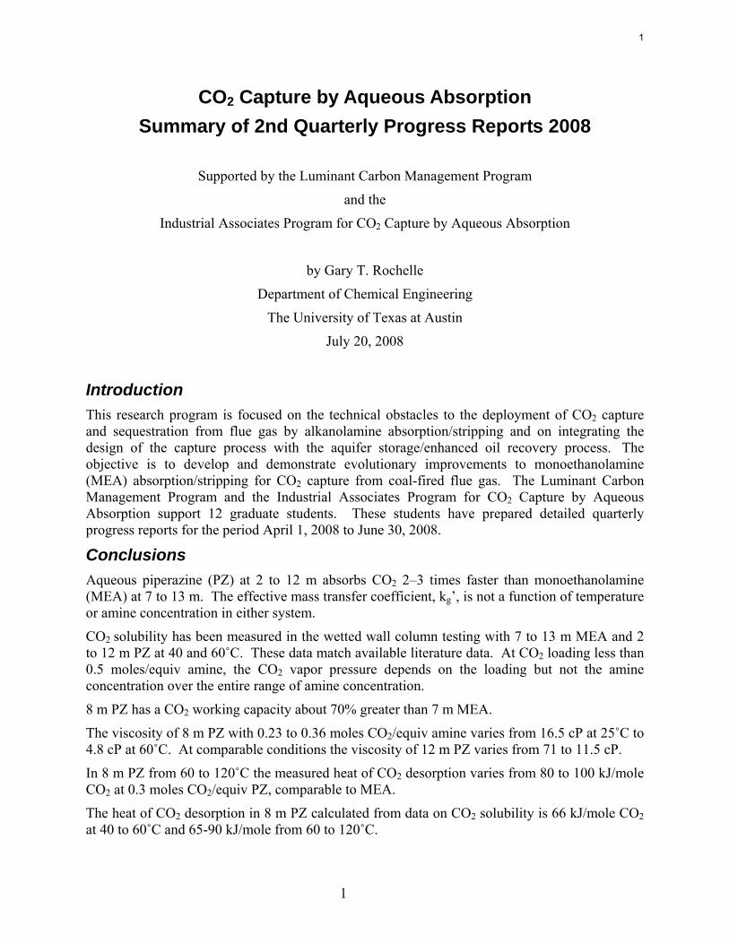
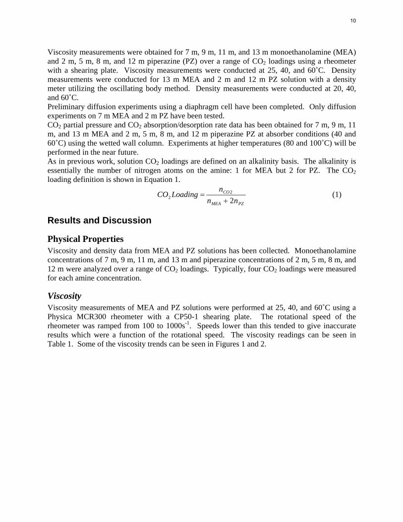
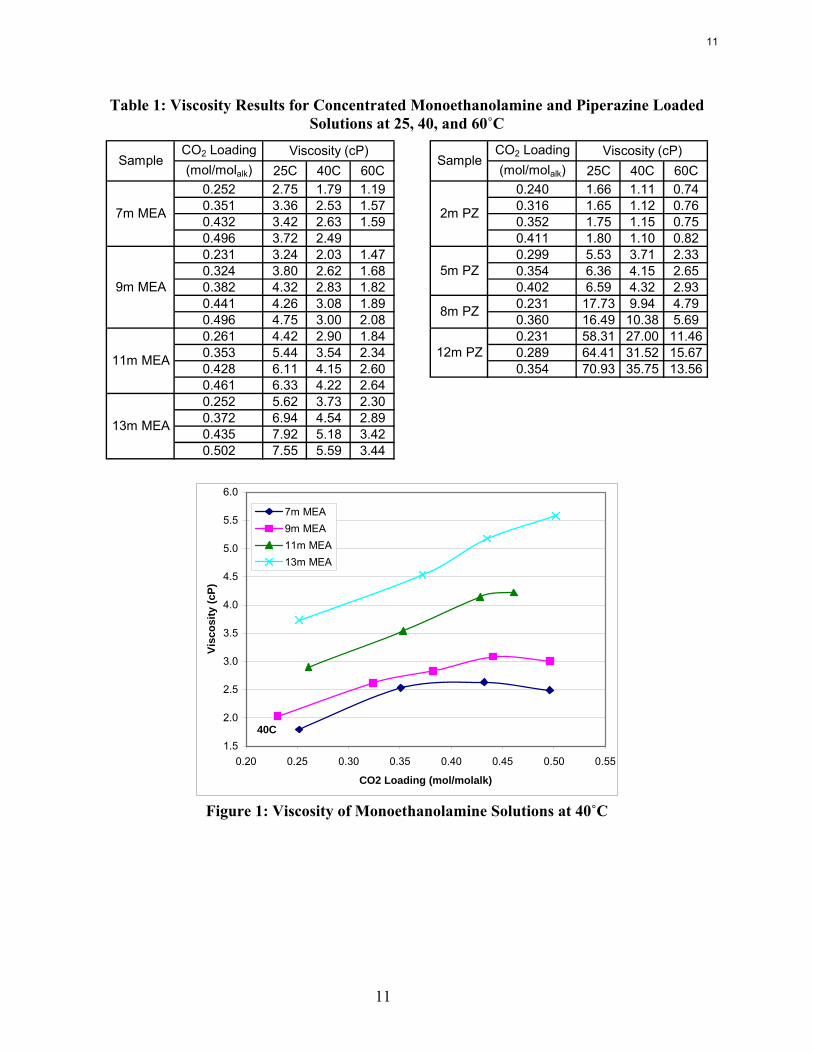
Viscosity Viscosity measurements of MEA and PZ solutions were performed at 25, 40, and 60˚C using a Physica MCR300 rheometer with a CP50-1 shearing plate. The rotational speed of the rheometer was ramped from 100 to 1000s-1. Speeds lower than this tended to give inaccurate results which were a function of the rotational speed. The viscosity readings can be seen in Table 1. Some of the viscosity trends can be seen in Figures 1 and 2.

10

11

Table 1: Viscosity Results for Concentrated Monoethanolamine and Piperazine Loaded Solutions at 25, 40, and 60˚C

CO2 Loading CO2 Loading(mol/molalk) 25C 40C 60C (mol/molalk) 25C 40C 60C

0.252 2.75 1.79 1.19 0.240 1.66 1.11 0.740.351 3.36 2.53 1.57 0.316 1.65 1.12 0.760.432 3.42 2.63 1.59 0.352 1.75 1.15 0.750.496 3.72 2.49 0.411 1.80 1.10 0.820.231 3.24 2.03 1.47 0.299 5.53 3.71 2.330.324 3.80 2.62 1.68 0.354 6.36 4.15 2.650.382 4.32 2.83 1.82 0.402 6.59 4.32 2.930.441 4.26 3.08 1.89 0.231 17.73 9.94 4.790.496 4.75 3.00 2.08 0.360 16.49 10.38 5.690.261 4.42 2.90 1.84 0.231 58.31 27.00 11.460.353 5.44 3.54 2.34 0.289 64.41 31.52 15.670.428 6.11 4.15 2.60 0.354 70.93 35.75 13.560.461 6.33 4.22 2.640.252 5.62 3.73 2.300.372 6.94 4.54 2.890.435 7.92 5.18 3.420.502 7.55 5.59 3.44

Viscosity (cP)Sample

7m MEA

9m MEA

11m MEA

13m MEA

2m PZ

5m PZ

8m PZ

12m PZ

SampleViscosity (cP)

40C1.5

2.0

2.5

3.0

3.5

4.0

4.5

5.0

5.5

6.0

0.20 0.25 0.30 0.35 0.40 0.45 0.50 0.55

CO2 Loading (mol/molalk)

Visc

osity

(cP)

7m MEA9m MEA11m MEA13m MEA

Figure 1: Viscosity of Monoethanolamine Solutions at 40˚C

11

12

40C1

10

100

0.20 0.25 0.30 0.35 0.40 0.45

CO2 Loading (mol/molalk)

Visc

osity

(cP)

2m PZ5m PZ8m PZ12m PZ

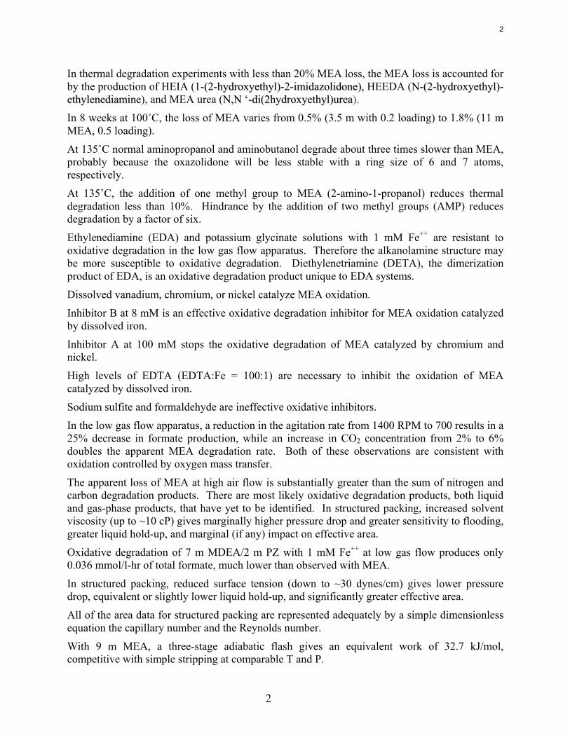
Figure 2: Viscosity of Piperazine Solutions at 40˚C

The viscosity of both MEA and PZ solutions increases with increases in amine concentration. However, the viscosity of the piperazine solutions increases much faster such that the viscosities can become prohibitive for CO2 absorption processes. These sharp increases in viscosity may be due to the fact that piperazine is a solid at room temperature whereas MEA is a liquid. Regardless, the viscosity will play a major part in the selection of a suitable amine concentration if piperazine is used for CO2 absorption.

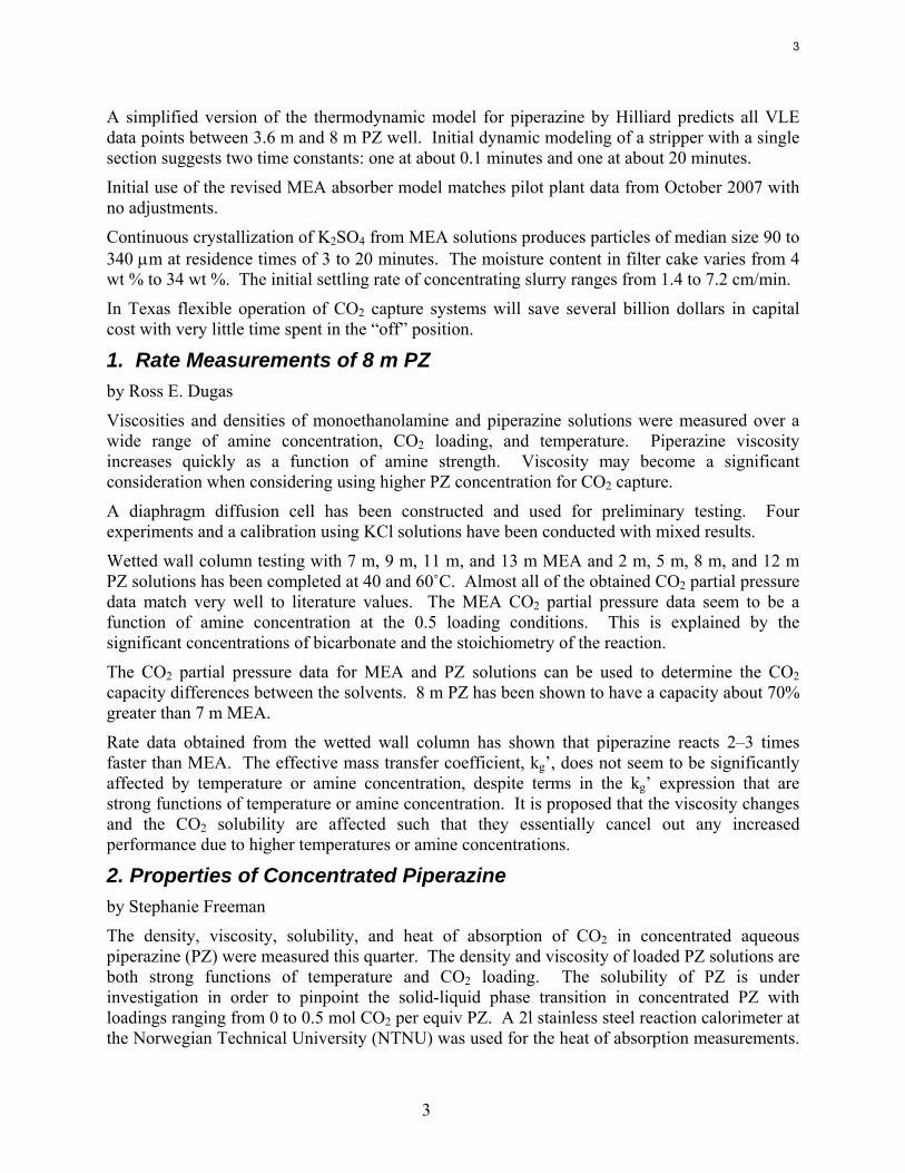
7m MEA = Filled Points2m PZ = Empty Points

0.5

1.0

1.5

2.0

2.5

3.0

3.5

4.0

0.20 0.25 0.30 0.35 0.40 0.45 0.50 0.55

CO2 Loading (mol/molalk)

Visc

osity

(cP)

25C40C60C

Figure 3: 7 m MEA and 2 m PZ Viscosity Data at 25, 40, and 60˚C

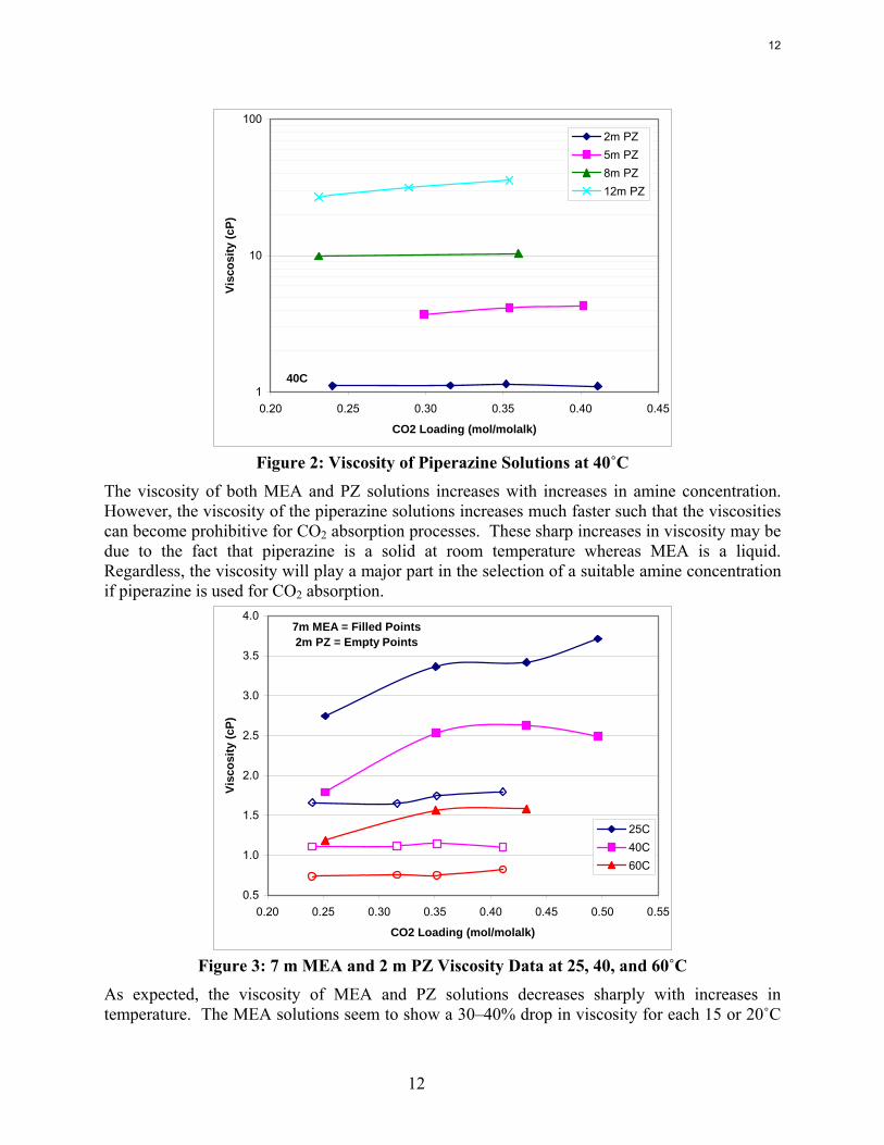
As expected, the viscosity of MEA and PZ solutions decreases sharply with increases in temperature. The MEA solutions seem to show a 30–40% drop in viscosity for each 15 or 20˚C

12

13

temperature increase. 2 m and 5 m piperazine solutions show a 30–40% drop in viscosity for the 15 and 20˚C temperature increases. 8 m PZ solutions tend to drop 40–50% while 12 m PZ solutions tend to drop 50–60% for each temperature change.

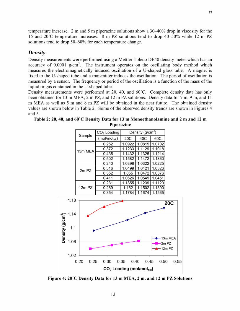
Density Density measurements were performed using a Mettler Toledo DE40 density meter which has an accuracy of 0.0001 g/cm3. The instrument operates on the oscillating body method which measures the electromagnetically induced oscillation of a U-shaped glass tube. A magnet is fixed to the U-shaped tube and a transmitter induces the oscillation. The period of oscillation is measured by a sensor. The frequency or period of the oscillation is a function of the mass of the liquid or gas contained in the U-shaped tube. Density measurements were performed at 20, 40, and 60˚C. Complete density data has only been obtained for 13 m MEA, 2 m PZ, and 12 m PZ solutions. Density data for 7 m, 9 m, and 11 m MEA as well as 5 m and 8 m PZ will be obtained in the near future. The obtained density values are shown below in Table 2. Some of the observed density trends are shown in Figures 4 and 5.

Table 2: 20, 40, and 60˚C Density Data for 13 m Monoethanolamine and 2 m and 12 m Piperazine

CO2 Loading(mol/molalk) 20C 40C 60C

0.252 1.0922 1.0815 1.07020.372 1.1233 1.1129 1.10180.435 1.1432 1.1325 1.12140.502 1.1582 1.1472 1.13600.240 1.0398 1.0322 1.02250.316 1.0499 1.0421 1.03260.352 1.055 1.0472 1.03760.411 1.0626 1.0549 1.04510.231 1.1355 1.1239 1.11200.289 1.162 1.1502 1.13900.354 1.1784 1.1674 1.1565

Density (g/cm3)

13m MEA

2m PZ

12m PZ

Sample

20C

1.02

1.06

1.1

1.14

1.18

0.20 0.25 0.30 0.35 0.40 0.45 0.50 0.55

CO2 Loading (mol/molalk)

Den

sity

(g/c

m3 )

13m MEA2m PZ12m PZ

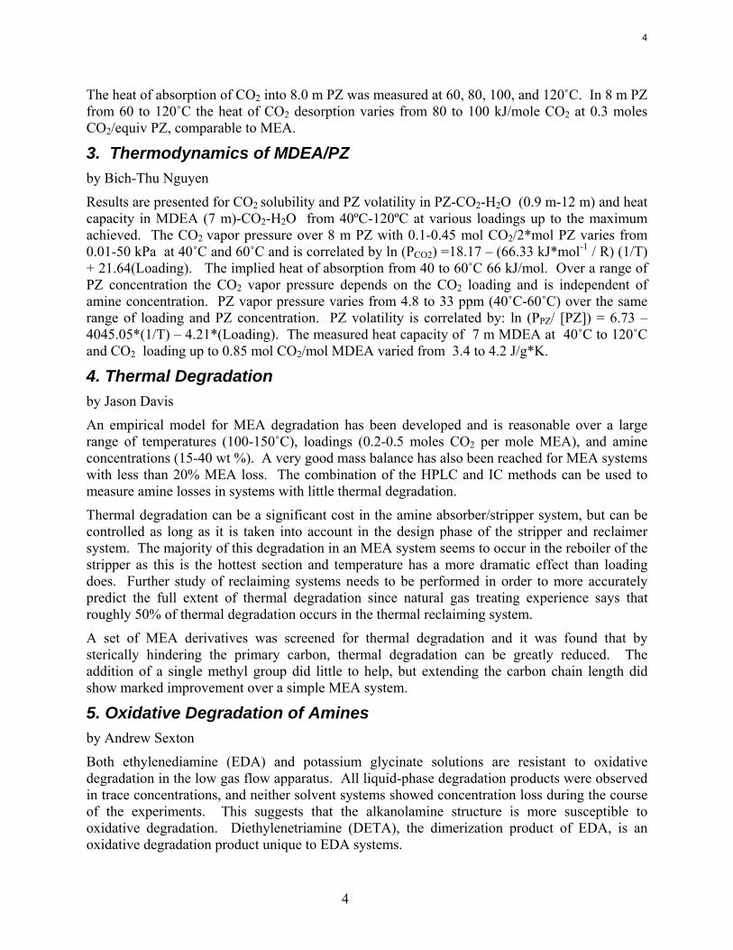
Figure 4: 20˚C Density Data for 13 m MEA, 2 m, and 12 m PZ Solutions

13

14

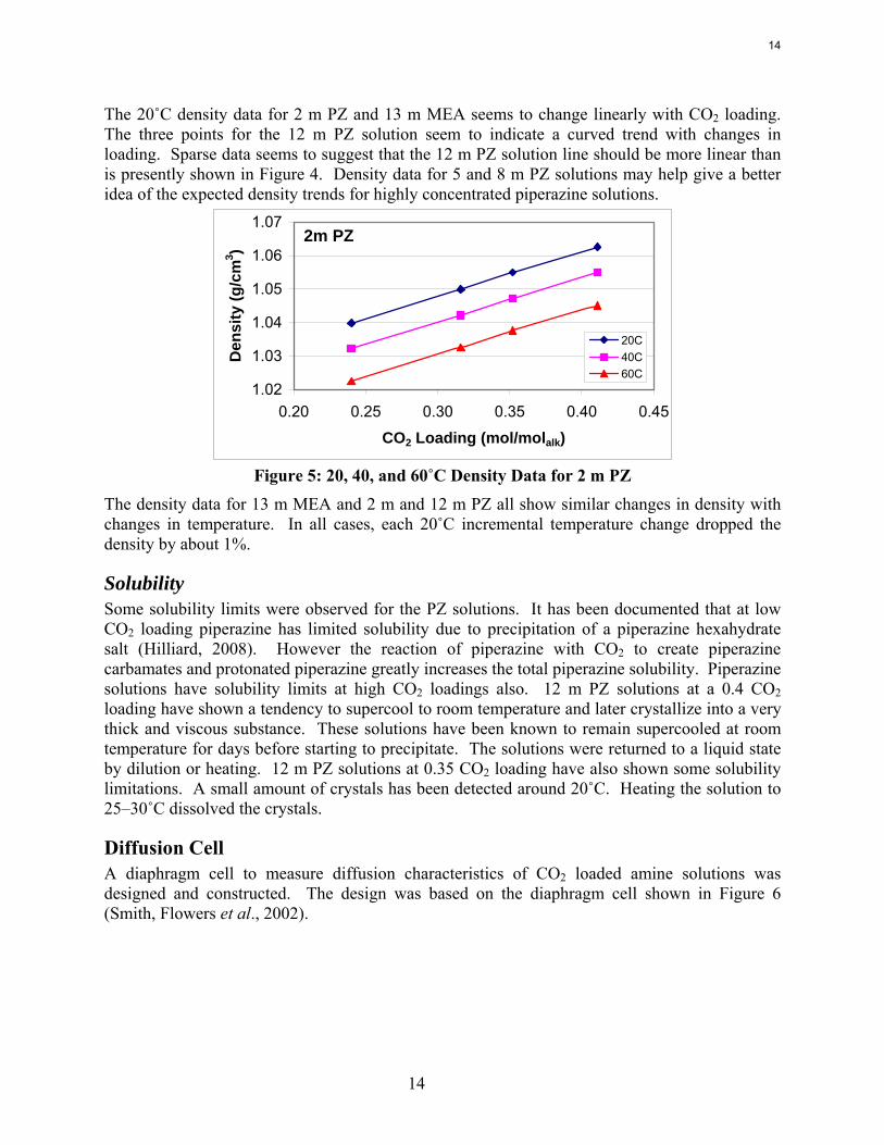
The 20˚C density data for 2 m PZ and 13 m MEA seems to change linearly with CO2 loading. The three points for the 12 m PZ solution seem to indicate a curved trend with changes in loading. Sparse data seems to suggest that the 12 m PZ solution line should be more linear than is presently shown in Figure 4. Density data for 5 and 8 m PZ solutions may help give a better idea of the expected density trends for highly concentrated piperazine solutions.

2m PZ

1.02

1.03

1.04

1.05

1.06

1.07

0.20 0.25 0.30 0.35 0.40 0.45

CO2 Loading (mol/molalk)

Den

sity

(g/c

m3 )

20C40C60C

Figure 5: 20, 40, and 60˚C Density Data for 2 m PZ

The density data for 13 m MEA and 2 m and 12 m PZ all show similar changes in density with changes in temperature. In all cases, each 20˚C incremental temperature change dropped the density by about 1%.

Solubility Some solubility limits were observed for the PZ solutions. It has been documented that at low CO2 loading piperazine has limited solubility due to precipitation of a piperazine hexahydrate salt (Hilliard, 2008). However the reaction of piperazine with CO2 to create piperazine carbamates and protonated piperazine greatly increases the total piperazine solubility. Piperazine solutions have solubility limits at high CO2 loadings also. 12 m PZ solutions at a 0.4 CO2 loading have shown a tendency to supercool to room temperature and later crystallize into a very thick and viscous substance. These solutions have been known to remain supercooled at room temperature for days before starting to precipitate. The solutions were returned to a liquid state by dilution or heating. 12 m PZ solutions at 0.35 CO2 loading have also shown some solubility limitations. A small amount of crystals has been detected around 20˚C. Heating the solution to 25–30˚C dissolved the crystals.

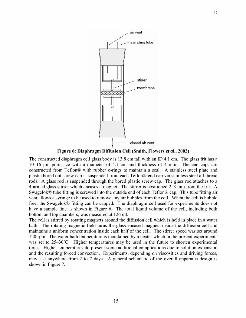
Diffusion Cell A diaphragm cell to measure diffusion characteristics of CO2 loaded amine solutions was designed and constructed. The design was based on the diaphragm cell shown in Figure 6 (Smith, Flowers et al., 2002).

14

15

Figure 6: Diaphragm Diffusion Cell (Smith, Flowers et al., 2002)

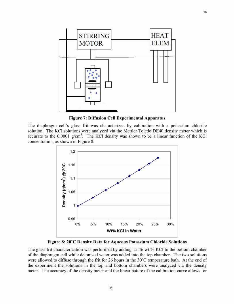
The constructed diaphragm cell glass body is 13.8 cm tall with an ID 4.1 cm. The glass frit has a 10–16 μm pore size with a diameter of 4.1 cm and thickness of 4 mm. The end caps are constructed from Teflon® with rubber o-rings to maintain a seal. A stainless steel plate and plastic bored out screw cap is suspended from each Teflon® end cap via stainless steel all thread rods. A glass rod is suspended through the bored plastic screw cap. The glass rod attaches to a 4-armed glass stirrer which encases a magnet. The stirrer is positioned 2–3 mm from the frit. A Swagelok® tube fitting is screwed into the outside end of each Teflon® cap. This tube fitting air vent allows a syringe to be used to remove any air bubbles from the cell. When the cell is bubble free, the Swagelok® fitting can be capped. The diaphragm cell used for experiments does not have a sample line as shown in Figure 6. The total liquid volume of the cell, including both bottom and top chambers, was measured at 126 ml. The cell is stirred by rotating magnets around the diffusion cell which is held in place in a water bath. The rotating magnetic field turns the glass encased magnets inside the diffusion cell and maintains a uniform concentration inside each half of the cell. The stirrer speed was set around 120 rpm. The water bath temperature is maintained by a heater which in the present experiments was set to 25–30˚C. Higher temperatures may be used in the future to shorten experimental times. Higher temperatures do present some additional complications due to solution expansion and the resulting forced convection. Experiments, depending on viscosities and driving forces, may last anywhere from 2 to 7 days. A general schematic of the overall apparatus design is shown in Figure 7.

15

16

Figure 7: Diffusion Cell Experimental Apparatus

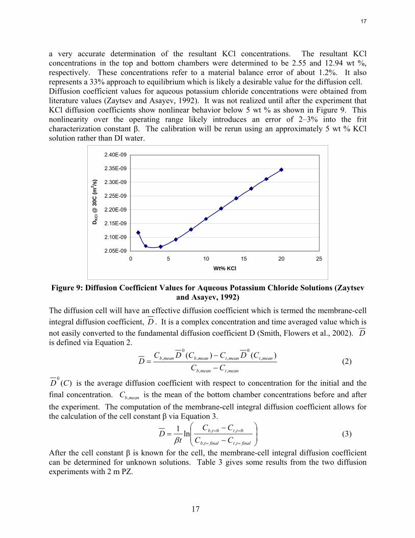
The diaphragm cell’s glass frit was characterized by calibration with a potassium chloride solution. The KCl solutions were analyzed via the Mettler Toledo DE40 density meter which is accurate to the 0.0001 g/cm3. The KCl density was shown to be a linear function of the KCl concentration, as shown in Figure 8.

0.95

1

1.05

1.1

1.15

1.2

0% 5% 10% 15% 20% 25% 30%

Wt% KCl in Water

Den

sity

(g/c

m3 ) @

20C

Figure 8: 20˚C Density Data for Aqueous Potassium Chloride Solutions

The glass frit characterization was performed by adding 15.46 wt % KCl to the bottom chamber of the diaphragm cell while deionized water was added into the top chamber. The two solutions were allowed to diffuse through the frit for 26 hours in the 30˚C temperature bath. At the end of the experiment the solutions in the top and bottom chambers were analyzed via the density meter. The accuracy of the density meter and the linear nature of the calibration curve allows for

16

17

a very accurate determination of the resultant KCl concentrations. The resultant KCl concentrations in the top and bottom chambers were determined to be 2.55 and 12.94 wt %, respectively. These concentrations refer to a material balance error of about 1.2%. It also represents a 33% approach to equilibrium which is likely a desirable value for the diffusion cell. Diffusion coefficient values for aqueous potassium chloride concentrations were obtained from literature values (Zaytsev and Asayev, 1992). It was not realized until after the experiment that KCl diffusion coefficients show nonlinear behavior below 5 wt % as shown in Figure 9. This nonlinearity over the operating range likely introduces an error of 2–3% into the frit characterization constant β. The calibration will be rerun using an approximately 5 wt % KCl solution rather than DI water.

2.05E-09

2.10E-09

2.15E-09

2.20E-09

2.25E-09

2.30E-09

2.35E-09

2.40E-09

0 5 10 15 20 25

Wt% KCl

DK

Cl @

30C

(m2 /s

)

Figure 9: Diffusion Coefficient Values for Aqueous Potassium Chloride Solutions (Zaytsev

and Asayev, 1992) The diffusion cell will have an effective diffusion coefficient which is termed the membrane-cell integral diffusion coefficient, D . It is a complex concentration and time averaged value which is not easily converted to the fundamental diffusion coefficient D (Smith, Flowers et al., 2002). D is defined via Equation 2.

meantmeanb

meantmeantmeanbmeanb

CCCDCCDC

D,,

,

0

,,

0

, )()(−

−= (2)

)(0

CD is the average diffusion coefficient with respect to concentration for the initial and the final concentration. meanbC , is the mean of the bottom chamber concentrations before and after the experiment. The computation of the membrane-cell integral diffusion coefficient allows for the calculation of the cell constant β via Equation 3.

⎟⎟⎠

⎞⎜⎜⎝

⎛

−

−=

==

==

finalttfinaltb

tttb

CCCC

tD

,,

0,0,ln1β

(3)

After the cell constant β is known for the cell, the membrane-cell integral diffusion coefficient can be determined for unknown solutions. Table 3 gives some results from the two diffusion experiments with 2 m PZ.

17

18

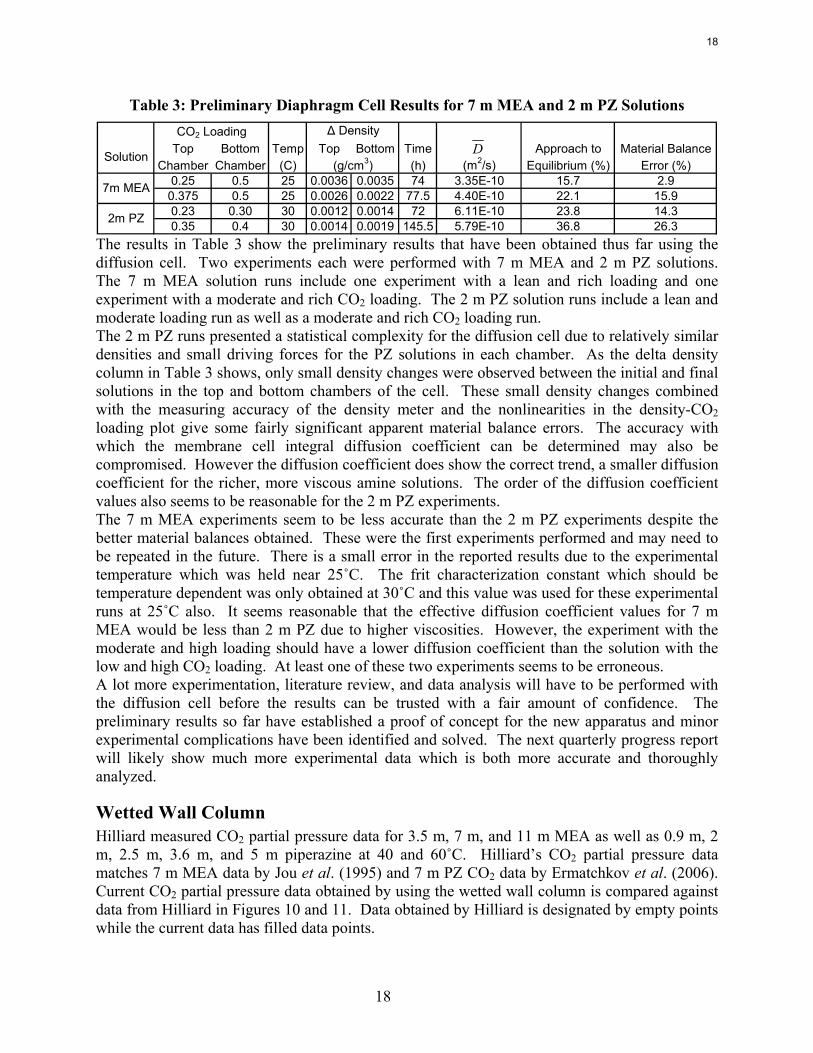
Table 3: Preliminary Diaphragm Cell Results for 7 m MEA and 2 m PZ Solutions

Top Bottom Temp Top Bottom Time Approach to Material BalanceChamber Chamber (C) (h) (m2/s) Equilibrium (%) Error (%)

0.25 0.5 25 0.0036 0.0035 74 3.35E-10 15.7 2.90.375 0.5 25 0.0026 0.0022 77.5 4.40E-10 22.1 15.90.23 0.30 30 0.0012 0.0014 72 6.11E-10 23.8 14.30.35 0.4 30 0.0014 0.0019 145.5 5.79E-10 36.8 26.3

CO2 Loading

2m PZ

7m MEA

(g/cm3)

Δ Density

Solution D

The results in Table 3 show the preliminary results that have been obtained thus far using the diffusion cell. Two experiments each were performed with 7 m MEA and 2 m PZ solutions. The 7 m MEA solution runs include one experiment with a lean and rich loading and one experiment with a moderate and rich CO2 loading. The 2 m PZ solution runs include a lean and moderate loading run as well as a moderate and rich CO2 loading run. The 2 m PZ runs presented a statistical complexity for the diffusion cell due to relatively similar densities and small driving forces for the PZ solutions in each chamber. As the delta density column in Table 3 shows, only small density changes were observed between the initial and final solutions in the top and bottom chambers of the cell. These small density changes combined with the measuring accuracy of the density meter and the nonlinearities in the density-CO2 loading plot give some fairly significant apparent material balance errors. The accuracy with which the membrane cell integral diffusion coefficient can be determined may also be compromised. However the diffusion coefficient does show the correct trend, a smaller diffusion coefficient for the richer, more viscous amine solutions. The order of the diffusion coefficient values also seems to be reasonable for the 2 m PZ experiments. The 7 m MEA experiments seem to be less accurate than the 2 m PZ experiments despite the better material balances obtained. These were the first experiments performed and may need to be repeated in the future. There is a small error in the reported results due to the experimental temperature which was held near 25˚C. The frit characterization constant which should be temperature dependent was only obtained at 30˚C and this value was used for these experimental runs at 25˚C also. It seems reasonable that the effective diffusion coefficient values for 7 m MEA would be less than 2 m PZ due to higher viscosities. However, the experiment with the moderate and high loading should have a lower diffusion coefficient than the solution with the low and high CO2 loading. At least one of these two experiments seems to be erroneous. A lot more experimentation, literature review, and data analysis will have to be performed with the diffusion cell before the results can be trusted with a fair amount of confidence. The preliminary results so far have established a proof of concept for the new apparatus and minor experimental complications have been identified and solved. The next quarterly progress report will likely show much more experimental data which is both more accurate and thoroughly analyzed.

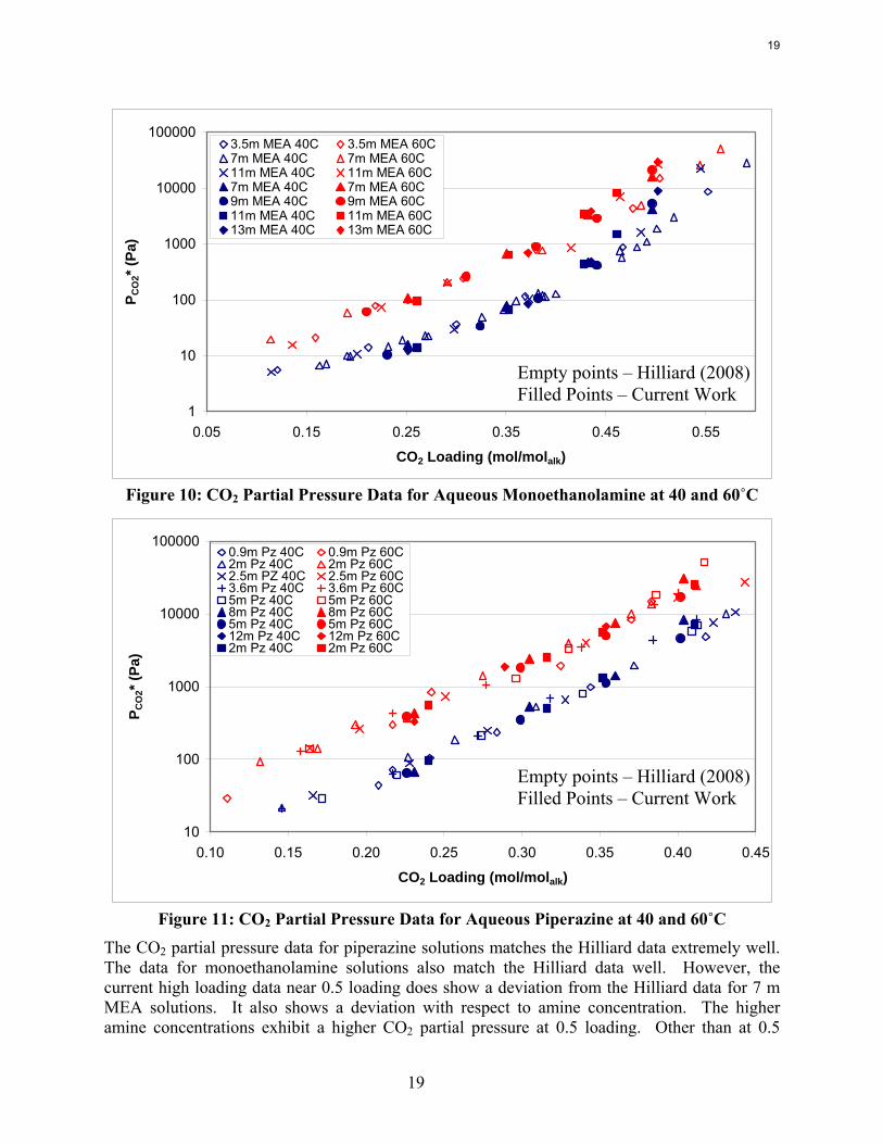
Wetted Wall Column Hilliard measured CO2 partial pressure data for 3.5 m, 7 m, and 11 m MEA as well as 0.9 m, 2 m, 2.5 m, 3.6 m, and 5 m piperazine at 40 and 60˚C. Hilliard’s CO2 partial pressure data matches 7 m MEA data by Jou et al. (1995) and 7 m PZ CO2 data by Ermatchkov et al. (2006). Current CO2 partial pressure data obtained by using the wetted wall column is compared against data from Hilliard in Figures 10 and 11. Data obtained by Hilliard is designated by empty points while the current data has filled data points.

18

19

1

10

100

1000

10000

100000

0.05 0.15 0.25 0.35 0.45 0.55

CO2 Loading (mol/molalk)

P CO

2* (P

a)3.5m MEA 40C 3.5m MEA 60C7m MEA 40C 7m MEA 60C11m MEA 40C 11m MEA 60C7m MEA 40C 7m MEA 60C9m MEA 40C 9m MEA 60C11m MEA 40C 11m MEA 60C13m MEA 40C 13m MEA 60C

Figure 10: CO2 Partial Pressure Data for Aqueous Monoethanolamine at 40 and 60˚C

10

100

1000

10000

100000

0.10 0.15 0.20 0.25 0.30 0.35 0.40 0.45

CO2 Loading (mol/molalk)

P CO

2* (P

a)

0.9m Pz 40C 0.9m Pz 60C2m Pz 40C 2m Pz 60C2.5m PZ 40C 2.5m Pz 60C3.6m Pz 40C 3.6m Pz 60C5m Pz 40C 5m Pz 60C8m Pz 40C 8m Pz 60C5m Pz 40C 5m Pz 60C12m Pz 40C 12m Pz 60C2m Pz 40C 2m Pz 60C

Figure 11: CO2 Partial Pressure Data for Aqueous Piperazine at 40 and 60˚C

The CO2 partial pressure data for piperazine solutions matches the Hilliard data extremely well. The data for monoethanolamine solutions also match the Hilliard data well. However, the current high loading data near 0.5 loading does show a deviation from the Hilliard data for 7 m MEA solutions. It also shows a deviation with respect to amine concentration. The higher amine concentrations exhibit a higher CO2 partial pressure at 0.5 loading. Other than at 0.5

Empty points – Hilliard (2008) Filled Points – Current Work

Empty points – Hilliard (2008) Filled Points – Current Work

19

20

loading, the CO2 partial pressure is independent of changes in amine concentration. This trend is expected and can be easily explained by the significant concentrations of bicarbonate which are present at 0.5 loading. This effect is due to the chemistry of the two reactions shown in Equations 4 and 5. It is correct to assume that MEA is the most likely base which will be protonated. −+ +↔+ MEACOOMEAHCOMEA 22 (4) −+ +↔++ 322 HCOMEAHOHCOMEA (5) The equilibrium rate constant of Equation 4 can be written as shown in Equation 6. It is important to remember that the [MEA] is the free or un-reacted concentration of MEA, not the total MEA concentration.

2

2, ][]][[

COcarbamateeq PMEA

MEAHMEACOOK+−

= (6)

Since this analysis only concerns carbamate production and bicarbonate production is considered insignificant, the following assumptions are valid and relate [MEACOO-], [MEAH+], and [MEA]. TotalMEAldgMEACOOMEA ][][][ == −+ (7) TotalMEAldgMEA ])[21(][ −= (8) Equations 7 and 8 can then be substituted into Equation 6 which is reorganized to solve for the CO2 partial pressure.

2,

2

22

22

2 )21(][)21(][

ldgKldg

MEAldgKMEAldg

PcarbamateeqTotaleq

TotalCO −

=−

= (9)

So according to Equation 9, the partial pressure of CO2 is independent of amine concentration when only carbamate is produced. When the same analysis is performed for the bicarbonate formation reaction, Equation 10, it can be seen that the partial pressure of CO2 is proportional to the total amine concentration. This does assume that the speciation of the solution is independent of the amine concentration which is not quite true. However the speciation remains constant enough that the assumption does not discredit the analysis. Therefore, it should be expected that the CO2 partial pressure should be a function of MEA concentration at very high loadings where bicarbonate formation is significant. Although PZ concentrations near 0.4 loading exhibit similar partial pressures to MEA solutions at 0.5 loading, the bicarbonate concentrations are much lower so this phenomenon is not seen. Figures 10 and 11 seem to show exactly the partial pressure trends that should be expected for MEA and PZ solutions.

)1(

][

,

2

2 ldgKMEAldg

Pebicarbonateq

TotalCO −

= (10)

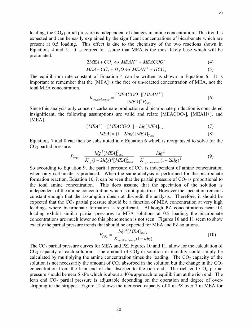
The CO2 partial pressure curves for MEA and PZ, Figures 10 and 11, allow for the calculation of CO2 capacity of each solution. The amount of CO2 in solution in molality could simply be calculated by multiplying the amine concentration times the loading. The CO2 capacity of the solution is not necessarily the amount of CO2 absorbed in the solution but the change in the CO2 concentration from the lean end of the absorber to the rich end. The rich end CO2 partial pressure should be near 5 kPa which is about a 40% approach to equilibrium at the rich end. The lean end CO2 partial pressure is adjustable depending on the operation and degree of over-stripping in the stripper. Figure 12 shows the increased capacity of 8 m PZ over 7 m MEA for

20

21

various values of lean partial pressure. It also shows some values of loading that correspond to the data points on the curves.

10

100

1000

10000

0.0 0.5 1.0 1.5 2.0 2.5

CO2 Capacity with a 5 kPa Rich Soln(mol CO2/kg(water+amine))

Lean

Par

tial P

ress

ure

(Pa)

.36 Ldg

.31

.23

.15

.47 Ldg

.31

.197m MEA

8m PZ

40˚C

Figure 12: CO2 Capacity of 7 m MEA and 8 m PZ Assuming a 5 kPa Rich Solution

Equilibrium CO2 Partial Pressure The correct basis to calculate capacity is most likely a CO2-free basis. The advantages of solution capacity are based on saving due to the sensible heat requirements of heating the stripper rich solution to the stripper lean temperature. Heat capacity data and cross-exchanger experience with MEA has shown that CO2 has nearly a zero net heat capacity. Essentially 2 moles of MEA has the same heat capacity as MEA carbamate plus protonated MEA on a mole basis. Therefore the amount of CO2 in the solution is not important and should be ignored. On a CO2-free basis 8 m PZ seems to have a capacity about 70% greater than 7 m MEA. CO2 absorption/desorption rate data for MEA and PZ solutions has been completed at 40 and 60˚C. 7 m, 9 m, 11 m, and 13 m MEA solutions and 2 m, 5 m, 8 m, and 12 m PZ solutions were tested. Figure 13 shows all the rate data for both the MEA and PZ solutions. In Figure 13, the open points represent MEA solutions while the filled points represent PZ solutions. The blue points represent 40˚C while 60˚C data points are designated by red markers. Rate measurements were obtained for at least 4 loadings for each solution at each temperature with the exception of 12 m PZ. 12 m PZ solutions were only analyzed at 60˚C. The solution was too viscous at 40˚C to effectively run experiments in the wetted wall column.

21

22

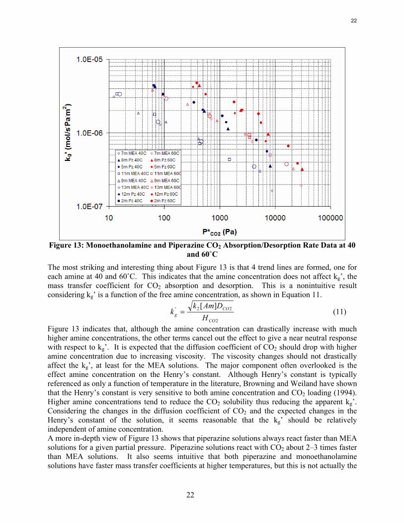
Figure 13: Monoethanolamine and Piperazine CO2 Absorption/Desorption Rate Data at 40

and 60˚C

The most striking and interesting thing about Figure 13 is that 4 trend lines are formed, one for each amine at 40 and 60˚C. This indicates that the amine concentration does not affect kg’, the mass transfer coefficient for CO2 absorption and desorption. This is a nonintuitive result considering kg’ is a function of the free amine concentration, as shown in Equation 11.

2

22' ][

CO

COg H

DAmkk = (11)

Figure 13 indicates that, although the amine concentration can drastically increase with much higher amine concentrations, the other terms cancel out the effect to give a near neutral response with respect to kg’. It is expected that the diffusion coefficient of CO2 should drop with higher amine concentration due to increasing viscosity. The viscosity changes should not drastically affect the kg’, at least for the MEA solutions. The major component often overlooked is the effect amine concentration on the Henry’s constant. Although Henry’s constant is typically referenced as only a function of temperature in the literature, Browning and Weiland have shown that the Henry’s constant is very sensitive to both amine concentration and CO2 loading (1994). Higher amine concentrations tend to reduce the CO2 solubility thus reducing the apparent kg’. Considering the changes in the diffusion coefficient of CO2 and the expected changes in the Henry’s constant of the solution, it seems reasonable that the kg’ should be relatively independent of amine concentration. A more in-depth view of Figure 13 shows that piperazine solutions always react faster than MEA solutions for a given partial pressure. Piperazine solutions react with CO2 about 2–3 times faster than MEA solutions. It also seems intuitive that both piperazine and monoethanolamine solutions have faster mass transfer coefficients at higher temperatures, but this is not actually the

22

23

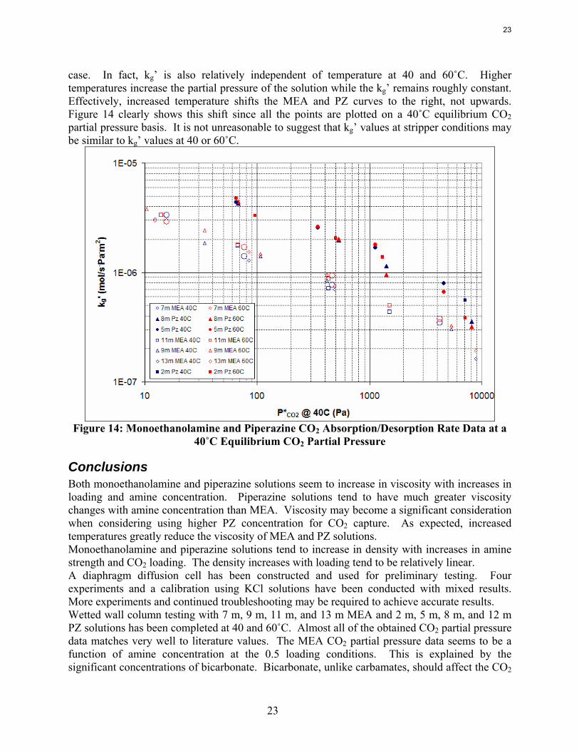
case. In fact, kg’ is also relatively independent of temperature at 40 and 60˚C. Higher temperatures increase the partial pressure of the solution while the kg’ remains roughly constant. Effectively, increased temperature shifts the MEA and PZ curves to the right, not upwards. Figure 14 clearly shows this shift since all the points are plotted on a 40˚C equilibrium CO2 partial pressure basis. It is not unreasonable to suggest that kg’ values at stripper conditions may be similar to kg’ values at 40 or 60˚C.

Figure 14: Monoethanolamine and Piperazine CO2 Absorption/Desorption Rate Data at a

40˚C Equilibrium CO2 Partial Pressure

Conclusions Both monoethanolamine and piperazine solutions seem to increase in viscosity with increases in loading and amine concentration. Piperazine solutions tend to have much greater viscosity changes with amine concentration than MEA. Viscosity may become a significant consideration when considering using higher PZ concentration for CO2 capture. As expected, increased temperatures greatly reduce the viscosity of MEA and PZ solutions. Monoethanolamine and piperazine solutions tend to increase in density with increases in amine strength and CO2 loading. The density increases with loading tend to be relatively linear. A diaphragm diffusion cell has been constructed and used for preliminary testing. Four experiments and a calibration using KCl solutions have been conducted with mixed results. More experiments and continued troubleshooting may be required to achieve accurate results. Wetted wall column testing with 7 m, 9 m, 11 m, and 13 m MEA and 2 m, 5 m, 8 m, and 12 m PZ solutions has been completed at 40 and 60˚C. Almost all of the obtained CO2 partial pressure data matches very well to literature values. The MEA CO2 partial pressure data seems to be a function of amine concentration at the 0.5 loading conditions. This is explained by the significant concentrations of bicarbonate. Bicarbonate, unlike carbamates, should affect the CO2

23

24

partial pressure based on the total concentration, not just the loading. The difference is based on the stoichiometry of the 2 reactions. The CO2 partial pressure data for MEA and PZ solutions can be used to determine the CO2 capacity differences between the solvents. 8 m PZ has been shown to have a capacity about 70% greater than 7 m MEA. This could result in significantly lower flow rates and decrease sensible heat requirements. Rate data obtained from the wetted wall column has shown that piperazine reacts 2–3 times faster than MEA. The effective mass transfer coefficient, kg’, does not seem to be significantly affected by temperature or amine concentration, despite terms in the kg’ expression that are strong functions of temperature or amine concentration. It is proposed that the viscosity changes and the CO2 solubility are affected such that they essentially cancel out any increased performance due to higher temperatures or amine concentrations.

References Browning GJ, Weiland RH. Physical Solubility of Carbon Dioxide in Aqueous Alkanolamine via

Nitrous Oxide Analogy. J Chem Eng Data.1994;39:817–822. Ermatchkov V, Perez-Salado Kamps A et al. Solubility of Carbon Dioxide in Aqueous Solutions

of Piperazine in the Low Gas Loading Region. J Chem Eng Data 2006;51(5):1788–1796. Hilliard M. A Predictive Thermodynamic Model for an Aqueous Blend of Potassium Carbonate,

Piperazine, and Monoethanolamine for Carbon Dioxide Capture from Flue Gas. University of Texas, Austin; 2008. Ph.D. Dissertation:1025.

Jou F-Y, Mather AE et al. The Solubility of CO2 in a 30 Mass Percent Monoethanolamine Solution. Can J Chem Eng 1995;73(1):140–147.

Smith MJ, Flowers TH et al. Method for the measurement of the diffusion coefficient of benzalkonium chloride. Water Research. 2002;36:1423–1428.

Zaytsev I, Asayev GG. Properties of Aqueous Solutions of Electrolytes. CRC Press Inc,1992.

24

25

Physical Properties and Heat of Absorption of Concentrated Aqueous Piperazine

Quarterly Report for April 1 – June 30, 2008

by Stephanie Freeman

Supported by the Luminant Carbon Management Program

and the

Industrial Associates Program for CO2 Capture by Aqueous Absorption

Department of Chemical Engineering

The University of Texas at Austin

July 25, 2008

Abstract The density of 8 m PZ ranged from 1.1113 g/cm3 at a loading of 0.235 mol CO2/equiv PZ to 1.1607 g/cm3 at a loading of 0.408. The density of 2, 5, and 20 m PZ ranged from 1.0068 g/cm3 for unloaded 2 m PZ to a maximum of 1.1664 g/cm3 for 20 m PZ with a loading of 0.248 mol CO2/equiv PZ. The viscosity of 8 m PZ ranged from 3.92 cP at 70°C and a loading of 0.24 to 22.78 cP at 20°C and a loading of 0.40 mol CO2/equiv PZ. The heat of absorption of CO2 into 8.0 m PZ increased as temperature increased and decreased as CO2 loading increased, following trends observed with other amines. At a loading of 0.025 mol CO2/equiv PZ, the heat of absorption was 90.3, 104.5, 115.7, and 123.1 kJ/mol CO2, respectively, at 60, 80, 100, and 120°C. After the initial loadings, there was little difference in the values for the heat of absorption between 80, 100, and 120°C. At all temperatures, the heat of absorption decreased as loading was increased and fell off as loading reached 0.4 mol CO2/equiv PZ, producing a trend different from other amines whose heat of absorption remains constant from loadings of 0 to 0.5 mol CO2/mol amine before dropping off.

Introduction Concentrated aqueous piperazine (PZ) is being investigated as a possible alternative to the standard 30 wt % (or 7 m) MEA in absorber/stripper systems to remove CO2 from coal-fired power plant flue gas. Aqueous PZ has been given a proprietary name of ROC20 for 10 m PZ and ROC16 for 8 m PZ. Previous reports include the proprietary name while the concentration of PZ will be explicitly used in this document.

Preliminary investigations of PZ have shown numerous advantages over 7 m MEA systems. Aqueous concentrated PZ produces less degradation both thermally and oxidatively as previously shown at concentrations of 5 and 8 m. The kinetics of CO2 absorption are faster in concentrated PZ, as shown by Tim Cullinane, and are currently being measured by Ross Dugas. The capacity of PZ is higher than that of MEA while the heat of absorption and volatilities are comparable.

As reported last quarter, the addition of copper catalyzed oxidative degradation of 8.0 m PZ to produce a variety of degradation products. On the other hand, the addition of iron, vanadium,

25

26

nickel, chromium, and copper in the presence of Inhibitor A did not significantly degrade the PZ. Under thermal stress, PZ showed appreciable degradation at 175°C while negligible degradation was observed at 135 and 150°C. Copper, iron, Inhibitor A, nickel, and chromium do not further catalyze the thermal degradation of 8 m PZ at 175°C.

This quarter was spent solely on the determination of density, viscosity, solubility, and the heat of absorption of CO2 into a variety of PZ solutions. Density measurements using the newly obtained Mettler-Toledo densitometer were performed on solutions ranging from of 2 to 20 m PZ. Viscosity measurements were performed on a cone and plate viscometer on solutions ranging from 5 to 12 m PZ. Solubility experiments were performed in an effort to understand the solubility window that exists for PZ solutions in terms of temperature, PZ concentration, and CO2 loading.

Previous work conducted by Inna Kim of NTNU and Marcus Hilliard determined the heat of absorption in MEA, MEA/PZ blends, K+/PZ blends, and 2.4 m PZ among other amine systems (Kim, 2007; Hilliard, 2008). No work at NTNU or discovered in the literature measured the heat of absorption in any PZ non-blended system with a concentration higher than 2.4 m PZ.

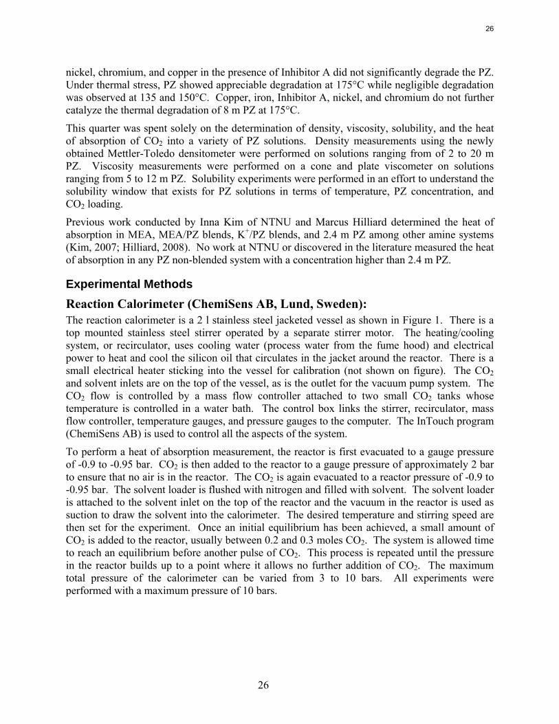
Experimental Methods Reaction Calorimeter (ChemiSens AB, Lund, Sweden): The reaction calorimeter is a 2 l stainless steel jacketed vessel as shown in Figure 1. There is a top mounted stainless steel stirrer operated by a separate stirrer motor. The heating/cooling system, or recirculator, uses cooling water (process water from the fume hood) and electrical power to heat and cool the silicon oil that circulates in the jacket around the reactor. There is a small electrical heater sticking into the vessel for calibration (not shown on figure). The CO2 and solvent inlets are on the top of the vessel, as is the outlet for the vacuum pump system. The CO2 flow is controlled by a mass flow controller attached to two small CO2 tanks whose temperature is controlled in a water bath. The control box links the stirrer, recirculator, mass flow controller, temperature gauges, and pressure gauges to the computer. The InTouch program (ChemiSens AB) is used to control all the aspects of the system.

To perform a heat of absorption measurement, the reactor is first evacuated to a gauge pressure of -0.9 to -0.95 bar. CO2 is then added to the reactor to a gauge pressure of approximately 2 bar to ensure that no air is in the reactor. The CO2 is again evacuated to a reactor pressure of -0.9 to -0.95 bar. The solvent loader is flushed with nitrogen and filled with solvent. The solvent loader is attached to the solvent inlet on the top of the reactor and the vacuum in the reactor is used as suction to draw the solvent into the calorimeter. The desired temperature and stirring speed are then set for the experiment. Once an initial equilibrium has been achieved, a small amount of CO2 is added to the reactor, usually between 0.2 and 0.3 moles CO2. The system is allowed time to reach an equilibrium before another pulse of CO2. This process is repeated until the pressure in the reactor builds up to a point where it allows no further addition of CO2. The maximum total pressure of the calorimeter can be varied from 3 to 10 bars. All experiments were performed with a maximum pressure of 10 bars.

26

27

Figure 1: Simplified Schematic of Reaction Calorimeter (ChemiSens AB)

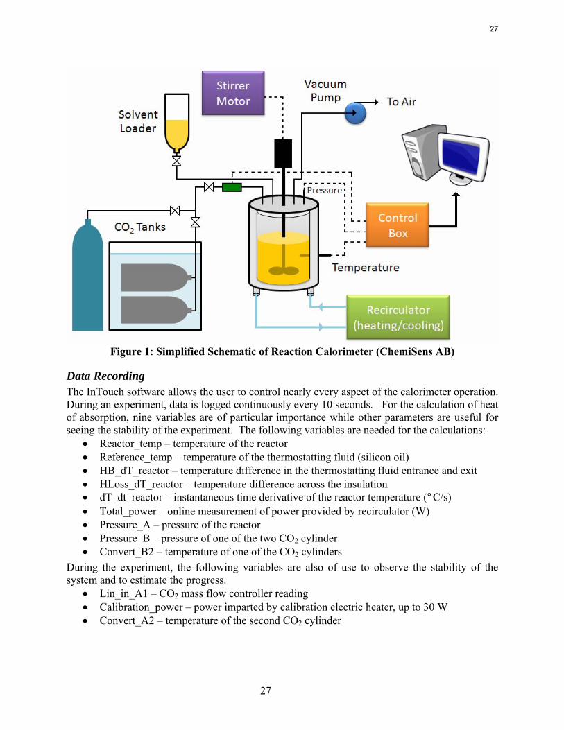
Data Recording The InTouch software allows the user to control nearly every aspect of the calorimeter operation. During an experiment, data is logged continuously every 10 seconds. For the calculation of heat of absorption, nine variables are of particular importance while other parameters are useful for seeing the stability of the experiment. The following variables are needed for the calculations:

• Reactor_temp – temperature of the reactor • Reference_temp – temperature of the thermostatting fluid (silicon oil) • HB_dT_reactor – temperature difference in the thermostatting fluid entrance and exit • HLoss_dT_reactor – temperature difference across the insulation • dT_dt_reactor – instantaneous time derivative of the reactor temperature (°C/s) • Total_power – online measurement of power provided by recirculator (W) • Pressure_A – pressure of the reactor • Pressure_B – pressure of one of the two CO2 cylinder • Convert_B2 – temperature of one of the CO2 cylinders

During the experiment, the following variables are also of use to observe the stability of the system and to estimate the progress.

• Lin_in_A1 – CO2 mass flow controller reading • Calibration_power – power imparted by calibration electric heater, up to 30 W • Convert_A2 – temperature of the second CO2 cylinder

27

28

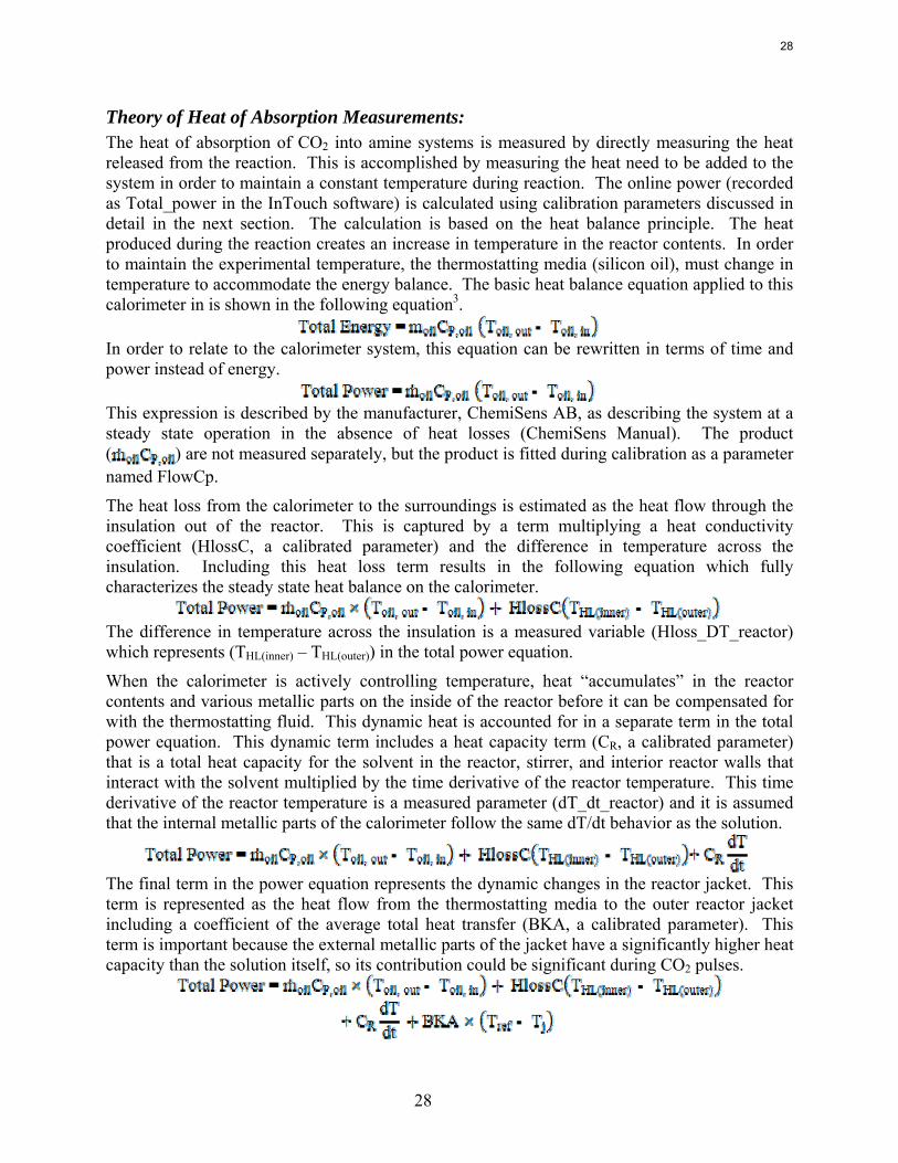
Theory of Heat of Absorption Measurements: The heat of absorption of CO2 into amine systems is measured by directly measuring the heat released from the reaction. This is accomplished by measuring the heat need to be added to the system in order to maintain a constant temperature during reaction. The online power (recorded as Total_power in the InTouch software) is calculated using calibration parameters discussed in detail in the next section. The calculation is based on the heat balance principle. The heat produced during the reaction creates an increase in temperature in the reactor contents. In order to maintain the experimental temperature, the thermostatting media (silicon oil), must change in temperature to accommodate the energy balance. The basic heat balance equation applied to this calorimeter in is shown in the following equation3.

In order to relate to the calorimeter system, this equation can be rewritten in terms of time and power instead of energy.

This expression is described by the manufacturer, ChemiSens AB, as describing the system at a steady state operation in the absence of heat losses (ChemiSens Manual). The product ( ) are not measured separately, but the product is fitted during calibration as a parameter named FlowCp.

The heat loss from the calorimeter to the surroundings is estimated as the heat flow through the insulation out of the reactor. This is captured by a term multiplying a heat conductivity coefficient (HlossC, a calibrated parameter) and the difference in temperature across the insulation. Including this heat loss term results in the following equation which fully characterizes the steady state heat balance on the calorimeter.

The difference in temperature across the insulation is a measured variable (Hloss_DT_reactor) which represents (THL(inner) – THL(outer)) in the total power equation.

When the calorimeter is actively controlling temperature, heat “accumulates” in the reactor contents and various metallic parts on the inside of the reactor before it can be compensated for with the thermostatting fluid. This dynamic heat is accounted for in a separate term in the total power equation. This dynamic term includes a heat capacity term (CR, a calibrated parameter) that is a total heat capacity for the solvent in the reactor, stirrer, and interior reactor walls that interact with the solvent multiplied by the time derivative of the reactor temperature. This time derivative of the reactor temperature is a measured parameter (dT_dt_reactor) and it is assumed that the internal metallic parts of the calorimeter follow the same dT/dt behavior as the solution.

The final term in the power equation represents the dynamic changes in the reactor jacket. This term is represented as the heat flow from the thermostatting media to the outer reactor jacket including a coefficient of the average total heat transfer (BKA, a calibrated parameter). This term is important because the external metallic parts of the jacket have a significantly higher heat capacity than the solution itself, so its contribution could be significant during CO2 pulses.

28

29

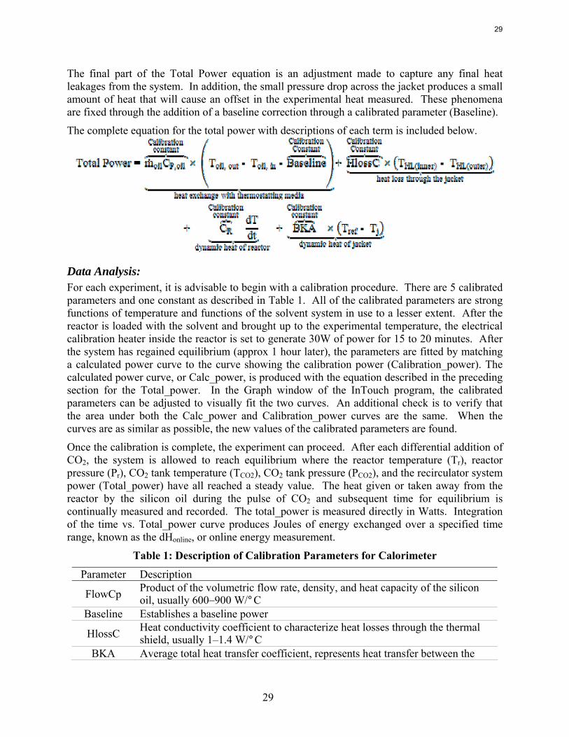
The final part of the Total Power equation is an adjustment made to capture any final heat leakages from the system. In addition, the small pressure drop across the jacket produces a small amount of heat that will cause an offset in the experimental heat measured. These phenomena are fixed through the addition of a baseline correction through a calibrated parameter (Baseline).

The complete equation for the total power with descriptions of each term is included below.

Data Analysis: For each experiment, it is advisable to begin with a calibration procedure. There are 5 calibrated parameters and one constant as described in Table 1. All of the calibrated parameters are strong functions of temperature and functions of the solvent system in use to a lesser extent. After the reactor is loaded with the solvent and brought up to the experimental temperature, the electrical calibration heater inside the reactor is set to generate 30W of power for 15 to 20 minutes. After the system has regained equilibrium (approx 1 hour later), the parameters are fitted by matching a calculated power curve to the curve showing the calibration power (Calibration_power). The calculated power curve, or Calc_power, is produced with the equation described in the preceding section for the Total_power. In the Graph window of the InTouch program, the calibrated parameters can be adjusted to visually fit the two curves. An additional check is to verify that the area under both the Calc_power and Calibration_power curves are the same. When the curves are as similar as possible, the new values of the calibrated parameters are found.

Once the calibration is complete, the experiment can proceed. After each differential addition of CO2, the system is allowed to reach equilibrium where the reactor temperature (Tr), reactor pressure (Pr), CO2 tank temperature (TCO2), CO2 tank pressure (PCO2), and the recirculator system power (Total_power) have all reached a steady value. The heat given or taken away from the reactor by the silicon oil during the pulse of CO2 and subsequent time for equilibrium is continually measured and recorded. The total_power is measured directly in Watts. Integration of the time vs. Total_power curve produces Joules of energy exchanged over a specified time range, known as the dHonline, or online energy measurement.

Table 1: Description of Calibration Parameters for Calorimeter

Parameter Description

FlowCp Product of the volumetric flow rate, density, and heat capacity of the silicon oil, usually 600–900 W/°C

Baseline Establishes a baseline power

HlossC Heat conductivity coefficient to characterize heat losses through the thermal shield, usually 1–1.4 W/°C

BKA Average total heat transfer coefficient, represents heat transfer between the

29

30

thermostatting media (silicon oil) and the outer reactor jacket, calibrated parameter based on dynamic system response during calibration

CB Heat capacity of the reactor jacket, constant for this calorimeter at 1500 J/°C

CR Heat capacity of the reactor contents, including the solution, contributions from the stirrer, reactor base, and interior walls; calibrated parameter based on solvent and temperature in use, usually 5500–7800 J/°C.

Once the dHonline is calculated, it can be directly associated with the amount of CO2 or amine to calculate the heat of absorption per mol CO2 or per mol amine. The amount of amine charged is known from when the solvent was loaded into the system at the beginning of the experiment. The amount of CO2 added to the calorimeter during each differential addition is calculated using the pressure-explicit version of the Peng-Robinson equation of state, whose terms are shown below (Smith et al., 1995; Tester & Modell, 1997).

The critical constants for CO2 used in the Peng-Robinson calculations are listed in Table 2.

Table 2: Critical Constants for CO2 (Perry, 1997)

Constant Value TC 304.21 K PC 73.9 bar ω 0.224

The moles of CO2 present in the CO2 storage tanks were calculated before and after each CO2 injection and the difference was the amount injected into the reactor. In the instances where the reactor pressure increased after a CO2 pulse, the change in vapor pressure of CO2 was calculated based on this pressure increase. The increase in reactor pressure was due to a portion of the CO2 not having been absorbed into the liquid because an equilibrium limit had been reached. The amount of CO2 remaining in the vapor phase was subtracted from the total amount added to the reactor to calculate the moles of CO2 that had been absorbed into the solvent during each CO2 pulse. Once the moles absorbed into the solvent were known, the loading at each point could be calculated based on the known amount of amine charged initially.

During the experiment, the progress was estimated by using the mass flow controller reading to estimate the amount of CO2 input into the reactor during each impulse. A calibration equation was used to produce a curve of the CO2 flow in liters per second. Integration of this curve over time produced a rough estimate of the liters of CO2 entering the reactor.

To perform these calculations, a MATLAB® program written by Inna Kim was used. An input file for each experiment contains the PCO2, TCO2, and Pr before and after each impulse as well as the integrated values for dHonline and the estimate for liters of CO2. The amount of CO2 added to

30

31

the reactor during each impulse was more accurately calculated as described above and the final values for the heat of absorption as a function of CO2 loading were produced.

Analytical Methods

Total Inorganic Carbon Analysis (TIC) Quantification of CO2 loading was performed using a total inorganic carbon analyzer. In this method, a sample was acidified with 30 wt % H3PO4 to release the CO2 present in solution. The CO2 was carried in the nitrogen carrier gas stream to the detector. PicoLog software was used to record the peaks that were produced from each sample. A calibration curve was prepared at the end of each analysis using a TIC standard mixture of K2CO3 and KHCO3. The TIC method quantified the CO2, CO3

-2, and HCO3- present in solution. These species were in equilibrium in

the series of reactions shown below. CO3

2− + 2H+ ↔ HCO3

− + H+ ↔ H2CO3 ↔ CO2 + H2O Acidification of the sample shifted the equilibrium toward CO2 which bubbled out of solution and was detected in the analyzer.

Barium Chloride Titration Assay The NTNU laboratories use a barium chloride titration method to determine CO2 loading. This assay was used when determining loading of samples after heat of absorption experiments. First, 25 ml of 0.5 M BaCl2 and 50 ml of 0.1 M NaOH were added to 0.5 ml of sample and heated to boiling point. This precipitated the CO2 in solution as barium carbonate according to the following reaction:

Ba2+ + CO2 + 2OH- → BaCO3(s) + H2O The solid was filtered and collected and dissolved in approximately 50–70 ml of DI water. Then 40 ml of 0.1 N HCl was added to dissolve the barium carbonate which reacted according to the following reaction:

BaCO3 + 2HCl → BaCl2 + CO2 + H2O After the solid was dissolved, the solution was titrated with 0.1 M NaOH to a pH of 5.2 using an automatic titrator (Metrohm AG, Herisau, Switzerland). The assay was run in duplicate with a blank solution that only received 10 ml of HCl and no sample.

Acid pH Titration Titration with 0.2 N H2SO4 was used to determine the concentration of amines in experimental samples. The automated Titrando apparatus (Metrohm AG, Herisau, Switzerland) was used for this method. A known mass of sample was diluted with water and the autotitration method was then used. The Titrando titrates the sample with acid while monitoring the pH. The equivalence points were recorded. The equivalence point around a pH of 3.9 corresponded to basic amine species in solution. The test is not sensitive to the type of amine, so if PZ has degraded to EDA, the titration test will detect the sum of contributions from the species.

Densitometer A Mettler-Toledo DE40 densitometer was acquired in the Rochelle laboratory in the first quarter of 2007 (Mettler-Toledo, Inc, Columbus, Ohio, USA). This densitometer measures density by vibrating the glass u-tube inside the meter at a certain frequency. When a liquid of a certain density is present, the frequency of vibration is changed. Samples with higher densities produce

31

32

lower frequencies. Calibration is performed with air and degassed-deionized (DDI) water at each temperature that measurements are taken. The accuracy is reported to be 0.0001 g/cm3 with a temperature range of 4 to 90°C (Mettler Toledo US, 2008). The goal of density measurements for the Rochelle lab is to develop a correlation between the density of amine solutions and the CO2 loading. Liquid samples are pumped into the measurement u-tube and pumped out after the measurement is completed. The u-tube is cleaned with DI water and acetone after each sample. The densitometer is connected to a computer to output the values after each measurement.

Viscosity Measurements Viscosity of solutions was measured using a Physica MCR 300 cone and plate rheometer (Anton Paar, Graz, Austria). The apparatus allows for precise temperature control for measuring viscosity at temperatures ranging from 25 to 70°C. To take a measurement, 700 ml of solution was loaded onto the measurement disk. The instrument accelerated the top disk at a predetermined angular speed and measured the shear stress over time. The program that was used increased the angular speed from 100 to 1000 over a period of 100 seconds, measuring shear stress every 10 seconds. Viscosity was calculated for each sampling instance and an average and standard deviation were calculated from the 10 individual measurements.

Results The focus of this quarter has been on density, viscosity, solubility, and heat of absorption measurements of concentrated PZ solutions.

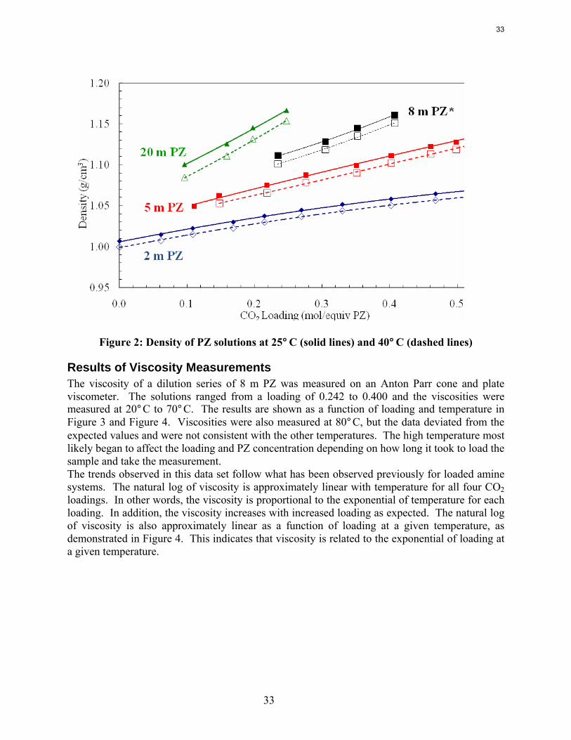
Results of Density Measurements The acquisition of the new Mettler-Toledo densitometer has made density measurements an easy and fast test. The density of multiple dilution series has been measured as a preliminary test of the instrument. Solutions of 2, 5, and 20 m that were created for solubility measurements were tested for density as well. The solutions were created with as high a loading as possible (see solubility section) and the solutions that remained liquid after a few days at room temperature were tested for density at 25 and 40°C. The results are shown in Figure 2 below. This figure also includes an 8 m PZ data set (in black, indicated with the asterisk) that was obtained by a ChE 264 group this spring (student project). Since I have not completed 8 m PZ density measurements, this data set is included as a reference since it is a crucial concentration.

32

33

Figure 2: Density of PZ solutions at 25°C (solid lines) and 40°C (dashed lines)

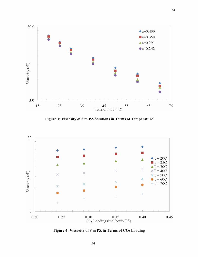
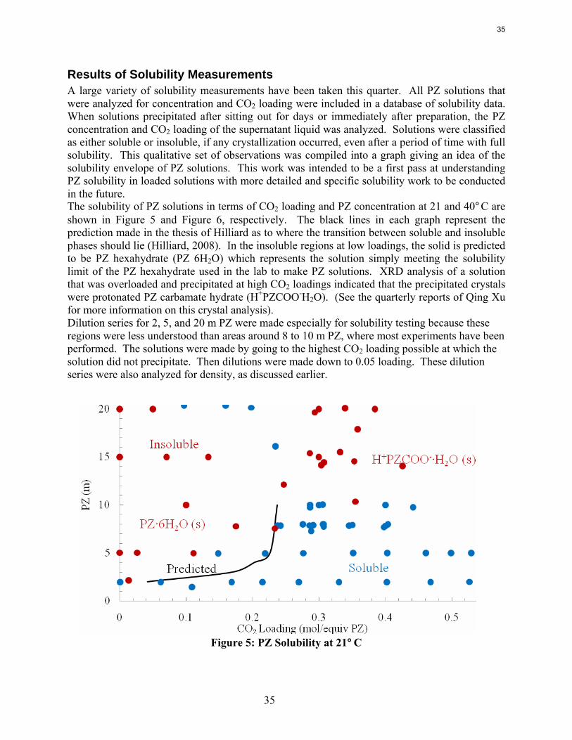
Results of Viscosity Measurements The viscosity of a dilution series of 8 m PZ was measured on an Anton Parr cone and plate viscometer. The solutions ranged from a loading of 0.242 to 0.400 and the viscosities were measured at 20°C to 70°C. The results are shown as a function of loading and temperature in Figure 3 and Figure 4. Viscosities were also measured at 80°C, but the data deviated from the expected values and were not consistent with the other temperatures. The high temperature most likely began to affect the loading and PZ concentration depending on how long it took to load the sample and take the measurement. The trends observed in this data set follow what has been observed previously for loaded amine systems. The natural log of viscosity is approximately linear with temperature for all four CO2 loadings. In other words, the viscosity is proportional to the exponential of temperature for each loading. In addition, the viscosity increases with increased loading as expected. The natural log of viscosity is also approximately linear as a function of loading at a given temperature, as demonstrated in Figure 4. This indicates that viscosity is related to the exponential of loading at a given temperature.

33

34

Figure 3: Viscosity of 8 m PZ Solutions in Terms of Temperature

Figure 4: Viscosity of 8 m PZ in Terms of CO2 Loading

34

35

Results of Solubility Measurements A large variety of solubility measurements have been taken this quarter. All PZ solutions that were analyzed for concentration and CO2 loading were included in a database of solubility data. When solutions precipitated after sitting out for days or immediately after preparation, the PZ concentration and CO2 loading of the supernatant liquid was analyzed. Solutions were classified as either soluble or insoluble, if any crystallization occurred, even after a period of time with full solubility. This qualitative set of observations was compiled into a graph giving an idea of the solubility envelope of PZ solutions. This work was intended to be a first pass at understanding PZ solubility in loaded solutions with more detailed and specific solubility work to be conducted in the future. The solubility of PZ solutions in terms of CO2 loading and PZ concentration at 21 and 40°C are shown in Figure 5 and Figure 6, respectively. The black lines in each graph represent the prediction made in the thesis of Hilliard as to where the transition between soluble and insoluble phases should lie (Hilliard, 2008). In the insoluble regions at low loadings, the solid is predicted to be PZ hexahydrate (PZ 6H2O) which represents the solution simply meeting the solubility limit of the PZ hexahydrate used in the lab to make PZ solutions. XRD analysis of a solution that was overloaded and precipitated at high CO2 loadings indicated that the precipitated crystals were protonated PZ carbamate hydrate (H+PZCOO-H2O). (See the quarterly reports of Qing Xu for more information on this crystal analysis). Dilution series for 2, 5, and 20 m PZ were made especially for solubility testing because these regions were less understood than areas around 8 to 10 m PZ, where most experiments have been performed. The solutions were made by going to the highest CO2 loading possible at which the solution did not precipitate. Then dilutions were made down to 0.05 loading. These dilution series were also analyzed for density, as discussed earlier.

Figure 5: PZ Solubility at 21°C

35

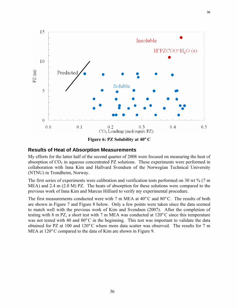
36

Figure 6: PZ Solubility at 40°C

Results of Heat of Absorption Measurements My efforts for the latter half of the second quarter of 2008 were focused on measuring the heat of absorption of CO2 in aqueous concentrated PZ solutions. These experiments were performed in collaboration with Inna Kim and Hallvard Svendsen of the Norwegian Technical University (NTNU) in Trondheim, Norway.

The first series of experiments were calibration and verification tests performed on 30 wt % (7 m MEA) and 2.4 m (2.0 M) PZ. The heats of absorption for these solutions were compared to the previous work of Inna Kim and Marcus Hilliard to verify my experimental procedure. The first measurements conducted were with 7 m MEA at 40°C and 80°C. The results of both are shown in Figure 7 and Figure 8 below. Only a few points were taken since the data seemed to match well with the previous work of Kim and Svendsen (2007). After the completion of testing with 8 m PZ, a short test with 7 m MEA was conducted at 120°C since this temperature was not tested with 40 and 80°C in the beginning. This test was important to validate the data obtained for PZ at 100 and 120°C where more data scatter was observed. The results for 7 m MEA at 120°C compared to the data of Kim are shown in Figure 9.

36

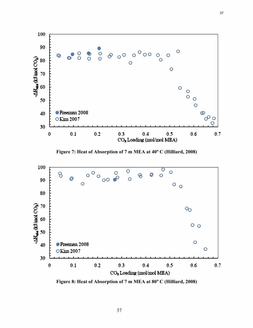
37

Figure 7: Heat of Absorption of 7 m MEA at 40°C (Hilliard, 2008)

Figure 8: Heat of Absorption of 7 m MEA at 80°C (Hilliard, 2008)

37

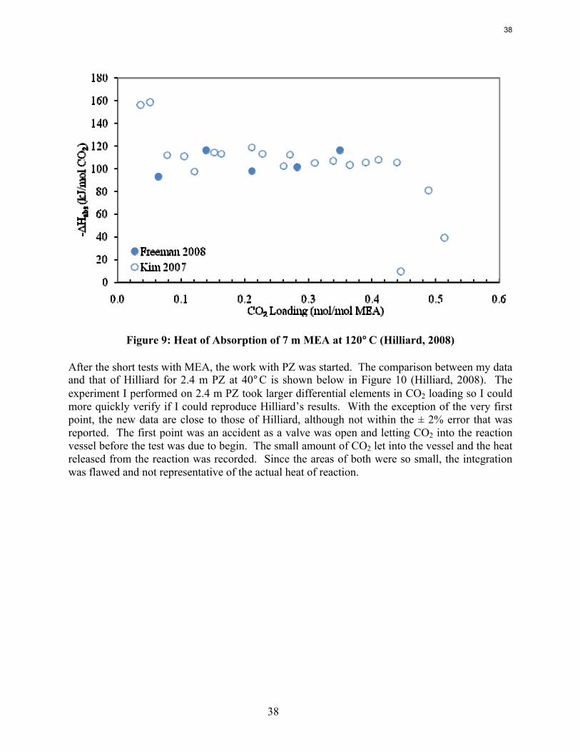
38

Figure 9: Heat of Absorption of 7 m MEA at 120°C (Hilliard, 2008)

After the short tests with MEA, the work with PZ was started. The comparison between my data and that of Hilliard for 2.4 m PZ at 40°C is shown below in Figure 10 (Hilliard, 2008). The experiment I performed on 2.4 m PZ took larger differential elements in CO2 loading so I could more quickly verify if I could reproduce Hilliard’s results. With the exception of the very first point, the new data are close to those of Hilliard, although not within the ± 2% error that was reported. The first point was an accident as a valve was open and letting CO2 into the reaction vessel before the test was due to begin. The small amount of CO2 let into the vessel and the heat released from the reaction was recorded. Since the areas of both were so small, the integration was flawed and not representative of the actual heat of reaction.

38

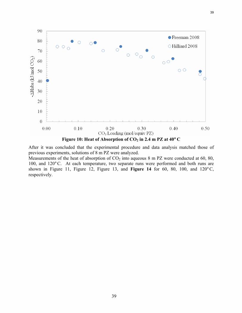
39

Figure 10: Heat of Absorption of CO2 in 2.4 m PZ at 40°C

After it was concluded that the experimental procedure and data analysis matched those of previous experiments, solutions of 8 m PZ were analyzed. Measurements of the heat of absorption of CO2 into aqueous 8 m PZ were conducted at 60, 80, 100, and 120°C. At each temperature, two separate runs were performed and both runs are shown in Figure 11, Figure 12, Figure 13, and Figure 14 for 60, 80, 100, and 120°C, respectively.

39

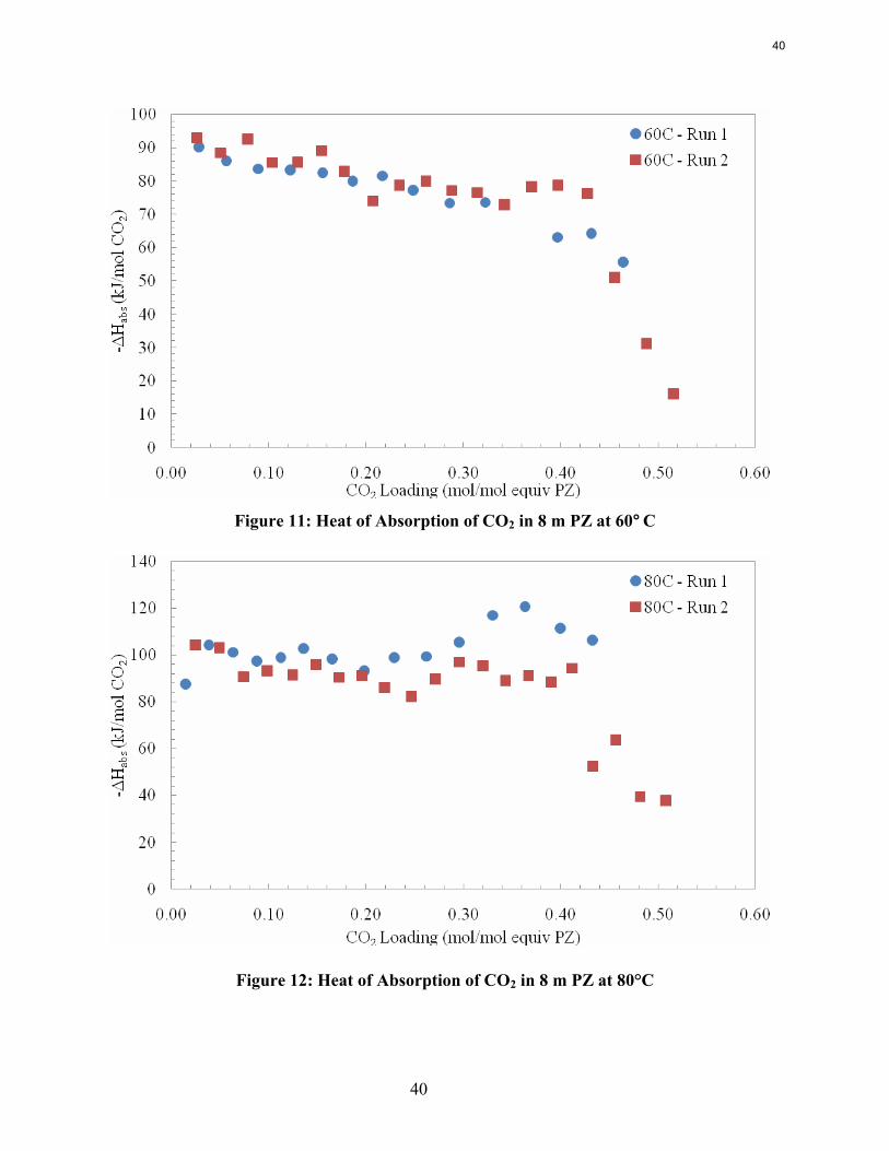
40

Figure 11: Heat of Absorption of CO2 in 8 m PZ at 60°C

Figure 12: Heat of Absorption of CO2 in 8 m PZ at 80°C

40

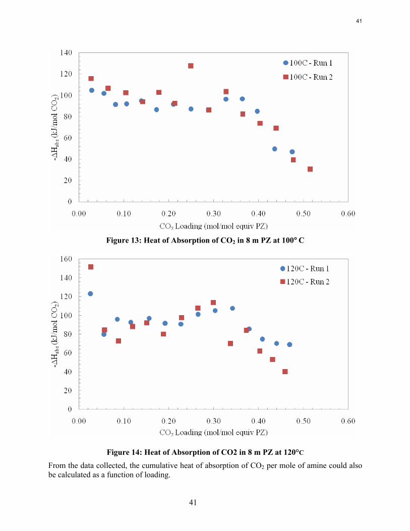
41

Figure 13: Heat of Absorption of CO2 in 8 m PZ at 100°C

Figure 14: Heat of Absorption of CO2 in 8 m PZ at 120°C

From the data collected, the cumulative heat of absorption of CO2 per mole of amine could also be calculated as a function of loading.

41

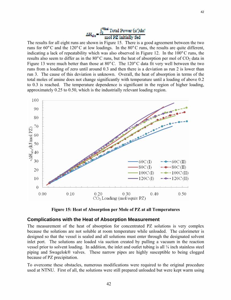
42

The results for all eight runs are shown in Figure 15. There is a good agreement between the two runs for 60°C and the 120°C at low loadings. In the 80°C runs, the results are quite different, indicating a lack of repeatability which was also observed in Figure 12. In the 100°C runs, the results also seem to differ as in the 80°C runs, but the heat of absorption per mol of CO2 data in Figure 13 were much better than those at 80°C. The 120°C data fit very well between the two runs from a loading of zero until around 0.3 and then there is a deviation as run 2 is lower than run 3. The cause of this deviation is unknown. Overall, the heat of absorption in terms of the total moles of amine does not change significantly with temperature until a loading of above 0.2 to 0.3 is reached. The temperature dependence is significant in the region of higher loading, approximately 0.25 to 0.50, which is the industrially relevant loading region.

Figure 15: Heat of Absorption per Mole of PZ at all Temperatures

Complications with the Heat of Absorption Measurement The measurement of the heat of absorption for concentrated PZ solutions is very complex because the solutions are not soluble at room temperature while unloaded. The calorimeter is designed so that the vessel is sealed and all solutions must enter through the designated solvent inlet port. The solutions are loaded via suction created by pulling a vacuum in the reaction vessel prior to solvent loading. In addition, the inlet and outlet tubing is all ¼ inch stainless steel piping and Swagelok® valves. These narrow pipes are highly susceptible to being clogged because of PZ precipitation.

To overcome these obstacles, numerous modifications were required to the original procedure used at NTNU. First of all, the solutions were still prepared unloaded but were kept warm using

42

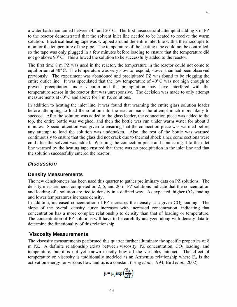
43

a water bath maintained between 45 and 50°C. The first unsuccessful attempt at adding 8 m PZ to the reactor demonstrated that the solvent inlet line needed to be heated to receive the warm solution. Electrical heating tape was wrapped around the entire inlet line with a thermocouple to monitor the temperature of the pipe. The temperature of the heating tape could not be controlled, so the tape was only plugged in a few minutes before loading to ensure that the temperature did not go above 90°C. This allowed the solution to be successfully added to the reactor.

The first time 8 m PZ was used in the reactor, the temperature in the reactor could not come to equilibrium at 40°C. The temperature was very slow to respond, slower than had been observed previously. The experiment was abandoned and precipitated PZ was found to be clogging the entire outlet line. It was speculated that the low temperature of 40°C was not high enough to prevent precipitation under vacuum and the precipitation may have interfered with the temperature sensor in the reactor that was unresponsive. The decision was made to only attempt measurements at 60°C and above for 8 m PZ solutions.

In addition to heating the inlet line, it was found that warming the entire glass solution loader before attempting to load the solution into the reactor made the attempt much more likely to succeed. After the solution was added to the glass loader, the connection piece was added to the top, the entire bottle was weighed, and then the bottle was run under warm water for about 3 minutes. Special attention was given to ensuring that the connection piece was warmed before any attempt to load the solution was undertaken. Also, the rest of the bottle was warmed continuously to ensure that the glass did not crack due to thermal shock since some sections were cold after the solvent was added. Warming the connection piece and connecting it to the inlet line warmed by the heating tape ensured that there was no precipitation in the inlet line and that the solution successfully entered the reactor.

Discussion

Density Measurements The new densitometer has been used this quarter to gather preliminary data on PZ solutions. The density measurements completed on 2, 5, and 20 m PZ solutions indicate that the concentration and loading of a solution are tied to density in a defined way. As expected, higher CO2 loading and lower temperatures increase density. In addition, increased concentration of PZ increases the density at a given CO2 loading. The slope of the overall density curve increases with increased concentration, indicating that concentration has a more complex relationship to density than that of loading or temperature. The concentration of PZ solutions will have to be carefully analyzed along with density data to determine the functionality of this relationship.

Viscosity Measurements The viscosity measurements performed this quarter further illuminate the specific properties of 8 m PZ. A definite relationship exists between viscosity, PZ concentration, CO2 loading, and temperature, but it is not yet known exactly how all the variables interact. The effect of temperature on viscosity is traditionally modeled as an Arrhenius relationship where EA is the activation energy for viscous flow and μ0 is a constant (Teng et al., 1994; Bird et al., 2002).

43

44

Fisher describes a number of other equations used to relate temperature to viscosity in particular systems (Fisher, 1998). For PZ, the issue at hand is how to include the effects of loading and concentration. If an Arrhenius-type relationship is used, the loading or concentration effects could be included in the two constants or through the addition of separate terms.

If the Arrhenius relationship is linearized, as shown below, the slope of a plot of ln μ vs. 1/T is the term EA/R.

An initial look at the data collected for 8 m PZ shows that the activation energy is different at each loading. Plotting the ln μ vs. inverse temperature produces Figure 16. The solid lines are linear trend lines through each of the four sets of data.

Figure 16: Logarithmic Viscosity vs. Inverse Temperature for 8 m PZ Solutions

It is clear from Figure 16 that the slopes of the curves for the loadings differ, producing varying activation energies. The activation energies calculated from the slopes in Figure 16 are shown in Table 3. The difference in activation energy over this range of loading is 3000 J or 3 kJ, a considerable change. A single activation energy value, therefore, would not accurately represent the system of loaded PZ. The activation energy must be dependent on CO2 loading in any model for viscosity for concentrated, aqueous PZ.

Table 3: Variation of Viscosity Activation Energy with CO2 Loading

CO2 Loading Activation Energy Mol CO2/equiv PZ J/mol

0.400 -24359.19 0.350 -25485.74 0.291 -25612.11 0.242 -27107.80

44

45

Solubility Measurements The solubility work completed this quarter is only a qualitative, first attempt to analyze the issue of PZ solubility and precipitation. The results indicate that there is a well defined envelope where PZ solutions are soluble. Questions remain about the definite borders of this envelope and discovering the exact solid-liquid phase behavior is crucial to the development of PZ as a viable industrial solvent. There is a clear range of loadings where 8 m PZ provides all the advantages of faster kinetics and will stay in solution.

Heat of Absorption Measurements Two types of heat of absorption data can be measured experimentally: the integral and the differential heats of absorption. The integral heat of absorption is the more standard measurement in literature and is commonly measured using a flow calorimeter (Mathonat et al., 1998; Carson et al., 2000). In flow calorimeters, two inlet streams of the amine and the CO2 are fed continuously at defined ratios and the heat released over the course of the apparatus to absorb the CO2 into the liquid is measured on-line. In this way, the heat needed to absorb all of the CO2 fed is measured. On the other hand, differential calorimetry measures the heat needed to absorb a small, differential amount of CO2 added to the system. In this way, the same solution is utilized to cover the entire range of CO2 loadings rather than a separate experiment to obtain each loading point, as with integral heats of absorption. When differential heats are measured, the integral heat can be calculated afterward according to the following equation for each loading point.

The reverse, calculating differential heats from integral heats is more difficult and usually contains more error. The calorimeter at NTNU is set up for differential heat of absorption measurements. The integral heats of absorption were calculated from the collected differential heat data and are shown for all eight runs in Figure 17.

45

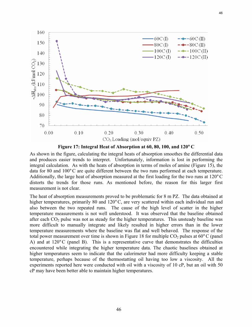
46

Figure 17: Integral Heat of Absorption at 60, 80, 100, and 120°C

As shown in the figure, calculating the integral heats of absorption smoothes the differential data and produces easier trends to interpret. Unfortunately, information is lost in performing the integral calculation. As with the heats of absorption in terms of moles of amine (Figure 15), the data for 80 and 100°C are quite different between the two runs performed at each temperature. Additionally, the large heat of absorption measured at the first loading for the two runs at 120°C distorts the trends for those runs. As mentioned before, the reason for this larger first measurement is not clear.

The heat of absorption measurements proved to be problematic for 8 m PZ. The data obtained at higher temperatures, primarily 80 and 120°C, are very scattered within each individual run and also between the two repeated runs. The cause of the high level of scatter in the higher temperature measurements is not well understood. It was observed that the baseline obtained after each CO2 pulse was not as steady for the higher temperatures. This unsteady baseline was more difficult to manually integrate and likely resulted in higher errors than in the lower temperature measurements where the baseline was flat and well behaved. The response of the total power measurement over time is shown in Figure 18 for multiple CO2 pulses at 60°C (panel A) and at 120°C (panel B). This is a representative curve that demonstrates the difficulties encountered while integrating the higher temperature data. The chaotic baselines obtained at higher temperatures seem to indicate that the calorimeter had more difficulty keeping a stable temperature, perhaps because of the thermostatting oil having too low a viscosity. All the experiments reported here were conducted with oil with a viscosity of 10 cP, but an oil with 50 cP may have been better able to maintain higher temperatures.

46

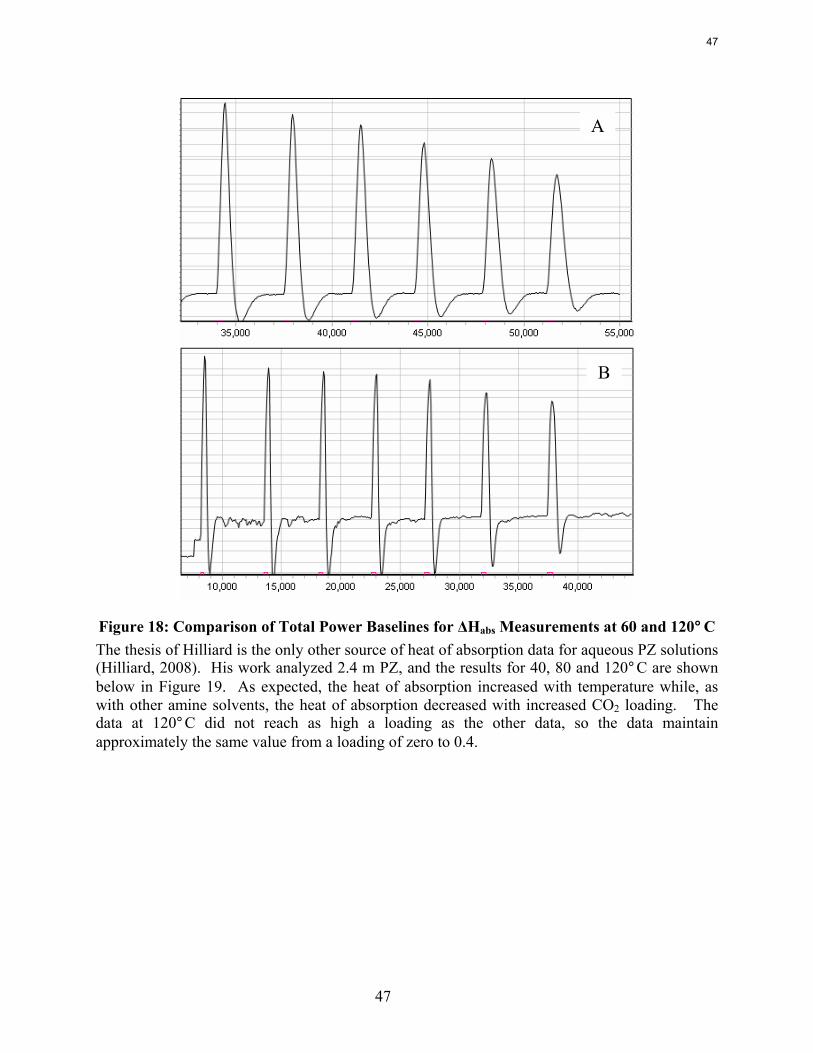
47

Figure 18: Comparison of Total Power Baselines for ΔHabs Measurements at 60 and 120°C The thesis of Hilliard is the only other source of heat of absorption data for aqueous PZ solutions (Hilliard, 2008). His work analyzed 2.4 m PZ, and the results for 40, 80 and 120°C are shown below in Figure 19. As expected, the heat of absorption increased with temperature while, as with other amine solvents, the heat of absorption decreased with increased CO2 loading. The data at 120°C did not reach as high a loading as the other data, so the data maintain approximately the same value from a loading of zero to 0.4.

A

B

47

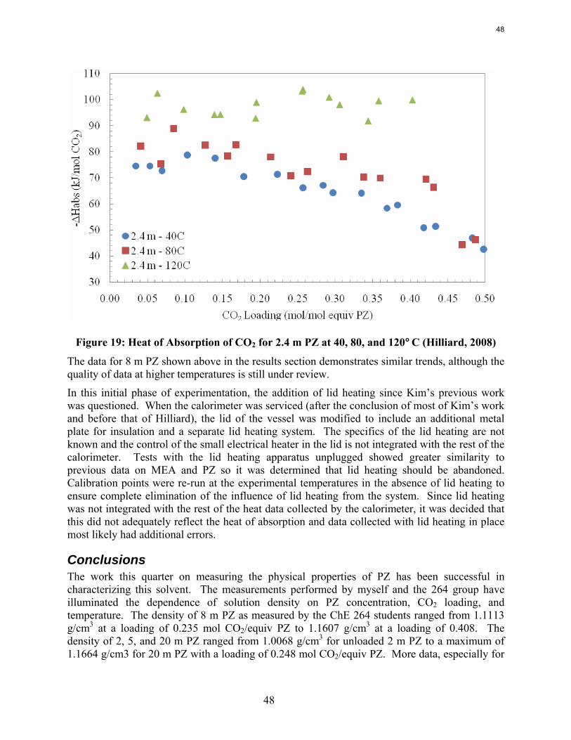
48

Figure 19: Heat of Absorption of CO2 for 2.4 m PZ at 40, 80, and 120°C (Hilliard, 2008)

The data for 8 m PZ shown above in the results section demonstrates similar trends, although the quality of data at higher temperatures is still under review.

In this initial phase of experimentation, the addition of lid heating since Kim’s previous work was questioned. When the calorimeter was serviced (after the conclusion of most of Kim’s work and before that of Hilliard), the lid of the vessel was modified to include an additional metal plate for insulation and a separate lid heating system. The specifics of the lid heating are not known and the control of the small electrical heater in the lid is not integrated with the rest of the calorimeter. Tests with the lid heating apparatus unplugged showed greater similarity to previous data on MEA and PZ so it was determined that lid heating should be abandoned. Calibration points were re-run at the experimental temperatures in the absence of lid heating to ensure complete elimination of the influence of lid heating from the system. Since lid heating was not integrated with the rest of the heat data collected by the calorimeter, it was decided that this did not adequately reflect the heat of absorption and data collected with lid heating in place most likely had additional errors.

Conclusions The work this quarter on measuring the physical properties of PZ has been successful in characterizing this solvent. The measurements performed by myself and the 264 group have illuminated the dependence of solution density on PZ concentration, CO2 loading, and temperature. The density of 8 m PZ as measured by the ChE 264 students ranged from 1.1113 g/cm3 at a loading of 0.235 mol CO2/equiv PZ to 1.1607 g/cm3 at a loading of 0.408. The density of 2, 5, and 20 m PZ ranged from 1.0068 g/cm3 for unloaded 2 m PZ to a maximum of 1.1664 g/cm3 for 20 m PZ with a loading of 0.248 mol CO2/equiv PZ. More data, especially for

48

49

the range of 7 to 10 m PZ is needed to fully understand the density in this crucial concentration range. The viscosity of 8 m PZ ranged from 3.92 cP at 70°C and a loading of 0.24 to 22.78 cP at 20°C and a loading of 0.40 mol CO2/equiv PZ. Attempts at regressing the viscosity data and fitting it to a temperature- and concentration-dependent model have not been completed due to a lack of data outside of 8 m PZ.

The heat of absorption measurements proved difficult due to solubility issues with the PZ and due to the differences in instrument stability at varying temperatures. Overall, the heat of absorption of PZ follows similar trends to other amines, such as MEA and MDEA, in that the heat of absorption trend stays relatively constant over a range of low loadings until a threshold loading is reached, when the value decreases rapidly. For PZ, this decrease was observed to begin around a loading of 0.4 mol CO2/equiv PZ or a loading of 0.9 to 1.0 mol CO2/mol PZ. In PZ, the data actually decrease slightly until the threshold, whereas in MEA, the data remains quite constant until the threshold of 0.5 mol CO2/mol MEA is reached. At a loading of 0.025 mol CO2/equiv PZ, the heat of absorption was 90.3, 104.5, 115.7, and 123.1 kJ/mol CO2, respectively, at 60, 80,100, and 120°C. After the initial loadings, there was little difference in the values for the heat of absorption between 80, 100, and 120°C.

Future Work The third quarter of 2008 will focus on preparing for the GHGT-9 conference and research review meeting in November. The measurement of physical properties of PZ solutions will continue focusing on density, viscosity, and solubility. A temperature controlled hot plate with stirrer will be utilized in an attempt to pinpoint the phase transition of crystallized PZ into liquid solutions. Further attempts to isolate the PZ solubility window using other techniques will continue. Density and viscosity of a wider range of solutions will be measured this quarter, focusing on 6-10 m PZ with loadings across the range of solubility.

The analysis of the heat of absorption data will also continue. These experimental data will be further analyzed and prepared for presentation at the research review meeting in November.

49

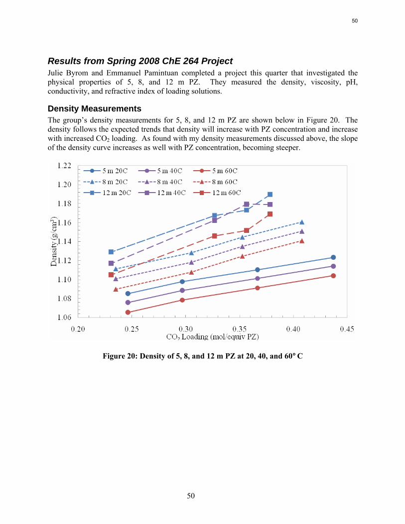
50

Results from Spring 2008 ChE 264 Project Julie Byrom and Emmanuel Pamintuan completed a project this quarter that investigated the physical properties of 5, 8, and 12 m PZ. They measured the density, viscosity, pH, conductivity, and refractive index of loading solutions.

Density Measurements The group’s density measurements for 5, 8, and 12 m PZ are shown below in Figure 20. The density follows the expected trends that density will increase with PZ concentration and increase with increased CO2 loading. As found with my density measurements discussed above, the slope of the density curve increases as well with PZ concentration, becoming steeper.

Figure 20: Density of 5, 8, and 12 m PZ at 20, 40, and 60°C

50

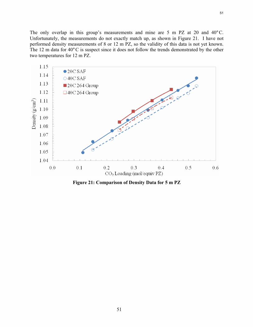
51

The only overlap in this group’s measurements and mine are 5 m PZ at 20 and 40°C. Unfortunately, the measurements do not exactly match up, as shown in Figure 21. I have not performed density measurements of 8 or 12 m PZ, so the validity of this data is not yet known. The 12 m data for 40°C is suspect since it does not follow the trends demonstrated by the other two temperatures for 12 m PZ.

Figure 21: Comparison of Density Data for 5 m PZ

51

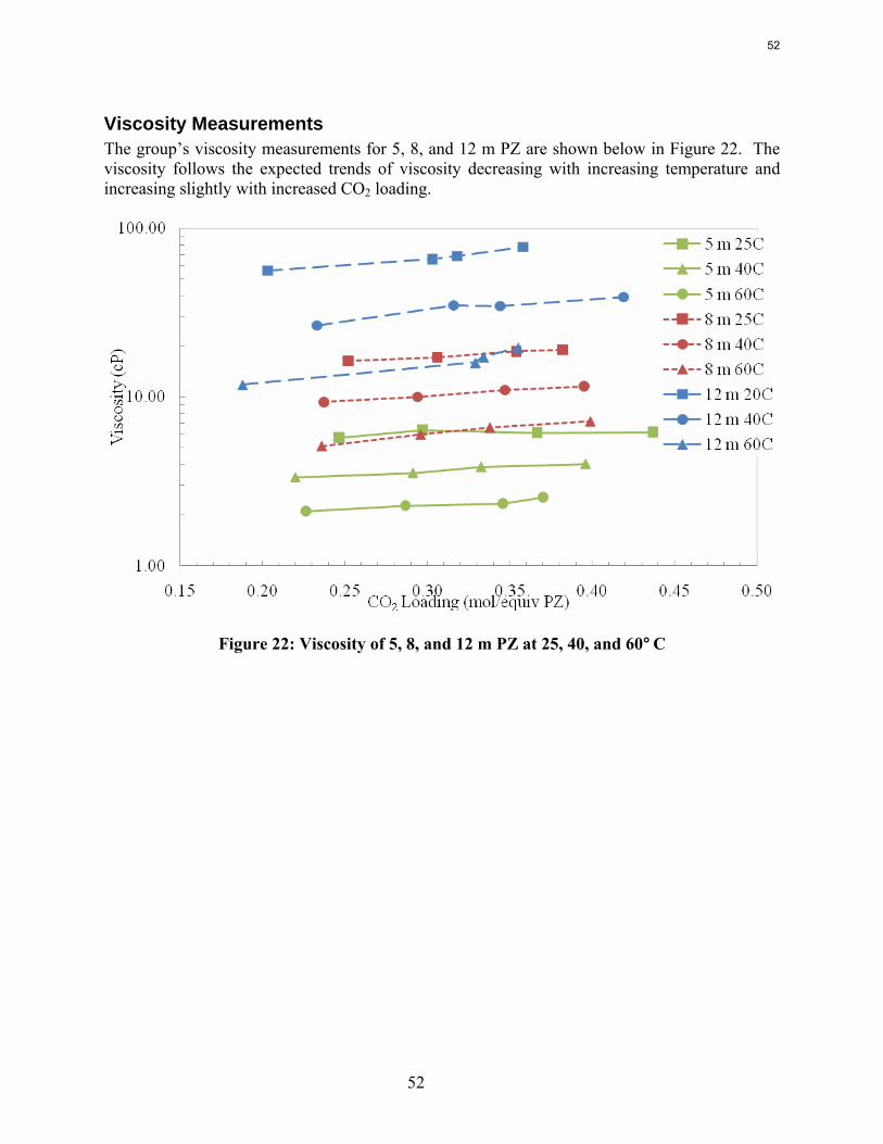
52

Viscosity Measurements The group’s viscosity measurements for 5, 8, and 12 m PZ are shown below in Figure 22. The viscosity follows the expected trends of viscosity decreasing with increasing temperature and increasing slightly with increased CO2 loading.

Figure 22: Viscosity of 5, 8, and 12 m PZ at 25, 40, and 60°C

52

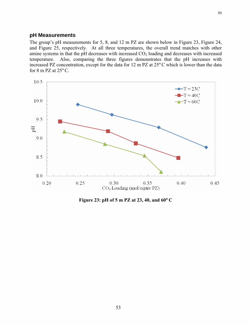
53

pH Measurements The group’s pH measurements for 5, 8, and 12 m PZ are shown below in Figure 23, Figure 24, and Figure 25, respectively. At all three temperatures, the overall trend matches with other amine systems in that the pH decreases with increased CO2 loading and decreases with increased temperature. Also, comparing the three figures demonstrates that the pH increases with increased PZ concentration, except for the data for 12 m PZ at 25°C which is lower than the data for 8 m PZ at 25°C.

Figure 23: pH of 5 m PZ at 23, 40, and 60°C

53

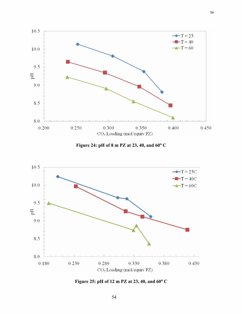
54

Figure 24: pH of 8 m PZ at 23, 40, and 60°C

Figure 25: pH of 12 m PZ at 23, 40, and 60°C

54

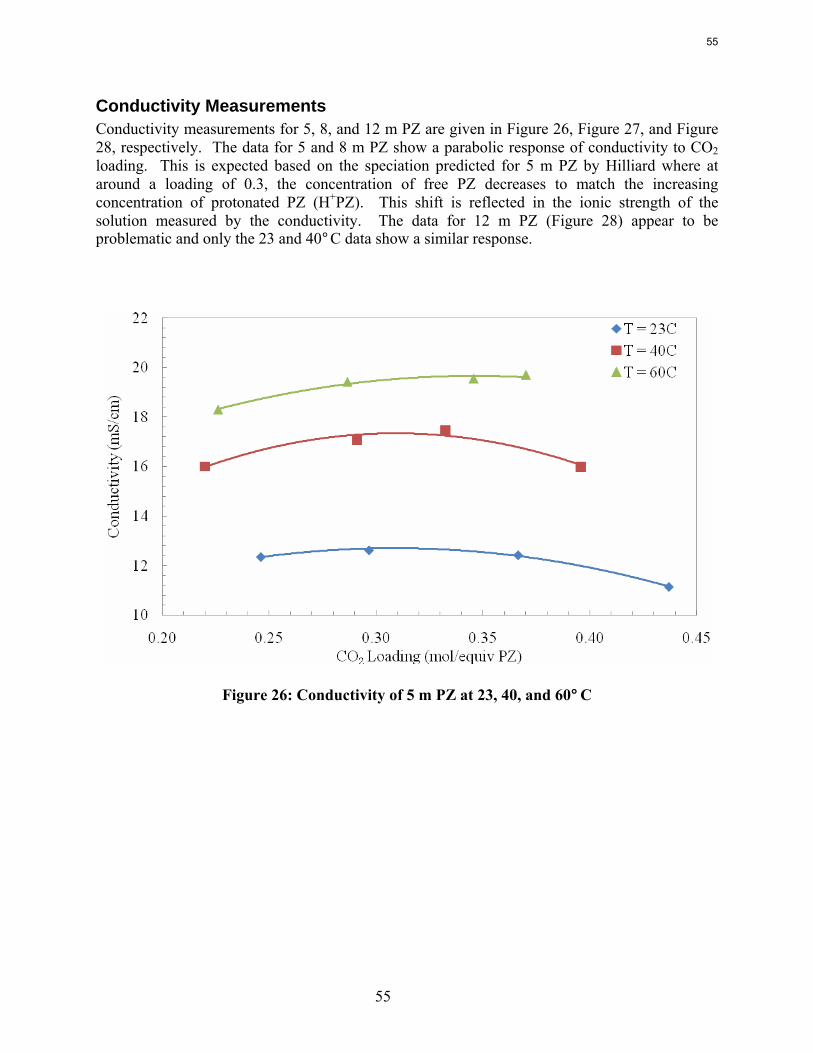
55

Conductivity Measurements Conductivity measurements for 5, 8, and 12 m PZ are given in Figure 26, Figure 27, and Figure 28, respectively. The data for 5 and 8 m PZ show a parabolic response of conductivity to CO2 loading. This is expected based on the speciation predicted for 5 m PZ by Hilliard where at around a loading of 0.3, the concentration of free PZ decreases to match the increasing concentration of protonated PZ (H+PZ). This shift is reflected in the ionic strength of the solution measured by the conductivity. The data for 12 m PZ (Figure 28) appear to be problematic and only the 23 and 40°C data show a similar response.

Figure 26: Conductivity of 5 m PZ at 23, 40, and 60°C

55

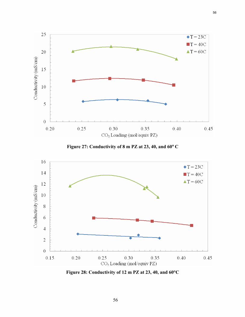
56

Figure 27: Conductivity of 8 m PZ at 23, 40, and 60°C

Figure 28: Conductivity of 12 m PZ at 23, 40, and 60°C

56

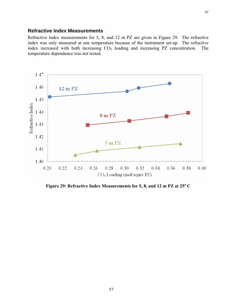
57

Refractive Index Measurements Refractive index measurements for 5, 8, and 12 m PZ are given in Figure 29. The refractive index was only measured at one temperature because of the instrument set-up. The refractive index increased with both increasing CO2 loading and increasing PZ concentration. The temperature dependence was not tested.

Figure 29: Refractive Index Measurements for 5, 8, and 12 m PZ at 25°C

57

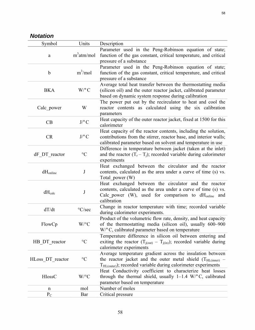
58

Notation Symbol Units Description

a m3atm/mol Parameter used in the Peng-Robinson equation of state; function of the gas constant, critical temperature, and critical pressure of a substance

b m3/mol Parameter used in the Peng-Robinson equation of state; function of the gas constant, critical temperature, and critical pressure of a substance

BKA W/°C Average total heat transfer between the thermostatting media (silicon oil) and the outer reactor jacket, calibrated parameter based on dynamic system response during calibration

Calc_power W The power put out by the recirculator to heat and cool the reactor contents as calculated using the six calibration parameters

CB J/°C Heat capacity of the outer reactor jacket, fixed at 1500 for this calorimeter

CR J/°C Heat capacity of the reactor contents, including the solution, contributions from the stirrer, reactor base, and interior walls; calibrated parameter based on solvent and temperature in use

dF_DT_reactor °C Difference in temperature between jacket (taken at the inlet) and the reactor (Tr – Tj); recorded variable during calorimeter experiments

dHonline J Heat exchanged between the circulator and the reactor contents, calculated as the area under a curve of time (s) vs. Total_power (W)

dHcalc J

Heat exchanged between the circulator and the reactor contents, calculated as the area under a curve of time (s) vs. Calc_power (W), used for comparison to dHonline and calibration

dT/dt °C/sec Change in reactor temperature with time; recorded variable during calorimeter experiments.

FlowCp W/°C Product of the volumetric flow rate, density, and heat capacity of the thermostatting media (silicon oil), usually 600–900 W/°C, calibrated parameter based on temperature

HB_DT_reactor °C Temperature difference in silicon oil between entering and exiting the reactor (Tj(out) – Tj(in)); recorded variable during calorimeter experiments

HLoss_DT_reactor °C Average temperature gradient across the insulation between the reactor jacket and the outer metal shield (THL(inner) – THL(outer)); recorded variable during calorimeter experiments

HlossC W/°C Heat Conductivity coefficient to characterize heat losses through the thermal shield, usually 1–1.4 W/°C, calibrated parameter based on temperature

n mol Number of moles PC Bar Critical pressure

58

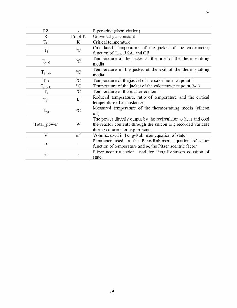
59

PZ - Piperazine (abbreviation) R J/mol-K Universal gas constant TC K Critical temperature

Tj °C Calculated Temperature of the jacket of the calorimeter; function of Tref, BKA, and CB

Tj(in) °C Temperature of the jacket at the inlet of the thermostatting media

Tj(out) °C Temperature of the jacket at the exit of the thermostatting media

Tj, i °C Temperature of the jacket of the calorimeter at point i Tj, (i-1) °C Temperature of the jacket of the calorimeter at point (i-1)

Tr °C Temperature of the reactor contents

TR K Reduced temperature, ratio of temperature and the critical temperature of a substance

Tref °C Measured temperature of the thermostatting media (silicon oil)

Total_power W The power directly output by the recirculator to heat and cool the reactor contents through the silicon oil; recorded variable during calorimeter experiments

V m3 Volume, used in Peng-Robinson equation of state

α - Parameter used in the Peng-Robinson equation of state; function of temperature and ω, the Pitzer acentric factor

ω - Pitzer acentric factor, used for Peng-Robinson equation of state

59

60

References Bird RB, Steward WE, Lightfoot E. Transport Phenomena. 2nd ed. New York: Wiley & Sons,

2002. Carson JK, Marsh KN, Mather AE. Enthalpy of solution of carbon dioxide in (water plus

monoethanolamine, or diethanolamine, or N-methyldiethanolamine) and (water plus monoethanolamine plus N-methyldiethanolamine) at T=298.15 K. J Chem Thermo. 2000;32(9):1285–1296.

ChemiSens, AB, "ChemiSens CPA 122 System Manual". Fisher CH. Correlating viscosity with temperature and other properties. J Amer Oil Chem Soc.

1998;75(10):1229–1232. Hilliard MD. A Predictive Thermodynamic Model for an Aqueous Blend of Potassium

Carbonate, Piperazine, and Monoethanolamine for Carbon Dioxide Capture from Flue Gas. University of Texas, Austin; 2008. Ph.D. Dissertation.

Kim I, Svendsen HF. Heat of absorption of carbon dioxide (CO2) in monoethanolamine (MEA) and 2-(Aminoethyl)ethanolamine (AEEA) solutions. Ind Eng Chem Res. 2007;46(17):5803–5809.

Mathonat C, Majer V, Mather AE, Grolier JPE. Use of flow calorimetry for determining enthalpies of absorption and the solubility of CO2 in aqueous monoethanolamine solutions. Ind Eng Chem Res, 1998;37(10):4136–4141.

Mettler Toledo US. Comparison of different measuring techniques for density and refractometry. http://us.mt.com/mt/ed/faq/Comparision_measuring_methods_for_DERE_Editorial-Faq_1092390712029.jsp (08 June), 2008.

Perry RH, Green DW. Perry's Chemical Engineers' Handbook. 7th ed. New York: McGraw-Hill, 1997.

Smith JM, Van Ness HC, Abbott M. Introduction to Chemical Engineering Thermodynamics. 5th ed. New York: McGraw-Hill, 1995.

Teng TT, Maham Y, Hepler LG, Mather AE. Viscosity of Aqueous Solutions of N-Methyldiethanolamine and Diethanolamine. J Chem Eng Data. 1994;39(2):290-293.

Tester W, Modell M. Thermodynamics and Its Applications. 3rd ed. Upper Saddle River, NJ: Prentice Hall, 1997.

60

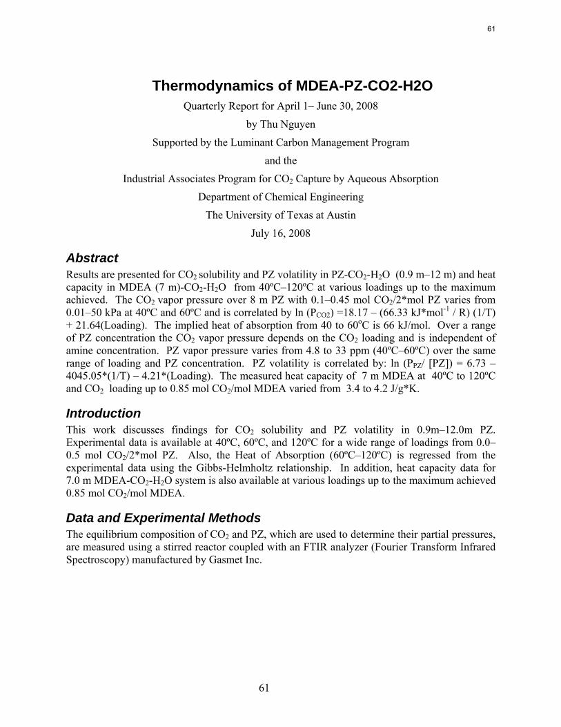
61

Thermodynamics of MDEA-PZ-CO2-H2O Quarterly Report for April 1– June 30, 2008

by Thu Nguyen

Supported by the Luminant Carbon Management Program

and the

Industrial Associates Program for CO2 Capture by Aqueous Absorption

Department of Chemical Engineering

The University of Texas at Austin

July 16, 2008

Abstract Results are presented for CO2 solubility and PZ volatility in PZ-CO2-H2O (0.9 m–12 m) and heat capacity in MDEA (7 m)-CO2-H2O from 40ºC–120ºC at various loadings up to the maximum achieved. The CO2 vapor pressure over 8 m PZ with 0.1–0.45 mol CO2/2*mol PZ varies from 0.01–50 kPa at 40ºC and 60ºC and is correlated by ln (PCO2) =18.17 – (66.33 kJ*mol-1 / R) (1/T) + 21.64(Loading). The implied heat of absorption from 40 to 60oC is 66 kJ/mol. Over a range of PZ concentration the CO2 vapor pressure depends on the CO2 loading and is independent of amine concentration. PZ vapor pressure varies from 4.8 to 33 ppm (40ºC–60ºC) over the same range of loading and PZ concentration. PZ volatility is correlated by: ln (PPZ/ [PZ]) = 6.73 – 4045.05*(1/T) – 4.21*(Loading). The measured heat capacity of 7 m MDEA at 40ºC to 120ºC and CO2 loading up to 0.85 mol CO2/mol MDEA varied from 3.4 to 4.2 J/g*K.

Introduction This work discusses findings for CO2 solubility and PZ volatility in 0.9m–12.0m PZ. Experimental data is available at 40ºC, 60ºC, and 120ºC for a wide range of loadings from 0.0–0.5 mol CO2/2*mol PZ. Also, the Heat of Absorption (60ºC–120ºC) is regressed from the experimental data using the Gibbs-Helmholtz relationship. In addition, heat capacity data for 7.0 m MDEA-CO2-H2O system is also available at various loadings up to the maximum achieved 0.85 mol CO2/mol MDEA.

Data and Experimental Methods The equilibrium composition of CO2 and PZ, which are used to determine their partial pressures, are measured using a stirred reactor coupled with an FTIR analyzer (Fourier Transform Infrared Spectroscopy) manufactured by Gasmet Inc.

61

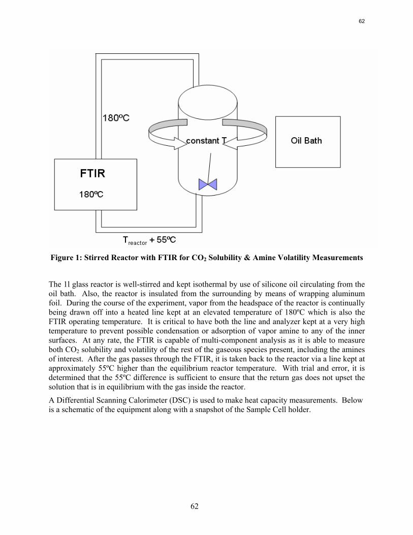
62

Figure 1: Stirred Reactor with FTIR for CO2 Solubility & Amine Volatility Measurements

The 1l glass reactor is well-stirred and kept isothermal by use of silicone oil circulating from the oil bath. Also, the reactor is insulated from the surrounding by means of wrapping aluminum foil. During the course of the experiment, vapor from the headspace of the reactor is continually being drawn off into a heated line kept at an elevated temperature of 180ºC which is also the FTIR operating temperature. It is critical to have both the line and analyzer kept at a very high temperature to prevent possible condensation or adsorption of vapor amine to any of the inner surfaces. At any rate, the FTIR is capable of multi-component analysis as it is able to measure both CO2 solubility and volatility of the rest of the gaseous species present, including the amines of interest. After the gas passes through the FTIR, it is taken back to the reactor via a line kept at approximately 55ºC higher than the equilibrium reactor temperature. With trial and error, it is determined that the 55ºC difference is sufficient to ensure that the return gas does not upset the solution that is in equilibrium with the gas inside the reactor.

A Differential Scanning Calorimeter (DSC) is used to make heat capacity measurements. Below is a schematic of the equipment along with a snapshot of the Sample Cell holder.

62

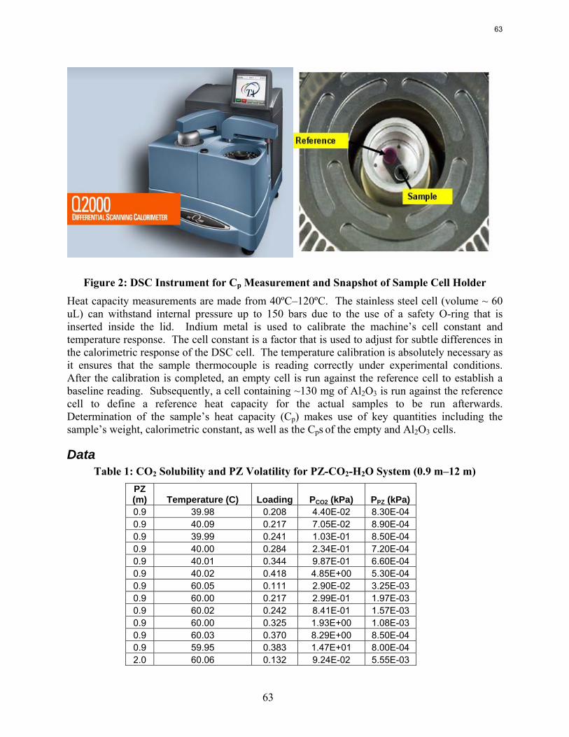
63

Figure 2: DSC Instrument for Cp Measurement and Snapshot of Sample Cell Holder Heat capacity measurements are made from 40ºC–120ºC. The stainless steel cell (volume ~ 60 uL) can withstand internal pressure up to 150 bars due to the use of a safety O-ring that is inserted inside the lid. Indium metal is used to calibrate the machine’s cell constant and temperature response. The cell constant is a factor that is used to adjust for subtle differences in the calorimetric response of the DSC cell. The temperature calibration is absolutely necessary as it ensures that the sample thermocouple is reading correctly under experimental conditions. After the calibration is completed, an empty cell is run against the reference cell to establish a baseline reading. Subsequently, a cell containing ~130 mg of Al2O3 is run against the reference cell to define a reference heat capacity for the actual samples to be run afterwards. Determination of the sample’s heat capacity (Cp) makes use of key quantities including the sample’s weight, calorimetric constant, as well as the Cps of the empty and Al2O3 cells.

Data Table 1: CO2 Solubility and PZ Volatility for PZ-CO2-H2O System (0.9 m–12 m)

PZ (m) Temperature (C) Loading PCO2 (kPa) PPZ (kPa) 0.9 39.98 0.208 4.40E-02 8.30E-04 0.9 40.09 0.217 7.05E-02 8.90E-04 0.9 39.99 0.241 1.03E-01 8.50E-04 0.9 40.00 0.284 2.34E-01 7.20E-04 0.9 40.01 0.344 9.87E-01 6.60E-04 0.9 40.02 0.418 4.85E+00 5.30E-04 0.9 60.05 0.111 2.90E-02 3.25E-03 0.9 60.00 0.217 2.99E-01 1.97E-03 0.9 60.02 0.242 8.41E-01 1.57E-03 0.9 60.00 0.325 1.93E+00 1.08E-03 0.9 60.03 0.370 8.29E+00 8.50E-04 0.9 59.95 0.383 1.47E+01 8.00E-04 2.0 60.06 0.132 9.24E-02 5.55E-03

63

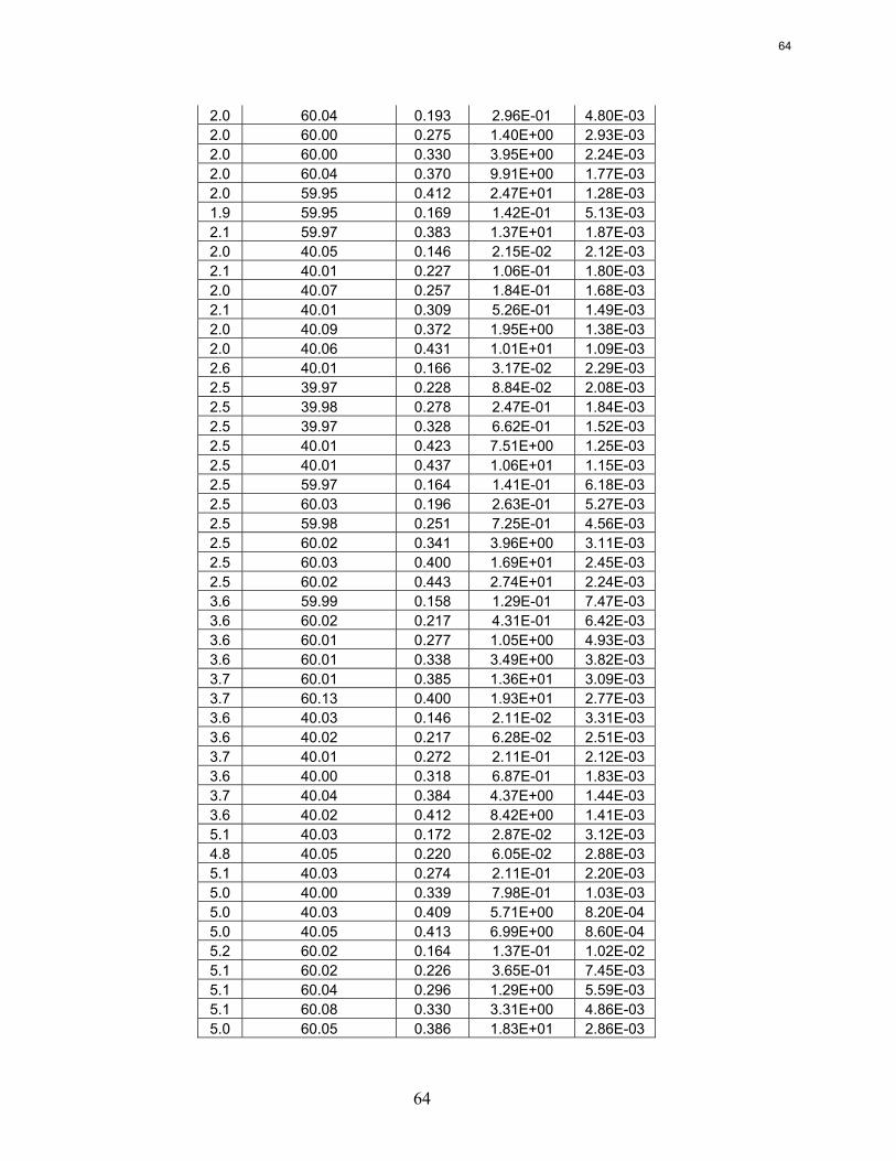
64

2.0 60.04 0.193 2.96E-01 4.80E-03 2.0 60.00 0.275 1.40E+00 2.93E-03 2.0 60.00 0.330 3.95E+00 2.24E-03 2.0 60.04 0.370 9.91E+00 1.77E-03 2.0 59.95 0.412 2.47E+01 1.28E-03 1.9 59.95 0.169 1.42E-01 5.13E-03 2.1 59.97 0.383 1.37E+01 1.87E-03 2.0 40.05 0.146 2.15E-02 2.12E-03 2.1 40.01 0.227 1.06E-01 1.80E-03 2.0 40.07 0.257 1.84E-01 1.68E-03 2.1 40.01 0.309 5.26E-01 1.49E-03 2.0 40.09 0.372 1.95E+00 1.38E-03 2.0 40.06 0.431 1.01E+01 1.09E-03 2.6 40.01 0.166 3.17E-02 2.29E-03 2.5 39.97 0.228 8.84E-02 2.08E-03 2.5 39.98 0.278 2.47E-01 1.84E-03 2.5 39.97 0.328 6.62E-01 1.52E-03 2.5 40.01 0.423 7.51E+00 1.25E-03 2.5 40.01 0.437 1.06E+01 1.15E-03 2.5 59.97 0.164 1.41E-01 6.18E-03 2.5 60.03 0.196 2.63E-01 5.27E-03 2.5 59.98 0.251 7.25E-01 4.56E-03 2.5 60.02 0.341 3.96E+00 3.11E-03 2.5 60.03 0.400 1.69E+01 2.45E-03 2.5 60.02 0.443 2.74E+01 2.24E-03 3.6 59.99 0.158 1.29E-01 7.47E-03 3.6 60.02 0.217 4.31E-01 6.42E-03 3.6 60.01 0.277 1.05E+00 4.93E-03 3.6 60.01 0.338 3.49E+00 3.82E-03 3.7 60.01 0.385 1.36E+01 3.09E-03 3.7 60.13 0.400 1.93E+01 2.77E-03 3.6 40.03 0.146 2.11E-02 3.31E-03 3.6 40.02 0.217 6.28E-02 2.51E-03 3.7 40.01 0.272 2.11E-01 2.12E-03 3.6 40.00 0.318 6.87E-01 1.83E-03 3.7 40.04 0.384 4.37E+00 1.44E-03 3.6 40.02 0.412 8.42E+00 1.41E-03 5.1 40.03 0.172 2.87E-02 3.12E-03 4.8 40.05 0.220 6.05E-02 2.88E-03 5.1 40.03 0.274 2.11E-01 2.20E-03 5.0 40.00 0.339 7.98E-01 1.03E-03 5.0 40.03 0.409 5.71E+00 8.20E-04 5.0 40.05 0.413 6.99E+00 8.60E-04 5.2 60.02 0.164 1.37E-01 1.02E-02 5.1 60.02 0.226 3.65E-01 7.45E-03 5.1 60.04 0.296 1.29E+00 5.59E-03 5.1 60.08 0.330 3.31E+00 4.86E-03 5.0 60.05 0.386 1.83E+01 2.86E-03

64

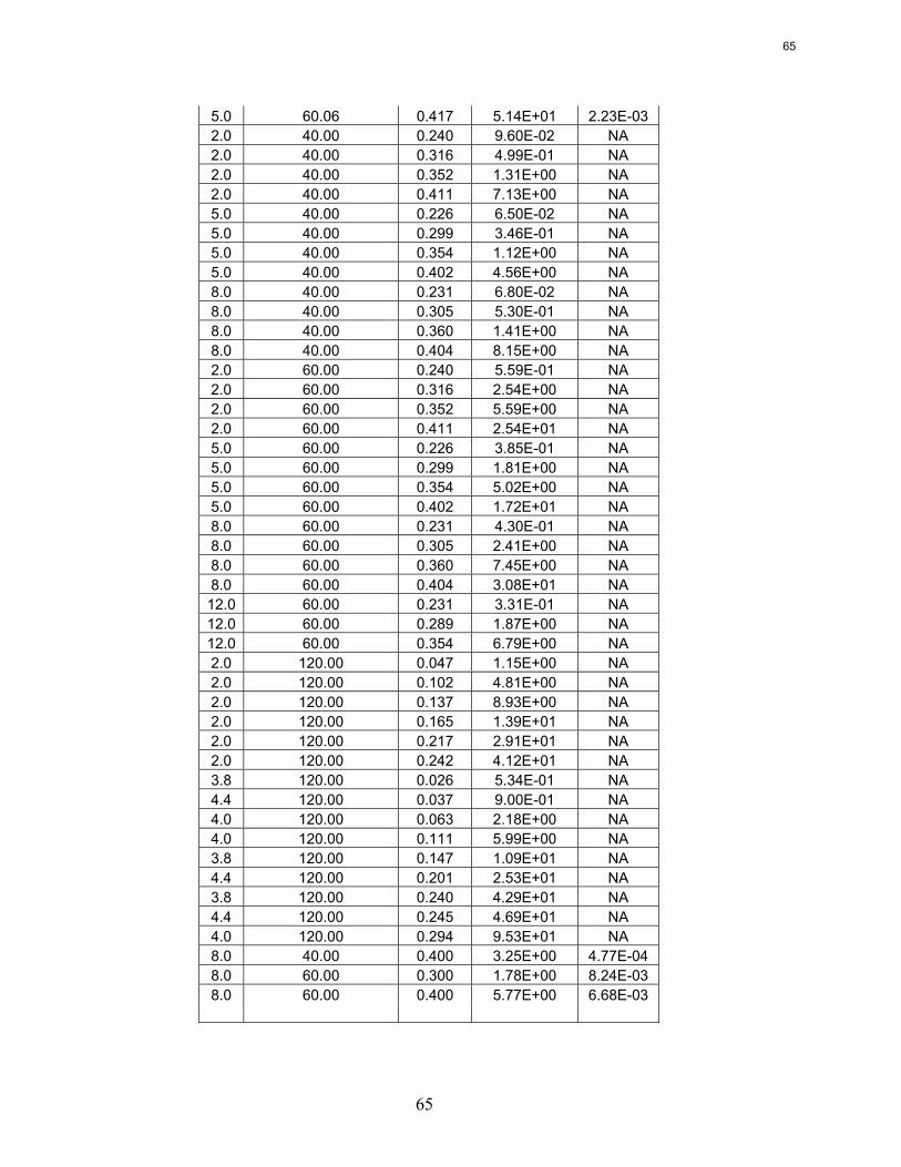
65

5.0 60.06 0.417 5.14E+01 2.23E-03 2.0 40.00 0.240 9.60E-02 NA 2.0 40.00 0.316 4.99E-01 NA 2.0 40.00 0.352 1.31E+00 NA 2.0 40.00 0.411 7.13E+00 NA 5.0 40.00 0.226 6.50E-02 NA 5.0 40.00 0.299 3.46E-01 NA 5.0 40.00 0.354 1.12E+00 NA 5.0 40.00 0.402 4.56E+00 NA 8.0 40.00 0.231 6.80E-02 NA 8.0 40.00 0.305 5.30E-01 NA 8.0 40.00 0.360 1.41E+00 NA 8.0 40.00 0.404 8.15E+00 NA 2.0 60.00 0.240 5.59E-01 NA 2.0 60.00 0.316 2.54E+00 NA 2.0 60.00 0.352 5.59E+00 NA 2.0 60.00 0.411 2.54E+01 NA 5.0 60.00 0.226 3.85E-01 NA 5.0 60.00 0.299 1.81E+00 NA 5.0 60.00 0.354 5.02E+00 NA 5.0 60.00 0.402 1.72E+01 NA 8.0 60.00 0.231 4.30E-01 NA 8.0 60.00 0.305 2.41E+00 NA 8.0 60.00 0.360 7.45E+00 NA 8.0 60.00 0.404 3.08E+01 NA 12.0 60.00 0.231 3.31E-01 NA 12.0 60.00 0.289 1.87E+00 NA 12.0 60.00 0.354 6.79E+00 NA 2.0 120.00 0.047 1.15E+00 NA 2.0 120.00 0.102 4.81E+00 NA 2.0 120.00 0.137 8.93E+00 NA 2.0 120.00 0.165 1.39E+01 NA 2.0 120.00 0.217 2.91E+01 NA 2.0 120.00 0.242 4.12E+01 NA 3.8 120.00 0.026 5.34E-01 NA 4.4 120.00 0.037 9.00E-01 NA 4.0 120.00 0.063 2.18E+00 NA 4.0 120.00 0.111 5.99E+00 NA 3.8 120.00 0.147 1.09E+01 NA 4.4 120.00 0.201 2.53E+01 NA 3.8 120.00 0.240 4.29E+01 NA 4.4 120.00 0.245 4.69E+01 NA 4.0 120.00 0.294 9.53E+01 NA 8.0 40.00 0.400 3.25E+00 4.77E-04 8.0 60.00 0.300 1.78E+00 8.24E-03 8.0 60.00 0.400 5.77E+00 6.68E-03

65

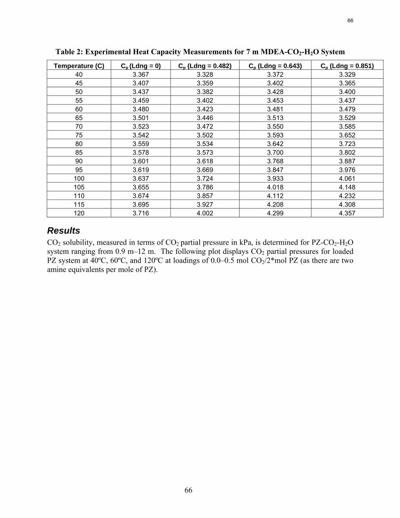
66

Table 2: Experimental Heat Capacity Measurements for 7 m MDEA-CO2-H2O System

Temperature (C) Cp (Ldng = 0) Cp (Ldng = 0.482) Cp (Ldng = 0.643) Cp (Ldng = 0.851) 40 3.367 3.328 3.372 3.329 45 3.407 3.359 3.402 3.365 50 3.437 3.382 3.428 3.400 55 3.459 3.402 3.453 3.437 60 3.480 3.423 3.481 3.479 65 3.501 3.446 3.513 3.529 70 3.523 3.472 3.550 3.585 75 3.542 3.502 3.593 3.652 80 3.559 3.534 3.642 3.723 85 3.578 3.573 3.700 3.802 90 3.601 3.618 3.768 3.887 95 3.619 3.669 3.847 3.976 100 3.637 3.724 3.933 4.061 105 3.655 3.786 4.018 4.148 110 3.674 3.857 4.112 4.232 115 3.695 3.927 4.208 4.308 120 3.716 4.002 4.299 4.357

Results CO2 solubility, measured in terms of CO2 partial pressure in kPa, is determined for PZ-CO2-H2O system ranging from 0.9 m–12 m. The following plot displays CO2 partial pressures for loaded PZ system at 40ºC, 60ºC, and 120ºC at loadings of 0.0–0.5 mol CO2/2*mol PZ (as there are two amine equivalents per mole of PZ).

66

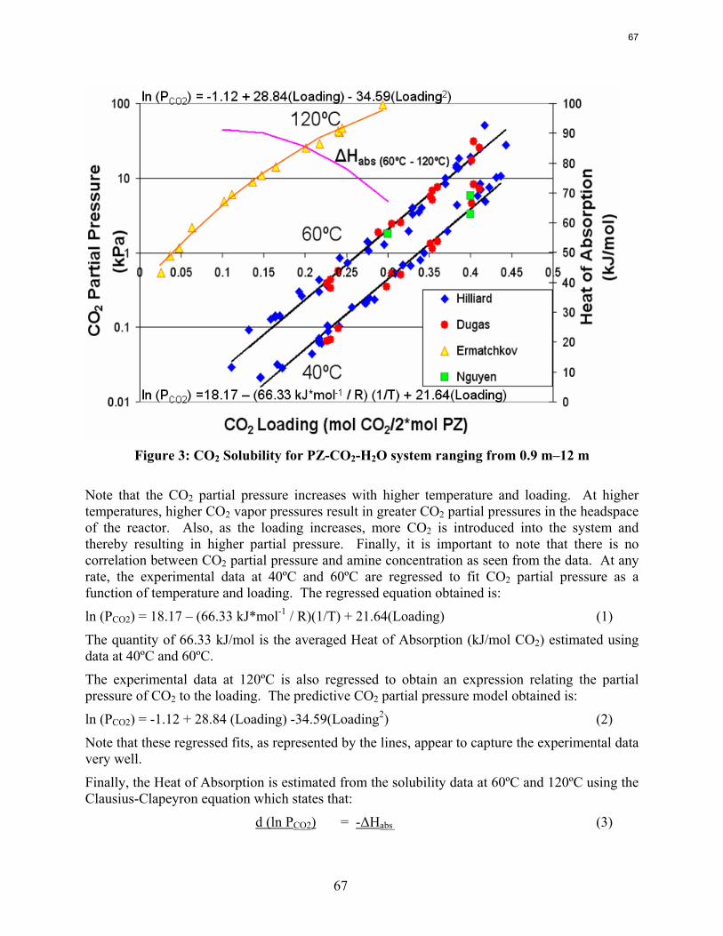
67

Figure 3: CO2 Solubility for PZ-CO2-H2O system ranging from 0.9 m–12 m

Note that the CO2 partial pressure increases with higher temperature and loading. At higher temperatures, higher CO2 vapor pressures result in greater CO2 partial pressures in the headspace of the reactor. Also, as the loading increases, more CO2 is introduced into the system and thereby resulting in higher partial pressure. Finally, it is important to note that there is no correlation between CO2 partial pressure and amine concentration as seen from the data. At any rate, the experimental data at 40ºC and 60ºC are regressed to fit CO2 partial pressure as a function of temperature and loading. The regressed equation obtained is:

ln (PCO2) = 18.17 – (66.33 kJ*mol-1 / R)(1/T) + 21.64(Loading) (1)

The quantity of 66.33 kJ/mol is the averaged Heat of Absorption (kJ/mol CO2) estimated using data at 40ºC and 60ºC.

The experimental data at 120ºC is also regressed to obtain an expression relating the partial pressure of CO2 to the loading. The predictive CO2 partial pressure model obtained is:

ln (PCO2) = -1.12 + 28.84 (Loading) -34.59(Loading2) (2)

Note that these regressed fits, as represented by the lines, appear to capture the experimental data very well.

Finally, the Heat of Absorption is estimated from the solubility data at 60ºC and 120ºC using the Clausius-Clapeyron equation which states that:

d (ln PCO2) = -ΔHabs (3)

67

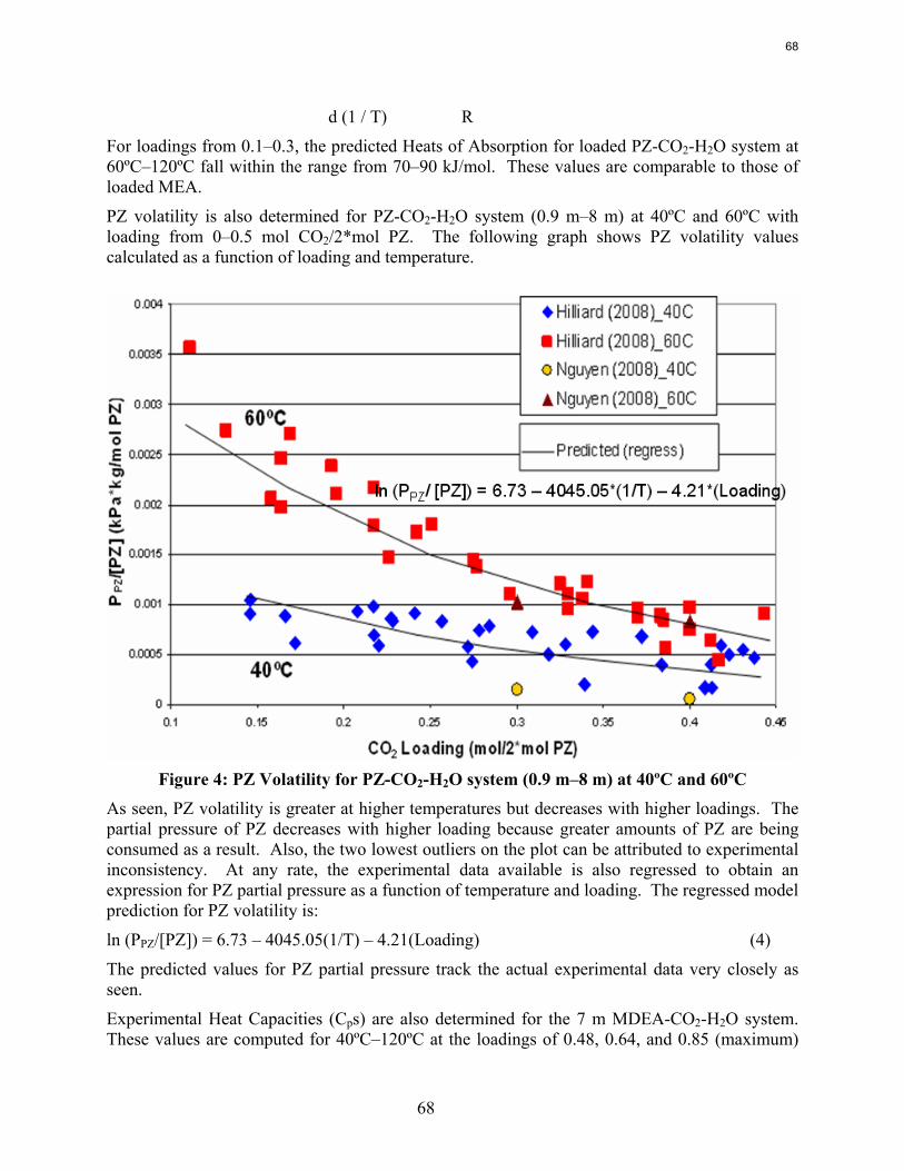
68

d (1 / T) R

For loadings from 0.1–0.3, the predicted Heats of Absorption for loaded PZ-CO2-H2O system at 60ºC–120ºC fall within the range from 70–90 kJ/mol. These values are comparable to those of loaded MEA.

PZ volatility is also determined for PZ-CO2-H2O system (0.9 m–8 m) at 40ºC and 60ºC with loading from 0–0.5 mol CO2/2*mol PZ. The following graph shows PZ volatility values calculated as a function of loading and temperature.

Figure 4: PZ Volatility for PZ-CO2-H2O system (0.9 m–8 m) at 40ºC and 60ºC

As seen, PZ volatility is greater at higher temperatures but decreases with higher loadings. The partial pressure of PZ decreases with higher loading because greater amounts of PZ are being consumed as a result. Also, the two lowest outliers on the plot can be attributed to experimental inconsistency. At any rate, the experimental data available is also regressed to obtain an expression for PZ partial pressure as a function of temperature and loading. The regressed model prediction for PZ volatility is:

ln (PPZ/[PZ]) = 6.73 – 4045.05(1/T) – 4.21(Loading) (4)

The predicted values for PZ partial pressure track the actual experimental data very closely as seen.

Experimental Heat Capacities (Cps) are also determined for the 7 m MDEA-CO2-H2O system. These values are computed for 40ºC–120ºC at the loadings of 0.48, 0.64, and 0.85 (maximum)

68

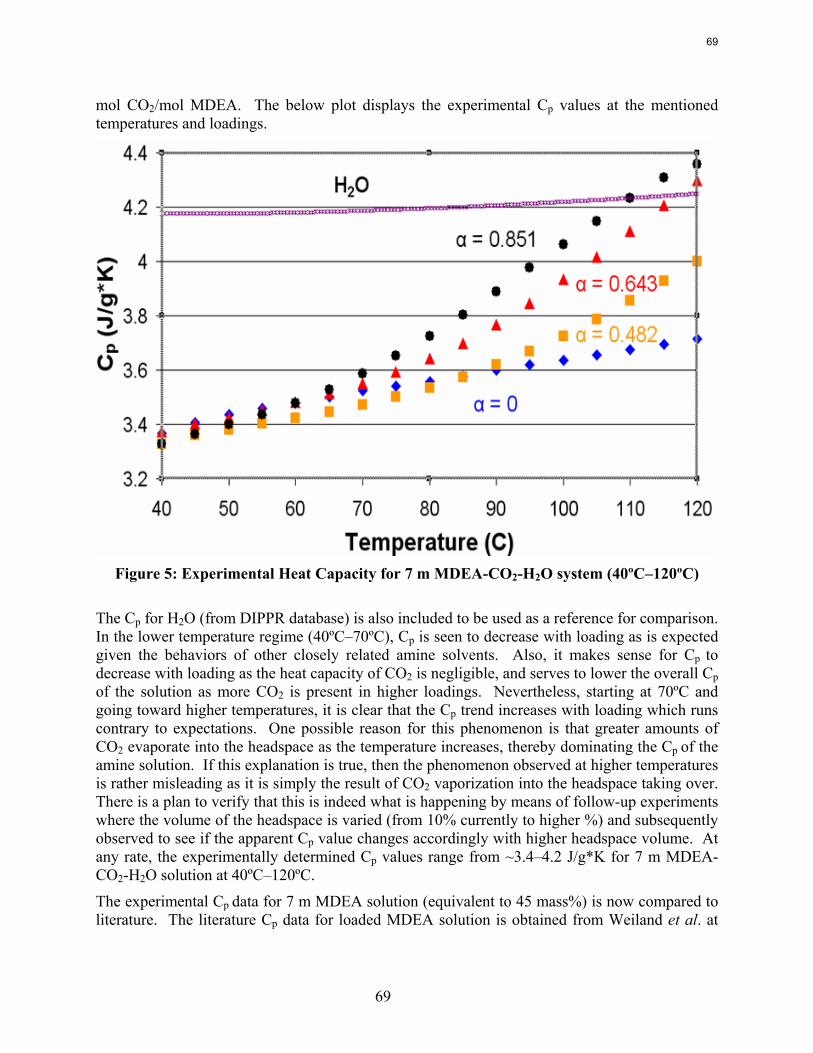
69

mol CO2/mol MDEA. The below plot displays the experimental Cp values at the mentioned temperatures and loadings.

Figure 5: Experimental Heat Capacity for 7 m MDEA-CO2-H2O system (40ºC–120ºC)

The Cp for H2O (from DIPPR database) is also included to be used as a reference for comparison. In the lower temperature regime (40ºC–70ºC), Cp is seen to decrease with loading as is expected given the behaviors of other closely related amine solvents. Also, it makes sense for Cp to decrease with loading as the heat capacity of CO2 is negligible, and serves to lower the overall Cp of the solution as more CO2 is present in higher loadings. Nevertheless, starting at 70ºC and going toward higher temperatures, it is clear that the Cp trend increases with loading which runs contrary to expectations. One possible reason for this phenomenon is that greater amounts of CO2 evaporate into the headspace as the temperature increases, thereby dominating the Cp of the amine solution. If this explanation is true, then the phenomenon observed at higher temperatures is rather misleading as it is simply the result of CO2 vaporization into the headspace taking over. There is a plan to verify that this is indeed what is happening by means of follow-up experiments where the volume of the headspace is varied (from 10% currently to higher %) and subsequently observed to see if the apparent Cp value changes accordingly with higher headspace volume. At any rate, the experimentally determined Cp values range from ~3.4–4.2 J/g*K for 7 m MDEA-CO2-H2O solution at 40ºC–120ºC.

The experimental Cp data for 7 m MDEA solution (equivalent to 45 mass%) is now compared to literature. The literature Cp data for loaded MDEA solution is obtained from Weiland et al. at

69

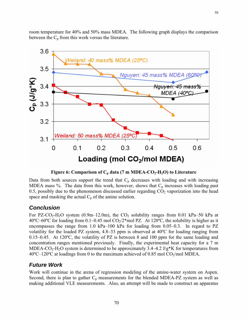
70

room temperature for 40% and 50% mass MDEA. The following graph displays the comparison between the Cp from this work versus the literature.

Figure 6: Comparison of Cp data (7 m MDEA-CO2-H2O) to Literature

Data from both sources support the trend that Cp decreases with loading and with increasing MDEA mass %. The data from this work, however, shows that Cp increases with loading past 0.5, possibly due to the phenomenon discussed earlier regarding CO2 vaporization into the head space and masking the actual Cp of the amine solution.

Conclusion For PZ-CO2-H2O system (0.9m–12.0m), the CO2 solubility ranges from 0.01 kPa–50 kPa at 40ºC–60ºC for loading from 0.1–0.45 mol CO2/2*mol PZ. At 120ºC, the solubility is higher as it encompasses the range from 1.0 kPa–100 kPa for loading from 0.05–0.3. In regard to PZ volatility for the loaded PZ system, 4.8–33 ppm is observed at 40ºC for loading ranging from 0.15–0.45. At 120ºC, the volatility of PZ is between 8 and 100 ppm for the same loading and concentration ranges mentioned previously. Finally, the experimental heat capacity for a 7 m MDEA-CO2-H2O system is determined to be approximately 3.4–4.2 J/g*K for temperatures from 40ºC–120ºC at loadings from 0 to the maximum achieved of 0.85 mol CO2/mol MDEA.

Future Work Work will continue in the arena of regression modeling of the amine-water system on Aspen. Second, there is plan to gather Cp measurements for the blended MDEA-PZ system as well as making additional VLE measurements. Also, an attempt will be made to construct an apparatus

70

71

for high temperature VLE measurements from 100ºC–160ºC for the MDEA-PZ blend. Finally, there will be some work done to run NMR speciation analysis in order to identify the exact liquid phase species and their compositions in the solutions used for VLE experiments.

71

72

72

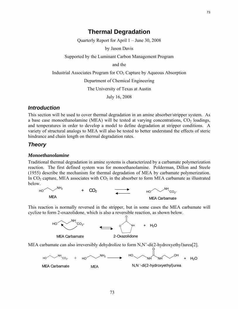
73

Thermal Degradation Quarterly Report for April 1 – June 30, 2008

by Jason Davis

Supported by the Luminant Carbon Management Program

and the

Industrial Associates Program for CO2 Capture by Aqueous Absorption

Department of Chemical Engineering

The University of Texas at Austin

July 16, 2008

Introduction This section will be used to cover thermal degradation in an amine absorber/stripper system. As a base case monoethanolamine (MEA) will be tested at varying concentrations, CO2 loadings, and temperatures in order to develop a model to define degradation at stripper conditions. A variety of structural analogs to MEA will also be tested to better understand the effects of steric hindrance and chain length on thermal degradation rates.

Theory

Monoethanolamine Traditional thermal degradation in amine systems is characterized by a carbamate polymerization reaction. The first defined system was for monoethanolamine. Polderman, Dillon and Steele (1955) describe the mechanism for thermal degradation of MEA by carbamate polymerization. In CO2 capture, MEA associates with CO2 in the absorber to form MEA carbamate as illustrated below.

This reaction is normally reversed in the stripper, but in some cases the MEA carbamate will cyclize to form 2-oxazolidone, which is also a reversible reaction, as shown below.

MEA carbamate can also irreversibly dehydrolize to form N,N’-di(2-hydroxyethyl)urea[2].

NH2OH

NHOH CO2-++ CCOO22

MMEEAA CCaarrbbaammaattee MMEEAA

NHO

O

22--OOxxaazzoolliiddoonnee

++ HH22OO

MMEEAA CCaarrbbaammaattee

NHOH CO2-

OHNHNH

OH

O

++ HH22OO

NN,,NN ‘‘--ddii((22--hhyyddrrooxxyyeetthhyyll))uurreeaa

NHOH CO2-

MMEEAA CCaarrbbaammaattee

NH2OH+

MEA

73

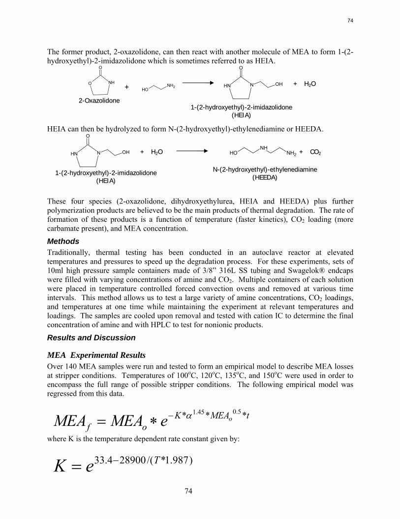
74

The former product, 2-oxazolidone, can then react with another molecule of MEA to form 1-(2-hydroxyethyl)-2-imidazolidone which is sometimes referred to as HEIA.

HEIA can then be hydrolyzed to form N-(2-hydroxyethyl)-ethylenediamine or HEEDA.

These four species (2-oxazolidone, dihydroxyethylurea, HEIA and HEEDA) plus further polymerization products are believed to be the main products of thermal degradation. The rate of formation of these products is a function of temperature (faster kinetics), CO2 loading (more carbamate present), and MEA concentration.

Methods Traditionally, thermal testing has been conducted in an autoclave reactor at elevated temperatures and pressures to speed up the degradation process. For these experiments, sets of 10ml high pressure sample containers made of 3/8” 316L SS tubing and Swagelok® endcaps were filled with varying concentrations of amine and CO2. Multiple containers of each solution were placed in temperature controlled forced convection ovens and removed at various time intervals. This method allows us to test a large variety of amine concentrations, CO2 loadings, and temperatures at one time while maintaining the experiment at relevant temperatures and loadings. The samples are cooled upon removal and tested with cation IC to determine the final concentration of amine and with HPLC to test for nonionic products.

Results and Discussion

MEA Experimental Results Over 140 MEA samples were run and tested to form an empirical model to describe MEA losses at stripper conditions. Temperatures of 100oC, 120oC, 135oC, and 150oC were used in order to encompass the full range of possible stripper conditions. The following empirical model was regressed from this data. where K is the temperature dependent rate constant given by:

NNH

O

OH ++ HH22OO

11--((22--hhyyddrrooxxyyeetthhyyll))--22--iimmiiddaazzoolliiddoonnee ((HHEEIIAA))

NHO

O

22--OOxxaazzoolliiddoonnee

++ NH2OH

NHOH NH2 ++ CCOO22

NN--((22--hhyyddrrooxxyyeetthhyyll))--eetthhyylleenneeddiiaammiinnee ((HHEEEEDDAA))

NNH

O

OH ++ HH22OO

tMEAKof

oeMEAMEA *** 5.045.1α−∗=

)987.1*/(289004.33 TeK −=

11--((22--hhyyddrrooxxyyeetthhyyll))--22--iimmiiddaazzoolliiddoonnee ((HHEEIIAA))

74

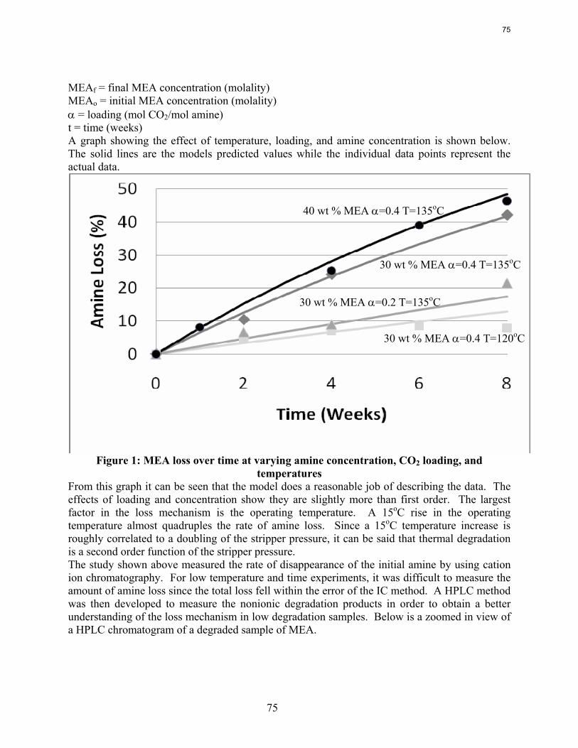
75

MEAf = final MEA concentration (molality) MEAo = initial MEA concentration (molality) α = loading (mol CO2/mol amine) t = time (weeks) A graph showing the effect of temperature, loading, and amine concentration is shown below. The solid lines are the models predicted values while the individual data points represent the actual data.

Figure 1: MEA loss over time at varying amine concentration, CO2 loading, and

temperatures From this graph it can be seen that the model does a reasonable job of describing the data. The effects of loading and concentration show they are slightly more than first order. The largest factor in the loss mechanism is the operating temperature. A 15oC rise in the operating temperature almost quadruples the rate of amine loss. Since a 15oC temperature increase is roughly correlated to a doubling of the stripper pressure, it can be said that thermal degradation is a second order function of the stripper pressure. The study shown above measured the rate of disappearance of the initial amine by using cation ion chromatography. For low temperature and time experiments, it was difficult to measure the amount of amine loss since the total loss fell within the error of the IC method. A HPLC method was then developed to measure the nonionic degradation products in order to obtain a better understanding of the loss mechanism in low degradation samples. Below is a zoomed in view of a HPLC chromatogram of a degraded sample of MEA.

40 wt % MEA α=0.4 T=135oC

30 wt % MEA α=0.4 T=135oC

30 wt % MEA α=0.2 T=135oC

30 wt % MEA α=0.4 T=120oC

75

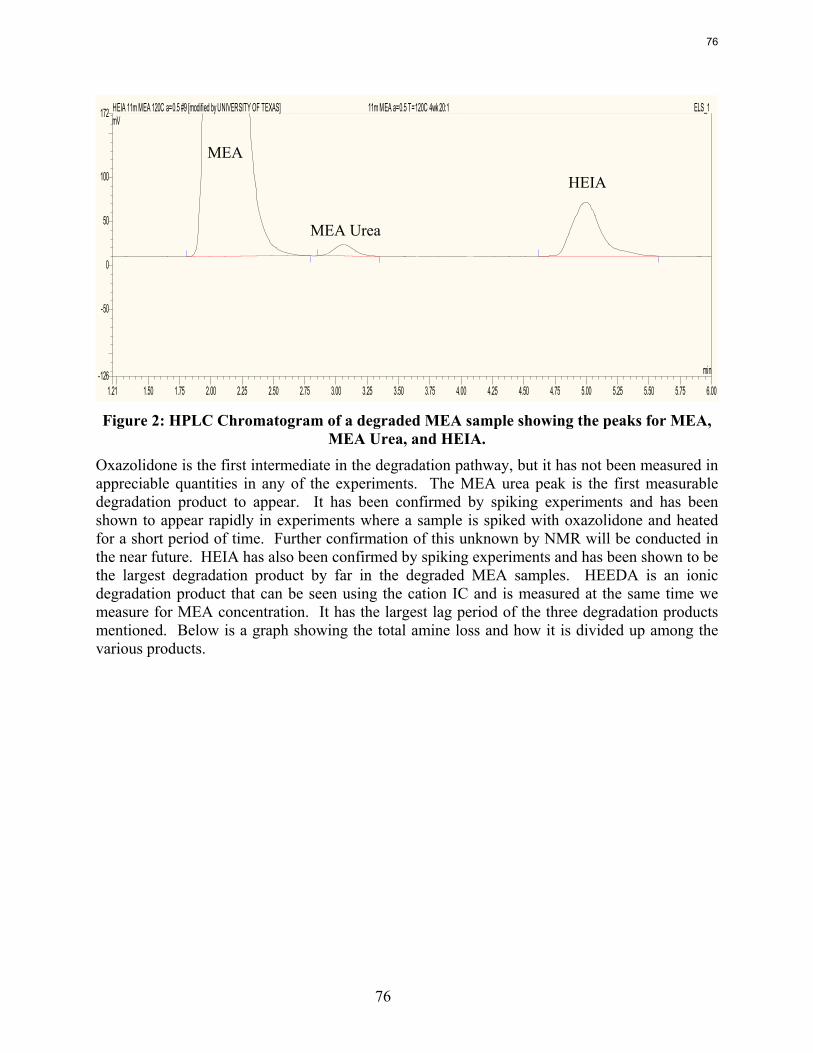
76

1.21 1.50 1.75 2.00 2.25 2.50 2.75 3.00 3.25 3.50 3.75 4.00 4.25 4.50 4.75 5.00 5.25 5.50 5.75 6.00-126

-50

0

50

100

172 HEIA 11m MEA 120C a=0.5 #9 [modified by UNIVERSITY OF TEXAS] 11m MEA a=0.5 T=120C 4wk 20:1 ELS_1mV

min

Figure 2: HPLC Chromatogram of a degraded MEA sample showing the peaks for MEA,

MEA Urea, and HEIA.

Oxazolidone is the first intermediate in the degradation pathway, but it has not been measured in appreciable quantities in any of the experiments. The MEA urea peak is the first measurable degradation product to appear. It has been confirmed by spiking experiments and has been shown to appear rapidly in experiments where a sample is spiked with oxazolidone and heated for a short period of time. Further confirmation of this unknown by NMR will be conducted in the near future. HEIA has also been confirmed by spiking experiments and has been shown to be the largest degradation product by far in the degraded MEA samples. HEEDA is an ionic degradation product that can be seen using the cation IC and is measured at the same time we measure for MEA concentration. It has the largest lag period of the three degradation products mentioned. Below is a graph showing the total amine loss and how it is divided up among the various products.

MEA Urea

HEIA

MEA

76

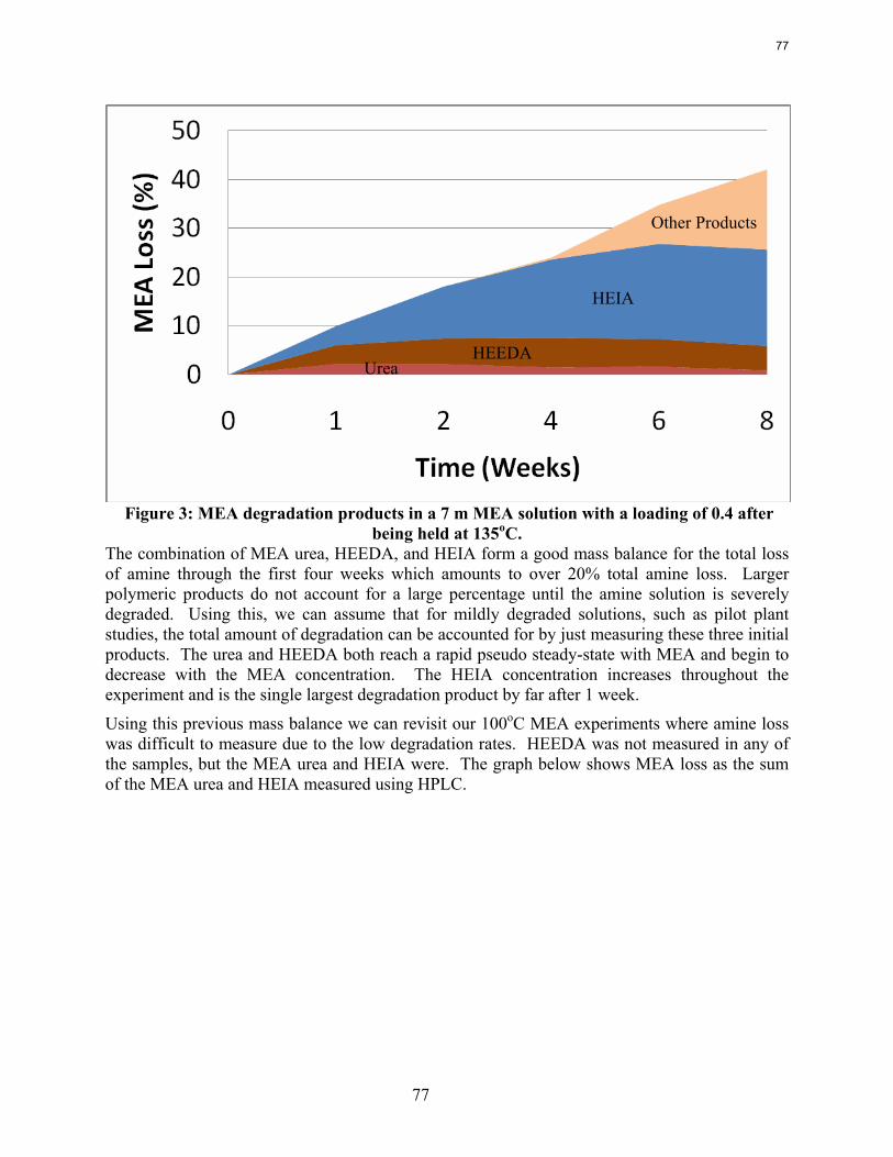
77

Figure 3: MEA degradation products in a 7 m MEA solution with a loading of 0.4 after being held at 135oC.

The combination of MEA urea, HEEDA, and HEIA form a good mass balance for the total loss of amine through the first four weeks which amounts to over 20% total amine loss. Larger polymeric products do not account for a large percentage until the amine solution is severely degraded. Using this, we can assume that for mildly degraded solutions, such as pilot plant studies, the total amount of degradation can be accounted for by just measuring these three initial products. The urea and HEEDA both reach a rapid pseudo steady-state with MEA and begin to decrease with the MEA concentration. The HEIA concentration increases throughout the experiment and is the single largest degradation product by far after 1 week.

Using this previous mass balance we can revisit our 100oC MEA experiments where amine loss was difficult to measure due to the low degradation rates. HEEDA was not measured in any of the samples, but the MEA urea and HEIA were. The graph below shows MEA loss as the sum of the MEA urea and HEIA measured using HPLC.

Other Products

HEIA

HEEDA Urea

77

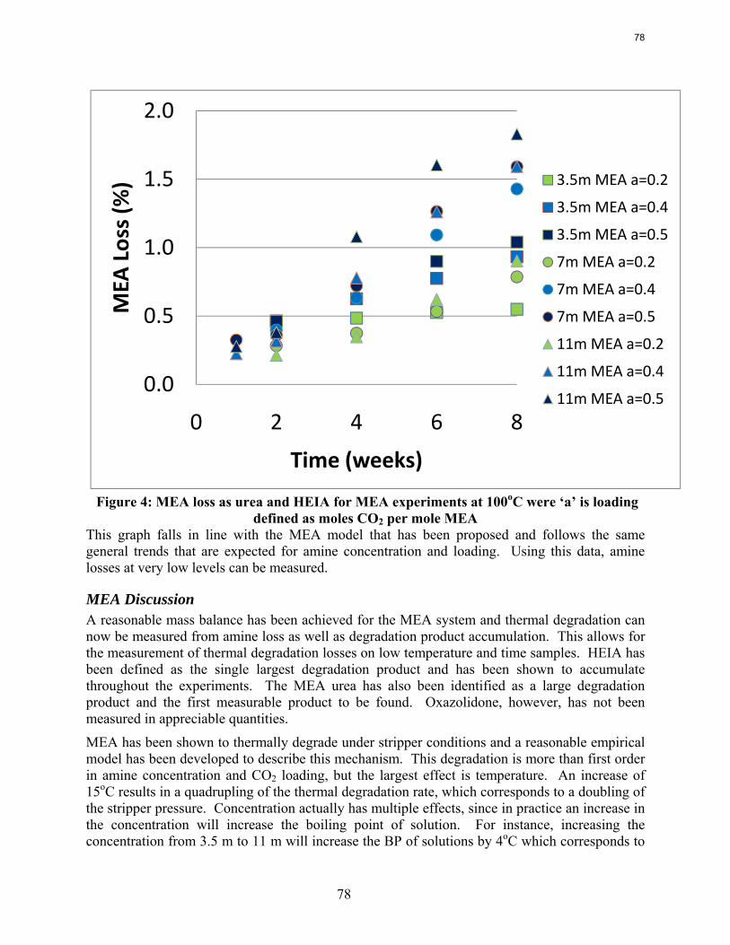
78

0.0

0.5

1.0

1.5

2.0

0 2 4 6 8

MEA

 Loss (%

)

Time (weeks)

3.5m MEA a=0.2

3.5m MEA a=0.4

3.5m MEA a=0.5

7m MEA a=0.2

7m MEA a=0.4

7m MEA a=0.5

11m MEA a=0.2

11m MEA a=0.4

11m MEA a=0.5

Figure 4: MEA loss as urea and HEIA for MEA experiments at 100oC were ‘a’ is loading defined as moles CO2 per mole MEA

This graph falls in line with the MEA model that has been proposed and follows the same general trends that are expected for amine concentration and loading. Using this data, amine losses at very low levels can be measured.

MEA Discussion A reasonable mass balance has been achieved for the MEA system and thermal degradation can now be measured from amine loss as well as degradation product accumulation. This allows for the measurement of thermal degradation losses on low temperature and time samples. HEIA has been defined as the single largest degradation product and has been shown to accumulate throughout the experiments. The MEA urea has also been identified as a large degradation product and the first measurable product to be found. Oxazolidone, however, has not been measured in appreciable quantities.

MEA has been shown to thermally degrade under stripper conditions and a reasonable empirical model has been developed to describe this mechanism. This degradation is more than first order in amine concentration and CO2 loading, but the largest effect is temperature. An increase of 15oC results in a quadrupling of the thermal degradation rate, which corresponds to a doubling of the stripper pressure. Concentration actually has multiple effects, since in practice an increase in the concentration will increase the boiling point of solution. For instance, increasing the concentration from 3.5 m to 11 m will increase the BP of solutions by 4oC which corresponds to

78

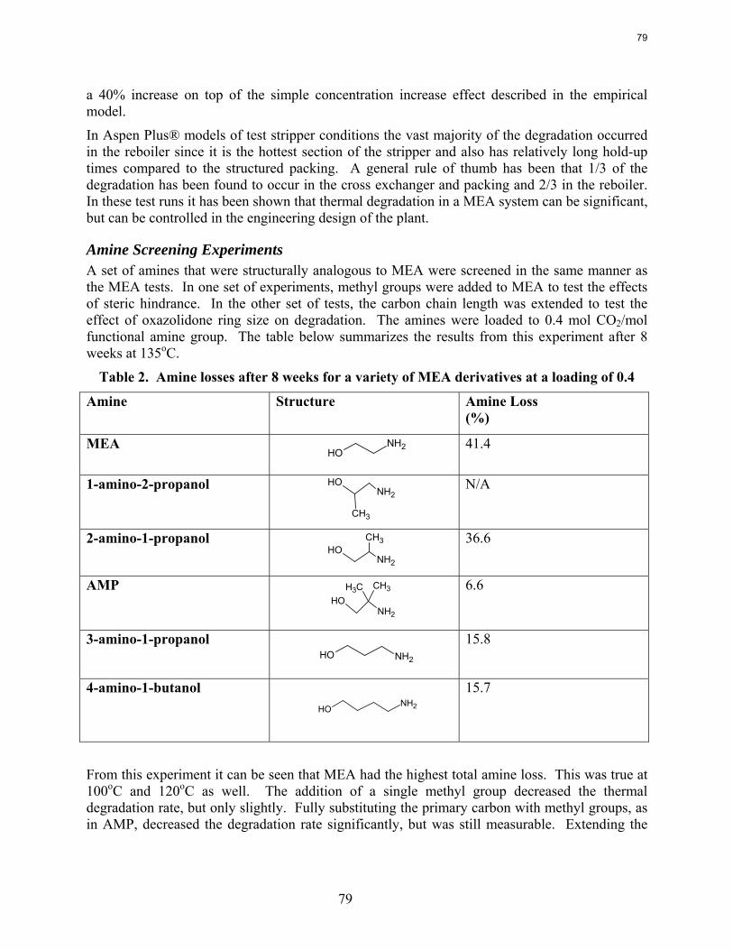
79

a 40% increase on top of the simple concentration increase effect described in the empirical model.

In Aspen Plus® models of test stripper conditions the vast majority of the degradation occurred in the reboiler since it is the hottest section of the stripper and also has relatively long hold-up times compared to the structured packing. A general rule of thumb has been that 1/3 of the degradation has been found to occur in the cross exchanger and packing and 2/3 in the reboiler. In these test runs it has been shown that thermal degradation in a MEA system can be significant, but can be controlled in the engineering design of the plant.

Amine Screening Experiments A set of amines that were structurally analogous to MEA were screened in the same manner as the MEA tests. In one set of experiments, methyl groups were added to MEA to test the effects of steric hindrance. In the other set of tests, the carbon chain length was extended to test the effect of oxazolidone ring size on degradation. The amines were loaded to 0.4 mol CO2/mol functional amine group. The table below summarizes the results from this experiment after 8 weeks at 135oC.

Table 2. Amine losses after 8 weeks for a variety of MEA derivatives at a loading of 0.4

Amine Structure Amine Loss (%)

MEA

41.4

1-amino-2-propanol

N/A

2-amino-1-propanol

36.6

AMP

6.6

3-amino-1-propanol

15.8

4-amino-1-butanol

15.7

From this experiment it can be seen that MEA had the highest total amine loss. This was true at 100oC and 120oC as well. The addition of a single methyl group decreased the thermal degradation rate, but only slightly. Fully substituting the primary carbon with methyl groups, as in AMP, decreased the degradation rate significantly, but was still measurable. Extending the

NH2OH

OHNH2

CH3

OHNH2

CH3

OHNH2

CH3CH3

NH2OH

NH2OH

79

80

carbon chain length also significantly reduced the amount of thermal degradation, but was still more than twice the amount of AMP.

Conclusions A reasonable empirical model for MEA degradation has been developed and is reasonable over a large range of temperatures (100–150oC), loadings (0.2–0.5 moles CO2 per mole MEA), and amine concentrations (15–40 wt %). A very good mass balance has also been reached for MEA systems with less than 20% MEA loss. The combination of the HPLC and IC methods can be used to measure amine losses in systems with little thermal degradation. Thermal degradation can be a significant cost in the amine absorber/stripper system, but can be controlled as long as it is taken into account in the design phase of the stripper and reclaimer system. The majority of this degradation in an MEA system seems to occur in the reboiler of the stripper as this is the hottest section and temperature has a more dramatic effect than loading does. Further study of reclaiming systems needs to be performed in order to more accurately predict the full extent of thermal degradation since natural gas treating experience says that roughly 50% of thermal degradation occurs in the thermal reclaiming system. A set of MEA derivatives were screened for thermal degradation and it was found that by sterically hindering the primary carbon, thermal degradation can be greatly reduced. The addition of a single methyl group did little to help, but extending the carbon chain length did show marked improvement over a simple MEA system.

References Polderman LD, Dillon CP, Steele AB. Why monoethanolamine solution breaks down in gas-

treating service. Oil Gas J. 1955;54(2):180–183. Yazvikova NV, Zelenskaya LG, Balyasnikova LV. Mechanism of Side reactions During removal

of Carbon Dioxide from Gases by Treatment with Monoethanolamine. Zhurnal Prikladnoi Khimii. 1975;48(3):674–676.

80

81

Oxidative Degradation of Amines Quarterly Report for April 1– June 30, 2008

by Andrew Sexton Supported by the Luminant Carbon Management Program

and the Industrial Associates Program for CO2 Capture by Aqueous Absorption

Department of Chemical Engineering The University of Texas at Austin

July 20, 2008

Abstract Both ethylenediamine (EDA) and potassium glycinate solutions are resistant to oxidative degradation in the low gas flow apparatus. All liquid-phase degradation products were observed in trace concentrations, and neither solvent system showed any concentration loss during the course of the experiments. This suggests that the alkanolamine structure is more susceptible to oxidative degradation. Diethylenetriamine (DETA), the dimerization product of EDA, is an oxidative degradation product unique to EDA systems.

MEA systems catalyzed by vanadium produce less formate and more oxalate than MEA systems catalyzed by iron, but overall carbon and nitrogen formation rates were similar. Chromium and nickel, two metals present in stainless steel alloys, also catalyze the degradation of MEA. The two catalysts have a synergistic effect on the production of formate.

Inhibitor B is an effective oxidative degradation inhibitor for iron-catalyzed systems, while the addition of 100 mM Inhibitor A effectively stopped the oxidative degradation of MEA catalyzed by chromium and nickel. Subsequent EDTA experiments showed that a high ratio of EDTA:Fe (100:1 to be exact) is necessary to sufficiently inhibit the oxidation of MEA. Sodium sulfite, an oxygen scavenger, and formaldehyde were ineffective oxidative degradation inhibitors.

A reduction in the agitation rate from 1400 RPM to 700 resulted in a 25% decrease in formate production, while an increase in CO2 concentration from 2% to 6% doubles the apparent MEA degradation rate.

Analysis of the high gas flow experiments suggests that the material balance does not close. There are most likely oxidative degradation products, both liquid and gas-phase products, that have yet to be identified. Possible products include non-polar species in the liquid phase and CO2 in the gas phase. A fundamental difference in the low and high gas experiments is that nitrite, nitrate, and oxalate production relative to formate in the liquid phase is much lower in the high gas flow apparatus. Products stripped out in the gas phase prevent the formation of these products. Piperazine in the absence of catalyst does not degrade to form NH3; major degradation products are EDA and NOx.

81

82

Introduction This effort is an extension of work by George Goff on the oxidative degradation of MEA. Goff showed that oxidative degradation, under high catalyst conditions, is mass-transfer limited by the physical absorption of O2 into the amine and not by reaction kinetics. Goff also theorized that the oxidative degradation of MEA produced volatile ammonia as well as a host of other proposed degradation products. The major liquid-phase degradation products among these include the heat stable salts of carboxylic acids, nitrite, and nitrate.

The oxygen stoichiometry necessary to produce these degradation products varies for each individual component; overall, it varies anywhere from 0.5 to 2.5 (Goff, 2004). It is believed that the particular degradation products are specific to certain metal catalysts present in the absorption/stripping system – specifically iron and copper. For example, the following balanced reactions illustrate the differences in oxygen consumption based on the end products:

MEA + 1.5 O2 2 Formate + Ammonia MEA+ 3.5 O2 2 Formate + Nitrate + Water MEA + O2 Glycolate + Ammonia

Goff’s work on MEA degradation was limited to analyzing MEA degradation rates via the evolution of NH3. The ammonia evolution rates were measured using a Fourier Transform Infrared (FTIR) analyzer.

This effort extends Goff’s gas-phase analysis by applying various methods of liquid-phase analysis, specifically ion chromatography. These analytical methods will be used to quantify the rate of amine degradation as well as the rate of degradation product formation for amine systems.

Since most gas treating processes using alkanolamines for CO2 removal are performed in the absence of oxygen, oxidative degradation is a source of solvent degradation that has not been properly quantified. Oxidative degradation is important because it can impact the environment, process economics, and decrease equipment life due to corrosion.

The environmental effects refer to the degradation products themselves: what is being produced, how much of it is being produced, and how can it be disposed of without doing significant damage to the environment. Process economics being impacted are the solvent make-up rate and design of the reclaiming operation. If amine is continually being degraded, then fresh amine must be continually added to the process at a significant cost. In addition, CO2 loaded amine solutions corrode carbon steel equipment, which catalyzes oxidative degradation even further. It is imperative to quantify how much of this solvent make-up rate is due to oxidative degradation.

Experimental As stated in prior reports, ion chromatography is the most extensively used liquid-phase analytical method. Anion chromatography utilizes an AS15 (a low-capacity column designed to separate low-molecular weight anions, specifically acetate, glycolate, and formate) IonPac column and an ASRS 4-mm self-regenerating suppressor made by Dionex, while cation analysis uses a CS17 and a CSRS 4-mm self-regenerating suppressor. Anion analysis employs a linear gradient of NaOH eluent, while cation analysis uses a step-change from low to high concentration of methanesulfonic acid (MSA) eluent. Refer to prior quarterly reports for detailed descriptions of the Dionex ICS2500 and ICS3000 analytical equipment.

82

83

Amides are a class of compounds that were detected in an HPLC-MS screening performed by the Hunstman Chemical analytical department. Amides are formed from the condensation reaction of an amine with a carboxylic acid. Since both of these species are known to exist in appreciable quantities in degraded amine solutions, it is conceivable that amides are present. Amides can be detected using HPLC with UV detection, but amides absorb at 200 nm, thus making it difficult to separate them from other species in the solution.

Koike et al. (1987) concluded that the addition of excess NaOH was successful at reversing the amide formation reaction back to amine and carboxylic acid. This hypothesis was tested using various concentrations of sodium hydroxide reacted with formamide and N-(hydroxymethyl)acetamide. It was concluded that reacting 1g of sample with 1g of 5 M NaOH at 25ºC and allowing the solution to sit for twenty-four hours was sufficient to reverse the amide reaction. Using the anion IC procedure detailed previously, all experimental samples are analyzed pre- and post-addition of NaOH to determine carboxylic acid and amide concentrations. All amide concentrations (as calculated by the difference between the carboxylic acid concentrations pre- and post-NaOH addition) will still be reported as carboxylic acids.

As stated in previous reports, amine solutions in the low gas flow degradation apparatus are oxidized for 12 to 14 days in a low-gas flow jacketed reactor at 55ºC. The solutions are agitated at 1400 RPM to produce a high level of gas/liquid mass transfer by vortexing. 98% O2/2% CO2 at 100 ml/min is introduced across the vortexed surface of 350 ml of aqueous amine. Samples are taken from the reactor at regular intervals in order to determine how degradation products formed over the course of the experiment. Prior quarterly reports provide a detailed explanation of the low gas flow degradation apparatus.

Four low gas flow apparatus are now operating in parallel. Two systems operates via the original configuration, which uses an inlet gas of 98% O2/2% CO2 premixed in a cylinder provided by Matheson Tri-Gas. A Cole-Parmer rotameter is used to control the flowrate at 100 ml/min. The other two apparatus are setup for the modified configuration, which operates with two separate cylinders provided by Matheson Tri-Gas – a pure oxygen cylinder and a pure CO2 cylinder. The 98% O2/2% CO2 mixture is achieved using a 4 channel Brose box made by Brooks and two model 5850E mass flow controllers also manufactured by Brooks. In one setup (Channels 1 and 2), oxygen flowrate is controlled by a 100 cc flow controller, while carbon dioxide is controlled by a 20 cc flow controller. The other setup employs a 250 cc oxygen mass flow controller and a 5cc CO2 mass flow controller. The control box displays a digital readout corresponding to the % open of the valve on the mass flow controller. The valve % open corresponds to a gas flowrate, which is determined from the calibration curve constructed for each flowmeter.

The original setup is limited by the fact that the partial pressure of CO2 over the top of the amine solution entering low gas flow apparatus is fixed. Therefore, the loading of each amine solution is fixed and corresponds to 2% CO2 concentration in the vapor space above the amine solution. The modified setup allows for variations in the CO2 concentration such that a particular loading in the amine solution can be achieved by adjusting the incoming CO2 concentration via the flow controllers. Amine loading has become a variable, whereas in the past it was constrained.

Experiments are performed in the high gas flow degradation apparatus by sparging gas through an agitated amine solution in a temperature controlled semi-batch reactor. Reaction gas, consisting of a mixture of house air, nitrogen, and CO2 is bubbled through water to presaturate

83

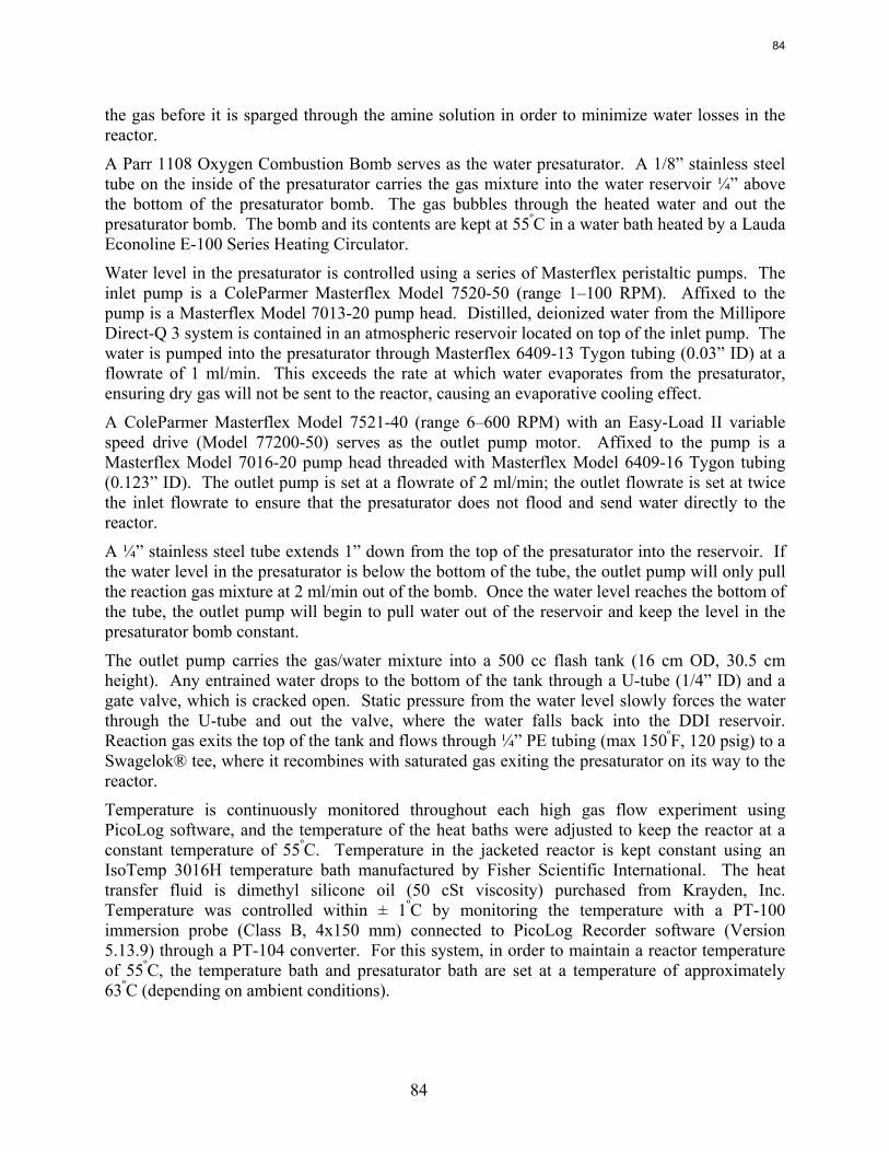
84

the gas before it is sparged through the amine solution in order to minimize water losses in the reactor.

A Parr 1108 Oxygen Combustion Bomb serves as the water presaturator. A 1/8” stainless steel tube on the inside of the presaturator carries the gas mixture into the water reservoir ¼” above the bottom of the presaturator bomb. The gas bubbles through the heated water and out the presaturator bomb. The bomb and its contents are kept at 55ºC in a water bath heated by a Lauda Econoline E-100 Series Heating Circulator.

Water level in the presaturator is controlled using a series of Masterflex peristaltic pumps. The inlet pump is a ColeParmer Masterflex Model 7520-50 (range 1–100 RPM). Affixed to the pump is a Masterflex Model 7013-20 pump head. Distilled, deionized water from the Millipore Direct-Q 3 system is contained in an atmospheric reservoir located on top of the inlet pump. The water is pumped into the presaturator through Masterflex 6409-13 Tygon tubing (0.03” ID) at a flowrate of 1 ml/min. This exceeds the rate at which water evaporates from the presaturator, ensuring dry gas will not be sent to the reactor, causing an evaporative cooling effect.

A ColeParmer Masterflex Model 7521-40 (range 6–600 RPM) with an Easy-Load II variable speed drive (Model 77200-50) serves as the outlet pump motor. Affixed to the pump is a Masterflex Model 7016-20 pump head threaded with Masterflex Model 6409-16 Tygon tubing (0.123” ID). The outlet pump is set at a flowrate of 2 ml/min; the outlet flowrate is set at twice the inlet flowrate to ensure that the presaturator does not flood and send water directly to the reactor.

A ¼” stainless steel tube extends 1” down from the top of the presaturator into the reservoir. If the water level in the presaturator is below the bottom of the tube, the outlet pump will only pull the reaction gas mixture at 2 ml/min out of the bomb. Once the water level reaches the bottom of the tube, the outlet pump will begin to pull water out of the reservoir and keep the level in the presaturator bomb constant.

The outlet pump carries the gas/water mixture into a 500 cc flash tank (16 cm OD, 30.5 cm height). Any entrained water drops to the bottom of the tank through a U-tube (1/4” ID) and a gate valve, which is cracked open. Static pressure from the water level slowly forces the water through the U-tube and out the valve, where the water falls back into the DDI reservoir. Reaction gas exits the top of the tank and flows through ¼” PE tubing (max 150ºF, 120 psig) to a Swagelok® tee, where it recombines with saturated gas exiting the presaturator on its way to the reactor.

Temperature is continuously monitored throughout each high gas flow experiment using PicoLog software, and the temperature of the heat baths were adjusted to keep the reactor at a constant temperature of 55ºC. Temperature in the jacketed reactor is kept constant using an IsoTemp 3016H temperature bath manufactured by Fisher Scientific International. The heat transfer fluid is dimethyl silicone oil (50 cSt viscosity) purchased from Krayden, Inc. Temperature was controlled within ± 1ºC by monitoring the temperature with a PT-100 immersion probe (Class B, 4x150 mm) connected to PicoLog Recorder software (Version 5.13.9) through a PT-104 converter. For this system, in order to maintain a reactor temperature of 55ºC, the temperature bath and presaturator bath are set at a temperature of approximately 63ºC (depending on ambient conditions).

84

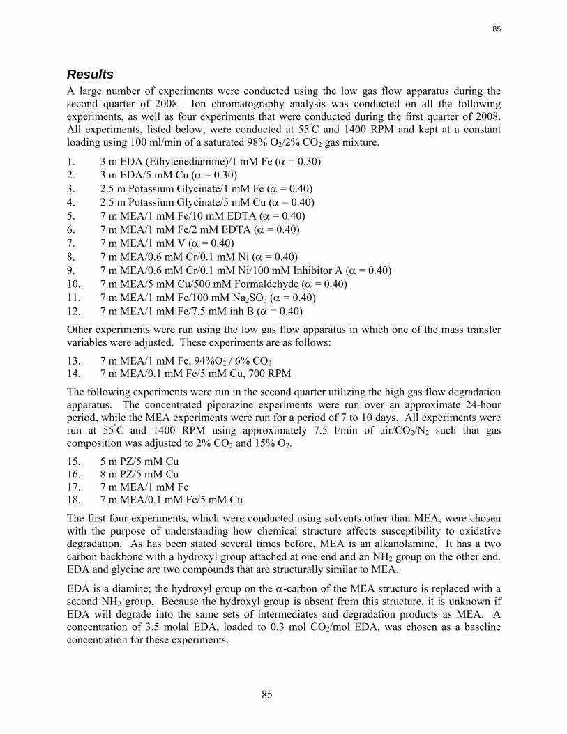
85

Results A large number of experiments were conducted using the low gas flow apparatus during the second quarter of 2008. Ion chromatography analysis was conducted on all the following experiments, as well as four experiments that were conducted during the first quarter of 2008. All experiments, listed below, were conducted at 55ºC and 1400 RPM and kept at a constant loading using 100 ml/min of a saturated 98% O2/2% CO2 gas mixture.

1. 3 m EDA (Ethylenediamine)/1 mM Fe (α = 0.30) 2. 3 m EDA/5 mM Cu (α = 0.30) 3. 2.5 m Potassium Glycinate/1 mM Fe (α = 0.40) 4. 2.5 m Potassium Glycinate/5 mM Cu (α = 0.40) 5. 7 m MEA/1 mM Fe/10 mM EDTA (α = 0.40) 6. 7 m MEA/1 mM Fe/2 mM EDTA (α = 0.40) 7. 7 m MEA/1 mM V (α = 0.40) 8. 7 m MEA/0.6 mM Cr/0.1 mM Ni (α = 0.40) 9. 7 m MEA/0.6 mM Cr/0.1 mM Ni/100 mM Inhibitor A (α = 0.40) 10. 7 m MEA/5 mM Cu/500 mM Formaldehyde (α = 0.40) 11. 7 m MEA/1 mM Fe/100 mM Na2SO3 (α = 0.40) 12. 7 m MEA/1 mM Fe/7.5 mM inh B (α = 0.40)

Other experiments were run using the low gas flow apparatus in which one of the mass transfer variables were adjusted. These experiments are as follows:

13. 7 m MEA/1 mM Fe, 94%O2 / 6% CO2 14. 7 m MEA/0.1 mM Fe/5 mM Cu, 700 RPM

The following experiments were run in the second quarter utilizing the high gas flow degradation apparatus. The concentrated piperazine experiments were run over an approximate 24-hour period, while the MEA experiments were run for a period of 7 to 10 days. All experiments were run at 55ºC and 1400 RPM using approximately 7.5 l/min of air/CO2/N2 such that gas composition was adjusted to 2% CO2 and 15% O2.

15. 5 m PZ/5 mM Cu 16. 8 m PZ/5 mM Cu 17. 7 m MEA/1 mM Fe 18. 7 m MEA/0.1 mM Fe/5 mM Cu

The first four experiments, which were conducted using solvents other than MEA, were chosen with the purpose of understanding how chemical structure affects susceptibility to oxidative degradation. As has been stated several times before, MEA is an alkanolamine. It has a two carbon backbone with a hydroxyl group attached at one end and an NH2 group on the other end. EDA and glycine are two compounds that are structurally similar to MEA.

EDA is a diamine; the hydroxyl group on the α-carbon of the MEA structure is replaced with a second NH2 group. Because the hydroxyl group is absent from this structure, it is unknown if EDA will degrade into the same sets of intermediates and degradation products as MEA. A concentration of 3.5 molal EDA, loaded to 0.3 mol CO2/mol EDA, was chosen as a baseline concentration for these experiments.

85

86

Glycine is an amino acid; the hydroxyl group of MEA is oxidized to a carboxylic acid functional group while the rest of the structure remains the same. Literature from van Holst (2006) proposes that salts of amino acids are an attractive alternative for CO2 capture. Sorensen (1998) states that the degradation products of glycinate in the presence of UV and H2O2 are glyoxylate, oxalate, and formate – at concentrations very close to the minimum detection limit. A 2.5 molal potassium glycinate solution was created using glycine, potassium carbonate, and potassium hydroxide. 1 molal of potassium carbonate was initially dissolved in water. Potassium hydroxide was then added to achieve a concentration of 2.5 molal of potassium ion in solution. Last, 2.5 molal of glycine was dissolved in the mixture, resulting in a 2.5 molal potassium glycinate solution with a loading of 0.4 mol CO2/mol glycine.

Figures 1 through 4 illustrate concentration versus time graphs for experiments 1 through 4. Figures 1 and 2 detail the formation of oxidative degradation products of potassium glycinate solutions (run by a senior lab group under my supervision), while Figures 3 and 4 illustrate product formation for the 3.5 m EDA experiments (run as an independent project by a senior undergraduate under my supervision). For all of the experiments, oxidative degradation product concentrations are all relatively low at the end of each experiment. Formate is the most concentrated product, while all other products are present in trace concentrations. DETA (diethylenetriamine), which is the dimerization product of EDA, was discovered as a notable product of EDA degradation. It is present in concentrations of that similar to total formate.

Reaction Rate for Potassium Glycinate Degradation Products With Copper Catalyst

0.0001.0002.0003.0004.0005.0006.0007.0008.0009.000

10.00011.00012.00013.000

0 50 100 150 200 250 300

Time (hrs)

Con

cent

ratio

n (m

M)

AcetateFormateNitriteOxalateNitrate

F

igure 1: Oxidative Degradation Products of 2.5 m Potassium Glycinate/5 mM Cu

86

87

Degradation of Glycine with Iron Catalyst

0

1

2

3

4

5

6

7

0 50 100 150 200 250 300

Time (hrs)

Con

cent

ratio

n (m

M)

AcetateFormateNitriteOxalateNitrate

Figure 2: Oxidative Degradation Products of 2.5 m Potassium Glycinate/1 mM Fe

Figure 3: Oxidative Degradation Products of 3.5 m EDA/5 mM Cu

87

88

Figure 4: Oxidative Degradation Products of 3 m EDA/1 mM Fe

In the prior quarter, a low gas flow experiment was run on MEA catalyzed by iron, but inhibited with EDTA. This experiment was conducted because EDTA (ethylenediaminetetracetic acid) has been identified by Blachly and Ravner (1967) and Goff (2005) as an excellent chelating agent. Due to its unique structure, EDTA has four active sites that can react with metals in solution and effectively bind the metal ions, thereby preventing them from catalyzing free radical reactions that promote oxidative degradation. A 1:1 (equimolar) ratio of EDTA:Fe was typically used by Goff, but a 100:1 ratio of EDTA:Fe (representing excess EDTA) was used for the initial low gas experiment.

Figures 5 and 6 illustrate the accumulation of degradation products for the MEA/Fe/EDTA experiments, run at 10:1 and 2:1 EDTA to Fe ratios, respectively. Formate remains the major identified product, and is observed in greater quantities as the ratio Fe to EDTA decreases. Furthermore, total oxalate becomes significant at low Fe:EDTA ratio.

88

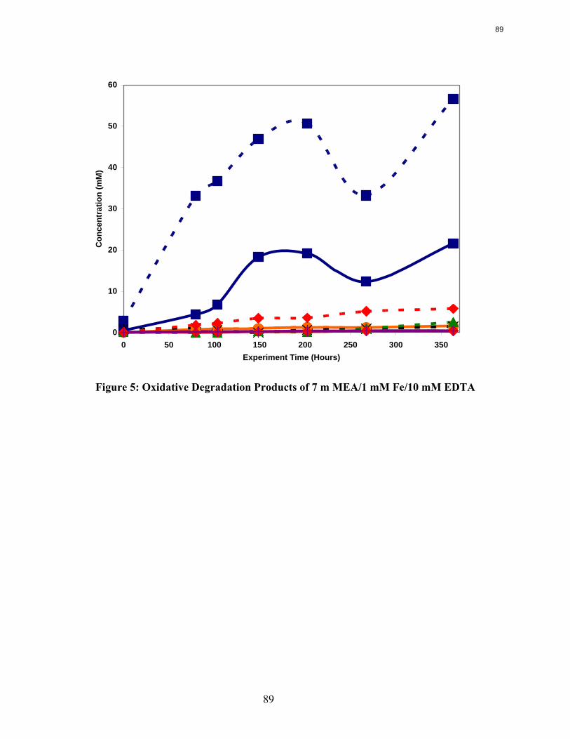
89

0

10

20

30

40

50

60

0 50 100 150 200 250 300 350Experiment Time (Hours)

Con

cent

ratio

n (m

M)

Figure 5: Oxidative Degradation Products of 7 m MEA/1 mM Fe/10 mM EDTA

89

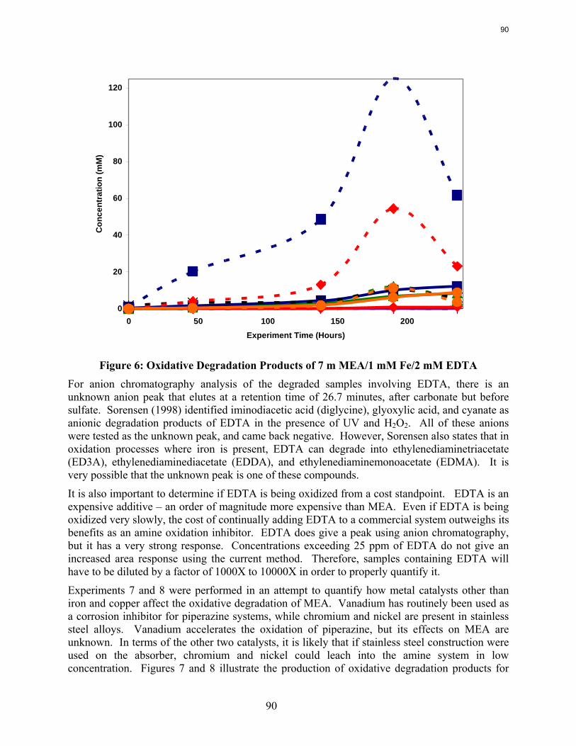
90

0

20

40

60

80

100

120

0 50 100 150 200Experiment Time (Hours)

Con

cent

ratio

n (m

M)

Figure 6: Oxidative Degradation Products of 7 m MEA/1 mM Fe/2 mM EDTA

For anion chromatography analysis of the degraded samples involving EDTA, there is an unknown anion peak that elutes at a retention time of 26.7 minutes, after carbonate but before sulfate. Sorensen (1998) identified iminodiacetic acid (diglycine), glyoxylic acid, and cyanate as anionic degradation products of EDTA in the presence of UV and H2O2. All of these anions were tested as the unknown peak, and came back negative. However, Sorensen also states that in oxidation processes where iron is present, EDTA can degrade into ethylenediaminetriacetate (ED3A), ethylenediaminediacetate (EDDA), and ethylenediaminemonoacetate (EDMA). It is very possible that the unknown peak is one of these compounds.

It is also important to determine if EDTA is being oxidized from a cost standpoint. EDTA is an expensive additive – an order of magnitude more expensive than MEA. Even if EDTA is being oxidized very slowly, the cost of continually adding EDTA to a commercial system outweighs its benefits as an amine oxidation inhibitor. EDTA does give a peak using anion chromatography, but it has a very strong response. Concentrations exceeding 25 ppm of EDTA do not give an increased area response using the current method. Therefore, samples containing EDTA will have to be diluted by a factor of 1000X to 10000X in order to properly quantify it.

Experiments 7 and 8 were performed in an attempt to quantify how metal catalysts other than iron and copper affect the oxidative degradation of MEA. Vanadium has routinely been used as a corrosion inhibitor for piperazine systems, while chromium and nickel are present in stainless steel alloys. Vanadium accelerates the oxidation of piperazine, but its effects on MEA are unknown. In terms of the other two catalysts, it is likely that if stainless steel construction were used on the absorber, chromium and nickel could leach into the amine system in low concentration. Figures 7 and 8 illustrate the production of oxidative degradation products for

90

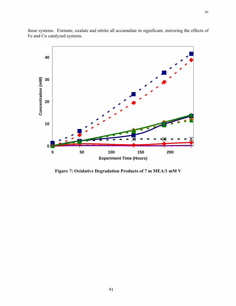
91

these systems. Formate, oxalate and nitrite all accumulate in significant, mirroring the effects of Fe and Cu catalyzed systems.

0

10

20

30

40

0 50 100 150 200Experiment Time (Hours)

Con

cent

ratio

n (m

M)

Figure 7: Oxidative Degradation Products of 7 m MEA/1 mM V

91

92

0

50

100

150

200

250

0 50 100 150 200 250 300

Experiment Time (Hours)

Con

cent

ratio

n (m

M)

Figure

8: Oxidative Degradation Products of 7 m MEA/0.6 mM Cr/0.1 mM Ni

Experiments 9 through 12 represent catalyzed MEA systems run under inhibited (and most likely kinetics-controlled) conditions. Inhibitor A has proven to be effective under iron and copper catalyzed MEA systems, so it is necessary to test its effectiveness with metals present in stainless steel systems. Per Goff, Na2SO3 is a known oxygen scavenger that is used in a range of applications varying from boiler feedwater treating to food packaging.

Formaldehyde is an expected intermediate in the oxidative degradation of MEA, and it is likely that formate (an observed degradation product present in high concentration) comes from the oxidation of formaldehyde. If formaldehyde is present in high enough concentration, it is feasible that the aldehyde could protect MEA from oxidizing. Limestone slurry scrubbers for SOx removal use organic acids as pH buffers, and Inhibitor B has been shown to be an effective inhibitor for organic acid oxidation. Figures 9 through 12 show the accumulation of oxidative degradation products under the proposed inhibited conditions.

Inhibitor A appears to be an extremely effective oxidative degradation inhibitor for MEA systems in the presence of chromium and nickel (a 99% reduction in the formation of all detectable products), while inhibitor B was moderately effective at inhibiting degradation (an approximately 75% reduction on the formation of detectable products) in the presence of iron catalyst.

Sodium sulfite and formaldehyde were both ineffective as degradation inhibitors for the observed MEA systems. For the first 50 to 75 hours, it appears that oxidative degradation products were being formed at a reduced rate, suggesting that sulfite was oxidizing to sulfate and was

92

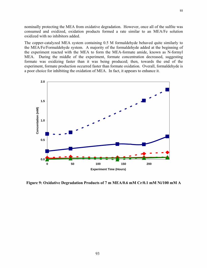
93

nominally protecting the MEA from oxidative degradation. However, once all of the sulfite was consumed and oxidized, oxidation products formed a rate similar to an MEA/Fe solution oxidized with no inhibitors added.

The copper-catalyzed MEA system containing 0.5 M formaldehyde behaved quite similarly to the MEA/Fe/Formaldehyde system. A majority of the formaldehyde added at the beginning of the experiment reacted with the MEA to form the MEA-formate amide, known as N-formyl MEA. During the middle of the experiment, formate concentration decreased, suggesting formate was oxidizing faster than it was being produced; then, towards the end of the experiment, formate production occurred faster than formate oxidation. Overall, formaldehyde is a poor choice for inhibiting the oxidation of MEA. In fact, it appears to enhance it.

0.0

0.5

1.0

1.5

2.0

0 50 100 150 200

Experiment Time (Hours)

Con

cent

atio

n (m

M)

Figure 9: Oxidative Degradation Products of 7 m MEA/0.6 mM Cr/0.1 mM Ni/100 mM A

93

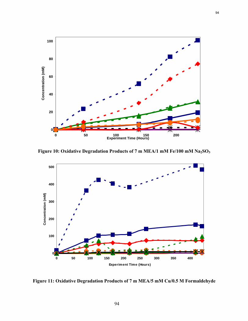
94

0

20

40

60

80

100

0 50 100 150 200Experiment Time (Hours)

Con

cent

ratio

n (m

M)

Figure 10: Oxidative Degradation Products of 7 m MEA/1 mM Fe/100 mM Na2SO3

0

100

200

300

400

500

0 50 100 150 200 250 300 350 400

Experiment Time (Hours)

Con

cent

ratio

n (m

M)

Figure 11: Oxidative Degradation Products of 7 m MEA/5 mM Cu/0.5 M Formaldehyde

94

95

0

10

20

30

40

50

0 50 100 150 200

Experiment Time (Hours)

Con

cent

ratio

n (m

M)

Figure 12: Oxidative Degradation Products of 7 m MEA/1 mM Fe/7.5 mM Inh B

Figures 13 and 14 display the formation of oxidative degradation products for MEA experiments in which control variables in the baseline experiment have been altered. Figure 13 shows the accumulation of degradation products for a degraded MEA/Fe/Cu solution that was agitated at only 700 RPM, versus the typical 1400 RPM. The experiment depicted in Figure 14 is an MEA/Fe solution that was degraded with 100 cc/min of 94% O2/6% CO2 gas mixture, as opposed to the typical 2% CO2 concentration. This CO2 content represents a loading of around 0.5, which would be the rich loading expected leaving the absorber to the stripper.

For both experiments, formate and oxalate amide are present in high concentration. For the 700 RPM experiment, formamide is present in 6X the concentration of formate, while oxamide is present in concentrations 25X the concentration of oxalate. For the “rich” loading experiment involving MEA and Fe, formamide concentrations were 4X greater than formate concentrations, while oxamide concentrations were 15X greater than oxalate concentrations. This goes to show that a large percentage of degradation products may have gone undetected before NaOH treatment was performed on the raw, degraded samples.

95

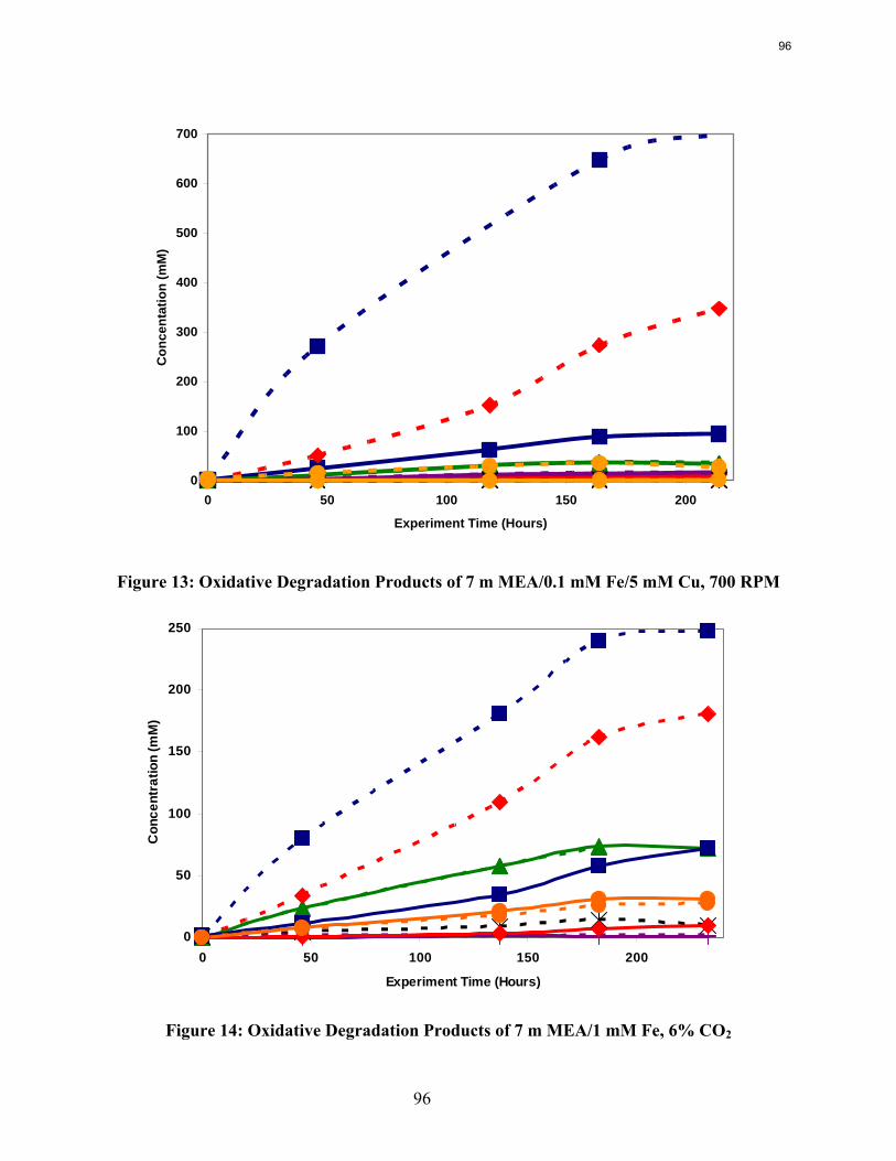
96

0

100

200

300

400

500

600

700

0 50 100 150 200

Experiment Time (Hours)

Con

cent

atio

n (m

M)

Figure 13: Oxidative Degradation Products of 7 m MEA/0.1 mM Fe/5 mM Cu, 700 RPM

0

50

100

150

200

250

0 50 100 150 200

Experiment Time (Hours)

Con

cent

ratio

n (m

M)

Figure 14: Oxidative Degradation Products of 7 m MEA/1 mM Fe, 6% CO2

96

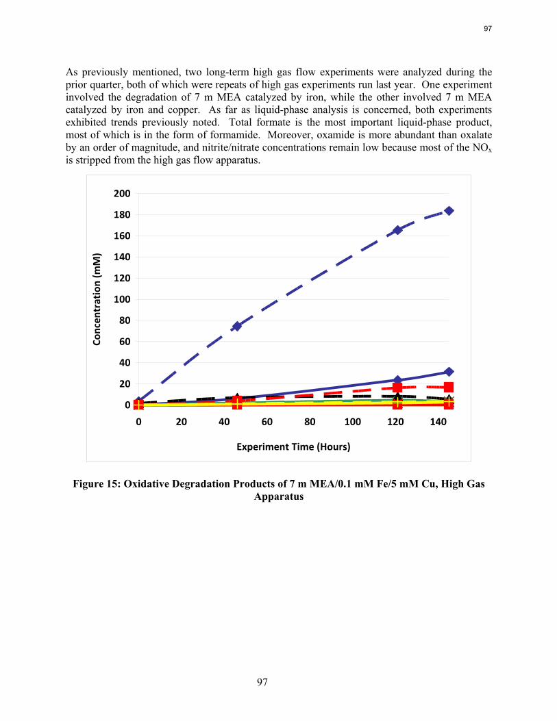
97

As previously mentioned, two long-term high gas flow experiments were analyzed during the prior quarter, both of which were repeats of high gas experiments run last year. One experiment involved the degradation of 7 m MEA catalyzed by iron, while the other involved 7 m MEA catalyzed by iron and copper. As far as liquid-phase analysis is concerned, both experiments exhibited trends previously noted. Total formate is the most important liquid-phase product, most of which is in the form of formamide. Moreover, oxamide is more abundant than oxalate by an order of magnitude, and nitrite/nitrate concentrations remain low because most of the NOx is stripped from the high gas flow apparatus.

0

20

40

60

80

100

120

140

160

180

200

0 20 40 60 80 100 120 140

Experiment Time (Hours)

Concen

tration (m

M)

Figure 15: Oxidative Degradation Products of 7 m MEA/0.1 mM Fe/5 mM Cu, High Gas Apparatus

97

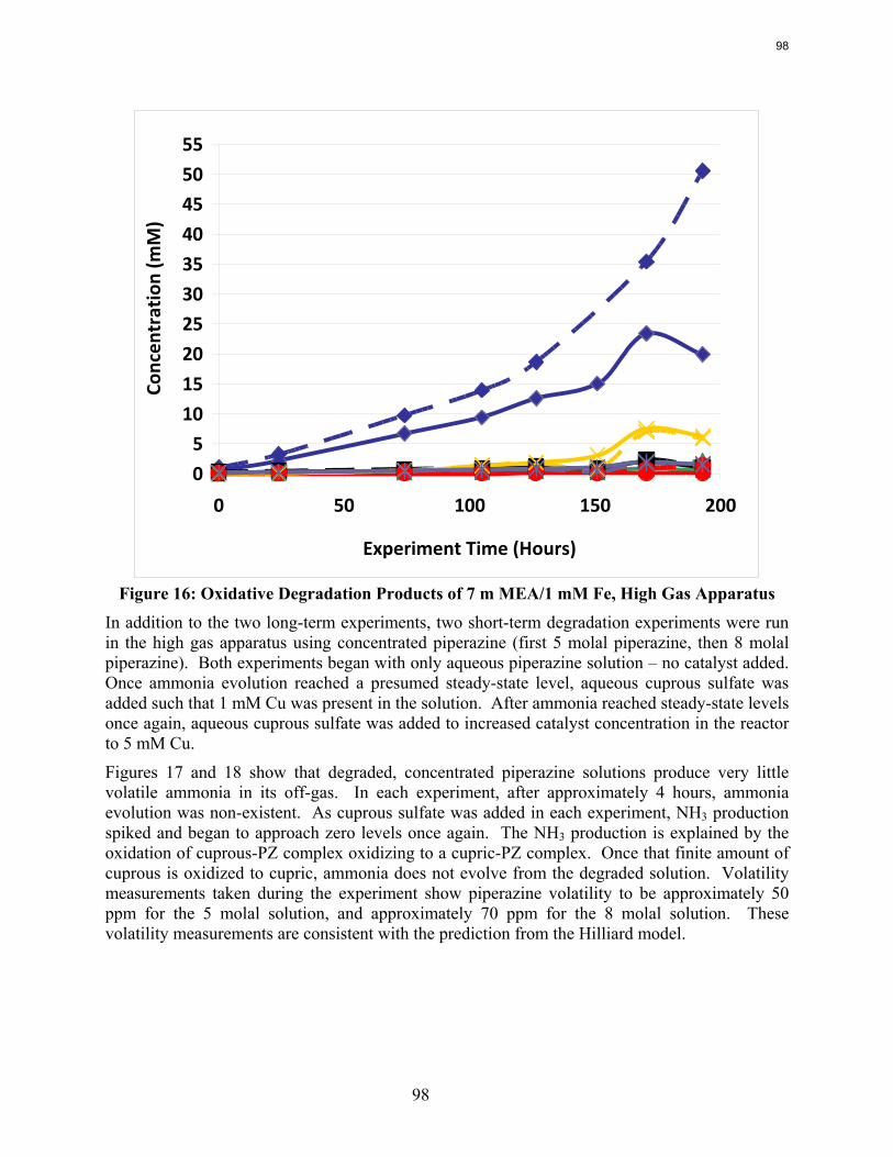
98

0

5

10

15

20

25

30

35

40

45

50

55

0 50 100 150 200

Experiment Time (Hours)

Concen

tration (m

M)

Figure 16: Oxidative Degradation Products of 7 m MEA/1 mM Fe, High Gas Apparatus

In addition to the two long-term experiments, two short-term degradation experiments were run in the high gas apparatus using concentrated piperazine (first 5 molal piperazine, then 8 molal piperazine). Both experiments began with only aqueous piperazine solution – no catalyst added. Once ammonia evolution reached a presumed steady-state level, aqueous cuprous sulfate was added such that 1 mM Cu was present in the solution. After ammonia reached steady-state levels once again, aqueous cuprous sulfate was added to increased catalyst concentration in the reactor to 5 mM Cu.

Figures 17 and 18 show that degraded, concentrated piperazine solutions produce very little volatile ammonia in its off-gas. In each experiment, after approximately 4 hours, ammonia evolution was non-existent. As cuprous sulfate was added in each experiment, NH3 production spiked and began to approach zero levels once again. The NH3 production is explained by the oxidation of cuprous-PZ complex oxidizing to a cupric-PZ complex. Once that finite amount of cuprous is oxidized to cupric, ammonia does not evolve from the degraded solution. Volatility measurements taken during the experiment show piperazine volatility to be approximately 50 ppm for the 5 molal solution, and approximately 70 ppm for the 8 molal solution. These volatility measurements are consistent with the prediction from the Hilliard model.

98

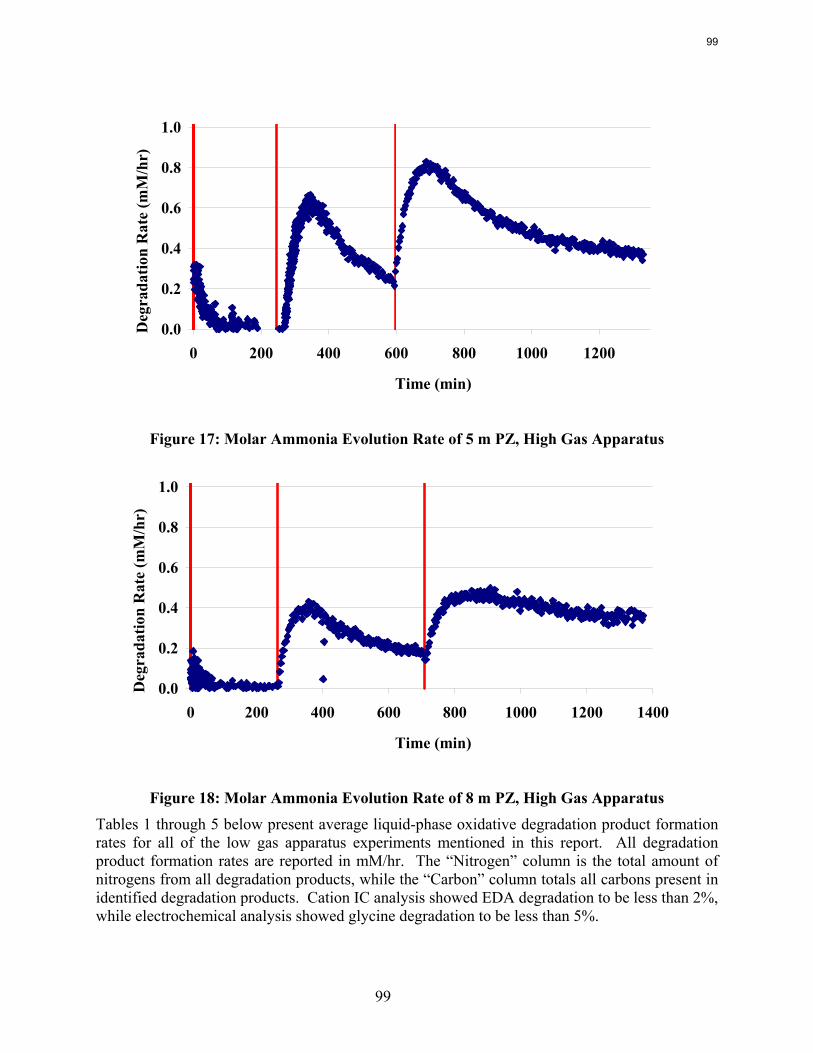
99

0.0

0.2

0.4

0.6

0.8

1.0

0 200 400 600 800 1000 1200

Time (min)

Deg

rada

tion

Rat

e (m

M/h

r)

Figure 17: Molar Ammonia Evolution Rate of 5 m PZ, High Gas Apparatus

0.0

0.2

0.4

0.6

0.8

1.0

0 200 400 600 800 1000 1200 1400

Time (min)

Deg

rada

tion

Rat

e (m

M/h

r)

Figure 18: Molar Ammonia Evolution Rate of 8 m PZ, High Gas Apparatus Tables 1 through 5 below present average liquid-phase oxidative degradation product formation rates for all of the low gas apparatus experiments mentioned in this report. All degradation product formation rates are reported in mM/hr. The “Nitrogen” column is the total amount of nitrogens from all degradation products, while the “Carbon” column totals all carbons present in identified degradation products. Cation IC analysis showed EDA degradation to be less than 2%, while electrochemical analysis showed glycine degradation to be less than 5%.

99

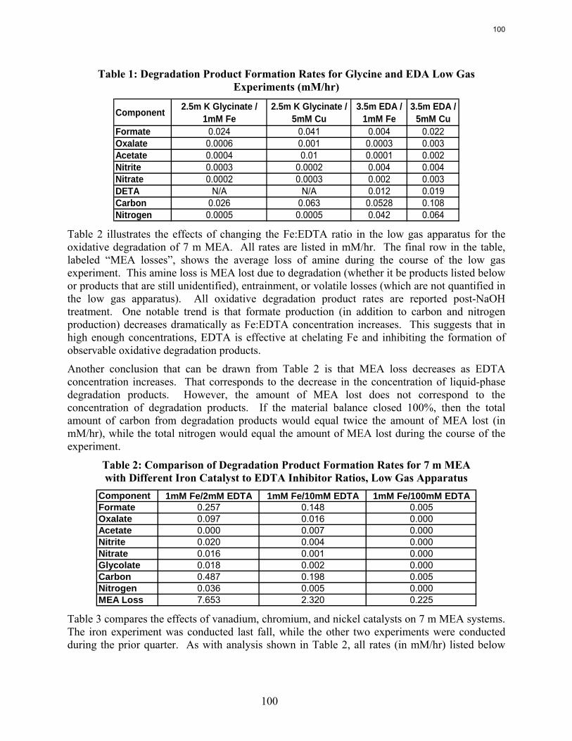
100

Table 1: Degradation Product Formation Rates for Glycine and EDA Low Gas Experiments (mM/hr)

Component 2.5m K Glycinate / 1mM Fe

2.5m K Glycinate / 5mM Cu

3.5m EDA / 1mM Fe

3.5m EDA / 5mM Cu

Formate 0.024 0.041 0.004 0.022Oxalate 0.0006 0.001 0.0003 0.003Acetate 0.0004 0.01 0.0001 0.002Nitrite 0.0003 0.0002 0.004 0.004Nitrate 0.0002 0.0003 0.002 0.003DETA N/A N/A 0.012 0.019Carbon 0.026 0.063 0.0528 0.108Nitrogen 0.0005 0.0005 0.042 0.064

Table 2 illustrates the effects of changing the Fe:EDTA ratio in the low gas apparatus for the oxidative degradation of 7 m MEA. All rates are listed in mM/hr. The final row in the table, labeled “MEA losses”, shows the average loss of amine during the course of the low gas experiment. This amine loss is MEA lost due to degradation (whether it be products listed below or products that are still unidentified), entrainment, or volatile losses (which are not quantified in the low gas apparatus). All oxidative degradation product rates are reported post-NaOH treatment. One notable trend is that formate production (in addition to carbon and nitrogen production) decreases dramatically as Fe:EDTA concentration increases. This suggests that in high enough concentrations, EDTA is effective at chelating Fe and inhibiting the formation of observable oxidative degradation products.

Another conclusion that can be drawn from Table 2 is that MEA loss decreases as EDTA concentration increases. That corresponds to the decrease in the concentration of liquid-phase degradation products. However, the amount of MEA lost does not correspond to the concentration of degradation products. If the material balance closed 100%, then the total amount of carbon from degradation products would equal twice the amount of MEA lost (in mM/hr), while the total nitrogen would equal the amount of MEA lost during the course of the experiment.

Table 2: Comparison of Degradation Product Formation Rates for 7 m MEA with Different Iron Catalyst to EDTA Inhibitor Ratios, Low Gas Apparatus

Component 1mM Fe/2mM EDTA 1mM Fe/10mM EDTA 1mM Fe/100mM EDTAFormate 0.257 0.148 0.005Oxalate 0.097 0.016 0.000Acetate 0.000 0.007 0.000Nitrite 0.020 0.004 0.000Nitrate 0.016 0.001 0.000Glycolate 0.018 0.002 0.000Carbon 0.487 0.198 0.005Nitrogen 0.036 0.005 0.000MEA Loss 7.653 2.320 0.225

Table 3 compares the effects of vanadium, chromium, and nickel catalysts on 7 m MEA systems. The iron experiment was conducted last fall, while the other two experiments were conducted during the prior quarter. As with analysis shown in Table 2, all rates (in mM/hr) listed below

100

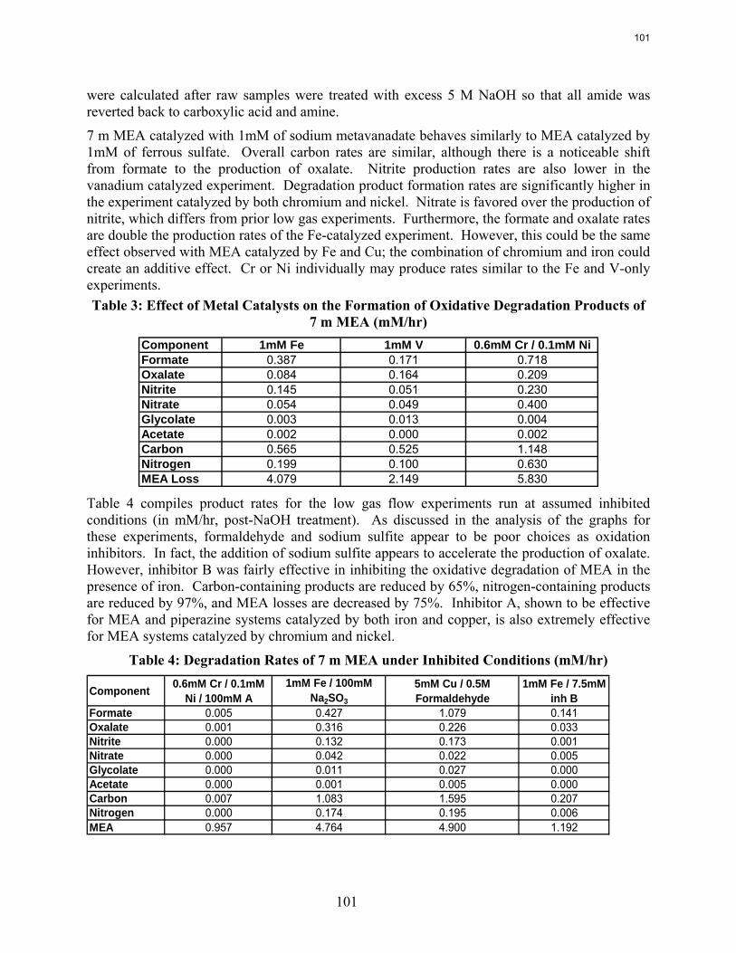
101

were calculated after raw samples were treated with excess 5 M NaOH so that all amide was reverted back to carboxylic acid and amine.

7 m MEA catalyzed with 1mM of sodium metavanadate behaves similarly to MEA catalyzed by 1mM of ferrous sulfate. Overall carbon rates are similar, although there is a noticeable shift from formate to the production of oxalate. Nitrite production rates are also lower in the vanadium catalyzed experiment. Degradation product formation rates are significantly higher in the experiment catalyzed by both chromium and nickel. Nitrate is favored over the production of nitrite, which differs from prior low gas experiments. Furthermore, the formate and oxalate rates are double the production rates of the Fe-catalyzed experiment. However, this could be the same effect observed with MEA catalyzed by Fe and Cu; the combination of chromium and iron could create an additive effect. Cr or Ni individually may produce rates similar to the Fe and V-only experiments. Table 3: Effect of Metal Catalysts on the Formation of Oxidative Degradation Products of

7 m MEA (mM/hr) Component 1mM Fe 1mM V 0.6mM Cr / 0.1mM NiFormate 0.387 0.171 0.718Oxalate 0.084 0.164 0.209Nitrite 0.145 0.051 0.230Nitrate 0.054 0.049 0.400Glycolate 0.003 0.013 0.004Acetate 0.002 0.000 0.002Carbon 0.565 0.525 1.148Nitrogen 0.199 0.100 0.630MEA Loss 4.079 2.149 5.830

Table 4 compiles product rates for the low gas flow experiments run at assumed inhibited conditions (in mM/hr, post-NaOH treatment). As discussed in the analysis of the graphs for these experiments, formaldehyde and sodium sulfite appear to be poor choices as oxidation inhibitors. In fact, the addition of sodium sulfite appears to accelerate the production of oxalate. However, inhibitor B was fairly effective in inhibiting the oxidative degradation of MEA in the presence of iron. Carbon-containing products are reduced by 65%, nitrogen-containing products are reduced by 97%, and MEA losses are decreased by 75%. Inhibitor A, shown to be effective for MEA and piperazine systems catalyzed by both iron and copper, is also extremely effective for MEA systems catalyzed by chromium and nickel.

Table 4: Degradation Rates of 7 m MEA under Inhibited Conditions (mM/hr)

Component 0.6mM Cr / 0.1mM Ni / 100mM A

1mM Fe / 100mM Na2SO3

5mM Cu / 0.5M Formaldehyde

1mM Fe / 7.5mM inh B

Formate 0.005 0.427 1.079 0.141Oxalate 0.001 0.316 0.226 0.033Nitrite 0.000 0.132 0.173 0.001Nitrate 0.000 0.042 0.022 0.005Glycolate 0.000 0.011 0.027 0.000Acetate 0.000 0.001 0.005 0.000Carbon 0.007 1.083 1.595 0.207Nitrogen 0.000 0.174 0.195 0.006MEA 0.957 4.764 4.900 1.192

101

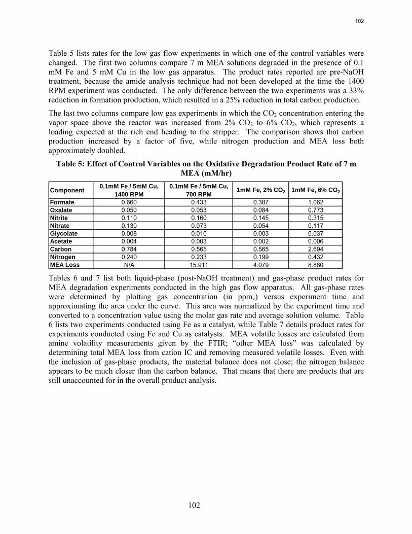
102

Table 5 lists rates for the low gas flow experiments in which one of the control variables were changed. The first two columns compare 7 m MEA solutions degraded in the presence of 0.1 mM Fe and 5 mM Cu in the low gas apparatus. The product rates reported are pre-NaOH treatment, because the amide analysis technique had not been developed at the time the 1400 RPM experiment was conducted. The only difference between the two experiments was a 33% reduction in formation production, which resulted in a 25% reduction in total carbon production.

The last two columns compare low gas experiments in which the CO2 concentration entering the vapor space above the reactor was increased from 2% CO2 to 6% CO2, which represents a loading expected at the rich end heading to the stripper. The comparison shows that carbon production increased by a factor of five, while nitrogen production and MEA loss both approximately doubled.

Table 5: Effect of Control Variables on the Oxidative Degradation Product Rate of 7 m MEA (mM/hr)

Component 0.1mM Fe / 5mM Cu, 1400 RPM

0.1mM Fe / 5mM Cu, 700 RPM

1mM Fe, 2% CO2 1mM Fe, 6% CO2

Formate 0.660 0.433 0.387 1.062Oxalate 0.050 0.053 0.084 0.773Nitrite 0.110 0.160 0.145 0.315Nitrate 0.130 0.073 0.054 0.117Glycolate 0.008 0.010 0.003 0.037Acetate 0.004 0.003 0.002 0.006Carbon 0.784 0.565 0.565 2.694Nitrogen 0.240 0.233 0.199 0.432MEA Loss N/A 15.911 4.079 8.880 Tables 6 and 7 list both liquid-phase (post-NaOH treatment) and gas-phase product rates for MEA degradation experiments conducted in the high gas flow apparatus. All gas-phase rates were determined by plotting gas concentration (in ppmv) versus experiment time and approximating the area under the curve. This area was normalized by the experiment time and converted to a concentration value using the molar gas rate and average solution volume. Table 6 lists two experiments conducted using Fe as a catalyst, while Table 7 details product rates for experiments conducted using Fe and Cu as catalysts. MEA volatile losses are calculated from amine volatility measurements given by the FTIR; “other MEA loss” was calculated by determining total MEA loss from cation IC and removing measured volatile losses. Even with the inclusion of gas-phase products, the material balance does not close; the nitrogen balance appears to be much closer than the carbon balance. That means that there are products that are still unaccounted for in the overall product analysis.

102

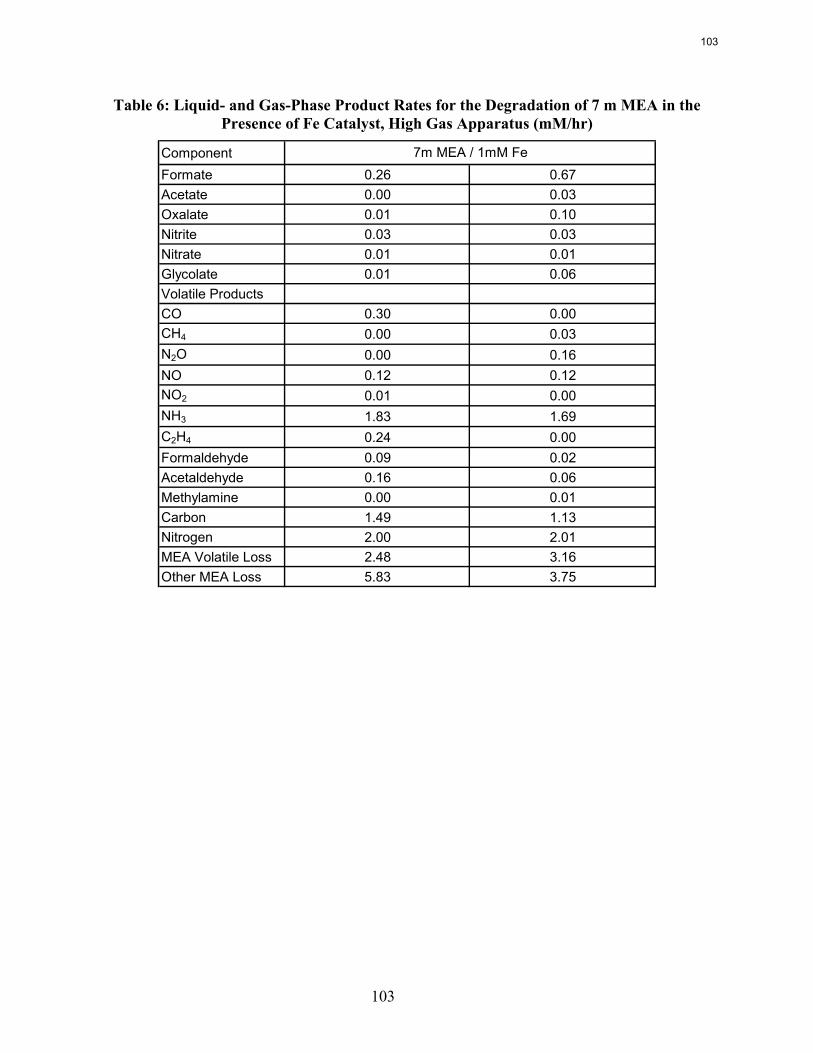
103

Table 6: Liquid- and Gas-Phase Product Rates for the Degradation of 7 m MEA in the Presence of Fe Catalyst, High Gas Apparatus (mM/hr)

ComponentFormate 0.26 0.67Acetate 0.00 0.03Oxalate 0.01 0.10Nitrite 0.03 0.03Nitrate 0.01 0.01Glycolate 0.01 0.06Volatile ProductsCO 0.30 0.00CH4 0.00 0.03N2O 0.00 0.16NO 0.12 0.12NO2 0.01 0.00NH3 1.83 1.69C2H4 0.24 0.00Formaldehyde 0.09 0.02Acetaldehyde 0.16 0.06Methylamine 0.00 0.01Carbon 1.49 1.13Nitrogen 2.00 2.01MEA Volatile Loss 2.48 3.16Other MEA Loss 5.83 3.75

7m MEA / 1mM Fe

103

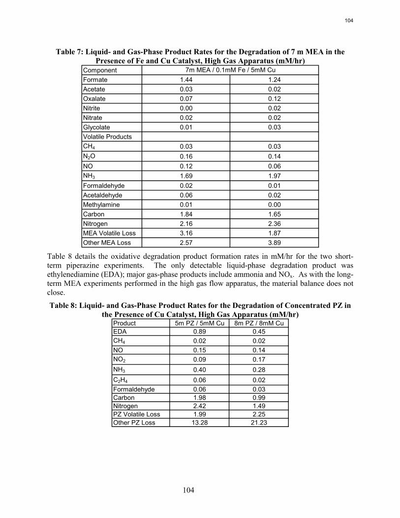
104

Table 7: Liquid- and Gas-Phase Product Rates for the Degradation of 7 m MEA in the Presence of Fe and Cu Catalyst, High Gas Apparatus (mM/hr)

ComponentFormate 1.44 1.24Acetate 0.03 0.02Oxalate 0.07 0.12Nitrite 0.00 0.02Nitrate 0.02 0.02Glycolate 0.01 0.03Volatile ProductsCH4 0.03 0.03N2O 0.16 0.14NO 0.12 0.06NH3 1.69 1.97Formaldehyde 0.02 0.01Acetaldehyde 0.06 0.02Methylamine 0.01 0.00Carbon 1.84 1.65Nitrogen 2.16 2.36MEA Volatile Loss 3.16 1.87Other MEA Loss 2.57 3.89

7m MEA / 0.1mM Fe / 5mM Cu

Table 8 details the oxidative degradation product formation rates in mM/hr for the two short-term piperazine experiments. The only detectable liquid-phase degradation product was ethylenediamine (EDA); major gas-phase products include ammonia and NOx. As with the long-term MEA experiments performed in the high gas flow apparatus, the material balance does not close.

Table 8: Liquid- and Gas-Phase Product Rates for the Degradation of Concentrated PZ in the Presence of Cu Catalyst, High Gas Apparatus (mM/hr)

Product 5m PZ / 5mM Cu 8m PZ / 8mM CuEDA 0.89 0.45CH4 0.02 0.02NO 0.15 0.14NO2 0.09 0.17NH3 0.40 0.28C2H4 0.06 0.02Formaldehyde 0.06 0.03Carbon 1.98 0.99Nitrogen 2.42 1.49PZ Volatile Loss 1.99 2.25Other PZ Loss 13.28 21.23

104

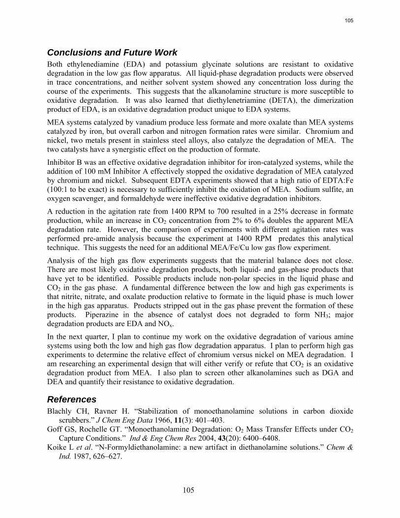
105

Conclusions and Future Work Both ethylenediamine (EDA) and potassium glycinate solutions are resistant to oxidative degradation in the low gas flow apparatus. All liquid-phase degradation products were observed in trace concentrations, and neither solvent system showed any concentration loss during the course of the experiments. This suggests that the alkanolamine structure is more susceptible to oxidative degradation. It was also learned that diethylenetriamine (DETA), the dimerization product of EDA, is an oxidative degradation product unique to EDA systems.

MEA systems catalyzed by vanadium produce less formate and more oxalate than MEA systems catalyzed by iron, but overall carbon and nitrogen formation rates were similar. Chromium and nickel, two metals present in stainless steel alloys, also catalyze the degradation of MEA. The two catalysts have a synergistic effect on the production of formate.

Inhibitor B was an effective oxidative degradation inhibitor for iron-catalyzed systems, while the addition of 100 mM Inhibitor A effectively stopped the oxidative degradation of MEA catalyzed by chromium and nickel. Subsequent EDTA experiments showed that a high ratio of EDTA:Fe (100:1 to be exact) is necessary to sufficiently inhibit the oxidation of MEA. Sodium sulfite, an oxygen scavenger, and formaldehyde were ineffective oxidative degradation inhibitors.

A reduction in the agitation rate from 1400 RPM to 700 resulted in a 25% decrease in formate production, while an increase in CO2 concentration from 2% to 6% doubles the apparent MEA degradation rate. However, the comparison of experiments with different agitation rates was performed pre-amide analysis because the experiment at 1400 RPM predates this analytical technique. This suggests the need for an additional MEA/Fe/Cu low gas flow experiment.

Analysis of the high gas flow experiments suggests that the material balance does not close. There are most likely oxidative degradation products, both liquid- and gas-phase products that have yet to be identified. Possible products include non-polar species in the liquid phase and CO2 in the gas phase. A fundamental difference between the low and high gas experiments is that nitrite, nitrate, and oxalate production relative to formate in the liquid phase is much lower in the high gas apparatus. Products stripped out in the gas phase prevent the formation of these products. Piperazine in the absence of catalyst does not degraded to form NH3; major degradation products are EDA and NOx.

In the next quarter, I plan to continue my work on the oxidative degradation of various amine systems using both the low and high gas flow degradation apparatus. I plan to perform high gas experiments to determine the relative effect of chromium versus nickel on MEA degradation. I am researching an experimental design that will either verify or refute that CO2 is an oxidative degradation product from MEA. I also plan to screen other alkanolamines such as DGA and DEA and quantify their resistance to oxidative degradation.

References Blachly CH, Ravner H. “Stabilization of monoethanolamine solutions in carbon dioxide

scrubbers.” J Chem Eng Data 1966, 11(3): 401–403. Goff GS, Rochelle GT. “Monoethanolamine Degradation: O2 Mass Transfer Effects under CO2

Capture Conditions.” Ind & Eng Chem Res 2004, 43(20): 6400–6408. Koike L et al. “N-Formyldiethanolamine: a new artifact in diethanolamine solutions.” Chem &

Ind. 1987, 626–627.

105

106

Sorensen M et al. “Degradation Pathway of the Photochemical Oxidation of Ethylenediaminetetraacetate (EDTA) in the UV/H2O2-process.” Acta hydrochim 1998, 26(2): 109–115.

Van Holst J et al. “CO2 Capture from flue gas using amino acid salt solutions.” Greenhouse Gas Control Technologies, Proceedings of the International Conference on Greenhouse Gas Control Technologies, 8th, Trondheim, Norway 2006.

106

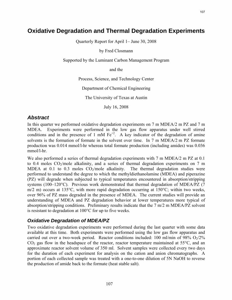
107

Oxidative Degradation and Thermal Degradation Experiments Quarterly Report for April 1– June 30, 2008

by Fred Closmann

Supported by the Luminant Carbon Management Program

and the

Process, Science, and Technology Center

Department of Chemical Engineering

The University of Texas at Austin

July 16, 2008

Abstract In this quarter we performed oxidative degradation experiments on 7 m MDEA/2 m PZ and 7 m MDEA. Experiments were performed in the low gas flow apparatus under well stirred conditions and in the presence of 1 mM Fe+2. A key indicator of the degradation of amine solvents is the formation of formate in the solvent over time. In 7 m MDEA/2 m PZ formate production was 0.014 mmol/l-hr whereas total formate production (including amides) was 0.036 mmol/l-hr.

We also performed a series of thermal degradation experiments with 7 m MDEA/2 m PZ at 0.1 to 0.4 moles CO2/mole alkalinity, and a series of thermal degradation experiments on 7 m MDEA at 0.1 to 0.3 moles CO2/mole alkalinity. The thermal degradation studies were performed to understand the degree to which the methyldiethanolamine (MDEA) and piperazine (PZ) will degrade when subjected to typical temperatures encountered in absorption/stripping systems (100–120°C). Previous work demonstrated that thermal degradation of MDEA/PZ (7 m/2 m) occurs at 135°C, with more rapid degradation occurring at 150°C; within two weeks, over 96% of PZ mass degraded in the presence of MDEA. The current studies will provide an understanding of MDEA and PZ degradation behavior at lower temperatures more typical of absorption/stripping conditions. Preliminary results indicate that the 7 m/2 m MDEA/PZ solvent is resistant to degradation at 100°C for up to five weeks.

Oxidative Degradation of MDEA/PZ Two oxidative degradation experiments were performed during the last quarter with some data available at this time. Both experiments were performed using the low gas flow apparatus and carried out over a two-week period. Reactor conditions included: 100 ml/min of 98% O2/2% CO2 gas flow in the headspace of the reactor, reactor temperature maintained at 55°C, and an approximate reactor solvent volume of 350 ml. Solvent samples were collected every two days for the duration of each experiment for analysis on the cation and anion chromatographs. A portion of each collected sample was treated with a one-to-one dilution of 5N NaOH to reverse the production of amide back to the formate (heat stable salt).

107

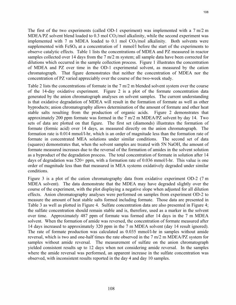
108

The first of the two experiments (called OD-1 experiment) was implemented with a 7 m/2 m MDEA/PZ solvent blend loaded to 0.3 mol CO2/mol alkalinity, while the second experiment was implemented with 7 m MDEA loaded to 0.1 mol CO2/mol alkalinity. Both solvents were supplemented with FeSO4 at a concentration of 1 mmol/l before the start of the experiments to observe catalytic effects. Table 1 lists the concentrations of MDEA and PZ measured in reactor samples collected over 14 days from the 7 m/2 m system; all sample data have been corrected for dilutions which occurred in the sample collection process. Figure 1 illustrates the concentration of MDEA and PZ over time in the OD-1 experimental solvent, as measured by the cation chromatograph. That figure demonstrates that neither the concentration of MDEA nor the concentration of PZ varied appreciably over the course of the two-week study.

Table 2 lists the concentrations of formate in the 7 m/2 m blended solvent system over the course of the 14-day oxidative experiment. Figure 2 is a plot of the formate concentration data generated by the anion chromatograph analyses on solvent samples. The current understanding is that oxidative degradation of MDEA will result in the formation of formate as well as other byproducts; anion chromatography allows determination of the amount of formate and other heat stable salts resulting from the production of organic acids. Figure 2 demonstrates that approximately 200 ppm formate was formed in the 7 m/2 m MDEA/PZ solvent by day 14. Two sets of data are plotted on that figure. The first set (diamonds) illustrates the formation of formate (formic acid) over 14 days, as measured directly on the anion chromatograph. The formation rate is 0.014 mmol/l-hr, which is an order of magnitude less than the formation rate of formate in concentrated MEA solutions under similar conditions. The second set of data (squares) demonstrates that, when the solvent samples are treated with 5N NaOH, the amount of formate measured increases due to the reversal of the formation of amides in the solvent solution as a byproduct of the degradation process. The total concentration of formate in solution after 14 days of degradation was 520+ ppm, with a formation rate of 0.036 mmol/l-hr. This value is one order of magnitude less than that measured in MEA systems oxidatively degraded under similar conditions.

Figure 3 is a plot of the cation chromatography data from oxidative experiment OD-2 (7 m MDEA solvent). The data demonstrate that the MDEA may have degraded slightly over the course of the experiment, with the plot displaying a negative slope when adjusted for all dilution effects. Anion chromatography analyses were performed on samples from experiment OD-2 to measure the amount of heat stable salts formed including formate. Those data are presented in Table 3 as well as plotted in Figure 4. Sulfate concentration data are also presented in Figure 4; the sulfate concentration should remain stable and is, therefore, used as a marker in the solvent over time. Approximately 487 ppm of formate was formed after 14 days in the 7 m MDEA solvent. When the formation of amide was reversed, the concentration of formate measured after 14 days increased to approximately 320 ppm in the 7 m MDEA solvent (day 14 result ignored). The rate of formate production was calculated as 0.035 mmol/l-hr in samples without amide reversal, which is two and one-half times the rate observed in the 7 m/2 m MDEA/PZ system for samples without amide reversal. The measurement of sulfate on the anion chromatograph yielded consistent results up to 12 days when not considering amide reversal. In the samples where the amide reversal was performed, an apparent increase in the sulfate concentration was observed, with inconsistent results reported in the day 4 and day 10 samples.

108

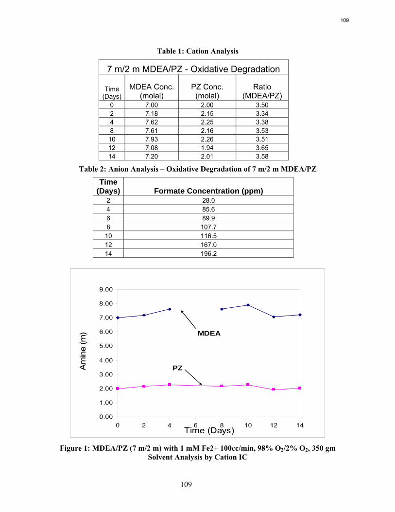
109

Table 1: Cation Analysis

7 m/2 m MDEA/PZ - Oxidative Degradation

Time (Days)

MDEA Conc. (molal)

PZ Conc. (molal)

Ratio (MDEA/PZ)

0 7.00 2.00 3.50 2 7.18 2.15 3.34 4 7.62 2.25 3.38 8 7.61 2.16 3.53

10 7.93 2.26 3.51 12 7.08 1.94 3.65 14 7.20 2.01 3.58

Table 2: Anion Analysis – Oxidative Degradation of 7 m/2 m MDEA/PZ

Time (Days) Formate Concentration (ppm)

2 28.0 4 85.6 6 89.9 8 107.7 10 116.5 12 167.0 14 196.2

0.00

1.00

2.00

3.00

4.00

5.00

6.00

7.00

8.00

9.00

0 2 4 6 8 10 12 14Time (Days)

Am

ine

(m) MDEA

PZ

Figure 1: MDEA/PZ (7 m/2 m) with 1 mM Fe2+ 100cc/min, 98% O2/2% O2, 350 gm

Solvent Analysis by Cation IC

109

110

0.0

100.0

200.0

300.0

400.0

500.0

600.0

0 5 10 15

Time (Days)

Form

ate

(ppm

) Formate Production

Formate Production -Amide Reversal

Poly. (FormateProduction - AmideReversal)Poly. (FormateProduction)

Figure 2: Formate Production in MDEA/PZ (7 m/2 m) with 1 mM Fe2+

Analysis by Anion IC

y = -0.0327x + 7.0345

6.2

6.4

6.6

6.8

7

7.2

7.4

7.6

7.8

0 5 10 15

Time (Days)

MD

EA C

once

ntra

tion

(mol

al)

7m MDEA Concentration

Figure 3: MDEA Concentration in 7 m MDEA with 1 mM Fe2+

Analysis by Cation IC

110

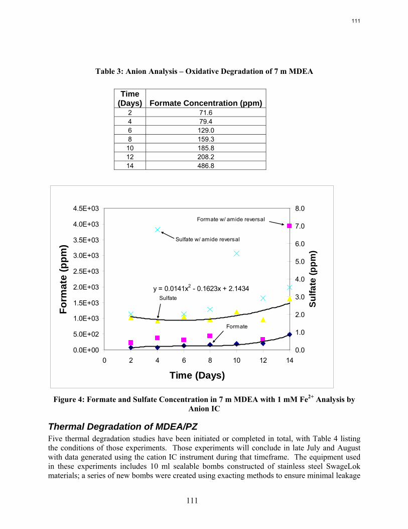
111

Table 3: Anion Analysis – Oxidative Degradation of 7 m MDEA

Time (Days) Formate Concentration (ppm)

2 71.6 4 79.4 6 129.0 8 159.3 10 185.8 12 208.2 14 486.8

y = 0.0141x2 - 0.1623x + 2.1434

0.0E+00

5.0E+02

1.0E+03

1.5E+03

2.0E+03

2.5E+03

3.0E+03

3.5E+03

4.0E+03

4.5E+03

0 2 4 6 8 10 12 14

Time (Days)

Form

ate

(ppm

)

0.0

1.0

2.0

3.0

4.0

5.0

6.0

7.0

8.0

Sulfa

te (p

pm)

Formate w/ amide reversal

Sulfate w/ amide reversal

Sulfate

Formate

Figure 4: Formate and Sulfate Concentration in 7 m MDEA with 1 mM Fe2+ Analysis by

Anion IC

Thermal Degradation of MDEA/PZ Five thermal degradation studies have been initiated or completed in total, with Table 4 listing the conditions of those experiments. Those experiments will conclude in late July and August with data generated using the cation IC instrument during that timeframe. The equipment used in these experiments includes 10 ml sealable bombs constructed of stainless steel SwageLok materials; a series of new bombs were created using exacting methods to ensure minimal leakage

111

112

of solvents over the course of the experiments. Of the five thermal degradation experiments in progress, the three most recently initiated experiments utilized the new SwageLok bombs.

Data generated by the Thermal No. 1 experiment (100°F) are limited to just two to five weeks of degradation due to bomb failure and loss of samples. A preliminary review of that data indicates that no measurable degradation MDEA or PZ occurred in the 7 m/2 m MDEA/PZ solvent at 100°C at loadings of 0.25 and 0.435 mols CO2/mol alkalinity; no data is available at 120°C from this experiment.

Table 4: Thermal Degradation Experiments in Progress

Thermal Test

Start Date

Solvent Loading(s)

Temp (°F) Data Available

Materials (Old/New)

Thermal No. 1

5/28/08 7 m MDEA/2 m PZ

0.25, 0.43

100, 120 Now Old

Thermal No. 2

6/2/08 7 m MDEA 0.3 100, 120 Week of 7/08

Old

Thermal No. 3

6/13/08 7 m MDEA/2 m PZ

0.1, 0.2 100, 120 Week of 8/08

New

Thermal No. 4

6/26/08 7 m MDEA 0.06, 0.12

100, 120 Week of 8/15

New

Thermal No. 5

7/16/08 7 m MDEA/2 m PZ

0.1, 1mM Fe2+

100, 120 Week of 8/30

New

Future Work Samples from both the 7 m/2 m MDEA/PZ and 7 m MDEA experiments will be analyzed to determine what degradation byproducts are formed during the oxidative degradation process. It is suspected that heat stable salts other than formate will have formed during the oxidative degradation process, and analytical data will be analyzed to identify and quantify those compounds. We will continue to investigate the formation of an amide product in the oxidative degradation process, and to quantify this formation by its reversal with 5N NaOH.

A fourteen-day oxidative degradation experiment (OD-3) on 7 m/2 m MDEA/PZ with 0.6 mM Cr, 0.1 mM Fe, and 0.1 mM Ni was initiated on 7/23/08. This experiment is designed to measure the effects of other anions in solution with respect to catalysis of oxidative degradation of the amine solvent. Additionally, a fourteen-day oxidative degradation experiment (OD-4) on 7 m/2 m MDEA/PZ was initiated on 7/24/08 with 0.1 mM Fe2+ and 5 mM copper (as CuSO4*5H2O) to confirm whether copper has a catalytic effect on oxidative degradation as has been seen in other amine systems such as MEA. Iron has been added at the lower concentration to mimic the corrosion inhibiting effect of copper in process equipment. All reactor samples will be analyzed on the cation and anion IC instruments to determine the amount of degradation occurring as well as the degradation products formed. Anion and cation chromatography results from the OD-3 and OD-4 experiments should be available no later than the week of August 11, 2008.

112

113

Additional oxidative degradation experiments will be performed on 7 m MDEA alone to mimic the conditions of experiments OD-3 and OD-4 wherein additional work to investigate the catalytic effects of various metals is being performed.

The data generated by the five thermal degradation experiments currently being performed will be reviewed to determine a lower bound in temperature where the 7 m/2 m MDEA/PZ solvent system is thermally resistant. Additional thermal degradation experiments will be performed on the same solvents utilized in the most recent experiments with similar loadings. Experiments will be repeated with iron and other metals in solution to determine the effect these metals have on the thermal degradation process. These experiments will parallel the oxidative experiments to be performed.

113

114

114

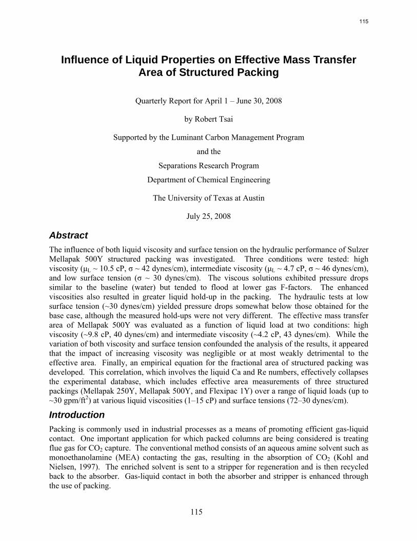
115

Influence of Liquid Properties on Effective Mass Transfer Area of Structured Packing

Quarterly Report for April 1 – June 30, 2008

by Robert Tsai

Supported by the Luminant Carbon Management Program

and the

Separations Research Program

Department of Chemical Engineering

The University of Texas at Austin

July 25, 2008

Abstract The influence of both liquid viscosity and surface tension on the hydraulic performance of Sulzer Mellapak 500Y structured packing was investigated. Three conditions were tested: high viscosity (μL ~ 10.5 cP, σ ~ 42 dynes/cm), intermediate viscosity (μL ~ 4.7 cP, σ ~ 46 dynes/cm), and low surface tension (σ ~ 30 dynes/cm). The viscous solutions exhibited pressure drops similar to the baseline (water) but tended to flood at lower gas F-factors. The enhanced viscosities also resulted in greater liquid hold-up in the packing. The hydraulic tests at low surface tension (~30 dynes/cm) yielded pressure drops somewhat below those obtained for the base case, although the measured hold-ups were not very different. The effective mass transfer area of Mellapak 500Y was evaluated as a function of liquid load at two conditions: high viscosity (~9.8 cP, 40 dynes/cm) and intermediate viscosity (~4.2 cP, 43 dynes/cm). While the variation of both viscosity and surface tension confounded the analysis of the results, it appeared that the impact of increasing viscosity was negligible or at most weakly detrimental to the effective area. Finally, an empirical equation for the fractional area of structured packing was developed. This correlation, which involves the liquid Ca and Re numbers, effectively collapses the experimental database, which includes effective area measurements of three structured packings (Mellapak 250Y, Mellapak 500Y, and Flexipac 1Y) over a range of liquid loads (up to ~30 gpm/ft2) at various liquid viscosities (1–15 cP) and surface tensions (72–30 dynes/cm).

Introduction Packing is commonly used in industrial processes as a means of promoting efficient gas-liquid contact. One important application for which packed columns are being considered is treating flue gas for CO2 capture. The conventional method consists of an aqueous amine solvent such as monoethanolamine (MEA) contacting the gas, resulting in the absorption of CO2 (Kohl and Nielsen, 1997). The enriched solvent is sent to a stripper for regeneration and is then recycled back to the absorber. Gas-liquid contact in both the absorber and stripper is enhanced through the use of packing.

115

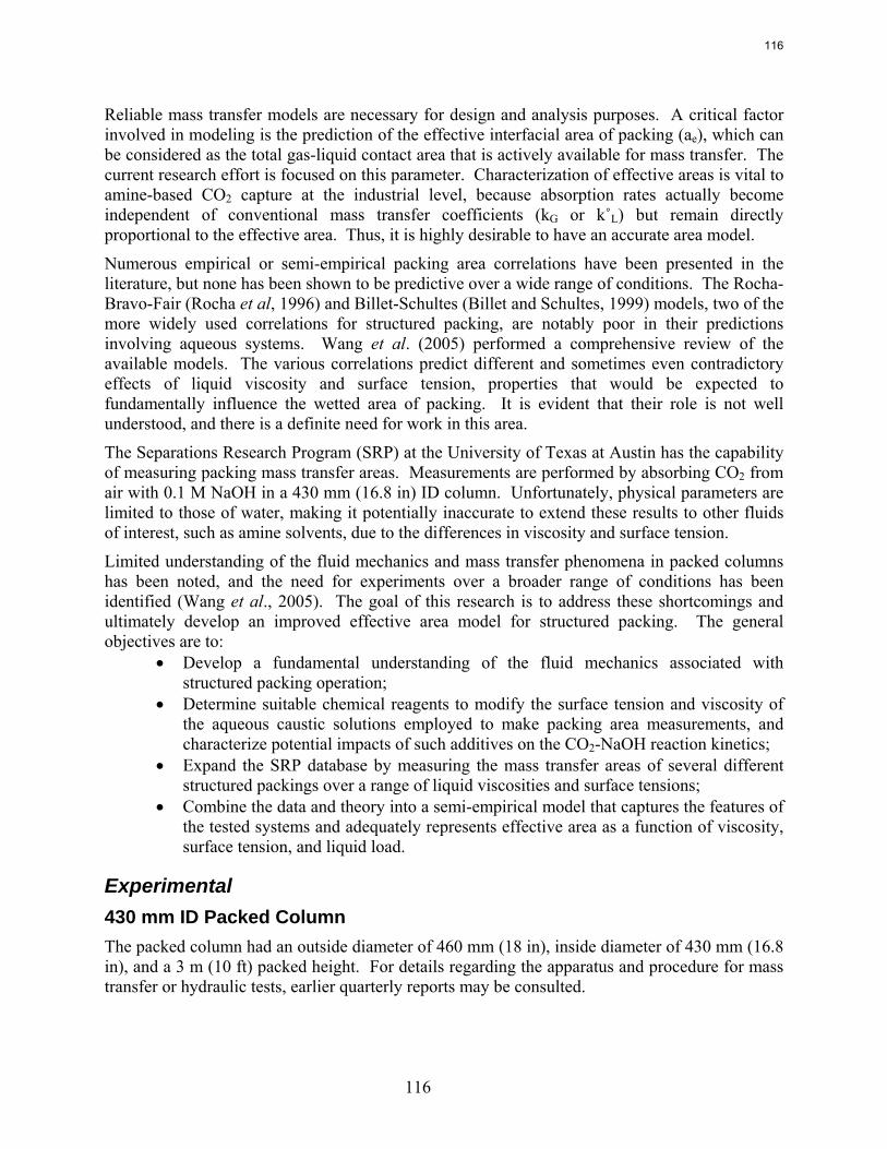
116

Reliable mass transfer models are necessary for design and analysis purposes. A critical factor involved in modeling is the prediction of the effective interfacial area of packing (ae), which can be considered as the total gas-liquid contact area that is actively available for mass transfer. The current research effort is focused on this parameter. Characterization of effective areas is vital to amine-based CO2 capture at the industrial level, because absorption rates actually become independent of conventional mass transfer coefficients (kG or k˚L) but remain directly proportional to the effective area. Thus, it is highly desirable to have an accurate area model.

Numerous empirical or semi-empirical packing area correlations have been presented in the literature, but none has been shown to be predictive over a wide range of conditions. The Rocha-Bravo-Fair (Rocha et al, 1996) and Billet-Schultes (Billet and Schultes, 1999) models, two of the more widely used correlations for structured packing, are notably poor in their predictions involving aqueous systems. Wang et al. (2005) performed a comprehensive review of the available models. The various correlations predict different and sometimes even contradictory effects of liquid viscosity and surface tension, properties that would be expected to fundamentally influence the wetted area of packing. It is evident that their role is not well understood, and there is a definite need for work in this area.

The Separations Research Program (SRP) at the University of Texas at Austin has the capability of measuring packing mass transfer areas. Measurements are performed by absorbing CO2 from air with 0.1 M NaOH in a 430 mm (16.8 in) ID column. Unfortunately, physical parameters are limited to those of water, making it potentially inaccurate to extend these results to other fluids of interest, such as amine solvents, due to the differences in viscosity and surface tension.

Limited understanding of the fluid mechanics and mass transfer phenomena in packed columns has been noted, and the need for experiments over a broader range of conditions has been identified (Wang et al., 2005). The goal of this research is to address these shortcomings and ultimately develop an improved effective area model for structured packing. The general objectives are to:

• Develop a fundamental understanding of the fluid mechanics associated with structured packing operation;

• Determine suitable chemical reagents to modify the surface tension and viscosity of the aqueous caustic solutions employed to make packing area measurements, and characterize potential impacts of such additives on the CO2-NaOH reaction kinetics;

• Expand the SRP database by measuring the mass transfer areas of several different structured packings over a range of liquid viscosities and surface tensions;

• Combine the data and theory into a semi-empirical model that captures the features of the tested systems and adequately represents effective area as a function of viscosity, surface tension, and liquid load.

Experimental 430 mm ID Packed Column The packed column had an outside diameter of 460 mm (18 in), inside diameter of 430 mm (16.8 in), and a 3 m (10 ft) packed height. For details regarding the apparatus and procedure for mass transfer or hydraulic tests, earlier quarterly reports may be consulted.

116

117

Wetted-Wall Column (WWC) The wetted-wall column (WWC) is a vapor-liquid contactor with a known interfacial area and is the same apparatus that Mshewa (1995), Bishnoi (2000), and Cullinane (2006) employed to measure the kinetics of various CO2-amine systems. The associated equipment and experimental protocol are archived elsewhere (e.g. Q3 2006 report).

Goniometer The goniometer (ramé-hart Inc., Model #100-00) was equipped with an adjustable stage; the overall setup included a computer-linked camera for live image display and a light source (see Q3 2006 report). The apparatus was utilized in conjunction with FTA32 Video 2.0 software (developed by First Ten Angstroms, Inc.) to make surface tension measurements via the pendant drop method.

Rheometer The rheometer employed for viscosity measurements was first described in the Q4 2006 report. The apparatus (Physica MCR 300) was manufactured by Anton Paar USA. Temperature was regulated with a Peltier TEK 150P-C unit and a Julabo F25 water bath unit. Measurement profiles consisted of a logarithmically increased or decreased shear rate (generally ranging from 100 to 500 s-1), with 10–20 data points recorded at 15 second intervals. Viscosity was determined from a plot of shear stress (measured) vs. shear rate.

Materials 0.1 M NaOH solution (certified) for WWC experiments was purchased from Fisher Scientific. The solid NaOH pellets (ACS grade) used in packed tower experiments were obtained from PHARMCO-AAPER. TergitolTM NP-7 nonionic surfactant and POLYOXTM WSR N750 (pharmaceutical (NF) grade) were procured from Dow Chemical. Antifoam agent (Dow Corning® Q2-3183A) was supplied by Dow Corning®.

Results and Discussion

Theoretical Analysis of Data The primary equation used to interpret both the WWC and packed column results is presented in equation 1. The overall mass transfer resistance is expressed as a series relationship of the gas and liquid contributions. KG, kG, and kg′ represent the overall, gas-side, and liquid-side mass transfer coefficients, respectively.

'k1

k1

K1

gGG+= (1)

For the WWC, the overall mass transfer coefficient is calculated from the CO2 flux and the partial pressure driving force.

⎟⎟⎠

⎞⎜⎜⎝

⎛

−==

outCO

inCO

outCOinCO

CO

LMCO

COG

2

2

22

2

2

2

yy

ln)yy(P

NPN

K (2)

A gas-side mass transfer coefficient correlation for the WWC was developed by absorption of SO2 into 0.1 M NaOH, an entirely gas-film controlled process (Bishnoi, 2000). Equation 3 is a

117

118

rearrangement of this correlation, which involved the Sherwood, Reynolds, and Schmidt numbers and the physical dimensions of the system.

⎟⎟⎠

⎞⎜⎜⎝

⎛⎟⎟⎠

⎞⎜⎜⎝

⎛=

RTdD

DLdu

075.1k G,CO85.0

G,CO

2G

G2

2

(3)

Equations 1-3 are used to calculate kg′, which has been defined as a liquid-side mass transfer coefficient expressed in terms of a CO2 partial pressure driving force.

2

2

CO

L,COOH'g H

D]OH[kk

−−

= (4)

For comparison, equation 4 can be evaluated using literature correlations for the diffusivity of CO2 in electrolyte solutions (DCO2,L), the Henry’s constant of CO2 in electrolyte solutions (HCO2), and the rate constant (kOH-) (Pohorecki and Moniuk, 1988).

Equation 1 is also central to the analysis of data gathered using the 430 mm ID packed column. Gas-side resistance is intentionally limited by using dilute caustic solution (0.1 M) and operating at high superficial air velocities (0.6, 1.0, or 1.5 m/s). Even under the worst circumstances, this resistance (estimated using the correlation for kG proposed by Rocha et al. (1996)) should be accountable for no more than 1–2% of the overall mass transfer resistance. Therefore, gas-side resistance is ignored in the analysis, and KG is assumed to be equal to kg′. This approximation enables the effective packing area (ae) to be determined, by separating it from the volumetric mass transfer coefficient, KGae, as shown in equation 5.

RTkZ

yy

lnu

RTKZ

yy

lnu

a 'g

outCO

inCOG

G

outCO

inCOG

e2

2

2

2

⎟⎟⎠

⎞⎜⎜⎝

⎛

≈⎟⎟⎠

⎞⎜⎜⎝

⎛

= (5)

Wetted-Wall Column (WWC) The purpose of the WWC was two-fold. First, it served to verify the literature correlations (Pohorecki and Moniuk, 1988) historically employed by the SRP to interpret the packed column mass transfer data. Second, it was utilized to evaluate the impact of additives on the CO2-NaOH kinetics. The data from these studies have been discussed in other quarterly reports. In short, the correlations of Pohorecki and Moniuk have been deemed to be acceptable. Furthermore, the particular additives selected for use in this body of work have been concluded to have limited (POLYOX™) or no (surfactant) impact on kg′.

Mellapak 500Y – Hydraulics The hydraulic behavior of Sulzer Mellapak 500Y structured packing was measured at several different liquid viscosities and surface tensions. Three test cases were run: high viscosity (μL ~ 10.5 cP, σ ~ 42 dynes/cm), intermediate viscosity (μL ~ 4.7 cP, σ ~ 46 dynes/cm), and low surface tension (σ ~ 30 dynes/cm). Property modifications were achieved with POLYOXTM WSR N750 (both viscosity and surface tension) or TergitolTM NP-7 surfactant (surface tension). All solutions also contained antifoam, which contributed (along with the POLYOXTM itself) to the reduced surface tensions of the polymer solutions. Figures 1–3 display the three data sets.

118

119

0.1

1

0.5 0.6 0.7 0.8 0.9 1 2 3 4

SRP0815AWH: Sulzer Mellapak 500Y (10x cP)

Dry1 gpm/ft2

1.75 gpm/ft2

2.5 gpm/ft2

3.75 gpm/ft2

5 gpm/ft2

7.5 gpm/ft2

10 gpm/ft2Pres

sure

dro

p (in

H2O

/ ft

pack

ing)

F-factor (ft/s)(lb/ft3)0.5

Figure 1: Mellapak 500Y pressure drop data (μL ~ 10.5 cP, σ ~ 42 dynes/cm). Solution

contained approximately 50–125 ppmv antifoam.

119

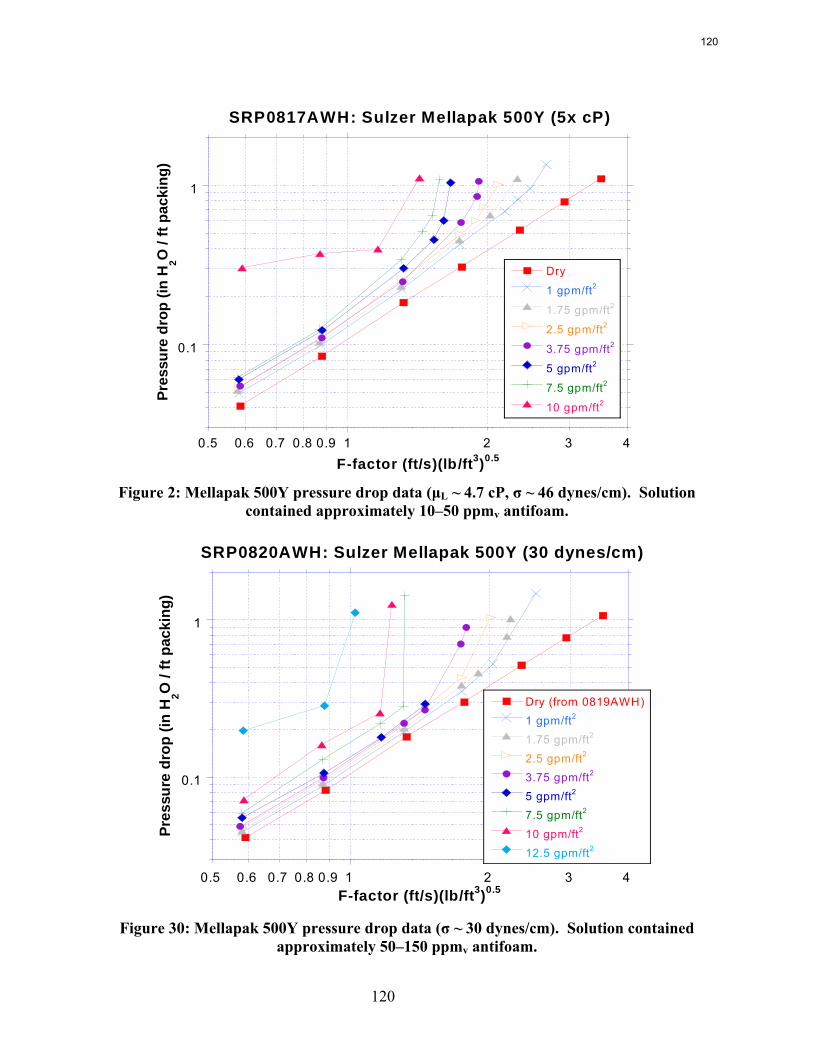
120

0.1

1

0.5 0.6 0.7 0.8 0.9 1 2 3 4

SRP0817AWH: Sulzer Mellapak 500Y (5x cP)

Dry

1 gpm/ft2

1.75 gpm/ft2

2.5 gpm/ft2

3.75 gpm/ft2

5 gpm/ft2

7.5 gpm/ft2

10 gpm/ft2Pres

sure

dro

p (in

H2O

/ ft

pack

ing)

F-factor (ft/s)(lb/ft3)0.5

Figure 2: Mellapak 500Y pressure drop data (μL ~ 4.7 cP, σ ~ 46 dynes/cm). Solution

contained approximately 10–50 ppmv antifoam.

0.1

1

0.5 0.6 0.7 0.8 0.9 1 2 3 4

SRP0820AWH: Sulzer Mellapak 500Y (30 dynes/cm)

Dry (from 0819AWH)1 gpm/ft2

1.75 gpm/ft2

2.5 gpm/ft2

3.75 gpm/ft2

5 gpm/ft2

7.5 gpm/ft2

10 gpm/ft2

12.5 gpm/ft2

Pres

sure

dro

p (in

H2O

/ ft

pack

ing)

F-factor (ft/s)(lb/ft3)0.5

Figure 30: Mellapak 500Y pressure drop data (σ ~ 30 dynes/cm). Solution contained

approximately 50–150 ppmv antifoam.

120

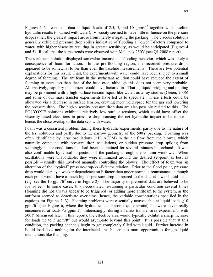
121

Figures 4–6 present the data at liquid loads of 2.5, 5, and 10 gpm/ft2 together with baseline hydraulic results (obtained with water). Viscosity seemed to have little influence on the pressure drop; rather, the greatest impact arose from merely irrigating the packing. The viscous solutions generally exhibited pressure drop spikes indicative of flooding at lower F-factors compared to water, with higher viscosity resulting in greater sensitivity, as would be anticipated (Figures 4 and 5). Recall that the same trends were observed with Mellapak 250Y (see Q1 2008 report).

The surfactant solution displayed somewhat inconsistent flooding behavior, which was likely a consequence of foam formation. In the pre-flooding region, the recorded pressure drops appeared to be somewhat lower than even the baseline measurements. There are two potential explanations for this result. First, the experiments with water could have been subject to a small degree of foaming. The antifoam in the surfactant solution could have reduced the extent of foaming to even less than that of the base case, although this does not seem very probable. Alternatively, capillary phenomena could have factored in. That is, liquid bridging and pooling may be prominent with a high surface tension liquid like water, as x-ray studies (Green, 2006) and some of our mass transfer experiments have led us to speculate. These effects could be alleviated via a decrease in surface tension, creating more void space for the gas and lowering the pressure drop. The high viscosity pressure drop data are also possibly related to this. The POLYOX™ solutions exhibited relatively low surface tensions, which could have offset the viscosity-based elevations in pressure drop, causing the net hydraulic impact to be minor – hence, the close overlap of the data sets with water.

Foam was a consistent problem during these hydraulic experiments, partly due to the nature of the test solutions and partly due to the narrow geometry of the 500Y packing. Foaming was often identifiable by large oscillations (>10 ACFM) in the air flow from the blower, which naturally coincided with pressure drop oscillations, or sudden pressure drop spiking from seemingly stable conditions that had been maintained for several minutes beforehand. It was also confirmable by visual inspection of the packing through the column windows. When oscillations were unavoidable, they were minimized around the desired set-point as best as possible – usually this involved manually controlling the blower. The effect of foam was an alteration of the “typical” pressure-drop-vs.-F-factor relation. Prior to the flood point, pressure drop would display a weaker dependence on F-factor than under normal circumstances, although each point would have a much higher pressure drop compared to the data at lower liquid loads (e.g. see the 10 gpm/ft2 curve in Figure 2). The majority of presented data are believed to be foam-free. In some cases, this necessitated re-running a particular condition several times (foaming did not always appear to be triggered) or adding more antifoam to the system, as the antifoam seemed to deactivate over time (hence, the variable concentrations specified in the captions for Figures 1–3). Foaming problems were essentially unavoidable at liquid loads ≥10 gpm/ft2 (see Figure 6, where the hydraulic data become quite erratic) but were never really encountered at loads ≤5 gpm/ft2. Interestingly, during all mass transfer area experiments with 500Y (discussed later in this report), the effective area would typically exhibit a sharp increase for loads up to 5 gpm/ft2 but would asymptote beyond this point. It is possible that at this condition, the packing channels begin to get completely filled with liquid. Further increase in liquid load does nothing for the interfacial area but creates more opportunities for gas-liquid interactions like foaming.

121

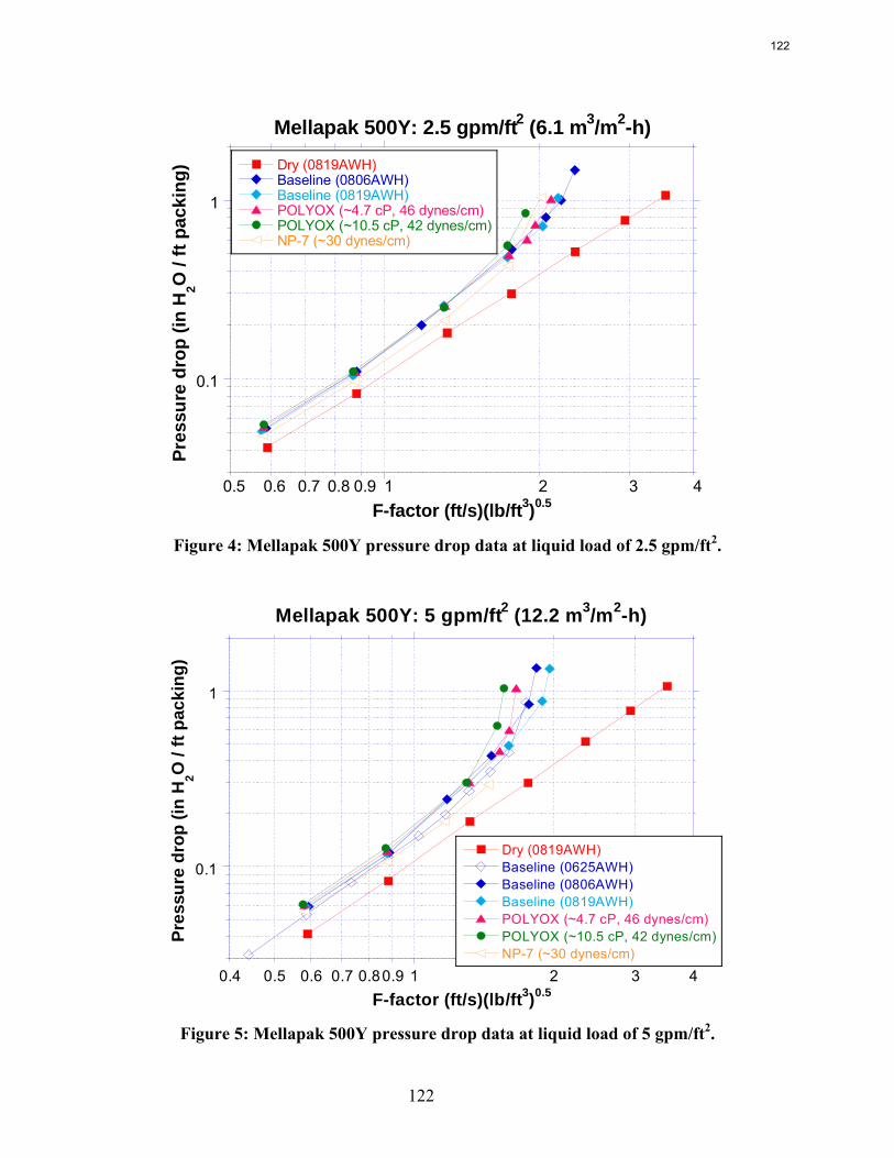
122

0.1

1

0.5 0.6 0.7 0.8 0.9 1 2 3 4

Mellapak 500Y: 2.5 gpm/ft2 (6.1 m3/m2-h)

Dry (0819AWH)Baseline (0806AWH)Baseline (0819AWH)POLYOX (~4.7 cP, 46 dynes/cm)POLYOX (~10.5 cP, 42 dynes/cm)NP-7 (~30 dynes/cm)

Pres

sure

dro

p (in

H2O

/ ft

pack

ing)

F-factor (ft/s)(lb/ft3)0.5

Figure 4: Mellapak 500Y pressure drop data at liquid load of 2.5 gpm/ft2.

0.1

1

0.4 0.5 0.6 0.7 0.80.9 1 2 3 4

Mellapak 500Y: 5 gpm/ft2 (12.2 m3/m2-h)

Dry (0819AWH)Baseline (0625AWH)Baseline (0806AWH)Baseline (0819AWH)POLYOX (~4.7 cP, 46 dynes/cm)POLYOX (~10.5 cP, 42 dynes/cm)NP-7 (~30 dynes/cm)

Pres

sure

dro

p (in

H2O

/ ft

pack

ing)

F-factor (ft/s)(lb/ft3)0.5

Figure 5: Mellapak 500Y pressure drop data at liquid load of 5 gpm/ft2.

122

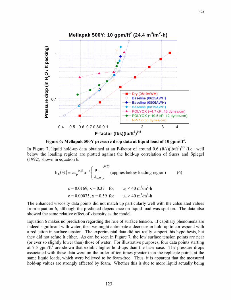
123

0.1

1

0.4 0.5 0.6 0.7 0.80.9 1 2 3 4

Mellapak 500Y: 10 gpm/ft2 (24.4 m3/m2-h)

Dry (0819AWH)Baseline (0625AWH)Baseline (0806AWH)Baseline (0819AWH)POLYOX (~4.7 cP, 46 dynes/cm)POLYOX (~10.5 cP, 42 dynes/cm)NP-7 (~30 dynes/cm)

Pres

sure

dro

p (in

H2O

/ ft

pack

ing)

F-factor (ft/s)(lb/ft3)0.5

Figure 6: Mellapak 500Y pressure drop data at liquid load of 10 gpm/ft2. In Figure 7, liquid hold-up data obtained at an F-factor of around 0.6 (ft/s)(lb/ft3)0.5 (i.e., well below the loading region) are plotted against the hold-up correlation of Suess and Spiegel (1992), shown in equation 6.

( )25.0

0,L

LxL

83.0pL μ

μuca%h ⎟

⎟⎠

⎞⎜⎜⎝

⎛= (applies below loading region) (6)

c = 0.0169, x = 0.37 for uL < 40 m3/m2-h

c = 0.00075, x = 0.59 for uL > 40 m3/m2-h

The enhanced viscosity data points did not match up particularly well with the calculated values from equation 6, although the predicted dependence on liquid load was spot-on. The data also showed the same relative effect of viscosity as the model.

Equation 6 makes no prediction regarding the role of surface tension. If capillary phenomena are indeed significant with water, then we might anticipate a decrease in hold-up to correspond with a reduction in surface tension. The experimental data did not really support this hypothesis, but they did not refute it either. As can be seen in Figure 7, the low surface tension points are near (or ever so slightly lower than) those of water. For illustrative purposes, four data points starting at 7.5 gpm/ft2 are shown that exhibit higher hold-ups than the base case. The pressure drops associated with these data were on the order of ten times greater than the replicate points at the same liquid loads, which were believed to be foam-free. Thus, it is apparent that the measured hold-up values are strongly affected by foam. Whether this is due to more liquid actually being

123

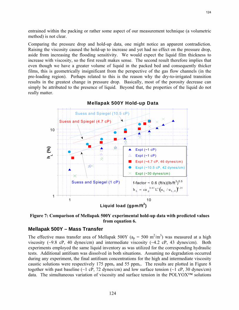
124

entrained within the packing or rather some aspect of our measurement technique (a volumetric method) is not clear.

Comparing the pressure drop and hold-up data, one might notice an apparent contradiction. Raising the viscosity caused the hold-up to increase and yet had no effect on the pressure drop, aside from increasing the flooding sensitivity. We would expect the liquid film thickness to increase with viscosity, so the first result makes sense. The second result therefore implies that even though we have a greater volume of liquid in the packed bed and consequently thicker films, this is geometrically insignificant from the perspective of the gas flow channels (in the pre-loading region). Perhaps related to this is the reason why the dry-to-irrigated transition results in the greatest change in pressure drop. Basically, most of the porosity decrease can simply be attributed to the presence of liquid. Beyond that, the properties of the liquid do not really matter.

( ) 25.00,LL

x83.0pL u/uLcah =

1

10

1 10

Mellapak 500Y Hold-up Data

Expt (~1 cP)

Expt (~1 cP)

Expt (~4.7 cP, 46 dynes/cm)

Expt (~10.5 cP, 42 dynes/cm)

Expt (~30 dynes/cm)

h L (%)

Liquid load (gpm/ft2)

f-factor ~ 0.6 (ft/s)(lb/ft3)0.5

Suess and Spiegel (10.5 cP)

Suess and Spiegel (4.7 cP)

Suess and Spiegel (1 cP)

Figure 7: Comparison of Mellapak 500Y experimental hold-up data with predicted values

from equation 6.

Mellapak 500Y – Mass Transfer The effective mass transfer area of Mellapak 500Y (ap = 500 m2/m3) was measured at a high viscosity (~9.8 cP, 40 dynes/cm) and intermediate viscosity (~4.2 cP, 43 dynes/cm). Both experiments employed the same liquid inventory as was utilized for the corresponding hydraulic tests. Additional antifoam was dissolved in both situations. Assuming no degradation occurred during any experiment, the final antifoam concentrations for the high and intermediate viscosity caustic solutions were respectively 175 ppmv and 55 ppmv. The results are plotted in Figure 8 together with past baseline (~1 cP, 72 dynes/cm) and low surface tension (~1 cP, 30 dynes/cm) data. The simultaneous variation of viscosity and surface tension in the POLYOX™ solutions

124

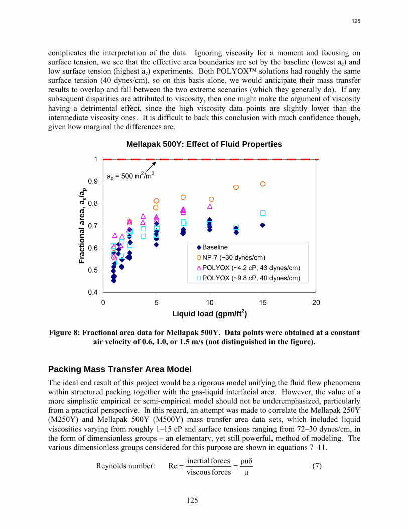
125

complicates the interpretation of the data. Ignoring viscosity for a moment and focusing on surface tension, we see that the effective area boundaries are set by the baseline (lowest ae) and low surface tension (highest ae) experiments. Both POLYOX™ solutions had roughly the same surface tension (40 dynes/cm), so on this basis alone, we would anticipate their mass transfer results to overlap and fall between the two extreme scenarios (which they generally do). If any subsequent disparities are attributed to viscosity, then one might make the argument of viscosity having a detrimental effect, since the high viscosity data points are slightly lower than the intermediate viscosity ones. It is difficult to back this conclusion with much confidence though, given how marginal the differences are.

Mellapak 500Y: Effect of Fluid Properties

0.4

0.5

0.6

0.7

0.8

0.9

1

0 5 10 15 20Liquid load (gpm/ft2)

Frac

tiona

l are

a, a

e/ap

BaselineNP-7 (~30 dynes/cm)POLYOX (~4.2 cP, 43 dynes/cm)POLYOX (~9.8 cP, 40 dynes/cm)

ap = 500 m2/m3

Figure 8: Fractional area data for Mellapak 500Y. Data points were obtained at a constant

air velocity of 0.6, 1.0, or 1.5 m/s (not distinguished in the figure).

Packing Mass Transfer Area Model The ideal end result of this project would be a rigorous model unifying the fluid flow phenomena within structured packing together with the gas-liquid interfacial area. However, the value of a more simplistic empirical or semi-empirical model should not be underemphasized, particularly from a practical perspective. In this regard, an attempt was made to correlate the Mellapak 250Y (M250Y) and Mellapak 500Y (M500Y) mass transfer area data sets, which included liquid viscosities varying from roughly 1–15 cP and surface tensions ranging from 72–30 dynes/cm, in the form of dimensionless groups – an elementary, yet still powerful, method of modeling. The various dimensionless groups considered for this purpose are shown in equations 7–11.

Reynolds number: μδuρ

forcesviscousforcesinertialRe == (7)

125

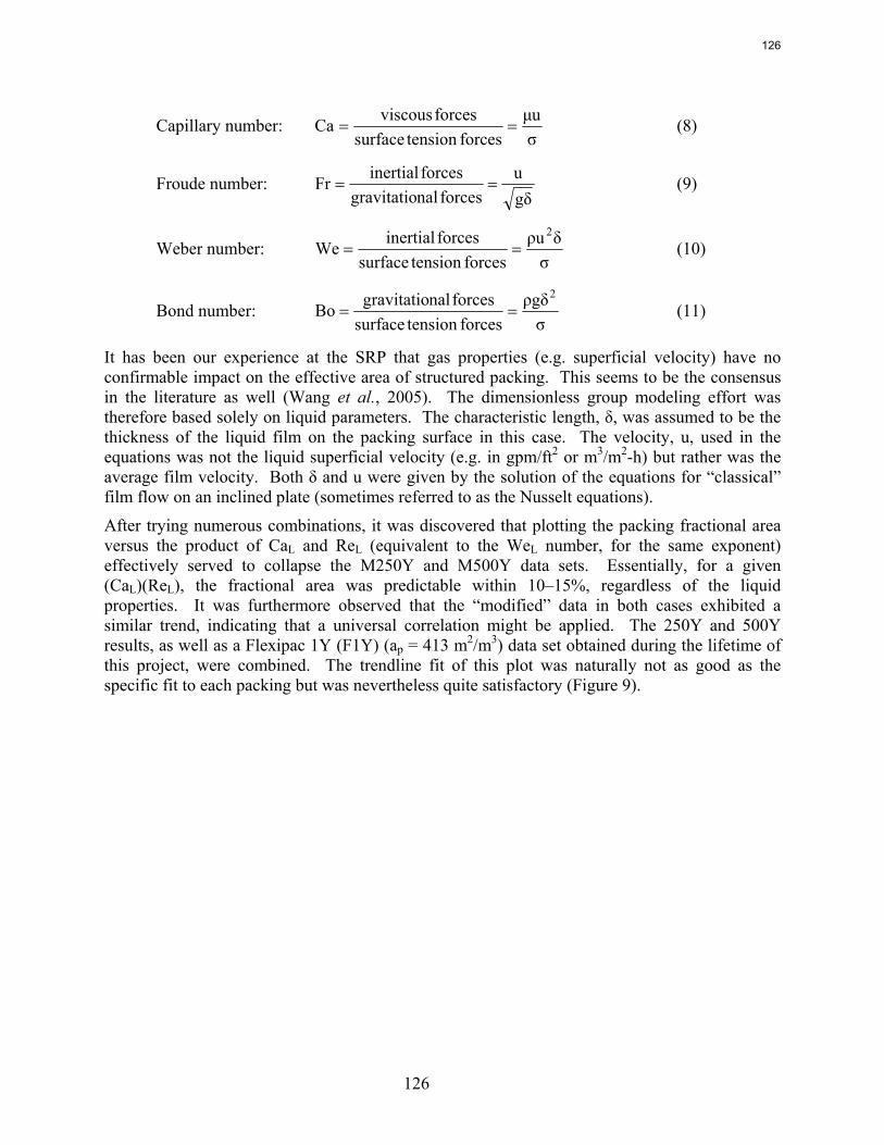
126

Capillary number: σuμ

forcestensionsurfaceforcesviscousCa == (8)

Froude number: δg

uforcesnalgravitatio

forcesinertialFr == (9)

Weber number: σδuρ

forcestensionsurfaceforcesinertialWe

2== (10)

Bond number: σδgρ

forcestensionsurfaceforcesnalgravitatioBo

2== (11)

It has been our experience at the SRP that gas properties (e.g. superficial velocity) have no confirmable impact on the effective area of structured packing. This seems to be the consensus in the literature as well (Wang et al., 2005). The dimensionless group modeling effort was therefore based solely on liquid parameters. The characteristic length, δ, was assumed to be the thickness of the liquid film on the packing surface in this case. The velocity, u, used in the equations was not the liquid superficial velocity (e.g. in gpm/ft2 or m3/m2-h) but rather was the average film velocity. Both δ and u were given by the solution of the equations for “classical” film flow on an inclined plate (sometimes referred to as the Nusselt equations).

After trying numerous combinations, it was discovered that plotting the packing fractional area versus the product of CaL and ReL (equivalent to the WeL number, for the same exponent) effectively served to collapse the M250Y and M500Y data sets. Essentially, for a given (CaL)(ReL), the fractional area was predictable within 10–15%, regardless of the liquid properties. It was furthermore observed that the “modified” data in both cases exhibited a similar trend, indicating that a universal correlation might be applied. The 250Y and 500Y results, as well as a Flexipac 1Y (F1Y) (ap = 413 m2/m3) data set obtained during the lifetime of this project, were combined. The trendline fit of this plot was naturally not as good as the specific fit to each packing but was nevertheless quite satisfactory (Figure 9).

126

127

0.4

0.5

0.6

0.7

0.8

0.9

1

0.001 0.01 0.1 1

SRP Packing Mass Transfer Area Database

M250Y - BaselineM250Y - NP-7 (~35 dynes/cm)M250Y - POLYOX (~13.8 cP, 42 dynes/cm)M500Y - BaselineM500Y - NP-7 (~30 dynes/cm)M500Y - POLYOX (~4.2 cP, 43 dynes/cm)M500Y - POLYOX (~9.8 cP, 40 dynes/cm)F1Y - BaselineF1Y - POLYOX (~5.8 cP, 60 dynes/cm)

Frac

tiona

l are

a, a

e/ap

(CaL)(Re

L)

ae/a

p = 1.006[(Ca

L)(Re

L)]0.088

-15%

+15%1.3

Figure 9: Packing mass transfer area data as a function of (CaL)(ReL).

The application of exponents of 1 to the CaL and ReL numbers clearly worked well but was a completely arbitrary decision. To formally determine the “correct” (or optimum) exponents that should be applied, an Excel regression in the following form was performed:

b2

a1 xcxy = (12)

Equation 13 was the result of the analysis. 0572.0

L0868.0

Lf ReCa089.3a = (13)

This suggested that the relative exponential weighting of the ReL to CaL numbers should be 0.0572/0.0868, which interestingly turns out to be very close to 2/3. Figure 10 is a re-plot of the packing mass transfer database as a function of (CaL)(ReL)2/3. The differences from Figure 9 are subtle. The M500Y and F1Y baseline results, as well as the high viscosity M250Y data, are merged closer to the center line, whereas the high viscosity M500Y data are shifted away somewhat. The data points also fall into more distinct vertical alignments. For discussion henceforth, the trendline equation (equation 14) will be considered as the proposed model for the effective mass transfer area of structured packing. (This is primarily because it has some statistical basis, as opposed to the model from Figure 9.)

127

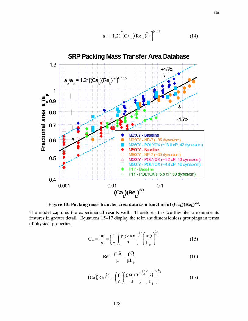
128

( )( )115.0

32

LLf ReCa21.1a ⎥⎦⎤

⎢⎣⎡= (14)

0.4

0.5

0.6

0.7

0.8

0.9

1

0.001 0.01 0.1

SRP Packing Mass Transfer Area Database

M250Y - BaselineM250Y - NP-7 (~35 dynes/cm)M250Y - POLYOX (~13.8 cP, 42 dynes/cm)M500Y - BaselineM500Y - NP-7 (~30 dynes/cm)M500Y - POLYOX (~4.2 cP, 43 dynes/cm)M500Y - POLYOX (~9.8 cP, 40 dynes/cm)F1Y - BaselineF1Y - POLYOX (~5.8 cP, 60 dynes/cm)

Frac

tiona

l are

a, a

e/ap

(CaL)(Re

L)2/3

ae/a

p = 1.21[(Ca

L)(Re

L)2/3]0.115

-15%

+15%1.3

Figure 10: Packing mass transfer area data as a function of (CaL)(ReL)2/3.

The model captures the experimental results well. Therefore, it is worthwhile to examine its features in greater detail. Equations 15–17 display the relevant dimensionless groupings in terms of physical properties.

32

p

31

LQμ

3αsingρ

σ1

σuμCa ⎟

⎟⎠

⎞⎜⎜⎝

⎛⎟⎠⎞

⎜⎝⎛

⎟⎠⎞

⎜⎝⎛== (15)

pLμQρ

μδuρRe == (16)

( )( )3

4

p

31

32

LQ

3αsing

σρReCa ⎟

⎟⎠

⎞⎜⎜⎝

⎛⎟⎠⎞

⎜⎝⎛

⎟⎠⎞

⎜⎝⎛= (17)

128

129

Substitution of equation 17 into equation 14 yields: 115.0

34

p

31

f LQ

3αsing

σρ21.1a

⎥⎥⎥

⎦

⎤

⎢⎢⎢

⎣

⎡

⎟⎟⎠

⎞⎜⎜⎝

⎛⎟⎠⎞

⎜⎝⎛

⎟⎠⎞

⎜⎝⎛= (18)

We can see from equation 18 that the effective area is most heavily tied to the liquid load term (Q/Lp). It should be noted that Lp, the wetted perimeter in a cross-sectional slice of packing, was estimated via geometric arguments. Lp was respectively calculated as 15.46, 35.31, and 30.23 m for M250Y, M500Y, and F1Y (assuming 16.8-in elements). The correlation also shows liquid density and surface tension to be relatively important properties. This implies that density could be another interesting variable to study. In the scope of this project, though, such an endeavor would probably not be worthwhile. First, there would be challenges associated with altering density enough to substantiate observed effects (if any). Moreover, for most amine solvents of interest, we would not expect densities to differ much from water (typically within about 20%). A reduction in surface tension is predicted by equation 18 to result in greater mass transfer area, with the (1/σ) effect being more significant at smaller values of (Q/Lp). This means that we would anticipate a stronger surface tension impact at lower liquid rates, which is logical, since the packing is less inclined to be fully wetted at these conditions. Surface tension also becomes more important as the specific packing area (related to Lp) increases. This is in agreement with our observations for M250Y (limited surface tension effect) and M500Y (significant surface tension effect). Viscosity is notably absent from equation 18. One could make the argument that viscosity has had a negligible effect in the tests we have performed thus far (see the Mellapak 500Y-Mass Transfer discussion), so for the representation of our data, the lack of a viscosity term makes sense. This omission could constrain the extrapolative freedom of the correlation though, as it is hard to imagine viscosity not having some kind of impact on gas-liquid interfacial area in an extreme limit (e.g. 102 or 103 cP). Last, equation 18 predicts a weak, albeit direct correspondence of mass transfer area and corrugation angle. In other words, the effective area of M250Y (45˚) should be lower than that of M250X (60˚). This is questionable, as some literature studies (Brunazzi et al., 1995) would agree, whereas past SRP experience and other sources (e.g. Rocha et al, 1996) would suggest the opposite. Since ae is often back-calculated from a volumetric coefficient (e.g. KGae), the confusion may stem from the interpretation of the paired mass transfer coefficient for the differently angled packings.

There are potential shortcomings beyond those already discussed. It is evident that some of the data sets in Figure 10 appear to be partitioned. For instance, the M250Y baseline data points primarily fall above the trendline, while the M250Y low surface tension data are below it. In addition, for M500Y and to a lesser extent for F1Y, the effective area tends to asymptote on reaching a certain liquid load (e.g. around 5 gpm/ft2 for M500Y). This behavior has not really been observed for M250Y, either because we have not operated at high enough liquid loads to see it or perhaps because the packing is more conducive to the formation of “free” liquid drops and jets that enable mass transfer to occur beyond its geometric limitations. Whatever the reason may be for the differentiation in performance, the bottom line is that not all data are represented equally well by the model. Improvements to its theoretical foundation could help to resolve these issues. Recall that the Nusselt film thickness and velocity are defined based on laminar flow down a smooth inclined plate. It is possible that these fundamental equations may need to be readdressed. For example, they may be better suited for a coarse packing like M250Y than

129

130

for finer packings like F1Y or M500Y, since the latter types are more likely to deviate from ideality, due to the many “corners” within their structures. Surface texture could also factor into a modification of the Nusselt equations.

Conclusions The hydraulic and mass transfer performance of Mellapak 500Y was studied at different viscosities and surface tensions in this reporting period. The apparent influence of viscosity (up to ~10 cP) can be summarized as follows:

• Marginally higher pressure drop and greater sensitivity to flooding; • Higher liquid hold-up; • Marginal (if any) impact on effective area.

Likewise, the effects of surface tension (down to ~30 dynes/cm) are: • Lower pressure drop; • Equivalent or slightly lower liquid hold-up; • Significantly higher effective areas.

Several authors in the literature (e.g. Rocha et al., 1993) suggest that pressure drop, hold-up, and effective area should all be relatable. However, the data we have obtained do not show much of a correlation among these parameters.

The proposed mass transfer area model is quite satisfactory. It not only is able to represent the entire spectrum of experimental data within adequate limits (±15%) but also does a good job of explicitly capturing some of the important underlying property interactions.

Future Work The mass transfer performance of M250Y at an intermediate viscosity (~5 cP) will be measured in order to complete the originally planned experimental design (1, 5, 10 cP). The hydraulic behavior of M250Y at low surface tension (~30 dynes/cm) will be evaluated as well, since this information is currently missing from the SRP database. Both the hydraulic and mass transfer performance of Mellapak 250X (60˚ corrugations) and Mellapak 252Y (high capacity / modified joints) at various viscosities and surface tensions will be tested in the future.

On the modeling side, work will also continue. Additional experimental effective area data – from past SRP packing tests or from external literature sources – will be located in an effort to further validate the current model. From a theoretical standpoint, there are still many aspects that can be addressed, such as the applicability of the Nusselt film equations. The fluid dynamics literature will, it is hoped, be able to provide insight in regard to problems like these.

Nomenclature ae = effective area of packing, m2/m3

ap = specific (geometric) area of packing, m2/m3

DCO2 = diffusivity of CO2, m2/s

d = estimated hydraulic diameter of WWC reaction chamber, m

g = gravitational constant; 9.81 m/s2

130

131

HCO2 = Henry’s constant of CO2, m3·Pa/kmol

hL = (total) liquid hold-up, dimensionless

KG = overall gas-side mass transfer coefficient, kmol/(m2·Pa·s)

kG = gas-side mass transfer coefficient, kmol/(m2·Pa·s)

kg′ = liquid-side mass transfer coefficient, kmol/(m2·Pa·s)

k˚L = physical liquid-side mass transfer coefficient, m/s

kOH- = second-order reaction rate constant, m3/(kmol·s)

L = exposed length of WWC, m

Lp = wetted perimeter of packing cross-section, m

NCO2 = molar flux of CO2, kmol/(m2·s)

P = pressure, Pa

Q = volumetric flow rate, m3/s

R = ideal gas constant, (m3·Pa)/(kmol·K)

T = absolute temperature, K

u = velocity, m/s

yCO2 in/out = mole fraction of CO2 at inlet/outlet

Z = packed height, m

Greek Symbols

α = corrugation angle (with respect to the horizontal), deg

δ = characteristic length (film thickness), m

μ = dynamic viscosity, kg/(m-s)

μL,0 = dynamic viscosity of water at 20˚C, kg/(m-s)

ρ = density, kg/m3

σ = surface tension, N/m

Subscripts

G = gas phase

L = liquid phase

Dimensionless Groups

af = fractional area of packing, ae/ap

Bo = Bond number, σδgρ 2

131

132

Ca = Capillary number, σuμ

Fr = Froude number, δg

u

Re = Reynolds number, μδuρ

We = Weber number, σδuρ 2

References Billet R, Schultes M. Prediction of Mass Transfer Columns with Dumped and Arranged

Packings: Updated Summary of the Calculation Method of Billet and Schultes. Chem. Eng. Res. Des. 1999;77(A6):498–504.

Bishnoi S. Absorption of Carbon Dioxide into Aqueous Piperazine: Reaction Kinetics, Mass Transfer, and Solubility. Chem. Eng. Sci. 2000;55(22):5531–5543.

Brunazzi E, Nardini G, Paglianti A, Petarca L. Interfacial Area of Mellapak Packing: Absorption of 1,1,1-Trichloroethane by Genosorb 300. Chem. Eng. Technol. 1995;18(4):248–255.

Cullinane JT. Kinetics of Carbon Dioxide Absorption into Aqueous Potassium Carbonate and Piperazine. Ind. Eng. Chem. Res. 2006;45(8):2531–2545.

Green CW. Hydraulic Characterization of Structured Packing via X-Ray Computed Tomography. University of Texas, Austin; 2006. Ph.D. Thesis.

Kohl A, Nielsen R. Gas Purification; Houston: Gulf Publishing Co., 1997. Mshewa MM. Carbon Dioxide Desorption/Absorption with Aqueous Mixtures of

Methyldiethanolamine and Diethanolamine at 40 to 120oC. University of Texas, Austin;. 1995. Ph.D. Thesis.

Pohorecki R, Moniuk W. Kinetics of Reaction between Carbon Dioxide and Hydroxyl Ions in Aqueous Electrolyte Solutions. Chem. Eng. Sci. 1988;43(7):1677–1684.

Rocha JA, Bravo JL, Fair JR. Distillation Columns Containing Structured Packings: A Comprehensive Model for Their Performance. 1. Hydraulic Models. Ind. Eng. Chem. Res. 1993;32(4):641–651.

Rocha JA, Bravo JL, Fair JR. Distillation Columns Containing Structured Packings: A Comprehensive Model for Their Performance. 2. Mass-Transfer Model. Ind. Eng. Chem. Res. 1996;35 (5):1660–1667.

Suess P, Spiegel L. Hold-up of Mellapak Structured Packings. Chem. Eng. Process. 1992;31(2):119–124.

Wang GQ, Yuan XG, Yu KT. Review of Mass-Transfer Correlations for Packed Columns. Ind. Eng. Chem. Res. 2005;44(23):8715–8729.

132

133

Modeling Stripper Performance for CO2 Removal

Quarterly Report for April 1 – June 30, 2008

by David Van Wagener

Supported by the Luminant Carbon Management Program

and the

Industrial Associates Program for CO2 Capture by Aqueous Absorption

Department of Chemical Engineering

The University of Texas at Austin

July 20, 2008

Abstract This quarter focused on optimizing a solar heated three-stage flash configuration and progressing new parameters for a piperazine thermodynamic model. The configuration from the previous quarter was altered by combining the preheater and the first flash tank to make a heated flash. In every run the maximum temperature in the heater was set so that the lean pressure was around 110 kPa. This specification avoided vacuum stripping and also generally kept the temperatures below 120°C, a ceiling motivated by thermal degradation. The three-stage flash configuration performed better than the base case, an atmospheric simple stripper, as well as a high pressure simple stripper. Using solar heat was beneficial for the three-stage flash, reducing the total equivalent work from 33.3 kJ/mol CO2 to 32.7 kJ/mol CO2. Solar heat decreased the effectiveness of supplying the energy in the simple stripper, so if solar heat is available as an energy source for stripping, it would much better be used in the three-stage flash. Next, the piperazine thermodynamic model developed by Hilliard was revisited to ensure that it will perform well for future simulations using high piperazine concentrations and high stripping temperatures. Irrelevant data was located and removed, and additional high concentration and high temperature data was introduced to the data sets for the regression. The regression was rerun, and the VLE shown to be accurate for the desired concentrations and temperatures. Reproducing accurate heat capacity data is still troublesome, as it was in Hilliard's regression attempts.

Introduction The aim of stripper modeling is to increase the efficiency and performance of the stripper section without dramatically increasing its complexity. In this quarter, work on flashing strippers as a method of solvent regeneration has continued. Flashing strippers operate by sending the rich solvent through the typical cross exchanger and then an additional preheater. The solvent reaches a higher temperature compared to that in a simple stripper configuration. The solvent is then passed through adiabatic flash tanks in the series, each reducing the temperature and

133

134

pressure of the liquid. Carbon dioxide and water vapor are released in each flash, and the liquid decreases in loading. In this work, a three-step flash is used. A four-step flash was considered, but the increase in complexity was determined to be prohibitive. In preliminary analyses, the three-step flash configuration results in a pressure ratio between each stage which falls close to the optimal compression ratio for vapor compressors, whereas the difference in pressure between each stage for a four-stage configuration would be too small.

The benefit of the flashing stripper configuration is that solar energy can be used where the heat is applied over a range of temperatures. Steam heating in traditional reboilers is provided at one temperature level, the condensation temperature of water at the source pressure. When converting the heat to an equivalent work, a 75% Carnot efficiency is calculated with a 10°C approach at the reboiler:

∑=

⎟⎟⎠

⎞⎜⎜⎝

⎛+

−+=

reboilersn

i i

iieq KT

TKTQW

1

sink

1010

*75.0 (1)

where Tsink is 313K, the sink temperature for the turbines converting the coal-generated steam into electricity in the power plant. A heater for the three-stage flash configuration is not in a well-mixed tank like a stripper reboiler. Instead the rich solvent would be heated without mixing. The variable solvent temperature increases the driving force on the cold side when isothermal steam heating is used. When using a heating medium besides steam, its temperature is not constant throughout heating, so the temperature driving force is decreased. The lower temperature driving force reduces the lost work and equivalent work for heating. The new equivalent work can be calculated by integrating equation 1 from the initial to final temperature in the case where there is only one heater:

⎟⎟⎟⎟⎟

⎠

⎞

⎜⎜⎜⎜⎜

⎝

⎛

−

⎟⎟⎠

⎞⎜⎜⎝

⎛−−

=of

o

fof

eq TTTT

TTTQW

ln*75.0

sink

(2)

Flashing is not a common approach for stripping of solvents. One reason it is generally avoided is because the CO2/H2O selectivity can be very low if flashing directly from the high temperature to the final temperature. However, by using three flashes, some of the stripping is done at high pressure. High-pressure stripping has been shown to be beneficial for CO2 selectivity in the multi-pressure and double matrix stripper configurations (Oyenekan, 2007).

In addition to working on the three-stage flash, the recent Hilliard (2008) PZ-CO2-H2O thermodynamic model was analyzed. In the future this model will be used to simulate stripper configurations using solvents with high piperazine concentrations, such as 8 m PZ. However, the Hilliard thermodynamic model was generated using mostly low solvent concentrations (0.9 m–5 m PZ) and low temperatures (mostly 40°C and 60°C). To avoid extrapolation and potentially wildly inaccurate results, parameters were regressed for the proposed stripper conditions.

134

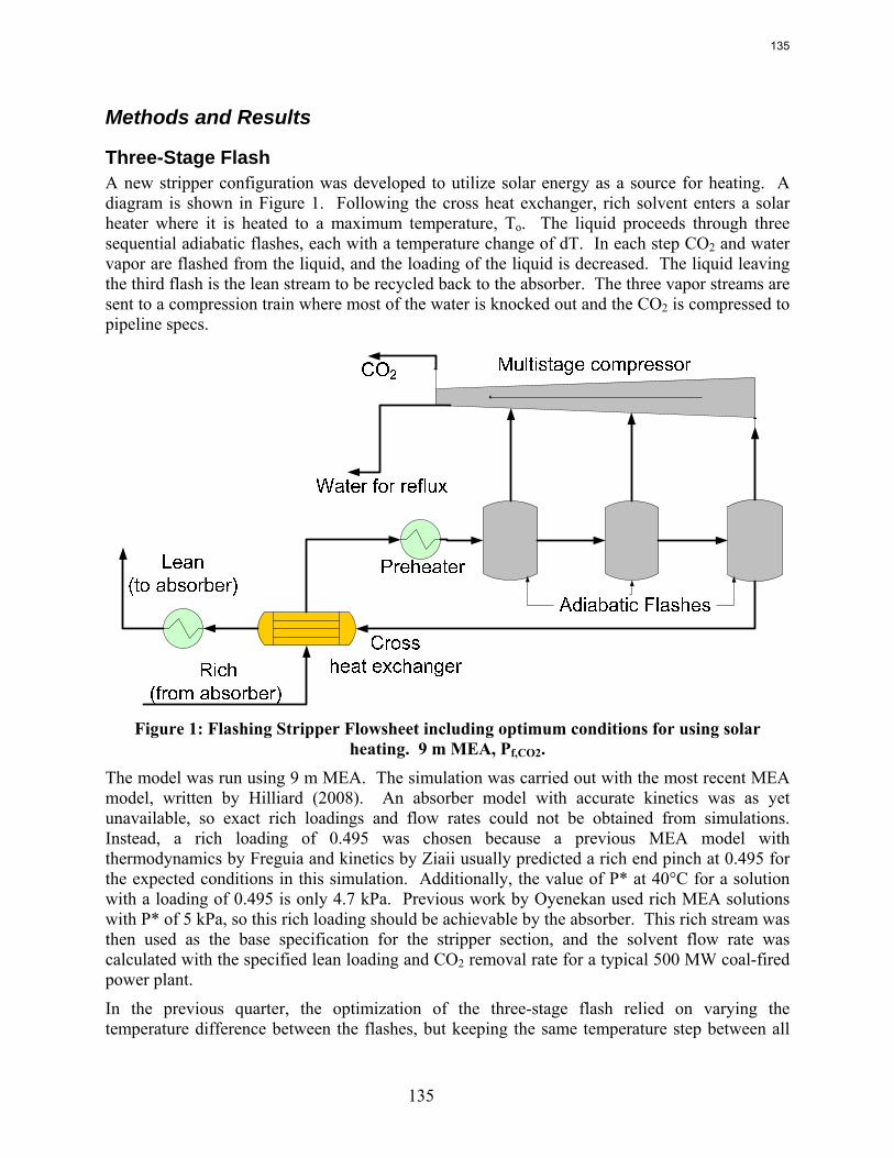
135

Methods and Results

Three-Stage Flash A new stripper configuration was developed to utilize solar energy as a source for heating. A diagram is shown in Figure 1. Following the cross heat exchanger, rich solvent enters a solar heater where it is heated to a maximum temperature, To. The liquid proceeds through three sequential adiabatic flashes, each with a temperature change of dT. In each step CO2 and water vapor are flashed from the liquid, and the loading of the liquid is decreased. The liquid leaving the third flash is the lean stream to be recycled back to the absorber. The three vapor streams are sent to a compression train where most of the water is knocked out and the CO2 is compressed to pipeline specs.

Figure 1: Flashing Stripper Flowsheet including optimum conditions for using solar heating. 9 m MEA, Pf,CO2.

The model was run using 9 m MEA. The simulation was carried out with the most recent MEA model, written by Hilliard (2008). An absorber model with accurate kinetics was as yet unavailable, so exact rich loadings and flow rates could not be obtained from simulations. Instead, a rich loading of 0.495 was chosen because a previous MEA model with thermodynamics by Freguia and kinetics by Ziaii usually predicted a rich end pinch at 0.495 for the expected conditions in this simulation. Additionally, the value of P* at 40°C for a solution with a loading of 0.495 is only 4.7 kPa. Previous work by Oyenekan used rich MEA solutions with P* of 5 kPa, so this rich loading should be achievable by the absorber. This rich stream was then used as the base specification for the stripper section, and the solvent flow rate was calculated with the specified lean loading and CO2 removal rate for a typical 500 MW coal-fired power plant.

In the previous quarter, the optimization of the three-stage flash relied on varying the temperature difference between the flashes, but keeping the same temperature step between all

135

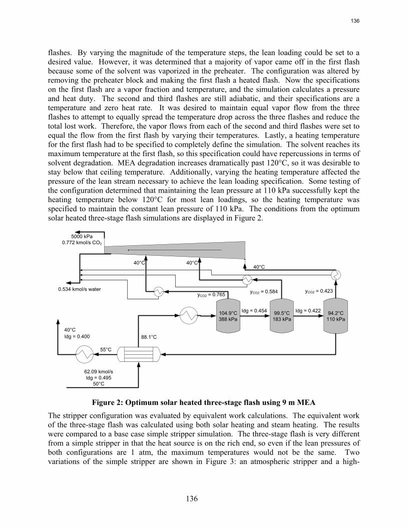
136

flashes. By varying the magnitude of the temperature steps, the lean loading could be set to a desired value. However, it was determined that a majority of vapor came off in the first flash because some of the solvent was vaporized in the preheater. The configuration was altered by removing the preheater block and making the first flash a heated flash. Now the specifications on the first flash are a vapor fraction and temperature, and the simulation calculates a pressure and heat duty. The second and third flashes are still adiabatic, and their specifications are a temperature and zero heat rate. It was desired to maintain equal vapor flow from the three flashes to attempt to equally spread the temperature drop across the three flashes and reduce the total lost work. Therefore, the vapor flows from each of the second and third flashes were set to equal the flow from the first flash by varying their temperatures. Lastly, a heating temperature for the first flash had to be specified to completely define the simulation. The solvent reaches its maximum temperature at the first flash, so this specification could have repercussions in terms of solvent degradation. MEA degradation increases dramatically past 120°C, so it was desirable to stay below that ceiling temperature. Additionally, varying the heating temperature affected the pressure of the lean stream necessary to achieve the lean loading specification. Some testing of the configuration determined that maintaining the lean pressure at 110 kPa successfully kept the heating temperature below 120°C for most lean loadings, so the heating temperature was specified to maintain the constant lean pressure of 110 kPa. The conditions from the optimum solar heated three-stage flash simulations are displayed in Figure 2.

40°C

62.09 kmol/sldg = 0.495

50°C

0.534 kmol/s water

5000 kPa0.772 kmol/s CO2

88.1°C

104.9°C388 kPa

94.2°C110 kPa

99.5°C183 kPa

55°C

yCO2 = 0.423yCO2 = 0.765 yCO2 = 0.584

40°C40°C40°C

ldg = 0.454

ldg = 0.400

ldg = 0.422

Figure 2: Optimum solar heated three-stage flash using 9 m MEA

The stripper configuration was evaluated by equivalent work calculations. The equivalent work of the three-stage flash was calculated using both solar heating and steam heating. The results were compared to a base case simple stripper simulation. The three-stage flash is very different from a simple stripper in that the heat source is on the rich end, so even if the lean pressures of both configurations are 1 atm, the maximum temperatures would not be the same. Two variations of the simple stripper are shown in Figure 3: an atmospheric stripper and a high-

136

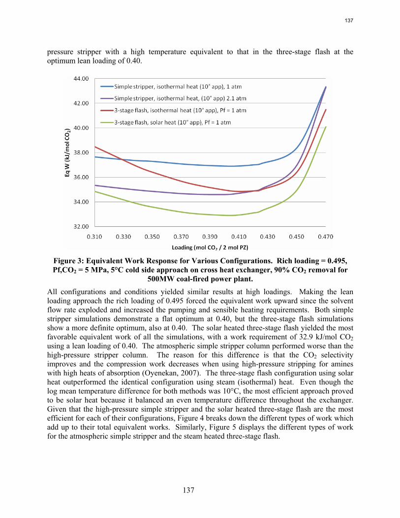
137

pressure stripper with a high temperature equivalent to that in the three-stage flash at the optimum lean loading of 0.40.

Figure 3: Equivalent Work Response for Various Configurations. Rich loading = 0.495, Pf,CO2 = 5 MPa, 5°C cold side approach on cross heat exchanger, 90% CO2 removal for

500MW coal-fired power plant.

All configurations and conditions yielded similar results at high loadings. Making the lean loading approach the rich loading of 0.495 forced the equivalent work upward since the solvent flow rate exploded and increased the pumping and sensible heating requirements. Both simple stripper simulations demonstrate a flat optimum at 0.40, but the three-stage flash simulations show a more definite optimum, also at 0.40. The solar heated three-stage flash yielded the most favorable equivalent work of all the simulations, with a work requirement of 32.9 kJ/mol CO2 using a lean loading of 0.40. The atmospheric simple stripper column performed worse than the high-pressure stripper column. The reason for this difference is that the CO2 selectivity improves and the compression work decreases when using high-pressure stripping for amines with high heats of absorption (Oyenekan, 2007). The three-stage flash configuration using solar heat outperformed the identical configuration using steam (isothermal) heat. Even though the log mean temperature difference for both methods was 10°C, the most efficient approach proved to be solar heat because it balanced an even temperature difference throughout the exchanger. Given that the high-pressure simple stripper and the solar heated three-stage flash are the most efficient for each of their configurations, Figure 4 breaks down the different types of work which add up to their total equivalent works. Similarly, Figure 5 displays the different types of work for the atmospheric simple stripper and the steam heated three-stage flash.

137

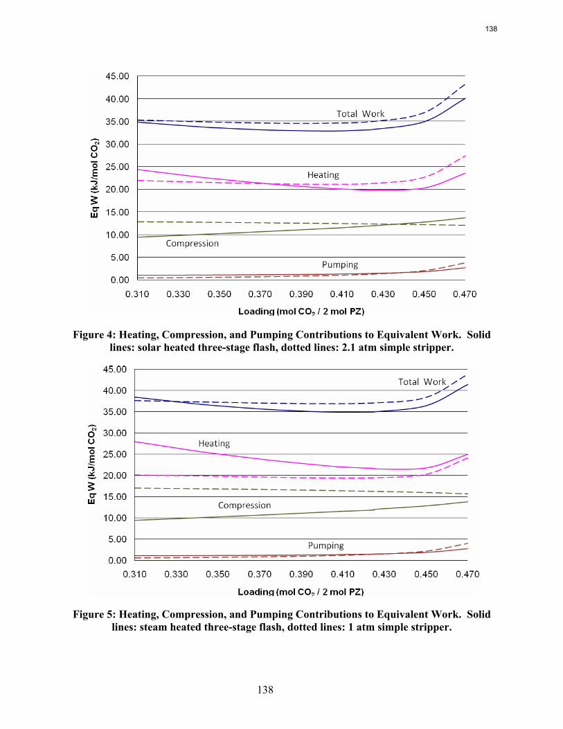
138

Figure 4: Heating, Compression, and Pumping Contributions to Equivalent Work. Solid

lines: solar heated three-stage flash, dotted lines: 2.1 atm simple stripper.

Figure 5: Heating, Compression, and Pumping Contributions to Equivalent Work. Solid

lines: steam heated three-stage flash, dotted lines: 1 atm simple stripper.

138

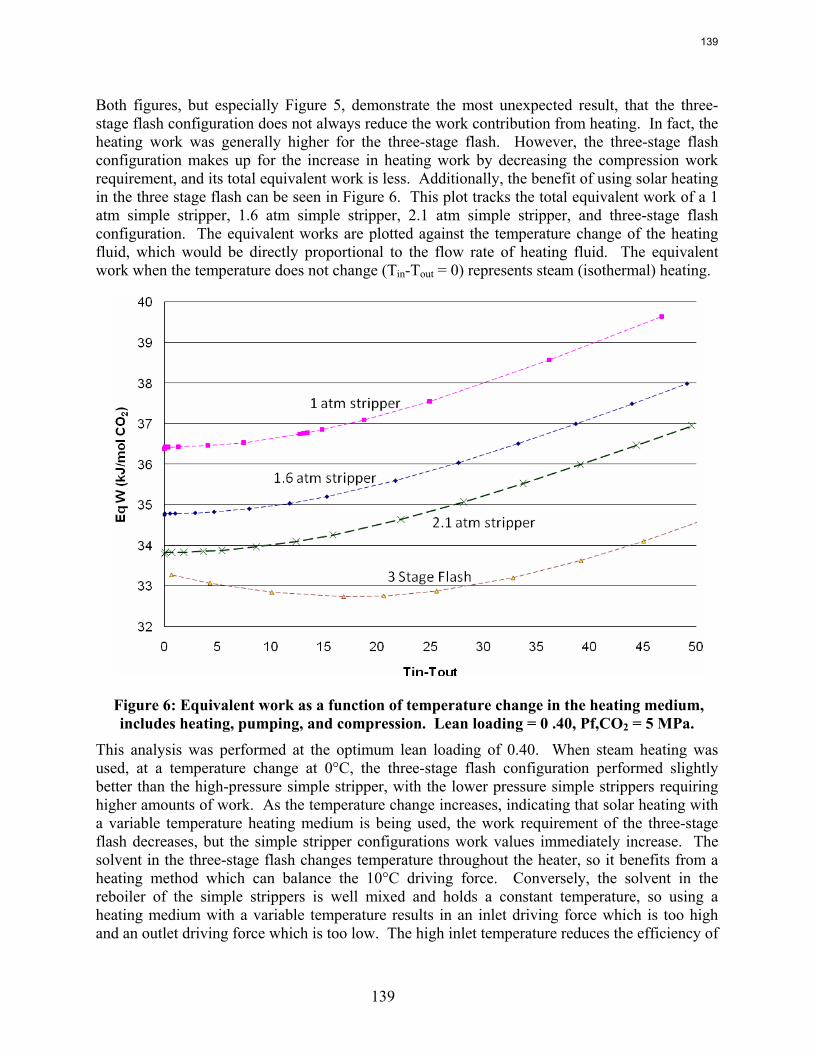
139

Both figures, but especially Figure 5, demonstrate the most unexpected result, that the three-stage flash configuration does not always reduce the work contribution from heating. In fact, the heating work was generally higher for the three-stage flash. However, the three-stage flash configuration makes up for the increase in heating work by decreasing the compression work requirement, and its total equivalent work is less. Additionally, the benefit of using solar heating in the three stage flash can be seen in Figure 6. This plot tracks the total equivalent work of a 1 atm simple stripper, 1.6 atm simple stripper, 2.1 atm simple stripper, and three-stage flash configuration. The equivalent works are plotted against the temperature change of the heating fluid, which would be directly proportional to the flow rate of heating fluid. The equivalent work when the temperature does not change (Tin-Tout = 0) represents steam (isothermal) heating.

Figure 6: Equivalent work as a function of temperature change in the heating medium, includes heating, pumping, and compression. Lean loading = 0 .40, Pf,CO2 = 5 MPa.

This analysis was performed at the optimum lean loading of 0.40. When steam heating was used, at a temperature change at 0°C, the three-stage flash configuration performed slightly better than the high-pressure simple stripper, with the lower pressure simple strippers requiring higher amounts of work. As the temperature change increases, indicating that solar heating with a variable temperature heating medium is being used, the work requirement of the three-stage flash decreases, but the simple stripper configurations work values immediately increase. The solvent in the three-stage flash changes temperature throughout the heater, so it benefits from a heating method which can balance the 10°C driving force. Conversely, the solvent in the reboiler of the simple strippers is well mixed and holds a constant temperature, so using a heating medium with a variable temperature results in an inlet driving force which is too high and an outlet driving force which is too low. The high inlet temperature reduces the efficiency of

139

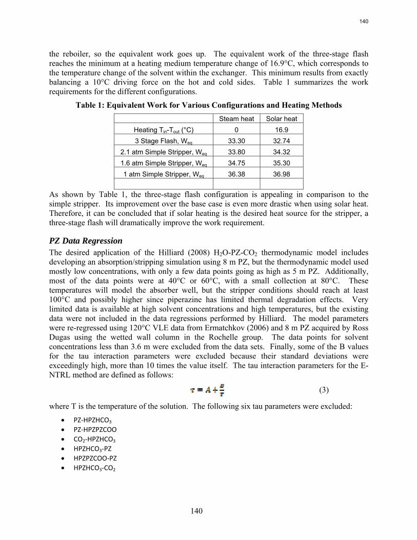
140

the reboiler, so the equivalent work goes up. The equivalent work of the three-stage flash reaches the minimum at a heating medium temperature change of 16.9°C, which corresponds to the temperature change of the solvent within the exchanger. This minimum results from exactly balancing a 10°C driving force on the hot and cold sides. Table 1 summarizes the work requirements for the different configurations.

Table 1: Equivalent Work for Various Configurations and Heating Methods Steam heat Solar heat

Heating Tin-Tout (°C) 0 16.9 3 Stage Flash, Weq 33.30 32.74

2.1 atm Simple Stripper, Weq 33.80 34.32 1.6 atm Simple Stripper, Weq 34.75 35.30 1 atm Simple Stripper, Weq 36.38 36.98

As shown by Table 1, the three-stage flash configuration is appealing in comparison to the simple stripper. Its improvement over the base case is even more drastic when using solar heat. Therefore, it can be concluded that if solar heating is the desired heat source for the stripper, a three-stage flash will dramatically improve the work requirement.

PZ Data Regression The desired application of the Hilliard (2008) H2O-PZ-CO2 thermodynamic model includes developing an absorption/stripping simulation using 8 m PZ, but the thermodynamic model used mostly low concentrations, with only a few data points going as high as 5 m PZ. Additionally, most of the data points were at 40°C or 60°C, with a small collection at 80°C. These temperatures will model the absorber well, but the stripper conditions should reach at least 100°C and possibly higher since piperazine has limited thermal degradation effects. Very limited data is available at high solvent concentrations and high temperatures, but the existing data were not included in the data regressions performed by Hilliard. The model parameters were re-regressed using 120°C VLE data from Ermatchkov (2006) and 8 m PZ acquired by Ross Dugas using the wetted wall column in the Rochelle group. The data points for solvent concentrations less than 3.6 m were excluded from the data sets. Finally, some of the B values for the tau interaction parameters were excluded because their standard deviations were exceedingly high, more than 10 times the value itself. The tau interaction parameters for the E-NTRL method are defined as follows:

(3)

where T is the temperature of the solution. The following six tau parameters were excluded:

• PZ‐HPZHCO3 • PZ‐HPZPZCOO • CO2‐HPZHCO3 • HPZHCO3‐PZ • HPZPZCOO‐PZ • HPZHCO3‐CO2

140

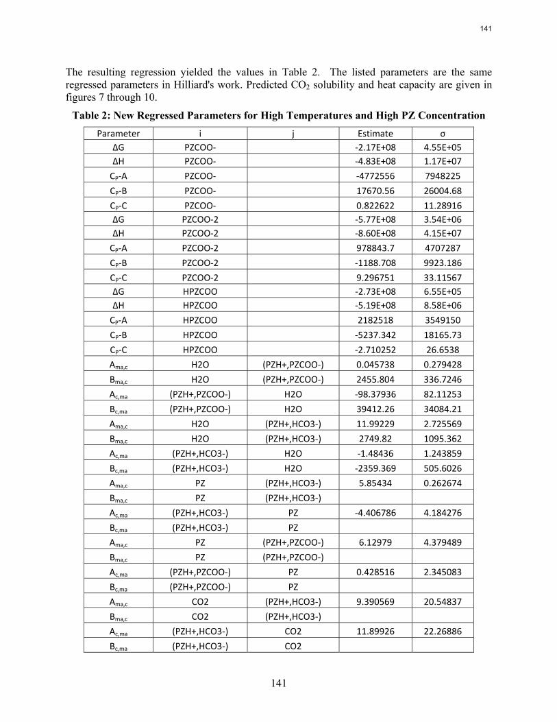
141

The resulting regression yielded the values in Table 2. The listed parameters are the same regressed parameters in Hilliard's work. Predicted CO2 solubility and heat capacity are given in figures 7 through 10.

Table 2: New Regressed Parameters for High Temperatures and High PZ Concentration Parameter  i  j  Estimate  σ 

ΔG  PZCOO‐     ‐2.17E+08  4.55E+05 ΔH  PZCOO‐     ‐4.83E+08  1.17E+07 CP‐A  PZCOO‐     ‐4772556  7948225 CP‐B  PZCOO‐     17670.56  26004.68 CP‐C  PZCOO‐     0.822622  11.28916 ΔG  PZCOO‐2     ‐5.77E+08  3.54E+06 ΔH  PZCOO‐2     ‐8.60E+08  4.15E+07 CP‐A  PZCOO‐2     978843.7  4707287 CP‐B  PZCOO‐2     ‐1188.708  9923.186 CP‐C  PZCOO‐2     9.296751  33.11567 ΔG  HPZCOO     ‐2.73E+08  6.55E+05 ΔH  HPZCOO     ‐5.19E+08  8.58E+06 CP‐A  HPZCOO     2182518  3549150 CP‐B  HPZCOO     ‐5237.342  18165.73 CP‐C  HPZCOO     ‐2.710252  26.6538 Ama,c  H2O  (PZH+,PZCOO‐)  0.045738  0.279428 Bma,c  H2O  (PZH+,PZCOO‐)  2455.804  336.7246 Ac,ma  (PZH+,PZCOO‐)  H2O  ‐98.37936  82.11253 Bc,ma  (PZH+,PZCOO‐)  H2O  39412.26  34084.21 Ama,c  H2O  (PZH+,HCO3‐)  11.99229  2.725569 Bma,c  H2O  (PZH+,HCO3‐)  2749.82  1095.362 Ac,ma  (PZH+,HCO3‐)  H2O  ‐1.48436  1.243859 Bc,ma  (PZH+,HCO3‐)  H2O  ‐2359.369  505.6026 Ama,c  PZ  (PZH+,HCO3‐)  5.85434  0.262674 Bma,c  PZ  (PZH+,HCO3‐)     Ac,ma  (PZH+,HCO3‐)  PZ  ‐4.406786  4.184276 Bc,ma  (PZH+,HCO3‐)  PZ     Ama,c  PZ  (PZH+,PZCOO‐)  6.12979  4.379489 Bma,c  PZ  (PZH+,PZCOO‐)     Ac,ma  (PZH+,PZCOO‐)  PZ  0.428516  2.345083 Bc,ma  (PZH+,PZCOO‐)  PZ     Ama,c  CO2  (PZH+,HCO3‐)  9.390569  20.54837 Bma,c  CO2  (PZH+,HCO3‐)     Ac,ma  (PZH+,HCO3‐)  CO2  11.89926  22.26886 Bc,ma  (PZH+,HCO3‐)  CO2     

141

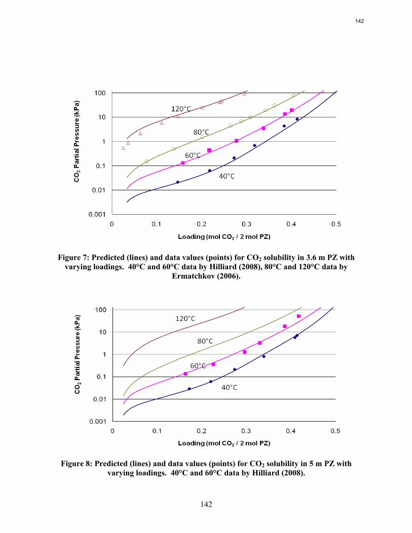
142

Figure 7: Predicted (lines) and data values (points) for CO2 solubility in 3.6 m PZ with

varying loadings. 40°C and 60°C data by Hilliard (2008), 80°C and 120°C data by Ermatchkov (2006).

Figure 8: Predicted (lines) and data values (points) for CO2 solubility in 5 m PZ with

varying loadings. 40°C and 60°C data by Hilliard (2008).

142

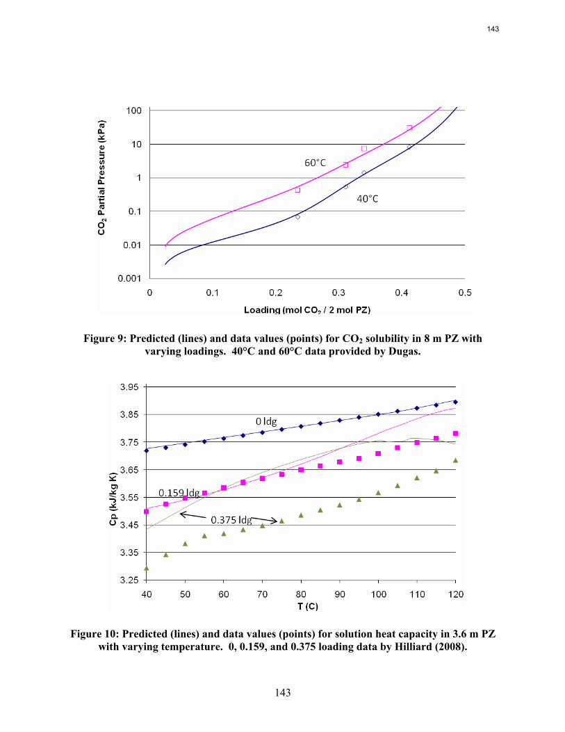
143

Figure 9: Predicted (lines) and data values (points) for CO2 solubility in 8 m PZ with

varying loadings. 40°C and 60°C data provided by Dugas.

Figure 10: Predicted (lines) and data values (points) for solution heat capacity in 3.6 m PZ

with varying temperature. 0, 0.159, and 0.375 loading data by Hilliard (2008).

143

144

The VLE data fits very well, even at high solvent concentrations and high temperatures. Heat capacity, on the other hand, does not fit well. Heat capacity was always a troubled area for piperazine regressions in Hilliard's work. It has been proposed that the problem might be inaccurate heat of absorption data.

Conclusions The three-stage flash configuration was simulated using 9 m MEA and compared against a simple stripper base case. Additionally, a 2.1 atm high-pressure simple stripper was evaluated to approximate similar maximum temperatures achieved in the specified three-stage flash configuration. The three-stage flash performed better than the simple stripper, and solar heating proved to be advantageous for the three-stage flash, but it was a disadvantage for the simple strippers. The best performance was with a solar heated three-stage flash, which resulted in a total equivalent work of 32.7 kJ/mol CO2. The thermodynamic model for piperazine recently completed by Hilliard was revisited to regress new parameters and make the model adequate for simulating cases with high solvent concentrations and high temperatures. Low concentration data points were removed, and available high concentration at high temperature data points were added. Irrelevant tau parameters, values with very large uncertainties, were removed to improve the precision of the regression. The new parameters predict all VLE data points between 3.6 m and 8 m PZ well, but the heat capacity predictions are no improvement over the initial Hilliard model.

References Chen E. Carbon Dioxide Absorption into Piperazine Promoting Potassium Carbonate Using

Structured Packing. University of Texas, Austin; 2007. Ph.D. Dissertation. Hilliard M. A Predictive Thermodynamic Model for an Aqueous Blend of Potassium Carbonate,

Piperazine, and Monoethanolamine for Carbon Dioxide Capture from Flue Gas. University of Texas, Austin; 2008. Ph.D. Dissertation.

Oyenekan B. Modeling of Strippers for CO2 Capture by Aqueous Amines. University of Texas, Austin; 2007. Ph.D. Dissertation.

144

145

Modeling CO2 Absorption Using Aqueous Amines Progress Report for April – June, 2008

by Jorge M. Plaza

Supported by the Luminant Carbon Management Program

and the

Industrial Associates Program for CO2 Capture by Aqueous Absorption

Department of Chemical Engineering

The University of Texas at Austin

July 24, 2008

Abstract A new model for the absorption of carbon dioxide from flue gas by aqueous MEA has been developed. It incorporates the thermodynamic model by Hilliard (2008) and simplified kinetics consisting of two equilibrium equations and four kinetic reactions. Carbamate formation rates were obtained by simulating the conditions of the laminar jet used by Aboudheir (2002) with an absorber model generated in Aspen Plus®. The bicarbonate forward rate was approximated using data presented by Rochelle et al. (2001).

Pilot plant data generated with 35% MEA in October 2007 were simulated using the new model. Temperature profiles and CO2 loading results are compared to the model. This report includes details on the development of the model and preliminary results of the model validation.

Description MEA Model Development Aboudheir (2002) generated rate data for CO2 absorption in MEA using a laminar jet at various amine concentrations, CO2 loadings, and temperatures. This data was used to evaluate the forward rate constants for the formation of carbamate using Aspen Plus® RateSep™. An absorber model was set up that included the new thermodynamic model developed by Hilliard (2008). Kinetics were represented using the following set of two reversible reactions:

2 MEA + CO2 → MEA+ + MEACOO- (1) MEA+ + MEACOO- → 2 MEA + CO2 (2) MEA + CO2 + H2O→ HCO3

- + MEA+ (3) MEA+ + HCO3

- → MEA + CO2 + H2O (4)

Two similar equilibrium reactions were used to represent the chemistry:

2 MEA + CO2 ↔ MEA+ + MEACOO- (5)

MEA + CO2 + H2O↔ HCO3- + MEA+ (6)

145

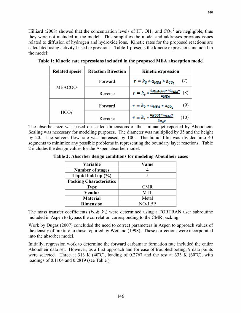
146

Hilliard (2008) showed that the concentration levels of H+, OH-, and CO3-2 are negligible, thus

they were not included in the model. This simplifies the model and addresses previous issues related to diffusion of hydrogen and hydroxide ions. Kinetic rates for the proposed reactions are calculated using activity-based expressions. Table 1 presents the kinetic expressions included in the model:

Table 1: Kinetic rate expressions included in the proposed MEA absorption model

Related specie Reaction Direction Kinetic expression

Forward (7) MEACOO-

Reverse (8)

Forward (9) HCO3

-

Reverse (10)

The absorber size was based on scaled dimensions of the laminar jet reported by Aboudheir. Scaling was necessary for modeling purposes. The diameter was multiplied by 35 and the height by 20. The solvent flow rate was increased by 100. The liquid film was divided into 40 segments to minimize any possible problems in representing the boundary layer reactions. Table 2 includes the design values for the Aspen absorber model.

Table 2: Absorber design conditions for modeling Aboudheir cases

Variable Value Number of stages 4

Liquid hold up (%) 5 Packing Characteristics

Type CMR Vendor MTL

Material Metal Dimension NO-1.5P

The mass transfer coefficients (kL & kG) were determined using a FORTRAN user subroutine included in Aspen to bypass the correlation corresponding to the CMR packing.

Work by Dugas (2007) concluded the need to correct parameters in Aspen to approach values of the density of mixture to those reported by Weiland (1998). These corrections were incorporated into the absorber model.

Initially, regression work to determine the forward carbamate formation rate included the entire Aboudheir data set. However, as a first approach and for ease of troubleshooting, 9 data points were selected. Three at 313 K (40oC), loading of 0.2767 and the rest at 333 K (60oC), with loadings of 0.1104 and 0.2819 (see Table ).

146

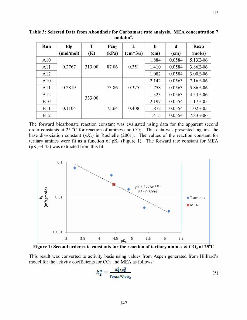
147

Table 3: Selected Data from Aboudheir for Carbamate rate analysis. MEA concentration 7 mol/dm3.

Run ldg T Pco2 L h d Rexp (mol/mol) (K) (kPa) (cm^3/s) (cm) (cm) (mol/s)

A10 1.884 0.0584 5.13E-06 A11 1.410 0.0584 3.86E-06 A12

0.2767 313.00 87.06 0.351 1.082 0.0584 3.00E-06

A10 2.142 0.0563 7.16E-06 A11 1.758 0.0563 5.86E-06 A12

0.2819 73.86 0.375 1.323 0.0563 4.53E-06

B10 2.197 0.0554 1.17E-05 B11 1.872 0.0554 1.02E-05 B12

0.1104

333.00

75.64 0.408 1.415 0.0554 7.83E-06

The forward bicarbonate reaction constant was evaluated using data for the apparent second order constants at 25 oC for reaction of amines and CO2. This data was presented against the base dissociation constant (pKb) in Rochelle (2001). The values of the reaction constant for tertiary amines were fit as a function of pKb (Figure 1). The forward rate constant for MEA (pKb=4.45) was extracted from this fit.

Figure 1: Second order rate constants for the reaction of tertiary amines & CO2 at 25oC

This result was converted to activity basis using values from Aspen generated from Hilliard’s model for the activity coefficients for CO2 and MEA as follows:

(5)

147

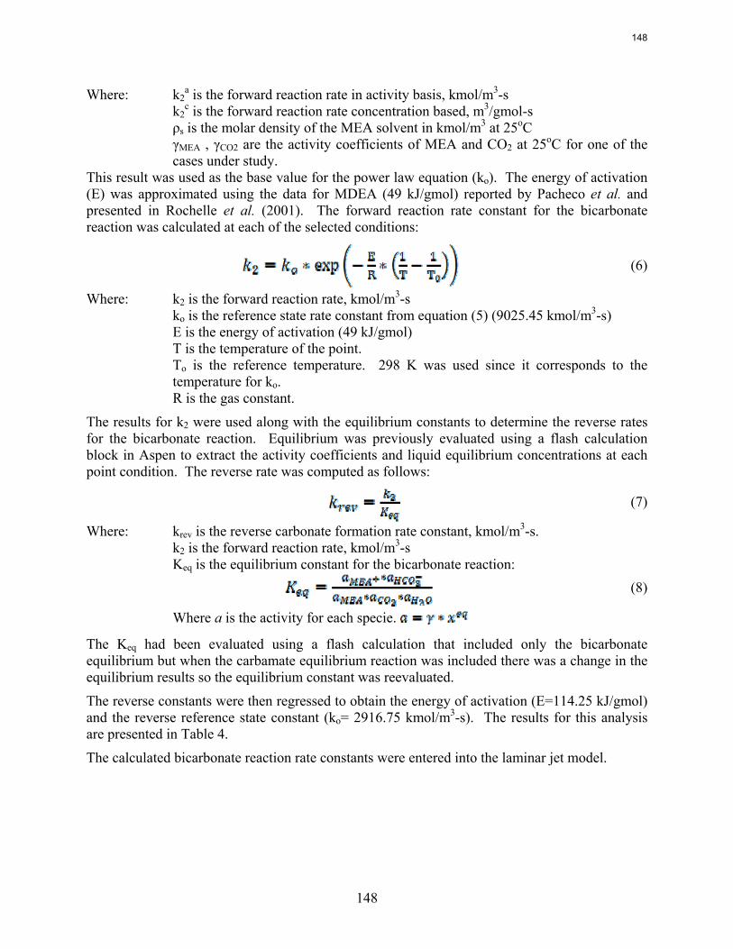
148

Where: k2a is the forward reaction rate in activity basis, kmol/m3-s

k2c is the forward reaction rate concentration based, m3/gmol-s

ρs is the molar density of the MEA solvent in kmol/m3 at 25oC γMEA , γCO2 are the activity coefficients of MEA and CO2 at 25oC for one of the cases under study.

This result was used as the base value for the power law equation (ko). The energy of activation (E) was approximated using the data for MDEA (49 kJ/gmol) reported by Pacheco et al. and presented in Rochelle et al. (2001). The forward reaction rate constant for the bicarbonate reaction was calculated at each of the selected conditions:

(6)

Where: k2 is the forward reaction rate, kmol/m3-s ko is the reference state rate constant from equation (5) (9025.45 kmol/m3-s) E is the energy of activation (49 kJ/gmol) T is the temperature of the point.

To is the reference temperature. 298 K was used since it corresponds to the temperature for ko. R is the gas constant.

The results for k2 were used along with the equilibrium constants to determine the reverse rates for the bicarbonate reaction. Equilibrium was previously evaluated using a flash calculation block in Aspen to extract the activity coefficients and liquid equilibrium concentrations at each point condition. The reverse rate was computed as follows:

(7)

Where: krev is the reverse carbonate formation rate constant, kmol/m3-s. k2 is the forward reaction rate, kmol/m3-s Keq is the equilibrium constant for the bicarbonate reaction:

(8)

Where a is the activity for each specie.

The Keq had been evaluated using a flash calculation that included only the bicarbonate equilibrium but when the carbamate equilibrium reaction was included there was a change in the equilibrium results so the equilibrium constant was reevaluated.

The reverse constants were then regressed to obtain the energy of activation (E=114.25 kJ/gmol) and the reverse reference state constant (ko= 2916.75 kmol/m3-s). The results for this analysis are presented in Table 4.

The calculated bicarbonate reaction rate constants were entered into the laminar jet model.

148

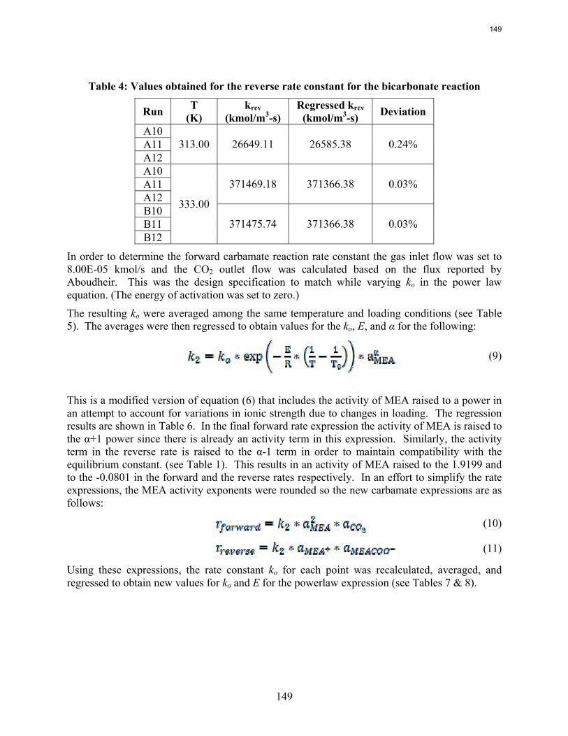
149

Table 4: Values obtained for the reverse rate constant for the bicarbonate reaction

Run T (K)

krev (kmol/m3-s)

Regressed krev (kmol/m3-s) Deviation

A10 A11 A12

313.00 26649.11 26585.38 0.24%

A10 A11 A12

371469.18 371366.38 0.03%

B10 B11 B12

333.00

371475.74 371366.38 0.03%

In order to determine the forward carbamate reaction rate constant the gas inlet flow was set to 8.00E-05 kmol/s and the CO2 outlet flow was calculated based on the flux reported by Aboudheir. This was the design specification to match while varying ko in the power law equation. (The energy of activation was set to zero.)

The resulting ko were averaged among the same temperature and loading conditions (see Table 5). The averages were then regressed to obtain values for the ko, E, and α for the following:

(9)

This is a modified version of equation (6) that includes the activity of MEA raised to a power in an attempt to account for variations in ionic strength due to changes in loading. The regression results are shown in Table 6. In the final forward rate expression the activity of MEA is raised to the α+1 power since there is already an activity term in this expression. Similarly, the activity term in the reverse rate is raised to the α-1 term in order to maintain compatibility with the equilibrium constant. (see Table 1). This results in an activity of MEA raised to the 1.9199 and to the -0.0801 in the forward and the reverse rates respectively. In an effort to simplify the rate expressions, the MEA activity exponents were rounded so the new carbamate expressions are as follows:

(10)

(11)

Using these expressions, the rate constant ko for each point was recalculated, averaged, and regressed to obtain new values for ko and E for the powerlaw expression (see Tables 7 & 8).

149

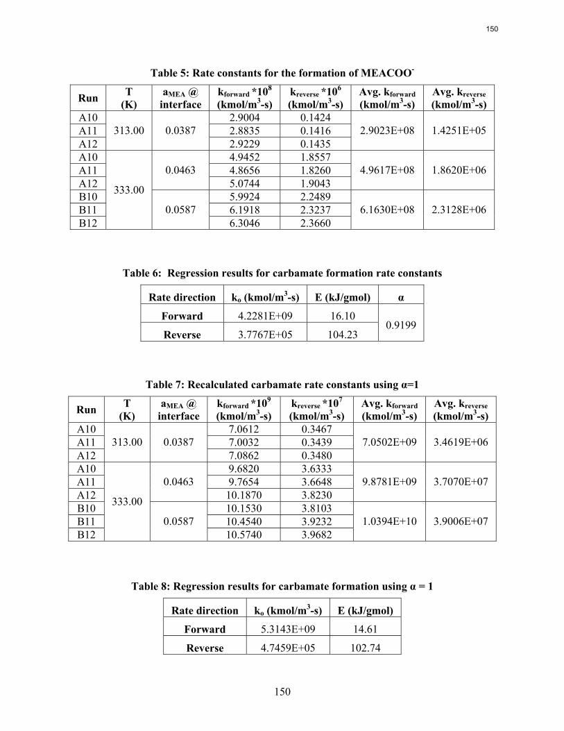
150

Table 5: Rate constants for the formation of MEACOO-

Run T (K)

aMEA @ interface

kforward *108

(kmol/m3-s) kreverse *106

(kmol/m3-s) Avg. kforward (kmol/m3-s)

Avg. kreverse (kmol/m3-s)

A10 2.9004 0.1424 A11 2.8835 0.1416 A12

313.00 0.0387 2.9229 0.1435

2.9023E+08 1.4251E+05

A10 4.9452 1.8557 A11 4.8656 1.8260 A12

0.0463 5.0744 1.9043

4.9617E+08 1.8620E+06

B10 5.9924 2.2489 B11 6.1918 2.3237 B12

333.00

0.0587 6.3046 2.3660

6.1630E+08 2.3128E+06

Table 6: Regression results for carbamate formation rate constants

Rate direction ko (kmol/m3-s) E (kJ/gmol) α

Forward 4.2281E+09 16.10

Reverse 3.7767E+05 104.23 0.9199

Table 7: Recalculated carbamate rate constants using α=1

Run T (K)

aMEA @ interface

kforward *109

(kmol/m3-s) kreverse *107

(kmol/m3-s) Avg. kforward (kmol/m3-s)

Avg. kreverse (kmol/m3-s)

A10 7.0612 0.3467 A11 7.0032 0.3439 A12

313.00 0.0387 7.0862 0.3480

7.0502E+09 3.4619E+06

A10 9.6820 3.6333 A11 9.7654 3.6648 A12

0.0463 10.1870 3.8230

9.8781E+09 3.7070E+07

B10 10.1530 3.8103 B11 10.4540 3.9232 B12

333.00

0.0587 10.5740 3.9682

1.0394E+10 3.9006E+07

Table 8: Regression results for carbamate formation using α = 1

Rate direction ko (kmol/m3-s) E (kJ/gmol)

Forward 5.3143E+09 14.61

Reverse 4.7459E+05 102.74

150

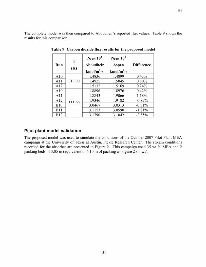
151

The complete model was then compared to Aboudheir’s reported flux values. Table 9 shows the results for this comparison.

Table 9: Carbon dioxide flux results for the proposed model

Run T

(K)

NCO2 104

Aboudheir

kmol/m2-s

NCO2 104

Aspen

kmol/m2-s

Difference

A10 1.4836 1.4899 0.43% A11 1.4925 1.5045 0.80% A12

313.00 1.5132 1.5169 0.24%

A10 1.8896 1.8976 0.42% A11 1.8843 1.9066 1.18% A12 1.9346 1.9182 -0.85% B10 3.0467 3.0313 -0.51% B11 3.1153 3.0590 -1.81% B12

333.00

3.1790 3.1042 -2.35%

Pilot plant model validation The proposed model was used to simulate the conditions of the October 2007 Pilot Plant MEA campaign at the University of Texas at Austin, Pickle Research Center. The stream conditions recorded for the absorber are presented in Figure 2. This campaign used 35 wt % MEA and 2 packing beds of 3.05 m (equivalent to 6.10 m of packing as Figure 2 shows).

151

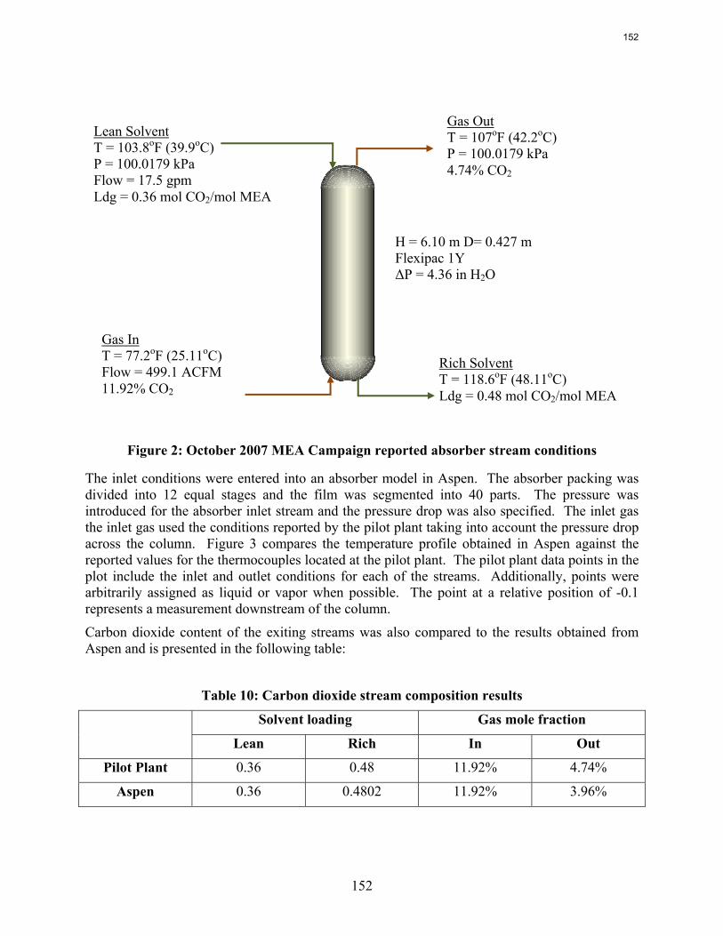
152

Figure 2: October 2007 MEA Campaign reported absorber stream conditions

The inlet conditions were entered into an absorber model in Aspen. The absorber packing was divided into 12 equal stages and the film was segmented into 40 parts. The pressure was introduced for the absorber inlet stream and the pressure drop was also specified. The inlet gas the inlet gas used the conditions reported by the pilot plant taking into account the pressure drop across the column. Figure 3 compares the temperature profile obtained in Aspen against the reported values for the thermocouples located at the pilot plant. The pilot plant data points in the plot include the inlet and outlet conditions for each of the streams. Additionally, points were arbitrarily assigned as liquid or vapor when possible. The point at a relative position of -0.1 represents a measurement downstream of the column.

Carbon dioxide content of the exiting streams was also compared to the results obtained from Aspen and is presented in the following table:

Table 10: Carbon dioxide stream composition results

Solvent loading Gas mole fraction

Lean Rich In Out

Pilot Plant 0.36 0.48 11.92% 4.74%

Aspen 0.36 0.4802 11.92% 3.96%

H = 6.10 m D= 0.427 m Flexipac 1Y ΔP = 4.36 in H2O

Gas Out T = 107oF (42.2oC) P = 100.0179 kPa 4.74% CO2

Lean Solvent T = 103.8oF (39.9oC) P = 100.0179 kPa Flow = 17.5 gpm Ldg = 0.36 mol CO2/mol MEA

Gas In T = 77.2oF (25.11oC) Flow = 499.1 ACFM 11.92% CO2

Rich Solvent T = 118.6oF (48.11oC) Ldg = 0.48 mol CO2/mol MEA

152

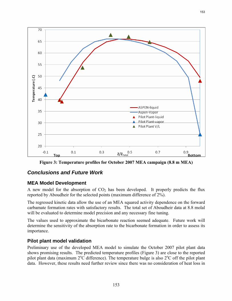
153

Figure 3: Temperature profiles for October 2007 MEA campaign (8.8 m MEA)

Conclusions and Future Work

MEA Model Development A new model for the absorption of CO2 has been developed. It properly predicts the flux reported by Aboudheir for the selected points (maximum difference of 2%).

The regressed kinetic data allow the use of an MEA squared activity dependence on the forward carbamate formation rates with satisfactory results. The total set of Aboudheir data at 8.8 molal will be evaluated to determine model precision and any necessary fine tuning.

The values used to approximate the bicarbonate reaction seemed adequate. Future work will determine the sensitivity of the absorption rate to the bicarbonate formation in order to assess its importance.

Pilot plant model validation Preliminary use of the developed MEA model to simulate the October 2007 pilot plant data shows promising results. The predicted temperature profiles (Figure 3) are close to the reported pilot plant data (maximum 2oC difference). The temperature bulge is also 2oC off the pilot plant data. However, these results need further review since there was no consideration of heat loss in

153

154

the absorber. This may imply that the obtained profiles are low with respect to the pilot plant data.

The results of the CO2 composition analysis show that the loadings have been matched yet the removal is off by approximately 11%. This requires further evaluation to determine if the initial loadings are correct or if the outlet conditions need revision.

Further analysis will include the secondary equipment which consists of two pumps and additional valves. It is also necessary to revise the location of the pressure and temperature measurements in the pilot plant.

Finally, variable reconciliation using Aspen will be conducted as part of the model analysis and validation.

References Aboudheir A. Kinetics, Modeling and Simulation of CO2 Absorption into Highly Concentrated

and Loaded MEA Solutions. University of Regina; 2002. Ph.D. Dissertation. Dugas R. Personal communication, Austin, TX; 2007. Hilliard M. A Predictive Thermodynamic Model for an Aqueous Blend of Potassium Carbonate,

Piperazine, and Monoethanolamine for Carbon Dioxide Capture from Flue Gas. University of Texas, Austin; 2008. Ph.D. Dissertation.

Rochelle GT, Chi S, et al. Research Needs for CO2 Capture from Flue Gas by Aqueous Absorption/Stripping. Austin, TX, U.S. Department of Energy - Federal Energy Technology Center; 2001.

Weiland R, Dingman J, et al. Density and Viscosity of Some Partially Carbonated Aqueous Alkanolamine Solutions and Their Blends. J. Chem. Eng. Data 1998;43:378–382.

154

155

Reclaiming by Crystallization of Potassium Sulfate Progress Report for April 1 – June 30, 2008

by Qing Xu

Supported by the Luminant Carbon Management Program

and the

Industrial Associates Program for CO2 Capture by Aqueous Absorption

Department of Chemical Engineering

The University of Texas at Austin

July 20, 2008

Abstract One side reaction in CO2 capture when using MEA/PZ is the generation of sulfate from SO2. This sulfate has to be removed so that the MEA/PZ solution can be reused for CO2 capture. Potassium sulfate can be crystallized and separated from MEA/PZ solvent by the addition of potassium hydroxide. In previous work, continuous crystallization of potassium sulfate was conducted under various temperatures, MEA/PZ concentrations, CO2 loading, agitation rates, and the ratio of SO4

-2/K+. The samples were analyzed by a Mastersizer particle size analyzer, SEM, and light microscopy. Regression for interaction parameters in CO2-MEA-H2O-K+-SO4

-2

system using Aspen Plus® Electrolyte-NRTL model was developed. In this period more crystallization experiments with various additives were conducted and the samples were analyzed. Empirical nucleation and growth rate kinetics models were developed from the particle size distribution data.

Introduction In previous work, the solubility of potassium sulfate was measured with variable MEA/PZ concentration, CO2 loading, and temperature. A model predicting empirical Ksp was developed. An interaction parameter set for a CO2-MEA-H2O-K+-SO4

-2 system in E-NRTL model was developed using the Data Regression System in Aspen Plus®. Continuous crystallization of potassium sulfate was conducted over a wide range of conditions and the solids were characterized by laser sizing and microscopy. In this quarter more continuous crystallizations with additives were conducted, empirical nucleation and growth rate kinetics models were developed.

Experimental Methods 1) Continuous crystallization The amine stock solution and KOH stock solution were prepared separately. The amine feed included CO2 and enough K2SO4 to be close to K2SO4 saturation. Sulfuric acid was added to the amine feed to adjust SO4

-2/K+. In 4 experiments, various combinations of additives (Fe+2, Ni+2,

155

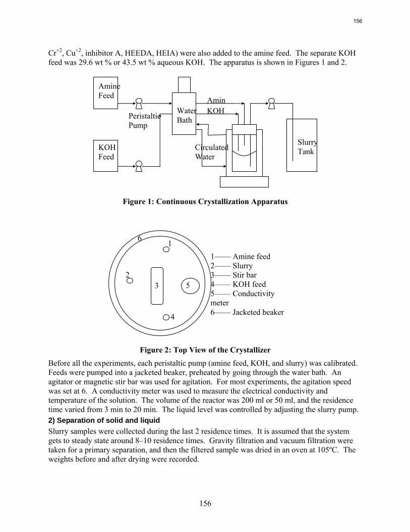
156

Cr+2, Cu+2, inhibitor A, HEEDA, HEIA) were also added to the amine feed. The separate KOH feed was 29.6 wt % or 43.5 wt % aqueous KOH. The apparatus is shown in Figures 1 and 2.

Figure 1: Continuous Crystallization Apparatus

Figure 2: Top View of the Crystallizer

Before all the experiments, each peristaltic pump (amine feed, KOH, and slurry) was calibrated. Feeds were pumped into a jacketed beaker, preheated by going through the water bath. An agitator or magnetic stir bar was used for agitation. For most experiments, the agitation speed was set at 6. A conductivity meter was used to measure the electrical conductivity and temperature of the solution. The volume of the reactor was 200 ml or 50 ml, and the residence time varied from 3 min to 20 min. The liquid level was controlled by adjusting the slurry pump. 2) Separation of solid and liquid Slurry samples were collected during the last 2 residence times. It is assumed that the system gets to steady state around 8–10 residence times. Gravity filtration and vacuum filtration were taken for a primary separation, and then the filtered sample was dried in an oven at 105ºC. The weights before and after drying were recorded.

Amine Feed

KOH Feed

Peristaltic Pump

Water Bath

Slurry Tank

KOH Amin

Circulated Water

1

3 2

4

5

6

1—— Amine feed 2—— Slurry 3—— Stir bar 4—— KOH feed 5—— Conductivity meter 6—— Jacketed beaker

156

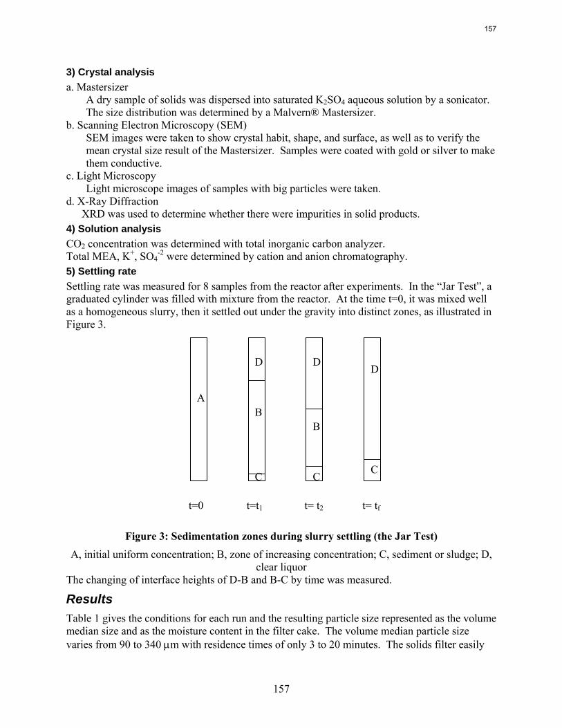
157

3) Crystal analysis a. Mastersizer

A dry sample of solids was dispersed into saturated K2SO4 aqueous solution by a sonicator. The size distribution was determined by a Malvern® Mastersizer.

b. Scanning Electron Microscopy (SEM) SEM images were taken to show crystal habit, shape, and surface, as well as to verify the mean crystal size result of the Mastersizer. Samples were coated with gold or silver to make them conductive.

c. Light Microscopy Light microscope images of samples with big particles were taken.

d. X-Ray Diffraction XRD was used to determine whether there were impurities in solid products.

4) Solution analysis CO2 concentration was determined with total inorganic carbon analyzer. Total MEA, K+, SO4

-2 were determined by cation and anion chromatography. 5) Settling rate Settling rate was measured for 8 samples from the reactor after experiments. In the “Jar Test”, a graduated cylinder was filled with mixture from the reactor. At the time t=0, it was mixed well as a homogeneous slurry, then it settled out under the gravity into distinct zones, as illustrated in Figure 3.

Figure 3: Sedimentation zones during slurry settling (the Jar Test)

A, initial uniform concentration; B, zone of increasing concentration; C, sediment or sludge; D, clear liquor

The changing of interface heights of D-B and B-C by time was measured.

Results Table 1 gives the conditions for each run and the resulting particle size represented as the volume median size and as the moisture content in the filter cake. The volume median particle size varies from 90 to 340 μm with residence times of only 3 to 20 minutes. The solids filter easily

A

D

B

t=0

D D

B

C C

t=t1 t= t2 t= tf

C

157

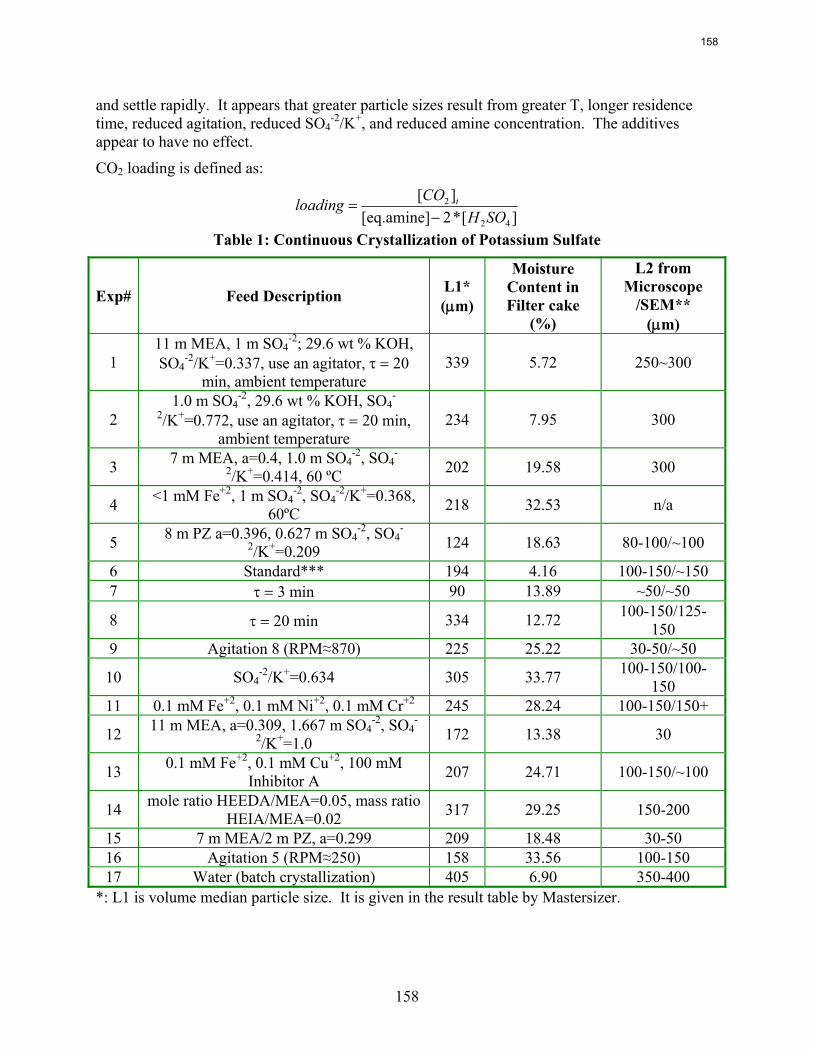
158

and settle rapidly. It appears that greater particle sizes result from greater T, longer residence time, reduced agitation, reduced SO4

-2/K+, and reduced amine concentration. The additives appear to have no effect.

CO2 loading is defined as:

][*2[eq.amine]][

42

2

SOHCOloading t

−=

Table 1: Continuous Crystallization of Potassium Sulfate

Exp# Feed Description L1* (μm)

Moisture Content in Filter cake

(%)

L2 from Microscope

/SEM** (μm)

1 11 m MEA, 1 m SO4

-2; 29.6 wt % KOH, SO4

-2/K+=0.337, use an agitator, τ = 20 min, ambient temperature

339 5.72 250~300

2 1.0 m SO4

-2, 29.6 wt % KOH, SO4-

2/K+=0.772, use an agitator, τ = 20 min, ambient temperature

234 7.95 300

3 7 m MEA, a=0.4, 1.0 m SO4-2, SO4

-

2/K+=0.414, 60 ºC 202 19.58 300

4 <1 mM Fe+2, 1 m SO4-2, SO4

-2/K+=0.368, 60ºC 218 32.53 n/a

5 8 m PZ a=0.396, 0.627 m SO4-2, SO4

-

2/K+=0.209 124 18.63 80-100/~100

6 Standard*** 194 4.16 100-150/~150 7 τ = 3 min 90 13.89 ~50/~50

8 τ = 20 min 334 12.72 100-150/125-150

9 Agitation 8 (RPM≈870) 225 25.22 30-50/~50

10 SO4-2/K+=0.634 305 33.77 100-150/100-

150 11 0.1 mM Fe+2, 0.1 mM Ni+2, 0.1 mM Cr+2 245 28.24 100-150/150+

12 11 m MEA, a=0.309, 1.667 m SO4-2, SO4

-

2/K+=1.0 172 13.38 30

13 0.1 mM Fe+2, 0.1 mM Cu+2, 100 mM Inhibitor A 207 24.71 100-150/~100

14 mole ratio HEEDA/MEA=0.05, mass ratio HEIA/MEA=0.02 317 29.25 150-200

15 7 m MEA/2 m PZ, a=0.299 209 18.48 30-50 16 Agitation 5 (RPM≈250) 158 33.56 100-150 17 Water (batch crystallization) 405 6.90 350-400

*: L1 is volume median particle size. It is given in the result table by Mastersizer.

158

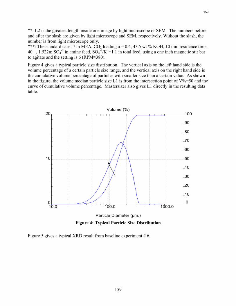
159

**: L2 is the greatest length inside one image by light microscope or SEM. The numbers before and after the slash are given by light microscope and SEM, respectively. Without the slash, the number is from light microscope only. ***: The standard case: 7 m MEA, CO2 loading a = 0.4, 43.5 wt % KOH, 10 min residence time, 40�, 1.522m SO4

-2 in amine feed, SO4-2/K+=1.1 in total feed, using a one inch magnetic stir bar

to agitate and the setting is 6 (RPM≈380).

Figure 4 gives a typical particle size distribution. The vertical axis on the left hand side is the volume percentage of a certain particle size range, and the vertical axis on the right hand side is the cumulative volume percentage of particles with smaller size than a certain value. As shown in the figure, the volume median particle size L1 is from the intersection point of V%=50 and the curve of cumulative volume percentage. Mastersizer also gives L1 directly in the resulting data table.

Figure 4: Typical Particle Size Distribution

Figure 5 gives a typical XRD result from baseline experiment # 6.

Particle Diameter (µm.)

Volume (%)

0

10

20

0

10

20

30

40

50

60

70

80

90

100

10.0 100.0 1000.0

159

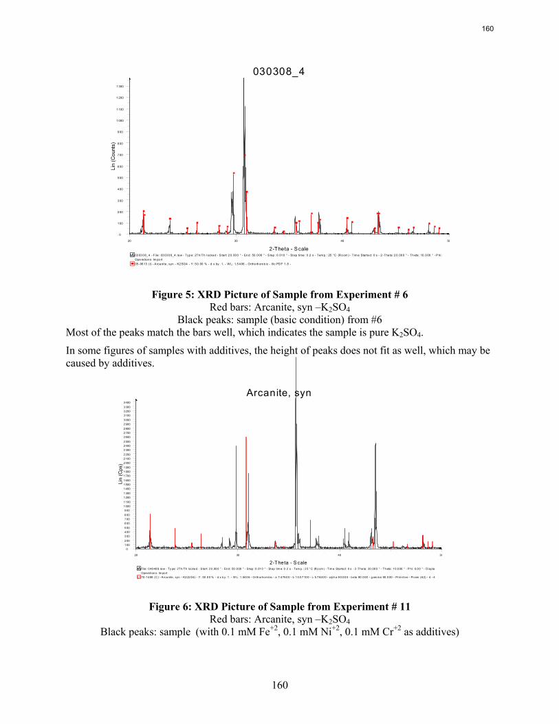
160

030308_4

05 -06 13 (I) - A rca nite , syn - K2 SO4 - Y: 5 0. 00 % - d x by : 1. - W L: 1.5 4 06 - Ortho rh om b ic - I/Ic PDF 1 .8 - Ope ra tion s: Im po rt03 03 0 8_ 4 - File: 03 03 0 8_ 4. ra w - Typ e: 2Th /Th locke d - S tart: 2 0. 00 0 ° - En d: 50 .0 00 ° - S tep : 0 .01 0 ° - St ep time : 0 .2 s - Tem p. : 25 °C (Ro om ) - Tim e Starte d: 0 s - 2 -The ta: 2 0 .00 0 ° - Th eta : 10 .0 00 ° - P hi:

Lin

(Cou

nts)

0

1 00

2 00

3 00

4 00

5 00

6 00

7 00

8 00

9 00

1 000

1 100

1 200

1 300

2-Theta - S cale

20 30 40 50

Figure 5: XRD Picture of Sample from Experiment # 6

Red bars: Arcanite, syn –K2SO4 Black peaks: sample (basic condition) from #6

Most of the peaks match the bars well, which indicates the sample is pure K2SO4.

In some figures of samples with additives, the height of peaks does not fit as well, which may be caused by additives.

Figure 6: XRD Picture of Sample from Experiment # 11

Red bars: Arcanite, syn –K2SO4 Black peaks: sample (with 0.1 mM Fe+2, 0.1 mM Ni+2, 0.1 mM Cr+2 as additives)

Arcanite, syn

70 -14 88 (C ) - A rca nite , syn - K2 (S O4) - Y: 50 .0 0 % - d x b y: 1 . - W L : 1 .54 0 6 - Orth orho m bic - a 7.4 76 0 0 - b 1 0.0 7 10 0 - c 5.7 63 0 0 - a lp h a 9 0.0 0 0 - b eta 90 .0 00 - g am ma 90 .0 00 - Pr im itive - Pn am (6 2) - 4 - 4Ope ra tion s: Im po rtF ile : 0 40 40 8. ra w - Ty pe: 2Th /Th locke d - S tart: 2 0 .00 0 ° - En d : 50 .0 00 ° - S tep : 0 .01 0 ° - St ep tim e: 0 .2 s - Tem p .: 2 5 ° C (Ro om ) - T im e Sta rte d: 0 s - 2 -The ta: 20 .00 0 ° - Th eta : 1 0.0 00 ° - P hi: 0.0 0 ° - D ispla

Lin

(Cps

)

01 002 003 004 005 006 007 008 009 00

1 0001 1001 2001 3001 4001 5001 6001 7001 8001 9002 0002 1002 2002 3002 4002 5002 6002 7002 8002 9003 0003 1003 2003 3003 400

2-Theta - S cale20 30 40 50

160

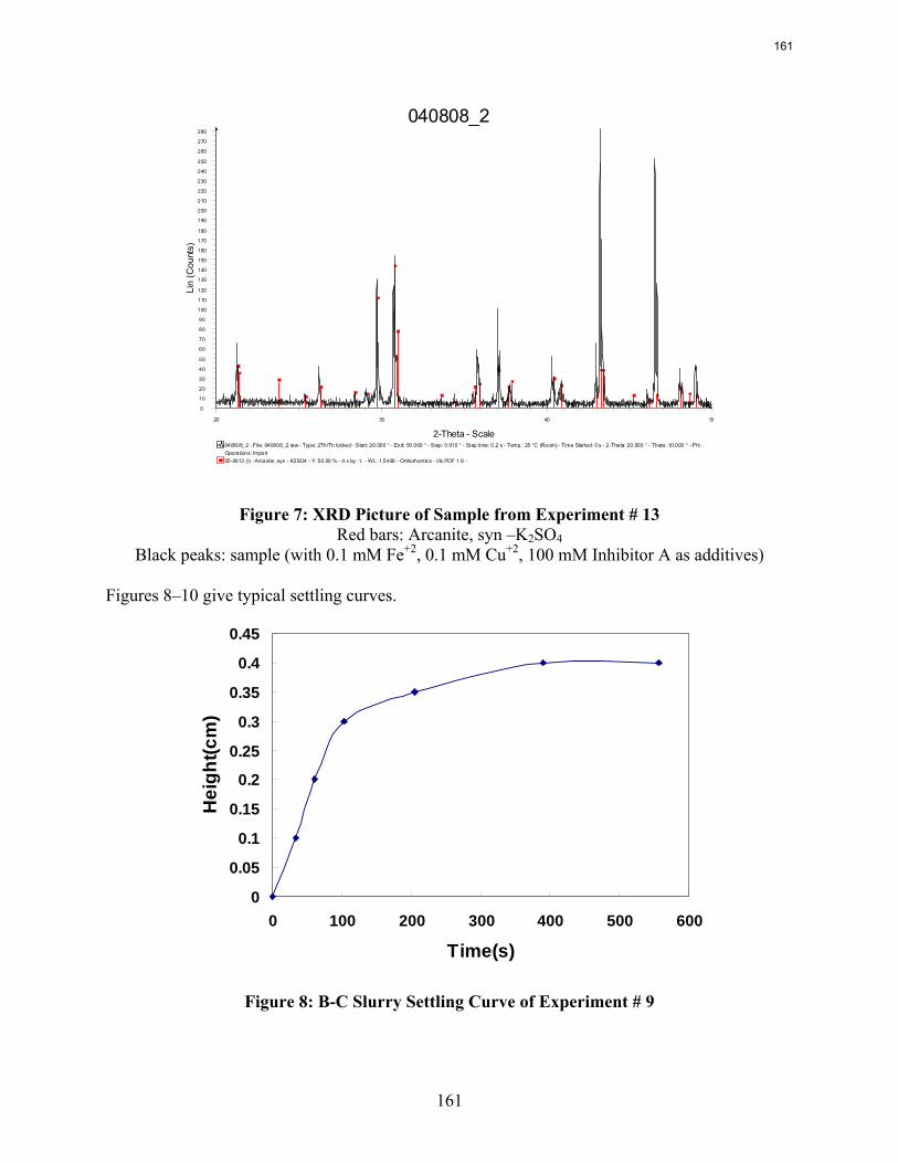
161

Figure 7: XRD Picture of Sample from Experiment # 13

Red bars: Arcanite, syn –K2SO4 Black peaks: sample (with 0.1 mM Fe+2, 0.1 mM Cu+2, 100 mM Inhibitor A as additives)

Figures 8–10 give typical settling curves.

0

0.05

0.1

0.15

0.2

0.25

0.3

0.35

0.4

0.45

0 100 200 300 400 500 600

Time(s)

Hei

ght(c

m)

Figure 8: B-C Slurry Settling Curve of Experiment # 9

040808_2

05-0613 (I) - Arcanite, syn - K2SO4 - Y: 50.00 % - d x by : 1. - WL: 1.5406 - Orthorhombic - I/Ic PDF 1.8 - Operations: Import040808_2 - File: 040808_2.raw - Type: 2Th/Th locked - Start: 20.000 ° - End: 50.000 ° - Step: 0.010 ° - Step time: 0.2 s - Temp.: 25 °C (Room) - Time Started: 0 s - 2-Theta: 20.000 ° - Theta: 10.000 ° - Phi:

Lin

(Cou

nts)

0

10

20

30

40

50

60

70

80

90

100

110

120

130

140

150

160

170

180

190

200

210

220

230

240

250

260

270

280

2-Theta - Scale

20 30 40 50

161

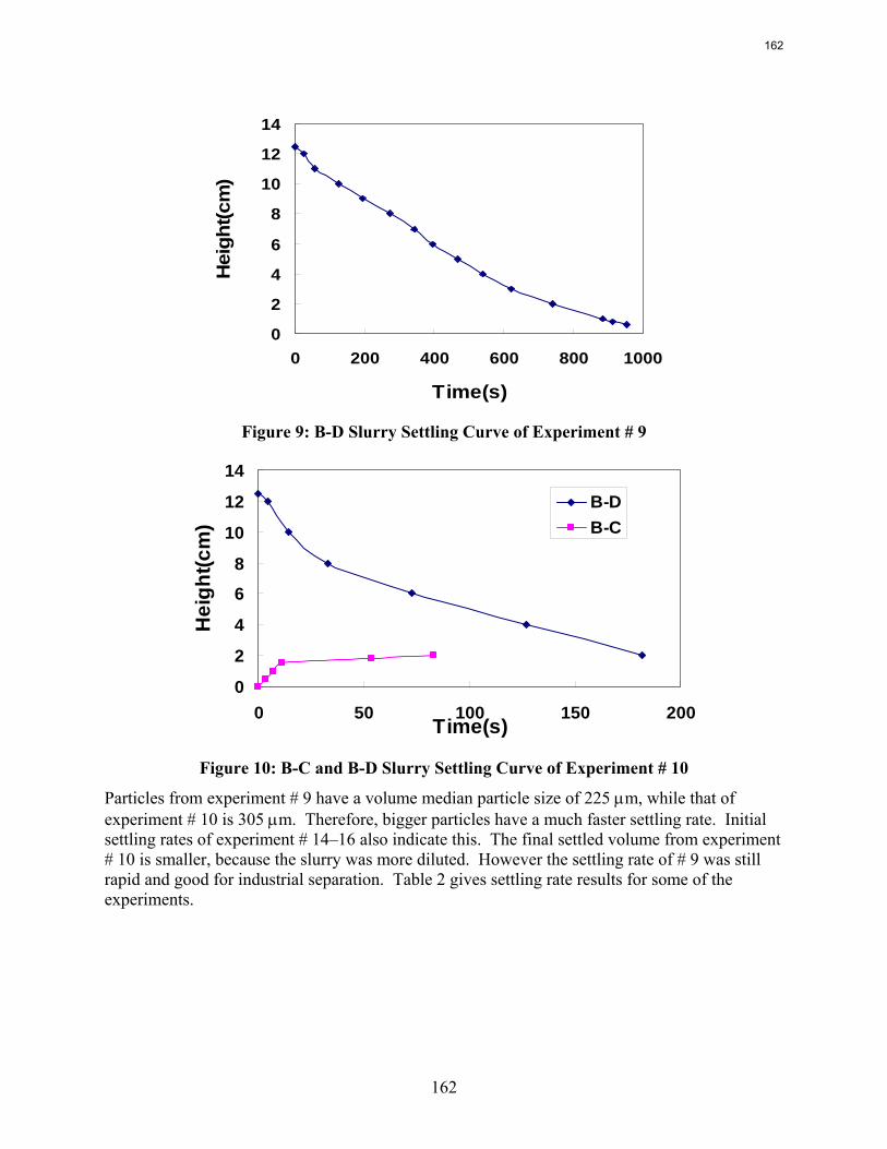
162

0

2

4

6

8

10

12

14

0 200 400 600 800 1000

Time(s)

Hei

ght(c

m)

Figure 9: B-D Slurry Settling Curve of Experiment # 9

0

2

4

6

8

10

12

14

0 50 100 150 200Time(s)

Hei

ght(c

m)

B-DB-C

Figure 10: B-C and B-D Slurry Settling Curve of Experiment # 10

Particles from experiment # 9 have a volume median particle size of 225 μm, while that of experiment # 10 is 305 μm. Therefore, bigger particles have a much faster settling rate. Initial settling rates of experiment # 14–16 also indicate this. The final settled volume from experiment # 10 is smaller, because the slurry was more diluted. However the settling rate of # 9 was still rapid and good for industrial separation. Table 2 gives settling rate results for some of the experiments.

162

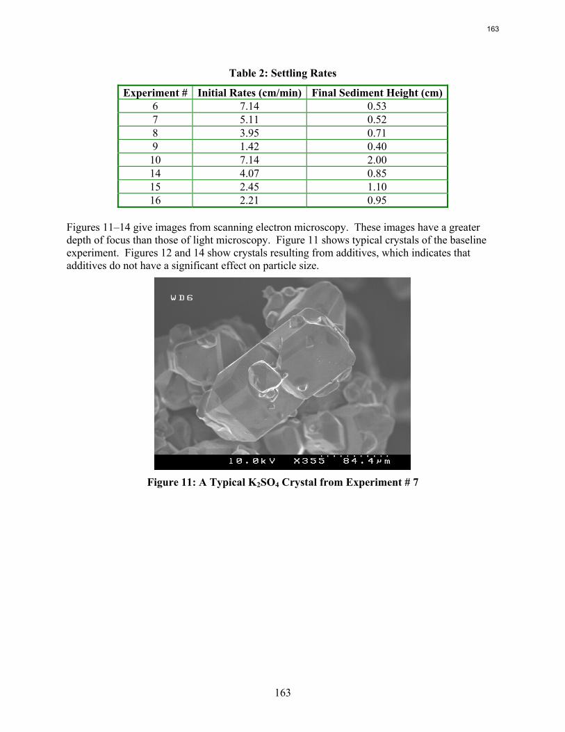
163

Table 2: Settling Rates

Experiment # Initial Rates (cm/min) Final Sediment Height (cm) 6 7.14 0.53 7 5.11 0.52 8 3.95 0.71 9 1.42 0.40 10 7.14 2.00 14 4.07 0.85 15 2.45 1.10 16 2.21 0.95

Figures 11–14 give images from scanning electron microscopy. These images have a greater depth of focus than those of light microscopy. Figure 11 shows typical crystals of the baseline experiment. Figures 12 and 14 show crystals resulting from additives, which indicates that additives do not have a significant effect on particle size.

Figure 11: A Typical K2SO4 Crystal from Experiment # 7

163

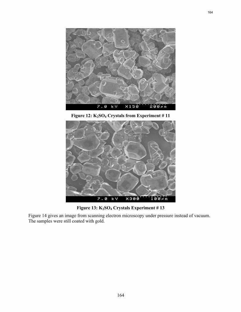
164

Figure 12: K2SO4 Crystals from Experiment # 11

Figure 13: K2SO4 Crystals Experiment # 13

Figure 14 gives an image from scanning electron microscopy under pressure instead of vacuum. The samples were still coated with gold.

164

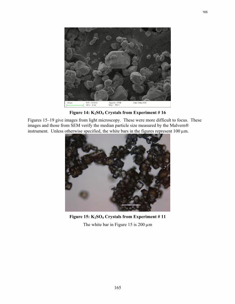
165

Figure 14: K2SO4 Crystals from Experiment # 16

Figures 15–19 give images from light microscopy. These were more difficult to focus. These images and those from SEM verify the median particle size measured by the Malvern® instrument. Unless otherwise specified, the white bars in the figures represent 100 μm.

Figure 15: K2SO4 Crystals from Experiment # 11

The white bar in Figure 15 is 200 μm

165

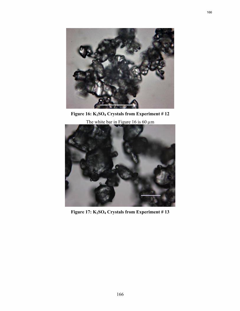
166

Figure 16: K2SO4 Crystals from Experiment # 12

The white bar in Figure 16 is 60 μm

Figure 17: K2SO4 Crystals from Experiment # 13

166

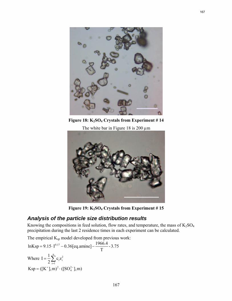
167

Figure 18: K2SO4 Crystals from Experiment # 14

The white bar in Figure 18 is 200 μm

Figure 19: K2SO4 Crystals from Experiment # 15

Analysis of the particle size distribution results Knowing the compositions in feed solution, flow rates, and temperature, the mass of K2SO4 precipitation during the last 2 residence times in each experiment can be calculated.

The empirical Ksp model developed from previous work:

3.75-T

1966.4ine]0.36[eq.amI9.15lnKsp 0.17 −−⋅=

Where ∑=

=n

1i

2iizc

21I

)m],SO([)m],K([Ksp 24

2 −+ ⋅=

167

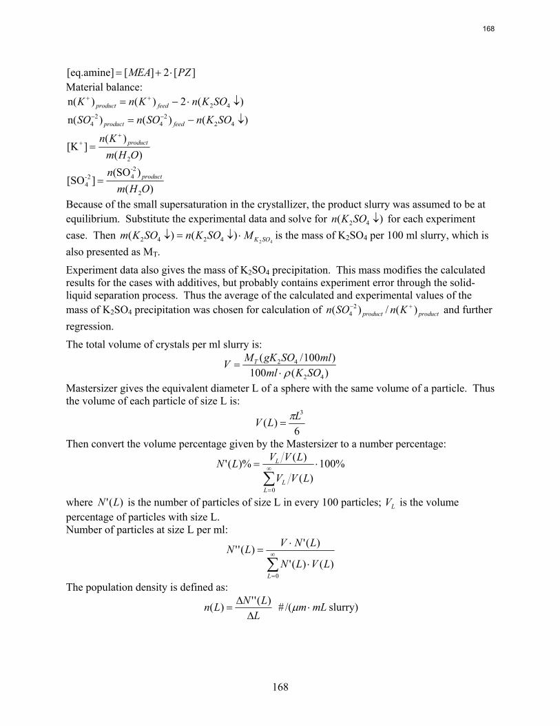
168

][2][[eq.amine] PZMEA ⋅+= Material balance:

)(2)()n( 42 ↓⋅−= ++ SOKnKnK feedproduct

)()()n( 422

42

4 ↓−= −− SOKnSOnSO feedproduct

)()(

][K2OHm

Kn product+

+ =

)()SO(

][SO2

-242-

4 OHmn product=

Because of the small supersaturation in the crystallizer, the product slurry was assumed to be at equilibrium. Substitute the experimental data and solve for )( 42 ↓SOKn for each experiment case. Then

42)()( 4242 SOKMSOKnSOKm ⋅↓=↓ is the mass of K2SO4 per 100 ml slurry, which is

also presented as MT.

Experiment data also gives the mass of K2SO4 precipitation. This mass modifies the calculated results for the cases with additives, but probably contains experiment error through the solid-liquid separation process. Thus the average of the calculated and experimental values of the mass of K2SO4 precipitation was chosen for calculation of productproduct KnSOn )(/)( 2

4+− and further

regression.

The total volume of crystals per ml slurry is:

)(100)100/(

42

42

SOKmlmlSOgKMV T

ρ⋅=

Mastersizer gives the equivalent diameter L of a sphere with the same volume of a particle. Thus the volume of each particle of size L is:

6)(

3LLV π=

Then convert the volume percentage given by the Mastersizer to a number percentage:

%100)(

)()%('

0

⋅=

∑∞

=LL

L

LVV

LVVLN

where )(' LN is the number of particles of size L in every 100 particles; LV is the volume percentage of particles with size L. Number of particles at size L per ml:

∑∞

=

⋅

⋅=

0)()('

)(')(''

LLVLN

LNVLN

The population density is defined as:

LLNLn

ΔΔ

=)('')( mLm ⋅μ/(# slurry)

168

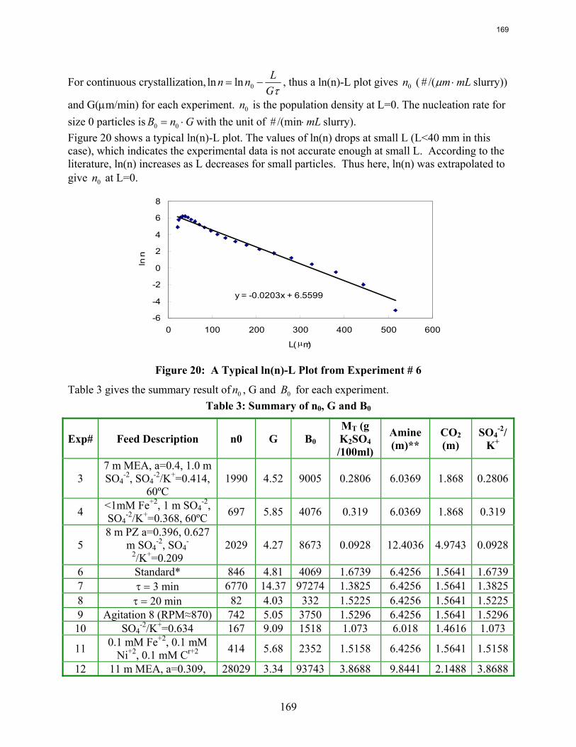
169

For continuous crystallization,τG

Lnn −= 0lnln , thus a ln(n)-L plot gives 0n ( mLm ⋅μ/(# slurry))

and G(μm/min) for each experiment. 0n is the population density at L=0. The nucleation rate for size 0 particles is GnB ⋅= 00 with the unit of mL⋅/(min# slurry). Figure 20 shows a typical ln(n)-L plot. The values of ln(n) drops at small L (L<40 mm in this case), which indicates the experimental data is not accurate enough at small L. According to the literature, ln(n) increases as L decreases for small particles. Thus here, ln(n) was extrapolated to give 0n at L=0.

y = -0.0203x + 6.5599

-6

-4

-2

0

2

4

6

8

0 100 200 300 400 500 600

L( μm)

ln n

Figure 20: A Typical ln(n)-L Plot from Experiment # 6

Table 3 gives the summary result of 0n , G and 0B for each experiment. Table 3: Summary of n0, G and B0

Exp# Feed Description n0 G B0 MT (g K2SO4 /100ml)

Amine (m)**

CO2 (m)

SO4-2/

K+

3 7 m MEA, a=0.4, 1.0 m SO4

-2, SO4-2/K+=0.414,

60ºC 1990 4.52 9005 0.2806 6.0369 1.868 0.2806

4 <1mM Fe+2, 1 m SO4-2,

SO4-2/K+=0.368, 60ºC 697 5.85 4076 0.319 6.0369 1.868 0.319

5 8 m PZ a=0.396, 0.627

m SO4-2, SO4

-

2/K+=0.209 2029 4.27 8673 0.0928 12.4036 4.9743 0.0928

6 Standard* 846 4.81 4069 1.6739 6.4256 1.5641 1.67397 τ = 3 min 6770 14.37 97274 1.3825 6.4256 1.5641 1.38258 τ = 20 min 82 4.03 332 1.5225 6.4256 1.5641 1.52259 Agitation 8 (RPM≈870) 742 5.05 3750 1.5296 6.4256 1.5641 1.529610 SO4

-2/K+=0.634 167 9.09 1518 1.073 6.018 1.4616 1.073

11 0.1 mM Fe+2, 0.1 mM Ni+2, 0.1 mM Cr+2 414 5.68 2352 1.5158 6.4256 1.5641 1.5158

12 11 m MEA, a=0.309, 28029 3.34 93743 3.8688 9.8441 2.1488 3.8688

169

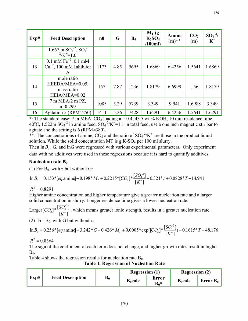
170

Exp# Feed Description n0 G B0 MT (g K2SO4 /100ml)

Amine (m)**

CO2 (m)

SO4-2/

K+

1.667 m SO4-2, SO4

-

2/K+=1.0

13 0.1 mM Fe+2, 0.1 mM

Cu+2, 100 mM Inhibitor A

1173 4.85 5695 1.6869 6.4256 1.5641 1.6869

14

mole ratio HEEDA/MEA=0.05,

mass ratio HEIA/MEA=0.02

157 7.87 1236 1.8179 6.6999 1.56 1.8179

15 7 m MEA/2 m PZ, a=0.299 1085 5.29 5739 3.349 9.941 1.6988 3.349

16 Agitation 5 (RPM≈250) 1411 5.26 7428 1.6291 6.4256 1.5641 1.6291*: The standard case: 7 m MEA, CO2 loading a = 0.4, 43.5 wt % KOH, 10 min residence time, 40oC, 1.522m SO4

-2 in amine feed, SO4-2/K+=1.1 in total feed, use a one inch magnetic stir bar to

agitate and the setting is 6 (RPM≈380). **: The concentrations of amine, CO2 and the ratio of SO4

-2/K+ are those in the product liquid solution. While the solid concentration MT is g K2SO4 per 100 ml slurry. Then ln 0B , G, and lnG were regressed with various experimental parameters. Only experiment data with no additives were used in these regressions because it is hard to quantify additives. Nucleation rate B0

(1) For B0, with τ but without G:

941.14*0828.0*321.0][][*][*2215.0*198.0]amine.[*153.0ln

24

20 −+−+−= +

−

TK

SOCOMeqB T τ

8291.02 =R Higher amine concentration and higher temperature give a greater nucleation rate and a larger solid concentration in slurry. Longer residence time gives a lower nucleation rate.

Larger][][*][

24

2 +

−

KSOCO , which means greater ionic strength, results in a greater nucleation rate.

(2) For B0, with G but without τ:

176.48*1615.0)][][*]exp([*0005.0*426.0*242.3]amine.[*256.0ln

24

20 −++−+= +

−

TK

SOCOMGeqB T

8364.02 =R The sign of the coefficient of each term does not change, and higher growth rates result in higher B0. Table 4 shows the regression results for nucleation rate B0.

Table 4: Regression of Nucleation Rate

Regression (1) Regression (2) Exp# Feed Description B0 B0calc Error

B0* B0calc Error B0

170

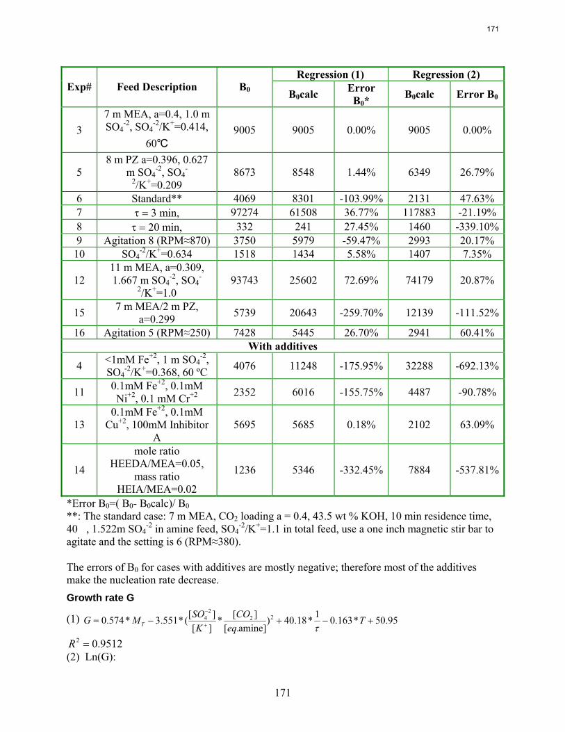
171

Regression (1) Regression (2) Exp# Feed Description B0 B0calc Error

B0* B0calc Error B0

3 7 m MEA, a=0.4, 1.0 m SO4

-2, SO4-2/K+=0.414,

60℃ 9005 9005 0.00% 9005 0.00%

5 8 m PZ a=0.396, 0.627

m SO4-2, SO4

-

2/K+=0.209 8673 8548 1.44% 6349 26.79%

6 Standard** 4069 8301 -103.99% 2131 47.63% 7 τ = 3 min, 97274 61508 36.77% 117883 -21.19% 8 τ = 20 min, 332 241 27.45% 1460 -339.10%9 Agitation 8 (RPM≈870) 3750 5979 -59.47% 2993 20.17% 10 SO4

-2/K+=0.634 1518 1434 5.58% 1407 7.35%

12 11 m MEA, a=0.309, 1.667 m SO4

-2, SO4-

2/K+=1.0 93743 25602 72.69% 74179 20.87%

15 7 m MEA/2 m PZ, a=0.299 5739 20643 -259.70% 12139 -111.52%

16 Agitation 5 (RPM≈250) 7428 5445 26.70% 2941 60.41% With additives

4 <1mM Fe+2, 1 m SO4-2,

SO4-2/K+=0.368, 60 ºC 4076 11248 -175.95% 32288 -692.13%

11 0.1mM Fe+2, 0.1mM Ni+2, 0.1 mM Cr+2 2352 6016 -155.75% 4487 -90.78%

13 0.1mM Fe+2, 0.1mM

Cu+2, 100mM Inhibitor A

5695 5685 0.18% 2102 63.09%

14

mole ratio HEEDA/MEA=0.05,

mass ratio HEIA/MEA=0.02

1236 5346 -332.45% 7884 -537.81%

*Error B0=( B0- B0calc)/ B0 **: The standard case: 7 m MEA, CO2 loading a = 0.4, 43.5 wt % KOH, 10 min residence time, 40�, 1.522m SO4

-2 in amine feed, SO4-2/K+=1.1 in total feed, use a one inch magnetic stir bar to

agitate and the setting is 6 (RPM≈380). The errors of B0 for cases with additives are mostly negative; therefore most of the additives make the nucleation rate decrease. Growth rate G

(1) 95.50*163.01*18.40)amine].[

][*][][(*551.3*574.0 22

24 +−+−= +

−

Teq

COK

SOMG T τ

9512.02 =R (2) Ln(G):

171

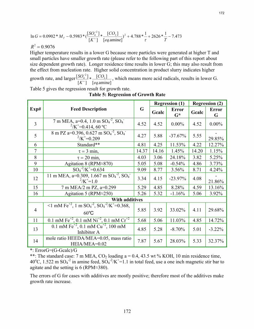
172

473.71*26261*788.4)amine].[

][*

][][

(*5983.0*0902.0ln 222

4 −++−= +

−

TeqCO

KSO

MG T τ

9076.02 =R Higher temperature results in a lower G because more particles were generated at higher T and small particles have smaller growth rate (please refer to the following part of this report about size dependent growth rate). Longer residence time results in lower G; this may also result from the effect from nucleation rate. Higher solid concentration in product slurry indicates higher

growth rate, and largeramine].[

][*][][ 2

24

eqCO

KSO

+

−

, which means more acid radicals, results in lower G.

Table 5 gives the regression result for growth rate. Table 5: Regression of Growth Rate

Regression (1) Regression (2) Exp# Feed Description G

Gcalc Error G* Gcalc Error

G

3 7 m MEA, a=0.4, 1.0 m SO4-2, SO4

-

2/K+=0.414, 60 ºC 4.52 4.52 0.00% 4.52 0.00%

5 8 m PZ a=0.396, 0.627 m SO4-2, SO4

-

2/K+=0.209 4.27 5.88 -37.67% 5.55 -29.85%

6 Standard** 4.81 4.25 11.53% 4.22 12.27%7 τ = 3 min, 14.37 14.16 1.45% 14.20 1.15% 8 τ = 20 min, 4.03 3.06 24.18% 3.82 5.25% 9 Agitation 8 (RPM≈870) 5.05 5.08 -0.54% 4.86 3.73% 10 SO4

-2/K+=0.634 9.09 8.77 3.56% 8.71 4.24%

12 11 m MEA, a=0.309, 1.667 m SO4-2, SO4

-

2/K+=1.0 3.34 4.15 -23.97% 4.08 -21.86%

15 7 m MEA/2 m PZ, a=0.299 5.29 4.85 8.28% 4.59 13.16%16 Agitation 5 (RPM≈250) 5.26 5.32 -1.16% 5.06 3.92%

With additives

4 <1 mM Fe+2, 1 m SO4

-2, SO4-2/K+=0.368,

60℃ 5.85 3.92 33.02% 4.11 29.68%

11 0.1 mM Fe+2, 0.1 mM Ni+2, 0.1 mM Cr+2 5.68 5.06 11.03% 4.85 14.72%

13 0.1 mM Fe+2, 0.1 mM Cu+2, 100 mM Inhibitor A 4.85 5.28 -8.70% 5.01 -3.22%

14 mole ratio HEEDA/MEA=0.05, mass ratio HEIA/MEA=0.02 7.87 5.67 28.03% 5.33 32.37%

*: ErrorG=(G-Gcalc)/G **: The standard case: 7 m MEA, CO2 loading a = 0.4, 43.5 wt % KOH, 10 min residence time, 40oC, 1.522 m SO4

-2 in amine feed, SO4-2/K+=1.1 in total feed, use a one inch magnetic stir bar to

agitate and the setting is 6 (RPM≈380).

The errors of G for cases with additives are mostly positive; therefore most of the additives make growth rate increase.

172

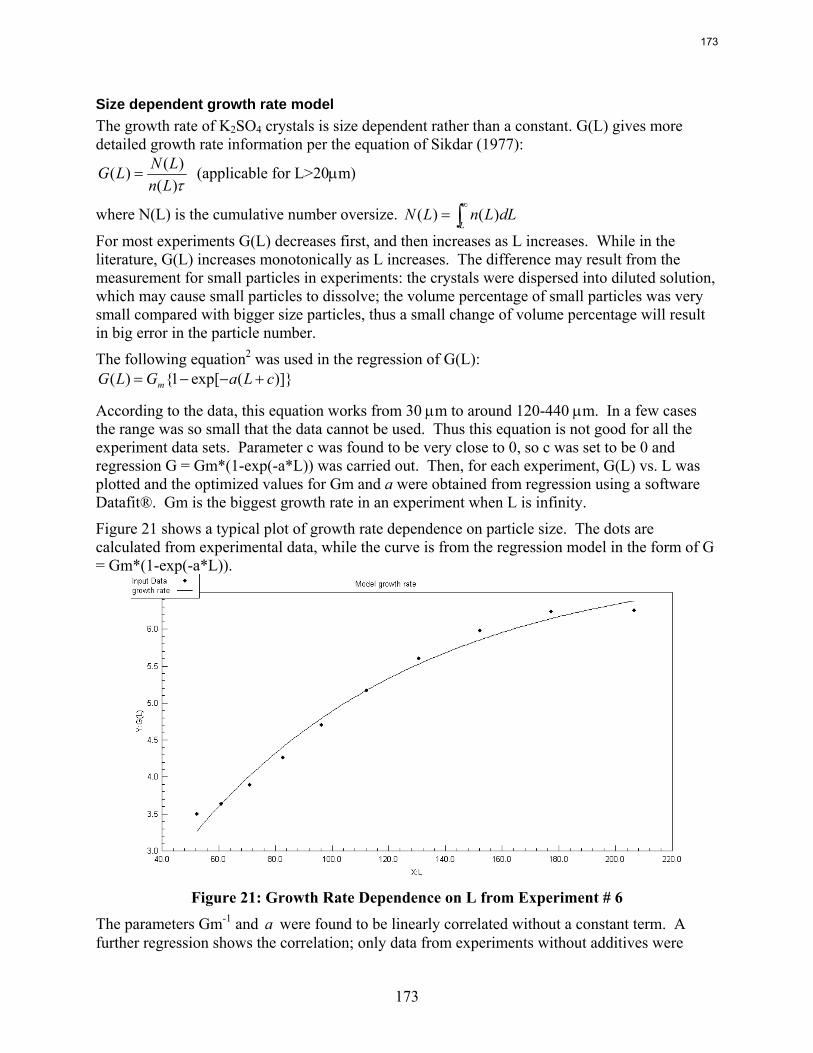
173

Size dependent growth rate model The growth rate of K2SO4 crystals is size dependent rather than a constant. G(L) gives more detailed growth rate information per the equation of Sikdar (1977):

τ)()()(

LnLNLG = (applicable for L>20μm)

where N(L) is the cumulative number oversize. ∫∞

=L

dLLnLN )()(

For most experiments G(L) decreases first, and then increases as L increases. While in the literature, G(L) increases monotonically as L increases. The difference may result from the measurement for small particles in experiments: the crystals were dispersed into diluted solution, which may cause small particles to dissolve; the volume percentage of small particles was very small compared with bigger size particles, thus a small change of volume percentage will result in big error in the particle number.

The following equation2 was used in the regression of G(L): )]}(exp[1{)( cLaGLG m +−−=

According to the data, this equation works from 30 μm to around 120-440 μm. In a few cases the range was so small that the data cannot be used. Thus this equation is not good for all the experiment data sets. Parameter c was found to be very close to 0, so c was set to be 0 and regression G = Gm*(1-exp(-a*L)) was carried out. Then, for each experiment, G(L) vs. L was plotted and the optimized values for Gm and a were obtained from regression using a software Datafit®. Gm is the biggest growth rate in an experiment when L is infinity.

Figure 21 shows a typical plot of growth rate dependence on particle size. The dots are calculated from experimental data, while the curve is from the regression model in the form of G = Gm*(1-exp(-a*L)).

Figure 21: Growth Rate Dependence on L from Experiment # 6

The parameters Gm-1 and a were found to be linearly correlated without a constant term. A further regression shows the correlation; only data from experiments without additives were

173

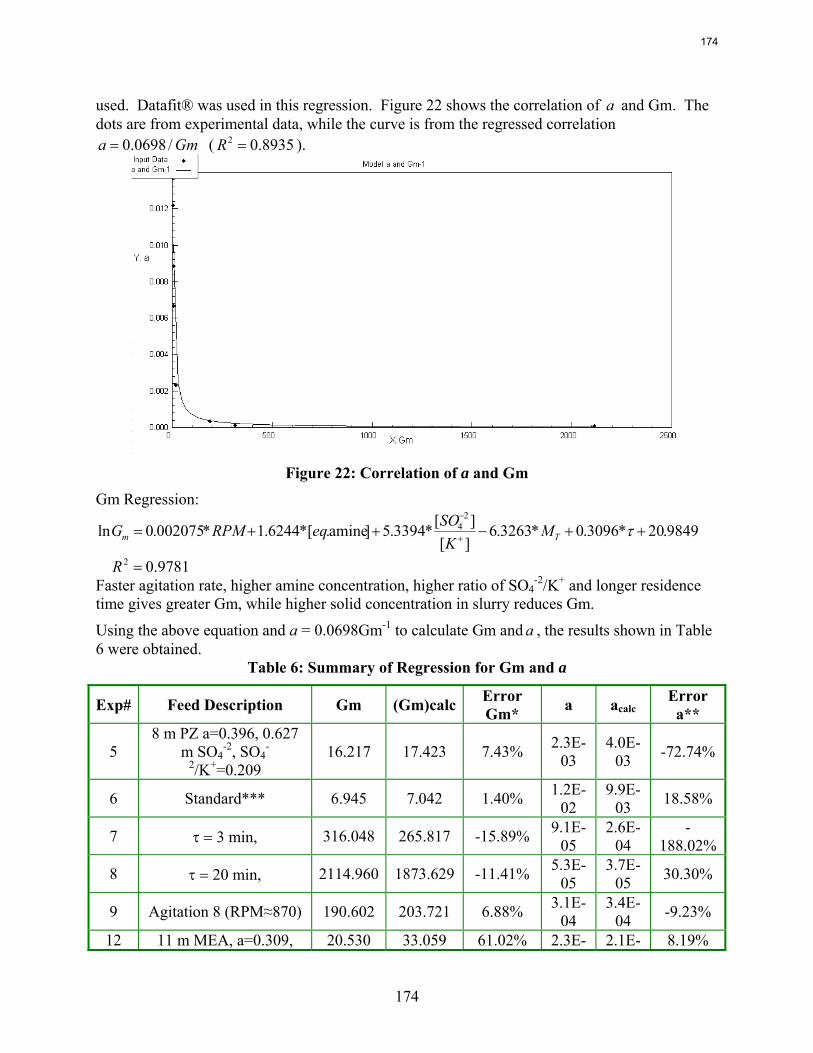
174

used. Datafit® was used in this regression. Figure 22 shows the correlation of a and Gm. The dots are from experimental data, while the curve is from the regressed correlation

Gma /0698.0= ( 8935.02 =R ).

Figure 22: Correlation of a and Gm

Gm Regression:

9849.20*3096.0*3263.6][][*3394.5]amine.[*6244.1*002075.0ln

24 ++−++= +

−

τTm MK

SOeqRPMG

9781.02 =R Faster agitation rate, higher amine concentration, higher ratio of SO4

-2/K+ and longer residence time gives greater Gm, while higher solid concentration in slurry reduces Gm.

Using the above equation and a = 0.0698Gm-1 to calculate Gm and a , the results shown in Table 6 were obtained.

Table 6: Summary of Regression for Gm and a

Exp# Feed Description Gm (Gm)calc Error Gm* a acalc

Error a**

5 8 m PZ a=0.396, 0.627

m SO4-2, SO4

-

2/K+=0.209 16.217 17.423 7.43% 2.3E-

03 4.0E-

03 -72.74%

6 Standard*** 6.945 7.042 1.40% 1.2E-02

9.9E-03 18.58%

7 τ = 3 min, 316.048 265.817 -15.89% 9.1E-05

2.6E-04

-188.02%

8 τ = 20 min, 2114.960 1873.629 -11.41% 5.3E-05

3.7E-05 30.30%

9 Agitation 8 (RPM≈870) 190.602 203.721 6.88% 3.1E-04

3.4E-04 -9.23%

12 11 m MEA, a=0.309, 20.530 33.059 61.02% 2.3E- 2.1E- 8.19%

174

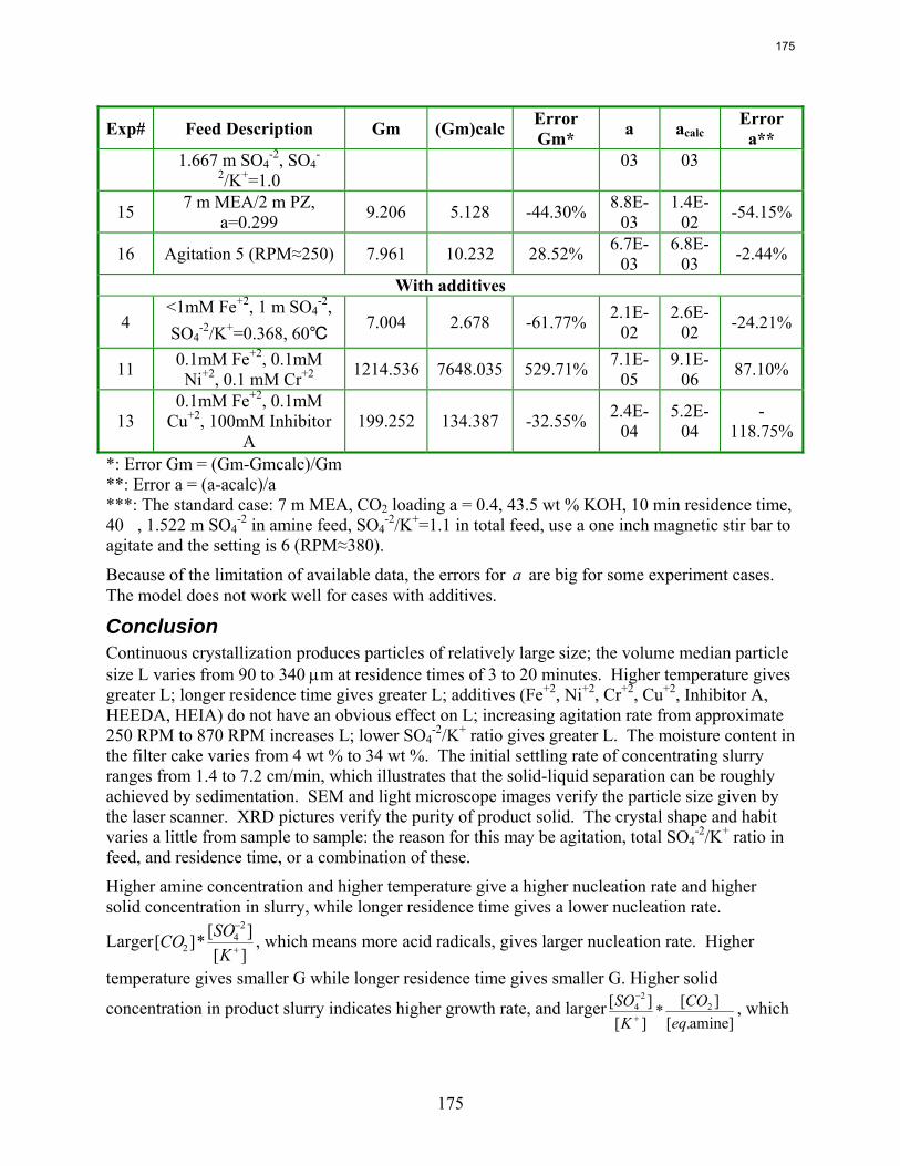
175

Exp# Feed Description Gm (Gm)calc Error Gm* a acalc

Error a**

1.667 m SO4-2, SO4

-

2/K+=1.0 03 03

15 7 m MEA/2 m PZ, a=0.299 9.206 5.128 -44.30% 8.8E-

03 1.4E-

02 -54.15%

16 Agitation 5 (RPM≈250) 7.961 10.232 28.52% 6.7E-03

6.8E-03 -2.44%

With additives

4 <1mM Fe+2, 1 m SO4

-2, SO4

-2/K+=0.368, 60℃ 7.004 2.678 -61.77% 2.1E-02

2.6E-02 -24.21%

11 0.1mM Fe+2, 0.1mM Ni+2, 0.1 mM Cr+2 1214.536 7648.035 529.71% 7.1E-

05 9.1E-

06 87.10%

13 0.1mM Fe+2, 0.1mM

Cu+2, 100mM Inhibitor A

199.252 134.387 -32.55% 2.4E-04

5.2E-04

-118.75%

*: Error Gm = (Gm-Gmcalc)/Gm **: Error a = (a-acalc)/a ***: The standard case: 7 m MEA, CO2 loading a = 0.4, 43.5 wt % KOH, 10 min residence time, 40�, 1.522 m SO4

-2 in amine feed, SO4-2/K+=1.1 in total feed, use a one inch magnetic stir bar to

agitate and the setting is 6 (RPM≈380).

Because of the limitation of available data, the errors for a are big for some experiment cases. The model does not work well for cases with additives.

Conclusion Continuous crystallization produces particles of relatively large size; the volume median particle size L varies from 90 to 340 μm at residence times of 3 to 20 minutes. Higher temperature gives greater L; longer residence time gives greater L; additives (Fe+2, Ni+2, Cr+2, Cu+2, Inhibitor A, HEEDA, HEIA) do not have an obvious effect on L; increasing agitation rate from approximate 250 RPM to 870 RPM increases L; lower SO4

-2/K+ ratio gives greater L. The moisture content in the filter cake varies from 4 wt % to 34 wt %. The initial settling rate of concentrating slurry ranges from 1.4 to 7.2 cm/min, which illustrates that the solid-liquid separation can be roughly achieved by sedimentation. SEM and light microscope images verify the particle size given by the laser scanner. XRD pictures verify the purity of product solid. The crystal shape and habit varies a little from sample to sample: the reason for this may be agitation, total SO4

-2/K+ ratio in feed, and residence time, or a combination of these.

Higher amine concentration and higher temperature give a higher nucleation rate and higher solid concentration in slurry, while longer residence time gives a lower nucleation rate.

Larger][][*][

24

2 +

−

KSOCO , which means more acid radicals, gives larger nucleation rate. Higher

temperature gives smaller G while longer residence time gives smaller G. Higher solid

concentration in product slurry indicates higher growth rate, and largeramine].[

][*][][ 2

24

eqCO

KSO

+

−

, which

175

176

means more acid radicals, gives smaller G. Additives result in higher nucleation rate but lower growth rate.

Growth rate is size dependent for K2SO4 crystallization. Within certain ranges, G(L) can be predicted by a model containing the parameter Gm, which is the maximum G at infinite L. Further, an empirical model predicting Gm was developed.

Future Work 1. Complete the regression for interaction parameters in CO2-MEA-H2O-K+-SO4

-2 system in Aspen Plus®.

2. Variable pressure SEM imaging without coating for more samples. 3. X-ray diffraction of solid samples to analyze impurities that might exist in the product

samples. 4. Develop the model of reclaiming process to remove sulfate by potassium sulfate

crystallization in Aspen Plus®. 5. Mass balance and population balance calculation based on the results from interaction

parameter regression and crystallization kinetics data. 6. Literature review for reclaiming using Ca(OH) 2 or NaOH or other methods.

References Jones AG. Crystallization Process Systems, 2002. Oxford: Butterworth-Heinemann. Mydlarz J & AG Jones. On the estimation of size-dependent crystal growth rate functions in

MSMPR crystallizers. Chem. Eng. J. 1993;53:125–135. Randolph AD & MA Larson. Theory of Particulate Processes Analysis and Techniques of

Continuous Crystallization, 2nd ed. Orlando: Academic Press, 1988. Sikdar SK. Size-Dependent Growth Rate from Curved Ln n(L) vs. L Steady-State Data. Ind.

Eng. Chem. Fundam. 1977;16(3):1977.

176

177

MEA Dynamic Modeling

Quarterly Report for April 1 – June 30, 2008

by Sepideh Ziaii Fashami

Supported by the Luminant Carbon Management Program

and the

Industrial Associates Program for CO2 Capture by Aqueous Absorption

Department of Chemical Engineering

The University of Texas at Austin

July 8, 2008

Abstract This quarter’s work focuses on rate-based dynamic modeling of the stripper with 30% monoethanolamine in a flow sheet of Aspen Custom Modeler®. The dynamic model of a packed column with one segment and a reboiler as an equilibrium stage was created and run successfully in both steady state and dynamic modes. The results show a reasonable and explainable dynamic behavior of process in response to the rich solution flow rate change.

Introduction On/off operation of CO2 capture in coal-fired power plants has been proposed as a policy to operate the capture at a lower cost. Turning CO2 capture “off” at periods of high electricity demand can recover plant generation capacity lost due to CO2 capture, thereby eliminating the capital cost of installing additional capacity. Over the last quarter, we have introduced different dynamic strategies for CO2 capture operation and evaluated their advantages and disadvantages.

For analysis of on/off operation, we need a dynamic model of the process, which should be rigorous enough to represent the unsteady-state operation of the system and simple enough to be solved by available modeling tools.

In this work, the dynamic behavior of a segment of the packed column stripper linked to one equilibrium stage reboiler in response to the rich solution flow rate change is carefully examined and the results are given with some justifications.

Case Study The case study observed in this work is a stripper including a packed column as a segment filled with Mellapack 250Y and a reboiler as an equilibrium stage with heat duty. The operating condition and capacity is based on one of the created Aspen Plus® models of a 500 MW coal-fired power plant. Figure 1 shows the input information of this case study

177

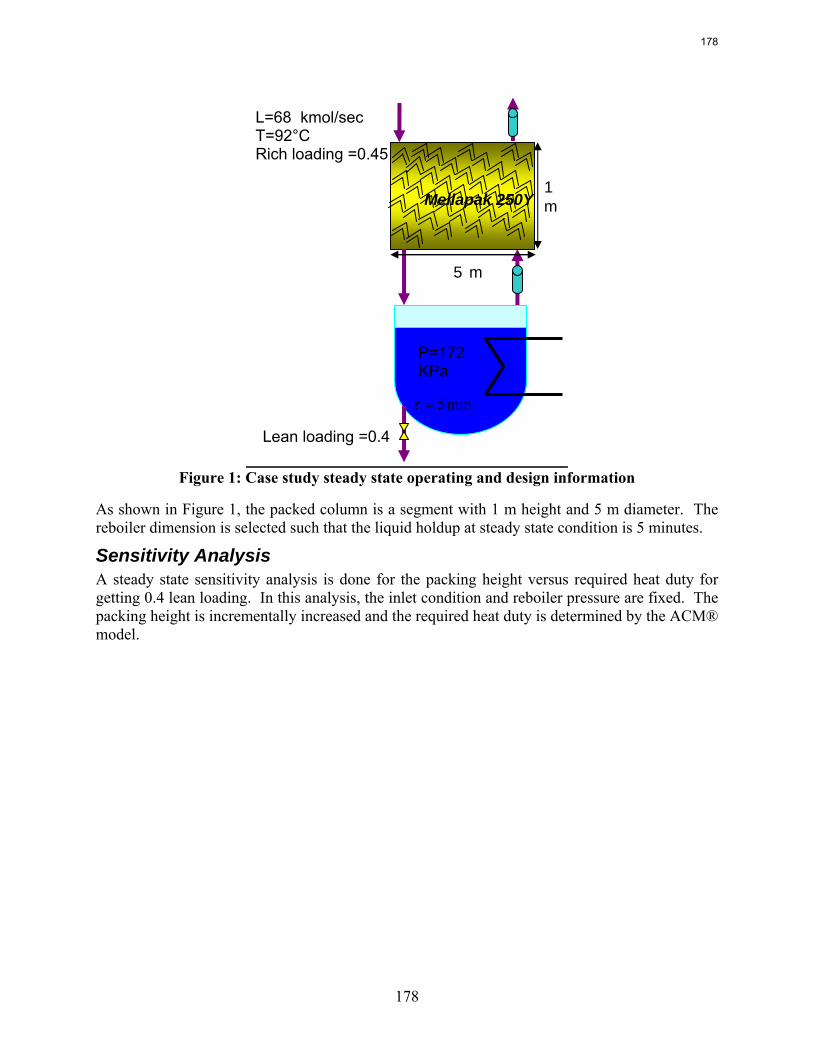
178

Figure 1: Case study steady state operating and design information

As shown in Figure 1, the packed column is a segment with 1 m height and 5 m diameter. The reboiler dimension is selected such that the liquid holdup at steady state condition is 5 minutes.

Sensitivity Analysis A steady state sensitivity analysis is done for the packing height versus required heat duty for getting 0.4 lean loading. In this analysis, the inlet condition and reboiler pressure are fixed. The packing height is incrementally increased and the required heat duty is determined by the ACM® model.

L=68 kmol/sec T=92°C Rich loading =0.45

Mellapak 250Y 1 m

Lean loading =0.4

P=172 KPa min5=τ

5 m

178

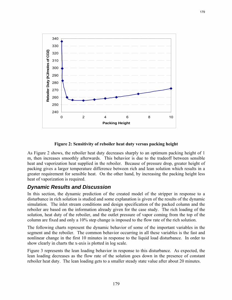
179

Figure 2: Sensitivity of reboiler heat duty versus packing height

As Figure 2 shows, the reboiler heat duty decreases sharply to an optimum packing height of 1 m, then increases smoothly afterwards. This behavior is due to the tradeoff between sensible heat and vaporization heat supplied in the reboiler. Because of pressure drop, greater height of packing gives a larger temperature difference between rich and lean solution which results in a greater requirement for sensible heat. On the other hand, by increasing the packing height less heat of vaporization is required.

Dynamic Results and Discussion In this section, the dynamic prediction of the created model of the stripper in response to a disturbance in rich solution is studied and some explanation is given of the results of the dynamic simulation. The inlet stream conditions and design specification of the packed column and the reboiler are based on the information already given for the case study. The rich loading of the solution, heat duty of the reboiler, and the outlet pressure of vapor coming from the top of the column are fixed and only a 10% step change is imposed to the flow rate of the rich solution.

The following charts represent the dynamic behavior of some of the important variables in the segment and the reboiler. The common behavior occurring in all these variables is the fast and nonlinear change in the first 10 minutes in response to the liquid load disturbance. In order to show clearly in charts the x-axis is plotted in log scale.

Figure 3 represents the lean loading behavior in response to this disturbance. As expected, the lean loading decreases as the flow rate of the solution goes down in the presence of constant reboiler heat duty. The lean loading gets to a smaller steady state value after about 20 minutes.

240

250

260

270

280

290

300

310

320

330

340

0 2 4 6 8 10

Packing Height

Reb

oile

r Dut

y (K

J/m

oles

of C

O2)

179

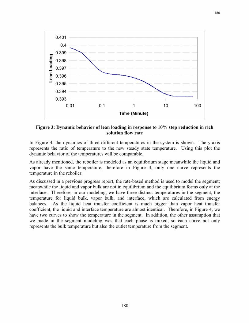
180

0.393

0.394

0.395

0.396

0.397

0.398

0.399

0.4

0.401

0.01 0.1 1 10 100

Time (Minute)

Lean

Loa

ding

Figure 3: Dynamic behavior of lean loading in response to 10% step reduction in rich

solution flow rate

In Figure 4, the dynamics of three different temperatures in the system is shown. The y-axis represents the ratio of temperature to the new steady state temperature. Using this plot the dynamic behavior of the temperatures will be comparable.

As already mentioned, the reboiler is modeled as an equilibrium stage meanwhile the liquid and vapor have the same temperature, therefore in Figure 4, only one curve represents the temperature in the reboiler.

As discussed in a previous progress report, the rate-based method is used to model the segment; meanwhile the liquid and vapor bulk are not in equilibrium and the equilibrium forms only at the interface. Therefore, in our modeling, we have three distinct temperatures in the segment, the temperature for liquid bulk, vapor bulk, and interface, which are calculated from energy balances. As the liquid heat transfer coefficient is much bigger than vapor heat transfer coefficient, the liquid and interface temperature are almost identical. Therefore, in Figure 4, we have two curves to show the temperature in the segment. In addition, the other assumption that we made in the segment modeling was that each phase is mixed, so each curve not only represents the bulk temperature but also the outlet temperature from the segment.

180

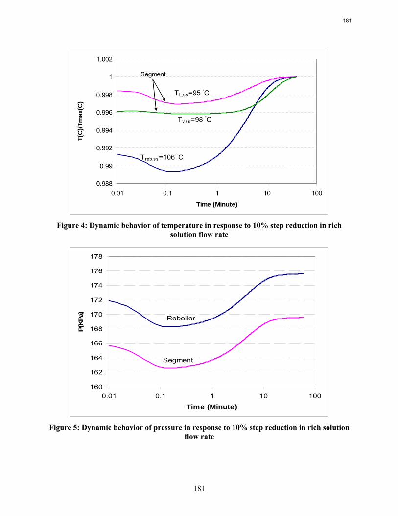
181

0.988

0.99

0.992

0.994

0.996

0.998

1

1.002

0.01 0.1 1 10 100

Time (Minute)

T(C

)/Tm

ax(C

)

Tv,ss=98 ◦C

Treb,ss=106 ◦C

TL,ss=95 ◦C

Segment

Figure 4: Dynamic behavior of temperature in response to 10% step reduction in rich

solution flow rate

160

162

164

166

168

170

172

174

176

178

0.01 0.1 1 10 100

Time (Minute)

P(K

Pa)

Reboiler

Segment

Figure 5: Dynamic behavior of pressure in response to 10% step reduction in rich solution

flow rate

181

182

Figure 5 shows the dynamics of the pressure in the reboiler and the segment in the presence of step disturbance. In the modeling, we assumed that there is no pressure driving force between liquid and gas phases in the segment and they have the same pressure, therefore only one curve represents the pressure in the segment.

The constant pressure in the system is the pressure of outlet vapor from the segment that is fixed at atmospheric pressure. There are two restrictions considered on the vapor streams coming out from the reboiler and the segment. Each restriction dictates a pressure flow equation in the model.

The initial decrease in the pressure seems to cause flash in the reboiler and segment, which results in fast decrease in the lean loading. From the figures, the estimated response time for the temperature and the pressure is about 40 minutes; however, the lean loading reaches steady state in 20 minutes. Therefore, temperature and pressure variables are sluggish compared to the loading.

Conclusions and Future Work In this quarter, a dynamic model of an equilibrium stage reboiler was created in ACM® and connected to the model of a segment. The whole model was executed in both steady state and dynamic modes. The steady state sensitivity analysis shows a minimum heat duty versus packing height. The dynamics of the temperature, pressure, and lean loading follow each other.

In the next quarter, the model of the stripper will be run with multiple segments and the effect of the number of segments will be investigated in steady state and dynamic modes. In addition, the characteristic curve of a multistage compressor will be added to the stripper model to simulate the compression system, calculate compression work, and further control design.

In order to minimize amine thermal degradation, we propose to use the themosyphon reboiler since it has a higher circulation rate and lower holding time in contact with hot metal. I plan to focus on the theory and equations of this type of reboiler and create its model in ACM®.

182

183

System Level Implications of Flexible CO2 Capture Operation

Progress Report for April 1 – June 30, 2008

by Stuart Cohen

Supported by the Luminant Carbon Management Program

and the

Industrial Associates Program for CO2 Capture by Aqueous Absorption

Department of Chemical Engineering

The University of Texas at Austin

Month DDJuly 31, 2008

Abstract Flexible or “on/off” carbon dioxide (CO2) capture can prevent the need for building new capacity to replace that lost when CO2 capture is running, and it can allow plant operators to improve profits relative compared to a continuous CO2 capture system by selling high priced electricity when CO2 capture is “off.” A basic model of the Electric Reliability Council of Texas (ERCOT) grid using historical 2006 data demonstrates that turning CO2 capture off for just 99 hours of the year prevents the need to build over 4400MW of new capacity, which would amount to $12.8 billion if this replacement capacity were to be coal-based generation with CO2 capture. Despite the CO2 capture “off” time, CO2 capture operated in this way reduces grid CO2 emissions by nearly 50%. Recent modeling efforts have produced a more detailed ERCOT model that incorporates individual plant performance and a simplified representation of CO2 regulations, plant dispatch, and the ERCOT market for electricity to allow investigation of flexible CO2 capture in response to electricity price variations when there may be a cost associated with CO2 emissions. Preliminary results show that if CO2 is vented in the “off” configuration, flexibility may improve the economics of plants that have CO2 capture installed, though at the expense of added CO2 emissions. In contrast to current literature that suggests that a CO2 price around $40/tCO2 is required for economic viability of CO2 capture, this study recognizes that while a high CO2 price may be required to justify building a CO2 capture system, CO2 prices on the order of $10/tCO2 are sufficient to justify operation of a CO2 facility once it is installed. For flexible systems that store CO2-rich solvent in the “off” configuration, initial calculations of solvent storage capacity and solvent inventory cost indicate that there may be a tradeoff between large storage volume requirements for inexpensive, low CO2 capacity solvents and smaller storage volumes for expensive, high CO2 capacity solvents.

Introduction to Flexible CO2 Capture Operating post combustion (PC) carbon dioxide (CO2) capture systems flexibly may permit plant operators to recover some or all of the energy required for CO2 capture for use in power production when electric grid conditions allow this practice to be economical. Because PC CO2 capture is installed downstream of all other flue gas processing steps, it is reasonable to suggest

183

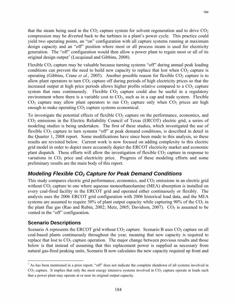
184

that the steam being used in the CO2 capture system for solvent regeneration and to drive CO2 compression may be diverted back to the turbines in a plant’s power cycle. This practice could yield two operating points, an “on” configuration with all capture systems running at maximum design capacity and an “off” position where most or all process steam is used for electricity generation. The “off” configuration would then allow a power plant to regain most or all of its original design output1 (Lucquiaud and Gibbins, 2008).

Flexible CO2 capture may be valuable because turning systems “off” during annual peak loading conditions can prevent the need to build new capacity to replace that lost when CO2 capture is operating (Gibbins, Crane et al., 2005). Another possible reason for flexible CO2 capture is to allow plant operators to turn CO2 capture off during periods of high electricity prices so that the increased output at high price periods allows higher profits relative compared to a CO2 capture system that runs continuously. Flexible CO2 capture could also be useful in a regulatory environment where there is a variable cost to CO2, such as in a cap and trade system. Flexible CO2 capture may allow plant operators to run CO2 capture only when CO2 prices are high enough to make operating CO2 capture systems economical.

To investigate the potential effects of flexible CO2 capture on the performance, economics, and CO2 emissions in the Electric Reliability Council of Texas (ERCOT) electric grid, a series of modeling studies is being undertaken. The first of these studies, which investigated the use of flexible CO2 capture to turn systems “off” at peak demand conditions, is described in detail in the Quarter 1, 2008 report. Some modifications have since been made to this analysis, so these results are revisited below. Current work is now focused on adding complexity to this electric grid model in order to depict more accurately depict the ERCOT electricity market and economic plant dispatch. These efforts will allow the investigation of flexible CO2 capture in response to variations in CO2 price and electricity price. Progress of these modeling efforts and some preliminary results are the main body of this report.

Modeling Flexible CO2 Capture for Peak Demand Conditions This study compares electric grid performance, economics, and CO2 emissions in an electric grid without CO2 capture to one where aqueous monoethanolamine (MEA) absorption is installed on every coal-fired facility in the ERCOT grid and operated either continuously or flexibly. The analysis uses the 2006 ERCOT grid configuration with 2006 historical load data, and the MEA systems are assumed to require 30% of plant output capacity while capturing 90% of the CO2 in the plant flue gas (Rao and Rubin, 2002; Metz, 2005; Davidson, 2007). CO2 is assumed to be vented in the “off” configuration.

Scenario Descriptions Scenario A represents the ERCOT grid without CO2 capture. Scenario B uses CO2 capture on all coal-based plants continuously throughout the year, meaning that new capacity is required to replace that lost to CO2 capture operation. The major change between previous results and those below is that instead of assuming that this replacement power is supplied as necessary from natural gas-fired peaking units, Scenario B now calculates the new capacity required up front and

1 As has been mentioned in a prior report, “off” does not indicate the complete shutdown of all systems involved in CO2 capture. It implies that only the most energy intensive systems involved in CO2 capture operate at loads such that a power plant may operate at or near its original output capacity.

184

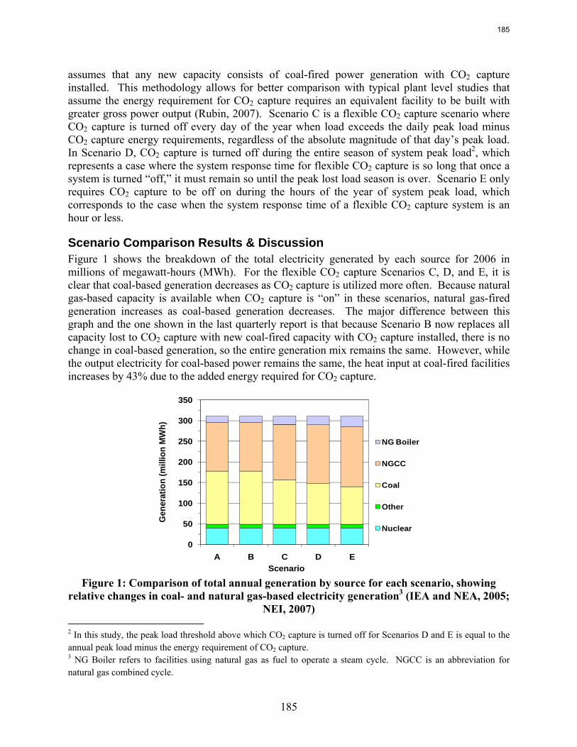
185

assumes that any new capacity consists of coal-fired power generation with CO2 capture installed. This methodology allows for better comparison with typical plant level studies that assume the energy requirement for CO2 capture requires an equivalent facility to be built with greater gross power output (Rubin, 2007). Scenario C is a flexible CO2 capture scenario where CO2 capture is turned off every day of the year when load exceeds the daily peak load minus CO2 capture energy requirements, regardless of the absolute magnitude of that day’s peak load. In Scenario D, CO2 capture is turned off during the entire season of system peak load2, which represents a case where the system response time for flexible CO2 capture is so long that once a system is turned “off,” it must remain so until the peak lost load season is over. Scenario E only requires CO2 capture to be off on during the hours of the year of system peak load, which corresponds to the case when the system response time of a flexible CO2 capture system is an hour or less.

Scenario Comparison Results & Discussion Figure 1 shows the breakdown of the total electricity generated by each source for 2006 in millions of megawatt-hours (MWh). For the flexible CO2 capture Scenarios C, D, and E, it is clear that coal-based generation decreases as CO2 capture is utilized more often. Because natural gas-based capacity is available when CO2 capture is “on” in these scenarios, natural gas-fired generation increases as coal-based generation decreases. The major difference between this graph and the one shown in the last quarterly report is that because Scenario B now replaces all capacity lost to CO2 capture with new coal-fired capacity with CO2 capture installed, there is no change in coal-based generation, so the entire generation mix remains the same. However, while the output electricity for coal-based power remains the same, the heat input at coal-fired facilities increases by 43% due to the added energy required for CO2 capture.

0

50

100

150

200

250

300

350

A B C D E

Gen

erat

ion

(mill

ion

MW

h)

Scenario

NG Boiler

NGCC

Coal

Other

Nuclear

Figure 1: Comparison of total annual generation by source for each scenario, showing

relative changes in coal- and natural gas-based electricity generation3 (IEA and NEA, 2005; NEI, 2007)

2 In this study, the peak load threshold above which CO2 capture is turned off for Scenarios D and E is equal to the annual peak load minus the energy requirement of CO2 capture. 3 NG Boiler refers to facilities using natural gas as fuel to operate a steam cycle. NGCC is an abbreviation for natural gas combined cycle.

185

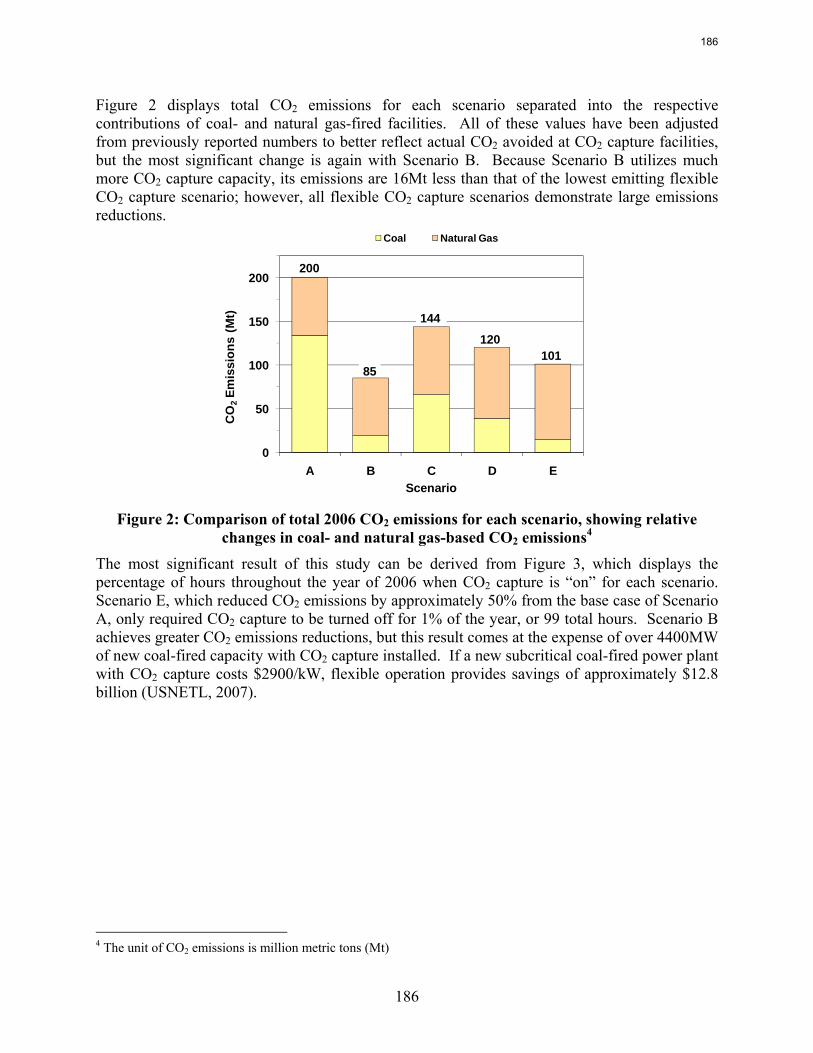
186

Figure 2 displays total CO2 emissions for each scenario separated into the respective contributions of coal- and natural gas-fired facilities. All of these values have been adjusted from previously reported numbers to better reflect actual CO2 avoided at CO2 capture facilities, but the most significant change is again with Scenario B. Because Scenario B utilizes much more CO2 capture capacity, its emissions are 16Mt less than that of the lowest emitting flexible CO2 capture scenario; however, all flexible CO2 capture scenarios demonstrate large emissions reductions.

0

50

100

150

200

A B C D E

CO

2Em

issi

ons

(Mt)

Scenario

Coal Natural Gas

200

85

144

120101

Figure 2: Comparison of total 2006 CO2 emissions for each scenario, showing relative

changes in coal- and natural gas-based CO2 emissions4

The most significant result of this study can be derived from Figure 3, which displays the percentage of hours throughout the year of 2006 when CO2 capture is “on” for each scenario. Scenario E, which reduced CO2 emissions by approximately 50% from the base case of Scenario A, only required CO2 capture to be turned off for 1% of the year, or 99 total hours. Scenario B achieves greater CO2 emissions reductions, but this result comes at the expense of over 4400MW of new coal-fired capacity with CO2 capture installed. If a new subcritical coal-fired power plant with CO2 capture costs $2900/kW, flexible operation provides savings of approximately $12.8 billion (USNETL, 2007).

4 The unit of CO2 emissions is million metric tons (Mt)

186

187

0%

100%

56%

79%

99%

0%

20%

40%

60%

80%

100%

A B C D E

% H

ours

of t

he Y

ear

Scenario Figure 3: Comparison of the percent of hours in 2006 that CO2 capture is turned on for

each scenario, showing the difference between “always on” CO2 capture (B) and the flexible CO2 capture scenarios (C, D, E).

Modeling Flexible CO2 Capture in Response to CO2 Price and Electricity Price Variations

Model Purpose and Limitations The previous modeling study involved a basic representation of the ERCOT grid in order to demonstrate some of the tradeoffs associated with flexible CO2 capture and the potential for flexible operation to alleviate capacity constraints imposed by the energy requirement of CO2 capture. Most of the work done in the past quarter, however, has been focused on more detailed modeling efforts that can investigate the operation of flexible CO2 capture in response to electricity price variations and in the context of a regulatory regime that places a cost on CO2 emissions.

A Dispatch Model Based on Operating Costs and ERCOT Market Operations The new model first determines the CO2 emissions cost in dollars per metric ton of CO2 ($/tCO2) for each day of the year based on the chosen regulatory regime and known electricity demand. CO2 price may remain constant to represent a CO2 tax, or the price may vary around a central value to characterize a cap and trade system. Rather than attempt to predict the CO2 price that results from a particular emissions cap, a cap and trade scenario simply allows CO2 price to vary proportionally to electricity demand variations, with this proportionality being another model parameter. This methodology is chosen as a first-order approximation because increased electricity demand is likely to result in the dispatch of less efficient generators that emit more CO2, resulting in increased demand for CO2 allowances, which may then cause an increase in CO2 price. The model also allows for the option to set upper or lower limits on CO2 price in order to simulate the effects of a maximum “safety valve” CO2 price or a minimum CO2 price below which CO2 allowances may be “banked” and kept for future use (Parry and Pizer, 2007).

187

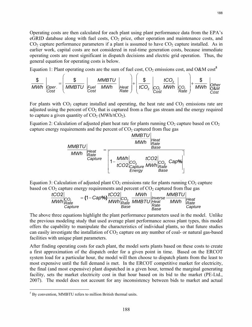
188

Operating costs are then calculated for each plant using plant performance data from the EPA’s eGRID database along with fuel costs, CO2 price, other operation and maintenance costs, and CO2 capture performance parameters if a plant is assumed to have CO2 capture installed. As in earlier work, capital costs are not considered in real-time generation costs, because immediate operating costs are most significant in dispatch decisions and electric grid operation. Thus, the general equation for operating costs is below.

Equation 1: Plant operating costs are the sum of fuel cost, CO2 emissions cost, and O&M cost5

OtherOper Fuel Heat COCO O MRateCostCost RateCost Cost

tCOMMBTUMWh MMBTU MWh tCO MWh MWh

⎛ ⎞⎛ ⎞⎜ ⎟⎜ ⎟= + +⎜ ⎟⎜ ⎟⎜ ⎟ ⎜ ⎟⎝ ⎠ ⎝ ⎠

22

2

2. &

$ $ $ $

For plants with CO2 capture installed and operating, the heat rate and CO2 emissions rate are adjusted using the percent of CO2 that is captured from a flue gas stream and the energy required to capture a given quantity of CO2 (MWh/tCO2).

Equation 2: Calculation of adjusted plant heat rate for plants running CO2 capture based on CO2 capture energy requirements and the percent of CO2 captured from flue gas

HeatRateBase

HeatRateCapture

CO COCapture Rate

BaseEnergy

MMBTUMWh

MMBTUMWh

MWh tCO CaptCO MWh

%

=⎡ ⎤⎢ ⎥

−⎢ ⎥⎢ ⎥⎣ ⎦

2 2

212

Equation 3: Calculation of adjusted plant CO2 emissions rate for plants running CO2 capture based on CO2 capture energy requirements and percent of CO2 captured from flue gas

InverseCOCO HeatHeatRate Rate RateRateBaseCapture CaptureBase

tCO tCO MWh MMBTUCapMWh MWh MMBTU MWh

( %)= −2 2

2 21

The above three equations highlight the plant performance parameters used in the model. Unlike the previous modeling study that used average plant performance across plant types, this model offers the capability to manipulate the characteristics of individual plants, so that future studies can easily investigate the installation of CO2 capture on any number of coal- or natural gas-based facilities with unique plant parameters.

After finding operating costs for each plant, the model sorts plants based on these costs to create a first approximation of the dispatch order for a given point in time. Based on the ERCOT system load for a particular hour, the model will then choose to dispatch plants from the least to most expensive until the full demand is met. In the ERCOT competitive market for electricity, the final (and most expensive) plant dispatched in a given hour, termed the marginal generating facility, sets the market electricity cost in that hour based on its bid to the market (PE-Ltd., 2007). The model does not account for any inconsistency between bids to market and actual

5 By convention, MMBTU refers to million British thermal units.

188

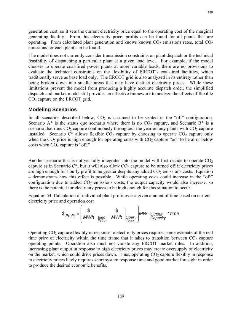
189

generation cost, so it sets the current electricity price equal to the operating cost of the marginal generating facility. From this electricity price, profits can be found for all plants that are operating. From calculated plant generation and knows known CO2 emissions rates, total CO2 emissions for each plant can be found.

The model does not currently consider transmission constraints on plant dispatch or the technical feasibility of dispatching a particular plant at a given load level. For example, if the model chooses to operate coal-fired power plants at more variable loads, there are no provisions to evaluate the technical constraints on the flexibility of ERCOT’s coal-fired facilities, which traditionally serve as base load only. The ERCOT grid is also analyzed in its entirety rather than being broken down into smaller areas that may have distinct electricity prices. While these limitations prevent the model from producing a highly accurate dispatch order, the simplified dispatch and market model still provides an effective framework to analyze the effects of flexible CO2 capture on the ERCOT grid.

Modeling Scenarios In all scenarios described below, CO2 is assumed to be vented in the “off” configuration. Scenario A* is the status quo scenario where there is no CO2 capture, and Scenario B* is a scenario that runs CO2 capture continuously throughout the year on any plants with CO2 capture installed. Scenario C* allows flexible CO2 capture by choosing to operate CO2 capture only when the CO2 price is high enough for operating costs with CO2 capture “on” to be at or below costs when CO2 capture is “off.”

Another scenario that is not yet fully integrated into the model will first decide to operate CO2 capture as in Scenario C*, but it will also allow CO2 capture to be turned off if electricity prices are high enough for hourly profit to be greater despite any added CO2 emissions costs. Equation 4 demonstrates how this effect is possible. While operating costs could increase in the “off” configuration due to added CO2 emissions costs, the output capacity would also increase, so there is the potential for electricity prices to be high enough for this situation to occur.

Equation 54: Calculation of individual plant profit over a given amount of time based on current electricity price and operation cost

OutputProfit OperElec CapacityPrice Cost

MW timeMWh MWh

−

⎛ ⎞⎜ ⎟= ⎜ ⎟⎜ ⎟⎝ ⎠

.$ $$ *

Operating CO2 capture flexibly in response to electricity prices requires some estimate of the real time price of electricity within the time frame that it takes to transition between CO2 capture operating points. Operation also must not violate any ERCOT market rules. In addition, increasing plant output in response to high electricity prices may create oversupply of electricity on the market, which could drive prices down. Thus, operating CO2 capture flexibly in response to electricity prices likely requires short system response time and good market foresight in order to produce the desired economic benefits.

189

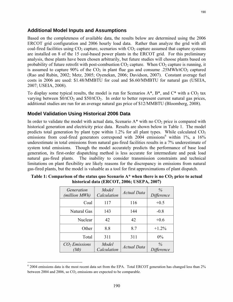
190

Additional Model Inputs and Assumptions Based on the completeness of available data, the results below are determined using the 2006 ERCOT grid configuration and 2006 hourly load data. Rather than analyze the grid with all coal-fired facilities using CO2 capture, scenarios with CO2 capture assumed that capture systems are installed on 8 of the 15 coal-based power plants in the ERCOT grid. For this preliminary analysis, these plants have been chosen arbitrarily, but future studies will choose plants based on probability of future retrofit with post-combustion CO2 capture. When CO2 capture is running, it is assumed to capture 90% of the CO2 in plant flue gas and consume .25MWh/tCO2 captured (Rao and Rubin, 2002; Metz, 2005; Oyenekan, 2006; Davidson, 2007). Constant average fuel costs in 2006 are used: $1.48/MMBTU for coal and $6.60/MMBTU for natural gas (USEIA, 2007; USEIA, 2008).

To display some typical results, the model is run for Scenarios A*, B*, and C* with a CO2 tax varying between $0/tCO2 and $50/tCO2. In order to better represent current natural gas prices, additional studies are run for an average natural gas price of $12/MMBTU (Bloomberg, 2008).

Model Validation Using Historical 2006 Data In order to validate the model with actual data, Scenario A* with no CO2 price is compared with historical generation and electricity price data. Results are shown below in Table 1. The model predicts total generation by plant type within 1.2% for all plant types. While calculated CO2 emissions from coal-fired generators correspond with 2004 emissions6 within 1%, a 16% underestimate in total emissions from natural gas-fired facilities results in a 7% underestimate of system total emissions. Though the model accurately predicts the performance of base load generation, its first-order dispatching method is less accurate for intermediate and peak load natural gas-fired plants. The inability to consider transmission constraints and technical limitations on plant flexibility are likely reasons for the discrepancy in emissions from natural gas-fired plants, but the model is valuable as a tool for first approximations of plant dispatch.

Table 1: Comparison of the status quo Scenario A* when there is no CO2 price to actual historical data (ERCOT, 2006; USEPA, 2007)

Generation (million MWh)

Model Calculation Actual Data %

Difference

Coal 117 116 +0.5

Natural Gas 143 144 -0.8

Nuclear 42 42 +0.6

Other 8.8 8.7 +1.2%

Total 311 311 0% CO2 Emissions

(Mt) Model

Calculation Actual Data % Difference

6 2004 emissions data is the most recent data set from the EPA. Total ERCOT generation has changed less than 2% between 2004 and 2006, so CO2 emissions are expected to be comparable.

190

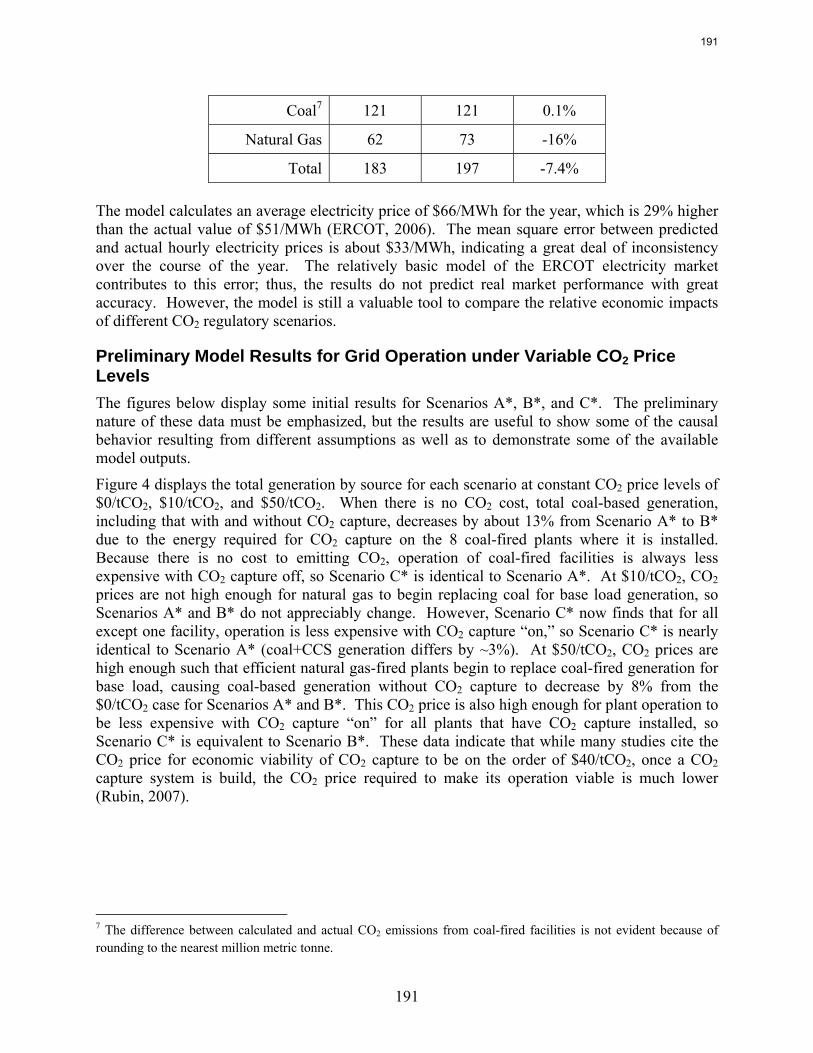
191

Coal7 121 121 0.1%

Natural Gas 62 73 -16%

Total 183 197 -7.4%

The model calculates an average electricity price of $66/MWh for the year, which is 29% higher than the actual value of $51/MWh (ERCOT, 2006). The mean square error between predicted and actual hourly electricity prices is about $33/MWh, indicating a great deal of inconsistency over the course of the year. The relatively basic model of the ERCOT electricity market contributes to this error; thus, the results do not predict real market performance with great accuracy. However, the model is still a valuable tool to compare the relative economic impacts of different CO2 regulatory scenarios.

Preliminary Model Results for Grid Operation under Variable CO2 Price Levels The figures below display some initial results for Scenarios A*, B*, and C*. The preliminary nature of these data must be emphasized, but the results are useful to show some of the causal behavior resulting from different assumptions as well as to demonstrate some of the available model outputs.

Figure 4 displays the total generation by source for each scenario at constant CO2 price levels of $0/tCO2, $10/tCO2, and $50/tCO2. When there is no CO2 cost, total coal-based generation, including that with and without CO2 capture, decreases by about 13% from Scenario A* to B* due to the energy required for CO2 capture on the 8 coal-fired plants where it is installed. Because there is no cost to emitting CO2, operation of coal-fired facilities is always less expensive with CO2 capture off, so Scenario C* is identical to Scenario A*. At $10/tCO2, CO2 prices are not high enough for natural gas to begin replacing coal for base load generation, so Scenarios A* and B* do not appreciably change. However, Scenario C* now finds that for all except one facility, operation is less expensive with CO2 capture “on,” so Scenario C* is nearly identical to Scenario A* (coal+CCS generation differs by ~3%). At $50/tCO2, CO2 prices are high enough such that efficient natural gas-fired plants begin to replace coal-fired generation for base load, causing coal-based generation without CO2 capture to decrease by 8% from the $0/tCO2 case for Scenarios A* and B*. This CO2 price is also high enough for plant operation to be less expensive with CO2 capture “on” for all plants that have CO2 capture installed, so Scenario C* is equivalent to Scenario B*. These data indicate that while many studies cite the CO2 price for economic viability of CO2 capture to be on the order of $40/tCO2, once a CO2 capture system is build, the CO2 price required to make its operation viable is much lower (Rubin, 2007).

7 The difference between calculated and actual CO2 emissions from coal-fired facilities is not evident because of rounding to the nearest million metric tonne.

191

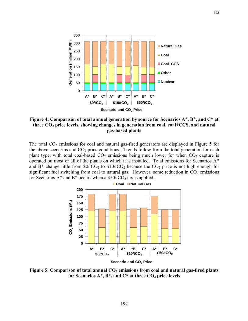
192

0

50

100

150

200

250

300

350

A* B* C* A* B* C* A* B* C*

Gen

erat

ion

(mill

ion

MW

h)

Scenario and CO2 Price

Natural Gas

Coal

Coal+CCS

Other

Nuclear

$0/tCO2 $10/tCO2 $50/tCO2

Figure 4: Comparison of total annual generation by source for Scenarios A*, B*, and C* at

three CO2 price levels, showing changes in generation from coal, coal+CCS, and natural gas-based plants

The total CO2 emissions for coal and natural gas-fired generators are displayed in Figure 5 for the above scenarios and CO2 price conditions. Trends follow from the total generation for each plant type, with total coal-based CO2 emissions being much lower for when CO2 capture is operated on most or all of the plants on which it is installed. Total emissions for Scenarios A* and B* change little from $0/tCO2 to $10/tCO2 because the CO2 price is not high enough for significant fuel switching from coal to natural gas. However, some reduction in CO2 emissions for Scenarios A* and B* occurs when a $50/tCO2 tax is applied.

0

25

50

75

100

125

150

175

200

A* B* C* A* *B C* A* B* C*

CO

2Em

issi

ons

(Mt)

Scenario and CO2 Price

Coal Natural Gas

$0/tCO2 $10/tCO2 $50/tCO2

Figure 5: Comparison of total annual CO2 emissions from coal and natural gas-fired plants

for Scenarios A*, B*, and C* at three CO2 price levels

192

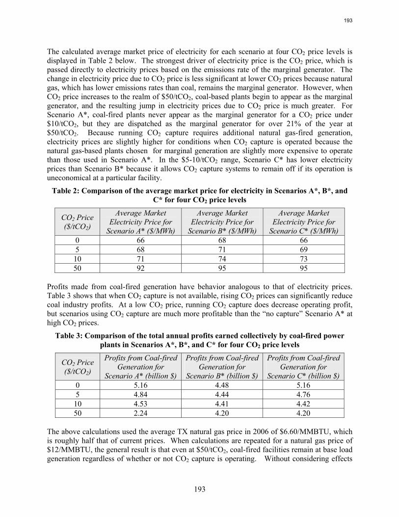
193

The calculated average market price of electricity for each scenario at four CO2 price levels is displayed in Table 2 below. The strongest driver of electricity price is the CO2 price, which is passed directly to electricity prices based on the emissions rate of the marginal generator. The change in electricity price due to CO2 price is less significant at lower CO2 prices because natural gas, which has lower emissions rates than coal, remains the marginal generator. However, when CO2 price increases to the realm of $50/tCO2, coal-based plants begin to appear as the marginal generator, and the resulting jump in electricity prices due to CO2 price is much greater. For Scenario A*, coal-fired plants never appear as the marginal generator for a CO2 price under $10/tCO2, but they are dispatched as the marginal generator for over 21% of the year at $50/tCO2. Because running CO2 capture requires additional natural gas-fired generation, electricity prices are slightly higher for conditions when CO2 capture is operated because the natural gas-based plants chosen for marginal generation are slightly more expensive to operate than those used in Scenario A*. In the $5-10/tCO2 range, Scenario C* has lower electricity prices than Scenario B* because it allows CO2 capture systems to remain off if its operation is uneconomical at a particular facility.

Table 2: Comparison of the average market price for electricity in Scenarios A*, B*, and C* for four CO2 price levels

CO2 Price ($/tCO2)

Average Market Electricity Price for

Scenario A* ($/MWh)

Average Market Electricity Price for

Scenario B* ($/MWh)

Average Market Electricity Price for

Scenario C* ($/MWh) 0 66 68 66 5 68 71 69 10 71 74 73 50 92 95 95

Profits made from coal-fired generation have behavior analogous to that of electricity prices. Table 3 shows that when CO2 capture is not available, rising CO2 prices can significantly reduce coal industry profits. At a low CO2 price, running CO2 capture does decrease operating profit, but scenarios using CO2 capture are much more profitable than the “no capture” Scenario A* at high CO2 prices.

Table 3: Comparison of the total annual profits earned collectively by coal-fired power plants in Scenarios A*, B*, and C* for four CO2 price levels

CO2 Price ($/tCO2)

Profits from Coal-fired Generation for

Scenario A* (billion $)

Profits from Coal-fired Generation for

Scenario B* (billion $)

Profits from Coal-fired Generation for

Scenario C* (billion $) 0 5.16 4.48 5.16 5 4.84 4.44 4.76 10 4.53 4.41 4.42 50 2.24 4.20 4.20

The above calculations used the average TX natural gas price in 2006 of $6.60/MMBTU, which is roughly half that of current prices. When calculations are repeated for a natural gas price of $12/MMBTU, the general result is that even at $50/tCO2, coal-fired facilities remain at base load generation regardless of whether or not CO2 capture is operating. Without considering effects

193

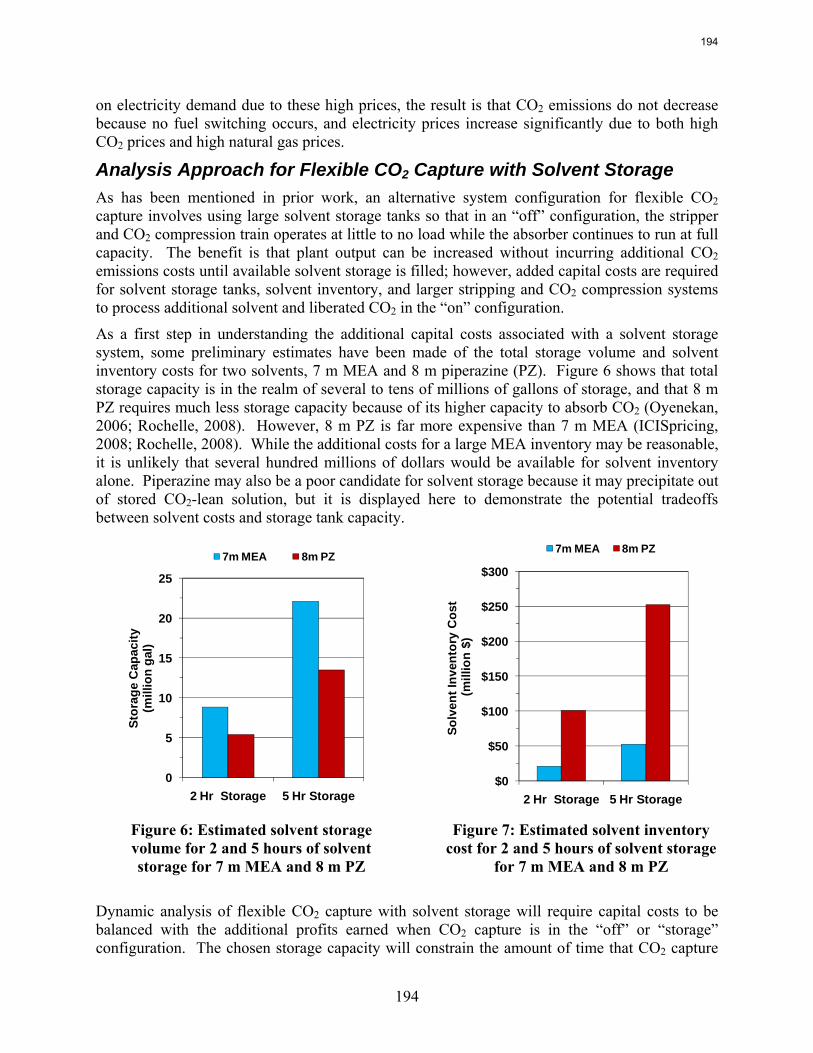
194

on electricity demand due to these high prices, the result is that CO2 emissions do not decrease because no fuel switching occurs, and electricity prices increase significantly due to both high CO2 prices and high natural gas prices.

Analysis Approach for Flexible CO2 Capture with Solvent Storage As has been mentioned in prior work, an alternative system configuration for flexible CO2 capture involves using large solvent storage tanks so that in an “off” configuration, the stripper and CO2 compression train operates at little to no load while the absorber continues to run at full capacity. The benefit is that plant output can be increased without incurring additional CO2 emissions costs until available solvent storage is filled; however, added capital costs are required for solvent storage tanks, solvent inventory, and larger stripping and CO2 compression systems to process additional solvent and liberated CO2 in the “on” configuration.

As a first step in understanding the additional capital costs associated with a solvent storage system, some preliminary estimates have been made of the total storage volume and solvent inventory costs for two solvents, 7 m MEA and 8 m piperazine (PZ). Figure 6 shows that total storage capacity is in the realm of several to tens of millions of gallons of storage, and that 8 m PZ requires much less storage capacity because of its higher capacity to absorb CO2 (Oyenekan, 2006; Rochelle, 2008). However, 8 m PZ is far more expensive than 7 m MEA (ICISpricing, 2008; Rochelle, 2008). While the additional costs for a large MEA inventory may be reasonable, it is unlikely that several hundred millions of dollars would be available for solvent inventory alone. Piperazine may also be a poor candidate for solvent storage because it may precipitate out of stored CO2-lean solution, but it is displayed here to demonstrate the potential tradeoffs between solvent costs and storage tank capacity.

0

5

10

15

20

25

2 Hr Storage 5 Hr Storage

Stor

age

Cap

acity

(m

illio

n ga

l)

7m MEA 8m PZ

$0

$50

$100

$150

$200

$250

$300

2 Hr Storage 5 Hr Storage

Solv

ent I

nven

tory

Cos

t(m

illio

n $)

7m MEA 8m PZ

Figure 6: Estimated solvent storage volume for 2 and 5 hours of solvent storage for 7 m MEA and 8 m PZ

Figure 7: Estimated solvent inventory cost for 2 and 5 hours of solvent storage

for 7 m MEA and 8 m PZ

Dynamic analysis of flexible CO2 capture with solvent storage will require capital costs to be balanced with the additional profits earned when CO2 capture is in the “off” or “storage” configuration. The chosen storage capacity will constrain the amount of time that CO2 capture

194

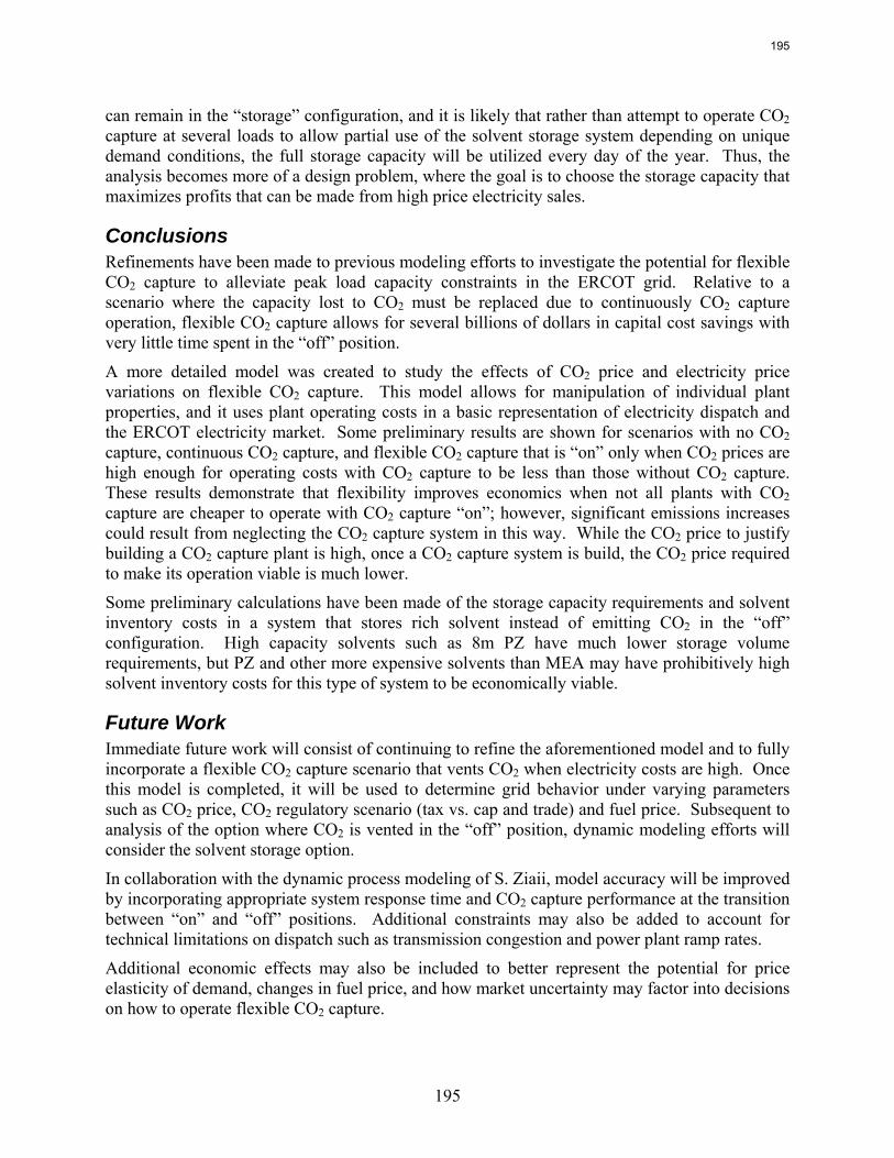
195

can remain in the “storage” configuration, and it is likely that rather than attempt to operate CO2 capture at several loads to allow partial use of the solvent storage system depending on unique demand conditions, the full storage capacity will be utilized every day of the year. Thus, the analysis becomes more of a design problem, where the goal is to choose the storage capacity that maximizes profits that can be made from high price electricity sales.

Conclusions Refinements have been made to previous modeling efforts to investigate the potential for flexible CO2 capture to alleviate peak load capacity constraints in the ERCOT grid. Relative to a scenario where the capacity lost to CO2 must be replaced due to continuously CO2 capture operation, flexible CO2 capture allows for several billions of dollars in capital cost savings with very little time spent in the “off” position.

A more detailed model was created to study the effects of CO2 price and electricity price variations on flexible CO2 capture. This model allows for manipulation of individual plant properties, and it uses plant operating costs in a basic representation of electricity dispatch and the ERCOT electricity market. Some preliminary results are shown for scenarios with no CO2 capture, continuous CO2 capture, and flexible CO2 capture that is “on” only when CO2 prices are high enough for operating costs with CO2 capture to be less than those without CO2 capture. These results demonstrate that flexibility improves economics when not all plants with CO2 capture are cheaper to operate with CO2 capture “on”; however, significant emissions increases could result from neglecting the CO2 capture system in this way. While the CO2 price to justify building a CO2 capture plant is high, once a CO2 capture system is build, the CO2 price required to make its operation viable is much lower.

Some preliminary calculations have been made of the storage capacity requirements and solvent inventory costs in a system that stores rich solvent instead of emitting CO2 in the “off” configuration. High capacity solvents such as 8m PZ have much lower storage volume requirements, but PZ and other more expensive solvents than MEA may have prohibitively high solvent inventory costs for this type of system to be economically viable.

Future Work Immediate future work will consist of continuing to refine the aforementioned model and to fully incorporate a flexible CO2 capture scenario that vents CO2 when electricity costs are high. Once this model is completed, it will be used to determine grid behavior under varying parameters such as CO2 price, CO2 regulatory scenario (tax vs. cap and trade) and fuel price. Subsequent to analysis of the option where CO2 is vented in the “off” position, dynamic modeling efforts will consider the solvent storage option.

In collaboration with the dynamic process modeling of S. Ziaii, model accuracy will be improved by incorporating appropriate system response time and CO2 capture performance at the transition between “on” and “off” positions. Additional constraints may also be added to account for technical limitations on dispatch such as transmission congestion and power plant ramp rates.

Additional economic effects may also be included to better represent the potential for price elasticity of demand, changes in fuel price, and how market uncertainty may factor into decisions on how to operate flexible CO2 capture.

195

196

References Bloomberg. Energy Prices. 2008. http://www.bloomberg.com/energy/. retrieved July 2, 2008. Davidson RM. Post-combustion carbon capture from coal fired plants – solvent scrubbing, IEA

Clean Coal Centre. 2007. ERCOT. 2006 Annual Report. 2006. ERCOT. Balancing Energy Services Market Clearing Prices for Energy Annual Report.

MCPER_MCPEL_2006.xls. 2006. Gibbins JR, Crane RI et al. Maximizing the Effectiveness of Post Combustions CO2 Capture

Systems. The Seventh International Conference on Greenhouse Gas Control Technologies: GHGT-7. E. S. Rubin, D. W. Keith and C. F. Gilboy. Vancouver, Canada, Oxford, UK.2005;I:139–146.

ICISpricing. (2008) from http://www.icispricing.com/. retrieved May 28, 2008. IEA and NEA. Projected Costs of Generating Electricity: 2005 Update. Paris, France, OECD.

2005 Lucquiaud M, Gibbins J. Carbon Dioxide Capture-Ready Steam Turbine Options for Post-

Combustion Capture Systems using Aqueous Solvents. London, UK, Imperial College London. 2008.

Metz B, Davidson O, et al. IPCC Special Report on Carbon Dioxide Capture and Storage. 2005. NEI. U.S. Electricity Production Costs and Components.

u.s._electricity_production_costs_and_components.xls. Washington, DC. 2007. Oyenekan B. Modeling of Strippers for CO2 capture by Aqueous Amines. University of Texas,

Austin; 2006. Ph.D Dissertation. 291. Oyenekan B, GT Rochelle. Alternative Stripper Configurations to Minimize Energy for CO2

Capture. GHGT-8. 2006. Parry IWH and Pizer WA. Emissions Trading versus CO2 Taxes versus Standards. Weathervane

Backgrounder. Washington D.C., Resources for the Future. 2007. PE-Ltd. 2006 State of the Market Report for the ERCOT Wholesale Electricity Markets,

Potomac Economics, Ltd. 2007. Rao AB, and Rubin ES. A Technical, Economic, and Environmental Assessment of Amine-

Based CO2 Capture Technology for Power Plant Greenhouse Gas Control. Environ. Sci. Technol. 2002;36(20):4467–4475.

Rochelle GT. Personal Communication. Austin. 2008. Rubin ES, Chen C, Rao AB. Cost and performance of fossil fuel power plants with CO2 capture

and storage. Energy Policy. 2007;35:4444–4454. USEIA. Average Cost of Coal Delivered for Electricity Generation by State, Year-to-Date

through October 2007 and 2006. epmxlfile4_10_b.xls, USDOE. 2007. USEIA. Texas Natural Gas Wellhead Price, USDOE. 2008. USEPA. Emissions & Generation Resource Integrated Database (eGRID).

eGRID2006_Version_2_1. 2007. USNETL. Cost and Performance Baseline for Fossil Energy Plants. Bituminous Coal and

Natural Gas to Electricity. JM Klara. 1. 2007.

196