Embed Size (px)
Citation preview
1
CO2 Capture by Aqueous Absorption Summary of 1st Quarterly Progress Reports 2009
Supported by the Luminant Carbon Management Program
and the
Industrial Associates Program for CO2 Capture by Aqueous Absorption
by Gary T. Rochelle
Department of Chemical Engineering
The University of Texas at Austin
May 3, 2009
Introduction This research program is focused on the technical obstacles to the deployment of CO2 capture and sequestration from flue gas by alkanolamine absorption/stripping and on integrating the design of the capture process with the aquifer storage/enhanced oil recovery process. The objective is to develop and demonstrate evolutionary improvements to monoethanolamine (MEA) absorption/stripping for CO2 capture from coal-fired flue gas. The Luminant Carbon Management Program and the Industrial Associates Program for CO2 Capture by Aqueous Absorption support 14 graduate students. These students have prepared detailed quarterly progress reports for the period January 1, 2009 to March 31, 2009. Five original paper manuscripts are included; Cohen et al., Freeman et al., Plaza et al., and two by Sexton. Three Ph.D. research proposals are attached: Freeman, Van Wagener, and Plaza. We have also attached Powerpoint presentations made by Rochelle and Closmann at the semiannual meeting of the Process Science and Technology Center.
Conclusions 7.7 m hydroxyethylpiperazine (HEP), 4.8 m aminomethylpropanol (AMP), and 8 m 2-piperidine ethanol provide a CO2 capacity of 0.7, 1.0, and 1.2 moles/mole (water+amine) and a normalized CO2 flux (kg’) at rich conditions of 2.9e-10, 1.7e-10, and 2.0e-10 kmol/s.PA.m2, respectively. These capacities are greater than 7 m MEA (0.5) and in the same range at 8 m PZ (0.8). The rates are less than MEA (3.1e-10) and piperazine (5.3e-10). The heat of CO2 desorption in the three new amines was 69, 73, and 73 kJ/mol, respectively compared to 70 for 8 m PZ and 82 for 7 m MEA.
Structured packing M250X (60o flow) provided 40% less pressure drop and 20% greater capacity than M250Y (45o), but the mass transfer area was practically the same.
Packing without surface texturing (M250YS) provided 20% less pressure drop and 10% less area than the comparable textured packing (M250X).
The PZ thermodynamic model developed by Hilliard has been successfully modified to represent accurately the VLE by Dugas and the heat capacity data by Nguyen. It now provides stable predictions up to 150 oC.
1
2
With 8 m PZ in a three-stage heated flash at 150 oC, the equivalent work requirement was 35.0 kJ/mol CO2, compared to 36.3 kJ/mol CO2 and 40.3 kJ/mol CO2 for simple strippers using 8 m PZ and 7 m MEA, respectively.
The activation energy for the thermal degradation of 7 m MDEA/2 m PZ is approximately 104 kJ/gmol. The thermal degradation rates of MDEA and PZ are 59 ± 25 and 66 ± 21 mmolal/day at 150 °C and 0.26 moles CO2/mole alkalinity.
Analyses of solution from the pilot plant campaign in Fall 2008 with concentrated piperazine showed no signs of oxidation or thermal degradation. Nor did these samples have any significant foaming tendency.
With 18 weeks at 150 oC, the degradation rate of 8 m PZ was 0.44%/week. The most prevalent degradation products identified were ethylenediamine (1.2 mM/wk), formate (0.9 mM /wk), and formamide (2.3 mM/wk).
For 8 m PZ solution with 0.306 CO2 loading, the total pressure is 0.9 bar at 100 ºC. For 8 m PZ solution with 0.424 CO2 loading, the total pressure is 24 bars at 150 ºC.
7 m MEA is approximately twice as volatile as 8 m PZ and is roughly 2.5 times more volatile than the 7m MDEA/2 m PZ. 5 m AMP 1.5–3 times more volatile than 7 m MEA.
In loaded PZ solutions the partial Cp for liquid PZ is approximately 2.33 J/g-K. The partial Cp of CO2 is only 0.76 J/g-K. The Cp of loaded 8 m PZ from 40 ºC–120 ºC varies from 3.1–3.6 J/g-K.
Inhibitor B reduced the apparent degradation of MEA by about 50% at a variety of catalyst conditions.
Thermal degradation of loaded MEA at anaerobic conditions in stainless steel bombs results in corrosion with production of up to 765 ppm Fe++, 400 ppm Ni++, and 300 ppm Cr+2.
Accurate modeling of absorber performance may require a Gaussian distribution of stage packing height, with a finer grid at the top and bottom of the column.
1. Wetted Wall Column Rate Measurements p. 11 by Xi Chen
The CO2 solubility and adsorption/desorption rate were measured in the wetted wall column for 7.7 m N-(2-hydroxyethyl)piperazine (HEP), 5 m 2-amino-2-methyl-1-propanol (AMP) and 8 m 2-piperidineethanol (2-PE). VLE models of CO2 were regressed from experimental data to calculate CO2 capacity and enthalpy of CO2 absorption (∆Habs). The liquid film mass transfer coefficients (kg’) and CO2 partial pressures (P*) obtained are compared to those of 8 m piperazine (PZ) and 7 m monoethanolamine (MEA).
2. Influence of Liquid Properties on Effective Mass Transfer Area of Structured Packing p. 22 by Robert Tsai (also supported by the Separations Research Program)
Two Sulzer structured packings were evaluated: an untextured (smooth) version of Mellapak 250Y (M250YS) and Mellapak 250X (M250X).
2
3
M250YS exhibited 15–20% lower pressure drop and hold-up than standard (textured) Mellapak 250Y (M250Y). Baseline (0.1 M NaOH) mass transfer tests revealed texture to have only a minor impact on effective area; measured area for M250YS was at most 10% lower than for M250Y. A reduction in surface tension to 30 dynes/cm appeared to impact both packings in the same manner, marginally increasing effective area (10%).
M250X displayed drastically better hydraulic performance than M250Y. Pressure drop was 40% that of M250Y, and capacity was 20% greater, although hold-up was only around 10% lower. Interestingly, mass transfer area did not suffer as a consequence of the improved hydraulics. While the measured area for M250X was observed to be lower than for M250Y, this was by a very small margin (less than 5%) – essentially indistinct relative to the experimental noise.
The mass transfer area database was updated, and the current global (ae/ap) correlation, able to represent the entire database within limits of ±15%, is as follows:
( )( )[ ] 116.03
1LL
p
e 327.1 −= FrWeaa
3. Modeling Stripper Performance for CO2 Removal p. 35 by David Van Wagener
Since Hilliard developed thermodynamic models for various amine solvents, additional experimental data has been collected at new conditions. The data primarily of interest has been for concentrated piperazine (PZ). The Hilliard model predicted well for low concentrations, 0.9 m–5 m, but 8 m PZ will be used in future simulations. VLE data collected by Dugas as well as heat capacity data collected by Nguyen for concentrated piperazine was incorporated into previous parameter regression files. The parameters to be regressed were reconsidered, and more focus was put on the heat capacity parameters of the dominant species at relevant loadings. The predictions by the newly regressed model were near-perfect for the relevant loading range, 0.3–0.4, and only had a maximum deviation of 5% at a loading of 0.2. The accuracy of the VLE predictions was not significantly compromised at these loadings with the new parameter values. The performance of multi-stage flash configurations with concentrated PZ was also assessed. Compressing to 150 atm, a three-stage flash operated with 8 m PZ had an equivalent work of 35.0 kJ/mol CO2 compared to the 40.3 kJ/mol CO2 required for a simple stripper using 7 m MEA.
4. Solvent Management of MDEA/Piperazine p. 50 by Fred Closmann
(also supported by the Process Science & Technology Center)
Thermal degradation experiments were conducted on 7 m MDEA/2 m PZ in the past quarter. The compounds dimethylaminoethanol (DMAE), diethanolamine (DEA), methylaminoethanol (MAE), ethylenediamine (EDA), methyl piperazine, dimethyl piperazine, and N,N-diethylethanolamine were identified in degraded solvent samples through ion chromatography mass spectrometry (IC-MS). MDEA and PZ degrade with a stoichiometric one-to-one relationship and a mechanism that may be first order in both amines, until the PZ has approached zero concentration. Thereafter, the loss of MDEA slows. Our findings are consistent with the literature which indicates that MDEA degrades through disproportionation processes, and can then react with piperazine (PZ) to form diamine compounds through arm-switching processes
3
4
when both MDEA and PZ are present in the solvent. The activation energy for the degradation of MDEA and PZ is approximately 104 kJ/gmol, and rates of degradation of MDEA and PZ are 59 ± 25 and 66 ± 21 mmolal/day at 150 °C and α=0.26.
5. Solvent Management of Concentrated Piperazine p. 59 by Stephanie Freeman
The solution analysis of the pilot plant was completed this quarter and all the measured values are reported. There is slight disagreement between the measurements taken at the pilot plant during the actual campaign and those completed afterward in the laboratory. There was not a significant production of degradation products with the highest concentrations of anions below 0.5 mM. A small amount of ethylenediamine (EDA) was detected with the samples ranging from 0.61 mM, well below the baseline detection limit of the cation IC, to 9.79 mM. A foaming test of the final campaign solution indicated that very little foaming occurred during the test. The foaminess coefficient of the solution was 44 x 10-3 m2-s compared to the coefficient of 27 x 10-3 m2-s for a neat 5 m PZ solution. The low foaminess coefficient and lack of degradation products indicates that PZ resisted oxidation and thermal degradation during the three-week pilot plant campaign.
The low gas flow apparatus was analyzed to determine the source of PZ loss when degradation products alone cannot account for it. A baseline experiment using nitrogen and CO2 was performed to determine the loss due to volatility. It was determined that volatility alone cannot account for the amount of PZ loss seen in a typical low gas flow experiment with 8 m PZ. Other probable causes such as liquid entrainment and dilution will be analyzed in the future.
A long term thermal degradation experiment demonstrated the thermal resistance of concentrated PZ. After 18 weeks at 150 °C, only 8.0% of the initial PZ was lost. This amounts to a loss only 0.44% of the original PZ per week. The most prevalent degradation products were EDA (1.2 mM/wk), formate (0.9 mM /wk), and formamide (2.3 mM/wk).
6. Thermal Degradation p. 77 by Jason Davis
Aqueous amine solutions loaded with CO2 were degraded in stainless steel sealed containers in forced convection ovens. Amine loss and degradation products were, measured as function of time by cation chromatography (IC), HPLC, and IC/mass spectrometry. A full kinetic model was developed for 15–40 wt % MEA (monoethanolamine) with 0.2–0.5 mol CO2/mol MEA at 100 oC to 150 oC. Experiments using amines blended with MEA demonstrate that oxazolidone formation is the rate-limiting step in the carbamate polymerization pathway. With 30 wt % MEA at 0.4 mol CO2/mol MEA and 120 oC for 16 weeks there is a 29% loss of MEA with 13% as hydroxyethylimidazolidone (HEIA), 9% as hydroxyethylethylenediamine (HEEDA), 4% as the cyclic urea of the MEA trimer, 1-[2-[(2-hydroxyethyl)amino]ethyl]-2-imidazolidone, 3% as the MEA trimer, 1-(2-hydroxyethyl)diethylenetriamine, and less than 1% as larger polymeric products. In the isothermal experimentals, thermal degradation was slightly more than first order with amine concentration and first order with CO2 concentration with an activation energy of 33 kcal/mol. In a modeled isobaric system, the amount of thermal degradation increased with stripper pressure, but decreased with an increase in amine concentration and CO2 concentration due to a reduction in reboiler temperature from the changing partial pressure of CO2. Three-fourths of thermal degradation in the stripper occurred in the reboiler due to the elevated
4

5
temperature and long residence time which offset the decrease in CO2 concentration compared to the packing.
7. Rate Measurements for MEA and PZ p. 150 by Ross E. Dugas
An Aspen Plus® RateSep™ model of the wetted wall column is being created to study the effects of CO2 mass transfer rates in monoethanolamine (MEA), piperazine (PZ) and MEA/PZ solutions. The model will simulate wetted wall column experiments which include 7–13 m MEA, 2–12 m PZ and 7 m MEA/2 m PZ solutions at temperatures of 40, 60, 80, and 100 ˚C.
The thermodynamic model from Hilliard (2008) was used as a starting point but required significant adjustments to accurately predict 7–13 m MEA, 2–12 m PZ, and 7 m MEA/2 m PZ. In order to accomplish this, higher amine concentration data was added into the regressions. Some of the lower amine concentration data and data which had CO2 loadings outside the relevant range for CO2 capture from flue gas were deleted. A special emphasis was put on obtaining good CO2 partial pressure predictions from the model. The model does have some trouble predicting CO2 partial pressure at the higher MEA concentrations, but it does a very good job of predicting CO2 partial pressure in the 7 and 9 m MEA, PZ and the 7 m MEA/2 m PZ blend solutions.
The Hilliard (2008) thermodynamic model does not consider physical properties since they do not affect thermodynamics. However, the rate-based model of the wetted wall column does require accurate physical properties. Density and viscosity parameters were regressed for 7–13 m MEA based on a literature correlation (Weiland, Dingman et al., 1998). Only density parameters were regressed for PZ. These data were obtained from Freeman (Rochelle, Dugas et al., 2008). Thus far, no adequate viscosity regression for PZ has been obtained. The model may require a Fortran subroutine to properly predict the viscosity of the PZ solutions.
The model cannot be designed geometrically like the wetted wall column in which the gas flows through an annulus. Although the model uses standard, cylindrical columns, it provides the same cross sectional area and wetted area as the wetted wall column. Fortran subroutines were coded to ensure the model used the same liquid and gas phase mass transfer coefficients as the wetted wall column.
The model utilizes 15 forward kinetic reactions, 15 reverse kinetic reactions, and 4 equilibrium reactions. The 15 reverse reactions are not independent and can be linked to the forward reaction rates by Keq relationships. Keq was calculated for 7 primary reactions (4 kinetic and 3 equilibrium) at 40, 60, 80, and 100 ˚C. Keq can be calculated for all 34 reactions using Keq combinations of the 7 primary reactions. The Keq values at the 4 temperatures were regressed into a form which translated easily to the power law rate expression Aspen Plus® uses to determine mass transfer. Using the Keq relationships, the reverse rate expression can be directly linked to the forward rate expressions. The 15 forward reactions can be simplified into 4 reactions in which rate constants scale by Bronsted theory (1928) depending on the catalyst. With these simplifications, the rate expression for only 4 reactions should need to be regressed by the wetted wall column data.
8. CO2 Absorption Modeling Using Aqueous Amines p. 167 by Jorge M. Plaza
5
6
An extensive literature search was conducted to develop a Ph.D. dissertation proposal. The results include a list of the most recent rate-based models for MEA. Although a number of models for MEA exist, only a few include a rigorous approach to the boundary layer problem. PROMAX and PROTREATTM are included in this list to illustrate commercially available software specialized in CO2 absorption/stripping. The complete list of models can be found in the attached proposal. For piperazine (PZ) most of the works found include it as a promoter so data are at lower concentrations than the proposed 8 m solvent. The only available data for concentrated PZ are from Freeman et al. (Freeman, Dugas et al. 2008).
9. Total Pressure Measurement of CO2 Loaded Aqueous Amines at High T and P p. 202 by Qing Xu, Martin Metzner
In this quarter a series of total pressure measurements were conducted to CO2 loaded 7 m monoethanolamine (MEA) or concentrated piperazine (PZ) at temperatures from 80 to 180 ºC. A 400 mL calorimeter and a 500 mL autoclave were used as equilibrium cells. The total pressure of 8 m PZ with 0.42 CO2 loading varied from 1.5 to 24 bar at 80 to 150 ºC. The total pressure of 7 m MEA with 0.48 CO2 loading is from 1.9 to 20 bar at 100 to 160 ºC.
The partial pressure of CO2 at each experimental condition was calculated by subtracting partial pressures of water and amines. The results fairly match the extrapolation curves of the low temperature data. The regression based on data from 40 to 180 ºC gives an empirical model for CO2 partial pressure over loaded aqueous PZ:
2
21ln 5.9 6.56ln (84.4 . / ) 21.3 13392 2.92COP T kJ mol RT T
αα α= − + − ⋅ − + + .
10. Volatility and heat capacity of amine alternatives p. 223 by Bich-Thu Nguyen
The volatility of amines is an important screening criterion used to evaluate its viability for use as a CO2 capture solvent. Several amine systems have been evaluated for volatility at absorber operating conditions, which are 40–60 ºC at nominal lean and rich loadings corresponding to about 500 Pa and 5000 Pa, respectively. In comparing different amine systems studied to date, the 7 m MDEA/2 m PZ blend appears to be the least volatile. It is roughly 2.5 times less volatile than the baseline 7 m MEA solvent. 8 m PZ is also a very viable amine candidate as it is only half as volatile as the baseline solvent. On the other hand, 5 m AMP appears to be the most volatile so far; in fact, it is 1.5–3 times more volatile than 7 m MEA at lean and rich conditions defined earlier. In the arena of heat capacity studies, the averaged Cp of 8 m PZ solutions is found to be approximately 3.1–3.6 J/g-K. The Cp of pure liquid PZ in these solutions is regressed to be 2.33 J/g-K and that of CO2 is approximately 0.76 J/g-K.
11. Oxidative Degradation of MEA p. 233 by Alex Voice
Oxidative degradation of monoethanolamine (MEA) was studied in the high gas flow (HGF) apparatus this quarter. The base case conditions, which remained constant in all experiments this quarter, were MEA concentration (30 wt % = 7 m = 4.8 M), loading (0.4 moles CO2/mole MEA), temperature (55 ºC), dry gas composition (17.5% O2, 2.1% CO2), and total solution
6
7
volume (350 mL). 5 mM of Inhibitor B decreased the degradation rate in the presence of 1 mM Fe, 0.1 mM Ni, 0.1 mM Cr, and 5 mM Cu by 43%; additional B did not result in a further decrease in degradation. 20 mM B decreased the degradation rate of MEA in the presence of 1mM Fe by 53%. Sodium sulfide initially increased ammonia production, but did not change the steady-state degradation rate. MEA degradation in the HGF apparatus was determined to be kinetically controlled in the presence of 50mM A, no catalyst, and an agitation rate of 1500 rpm. Heat stable salt concentrations (analyzed this quarter) from the HGF experiment described in a previous report (Rochelle et al., 2009) all increased with time except glycolate. MEA concentration decreased by 10% after 4300 minutes of degradation in this experiment.
A flame atomic absorption method was developed this quarter. Thermally degraded samples extracted from stainless steel bombs contained 115–765 ppm iron, 25–400 ppm nickel, and 37–300 ppm chromium. Solutions with no iron added were found to contain a range of iron concentrations; nonetheless, a T-test revealed that samples degraded for 2–3 hours in the HGF contain more iron than initial samples at 95% confidence. Flame AA was also used to determine the solubility of inhibitor B as .016 mM in a degraded solution.
12. Dynamic Operation of CO2 Capture p. 251 by Sepideh Ziaii
The work in the first quarter focused on dynamic modeling of the absorber for CO2 absorption by monoethanolamine (MEA) in Aspen Custom Modeler®. The absorber column is a packed bed divided into a number of segments. In this study, discrete Gaussian distribution is proposed as a new method for segmentation. The simulation results show that the Gaussian distribution gives more realistic McCabe-Thiele diagrams for low lean loading, e.g. 0.36; however, there is advantage to decreasing the required number of segments. We still need to consider an adequate number of segments to get an accurate CO2 removal. For higher lean loadings, e.g. 0.4 and 0.45, using Gaussian distribution with Lmax/Lmin≈10 (the ratio of maximum to minimum length of the segments) enables us to calculate the removal with sufficient accuracy with smaller number of segments and significantly decrease the computation time. The CPU time reduction is especifically beneficial for dynamic simulation and dynamic analysis.
13. Electric Grid Level Implications of Flexible CO2 Capture Operation p. 259 by Stuart Cohen
Flexible CO2 capture systems can choose how much CO2 to capture based on the competition between CO2 and electricity prices and a desire to either minimize operating costs or maximize operating profits. Coal and natural gas prices have varying degrees of predictability and volatility, and the relative prices of these fuels have a major impact on power plant operating costs and the resulting plant dispatch sequence. Because the chosen operating point in a flexible CO2 capture system affects net power plant efficiency, fuel prices also influence which CO2 capture operating point may be the most economical and the resulting dispatch of power plants with CO2 capture. This report contains an analysis of flexible CO2 capture in of how coal and natural gas prices affect the operation of flexible CO2 capture in the Electric Reliability Council of Texas (ERCOT) electric grid and the resulting economic and environmental impacts at the power plant and electric grid levels. All permutations of $1.5/MMBTU and $3/MMBTU coal and $6.6/MMBTU and $9.6/MMBTU are considered.
7
8
When choosing the operating point of a flexible CO2 capture system based on marginal costs alone, higher coal prices result in higher CO2 prices required to justify full-load CO2 capture because larger emissions cost reductions are necessary to offset the increased fuel costs of CO2 capture. When choosing a CO2 capture operating point based on the most profitable combination of cost, output, and electricity price, higher natural gas prices will increase the CO2 price needed to justify continuous full-load CO2 capture. Higher natural gas prices lead to increased electricity prices, so additional electricity sales during partial- or zero-load CO2 capture offset CO2 emissions costs at higher CO2 prices. Coal prices had little effect on profit-motivated flexible CO2 capture, demonstrating that the value of electricity on the grid is more important to profitability than the value of electricity at the plant. For each fuel price combination, there are ranges of CO2 prices where profit-motivated flexible CO2 capture can allow greater operating profits over those without CO2 capture, with inflexible CO2 capture, and with flexible capture based on marginal costs. These CO2 price ranges increase and the benefits grow as natural gas prices rise and as coal prices fall for a given natural gas price. Across eight coal-fired plants in ERCOT, annual operating profits in these CO2 price regimes could be several $100 millions greater than those earned with inflexible or cost driven flexible CO2 capture and $10s to ~$100s million greater than with no CO2 capture.
14. Modeling Absorber/Stripper Performance with MDEA/PZ p. 283 by Peter Frailie
The goal of this study is to evaluate the performance of an absorber/stripper operation that utilizes the MDEA/PZ blended amine system. Due to the complexity of this system the model will be developed in several smaller, more manageable parts that can later be combined to form the final model. The first section that will be developed is an MDEA/PZ model based on thermodynamic data, which must initially be developed as separate MDEA and PZ models. Once the MDEA/PZ model has been completed it must be incorporated into separate absorber and stripper models similar to those developed by Van Wagener and Plaza. Those models can then be combined to form the final MDEA/PZ absorber/stripper model. This study is currently in the process of developing the MDEA/PZ model based on thermodynamic data. Over the next three months the thermodynamic model should be completed and work should have begun on the absorber and stripper models.
15. Measurement of Packing Liquid Phase Film Mass Transfer Coefficient p. 286 by Chao Wang
Packings are widely used in distillation, stripping, and scrubbing processes because of their relatively low pressure drop and good mass transfer efficiency. Since the post combustion carbon capture process will require an operationally expensive fan, the absorber contains high performance packing to minimize pressure drop and maximize mass transfer efficiency. The design of packed absorbers for carbon dioxide capture will require the reliable measurement and accurate prediction of the liquid film mass transfer coefficient. A variety of experimental methods of measuring liquid side mass transfer coefficient kLa have been explored and reported.
Chemical reaction enhanced and physical liquid phase film mass transfer coefficients are discussed in this report. Test systems are chosen where the gas film mass transfer resistance is negligible compared to the liquid resistance. Therefore the liquid phase film mass transfer
8
9
coefficient (kLa) may be calculated directly from the values of KoLa or KoGa. Suitable systems are stripping of toluene from water or absorption of toluene with water, absorption of pure gas (O2/H2/CO2) with water, and desorption of O2 from water with pure N2 stream. The physical liquid side mass transfer coefficient kL can be calculated by dividing the measured kLa by the measured gas/liquid contact area. Measurement of the gas/liquid contact area has been discussed by Tsai and reported by Lewis and Seibert of the Separations Research Program.
Predictive models of the liquid phase film mass transfer coefficient (kL) are discussed in this quarterly report, which focuses on a preliminary literature review of liquid film mass transfer coefficient measurements and models. A highly accurate SO2 analyzer has been purchased using Process Science and Technology Center funds provided by the project co-advisor, Frank Seibert. It is currently being installed and will be used for packing studies planned for the summer.
Attachments Freeman, S.A. et al. “Carbon dioxide capture with concentrated, aqueous piperazine” p. 305 Plaza, J.M. et al. “Modeling CO2 Capture with Aqueous Monoethanolamine” p. 318 Sexton, A.J. & Rochelle, G.T. “Effect of Catalysts and Inhibitors on the Oxidative Degradation
of Aqueous Monoethanolamine” p. 332 Sexton, A.J. & Rochelle, G.T. “Reaction Products from the Oxidative Degradation of MEA” p. 366 Freeman, S.A. Research Proposal p. 387 Van Wagener, D.H. Research Proposal p. 408 Rochelle, G.T. “Amine Selection for CO2 Capture to Minimize Energy” (presentation given at
PSTC meeting, April 2009) p. 462 Closmann, F.B. “Management of MDEA/PZ for CO2 Capture”(presentation given at PSTC
meeting, April 2009) p. 482
9

10
1
Wetted Wall Column Rate Measurements
Quarterly Report for January 1 – March 31, 2009
by Xi Chen
Supported by the Luminant Carbon Management Program
and the
Industrial Associates Program for CO2 Capture by Aqueous Absorption
Department of Chemical Engineering
The University of Texas at Austin
April 30, 2009
Abstract The CO2 solubility and adsorption/desorption rate were measured in the wetted wall column for 7.7 m N-(2-hydroxyethyl)piperazine (HEP), 5 m 2-amino-2-methyl-1-propanol (AMP), and 8 m 2-piperidineethanol (2-PE). VLE models of CO2 were regressed from experimental data to calculate CO2 capacity and enthalpy of CO2 absorption (∆Habs). The liquid film mass transfer coefficients (kg’) and CO2 partial pressures (P*) obtained are compared to those of 8 m piperazine (PZ) and 7 m monoethanolamine (MEA).
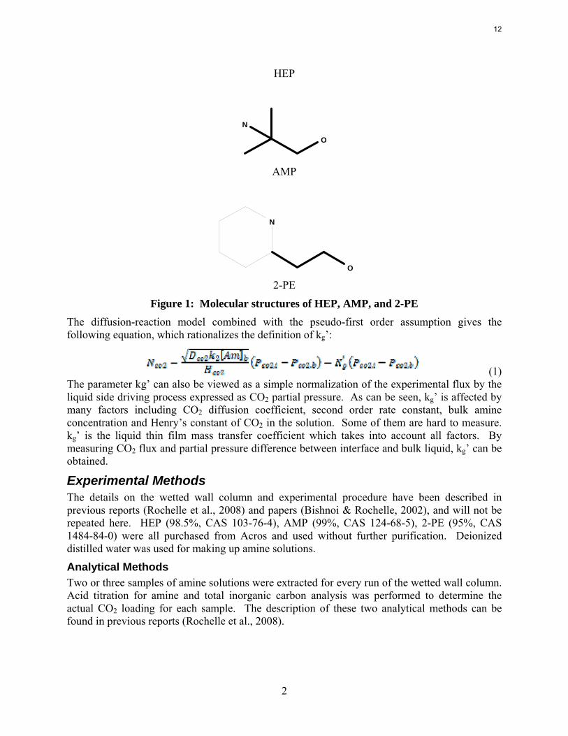
Introduction CO2 absorption/desorption data and partial pressure have previously been measured and reported for MEA, PZ and MEA/PZ (Rochelle et al., 2008). Despite their high absorption/desorption rates, primary amines have relatively low CO2 capacity and high heat of absorption. HEP (N-(2-hydroxyethyl)piperazine), virtually a combination of PZ and MEA, has both primary and tertiary amine groups in its molecule (Figure 1), which could possibly give the advantages of both primary and tertiary amines. However, currently there is no open literature reporting kinetic rates of CO2 absorption for HEP. Sterically hindered amines like AMP (2-amino-2-methyl-1-propanol) and 2-PE(2-piperidineethanol) are also of interest because of the high CO2 capacity due to very low carbamate stability. Although there are some kinetics data available on AMP (Xu et al., 1996; Mandal and Bandyopadhyay, 2006; Zhang et al., 2007) and 2-PE (Paul et al., 2009) in terms of secondary-order reaction rate, most of them measure rates with low amine concentration at zero or low CO2 loading. A complete measurement of kg’ and P* over different CO2 loading at high amine concentration are the focus of this study.
N
O
N
11
2
HEP
O
N
AMP
N
O 2-PE
Figure 1: Molecular structures of HEP, AMP, and 2-PE The diffusion-reaction model combined with the pseudo-first order assumption gives the following equation, which rationalizes the definition of kg’:
(1) The parameter kg’ can also be viewed as a simple normalization of the experimental flux by the liquid side driving process expressed as CO2 partial pressure. As can be seen, kg’ is affected by many factors including CO2 diffusion coefficient, second order rate constant, bulk amine concentration and Henry’s constant of CO2 in the solution. Some of them are hard to measure. kg’ is the liquid thin film mass transfer coefficient which takes into account all factors. By measuring CO2 flux and partial pressure difference between interface and bulk liquid, kg’ can be obtained.
Experimental Methods The details on the wetted wall column and experimental procedure have been described in previous reports (Rochelle et al., 2008) and papers (Bishnoi & Rochelle, 2002), and will not be repeated here. HEP (98.5%, CAS 103-76-4), AMP (99%, CAS 124-68-5), 2-PE (95%, CAS 1484-84-0) were all purchased from Acros and used without further purification. Deionized distilled water was used for making up amine solutions.
Analytical Methods Two or three samples of amine solutions were extracted for every run of the wetted wall column. Acid titration for amine and total inorganic carbon analysis was performed to determine the actual CO2 loading for each sample. The description of these two analytical methods can be found in previous reports (Rochelle et al., 2008).
12
3
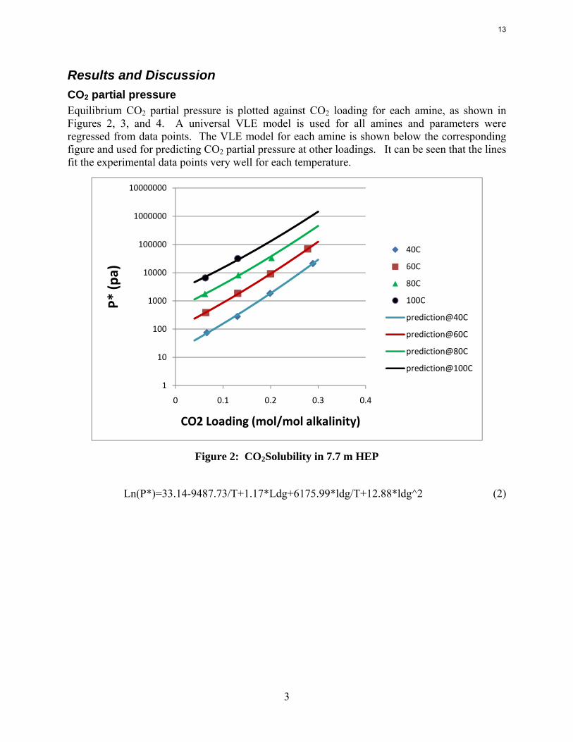
Results and Discussion CO2 partial pressure Equilibrium CO2 partial pressure is plotted against CO2 loading for each amine, as shown in Figures 2, 3, and 4. A universal VLE model is used for all amines and parameters were regressed from data points. The VLE model for each amine is shown below the corresponding figure and used for predicting CO2 partial pressure at other loadings. It can be seen that the lines fit the experimental data points very well for each temperature.
1
10
100
1000
10000
100000
1000000
10000000
0 0.1 0.2 0.3 0.4
P* (p
a)
CO2 Loading (mol/mol alkalinity)
40C
60C
80C
100C
prediction@40C
prediction@60C
prediction@80C
prediction@100C
Figure 2: CO2Solubility in 7.7 m HEP
Ln(P*)=33.14-9487.73/T+1.17*Ldg+6175.99*ldg/T+12.88*ldg^2 (2)
13
4
1
10
100
1000
10000
100000
1000000
0 0.2 0.4 0.6 0.8
P* (p
a)
CO2 Loading (mol/mol alkalinity)
40C
60C
80C
100C
prediction@40C
prediction@60C
prediction@80C
prediction@100C
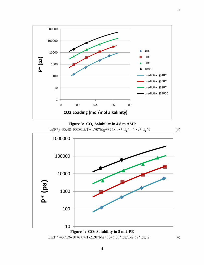
Figure 3: CO2 Solubility in 4.8 m AMP
Ln(P*)=35.48-10080.5/T+1.70*ldg+3258.08*ldg/T-4.89*ldg^2 (3)
10
100
1000
10000
100000
1000000
P* (p
a)
Figure 4: CO2 Solubility in 8 m 2-PE
Ln(P*)=37.26-10767.7/T-2.20*ldg+3845.03*ldg/T-2.57*ldg^2 (4)
14
5
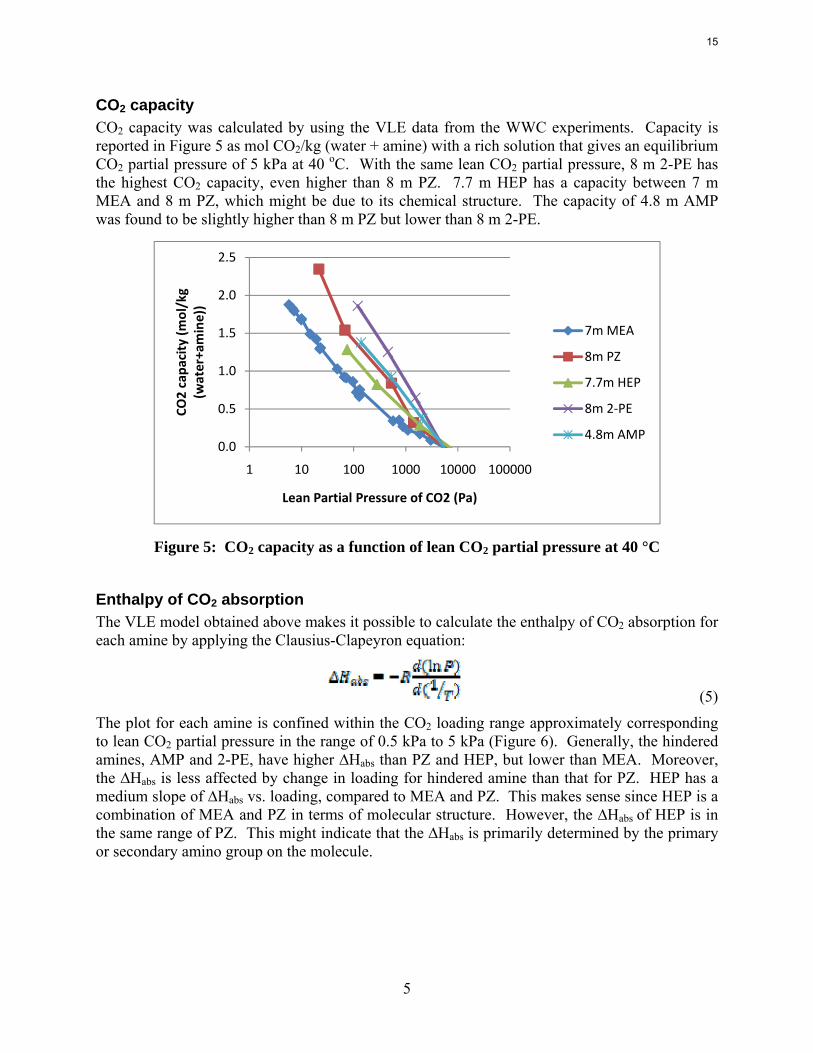
CO2 capacity CO2 capacity was calculated by using the VLE data from the WWC experiments. Capacity is reported in Figure 5 as mol CO2/kg (water + amine) with a rich solution that gives an equilibrium CO2 partial pressure of 5 kPa at 40 oC. With the same lean CO2 partial pressure, 8 m 2-PE has the highest CO2 capacity, even higher than 8 m PZ. 7.7 m HEP has a capacity between 7 m MEA and 8 m PZ, which might be due to its chemical structure. The capacity of 4.8 m AMP was found to be slightly higher than 8 m PZ but lower than 8 m 2-PE.
0.0
0.5
1.0
1.5
2.0
2.5
1 10 100 1000 10000 100000
CO2 capa
city (m
ol/kg
(water+amine))
Lean Partial Pressure of CO2 (Pa)
7m MEA
8m PZ
7.7m HEP
8m 2‐PE
4.8m AMP
Figure 5: CO2 capacity as a function of lean CO2 partial pressure at 40 °C
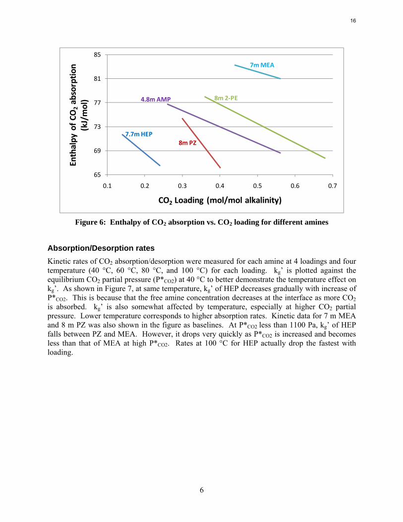
Enthalpy of CO2 absorption The VLE model obtained above makes it possible to calculate the enthalpy of CO2 absorption for each amine by applying the Clausius-Clapeyron equation:
(5)
The plot for each amine is confined within the CO2 loading range approximately corresponding to lean CO2 partial pressure in the range of 0.5 kPa to 5 kPa (Figure 6). Generally, the hindered amines, AMP and 2-PE, have higher ∆Habs than PZ and HEP, but lower than MEA. Moreover, the ∆Habs is less affected by change in loading for hindered amine than that for PZ. HEP has a medium slope of ∆Habs vs. loading, compared to MEA and PZ. This makes sense since HEP is a combination of MEA and PZ in terms of molecular structure. However, the ∆Habs of HEP is in the same range of PZ. This might indicate that the ∆Habs is primarily determined by the primary or secondary amino group on the molecule.
15
6
65
69
73
77
81
85
0.1 0.2 0.3 0.4 0.5 0.6 0.7
Enthalpy
of C
O2absorptio
n (kJ/mol)
CO2 Loading (mol/mol alkalinity)
7.7m HEP
8m 2‐PE4.8m AMP
8m PZ
7m MEA
Figure 6: Enthalpy of CO2 absorption vs. CO2 loading for different amines
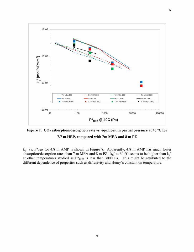
Absorption/Desorption rates Kinetic rates of CO2 absorption/desorption were measured for each amine at 4 loadings and four temperature (40 °C, 60 °C, 80 °C, and 100 °C) for each loading. kg’ is plotted against the equilibrium CO2 partial pressure (P*CO2) at 40 °C to better demonstrate the temperature effect on kg’. As shown in Figure 7, at same temperature, kg’ of HEP decreases gradually with increase of P*CO2. This is because that the free amine concentration decreases at the interface as more CO2 is absorbed. kg’ is also somewhat affected by temperature, especially at higher CO2 partial pressure. Lower temperature corresponds to higher absorption rates. Kinetic data for 7 m MEA and 8 m PZ was also shown in the figure as baselines. At P*CO2 less than 1100 Pa, kg’ of HEP falls between PZ and MEA. However, it drops very quickly as P*CO2 is increased and becomes less than that of MEA at high P*CO2. Rates at 100 °C for HEP actually drop the fastest with loading.
16
7
1E-08
1E-07
1E-06
1E-05
10 100 1000 10000 100000
k g' (
mol
/s. P
a.m
2 )
P*CO2 @ 40C (Pa)
7m MEA 40C 7m MEA 60C 7m MEA 80C 7m MEA 100C
8m Pz 40C 8m Pz 60C 8m PZ 80C 8m PZ 100C
7.7m HEP 40C 7.7m HEP 60C 7.7m HEP 80C 7.7m HEP 100C
Figure 7: CO2 asborption/desorption rate vs. equilibrium partial pressure at 40 °C for
7.7 m HEP, compared with 7m MEA and 8 m PZ
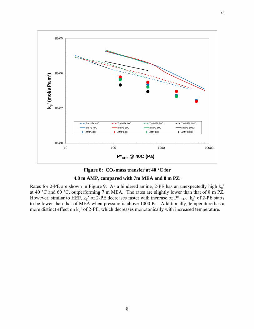
kg’ vs. P*CO2 for 4.8 m AMP is shown in Figure 8. Apparently, 4.8 m AMP has much lower absorption/desorption rates than 7 m MEA and 8 m PZ. kg’ at 60 °C seems to be higher than kg’ at other temperatures studied as P*CO2 is less than 3000 Pa. This might be attributed to the different dependence of properties such as diffusivity and Henry’s constant on temperature.
17
8
1E-08
1E-07
1E-06
1E-05
10 100 1000 10000
k g' (
mol
/s. P
a.m
2 )
P*CO2 @ 40C (Pa)
7m MEA 40C 7m MEA 60C 7m MEA 80C 7m MEA 100C
8m Pz 40C 8m Pz 60C 8m PZ 80C 8m PZ 100C
AMP 40C AMP 60C AMP 80C AMP 100C
Figure 8: CO2 mass transfer at 40 °C for
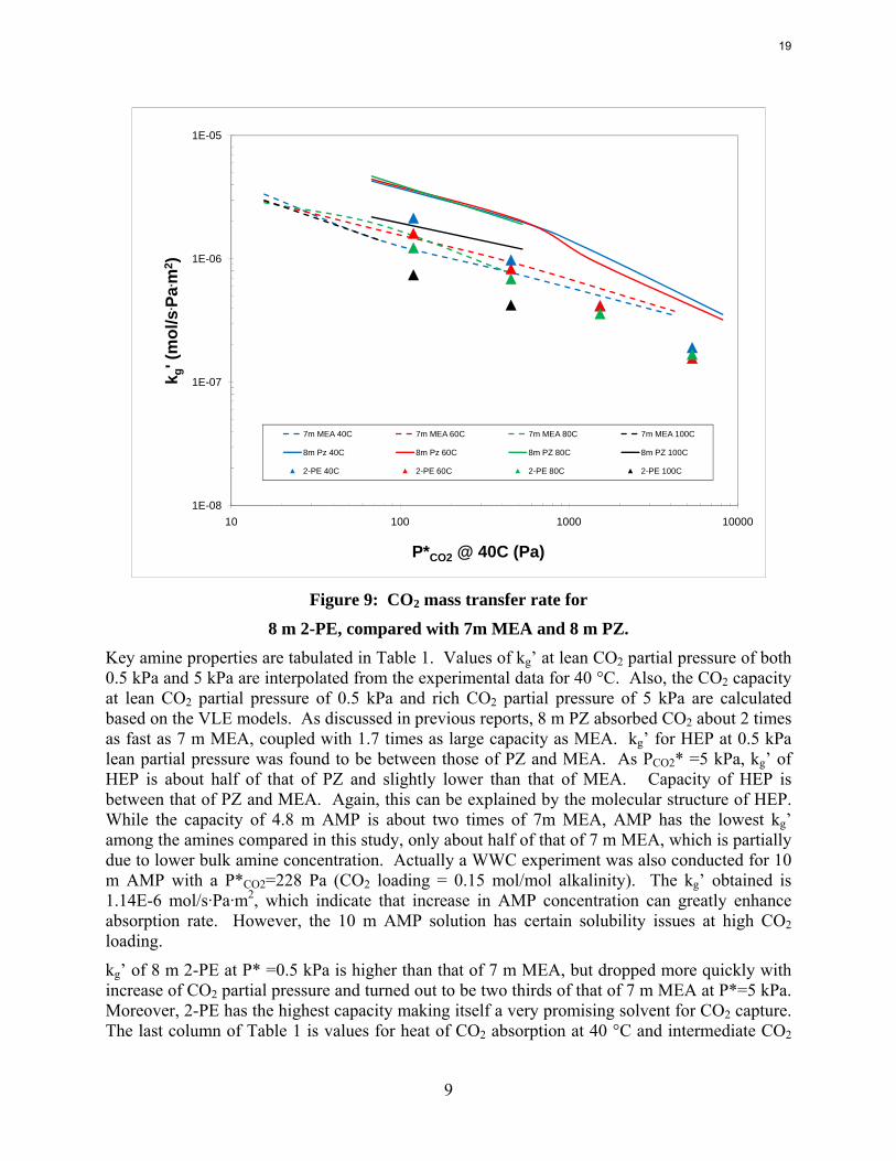
4.8 m AMP, compared with 7m MEA and 8 m PZ. Rates for 2-PE are shown in Figure 9. As a hindered amine, 2-PE has an unexpectedly high kg’ at 40 °C and 60 °C, outperforming 7 m MEA. The rates are slightly lower than that of 8 m PZ. However, similar to HEP, kg’ of 2-PE decreases faster with increase of P*CO2. kg’ of 2-PE starts to be lower than that of MEA when pressure is above 1000 Pa. Additionally, temperature has a more distinct effect on kg’ of 2-PE, which decreases monotonically with increased temperature.
18
9
1E-08
1E-07
1E-06
1E-05
10 100 1000 10000
k g' (
mol
/s. P
a.m
2 )
P*CO2 @ 40C (Pa)
7m MEA 40C 7m MEA 60C 7m MEA 80C 7m MEA 100C
8m Pz 40C 8m Pz 60C 8m PZ 80C 8m PZ 100C
2-PE 40C 2-PE 60C 2-PE 80C 2-PE 100C
Figure 9: CO2 mass transfer rate for
8 m 2-PE, compared with 7m MEA and 8 m PZ. Key amine properties are tabulated in Table 1. Values of kg’ at lean CO2 partial pressure of both 0.5 kPa and 5 kPa are interpolated from the experimental data for 40 °C. Also, the CO2 capacity at lean CO2 partial pressure of 0.5 kPa and rich CO2 partial pressure of 5 kPa are calculated based on the VLE models. As discussed in previous reports, 8 m PZ absorbed CO2 about 2 times as fast as 7 m MEA, coupled with 1.7 times as large capacity as MEA. kg’ for HEP at 0.5 kPa lean partial pressure was found to be between those of PZ and MEA. As PCO2* =5 kPa, kg’ of HEP is about half of that of PZ and slightly lower than that of MEA. Capacity of HEP is between that of PZ and MEA. Again, this can be explained by the molecular structure of HEP. While the capacity of 4.8 m AMP is about two times of 7m MEA, AMP has the lowest kg’ among the amines compared in this study, only about half of that of 7 m MEA, which is partially due to lower bulk amine concentration. Actually a WWC experiment was also conducted for 10 m AMP with a P*CO2=228 Pa (CO2 loading = 0.15 mol/mol alkalinity). The kg’ obtained is 1.14E-6 mol/s·Pa·m2, which indicate that increase in AMP concentration can greatly enhance absorption rate. However, the 10 m AMP solution has certain solubility issues at high CO2 loading.
kg’ of 8 m 2-PE at P* =0.5 kPa is higher than that of 7 m MEA, but dropped more quickly with increase of CO2 partial pressure and turned out to be two thirds of that of 7 m MEA at P*=5 kPa. Moreover, 2-PE has the highest capacity making itself a very promising solvent for CO2 capture. The last column of Table 1 is values for heat of CO2 absorption at 40 °C and intermediate CO2
19
10
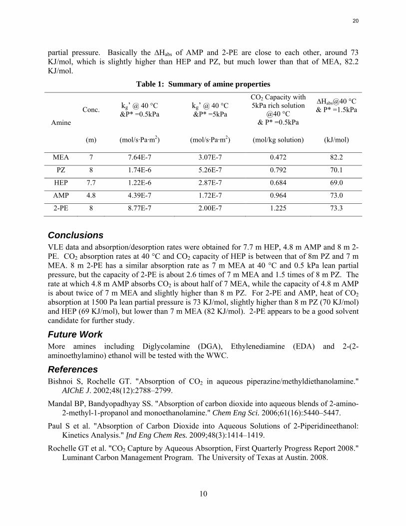
partial pressure. Basically the ∆Habs of AMP and 2-PE are close to each other, around 73 KJ/mol, which is slightly higher than HEP and PZ, but much lower than that of MEA, 82.2 KJ/mol.
Table 1: Summary of amine properties
Conc. kg’ @ 40 °C &P* =0.5kPa
kg’ @ 40 °C &P* =5kPa
CO2 Capacity with 5kPa rich solution
@40 °C & P* =0.5kPa
∆Habs@40 °C& P* =1.5kPa
Amine
(m) (mol/s·Pa·m2) (mol/s·Pa·m2) (mol/kg solution) (kJ/mol)
MEA 7 7.64E-7 3.07E-7 0.472 82.2
PZ 8 1.74E-6 5.26E-7 0.792 70.1
HEP 7.7 1.22E-6 2.87E-7 0.684 69.0
AMP 4.8 4.39E-7 1.72E-7 0.964 73.0
2-PE 8 8.77E-7 2.00E-7 1.225 73.3
Conclusions VLE data and absorption/desorption rates were obtained for 7.7 m HEP, 4.8 m AMP and 8 m 2-PE. CO2 absorption rates at 40 °C and CO2 capacity of HEP is between that of 8m PZ and 7 m MEA. 8 m 2-PE has a similar absorption rate as 7 m MEA at 40 °C and 0.5 kPa lean partial pressure, but the capacity of 2-PE is about 2.6 times of 7 m MEA and 1.5 times of 8 m PZ. The rate at which 4.8 m AMP absorbs CO2 is about half of 7 MEA, while the capacity of 4.8 m AMP is about twice of 7 m MEA and slightly higher than 8 m PZ. For 2-PE and AMP, heat of CO2 absorption at 1500 Pa lean partial pressure is 73 KJ/mol, slightly higher than 8 m PZ (70 KJ/mol) and HEP (69 KJ/mol), but lower than 7 m MEA (82 KJ/mol). 2-PE appears to be a good solvent candidate for further study.
Future Work More amines including Diglycolamine (DGA), Ethylenediamine (EDA) and 2-(2-aminoethylamino) ethanol will be tested with the WWC.
References Bishnoi S, Rochelle GT. "Absorption of CO2 in aqueous piperazine/methyldiethanolamine."
AIChE J. 2002;48(12):2788–2799.
Mandal BP, Bandyopadhyay SS. "Absorption of carbon dioxide into aqueous blends of 2-amino-2-methyl-1-propanol and monoethanolamine." Chem Eng Sci. 2006;61(16):5440–5447.
Paul S et al. "Absorption of Carbon Dioxide into Aqueous Solutions of 2-Piperidineethanol: Kinetics Analysis." Ind Eng Chem Res. 2009;48(3):1414–1419.
Rochelle GT et al. "CO2 Capture by Aqueous Absorption, First Quarterly Progress Report 2008." Luminant Carbon Management Program. The University of Texas at Austin. 2008.
20
11
Rochelle GT et al. "CO2 Capture by Aqueous Absorption, Second Quarterly Progress Report 2008." Luminant Carbon Management Program. The University of Texas at Austin. 2008.
Rochelle GT et al. "CO2 Capture by Aqueous Absorption, Third Quarterly Progress Report 2008." Luminant Carbon Management Program. The University of Texas at Austin. 2008.
Rochelle GT et al. "CO2 Capture by Aqueous Absorption, Fourth Quarterly Progress Report 2008." Luminant Carbon Management Program. The University of Texas at Austin. 2009.
Xu S et al. "Kinetics of the reaction of carbon dioxide with 2-amino-2-methyl-1-propanol solutions." Chem Eng Sci. 1996;51(6):841–50.
Zhang P et al. "Kinetics region and model for mass transfer in carbon dioxide absorption into aqueous solution of 2-amino-2-methyl-1-propanol." Sep Purif Technol. 2007;56(3):340–347.
21
1
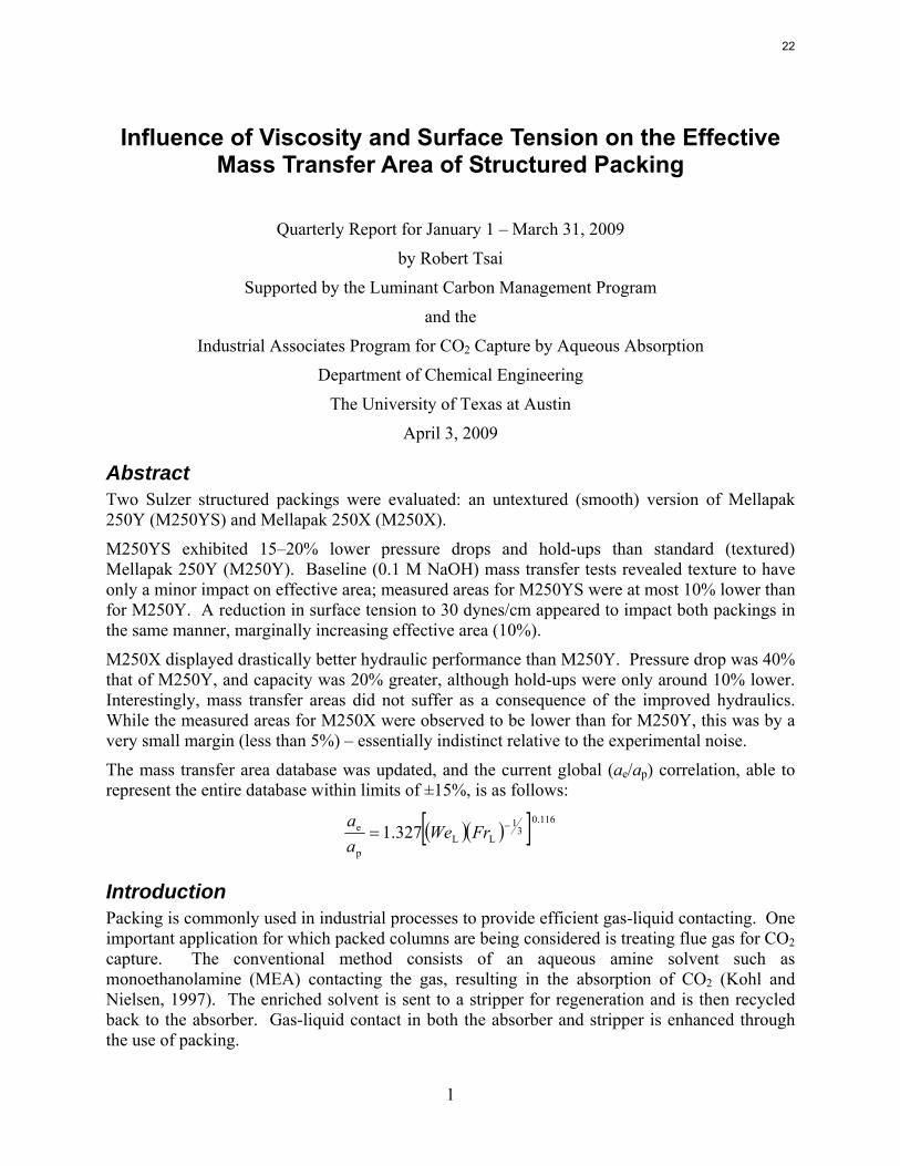
Influence of Viscosity and Surface Tension on the Effective Mass Transfer Area of Structured Packing
Quarterly Report for January 1 – March 31, 2009
by Robert Tsai
Supported by the Luminant Carbon Management Program
and the
Industrial Associates Program for CO2 Capture by Aqueous Absorption
Department of Chemical Engineering
The University of Texas at Austin
April 3, 2009
Abstract Two Sulzer structured packings were evaluated: an untextured (smooth) version of Mellapak 250Y (M250YS) and Mellapak 250X (M250X).
M250YS exhibited 15–20% lower pressure drops and hold-ups than standard (textured) Mellapak 250Y (M250Y). Baseline (0.1 M NaOH) mass transfer tests revealed texture to have only a minor impact on effective area; measured areas for M250YS were at most 10% lower than for M250Y. A reduction in surface tension to 30 dynes/cm appeared to impact both packings in the same manner, marginally increasing effective area (10%).
M250X displayed drastically better hydraulic performance than M250Y. Pressure drop was 40% that of M250Y, and capacity was 20% greater, although hold-ups were only around 10% lower. Interestingly, mass transfer areas did not suffer as a consequence of the improved hydraulics. While the measured areas for M250X were observed to be lower than for M250Y, this was by a very small margin (less than 5%) – essentially indistinct relative to the experimental noise.
The mass transfer area database was updated, and the current global (ae/ap) correlation, able to represent the entire database within limits of ±15%, is as follows:
( )( )[ ] 116.03
1LL
p
e 327.1 −= FrWeaa
Introduction Packing is commonly used in industrial processes to provide efficient gas-liquid contacting. One important application for which packed columns are being considered is treating flue gas for CO2 capture. The conventional method consists of an aqueous amine solvent such as monoethanolamine (MEA) contacting the gas, resulting in the absorption of CO2 (Kohl and Nielsen, 1997). The enriched solvent is sent to a stripper for regeneration and is then recycled back to the absorber. Gas-liquid contact in both the absorber and stripper is enhanced through the use of packing.
22
2
Reliable mass transfer models are important for design and analysis of these systems. A critical factor involved in modeling is the prediction of the effective interfacial area of packing (ae), which can be considered as the total gas-liquid contact area that is actively available for mass transfer. The current research effort is focused on this parameter. The effective area is especially critical for CO2 capture by amine absorption, because the CO2 absorption rate typically becomes independent of conventional mass transfer coefficients (kG or kL
0) but remains directly proportional to the area. Thus, it is highly desirable to have an accurate area model.
Numerous packing area correlations have been presented in the literature, but none has been shown to be predictive over a wide range of conditions. The Rocha-Bravo-Fair (Rocha et al., 1996) and Billet-Schultes (1993) models, two of the more widely used correlations for structured packing, seem to be notably poor in their predictions involving aqueous systems (Tsai et al., 2008). Wang et al. (2005) performed a comprehensive review of the available models. The various correlations predict different and sometimes even contradictory effects of liquid viscosity and surface tension, properties that would be expected to fundamentally influence the wetted area of packing. It is evident that their role is not well understood, and there is a definite need for work in this subject matter.
Limited understanding of the fluid mechanics and mass transfer phenomena in packed columns has been noted, and the need for experiments over a broader range of conditions has been identified (Wang et al., 2005). The Separations Research Program (SRP) at the University of Texas at Austin has the capability of measuring packing mass transfer areas. Measurements are performed by absorbing CO2 from air with 0.1 M NaOH in a 427 mm (16.8 in) ID column. However, it is potentially inaccurate to extend these results to other fluids of interest, such as amine solvents, due to variations in viscosity and surface tension.
The goal of this research is to ultimately develop an improved effective area model for structured packing. The general objectives are to:
• Develop a fundamental understanding of the fluid mechanics associated with structured packing operation;
• Determine suitable chemical reagents to modify the surface tension and viscosity of the aqueous caustic solutions employed to make packing area measurements, and characterize potential impacts of such additives on the CO2-NaOH reaction kinetics;
• Expand the SRP database by measuring the hydraulic performance and mass transfer areas of several different structured packings over a range of liquid viscosities and surface tensions;
• Combine the data and theory into a semi-empirical model that captures the features of the tested systems and adequately represents effective area as a function of viscosity, surface tension, and liquid load.
Experimental Methods
Packed Column The packed column had an outside diameter of 460 mm (18 in), inside diameter of 427 mm (16.8 in), and a 3 m (10 ft) packed height. For details regarding the apparatus and procedure for mass transfer or hydraulic tests, earlier quarterly reports may be consulted.
23
3
Goniometer The goniometer (ramé-hart Inc., Model #100-00) included an adjustable stage, a syringe support arm, a computer-linked camera for live image display, and a light source (see Q3 2006 report). This system was used in conjunction with FTA32 Video 2.0 software (developed by First Ten Angstroms, Inc.) to make surface tension measurements via the pendant drop method.
Materials A nonionic surfactant, TergitolTM NP-7 (Dow), was used to reduce the surface tension of solutions. Dow Corning® Q2-3183A antifoam was used for foam suppression.
Results and Discussion
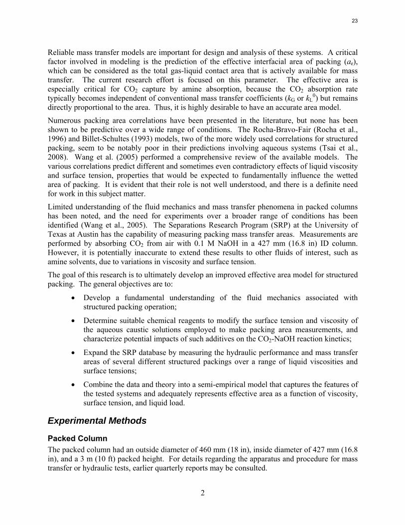
Mellapak 250Y (Smooth) (M250YS) – Mass Transfer Aside from the obvious texture difference, the smooth Mellapak 250Y packing (M250YS) appeared to be identical to standard Mellapak 250Y (M250Y) in all regards (i.e. channel dimensions and perforations). Both packings were assumed to have a specific area of 250 m2/m3. Figure 1 displays mass transfer area results for baseline (0.1 M NaOH) and low surface tension conditions (30 dynes/cm). The data at a given liquid load have been averaged in each case for clarity.
0.6
0.7
0.8
0.9
1
1.1
1.2
0 5 10 15 20 25 30
Fra
ctio
nal
are
a, a
e/a p
Liquid load (gpm/ft2)
M250Y - Baseline30 dynes/cm
M250YS - Baseline30 dynes/cm
Figure 1: M250Y and M250YS (ap = 250 m2/m3) mass transfer area data.
It was anticipated that surface texture would primarily have an impact at low liquid loads (i.e. 5 gpm/ft2 and below), due to limited liquid spreading in this regime. That is, M250YS was expected to exhibit significantly lower effective areas than M250Y at these conditions but perform similarly at higher loads. However, the baseline data show a small (10%) albeit
24
4
consistent depression across the entire range of experimental liquid rates. It would appear that texture has a rather minor impact on the effective mass transfer area. Surface tension was also expected to be more of a factor at low liquid loads. The results, though, indicate a fairly constant effect due to the reduced surface tension, with both packings exhibiting a slight improvement (10%) in effective area.
It is conceivable that texture might increase the effective mass transfer area via two mechanisms: greater liquid spreading and enhanced turbulence (McGlamery, 1988). If the divergence in the baseline data sets could be attributed to liquid spreading, then M250YS should have benefitted more than M250Y from an increase in liquid load or a decrease in surface tension. This was not the case. Therefore, turbulence would seem to be the more reasonable explanation when interpreting the baseline data.
The equivalent impact of surface tension for the two packings might be justified by considering mechanisms like liquid pooling or formation of satellite droplets, which would not necessarily be influenced by texture. Droplets could arise from liquid falling through perforations (common feature to both packings) or off the underside of the channels. The two packings had identical channel dimensions, so the underside liquid drop-off phenomena would presumably be analogous.
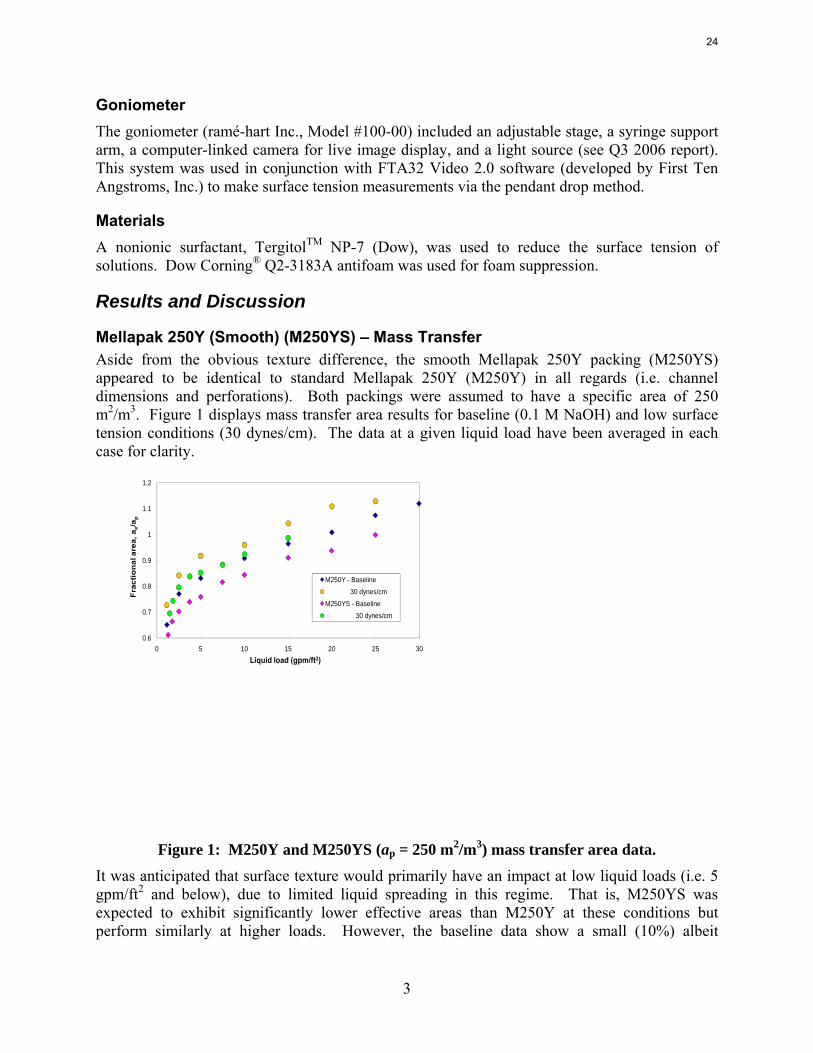
Mellapak 250Y (Smooth) (M250YS) – Hydraulics Dry pressure drop data for M250YS are shown in Figure 2, plotted against several replicated M250Y data sets. The results have been normalized by equation 1, a simple power law expression obtained from a regression of all of the dry M250Y data; this was done to exaggerate the difference between the packings.
856.1M250Ydry, 309.0Z
FP
=Δ
(1)
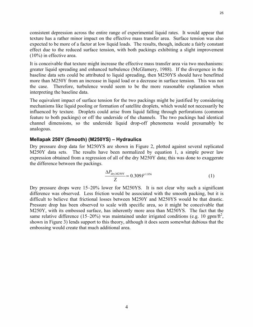
Dry pressure drops were 15–20% lower for M250YS. It is not clear why such a significant difference was observed. Less friction would be associated with the smooth packing, but it is difficult to believe that frictional losses between M250Y and M250YS would be that drastic. Pressure drop has been observed to scale with specific area, so it might be conceivable that M250Y, with its embossed surface, has inherently more area than M250YS. The fact that the same relative difference (15–20%) was maintained under irrigated conditions (e.g. 10 gpm/ft2, shown in Figure 3) lends support to this theory, although it does seem somewhat dubious that the embossing would create that much additional area.
25
5
0.75
0.8
0.85
0.9
0.95
1
1.05
1.1
0 0.5 1 1.5 2 2.5 3 3.5 4 4.5 5
ΔP
/ ΔP d
ry, M
250Y
M250Y(ΔP/ΔPdry, M250Y ~ 1)
M250YS(ΔP/ΔPdry, M250Y ~ 0.8-0.85)
Figure 2: M250Y and M250YS dry pressure drop data.
10 0.5 1 1.5 2 2.5 3 3.5
ΔP
/ ΔP d
ry, M
250Y
F-factor (Pa)0.5
M250Y(ΔP/ΔPdry, M250Y ~ 1.3)
M250YS(ΔP/ΔPdry, M250Y ~ 1.1)
Figure 3: M250Y and M250YS pressure drop data at liquid load of 10 gpm/ft2.
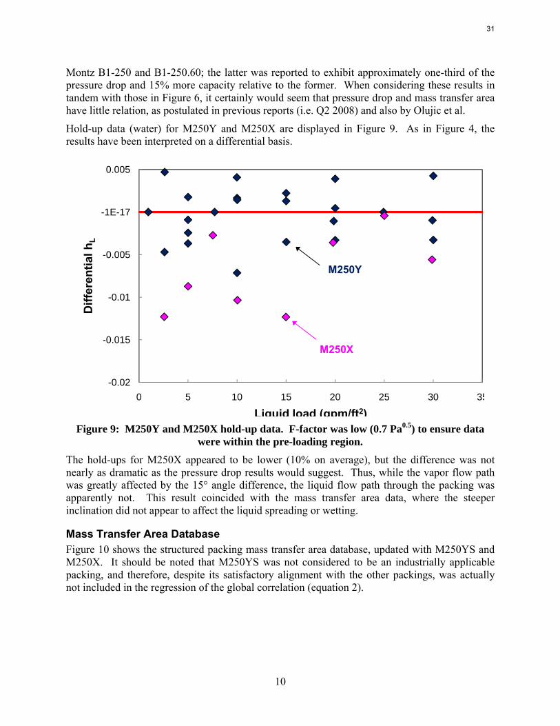
Hold-up data (water) for M250Y and M250YS are presented in Figure 4. The results are displayed on a differential basis, where each measured fractional hold-up (hL) has had a baseline
26
6
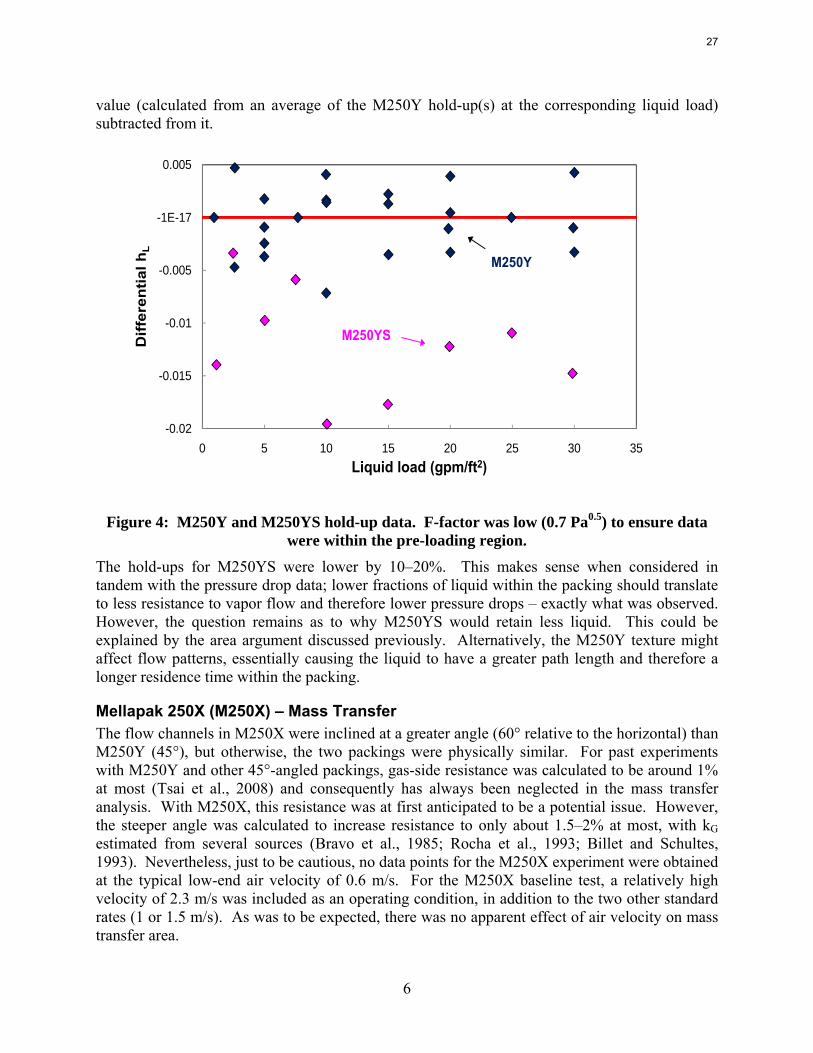
value (calculated from an average of the M250Y hold-up(s) at the corresponding liquid load) subtracted from it.
-0.02
-0.015
-0.01
-0.005
-1E-17
0.005
0 5 10 15 20 25 30 35
Diff
eren
tial h
L
Liquid load (gpm/ft2)
M250Y
M250YS
Figure 4: M250Y and M250YS hold-up data. F-factor was low (0.7 Pa0.5) to ensure data
were within the pre-loading region. The hold-ups for M250YS were lower by 10–20%. This makes sense when considered in tandem with the pressure drop data; lower fractions of liquid within the packing should translate to less resistance to vapor flow and therefore lower pressure drops – exactly what was observed. However, the question remains as to why M250YS would retain less liquid. This could be explained by the area argument discussed previously. Alternatively, the M250Y texture might affect flow patterns, essentially causing the liquid to have a greater path length and therefore a longer residence time within the packing.
Mellapak 250X (M250X) – Mass Transfer The flow channels in M250X were inclined at a greater angle (60° relative to the horizontal) than M250Y (45°), but otherwise, the two packings were physically similar. For past experiments with M250Y and other 45°-angled packings, gas-side resistance was calculated to be around 1% at most (Tsai et al., 2008) and consequently has always been neglected in the mass transfer analysis. With M250X, this resistance was at first anticipated to be a potential issue. However, the steeper angle was calculated to increase resistance to only about 1.5–2% at most, with kG estimated from several sources (Bravo et al., 1985; Rocha et al., 1993; Billet and Schultes, 1993). Nevertheless, just to be cautious, no data points for the M250X experiment were obtained at the typical low-end air velocity of 0.6 m/s. For the M250X baseline test, a relatively high velocity of 2.3 m/s was included as an operating condition, in addition to the two other standard rates (1 or 1.5 m/s). As was to be expected, there was no apparent effect of air velocity on mass transfer area.
27
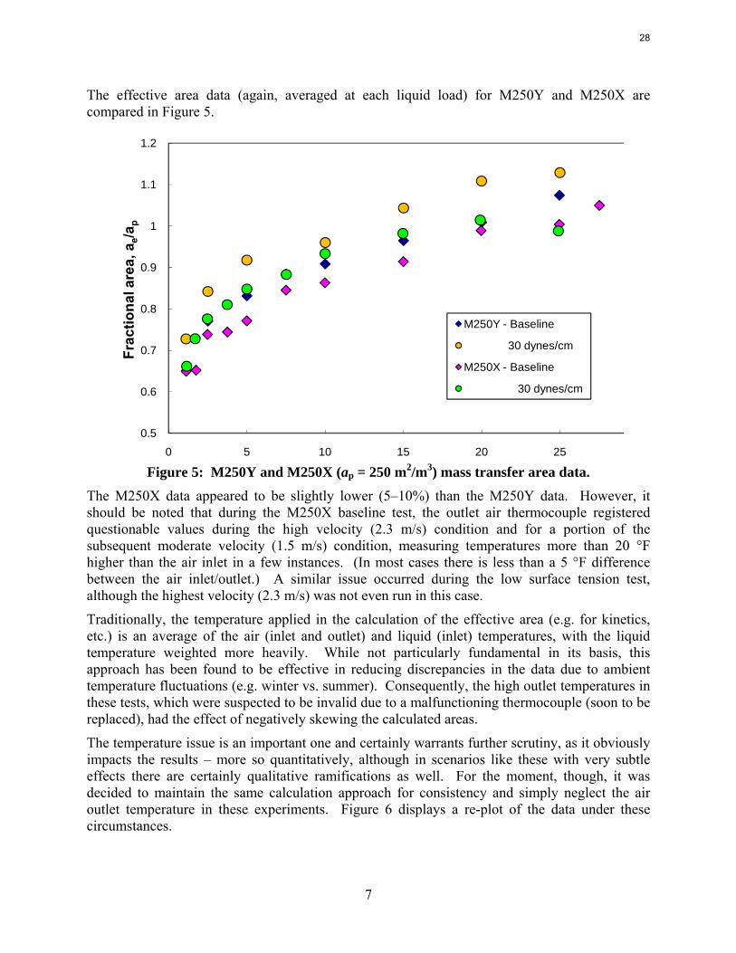
7
The effective area data (again, averaged at each liquid load) for M250Y and M250X are compared in Figure 5.
0.5
0.6
0.7
0.8
0.9
1
1.1
1.2
0 5 10 15 20 25
Frac
tiona
l are
a, a
e/ap
M250Y - Baseline
30 dynes/cm
M250X - Baseline
30 dynes/cm
Figure 5: M250Y and M250X (ap = 250 m2/m3) mass transfer area data.
The M250X data appeared to be slightly lower (5–10%) than the M250Y data. However, it should be noted that during the M250X baseline test, the outlet air thermocouple registered questionable values during the high velocity (2.3 m/s) condition and for a portion of the subsequent moderate velocity (1.5 m/s) condition, measuring temperatures more than 20 °F higher than the air inlet in a few instances. (In most cases there is less than a 5 °F difference between the air inlet/outlet.) A similar issue occurred during the low surface tension test, although the highest velocity (2.3 m/s) was not even run in this case.
Traditionally, the temperature applied in the calculation of the effective area (e.g. for kinetics, etc.) is an average of the air (inlet and outlet) and liquid (inlet) temperatures, with the liquid temperature weighted more heavily. While not particularly fundamental in its basis, this approach has been found to be effective in reducing discrepancies in the data due to ambient temperature fluctuations (e.g. winter vs. summer). Consequently, the high outlet temperatures in these tests, which were suspected to be invalid due to a malfunctioning thermocouple (soon to be replaced), had the effect of negatively skewing the calculated areas.
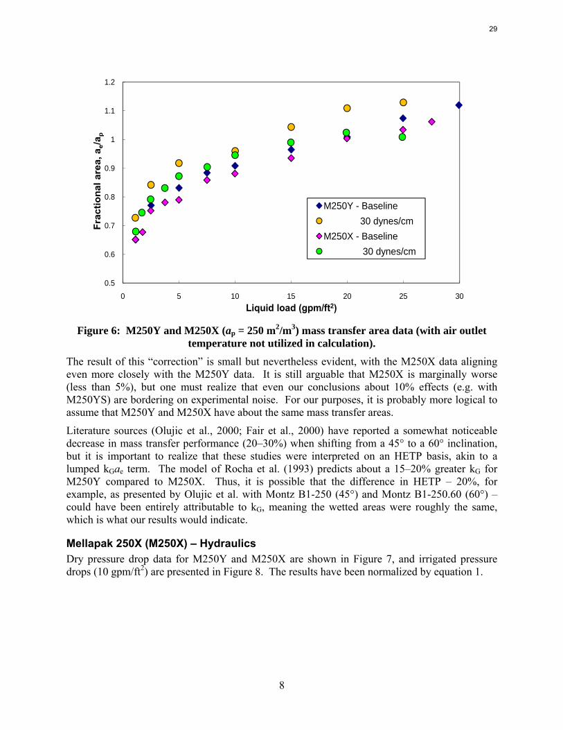
The temperature issue is an important one and certainly warrants further scrutiny, as it obviously impacts the results – more so quantitatively, although in scenarios like these with very subtle effects there are certainly qualitative ramifications as well. For the moment, though, it was decided to maintain the same calculation approach for consistency and simply neglect the air outlet temperature in these experiments. Figure 6 displays a re-plot of the data under these circumstances.
28
8
0.5
0.6
0.7
0.8
0.9
1
1.1
1.2
0 5 10 15 20 25 30
Frac
tiona
l are
a, a
e/ap
Liquid load (gpm/ft2)
M250Y - Baseline30 dynes/cm
M250X - Baseline30 dynes/cm
Figure 6: M250Y and M250X (ap = 250 m2/m3) mass transfer area data (with air outlet
temperature not utilized in calculation). The result of this “correction” is small but nevertheless evident, with the M250X data aligning even more closely with the M250Y data. It is still arguable that M250X is marginally worse (less than 5%), but one must realize that even our conclusions about 10% effects (e.g. with M250YS) are bordering on experimental noise. For our purposes, it is probably more logical to assume that M250Y and M250X have about the same mass transfer areas.
Literature sources (Olujic et al., 2000; Fair et al., 2000) have reported a somewhat noticeable decrease in mass transfer performance (20–30%) when shifting from a 45° to a 60° inclination, but it is important to realize that these studies were interpreted on an HETP basis, akin to a lumped kGae term. The model of Rocha et al. (1993) predicts about a 15–20% greater kG for M250Y compared to M250X. Thus, it is possible that the difference in HETP – 20%, for example, as presented by Olujic et al. with Montz B1-250 (45°) and Montz B1-250.60 (60°) – could have been entirely attributable to kG, meaning the wetted areas were roughly the same, which is what our results would indicate.
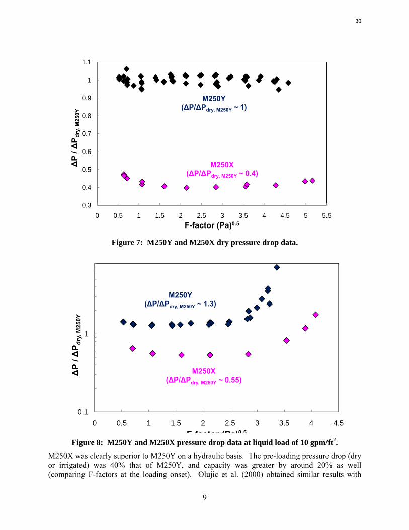
Mellapak 250X (M250X) – Hydraulics Dry pressure drop data for M250Y and M250X are shown in Figure 7, and irrigated pressure drops (10 gpm/ft2) are presented in Figure 8. The results have been normalized by equation 1.
29
9
0.3
0.4
0.5
0.6
0.7
0.8
0.9
1
1.1
0 0.5 1 1.5 2 2.5 3 3.5 4 4.5 5 5.5
ΔP
/ ΔP d
ry, M
250Y
F-factor (Pa)0.5
M250Y(ΔP/ΔPdry, M250Y ~ 1)
M250X(ΔP/ΔPdry, M250Y ~ 0.4)
Figure 7: M250Y and M250X dry pressure drop data.
0.1
1
0 0.5 1 1.5 2 2.5 3 3.5 4 4.5
ΔP
/ ΔP d
ry, M
250Y
F factor (Pa)0 5
M250Y(ΔP/ΔPdry, M250Y ~ 1.3)
M250X(ΔP/ΔPdry, M250Y ~ 0.55)
Figure 8: M250Y and M250X pressure drop data at liquid load of 10 gpm/ft2.
M250X was clearly superior to M250Y on a hydraulic basis. The pre-loading pressure drop (dry or irrigated) was 40% that of M250Y, and capacity was greater by around 20% as well (comparing F-factors at the loading onset). Olujic et al. (2000) obtained similar results with
30
10
Montz B1-250 and B1-250.60; the latter was reported to exhibit approximately one-third of the pressure drop and 15% more capacity relative to the former. When considering these results in tandem with those in Figure 6, it certainly would seem that pressure drop and mass transfer area have little relation, as postulated in previous reports (i.e. Q2 2008) and also by Olujic et al.
Hold-up data (water) for M250Y and M250X are displayed in Figure 9. As in Figure 4, the results have been interpreted on a differential basis.
-0.02
-0.015
-0.01
-0.005
-1E-17
0.005
0 5 10 15 20 25 30 35
Diff
eren
tial h
L
Liquid load (gpm/ft2)
M250Y
M250X
Figure 9: M250Y and M250X hold-up data. F-factor was low (0.7 Pa0.5) to ensure data
were within the pre-loading region. The hold-ups for M250X appeared to be lower (10% on average), but the difference was not nearly as dramatic as the pressure drop results would suggest. Thus, while the vapor flow path was greatly affected by the 15° angle difference, the liquid flow path through the packing was apparently not. This result coincided with the mass transfer area data, where the steeper inclination did not appear to affect the liquid spreading or wetting.
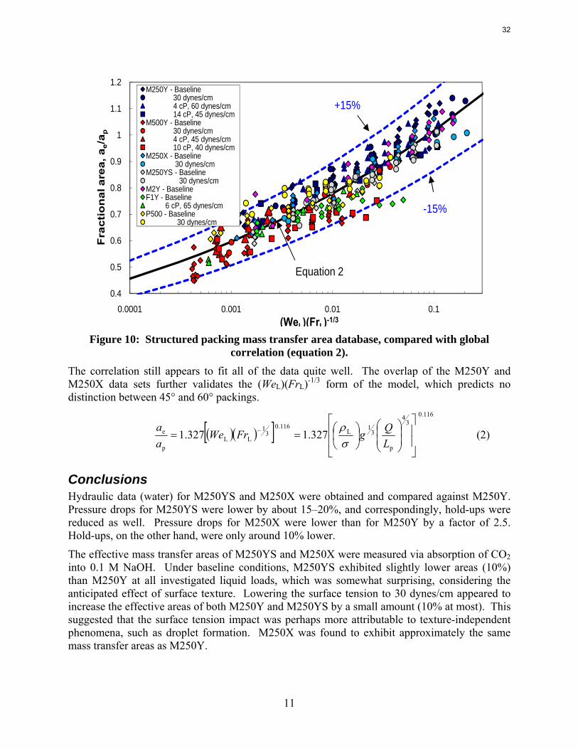
Mass Transfer Area Database Figure 10 shows the structured packing mass transfer area database, updated with M250YS and M250X. It should be noted that M250YS was not considered to be an industrially applicable packing, and therefore, despite its satisfactory alignment with the other packings, was actually not included in the regression of the global correlation (equation 2).
31
11
0.4
0.5
0.6
0.7
0.8
0.9
1
1.1
1.2
0.0001 0.001 0.01 0.1
Fra
ctio
nal
are
a, a
e/a p
(WeL)(FrL)-1/3
M250Y - Baseline30 dynes/cm4 cP, 60 dynes/cm14 cP, 45 dynes/cm
M500Y - Baseline30 dynes/cm4 cP, 45 dynes/cm10 cP, 40 dynes/cm
M250X - Baseline30 dynes/cm
M250YS - Baseline30 dynes/cm
M2Y - BaselineF1Y - Baseline
6 cP, 65 dynes/cmP500 - Baseline
30 dynes/cm-15%
+15%
Equation 2
Figure 10: Structured packing mass transfer area database, compared with global
correlation (equation 2). The correlation still appears to fit all of the data quite well. The overlap of the M250Y and M250X data sets further validates the (WeL)(FrL)-1/3 form of the model, which predicts no distinction between 45° and 60° packings.
( )( )[ ]116.0
34
p
31L
116.03
1LL
p
e 327.1327.1⎥⎥
⎦
⎤
⎢⎢
⎣
⎡
⎟⎟⎠
⎞⎜⎜⎝
⎛⎟⎠⎞
⎜⎝⎛== −
LQgFrWe
aa
σρ
(2)
Conclusions Hydraulic data (water) for M250YS and M250X were obtained and compared against M250Y. Pressure drops for M250YS were lower by about 15–20%, and correspondingly, hold-ups were reduced as well. Pressure drops for M250X were lower than for M250Y by a factor of 2.5. Hold-ups, on the other hand, were only around 10% lower.
The effective mass transfer areas of M250YS and M250X were measured via absorption of CO2 into 0.1 M NaOH. Under baseline conditions, M250YS exhibited slightly lower areas (10%) than M250Y at all investigated liquid loads, which was somewhat surprising, considering the anticipated effect of surface texture. Lowering the surface tension to 30 dynes/cm appeared to increase the effective areas of both M250Y and M250YS by a small amount (10% at most). This suggested that the surface tension impact was perhaps more attributable to texture-independent phenomena, such as droplet formation. M250X was found to exhibit approximately the same mass transfer areas as M250Y.
32
12
The mass transfer area database (updated to include M250YS and M250X) continued to be represented well by the correlation that was regressed as a function of (WeL)(FrL)-1/3.
Future Work
Additional hydraulic and mass transfer experiments with M250X are planned at a high viscosity (10 cP). A full range of tests are also planned for MellapakPlus 252Y (modified joint transition) and Mellapak 125Y. The current mass transfer model will be further refined by these additional data.
Nomenclature
ae = effective area of packing, m2/m3
ap = specific (geometric) area of packing, m2/m3
F = gas flow factor, (m/s)(kg/m3)0.5 or Pa0.5
g = gravitational constant; 9.81 m/s2
hL = (total) liquid hold-up, m3/m3
kG = gas-side mass transfer coefficient, kmol/(m2·Pa·s)
kL0 = physical liquid-side mass transfer coefficient, m/s
Lp = wetted perimeter in cross-sectional slice of packing, m
ΔP = pressure drop, Pa
Q = volumetric flow rate, m3/s
u = velocity, m/s
Z = packed height, m
Greek Symbols
δ = film thickness, m
ρ = density, kg/m3
σ = surface tension, N/m
Subscripts
G = gas phase
L = liquid phase
Dimensionless Groups
af = fractional area of packing, ae/ap
33
13
Fr = Froude number, δg
u 2
We = Weber number, σδρ 2u
References Billet R, Schultes M. "Predicting Mass Transfer in Packed Columns." Chem Eng Technol.
1993;16(1):1–9.
Bravo JL, Rocha JA, et al. "Mass Transfer in Gauze Packings." Hydro Proc. 1985;64(1):91–95.
Fair JR, Seibert AF, et al. "Structured Packing Performance - Experimental Evaluation of Two Predictive Models." Ind Eng Chem Res. 2000;39(6):1788–1796.
Kohl A, Nielsen R. Gas Purification. Houston, Gulf Publishing Co.: 1997.
McGlamery GG. Liquid Film Transport Characteristics of Textured Metal Surfaces. University of Texas at Austin. Ph.D. Dissertation. 1988.
Olujic Z, Seibert AF, et al. "Influence of Corrugation Geometry on the Performance of Structured Packings: An Experimental Study." Chem Eng Proc. 2000;39(4):335–342.
Rocha JA, Bravo JL, et al. "Distillation Columns Containing Structured Packings: A Comprehensive Model for Their Performance. 1. Hydraulic Models." Ind Eng Chem Res. 1993;32(4):641–651.
Rocha JA, Bravo JL, et al. "Distillation Columns Containing Structured Packings: A Comprehensive Model for Their Performance. 2. Mass-Transfer Model." Ind Eng Chem Res. 1996;35(5):1660–1667.
Tsai RE, Seibert AF, et al. "Influence of Viscosity and Surface Tension on the Effective Mass Transfer Area of Structured Packing." GHGT-9, Washington D.C. 2008.
Wang GQ, Yuan XG, et al. Review of "Mass-Transfer Correlations for Packed Columns." Ind Eng Chem Res. 2005;44(23):8715–8729.
34
1
Modeling Stripper Performance for CO2 Removal with Amine Solvents
Quarterly Report for January 1 – March 31, 2009
by David Van Wagener
Supported by the Luminant Carbon Management Program
and the
Industrial Associates Program for CO2 Capture by Aqueous Absorption
Department of Chemical Engineering
The University of Texas at Austin
April 1, 2009
Abstract Since Hilliard developed thermodynamic models for various amine solvents, additional experimental data has been collected at new conditions. The data primarily of interest have been for concentrated piperazine (PZ). The Hilliard model predicted well for low concentrations, 0.9 m–5 m, but 8 m PZ will be used in future simulations. VLE data collected by Dugas as well as heat capacity data collected by Nguyen for concentrated piperazine were incorporated into previous parameter regression files. The parameters to be regressed were reconsidered, and more focus was put on the heat capacity parameters of the dominant species at relevant loadings. The predictions by the newly regressed model were near-perfect for the relevant loading range, 0.3–0.4, and only had a maximum deviation of 5% at a loading of 0.2. The accuracy of the VLE predictions was not significantly compromised at these loadings with the new parameter values. The performance of multistage flash configurations with concentrated piperazine was also assessed. Compressing to 150 atm, a three-stage flash operated with 8 m PZ had an equivalent work of 35.0 kJ/mol CO2 compared to the 40.3 kJ/mol CO2 required for a simple stripper using 7 m MEA.
Introduction Piperazine (PZ) is of interest as a solvent for CO2 capture because it has significantly higher capacity than monoethanolamine (MEA), the baseline and industry standard. A piperazine molecule has two amine groups, which leads to this increased capacity. High solvent capacity leads to less solvent being circulated between the absorber and stripper, so the stripper reboiler duty reduces since the sensible heat input for the solvent is lowered. The CO2 absorption rate for piperazine is enhanced over MEA as well, also due to the two amine groups per molecule. As an added benefit, PZ has no detectable thermal degradation up to at least 150 °C. Many explored stripper configurations operate more efficiently at high temperatures, so it is expected that piperazine will perform better than MEA (Freeman et al., 2008).
35
2
Previously, a thermodynamic model was developed for PZ (Hilliard, 2008), and it was used to simulate a simple stripper with the accompanying rich and lean pumps, cross heat exchanger, and multi-stage compressor. The simulations produced results with few convergence errors; however, the behavior while varying the lean loading specification was unexpected. Typically the calculated equivalent work of the stripper has a single distinct optimum lean loading (Oyenekan, 2007). Conversely, the PZ stimulation demonstrated both a local and global optimum (Rochelle et al., 2008). The local optimum was at a lean loading of 0.30, an expected value based on the measured VLE at absorber conditions. The global optimum was at a lean loading of 0.15, and the temperature profile was very hot; reaching temperatures over 120 °C. A suggested source for this unusual behavior was the accuracy of the predictions of thermodynamic values for the solvent. The predictions that seemed particularly questionable were the solvent heat capacity and heat of absorption of CO2. Work in the previous quarter generated heat capacity data for 8 m PZ and regressed the model parameters to better predict heat capacity. However, the fit was not improved. The heat capacity data used for the regression was extrapolated from values at lower PZ concentrations. Though not an ideal source of data, these values were the only ones available at the time.
As previously described, an advantage of using PZ over MEA is a decrease in thermal degradation risk. It has been advised that PZ can be used at temperatures up to 150 °C, whereas the ceiling temperature for MEA was 120 °C. Stripping at higher temperatures and pressures as typically been found to increase the selectivity of CO2 over water for the exiting vapor, thus decreasing the energy put into vaporizing extra stripping steam. The Aspen Plus® thermodynamic model for PZ is not yet trustworthy due to the inaccurate heat capacity predictions, but fundamental calculations based on thermodynamic relationships and correlations for PZ can be used to estimate the energy requirement for the three-stage flash with PZ at elevated temperatures.
Methods and Results PZ Model Regression: The first task this quarter involved improving the Aspen Plus®
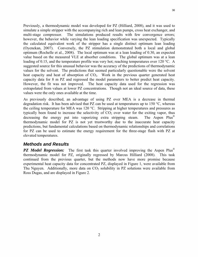
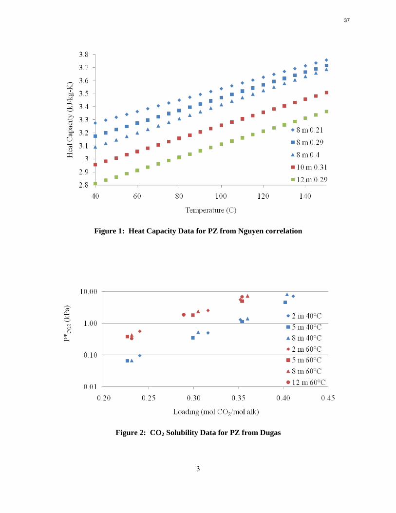
thermodynamic model for PZ, originally regressed by Marcus Hilliard (2008). This task continued from the previous quarter, but the methods now have more promise because experimental heat capacity data for concentrated PZ, displayed in Figure 1, were available from Thu Nguyen. Additionally, more data on CO2 solubility in PZ solutions were available from Ross Dugas, and are displayed in Figure 2.
36
3
Figure 1: Heat Capacity Data for PZ from Nguyen correlation
Figure 2: CO2 Solubility Data for PZ from Dugas
37
4
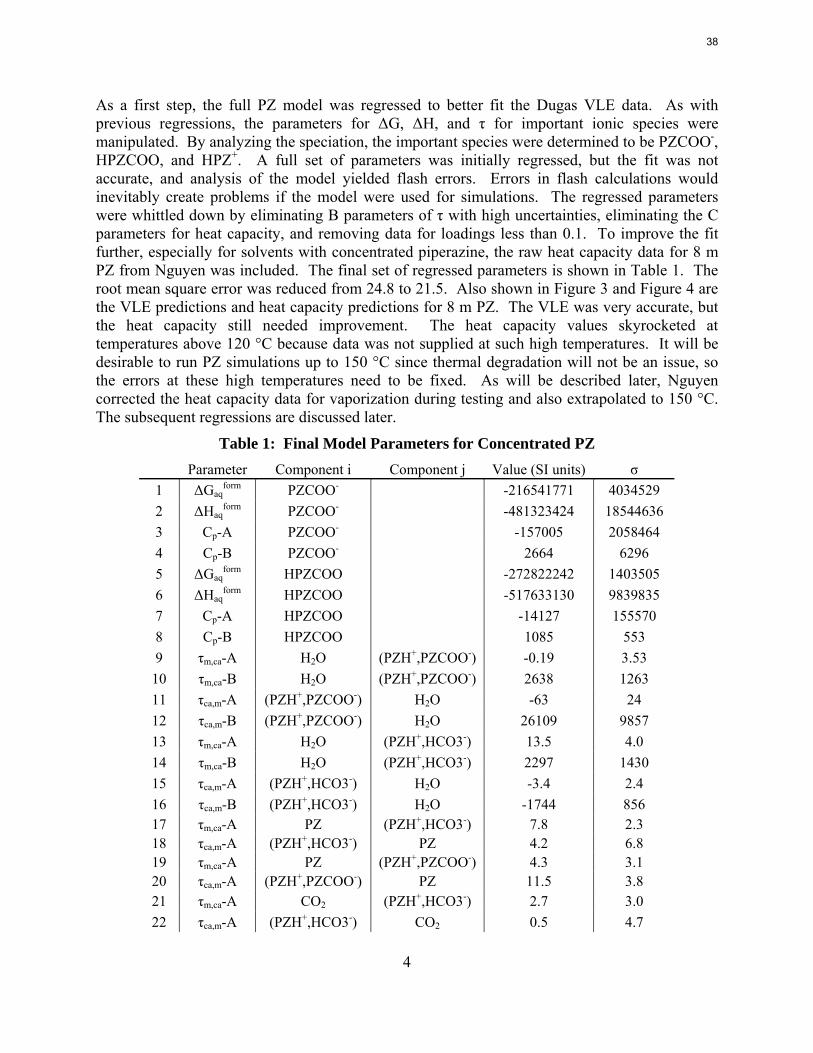
As a first step, the full PZ model was regressed to better fit the Dugas VLE data. As with previous regressions, the parameters for ΔG, ΔH, and τ for important ionic species were manipulated. By analyzing the speciation, the important species were determined to be PZCOO-, HPZCOO, and HPZ+. A full set of parameters was initially regressed, but the fit was not accurate, and analysis of the model yielded flash errors. Errors in flash calculations would inevitably create problems if the model were used for simulations. The regressed parameters were whittled down by eliminating B parameters of τ with high uncertainties, eliminating the C parameters for heat capacity, and removing data for loadings less than 0.1. To improve the fit further, especially for solvents with concentrated piperazine, the raw heat capacity data for 8 m PZ from Nguyen was included. The final set of regressed parameters is shown in Table 1. The root mean square error was reduced from 24.8 to 21.5. Also shown in Figure 3 and Figure 4 are the VLE predictions and heat capacity predictions for 8 m PZ. The VLE was very accurate, but the heat capacity still needed improvement. The heat capacity values skyrocketed at temperatures above 120 °C because data was not supplied at such high temperatures. It will be desirable to run PZ simulations up to 150 °C since thermal degradation will not be an issue, so the errors at these high temperatures need to be fixed. As will be described later, Nguyen corrected the heat capacity data for vaporization during testing and also extrapolated to 150 °C. The subsequent regressions are discussed later.
Table 1: Final Model Parameters for Concentrated PZ Parameter Component i Component j Value (SI units) σ 1 ΔGaq
form PZCOO- -216541771 4034529 2 ΔHaq
form PZCOO- -481323424 18544636 3 Cp-A PZCOO- -157005 2058464 4 Cp-B PZCOO- 2664 6296 5 ΔGaq
form HPZCOO -272822242 1403505 6 ΔHaq
form HPZCOO -517633130 9839835 7 Cp-A HPZCOO -14127 155570 8 Cp-B HPZCOO 1085 553 9 τm,ca-A H2O (PZH+,PZCOO-) -0.19 3.53
10 τm,ca-B H2O (PZH+,PZCOO-) 2638 1263 11 τca,m-A (PZH+,PZCOO-) H2O -63 24 12 τca,m-B (PZH+,PZCOO-) H2O 26109 9857 13 τm,ca-A H2O (PZH+,HCO3-) 13.5 4.0 14 τm,ca-B H2O (PZH+,HCO3-) 2297 1430 15 τca,m-A (PZH+,HCO3-) H2O -3.4 2.4 16 τca,m-B (PZH+,HCO3-) H2O -1744 856 17 τm,ca-A PZ (PZH+,HCO3-) 7.8 2.3 18 τca,m-A (PZH+,HCO3-) PZ 4.2 6.8 19 τm,ca-A PZ (PZH+,PZCOO-) 4.3 3.1 20 τca,m-A (PZH+,PZCOO-) PZ 11.5 3.8 21 τm,ca-A CO2 (PZH+,HCO3-) 2.7 3.0 22 τca,m-A (PZH+,HCO3-) CO2 0.5 4.7
38
5
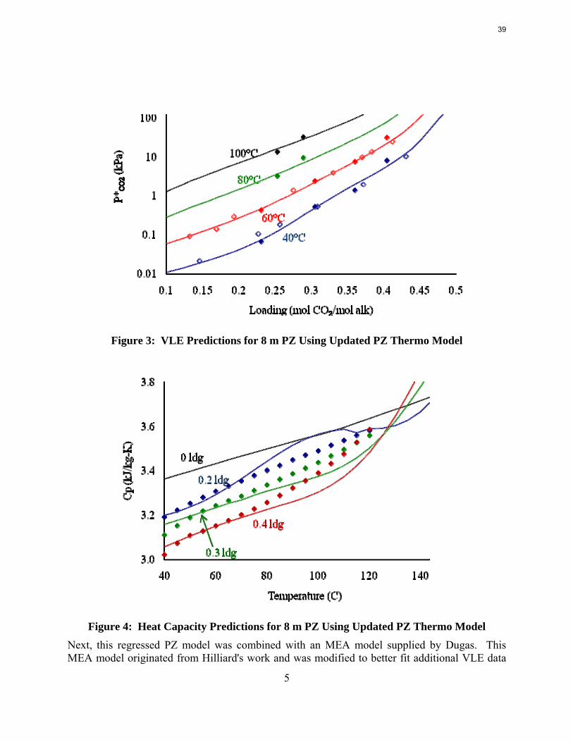
Figure 3: VLE Predictions for 8 m PZ Using Updated PZ Thermo Model
Figure 4: Heat Capacity Predictions for 8 m PZ Using Updated PZ Thermo Model
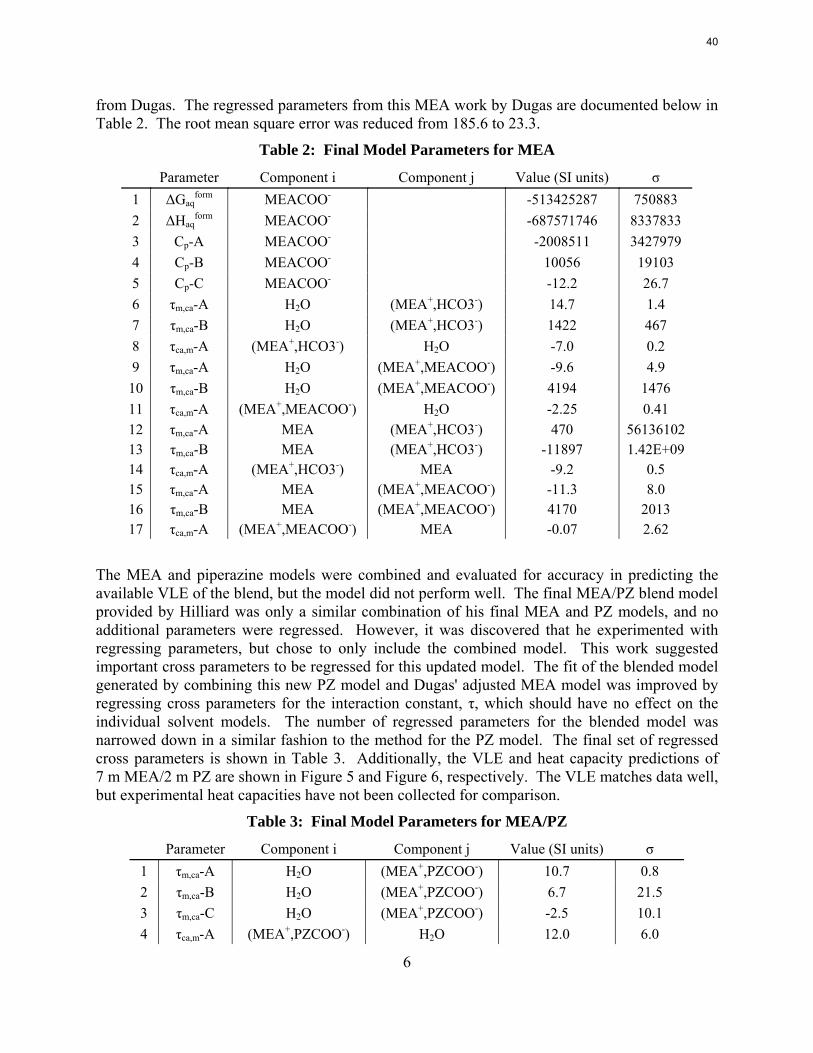
Next, this regressed PZ model was combined with an MEA model supplied by Dugas. This MEA model originated from Hilliard's work and was modified to better fit additional VLE data
39
6
from Dugas. The regressed parameters from this MEA work by Dugas are documented below in Table 2. The root mean square error was reduced from 185.6 to 23.3.
Table 2: Final Model Parameters for MEA
Parameter Component i Component j Value (SI units) σ 1 ΔGaq
form MEACOO- -513425287 750883 2 ΔHaq
form MEACOO- -687571746 8337833 3 Cp-A MEACOO- -2008511 3427979 4 Cp-B MEACOO- 10056 19103 5 Cp-C MEACOO- -12.2 26.7 6 τm,ca-A H2O (MEA+,HCO3-) 14.7 1.4 7 τm,ca-B H2O (MEA+,HCO3-) 1422 467 8 τca,m-A (MEA+,HCO3-) H2O -7.0 0.2 9 τm,ca-A H2O (MEA+,MEACOO-) -9.6 4.9
10 τm,ca-B H2O (MEA+,MEACOO-) 4194 1476 11 τca,m-A (MEA+,MEACOO-) H2O -2.25 0.41 12 τm,ca-A MEA (MEA+,HCO3-) 470 56136102 13 τm,ca-B MEA (MEA+,HCO3-) -11897 1.42E+09 14 τca,m-A (MEA+,HCO3-) MEA -9.2 0.5 15 τm,ca-A MEA (MEA+,MEACOO-) -11.3 8.0 16 τm,ca-B MEA (MEA+,MEACOO-) 4170 2013 17 τca,m-A (MEA+,MEACOO-) MEA -0.07 2.62
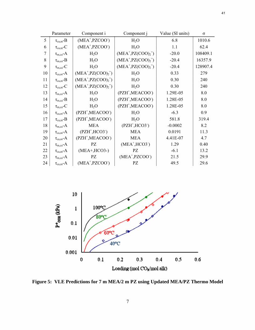
The MEA and piperazine models were combined and evaluated for accuracy in predicting the available VLE of the blend, but the model did not perform well. The final MEA/PZ blend model provided by Hilliard was only a similar combination of his final MEA and PZ models, and no additional parameters were regressed. However, it was discovered that he experimented with regressing parameters, but chose to only include the combined model. This work suggested important cross parameters to be regressed for this updated model. The fit of the blended model generated by combining this new PZ model and Dugas' adjusted MEA model was improved by regressing cross parameters for the interaction constant, τ, which should have no effect on the individual solvent models. The number of regressed parameters for the blended model was narrowed down in a similar fashion to the method for the PZ model. The final set of regressed cross parameters is shown in Table 3. Additionally, the VLE and heat capacity predictions of 7 m MEA/2 m PZ are shown in Figure 5 and Figure 6, respectively. The VLE matches data well, but experimental heat capacities have not been collected for comparison.
Table 3: Final Model Parameters for MEA/PZ
Parameter Component i Component j Value (SI units) σ 1 τm,ca-A H2O (MEA+,PZCOO-) 10.7 0.8 2 τm,ca-B H2O (MEA+,PZCOO-) 6.7 21.5 3 τm,ca-C H2O (MEA+,PZCOO-) -2.5 10.1 4 τca,m-A (MEA+,PZCOO-) H2O 12.0 6.0
40
7
Parameter Component i Component j Value (SI units) σ 5 τca,m-B (MEA+,PZCOO-) H2O 6.8 1010.6 6 τca,m-C (MEA+,PZCOO-) H2O 1.1 62.4 7 τm,ca-A H2O (MEA+,PZ(COO)2
=) -20.0 108409.18 τm,ca-B H2O (MEA+,PZ(COO)2
=) -20.4 16357.9 9 τm,ca-C H2O (MEA+,PZ(COO)2
=) -20.4 128907.410 τca,m-A (MEA+,PZ(COO)2
=) H2O 0.33 279 11 τca,m-B (MEA+,PZ(COO)2
=) H2O 0.30 240 12 τca,m-C (MEA+,PZ(COO)2
=) H2O 0.30 240 13 τm,ca-A H2O (PZH+,MEACOO-) 1.29E-05 8.0 14 τm,ca-B H2O (PZH+,MEACOO-) 1.28E-05 8.0 15 τm,ca-C H2O (PZH+,MEACOO-) 1.28E-05 8.0 16 τca,m-A (PZH+,MEACOO-) H2O -6.3 0.9 17 τca,m-B (PZH+,MEACOO-) H2O 581.8 319.4 18 τm,ca-A MEA (PZH+,HCO3-) -0.0002 8.2 19 τca,m-A (PZH+,HCO3-) MEA 0.0191 11.3 20 τca,m-A (PZH+,MEACOO-) MEA 4.41E-07 4.7 21 τm,ca-A PZ (MEA+,HCO3-) 1.29 0.40 22 τca,m-A (MEA+,HCO3-) PZ -6.1 13.2 23 τm,ca-A PZ (MEA+,PZCOO-) 21.5 29.9 24 τca,m-A (MEA+,PZCOO-) PZ 49.5 29.6
Figure 5: VLE Predictions for 7 m MEA/2 m PZ using Updated MEA/PZ Thermo Model
41
8
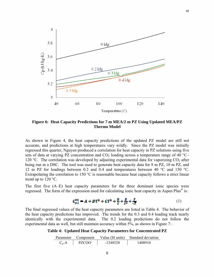
Figure 6: Heat Capacity Predictions for 7 m MEA/2 m PZ Using Updated MEA/PZ
Thermo Model
As shown in Figure 4, the heat capacity predictions of the updated PZ model are still not accurate, and predictions at high temperatures vary wildly. Since the PZ model was initially regressed this quarter, Nguyen produced a correlation for heat capacity in PZ solutions using five sets of data at varying PZ concentration and CO2 loading across a temperature range of 40 °C–120 °C. The correlation was developed by adjusting experimental data for vaporizing CO2 after being run in a DSC. The tool was used to generate heat capacity data for 8 m PZ, 10 m PZ, and 12 m PZ for loadings between 0.2 and 0.4 and temperatures between 40 °C and 150 °C. Extrapolating the correlation to 150 °C is reasonable because heat capacity follows a strict linear trend up to 120 °C.
The first five (A–E) heat capacity parameters for the three dominant ionic species were regressed. The form of the expression used for calculating ionic heat capacity in Aspen Plus® is:
(1)
The final regressed values of the heat capacity parameters are listed in Table 4. The behavior of the heat capacity predictions has improved. The trends for the 0.3 and 0.4 loading track nearly identically with the experimental data. The 0.2 loading predictions do not follow the experimental data as well, but still maintain accuracy within 5%, as shown in Figure 7: .
Table 4: Updated Heat Capacity Parameters for Concentrated PZ Parameter Component Value (SI units) Standard deviation
Cp-A PZCOO- -1248528 1408910
42
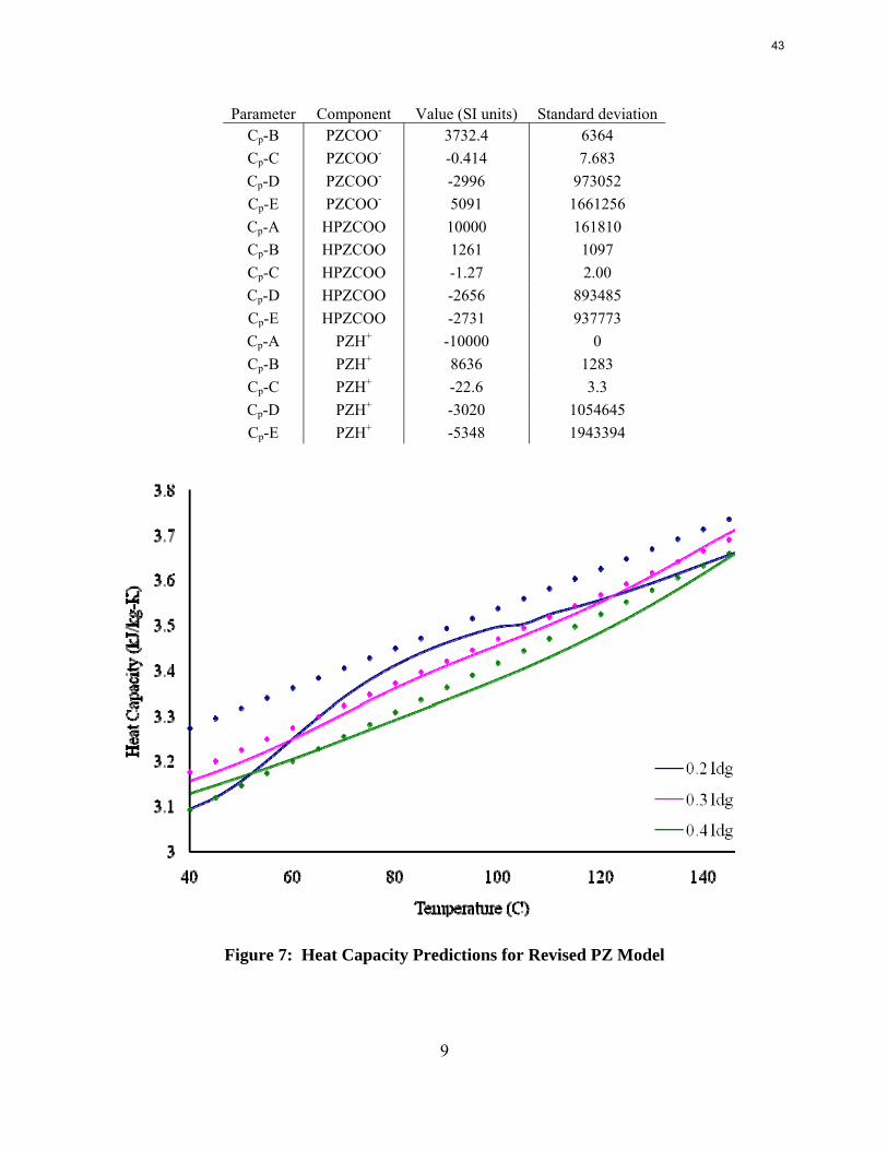
9
Parameter Component Value (SI units) Standard deviation Cp-B PZCOO- 3732.4 6364 Cp-C PZCOO- -0.414 7.683 Cp-D PZCOO- -2996 973052 Cp-E PZCOO- 5091 1661256 Cp-A HPZCOO 10000 161810 Cp-B HPZCOO 1261 1097 Cp-C HPZCOO -1.27 2.00 Cp-D HPZCOO -2656 893485 Cp-E HPZCOO -2731 937773 Cp-A PZH+ -10000 0 Cp-B PZH+ 8636 1283 Cp-C PZH+ -22.6 3.3 Cp-D PZH+ -3020 1054645 Cp-E PZH+ -5348 1943394
Figure 7: Heat Capacity Predictions for Revised PZ Model
43
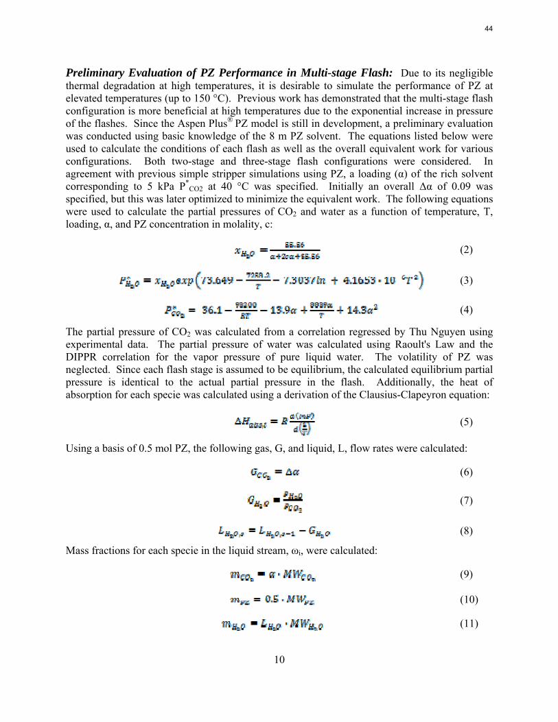
10
Preliminary Evaluation of PZ Performance in Multi-stage Flash: Due to its negligible thermal degradation at high temperatures, it is desirable to simulate the performance of PZ at elevated temperatures (up to 150 °C). Previous work has demonstrated that the multi-stage flash configuration is more beneficial at high temperatures due to the exponential increase in pressure of the flashes. Since the Aspen Plus® PZ model is still in development, a preliminary evaluation was conducted using basic knowledge of the 8 m PZ solvent. The equations listed below were used to calculate the conditions of each flash as well as the overall equivalent work for various configurations. Both two-stage and three-stage flash configurations were considered. In agreement with previous simple stripper simulations using PZ, a loading (α) of the rich solvent corresponding to 5 kPa P*
CO2 at 40 °C was specified. Initially an overall Δα of 0.09 was specified, but this was later optimized to minimize the equivalent work. The following equations were used to calculate the partial pressures of CO2 and water as a function of temperature, T, loading, α, and PZ concentration in molality, c:
(2)
(3)
(4)
The partial pressure of CO2 was calculated from a correlation regressed by Thu Nguyen using experimental data. The partial pressure of water was calculated using Raoult's Law and the DIPPR correlation for the vapor pressure of pure liquid water. The volatility of PZ was neglected. Since each flash stage is assumed to be equilibrium, the calculated equilibrium partial pressure is identical to the actual partial pressure in the flash. Additionally, the heat of absorption for each specie was calculated using a derivation of the Clausius-Clapeyron equation:
(5)
Using a basis of 0.5 mol PZ, the following gas, G, and liquid, L, flow rates were calculated:
(6)
(7)
(8)
Mass fractions for each specie in the liquid stream, ωi, were calculated:
(9)
(10)
(11)
44
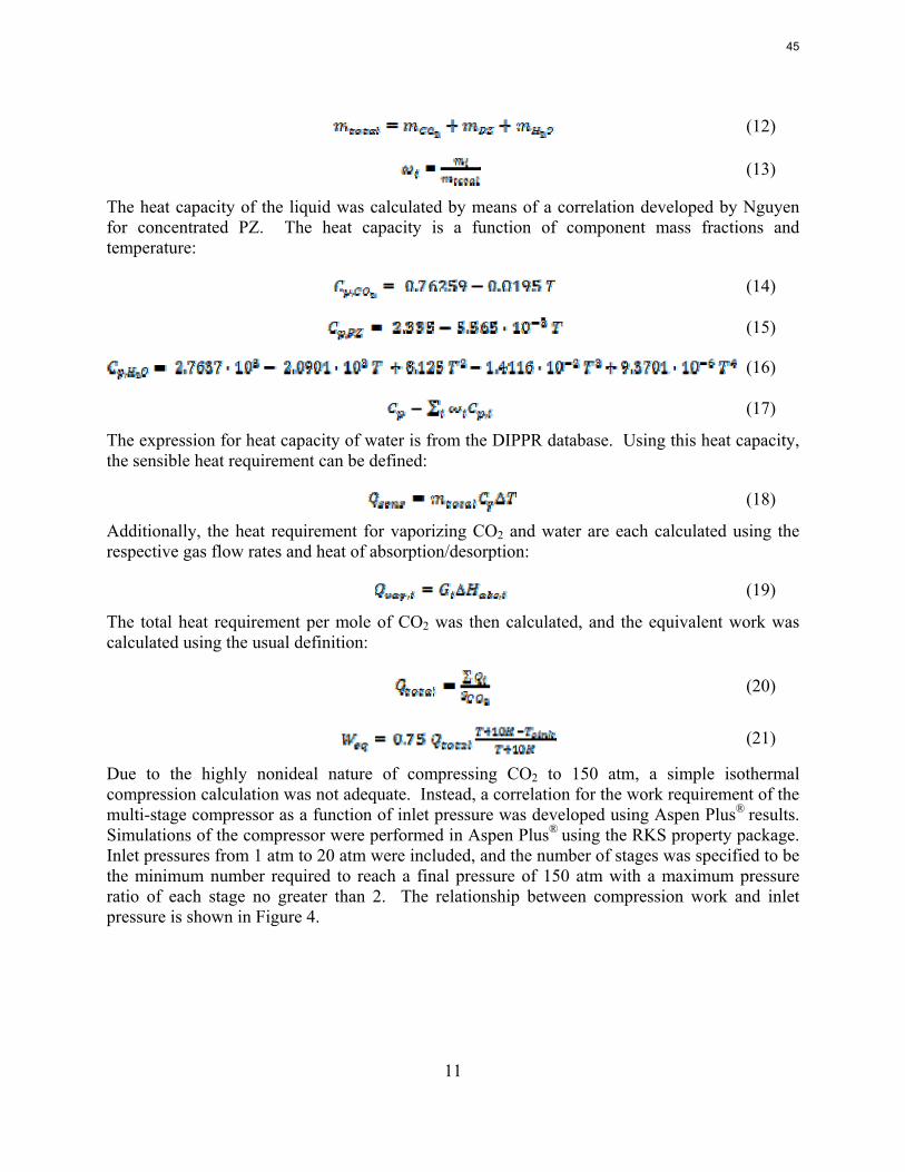
11
(12)
(13)
The heat capacity of the liquid was calculated by means of a correlation developed by Nguyen for concentrated PZ. The heat capacity is a function of component mass fractions and temperature:
(14)
(15)
(16)
(17)
The expression for heat capacity of water is from the DIPPR database. Using this heat capacity, the sensible heat requirement can be defined:
(18)
Additionally, the heat requirement for vaporizing CO2 and water are each calculated using the respective gas flow rates and heat of absorption/desorption:
(19)
The total heat requirement per mole of CO2 was then calculated, and the equivalent work was calculated using the usual definition:
(20)
(21)
Due to the highly nonideal nature of compressing CO2 to 150 atm, a simple isothermal compression calculation was not adequate. Instead, a correlation for the work requirement of the multi-stage compressor as a function of inlet pressure was developed using Aspen Plus® results. Simulations of the compressor were performed in Aspen Plus® using the RKS property package. Inlet pressures from 1 atm to 20 atm were included, and the number of stages was specified to be the minimum number required to reach a final pressure of 150 atm with a maximum pressure ratio of each stage no greater than 2. The relationship between compression work and inlet pressure is shown in Figure 4.
45
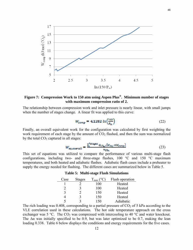
12
Figure 7: Compression Work to 150 atm using Aspen Plus®. Minimum number of stages
with maximum compression ratio of 2. The relationship between compression work and inlet pressure is nearly linear, with small jumps when the number of stages change. A linear fit was applied to this curve:
(22)
Finally, an overall equivalent work for the configuration was calculated by first weighting the work requirement of each stage by the amount of CO2 flashed, and then the sum was normalized by the total CO2 captured in all stages:
(23)
This set of equations was utilized to compare the performance of various multi-stage flash configurations, including two- and three-stage flashes, 100 °C and 150 °C maximum temperatures, and both heated and adiabatic flashes. Adiabatic flash cases include a preheater to supply the energy needed for flashing. The different cases are summarized below in Table 5.
Table 5: Multi-stage Flash Simulations Case Stages Tmax (°C) Flash operation
1 2 100 Heated 2 3 100 Heated 3 2 150 Heated 4 3 150 Heated 5 3 150 Adiabatic
The rich loading was 0.408, corresponding to a partial pressure of CO2 of 5 kPa according to the VLE correlation used in these calculations. The hot side temperature approach on the cross exchanger was 5 °C. The CO2 was compressed with intercooling to 40 °C and water knockout. The Δα was initially specified to be 0.9, but was later optimized to be 0.7, making the lean loading 0.338. Table 6 below displays the conditions and energy requirements for the five cases.
46
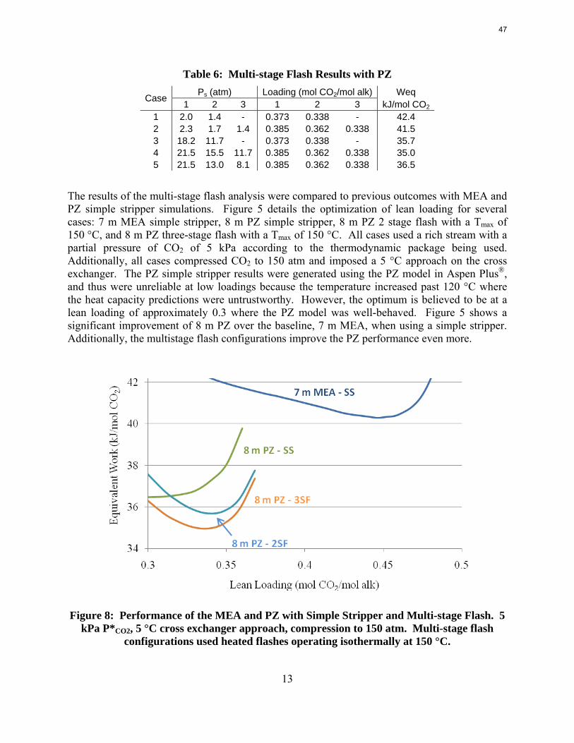
13
Table 6: Multi-stage Flash Results with PZ Ps (atm) Loading (mol CO2/mol alk) Weq Case 1 2 3 1 2 3 kJ/mol CO2
1 2.0 1.4 - 0.373 0.338 - 42.4 2 2.3 1.7 1.4 0.385 0.362 0.338 41.5 3 18.2 11.7 - 0.373 0.338 - 35.7 4 21.5 15.5 11.7 0.385 0.362 0.338 35.0 5 21.5 13.0 8.1 0.385 0.362 0.338 36.5
The results of the multi-stage flash analysis were compared to previous outcomes with MEA and PZ simple stripper simulations. Figure 5 details the optimization of lean loading for several cases: 7 m MEA simple stripper, 8 m PZ simple stripper, 8 m PZ 2 stage flash with a Tmax of 150 °C, and 8 m PZ three-stage flash with a Tmax of 150 °C. All cases used a rich stream with a partial pressure of CO2 of 5 kPa according to the thermodynamic package being used. Additionally, all cases compressed CO2 to 150 atm and imposed a 5 °C approach on the cross exchanger. The PZ simple stripper results were generated using the PZ model in Aspen Plus®, and thus were unreliable at low loadings because the temperature increased past 120 °C where the heat capacity predictions were untrustworthy. However, the optimum is believed to be at a lean loading of approximately 0.3 where the PZ model was well-behaved. Figure 5 shows a significant improvement of 8 m PZ over the baseline, 7 m MEA, when using a simple stripper. Additionally, the multistage flash configurations improve the PZ performance even more.
Figure 8: Performance of the MEA and PZ with Simple Stripper and Multi-stage Flash. 5
kPa P*CO2, 5 °C cross exchanger approach, compression to 150 atm. Multi-stage flash configurations used heated flashes operating isothermally at 150 °C.
47
14
Discussion The regression of the PZ model has proven to be difficult. The VLE can match very well by adjusting formation constants, heat capacity constants, and tau parameters for the iconic species. However, the heat capacity predictions have been trickier to match with external data as compared to the MEA model. Part of the reason for this difficulty can be attributed to the increased number of ionic species as well as more reactions. The chemistry of PZ reacting with CO2 is not as well known as MEA, especially with regards to which reactions and components are most dominant for different loadings and temperatures. The progress this quarter in improving the heat capacity predictions by Aspen Plus® is encouraging. The accuracy of predictions for 0.3–0.4 loadings in 8 m PZ is excellent, and 0.2 loading is only a maximum of 5% off. Some more analysis of the reactions which occur at different temperatures and loadings could give insight into whether the correct parameters are being manipulated, but this model may be near completion. Another measurement which should be compared with experimental data is heat of absorption. To this point only VLE and heat capacity have been a high priority, assuming that if predictions of the latter values are accurate, heat of absorption predictions would also be accurate. This needs to be verified.
The multi-stage flash results are also encouraging. As was predicted by analogous results using MEA, the multi-stage flash improves performance over the simple stripper. Multi-stage flash configurations will be especially appealing for PZ solvents due to their low thermal degradation at high temperatures (up to 150 °C). The simulations using MEA capped the temperature at 120 °C since thermal degradation would become an issue. High temperature operation using the multi-stage flash is highly beneficial because CO2 is collected at each flash stage, providing significantly higher pressure CO2 compared to simple strippers operating at 160 kPa. Once the Aspen Plus® PZ model is completed, it will be important to perform comparative analyses of the simple stripper and multi-stage flash configurations with the same thermodynamic model. This analysis will make the conclusions more robust and trustworthy.
Conclusions The PZ model developed by Hilliard in Aspen Plus® was regressed to better fit VLE provided by Dugas. Similarly, the MEA model developed by Hilliard was regressed by Dugas to better fit MEA VLE data. Finally, the MEA and PZ models were combined and cross tau parameters were regressed to improve the predictions of MEA/PZ blend CO2 solubility data. The VLE fits are all very good, but the heat capacity predictions are not accurate. Following this work, the PZ model was readdressed to improve the heat capacity predictions. Nguyen provided experimental heat capacity measurements for 8 m PZ, 10 m PZ, and 12 m PZ corrected for vaporization of CO2 during measurement and extrapolated to 150 °C. The heat capacity parameters of the dominant species were regressed, and the heat capacity could then be predicted within 5% error for 8 m PZ with loadings between 0.2–0.4.
A model for predicting multi-stage flash performance using 8 m PZ was developed using correlations and approximations. The most efficient configuration of the ones analyzed was a three-stage heated flash with all three stages operating at 150 °C. The equivalent work was 35.0 kJ/mol CO2, as compared to 36.3 kJ/mol CO2 and 40.3 kJ/mol CO2 for simple strippers using 8 m PZ and 7 m MEA, respectively.
48
15
Future Work The PZ model in Aspen Plus® will be finalized so that it acceptably predicts the VLE, heat capacity, and heat of absorption. Once this model is finished, the simple stripper results for 8 m PZ can be verified and the multi-stage flash configurations can be simulated in the same model as well. The PZ model will also be used to validate recent pilot plant results using 8 m PZ. This process will also help to verify that the thermodynamic model is working properly.
Configurations with varying complexity will also start to be analyzed with the end goal of correlating configuration complexity with performance. The analysis will begin with simple flowsheets such as a single flash, a simple stripper, and a stripper with a preflash. The analysis will continue through more complex options such as a double matrix.
References Freeman SA et al. "Carbon dioxide capture with concentrated, aqueous piperazine." GHGT-9.
Washington, DC: Elsevier, 2008.
Hilliard MD. A Predictive Thermodynamic Model for an Aqueous Blend of Potassium Carbonate, Piperazine, and Monoethanolamine for Carbon Dioxide Capture from Flue Gas. The University Of Texas at Austin. Ph.D. Dissertation. 2008.
Oyenekan B. Modeling of Strippers for CO2 Capture by Aqueous Amines. The University Of Texas at Austin. Ph.D. Dissertation. 2007.
Rochelle GT et al. "CO2 Capture by Aqueous Absorption, Third Quarterly Progress Report 2008." Luminant Carbon Management Program. The University of Texas at Austin. 2008.
49
1
Solvent Management of MDEA/PZ
Quarterly Report for January 1 – March 31, 2009
by Fred Closmann
Supported by the Luminant Carbon Management Program
and the
Industrial Associates Program for CO2 Capture by Aqueous Absorption
Department of Chemical Engineering
The University of Texas at Austin
April 5, 2009
Abstract Thermal degradation experiments were conducted on 7 m MDEA/2 m PZ in the past quarter. The compounds dimethylaminoethanol (DMAE), diethanolamine (DEA), methylaminoethanol (MAE), ethylenediamine (EDA), methyl piperazine, dimethyl piperazine, and N,N-diethylethanolamine were identified in degraded solvent samples through ion chromatography mass spectrometry (IC-MS). MDEA and PZ degrade with a stoichiometric one-to-one relationship and a mechanism that may be first order in both amines, until the PZ has approached zero concentration. Thereafter, the loss of MDEA slows. Our findings are consistent with the literature which indicates that MDEA degrades through disproportionation processes, and can then react with piperazine (PZ) to form diamine compounds through arm-switching processes when both MDEA and PZ are present in the solvent. The activation energy for the degradation of MDEA and PZ is approximately 104 kJ/gmol, and rates of degradation of MDEA and PZ are 59 ± 25 and 66 ± 21 mmolal/day at 150 °C and α=0.26.
Introduction During the 1st Quarter 2009, thermal degradation experiments using 7 m MDEA/2 m PZ were conducted. Methods of analyses for samples included cation chromatography (IC) to identify compounds through comparison to standards, mass spectrometry (MS) coupled with IC to confirm the identity of breakdown byproducts, and high pressure liquid chromatrogaphy (HPLC) to separate and identify non-polar breakdown products created through degradation of the solvent. Three separate thermal degradation experiments were initiated or completed during the previous quarter using the blended solvent, while a fourth was started using 7 m MDEA alone. Thermal No. 7 entailed degrading samples at 135 and 150 °C at loadings of 0.11 and 0.26 moles CO2/mole alkalinity. Thermal No. 8 used the solvent at loadings of 0.0, 0.02, and 0.3 moles CO2/mole alkalinity. Thermal No. 9 utilized the solvent on an unloaded basis, but treated with H2SO4 in sufficient quantity to neutralize 10% of the alkalinity. Thermal No. 10 utilized 7 m MDEA at loadings of 0.1 and 0.2 moles CO2/mole alkalinity at 100, 120, 135, and 150 °C.
The compounds dimethylaminoethanol (DMAE), diethanolamine (DEA), methylaminoethanol (MAE), ethylenediamine (EDA), methyl piperazine, dimethyl piperazine, and N,N-
50
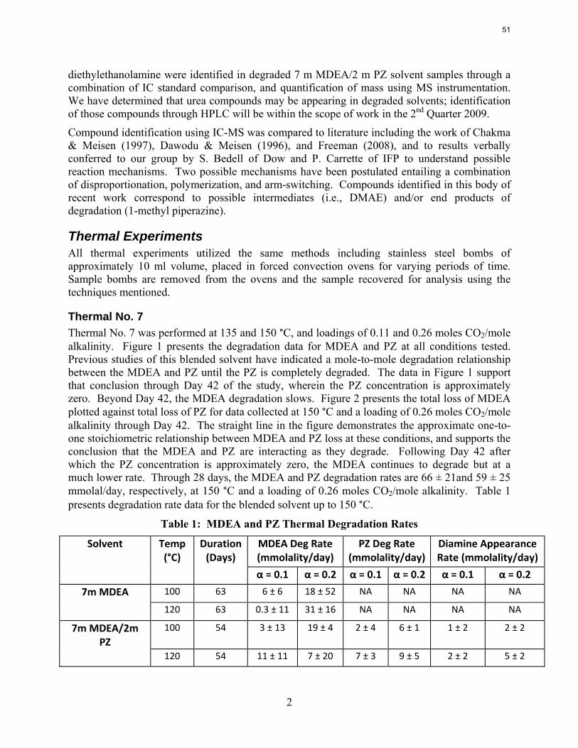
2
diethylethanolamine were identified in degraded 7 m MDEA/2 m PZ solvent samples through a combination of IC standard comparison, and quantification of mass using MS instrumentation. We have determined that urea compounds may be appearing in degraded solvents; identification of those compounds through HPLC will be within the scope of work in the 2nd Quarter 2009.
Compound identification using IC-MS was compared to literature including the work of Chakma & Meisen (1997), Dawodu & Meisen (1996), and Freeman (2008), and to results verbally conferred to our group by S. Bedell of Dow and P. Carrette of IFP to understand possible reaction mechanisms. Two possible mechanisms have been postulated entailing a combination of disproportionation, polymerization, and arm-switching. Compounds identified in this body of recent work correspond to possible intermediates (i.e., DMAE) and/or end products of degradation (1-methyl piperazine).
Thermal Experiments All thermal experiments utilized the same methods including stainless steel bombs of approximately 10 ml volume, placed in forced convection ovens for varying periods of time. Sample bombs are removed from the ovens and the sample recovered for analysis using the techniques mentioned.
Thermal No. 7 Thermal No. 7 was performed at 135 and 150 °C, and loadings of 0.11 and 0.26 moles CO2/mole alkalinity. Figure 1 presents the degradation data for MDEA and PZ at all conditions tested. Previous studies of this blended solvent have indicated a mole-to-mole degradation relationship between the MDEA and PZ until the PZ is completely degraded. The data in Figure 1 support that conclusion through Day 42 of the study, wherein the PZ concentration is approximately zero. Beyond Day 42, the MDEA degradation slows. Figure 2 presents the total loss of MDEA plotted against total loss of PZ for data collected at 150 °C and a loading of 0.26 moles CO2/mole alkalinity through Day 42. The straight line in the figure demonstrates the approximate one-to-one stoichiometric relationship between MDEA and PZ loss at these conditions, and supports the conclusion that the MDEA and PZ are interacting as they degrade. Following Day 42 after which the PZ concentration is approximately zero, the MDEA continues to degrade but at a much lower rate. Through 28 days, the MDEA and PZ degradation rates are 66 ± 21and 59 ± 25 mmolal/day, respectively, at 150 °C and a loading of 0.26 moles CO2/mole alkalinity. Table 1 presents degradation rate data for the blended solvent up to 150 °C.
Table 1: MDEA and PZ Thermal Degradation Rates
Solvent Temp (°C)
Duration (Days)
MDEA Deg Rate (mmolality/day)
PZ Deg Rate (mmolality/day)
Diamine Appearance Rate (mmolality/day)
α = 0.1 α = 0.2 α = 0.1 α = 0.2 α = 0.1 α = 0.2
7m MDEA 100 63 6 ± 6 18 ± 52 NA NA NA NA
120 63 0.3 ± 11 31 ± 16 NA NA NA NA
7m MDEA/2m PZ
100 54 3 ± 13 19 ± 4 2 ± 4 6 ± 1 1 ± 2 2 ± 2
120 54 11 ± 11 7 ± 20 7 ± 3 9 ± 5 2 ± 2 5 ± 2
51
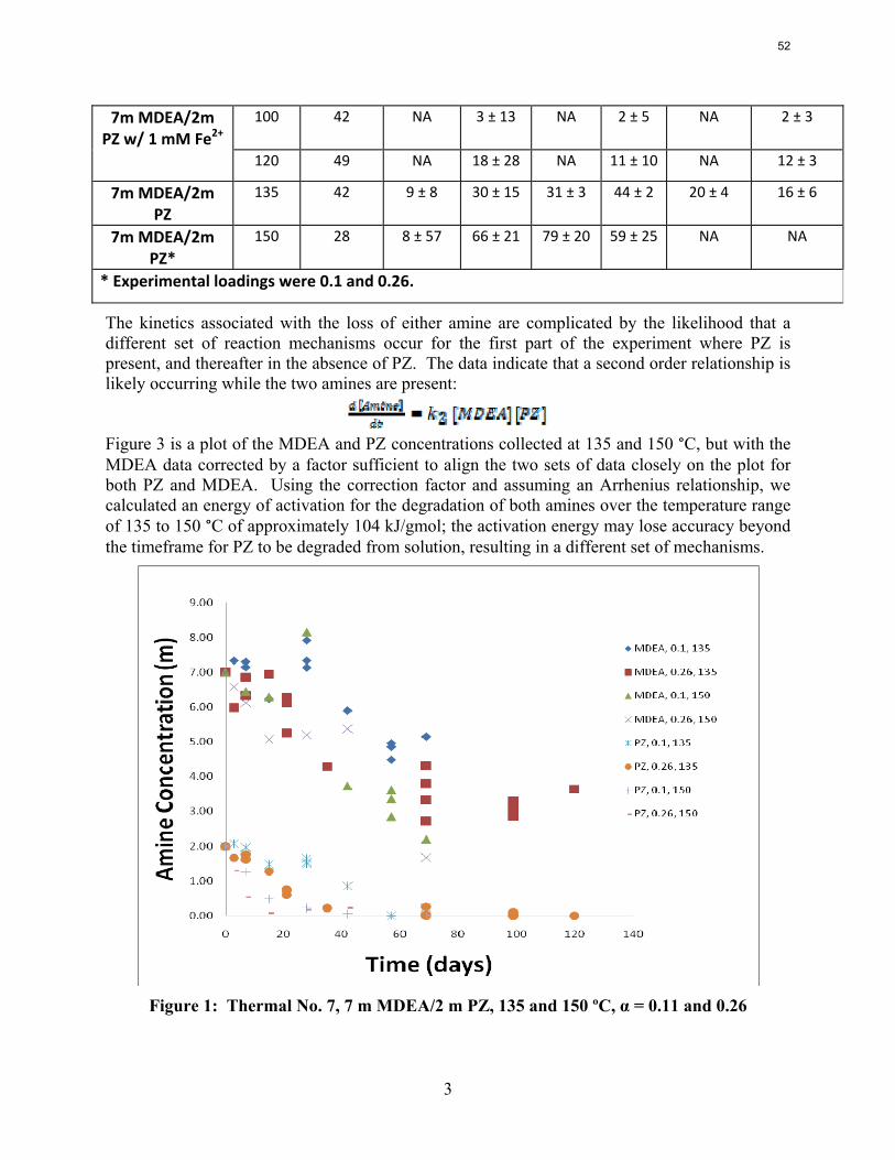
3
7m MDEA/2m PZ w/ 1 mM Fe2+
100 42 NA 3 ± 13 NA 2 ± 5 NA 2 ± 3
120 49 NA 18 ± 28 NA 11 ± 10 NA 12 ± 3
7m MDEA/2m PZ
135 42 9 ± 8 30 ± 15 31 ± 3 44 ± 2 20 ± 4 16 ± 6
7m MDEA/2m PZ*
150 28 8 ± 57 66 ± 21 79 ± 20 59 ± 25 NA NA
* Experimental loadings were 0.1 and 0.26.
The kinetics associated with the loss of either amine are complicated by the likelihood that a different set of reaction mechanisms occur for the first part of the experiment where PZ is present, and thereafter in the absence of PZ. The data indicate that a second order relationship is likely occurring while the two amines are present:
Figure 3 is a plot of the MDEA and PZ concentrations collected at 135 and 150 °C, but with the MDEA data corrected by a factor sufficient to align the two sets of data closely on the plot for both PZ and MDEA. Using the correction factor and assuming an Arrhenius relationship, we calculated an energy of activation for the degradation of both amines over the temperature range of 135 to 150 °C of approximately 104 kJ/gmol; the activation energy may lose accuracy beyond the timeframe for PZ to be degraded from solution, resulting in a different set of mechanisms.
Figure 1: Thermal No. 7, 7 m MDEA/2 m PZ, 135 and 150 ºC, α = 0.11 and 0.26
52
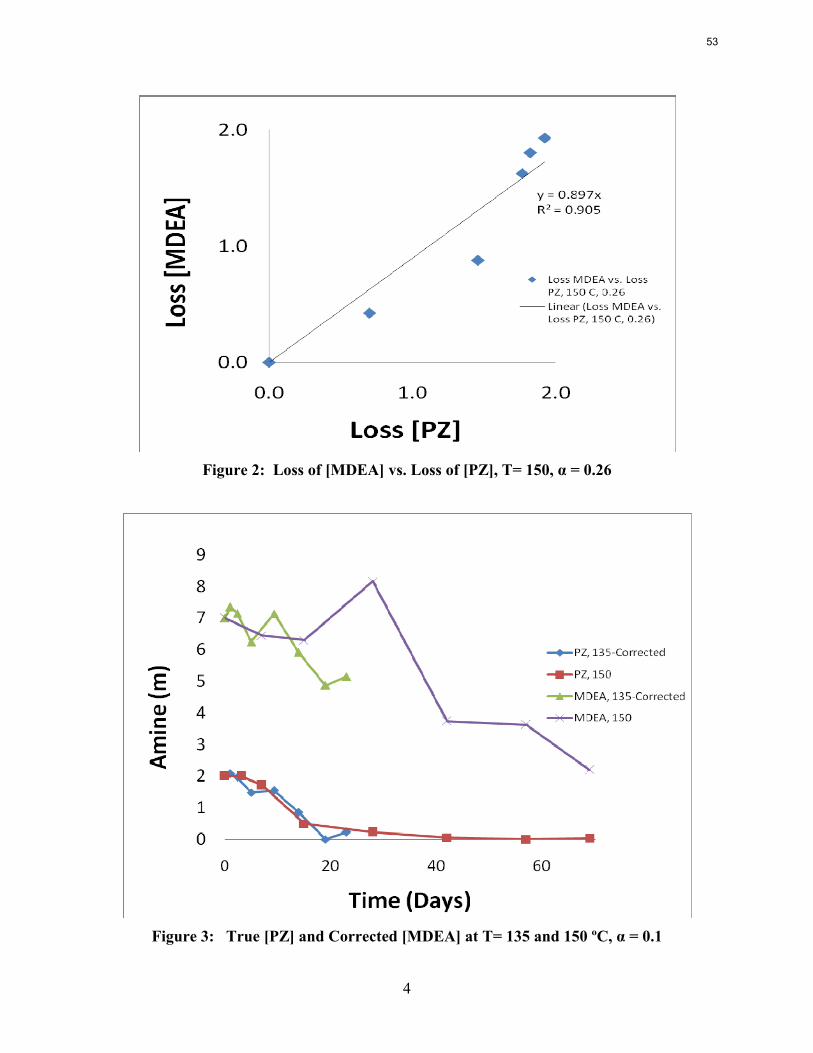
4
Figure 2: Loss of [MDEA] vs. Loss of [PZ], T= 150, α = 0.26
Figure 3: True [PZ] and Corrected [MDEA] at T= 135 and 150 ºC, α = 0.1
53
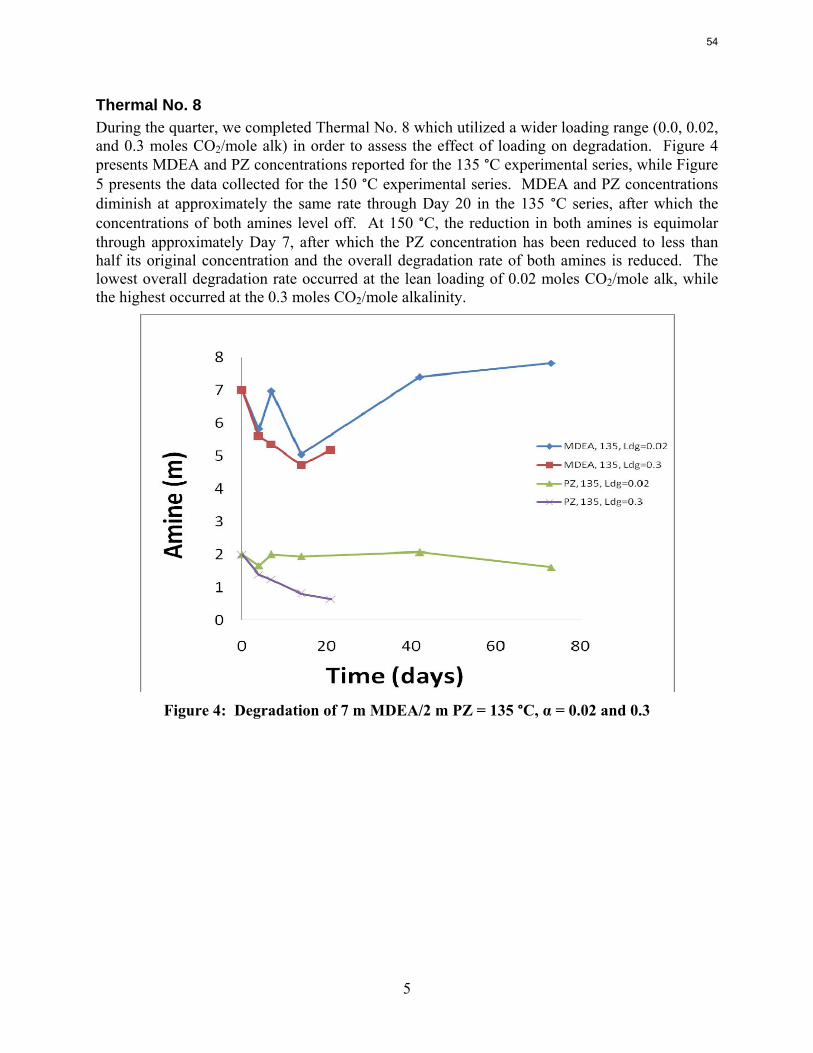
5
Thermal No. 8 During the quarter, we completed Thermal No. 8 which utilized a wider loading range (0.0, 0.02, and 0.3 moles CO2/mole alk) in order to assess the effect of loading on degradation. Figure 4 presents MDEA and PZ concentrations reported for the 135 °C experimental series, while Figure 5 presents the data collected for the 150 °C experimental series. MDEA and PZ concentrations diminish at approximately the same rate through Day 20 in the 135 °C series, after which the concentrations of both amines level off. At 150 °C, the reduction in both amines is equimolar through approximately Day 7, after which the PZ concentration has been reduced to less than half its original concentration and the overall degradation rate of both amines is reduced. The lowest overall degradation rate occurred at the lean loading of 0.02 moles CO2/mole alk, while the highest occurred at the 0.3 moles CO2/mole alkalinity.
Figure 4: Degradation of 7 m MDEA/2 m PZ = 135 °C, α = 0.02 and 0.3
54
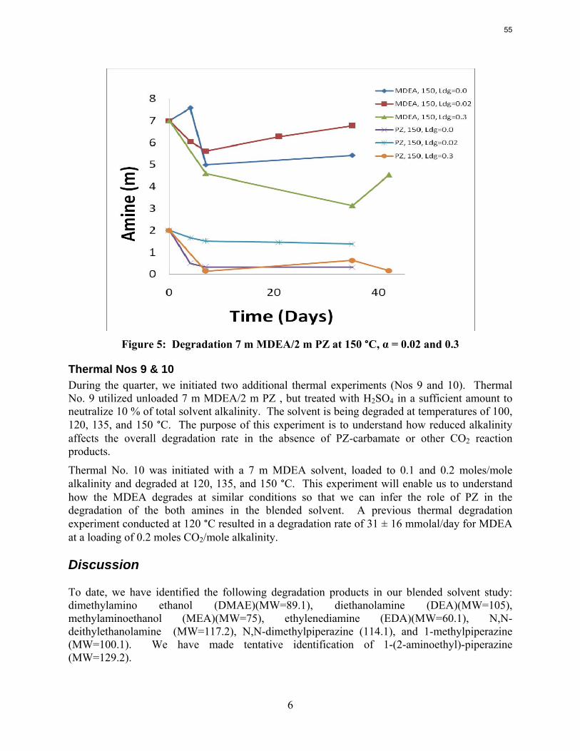
6
Figure 5: Degradation 7 m MDEA/2 m PZ at 150 °C, α = 0.02 and 0.3
Thermal Nos 9 & 10 During the quarter, we initiated two additional thermal experiments (Nos 9 and 10). Thermal No. 9 utilized unloaded 7 m MDEA/2 m PZ , but treated with H2SO4 in a sufficient amount to neutralize 10 % of total solvent alkalinity. The solvent is being degraded at temperatures of 100, 120, 135, and 150 °C. The purpose of this experiment is to understand how reduced alkalinity affects the overall degradation rate in the absence of PZ-carbamate or other CO2 reaction products.
Thermal No. 10 was initiated with a 7 m MDEA solvent, loaded to 0.1 and 0.2 moles/mole alkalinity and degraded at 120, 135, and 150 °C. This experiment will enable us to understand how the MDEA degrades at similar conditions so that we can infer the role of PZ in the degradation of the both amines in the blended solvent. A previous thermal degradation experiment conducted at 120 °C resulted in a degradation rate of 31 ± 16 mmolal/day for MDEA at a loading of 0.2 moles CO2/mole alkalinity.
Discussion
To date, we have identified the following degradation products in our blended solvent study: dimethylamino ethanol (DMAE)(MW=89.1), diethanolamine (DEA)(MW=105), methylaminoethanol (MEA)(MW=75), ethylenediamine (EDA)(MW=60.1), N,N-deithylethanolamine (MW=117.2), N,N-dimethylpiperazine (114.1), and 1-methylpiperazine (MW=100.1). We have made tentative identification of 1-(2-aminoethyl)-piperazine (MW=129.2).
55
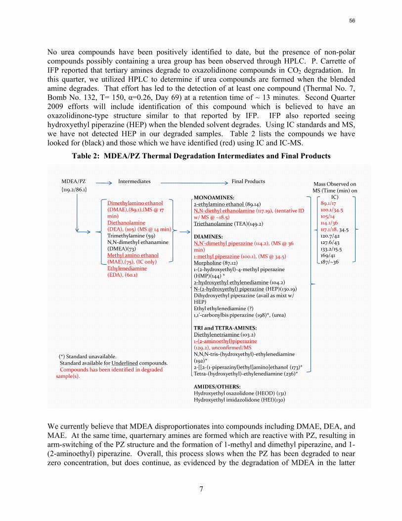
7
No urea compounds have been positively identified to date, but the presence of non-polar compounds possibly containing a urea group has been observed through HPLC. P. Carrette of IFP reported that tertiary amines degrade to oxazolidinone compounds in CO2 degradation. In this quarter, we utilized HPLC to determine if urea compounds are formed when the blended amine degrades. That effort has led to the detection of at least one compound (Thermal No. 7, Bomb No. 132, T= 150, α=0.26, Day 69) at a retention time of ~ 13 minutes. Second Quarter 2009 efforts will include identification of this compound which is believed to have an oxazolidinone-type structure similar to that reported by IFP. IFP also reported seeing hydroxyethyl piperazine (HEP) when the blended solvent degrades. Using IC standards and MS, we have not detected HEP in our degraded samples. Table 2 lists the compounds we have looked for (black) and those which we have identified (red) using IC and IC-MS.
Table 2: MDEA/PZ Thermal Degradation Intermediates and Final Products
MDEA/PZ Intermediates Final Products
Dimethylamino ethanol (DMAE),(89.1),(MS @ 17 min)Diethanolamine(DEA), (105) (MS @ 14 min)Trimethylamine (59)N,N‐dimethyl ethanamine(DMEA)(73)Methyl amino ethanol (MAE),(75), (IC only)Ethylenediamine(EDA), (60.1)
MONOAMINES:2‐ethylamino ethanol (89.14)N,N‐diethyl ethanolamine (117.19), (tentative ID w/ MS @ ~18.5)Triethanolamine (TEA)(149.2)
DIAMINES:N,N’‐dimethyl piperazine (114.2), (MS @ 36 min)1‐methyl piperazine (100.1), (MS @ 34.5)Morpholine (87.12)1‐(2‐hydroxyethyl)‐4‐methyl piperazine(HMP)(144) *2‐hydroxyethyl ethylenediamine (104.2)N‐(2‐hydroxyethyl) piperazine (HEP)(130.19)Dihydroxyethyl piperazine (avail as mixt w/ HEP)Ethyl ethylenediamine (?)1,1’‐carbonylbis piperazine (198)*, (urea)
TRI and TETRA‐AMINES:Diethylenetriamine (103.2)1‐(2‐aminoethyl)piperazine(129.2), unconfirmed/MSN,N,N‐tris‐(hydroxyethyl)‐ethylenediamine(192)*2‐[[2‐(1‐piperazinyl)ethyl]amino]ethanol (173)*Tetra‐(hydroxyethyl)‐ethylenediamine (236)*
AMIDES/OTHERS:Hydroxyethyl oxazolidone (HEOD) (131)Hydroxyethyl imidazolidone (HEI)(130)
Mass Observed on MS (Time (min) on
IC)89.1/17100.1/34.5105/14114.1/36117.1/18, 34.5120.7/42127.6/43133.2/15.5169/41187/~36
{119.2/86.1}
(*) Standard unavailable.Standard available for Underlined compounds.Compounds has been identified in degraded
sample(s).
We currently believe that MDEA disproportionates into compounds including DMAE, DEA, and MAE. At the same time, quarternary amines are formed which are reactive with PZ, resulting in arm-switching of the PZ structure and the formation of 1-methyl and dimethyl piperazine, and 1-(2-aminoethyl) piperazine. Overall, this process slows when the PZ has been degraded to near zero concentration, but does continue, as evidenced by the degradation of MDEA in the latter
56
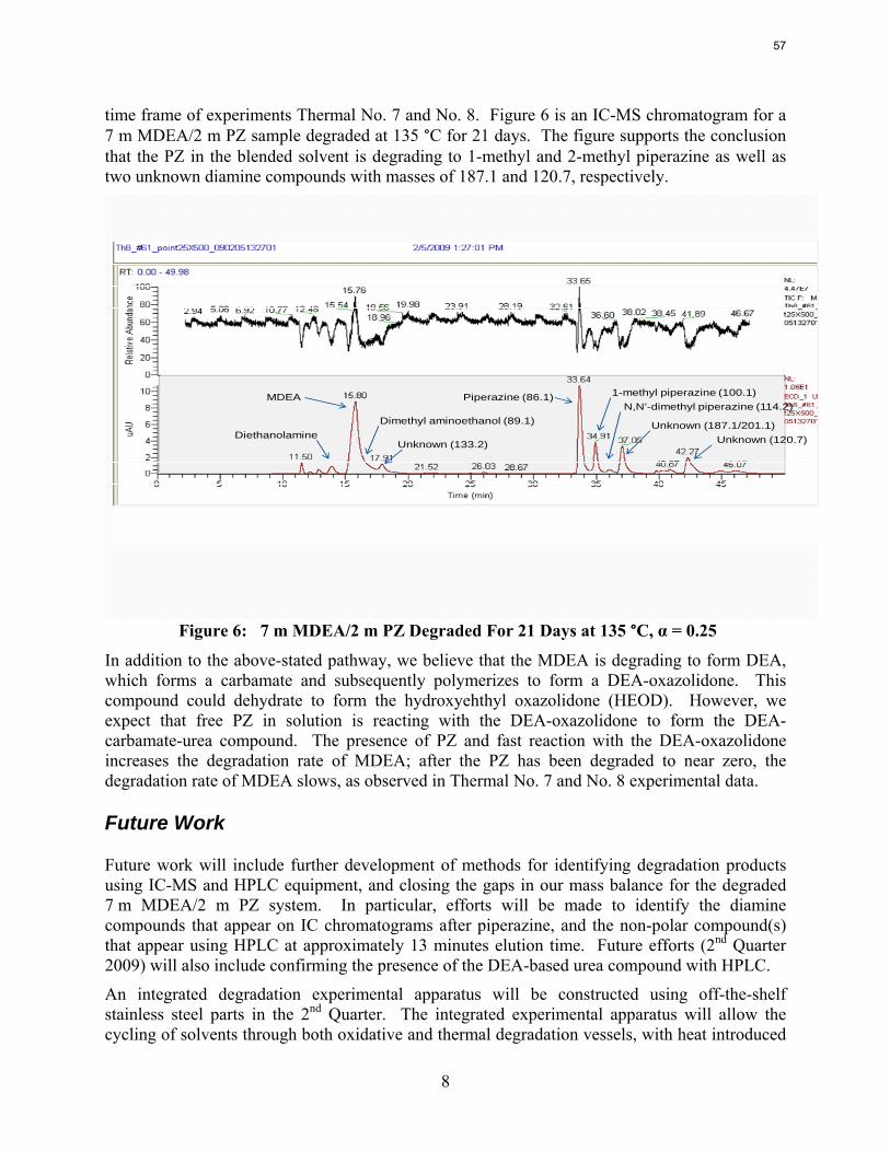
8
time frame of experiments Thermal No. 7 and No. 8. Figure 6 is an IC-MS chromatogram for a 7 m MDEA/2 m PZ sample degraded at 135 °C for 21 days. The figure supports the conclusion that the PZ in the blended solvent is degrading to 1-methyl and 2-methyl piperazine as well as two unknown diamine compounds with masses of 187.1 and 120.7, respectively.
Piperazine (86.1) 1-methyl piperazine (100.1)N,N’-dimethyl piperazine (114.2)
Unknown (187.1/201.1)Dimethyl aminoethanol (89.1)
Unknown (133.2) Unknown (120.7)Diethanolamine
MDEA
Figure 6: 7 m MDEA/2 m PZ Degraded For 21 Days at 135 °C, α = 0.25
In addition to the above-stated pathway, we believe that the MDEA is degrading to form DEA, which forms a carbamate and subsequently polymerizes to form a DEA-oxazolidone. This compound could dehydrate to form the hydroxyehthyl oxazolidone (HEOD). However, we expect that free PZ in solution is reacting with the DEA-oxazolidone to form the DEA-carbamate-urea compound. The presence of PZ and fast reaction with the DEA-oxazolidone increases the degradation rate of MDEA; after the PZ has been degraded to near zero, the degradation rate of MDEA slows, as observed in Thermal No. 7 and No. 8 experimental data.
Future Work
Future work will include further development of methods for identifying degradation products using IC-MS and HPLC equipment, and closing the gaps in our mass balance for the degraded 7 m MDEA/2 m PZ system. In particular, efforts will be made to identify the diamine compounds that appear on IC chromatograms after piperazine, and the non-polar compound(s) that appear using HPLC at approximately 13 minutes elution time. Future efforts (2nd Quarter 2009) will also include confirming the presence of the DEA-based urea compound with HPLC.
An integrated degradation experimental apparatus will be constructed using off-the-shelf stainless steel parts in the 2nd Quarter. The integrated experimental apparatus will allow the cycling of solvents through both oxidative and thermal degradation vessels, with heat introduced
57
9
to the system conserved with a cross exchanger. Analytical methods developed for the batch thermal and oxidative degradation experiments over the last year will be utilized to analyze samples collected from the cycling apparatus.
References
Bedell, Steve, Dow Chemical Company, Personal Communication, Feb. 25, 2009.
Carrette, Pierre, IFP, Personal Communication at GHGT-9, Washington D.C., November, 2008.
Chakma A & Meisen A. "Methyl-Diethanolamine Degradation - Mechanism and Kinetics." Can J Chem Eng. 1977:75.
Dawodu OF & Meisen A. "Degradation of Alkanolamine Blends by Carbon Dioxide." Can J Chem Eng. 1996:74.
Freeman SA. "Carbon dioxide capture with concentrated, aqueous piperazine." GHGT-9, Washington D.C. 2008.
58
1
Degradation of Concentrated Piperazine and a Summary of the 8 m Piperazine Pilot Plant Campaign
Quarterly Report for January 1 – March 31, 2009
by Stephanie A. Freeman
Supported by the Luminant Carbon Management Program
and the
Industrial Associates Program for CO2 Capture by Aqueous Absorption
Department of Chemical Engineering
The University of Texas at Austin
April 1, 2009
Abstract The solution analysis of the pilot plant was completed this quarter and all the measured values are reported. There is slight disagreement between the measurements taken at the pilot plant during the actual campaign and those completed afterwards in the laboratory. There was not a significant production of degradation products with the highest concentrations of anions below 0.5 mM. A small amount of ethylenediamine (EDA) was detected with the samples ranging from 0.61 mM, well below the baseline detection limit of the cation IC, to 9.79 mM. A foaming test of the final campaign solution indicated that very little foaming occurred during the test. The foaminess coefficient of the solution was 44 x 10-3 m2-s compared to the coefficient of 27 x 10-3 m2-s for a neat 5 m PZ solution. The low foaminess coefficient and lack of degradation products indicates that PZ resisted oxidation and thermal degradation during the three-week pilot plant campaign.
The low gas flow apparatus was analyzed to determine the source of PZ loss when degradation products alone cannot account for it. A baseline experiment using nitrogen and CO2 was performed to determine the loss due to volatility. It was determined that volatility alone cannot account for the amount of PZ loss seen in a typical low gas flow experiment with 8 m PZ. Other probable causes such as liquid entrainment and dilution will be analyzed in the future.
A long term thermal degradation experiment demonstrated the thermal resistance of concentrated PZ. After 18 weeks at 150 °C, only 8.0% of the initial PZ was lost. This amounts to a loss of only 0.44% of the original PZ per week. The most prevalent degradation products were EDA (1.2 mM/wk), formate (0.9 mM /wk), and N-formyl amides (2.3 mM/wk).
Introduction Concentrated aqueous piperazine (PZ) is being investigated as a possible alternative to 30 wt % (or 7 m) MEA in absorber/stripper systems to remove CO2 from coal-fired power plant flue gas. Aqueous PZ has been given a proprietary name of ROC20 for 10 m PZ and ROC16 for 8 m PZ. Previous reports include the proprietary name, while the concentration of PZ will be explicitly used in this document.
59
2
Preliminary investigations of PZ have shown numerous advantages over 7 m MEA systems (Freeman, 2008a). Aqueous concentrated PZ solutions have less oxidative and thermal degradation, as previously shown at concentrations of 5 and 8 m PZ (see previous quarterly reports). The kinetics of CO2 absorption are faster in concentrated PZ, as shown by Cullinane, and are currently being measured by Dugas (Cullinane and Rochelle, 2006; Dugas, 2008). The capacity of concentrated PZ is greater than that of MEA while the heat of absorption and volatilities are comparable.
This quarter was focused on short term oxidative degradation experiments with 8 m PZ and finishing analysis of last quarter’s pilot plant campaign. The oxidation experiment was conducted in an attempt to quantify the volatility of PZ in the low gas flow apparatus.
Experimental Methods Analytical Methods Total Inorganic Carbon Analysis (TIC): Quantification of CO2 loading was performed using a total inorganic carbon analyzer. In this method, a sample is acidified with 30 wt % H3PO4 to release the CO2 present in solution (Hilliard, 2008). The CO2 is carried in the nitrogen carrier gas stream to the detector. PicoLog software is used to record the peaks that are produced from each sample. A calibration curve is prepared at the end of each analysis using a TIC standard mixture of K2CO3 and KHCO3. The TIC method quantifies the CO2, CO3
-2, and HCO3- present
in solution. These species are in equilibrium in the series of reactions shown below.
CO32−
+ 2H+ ↔ HCO3− + H+ ↔ H2CO3 ↔ CO2 + H2O
Acidification of the sample shifts the equilibrium toward CO2 which bubbles out of solution and is detected in the analyzer.
Acid pH Titration: Titration with 0.2 N H2SO4 is used to determine the concentration of amines in experimental samples. The automated Titrando apparatus (Metrohm AG, Herisau, Switzerland) is used for this method. A known mass of sample is diluted with water and the autotitration method is then used. The Titrando titrates the sample with acid while monitoring the pH. The equivalence points are recorded. The equivalence point around a pH of 3.9 corresponds to basic amine species in solution (Hilliard, 2008). The test is not sensitive to the type of amine, so if PZ has degraded to EDA, the titration test will detect the sum of contributions from the species.
Anion IC: The anion IC was used to determine the concentration of glycolate, acetate, formate, chloride, nitrite, sulfate, oxalate, and nitrate in experimental samples. A Dionex ICS-3000 instrument with AS15 IonPac column, ASRS 4mm self-regenerating suppressor, carbonate removal device (CRD), and carbonate removal from eluent generation was used as previously described by Andrew Sexton using a linear KOH eluent concentration (Sexton, 2008). No major modifications have been made to the method in this quarter.
Cation IC: The cation IC was used to determine the concentration of PZ and ethylenediamine (EDA) in experimental samples. A Dionex ICS-2500 instrument with CS17 IonPac column with CSRS 4-mm self-regeneraing suppressor was used as previously described by Andrew Sexton with a linear increase of methanesulfonic acid (MSA) concentration in the eluent (Sexton, 2008). No major modifications have been made to the method in this quarter.
60
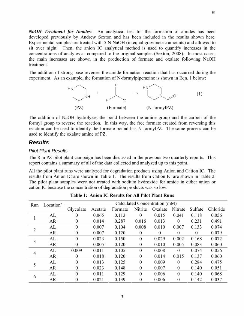
3
NaOH Treatment for Amides: An analytical test for the formation of amides has been developed previously by Andrew Sexton and has been included in the results shown here. Experimental samples are treated with 5 N NaOH (in equal gravimetric amounts) and allowed to sit over night. Then, the anion IC analytical method is used to quantify increases in the concentrations of analytes as compared to the original samples (Sexton, 2008). In most cases, the main increases are shown in the production of formate and oxalate following NaOH treatment.
The addition of strong base reverses the amide formation reaction that has occurred during the experiment. As an example, the formation of N-formylpiperazine is shown in Eqn. 1 below:
(1)
The addition of NaOH hydrolyzes the bond between the amine group and the carbon of the formyl group to reverse the reaction. In this way, the free formate created from reversing this reaction can be used to identify the formate bound has N-formylPZ. The same process can be used to identify the oxalate amine of PZ.
Results Pilot Plant Results The 8 m PZ pilot plant campaign has been discussed in the previous two quarterly reports. This report contains a summary of all of the data collected and analyzed up to this point.
All the pilot plant runs were analyzed for degradation products using Anion and Cation IC. The results from Anion IC are shown in Table 1. The results from Cation IC are shown in Table 2. The pilot plant samples were not treated with sodium hydroxide for amide in either anion or cation IC because the concentration of degradation products was so low.
Table 1: Anion IC Results for All Pilot Plant Runs
Calculated Concentration (mM) Run Locationa Glycolate Acetate Formate Nitrite Oxalate Nitrate Sulfate Chloride
AL 0 0.065 0.113 0 0.015 0.041 0.118 0.056 1 AR 0 0.014 0.287 0.016 0.013 0 0.231 0.491 AL 0 0.007 0.104 0.008 0.010 0.007 0.133 0.074 2 AR 0 0.007 0.120 0 0 0 0 0.079 AL 0 0.023 0.150 0 0.029 0.002 0.168 0.072 3 AR 0 0.005 0.120 0 0.010 0.005 0.083 0.060 AL 0.009 0.011 0.105 0 0.008 0 0.074 0.056 4 AR 0 0.018 0.120 0 0.014 0.015 0.137 0.060 AL 0 0.013 0.125 0 0.009 0 0.284 0.475 5 AR 0 0.023 0.148 0 0.007 0 0.140 0.051 AL 0 0.011 0.129 0 0.006 0 0.140 0.068 6 AR 0 0.021 0.139 0 0.006 0 0.142 0.037
+
→
(PZ) (Formate) (N-formylPZ)
61
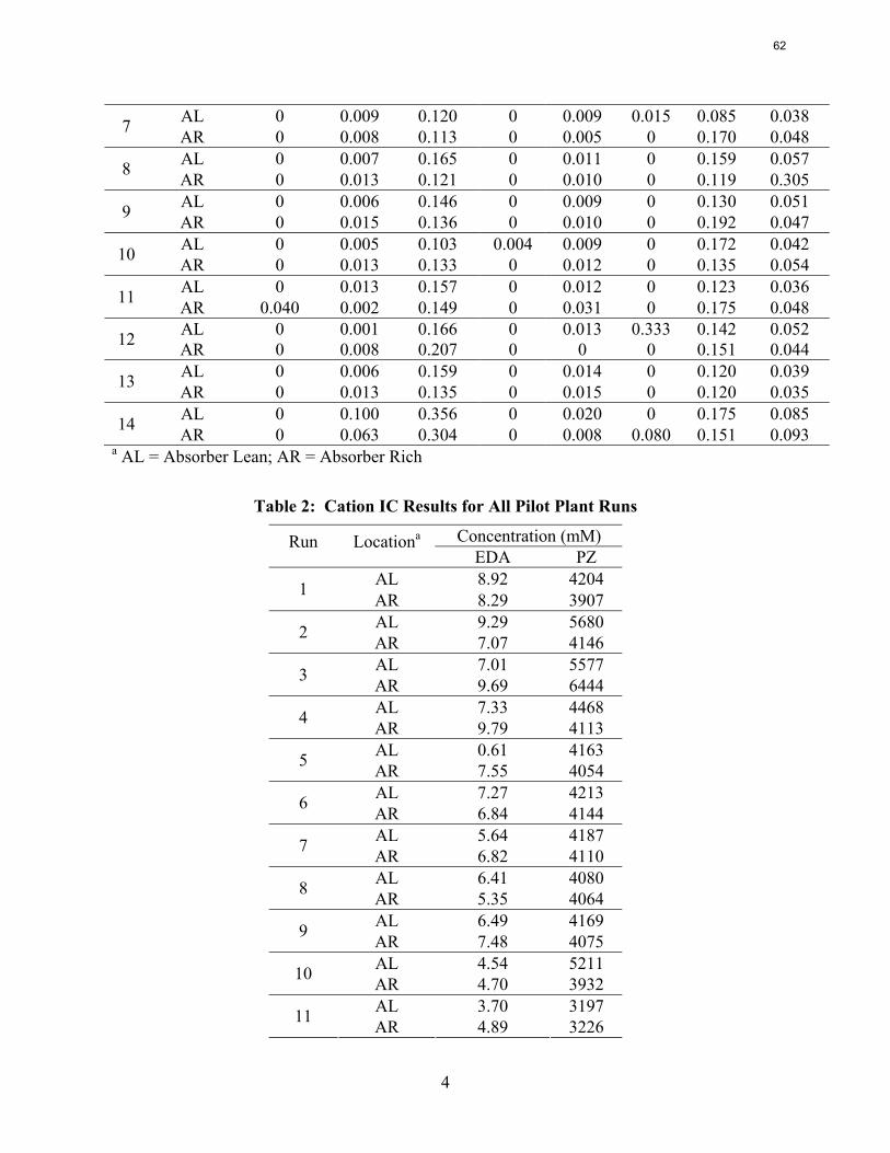
4
AL 0 0.009 0.120 0 0.009 0.015 0.085 0.038 7 AR 0 0.008 0.113 0 0.005 0 0.170 0.048 AL 0 0.007 0.165 0 0.011 0 0.159 0.057 8 AR 0 0.013 0.121 0 0.010 0 0.119 0.305 AL 0 0.006 0.146 0 0.009 0 0.130 0.051 9 AR 0 0.015 0.136 0 0.010 0 0.192 0.047 AL 0 0.005 0.103 0.004 0.009 0 0.172 0.042 10 AR 0 0.013 0.133 0 0.012 0 0.135 0.054 AL 0 0.013 0.157 0 0.012 0 0.123 0.036 11 AR 0.040 0.002 0.149 0 0.031 0 0.175 0.048 AL 0 0.001 0.166 0 0.013 0.333 0.142 0.052 12 AR 0 0.008 0.207 0 0 0 0.151 0.044 AL 0 0.006 0.159 0 0.014 0 0.120 0.039 13 AR 0 0.013 0.135 0 0.015 0 0.120 0.035 AL 0 0.100 0.356 0 0.020 0 0.175 0.085 14 AR 0 0.063 0.304 0 0.008 0.080 0.151 0.093
a AL = Absorber Lean; AR = Absorber Rich
Table 2: Cation IC Results for All Pilot Plant Runs
Concentration (mM) Run Locationa EDA PZ
AL 8.92 4204 1 AR 8.29 3907 AL 9.29 5680 2 AR 7.07 4146 AL 7.01 5577 3 AR 9.69 6444 AL 7.33 4468 4 AR 9.79 4113 AL 0.61 4163 5 AR 7.55 4054 AL 7.27 4213 6 AR 6.84 4144 AL 5.64 4187 7 AR 6.82 4110 AL 6.41 4080 8 AR 5.35 4064 AL 6.49 4169 9 AR 7.48 4075 AL 4.54 5211 10 AR 4.70 3932 AL 3.70 3197 11 AR 4.89 3226
62
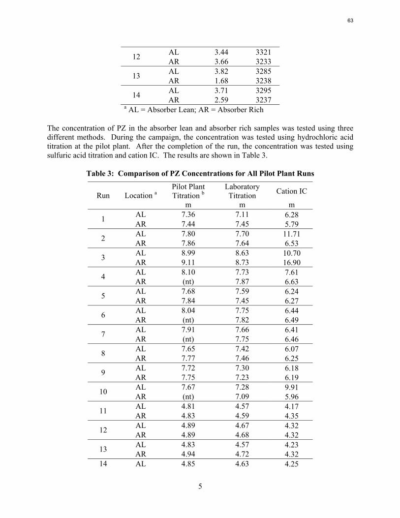
5
AL 3.44 3321 12 AR 3.66 3233 AL 3.82 3285 13 AR 1.68 3238 AL 3.71 3295 14 AR 2.59 3237
a AL = Absorber Lean; AR = Absorber Rich
The concentration of PZ in the absorber lean and absorber rich samples was tested using three different methods. During the campaign, the concentration was tested using hydrochloric acid titration at the pilot plant. After the completion of the run, the concentration was tested using sulfuric acid titration and cation IC. The results are shown in Table 3.
Table 3: Comparison of PZ Concentrations for All Pilot Plant Runs
Pilot Plant Titration b
Laboratory Titration Cation IC Run Location a
m m m AL 7.36 7.11 6.28 1 AR 7.44 7.45 5.79 AL 7.80 7.70 11.71 2 AR 7.86 7.64 6.53 AL 8.99 8.63 10.70 3 AR 9.11 8.73 16.90 AL 8.10 7.73 7.61 4 AR (nt) 7.87 6.63 AL 7.68 7.59 6.24 5 AR 7.84 7.45 6.27 AL 8.04 7.75 6.44 6 AR (nt) 7.82 6.49 AL 7.91 7.66 6.41 7 AR (nt) 7.75 6.46 AL 7.65 7.42 6.07 8 AR 7.77 7.46 6.25 AL 7.72 7.30 6.18 9 AR 7.75 7.23 6.19 AL 7.67 7.28 9.91 10 AR (nt) 7.09 5.96 AL 4.81 4.57 4.17 11 AR 4.83 4.59 4.35 AL 4.89 4.67 4.32 12 AR 4.89 4.68 4.32 AL 4.83 4.57 4.23 13 AR 4.94 4.72 4.32
14 AL 4.85 4.63 4.25
63
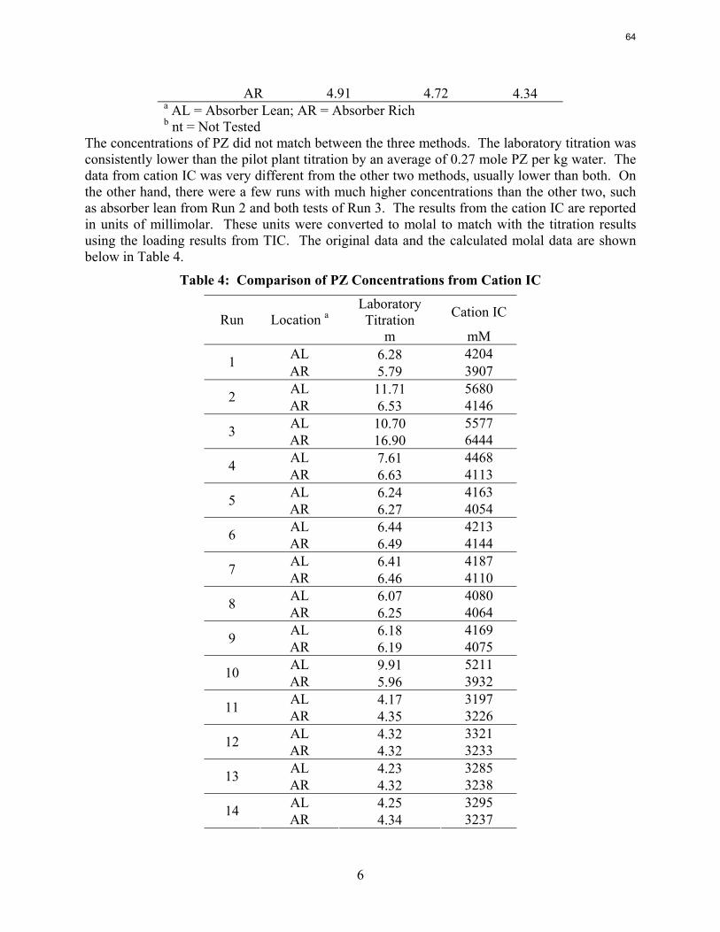
6
AR 4.91 4.72 4.34 a AL = Absorber Lean; AR = Absorber Rich b nt = Not Tested
The concentrations of PZ did not match between the three methods. The laboratory titration was consistently lower than the pilot plant titration by an average of 0.27 mole PZ per kg water. The data from cation IC was very different from the other two methods, usually lower than both. On the other hand, there were a few runs with much higher concentrations than the other two, such as absorber lean from Run 2 and both tests of Run 3. The results from the cation IC are reported in units of millimolar. These units were converted to molal to match with the titration results using the loading results from TIC. The original data and the calculated molal data are shown below in Table 4.
Table 4: Comparison of PZ Concentrations from Cation IC
Laboratory Titration Cation IC Run Location a
m mM AL 6.28 4204 1 AR 5.79 3907 AL 11.71 5680 2 AR 6.53 4146 AL 10.70 5577 3 AR 16.90 6444 AL 7.61 4468 4 AR 6.63 4113 AL 6.24 4163 5 AR 6.27 4054 AL 6.44 4213 6 AR 6.49 4144 AL 6.41 4187 7 AR 6.46 4110 AL 6.07 4080 8 AR 6.25 4064 AL 6.18 4169 9 AR 6.19 4075 AL 9.91 5211 10 AR 5.96 3932 AL 4.17 3197 11 AR 4.35 3226 AL 4.32 3321 12 AR 4.32 3233 AL 4.23 3285 13 AR 4.32 3238 AL 4.25 3295 14 AR 4.34 3237
64
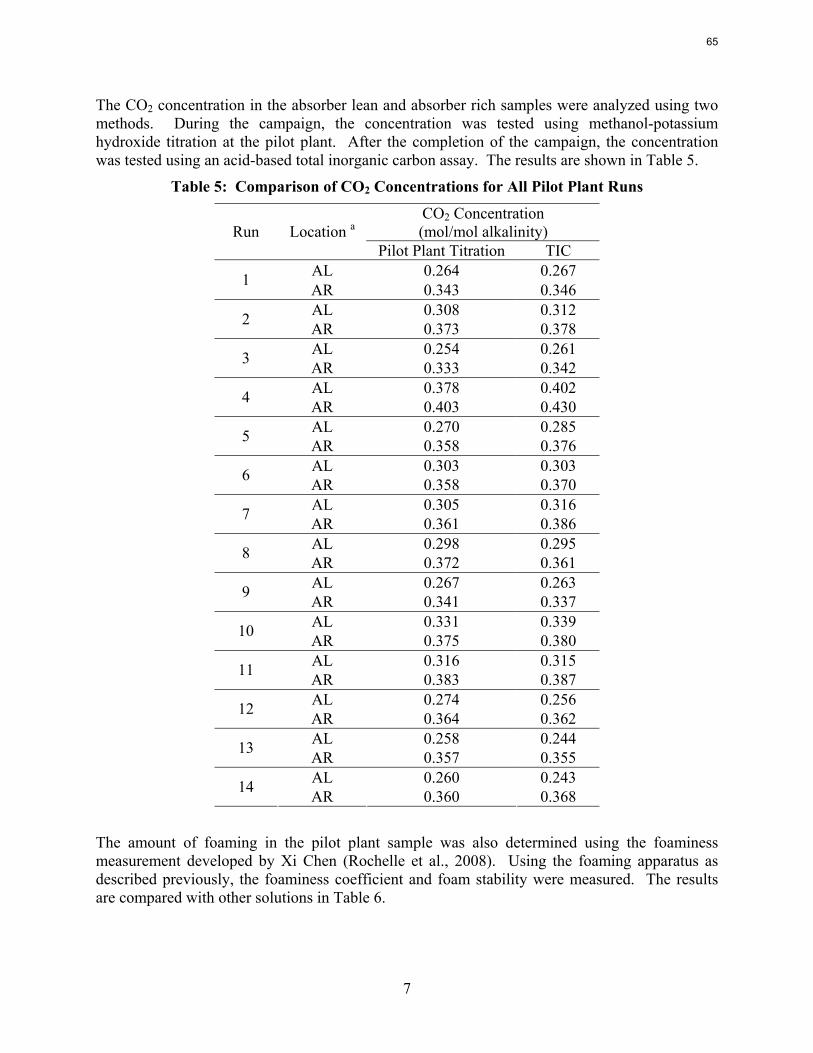
7
The CO2 concentration in the absorber lean and absorber rich samples were analyzed using two methods. During the campaign, the concentration was tested using methanol-potassium hydroxide titration at the pilot plant. After the completion of the campaign, the concentration was tested using an acid-based total inorganic carbon assay. The results are shown in Table 5.
Table 5: Comparison of CO2 Concentrations for All Pilot Plant Runs
CO2 Concentration (mol/mol alkalinity) Run Location a
Pilot Plant Titration TIC AL 0.264 0.267 1 AR 0.343 0.346 AL 0.308 0.312 2 AR 0.373 0.378 AL 0.254 0.261 3 AR 0.333 0.342 AL 0.378 0.402 4 AR 0.403 0.430 AL 0.270 0.285 5 AR 0.358 0.376 AL 0.303 0.303 6 AR 0.358 0.370 AL 0.305 0.316 7 AR 0.361 0.386 AL 0.298 0.295 8 AR 0.372 0.361 AL 0.267 0.263 9 AR 0.341 0.337 AL 0.331 0.339 10 AR 0.375 0.380 AL 0.316 0.315 11 AR 0.383 0.387 AL 0.274 0.256 12 AR 0.364 0.362 AL 0.258 0.244 13 AR 0.357 0.355 AL 0.260 0.243 14 AR 0.360 0.368
The amount of foaming in the pilot plant sample was also determined using the foaminess measurement developed by Xi Chen (Rochelle et al., 2008). Using the foaming apparatus as described previously, the foaminess coefficient and foam stability were measured. The results are compared with other solutions in Table 6.
65
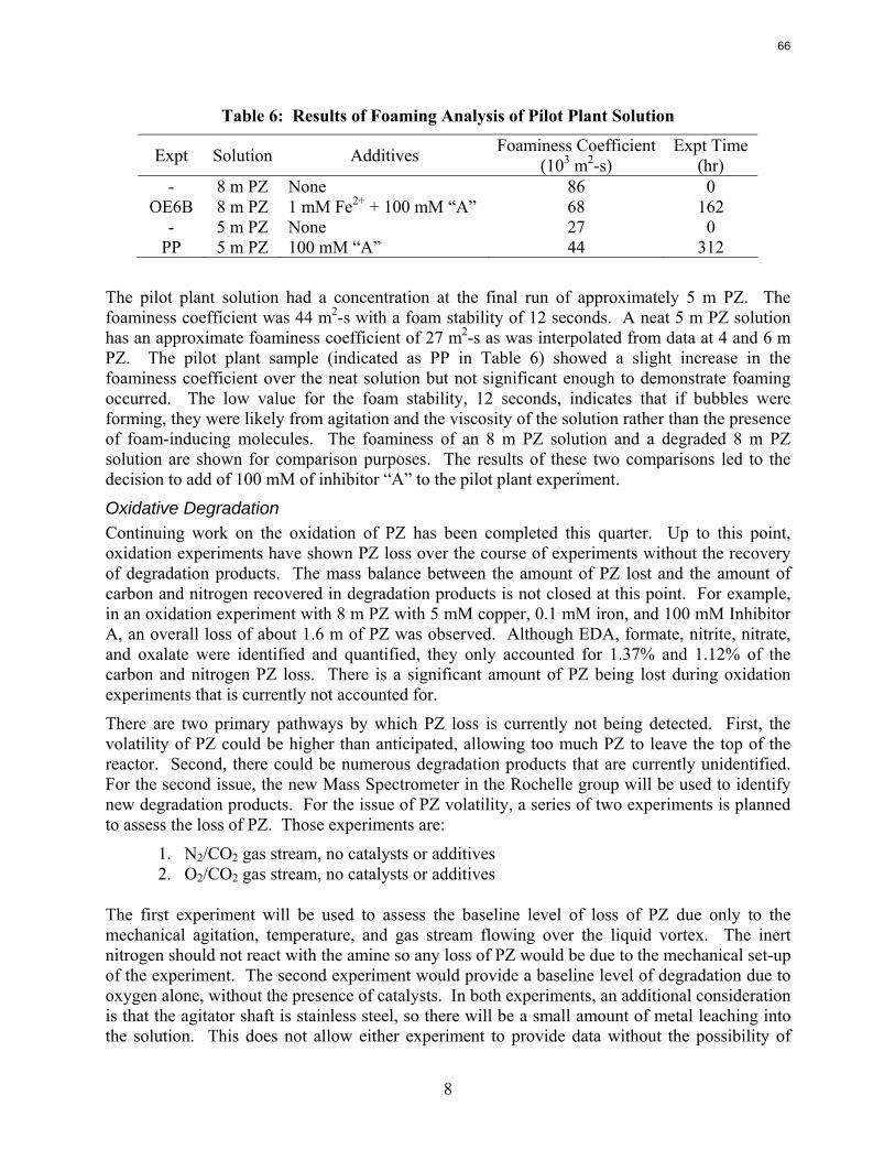
8
Table 6: Results of Foaming Analysis of Pilot Plant Solution
Expt Solution Additives Foaminess Coefficient (103 m2-s)
Expt Time (hr)
- 8 m PZ None 86 0 OE6B 8 m PZ 1 mM Fe2+ + 100 mM “A” 68 162
- 5 m PZ None 27 0 PP 5 m PZ 100 mM “A” 44 312
The pilot plant solution had a concentration at the final run of approximately 5 m PZ. The foaminess coefficient was 44 m2-s with a foam stability of 12 seconds. A neat 5 m PZ solution has an approximate foaminess coefficient of 27 m2-s as was interpolated from data at 4 and 6 m PZ. The pilot plant sample (indicated as PP in Table 6) showed a slight increase in the foaminess coefficient over the neat solution but not significant enough to demonstrate foaming occurred. The low value for the foam stability, 12 seconds, indicates that if bubbles were forming, they were likely from agitation and the viscosity of the solution rather than the presence of foam-inducing molecules. The foaminess of an 8 m PZ solution and a degraded 8 m PZ solution are shown for comparison purposes. The results of these two comparisons led to the decision to add of 100 mM of inhibitor “A” to the pilot plant experiment.
Oxidative Degradation Continuing work on the oxidation of PZ has been completed this quarter. Up to this point, oxidation experiments have shown PZ loss over the course of experiments without the recovery of degradation products. The mass balance between the amount of PZ lost and the amount of carbon and nitrogen recovered in degradation products is not closed at this point. For example, in an oxidation experiment with 8 m PZ with 5 mM copper, 0.1 mM iron, and 100 mM Inhibitor A, an overall loss of about 1.6 m of PZ was observed. Although EDA, formate, nitrite, nitrate, and oxalate were identified and quantified, they only accounted for 1.37% and 1.12% of the carbon and nitrogen PZ loss. There is a significant amount of PZ being lost during oxidation experiments that is currently not accounted for.
There are two primary pathways by which PZ loss is currently not being detected. First, the volatility of PZ could be higher than anticipated, allowing too much PZ to leave the top of the reactor. Second, there could be numerous degradation products that are currently unidentified. For the second issue, the new Mass Spectrometer in the Rochelle group will be used to identify new degradation products. For the issue of PZ volatility, a series of two experiments is planned to assess the loss of PZ. Those experiments are:
1. N2/CO2 gas stream, no catalysts or additives 2. O2/CO2 gas stream, no catalysts or additives
The first experiment will be used to assess the baseline level of loss of PZ due only to the mechanical agitation, temperature, and gas stream flowing over the liquid vortex. The inert nitrogen should not react with the amine so any loss of PZ would be due to the mechanical set-up of the experiment. The second experiment would provide a baseline level of degradation due to oxygen alone, without the presence of catalysts. In both experiments, an additional consideration is that the agitator shaft is stainless steel, so there will be a small amount of metal leaching into the solution. This does not allow either experiment to provide data without the possibility of
66
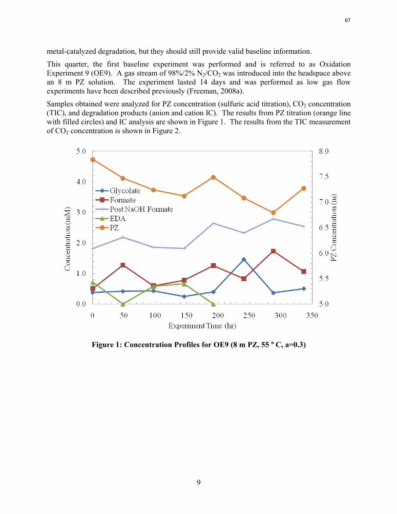
9
metal-catalyzed degradation, but they should still provide valid baseline information.
This quarter, the first baseline experiment was performed and is referred to as Oxidation Experiment 9 (OE9). A gas stream of 98%/2% N2/CO2 was introduced into the headspace above an 8 m PZ solution. The experiment lasted 14 days and was performed as low gas flow experiments have been described previously (Freeman, 2008a).
Samples obtained were analyzed for PZ concentration (sulfuric acid titration), CO2 concentration (TIC), and degradation products (anion and cation IC). The results from PZ titration (orange line with filled circles) and IC analysis are shown in Figure 1. The results from the TIC measurement of CO2 concentration is shown in Figure 2.
Figure 1: Concentration Profiles for OE9 (8 m PZ, 55 °C, a=0.3)
67
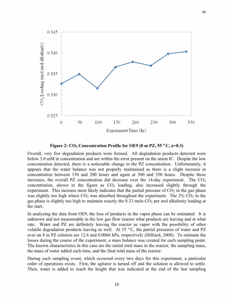
10
Figure 2: CO2 Concentration Profile for OE9 (8 m PZ, 55 °C, a=0.3)
Overall, very few degradation products were formed. All degradation products detected were below 3.0 mM in concentration and are within the error present on the anion IC. Despite the low concentration detected, there is a noticeable change in the PZ concentration. Unfortunately, it appears that the water balance was not properly maintained as there is a slight increase in concentration between 150 and 200 hours and again at 300 and 350 hours. Despite these increases, the overall PZ concentration did decrease over the 14-day experiment. The CO2 concentration, shown in the figure as CO2 loading, also increased slightly through the experiment. This increase most likely indicates that the partial pressure of CO2 in the gas phase was slightly too high where CO2 was absorbed throughout the experiment. The 2% CO2 in the gas phase is slightly too high to maintain exactly the 0.33 mole CO2 per mol alkalinity loading at the start.
In analyzing the data from OE9, the loss of products in the vapor phase can be estimated. It is unknown and not measureable in the low gas flow reactor what products are leaving and at what rate. Water and PZ are definitely leaving the reactor as vapor with the possibility of other volatile degradation products leaving as well. At 55 °C, the partial pressures of water and PZ over an 8 m PZ solution are 12.6 and 0.0066 kPa, respectively (Hilliard, 2008). To estimate the losses during the course of the experiment, a mass balance was created for each sampling point. The known characteristics in this case are the initial total mass in the reactor, the sampling mass, the mass of water added each time, and the final total mass of the reactor.
During each sampling event, which occurred every two days for this experiment, a particular order of operations exists. First, the agitator is turned off and the solution is allowed to settle. Then, water is added to reach the height that was indicated at the end of the last sampling
68
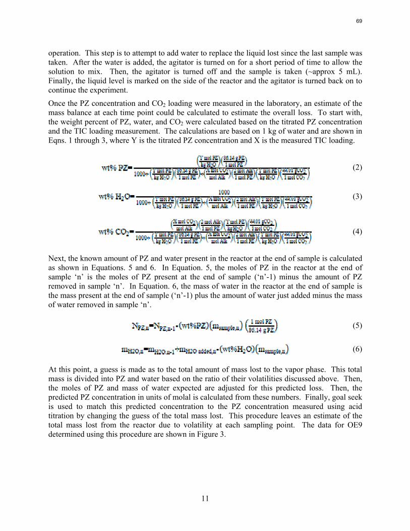
11
operation. This step is to attempt to add water to replace the liquid lost since the last sample was taken. After the water is added, the agitator is turned on for a short period of time to allow the solution to mix. Then, the agitator is turned off and the sample is taken (~approx 5 mL). Finally, the liquid level is marked on the side of the reactor and the agitator is turned back on to continue the experiment.
Once the PZ concentration and CO2 loading were measured in the laboratory, an estimate of the mass balance at each time point could be calculated to estimate the overall loss. To start with, the weight percent of PZ, water, and CO2 were calculated based on the titrated PZ concentration and the TIC loading measurement. The calculations are based on 1 kg of water and are shown in Eqns. 1 through 3, where Y is the titrated PZ concentration and X is the measured TIC loading.
(2)
(3)
(4)
Next, the known amount of PZ and water present in the reactor at the end of sample is calculated as shown in Equations. 5 and 6. In Equation. 5, the moles of PZ in the reactor at the end of sample ‘n’ is the moles of PZ present at the end of sample (‘n’-1) minus the amount of PZ removed in sample ‘n’. In Equation. 6, the mass of water in the reactor at the end of sample is the mass present at the end of sample (‘n’-1) plus the amount of water just added minus the mass of water removed in sample ‘n’.
(5)
(6)
At this point, a guess is made as to the total amount of mass lost to the vapor phase. This total mass is divided into PZ and water based on the ratio of their volatilities discussed above. Then, the moles of PZ and mass of water expected are adjusted for this predicted loss. Then, the predicted PZ concentration in units of molal is calculated from these numbers. Finally, goal seek is used to match this predicted concentration to the PZ concentration measured using acid titration by changing the guess of the total mass lost. This procedure leaves an estimate of the total mass lost from the reactor due to volatility at each sampling point. The data for OE9 determined using this procedure are shown in Figure 3.
69
12
Figure 3: Estimated Total Mass Lost During OE9 (8 m PZ, 55 °C, a=0.3)
This procedure predicted a total mass loss of between 2.9 to 31.9 grams during the experiment. The average loss was 16.6 ± 9.4 grams. Each time, the interval between sampling was approximately 48 hours, ranging from 47 to 49 hours, so the variation in mass loss is not due to differences in sample timing. One possible reason for a variation in the mass lost was variation in the temperature of the reactor. The water bath connected to the unit automatically turns off if the water level gets too low. It is probably that the water bath discontinued heating at some points during the experiment allowing the reactor temperature to decrease, causing a decrease in volatility. It is most likely the reactor cool down occurred before the samples at 150 and 240 hours, causing the noticeable decrease in volatility.
Thermal Degradation A long term thermal degradation experiment that was started in the third quarter of 2008 was completed this quarter. This experiment, called TE9, was 18 weeks in length and determined the thermal degradation of 8 m PZ with a loading of 0.3 mole CO2 per mole alkalinity at 150 °C. The bombs were pulled periodically, usually with one or two weeks in between each sampling. At six weeks, three bombs were pulled so the repeatability of the experiment could be determined. The concentration profiles for PZ and degradation products found are shown in Figure 4. The error bars on the data at six weeks indicates the standard deviation between the three bombs pulled at the same time. The standard deviation was calculated as the standard deviation of the concentration found from the anion IC, cation IC, or titration after all calculations were performed. In other words, each of the three bombs was analyzed wholly independently and the results were analyzed for the standard deviation.
70
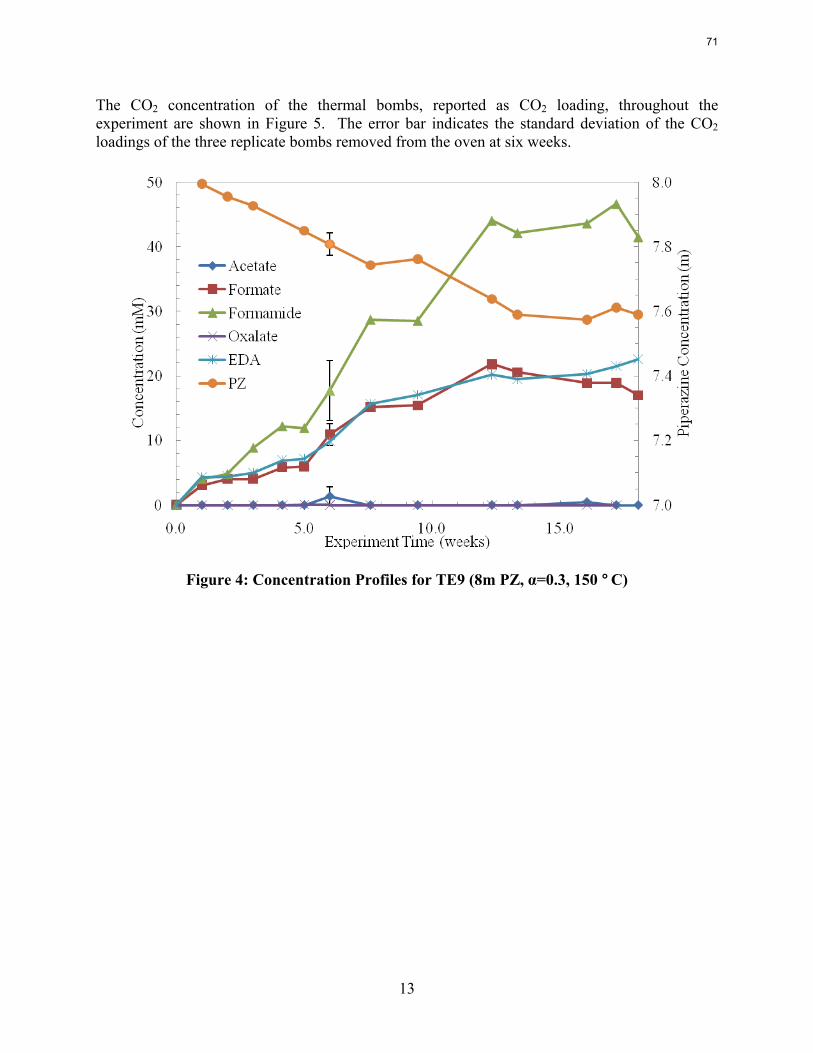
13
The CO2 concentration of the thermal bombs, reported as CO2 loading, throughout the experiment are shown in Figure 5. The error bar indicates the standard deviation of the CO2 loadings of the three replicate bombs removed from the oven at six weeks.
Figure 4: Concentration Profiles for TE9 (8m PZ, α=0.3, 150 °C)
71
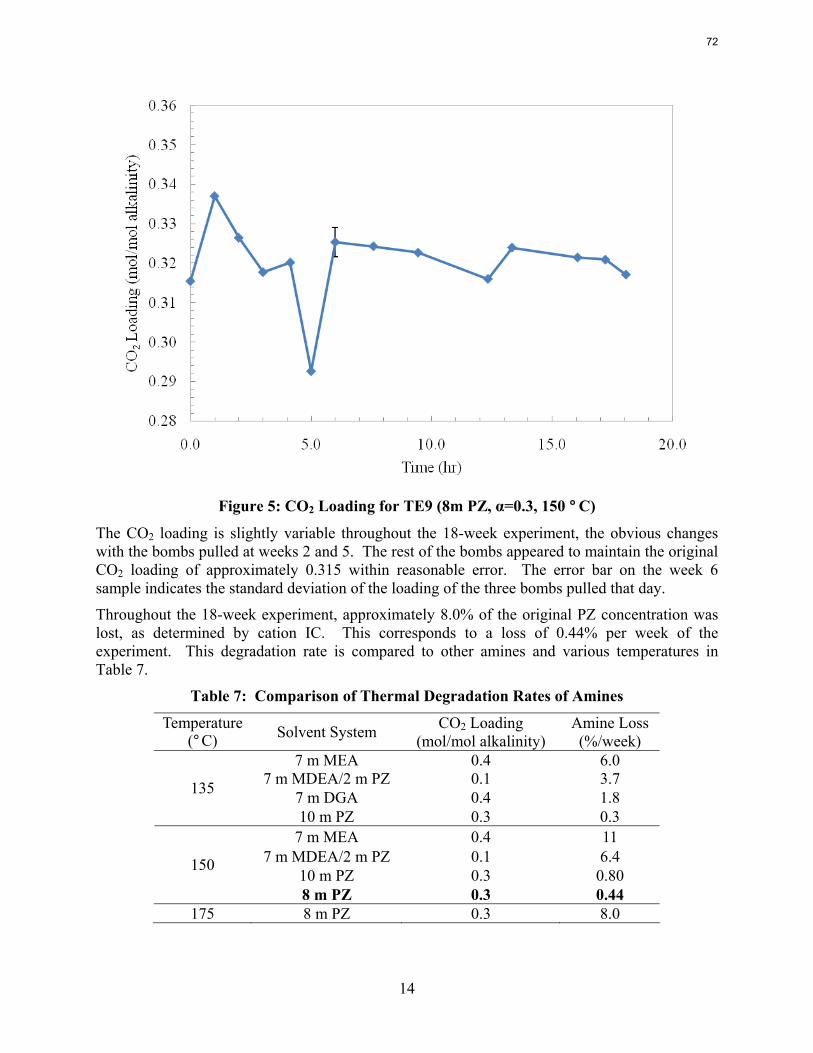
14
Figure 5: CO2 Loading for TE9 (8m PZ, α=0.3, 150 °C)
The CO2 loading is slightly variable throughout the 18-week experiment, the obvious changes with the bombs pulled at weeks 2 and 5. The rest of the bombs appeared to maintain the original CO2 loading of approximately 0.315 within reasonable error. The error bar on the week 6 sample indicates the standard deviation of the loading of the three bombs pulled that day.
Throughout the 18-week experiment, approximately 8.0% of the original PZ concentration was lost, as determined by cation IC. This corresponds to a loss of 0.44% per week of the experiment. This degradation rate is compared to other amines and various temperatures in Table 7.
Table 7: Comparison of Thermal Degradation Rates of Amines
Temperature (°C) Solvent System CO2 Loading
(mol/mol alkalinity) Amine Loss (%/week)
7 m MEA 0.4 6.0 7 m MDEA/2 m PZ 0.1 3.7
7 m DGA 0.4 1.8 135
10 m PZ 0.3 0.3 7 m MEA 0.4 11
7 m MDEA/2 m PZ 0.1 6.4 10 m PZ 0.3 0.80
150
8 m PZ 0.3 0.44 175 8 m PZ 0.3 8.0
72
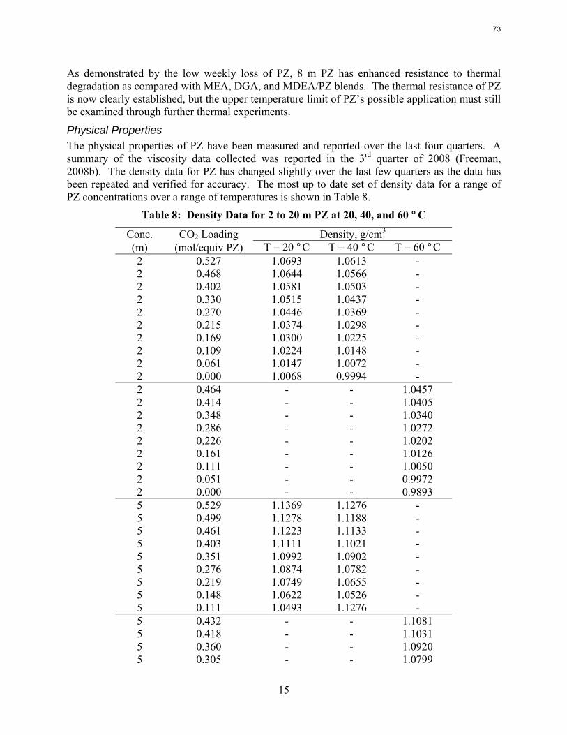
15
As demonstrated by the low weekly loss of PZ, 8 m PZ has enhanced resistance to thermal degradation as compared with MEA, DGA, and MDEA/PZ blends. The thermal resistance of PZ is now clearly established, but the upper temperature limit of PZ’s possible application must still be examined through further thermal experiments.
Physical Properties The physical properties of PZ have been measured and reported over the last four quarters. A summary of the viscosity data collected was reported in the 3rd quarter of 2008 (Freeman, 2008b). The density data for PZ has changed slightly over the last few quarters as the data has been repeated and verified for accuracy. The most up to date set of density data for a range of PZ concentrations over a range of temperatures is shown in Table 8.
Table 8: Density Data for 2 to 20 m PZ at 20, 40, and 60 °C
Conc. CO2 Loading Density, g/cm3
(m) (mol/equiv PZ) T = 20 °C T = 40 °C T = 60 °C 2 0.527 1.0693 1.0613 - 2 0.468 1.0644 1.0566 - 2 0.402 1.0581 1.0503 - 2 0.330 1.0515 1.0437 - 2 0.270 1.0446 1.0369 - 2 0.215 1.0374 1.0298 - 2 0.169 1.0300 1.0225 - 2 0.109 1.0224 1.0148 - 2 0.061 1.0147 1.0072 - 2 0.000 1.0068 0.9994 - 2 0.464 - - 1.0457 2 0.414 - - 1.0405 2 0.348 - - 1.0340 2 0.286 - - 1.0272 2 0.226 - - 1.0202 2 0.161 - - 1.0126 2 0.111 - - 1.0050 2 0.051 - - 0.9972 2 0.000 - - 0.9893 5 0.529 1.1369 1.1276 - 5 0.499 1.1278 1.1188 - 5 0.461 1.1223 1.1133 - 5 0.403 1.1111 1.1021 - 5 0.351 1.0992 1.0902 - 5 0.276 1.0874 1.0782 - 5 0.219 1.0749 1.0655 - 5 0.148 1.0622 1.0526 - 5 0.111 1.0493 1.1276 - 5 0.432 - - 1.1081 5 0.418 - - 1.1031 5 0.360 - - 1.0920 5 0.305 - - 1.0799
73
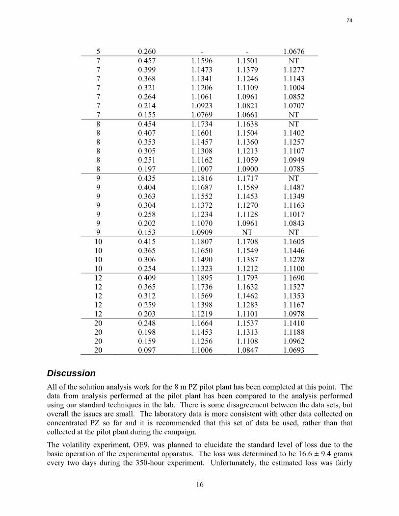
16
5 0.260 - - 1.0676 7 0.457 1.1596 1.1501 NT 7 0.399 1.1473 1.1379 1.1277 7 0.368 1.1341 1.1246 1.1143 7 0.321 1.1206 1.1109 1.1004 7 0.264 1.1061 1.0961 1.0852 7 0.214 1.0923 1.0821 1.0707 7 0.155 1.0769 1.0661 NT 8 0.454 1.1734 1.1638 NT 8 0.407 1.1601 1.1504 1.1402 8 0.353 1.1457 1.1360 1.1257 8 0.305 1.1308 1.1213 1.1107 8 0.251 1.1162 1.1059 1.0949 8 0.197 1.1007 1.0900 1.0785 9 0.435 1.1816 1.1717 NT 9 0.404 1.1687 1.1589 1.1487 9 0.363 1.1552 1.1453 1.1349 9 0.304 1.1372 1.1270 1.1163 9 0.258 1.1234 1.1128 1.1017 9 0.202 1.1070 1.0961 1.0843 9 0.153 1.0909 NT NT 10 0.415 1.1807 1.1708 1.1605 10 0.365 1.1650 1.1549 1.1446 10 0.306 1.1490 1.1387 1.1278 10 0.254 1.1323 1.1212 1.1100 12 0.409 1.1895 1.1793 1.1690 12 0.365 1.1736 1.1632 1.1527 12 0.312 1.1569 1.1462 1.1353 12 0.259 1.1398 1.1283 1.1167 12 0.203 1.1219 1.1101 1.0978 20 0.248 1.1664 1.1537 1.1410 20 0.198 1.1453 1.1313 1.1188 20 0.159 1.1256 1.1108 1.0962 20 0.097 1.1006 1.0847 1.0693
Discussion All of the solution analysis work for the 8 m PZ pilot plant has been completed at this point. The data from analysis performed at the pilot plant has been compared to the analysis performed using our standard techniques in the lab. There is some disagreement between the data sets, but overall the issues are small. The laboratory data is more consistent with other data collected on concentrated PZ so far and it is recommended that this set of data be used, rather than that collected at the pilot plant during the campaign.
The volatility experiment, OE9, was planned to elucidate the standard level of loss due to the basic operation of the experimental apparatus. The loss was determined to be 16.6 ± 9.4 grams every two days during the 350-hour experiment. Unfortunately, the estimated loss was fairly
74
17
inconsistent with a high standard deviation. Despite this, the level of loss predicted does cover a reasonable range of values. Previous experiments, such as OE3 and OE4, both had approximate water losses of 12 grams every two days, which is on the same order as the loss predicted for OE9. This experiment will be repeated during the next quarter in an attempt to achieve more accurate data, as well as continuing on to the second baseline experiment with O2 and CO2.
As demonstrated by the low weekly loss of PZ, 8 m PZ has enhanced resistance to thermal degradation as compared with MEA, DGA, and MDEA/PZ blends. The thermal resistance of PZ is now clearly established, but the upper temperature limit of PZ’s possible application must still be examined through further thermal experiments.
Conclusions The solution analysis of the 8 m PZ pilot plant campaign is complete and all data collected are included in this document. The data are still being analyzed by other members of the Rochelle group. The solution did not show signs of oxidation or thermal degradation. The foaming analysis demonstrated that the solution did not foam during the campaign and there was likely little interference in the mass-transfer area in the absorber.
The initial baseline volatility experiment for the low gas flow apparatus has demonstrated that very little of the total loss of PZ is due to volatility alone. The loss due to volatility cannot be responsible for the large discrepancy in PZ loss seen in the other oxidative degradation experiments. To maintain a mass balance on water and PZ, an average loss of 0.346 gram per hour of solution is needed due to volatility. This represents the loss of 1.82 x 10⁻⁴ and 0.346 grams per hour for PZ and water, respectively, as determined by their volatility at 55 °C. Further work is still needed to make definitive conclusions on the baseline level of loss and more experiments will be performed to this end.
The 18-week thermal degradation experiment completed this quarter further solidifies PZ thermal resistance compared to other amines. After 18 weeks, only 8.0% of the original PZ was lost, or 0.44% of the original amine per week. During the experiment, 22, 17, and 42 mM of EDA, formate, and N-formyl amides were the most prevalent degradation products.
Future Work In the next quarter, the baseline experiments for the low gas flow experiment will be completed. The volatility of PZ in this particular apparatus will be fully characterized by the end of the quarter. Also, other aspects of the apparatus that may be leading to unaccounted for PZ loss will be examined. This includes redesigning the apparatus to remove the possibility that PZ is being absorbed into the rubber stopper on the top of the reactor. On a separate front, the use of the Cation IC-MS will be started in earnest in an attempt to identify the degradation products that can account for the loss of PZ observed.
References Cullinane JT, Rochelle GR. Kinetics of carbon dioxide absorption into aqueous potassium
carbonate and piperazine. Ind Eng Chem Res. 2007;45(8):2531–2545.
75
18
Dugas R. Absorption and desorption rates of carbon dioxide with monoethanolamine and piperazine. GHGT-9, Washington D.C. 2008.
Freeman SA. Carbon dioxide capture with concentrated, aqueous piperazine. GHGT-9, Washington D.C. 2008a.
Freeman, SA. "Physical Properties of Concentrated Aqueous Piperazine." 3rd Quarterly Progress Report of 2008 for the Rochelle Research Group. 2008b.
Hilliard MD. A Predictive Thermodynamic Model for an Aqueous Blend of Potassium Carbonate, Piperazine, and Monoethanolamine for Carbon Dioxide Capture from Flue Gas. The University of Texas at Austin. Ph.D. Dissertation. 2008.
Rochelle GT et al. "CO2 Capture by Aqueous Absorption, Third Quarterly Progress Report 2008." Luminant Carbon Management Program. The University of Texas at Austin. 2008.
Sexton A. Amine Oxidation in CO2 Capture Processes. The University of Texas at Austin. Ph.D. Dissertation. 2008.
76
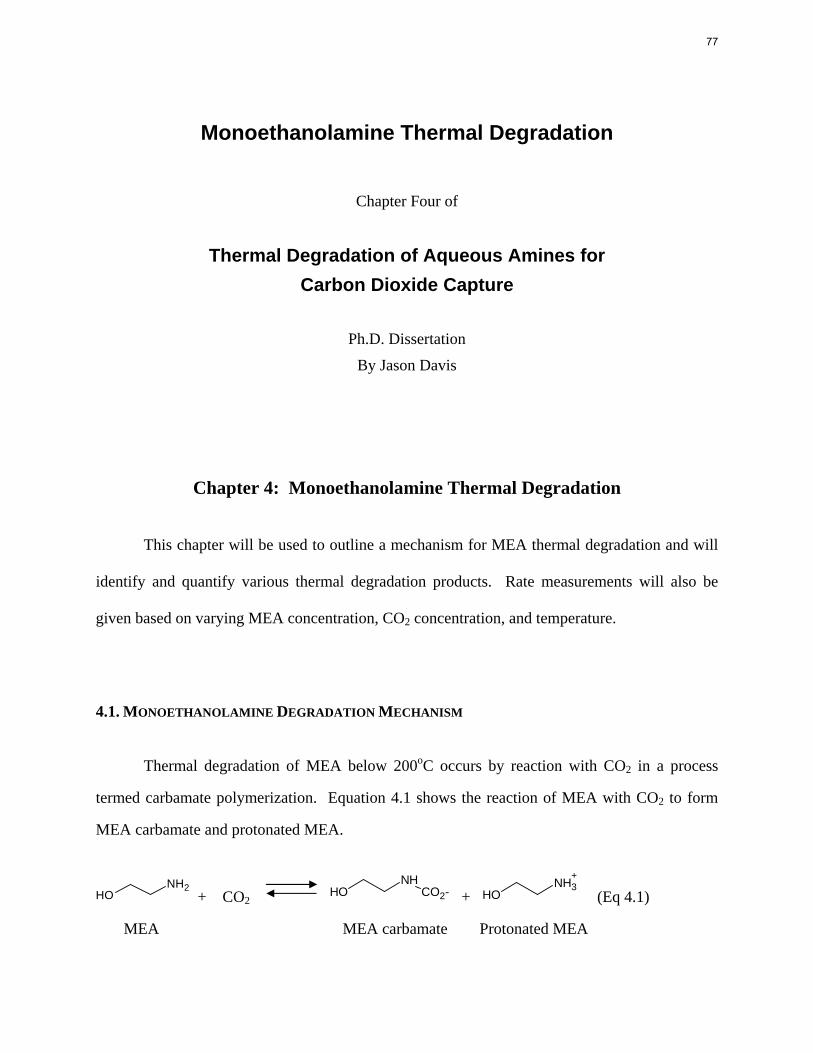
Monoethanolamine Thermal Degradation
Chapter Four of
Thermal Degradation of Aqueous Amines for Carbon Dioxide Capture
Ph.D. Dissertation
By Jason Davis
Chapter 4: Monoethanolamine Thermal Degradation
This chapter will be used to outline a mechanism for MEA thermal degradation and will
identify and quantify various thermal degradation products. Rate measurements will also be
given based on varying MEA concentration, CO2 concentration, and temperature.
4.1. MONOETHANOLAMINE DEGRADATION MECHANISM
Thermal degradation of MEA below 200oC occurs by reaction with CO2 in a process
termed carbamate polymerization. Equation 4.1 shows the reaction of MEA with CO2 to form
MEA carbamate and protonated MEA.
NH2
OH + CO2 NH
OH CO2- + NH3
+
OH (Eq 4.1)
MEA MEA carbamate Protonated MEA
77
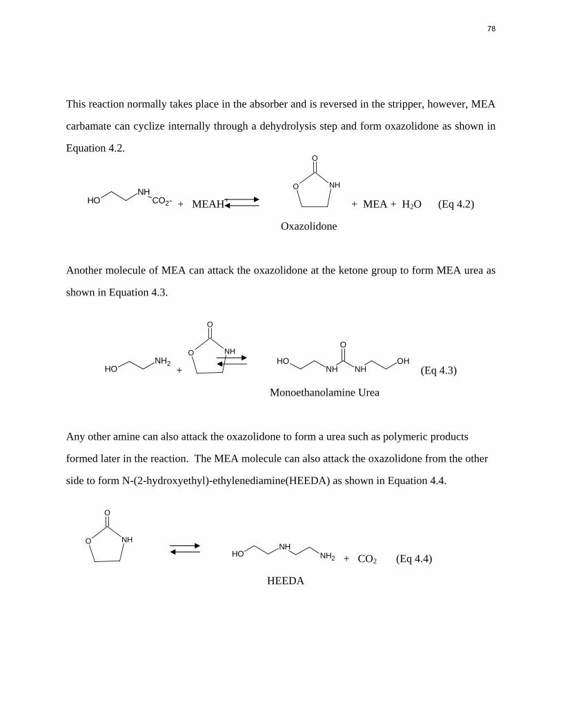
This reaction normally takes place in the absorber and is reversed in the stripper, however, MEA
carbamate can cyclize internally through a dehydrolysis step and form oxazolidone as shown in
Equation 4.2.
NHOH CO2- + MEAH+
NHO
O
+ MEA + H2O (Eq 4.2)
Oxazolidone
Another molecule of MEA can attack the oxazolidone at the ketone group to form MEA urea as
shown in Equation 4.3.
NH2OH +
NHO
O
OH
NHNHOH
O
(Eq 4.3)
Monoethanolamine Urea
Any other amine can also attack the oxazolidone to form a urea such as polymeric products
formed later in the reaction. The MEA molecule can also attack the oxazolidone from the other
side to form N-(2-hydroxyethyl)-ethylenediamine(HEEDA) as shown in Equation 4.4.
NHO
O
OHNH
NH2 + CO2 (Eq 4.4)
HEEDA
78
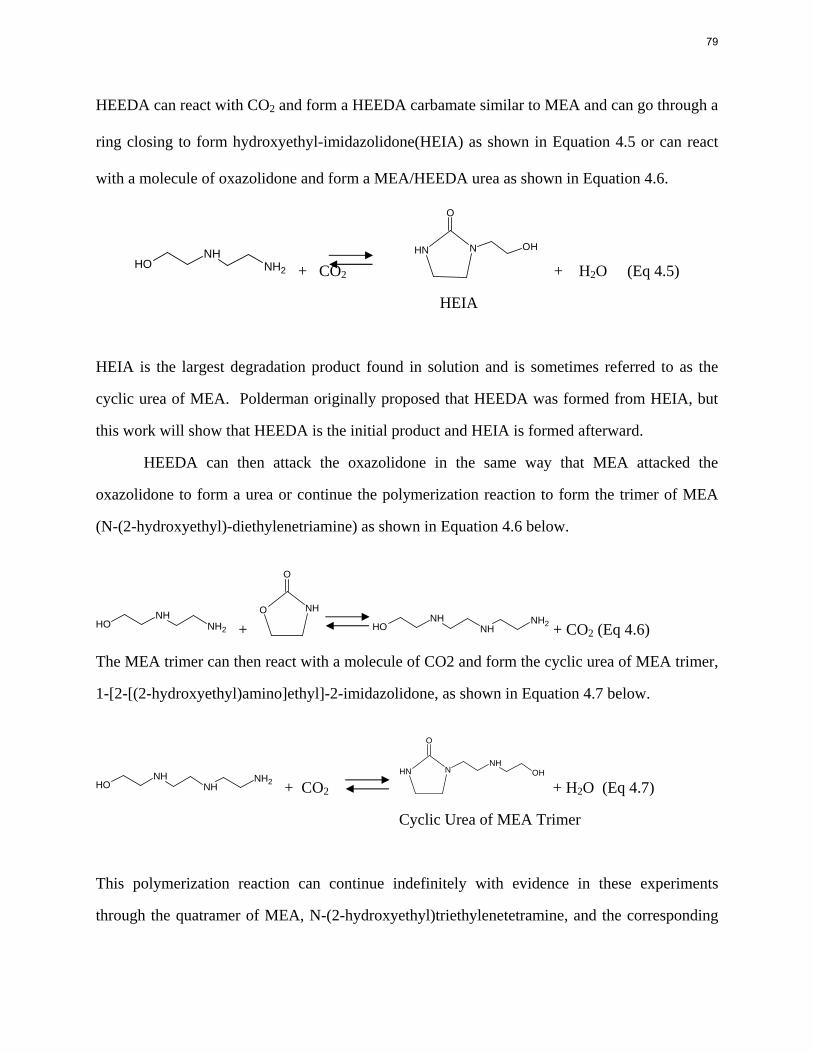
HEEDA can react with CO2 and form a HEEDA carbamate similar to MEA and can go through a
ring closing to form hydroxyethyl-imidazolidone(HEIA) as shown in Equation 4.5 or can react
with a molecule of oxazolidone and form a MEA/HEEDA urea as shown in Equation 4.6.
OHNH
NH2 + CO2 NNH
O
OH
+ H2O (Eq 4.5)
HEIA
HEIA is the largest degradation product found in solution and is sometimes referred to as the
cyclic urea of MEA. Polderman originally proposed that HEEDA was formed from HEIA, but
this work will show that HEEDA is the initial product and HEIA is formed afterward.
HEEDA can then attack the oxazolidone in the same way that MEA attacked the
oxazolidone to form a urea or continue the polymerization reaction to form the trimer of MEA
(N-(2-hydroxyethyl)-diethylenetriamine) as shown in Equation 4.6 below.
OHNH
NH2 + NHO
O
OHNH
NHNH2 + CO2 (Eq 4.6)
The MEA trimer can then react with a molecule of CO2 and form the cyclic urea of MEA trimer,
1-[2-[(2-hydroxyethyl)amino]ethyl]-2-imidazolidone, as shown in Equation 4.7 below.
OHNH
NHNH2 + CO2
NNH
O
NHOH
+ H2O (Eq 4.7)
Cyclic Urea of MEA Trimer
This polymerization reaction can continue indefinitely with evidence in these experiments
through the quatramer of MEA, N-(2-hydroxyethyl)triethylenetetramine, and the corresponding
79

cyclic urea, 1-[2-[[2-[(2-hydroxyethyl)amino]ethyl]amino)ethyl]-2-imidazolidone. Figure 4.1
shows the entire reaction pathway with possible branch points for MEA thermal degradation.
80
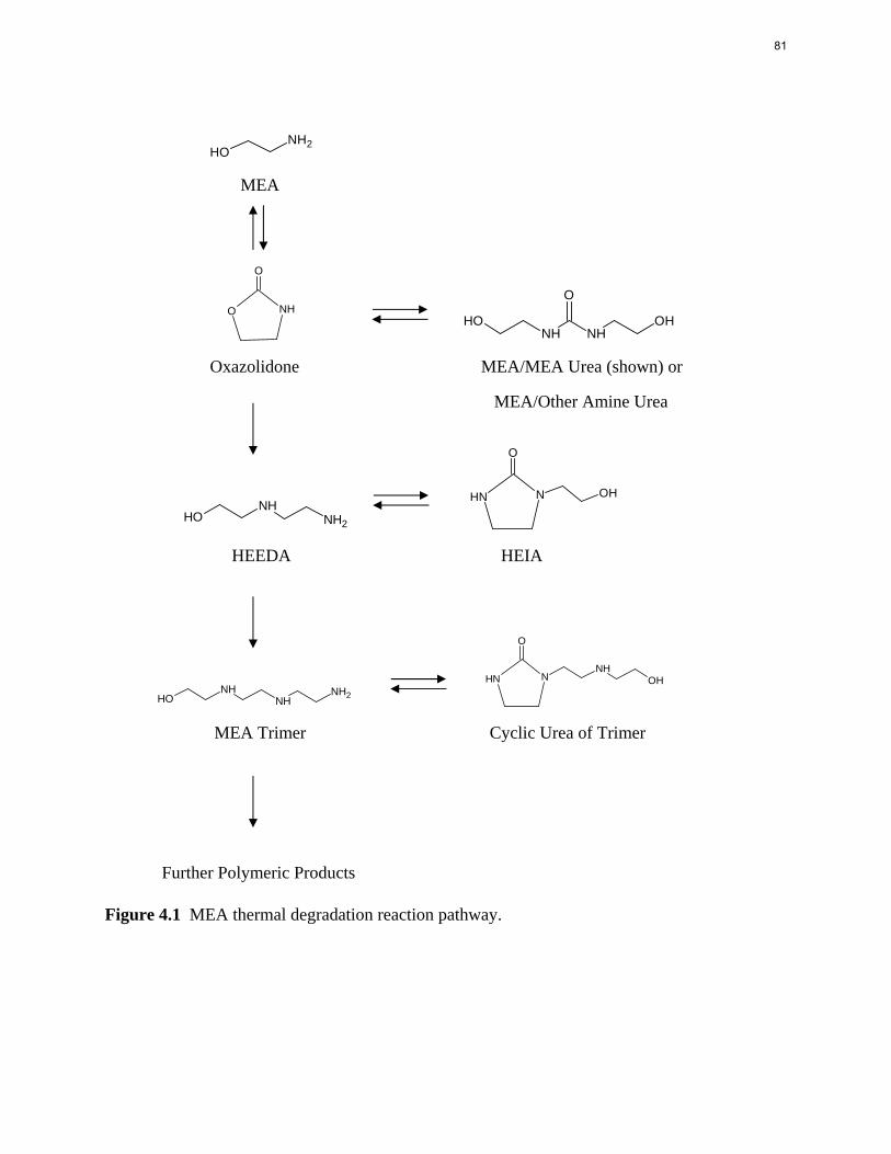
NH2
OH
MEA
NHO
O
OH
NHNHOH
O
Oxazolidone MEA/MEA Urea (shown) or
MEA/Other Amine Urea
OHNH
NH2
NNH
O
OH
HEEDA HEIA
OHNH
NHNH2
NNH
O
NHOH
MEA Trimer Cyclic Urea of Trimer
Further Polymeric Products
Figure 4.1 MEA thermal degradation reaction pathway.
81
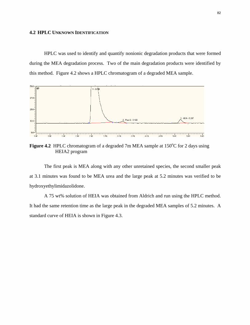
4.2 HPLC UNKNOWN IDENTIFICATION
HPLC was used to identify and quantify nonionic degradation products that were formed
during the MEA degradation process. Two of the main degradation products were identified by
this method. Figure 4.2 shows a HPLC chromatogram of a degraded MEA sample.
Figure 4.2 HPLC chromatogram of a degraded 7m MEA sample at 150oC for 2 days using HEIA2 program
The first peak is MEA along with any other unretained species, the second smaller peak
at 3.1 minutes was found to be MEA urea and the large peak at 5.2 minutes was verified to be
hydroxyethylimidazolidone.
A 75 wt% solution of HEIA was obtained from Aldrich and run using the HPLC method.
It had the same retention time as the large peak in the degraded MEA samples of 5.2 minutes. A
standard curve of HEIA is shown in Figure 4.3.
82
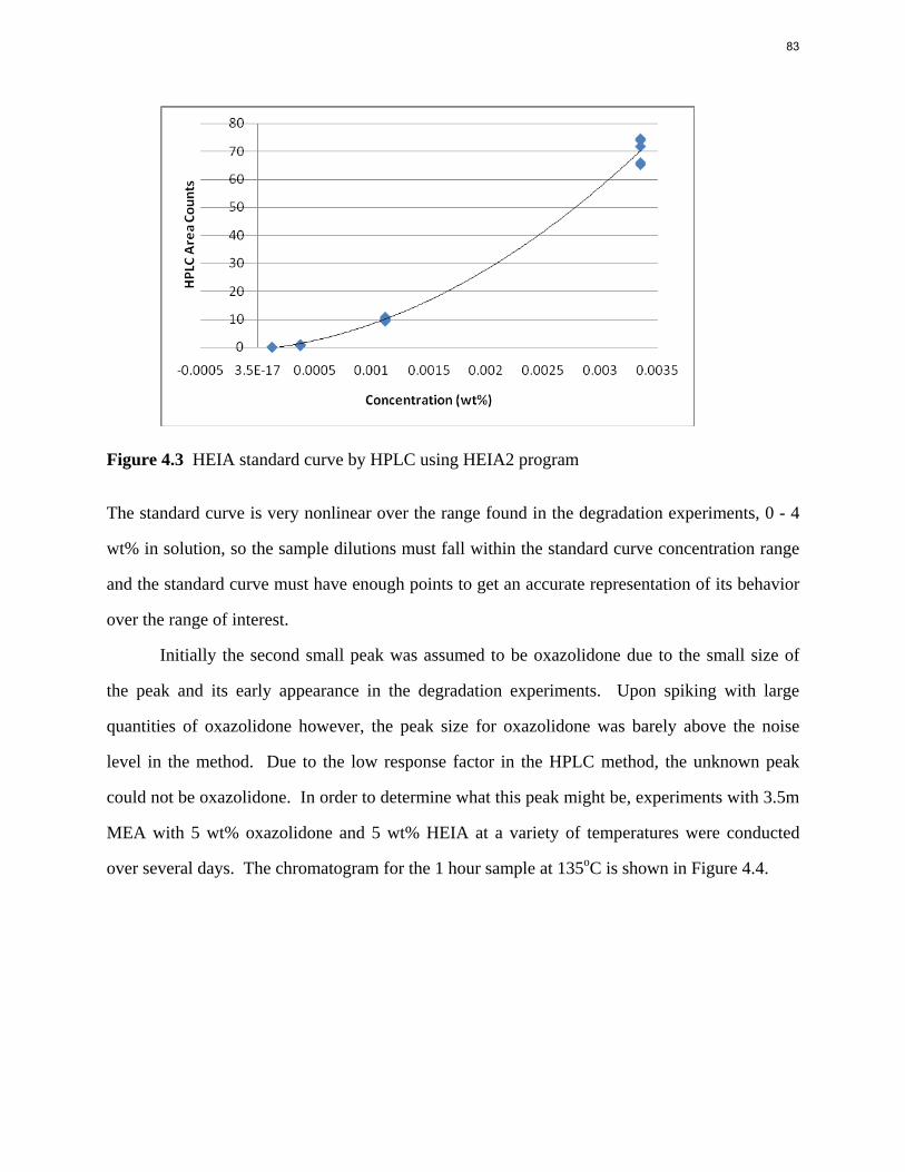
Figure 4.3 HEIA standard curve by HPLC using HEIA2 program
The standard curve is very nonlinear over the range found in the degradation experiments, 0 - 4
wt% in solution, so the sample dilutions must fall within the standard curve concentration range
and the standard curve must have enough points to get an accurate representation of its behavior
over the range of interest.
Initially the second small peak was assumed to be oxazolidone due to the small size of
the peak and its early appearance in the degradation experiments. Upon spiking with large
quantities of oxazolidone however, the peak size for oxazolidone was barely above the noise
level in the method. Due to the low response factor in the HPLC method, the unknown peak
could not be oxazolidone. In order to determine what this peak might be, experiments with 3.5m
MEA with 5 wt% oxazolidone and 5 wt% HEIA at a variety of temperatures were conducted
over several days. The chromatogram for the 1 hour sample at 135oC is shown in Figure 4.4.
83
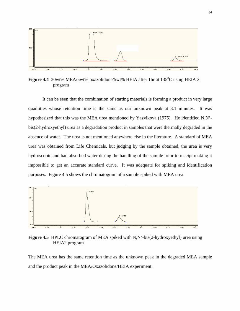
Figure 4.4 30wt% MEA/5wt% oxazolidone/5wt% HEIA after 1hr at 135oC using HEIA 2 program
It can be seen that the combination of starting materials is forming a product in very large
quantities whose retention time is the same as our unknown peak at 3.1 minutes. It was
hypothesized that this was the MEA urea mentioned by Yazvikova (1975). He identified N,N’-
bis(2-hydroxyethyl) urea as a degradation product in samples that were thermally degraded in the
absence of water. The urea is not mentioned anywhere else in the literature. A standard of MEA
urea was obtained from Life Chemicals, but judging by the sample obtained, the urea is very
hydroscopic and had absorbed water during the handling of the sample prior to receipt making it
impossible to get an accurate standard curve. It was adequate for spiking and identification
purposes. Figure 4.5 shows the chromatogram of a sample spiked with MEA urea.
Figure 4.5 HPLC chromatogram of MEA spiked with N,N’-bis(2-hydroxyethyl) urea using HEIA2 program
The MEA urea has the same retention time as the unknown peak in the degraded MEA sample
and the product peak in the MEA/Oxazolidone/HEIA experiment.
84
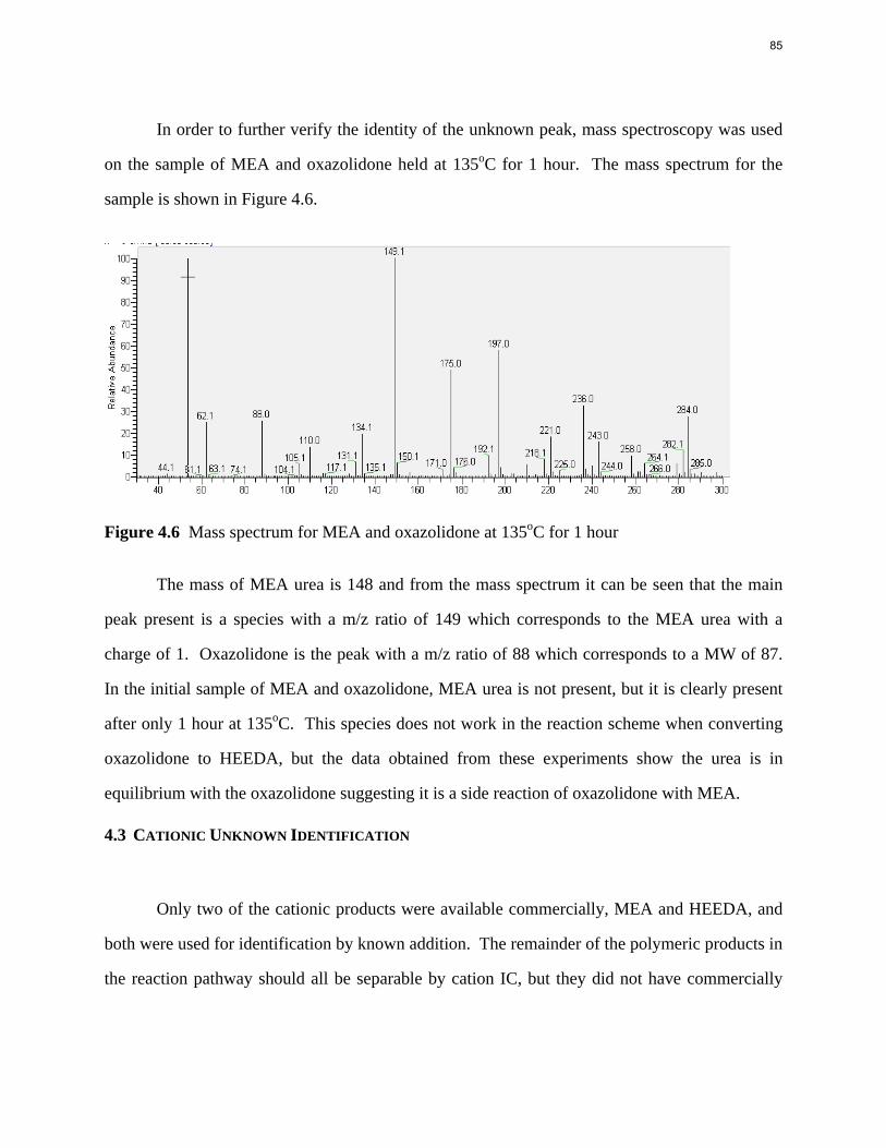
In order to further verify the identity of the unknown peak, mass spectroscopy was used
on the sample of MEA and oxazolidone held at 135oC for 1 hour. The mass spectrum for the
sample is shown in Figure 4.6.
Figure 4.6 Mass spectrum for MEA and oxazolidone at 135oC for 1 hour
The mass of MEA urea is 148 and from the mass spectrum it can be seen that the main
peak present is a species with a m/z ratio of 149 which corresponds to the MEA urea with a
charge of 1. Oxazolidone is the peak with a m/z ratio of 88 which corresponds to a MW of 87.
In the initial sample of MEA and oxazolidone, MEA urea is not present, but it is clearly present
after only 1 hour at 135oC. This species does not work in the reaction scheme when converting
oxazolidone to HEEDA, but the data obtained from these experiments show the urea is in
equilibrium with the oxazolidone suggesting it is a side reaction of oxazolidone with MEA.
4.3 CATIONIC UNKNOWN IDENTIFICATION
Only two of the cationic products were available commercially, MEA and HEEDA, and
both were used for identification by known addition. The remainder of the polymeric products in
the reaction pathway should all be separable by cation IC, but they did not have commercially
85
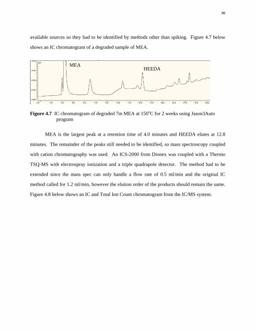
available sources so they had to be identified by methods other than spiking. Figure 4.7 below
shows an IC chromatogram of a degraded sample of MEA.
Figure 4.7 IC chromatogram of degraded 7m MEA at 150oC for 2 weeks using Jason3Auto program
MEA is the largest peak at a retention time of 4.0 minutes and HEEDA elutes at 12.8
minutes. The remainder of the peaks still needed to be identified, so mass spectroscopy coupled
with cation chromatography was used. An ICS-2000 from Dionex was coupled with a Thermo
TSQ-MS with electrospray ionization and a triple quadrapole detector. The method had to be
extended since the mass spec can only handle a flow rate of 0.5 ml/min and the original IC
method called for 1.2 ml/min, however the elution order of the products should remain the same.
Figure 4.8 below shows an IC and Total Ion Count chromatogram from the IC/MS system.
MEA HEEDA
86
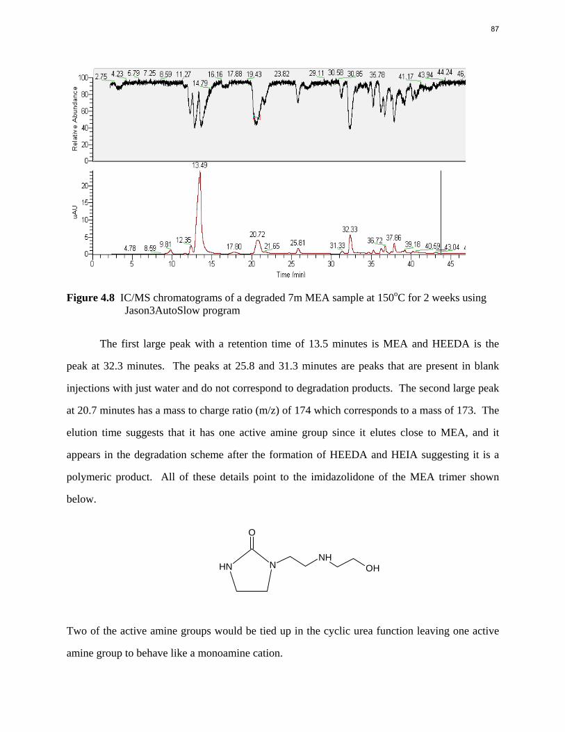
Figure 4.8 IC/MS chromatograms of a degraded 7m MEA sample at 150oC for 2 weeks using Jason3AutoSlow program
The first large peak with a retention time of 13.5 minutes is MEA and HEEDA is the
peak at 32.3 minutes. The peaks at 25.8 and 31.3 minutes are peaks that are present in blank
injections with just water and do not correspond to degradation products. The second large peak
at 20.7 minutes has a mass to charge ratio (m/z) of 174 which corresponds to a mass of 173. The
elution time suggests that it has one active amine group since it elutes close to MEA, and it
appears in the degradation scheme after the formation of HEEDA and HEIA suggesting it is a
polymeric product. All of these details point to the imidazolidone of the MEA trimer shown
below.
NNH
O
NHOH
Two of the active amine groups would be tied up in the cyclic urea function leaving one active
amine group to behave like a monoamine cation.
87
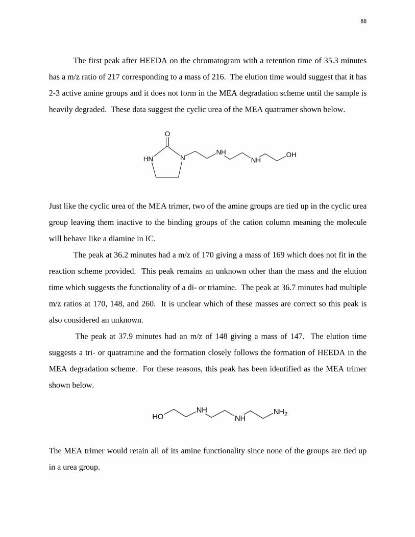
The first peak after HEEDA on the chromatogram with a retention time of 35.3 minutes
has a m/z ratio of 217 corresponding to a mass of 216. The elution time would suggest that it has
2-3 active amine groups and it does not form in the MEA degradation scheme until the sample is
heavily degraded. These data suggest the cyclic urea of the MEA quatramer shown below.
NNH
O
NHNH
OH
Just like the cyclic urea of the MEA trimer, two of the amine groups are tied up in the cyclic urea
group leaving them inactive to the binding groups of the cation column meaning the molecule
will behave like a diamine in IC.
The peak at 36.2 minutes had a m/z of 170 giving a mass of 169 which does not fit in the
reaction scheme provided. This peak remains an unknown other than the mass and the elution
time which suggests the functionality of a di- or triamine. The peak at 36.7 minutes had multiple
m/z ratios at 170, 148, and 260. It is unclear which of these masses are correct so this peak is
also considered an unknown.
The peak at 37.9 minutes had an m/z of 148 giving a mass of 147. The elution time
suggests a tri- or quatramine and the formation closely follows the formation of HEEDA in the
MEA degradation scheme. For these reasons, this peak has been identified as the MEA trimer
shown below.
OHNH
NHNH2
The MEA trimer would retain all of its amine functionality since none of the groups are tied up
in a urea group.
88
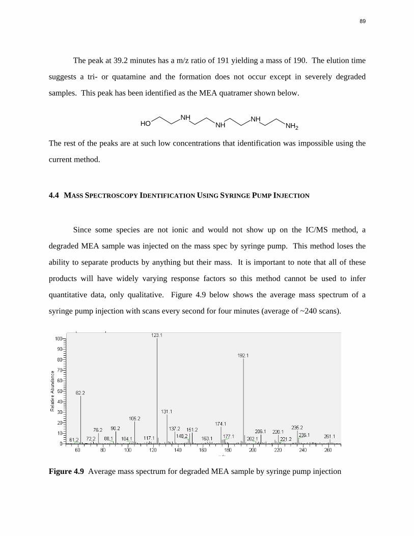
The peak at 39.2 minutes has a m/z ratio of 191 yielding a mass of 190. The elution time
suggests a tri- or quatamine and the formation does not occur except in severely degraded
samples. This peak has been identified as the MEA quatramer shown below.
OHNH
NHNH
NH2
The rest of the peaks are at such low concentrations that identification was impossible using the
current method.
4.4 MASS SPECTROSCOPY IDENTIFICATION USING SYRINGE PUMP INJECTION
Since some species are not ionic and would not show up on the IC/MS method, a
degraded MEA sample was injected on the mass spec by syringe pump. This method loses the
ability to separate products by anything but their mass. It is important to note that all of these
products will have widely varying response factors so this method cannot be used to infer
quantitative data, only qualitative. Figure 4.9 below shows the average mass spectrum of a
syringe pump injection with scans every second for four minutes (average of ~240 scans).
Figure 4.9 Average mass spectrum for degraded MEA sample by syringe pump injection
89
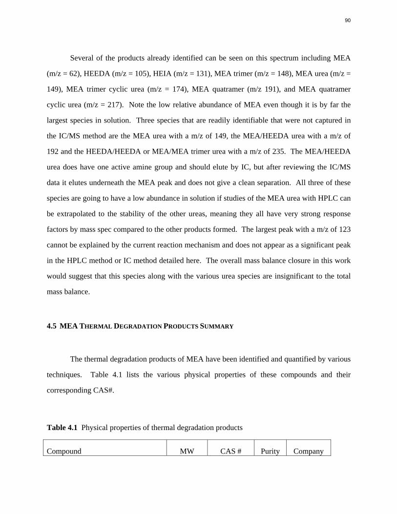
Several of the products already identified can be seen on this spectrum including MEA
(m/z = 62), HEEDA (m/z = 105), HEIA (m/z = 131), MEA trimer (m/z = 148), MEA urea (m/z =
149), MEA trimer cyclic urea (m/z = 174), MEA quatramer (m/z 191), and MEA quatramer
cyclic urea (m/z = 217). Note the low relative abundance of MEA even though it is by far the
largest species in solution. Three species that are readily identifiable that were not captured in
the IC/MS method are the MEA urea with a m/z of 149, the MEA/HEEDA urea with a m/z of
192 and the HEEDA/HEEDA or MEA/MEA trimer urea with a m/z of 235. The MEA/HEEDA
urea does have one active amine group and should elute by IC, but after reviewing the IC/MS
data it elutes underneath the MEA peak and does not give a clean separation. All three of these
species are going to have a low abundance in solution if studies of the MEA urea with HPLC can
be extrapolated to the stability of the other ureas, meaning they all have very strong response
factors by mass spec compared to the other products formed. The largest peak with a m/z of 123
cannot be explained by the current reaction mechanism and does not appear as a significant peak
in the HPLC method or IC method detailed here. The overall mass balance closure in this work
would suggest that this species along with the various urea species are insignificant to the total
mass balance.
4.5 MEA THERMAL DEGRADATION PRODUCTS SUMMARY
The thermal degradation products of MEA have been identified and quantified by various
techniques. Table 4.1 lists the various physical properties of these compounds and their
corresponding CAS#.
Table 4.1 Physical properties of thermal degradation products
Compound MW CAS # Purity Company
90
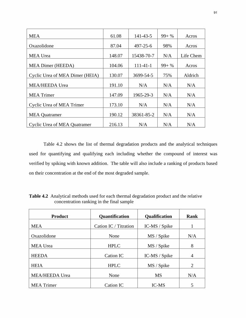
MEA 61.08 141-43-5 99+ % Acros
Oxazolidone 87.04 497-25-6 98% Acros
MEA Urea 148.07 15438-70-7 N/A Life Chem
MEA Dimer (HEEDA) 104.06 111-41-1 99+ % Acros
Cyclic Urea of MEA Dimer (HEIA) 130.07 3699-54-5 75% Aldrich
MEA/HEEDA Urea 191.10 N/A N/A N/A
MEA Trimer 147.09 1965-29-3 N/A N/A
Cyclic Urea of MEA Trimer 173.10 N/A N/A N/A
MEA Quatramer 190.12 38361-85-2 N/A N/A
Cyclic Urea of MEA Quatramer 216.13 N/A N/A N/A
Table 4.2 shows the list of thermal degradation products and the analytical techniques
used for quantifying and qualifying each including whether the compound of interest was
verified by spiking with known addition. The table will also include a ranking of products based
on their concentration at the end of the most degraded sample.
Table 4.2 Analytical methods used for each thermal degradation product and the relative concentration ranking in the final sample
Product Quantification Qualification Rank
MEA Cation IC / Titration IC-MS / Spike 1
Oxazolidone None MS / Spike N/A
MEA Urea HPLC MS / Spike 8
HEEDA Cation IC IC-MS / Spike 4
HEIA HPLC MS / Spike 2
MEA/HEEDA Urea None MS N/A
MEA Trimer Cation IC IC-MS 5
91
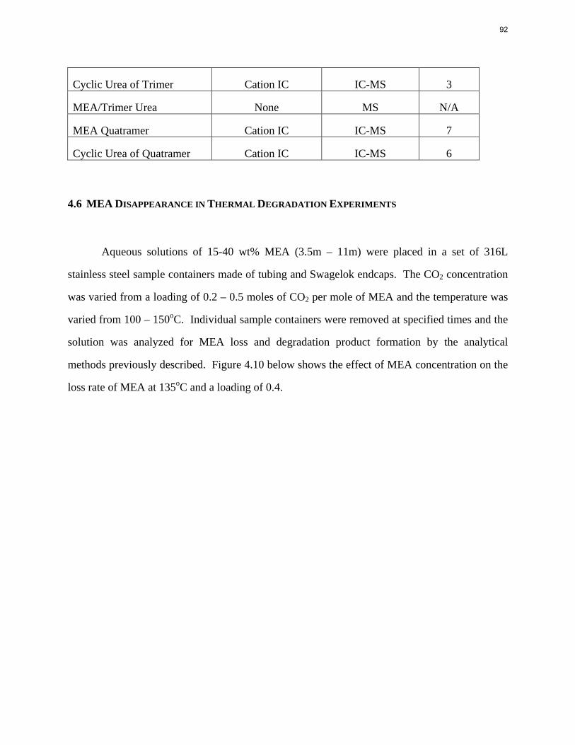
Cyclic Urea of Trimer Cation IC IC-MS 3
MEA/Trimer Urea None MS N/A
MEA Quatramer Cation IC IC-MS 7
Cyclic Urea of Quatramer Cation IC IC-MS 6
4.6 MEA DISAPPEARANCE IN THERMAL DEGRADATION EXPERIMENTS
Aqueous solutions of 15-40 wt% MEA (3.5m – 11m) were placed in a set of 316L
stainless steel sample containers made of tubing and Swagelok endcaps. The CO2 concentration
was varied from a loading of 0.2 – 0.5 moles of CO2 per mole of MEA and the temperature was
varied from 100 – 150oC. Individual sample containers were removed at specified times and the
solution was analyzed for MEA loss and degradation product formation by the analytical
methods previously described. Figure 4.10 below shows the effect of MEA concentration on the
loss rate of MEA at 135oC and a loading of 0.4.
92
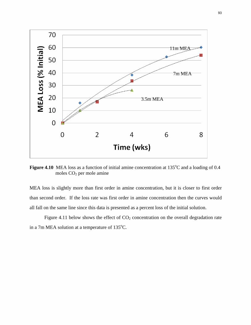
Figure 4.10 MEA loss as a function of initial amine concentration at 135oC and a loading of 0.4 moles CO2 per mole amine
MEA loss is slightly more than first order in amine concentration, but it is closer to first order
than second order. If the loss rate was first order in amine concentration then the curves would
all fall on the same line since this data is presented as a percent loss of the initial solution.
Figure 4.11 below shows the effect of CO2 concentration on the overall degradation rate
in a 7m MEA solution at a temperature of 135oC.
3.5m MEA
7m MEA
11m MEA
93
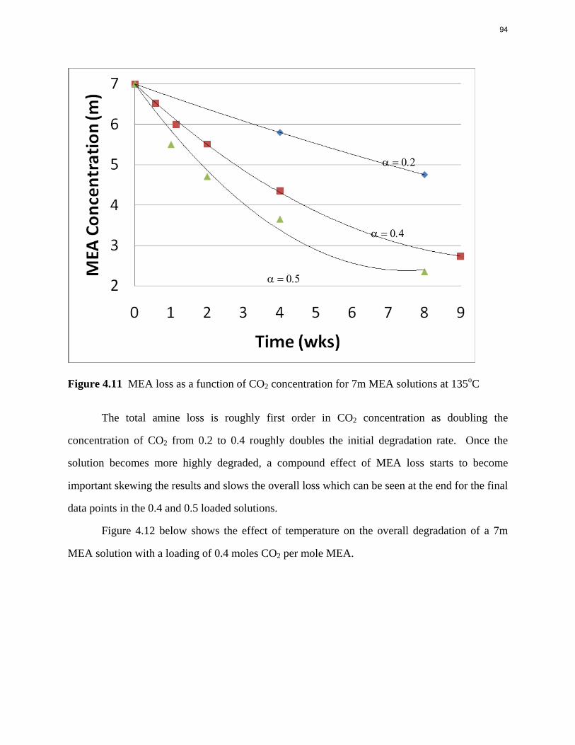
Figure 4.11 MEA loss as a function of CO2 concentration for 7m MEA solutions at 135oC
The total amine loss is roughly first order in CO2 concentration as doubling the
concentration of CO2 from 0.2 to 0.4 roughly doubles the initial degradation rate. Once the
solution becomes more highly degraded, a compound effect of MEA loss starts to become
important skewing the results and slows the overall loss which can be seen at the end for the final
data points in the 0.4 and 0.5 loaded solutions.
Figure 4.12 below shows the effect of temperature on the overall degradation of a 7m
MEA solution with a loading of 0.4 moles CO2 per mole MEA.
α = 0.5
α = 0.4
α = 0.2
94
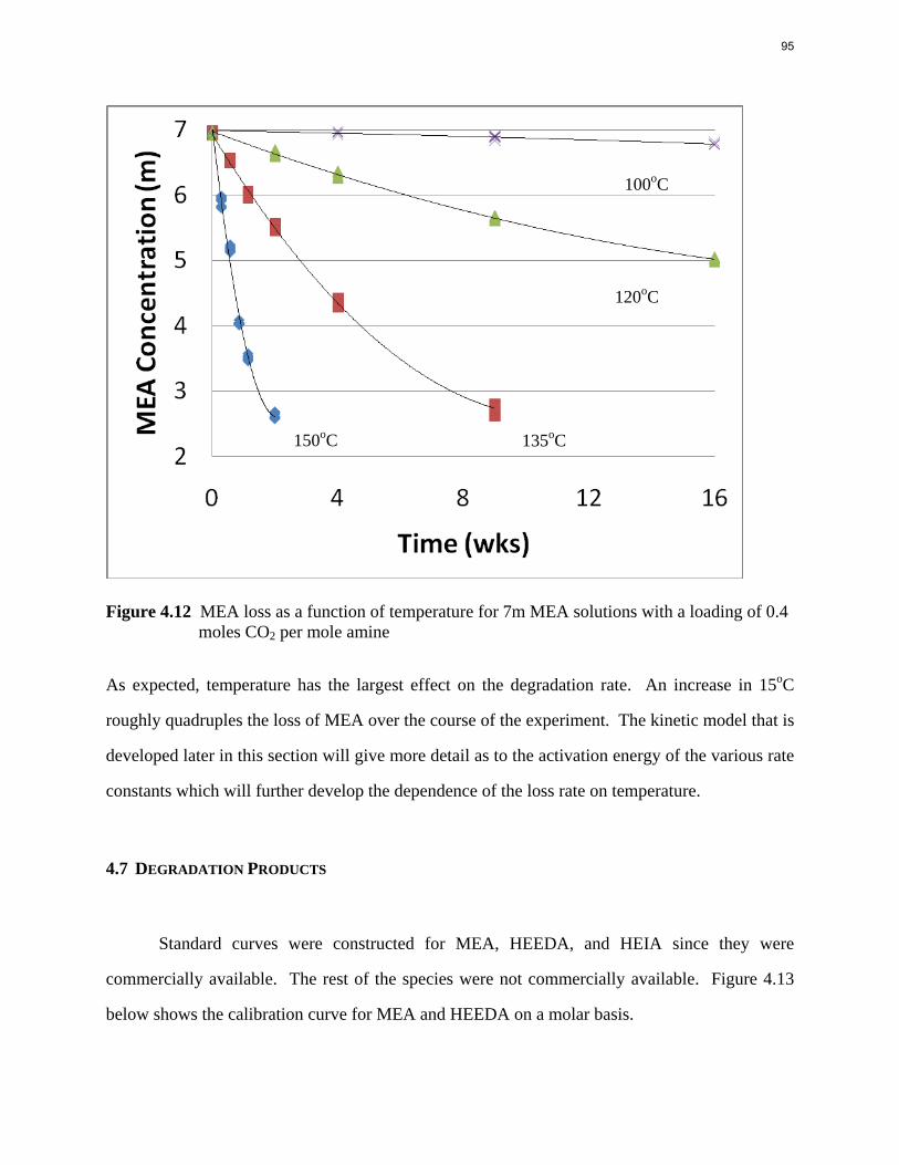
Figure 4.12 MEA loss as a function of temperature for 7m MEA solutions with a loading of 0.4 moles CO2 per mole amine
As expected, temperature has the largest effect on the degradation rate. An increase in 15oC
roughly quadruples the loss of MEA over the course of the experiment. The kinetic model that is
developed later in this section will give more detail as to the activation energy of the various rate
constants which will further develop the dependence of the loss rate on temperature.
4.7 DEGRADATION PRODUCTS
Standard curves were constructed for MEA, HEEDA, and HEIA since they were
commercially available. The rest of the species were not commercially available. Figure 4.13
below shows the calibration curve for MEA and HEEDA on a molar basis.
150oC 135oC
120oC
100oC
95
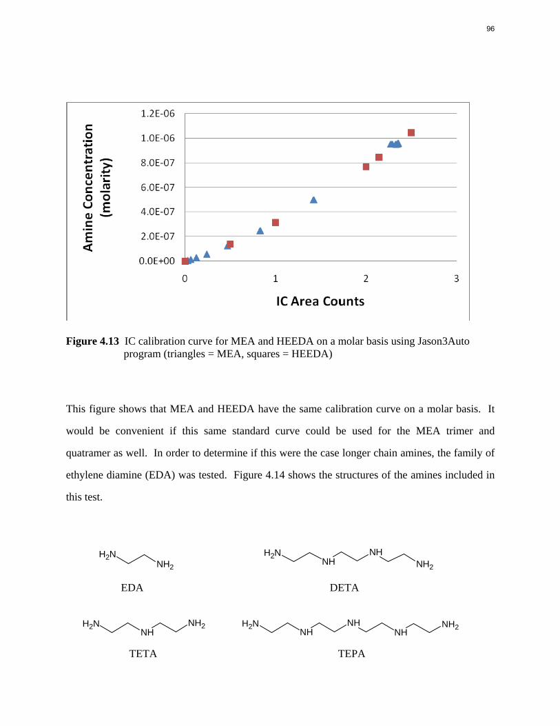
Figure 4.13 IC calibration curve for MEA and HEEDA on a molar basis using Jason3Auto program (triangles = MEA, squares = HEEDA)
This figure shows that MEA and HEEDA have the same calibration curve on a molar basis. It
would be convenient if this same standard curve could be used for the MEA trimer and
quatramer as well. In order to determine if this were the case longer chain amines, the family of
ethylene diamine (EDA) was tested. Figure 4.14 shows the structures of the amines included in
this test.
NH2
NH2 NH2
NHNH
NH2
EDA DETA
NH2
NHNH2
NH2
NHNH
NHNH2
TETA TEPA
96
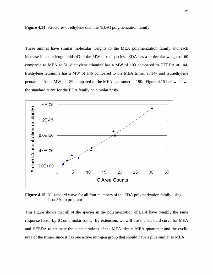
Figure 4.14 Structures of ethylene diamine (EDA) polymerization family
These amines have similar molecular weights to the MEA polymerization family and each
increase in chain length adds 43 to the MW of the species. EDA has a molecular weight of 60
compared to MEA at 61, diethylene triamine has a MW of 103 compared to HEEDA at 104,
triethylene tetramine has a MW of 146 compared to the MEA trimer at 147 and tetraethylene
pentamine has a MW of 189 compared to the MEA quatramer at 190. Figure 4.15 below shows
the standard curve for the EDA family on a molar basis.
Figure 4.15 IC standard curve for all four members of the EDA polymerization family using Jason3Auto program
This figure shows that all of the species in the polymerization of EDA have roughly the same
response factor by IC on a molar basis. By extension, we will use the standard curve for MEA
and HEEDA to estimate the concentrations of the MEA trimer, MEA quatramer and the cyclic
urea of the trimer since it has one active nitrogen group that should have a pKa similar to MEA.
97
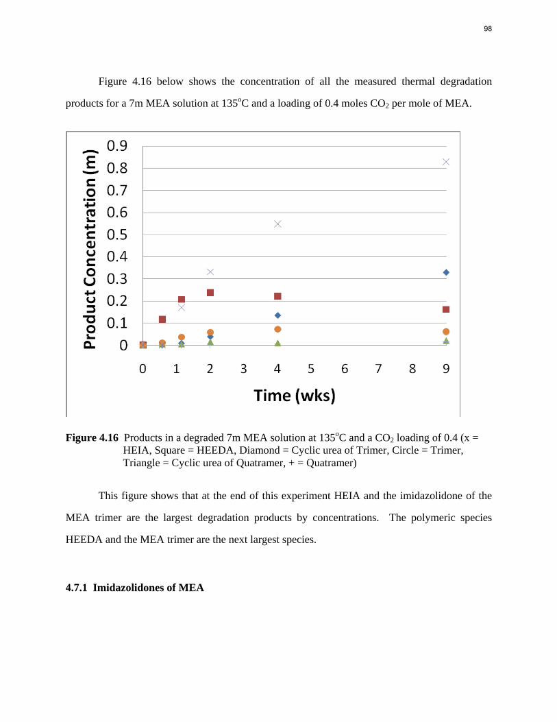
Figure 4.16 below shows the concentration of all the measured thermal degradation
products for a 7m MEA solution at 135oC and a loading of 0.4 moles CO2 per mole of MEA.
Figure 4.16 Products in a degraded 7m MEA solution at 135oC and a CO2 loading of 0.4 (x = HEIA, Square = HEEDA, Diamond = Cyclic urea of Trimer, Circle = Trimer, Triangle = Cyclic urea of Quatramer, + = Quatramer)
This figure shows that at the end of this experiment HEIA and the imidazolidone of the
MEA trimer are the largest degradation products by concentrations. The polymeric species
HEEDA and the MEA trimer are the next largest species.
4.7.1 Imidazolidones of MEA
98
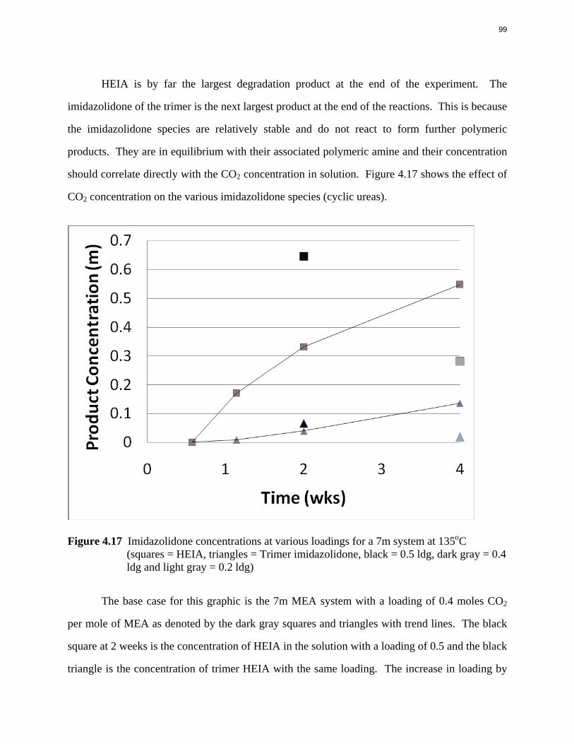
HEIA is by far the largest degradation product at the end of the experiment. The
imidazolidone of the trimer is the next largest product at the end of the reactions. This is because
the imidazolidone species are relatively stable and do not react to form further polymeric
products. They are in equilibrium with their associated polymeric amine and their concentration
should correlate directly with the CO2 concentration in solution. Figure 4.17 shows the effect of
CO2 concentration on the various imidazolidone species (cyclic ureas).
Figure 4.17 Imidazolidone concentrations at various loadings for a 7m system at 135oC (squares = HEIA, triangles = Trimer imidazolidone, black = 0.5 ldg, dark gray = 0.4 ldg and light gray = 0.2 ldg)
The base case for this graphic is the 7m MEA system with a loading of 0.4 moles CO2
per mole of MEA as denoted by the dark gray squares and triangles with trend lines. The black
square at 2 weeks is the concentration of HEIA in the solution with a loading of 0.5 and the black
triangle is the concentration of trimer HEIA with the same loading. The increase in loading by
99
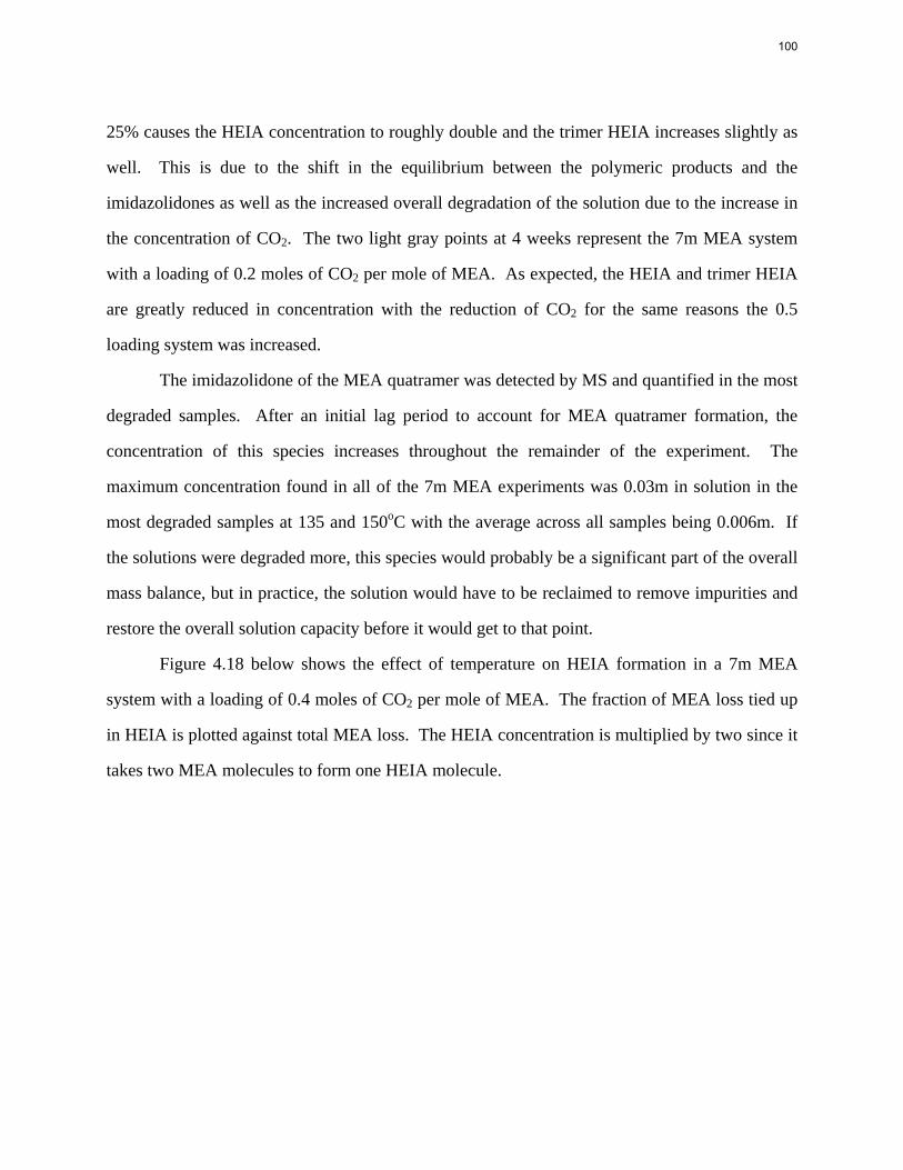
25% causes the HEIA concentration to roughly double and the trimer HEIA increases slightly as
well. This is due to the shift in the equilibrium between the polymeric products and the
imidazolidones as well as the increased overall degradation of the solution due to the increase in
the concentration of CO2. The two light gray points at 4 weeks represent the 7m MEA system
with a loading of 0.2 moles of CO2 per mole of MEA. As expected, the HEIA and trimer HEIA
are greatly reduced in concentration with the reduction of CO2 for the same reasons the 0.5
loading system was increased.
The imidazolidone of the MEA quatramer was detected by MS and quantified in the most
degraded samples. After an initial lag period to account for MEA quatramer formation, the
concentration of this species increases throughout the remainder of the experiment. The
maximum concentration found in all of the 7m MEA experiments was 0.03m in solution in the
most degraded samples at 135 and 150oC with the average across all samples being 0.006m. If
the solutions were degraded more, this species would probably be a significant part of the overall
mass balance, but in practice, the solution would have to be reclaimed to remove impurities and
restore the overall solution capacity before it would get to that point.
Figure 4.18 below shows the effect of temperature on HEIA formation in a 7m MEA
system with a loading of 0.4 moles of CO2 per mole of MEA. The fraction of MEA loss tied up
in HEIA is plotted against total MEA loss. The HEIA concentration is multiplied by two since it
takes two MEA molecules to form one HEIA molecule.
100
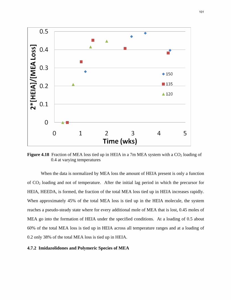
Figure 4.18 Fraction of MEA loss tied up in HEIA in a 7m MEA system with a CO2 loading of 0.4 at varying temperatures
When the data is normalized by MEA loss the amount of HEIA present is only a function
of CO2 loading and not of temperature. After the initial lag period in which the precursor for
HEIA, HEEDA, is formed, the fraction of the total MEA loss tied up in HEIA increases rapidly.
When approximately 45% of the total MEA loss is tied up in the HEIA molecule, the system
reaches a pseudo-steady state where for every additional mole of MEA that is lost, 0.45 moles of
MEA go into the formation of HEIA under the specified conditions. At a loading of 0.5 about
60% of the total MEA loss is tied up in HEIA across all temperature ranges and at a loading of
0.2 only 38% of the total MEA loss is tied up in HEIA.
4.7.2 Imidazolidones and Polymeric Species of MEA
101
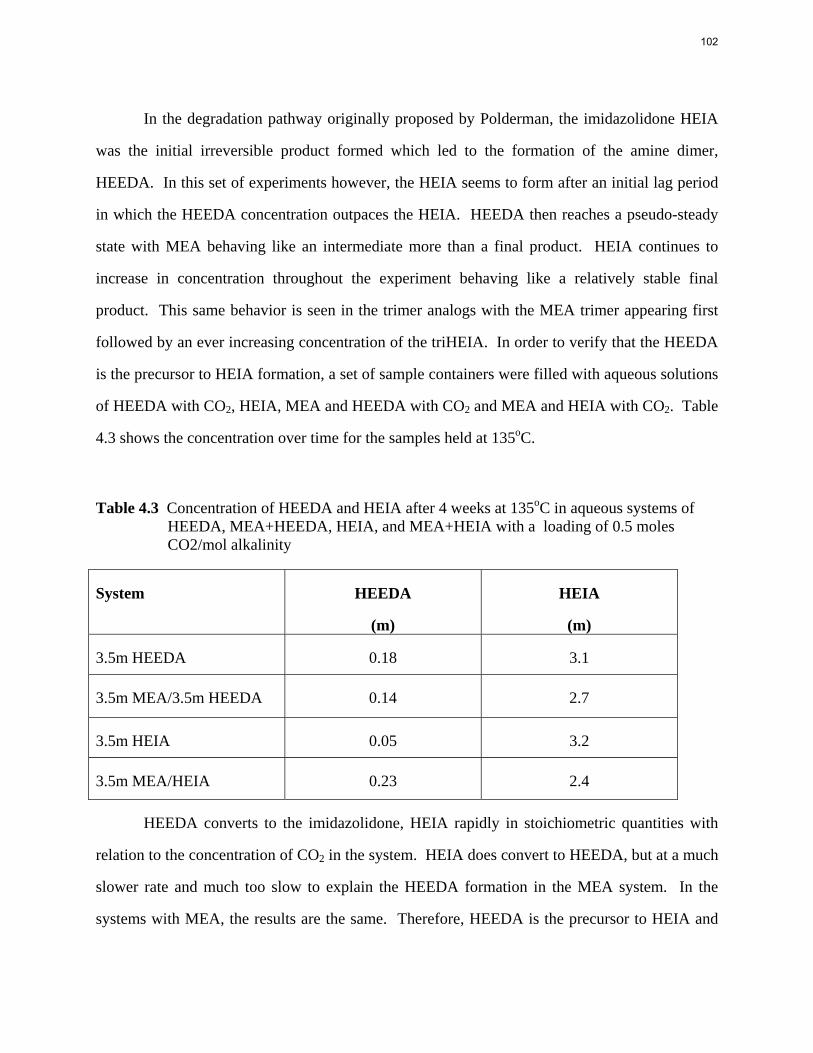
In the degradation pathway originally proposed by Polderman, the imidazolidone HEIA
was the initial irreversible product formed which led to the formation of the amine dimer,
HEEDA. In this set of experiments however, the HEIA seems to form after an initial lag period
in which the HEEDA concentration outpaces the HEIA. HEEDA then reaches a pseudo-steady
state with MEA behaving like an intermediate more than a final product. HEIA continues to
increase in concentration throughout the experiment behaving like a relatively stable final
product. This same behavior is seen in the trimer analogs with the MEA trimer appearing first
followed by an ever increasing concentration of the triHEIA. In order to verify that the HEEDA
is the precursor to HEIA formation, a set of sample containers were filled with aqueous solutions
of HEEDA with CO2, HEIA, MEA and HEEDA with CO2 and MEA and HEIA with CO2. Table
4.3 shows the concentration over time for the samples held at 135oC.
Table 4.3 Concentration of HEEDA and HEIA after 4 weeks at 135oC in aqueous systems of HEEDA, MEA+HEEDA, HEIA, and MEA+HEIA with a loading of 0.5 moles CO2/mol alkalinity
System HEEDA
(m)
HEIA
(m)
3.5m HEEDA 0.18 3.1
3.5m MEA/3.5m HEEDA 0.14 2.7
3.5m HEIA 0.05 3.2
3.5m MEA/HEIA 0.23 2.4
HEEDA converts to the imidazolidone, HEIA rapidly in stoichiometric quantities with
relation to the concentration of CO2 in the system. HEIA does convert to HEEDA, but at a much
slower rate and much too slow to explain the HEEDA formation in the MEA system. In the
systems with MEA, the results are the same. Therefore, HEEDA is the precursor to HEIA and
102
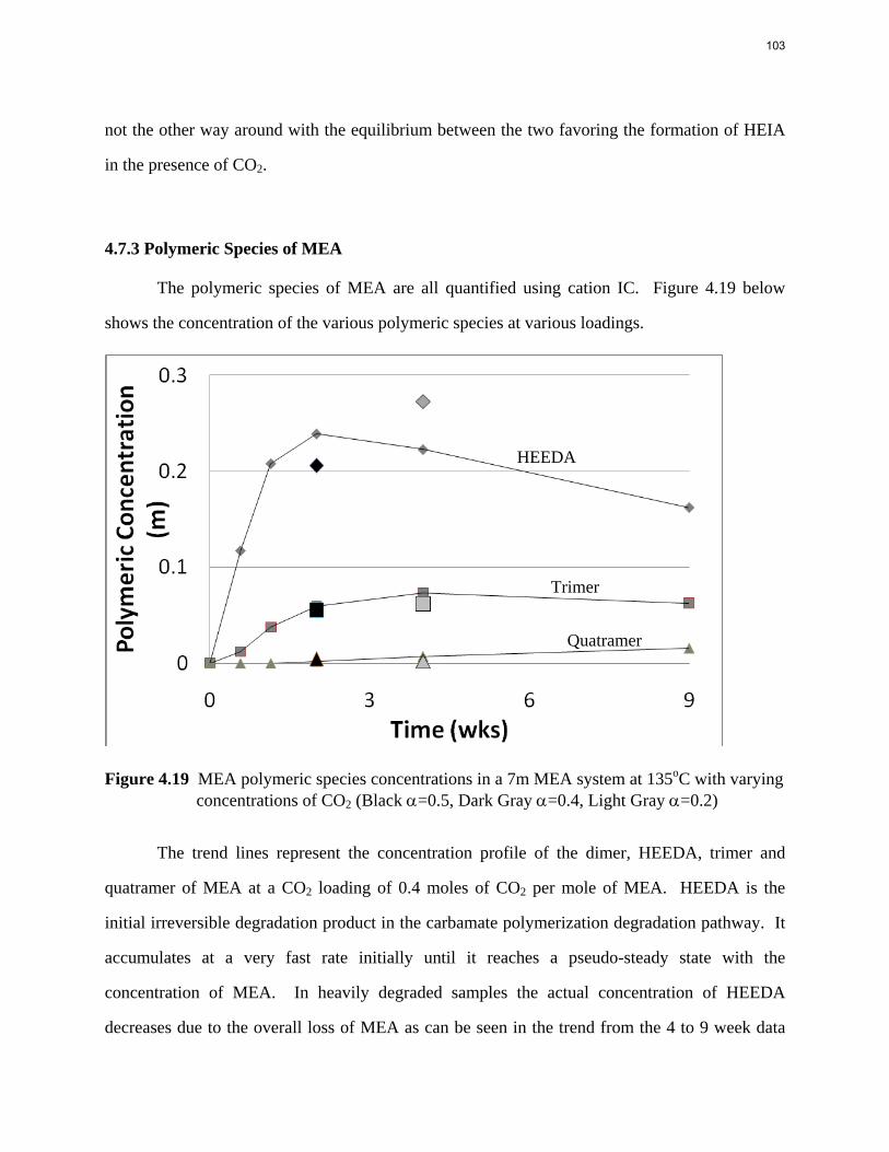
not the other way around with the equilibrium between the two favoring the formation of HEIA
in the presence of CO2.
4.7.3 Polymeric Species of MEA
The polymeric species of MEA are all quantified using cation IC. Figure 4.19 below
shows the concentration of the various polymeric species at various loadings.
Figure 4.19 MEA polymeric species concentrations in a 7m MEA system at 135oC with varying concentrations of CO2 (Black α=0.5, Dark Gray α=0.4, Light Gray α=0.2)
The trend lines represent the concentration profile of the dimer, HEEDA, trimer and
quatramer of MEA at a CO2 loading of 0.4 moles of CO2 per mole of MEA. HEEDA is the
initial irreversible degradation product in the carbamate polymerization degradation pathway. It
accumulates at a very fast rate initially until it reaches a pseudo-steady state with the
concentration of MEA. In heavily degraded samples the actual concentration of HEEDA
decreases due to the overall loss of MEA as can be seen in the trend from the 4 to 9 week data
HEEDA
Trimer
Quatramer
103
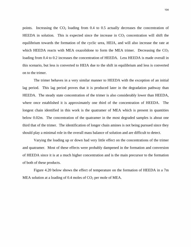
points. Increasing the CO2 loading from 0.4 to 0.5 actually decreases the concentration of
HEEDA in solution. This is expected since the increase in CO2 concentration will shift the
equilibrium towards the formation of the cyclic urea, HEIA, and will also increase the rate at
which HEEDA reacts with MEA oxazolidone to form the MEA trimer. Decreasing the CO2
loading from 0.4 to 0.2 increases the concentration of HEEDA. Less HEEDA is made overall in
this scenario, but less is converted to HEIA due to the shift in equilibrium and less is converted
on to the trimer.
The trimer behaves in a very similar manner to HEEDA with the exception of an initial
lag period. This lag period proves that it is produced later in the degradation pathway than
HEEDA. The steady state concentration of the trimer is also considerably lower than HEEDA,
where once established it is approximately one third of the concentration of HEEDA. The
longest chain identified in this work is the quatramer of MEA which is present in quantities
below 0.02m. The concentration of the quatramer in the most degraded samples is about one
third that of the trimer. The identification of longer chain amines is not being pursued since they
should play a minimal role in the overall mass balance of solution and are difficult to detect.
Varying the loading up or down had very little effect on the concentrations of the trimer
and quatramer. Most of these effects were probably dampened in the formation and conversion
of HEEDA since it is at a much higher concentration and is the main precursor to the formation
of both of these products.
Figure 4.20 below shows the effect of temperature on the formation of HEEDA in a 7m
MEA solution at a loading of 0.4 moles of CO2 per mole of MEA.
104
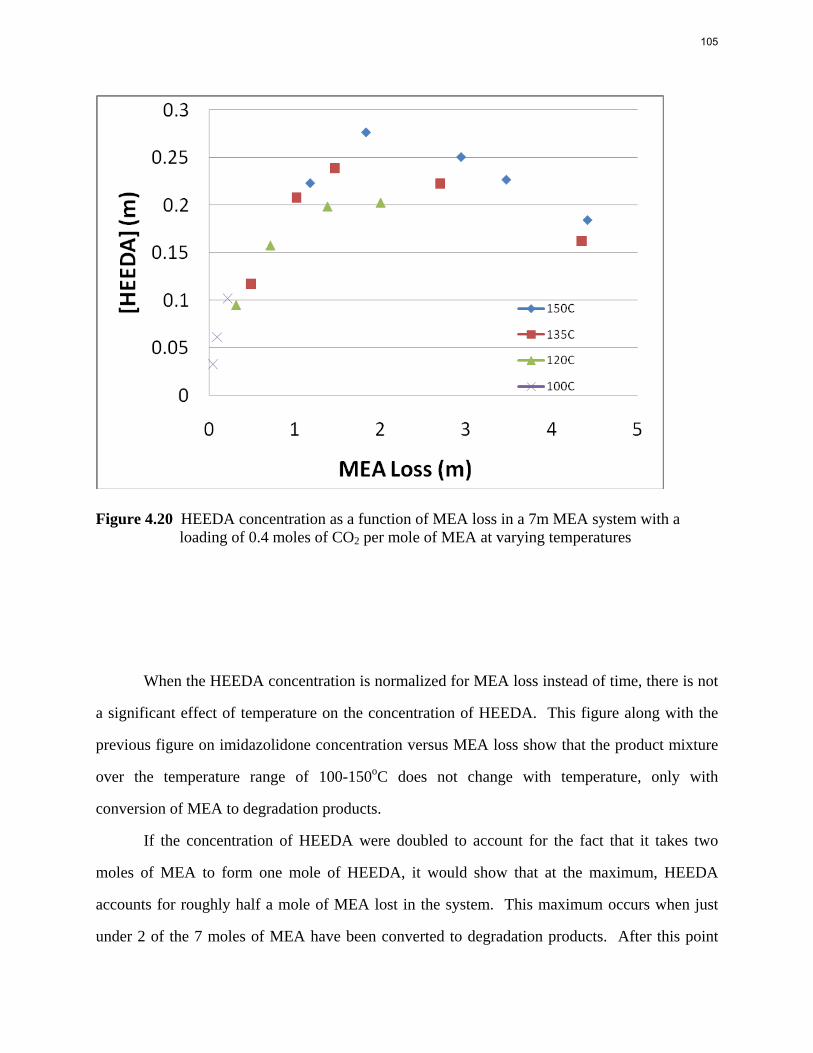
Figure 4.20 HEEDA concentration as a function of MEA loss in a 7m MEA system with a loading of 0.4 moles of CO2 per mole of MEA at varying temperatures
When the HEEDA concentration is normalized for MEA loss instead of time, there is not
a significant effect of temperature on the concentration of HEEDA. This figure along with the
previous figure on imidazolidone concentration versus MEA loss show that the product mixture
over the temperature range of 100-150oC does not change with temperature, only with
conversion of MEA to degradation products.
If the concentration of HEEDA were doubled to account for the fact that it takes two
moles of MEA to form one mole of HEEDA, it would show that at the maximum, HEEDA
accounts for roughly half a mole of MEA lost in the system. This maximum occurs when just
under 2 of the 7 moles of MEA have been converted to degradation products. After this point
105
the amount of MEA loss that is tied up in HEEDA decreases as it is converted to imidazolidone
and larger polymeric products.
In order to get a better idea of what the equilibrium constants for the HEEDA/HEIA
equilibrium and the Trimer/TriHEIA equilibrium are, Figure 4.21 below shows the ratio of HEIA
to HEEDA and TriHEIA to MEA Trimer for a 7m MEA system with a loading of 0.4 moles of
CO2 per mole of MEA over a temperature range of 100 to 150oC.
Figure 4.21 Ratio of HEIA:HEEDA and TriHEIA:Trimer versus MEA loss for a 7m MEA system with a loading of 0.4 moles of CO2/mole of MEA and temperatures varying from 100 to 150oC.
From this data it is difficult to tell what the final equilibrium constant will be for either
set of species since not enough of the imidazolidone species has been created to see where the
ratio will level off. The equilibrium constant will be evaluated later when this data is regressed
for the kinetic model. One thing to note is the ratio of HEIA to HEEDA and TriHEIA to MEA
106
trimer track each other very well over the course of these experiments over all temperatures
when normalized for total MEA loss. This could mean the equilibrium constant for the two sets
of species are similar.
4.8 MEA SPIKED WITH VARIOUS METALS
Various metals have been shown to enhance the oxidative degradation rate of various
amines (Sexton, 2008). In order to test if the thermal degradation rate is catalyzed by metals, 7m
MEA samples with a loading of 0.4 were spiked with 100mM quantities of Fe, Ni, Cr, Cu, or V.
Iron, nickel and chromium would be found in most industrial settings as metals leached from
stainless steel equipment. Copper and vanadium are sometimes used as corrosion inhibitors in
amine systems. The sample containers were placed in a forced convection oven at 150oC for 4
days. Figure 4.22 shows the final concentration of MEA for all samples including one that was
not spiked with any metals.
107
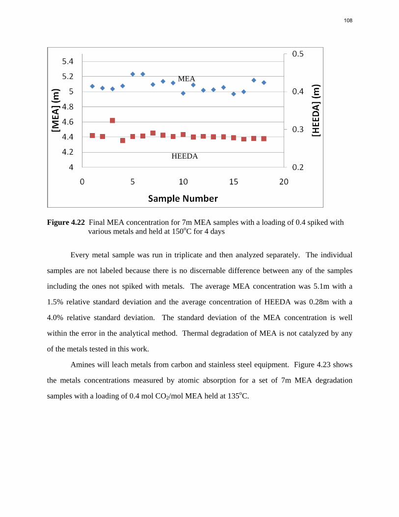
Figure 4.22 Final MEA concentration for 7m MEA samples with a loading of 0.4 spiked with various metals and held at 150oC for 4 days
Every metal sample was run in triplicate and then analyzed separately. The individual
samples are not labeled because there is no discernable difference between any of the samples
including the ones not spiked with metals. The average MEA concentration was 5.1m with a
1.5% relative standard deviation and the average concentration of HEEDA was 0.28m with a
4.0% relative standard deviation. The standard deviation of the MEA concentration is well
within the error in the analytical method. Thermal degradation of MEA is not catalyzed by any
of the metals tested in this work.
Amines will leach metals from carbon and stainless steel equipment. Figure 4.23 shows
the metals concentrations measured by atomic absorption for a set of 7m MEA degradation
samples with a loading of 0.4 mol CO2/mol MEA held at 135oC.
MEA
HEEDA
108
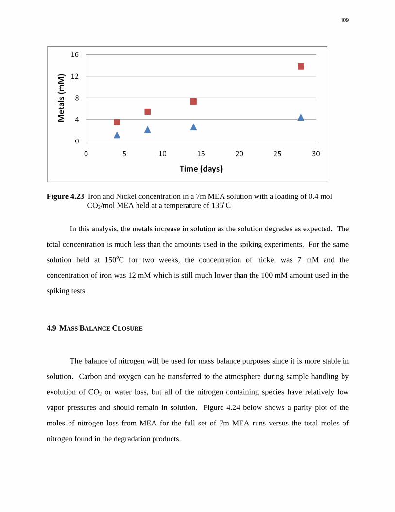
Figure 4.23 Iron and Nickel concentration in a 7m MEA solution with a loading of 0.4 mol CO2/mol MEA held at a temperature of 135oC
In this analysis, the metals increase in solution as the solution degrades as expected. The
total concentration is much less than the amounts used in the spiking experiments. For the same
solution held at 150oC for two weeks, the concentration of nickel was 7 mM and the
concentration of iron was 12 mM which is still much lower than the 100 mM amount used in the
spiking tests.
4.9 MASS BALANCE CLOSURE
The balance of nitrogen will be used for mass balance purposes since it is more stable in
solution. Carbon and oxygen can be transferred to the atmosphere during sample handling by
evolution of CO2 or water loss, but all of the nitrogen containing species have relatively low
vapor pressures and should remain in solution. Figure 4.24 below shows a parity plot of the
moles of nitrogen loss from MEA for the full set of 7m MEA runs versus the total moles of
nitrogen found in the degradation products.
109
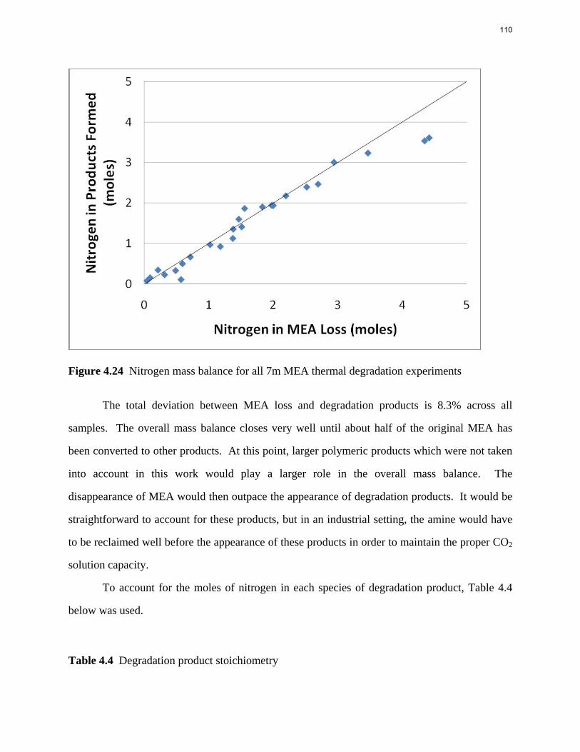
Figure 4.24 Nitrogen mass balance for all 7m MEA thermal degradation experiments
The total deviation between MEA loss and degradation products is 8.3% across all
samples. The overall mass balance closes very well until about half of the original MEA has
been converted to other products. At this point, larger polymeric products which were not taken
into account in this work would play a larger role in the overall mass balance. The
disappearance of MEA would then outpace the appearance of degradation products. It would be
straightforward to account for these products, but in an industrial setting, the amine would have
to be reclaimed well before the appearance of these products in order to maintain the proper CO2
solution capacity.
To account for the moles of nitrogen in each species of degradation product, Table 4.4
below was used.
Table 4.4 Degradation product stoichiometry
110
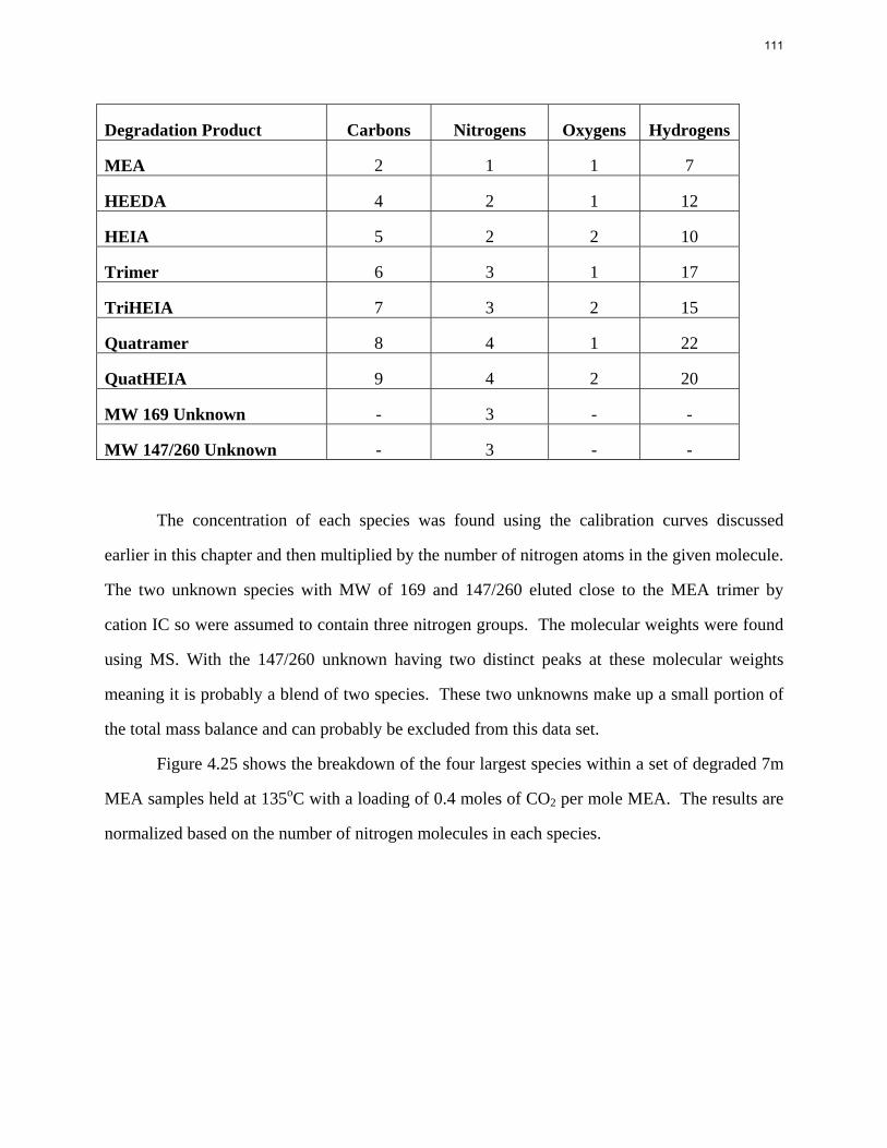
Degradation Product Carbons Nitrogens Oxygens Hydrogens
MEA 2 1 1 7
HEEDA 4 2 1 12
HEIA 5 2 2 10
Trimer 6 3 1 17
TriHEIA 7 3 2 15
Quatramer 8 4 1 22
QuatHEIA 9 4 2 20
MW 169 Unknown - 3 - -
MW 147/260 Unknown - 3 - -
The concentration of each species was found using the calibration curves discussed
earlier in this chapter and then multiplied by the number of nitrogen atoms in the given molecule.
The two unknown species with MW of 169 and 147/260 eluted close to the MEA trimer by
cation IC so were assumed to contain three nitrogen groups. The molecular weights were found
using MS. With the 147/260 unknown having two distinct peaks at these molecular weights
meaning it is probably a blend of two species. These two unknowns make up a small portion of
the total mass balance and can probably be excluded from this data set.
Figure 4.25 shows the breakdown of the four largest species within a set of degraded 7m
MEA samples held at 135oC with a loading of 0.4 moles of CO2 per mole MEA. The results are
normalized based on the number of nitrogen molecules in each species.
111
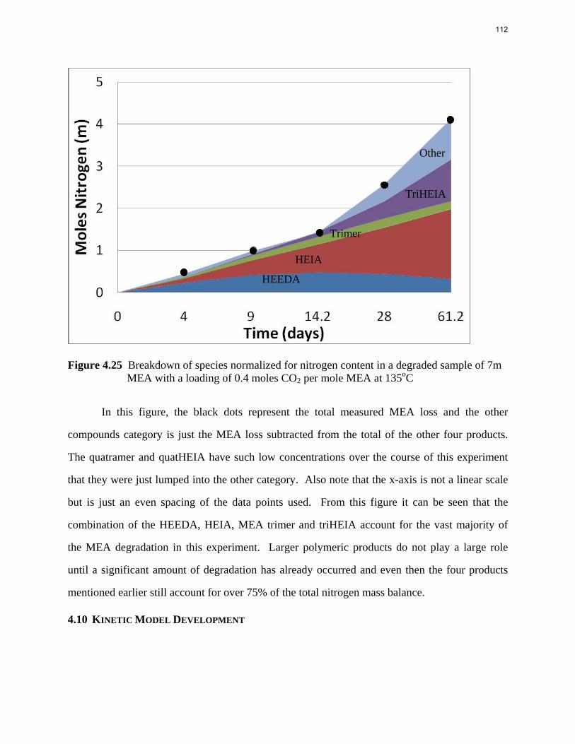
Figure 4.25 Breakdown of species normalized for nitrogen content in a degraded sample of 7m MEA with a loading of 0.4 moles CO2 per mole MEA at 135oC
In this figure, the black dots represent the total measured MEA loss and the other
compounds category is just the MEA loss subtracted from the total of the other four products.
The quatramer and quatHEIA have such low concentrations over the course of this experiment
that they were just lumped into the other category. Also note that the x-axis is not a linear scale
but is just an even spacing of the data points used. From this figure it can be seen that the
combination of the HEEDA, HEIA, MEA trimer and triHEIA account for the vast majority of
the MEA degradation in this experiment. Larger polymeric products do not play a large role
until a significant amount of degradation has already occurred and even then the four products
mentioned earlier still account for over 75% of the total nitrogen mass balance.
4.10 KINETIC MODEL DEVELOPMENT
HEEDA
HEIA
Trimer
TriHEIA
Other
112
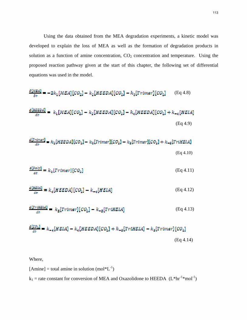
Using the data obtained from the MEA degradation experiments, a kinetic model was
developed to explain the loss of MEA as well as the formation of degradation products in
solution as a function of amine concentration, CO2 concentration and temperature. Using the
proposed reaction pathway given at the start of this chapter, the following set of differential
equations was used in the model.
(Eq 4.8)
(Eq 4.9)
(Eq 4.10)
(Eq 4.11)
(Eq 4.12)
(Eq 4.13)
(Eq 4.14)
Where,
[Amine] = total amine in solution (mol*L-1)
k1 = rate constant for conversion of MEA and Oxazolidone to HEEDA (L*hr-1*mol-1)
113
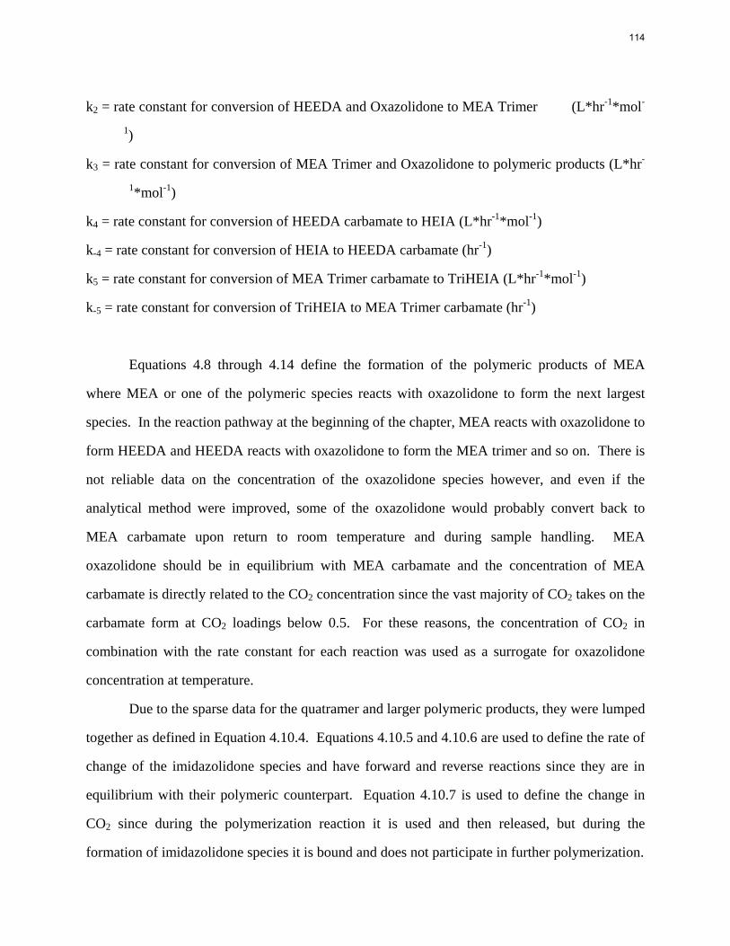
k2 = rate constant for conversion of HEEDA and Oxazolidone to MEA Trimer (L*hr-1*mol-
1)
k3 = rate constant for conversion of MEA Trimer and Oxazolidone to polymeric products (L*hr-
1*mol-1)
k4 = rate constant for conversion of HEEDA carbamate to HEIA (L*hr-1*mol-1)
k-4 = rate constant for conversion of HEIA to HEEDA carbamate (hr-1)
k5 = rate constant for conversion of MEA Trimer carbamate to TriHEIA (L*hr-1*mol-1)
k-5 = rate constant for conversion of TriHEIA to MEA Trimer carbamate (hr-1)
Equations 4.8 through 4.14 define the formation of the polymeric products of MEA
where MEA or one of the polymeric species reacts with oxazolidone to form the next largest
species. In the reaction pathway at the beginning of the chapter, MEA reacts with oxazolidone to
form HEEDA and HEEDA reacts with oxazolidone to form the MEA trimer and so on. There is
not reliable data on the concentration of the oxazolidone species however, and even if the
analytical method were improved, some of the oxazolidone would probably convert back to
MEA carbamate upon return to room temperature and during sample handling. MEA
oxazolidone should be in equilibrium with MEA carbamate and the concentration of MEA
carbamate is directly related to the CO2 concentration since the vast majority of CO2 takes on the
carbamate form at CO2 loadings below 0.5. For these reasons, the concentration of CO2 in
combination with the rate constant for each reaction was used as a surrogate for oxazolidone
concentration at temperature.
Due to the sparse data for the quatramer and larger polymeric products, they were lumped
together as defined in Equation 4.10.4. Equations 4.10.5 and 4.10.6 are used to define the rate of
change of the imidazolidone species and have forward and reverse reactions since they are in
equilibrium with their polymeric counterpart. Equation 4.10.7 is used to define the change in
CO2 since during the polymerization reaction it is used and then released, but during the
formation of imidazolidone species it is bound and does not participate in further polymerization.
114
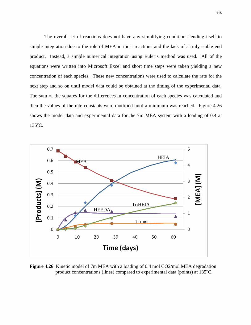
The overall set of reactions does not have any simplifying conditions lending itself to
simple integration due to the role of MEA in most reactions and the lack of a truly stable end
product. Instead, a simple numerical integration using Euler’s method was used. All of the
equations were written into Microsoft Excel and short time steps were taken yielding a new
concentration of each species. These new concentrations were used to calculate the rate for the
next step and so on until model data could be obtained at the timing of the experimental data.
The sum of the squares for the differences in concentration of each species was calculated and
then the values of the rate constants were modified until a minimum was reached. Figure 4.26
shows the model data and experimental data for the 7m MEA system with a loading of 0.4 at
135oC.
Figure 4.26 Kinetic model of 7m MEA with a loading of 0.4 mol CO2/mol MEA degradation product concentrations (lines) compared to experimental data (points) at 135oC.
HEEDA
HEIA MEA
TriHEIA
Trimer
115
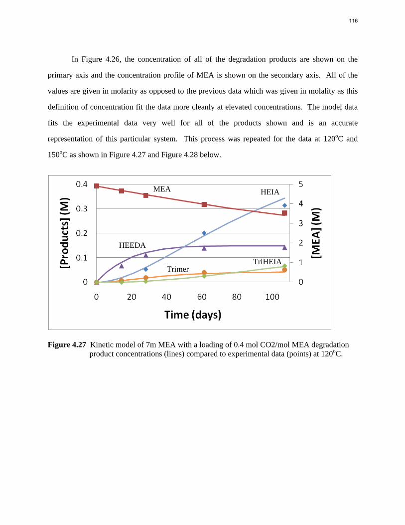
In Figure 4.26, the concentration of all of the degradation products are shown on the
primary axis and the concentration profile of MEA is shown on the secondary axis. All of the
values are given in molarity as opposed to the previous data which was given in molality as this
definition of concentration fit the data more cleanly at elevated concentrations. The model data
fits the experimental data very well for all of the products shown and is an accurate
representation of this particular system. This process was repeated for the data at 120oC and
150oC as shown in Figure 4.27 and Figure 4.28 below.
Figure 4.27 Kinetic model of 7m MEA with a loading of 0.4 mol CO2/mol MEA degradation product concentrations (lines) compared to experimental data (points) at 120oC.
MEA HEIA
HEEDA
Trimer TriHEIA
116
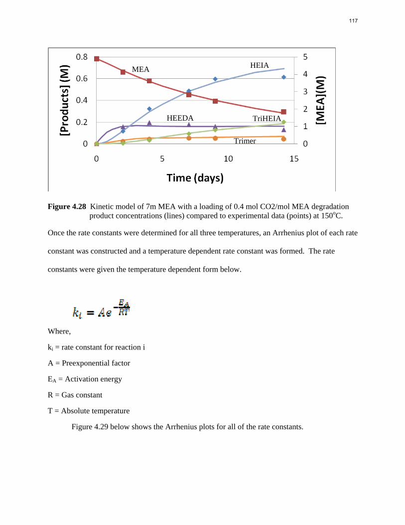
Figure 4.28 Kinetic model of 7m MEA with a loading of 0.4 mol CO2/mol MEA degradation product concentrations (lines) compared to experimental data (points) at 150oC.
Once the rate constants were determined for all three temperatures, an Arrhenius plot of each rate
constant was constructed and a temperature dependent rate constant was formed. The rate
constants were given the temperature dependent form below.
Where,
ki = rate constant for reaction i
A = Preexponential factor
EA = Activation energy
R = Gas constant
T = Absolute temperature
Figure 4.29 below shows the Arrhenius plots for all of the rate constants.
MEA HEIA
HEEDA
Trimer
TriHEIA
117
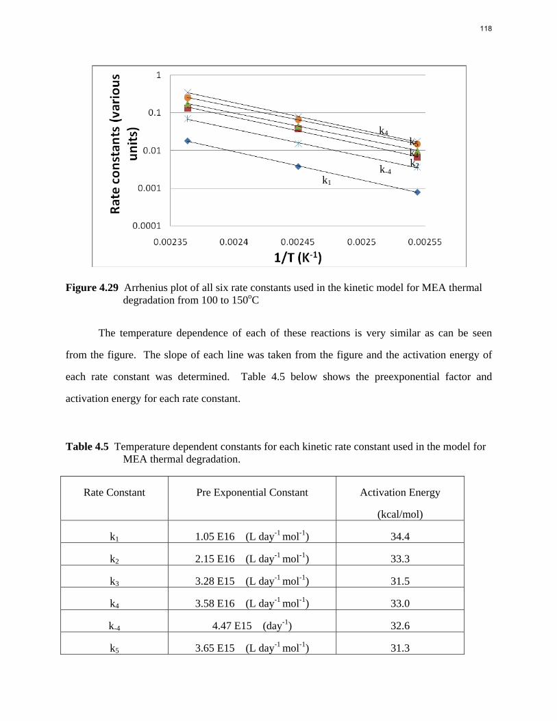
Figure 4.29 Arrhenius plot of all six rate constants used in the kinetic model for MEA thermal degradation from 100 to 150oC
The temperature dependence of each of these reactions is very similar as can be seen
from the figure. The slope of each line was taken from the figure and the activation energy of
each rate constant was determined. Table 4.5 below shows the preexponential factor and
activation energy for each rate constant.
Table 4.5 Temperature dependent constants for each kinetic rate constant used in the model for MEA thermal degradation.
Rate Constant Pre Exponential Constant
Activation Energy
(kcal/mol)
k1 1.05 E16 (L day-1 mol-1) 34.4
k2 2.15 E16 (L day-1 mol-1) 33.3
k3 3.28 E15 (L day-1 mol-1) 31.5
k4 3.58 E16 (L day-1 mol-1) 33.0
k-4 4.47 E15 (day-1) 32.6
k5 3.65 E15 (L day-1 mol-1) 31.3
k1
k-4 k2 k3
k5
k4
118
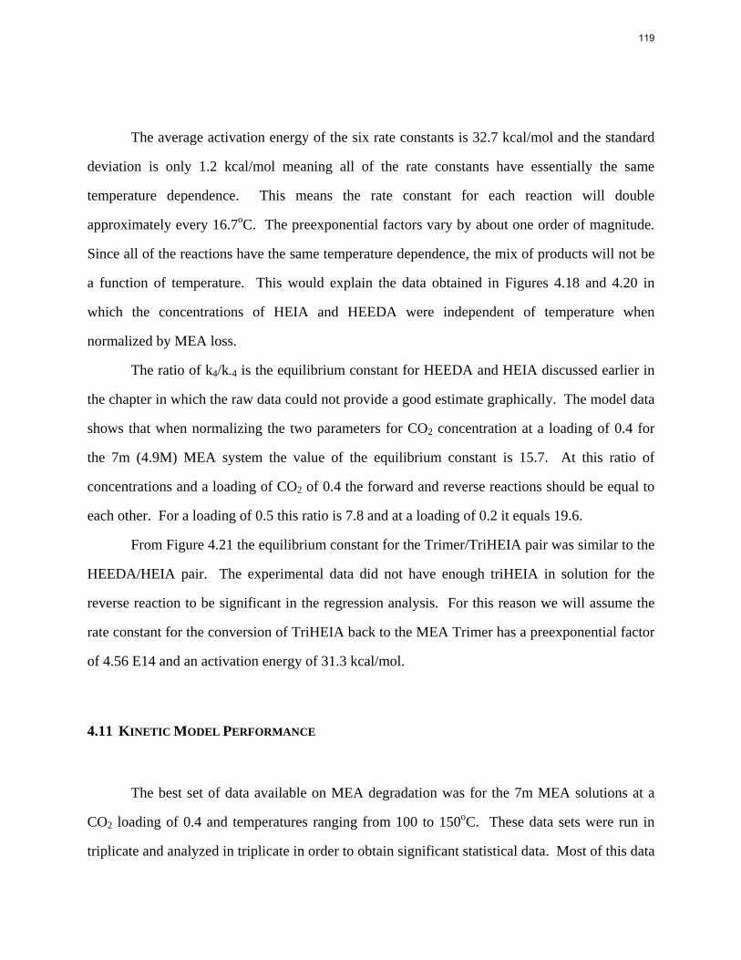
The average activation energy of the six rate constants is 32.7 kcal/mol and the standard
deviation is only 1.2 kcal/mol meaning all of the rate constants have essentially the same
temperature dependence. This means the rate constant for each reaction will double
approximately every 16.7oC. The preexponential factors vary by about one order of magnitude.
Since all of the reactions have the same temperature dependence, the mix of products will not be
a function of temperature. This would explain the data obtained in Figures 4.18 and 4.20 in
which the concentrations of HEIA and HEEDA were independent of temperature when
normalized by MEA loss.
The ratio of k4/k-4 is the equilibrium constant for HEEDA and HEIA discussed earlier in
the chapter in which the raw data could not provide a good estimate graphically. The model data
shows that when normalizing the two parameters for CO2 concentration at a loading of 0.4 for
the 7m (4.9M) MEA system the value of the equilibrium constant is 15.7. At this ratio of
concentrations and a loading of CO2 of 0.4 the forward and reverse reactions should be equal to
each other. For a loading of 0.5 this ratio is 7.8 and at a loading of 0.2 it equals 19.6.
From Figure 4.21 the equilibrium constant for the Trimer/TriHEIA pair was similar to the
HEEDA/HEIA pair. The experimental data did not have enough triHEIA in solution for the
reverse reaction to be significant in the regression analysis. For this reason we will assume the
rate constant for the conversion of TriHEIA back to the MEA Trimer has a preexponential factor
of 4.56 E14 and an activation energy of 31.3 kcal/mol.
4.11 KINETIC MODEL PERFORMANCE
The best set of data available on MEA degradation was for the 7m MEA solutions at a
CO2 loading of 0.4 and temperatures ranging from 100 to 150oC. These data sets were run in
triplicate and analyzed in triplicate in order to obtain significant statistical data. Most of this data
119
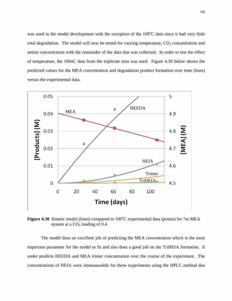
was used in the model development with the exception of the 100oC data since it had very little
total degradation. The model will now be tested for varying temperature, CO2 concentration and
amine concentration with the remainder of the data that was collected. In order to test the effect
of temperature, the 100oC data from the triplicate runs was used. Figure 4.30 below shows the
predicted values for the MEA concentration and degradation product formation over time (lines)
versus the experimental data.
Figure 4.30 Kinetic model (lines) compared to 100oC experimental data (points) for 7m MEA system at a CO2 loading of 0.4
The model does an excellent job of predicting the MEA concentration which is the most
important parameter for the model to fit and also does a good job on the TriHEIA formation. It
under predicts HEEDA and MEA trimer concentration over the course of the experiment. The
concentrations of HEIA were immeasurable for these experiments using the HPLC method due
MEA HEEDA
Trimer
HEIA
TriHEIA
120
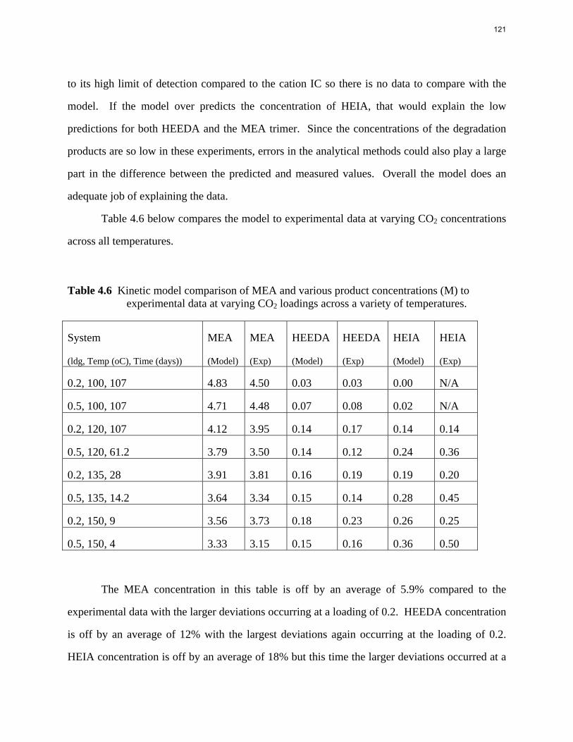
to its high limit of detection compared to the cation IC so there is no data to compare with the
model. If the model over predicts the concentration of HEIA, that would explain the low
predictions for both HEEDA and the MEA trimer. Since the concentrations of the degradation
products are so low in these experiments, errors in the analytical methods could also play a large
part in the difference between the predicted and measured values. Overall the model does an
adequate job of explaining the data.
Table 4.6 below compares the model to experimental data at varying CO2 concentrations
across all temperatures.
Table 4.6 Kinetic model comparison of MEA and various product concentrations (M) to experimental data at varying CO2 loadings across a variety of temperatures.
System
(ldg, Temp (oC), Time (days))
MEA
(Model)
MEA
(Exp)
HEEDA
(Model)
HEEDA
(Exp)
HEIA
(Model)
HEIA
(Exp)
0.2, 100, 107 4.83 4.50 0.03 0.03 0.00 N/A
0.5, 100, 107 4.71 4.48 0.07 0.08 0.02 N/A
0.2, 120, 107 4.12 3.95 0.14 0.17 0.14 0.14
0.5, 120, 61.2 3.79 3.50 0.14 0.12 0.24 0.36
0.2, 135, 28 3.91 3.81 0.16 0.19 0.19 0.20
0.5, 135, 14.2 3.64 3.34 0.15 0.14 0.28 0.45
0.2, 150, 9 3.56 3.73 0.18 0.23 0.26 0.25
0.5, 150, 4 3.33 3.15 0.15 0.16 0.36 0.50
The MEA concentration in this table is off by an average of 5.9% compared to the
experimental data with the larger deviations occurring at a loading of 0.2. HEEDA concentration
is off by an average of 12% with the largest deviations again occurring at the loading of 0.2.
HEIA concentration is off by an average of 18% but this time the larger deviations occurred at a
121
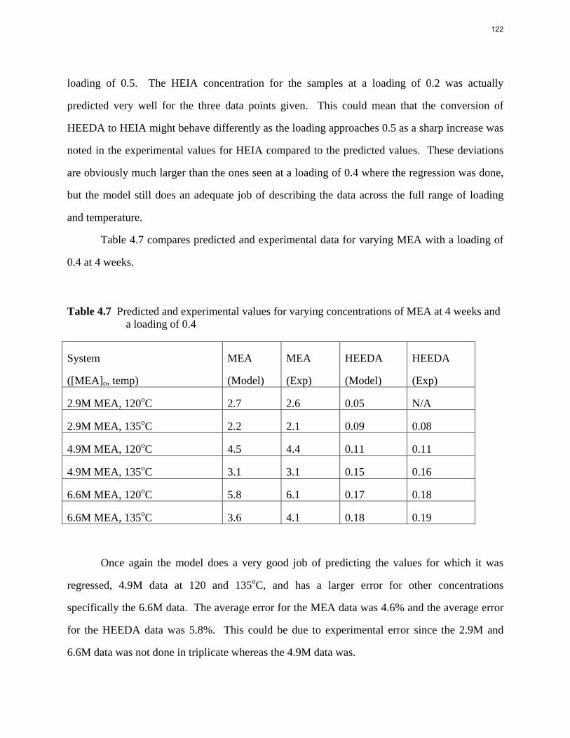
loading of 0.5. The HEIA concentration for the samples at a loading of 0.2 was actually
predicted very well for the three data points given. This could mean that the conversion of
HEEDA to HEIA might behave differently as the loading approaches 0.5 as a sharp increase was
noted in the experimental values for HEIA compared to the predicted values. These deviations
are obviously much larger than the ones seen at a loading of 0.4 where the regression was done,
but the model still does an adequate job of describing the data across the full range of loading
and temperature.
Table 4.7 compares predicted and experimental data for varying MEA with a loading of
0.4 at 4 weeks.
Table 4.7 Predicted and experimental values for varying concentrations of MEA at 4 weeks and a loading of 0.4
System
([MEA]o, temp)
MEA
(Model)
MEA
(Exp)
HEEDA
(Model)
HEEDA
(Exp)
2.9M MEA, 120oC 2.7 2.6 0.05 N/A
2.9M MEA, 135oC 2.2 2.1 0.09 0.08
4.9M MEA, 120oC 4.5 4.4 0.11 0.11
4.9M MEA, 135oC 3.1 3.1 0.15 0.16
6.6M MEA, 120oC 5.8 6.1 0.17 0.18
6.6M MEA, 135oC 3.6 4.1 0.18 0.19
Once again the model does a very good job of predicting the values for which it was
regressed, 4.9M data at 120 and 135oC, and has a larger error for other concentrations
specifically the 6.6M data. The average error for the MEA data was 4.6% and the average error
for the HEEDA data was 5.8%. This could be due to experimental error since the 2.9M and
6.6M data was not done in triplicate whereas the 4.9M data was.
122
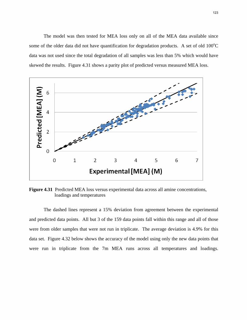
The model was then tested for MEA loss only on all of the MEA data available since
some of the older data did not have quantification for degradation products. A set of old 100oC
data was not used since the total degradation of all samples was less than 5% which would have
skewed the results. Figure 4.31 shows a parity plot of predicted versus measured MEA loss.
Figure 4.31 Predicted MEA loss versus experimental data across all amine concentrations, loadings and temperatures
The dashed lines represent a 15% deviation from agreement between the experimental
and predicted data points. All but 3 of the 159 data points fall within this range and all of those
were from older samples that were not run in triplicate. The average deviation is 4.9% for this
data set. Figure 4.32 below shows the accuracy of the model using only the new data points that
were run in triplicate from the 7m MEA runs across all temperatures and loadings.
123
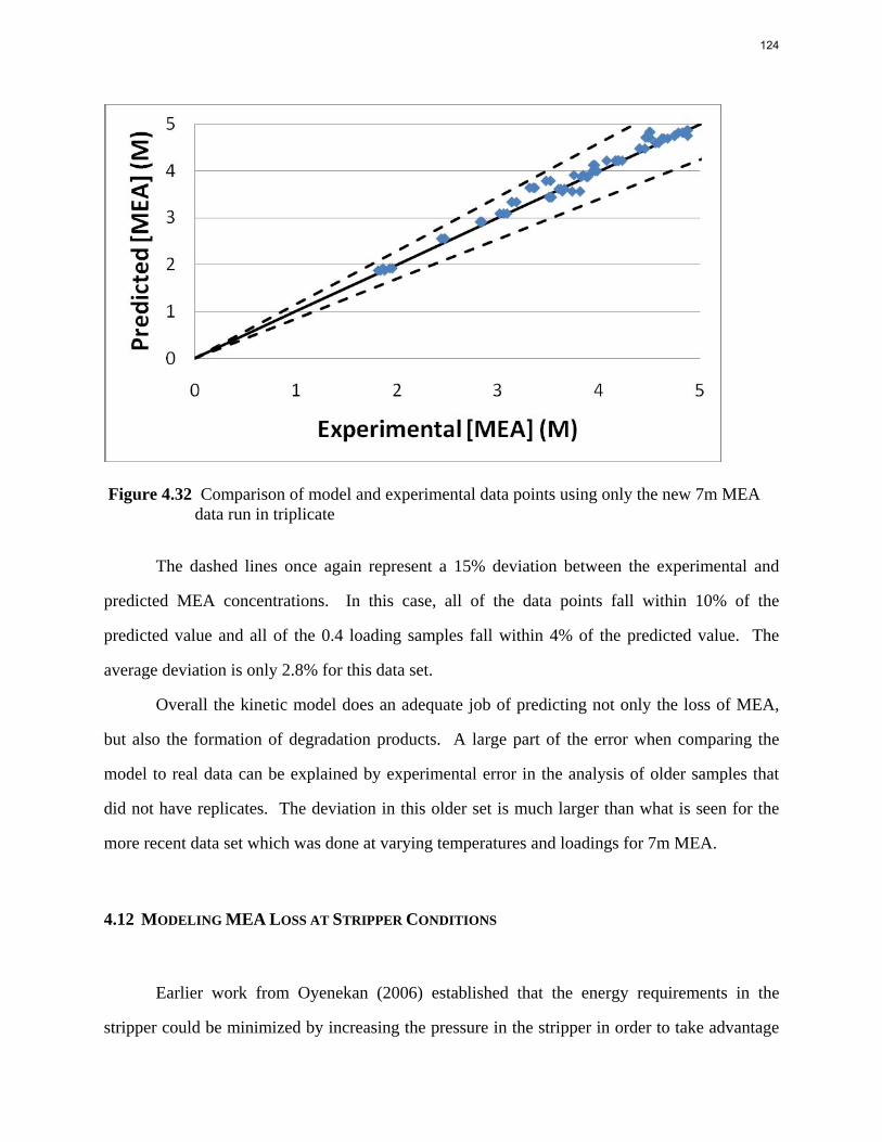
Figure 4.32 Comparison of model and experimental data points using only the new 7m MEA data run in triplicate
The dashed lines once again represent a 15% deviation between the experimental and
predicted MEA concentrations. In this case, all of the data points fall within 10% of the
predicted value and all of the 0.4 loading samples fall within 4% of the predicted value. The
average deviation is only 2.8% for this data set.
Overall the kinetic model does an adequate job of predicting not only the loss of MEA,
but also the formation of degradation products. A large part of the error when comparing the
model to real data can be explained by experimental error in the analysis of older samples that
did not have replicates. The deviation in this older set is much larger than what is seen for the
more recent data set which was done at varying temperatures and loadings for 7m MEA.
4.12 MODELING MEA LOSS AT STRIPPER CONDITIONS
Earlier work from Oyenekan (2006) established that the energy requirements in the
stripper could be minimized by increasing the pressure in the stripper in order to take advantage
124
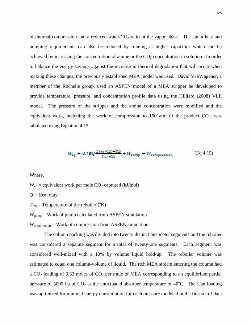
of thermal compression and a reduced water/CO2 ratio in the vapor phase. The latent heat and
pumping requirements can also be reduced by running at higher capacities which can be
achieved by increasing the concentration of amine or the CO2 concentration in solution. In order
to balance the energy savings against the increase in thermal degradation that will occur when
making these changes, the previously established MEA model was used. David VanWagener, a
member of the Rochelle group, used an ASPEN model of a MEA stripper he developed to
provide temperature, pressure, and concentration profile data using the Hilliard (2008) VLE
model. The pressure of the stripper and the amine concentration were modified and the
equivalent work, including the work of compression to 150 atm of the product CO2, was
tabulated using Equation 4.15.
(Eq 4.15)
Where,
Weq = equivalent work per mole CO2 captured (kJ/mol)
Q = Heat duty
Treb = Temperature of the reboiler (oK)
Wpump = Work of pump calculated from ASPEN simulation
Wcompression = Work of compression from ASPEN simulation
The column packing was divided into twenty distinct one meter segments and the reboiler
was considered a separate segment for a total of twenty-one segments. Each segment was
considered well-mixed with a 10% by volume liquid hold-up. The reboiler volume was
estimated to equal one column-volume of liquid. The rich MEA stream entering the column had
a CO2 loading of 0.52 moles of CO2 per mole of MEA corresponding to an equilibrium partial
pressure of 5000 Pa of CO2 at the anticipated absorber temperature of 40oC. The lean loading
was optimized for minimal energy consumption for each pressure modeled in the first set of data
125
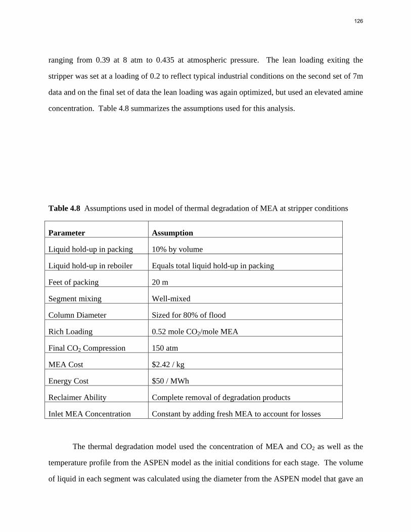
ranging from 0.39 at 8 atm to 0.435 at atmospheric pressure. The lean loading exiting the
stripper was set at a loading of 0.2 to reflect typical industrial conditions on the second set of 7m
data and on the final set of data the lean loading was again optimized, but used an elevated amine
concentration. Table 4.8 summarizes the assumptions used for this analysis.
Table 4.8 Assumptions used in model of thermal degradation of MEA at stripper conditions
Parameter Assumption
Liquid hold-up in packing 10% by volume
Liquid hold-up in reboiler Equals total liquid hold-up in packing
Feet of packing 20 m
Segment mixing Well-mixed
Column Diameter Sized for 80% of flood
Rich Loading 0.52 mole CO2/mole MEA
Final CO2 Compression 150 atm
MEA Cost $2.42 / kg
Energy Cost $50 / MWh
Reclaimer Ability Complete removal of degradation products
Inlet MEA Concentration Constant by adding fresh MEA to account for losses
The thermal degradation model used the concentration of MEA and CO2 as well as the
temperature profile from the ASPEN model as the initial conditions for each stage. The volume
of liquid in each segment was calculated using the diameter from the ASPEN model that gave an
126
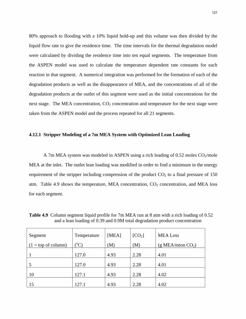
80% approach to flooding with a 10% liquid hold-up and this volume was then divided by the
liquid flow rate to give the residence time. The time intervals for the thermal degradation model
were calculated by dividing the residence time into ten equal segments. The temperature from
the ASPEN model was used to calculate the temperature dependent rate constants for each
reaction in that segment. A numerical integration was performed for the formation of each of the
degradation products as well as the disappearance of MEA, and the concentrations of all of the
degradation products at the outlet of this segment were used as the initial concentrations for the
next stage. The MEA concentration, CO2 concentration and temperature for the next stage were
taken from the ASPEN model and the process repeated for all 21 segments.
4.12.1 Stripper Modeling of a 7m MEA System with Optimized Lean Loading
A 7m MEA system was modeled in ASPEN using a rich loading of 0.52 moles CO2/mole
MEA at the inlet. The outlet lean loading was modified in order to find a minimum in the energy
requirement of the stripper including compression of the product CO2 to a final pressure of 150
atm. Table 4.9 shows the temperature, MEA concentration, CO2 concentration, and MEA loss
for each segment.
Table 4.9 Column segment liquid profile for 7m MEA run at 8 atm with a rich loading of 0.52 and a lean loading of 0.39 and 0.9M total degradation product concentration
Segment
(1 = top of column)
Temperature
(oC)
[MEA]
(M)
[CO2]
(M)
MEA Loss
(g MEA/mton CO2)
1 127.0 4.93 2.28 4.01
5 127.0 4.93 2.28 4.01
10 127.1 4.93 2.28 4.02
15 127.1 4.93 2.28 4.02
127
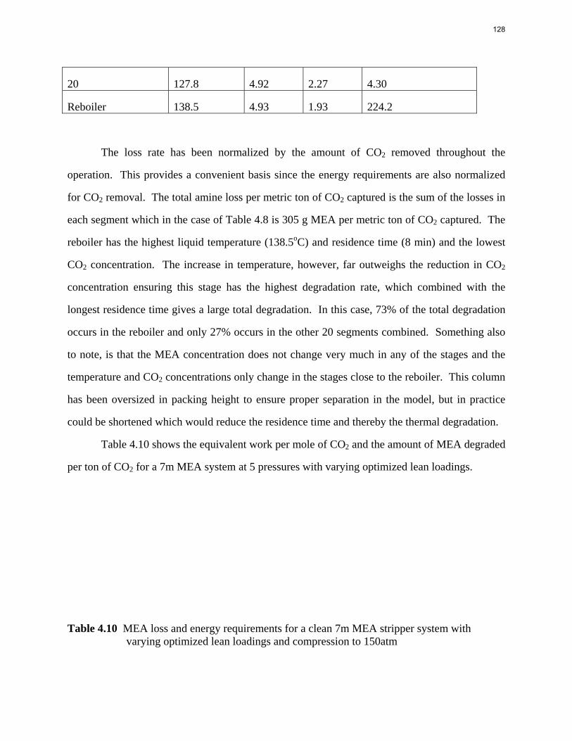
20 127.8 4.92 2.27 4.30
Reboiler 138.5 4.93 1.93 224.2
The loss rate has been normalized by the amount of CO2 removed throughout the
operation. This provides a convenient basis since the energy requirements are also normalized
for CO2 removal. The total amine loss per metric ton of CO2 captured is the sum of the losses in
each segment which in the case of Table 4.8 is 305 g MEA per metric ton of CO2 captured. The
reboiler has the highest liquid temperature (138.5oC) and residence time (8 min) and the lowest
CO2 concentration. The increase in temperature, however, far outweighs the reduction in CO2
concentration ensuring this stage has the highest degradation rate, which combined with the
longest residence time gives a large total degradation. In this case, 73% of the total degradation
occurs in the reboiler and only 27% occurs in the other 20 segments combined. Something also
to note, is that the MEA concentration does not change very much in any of the stages and the
temperature and CO2 concentrations only change in the stages close to the reboiler. This column
has been oversized in packing height to ensure proper separation in the model, but in practice
could be shortened which would reduce the residence time and thereby the thermal degradation.
Table 4.10 shows the equivalent work per mole of CO2 and the amount of MEA degraded
per ton of CO2 for a 7m MEA system at 5 pressures with varying optimized lean loadings.
Table 4.10 MEA loss and energy requirements for a clean 7m MEA stripper system with varying optimized lean loadings and compression to 150atm
128
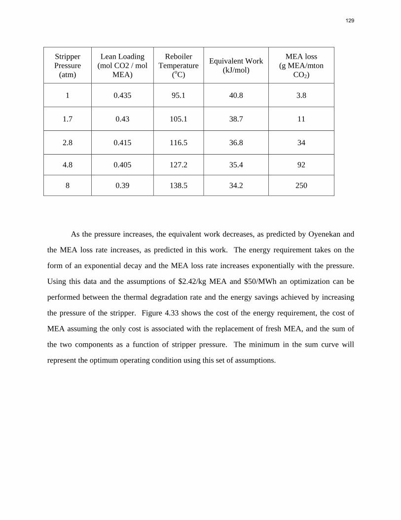
Stripper Pressure
(atm)
Lean Loading (mol CO2 / mol
MEA)
Reboiler Temperature
(oC)
Equivalent Work (kJ/mol)
MEA loss (g MEA/mton
CO2)
1 0.435 95.1 40.8 3.8
1.7 0.43 105.1 38.7 11
2.8 0.415 116.5 36.8 34
4.8 0.405 127.2 35.4 92
8 0.39 138.5 34.2 250
As the pressure increases, the equivalent work decreases, as predicted by Oyenekan and
the MEA loss rate increases, as predicted in this work. The energy requirement takes on the
form of an exponential decay and the MEA loss rate increases exponentially with the pressure.
Using this data and the assumptions of $2.42/kg MEA and $50/MWh an optimization can be
performed between the thermal degradation rate and the energy savings achieved by increasing
the pressure of the stripper. Figure 4.33 shows the cost of the energy requirement, the cost of
MEA assuming the only cost is associated with the replacement of fresh MEA, and the sum of
the two components as a function of stripper pressure. The minimum in the sum curve will
represent the optimum operating condition using this set of assumptions.
129
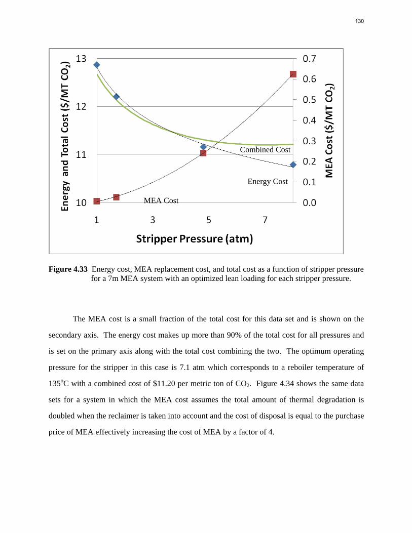
Figure 4.33 Energy cost, MEA replacement cost, and total cost as a function of stripper pressure for a 7m MEA system with an optimized lean loading for each stripper pressure.
The MEA cost is a small fraction of the total cost for this data set and is shown on the
secondary axis. The energy cost makes up more than 90% of the total cost for all pressures and
is set on the primary axis along with the total cost combining the two. The optimum operating
pressure for the stripper in this case is 7.1 atm which corresponds to a reboiler temperature of
135oC with a combined cost of $11.20 per metric ton of CO2. Figure 4.34 shows the same data
sets for a system in which the MEA cost assumes the total amount of thermal degradation is
doubled when the reclaimer is taken into account and the cost of disposal is equal to the purchase
price of MEA effectively increasing the cost of MEA by a factor of 4.
MEA Cost
Energy Cost
Combined Cost
130
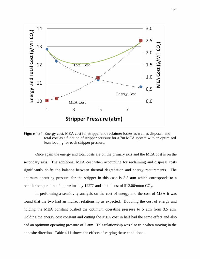
Figure 4.34 Energy cost, MEA cost for stripper and reclaimer losses as well as disposal, and total cost as a function of stripper pressure for a 7m MEA system with an optimized lean loading for each stripper pressure.
Once again the energy and total costs are on the primary axis and the MEA cost is on the
secondary axis. The additional MEA cost when accounting for reclaiming and disposal costs
significantly shifts the balance between thermal degradation and energy requirements. The
optimum operating pressure for the stripper in this case is 3.5 atm which corresponds to a
reboiler temperature of approximately 122oC and a total cost of $12.06/mton CO2.
In performing a sensitivity analysis on the cost of energy and the cost of MEA it was
found that the two had an indirect relationship as expected. Doubling the cost of energy and
holding the MEA constant pushed the optimum operating pressure to 5 atm from 3.5 atm.
Holding the energy cost constant and cutting the MEA cost in half had the same effect and also
had an optimum operating pressure of 5 atm. This relationship was also true when moving in the
opposite direction. Table 4.11 shows the effects of varying these conditions.
MEA Cost
Energy Cost
Total Cost
131
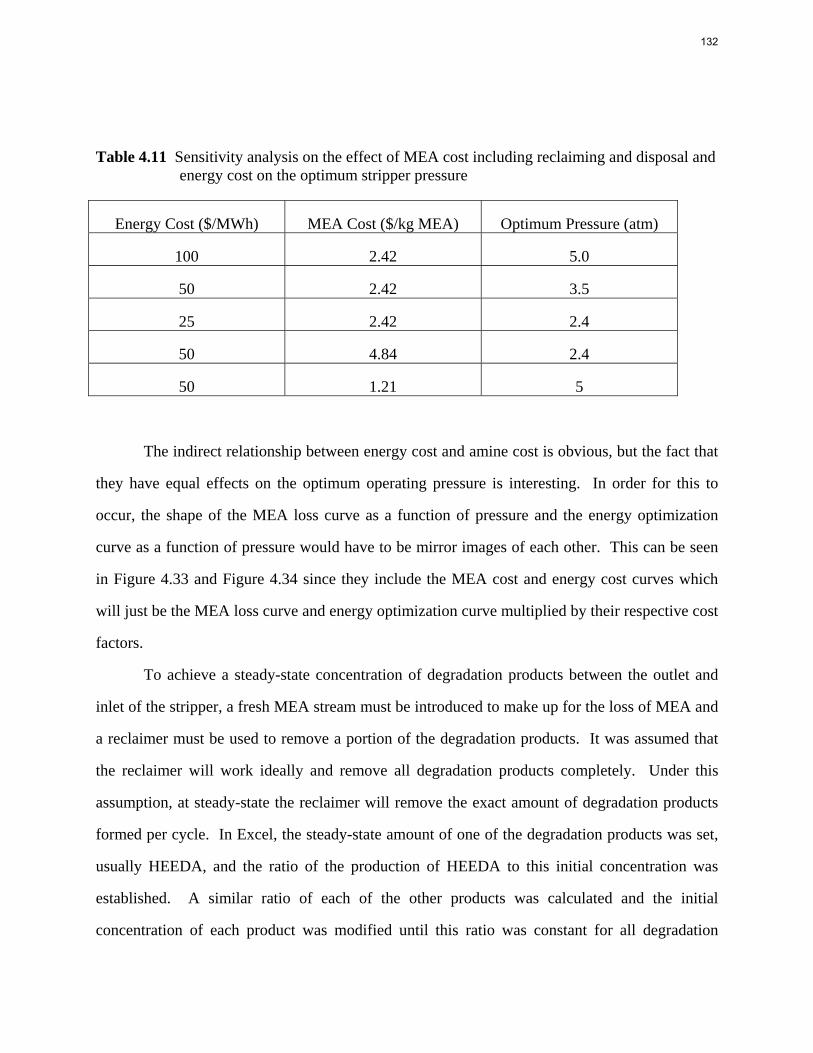
Table 4.11 Sensitivity analysis on the effect of MEA cost including reclaiming and disposal and energy cost on the optimum stripper pressure
Energy Cost ($/MWh) MEA Cost ($/kg MEA) Optimum Pressure (atm)
100 2.42 5.0
50 2.42 3.5
25 2.42 2.4
50 4.84 2.4
50 1.21 5
The indirect relationship between energy cost and amine cost is obvious, but the fact that
they have equal effects on the optimum operating pressure is interesting. In order for this to
occur, the shape of the MEA loss curve as a function of pressure and the energy optimization
curve as a function of pressure would have to be mirror images of each other. This can be seen
in Figure 4.33 and Figure 4.34 since they include the MEA cost and energy cost curves which
will just be the MEA loss curve and energy optimization curve multiplied by their respective cost
factors.
To achieve a steady-state concentration of degradation products between the outlet and
inlet of the stripper, a fresh MEA stream must be introduced to make up for the loss of MEA and
a reclaimer must be used to remove a portion of the degradation products. It was assumed that
the reclaimer will work ideally and remove all degradation products completely. Under this
assumption, at steady-state the reclaimer will remove the exact amount of degradation products
formed per cycle. In Excel, the steady-state amount of one of the degradation products was set,
usually HEEDA, and the ratio of the production of HEEDA to this initial concentration was
established. A similar ratio of each of the other products was calculated and the initial
concentration of each product was modified until this ratio was constant for all degradation
132
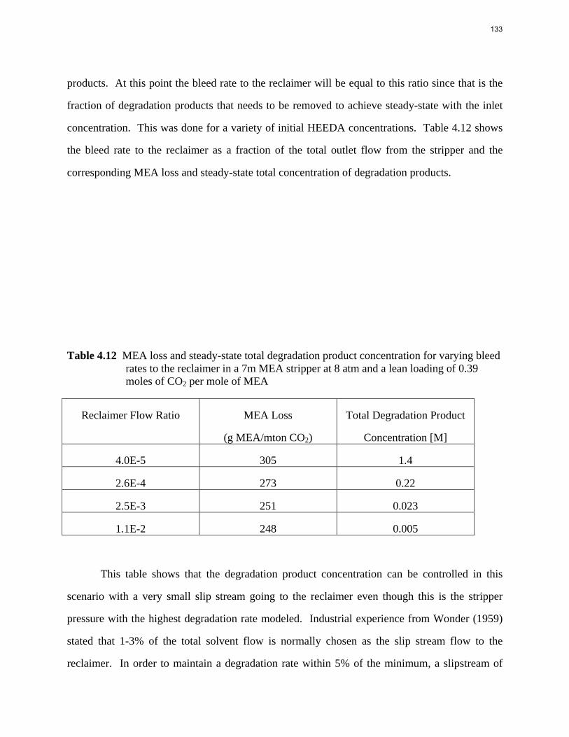
products. At this point the bleed rate to the reclaimer will be equal to this ratio since that is the
fraction of degradation products that needs to be removed to achieve steady-state with the inlet
concentration. This was done for a variety of initial HEEDA concentrations. Table 4.12 shows
the bleed rate to the reclaimer as a fraction of the total outlet flow from the stripper and the
corresponding MEA loss and steady-state total concentration of degradation products.
Table 4.12 MEA loss and steady-state total degradation product concentration for varying bleed rates to the reclaimer in a 7m MEA stripper at 8 atm and a lean loading of 0.39 moles of CO2 per mole of MEA
Reclaimer Flow Ratio MEA Loss
(g MEA/mton CO2)
Total Degradation Product
Concentration [M]
4.0E-5 305 1.4
2.6E-4 273 0.22
2.5E-3 251 0.023
1.1E-2 248 0.005
This table shows that the degradation product concentration can be controlled in this
scenario with a very small slip stream going to the reclaimer even though this is the stripper
pressure with the highest degradation rate modeled. Industrial experience from Wonder (1959)
stated that 1-3% of the total solvent flow is normally chosen as the slip stream flow to the
reclaimer. In order to maintain a degradation rate within 5% of the minimum, a slipstream of
133
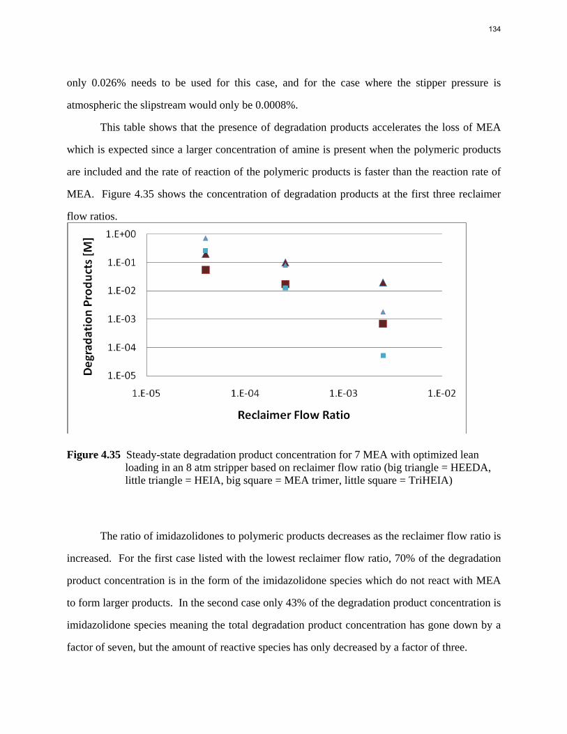
only 0.026% needs to be used for this case, and for the case where the stipper pressure is
atmospheric the slipstream would only be 0.0008%.
This table shows that the presence of degradation products accelerates the loss of MEA
which is expected since a larger concentration of amine is present when the polymeric products
are included and the rate of reaction of the polymeric products is faster than the reaction rate of
MEA. Figure 4.35 shows the concentration of degradation products at the first three reclaimer
flow ratios.
Figure 4.35 Steady-state degradation product concentration for 7 MEA with optimized lean loading in an 8 atm stripper based on reclaimer flow ratio (big triangle = HEEDA, little triangle = HEIA, big square = MEA trimer, little square = TriHEIA)
The ratio of imidazolidones to polymeric products decreases as the reclaimer flow ratio is
increased. For the first case listed with the lowest reclaimer flow ratio, 70% of the degradation
product concentration is in the form of the imidazolidone species which do not react with MEA
to form larger products. In the second case only 43% of the degradation product concentration is
imidazolidone species meaning the total degradation product concentration has gone down by a
factor of seven, but the amount of reactive species has only decreased by a factor of three.
134
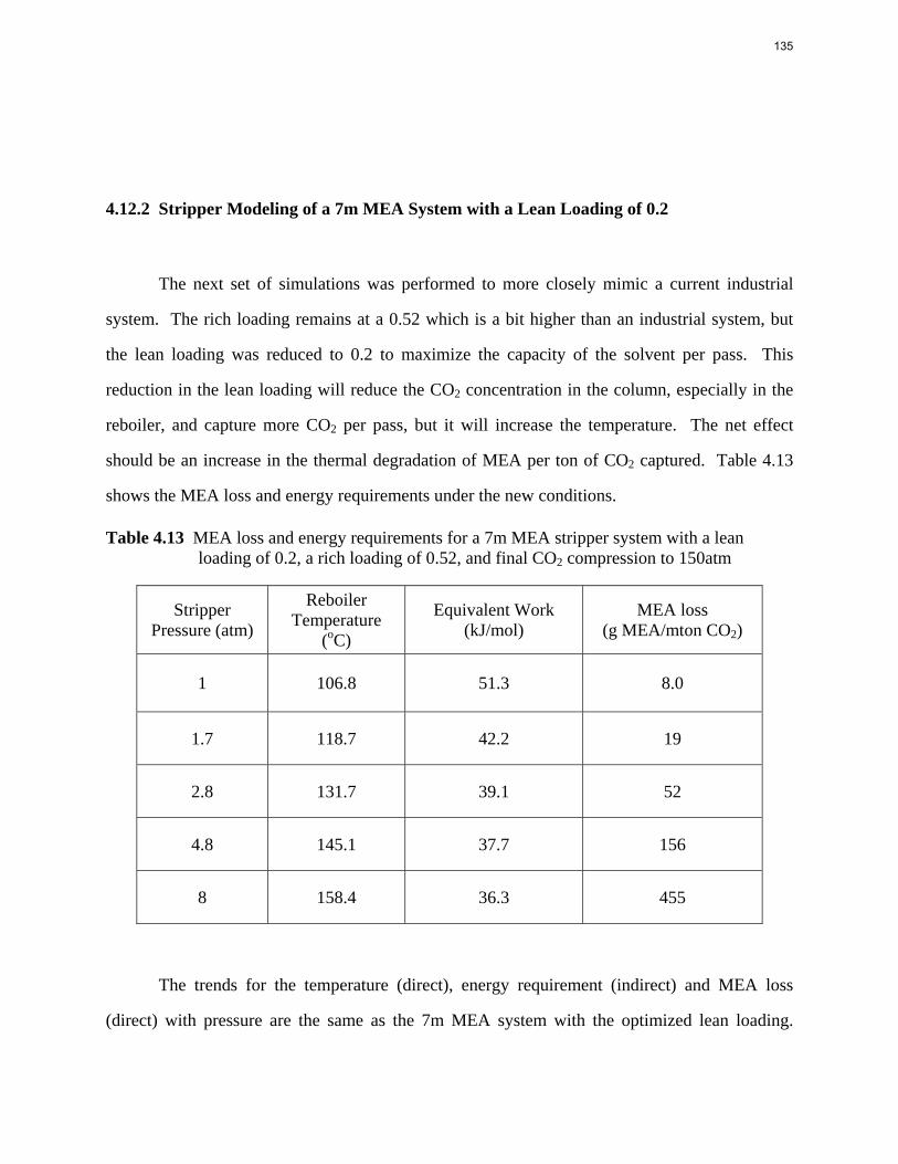
4.12.2 Stripper Modeling of a 7m MEA System with a Lean Loading of 0.2
The next set of simulations was performed to more closely mimic a current industrial
system. The rich loading remains at a 0.52 which is a bit higher than an industrial system, but
the lean loading was reduced to 0.2 to maximize the capacity of the solvent per pass. This
reduction in the lean loading will reduce the CO2 concentration in the column, especially in the
reboiler, and capture more CO2 per pass, but it will increase the temperature. The net effect
should be an increase in the thermal degradation of MEA per ton of CO2 captured. Table 4.13
shows the MEA loss and energy requirements under the new conditions.
Table 4.13 MEA loss and energy requirements for a 7m MEA stripper system with a lean loading of 0.2, a rich loading of 0.52, and final CO2 compression to 150atm
Stripper Pressure (atm)
Reboiler Temperature
(oC)
Equivalent Work (kJ/mol)
MEA loss (g MEA/mton CO2)
1 106.8 51.3 8.0
1.7 118.7 42.2 19
2.8 131.7 39.1 52
4.8 145.1 37.7 156
8 158.4 36.3 455
The trends for the temperature (direct), energy requirement (indirect) and MEA loss
(direct) with pressure are the same as the 7m MEA system with the optimized lean loading.
135
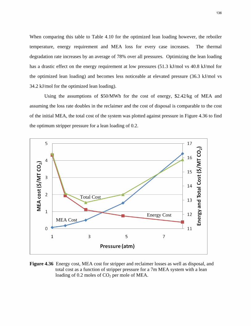
When comparing this table to Table 4.10 for the optimized lean loading however, the reboiler
temperature, energy requirement and MEA loss for every case increases. The thermal
degradation rate increases by an average of 78% over all pressures. Optimizing the lean loading
has a drastic effect on the energy requirement at low pressures (51.3 kJ/mol vs 40.8 kJ/mol for
the optimized lean loading) and becomes less noticeable at elevated pressure (36.3 kJ/mol vs
34.2 kJ/mol for the optimized lean loading).
Using the assumptions of $50/MWh for the cost of energy, $2.42/kg of MEA and
assuming the loss rate doubles in the reclaimer and the cost of disposal is comparable to the cost
of the initial MEA, the total cost of the system was plotted against pressure in Figure 4.36 to find
the optimum stripper pressure for a lean loading of 0.2.
Figure 4.36 Energy cost, MEA cost for stripper and reclaimer losses as well as disposal, and total cost as a function of stripper pressure for a 7m MEA system with a lean loading of 0.2 moles of CO2 per mole of MEA.
MEA Cost Energy Cost
Total Cost
136
The overall cost for the 7m MEA system with a lean loading of 0.2 is higher than the
optimized case. For the optimized case the total cost ranged from $12 to $13/mton CO2 with a
minimum at $12.06, but in the 0.2 lean loading case the overall cost ranges from $13 to
$16/mton CO2 with a minimum of $12.85. The optimum pressure for this case is around 3 atm
which corresponds to a reboiler temperature of 132oC. The energy requirement dominates the
cost at low pressures but as the pressure is increased, the incremental savings from increasing the
pressure is quickly offset by the cost of MEA losses.
Table 4.14 shows the bleed rate to the reclaimer as a fraction of the total outlet flow from
the stripper and the corresponding MEA loss and steady-state total concentration of degradation
products.
Table 4.14 MEA loss and steady-state total degradation product concentration for varying bleed rates to the reclaimer in a 7m MEA stripper at 8 atm and a lean loading of 0.2 moles of CO2 per mole of MEA
Reclaimer Flow Ratio MEA Loss
(g MEA/mton CO2)
Total Degradation Product
Concentration [M]
2.8E-4 552 0.93
1.1E-4 504 0.24
3.8E-3 475 0.07
1.2E-2 462 0.02
In this case the total concentration of degradation products has decreased compared to the
optimized lean loading case because the stable imidazolidones are not favored at lowered CO2
concentrations. As a consequence, a larger fraction of the degradation product concentration is
made up of reactive polymeric species such as HEEDA and the MEA trimer. Once again, the
increase in degradation products yields an increase in the overall MEA loss rate in the stripper.
To be within 5% of the minimum MEA degradation rate, a reclaimer flow ratio of 0.35% needs
137
to be used for the 8 atm case and a flow ratio of 0.006% is required for an atmospheric stripper.
Both of these flow rates are about 15 times larger than the flow rates for the optimized cases at
the same stripper pressures meaning much more reclaiming will be needed for these conditions
compared to the optimized lean loading case.
As a tradeoff in the operating cost, this system would require less pumping work, but that
would only make-up a small amount of the energy difference shown. There would also be some
capital cost considerations with regard to the sizing of the absorber, cross exchanger and stripper.
The absorber and stripper diameter would only decrease slightly as the sizing of each would
mainly be controlled by the vapor flow rate. The cross exchanger would decrease in size due to
the drastically decreased liquid flow rates, but the decrease would be slightly offset by the
increased ΔT between the hot and cold side of the exchanger.
4.12.3 Stripper Modeling of an 11m MEA system with optimized lean loading
In this case the concentration of MEA was increased from 7m (30wt%) to 11m (40wt%)
to test the effects of concentration on thermal degradation in a simulated system. When the
temperature and CO2 loadings are held constant, the rate of thermal degradation increases as the
concentration increases. The boiling point of an MEA/water system increases as the
concentration increases at a given pressure which would mean the thermal degradation rate
should increase as well. Table 4.15 shows the effect of pressure on the reboiler temperature,
thermal degradation rate and energy requirement.
138
Table 4.15 MEA loss and energy requirements for an 11m MEA stripper with a rich loading of 0.485, optimized lean loading for each pressure and final CO2 compression to 150atm
Stripper Pressure
(atm)
Lean Loading (mol CO2 / mol
MEA)
Reboiler Temperature
(oC)
Equivalent Work (kJ/mol)
MEA loss (g MEA/mton
CO2)
1 0.37 91.0 37.8 2.0
1.7 0.365 98.7 35.9 4.5
2.8 0.36 106.3 34.4 10
4.8 0.355 114.2 33.3 22
8 0.345 123.3 32.5 52
The same general trends appear as for the 7m cases where the MEA loss increases with
pressure and the energy requirement decreases. The energy requirements went down as expected
for the higher capacity solvent. For the 8 atm pressure case and the atmospheric case the energy
requirement dropped 1.7 kJ/mol and 3.0 kJ/mol respectively. The unexpected trend is the
decrease in the thermal degradation rate when compared to the 7m MEA case at similar
conditions. The reason can be seen in the reboiler temperatures. Table 4.16 shows the reboiler
temperatures and MEA loss rates for the 7m MEA with optimized lean loading and the 11m
MEA with optimized lean loading.
Table 4.16 MEA loss and reboiler temperature for 7m MEA with optimized lean loading and a rich loading of 0.52 and an 11m MEA with optimized lean loading and a rich loading of 0.485
139
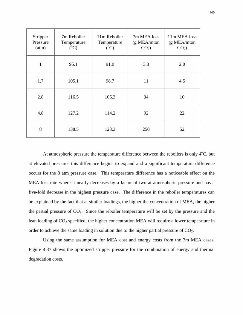
Stripper Pressure
(atm)
7m Reboiler Temperature
(oC)
11m Reboiler Temperature
(oC)
7m MEA loss (g MEA/mton
CO2)
11m MEA loss (g MEA/mton
CO2)
1 95.1 91.0 3.8 2.0
1.7 105.1 98.7 11 4.5
2.8 116.5 106.3 34 10
4.8 127.2 114.2 92 22
8 138.5 123.3 250 52
At atmospheric pressure the temperature difference between the reboilers is only 4oC, but
at elevated pressures this difference begins to expand and a significant temperature difference
occurs for the 8 atm pressure case. This temperature difference has a noticeable effect on the
MEA loss rate where it nearly decreases by a factor of two at atmospheric pressure and has a
five-fold decrease in the highest pressure case. The difference in the reboiler temperatures can
be explained by the fact that at similar loadings, the higher the concentration of MEA, the higher
the partial pressure of CO2. Since the reboiler temperature will be set by the pressure and the
lean loading of CO2 specified, the higher concentration MEA will require a lower temperature in
order to achieve the same loading in solution due to the higher partial pressure of CO2.
Using the same assumption for MEA cost and energy costs from the 7m MEA cases,
Figure 4.37 shows the optimized stripper pressure for the combination of energy and thermal
degradation costs.
140
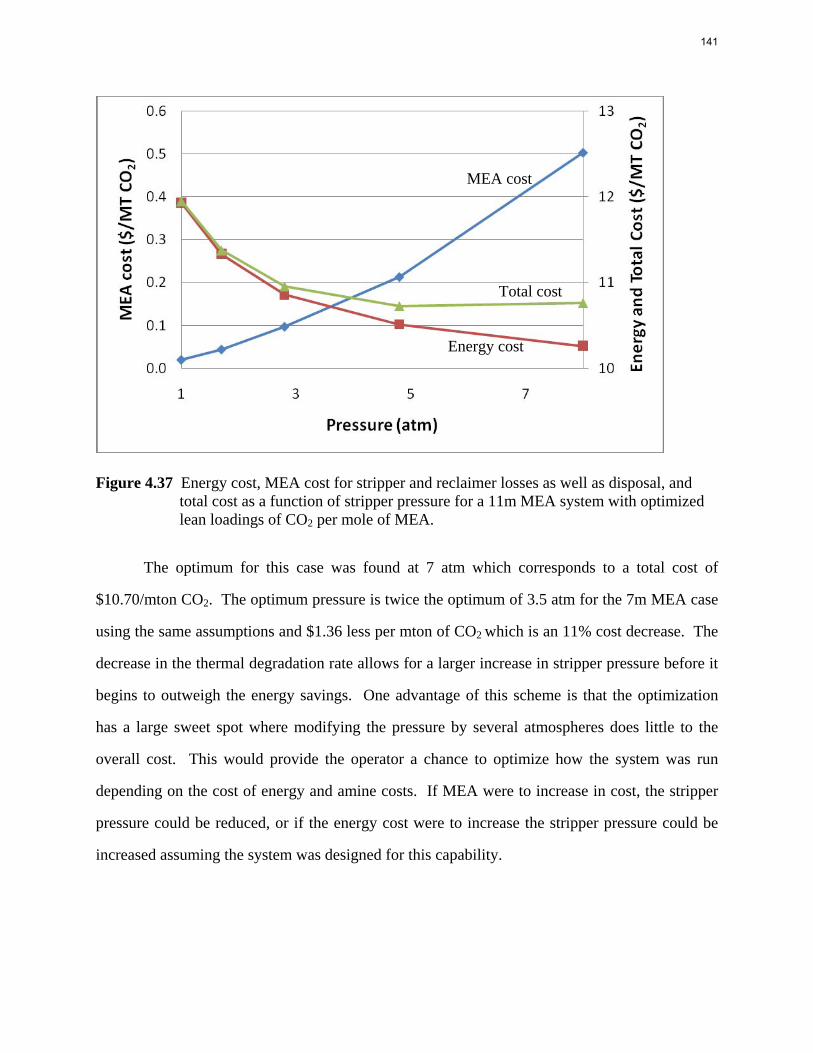
Figure 4.37 Energy cost, MEA cost for stripper and reclaimer losses as well as disposal, and total cost as a function of stripper pressure for a 11m MEA system with optimized lean loadings of CO2 per mole of MEA.
The optimum for this case was found at 7 atm which corresponds to a total cost of
$10.70/mton CO2. The optimum pressure is twice the optimum of 3.5 atm for the 7m MEA case
using the same assumptions and $1.36 less per mton of CO2 which is an 11% cost decrease. The
decrease in the thermal degradation rate allows for a larger increase in stripper pressure before it
begins to outweigh the energy savings. One advantage of this scheme is that the optimization
has a large sweet spot where modifying the pressure by several atmospheres does little to the
overall cost. This would provide the operator a chance to optimize how the system was run
depending on the cost of energy and amine costs. If MEA were to increase in cost, the stripper
pressure could be reduced, or if the energy cost were to increase the stripper pressure could be
increased assuming the system was designed for this capability.
MEA cost
Total cost
Energy cost
141
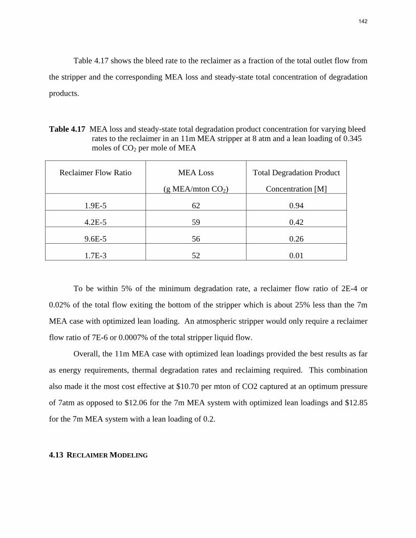
Table 4.17 shows the bleed rate to the reclaimer as a fraction of the total outlet flow from
the stripper and the corresponding MEA loss and steady-state total concentration of degradation
products.
Table 4.17 MEA loss and steady-state total degradation product concentration for varying bleed rates to the reclaimer in an 11m MEA stripper at 8 atm and a lean loading of 0.345 moles of CO2 per mole of MEA
Reclaimer Flow Ratio MEA Loss
(g MEA/mton CO2)
Total Degradation Product
Concentration [M]
1.9E-5 62 0.94
4.2E-5 59 0.42
9.6E-5 56 0.26
1.7E-3 52 0.01
To be within 5% of the minimum degradation rate, a reclaimer flow ratio of 2E-4 or
0.02% of the total flow exiting the bottom of the stripper which is about 25% less than the 7m
MEA case with optimized lean loading. An atmospheric stripper would only require a reclaimer
flow ratio of 7E-6 or 0.0007% of the total stripper liquid flow.
Overall, the 11m MEA case with optimized lean loadings provided the best results as far
as energy requirements, thermal degradation rates and reclaiming required. This combination
also made it the most cost effective at $10.70 per mton of CO2 captured at an optimum pressure
of 7atm as opposed to $12.06 for the 7m MEA system with optimized lean loadings and $12.85
for the 7m MEA system with a lean loading of 0.2.
4.13 RECLAIMER MODELING
142
Modeling of the reclaimer is difficult since there is not a good set of vapor-liquid
equilibrium data for a MEA/water/CO2 system at elevated temperature and concentration of
MEA. In order to get an estimate of how much degradation is occurring in the reclaimer, we will
make some assumptions using some information from industrial experience in Wonder (1959).
For a typical run, a 1-3% slipstream coming off the stripper reboiler is sent to a semibatch
distillation still. The solution is heated and concentrated until the overhead concentration of
MEA is equal to the inlet concentration of MEA. At this point the slip stream from the stripper
bottoms is continuously fed to the reclaiming unit with the recovered MEA returning to the
stripper and the degradation products accumulating in the bottoms of the reclaiming unit. As the
degradation products accumulate, the temperature of the unit will increase. In the case of a
stripper operated at 15 wt% MEA and 5 psig, the initial boiling point of solution is about 124oC
and the process is stopped when the bottoms temperature reaches approximately 150oC at which
point some of the degradation products start to coelute with the MEA in the overheads. The feed
is shut off, caustic is added to break any heat stable salts and water is added to the system and as
much of the remaining MEA is removed from the system as possible. The bottoms are drummed
off to waste.
For our system we will assume that a continuous unit will be used to avoid the stopping
and starting of the semi-batch unit and that the unit is sized for a 10 minute residence time. The
concentration of MEA in the liquid phase will be estimated based on MEA/water VLE curves by
using the vapor phase that equals the inlet concentration of MEA from Wonder (1959) which are
available at 5, 10, and 25psig. The CO2 concentration will be estimated at half of the inlet
concentration which will correspond to a loading of approximately 0.1 for the 30wt% MEA
optimized cases. The temperature in the reclaimer will be set at 15oC above the initial boiling
point of solution taken from the MEA/water VLE curves which for the 7m MEA case at 25 psig
corresponds to 169oC, 10 psig will correspond to 157oC and 5 psig will correspond to 150oC.
The thermal degradation model developed from the experimental data will be used even though
the MEA concentrations and some the temperatures in the reclaimer will fall outside of range of
143
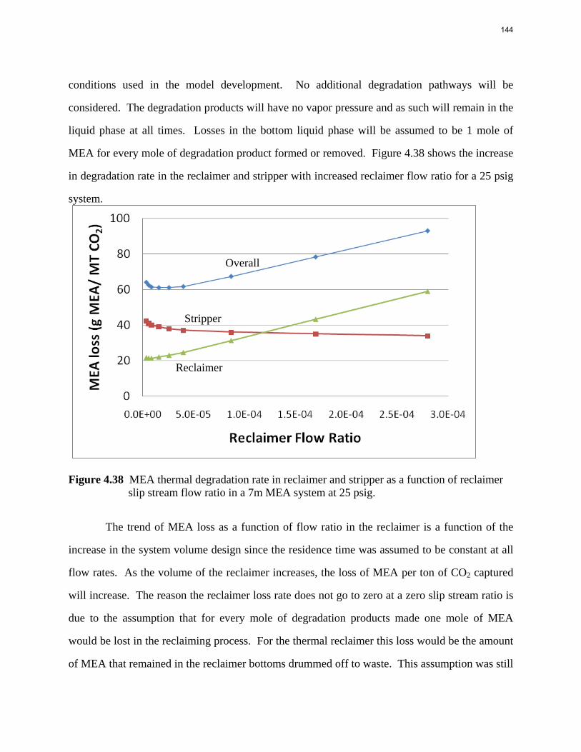
conditions used in the model development. No additional degradation pathways will be
considered. The degradation products will have no vapor pressure and as such will remain in the
liquid phase at all times. Losses in the bottom liquid phase will be assumed to be 1 mole of
MEA for every mole of degradation product formed or removed. Figure 4.38 shows the increase
in degradation rate in the reclaimer and stripper with increased reclaimer flow ratio for a 25 psig
system.
Figure 4.38 MEA thermal degradation rate in reclaimer and stripper as a function of reclaimer slip stream flow ratio in a 7m MEA system at 25 psig.
The trend of MEA loss as a function of flow ratio in the reclaimer is a function of the
increase in the system volume design since the residence time was assumed to be constant at all
flow rates. As the volume of the reclaimer increases, the loss of MEA per ton of CO2 captured
will increase. The reason the reclaimer loss rate does not go to zero at a zero slip stream ratio is
due to the assumption that for every mole of degradation products made one mole of MEA
would be lost in the reclaiming process. For the thermal reclaimer this loss would be the amount
of MEA that remained in the reclaimer bottoms drummed off to waste. This assumption was still
Reclaimer
Stripper
Overall
144
used at a zero slip stream ratio as a way of accounting for losses in a non-thermal reclaiming
method since the removal of impurities will still be necessary and no matter the separation
method will still involve some MEA losses.
Previously it was shown that the stripper loss rate decreases with increasing reclaimer
flow ratio due to the reduction in more reactive degradation products. The combination of these
two effects is shown by the green triangles in Figure 4.37 and a minimum is found around a
reclaimer flow ratio of 2x10⁻⁵ or 0.002% of the liquid exiting the bottom of the stripper which
corresponds to a loss rate of 61g MEA/mton CO2 total where 38g of the MEA loss occurs in the
stripper. The steady state concentration of HEEDA would be 0.11M and the sum of all
degradation products would be 0.31M. Wonder (1959) gave an analysis of a typical MEA
solution and the HEEDA concentration was 1.1% by weight which would be approximately
0.11M in a CO2 free solution. As the reclaimer flow ratio is increased, the incremental
improvement in the stripper is overshadowed by the steady increase of the loss rate in the
reclaimer.
If a flow ratio of 1% were used as in the literature, a loss rate for the reclaimer would be
1532g MEA/mton CO2 which is much larger than the loss rate in the stripper of about 35g
MEA/mton CO2. Under typical industrial conditions where the concentration of MEA is held at
15wt%, instead of 30wt% used here, and at 5 psig, instead of 25 psig, with a lean loading of 0.2,
the loss rate for a 1% flow ratio would only be 27g MEA/mton CO2 and the loss rate in the
stripper would be 16g MEA/mton CO2. This is close to the estimate of equal losses of MEA in
the stripper and reclaimer and at least partially validates the assumptions used in this model.
Table 4.18 shows the optimum loss rate at each pressure and the contributions from the
stripper and reclaimer.
145
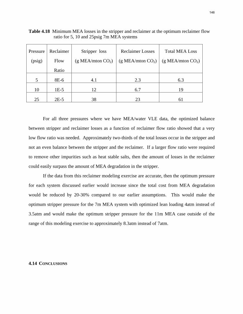
Table 4.18 Minimum MEA losses in the stripper and reclaimer at the optimum reclaimer flow ratio for 5, 10 and 25psig 7m MEA systems
Pressure
(psig)
Reclaimer
Flow
Ratio
Stripper loss
(g MEA/mton CO2)
Reclaimer Losses
(g MEA/mton CO2)
Total MEA Loss
(g MEA/mton CO2)
5 8E-6 4.1 2.3 6.3
10 1E-5 12 6.7 19
25 2E-5 38 23 61
For all three pressures where we have MEA/water VLE data, the optimized balance
between stripper and reclaimer losses as a function of reclaimer flow ratio showed that a very
low flow ratio was needed. Approximately two-thirds of the total losses occur in the stripper and
not an even balance between the stripper and the reclaimer. If a larger flow ratio were required
to remove other impurities such as heat stable salts, then the amount of losses in the reclaimer
could easily surpass the amount of MEA degradation in the stripper.
If the data from this reclaimer modeling exercise are accurate, then the optimum pressure
for each system discussed earlier would increase since the total cost from MEA degradation
would be reduced by 20-30% compared to our earlier assumptions. This would make the
optimum stripper pressure for the 7m MEA system with optimized lean loading 4atm instead of
3.5atm and would make the optimum stripper pressure for the 11m MEA case outside of the
range of this modeling exercise to approximately 8.3atm instead of 7atm.
4.14 CONCLUSIONS
146
A new reaction pathway for MEA thermal degradation has been proposed and validated
via IC, HPLC, MS and IC/MS. The presence of MEA urea and ureas of MEA and other
polymeric products were identified but not quantified. The dimer of MEA, HEEDA, precedes
the formation of the imidazolidone species, HEIA, instead of the other way around as originally
proposed by Polderman. Degradation products were quantified using known addition where
applicable and justification was given for the concentration determination of other products.
HEIA was the single largest degradation product across all experiments after the initial lag
period in which the concentration of HEEDA was established. The imidazolidone of the MEA
trimer is the second largest product at high losses of MEA. MEA thermal degradation is not
catalyzed by stainless steel metals or copper and vanadium which are sometimes used as
corrosion inhibitors. The total nitrogen mass balance between MEA losses and measured
degradation products closes to within 8.3% on average across all samples and only begins to
deteriorate when the samples are over 50% degraded. No industrial systems will be operated at
this point, and as such a full mass balance closure beyond this point will not be pursued.
The MEA and degradation product concentration data from a set of 7m MEA
experiments was used to develop a kinetic model with a set of six temperature dependent rate
constants. This model uses numerical integration using Euler’s method to predict not only the
concentration of MEA, but also the concentration of the five largest degradation products. The
agreement between the model and experimental data for MEA concentration showed that only 3
out of 159 experiments were more than 15% apart and the average deviation in MEA
concentration was less than 5% across all temperatures, MEA concentrations and CO2
concentrations. All of the rate constants have similar activation energies of about 33 kcal/mol
which corresponds to a quadrupling in the rate of each reaction every 16.7oC. Since all of the
rate constants are similar, the product mix will not change as a function of temperature as was
shown for the concentration of HEEDA, HEIA, MEA trimer and triHEIA when normalized by
MEA loss.
147
The MEA thermal degradation model was then used in conjunction with an ASPEN
model of a MEA stripper by Van Wagener using the Hilliard (2008) VLE model in order to
estimate amine losses under industrial conditions. Roughly three-fourths of all degradation
occurs in the stripper reboiler where the temperature is highest and CO2 concentration is the
lowest. Even though the packing has the same liquid volume as the reboiler and an elevated CO2
concentration, the lower temperature outweighs the CO2 effect and only 27% of thermal
degradation in the stripper occurs here. For a clean 7m MEA system with an optimized lean
loading for minimal stripper energy requirements, the MEA loss rate in the stripper varied from
3.8g MEA/mton CO2 for an atmospheric stripper to 250g MEA/mton CO2 for a stripper operated
at 8atm. The optimum pressure when assuming an MEA cost of $2.42/kg and an energy cost of
$50/MWh with provisions for reclaiming and disposal was 3.5atm with an estimated total cost of
$12.06/mton CO2. The lean loading was reduced to a constant value of 0.2 moles of CO2 per
mole of MEA, but the MEA loss rate in the stripper actually increased due to an increase in the
reboiler temperature. The losses increased from 3.8 to 8g MEA/mton CO2 for the atmospheric
case and from 250 to 455g MEA/mton CO2 for the 8atm case. The optimum pressure decreased
to 3atm and the estimated total cost increased to $12.85/mton CO2. Increasing the MEA
concentration to 11m MEA had the unexpected effect of decreasing the thermal degradation rate.
This was due to a decrease in the reboiler temperature of the stripper at the optimum lean loading
since the 11m MEA system has a higher partial pressure of CO2 at a given loading than the 7m
MEA system. The loss rate ranged from 2-52g MEA/mton CO2 with an optimum pressure of 7
atm corresponding to a total cost of $10.70 which is substantially less than either of the 7m MEA
cases. In all cases, the MEA cost was less than 10% of the energy cost at the optimum pressure,
however the MEA cost is still a significant operating cost if the optimum pressure is used.
Increasing the amine concentration can have an adverse effect on corrosion and would also
increase the solution viscosity which would affect mass transfer, pumping characteristics and
would reduce the thermal conductivity of the solution, but if it resulted in an 11% decrease in the
operating cost of the stripper, it would definitely be worth looking into.
148
The MEA loss rate increased with increasing temperature in the experiments and was
shown to increase with increasing pressure in the stripper since this elevates the reboiler
temperature. Decreasing the CO2 concentration of the solution decreased the thermal
degradation rate in the isothermal degradation experiments. In a real isobaric system however in
order to achieve a lower CO2 concentration, the reboiler had to be run at a higher temperature
which outweighed the decrease in CO2 concentration and actually increased the thermal
degradation rate. Increasing the concentration of MEA increased the rate of thermal degradation
in the experimental isothermal system. In an isobaric system, increasing the concentration of
amine and keeping the loading constant caused a decrease in the reboiler temperature due to the
higher partial pressure of CO2 which outweighed the effect of concentration and actually
decreased the amount of thermal degradation in the system. Two of the three variables used in
this set of experiments, CO2 loading and amine concentration, ended up having the opposite
effect on thermal degradation in the system modeling than in the experiments themselves since
the experiment was run isothermally and the real system was isobaric. The model of MEA
thermal degradation has been useful in weighing the effects of temperature, amine concentration
and CO2 loading.
Using several rough assumptions for the reclaimer, it was determined that the model did a
reasonable job of matching what is seen in industrial conditions where the losses of the reclaimer
roughly matched the thermal degradation in the stripper when a 1% slip stream from the reboiler
of the stripper is sent to the reclaiming unit. The optimum slip stream ratio for thermal
degradation in three test cases at 5, 10 and 25psig was found to be much less than 1% on a purely
MEA loss basis. As the stripper pressure increases, the optimum slip stream ratio increases, but
for the highest pressure system with VLE data available, 25psig or 1.7atm, the optimum slip
stream ratio was still only 0.002% of the total flow exiting the reboiler of the stripper. At this
slip stream ratio, the steady-state HEEDA concentration would be 0.11M and the sum of all
thermal degradation products would be 0.31M. At the optimum slip stream flow in all cases,
about two-thirds of MEA loss occurs in the stripper.
149
1
Rate and CO2 Partial Pressure Modeling for Monoethanolamine and Piperazine Solutions
Quarterly Report for January 1 – March 31, 2009
by Ross Dugas
Supported by the Luminant Carbon Management Program
and the
Industrial Associates Program for CO2 Capture by Aqueous Absorption
Department of Chemical Engineering
The University of Texas at Austin
March 31, 2009
Abstract An Aspen Plus® RateSep™ model of the wetted wall column is being created to study the effects of CO2 mass transfer rates in Monoethanolamine (MEA), Piperazine (PZ) and MEA/PZ solutions. The model will simulate wetted wall column experiments which include 7–13 m MEA, 2–12 m PZ and 7 m MEA/2 m PZ solutions at temperatures of 40, 60, 80, and 100 ˚C.
The thermodynamic model from Hilliard (2008) was used as a starting point but required significant adjustments to accurately predict 7–13 m MEA, 2–12 m PZ and 7 m MEA/2 m PZ. In order to accomplish this, higher amine concentration data were added into the regressions. Some of the lower amine concentration data and data which had CO2 loadings outside the relevant range for CO2 capture from flue gas were deleted. A special emphasis was put on obtaining good CO2 partial pressure predictions from the model. The model does have some trouble predicting CO2 partial pressure at the higher MEA concentrations, but it does a very good job of predicting CO2 partial pressure in the 7 and 9 m MEA, PZ and the 7 m MEA/2 m PZ blend solutions.
The Hilliard (2008) thermodynamic model does not consider physical properties since they do not affect thermodynamics. However, the rate-based model of the wetted wall column does require accurate physical properties. Density and viscosity parameters were regressed for 7–13 m MEA based on a literature correlation (Weiland et al., 1988). Only density parameters were regressed for PZ. These data were obtained from Freeman (Rochelle, Dugas et al., 2008). Thus far, no adequate viscosity regression for PZ has been obtained. The model may require a Fortran subroutine to properly predict the viscosity of the PZ solutions.
The model cannot be designed geometrically like the wetted wall column in which the gas flows through an annulus. Although the model uses standard, cylindrical columns, it provides the same cross sectional area and wetted area as the wetted wall column. Fortran subroutines were coded to ensure the model used the same liquid and gas phase mass transfer coefficients as the wetted wall column.
The model utilizes 15 forward kinetic reactions, 15 reverse kinetic reactions, and 4 equilibrium reactions. The 15 reverse reactions are not independent and can be linked to the forward reaction
150
2
rates by Keq relationships. Keq was calculated for 7 primary reactions (4 kinetic and 3 equilibrium) at 40, 60, 80, and 100 ˚C. Keq can be calculated for all 34 reactions using Keq combinations of the 7 primary reactions. The Keq values at the 4 temperatures were regressed into a form which translated easily to the power law rate expression Aspen Plus® uses to determine mass transfer. Using the Keq relationships, the reverse rate expression can be directly linked to the forward rate expressions. The 15 forward reactions can be simplified into 4 reactions in which rate constants scale by Bronsted theory (1928) depending on the catalyst. With these simplifications, the rate expression for only 4 reactions should need to be regressed by the wetted wall column data.
Introduction An Aspen Plus® RateSep™ (Version 2006.5) model of the wetted wall column is being created to further study mass transfer rates of CO2 into monoethanolamine (MEA) and piperazine (PZ) solutions. MEA, PZ, and MEA/PZ wetted wall column experiments will be modeled. MEA conditions include 7, 9, 11, and 13 m MEA at 40, 60, 80, and 100 ˚C with CO2 loading from 0.23 to 0.50 molCO2/molalk. Piperazine conditions include 2, 5, 8, and 12 m PZ at 40, 60, 80, and 100 ˚C with CO2 loading from 0.23 to 0.41 molCO2/molalk. A 7 m MEA/2 m PZ solution was also tested in the wetted wall column at 40, 60, 80, and 100 ˚C with CO2 loading of 0.24 to 0.48 mol/molalk. Recall that PZ has 2 moles of alkalinity (nitrogen groups) per mole.
This report can be broken up into three sections of modeling activity: vapor-liquid equilibrium, physical property, and rate modeling.
The Hilliard (2008) model was used as a starting point. However, the limitations of the Hilliard model with respect to amine concentration required significant adjustments. With the help of my colleague, David Van Wagener, the VLE model aspects of the wetted wall column model have essentially been completed.
Density and viscosity parameter regression for MEA solutions was based on correlations developed by Weiland (1998). Density parameter regression for PZ solutions was performed using data obtained by my colleague, Stephanie Freeman, (Rochelle, Dugas et al., 2008). Viscosity has not yet been adequately fit for PZ solutions.
The implementation of the rate aspects into the model is an ongoing process. Both the kinetic and equilibrium reactions for the MEA/PZ/H2O/ CO2 system have been rewritten in a simplified form. The basic design and methodology to be implemented into the rate model are described in this report.
Vapor-Liquid Equilibrium Modeling The Hilliard (2008) model was used as a starting point for this modeling work. The model required modifications since Hilliard regressed data only up to 11 m MEA and 5 m PZ. Wetted wall column experiments utilized amine concentrations up to 13 m MEA and 12 m PZ. The Hilliard model did not accurately extrapolate to these higher amine concentrations.
The modified VLE model was created with the same sequential regression approach that Hilliard employed. Hilliard used heat of absorption, nuclear magnetic resonance, heat capacity, amine partial pressure, and CO2 partial pressure data to regress thermodynamic parameters. The data within each data type were modified to exclude data not relevant to the conditions of the wetted wall column experiments. In an effort to simplify the regressions and obtain better CO2 partial
151
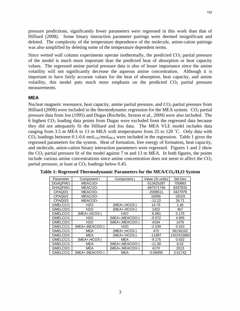
3
pressure predictions, significantly fewer parameters were regressed in this work than that of Hilliard (2008). Some binary interaction parameter pairings were deemed insignificant and deleted. The complexity of the temperature dependence of the molecule, anion-cation pairings was also simplified by deleting some of the temperature dependent terms.
Since wetted wall column experiments operate isothermally, the predicted CO2 partial pressure of the model is much more important than the predicted heat of absorption or heat capacity values. The regressed amine partial pressure data is also of lesser importance since the amine volatility will not significantly decrease the aqueous amine concentration. Although it is important to have fairly accurate values for the heat of absorption, heat capacity, and amine volatility, this model puts much more emphasis on the predicted CO2 partial pressure measurements.
MEA Nuclear magnetic resonance, heat capacity, amine partial pressure, and CO2 partial pressure from Hilliard (2008) were included in the thermodynamic regression for the MEA system. CO2 partial pressure data from Jou (1995) and Dugas (Rochelle, Sexton et al., 2009) were also included. The 6 highest CO2 loading data points from Dugas were excluded from the regressed data because they did not adequately fit the Hilliard and Jou data. The MEA VLE model includes data ranging from 3.5 m MEA to 13 m MEA with temperatures from 25 to 120 ˚C. Only data with CO2 loadings between 0.1-0.6 molCO2/molMEA were included in the regression. Table 1 gives the regressed parameters for the system. Heat of formation, free energy of formation, heat capacity, and molecule, anion-cation binary interaction parameters were regressed. Figures 1 and 2 show the CO2 partial pressure fit of the model against 7 m and 13 m MEA. In both figures, the points include various amine concentrations since amine concentration does not seem to affect the CO2 partial pressure, at least at CO2 loadings below 0.45.
Table 1: Regressed Thermodynamic Parameters for the MEA/CO2/H2O System Parameter Component i Component j Value (SI units) Std DevDGAQFM/1 MEACOO- -513425287 750883DHAQFM/1 MEACOO- -687571746 8337833CPAQ0/1 MEACOO- -2008511 3427979CPAQ0/2 MEACOO- 10056 19103CPAQ0/3 MEACOO- -12.22 26.71
GMELCC/1 H2O (MEA+,HCO3-) 14.75 1.45GMELCD/1 H2O (MEA+,HCO3-) 1422 467GMELCC/1 (MEA+,HCO3-) H2O -6.981 0.175GMELCC/1 H2O (MEA+,MEACOO-) -9.572 4.905GMELCD/1 H2O (MEA+,MEACOO-) 4194 1476GMELCC/1 (MEA+,MEACOO-) H2O -2.249 0.410GMELCC/1 MEA (MEA+,HCO3-) 470 56136102GMELCD/1 MEA (MEA+,HCO3-) -11897 1422415860GMELCC/1 (MEA+,HCO3-) MEA -9.175 0.532GMELCC/1 MEA (MEA+,MEACOO-) -11.30 8.02GMELCD/1 MEA (MEA+,MEACOO-) 4170 2013GMELCC/1 (MEA+,MEACOO-) MEA -0.06990 2.61742
152
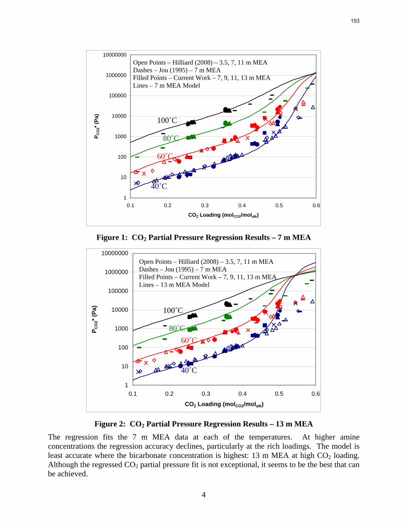
4
1
10
100
1000
10000
100000
1000000
10000000
0.1 0.2 0.3 0.4 0.5 0.6
CO2 Loading (molCO2/molalk)
P CO
2* (P
a)
Figure 1: CO2 Partial Pressure Regression Results – 7 m MEA
1
10
100
1000
10000
100000
1000000
10000000
0.1 0.2 0.3 0.4 0.5 0.6
CO2 Loading (molCO2/molalk)
P CO
2* (P
a)
Figure 2: CO2 Partial Pressure Regression Results – 13 m MEA
The regression fits the 7 m MEA data at each of the temperatures. At higher amine concentrations the regression accuracy declines, particularly at the rich loadings. The model is least accurate where the bicarbonate concentration is highest: 13 m MEA at high CO2 loading. Although the regressed CO2 partial pressure fit is not exceptional, it seems to be the best that can be achieved.
100˚C
80˚C
60˚C
40˚C
Open Points – Hilliard (2008) – 3.5, 7, 11 m MEA Dashes – Jou (1995) – 7 m MEA Filled Points – Current Work – 7, 9, 11, 13 m MEA Lines – 7 m MEA Model
Open Points – Hilliard (2008) – 3.5, 7, 11 m MEA Dashes – Jou (1995) – 7 m MEA Filled Points – Current Work – 7, 9, 11, 13 m MEA Lines – 13 m MEA Model
100˚C
80˚C 60˚C
40˚C
153
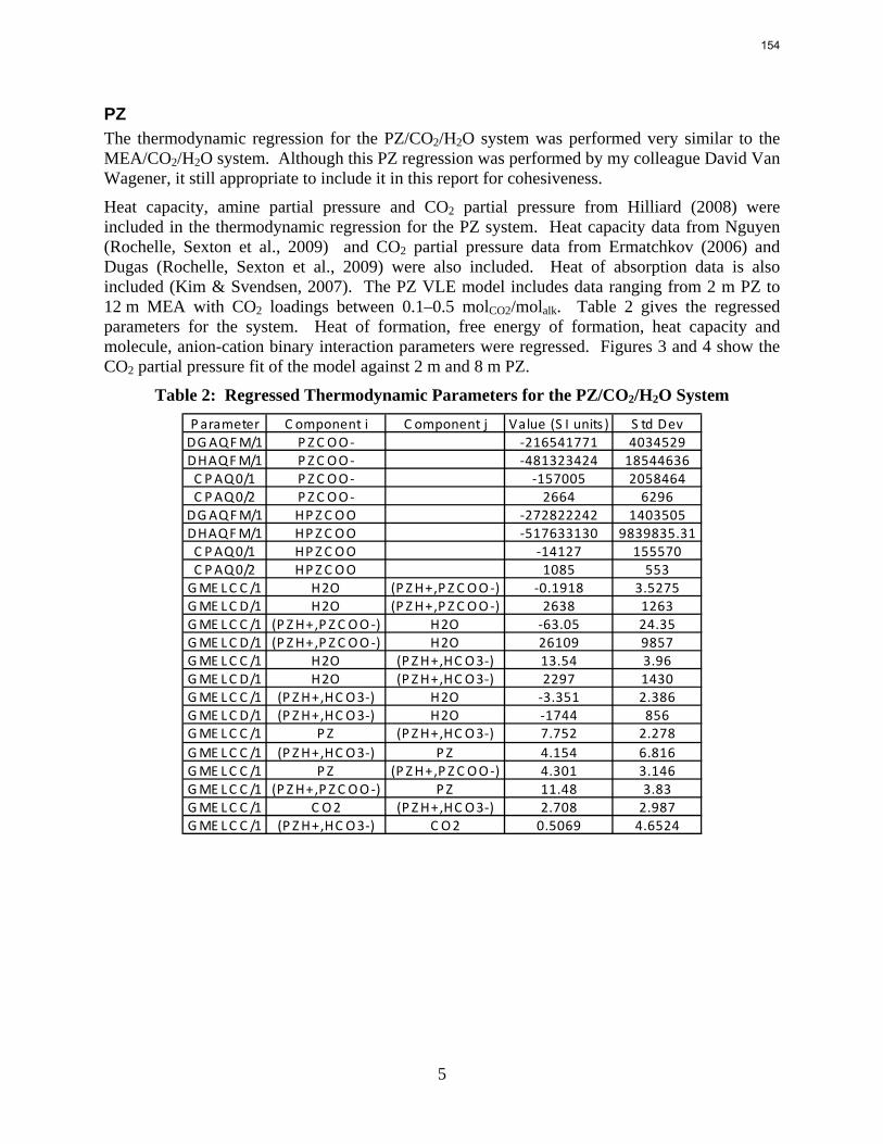
5
PZ The thermodynamic regression for the PZ/CO2/H2O system was performed very similar to the MEA/CO2/H2O system. Although this PZ regression was performed by my colleague David Van Wagener, it still appropriate to include it in this report for cohesiveness.
Heat capacity, amine partial pressure and CO2 partial pressure from Hilliard (2008) were included in the thermodynamic regression for the PZ system. Heat capacity data from Nguyen (Rochelle, Sexton et al., 2009) and CO2 partial pressure data from Ermatchkov (2006) and Dugas (Rochelle, Sexton et al., 2009) were also included. Heat of absorption data is also included (Kim & Svendsen, 2007). The PZ VLE model includes data ranging from 2 m PZ to 12 m MEA with CO2 loadings between 0.1–0.5 molCO2/molalk. Table 2 gives the regressed parameters for the system. Heat of formation, free energy of formation, heat capacity and molecule, anion-cation binary interaction parameters were regressed. Figures 3 and 4 show the CO2 partial pressure fit of the model against 2 m and 8 m PZ.
Table 2: Regressed Thermodynamic Parameters for the PZ/CO2/H2O System Parameter C omponent i C omponent j Value (S I units ) S td DevDGAQFM/1 P ZC OO ‐ ‐216541771 4034529DHAQFM/1 P ZC OO ‐ ‐481323424 18544636C PAQ0/1 P ZC OO ‐ ‐157005 2058464C PAQ0/2 P ZC OO ‐ 2664 6296DGAQFM/1 HPZC OO ‐272822242 1403505DHAQFM/1 HPZC OO ‐517633130 9839835.31C PAQ0/1 HPZC OO ‐14127 155570C PAQ0/2 HPZC OO 1085 553GME LC C /1 H2O (P ZH+,P ZC OO ‐) ‐0.1918 3.5275GME LC D/1 H2O (P ZH+,P ZC OO ‐) 2638 1263GME LC C /1 (P ZH+,P ZC OO ‐) H2O ‐63.05 24.35GME LC D/1 (P ZH+,P ZC OO ‐) H2O 26109 9857GME LC C /1 H2O (P ZH+,HC O3‐) 13.54 3.96GME LC D/1 H2O (P ZH+,HC O3‐) 2297 1430GME LC C /1 (P ZH+,HC O3‐) H2O ‐3.351 2.386GME LC D/1 (P ZH+,HC O3‐) H2O ‐1744 856GME LC C /1 P Z (P ZH+,HC O3‐) 7.752 2.278GME LC C /1 (P ZH+,HC O3‐) P Z 4.154 6.816GME LC C /1 P Z (P ZH+,P ZC OO ‐) 4.301 3.146GME LC C /1 (P ZH+,P ZC OO ‐) P Z 11.48 3.83GME LC C /1 C O2 (P ZH+,HC O3‐) 2.708 2.987GME LC C /1 (P ZH+,HC O3‐) C O2 0.5069 4.6524
154
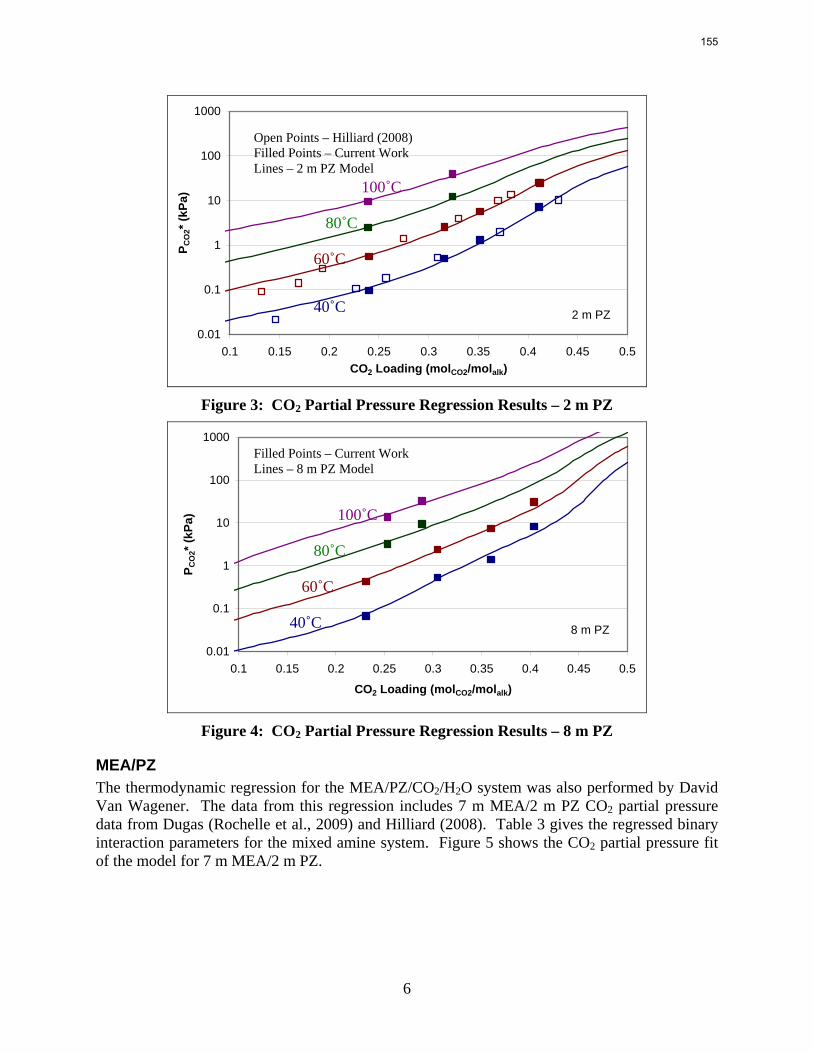
6
2 m PZ0.01
0.1
1
10
100
1000
0.1 0.15 0.2 0.25 0.3 0.35 0.4 0.45 0.5CO2 Loading (molCO2/molalk)
P CO
2* (k
Pa)
Figure 3: CO2 Partial Pressure Regression Results – 2 m PZ
8 m PZ
0.01
0.1
1
10
100
1000
0.1 0.15 0.2 0.25 0.3 0.35 0.4 0.45 0.5
CO2 Loading (molCO2/molalk)
P CO
2* (k
Pa)
Figure 4: CO2 Partial Pressure Regression Results – 8 m PZ
MEA/PZ The thermodynamic regression for the MEA/PZ/CO2/H2O system was also performed by David Van Wagener. The data from this regression includes 7 m MEA/2 m PZ CO2 partial pressure data from Dugas (Rochelle et al., 2009) and Hilliard (2008). Table 3 gives the regressed binary interaction parameters for the mixed amine system. Figure 5 shows the CO2 partial pressure fit of the model for 7 m MEA/2 m PZ.
Open Points – Hilliard (2008) Filled Points – Current Work Lines – 2 m PZ Model
100˚C
80˚C
60˚C
40˚C
Filled Points – Current Work Lines – 8 m PZ Model
100˚C
80˚C
60˚C
40˚C
155
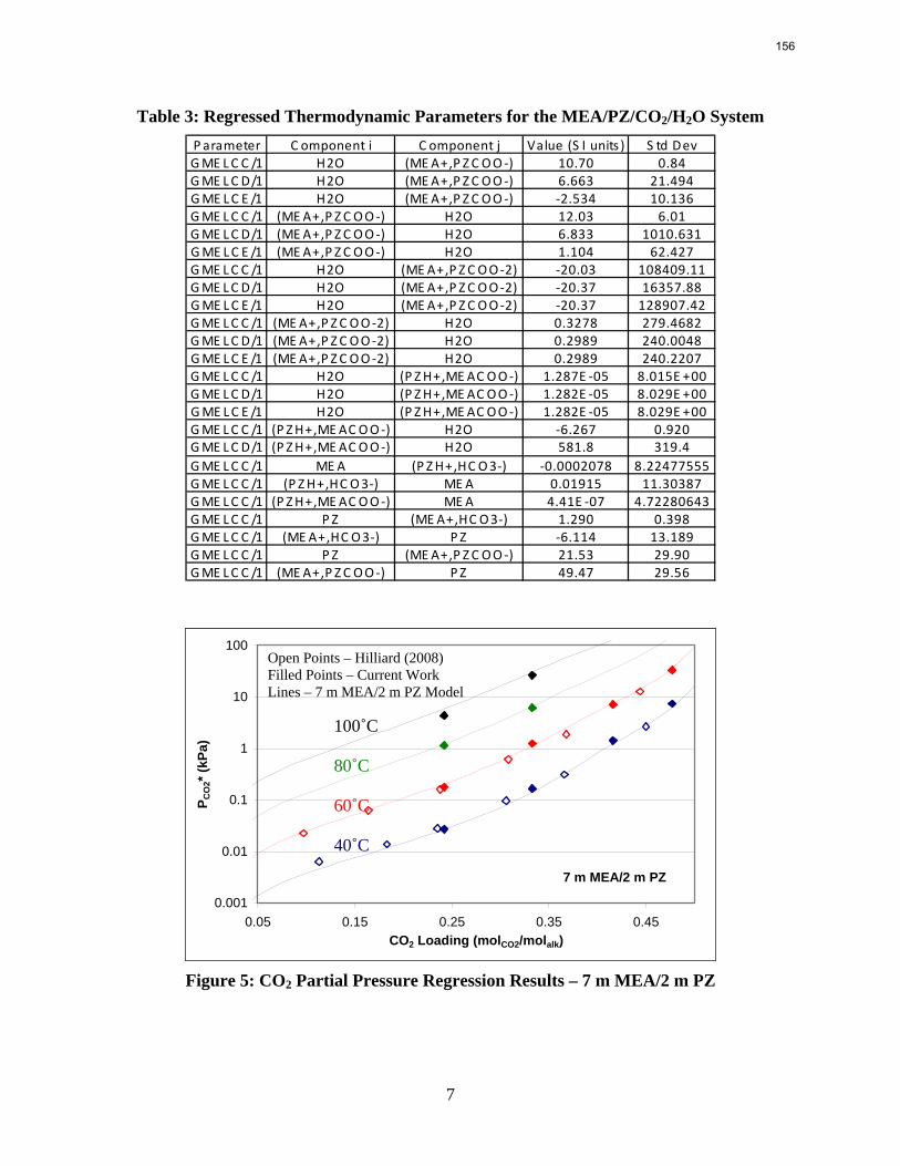
7
Table 3: Regressed Thermodynamic Parameters for the MEA/PZ/CO2/H2O System Parameter C omponent i C omponent j Value (S I units ) S td DevGME LC C /1 H2O (MEA+,P ZC OO ‐) 10.70 0.84GME LC D/1 H2O (MEA+,P ZC OO ‐) 6.663 21.494GME LC E /1 H2O (MEA+,P ZC OO ‐) ‐2.534 10.136GME LC C /1 (ME A+,P ZC OO ‐) H2O 12.03 6.01GME LC D/1 (ME A+,P ZC OO ‐) H2O 6.833 1010.631GME LC E /1 (ME A+,P ZC OO ‐) H2O 1.104 62.427GME LC C /1 H2O (MEA+,P ZC OO ‐2) ‐20.03 108409.11GME LC D/1 H2O (MEA+,P ZC OO ‐2) ‐20.37 16357.88GME LC E /1 H2O (MEA+,P ZC OO ‐2) ‐20.37 128907.42GME LC C /1 (ME A+,P ZC OO ‐2) H2O 0.3278 279.4682GME LC D/1 (ME A+,P ZC OO ‐2) H2O 0.2989 240.0048GME LC E /1 (ME A+,P ZC OO ‐2) H2O 0.2989 240.2207GME LC C /1 H2O (P ZH+,ME AC OO ‐) 1.287E ‐05 8.015E +00GME LC D/1 H2O (P ZH+,ME AC OO ‐) 1.282E ‐05 8.029E +00GME LC E /1 H2O (P ZH+,ME AC OO ‐) 1.282E ‐05 8.029E +00GME LC C /1 (P ZH+,ME AC OO ‐) H2O ‐6.267 0.920GME LC D/1 (P ZH+,ME AC OO ‐) H2O 581.8 319.4GME LC C /1 ME A (P ZH+,HC O3‐) ‐0.0002078 8.22477555GME LC C /1 (P ZH+,HC O3‐) ME A 0.01915 11.30387GME LC C /1 (P ZH+,ME AC OO ‐) ME A 4.41E ‐07 4.72280643GME LC C /1 P Z (ME A+,HC O3‐) 1.290 0.398GME LC C /1 (ME A+,HC O3‐) P Z ‐6.114 13.189GME LC C /1 P Z (ME A+,P ZC OO ‐) 21.53 29.90GME LC C /1 (ME A+,P ZC OO ‐) P Z 49.47 29.56
7 m MEA/2 m PZ
0.001
0.01
0.1
1
10
100
0.05 0.15 0.25 0.35 0.45CO2 Loading (molCO2/molalk)
P CO
2* (k
Pa)
Figure 5: CO2 Partial Pressure Regression Results – 7 m MEA/2 m PZ
Open Points – Hilliard (2008) Filled Points – Current Work Lines – 7 m MEA/2 m PZ Model
100˚C
80˚C
60˚C
40˚C
156
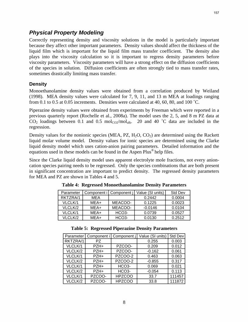
8
Physical Property Modeling Correctly representing density and viscosity solutions in the model is particularly important because they affect other important parameters. Density values should affect the thickness of the liquid film which is important for the liquid film mass transfer coefficient. The density also plays into the viscosity calculation so it is important to regress density parameters before viscosity parameters. Viscosity parameters will have a strong effect on the diffusion coefficients of the species in solution. Diffusion coefficients are often strongly tied to mass transfer rates, sometimes drastically limiting mass transfer.
Density Monoethanolamine density values were obtained from a correlation produced by Weiland (1998). MEA density values were calculated for 7, 9, 11, and 13 m MEA at loadings ranging from 0.1 to 0.5 at 0.05 increments. Densities were calculated at 40, 60, 80, and 100 ˚C.
Piperazine density values were obtained from experiments by Freeman which were reported in a previous quarterly report (Rochelle et al., 2008a). The model uses the 2, 5, and 8 m PZ data at CO2 loadings between 0.1 and 0.5 molCO2/molalk. 20 and 40 ˚C data are included in the regression.
Density values for the nonionic species (MEA, PZ, H2O, CO2) are determined using the Rackett liquid molar volume model. Density values for ionic species are determined using the Clarke liquid density model which uses cation-anion pairing parameters. Detailed information and the equations used in these models can be found in the Aspen Plus® help files.
Since the Clarke liquid density model uses apparent electrolyte mole fractions, not every anion-cation species pairing needs to be regressed. Only the species combinations that are both present in significant concentration are important to predict density. The regressed density parameters for MEA and PZ are shown in Tables 4 and 5.
Table 4: Regressed Monoethanolamine Density Parameters Parameter Component i Component j Value (SI units) Std DevRKTZRA/1 MEA 0.2442 0.0004VLCLK/1 MEA+ MEACOO- 0.1225 0.0023VLCLK/2 MEA+ MEACOO- -0.0146 0.0104VLCLK/1 MEA+ HCO3- 0.0739 0.0527VLCLK/2 MEA+ HCO3- 0.0130 0.2512
Table 5: Regressed Piperazine Density Parameters Parameter Component i Component j Value (SI units) Std DevRKTZRA/1 PZ 0.255 0.003VLCLK/1 PZH+ PZCOO- 0.209 0.012VLCLK/2 PZH+ PZCOO- -0.162 0.061VLCLK/1 PZH+ PZCOO-2 0.463 0.063VLCLK/2 PZH+ PZCOO-2 -0.855 0.317VLCLK/1 PZH+ HCO3- 0.069 0.021VLCLK/2 PZH+ HCO3- -0.054 0.113VLCLK/1 PZCOO- HPZCOO 33.7 111457VLCLK/2 PZCOO- HPZCOO 33.8 111872
157
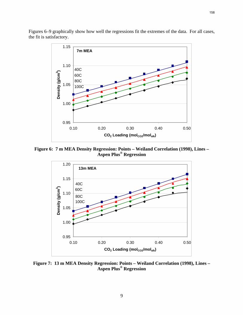
9
Figures 6–9 graphically show how well the regressions fit the extremes of the data. For all cases, the fit is satisfactory.
7m MEA
0.95
1.00
1.05
1.10
1.15
0.10 0.20 0.30 0.40 0.50
CO2 Loading (molCO2/molalk)
Den
sity
(g/c
m3 ) 40C
60C80C100C
Figure 6: 7 m MEA Density Regression: Points – Weiland Correlation (1998), Lines –
Aspen Plus® Regression
13m MEA
0.95
1.00
1.05
1.10
1.15
1.20
0.10 0.20 0.30 0.40 0.50
CO2 Loading (molCO2/molalk)
Den
sity
(g/c
m3 )
60C40C
80C100C
Figure 7: 13 m MEA Density Regression: Points – Weiland Correlation (1998), Lines –
Aspen Plus® Regression
158
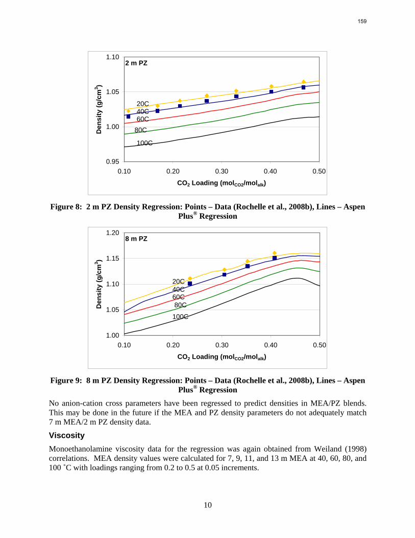
10
2 m PZ
0.95
1.00
1.05
1.10
0.10 0.20 0.30 0.40 0.50
CO2 Loading (molCO2/molalk)
Den
sity
(g/c
m3 )
20C40C60C
80C
100C
Figure 8: 2 m PZ Density Regression: Points – Data (Rochelle et al., 2008b), Lines – Aspen
Plus® Regression
8 m PZ
1.00
1.05
1.10
1.15
1.20
0.10 0.20 0.30 0.40 0.50
CO2 Loading (molCO2/molalk)
Den
sity
(g/c
m3 )
60C
20C40C
80C
100C
Figure 9: 8 m PZ Density Regression: Points – Data (Rochelle et al., 2008b), Lines – Aspen
Plus® Regression
No anion-cation cross parameters have been regressed to predict densities in MEA/PZ blends. This may be done in the future if the MEA and PZ density parameters do not adequately match 7 m MEA/2 m PZ density data.
Viscosity Monoethanolamine viscosity data for the regression was again obtained from Weiland (1998) correlations. MEA density values were calculated for 7, 9, 11, and 13 m MEA at 40, 60, 80, and 100 ˚C with loadings ranging from 0.2 to 0.5 at 0.05 increments.
159
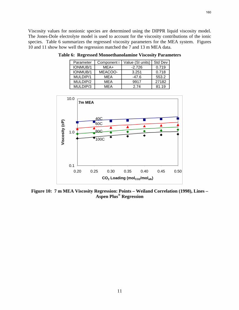
11
Viscosity values for nonionic species are determined using the DIPPR liquid viscosity model. The Jones-Dole electrolyte model is used to account for the viscosity contributions of the ionic species. Table 6 summarizes the regressed viscosity parameters for the MEA system. Figures 10 and 11 show how well the regression matched the 7 and 13 m MEA data.
Table 6: Regressed Monoethanolamine Viscosity Parameters Parameter Component i Value (SI units) Std DevIONMUB/1 MEA+ -2.726 0.719IONMUB/1 MEACOO- 3.251 0.718MULDIP/1 MEA -47.6 553.2MULDIP/2 MEA 9917 27182MULDIP/3 MEA 2.74 81.19
7m MEA
0.1
1.0
10.0
0.20 0.25 0.30 0.35 0.40 0.45 0.50
CO2 Loading (molCO2/molalk)
Visc
osity
(cP)
40C60C
80C
100C
Figure 10: 7 m MEA Viscosity Regression: Points – Weiland Correlation (1998), Lines –
Aspen Plus® Regression
160
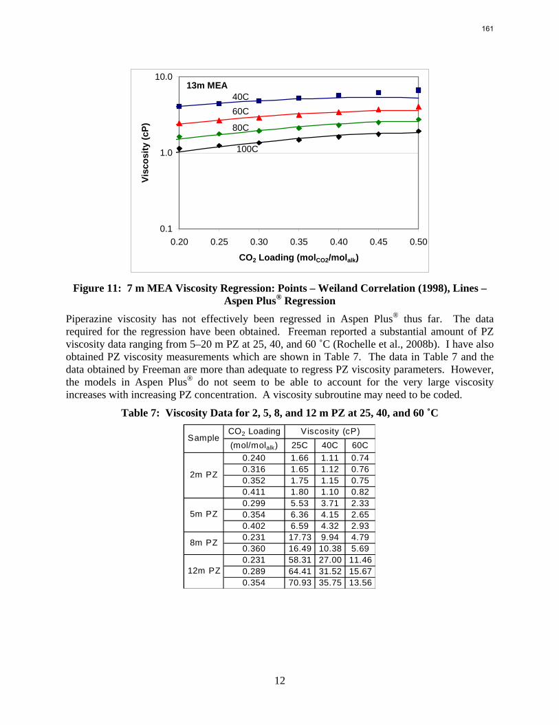
12
13m MEA
0.1
1.0
10.0
0.20 0.25 0.30 0.35 0.40 0.45 0.50
CO2 Loading (molCO2/molalk)
Visc
osity
(cP)
60C40C
80C
100C
Figure 11: 7 m MEA Viscosity Regression: Points – Weiland Correlation (1998), Lines –
Aspen Plus® Regression Piperazine viscosity has not effectively been regressed in Aspen Plus® thus far. The data required for the regression have been obtained. Freeman reported a substantial amount of PZ viscosity data ranging from 5–20 m PZ at 25, 40, and 60 ˚C (Rochelle et al., 2008b). I have also obtained PZ viscosity measurements which are shown in Table 7. The data in Table 7 and the data obtained by Freeman are more than adequate to regress PZ viscosity parameters. However, the models in Aspen Plus® do not seem to be able to account for the very large viscosity increases with increasing PZ concentration. A viscosity subroutine may need to be coded.
Table 7: Viscosity Data for 2, 5, 8, and 12 m PZ at 25, 40, and 60 ˚C CO2 Loading
(mol/molalk) 25C 40C 60C0.240 1.66 1.11 0.740.316 1.65 1.12 0.760.352 1.75 1.15 0.750.411 1.80 1.10 0.820.299 5.53 3.71 2.330.354 6.36 4.15 2.650.402 6.59 4.32 2.930.231 17.73 9.94 4.790.360 16.49 10.38 5.690.231 58.31 27.00 11.460.289 64.41 31.52 15.670.354 70.93 35.75 13.56
2m PZ
5m PZ
8m PZ
12m PZ
SampleViscosity (cP)
161
13
Rate Modeling
General Design The wetted wall column is modeled as an Aspen Plus® RateSep™ column. The actual wetted wall column has an annulus geometry since the liquid film flows over a rod and the gas flows around it. Aspen Plus®’s RateSep™ module cannot mimic this geometry. The column in the model is designed as a typical, cylindrical column. The diameter was adjusted so the column would have the same cross-sectional area as the wetted wall column. The design height of the column is the height of the wetted wall column: 9.1 cm.
Mimicking the wetted area of the column requires a similar manipulation. In the wetted wall column, the contact area is essentially the surface area of a metal rod which is coated with a thin film of liquid. The model assumes an arbitrary packing. An interfacial area subroutine was written to ensure that the wetted area of the wetted wall column, 38.52 cm2, would be duplicated in the model.
Thus far the model operates with 3 countercurrent stages. More stages may be required. The model does not consider pressure drop.
Mass Transfer Coefficients Gas film mass transfer coefficients were determined for the wetted wall column based on gas film controlled systems. The gas film mass transfer coefficient is correlated to pressure, temperature, and gas flow rate. This correlation has been verified and used by numerous operators of the wetted wall column (Pacheco, 1998; Bishnoi, 2000; Cullinane, 2005). The correlation was programmed into a Fortran subroutine so Aspen Plus® would use the same gas film mass transfer coefficients as the wetted wall column.
The liquid film mass transfer coefficient for physical mass transfer is based on the theory of a falling film around an annulus. Unlike the gas film mass transfer coefficient, the liquid film mass transfer coefficient is not easily obtained from experiment. It is dependent on the liquid flow rate, viscosity, temperature, geometry, and the diffusion coefficient of CO2. This correlation has been used by Pacheco, Bishnoi, and Cullinane, among others. This theoretical correlation was also input into the model via a Fortran subroutine. Modeling wetted wall column experiments may show the validity or limitations of this correlation.
Reactions The reactions for the MEA/PZ/CO2/H2O system are shown in Table 8. Fifteen pairs of forward and reverse rate reactions were used. Reactions 1–15 represent the forward reactions. Reactions 51–65 correspond to the reverse reactions. The reaction numbering system was designed so each reverse reaction number is 50 greater than the corresponding forward reaction. Four proton transfer reactions were modeled as equilibrium reactions.
162
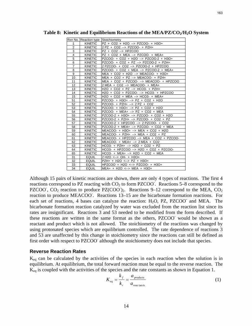
14
Table 8: Kinetic and Equilibrium Reactions of the MEA/PZ/CO2/H2O System Rxn No. Reaction type Stoichiometry
1 KINETIC PZ + CO2 + H2O --> PZCOO- + H3O+2 KINETIC 2 PZ + CO2 --> PZCOO- + PZH+3 KINETIC PZ + CO2 --> HPZCOO4 KINETIC PZ + CO2 + MEA --> PZCOO- + MEA+5 KINETIC PZCOO- + CO2 + H2O --> PZCOO-2 + H3O+6 KINETIC PZCOO- + CO2 + PZ --> PZCOO-2 + PZH+7 KINETIC 2 PZCOO- + CO2 --> PZCOO-2 + HPZCOO8 KINETIC PZCOO- + CO2 + MEA --> PZCOO-2 + MEA+9 KINETIC MEA + CO2 + H2O --> MEACOO- + H3O+
10 KINETIC MEA + CO2 + PZ --> MEACOO- + PZH+11 KINETIC MEA + CO2 + PZCOO- --> MEACOO- + HPZCOO12 KINETIC 2 MEA + CO2 --> MEACOO- + MEA+13 KINETIC H2O + CO2 + PZ --> HCO3- + PZH+14 KINETIC H2O + CO2 + PZCOO- --> HCO3- + HPZCOO15 KINETIC H2O + CO2 + MEA --> HCO3- + MEA+51 KINETIC PZCOO- + H3O+ --> PZ + CO2 + H2O52 KINETIC PZCOO- + PZH+ --> 2 PZ + CO253 KINETIC PZCOO- + H3O+ --> PZ + CO2 + H2O54 KINETIC PZCOO- + MEA+ --> PZ + CO2 + MEA55 KINETIC PZCOO-2 + H3O+ --> PZCOO- + CO2 + H2O56 KINETIC PZCOO-2 + PZH+ --> PZCOO- + CO2 + PZ57 KINETIC PZCOO-2 + HPZCOO --> 2 PZCOO- + CO258 KINETIC PZCOO-2 + MEA+ --> PZCOO- + CO2 + MEA59 KINETIC MEACOO- + H3O+ --> MEA + CO2 + H2O60 KINETIC MEACOO- + PZH+ --> MEA + CO2 + PZ61 KINETIC MEACOO- + HPZCOO --> MEA + CO2 + PZCOO-62 KINETIC MEACOO- + MEA+ --> 2 MEA + CO263 KINETIC HCO3- + PZH+ --> H2O + CO2 + PZ64 KINETIC HCO3- + HPZCOO --> H2O + CO2 + PZCOO-65 KINETIC HCO3- + MEA+ --> H2O + CO2 + MEA31 EQUIL 2 H2O <--> OH- + H3O+32 EQUIL PZH+ + H2O <--> PZ + H3O+33 EQUIL HPZCOO + H2O <--> PZCOO- + H3O+34 EQUIL MEA+ + H2O <--> MEA + H3O+
Although 15 pairs of kinetic reactions are shown, there are only 4 types of reactions. The first 4 reactions correspond to PZ reacting with CO2 to form PZCOO-. Reactions 5–8 correspond to the PZCOO-, CO2 reaction to produce PZ(COO-)2. Reactions 9–12 correspond to the MEA, CO2 reaction to produce MEACOO-. Reactions 13–15 are the bicarbonate formation reactions. For each set of reactions, 4 bases can catalyze the reaction: H2O, PZ, PZCOO- and MEA. The bicarbonate formation reaction catalyzed by water was excluded from the reaction list since its rates are insignificant. Reactions 3 and 53 needed to be modified from the form described. If these reactions are written in the same format as the others, PZCOO- would be shown as a reactant and product which is not allowed. The stoichiometry of the reactions was changed by using protonated species which are equilibrium controlled. The rate dependence of reactions 3 and 53 are unaffected by this change in stoichiometry since the reactions can still be defined as first order with respect to PZCOO- although the stoichiometry does not include that species.
Reverse Reaction Rates Keq can be calculated by the activities of the species in each reaction when the solution is in equilibrium. At equilibrium, the total forward reaction must be equal to the reverse reaction. The Keq is coupled with the activities of the species and the rate constants as shown in Equation 1.
tsreac
products
r
feq a
akk
Ktan
== (1)
163
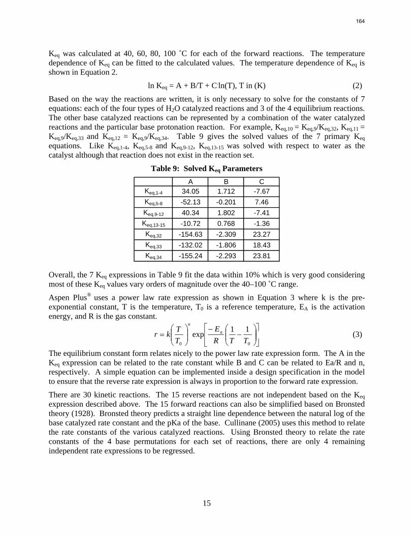
15
Keq was calculated at 40, 60, 80, 100 ˚C for each of the forward reactions. The temperature dependence of Keq can be fitted to the calculated values. The temperature dependence of Keq is shown in Equation 2.
ln Keq = A + B/T + C.ln(T), T in (K) (2)
Based on the way the reactions are written, it is only necessary to solve for the constants of 7 equations: each of the four types of H2O catalyzed reactions and 3 of the 4 equilibrium reactions. The other base catalyzed reactions can be represented by a combination of the water catalyzed reactions and the particular base protonation reaction. For example, Keq,10 = Keq,9/Keq,32, Keq,11 = Keq,9/Keq,33 and Keq,12 = Keq,9/Keq,34. Table 9 gives the solved values of the 7 primary Keq equations. Like Keq,1-4, Keq,5-8 and Keq,9-12, Keq,13-15 was solved with respect to water as the catalyst although that reaction does not exist in the reaction set.
Table 9: Solved Keq Parameters A B C
Keq,1-4 34.05 1.712 -7.67Keq,5-8 -52.13 -0.201 7.46Keq,9-12 40.34 1.802 -7.41Keq,13-15 -10.72 0.768 -1.36Keq,32 -154.63 -2.309 23.27Keq,33 -132.02 -1.806 18.43Keq,34 -155.24 -2.293 23.81
Overall, the 7 Keq expressions in Table 9 fit the data within 10% which is very good considering most of these Keq values vary orders of magnitude over the 40–100 ˚C range.
Aspen Plus® uses a power law rate expression as shown in Equation 3 where k is the pre-exponential constant, T is the temperature, T0 is a reference temperature, EA is the activation energy, and R is the gas constant.
⎥⎦
⎤⎢⎣
⎡⎟⎟⎠
⎞⎜⎜⎝
⎛−
−⎟⎟⎠
⎞⎜⎜⎝
⎛=
00
11expTTR
ETTkr a
n
(3)
The equilibrium constant form relates nicely to the power law rate expression form. The A in the Keq expression can be related to the rate constant while B and C can be related to Ea/R and n, respectively. A simple equation can be implemented inside a design specification in the model to ensure that the reverse rate expression is always in proportion to the forward rate expression.
There are 30 kinetic reactions. The 15 reverse reactions are not independent based on the Keq expression described above. The 15 forward reactions can also be simplified based on Bronsted theory (1928). Bronsted theory predicts a straight line dependence between the natural log of the base catalyzed rate constant and the pKa of the base. Cullinane (2005) uses this method to relate the rate constants of the various catalyzed reactions. Using Bronsted theory to relate the rate constants of the 4 base permutations for each set of reactions, there are only 4 remaining independent rate expressions to be regressed.
164
16
Conclusions An Aspen Plus® RateSep™ model of the wetted wall column is mostly completed. The thermodynamic model from Hilliard (2008) was adjusted so the wetted wall column would effectively represent 7–13 m MEA, 2–12 m PZ, and 7 m MEA/2 m PZ. The model has some trouble predicting CO2 partial pressure at the higher MEA concentrations. The model does a very good job of predicting CO2 partial pressure in the 7 and 9 m MEA, PZ, and the 7 m MEA/2 m PZ blend solutions.
Density and viscosity parameters were regressed for MEA. Only density parameters were regressed for PZ. Thus far, no adequate viscosity regression for PZ has been obtained. The model may require a Fortran subroutine to properly predict the viscosity of the PZ solutions.
The model provides the same cross sectional area, wetted area, and liquid and gas phase mass transfer coefficients as the actual wetted wall column. The model utilizes 15 forward reactions, 15 reverse reactions, and 4 equilibrium reactions. The 15 reverse reactions are not independent and can be linked to the forward reaction rates by the solved Keq relationships. The 15 forward reactions can be simplified into 4 reactions in which rate constants scale by Bronsted theory.
References Bishnoi S. Carbon Dioxide Absorption and solution equilibrium in piperazine activated
methyldiethanolamine. The University of Texas at Austin. Ph.D. Dissertation. 2008;270.
Bronsted JN. Acid and basic catalysis. Chemical Reviews. 1928;5:231–338.
Cullinane JT. Thermodynamics and Kinetics of aqueous piperazine with potassium carbonate for carbon dioxide absorption. The University of Texas at Austin. Ph.D. Dissertation. 2005;295.
Ermatchkov V et al. "Solubility of Carbon Dioxide in Aqueous Solutions of Piperazine in the Low Gas Loading Region." J Chem Eng Data. 2006; 51(5):1788–1796.
Hilliard M. A Predictive Thermodynamic Model for an Aqueous Blend of Potassium Carbonate, Piperazine, and Monoethanolamine for Carbon Dioxide Capture from Flue Gas. The University of Texas at Austin. Ph.D. Dissertation.. 2008;1025.
Jou F-Y et al. "The Solubility of CO2 in a 30 Mass Percent Monoethanolamine Solution." Can J Chem Eng. 1995;73(1):140–147.
Kim I & Svendsen HF. "Heat of absorption of carbon dioxide (CO2) in monoethanolamine (MEA) and 2-(aminoethyl)ethanolamine (AEEA) solutions." Ind Eng Chem Res. 2007;46(17):5803–5809.
Pacheco MA. Mass Transfer, Kinetics and Rate-Based Modeling of Reactive Absorption. The University of Texas at Austin. Ph.D. Dissertation. 1998;291.
Rochelle GT et al. "CO2 Capture by Aqueous Absorption, Second Quarterly Progress Report 2008." Luminant Carbon Management Program. The University of Texas at Austin. 2008a.
Rochelle GT et al. "CO2 Capture by Aqueous Absorption, Third Quarterly Progress Report 2008." Luminant Carbon Management Program. The University of Texas at Austin. 2008b.
Rochelle GT et al. "CO2 Capture by Aqueous Absorption, Fourth Quarterly Progress Report 2008." Luminant Carbon Management Program. The University of Texas at Austin. 2009.
165

17
Weiland RH, et al. "Density and Viscosity of Some Partially Carbonated Aqueous Alkanolamine Solutions and Their Blends." J Chem Eng Data. 1998;43(3):378–382.
166
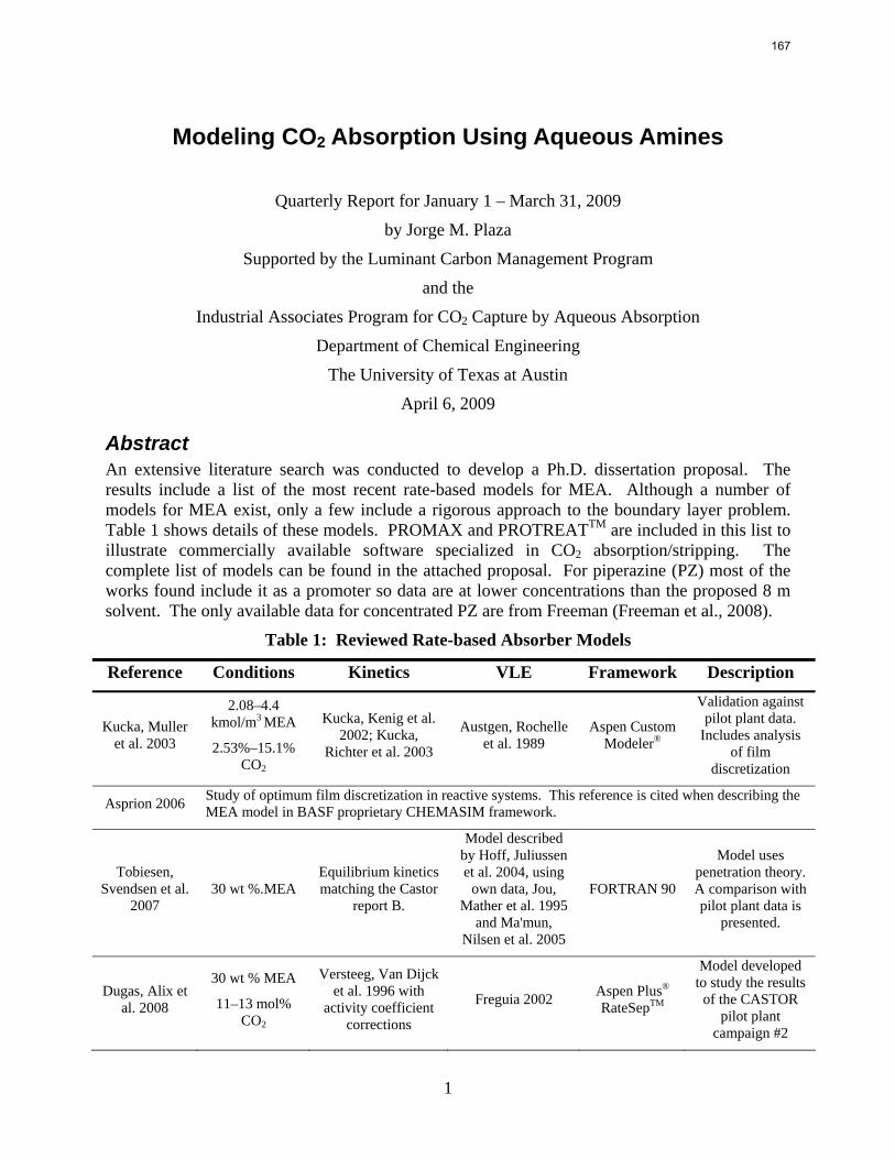
1
Modeling CO2 Absorption Using Aqueous Amines
Quarterly Report for January 1 – March 31, 2009
by Jorge M. Plaza
Supported by the Luminant Carbon Management Program
and the
Industrial Associates Program for CO2 Capture by Aqueous Absorption
Department of Chemical Engineering
The University of Texas at Austin
April 6, 2009
Abstract An extensive literature search was conducted to develop a Ph.D. dissertation proposal. The results include a list of the most recent rate-based models for MEA. Although a number of models for MEA exist, only a few include a rigorous approach to the boundary layer problem. Table 1 shows details of these models. PROMAX and PROTREATTM are included in this list to illustrate commercially available software specialized in CO2 absorption/stripping. The complete list of models can be found in the attached proposal. For piperazine (PZ) most of the works found include it as a promoter so data are at lower concentrations than the proposed 8 m solvent. The only available data for concentrated PZ are from Freeman (Freeman et al., 2008).
Table 1: Reviewed Rate-based Absorber Models
Reference Conditions Kinetics VLE Framework Description
Kucka, Muller et al. 2003
2.08–4.4 kmol/m3 MEA
2.53%–15.1% CO2
Kucka, Kenig et al. 2002; Kucka,
Richter et al. 2003
Austgen, Rochelle et al. 1989
Aspen Custom Modeler®
Validation against pilot plant data.
Includes analysis of film
discretization
Asprion 2006 Study of optimum film discretization in reactive systems. This reference is cited when describing the MEA model in BASF proprietary CHEMASIM framework.
Tobiesen, Svendsen et al.
2007 30 wt %.MEA
Equilibrium kinetics matching the Castor
report B.
Model described by Hoff, Juliussen et al. 2004, using
own data, Jou, Mather et al. 1995
and Ma'mun, Nilsen et al. 2005
FORTRAN 90
Model uses penetration theory. A comparison with pilot plant data is
presented.
Dugas, Alix et al. 2008
30 wt % MEA
11–13 mol% CO2
Versteeg, Van Dijck et al. 1996 with
activity coefficient corrections
Freguia 2002 Aspen Plus® RateSepTM
Model developed to study the results
of the CASTOR pilot plant
campaign #2
167
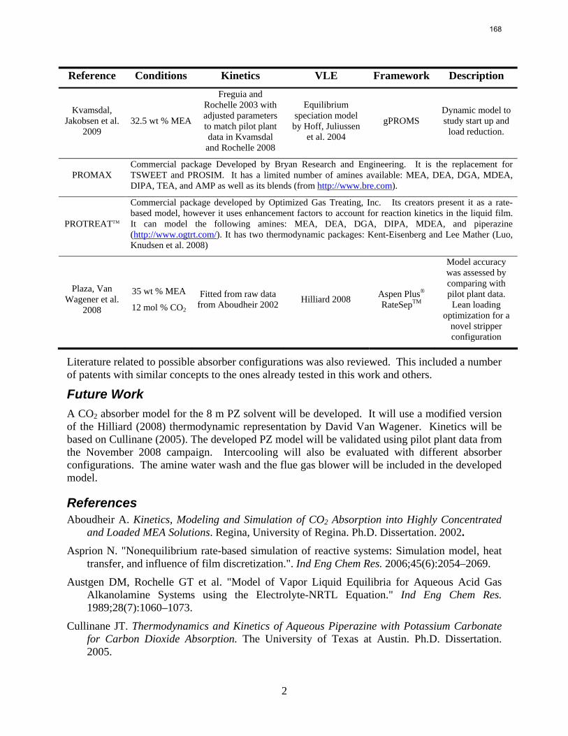
2
Reference Conditions Kinetics VLE Framework Description
Kvamsdal, Jakobsen et al.
2009 32.5 wt % MEA
Freguia and Rochelle 2003 with adjusted parameters to match pilot plant data in Kvamsdal
and Rochelle 2008
Equilibrium speciation model
by Hoff, Juliussen et al. 2004
gPROMS Dynamic model to study start up and
load reduction.
PROMAX Commercial package Developed by Bryan Research and Engineering. It is the replacement for TSWEET and PROSIM. It has a limited number of amines available: MEA, DEA, DGA, MDEA, DIPA, TEA, and AMP as well as its blends (from http://www.bre.com).
PROTREATTM
Commercial package developed by Optimized Gas Treating, Inc. Its creators present it as a rate-based model, however it uses enhancement factors to account for reaction kinetics in the liquid film. It can model the following amines: MEA, DEA, DGA, DIPA, MDEA, and piperazine (http://www.ogtrt.com/). It has two thermodynamic packages: Kent-Eisenberg and Lee Mather (Luo, Knudsen et al. 2008)
Plaza, Van Wagener et al.
2008
35 wt % MEA
12 mol % CO2
Fitted from raw data from Aboudheir 2002 Hilliard 2008 Aspen Plus®
RateSepTM
Model accuracy was assessed by comparing with pilot plant data.
Lean loading optimization for a
novel stripper configuration
Literature related to possible absorber configurations was also reviewed. This included a number of patents with similar concepts to the ones already tested in this work and others.
Future Work A CO2 absorber model for the 8 m PZ solvent will be developed. It will use a modified version of the Hilliard (2008) thermodynamic representation by David Van Wagener. Kinetics will be based on Cullinane (2005). The developed PZ model will be validated using pilot plant data from the November 2008 campaign. Intercooling will also be evaluated with different absorber configurations. The amine water wash and the flue gas blower will be included in the developed model.
References Aboudheir A. Kinetics, Modeling and Simulation of CO2 Absorption into Highly Concentrated
and Loaded MEA Solutions. Regina, University of Regina. Ph.D. Dissertation. 2002.
Asprion N. "Nonequilibrium rate-based simulation of reactive systems: Simulation model, heat transfer, and influence of film discretization.". Ind Eng Chem Res. 2006;45(6):2054–2069.
Austgen DM, Rochelle GT et al. "Model of Vapor Liquid Equilibria for Aqueous Acid Gas Alkanolamine Systems using the Electrolyte-NRTL Equation." Ind Eng Chem Res. 1989;28(7):1060–1073.
Cullinane JT. Thermodynamics and Kinetics of Aqueous Piperazine with Potassium Carbonate for Carbon Dioxide Absorption. The University of Texas at Austin. Ph.D. Dissertation. 2005.
168
3
Dugas R, Alix P et al. "Creation of an Aspen RateSep Absorber Model for the Evaluation of CASTOR Pilot Plant Data." Am Chem Soc, Div Petro Chem. 2008;53(1):89–92.
Freeman SA et al. "Carbon Dioxide Capture with Concentrated, Aqueous Piperazine." GHGT-9. Washington D.C. 2008.
Freguia S. Modeling of CO2 Removal from Flue Gas with Monoethanolamine. The University of Texas at Austin. M.S. Thesis. 2002.
Freguia S & Rochelle GT. Modeling of CO2 capture by Aqueous Monoethanolamine. AIChE J. 2003;49(7):1676–1686.
Hilliard MD. A Predictive Thermodynamic Model for an Aqueous Blend of Potassium Carbonate, Piperazine, and Monoethanolamine for Carbon Dioxide Capture from Flue Gas. The University of Texas at Austin. Ph.D. Dissertation. 2008.
Hoff KA, Juliussen O et al. "Modeling and experimental study of carbon dioxide absorption in aqueous alkanolamine solutions using a membrane contactor." Ind Eng Chem Res. 2004;43(16):4908–4921.
Jou F-Y, Mather AE et al. "The Solubility of CO2 in a 30 mass percent monoethanolamine solution." Can J Chem Eng. 1995(73):7.
Kucka L, Kenig EY et al. "Kinetics of the gas-liquid reaction between carbon dioxide and hydroxide ions." Ind Eng Chem Res. 2002;41(24):5952–5957.
Kucka L, Muller I et al. "On the Modeling and Simulation of sour gas absorption by aqueous amine solutions." Chem Eng Sci. 2003;58.
Kucka L, Richter J et al. "Determination of gas-liquid reaction kinetics with a stirred cell reactor." Sep Purif Technol. 2003;31(2):163–175.
Kvamsdal HM, Jakobsen JP et al. "Dynamic modeling and simulation of a CO2 absorber column for post-combustion CO2 capture." Chem Eng Process. 2009;48(1):135–144.
Kvamsdal HM & Rochelle GT. "Effects of the temperature bulge in CO2 absorption from flue gas by aqueous monoethanolamine." Ind Eng Chem Res. 2008;47(3):867–875.
Luo X, Knudsen JN et al. "Comparison and Validation of Simulation Codes against Sixteen Sets of Data from Four Different Pilot Plants." GHGT-9. Washington D.C, 2008.
Ma'mu S, Nilsen R et al. "Solubility of carbon dioxide in 30 mass % monoethanolamine and 50 mass % methyldiethanolamine solutions." J Chem Eng Data. 2005;50(2):630–634.
Plaza JM, Van Wagener DH et al. "Modeling CO2 Capture with Aqueous Monoethanolamine." GHGT-9. Washington D.C, 2008,
Tobiesen FA, Svendsen HF et al. "Experimental validation of a rigorous absorber model for CO2 postcombustion capture." AIChE J. 2007;53(4):846–865.
Versteeg GF, Van Dijck LAJ et al. "On the kinetics between CO2 and alkanolamines both in aqueous and non-aqueous solutions. An overview." Chem Eng Commun. 1996;144:113–158.
169
THE UNIVERSITY OF TEXAS AT AUSTIN DEPARTMENT OF CHEMICAL ENGINEERING
PHD DISSERTATION PROPOSAL
MODELING ABSORPTION OF CO2 USING AMINES
JORGE M. PLAZA
APRIL 2009
170
J o r g e M . P l a z a – D i s s e r t a t i o n P r o p o s a l
2
INTRODUCTION Emissions of greenhouse gases (GHGs) have altered the energy balance of the earth’s climate
system by increasing atmospheric absorption of the sun’s outgoing radiation thus raising the
planet’s global average temperature (0.74oC for the 1906-2005 period(Core-Writing-Team 2007).
The increase of various GHGs in the industrial era appears as the dominant factor in climate change.
(Solomon, Qin et al. 2007) Although several of the major GHGs are naturally occurring, their
concentration change in the atmosphere during the past 250 years has been strongly linked to
human activity. Among the GHGs special attention is given to carbon dioxide (CO2), nitrous oxide
(N2O), and methane (CH4) because of their long term influence on climate due to their chemical
stability allowing them to remain in the atmosphere at time scales longer than decades or centuries.
In the case of CO2 atmospheric concentrations have gone from 180 ppm to more than 300 ppm as
determined from ice core analysis. (2007). Its concentration increased around 35% from its pre-
industrial value to 379 ppm as of 2005.(2007). Most of this increase is related to anthropogenic
emissions of which two thirds come from fossil fuel burning accounting for approximately 1100 Gt
emitted into the atmosphere since the mid 19th century (Sims, Schock et al. 2007).
The largest increase in anthropogenic emissions of CO2 comes from the power generation sector
(over 27% by 2004) (Rogner, Zhou et al. 2007). This sector comprises generation from coal and
natural gas fired power plants. Flue gas from these sources contains 13 mol % CO2 for the former
to 3 mol % CO2 for the latter. Emissions from this sector are tied to policy and their change will
depend on the requirement of nations to obtain sources and carriers with long term security of
supply, affordability and minimal environmental impact. Due to their abundance and cost
(especially for coal) fossil power plants are expected to maintain a considerable role in the supply
of worldwide energy. However, their indiscriminated deployment and continued use is not
sustainable. For this reason research has sprung with the intention to reduce their impact on the
planet. Among the options available to reduce this sector’s emissions is Carbon Capture and
Sequestration (CCS) that consists in removal and later storage of CO2 from emission points. Its
potential has been identified not only for coal, gas, or biomass fired generation or cogeneration but
also for major energy intensive industries (i.e. refineries), synthetic fuel plants, natural gas fields,
and chemical facilities for producing ammonia, hydrogen, cement and coke (Sims, Schock et al.
2007). Its future role has been seen as a “transitional technology” (Sims, Schock et al. 2007) that
will peak as efforts to reduce climate change are increased and will decline as the desired
decarbonization of energy sources advances.
Carbon capture technologies have been classified in absorption, adsorption, membrane separation
and cryogenic processes (Saxena and Flintoff 2006). Based on process conditions and current
available technology, chemical absorption has been proposed as the most viable to reduce
emissions of CO2 from low CO2 partial pressure sources (500 mbar). The technology basis for
chemical absorption systems has been around for more than 70 years (Bottoms 1930) . It was
previously used in the separation of CO2 from hydrogen and natural gas, an application less
stringent in energy requirements and with a smaller scale than the proposed flue gas removal. The
latter requires absorption capabilities at low CO2 partial pressures, handling oxygen, SOx, fly ash,
soot, NOx, and high flue gas temperatures (Chapel, Mariz et al. 1999). The successful
171
J o r g e M . P l a z a – D i s s e r t a t i o n P r o p o s a l
3
implementation of this technology depends on reduction of energy consumption and capital costs.
For the former, reduction of steam consumption and absorber pressure drop along with integration
of the stripper with the power generation have been identified as promising improvement areas.
Capital costs will benefit from cheaper absorber and flue gas cooling vessel materials, absorber size,
economies of scale and improved oxidation inhibitors (Chapel, Mariz et al. 1999). The mentioned
process improvements may be accomplished by research and development of new solvents,
contactor types, energy optimization, degradation, corrosion, and system simplification. (Rochelle,
Chi et al. 2001). The proposed work will contribute in the three initial items focusing in the
absorption component of the technology.
RESEARCH OBJECTIVES Research will be divided in three parts. The first one centers in the development of rigorous CO2
absorption models to test new solvents. The second will analyze various absorber configurations
including absorber intercooling and hybrid packing. The third focus of research consists in
providing a better fundamental understanding of the phenomena related to mass transfer with
chemical reaction and its adequate modeling applied to CO2 absorption. All of this work will be
conducted using Aspen Plus ® RateSepTM.
ABSORBER MODEL DEVELOPMENT
Models will be generated for aqueous MEA (7m – 9m), and Piperazine (8m). The developed models
will be reconciled and validated using pilot plant data obtained from campaigns conducted at the
Pickle Research Center. The following are the goals for this research focus:
Development of an absorber model for MEA (7m – 9m)
Development of an absorber model for 8 m Piperazine (PZ)
Pilot plant validation and reconciliation for the developed models.
Assess the importance of the bicarbonate formation reaction in CO2 absorption modeling
CONFIGURATION ANALYSIS AND INNOVATION
The developed models will be used to analyze absorber process configurations to increase removal
performance. Options will be evaluated for their technical feasibility and economic viability. The
goals under this focus are:
Evaluate absorber intercooling use for MEA, PZ and a blend of K+/PZ
Development of a method to predict the critical gas/liquid ratio (L/G) for various solvents
Analyze various packing types and their performance in CO2 absorption to assess the effect
of pressure drop and contact area and determine their influence in optimum packing
selection.
Evaluate liquid and gas mass transfer coefficients (kL & kG) and liquid holdup under various
process conditions to determine under what conditions these variables become important
in CO2 absorption.
172
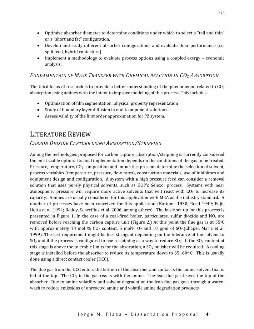
J o r g e M . P l a z a – D i s s e r t a t i o n P r o p o s a l
4
Optimize absorber diameter to determine conditions under which to select a “tall and thin”
or a “short and fat” configuration.
Develop and study different absorber configurations and evaluate their performance (i.e.
split feed, hybrid contactors)
Implement a methodology to evaluate process options using a coupled exergy – economic
analysis.
FUNDAMENTALS OF MASS TRANSFER WITH CHEMICAL REACTION IN CO2 ABSORPTION
The third focus of research is to provide a better understanding of the phenomenon related to CO2
absorption using amines with the intent to improve modeling of this process. This includes:
Optimization of film segmentation, physical property representation
Study of boundary layer diffusion in multicomponent solutions.
Assess validity of the first order approximation for PZ system.
LITERATURE REVIEW CARBON DIOXIDE CAPTURE USING ABSORPTION/STRIPPING
Among the technologies proposed for carbon capture, absorption/stripping is currently considered
the most viable option. Its final implementation depends on the conditions of the gas to be treated.
Pressure, temperature, CO2 composition and impurities present, determine the selection of solvent,
process variables (temperature, pressure, flow rates), construction materials, use of inhibitors and
equipment design and configuration. A system with a high pressure feed can consider a removal
solution that uses purely physical solvents, such as UOP’s Selexol process. Systems with near
atmospheric pressure will require more active solvents that will react with CO2 to increase its
capacity. Amines are usually considered for this application with MEA as the industry standard. A
number of processes have been conceived for this application (Bottoms 1930; Reed 1949; Fujii,
Hotta et al. 1994; Reddy, Scherffius et al. 2006, among others). The basic set up for this process is
presented in Figure 1. In the case of a coal-fired boiler, particulates, sulfur dioxide and NOx are
removed before reaching the carbon capture unit (Figure 2.) At this point the flue gas is at 55oC
with approximately 13 mol % CO2 content, 5 mol% O2 and 10 ppm of SO2.(Chapel, Mariz et al.
1999). The last requirement might be less stringent depending on the tolerance of the solvent to
SO2 and if the process is configured to use reclaiming as a way to reduce SO2. If the SO2 content at
this stage is above the tolerable limits for the absorption, a SO2 polisher will be required. A cooling
stage is installed before the absorber to reduce its temperature down to 35 -60o C. This is usually
done using a direct contact cooler (DCC).
The flue gas from the DCC enters the bottom of the absorber and contact s the amine solvent that is
fed at the top. The CO2 in the gas reacts with the amine. The lean flue gas leaves the top of the
absorber. Due to amine volatility and solvent degradation the lean flue gas goes through a water-
wash to reduce emissions of unreacted amine and volatile amine degradation products
173
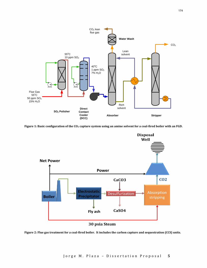
J o r g e M . P l a z a – D i s s e r t a t i o n P r o p o s a l
5
CO2
Flue Gas
55oC
50 ppm SO2
15% H2O
40oC
1 ppm SO2
7% H2O
CO2 lean
flue gas
Rich
solvent
Lean
solvent
Direct
Contact
Cooler
(DCC)StripperAbsorber
Water Wash
SO2 Polisher
55oC
10 ppm SO2
Figure 1: Basic configuration of the CO2 capture system using an amine solvent for a coal-fired boiler with an FGD.
Figure 2: Flue gas treatment for a coal-fired boiler. It includes the carbon capture and sequestration (CCS) units.
174
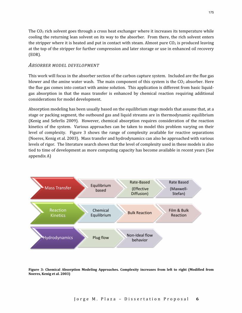
J o r g e M . P l a z a – D i s s e r t a t i o n P r o p o s a l
6
The CO2 rich solvent goes through a cross heat exchanger where it increases its temperature while
cooling the returning lean solvent on its way to the absorber. From there, the rich solvent enters
the stripper where it is heated and put in contact with steam. Almost pure CO2 is produced leaving
at the top of the stripper for further compression and later storage or use in enhanced oil recovery
(EOR).
ABSORBER MODEL DEVELOPMENT
This work will focus in the absorber section of the carbon capture system. Included are the flue gas
blower and the amine water wash. The main component of this system is the CO2 absorber. Here
the flue gas comes into contact with amine solution. This application is different from basic liquid-
gas absorption in that the mass transfer is enhanced by chemical reaction requiring additional
considerations for model development.
Absorption modeling has been usually based on the equilibrium stage models that assume that, at a
stage or packing segment, the outbound gas and liquid streams are in thermodynamic equilibrium
(Kenig and Seferlis 2009). However, chemical absorption requires consideration of the reaction
kinetics of the system. Various approaches can be taken to model this problem varying on their
level of complexity. Figure 3 shows the range of complexity available for reactive separations
(Noeres, Kenig et al. 2003). Mass transfer and hydrodynamics can also be approached with various
levels of rigor. The literature search shows that the level of complexity used in these models is also
tied to time of development as more computing capacity has become available in recent years (See
appendix A)
Figure 3: Chemical Absorption Modeling Approaches. Complexity increases from left to right (Modified from Noeres, Kenig et al. 2003)
Mass TransferEquilibrium
based
Rate-Based
(Effective Diffusion)
Rate Based
(Maxwell-Stefan)
Reaction Kinetics
Chemical Equilibrium
Bulk ReactionFilm & Bulk
Reaction
Hydrodynamics Plug flowNon-Ideal flow
behavior
175
J o r g e M . P l a z a – D i s s e r t a t i o n P r o p o s a l
7
The more complex and rigorous treatment of absorption processes entails the use of Maxwell-
Stefan diffusivities, additional considerations at liquid-vapor interface and process hydrodynamics
that include correlations for hold-up, pressure drop and interfacial area. This is the “rate-based”
approach that aims to describe actual rates for mass and heat transfer and chemical reactions.
(Kenig, Kucka et al. 2003).
Mass transfer at the interface is a challenging component of the rigorous modeling approach.
Among the models proposed for its treatment are the film model, the surface renewal or
penetration models and the eddy diffusivity based models (Taylor and Krishna 1993). The latter
two are unsteady-state models in which fluid elements (or eddies) arrive at the interface from the
bulk region with the local mean composition and stay there for an exposure time in which mass
transfer takes place. During this time there is no convective phenomenon and all mass transfer
occurs through diffusion (Danckwerts 1951,1970;Astarita 1967; Taylor and Krishna 1993). After
this the element returns to the bulk to be replaced by a new element. Modifications to this model
propose a film of definite thickness that is uniformly mixed at intervals (Danckwerts 1970).
The film model is the simplest and oldest of the available models (Taylor and Krishna 1993). This
model assumes that the mass transfer resistance lies at the film layers next to the gas liquid
interface. Mass transfer in these layers occurs solely by steady-state molecular diffusion. At the
bulk, the level of mixing or turbulence is so high that it is a well-mixed system with uniform
temperature and concentration. At the interface, the liquid and the vapor are in equilibrium.
(Sherwood and Pigford 1952; Astarita 1967; Danckwerts 1970;Taylor and Krishna 1993;Asprion
2006). This is the model used in AspenTech’s RateSep so it will be used in the models proposed for
this work.
Reaction rates in the film and their effect on enhancing mass transfer need to be considered to
properly model the absorption process. When the rates are very slow it is possible simplify the
problem by using a single film segment or eliminating the film all together. However, in many cases
it is necessary to differentiate the reaction regime present in the film and its enhancement on
physical mass transfer. The Hatta number (Ha) represents a ratio of the maximum possible
reaction and mass transfer rates (Vaidya and Kenig 2007). It serves as an indicator of the rate of
reaction. A low Ha number represents slow kinetics. If Ha>3 then the concentration of the amine
can be assumed constant in the boundary layer (Tobiesen, Svendsen et al. 2007). The Hatta
number is then defined as:
𝐻𝑎 =
𝐷𝐶𝑂2𝑘𝑓 𝐴𝑀
𝑘𝐶𝑂2𝑜
(1)
Where DCO2 is the binary diffusion of CO2 in the solvent
kf is the forward rate constant for the controlling absorption reaction
[AM] represents the amine concentration
176
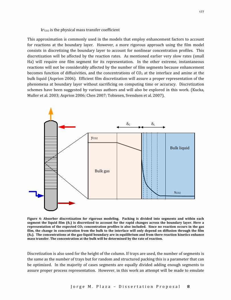
J o r g e M . P l a z a – D i s s e r t a t i o n P r o p o s a l
8
koCO2 is the physical mass transfer coefficient
This approximation is commonly used in the models that employ enhancement factors to account
for reactions at the boundary layer. However, a more rigorous approach using the film model
consists in discretizing the boundary layer to account for nonlinear concentration profiles. This
discretization will be affected by the reaction rates. As mentioned earlier very slow rates (small
Ha) will require one film segment for its representation. In the other extreme, instantaneous
reactions will not be considerably affected by the number of film segments because enhancement
becomes function of diffusivities, and the concentrations of CO2 at the interface and amine at the
bulk liquid (Asprion 2006). Efficient film discretization will assure a proper representation of the
phenomena at boundary layer without sacrificing on computing time or accuracy. Discretization
schemes have been suggested by various authors and will also be explored in this work. (Kucka,
Muller et al. 2003; Asprion 2006; Chen 2007; Tobiesen, Svendsen et al. 2007).
Discretization is also used for the height of the column. If trays are used, the number of segments is
the same as the number of trays but for random and structured packing this is a parameter that can
be optimized. In the majority of cases segments are equally divided adding enough segments to
assure proper process representation. However, in this work an attempt will be made to emulate
Figure 4: Absorber discretization for rigorous modeling. Packing is divided into segments and within each segment the liquid film (δL) is discretized to account for the rapid changes across the boundary layer. Here a representation of the expected CO2 concentration profiles is also included. Since no reaction occurs in the gas film, the change in concentration from the bulk to the interface will only depend on diffusion through the film (δG). The concentrations at the gas-liquid boundary are in equilibrium and from there reaction kinetics enhance mass transfer. The concentration at the bulk will be determined by the rate of reaction.
δG δL
Bulk liquid
Bulk gas
yCO2
xCO2
177
J o r g e M . P l a z a – D i s s e r t a t i o n P r o p o s a l
9
the discretization process used for the liquid film. In the absorber column, the slopes of the
temperature and concentration profiles change rapidly at the extremes so the idea is to divide into
smaller segments the extremes of the column to account for this factor. The main goal is to reduce
computing time and convergence issues while maintaining accuracy. Figure 4 shows the absorber
model discretization.
Modeling CO2 absorption using aqueous amines needs to also take into consideration the presence
of electrolyte species that generate as products from gas absorption or dissociation of dissolved
salts. There are various models that describe mixtures containing electrolytes (Kenig, Kucka et al.
2003). The Electrolyte non random two liquid (NRTL) model (Chen, Britt et al. 1982) estimates
activity coefficients for ionic species in aqueous and mixed-solvent electrolyte systems using binary
pair parameters. (Kenig and Seferlis 2009). The Pitzer model (Pitzer 1973) suggests a general
expression for the excess Gibbs energy that includes an electrostatic term, a term describing short-
range forces between two solutes and a term for triple solute collisions (Kenig, Kucka et al. 2003).
The former will be the model used in this work. It has been successfully implemented in the
Rochelle research group within the Aspen Plus framework (Austgen 1989; Freguia 2002; Hilliard
2005,2008).
ABSORPTION WITH AQUEOUS MONOETHANOLAMINE (MEA)
Aqueous Monoethanolamine (MEA) with a concentration between 15- 30 % has been previously
used and is currently considered the state of the art technology for CO2 absorption/stripping. It is
an economic solvent with a high heat of absorption and fast kinetics. It had been proposed for the
removal of CO2 from gas mixtures as early as 1949 (Reed 1949). However, its main application was
for natural gas. In the 1970’s and 80’s Dow Chemical and Union Carbide developed 30 wt% MEA
processes to generate CO2 for enhanced oil recovery (EOR) (Chapel, Mariz et al. 1999; Butwell and
Kubek 1980). In 1989 Dow Chemical sold its process to FLUOR Daniels and it is what is now known
as Econamine FGSM. This process has been implemented for removal of CO2 from natural gas-boiler
flue gas for EOR, urea production and the food industry. ABB Lummus Crest/Kerr McGee also have
built a CO2 capture process that uses 20% MEA (Barchas and Davis 1992). Mitsubishi/Kansai
Electric have also patented processes that use MEA (Fujii, Hotta et al. 1994; Fujii, Hotta et al. 2001).
FLUOR updated its MEA process (Econamine FG PlusSM) and claims to have decreased in 20% the
energy requirement of their Econamine FGSM (Reddy, Scherffius et al. 2003; Reddy, Scherffius et al.
2006).
Currently a plethora of models exist for the absorption of CO2 using MEA. Their complexity ranges
from enhancement factor calculations to the more complex rate-based approach. Table 1 includes
the rate-based absorber MEA models found in the published literature. The complete list of
absorber models reviewed is presented in Appendix A.
The models in Table 1 are the most similar to the goal of the proposed work. They all use activity
based equilibrium and rate expressions, liquid film segmentation and heat and mass transfer rate
calculations. PROMAX and PROTREATTM are included in this list to illustrate commercially available
software specialized in CO2 absorption/stripping. The last entry in Table 1 (Plaza, Van Wagener et
178
J o r g e M . P l a z a – D i s s e r t a t i o n P r o p o s a l
10
al. 2008) is a partial product of this research. It will be improved to include recent kinetic data by
Ross Dugas and additional improvements to the VLE and physical properties packages.
ABSORPTION WITH CONCENTRATED PIPERAZINE (PZ)
Piperazine has been used mainly as a promoter to increase absorption rates and capacity in
solvents. It has been proposed as promoter in the K2CO3 solvent at various concentrations
(Cullinane 2005; Chen 2007; Oexmann, Hensel et al. 2008). It has been used by BASF A.G. as a
promoter for their processes for natural gas sweetening blended with MDEA (Appl, Wagner et al.
1982; Asprion and Grossmann 2004). It has also been studied as an accelerator for N,N-
diethylethanolamine (presented as a renewable amine because it can be obtained from ethanol)
(Vaidya and Kenig 2008). Recently, PZ has been suggested as a solvent at high concentrations
(>8m). Freeman, Dugas et al. (2008) showed that 8 m PZ has a volatility similar to MEA but the
advantage of faster kinetics (more than twice) and higher capacity (double) than MEA. It is also
more resistant to oxidative and thermal degradation (degrades at temperatures higher than 150oC).
Its process limitation is related to PZ solubility. At room temperature (20oC) 8 m PZ requires a
loading of 0.25 mol CO2/mol of alkalinity to stay in solution. This will need to be considered when
designing and optimizing absorbers to operate with this solvent.
The development of an absorption model for this solvent is one of the final products of the
proposed research. Most of the previous modeling with PZ is at lower concentrations and as part of
a blend. A VLE is already available for this system (Hilliard 2008). Kinetics data will be taken from
work currently conducted by Ross Dugas from The Rochelle Group at The University of Texas at
Austin.
PILOT PLANT TESTING AND MODEL VALIDATION
Pilot plant testing is vital part of model development. It allows verifying applicability and necessary
compensations to make the model useful in predicting large scale system performance. A number
of pilot plant studies have been used to validate model performance for CO2 absorption systems
(Wilson, Tontiwachwuthikul et al. 2004; Idem, Wilson et al. 2006; Chen 2007; Thiele, Faber et al.
2007; Luo, Knudsen et al. 2008; Plaza, Van Wagener et al. 2008).
The developed models will be tested and validated using pilot plant data generated at The J.J. Pickle
Research Center of The University of Texas at Austin. The basic system consists of two twin
columns with a diameter of 42.7 cm and a packing height of 6.10 m (Chen 2007). The system allows
for testing of various packing, flow, temperature and loading conditions. A single point campaign
has already been conducted for MEA (Plaza, Van Wagener et al. 2008) and data for a one month
campaign with concentrated PZ is available. Future runs will explore process configurations such
as absorber intercooling and semilean feed (Plaza, Van Wagener et al. 2008)
179
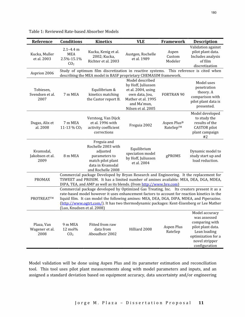
J o r g e M . P l a z a – D i s s e r t a t i o n P r o p o s a l
11
Table 1: Reviewed Rate-based Absorber Models
Reference Conditions Kinetics VLE Framework Description
Kucka, Muller et al. 2003
2.1–4.4 m
MEA 2.5%-15.1%
CO2
Kucka, Kenig et al. 2002; Kucka,
Richter et al. 2003
Austgen, Rochelle et al. 1989
Aspen Custom Modeler
Validation against pilot plant data.
Includes analysis of film
discretization
Asprion 2006 Study of optimum film discretization in reactive systems. This reference is cited when describing the MEA model in BASF proprietary CHEMASIM framework.
Tobiesen, Svendsen et al.
2007 7 m MEA
Equilibrium & kinetics matching
the Castor report B.
Model described by Hoff, Juliussen et al. 2004, using
own data, Jou, Mather et al. 1995
and Ma'mun, Nilsen et al. 2005
FORTRAN 90
Model uses penetration
theory. A comparison with pilot plant data is
presented.
Dugas, Alix et al. 2008
7 m MEA 11-13 % CO2
Versteeg, Van Dijck et al. 1996 with
activity coefficient corrections
Freguia 2002 Aspen Plus® RateSepTM
Model developed to study the
results of the CASTOR pilot
plant campaign #2
Kvamsdal, Jakobsen et al.
2009 8 m MEA
Freguia and Rochelle 2003 with
adjusted parameters to
match pilot plant data in Kvamsdal
and Rochelle 2008
Equilibrium speciation model by Hoff, Juliussen
et al. 2004
gPROMS Dynamic model to study start up and
load reduction.
PROMAX Commercial package Developed by Bryan Research and Engineering. It the replacement for TSWEET and PROSIM. It has a limited number of amines available: MEA, DEA, DGA, MDEA, DIPA, TEA, and AMP as well as its blends. (from http://www.bre.com)
PROTREATTM
Commercial package developed by Optimized Gas Treating, Inc. Its creators present it as a rate-based model however it uses enhancement factors to account for reaction kinetics in the liquid film. It can model the following amines: MEA, DEA, DGA, DIPA, MDEA, and Piperazine. (http://www.ogtrt.com/). It has two thermodynamic packages: Kent-Eisenberg or Lee Mather (Luo, Knudsen et al. 2008)
Plaza, Van Wagener et al.
2008
9 m MEA 12 mol%
CO2
Fitted from raw data from
Aboudheir 2002 Hilliard 2008
Aspen Plus RateSep
Model accuracy was assessed
comparing with pilot plant data.
Lean loading optimization for a
novel stripper configuration
Model validation will be done using Aspen Plus and its parameter estimation and reconciliation
tool. This tool uses pilot plant measurements along with model parameters and inputs, and an
assigned a standard deviation based on equipment accuracy, data uncertainty and/or engineering
180
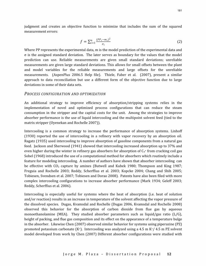
J o r g e M . P l a z a – D i s s e r t a t i o n P r o p o s a l
12
judgment and creates an objective function to minimize that includes the sum of the squared
measurement errors:
𝑓 = (𝑃𝑃𝑖−𝑚 𝑖)
2
𝜎𝑖
𝑛𝑖=1 (2)
Where PP represents the experimental data, m is the model prediction of the experimental data and
σ is the assigned standard deviation. The later serves as boundary for the values that the model
prediction can use. Reliable measurements are given small standard deviations; unreliable
measurements are given large standard deviations. This allows for small offsets between the plant
and model variables for the reliable measurements and large offsets for the unreliable
measurements. (AspenPlus 2006.5 Help file). Thiele, Faber et al. (2007), present a similar
approach to data reconciliation but use a different form of the objective function due to large
deviations in some of their data sets.
PROCESS CONFIGURATION AND OPTIMIZATION
An additional strategy to improve efficiency of absorption/stripping systems relies in the
implementation of novel and optimized process configurations that can reduce the steam
consumption in the stripper and the capital costs for the unit. Among the strategies to improve
absorber performance is the use of liquid intercooling and the multipoint solvent feed (tied to the
matrix stripper (Oyenekan and Rochelle 2007)).
Intercooling is a common strategy to increase the performance of absorption systems. Linhoff
(1930) reported the use of intercooling in a refinery with vapor recovery by an absorption oil.
Ragatz (1935) used intercooling to improve absorption of gasoline components from a natural gas
feed. Jackson and Sherwood (1941) showed that intercooling increased absorption up to 37% and
even higher during the winter in refinery gas absorbers for absorption of C4+ from cracking coil gas
Sobel (1968) introduced the use of a computational method for absorbers which routinely include a
feature for modeling intercooling. A number of authors have shown that absorber intercooling can
be effective with CO2 capture by amines (Butwell and Kubek 1980; Thompson and King 1987;
Freguia and Rochelle 2003; Reddy, Scherffius et al. 2003; Kopcke 2004; Chang and Shih 2005;
Tobiesen, Svendsen et al. 2007; Tobiesen and Dorao 2008). Patents have also been filed with more
complex intercooling configurations to increase absorber performance (Mark 1934; Geleff 2003;
Reddy, Scherffius et al. 2006).
Intercooling is especially useful for systems where the heat of absorption (i.e. heat of solution
and/or reaction) results in an increase in temperature of the solvent affecting the vapor pressure of
the dissolved species. Dugas, Kvamsdal and Rochelle (Dugas 2006, Kvamsdal and Rochelle 2008)
observed this behavior for the absorption of carbon dioxide from flue gas by aqueous
monoethanolamine (MEA). They studied absorber parameters such as liquid/gas ratio (L/G),
height of packing, and flue gas composition and its effect on the appearance of a temperature bulge
in the absorber. Likewise Chen (2007) observed similar behavior for systems using piperazine (PZ)
promoted potassium carbonate (K+). Intercooling was analyzed using a 4.5 m K+/ 4.5 m PZ solvent
model developed from work by Chen (2007) Different absorber configurations were studied with
181
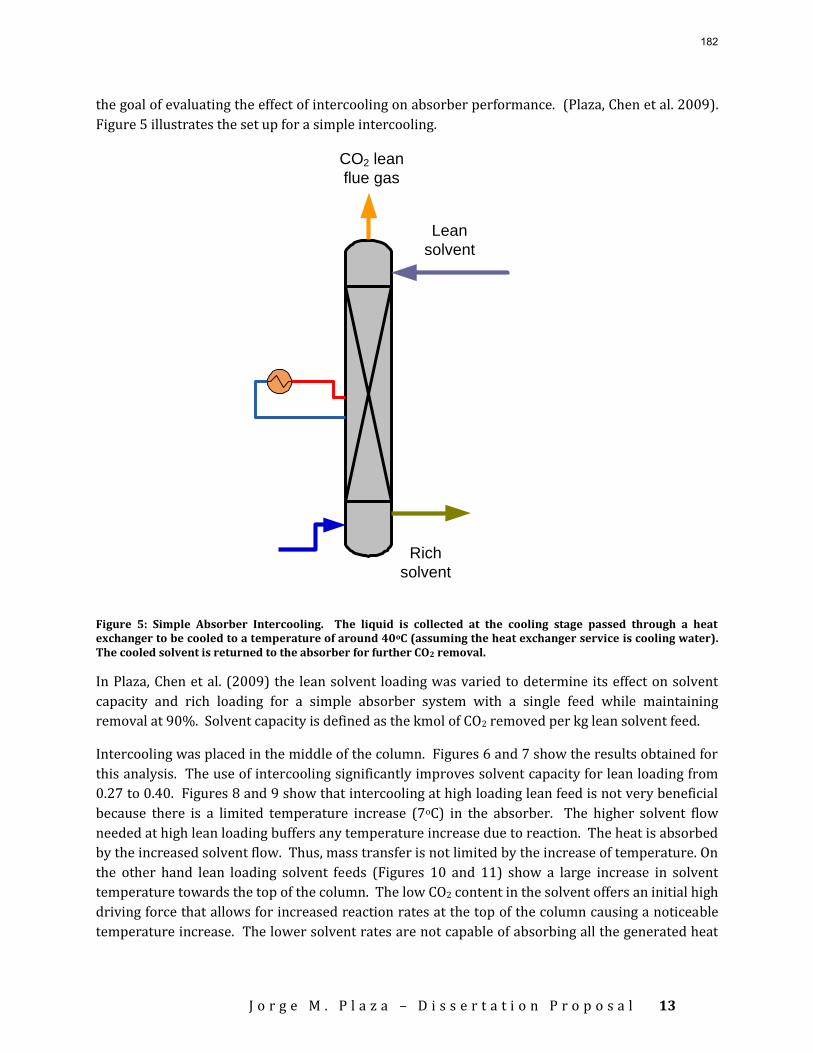
J o r g e M . P l a z a – D i s s e r t a t i o n P r o p o s a l
13
the goal of evaluating the effect of intercooling on absorber performance. (Plaza, Chen et al. 2009).
Figure 5 illustrates the set up for a simple intercooling.
CO2 lean
flue gas
Rich
solvent
Lean
solvent
Figure 5: Simple Absorber Intercooling. The liquid is collected at the cooling stage passed through a heat exchanger to be cooled to a temperature of around 40oC (assuming the heat exchanger service is cooling water). The cooled solvent is returned to the absorber for further CO2 removal.
In Plaza, Chen et al. (2009) the lean solvent loading was varied to determine its effect on solvent
capacity and rich loading for a simple absorber system with a single feed while maintaining
removal at 90%. Solvent capacity is defined as the kmol of CO2 removed per kg lean solvent feed.
Intercooling was placed in the middle of the column. Figures 6 and 7 show the results obtained for
this analysis. The use of intercooling significantly improves solvent capacity for lean loading from
0.27 to 0.40. Figures 8 and 9 show that intercooling at high loading lean feed is not very beneficial
because there is a limited temperature increase (7oC) in the absorber. The higher solvent flow
needed at high lean loading buffers any temperature increase due to reaction. The heat is absorbed
by the increased solvent flow. Thus, mass transfer is not limited by the increase of temperature. On
the other hand lean loading solvent feeds (Figures 10 and 11) show a large increase in solvent
temperature towards the top of the column. The low CO2 content in the solvent offers an initial high
driving force that allows for increased reaction rates at the top of the column causing a noticeable
temperature increase. The lower solvent rates are not capable of absorbing all the generated heat
182
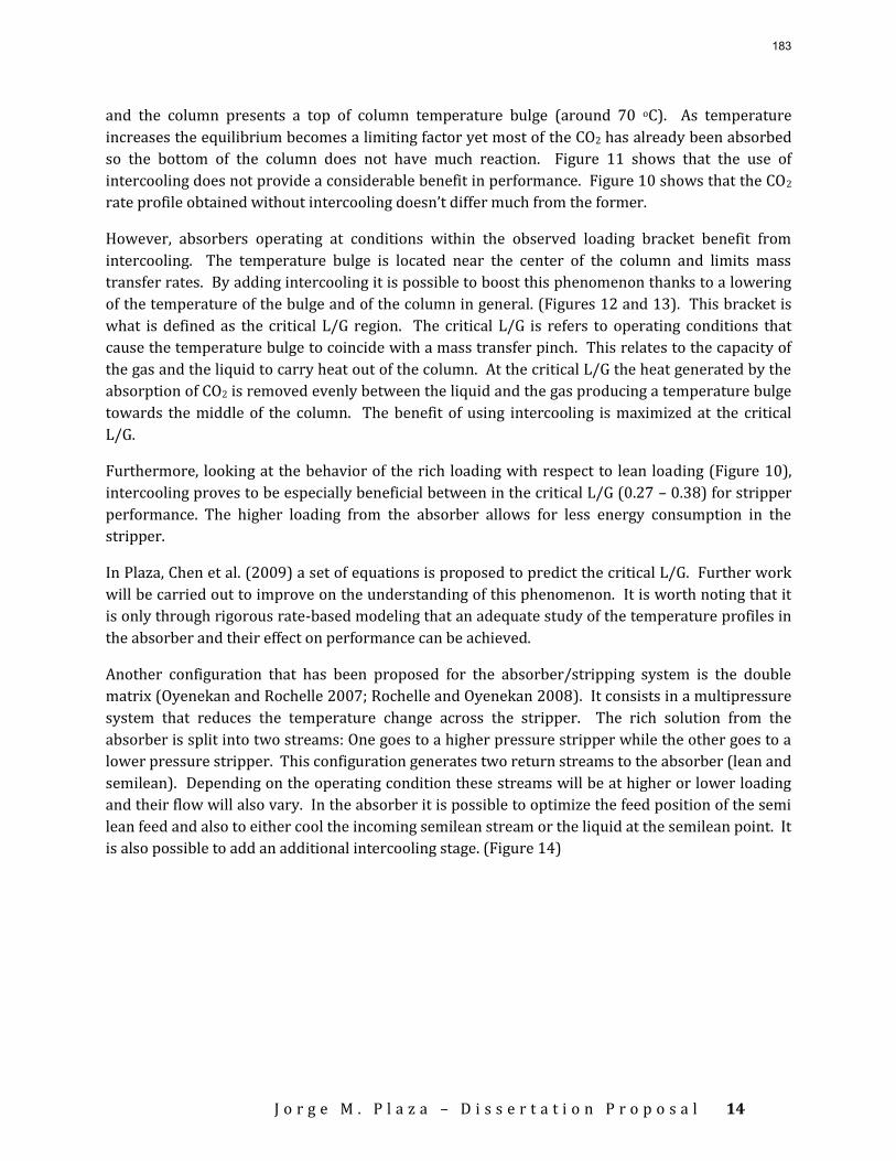
J o r g e M . P l a z a – D i s s e r t a t i o n P r o p o s a l
14
and the column presents a top of column temperature bulge (around 70 oC). As temperature
increases the equilibrium becomes a limiting factor yet most of the CO2 has already been absorbed
so the bottom of the column does not have much reaction. Figure 11 shows that the use of
intercooling does not provide a considerable benefit in performance. Figure 10 shows that the CO2
rate profile obtained without intercooling doesn’t differ much from the former.
However, absorbers operating at conditions within the observed loading bracket benefit from
intercooling. The temperature bulge is located near the center of the column and limits mass
transfer rates. By adding intercooling it is possible to boost this phenomenon thanks to a lowering
of the temperature of the bulge and of the column in general. (Figures 12 and 13). This bracket is
what is defined as the critical L/G region. The critical L/G is refers to operating conditions that
cause the temperature bulge to coincide with a mass transfer pinch. This relates to the capacity of
the gas and the liquid to carry heat out of the column. At the critical L/G the heat generated by the
absorption of CO2 is removed evenly between the liquid and the gas producing a temperature bulge
towards the middle of the column. The benefit of using intercooling is maximized at the critical
L/G.
Furthermore, looking at the behavior of the rich loading with respect to lean loading (Figure 10),
intercooling proves to be especially beneficial between in the critical L/G (0.27 – 0.38) for stripper
performance. The higher loading from the absorber allows for less energy consumption in the
stripper.
In Plaza, Chen et al. (2009) a set of equations is proposed to predict the critical L/G. Further work
will be carried out to improve on the understanding of this phenomenon. It is worth noting that it
is only through rigorous rate-based modeling that an adequate study of the temperature profiles in
the absorber and their effect on performance can be achieved.
Another configuration that has been proposed for the absorber/stripping system is the double
matrix (Oyenekan and Rochelle 2007; Rochelle and Oyenekan 2008). It consists in a multipressure
system that reduces the temperature change across the stripper. The rich solution from the
absorber is split into two streams: One goes to a higher pressure stripper while the other goes to a
lower pressure stripper. This configuration generates two return streams to the absorber (lean and
semilean). Depending on the operating condition these streams will be at higher or lower loading
and their flow will also vary. In the absorber it is possible to optimize the feed position of the semi
lean feed and also to either cool the incoming semilean stream or the liquid at the semilean point. It
is also possible to add an additional intercooling stage. (Figure 14)
183
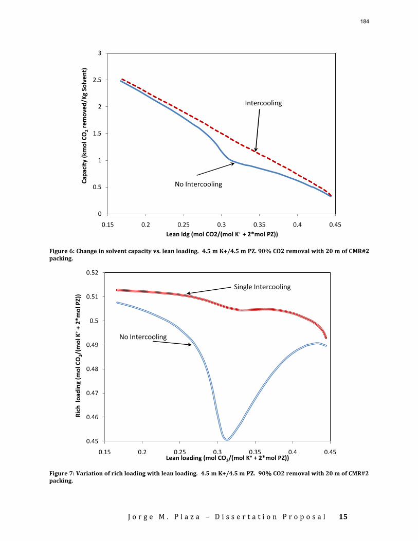
J o r g e M . P l a z a – D i s s e r t a t i o n P r o p o s a l
15
Figure 6: Change in solvent capacity vs. lean loading. 4.5 m K+/4.5 m PZ. 90% CO2 removal with 20 m of CMR#2 packing.
Figure 7: Variation of rich loading with lean loading. 4.5 m K+/4.5 m PZ. 90% CO2 removal with 20 m of CMR#2 packing.
0
0.5
1
1.5
2
2.5
3
0.15 0.2 0.25 0.3 0.35 0.4 0.45
Cap
acit
y (k
mo
l CO
2re
mo
ved
/Kg
Solv
en
t)
Lean ldg (mol CO2/(mol K+ + 2*mol PZ))
No Intercooling
Intercooling
0.45
0.46
0.47
0.48
0.49
0.5
0.51
0.52
0.15 0.2 0.25 0.3 0.35 0.4 0.45
Ric
h l
oad
ing
(mo
l CO
2/(m
ol K
++
2*m
ol P
Z))
Lean loading (mol CO2/(mol K+ + 2*mol PZ))
No Intercooling
Single Intercooling
184
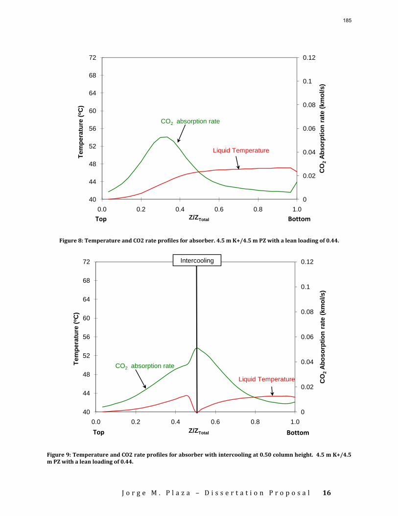
J o r g e M . P l a z a – D i s s e r t a t i o n P r o p o s a l
16
Figure 8: Temperature and CO2 rate profiles for absorber. 4.5 m K+/4.5 m PZ with a lean loading of 0.44.
Figure 9: Temperature and CO2 rate profiles for absorber with intercooling at 0.50 column height. 4.5 m K+/4.5 m PZ with a lean loading of 0.44.
0
0.02
0.04
0.06
0.08
0.1
0.12
40
44
48
52
56
60
64
68
72
0.0 0.2 0.4 0.6 0.8 1.0
CO
2A
bso
rpti
on
rate
(km
ol/s)
Tem
pera
ture
(oC
)
Z/ZTotal
CO2 absorption rate
Liquid Temperature
Top Bottom
0
0.02
0.04
0.06
0.08
0.1
0.12
40
44
48
52
56
60
64
68
72
0.0 0.2 0.4 0.6 0.8 1.0
CO
2A
bo
so
rpti
on
rate
(km
ol/s)
Tem
pera
ture
(oC
)
Z/ZTotal
CO2 absorption rate
Liquid Temperature
Top Bottom
Intercooling
185
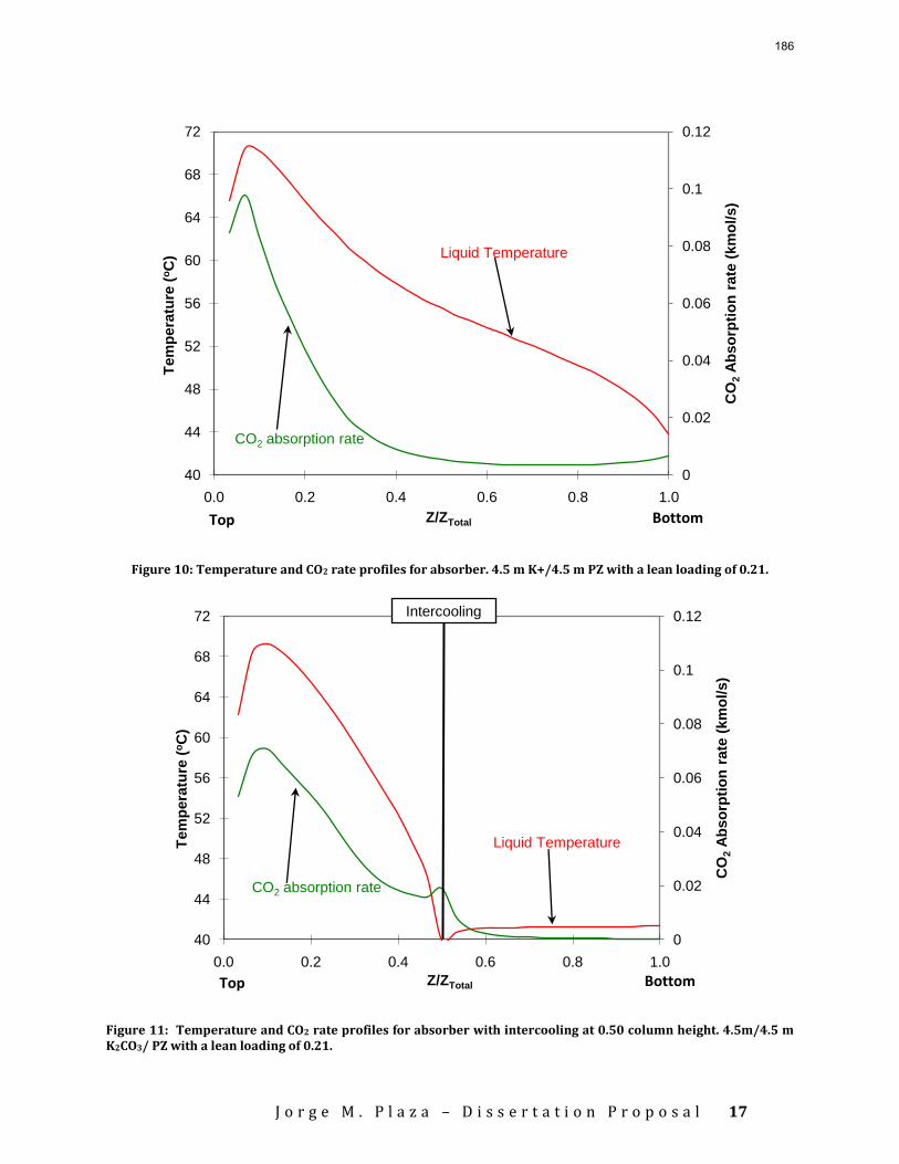
J o r g e M . P l a z a – D i s s e r t a t i o n P r o p o s a l
17
Figure 10: Temperature and CO2 rate profiles for absorber. 4.5 m K+/4.5 m PZ with a lean loading of 0.21.
Figure 11: Temperature and CO2 rate profiles for absorber with intercooling at 0.50 column height. 4.5m/4.5 m K2CO3/ PZ with a lean loading of 0.21.
0
0.02
0.04
0.06
0.08
0.1
0.12
40
44
48
52
56
60
64
68
72
0.0 0.2 0.4 0.6 0.8 1.0
CO
2A
bso
rpti
on
rate
(km
ol/s)
Tem
pe
ratu
re (
oC
)
Z/ZTotal
CO2 absorption rate
Liquid Temperature
Top Bottom
0
0.02
0.04
0.06
0.08
0.1
0.12
40
44
48
52
56
60
64
68
72
0.0 0.2 0.4 0.6 0.8 1.0
CO
2A
bso
rpti
on
rate
(km
ol/s)
Tem
pera
ture
(oC
)
Z/ZTotal
CO2 absorption rate
Liquid Temperature
Intercooling
Top Bottom
186
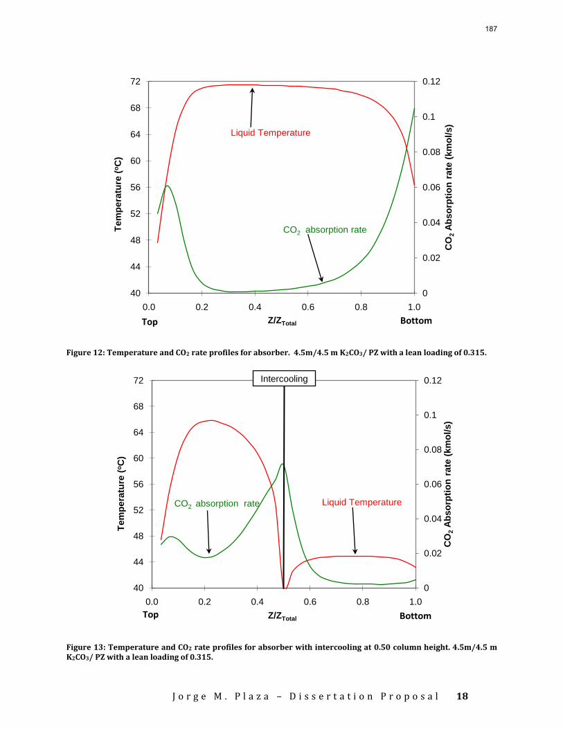
J o r g e M . P l a z a – D i s s e r t a t i o n P r o p o s a l
18
Figure 12: Temperature and CO2 rate profiles for absorber. 4.5m/4.5 m K2CO3/ PZ with a lean loading of 0.315.
Figure 13: Temperature and CO2 rate profiles for absorber with intercooling at 0.50 column height. 4.5m/4.5 m K2CO3/ PZ with a lean loading of 0.315.
0
0.02
0.04
0.06
0.08
0.1
0.12
40
44
48
52
56
60
64
68
72
0.0 0.2 0.4 0.6 0.8 1.0
CO
2A
bso
rpti
on
rate
(km
ol/s)
Tem
pera
ture
(oC
)
Z/ZTotal
CO2 absorption rate
Liquid Temperature
Top Bottom
0
0.02
0.04
0.06
0.08
0.1
0.12
40
44
48
52
56
60
64
68
72
0.0 0.2 0.4 0.6 0.8 1.0
CO
2A
bso
rpti
on
rate
(km
ol/s)
Tem
pera
ture
(oC
)
Z/ZTotal
CO2 absorption rate Liquid Temperature
Intercooling
Top Bottom
187
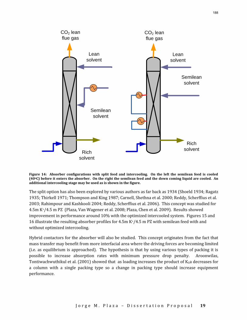
J o r g e M . P l a z a – D i s s e r t a t i o n P r o p o s a l
19
CO2 lean
flue gas
Rich
solvent
Lean
solvent
Semilean
solvent
CO2 lean
flue gas
Rich
solvent
Lean
solvent
Semilean
solvent
Figure 14: Absorber configurations with split feed and intercooling. On the left the semilean feed is cooled (40oC) before it enters the absorber. On the right the semilean feed and the down coming liquid are cooled. An additional intercooling stage may be used as is shown in the figure.
The split option has also been explored by various authors as far back as 1934 (Shoeld 1934; Ragatz
1935; Thirkell 1971; Thompson and King 1987; Carnell, Shethna et al. 2000; Reddy, Scherffius et al.
2003; Rahimpour and Kashkooli 2004; Reddy, Scherffius et al. 2006). This concept was studied for
4.5m K+/4.5 m PZ (Plaza, Van Wagener et al. 2008; Plaza, Chen et al. 2009). Results showed
improvement in performance around 10% with the optimized intercooled system. Figures 15 and
16 illustrate the resulting absorber profiles for 4.5m K+/4.5 m PZ with semilean feed with and
without optimized intercooling.
Hybrid contactors for the absorber will also be studied. This concept originates from the fact that
mass transfer may benefit from more interfacial area where the driving forces are becoming limited
(i.e. as equilibrium is approached). The hypothesis is that by using various types of packing it is
possible to increase absorption rates with minimum pressure drop penalty. Aroonwilas,
Tontiwachwuthikul et al. (2001) showed that as loading increases the product of KGa decreases for
a column with a single packing type so a change in packing type should increase equipment
performance.
188
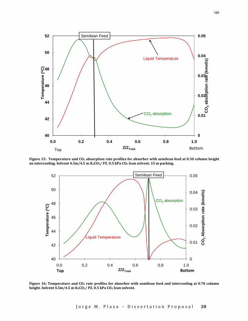
J o r g e M . P l a z a – D i s s e r t a t i o n P r o p o s a l
20
Figure 15: Temperature and CO2 absorption rate profiles for absorber with semilean feed at 0.30 column height no intercooling. Solvent 4.5m/4.5 m K2CO3/ PZ. 0.5 kPa CO2 lean solvent. 15 m packing.
Figure 16: Temperature and CO2 rate profiles for absorber with semilean feed and intercooling at 0.70 column height. Solvent 4.5m/4.5 m K2CO3/ PZ. 0.5 kPa CO2 lean solvent.
0
0.01
0.02
0.03
0.04
0.05
40
42
44
46
48
50
52
0.0 0.2 0.4 0.6 0.8 1.0
CO
2ab
so
rpti
on
rate
(km
ol/s)
Tem
pera
ture
(oC
)
Z/ZTotal
CO2 absorption
Liquid Temperature
Top Bottom
Semilean Feed
0
0.01
0.02
0.03
0.04
0.05
40
42
44
46
48
50
52
0.0 0.2 0.4 0.6 0.8 1.0
CO
2A
bso
rpti
on
rate
(km
ol/s)
Tem
pe
ratu
re (
oC
)
Z/ZTotal
CO2 absorption
Liquid Temperature
Semilean Feed
Top Bottom
189
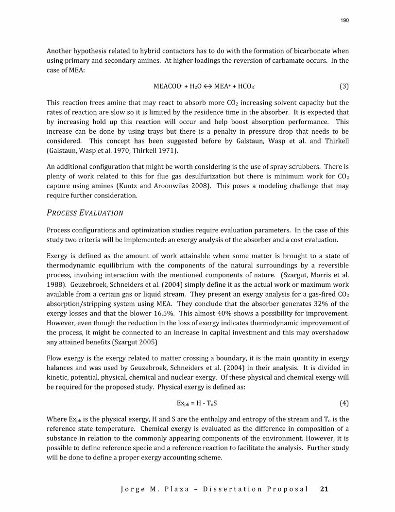
J o r g e M . P l a z a – D i s s e r t a t i o n P r o p o s a l
21
Another hypothesis related to hybrid contactors has to do with the formation of bicarbonate when
using primary and secondary amines. At higher loadings the reversion of carbamate occurs. In the
case of MEA:
MEACOO- + H2O ↔ MEA+ + HCO3- (3)
This reaction frees amine that may react to absorb more CO2 increasing solvent capacity but the
rates of reaction are slow so it is limited by the residence time in the absorber. It is expected that
by increasing hold up this reaction will occur and help boost absorption performance. This
increase can be done by using trays but there is a penalty in pressure drop that needs to be
considered. This concept has been suggested before by Galstaun, Wasp et al. and Thirkell
(Galstaun, Wasp et al. 1970; Thirkell 1971).
An additional configuration that might be worth considering is the use of spray scrubbers. There is
plenty of work related to this for flue gas desulfurization but there is minimum work for CO2
capture using amines (Kuntz and Aroonwilas 2008). This poses a modeling challenge that may
require further consideration.
PROCESS EVALUATION
Process configurations and optimization studies require evaluation parameters. In the case of this
study two criteria will be implemented: an exergy analysis of the absorber and a cost evaluation.
Exergy is defined as the amount of work attainable when some matter is brought to a state of
thermodynamic equilibrium with the components of the natural surroundings by a reversible
process, involving interaction with the mentioned components of nature. (Szargut, Morris et al.
1988). Geuzebroek, Schneiders et al. (2004) simply define it as the actual work or maximum work
available from a certain gas or liquid stream. They present an exergy analysis for a gas-fired CO2
absorption/stripping system using MEA. They conclude that the absorber generates 32% of the
exergy losses and that the blower 16.5%. This almost 40% shows a possibility for improvement.
However, even though the reduction in the loss of exergy indicates thermodynamic improvement of
the process, it might be connected to an increase in capital investment and this may overshadow
any attained benefits (Szargut 2005)
Flow exergy is the exergy related to matter crossing a boundary, it is the main quantity in exergy
balances and was used by Geuzebroek, Schneiders et al. (2004) in their analysis. It is divided in
kinetic, potential, physical, chemical and nuclear exergy. Of these physical and chemical exergy will
be required for the proposed study. Physical exergy is defined as:
Exph = H - ToS (4)
Where Exph is the physical exergy, H and S are the enthalpy and entropy of the stream and To is the
reference state temperature. Chemical exergy is evaluated as the difference in composition of a
substance in relation to the commonly appearing components of the environment. However, it is
possible to define reference specie and a reference reaction to facilitate the analysis. Further study
will be done to define a proper exergy accounting scheme.
190
J o r g e M . P l a z a – D i s s e r t a t i o n P r o p o s a l
22
A number of economical analysis have been conducted related to CO2 capture with MEA (Singh,
Croiset et al. 2003; Rochelle, Fisher et al. 2005; Abu-Zahra, Niederer et al. 2007) they will serve as
guidelines for the analysis for this work. The goal will be to integrate the exergy analysis with the
economic estimates to determine optimum conditions for the resulting process configurations.
Additionally, comparisons between solvents will also be conducted. Results will include
recommendations on the best configurations for each solvent based on the minimization of exergy
and capital costs. These analyses will be centered in the absorber but a methodology will be
defined to account for the stripper.
TIMELINE The proposed timeline includes the activities and expected results for each semester.
SPRING 2009
Develop an absorber rate-based model for PZ using the VLE framework by Hilliard (Hilliard
2008) and adapted by David Van Wagener for high PZ concentrations; and the kinetic data
provided by Ross Dugas.
Verify PZ physical properties for the absorber model.
Reconcile PZ model with data from the PZ campaign.
SUMMER 2009
Continue reconciliation of model with data from the PZ campaign.
Generate operating conditions for the PZ campaign and the MEA baseline of Fall 2009. This
campaign will include intercooling so the critical L/G for the pilot plant will be predicted.
Revisit the developed MEA model (Plaza, Van Wagener et al. 2008; Zhang, Chen et al. 2009)
to verify adequate physical properties and include recent data by Ross Dugas.
Develop the framework for the exergy and economic analysis
FALL 2009
Work on the film and packing height segmentation.
Help run the PZ pilot plant campaign.
Reconcile PZ model using data from the Fall 2009 PZ campaign
Reconcile the MEA model with the baseline run for the Fall 2009 pilot plant campaign.
SPRING 2010
Evaluate absorber performance with various packings with different interfacial area and
pressure drop.
Study intercooling (simple and with split feed) for the PZ solvent.
191
J o r g e M . P l a z a – D i s s e r t a t i o n P r o p o s a l
23
SUMMER 2010
Study absorber height-diameter relations to asses conditions under which mass transfer
begins to be limited by kL or kG and not by the interfacial area.
Evaluate liquid hold up and analyze its effects in the formation of bicarbonate.
FALL 2010
Study the use of hybrid contactors to increase absorber performance.
Conduct economic and exergy analysis on the configurations proposed for CO2 absorption:
intercooling, split feed, hybrid contactors and any others.
SPRING 2011
Establish optimum conditions and configurations for MEA and PZ.
Define guidelines for adequate and efficient rate-based absorber model development using
AspenPlus.
Dissertation write up
Graduation
ATTACHMENTS Attachment A consists of a table of all of the MEA models found during the literature review.
REFERENCES (2007). IPCC, 2007: Summary for Policymakers. Climate Change 2007: The Physical Science Basis.
Contribution of Working Group I to the Fourth Assessment Report of the Intergovernmental Panel on Climate Change S. Solomon, D. Qin, M. Manninget al. Cambridge, UK and New York, NY, USA, Cambridge University Press.
Aboudheir, A. (2002). Kinetics, Modeling and Simulation of CO2 Absorption into Highly Concentrated and Loaded MEA Solutions. Chemical Engineering. Regina, University of Regina. Ph.D
Abu-Zahra, M. R. M., J. P. M. Niederer, et al. (2007). "CO2 capture from power plants - Part II. A parametric study of the economical performance based on mono-ethanolamine." International Journal of Greenhouse Gas Control 1(2): 135-142.
Abu-Zahra, M. R. M., L. H. J. Schneiders, et al. (2007). "CO2 capture from power plants. Part I. A parametric study of the technical-performance based on monoethanolamine." International Journal of Greenhouse Gas Control 1(1): 37-46.
Al-Baghli, N. A., S. A. Pruess, et al. (2001). "A rate-based model for the design of gas absorbers for the removal Of CO2 and H2S using aqueous solutions of MEA and DEA." Fluid Phase Equilibria 185(1-2): 31-43.
Alatiqi, I., M. F. Sabri, et al. (1994). "Steady-State Rate-Based Modeling for Co2/Amine Absorption Desorption Systems." Gas Separation & Purification 8(1): 3-11.
Alie, C., L. Backham, et al. (2005). "Simulation of CO2 capture using MEA scrubbing: a flowsheet decomposition method." Energy Conversion and Management 46(3): 475-487.
192
J o r g e M . P l a z a – D i s s e r t a t i o n P r o p o s a l
24
Appl, M., U. Wagner, et al. (1982). Removal of CO2 and/or COS from Gases Containing these Constituents U. S. P. Office. United States of America, BASF Aktiengesellschaft. 4336233.
Aroonwilas, A., P. Tontiwachwuthikul, et al. (2001). "Effects of operating and design parameters on CO2 absorption in columns with structured packings." Separation and Purification Technology 24(3): 403-411.
Asprion, N. (2006). "Nonequilibrium rate-based simulation of reactive systems: Simulation model, heat transfer, and influence of film discretization." Industrial & Engineering Chemistry Research 45(6): 2054-2069.
Asprion, N. and C. Grossmann (2004). Method for Removal of Acid Gases from a Glass Flow. U. S. P. Office. United States of America. US2004/0154469A1.
Astarita, G. (1967). Mass Transfer with Chemical Reaction. Amsterdam, Elsevier Publishing Company.
Austgen, D. M. (1989). A Model of Vapor-Liquid Equlibria for Acid Gas-Alkanolamine-Water System. Chemical Engineering. Austin, Texas, The University of Texas at Austin. Ph.D.
Austgen, D. M., G. T. Rochelle, et al. (1989). "Model of Vapor Liquid Equilibria for Aqueous Acid Gas Alkanolamine Systems Using the Electrolyte Nrtl Equation." Industrial & Engineering Chemistry Research 28(7): 1060-1073.
Barchas, R. and R. Davis (1992). "The Kerr-Mcgee Abb Lummus Crest Technology for the Recovery of Co2 from Stack Gases." Energy Conversion and Management 33(5-8): 333-340.
Bottoms, R. R. (1930). Process for Separating Acid Gases. U. S. P. Office. United States, Girdler Corporation. 1783901.
Butwell, K. and D. Kubek (1980). Process for CO2 Removal. U. S. P. Office. United States, Union Carbide Corporation. 4184855.
Carnell, P. J. H., H. Shethna, et al. (2000). Gas Absorption. U. S. P. Office. United States of America, Imperial Chemical Industries PLC. 6139605.
Chang, H. and C. M. Shih (2005). "Simulation and optimization for power plant flue gas CO2 absorption-stripping systems." Separation Science and Technology 40(4): 877-909.
Chapel, D. G., C. Mariz, et al. (1999). Recovery of CO2 from Flue Gases: Commercial Trends. Canadian Society of Chemical Engineers Annual Meeting. Saskatoon, Saskatchewan, Canada.
Chen, C. C., H. I. Britt, et al. (1982). "Local Composition Model for Excess Gibbs Energy for Electrolyte Systems." AIChE Journal 28(4): 588-596.
Chen, E. (2007). Carbon Dioxide Absorption into Piperazine Promoted Potassium Carbonate using Structured Packing. Chemical Engineering. Austin, Texas, The University of Texas at Austin. PhD.
Core-Writing-Team (2007). Climate Change 2007 Synthesis Report. IPCC Fourth Assessment Report. R. K. Pachauri and A. Reisinger. Geneva, Switzerland.
Cullinane, J. T. (2005). Thermodynamics and Kinetics of Aqueous Piperazine with Potassium Carbonate for Carbon Dioxide Absorption. Chemical Engineering. Austin, Texas, The University of Texas at Austin. Ph.D.
Danckwerts, P. V. (1951). " Significance of liquid-film coefficients in gas absorption." Journal of Industrial and Engineering Chemistry (Washington, D. C.) 43: 1460-7.
Danckwerts, P. V. (1970). Gas-Liquid Reactions. New York, McGraw-Hill Inc. Danckwerts, P. V. (1979). "Reaction of CO2 with Ethanolamines." Chemical Engineering Science
34(4): 443-446. Danckwerts, P. V. and S. M.M (1966). "The Absorption of Carbon Dioxide into Solutions of Alkalis
and Amines (With Some Notes on Hydrogen Sulphide and Carbonyl Sulphide)." The Chemical Engineer(October).
Dang, H. (2000). CO2 Absorption Rate and Solubility in MEA/PZ/H2O. Chemical Engineering. Austin, TX, The University of Texas at Austin. Msc.
193
J o r g e M . P l a z a – D i s s e r t a t i o n P r o p o s a l
25
Dugas, R. (2006). Pilot Plant Study of Carbon Dioxide Capture by Aqueous Monoethanolamine. Chemical Engineering. Austin, Texas, The University of Texas at Austin. Master.
Dugas, R., P. Alix, et al. (2008). "Creation of an Aspen RateSep Absorber Model for the Evaluation of CASTOR Pilot Plant Data." American Chemical Society, Division of Petroleum Chemistry 53(1): 89-92.
Freeman, S., R. Dugas, et al. (2008). Carbon Dioxide Capture with Concentrated, Aqueous Piperazine. 9th International Conference on Greenhouse Gas Control Technologies. Washington D.C., Elsevier.
Freguia, S. (2002). Modeling of CO2 Removal from Flue Gas with Monoethanolamine. Chemical Engineering. Austin, Texas, The University of Texas at Austin. Masters.
Freguia, S. and G. T. Rochelle (2003). "Modeling of CO2 capture by aqueous monoethanolamine." AIChE Journal 49(7): 1676-1686.
Fujii, M., Y. Hotta, et al. (1994). Apparatus and Process for Removing Carbon Dioxide from Combustion Exhaust Gas. U. S. P. Office. United States of America, Mitsubishi Jukogyo Kabushiki & Kansai Electric Power Co., Inc. 5318758.
Fujii, M., Y. Hotta, et al. (2001). Recovery of Carbon Dioxide from Combustion Exhaust Gas. U. S. P. Office. United States of America, Mitsubishi Jukogyo Kabushiki & Kansai Electric Power Co., Inc. 6274108.
Galstaun, L., B. Wasp, et al. (1970). Method of Removing Carbon Dioxide from Gases. U. S. P. Office. United States of America, Bechtel International Corporation. 3489506.
Geleff, S. (2003). Method and Device for Recovery of Thermal Energy from an Exothermic Carbon Dioxide Absorption Process W. I. P. Organization.
Geuzebroek, F. H., L. H. J. M. Schneiders, et al. (2004). "Exergy analysis of alkanolamine-based CO2 removal unit with AspenPlus." Energy 29(9-10): 1241-1248.
Glasscock, D. A., J. E. Critchfield, et al. (1991). "Co2 Absorption Desorption in Mixtures of Methyldiethanolamine with Monoethanolamine or Diethanolamine." Chemical Engineering Science 46(11): 2829-2845.
Hikita, H., S. Asai, et al. (1979). "Absorption of Carbon-Dioxide into Aqueous Monoethanolamine Solutions." Aiche Journal 25(5): 793-800.
Hilliard, M. (2005). Thermodynamics of Aqueous Piperazine/Potassium Carbonate/Carbon Dioxide Characterized by the Electrolyte NRT Model within Aspen Plus®. Chemical Engineering. Austin, Texas, The University of Texas at Austin. Masters.
Hilliard, M. D. (2008). A Predictive Thermodynamic Model for an Aqueous Blend of Potassium Carbonate, Piperazine, and Monoethanolamine for Carbon Dioxide Capture from Flue Gas,. Chemical Engineering. Austin, Texas, The University of Texas at Austin. Ph.D.
Hoff, K. A., O. Juliussen, et al. (2004). "Modeling and experimental study of carbon dioxide absorption in aqueous alkanolamine solutions using a membrane contactor." Industrial & Engineering Chemistry Research 43(16): 4908-4921.
Idem, R., M. Wilson, et al. (2006). "Pilot plant studies of the CO2 capture performance of aqueous MEA and mixed MEA/MDEA solvents at the University of Regina CO2 capture technology development plant and the Boundary Dam CO2 capture demonstration." Industrial & Engineering Chemistry Research 45(8): 2414-2420.
Jackson, R. M. and T. K. Sherwood (1941). "Performance of Refinery Gas Absorbers with and without Intercoolers." American Institute of Chemical Engineers Transactions 37: 959-978.
Jamal, A., A. Meisen, et al. (2006). "Kinetics of carbon dioxide absorption and desorption in aqueous alkanolamine solutions using a novel hemispherical contactor - I. Experimental apparatus and mathematical modeling." Chemical Engineering Science 61(19): 6571-6589.
Jou, F. Y., A. E. Mather, et al. (1995). "The Solubility of Co2 in a 30-Mass-Percent Monoethanolamine Solution." Canadian Journal of Chemical Engineering 73(1): 140-147.
194
J o r g e M . P l a z a – D i s s e r t a t i o n P r o p o s a l
26
Jou, F. Y., A. E. Mather, et al. (1995). "The Solubility of CO2 in a 30 mass percent monoethanolamine solution." Can J Chem Eng. 1995(73): 7.
Kenig, E., L. Kucka, et al. (2003). "Rigorous Modeling of Reactive Absorption Processes." Chem. Eng. Technol. 26(6).
Kenig, E. and P. Seferlis (2009). "Modeling Reactive Absorption." Chemical Engineering Progress 105(1): 65-73.
Kent, R. L. and B. Eisenberg (1976). "Better Data for Amine Treating." Hydrocarbon Processing 55(2): 87-90.
Kopcke, M. (2004). CO2 Removal from Flue Gas in Power Generation: Simulation Study of MEA Absorption. Department of Chemical Engineering. Gothemburg, Sweden, Chalmers University of Technology. Masters.
Kucka, L., E. Y. Kenig, et al. (2002). "Kinetics of the gas-liquid reaction between carbon dioxide and hydroxide ions." Industrial & Engineering Chemistry Research 41(24): 5952-5957.
Kucka, L., I. Muller, et al. (2003). "On the Modelling and Simulation of sour gas absorption by aqueous amine solutions." Chemical Engineering Science 58.
Kucka, L., J. Richter, et al. (2003). "Determination of gas-liquid reaction kinetics with a stirred cell reactor." Separation and Purification Technology 31(2): 163-175.
Kuntz, J. and A. Aroonwilas (2008). "Performance of spray column for CO2 capture application." Industrial & Engineering Chemistry Research 47(1): 145-153.
Kvamsdal, H. M., J. P. Jakobsen, et al. (2009). "Dynamic modeling and simulation of a CO2 absorber column for post-combustion CO2 capture." Chemical Engineering and Processing 48(1): 135-144.
Kvamsdal, H. M. and G. T. Rochelle (2008). "Effects of the temperature bulge in CO2 absorption from flue gas by aqueous monoethanolamine." Industrial & Engineering Chemistry Research 47(3): 867-875.
Licht and R. Weiland (1989). Density and Physical Stability of Carbon Dioxide in Partially Loaded Solutions of MDEA, DEA, and MEA. AIChE Spring National Meeting.
Linhoff, H. R. (1930). "Intercoolers used in absorber at vapor-recovery plants." National Petroleum News 22(20).
Liu, G. B., K. T. Yu, et al. (2006). "Simulations of chemical absorption in pilot-scale and industrial-scale packed columns by computational mass transfer." Chemical Engineering Science 61(19): 6511-6529.
Luo, X., J. N. Knudsen, et al. (2008). Comparison and Validation of Simulation Codes against Sixteen Sets of Data from Four Different Pilot Plants. 9th International Conference on Greenhouse Gas Control Technologies. Washington D.C, Elsevier.
Ma'mun, S., R. Nilsen, et al. (2005). "Solubility of carbon dioxide in 30 mass % monoethanolamine and 50 mass % methyldiethanolamine solutions." Journal of Chemical and Engineering Data 50(2): 630-634.
Mark, S. (1934). Purification and Separation of Gaseous Mixtures. U. S. P. Office. United States of America. 1971798.
Mofarahi, M., Y. Khojasteh, et al. (2008). "Design of CO2 absorption plant for recovery of CO2 from flue gases of gas turbine." Energy 33(8): 1311-1319.
Noeres, C., E. Y. Kenig, et al. (2003). "Modelling of reactive separation processes: reactive absorption and reactive distillation." Chemical Engineering and Processing 42(3): 157-178.
Oexmann, J., C. Hensel, et al. (2008). "Post-combustion CO2-capture from coal-fired power plants: Preliminary evaluation of an integrated chemical absorption process with piperazine-promoted potassium carbonate." International Journal of Greenhouse Gas Control 2(4): 539-552.
Oi, L. E. (2007). Aspen HYSYS Simulation of CO2 Removal by Amine Absorption from a Gas Based Power Plant. SIMS2007 Conference. Gothenburg, Sweden.
195
J o r g e M . P l a z a – D i s s e r t a t i o n P r o p o s a l
27
Oyenekan, B. A. and G. T. Rochelle (2007). "Alternative stripper configurations for CO2 capture by aqueous amines." Aiche Journal 53(12): 3144-3154.
Pacheco, M. A. and D. G. Rochelle (1998). "Rate-Based Modeling of Reactive Absorption of CO2 and H2S into Aqueous Methyldiethanolamine." Ind. Eng. Chem. Res. 37: 10.
Pintola, T., P. Tontiwachwuthikul, et al. (1993). "Simulation of pilot plant and industrial carbon dioxide-MEA absorbers. ." Gas Separation & Purification 7(1): 47-52.
Pitzer, K. (1973). "Thermodynamics of Electrolytes. I. Theoretical Basis and General Equations." Journal of Physical Chemistry 77(2): 268-277.
Plaza, J. M., E. Chen, et al. (2009). "Absorber Intercooling in CO2 Absorption by Piperazine Promoted Potassium Carbonate." AIChE Journal Submitted for publication.
Plaza, J. M., D. Van Wagener, et al. (2008). Modeling CO2 Capture with Aqueous Monoethanolamine. 9th International Conference on Greenhouse Gas Control Technologies. Washington D.C, Elsevier.
Ragatz, E. (1935). Method for the Absorption of Gases. U. S. P. Office. United States of America, Union Oil Company. 1987267.
Rahimpour, M. R. and A. Z. Kashkooli (2004). "Enhanced carbon dioxide removal by promoted hot potassium carbonate in a split-flow absorber." Chemical Engineering and Processing 43(7): 857-865.
Reddy, S., J. Scherffius, et al. (2003). Fluor's Econamine FG PlusSM Technology : An Enhanced Amine-Based CO2 Capture Process. Second National Conference on Carbon Sequestration. Alexandria, VA.
Reddy, S., J. Scherffius, et al. (2006). Split Flow Process and Apparatus. United States of America US20060032377A1.
Reed, R. (1949). Method of and Apparatus for the Separation of Acidic Gases from Gaseous Mixtures. U. S. P. Office. United States of America, The Girdler Corporation. 2466183.
Rochelle, G., S. Chi, et al. (2001). Research Needs for CO2 Capture from Flue Gas by Aqueous Absorption/Stripping. Austin, TX, U.S. Department of Energy - Federal Energy Technology Center.
Rochelle, G. T., K. S. Fisher, et al. (2005). Integrating MEA Regeneration with CO2 Compression and Peaking to Reduce CO2 Capture Costs, DOE Final Report for Trimeric Corp.
Rochelle, G. T. and B. A. Oyenekan (2008). Regeneration of an aqueous solution from an acid gas absorption process by matrix stripping. U. S. P. Office. United States of America.
Rogner, H.-H., D. Zhou, et al. (2007). Introduction. Climate Change 2007: Mitigation. Contribution of Working Group III to the Forth Assessment Report of the Intergovermental Panel on Climate Change. B. Metz, O. R. Davidson, P. R. Bosch, R. Dave and L. A. Meyer. Cambridge, UK and New York, NY, USA, Cambridge University Press.
Saxena, M. N. and W. Flintoff (2006). "Engineering and economics of CO2 removal and sequestration." Hydrocarbon Processing 85(12): 57-64.
Sherwood, T. K. and R. Pigford (1952). Absorption and Extraction. New York, McGraw-Hill Book Company, Inc.
Shoeld, M. (1934). Purification and Separation of Gaseous Mixtures. U. S. P. Office. United States of America, The Koppers Co. 1971798.
Sims, R. E. H., R. N. Schock, et al. (2007). Energy Supply. Climate Change 2007: Mitigation. Contribution of Working Group III to the Forth Assessment Report of the Intergovermental Panel on Climate Change. B. Metz, O. R. Davidson, P. R. Bosch, R. Dave and L. A. Meyer. Cambridge, UK and New York, NY, USA, Cambridge University Press.
Singh, D., E. Croiset, et al. (2003). "Techno-economic study of CO2 capture from an existing coal-fired power plant: MEA scrubbing vs. O-2/CO2 recycle combustion." Energy Conversion and Management 44(19): 3073-3091.
196
J o r g e M . P l a z a – D i s s e r t a t i o n P r o p o s a l
28
Sobel, B. A. (1968). "Iterative processes: a relaxation operator and its application to the the computation of absorber columns." American Chemical Society, Division of Petroleum Chemistry 13(3): 5.
Solomon, S., D. Qin, et al. (2007). 2007: Technical Summary. Climate Change 2007: The Physical Science Basis. Contribution of Working Group I to the Fourth Assessment Report of the Intergovernmental Panel on Climate Change S. Solomon, D. Qin, M. Manninget al. Cambridge, UK and New York, NY, USA, Cambridge University Press.
Szargut, J. (2005). Exergy Method Technical and Ecological Applications. Billerica, MA, WIT Press. Szargut, J., D. Morris, et al. (1988). Exergy Analysis of Thermal, Chemical and Metallurgical
Processes. New York City, Hemisphere Publishing. Taylor, R. and R. Krishna (1993). Multicomponent Mass Transfer. New York City, John Wiley & Sons. Thiele, R., R. Faber, et al. (2007). "Design of industrial reactive absorption processes in sour gas
treatment using rigorous modelling and accurate experimentation." Chemical Engineering Research & Design 85(A1): 74-87.
Thirkell, H. (1971). Removal of Acidic Gases from Gaseous Mixtures. U. S. P. Office. United States of America, The Power-Gas Corporation Limited. 3565573.
Thompson, R. E. and C. J. King (1987). "Energy conservation in regenerated chemical absorption processes." Chemical Engineering and Processing 21(3): 14.
Tobiesen, F. A. and C. A. Dorao (2008). A simulation Study of Alternative Process Configurations for a CO2 Absorption Plant Using CO2SIM 9th International Conference on Greenhouse Gas Control Technologies. Washington D.C., Elsevier.
Tobiesen, F. A., H. F. Svendsen, et al. (2007). "Experimental validation of a rigorous absorber model for CO2 postcombustion capture." AIChe Journal 53(4): 846-865.
Tobiesen, F. A., H. F. Svendsen, et al. (2007). "Modeling of blast furnace CO2 capture using amine absorbents." Industrial & Engineering Chemistry Research 46(23): 7811-7819.
Tontiwachwuthikul, P., A. Meisen, et al. (1992). "Co2 Absorption by Naoh, Monoethanolamine and 2-Amino-2-Methyl-1-Propanol Solutions in a Packed-Column." Chemical Engineering Science 47(2): 381-390.
Vaidya, P. and E. Kenig (2007). "Gas-Liquid Reaction Kinetics: A Review of Determination Methods." Chemical Engineering Communications 194.
Vaidya, P. and E. Kenig (2008). "Acceleration of CO2 with N,N-Diethylethanolamine in Aqueous Solutions by Piperazine." Ind. Eng. Chem. Res. 47: 34-38.
Versteeg, G. F., L. A. J. Van Dijck, et al. (1996). "On the kinetics between CO2 and alkanolamines both in aqueous and non-aqueous solutions. An overview." Chemical Engineering Communications 144: 113-158.
Wellek, R. M., R. J. Brunson, et al. (1978). "Enhancement Factors for Gas-Absorption with 2nd-Order Irreversible Chemical-Reaction." Canadian Journal of Chemical Engineering 56(2): 181-186.
Wilson, M., P. Tontiwachwuthikul, et al. (2004). "Test results from a CO2 extraction pilot plant at boundary dam coal-fired power station." Energy 29(9-10): 1259-1267.
Zhang, Y., C.-C. Chen, et al. (2009). "Rate-Based Process Modeling Study of CO2 Capture with Aqueous Monoethanolamine Solution." Industrial & Engineering Chemistry Research Submitted for Publication.
197
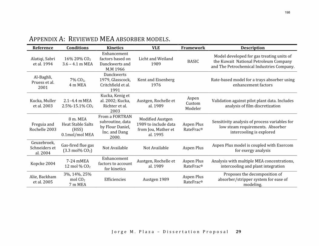
J o r g e M . P l a z a – D i s s e r t a t i o n P r o p o s a l
29
APPENDIX A: REVIEWED MEA ABSORBER MODELS. Reference Conditions Kinetics VLE Framework Description
Alatiqi, Sabri et al. 1994
16% 20% CO2 3.6 – 4.1 m MEA
Enhancement factors based on Danckwerts and
M.M 1966
Licht and Weiland 1989
BASIC Model developed for gas treating units of the Kuwait National Petroleum Company
and The Petrochemical Industries Company.
Al-Baghli, Pruess et al.
2001
7% CO2, 4 m MEA
Danckwerts 1979, Glasscock, Critchfield et al.
1991
Kent and Eisenberg 1976
Rate-based model for a trays absorber using
enhancement factors
Kucka, Muller et al. 2003
2.1–4.4 m MEA 2.5%-15.1% CO2
Kucka, Kenig et al. 2002; Kucka,
Richter et al. 2003
Austgen, Rochelle et al. 1989
Aspen Custom Modeler
Validation against pilot plant data. Includes analysis of film discretization
Freguia and Rochelle 2003
8 m. MEA Heat Stable Salts
(HSS) 0.1mol/mol MEA
From a FORTRAN subroutine, data by Flour Daniel,
Inc. and Dang 2000.
Modified Austgen 1989 to include data from Jou, Mather et
al. 1995
Aspen Plus RateFrac®
Sensitivity analysis of process variables for low steam requirements. Absorber
intercooling is explored
Geuzebroek, Schneiders et
al. 2004
Gas-fired flue gas (3.3 mol% CO2)
Not Available Not Available Aspen Plus Aspen Plus model is coupled with Exercom
for exergy analysis
Kopcke 2004 7-24 mMEA
12 mol % CO2
Enhancement factors to account
for kinetics
Austgen, Rochelle et al. 1989
Aspen Plus RateFrac®
Analysis with multiple MEA concentrations, intercooling and plant integration
Alie, Backham et al. 2005
3%, 14%, 25% mol CO2
7 m MEA Efficiencies Austgen 1989
Aspen Plus RateFrac®
Proposes the decomposition of absorber/stripper system for ease of
modeling.
198
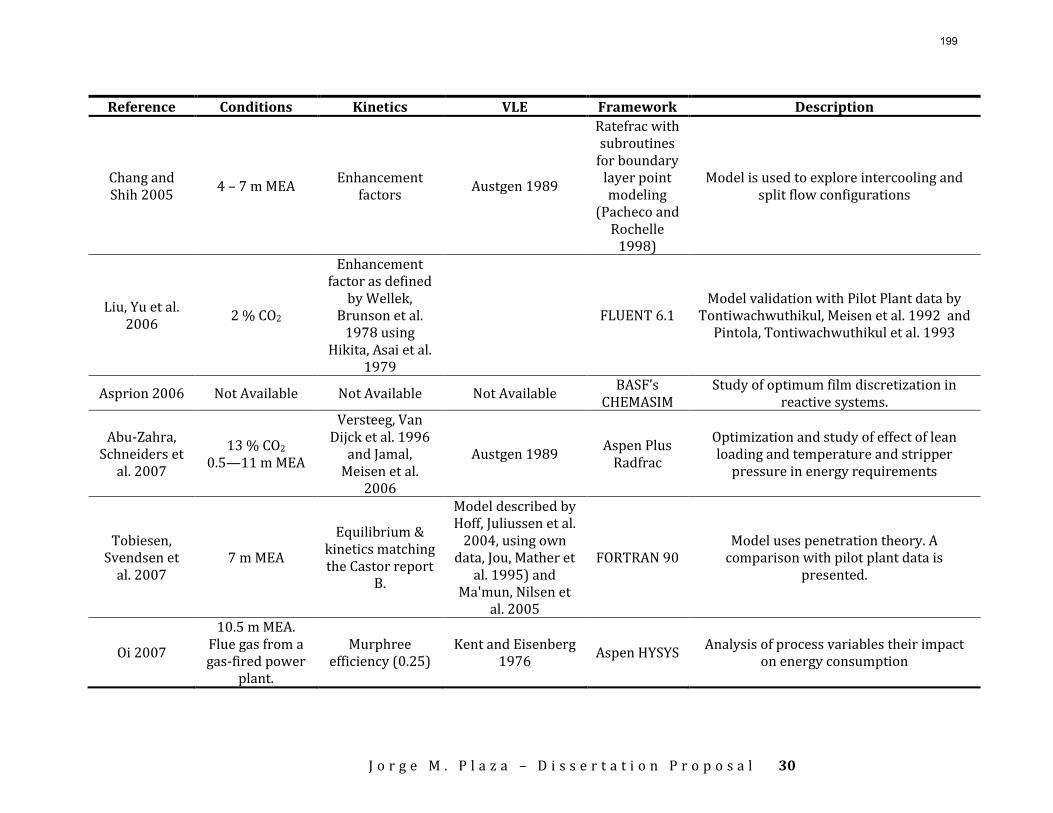
J o r g e M . P l a z a – D i s s e r t a t i o n P r o p o s a l
30
Reference Conditions Kinetics VLE Framework Description
Chang and Shih 2005
4 – 7 m MEA Enhancement
factors Austgen 1989
Ratefrac with subroutines
for boundary layer point modeling
(Pacheco and Rochelle
1998)
Model is used to explore intercooling and split flow configurations
Liu, Yu et al. 2006
2 % CO2
Enhancement factor as defined
by Wellek, Brunson et al.
1978 using Hikita, Asai et al.
1979
FLUENT 6.1 Model validation with Pilot Plant data by
Tontiwachwuthikul, Meisen et al. 1992 and Pintola, Tontiwachwuthikul et al. 1993
Asprion 2006 Not Available Not Available Not Available BASF’s
CHEMASIM Study of optimum film discretization in
reactive systems.
Abu-Zahra, Schneiders et
al. 2007
13 % CO2 0.5—11 m MEA
Versteeg, Van Dijck et al. 1996
and Jamal, Meisen et al.
2006
Austgen 1989 Aspen Plus
Radfrac
Optimization and study of effect of lean loading and temperature and stripper
pressure in energy requirements
Tobiesen, Svendsen et
al. 2007 7 m MEA
Equilibrium & kinetics matching the Castor report
B.
Model described by Hoff, Juliussen et al.
2004, using own data, Jou, Mather et
al. 1995) and Ma'mun, Nilsen et
al. 2005
FORTRAN 90 Model uses penetration theory. A
comparison with pilot plant data is presented.
Oi 2007
10.5 m MEA. Flue gas from a gas-fired power
plant.
Murphree efficiency (0.25)
Kent and Eisenberg 1976
Aspen HYSYS Analysis of process variables their impact
on energy consumption
199
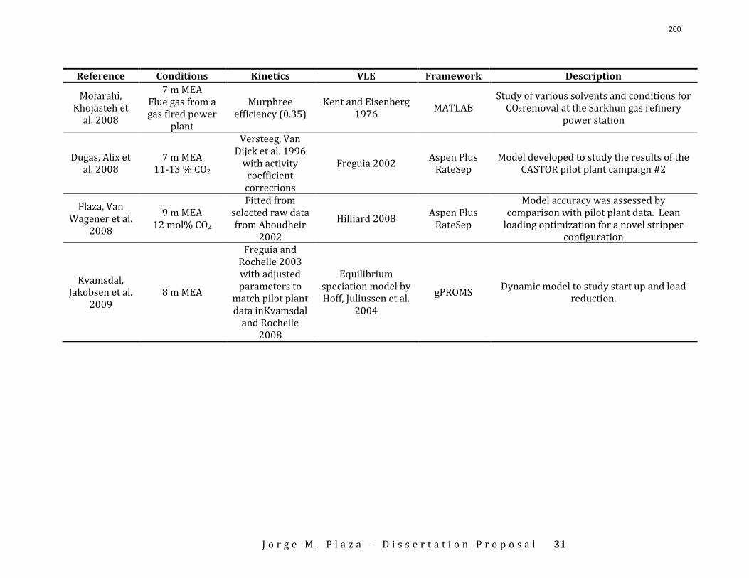
J o r g e M . P l a z a – D i s s e r t a t i o n P r o p o s a l
31
Reference Conditions Kinetics VLE Framework Description
Mofarahi, Khojasteh et
al. 2008
7 m MEA Flue gas from a gas fired power
plant
Murphree efficiency (0.35)
Kent and Eisenberg 1976
MATLAB Study of various solvents and conditions for
CO2removal at the Sarkhun gas refinery power station
Dugas, Alix et al. 2008
7 m MEA 11-13 % CO2
Versteeg, Van Dijck et al. 1996
with activity coefficient corrections
Freguia 2002 Aspen Plus
RateSep Model developed to study the results of the
CASTOR pilot plant campaign #2
Plaza, Van Wagener et al.
2008
9 m MEA 12 mol% CO2
Fitted from selected raw data from Aboudheir
2002
Hilliard 2008 Aspen Plus
RateSep
Model accuracy was assessed by comparison with pilot plant data. Lean
loading optimization for a novel stripper configuration
Kvamsdal, Jakobsen et al.
2009 8 m MEA
Freguia and Rochelle 2003 with adjusted parameters to
match pilot plant data inKvamsdal
and Rochelle 2008
Equilibrium speciation model by Hoff, Juliussen et al.
2004
gPROMS Dynamic model to study start up and load
reduction.
200

J o r g e M . P l a z a – D i s s e r t a t i o n P r o p o s a l
32
201
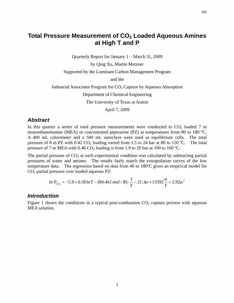
1
Total Pressure Measurement of CO2 Loaded Aqueous Amines at High T and P
Quarterly Report for January 1 – March 31, 2009
by Qing Xu, Martin Metzner
Supported by the Luminant Carbon Management Program
and the
Industrial Associates Program for CO2 Capture by Aqueous Absorption
Department of Chemical Engineering
The University of Texas at Austin
April 7, 2009
Abstract In this quarter a series of total pressure measurements were conducted to CO2 loaded 7 m monoethanolamine (MEA) or concentrated piperazine (PZ) at temperatures from 80 to 180 ºC. A 400 mL calorimeter and a 500 mL autoclave were used as equilibrium cells. The total pressure of 8 m PZ with 0.42 CO2 loading varied from 1.5 to 24 bar at 80 to 150 ºC. The total pressure of 7 m MEA with 0.48 CO2 loading is from 1.9 to 20 bar at 100 to 160 ºC.
The partial pressure of CO2 at each experimental condition was calculated by subtracting partial pressures of water and amines. The results fairly match the extrapolation curves of the low temperature data. The regression based on data from 40 to 180ºC gives an empirical model for CO2 partial pressure over loaded aqueous PZ:
2
21ln 5.9 6.56ln (84.4 . / ) 21.3 13392 2.92COP T kJ mol RT T
αα α= − + − ⋅ − + +
Introduction Figure 1 shows the conditions in a typical post-combustion CO2 capture process with aqueous MEA solution.
202
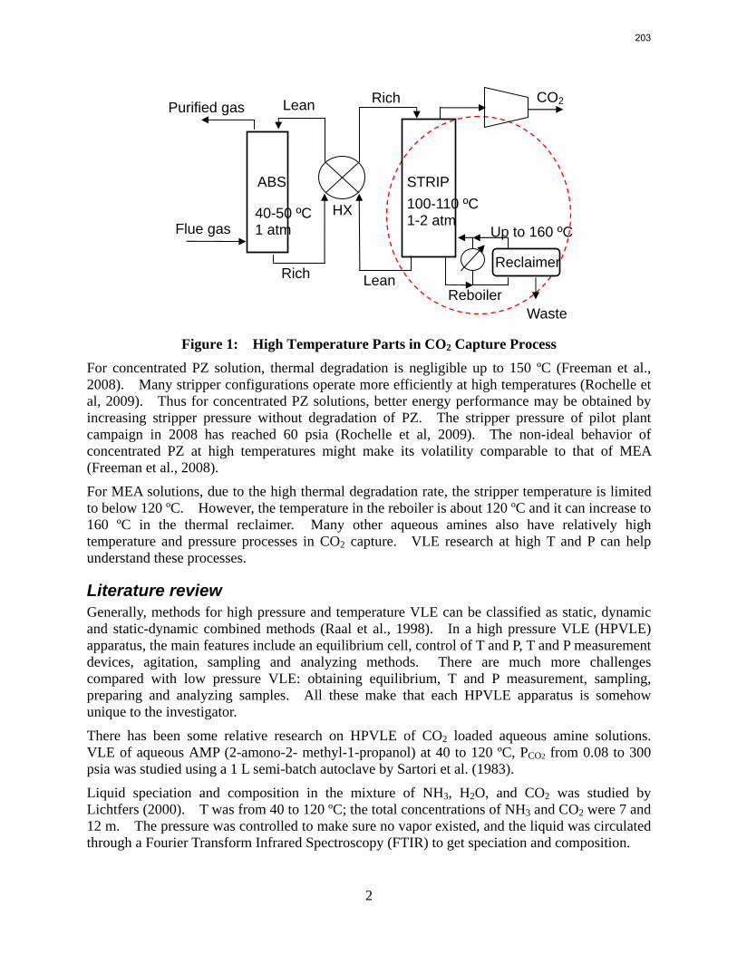
2
Figure 1: High Temperature Parts in CO2 Capture Process
For concentrated PZ solution, thermal degradation is negligible up to 150 ºC (Freeman et al., 2008). Many stripper configurations operate more efficiently at high temperatures (Rochelle et al, 2009). Thus for concentrated PZ solutions, better energy performance may be obtained by increasing stripper pressure without degradation of PZ. The stripper pressure of pilot plant campaign in 2008 has reached 60 psia (Rochelle et al, 2009). The non-ideal behavior of concentrated PZ at high temperatures might make its volatility comparable to that of MEA (Freeman et al., 2008).
For MEA solutions, due to the high thermal degradation rate, the stripper temperature is limited to below 120 ºC. However, the temperature in the reboiler is about 120 ºC and it can increase to 160 ºC in the thermal reclaimer. Many other aqueous amines also have relatively high temperature and pressure processes in CO2 capture. VLE research at high T and P can help understand these processes.
Literature review Generally, methods for high pressure and temperature VLE can be classified as static, dynamic and static-dynamic combined methods (Raal et al., 1998). In a high pressure VLE (HPVLE) apparatus, the main features include an equilibrium cell, control of T and P, T and P measurement devices, agitation, sampling and analyzing methods. There are much more challenges compared with low pressure VLE: obtaining equilibrium, T and P measurement, sampling, preparing and analyzing samples. All these make that each HPVLE apparatus is somehow unique to the investigator.
There has been some relative research on HPVLE of CO2 loaded aqueous amine solutions. VLE of aqueous AMP (2-amono-2- methyl-1-propanol) at 40 to 120 ºC, PCO2 from 0.08 to 300 psia was studied using a 1 L semi-batch autoclave by Sartori et al. (1983).
Liquid speciation and composition in the mixture of NH3, H2O, and CO2 was studied by Lichtfers (2000). T was from 40 to 120 ºC; the total concentrations of NH3 and CO2 were 7 and 12 m. The pressure was controlled to make sure no vapor existed, and the liquid was circulated through a Fourier Transform Infrared Spectroscopy (FTIR) to get speciation and composition.
CO2
Waste
Flue gas
ABS
HX
STRIP
Lean
Rich
Purified gas
Lean
Rich
Reclaimer
Reboiler
40-50 ºC 1 atm
100-110 ºC 1-2 atm
Up to 160 ºC
203
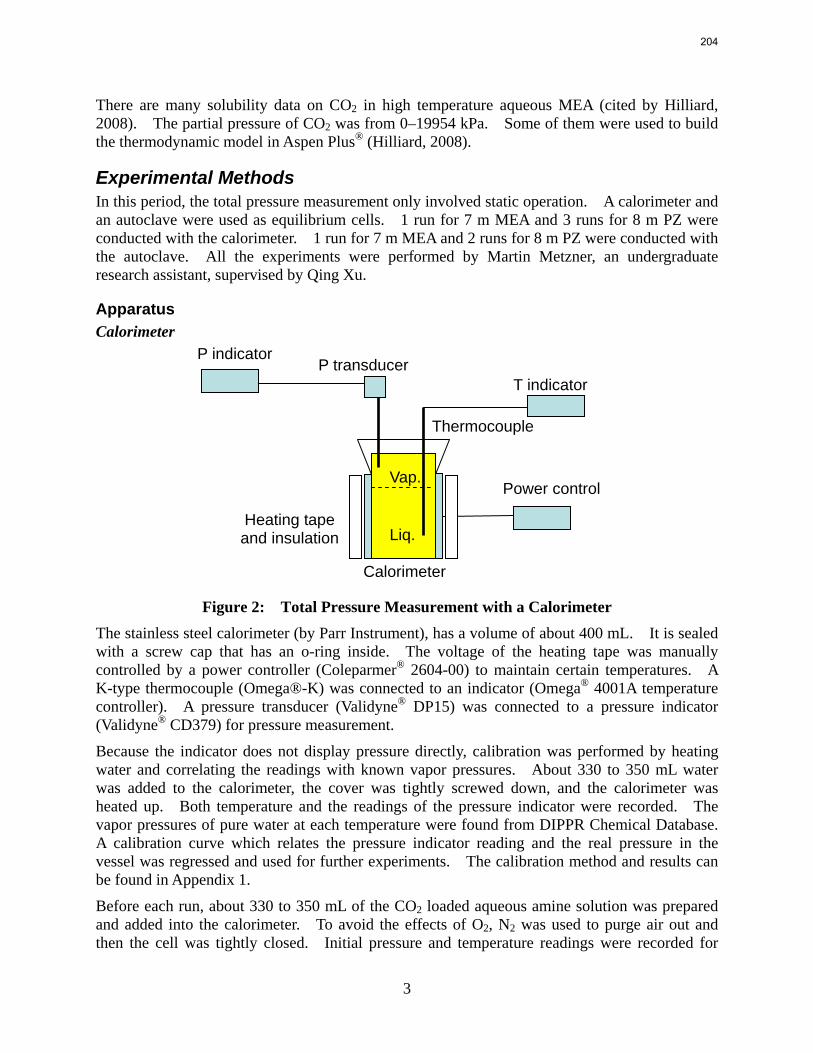
3
There are many solubility data on CO2 in high temperature aqueous MEA (cited by Hilliard, 2008). The partial pressure of CO2 was from 0–19954 kPa. Some of them were used to build the thermodynamic model in Aspen Plus® (Hilliard, 2008).
Experimental Methods In this period, the total pressure measurement only involved static operation. A calorimeter and an autoclave were used as equilibrium cells. 1 run for 7 m MEA and 3 runs for 8 m PZ were conducted with the calorimeter. 1 run for 7 m MEA and 2 runs for 8 m PZ were conducted with the autoclave. All the experiments were performed by Martin Metzner, an undergraduate research assistant, supervised by Qing Xu.
Apparatus Calorimeter
Figure 2: Total Pressure Measurement with a Calorimeter
The stainless steel calorimeter (by Parr Instrument), has a volume of about 400 mL. It is sealed with a screw cap that has an o-ring inside. The voltage of the heating tape was manually controlled by a power controller (Coleparmer® 2604-00) to maintain certain temperatures. A K-type thermocouple (Omega®-K) was connected to an indicator (Omega® 4001A temperature controller). A pressure transducer (Validyne® DP15) was connected to a pressure indicator (Validyne® CD379) for pressure measurement.
Because the indicator does not display pressure directly, calibration was performed by heating water and correlating the readings with known vapor pressures. About 330 to 350 mL water was added to the calorimeter, the cover was tightly screwed down, and the calorimeter was heated up. Both temperature and the readings of the pressure indicator were recorded. The vapor pressures of pure water at each temperature were found from DIPPR Chemical Database. A calibration curve which relates the pressure indicator reading and the real pressure in the vessel was regressed and used for further experiments. The calibration method and results can be found in Appendix 1.
Before each run, about 330 to 350 mL of the CO2 loaded aqueous amine solution was prepared and added into the calorimeter. To avoid the effects of O2, N2 was used to purge air out and then the cell was tightly closed. Initial pressure and temperature readings were recorded for
Power control
P indicator
T indicator P transducer
Thermocouple
Heating tape and insulation Liq.
Vap.
Calorimeter
204
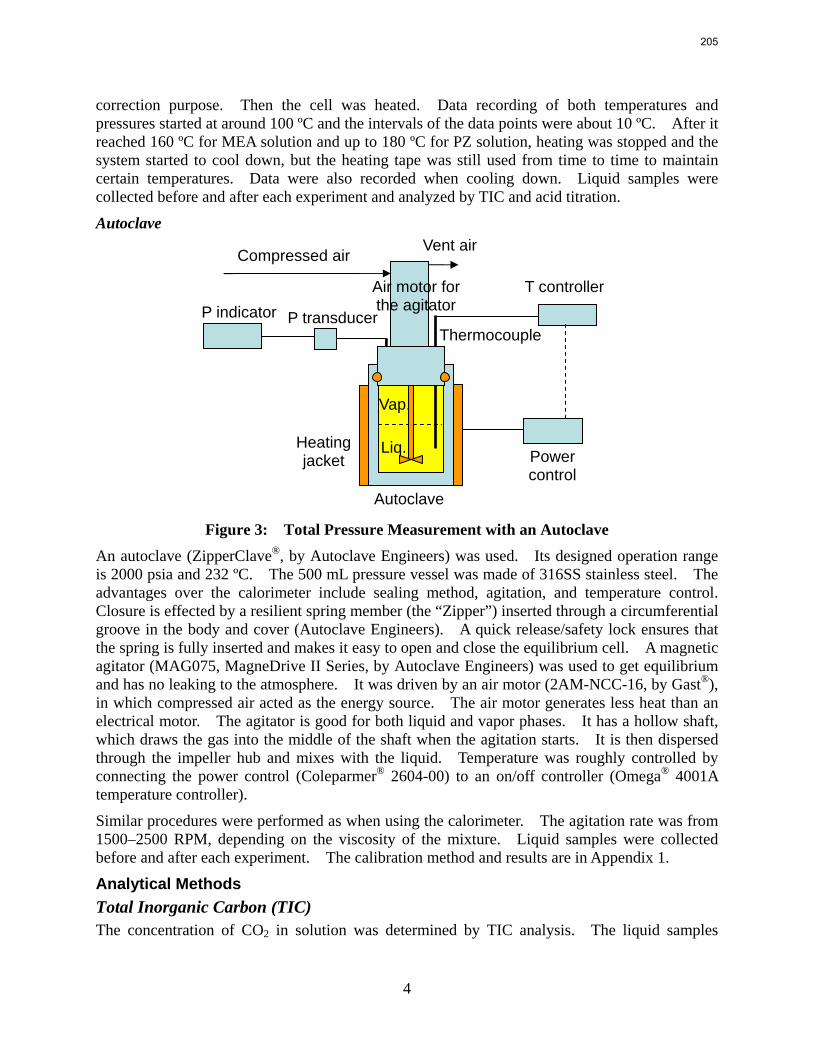
4
correction purpose. Then the cell was heated. Data recording of both temperatures and pressures started at around 100 ºC and the intervals of the data points were about 10 ºC. After it reached 160 ºC for MEA solution and up to 180 ºC for PZ solution, heating was stopped and the system started to cool down, but the heating tape was still used from time to time to maintain certain temperatures. Data were also recorded when cooling down. Liquid samples were collected before and after each experiment and analyzed by TIC and acid titration.
Autoclave
Figure 3: Total Pressure Measurement with an Autoclave
An autoclave (ZipperClave®, by Autoclave Engineers) was used. Its designed operation range is 2000 psia and 232 ºC. The 500 mL pressure vessel was made of 316SS stainless steel. The advantages over the calorimeter include sealing method, agitation, and temperature control. Closure is effected by a resilient spring member (the “Zipper”) inserted through a circumferential groove in the body and cover (Autoclave Engineers). A quick release/safety lock ensures that the spring is fully inserted and makes it easy to open and close the equilibrium cell. A magnetic agitator (MAG075, MagneDrive II Series, by Autoclave Engineers) was used to get equilibrium and has no leaking to the atmosphere. It was driven by an air motor (2AM-NCC-16, by Gast®), in which compressed air acted as the energy source. The air motor generates less heat than an electrical motor. The agitator is good for both liquid and vapor phases. It has a hollow shaft, which draws the gas into the middle of the shaft when the agitation starts. It is then dispersed through the impeller hub and mixes with the liquid. Temperature was roughly controlled by connecting the power control (Coleparmer® 2604-00) to an on/off controller (Omega® 4001A temperature controller).
Similar procedures were performed as when using the calorimeter. The agitation rate was from 1500–2500 RPM, depending on the viscosity of the mixture. Liquid samples were collected before and after each experiment. The calibration method and results are in Appendix 1.
Analytical Methods Total Inorganic Carbon (TIC) The concentration of CO2 in solution was determined by TIC analysis. The liquid samples
T controller
Autoclave
Vent air Compressed air
P transducer Thermocouple
Heating jacket Power
control
Liq.
Vap.
P indicator Air motor for the agitator
205
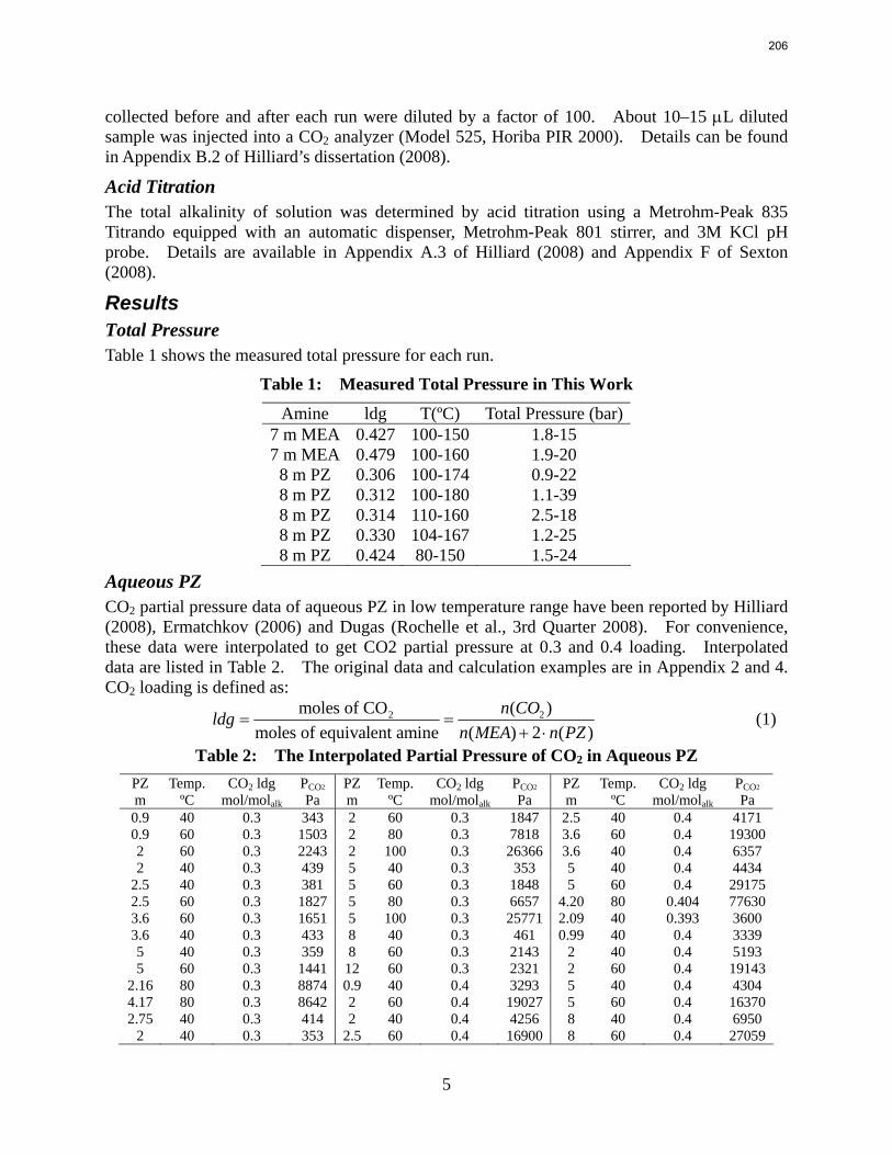
5
collected before and after each run were diluted by a factor of 100. About 10–15 μL diluted sample was injected into a CO2 analyzer (Model 525, Horiba PIR 2000). Details can be found in Appendix B.2 of Hilliard’s dissertation (2008).
Acid Titration The total alkalinity of solution was determined by acid titration using a Metrohm-Peak 835 Titrando equipped with an automatic dispenser, Metrohm-Peak 801 stirrer, and 3M KCl pH probe. Details are available in Appendix A.3 of Hilliard (2008) and Appendix F of Sexton (2008).
Results Total Pressure Table 1 shows the measured total pressure for each run.
Table 1: Measured Total Pressure in This Work
Amine ldg T(ºC) Total Pressure (bar)7 m MEA 0.427 100-150 1.8-15 7 m MEA 0.479 100-160 1.9-20
8 m PZ 0.306 100-174 0.9-22 8 m PZ 0.312 100-180 1.1-39 8 m PZ 0.314 110-160 2.5-18 8 m PZ 0.330 104-167 1.2-25 8 m PZ 0.424 80-150 1.5-24
Aqueous PZ CO2 partial pressure data of aqueous PZ in low temperature range have been reported by Hilliard (2008), Ermatchkov (2006) and Dugas (Rochelle et al., 3rd Quarter 2008). For convenience, these data were interpolated to get CO2 partial pressure at 0.3 and 0.4 loading. Interpolated data are listed in Table 2. The original data and calculation examples are in Appendix 2 and 4. CO2 loading is defined as:
2 2moles of CO ( )moles of equivalent amine ( ) 2 ( )
n COldgn MEA n PZ
= =+ ⋅
(1)
Table 2: The Interpolated Partial Pressure of CO2 in Aqueous PZ PZ Temp. CO2 ldg PCO2 PZ Temp. CO2 ldg PCO2 PZ Temp. CO2 ldg PCO2 m ºC mol/molalk Pa m ºC mol/molalk Pa m ºC mol/molalk Pa 0.9 40 0.3 343 2 60 0.3 1847 2.5 40 0.4 4171 0.9 60 0.3 1503 2 80 0.3 7818 3.6 60 0.4 19300 2 60 0.3 2243 2 100 0.3 26366 3.6 40 0.4 6357 2 40 0.3 439 5 40 0.3 353 5 40 0.4 4434
2.5 40 0.3 381 5 60 0.3 1848 5 60 0.4 29175 2.5 60 0.3 1827 5 80 0.3 6657 4.20 80 0.404 77630 3.6 60 0.3 1651 5 100 0.3 25771 2.09 40 0.393 3600 3.6 40 0.3 433 8 40 0.3 461 0.99 40 0.4 3339 5 40 0.3 359 8 60 0.3 2143 2 40 0.4 5193 5 60 0.3 1441 12 60 0.3 2321 2 60 0.4 19143
2.16 80 0.3 8874 0.9 40 0.4 3293 5 40 0.4 4304 4.17 80 0.3 8642 2 60 0.4 19027 5 60 0.4 16370 2.75 40 0.3 414 2 40 0.4 4256 8 40 0.4 6950
2 40 0.3 353 2.5 60 0.4 16900 8 60 0.4 27059
206
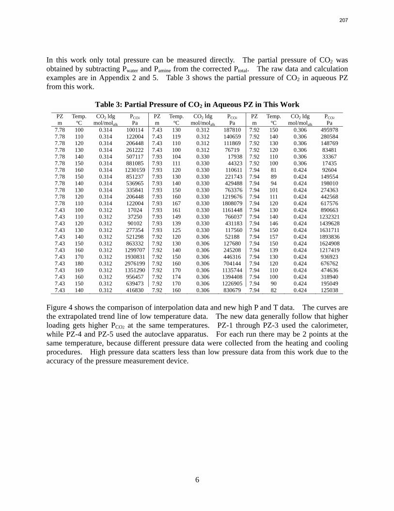
6
In this work only total pressure can be measured directly. The partial pressure of CO2 was obtained by subtracting Pwater and Pamine from the corrected Ptotal. The raw data and calculation examples are in Appendix 2 and 5. Table 3 shows the partial pressure of CO2 in aqueous PZ from this work.
Table 3: Partial Pressure of CO2 in Aqueous PZ in This Work PZ Temp. CO2 ldg PCO2 PZ Temp. CO2 ldg PCO2 PZ Temp. CO2 ldg PCO2 m ºC mol/molalk Pa m ºC mol/molalk Pa m ºC mol/molalk Pa
7.78 100 0.314 100114 7.43 130 0.312 187810 7.92 150 0.306 495978 7.78 110 0.314 122004 7.43 119 0.312 140659 7.92 140 0.306 280584 7.78 120 0.314 206448 7.43 110 0.312 111869 7.92 130 0.306 148769 7.78 130 0.314 261222 7.43 100 0.312 76719 7.92 120 0.306 83481 7.78 140 0.314 507117 7.93 104 0.330 17938 7.92 110 0.306 33367 7.78 150 0.314 881085 7.93 111 0.330 44323 7.92 100 0.306 17435 7.78 160 0.314 1230159 7.93 120 0.330 110611 7.94 81 0.424 92604 7.78 150 0.314 851237 7.93 130 0.330 221743 7.94 89 0.424 149554 7.78 140 0.314 536965 7.93 140 0.330 429488 7.94 94 0.424 198010 7.78 130 0.314 335841 7.93 150 0.330 763376 7.94 101 0.424 274363 7.78 120 0.314 206448 7.93 160 0.330 1219676 7.94 111 0.424 442568 7.78 110 0.314 122004 7.93 167 0.330 1808079 7.94 120 0.424 617576 7.43 100 0.312 17024 7.93 161 0.330 1161448 7.94 130 0.424 890663 7.43 110 0.312 37250 7.93 149 0.330 766037 7.94 140 0.424 1232321 7.43 120 0.312 90102 7.93 139 0.330 431183 7.94 146 0.424 1439628 7.43 130 0.312 277354 7.93 125 0.330 117560 7.94 150 0.424 1631711 7.43 140 0.312 521298 7.92 120 0.306 52188 7.94 157 0.424 1893836 7.43 150 0.312 863332 7.92 130 0.306 127680 7.94 150 0.424 1624908 7.43 160 0.312 1299707 7.92 140 0.306 245208 7.94 139 0.424 1217419 7.43 170 0.312 1930831 7.92 150 0.306 446316 7.94 130 0.424 936923 7.43 180 0.312 2976199 7.92 160 0.306 704144 7.94 120 0.424 676762 7.43 169 0.312 1351290 7.92 170 0.306 1135744 7.94 110 0.424 474636 7.43 160 0.312 956457 7.92 174 0.306 1394408 7.94 100 0.424 318940 7.43 150 0.312 639473 7.92 170 0.306 1226905 7.94 90 0.424 195049 7.43 140 0.312 416830 7.92 160 0.306 830679 7.94 82 0.424 125038
Figure 4 shows the comparison of interpolation data and new high P and T data. The curves are the extrapolated trend line of low temperature data. The new data generally follow that higher loading gets higher PCO2 at the same temperatures. PZ-1 through PZ-3 used the calorimeter, while PZ-4 and PZ-5 used the autoclave apparatus. For each run there may be 2 points at the same temperature, because different pressure data were collected from the heating and cooling procedures. High pressure data scatters less than low pressure data from this work due to the accuracy of the pressure measurement device.
207
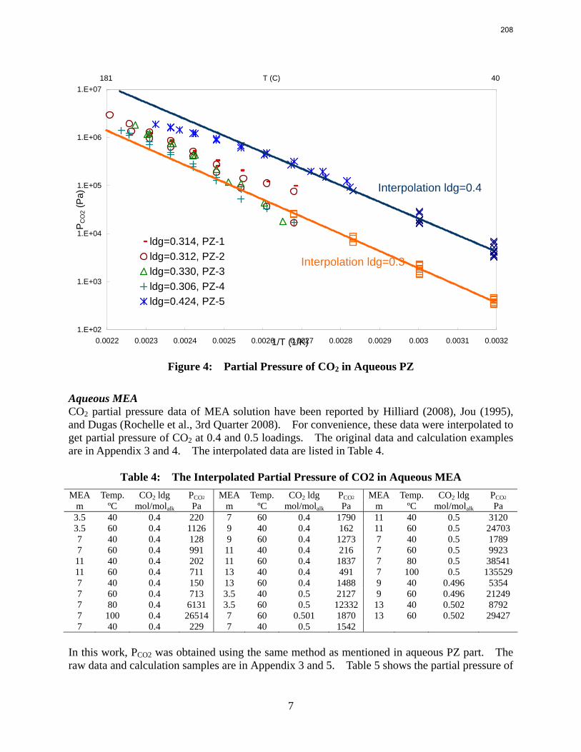
7
1.E+02
1.E+03
1.E+04
1.E+05
1.E+06
1.E+07
0.0022 0.0023 0.0024 0.0025 0.0026 0.0027 0.0028 0.0029 0.003 0.0031 0.00321/T (1/K)
P CO
2 (Pa
)40181 T (C)
ldg=0.314, PZ-1ldg=0.312, PZ-2ldg=0.330, PZ-3ldg=0.306, PZ-4ldg=0.424, PZ-5
Figure 4: Partial Pressure of CO2 in Aqueous PZ
Aqueous MEA CO2 partial pressure data of MEA solution have been reported by Hilliard (2008), Jou (1995), and Dugas (Rochelle et al., 3rd Quarter 2008). For convenience, these data were interpolated to get partial pressure of CO2 at 0.4 and 0.5 loadings. The original data and calculation examples are in Appendix 3 and 4. The interpolated data are listed in Table 4.
Table 4: The Interpolated Partial Pressure of CO2 in Aqueous MEA MEA Temp. CO2 ldg PCO2 MEA Temp. CO2 ldg PCO2 MEA Temp. CO2 ldg PCO2
m ºC mol/molalk Pa m ºC mol/molalk Pa m ºC mol/molalk Pa 3.5 40 0.4 220 7 60 0.4 1790 11 40 0.5 3120 3.5 60 0.4 1126 9 40 0.4 162 11 60 0.5 24703 7 40 0.4 128 9 60 0.4 1273 7 40 0.5 1789 7 60 0.4 991 11 40 0.4 216 7 60 0.5 9923 11 40 0.4 202 11 60 0.4 1837 7 80 0.5 38541 11 60 0.4 711 13 40 0.4 491 7 100 0.5 135529 7 40 0.4 150 13 60 0.4 1488 9 40 0.496 5354 7 60 0.4 713 3.5 40 0.5 2127 9 60 0.496 21249 7 80 0.4 6131 3.5 60 0.5 12332 13 40 0.502 8792 7 100 0.4 26514 7 60 0.501 1870 13 60 0.502 29427 7 40 0.4 229 7 40 0.5 1542
In this work, PCO2 was obtained using the same method as mentioned in aqueous PZ part. The raw data and calculation samples are in Appendix 3 and 5. Table 5 shows the partial pressure of
Interpolation ldg=0.3
Interpolation ldg=0.4
208
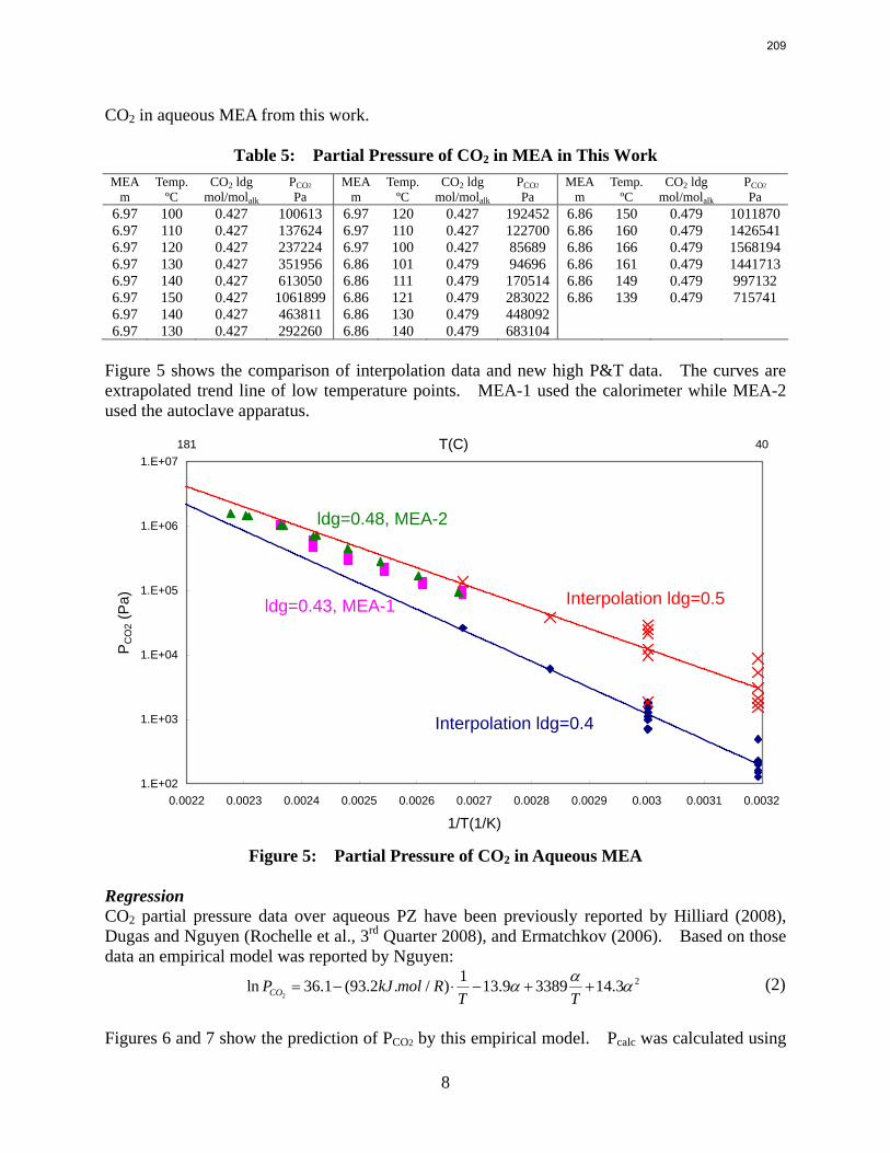
8
CO2 in aqueous MEA from this work.
Table 5: Partial Pressure of CO2 in MEA in This Work MEA Temp. CO2 ldg PCO2 MEA Temp. CO2 ldg PCO2 MEA Temp. CO2 ldg PCO2
m ºC mol/molalk Pa m ºC mol/molalk Pa m ºC mol/molalk Pa 6.97 100 0.427 100613 6.97 120 0.427 192452 6.86 150 0.479 1011870 6.97 110 0.427 137624 6.97 110 0.427 122700 6.86 160 0.479 1426541 6.97 120 0.427 237224 6.97 100 0.427 85689 6.86 166 0.479 1568194 6.97 130 0.427 351956 6.86 101 0.479 94696 6.86 161 0.479 1441713 6.97 140 0.427 613050 6.86 111 0.479 170514 6.86 149 0.479 997132 6.97 150 0.427 1061899 6.86 121 0.479 283022 6.86 139 0.479 715741 6.97 140 0.427 463811 6.86 130 0.479 448092 6.97 130 0.427 292260 6.86 140 0.479 683104
Figure 5 shows the comparison of interpolation data and new high P&T data. The curves are extrapolated trend line of low temperature points. MEA-1 used the calorimeter while MEA-2 used the autoclave apparatus.
1.E+02
1.E+03
1.E+04
1.E+05
1.E+06
1.E+07
0.0022 0.0023 0.0024 0.0025 0.0026 0.0027 0.0028 0.0029 0.003 0.0031 0.0032
1/T(1/K)
PC
O2 (
Pa)
40181 T(C)
Figure 5: Partial Pressure of CO2 in Aqueous MEA
Regression CO2 partial pressure data over aqueous PZ have been previously reported by Hilliard (2008), Dugas and Nguyen (Rochelle et al., 3rd Quarter 2008), and Ermatchkov (2006). Based on those data an empirical model was reported by Nguyen:
2
21ln 36.1 (93.2 . / ) 13.9 3389 14.3COP kJ mol RT T
αα α= − ⋅ − + + (2)
Figures 6 and 7 show the prediction of PCO2 by this empirical model. Pcalc was calculated using
Interpolation ldg=0.4
Interpolation ldg=0.5
ldg=0.48, MEA-2
ldg=0.43, MEA-1
209
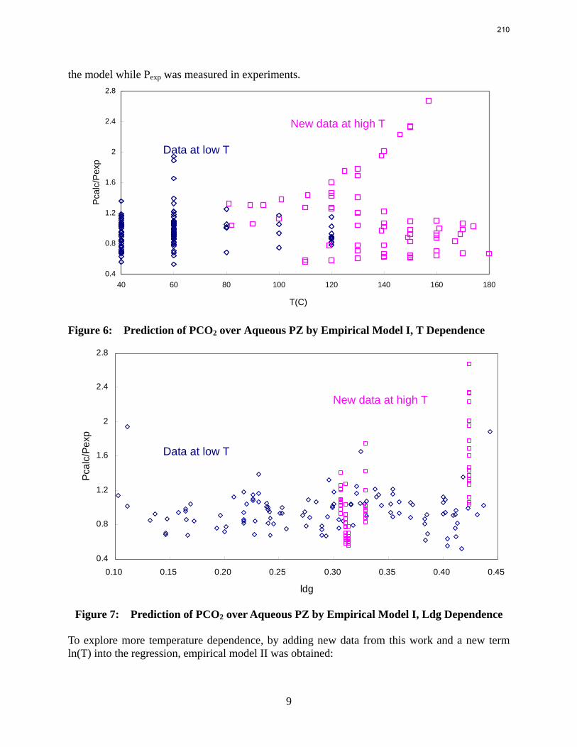
9
the model while Pexp was measured in experiments.
0.4
0.8
1.2
1.6
2
2.4
2.8
40 60 80 100 120 140 160 180
T(C)
Pca
lc/P
exp
Figure 6: Prediction of PCO2 over Aqueous PZ by Empirical Model I, T Dependence
0.4
0.8
1.2
1.6
2
2.4
2.8
0.10 0.15 0.20 0.25 0.30 0.35 0.40 0.45
ldg
Pcal
c/Pe
xp
Figure 7: Prediction of PCO2 over Aqueous PZ by Empirical Model I, Ldg Dependence To explore more temperature dependence, by adding new data from this work and a new term ln(T) into the regression, empirical model II was obtained:
Data at low T
New data at high T
Data at low T
New data at high T
210
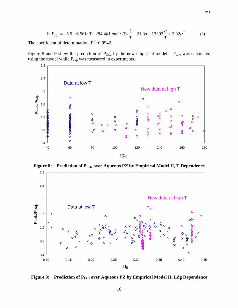
10
2
21ln 5.9 6.56ln (84.4 . / ) 21.3 13392 2.92COP T kJ mol RT T
αα α= − + − ⋅ − + + (3)
The coefficient of determination, R2=0.9942. Figure 8 and 9 show the prediction of PCO2 by the new empirical model. Pcalc was calculated using the model while Pexp was measured in experiments.
0.4
0.8
1.2
1.6
2
2.4
2.8
40 60 80 100 120 140 160 180
T(C)
Pca
lc/P
exp
Figure 8: Prediction of PCO2 over Aqueous PZ by Empirical Model II, T Dependence
0.4
0.8
1.2
1.6
2
2.4
2.8
0.10 0.15 0.20 0.25 0.30 0.35 0.40 0.45
ldg
Pcal
c/Pe
xp
Figure 9: Prediction of PCO2 over Aqueous PZ by Empirical Model II, Ldg Dependence
Data at low T New data at high T
Data at low T
New data at high T
211
11
Discussion Generally the new data at high T and P fit well with the extrapolation from low temperature data, but there is a departing trend above temperatures from 130 to 140 ºC. Regression comparison results also indicate there is more temperature independence of PCO2, which suggests temperature dependence of heat of absorption.
Both the calorimeter and the autoclave apparatus work better in high pressure range. The errors in the experiments mainly come from measurement devices, temperature control, and the obtaining of equilibrium. The Validyne® pressure transducer has an accuracy of ± 0.25% full scale (500 psig) and the Omega® K-type thermocouple (-200 ºC to 1250 ºC) has an accuracy of ± 2.2 ºC. Temperature control is crucial for equilibrium. However in the calorimeter apparatus it was controlled manually and in the autoclave apparatus it was done by an on-and-off controller. Temperature fluctuated when it was supposed to be constant. The temperature usually swung within 1–3ºC, especially when it was in high temperature range. Pressure reading was corrected by taking the average of max P and min P during 1 ºC fluctuations to minimize this error. Further, it was assumed that both the indicators of T and P read signals instantly, but there might be lags in T and P measurement. The error from calibration is relatively small. The liquid analysis of samples before and after each experiment indicates little leaking of the apparatus.
Conclusions The CO2 partial pressure over loaded aqueous MEA or PZ obtained by this total pressure measurement generally matches the extrapolation from previous data at low temperatures. For 8 m PZ solution with 0.306 CO2 loading, the total pressure is 0.9 bar at 100 ºC. For 8 m PZ solution with 0.424 CO2 loading, the total pressure is 24 bars at 150 ºC. For a specific amine solution PCO2 is a function of temperature and CO2 loading. A new empirical model for aqueous PZ was developed based on data at both high and low temperatures (from 40 to 180 ºC):
2
21ln 5.9 6.56ln (84.4 . / ) 21.3 13392 2.92COP T kJ mol RT T
αα α= − + − ⋅ − + +
Future Work The work planned for the forthcoming period includes modifying the total pressure measurement, improving the measurement and temperature control devices, and adding a data acquisition system. We will then conduct more experiments on various CO2 loadings for concentrated PZ solution.
We will design and build an apparatus for (x, y, P, T) measurement at high temperature and pressure. A draft design has been developed, but details and potential problems need to be fixed. The autoclave will be used as the equilibrium cell; vapor sample will be diluted with nitrogen and circulated through FTIR.
Further goals include exploring the temperature dependence of heat of absorption of CO2 loaded amine solutions and conducting experiments using other aqueous amines.
212
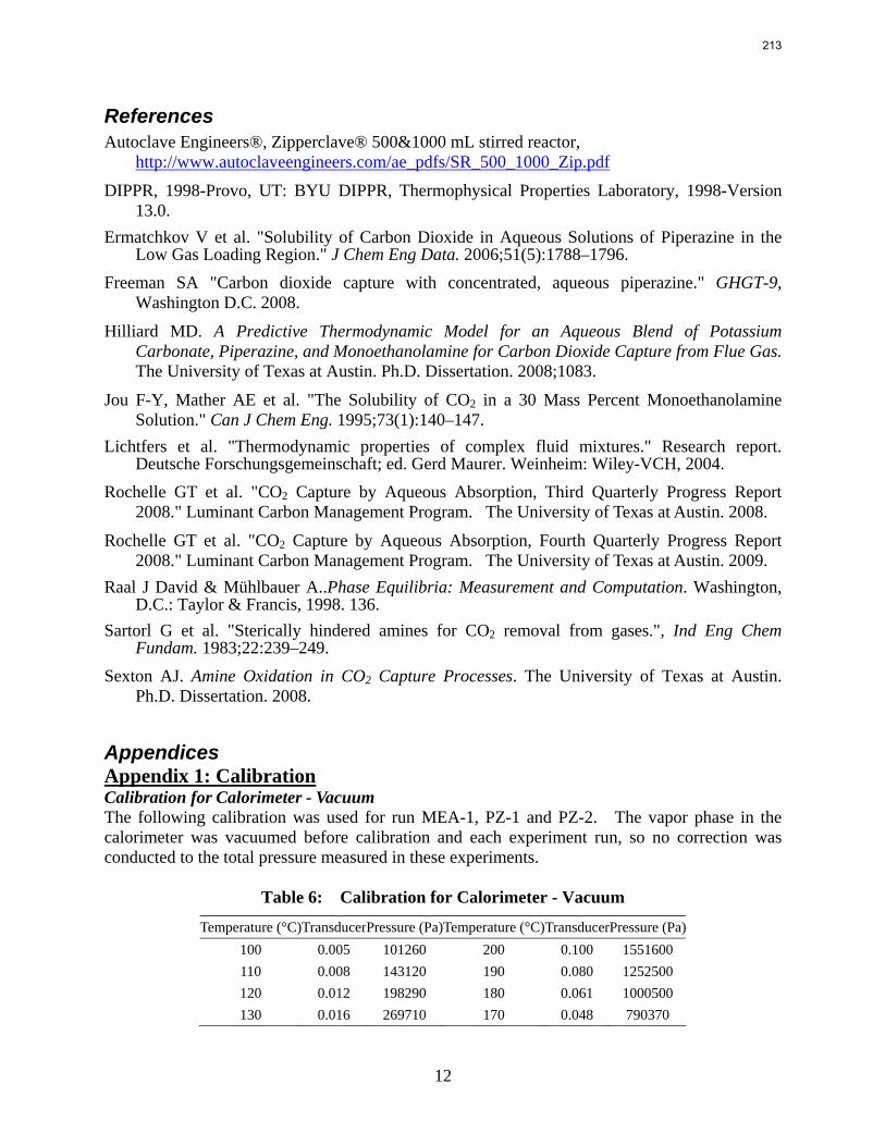
12
References Autoclave Engineers®, Zipperclave® 500&1000 mL stirred reactor,
http://www.autoclaveengineers.com/ae_pdfs/SR_500_1000_Zip.pdf
DIPPR, 1998-Provo, UT: BYU DIPPR, Thermophysical Properties Laboratory, 1998-Version 13.0.
Ermatchkov V et al. "Solubility of Carbon Dioxide in Aqueous Solutions of Piperazine in the Low Gas Loading Region." J Chem Eng Data. 2006;51(5):1788–1796.
Freeman SA "Carbon dioxide capture with concentrated, aqueous piperazine." GHGT-9, Washington D.C. 2008.
Hilliard MD. A Predictive Thermodynamic Model for an Aqueous Blend of Potassium Carbonate, Piperazine, and Monoethanolamine for Carbon Dioxide Capture from Flue Gas. The University of Texas at Austin. Ph.D. Dissertation. 2008;1083.
Jou F-Y, Mather AE et al. "The Solubility of CO2 in a 30 Mass Percent Monoethanolamine Solution." Can J Chem Eng. 1995;73(1):140–147.
Lichtfers et al. "Thermodynamic properties of complex fluid mixtures." Research report. Deutsche Forschungsgemeinschaft; ed. Gerd Maurer. Weinheim: Wiley-VCH, 2004.
Rochelle GT et al. "CO2 Capture by Aqueous Absorption, Third Quarterly Progress Report 2008." Luminant Carbon Management Program. The University of Texas at Austin. 2008.
Rochelle GT et al. "CO2 Capture by Aqueous Absorption, Fourth Quarterly Progress Report 2008." Luminant Carbon Management Program. The University of Texas at Austin. 2009.
Raal J David & Mühlbauer A..Phase Equilibria: Measurement and Computation. Washington, D.C.: Taylor & Francis, 1998. 136.
Sartorl G et al. "Sterically hindered amines for CO2 removal from gases.", Ind Eng Chem Fundam. 1983;22:239–249.
Sexton AJ. Amine Oxidation in CO2 Capture Processes. The University of Texas at Austin. Ph.D. Dissertation. 2008.
Appendices Appendix 1: Calibration Calibration for Calorimeter - Vacuum The following calibration was used for run MEA-1, PZ-1 and PZ-2. The vapor phase in the calorimeter was vacuumed before calibration and each experiment run, so no correction was conducted to the total pressure measured in these experiments.
Table 6: Calibration for Calorimeter - Vacuum
Temperature (°C)TransducerPressure (Pa)Temperature (°C)TransducerPressure (Pa)100 0.005 101260 200 0.100 1551600 110 0.008 143120 190 0.080 1252500 120 0.012 198290 180 0.061 1000500 130 0.016 269710 170 0.048 790370
213
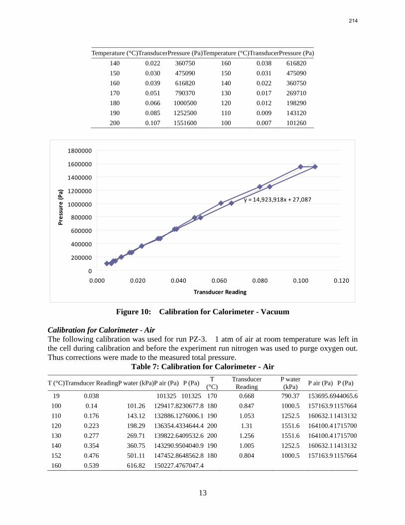
13
Temperature (°C)TransducerPressure (Pa)Temperature (°C)TransducerPressure (Pa)140 0.022 360750 160 0.038 616820 150 0.030 475090 150 0.031 475090 160 0.039 616820 140 0.022 360750 170 0.051 790370 130 0.017 269710 180 0.066 1000500 120 0.012 198290 190 0.085 1252500 110 0.009 143120 200 0.107 1551600 100 0.007 101260
y = 14,923,918x + 27,087
0
200000
400000
600000
800000
1000000
1200000
1400000
1600000
1800000
0.000 0.020 0.040 0.060 0.080 0.100 0.120
Transducer Reading
Pressure (P
a)
Figure 10: Calibration for Calorimeter - Vacuum
Calibration for Calorimeter - Air The following calibration was used for run PZ-3. 1 atm of air at room temperature was left in the cell during calibration and before the experiment run nitrogen was used to purge oxygen out. Thus corrections were made to the measured total pressure.
Table 7: Calibration for Calorimeter - Air
T (°C)Transducer ReadingP water (kPa)P air (Pa) P (Pa) T (°C)
Transducer Reading
P water (kPa) P air (Pa) P (Pa)
19 0.038 101325 101325 170 0.668 790.37 153695.6944065.6100 0.14 101.26 129417.8230677.8 180 0.847 1000.5 157163.9 1157664110 0.176 143.12 132886.1276006.1 190 1.053 1252.5 160632.11413132120 0.223 198.29 136354.4334644.4 200 1.31 1551.6 164100.41715700130 0.277 269.71 139822.6409532.6 200 1.256 1551.6 164100.41715700140 0.354 360.75 143290.9504040.9 190 1.005 1252.5 160632.11413132152 0.476 501.11 147452.8648562.8 180 0.804 1000.5 157163.9 1157664160 0.539 616.82 150227.4767047.4
214
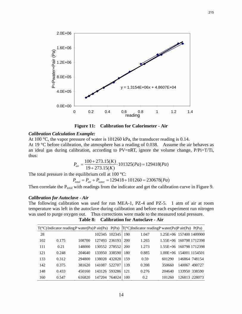
14
y = 1.3154E+06x + 4.8607E+04
0.0E+00
4.0E+05
8.0E+05
1.2E+06
1.6E+06
2.0E+06
0 0.2 0.4 0.6 0.8 1 1.2 1.4reading
P=Pw
ater
+Pai
r (Pa
)
Figure 11: Calibration for Calorimeter - Air
Calibration Calculation Example: At 100 °C, the vapor pressure of water is 101260 kPa, the transducer reading is 0.14. At 19 °C before calibration, the atmosphere has a reading of 0.038. Assume the air behaves as an ideal gas during calibration, according to PV=nRT, ignore the volume change, P/Pi=T/Ti, thus:
100 273.15( ) 101325( ) 129418( )19 273.15( )air
KP Pa PaK
+= ⋅ =
+
The total pressure in the equilibrium cell at 100 °C: 129418 101260 230678( )total air waterP P P Pa= + = + =
Then correlate the Ptotal with readings from the indicator and get the calibration curve in Figure 9. Calibration for Autoclave - Air The following calibration was used for run MEA-1, PZ-4 and PZ-5. 1 atm of air at room temperature was left in the autoclave during calibration and before each experiment run nitrogen was used to purge oxygen out. Thus corrections were made to the measured total pressure.
Table 8: Calibration for Autoclave - Air
T(°C) Indicator reading P water(Pa) P air(Pa) P(Pa) T(°C)Indicator readingP water(Pa)P air(Pa) P(Pa) 28 102345 102345 190 1.047 1.25E+06 157400 1409900102 0.175 108700 127493 236193 200 1.265 1.55E+06 160798 1712398111 0.21 148000 130552 278552 200 1.273 1.55E+06 160798 1712398121 0.248 204640 133950 338590 180 0.885 1.00E+06 154001 1154501133 0.312 294800 138028 432828 159 0.59 601290 146864 748154142 0.375 381620 141087 522707 139 0.398 350660 140067 490727148 0.433 450160 143126 593286 121 0.276 204640 133950 338590160 0.547 616820 147204 764024 100 0.2 101260 126813 228073
215
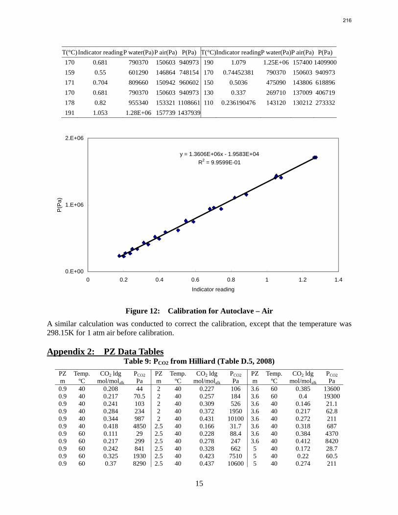
15
T(°C) Indicator reading P water(Pa) P air(Pa) P(Pa) T(°C)Indicator readingP water(Pa)P air(Pa) P(Pa) 170 0.681 790370 150603 940973 190 1.079 1.25E+06 157400 1409900159 0.55 601290 146864 748154 170 0.74452381 790370 150603 940973171 0.704 809660 150942 960602 150 0.5036 475090 143806 618896170 0.681 790370 150603 940973 130 0.337 269710 137009 406719178 0.82 955340 153321 1108661 110 0.236190476 143120 130212 273332191 1.053 1.28E+06 157739 1437939
y = 1.3606E+06x - 1.9583E+04R2 = 9.9599E-01
0.E+00
1.E+06
2.E+06
0 0.2 0.4 0.6 0.8 1 1.2 1.4
Indicator reading
P(P
a)
Figure 12: Calibration for Autoclave – Air
A similar calculation was conducted to correct the calibration, except that the temperature was 298.15K for 1 atm air before calibration. Appendix 2: PZ Data Tables
Table 9: PCO2 from Hilliard (Table D.5, 2008) PZ Temp. CO2 ldg PCO2 PZ Temp. CO2 ldg PCO2 PZ Temp. CO2 ldg PCO2 m ºC mol/molalk Pa m ºC mol/molalk Pa m ºC mol/molalk Pa 0.9 40 0.208 44 2 40 0.227 106 3.6 60 0.385 13600 0.9 40 0.217 70.5 2 40 0.257 184 3.6 60 0.4 19300 0.9 40 0.241 103 2 40 0.309 526 3.6 40 0.146 21.1 0.9 40 0.284 234 2 40 0.372 1950 3.6 40 0.217 62.8 0.9 40 0.344 987 2 40 0.431 10100 3.6 40 0.272 211 0.9 40 0.418 4850 2.5 40 0.166 31.7 3.6 40 0.318 687 0.9 60 0.111 29 2.5 40 0.228 88.4 3.6 40 0.384 4370 0.9 60 0.217 299 2.5 40 0.278 247 3.6 40 0.412 8420 0.9 60 0.242 841 2.5 40 0.328 662 5 40 0.172 28.7 0.9 60 0.325 1930 2.5 40 0.423 7510 5 40 0.22 60.5 0.9 60 0.37 8290 2.5 40 0.437 10600 5 40 0.274 211
216
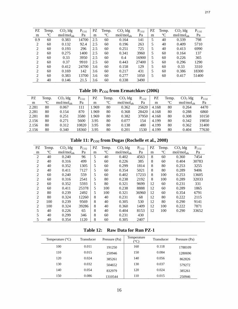
16
PZ Temp. CO2 ldg PCO2 PZ Temp. CO2 ldg PCO2 PZ Temp. CO2 ldg PCO2 m ºC mol/molalk Pa m ºC mol/molalk Pa m ºC mol/molalk Pa 0.9 60 0.383 14700 2.5 60 0.164 141 5 40 0.339 798 2 60 0.132 92.4 2.5 60 0.196 263 5 40 0.409 5710 2 60 0.193 296 2.5 60 0.251 725 5 40 0.413 6990 2 60 0.275 1400 2.5 60 0.341 3960 5 60 0.164 137 2 60 0.33 3950 2.5 60 0.4 16900 5 60 0.226 365 2 60 0.37 9910 2.5 60 0.443 27400 5 60 0.296 1290 2 60 0.412 24700 3.6 60 0.158 129 5 60 0.33 3310 2 60 0.169 142 3.6 60 0.217 431 5 60 0.386 18300 2 60 0.383 13700 3.6 60 0.277 1050 5 60 0.417 51400 2 40 0.146 21.5 3.6 60 0.338 3490
Table 10: PCO2 from Ermatchkov (2006)
PZ Temp. CO2 ldg PCO2 PZ Temp. CO2 ldg PCO2 PZ Temp. CO2 ldg PCO2 m ºC mol/molalk Pa m ºC mol/molalk Pa m ºC mol/molalk Pa
2.281 80 0.067 111 1.969 80 0.362 25620 4.168 80 0.264 4470 2.281 80 0.154 870 1.969 80 0.368 28420 4.168 80 0.288 6860 2.281 80 0.251 3580 1.969 80 0.382 37950 4.168 80 0.308 10150 2.156 80 0.271 5600 3.95 80 0.077 154 4.199 80 0.342 19850 2.156 80 0.312 10820 3.95 80 0.138 480 4.199 80 0.362 31400 2.156 80 0.340 18360 3.95 80 0.201 1530 4.199 80 0.404 77630
Table 11: PCO2 from Dugas (Rochelle et al., 2008) PZ Temp. CO2 ldg PCO2 PZ Temp. CO2 ldg PCO2 PZ Temp. CO2 ldg PCO2 m ºC mol/molalk Pa m ºC mol/molalk Pa m ºC mol/molalk Pa 2 40 0.240 96 5 40 0.402 4563 8 60 0.360 7454 2 40 0.316 499 5 60 0.226 385 8 60 0.404 30783 2 40 0.352 1305 5 60 0.299 1814 8 80 0.253 3255 2 40 0.411 7127 5 60 0.354 5021 8 80 0.289 9406 2 60 0.240 559 5 60 0.402 17233 8 100 0.253 13605 2 60 0.316 2541 5 80 0.238 2192 8 100 0.289 32033 2 60 0.352 5593 5 80 0.321 9699 12 60 0.231 331 2 60 0.411 25378 5 100 0.238 8888 12 60 0.289 1865 2 80 0.239 2492 5 100 0.321 36960 12 60 0.354 6791 2 80 0.324 12260 8 40 0.231 68 12 80 0.222 2115 2 100 0.239 9569 8 40 0.305 530 12 80 0.290 9141 2 100 0.324 39286 8 40 0.360 1409 12 100 0.222 7871 5 40 0.226 65 8 40 0.404 8153 12 100 0.290 33652 5 40 0.299 346 8 60 0.231 430 5 40 0.354 1120 8 60 0.305 2407
Table 12: Raw Data for Run PZ-1
Temperature (°C) Transducer Pressure (Pa) Temperature (°C) Transducer Pressure (Pa)
100 0.011 191250 160 0.118 1788109 110 0.015 250946 150 0.084 1280696 120 0.024 385261 140 0.056 862826 130 0.032 504652 130 0.037 579272 140 0.054 832979 120 0.024 385261 150 0.086 1310544 110 0.015 250946
217
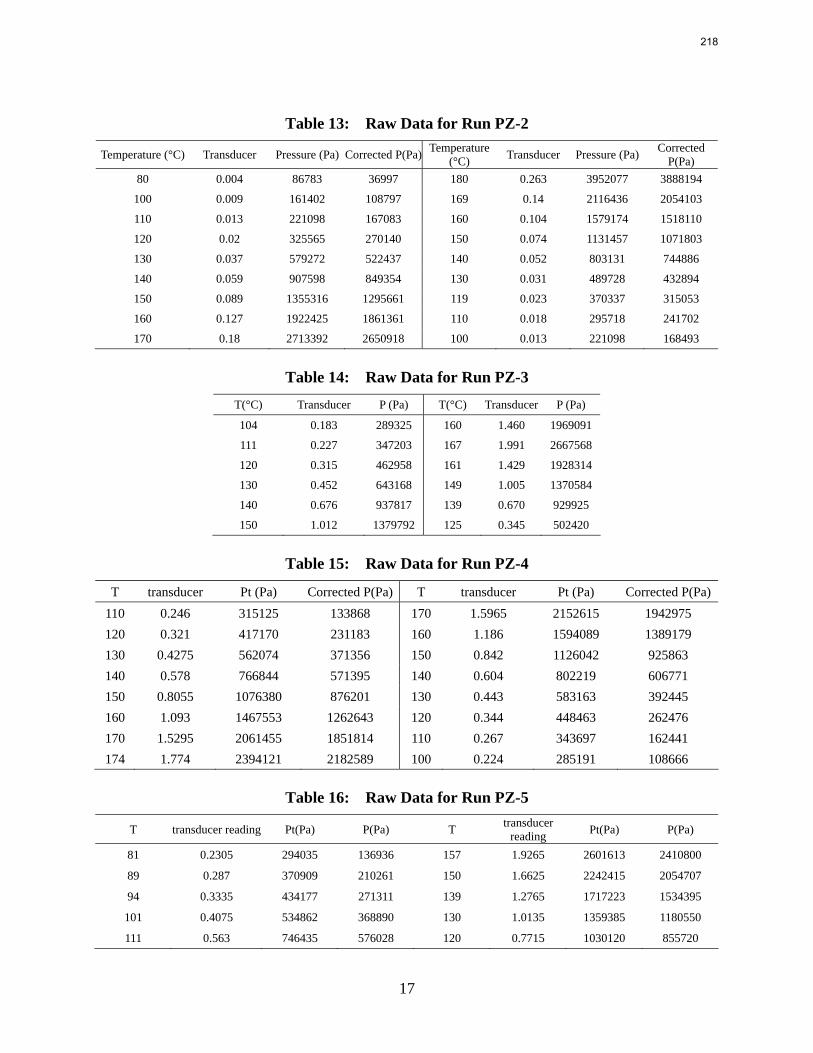
17
Table 13: Raw Data for Run PZ-2
Temperature (°C) Transducer Pressure (Pa) Corrected P(Pa) Temperature (°C) Transducer Pressure (Pa) Corrected
P(Pa) 80 0.004 86783 36997 180 0.263 3952077 3888194
100 0.009 161402 108797 169 0.14 2116436 2054103
110 0.013 221098 167083 160 0.104 1579174 1518110
120 0.02 325565 270140 150 0.074 1131457 1071803
130 0.037 579272 522437 140 0.052 803131 744886
140 0.059 907598 849354 130 0.031 489728 432894
150 0.089 1355316 1295661 119 0.023 370337 315053
160 0.127 1922425 1861361 110 0.018 295718 241702
170 0.18 2713392 2650918 100 0.013 221098 168493
Table 14: Raw Data for Run PZ-3
T(°C) Transducer P (Pa) T(°C) Transducer P (Pa)
104 0.183 289325 160 1.460 1969091
111 0.227 347203 167 1.991 2667568
120 0.315 462958 161 1.429 1928314
130 0.452 643168 149 1.005 1370584
140 0.676 937817 139 0.670 929925
150 1.012 1379792 125 0.345 502420
Table 15: Raw Data for Run PZ-4
T transducer Pt (Pa) Corrected P(Pa) T transducer Pt (Pa) Corrected P(Pa) 110 0.246 315125 133868 170 1.5965 2152615 1942975 120 0.321 417170 231183 160 1.186 1594089 1389179 130 0.4275 562074 371356 150 0.842 1126042 925863 140 0.578 766844 571395 140 0.604 802219 606771 150 0.8055 1076380 876201 130 0.443 583163 392445 160 1.093 1467553 1262643 120 0.344 448463 262476 170 1.5295 2061455 1851814 110 0.267 343697 162441 174 1.774 2394121 2182589 100 0.224 285191 108666
Table 16: Raw Data for Run PZ-5
T transducer reading Pt(Pa) P(Pa) T transducer reading Pt(Pa) P(Pa)
81 0.2305 294035 136936 157 1.9265 2601613 2410800
89 0.287 370909 210261 150 1.6625 2242415 2054707
94 0.3335 434177 271311 139 1.2765 1717223 1534395
101 0.4075 534862 368890 130 1.0135 1359385 1180550
111 0.563 746435 576028 120 0.7715 1030120 855720
218
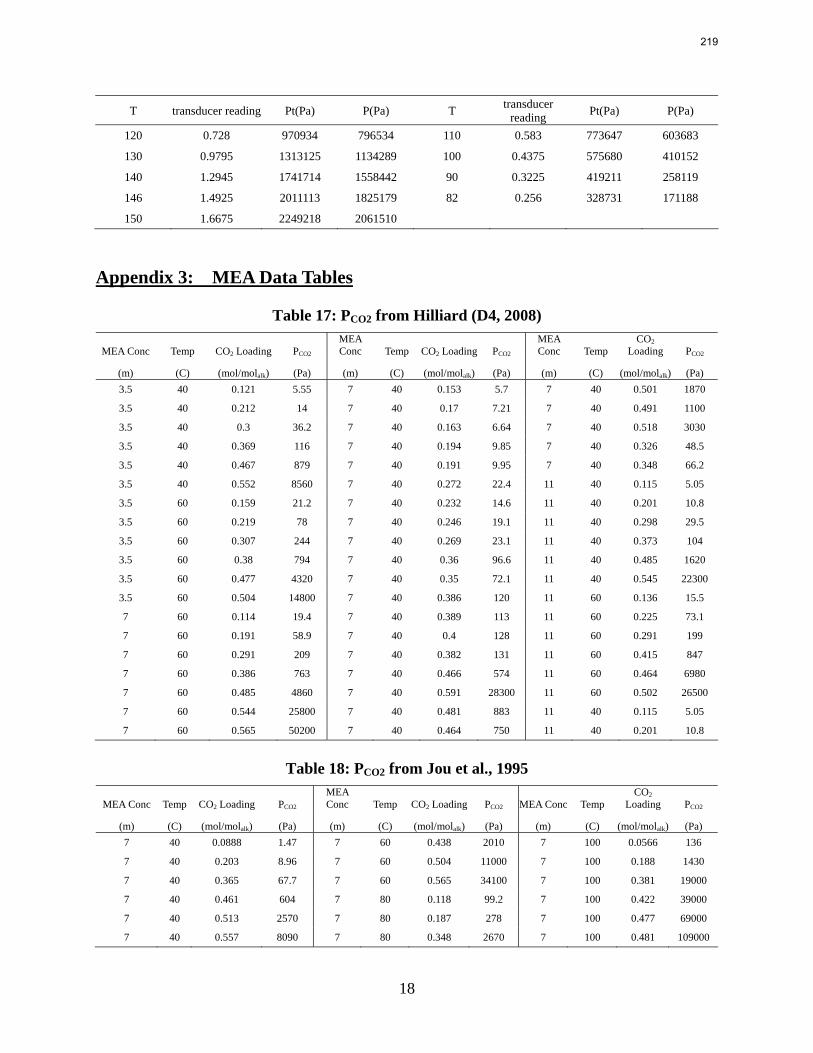
18
T transducer reading Pt(Pa) P(Pa) T transducer reading Pt(Pa) P(Pa)
120 0.728 970934 796534 110 0.583 773647 603683
130 0.9795 1313125 1134289 100 0.4375 575680 410152
140 1.2945 1741714 1558442 90 0.3225 419211 258119
146 1.4925 2011113 1825179 82 0.256 328731 171188
150 1.6675 2249218 2061510
Appendix 3: MEA Data Tables
Table 17: PCO2 from Hilliard (D4, 2008)
MEA Conc Temp CO2 Loading PCO2 MEA Conc Temp CO2 Loading PCO2
MEA Conc Temp
CO2 Loading PCO2
(m) (C) (mol/molalk) (Pa) (m) (C) (mol/molalk) (Pa) (m) (C) (mol/molalk) (Pa) 3.5 40 0.121 5.55 7 40 0.153 5.7 7 40 0.501 1870
3.5 40 0.212 14 7 40 0.17 7.21 7 40 0.491 1100
3.5 40 0.3 36.2 7 40 0.163 6.64 7 40 0.518 3030
3.5 40 0.369 116 7 40 0.194 9.85 7 40 0.326 48.5
3.5 40 0.467 879 7 40 0.191 9.95 7 40 0.348 66.2
3.5 40 0.552 8560 7 40 0.272 22.4 11 40 0.115 5.05
3.5 60 0.159 21.2 7 40 0.232 14.6 11 40 0.201 10.8
3.5 60 0.219 78 7 40 0.246 19.1 11 40 0.298 29.5
3.5 60 0.307 244 7 40 0.269 23.1 11 40 0.373 104
3.5 60 0.38 794 7 40 0.36 96.6 11 40 0.485 1620
3.5 60 0.477 4320 7 40 0.35 72.1 11 40 0.545 22300
3.5 60 0.504 14800 7 40 0.386 120 11 60 0.136 15.5
7 60 0.114 19.4 7 40 0.389 113 11 60 0.225 73.1
7 60 0.191 58.9 7 40 0.4 128 11 60 0.291 199
7 60 0.291 209 7 40 0.382 131 11 60 0.415 847
7 60 0.386 763 7 40 0.466 574 11 60 0.464 6980
7 60 0.485 4860 7 40 0.591 28300 11 60 0.502 26500
7 60 0.544 25800 7 40 0.481 883 11 40 0.115 5.05
7 60 0.565 50200 7 40 0.464 750 11 40 0.201 10.8
Table 18: PCO2 from Jou et al., 1995
MEA Conc Temp CO2 Loading PCO2 MEA Conc Temp CO2 Loading PCO2 MEA Conc Temp
CO2 Loading PCO2
(m) (C) (mol/molalk) (Pa) (m) (C) (mol/molalk) (Pa) (m) (C) (mol/molalk) (Pa) 7 40 0.0888 1.47 7 60 0.438 2010 7 100 0.0566 136
7 40 0.203 8.96 7 60 0.504 11000 7 100 0.188 1430
7 40 0.365 67.7 7 60 0.565 34100 7 100 0.381 19000
7 40 0.461 604 7 80 0.118 99.2 7 100 0.422 39000
7 40 0.513 2570 7 80 0.187 278 7 100 0.477 69000
7 40 0.557 8090 7 80 0.348 2670 7 100 0.481 109000
219
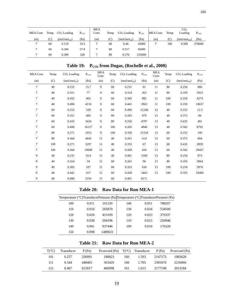
19
MEA Conc Temp CO2 Loading PCO2 MEA Conc Temp CO2 Loading PCO2 MEA Conc Temp
CO2 Loading PCO2
(m) (C) (mol/molalk) (Pa) (m) (C) (mol/molalk) (Pa) (m) (C) (mol/molalk) (Pa) 7 60 0.119 19.3 7 80 0.46 16000 7 100 0.589 376000
7 60 0.206 57.9 7 80 0.517 56000
7 60 0.389 528 7 80 0.576 235000
Table 19: PCO2 from Dugas, (Rochelle et al., 2008)
MEA Conc Temp CO2 Loading PCO2 MEA Conc Temp CO2 Loading PCO2
MEA Conc Temp CO2 Loading PCO2
(m) (C) (mol/molalk) (Pa) (m) (C) (mol/molalk) (Pa) (m) (C) (mol/molalk) (Pa)
7 40 0.252 15.7 9 60 0.231 61 11 80 0.256 860
7 40 0.351 77 9 60 0.324 263 11 80 0.359 3923
7 40 0.432 465 9 60 0.382 892 11 100 0.256 4274
7 40 0.496 4216 9 60 0.441 2862 11 100 0.359 18657
7 60 0.252 109 9 60 0.496 21249 13 40 0.252 12.3
7 60 0.351 660 9 80 0.265 979 13 40 0.372 84
7 60 0.432 3434 9 80 0.356 4797 13 40 0.435 491
7 60 0.496 16157 9 100 0.265 4940 13 40 0.502 8792
7 80 0.271 1053 9 100 0.356 21534 13 60 0.252 100
7 80 0.366 4443 11 40 0.261 14.0 13 60 0.372 694
7 100 0.271 5297 11 40 0.353 67 13 60 0.435 3859
7 100 0.366 19008 11 40 0.428 434 13 60 0.502 29427
9 40 0.231 10.4 11 40 0.461 1509 13 80 0.254 873
9 40 0.324 34 11 60 0.261 96 13 80 0.355 3964
9 40 0.382 107 11 60 0.353 634 13 100 0.254 3876
9 40 0.441 417 11 60 0.428 3463 13 100 0.355 18406
9 40 0.496 5354 11 60 0.461 8171
Table 20: Raw Data for Run MEA-1
Temperature (°C)TransducerPressure (Pa)Temperature (°C)TransducerPressure (Pa)
100 0.011 191250 140 0.051 788207
110 0.016 265870 130 0.034 534500
120 0.026 415109 120 0.023 370337
130 0.038 594196 110 0.015 250946
140 0.061 937446 100 0.010 176326
150 0.098 1489631
Table 21: Raw Data for Run MEA-2
T(°C) Transducer P (Pa) Pcorrcted (Pa) T(°C) Transducer P (Pa) Pcorrcted (Pa)
101 0.257 330091 188823 160 1.593 2147173 1983628
111 0.344 448463 303420 166 1.765 2381876 2216066
121 0.467 615817 466998 161 1.615 2177106 2013184
220
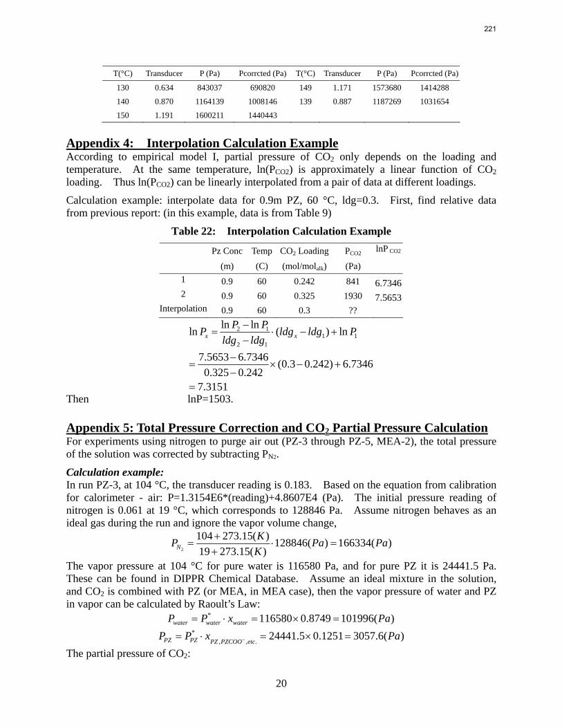
20
T(°C) Transducer P (Pa) Pcorrcted (Pa) T(°C) Transducer P (Pa) Pcorrcted (Pa)
130 0.634 843037 690820 149 1.171 1573680 1414288
140 0.870 1164139 1008146 139 0.887 1187269 1031654
150 1.191 1600211 1440443
Appendix 4: Interpolation Calculation Example According to empirical model I, partial pressure of CO2 only depends on the loading and temperature. At the same temperature, ln(PCO2) is approximately a linear function of CO2 loading. Thus ln(PCO2) can be linearly interpolated from a pair of data at different loadings.
Calculation example: interpolate data for 0.9m PZ, 60 °C, ldg=0.3. First, find relative data from previous report: (in this example, data is from Table 9)
Table 22: Interpolation Calculation Example Pz Conc Temp CO2 Loading PCO2 lnP CO2
(m) (C) (mol/molalk) (Pa)
1 0.9 60 0.242 841 6.7346 2 0.9 60 0.325 1930 7.5653
Interpolation 0.9 60 0.3 ?? 2 1
1 12 1
ln lnln ( ) ln
7.5653 6.7346 (0.3 0.242) 6.73460.325 0.242
7.3151
x xP PP ldg ldg P
ldg ldg−
= ⋅ − +−
−= × − +
−=
Then lnP=1503. Appendix 5: Total Pressure Correction and CO2 Partial Pressure Calculation For experiments using nitrogen to purge air out (PZ-3 through PZ-5, MEA-2), the total pressure of the solution was corrected by subtracting PN2.
Calculation example: In run PZ-3, at 104 °C, the transducer reading is 0.183. Based on the equation from calibration for calorimeter - air: P=1.3154E6*(reading)+4.8607E4 (Pa). The initial pressure reading of nitrogen is 0.061 at 19 °C, which corresponds to 128846 Pa. Assume nitrogen behaves as an ideal gas during the run and ignore the vapor volume change,
2
104 273.15( ) 128846( ) 166334( )19 273.15( )N
KP Pa PaK
+= ⋅ =
+
The vapor pressure at 104 °C for pure water is 116580 Pa, and for pure PZ it is 24441.5 Pa. These can be found in DIPPR Chemical Database. Assume an ideal mixture in the solution, and CO2 is combined with PZ (or MEA, in MEA case), then the vapor pressure of water and PZ in vapor can be calculated by Raoult’s Law:
* 116580 0.8749 101996( )water water waterP P x Pa= ⋅ = × = *
, , .24441.5 0.1251 3057.6( )PZ PZ PZ PZCOO etc
P P x Pa−= ⋅ = × = The partial pressure of CO2:
221
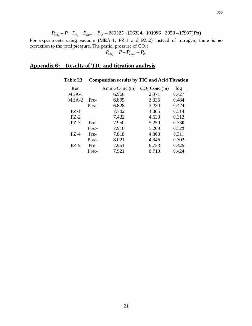
21
2 2289325 166334 101996 3058 17937( )CO N water PZP P P P P Pa= − − − = − − − =
For experiments using vacuum (MEA-1, PZ-1 and PZ-2) instead of nitrogen, there is no correction to the total pressure. The partial pressure of CO2:
2CO water PZP P P P= − − Appendix 6: Results of TIC and titration analysis
Table 23: Composition results by TIC and Acid Titration
Run Amine Conc (m) CO2 Conc (m) ldg MEA-1 6.966 2.971 0.427 MEA-2 Pre- 6.895 3.335 0.484
Post- 6.828 3.239 0.474 PZ-1 7.782 4.885 0.314 PZ-2 7.432 4.630 0.312 PZ-3 Pre- 7.950 5.250 0.330
Post- 7.918 5.209 0.329 PZ-4 Pre- 7.818 4.860 0.311
Post- 8.021 4.846 0.302 PZ-5 Pre- 7.951 6.753 0.425
Post- 7.921 6.719 0.424
222
1
Amine Volatility and Heat Capacity for Concentrated Piperazine
Progress Report for January 1 – March 31, 2009
by Thu Nguyen
Supported by the Luminant Carbon Management Program
and the
Industrial Associates Program for CO2 Capture by Aqueous Absorption
Department of Chemical Engineering
The University of Texas at Austin
April 1, 2009
Abstract The volatility of amines is an important screening criterion used to evaluate its viability for use as a CO2 capture solvent. Several amine systems have been evaluated for volatility at absorber operating conditions, which are 40 ºC–60 ºC at nominal lean and rich loadings corresponding to about 500 Pa and 5000 Pa, respectively. In comparing different amine systems studied to date, the 7 m MDEA/2 m PZ blend appears to be the least volatile. It is roughly 2.5 times less volatile than the baseline 7 m MEA solvent. 8 m PZ is also a very viable amine candidate as it is only half as volatile as the baseline solvent. On the other hand, 5 m AMP appears to be the most volatile so far; in fact, it is 1.5–3 times more volatile than 7 m MEA at lean and rich conditions defined earlier. In the arena of heat capacity studies, the averaged Cp of 8 m PZ solutions is approximately 3.1–3.6 J/g*K. The Cp of pure liquid PZ in these solutions is regressed to be 2.33 J/g*K and that of CO2 is approximately 0.76 J/g*K.
Introduction This report discusses the volatility of different amine systems at 40 ºC and 60 ºC and nominal lean and rich loading corresponding to CO2 partial pressure of 500 Pa and 5000 Pa, respectively. The systems that have been studied to date are baseline 7 m MEA, 8 m PZ, 7 m MDEA/2 m PZ, and 5 m AMP. The volatility of a particular solvent is an important screening criterion that justifies its use for CO2 capture over competing solvents. Work has also been done to model heat capacity for loaded 8 m PZ solutions. Key values for pure component PZ and CO2 heat capacity in these solutions have been regressed for temperatures ranging from 40 ºC–120 ºC.
223
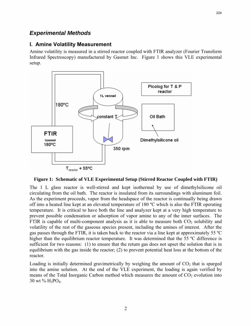
2
Experimental Methods
I. Amine Volatility Measurement Amine volatility is measured in a stirred reactor coupled with FTIR analyzer (Fourier Transform Infrared Spectroscopy) manufactured by Gasmet Inc. Figure 1 shows this VLE experimental setup.
Figure 1: Schematic of VLE Experimental Setup (Stirred Reactor Coupled with FTIR)
The 1 L glass reactor is well-stirred and kept isothermal by use of dimethylsilicone oil circulating from the oil bath. The reactor is insulated from its surroundings with aluminum foil. As the experiment proceeds, vapor from the headspace of the reactor is continually being drawn off into a heated line kept at an elevated temperature of 180 ºC which is also the FTIR operating temperature. It is critical to have both the line and analyzer kept at a very high temperature to prevent possible condensation or adsorption of vapor amine to any of the inner surfaces. The FTIR is capable of multi-component analysis as it is able to measure both CO2 solubility and volatility of the rest of the gaseous species present, including the amines of interest. After the gas passes through the FTIR, it is taken back to the reactor via a line kept at approximately 55 ºC higher than the equilibrium reactor temperature. It was determined that the 55 ºC difference is sufficient for two reasons: (1) to ensure that the return gas does not upset the solution that is in equilibrium with the gas inside the reactor; (2) to prevent potential heat loss at the bottom of the reactor.
Loading is initially determined gravimetrically by weighing the amount of CO2 that is sparged into the amine solution. At the end of the VLE experiment, the loading is again verified by means of the Total Inorganic Carbon method which measures the amount of CO2 evolution into 30 wt % H3PO4.
224
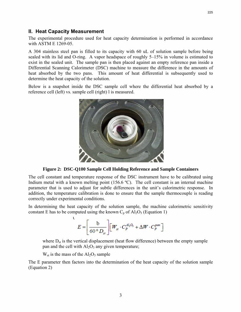
3
II. Heat Capacity Measurement The experimental procedure used for heat capacity determination is performed in accordance with ASTM E 1269-05.
A 304 stainless steel pan is filled to its capacity with 60 uL of solution sample before being sealed with its lid and O-ring. A vapor headspace of roughly 5–15% in volume is estimated to exist in the sealed unit. The sample pan is then placed against an empty reference pan inside a Differential Scanning Calorimeter (DSC) machine to measure the difference in the amounts of heat absorbed by the two pans. This amount of heat differential is subsequently used to determine the heat capacity of the solution.
Below is a snapshot inside the DSC sample cell where the differential heat absorbed by a reference cell (left) vs. sample cell (right) l is measured.
Figure 2: DSC-Q100 Sample Cell Holding Reference and Sample Containers
The cell constant and temperature response of the DSC instrument have to be calibrated using Indium metal with a known melting point (156.6 ºC). The cell constant is an internal machine parameter that is used to adjust for subtle differences in the unit’s calorimetric response. In addition, the temperature calibration is done to ensure that the sample thermocouple is reading correctly under experimental conditions.
In determining the heat capacity of the solution sample, the machine calorimetric sensitivity constant E has to be computed using the known Cp of Al2O3 (Equation 1)
where Dst is the vertical displacement (heat flow difference) between the empty sample pan and the cell with Al2O3 any given temperature;
Wst is the mass of the Al2O3 sample
The E parameter then factors into the determination of the heat capacity of the solution sample (Equation 2)
225
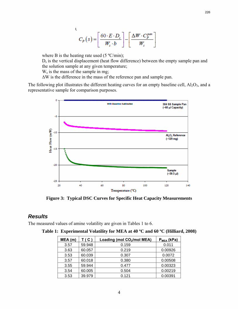
4
where B is the heating rate used (5 ºC/min); Ds is the vertical displacement (heat flow difference) between the empty sample pan and the solution sample at any given temperature; Ws is the mass of the sample in mg; ∆W is the difference in the mass of the reference pan and sample pan.
The following plot illustrates the different heating curves for an empty baseline cell, Al2O3, and a representative sample for comparison purposes.
Figure 3: Typical DSC Curves for Specific Heat Capacity Measurements
Results The measured values of amine volatility are given in Tables 1 to 6.
Table 1: Experimental Volatility for MEA at 40 ºC and 60 ºC (Hilliard, 2008)
MEA (m) T ( C ) Loading (mol CO2/mol MEA) PMEA (kPa) 3.57 59.948 0.159 0.011 3.63 60.057 0.219 0.00926 3.53 60.039 0.307 0.0072 3.57 60.018 0.380 0.00508 3.55 59.944 0.477 0.00323 3.54 60.005 0.504 0.00219 3.53 39.979 0.121 0.00391
226
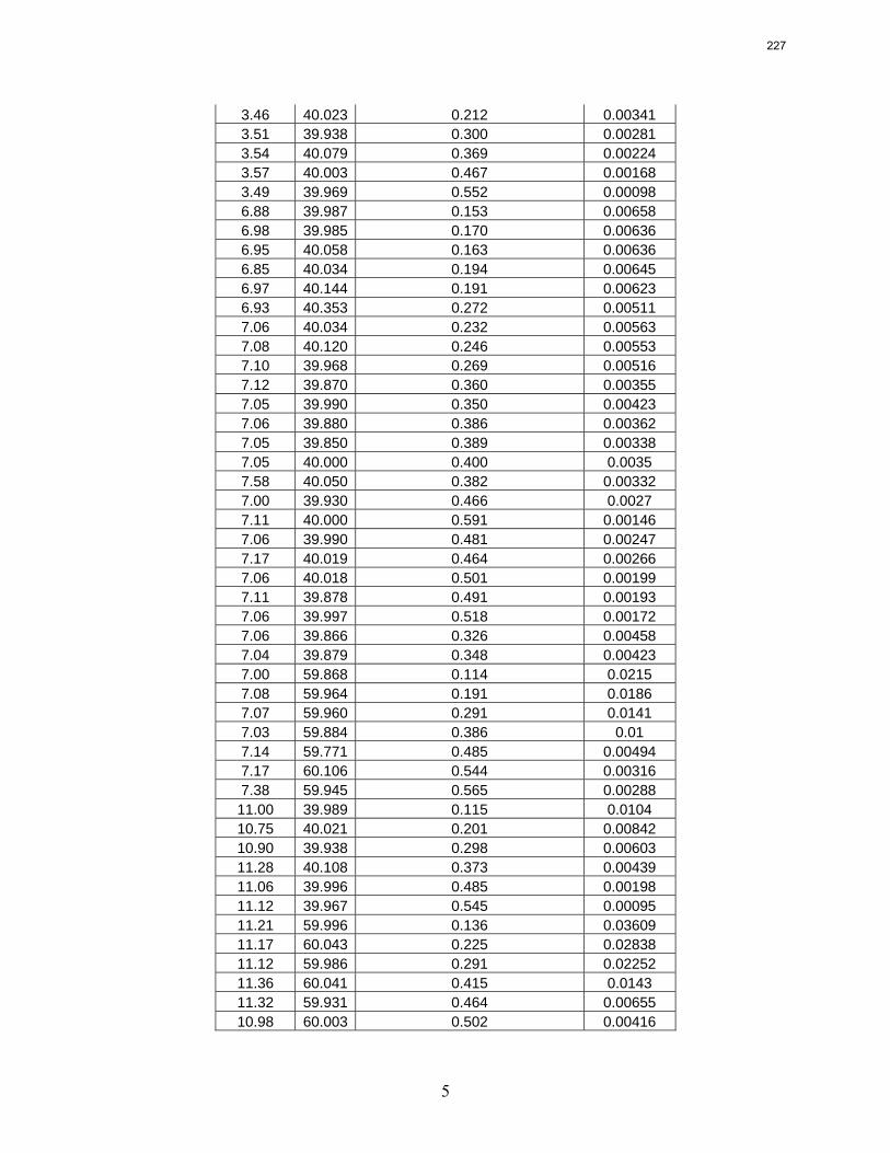
5
3.46 40.023 0.212 0.00341 3.51 39.938 0.300 0.00281 3.54 40.079 0.369 0.00224 3.57 40.003 0.467 0.00168 3.49 39.969 0.552 0.00098 6.88 39.987 0.153 0.00658 6.98 39.985 0.170 0.00636 6.95 40.058 0.163 0.00636 6.85 40.034 0.194 0.00645 6.97 40.144 0.191 0.00623 6.93 40.353 0.272 0.00511 7.06 40.034 0.232 0.00563 7.08 40.120 0.246 0.00553 7.10 39.968 0.269 0.00516 7.12 39.870 0.360 0.00355 7.05 39.990 0.350 0.00423 7.06 39.880 0.386 0.00362 7.05 39.850 0.389 0.00338 7.05 40.000 0.400 0.0035 7.58 40.050 0.382 0.00332 7.00 39.930 0.466 0.0027 7.11 40.000 0.591 0.00146 7.06 39.990 0.481 0.00247 7.17 40.019 0.464 0.00266 7.06 40.018 0.501 0.00199 7.11 39.878 0.491 0.00193 7.06 39.997 0.518 0.00172 7.06 39.866 0.326 0.00458 7.04 39.879 0.348 0.00423 7.00 59.868 0.114 0.0215 7.08 59.964 0.191 0.0186 7.07 59.960 0.291 0.0141 7.03 59.884 0.386 0.01 7.14 59.771 0.485 0.00494 7.17 60.106 0.544 0.00316 7.38 59.945 0.565 0.00288 11.00 39.989 0.115 0.0104 10.75 40.021 0.201 0.00842 10.90 39.938 0.298 0.00603 11.28 40.108 0.373 0.00439 11.06 39.996 0.485 0.00198 11.12 39.967 0.545 0.00095 11.21 59.996 0.136 0.03609 11.17 60.043 0.225 0.02838 11.12 59.986 0.291 0.02252 11.36 60.041 0.415 0.0143 11.32 59.931 0.464 0.00655 10.98 60.003 0.502 0.00416
227
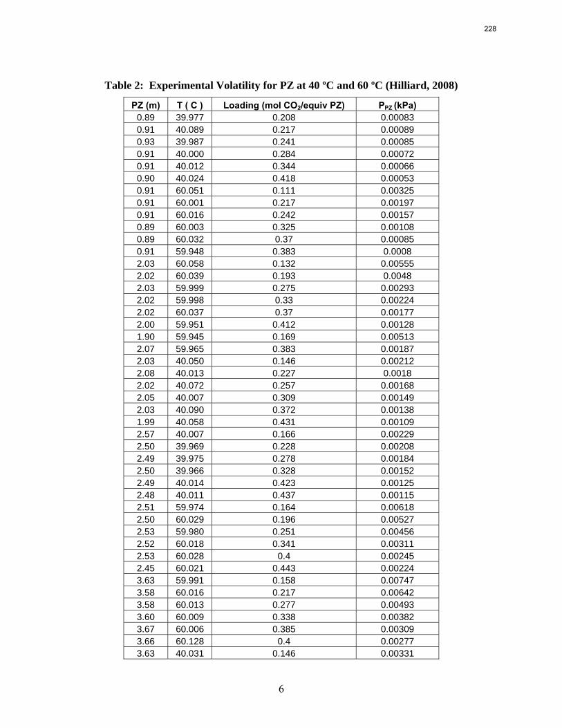
6
Table 2: Experimental Volatility for PZ at 40 ºC and 60 ºC (Hilliard, 2008)
PZ (m) T ( C ) Loading (mol CO2/equiv PZ) PPZ (kPa) 0.89 39.977 0.208 0.00083 0.91 40.089 0.217 0.00089 0.93 39.987 0.241 0.00085 0.91 40.000 0.284 0.00072 0.91 40.012 0.344 0.00066 0.90 40.024 0.418 0.00053 0.91 60.051 0.111 0.00325 0.91 60.001 0.217 0.00197 0.91 60.016 0.242 0.00157 0.89 60.003 0.325 0.00108 0.89 60.032 0.37 0.00085 0.91 59.948 0.383 0.0008 2.03 60.058 0.132 0.00555 2.02 60.039 0.193 0.0048 2.03 59.999 0.275 0.00293 2.02 59.998 0.33 0.00224 2.02 60.037 0.37 0.00177 2.00 59.951 0.412 0.00128 1.90 59.945 0.169 0.00513 2.07 59.965 0.383 0.00187 2.03 40.050 0.146 0.00212 2.08 40.013 0.227 0.0018 2.02 40.072 0.257 0.00168 2.05 40.007 0.309 0.00149 2.03 40.090 0.372 0.00138 1.99 40.058 0.431 0.00109 2.57 40.007 0.166 0.00229 2.50 39.969 0.228 0.00208 2.49 39.975 0.278 0.00184 2.50 39.966 0.328 0.00152 2.49 40.014 0.423 0.00125 2.48 40.011 0.437 0.00115 2.51 59.974 0.164 0.00618 2.50 60.029 0.196 0.00527 2.53 59.980 0.251 0.00456 2.52 60.018 0.341 0.00311 2.53 60.028 0.4 0.00245 2.45 60.021 0.443 0.00224 3.63 59.991 0.158 0.00747 3.58 60.016 0.217 0.00642 3.58 60.013 0.277 0.00493 3.60 60.009 0.338 0.00382 3.67 60.006 0.385 0.00309 3.66 60.128 0.4 0.00277 3.63 40.031 0.146 0.00331
228
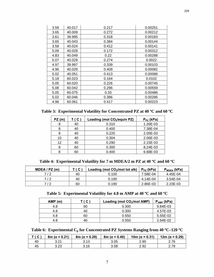
7
3.59 40.017 0.217 0.00251 3.65 40.009 0.272 0.00212 3.61 39.995 0.318 0.00183 3.65 40.043 0.384 0.00144 3.58 40.024 0.412 0.00141 5.09 40.028 0.172 0.00312 4.83 40.049 0.22 0.00288 5.07 40.029 0.274 0.0022 4.97 39.997 0.339 0.00103 4.96 40.029 0.409 0.00082 5.02 40.051 0.413 0.00086 5.18 60.023 0.164 0.0102 5.05 60.020 0.226 0.00745 5.08 60.042 0.296 0.00559 5.05 60.075 0.33 0.00486 5.02 60.046 0.386 0.00286 4.96 60.061 0.417 0.00223
Table 3: Experimental Volatility for Concentrated PZ at 40 ºC and 60 ºC
Table 4: Experimental Volatility for 7 m MDEA/2 m PZ at 40 ºC and 60 ºC
MDEA / PZ (m) T ( C ) Loading (mol CO2/mol tot alk) PPZ (kPa) PMDEA (kPa) 7 / 2 40 0.100 7.58E-04 4.45E-04 7 / 2 40 0.190 4.14E-04 3.54E-04 7 / 2 60 0.190 2.86E-03 2.23E-03
Table 5: Experimental Volatility for 4.8 m AMP at 40 ºC and 60 ºC
AMP (m) T ( C ) Loading (mol CO2/mol AMP) PAMP (kPa) 4.8 60 0.300 9.84E-03 4.8 40 0.300 4.57E-03 4.8 60 0.550 5.55E-02 4.8 40 0.550 2.64E-02
Table 6: Experimental Cp for Concentrated PZ Systems Ranging from 40 ºC–120 ºC T ( C ) 8m (α = 0.21) 8m (α = 0.29) 8m (α = 0.40) 10m (α = 0.31) 12m (α = 0.29)
40 3.21 3.13 3.05 2.90 2.76 45 3.23 3.16 3.08 2.92 2.79
PZ (m) T ( C ) Loading (mol CO2/equiv PZ) PPZ (kPa) 8 40 0.310 1.26E-03 8 40 0.400 7.38E-04 8 40 0.220 2.05E-03 10 40 0.304 2.06E-03 12 40 0.290 2.15E-03 8 60 0.300 8.24E-03 8 60 0.400 6.68E-03
229
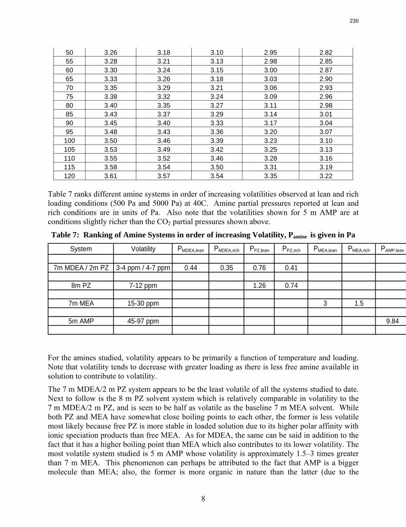
8
50 3.26 3.18 3.10 2.95 2.82 55 3.28 3.21 3.13 2.98 2.85 60 3.30 3.24 3.15 3.00 2.87 65 3.33 3.26 3.18 3.03 2.90 70 3.35 3.29 3.21 3.06 2.93 75 3.38 3.32 3.24 3.09 2.96 80 3.40 3.35 3.27 3.11 2.98 85 3.43 3.37 3.29 3.14 3.01 90 3.45 3.40 3.33 3.17 3.04 95 3.48 3.43 3.36 3.20 3.07
100 3.50 3.46 3.39 3.23 3.10 105 3.53 3.49 3.42 3.25 3.13 110 3.55 3.52 3.46 3.28 3.16 115 3.58 3.54 3.50 3.31 3.19 120 3.61 3.57 3.54 3.35 3.22
Table 7 ranks different amine systems in order of increasing volatilities observed at lean and rich loading conditions (500 Pa and 5000 Pa) at 40C. Amine partial pressures reported at lean and rich conditions are in units of Pa. Also note that the volatilities shown for 5 m AMP are at conditions slightly richer than the CO2 partial pressures shown above.
Table 7: Ranking of Amine Systems in order of increasing Volatility, Pamine is given in Pa
System Volatility PMDEA,lean PMDEA,rich PPZ,lean PPZ,rich PMEA,lean PMEA,rich PAMP,lean
7m MDEA / 2m PZ 3-4 ppm / 4-7 ppm 0.44 0.35 0.76 0.41
8m PZ 7-12 ppm 1.26 0.74
7m MEA 15-30 ppm 3 1.5
5m AMP 45-97 ppm 9.84
For the amines studied, volatility appears to be primarily a function of temperature and loading. Note that volatility tends to decrease with greater loading as there is less free amine available in solution to contribute to volatility.
The 7 m MDEA/2 m PZ system appears to be the least volatile of all the systems studied to date. Next to follow is the 8 m PZ solvent system which is relatively comparable in volatility to the 7 m MDEA/2 m PZ, and is seen to be half as volatile as the baseline 7 m MEA solvent. While both PZ and MEA have somewhat close boiling points to each other, the former is less volatile most likely because free PZ is more stable in loaded solution due to its higher polar affinity with ionic speciation products than free MEA. As for MDEA, the same can be said in addition to the fact that it has a higher boiling point than MEA which also contributes to its lower volatility. The most volatile system studied is 5 m AMP whose volatility is approximately 1.5–3 times greater than 7 m MEA. This phenomenon can perhaps be attributed to the fact that AMP is a bigger molecule than MEA; also, the former is more organic in nature than the latter (due to the
230
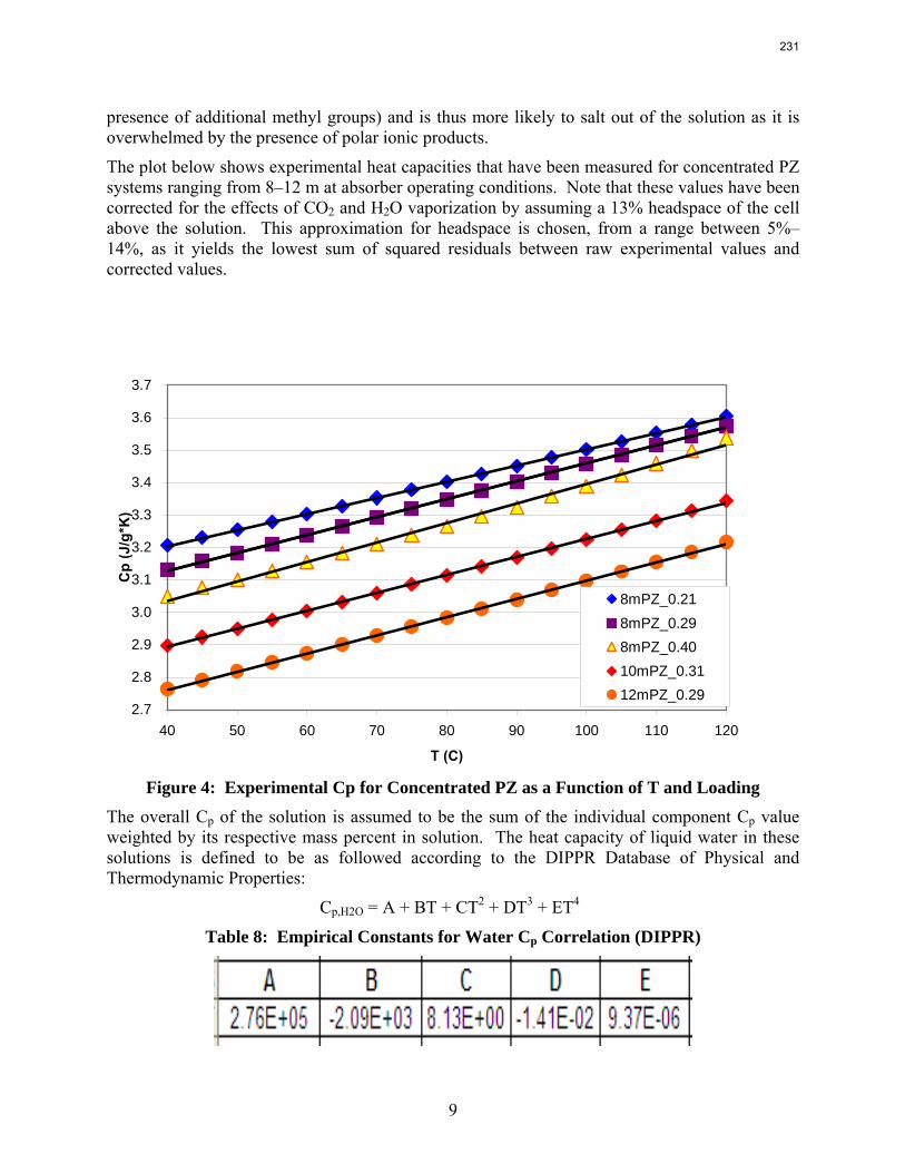
9
presence of additional methyl groups) and is thus more likely to salt out of the solution as it is overwhelmed by the presence of polar ionic products.
The plot below shows experimental heat capacities that have been measured for concentrated PZ systems ranging from 8–12 m at absorber operating conditions. Note that these values have been corrected for the effects of CO2 and H2O vaporization by assuming a 13% headspace of the cell above the solution. This approximation for headspace is chosen, from a range between 5%–14%, as it yields the lowest sum of squared residuals between raw experimental values and corrected values.
2.7
2.8
2.9
3.0
3.1
3.2
3.3
3.4
3.5
3.6
3.7
40 50 60 70 80 90 100 110 120
T (C)
Cp
(J/g
*K)
8mPZ_0.218mPZ_0.298mPZ_0.4010mPZ_0.3112mPZ_0.29
Figure 4: Experimental Cp for Concentrated PZ as a Function of T and Loading The overall Cp of the solution is assumed to be the sum of the individual component Cp value weighted by its respective mass percent in solution. The heat capacity of liquid water in these solutions is defined to be as followed according to the DIPPR Database of Physical and Thermodynamic Properties:
Cp,H2O = A + BT + CT2 + DT3 + ET4
Table 8: Empirical Constants for Water Cp Correlation (DIPPR)
231
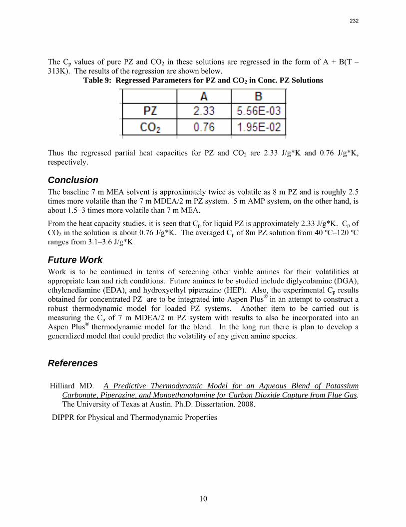
10
The Cp values of pure PZ and CO2 in these solutions are regressed in the form of A + B(T – 313K). The results of the regression are shown below.
Table 9: Regressed Parameters for PZ and CO2 in Conc. PZ Solutions
Thus the regressed partial heat capacities for PZ and CO2 are 2.33 J/g*K and 0.76 J/g*K, respectively.
Conclusion The baseline 7 m MEA solvent is approximately twice as volatile as 8 m PZ and is roughly 2.5 times more volatile than the 7 m MDEA/2 m PZ system. 5 m AMP system, on the other hand, is about 1.5–3 times more volatile than 7 m MEA.
From the heat capacity studies, it is seen that Cp for liquid PZ is approximately 2.33 J/g*K. Cp of CO2 in the solution is about 0.76 J/g*K. The averaged Cp of 8m PZ solution from 40 ºC–120 ºC ranges from 3.1–3.6 J/g*K.
Future Work Work is to be continued in terms of screening other viable amines for their volatilities at appropriate lean and rich conditions. Future amines to be studied include diglycolamine (DGA), ethylenediamine (EDA), and hydroxyethyl piperazine (HEP). Also, the experimental Cp results obtained for concentrated PZ are to be integrated into Aspen Plus® in an attempt to construct a robust thermodynamic model for loaded PZ systems. Another item to be carried out is measuring the Cp of 7 m MDEA/2 m PZ system with results to also be incorporated into an Aspen Plus® thermodynamic model for the blend. In the long run there is plan to develop a generalized model that could predict the volatility of any given amine species.
References Hilliard MD. A Predictive Thermodynamic Model for an Aqueous Blend of Potassium
Carbonate, Piperazine, and Monoethanolamine for Carbon Dioxide Capture from Flue Gas. The University of Texas at Austin. Ph.D. Dissertation. 2008.
DIPPR for Physical and Thermodynamic Properties
232
1
Oxidative Degradation of MEA
Quarterly Report for January 1 – March 31, 2009
by Alexander Voice
Supported by the Luminant Carbon Management Program
and the
Industrial Associates Program for CO2 Capture by Aqueous Absorption
Department of Chemical Engineering
The University of Texas at Austin
March 31, 2009
Abstract Oxidative degradation of monoethanolamine (MEA) was studied in the high gas flow (HGF) apparatus this quarter. The base case conditions, which remained constant in all experiments this quarter were MEA concentration (30wt % = 7 m = 4.8 M), loading (0.4 moles CO2/mole MEA), temperature (55 ºC), dry gas composition (17.5% O2, 2.1% CO2), and total solution volume (350 mL). 5 mM of inhibitor B decreased the degradation rate in the presence of 1 mM Fe, 0.1 mM Ni, 0.1 mM Cr, and 5 mM Cu by 43%; additional B did not result in a further decrease in degradation. 20 mM B decreased the degradation rate of MEA in the presence of 1 mM Fe by 53%. Sodium sulfide initially increased ammonia production, but did not change the steady-state degradation rate. MEA degradation in the HGF apparatus was determined to be kinetically controlled in the presence of 50mM A, no catalyst, and an agitation rate of 1500 rpm. Heat stable salt concentrations (analyzed this quarter) from the HGF experiment described in a previous report (Rochelle et al., 2009) all increased with time except glycolate. MEA concentration decreased by 10% after 4300 minutes of degradation in this experiment.
A flame atomic absorption method was developed this quarter. Thermally degraded samples extracted from stainless steel bombs contained 115–765 ppm iron, 25–400 ppm nickel, and 37–300 ppm chromium. Solutions with no iron added were found to contain a range of iron concentrations; nonetheless, a T-test revealed that samples degraded for 2–3 hours in the HGF contain more iron than initial samples at 95% confidence. Flame AA was also used to determine the solubility of inhibitor B as .016 mM in a degraded solution.
Introduction MEA has been investigated as a cheap amine solvent to be used in absorber/stripper systems for carbon dioxide separation from flue gas. MEA costs less than $1/lb, while other amine solvents can cost five to ten times as much. However, MEA degrades in the presence of oxygen (in the absorber) and at high temperature (in the stripper). Flue gas entering the absorber may contain 5–10% oxygen due to the excess oxygen used for efficient combustion. Oxygen is not present in high concentration in the stripper, however, elevated temperatures used to release carbon dioxide from the amine solvent can cause the solvent to thermally degrade. The objective of the work
233
2
described in this report was to study oxidative degradation at absorber conditions, while ignoring the effect of any thermal or oxidative degradation occurring in the stripper. Most oxidative degradation will occur at the bottom of the absorber when the oxygen rich flue gas first contacts the solvent. For this reason, a base case for oxidative degradation was chosen as 55 °C and a rich loading of 0.4 moles CO2/mole MEA.
Inhibitor B and inhibitor A can potentially inhibit oxidative degradation catalytically. Thus, only a one-time addition of the inhibitor is required (rather than continuous addition, as with EDTA). A and B were investigated as possible degradation inhibitors for 7 m MEA solutions in a typical absorber used to remove CO2 from coal-fired power plant flue gas.
Mechanisms of oxidative degradation of amines have been previously studied, though the exact mechanism of MEA degradation is unknown. Degradation proceeds by way of formation of a free radical (rate limiting), which can be catalyzed by metal ions present in an industrial setting. Metal ions typically present in an industrial setting include iron, which leaches in from pipes and equipment, and copper, which is added to inhibit corrosion of equipment by the MEA. Inhibitors work by reacting with free radicals and preventing them from reacting with and degrading MEA. Because the free radical mechanism can regenerate a free radical, 1 mol of inhibitor can potentially protect significantly more than 1 mol of MEA from oxidation (Sexton, 2008).
Ammonia is the primary degradation product predicted by the proposed oxidative degradation mechanisms. Ammonia is produced approximately on a one-to-one molar basis with the disappearance of MEA; thus the oxidative degradation rate can be estimated by measuring ammonia production. In addition, ammonia is volatile and will be stripped out of the solution by the gas being sparged into the reactor (Goff, 2005).
Background Oxidative degradation of various amine solvents has been previously studied under a variety of conditions. Unfortunately, the degradation rates reported in many previous studies were determined under conditions that were oxygen mass-transfer limited (Goff, 2005). Thus, although the absolute rate reported is only valid for the specific apparatus used to conduct degradation, it is useful to examine the relative degradation rates of various solvents under different conditions.
Blachly and Ravner (1964) conducted some oxidative degradation research on MEA as part of an effort to improve the degradation inhibition “packet” of additives for CO2 capture systems on submarines. MEA was studied at 4 M concentration and a loading corresponding to 1% CO2 in the vapor phase. They determined that copper was a potent catalyst of oxidative degradation, with nickel and iron also showing catalytic activity. Chromium was not found to catalyze oxidative degradation. VSF, or bicine, was a successful inhibitor at 55 ºC with no metals present, while EDTA was used to inhibit oxidative degradation at 55 ºC in the presence of copper. At higher temperatures (98 ºC), both EDTA and bicine were required to inhibit oxidative degradation.
Rooney et al. (1998) studied oxidative degradation of 20% MEA and other amines in a 1 L glass reactor at 81 ºC. They analyzed degraded solutions for the presence of heat stable salts, including formate, glycolate, acetate, oxalate, nitrate, and nitrite using ion chromatography. 30% MDEA degraded faster than 20% MEA in a loaded solution, but MEA degraded faster in an
234
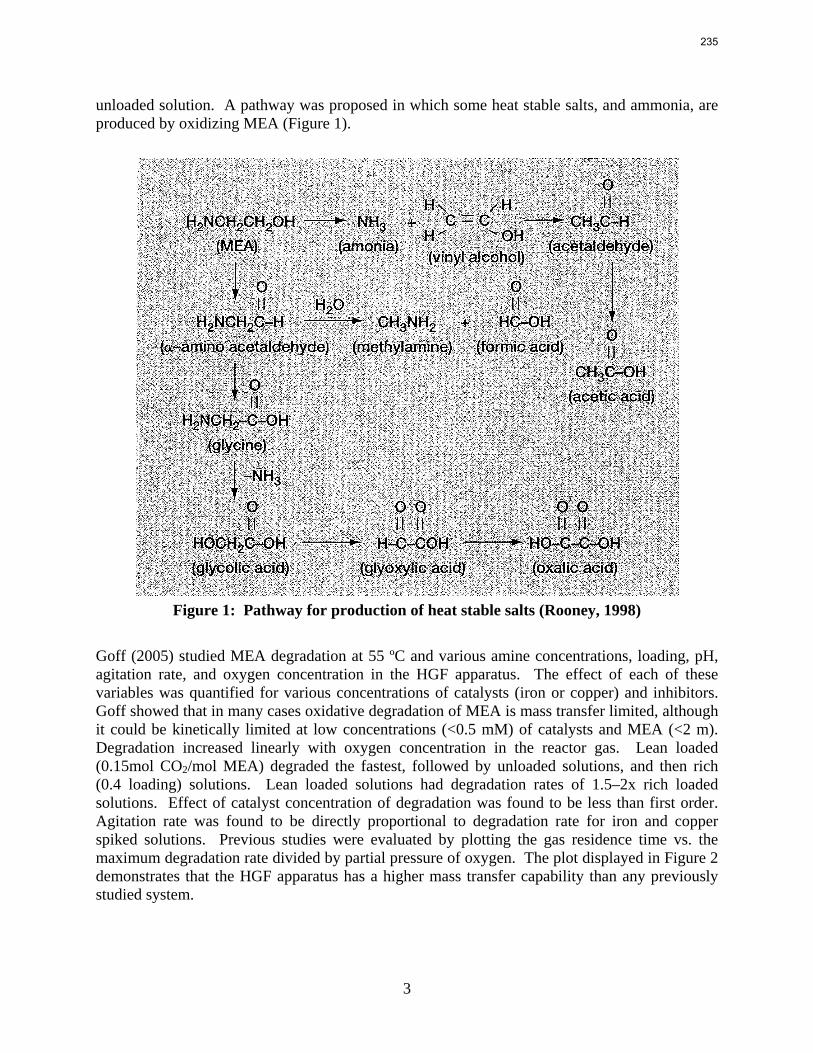
3
unloaded solution. A pathway was proposed in which some heat stable salts, and ammonia, are produced by oxidizing MEA (Figure 1).
Figure 1: Pathway for production of heat stable salts (Rooney, 1998)
Goff (2005) studied MEA degradation at 55 ºC and various amine concentrations, loading, pH, agitation rate, and oxygen concentration in the HGF apparatus. The effect of each of these variables was quantified for various concentrations of catalysts (iron or copper) and inhibitors. Goff showed that in many cases oxidative degradation of MEA is mass transfer limited, although it could be kinetically limited at low concentrations (<0.5 mM) of catalysts and MEA (<2 m). Degradation increased linearly with oxygen concentration in the reactor gas. Lean loaded (0.15mol CO2/mol MEA) degraded the fastest, followed by unloaded solutions, and then rich (0.4 loading) solutions. Lean loaded solutions had degradation rates of 1.5–2x rich loaded solutions. Effect of catalyst concentration of degradation was found to be less than first order. Agitation rate was found to be directly proportional to degradation rate for iron and copper spiked solutions. Previous studies were evaluated by plotting the gas residence time vs. the maximum degradation rate divided by partial pressure of oxygen. The plot displayed in Figure 2 demonstrates that the HGF apparatus has a higher mass transfer capability than any previously studied system.
235
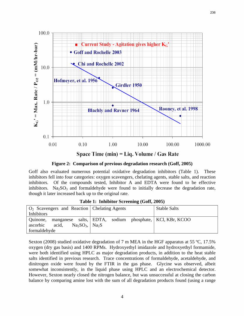
4
Figure 2: Comparison of previous degradation research (Goff, 2005) Goff also evaluated numerous potential oxidative degradation inhibitors (Table 1). These inhibitors fell into four categories: oxygen scavengers, chelating agents, stable salts, and reaction inhibitors. Of the compounds tested, Inhibitor A and EDTA were found to be effective inhibitors. Na2SO3 and formaldehyde were found to initially decrease the degradation rate, though it later increased back up to the original rate.
Table 1: Inhibitor Screening (Goff, 2005) O2 Scavengers and Reaction Inhibitors
Chelating Agents Stable Salts
Quinone, manganese salts, ascorbic acid, Na2SO3, formaldehyde
EDTA, sodium phosphate, Na2S
KCl, KBr, KCOO
Sexton (2008) studied oxidative degradation of 7 m MEA in the HGF apparatus at 55 ºC, 17.5% oxygen (dry gas basis) and 1400 RPMs. Hydroxyethyl imidazole and hydroxyethyl formamide, were both identified using HPLC as major degradation products, in addition to the heat stable salts identified in previous research. Trace concentrations of formaldehyde, acetaldehyde, and dinitrogen oxide were found by the FTIR in the gas phase. Glycine was observed, albeit somewhat inconsistently, in the liquid phase using HPLC and an electrochemical detector. However, Sexton nearly closed the nitrogen balance, but was unsuccessful at closing the carbon balance by comparing amine lost with the sum of all degradation products found (using a range
236
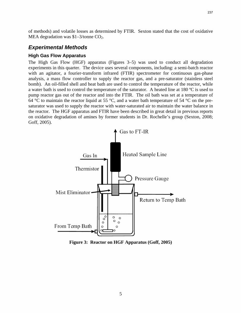
5
of methods) and volatile losses as determined by FTIR. Sexton stated that the cost of oxidative MEA degradation was $1–3/tonne CO2.
Experimental Methods High Gas Flow Apparatus The High Gas Flow (HGF) apparatus (Figures 3–5) was used to conduct all degradation experiments in this quarter. The device uses several components, including: a semi-batch reactor with an agitator, a fourier-transform infrared (FTIR) spectrometer for continuous gas-phase analysis, a mass flow controller to supply the reactor gas, and a pre-saturator (stainless steel bomb). An oil-filled shell and heat bath are used to control the temperature of the reactor, while a water bath is used to control the temperature of the saturator. A heated line at 180 ºC is used to pump reactor gas out of the reactor and into the FTIR. The oil bath was set at a temperature of 64 °C to maintain the reactor liquid at 55 °C, and a water bath temperature of 54 °C on the pre-saturator was used to supply the reactor with water-saturated air to maintain the water balance in the reactor. The HGF apparatus and FTIR have been described in great detail in previous reports on oxidative degradation of amines by former students in Dr. Rochelle’s group (Sexton, 2008; Goff, 2005).
Figure 3: Reactor on HGF Apparatus (Goff, 2005)
237
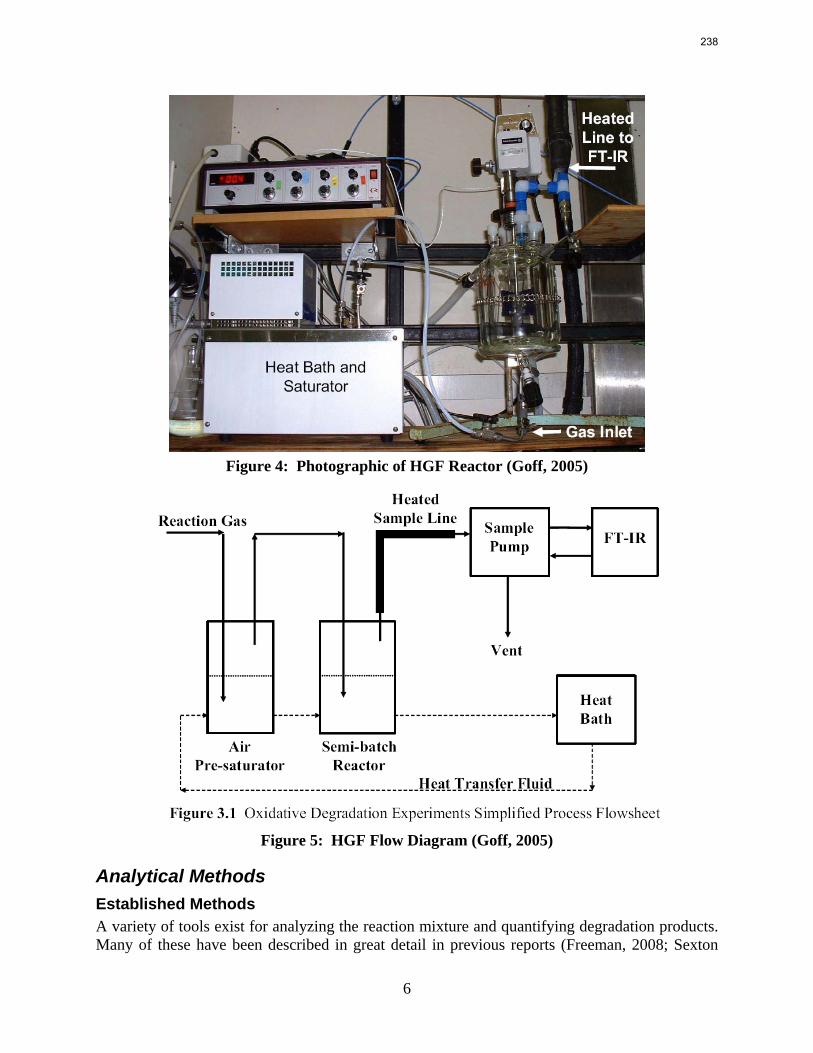
6
Figure 4: Photographic of HGF Reactor (Goff, 2005)
Figure 5: HGF Flow Diagram (Goff, 2005)
Analytical Methods Established Methods A variety of tools exist for analyzing the reaction mixture and quantifying degradation products. Many of these have been described in great detail in previous reports (Freeman, 2008; Sexton
238
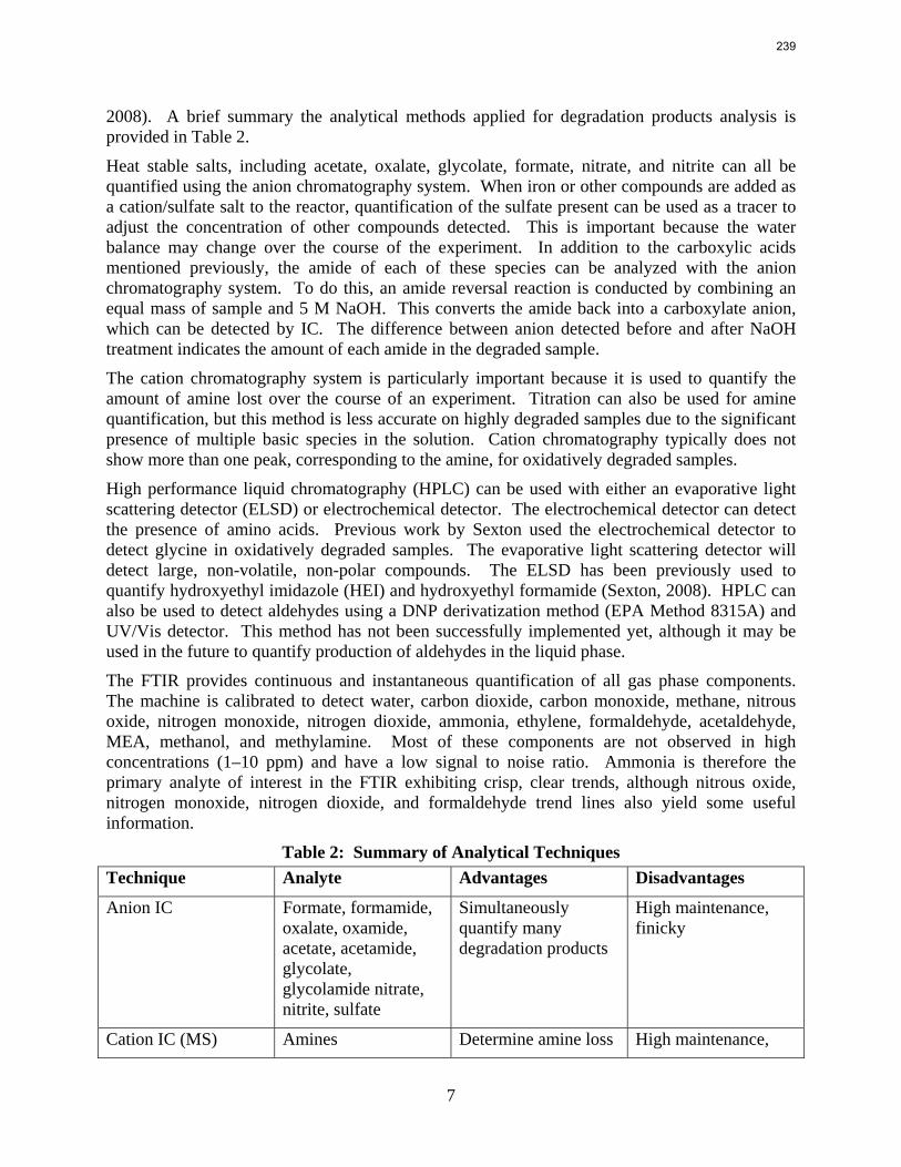
7
2008). A brief summary the analytical methods applied for degradation products analysis is provided in Table 2.
Heat stable salts, including acetate, oxalate, glycolate, formate, nitrate, and nitrite can all be quantified using the anion chromatography system. When iron or other compounds are added as a cation/sulfate salt to the reactor, quantification of the sulfate present can be used as a tracer to adjust the concentration of other compounds detected. This is important because the water balance may change over the course of the experiment. In addition to the carboxylic acids mentioned previously, the amide of each of these species can be analyzed with the anion chromatography system. To do this, an amide reversal reaction is conducted by combining an equal mass of sample and 5 M NaOH. This converts the amide back into a carboxylate anion, which can be detected by IC. The difference between anion detected before and after NaOH treatment indicates the amount of each amide in the degraded sample.
The cation chromatography system is particularly important because it is used to quantify the amount of amine lost over the course of an experiment. Titration can also be used for amine quantification, but this method is less accurate on highly degraded samples due to the significant presence of multiple basic species in the solution. Cation chromatography typically does not show more than one peak, corresponding to the amine, for oxidatively degraded samples.
High performance liquid chromatography (HPLC) can be used with either an evaporative light scattering detector (ELSD) or electrochemical detector. The electrochemical detector can detect the presence of amino acids. Previous work by Sexton used the electrochemical detector to detect glycine in oxidatively degraded samples. The evaporative light scattering detector will detect large, non-volatile, non-polar compounds. The ELSD has been previously used to quantify hydroxyethyl imidazole (HEI) and hydroxyethyl formamide (Sexton, 2008). HPLC can also be used to detect aldehydes using a DNP derivatization method (EPA Method 8315A) and UV/Vis detector. This method has not been successfully implemented yet, although it may be used in the future to quantify production of aldehydes in the liquid phase.
The FTIR provides continuous and instantaneous quantification of all gas phase components. The machine is calibrated to detect water, carbon dioxide, carbon monoxide, methane, nitrous oxide, nitrogen monoxide, nitrogen dioxide, ammonia, ethylene, formaldehyde, acetaldehyde, MEA, methanol, and methylamine. Most of these components are not observed in high concentrations (1–10 ppm) and have a low signal to noise ratio. Ammonia is therefore the primary analyte of interest in the FTIR exhibiting crisp, clear trends, although nitrous oxide, nitrogen monoxide, nitrogen dioxide, and formaldehyde trend lines also yield some useful information.
Table 2: Summary of Analytical Techniques Technique Analyte Advantages Disadvantages
Anion IC Formate, formamide, oxalate, oxamide, acetate, acetamide, glycolate, glycolamide nitrate, nitrite, sulfate
Simultaneously quantify many degradation products
High maintenance, finicky
Cation IC (MS) Amines Determine amine loss High maintenance,
239
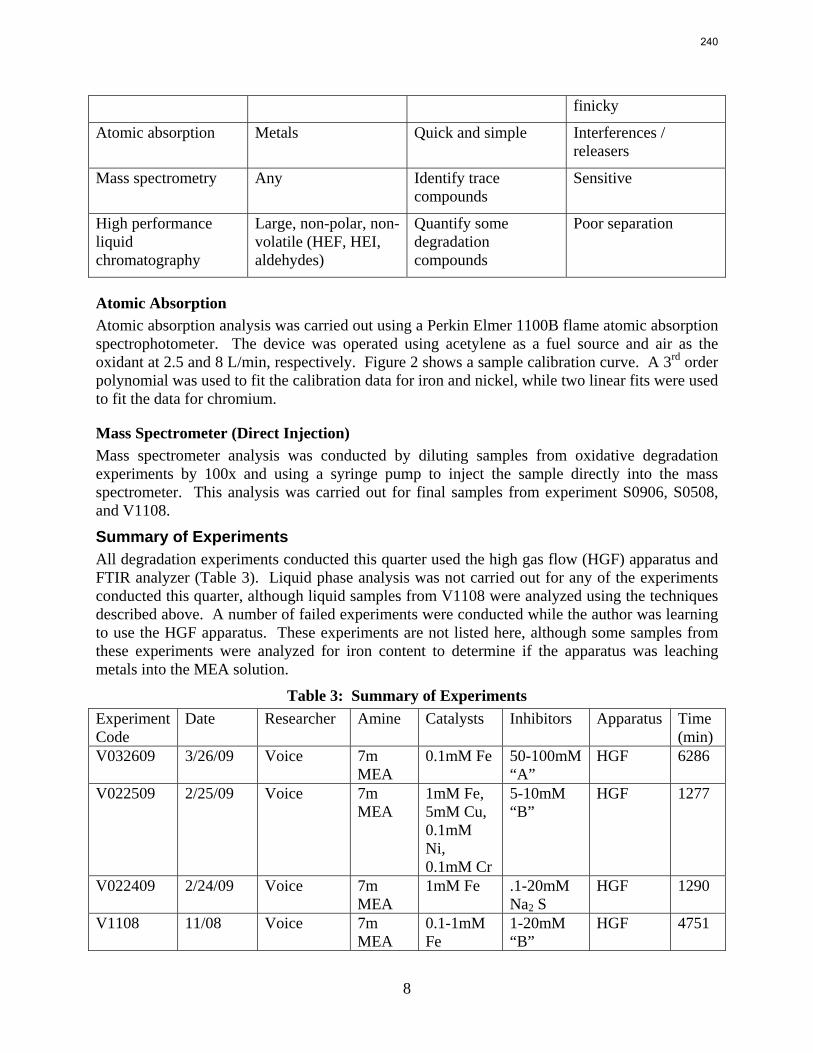
8
finicky
Atomic absorption Metals Quick and simple Interferences / releasers
Mass spectrometry Any Identify trace compounds
Sensitive
High performance liquid chromatography
Large, non-polar, non-volatile (HEF, HEI, aldehydes)
Quantify some degradation compounds
Poor separation
Atomic Absorption Atomic absorption analysis was carried out using a Perkin Elmer 1100B flame atomic absorption spectrophotometer. The device was operated using acetylene as a fuel source and air as the oxidant at 2.5 and 8 L/min, respectively. Figure 2 shows a sample calibration curve. A 3rd order polynomial was used to fit the calibration data for iron and nickel, while two linear fits were used to fit the data for chromium.
Mass Spectrometer (Direct Injection) Mass spectrometer analysis was conducted by diluting samples from oxidative degradation experiments by 100x and using a syringe pump to inject the sample directly into the mass spectrometer. This analysis was carried out for final samples from experiment S0906, S0508, and V1108.
Summary of Experiments All degradation experiments conducted this quarter used the high gas flow (HGF) apparatus and FTIR analyzer (Table 3). Liquid phase analysis was not carried out for any of the experiments conducted this quarter, although liquid samples from V1108 were analyzed using the techniques described above. A number of failed experiments were conducted while the author was learning to use the HGF apparatus. These experiments are not listed here, although some samples from these experiments were analyzed for iron content to determine if the apparatus was leaching metals into the MEA solution.
Table 3: Summary of Experiments Experiment Code
Date Researcher Amine Catalysts Inhibitors Apparatus Time (min)
V032609 3/26/09 Voice 7m MEA
0.1mM Fe 50-100mM “A”
HGF 6286
V022509 2/25/09 Voice 7m MEA
1mM Fe, 5mM Cu, 0.1mM Ni, 0.1mM Cr
5-10mM “B”
HGF 1277
V022409 2/24/09 Voice 7m MEA
1mM Fe .1-20mM Na2 S
HGF 1290
V1108 11/08 Voice 7m MEA
0.1-1mM Fe
1-20mM “B”
HGF 4751
240
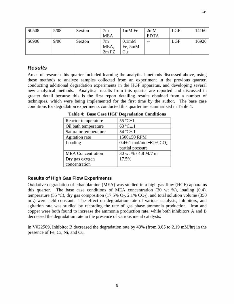
9
S0508 5/08 Sexton 7m MEA
1mM Fe 2mM EDTA
LGF 14160
S0906 9/06 Sexton 7m MEA, 2m PZ
0.1mM Fe, 5mM Cu
-- LGF 16920
Results Areas of research this quarter included learning the analytical methods discussed above, using these methods to analyze samples collected from an experiment in the previous quarter, conducting additional degradation experiments in the HGF apparatus, and developing several new analytical methods. Analytical results from this quarter are reported and discussed in greater detail because this is the first report detailing results obtained from a number of techniques, which were being implemented for the first time by the author. The base case conditions for degradation experiments conducted this quarter are summarized in Table 4.
Table 4: Base Case HGF Degradation Conditions Reactor temperature 55 ºC±1 Oil bath temperature 63 ºC±.1 Saturator temperature 54 ºC±.1 Agitation rate 1500±50 RPM Loading 0.4±.1 mol/mol 2% CO2
partial pressure MEA Concentration 30 wt % / 4.8 M/7 m Dry gas oxygen concentration
17.5%
Results of High Gas Flow Experiments Oxidative degradation of ethanolamine (MEA) was studied in a high gas flow (HGF) apparatus this quarter. The base case conditions of MEA concentration (30 wt %), loading (0.4), temperature (55 ºC), dry gas composition (17.5% O2, 2.1% CO2), and total solution volume (350 mL) were held constant. The effect on degradation rate of various catalysts, inhibitors, and agitation rate was studied by recording the rate of gas phase ammonia production. Iron and copper were both found to increase the ammonia production rate, while both inhibitors A and B decreased the degradation rate in the presence of various metal catalysts. In V022509, Inhibitor B decreased the degradation rate by 43% (from 3.85 to 2.19 mM/hr) in the presence of Fe, Cr, Ni, and Cu.
241
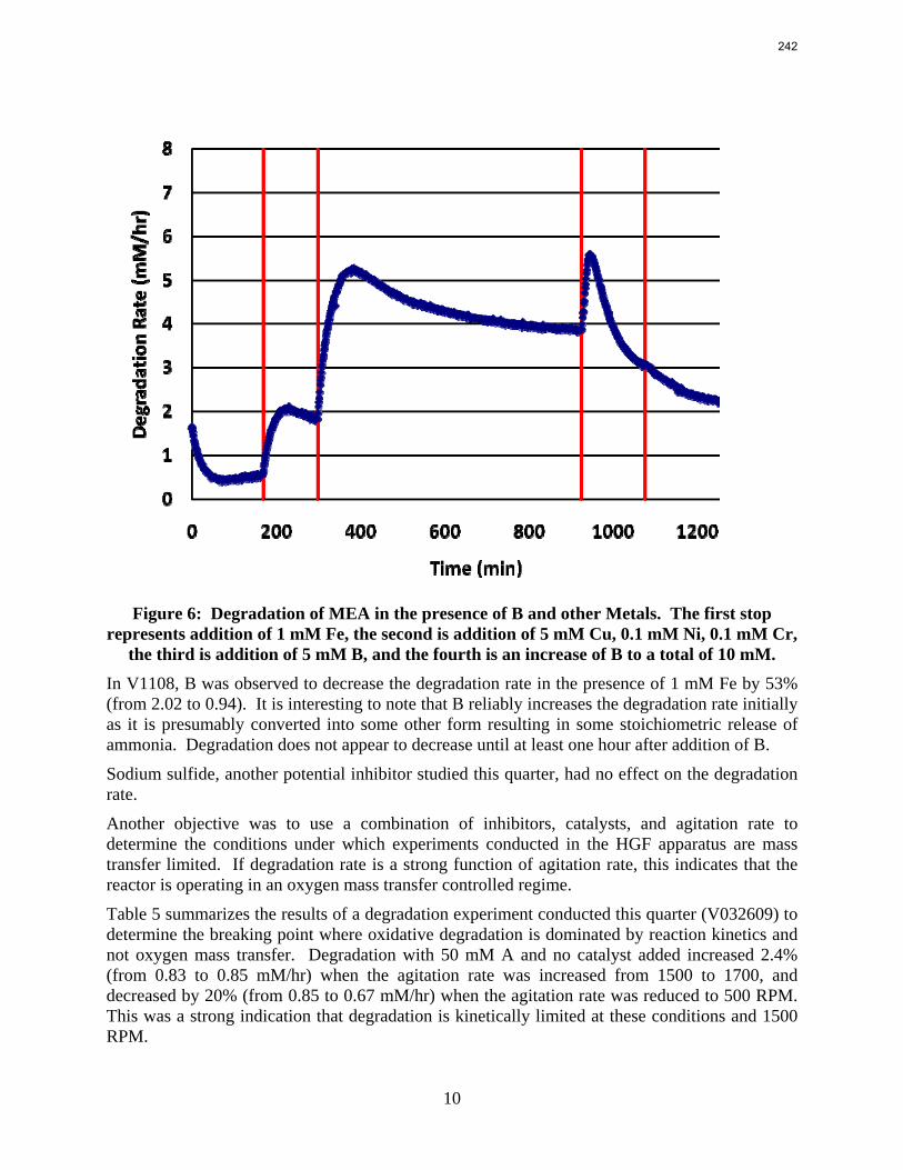
10
Figure 6: Degradation of MEA in the presence of B and other Metals. The first stop
represents addition of 1 mM Fe, the second is addition of 5 mM Cu, 0.1 mM Ni, 0.1 mM Cr, the third is addition of 5 mM B, and the fourth is an increase of B to a total of 10 mM.
In V1108, B was observed to decrease the degradation rate in the presence of 1 mM Fe by 53% (from 2.02 to 0.94). It is interesting to note that B reliably increases the degradation rate initially as it is presumably converted into some other form resulting in some stoichiometric release of ammonia. Degradation does not appear to decrease until at least one hour after addition of B.
Sodium sulfide, another potential inhibitor studied this quarter, had no effect on the degradation rate.
Another objective was to use a combination of inhibitors, catalysts, and agitation rate to determine the conditions under which experiments conducted in the HGF apparatus are mass transfer limited. If degradation rate is a strong function of agitation rate, this indicates that the reactor is operating in an oxygen mass transfer controlled regime.
Table 5 summarizes the results of a degradation experiment conducted this quarter (V032609) to determine the breaking point where oxidative degradation is dominated by reaction kinetics and not oxygen mass transfer. Degradation with 50 mM A and no catalyst added increased 2.4% (from 0.83 to 0.85 mM/hr) when the agitation rate was increased from 1500 to 1700, and decreased by 20% (from 0.85 to 0.67 mM/hr) when the agitation rate was reduced to 500 RPM. This was a strong indication that degradation is kinetically limited at these conditions and 1500 RPM.
242
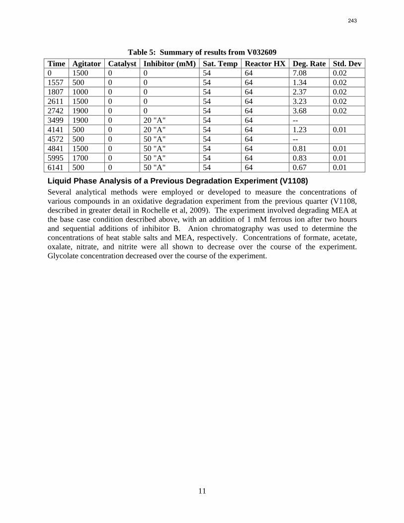
11
Table 5: Summary of results from V032609 Time Agitator Catalyst Inhibitor (mM) Sat. Temp Reactor HX Deg. Rate Std. Dev0 1500 0 0 54 64 7.08 0.02 1557 500 0 0 54 64 1.34 0.02 1807 1000 0 0 54 64 2.37 0.02 2611 1500 0 0 54 64 3.23 0.02 2742 1900 0 0 54 64 3.68 0.02 3499 1900 0 20 "A" 54 64 -- 4141 500 0 20 "A" 54 64 1.23 0.01 4572 500 0 50 "A" 54 64 -- 4841 1500 0 50 "A" 54 64 0.81 0.01 5995 1700 0 50 "A" 54 64 0.83 0.01 6141 500 0 50 "A" 54 64 0.67 0.01
Liquid Phase Analysis of a Previous Degradation Experiment (V1108) Several analytical methods were employed or developed to measure the concentrations of various compounds in an oxidative degradation experiment from the previous quarter (V1108, described in greater detail in Rochelle et al, 2009). The experiment involved degrading MEA at the base case condition described above, with an addition of 1 mM ferrous ion after two hours and sequential additions of inhibitor B. Anion chromatography was used to determine the concentrations of heat stable salts and MEA, respectively. Concentrations of formate, acetate, oxalate, nitrate, and nitrite were all shown to decrease over the course of the experiment. Glycolate concentration decreased over the course of the experiment.
243
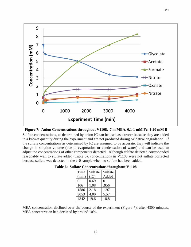
12
0
1
2
3
4
5
6
7
8
9
0 1000 2000 3000 4000
Concen
tration (m
M)
Experiment Time (min)
Glycolate
Acetate
Formate
Nitrite
Oxalate
Nitrate
Figure 7: Anion Concentrations throughout V1108. 7 m MEA, 0.1-1 mM Fe, 1-20 mM B Sulfate concentrations, as determined by anion IC can be used as a tracer because they are added in a known quantity during the experiment and are not produced during oxidative degradation. If the sulfate concentrations as determined by IC are assumed to be accurate, they will indicate the change in solution volume (due to evaporation or condensation of water) and can be used to adjust the concentrations of other components detected. Although sulfate detected corresponded reasonably well to sulfate added (Table 6), concentrations in V1108 were not sulfate corrected because sulfate was detected in the t=0 sample when no sulfate had been added.
Table 6: Sulfate Concentrations throughout V1108 Time (min)
Sulfate (IC)
Sulfate Added
0 0.69 0 106 1.08 .956 1586 2.18 1.97 3053 4.80 5.57 4342 19.6 18.8
MEA concentration declined over the course of the experiment (Figure 7); after 4300 minutes, MEA concentration had declined by around 10%.
244
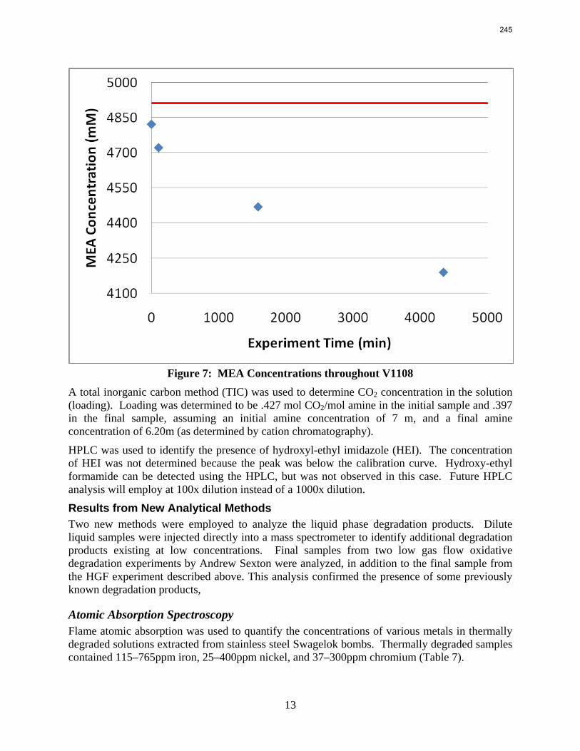
13
Figure 7: MEA Concentrations throughout V1108
A total inorganic carbon method (TIC) was used to determine CO2 concentration in the solution (loading). Loading was determined to be .427 mol CO2/mol amine in the initial sample and .397 in the final sample, assuming an initial amine concentration of 7 m, and a final amine concentration of 6.20m (as determined by cation chromatography).
HPLC was used to identify the presence of hydroxyl-ethyl imidazole (HEI). The concentration of HEI was not determined because the peak was below the calibration curve. Hydroxy-ethyl formamide can be detected using the HPLC, but was not observed in this case. Future HPLC analysis will employ at 100x dilution instead of a 1000x dilution.
Results from New Analytical Methods Two new methods were employed to analyze the liquid phase degradation products. Dilute liquid samples were injected directly into a mass spectrometer to identify additional degradation products existing at low concentrations. Final samples from two low gas flow oxidative degradation experiments by Andrew Sexton were analyzed, in addition to the final sample from the HGF experiment described above. This analysis confirmed the presence of some previously known degradation products,
Atomic Absorption Spectroscopy Flame atomic absorption was used to quantify the concentrations of various metals in thermally degraded solutions extracted from stainless steel Swagelok bombs. Thermally degraded samples contained 115–765ppm iron, 25–400ppm nickel, and 37–300ppm chromium (Table 7).
245
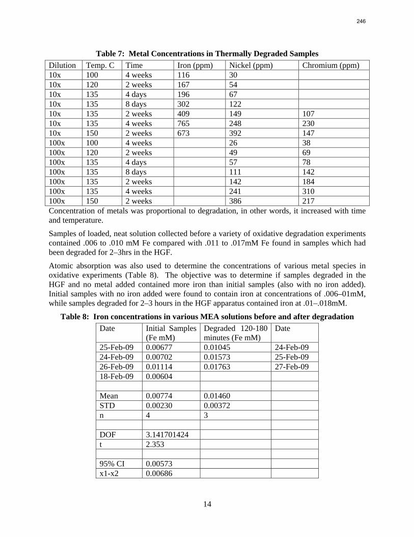
14
Table 7: Metal Concentrations in Thermally Degraded Samples Dilution Temp. C Time Iron (ppm) Nickel (ppm) Chromium (ppm) 10x 100 4 weeks 116 30 10x 120 2 weeks 167 54 10x 135 4 days 196 67 10x 135 8 days 302 122 10x 135 2 weeks 409 149 107 10x 135 4 weeks 765 248 230 10x 150 2 weeks 673 392 147 100x 100 4 weeks 26 38 100x 120 2 weeks 49 69 100x 135 4 days 57 78 100x 135 8 days 111 142 100x 135 2 weeks 142 184 100x 135 4 weeks 241 310 100x 150 2 weeks 386 217 Concentration of metals was proportional to degradation, in other words, it increased with time and temperature.
Samples of loaded, neat solution collected before a variety of oxidative degradation experiments contained .006 to .010 mM Fe compared with .011 to .017mM Fe found in samples which had been degraded for 2–3hrs in the HGF.
Atomic absorption was also used to determine the concentrations of various metal species in oxidative experiments (Table 8). The objective was to determine if samples degraded in the HGF and no metal added contained more iron than initial samples (also with no iron added). Initial samples with no iron added were found to contain iron at concentrations of .006–01mM, while samples degraded for 2–3 hours in the HGF apparatus contained iron at .01–.018mM.
Table 8: Iron concentrations in various MEA solutions before and after degradation Date Initial Samples
(Fe mM) Degraded 120-180 minutes (Fe mM)
Date
25-Feb-09 0.00677 0.01045 24-Feb-09 24-Feb-09 0.00702 0.01573 25-Feb-09 26-Feb-09 0.01114 0.01763 27-Feb-09 18-Feb-09 0.00604 Mean 0.00774 0.01460 STD 0.00230 0.00372 n 4 3 DOF 3.141701424 t 2.353 95% CI 0.00573 x1-x2 0.00686
246
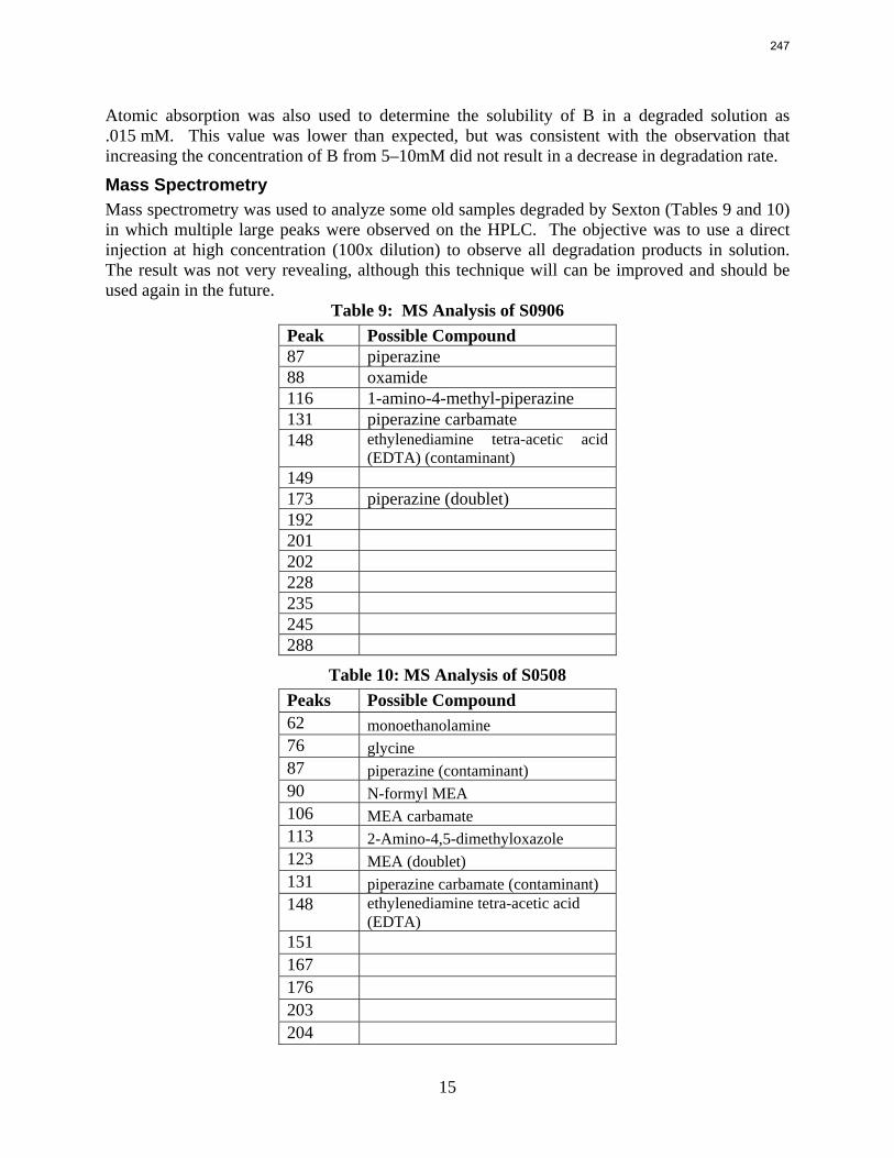
15
Atomic absorption was also used to determine the solubility of B in a degraded solution as .015 mM. This value was lower than expected, but was consistent with the observation that increasing the concentration of B from 5–10mM did not result in a decrease in degradation rate.
Mass Spectrometry Mass spectrometry was used to analyze some old samples degraded by Sexton (Tables 9 and 10) in which multiple large peaks were observed on the HPLC. The objective was to use a direct injection at high concentration (100x dilution) to observe all degradation products in solution. The result was not very revealing, although this technique will can be improved and should be used again in the future.
Table 9: MS Analysis of S0906 Peak Possible Compound 87 piperazine 88 oxamide 116 1-amino-4-methyl-piperazine 131 piperazine carbamate 148 ethylenediamine tetra-acetic acid
(EDTA) (contaminant) 149 173 piperazine (doublet) 192 201 202 228 235 245 288
Table 10: MS Analysis of S0508 Peaks Possible Compound 62 monoethanolamine 76 glycine 87 piperazine (contaminant) 90 N-formyl MEA 106 MEA carbamate 113 2-Amino-4,5-dimethyloxazole 123 MEA (doublet) 131 piperazine carbamate (contaminant) 148 ethylenediamine tetra-acetic acid
(EDTA) 151 167 176 203 204
247
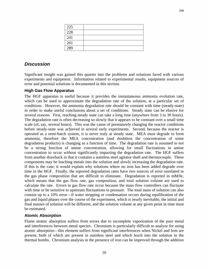
16
225 228 241 261 289
Discussion Significant insight was gained this quarter into the problems and solutions faced with various experiments and equipment. Information related to experimental results, equipment sources of error and potential solutions is documented in this section.
High Gas Flow Apparatus The HGF apparatus is useful because it provides the instantaneous ammonia evolution rate, which can be used to approximate the degradation rate of the solution, at a particular set of conditions. However, the ammonia degradation rate should be constant with time (steady-state) in order to make useful conclusions about a set of conditions. Steady state can be elusive for several reasons. First, reaching steady state can take a long time (anywhere from 3 to 30 hours). The degradation rate is often decreasing so slowly that it appears to be constant over a small time scale (of, say, several hours). This was the cause of prematurely changing the reactor conditions before steady-state was achieved in several early experiments. Second, because the reactor is operated as a semi-batch system, it is never truly at steady state. MEA must degrade to form ammonia, therefore the MEA concentration (and doubtless the concentration of some degradation products) is changing as a function of time. The degradation rate is assumed to not be a strong function of amine concentration, allowing for small fluctuations in amine concentration to occur without significantly impacting the degradation rate. The HGF suffers from another drawback in that it contains a stainless steel agitator shaft and thermocouple. These components may be leaching metals into the solution and slowly increasing the degradation rate. If this is the case, it would explain why solutions where no iron has been added degrade over time in the HGF. Finally, the reported degradation rates have two sources of error unrelated to the gas phase composition that are difficult to eliminate. Degradation is reported in mM/hr, which means that the gas flow rate, gas composition, and total solution volume are used to calculate the rate. Errors in gas flow rate occur because the mass flow controllers can fluctuate with time or be sensitive to upstream fluctuations in pressure. The total mass of solution can also contain up to a 10% error—if water stripping or condensation occurs during equilibration of the gas and liquid phases over the course of the experiment, which is nearly inevitable, the initial and final masses of solution will be different, and the solution volume at any given point in time must be estimated.
Atomic Absorption Flame atomic absorption suffers from errors due to incomplete vaporization of the pure metal and interferences between metal species. Chromium is particularly difficult to analyze for using atomic absorption—this element suffers from significant interferences when Nickel and Iron are present, both of which are present in stainless steel and which leach into the solution in the thermal bombs. Chromium analysis in the presence of iron can be improved through the addition
248
17
of 2% ammonium chloride and by using a rich flame. The concentration of nickel is known to be enhanced by the presence of iron, however this effect can be mitigated by using a lean flame. Iron suffers from interferences from nickel, copper, and cobalt, although using a lean flame can reduce these interferences. Because only one sample was analyzed, potential interferences associated with “B” were not investigated. Several articles on reducing chromium interferences, the most problematic metal of the three, were discovered and will be reviewed before pursuing further Cr analysis. Despite interferences, the flame atomic absorption data yielded useful results. Concentrations of iron, nickel, and chromium are all likely to be in the 100-1000ppm range. This is well into the range of catalyst concentration known to be effective in catalyzing oxidative degradation. Therefore, future thermal degradation experiments should control or attempt to quantify the effect of metals concentration on degradation.
Mass Spectrometer Direct injection into the mass spectrometer has provided a useful way to identify degradation products existing at trace concentrations. The mass spectrometer is fairly sensitive and is capable of simultaneously recognizing various compounds even when they appear at vastly different concentrations. The most comprehensive analysis is therefore achieved by injecting a relatively concentrated sample (100x) and observing the full gambit of peaks detected by the MS analyzer. This strategy, however, suffers from two drawbacks. First, compounds which are present in high concentrations in the sample tend to form phantom peaks equal to twice the molecular weight plus one. For example, a degradation sample with a large amount of MEA present would have a normal peak at 62.08 (MW +1) and a phantom peak at 123.16. Upon further dilution, the peak at 123.16 shrinks and eventually disappears. The reason for this behavior is unknown. Second, injecting concentrated samples causes the injection cone to become contaminated; this was evidenced by the appearance of MEA, MDEA, and piperazine peaks in samples which did not contain these amines. Future direct injection analysis will use concentrations of 10,000x to avoid this issue at the cost of missing some trace compounds. Another solution to this problem is to use some form of separation before injecting the sample into the MS. For most oxidative samples, the cation IC does not provide this separation due to the fact that the amine is often the only cation present in solution. An HPLC-MS is under repair and ade of become available for analytical work in the near future. Previous degradation work has yielded unidentifiable peaks in the HPLC that may be identified with the aid of a mass spectrometer (Sexton). Anion Chromatography Recently it has been suggested that the procedure discussed in the Experimental Methods section for quantifying carboxylic acids and amides in degraded samples may suffer from an inherent problem with the anion chromatography system. The anion chromatogram contains NaOH, which can catalyze the conversion of amides to carboxylic acids, within the column. It had been previously assumed that the difference in anion concentrations before and after treating a sample with NaOH was indicative of amide concentration. However, some of the amides may in fact be getting converted to carboxylic acids during the analysis with no NaOH treatment. Though difficult to test, this may be the cause of the carbon imbalance documented by Sexton (N-formyl-MEA contains two more carbons than formate). Quantifying the amount of amide conversion occurring in the column is tricky because N-formyl-MEA cannot be purchased, and synthesis involves a highly exothermic reaction and may produce some formate.
249
18
Future Analytical Methods Several analytical methods are being looked at for the future in order to gain a better understanding of amine degradation. As mentioned previously, unknown peaks appearing on the HPLC chromatogram will soon be identified using HPLC-MS. In addition, the use of dissolved oxygen (DO) sensors is being investigated for use in the HGF apparatus. DO sensors will help lend a better understanding of the degradation mechanism, and will, importantly give a better indication as to when degradation is oxygen mass transfer limited. Finally, aldehydes are an important part of the degradation process that has thus far eluded rigorous study. Although the FTIR has been calibrated to detect acetaldehyde and formaldehyde exiting the reactor in the gas phase, the presence of aldehydes in the liquid phase is as of yet unknown. Formaldehyde is likely to be formed, but may exist only as a reactive intermediate. Sexton attempted to develop an HPLC method for detecting formaldehyde (EPA 8315A), but was unsuccessful. The quantification of formaldehyde either by a colorimetric method or by gas chromatography may be another option. Colorimetry may be difficult because degraded MEA are typically highly colored, due to the presence of metals and colored degradation products. Gas chromatography is also non-ideal because high temperatures in the injection port to volatilize the sample can cause high-temperature degradation.
References Blachly CH, Ravner H. The Stabilization of Monoethanolamine Solutions for Submarine Carbon
Dioxide Scrubbers. AD609888; NRL-FR-6189; NRL-6189; Naval Research Laboratory: Washington, D.C., 1964.
Freeman SA. “Carbon dioxide capture with concentrated, aqueous piperazine.” GHGT-9, Washington D.C. 2008
Goff GS. Oxidative Degradation of Aqueous Monoethanolamine in CO2 Capture Processes: Iron and Copper Catalysis, Inhibition, and O2 Mass Transfer. The University of Texas at Austin. Ph.D. Dissertation. 2005
International Chemical Information Service (2009). http://www.icis.com/staticpages/prices.htm. Accessed 17 January 2009.
Rooney PC, DuPart MS, Bacon TR, “Oxygen's Role in Alkanolamine Degradation.” Hydroc Proc, Int Ed. 1998;77(7):109–113.
Sexton AJ. Amine Oxidation in CO2 Capture Processes. The University of Texas at Austin. Ph.D. Dissertation. 2008
Rochelle GT et al. "CO2 Capture by Aqueous Absorption, Fourth Quarterly Progress Report 2008." Luminant Carbon Management Program. The University of Texas at Austin. 2009.
250
1
Dynamic Modeling of the Absorber in Aspen Custom Modeler®
Quarterly Report for January 1 – March 31, 2009
by Sepideh Ziaii Fashami
Supported by the Luminant Carbon Management Program
and the
Industrial Associates Program for CO2 Capture by Aqueous Absorption
Department of Chemical Engineering
The University of Texas at Austin
April 8, 2009
Abstract The work in the first quarter focuses on dynamic modeling of the absorber for CO2 absorption by monoethanolamine (MEA) in Aspen Custom Modeler® (ACM®). The absorber column is a packed bed divided into a number of segments. In this study, discrete Gaussian distribution is proposed as a new method for segmentation. The simulation results show that the Gaussian distribution gives more realistic McCabe Thiele diagrams for low lean loading, e.g. 0.36; however, there is no advantage to decreasing the required number of segments. We still need to use an adequate number of segments to get an accurate CO2 removal. For higher lean loadings, e.g. 0.4 and 0.45, using Gaussian distribution with Lmax/Lmin≈10 (the ratio of maximum to minimum length of the segments) enables us to calculate the removal with sufficient accuracy with a smaller number of segments and significantly decrease the computation time. The CPU time reduction is specifically beneficial for dynamic simulation and dynamic analysis.
Modeling The ACM® model of the absorber is briefly described in this section. This model, which is based on the film theory, enables the calculation of effective mass transfer coefficient in the presence of reactions occurring in the liquid phase between MEA and CO2. In this model, the packed column is divided into several segments, and the material balances, energy balances, mass transfer, energy transfer, and phase equilibrium are determined for each segment. This model assumes that the variation of the conditions in radial direction is negligible in both liquid phase and gas phases. Furthermore, in this model each segment is assumed to be well-mixed.
Model Equations The ACM® model used here is a dynamic one, and the time dependent energy and mass balances are solved at each time step for both phases. The following equations are molar component balances and energy balances for liquid and gas phases for the jth segment of the packed column:
251
2
jijjcjijjij
Lji NalDxLxL
dtdM
,2
,1,1,
4π
+−= −− (1)
jijjcjijjij
Vji NalDyVyV
dtdM
,2
,1,1,
4π
−−= −+ (2)
⎜⎝⎛+−= −−
LjCOjCOjjc
Ljj
Ljj
Lj HNalDHLHL
dt
dE,2,2
211 4
π
⎟⎠⎞+ L
jOHjOH HN ,2,2 (3)
⎜⎝⎛ +−−−= ++
VjCOjCO
Lj
Vj
Vjjjc
Vjj
Vjj
Vj HNTThalDHVHV
dt
dE,2,2
211 )(
4π
⎟⎠⎞+ V
jOHjOH HN ,2,2 (4)
For i=CO2, H2O, N2, O2
In this model, it is assumed that MEA is a non-volatile solvent and O2 and N2 are not dissolved in the solution. The mole flux of CO2 and H2O is found from the following equation:
)( 2*
222 COCOCOCO PyPKGN −= (5)
Where 2COKG is a total mass transfer coefficient that involves the combination of the resistance
to mass transfer in both liquid phase ( 2COgK ′ ) and gas phase (KgCO2). (Eq. 6)
222
111
COCOCO kggkKG+
′= (6)
2COgK ′ , liquid side mass transfer coefficient, is calculated from a correlation as a function of partial pressure of CO2 based on Aboudheir’s data.
98.4)(log42.0log *22 −−=′ PaPgK COCO (7)
It is also assumed that the mass transfer resistance for H2O in the liquid phase is negligible and H2O mass flux is calculated from the following equation:
)(2
*222 OHOHOHOH PyPKgN −= (8)
The thermodynamics is described with electrolyte-NRTL model and *2COP and absHΔ are
determined by equations regressed the points from flash calculation in Aspen Plus® model by Hilliard.
Table 1 provides an overview of the important parameters in the model, along with their sources and literature.
252
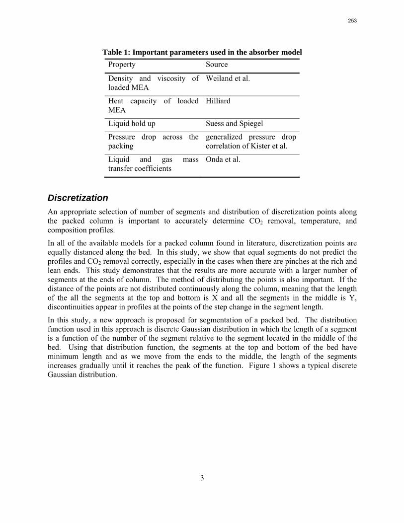
3
Table 1: Important parameters used in the absorber model Property Source
Density and viscosity of loaded MEA
Weiland et al.
Heat capacity of loaded MEA
Hilliard
Liquid hold up Suess and Spiegel
Pressure drop across the packing
generalized pressure drop correlation of Kister et al.
Liquid and gas mass transfer coefficients
Onda et al.
Discretization An appropriate selection of number of segments and distribution of discretization points along the packed column is important to accurately determine CO2 removal, temperature, and composition profiles.
In all of the available models for a packed column found in literature, discretization points are equally distanced along the bed. In this study, we show that equal segments do not predict the profiles and CO2 removal correctly, especially in the cases when there are pinches at the rich and lean ends. This study demonstrates that the results are more accurate with a larger number of segments at the ends of column. The method of distributing the points is also important. If the distance of the points are not distributed continuously along the column, meaning that the length of the all the segments at the top and bottom is X and all the segments in the middle is Y, discontinuities appear in profiles at the points of the step change in the segment length.
In this study, a new approach is proposed for segmentation of a packed bed. The distribution function used in this approach is discrete Gaussian distribution in which the length of a segment is a function of the number of the segment relative to the segment located in the middle of the bed. Using that distribution function, the segments at the top and bottom of the bed have minimum length and as we move from the ends to the middle, the length of the segments increases gradually until it reaches the peak of the function. Figure 1 shows a typical discrete Gaussian distribution.
253

4
Figure 1: Discrete Gaussian distribution function
Formulation:
2)(2)( ncnakenf −−= (9)
Where a is a parameter relating to Lmax/Lmin and k is a parameter calculated by the following equation:
∑ = 1)(nf (10)
Sensitivity Analysis In this analysis, we discuss the effect of Gaussian distribution versus equidistance discretization on the absorber profiles and CO2 removal in steady state condition.
Several cases were simulated for the absorber in steady state with the model created in ACM®. For all cases, the lean solution is 7 m MEA and Mellapak 250Y is selected as the packing material.
Table 2: Percentage of CO2 removal, H=20 m, Dc=11.2 m, Llean=96 Kmol/s, inlet gas flow rate= 5.5 kmol/s
Lean loading =0.36 Lean loading =0.4 Lean loading =0.45
Seg# Lmax/Lmin=1 Lmax/Lmin=10 Lmax/Lmin=1 Lmax/Lmin=10 Lmax/Lmin=1 Lmax/Lmin=10
101 98 94 90 87 78 74
29 99.6 98.9 97 92 78 75
1 n n
Lmax
Lmin
F(n)
254
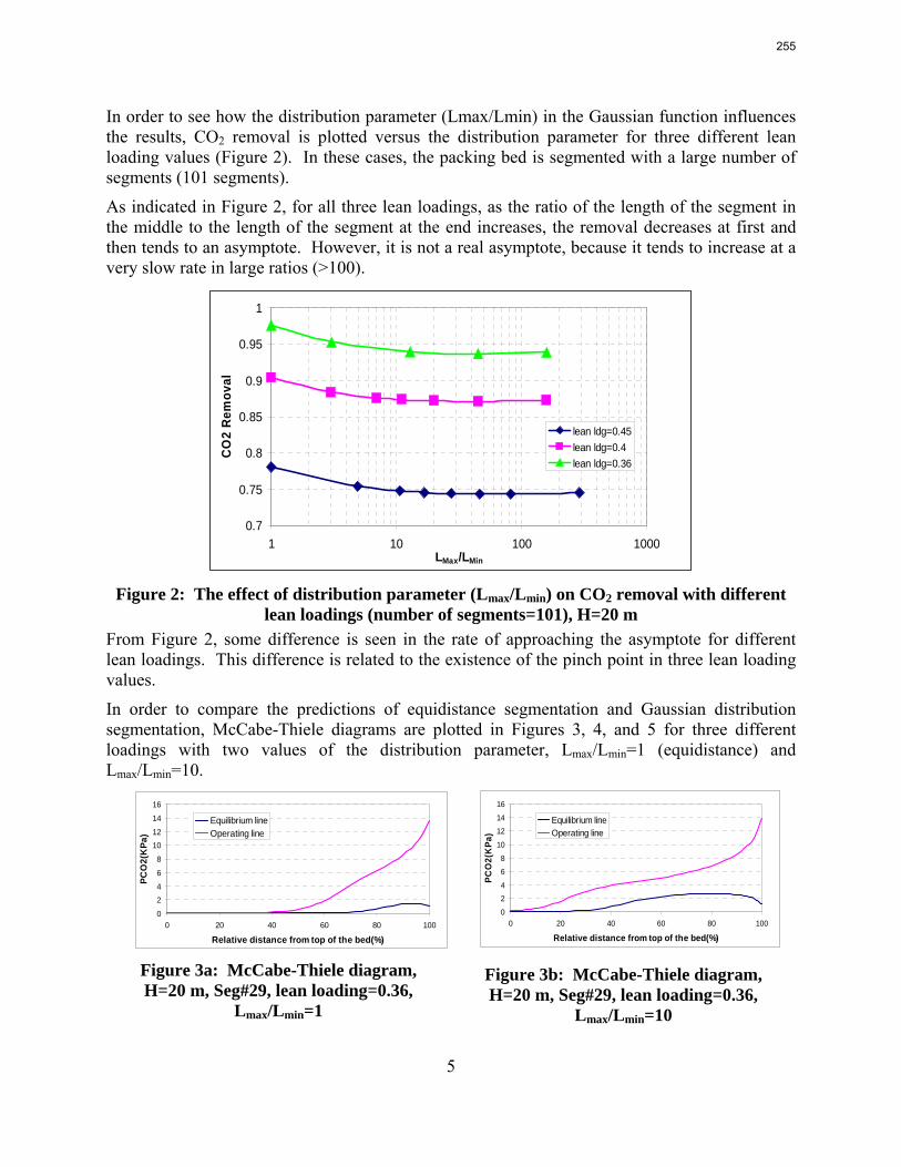
5
In order to see how the distribution parameter (Lmax/Lmin) in the Gaussian function influences the results, CO2 removal is plotted versus the distribution parameter for three different lean loading values (Figure 2). In these cases, the packing bed is segmented with a large number of segments (101 segments).
As indicated in Figure 2, for all three lean loadings, as the ratio of the length of the segment in the middle to the length of the segment at the end increases, the removal decreases at first and then tends to an asymptote. However, it is not a real asymptote, because it tends to increase at a very slow rate in large ratios (>100).
0.7
0.75
0.8
0.85
0.9
0.95
1
1 10 100 1000LMax/LMin
CO
2 R
emov
al
lean ldg=0.45lean ldg=0.4lean ldg=0.36
Figure 2: The effect of distribution parameter (Lmax/Lmin) on CO2 removal with different
lean loadings (number of segments=101), H=20 m From Figure 2, some difference is seen in the rate of approaching the asymptote for different lean loadings. This difference is related to the existence of the pinch point in three lean loading values.
In order to compare the predictions of equidistance segmentation and Gaussian distribution segmentation, McCabe-Thiele diagrams are plotted in Figures 3, 4, and 5 for three different loadings with two values of the distribution parameter, Lmax/Lmin=1 (equidistance) and Lmax/Lmin=10.
0
24
6
8
1012
14
16
0 20 40 60 80 100
Relative distance from top of the bed(%)
PCO
2(K
Pa)
Equilibrium lineOperating line
0
24
68
10
1214
16
0 20 40 60 80 100
Relative distance from top of the bed(%)
PCO
2(K
Pa)
Equilibrium lineOperating line
Figure 3a: McCabe-Thiele diagram, H=20 m, Seg#29, lean loading=0.36,
Lmax/Lmin=1
Figure 3b: McCabe-Thiele diagram, H=20 m, Seg#29, lean loading=0.36,
Lmax/Lmin=10
255
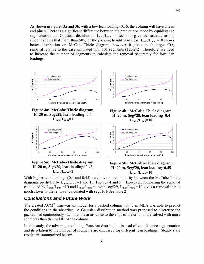
6
As shown in figures 3a and 3b, with a low lean loading=0.36, the column will have a lean end pinch. There is a significant difference between the predictions made by equidistance segmentation and Gaussian distribution. Lmax/Lmin =1 seems to give less realistic results since it shows that more than 50% of the packing height is useless. Lmax/Lmin =10 shows better distribution on McCabe-Thiele diagram, however it gives much larger CO2 removal relative to the case simulated with 101 segments (Table 2). Therefore, we need to increase the number of segments to calculate the removal accurately for low lean loadings.
0
2
4
68
10
12
14
16
0 20 40 60 80 100
Relative distance from top of the bed(%)
PCO
2(K
Pa)
Equilibrium lineOperating line
02
46
810
1214
16
0 20 40 60 80 100
Relative distance from top of the bed(%)
PCO
2(K
Pa)
Equilibrium lineOperating line
Figure 4a: McCabe-Thiele diagram, H=20 m, Seg#29, lean loading=0.4,
Lmax/Lmin=1
Figure 4b: McCabe-Thiele diagram, H=20 m, Seg#29, lean loading=0.4
Lmax/Lmin=10
02468
10121416
0 20 40 60 80 100
Relative distance from top of the bed(%)
PCO
2(K
Pa)
Equilibrium lineOperating line
02
468
1012
1416
0 20 40 60 80 100
Relative distance from top of the bed(%)
PCO
2(K
Pa)
Equilibrium lineOperating line
Figure 5a: McCabe-Thiele diagram, H=20 m, Seg#29, lean loading=0.45,
Lmax/Lmin=1
Figure 5b: McCabe-Thiele diagram, H=20 m, Seg#29, lean loading=0.45
Lmax/Lmin=10 With higher lean loadings (0.4 and 0.45) , we have more similarity between the McCabe-Thiele diagrams predicted by Lmax/Lmin =1 and 10 (Figures 4 and 5). However, comparing the removal calculated by Lmax/Lmin =10 and Lmax/Lmin =1 with seg#29, Lmax/Lmin =10 gives a removal that is much closer to the removal calculated with seg#101(See table 2).
Conclusions and Future Work The created ACM® time-variant model for a packed column with 7 m MEA was able to predict the conditions in the absorber. A Gaussian distribution method was proposed to discretize the packed bed continuously such that the areas close to the ends of the column are solved with more segments than the middle of the column.
In this study, the advantages of using Gaussian distribution instead of equidistance segmentation and its relation to the number of segments are discussed for different lean loadings. Steady state results are summarized below.
256
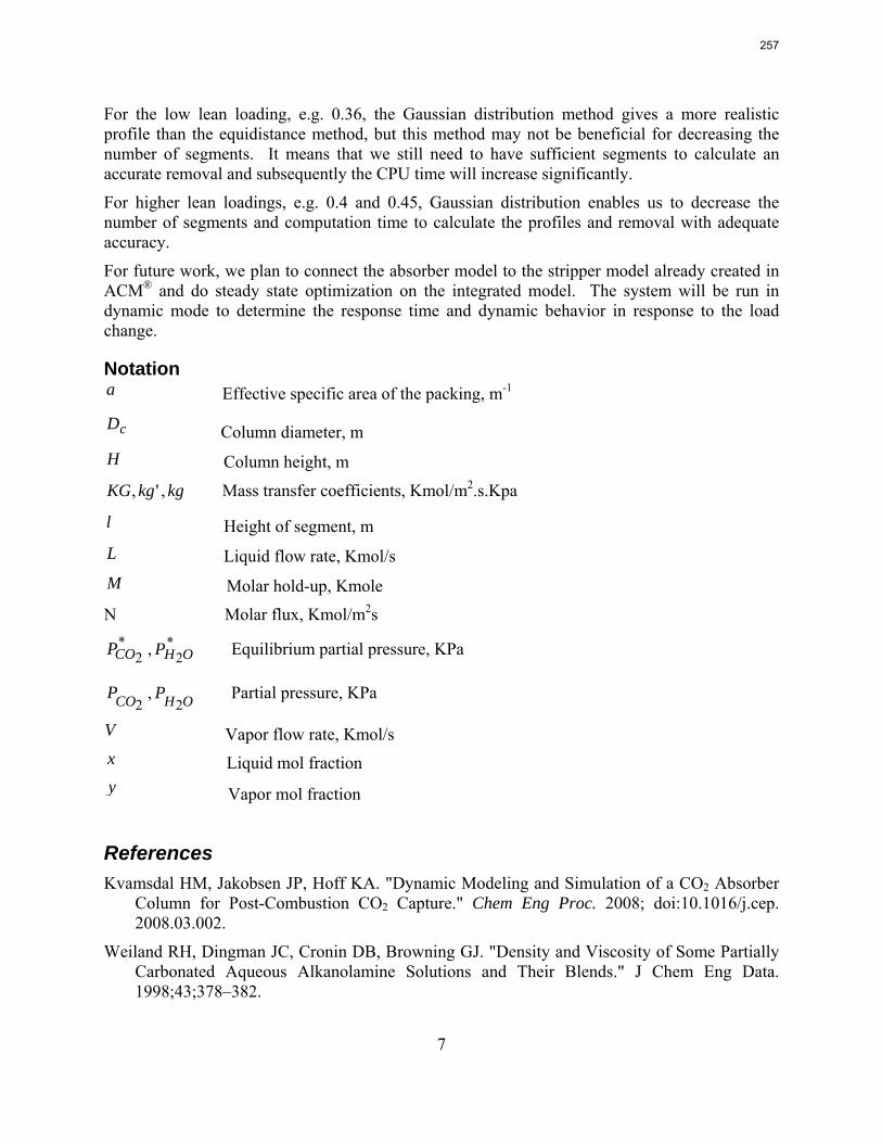
7
For the low lean loading, e.g. 0.36, the Gaussian distribution method gives a more realistic profile than the equidistance method, but this method may not be beneficial for decreasing the number of segments. It means that we still need to have sufficient segments to calculate an accurate removal and subsequently the CPU time will increase significantly.
For higher lean loadings, e.g. 0.4 and 0.45, Gaussian distribution enables us to decrease the number of segments and computation time to calculate the profiles and removal with adequate accuracy.
For future work, we plan to connect the absorber model to the stripper model already created in ACM® and do steady state optimization on the integrated model. The system will be run in dynamic mode to determine the response time and dynamic behavior in response to the load change.
Notation a Effective specific area of the packing, m-1
cD Column diameter, m H Column height, m
kgkgKG ,', Mass transfer coefficients, Kmol/m2.s.Kpa
l Height of segment, m L Liquid flow rate, Kmol/s M Molar hold-up, Kmole
N Molar flux, Kmol/m2s *
2COP , *2OHP Equilibrium partial pressure, KPa
2COP , OHP2
Partial pressure, KPa
V Vapor flow rate, Kmol/s x Liquid mol fraction y Vapor mol fraction
References Kvamsdal HM, Jakobsen JP, Hoff KA. "Dynamic Modeling and Simulation of a CO2 Absorber
Column for Post-Combustion CO2 Capture." Chem Eng Proc. 2008; doi:10.1016/j.cep. 2008.03.002.
Weiland RH, Dingman JC, Cronin DB, Browning GJ. "Density and Viscosity of Some Partially Carbonated Aqueous Alkanolamine Solutions and Their Blends." J Chem Eng Data. 1998;43;378–382.
257
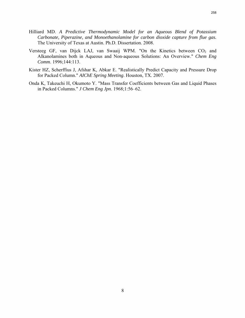
8
Hilliard MD. A Predictive Thermodynamic Model for an Aqueous Blend of Potassium Carbonate, Piperazine, and Monoethanolamine for carbon dioxide capture from flue gas. The University of Texas at Austin. Ph.D. Dissertation. 2008.
Versteeg GF, van Dijck LAJ, van Swaaij WPM. "On the Kinetics between CO2 and Alkanolamines both in Aqueous and Non-aqueous Solutions: An Overview." Chem Eng Comm. 1996;144:113.
Kister HZ, Scherffius J, Afshar K, Abkar E. "Realistically Predict Capacity and Pressure Drop for Packed Column." AIChE Spring Meeting. Houston, TX. 2007.
Onda K, Takeuchi H, Okumoto Y. "Mass Transfer Coefficients between Gas and Liquid Phases in Packed Columns." J Chem Eng Jpn. 1968;1:56–62.
258
1
Electric Grid Level Implications of
Flexible CO2 Capture Operation
Progress Report for January 1 – March 31, 2009
by Stuart Cohen
Supported by the Luminant Carbon Management Program
and the
Industrial Associates Program for CO2 Capture by Aqueous Absorption
Department of Chemical Engineering
The University of Texas at Austin
April 25, 2009
Abstract Flexible CO2 capture systems can choose how much CO2 to capture based on the competition between CO2 and electricity prices and a desire to either minimize operating costs or maximize operating profits. Coal and natural gas prices have varying degrees of predictability and volatility, and the relative prices of these fuels have a major impact on power plant operating costs and the resulting plant dispatch sequence. Because the chosen operating point in a flexible CO2 capture system affects net power plant efficiency, fuel prices also influence which CO2 capture operating point may be the most economical and the resulting dispatch of power plants with CO2 capture. This report contains an analysis of flexible CO2 capture in of how coal and natural gas prices affect the operation of flexible CO2 capture in the Electric Reliability Council of Texas (ERCOT) electric grid and the resulting economic and environmental impacts at the power plant and electric grid levels. All permutations of $1.5/MMBTU and $3/MMBTU coal and $6.6/MMBTU and $9.6/MMBTU are considered.
When choosing the operating point of a flexible CO2 capture system based on marginal costs alone, higher coal prices result in higher CO2 prices required to justify full-load CO2 capture because larger emissions cost reductions are necessary to offset the increased fuel costs of CO2 capture. When choosing a CO2 capture operating point based on the most profitable combination of cost, output, and electricity price, higher natural gas prices will increase the CO2 price needed to justify continuous full-load CO2 capture. Higher natural gas prices lead to increased electricity prices, so additional electricity sales during partial- or zero-load CO2 capture offset CO2 emissions costs at higher CO2 prices. Coal prices had little effect on profit-motivated flexible CO2 capture, demonstrating that the value of electricity on the grid is more important to profitability than the value of electricity at the plant. For each fuel price combination, there are ranges of CO2 prices where profit-motivated flexible CO2 capture can allow greater operating profits over those without CO2 capture, with inflexible CO2 capture, and with flexible capture based on marginal costs. These CO2 price ranges increase and the benefits grow as natural gas
259
2
prices rise and as coal prices fall for a given natural gas price. Across eight coal-fired plants in ERCOT, annual operating profits in these CO2 price regimes could be several $100 millions greater than those earned with inflexible or cost-driven flexible CO2 capture and $10s to ~$100s million greater than with no CO2 capture.
Studying the Sensitivity of Flexible CO2 Capture Operation to Coal and Natural Gas Prices The bulk of this report consists of a paper submitted to the American Society of Mechanical Engineers (ASME) 3rd Annual Conference on Energy Sustainability. This paper, which follows Other In-Progress Activities and Future Work below, describes analysis that uses the previously developed model of electricity dispatch and the ERCOT electricity market to investigate the effect of coal and natural gas prices on flexible CO2 capture operation. The study considers several fossil fuel price combinations in order to investigate how absolute and relative fuel prices impact the operation of flexible CO2 capture facilities and the resulting economics and CO2 emissions at the power plant and grid levels.
Other In-Progress Research Activities and Future Work Another primary research activity in the past quarter has been the compilation of a Master’s thesis that documents my research from August 2007 and December 2008. The final version of the thesis will be included with the 2nd Quarterly report in July.
Continuing the long-term analysis methodology presented in the last quarterly report, some recent work has been done to identify several 20-year fuel and CO2 price path projections so that the long-term analysis can be used to investigate the effects of these price paths on flexible CO2 capture systems over an investment life. Data collection and analysis for these price path combinations will take place during the next quarter.
In March, Hannah Chalmers from Imperial College London visited UT Austin, and we discussed collaborative work between UT and Imperial College that compares the ERCOT and United Kingdom electric grids in terms of the barriers and opportunities for flexible CO2 capture. Over the next few months, Hannah and I will collaborate on this comparative analysis, which will include a qualitative comparison of the two electric grids and quantitative comparisons using my modeling code. This work will provide insight into how differences in electricity market conditions and power plant fleet affect flexible CO2 capture operation.
Most research so far has been focused on flexible CO2 capture configurations that vent additional CO2 when capture systems are at partial- or zero-load. I have done some work this quarter where I consider flexible CO2 capture that uses large-scale solvent storage to continue to absorb CO2 from flue gas at full capacity when stripping and compression systems are at partial- or zero-load. This configuration allows increased output during high electricity price times without additional CO2 emissions and any associated CO2 emissions costs, so operating profits may be improved relative to a configuration that vents additional CO2 at partial- or zero-load CO2 capture. However, since additional solvent must be regenerated when stripping and compression systems operate at full load, the CO2 capture energy penalty is greater during full-load CO2 capture, stripping and compression systems must be larger, and solvent inventory and storage facilities incur additional capital costs. As part of a course in optimization, I will formulate and solve an optimization problem that seeks to find the optimal size of a solvent storage facility.
260

3
The Effect of Fossil Fuel Prices on Flexible CO2 Capture Operation
ES2009-90308 (draft) Proceedings of ES2009
Energy Sustainability 2009 July 19-23, 2008, San Francisco, California, USA
261

4
Stuart M. Cohen
[email protected] John Fyffe
Gary T. Rochelle [email protected]
Michael E. Webber [email protected]
Introduction
Carbon Dioxide Capture for Climate Change Mitigation There is broad scientific consensus that global warming and climate change are progressing at an alarming rate and that the primary cause is anthropogenic carbon dioxide (CO2) emissions from fossil fuel burning. Coal-fired power plants emit over one third of anthropogenic CO2 emissions, making them a primary target for emissions reduction efforts (Metz 2005). Eliminating coal from the electricity sector may be a plausible long-term strategy, but the prevalence and longevity of coal-fired power plants means that coal will likely remain a vital part of U.S. electricity generation for several decades. Coal is also an abundant, politically secure, and relatively inexpensive fuel, making it attractive in spite of the negative environmental effects associated with flue gas emissions. Thus, carbon dioxide capture and sequestration (CCS) systems are appealing because they allow continued coal use without the negative environmental impacts of CO2 emissions. Comparative assessments of CO2 capture technology consistently point to post-combustion capture with amine absorption and stripping as one leading CO2 capture technology, especially in the near-term because of industrial experience and its availability for retrofit to current plants (Aaron and Tsouris 2005; Davidson 2007). However, systems are capital intensive, and process energy requirements can reduce net plant output by 11-40% relative to output without CO2 capture (Bergerson and Lave 2007; Davidson 2007; USEIA 2007; USNETL 2007). Figure 1, a simplified diagram of amine absorption/stripping integrated into a coal-fired power plant, displays the primary contributors to the energy requirement for amine absorption/stripping: steam to heat CO2-rich solvent to the temperature required to liberate CO2, and work required to compress CO2 to pressures suitable for pipeline transport and storage.
262
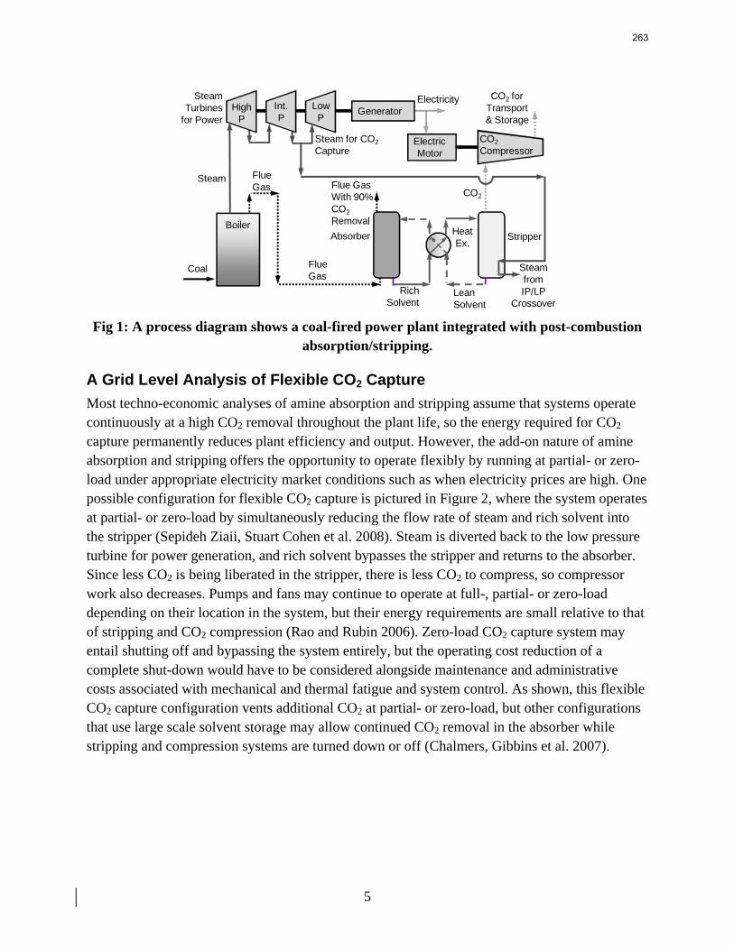
5
Boiler
Steam Turbines
for Power
Steam for CO2Capture
Flue Gas
Steam
Stripper
Flue Gas
Rich Solvent
CO2 forTransport& Storage
CO2
Steam fromIP/LP
Crossover
Absorber
Lean Solvent
Flue Gas With 90% CO2Removal
CO2Compressor
Coal
Electricity
Heat Ex.
HighP
Int.P
LowP
Generator
Electric Motor
Fig 1: A process diagram shows a coal-fired power plant integrated with post-combustion
absorption/stripping.
A Grid Level Analysis of Flexible CO2 Capture Most techno-economic analyses of amine absorption and stripping assume that systems operate continuously at a high CO2 removal throughout the plant life, so the energy required for CO2 capture permanently reduces plant efficiency and output. However, the add-on nature of amine absorption and stripping offers the opportunity to operate flexibly by running at partial- or zero-load under appropriate electricity market conditions such as when electricity prices are high. One possible configuration for flexible CO2 capture is pictured in Figure 2, where the system operates at partial- or zero-load by simultaneously reducing the flow rate of steam and rich solvent into the stripper (Sepideh Ziaii, Stuart Cohen et al. 2008). Steam is diverted back to the low pressure turbine for power generation, and rich solvent bypasses the stripper and returns to the absorber. Since less CO2 is being liberated in the stripper, there is less CO2 to compress, so compressor work also decreases. Pumps and fans may continue to operate at full-, partial- or zero-load depending on their location in the system, but their energy requirements are small relative to that of stripping and CO2 compression (Rao and Rubin 2006). Zero-load CO2 capture system may entail shutting off and bypassing the system entirely, but the operating cost reduction of a complete shut-down would have to be considered alongside maintenance and administrative costs associated with mechanical and thermal fatigue and system control. As shown, this flexible CO2 capture configuration vents additional CO2 at partial- or zero-load, but other configurations that use large scale solvent storage may allow continued CO2 removal in the absorber while stripping and compression systems are turned down or off (Chalmers, Gibbins et al. 2007).
263
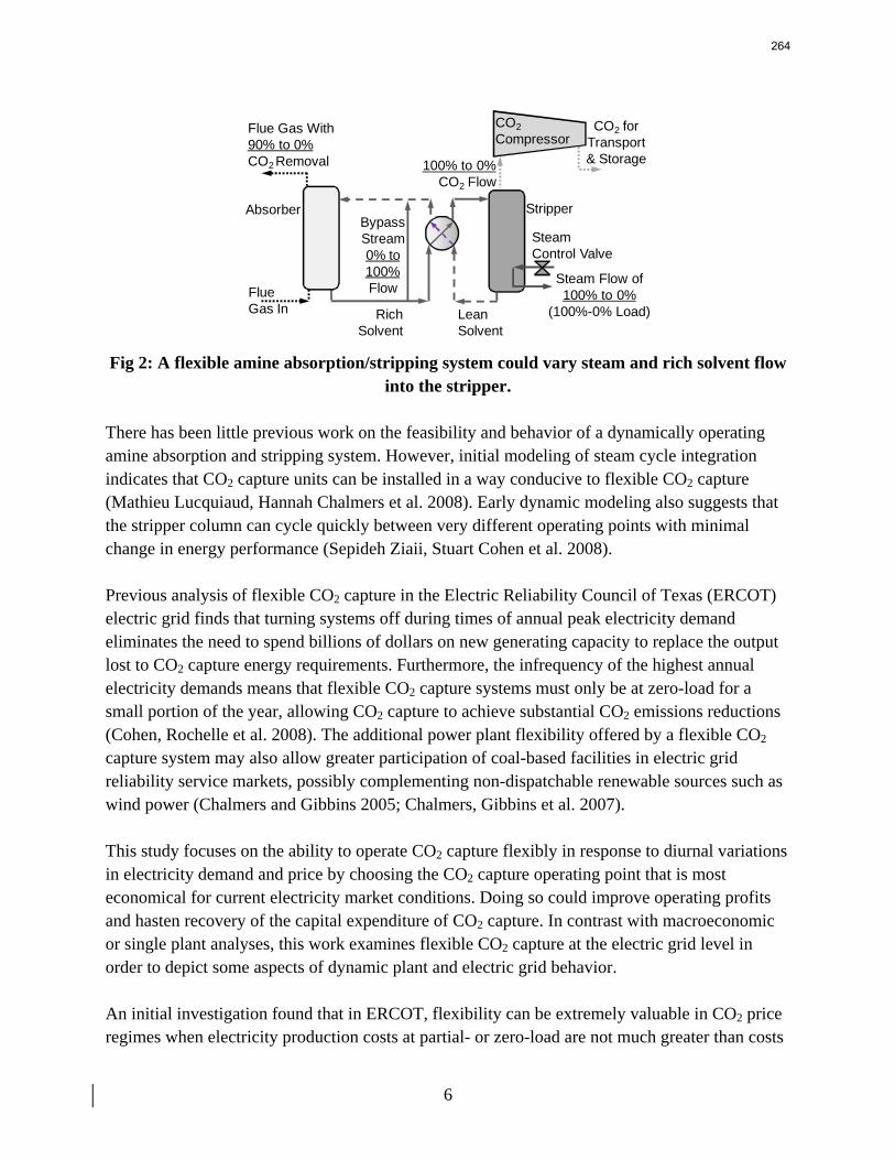
6
Stripper
Rich Solvent
Steam Flow of 100% to 0%
(100%-0% Load)
Absorber
Steam Control Valve
Lean Solvent
100% to 0%CO2 Flow
Flue Gas With 90% to 0% CO2 Removal
CO2 forTransport& Storage
Bypass Stream 0% to 100% FlowFlue
Gas In
CO2Compressor
Fig 2: A flexible amine absorption/stripping system could vary steam and rich solvent flow
into the stripper. There has been little previous work on the feasibility and behavior of a dynamically operating amine absorption and stripping system. However, initial modeling of steam cycle integration indicates that CO2 capture units can be installed in a way conducive to flexible CO2 capture (Mathieu Lucquiaud, Hannah Chalmers et al. 2008). Early dynamic modeling also suggests that the stripper column can cycle quickly between very different operating points with minimal change in energy performance (Sepideh Ziaii, Stuart Cohen et al. 2008). Previous analysis of flexible CO2 capture in the Electric Reliability Council of Texas (ERCOT) electric grid finds that turning systems off during times of annual peak electricity demand eliminates the need to spend billions of dollars on new generating capacity to replace the output lost to CO2 capture energy requirements. Furthermore, the infrequency of the highest annual electricity demands means that flexible CO2 capture systems must only be at zero-load for a small portion of the year, allowing CO2 capture to achieve substantial CO2 emissions reductions (Cohen, Rochelle et al. 2008). The additional power plant flexibility offered by a flexible CO2 capture system may also allow greater participation of coal-based facilities in electric grid reliability service markets, possibly complementing non-dispatchable renewable sources such as wind power (Chalmers and Gibbins 2005; Chalmers, Gibbins et al. 2007). This study focuses on the ability to operate CO2 capture flexibly in response to diurnal variations in electricity demand and price by choosing the CO2 capture operating point that is most economical for current electricity market conditions. Doing so could improve operating profits and hasten recovery of the capital expenditure of CO2 capture. In contrast with macroeconomic or single plant analyses, this work examines flexible CO2 capture at the electric grid level in order to depict some aspects of dynamic plant and electric grid behavior. An initial investigation found that in ERCOT, flexibility can be extremely valuable in CO2 price regimes when electricity production costs at partial- or zero-load are not much greater than costs
264
7
with full-load CO2 capture (Sepideh Ziaii, Stuart Cohen et al. 2008). That work found that electricity production costs1,2 are lower with full-load CO2 capture above $25/tCO2, and plants with flexible CO2 capture earn much greater operating profits than inflexible plants below $30/tCO2. However, these data only consider a $1.48/MMBTU3 coal price and $6.60/MMBTU natural gas price. In reality, fossil fuel prices may change considerably over time; natural gas price volatility is particularly notorious. Fossil fuel prices play a major role in generation costs at coal- and natural gas-fired facilities both with and without CO2 capture. Because the flexible CO2 capture operating point directly affects power plant efficiency, fuel prices play a major role in determining the most economical CO2 capture operating point. Fossil fuel prices affect the relative costs of different power plant types, which can significantly influence electricity dispatch. In order to better understand the effects of fossil fuel price on the dispatch and operation of flexible CO2 capture systems, this study investigates several coal and natural gas price combinations in a dynamic model of the ERCOT electric grid. Each fuel price combination is analyzed for a range of possible CO2 prices in order to determine the impact of fuel prices on flexible CO2 capture utilization and the resulting power plant and electric grid economics and CO2 emissions.
Methodology
Model Scope and a Description of ERCOT A deterministic model is created in MATLAB and used to compare the ERCOT electric grid without CO2 capture to scenarios with inflexible and flexible CO2 capture available. In contrast to a rigorous electric grid analysis seeking optimal economic or environmental behavior, this approach seeks to estimate the general performance, economic, and environmental implications of flexible CO2 capture for a range of fuel and CO2 prices. These results can then provide insight into the role of flexible CO2 capture in the electric grid and the potential for flexible CO2 capture to improve upon the prospects of widespread CCS deployment. The analysis exclusively considers the ERCOT electric grid as configured in 2006. This year is chosen to maintain consistency with previous work and because of the availability of input data. ERCOT installed capacity, which accounts for expected plant availability, was 71,812MW in 2006 and consisted of 20.5% coal-based, 71.7% natural gas-based, 6.4% nuclear, and 1.5% wind/other capacity (ERCOT 2006). Historically, nuclear, renewable, and coal-based facilities have the lowest operating costs, so these plants are used to meet base load electricity demand, while natural gas-fired facilities supply the remaining demand. Thus, the percent of actual generation from natural gas is far less than its 72% contribution to installed capacity, with coal-
1 All cost values are reported as 2006 U.S. dollars. 2 Quantities of CO2 are reported in metric tons (tCO2). 3 MMBTU is an abbreviation for million British thermal units
265
8
based and nuclear capacity contributing much more to actual generation than their percent of installed capacity may indicate (see Table 2) (ERCOT 2006). ERCOT manages electricity dispatch through a competitive market. Currently, approximately 95% of electricity consumed is traded scheduled confidential bilateral contracts. The remaining 5% of electricity is traded on the wholesale balancing energy market administered by ERCOT (Smitherman, Nelson et al. 2009). While electricity prices in bilateral contracts are not publicly known, the clearing price in the balancing energy market is a reasonable and likely high estimate of the price of electricity in bilateral contracts because it represents the value of electricity at any time (PE-Ltd. 2007). Generators participate in the balancing energy market by submitting offers of marginal electricity production costs across their output range, and then ERCOT dispatches plants in the most economical way possible given power plant and electric grid constraints. Marginal cost offers do not necessarily equal actual marginal costs, but a well functioning market will incentivize generators to submit offers at or near their marginal costs. The wholesale electricity price is “set” by the offer price of the last and most expensive plant dispatched at a given time, termed the marginal generating facility. All market participants then receive this price for their output, so plants earn profit if marginal costs are lower than the electricity price. Since ERCOT electricity demand rarely drops below the cumulative available output at nuclear, renewable, and coal-fired facilities, natural-gas fired plants typically set the balancing energy price. It is important to recognize that the continually varying wholesale price of electricity does not directly represent the retail price of electricity paid by retail consumers. Retail service providers set prices based on wholesale electricity prices over a long period of time as well as transmission costs and any other marketing and administration costs. Because this work is primarily concerned with the power plant operating behavior, the focus is on the wholesale electricity market.
Model Assumptions and Input Parameters
Plant Dispatch and Electricity Market Model
The model calculates marginal generating costs for each fossil fueled power plant in the ERCOT grid using specified fuel and CO2 prices, plant performance parameters from the Environmental Protection Agency’s (EPA) eGRID database, capacity installation reports from the Public Utilities Commission of Texas, and non-fuel operation and maintenance (O&M) costs from literature. Marginal costs at nuclear facilities are specified from literature, as are the costs of any remaining plants, which are grouped and assigned properties of wind generation because 75% of the generation from non-fossil or nuclear facilities came from wind power in 2006 (ERCOT 2006). As an approximation, each plant has constant marginal costs up to its installed capacity. Installed plant capacity is used as the maximum plant output rather than rated capacity in order to
266
9
account for average plant availability. Since capital charges are not included in the marginal cost offers used to determine ERCOT electricity dispatch, they are not incorporated into the model’s cost calculation. The model examines 2006 historical electricity demand in each hour then dispatches plants by choosing the cheapest available plants until demand is met. Electricity price in each hour is then set equal to the marginal cost of the last plant dispatched in the hour (the marginal generating facility). Marginal costs, electricity price, and plant output is used to calculate operating profits. Once the generation of each plant is determined for the entire year, CO2 emissions can be found using emissions rates from the eGRID database. The model does not consider transmission constraints on plant dispatch or any other technical or geographical influences on plant generation such as ramp rate or minimum sustainable generation. The ERCOT grid is analyzed in its entirety rather than being broken down into smaller areas that may have distinct electricity prices. While these limitations prevent the model from producing a highly accurate dispatch order, the simplified dispatch and market model still provides an effective framework to analyze the effects of flexible CO2 capture on the ERCOT grid in a more rapid and straightforward manner than a comprehensive electric grid simulation.
CO2 Capture Systems
For scenarios with CO2 capture facilities available, all CO2 capture systems use a monoethanolamine (MEA) solvent for CO2 capture at coal-fired facilities. MEA is commonly considered a baseline solvent for CO2 capture because its properties are relatively well known. CO2 capture at natural gas-fired plants is not considered in this study because these plants are expected to have higher CO2 avoidance costs and thus will emerge as CO2 capture candidates later than coal-fired facilities. Eight of ERCOT’s 15 coal-based plants are chosen to be considered for CO2 capture so that continuous full-load CO2 capture at all eight plants will reduce coal fleet emissions by approximately 50%, giving the ERCOT coal fleet an average emissions rate near that of a typical natural gas-fired facility. Coal-fired plants chosen for CO2 capture have the lowest sum of operating costs with full-load CO2 capture and capital charges for CO2 capture equipment and any additional sulfur dioxide (SO2) removal equipment required to achieve sufficient SO2 removal to mitigate solvent degradation (Rao and Rubin 2002). Flexible CO2 capture systems may choose between full-load (100% load) and 20% load, defining load as the percent of the stripping steam and compression work required for 100% load CO2 capture. Two operating points are chosen since it is unlikely that a system could operate efficiently at all CO2 capture loads. 20% and 100% load are chosen because of available energy performance and CO2 removal data from a dynamic model. CO2 capture energy is
267
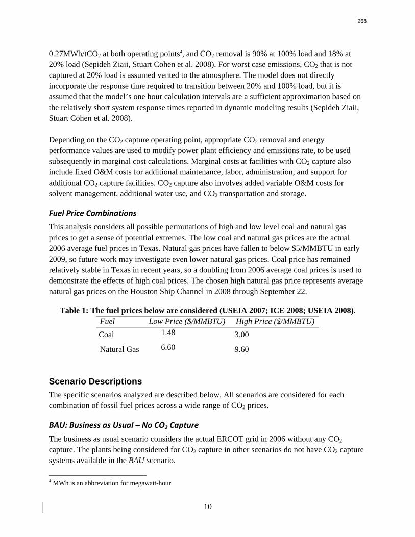
10
0.27MWh/tCO2 at both operating points4, and CO2 removal is 90% at 100% load and 18% at 20% load (Sepideh Ziaii, Stuart Cohen et al. 2008). For worst case emissions, CO2 that is not captured at 20% load is assumed vented to the atmosphere. The model does not directly incorporate the response time required to transition between 20% and 100% load, but it is assumed that the model’s one hour calculation intervals are a sufficient approximation based on the relatively short system response times reported in dynamic modeling results (Sepideh Ziaii, Stuart Cohen et al. 2008). Depending on the CO2 capture operating point, appropriate CO2 removal and energy performance values are used to modify power plant efficiency and emissions rate, to be used subsequently in marginal cost calculations. Marginal costs at facilities with CO2 capture also include fixed O&M costs for additional maintenance, labor, administration, and support for additional CO2 capture facilities. CO2 capture also involves added variable O&M costs for solvent management, additional water use, and CO2 transportation and storage.
Fuel Price Combinations
This analysis considers all possible permutations of high and low level coal and natural gas prices to get a sense of potential extremes. The low coal and natural gas prices are the actual 2006 average fuel prices in Texas. Natural gas prices have fallen to below $5/MMBTU in early 2009, so future work may investigate even lower natural gas prices. Coal price has remained relatively stable in Texas in recent years, so a doubling from 2006 average coal prices is used to demonstrate the effects of high coal prices. The chosen high natural gas price represents average natural gas prices on the Houston Ship Channel in 2008 through September 22.
Table 1: The fuel prices below are considered (USEIA 2007; ICE 2008; USEIA 2008). Fuel Low Price ($/MMBTU) High Price ($/MMBTU) Coal 1.48 3.00
Natural Gas 6.60 9.60
Scenario Descriptions The specific scenarios analyzed are described below. All scenarios are considered for each combination of fossil fuel prices across a wide range of CO2 prices.
BAU: Business as Usual – No CO2 Capture The business as usual scenario considers the actual ERCOT grid in 2006 without any CO2 capture. The plants being considered for CO2 capture in other scenarios do not have CO2 capture systems available in the BAU scenario.
4 MWh is an abbreviation for megawatt-hour
268
11
CCS Base: Inflexible CO2 Capture In the base case CO2 capture scenario, CO2 capture systems are operated at 100% load continuously throughout the year, hence, CO2 capture flexibility is not available. Typical analysis often assumes that installing CO2 capture on any existing facilities requires new generation capacity to replace output that is permanently lost to CO2 capture energy requirements. However, the capital cost and electric grid implications of replacement capacity are not considered in this study.
FLEX Op Costs: Flexible CO2 Capture Option
Plants with CO2 capture choose the operating condition (20% or 100% load) with the lowest marginal costs of electricity production. When there is no cost of emitting CO2, it will always be least expensive to operate at 20% load; higher CO2 prices will eventually allow lower costs at 100% load. Since each annual calculation period uses constant fuel and CO2 prices, CO2 capture facilities will choose either continuous 20% load or continuous 100% load in this scenario.
FLEX Profit: Flexible CO2 Capture Option
This flexible scenario operates under the assumption of perfect knowledge of electricity demand and dispatch ordering prior to deciding on a CO2 capture load. This assumption is unrealistic, but public ERCOT planning information and industry experience allow plant operators to approximate market behavior when making decisions. In every hour, each plant with CO2 capture calculates its hourly profits for two scenarios: if all plants with CO2 capture operate at (A) 100% load or (B) 20% load. If profits are greater for a particular plant for Option A, that plant will operate capture at 100% load; otherwise, it will operate at 20% load. Though CO2 price may be high enough for marginal costs to be greater at 20% load, the additional plant output at 20% load may allow profits to be greater if electricity prices are high enough. However, since the output capacity of plants with CO2 capture is lower at 100% load, Option A will likely have a higher electricity price. Facilities with CO2 capture may act individually, but decisions are based on collective action, which is not a realistic representation of strategic behavior based on specific company preferences. However, a sophisticated treatment of such strategic behavior is outside the scope of this work.
RESULTS & DISCUSSION
Model Validation To validate the model, the BAU scenario with no CO2 price and historical average 2006 fossil fuel prices is compared with historical generation and electricity price data from the EPA and ERCOT. Results are shown in Table 2. The model predicts total generation of each plant type within 1.2%. While calculated CO2 emissions from coal-fired generators correspond with 2004
269
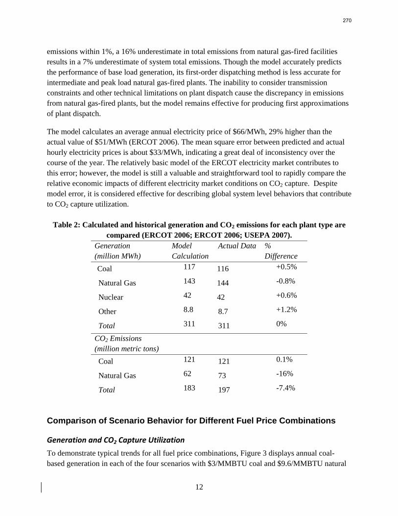
12
emissions within 1%, a 16% underestimate in total emissions from natural gas-fired facilities results in a 7% underestimate of system total emissions. Though the model accurately predicts the performance of base load generation, its first-order dispatching method is less accurate for intermediate and peak load natural gas-fired plants. The inability to consider transmission constraints and other technical limitations on plant dispatch cause the discrepancy in emissions from natural gas-fired plants, but the model remains effective for producing first approximations of plant dispatch. The model calculates an average annual electricity price of $66/MWh, 29% higher than the actual value of $51/MWh (ERCOT 2006). The mean square error between predicted and actual hourly electricity prices is about $33/MWh, indicating a great deal of inconsistency over the course of the year. The relatively basic model of the ERCOT electricity market contributes to this error; however, the model is still a valuable and straightforward tool to rapidly compare the relative economic impacts of different electricity market conditions on CO2 capture. Despite model error, it is considered effective for describing global system level behaviors that contribute to CO2 capture utilization.
Table 2: Calculated and historical generation and CO2 emissions for each plant type are compared (ERCOT 2006; ERCOT 2006; USEPA 2007).
Generation (million MWh)
Model Calculation
Actual Data % Difference
Coal 117 116 +0.5%
Natural Gas 143 144 -0.8%
Nuclear 42 42 +0.6%
Other 8.8 8.7 +1.2%
Total 311 311 0%
CO2 Emissions (million metric tons)
Coal 121 121 0.1%
Natural Gas 62 73 -16%
Total 183 197 -7.4%
Comparison of Scenario Behavior for Different Fuel Price Combinations
Generation and CO2 Capture Utilization To demonstrate typical trends for all fuel price combinations, Figure 3 displays annual coal-based generation in each of the four scenarios with $3/MMBTU coal and $9.6/MMBTU natural
270
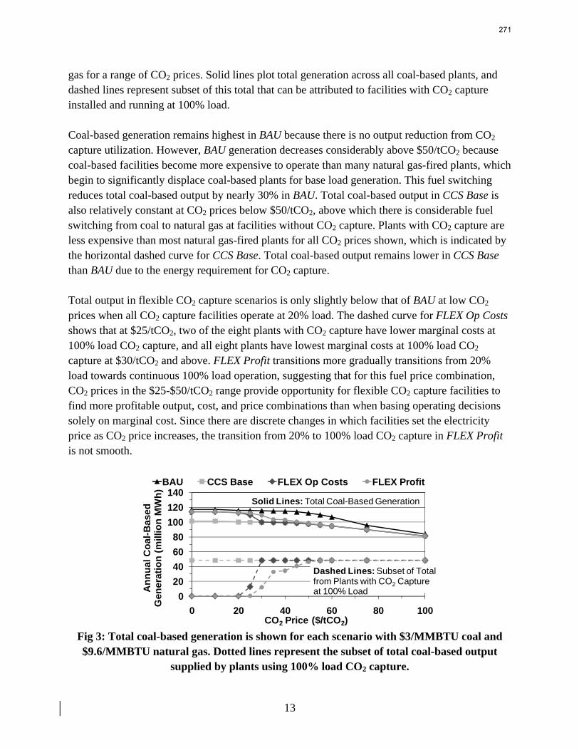
13
gas for a range of CO2 prices. Solid lines plot total generation across all coal-based plants, and dashed lines represent subset of this total that can be attributed to facilities with CO2 capture installed and running at 100% load. Coal-based generation remains highest in BAU because there is no output reduction from CO2 capture utilization. However, BAU generation decreases considerably above $50/tCO2 because coal-based facilities become more expensive to operate than many natural gas-fired plants, which begin to significantly displace coal-based plants for base load generation. This fuel switching reduces total coal-based output by nearly 30% in BAU. Total coal-based output in CCS Base is also relatively constant at CO2 prices below $50/tCO2, above which there is considerable fuel switching from coal to natural gas at facilities without CO2 capture. Plants with CO2 capture are less expensive than most natural gas-fired plants for all CO2 prices shown, which is indicated by the horizontal dashed curve for CCS Base. Total coal-based output remains lower in CCS Base than BAU due to the energy requirement for CO2 capture. Total output in flexible CO2 capture scenarios is only slightly below that of BAU at low CO2 prices when all CO2 capture facilities operate at 20% load. The dashed curve for FLEX Op Costs shows that at $25/tCO2, two of the eight plants with CO2 capture have lower marginal costs at 100% load CO2 capture, and all eight plants have lowest marginal costs at 100% load CO2 capture at $30/tCO2 and above. FLEX Profit transitions more gradually transitions from 20% load towards continuous 100% load operation, suggesting that for this fuel price combination, CO2 prices in the $25-$50/tCO2 range provide opportunity for flexible CO2 capture facilities to find more profitable output, cost, and price combinations than when basing operating decisions solely on marginal cost. Since there are discrete changes in which facilities set the electricity price as CO2 price increases, the transition from 20% to 100% load CO2 capture in FLEX Profit is not smooth.
020406080
100120140
0 20 40 60 80 100
Ann
ual C
oal-B
ased
Gen
erat
ion
(mill
ion
MW
h)
CO2 Price ($/tCO2)
BAU CCS Base FLEX Op Costs FLEX Profit
Solid Lines: Total Coal-Based Generation
Dashed Lines: Subset of Total from Plants with CO2 Capture at 100% Load
Fig 3: Total coal-based generation is shown for each scenario with $3/MMBTU coal and $9.6/MMBTU natural gas. Dotted lines represent the subset of total coal-based output
supplied by plants using 100% load CO2 capture.
271

14
Figure 4 displays fuel switching behavior for each coal and natural gas price combinations by plotting coal-based generation in CCS Base for each fuel price permutation. Recall that plants with CO2 capture in CCS Base may only operate at 100% load CO2 capture. As before, solid lines represent total coal-based generation in both capture and non-capture plants, and dashed lines represent the subset of this total consisting of output from plants operating CO2 capture at 100% load. Except with $3/MMBTU coal and $6.6/MMBTU natural gas, plants with CO2 capture are always base load capacity, operating at maximum output continuously throughout the year. Thus, any reduction in coal-based generation can be attributed to fuel switching from coal-fired plants without CO2 capture to less expensive natural gas-based facilities. High natural gas prices delay the onset of fuel switching to higher CO2 prices and decrease the overall magnitude of fuel switching behavior. With $1.5/MMBTU coal and $9.6/MMBTU natural gas, total coal-based generation decreases only 10% when CO2 emissions cost $100/tCO2. High CO2 prices are required for fuel switching from coal to natural gas because ERCOT has a relatively small fraction of total installed capacity consisting of coal-based facilities. In electric grids with greater coal dependency, fuel switching is likely to occur at lower CO2 prices for a given fuel price combination. The $3/MMBTU coal and $6.6/MMBTU natural gas combination has the smallest gas/coal price ratio, producing the unique result that below $40/tCO2, natural gas-fired facilities actually displace coal-based plants with CO2 capture for base load generation. Thus, coal-based output at low CO2 prices is far below that of other fuel price combinations. Above $40/tCO2, the small gas/coal ratio then allows natural gas-fired plants to displace coal-fired facilities without CO2 capture, so that total coal-based generation remains below that of other fuel price groupings.
0
20
40
60
80
100
120
0 20 40 60 80 100
Ann
ual C
oal-B
ased
G
ener
atio
n in
CC
S B
ase
(mill
ion
MW
h)
CO2 Price ($/tCO2)
Subset of Total from Plants with CO2Capture at 100% Load for $3 Coal, $6.6 NG
Subset of Total from Plants with CO2 Capture at 100% Load for all other fuel price combinations
$1.5 Coal, $9.6 NG
$3/$9.6
$3/$6.6$1.5/$6.6
Solid Lines: Total Coal-Based Generation
272
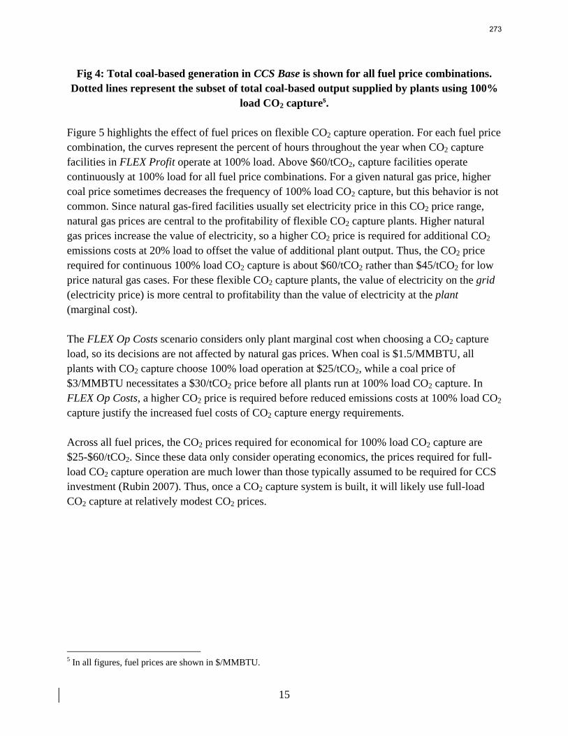
15
Fig 4: Total coal-based generation in CCS Base is shown for all fuel price combinations. Dotted lines represent the subset of total coal-based output supplied by plants using 100%
load CO2 capture5. Figure 5 highlights the effect of fuel prices on flexible CO2 capture operation. For each fuel price combination, the curves represent the percent of hours throughout the year when CO2 capture facilities in FLEX Profit operate at 100% load. Above $60/tCO2, capture facilities operate continuously at 100% load for all fuel price combinations. For a given natural gas price, higher coal price sometimes decreases the frequency of 100% load CO2 capture, but this behavior is not common. Since natural gas-fired facilities usually set electricity price in this CO2 price range, natural gas prices are central to the profitability of flexible CO2 capture plants. Higher natural gas prices increase the value of electricity, so a higher CO2 price is required for additional CO2 emissions costs at 20% load to offset the value of additional plant output. Thus, the CO2 price required for continuous 100% load CO2 capture is about $60/tCO2 rather than $45/tCO2 for low price natural gas cases. For these flexible CO2 capture plants, the value of electricity on the grid (electricity price) is more central to profitability than the value of electricity at the plant (marginal cost). The FLEX Op Costs scenario considers only plant marginal cost when choosing a CO2 capture load, so its decisions are not affected by natural gas prices. When coal is $1.5/MMBTU, all plants with CO2 capture choose 100% load operation at $25/tCO2, while a coal price of $3/MMBTU necessitates a $30/tCO2 price before all plants run at 100% load CO2 capture. In FLEX Op Costs, a higher CO2 price is required before reduced emissions costs at 100% load CO2 capture justify the increased fuel costs of CO2 capture energy requirements. Across all fuel prices, the CO2 prices required for economical for 100% load CO2 capture are $25-$60/tCO2. Since these data only consider operating economics, the prices required for full-load CO2 capture operation are much lower than those typically assumed to be required for CCS investment (Rubin 2007). Thus, once a CO2 capture system is built, it will likely use full-load CO2 capture at relatively modest CO2 prices.
5 In all figures, fuel prices are shown in $/MMBTU.
273
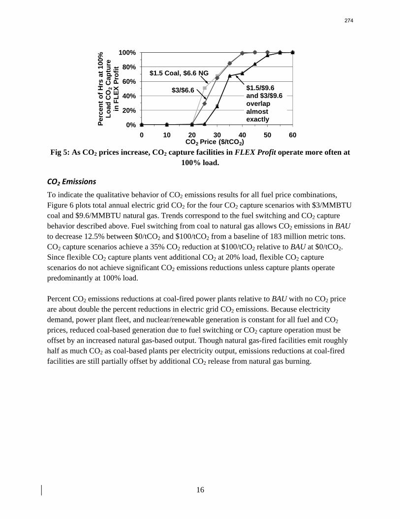
16
0%
20%
40%
60%
80%
100%
0 10 20 30 40 50 60
Perc
ent o
f Hrs
at 1
00%
Lo
ad C
O2
Cap
ture
in
FLE
X Pr
ofit
CO2 Price ($/tCO2)
$1.5 Coal, $6.6 NG
$3/$6.6 $1.5/$9.6 and $3/$9.6overlap almost exactly
Fig 5: As CO2 prices increase, CO2 capture facilities in FLEX Profit operate more often at
100% load.
CO2 Emissions To indicate the qualitative behavior of CO2 emissions results for all fuel price combinations, Figure 6 plots total annual electric grid CO2 for the four CO2 capture scenarios with $3/MMBTU coal and $9.6/MMBTU natural gas. Trends correspond to the fuel switching and CO2 capture behavior described above. Fuel switching from coal to natural gas allows CO2 emissions in BAU to decrease 12.5% between $0/tCO2 and $100/tCO2 from a baseline of 183 million metric tons. CO2 capture scenarios achieve a 35% CO2 reduction at $100/tCO2 relative to BAU at $0/tCO2. Since flexible CO2 capture plants vent additional CO2 at 20% load, flexible CO2 capture scenarios do not achieve significant CO2 emissions reductions unless capture plants operate predominantly at 100% load. Percent CO2 emissions reductions at coal-fired power plants relative to BAU with no CO2 price are about double the percent reductions in electric grid CO2 emissions. Because electricity demand, power plant fleet, and nuclear/renewable generation is constant for all fuel and CO2 prices, reduced coal-based generation due to fuel switching or CO2 capture operation must be offset by an increased natural gas-based output. Though natural gas-fired facilities emit roughly half as much CO2 as coal-based plants per electricity output, emissions reductions at coal-fired facilities are still partially offset by additional CO2 release from natural gas burning.
274
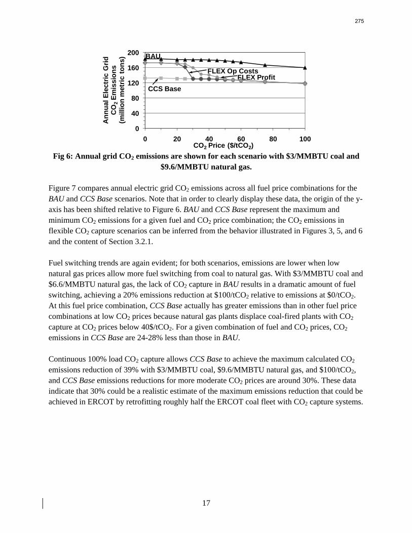
17
0
40
80
120
160
200
0 20 40 60 80 100
Ann
ual E
lect
ric G
rid
CO
2Em
issi
ons
(mill
ion
met
ric to
ns)
CO2 Price ($/tCO2)
BAU
CCS Base
FLEX Op CostsFLEX Profit
Fig 6: Annual grid CO2 emissions are shown for each scenario with $3/MMBTU coal and
$9.6/MMBTU natural gas. Figure 7 compares annual electric grid CO2 emissions across all fuel price combinations for the BAU and CCS Base scenarios. Note that in order to clearly display these data, the origin of the y-axis has been shifted relative to Figure 6. BAU and CCS Base represent the maximum and minimum CO2 emissions for a given fuel and CO2 price combination; the CO2 emissions in flexible CO2 capture scenarios can be inferred from the behavior illustrated in Figures 3, 5, and 6 and the content of Section 3.2.1. Fuel switching trends are again evident; for both scenarios, emissions are lower when low natural gas prices allow more fuel switching from coal to natural gas. With $3/MMBTU coal and $6.6/MMBTU natural gas, the lack of CO2 capture in BAU results in a dramatic amount of fuel switching, achieving a 20% emissions reduction at $100/tCO2 relative to emissions at $0/tCO2. At this fuel price combination, CCS Base actually has greater emissions than in other fuel price combinations at low CO2 prices because natural gas plants displace coal-fired plants with CO2 capture at CO2 prices below 40$/tCO2. For a given combination of fuel and CO2 prices, CO2 emissions in CCS Base are 24-28% less than those in BAU. Continuous 100% load CO2 capture allows CCS Base to achieve the maximum calculated CO2 emissions reduction of 39% with $3/MMBTU coal, $9.6/MMBTU natural gas, and $100/tCO2, and CCS Base emissions reductions for more moderate CO2 prices are around 30%. These data indicate that 30% could be a realistic estimate of the maximum emissions reduction that could be achieved in ERCOT by retrofitting roughly half the ERCOT coal fleet with CO2 capture systems.
275
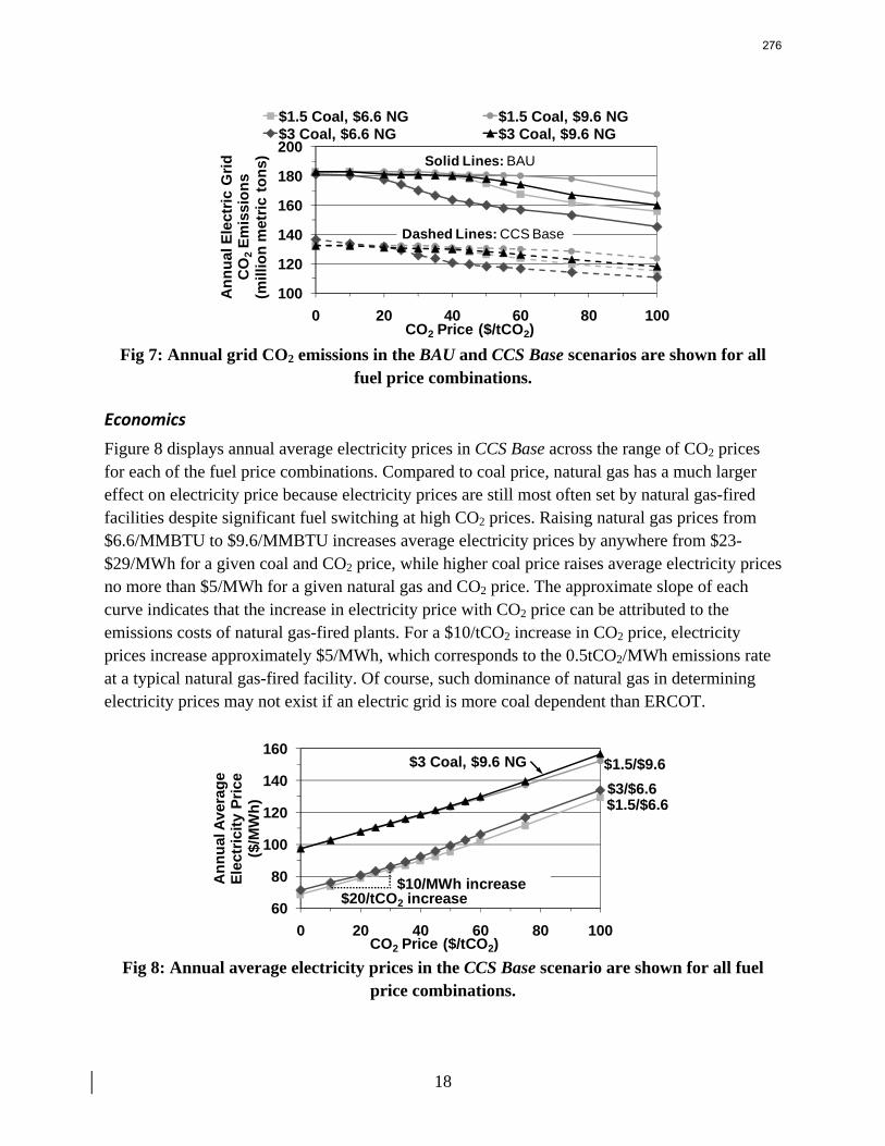
18
100
120
140
160
180
200
0 20 40 60 80 100
Ann
ual E
lect
ric G
rid
CO
2Em
issi
ons
(m
illio
n m
etric
tons
)
CO2 Price ($/tCO2)
$1.5 Coal, $6.6 NG $1.5 Coal, $9.6 NG$3 Coal, $6.6 NG $3 Coal, $9.6 NG
Dashed Lines: CCS Base
Solid Lines: BAU
Fig 7: Annual grid CO2 emissions in the BAU and CCS Base scenarios are shown for all
fuel price combinations.
Economics Figure 8 displays annual average electricity prices in CCS Base across the range of CO2 prices for each of the fuel price combinations. Compared to coal price, natural gas has a much larger effect on electricity price because electricity prices are still most often set by natural gas-fired facilities despite significant fuel switching at high CO2 prices. Raising natural gas prices from $6.6/MMBTU to $9.6/MMBTU increases average electricity prices by anywhere from $23-$29/MWh for a given coal and CO2 price, while higher coal price raises average electricity prices no more than $5/MWh for a given natural gas and CO2 price. The approximate slope of each curve indicates that the increase in electricity price with CO2 price can be attributed to the emissions costs of natural gas-fired plants. For a $10/tCO2 increase in CO2 price, electricity prices increase approximately $5/MWh, which corresponds to the 0.5tCO2/MWh emissions rate at a typical natural gas-fired facility. Of course, such dominance of natural gas in determining electricity prices may not exist if an electric grid is more coal dependent than ERCOT.
60
80
100
120
140
160
0 20 40 60 80 100
Ann
ual A
vera
ge
Elec
tric
ity P
rice
($/M
Wh)
CO2 Price ($/tCO2)
$3 Coal, $9.6 NG
$3/$6.6$1.5/$9.6
$1.5/$6.6
$20/tCO2 increase$10/MWh increase
Fig 8: Annual average electricity prices in the CCS Base scenario are shown for all fuel
price combinations.
276
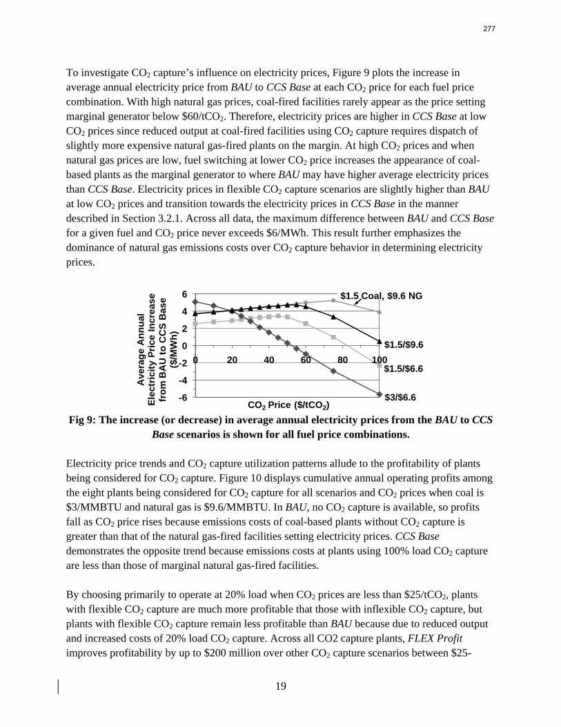
19
To investigate CO2 capture’s influence on electricity prices, Figure 9 plots the increase in average annual electricity price from BAU to CCS Base at each CO2 price for each fuel price combination. With high natural gas prices, coal-fired facilities rarely appear as the price setting marginal generator below $60/tCO2. Therefore, electricity prices are higher in CCS Base at low CO2 prices since reduced output at coal-fired facilities using CO2 capture requires dispatch of slightly more expensive natural gas-fired plants on the margin. At high CO2 prices and when natural gas prices are low, fuel switching at lower CO2 price increases the appearance of coal-based plants as the marginal generator to where BAU may have higher average electricity prices than CCS Base. Electricity prices in flexible CO2 capture scenarios are slightly higher than BAU at low CO2 prices and transition towards the electricity prices in CCS Base in the manner described in Section 3.2.1. Across all data, the maximum difference between BAU and CCS Base for a given fuel and CO2 price never exceeds $6/MWh. This result further emphasizes the dominance of natural gas emissions costs over CO2 capture behavior in determining electricity prices.
-6
-4
-2
0
2
4
6
0 20 40 60 80 100
CO2 Price ($/tCO2)
$1.5 Coal, $9.6 NG
$3/$6.6
$1.5/$9.6
$1.5/$6.6
Ave
rage
Ann
ual
Elec
tric
ity P
rice
Incr
ease
fr
om B
AU
to C
CS
Bas
e ($
/MW
h)
Fig 9: The increase (or decrease) in average annual electricity prices from the BAU to CCS
Base scenarios is shown for all fuel price combinations. Electricity price trends and CO2 capture utilization patterns allude to the profitability of plants being considered for CO2 capture. Figure 10 displays cumulative annual operating profits among the eight plants being considered for CO2 capture for all scenarios and CO2 prices when coal is $3/MMBTU and natural gas is $9.6/MMBTU. In BAU, no CO2 capture is available, so profits fall as CO2 price rises because emissions costs of coal-based plants without CO2 capture is greater than that of the natural gas-fired facilities setting electricity prices. CCS Base demonstrates the opposite trend because emissions costs at plants using 100% load CO2 capture are less than those of marginal natural gas-fired facilities. By choosing primarily to operate at 20% load when CO2 prices are less than $25/tCO2, plants with flexible CO2 capture are much more profitable that those with inflexible CO2 capture, but plants with flexible CO2 capture remain less profitable than BAU because due to reduced output and increased costs of 20% load CO2 capture. Across all CO2 capture plants, FLEX Profit improves profitability by up to $200 million over other CO2 capture scenarios between $25-
277
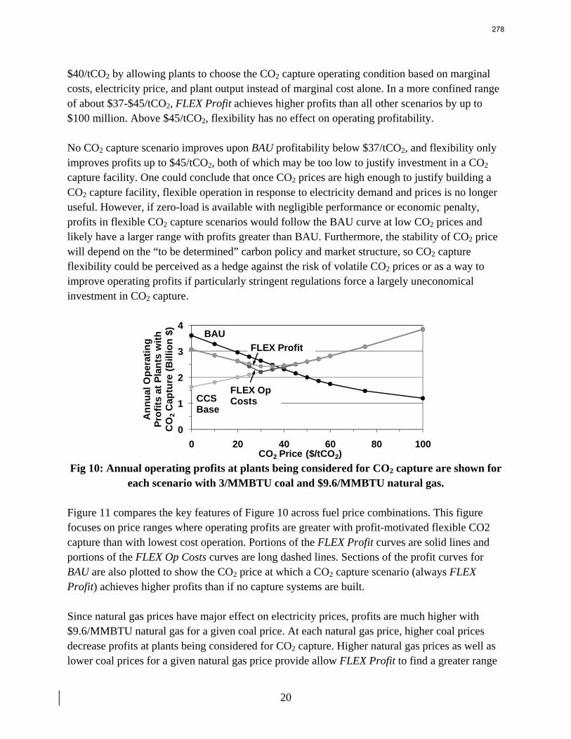
20
$40/tCO2 by allowing plants to choose the CO2 capture operating condition based on marginal costs, electricity price, and plant output instead of marginal cost alone. In a more confined range of about $37-$45/tCO2, FLEX Profit achieves higher profits than all other scenarios by up to $100 million. Above $45/tCO2, flexibility has no effect on operating profitability. No CO2 capture scenario improves upon BAU profitability below $37/tCO2, and flexibility only improves profits up to $45/tCO2, both of which may be too low to justify investment in a CO2 capture facility. One could conclude that once CO2 prices are high enough to justify building a CO2 capture facility, flexible operation in response to electricity demand and prices is no longer useful. However, if zero-load is available with negligible performance or economic penalty, profits in flexible CO2 capture scenarios would follow the BAU curve at low CO2 prices and likely have a larger range with profits greater than BAU. Furthermore, the stability of CO2 price will depend on the “to be determined” carbon policy and market structure, so CO2 capture flexibility could be perceived as a hedge against the risk of volatile CO2 prices or as a way to improve operating profits if particularly stringent regulations force a largely uneconomical investment in CO2 capture.
0
1
2
3
4
0 20 40 60 80 100
Ann
ual O
pera
ting
Prof
its a
t Pla
nts
with
C
O2
Cap
ture
(Bill
ion
$)
CO2 Price ($/tCO2)
BAU
CCS Base
FLEX Op Costs
FLEX Profit
Fig 10: Annual operating profits at plants being considered for CO2 capture are shown for
each scenario with 3/MMBTU coal and $9.6/MMBTU natural gas. Figure 11 compares the key features of Figure 10 across fuel price combinations. This figure focuses on price ranges where operating profits are greater with profit-motivated flexible CO2 capture than with lowest cost operation. Portions of the FLEX Profit curves are solid lines and portions of the FLEX Op Costs curves are long dashed lines. Sections of the profit curves for BAU are also plotted to show the CO2 price at which a CO2 capture scenario (always FLEX Profit) achieves higher profits than if no capture systems are built. Since natural gas prices have major effect on electricity prices, profits are much higher with $9.6/MMBTU natural gas for a given coal price. At each natural gas price, higher coal prices decrease profits at plants being considered for CO2 capture. Higher natural gas prices as well as lower coal prices for a given natural gas price provide allow FLEX Profit to find a greater range
278
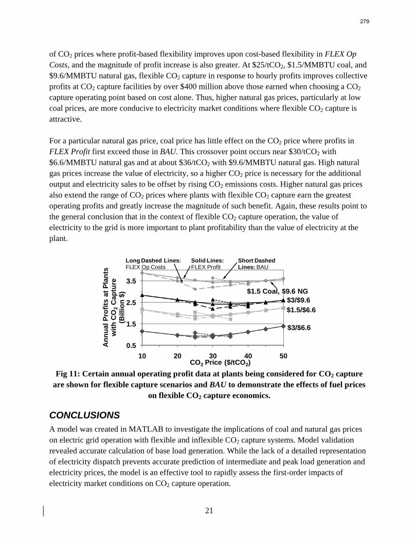
21
of CO2 prices where profit-based flexibility improves upon cost-based flexibility in FLEX Op Costs, and the magnitude of profit increase is also greater. At $25/tCO2, $1.5/MMBTU coal, and $9.6/MMBTU natural gas, flexible CO2 capture in response to hourly profits improves collective profits at CO2 capture facilities by over $400 million above those earned when choosing a CO2 capture operating point based on cost alone. Thus, higher natural gas prices, particularly at low coal prices, are more conducive to electricity market conditions where flexible CO2 capture is attractive. For a particular natural gas price, coal price has little effect on the CO2 price where profits in FLEX Profit first exceed those in BAU. This crossover point occurs near $30/tCO2 with $6.6/MMBTU natural gas and at about $36/tCO2 with $9.6/MMBTU natural gas. High natural gas prices increase the value of electricity, so a higher CO2 price is necessary for the additional output and electricity sales to be offset by rising CO2 emissions costs. Higher natural gas prices also extend the range of CO2 prices where plants with flexible CO2 capture earn the greatest operating profits and greatly increase the magnitude of such benefit. Again, these results point to the general conclusion that in the context of flexible CO2 capture operation, the value of electricity to the grid is more important to plant profitability than the value of electricity at the plant.
0.5
1.5
2.5
3.5
10 20 30 40 50
Ann
ual P
rofit
s at
Pla
nts
with
CO
2C
aptu
re
(Bill
ion
$)
CO2 Price ($/tCO2)
Long Dashed Lines: FLEX Op Costs
Short Dashed Lines: BAU
Solid Lines: FLEX Profit
$3/$9.6
$3/$6.6
$1.5 Coal, $9.6 NG
$1.5/$6.6
Fig 11: Certain annual operating profit data at plants being considered for CO2 capture
are shown for flexible capture scenarios and BAU to demonstrate the effects of fuel prices on flexible CO2 capture economics.
CONCLUSIONS A model was created in MATLAB to investigate the implications of coal and natural gas prices on electric grid operation with flexible and inflexible CO2 capture systems. Model validation revealed accurate calculation of base load generation. While the lack of a detailed representation of electricity dispatch prevents accurate prediction of intermediate and peak load generation and electricity prices, the model is an effective tool to rapidly assess the first-order impacts of electricity market conditions on CO2 capture operation.
279
22
Significant CO2 emissions reductions can be achieved when CO2 prices are high enough to promote fuel switching from coal to natural gas for base load generation and when electricity market conditions provide incentive for continuous or near-continuous full-load CO2 capture. Fuel switching in the absence of CO2 capture can achieve up to a 20% reduction in ERCOT CO2 emissions with $3/MMBTU coal, $6.6/MMBTU natural gas, and $100/tCO2 CO2 price; however, total grid emissions reductions on the order of 30% are achievable at moderate CO2 prices with continuous full-load CO2 capture on approximately half of the ERCOT coal fleet. However, some of the emissions reductions achieved by CO2 capture operation are offset by additional use of natural gas to replace the output lost to CO2 capture energy requirements. If flexible CO2 capture systems emit additional CO2 at partial- or zero-load, emissions reductions may not be significant with CO2 prices too low to justify full-load CO2 capture. Since a relatively small fraction of ERCOT installed capacity consists of coal-based plants, high CO2 prices of $50/tCO2 and above are often required to promote considerable fuel switching from non-capture coal- to natural gas-based facilities. High natural gas prices relative to coal both delay the onset and decrease the magnitude of fuel switching, which partially limits CO2 emissions reductions. However, when low natural gas prices accompany high coal prices, substantial fuel switching from coal-based plants without CO2 capture can occur as low as $20/tCO2, and coal-fired plants with CO2 capture may be displaced by natural gas-fired facilities below $40/tCO2. At low natural gas, high coal, and low CO2 prices, CO2 capture flexibility may be essential for continued base load operation of a coal-fired facility with CO2 capture. Natural gas-fired facilities primarily set ERCOT electricity prices unless CO2 prices are very high and the natural gas to coal price ratio is relatively small. Thus, electricity prices tend to increase with CO2 price at the emissions cost of natural gas-fired generators, and fuel switching and CO2 capture have a minor effect on electricity price. When choosing the operating point of a flexible CO2 capture system based on marginal costs alone, higher coal prices means that a higher CO2 price is required to justify full-load CO2 capture because it takes a larger emissions cost reduction to offset the increased fuel costs of CO2 capture. When choosing a CO2 capture operating point based on the most profitable combination of cost, output, and electricity price, higher natural gas prices will increase the CO2 price needed to justify continuous full-load CO2 capture. By raising electricity prices, higher natural gas prices create incentive for partial- or zero-load CO2 capture because additional electricity sales may offset CO2 emissions costs. Coal prices had little effect on profit-motivated flexible CO2 capture; the value of electricity on the grid is more important to profitability than the value of electricity at the plant. Amongst flexible CO2 capture scenarios, $25-$60/tCO2 is required to promote continuous full-load operation. Thus, once a CO2 capture system is built, the CO2 price to justify full-load operation may be much lower than that required for CO2 capture plant investment.
280
23
As CO2 price rises, the change in a plant’s annual operating profits depends on the plant’s emissions rate relative to that of the typical marginal generating facility, usually a natural gas-based generator. For each combination of coal and natural gas prices, there is a range of CO2 prices where profit-motivated flexible CO2 capture can allow greater operating profits than when choosing CO2 capture operating point based solely on marginal costs. This CO2 price range broadens and the benefits increase as natural gas prices rise and as coal prices fall for a given natural gas price. Across eight coal-fired plants in ERCOT, annual operating profits could be several hundred millions of dollars greater than those earned with inflexible CO2 capture or flexible CO2 capture based only on marginal costs. The CO2 price above which annual profits at coal-fired facilities are greater with CO2 capture than without it will increase with natural gas price because greater CO2 cost savings are required to offset the benefit of additional electricity sales. There is a limited range of CO2 prices above this point where flexibility improves operating profits at plants with CO2 capture, but this range and the total benefit increases with higher natural gas prices and lower coal prices. CO2 capture flexibility is not utilized at or above CO2 prices that may be required for CO2 capture investment, but flexible CO2 capture can help mitigate the risk of CO2 price uncertainty.
References Aaron, D. and C. Tsouris (2005). "Separation of CO2 from Flue Gas: A Review." Separation
Science and Technology 40(1): 321 - 348. Bergerson, J. A. and L. B. Lave (2007). "Baseload Coal Investment Decisions under Uncertain
Carbon Legislation." Environ. Sci. Technol. 41(10): 3431-3436. Chalmers, H. and J. Gibbins (2005). Scope for Synergy Between Renewables and Carbon
Dioxide Capture and Storage: A Bridge to Sustainable Electricity Generation in the UK? Energy Technology for Sustainable Development Group. London, Imperial College.
Chalmers, H., J. Gibbins, et al. (2007). Initial Assessment of Flexibility of Pulverised Coal-Fired Power Plants with CO2 Capture. 3rd International Conference on Clean Coal Technologies for our Future. Sardinia, Italy.
Cohen, S. M., G. T. Rochelle, et al. (2008). Turning CO2 Capture On & Off in Response to Electric Grid Demand: A Baseline Analysis of Emissions and Economics. ASME 2nd International Conference on Energy Sustainability. Jacksonville.
Davidson, R. M. (2007). Post-combustion carbon capture from coal fired plants – solvent scrubbing, IEA Clean Coal Centre.
ERCOT (2006). 2006 Annual Report. ERCOT (2006). 2006 ERCOT Hourly Load Data. 2006_ERCOT_Hourly_Load_Data.xls. ERCOT (2006). Balancing Energy Services Market Clearing Prices for Energy Annual Report.
MCPER_MCPEL_2006.xls. ICE (2008). ICE Day Ahead Natural Gas Price Report: Houston Ship Channel. Mathieu Lucquiaud, Hannah Chalmers, et al. (2008). Capture-ready supercritical coal-fired
power plants and flexible post-combustion CO2 capture. 9th International Conference on Greenhouse Gas Control Technologies. Washington, DC, Elsevier.
281
24
Metz, B., O. Davidson et.al. (2005). IPCC Special Report on Carbon Dioxide Capture and Storage.
PE-Ltd. (2007). 2006 State of the Market Report for the ERCOT Wholesale Electricity Markets, Potomac Economics, Ltd.
Rao, A. B. and E. S. Rubin (2002). "A Technical, Economic, and Environmental Assessment of Amine-Based CO2 Capture Technology for Power Plant Greenhouse Gas Control." Environ. Sci. Technol. 36(20): 4467-4475.
Rao, A. B. and E. S. Rubin (2006). "Identifying Cost-Effective CO2 Control Levels for Amine-Based CO2 Capture Systems." Ind. Eng. Chem. Res. 45(8): 2421-2429.
Rubin, E. S., C. Chen, and A. B. Rao (2007). "Cost and performance of fossil fuel power plants with CO2 capture and storage." Energy Policy 35: 4444-4454.
Sepideh Ziaii, Stuart Cohen, et al. (2008). Dynamic operation of amine scrubbing in response to electricity demand and pricing. 9th International Conference on Greenhouse Gas Technologies. Washington, DC, Elsevier.
Smitherman, B. T., D. L. Nelson, et al. (2009). Scope of Competition in Electric Markets in Texas. Report to the 81st Texas Legislature. Austin, TX, Public Utility Commission of Texas.
USEIA (2007). Average Cost of Coal Delivered for Electricity Generation by State, Year-to-Date through October 2007 and 2006. epmxlfile4_10_b.xls, USDOE.
USEIA. (2007). "World Carbon Dioxide Emissions from the Use of Fossil Fuels." International Energy Annual 2005 Retrieved 26 October, 2007, 2007, from http://www.eia.doe.gov/emeu/iea/carbon.html.
USEIA (2008). Texas Natural Gas Wellhead Price, USDOE. USEPA (2007). Emissions & Generation Resource Integrated Database (eGRID).
eGRID2006_Version_2_1. USNETL (2007). Cost and Performance Baseline for Fossil Energy Plants. Bituminous Coal and
Natural Gas to Electricity. J. M. Klara. 1.
282
Modeling Absorber/Stripper Performance with MDEA/PZ
Quarterly Report for January 1 – March 31, 2009
by Peter Frailie
Supported by the Luminant Carbon Management Program
and the
Industrial Associates Program for CO2 Capture by Aqueous Absorption
Department of Chemical Engineering
The University of Texas at Austin
April 1, 2009
Abstract The goal of this study is to evaluate the performance of an absorber/stripper operation that utilizes the MDEA/PZ blended amine system. Due to the complexity of this system the model will be developed in several smaller, more manageable parts that can later be combined. The first section that will be developed is an MDEA/PZ model based on thermodynamic data, which must initially be developed as separate MDEA and PZ models. Once the MDEA/PZ model has been completed it must be incorporated into separate absorber and stripper models similar to those developed by Van Wagener and Plaza. Those models can then be combined to form the final MDEA/PZ absorber/stripper model. This study is currently in the process of developing the MDEA/PZ model based on thermodynamic data. Over the next three months the thermodynamic model should be completed and work should have begun on the absorber and stripper models.
Introduction The removal of CO2 from process gases using alkanolamine absorption/stripping has been extensively studied for several solvents and solvent blends. An advantage of using blends is that the addition of certain solvents can enhance the overall performance of the CO2 removal system. A disadvantage of using blends is that the system becomes much more complex relative to a single solvent system, thus making it more difficult to model.
This study will focus on a blended amine solvent system containing piperazine (PZ) and methyldiethanolamine (MDEA). Previous studies have shown that this particular blend has the potential to combine the high capacity of MDEA with the attractive kinetics of PZ (Bishnoi, 2000). These studies have supplied a rudimentary Aspen Plus®-based model for an absorber with the MDEA/PZ system. The report also makes the recommendation that more kinetic and thermodynamic data must be acquired concerning the MDEA/PZ system before the model can be significantly improved. Two researchers in the Rochelle lab are currently acquiring these data, but they have not yet been incorporated into an absorber/stripper model. One of the major goals of this study will be to improve the supplied Aspen Plus® absorber model with up-to-date thermodynamic and kinetic data. Another major goal of this study will be to combine absorber and stripper models to evaluate the overall system performance.
283
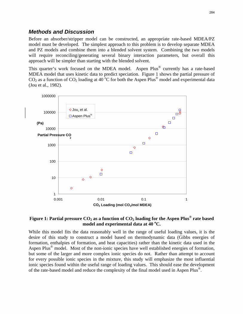
Methods and Discussion Before an absorber/stripper model can be constructed, an appropriate rate-based MDEA/PZ model must be developed. The simplest approach to this problem is to develop separate MDEA and PZ models and combine them into a blended solvent system. Combining the two models will require reconciling/generating several binary interaction parameters, but overall this approach will be simpler than starting with the blended solvent.
This quarter’s work focused on the MDEA model. Aspen Plus® currently has a rate-based MDEA model that uses kinetic data to predict speciation. Figure 1 shows the partial pressure of CO2 as a function of CO2 loading at 40 oC for both the Aspen Plus® model and experimental data (Jou et al., 1982).
Figure 1: Partial pressure CO2 as a function of CO2 loading for the Aspen Plus® rate based
model and experimental data at 40 oC. While this model fits the data reasonably well in the range of useful loading values, it is the desire of this study to construct a model based on thermodynamic data (Gibbs energies of formation, enthalpies of formation, and heat capacities) rather than the kinetic data used in the Aspen Plus® model. Most of the non-ionic species have well established energies of formation, but some of the larger and more complex ionic species do not. Rather than attempt to account for every possible ionic species in the mixture, this study will emphasize the most influential ionic species found within the useful range of loading values. This should ease the development of the rate-based model and reduce the complexity of the final model used in Aspen Plus®.
1
10
100
1000
10000
100000
1000000
0.001 0.01 0.1 1 CO2 Loading (mol CO2/mol MDEA)
Partial Pressure CO2
(Pa)
Jou, et al. Aspen Plus®
284
At every stage of the development process the model obviously has to be compared to experimental data. The literature contains an abundance of data concerning MDEA and PZ systems, but this study also requires thermodynamic data specific to the MDEA/PZ blended solvent system. These data are currently being collected by Thu Nguyen, and they will be regressed and incorporated into this model as they become available.
Future Work The main goal over the next three months will be to finish developing the MDEA/PZ rate based model using experimentally obtained thermodynamic data. The first step in this process will be finalizing the MDEA model. Once that has been completed, it can be combined with the PZ model that is currently being developed by David Van Wagener to form the MDEA/PZ blended system. At that point the experimental MDEA/PZ data will be necessary to reconcile the two models, as well as account for the additional binary interaction parameters found in the blended system.
Once the rate based model has been finalized, it will be applied to an absorber/stripper operation. Just like in the development of the rate based model, this model will first be split into two sections (absorber and stripper) for early development, which will be combined later to form the final model. This is similar to the approach used by Jorge Plaza and David Van Wagener, though they did not combine their models into a single operation. Their work and methodology will serve as the basis for the development of the separate absorber and stripper models.
References Bishnoi, S. Carbon Dioxide Absorption and Solution Equilibrium in Piperazine Activated
Methyldiethanolamine. The University of Texas at Austin. Ph.D. Dissertation. 2000.
Jou F-Y, Mather AE, Otto FD. “Solubility of hydrogen sulfide and carbon dioxide in aqueous methyldiethanolamine solutions.” Ind Eng Chem Proc Des Dev. 1982;21(4):539–544.
285
1
Measurement of Packing Liquid Phase Film
Mass Transfer Coefficient
Quarterly Report for January 1 – March 31, 2009
Chao Wang
Supported by the Luminant Carbon Management Program,
Industrial Associates Program for CO2 Capture by Aqueous Absorption,
and the Process Science and Technology Center
Department of Chemical Engineering
The University of Texas at Austin
April 12, 2009
Abstract Packings are widely used in distillation, stripping, and scrubbing processes because of their relatively low pressure drop and good mass transfer efficiency. Since the post combustion carbon capture process will require an operationally expensive fan, the absorber contains high performance packing to minimize pressure drop and maximize mass transfer efficiency. The design of packed absorbers for carbon dioxide capture will require the reliable measurement and accurate prediction of the liquid film mass transfer coefficient. A variety of experimental methods of measuring liquid side mass transfer coefficient kLa have been explored and reported.
Chemical reaction enhanced and physical liquid phase film mass transfer coefficients are discussed in this report. Test systems are chosen where the gas film mass transfer resistance is negligible compared to the liquid resistance. Therefore the liquid phase film mass transfer coefficient (kLa) may be calculated directly from the values of KoLa or KoGa. Suitable systems are stripping of toluene from water or absorption of toluene with water, absorption of pure gas (O2/H2/CO2) with water, and desorption of O2 from water with pure N2 stream. The physical liquid side mass transfer coefficient kL can be calculated by dividing the measured kLa by the measured gas/liquid contact area (a). Measurements of the gas/liquid contact area has been discussed by Tsai and reported by Lewis and Seibert of the Separations Research Program.
Predictive models of the liquid phase film mass transfer coefficient (kL) are discussed in this quarterly report, which focuses on a preliminary literature review of liquid film mass transfer coefficient measurements and models. A highly accurate SO2 analyzer has been purchased and is currently being installed for packing studies planned for the summer. The SO2 analyzer was purchased and installed using Process Science and Technology Center funds provided by the project co-advisor, Frank Seibert.
286
2
Introduction This quarterly report continues with the literature review of packed column measurement methods used to determine the liquid phase film mass transfer coefficient. Packing is often used in absorption, stripping, and distillation processes. There are two types of packing: random and structured. Random packing is inexpensive and often used in smaller diameter columns and in environmental separations. Relative to random packing, structured packing provides a large effective area per unit of pressure drop and is more expensive and requires good initial liquid distribution. For most commercial packings, mass transfer and hydraulic characteristics and correlating fitting constants are usually unknown. Prediction or measurement of effective gas/liquid contact area (a), gas phase film mass transfer coefficient (kG), liquid phase film mass transfer coefficient (kL) are required for the reliable design of packed column height. This report is focused on measurement or predictive methods of liquid film mass transfer coefficient (kL). A review of the pertinent literature follows.
Chemical reaction enhanced liquid phase film mass transfer coefficient
Sharma and Danckwerts (1970) used the chemical method with first order reaction: A+ZB→products. Under certain conditions, the reaction is fast enough to keep the concentration of A in the bulk of the B-phase equal to zero, while it is not fast enough for any appreciable amount of A to react in the diffusion-film at the surface of the B-phase. Under these conditions, the rate of transfer is that for physical transfer with AB =0 that is:
*AkR L= (1). The condition to be satisfied if AB is to be zero is:
kLa << lk2B0 (2) where
AB = bulk concentration of A in the B-phase, gmole/cm3 A* = concentration of A at surface B-phase, gmole/cm3 B0 = concentration of B in the bulk of B-phase, gmole/cm3 l = volume of B-phase per unit volume of the system.
The condition to be satisfied if no A is to react in the diffusion film is: Dk2 B0/kL
2 << 1 (3) where
D = diffusivity of A in the B-phase, cm2/s. The reaction is mth order to A and nth order to B, while the local rate is expressed as kmn[A]m[B]n. The condition for AB to be zero is:
nmmnL BAlkaAk )()( 01** −<< (4)
and for no reaction in the film 1/)()()1/2( 201* <<+ −
Lnm
mn kBADkm (5). For the packed column system, kLa can be calculated by the equation
dhaAkGdA L*0 −= (6)
and A*=KA0 (7)
where
287
3
h = height measured from the bottom of the column, G = superficial velocity of the carrier-gas and K is the Henry’s constant.
Mandal (2003) measured liquid side volumetric mass transfer coefficient kLa as well as gas/liquid contact area (a). The method utilized the Danckwerts approach and the test system, Air/CO2-NaOH. The condition is made to let the concentration of CO2 in the bulk liquid phase approach zero while no appreciable reaction takes place in the diffusion films. The condition to be satisfied is, as mentioned before:
02 BLL Ckak α<< (8)
and
12
02 <<L
BA
kCkD (9)
where Lα = fractional liquid hold-up,
k2 = second order reaction rate constant, cm/s, DA = diffusivity of dissolved gas A, cm2/s, and CB
0 = concentration of B in the bulk of the solution. When these conditions were satisfied, the rate of mass transfer is:
*ALaCkRa = (10)
By measuring Ra, the volumetric liquid film mass transfer coefficient, kLa, can be determined.
Physical Liquid Phase Film Mass Transfer Coefficient Onda (1959) investigated the physical absorption of gas into water using a tower packed with Raschig rings. The liquid phase film mass transfer coefficient was separated by dividing the volumetric liquid phase mass transfer coefficient (kLa) by the wetted surface area. Fundamental equations to predict kL using dimensionless groups are discussed based on two-film and penetration theory.
Akita (1973) measured the fractional gas hold-up and the volumetric liquid phase mass transfer coefficient kLa in bubble columns with various test systems.
Linek (1984) measured the liquid side volumetric mass transfer coefficient kLa for Pall rings of nominal sizes 15, 25, 35, and 50 mm made of polypropylene and polyvinylidenflouride. The plastic packing surface was either untreated or was rendered hydrophilic chemically. The kLa values were obtained by physical desorption of oxygen from water into pure nitrogen stream.
While kLa may be determined directly from experimental measurements, independent measurements of liquid phase film mass transfer coefficient (kL) and gas/liquid contact area (a) is challenging. There is a lack of fundamental knowledge in determining kL. Liquid phase mass transfer coefficient data for new high performance packings is scarce. The goal of this research is to address these shortcomings and ultimately develop an improved liquid side mass transfer model. General objectives are to:
• Develop a fundamental understanding of the fluid mechanics associated with packing operation;
• Determine a suitable system to measure the physical liquid side mass transfer coefficient;
288
4
• Expand the SRP database by measuring the physical liquid side mass transfer coefficient of several different structured and random packings over a range of liquid and gas superficial velocities;
• Combine the data and theory into a mechanistic model that captures the features of the tested systems and adequately represents liquid side mass transfer coefficient as a function of gas velocity, liquid density, and liquid load.
Experimental Methods Chemical Reaction Enhanced Liquid Phase Film Coefficient Sharma and Danckwerts (1970) used a gas-liquid system where CO2 was chemically absorbed into a carbonate-bicarbonate buffer solution. The reaction
CO2 + OH- → HCO3-
is second-order (m=1, n=1). Another potential test system is the absorption of oxygen from air into dilute acid solutions of CuCl which is oxidized to CuCl2. In these experiments, glass-lined or plastic equipment must be used to prevent corrosion. Oxygen may be also absorbed from air into sodium sulfite solution using CoSO4 or CuSO4 as a catalyst. The reaction appears to be second-order in O2 and zero order in SO3
2- under usual conditions.
If k2B0 is varied while keeping kLa constant, a plot of 1/kOLa against 1/k2B0 will provide a straight line of slope 1/l with intercept 1/kLa.
Another chemical method for determining kLa was discussed by Sharma and Danckwerts in the same paper. Suppose A undergoes a second-order reaction with B, and the following condition is fulfilled:
)/1(10/ *0202 ZABkBDk L +> (11).
Or if A undergoes a reaction of m, nth order with B and the following condition is fulfilled:
)/1(10/)()()1/2( *0201* ZABkBADkm Lnm
mn +>+ − (12). Or if the reaction between A and B is instantaneous and if, in addition,
B0 >>A* (13) then the rate of transfer of A is:
DDZaBkRa L /)/( '0= (14) D’ is the diffusivity of B in the B-phase and Z moles of B react with one of A.
The rate of transfer of A is independent of A*- that is, of the concentration of A in the A-phase.
It follows that it is not necessary to know the solubility of A in the B-phase, which may be an advantage in practice. The rate of transfer can often be most easily determined by analyzing the B-phase for unreacted B or for the product of the reaction. It is essential to ensure that the resistance to mass-transfer is confined to the B-phase only. In the case of gas-absorption the relevant condition is:
kGp>>kLB0 (15) where:
kG = gas phase film mass transfer coefficient
289
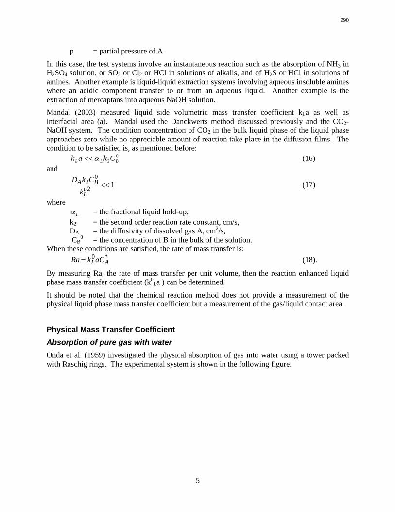
5
p = partial pressure of A.
In this case, the test systems involve an instantaneous reaction such as the absorption of NH3 in H2SO4 solution, or SO2 or Cl2 or HCl in solutions of alkalis, and of H2S or HCl in solutions of amines. Another example is liquid-liquid extraction systems involving aqueous insoluble amines where an acidic component transfer to or from an aqueous liquid. Another example is the extraction of mercaptans into aqueous NaOH solution.
Mandal (2003) measured liquid side volumetric mass transfer coefficient kLa as well as interfacial area (a). Mandal used the Danckwerts method discussed previously and the CO2-NaOH system. The condition concentration of CO2 in the bulk liquid phase of the liquid phase approaches zero while no appreciable amount of reaction take place in the diffusion films. The condition to be satisfied is, as mentioned before:
02 BLL Ckak α<< (16)
and
DAk2CB0
kLo2 <<1 (17)
where Lα = the fractional liquid hold-up,
k2 = the second order reaction rate constant, cm/s, DA = the diffusivity of dissolved gas A, cm2/s, CB
0 = the concentration of B in the bulk of the solution. When these conditions are satisfied, the rate of mass transfer is:
Ra = kL0aCA
* (18).
By measuring Ra, the rate of mass transfer per unit volume, then the reaction enhanced liquid phase mass transfer coefficient (k0
La ) can be determined.
It should be noted that the chemical reaction method does not provide a measurement of the physical liquid phase mass transfer coefficient but a measurement of the gas/liquid contact area.
Physical Mass Transfer Coefficient Absorption of pure gas with water Onda et al. (1959) investigated the physical absorption of gas into water using a tower packed with Raschig rings. The experimental system is shown in the following figure.
290
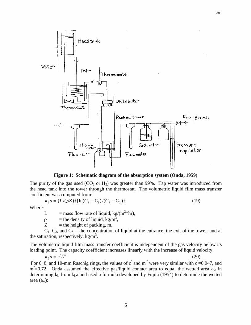
6
Figure 1: Schematic diagram of the absorption system (Onda, 1959)
The purity of the gas used (CO2 or H2) was greater than 99%. Tap water was introduced from the head tank into the tower through the thermostat. The volumetric liquid film mass transfer coefficient was computed from:
)}/())}{ln(/({ 21 CCCCZLak SSL −−= ρ (19) Where:
L = mass flow rate of liquid, kg/(m2*hr), ρ = the density of liquid, kg/m3, Z = the height of packing, m, C1, C2, and CS = the concentration of liquid at the entrance, the exit of the towe,r and at
the saturation, respectively, kg/m3.
The volumetric liquid film mass transfer coefficient is independent of the gas velocity below its loading point. The capacity coefficient increases linearly with the increase of liquid velocity.
''' mL Lcak = (20).
For 6, 8, and 10-mm Raschig rings, the values of c’ and m’’ were very similar with c’=0.047, and m”=0.72. Onda assumed the effective gas/liquid contact area to equal the wetted area aw in determining kL from kLa and used a formula developed by Fujita (1954) to determine the wetted area (aw):
291
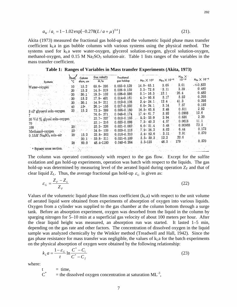
7
])/(278.0exp[02.11/ 4.0μ+−−= aLaa tW (21).
Akita (1973) measured the fractional gas hold-up and the volumetric liquid phase mass transfer coefficient kLa in gas bubble columns with various systems using the physical method. The systems used for kLa were water-oxygen, glycerol solution-oxygen, glycol solution-oxygen, methanol-oxygen, and 0.15 M Na2SO3 solution-air. Table 1 lists ranges of the variables in the mass transfer coefficient.
Table 1: Ranges of Variables in Mass transfer Experiments (Akita, 1973)
The column was operated continuously with respect to the gas flow. Except for the sulfite oxidation and gas hold-up experiments, operation was batch with respect to the liquids. The gas hold-up was determined by measuring level of the aerated liquid during operation ZF and that of clear liquid ZL. Thus, the average fractional gas hold-up Gε is given as:
F
LFG Z
ZZ −=ε (22)
Values of the volumetric liquid phase film mass coefficient (kLa) with respect to the unit volume of aerated liquid were obtained from experiments of absorption of oxygen into various liquids. Oxygen from a cylinder was supplied to the gas chamber at the column bottom through a surge tank. Before an absorption experiment, oxygen was desorbed from the liquid in the column by sparging nitrogen for 5–10 min at a superficial gas velocity of about 100 meters per hour. After the clear liquid height was measured, an absorption run was started. It lasted 1–5 min, depending on the gas rate and other factors. The concentration of dissolved oxygen in the liquid sample was analyzed chemically by the Winkler method (Treadwell and Hall, 1942). Since the gas phase resistance for mass transfer was negligible, the values of kLa for the batch experiments on the physical absorption of oxygen were obtained by the following relationship:
f
iGL CC
CCt
ak−−−
= *
*
ln1 ε
(23)
where: t = time, C* = the dissolved oxygen concentration at saturation ML-3,
292
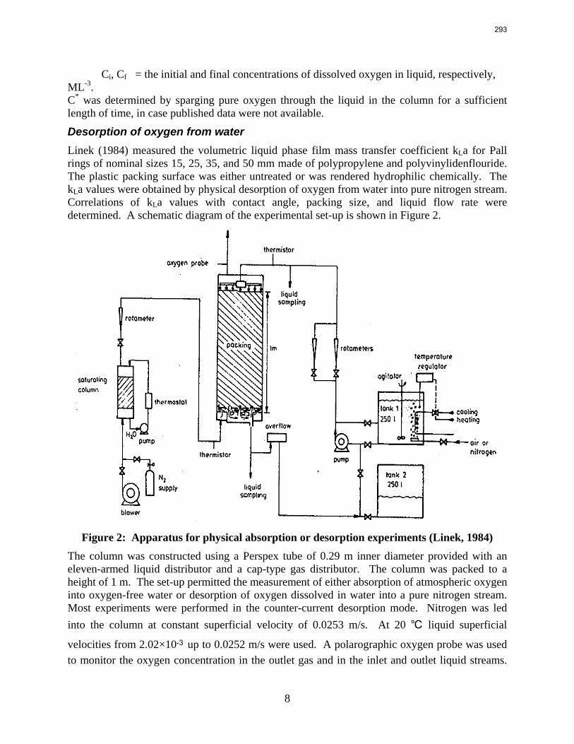
8
Ci, Cf = the initial and final concentrations of dissolved oxygen in liquid, respectively, ML-3. C* was determined by sparging pure oxygen through the liquid in the column for a sufficient length of time, in case published data were not available.
Desorption of oxygen from water Linek (1984) measured the volumetric liquid phase film mass transfer coefficient kLa for Pall rings of nominal sizes 15, 25, 35, and 50 mm made of polypropylene and polyvinylidenflouride. The plastic packing surface was either untreated or was rendered hydrophilic chemically. The kLa values were obtained by physical desorption of oxygen from water into pure nitrogen stream. Correlations of kLa values with contact angle, packing size, and liquid flow rate were determined. A schematic diagram of the experimental set-up is shown in Figure 2.
Figure 2: Apparatus for physical absorption or desorption experiments (Linek, 1984)
The column was constructed using a Perspex tube of 0.29 m inner diameter provided with an eleven-armed liquid distributor and a cap-type gas distributor. The column was packed to a height of 1 m. The set-up permitted the measurement of either absorption of atmospheric oxygen into oxygen-free water or desorption of oxygen dissolved in water into a pure nitrogen stream. Most experiments were performed in the counter-current desorption mode. Nitrogen was led into the column at constant superficial velocity of 0.0253 m/s. At 20 ℃ liquid superficial
velocities from 2.02×10⁻³ up to 0.0252 m/s were used. A polarographic oxygen probe was used to monitor the oxygen concentration in the outlet gas and in the inlet and outlet liquid streams.
293
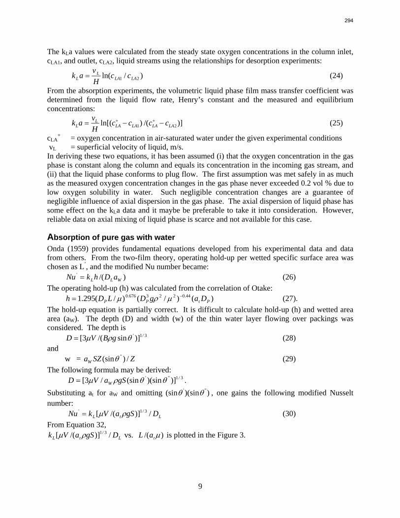
9
The kLa values were calculated from the steady state oxygen concentrations in the column inlet, cLA1, and outlet, cLA2, liquid streams using the relationships for desorption experiments:
)/ln( 21 LALAL
L ccHv
ak = (24)
From the absorption experiments, the volumetric liquid phase film mass transfer coefficient was determined from the liquid flow rate, Henry’s constant and the measured and equilibrium concentrations:
)]/()ln[( 21 LALALALAL
L ccccHvak −−= ++ (25)
cLA+ = oxygen concentration in air-saturated water under the given experimental conditions
vL = superficial velocity of liquid, m/s. In deriving these two equations, it has been assumed (i) that the oxygen concentration in the gas phase is constant along the column and equals its concentration in the incoming gas stream, and (ii) that the liquid phase conforms to plug flow. The first assumption was met safely in as much as the measured oxygen concentration changes in the gas phase never exceeded 0.2 vol % due to low oxygen solubility in water. Such negligible concentration changes are a guarantee of negligible influence of axial dispersion in the gas phase. The axial dispersion of liquid phase has some effect on the kLa data and it maybe be preferable to take it into consideration. However, reliable data on axial mixing of liquid phase is scarce and not available for this case.
Absorption of pure gas with water Onda (1959) provides fundamental equations developed from his experimental data and data from others. From the two-film theory, operating hold-up per wetted specific surface area was chosen as L’, and the modified Nu number became: )/('
WLL aDhkNu = (26) The operating hold-up (h) was calculated from the correlation of Otake: )()/()/(295.1 44.0223676.0
PtPP DagDLDh −= μρμ (27). The hold-up equation is partially correct. It is difficult to calculate hold-up (h) and wetted area area (aW). The depth (D) and width (w) of the thin water layer flowing over packings was considered. The depth is 3/1' )]sin/(3[ θρμ gBVD = (28) and w = ZSZaW /)(sin "θ (29) The following formula may be derived: 3/1"' )])(sin(sin/3[ θθρμ gSaVD W= . Substituting at for aW and omitting ))(sin(sin "' θθ , one gains the following modified Nusselt number: LtL DgSaVkNu /)]/([ 3/1' ρμ= (30) From Equation 32,
LtL DgSaVk /)]/([ 3/1ρμ vs. )/( μtaL is plotted in the Figure 3.
294
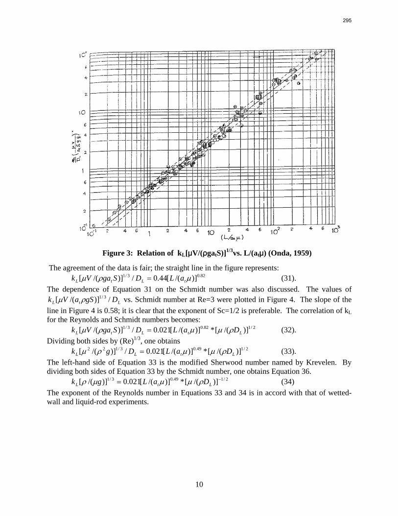
10
Figure 3: Relation of kL[μV/(ρgatS)]1/3vs. L/(atμ) (Onda, 1959)
The agreement of the data is fair; the straight line in the figure represents: 82.03/1 )]/([44.0/)]/([ μρμ tLtL aLDSgaVk = (31).
The dependence of Equation 31 on the Schmidt number was also discussed. The values of LtL DgSaVk /)]/([ 3/1ρμ vs. Schmidt number at Re=3 were plotted in Figure 4. The slope of the
line in Figure 4 is 0.58; it is clear that the exponent of Sc=1/2 is preferable. The correlation of kL for the Reynolds and Schmidt numbers becomes:
2/182.03/1 )]/([*)]/([021.0/)]/([ LtLtL DaLDSgaVk ρμμρμ = (32). Dividing both sides by (Re)1/3, one obtains
2/149.03/122 )]/([*)]/([021.0/)]/([ LtLL DaLDgk ρμμρμ = (33). The left-hand side of Equation 33 is the modified Sherwood number named by Krevelen. By dividing both sides of Equation 33 by the Schmidt number, one obtains Equation 36.
2/149.03/1 )]/([*)]/([021.0)]/([ −= LtL DaLgk ρμμμρ (34) The exponent of the Reynolds number in Equations 33 and 34 is in accord with that of wetted-wall and liquid-rod experiments.
295
11
Figure 4: Relation of kL[μV/(ρgatS)]1/3vs. Schmidt number at Re=3 (Onda, 1959)
Derivation of the formula from the standpoint of penetration theory was also done. By Higbie’s penetration theory kL can be described as:
2/1)]/([2 πθLL Dk = (35). Using an idea similar to that described in the two-film theory one can consider the following dimensionless formula:
][/][ 2/12/1 essDimensionlDTk LL = (36). θ = time the elementary surface of the liquid is exposed to the gas depends on the operating
conditions, the physical properties of the liquid, and the characteristics of the tower and packings; it can be assumed as ),,,,,( LaDgf ttμρθ = .
By dimensional analysis various combinations of dimensionless groups were obtained, and from the many results reported the next relation was selected:
''322'' )()]/([)]/([)]/()[/1( ntt
nt
mtt aDagaLcLa μρμρθ = (37).
From equations 35 and 37 the following is obtained: p
ttn
tm
tLtL aDagaLcDLak )(*)]/([)]/([/)]/([ 3222/12/1 μρμρ = (38). From the analysis of the dependence of equation on Galilei’s number and the tower diameter, Equation 38 was modified as:
38.03222/12/1 )]/([013.0/)]/([ tLtL agDLak μρρ = (39). The exponent of Galilei’s number in Equation 39 may be assumed to be 1/3; then Equation 39 becomes:
2/12/12/12/1 )]/([)]/([013.0/)]/([ −= ρμμρ LtLtL DaLDLak (40).
296
12
The coincidence of the equation derived by the two-film theory and by the penetration theory is most satisfactory, and the correlation of kL from both theories becomes:
2/12/13/1 )]/([)]/([)]/([ −= LtL DaLcgk ρμμμρ (41) c=0.01~0.02.
Akita (1973) provides fundamental correlated dimensionless numbers to determine kLa. Factors that conceivably affect the volumetric mass transfer coefficient kLa are:
• liquid phase diffusivity DL, l • liquid kinematic viscosity Lυ ,
• surface tension γ , liquid density ρL, • gravity g, column diameter D, and the • superficial gas velocity UG.
The effect of the liquid rate on kLa, studied with a continuous countercurrent and co-current sulfite oxidation experiments, was found to be negligible. Thus, dimensional analysis gives:
),,,()( FrGaBoScSh NNNNfaDN = (42) where:
LLSh DDkN /= Sherwood number,
LLSc DN /υ= Schmidt number. Elimination of NFr gives:
),,,()( 2 GGaBoScSh NNNfaDN ε= (43). It is assumed that r
Gq
Gap
BoScSh NNNcaDN ε2/12)( = (44).
Assuming a value of 1/2 for the exponent on the Schmidt number seems reasonable since the penetration or the random surface renewal model is considered to hold for the liquid phase mass transfer at the gas-liquid interface. The liquid phase volumetric mass transfer coefficient, kLa varies with Gε to the 1.1 power except for very small columns.
In Figure 5, kLa and Gε data for the sodium sulfite solution-air system using four columns diameters are given. In Figure 6, data for the water-oxygen system using three different column diameters are provided.
297
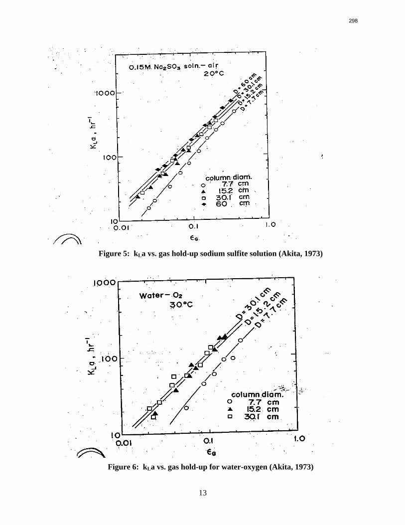
13
Figure 5: kLa vs. gas hold-up sodium sulfite solution (Akita, 1973)
Figure 6: kLa vs. gas hold-up for water-oxygen (Akita, 1973)
298
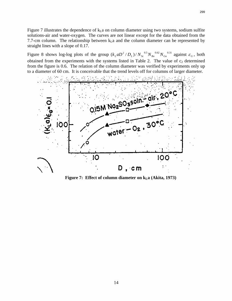
14
Figure 7 illustrates the dependence of kLa on column diameter using two systems, sodium sulfite solutions-air and water-oxygen. The curves are not linear except for the data obtained from the 7.7-cm column. The relationship between kLa and the column diameter can be represented by straight lines with a slope of 0.17.
Figure 8 shows log-log plots of the group 31.062.05.02 /)/( GaBoScLL NNNDaDk against Gε , both obtained from the experiments with the systems listed in Table 2. The value of c2 determined from the figure is 0.6. The relation of the column diameter was verified by experiments only up to a diameter of 60 cm. It is conceivable that the trend levels off for columns of larger diameter.
Figure 7: Effect of column diameter on kLa (Akita, 1973)
299
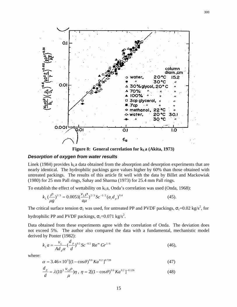
15
Figure 8: General correlation for kLa (Akita, 1973)
Desorption of oxygen from water results Linek (1984) provides kLa data obtained from the absorption and desorption experiments that are nearly identical. The hydrophilic packings gave values higher by 60% than those obtained with untreated packings. The results of this article fit well with the data by Billet and Mackowiak (1980) for 25 mm Pall rings, Sahay and Sharma (1973) for 25.4 mm Pall rings.
To establish the effect of wettability on kLa, Onda’s correlation was used (Onda, 1968):
4.02/13/23/1 )()(0051.0)( ptL
L daScav
gk −=
μρ
μρ (45).
The critical surface tension σc was used, for untreated PP and PVDF packings, σc=0.02 kg/s2, for
hydrophilic PP and PVDF packings, σc=0.071 kg/s2.
Data obtained from these experiments agree with the correlation of Onda. The deviation does not exceed 5%. The author also compared the data with a fundamental, mechanistic model derived by Ponter (1982):
6/15.05.0 Re)( GrScd
dAd
vak mp
p
LL
−=α
(46),
where: 728.02.06.02 ])cos1[(1046.3 Kaθα −×= (47)
ημρ
λ )10( 3 Lp vd
d= , 126.02.06.0 ])cos1[(2 −−= Kaθη (48)
300
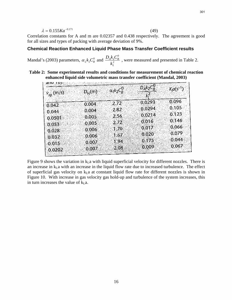
16
171.0155.0 −= Kaλ (49) Correlation constants for A and m are 0.02357 and 0.438 respectively. The agreement is good for all sizes and types of packing with average deviation of 9%.
Chemical Reaction Enhanced Liquid Phase Mass Transfer Coefficient results
Mandal’s (2003) parameters, 02 BL Ckα and 2
02
L
BA
kCkD , were measured and presented in Table 2.
Table 2: Some experimental results and conditions for measurement of chemical reaction enhanced liquid side volumetric mass transfer coefficient (Mandal, 2003)
Figure 9 shows the variation in kLa with liquid superficial velocity for different nozzles. There is an increase in kLa with an increase in the liquid flow rate due to increased turbulence. The effect of superficial gas velocity on kLa at constant liquid flow rate for different nozzles is shown in Figure 10. With increase in gas velocity gas hold-up and turbulence of the system increases, this in turn increases the value of kLa.
301
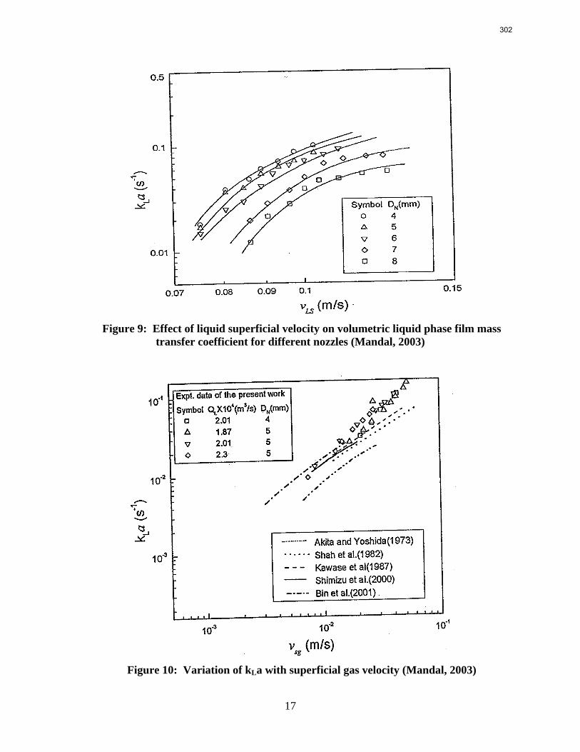
17
Figure 9: Effect of liquid superficial velocity on volumetric liquid phase film mass
transfer coefficient for different nozzles (Mandal, 2003)
Figure 10: Variation of kLa with superficial gas velocity (Mandal, 2003)
302
18
Shah (Shah, 1982) proposed the following correlation: 82.0467.0 sgL vak ×= (50)
The data of this article fits well in the correlation.
Future Work Several methods to measure mass transfer enhanced by chemical reaction and physical liquid mass transfer coefficients are provided in this quarterly report. My research will focus on measuring the physical liquid phase film mass transfer coefficient and gas phase film mass transfer coefficient. Pilot plant experiments are planned for this summer. Gas/liquid contact area, physical liquid phase mass transfer coefficient, and gas phase film mass transfer coefficients will be measured using 3–4 structured packings.
A discussion of alternative test systems for measuring physical liquid phase film mass transfer coefficients will be provided in the next quarterly report. The stripping of toluene from water using air is liquid phase controlled because of the high toluene activity coefficient. This system has been studied by the SRP with success. MellaPak 2X, Raschig-Jaeger RSP250wSE, Flexipac 1.6Y HC and MellaPak 252Y will likely be studied.
Reviews of the literature addressing physical liquid and gas phase film mass transfer coefficients will continue. Data will be extracted from published papers and incorporated into a database for future model development.
References Akita K & Yoshida F. "Gas hold-up and volumetric mass transfer coefficient in bubble
columns." Ind Eng Chem Process Des Develop.1973;12:76–80
Billet R & Mackowiak J. "Recent progress in distillation design." Proceedings of the 5th International Congress in Scandinavia on Chemical Engineering. 1980;141–176.
Linek V & Petericek P. "Effective interfacial area and liquid side mass transfer coefficients in aborption columns packed with hydrophilised and untreated plastic packings." Chem Eng Res Des. 1984;62:13–21.
Mandal A & Kundu G. "Interfacial area and liquid-side volumetric mass transfer coefficient in a downflow bubble column." Can J Chem Eng. 2003;81:212–219.
Ponter AB & Au-Yeung PH. "Estimation of liquid film mass transfer coefficients in columns packed randomly with partially wetted rings." Can J Chem Eng. 1982;60(1):94-99.
Sahay BN. & Sharma MM. "Effective interfacial area and liquid and gas side mass transfer coefficients in a packed column." Chem Eng Sci. 1973;28:41-47.
Shah YT, Kelkar BG et al. "Design parameter estimations for bubble column reactors." AIChE J. 1982;28:353–379.
Sharma MM & Danckwerts PV. "Chemical methods of measuring interfacial area and mass transfer coefficients in two-fluid systems." Brit Chem Eng. 1970;15:522–528.
Onda K. "Mass transfer coefficients between gas and liquid phases in packed columns." Chem Eng Jpn. 1968;1:56–62.
303

19
Onda K & Sada E. "Liquid-side mass transfer coefficient packed towers." AIChE J. 1959;5:235–239.
304
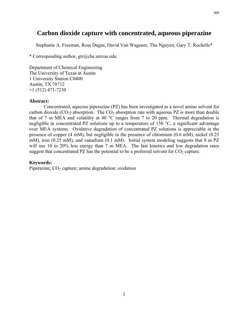
1
Carbon dioxide capture with concentrated, aqueous piperazine
Stephanie A. Freeman, Ross Dugas, David Van Wagener, Thu Nguyen, Gary T. Rochelle* * Corresponding author, [email protected] Department of Chemical Engineering The University of Texas at Austin 1 University Station C0400 Austin, TX 78712 +1 (512) 471-7230 Abstract:
Concentrated, aqueous piperazine (PZ) has been investigated as a novel amine solvent for carbon dioxide (CO2) absorption. The CO2 absorption rate with aqueous PZ is more than double that of 7 m MEA and volatility at 40 °C ranges from 7 to 20 ppm. Thermal degradation is negligible in concentrated PZ solutions up to a temperature of 150 °C, a significant advantage over MEA systems. Oxidative degradation of concentrated PZ solutions is appreciable in the presence of copper (4 mM), but negligible in the presence of chromium (0.6 mM), nickel (0.25 mM), iron (0.25 mM), and vanadium (0.1 mM). Initial system modeling suggests that 8 m PZ will use 10 to 20% less energy than 7 m MEA. The fast kinetics and low degradation rates suggest that concentrated PZ has the potential to be a preferred solvent for CO2 capture. Keywords: Piperazine; CO2 capture; amine degradation; oxidation
305
2
1. Introduction
The increase in the anthropogenic carbon dioxide (CO2) concentration in the atmosphere over the past few decades is known to be part of the cause of global warming (IPCC, 2001). A large impact on CO2 emissions can be made by targeting large point sources such as coal-fired power plants. Amine based absorption and stripping systems have been studied for CO2 capture from coal-fired power plants and have shown the most promise for effective CO2 control. Traditional amines such as monoethanolamine (MEA) and amine blends such as potassium carbonate/piperazine (K+CO3/PZ) and methyldiethanolamine/piperazine MDEA/PZ have been investigated extensively for this application (Bishnoi, 2000; Cullinane and Rochelle, 2005; Hilliard, 2008).
Piperazine (PZ) is a diamine that has previously been studied as a promoter for amine systems to improve kinetics, such as MDEA/PZ or MEA/PZ blends. The concentration of PZ when used as a promoter has been low, between 0.5 to 2.5 m PZ, because PZ is not highly soluble. Given the nature and magnitude of absorption/stripping systems, any possibility of precipitation ruled out PZ for use at concentrations above its room temperature solubility. Additionally, the boiling point of PZ (146.5 °C) is lower than that of MEA (170 °C), indicating the possibility for higher volatility. Recent work has indicated that the volatility of PZ is comparable to that of MEA due to the non-ideality of PZ in solution (Hilliard, 2008). Increasing the concentration of PZ in solution allows for increased solvent capacity and faster kinetics.
PZ has been studied as a solvent for absorption/stripping systems for the removal of CO2 from the flue gas of coal-fired power plants. The current work examines solid solubility, oxidative degradation, and thermal degradation of concentrated aqueous PZ solutions. Additionally, extensive work on the kinetics of the absorption of CO2 into PZ is reported. Finally, preliminary modeling work indicates that stripper performance with a concentrated PZ solvent is slightly enhanced as compared to MEA systems. 2. Materials and methods 2.1 Solution preparation
Aqueous piperazine solutions were created by heating anhydrous piperazine (99% pure, Fluka) with water until the solid crystals melted into a solution. The warm solution was transferred to a glass cylinder with a CO2 gas sparger and the cylinder was placed on a scale. The scale was used to gravimetrically add CO2 to achieve the desired loading. 2.2 CO2 loading through total inorganic carbon (TIC)
The concentration of CO2 in solution was determined by total inorganic carbon analysis (Hilliard, 2008). The sample is diluted and then acidified in 30 wt % phosphoric acid to release aqueous CO2, carbamate, and bicarbonate species as gaseous CO2. The CO2 is carried in a nitrogen stream to an infrared analyzer which detects and records changes in voltage. The resulting voltage peaks are integrated and correlated to CO2 concentrations using a 1000 ppm inorganic carbon standard made from a mixture of potassium carbonate and potassium bicarbonate. CO2 loading is reported as moles CO2 per mole alkalinity or moles CO2 per equivalence of PZ, where two moles of alkalinity per mole PZ is the conversion factor. 2.3 Amine titration
The concentration of piperazine in solution was determined using acid titration (Hilliard,
306
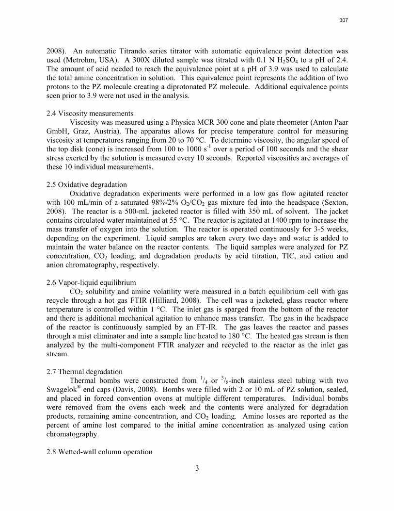
3
2008). An automatic Titrando series titrator with automatic equivalence point detection was used (Metrohm, USA). A 300X diluted sample was titrated with 0.1 N H2SO4 to a pH of 2.4. The amount of acid needed to reach the equivalence point at a pH of 3.9 was used to calculate the total amine concentration in solution. This equivalence point represents the addition of two protons to the PZ molecule creating a diprotonated PZ molecule. Additional equivalence points seen prior to 3.9 were not used in the analysis. 2.4 Viscosity measurements
Viscosity was measured using a Physica MCR 300 cone and plate rheometer (Anton Paar GmbH, Graz, Austria). The apparatus allows for precise temperature control for measuring viscosity at temperatures ranging from 20 to 70 °C. To determine viscosity, the angular speed of the top disk (cone) is increased from 100 to 1000 s-1 over a period of 100 seconds and the shear stress exerted by the solution is measured every 10 seconds. Reported viscosities are averages of these 10 individual measurements. 2.5 Oxidative degradation
Oxidative degradation experiments were performed in a low gas flow agitated reactor with 100 mL/min of a saturated 98%/2% O2/CO2 gas mixture fed into the headspace (Sexton, 2008). The reactor is a 500-mL jacketed reactor is filled with 350 mL of solvent. The jacket contains circulated water maintained at 55 °C. The reactor is agitated at 1400 rpm to increase the mass transfer of oxygen into the solution. The reactor is operated continuously for 3-5 weeks, depending on the experiment. Liquid samples are taken every two days and water is added to maintain the water balance on the reactor contents. The liquid samples were analyzed for PZ concentration, CO2 loading, and degradation products by acid titration, TIC, and cation and anion chromatography, respectively. 2.6 Vapor-liquid equilibrium
CO2 solubility and amine volatility were measured in a batch equilibrium cell with gas recycle through a hot gas FTIR (Hilliard, 2008). The cell was a jacketed, glass reactor where temperature is controlled within 1 °C. The inlet gas is sparged from the bottom of the reactor and there is additional mechanical agitation to enhance mass transfer. The gas in the headspace of the reactor is continuously sampled by an FT-IR. The gas leaves the reactor and passes through a mist eliminator and into a sample line heated to 180 °C. The heated gas stream is then analyzed by the multi-component FTIR analyzer and recycled to the reactor as the inlet gas stream. 2.7 Thermal degradation
Thermal bombs were constructed from 1/4 or 3/8-inch stainless steel tubing with two Swagelok® end caps (Davis, 2008). Bombs were filled with 2 or 10 mL of PZ solution, sealed, and placed in forced convention ovens at multiple different temperatures. Individual bombs were removed from the ovens each week and the contents were analyzed for degradation products, remaining amine concentration, and CO2 loading. Amine losses are reported as the percent of amine lost compared to the initial amine concentration as analyzed using cation chromatography. 2.8 Wetted-wall column operation
307
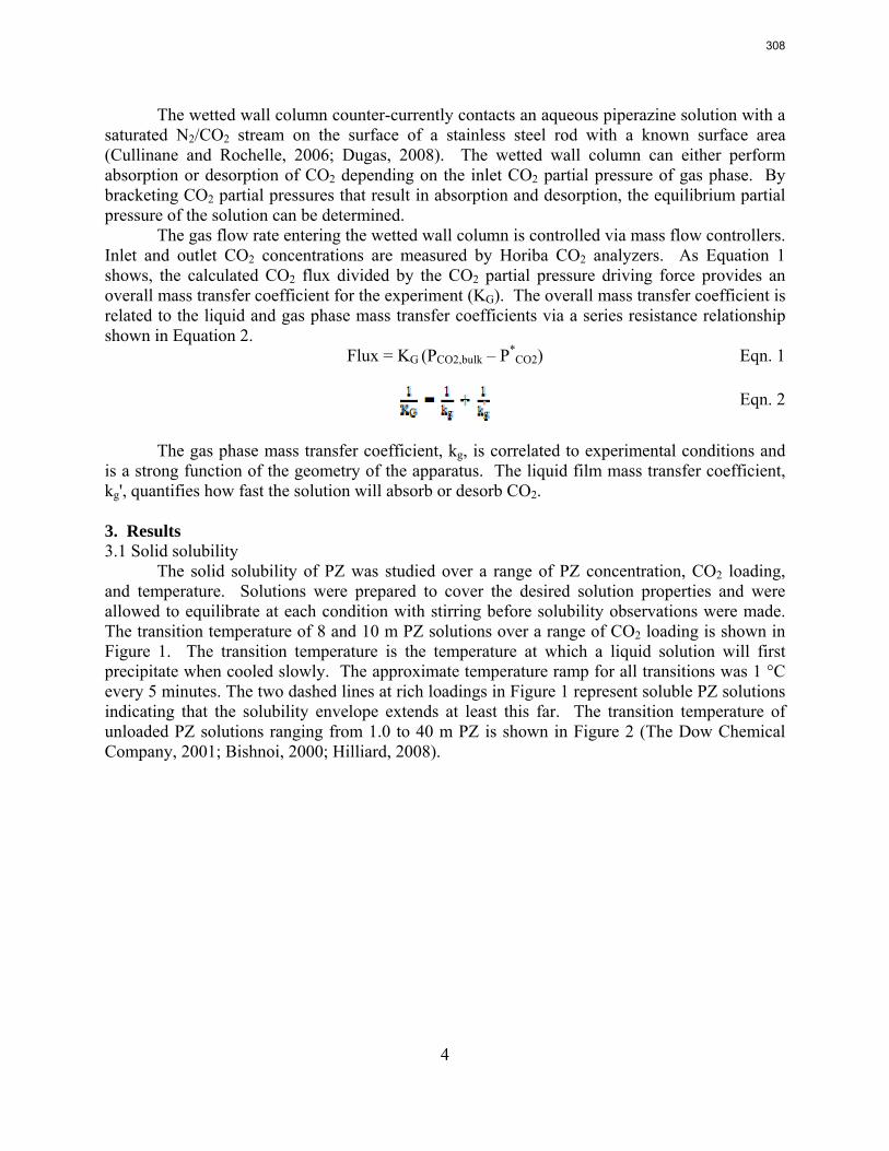
4
The wetted wall column counter-currently contacts an aqueous piperazine solution with a saturated N2/CO2 stream on the surface of a stainless steel rod with a known surface area (Cullinane and Rochelle, 2006; Dugas, 2008). The wetted wall column can either perform absorption or desorption of CO2 depending on the inlet CO2 partial pressure of gas phase. By bracketing CO2 partial pressures that result in absorption and desorption, the equilibrium partial pressure of the solution can be determined.
The gas flow rate entering the wetted wall column is controlled via mass flow controllers. Inlet and outlet CO2 concentrations are measured by Horiba CO2 analyzers. As Equation 1 shows, the calculated CO2 flux divided by the CO2 partial pressure driving force provides an overall mass transfer coefficient for the experiment (KG). The overall mass transfer coefficient is related to the liquid and gas phase mass transfer coefficients via a series resistance relationship shown in Equation 2. Flux = KG (PCO2,bulk – P*
CO2) Eqn. 1 Eqn. 2
The gas phase mass transfer coefficient, kg, is correlated to experimental conditions and
is a strong function of the geometry of the apparatus. The liquid film mass transfer coefficient, kg', quantifies how fast the solution will absorb or desorb CO2.
3. Results 3.1 Solid solubility
The solid solubility of PZ was studied over a range of PZ concentration, CO2 loading, and temperature. Solutions were prepared to cover the desired solution properties and were allowed to equilibrate at each condition with stirring before solubility observations were made. The transition temperature of 8 and 10 m PZ solutions over a range of CO2 loading is shown in Figure 1. The transition temperature is the temperature at which a liquid solution will first precipitate when cooled slowly. The approximate temperature ramp for all transitions was 1 °C every 5 minutes. The two dashed lines at rich loadings in Figure 1 represent soluble PZ solutions indicating that the solubility envelope extends at least this far. The transition temperature of unloaded PZ solutions ranging from 1.0 to 40 m PZ is shown in Figure 2 (The Dow Chemical Company, 2001; Bishnoi, 2000; Hilliard, 2008).
308
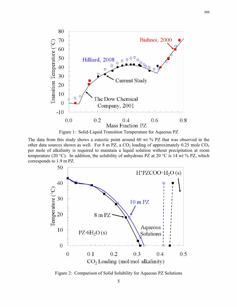
5
Figure 1: Solid-Liquid Transition Temperature for Aqueous PZ
The data from this study shows a eutectic point around 60 wt % PZ that was observed in the other data sources shown as well. For 8 m PZ, a CO2 loading of approximately 0.25 mole CO2 per mole of alkalinity is required to maintain a liquid solution without precipitation at room temperature (20 °C). In addition, the solubility of anhydrous PZ at 20 °C is 14 wt % PZ, which corresponds to 1.9 m PZ.
Figure 2: Comparison of Solid Solubility for Aqueous PZ Solutions
309
6
3.2 Viscosity The viscosity of aqueous PZ solutions has been measured from 0.20 to 0.45 mole CO2 per mole alkalinity, 2 m PZ to 20 m PZ, and 25 °C to 60 °C. The viscosity of 8 and 10 m PZ is compared with other amines in Figure 3 (Huntsman Chemical, 2005; Closmann, 2008). The amine concentration is plotted in units of moles alkalinity per kilogram of water in order to compare mono- and diamines on a similar basis. All of the viscosities shown in Figure 3 are at 40°C and at the rich loading of the system (0.3 mole CO2 per mole alkalinity for MDEA and MDEA/PZ blend; 0.4 mole CO2 per mole alkalinity for PZ and DGA; 0.5 mole CO2 per mole alkalinity for MEA).
Comparison of the viscosity on this basis shows how the amine basic group affects overall viscosity. As the concentration of basic groups increases in a molecule, the viscosity increases in a linear direction. The viscosity of 8 m PZ is higher than that of 7 m MEA, but as compared to 60 wt % DGA®, the viscosity of PZ is lower for a higher alkalinity. Therefore, PZ has the advantage of having two amine functional groups without suffering an increase in viscosity over DGA®. DGA® solutions at 60 wt % are successfully used in natural gas treating (Al-Juaied, 2004).
Figure 3: Viscosity of Amine Solutions at Typical Rich Loading and 40°C 3.3 Oxidative degradation
Heavy metals are known to catalyze the oxidative degradation of amines (Goff and Rochelle, 2004). The results of oxidative degradation of concentrated PZ in the presence of several dissolved metals are shown in Table 1. The experiments simulated four scenarios: (1) leaching of stainless steel metals (iron, chromium, and nickel), (2) addition of a copper-based corrosion inhibitor, (3) addition of a vanadium-based corrosion inhibitor (low concentration), and (4) addition of a copper-based corrosion inhibitor and proprietary inhibitor A.
310
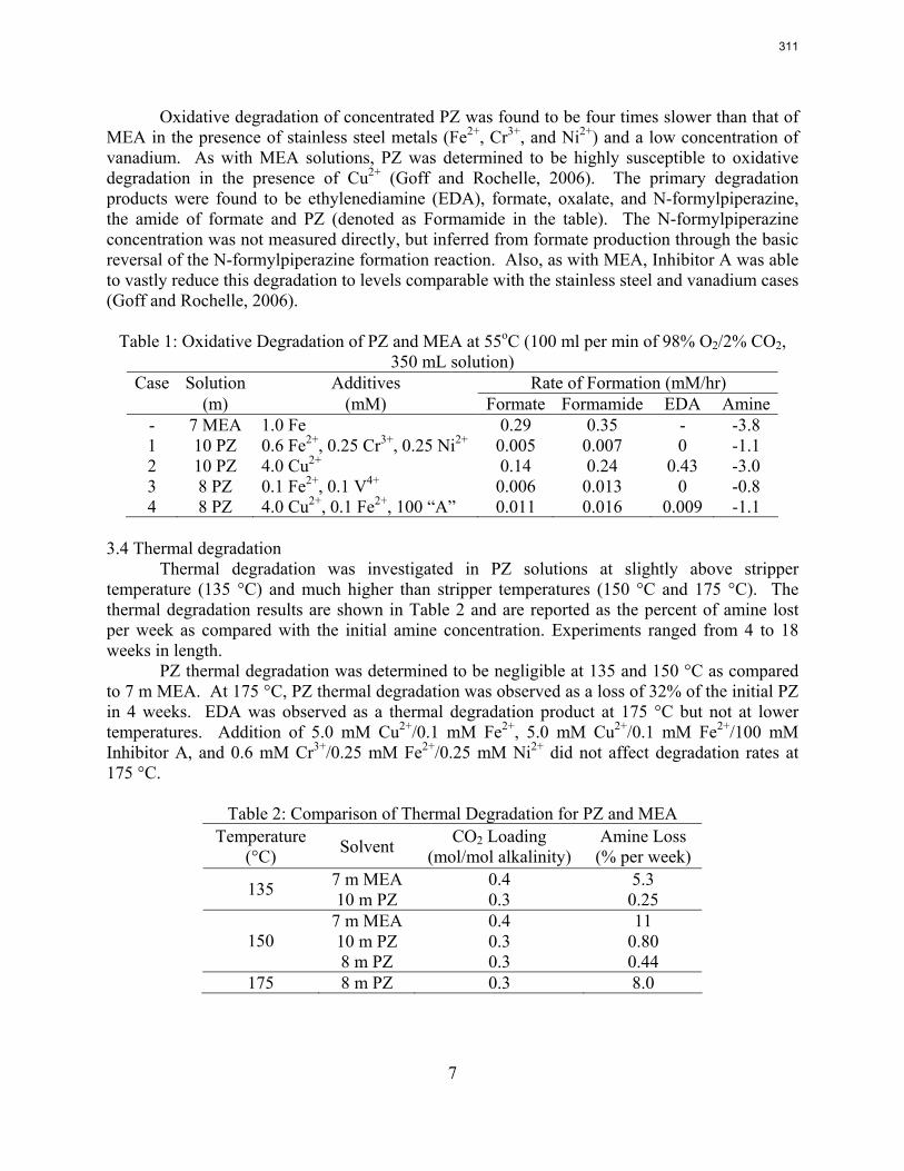
7
Oxidative degradation of concentrated PZ was found to be four times slower than that of MEA in the presence of stainless steel metals (Fe2+, Cr3+, and Ni2+) and a low concentration of vanadium. As with MEA solutions, PZ was determined to be highly susceptible to oxidative degradation in the presence of Cu2+ (Goff and Rochelle, 2006). The primary degradation products were found to be ethylenediamine (EDA), formate, oxalate, and N-formylpiperazine, the amide of formate and PZ (denoted as Formamide in the table). The N-formylpiperazine concentration was not measured directly, but inferred from formate production through the basic reversal of the N-formylpiperazine formation reaction. Also, as with MEA, Inhibitor A was able to vastly reduce this degradation to levels comparable with the stainless steel and vanadium cases (Goff and Rochelle, 2006).
Table 1: Oxidative Degradation of PZ and MEA at 55oC (100 ml per min of 98% O2/2% CO2, 350 mL solution)
Case Solution Additives Rate of Formation (mM/hr) (m) (mM) Formate Formamide EDA Amine- 7 MEA 1.0 Fe 0.29 0.35 - -3.8 1 10 PZ 0.6 Fe2+, 0.25 Cr3+, 0.25 Ni2+ 0.005 0.007 0 -1.1 2 10 PZ 4.0 Cu2+ 0.14 0.24 0.43 -3.0 3 8 PZ 0.1 Fe2+, 0.1 V4+ 0.006 0.013 0 -0.8 4 8 PZ 4.0 Cu2+, 0.1 Fe2+, 100 “A” 0.011 0.016 0.009 -1.1
3.4 Thermal degradation
Thermal degradation was investigated in PZ solutions at slightly above stripper temperature (135 °C) and much higher than stripper temperatures (150 °C and 175 °C). The thermal degradation results are shown in Table 2 and are reported as the percent of amine lost per week as compared with the initial amine concentration. Experiments ranged from 4 to 18 weeks in length. PZ thermal degradation was determined to be negligible at 135 and 150 °C as compared to 7 m MEA. At 175 °C, PZ thermal degradation was observed as a loss of 32% of the initial PZ in 4 weeks. EDA was observed as a thermal degradation product at 175 °C but not at lower temperatures. Addition of 5.0 mM Cu2+/0.1 mM Fe2+, 5.0 mM Cu2+/0.1 mM Fe2+/100 mM Inhibitor A, and 0.6 mM Cr3+/0.25 mM Fe2+/0.25 mM Ni2+ did not affect degradation rates at 175 °C.
Table 2: Comparison of Thermal Degradation for PZ and MEA Temperature
(°C) Solvent CO2 Loading (mol/mol alkalinity)
Amine Loss (% per week)
7 m MEA 0.4 5.3 135 10 m PZ 0.3 0.25 7 m MEA 0.4 11 10 m PZ 0.3 0.80 150 8 m PZ 0.3 0.44
175 8 m PZ 0.3 8.0
311
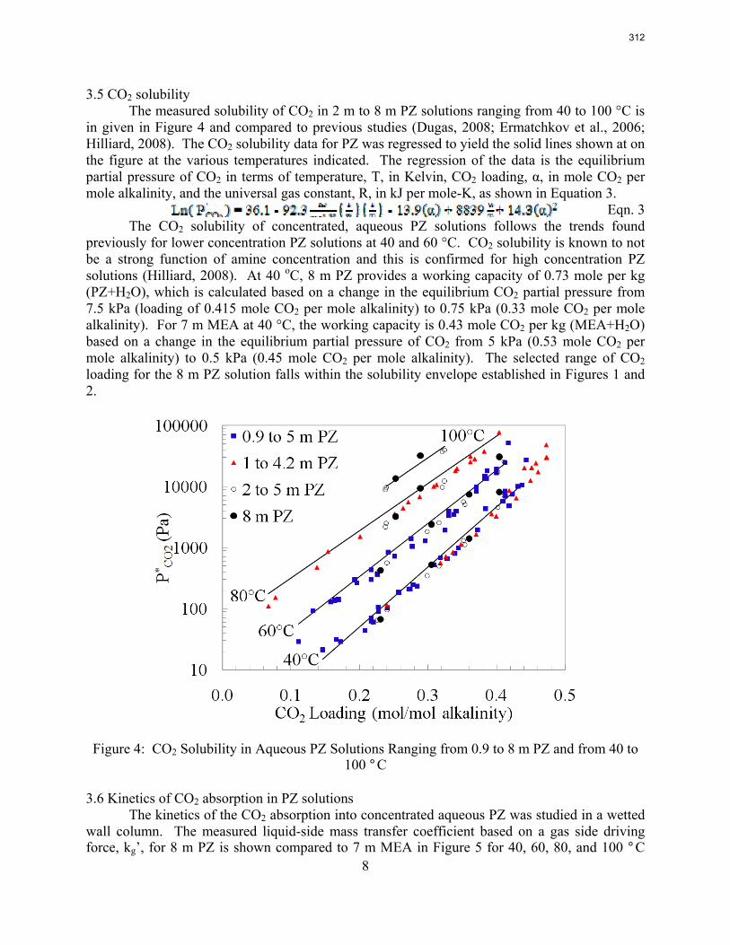
8
3.5 CO2 solubility The measured solubility of CO2 in 2 m to 8 m PZ solutions ranging from 40 to 100 °C is
in given in Figure 4 and compared to previous studies (Dugas, 2008; Ermatchkov et al., 2006; Hilliard, 2008). The CO2 solubility data for PZ was regressed to yield the solid lines shown at on the figure at the various temperatures indicated. The regression of the data is the equilibrium partial pressure of CO2 in terms of temperature, T, in Kelvin, CO2 loading, α, in mole CO2 per mole alkalinity, and the universal gas constant, R, in kJ per mole-K, as shown in Equation 3.
Eqn. 3 The CO2 solubility of concentrated, aqueous PZ solutions follows the trends found
previously for lower concentration PZ solutions at 40 and 60 °C. CO2 solubility is known to not be a strong function of amine concentration and this is confirmed for high concentration PZ solutions (Hilliard, 2008). At 40 oC, 8 m PZ provides a working capacity of 0.73 mole per kg (PZ+H2O), which is calculated based on a change in the equilibrium CO2 partial pressure from 7.5 kPa (loading of 0.415 mole CO2 per mole alkalinity) to 0.75 kPa (0.33 mole CO2 per mole alkalinity). For 7 m MEA at 40 °C, the working capacity is 0.43 mole CO2 per kg (MEA+H2O) based on a change in the equilibrium partial pressure of CO2 from 5 kPa (0.53 mole CO2 per mole alkalinity) to 0.5 kPa (0.45 mole CO2 per mole alkalinity). The selected range of CO2 loading for the 8 m PZ solution falls within the solubility envelope established in Figures 1 and 2.
Figure 4: CO2 Solubility in Aqueous PZ Solutions Ranging from 0.9 to 8 m PZ and from 40 to 100 °C
3.6 Kinetics of CO2 absorption in PZ solutions
The kinetics of the CO2 absorption into concentrated aqueous PZ was studied in a wetted wall column. The measured liquid-side mass transfer coefficient based on a gas side driving force, kg’, for 8 m PZ is shown compared to 7 m MEA in Figure 5 for 40, 60, 80, and 100 °C
312
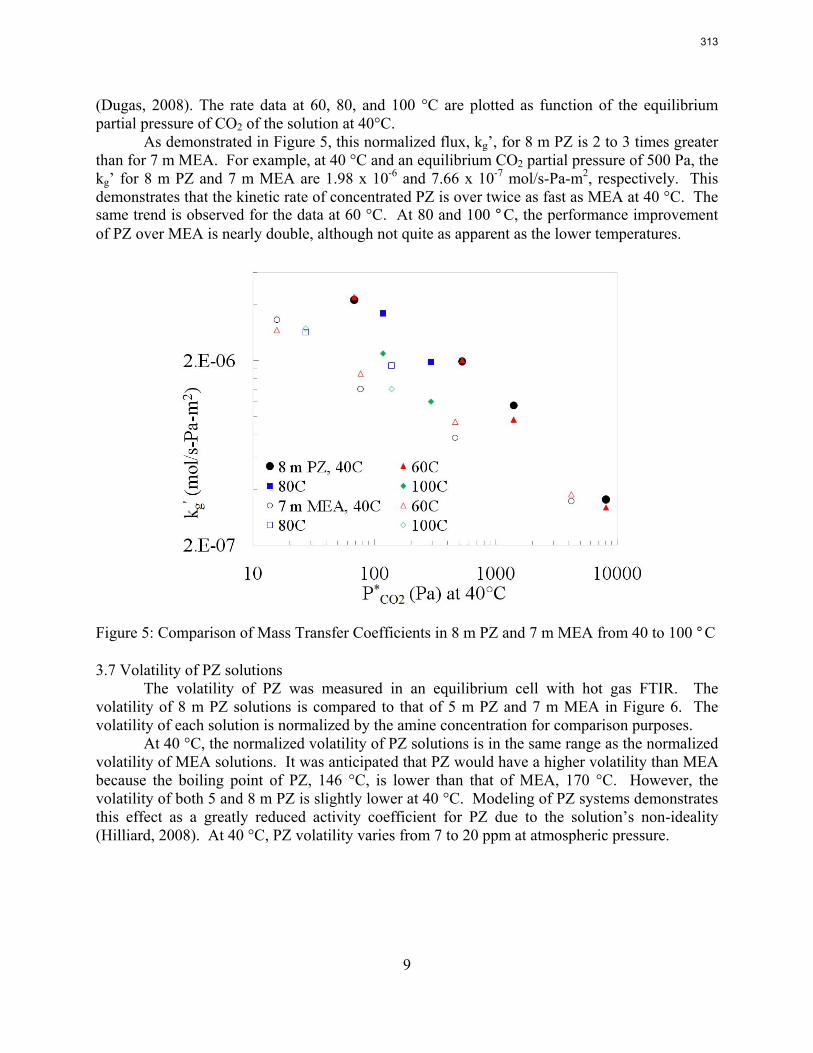
9
(Dugas, 2008). The rate data at 60, 80, and 100 °C are plotted as function of the equilibrium partial pressure of CO2 of the solution at 40°C.
As demonstrated in Figure 5, this normalized flux, kg’, for 8 m PZ is 2 to 3 times greater than for 7 m MEA. For example, at 40 °C and an equilibrium CO2 partial pressure of 500 Pa, the kg’ for 8 m PZ and 7 m MEA are 1.98 x 10⁻⁶ and 7.66 x 10⁻⁷ mol/s-Pa-m2, respectively. This demonstrates that the kinetic rate of concentrated PZ is over twice as fast as MEA at 40 °C. The same trend is observed for the data at 60 °C. At 80 and 100 °C, the performance improvement of PZ over MEA is nearly double, although not quite as apparent as the lower temperatures.
Figure 5: Comparison of Mass Transfer Coefficients in 8 m PZ and 7 m MEA from 40 to 100 °C
3.7 Volatility of PZ solutions The volatility of PZ was measured in an equilibrium cell with hot gas FTIR. The volatility of 8 m PZ solutions is compared to that of 5 m PZ and 7 m MEA in Figure 6. The volatility of each solution is normalized by the amine concentration for comparison purposes. At 40 °C, the normalized volatility of PZ solutions is in the same range as the normalized volatility of MEA solutions. It was anticipated that PZ would have a higher volatility than MEA because the boiling point of PZ, 146 °C, is lower than that of MEA, 170 °C. However, the volatility of both 5 and 8 m PZ is slightly lower at 40 °C. Modeling of PZ systems demonstrates this effect as a greatly reduced activity coefficient for PZ due to the solution’s non-ideality (Hilliard, 2008). At 40 °C, PZ volatility varies from 7 to 20 ppm at atmospheric pressure.
313
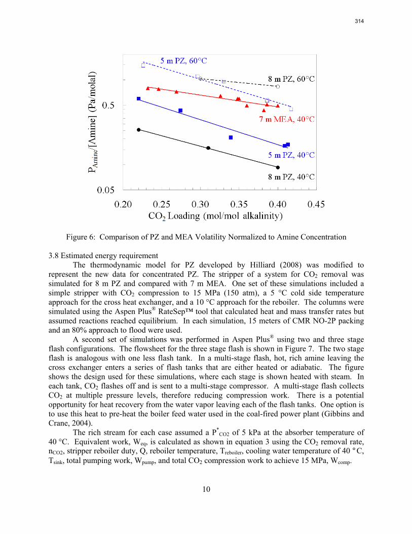
10
Figure 6: Comparison of PZ and MEA Volatility Normalized to Amine Concentration
3.8 Estimated energy requirement The thermodynamic model for PZ developed by Hilliard (2008) was modified to
represent the new data for concentrated PZ. The stripper of a system for CO2 removal was simulated for 8 m PZ and compared with 7 m MEA. One set of these simulations included a simple stripper with CO2 compression to 15 MPa (150 atm), a 5 °C cold side temperature approach for the cross heat exchanger, and a 10 °C approach for the reboiler. The columns were simulated using the Aspen Plus® RateSep™ tool that calculated heat and mass transfer rates but assumed reactions reached equilibrium. In each simulation, 15 meters of CMR NO-2P packing and an 80% approach to flood were used.
A second set of simulations was performed in Aspen Plus® using two and three stage flash configurations. The flowsheet for the three stage flash is shown in Figure 7. The two stage flash is analogous with one less flash tank. In a multi-stage flash, hot, rich amine leaving the cross exchanger enters a series of flash tanks that are either heated or adiabatic. The figure shows the design used for these simulations, where each stage is shown heated with steam. In each tank, CO2 flashes off and is sent to a multi-stage compressor. A multi-stage flash collects CO2 at multiple pressure levels, therefore reducing compression work. There is a potential opportunity for heat recovery from the water vapor leaving each of the flash tanks. One option is to use this heat to pre-heat the boiler feed water used in the coal-fired power plant (Gibbins and Crane, 2004).
The rich stream for each case assumed a P*CO2 of 5 kPa at the absorber temperature of
40 °C. Equivalent work, Weq, is calculated as shown in equation 3 using the CO2 removal rate, nCO2, stripper reboiler duty, Q, reboiler temperature, Treboiler, cooling water temperature of 40 °C, Tsink, total pumping work, Wpump, and total CO2 compression work to achieve 15 MPa, Wcomp.
314
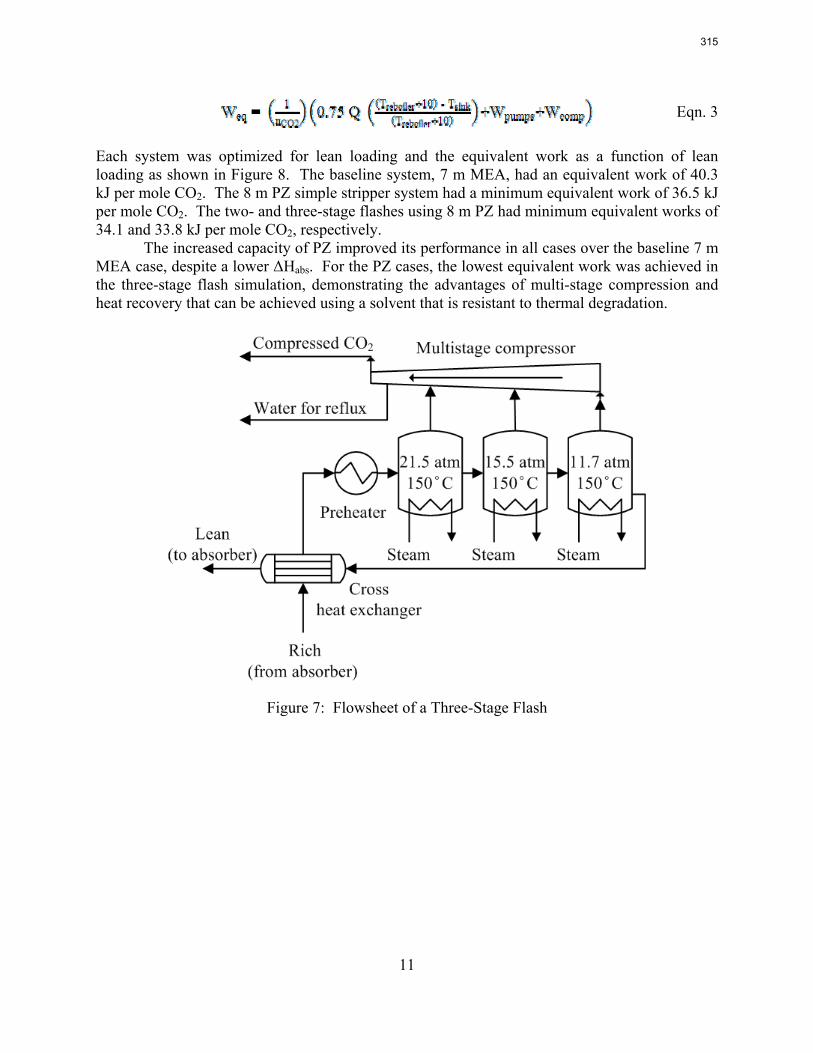
11
Eqn. 3 Each system was optimized for lean loading and the equivalent work as a function of lean loading as shown in Figure 8. The baseline system, 7 m MEA, had an equivalent work of 40.3 kJ per mole CO2. The 8 m PZ simple stripper system had a minimum equivalent work of 36.5 kJ per mole CO2. The two- and three-stage flashes using 8 m PZ had minimum equivalent works of 34.1 and 33.8 kJ per mole CO2, respectively.
The increased capacity of PZ improved its performance in all cases over the baseline 7 m MEA case, despite a lower ΔHabs. For the PZ cases, the lowest equivalent work was achieved in the three-stage flash simulation, demonstrating the advantages of multi-stage compression and heat recovery that can be achieved using a solvent that is resistant to thermal degradation.
Figure 7: Flowsheet of a Three-Stage Flash
315
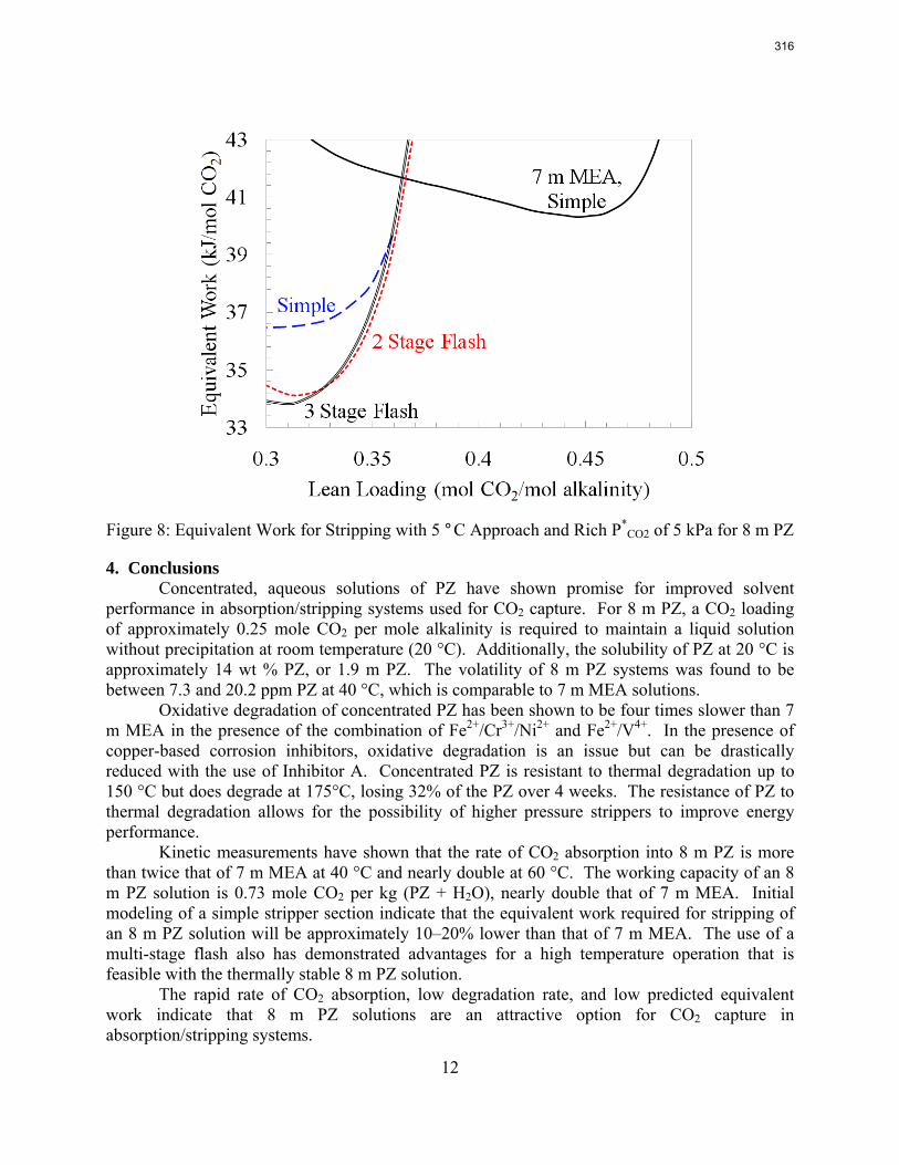
12
Figure 8: Equivalent Work for Stripping with 5 °C Approach and Rich P*CO2 of 5 kPa for 8 m PZ
4. Conclusions
Concentrated, aqueous solutions of PZ have shown promise for improved solvent performance in absorption/stripping systems used for CO2 capture. For 8 m PZ, a CO2 loading of approximately 0.25 mole CO2 per mole alkalinity is required to maintain a liquid solution without precipitation at room temperature (20 °C). Additionally, the solubility of PZ at 20 °C is approximately 14 wt % PZ, or 1.9 m PZ. The volatility of 8 m PZ systems was found to be between 7.3 and 20.2 ppm PZ at 40 °C, which is comparable to 7 m MEA solutions.
Oxidative degradation of concentrated PZ has been shown to be four times slower than 7 m MEA in the presence of the combination of Fe2+/Cr3+/Ni2+ and Fe2+/V4+. In the presence of copper-based corrosion inhibitors, oxidative degradation is an issue but can be drastically reduced with the use of Inhibitor A. Concentrated PZ is resistant to thermal degradation up to 150 °C but does degrade at 175°C, losing 32% of the PZ over 4 weeks. The resistance of PZ to thermal degradation allows for the possibility of higher pressure strippers to improve energy performance.
Kinetic measurements have shown that the rate of CO2 absorption into 8 m PZ is more than twice that of 7 m MEA at 40 °C and nearly double at 60 °C. The working capacity of an 8 m PZ solution is 0.73 mole CO2 per kg (PZ + H2O), nearly double that of 7 m MEA. Initial modeling of a simple stripper section indicate that the equivalent work required for stripping of an 8 m PZ solution will be approximately 10–20% lower than that of 7 m MEA. The use of a multi-stage flash also has demonstrated advantages for a high temperature operation that is feasible with the thermally stable 8 m PZ solution.
The rapid rate of CO2 absorption, low degradation rate, and low predicted equivalent work indicate that 8 m PZ solutions are an attractive option for CO2 capture in absorption/stripping systems.
316
13
5. Acknowledgements
The Luminant Carbon Management Program provided support for this research. 6. References Al-Juaied, M.A., 2004. Carbon Dioxide Removal from Natural Gas by Membranes in the
Presence of Heavy Hydrocarbons and by Aqueous Diglycolamine®/Morpholine. Doctoral dissertation, The University of Texas at Austin, Austin, TX.
Bishnoi, S., 2000. Carbon Dioxide Absorption and Solution Equilibrium in Piperazine Activated Methyldiethanolamine. Doctoral dissertation, The University of Texas at Austin, Austin, TX.
Closmann, F., 2008. MDEA/piperazine as a solvent for CO2 capture. GHGT-9, Washington D.C. Cullinane, J.T., Rochelle, G.T., 2005. Thermodynamics of aqueous potassium carbonate,
piperazine, and carbon dioxide. Fluid Phase Equilib. 227(2), 197-213. Cullinane, J.T., Rochelle, G.T., 2006. Kinetics of carbon dioxide absorption into aqueous
potassium carbonate and piperazine. Ind. Eng. Chem. Res. 45(8), 2531-2545. Davis, J., 2008. Thermal degradation of monoethanolamine at stripper conditions. GHGT-9,
Washington D.C. The Dow Chemical Company, 2001. Ethyleneamines. The Dow Chemical Company: Midland,
MI, August 2001. Dugas, R., 2008. Absorption and desorption rates of carbon dioxide with monoethanolamine and
piperazine. GHGT-9, Washington D.C. Ermatchkov, V., Kamps, A.P.S., Speyer, D., Maurer, G., 2006. Solubility of carbon dioxide in
aqueous solutions of piperazine in the low gas loading region. J. Chem. Eng. Data 51(5), 1788-1796.
Gibbins, J.R., Crane, R.I., 2004. Scope for reductions in the cost of CO2 capture using flue gas scrubbing with amine solvents. Proceedings of the Institution of Mechanical Engineers Part A-Journal of Power and Energy 218 (A4), 231-239.
Goff, G.S., Rochelle, G.T., 2004. Monoethanolamine degradation: O2 mass transfer effects under CO2 capture conditions. Ind. Eng. Chem. Res. 43(20), 6400-6408.
Goff, G.S., Rochelle, G.T., 2006. Oxidation inhibitors for copper and iron catalyzed degradation of monoethanolamine in CO2 capture processes. Ind. Eng. Chem. Res. 45(8), 2513-2521.
Hilliard, M.D., 2008. A Predictive Thermodynamic Model for an Aqueous Blend of Potassium Carbonate, Piperazine, and Monoethanolamine for Carbon Dioxide Capture from Flue Gas. Doctoral dissertation, The University of Texas at Austin, Austin, TX.
Huntsman Chemical, 2005. Diglycolamine® Agent - Product Information. Huntsman Chemical: 2005.
IPCC (2001). Climate Change 2001: The Scientific Basis. Contribution of Working Group I to the Third Assessment Report of the Intergovernmental Panel on Climate Change. [J. T. Houghton, Y. Ding, D. J. Griggs, M. Noguer, P. J. van der Linden, X. Dai, K. Maskell and C. A. Johnson (eds.)]. Cambridge University Press, Cambridge, United Kingdom, 881pp.
Sexton, A., 2008. Amine Oxidation in CO2 Capture Processes. Doctoral dissertation, The University of Texas at Austin, Austin, TX.
317
Modeling CO2 Capture with Aqueous Monoethanolamine
Jorge M. Plazaa, David H. Van Wagenera, Gary T. Rochellea,*1 aDepartment of Chemical Engineering, The University of Texas at Austin,
1 University Station, Austin TX 78712
Abstract
Hilliard completed several thermodynamic models in Aspen Plus® for modeling CO2 removal with amine solvents, including MEA-H2O-CO2. This solvent was selected to make a system model for CO2 removal by absorption/stripping. Both the absorber and the stripper used RateSepTM to rigorously calculate mass transfer rates. The accuracy of the new model was assessed using a recent pilot plant run with 35 wt % MEA. Absorber loadings and removal were matched and the temperature profile was approached within 5 oC. An average 3.8% difference between measured and calculated values was achieved in the stripper. A three-stage flash configuration which efficiently utilizes solar energy was developed. It reduces energy use by 6% relative to a simple stripper. Intercooling was used to reach 90% removal in the absorber at these optimized conditions. Keywords: kinetics; absorption; stripping; carbon dioxide; MEA; modeling
1. Introduction
CO2 capture by amine absorption and stripping is currently considered the most feasible option for the removal of carbon dioxide from coal- and natural gas-fired power plants. Monoethanolamine (MEA) is the proven solvent for this application. Previous models have been developed for this system. Freguia (Freguia and Rochelle, 2003) developed a model using Aspen Plus® RatefracTM that incorporated kinetic work by Dang (2000) and modified VLE by Austgen et al. (1989) to include work by Jou et al. (1994). Ziaii (Fisher et al., 2007) used Aspen Plus® RateSepTM with the thermodynamic framework by Freguia and approximated Aboudheir (2000) kinetics. This paper presents results with a new MEA model that uses a rigorous thermodynamic model developed by Hilliard (2008) and kinetics extracted from values obtained by Aboudheir (2002) with a laminar jet. The model was developed with the Aspen Plus® RatesepTM
* Corresponding author. Tel.:1-512-471-7230; fax:1-512-471-7060. E-mail address: [email protected]
318
framework and was validated with a pilot plant run with 35 wt % MEA. Additionally, an innovative stripper configuration was optimized and its corresponding absorber was specified.
2. Thermodynamic model The absorber and stripper models use the thermodynamic representation by
Hilliard (2008). Hilliard used the electrolyte nonrandom two-liquid (e-NRTL) activity coefficient model in Aspen Plus® to develop a rigorous and consistent thermodynamic representation of mixtures of MEA-H2O-CO2. His model differs from previous models in that it represents additional data on amine vapor pressure, enthalpies of absorption, heat capacity, and NMR speciation. This framework uses Gibbs free energy and enthalpy values within Aspen Plus® to maintain thermodynamic consistency.
3. Process Models
3.1. Absorber kinetics The kinetics for this model are based on selected measurements of CO2
absorption by Aboudheir (2002) in a laminar jet. These data were used to evaluate the forward rate constants for the formation of carbamate using Aspen Plus® RateSep™. An absorber model was set up using the Hilliard thermodynamic model and kinetics were represented using two reversible reactions:
2 MEA + CO2 ↔ MEAH+ + MEACOO- (1)
(1a)
(1b)
MEA + CO2 + H2O↔ HCO3- + MEAH+ (2)
(2a)
(2b)
The bicarbonate formation (2) rate constants were evaluated using data at 25 oC for reaction of tertiary amines and CO2. This data was correlated with the base dissociation constant (pKb) in Rochelle et al. (2001). The values of the reaction constant for tertiary amines were fit as a function of pKb and the forward rate constant for MEA (pKb=4.45) was extracted from this fit and converted to an activity/mole fraction basis with the activity coefficients from the Hilliard model. The energy of activation was approximated using data for MDEA (49 kJ/gmol) (Rochelle et al., 2001). The forward reaction rate constant for the bicarbonate
319
reaction was calculated with the conditions defined by the data set selected from Aboudheir and then used along with the equilibrium constants to determine the reverse rates for the bicarbonate reaction.
Nine points from Aboudheir (2002) were used to determine the forward carbamate formation rate (1a), three at 313 K (40 oC), loading of 0.2767 and the rest at 333 K (60 oC), with loadings of 0.1104 and 0.2819. A laminar jet was modeled in Aspen Plus® using the bicarbonate constants and thermodynamics from Hilliard (2008). Density, viscosity, thermal conductivity, and surface tension of the MEA-H2O-CO2 system, along with carbon dioxide diffusivity in water, were corrected based on work by Aspen Technology, Inc. (Huiling and Chen, 2008). Initially the energy of activation was set to zero and the reported flux by Aboudheir was matched by changing the pre-exponential factor in the power law. The resulting rate constants were averaged among the same temperature and loading conditions and then regressed to obtain values for the pre-exponential factor and activation energy. The activity of MEA was squared to represent apparent effects of changes in loading.
3.2. Stripper Model This Aspen Plus® simulation work assumes equilibrium reactions in the stripper.
RateSepTM rigorously calculates the heat and mass transfer for each stage of the simple stripper. The packing mass transfer and interfacial area model by Bravo et al. (1992) was used to estimate liquid mass transfer coefficients and area of packing. The reboiler was modeled as equilibrium. The necessary pumps and intercooled vapor compression were included, except for the pilot plant which did not require a compressor.
A nonconventional stripper section was used to simulate the reboiler configuration of the pilot plant. The reboiler was configured to heat only a fraction of the sump drawoff (Figure 2). The column is identical to the absorber, containing 6.1 m of packing (Mellapak 250Y) with a 0.43 m diameter. The pilot plant provided data for various points in the process, but several crucial values were unknown. For example, the split ratio of lean amine flow was not manipulated or measured, and it could not be calculated.
Stripper performance was evaluated using equivalent work, which calculates the total electrical energy usage of a power plant. The standard form is shown in equation 3, and this equation was integrated when a variable temperature energy source (solar heat) was used in the three-stage flash configuration (equation 4). This variable temperature source had an inlet temperature of To and an outlet temperature of Tf.
(3)
320
(4)
4. Pilot Plant Model Validation The proposed model was utilized to match experimental data from a pilot plant
run in October 2007 with 9 m MEA at the University of Texas at Austin (Chen, 2007) using the parameter estimation tool in Aspen Plus® 2006.5.
4.1 Absorber Section The operating mode was similar to that reported by Chen (2007), but the air was
not recycled back to the absorber. The absorber packing (Flexipac AQ Style 20) was modeled using Flexipac 1Y with 12 equal stages using the countercurrent flow model. The liquid mass transfer film was represented with 16 segments. The interfacial area was calculated using a new correlation developed by Tsai et al. (2008). Heat loss was neglected.
Variables and parameters used for the reconciliation and their chosen standard deviations along with the resulting model predictions are presented in Table 1. The only manipulated model parameter was the interfacial area factor which corrected the calculated interfacial area. High standard deviations (20 oC) were specified for the outlet gas and the top column temperatures because they were considered less reliable. The water (water – Lean) and CO2 content (CO2 – Lean) of the lean feed were treated as reconcilable experimental values. The resulting values give a lean loading of 0.365 which is 1% greater than the measured value (0.36). Figure 1 compares the resulting model temperature profiles with the experimental results. The point at a relative position of -0.1 represents a measurement downstream of the column.
The reconciled flow rates, compositions, and the CO2 removal are within 1 to 6% of reported values, reflecting moderate adjustments to close the mass balance. CO2 removal and other pilot plant measurements were matched by adjusting the wetted area prediction of the Tsai et al. (2008) model by a factor of 0.82.
4.2 Stripper Section The pilot plant run using 9 m MEA was also evaluated using the stripper model.
Table 2 summarizes important data and calculations from the process. There were six thermocouples in the column at various heights, each indicated by i in Table 2.
Data regressions were initially used in Aspen Plus® in an attempt to reconcile the results, but all regressions failed to produce close agreement. The best solution was determined to be adjusting heat duties in selected stages within the column to simulate heat loss. Pilot plant results did not include a profile of heat loss in the column, so it was specified to match column temperatures. The split ratio in the reboiler and its duty were adjusted to match the reboiler temperature and lean loading. Figure 4 displays the column profile as a function of column height for
321
the plant data, the initial Aspen Plus® calculation, and the final Aspen Plus® calculation with a matched temperature profile by adjusting to heat loss. The agreement between the values in Table 2 demonstrates that the CO2 removal at the pilot plant was verified with the model. The simulation predicted a nearly identical reboiler duty, and the heat loss was only 12% greater than the calculated heat loss at the pilot plant. The average variation between measured and calculated values was 3.8%.
5. Optimization case study
5.1. Three-Stage Flash A three-stage flash configuration was developed for the stripper (Figure 3).
Unlike configurations with reboilers, a countercurrent heat exchanger is used to preheat the rich stream exiting the cross heat exchanger before the stripping equipment. Preheating results in higher stripping temperatures, which yields greater CO2 selectivity. High stripping temperatures were previously avoided to reduce the risk of thermal degradation of the solvent. However, if thermal degradation is not an issue for new solvents, it would be preferable to use higher temperatures. Additionally, by using a countercurrent exchanger to heat the rich stream, a solar energy source with a variable heating temperature is expected to operate more efficiently. The flash assumes chemical and thermal equilibrium. The stripper was sized to remove 3000 tons/day of CO2 from a coal-fired power plant. A 5° cold side approach was specified on the cross heat exchanger, and a 10° LMTD driving force was specified for all other heat exchangers.
The three-stage flash configuration was run with 9 m MEA, and a constant rich loading of 0.495 was used corresponding approximately to 5 kPa P*CO2 in the absorber. The lean loading was optimized to minimize the total equivalent work. The equivalent work for various conditions was compared against the equivalent work for a similar system of conditions for a simple stripper, both atmospheric and 1.6 atm columns. The three-stage flash and simple stripper configurations responded differently to changes in lean loading; however, both configurations yielded an optimum lean loading of 0.40. Figure 5 displays the equivalent work response to lean loading for four scenarios: solar-heated, three-stage flash with an exiting lean pressure of 110 kPa; steam-heated, three-stage flash with an exiting lean pressure of 110 kPa; the baseline simple stripper configuration with steam heat operating at both 1 atm and 1.6 atm.
The 1.6 atm simple stripper was considered to be the most appropriate comparison to the three-stage flash because the maximum temperatures of these configurations were relatively equal: at the optimized lean loading the highest temperature was 105 °C. Whether using solar or steam heating, the three-stage flash required less energy than the 1.6 atm simple stripper. The three-stage flash with solar heating required 2.0 kJ/mol CO2 less energy than the 1.6 atm stripper.
322
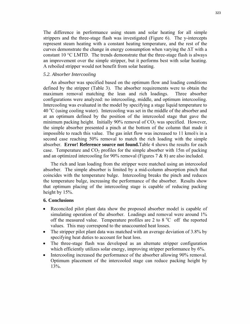
The difference in performance using steam and solar heating for all simple strippers and the three-stage flash was investigated (Figure 6). The y-intercepts represent steam heating with a constant heating temperature, and the rest of the curves demonstrate the change in energy consumption when varying the ΔT with a constant 10 °C LMTD. The trends demonstrate that the three-stage flash is always an improvement over the simple stripper, but it performs best with solar heating. A reboiled stripper would not benefit from solar heating.
5.2. Absorber Intercooling
An absorber was specified based on the optimum flow and loading conditions defined by the stripper (Table 3). The absorber requirements were to obtain the maximum removal matching the lean and rich loadings. Three absorber configurations were analyzed: no intercooling, middle, and optimum intercooling. Intercooling was evaluated in the model by specifying a stage liquid temperature to 40 oC (using cooling water). Intercooling was set in the middle of the absorber and at an optimum defined by the position of the intercooled stage that gave the minimum packing height. Initially 90% removal of CO2 was specified. However, the simple absorber presented a pinch at the bottom of the column that made it impossible to reach this value. The gas inlet flow was increased to 11 kmol/s in a second case reaching 50% removal to match the rich loading with the simple absorber. Error! Reference source not found.Table 4 shows the results for each case. Temperature and CO2 profiles for the simple absorber with 15m of packing and an optimized intercooling for 90% removal (Figures 7 & 8) are also included.
The rich and lean loading from the stripper were matched using an intercooled absorber. The simple absorber is limited by a mid-column absorption pinch that coincides with the temperature bulge. Intercooling breaks the pinch and reduces the temperature bulge, increasing the performance of the absorber. Results show that optimum placing of the intercooling stage is capable of reducing packing height by 15%.
6. Conclusions
• Reconciled pilot plant data show the proposed absorber model is capable of simulating operation of the absorber. Loadings and removal were around 1% off the measured value. Temperature profiles are 2 to 8 oC off the reported values. This may correspond to the unaccounted heat losses.
• The stripper pilot plant data was matched with an average deviation of 3.8% by specifying heat duties to account for heat loss.
• The three-stage flash was developed as an alternate stripper configuration which efficiently utilizes solar energy, improving stripper performance by 6%.
• Intercooling increased the performance of the absorber allowing 90% removal. Optimum placement of the intercooled stage can reduce packing height by 13%.
323
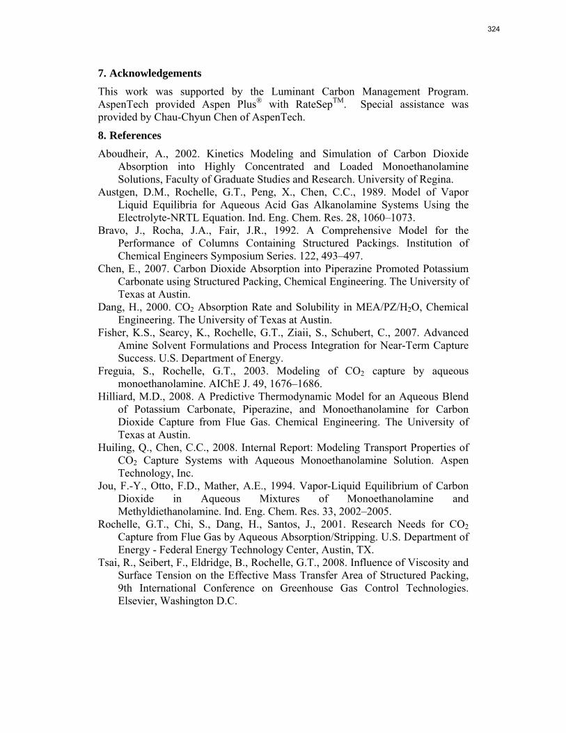
7. Acknowledgements This work was supported by the Luminant Carbon Management Program. AspenTech provided Aspen Plus® with RateSepTM. Special assistance was provided by Chau-Chyun Chen of AspenTech.
8. References Aboudheir, A., 2002. Kinetics Modeling and Simulation of Carbon Dioxide
Absorption into Highly Concentrated and Loaded Monoethanolamine Solutions, Faculty of Graduate Studies and Research. University of Regina.
Austgen, D.M., Rochelle, G.T., Peng, X., Chen, C.C., 1989. Model of Vapor Liquid Equilibria for Aqueous Acid Gas Alkanolamine Systems Using the Electrolyte-NRTL Equation. Ind. Eng. Chem. Res. 28, 1060–1073.
Bravo, J., Rocha, J.A., Fair, J.R., 1992. A Comprehensive Model for the Performance of Columns Containing Structured Packings. Institution of Chemical Engineers Symposium Series. 122, 493–497.
Chen, E., 2007. Carbon Dioxide Absorption into Piperazine Promoted Potassium Carbonate using Structured Packing, Chemical Engineering. The University of Texas at Austin.
Dang, H., 2000. CO2 Absorption Rate and Solubility in MEA/PZ/H2O, Chemical Engineering. The University of Texas at Austin.
Fisher, K.S., Searcy, K., Rochelle, G.T., Ziaii, S., Schubert, C., 2007. Advanced Amine Solvent Formulations and Process Integration for Near-Term Capture Success. U.S. Department of Energy.
Freguia, S., Rochelle, G.T., 2003. Modeling of CO2 capture by aqueous monoethanolamine. AIChE J. 49, 1676–1686.
Hilliard, M.D., 2008. A Predictive Thermodynamic Model for an Aqueous Blend of Potassium Carbonate, Piperazine, and Monoethanolamine for Carbon Dioxide Capture from Flue Gas. Chemical Engineering. The University of Texas at Austin.
Huiling, Q., Chen, C.C., 2008. Internal Report: Modeling Transport Properties of CO2 Capture Systems with Aqueous Monoethanolamine Solution. Aspen Technology, Inc.
Jou, F.-Y., Otto, F.D., Mather, A.E., 1994. Vapor-Liquid Equilibrium of Carbon Dioxide in Aqueous Mixtures of Monoethanolamine and Methyldiethanolamine. Ind. Eng. Chem. Res. 33, 2002–2005.
Rochelle, G.T., Chi, S., Dang, H., Santos, J., 2001. Research Needs for CO2 Capture from Flue Gas by Aqueous Absorption/Stripping. U.S. Department of Energy - Federal Energy Technology Center, Austin, TX.
Tsai, R., Seibert, F., Eldridge, B., Rochelle, G.T., 2008. Influence of Viscosity and Surface Tension on the Effective Mass Transfer Area of Structured Packing, 9th International Conference on Greenhouse Gas Control Technologies. Elsevier, Washington D.C.
324
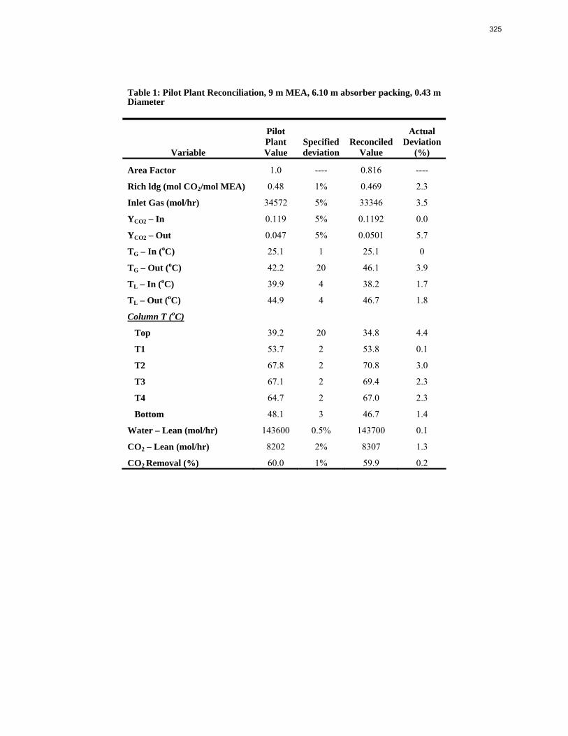
Table 1: Pilot Plant Reconciliation, 9 m MEA, 6.10 m absorber packing, 0.43 m Diameter
Variable
Pilot Plant Value
Specified deviation
Reconciled Value
Actual Deviation
(%)
Area Factor 1.0 ---- 0.816 ----
Rich ldg (mol CO2/mol MEA) 0.48 1% 0.469 2.3
Inlet Gas (mol/hr) 34572 5% 33346 3.5
YCO2 – In 0.119 5% 0.1192 0.0
YCO2 – Out 0.047 5% 0.0501 5.7
TG – In (oC) 25.1 1 25.1 0
TG – Out (oC) 42.2 20 46.1 3.9
TL – In (oC) 39.9 4 38.2 1.7
TL – Out (oC) 44.9 4 46.7 1.8
Column T (oC)
Top 39.2 20 34.8 4.4
T1 53.7 2 53.8 0.1
T2 67.8 2 70.8 3.0
T3 67.1 2 69.4 2.3
T4 64.7 2 67.0 2.3
Bottom 48.1 3 46.7 1.4
Water – Lean (mol/hr) 143600 0.5% 143700 0.1
CO2 – Lean (mol/hr) 8202 2% 8307 1.3
CO2 Removal (%) 60.0 1% 59.9 0.2
325

Table 2: Stripper Pilot Plant Results
Variable Pilot Plant
Aspen Plus® Variable
Pilot Plant
Aspen Plus®
Lean stream Column data T (°C) 44.9 44.9 T 1 (°C) 87.6 86.7 Flow (kg/min) 73.3 70.9 T 2 (°C) 86.3 86.3 Ldg (mol/mol) 0.36 0.36 T 3 (°C) 87.9 87.9
Rich stream T 4 (°C) 90.4 90.4 T (°C) 50.2 50.4 T 5 (°C) 91.0 91.0 Flow (kg/min) 70.6 69.0 T 6 (°C) 95.3 95.3 Ldg (mol/mol) 0.48 0.48 Reboiler T (°C) 102.7 102.7
Heat exchanger Ts Q (kW) 143.0 143.3 Lean in (°C) 44.9 44.9 Q loss (kW) 22.6 24.9 Lean out (°C) 91.6 93.1 Sump T (°C) 98.2 97.8 Rich in (°C) 98.6 99.7 Column P, bot (kPa) 105.0 105.0 Rich out (°C) 50.2 50.4 ΔP, top (kPa) 0.14 0.14
Performance ΔP, bot (kPa) 0.15 0.15 - Outlet vapor T (°C) 87.4 87.0 Eq Work
(kJ/mol CO2) 41.2 Packing ht (m) 6.10 1.52
Table 3: Defined specifications for absorber design
Lean stream Gas inlet T(°C) 40 T (°C) 40 Pressure (kPa) 101.1 P (kPa) 101.1 Flow (kmol/s) 57.6 Flow (kmol/s) 6.1 Ldg (mol CO2/mol MEA) 0.40 YCO2 0.133
Rich stream YH2O 0.066 Ldg (mol CO2/mol MEA) 0.495 YN2/O2 0.81
Column Specifications Dia. (m) 80% flooding 11.4 Packing Flexipac 1Y
326
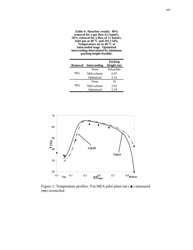
Table 4: Absorber results. 90% removal for a gas flow 6.1 kmol/s.
50% removal for a flow of 11 kmol/s. Inlet gas at 40 oC and 101.1 kPa.
Temperature set to 40 oC at intercooled stage. Optimized
intercooling determined by minimum packing height feasible.
Removal Intercooling Packing
Height (m) None Infeasible
Mid column 6.07 90% Optimized 5.16
None 18 Mid column 2.62 50% Optimized 2.34
Figure 1: Temperature profiles. 9 m MEA pilot plant run (▲) measured (▬) reconciled
327
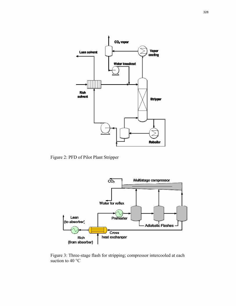
Figure 2: PFD of Pilot Plant Stripper
Figure 3: Three-stage flash for stripping; compressor intercooled at each suction to 40 °C
328
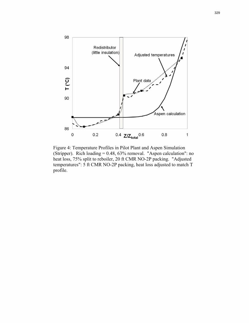
Figure 4: Temperature Profiles in Pilot Plant and Aspen Simulation (Stripper). Rich loading = 0.48, 63% removal. "Aspen calculation": no heat loss, 75% split to reboiler, 20 ft CMR NO-2P packing. "Adjusted temperatures": 5 ft CMR NO-2P packing, heat loss adjusted to match T profile.
329
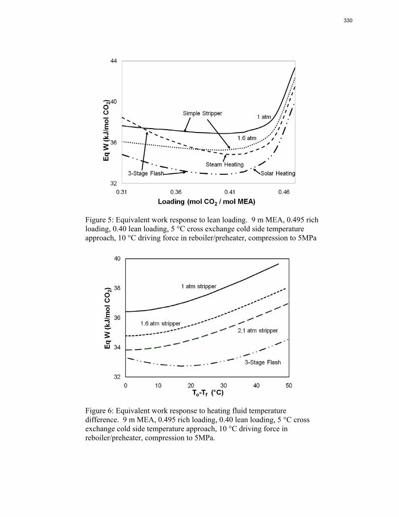
Figure 5: Equivalent work response to lean loading. 9 m MEA, 0.495 rich loading, 0.40 lean loading, 5 °C cross exchange cold side temperature approach, 10 °C driving force in reboiler/preheater, compression to 5MPa
Figure 6: Equivalent work response to heating fluid temperature difference. 9 m MEA, 0.495 rich loading, 0.40 lean loading, 5 °C cross exchange cold side temperature approach, 10 °C driving force in reboiler/preheater, compression to 5MPa.
330
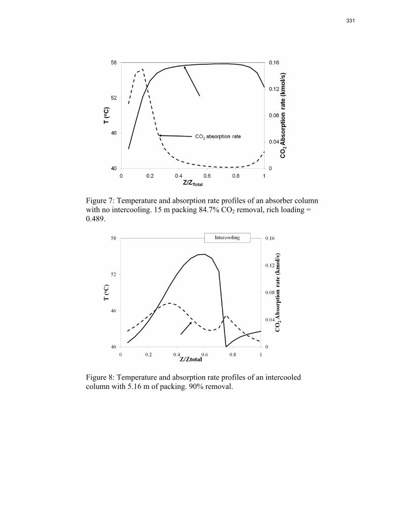
Figure 7: Temperature and absorption rate profiles of an absorber column with no intercooling. 15 m packing 84.7% CO2 removal, rich loading = 0.489.
Figure 8: Temperature and absorption rate profiles of an intercooled column with 5.16 m of packing. 90% removal.
331
2
Catalysts and Inhibitors for Oxidative Degradation of
Monoethanolamine
Andrew J. Sexton, Gary T. Rochelle
Department of Chemical Engineering, University of Texas at Austin,
1 University Station, Austin, TX 78712
Abstract
MEA solutions were subjected to oxidative degradation at both low and high gas
rates. Solutions were degraded with 100 mL/min of 98%O2/2%CO2 with mass transfer
achieved by vortexing. Solutions were analyzed for degradation products by IC and
HPLC. In a parallel apparatus 7.5 L/min of 15%O2/2%CO2 was sparged through
solution, with additional mass transfer achieved by vortexing. A Fourier Transform
Infrared (FTIR) analyzer collected continuous gas-phase data on volatile products.
Hydroxyethyl-formamide (HEF) and hydroxyethylimidazole (HEI) are the major
liquid-phase oxidation products. In the presence of Fe+2 and Cu+2, HEF, HEI, and MEA
losses increase by a factor of 3 as compared to a system with Fe+2 alone. Cr+3 and Ni+2,
two metals present in stainless steel alloys, resulted in MEA losses that are 55%
greater. In terms of oxidative degradation potential (greatest to lowest): Cu+2 > Cr+3/Ni+2
> Fe+2 >V+5.
Inhibitor A reduces the formation of known products by 90% in a system catalyzed
by Fe+2 and Cu+2 and by 99% in combined Cr+3/Ni+2 systems. Inhibitor B reduces
332
3
product rates by 97% and MEA losses by 75%, while a 100:1 ratio of EDTA to Fe+2
completely inhibits oxidation.
Keywords
Monoethanolamine, oxidation, degradation, catalyst, inhibitor
Introduction
Both pre-combustion and post-combustion capture of CO2 from flue gas are being
considered to address global climate change (Davison et al., 2001). Post-combustion
capture involves removing CO2 from flue gas at the end of a power plant cycle. The most
common technologies for post-combustion capture are cryogenics, membranes,
adsorption, and aqueous absorption/stripping (Davison et al., 2001; IEA, 1999; IEA,
2003). Aqueous absorption/stripping involves counter-currently contacting the flue gas
with an aqueous solvent that reacts reversibly with the CO2 in an absorber column. The
solvent is then regenerated in the stripper by applying heat to reverse the reaction and
liberate the CO2.
Several amines are already commonly used in absorption/stripping for natural gas
treating, H2 purification, and NH3 production to remove CO2 and H2S (Kohl & Nielsen,
1997). An illustration of this system is shown in Sexton (Sexton, 2008; Sexton &
Rochelle, in progress).
Oxidation Catalysts: Degradation of the solvent in MEA absorption/stripping occurs by
oxidation and carbamate polymerization (Rochelle & Chi, 2000; Rochelle et al., 2001).
Oxidative degradation is significant in flue gas applications typically containing 5% O2.
333
4
Since most gas treating processes using alkanolamines for CO2 removal are
performed in the absence of oxygen, oxidative degradation is a source of solvent
degradation that has not been properly quantified. Oxidative degradation is important
because it can impact the environment and process economics and decrease equipment
life due to corrosion. Rao and Rubin (2002) estimate solvent degradation to be around
10% of the total cost of CO2 capture.
Two mechanisms for MEA oxidation have been studied by the U.S. Army: electron
abstraction and hydrogen abstraction (Rosenblatt et al., 1963; Rosenblatt et al., 1967;
Dennis et al., 1967; Hull et al., 1967; Petryaev et al., 1984; Alejandre et al., 2000; Button
et al., 1996; Vorobyov et al, 2002). Ammonia, aldehydes, and carboxylic acid
degradation products from MEA oxidation have been noted in several experimental
studies (Fessenden & Fessenden, 1994; Blachly & Ravner, 1964; Rooney et al.,1998;
Critchfield & Jenkins, 1999).
Dissolved iron catalyzes the oxidation of amines (Hall & Barron, 1981; Lee &
Rochelle, 1987; Russell, 1960). The U.S. Navy screened a number of amines for their
relative resistance to oxidative degradation in the presence of 25 to 60 ppm dissolved iron
(Girdler, 1950; Kindrick et al., 1950a & 1950b). Chi (2002) found that dissolved iron
catalyzed MEA degradation rates. Sexton (2008; Sexton & Rochelle, in progress)
observed hydroxyethyl-formamide (HEF) and hydroxyethylimidazole (HEI) as important
products of MEA oxidation in the presence of Fe+2.
Due to the corrosive nature of alkanolamine solvents and their degradation products,
corrosion inhibitors must be added to solutions to prevent equipment destruction
(Polderman et al., 1955; Tanthapanichakoon et al., 2003). These corrosion inhibitors are
334
5
frequently heavy metal salts of vanadium or copper (Asperger et al., 1998; Mago et al.,
1998; Pearce, 1984; Pearce et al., 1984; Ranney 1976). Several studies have shown that
the oxidation of MEA is catalyzed by dissolved metals, including Fe+2, Cu+2, and V+5
(Blachly & Ravner, 1964; Girdler, 1950; Chi & Rochelle, 2002; Blachly & Ravner, 1963;
Hofmeyer et al., 1956).
Blachly and Ravner (1963) examined the effects of metals as oxidation catalysts in
MEA systems. They determined that as little as 10 ppm dissolved copper was sufficient
to cause serious degradation of the amine solution, and that the rates of copper catalyzed
degradation were higher than iron catalyzed degradation at the same metal concentration.
3.7 ppm of nickelous ion had no impact on MEA oxidation, but a tenfold increase in
concentration caused noticeable degradation.
Goff (2005) studied Cu+2 and Fe+2 catalyzed degradation of MEA and found that
copper had a greater catalytic effect than iron. Goff (Goff et al., 2004; 2006) also
examined O2 mass transfer effects and reaction kinetics by changing reaction conditions.
He showed that the rate of NH3 evolution is frequently controlled by the rate of O2
absorption into the amine.
Sexton (in progress; Sexton & Rochelle, 2000) showed in the presence of iron
catalyst, formate, HEF, HEI and ammonia are the major degradation products of MEA
oxidation – although 25% to 50% of degradation products remain unaccounted for.
Minor products include other carboxylic acids (formate, acetate, glycolate), nitrate/nitrite,
NOx/N2O, CO, C2H4, acetaldehyde and formaldehyde.
Oxidation Inhibitors: Ethyelenediaminetetraacetic acid (EDTA) has been identified as
an excellent chelating agent in the presence of copper and iron catalyst (Blachly &
335
6
Ravner, 1964; Chi, 2000; Blachly & Ravner, 1965). EDTA has four active sites that can
effectively bind the metal ions, thereby preventing them from catalyzing free radical
reactions that promote oxidative degradation. Chelation constants have been determined
for Fe-EDTA and Cu-EDTA complexes (Sunda & Huntsman, 2003; Olivieri &
Escandar).
Iron is a known catalyst for EDTA oxidation (Seibig et al., 1997). Iminodiacetic
acid (diglycine), glyoxylic acid, and cyanate have all been identified as anionic
degradation products of EDTA in the presence of UV and H2O2 (Sorensen et al., 1998).
Sorensen also shows that dissolved iron can catalyze EDTA degradation into organic
products ethylenediaminetriacetate (ED3A), ethylenediaminediacetate (EDDA) and
ethylenediaminemonoacetate (EDMA).
Inhibitor A – a reaction inhibitor – has proven to be effective with Fe+2 and Cu+2
catalyzed MEA systems (Goff 2005). Na2SO3 is a known oxygen scavenger that is used
in a range of applications varying from boiler feedwater treating to food packaging
(Somogyi, 2008; White, 2001; Hakka & Ouimet, 2004). The kinetics of sulfite oxidation
in aqueous solutions are known to be very fast, and the rate of oxidation is controlled by
the rate of oxygen absorption (Ulrich, 1983; Lee. 1986). SO2 reacts quickly with O2 in
MEA solutions to form sulfate (SO4-2), forming a heat stable salt with MEA. Previous
studies have shown that sulfite oxidation shows a square root dependence on catalyst
concentration, independent of the metal being used (Barron et al., 1966; Conklin et al,,
1988; Bengtsson et al, 1975; Chen et al, 1972).
Formaldehyde is an expected intermediate in the oxidative degradation of MEA
(Goff, 2005; Goff et al., 2004; 2006; Chi, 2000; Blachly & Ravner, 1965; Rochelle et al.,
336
7
2003). Formate is an observed product in the oxidation of formaldehyde.18,20 Since both
of these products likely compete with MEA for oxygen, they are suitable compounds to
screen as degradation inhibitors. Although formaldehyde itself is considered toxic under
the Clean Air Act EPA Technology Transfer Website), the presence of oxygen should
oxidize the formaldehyde to formate, or it may react with MEA to form hydroxyethyl-
formamide.
A major objective of this study was to compare and contrast key liquid and gas-
phase oxidation products of MEA in the presence of Fe+2, Cu+2, Cr+3, Ni+2 and V+5
catalysts. The other objective was to test the effectiveness of EDTA, sulfite, formate, and
proprietary Inhibitors A and B as oxidation inhibitors. An oxygen consumption rate is
calculated from product rates and their respective stoichiometries in order to determine
whether degradation is controlled by kinetics or by the oxygen mass transfer under each
set of reaction conditions.
Experimental Methods
Apparatus: Oxygen mass transfer was achieved at low gas rate by introducing 100
mL/min of 98%O2/2%CO2 gas into the vapor space above 350 mL of an agitated amine
solution in a temperature-controlled semi-batch reactor. In a different apparatus at high
gas rate, 7.5 L/min of 15%O2/2%CO2 was sparged through 350 mL of amine solution.
Sexton (2008; Sexton & Rochelle, 2000) provides a detailed description of these
apparatus.
Analytical Methods: Anions, cations, and molecules from oxidized MEA were
determined by ion chromatography and HPLC as described previously by Sexton (2008;
Sexton & Rochelle, 2000).
337
8
Oxygen Stoichiometry: Goff (2005) proposed that MEA reacts with oxygen to form
ammonia and other carbon containing degradation products. Each of the major
degradation products has a specific oxygen stoichiometry, which is listed in Sexton
(2008; Sexton & Rochelle, 2000).
Results
Oxidation experiments were performed at high and low gas rates under varying
inhibitor and catalyst conditions. Liquid phase product rates were calculated by dividing
the final concentration of each individual component by the total experiment time. For
each volatile component, the continuous production rate is integrated over the entire
experiment and reported as an average rate (mM/hr). MEA volatility was calculated and
quantified in the same manner.
Amides were determined by both HPLC (HEF only) and anion IC with pretreatment
by NaOH (acetamide, glycolamide, formamide, and oxamide). However, the HPLC is
believed to give a more reliable concentration for HEF. Therefore, it has been used in all
material balances. Concentrations for unknown peaks from HPLC were estimated using
the calibration curve for HEI.
Total MEA loss is calculated from initial and final MEA as determined by cation IC;
loss rates less than 0.3 mM/hr are too small to detect using this method. With high gas
rate, overall MEA loss was calculated using cation chromatography and volatile MEA
loss was calculated using FTIR. The difference between these two rates gave an MEA
degradation loss rate.
338
9
The total carbon and nitrogen in products was calculated without including
formamide by IC or unknowns by HPLC. Nitrogen in solution was determined using
Kjeldahl analysis; total organic carbon in solution was calculated using a Shimadzu TOC
analyzer. The nitrogen imbalance is nitrogen unaccounted for after MEA nitrogen and
product nitrogen concentrations are subtracted from total nitrogen in solution; the carbon
imbalance is calculated in a similar manner.
Total oxygen consumption is determined by calculating the summation of the oxygen
stoichiometry coefficient () for each degradation product multiplied by the respective
degradation rate of each product.
Catalyst Effect – Low Gas Rate: Figure 1 illustrates the formation of major oxidative
degradation products for systems catalyzed by Fe+2 and Cu+2. Major degradation
products include HEI, HEF, and formate.
Low gas experiments detailed in Table 1 were performed in an attempt to quantify
how metal catalysts affect the oxidative degradation of MEA. Vanadium has been
suggested as a corrosion inhibitor for piperazine systems, while chromium and nickel are
present in stainless steel alloys. Blachly and Ravner (1963) detailed the catalytic effects
of nickel and chromium on MEA.
With all four catalyst combinations, HEI, HEF, and formate are the most abundant
degradation products. The production rate of HEF is almost an order of magnitude
higher in the presence of Fe+2 and Cu+2 compared to Fe+2 alone, while the production of
HEI increases by a factor of three. This results in a carbon formation rate that is
approximately three times greater, and an MEA loss rate that is over double from when
copper is absent from solution.
339
10
The addition of copper to an oxidized MEA solution appears to enhance the mass
transfer characteristics of the solution; the oxygen consumption rate of this system is
considerably higher than the other catalyzed systems. On the other hand, vanadium
catalyzed systems exhibit lower degradation and oxygen consumption rates. Goff
concluded that all catalyzed systems were controlled by oxygen mass-transfer but the
data do not reflect that. However, the unidentified degradation products may affect these
calculated oxygen consumption rates. In terms of greatest to lowest oxidation potential
with regards to aqueous MEA systems, Fe+2/Cu+2 > Cr+3/Ni+2 > Fe+2 > V+5.
Figure 1:
Table 1.
Table 1 shows that 7 m MEA catalyzed with 1 mM of sodium metavanadate is
degraded less than with 1 mM Fe+2, which serves as our base case for comparison. There
is a noticeable shift from the production of formate to oxalate (as well as their respective
amides), but overall formation of carbon products is 75% lower in the presence of
vanadium. Nitrogen production (in the form of nitrite/nitrate) is also 75% lower in the
vanadium catalyzed experiment, and MEA losses are cut in half compared to the iron
catalyzed experiment. This reduction in carbon and nitrogen products is attributed to the
two major degradation products: HEF and HEI.
Carbon and nitrogen formation rates in the experiment catalyzed by both chromium
and nickel are approximately 15% lower than in the iron catalyzed experiment. Most of
340
11
this is accounted for by the reduced production of HEI. There is once again a noticeable
shift from formate (and formamide) to oxalate production. However, measured MEA
losses are 53% greater. This suggests that there are signifcant degradation products
unaccounted for in this experiment.
With the exception of the experiment performed in the presence of chromium and
nickel, the carbon material balance ranges from 87% to 104%. Moreover, the nitrogen
material balance ranges from 92% to 101% for the selected low gas experiments.
From HPLC-ELSD analysis, most degraded samples containing only Fe+2 have at
least 90% of raw peak area unidentified. On the other hand, 18% to 52% of the peak area
remains unidentified for degradation experiments with Cu+2. This suggests that the
formation of HEF and HEI is favored when Cu+2 is present.
Oxygen consumption ranges from 0.7 to 5.6 mM/hr for low gas experiments
performed in the absence of effective oxidative degradation inhibitors. Mass transfer of
oxygen into the interfacial layer of liquid determines the degradation rate for these low
gas experiments. The presence of Cu+2 enhances mass transfer such that the reaction is
taking place in the boundary layer.
Experiments performed in the presence of iron as well as a combination of chromium
and nickel gave similar O2 rates. The low oxygen rate calculated in the presence of
vanadium suggests MEA degradation may not be completely mass transfer controlled in
the presence of vanadium catalyst. It is important to note that oxygen consumption rates
do not take unidentified products into account.
341
12
An average oxygen stoichiometry for each experiment was calculated in which
HPLC analysis had been performed. An approximate MEA loss was calculated for each
experiment using the total C and N in products; for example, in the Fe+2 experiment,
MEA loss from detected products was 2.8 mM/hr. A formation rate of 2.5 mM/hr of N in
products correlates to 2.5 mM/hr of degraded MEA, while 6.3 mM/hr C in products
correlates to 3.15 mM/hr of degraded MEA; the mathematical average equates to 2.8
mM/hr. Since the oxygen consumption rate is 2.1 mM/hr, the average oxygen
stoichiometry is 0.75 mol O2/mol MEA degraded at iron-catalyzed conditions. The
average value ranges from 0.65 for Fe+2/Cu+2 catalyst to 0.76 at Cr+3/Ni+2 catalyst
conditions to 1.00 at V+5 conditions.
Catalyst Effect – High Gas: Table 2 lists both liquid-phase and gas-phase product rates
for MEA degradation experiments conducted in the high gas flow apparatus. For each
volatile component, a continuous plot of concentration (in ppmv) versus experiment time
was constructed and the area under the curve was approximated so that a total
concentration of each component evolved during the course of the experiment could be
calculated. This value was then converted into a production rate (using total experiment
time, molar gas rate and solution volume) in units of mM/hr. MEA volatility was
calculated and quantified in the same manner. For the high gas experiments, overall
MEA loss was calculated using cation chromatography and volatile MEA loss was
calculated using FTIR analysis. The difference between these two rates gave an MEA
degradation loss rate.
The major difference between the experiments with iron and experiments with iron
and copper is the increase in formate and HEF production. HEF production increases by
342
13
a factor of two when copper is added in the high gas apparatus. HEI is only detected in
the high gas apparatus in the presence of iron and copper and is present in much lower
concentrations than at low gas flow. The reduction of HEI at high gas rates could be
attributed to the stripping of aldehyde or ammonia needed for HEI synthesis.
Gas-phase aldehydes, whose concentrations are minor compared to the amides,
decrease when MEA is degraded in the presence of iron and copper. This suggests that
the aldehydes are reacting faster in the presence of both iron and copper, leaving a lower
concentration in solution. All other major degradation product formation rates, including
ammonia, are similar between the two systems. This contradicts the observation of Goff
(2005) that both copper and iron individually produced different steady-state ammonia
formation rates for MEA.
With high gas rate in the presence of iron and copper, 48% to 68% of the degraded
MEA carbons have been accounted for in measured degradation products; 75% to 100%
of the nitrogen loss has been accounted for in degradation products. Although the
material balance is not closed, the gap is smaller for the experiments conducted in the
presence of iron and copper. The carbon to nitrogen ratio ranges from 1.25:1 to 1.38:1
for this set of experiments.
With high gas rate, oxygen consumption ranged from 0.9 to 1.9 mM/hr. Rates
increased by approximately 85% in the presence of copper and iron versus iron only.
These oxygen rates only take into account identified products; the larger gap in the
material balance for the iron experiments could account for this oxygen difference.
Theoretically, oxygen consumption rates will increase as more products are discovered
343
14
and the gap in the material balance closes. The average value ranges from 0.65 to 0.85
at iron only conditions; it varies from 0.55 to 0.64 when both iron and copper are present.
Table 2.
Successful Inhibitors: Table 3 shows that Inhibitor A is an extremely effective
oxidative degradation inhibitor for MEA systems in the presence of chromium and nickel
(over a 99% reduction in the formation of all detectable products). Moreover, MEA loss
rate was reduced by a factor of eight and is approaching the detection limits of the cation
chromatography system.
Experimental results also show Inhibitor B to be effective at inhibiting degradation
in the presence of iron catalyst. Carbon and nitrogen-containing products are reduced by
97%, while MEA loss rates were reported in the range of the inhibited Cr+3/Ni+2 system –
only 25% the MEA loss rate of an uninhibited system catalyzed by iron. Rates for
experiments performed under inhibited conditions ranged from 0.0 to 0.9 mM/hr; the
degradation rate in these types of experiments is expected to be limited by reaction
kinetics. Since the rate is no longer oxygen mass transfer controlled, an average oxygen
stoichiometry was not calculated.
Figure 2 illustrates the effect of EDTA:Fe ratio on nitrogen and carbon production,
as well as MEA losses. A concentration of 100 mM EDTA completely inhibits any MEA
degradation. Table 3 details the product rates illustrated in Figure 2. Both degradation
product formation and MEA loss decrease as EDTA concentration is increased. This
suggests that in high enough concentration, EDTA is effective at chelating Fe+2 and
inhibiting the formation of observable oxidative degradation products. The major issue
with using EDTA in an industrial application as an inhibitor may be corrosion. Corrosion
344
15
creates an endless supply of Fe+2 to complex with EDTA, and the EDTA will continue to
complex the iron until all of its active sites are unavailable. The EDTA/Fe complex
would have to be reclaimed or fresh EDTA would have to be added to the solution – the
latter of which is not an economically viable option.
Table 3:
Figure 2:
Unsuccessful Inhibitors: Table 4 shows that sodium sulfite, formaldehyde, and formate
were all ineffective as degradation inhibitors for the observed MEA systems. For the first
50 to 75 hours of the sodium sulfite experiment, it appears that oxidative degradation
products were being formed at a reduced rate, suggesting that sulfite was oxidizing to
sulfate and was nominally protecting the MEA from oxidative degradation. However,
once all of the sulfite was consumed and oxidized, oxidation products formed at a rate
similar to an MEA/Fe+2 solution oxidized with no inhibitors added. While observed
products were reduced by 15% to 20%, the MEA loss rate increased by about 30% over
an iron catalyzed solution in the absence of sodium sulfite.
Figure 3 illustrates the formation of degradation products over time with low gas rate
in the presence of iron and formaldehyde. The hypothesis is that the reaction
intermediate (formaldehyde) would react faster with the available oxygen and be
consumed quicker than the MEA, thereby protecting it from oxidative degradation.
However, results from Table 4 show the addition of formaldehyde had little impact on
reducing product rates, and increased the MEA loss rate by about 30% – similar to the
sodium sulfite experiment. In the presence of copper, HEF rates double, while HEI
345
16
formation rates increase by a factor of 3. The MEA loss rate approaches the rate of an
MEA system catalyzed by iron and copper in the absence of formaldehyde.
Unlike other experiments, Figure 3 reveals that degradation products are not formed
at a constant rate in the presence of formaldehyde. A large concentration of formamide is
produced at the beginning of the experiment; this supports the theory that formamide can
be produced by directly reacting MEA with formaldehyde at these experimental
conditions. The figure also shows that after the initial formation of products, all ionic
product concentrations appear to be reaching some type of steady-state concentration.
After degradation began, the ratio of MEA formamide to formate stayed constant at 4:1.
Figure 4 illustrates the concentration of observed degradation products during the
course of a low gas experiment testing 500 mM formate as an oxidation inhibitor.
Initially, formate is observed at a concentration of 330 mM according to anion IC, even
though 500 mM was added. During the first 75 hours of the experiment, while formate
concentration remains constant, formamide concentration increases to approximately 170
mM – thus accounting for the “missing” formate.
During the middle of the experiment, formate (and formamide) concentration
decreased, suggesting formate was oxidizing faster than it was being produced. At 150
hours, formate concentration begins to increase once again, suggesting formate
production occurred faster than formate oxidation.
The copper-catalyzed MEA system containing 500 mM formaldehyde behaved quite
similarly to the iron-catalyzed formaldehyde experiment. HEF is present at a 4:1 ratio
with formate. Rates in Table 4 show formate performs slightly better than formaldehyde
346
17
in the presence of iron, but worse than a system in the absence of formate. Observed
carbon and nitrogen products are 20 to 30% lower, but MEA losses are 20% higher.
In the presence of iron only, the oxygen consumption rate was calculated between
1.6 and 1.7 mM/hr, independent of catalyst. The average oxygen stoichiometry was
between 0.65 and 0.75 mol O2 consumed/mol MEA degraded. However, when Cu+2 was
added to the formaldehyde system, the oxygen consumption increased to 3.6 mM/hr and
the stoichiometry dropped to 0.57. This is consistent with results at low and high gas
conditions in the absence of inhibitors.
Figure 3:
Figure 4:
Table 4.
Conclusions
When both iron and copper are present in solution, HEF production, HEI production
and MEA losses increase by a factor of 3 compared to a system absent of iron. High gas
experiments supported these observations. In terms of oxidative degradation potential:
copper > chromium/nickel > iron > vanadium.
Experiments with low gas flow reveal that HEF and HEI are the major oxidation
products of MEA. MEA systems catalyzed by 1 mM vanadium produce much less
formate (as well as formamide) and HEI, but more oxamide than systems catalyzed by
iron. Overall, carbon and nitrogen formation rates were lower, as well as MEA losses.
Chromium and nickel, two metals present in stainless steel alloys, also catalyze the
oxidative degradation of MEA. Observed carbon and nitrogen product rates are 20%
347
18
lower than in an iron catalyzed system, while MEA losses are 55% greater. This suggests
that chromium and nickel combined have a greater catalytic effect than iron by itself.
Data from experiments with high gas flow show that a combination of copper and
iron creates more HEF (the major carbon-containing degradation product) and HEI than
iron by itself. The presence of copper in aqueous MEA solution enhances the production
of both formate and HEF, which experiments show is created from either the reaction of
formaldehyde or a metal-formate complex with MEA.
Ammonia is the dominant nitrogen-containing degradation product at high gas. At
high gas rate, NOx is produced and stripped from the solution. On the other hand, at low
gas rate where gas is not stripped from solution, NOx is retained in the solution and
oxidized to nitrite and nitrate. High gas flow experiments show that average ammonia
production is independent of metal catalyst, which contradicts results of Goff.
Inhibitor A reduces the formation of known products by over 99% and cuts MEA
losses by a factor of eight in Cr+3/Ni+2 catalyzed systems; Sexton (2008; Sexton &
Rochelle, in progress) previously showed the presence of 100 mM Inhibitor A reduces
the formation of known degradation products by 90% in an MEA system catalyzed by
both iron and copper. In the presence of iron, Inhibitor B reduces product rates by 97%
and MEA losses by 75%. Low gas experiments show that a 100:1 ratio of EDTA to Fe+2
is necessary to sufficiently inhibit the oxidation of MEA. At this ratio, no observable
MEA losses or oxidative degradation products are detected.
The addition of formaldehyde, formate, or sodium sulfite had an unintended effect
on MEA losses. They actually increased the rate at which MEA degraded. While
observed products decreased, MEA losses increased by 20% to 30% in the presence of
348
19
these potential inhibitors; the greater concentration of unidentified products offsets the
decrease in observed products.
Under assumed mass transfer conditions in the low gas apparatus, calculated oxygen
consumption ranges from 1.6 to 1.9 mM/hr in all experiments performed in the presence
of Fe+2 and Cr+3/Ni+2, 3.6 to 5.6 mM/hr for experiments performed in the presence of
Cu+2, and 0.7 mM/hr in the presence of V+5. Oxygen consumption rates were 0.2 mM/hr
or less under assumed inhibited conditions. The experiment performed at 2 mM EDTA is
in the region controlled by both kinetics and mass transfer.
The value of the oxygen stoichiometry () is independent of the experimental
apparatus. Average stoichiometry varies from 0.65 to 0.75 in the presence of Fe+2 and
from 0.55 to 0.65 in the presence of both Fe+2 and Cu+2. Single experiments give a
calculated of 0.76 for Cr+3/Ni+2 and 1.00 for V+5 at low gas conditions.
Total carbon and nitrogen analysis shows that, with the exception of the low gas
experiment performed in the presence of Cr+3 and Ni+2 catalyst, there is over a 90%
material balance on all selected low and high gas flow experiments.
Acknowledgements
This work was supported by the Luminant Carbon Management Program at The
University of Texas at Austin. Mark Nelson of Air Quality Analytical helped develop
methods for the FTIR. Jason Davis at The University of Texas at Austin assisted in
developing the HPLC-ELSD method, and Robert Grigsby of Huntsman chemical aided in
positively identifying the HPLC peaks. Special thanks go to undergraduate research
assistants Jang Lee, Jon Mellin, and Humera Rafique.
349
20
References
Alejandre, J., Rivera, J.L., Mora, M.A., De la Garza, V., 2000. Force Field of
Monoethanolamine. J. Phys Chem B, 104(6), 1332–1337.
Asperger, R.G., Tebbal, S., Kane, R.D., 1998. (CLI International, Inc.) Corrosion
Inhibitor and Its Use; Patent Application WO 9828381 A1 19980702.
Barron, C.H. et al., 1966. Reaction Kinetics of Sodium Sulfite Oxidation by the Rapid
Mixing Methodology. Chem. Eng. Sci. 21, 397–404.
Bengtsson, S. et al., 1975. Catalytic Oxidation of Sulphite in Diluted Aqueous Solutions.
Chem. Eng. Sci. 30, 1429–1435.
Blachly, C.H., Ravner, H. 1963. The Effect of Trace Amounts of Copper on the Stability
of Monoethanolamine Scrubber Solutions; NRL-MR-1482; U.S. Naval Research
Laboratory: Washington, DC.
Blachly, C.H., Ravner, H., 1964. The Stabilization of Monoethanolamine Solutions for
Submarine Carbon Dioxide Scrubbers. AD609888, NRL-FR-6189; NRL-6189;
Naval Research Laboratory: Washington, DC.
Blachly, C.H., Ravner, H., 1965. Studies of Submarine Carbon Dioxide Scrubber
Operation: Effect of an Additive Package for the Stabilization of Monoethanolamine
Solutions; NRL-MR-1598; U.S. Naval Research Laboratory: Washington, DC.
Button, J.K., Gubbins, K.E., Tanaka, H., Nakanishi, K., 1996. Molecular Dynamics of
Hydrogen Bonding in Monoethanolamine. Fluid Phase Equilib. 116(1–2), 320–325.
Carbon Dioxide Absorbants. 1950. Girdler Corporation, Gas Processes Division,
Louisville, KY.
Chen, T.-I et al., 1972. Some Aspects of the Homogeneous Kinetics of Sulfite Oxidation.
Ind. Eng. Chem. Fund. 11(4), 466–470.
350
21
Chi, Q.S., 2000. Oxidative Degradation of Monoethanolamine. M.S. Thesis, The
University of Texas at Austin, Austin, TX.
Chi, S., Rochelle, G.T., 2002. Oxidative Degradation of Monoethanolamine. Ind. Eng.
Chem. Res. 41(17), 4178–4186.
Conklin, M.H. et al. 1988. Metal Ion-Sulfur(IV) Chemistry. 2. Kinetic Studies of the
Redox Chemistry of Copper(II)-Sulfur(IV) Complexes. Env. Eng. Sci. 22(8), 891–
898.
Critchfield, J.E. and Jenkins, L., 1999. Evidence for MDEA degradation in tail gas
treating plants. Petrol. Tech. Quarterly.
Davison, J., Freund, P., Smith, A., 2001. Putting Carbon Back into the Ground. IEA
Greenhouse Gas R&D Programme. 28.
Dennis, W.H., Jr., Hull, L.A., Rosenblatt, D.H. 1967. Oxidations of Amines. IV.
Oxidative Fragmentation. J. Org. Chem. 32(12): 3783-3787.
EPA Technology Transfer Network Air Toxics Website, The original list of hazardous air
pollutants, http://www.epa.gov/ttn/atw/orig189.html (Accessed January 2008).
Fessenden, R.J. Fessenden, J.S., 1994. Organic Chemistry. fifth ed. Brooks/Cole
Publishing Company, Pacific Grove, CA.
Goff, G.S., 2005. Oxidative Degradation of Aqueous Monoethanolamine in CO2 Capture
Processes: Iron and Copper Catalysis, Inhibition, and O2 Mass Transfer. Ph.D.
Dissertation, The University of Texas at Austin.
Goff, G.S. et al., 2004. Monoethanolamine Degradation: O2 Mass Transfer Effects under
CO2 Capture Conditions. Ind. Chem. Eng. Res. 43(20), 6400–6408.
351
22
Goff, G.S. et al., 2006. Oxidation Inhibitors for Cu Catalyzed Degradation of
Monoethanolamine in CO2 Capture Processes. Ind. Chem. Eng. Res. 45(8), 2513–
2521.
Hall, W.D. and Barron, J.G., 1981. Solving Gas Treating Problems – A Different
Approach. Presented at the Laurence Reid Gas Conditioning Conference, Norman,
OK.
Hakka, L.E., Ouimet, M.A. 2004. Recovery of CO2 from Waste Gas Streams Using
Amines as Absorbents; U.S. Patent Application 2004253159.
Hofmeyer, B.G. et al., 1956. Contamination and Corrosion in Monoethanolamine Gas
Treating Solutions. Am. Chem. Soc., Div. Petrol. Chem., Preprints. 1(2), 91–99.
Hull, L.A., Davis, G.T., Rosenblatt, D.H., Williams, H.K.R., Weglein, R.C., 1967.
Oxidations of Amines. III. Duality of Mechanism in the Reaction of Amines with
Chlorine Dioxide. J. Am. Chem. Soc. 89(5): 1163–1170.
IEA, 1999. Carbon Dioxide Capture from Power Stations. IEA Greenhouse Gas R&D
Programme: http://www.ieagreen.org.uk/capt1.htm (Accessed July 2008).
IEA, 2003. CO2 Capture at Power Stations and Other Major Point Sources. International
Energy Agency, Working Party on Fossil Fuels: Paris, France, 13.
Kindrick, R.C., Atwood, K., Arnold, M.R., 1950. The Relative Resistance to Oxidation
of Commercially Available Amines. Girdler Report No. T2.15-1-30, in “Report:
Carbon Dioxide Absorbents”, Contract No. NObs-50023, by Girdler Corp., Gas
Processes Division, Louisville, KY, for the Navy Department, Bureau of Ships,
Washington, DC (Code 649P).
352
23
Kindrick, R.C., Reitmweier, R.E., Arnold, M.R., 1950. A Prolonged Oxidation Test on
Amine Solutions Resistant to Oxidation. Girdler Report No. T2.15-1-31, in “Report:
Carbon Dioxide Absorbents”, Contract No. NObs-50023, by Girdler Corp., Gas
Processes Division, Louisville, KY, for the Navy Department, Bureau of Ships,
Washington, DC (Code 649P).
Kohl, A. and Nielsen, R., 1997. Gas Purification. 5th ed.; Gulf Publishing Co.: Houston.
Lee, Y.J., 1986. Oxidative Degradation of Organic Acids Conjugated with Sulfite
Oxidation in Flue Gas Desulfurization. Ph.D. Thesis, The University of Texas at
Austin, Austin, TX.
Lee, Y.J. and Rochelle, G.T., 1987. Oxidative Degradation of Organic Additives for Flue
Gas Desulfurization: Products, Kinetics, and Mechanism. Env. Sci. & Tech. 21, 266–
272.
Mago, B.F. et al., 1984. Corrosion Inhibitors for Alkanolamine Gas Treating System.
U.S. Patent 3 959 170.
Olivieri, A.C., and Escandar, G.M, 1997. Random Error Analysis in the Determination of
Equilibrium Constants of Very Stable Metal Complexes. Anal. Let. 30(10), 1967–
1980.
Pearce, R.L.. 1984. Removal of Carbon Dioxide From Industrial Gases. U.S. Patent 4 440
731.
Pearce, R.L. et al., 1984. Recovery of Carbon Dioxides from Gases. U.S. Patent 2 135
900.
Petryaev, E.P., Pavlov, A.V., Shadyro, O.I. 1984. Homolytic deamination of Amino
Alcohols. Zh. Org. Khim. 20(1), 29–34.
353
24
Polderman, L.D. et al., 1955. Why Monoethanolamine Solution Breaks Down in Gas-
Treating Service. Oil Gas J. 54(2), 180–183.
Ranney, M.W., 1976. Corrosion Inhibitors – Manufacture and Technology; Noyes Data
Corporation: Park Ridge, NJ.
Rao, A.B. and Rubin, E.S., 2002. A Technical, Economic, and Environmental
Assessment of Amine-Based CO2 Capture Technology for Power Plant Greenhouse
Gas Control. Env. Sci. & Tech. 36(20), 4467–4475.
Rochelle, G.T. and Chi, S., 2000. Oxidative Degradation of Monoethanolamine. First
National Conference on Carbon Sequestration, Washington, DC.
Rochelle, G.T., Bishnoi, S., Chi, S., Dang, H., Santos, J., 2001. Research Needs for CO2
Capture from Flue Gas by Aqueous Absorption/Stripping. DE-AF26-99FT01029;
U.S. Department of Energy – Federal Energy Technology Center: Pittsburgh, PA.
Rochelle, G.T. et al., 2003. Research Results for CO2 Capture from Flue Gas by Aqueous
Absorption/Stripping. LRGCC Conf. Proc. 53, 131–152.
Rooney, P.C., DuPart, M.S., Bacon, T.R., 1998 Oxygen’s Role in Alkanolamine
Degradation. Hydro. Proc., Int. Ed. 77(7), 109–113.
Rosenblatt, D.H., Hayes, A.J., Jr., Harrison, B.L., Streaty, R.A., Moore, K.A., 1963.
Reaction of Chlorine Dioxide with Triethylamine in Aqueous Solution. J. Org.
Chem. 28(10), 2790–2794.
Rosenblatt, D.H., Hull, L.A., DeLuca, D.C., Davis, G.T., Weglein, R.C., Williams,
H.K.R., 1967. Oxidations of Amines. II. Substituent Effects in Chlorine Dioxide
Oxidations. J. Am. Chem. Soc. 89(5), 1158–1163.
354
25
Russell, G.A., 1960. Peroxide Pathways to Autoxidation, in J. O. Edwards (Ed.),
Peroxide Reaction Mechanism Interscience Publishers, New York, pp. 107–128.
Seibig, S. et al., 1997. Kinetics of [FeII(EDTA)] Oxidation by Molecular Oxygen
Revisited. New Evidence for a Multistep Mechanism. Inorg. Chem. 36(18), 4115–
4120.
Sexton, A.J., 2008. Amine Oxidation in CO2 Capture Processes. Ph.D. Dissertation. The
University of Texas at Austin.
Sexton, A.J. and Rochelle, G.T., in progress. Reaction Products from the Oxidative
Degradation of MEA.
Somogyi, L.P. Food Additives in Kirk-Othmer Encyclopedia of Chemical Technology,
http://www.mrw.interscience.wiley.com/kirk/articles/foodfrie.a01/frame.html
(Accessed January 2008).
Sorensen, M., Zurell, S., Frimmel F.H., 1998. Degradation Pathway of the Photochemical
Oxidation of Ethylenediaminetetraacetate (EDTA) in the UV/H2O2 Process. Acta
Hydrochim. 26(2), 109–115.
Sunda, W. and Huntsman, S., 2003. Effect of pH, light, and temperature on Fe-EDTA
chelation and Fe hydrolysis in seawater. Marine Chem. 84(1–2), 35–47.
Tanthapanichakoon, W. et al., 2003. Heat Stable Salts and Corrosivity in Amine Treating
Units; Greenhouse Gas Control Technologies, Proceedings of the 6th International
Conference on Greenhouse Gas Control Technologies, Kyoto, Japan, October 1–4,
2002; Pergamon: New York, 2003; Vol. 2, pp 1591–1594.
355
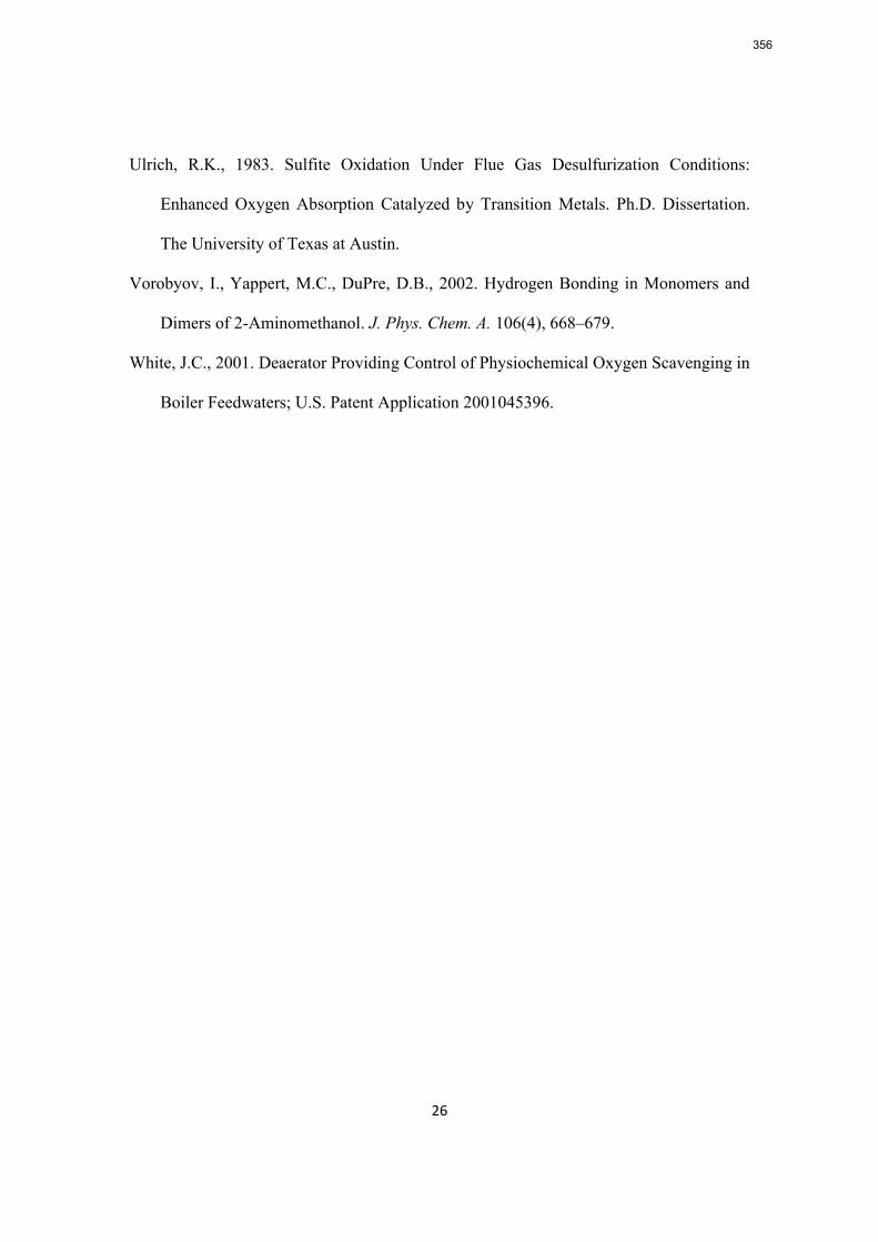
26
Ulrich, R.K., 1983. Sulfite Oxidation Under Flue Gas Desulfurization Conditions:
Enhanced Oxygen Absorption Catalyzed by Transition Metals. Ph.D. Dissertation.
The University of Texas at Austin.
Vorobyov, I., Yappert, M.C., DuPre, D.B., 2002. Hydrogen Bonding in Monomers and
Dimers of 2-Aminomethanol. J. Phys. Chem. A. 106(4), 668–679.
White, J.C., 2001. Deaerator Providing Control of Physiochemical Oxygen Scavenging in
Boiler Feedwaters; U.S. Patent Application 2001045396.
356
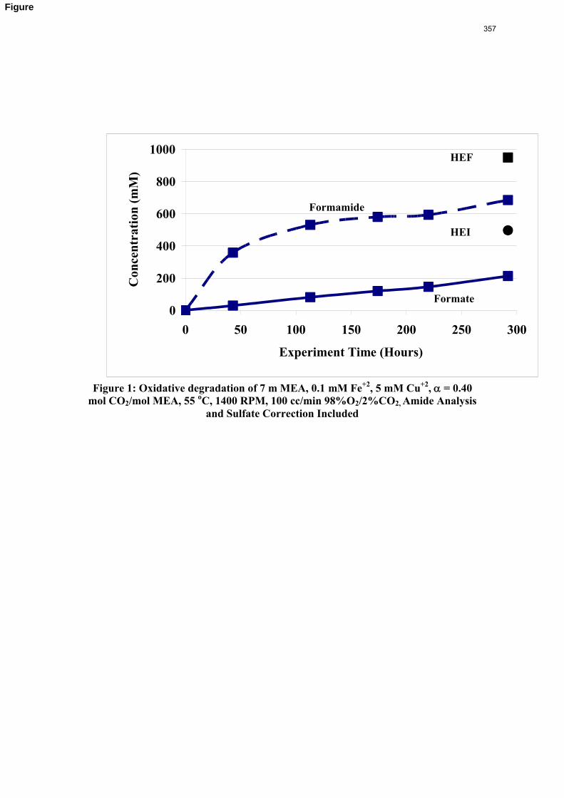
0
200
400
600
800
1000
0 50 100 150 200 250 300
Experiment Time (Hours)
Con
cent
rati
on (
mM
)
Figure 1: Oxidative degradation of 7 m MEA, 0.1 mM Fe+2, 5 mM Cu+2, = 0.40mol CO2/mol MEA, 55 oC, 1400 RPM, 100 cc/min 98%O2/2%CO2, Amide Analysis
and Sulfate Correction Included
HEF
HEI
Formamide
Formate
Figure
357
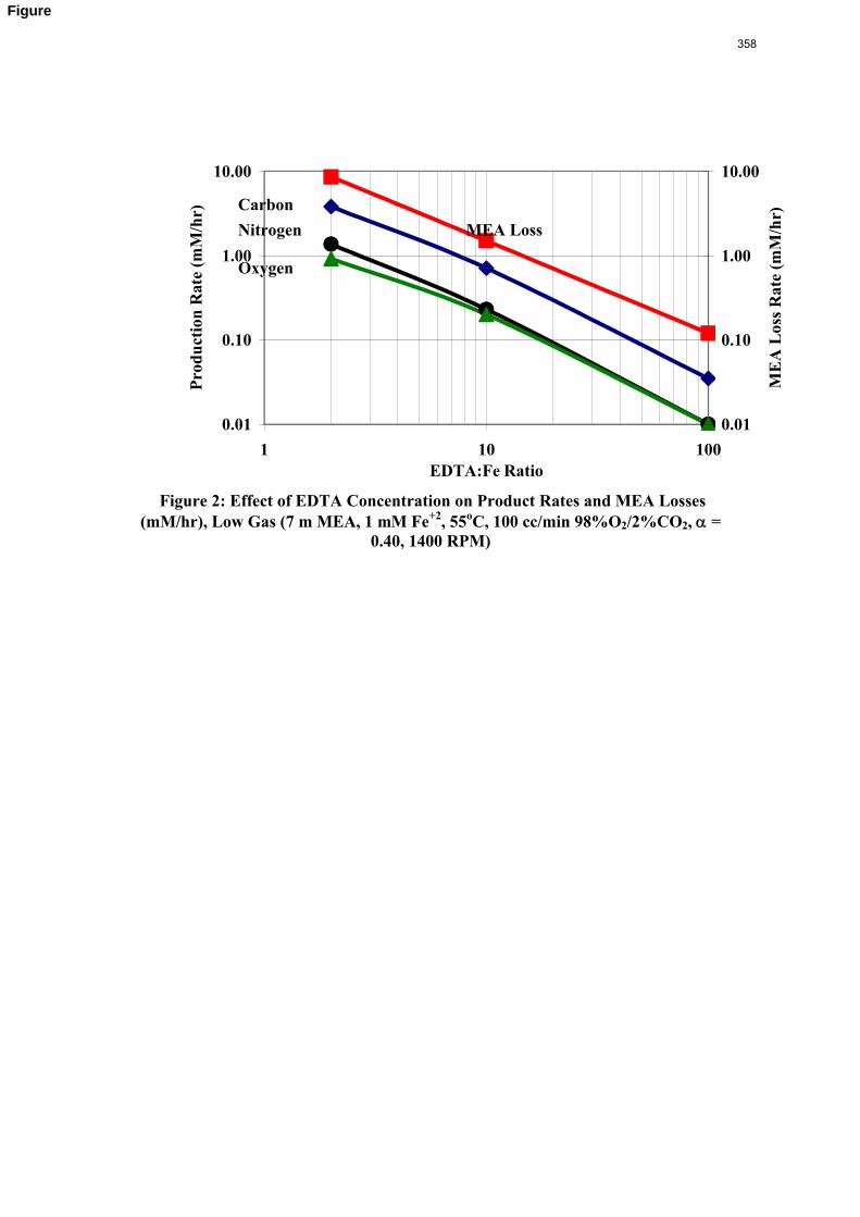
0.01
0.10
1.00
10.00
1 10 100EDTA:Fe Ratio
Pro
du
ctio
n R
ate
(mM
/hr)
0.01
0.10
1.00
10.00
ME
A L
oss
Rat
e (m
M/h
r)
Figure 2: Effect of EDTA Concentration on Product Rates and MEA Losses(mM/hr), Low Gas (7 m MEA, 1 mM Fe+2, 55oC, 100 cc/min 98%O2/2%CO2, =
0.40, 1400 RPM)
MEA Loss
Carbon
Nitrogen
Oxygen
Figure
358
0
50
100
150
200
250
0 50 100 150 200 250 300 350
Experiment Time (Hours)
Con
cent
rati
on (
mM
)
Figure 3: Oxidative degradation of 7 m MEA, 1 mM Fe+2, 500 mM Formaldehyde, = 0.40 mol CO2/mol MEA, 55 oC, 1400 RPM, 100 cc/min 98%O2/2%CO2, Amide
Analysis and Sulfate Correction included
Formamide
OxamideFormate
Nitrite
HEI
Figure
359
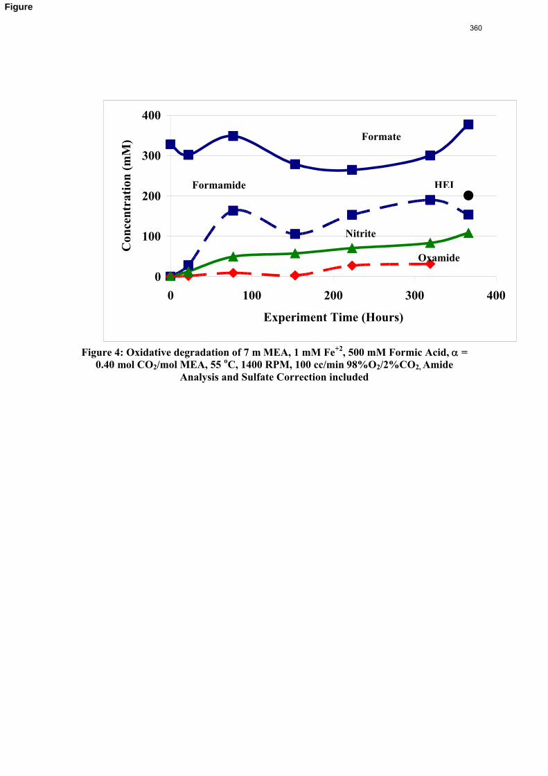
0
100
200
300
400
0 100 200 300 400
Experiment Time (Hours)
Con
cent
rati
on (
mM
)
Figure 4: Oxidative degradation of 7 m MEA, 1 mM Fe+2, 500 mM Formic Acid, = 0.40 mol CO2/mol MEA, 55 oC, 1400 RPM, 100 cc/min 98%O2/2%CO2, Amide
Analysis and Sulfate Correction included
Formate
Formamide
Oxamide
Nitrite
HEI
Figure
360
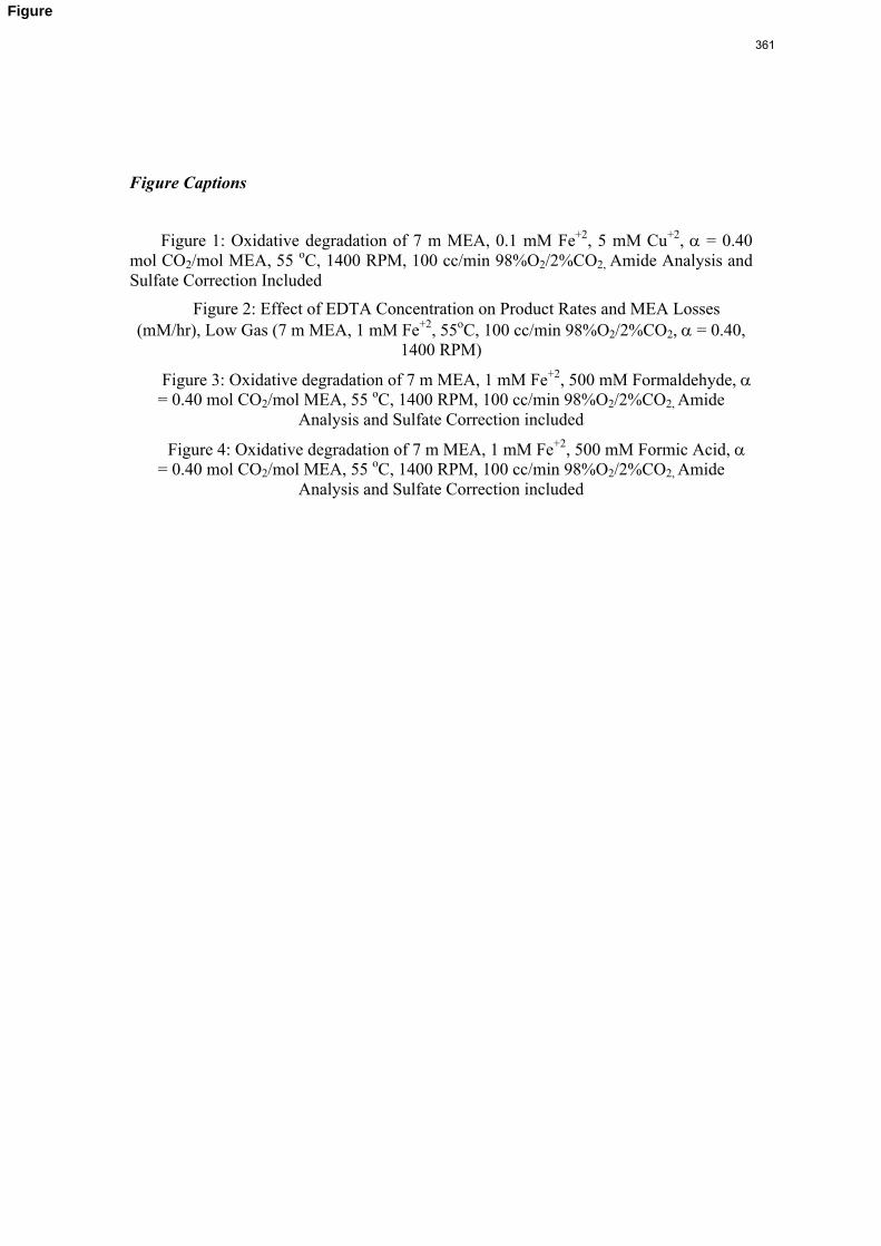
Figure Captions
Figure 1: Oxidative degradation of 7 m MEA, 0.1 mM Fe+2, 5 mM Cu+2, = 0.40 mol CO2/mol MEA, 55 oC, 1400 RPM, 100 cc/min 98%O2/2%CO2, Amide Analysis and Sulfate Correction Included
Figure 2: Effect of EDTA Concentration on Product Rates and MEA Losses (mM/hr), Low Gas (7 m MEA, 1 mM Fe+2, 55oC, 100 cc/min 98%O2/2%CO2, = 0.40,
1400 RPM)
Figure 3: Oxidative degradation of 7 m MEA, 1 mM Fe+2, 500 mM Formaldehyde, = 0.40 mol CO2/mol MEA, 55 oC, 1400 RPM, 100 cc/min 98%O2/2%CO2, Amide
Analysis and Sulfate Correction included
Figure 4: Oxidative degradation of 7 m MEA, 1 mM Fe+2, 500 mM Formic Acid, = 0.40 mol CO2/mol MEA, 55 oC, 1400 RPM, 100 cc/min 98%O2/2%CO2, Amide
Analysis and Sulfate Correction included
Figure
361
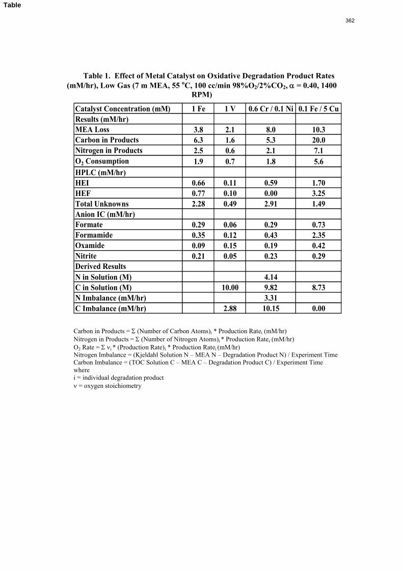
Table 1. Effect of Metal Catalyst on Oxidative Degradation Product Rates (mM/hr), Low Gas (7 m MEA, 55 oC, 100 cc/min 98%O2/2%CO2, = 0.40, 1400
RPM)
Catalyst Concentration (mM) 1 Fe 1 V 0.6 Cr / 0.1 Ni 0.1 Fe / 5 CuResults (mM/hr)MEA Loss 3.8 2.1 8.0 10.3Carbon in Products 6.3 1.6 5.3 20.0Nitrogen in Products 2.5 0.6 2.1 7.1O2 Consumption 1.9 0.7 1.8 5.6HPLC (mM/hr)HEI 0.66 0.11 0.59 1.70HEF 0.77 0.10 0.00 3.25Total Unknowns 2.28 0.49 2.91 1.49Anion IC (mM/hr)Formate 0.29 0.06 0.29 0.73Formamide 0.35 0.12 0.43 2.35Oxamide 0.09 0.15 0.19 0.42Nitrite 0.21 0.05 0.23 0.29Derived ResultsN in Solution (M) 4.14C in Solution (M) 10.00 9.82 8.73N Imbalance (mM/hr) 3.31C Imbalance (mM/hr) 2.88 10.15 0.00
Carbon in Products = (Number of Carbon Atoms)i * Production Ratei (mM/hr)Nitrogen in Products = (Number of Nitrogen Atoms)i * Production Ratei (mM/hr)O2 Rate = i * (Production Rate)i * Production Ratei (mM/hr)Nitrogen Imbalance = (Kjeldahl Solution N – MEA N – Degradation Product N) / Experiment TimeCarbon Imbalance = (TOC Solution C – MEA C – Degradation Product C) / Experiment Timewherei = individual degradation product = oxygen stoichiometry
Table
362
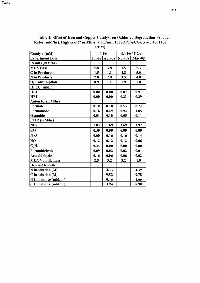
Table 2. Effect of Iron and Copper Catalyst on Oxidative Degradation Product Rates (mM/hr), High Gas (7 m MEA, 7.5 L/min 15%O2/2%CO2, = 0.40, 1400
RPM)
Catalyst (mM)Experiment Date Jul-08 Apr-08 Nov-08 May-08Results (mM/hr)MEA Loss 5.8 3.8 3.5 5.3C in Products 1.5 1.1 4.8 5.0N in Products 2.0 2.0 3.5 4.0O2 Consumption 0.9 1.1 1.9 1.8HPLC (mM/hr)HEF 0.00 0.00 0.87 0.91HEI 0.00 0.00 0.23 0.29Anion IC (mM/hr)Formate 0.10 0.18 0.53 0.22Formamide 0.16 0.49 0.92 1.05Oxamide 0.01 0.10 0.05 0.11FTIR (mM/hr)NH3 1.83 1.69 1.69 1.97
CO 0.30 0.00 0.00 0.00N2O 0.00 0.16 0.16 0.14
NO 0.12 0.12 0.12 0.06C2H4 0.24 0.00 0.00 0.00Formaldehyde 0.09 0.02 0.02 0.01Acetaldehyde 0.16 0.06 0.06 0.02MEA Volatile Loss 2.5 3.2 3.2 1.9Derived Results N in solution (M) 4.33 4.39C in solution (M) 9.52 9.78N Imbalance (mM/hr) 0.46 1.66C Imbalance (mM/hr) 3.94 8.90
1 Fe 0.1 Fe / 5 Cu
Table
363
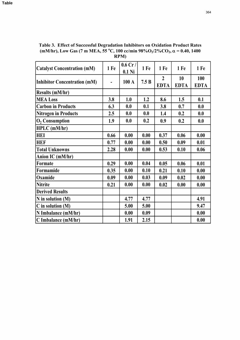
Table 3. Effect of Successful Degradation Inhibitors on Oxidation Product Rates (mM/hr), Low Gas (7 m MEA, 55 oC, 100 cc/min 98%O2/2%CO2, = 0.40, 1400
RPM)
Catalyst Concentration (mM) 1 Fe0.6 Cr / 0.1 Ni
1 Fe 1 Fe 1 Fe 1 Fe
Inhibitor Concentration (mM) - 100 A 7.5 B2
EDTA10
EDTA100
EDTAResults (mM/hr)MEA Loss 3.8 1.0 1.2 8.6 1.5 0.1Carbon in Products 6.3 0.0 0.1 3.8 0.7 0.0Nitrogen in Products 2.5 0.0 0.0 1.4 0.2 0.0O2 Consumption 1.9 0.0 0.2 0.9 0.2 0.0HPLC (mM/hr)HEI 0.66 0.00 0.00 0.37 0.06 0.00HEF 0.77 0.00 0.00 0.50 0.09 0.01Total Unknowns 2.28 0.00 0.00 0.53 0.10 0.06Anion IC (mM/hr)Formate 0.29 0.00 0.04 0.05 0.06 0.01Formamide 0.35 0.00 0.10 0.21 0.10 0.00Oxamide 0.09 0.00 0.03 0.09 0.02 0.00Nitrite 0.21 0.00 0.00 0.02 0.00 0.00Derived ResultsN in solution (M) 4.77 4.77 4.91C in solution (M) 5.00 5.00 9.47N Imbalance (mM/hr) 0.00 0.09 0.00C Imbalance (mM/hr) 1.91 2.15 0.00
Table
364
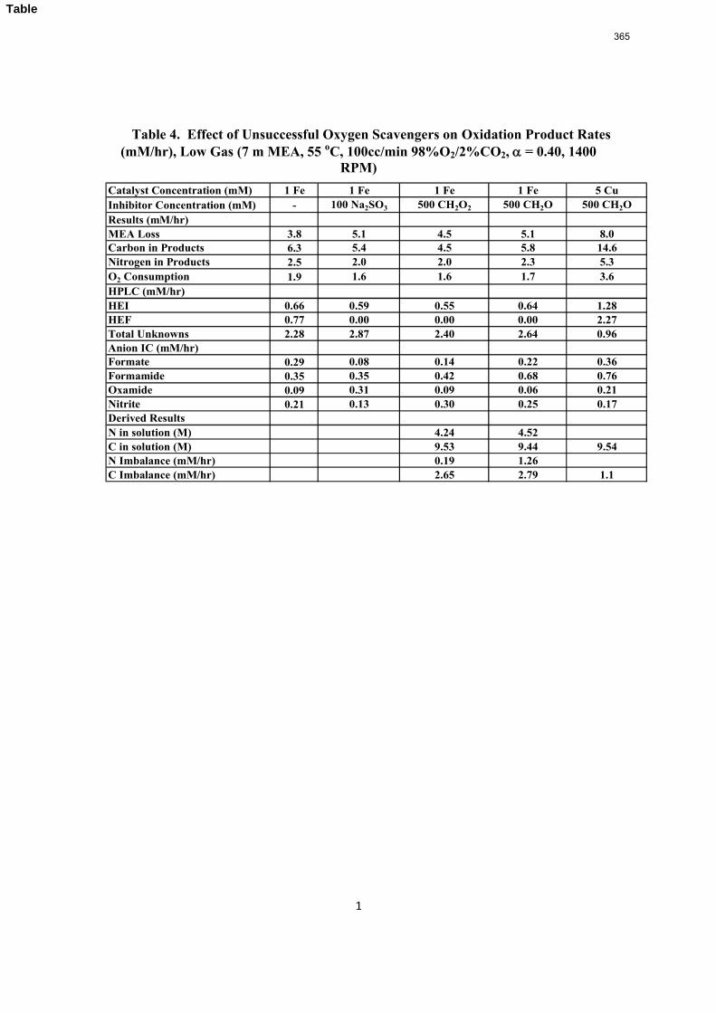
1
Table 4. Effect of Unsuccessful Oxygen Scavengers on Oxidation Product Rates (mM/hr), Low Gas (7 m MEA, 55 oC, 100cc/min 98%O2/2%CO2, = 0.40, 1400
RPM)
Catalyst Concentration (mM) 1 Fe 1 Fe 1 Fe 1 Fe 5 CuInhibitor Concentration (mM) - 100 Na2SO3 500 CH2O2 500 CH2O 500 CH2OResults (mM/hr)MEA Loss 3.8 5.1 4.5 5.1 8.0Carbon in Products 6.3 5.4 4.5 5.8 14.6Nitrogen in Products 2.5 2.0 2.0 2.3 5.3O2 Consumption 1.9 1.6 1.6 1.7 3.6HPLC (mM/hr)HEI 0.66 0.59 0.55 0.64 1.28HEF 0.77 0.00 0.00 0.00 2.27Total Unknowns 2.28 2.87 2.40 2.64 0.96Anion IC (mM/hr)Formate 0.29 0.08 0.14 0.22 0.36Formamide 0.35 0.35 0.42 0.68 0.76Oxamide 0.09 0.31 0.09 0.06 0.21Nitrite 0.21 0.13 0.30 0.25 0.17Derived ResultsN in solution (M) 4.24 4.52C in solution (M) 9.53 9.44 9.54N Imbalance (mM/hr) 0.19 1.26C Imbalance (mM/hr) 2.65 2.79 1.1
Table
365
1
Reaction Products from the Oxidative Degradation of MEA Andrew Sexton and Gary T. Rochelle
Department of Chemical Engineering
The University of Texas at Austin
Austin, Texas 78712
Aqueous monoethanolamine (MEA) is being considered as a solvent for CO2 capture
from flue gas. MEA solutions were subjected to oxidative degradation in 500 mL agitated
reactors at both low and high gas rates. Solutions were degraded with 100 mL/min of
98%O2/2%CO2 and mass transfer was achieved by vortexing. Liquid samples were analyzed by
ion chromatography and by HPLC with evaporative light scattering detection (ELSD). In a
parallel apparatus 7.5 L/min of 15% O2/2% CO2 was sparged through 350 mL of solution;
additional mass transfer was achieved by agitation. At the high gas rate a Fourier Transform
Infrared Analyzer collected continuous gas-phase data on amine volatility and volatile
degradation products.
Formate, hydroxyethyl-formamide (HEF) and hydroxyethylimidazole (HEI) account for
92% of the degraded carbon that has been quantified at low gas flow. These species account for
18% to 59% of the degraded carbon at high gas flow. Oxalate, its respective MEA amide,
glycolate and acetate are also present at much lower concentrations.
Ammonia, HEF and HEI account for 84% of the degraded nitrogen at low gas flow and
83% to 92% at high gas flow. At high gas rate, NOx is produced and stripped from the solution.
At low gas rate, NOx is retained in the solution and oxidized to nitrite and nitrate. At high gas
rate, NOx/N2O production is 15% of the rate of ammonia production. At low gas rate,
nitrite/nitrate production occurs at the same rate as NOx/N2O production at high gas rate. Other
volatile degradation products include CO, C2H4, formaldehyde and acetaldehyde.
A comparison of total carbon and nitrogen production rates to MEA losses show that 25
to 50% of oxidative degradation products currently remain unaccounted for. Oxygen
consumption rates vary from 1 to 2 mM/hr. The overall stoichiometry (ν) was 0.75 mol O2/mol
MEA degraded.
366
2
Introduction
Alkanolamines are used extensively in the gas processing industry to remove acid gases
such as carbon dioxide and hydrogen sulfide. Aqueous monoethanolamine (MEA) is the solvent
of choice for CO2 capture from flue gas because of its high capacity for CO2 absorption and fast
reaction kinetics.1
Figure 1 shows the typical aqueous absorption/stripping process used for CO2 capture. A
flue gas stream with 10% CO2 and 5% O2 enters the bottom of the absorber at 55oC and 1
atmosphere.2 Lean amine solution at a loading of 0.2 to 0.4 moles CO2/mole MEA
countercurrently contacts the flue gas. CO2 reacts reversibly with MEA to form MEA
carbamate. The rich amine solution, with a CO2 loading (α) of 0.45 to 0.5 mol/mol MEA, goes
through a cross heat exchanger, where it is preheated by the lean amine solution before entering
the top of the stripper at 120oC and 2 atm.
In the stripper, heat is provided in the reboiler by steam, which is used to reverse the
chemical equilibrium between the MEA and MEA-carbamate, liberating the CO2 and some
water. The vapor leaving the stripper is dehydrated and compressed before being pumped for
sequestration. The hot lean amine solution is passed back through the cross exchanger, where it
is cooled and recycled back to the top of the absorber. A reclaimer off the bottom of the stripper
takes a slip stream to remove heat stable salts and high molecular weight degradation products.
Degradation of the solvent in this absorption/stripping system occurs by oxidation and
carbamate polymerization.3 Carbamate polymerization occurs at stripper temperature with
alkanolamines that form carbamates.4 Oxidative degradation can be significant in flue gas
applications typically containing 3-15% O2.
367
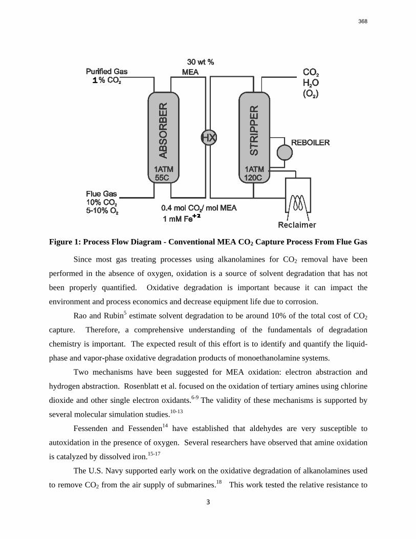
3
Figure 1: Process Flow Diagram - Conventional MEA CO2 Capture Process From Flue Gas
Since most gas treating processes using alkanolamines for CO2 removal have been
performed in the absence of oxygen, oxidation is a source of solvent degradation that has not
been properly quantified. Oxidative degradation is important because it can impact the
environment and process economics and decrease equipment life due to corrosion.
Rao and Rubin5 estimate solvent degradation to be around 10% of the total cost of CO2
capture. Therefore, a comprehensive understanding of the fundamentals of degradation
chemistry is important. The expected result of this effort is to identify and quantify the liquid-
phase and vapor-phase oxidative degradation products of monoethanolamine systems.
Two mechanisms have been suggested for MEA oxidation: electron abstraction and
hydrogen abstraction. Rosenblatt et al. focused on the oxidation of tertiary amines using chlorine
dioxide and other single electron oxidants.6-9 The validity of these mechanisms is supported by
several molecular simulation studies.10-13
Fessenden and Fessenden14 have established that aldehydes are very susceptible to
autoxidation in the presence of oxygen. Several researchers have observed that amine oxidation
is catalyzed by dissolved iron.15-17
The U.S. Navy supported early work on the oxidative degradation of alkanolamines used
to remove CO2 from the air supply of submarines.18 This work tested the relative resistance to
368
4
oxidative degradation of possible CO2 absorbents.19-20 The accelerated oxidation test involved
contacting 100 mL/min of a 50% CO2/50% O2 gas mixture with 100 mL of 2.5 N amine solution
at 80 oC and 25 to 60 ppm Fe. Evolved ammonia was detected by passing the reaction gas
through a weak acid solution to absorb the ammonia. Results showed that NH3 production
occurred as follows: tertiary amines < primary < secondary.
Blachly and Ravner21 measured the evolution of ammonia and the production of
peroxides by sparging air at 1 cc/mL solution-min through 300 mL of 4 M MEA at 55 oC for 3 to
13 days. Without CO2 in the air, they observed no perceptible degradation.
Rooney22 measured the formation of carboxylic acids in loaded (α=0.25) and unloaded
solutions of 20 wt % MEA, 50 wt % diglycolamine (DGATM), 30 wt % diethanolamine (DEA),
and both 30 and 50 wt % methyldiethanolamine (MDEA). The solutions were degraded by
bubbling air at 5.5 mL/min through 935 g of amine solution at 180 oF for 28 days. The study
identified acetate, formate, glycolate, and oxalate as oxidation products in the degraded amines.
These products were observed as well by Critchfield and Jenkins.23
Chi24,25 decreased the time necessary to quantify amine degradation by instantaneously
measuring evolved ammonia by Fourier-Transform infrared analysis. They found that dissolved
iron (Fe+2) at 0.0001 to 3 mM catalyzed degradation rates from 0.12 to 1.10 mM/hr NH3. Goff26-
28 examined O2 mass transfer effects and reaction kinetics by changing reaction conditions and
showed that the rate of NH3 evolution with dissolved iron catalysis is controlled by the rate of O2
mass transfer into the amine, not by degradation kinetics.
369
5
Experimental Methods
Apparatus. Figure 2 depicts the oxidation experiment with low gas flow. Oxygen mass
transfer was achieved by introducing 100 mL/min of 98%O2/2%CO2 gas into the vapor space
above 350 mL of an agitated amine solution in a temperature-controlled semi-batch reactor.
Agitation at 1400 rpm vortexed the reaction gas into the solution and transferred the oxygen
needed to degrade the amine. Reaction gas, consisting of a mixture of CO2 and O2, was bubbled
through water to pre-saturate the gas before being introduced into the vapor space above the
amine solution at atmospheric pressure.
Two types of physical processes occur in this apparatus. The oxygen dissolves into the
amine solution then reacts with MEA to form degradation products. Therefore, the overall rate
of degradation may depend on the rate of oxygen mass transfer as well as the kinetics of the
reaction of the amine with oxygen. The presence of dissolved metal catalyst ensures fast
reaction kinetics, so that the bulk concentration of dissolved oxygen is near zero and the rate of
degradation is controlled by oxygen mass transfer. Oxygen mass transfer is promoted by
vigorous agitation in the apparatus. In addition, the use of pure oxygen enhances the oxidation
of the amine solution without affecting the mix of products formed.
370
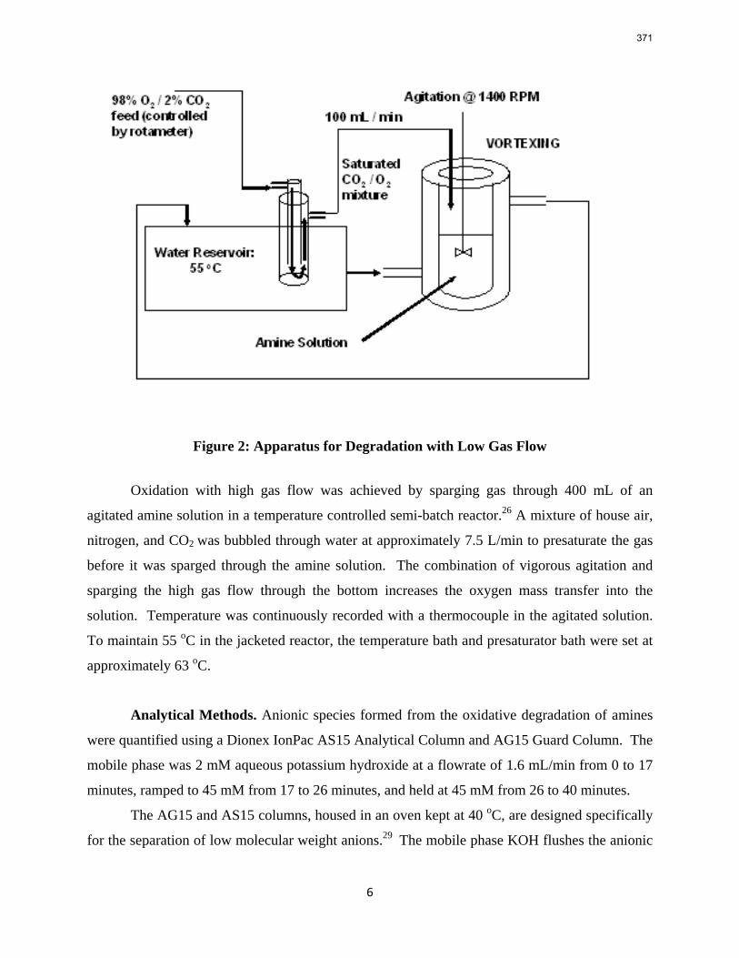
6
Figure 2: Apparatus for Degradation with Low Gas Flow
Oxidation with high gas flow was achieved by sparging gas through 400 mL of an
agitated amine solution in a temperature controlled semi-batch reactor.26 A mixture of house air,
nitrogen, and CO2 was bubbled through water at approximately 7.5 L/min to presaturate the gas
before it was sparged through the amine solution. The combination of vigorous agitation and
sparging the high gas flow through the bottom increases the oxygen mass transfer into the
solution. Temperature was continuously recorded with a thermocouple in the agitated solution.
To maintain 55 oC in the jacketed reactor, the temperature bath and presaturator bath were set at
approximately 63 oC.
Analytical Methods. Anionic species formed from the oxidative degradation of amines
were quantified using a Dionex IonPac AS15 Analytical Column and AG15 Guard Column. The
mobile phase was 2 mM aqueous potassium hydroxide at a flowrate of 1.6 mL/min from 0 to 17
minutes, ramped to 45 mM from 17 to 26 minutes, and held at 45 mM from 26 to 40 minutes.
The AG15 and AS15 columns, housed in an oven kept at 40 oC, are designed specifically
for the separation of low molecular weight anions.29 The mobile phase KOH flushes the anionic
371
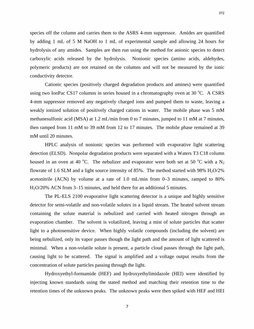
7
species off the column and carries them to the ASRS 4-mm suppressor. Amides are quantified
by adding 1 mL of 5 M NaOH to 1 mL of experimental sample and allowing 24 hours for
hydrolysis of any amides. Samples are then run using the method for anionic species to detect
carboxylic acids released by the hydrolysis. Nonionic species (amino acids, aldehydes,
polymeric products) are not retained on the columns and will not be measured by the ionic
conductivity detector.
Cationic species (positively charged degradation products and amines) were quantified
using two IonPac CS17 columns in series housed in a chromatography oven at 30 oC. A CSRS
4-mm suppressor removed any negatively charged ions and pumped them to waste, leaving a
weakly ionized solution of positively charged cations in water. The mobile phase was 5 mM
methanesulfonic acid (MSA) at 1.2 mL/min from 0 to 7 minutes, jumped to 11 mM at 7 minutes,
then ramped from 11 mM to 39 mM from 12 to 17 minutes. The mobile phase remained at 39
mM until 20 minutes.
HPLC analysis of nonionic species was performed with evaporative light scattering
detection (ELSD). Nonpolar degradation products were separated with a Waters T3 C18 column
housed in an oven at 40 oC. The nebulizer and evaporator were both set at 50 oC with a N2
flowrate of 1.6 SLM and a light source intensity of 85%. The method started with 98% H2O/2%
acetonitrile (ACN) by volume at a rate of 1.0 mL/min from 0–3 minutes, ramped to 80%
H2O/20% ACN from 3–15 minutes, and held there for an additional 5 minutes.
The PL-ELS 2100 evaporative light scattering detector is a unique and highly sensitive
detector for semi-volatile and non-volatile solutes in a liquid stream. The heated solvent stream
containing the solute material is nebulized and carried with heated nitrogen through an
evaporation chamber. The solvent is volatilized, leaving a mist of solute particles that scatter
light to a photosensitive device. When highly volatile compounds (including the solvent) are
being nebulized, only its vapor passes though the light path and the amount of light scattered is
minimal. When a non-volatile solute is present, a particle cloud passes through the light path,
causing light to be scattered. The signal is amplified and a voltage output results from the
concentration of solute particles passing through the light.
Hydroxyethyl-formamide (HEF) and hydroxyethylimidazole (HEI) were identified by
injecting known standards using the stated method and matching their retention time to the
retention times of the unknown peaks. The unknown peaks were then spiked with HEF and HEI
372
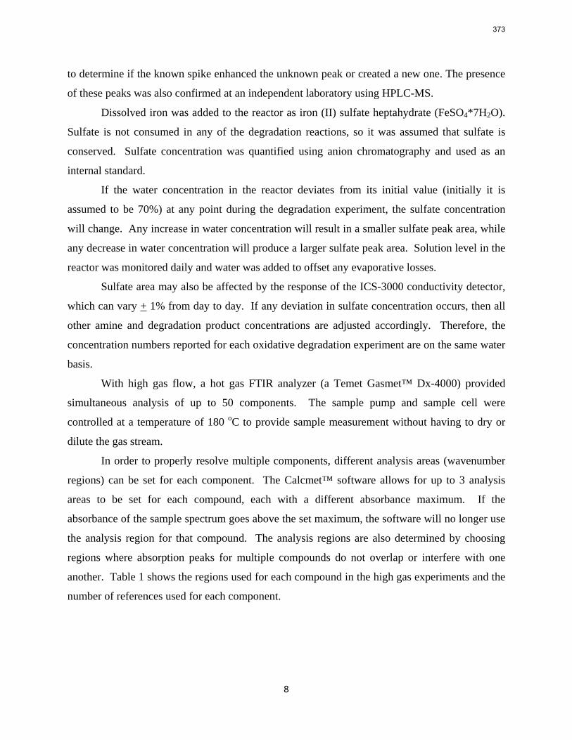
8
to determine if the known spike enhanced the unknown peak or created a new one. The presence
of these peaks was also confirmed at an independent laboratory using HPLC-MS.
Dissolved iron was added to the reactor as iron (II) sulfate heptahydrate (FeSO4*7H2O).
Sulfate is not consumed in any of the degradation reactions, so it was assumed that sulfate is
conserved. Sulfate concentration was quantified using anion chromatography and used as an
internal standard.
If the water concentration in the reactor deviates from its initial value (initially it is
assumed to be 70%) at any point during the degradation experiment, the sulfate concentration
will change. Any increase in water concentration will result in a smaller sulfate peak area, while
any decrease in water concentration will produce a larger sulfate peak area. Solution level in the
reactor was monitored daily and water was added to offset any evaporative losses.
Sulfate area may also be affected by the response of the ICS-3000 conductivity detector,
which can vary + 1% from day to day. If any deviation in sulfate concentration occurs, then all
other amine and degradation product concentrations are adjusted accordingly. Therefore, the
concentration numbers reported for each oxidative degradation experiment are on the same water
basis.
With high gas flow, a hot gas FTIR analyzer (a Temet Gasmet™ Dx-4000) provided
simultaneous analysis of up to 50 components. The sample pump and sample cell were
controlled at a temperature of 180 oC to provide sample measurement without having to dry or
dilute the gas stream.
In order to properly resolve multiple components, different analysis areas (wavenumber
regions) can be set for each component. The Calcmet™ software allows for up to 3 analysis
areas to be set for each compound, each with a different absorbance maximum. If the
absorbance of the sample spectrum goes above the set maximum, the software will no longer use
the analysis region for that compound. The analysis regions are also determined by choosing
regions where absorption peaks for multiple compounds do not overlap or interfere with one
another. Table 1 shows the regions used for each compound in the high gas experiments and the
number of references used for each component.
373
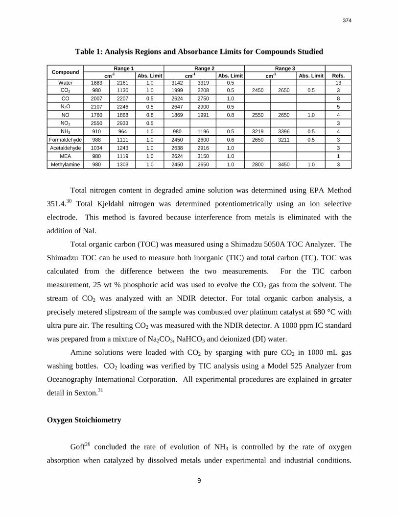
9
Table 1: Analysis Regions and Absorbance Limits for Compounds Studied
Abs. Limit Abs. Limit Abs. Limit Refs.Water 1883 2161 1.0 3142 3319 0.5 13CO2 980 1130 1.0 1999 2208 0.5 2450 2650 0.5 3CO 2007 2207 0.5 2624 2750 1.0 8N2O 2107 2246 0.5 2647 2900 0.5 5NO 1760 1868 0.8 1869 1991 0.8 2550 2650 1.0 4NO2 2550 2933 0.5 3NH3 910 964 1.0 980 1196 0.5 3219 3396 0.5 4
Formaldehyde 988 1111 1.0 2450 2600 0.6 2650 3211 0.5 3Acetaldehyde 1034 1243 1.0 2638 2916 1.0 3
MEA 980 1119 1.0 2624 3150 1.0 1Methylamine 980 1303 1.0 2450 2650 1.0 2800 3450 1.0 3
Range 2 Range 3cm-1 cm-1Compound
cm-1Range 1
Total nitrogen content in degraded amine solution was determined using EPA Method
351.4.30 Total Kjeldahl nitrogen was determined potentiometrically using an ion selective
electrode. This method is favored because interference from metals is eliminated with the
addition of NaI.
Total organic carbon (TOC) was measured using a Shimadzu 5050A TOC Analyzer. The
Shimadzu TOC can be used to measure both inorganic (TIC) and total carbon (TC). TOC was
calculated from the difference between the two measurements. For the TIC carbon
measurement, 25 wt % phosphoric acid was used to evolve the CO2 gas from the solvent. The
stream of CO2 was analyzed with an NDIR detector. For total organic carbon analysis, a
precisely metered slipstream of the sample was combusted over platinum catalyst at 680 °C with
ultra pure air. The resulting CO2 was measured with the NDIR detector. A 1000 ppm IC standard
was prepared from a mixture of Na2CO3, NaHCO3 and deionized (DI) water.
Amine solutions were loaded with CO2 by sparging with pure CO2 in 1000 mL gas
washing bottles. CO2 loading was verified by TIC analysis using a Model 525 Analyzer from
Oceanography International Corporation. All experimental procedures are explained in greater
detail in Sexton.31
Oxygen Stoichiometry
Goff26 concluded the rate of evolution of NH3 is controlled by the rate of oxygen
absorption when catalyzed by dissolved metals under experimental and industrial conditions.
374
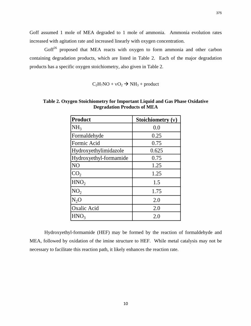
10
Goff assumed 1 mole of MEA degraded to 1 mole of ammonia. Ammonia evolution rates
increased with agitation rate and increased linearly with oxygen concentration.
Goff26 proposed that MEA reacts with oxygen to form ammonia and other carbon
containing degradation products, which are listed in Table 2. Each of the major degradation
products has a specific oxygen stoichiometry, also given in Table 2.
C2H7NO + νO2 NH3 + product
Table 2. Oxygen Stoichiometry for Important Liquid and Gas Phase Oxidative Degradation Products of MEA
Product Stoichiometry (ν)NH3 0.0Formaldehyde 0.25Formic Acid 0.75Hydroxyethylimidazole 0.625Hydroxyethyl-formamide 0.75NO 1.25CO2 1.25HNO2 1.5NO2 1.75N2O 2.0Oxalic Acid 2.0HNO3 2.0
Hydroxyethyl-formamide (HEF) may be formed by the reaction of formaldehyde and
MEA, followed by oxidation of the imine structure to HEF. While metal catalysis may not be
necessary to facilitate this reaction path, it likely enhances the reaction rate.
375
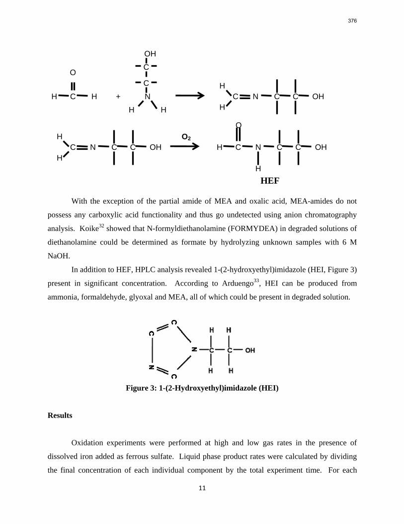
11
With the exception of the partial amide of MEA and oxalic acid, MEA-amides do not
possess any carboxylic acid functionality and thus go undetected using anion chromatography
analysis. Koike32 showed that N-formyldiethanolamine (FORMYDEA) in degraded solutions of
diethanolamine could be determined as formate by hydrolyzing unknown samples with 6 M
NaOH. In addition to HEF, HPLC analysis revealed 1-(2-hydroxyethyl)imidazole (HEI, Figure 3)
present in significant concentration. According to Arduengo33, HEI can be produced from
ammonia, formaldehyde, glyoxal and MEA, all of which could be present in degraded solution.
Figure 3: 1-(2-Hydroxyethyl)imidazole (HEI)
Results
Oxidation experiments were performed at high and low gas rates in the presence of
dissolved iron added as ferrous sulfate. Liquid phase product rates were calculated by dividing
the final concentration of each individual component by the total experiment time. For each
H C
O
H
HH
C
N + H
C N
C
OH
HC C OH
H C N
H C C OH
O2 C H C
O
N
H
C OH
HEF
376
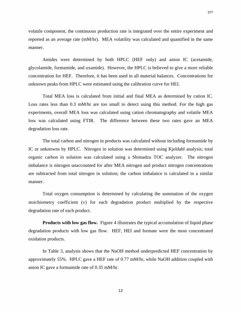
12
volatile component, the continuous production rate is integrated over the entire experiment and
reported as an average rate (mM/hr). MEA volatility was calculated and quantified in the same
manner.
Amides were determined by both HPLC (HEF only) and anion IC (acetamide,
glycolamide, formamide, and oxamide). However, the HPLC is believed to give a more reliable
concentration for HEF. Therefore, it has been used in all material balances. Concentrations for
unknown peaks from HPLC were estimated using the calibration curve for HEI.
Total MEA loss is calculated from initial and final MEA as determined by cation IC.
Loss rates less than 0.3 mM/hr are too small to detect using this method. For the high gas
experiments, overall MEA loss was calculated using cation chromatography and volatile MEA
loss was calculated using FTIR. The difference between these two rates gave an MEA
degradation loss rate.
The total carbon and nitrogen in products was calculated without including formamide by
IC or unknowns by HPLC. Nitrogen in solution was determined using Kjeldahl analysis; total
organic carbon in solution was calculated using a Shimadzu TOC analyzer. The nitrogen
imbalance is nitrogen unaccounted for after MEA nitrogen and product nitrogen concentrations
are subtracted from total nitrogen in solution; the carbon imbalance is calculated in a similar
manner.
Total oxygen consumption is determined by calculating the summation of the oxygen
stoichiometry coefficient (ν) for each degradation product multiplied by the respective
degradation rate of each product.
Products with low gas flow. Figure 4 illustrates the typical accumulation of liquid phase
degradation products with low gas flow. HEF, HEI and formate were the most concentrated
oxidation products.
In Table 3, analysis shows that the NaOH method underpredicted HEF concentration by
approximately 55%. HPLC gave a HEF rate of 0.77 mM/hr, while NaOH addition coupled with
anion IC gave a formamide rate of 0.35 mM/hr.
377
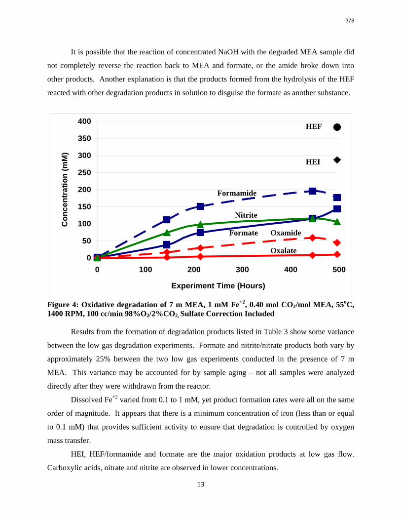
13
It is possible that the reaction of concentrated NaOH with the degraded MEA sample did
not completely reverse the reaction back to MEA and formate, or the amide broke down into
other products. Another explanation is that the products formed from the hydrolysis of the HEF
reacted with other degradation products in solution to disguise the formate as another substance.
0
50
100
150
200
250
300
350
400
0 100 200 300 400 500
Experiment Time (Hours)
Con
cent
ratio
n (m
M)
Figure 4: Oxidative degradation of 7 m MEA, 1 mM Fe+2, 0.40 mol CO2/mol MEA, 55oC, 1400 RPM, 100 cc/min 98%O2/2%CO2, Sulfate Correction Included
Results from the formation of degradation products listed in Table 3 show some variance
between the low gas degradation experiments. Formate and nitrite/nitrate products both vary by
approximately 25% between the two low gas experiments conducted in the presence of 7 m
MEA. This variance may be accounted for by sample aging – not all samples were analyzed
directly after they were withdrawn from the reactor.
Dissolved Fe+2 varied from 0.1 to 1 mM, yet product formation rates were all on the same
order of magnitude. It appears that there is a minimum concentration of iron (less than or equal
to 0.1 mM) that provides sufficient activity to ensure that degradation is controlled by oxygen
mass transfer.
HEI, HEF/formamide and formate are the major oxidation products at low gas flow.
Carboxylic acids, nitrate and nitrite are observed in lower concentrations.
Formate
Nitrite
HEF
HEI
Formamide
Oxamide
Oxalate
378
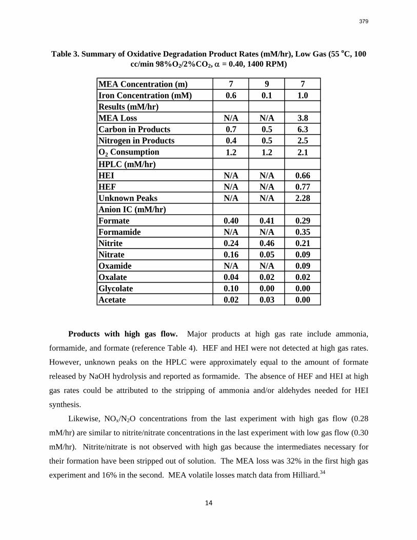
14
Table 3. Summary of Oxidative Degradation Product Rates (mM/hr), Low Gas (55 oC, 100 cc/min 98%O2/2%CO2, α = 0.40, 1400 RPM)
MEA Concentration (m) 7 9 7Iron Concentration (mM) 0.6 0.1 1.0Results (mM/hr)MEA Loss N/A N/A 3.8Carbon in Products 0.7 0.5 6.3Nitrogen in Products 0.4 0.5 2.5O2 Consumption 1.2 1.2 2.1HPLC (mM/hr)HEI N/A N/A 0.66HEF N/A N/A 0.77Unknown Peaks N/A N/A 2.28Anion IC (mM/hr)Formate 0.40 0.41 0.29Formamide N/A N/A 0.35Nitrite 0.24 0.46 0.21Nitrate 0.16 0.05 0.09Oxamide N/A N/A 0.09Oxalate 0.04 0.02 0.02Glycolate 0.10 0.00 0.00Acetate 0.02 0.03 0.00
Products with high gas flow. Major products at high gas rate include ammonia,
formamide, and formate (reference Table 4). HEF and HEI were not detected at high gas rates.
However, unknown peaks on the HPLC were approximately equal to the amount of formate
released by NaOH hydrolysis and reported as formamide. The absence of HEF and HEI at high
gas rates could be attributed to the stripping of ammonia and/or aldehydes needed for HEI
synthesis.
Likewise, NOx/N2O concentrations from the last experiment with high gas flow (0.28
mM/hr) are similar to nitrite/nitrate concentrations in the last experiment with low gas flow (0.30
mM/hr). Nitrite/nitrate is not observed with high gas because the intermediates necessary for
their formation have been stripped out of solution. The MEA loss was 32% in the first high gas
experiment and 16% in the second. MEA volatile losses match data from Hilliard.34
379
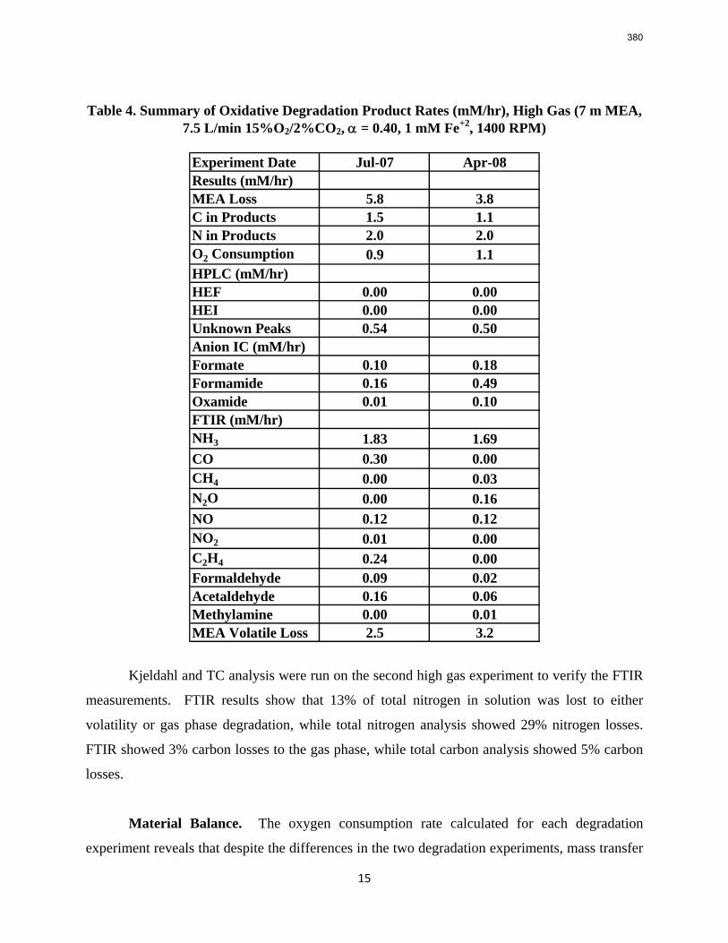
15
Table 4. Summary of Oxidative Degradation Product Rates (mM/hr), High Gas (7 m MEA,
7.5 L/min 15%O2/2%CO2, α = 0.40, 1 mM Fe+2, 1400 RPM)
Experiment Date Jul-07 Apr-08Results (mM/hr)MEA Loss 5.8 3.8C in Products 1.5 1.1N in Products 2.0 2.0O2 Consumption 0.9 1.1HPLC (mM/hr)HEF 0.00 0.00HEI 0.00 0.00Unknown Peaks 0.54 0.50Anion IC (mM/hr)Formate 0.10 0.18Formamide 0.16 0.49Oxamide 0.01 0.10FTIR (mM/hr)NH3 1.83 1.69CO 0.30 0.00CH4 0.00 0.03N2O 0.00 0.16NO 0.12 0.12NO2 0.01 0.00C2H4 0.24 0.00Formaldehyde 0.09 0.02Acetaldehyde 0.16 0.06Methylamine 0.00 0.01MEA Volatile Loss 2.5 3.2
Kjeldahl and TC analysis were run on the second high gas experiment to verify the FTIR
measurements. FTIR results show that 13% of total nitrogen in solution was lost to either
volatility or gas phase degradation, while total nitrogen analysis showed 29% nitrogen losses.
FTIR showed 3% carbon losses to the gas phase, while total carbon analysis showed 5% carbon
losses.
Material Balance. The oxygen consumption rate calculated for each degradation
experiment reveals that despite the differences in the two degradation experiments, mass transfer
380
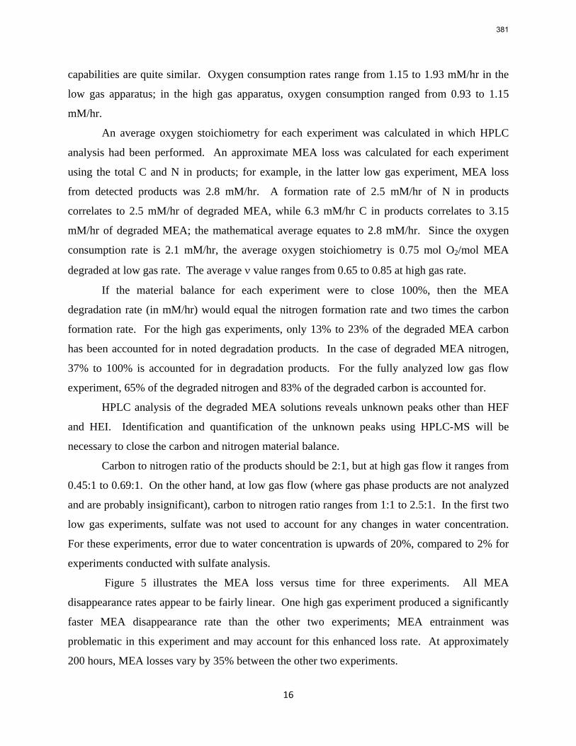
16
capabilities are quite similar. Oxygen consumption rates range from 1.15 to 1.93 mM/hr in the
low gas apparatus; in the high gas apparatus, oxygen consumption ranged from 0.93 to 1.15
mM/hr.
An average oxygen stoichiometry for each experiment was calculated in which HPLC
analysis had been performed. An approximate MEA loss was calculated for each experiment
using the total C and N in products; for example, in the latter low gas experiment, MEA loss
from detected products was 2.8 mM/hr. A formation rate of 2.5 mM/hr of N in products
correlates to 2.5 mM/hr of degraded MEA, while 6.3 mM/hr C in products correlates to 3.15
mM/hr of degraded MEA; the mathematical average equates to 2.8 mM/hr. Since the oxygen
consumption rate is 2.1 mM/hr, the average oxygen stoichiometry is 0.75 mol O2/mol MEA
degraded at low gas rate. The average ν value ranges from 0.65 to 0.85 at high gas rate.
If the material balance for each experiment were to close 100%, then the MEA
degradation rate (in mM/hr) would equal the nitrogen formation rate and two times the carbon
formation rate. For the high gas experiments, only 13% to 23% of the degraded MEA carbon
has been accounted for in noted degradation products. In the case of degraded MEA nitrogen,
37% to 100% is accounted for in degradation products. For the fully analyzed low gas flow
experiment, 65% of the degraded nitrogen and 83% of the degraded carbon is accounted for.
HPLC analysis of the degraded MEA solutions reveals unknown peaks other than HEF
and HEI. Identification and quantification of the unknown peaks using HPLC-MS will be
necessary to close the carbon and nitrogen material balance.
Carbon to nitrogen ratio of the products should be 2:1, but at high gas flow it ranges from
0.45:1 to 0.69:1. On the other hand, at low gas flow (where gas phase products are not analyzed
and are probably insignificant), carbon to nitrogen ratio ranges from 1:1 to 2.5:1. In the first two
low gas experiments, sulfate was not used to account for any changes in water concentration.
For these experiments, error due to water concentration is upwards of 20%, compared to 2% for
experiments conducted with sulfate analysis.
Figure 5 illustrates the MEA loss versus time for three experiments. All MEA
disappearance rates appear to be fairly linear. One high gas experiment produced a significantly
faster MEA disappearance rate than the other two experiments; MEA entrainment was
problematic in this experiment and may account for this enhanced loss rate. At approximately
200 hours, MEA losses vary by 35% between the other two experiments.
381
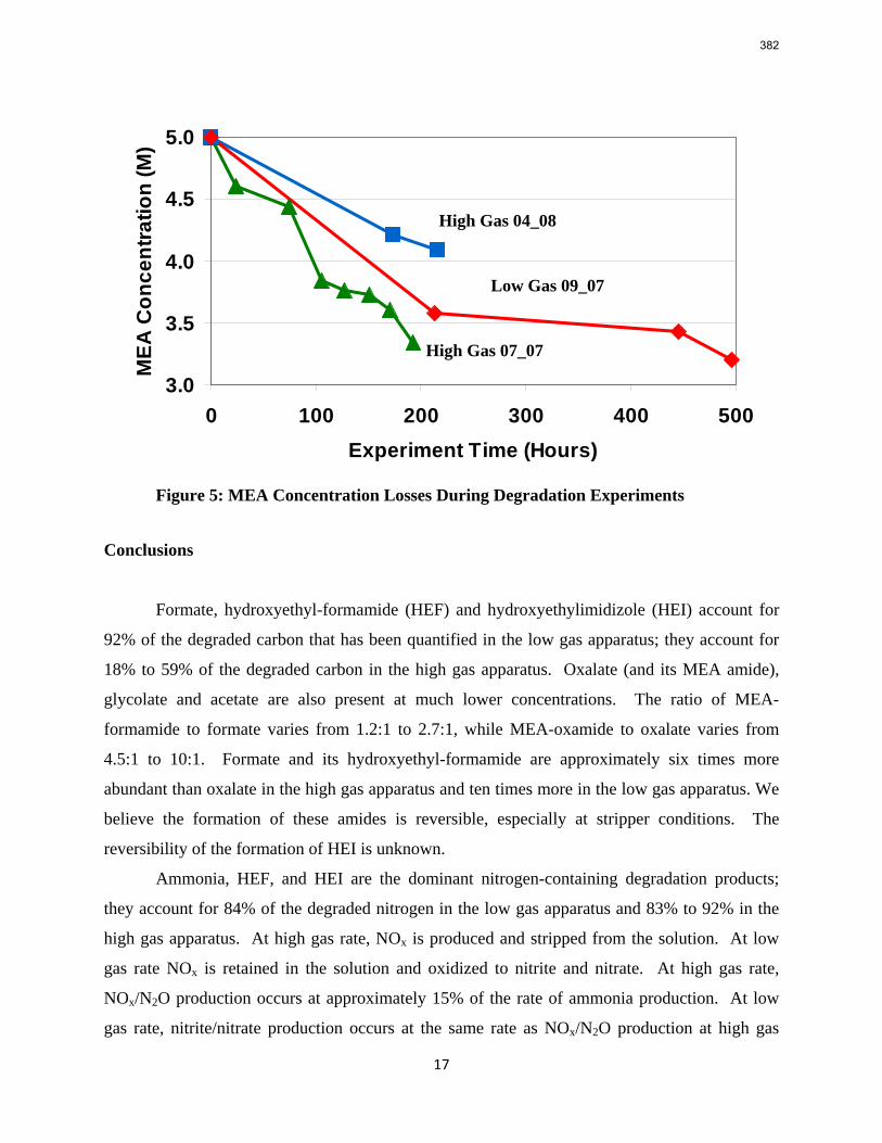
17
3.0
3.5
4.0
4.5
5.0
0 100 200 300 400 500Experiment Time (Hours)
MEA
Con
cent
ratio
n (M
)
Figure 5: MEA Concentration Losses During Degradation Experiments
Conclusions
Formate, hydroxyethyl-formamide (HEF) and hydroxyethylimidizole (HEI) account for
92% of the degraded carbon that has been quantified in the low gas apparatus; they account for
18% to 59% of the degraded carbon in the high gas apparatus. Oxalate (and its MEA amide),
glycolate and acetate are also present at much lower concentrations. The ratio of MEA-
formamide to formate varies from 1.2:1 to 2.7:1, while MEA-oxamide to oxalate varies from
4.5:1 to 10:1. Formate and its hydroxyethyl-formamide are approximately six times more
abundant than oxalate in the high gas apparatus and ten times more in the low gas apparatus. We
believe the formation of these amides is reversible, especially at stripper conditions. The
reversibility of the formation of HEI is unknown.
Ammonia, HEF, and HEI are the dominant nitrogen-containing degradation products;
they account for 84% of the degraded nitrogen in the low gas apparatus and 83% to 92% in the
high gas apparatus. At high gas rate, NOx is produced and stripped from the solution. At low
gas rate NOx is retained in the solution and oxidized to nitrite and nitrate. At high gas rate,
NOx/N2O production occurs at approximately 15% of the rate of ammonia production. At low
gas rate, nitrite/nitrate production occurs at the same rate as NOx/N2O production at high gas
High Gas 04_08
Low Gas 09_07
High Gas 07_07
382
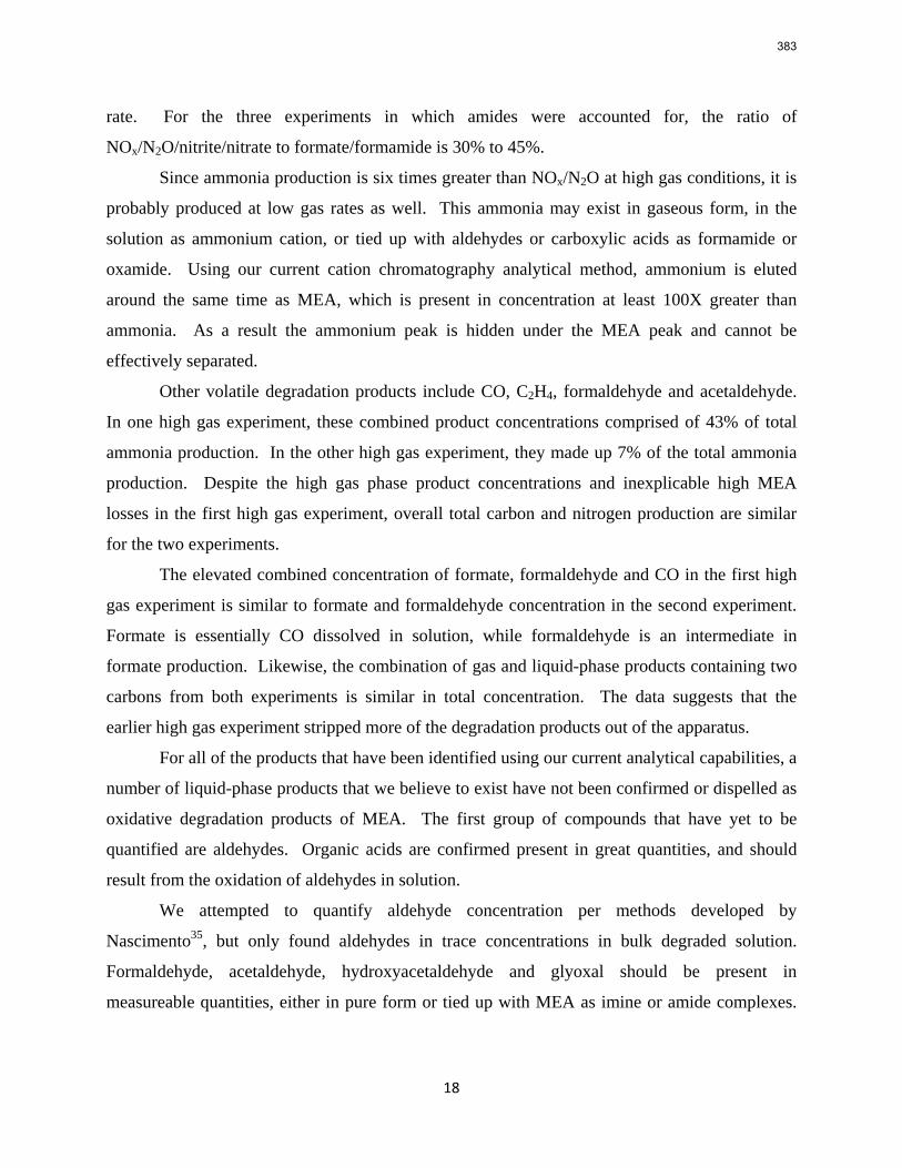
18
rate. For the three experiments in which amides were accounted for, the ratio of
NOx/N2O/nitrite/nitrate to formate/formamide is 30% to 45%.
Since ammonia production is six times greater than NOx/N2O at high gas conditions, it is
probably produced at low gas rates as well. This ammonia may exist in gaseous form, in the
solution as ammonium cation, or tied up with aldehydes or carboxylic acids as formamide or
oxamide. Using our current cation chromatography analytical method, ammonium is eluted
around the same time as MEA, which is present in concentration at least 100X greater than
ammonia. As a result the ammonium peak is hidden under the MEA peak and cannot be
effectively separated.
Other volatile degradation products include CO, C2H4, formaldehyde and acetaldehyde.
In one high gas experiment, these combined product concentrations comprised of 43% of total
ammonia production. In the other high gas experiment, they made up 7% of the total ammonia
production. Despite the high gas phase product concentrations and inexplicable high MEA
losses in the first high gas experiment, overall total carbon and nitrogen production are similar
for the two experiments.
The elevated combined concentration of formate, formaldehyde and CO in the first high
gas experiment is similar to formate and formaldehyde concentration in the second experiment.
Formate is essentially CO dissolved in solution, while formaldehyde is an intermediate in
formate production. Likewise, the combination of gas and liquid-phase products containing two
carbons from both experiments is similar in total concentration. The data suggests that the
earlier high gas experiment stripped more of the degradation products out of the apparatus.
For all of the products that have been identified using our current analytical capabilities, a
number of liquid-phase products that we believe to exist have not been confirmed or dispelled as
oxidative degradation products of MEA. The first group of compounds that have yet to be
quantified are aldehydes. Organic acids are confirmed present in great quantities, and should
result from the oxidation of aldehydes in solution.
We attempted to quantify aldehyde concentration per methods developed by
Nascimento35, but only found aldehydes in trace concentrations in bulk degraded solution.
Formaldehyde, acetaldehyde, hydroxyacetaldehyde and glyoxal should be present in
measureable quantities, either in pure form or tied up with MEA as imine or amide complexes.
383
19
Gloxylic acid, an intermediate in the formation of oxalic acid with carboxylic acid functionality,
has not been identified either.
According to TIC analysis, an unloaded 7 m MEA experiment run in the presence of 1
mM of iron and 0.5 M potassium formate in the high gas apparatus produced CO2 at a rate of
0.10 mM/hr. This rate of CO2 production is not enough to close the carbon gap in the material
balance. It is very likely that the gap in the material balance lies with the unidentified peaks that
appear using evaporative light scattering detection. A comparison of total carbon and nitrogen
production rates to MEA losses show that 25 to 50% of oxidative degradation products currently
remain unaccounted for.
Acknowledgements
This work was supported by the Luminant Carbon Management Program at The
University of Texas at Austin. Mark Nelson of Air Quality Analytical helped develop methods
for the FTIR. Jason Davis at The University of Texas at Austin assisted in developing the
HPLC-ELSD method, and Robert Grigsby of Huntsman aided in positively identifying the
HPLC peaks. Special thanks go to undergraduate research assistants Jang Lee and Humera
Rafique.
Literature Cited
1. Kohl, A.; Nielsen, R. Gas Purification. 5th edition; Gulf Publishing Co.: Houston, 1997. 2. Rochelle, G. T.; Chi, S. Oxidative Degradation of Monoethanolamine. First National
Conference on Carbon Sequestration, Washington, D. C., 2000. 3. Rochelle, G. T.; Bishnoi, S.; Chi, S.; Dang, H.; Santos, J. Research Needs for CO2 Capture
from Flue Gas by Aqueous Absorption/Stripping. DE-AF26-99FT01029; U.S. Department of Energy – Federal Energy Technology Center: Pittsburgh, PA, 2001.
4. Davis, J.; Rochelle, G. T. Thermal Degradation of Monoethanolamine at Stripper Conditions; Greenhouse Gas Control Technologies, Proceedings of the 9th International Conference on Greenhouse Gas Control Technologies, Washington, DC, November 17-20, 2008.
5. Rao, A. B.; Rubin, E. S. A Technical, Economic, and Environmental Assessment of Amine-Based CO2 Capture Technology for Power Plant Greenhouse Gas Control. Environmental Science and Technology 2002, 36(20), 4467-4475.
6. Rosenblatt, D. H.; Hayes, A. J., Jr.; Harrison, B. L.; Streaty, R. A.; Moore, K. A. Reaction of Chlorine Dioxide with Triethylamine in Aqueous Solution. Journal of Organic Chemistry 1963, 28(10), 2790-2794.
384
20
7. Rosenblatt, D. H.; Hull, L. A.; DeLuca, D. C.; Davis, G. T.; Weglein, R. C.; Williams, H. K. R. Oxidations of Amines. II. Substituent Effects in Chlorine Dioxide Oxidations. Journal of the American Chemical Society 1967, 89(5), 1158-1163.
8. Dennis, W. H., Jr.; Hull, L. A.; Rosenblatt, D. H. Oxidations of Amines. IV. Oxidative Fragmentation. Journal of Organic Chemistry 1967, 32(12): 3783-3787.
9. Hull, L.A.; Davis, G. T.; Rosenblatt, D. H.; Williams, H. K. R.; Weglein, R. C. Oxidations of Amines. III. Duality of Mechanism in the Reaction of Amines with Chlorine Dioxide. Journal of the American Chemical Society 1967, 89(5): 1163-1170.
10. Petryaev, E. P.; Pavlov, A. V.; Shadyro, O. I. Homolytic deamination of Amino Alcohols. Zh. Org. Khim. 1984, 20(1), 29-34.
11. Alejandre, J.; Rivera, J. L.; Mora, M. A.; De la Garza, V. Force Field of Monoethanolamine. Journal of Physical Chemistry B 2000, 104(6), 1332-1337.
12. Button, J. K.; Gubbins, K. E.; Tanaka, H.; Nakanishi, K. Molecular Dynamics of Hydrogen Bonding in Monoethanolamine. Fluid Phase Equilib. 1996, 116(1-2), 320-325.
13. Vorobyov, I.; Yappert, M. C.; DuPre, D. B. Hydrogen Bonding in Monomers and Dimers of 2-Aminomethanol. Journal of Physical Chemistry A 2002, 106(4), 668-679.
14. Fessenden, R. J.; Fessenden, J. S. Organic Chemistry. 5th ed.; Brooks/Cole Publishing Company: Pacific Grove, CA, 1994.
15. Hall, W. D.; Barron, J. G. Solving Gas Treating Problems – A Different Approach. Presented at the Laurence Reid Gas Conditioning Conference, Norman, OK, 1981.
16. Lee, Y. J.; Rochelle, G. T. Oxidative Degradation of Organic Additives for Flue Gas Desulfurization: Products, Kinetics, and Mechanism. Environmental Science and Technology 1987, 21, 266-272.
17. Russell, G. A. Peroxide Pathways to Autoxidation, p. 107-128 in Peroxide Reaction Mechanism ed. By J. O. Edwards, Interscience Publishers, New York, 1960.
18. Carbon Dioxide Absorbants. Girdler Corporation, Gas Processes Division, Louisville, KY, 1950.
19. Kindrick, R. C.; Atwood, K.; Arnold, M. R. The Relative Resistance to Oxidation of Commercially Available Amines. Girdler Report No. T2.15-1-30, in “Report: Carbon Dioxide Absorbents”, Contract No. NObs-50023, by Girdler Corp., Gas Processes Division, Louisville, KY, for the Navy Department, Bureau of Ships, Washington, DC (Code 649P), 1950.
20. Kindrick, R. C.; Reitmweier, R. E.; Arnold, M. R. A Prolonged Oxidation Test on Amine Solutions Resistant to Oxidation. Girdler Report No. T2.15-1-31, in “Report: Carbon Dioxide Absorbents”, Contract No. NObs-50023, by Girdler Corp., Gas Processes Division, Louisville, KY, for the Navy Department, Bureau of Ships, Washington, DC (Code 649P), 1950.
21. Blachly, C. H.; Ravner, H. The Stabilization of Monoethanolamine Solutions for Submarine Carbon Dioxide Scrubbers. AD609888, NRL-FR-6189; NRL-6189; Naval Research Laboratory: Washington, D.C., 1964.
22. Rooney, P. C.; DuPart, M. S.; Bacon, T. R. Oxygen’s Role in Alkanolamine Degradation. Hydrocarbon Process., Int. Ed. 1998, 77(7), 109-113.
23. Critchfield, J. E.; Jenkins, L. Evidence for MDEA degradation in tail gas treating plants. Petroleum Technology Quarterly 1999.
24. Chi, Q. S. Oxidative Degradation of Monoethanolamine. M.S. Thesis, The University of Texas at Austin, Austin, TX, 2000.
385
21
25. Chi, S.; Rochelle, G. T. Oxidative Degradation of Monoethanolamine. Industrial & Engineering Chemistry Research 2002, 41(17): 4178-4186.
26. Goff, G. S. Oxidative Degradation of Aqueous Monoethanolamine in CO2 Capture Processes: Iron and Copper Catalysis, Inhibition, and O2 Mass Transfer. Doctoral Thesis, The University of Texas at Austin, 2005.
27. Goff, G. S.; et al. Monoethanolamine Degradation: O2 Mass Transfer Effects under CO2 Capture Conditions. Industrial & Chemical Engineering Research 2004, 43(20), 6400-6408.
28. Goff, G. S.; et al. Oxidation Inhibitors for Cu Catalyzed Degradation of Monoethanolamine in CO2 Capture Processes. Industrial & Chemical Engineering Research 2006, 45(8), 2513-2521.
29. Dionex IonPac AS15 Analytical Column Product Manual. Revision 06, November 2002. http://www1.dionex.com/en-us/webdocs/4352_31362-06_AS15_V17.pdf
30. United States EPA National Exposure Research Laboratory. Total Kjeldahl Nitrogen by Ion Selective Electrode. 351.4-1 – 351.4-3. 1978.
31. Sexton, A. J. Amine Oxidation in CO2 Capture Processes. Doctoral Thesis, The University of Texas at Austin, 2008.
32. Koike, L. et al. N-Formyldiethanolamine: a new artifact in diethanolamine solutions. Chemistry and Industry 1987, 626-627.
33. Arduengo, A. J. et al. Process for Manufacture of Imidazoles. United States Patent 6,177,575. January 23, 2001. 7 pp.
34. Hilliard, M. A Predictive Thermodynamic Model for an Aqueous Blend of Potassium Carbonate, Piperazine, and Monoethanolamine for Carbon Dioxide Capture from Flue Gas. Doctoral Thesis, The University of Texas at Austin, Austin, TX, 2008.
35. Nascimento, R. F. et al. Qualitative and quantitative high-performance liquid chromatographic analysis of aldehydes in Brazilian sugar cane spirits and other distilled alcoholic beverages. Journal of Chromatography A 1997, 782(1), 13-23.
386
The University of Texas at Austin Cockrell School of Engineering
Research Proposal
Degradation of Concentrated Piperazine Used for Carbon Dioxide Capture
Stephanie A. Freeman
PhD Committee Supervisor: Prof. Gary T Rochelle
Prof. Jennifer Maynard Prof. Danny Reible Prof. Lynn Katz
Dr. Jim Critchfield, Shell Global Solutions
April 3rd, 2009
387
_____________________________________ Page i
Table of Contents 1.0 Introduction ............................................................................................................................ 1 2.0 Research Objectives ................................................................................................................ 2 3.0 Literature Review .................................................................................................................... 3 3.1 Piperazine (PZ)..................................................................................................................... 3 3.2 Physical Properties of PZ ..................................................................................................... 4 3.3 Oxidative Degradation......................................................................................................... 4 3.3.1 Catalyst effect of Metal Contaminants......................................................................... 5 3.3.2 Oxidative Degradation of PZ......................................................................................... 5
3.4 Thermal Degradation........................................................................................................... 5 3.5 Conclusions.......................................................................................................................... 5
4.0 Scope of Work ......................................................................................................................... 6 4.1 Oxidative Degradation......................................................................................................... 6 4.2 Thermal Degradation........................................................................................................... 7 4.3 Collaborative Degradation .................................................................................................. 8 4.4 Pilot Plant Applications........................................................................................................ 8 4.5 Other Considerations .......................................................................................................... 9
5.0 Principal Analytical Techniques............................................................................................. 10 5.1 CO2 Loading Through Total Inorganic Carbon (TIC)........................................................... 10 5.2 Amine Titration.................................................................................................................. 10 5.3 Total Organic Carbon (TOC)............................................................................................... 10 5.4 Kjeldahl Analysis for Total Nitrogen .................................................................................. 11 5.5 Anion Ion Chromatography (IC)......................................................................................... 11 5.6 Cation Ion Chromatography (IC)........................................................................................ 11 5.7 High Pressure Liquid Chromatography (HPLC).................................................................. 11 5.8 Mass Spectrometry (MS) ................................................................................................... 12 5.9 Nuclear Magnetic Resonance Spectroscopy (NMR).......................................................... 12 5.10 Atomic Absorption Spectoscopy (AA) ............................................................................. 13
6.0 Preliminary Results................................................................................................................ 13 6.1 Oxidative Degradation....................................................................................................... 13 6.2 Thermal Degradation......................................................................................................... 14
7.0 Engineering and Scientific Contributions.............................................................................. 15 8.0 Timeline for Completion of PhD Degree............................................................................... 16 9.0 References............................................................................................................................. 17
388
_____________________________________ Page 1
1.0 Introduction
The levels of carbon dioxide (CO2) in the atmosphere have been steadily rising since the industrial revolution. The Intergovermental Panel on Climate Change (IPCC) recently estimated that CO2 levels have increased 30% since pre‐industrial times and are currently increasing 0.4% per year (Intergovernmental Panel on Climate Change (IPCC) 2001). Anthropogenic CO2 releases and deforestation are now known to be the primary cause of this change in atmospheric conditions (Intergovernmental Panel on Climate Change (IPCC) 2001). The emission of CO2 from coal‐fired power plants contributes approximately 81% of the global CO2 released from all electricity generation and 33% of overall CO2 releases world‐wide from all industries (Energy Information Administration (EIA) 2008). The release of CO2 from transportation are also a significant portion of CO2 emissions, another 33% of the world wide total, but are hard to control because they are non‐stationary sources. The fact that coal‐fired power plants are large, stationary, point sources of CO2 makes them the perfect candidate for a focused attempt at reducing world‐wide CO2 emissions.
The most promising technology for CO2 capture is the removal of CO2 with an absorption/stripping system using an amine solvent. Alkanolamines such as monoethanolamine (MEA) and methyldiethanolamine (MDEA) have been traditionally investigated for this application. Other amines and amine blends have also been proposed for this application, 2‐amino‐2‐methyl‐1‐propanol (AMP), diglycolamine (DGA®), and piperazine (PZ) are the most promising non‐alkanolamines.
Absorption/stripping systems for CO2 capture are based on a recycled loop of an amine solution that absorbs CO2 in the absorber and then regenerates the solvent in the stripper (
Figure 1). Lean amine enters the top of the absorber and absorbs CO2 while descending through the column, counter‐currently contacting the flue gas. The rich amine exiting the absorber is sent thorough the main cross exchanger to heat up using the hot lean stream leaving the stripper. The rich solvent enters the top of the stripper and steam heating is used to desorb the captured CO2. The stripper reboiler is heated with steam taken off of the medium pressure turbines in the coal‐fired steam cycle in the power plant.
Solvent losses in an absorption/stripping system can occur at multiple points in the system through different processes. As shown in
Figure 1 below, solvent losses can occur at the top of the absorber (1), in the absorber packing sections (2), in the absorber sump (3), in the cross exchanger (4), in the stripper packing sections (5), and in the stripper sump (6).
Amine loss at the top of the absorber is due to volatility of the amine at absorber temperatures. Water washes are typically used to treat the flue gas exiting the top of the absorber to recover a majority of the amine lost through volatility. The volatility of an amine can be precisely measured using an equilibrium cell, such as is used in the Rochelle laboratory. This path of amine loss in generally well characterized.
In the absorber and absorber sump, the primary process to account for solvent loss is degradation of the amine through oxidation. Flue gas typically contains 3‐5% oxygen that is carried into the absorber where it can react with the amine. The hold‐up time in a sump is estimated to be 5 to 10 minutes, allowing oxidation reactions sufficient time to impact solvent loss. Research is needed into the oxidation characteristics of a specific amine in order to
389
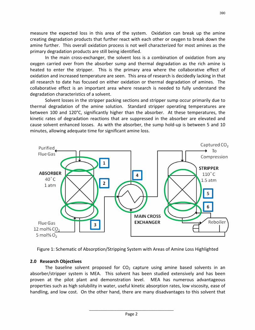
_____________________________________ Page 2
measure the expected loss in this area of the system. Oxidation can break up the amine creating degradation products that further react with each other or oxygen to break down the amine further. This overall oxidation process is not well characterized for most amines as the primary degradation products are still being identified.
In the main cross‐exchanger, the solvent loss is a combination of oxidation from any oxygen carried over from the absorber sump and thermal degradation as the rich amine is heated to enter the stripper. This is the primary area where the collaborative effect of oxidation and increased temperature are seen. This area of research is decidedly lacking in that all research to date has focused on either oxidation or thermal degradation of amines. The collaborative effect is an important area where research is needed to fully understand the degradation characteristics of a solvent.
Solvent losses in the stripper packing sections and stripper sump occur primarily due to thermal degradation of the amine solution. Standard stripper operating temperatures are between 100 and 120°C, significantly higher than the absorber. At these temperatures, the kinetic rates of degradation reactions that are suppressed in the absorber are elevated and cause solvent enhanced losses. As with the absorber, the sump hold‐up is between 5 and 10 minutes, allowing adequate time for significant amine loss.
Figure 1: Schematic of Absorption/Stripping System with Areas of Amine Loss Highlighted
2.0 Research Objectives The baseline solvent proposed for CO2 capture using amine based solvents in an absorber/stripper system is MEA. This solvent has been studied extensively and has been proven at the pilot plant and demonstration level. MEA has numerous advantageous properties such as high solubility in water, useful kinetic absorption rates, low viscosity, ease of handling, and low cost. On the other hand, there are many disadvantages to this solvent that
390
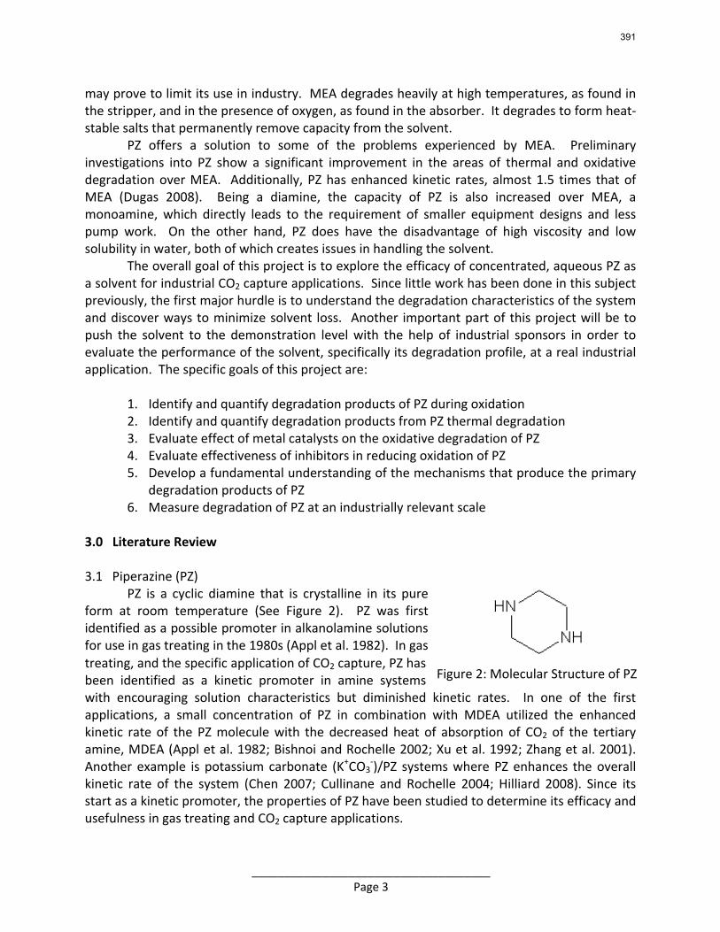
_____________________________________ Page 3
may prove to limit its use in industry. MEA degrades heavily at high temperatures, as found in the stripper, and in the presence of oxygen, as found in the absorber. It degrades to form heat‐stable salts that permanently remove capacity from the solvent. PZ offers a solution to some of the problems experienced by MEA. Preliminary investigations into PZ show a significant improvement in the areas of thermal and oxidative degradation over MEA. Additionally, PZ has enhanced kinetic rates, almost 1.5 times that of MEA (Dugas 2008). Being a diamine, the capacity of PZ is also increased over MEA, a monoamine, which directly leads to the requirement of smaller equipment designs and less pump work. On the other hand, PZ does have the disadvantage of high viscosity and low solubility in water, both of which creates issues in handling the solvent. The overall goal of this project is to explore the efficacy of concentrated, aqueous PZ as a solvent for industrial CO2 capture applications. Since little work has been done in this subject previously, the first major hurdle is to understand the degradation characteristics of the system and discover ways to minimize solvent loss. Another important part of this project will be to push the solvent to the demonstration level with the help of industrial sponsors in order to evaluate the performance of the solvent, specifically its degradation profile, at a real industrial application. The specific goals of this project are:
1. Identify and quantify degradation products of PZ during oxidation 2. Identify and quantify degradation products from PZ thermal degradation 3. Evaluate effect of metal catalysts on the oxidative degradation of PZ 4. Evaluate effectiveness of inhibitors in reducing oxidation of PZ 5. Develop a fundamental understanding of the mechanisms that produce the primary
degradation products of PZ 6. Measure degradation of PZ at an industrially relevant scale
3.0 Literature Review 3.1 Piperazine (PZ)
PZ is a cyclic diamine that is crystalline in its pure form at room temperature (See Figure 2). PZ was first identified as a possible promoter in alkanolamine solutions for use in gas treating in the 1980s (Appl et al. 1982). In gas treating, and the specific application of CO2 capture, PZ has been identified as a kinetic promoter in amine systems with encouraging solution characteristics but diminished kinetic rates. In one of the first applications, a small concentration of PZ in combination with MDEA utilized the enhanced kinetic rate of the PZ molecule with the decreased heat of absorption of CO2 of the tertiary amine, MDEA (Appl et al. 1982; Bishnoi and Rochelle 2002; Xu et al. 1992; Zhang et al. 2001). Another example is potassium carbonate (K+CO3
‐)/PZ systems where PZ enhances the overall kinetic rate of the system (Chen 2007; Cullinane and Rochelle 2004; Hilliard 2008). Since its start as a kinetic promoter, the properties of PZ have been studied to determine its efficacy and usefulness in gas treating and CO2 capture applications.
Figure 2: Molecular Structure of PZ
391
_____________________________________ Page 4
Although researchers quickly identified that PZ had enhanced reaction rates with CO2, the limited solubility of PZ restricted its use to below 2.0 or 2.5 m in blended amine systems. Most literature available on PZ is either a blended system, where solubility issues are remediated by dilution in another solvent, or at very low PZ concentration, below the 1.9 m PZ solubility limit at room temperature.
Outside of the CO2 capture field, PZ is a backbone molecule used in the pharmaceutical industry used in various stimulants, antihistamines, and treatments for psychiatric conditions (Erowid.org 2008). 3.2 Physical Properties of PZ
The physical properties of PZ have been studied since the compound was first identified. The low solubility of PZ has limited the amount of data available in literature for aqueous solutions of PZ above normal solubility. There are numerous sources reporting the density, viscosity, and diffusion coefficients in aqueous, low concentration, unloaded PZ solutions (Cook and Lowe 1976; Derks et al. 2005; Derks et al. 2008; Hamborg et al. 2008; Samanta and Bandyopadhyay 2006; Samanta et al. 2007). There are only a few sources of unloaded PZ solubility data that demonstrate the solid‐liquid equilibrium of PZ over a range of temperatures (The Dow Chemical Company 2001; Bishnoi 2000; Hilliard 2008).
Physical property data of aqueous PZ solutions loaded with CO2 are of particular importance to this research but, unfortunately, this type of data are rare in the current literature. Work in the Rochelle group has been the only notable contribution to this area of research. The theses of Hilliard (2008), Sexton (2008), and other current work in the group by R. Dugas and J. Davis all deal with loaded solutions of PZ (Davis 2008; Dugas 2008; Hilliard 2008; Sexton 2008). No property measurements have been done to date as other students have focused on vapor‐liquid equilibrium (Hilliard), kinetic rate measurements (Dugas), and degradation (Sexton and Davis). 3.3 Oxidative Degradation
The oxidative degradation, or oxidation, of amine solutions has been investigated since the 1950s. Initial work on the topic was performed by the U. S. Navy during the 1950s and 1960s while investigating CO2 scrubbers for submarine applications (The Girdler Corporation 1950; Blachly and Ravner 1964; Blachly and Ravner 1965; Blachly and Ravner 1966). Work performed by the Navy also began the process of identifying the many degradation product produced through MEA oxidation (Scheiman 1962). Rooney and colleagues expanded the scope of oxidation research to include amines besides MEA and contributed to identifying unknown degradation products (Rooney et al. 1998).
The oxidation work in the Rochelle group began with Chi and Goff who looked at oxidation of MEA under various conditions (Chi 2002; Goff 2005). Goff looked extensively at oxygen mass transfer conditions in the laboratory experiments as well as inhibitors for metal catalyzed degradation. The thesis of Sexton from the Rochelle group is the most comprehensive study of the oxidation of MEA to date (Sexton 2008). He investigated numerous combinations of metal catalysts, inhibitors, and other additives on MEA degradation, as well as performing oxidation screening experiments on other amines, including PZ, and MEA analogs.
392
_____________________________________ Page 5
3.3.1 Catalyst effect of Metal Contaminants The connection between corrosion products and amine degradation was identified in
the 1950s, indicating a link between metal‐based corrosion products and degradation (Hofmeyer et al. 1956). A sub‐set of oxidation research since then has been looking into the catalytic effect of metals on the oxidation of various amines. U. S. Navy work included this sub‐set of oxidation research after scrubber solvents were found to contain iron, nickel, chromium, and copper after use (Blachly and Ravner 1964). Their results indicated that copper had a serious catalytic effect for enhanced MEA degradation while iron and nickel only enhanced degradation slightly. The pair also tested various oxidation inhibitors including EDTA and N,N‐diethanolglycine (VFS) with some success. The work of Sexton on oxidation primarily looks at the effects of metals and inhibitors on the degradation characteristics of MEA (Sexton 2008). The results of Sexton results agree with the conclusions of Blanchly and Ravner and include the use of Inhibitors “A” and “B” to reduce MEA degradation.
3.3.2 Oxidative Degradation of PZ
One master’s thesis in the Rochelle group has looked exclusively at PZ oxidation, but the conclusions and experimental methods are questionable, especially the use of GC to quantify degradation products (Alawode 2005). Although the work of Sexton was primarily focused on the degradation of MEA, chapter 7 of the thesis focuses on low to mid‐level concentration PZ experiments (Sexton 2008). This work on PZ ranged from 2.5 to 5 m PZ and primarily took place in the low‐gas flow apparatus of the Rochelle Laboratory (described below). The primary conclusion was that PZ does oxidize, but at rates significantly lower than that of MEA. The conclusion of Sexton was that the metals tested ranked for catalyzing the most to least oxidation were: Cu > V > Fe. 3.4 Thermal Degradation
Thermal degradation of amines has been investigated only recently. Reza and colleagues published a paper focused on thermal degradation of MEA, diethanolamine (DEA), AMP, and blends of the three amines (Reza and Trejo 2006). Davis of the Rochelle group is currently finishing a thesis focused on thermal degradation of amines. His work focuses on MEA thermal degradation mechanisms as well as screening experiments including a variety of amines and amine blends (Davis 2008).
There is no thermal degradation data for concentrated PZ solutions available in literature outside of the Rochelle Group. The thesis work of Davis includes experiments performed on 5 m and 8 m PZ during screening experiments where the thermal degradation characteristics of a wide variety of solvents was examined (Davis 2008). Davis found very little thermal degradation occurred at either PZ concentration at 100, 120 and 135°C. The amount of degradation detected was close to or within the system errors for the cation IC and were reported by him as essentially zero percent degradation. The thermal tolerance of PZ in varying conditions is still an area where much can be discovered. 3.5 Conclusions Overall, the use of concentrated PZ as a CO2 capture or gas treating solvent has not been investigated to any real extent. The physical properties of concentrated PZ have not been
393
_____________________________________ Page 6
examined and only some data is available for low concentration, unloaded PZ. Some research has been done on low concentration PZ and the use of PZ in a blend with another amine for use in CO2 capture systems. This work does not specifically apply to the work of this project, but will provide a foundation to work off of to fill in the gaps in the literature.
Widespread work on the degradation of concentrated PZ is needed to elucidate its effectiveness in possible industrial applications. Analytical techniques for the detection of degradation products are a crucial part of this project. Anion and cation IC methods are already being used with great success in quantification of a variety of molecules. Unfortunately, a majority of the products formed due to oxidation and thermal degradation have not been identified or properly quantified up to this point. Additional work is needed to identify and quantify the products which are not detectable with the current methods. Primarily, the use of mass spectrometry will be explored in an effort to identify degradation products. The end goal is a complete mass balance that can account for a majority of the PZ degradation taking place due to oxidation and thermal degradation. Along with this knowledge of degradation products will hopefully come an understanding of the reaction mechanisms that are dominant in producing these products. Elucidating the oxidation mechanisms can further help in developing ways to minimize the effect of oxidation on capacity reduction.
The potential for industrial application is the long term goal for this solvent. There have been no pilot plant and demonstration level work reported in literature or industry that is publically available at this time. Demonstrating the efficacy of the solvent on a large scale is crucial to the development of this solvent and will be a final portion of this project. 4.0 Scope of Work
The degradation of various amines has been studied in conjunction with CO2 capture as a way to understand amine losses and minimize them. Degradation studies have been conducted by previous students of the Rochelle Group at the University of Texas at Austin as well as outside sources. Degradation of amines is a complicated subject that requires an understanding of all of the possible routes for solvent losses. As discussed above, a variety of routes exists for solvent capacity to be lost. Both oxidative and thermal degradation result in reduced solvent capacity as CO2‐accepting amine species are converted into heat stable salts, such as formate, acetate, and nitrate, or other organic products that do not react with CO2. The capacity of a solvent to remove CO2 is one of the most important attributes in the selection of a solvent because the sizing of equipment, solvent circulation rate, reclaiming needs, and CO2 removal are directly related to it.
4.1 Oxidative Degradation The degradation characteristics are a primary concern when selecting a solvent for CO2 capture. Oxidation of the solvent in the absorber, absorber sump, and piping leading to the cross‐exchanger can cause major solvent capacity losses. Flue gas entering CO2 capture systems will always contain between 4 to 6% oxygen due to the excess oxygen fed to the combustion boilers during coal combustion. Understanding oxidation is the first step to effectively managing and minimizing solvent losses.
The oxidation of PZ will be studied using techniques established in the Rochelle laboratory during the PhD work of Goff and Sexton (Goff 2005; Sexton 2008). Oxidative
394
_____________________________________ Page 7
degradation experiments are performed in a low gas flow agitated reactor fed with 100 mL/min of a saturated 98%/2% O2/CO2 gas mixture (Sexton 2008). The reactor is a 500‐mL jacketed reactor is filled with 350 mL of solvent. The jacket contains circulated water maintained at 55°C. The reactor is agitated at 1400 rpm to increase the mass transfer of oxygen into the solution. The reactor is operated continuously for 3‐5 weeks, depending on the experiment. Liquid samples are taken every two days and water is added to maintain the water balance on the reactor contents. The liquid samples were analyzed for PZ and degradation products by cation and anion chromatography.
Another apparatus used for oxidation experiments is the high gas flow reactor, which is a batch equilibrium cell with gas recycle through a hot gas Fourier transform infrared spectrometer (FTIR) (Hilliard 2008). The cell is a jacketed, glass reactor where temperature is controlled within 1°C. The inlet gas is sparged from the bottom of the reactor and there is additional mechanical agitation to enhance mass transfer. The gas in the headspace of the reactor is continuously sampled by the FTIR. The gas leaves the reactor and passes through a mist eliminator and into a sample line heated to 180°C. The heated gas stream is then analyzed by the multi‐component FTIR analyzer and recycled to the reactor as the inlet gas stream. This apparatus is advantageous because it can provide quantification of gas phase degradation products. The unit also provides real time data where the rate of production of particular products is visible directly.
Oxidation will be examined in the presence of metal catalyst that could be present in industrial applications due to metals leaching out of materials of construction (iron, chromium, nickel) or as additives use for corrosion inhibition (copper, vanadium). The use of oxidation inhibitors will also be studied with PZ systems to determine the efficacy of these reagents on minimizing metal‐catalyzed degradation. The low gas flow apparatus will be the primary oxidation experiment as it provides degraded samples quickly using exaggerated oxidation conditions. The high gas flow apparatus will be used when examining rates of degradation and the immediate reaction to the addition of catalyst or inhibitors. The two techniques will be used in conjunction with each other to provide a total picture of PZ oxidation. 4.2 Thermal Degradation Thermal degradation of CO2 capture solvents is an important issue relating to lost capacity. The high temperature in the stripper, usually between 100 and 120°C, increases the kinetic rate of degradation reactions that are not dominant in the low temperature of the absorber. The high temperature can also cause molecules to directly break apart. This degradation can also occur in the piping leading from the cross exchanger to the stripper and back, and in the sump of the stripper.
Techniques for thermal degradation experiments are thoroughly established in the Rochelle laboratory. Thermal bombs were constructed from 3/8‐inch stainless steel tubing with two Swagelok® end caps (Davis 2008). Bombs are filled with 10 mL of PZ solution, sealed, and placed in forced convention ovens at various temperatures. Bombs are removed from the ovens each week and the contents are analyzed for degradation products, remaining amine concentration, and CO2 loading. Amine losses are reported as a fraction of the initial amine that is remaining after the indicated time period as analyzed using cation ion chromatography (IC) or amine titration. Experiments will be conducted to degrade PZ under a variety of
395
_____________________________________ Page 8
conditions. Temperature ranging from 100 to 175°C will be tested. The addition of metal catalysts and inhibitors will also be tested to determine if they have an effect on thermal degradation.
The goal of these specific thermal experiments is to assess the degradation that might be expected in an industrial application using PZ. The overall goal of this portion of this project is to close the mass balance on PZ thermal degradation so the fate of PZ in the stripper is fundamentally understood. 4.3 Collaborative Degradation Up to this point in the Rochelle group, the effects of oxidation and thermal degradation have been studied independently. In real world applications, the collaborative effect of these processes has the potential to significantly impact and increase solvent degradation beyond the individual processes. An apparatus is being designed and constructed in collaboration with Fred Closmann of the Rochelle group to test this combined effect. The new apparatus consists of an oxidation reactor similar to the one currently used for low‐gas flow oxidation experiments. A section will be added on the bottom to simulate hold up in the sump and then the solvent will be pumped out and through a series of lab scale cross exchangers to heat up to approximately 100°C. The solvent will then enter a second reactor with a small amount of hold up time to simulate the high temperature degradation in the stripper. The solvent then travels back to the oxidation reactor after being cooled in the cross exchanger to the original temperature. These experiments are not meant to simulate a lab scale absorber/stripper system but to attempt to incorporate both oxidation and thermal degradation in one experiment. A lab scale absorber/stripper system would require a simulated flue gas to enter the oxidative reactor rather than the 2%/98% CO2/O2 gas mix currently used. Also, there would need to be recovery of CO2 off of the stripper reactor which is currently not incorporated into this experiment. The oxidative and thermal degradation work that is already conducted is done so in a way to overestimate and exaggerate the degradation that would occur in a real system. This apparatus follows that same approach, but incorporates the two phenomena in one reactor to gauge the catalytic effect of combining oxygen and high temperature. Concentrated PZ solvent will be tested in this combined apparatus for degradation products and PZ loss. The catalytic effect of metals will be tested, specifically iron, nickel, chromium, copper, and vanadium as well as oxidation inhibitors. 4.4 Pilot Plant Applications The last major portion of my PhD will involve analyzing PZ solutions from pilot scale experiments. This part of the project is crucial to understanding the possibility of PZ as a solvent in real industrial application. This portion of the project will be performed in active collaboration with research sponsors.
The Pickle Research Campus has the capability to perform medium scale pilot plant campaigns using simulated flue gas. This system is set up to use simulated flue gas with oxygen levels higher than traditional flue gas. One PZ pilot plant campaign has already been completed with success.
396
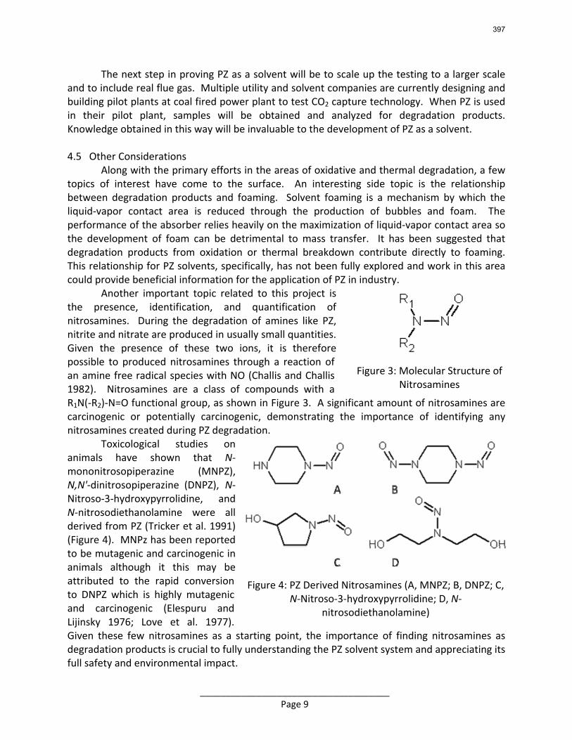
_____________________________________ Page 9
The next step in proving PZ as a solvent will be to scale up the testing to a larger scale and to include real flue gas. Multiple utility and solvent companies are currently designing and building pilot plants at coal fired power plant to test CO2 capture technology. When PZ is used in their pilot plant, samples will be obtained and analyzed for degradation products. Knowledge obtained in this way will be invaluable to the development of PZ as a solvent. 4.5 Other Considerations
Along with the primary efforts in the areas of oxidative and thermal degradation, a few topics of interest have come to the surface. An interesting side topic is the relationship between degradation products and foaming. Solvent foaming is a mechanism by which the liquid‐vapor contact area is reduced through the production of bubbles and foam. The performance of the absorber relies heavily on the maximization of liquid‐vapor contact area so the development of foam can be detrimental to mass transfer. It has been suggested that degradation products from oxidation or thermal breakdown contribute directly to foaming. This relationship for PZ solvents, specifically, has not been fully explored and work in this area could provide beneficial information for the application of PZ in industry.
Another important topic related to this project is the presence, identification, and quantification of nitrosamines. During the degradation of amines like PZ, nitrite and nitrate are produced in usually small quantities. Given the presence of these two ions, it is therefore possible to produced nitrosamines through a reaction of an amine free radical species with NO (Challis and Challis 1982). Nitrosamines are a class of compounds with a R1N(‐R2)‐N=O functional group, as shown in Figure 3. A significant amount of nitrosamines are carcinogenic or potentially carcinogenic, demonstrating the importance of identifying any nitrosamines created during PZ degradation.
Toxicological studies on animals have shown that N‐mononitrosopiperazine (MNPZ), N,N'‐dinitrosopiperazine (DNPZ), N‐Nitroso‐3‐hydroxypyrrolidine, and N‐nitrosodiethanolamine were all derived from PZ (Tricker et al. 1991) (Figure 4). MNPz has been reported to be mutagenic and carcinogenic in animals although it this may be attributed to the rapid conversion to DNPZ which is highly mutagenic and carcinogenic (Elespuru and Lijinsky 1976; Love et al. 1977). Given these few nitrosamines as a starting point, the importance of finding nitrosamines as degradation products is crucial to fully understanding the PZ solvent system and appreciating its full safety and environmental impact.
Figure 3: Molecular Structure of Nitrosamines
Figure 4: PZ Derived Nitrosamines (A, MNPZ; B, DNPZ; C, N‐Nitroso‐3‐hydroxypyrrolidine; D, N‐
nitrosodiethanolamine)
397
_____________________________________ Page 10
Similarly, the fate and transport of PZ in the environment is currently not well understood. Studies of the biodegradation of PZ with environmental bacteria are needed to fully understand the solvent. If a full scale industrial application is ever to come to fruition, the environmental impacts of a major spill or leak need to be understood in order to fully assess the safety and liability of using this solvent in the environment. Studies on the biodegradation of PZ using microbes from the North Sea have been completed, but do not fully elucidate the fate of PZ in the soil or in warmer climates (Haugmo 2008). 5.0 Principal Analytical Techniques
5.1 CO2 Loading Through Total Inorganic Carbon (TIC)
The concentration of CO2 in solution is determined by total inorganic carbon analysis (Hilliard 2008). The sample is diluted and then acidified in 30 wt% phosphoric acid to release aqueous CO2, carbonate, and bicarbonate species as gaseous CO2. The CO2 is carried through an infrared analyzer with nitrogen. The resulting analyzer peaks are integrated and correlated to CO2 concentrations using a 1000 ppm K2CO3/KHCO3 standard inorganic carbon solution. CO2 loading is reported as moles CO2/mole alkalinity or moles CO2/equiv PZ, where 2 moles alkalinity/mole PZ is the conversion factor. 5.2 Amine Titration
The concentration of PZ in solution is determined using acid titration (Hilliard 2008). An automatic Titrando series titrator with automatic equivalence point detection is used (Metrohm USA). The 300X diluted sample is titrated with 0.1 N H2SO4 to a pH of 2.4. The amount of acid needed to reach the equivalence point at a pH of 3.9 is used to calculate the total amine concentration in solution. 5.3 Total Organic Carbon (TOC)
Total organic carbon of a sample is measured using a Shimadzu 5050A TOC Analyzer (Shimadzu Corporation, Kyoto, Japan) (Chen 2007; Sexton 2008). The analyzer can measure the total inorganic carbon (TIC) and the total carbon in the sample. The total organic carbon (TOC) is the difference between these two measurements. To determine the TIC, 25wt% phosphoric acid (H3PO4) is used to liberate CO2 species from the sample including aqueous CO2, carbonate (CO3
‐2), bicarbonate (HCO3‐), and any amine carbamates. The acidic environment converts
these aqueous species to gaseous CO2 that evolves from the sample and is carried in the gas stream to a non‐dispersive infrared (NDIR) analyzer on the TOC apparatus. For the total carbon analysis, a specifically slipstream of the sample metered and combusted over a platinum catalyst at 680°C with ultra pure air. The CO2 created from this combustion is carried to the NDIR detector to be measured. This TOC unit has a detection limit of four parts per billion (ppb) and a range up to 4000 parts per million (ppm) for TIC and 5000 ppm for total carbon analysis. A standard is used for calibration that contains 1000 ppm of inorganic carbon made from a mixture of sodium carbonate (Na2CO3) and sodium bicarbonate (NaHCO3) in purified water.
398
_____________________________________ Page 11
5.4 Kjeldahl Analysis for Total Nitrogen Total nitrogen content is determined using the Kjeldahl method, a standard method
known as EPA Method 351.4 (Environmental Protection Agency (EPA) 2000). The total amount of nitrogen in a given sample is determined potentiometrically using an ion selective electrode. Nitrogen in the sample is converted to ammonia through chemical digestion using metal catalysts to speed up the decomposition of nitrogen to ammonia. The amount of ammonia is determined through titration. This work will be performed using an outside analytical lab. 5.5 Anion Ion Chromatography (IC) Anion IC is used to identify and quantify low molecular weight, negatively charged ions (anions) in solution. A Dionex ICS‐3000 modular Dual RFIC Ion Chromatography System with autosampler is used (Dionex Corporation, Sunnyvale, CA). The eluent contains varying concentrations of KOH in analytical grade water. The separation occurs using an IonPac AG15 guard column (4 x 50 mm) and an IonPac AS15 analytical column (4 x 250 mm). Both columns contain ethylvinylbenzene cross‐linked with 55% divinylbenzene resin affixed with quaternary ammonium groups as the primary separation medium. The system contains a 4‐mm Anionic Self‐Regenerating Suppressor (ASRS) to remove cationic species before anionic species are detected with a conductivity cell. Two carbonate removal devices are in place to remove excess carbonate species from the samples (Continuously Regenerated Anion Trap Column – CR‐ATC) and the analytical water (Carbonate Removal Device – CRD). Chromeleon software on the attached computer analyzes the conductivity output and controls the entire system. Currently, the anion IC is used to quantify glycolate, acetate, formate, chloride, nitrite, sulfate, oxalate, and nitrate. 5.6 Cation Ion Chromatography (IC) Cation IC is used to identify and quantify positively charged ions (cations) in solution. A Dionex ICS‐2500 Ion Chromatography System with autosampler is used (Dionex Corporation, Sunnyvale, CA). The eluent contains varying concentrations of methanesulfonic acid (MSA) in analytical grade water. The separation occurs in an IonPac CG17 guard column (4 x 50 mm) and an IonPac CS17 analytical column (4 x 250 mm). Both columns contain ethylvinylbenzene cross‐linked with 55% divinylbenzene resin as the primary separation medium. The system contains a 4‐mm Cationic Self‐Regenerating Suppressor (CSRS) to remove anionic species before cationic species are detected with a conductivity cell. Chromeleon software on the attached computer analyzes the conductivity output and controls the entire system. Currently, the cation IC is used to quantify ethylenediamine (EDA), MEA, PZ, DGA, MDEA, and numerous other amine species. 5.7 High Pressure Liquid Chromatography (HPLC) HPLC is used to identify and quantify nonionic species in solution. The HPLC unit is contained within the Dionex ICS‐3000 modular Dual RFIC Ion Chromatography System with autosampler (Dionex Corporation, Sunnyvale, CA). The eluent contains a varying concentration of acetonitrile in analytical grade water. The separation of compounds occurs in a Waters Atlantis T3 3 μm particle reversed‐phase column (4.6 x 150 mm) (Waters Corporation, Milford, MA). The column contains 3 μm silica particles with C18 chemistry as the primary separation medium. An evaporative light scattering detection (ELSD) unit is used to measure semi‐volatile
399
_____________________________________ Page 12
and non‐volatile solutions in the liquid stream. The eluent stream containing the sample is heated and nebulized in a heated nitrogen flow in the ELSD unit. The nebulization of non‐volatile and semi‐volatile compounds leaves a particle cloud that scatters light in the detector and creates the positive response. Highly volatile compounds, such as the solvent and eluent, are nebulized to a vapor phase that only minimally scatters light. The HPLC system uses the same autosampler, pump and column housing, and Chromeleon software as the Anion IC analysis system. 5.8 Mass Spectrometry (MS) Mass spectrometry (MS) is used to determine the elemental composition of a molecule or sample of interest. In MS, a sample is ionized to create charged particles in a gas stream. This ionized stream of particles is then subjected to electromagnetic fields that sort the particles by their mass. A detector then measures the amount of particles of each mass and the results is a spectrum of various charge‐to‐mass ratios versus the abundance found in the stream. The charge to mass ratio is essentially the molecular mass of a molecule plus a proton, divided by its charge of plus one. The charge‐to‐mass ratios are generally just one higher than the molecule of interest’s molecular weight, so this technique is useful in the identification of unknowns in a liquid mixture. The ionization setting of the apparatus can changed to identify neutral and positive species by using positive ionization or to detect neutral and negative species by using negative ionization depending on the desired application. When positive ionization is used, a proton is added to each molecule so neutral molecules have a positive charge and positively charged molecules receive an additional charge. Any negative charged species in solution then become neutral and are not detected.
The technique is primarily qualitative in nature and will be used in this project simple to help identify unknown degradation products. Also, the apparatus has the ability to be connected with a cation IC, anion IC, or HPLC column where the samples are first separated by the column of a specific method, and then sent to the MS. In this way, unknown peaks on cation, anion, or HPLC chromatographs can be identified specifically. This technique is also useful in the case of PZ where the high concentration of PZ can block some of the low concentration degradation products. 5.9 Nuclear Magnetic Resonance Spectroscopy (NMR) Nuclear magnetic resonance (NMR spectroscopy is a technique used to obtain information on the molecular structure of species in solution. Both 1H and 13C NMR measurements are performed at the University of Texas at Austin Department of Chemistry. In 1H NMR, or proton NMR, the position of hydrogen molecules are elucidated to help in determining the overall chemical structure of the molecules in the sample. In 13C NMR, or carbon NMR, the position of carbon molecules is elucidated in a similar way. During an NMR analysis, the sample of interest is subjected to a magnetic field and the result is a spectrum detailing the response of various functional groups within the molecule. Different functional groups have specific reactions that are interpretable from the spectra. The details of NMR analysis has been described previously in detail (Hilliard 2008).
For this specific project, the use of NMR will be focused on the possible identification of new degradation products. Currently, PZ degradation is hard to accurately determine due to
400
_____________________________________ Page 13
the large concentration of PZ and the detection limits of other analytical equipment. NMR can be used to see if a sample truly only has peaks representing PZ or if other, unidentified peaks exist. In this way, degradation of PZ can be confirmed as occurring or not in samples that are difficult to analyze using the other techniques described above.
5.10 Atomic Absorption Spectoscopy (AA) Atomic absorption spectroscopy is a method used to determine the concentration of a single metal in solution. The apparatus used is a Perkin Elmer AAnalyst 600 Spectrophotometer (Perkin Elmer, Waltham, MA). A lamp is used for the metal of interest that produces light at a very specific wavelength within the visible spectrum where that metal absorbs light. The apparatus has a light path from this lamp, through a small graphite furnace that is the primary measurement chamber, and then onto a detector and signal processor. The AA is able to very precisely control the temperature of this furnace with very quick temperature adjustments. The detector located at the end of the light path analyzes the portion of the visible light spectrum for the metal being measured and detects the absorbance of the sample over a short range of time.
To analyze a sample, a dilute liquid sample is injected into the furnace while the furnace is at the injection temperature (100°C). A sequence is then initiated that precisely increases the temperature of the furnace according to a method specific for the metal. Common among all metals is that there is an injection temperature of 110°C, then the temperature is raised to the pretreatment temperature (110°C) and held for 30 seconds. Then, there is a 15 second ramp up to the desolvation temperature (130°C) with a hold from 30 to 45 seconds a this temperature. During this step, the water in the sample is evaporated. Then, the furnace temperature is quickly raised to the vaporization temperature, usually ranging from 1000 to 1400°C, where it is held for another 20 seconds. At this temperature, the solid sample is vaporized to a gas. Next, the temperature is quickly raised to the atomization temperature, usually between 1900 and 2300°C, where it is held for only 5 seconds. This atomization step is where the metals are vaporized and absorb the light passing through the furnace. This absorption is detected by the apparatus and the integrated absorption over the 5 seconds of atomization is the measurement of metal concentration. There is a final step that increases the temperature of the furnace to 2450°C to clear the furnace of any remaining sample in preparation for the next analysis.
A calibration curve is created with a known standard of the metal of interest. The detection limit of this apparatus is approximately 10 ppb for most metals. Typical samples analyzed are diluted 100 to 10000X before analysis to ensure that the sample is between 10 and 80 ppb before analysis on the AA. 6.0 Preliminary Results
Investigations into the physical properties and degradation of PZ have already begun. One and one‐half years has been spent analyzing the concentrated, aqueous PZ solvent system.
6.1 Oxidative Degradation Initial work on the oxidative degradation of PZ has been performed. Solutions of 8 and 10 m PZ have been analyzed with a variety of metal catalysts and oxidation inhibitors. Overall,
401
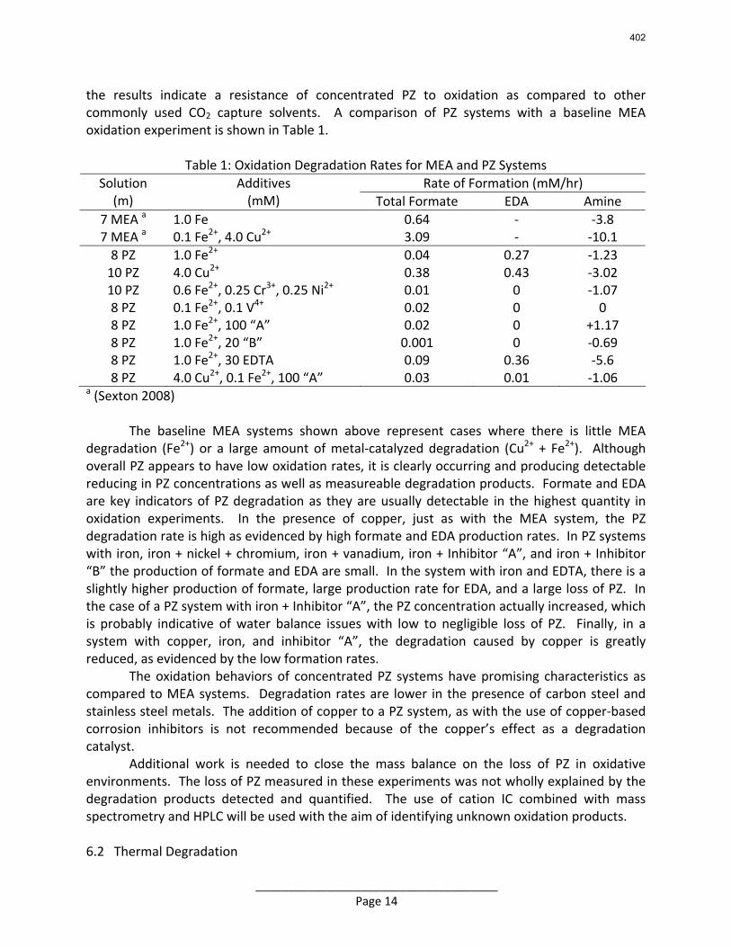
_____________________________________ Page 14
the results indicate a resistance of concentrated PZ to oxidation as compared to other commonly used CO2 capture solvents. A comparison of PZ systems with a baseline MEA oxidation experiment is shown in Table 1.
Table 1: Oxidation Degradation Rates for MEA and PZ Systems Rate of Formation (mM/hr) Solution
(m) Additives (mM) Total Formate EDA Amine
7 MEA a 1.0 Fe 0.64 ‐ ‐3.8 7 MEA a 0.1 Fe2+, 4.0 Cu2+ 3.09 ‐ ‐10.1 8 PZ 1.0 Fe2+ 0.04 0.27 ‐1.23 10 PZ 4.0 Cu2+ 0.38 0.43 ‐3.02 10 PZ 0.6 Fe2+, 0.25 Cr3+, 0.25 Ni2+ 0.01 0 ‐1.07 8 PZ 0.1 Fe2+, 0.1 V4+ 0.02 0 0 8 PZ 1.0 Fe2+, 100 “A” 0.02 0 +1.17 8 PZ 1.0 Fe2+, 20 “B” 0.001 0 ‐0.69 8 PZ 1.0 Fe2+, 30 EDTA 0.09 0.36 ‐5.6 8 PZ 4.0 Cu2+, 0.1 Fe2+, 100 “A” 0.03 0.01 ‐1.06
a (Sexton 2008)
The baseline MEA systems shown above represent cases where there is little MEA degradation (Fe2+) or a large amount of metal‐catalyzed degradation (Cu2+ + Fe2+). Although overall PZ appears to have low oxidation rates, it is clearly occurring and producing detectable reducing in PZ concentrations as well as measureable degradation products. Formate and EDA are key indicators of PZ degradation as they are usually detectable in the highest quantity in oxidation experiments. In the presence of copper, just as with the MEA system, the PZ degradation rate is high as evidenced by high formate and EDA production rates. In PZ systems with iron, iron + nickel + chromium, iron + vanadium, iron + Inhibitor “A”, and iron + Inhibitor “B” the production of formate and EDA are small. In the system with iron and EDTA, there is a slightly higher production of formate, large production rate for EDA, and a large loss of PZ. In the case of a PZ system with iron + Inhibitor “A”, the PZ concentration actually increased, which is probably indicative of water balance issues with low to negligible loss of PZ. Finally, in a system with copper, iron, and inhibitor “A”, the degradation caused by copper is greatly reduced, as evidenced by the low formation rates. The oxidation behaviors of concentrated PZ systems have promising characteristics as compared to MEA systems. Degradation rates are lower in the presence of carbon steel and stainless steel metals. The addition of copper to a PZ system, as with the use of copper‐based corrosion inhibitors is not recommended because of the copper’s effect as a degradation catalyst.
Additional work is needed to close the mass balance on the loss of PZ in oxidative environments. The loss of PZ measured in these experiments was not wholly explained by the degradation products detected and quantified. The use of cation IC combined with mass spectrometry and HPLC will be used with the aim of identifying unknown oxidation products.
6.2 Thermal Degradation
402
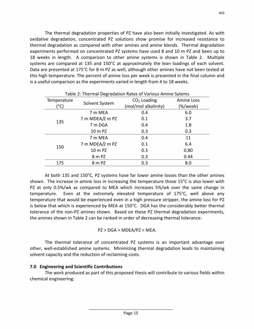
_____________________________________ Page 15
The thermal degradation properties of PZ have also been initially investigated. As with oxidative degradation, concentrated PZ solutions show promise for increased resistance to thermal degradation as compared with other amines and amine blends. Thermal degradation experiments performed on concentrated PZ systems have used 8 and 10 m PZ and been up to 18 weeks in length. A comparison to other amine systems is shown in Table 2. Multiple systems are compared at 135 and 150°C at approximately the lean loadings of each solvent. Data are presented at 175°C for 8 m PZ as well, although other amines have not been tested at this high temperature. The percent of amine loss per week is presented in the final column and is a useful comparison as the experiments varied in length from 4 to 18 weeks.
Table 2: Thermal Degradation Rates of Various Amine Sytems Temperature
(°C) Solvent System
CO2 Loading (mol/mol alkalinity)
Amine Loss (%/week)
7 m MEA 0.4 6.0 7 m MDEA/2 m PZ 0.1 3.7
7 m DGA 0.4 1.8 135
10 m PZ 0.3 0.3 7 m MEA 0.4 11
7 m MDEA/2 m PZ 0.1 6.4 10 m PZ 0.3 0.80
150
8 m PZ 0.3 0.44 175 8 m PZ 0.3 8.0
At both 135 and 150°C, PZ systems have far lower amine losses than the other amines
shown. The increase in amine loss in increasing the temperature those 15°C is also lower with PZ at only 0.5%/wk as compared to MEA which increases 5%/wk over the same change in temperature. Even at the extremely elevated temperature of 175°C, well above any temperature that would be experienced even in a high pressure stripper, the amine loss for PZ is below that which is experienced by MEA at 150°C. DGA has the considerably better thermal tolerance of the non‐PZ amines shown. Based on these PZ thermal degradation experiments, the amines shown in Table 2 can be ranked in order of decreasing thermal tolerance:
PZ > DGA > MDEA/PZ > MEA.
The thermal tolerance of concentrated PZ systems is an important advantage over
other, well‐established amine systems. Minimizing thermal degradation leads to maintaining solvent capacity and the reduction of reclaiming costs. 7.0 Engineering and Scientific Contributions
The work produced as part of this proposed thesis will contribute to various fields within chemical engineering:
403
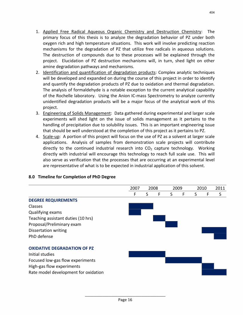
_____________________________________ Page 16
1. Applied Free Radical Aqueous Organic Chemistry and Destruction Chemistry: The primary focus of this thesis is to analyze the degradation behavior of PZ under both oxygen rich and high temperature situations. This work will involve predicting reaction mechanisms for the degradation of PZ that utilize free radicals in aqueous solutions. The destruction of compounds due to these processes will be explained through the project. Elucidation of PZ destruction mechanisms will, in turn, shed light on other amine degradation pathways and mechanisms.
2. Identification and quantification of degradation products: Complex analytic techniques will be developed and expanded on during the course of this project in order to identify and quantify the degradation products of PZ due to oxidation and thermal degradation. The analysis of formaldehyde is a notable exception to the current analytical capability of the Rochelle laboratory. Using the Anion IC‐mass Spectrometry to analyze currently unidentified degradation products will be a major focus of the analytical work of this project.
3. Engineering of Solids Management: Data gathered during experimental and larger scale experiments will shed light on the issue of solids management as it pertains to the handling of precipitation due to solubility issues. This is an important engineering issue that should be well understood at the completion of this project as it pertains to PZ.
4. Scale‐up: A portion of this project will focus on the use of PZ as a solvent at larger scale applications. Analysis of samples from demonstration scale projects will contribute directly to the continued industrial research into CO2 capture technology. Working directly with industrial will encourage this technology to reach full scale use. This will also serve as verification that the processes that are occurring at an experimental level are representative of what is to be expected in industrial application of this solvent.
8.0 Timeline for Completion of PhD Degree 2007 2008 2009 2010 2011 F S F S F S F S DEGREE REQUIREMENTS Classes Qualifying exams Teaching assistant duties (10 hrs) Proposal/Preliminary exam Dissertation writing PhD defense OXIDATIVE DEGRADATION OF PZ Initial studies Focused low‐gas flow experiments High‐gas flow experiments Rate model development for oxidation
404
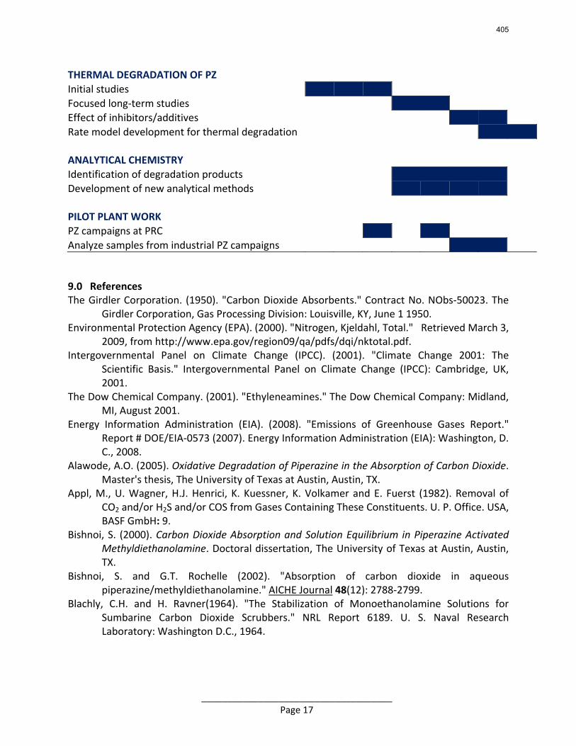
_____________________________________ Page 17
THERMAL DEGRADATION OF PZ Initial studies Focused long‐term studies Effect of inhibitors/additives Rate model development for thermal degradation ANALYTICAL CHEMISTRY Identification of degradation products Development of new analytical methods PILOT PLANT WORK PZ campaigns at PRC Analyze samples from industrial PZ campaigns 9.0 References The Girdler Corporation. (1950). "Carbon Dioxide Absorbents." Contract No. NObs‐50023. The
Girdler Corporation, Gas Processing Division: Louisville, KY, June 1 1950. Environmental Protection Agency (EPA). (2000). "Nitrogen, Kjeldahl, Total." Retrieved March 3,
2009, from http://www.epa.gov/region09/qa/pdfs/dqi/nktotal.pdf. Intergovernmental Panel on Climate Change (IPCC). (2001). "Climate Change 2001: The
Scientific Basis." Intergovernmental Panel on Climate Change (IPCC): Cambridge, UK, 2001.
The Dow Chemical Company. (2001). "Ethyleneamines." The Dow Chemical Company: Midland, MI, August 2001.
Energy Information Administration (EIA). (2008). "Emissions of Greenhouse Gases Report." Report # DOE/EIA‐0573 (2007). Energy Information Administration (EIA): Washington, D. C., 2008.
Alawode, A.O. (2005). Oxidative Degradation of Piperazine in the Absorption of Carbon Dioxide. Master's thesis, The University of Texas at Austin, Austin, TX.
Appl, M., U. Wagner, H.J. Henrici, K. Kuessner, K. Volkamer and E. Fuerst (1982). Removal of CO2 and/or H2S and/or COS from Gases Containing These Constituents. U. P. Office. USA, BASF GmbH: 9.
Bishnoi, S. (2000). Carbon Dioxide Absorption and Solution Equilibrium in Piperazine Activated Methyldiethanolamine. Doctoral dissertation, The University of Texas at Austin, Austin, TX.
Bishnoi, S. and G.T. Rochelle (2002). "Absorption of carbon dioxide in aqueous piperazine/methyldiethanolamine." AICHE Journal 48(12): 2788‐2799.
Blachly, C.H. and H. Ravner(1964). "The Stabilization of Monoethanolamine Solutions for Sumbarine Carbon Dioxide Scrubbers." NRL Report 6189. U. S. Naval Research Laboratory: Washington D.C., 1964.
405
_____________________________________ Page 18
Blachly, C.H. and H. Ravner(1965). "Studies of Submarie Carbon Dioxide Scrubber Operation: Effect of an Additive Package for the Stabilization of Monoethanolamine Solutions." NRL Memorandum Report 1598. Naval Research Laboratory: Washington D.C., 1965.
Blachly, C.H. and H. Ravner (1966). "Stabilization of Monoethanolamine Solutions in Carbon Dioxide Scrubbers." Journal of Chemical and Engineering Data 11(3): 401‐403.
Challis, B.C. and J.A. Challis (1982). N‐nitrosamines and N‐nitrosoimines. The chemistry of amino, nitroso and nitro compounds and their derivatives, Supplement F, Part 2. S. Patai. New York, John Wiley and Sons: 1151‐1223.
Chen, E. (2007). Carbon Dioxide Absorption into Promoted Potassium Carbonate in Structured Packing. Doctoral dissertation, The University of Texas at Austin, Austin, TX.
Chi, S.Q. (2002). Oxidative Degradation of Monoethanolamine. Doctorial dissertation, The University of Texas at Austin, Austin, TX.
Cook, H.L. and B.M. Lowe (1976). "Viscosity B‐Coefficients for Pinacol and Piperazine in Aqueous‐Solution at 25degreesc and 35degreesc." Electrochimica Acta 21(2): 153‐154.
Cullinane, J.T. and G.T. Rochelle (2004). "Carbon dioxide absorption with aqueous potassium carbonate promoted by piperazine." Chemical Engineering Science 59(17): 3619‐3630.
Davis, J. (2008). Thermal degradation of monoethanolamine at stripper conditions. GHGT‐9, Washington D.C.
Derks, P.W., K.J. Hogendoorn and G.F. Versteeg (2005). "Solubility of N2O in and density, viscosity, and surface tension of aqueous piperazine solutions." Journal of Chemical and Engineering Data 50(6): 1947‐1950.
Derks, P.W.J., E.S. Hamborg, J.A. Hogendoorn, J.P.M. Niederer and G.F. Versteeg (2008). "Densities, viscosities, and liquid diffusivities in aqueous piperazine and aqueous (piperazine plus N‐methyldiethanolamine) solutions." Journal of Chemical and Engineering Data 53(5): 1179‐1185.
Dugas, R. (2008). Absorption and desorption rates of carbon dioxide with monoethanolamine and piperazine. GHGT‐9, Washington D.C.
Elespuru, R.K. and W. Lijinsky (1976). "Mutagenicity of Cyclic Nitrosamines in Escherichia coli following Activation with Rat Liver Microsomes " Cancer Research 36: 4099‐4101.
Erowid.org (2008, February 25, 2008). "Piperazines." Retrieved January 15, 2009, from http://www.erowid.org/chemicals/piperazines/piperazines.shtml.
Goff, G.S. (2005). Oxidative Degradation of Aqueous Monoethanolamine in CO2 Capture Processes: Iron and Copper Catalysts, Inhibition, and O2 Mass Transfer. Doctoral dissertation, The University of Texas at Austin, Austin, TX.
Hamborg, E.S., P.W.J. Derks, S.R.A. Kersten, J.P.M. Niederer and G.F. Versteeg (2008). "Diffusion coefficients of N2O in aqueous piperazine solutions using the Taylor dispersion technique from (293 to 333) K and (0.3 to 1.4) mol.dm(‐3)." Journal of Chemical and Engineering Data 53(7): 1462‐1466.
Haugmo, I. (2008). Environmental impacts and aspects of absorbents used for CO2 capture. Rochelle Group Research Review Meeting, Austin, TX.
Hilliard, M.D. (2008). A Predictive Thermodynamic Model for an Aqueous Blend of Potassium Carbonate, Piperazine, and Monoethanolamine for Carbon Dioxide Capture from Flue Gas. Doctoral dissertation, The University of Texas at Austin, Austin, TX.
406
_____________________________________ Page 19
Hofmeyer, B.G., H.G. Scholten and W.G. Lloyd (1956). Contamination and corrosion in monoethanolamine gas treating systems. National Meeting of the American Chemical Society. Dallas, TX.
Love, L.A., W. Lijinsky, L. Keefer and H. Garcia (1977). "Chronic oral administration of 1‐nitrosopiperazine in high doses to MRC rats." Z. Krebsforsch: 69‐73.
Reza, J. and A. Trejo (2006). "Degradation of aqueous solutions of alkanolamine blends at high temperature, under the presence of CO2 and H2S." Chemical Engineering Communications 193(1): 129‐138.
Rooney, P.C., M.S. DuPart and T.R. Bacon (1998). "Oxygen's role in alkanolamine degradation." Hydrocarbon Processing 77(7): 109‐113.
Samanta, A. and S.S. Bandyopadhyay (2006). "Density and viscosity of aqueous solutions of piperazine and (2‐amino‐2‐methyl‐1‐propanol + piperazine) from 298 to 333 K." Journal of Chemical and Engineering Data 51(2): 467‐470.
Samanta, A., S. Roy and S.S. Bandyopadhyay (2007). "Physical solubility and diffusivity of N2O and CO2 in aqueous solutions of piperazine and (N‐methyldiethanolamine plus piperazine)." Journal of Chemical and Engineering Data 52(4): 1381‐1385.
Scheiman, M.A.(1962). "A review of monoethanolamine chemistry." Report No. 5746. U. S. Naval Research Laboratory: 1962.
Sexton, A. (2008). Amine Oxidation in CO2 Capture Processes. Doctoral dissertation, The University of Texas at Austin, Austin, TX.
Tricker, A.R., R. Kumar, M. Siddiqi, M.S. Khuroo and R. Preussmann (1991). "Endogenous formation of N‐nitrosamines from piperazine and their urinary excretion following antihelmintic treatment with piperazine citrate " Carcinogenesis 12(9): 1595‐1599.
Xu, G.W., C.F. Zhang, S.J. Qin and Y.W. Wang (1992). "Kinetics Study on Absorption of Carbon‐Dioxide into Solutions of Activated Methyldiethanolamine." Industrial & Engineering Chemistry Research 31(3): 921‐927.
Zhang, X., C.F. Zhang, S.J. Qin and Z.S. Zheng (2001). "A kinetics study on the absorption of carbon dioxide into a mixed aqueous solution of methyldiethanolamine and piperazine." Industrial & Engineering Chemistry Research 40(17): 3785‐3791.
407
The University of Texas at Austin
Department of Chemical Engineering
Ph.D. Research Proposal
Stripper Modeling for CO2 Removal using Monoethanolamine and Piperazine Solvents
David H. Van Wagener
Supervisor: Gary T. Rochelle
April 16, 2009
408
David Van Wagener Research Proposal Page 1
1 Introduction
A study of atmospheric carbon dioxide concentrations at Mauna Loa, Hawaii was conducted between
1960 and 2001. The study determined that CO2 levels have risen by about 17% in 41 years (Keeling and
Whorf 2004). Additionally, ice cores from the Antarctic show surface temperature and atmospheric CO2
cycles that nearly track each other. This trend suggests a direct correlation between atmospheric CO2
concentration and global temperatures (Petit 1999). The annual worldwide CO2 emissions continue to
rise each year, which have consequently increased the atmospheric CO2 concentration to 380 ppm from
preindustrial levels of 300 ppm (Bates and Kundzewicz 2008). In order to attempt to mitigate climate
change by reducing greenhouse gases in the atmosphere, the release of carbon dioxide should be
addressed. Coal is a fossil fuel which liberates a significant amount of CO2 when burned, and it is the
largest electricity producer in the United States, accounting for nearly 50% of the total production (EIA
2006). Therefore, coal-fired power plants are the most important target for reducing point source
emissions.
Absorption/stripping using alkanolamine solvents is one of the leading technologies for removing CO2
from the flue gas of coal-fired power plants. It is a tail-end process which could be installed with new
plants, but it could also be retrofitted to current plants with few changes to the existing power plant.
Monoethanolamine (MEA) is the current standard solvent because it has the most substantial research
base. It has also been used in the past for similar applications like H2S removal from natural gas. 90%
removal of CO2 using MEA is possible, but the capital cost and energy requirement of the current
technology is prohibitive (Rochelle 2007). The steam and electricity used for operating the pumps,
compressors, and stripper reboiler typically accounts for 30% of the total power plant output.
Computer modeling of these process units can improve the understanding of the underlying
mechanisms and help locate areas where work is lost. This knowledge can aid in the implementation of
improved configurations and solvents to reduce the overall energy usage. Energy consumption is the
main cost of this process, so the key to making absorption/stripping a practical option for carbon
capture is reducing this operating cost.
2 Literature Review
2.1 Absorption/Stripping Fundamentals
The aqueous absorption/stripping technology has already been used for acid gas treating. It has been
utilized for removal of CO2 and H2S from oil and natural gas, and it has also been applied to the
production of ammonia and syngas (Pierantozzi 2003). It has also been heavily researched; the use of an
organic base to purify gases was patented by Bottoms (1931), and the ability of various solvents to
absorb CO2 has been studied. Potassium carbonate solutions were researched by Benson (1954, 1956),
Shrier (1969), and Savage (1980). Potassium carbonate has high capacity for absorbing CO2, but its
reaction rates are not practical for industrial use as a stand-alone solvent. Therefore, the effect of using
alternative amine solvents was also investigated. For example, MEA was studied by Teller (1958), and
409
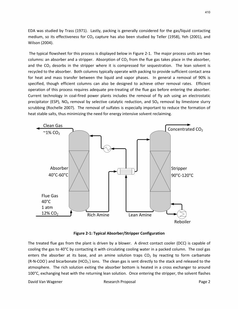
David Van Wagener Research Proposal Page 2
EDA was studied by Trass (1971). Lastly, packing is generally considered for the gas/liquid contacting
medium, so its effectiveness for CO2 capture has also been studied by Teller (1958), Yeh (2001), and
Wilson (2004).
The typical flowsheet for this process is displayed below in Figure 2-1. The major process units are two
columns: an absorber and a stripper. Absorption of CO2 from the flue gas takes place in the absorber,
and the CO2 desorbs in the stripper where it is compressed for sequestration. The lean solvent is
recycled to the absorber. Both columns typically operate with packing to provide sufficient contact area
for heat and mass transfer between the liquid and vapor phases. In general a removal of 90% is
specified, though efficient columns can also be designed to achieve other removal rates. Efficient
operation of this process requires adequate pre-treating of the flue gas before entering the absorber.
Current technology in coal-fired power plants includes the removal of fly ash using an electrostatic
precipitator (ESP), NOX removal by selective catalytic reduction, and SOX removal by limestone slurry
scrubbing (Rochelle 2007). The removal of sulfates is especially important to reduce the formation of
heat stable salts, thus minimizing the need for energy intensive solvent reclaiming.
Figure 2-1: Typical Absorber/Stripper Configuration
The treated flue gas from the plant is driven by a blower. A direct contact cooler (DCC) is capable of
cooling the gas to 40°C by contacting it with circulating cooling water in a packed column. The cool gas
enters the absorber at its base, and an amine solution traps CO2 by reacting to form carbamate
(R-N-COO-) and bicarbonate (HCO3-) ions. The clean gas is sent directly to the stack and released to the
atmosphere. The rich solution exiting the absorber bottom is heated in a cross exchanger to around
100°C, exchanging heat with the returning lean solution. Once entering the stripper, the solvent flashes
Flue Gas40°C1 atm12% CO2
Concentrated CO2
Clean Gas
~1% CO2
Lean AmineRich Amine
Stripper
90°C-120°C
Absorber
40°C-60°C
Reboiler
410
David Van Wagener Research Proposal Page 3
if the total vapor pressure of the solution is greater than operating pressure of the stripper. The
remaining liquid passes down through the packing and is stripped of CO2 by steam generated in the
reboiler. The removed CO2 inevitably leaves the column with extra stripping steam which must be
condensed and returned to the process to maintain its water balance. Next, multiple stages of
compressors with intercooling and liquid knockout compress and purify the CO2 to around 150 atm and
at least 99% CO2. Water is the most likely impurity of the compressed CO2, but ppb amounts of amine
could also exist due to its volatility in the stripper. This final product can be transported by pipeline for
sequestration or use in enhanced oil recovery (EOR). The lean solution exiting the bottom of the
stripper transfers heat in the cross exchanger, cools further in a trim cooler, and is returned to the
absorber (Cullinane 2005).
Carbon capture with this system can be highly effective, but it is energy intensive. The baseline design
of this system using 7 m MEA draws medium pressure steam directly from an intermediate turbine, and
additional energy is required to run the pumps, compressor, and blower. It is estimated that the total
deficit is approximately 20-40% of the overall energy production from a coal plant, thereby reducing the
capacity of the facility.
2.2 Solvent Models
Many amine solvents have been evaluated for their potential use in acid gas treating. The solvent with
the most focus has been MEA, especially 30 wt% (7 m). The foundation of a correct simulation of the
stripper is an accurate solvent model, a product of reliable data. Various authors have contributed data
on VLE and mass transfer characteristics of solvents other than MEA, including MEA/PZ, K+/PZ, and even
potential new solvents like AHPD, an amine, promoted with carbonic anhydrase to increase its reaction
rate with CO2 (Aroonwilas and Tontiwachwuthikul 1997, Cullinane 2002, Dang 2001, Le Tourneux, et al.
2008). Experimental work evaluating packing performance has also been conducted (Brunazzi and
Paglianti 1997).
A number of models have been developed in Aspen Plus to represent alkanolamine solutions for use in
CO2 capture. The thermodynamic framework most suited for modeling the solutions is the electrolyte-
NRTL model. This model uses interaction parameters between molecules and electrolytes to calculate
activity coefficients for solutions. An early model was developed by Austgen (1991) which broadly
predicts VLE for CO2 and H2S in MEA, MDEA, MDEA/MEA, and MDEA/DEA solutions. This MEA model
was updated by Freguia (2003) to include VLE data collected by Jou (1995). In his work Freguia also
developed a full process model for the absorber and stripper, incorporating reaction rates in the
absorber by utilizing experimental kinetic data at absorber conditions. Cullinane produced a model for
PZ promoted potassium. PZ was used as an additive to the potassium solvent to increase the reaction
rate with CO2 (Cullinane and Rochelle 2004). A broad thermodynamic model for MEA was recently
developed by Hilliard (2008) which included data sets for MEA from 3.5 m to 11 m and temperatures
from 40°C to 120°C. In addition to the MEA model, further solvent models were developed for PZ, K+,
and selected blends, including a global K+/MEA/PZ representation. His work found that attempting to
represent a broad range of solvents and conditions sacrificed accuracy of predictions.
411
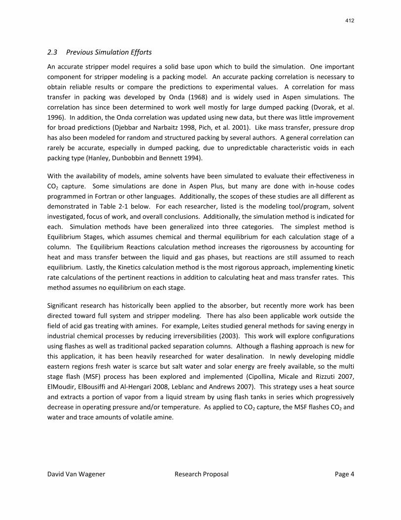
David Van Wagener Research Proposal Page 4
2.3 Previous Simulation Efforts
An accurate stripper model requires a solid base upon which to build the simulation. One important
component for stripper modeling is a packing model. An accurate packing correlation is necessary to
obtain reliable results or compare the predictions to experimental values. A correlation for mass
transfer in packing was developed by Onda (1968) and is widely used in Aspen simulations. The
correlation has since been determined to work well mostly for large dumped packing (Dvorak, et al.
1996). In addition, the Onda correlation was updated using new data, but there was little improvement
for broad predictions (Djebbar and Narbaitz 1998, Pich, et al. 2001). Like mass transfer, pressure drop
has also been modeled for random and structured packing by several authors. A general correlation can
rarely be accurate, especially in dumped packing, due to unpredictable characteristic voids in each
packing type (Hanley, Dunbobbin and Bennett 1994).
With the availability of models, amine solvents have been simulated to evaluate their effectiveness in
CO2 capture. Some simulations are done in Aspen Plus, but many are done with in-house codes
programmed in Fortran or other languages. Additionally, the scopes of these studies are all different as
demonstrated in Table 2-1 below. For each researcher, listed is the modeling tool/program, solvent
investigated, focus of work, and overall conclusions. Additionally, the simulation method is indicated for
each. Simulation methods have been generalized into three categories. The simplest method is
Equilibrium Stages, which assumes chemical and thermal equilibrium for each calculation stage of a
column. The Equilibrium Reactions calculation method increases the rigorousness by accounting for
heat and mass transfer between the liquid and gas phases, but reactions are still assumed to reach
equilibrium. Lastly, the Kinetics calculation method is the most rigorous approach, implementing kinetic
rate calculations of the pertinent reactions in addition to calculating heat and mass transfer rates. This
method assumes no equilibrium on each stage.
Significant research has historically been applied to the absorber, but recently more work has been
directed toward full system and stripper modeling. There has also been applicable work outside the
field of acid gas treating with amines. For example, Leites studied general methods for saving energy in
industrial chemical processes by reducing irreversibilities (2003). This work will explore configurations
using flashes as well as traditional packed separation columns. Although a flashing approach is new for
this application, it has been heavily researched for water desalination. In newly developing middle
eastern regions fresh water is scarce but salt water and solar energy are freely available, so the multi
stage flash (MSF) process has been explored and implemented (Cipollina, Micale and Rizzuti 2007,
ElMoudir, ElBousiffi and Al-Hengari 2008, Leblanc and Andrews 2007). This strategy uses a heat source
and extracts a portion of vapor from a liquid stream by using flash tanks in series which progressively
decrease in operating pressure and/or temperature. As applied to CO2 capture, the MSF flashes CO2 and
water and trace amounts of volatile amine.
412
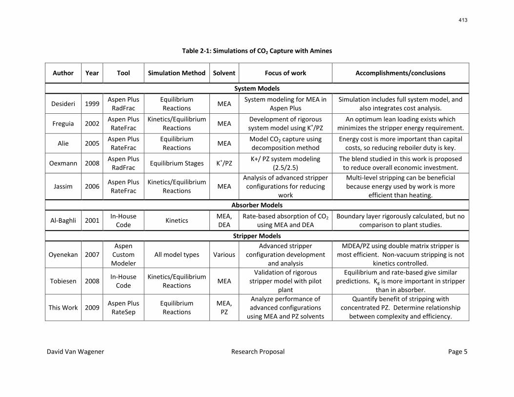
David Van Wagener Research Proposal Page 5
Table 2-1: Simulations of CO2 Capture with Amines
Author Year Tool Simulation Method Solvent Focus of work Accomplishments/conclusions
System Models
Desideri 1999 Aspen Plus
RadFrac Equilibrium Reactions
MEA System modeling for MEA in
Aspen Plus Simulation includes full system model, and
also integrates cost analysis.
Freguia 2002 Aspen Plus RateFrac
Kinetics/Equilibrium Reactions
MEA Development of rigorous system model using K+/PZ
An optimum lean loading exists which minimizes the stripper energy requirement.
Alie 2005 Aspen Plus RateFrac
Equilibrium Reactions
MEA Model CO2 capture using decomposition method
Energy cost is more important than capital costs, so reducing reboiler duty is key.
Oexmann 2008 Aspen Plus
RadFrac Equilibrium Stages K+/PZ
K+/ PZ system modeling (2.5/2.5)
The blend studied in this work is proposed to reduce overall economic investment.
Jassim 2006 Aspen Plus RateFrac
Kinetics/Equilibrium Reactions
MEA Analysis of advanced stripper configurations for reducing
work
Multi-level stripping can be beneficial because energy used by work is more
efficient than heating.
Absorber Models
Al-Baghli 2001 In-House
Code Kinetics
MEA, DEA
Rate-based absorption of CO2 using MEA and DEA
Boundary layer rigorously calculated, but no comparison to plant studies.
Stripper Models
Oyenekan 2007 Aspen
Custom Modeler
All model types Various Advanced stripper
configuration development and analysis
MDEA/PZ using double matrix stripper is most efficient. Non-vacuum stripping is not
kinetics controlled.
Tobiesen 2008 In-House
Code Kinetics/Equilibrium
Reactions MEA
Validation of rigorous stripper model with pilot
plant
Equilibrium and rate-based give similar predictions. Kg is more important in stripper
than in absorber.
This Work 2009 Aspen Plus
RateSep Equilibrium Reactions
MEA, PZ
Analyze performance of advanced configurations
using MEA and PZ solvents
Quantify benefit of stripping with concentrated PZ. Determine relationship
between complexity and efficiency.
413
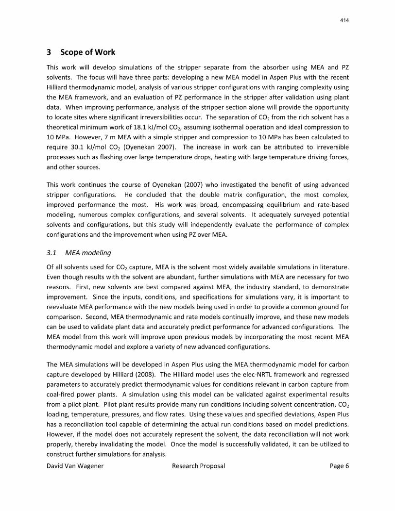
David Van Wagener Research Proposal Page 6
3 Scope of Work
This work will develop simulations of the stripper separate from the absorber using MEA and PZ
solvents. The focus will have three parts: developing a new MEA model in Aspen Plus with the recent
Hilliard thermodynamic model, analysis of various stripper configurations with ranging complexity using
the MEA framework, and an evaluation of PZ performance in the stripper after validation using plant
data. When improving performance, analysis of the stripper section alone will provide the opportunity
to locate sites where significant irreversibilities occur. The separation of CO2 from the rich solvent has a
theoretical minimum work of 18.1 kJ/mol CO2, assuming isothermal operation and ideal compression to
10 MPa. However, 7 m MEA with a simple stripper and compression to 10 MPa has been calculated to
require 30.1 kJ/mol CO2 (Oyenekan 2007). The increase in work can be attributed to irreversible
processes such as flashing over large temperature drops, heating with large temperature driving forces,
and other sources.
This work continues the course of Oyenekan (2007) who investigated the benefit of using advanced
stripper configurations. He concluded that the double matrix configuration, the most complex,
improved performance the most. His work was broad, encompassing equilibrium and rate-based
modeling, numerous complex configurations, and several solvents. It adequately surveyed potential
solvents and configurations, but this study will independently evaluate the performance of complex
configurations and the improvement when using PZ over MEA.
3.1 MEA modeling
Of all solvents used for CO2 capture, MEA is the solvent most widely available simulations in literature.
Even though results with the solvent are abundant, further simulations with MEA are necessary for two
reasons. First, new solvents are best compared against MEA, the industry standard, to demonstrate
improvement. Since the inputs, conditions, and specifications for simulations vary, it is important to
reevaluate MEA performance with the new models being used in order to provide a common ground for
comparison. Second, MEA thermodynamic and rate models continually improve, and these new models
can be used to validate plant data and accurately predict performance for advanced configurations. The
MEA model from this work will improve upon previous models by incorporating the most recent MEA
thermodynamic model and explore a variety of new advanced configurations.
The MEA simulations will be developed in Aspen Plus using the MEA thermodynamic model for carbon
capture developed by Hilliard (2008). The Hilliard model uses the elec-NRTL framework and regressed
parameters to accurately predict thermodynamic values for conditions relevant in carbon capture from
coal-fired power plants. A simulation using this model can be validated against experimental results
from a pilot plant. Pilot plant results provide many run conditions including solvent concentration, CO2
loading, temperature, pressures, and flow rates. Using these values and specified deviations, Aspen Plus
has a reconciliation tool capable of determining the actual run conditions based on model predictions.
However, if the model does not accurately represent the solvent, the data reconciliation will not work
properly, thereby invalidating the model. Once the model is successfully validated, it can be utilized to
construct further simulations for analysis.
414
David Van Wagener Research Proposal Page 7
3.2 Configuration Complexity
The trend in modeling new stripping configurations suggests that advanced, more complex
configurations yield better performance. Again, previous work with the double matrix stripper
configuration echoes this point. However, previous effort in the area has not attempted to directly
correlate complexity to performance. This work will take a systematic approach at developing
configurations of varying levels of complexity, and their rankings will be determined by the total pieces
of equipment utilized for separation. As a preliminary guideline, each component contributes 1 unit to
the complexity. The different types of equipment can include:
Packing sections
Vessels (flashes, separators, etc.)
Heat exchangers/reboilers
Pumps/compressors
The analysis of types of configurations will start at the most simple method of desorbing CO2 from the
amine, a heated flash. The flowsheet will be developed by adding one piece of equipment at a time and
include recycles as needed to improve performance. The simulations will be run using the robust
Hilliard MEA model. Examples of the range of configurations are detailed in Figures Figure 3-1– Figure
3-3.
Adiabatic Flash
Preheater
Water for reflux
CO2 Multistage compressor
Lean
Preheater
Water for reflux
CO2 Multistage compressor
Lean
Rich
Figure 3-1: Single heated flash (left) and simple stripper with preflash (right) configurations
Figure 3-1 shows the basic heated flash and its evolution to a simple stripper with a preflash. Figure 3-2
displays a more complicated flash configuration, a three stage flash. This flowsheet has a preheater
followed by three adiabatic flashes in series. Finally, the double matrix configuration is shown in Figure
3-3. This flowsheet contains a high pressure column and a low pressure column, a split feed, and both a
lean and semi-lean product.
415
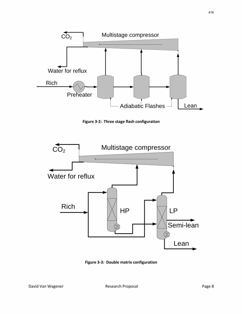
David Van Wagener Research Proposal Page 8
Adiabatic Flashes
Preheater
Water for reflux
CO2 Multistage compressor
Lean
Rich
Figure 3-2: Three stage flash configuration
Water for reflux
CO2 Multistage compressor
Lean
RichHP LP
Semi-lean
Figure 3-3: Double matrix configuration
416
David Van Wagener Research Proposal Page 9
The relationship between complexity and performance will be analyzed to determine:
Whether the pre-decided complexity ranking system is reflective of changes in
performance
Any occurrence of an optimum level of complexity
3.3 PZ Modeling
Concentrated piperazine (PZ) is an attractive solvent for use in CO2 capture due to its high capacity. A
large capacity yields low energy requirements because the sensible heat input decreases. In addition to
the high capacity, PZ also has a very low thermal degradation rate compared to MEA. Until now,
concentrated piperazine had not been considered as a solvent due to its low solubility in water at
absorber temperatures. However, since it has been shown to be soluble for the expected loading range
for carbon capture, 8 m PZ will be studied heavily in the future (Freeman, et al. 2008). Along with the
MEA model, Hilliard also completed a PZ model for CO2 removal. This model will be used to construct a
simulation with PZ to demonstrate its improvement over MEA.
The first task will be the use of Aspen Plus to simulate a simple stripper with the accompanying heat
exchanger, amine pumps, and multistage compressor. The use of concentrated piperazine in the three
stage flash configuration, mentioned in section 3.2, is also very appealing because this configuration
operates best at high temperatures. In addition to the development of a functioning simulation, the
results of the simulation will be compared against experimental data. A pilot plant campaign was run
with 8 m PZ at the J. J. Pickle Research Campus in November, 2008. As with the MEA campaign, the PZ
data will be used to validate the stripper model in Aspen Plus.
3.4 Additional Considerations
Additional topics related to this work may be considered if enough information is uncovered to
complete the tasks. The first topic of interest is the modeling of rate-based flashing in the stripper.
Flashing generally occurs when the superheated rich amine enters the stripper at a lower pressure.
Additionally, configurations like the three stage flash utilize flashing as the separation mechanism.
Aspen Plus treats these flashes as equilibrium, but depending on residence time and agitation, the
separation of gas and liquid may not reach equilibrium. It would be important to determine the
approach to equilibrium of these flashes to ensure that the results of the simulations are accurate.
Modeling of rate-based flashing can be pursued if experimental results on the approach to equilibrium
become available. Rate-based flash calculations are not an option for Aspen Plus simulations, but it is
possible to imitate non-equilibrium flashes. For example, work has been published using Aspen Plus to
simulate non-equilibrium/separation of ethylene from polyethylene based on experimental results
(Buchelli, et al. 2004).
Next, the PZ model developed by Hilliard was regressed using mostly low-temperature data, and the
heat capacity data used in the regressions may be inaccurate. Furthermore, the heat capacity and heat
absorption estimates from Aspen do not closely follow the lab results. Therefore, the data reconciliation
417
David Van Wagener Research Proposal Page 10
of pilot plant results is most likely to be difficult, and further simulations with the PZ model may be
inaccurate. To remedy this issue, the parameters in the PZ model can be regressed again if high
temperature VLE and more accurate heat capacity data become available. This re-regression would
calm any uneasiness arising from using the current PZ model as is.
Finally, the equilibrium assumption of the reboiler could be addressed. It is typically considered to be a
fair assumption to assign reboilers as equilibrium because there is significant contact time between the
liquid in the reboiler and the rising vapor bubbles that form. The vapor formation can also cause
turbulent flow, increasing the heat and mass transfer between liquid and gas. However, this assumption
has not been verified by lab work. Again, the simulations in this work will be more trustworthy if the
equilibrium assumption is confirmed.
4 Preliminary Results
Progress thus far has been made in the areas of absorption/stripping system modeling in Aspen Plus,
validation of pilot plant results using an Aspen Plus thermodynamic model, updating a thermodynamic
model for piperazine for simulations with high PZ concentration, and preliminary simulations with a
three stage flash configuration. These tasks have provided experience with data regression for
determining model parameter values, configuration development for improving stripper performance,
and optimization methods.
4.1 4 m K+/4 m PZ Double Matrix Modeling
Early work focused on completing an evaluation of K+/PZ as a potential solvent for CO2 absorption. An
absorber model including reaction kinetics and rigorous heat and mass transfer using RateSep was
developed by Jorge Plaza. The absorber utilized intercooling to 40°C in two stages to increase the
reaction rate with CO2. To directly implement feedback from the absorber while changing conditions in
the stripper, a system model was constructed, building the double matrix stripper, cross exchange, and
compression into the absorber simulation. The semi-lean return from the stripper was recycled to the
absorber, but the lean solution was not connected to the top of the absorber. Instead, a design
specification was used to match the CO2 flow rates of the absorber lean input and the stripper lean
calculation, but potential water balance issues were neglected. 4 m K+/4 m PZ was the most saturated
soluble solution, so the simulations used this solvent to obtain a larger capacity and improve the
performance.
Several design specifications were utilized to maintain consistency between cases and allow for
adequate comparison when chosen conditions were varied. These design specifications accomplished
the aforementioned equalization of CO2 flow of the lean streams, achieved 90% CO2 removal in the
absorber, maintained equal reboiler temperatures, and sustained cold side 5°C approaches on the lean
and semi-lean heat exchangers. An optimized simulation of the double matrix stripper with two stages
of intercooling was compared against a base case simulation with a non-intercooled absorber and a
418
David Van Wagener Research Proposal Page 11
simple stripper. The basis of comparison was equivalent work, accounting for the energy requirements
of the stripper reboilers, solvent pumps, and CO2 compressors. The equivalent work is calculated as:
𝑾𝒆𝒒 = 𝟎.𝟕𝟓 ∗ 𝑸 ∗ 𝑻𝒉𝒉𝒆𝒂𝒕𝒊𝒏𝒈 − 𝑻𝒔𝒊𝒏𝒌
𝑻𝒉𝒉𝒆𝒂𝒕𝒊𝒏𝒈 + 𝑾𝒑𝒖𝒎𝒑/𝒄𝒐𝒎𝒑 4.1
The lean loading was optimized in both cases to achieve a minimum work requirement. The non-
intercooled absorber/simple stripper configuration required 42.0 kJ/mol CO2, and the intercooled
absorber/double matrix stripper configuration required 39.7 kJ/mol CO2, a 5.3% improvement. These
results included CO2 compression to 10 MPa, the majority of whose energy usage is unaffected by
stripper configuration.
4.2 MEA pilot plant validation
The pilot plant facility at the J. J. Pickle Research Campus has been used in the past to investigate the
feasibility of proposed solvents and verify the accuracy of solvent models in Aspen (Oyenekan 2007,
Chen 2007). Generally, agreement between the pilot plant data and Aspen predictions has proved to be
difficult to accomplish, especially in the stripper section. The most recent thermodynamic model for
H2O- MEA-CO2 developed by Hilliard (2008) was applied to a pilot plant run completed in October 2007.
Raw data from the run was used as input to the simulation. The flowsheet included process units
outside the stripping column including the cross exchanger and vapor condenser. These units were
included because stream conditions for measured on the absorber (cold) side of the cross exchanger.
Additionally, the flowsheet was constructed to accurately reflect the pilot plant operation. This entailed
using a reboiler with a split feed and an unknown split ratio.
The completed simulation of the pilot plant closely matched the experimental data. The measured data
included flow rates, pressures, loadings, and temperatures, and the average deviation was 3.8%. The
most significant change was the height of packing. The pilot plant used 20 feet of MELLAPAK 250Y
packing, but the best agreement in all of the data resulted when only simulating 5 feet of packing. The
Onda correlation for heat and mass transfer and surface area was used, but it is suspected that a better
correlation is needed. An improved correlation has been developed within the Rochelle group (Tsai, et
al. 2008), and this can be implemented in the future using a subroutine.
4.3 PZ model regression
Another task has been a constant work in progress: regressing parameters in the Hilliard PZ model
(Hilliard 2008) to improve the predictions for concentrated PZ (8 m). The original model was developed
using concentrations only up to 5 m PZ, but the Rochelle group has recently been engaged in
experiments using 8 m PZ, and it will be desired to run simulations with this solvent. The available data
for concentrated PZ is limited, and the initial regression work only utilized VLE data gathered by Ross
Dugas. Using only this data, a stable thermodynamic model was developed which closely fit the VLE.
However, the heat capacity predictions were unreasonably scattered. Thu Nguyen later obtained heat
capacity data for concentrated PZ, and it was included in the previous regression. This greatly improved
419
David Van Wagener Research Proposal Page 12
the behavior of the heat capacity predictions, though the predictions are not perfect. Additionally, data
was not available above 120°C, so the predictions are unreliable. PZ, unlike MEA, has negligible thermal
degradation at high temperatures, and it is anticipated that stripping at high temperatures will be
beneficial. However, before the model is improved, the simulation results at high temperatures cannot
be used as an adequate comparison to lower temperature stripping and stripping with other solvents.
4.4 Three stage flash with MEA
The three stage flash configuration was developed as a simpler method for solvent regeneration which
efficiently utilizes heat available at variable temperatures. Preliminary simulations were run using 9 m
MEA. The simulation was carried out with the most recent MEA model, written by Hilliard (2008). An
absorber model with accurate kinetics was as yet unavailable for this new thermodynamic model, so
exact rich loadings and flow rates could not be obtained from simulations. Instead, a rich loading of
0.495 was chosen because a previous MEA models usually predicted a rich end pinch at 0.495 for the
expected conditions in this simulation. Additionally, the value of P*CO2 at 40°C for a solution with a
loading of 0.495 is only 4.7 kPa. Previous work by Oyenekan used rich MEA solutions with P* of 5 kPa,
so this rich loading has a higher driving force in previous assumptions, and should be achievable by the
absorber. This rich stream was then used as the base specification for the stripper section, and the
solvent flow rate was calculated with the specified lean loading and CO2 removal rate for a typical 500
MW coal-fired power plant (Fisher and Searcy 2007).
The flashes in the simulation were specified to have equal mole flows of liberated vapor. Next, the
second and third flashes would not be heated, so they are assumed to be adiabatic with a heat rate of
0W. Finally, the temperature of the heated first flash was specified to obtain a final outlet lean pressure
of 110 kPa, eliminating the chance of sub-atmospheric conditions. This stipulation on lean pressure also
kept the maximum temperature below 120°C, the imposed ceiling temperature for MEA due to thermal
degradation issues. The lean loading of this simulation was optimized to minimize equivalent work.
A simple stripper was also simulated and optimized with the Hilliard MEA model to provide a fair basis
of comparison to the three stage flash. The three stage flash was compared to the simple stripper with
equivalent lean conditions, a 1 atm column, as well as the simple stripper with an equivalent optimal
maximum temperature, a 1.6 atm column. The three stage flash with solar heating (variable
temperature heating medium) yielded the most favorable equivalent work of 32.9 kJ/mol CO2 at a lean
loading of 0.40. The 1 atm and 1.6 atm simple stripper simulations also had optimum lean loadings of
0.40, but both required more work for stripping than the three stage flash. The 1.6 atm stripper, the
more efficient of the two simple strippers, required 34.9 kJ/mol CO2. This study also concluded that
solar heating is beneficial for the three stage flash, whereas it results in higher energy consumption for
the simple stripper.
5 Research Objectives
Though there are no full-scale demonstrations of CO2 capture from coal-fired power plants, it is
projected that the addition of absorption/stripping the plant will decrease its output by 30%. Carbon
420
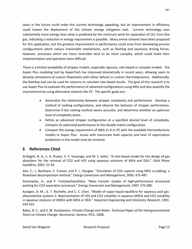
David Van Wagener Research Proposal Page 13
taxes in the future could make this current technology appealing, but an improvement in efficiency
could hasten the deployment of this climate change mitigation tool. Current technology uses
substantially more energy than what is predicted by the minimum work for separation of CO2 from flue
gas, indicating a reduction in energy requirement is possible. Many amine solvents have been proposed
for this application, but the greatest improvement in performance could arise from developing process
configurations which reduce irreversible mechanisms, such as flashing and excessive driving forces.
However, processes which are more reversible tend to be more complex, which could make their
implementation and operation more difficult.
There is a limited availability of stripper models, especially rigorous, rate-based or complex models. The
Aspen Plus modeling tool by AspenTech has improved dramatically in recent years, allowing users to
develop simulations of custom flowsheets with either default or custom thermodynamics. Additionally,
the RateSep tool can be used for columns to calculate rate-based results. The goal of this research is to
use Aspen Plus to evaluate the performance of advanced configurations using MEA and also quantify the
improvement by using alternative solvents like PZ. The specific goals are:
Generalize the relationship between stripper complexity and performance. Develop a
method of ranking configurations, and observe the behavior of stripper performance.
Determine if the ranking method seems accurate, and determine whether an optimum
level of complexity exists.
Refine an advanced stripper configuration at a specified desired level of complexity.
Compare its optimized performance to the double matrix configuration.
Compare the energy requirement of MEA to 8 m PZ with the available thermodynamic
models in Aspen Plus. Issues with inaccurate heat capacity and heat of vaporization
predictions in the model must be resolved.
6 References Cited
Al-Baghli, N. A., S. A. Pruess, V. F. Yesavage, and M. S. Selim. "A rate-based model for the design of gas absorbers for the removal of CO2 and H2S using aqueous solutions of MEA and DEA." Fluid Phase Equilibria, 2001: 31-43.
Alie, C., L. Backham, E. Croiset, and P. L. Douglas. "Simulation of CO2 capture using MEA scrubbing: a flowsheet decomposition method." Energy Conversion and Management, 2005: 475-487.
Aroonwilas, A., and P. Tontiwachwuthikul. "Mass transfer studies of high-performance structured packing for CO2 separation processes." Energy Conversion and Management, 1997: S75-S80.
Austgen, D. M., G. T. Rochelle, and C. C. Chen. "Model of vapor-liquid equilibria for aqueous acid gas-alkanolamine systems 2. Representation of H2S and CO2 solubility in aqueous MDEA and CO2 solubility in aqueous mixtures of MDEA with MEA or DEA." Industrial Engineering and Chemistry Research, 1991: 543-555.
Bates, B. C., and Z. W. Kundzewicz. Climate Change and Water. Technical Paper of the Intergovernmental Panel on Climate Change. Secretariat, Geneva: IPCC, 2008.
421
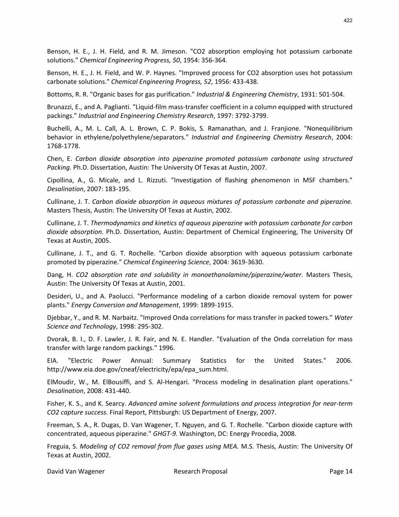
David Van Wagener Research Proposal Page 14
Benson, H. E., J. H. Field, and R. M. Jimeson. "CO2 absorption employing hot potassium carbonate solutions." Chemical Engineering Progress, 50, 1954: 356-364.
Benson, H. E., J. H. Field, and W. P. Haynes. "Improved process for CO2 absorption uses hot potassium carbonate solutions." Chemical Engineering Progress, 52, 1956: 433-438.
Bottoms, R. R. "Organic bases for gas purification." Industrial & Engineering Chemistry, 1931: 501-504.
Brunazzi, E., and A. Paglianti. "Liquid-film mass-transfer coefficient in a column equipped with structured packings." Industrial and Engineering Chemistry Research, 1997: 3792-3799.
Buchelli, A., M. L. Call, A. L. Brown, C. P. Bokis, S. Ramanathan, and J. Franjione. "Nonequilibrium behavior in ethylene/polyethylene/separators." Industrial and Engineering Chemistry Research, 2004: 1768-1778.
Chen, E. Carbon dioxide absorption into piperazine promoted potassium carbonate using structured Packing. Ph.D. Dissertation, Austin: The University Of Texas at Austin, 2007.
Cipollina, A., G. Micale, and L. Rizzuti. "Investigation of flashing phenomenon in MSF chambers." Desalination, 2007: 183-195.
Cullinane, J. T. Carbon dioxide absorption in aqueous mixtures of potassium carbonate and piperazine. Masters Thesis, Austin: The University Of Texas at Austin, 2002.
Cullinane, J. T. Thermodynamics and kinetics of aqueous piperazine with potassium carbonate for carbon dioxide absorption. Ph.D. Dissertation, Austin: Department of Chemical Engineering, The University Of Texas at Austin, 2005.
Cullinane, J. T., and G. T. Rochelle. "Carbon dioxide absorption with aqueous potassium carbonate promoted by piperazine." Chemical Engineering Science, 2004: 3619-3630.
Dang, H. CO2 absorption rate and solubility in monoethanolamine/piperazine/water. Masters Thesis, Austin: The University Of Texas at Austin, 2001.
Desideri, U., and A. Paolucci. "Performance modeling of a carbon dioxide removal system for power plants." Energy Conversion and Management, 1999: 1899-1915.
Djebbar, Y., and R. M. Narbaitz. "Improved Onda correlations for mass transfer in packed towers." Water Science and Technology, 1998: 295-302.
Dvorak, B. I., D. F. Lawler, J. R. Fair, and N. E. Handler. "Evaluation of the Onda correlation for mass transfer with large random packings." 1996.
EIA. "Electric Power Annual: Summary Statistics for the United States." 2006. http://www.eia.doe.gov/cneaf/electricity/epa/epa_sum.html.
ElMoudir, W., M. ElBousiffi, and S. Al-Hengari. "Process modeling in desalination plant operations." Desalination, 2008: 431-440.
Fisher, K. S., and K. Searcy. Advanced amine solvent formulations and process integration for near-term CO2 capture success. Final Report, Pittsburgh: US Department of Energy, 2007.
Freeman, S. A., R. Dugas, D. Van Wagener, T. Nguyen, and G. T. Rochelle. "Carbon dioxide capture with concentrated, aqueous piperazine." GHGT-9. Washington, DC: Energy Procedia, 2008.
Freguia, S. Modeling of CO2 removal from flue gases using MEA. M.S. Thesis, Austin: The University Of Texas at Austin, 2002.
422
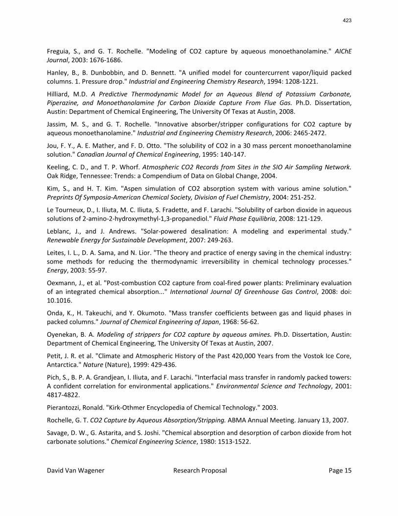
David Van Wagener Research Proposal Page 15
Freguia, S., and G. T. Rochelle. "Modeling of CO2 capture by aqueous monoethanolamine." AIChE Journal, 2003: 1676-1686.
Hanley, B., B. Dunbobbin, and D. Bennett. "A unified model for countercurrent vapor/liquid packed columns. 1. Pressure drop." Industrial and Engineering Chemistry Research, 1994: 1208-1221.
Hilliard, M.D. A Predictive Thermodynamic Model for an Aqueous Blend of Potassium Carbonate, Piperazine, and Monoethanolamine for Carbon Dioxide Capture From Flue Gas. Ph.D. Dissertation, Austin: Department of Chemical Engineering, The University Of Texas at Austin, 2008.
Jassim, M. S., and G. T. Rochelle. "Innovative absorber/stripper configurations for CO2 capture by aqueous monoethanolamine." Industrial and Engineering Chemistry Research, 2006: 2465-2472.
Jou, F. Y., A. E. Mather, and F. D. Otto. "The solubility of CO2 in a 30 mass percent monoethanolamine solution." Canadian Journal of Chemical Engineering, 1995: 140-147.
Keeling, C. D., and T. P. Whorf. Atmospheric CO2 Records from Sites in the SIO Air Sampling Network. Oak Ridge, Tennessee: Trends: a Compendium of Data on Global Change, 2004.
Kim, S., and H. T. Kim. "Aspen simulation of CO2 absorption system with various amine solution." Preprints Of Symposia-American Chemical Society, Division of Fuel Chemistry, 2004: 251-252.
Le Tourneux, D., I. Iliuta, M. C. Iliuta, S. Fradette, and F. Larachi. "Solubility of carbon dioxide in aqueous solutions of 2-amino-2-hydroxymethyl-1,3-propanediol." Fluid Phase Equilibria, 2008: 121-129.
Leblanc, J., and J. Andrews. "Solar-powered desalination: A modeling and experimental study." Renewable Energy for Sustainable Development, 2007: 249-263.
Leites, I. L., D. A. Sama, and N. Lior. "The theory and practice of energy saving in the chemical industry: some methods for reducing the thermodynamic irreversibility in chemical technology processes." Energy, 2003: 55-97.
Oexmann, J., et al. "Post-combustion CO2 capture from coal-fired power plants: Preliminary evaluation of an integrated chemical absorption..." International Journal Of Greenhouse Gas Control, 2008: doi: 10.1016.
Onda, K., H. Takeuchi, and Y. Okumoto. "Mass transfer coefficients between gas and liquid phases in packed columns." Journal of Chemical Engineering of Japan, 1968: 56-62.
Oyenekan, B. A. Modeling of strippers for CO2 capture by aqueous amines. Ph.D. Dissertation, Austin: Department of Chemical Engineering, The University Of Texas at Austin, 2007.
Petit, J. R. et al. "Climate and Atmospheric History of the Past 420,000 Years from the Vostok Ice Core, Antarctica." Nature (Nature), 1999: 429-436.
Pich, S., B. P. A. Grandjean, I. Iliuta, and F. Larachi. "Interfacial mass transfer in randomly packed towers: A confident correlation for environmental applications." Environmental Science and Technology, 2001: 4817-4822.
Pierantozzi, Ronald. "Kirk-Othmer Encyclopedia of Chemical Technology." 2003.
Rochelle, G. T. CO2 Capture by Aqueous Absorption/Stripping. ABMA Annual Meeting. January 13, 2007.
Savage, D. W., G. Astarita, and S. Joshi. "Chemical absorption and desorption of carbon dioxide from hot carbonate solutions." Chemical Engineering Science, 1980: 1513-1522.
423
David Van Wagener Research Proposal Page 16
Shrier, A. L., and P. V. Danckwerts. "Carbon dioxide absorption into amine-promoted potash solutions." Industrial and Engineering Chemistry Fundamentals, 1969: 415-423.
Teller, A. J., and R. E. Ford. "Packed column performance of carbon dioxide-monoethanolamine system." Industrial and Engineering Chemistry, 1958: 1201-1206.
Tobiesen, F. A., O. Juliussen, and H. F. Svendsen. "Experimental validation of a rigorous desorber model for CO2 post-combustion capture." Chemical Engineering Science, 2008: 2641-2656.
Trass, O., and R. H Weiland. "Sorption of carbon dioxide in ethylenediamine solutions II. Pilot Plant study of absorption and regeneration." The Canadian Journal of Chemical Engineering, 1971: 773-781.
Tsai, R., F. Seibert, B. Eldridge, and G. T. Rochelle. "Influence of Viscosity and Surface Tension on the Effective Mass Transfer Area of Structured Packing." 9th International Conference on Greenhouse Gas Control Technologies. Washington, DC: Elsevier, 2008.
Wilson, I. Gas-liquid contact area of random and structured packing. M.S. thesis, Austin: Department of Chemical Engineering, The University Of Texas at Austin, 2004.
Yeh, J. T., and H. W. Pennline. "Study of CO2 absorption and desorption in a packed column." Energy and Fuels, 2001: 274-278.
424

Amine Selection for CO2 Captureto Minimize Energy
ByGary T. Rochelle
Luminant Carbon Management ProgramDepartment of Chemical Engineering
The University of Texas at Austin
For theProcess Science and Technology CenterSemiannual Research Review Meeting
April 14, 2009
425
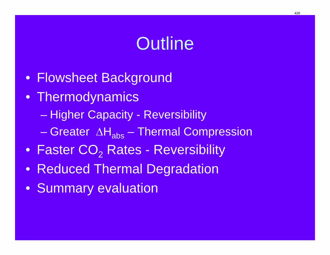
Outline
• Flowsheet Background• Thermodynamics
– Higher Capacity - Reversibility– Greater ΔHabs – Thermal Compression
• Faster CO2 Rates - Reversibility• Reduced Thermal Degradation• Summary evaluation
426
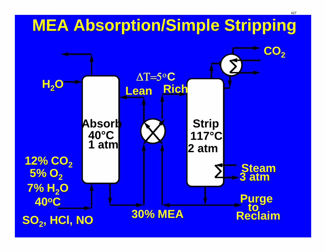
Absorb40°C1 atm
Steam 3 atm
CO2
Strip117°C2 atm
SO2, HCl, NO
12% CO25% O27% H2O
40oC30% MEA
Lean RichH2O
Purge to
Reclaim
MEA Absorption/Simple Stripping
ΔΤ=5οC
427
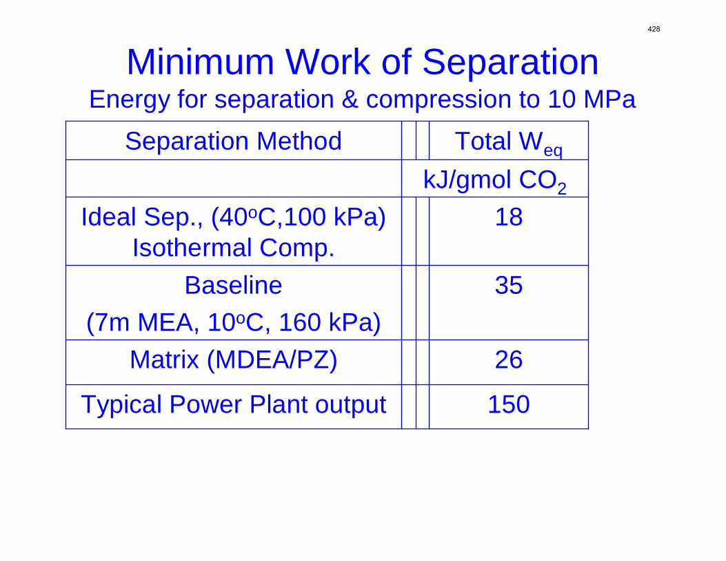
Minimum Work of SeparationEnergy for separation & compression to 10 MPa
150Typical Power Plant output
kJ/gmol CO2
26Matrix (MDEA/PZ)
35Baseline (7m MEA, 10oC, 160 kPa)
18Ideal Sep., (40oC,100 kPa) Isothermal Comp.
Total WeqSeparation Method
428
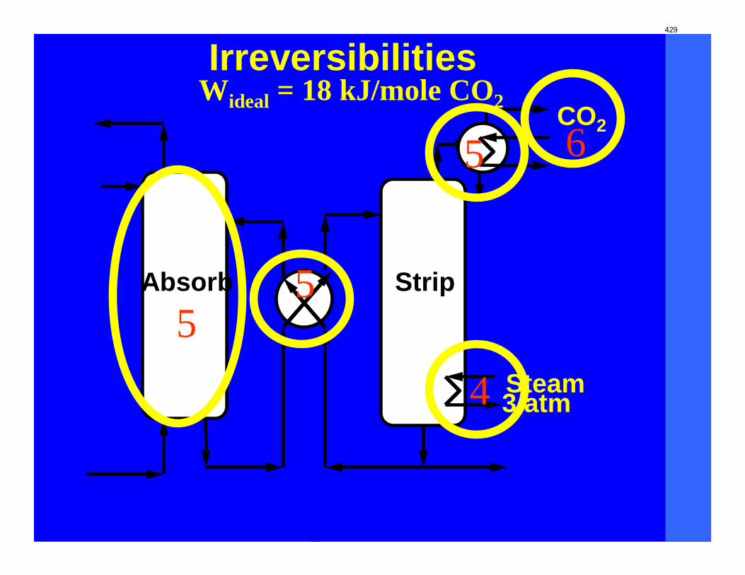
Absorb
Steam 3 atm
CO2
Strip
IrreversibilitiesWideal = 18 kJ/mole CO2
55
6
4
5
429
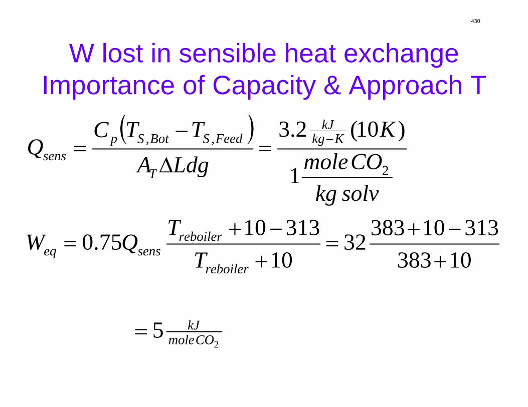
W lost in sensible heat exchangeImportance of Capacity & Approach T
( )
25
103833131038332
103131075.0
1
)10(2.3
2
,,
COmolekJ
reboiler
reboilersenseq
KkgkJ
T
FeedSBotSpsens
TTQW
solvkgCOmole
KLdgA
TTCQ
=
+−+
=+
−+=
=Δ
−= −
430
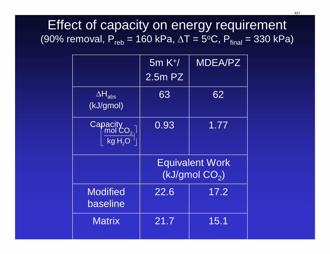
Effect of capacity on energy requirement(90% removal, Preb = 160 kPa, ΔT = 5oC, Pfinal = 330 kPa)
15.121.7Matrix
6263ΔHabs
(kJ/gmol)
MDEA/PZ5m K+/2.5m PZ
17.222.6Modified baseline
Capacity
Equivalent Work (kJ/gmol CO2)
0.93 1.77⎡ ⎤⎢ ⎥⎣ ⎦
2
2
mol COkg H O
431
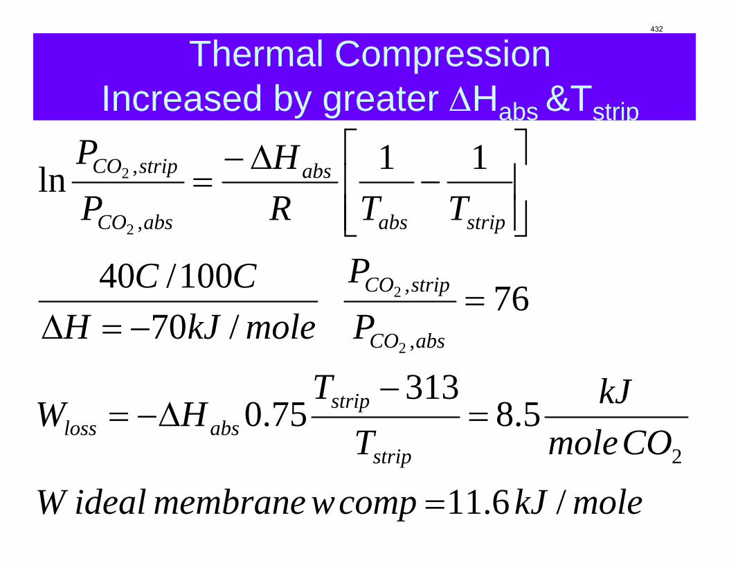
Thermal CompressionIncreased by greater ΔHabs &Tstrip
molekJcompwmembraneidealW
COmolekJ
TT
HW
PP
molekJHCC
TTRH
PP
strip
stripabsloss
absCO
stripCO
stripabs
abs
absCO
stripCO
/6.11
5.8313
75.0
76/70
100/40
11ln
2
,
,
,
,
2
2
2
2
=
=−
Δ−=
=−=Δ
⎥⎥⎦
⎤
⎢⎢⎣
⎡−
Δ−=
432
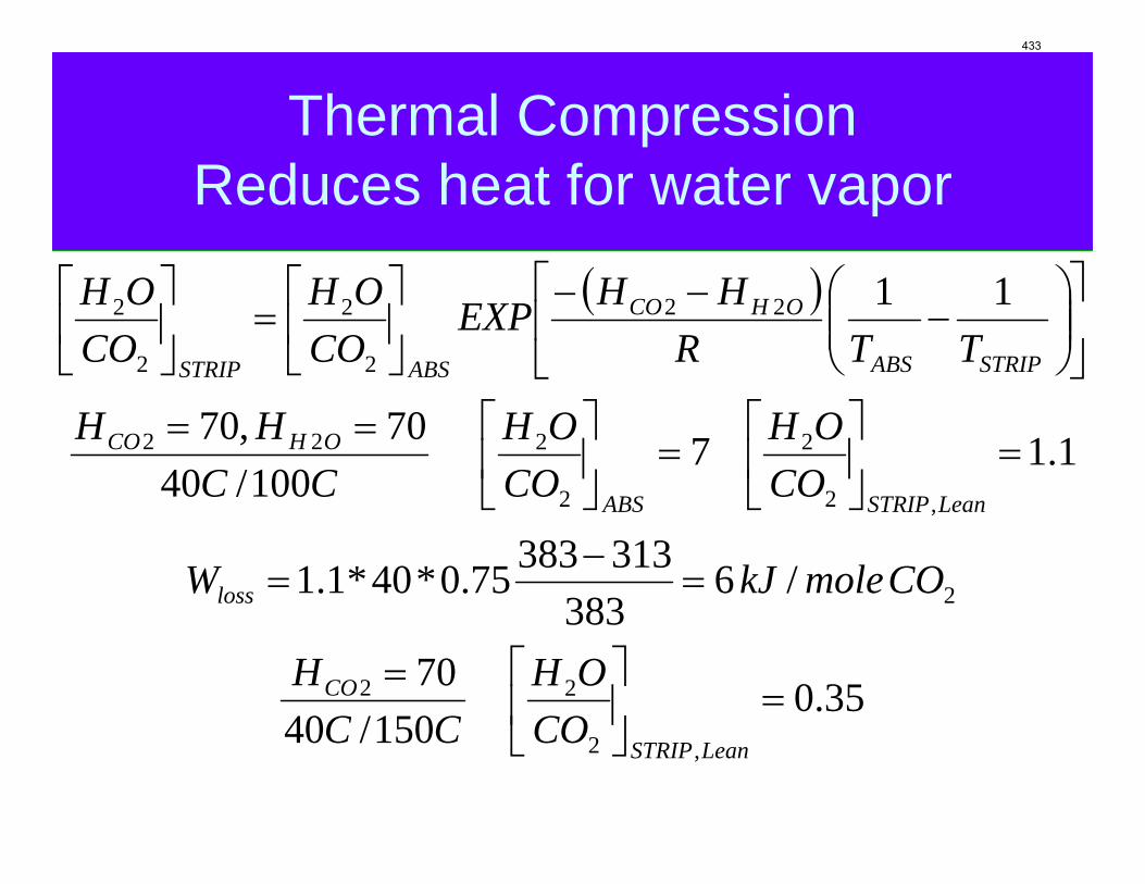
Thermal Compression Reduces heat for water vapor
( )
35.0150/40
70
/6383
31338375.0*40*1.1
1.17100/40
70,70
11
,2
22
2
,2
2
2
222
22
2
2
2
2
=⎥⎦
⎤⎢⎣
⎡=
=−
=
=⎥⎦
⎤⎢⎣
⎡=⎥
⎦
⎤⎢⎣
⎡==
⎥⎦
⎤⎢⎣
⎡⎟⎟⎠
⎞⎜⎜⎝
⎛−
−−⎥⎦
⎤⎢⎣
⎡=⎥
⎦
⎤⎢⎣
⎡
LeanSTRIP
CO
loss
LeanSTRIPABS
OHCO
STRIPABS
OHCO
ABSSTRIP
COOH
CCH
COmolekJW
COOH
COOH
CCHH
TTRHHEXP
COOH
COOH
433
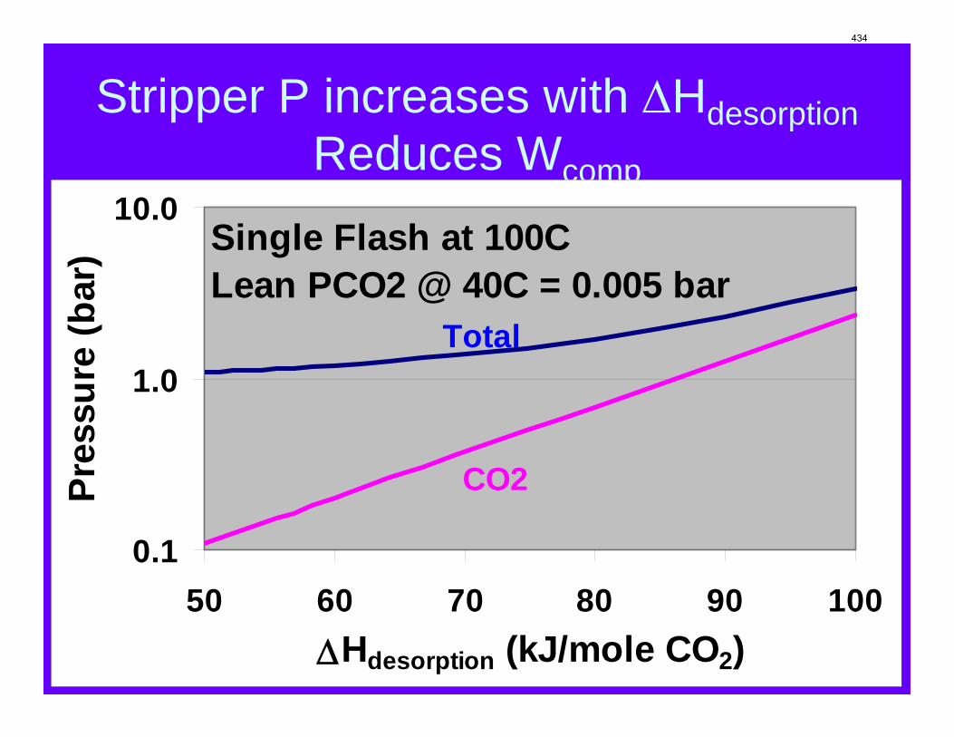
Stripper P increases with ΔHdesorptionReduces Wcomp
0.1
1.0
10.0
50 60 70 80 90 100ΔHdesorption (kJ/mole CO2)
Pres
sure
(bar
)
CO2
Total
Single Flash at 100CLean PCO2 @ 40C = 0.005 bar
434
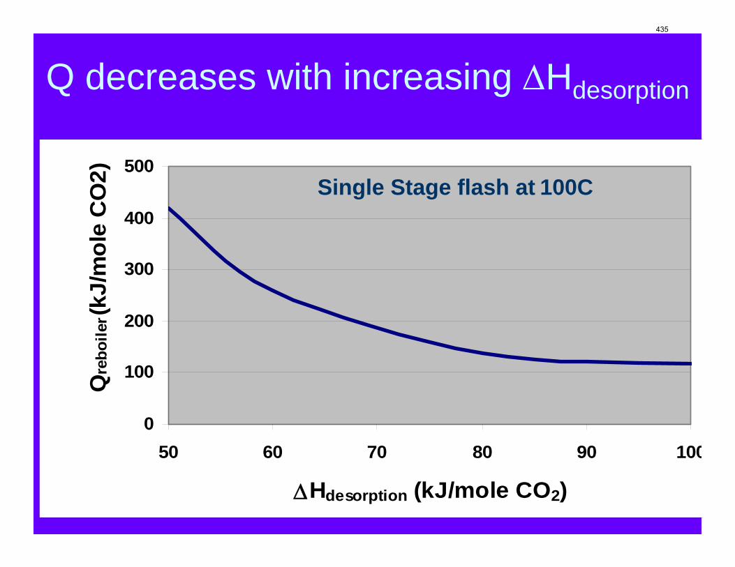
Q decreases with increasing ΔHdesorption
0
100
200
300
400
500
50 60 70 80 90 100
ΔHdesorption (kJ/mole CO2)
Qre
boile
r(kJ/
mol
e C
O2) Single Stage flash at 100C
435
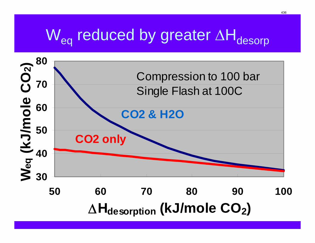
Weq reduced by greater ΔHdesorp
30
40
50
60
70
80
50 60 70 80 90 100
ΔHdesorption (kJ/mole CO2)
Weq
(kJ/
mol
e C
O2)
CO2 & H2O
CO2 only
Compression to 100 barSingle Flash at 100C
436
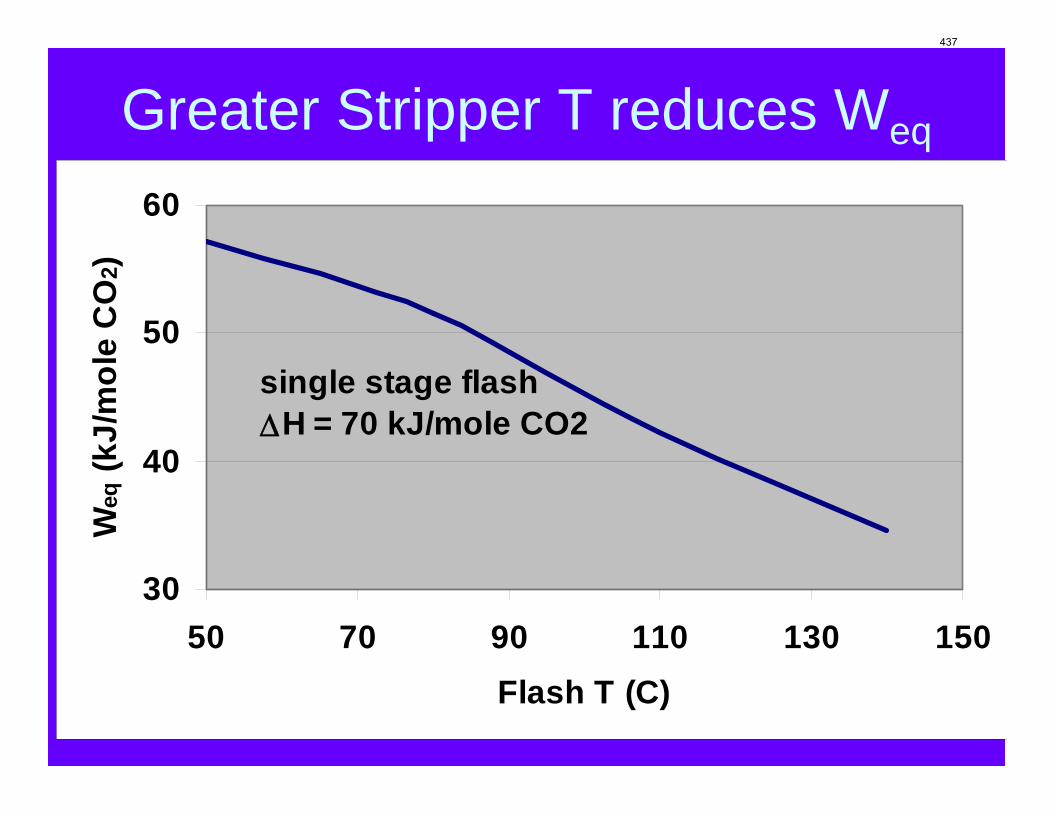
Greater Stripper T reduces Weq
30
40
50
60
50 70 90 110 130 150Flash T (C)
Weq
(kJ/
mol
e C
O2)
single stage flashΔH = 70 kJ/mole CO2
437
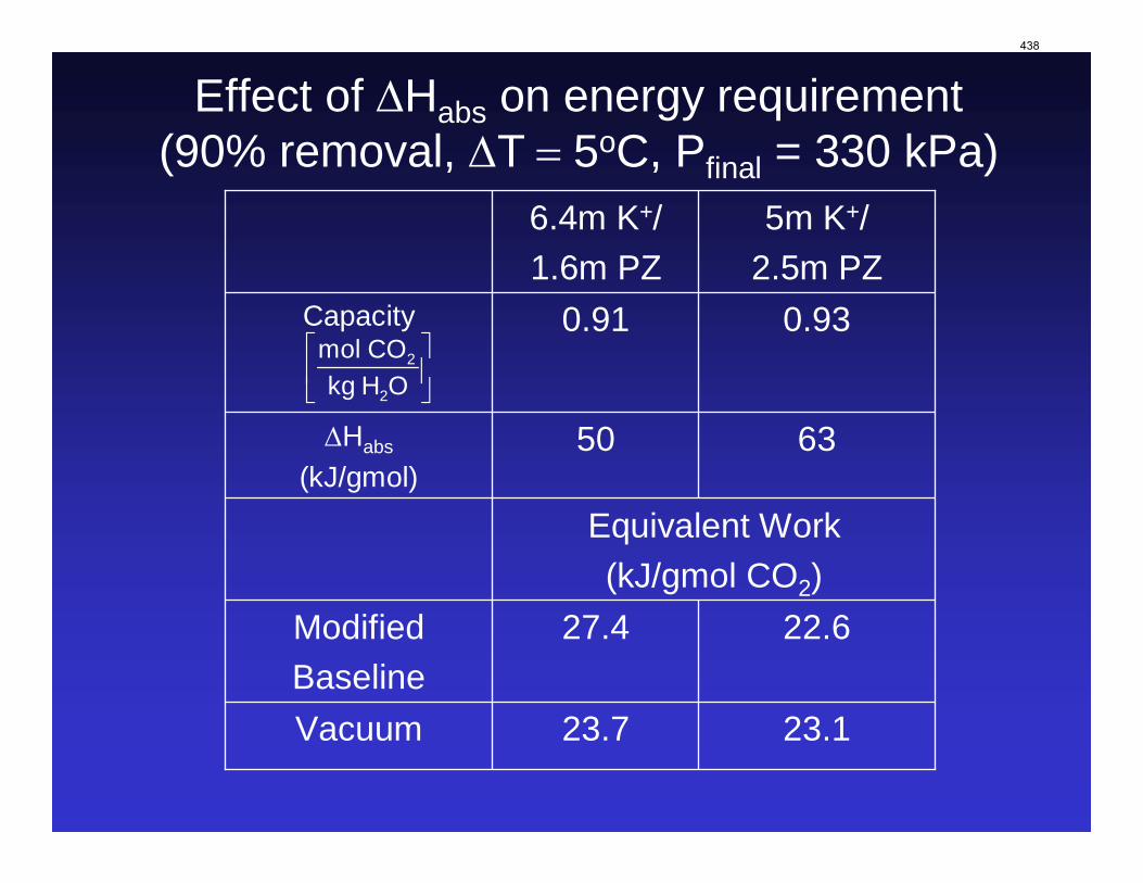
Effect of ΔHabs on energy requirement(90% removal, ΔT = 5oC, Pfinal = 330 kPa)
0.930.91Capacity
5m K+/2.5m PZ
6.4m K+/1.6m PZ
Vacuum
Modified Baseline
ΔHabs
(kJ/gmol)
23.7
27.4
Equivalent Work (kJ/gmol CO2)
50
23.1
22.6
63
⎡ ⎤⎢ ⎥⎣ ⎦
2
2
mol COkg H O
438
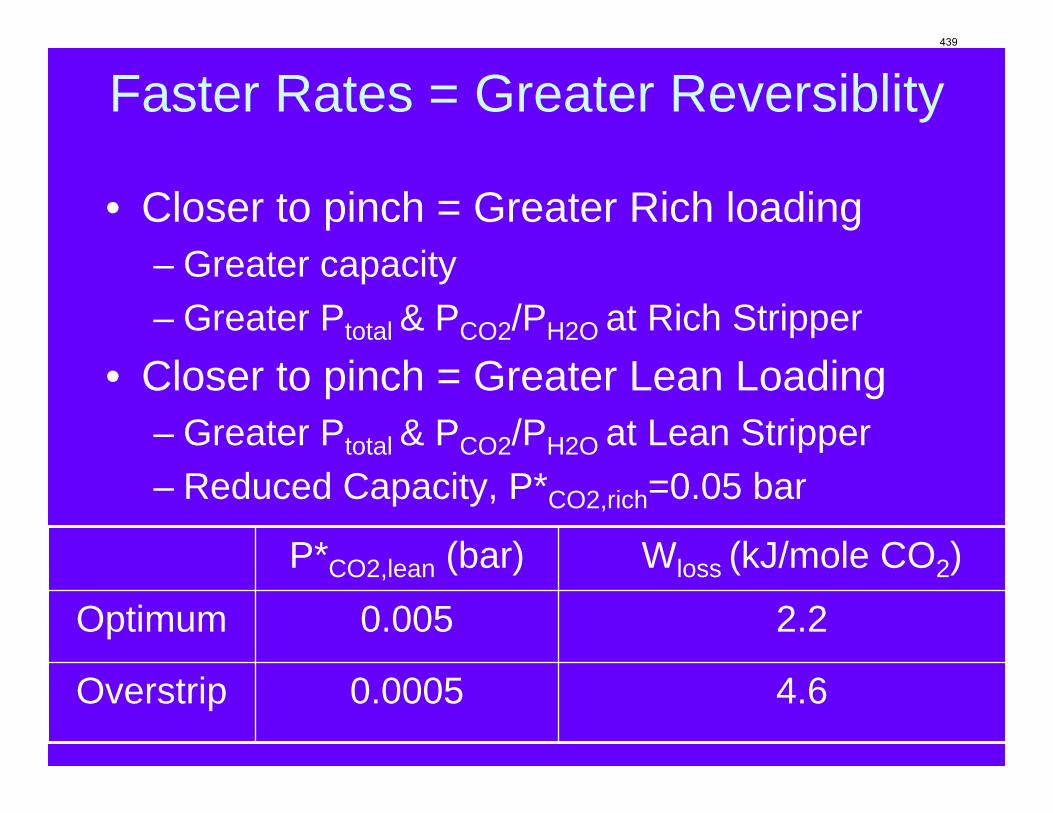
Faster Rates = Greater Reversiblity
• Closer to pinch = Greater Rich loading– Greater capacity– Greater Ptotal & PCO2/PH2O at Rich Stripper
• Closer to pinch = Greater Lean Loading– Greater Ptotal & PCO2/PH2O at Lean Stripper– Reduced Capacity, P*CO2,rich=0.05 bar
Overstrip
Optimum
4.60.0005
2.20.005
Wloss (kJ/mole CO2)P*CO2,lean (bar)
439
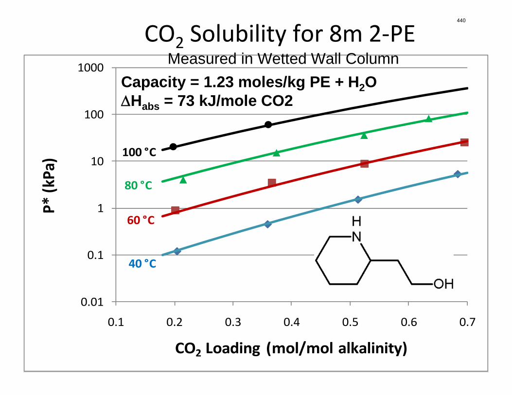
CO2 Solubility for 8m 2‐PE
0.01
0.1
1
10
100
1000
0.1 0.2 0.3 0.4 0.5 0.6 0.7
P* (k
Pa)
CO2 Loading (mol/mol alkalinity)
40 °C
60 °C
80 °C
100 °C
Measured in Wetted Wall ColumnCapacity = 1.23 moles/kg PE + H2OΔHabs = 73 kJ/mole CO2
440
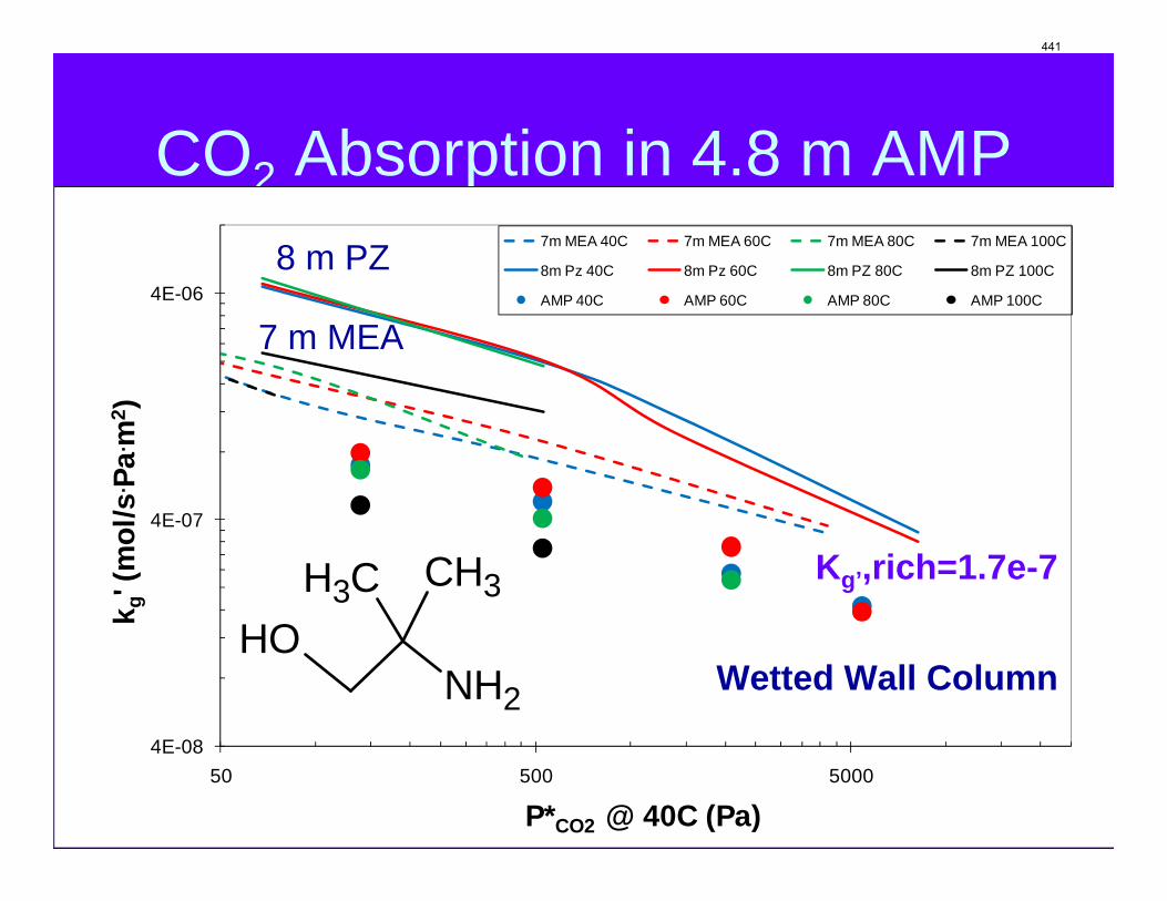
CO2 Absorption in 4.8 m AMP
• Typical data
4E-08
4E-07
4E-06
50 500 5000
k g' (
mol
/s. P
a. m2 )
P*CO2 @ 40C (Pa)
7m MEA 40C 7m MEA 60C 7m MEA 80C 7m MEA 100C
8m Pz 40C 8m Pz 60C 8m PZ 80C 8m PZ 100C
AMP 40C AMP 60C AMP 80C AMP 100C
Wetted Wall Column
8 m PZ
7 m MEA
Kg’,rich=1.7e-7
OHNH2
CH3CH3
441
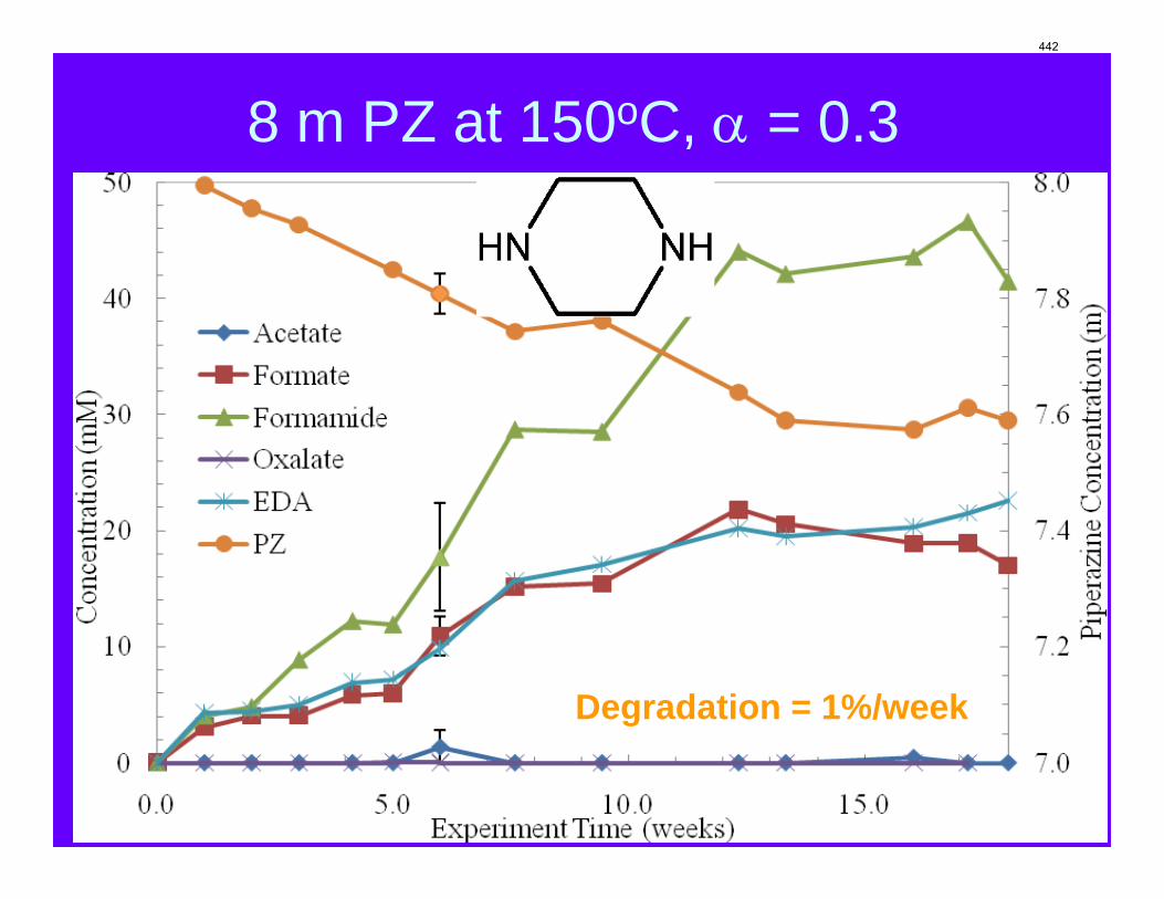
8 m PZ at 150oC, α = 0.3
Degradation = 1%/week
442
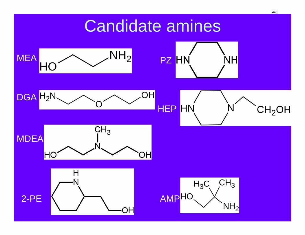
Candidate amines
OHNH2
CH3CH3
NH2O
OHNH N CH2OH
NH2OH
MEA
2-PE
DGA
AMP
HEP
MDEA
PZ
443
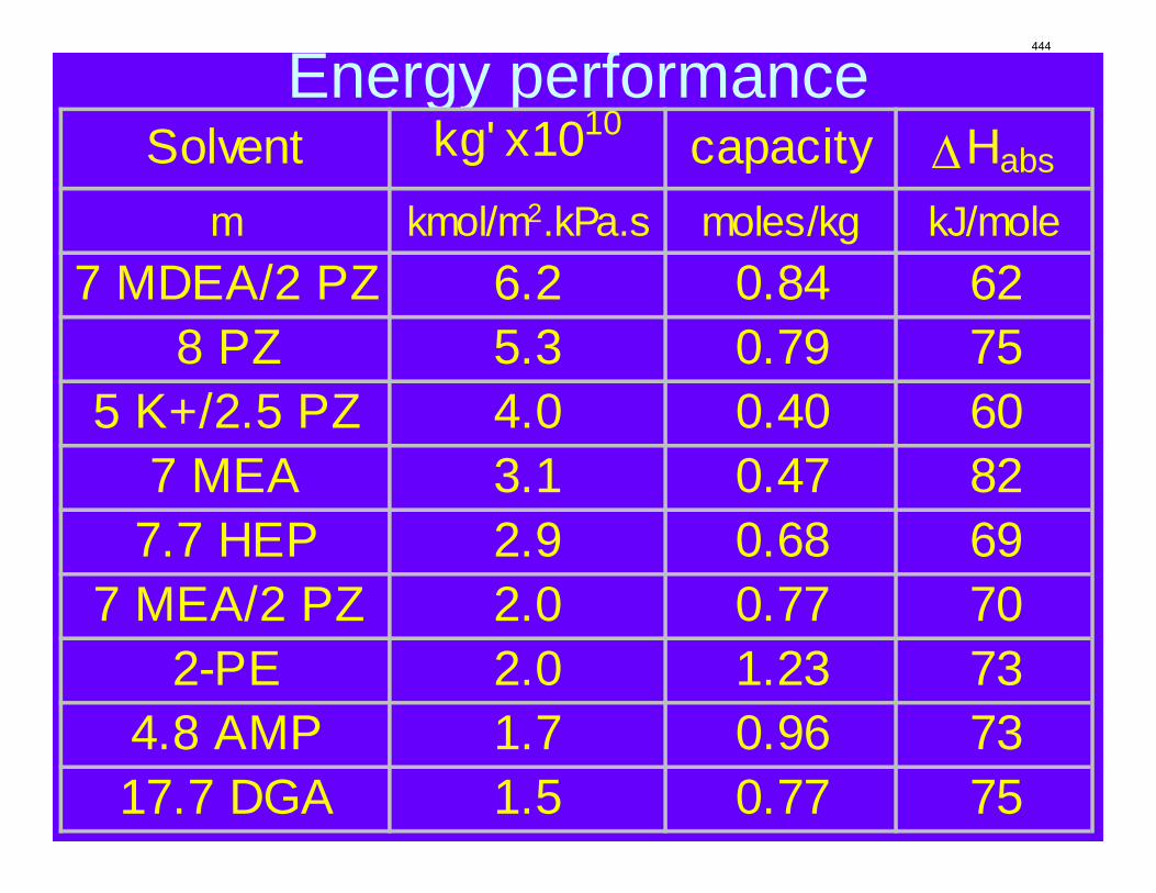
Energy performance Solvent kg' x1010 capacity ΔHabs
m kmol/m2.kPa.s moles/kg kJ/mole7 MDEA/2 PZ 6.2 0.84 62
8 PZ 5.3 0.79 755 K+/2.5 PZ 4.0 0.40 60
7 MEA 3.1 0.47 827.7 HEP 2.9 0.68 69
7 MEA/2 PZ 2.0 0.77 702-PE 2.0 1.23 73
4.8 AMP 1.7 0.96 7317.7 DGA 1.5 0.77 75
444
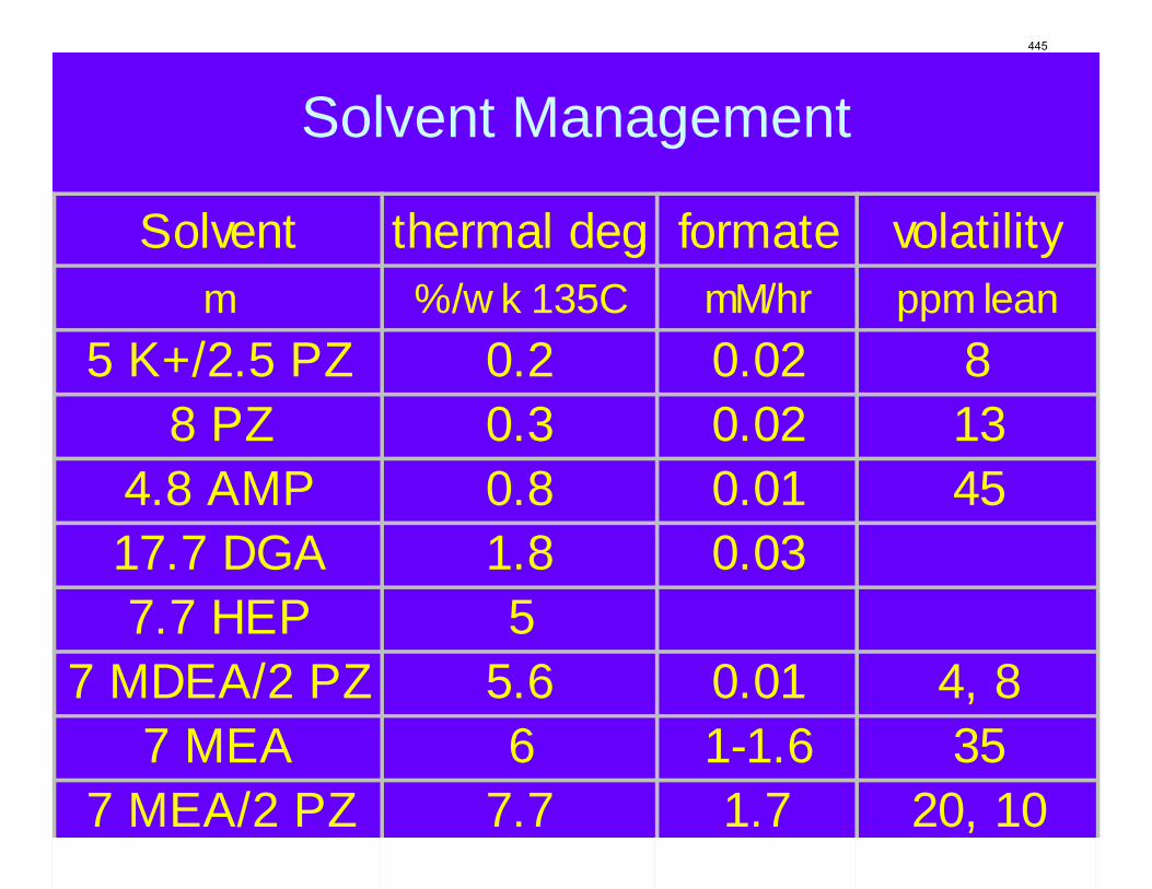
Solvent Management
Solvent thermal deg formate volatilitym %/w k 135C mM/hr ppm lean
5 K+/2.5 PZ 0.2 0.02 88 PZ 0.3 0.02 13
4.8 AMP 0.8 0.01 4517.7 DGA 1.8 0.037.7 HEP 5
7 MDEA/2 PZ 5.6 0.01 4, 87 MEA 6 1-1.6 35
7 MEA/2 PZ 7.7 1.7 20, 10
445
Other Factors
Cost – MEA is the least expensive amineAvailability – Usually correlated with costViscosity tradeoff with capacitySolids precipitation limits some solvents
446
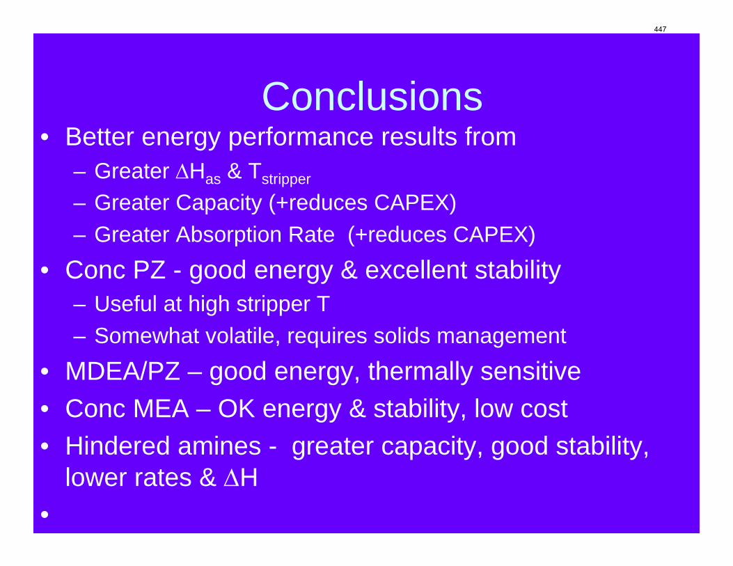
Conclusions• Better energy performance results from
– Greater ΔHas & Tstripper
– Greater Capacity (+reduces CAPEX)– Greater Absorption Rate (+reduces CAPEX)
• Conc PZ - good energy & excellent stability– Useful at high stripper T– Somewhat volatile, requires solids management
• MDEA/PZ – good energy, thermally sensitive• Conc MEA – OK energy & stability, low cost• Hindered amines - greater capacity, good stability,
lower rates & ΔH•
447
Future Work
• Fill in• Add Evaluation of Other amines
– Ethylenediamine & other diamines– Ethylaminopiperazine & other piperazines– Amino Acids– Other Hindered Amines
448
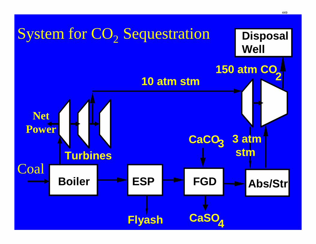
System for CO2 Sequestration
Boiler ESP
Flyash
FGD
CaSO4
CaCO3
Abs/Str
DisposalWell
Turbines3 atmstm
150 atm CO2
Coal
NetPower
10 atm stm
449
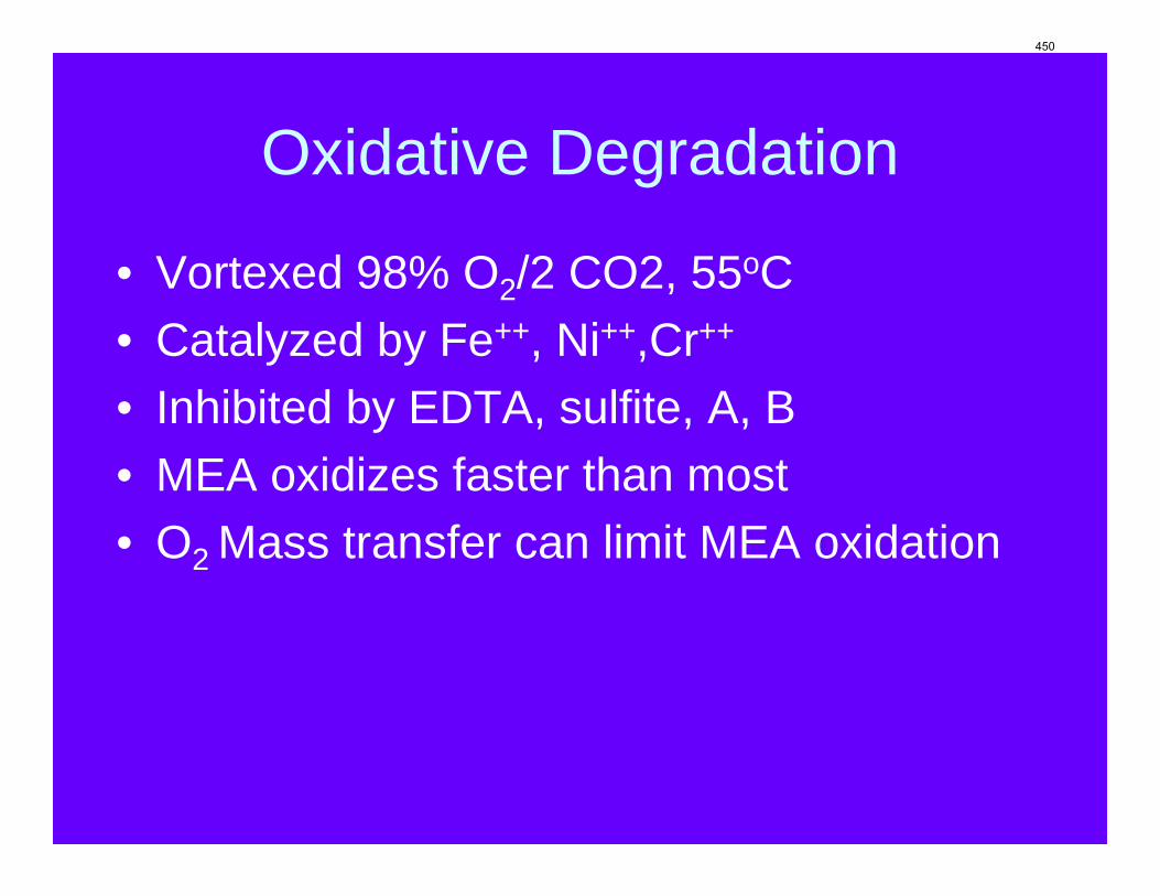
Oxidative Degradation
• Vortexed 98% O2/2 CO2, 55oC• Catalyzed by Fe++, Ni++,Cr++
• Inhibited by EDTA, sulfite, A, B• MEA oxidizes faster than most• O2 Mass transfer can limit MEA oxidation
450
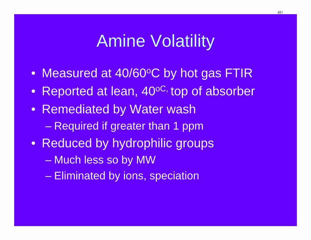
Amine Volatility
• Measured at 40/60oC by hot gas FTIR• Reported at lean, 40oC, top of absorber• Remediated by Water wash
– Required if greater than 1 ppm• Reduced by hydrophilic groups
– Much less so by MW– Eliminated by ions, speciation
451
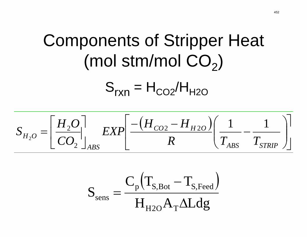
Components of Stripper Heat (mol stm/mol CO2)
Srxn = HCO2/HH2O
( )LdgAH
TTCS
TO2H
Feed,SBot,Spsens Δ
−=
( )⎥⎦
⎤⎢⎣
⎡⎟⎟⎠
⎞⎜⎜⎝
⎛−
−−⎥⎦
⎤⎢⎣
⎡=
STRIPABS
OHCO
ABSOH TTR
HHEXPCO
OHS 1122
2
22
452
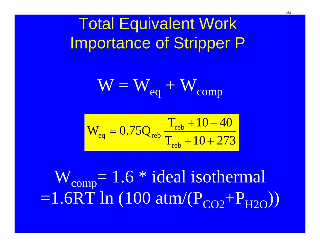
Total Equivalent WorkImportance of Stripper P
27310T4010TQ75.0W
reb
rebrebeq ++
−+=
W = Weq + Wcomp
Wcomp= 1.6 * ideal isothermal=1.6RT ln (100 atm/(PCO2+PH2O))
453
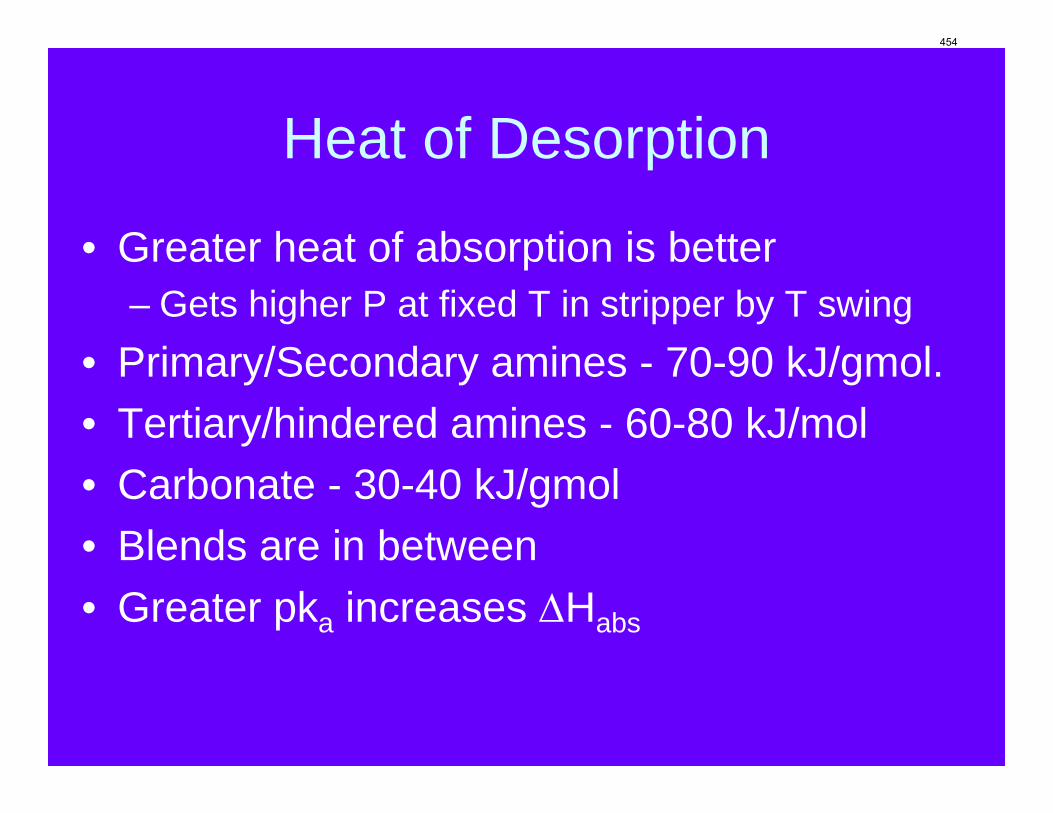
Heat of Desorption
• Greater heat of absorption is better– Gets higher P at fixed T in stripper by T swing
• Primary/Secondary amines - 70-90 kJ/gmol.• Tertiary/hindered amines - 60-80 kJ/mol• Carbonate - 30-40 kJ/gmol• Blends are in between• Greater pka increases ΔHabs
454
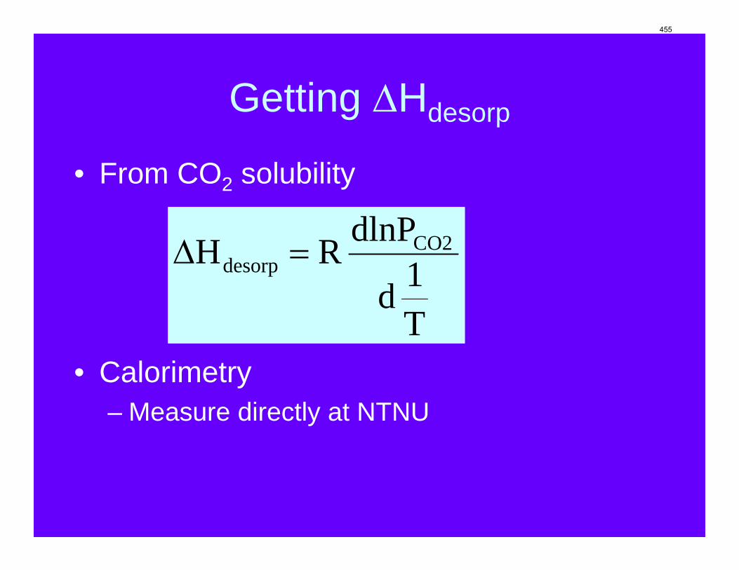
Getting ΔHdesorp
• From CO2 solubility
• Calorimetry– Measure directly at NTNU
T1d
dlnPRH CO2desorp =Δ
455
Why higher DHabs
• Consider single stage flash• Lean loading must provide for <0.01
456
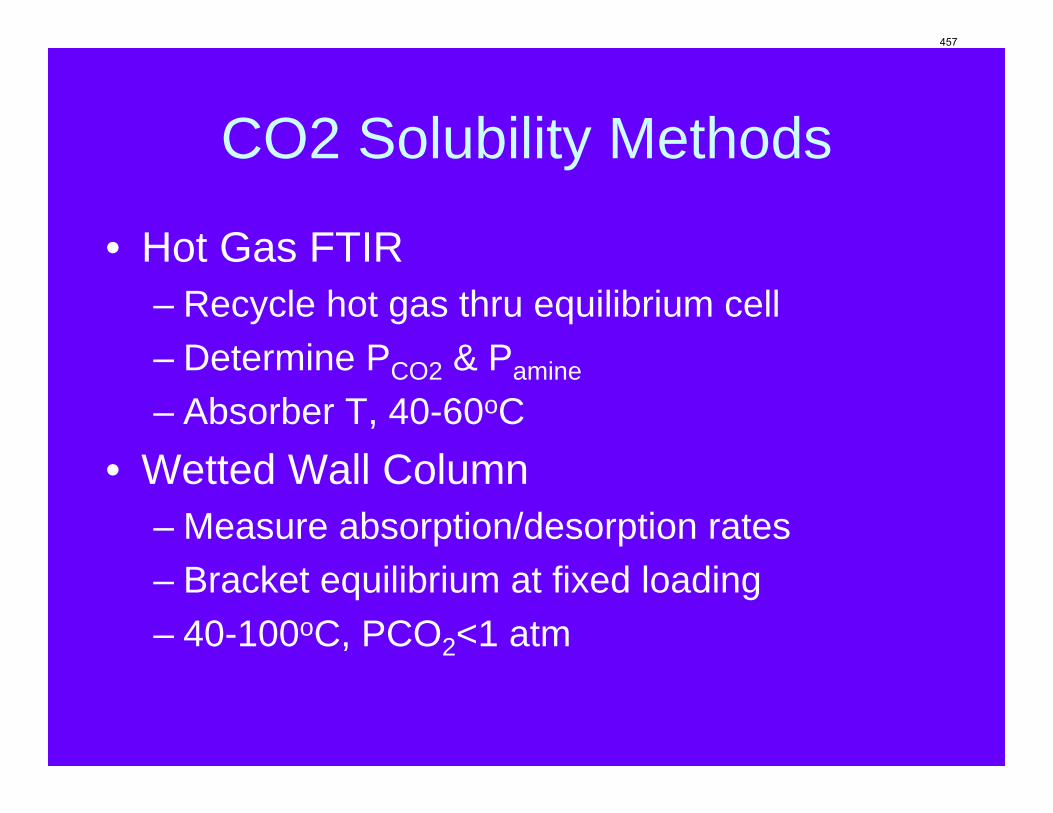
CO2 Solubility Methods
• Hot Gas FTIR– Recycle hot gas thru equilibrium cell– Determine PCO2 & Pamine
– Absorber T, 40-60oC• Wetted Wall Column
– Measure absorption/desorption rates– Bracket equilibrium at fixed loading– 40-100oC, PCO2<1 atm
457
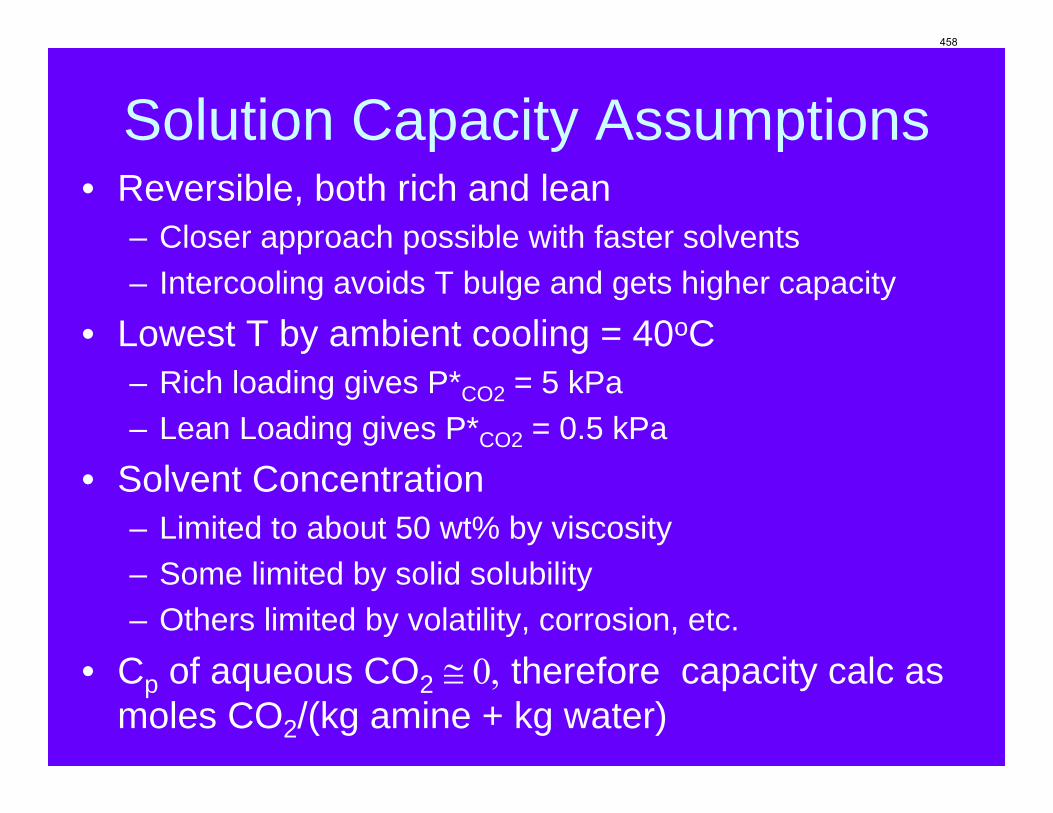
Solution Capacity Assumptions• Reversible, both rich and lean
– Closer approach possible with faster solvents– Intercooling avoids T bulge and gets higher capacity
• Lowest T by ambient cooling = 40oC– Rich loading gives P*CO2 = 5 kPa– Lean Loading gives P*CO2 = 0.5 kPa
• Solvent Concentration– Limited to about 50 wt% by viscosity– Some limited by solid solubility– Others limited by volatility, corrosion, etc.
• Cp of aqueous CO2 ≅ 0, therefore capacity calc as moles CO2/(kg amine + kg water)
458
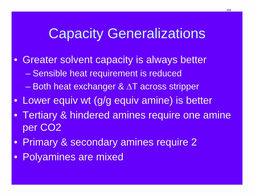
Capacity Generalizations
• Greater solvent capacity is always better– Sensible heat requirement is reduced– Both heat exchanger & ΔT across stripper
• Lower equiv wt (g/g equiv amine) is better• Tertiary & hindered amines require one amine
per CO2• Primary & secondary amines require 2• Polyamines are mixed
459
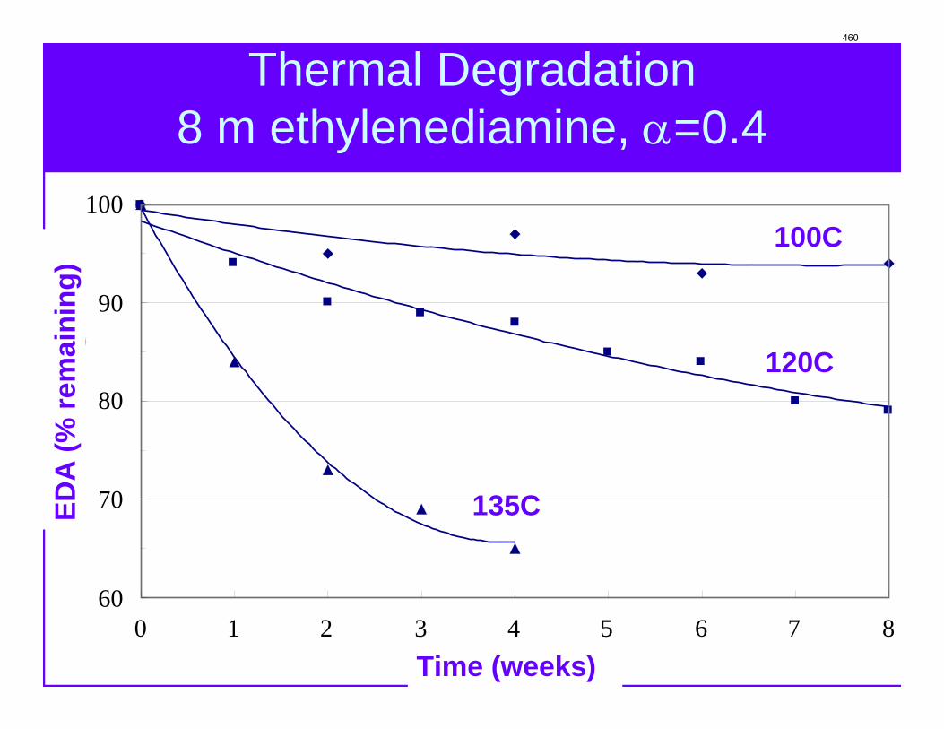
Thermal Degradation8 m ethylenediamine, α=0.4
60
70
80
90
100
0 1 2 3 4 5 6 7 8Time/week
EDA
Rem
aini
ng/%
135C
120C
100C
Time
EDA
(% re
mai
ning
)
Time (weeks)
460
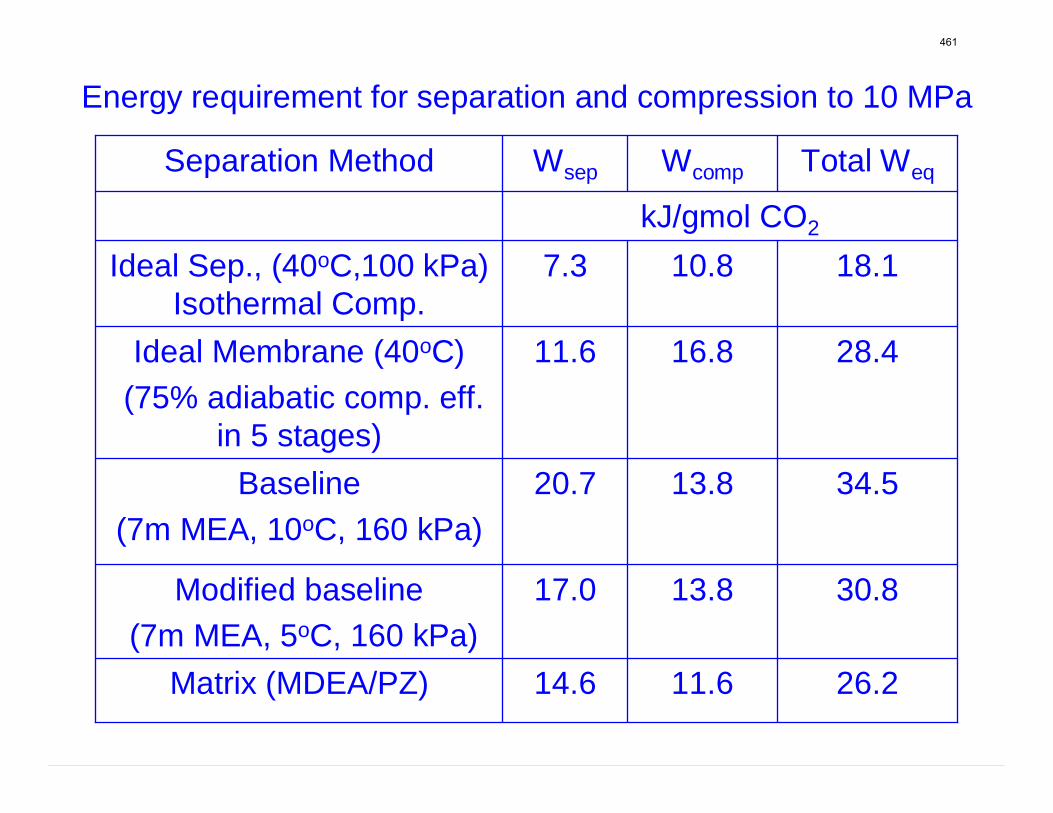
Energy requirement for separation and compression to 10 MPa
kJ/gmol CO2
30.813.817.0Modified baseline (7m MEA, 5oC, 160 kPa)
26.211.614.6Matrix (MDEA/PZ)
34.513.820.7Baseline (7m MEA, 10oC, 160 kPa)
28.416.811.6Ideal Membrane (40oC) (75% adiabatic comp. eff.
in 5 stages)
18.110.87.3Ideal Sep., (40oC,100 kPa) Isothermal Comp.
Total WeqWcompWsepSeparation Method
461
Fred ClosmannApril 14, 2009
Supported by:Process Science and Technology CenterLuminant Carbon Management Program
462
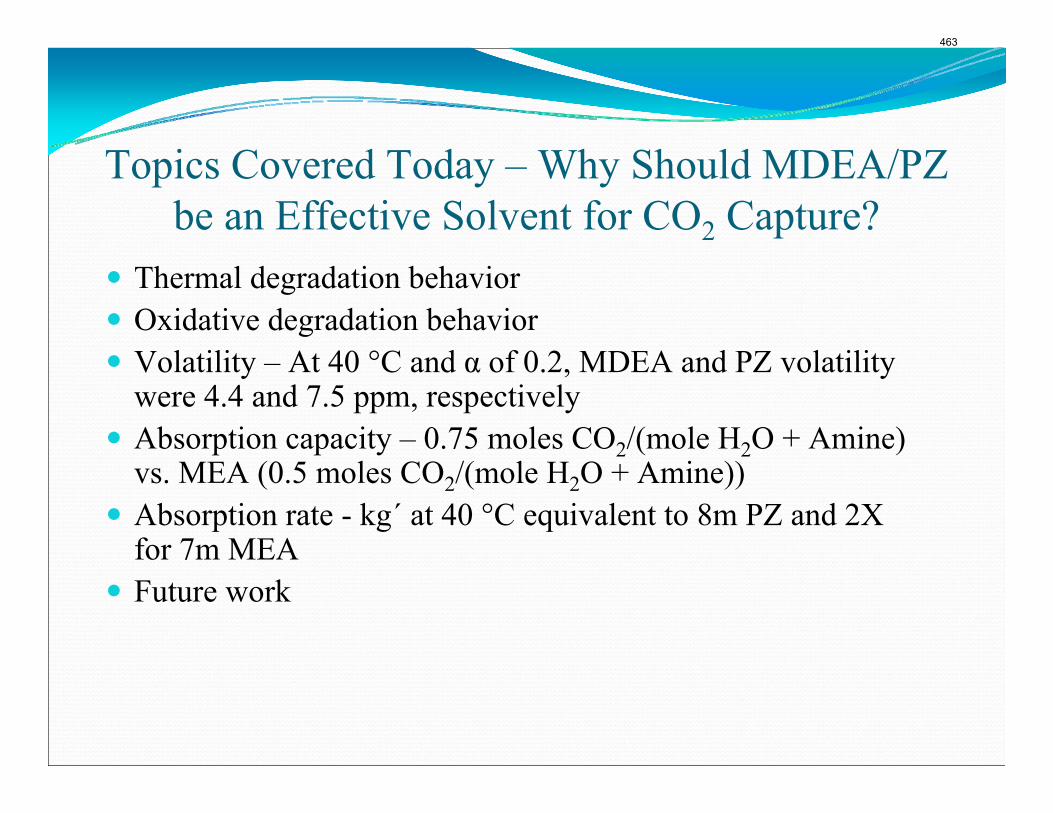
Topics Covered Today – Why Should MDEA/PZ be an Effective Solvent for CO2 Capture?
Thermal degradation behaviorOxidative degradation behaviorVolatility – At 40 °C and α of 0.2, MDEA and PZ volatility were 4.4 and 7.5 ppm, respectivelyAbsorption capacity – 0.75 moles CO2/(mole H2O + Amine) vs. MEA (0.5 moles CO2/(mole H2O + Amine))Absorption rate - kg´ at 40 °C equivalent to 8m PZ and 2X for 7m MEAFuture work
463
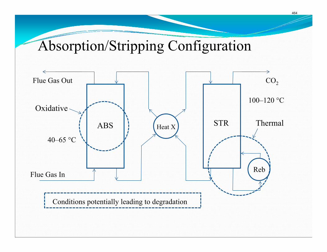
ABS STR
Oxidative
Thermal
Flue Gas In
Absorption/Stripping Configuration
Conditions potentially leading to degradation
40–65 °C
100–120 °C
Heat X
CO2Flue Gas Out
Reb
464
Thermal Degradation - LiteratureDawodu & Meisen (1996) degraded MDEA:Reported intermediates (Methylaminoethanol (MAE) and Diethanolamine (DEA))Other products included Dimethylaminoethanol (DMAE) and Hydroxyethyl oxazolidone (HEOD)Chakma & Meisen (1997):DMAE and Triethanolamine (TEA) formed and behave as intermediatesMDEA degradation not 1st order in [MDEA] – two methyl groups in DMAEMDEA/PZ systems (Bedell, 2009):Disproportionation primary process; homolytic cleavage not observedMDEA degrades to DMAE and TEA – can close initial balanceObserved 1-methyl PZ, very little Hydroxyethyl PZ (HEP) (IFP reported HEP)Difficult to close C-mass balance due to CO2 evolutionPiperazine stable up to 150 °C (Freeman, 2008)Davis (2008/2009):7m MEA/2m PZ at 135 °C; 12%/wk MEA loss, 32%/wk PZ lossBlended systems preferentially destroyed PZ
465
Thermal Degradation - MethodsMethod – Batch process using stainless steel sample containers maintained at pre-selected T (up to 14 weeks)Variable conditions – loading, concentration and TCation chromatography - amine concentrations, identification of byproducts (standards)MS – identify compounds in series with IC, and separately with syringe pumpHPLC – detection and identification of non-polar compoundsQuantified unidentified diamine compounds and correlated with PZ loss
466

467
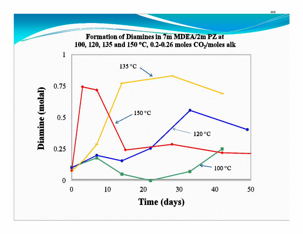
468
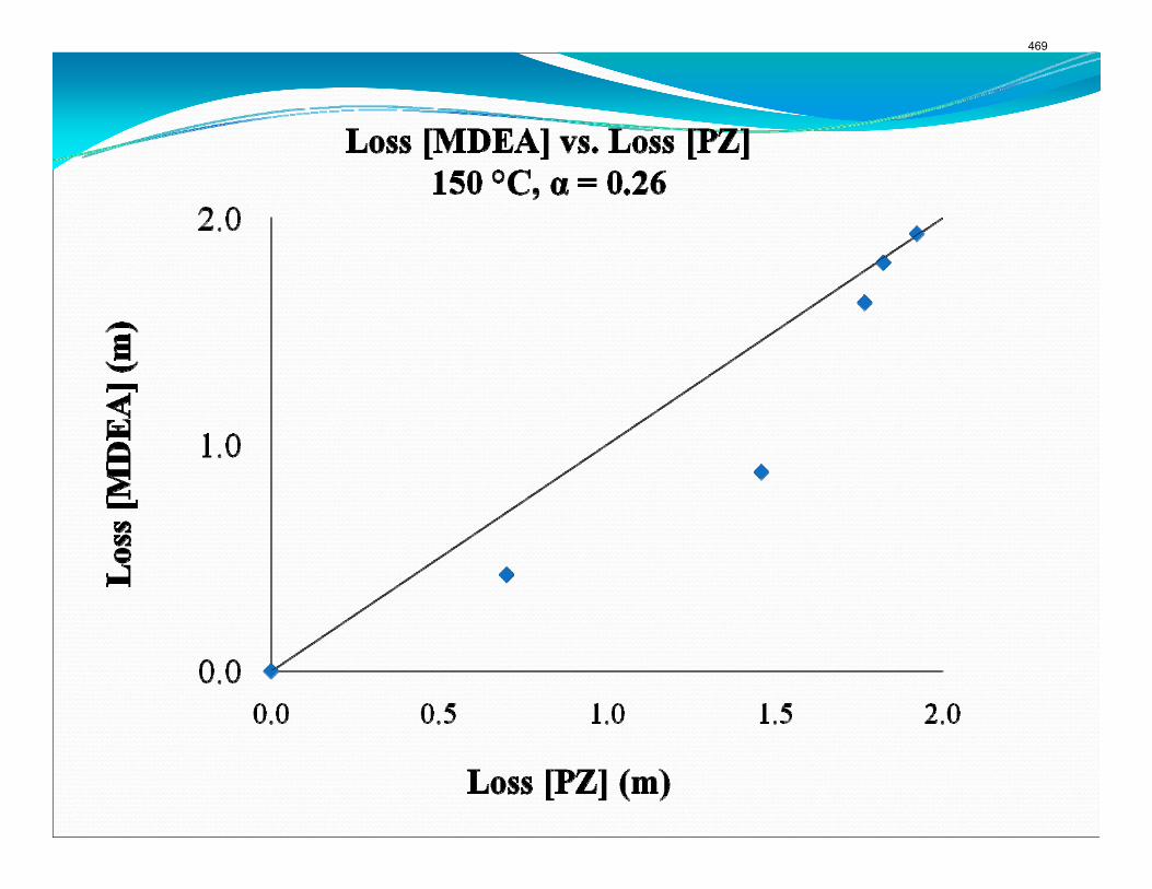
469
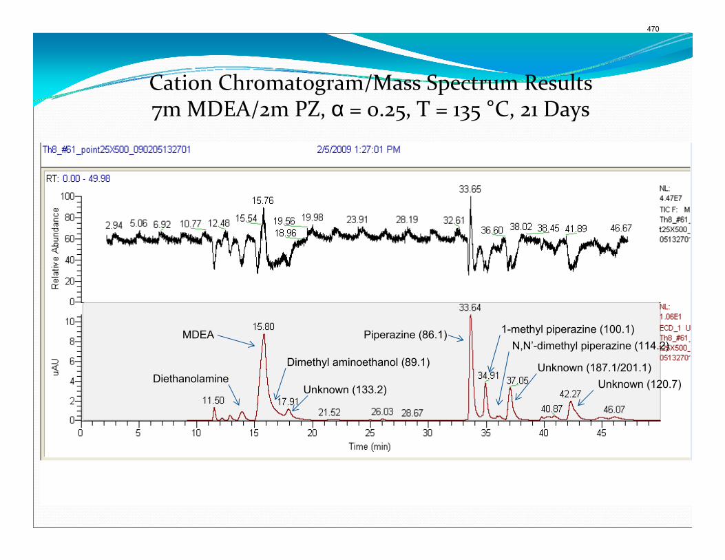
Piperazine (86.1) 1-methyl piperazine (100.1)N,N’-dimethyl piperazine (114.2)
Unknown (187.1/201.1)Dimethyl aminoethanol (89.1)
Unknown (133.2) Unknown (120.7)Diethanolamine
MDEA
Cation Chromatogram/Mass Spectrum Results7m MDEA/2m PZ, α = 0.25, T = 135 °C, 21 Days
470
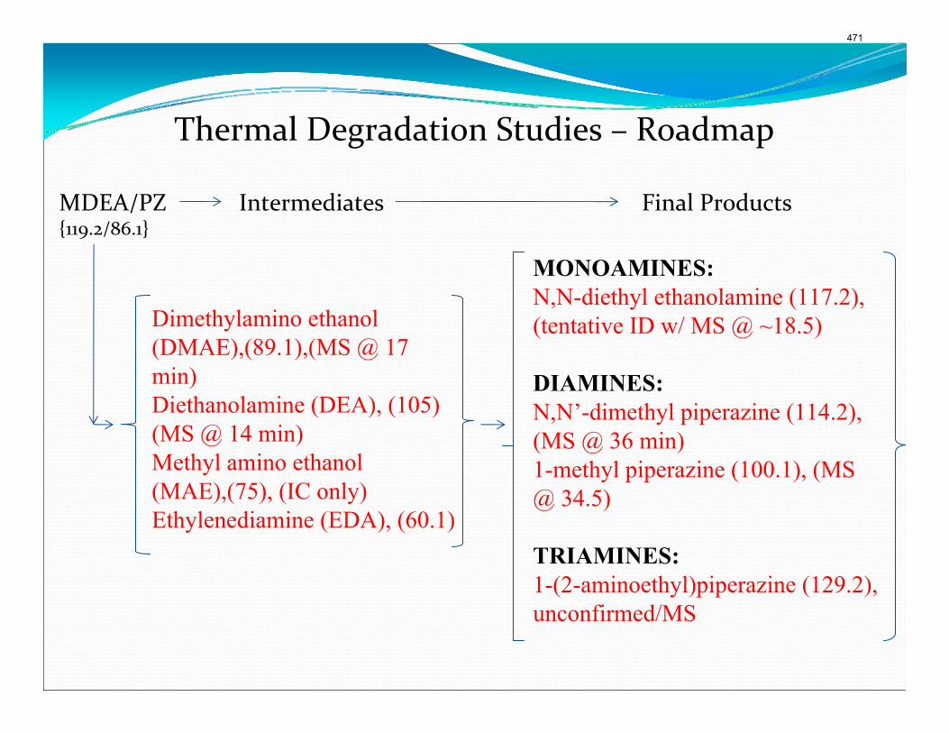
Thermal Degradation Studies – Roadmap
MDEA/PZ Intermediates Final Products
Dimethylamino ethanol (DMAE),(89.1),(MS @ 17 min)Diethanolamine (DEA), (105) (MS @ 14 min)Methyl amino ethanol (MAE),(75), (IC only)Ethylenediamine (EDA), (60.1)
MONOAMINES:N,N-diethyl ethanolamine (117.2), (tentative ID w/ MS @ ~18.5)
DIAMINES:N,N’-dimethyl piperazine (114.2), (MS @ 36 min)1-methyl piperazine (100.1), (MS @ 34.5)
TRIAMINES:1-(2-aminoethyl)piperazine (129.2), unconfirmed/MS
{119.2/86.1}
471
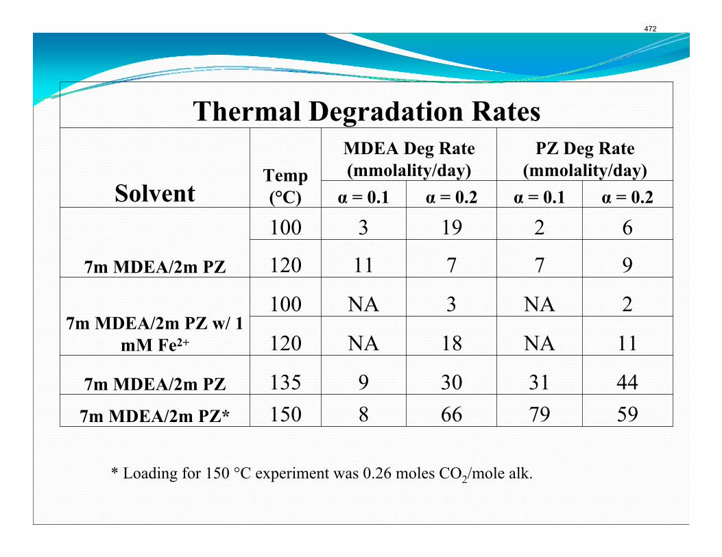
* Loading for 150 °C experiment was 0.26 moles CO2/mole alk.
Thermal Degradation Rates
SolventTemp (°C)
MDEA Deg Rate (mmolality/day)
PZ Deg Rate (mmolality/day)
α = 0.1 α = 0.2 α = 0.1 α = 0.2
7m MDEA/2m PZ
100 3 19 2 6
120 11 7 7 9
7m MDEA/2m PZ w/ 1 mM Fe2+
100 NA 3 NA 2
120 NA 18 NA 11
7m MDEA/2m PZ 135 9 30 31 447m MDEA/2m PZ* 150 8 66 79 59
472
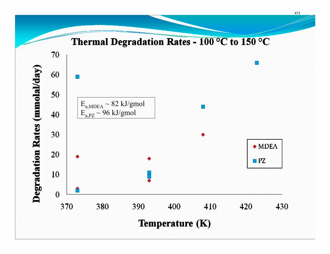
Ea,MDEA ~ 82 kJ/gmolEa,PZ ~ 96 kJ/gmol
473
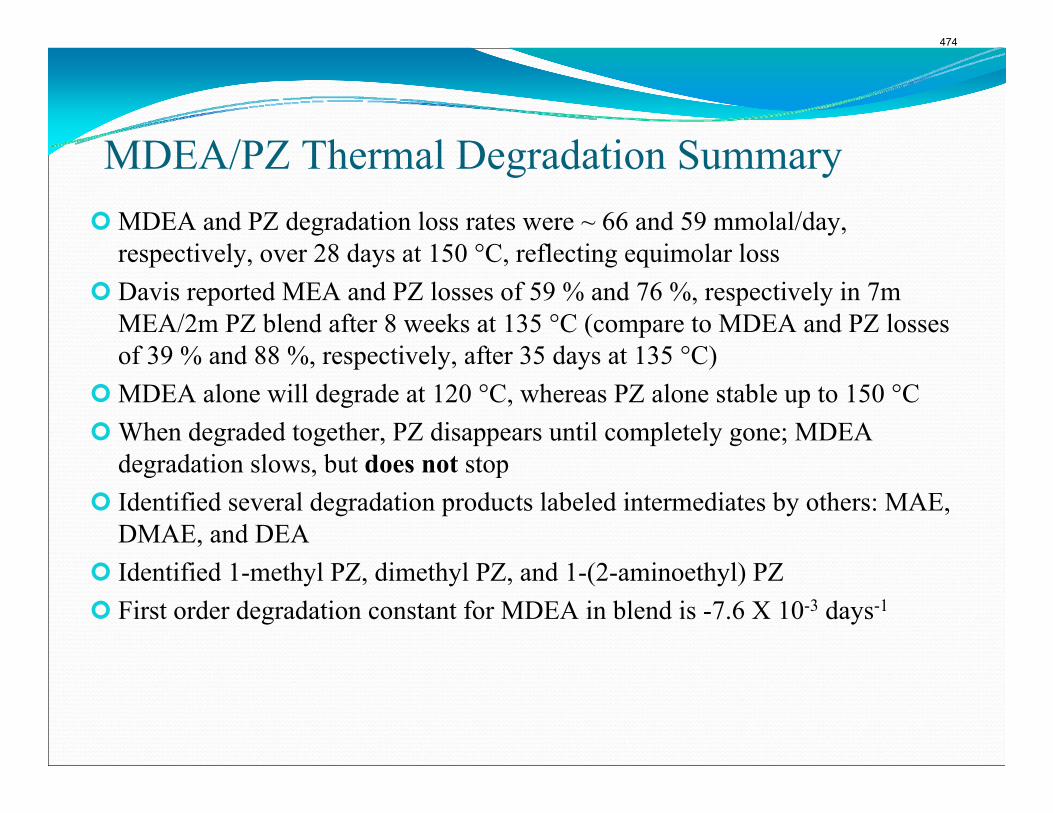
MDEA/PZ Thermal Degradation SummaryMDEA and PZ degradation loss rates were ~ 66 and 59 mmolal/day, respectively, over 28 days at 150 °C, reflecting equimolar lossDavis reported MEA and PZ losses of 59 % and 76 %, respectively in 7m MEA/2m PZ blend after 8 weeks at 135 °C (compare to MDEA and PZ losses of 39 % and 88 %, respectively, after 35 days at 135 °C)MDEA alone will degrade at 120 °C, whereas PZ alone stable up to 150 °CWhen degraded together, PZ disappears until completely gone; MDEA degradation slows, but does not stopIdentified several degradation products labeled intermediates by others: MAE, DMAE, and DEAIdentified 1-methyl PZ, dimethyl PZ, and 1-(2-aminoethyl) PZFirst order degradation constant for MDEA in blend is -7.6 X 10⁻³ days-1
474
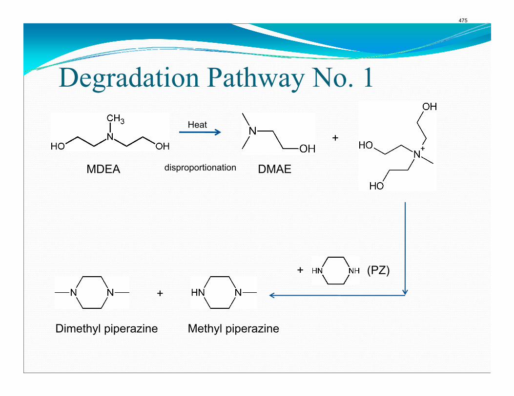
Degradation Pathway No. 1
+
MDEA DMAEdisproportionation
Heat
+ (PZ)
Methyl piperazine
+
Dimethyl piperazine
475
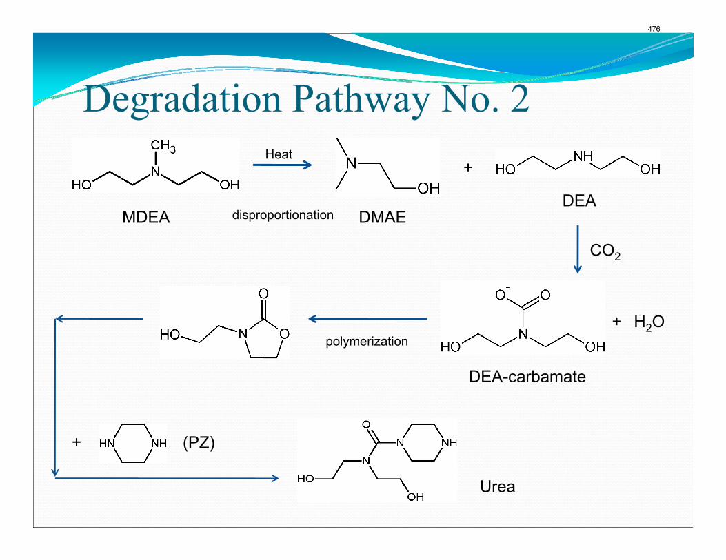
Degradation Pathway No. 2 +
MDEA DMAEDEA
CO2
disproportionation
polymerization
Heat
+ H2O
+
Urea
(PZ)
DEA-carbamate
476
Oxidative Degradation Studies
375-ml reactor stirred at 1400 rpm, purge of 98 % CO2/2 % O2 gas at 100 cc/minAnion and cation chromatography analysis of samples collected at two-day intervalsPrimary tool – measurement of heat stable salt formation (mostly formate, some glycolate) with anion chromatographyHydrolysis of samples with NaOH to reverse amide production and return to formate
477
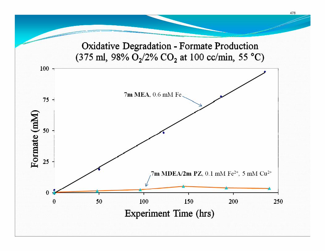
478
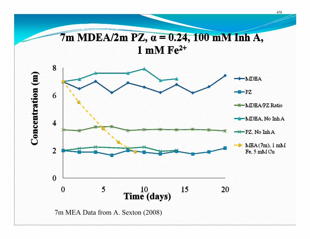
7m MEA Data from A. Sexton (2008)
479
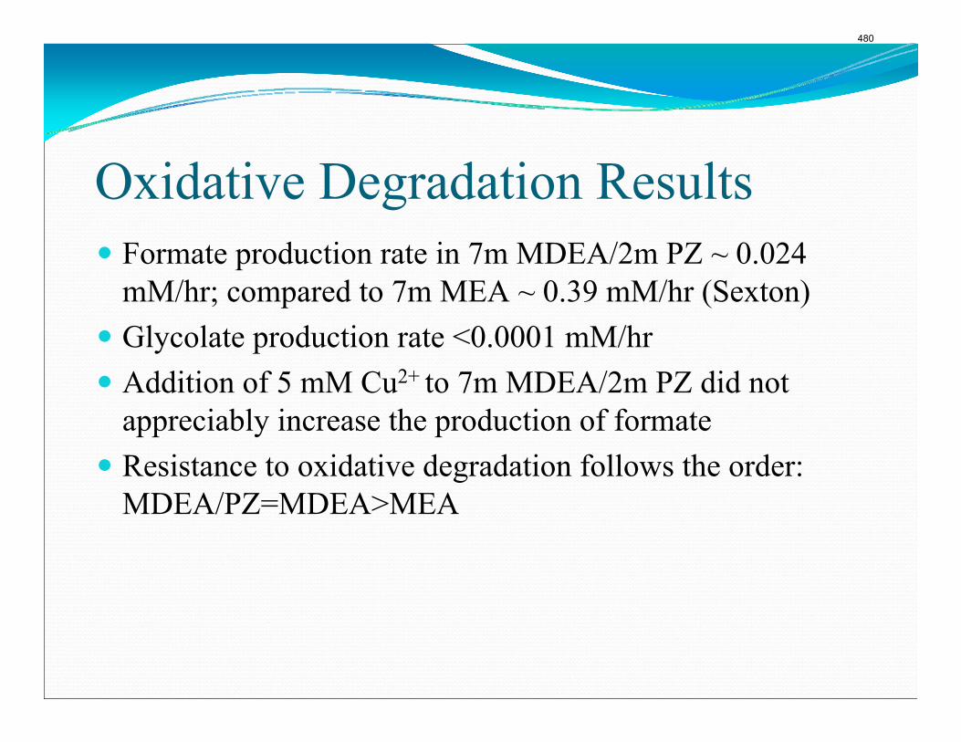
Oxidative Degradation ResultsFormate production rate in 7m MDEA/2m PZ ~ 0.024 mM/hr; compared to 7m MEA ~ 0.39 mM/hr (Sexton)Glycolate production rate <0.0001 mM/hrAddition of 5 mM Cu2+ to 7m MDEA/2m PZ did not appreciably increase the production of formateResistance to oxidative degradation follows the order: MDEA/PZ=MDEA>MEA
480
Future Work - Integrated degradation (Solvent cycling) Experiment (under construction)
Closed-loop apparatus:Oxidative reactor (glass) with 250 ml hold-upSS jacketed thermal reactorLauda heat bath – primary heat introductionTube-in-tube 316 stainless heat-XVariable speed positive displacement pumpExperimental Conditions:q ~ 100 ml/minτ ~ 5 min @ 55 °C (oxidative reactor)τ ~ 5 – 10 min @ 120+ °C (thermal reactor)Temperature approach = 10 °C
481
Future Work - ContinuedH2SO4 thermal degradation study (7m MDEA/2m PZ); mimic lean loaded solventFurther identify degradation products in thermal degradation studies using IC/MS and HPLCEstablish mechanism and kinetics for MDEA/PZ degradationOxidative degradation studies – MDEA and MDEA/PZ degradation with Inhibitor “A”Identify oxidative degradation unknowns including heat stable salts other than formateDegradation studies – PZ/hindered amine blends (AMP/PZ)Measure volatility of blended solvent over oxidative reactor to close mass balance on cycling experiment
482