Embed Size (px)
Citation preview

Clothing Consumption: Analyzing theApparel Industry’s Current and FutureImpact on Greenhouse Gas Emissions
The Harvard community has made thisarticle openly available. Please share howthis access benefits you. Your story matters
Citation Jacobs, Matthew. 2020. Clothing Consumption: Analyzing theApparel Industry’s Current and Future Impact on Greenhouse GasEmissions. Master's thesis, Harvard Extension School.
Citable link https://nrs.harvard.edu/URN-3:HUL.INSTREPOS:37365025
Terms of Use This article was downloaded from Harvard University’s DASHrepository, and is made available under the terms and conditionsapplicable to Other Posted Material, as set forth at http://nrs.harvard.edu/urn-3:HUL.InstRepos:dash.current.terms-of-use#LAA

Clothing Consumption: Analyzing the Apparel Industry’s
Current and Future Impact on Greenhouse Gas Emissions
Matthew Jacobs
A Thesis in the Field of Sustainability and Environmental Management
for the Degree of Master of Liberal Arts in Extension Studies
Harvard University
May 2020

Copyright 2020 Matthew Jacobs

Abstract
The highly pollutive apparel industry represents a significant global challenge in
light of forecasted population and economic growth – the two most significant drivers of
carbon dioxide emissions. Recent trends that have allowed consumers to “spend less, buy
more” are expected to continue for decades, including in developing countries where over
one billion new consumers will arise by 2030. Under the industry’s current operating
model, the aforementioned trends will cause a significant rise in greenhouse gas (GHG)
emissions. Surprisingly, the clothing we produce, consume, and discard has received little
attention when it comes to understanding the totality of its future impact on GHG
emissions across developed and developing countries.
My research sought to quantify and evaluate this impact against 2030 and 2050
climate mitigation targets under the IPCC’s 1.5°C and 2°C pathways by addressing four
main questions: What portion of GHG emissions are currently associated with the apparel
industry? What is the projected contribution of GHG emissions from the industry under
different scenarios of production, consumption, and post-consumption relative to the
IPCC’s 1.5°C and 2°C pathways? To what degree will apparel-related emissions represent
a greater proportion of GHG emissions in the future than they do today? Finally, to what
extent will apparel consumption impact emissions associated with developed and
developing countries?
Given the population and economic growth forecasts, I hypothesized that the
apparel industry would account for more than 30% of the 2050 carbon budget associated

with the IPCC’s 1.5°C pathway, and that developing countries would soon account for
greater emissions from apparel than developed countries despite having lower per capita
levels of consumption. To address the aforementioned questions and hypotheses, I
obtained population, economic, demographic, consumer, transportation, and industry-
specific data from dozens of publicly available sources and developed an Excel-based
model to assess current and forecasted GHG emissions associated with each phase of the
apparel life cycle for developed and developing countries.
The model was run to evaluate GHG emissions under four scenarios of varying
production, consumption, and post-consumption activities, including a separate baseline
“business as usual” scenario from which a sensitivity analysis was conducted to
determine which variables had the greatest impact on emissions. The sensitivity results
showed that consumption rates in both developed and developing countries had the
largest impact on apparel emissions, but for different reasons: for developing countries,
this result was due to the multiplication effect of rapidly rising population against the
carbon intensity of materials; for developed countries, it was strictly related to
overconsumption. Furthermore, the baseline scenario indicated that the apparel industry
will represent 20% of the remaining 2018 carbon budget under the 1.5°C pathway, and
up to 72% of the remaining budget when accounting for Earth-system feedbacks.
This thesis demonstrated that up to 85% of emissions from apparel occur in the
material production stage, indicating a need to rapidly reduce the carbon intensity of
materials and divert finished garments from landfill. If population growth and
corresponding demand for apparel cannot be decoupled from the carbon intensity of
production, it will be difficult to remain within 2°C of warming, much less 1.5°C.

v
Dedication
“Unless someone like you
cares a whole awful lot,
nothing is going to get better.
It’s not.”
Dr. Seuss, The Lorax

vi
Acknowledgments
This thesis – and the career change that has coincided with it – would not have
been possible without the love, patience, and support of my wife, Kristine, and two
daughters, Alexandra and Evelyn. I cannot thank the three of them enough, and I hope
that my chosen direction will play a small role in their future to help address some of
humanity’s most urgent issues on this miraculous planet.
I would also like to thank my parents, who strived against numerous odds to
provide me with a safe, comfortable life, and who continuously believed in and
demonstrated the value of education.
I am indebted to Dr. Jana Hawley, whose historical work served as an inspiration,
and whose guidance as my thesis director was instrumental in the completion of this
paper. Finally, a special thanks is due to Dr. Mark Leighton. His insights helped shaped
my proposal and his instruction made this program at Harvard an incredibly rewarding
experience.

vii
Table of Contents
Dedication ....................................................................................................................... v
Acknowledgments .......................................................................................................... vi
List of Tables ................................................................................................................. xi
List of Figures .............................................................................................................. xiv
Definition of Terms ...................................................................................................... xvi
I. Introduction ......................................................................................................... 1
Research Significance and Objectives .................................................................. 2
Background ......................................................................................................... 3
Global Changes in Population and Income ........................................................... 4
Impact of the Apparel Industry............................................................................. 7
The Apparel Industry’s Current Operating Model ..................................... 8
GHG Emissions of Apparel ...................................................................... 9
Research Questions, Hypotheses and Specific Aims........................................... 15
Specific Aims ......................................................................................... 16
II. Methods ............................................................................................................. 17
Phase 1 .............................................................................................................. 20
Part A: Production .................................................................................. 21
Part B: Consumption .............................................................................. 24
Part C: GWP of Manufacturing Scrap (Fabric Losses) ............................ 26
Part D: Transportation for Distribution ................................................... 27

viii
Phase 2 .............................................................................................................. 30
Part A: Washing ..................................................................................... 31
Part B: Drying ........................................................................................ 34
Part C: Detergent .................................................................................... 36
Phase 3 .............................................................................................................. 37
Part A: Collection and Sorting ................................................................ 38
Part B: Export/import of Used Clothing .................................................. 39
Part C: Landfill ...................................................................................... 46
Part D: Incineration ................................................................................ 49
Part E: Reuse .......................................................................................... 50
Part F: Recycling .................................................................................... 51
Carbon Budget ................................................................................................... 51
Independent Variables ....................................................................................... 57
Phase 1: Production ................................................................................ 58
Phase 2: Consumption ............................................................................ 63
Phase 3: Post-consumption ..................................................................... 70
Derived Variables .............................................................................................. 76
Phase 1: Production ................................................................................ 77
Phase 2: Consumption ............................................................................ 80
Phase 3: Post-consumption ..................................................................... 82
Multiple Phases ...................................................................................... 83
Greenhouse Gas Emissions ................................................................................ 85

ix
III. Results ............................................................................................................... 93
2015 Impacts ..................................................................................................... 93
Scenarios ........................................................................................................... 99
Baseline Scenario: Business as Usual ................................................... 100
Phase 1 ..................................................................................... 100
Phase 2 ..................................................................................... 103
Phase 3 ..................................................................................... 105
Summary of Scenarios 1 – 4 ................................................................. 112
Overview of Scenarios 1-4 ........................................................ 112
Comparison of results for all scenarios ...................................... 113
Summary of results for developing and developed countries ..... 116
Sensitivity Analysis ......................................................................................... 122
Sensitivity Analysis for All Countries................................................... 125
Sensitivity Analysis for Developing and Developed Countries ............. 126
IV. Discussion ....................................................................................................... 128
Current and Projected GHG Emissions ............................................................ 129
Carbon Budgets ............................................................................................... 133
Limitations and Future Research ...................................................................... 136
Future Research.................................................................................... 138
Developing and Developed Country Designations ................................ 139
Implications ..................................................................................................... 140
Conclusions ..................................................................................................... 144
Appendix 1 GWP by Phase for Scenarios 1 – 4 ........................................................... 147

x
Appendix 2 Sensitivity Analysis Values ...................................................................... 151
References ................................................................................................................... 153

xi
List of Tables
Table 1. Components of three life cycle phases of global apparel for analysis. ............... 17
Table 2. Allocation by fiber type in the global fiber mix. ............................................... 23
Table 3. Average cradle-to-gate global warming potential per kilogram by fiber type. ... 24
Table 4. Adjusted share of apparel imports by region..................................................... 28
Table 5. Average transportation distances for distribution in kilometers by zone. .......... 29
Table 6. Emission factors by transportation mode. ......................................................... 30
Table 7. Washing machine ownership, load sizes, cycles, and energy consumption. ...... 32
Table 8. Region-based kilograms of CO2 per kWh for washing machines. ..................... 33
Table 9. Region-based assumptions and estimates for drying machines. ........................ 35
Table 10. Estimated market share and GWP per wash by detergent type. ....................... 37
Table 11. Top 29 exporters of used clothing for 2015. ................................................... 41
Table 12. 2015 used apparel import volumes by region in kilograms. ............................ 42
Table 13. Portion of used apparel imports received by geographic region, 2015............. 44
Table 14. Average kilometers traveled for the export of used apparel by region. ............ 46
Table 15. Regional share of post-consumption destinations for used clothing. ............... 48
Table 16. Emission factors for landfill, incineration, reuse, and recycling. ..................... 49
Table 17. Carbon budgets and probabilities for 1.5°C and 2°C pathways. ...................... 52
Table 18. Remaining carbon budgets and estimates by year. .......................................... 55
Table 19. Annual emissions in GtC and associated GtCO2 equivalents. ......................... 55
Table 20. Independent variables for Phase 1. ................................................................. 58

xii
Table 21. Independent variables for Phase 2. ................................................................. 64
Table 22. Washing mechanism by region....................................................................... 66
Table 23. Independent variables for Phase 3. ................................................................. 71
Table 24. Derived variables for Phases 1, 2 and 3. ......................................................... 77
Table 25. Greenhouse gas emissions variables for Phases 1, 2, and 3. ............................ 85
Table 26. End-of-life destinations for manufacturing scrap. ........................................... 88
Table 27. 2015 apparel emissions by life cycle phase. ................................................... 94
Table 28. 2015 GWP of apparel for developing and developed countries. ...................... 95
Table 29. 2015 GWP of apparel by life cycle stage. ....................................................... 98
Table 30. Summary of modeled scenarios. ..................................................................... 99
Table 31. Phase 1 default values for Baseline scenario................................................. 101
Table 32. Phase 2 default values for Baseline scenario................................................. 104
Table 33. Phase 3 default values for Baseline scenario................................................. 106
Table 34. Baseline scenario GWP by life cycle stage, 2015 - 2050. ............................. 108
Table 35. Baseline scenario difference in emissions, 2050 vs. 2015. ............................ 109
Table 36. Baseline scenario, percent change in emissions by life cycle stage. .............. 111
Table 37. Summary of all scenarios by life cycle stage, 2015 - 2050. ........................... 114
Table 38. Summary of carbon budget expenditures for all scenarios. ........................... 115
Table 39. GWP by life cycle phase for developing and developed countries. ............... 116
Table 40. GWP of Phase 1 for developing and developed countries. ............................ 118
Table 41. GWP of Phase 2 for developing and developed countries. ............................ 119
Table 42. GWP of Phase 3 for developing and developed countries. ............................ 120
Table 43. Sensitivity spread for key variables (2015 – 2050). ...................................... 123

xiii
Table 44. Sensitivity spread for developing and developed countries (2015 – 2050). ... 124
Table 45. Remaining carbon budgets with revised Earth-system feedbacks.................. 136
Table 46. Scenario 1 GWP by life cycle stage, 2015 - 2050. ........................................ 147
Table 47. Scenario 2 GWP by life cycle stage, 2015 - 2050. ........................................ 148
Table 48. Scenario 3 GWP by life cycle stage, 2015 - 2050. ........................................ 148
Table 49. Scenario 4 GWP by life cycle stage, 2015 - 2050. ........................................ 149
Table 50. GWP scenarios summary, developed vs. developing countries. .................... 150
Table 51. Full set of Phase 3 values (expansion of Table 43) ....................................... 151
Table 52. Full set of Phase 3 values (expansion of Table 44). ...................................... 152

xiv
List of Figures
Figure 1. Regional CO2 emissions. .................................................................................. 6
Figure 2. Regional carbon budgets. .................................................................................. 7
Figure 3. Linear life cycle model for apparel. ................................................................ 10
Figure 4. Post-consumer destinations for discarded apparel in the United States. ........... 13
Figure 5. Architecture of the study................................................................................. 18
Figure 6. Phase 1 modeling process, excluding manufacturing losses & transportation. . 21
Figure 7. Phase 1 modeling process for distribution-related transportation. .................... 28
Figure 8. Phase 2 modeling process for washing, drying, and detergent impacts. ........... 31
Figure 9. Phase 3 modeling process for collection and sorting impacts. ......................... 39
Figure 10. Phase 3 modeling process for import/export of used clothing. ....................... 40
Figure 11. Phase 3 modeling process. ............................................................................ 47
Figure 12. Cumulative carbon emissions by 2050 and 2100. .......................................... 53
Figure 13. Allowable fossil-fuel carbon emissions. ........................................................ 57
Figure 14. Ranked percentage of 2015 apparel emissions by life cycle stage.................. 96
Figure 15. Baseline scenario, Phase 1 MT of CO2-eq. .................................................. 102
Figure 16. Baseline scenario, Phase 1 population and MT CO2-eq. .............................. 103
Figure 17. Baseline scenario, Phase 2 metric tons of CO2-eq. ...................................... 105
Figure 18. Baseline scenario, Phase 3 metric tons of CO2-eq. ...................................... 107
Figure 19. Baseline scenario emissions and population over time, 2015 - 2050. ........... 110
Figure 20. GWP by phase for all scenarios, developing vs. developed countries. ......... 117
Figure 21. Per capita emissions for developing and developed countries. ..................... 121

xv
Figure 22. Gt CO2-eq trend for all scenarios, 2015 – 2050. .......................................... 130
Figure 23. Baseline scenario share of apparel emissions by country type. .................... 131
Figure 24. Baseline scenario share of emissions by life cycle phase. ............................ 132
Figure 25. Remaining carbon budget scenarios based on 2018 carbon budget. ............. 134

xvi
Definition of Terms
BAU Business as usual
BP British Petroleum
CAGR Compound annual growth rate
CDR Carbon dioxide removal
CO2 Carbon dioxide
COP Conference of the parties
CH4 Methane
EIA Energy Information Administration
EPA Environmental Protection Agency
EU European Union
GDP Gross domestic product
GHG Greenhouse gas
GMT Global mean temperature
GWP Global warming potential
GtCO2 Giga tonnes of carbon dioxide (metric)
IEA International Energy Agency
IPCC Intergovernmental Panel on Climate Change
IRENA International Renewable Energy Agency
kg Kilograms
kg CO2-eq Kilograms of carbon dioxide equivalent
kWh Kilowatt hour

xvii
MMC Man-made cellulosic
MT Metric tons
NDC Nationally determined contribution
OECD Organisation for Economic Co-Operation
ROW Rest of world
UNFCCC United Nations Framework Convention on Climate Change

1
Chapter I
Introduction
The central aim of the Paris Agreement is to keep global temperatures below 2
degrees Celsius (°C) from pre-industrial levels (United Nations, 2018). According to the
Intergovernmental Panel on Climate Change (IPCC), this will require a reduction in total
greenhouse gas (GHG) emissions of 41-72% from 2010 levels by 2050 (Edenhofer et al.,
2014) when the United Nations (UN) projects global population will equal 9.2 billion, an
increase of 32%. (United Nations, 2017). The IPCC has identified population and
economic growth as the most significant drivers of carbon dioxide (CO2) emissions, both
of which have outpaced emission reductions and present a significant challenge for
industries that must contend with sharp increases in forecasted demand and consumer
spending power (Edenhofer et al., 2014).
In particular, the apparel industry’s production output is expected to increase
230% by 2050 (Morlet et al., 2017), and would thus correspond with a substantial rise in
emissions beyond the estimated 1.5 billion metric tons of CO2 emitted by the industry in
2015 (Eder-Hansen et al., 2017). Those emissions make the apparel industry one of the
most pollutive industries in the world (Morlet et al., 2017), yet the clothing we produce,
consume, and discard has received little attention when it comes to understanding the
totality of its impact on global GHG emissions. As global population and GDP per capita
increase, apparel consumption will grow, placing immense demands on land, livestock,
fossil fuels and other resources required for natural and synthetic fiber production. Those
fibers represent a source of increasing GHG emissions that will continue to climb unless

2
dramatic changes occur in production, consumption, and post-consumption activities.
This is particularly true among developing nations where the population is expected to
urbanize and expand by 17.4% by 2030, a rate that is three times faster than that of
developed countries and will result in over one billion new consumers (Gordon &
Hodgson, 2015).
Given that global GHG emissions have already exceeded planetary boundaries
(Steffen et al., 2015), the apparel industry’s expected growth will conflict with the
IPCC’s recommended warming limit of 2°C. Therefore, meeting climate mitigation
targets will require substantial declines in GHG emissions associated with the production,
consumption, and disposal of apparel to clothe a growing population under the demands
of developing economies.
Research Significance and Objectives
Given the apparel industry’s forecasted growth from rapidly increasing
population, urbanization, and per-capita incomes, my research analyzed, forecasted, and
evaluated scenarios among developed and developing countries that involve different
rates of apparel production, consumption, and post-consumption activities to assess the
industry’s contribution to climate change. Therefore, the objectives of my research were
to:
• Evaluate the apparel industry’s future contribution to global greenhouse gas
emissions and determine how those emissions might affect 2030 and 2050 climate
mitigation targets under the IPCC’s 1.5°C and 2°C pathways (as measured by
CO2-equivalent).

3
• Develop an analytical framework to forecast GHG-related implications for
scenarios of varying apparel production, consumption, and post-consumption
between developed and developing countries.
Background
During the twenty-first Conference of the Parties (COP 21) of the United Nations
Framework Convention on Climate Change (UNFCCC), 196 state parties met and
adopted the Paris Agreement to strengthen the global response to climate change (Paris
Agreement, n.d.). The goal of the Paris Agreement is to keep global temperatures below
2°C from pre-industrial levels and to limit the increase to 1.5°C (UNFCCC, 2015); it
obtained enough signatories to enter into force on November 4th, 2016 (United Nations
Treaty Collection, 2015). Under the Paris Agreement, each country must put forward
their best efforts to reduce emissions through their own nationally determined
contributions (NDCs). The NDCs reflect each country’s non-binding emission reduction
targets, which must be reported every five years and continue to progress over time
(UNFCCC, 2015).
Unfortunately, the currently pledged NDCs lead to estimated GHG emissions of
52-58 gigatonnes of carbon dioxide equivalent (GtCO2-eq) in 2030, an amount that falls
beyond the 2°C pathway and results in global temperatures of 3°C above pre-industrial
levels by 2100 with continued warming thereafter (Masson-Delmotte et al., 2018). To
make matters worse, the IPCC’s 2018 Special Report: Global Warming of 1.5°C revealed
that the impacts of 2°C would be worse than previously projected (Climate Nexus, n.d.)
and noted that limiting warming to 1.5°C would substantially lower the risks of droughts,
floods, heavy precipitation, species loss and extinction, diseases and vector-borne

4
diseases, water stress, and reduced crop yields (Masson-Delmotte et al., 2018). To avoid
those risks, a two-thirds chance of limiting warming to 1.5°C requires carbon neutrality in
20 years and restricts the remaining carbon budget to 420 GtCO2, substantially lower than
the estimated remaining budget of 1,170 GtCO2 to adhere to the 2°C pathway (Masson-
Delmotte et al., 2018). Moreover, it requires GHG emissions of 25-30 GtCO2 in 2030,
markedly lower than the aforementioned NDC pledges and current annual emissions of
42 GtCO2 (Masson-Delmotte et al., 2018). In short, dramatic measures must be taken to
reduce GHG emissions to adhere to both the 1.5°C and 2°C pathway.
Global Changes in Population and Income
According to Edenhofer et al. (2014), “Half the cumulative anthropogenic CO2
emissions between 1750 and 2010 occurred in the last 40 years” (p. 7), rising 81%
between 1970 (27 GtCO2eq/yr) and 2010 (49 GtCO2-eq/yr) (Edenhofer et al., 2014). This
dramatic rise in GHG emissions was primarily driven by the product of population and
GDP per capita, which grew 87% and 100%, respectively, from 1970 to 2010 (Edenhofer
et al., 2014). Unfortunately, “reductions in the energy intensity of economic output have
not been sufficient to offset the effect of GDP growth” (Edenhofer et al., 2014, p. 355).
Similarly, the “decreasing carbon intensity of energy supply has been insufficient to
offset the increase in global energy use” (Edenhofer et al., 2014, p. 355) (Figure 1).
These trends are forecast to continue whereby population and economic growth
result in global temperatures of 3.7 to 4.8°C above pre-industrial levels by 2100 if
additional efforts are not made to reduce GHG emissions beyond those already in place
(Edenhofer et al., 2014). Much of this growth will occur in Asian and African countries,

5
which are expected to account for 83% of the world’s population in 2100, up from 66%
today (Khokhar, 2015). What is more, the majority of mitigation efforts will occur in
non-Organisation for Economic Co-Operation (OECD) countries due to the fact that they
are projected to have greater overall emissions and carbon intensities than OECD
member countries, which tend to have high-income economies and are often referred to
as “developed countries” (Edenhofer et al., 2014) (Figure 2). In the future, a growing
share of emissions from non-OECD countries will stem from CO2 released from
manufacturing and producing products (Edenhofer et al., 2014), a condition that will be
exacerbated by increased population and GDP growth.
That expectation especially applies to the apparel industry, where more than 60%
of global apparel consumption occurs in OECD countries, while more than 60% of
production occurs in seven non-OECD countries: India, Pakistan, Bangladesh, China,
Vietnam, Thailand, and Indonesia (Kirchain, Olivetti, Miller, & Greene, 2015). The CO2
emissions embedded in this trade flow are currently reflected in decreased territorial CO2
emissions and increased consumption-based CO2 emissions among OECD countries
(Edenhofer et al., 2014). However, this gap between territorial and consumption-based
emissions will change through 2050 as OECD countries decline in population while the
seven aforementioned non-OECD countries not only increase in population, but more
than double (India, Pakistan, China, Thailand) or triple (Bangladesh, Vietnam) their per
capita GDP (Pricewaterhouse Coopers, 2017). Much of this will be driven by China’s
transition to a consumer-driven economy, and by the fast-growing working-age
populations of Vietnam, India, and Bangladesh where labor will be inexpensive enough

6
to incentivize multinational companies to shift production from China (Pricewaterhouse
Coopers, 2017).
Figure 1. Regional CO2 emissions.
Regional CO2 emissions associated with population, GDP per capita, energy intensity, and the carbon intensity of the energy system, 1970-2010 (Edenhofer et al., 2014). The y-axis serves as an index where 1 represents fossil fuel combustion in 1970; data are based on purchasing power parity-adjusted GDP.

7
Figure 2. Regional carbon budgets.
Regional carbon budgets (left) for OECD countries, Asia, Latin America (LAM), Middle East and Africa (MAF) and economies in transition (EIT), and corresponding mitigation scenarios (right) reaching 430 – 530 ppm CO2-eq in 2100 based on cumulative emissions from 2010 to 2100 (Edenhofer et al., 2014).
Impact of the Apparel Industry
The apparel industry is one of the most important consumer industries in the
world, generating nearly $1.7 trillion in revenues (Statista, 2018) and representing two
percent of the world’s GDP (Fashion United, 2018). As the world’s population grows,
apparel consumption is expected to increase from 56 million metric tons today to 92
million metric tons by 2030, a rise of 63% (Eder-Hansen et al., 2017). If the majority of
the developing world adopts the per capita consumption habits of the developed world,
these figures could increase further. This is particularly worrisome given the fact that
large apparel markets like the US spend 37% less on clothing today, but buy 75% more
garments than they did in 1990 (Bureau of Labor Statistics, 2016; Reed, 2014; Tan, 2016;
U.S. Census Bureau, 2016; U.S. Department of Labor, 2012; U.S. Department of Labor,
2016; Vatz, 2013). Such consumption habits stem from automation advancements,

8
opaque supply chains that emphasize the use of petroleum-based synthetic materials and
low-wage labor (Cline, 2016; Cline, 2014), rising disposable income (Kozinets &
Handelman, 2004), consumer technologies that provide mass exposure to desirable styles
(Bhardwaj & Fairhurst, 2010; Macquarie Research, 2017), and corporate supply chain
improvements that accelerate design and production cycles to create and capture demand
(Amed, Berg, Brantberg, & Hedrich, 2016; Remy, Speelman, & Swartz, 2016).
The Apparel Industry’s Current Operating Model
The rise of fast fashion – a business model that emphasizes low prices, intensified
production, and limited quantities of poorly made garments – has disproportionately
contributed to the doubling of production that has occurred in the broader apparel
industry over the last 15 years (Morlet et al., 2017). This business model has been a
potent recipe for growth, as exemplified by H&M and Zara who have become two of the
largest fashion brands in the world with combined annual revenues exceeding $50 billion
(H&M, 2017; Inditex, 2017). Despite the negative environmental and social externalities
of the business model, it has been increasingly adopted by large retailers who have
sought to compete by abandoning the traditional two-season fashion cycle (Logistics
Bureau, 2017).
This intensified production volume has been a massive resource drain and source
of pollution, and according to recent industry reports, it will likely result in catastrophic
outcomes (Cobbing & Vicaire, 2016; Eder-Hansen et al., 2017; Morlet et al., 2017).
Much of this stems from the fact that nearly all production inputs currently exceed
planetary boundaries (Eder-Hansen et al., 2017) and involve resource-intensive crops,
hazardous chemicals, excessive fossil fuels, and low-wage labor in countries with weak

9
environmental regulations (Cline, 2016; Cline, 2014). In other words, nearly every step in
the apparel life cycle (Figure 3) represents an industrial system that requires energy,
generates waste, and contributes to biodiversity loss and climate change (Williams,
2015). Much of this is due to the extraction and refining of non-renewable inputs for
synthetic fibers, the use of fertilizers and pesticides required for growing cotton, the
intensive use of hazardous chemicals in manufacturing and production, and the pollution
associated with global transportation logistics. The industrial systems associated with
these factors wreak havoc on the environment and are magnified by the industry’s
intensified production cycles. According to a recent industry report, these industrial
systems already exceed the planet’s safe operating boundaries for energy emissions, land
use, chemical use, and waste creation, and will reach catastrophic levels by 2030, thereby
preventing the industry from continuing under its current operating model (Eder-Hansen
et al., 2017).
GHG Emissions of Apparel
The apparel industry requires enormous amounts of energy to manufacture and
transport its products, processes that generate 400% more CO2 emissions than the airline
industry (Bedat, 2016; Cobbing & Vicaire, 2016). What is more, many of the clothes are
not built to last and the combination of low cost and low quality have resulted in a 200%
increase in consumer textile waste since 1990 (U.S. Environmental Protection Agency,
2016), 85% of which goes to a landfill where every discarded kilogram contributes
approximately 3.69 kilograms of CO2 to the atmosphere (CO2list.org, 2012; U.S.
Environmental Protection Agency, 2016).

10
Figure 3. Linear life cycle model for apparel.
Source: Durham, Hewitt, Bell, & Russell (2015).
Few industries influence natural systems as significantly as the apparel industry,
which relies heavily on the continued access and availability of increasingly scarce
material resources (Eder-Hansen et al., 2017; Sumner, 2015). The majority of impacts
occur at the beginning of the apparel life cycle with the production of raw materials,
fibers, and garments. To understand where influences on natural systems begin, it is
important to know where the raw material inputs come from. Of the nearly 91 million
metric tons of yarn annually produced for apparel, 37% are agriculturally derived (e.g.,
cotton, wool, hemp) and 63% are synthetically produced from carbon-intensive,
nonrenewable fossil fuel stocks (e.g., acrylic, nylon, polyester) (Sandin & Peters, 2018),
corresponding to an average per capita consumption of 9.5 kilograms (Kirchain, Olivetti,
Miller, & Greene, 2015; Palamutcu, 2015; United Nations, 2018). Cotton alone accounts

11
for 24% - 30% of apparel fiber (Remy, Speelman, & Swartz, 2016; Sandin & Peters,
2018) and requires 2.5% of the world’s arable land (Morlet et al., 2017). The industrial-
scale cultivation of cotton – 75% of which comes from genetically engineered seed
(Allen, 2004) – involves 25% of all insecticides used globally (Wallander, 2014), many
of which are harmful to humans and ecosystems (Eder-Hansen et al., 2017) beyond the
CO2 emissions of their production (Roos, Posner, Jonsson & Peters, 2015). Other natural
fibers require animal husbandry, an activity that generates potent greenhouse gases (e.g.,
methane) and typically requires vast amounts of land, often exceeding 275 hectares per
metric ton of fiber (Morlet et al., 2017).
Powering textile production facilities with renewables is being pursued by a
number of major fashion brands. However, those brands don not own or operate those
production facilities, the majority of which run on fossil fuels in off-shore facilities.
Adopting eco-efficiency methods to conserve energy – and thus limit GHG emissions –
could reduce energy consumption by 11% - 26% and waste flue gas emissions by as
much as 18% (Ozturk et al., 2016). A comprehensive review of energy efficiency
measures for the textile industry identified 184 energy efficiency measures applicable to
textile production facilities, most of which have a low payback period (Hasanbeigi &
Lynn, 2012). In fact, one life cycle assessment study found that 20% increased energy
efficiency in garment production could reduce the climate impact of the entire life cycle
by 15% (Roos et al., 2016), making clear that the adoption of energy efficiency measures
could be instrumental in reducing the emissions impact of the apparel industry.
Apparel’s impact on natural systems and its contribution to GHG emissions is not
limited to the pre-consumer stages of the apparel life cycle, but also has an outsize effect

12
on the consumer phase. For example, published lifecycle analyses of common garments
such as t-shirts and jeans have shown that the consumer use phase can account for 37% of
a garment’s climate change impact (Hurst, 2017; Kirchain et al., 2015; Levi Strauss &
Co., 2015; Wallander, 2011). Additionally, washing and drying cycles are energy-
intensive and currently account for more than 120 million metric tons of CO2 equivalent
per year (Morlet et al., 2017), though washing and drying habits vary extensively across
the globe, which means this estimation may be highly conservative since it does not
factor in potential contributions from detergents or regions such as South and Central
America, Indonesia, Africa, and India (Pakula & Stamminger, 2010).
As noted above, landfilled textiles contribute to CO2 emissions, but they also
generate methane as a by-product of decomposition. This is concerning for two reasons.
First, methane (CH4) is 25 times more potent than CO2 at trapping heat in the atmosphere
(U.S. Environmental Protection Agency, 2017), and contributes to global warming at a
more accelerated rate. Second, the growth rate of textiles in landfills has increased more
than any other waste category in many developed countries, exacerbating the
environmental damage caused by landfills, which happen to be the third largest source of
CH4 emissions in the US (U.S. Environmental Protection Agency, 2017). Unfortunately,
85% of discarded apparel in the US goes to a landfill (Hawley, 2006). According to
Hawley (2006), the remaining 15% is recycled via used clothing markets, transformed
into wiping/polishing cloths, made into new products, or incinerated (Figure 4).

13
Figure 4. Post-consumer destinations for discarded apparel in the United States. Source: Hawley (2006).
Used clothing markets receive 45% of recycled clothing, which is resold
domestically or exported for bulk sale to developing countries (Figure 4). Foreign
clothing exports account for 15% of global trade (Hawley, 2015; Lewis, 2015) and often
represent an environmental concern beyond emissions associated with their transport
because they are predominantly exported to the developing world where textile recycling
infrastructure is extremely limited or nonexistent (Lewis, 2015). GHG emissions
associated with domestic reuse are difficult to estimate due to the fact that reuse does not
necessarily substitute for new product consumption (Fortuna & Diyamandoglu, 2017).
Wiping/polishing cloths represent 30% of recycled apparel, which gets cut and
converted into rags by rag graders (Hawley, 2006), who obtain most of their stock from
thrift stores and charities that are unable to sell 80% of what they receive (Claudio,
2007). Of course, this process of remanufacturing represents yet another source of GHG
emissions.
New products are developed from 20% of all recycled apparel, which gets re-spun
into yarns or converted into new material (Hawley, 2006). These materials are typically

14
downcycled into pet beds, sound-proofing, low-end blankets, building materials, and
currency (Hawley, 2006) because they are composed of mixed fibers that cannot be
separated with today’s recycling technology. As a result, these products are one step
away from prolonged decomposition in landfill. This reality highlights why 97% of the
material used to create new clothing is virgin feedstock – the majority being petroleum-
based – and only 1% of which is recycled into new clothing (Morlet et al., 2017).
Incineration is the end-state for roughly 5% of discarded consumers textiles
(Hawley, 2006), which generates greenhouse gasses. Oftentimes these articles are soiled,
moldy, and unusable, though a number of retailers – including the fast fashion giant
H&M – have been caught incinerating vast amounts of unsold inventory (The Fashion
Law, 2017).
The post-consumer destinations for discarded apparel detailed above pertain to the
United States but similarly apply to the European Union. While these data are not
available for every country, assumptions can be made for many countries due to the fact
that recycling infrastructure is largely non-existent. Moreover, much of the post-
consumer emissions impacts occur in Western markets where Sandin and Peters (2018)
state that the impact per garment must be reduced by 30% - 100% by 2050 to stay within
the planetary boundaries outlined by Steffen et al. (2015).
An extensive amount of research has been conducted on individual stages of the
apparel life cycle, but no studies have been published about the global impact of apparel
as it pertains to GHG emissions for the full life cycle. Much of this may be due to the fact
that there are substantial differences in production processes, consumer behaviors
influencing consumption and use, and post-consumer activities across the globe. This

15
complexity has, in part, made it difficult to understand the apparel industry’s contribution
to GHG emissions. Surprisingly, major research publications focused on climate
mitigation solutions have avoided apparel altogether (e.g., Drawdown), underscoring the
need to understand its impact to avoid potentially catastrophic contributions to GHG
emissions limits that must be achieved to keep global temperatures below 2°C from pre-
industrial levels. While select reports have made estimates on the industry’s carbon
impact, they have opted to focus on the production phase where the majority of GHG
emissions tend to occur for large fashion retailers. Moreover, few studies have considered
where GHG emissions stemming from the apparel industry might occur in the future
between developed and developing countries as the dynamics of population growth and
economic development influence regional GHG mitigation targets.
Research Questions, Hypotheses and Specific Aims
The questions my research aimed to answer were: What portion of global GHG
emissions are currently associated with the apparel industry? What is the projected
contribution of GHG emissions from the apparel industry in 2030 and 2050 under
different scenarios of production, consumption, and post-consumption activities relative
to the IPCC’s 1.5°C and 2°C pathways? To what degree will emissions from the apparel
industry represent a greater proportion of global GHG emissions in the future than they
do today? Finally, to what extent will apparel consumption impact emissions associated
with developed and developing countries?
These questions were explored by testing the following hypotheses:

16
1. The apparel industry will account for more than 30% of the 2050 carbon budget
associated with the IPCC’s 1.5°C pathway, representing a significant increase in
GHG emissions over current contributions.
2. Developing countries will account for greater emissions from apparel than
developed countries, assuming that 50% of the population in developing countries
achieve similar clothing consumption levels as developed countries by 2030.
Specific Aims
To test these hypotheses, the specific aims of my research were to:
1. Develop and evaluate a data set comprised of current and forecasted economic and
demographic variables for developed and developing countries.
2. Understand recent and forecasted production volumes by fiber type and calculate
associated GHG emissions.
3. Investigate resource requirements associated with each fiber type and determine
planetary boundaries for the potential 2030 and 2050 fiber mix.
4. Determine the GHG emissions associated with current and future (2030 and 2050)
production and consumption patterns for developed and developing countries.
5. Calculate and develop model assumptions for post-consumption volumes and GHG
emissions for re-use, landfill, recycling, and incineration by country.
6. Conduct analyses and explore the impacts of apparel-related GHG emissions for
several production, consumption, and post-consumption scenarios.
17
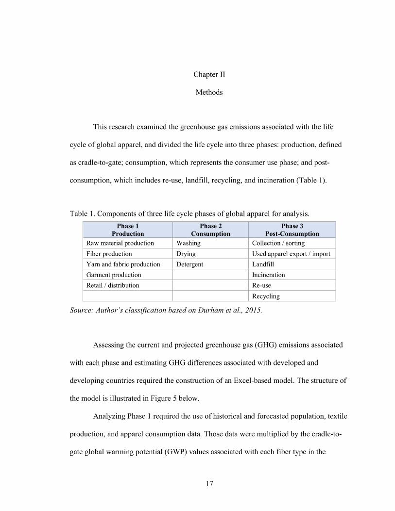
Chapter II
Methods
This research examined the greenhouse gas emissions associated with the life
cycle of global apparel, and divided the life cycle into three phases: production, defined
as cradle-to-gate; consumption, which represents the consumer use phase; and post-
consumption, which includes re-use, landfill, recycling, and incineration (Table 1).
Table 1. Components of three life cycle phases of global apparel for analysis. Phase 1
Production Phase 2
Consumption Phase 3
Post-Consumption Raw material production Washing Collection / sorting Fiber production Drying Used apparel export / import Yarn and fabric production Detergent Landfill Garment production Incineration Retail / distribution Re-use Recycling
Source: Author’s classification based on Durham et al., 2015.
Assessing the current and projected greenhouse gas (GHG) emissions associated
with each phase and estimating GHG differences associated with developed and
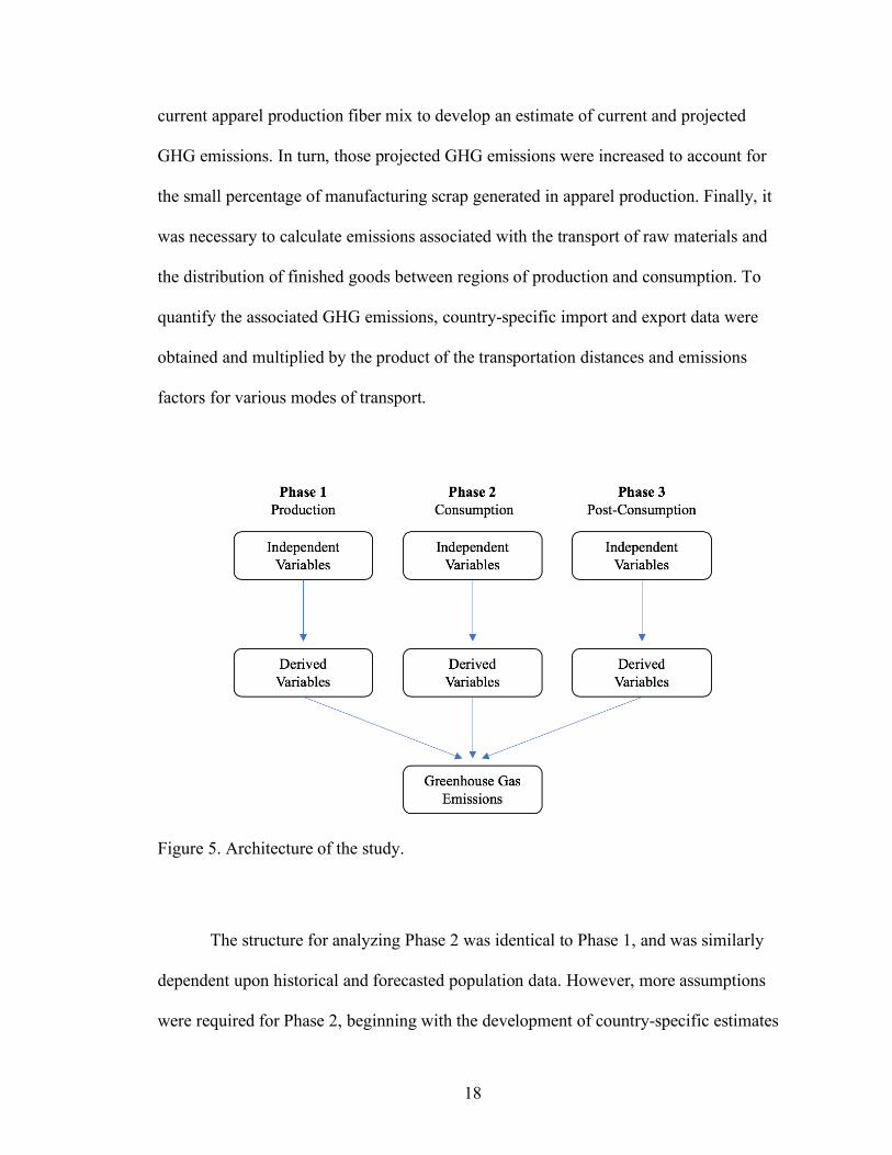
developing countries required the construction of an Excel-based model. The structure of
the model is illustrated in Figure 5 below.
Analyzing Phase 1 required the use of historical and forecasted population, textile
production, and apparel consumption data. Those data were multiplied by the cradle-to-
gate global warming potential (GWP) values associated with each fiber type in the
18
current apparel production fiber mix to develop an estimate of current and projected
GHG emissions. In turn, those projected GHG emissions were increased to account for
the small percentage of manufacturing scrap generated in apparel production. Finally, it
was necessary to calculate emissions associated with the transport of raw materials and
the distribution of finished goods between regions of production and consumption. To
quantify the associated GHG emissions, country-specific import and export data were
obtained and multiplied by the product of the transportation distances and emissions
factors for various modes of transport.
Figure 5. Architecture of the study.
The structure for analyzing Phase 2 was identical to Phase 1, and was similarly
dependent upon historical and forecasted population data. However, more assumptions
were required for Phase 2, beginning with the development of country-specific estimates

19
for household size, as well as washing and drying machine ownership and usage
estimates, all of which varied based on anticipated changes in population and income
over time. The GHG emissions associated with washing and drying machine usage were
derived by multiplying usage-based energy consumption estimates by the projected
emissions associated with current and forecasted fuel types through 2050. Lastly, the
GHG emissions associated with the use of various types of detergent were added to
complete the total emissions estimate for Phase 2.
Analyzing Phase 3 required the use of country-specific import and export data
associated with used clothing volumes and trade distances to calculate import-specific
GHG emissions. The GHG emission calculations for the remaining post-consumption
activities – landfill, incineration, reuse, and recycling – were based on aggregate disposal
volumes. Reliable volumetric data for each of those activities were available for
developed countries, but informed assumptions were required to account for the
allocation of disposed clothing across those activities in developing countries where data
were limited or nonexistent. Volumes for each post-consumption activity were then
multiplied by an emission factor or an avoided emission factor to determine each
activity’s total GHG emissions or savings.
Each of the three phases required developing forecasts to extrapolate data out to
2030 and 2050, as well as adjustments to account for differences between data sources. In
particular, the Excel model for Phases 2 and 3 required deductions and extrapolations to
account for country-specific data gaps frequently associated with developing countries;
these were often addressed by applying assumptions and triangulations associated with
regional data. The methods used in in the Excel model to process the GHG emissions

20
associated with each phase are detailed by phase below and are followed by an
explanation of the carbon budget and the independent, derived, and greenhouse gas
variables used in my analysis.
Phase 1
Calculating GHG emissions at the country level required triangulating between
global textile production and consumption data, consumption estimates for major
countries and regions, and the cradle-to-gate GWP estimates associated with finished
fibers in the global fiber mix. This approach was necessary to associate the amount of
each fiber produced – which is commonly reported in metric tons – with apparel
consumption data, which are reported in terms of spend by country, not weight. What is
more, this approach allowed me to validate that country-level consumption estimates in
the model were directionally aligned with more accurate and frequently reported global
fiber production volumes. Phase 1 modeling also required calculating the GWP
associated with fabric losses that occur in the manufacturing process, as well as
transportation estimates associated with distribution from the point of assembly to retail.
In short, there were four distinct parts to the Phase 1 modeling process, Parts A through
D, each of which are detailed below.
As illustrated in Figure 6, the modeling for Parts A and B was comprised of five
steps. The product of steps one through three, which were based on global production and
consumption volumes, was compared with the product of steps four and five, which were
based on country-level consumption estimates. This process gave me the ability to
conduct the aforementioned validity check between the GWP total based on global

21
production and the GWP total based on country-level consumption; it also yielded
country-specific GWP data that could be sub-divided into geographic regions as well as
IMF designations for developed and developing countries. Finally, forecasts for 2030 and
2050 were developed by calculating the compound annual growth rates (CAGR) for
many of the independent and derived variables, providing GWP totals beyond 2015,
which was used as the base year in my calculations.
Figure 6. Phase 1 modeling process, excluding manufacturing losses & transportation.
Part A: Production
Step 1 relied on global population data and forecasts through 2050 from the
United Nations. Global population was the only variable in my model that was available
for all countries and did not require my own forecasting. In contrast, global apparel

22
consumption per capita was only forecast to 2025. I developed low and high forecasts for
global apparel consumption per capita based on two periods, 2005 – 2015 and 2015 –
2025, respectively. That allowed me to create an average CAGR based on a period of
economic downturn and recovery (2005 – 2015) and a second period that incorporated
those same conditions but was marked by a sharper rise in population, GDP, and
urbanization (2015 – 2025), which are three of the strongest predictors of apparel
consumption. Utilizing the average CAGR from these two periods allowed me to account
for economic uncertainties when calculating the global production volume for apparel.
Step 2 required the use of well-documented global textile production data and
forecasts from major textile corporations, analyst groups, and non-profit organizations
such as Lenzing, PCI Wood Makenzie, and Textile Exchange. None of those forecasts
went beyond 2025, so data for all subsequent years up to and including 2050 were
calculated using a CAGR based on 2005 – 2017 data. Dividing the global production
volume for apparel (the outcome of Step 1) by the global textile production data and
related forecasts thus yielded the average percentage of global textile production used for
apparel.
Step 3 leveraged fiber-specific textile production data and forecasts available
from the same sources noted in Step 2, and required multiplying the percent each fiber
represented in the global fiber mix by the global production volume for apparel (again,
the outcome of Step 1). That calculation yielded the global production by fiber type for
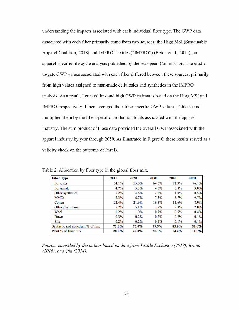
the apparel industry. Each fiber’s allocation in the global fiber mix (Table 2) is forecast to
change over time, primarily due to the anticipated increase in the industry’s reliance on
synthetics. As a result, the GWP associated with Phase 1 could not be calculated without
23
understanding the impacts associated with each individual fiber type. The GWP data
associated with each fiber primarily came from two sources: the Higg MSI (Sustainable
Apparel Coalition, 2018) and IMPRO Textiles (“IMPRO”) (Beton et al., 2014), an
apparel-specific life cycle analysis published by the European Commission. The cradle-
to-gate GWP values associated with each fiber differed between these sources, primarily
from high values assigned to man-made cellulosics and synthetics in the IMPRO
analysis. As a result, I created low and high GWP estimates based on the Higg MSI and
IMPRO, respectively. I then averaged their fiber-specific GWP values (Table 3) and
multiplied them by the fiber-specific production totals associated with the apparel
industry. The sum product of those data provided the overall GWP associated with the
apparel industry by year through 2050. As illustrated in Figure 6, these results served as a
validity check on the outcome of Part B.
Table 2. Allocation by fiber type in the global fiber mix.
Source: compiled by the author based on data from Textile Exchange (2018), Bruna (2016), and Qin (2014).

24
Table 3. Average cradle-to-gate global warming potential per kilogram by fiber type.
Source: compiled by the author based on Sustainable Apparel Coalition (2018) and Beton et al. (2014).
Part B: Consumption
Like Step 1, Step 4 relied on country-level population data and forecasts through
2050 from the United Nations. Those population data could not be multiplied by country-
specific import/export data for new clothing due to the fact that import/export data are
reported in currencies, not weights that can be multiplied by the GWP values from the
Higg MSI and IMPRO. Instead, clothing consumption per capita data were used, which
were limited but available for a few major countries and all regions of the world except
Latin America. Countries that had no consumption per capita estimates were assigned
estimates associated with their region. To calculate apparel consumption per capita for
Latin America, I used the average consumption per capita in kilograms for all developing
countries.
For Step 5 I utilized the output of Step 4, the apparel consumption by country, and
multiplied it by the percentage of each fiber type in the global fiber mix to determine the
consumption volume by fiber. In turn, those data were multiplied by the average GWP
values by fiber, thus providing an estimate of each country’s total GWP associated with

25
apparel consumption. The aggregated GWP of all countries was then compared to the
output of Step 3 to validate that both GWP totals were directionally aligned.
Validating the alignment of outputs between Steps 3 and 5 was critical for
assessing the directional accuracy of regionally-based per capita consumption figures that
were applied to countries where per capita consumption data were historically absent.
Once that validation was complete, I was able to develop forecasts for apparel
consumption by country. However, only one public data source, Textile Exchange
(2018), had forecasted consumption per capita for major regions around the world, but
only through 2020. Another data source, the International Cotton Advisory Committee,
(Hughes, 2018), forecasted global consumption per capita through 2025. I combined
historical and forecasted data from both sources to develop compound annual growth
rates (CAGR) that could be used to forecast a global consumption per capita rate increase
through 2050. The first CAGR was based on historical data from 2005 to 2015 to account
for reduced consumption. The second CAGR was based on 2015 data and forecasts from
the aforementioned sources through 2025, both of which predict increased consumption. I
extrapolated forecasts based on both CAGRs out to 2050 and averaged their results.
The 2015 – 2050 CAGR resulting from the averaged results was 1.1%, which
increased global consumption per capita from 11.4 kg in 2015 to 16.5 kg in 2050, a
difference of 45%. This 45% difference in consumption per capita serves as the baseline
assumption in my model but is only applied to developing countries where population
and GDP are expected to rise in the coming decades (Pricewaterhouse Coopers, 2017;
United Nations, 2017). Notably, many of these countries are also classified by the UN as
either “pre-demographic dividend” or “early demographic dividend,” an indication that

26
their economic growth potential and corresponding consumption will rise in the decades
ahead. Conversely, developed countries already have exceptionally high apparel
consumption rates and their aging populations are classified as “post-demographic
dividend” (United Nations, 2016). To address the post-demographic dividend in my
model, I applied a consumption discount rate of 13%. I obtained the discount rate from a
data assessment on three consumer generations in the United States and the United
Kingdom, which analyzed the effect of aging on fiber consumption. The assessment
showed consumption declines of 7% and 19% for the 50-60 year old age group and the
60 and over age group, respectively (Bruna, 2016). 13% is simply the averaged
consumption decline for both groups. In summary, I developed my model to forecast
GWP impacts based on numerical and age-based population changes, anticipated changes
in the global fiber mix, and potential changes in consumption rates over time.
Part C: GWP of Manufacturing Scrap (Fabric Losses)
The GWP associated with fabric and yarn losses that occur in manufacturing were
excluded in the consumption per capita calculations noted above. The amount of
manufacturing scrap generated accounts for 5% to 18% of the raw materials required for
finished products depending on the type of apparel and accessories being produced
(Beton et al., 2014). I accounted for that variance by averaging fabric and yarn losses
across all available apparel and accessory product categories. I then applied a 35%
discount rate to that average per decade to account for material scarcity and technological
advances in manufacturing. While no data were available to validate the 35% discount
rate, I chose to err on the side of caution, which may underestimate the GWP associated

27
with manufacturing scrap. To determine the GWP associated with fabric and yarn losses,
I multiplied the average loss percentage by the sum of each country’s apparel
consumption and determined the total GWP using the same process outlined in Step 5.
Part D: Transportation for Distribution
Transportation occurs throughout sections of the supply chain associated with
Phase 1, from raw material production to distribution. For example, buttons, zippers, and
other apparel components may be imported to the country where garment assembly
occurs, which I refer to as the country of origin. Accurate data were not available to
determine average distances associated with many of the steps involved, so I chose to
focus on distribution between countries of origin and countries of consumption given that
apparel production and consumption predominantly occur in different regions of the
world (Kirchain et al., 2015) and therefore involve the longest distances and greatest
material volumes. Figure 7 illustrates the 3-step modeling process associated with
distribution-related transportation impacts.
Step 1 required obtaining apparel-related import and export amounts from the
World Bank for each country, which are reported in currencies. I determined the
percentage of each country’s imports associated with apparel based on US dollars and
multiplied it by each country’s estimated apparel consumption in kilograms as
determined in Part B – Step 4 above. This calculation yielded each country’s estimated
apparel imports by weight.
Step 2 required dividing the outcome of Step 1 into import regions to understand
where each country’s apparel imports primarily come from. Those data were available for

28
knitted and woven garments, so I averaged the results of both garment types and applied
the adjusted averages as seen in Table 4 below. All regions except Sub-Saharan Africa
were accounted for, so I applied the global average of import shares to that region.
Figure 7. Phase 1 modeling process for distribution-related transportation.
Table 4. Adjusted share of apparel imports by region.
Source: Compiled by the author.

29
Step 3 utilized the regional outcomes of Step 2 and converted each country’s
region-specific import weight to ton-miles by transportation mode. This was done based
on assumptions from the IMPRO Textiles report, which indicated that 92% of imports
arrive from maritime transport to a major port and the remaining 8% arrive via air
shipment, after which goods are trucked to distribution centers and retailers (Beton et al.,
2014). The average distances for maritime and air transport are denoted by region in
Table 5 below. A trucking distance of 600 kilometers was also assumed in my model,
mirroring the same assumption used by Beton et al. (2014) to account for the transport of
finished apparel from maritime ports and airports to warehouses and retail destinations.
Table 5. Average transportation distances for distribution in kilometers by zone.
Source: Compiled by the author based on Beton et al. (2014).
After each country’s region-specific volumes were converted to ton-miles, they
were multiplied by the emission factor associated with each transportation mode.
Regional results were summed to obtain each country’s transportation-specific impact in
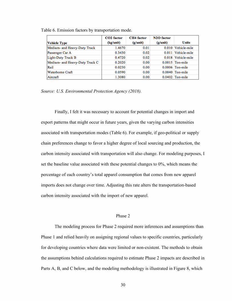
metric tons of carbon dioxide for Phase 1. The emission factors are noted in Table 6
below.
30
Table 6. Emission factors by transportation mode.
Source: U.S. Environmental Protection Agency (2018).
Finally, I felt it was necessary to account for potential changes in import and
export patterns that might occur in future years, given the varying carbon intensities
associated with transportation modes (Table 6). For example, if geo-political or supply
chain preferences change to favor a higher degree of local sourcing and production, the
carbon intensity associated with transportation will also change. For modeling purposes, I
set the baseline value associated with these potential changes to 0%, which means the
percentage of each country’s total apparel consumption that comes from new apparel
imports does not change over time. Adjusting this rate alters the transportation-based
carbon intensity associated with the import of new apparel.
Phase 2
The modeling process for Phase 2 required more inferences and assumptions than
Phase 1 and relied heavily on assigning regional values to specific countries, particularly
for developing countries where data were limited or non-existent. The methods to obtain
the assumptions behind calculations required to estimate Phase 2 impacts are described in
Parts A, B, and C below, and the modeling methodology is illustrated in Figure 8, which

31
excludes dry cleaning, launderettes, and ironing due to the absence of data for those
activities.
Figure 8. Phase 2 modeling process for washing, drying, and detergent impacts.
Part A: Washing
Step 1 required estimating household sizes by country. These data were available
from the UN, EUROSTAT, and the World Bank for all major geographic regions but not
for all countries. As a result, countries with missing household data were assigned the
average household size for their respective region. Additionally, household sizes were not
forecasted by any known data source beyond 2012 so the modeling utilizes a fixed
household size for all subsequent years. That introduces a level of uncertainty for
developed countries where household size is expected to decline and for developing
countries where both increases and decreases in household size are anticipated.

32
The percentage of households with washers (see Ownership rate of washing
machines in Table 7) was obtained from two sources, Pakula and Stamminger (2010) and
Nielsen (2016), and those figures were further modified based on income group
designations from the United Nations. For example, a “low income” country was
automatically given a washing machine ownership rate of 0%, thus undercounting
ownership at the country level. Ownership for “lower middle income” countries was
discounted 50% from the regional ownership rate noted by Pakula and Stamminger
(2010) or Nielsen (2016). Washing machine ownership rates for “upper middle” and
“high income” countries were assigned the ownership rate associated with their region by
Pakula and Stamminger (2010) or Nielsen (2016) as seen in Table 7 below.
Table 7. Washing machine ownership, load sizes, cycles, and energy consumption.
Source: Derived from Pakula and Stamminger (2010).
Step 2 utilized results from Pakula and Stamminger (2010) to assign the estimated
annual energy consumption for washing machines to each country. As noted in Table 7
above, data were not available for all countries and regions. I applied assumptions to
account for missing data in the following ways: for the East Asia & Pacific and South
East Asia regions, energy data associated with China was used, except for Australia,

33
South Korea, and Japan where data were available; Australia’s value was used for New
Zealand; Eastern European data values were applied to countries designated as members
of that region by the UN Statistics Division, specifically Bulgaria, Hungary, Czech
Republic, Ukraine, Moldova, Belarus, Russian Federation, Slovakia, Romania, and
Poland; North America data was applied to all the Americas, likely underestimating the
energy required given that Latin America and South America have higher energy costs
according to the International Energy Agency (IEA); and finally, a global average was
used for the Middle East/North Africa and Sub-Saharan Africa where no data were
available.
Table 8. Region-based kilograms of CO2 per kWh for washing machines.
Source: Derived by the author from IEA (2017) and BP (2019).
The annual energy consumption estimates for washing machines by country were
multiplied by the outcome of Step 1 above. Their product was then multiplied by the
estimated kilograms of CO2 per kilowatt hour. To determine the kilograms of CO2 per

34
kilowatt hour I referred to regional IEA statistics (IEA, 2011; IEA, 2017) and British
Petroleum’s Energy Outlook (BP, 2019), which account for differences in historical and
forecasted fuel types in the energy mix but exclude GHGs associated with the
manufacture of renewables. Finally, IEA data were only available through 2015, so
forecasts were developed for all subsequent years based on region-specific CAGRs
derived from 2005 – 2015 data. The region-based kilograms per kilowatt hour associated
with washing machines is noted in Table 8 above.
Part B: Drying
To account for the absence of dryer ownership data required for Step 3, I based
my assumptions on washing machine ownership rates outlined in Part A for Phase 2 and
on data from the National Resources Defense Council (Horowitz, 2014), the U.S.
Department of Energy (U.S. Department of Energy, 2011) and the IMPRO Textiles
report (Beton et al., 2014). I applied assumptions to countries in the following ways:
Ownership for European countries was based on the average ownership rates available
for the UK and Germany; Eastern European countries were assumed to have a 30%
ownership rate due to the fact that their washing machine ownership rate was lower than
the corresponding rate for other EU countries; and finally, all remaining countries
received an ownership rate estimate of 30% unless their washer ownership was below
50%. In cases where washing machine ownership was below 50%, the dryer ownership
estimate was determined by multiplying the washer ownership by the global dryer
ownership assumption of 30%. For example, if Vietnam had a washer ownership rate of
30%, the dryer ownership rate of 30% was used as a multiplier, resulting in an 8.85%
dryer ownership rate. Each country’s dryer ownership rate was multiplied by the

35
estimated number of households determined in Part A – Step 1 to calculate the total
households with dryers.
For Step 4, I multiplied the output of Step 3 by the estimated annual energy
consumption for dryers, which was assigned by country using the same regionally-based
assumptions noted for washing machines in Part A – Step 2 for Phase 2. The energy
consumption estimates are noted in Table 9 below and were derived from data and
efficiency estimates associated with dryer types (i.e., gas and electric) available from the
NRDC (Horowitz, 2014) and IMPRO Textiles (Beton et al., 2014). The estimated
kilograms of CO2 per kilowatt hour for dryers was calculated using the same
methodology noted above for washing machines in Part A – Step 2 for Phase 2, which
excludes impacts associated with appliance production, repair, and end-of-life (Beton et
al., 2014).
Table 9. Region-based assumptions and estimates for drying machines.
Source: Compiled by the author based on assumptions from Beton et al. (2014), Carbon Footprint. (n.d.), Horowitz (2014), IEA (2017), and the U.S. Department of Energy (2011).

36
Part C: Detergent
Step 5 required assigning country-specific assumptions for washing machine
cycle loads based on regionally available data; these can be found in Table 7 above. I
utilized China’s wash cycle count for all countries where regional data were unavailable.
China’s cycle count was the lowest of all countries and regions, which introduces some
uncertainty in the model by potentially undercounting the number of annual household
wash cycles.
After annual washing machine cycle counts were assigned to countries, I
determined the market share of each detergent type and the corresponding GWP per wash
in kg CO2-eq, which are provided in Table 10 below. Data were not available for all three
types of liquid detergent so I assigned a 75% share of the liquid detergent market to the
widely available double concentrated detergent type (“Liquid Concentrated 2x”). No data
were available to support this assumption beyond what consumers can observe in
domestic and international stores and ecommerce sites. I assigned a 20% share of the
liquid detergent market to the “super concentrated” detergent type and a 5% share to
“ultra-concentrated,” assuming that ultra-concentrated detergents akin to those currently
offered by Method Products and Seventh Generation would gain market share over time
despite “green” detergents accounting for 3% of the household laundry market today
(Packaged Facts, 2015). The sum product of these market share and GWP data were
captured in the “Estimated global kg CO2-eq for detergent” data point seen in Table 7
(0.20 kg CO2-eq per wash), which was multiplied by the wash cycle count and total
households with washers to calculate the overall GWP of detergent use per country.

37
In constructing the final modeling approach for Phase 2, I did not find reliable
energy data associated with dry cleaning and laundromats, nor did I find average
transportation distances between those facilities and households. As a result, my final
model accounts for the use of different detergent types and allows for decade-specific
adjustments to washing and drying machine ownership rates, all of which change the
GWP associated with Phase 2. However, countries that currently have zero washer or
dryer appliance ownership were assumed to continue with a 0% ownership rate in
perpetuity, which may underestimate the GWP associated with Phase 2 for a limited
number of countries. The model does not assume any changes to the number of washing
or drying cycles assigned to each country. Finally, the baseline model assumes the GWP
for detergent is 0.205 kg CO2 per wash, reflecting the anticipated detergent mix and
associated GWP figures noted in Table 10.
Table 10. Estimated market share and GWP per wash by detergent type.
Source: Compiled by author CO2List.org (2012), Packaged Facts (2015), Grand View Research (2017), and K. Gebhardt (personal communication, February 15, 2019).
Phase 3
The GHG emissions calculations for post-consumption activities were based on
the aggregate Apparel Consumption by Country volumes from Phase 1, which were

38
assumed to equal disposal volumes. Country-specific disposal volumes were then
multiplied by emission factors to determine the GWP for all post-consumption activities
except for the export/import of used clothing. The modeling methodology for each of the
post-consumption activities is noted in Parts A through F below.
Part A: Collection and Sorting
When a consumer discards an article of clothing, it gets collected and sorted
before it is landfilled, exported for reuse, incinerated, reused domestically, or recycled.
Collection and sorting therefore incur emissions associated with transportation, building
usage, and the machinery used in the sorting process. Given the disparities associated
with every municipality’s energy mix and infrastructure, I narrowed the scope of my
GHG calculations for collection and sorting by focusing on transportation-specific
emissions.
Transportation-specific emissions must be based on disposal volumes. As noted
above and illustrated in Figure 9 below, the GWP for Step 1 was based on each country’s
disposal volume, which was assumed to equal its consumption volume. Recall that each
country’s consumption volume was determined in Phase 1, specifically Part B – Step 4.
Country-specific disposal volumes were then converted to ton-miles under the
assumption that used clothing traveled an average distance of 50 kilometers (31 miles)
before being exported to another country, landfilled, incinerated, reused, or recycled.
While a 50 kilometer roundtrip distance is sensible as a national average for most
developed countries possessing the infrastructure to handle clothing disposal, it may
understate the average distance in developing countries where disposal infrastructure is
comparatively limited, at least in the short term. Finally, ton-miles were multiplied by the

39
emission factor for “Medium and Heavy-Duty Truck” noted in Table 6 to determine the
GWP for collection and sorting. All Part A emissions were assigned to the country of
consumption.
Figure 9. Phase 3 modeling process for collection and sorting impacts.
Part B: Export/import of Used Clothing
The methodology for calculating the transportation-based carbon emission
impacts associated with the export and import of used clothing is illustrated in Figure 10
below. The methodology was similar to the approach I used for collection and sorting in
Part A above, but differed in two ways: First, emission impacts were assigned to the
importing country rather than the exporting country, and second, maritime distances had
to be determined between major ports due to differences in export and import trade

40
patterns that did not align with the production-based distribution patterns and distances
noted in Table 5.
Figure 10. Phase 3 modeling process for import/export of used clothing.
My first task in quantifying emissions associated with used clothing exports was
to analyze used clothing export and import weights by country. I used the UN Comtrade
database (United Nations, 2019) to compare year-over-year data for 2000 – 2018 and
discovered that the top 29 countries (Table 11) consistently accounted for 90% of used
clothing exports by weight. I then analyzed the destinations of used clothing exports from

41
the top 29 countries, which revealed that each country exported to an average of 91
destinations, although not all export destinations were countries.
Table 11. Top 29 exporters of used clothing for 2015.
Source: compiled by the author based on United Nations (2019).
For example, approximately 1.5% of all used clothing exports are sent to bunkers,
which are defined as ship stores (United Nations, 2011), and regional locations

42
designated as “areas not elsewhere specified,” which typically represent groups of
unknown or intentionally unspecified countries (United Nations, 2017). As a result of this
1.5% discrepancy, my analysis underrepresents the carbon impacts associated with the
export and import of used clothing because it excludes impacts associated with bunkers
and unspecified countries.
To determine the total imports of used apparel by country (Figure 7, Step 2), the
country-specific weights associated with used clothing imports were summarized by
region (Table 12) using data from the UN Comtrade database (United Nations, 2019). I
then used figures noted in Table 12 to derive Table 13, which tabulates the allocation of
used apparel imports each importing region receives from another region.
Table 12. 2015 used apparel import volumes by region in kilograms.
Source: compiled by the author based on United Nations, 2019.

43
As noted in Table 13, this means a country located in South Asia receives 21.4%
of its imported used clothing from a country in North America and another 40.7% from
countries in Europe and Central Asia. I used these data as multipliers to help determine
the used apparel import volume each country receives from a given region. This approach
was valuable since the percentages could be used as proxies for the 163 countries that
account for the remaining 10% of used clothing imports beyond the top 29 countries
noted in Table 11. Fortunately, the risk of data inaccuracy for the remaining 163
countries is relatively low given how little they contribute to used clothing import
volumes.
For forecasting purposes, I needed a methodology to determine each country’s
used apparel import volume and the estimated percent of used apparel imports each
country receives by region beyond the 2015 baseline year. Those volumes were derived
from a four-step process utilizing country-specific used clothing import volumes from the
UN Comtrade database. First, I determined the global volume of used clothing imports as
a percentage of total clothing consumption. That statistic was 5.56% and was based on
the product of (a) the 5-year average of each country’s used clothing import volumes for
2011-2015 and (b) the Total Estimated Apparel Consumption by Country output from
Phase 1, Part B – Step 4. Second, I multiplied the global volume of used clothing imports
as a percentage of total clothing consumption (5.56%) by the forecasted consumption
volume for 2016 – 2050 from Phase 1 to obtain each year’s estimated volume of used
clothing imports. Third, I determined each country’s share of global used clothing
imports by calculating the 5-year average of used clothing imports for each country,
dividing that average by the global volume of used clothing imports, and multiplying that

44
output by each year’s estimated volume of used clothing imports. Finally, the estimated
volume of used apparel each country receives by region was determined by taking the
output of the previous step and multiplying it by data from Table 13. This methodology
introduces potential unavoidable inaccuracies since historical data may not be a good
predictor of future import values. For example, changes in trade patterns could result
from a substantial number of countries in a given region enacting laws that ban used
clothing imports, thus changing the volumes and distances used to determine the GWP
associated with each country’s used clothing imports.
Table 13. Portion of used apparel imports received by geographic region, 2015.
Source: United Nations, 2019.
After obtaining the country-specific and regionally averaged import weights of
used clothing received by the top 29 exporters, I determined the overland and maritime
distances between exporting and importing countries. This effort required 2,661 manual
calculations using data from Sea-Distances.org (2019) for maritime transport and Google
Maps for overland transport. For countries outside the European Union, I assumed
maritime transport was the primary mode of transportation between countries. I tabulated
the number of nautical miles between exporting and importing countries based on the

45
shortest possible port-to-port distance, then used a multiplication factor of 1.15078 to
transform nautical miles from Sea-distances.org into standard miles.
In cases where a country did not have a major maritime port to receive used
apparel imports, I calculated the overland distance between the country’s capital and the
nearest foreign port using Google Maps and assumed trucking was the mode of transport.
Additionally, 600 kilometers of truck-based transport was assigned to all importing
countries to account for the domestic transportation required to deliver used apparel to
consumers. This assumption was based on data from Beton et al. (2014). After obtaining
all country-specific maritime and truck-based transportation figures, I averaged the
distances by region, which are noted in Table 14 below.
Finally, I multiplied the import weights and transportation distances referenced
above to obtain the total ton-miles by transportation mode. Regional data from Tables 13
and 14 were used to calculate ton-miles for the remaining 10% of used clothing exports
that were not accounted for by the top 29 countries. Those totals were then multiplied by
the emission factors noted in Table 6 for maritime and truck-based transport to obtain the
total metric tons of carbon dioxide associated with used apparel imports.

46
Table 14. Average kilometers traveled for the export of used apparel by region.
Source: compiled the author based on United Nations (2019).
Part C: Landfill
The methodology for determining emissions associated with landfill, incineration,
reuse, and recycling was nearly identical as illustrated in Figure 11 below. Each of these
Phase 3 outcomes relied on the previously noted assumption that each year’s disposal
volume equals that year’s consumption volume. Disposal volumes were multiplied by the
regional share of each post-consumption outcome (Table 15), which was then multiplied
by an associated emission factor (Table 16) to determine the corresponding GWP.

47
Figure 11. Phase 3 modeling process. Includes emissions associated with landfill, incineration, reuse and recycling.
The regional share of post-consumption destinations for used clothing was
determined from Beton et al. (2014), Hawley (2006, 2016), J. Hawley (personal
communication, October 8, 2019), and ThredUp (2019). For forecasting purposes, I
developed a CAGR for Reuse and Recycling (8.4%) based on data from ThredUp (2019)
and assigned a discount rate of 60% to the CAGR for years beyond 2023, the final year in
their analysis, to temper the aggressive effects of a near-term trend that has no historical
precedent. I assumed that forecasted reuse and recycling outcomes would steal share
from landfill and incineration, so I adjusted the regional shares for landfill and
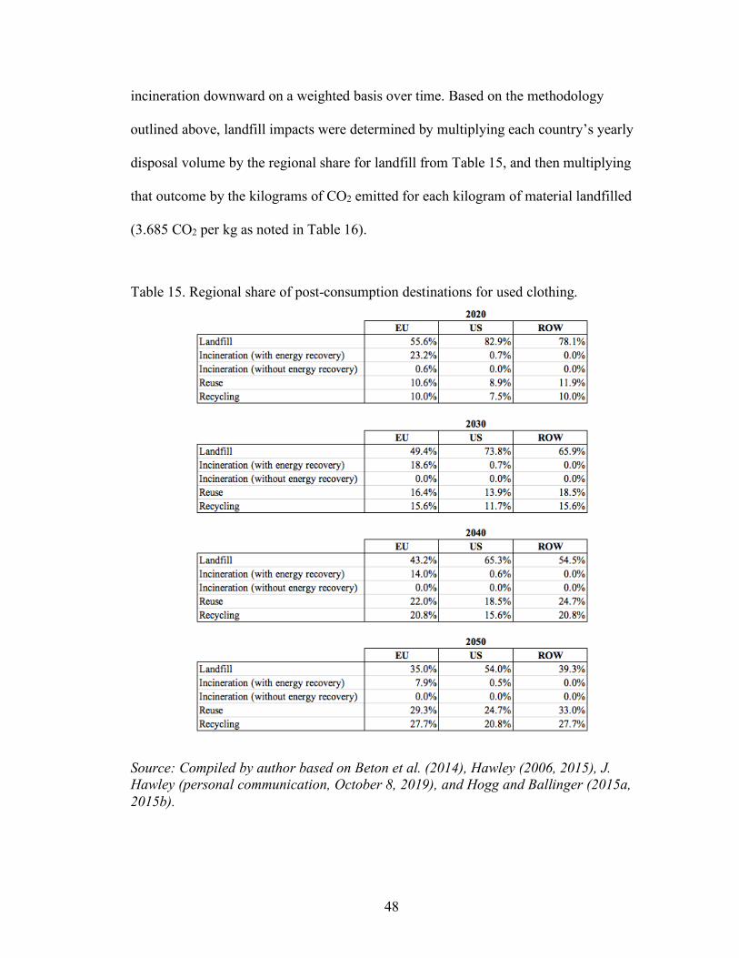
48
incineration downward on a weighted basis over time. Based on the methodology
outlined above, landfill impacts were determined by multiplying each country’s yearly
disposal volume by the regional share for landfill from Table 15, and then multiplying
that outcome by the kilograms of CO2 emitted for each kilogram of material landfilled
(3.685 CO2 per kg as noted in Table 16).
Table 15. Regional share of post-consumption destinations for used clothing.
Source: Compiled by author based on Beton et al. (2014), Hawley (2006, 2015), J. Hawley (personal communication, October 8, 2019), and Hogg and Ballinger (2015a, 2015b).

49
Table 16. Emission factors for landfill, incineration, reuse, and recycling.
Source: compiled by the author based on Planet Aid (n.d.), Beton et al. (2014), the Ecoinvent 2.0 database (as cited in Beton et al., 2014), and Hogg and Ballinger (2015a, 2015b).
Part D: Incineration
Incineration volumes were considered with and without energy recovery as a
percentage of each country’s disposal volume based on Table 15 above, and involved an
additional calculation that was not necessary for Parts C, E, and F to account for the
impacts of synthetic and non-plant fibers in the global fiber mix (Table 2). More
specifically, I assumed that CO2 from the incineration of natural fibers was compensated
by the CO2 absorbed during plant growth (Beton et al., 2014) and assigned an emission
factor of +/-0.00015 metric tons of CO2 per kilogram incinerated for synthetics (Beton et
al., 2014). Thus, incineration with energy recovery was calculated by taking the
corresponding incineration volume, multiplying it by the synthetic and non-plant
percentage of the fiber mix from Table 2, and multiplying that output by the emission
factor noted in Table 16 (-0.00015 MT CO2 per kg incinerated). This resulted in the
recovery of emissions associated with the synthetic and non-plant portion of the
incineration volume. Conversely, the incineration volume without energy recovery
resulted in an emissions impact due to the generation of 0.00015 MT CO2 per kg
incinerated as noted in Table 16.

50
Part E: Reuse
The reuse percentages in Table 15 were based on a report from ThredUp (2019)
that predicted a doubling of the secondhand market in 5 years, from $24 billion in 2018
to $51 billion in 2023. As noted above, I assigned a discount rate of 60% to the reuse
percentages for 2024 through 2050 to reflect the fact that reuse will likely continue
growing as raw material inputs become more limited (Eder-Hansen et al., 2017), but will
not retain the same level of accelerated growth that is expected in the near-term. This
assumption is fueled by the fact that current reuse volumes – which are a combination of
thrift, donations, and resale – are very low in all countries and will primarily accelerate in
the resale category (ThredUp, 2019) as enhanced logistics capabilities and digital
platforms enable access to inventory via three business models: rental services from
companies such as Rent the Runway and retailers like Ann Taylor and Bloomingdale’s,
peer-to-peer selling via sites like The RealReal and Grailed, and peer-to-peer rental with
entities like ByRotation and YCloset. While it is too early to estimate when adoption
rates for these services will plateau, I felt that a mid-range discount rate would both
temper long-term growth rates and acknowledge the technology-driven growth of resale
that could continue over time as population and resource constraints grow in tandem.
After I calculated the reuse percentages over time for Table 15, I multiplied them
by each country’s disposal volume. I took the resulting reuse volume and multiplied it by
the emission factor of -24.3 kg CO2 per metric ton (Hogg & Ballinger, 2015b). to obtain
the avoided emissions associated with reuse. Avoided emissions from reuse are assumed
to come from the avoided production of new garments.

51
Part F: Recycling
The methodology for determining recycling volumes was similar to the approach
used for Reuse in Part E, leveraging the aforementioned 8.4% CAGR and discount rate
for years 2024 – 2050 to obtain the values appearing in Table 15. The rates in Table 15
were then multiplied by each country’s disposal volume and the emission factor of -4.95
metric tons of CO2 per metric ton recycled (Hogg & Ballinger, 2015b) noted in Table 16
to obtain the avoided emissions associated with recycling.
Carbon Budget
The IPCC defines the carbon budget as the “Estimated cumulative net global
anthropogenic CO2 emissions from the pre-industrial period to the time that
anthropogenic CO2 emissions reach net zero that would result, at some probability, in
limiting global warming to a given level, accounting for the impact of other
anthropogenic emissions” (Masson-Delmotte et al., 2018). For the purposes of my
analysis, I looked at both 1.5°C and 2°C global warming levels – often referred to as the
1.5°C and 2°C pathways – and only considered carbon budget scenarios associated with a
66% probability of staying below 1.5°C and 2°C. As indicated in Table 17, the IPCC
made significant revisions to the carbon budget when they published the SR15 special
report in 2018, expanding the budget from figures found in their AR5 report from 2014.
The difference primarily stems from the use of observations in SR15 rather than values
from earth system models (ESMs) to estimate emissions inputs for climate modeling,
which eliminates historical problems associated with ESMs underestimating past
emissions and overestimating future temperatures (Hausfather, 2018).
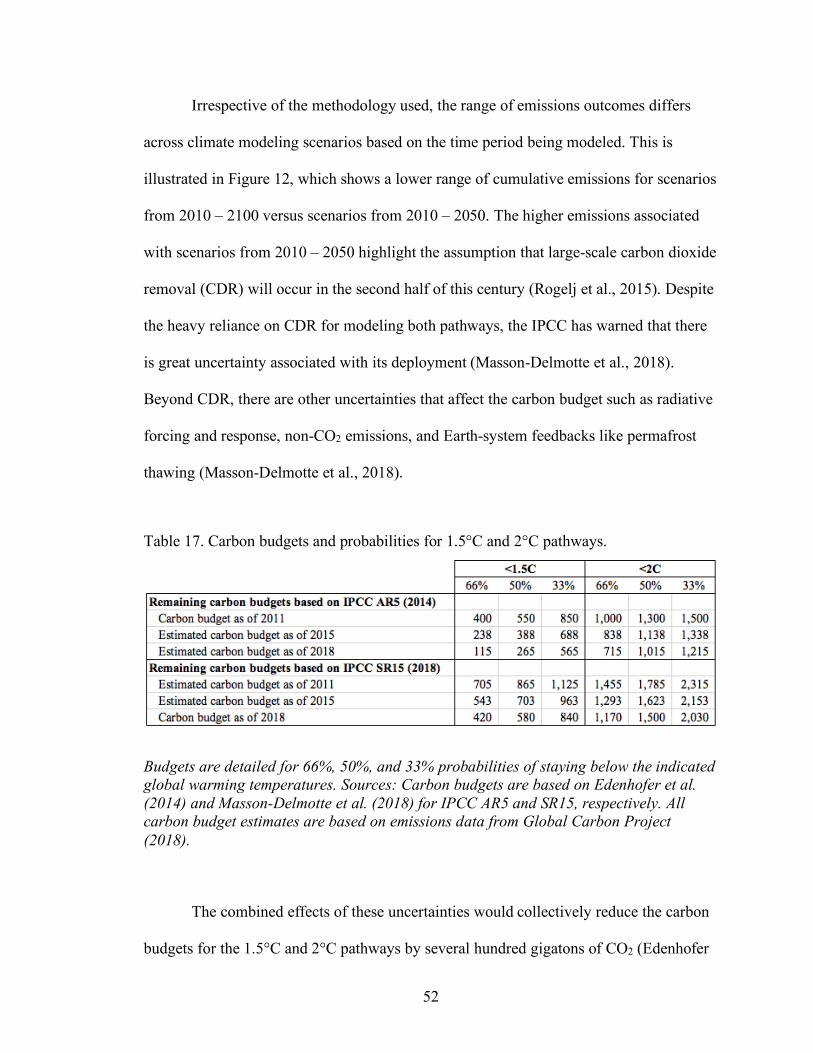
52
Irrespective of the methodology used, the range of emissions outcomes differs
across climate modeling scenarios based on the time period being modeled. This is
illustrated in Figure 12, which shows a lower range of cumulative emissions for scenarios
from 2010 – 2100 versus scenarios from 2010 – 2050. The higher emissions associated
with scenarios from 2010 – 2050 highlight the assumption that large-scale carbon dioxide
removal (CDR) will occur in the second half of this century (Rogelj et al., 2015). Despite
the heavy reliance on CDR for modeling both pathways, the IPCC has warned that there
is great uncertainty associated with its deployment (Masson-Delmotte et al., 2018).
Beyond CDR, there are other uncertainties that affect the carbon budget such as radiative
forcing and response, non-CO2 emissions, and Earth-system feedbacks like permafrost
thawing (Masson-Delmotte et al., 2018).
Table 17. Carbon budgets and probabilities for 1.5°C and 2°C pathways.
Budgets are detailed for 66%, 50%, and 33% probabilities of staying below the indicated global warming temperatures. Sources: Carbon budgets are based on Edenhofer et al. (2014) and Masson-Delmotte et al. (2018) for IPCC AR5 and SR15, respectively. All carbon budget estimates are based on emissions data from Global Carbon Project (2018).
The combined effects of these uncertainties would collectively reduce the carbon
budgets for the 1.5°C and 2°C pathways by several hundred gigatons of CO2 (Edenhofer

53
et al., 2014; Masson-Delmotte et al., 2018). However, due to the uncertainty associated
with these effects, the IPCC has excluded them from the carbon budget of both pathways,
thus making the budgets applicable to the mid-century (Masson-Delmotte et al., 2018)
and reducing the apparel industry’s contribution to the remaining carbon budget for the
1.5°C and 2°C pathways in my analysis.
Figure 12. Cumulative carbon emissions by 2050 and 2100.
The three scenario sets are: scenarios that will return warming to 1.5°C with a >50% chance, scenarios that will keep global warming below 2°C with a >66% chance, and scenarios that have a 50-66% chance of keeping warming below 2°C relative to pre-industrial levels. Source: Rogelj et al. (2015).
Quantifying the annual GHG emissions associated with the apparel industry
required aggregating emissions for Phases 1, 2, and 3 and dividing the sum by the total

54
global emissions for the associated year. I completed this calculation for my baseline
year, 2015, and developed forecasts out to 2050 to calculate the projected contribution of
the apparel industry on the remaining carbon budget. Determining the remaining carbon
budget required analyzing no fewer than a dozen research papers on the topic, most of
which were composed by contributors to the IPCC’s SR15 report prior to its release in
October 2018. That research helped validate data points for annual global emissions,
enabling me to estimate carbon budgets for years included in my analysis that were not
specifically referred to in the most recent IPCC’s SR15 report. For example, my analysis
primarily focuses on the carbon budgets associated with 2015 – 2050, but the IPCC did
not provide pre-2018 carbon budgets in SR15 for the 1.5°C and 2°C pathways. As
illustrated in Table 18, the remaining carbon budgets associated with the 1.5°C and 2°C
pathways for 2018 are 420 GtCO2 and 1,170 GtCO2, respectively.
To estimate the remaining carbon budget for 2015 that corresponds with the
IPCC’s SR15 report, I pulled the annual emissions data from Global Carbon Project
(2018) noted in Table 19 below for 2015 - 2017, transformed the data from gigatons of
carbon (GtC) to gigatons of carbon dioxide (GtCO2) by multiplying GtC figures by
3.664, and added the sum to the IPCC’s aforementioned 2018 carbon budgets for both
pathways. All estimated carbon budgets noted in Table 18 were derived in this manner
and utilized emissions associated with fossil fuels, industry, and land-use change (Table
19) because the associated totals for 2011 – 2017 noted by Global Carbon Project (285
GtCO2) closely aligned with the emissions sum for the same period noted in the IPCC’s
SR15 report (290 GtCO2) (Masson-Delmotte et al., 2018, p. 113).

55
Table 18. Remaining carbon budgets and estimates by year.
Estimates are associated with a 66% probability of staying below 1.5°C and 2°C for IPCC AR5 and IPCC SR15, a 66% probability of staying below 2°C for IEA/IRENA, and 80% probability of staying below 2°C for Potsdam Climate Institute estimates. GtCO2 associated with Earth-system feedbacks by 2100 subtract 100 GtCO2 associated with permafrost thawing. Sources: Edenhofer et al., 2014, Leaton (2011), Masson-Delmotte et al. (2018), and OECD/IEA and IRENA (2017).
Table 19. Annual emissions in GtC and associated GtCO2 equivalents.
Source: Global Carbon Project (2018).

56
Finally, the carbon budgets I primarily focus on in my analysis were derived from
the IPCC’s SR15 report, which offered the most recent assessment and scientific
consensus on carbon budgets. As noted above, the carbon budgets for the 1.5°C and 2°C
pathways noted in SR15 are significantly higher than carbon budgets that were previously
published by the IPCC and other organizations such as the Potsdam Climate Institute. For
comparative purposes, I have illustrated those differences in Table 18 and have included
an emissions adjustment to account for 100 GtCO2 that could arise from Earth system
feedbacks this century (Masson-Delmotte et al., 2018), specifically permafrost thawing.
All of the carbon budgets noted in Table 18 allow for global mean temperatures (GMT)
to “overshoot” their associated temperature limit of 1.5°C or 2°C. As Rogelj, Schleussner
and Hare (2017) stated, if we do not allow the annual GMT to exceed the temperature
limit more than once every 20 years, the associated carbon budgets would be reduced by
more than 400 GtCO2, but if overshoot is entirely disallowed, then the carbon budget
associated with the 1.5°C pathway has already been depleted. Other research has
cautioned that temperature limits are not comprehensive enough to limit risks from
anthropogenic emissions, resulting in higher allowable emissions (Steinacher, Joos, &
Stocker, 2013) and thus larger carbon budgets. This is illustrated in Figure 13 below
which shows significantly lower targets than those noted in Table 18 and underscores the
fact that my use of IPCC SR15-based carbon budgets potentially understates the
contribution of the apparel industry on the remaining carbon budget for the 1.5°C and
2°C pathways.

57
Figure 13. Allowable fossil-fuel carbon emissions.
“Allowable fossil fuel carbon emissions for a likely (66%) and very likely (90%) chance of staying below 1.5°C and 2°C temperature targets in the twenty-first century. Blue symbols are temperature-only targets, red symbols are for multiple targets, and green symbols illustrate multiple targets when allowing for overshoot.” Source: Steinacher, Joos, and Stocker (2013).
Independent Variables
I identified 46 independent variables (Tables 20, 21, and 23) that were necessary
to determine global and country-specific emissions associated with the apparel industry.
The methods used to obtain data for these variables are described below under headings
for each life cycle phase.

58
Phase 1: Production
A total of 13 independent variables were associated with Phase 1 to account for
the steps illustrated in Figures 2 and 3. These are detailed in Table 20 below.
Table 20. Independent variables for Phase 1.
Source: Compiled by the author.
• Population: I obtained population data from the United Nations Population Division
and augmented individual country data with regional designations from the World
Bank (e.g., East Asia & Pacific, Europe & Central Asia, Latin America & the
Caribbean, Middle East & North Africa, North America, South Asia, and Sub-
Saharan Africa) (World Bank, 2019), economic growth potential designations from
the World Bank (e.g., pre-demographic dividend, early demographic dividend, late
demographic dividend, and post-demographic dividend) (World Bank, 2019), and
IMF designations to classify countries as developed or developing (International

59
Monetary Fund, 2018). These data served to enrich the data set to segment the
outcomes of my analysis.
• Per capita apparel consumption by country: Per capita apparel consumption data were
available for select countries from the United Nations Statistics Division (2019), the
OECD (2019), and the World Bank (2018), but were regionally-based for countries
where per capita consumption data were absent. These data were utilized to validate
that global apparel consumption was aligned with global textile production used for
apparel and were used in my scenario modeling to estimate future consumption.
• Global warming potential (GWP) by fiber type: The GWP of each fiber is expressed
in kilograms, metric tons, or gigatons of CO2 equivalent (kg CO2-eq) and those values
represent the most important and influential measure of impact in my analysis. I
determined the cradle-to-gate GWP for each fiber by averaging midpoint values
available from the Higg MSI (Sustainable Apparel Coalition, 2018), IMPRO (Beton
et al., 2014), and the Ecoinvent 2.0 database, which cover impacts associated with
raw material production and processing, pretreatment, spinning, fabric creation,
finishing, printing, and dyeing, but do not include garment assembly. These values
can be found in Table 3, and in some cases represent a categorical average. For
example, the GWP for man-made cellulosics (MMCs) is comprised of midpoint
values that were averaged across sources for viscose, acetate, lyocell, and modal,
among others. For bast fibers such as jute, flax, and kenaf, I had limited data to work
from so I utilized midpoint values associated with other bast fibers and assigned them
to the “Other plant-based” fiber category in my analysis, separate from cotton.

60
• Global fiber production volume by fiber type: These data were readily available from
sources such as Textile Exchange (2018), PCI WoodMackenzie (Bruna, 2016), and
Textile World (2015). I analyzed these data for all available years between 1990 and
2017 and utilized them to validate my calculations for global apparel consumption
and country-specific apparel consumption for the aforementioned years.
• Fiber allocation in global fiber mix: Each fiber’s allocation in the global fiber mix
was calculated by dividing its production volume by the total production volume of
all fibers. The resulting percentages were used as multipliers to determine each fiber’s
historical and forecasted GWP given the large differences in GWP by fiber type.
• Fabric loss from textile manufacturing: Apparel manufacturing produces textile scrap,
which varies as a percentage of production based on the type of apparel being
produced. For example, slips and petticoats generate a high percentage of scrap (18%)
whereas scarves and shawls are comparatively lower (4%) (Beton et al., 2014). I
analyzed manufacturing losses associated with all apparel categories but could not
find production volumes by product type to develop a weighted average for fabric
loss. As a result, I averaged the fabric loss percentages across 24 apparel product
categories to generate a global average of 13.4%. I utilized this average to determine
the volume of manufacturing scrap associated with apparel consumption and assumed
the same fiber mix and GWP by fiber type to calculate emissions associated with
manufacturing scrap.
• Portion of manufacturing scrap recycled: Manufacturing scrap is recycled, landfilled,
and incinerated at different rates than consumer textiles. I was only able to find a
single source for this data point, the IMPRO report (Beton et al., 2014), which noted

61
that 50% of manufacturing scrap was recycled. In my discussions with apparel
makers in the United States, I found this figure to be relatively accurate with most
firms recycling 50% to 100% of their scrap while others recycled none. Much of the
discrepancy I ran into was based on economics. For example, firms that were
recycling were either paying $0.08 to $0.14 cents per pound to recycle their scrap or
were able to offload it for free to a recycler after trucking it themselves or paying for
delivery. Companies that were not recycling were quick to note that they were no
longer able to sell their scrap to a recycler and found that landfilling was less
expensive.
• Portion of manufacturing scrap landfilled: This statistic was derived from the IMPRO
report (Beton et al., 2014), which indicated that 34.8% of all manufacturing scrap
reaches a landfill. The calculated volumes for landfilled manufacturing scrap were
multiplied by the corresponding emission factor noted in Table 16.
• Portion of manufacturing scrap incinerated with energy recovery: Similar to the
aforementioned recycling and landfill volumes, I obtained the 14.8% data point for
incineration with energy recovery from the IMPRO report (Beton et al., 2014). I then
multiplied the volume by the associated emission factor in Table 16.
• Portion of manufacturing scrap incinerated without energy recovery: According to the
IMPRO report (Beton et al., 2014), very little manufacturing scrap is incinerated
without energy recovery (0.4%). Like the other metrics associated with
manufacturing scrap above, volumes for this statistic were multiplied by the related
emission factor in Table 16.

62
• Share of new clothing imports by region: I analyzed clothing-specific import and
export data from the World Bank to understand weight-based volumes that could be
used to calculate transportation-based emissions. Unfortunately, those country-
specific data did not indicate which countries or regions apparel was being imported
from. As a result, I relied on regional import percentages from IMPRO (Beton et al.,
2014) associated with two garment categories, woven and knitted, and averaged them
to create an adjusted average of new clothing imports by region. I then utilized those
adjusted regional averages as multipliers for all countries to determine which portion
of a given region’s imports came from another region. Since no data were available
for sub-Saharan Africa, I calculated the global average for garment imports by region
and applied it to sub-Saharan Africa. The final share of apparel imports by region can
be seen in Table 4.
• Average distance for new clothing imports by transportation mode: The majority of
apparel consumption occurs in North America, Europe, and China, whereas the
majority of production occurs in India, Pakistan, Bangladesh, Vietnam, Thailand,
China, and India (Kirchain et al. (2015). I assumed transportation distances between
regions of production and consumption would not change significantly in the coming
decades. Based on that assumption, I assigned regionally-based transportation
distances for maritime and air transport (Table 5) found in the IMPRO report (Beton
et al., 2014) to each country and assumed a standardized trucking distance of 600
kilometers for imports of new apparel.
The distances I applied in my emissions calculations for the transportation of
new apparel were strictly associated with finished goods and therefore understate the

63
associated GWP. For fibers, I was unable to find reliable transportation data to gauge
distances between common production activities like raw material extraction,
spinning, dyeing, and assembly. What is more, I could not find data associated with
apparel components such as buttons and zippers, which are produced and transported
to and within the aforementioned countries of production.
• Transportation emission factor by vehicle type: The U.S. Environmental Protection
Agency (EPA) provides emission factors for trucks, passenger cars, waterborne craft,
and aircraft (Table 6), which were used throughout my analysis to calculate CO2-
based emissions for the transportation of new and used apparel. The EPA also
provides emission factors for methane and nitrous oxide, which were not factored into
my carbon-focused calculations. Had I factored methane and nitrous oxide into my
calculations, my transportation emissions would increase approximately 6%, which
would have a negligible effect on the overall GWP of apparel.
Phase 2: Consumption
A total of 17 independent variables were associated with Phase 2 to account for
the steps illustrated in Figure 8. These are detailed in Table 21 below.
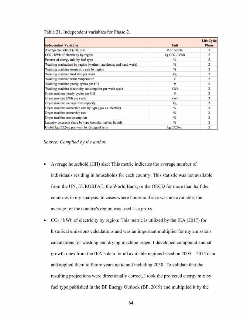
64
Table 21. Independent variables for Phase 2.
Source: Compiled by the author.
• Average household (HH) size: This metric indicates the average number of
individuals residing in households for each country. This statistic was not available
from the UN, EUROSTAT, the World Bank, or the OECD for more than half the
countries in my analysis. In cases where household size was not available, the
average for the country's region was used as a proxy.
• CO2 / kWh of electricity by region: This metric is utilized by the IEA (2017) for
historical emissions calculations and was an important multiplier for my emissions
calculations for washing and drying machine usage. I developed compound annual
growth rates from the IEA’s data for all available regions based on 2005 – 2015 data
and applied them to future years up to and including 2050. To validate that the
resulting projections were directionally correct, I took the projected energy mix by
fuel type published in the BP Energy Outlook (BP, 2019) and multiplied it by the

65
kilograms of CO2 per kWh by fuel type. Multiple sources contained different values
for the CO2 per kWh by fuel type, such as Jancovici (2003), Quaschning (2015), and
CO2list.org (2012), so I ran calculations for all available values and developed high
and low global estimates to compare against my CAGR-based projections by region
(Table 8).
• Percent of energy mix by fuel type: The BP Energy Outlook (BP, 2019) provides a
forecast for energy consumption by source, specifically for oil, gas, coal, nuclear,
hydro, and renewables. I used those data to determine the portion of the future energy
mix each energy source would account for and used the resulting percentages as a
multiplier as described in the metric above, CO2 per kWh of electricity by region.
• Washing mechanism by region (washer, launderette, and hand wash): This refers to
the washing method employed in each global region, as detailed in Table 7 and in
Table 21 below. The combined data from these tables were used to assign a washing
machine ownership rate for countries in each region. Data were surprisingly limited
on washing habits beyond Europe, North America, and major countries within other
regions mentioned in Table 7 (e.g., China, Japan, Australia). I was unable to obtain
data on launderettes to determine what the associated carbon impacts might be. As a
result, my analysis excludes impacts associated with launderettes. As Table 22
suggests, this exclusion disproportionately understates washing-related impacts in
Africa and the Middle East where nearly one third of the population uses launderettes.

66
Table 22. Washing mechanism by region.
Source: Compiled by the author based on Nielsen (2016).
The limited nature of data availability for this metric stems from the fact that
there are few studies on regional or country-based washing and drying habits. The
majority of my metrics associated with washing and drying habits are based on
research by Pakula and Stamminger (2010) and select statistics published by Nielsen
(2016) and the National Resources Defense Council (Horowitz, 2014).
• Washing machine ownership rate by region: Ownership rates for washing machines
were assigned to individual countries based on the geographic region they belong to
as seen in Table 7 and Table 22. I made additional ownership assumptions based on a
country’s income group designation. For example, a "low income" country was
automatically given 0% washer ownership, thus undercounting washer ownership at
the country level whereas ownership for "lower middle income" countries were
discounted 50% from the regional ownership rate. Similarly, ownership for "upper
middle" and "upper income" countries were assigned the ownership rate associated
with their region.
• Washing machine load size per wash: This refers to the number of kilograms
associated with each wash load and was assigned to countries based on their

67
geographic region as shown in Table 7. Data for South America was missing from the
literature so I employed values associated with North America, which were lower
than the global average. These figures determined the electricity consumption per
wash cycle.
• Washing machine wash temperature: Wash temperatures have a major effect on
energy consumption associated with machine washing. On average, countries that
wash in cold water consume 30% of the energy per wash that is typically expended
by countries washing in warm or hot water.
• Washing machine yearly cycles per HH: The number of wash cycles per household
varied widely across the globe. As indicated in Table 7, this factor was not an
important determinant of washing-related emissions on its own, but had to be
considered alongside other metrics such as wash temperature and load size. For
example, the high number of washing cycles in Japan coupled with cold wash
temperatures and average load sizes does not result in high energy consumption. In
comparison, Western Europe’s large load sizes, hot wash temperatures, and below
average wash cycles results in energy consumption three times higher than Japan’s.
• Washing machine electricity consumption per wash cycle: This refers to the kilowatt
hours required per wash cycle. I utilized baseline numbers available from Pakula and
Stamminger (2010), which appear in Table 7 and were assigned to countries on the
same basis as washing machine ownership.
• Dryer machine yearly cycles per HH: No data were available to determine the annual
number of dryer cycles per household. To account for this, I utilized the equivalent
metric for washing machines noted above and discounted the total by 50%. In other

68
words, I assumed that 50% of wash loads per household would be tumble dried in a
vented dryer before accounting for dryer machine ownership rates.
• Dryer machine kWh per cycle: I extrapolated this metric by multiplying the estimated
load size per wash – which was assumed to equal the load size for drying – by the
dryer-specific kilowatt hours per kilogram of laundry (0.59 kWh per kg). I obtained
the kilowatt hours per kilogram statistic from Beton et al. (2014), which was
associated with efficient gas and heat pump-powered tumble dryers and may
therefore underestimate impacts associated with dryer-related energy use.
• Dryer machine average load capacity: I assumed dryer machine load capacities were
equal to washing machine load capacities. No academic data were available to verify
this assumption, but searches conducted on international ecommerce sites anecdotally
confirmed that dryer capacities were as large or larger than washer capacities.
• Dryer machine ownership rate: Dryer ownership primarily depends on household
income and climate conditions (Beton et al., 2014) and therefore varies considerably
around the world as seen in Table 9. As mentioned in Phase 2 – Part B above, I
employed a conservative methodology to assign dryer ownership rates by country,
discounting many countries I did not have data for well below the baseline ownership
rate assumption of 35% for households with washers.
• Dryer machine type (gas vs. electric): Historically, gas dryers have been more energy
efficient than their electric counterparts, but ownership rates for gas versus electric
among dryer owners were not found in the literature beyond data from Horowitz
(2014). In the absence of a better alternative, I assumed a 50% ownership rate for
both gas and electric dryers among dryer owners in all countries except the US where

69
inefficient electric dryers are widespread and rarely connected to a heat pump to
improve energy efficiency (Horowitz, 2014).
• Dryer machine use assumption: Dryer ownership rates were not sufficient on their
own to determine usage frequency among dryer owners, so I applied a 50% usage rate
to households with dryers based on research cited by Beton et al. (2014). By using
this assumption, my results may overstate the GWP associated with dryer usage in
warmer and wealthier countries while understating it in countries with colder
climates. The degree to which these effects might cancel each other out is unknown.
• Laundry detergent share by type (powder, tablet, liquid): Powder detergents have
been widely available for decades, but highly concentrated liquid and tablet-based
detergents are relatively new entrants to the market, particularly ultra-concentrated
detergents such as those offered by Method Products and Seventh Generation.
Unfortunately, market share data were not available for the different concentrations of
liquid detergent, so I analyzed the products that were available in several US grocery
stores, on global ecommerce sites, and on detergent manufacturer websites to
understand the number of SKUs being offered by liquid detergent type. I then
researched the market for green household cleaning products and found it accounted
for only 3% of the total market. Based on my observations and directionally
informative market data, I assumed the following for liquid detergents: double
concentrated formulations (2x) comprised 75% of the liquid detergent market (19.5%
of the total detergent market), super concentrated formulations (4x) represented 20%
of the liquid detergent market (5.2% of the total market), and ultra-concentrated
formulations (8x) made up 5% of all liquid detergents (1.3% of the total detergent

70
market). These assumptions are relatively aggressive for super and ultra-concentrated
detergents, which qualify as “green” products, but this approach was used to account
for the fact that historical data may not represent future conditions as manufacturers
continue to focus on limiting their carbon footprints and consumers become more
educated about the impacts of their laundry habits.
• Global kg CO2-eq per wash by detergent type: Several life cycle analyses have been
conducted on detergents to determine the kilograms of carbon dioxide required per
wash. I took the product of those data and the market share associated with each
detergent type to determine the global kilograms of carbon dioxide associated with
laundry detergent (Table 10).
Phase 3: Post-consumption
A total of 16 independent variables were associated with Phase 3 to account for
the steps illustrated in Figures 9, 10, and 11. These are detailed in Table 23 below.

71
Table 23. Independent variables for Phase 3.
Source: Compiled by the author.
• Export weight of used clothes: These data were available from the UN Comtrade
database and represent the more accurate basis for transportation-specific emission
calculations than import weights assigned to countries. As previously noted, this is
due to the fact that roughly 1.5% of all used clothing is shipped to bunkers and
unspecified countries; my analysis excludes these emissions and therefore understates
the GWP associated with used clothing exports.
• Import weight of used clothes: This metric was used to calculate the transportation
emissions associated with used clothing imports. I was able to obtain import weights
for all used clothing destinations but was not able to obtain transportation distances
for bunkers and unspecified countries to complete emission calculations for global
apparel. As a result, this metric in my analysis is strictly associated with specified
countries to which the associated transportation emissions could be assigned.

72
• Distances between major ports for used clothing exports (by country): These metrics
(Table 14) represent the shortest average distance between major ports for countries
involved in the export and import of used clothing in each region. I found that
distances were meaningfully different between developing and developed countries in
the same region, thus improving the accuracy of transportation emission calculations
versus using single distance for each region.
• Avoided emissions impact of recycling used clothing: Recycling used clothing helps
avoid emissions that would otherwise be generated by the production of new apparel.
Studies have shown that the avoided emissions vary by garment type. For example,
poor quality garments avoid fewer emissions (-1.75 MT CO2-eq per metric ton
recycled) than standard garments (-4.29 to -7.87 MT CO2-eq per metric ton recycled)
(Hogg & Ballinger, 2015b, pg. 7). I averaged the avoided emissions statistics I found
in the literature and utilized -4.95 MT CO2-eq per metric ton recycled to calculate
avoided emissions associated with recycling used clothing.
• Avoided emissions impact of reusing used clothing: This refers to the avoided
emissions associated with the reuse of used clothing, which was calculated by Hogg
and Ballinger (2015b) to be -24.3 kg CO2 per metric ton.
• Emissions impact of landfilling used clothes: This metric represents the carbon
dioxide emissions generated by landfilling textiles, which is 3.69 kg CO2 per
kilogram landfilled (derived from CO2list.org, 2012). Unfortunately, I was unable to
find publicly available emissions factors by fiber type for landfilled textiles and
therefore could not determine the degree to which landfill impacts would vary over
time as the global fiber mix changes. In theory, CO2 emissions per kilogram of

73
landfilled textiles should rise over time as synthetics increase as a percentage of the
fiber mix. The future availability of such data may increase the accuracy of emissions
calculations associated with landfilling apparel.
• Emissions impact of incinerating used clothing (with energy recovery): Incineration
can recover heat and electricity that would otherwise generate CO2 emissions from
sources like coal and natural gas. For the purposes of my analysis, I assumed an
environmental benefit of 0.000151 metric tons of CO2 per kilogram of synthetic-
based apparel incinerated with energy recovery. I derived that metric by using three
assumptions provided by Beton et al. (2014): first, the CO2 emissions associated with
natural fibers would be canceled out from plant growth; second, 1.36 megajoules of
heat and 2.86 megajoules of electricity are recovered per kilogram of apparel
incinerated; and third, the heat and electricity being avoided would otherwise be
obtained from the use of natural gas and the current electricity mix of the European
Union. I then determined the emissions associated with each fuel type using an online
emission calculator (Energy Efficiency & Conservation Authority, 2019) and
validated those results with data from the U.S. Energy Information Administration
(EIA) (U.S. Energy Information Administration, 2019). My EIA-based calculations
yielded a lower environmental benefit of 0.000143 metric tons of CO2 per kilogram
of synthetic-based apparel incinerated with energy recovery. I chose to use the higher
of the two estimates as my metric to account for future efficiency gains in the event
that the EIA-based calculation more accurately represents current recovery potential.
• Emissions impact of incinerating used clothing (without energy recovery): None of
my data sources indicated that incineration without energy recovery accounted for

74
more than 1% of all end-of-life destinations. Given how little it is currently utilized as
an end-of-life destination for apparel, my model assumes that incineration without
energy recovery will be discontinued entirely by 2030. Nevertheless, I accounted for
the associated pre-2030 environmental loss by using the same multiplier mentioned
above for incineration with energy recovery (0.000151 metric tons of CO2 per kg of
apparel incinerated).
• Used clothing landfill rate: This metric indicates the percentage of used apparel being
sent to landfill. Historical data from the US and EU were readily available from the
literature, most notably from Hawley (2006, 2015) as well as select sources such as
Beton et al. (2014) and the U.S. EPA which were used to validate historical disposal
rates for forecasting purposes. Reliable data associated with countries beyond the EU
and the United States were virtually non-existent, so I conferred with industry experts
to obtain data for modeling assumptions associated with all other countries,
collectively referred to as “rest of world” (ROW) in my model. Overall, the landfill
rate declines over time in my model for all countries relative to forecasted upticks in
reuse and recycling rates.
• Used clothing incineration (with energy recovery) rate: This indicates the rate at
which used clothing is incinerated with energy recovery as an end-of-life destination
in the US, EU, and ROW, whereby all countries not in the US or EU have been
assigned rates associated with ROW estimates.
• Used clothing incineration (without energy recovery) rate: This metric is related to
the metric above but is associated with incineration that does not involve energy
recovery and therefore results in higher emissions. As with other end-of-life

75
destinations, the metric was applied to countries based on US, EU, and ROW
designations due to limited data availability.
• Used clothing reuse rate: This metric refers to the rate at which clothing is reused,
primarily via secondhand apparel markets. I based my reuse growth assumptions on
the ThredUp 2019 report, which anticipates a doubling of the secondhand apparel
market over the next 5 years, making reuse the highest growth category among all
end-of-life apparel destinations in my model (ThredUp, 2019). In the absence country
and regional data beyond the US and EU, I applied the same rate of forecasted growth
to all countries.
• Used clothing recycling rate: This refers to the percentage of apparel that gets
recycled, which is predominantly associated with downcycling. Again, data were
limited beyond the aforementioned sources for other end-of-life apparel destinations,
so my growth assumptions were based on two trends: the rise of innovative fiber
recycling technology from firms such as BlockTexx and Evernu, and the anticipated
increase in popularity for reuse, which I assumed would coincide with recycling as a
related sensibility among consumers and increasingly conscious apparel brands.
• Trucking distance for imported clothing: This metric captures the 600 kilometer
distance that was assumed for trucking large volumes of imported apparel between
pick-up locations, maritime ports, storage warehouses, and other facilities in the
country of origin and the destination country. The impacts associated with trucking
were applied to the importing country.
• Domestic travel distance to end-of-life destinations: This metric is a measure of the
distance associated with the collection and sorting of used apparel. I utilized 50

76
kilometers as a distance assumption for all countries and multiplied it against the total
weight of disposed apparel. My model assumes that all disposed apparel is collected
and sorted, and that collection and sorting is required for landfilling, incineration,
reuse, and recycling.
• Carbon budget: The carbon budget is a figure typically expressed in metric tons or
gigatons, indicating the cumulative amount of carbon dioxide permitted to stay within
a specified temperature threshold (Sussams, 2018). Carbon budget figures are used in
my analysis as a means of understanding the apparel industry’s projected contribution
to the remaining carbon budgets for the 1.5°C and 2°C pathways. Such comparisons
are meant to illustrate the degree to which apparel could be contributing to the
consequences of climate change. However, these comparisons are not meant to
contort the data, as nearly every industry’s projected contribution to a remaining
carbon budget will be larger than that industry’s share of current global emissions.
Derived Variables
Values for 22 variables derived from independent variables are noted below based
on the phase they applied to in my analysis. In some cases, metrics associated with
derived variables applied to multiple phases; these appear under the “Multiple phases”
heading following headings for Phases 1, 2, and 3 below.

77
Table 24. Derived variables for Phases 1, 2 and 3.
Source: Compiled by the author.
Phase 1: Production
• Estimated global production of textiles: This metric was readily available from
Textile Exchange (2018), PCI WoodMackenzie (Bruna, 2016), and Tecnon Orbichem
(Qin, 2014) by fiber type for 1990 – 2017, but forecasts beyond 2025 were not. I
developed forecasts for global textile production by fiber type using the CAGR
associated with 2005 to 2017 production data. Basing the CAGR on a lengthier time
period was not considered due to the fact that modernized, digitally-enabled access to
fashion was not similarly prevalent prior to this period and would therefore
underestimate the potential growth rate of apparel consumption in the future. The

78
CAGR for each fiber type was used as a multiplier to project production by fiber type
and overall textile production through 2050.
• Estimated production by fiber type: This metric estimates the total production of each
fiber type in metric tons. As noted above, the estimated global production of textiles
was determined by fiber type to arrive at a global total using CAGR-based forecasts
for 2018 – 2050.
• Annual production growth rate by fiber: I was able to obtain or derive each fiber’s
production growth rate from sources such as Textile Exchange and PCI
WoodMackenzie, among others. Historical and near-term forecasts were available to
calculate CAGRs that could be used to forecast the fiber mix out to 2050.
• Estimated global production of textiles for apparel: Textiles produced for apparel are
a subset of overall textile production, which includes product for both consumer and
commercial purposes (e.g., bedding, drapes, car seats, etc.). To estimate the global
production of textiles used for apparel, I first utilized apparel production data for
2005 and 2010 from the FAO/ICAC World Apparel Fiber Consumption Survey
(Shangnan & Plastina, 2013) and divided it by the global textile production volume
for those years to derive the percentage of textile production used for apparel.
Thereafter, I multiplied each country’s population by the “Per capital apparel
consumption by country” metric (see Phase 1 independent variables) to validate that
the resulting sum value of all countries aligned with data from the aforementioned
FAO/ICAC survey. After validating the alignment of those values, I determined the
estimated global production of apparel for all future years by multiplying the
previously mentioned per capita apparel consumption metric by each country’s

79
forecasted population. Thus, the total for all countries yielded the global production
volume for apparel.
• Estimated production of manufacturing scrap (total): The estimated production of
manufacturing scrap was derived by averaging the percentage of fabric losses
associated with 24 categories of apparel (e.g., t-shirts, raincoats, nightwear, globes,
dresses, ties, etc.) noted by Beton et al. (2014) and multiplying the resulting value of
13.38% by the estimated global production of textiles for apparel. As previously
noted, production volumes were assumed to equal consumption volumes, so the
calculation for manufacturing scrap was applied to each country’s consumption
volume.
I modified this metric for future years by assuming that manufacturing
improvements and technical innovations would reduce the amount of scrap by 35%
per decade. I found no data to support this assumption but felt it was important to
account for possible advancements and to include a means of adjusting for them in
my model. Such improvements can include scaling current manufacturing methods by
brands to use fewer materials (e.g., Nike Flyknit), fiber separation technologies that
can re-spin textiles and manufacturing scrap into new fibers (e.g., BlockTexx and
Evrnu), and other material engineering advancements that spin textiles and polymers
into fibers for apparel (e.g., Bionic Yarn and Seaqual by Santanderina, among others).
• Estimated production of manufacturing scrap (by fiber type): This metric was derived
by taking the estimated production volume of manufacturing scrap for a given year
and multiplying it by the estimated production by fiber type as a percentage of the
fiber mix for the corresponding year.

80
• Estimated apparel consumption by country: Each country’s estimated apparel
consumption was derived by multiplying its per capita apparel consumption by its
past, present, and predicted population.
• Percent of country's apparel imported: This metric estimates the portion of each
country’s total apparel consumption that is imported. It was derived from World Bank
TradeStats data by taking each country’s total apparel imports and dividing that
amount by the country’s total apparel consumption. This metric was utilized to help
determine the transportation impacts associated with each country’s apparel
consumption.
• Percent of world apparel imports: Each country’s share of global apparel imports was
calculated from the aforementioned World Bank data by dividing each country’s total
imports by the sum total of global apparel imports.
Phase 2: Consumption
• Estimated households with washers: The number of households with washers in each
country was derived by combining country and region-specific washing machine
ownership rates from Pakula and Stamminger (2010) with region-based machine
washing habits from Nielsen (2016) (Table 22). As previously noted, additional
assumptions were made based on each country’s income group. For example, the
percentage of households with washers in “lower middle income” countries in Latin
America were discounted 50% from the assigned rate of 74% (Table 22). I utilized
this approach to estimate the percentage of households owning and using washing
81
machines in each country, then multiplied those percentages by each country’s
population.
• Estimated annual energy consumption per HH for washers: This metric was derived
by multiplying the number of regionally-based washing machine cycles per
household by the estimated electricity consumption in kilowatt hours per wash cycle.
This metric relied on the following assumptions, which were also applied to other
metrics appearing in Table 7: first, East Asia & Pacific and South East Asia use data
associated with China, except for Australia, S. Korea, and Japan where data were
available; second, Australia's data was used for New Zealand; third, Eastern European
data was applied to countries the UN Statistics Division lists for that region, which
include Bulgaria, Hungary, Czech Republic, Ukraine, Moldova, Belarus, Russian
Federation, Slovakia, Romania, and Poland; fourth, North America data was applied
to all the Americas; and finally, the global average of available data was used for the
Middle East/North Africa an Sub-Saharan Africa. Naturally, these regionally-based
assumptions create inaccuracies in my estimates. For example, energy costs published
by the IEA clearly show higher costs for Latin American countries versus North
American countries, which means my approach likely underestimates the energy
consumption for that region. However, in the absence of data, I opted for a
directionally accurate estimate.
• Estimated households with dryers: For the purposes of my analysis, I assumed the
number of households with dryers would depend in part on income and climate, with
countries in warmer climatic regions having less of a need for dryers. As a result of
ownership data being unavailable for countries beyond North America and Europe, I

82
applied a flat ownership rate of 35% to all countries unless their washer ownership
was below 50%. In cases where washer ownership was below 50%, the dryer
ownership estimate was determined multiplying the washer ownership by the global
dryer ownership assumption of 35%, thus steeply discounting dryer ownership.
• Estimated dryer machine emissions per cycle: This metric relied on multiplying the
IEA’s estimated emissions per kilowatt hour featured in Table 8 by the number of
household dryer cycles before dividing the result of that calculation by the number of
household dryer cycles.
• Estimated annual energy consumption for dryers: In the absence of data for this
metric, I derived it by discounting the number of regionally-based yearly washing
machine cycles by 50% to obtain the number of yearly household dryer cycles. I then
multiplied that outcome by the load-based kilowatt hours per dryer load, which was
based on the estimated load size being washed in each region. The resulting number
of yearly dryer cycles per household was multiplied by the kilowatt hours per load
dried to determine the estimated annual household energy consumption for dryers.
Phase 3: Post-consumption
• Portion of global used clothing imports: This metric represents each country’s portion
of total global apparel imports and was derived by taking the 5-year average of each
country’s apparel imports by weight and dividing that by the associated 5-year
average for all countries. The 5-year averages were derived from the UN Comtrade
database for the years 2011 – 2015. This metric was important to include in my
calculations to determine each country’s future contribution to import-based

83
emissions associated with used clothing, although it contains an inherent level of
inaccuracy for future decades as a result of being based on a 5-year average.
• Global used clothing imports (kg) as a percent of total clothing consumption (kg):
This metric was derived by taking the 5-year average (2011 – 2015) of used clothing
imports by weight for each country and dividing it by the 5-year average (2011 –
2015) of new clothing consumption by country. The resulting percentage, 5.56%, was
used as a multiplier against projected consumption to determine the global volume of
used clothing imports for years beyond 2015.
• Total imports of used clothing by country: This metric represents the total kilograms
of used clothing imported by each country and was derived for 2018 – 2050 by
multiplying each country’s Portion of global used clothing imports metric by the
global used clothing imports for each year.
Multiple Phases
• Weight of imported/exported apparel transported by mode (shipping, air, trucking):
The import and export weights of new and used apparel being transported by ship, air,
and truck were calculated for Phases 1 and 3 by multiplying the total associated
weight per country by the assumed percentage of weight being handled by each
transportation mode. I utilized data from Beton et al. (2014), which assumed 92% of
all imports and exports were transported by ship, 8% were transported by air, and
100% of each country’s import and export weights involved trucking. For Phase 1, I
took each of these weights by country and multiplied them by the estimated
percentage of imports received by each region (Table 4); I followed the same

84
approach for Phase 3 using a different set of regional values specific to used apparel
(Table 13).
• Distance transported for imported/exported apparel by transportation mode (shipping,
air, trucking): Similar to the weight of imported and exported apparel by
transportation mode, distances were regionally derived by multiplying the estimated
travel distances for new and used apparel as described in Phase 1 (Table 5) and Phase
3 (Table 14) above by the corresponding percentage of imports and exports associated
with each region as illustrated in Table 4 for Phase 1 and Table 13 for Phase 3.
• Ton-miles of imported/exported apparel by transportation mode (shipping, air,
trucking): My model required transforming the distance and weight calculations noted
above for new and used clothing imports and exports into ton-miles so I could
multiply them by the emission factors specified by the EPA for each transport mode
(Table 6). The ton-miles were a simple multiplication of the weights and distances
referenced in the two metrics noted directly above.
• Estimated remaining carbon budget: This metric indicates the portion of the carbon
budget remaining after a specific year. I calculated the remaining carbon budgets for
estimates produced by the IPCC, IEA/IRENA, and the Potsdam Institute by taking
their published budgets and adding or subtracting annual emissions that have
occurred and were published by the Global Carbon Project (2018). For example,
IEA/IRENA stated that the remaining carbon budget as of 2015 was 790 GtCO2. To
estimate the corresponding 2018 budget for IEA/IRENA – which was desired for
comparing other carbon budget estimates for that year – I subtracted the total

85
emissions for 2015 – 2017 (91 GtCO2) from 790 GtCO2, resulting in an estimated
remaining 2018 carbon budget of 699 GtCO2 for IEA/IRENA (Table 17).
Greenhouse Gas Emissions
The 18 greenhouse gas variables noted in Table 25 represent the primary outputs
of my analysis for Phases 1, 2, and 3 based on the independent and derived variables
detailed above.
Table 25. Greenhouse gas emissions variables for Phases 1, 2, and 3.
Source: Compiled by the author.
• Estimated global warming potential (GWP) for apparel by fiber type: This metric
captures the projected emissions associated with the apparel-specific production
volumes of each fiber for all forecasted years in my analysis. To calculate this metric,
I multiplied the total metric tons of apparel produced for a given year by the projected

86
percent each fiber represented in that year’s global fiber mix to get the number of
metric tons produced of each fiber. I then multiplied the volume of each fiber in
kilograms by its associated GWP value (Table 3). Note that this metric should not be
confused with the GWP by fiber type metric described in the independent variables
for Phase 1, which reflects the GWP values assigned to each fiber based on data from
the Higg MSI (Sustainable Apparel Coalition, 2018) and the IMPRO LCA (Beton et
al., 2014).
• GWP for material production of apparel: This metric is the summation of the
“Estimated GWP for apparel by fiber type” described above after it was calculated for
all countries based on historical and forecasted consumption.
• Estimated GWP of apparel consumption by IMF country designation (developed vs.
developing): This metric is a derivation of the two metrics above, aggregating
country-specific GWP totals for apparel consumption into the IMF categories for
developing and developed countries.
• GWP for manufacturing scrap (production): This metric captures the global warming
potential for the production of manufacturing scrap, which was assumed to mirror the
fiber mix of global production featured in Table 2. The methodology for calculating
the GWP associated with the production of each fiber involved multiplying the
derived variable, Estimated production of manufacturing scrap by fiber type, by the
GWP values for each fiber type (Table 3).
• GWP for manufacturing scrap (landfill, incineration, reuse, recycling): According to
Beton et al. (2014), manufacturing scrap immediately enters one of several end-of-life
destinations shortly after production (Table 26). I multiplied volumes associated with

87
these end-of-life destinations by the emission factors noted in Table 16 to determine
the GWP for manufacturing scrap.
My personal experience in this field alongside consultations with several
fashion brands confirmed the end-of-life allocations noted in Table 26 below;
however, my analysis does not account for changes to them despite the fact that every
brand I spoke with is focused on reducing all forms of disposal. Instead, I opted to
capture the majority of improvements associated with manufacturing scrap in the
production phase as noted under the derived variable, Estimated production of
manufacturing scrap (total), which assumed a 35% reduction in manufacturing scrap
per decade. The rationale for this decision was based on the fact that brands have a
greater incentive to address the high economic and environmental costs associated
with raw materials, which greatly exceed the price per pound for selling or disposing
of these materials. For example, baled manufacturing scrap can currently be sold in
the United States for $0.02 to $0.05 per pound and disposal costs vary from $0.08 to
$0.14 per pound. These prices can vary greatly from year to year and represent too
small a fraction of raw material costs for brands to meaningfully recoup their losses
by selling the materials. Moreover, disposal costs have not been high enough for
many to catalyze innovation by textile recycling businesses and entrepreneurs to
utilize the materials for feedstock beyond existing uses (e.g., fill material for
mattresses and seat cushions). In short, I assumed these conditions and market forces
would result in production-based optimization that would effectively reduce end-of-
life volumes.

88
Table 26. End-of-life destinations for manufacturing scrap.
Source: compiled by author based on Beton et al. (2014).
• GWP for distribution (transportation of newly manufactured clothing): This metric
was calculated from multiple independent and derived variables, culminating in the
multiplication of the independent variable, Transportation emission factor by vehicle
type (Table 6) by the derived variable, Ton-miles of imported/exported apparel by
transportation mode (shipping, air, trucking). As previously mentioned, countries
import apparel from multiple regions around the world. The regional volumes,
distances, and corresponding emission factors by transportation mode associated with
apparel imports for each country were summed to create total GWP results by country
and by the IMF designations for developed and developing countries.
• GWP for washing: This metric captures the carbon dioxide impacts associated with
consumers washing apparel prior to disposal and does not include manufacturing or
end-of-life impacts associated with washing machines. It was calculated by
multiplying two derived variables, Estimated households with washers, and Estimated
annual energy consumption per household for washers, which both relied on several
corresponding independent variables.

89
• GWP for drying: The methodology for determining the GWP for dryers was identical
to the methodology for washers noted above, and thus excludes manufacturing and
end-of-life impacts associated with drying machines.
• GWP for detergent: The GWP for detergent was calculated by multiplying the
estimated number of households with washers in each country by the independent
variable, Washing machine yearly cycles per household, and the estimated global
kilograms of CO2-eq per wash for detergent (Table 10). Unlike the GWP for washers
and dryers, the GWP for detergent includes impacts associated with product
packaging and transportation from manufacturing to retail, and from retail to
consumer. Data I obtained from the literature (CO2list.org, 2012; Grand View
Research, 2017; and Packaged Facts, 2015) was confirmed from consultations with
consumer packaged goods companies who have conducted life cycle analyses on their
detergents.
• GWP for transportation of imported used clothing: This metric summarizes the GWP
associated with the transportation of used clothing imports globally and by country.
The calculation required multiplying the derived variable, Ton-miles of
imported/exported apparel by transportation mode (shipping, air, trucking), by the
emission factors specific to each transportation mode (Table 6). Recall that the ton-
miles for each country were determined by aggregating import volumes and distances
associated with regions from which each country receives its used apparel imports.
Thus, the final GWP for this metric required summarizing impacts associated with
imports from six regions for each country.

90
• GWP for post-consumer collection and sorting: This captures the final carbon dioxide
impacts associated with the collection and sorting of used apparel for all end-of-life
stages noted in Table 15 and is incremental to the transportation emissions associated
with importing used clothing. This metric was calculated by multiplying the
independent variable, Domestic travel distance to end-of-life destinations, by the
derived variable, Estimated apparel consumption by country, and the emission factor
of 0.02 kg CO2 per ton-mile denoted in Table 6 for medium and heavy-duty trucks.
• GWP for landfill (used clothing): The GWP for landfill was based on multiplying
each country’s consumption volume by its region-specific landfill rate (Table 15).
The resulting landfill volume was then multiplied by its end-of-life emission factor
(Table 16).
• GWP for incineration, with energy recovery (used clothing): This metric captures the
total GWP associated with incineration involving energy recovery. In the absence of
country-specific data, calculating this metric followed the same methodology noted
above for the GWP for landfill, but used an emission factor specific to incineration
with energy recovery (Table 16). Because energy is being recovered, the GWP
associated with this metric results in negative emissions when sufficient volume
exists to overcome the impacts associated with the energy required for incineration.
• GWP for incineration, without energy recovery (used clothing): This metric captures
the GWP for incinerating used clothes without energy recovery. The methodology for
calculating this metric mirrors the related metric above, but uses a positive emission
factor (Table 16) and therefore generates emissions in the absence of energy
recovery.
91
• GWP for reuse (used clothing): As shown in Table 16, the emission factor for reuse
always results in negative emissions, thus helping to reduce the aggregated impacts
associated with all end-of-life stages. Calculating the GWP for reuse involved
multiplying each country’s consumption volume by its region-specific reuse rate
(Table 15) before multiplying the resulting volume by its associated emission factor.
• GWP for recycling (used clothing): Like the GWP for reuse, recycling used clothing
results in negative emissions by multiplying each country’s consumption volume by
its region-specific recycling rate (Table 15), then multiplying the result by the
recycling emission factor (Table 16).
• Total GWP for apparel (all phases): This metric captures the total GWP for apparel
across all 3 phases and 14 stages in my analysis: Phase 1 GWP impacts from fiber
production, the production of manufacturing scrap, end-of-life stages for
manufacturing scrap (landfill, incineration with and without energy recovery, reuse
and recycling), and the transportation of newly manufactured apparel; Phase 2 GWP
impacts from washing, drying, and detergent use; and Phase 3 GWP impacts from the
transportation of used apparel, collection and sorting of used apparel, landfilling used
apparel, incineration of used apparel with energy recovery, incineration of used
apparel without energy recovery, reuse of used apparel, and recycling of used apparel.
• Percent of remaining carbon budget: This metric is derived by data predominantly
sourced from the IPCC specifying the amount of carbon dioxide permitted to remain
below a specified temperature threshold at a given level of probability (Table 18)
(Carbon Tracker, n.d.). The metric, which is expressed in metric tons and gigatons of
CO2-equivalent, is referenced throughout my analysis as a comparative reference to

92
the calculated Total GWP for apparel (all phases) metric associated with current and
projected scenario-based emissions.
93
Chapter III
Results
This study aimed to quantify the current and future GWP of the apparel industry,
how the industry’s carbon dioxide emissions would affect developing and developed
countries, and the remaining carbon budget under different scenarios of production,
consumption, and post-consumption relative to the IPCC’s 1.5°C and 2°C pathways.
The results of this study are detailed in three sections below: 2015 Impacts,
Scenarios, and Sensitivity Analysis. The 2015 Impacts section summarizes the GWP
associated with the apparel industry for the baseline year of my study. The Scenarios
section contains analyses of five scenarios, each with different levels of production,
consumption, and post-consumption that were modeled from independent and derived
variables in the spreadsheet model. Finally, the Sensitivity Analysis reviews the relative
sensitivity of independent variables on the carbon dioxide emissions associated with each
of the three life cycle phases outlined in Table 1.
2015 Impacts
This section examines the global warming potential associated with the apparel
industry for the baseline year of my analysis, 2015. While data were collected and
analyzed from 1990 through 2018, 2015 was the last year data were available for all
major countries.
Utilizing the methods outlined in Chapter II, I calculated 2015 emissions
associated with the apparel industry to be 2.19 gigatons, 83.7% of which were associated

94
with the Production phase of the apparel life cycle (Table 27). According to Global
Carbon Project (2018), 2015 CO2 emissions from fossil fuels and industry were 35.5
gigatons, which means the apparel industry represented 6.2% of global 2015 CO2
emissions. Apparel’s contribution to global CO2 emissions decreases to 5.3% when
emissions from land use change are considered alongside those coming from fossil fuels
and industry.
Only a small fraction of emissions was captured, saved, or prevented in the
apparel lifecycle, mainly through reuse and recycling in Phase 3 (Table 27). The 40.7
million metric tons of CO2 emissions captured and saved in Phase 3 were relatively
inconsequential compared to the 2.19 gigatons of CO2 being emitted in 2015 – a figure
that underestimates total emissions from apparel due to the exclusion of impacts from
garment assembly, ironing, and the use of launderettes for which data were unavailable.
Table 27. 2015 apparel emissions by life cycle phase.
As noted in Chapter I, I hypothesized that developing countries would account for
greater emissions than developed countries, assuming that 50% of the population in
developing countries would achieve similar clothing consumption levels as developed
countries by 2030. However, my analysis revealed that developing countries already
account for 62.6% of global emissions from apparel (Table 28) and amass higher

95
emissions than developed countries for all phases of the apparel life cycle. At a global
level, this finding is not remarkable given that developing countries currently represent
over 85% of the world’s population. The more astounding finding is that 37.4% of all
apparel emissions come from 14.5% of the global population living in developed
countries (Table 28). This extreme level of disproportionate consumption is consistent
across Phases 1 and 3 but is most pronounced in Phase 2 where developed countries
account for 47% of Phase 2 emissions (Table 28), which amounts to more than 52 million
metric tons of carbon dioxide.
Table 28. 2015 GWP of apparel for developing and developed countries.
All data in metric tons of CO2-eq.
Over 80% of 2015 emissions occurred in the production of materials that were
ultimately used in garments or wound up as manufacturing scrap (Figure 14). These
impacts are a function of the fiber mix (Table 2) and the cradle-to-gate GWP associated
with each fiber (Table 3). The degree to which material production dominates emissions
from apparel suggests that no amount of greener distribution, behavioral change among
consumers (e.g., washing, drying, detergent use) or end-of-life conservation (e.g., reuse

96
and recycling) will be enough to mitigate the impacts associated with the current means
of production for today’s fiber mix.
Figure 14. Ranked percentage of 2015 apparel emissions by life cycle stage.
Landfilling used clothing was the second highest source of apparel emissions in
2015 (Figure 14). As indicated in Table 29, developed countries were responsible for
over 83 million metric tons of CO2 emissions, or 35% of total landfill-related emissions.
Again, this reflects the high consumption patterns of developed countries that collectively
represent less than 15% of the global population. What is more, this result is indicative of
the abysmal apparel recycling rates among developed countries that have the
infrastructure to enable reuse and recycling, unlike most developing countries.
Distribution-related emissions for new clothing was the fourth largest source of
apparel emissions (Figure 14), 55% of which were associated with developed countries.

97
As expected, this stems from high consumption among developed countries that rely on
cheap production of finished goods imported from developing countries. As noted in
Chapter II, I assigned production emissions associated with new apparel to countries
where consumption occurs; emissions associated with the consumption of used clothing
were similarly assigned. As shown in Table 29, the distribution of used clothing
accounted for 0.19% of global apparel emissions, the majority of which were associated
with developing countries that received used garments from a small handful of high-
consumption developed countries (Table 11). If developing countries had displaced their
consumption of used apparel imports with new garments in 2015, they would have
generated an additional 70.4 million metric tons of CO2 emissions from material
production alone, equating to 5% of 2015 emissions for developing countries and 3.2% of
global apparel emissions. In short, if it were not for the consumption habits of developing
countries, global apparel emissions would be substantially higher.
Collectively, detergent use, washing, and drying represented over 5% of apparel
emissions. The most unexpected finding was the high emissions associated with detergent
use (Figure 14), which exceeded both washer and dryer use in developed and developing
countries (Table 29). As mentioned above, 47% of all Phase 2 emissions came from
developed countries. This result is driven by higher GDP and the corresponding ability of
households in developed countries to own and operate washing and drying machines.
While the energy-related CO2 impacts per kilowatt hour are lower in developed countries
(Table 8), the higher wash temperatures, washing and drying cycles, and electricity
consumption per cycle among developed countries (Table 7) generate far greater

98
emissions per capita than developing countries across Phase 2 stages of the apparel life
cycle.
Table 29. 2015 GWP of apparel by life cycle stage.
Finally, nearly all the emissions that are captured, saved, or prevented occur in
Phase 3 with the exception of manufacturing scrap that gets recycled in Phase 1. As
shown in Table 29, incineration with energy recovery is more prevalent in developed
countries where it is traditionally used for soiled clothing that cannot be recycled, but it
has been recently employed to dispose of new, overproduced, or out-of-style fast fashion
garments that cannot be sold or exported due to their low quality (Hendriksz, 2017;
Thomas, 2019). Additionally, the rate of reuse and recycling among developing countries
is slightly greater as a percentage of developing country emissions when compared to
developed countries. This is somewhat surprising given that developing countries lack the
infrastructure to support those end-of-life stages and people in those countries generally

99
wear their clothes until the end of their useful life (J. Hawley, personal communication,
October 8, 2019).
Scenarios
To evaluate the apparel industry’s future contribution to carbon dioxide emissions
and the remaining carbon budget under different scenarios of production, consumption,
and post-consumption, I developed five scenarios based on the independent and derived
variables calculated in the spreadsheet model. Table 30 summarizes these scenarios,
beginning with a baseline scenario representing a “business as usual” continuation of
current values associated with variables in all three phases of the apparel life cycle
outlined in this study. Scenarios 1 and 2 both model high production and consumption
but consider different rates for Phase 3. Scenarios 3 and 4 model low production and
consumption and consider different rates for Phase 3 as well.
Table 30. Summary of modeled scenarios.
Scenario Phase 1 Phase 2 Phase 3 Baseline Business as usual (continuation of 2010 – 2015 rates across phases) Scenario 1 High production High consumption High reuse & recycling Scenario 2 High production High consumption Low reuse & recycling Scenario 3 Low production Low consumption High reuse & recycling Scenario 4 Low production Low consumption Low reuse & recycling
High and low values in Scenarios 1 through 4 are defined by a 15% increase and a
15% decrease associated with key variables in each phase, except for Phase 2 where low
values are defined by a 0% change from the “business as usual” values utilized in the
Baseline scenario. As noted in Chapter II, there are a total of 86 variables in the
spreadsheet model; a subset of these represent key variables that can be manipulated in

100
the spreadsheet model to alter the GWP associated with each phase in the apparel
lifecycle. By and large, key variables represent major drivers of GWP and decisions that
can be made by countries, companies, or consumers. For example, consumers can choose
to consume more clothing, use a more eco-friendly detergent, or recycle their used
clothing. However, they cannot alter the global fiber mix (Table 2) or the GWP
associated with each fiber (Table 3).
The key variables are broken out by phase in Tables 31, 32, and 33 below. These
tables depict values associated with the Baseline scenario, which were derived from 2015
data and 5-year averages for the period ending with 2015. In many cases the values noted
in these tables represent forecasts that have a high degree of confidence behind them and
are supported by multiple academic and industry sources. Additional rationale for
choosing the values appearing in Tables 31, 32, and 33 is provided in Chapter II.
Baseline Scenario: Business as Usual
The Baseline scenario forecasts what will occur if the current rates of production,
consumption, and post-consumption continue through 2050 as global population and
discretionary income rise as anticipated. The outcomes for each phase are outlined below.
Phase 1. As noted in Table 31, this scenario assumes that developing countries will
increase their per capita apparel consumption 45% between 2015 and 2050, rising from
11.4 kg to 16.5 kg over that time period. As mentioned in Chapter II, this increase was
based on the calculated CAGR from published forecasts and therefore does not represent
an increase above the expected rate of consumption. Additionally, no percentage of the

101
population in any developing country achieves the same per capita consumption as
developed countries.
Table 31. Phase 1 default values for Baseline scenario.
Similarly, developed countries do not experience a change in their consumption
rates except after 2040 when the effects of the post-demographic dividend kick in,
resulting in decreased apparel consumption for older consumers. Beyond assumptions for
consumption, manufacturing scrap reductions are assumed to improve 35% each decade,
but changes in shipping modes and the percentage of clothing imports from foreign
countries remain unchanged.
As seen in Figure 15, the continuation of “business as usual” consumption results
in a sharp rise in CO2 from material production for developing countries between 2020
and 2030 as their populations rapidly grow (Figure 16), with a slower but steady rise

102
thereafter through 2050. Conversely, the CO2 emissions trend for developed countries
remains relatively flat through 2030 and begins to decline slowly thereafter as their
populations age and consume less.
Figure 15. Baseline scenario, Phase 1 MT of CO2-eq.

103
Figure 16. Baseline scenario, Phase 1 population and MT CO2-eq.
Phase 2. The model assumes that washer and dryer ownership correspond with appliance
usage. As indicated in Table 32, the rate of washer and dryer ownership does not change
over time, which means that increased GDP in developing countries will not result in a
higher household appliance ownership rate compared to the average associated with the
five-year period ending in 2015. Furthermore, this means developing countries that had a
0% appliance ownership rate in 2015 will maintain that rate through 2050, which may
understate appliance ownership and usage for a select few countries. Finally, the Baseline
scenario assumes that the GWP associated with detergent remains flat over time.
However, as noted in Chapter II, the baseline value associated with this variable was an
aggressive assumption to account for manufacturer improvements.

104
Table 32. Phase 2 default values for Baseline scenario.
The modeled results for Phase 2 (Figure 17) show a similar inverse emissions
trend that was seen in Phase 1 between developing and developed countries. The rising
emissions trend in developing countries is driven largely by population and GDP growth,
resulting in a higher number of washers and dryers in use. The growing scale of washer
and dryer appliance use results in emissions that outpace the greening of the energy mix
in developing countries. Developed countries experience a rise in population through
2050, but the corresponding emissions from appliance use are offset to a greater degree
due to a more rapidly greening energy mix in those countries. As mentioned in Chapter
II, the embedded emissions associated with the manufacture and disposal of appliances
are not factored into these results, whereas embedded emissions are included for
detergents. However, Phase 2 emissions associated with detergents are not driven by the
energy mix to the same degree that they are for appliance use, and are therefore offset to
a much lesser degree.

105
Figure 17. Baseline scenario, Phase 2 metric tons of CO2-eq.
Phase 3. The Baseline scenario assumes end-of-life destination rates (Table 33) based on
forecasts described in Chapter II. Over time, these assumptions result in declining rates
for landfill and incineration that are offset by increasing rates for reuse and recycling.
The modeled results for Phase 3 (Figure 18) illustrate two expected trends: first, a
rise in landfill emissions for developing countries through 2040 due to the production of
apparel for rapidly growing populations, which outpace the rise of reuse and recycling;
and second, rapid growth of negative emissions for both developing and developed
countries due to the volume and emissions factor associated with recycling (Table 16).
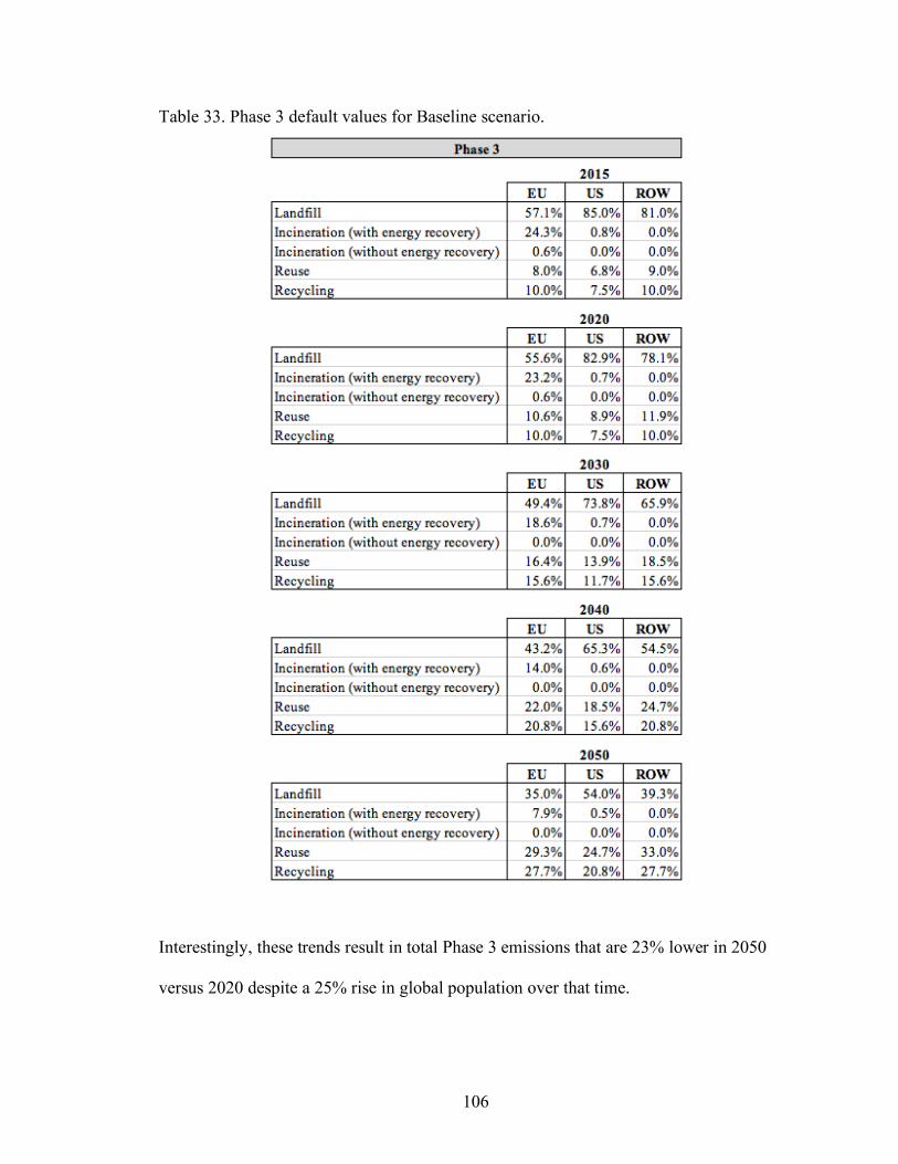
106
Table 33. Phase 3 default values for Baseline scenario.
Interestingly, these trends result in total Phase 3 emissions that are 23% lower in 2050
versus 2020 despite a 25% rise in global population over that time.

107
Figure 18. Baseline scenario, Phase 3 metric tons of CO2-eq.
The summary table of emissions for the Baseline scenario (Table 34) indicates
that the apparel industry will generate 92.8 gigatons of CO2-eq between 2015 and 2050,
representing 7.2% of the remaining carbon budget with a 66% likelihood of remaining
below 2°C, and 17.1% of the remaining carbon budget under the 1.5°C pathway. The
overwhelming majority of emissions (79%) for developing and developed countries will
be generated in Phase 1 from material production (Table 34), followed distantly by
landfill (9.3%) in Phase 3. As seen in the 2015 Impacts section above, developed
countries’ excessive consumption is further reflected in their Phase 2 emissions, which

108
account for 41% of all Phase 2 emissions despite the fact that developed countries
represent less than 15% of the global population.
Table 34. Baseline scenario GWP by life cycle stage, 2015 - 2050.
Over time, total emissions from Phase 2 and Phase 3 steadily decline while Phase
1 emissions rise. This trend is evident when comparing total projected emissions from
2050 to those from 2015 (Table 35). As expected, the majority of emissions occur in
Phase 1 and are associated with developing countries due to population growth. However,
the reduced carbon intensity of the energy mix in developed countries coupled with their
low population growth results in an overall reduction of Phase 2 emissions in 2050
compared to 2015. Finally, higher recycling rates result in reduced landfill emissions in
Phase 3 over time, the effects of which are especially pronounced in high consumption
developed countries where negative emissions exceed those of more populous developing
countries (Table 35) despite their having equal or greater recycling rates than developed
countries by 2050 (Table 33).

109
Table 35. Baseline scenario difference in emissions, 2050 vs. 2015.
Table 35 represents the difference between 2050 emissions and 2015 emissions by subtracting the latter from the former.
As seen in Figure 19, aggregated emissions from all phases grow 49% for
developing countries between 2015 and 2050 while their corresponding population rises
36%. Conversely, developed countries’ emissions will decline 18% over the same period
while their population grows 6%. Despite the rapid growth of emissions in developing
countries between 2015 and 2050, their share of total emissions from apparel (71%) will
remain below their share of the world’s population (88%). Meanwhile, developed
countries will continue to overconsume and will represent 25% of apparel emissions with
only 11.6% of the global population in 2050.
When changes in emissions by life cycle stage are analyzed for two time periods,
2015 – 2030 and 2015 – 2050 (Table 36), it is clear that a large percentage of emission
gains occur by 2030 whereas the highest percentage of emission reductions occur
thereafter. For example, material production – which is responsible for the majority of
apparel emissions – grows 63% between 2015 and 2030 for developed countries, but only
grows 78% over the 2015 – 2050 time period, indicating a slower growth rate after 2030.
Between 2015 and 2030, the largest source of negative emissions, recycling, rises 153%
and 67% for developing and developed countries, respectively. Thereafter, recycling rises
even more significantly as indicated by the 2015 – 2050 growth rates in Table 36.

110
Figure 19. Baseline scenario emissions and population over time, 2015 - 2050.
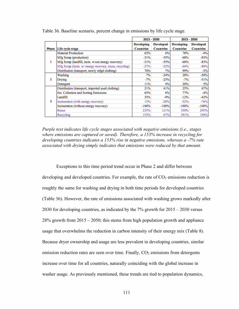
111
Table 36. Baseline scenario, percent change in emissions by life cycle stage.
Purple text indicates life cycle stages associated with negative emissions (i.e., stages where emissions are captured or saved). Therefore, a 153% increase in recycling for developing countries indicates a 153% rise in negative emissions, whereas a -7% rate associated with drying simply indicates that emissions were reduced by that amount.
Exceptions to this time period trend occur in Phase 2 and differ between
developing and developed countries. For example, the rate of CO2 emissions reduction is
roughly the same for washing and drying in both time periods for developed countries
(Table 36). However, the rate of emissions associated with washing grows markedly after
2030 for developing countries, as indicated by the 7% growth for 2015 – 2030 versus
28% growth from 2015 – 2050; this stems from high population growth and appliance
usage that overwhelms the reduction in carbon intensity of their energy mix (Table 8).
Because dryer ownership and usage are less prevalent in developing countries, similar
emission reduction rates are seen over time. Finally, CO2 emissions from detergents
increase over time for all countries, naturally coinciding with the global increase in
washer usage. As previously mentioned, these trends are tied to population dynamics,

112
namely from high population growth in developing countries and low population growth
marked by an aging population in developed countries that continues to overconsume.
Summary of Scenarios 1 – 4
This section provides a summary of results for Scenarios 1 through 4 as outlined
in Table 30 and is comprised of three parts: an overview of Scenarios 1-4, a comparison
of results for all scenarios, and an in-depth summary of results for developed and
developing countries.
Overview of Scenarios 1-4. The descriptions below highlight the differences associated
with key variables in each scenario. Tables containing specific values used for each
scenario can be found in Appendix 1.
• Scenario 1: High production/consumption, high recycling and reuse: This scenario
models a 15% increase in most Phase 1 variables above the Baseline values noted
in Table 31, but does not alter shipping allocation values for air and maritime
freight. Because this scenario is modeling high production, it was assumed that
high production – which is synonymous with per capita consumption – would
correspond with an increase in Phase 2 values. As such, washer and dryer
ownership rates increase 15% above all Baseline values noted in Table 32.
Finally, a 15% reduction in landfill rates below the Baseline values noted in Table
33 was assumed for Phase 3, which drives a higher allocation to reuse and
recycling than a 15% increase in recycling and reuse combined.

113
• Scenario 2: High production/consumption, low recycling and reuse: Values for
key variables associated with Phases 1 and 2 are identical to those used in
Scenario 1. For Phase 3, a 15% increase in landfill rates was used, which drives a
lower allocation toward recycling and reuse than a 15% decrease in recycling and
reused combined.
• Scenario 3: Low production/consumption, high recycling and reuse: This scenario
models a 15% decrease in most Phase 1 variables below the Baseline values noted
in Table 31; like Scenario 1, shipping allocation values remain unchanged from
Baseline values. To coincide with low production, values from the Baseline
scenario were utilized for Phase 2 based on the assumption that laundry habits
would remain unchanged with reduced consumption. A 15% decrease was
assumed for landfill values in Phase 3, thus driving a higher allocation toward
reuse and recycling.
• Scenario 4: Low production/consumption, low recycling and reuse: Values for
key variables associated with Phases 1 and 2 are identical to those used in
Scenario 3, however, a 15% increase in landfill rates was assumed in Phase 3,
resulting in lower reuse and recycling rates.
Comparison of results for all scenarios. In the event that a high consumption scenario
occurs such as Scenario 1 or 2, cumulative 2015 – 2050 CO2 emissions from apparel will
increase to 108-111 gigatons CO2-eq (Table 37), elevating emissions 17% to 20% above
the Baseline scenario. Between Scenarios 1 and 2, 73% to 86% of emissions are
generated in Phase 1. As seen in Table 37 for Scenario 1, a 15% decrease in landfill rates

114
that corresponds with an increase in recycling and reuse rates will help mitigate over 1.5
gigatons of emissions associated with Phase 3 when compared to the Baseline scenario.
However, under Scenario 2 we see that a 15% increase in landfill rates adds nearly 3
gigatons of CO2-eq to cumulative apparel emissions. Additionally, both of these high-
consumption scenarios generate incremental emissions of 1.4 gigatons of CO2-eq under
Phase 2 above the Baseline scenario, and those emissions are only countered by landfill
avoidance associated with elevated recycling as seen in Scenario 1.
Table 37. Summary of all scenarios by life cycle stage, 2015 - 2050.
Under the low consumption scenarios, Scenarios 3 and 4, cumulative 2015 – 2050
emissions from Phase 1 only decline 7% versus the Baseline scenario (Table 37). While
this represents a meaningful reduction of nearly 4.9 GtCO2-eq, it is remarkably different
from the 14.2 gigaton gain that occurs in Phase 1 emissions under Scenarios 1 and 2.
Comparatively, this difference indicates how influential developing country consumption
rates are, specifically the consumption rates associated with a relatively small subsegment
of their populations that adopt developed country consumption habits. Finally, the effects

115
associated with reduced landfill disposal and increased recycling rates are especially
pronounced in Scenario 3 where cumulative Phase 3 emissions are 2.2 gigatons lower
than they are in Scenario 4, and 1.6 gigatons lower than related emissions under the
Baseline scenario.
Despite the fact that Scenario 3 achieves meaningful reductions in Phase 1 and
Phase 3 emissions, its cumulative 2015 – 2050 emissions will account for 6.7% of the
remaining 2015 carbon budget with a 66% likelihood of remaining below only 2°C
(Table 38). In other words, Scenario 3 – which represents the best case scenario in this
study – does not result in a significant reduction of apparel’s contribution to the
remaining carbon budget compared to the aforementioned 7.2% for the Baseline scenario.
As indicated in Table 38, the apparel industry will account for an even larger portion of
the remaining carbon budget when emissions for 2015 – 2017 have been accounted for.
Once those emissions have been subtracted from the 2015 carbon budget, the apparel
industry will account for 6.8% to 9% of the remaining 2018 carbon budget with a 66%
likelihood of remaining below 2°C, and 19% to 25% of the remaining 2018 carbon
budget under the 1.5°C pathway.
Table 38. Summary of carbon budget expenditures for all scenarios.

116
Summary of results for developing and developed countries. Predictably, the largest gains
in emissions occur in developing countries when consumption rates increase beyond
baseline rates under Scenarios 1 and 2 (Figure 20). Despite the significance of these
gains, the percentage of overall emissions associated with developing and developed
countries remains remarkably stable across Scenarios 1 through 4 (Table 39). In no
scenarios do developed countries account for less than 27.4% of cumulative 2015 – 2050
emissions from apparel. The ratio of total emissions associated with developed and
developing countries is largely due to population growth in developing countries and
exceptionally high per capita consumption in developed countries.
Table 39. GWP by life cycle phase for developing and developed countries.

117
Figure 20. GWP by phase for all scenarios, developing vs. developed countries.
Masked behind this consistency are differences that occur across scenarios
between developing and developed countries within each of the three life cycle phases.
For example, in Scenarios 1 and 2, the effects of increased consumption in developing
and developed countries is especially pronounced in the Material Production stage of
Phase 1 (Table 40). However, when consumption declines for developing countries in
Scenarios 3 and 4 while remaining at Baseline scenario rates for developed countries, the

118
GWP associated with Material Production remains high but is much less significant. This
of course highlights the high impact of developed country consumption rates. A similar
effect is also evident in the Distribution stage of Phase 1 where the GWP grows
significantly in Scenarios 1 and 2 versus the Baseline scenario, but declines less
significantly in Scenarios 3 and 4. Again, this is due to high consumption rates among
developed countries and stems from their reliance on apparel imports from developing
countries (Table 40).
Table 40. GWP of Phase 1 for developing and developed countries.
Across all scenarios, developed countries account for at least 40.8% of all Phase 2
emissions, highlighting the comparatively high impacts associated with washing and
drying behaviors in these countries (Table 41). As previously noted, developed countries
represent less than 15% of the global population and have a greener energy mix than
developing countries, which makes their disproportionate share of Phase 2 emissions all
the more startling. If developing countries had a greener energy mix, the proportional
share of emissions from developed countries would be even higher. The high emissions
associated with detergent use are particularly high among developed countries too,

119
accounting for no less than 44.4% of all detergent-related emissions (Table 41). Even
when consumption rises in Scenarios 1 and 2, developing countries do not procure and
use washers, dryers, and detergent enough to substantially increase their contribution to
Phase 2 emissions relative to developed countries. In fact, even if developing countries
had a washer ownership rate of 100%, they would only increase their shares of washing,
drying, and detergent emissions to 70.3%, 61.4%, and 63.4%, respectively – well below
their relative share of the global population. Clearly, significant changes would be
required among developed countries to reduce the GWP associated with their Phase 2
emissions, which remain stubbornly high across all scenarios due to the high number of
wash cycles and corresponding detergent use, and their high dryer ownership and use
rates.
Table 41. GWP of Phase 2 for developing and developed countries.
As indicated by the scenario results in Table 42, Phase 3 emissions are strongly
correlated with apparel consumption rates and can disproportionately affect developing
and developed countries within each stage. For example, high production under Scenarios
1 and 2 will cause Distribution and Collection stage emissions to spike in developing
countries by 18% and 22%, respectively, over the Baseline scenario. Naturally, this stems

120
from the fact that developing countries rely on a higher percentage of used clothing
imports and will naturally have a higher volume of collection versus developed countries
due to differences in population. Conversely, lower consumption under Scenarios 3 and 4
will cause a greater rate of emissions reduction in the Collection (-11%) and Landfill
(-22%) stages for developed countries that have much higher per capita baseline
consumption rates than developing countries. Lastly and most importantly, developed
countries have a much lower share of negative emissions from Recycling (Table 42)
compared to their share of emissions from Material Production (Table 40). This
difference is exclusively driven by poor recycling rates in the United States, resulting in a
higher percentage of landfill volume across all scenarios for developed countries.
Table 42. GWP of Phase 3 for developing and developed countries.
As noted throughout the phase-specific results above, the disproportionate
emissions associated with developed countries are driven by their perniciously high
consumption rates. As illustrated in Figure 21, the average emissions per capita for

121
developed countries is 124% higher than it is for developing countries across Scenarios 1
through 4, but is highest under the Baseline scenario at 152%. As expected, the high
consumption scenarios (Scenarios 1 and 2) cause per capita emission rates to increase
Figure 21. Per capita emissions for developing and developed countries.

122
dramatically through 2030 as the global population rapidly expands prior to our
forecasted ability to achieve a greener energy mix or the anticipated reduction in
consumption among aging populations in developed countries. This trend continues for
developing countries in Scenarios 2 and 3, but diverges for developing countries in those
scenarios as a result of their gradual population rise coupled with a more rapidly greening
energy mix and reduced landfill rates in the EU. After the population surge transpires
between 2020 and 2030, per capita emission rates go down across all scenarios for all
countries, primarily from declines in manufacturing scrap volumes, landfill rates, and the
carbon intensity of the global energy mix. As expected, these effects are more
pronounced over time in developed countries due to their more rapidly greening energy
mix and their aging populations. In fact, in all scenarios, developed countries are
anticipated to have lower per capita emissions in 2050 than they have today. Conversely,
developing countries do not return to their current per capita emission rates before 2050.
Sensitivity Analysis
I developed a sensitivity analysis table to better understand how each of the key
variables impacted the GWP of apparel. In constructing the analysis, I applied the same
baseline values that were utilized in the Baseline scenario described above, then
developed a spread value by subtracting the difference associated with a 15% increase
and a 15% decrease for each variable. The analysis is presented in two parts below: the
first provides an aggregated view for all countries (Table 43), and the second highlights
differences between developing and developed countries (Table 44). Expanded values for
Tables 43 and 44 can be found in Appendix 2.

123
Table 43. Sensitivity spread for key variables (2015 – 2050).
Based on Baseline values for key variables. Expanded values for Phase 3 can be found in Appendix 2.

124
Table 44. Sensitivity spread for developing and developed countries (2015 – 2050).
Based on Baseline values for key variables. Expanded values for Phase 3 can be found in Appendix 2.

125
Sensitivity Analysis for All Countries
Six variables accounted for 85% of the total spread. The most important variable
was the Percent of Population in Developing Countries that Achieves the Average
Developed Country Consumption Rate. This variable determined 34.3% of the spread
(Table 43) despite the fact that it only applied to 15% of the population in developing
countries. The second most influential variable was the Developed Country Percent
Increase or Decrease in Consumption above the 2015 Base Rate, and accounted for
15.5% of the spread. The remaining variables of importance were the Developing
Countries Percent Increase in Consumption Per Capita (13.4%), the Upstream Shipping
Method – Maritime (reduction defaults to air) (9.3%), Landfill Rate (7%), and the
Change in Washer Ownership (5.9%).
The importance of the top three variables was expected, given the carbon intensity
associated with production, which is directly influenced by consumption rates. However,
the sensitivity analysis highlights the unexpected importance of utilizing maritime
transport over air, which was not modeled in the five scenarios detailed in the sections
above. As indicated in Table 43, a 15% reduction in maritime transport defaults to the use
of air shipping, which had the fourth highest influence on the GWP of apparel. The
importance of avoiding landfill impacts has been seen throughout the modeled scenarios
of my analysis, but the relative importance of washer ownership was less expected and
highlights the significance of consumption, which is tied to washer ownership.

126
Sensitivity Analysis for Developing and Developed Countries
Table 44 highlights several key differences between developing and developed
countries. First, nearly 68% of the total spread associated with developing countries
stemmed from two variables, Percent of Population in Developing Countries that
Achieves the Average Developed Country Consumption Rate (48.7%), and Developing
Countries Percent Increase in Consumption Per Capita (19%). The most remarkable
aspect of that result relates to the fact that a change in consumption for the entire
population living in developing countries has less influence than a comparatively small
segment of their population adopting the high consumption rate of developed countries.
Comparatively, upstream shipping methods are less influential for developing countries
compared to developed countries, largely because developing countries are now centers
of apparel production. However, the importance of landfill rates was higher for
developing countries (Table 44) than the overall rate for the same variable noted in Table
43, suggesting that the volume of apparel in these countries will represent a visible end-
of-life challenge to be addressed.
The most important variable for developed countries was naturally the Developed
Country Percent Increase or Decrease in Consumption above the 2015 Base Rate,
accounting for 52% of the total spread. The variable with the second highest sensitivity
for developed countries was the Upstream Shipping Method – Maritime (reduction
defaults to air), which accounted for 13.7% of the spread (Table 44). As expected, this
variable was more influential for developed countries who rely on overseas production
for much of their apparel consumption and would therefore be more impacted by the high
carbon intensity of air transport. Lastly, it was assumed that Landfill Rate would be more

127
influential for developed countries as a result of comparatively low landfill rates in the
United States. However, this proved not to be the case with 6.6% of the spread and was
surprisingly surpassed in sensitivity by the Change in Washer Ownership variable
(7.96%).

128
Chapter IV
Discussion
The purpose of this study was threefold: to investigate the GHG emissions
currently associated with the apparel industry; to understand the industry’s projected
2050 emissions under different scenarios of production, consumption, and post-
consumption relative to the remaining carbon budgets under the IPCC’s 1.5°C and 2°C
pathways; and to assess how emissions might impact countries designated as “developed”
and “developing” by the IMF. The assessment required developing a robust spreadsheet
model comprised of 86 variables and extensive supporting data to address the two
primary hypotheses: first, the apparel industry will account for more than 30% of the
2050 carbon budget associated with the IPCC’s 1.5°C pathway, representing a significant
increase in GHG emissions over current contributions; and second, developing countries
will account for greater emissions from apparel than developed countries, assuming that
50% of the population in developing countries achieve similar clothing consumption
levels as developed countries by 2030.
In this chapter, I summarize the key findings of my research, beginning with the
industry’s current and projected GHG emissions under different scenarios of production,
consumption, and post-consumption. I will then explore the impacts of the apparel
industry in relation to the remaining 2018 carbon budgets under the IPCC’s 1.5°C and 2°C
pathways. Finally, I will reflect on the limitations of my research and discuss
implications for the apparel industry going forward.

129
Current and Projected GHG Emissions
The results of this study indicate that the apparel industry accounted for at least
5.3% of global emissions in 2015. Simulating current rates of production, consumption,
and post-consumption activities – which were respectively categorized as Phases 1, 2,
and 3 in my analysis – resulted in a Baseline scenario that mimicked “business as usual”
conditions through 2050. Under that scenario, the industry’s annual emissions rise from a
low point of 2.19 gigatons in 2015 to a projected peak of 2.8 gigatons in 2030 before
gradually declining to 2.72 gigatons in 2050 (Figure 22). Over that time period, the rapid
population expansion in developing countries will result in the addition of one billion
new consumers, most of whom arrive by 2030. The increased consumer demand from
developing countries coupled with continued overconsumption in developed countries
will require a 47% increase in global apparel production.
Collectively, these factors will increase developing countries’ share of apparel
emissions from 62.6% in 2015 to 75.2% in 2050 (Figure 23). While developed countries’
share of global apparel emissions obviously declines over time – and was not higher than
emissions from developing countries as I had hypothesized – that trend masks the fact
that they will continue to account for a disproportionate share of overall emissions
relative to their population. Specifically, their share of apparel-based emissions will
decline from 37.4% in 2015 – with a mere 14.5% of the global population – to 24.8% in
2050 with only 11.6% of the global population. Shockingly, developed countries would
need to reduce their baseline consumption rates by 95% to proportionally align their
emissions with their population.

130
Figure 22. Gt CO2-eq trend for all scenarios, 2015 – 2050.
The most obvious trend in this analysis is also the most worrisome: annual
emissions from apparel are forecast to rise 24% between 2015 and 2050 under the
Baseline scenario (Figure 22), amassing 92.8 GtCO2-eq. Under conditions of high
consumption, as exemplified by Scenarios 1 and 2, annual emissions increase more than
56% despite the fact that these scenarios modelled a modest 15% rise in consumption
rates (Figure 22). Even Scenarios 3 and 4 are cause for concern, as they both represent a
15% decrease in consumption below baseline rates yet result in a 13% increase in

131
emissions from apparel; they also accrue no less than 86.3 GtCO2-eq in cumulative 2015
– 2050 emissions.
Figure 23. Baseline scenario share of apparel emissions by country type.
Another notable trend was persistent across all modeled scenarios: over time,
Phase 1 emissions – and more specifically, emissions associated with material production
– were so dominant that the elimination of impacts from Phases 2 and 3 does not
significantly reduce overall emissions from apparel. A snapshot of this outcome is
illustrated for each scenario in Figure 20. The primary reason Phase 1 emissions are so
high has to do with the cradle-to-gate GWP of the fiber mix (Table 3), which does not
change over time despite the dramatic change in allocation by fiber type between 2015
and 2050 (Table 2). In other words, there appears to be no carbon savings associated with

132
the forecasted dominance of synthetics in the global fiber mix. Surprisingly, even when
the GWP values of each fiber are reduced by 75%, global 2015 – 2050 apparel emissions
under “business as usual” rates exceed 34.7 GtCO2-eq, 63% of which remain associated
with Phase 1. While this represents a dramatic reduction in the intensity of GWP
associated with Phase 1 – especially when compared against the forecasted Baseline
scenario rates shown in Figure 24 – it does not eliminate concerns for the aforementioned
trend.
Figure 24. Baseline scenario share of emissions by life cycle phase.

133
On one hand, these are disheartening results that suggest no amount of behavioral
change in washing and drying habits (Phase 2) or vigilance in recycling and landfill
avoidance (Phase 3) can significantly alter the rapid growth of emissions from apparel.
On the other hand, they emphasize the immediate need to consume less and invest in
materials innovation to bring down the GWP of fibers in the fiber mix. On a lighter note,
the trend for the Baseline scenario in Figure 24 suggests that impacts associated with
Phases 2 and 3 will lessen over time, offset in part by a greening energy mix alongside
improved recycling and landfill avoidance. If trends for Phases 2 and 3 can be further
improved and paired with circularity practices that coincide with reduced GWP
intensities of fibers, overall emissions associated with the apparel industry can be
radically reduced. If such changes do not transpire, we risk clothing our way to a climate
emergency as indicated by the remaining carbon budgets in the section below.
Carbon Budgets
The results obtained from this study revealed the degree to which the apparel
industry’s cumulative 2015 – 2050 emissions would impact the remaining carbon budgets
detailed in the IPCC’s 2018 Special Report: Global Warming of 1.5°C. While none of the
modeled scenarios resulted in emissions exceeding 30% of the remaining carbon budget
as I had hypothesized, the final results were alarming nonetheless. As seen in Figure 25,
the Baseline scenario – which represents “business as usual” – projects that apparel will
account for 7.4% of the remaining 2018 carbon budget under the 2°C pathway, and
20.5% of the budget under the 1.5°C pathway. In the most extreme case of high
consumption and high landfill rates (Scenario 2), the apparel industry will represent no
less than 9% and 25% of the remaining 2°C and 1.5°C budgets, respectively.

134
Figure 25. Remaining carbon budget scenarios based on 2018 carbon budget.
It is worth emphasizing that these projections – and my original hypothesis – did
not incorporate Earth-system feedbacks into the remaining carbon budgets. However,
with each assessment released by the IPCC and the climate science community, there is
an obvious and harrowing trend: climate change is accelerating more rapidly than
expected, increasing our knowledge of feedback loops, and providing more evidence that
a planetary emergency is much closer and far worse than previously projected. Given that
the effects of climate change are large, complex and irreversible, a proper risk assessment

135
should consider these Earth-system feedbacks in the remaining carbon budgets (Lenton et
al., 2019).
These feedbacks, which are associated with permafrost thawing and dieback in
the Amazon and boreal forests, are projected to harbor at least 300 GtCO2-eq (Lenton et
al., 2019). When these revised feedbacks are incorporated into the remaining carbon
budgets, climate change quickly transforms from an existential threat to an imminent one.
As seen in Table 45, the remaining 2018 carbon budget associated with a 66% probability
of staying below 1.5°C – assuming the inclusion of these revised feedbacks – is 120 Gt.
This means we have approximately 5 years left before we deplete the remaining carbon
budget under the 1.5°C pathway, and 21 years under the 2°C pathway, assuming today’s
annual emissions rate of 42 GtCO2-eq.
When the apparel industry’s projected emissions are compared against carbon
budgets that include these revised Earth-system feedbacks, we see that in the best case
scenario – which is represented by Scenario 3 in Figure 25 – the industry will account for
9.2% of the remaining 2018 carbon budget under the 2°C pathway, and 66.5% of the
budget under the 1.5°C pathway. As Figure 25 makes clear, the best case scenario that
accounts for these revised Earth-system feedbacks (Scenario 3) is worse than the worst
case scenario that excludes them (Scenario 2, without Earth-system feedbacks). This
degree of risk – which more than doubles the originally hypothesized severity of
apparel’s GWP under the 1.5°C pathway – underscores the criticality of addressing
apparel’s cradle-to-gate emissions as quickly as possible, especially in light of forecasted
GDP and population growth.

136
Table 45. Remaining carbon budgets with revised Earth-system feedbacks.
Extension of Table 18 incorporating revised estimates for Earth-system feedbacks from Lenton et al. (2019) associated with a 66% probability of staying below 1.5°C and 2°C for IPCC AR5 and IPCC SR15, a 66% probability of staying below 2°C for IEA/IRENA, and 80% probability of staying below 2°C for Potsdam Climate Institute estimates. GtCO2 associated with revised Earth-system feedbacks by 2100 subtract 300 GtCO2 associated with impacts from Amazon dieback (90 GtCO2-eq) and boreal forests (110 GtCO2-eq), as well as permafrost thawing (100 GtCO2-eq, which excludes methane from deep permafrost and undersea hydrates).
Limitations and Future Research
This study relied upon publicly available data and triangulations from a multitude
of sources, but excluded apparel-specific information from proprietary databases and
other paywalled services. During the course of my research, I also discovered that
desirable data associated with the apparel life cycle were limited, incomplete,
unavailable, or missing. As a result, my study could not include emissions associated
with several activities in each of the study’s three phases. These missing elements are
detailed by phase below.

137
Phase 1 emissions data associated with various aspects of fiber production and
garment assembly were not sufficiently available to develop assumptions and
extrapolations. For example, the energy and transportation impacts associated with
geographically distributed production steps such as spinning, dyeing, cutting, sewing, and
finishing are surely a substantial source of GHG emissions, however, I was not able to
obtain the requisite distance, transportation mode, or regional energy mix data to
calculate impacts associated with many of those steps in countries of production. Total
emissions for Phase 1 also exclude impacts specific to the manufacture and transportation
of apparel components such as zippers, buttons, binding material, and rivets, among other
items.
Additionally, the adoption of recycled fibers has increased dramatically over the
last five years, with large brands such as Nike, Adidas, and Under Armour, among others,
mainstreaming the use of recycled nylon, polyester, and cotton into their garments. I did
not have reliable data points for the cradle-to-gate GWP of these fibers, and while they do
not make up more than a single digit percentage of the global fiber mix today, their
adoption rate warrants revising the results of this study when those data become
available.
Considering Phase 2, while the literature contained limited information about
consumer washing and drying habits, data for ironing, dry cleaning, and the use of
launderettes was non-existent. These consumer habits and the energy-based emissions
associated with them likely vary by region and by country. What is more, my research
did not include emissions associated with the manufacture, transportation, and end-of-life

138
phases of washing and drying machines. These data were not found in any publicly
available source but could add substantial emissions to Phase 2 results.
Surprisingly few studies have been conducted on emissions associated with Phase
3 life cycle stages. For example, data were especially limited on volumes associated with
each end-of-life stage, and no data were found on the portion of landfilled apparel
emissions being mitigated by gas capture, which is common in many countries and could
meaningfully reduce Phase 3 emissions. Finally, data associated with recycling activities
such as shredding, disassembly, and fiber separation were not available; their inclusion
would serve to increase Phase 3 emissions until carbon neutrality is achieved in the
energy sector.
Future Research
Beyond addressing the aforementioned gaps within each of three phases, two
areas of research would be especially beneficial to enhance the results of this study. First,
attitudes associated with apparel consumption – and the degree to which consumption has
gained cultural centricity – are largely undocumented beyond the United States, Canada,
and select countries in the European Union. Anecdotally, understanding those attitudes
and how they differ by age group, gender, and income would greatly inform assumptions
associated with consumption in developing countries.
Second, demographic and economic data for variables such as age, gender,
income and disposable income, GDP, and apparel consumption were limited for
developing countries. More robust data for these variables would help fuel country-
specific regression models that could better predict country-level apparel consumption. In
fact, my research began by developing over 30 country-specific regression models that I

139
intended to use to more accurately predict apparel consumption. These models provided a
rich understanding of consumption drivers for a number of developed countries, but
notable country-level differences were discovered and the results could not be applied to
the outstanding majority of developing countries. Moreover, GDP forecasts were limited
for developing countries and the econometric modeling required to extend those forecasts
to 2050 was well beyond the scope of this study.
Developing and Developed Country Designations
This study made use of IMF economic designations for “developed” and
“developing” countries, which appeared throughout several of my primary data sources.
On one hand, utilizing these designations was useful for developing the data set, and they
might help others who wish to use the data in the future. On the other hand, the use of
these designations presents two problems. First, the results of this study – which highlight
rampant overconsumption – call into question the accuracy of that ironic designation for
so-called “developed” countries that are responsible for a disproportionate share of
historical and forecasted emissions from apparel, to say nothing of the associated
chemical, water, and waste impacts excluded from this study. Second, labeling a country
as “developing” could be deemed both culturally and ethically questionable. After all,
much of the apparel industry’s supply chain is driven by labor and environmental
exploitation that originates from companies in “developed” countries. As a result, the
term “developing” could be interpreted as a missionary-oriented designation, or at
minimum, one that embeds the presumption that these countries are “less than” or
somehow inferior for not subscribing to the same economic system as their “developed”
counterparts. In short, the use of these designations will likely become less relevant and

140
possibly derogatory over time, and arguably should not be used in the near term unless
they are heavily relied upon in source data. However, they remain in this study as an
unintentional artifact.
Implications
The results of this study reveal a number of challenges and opportunities across
the apparel life cycle, most of which can be intuited from the linear “take-make-waste”
model that has been employed throughout the industry for the last forty years and
exacerbated by social media and the widespread adoption of fast fashion’s intensified
production model. Undoubtedly, the greatest challenge – and the most profoundly
important opportunity – relates to the use and reuse of raw materials as demand
skyrockets with population growth. Simply put, a brand’s chosen fiber mix is the single
biggest determinant of apparel emissions. Given the cradle-to-gate GWP values
associated with each fiber, a brand can choose to use less emissions-intensive materials,
including recycled and low impact man-made fibers, which essentially makes
sustainability a design decision. As with all design decisions, there are complexities and
trade-offs to consider. However, the results of this study demonstrate that brands should
design for three key outcomes to reduce Phase 1 emissions: emission reductions through
the use of more sustainable materials that involve a fraction of the cradle-to-gate
emissions associated with conventional fibers; durability to limit the need for non-
essential draws on finite resources, particularly non-renewables; and recyclability to
enable the reuse of pre and post-consumer materials that can be remade into fibers, not
simply downcycled for alternative uses like rags, seat cushions, and acoustic fill.

141
Collectively, such decisions can dramatically reduce Phase 1 emissions and will extend to
Phase 3 emission reductions as well.
Fortunately, there has been an explosion of materials innovation over the last
decade, giving apparel brands the ability to incorporate more sustainable materials in
their clothing lines. Some of these materials have been widely available but seldom used,
such as hemp, and warrant more consideration in light of their low GWP values, soil
benefits, and ability to sequester carbon. Other materials are relatively new, such as those
being developed by AlgiKnit, Bolt Threads, Ecovative Designs, and BIONIC, among
others. Brands that seek to use such materials often need to conduct enough research and
development on their own to ensure that the new fibers can be used in their
manufacturing processes and will perform as desired for consumers. This often requires
time and dedicated efforts above and beyond their existing operations, and in some cases
it requires significant investment when purchase minimums for materials are
exceptionally high. These conditions favor large apparel brands who can afford such
experimentation and innovation, and arguably represent an economic disadvantage to
small and medium-sized brands.
When it comes to recyclability, brands should consider making garments from
materials that can be easily separated for recycling. Companies such as BlockTexx and
Evrnu have developed technologies that are capable of recovering fibers from discarded
garments and remaking them into new yarns. These technologies only work for select
fiber combinations today such as cotton and polyester, but brands should arguably
increase efforts to develop garments Evrnu and BlockTexx can work with while

142
sponsoring efforts for these companies to develop additional circularity-minded
breakthroughs.
Some of the impacts associated with Phase 2 were not expected. For example, the
use of detergent – which directly correlates with the use of washing machines – was more
significant than anticipated. As the sensitivity analysis revealed, emissions from
detergents were almost as significant as emissions from dryers in developing countries,
and were more significant than dryers in high-consumption developed countries. What is
more, the emissions associated with detergent use will grow more quickly over the
coming decades as washer adoption accelerates with population growth. Clearly, there is
an opportunity to educate consumers about the impacts of their detergent use and the
benefits of using an ultra-concentrated formula over the standard double concentrated and
powder-based formulas that currently represent 81% of the global market. After all, ultra-
concentrated formulas represent a 75% reduction in emissions versus double concentrated
and standard powder-based formulas, and an 83% reduction over tablet-based detergents.
Additionally, detergent brands and retailers can meaningfully reduce their carbon
footprints by mainstreaming ultra-concentrated detergents, which not only require fewer
resources to produce, but are inherently more efficient to transport, merchandize, and
recycle on a per unit basis due to their smaller size and lighter weight.
Beyond detergents, apparel brands and appliance manufacturers can also educate
consumers about washing. Companies such as Levi Strauss and Patagonia have strongly
encouraged consumers to wash less frequently and to use cold water, which both serve to
reduce washing-related emissions and other impacts not discussed in this analysis (e.g.,
reduced microfiber pollution and water use). However, appliance manufacturers can

143
make simple changes, too. For example, brands such as GE, LG, and Samsung often
default to a warm water setting when their washing machines are turned on. Simply
defaulting to a cold water setting and configuring their machines to allow for shorter
wash cycles will likely help reduce washing-related emissions.
When it comes to dryers, natural gas powered dryers have historically been more
efficient than their electric counterparts and are prevalent throughout Europe. However,
the use of natural gas – particularly natural gas that has been sourced from fracking –
comes with other externalities and involves emissions that are frequently excluded in
calculations associated with dryer use. Incentivizing building developers and consumers
to install heat pump dryers could reduce dryer emissions by as much as 50%.
The landfill emissions calculated under Phase 3 were much larger than anticipated
and underscore the importance of diverting as much apparel as possible from this end-of-
life stage, especially in high-consumption developed countries. The aforementioned
design decisions for durability and recyclability are clearly critical for reducing Phase 3
emissions, and while it is not clear that the increasing prevalence of retail take-back
programs is having a meaningful effect, such efforts can certainly help limit landfill
impacts when paired with education that is focused on reducing consumption.
Finally, this thesis was based on publicly available information that was
challenging and time consuming to find, aggregate, and analyze across a wide range of
sources. While databases containing more accurate information about activities in the
apparel life cycle do exist, they are either inaccessible to the public or reside behind
paywalls. It is my intent to make the data and the model associated with this thesis
publicly available so other individuals and organizations have a baseline to work from to

144
conduct their own analyses. In doing so, I hope the information I have gathered and the
assumptions I have made will be modified and improved upon as we learn more about the
complexities of the apparel life cycle.
Conclusions
The fashion industry is unsustainable by definition, but apparel need not be. Over
the last 50 years, the former has subscribed to a socially and ecologically destructive
“take-make-waste” model that represents one of the world’s most wicked sustainability
challenges, while the latter has the potential to transform into an industry that is not
inherently destructive, includes more regenerative than degenerative practices, and can
legitimately achieve a significant amount of circularity with materials. As the “business
as usual” results of this study make clear, the potential for climate-positive
transformations in apparel has significant headwinds in the form of forecasted GDP
growth and rapidly rising population, which are projected to fuel 92.8 GtCO2-eq from
apparel consumption between 2015 and 2050. Those emissions represent at least 20% of
the remaining 2018 carbon budget with a 66% likelihood of staying under 1.5°C. While I
was unable to demonstrate that the apparel industry would account for more than 30% of
the remaining carbon budget under the 1.5°C pathway using budgets that excluded Earth-
system feedbacks, incorporating such feedbacks in carbon budget calculations appears
increasingly prudent considering the accelerating pace of climate change and the failure
of many of the world’s largest emitters to remain on track with their NDCs (United
Nations Environment Programme, 2019), which would result in a fairly catastrophic 3°C
of warming if achieved. When Earth-system feedbacks are factored into the remaining

145
carbon budget, apparel emissions under the “business as usual” scenario will account for
72% of the remaining budget under the 1.5°C pathway.
Such results – and the risks they represent – demand immediate attention by
apparel brands and consumers alike. The immediacy is driven in part by the dramatic rise
in population that will occur over the next decade, which will cause emissions from
apparel to spike significantly. A disproportionate amount of those emissions will
originate from developed countries whose populations chronically overconsume.
Thankfully, developing countries have not had the consumption habits of developed
countries, nor are they forecasted to acquire them. If they did, 2015 – 2050 emissions
from apparel would soar to nearly 170 GtCO2-eq, 84% higher than the projected
emissions under the “business as usual” scenario – a sum that would more than eliminate
the remaining budget under the 1.5°C pathway, assuming Earth-system feedbacks are
accounted for.
The most critical area to address emissions from apparel is in the material
production stage, which represents a broad category of cradle-to-gate activities in this
study, including raw material sourcing, spinning, dyeing, and finishing. This stage
accounted for 70% to 85% of all emissions across every scenario modeled in my analysis.
Clearly, the carbon intensity of materials must decline quickly in the coming years and
should be paired with efforts to divert apparel from landfills and enhance recycling so
discarded apparel can be used as feedstock for material production. If we do not find
ways to decouple population growth and corresponding demand for apparel from the
carbon pollution and increasingly constrained resources that are currently required for
apparel production, it will be difficult to remain within 2°C of warming, much less 1.5°C.

146
It is impossible to consider the results of this study without reflecting on the
controversial topic of overpopulation projected for developing countries and the insidious
problem of continued overconsumption in developed countries. These issues will act as
compounding factors on apparel-related emissions through mid-century. Unfortunately –
as with all matters of climate justice – those emissions will harm developing countries
first and worst while affecting overconsuming developed countries least and last, despite
the fact that developing countries will have proportionally contributed the least to
apparel’s carbon pollution.

147
Appendix 1
GWP by Phase for Scenarios 1 – 4
Table 46. Scenario 1 GWP by life cycle stage, 2015 - 2050.

148
Table 47. Scenario 2 GWP by life cycle stage, 2015 - 2050.
Table 48. Scenario 3 GWP by life cycle stage, 2015 - 2050.

149
Table 49. Scenario 4 GWP by life cycle stage, 2015 - 2050.

150
Table 50. GWP scenarios summary, developed vs. developing countries.

151
Appendix 2
Sensitivity Analysis Values
Table 51. Full set of Phase 3 values (expansion of Table 43)
Expanded view of Table 43 illustrating the full set of baseline values for Phase 3.

152
Table 52. Full set of Phase 3 values (expansion of Table 44).
Expanded view of Table 44 illustrating the full set of developing and developed country values for Phase 3.

153
References
Allen, W. (2004). Fact sheet on US cotton subsidies and cotton production. Retrieved on January 1, 2019 from https://www.organicconsumers.org/old_articles/clothes/224subsidies.php.
Amed, I., Berg, A., Brantberg, L, & Hedrich, S. (2016). The state of fashion. Retrieved on January 1, 2019 from https://www.mckinsey.com/industries/retail/our-insights/the-state-of-fashion.
Bedat, M. (2016). Our love of cheap clothing has a hidden cost – it’s time for a fashion revolution. Retrieved on January 14, 2019 from https://www.weforum.org/agenda/2016/04/our-love-of-cheap-clothing-has-a-hidden-cost-it-s-time-the-fashion-industry-changed.
Beton, A., Dias, D., Farrant, L., Gibon, T., Le Guem, Y., Desaxce, M., … Dodd, N. (2014). Environmental Improvement Potential of Textiles (IMPRO Textiles). Sevilla, Spain: European Commission Joint Research Centre Institute for Prospective Technological Studies (IPTS).
Bhardwaj, V., & Fairhurst, A. (2010). Fast fashion: Response to changes in the fashion industry. The International Review of Retail, Distribution and Consumer Research, 20(1), 165-172. doi:10.1080/09593960903498300
BP. (2019). BP Energy Outlook 2019 edition. Retrieved on January 15, 2019 from https://www.bp.com/en/global/corporate/energy-economics/energy-outlook/energy-outlook-downloads.html.
Bruna, A. (2016). IWTO 2016 Congress, Sydney [PowerPoint slides]. Retrieved from http://www.woolindustries.org/EN._Item_1._Bruna_Angel_-_Demand_for_fibres_adjusting_to_different_priorities_-_it_is_not_just_about_volume.pdf
Bureau of Labor Statistics. (2016). CPI inflation calculator. Retrieved on December 12, 2018 from: https://www.bls.gov/data/inflation_calculator.htm.
Carbon Footprint. (n.d.). Household energy consumption. Retrieved December 13, 2018, from https://www.carbonfootprint.com/energyconsumption.html.
Carbon Tracker Initiative. (n.d.). References and resources terms list. Retrieved from https://www.carbontracker.org/refs-and-resources/terms-list/#carbon-budgets

154
Claudio, L. (2007). Waste couture: Environmental impact of the clothing industry. Environmental Health Perspectives, 115(9), A449–A454. Retrieved from https://www.ncbi.nlm.nih.gov/pmc/articles/PMC1964887/.
Climate Nexus. (n.d.). IPCC 1.5C report: planet nearing tipping point. Retrieved on December 10, 2018 from https://climatenexus.org/international/ipcc/ipcc-1-5c-report-planet-nearing-tipping-point/.
Cline, E. (2014). Where does discarded clothing go? The Atlantic. Retrieved on December 10, 2018 from http://www.theatlantic.com/business/archive/2014/07/where-does-discarded-clothinggo/374613/.
Cline, E. (2016). The power of buying less by buying better. The Atlantic.Retrieved on December 11, 2018 from http://www.theatlantic.com/amp/article/462639/
CO2List.org. (2012). Amounts of CO2 Released when Making & Using Products. Retrieved December 3, 2018, from http://www.co2list.org/files/carbon.htm.
Cobbing, M., & Vicaire, Y. (2016). Timeout for fast fashion. Retrieved on December 12, 2018 from http://www.greenpeace.org/international/Global/international/briefings/toxics/2016/Fact-Sheet-Timeout-for-fast-fashion.pdf
Durham, E., Hewitt, A., Bell, R., & Russel, S. (2015). Technical design for recycling of clothing. Sustainable Apparel, 187-198. doi:10.1016/B978-1-78242-339-3.00007-8.
Eder-Hansen, J., Chalmer, C., Tarneberg, S., Tochtermann, T., Seara, J., Boger, S., . . . Jager, K. (2017). Pulse of the fashion industry. Retrieved on December 9, 2018 from https://www.globalfashionagenda.com/wp-content/uploads/2017/05/Pulse-of-the-Fashion-Industry_2017.pdf
Edenhofer, O., R. Pichs-Madruga, Y. Sokona, E. Farahani, S. Kadner, K. Seyboth,...J.C. Minx. (2014). Climate Change 2014: Mitigation of Climate Change. Contribution of Working Group III to the Fifth Assessment Report of the Intergovernmental Panel on Climate Change. Retrieved on September 6, 2018 from https://www.ipcc.ch/report/ar5/syr/.
Energy Efficiency & Conservation Authority. (2019). CO2 emission calculator. Retrieved from https://www.eecabusiness.govt.nz/tools/wood-energy-calculators/co2-emission-calculator/
Fashion United. (2018). Global fashion industry statistics – global apparel market. Retrieved on December 9, 2018 from https://fashionunited.com/global-fashion-industry-statistics.

155
Fortuna, L., & Diyamandoglu, V. (2017). Optimization of greenhouse gas emissions in second-hand consumer product recovery through reuse platforms. Waste Management, 66, 178-189. https://doi.org/10.1016/j.jclepro.2018.02.266
Global Carbon Project. (2018). Global Carbon Budget 2018 (Version 1.0) [Data set]. Retrieved on August 4, 2019 from https://doi.org/10.18160/gcp-20182018
Gordon, L., & Hodgson, A. (2015). Top 3 drivers of consumer expenditure in emerging and developing economies. Retrieved on December 8, 2018 from https://blog.euromonitor.com/top-3-drivers-of-consumer-expenditure-in-emerging-and-developing-economies/.
Grand View Research. (2017). Laundry Detergent Market Analysis By Product (Powder, Liquid, Fabric Softeners, Detergent Tablets), By Application (Household, Industrial or Institutional), By Region, And Segment Forecasts, 2018 - 2025. Retrieved November 28, 2018, from https://www.grandviewresearch.com/industry-analysis/laundry-detergent-market.
H&M. (2017). H&M annual report 2016. Retrieved on December 14, 2018 from https://about.hm.com/content/dam/hmgroup/groupsite/documents/masterlanguage/Annual%20Report/Annual%20Report%202016.pdf
Hasanbeigi, A., & Lynn, P. (2012). A review of energy use and energy efficiency technologies for the textile industry. Renewable and Sustainable Energy Reviews, 16(6), 3648-3665.
Hausfather, Z. (2018). Analysis: Why the IPCC 1.5C report expanded the carbon budget. Retrieved June 14, 2019, from https://www.carbonbrief.org/analysis-why-the-ipcc-1-5c-report-expanded-the-carbon-budget.
Hawley, J.M. (2006). Textile recycling: A systems perspective. Recycling in Textiles, 7-24. doi.org/10.1533/9781845691424.1.7
Hawley, J.M. (2015). Apparel recycling. Sustainable Apparel, 251-262.doi:10.1016/B978-1-78242-339-3.00011-X
Hendriksz , V. (2017). H&M accused of burning 12 tonnes of new, unsold clothing per year. Retrieved November 17, 2018, from https://fashionunited.uk/news/fashion/h-m-accused-of-burning-12-tonnes-of-new-unsold-clothing-per-year/2017101726341.
Hogg, D., & Ballinger, A. (2015a). The potential contribution of waste management to a low carbon economy. Eunomia. Retrieved on November 2, 2018 from https://www.eunomia.co.uk/reports-tools/the-potential-contribution-of-waste-management-to-a-low-carbon-economy/

156
Hogg, D., & Ballinger, A. (2015b). The potential contribution of waste management to a low carbon economy, technical appendices. Eunomia. Retrieved on November 2, 2018 from https://www.eunomia.co.uk/wp-content/uploads/2015/11/Technical-Appendices-EN-1.pdf
Horowitz, N. (2014). Call to Action: Make Clothes Dryers More Energy-Efficient to Save Consumers Up to $4 Billion. Retrieved January 14, 2019, from https://www.nrdc.org/experts/noah-horowitz/call-action-make-clothes-dryers-more-energy-efficient-save-consumers-4-billion.
Hughes, K. (2018). Cotton report: Cotton production and trade trends. International Cotton Advisory Committee [PowerPoint Slides]. Retrieved from https://www.wto.org/english/news_e/news17_e/trade-cdac_17nov17_e.pdf
Hurst, N. (2017). What's the environmental footprint of a t-shirt? Retrieved on December 9, 2018 from https://www.smithsonianmag.com/innovation/whats-environmental-footprint-t-shirt-180962885/.
IEA. (2011). CO2 Emissions from Fuel Combustion 2011, OECD Publishing. Retrieved on January 5, 2019 from https://www.oecd-ilibrary.org/energy/co2-emissions-from-fuel-combustion-2011_co2_fuel-2011-en.
IEA. (2017). CO2 Emissions from Fuel Combustion 2017, OECD Publishing. Retrieved on January 5, 2019 from https://www.oecd-ilibrary.org/energy/co2-emissions-from-fuel-combustion-2017_co2_fuel-2017-en.
Inditex. (2017). Inditex annual report 2016. Retrieved on December 13, 2018 from https://www.inditex.com/documents/10279/319575/Inditex+Annual+Report+2016/6f8a6f55-ed5b-41f4-b043-6c104a305035.
International Monetary Fund. (2018). World economic outlook: Database – WEO groups and aggregates information. Retrieved November 18, 2018 from https://www.imf.org/external/pubs/ft/weo/2018/02/weodata/groups.htm
Jancovici, J. (2003). What is the carbon inventory . Retrieved November 24, 2018, from https://jancovici.com/en/climate-change/ghgs-and-us/what-is-the-carbon-inventory/.
Khokhar, T. (2015). The future of the world’s population in 4 charts. Retrieved from https://blogs.worldbank.org/opendata/future-world-s-population-4-charts.
Kirchain, R., Olivetti, E., Miller, T. R., & Greene, S. (2015). Sustainable Apparel Materials. An overview of what we know and what could be done about the impact of four major apparel materials: Cotton, polyester, leather, & rubber. Massachusetts Institute of Technology, Materials Systems Laboratory. No longer available, previously retrieved from http://msl.mit.edu/publications/SustainableApparelMaterials.pdf

157
Kozinets, R., & Handelman, J. (2004). Adversaries of consumption: Consumer movements, activism, and ideology. Journal of Consumer Research, 31(3), 691-704. https://doi.org/10.1086/425104
Leaton, J. (2011). Unburnable Carbon – Are the world’s financial markets carrying a carbon bubble? Carbon Tracker Initiative. Retrieved from https://www.carbontracker.org/reports/carbon-bubble/
Lenton, T., Rockström,, J., Faffney, O., Rahmstorf, S., Richardson, K., Steffen, W., & Schellnhuber, H. (2019). Climate tipping points – too risky to bet against. Nature, 575, 592–595. doi: 10.1038/d41586-019-03595-0
Lewis, T. (2015). Apparel disposal and reuse. Sustainable Apparel, 233-250.doi:10.1016/b978-1-78242-339-3.00010-8
Levi Strauss & Co. (2015). The life cycle of a jean – Understanding the environmental impact of a pair of Levi’s 501 jeans. Retrieved from https://www.levistrauss.com/wp-content/uploads/2015/03/Full-LCA-Results-Deck-FINAL.pdf
Logistics Bureau. (2017). From traditional to fast fashion retail: the supply chain transition. Retrieved on January 10, 2019 from https://www.logisticsbureau.com/traditional-to-fast-fashion-retail/.
Macquarie Research. (2017). Fast fashion consumers disrupt the retail market. Retrieved on December 3, 2018 from Macquarie Research website: https://www.macquarie.com/ie/corporate/expertise/fast-fashion-disrupt-retail.
Masson-Delmotte, V., P. Zhai, H.-O. Pörtner, D. Roberts, J. Skea, P.R. Shukla,...T. Waterfield. (2018). Global Warming of 1.5°C. An IPCC Special Report on the impacts of global warming of 1.5°C above pre-industrial levels and related global greenhouse gas emission pathways, in the context of strengthening the global response to the threat of climate change, sustainable development, and efforts to eradicate poverty. Retrieved on January 3, 2019 from https://www.ipcc.ch/site/assets/uploads/sites/2/2019/06/SR15_Full_Report_High_Res.pdf
Morlet, A., Opsomer, R., Herrmann, S., Balmond, L., Gillet, C., & Fuchs, L. (2017). A new textiles economy: Redesigning fashion's future (Rep.). Ellen MacArthur Foundation.
Nielsen. (2016). The dirt on cleaning: Home cleaning/laundry attitudes and trends around the world. No longer available, previously retrieved from http://www.nielsen.com/content/dam/nielsenglobal/eu/docs/pdf/Nielsen%20Global%20Home%20Care%20Report.pdf
158
OECD/IEA and IRENA. (2017). Perspectives for the energy transition – investment needs for a low-carbon energy system. IEA/IRENA. Retrieved from https://www.irena.org/publications/2017/Mar/Perspectives-for-the-energy-transition-Investment-needs-for-a-low-carbon-energy-system
OECD. (2019). Final consumption expenditure of households [Data file]. Retrieved from https://stats.oecd.org/Index.aspx?DataSetCode=SNA_TABLE5
Ozturk, E., Koseoglu, H., Karaboyaci, M., Yigit, N.O., Yetix, U., & Kitis, M. (2016). Sustainable textile production: cleaner assessment/eco-efficiency analysis study in a textile mill. Journal of Cleaner Production, 138(2), 248-263. https://doi.org/10.1016/j.jclepro.2016.02.071
Packaged Facts. (2015). Green Household Cleaning Products in the U.S., 3rd Edition. Retrieved December 3, 2018, from https://www.packagedfacts.com/Green-Household-Cleaning-8825323/.
Pakula, C., & Stamminger, R. (2010). Electricity and water consumption for laundry washing by washing machine worldwide. Energy Efficiency, 3(4), 365-382. https://doi.org/10.1007/s12053-009-9072-8
Palamutcu, S., (2015). Energy footprints in the textile industry. Handbook of Life Cycle Assessment (LCA) of Textiles and Clothing, 31-61. https://doi.org/10.1016/B978-0-08-100169-1.00002-2
Paris Agreement. (n.d.). In Wikipedia. Retrieved January 17, 2019, from https://en.wikipedia.org/wiki/Paris_Agreement.
Planet Aid. (n.d.). What happens to your used clothing? Retrieved on January 4, 2019 from http://www.planetaid.org/what-we-do/for-the-environment/what-happens-to-your-usedclothing.
Pricewaterhouse Coopers. (2017). The long view: How will the global economic order change by 2050 (Rep.). Retrieved on January 15, 2019 from https://www.pwc.com/gx/en/world-2050/assets/pwc-the-world-in-2050-full-report-feb-2017.pdf
Qin, Y. (2014). Global fibres overview: Synthetic fibres raw materials committee meeting at APIC 2014 [PowerPoint slides]. Retrieved from https://www.orbichem.com/userfiles/APIC 2014/APIC2014_Yang_Qin.pdf
Quaschning, V. (2015). Specific Carbon Dioxide Emissions of Various Fuels. Retrieved November 22, 2018, from https://www.volker-quaschning.de/datserv/CO2-spez/index_e.php.
Reed, S. (2014). One hundred years of price change: The consumer price index and theAmerican inflation experience. Monthly Labor Review. https://doi.org/10.21916/mlr.2014.14

159
Remy, N., Speelman, E., & Swartz, S. (2016). Style that’s sustainable: A new fast-fashion formula. Retrieved on December 10, 2019 from https://www.mckinsey.com/business-functions/sustainability-and-resource-productivity/our-insights/style-thats-sustainable-a-new-fast-fashion-formula.
Rogelj, R., Luderer, G., Pietzcker, R., Kriegler, E., Schaeffer, M., Krey, V., & Riahi, K. (2015). Energy system transformations for limiting end-of-century warming to below 1.5°C. Nature Climate Change, 5(June), 519–528. https://doi.org/10.1038/NCLIMATE2572
Rogelj, J., Schleussner, C., & Hare, W. (2017). Getting It Right Matters: Temperature Goal Interpretations in Geoscience Research. Geophysical Research Letters, 44(20), 10622–10655. https://doi.org/10.1002/2017GL075612
Roos, S., Posner, S., Jonsson, C., Peters, G.M. (2015). Is unbleached cotton better than bleached? Exploring the limits of life-cycle assessment in the textile sector. Clothing and Textiles Research Journal, 33(4), 231-247
Roos., S., Zamani, B., Sandin, G., Peters, G., Svanstrom, M. (2016). A life cycle assessment (LCA)-based approach to guiding an industry sector towards sustainability: the case of the Swedish apparel sector. Journal of Cleaner Production, 133, 691-700. https://doi.org/10.1016/j.jclepro.2016.05.146
Sandin, G., & Peters, G. (2018). Environmental impact of textile reuse and recycling – a review. Journal of Cleaner Production, 184, 353-365. https://doi.org/10.1016/j.jclepro.2018.02.266
Sea-distances.org. (2019). Sea distances and port distances - online tool for calculation distances between sea ports. Retrieved August 12, 2019, from https://sea-distances.org/.
Shangnan, S., & Plastina, A. (2013). FAO/ICAC World Apparel Fibre Consumption Survey, July 2013. Washington D.C. Food and Agriculture Organization of the United Nations and International Cotton Advisory Committee.
Statista. (2018). Global apparel market size projections from 2012 to 2025, by region (in billion U.S. dollars). Retrieved on December 9, 2018 from https://www.statista.com/statistics/279757/apparel-market-size-projections-by-region/.
Steffen, W., Richardson, K., Rockstrom, J., Cornell, S., Fetzer, I., Bennett, E.M., …Sorlin, S. (2015). Planetary boundaries: guiding human development on a changing planet. Science, 347(6223), 1259855. https://doi.org/10.1126/science.1259855
Steinacher, M., Joos, F., & Stocker, T. (2013). Allowable carbon emissions lowered by multiple climate targets. Nature, 499, 197–201. https://doi:10.1038/nature12269

160
Sumner, M.P. (2015). Sustainable apparel retail. Sustainable Apparel, 199-217. doi:10.1016/B978-1-78242-339-3.00008-X
Sussams, L. (2018). Carbon budgets explained. Retrieved August 3, 2019, from https://www.carbontracker.org/carbon-budgets-explained/.
Sustainable Apparel Coalition. (2018). Higg Materials Sustainability Index. Retrieved from https://apparelcoalition.org/higg-msi/.
Tan, Z.Y. (2016). What happens when fashion becomes fast, disposable and cheap? Retrieved December 4, 2018 from http://www.npr.org/2016/04/08/473513620/what-happens-when-fashionbecomes-fast-disposable-and-cheap.
Textile Exchange. (2018). Preferred Fiber & Materials Market Report 2018. Retrieved from https://store.textileexchange.org/product/2018-preferred-fiber-and-materials-market-report/.
Textile World. (2015). Man-made fibers continue to grow. Retrieved November 28, 2018, from https://www.textileworld.com/textile-world/fiber-world/2015/02/man-made-fibers-continue-to-grow/.
The Fashion Law. (2017). Updated: H&M accused of destroying 60 tons of recyclable garments in Danish TV investigation. Retrieved on December 13, 2018 from https://www.thefashionlaw.com/home/hm-accused-of-destroying-over-60-tons-of-recyclable-garments-in-danish-tv-investigation.
Thomas, D. (2019). The High Price of Fast Fashion . Retrieved September 4, 2019, from https://www.wsj.com/articles/the-high-price-of-fast-fashion-11567096637.
ThredUp. (2019). ThredUp 2019 resale report. Retrieved May 9, 2019, from https://www.thredup.com/resale.
United Nations. (2011). UN trade statistics: Free zones and bunkers. Retrieved February 3, 2019, from https://unstats.un.org/unsd/tradekb/Knowledgebase/50135/Free-Zones-and-Bunkers.
United Nations. (2016). United Nations population division, world population prospects, 2017. Retrieved on January 1, 2019 from https://population.un.org/wpp/DataQuery/.
United Nations. (2017). World population projected to reach 9.8 billion in 2050, and 11.2 billion in 2100. Retrieved on January 9, 2019 from https://www.un.org/development/desa/en/news/population/world-population-prospects-2017.html.

161
United Nations. (2017). UN trade statistics: Areas not elsewhere specified. Retrieved February 3, 2019, from https://unstats.un.org/unsd/tradekb/Knowledgebase/50042/Areas-not-elsewhere-specified.
United Nations. (2018). The Paris Agreement: essential elements. Retrieved on December 15, 2018 from https://unfccc.int/process-and-meetings/the-paris-agreement/the-paris-agreement.
United Nations. (2019). Imports and exports of old clothing [Data file]. Retrieved from https://comtrade.un.org/db/dqBasicQueryResults.aspx?cc=269&px=S2&y=2015&rg=1&so=9999.
United Nations Environment Programme. (2019). Emissions gap report 2019. Nairobi: UNEP. Retrieved on November 26, 2019 from https://www.unenvironment.org/resources/emissions-gap-report-2019
United Nations Framework Convention on Climate Change (UNFCCC). (2015). Conference of the parties twenty-first session, adoption of the Paris agreement (Rep.). Retrieved on January 10, 2019 from unfccc.int/resource/docs/2015/cop21/eng/l09.pdf
United Nations Statistics Division. (2019). Individual consumption expenditure of households, NPISHs, and general government at current prices [Data file]. Retrieved from http://data.un.org/Data.aspx?d=SNA&f=group_code%3A302
United Nations Treaty Collection. (2015). Chapter XXVII, Environment. Retrieved on January 13, 2019 from https://treaties.un.org/Pages/ViewDetails.aspx?src=TREATY&mtdsg_no=XXVII-7-d&chapter=27&clang=_en.
U.S. Census Bureau. (2016). Historical household tables. Retrieved on December 5, 2018 from https://www.census.gov/data/tables/time-series/demo/families/households.html.
U.S. Department of Energy. (2011). ENERGY STAR market & industry scoping report, residential clothes dryers. Retrieved on December 8, 2018 from http://www.energystar.gov/ia/products/downloads/ENERGY_STAR_Scoping_Report_Residential_Clothes_Dryers.pdf
U.S. Department of Labor. (2012). Spotlight on statistics: Fashion. Retrieved on December 5, 2018 from https://www.bls.gov/spotlight/2012/fashion/.
U.S. Department of Labor. (2016). Consumer expenditure survey. Retrieved on January 1, 2019 from https://beta.bls.gov/dataViewer/view/timeseries/CXUAPPARELLB0101M.

162
U.S. Energy Information Administration. (2019). How much carbon dioxide is produced when different fuels are burned? Retrieved from https://www.eia.gov/tools/faqs/faq.php?id=73&t=11
U.S. Environmental Protection Agency. (2016). Advancing sustainable materials management: 2014 tables and figures. Retrieved on January 1, 2019 from https://www.epa.gov/sites/production/files/2016-11/documents/ 2014_smm_tablesfigures_508.pdf
U.S. Environmental Protection Agency. (2017). Inventory of U.S. greenhouse gas emissions and sinks: 1990-2015. Retrieved on January 1, 2019 from https://www.epa.gov/sites/production/files/2017-02/documents/2017_complete_report.pdf
U.S. Environmental Protection Agency. (2018). Emission factors for greenhouse gas inventories. Retrieved on January 2, 2019 from https://www.epa.gov/sites/production/files/2018-03/documents/emission-factors_mar_2018_0.pdf
Vatz, S. (2013). Why America stopped making its own clothes. Retrieved on January 1, 2019 from http://ww2.kqed.org/lowdown/2013/05/24/madeinamerica/.
Wallander, M. (2011). The lifecycle of a t-shirt. Retrieved on January 1, 2019 fromhttps://www.huffingtonpost.com/mattias-wallander/the-lifecycle-of-atshirt_b_887133.html
Wallander, M. (2014). Organic cotton: Threading its way into our closets. Retrieved on January 1, 2019 from http://www.huffingtonpost.com/mattias-wallander/organic-cottonthreading-_b_4784430.html.
Williams, D. (2015). Fashion design and sustainability. Sustainable Apparel, 163-185. doi:10.1016/B978-1-78242-339-3.00006-6
World Bank. (2017). World integrated trade solution trade stats – world textiles and clothing imports [Data file]. Retrieved from https://wits.worldbank.org/CountryProfile/en/Country/WLD/Year/2017/TradeFlow/Import/Partner/all/Product/50-63_TextCloth
World Bank. (2018). Global consumption database – tables, charts, and technical notes [Data file]. Retrieved from http://datatopics.worldbank.org/consumption/detail
World Bank. (2019). World Bank country and lending groups. Retrieved January 8, 2019, from https://datahelpdesk.worldbank.org/knowledgebase/articles/906519-world-bank-country-and-lending-groups.