Closing the Gap: Modeling Within-School Variance Heterogeneity in School Effect Studies

CSE Report 689

Kilchan Choi and Junyeop Kim

National Center for Research on Evaluation, Standards, and Student Testing (CRESST)

University of California, Los Angeles

July 2006

National Center for Research on Evaluation, Standards, and Student Testing (CRESST) Center for the Study of Evaluation (CSE)

Graduate School of Education & Information Studies University of California, Los Angeles

GSE&IS Building, Box 951522 Los Angeles, CA 90095-1522

(310) 206-1532

-

Project 3.1 Methodologies for Assessing Student Progress Strand 2 Kilchan Choi and Pete Goldschmidt, Project Directors, CRESST/University of California, Los Angeles

Copyright © 2006 The Regents of the University of California

The work reported herein was supported under the Educational Research and Development Centers Program, PR/Award Number R305B960002, as administered by the Institute of Education Sciences (IES), U.S. Department of Education.

The findings and opinions expressed in this report do not reflect the positions or policies of the National Center for Education Research, the Institute of Education Sciences (IES), or the U.S. Department of Education.

1

CLOSING THE GAP: MODELING WITHIN-SCHOOL VARIANCE

HETEROGENEITY IN SCHOOL EFFECT STUDIES

Kilchan Choi and Junyeop Kim

CRESST/University of California, Los Angeles

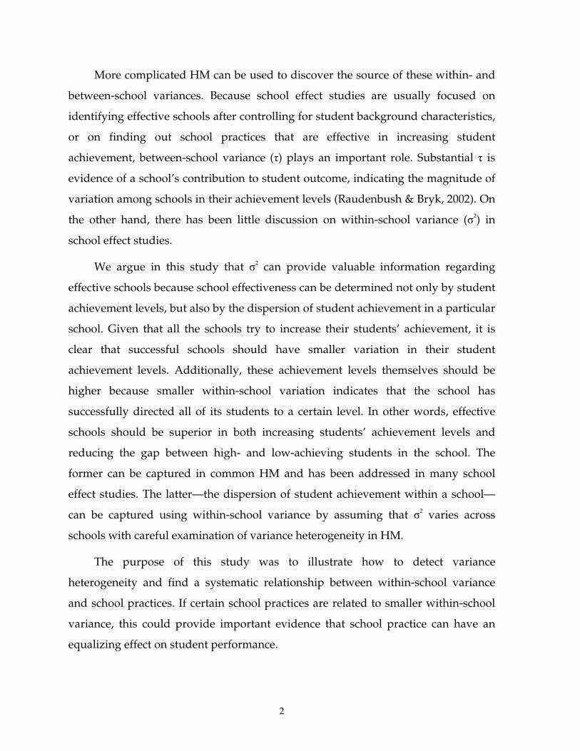
Abstract

Effective schools should be superior in both enhancing students’ achievement levels and reducing the gap between high- and low-achieving students in the school. However, the focus has been placed mainly on schools’ achievement levels in most school effect studies. In this article, we attend to the school-specific achievement dispersion as well as achievement level in determining effective schools. The achievement dispersion in a particular school can be captured by within-school variance in achievement (σ2). Assuming heterogeneous within-school variance across schools in hierarchical modeling, we identified school factors related to high achievement level and a small gap between high- and low-achieving students. Schools with a high achievement level tended to be more homogeneous in achievement dispersion, but even among schools with the same achievement level, schools varied in their achievement dispersion, depending on classroom practices.

One of the fundamental questions that most school effect studies have

continuously addressed is whether schools make a difference in student

achievement, and if so, how much of the student achievement can be attributable to

schools’ effort. Regarding this question, most researchers have agreed that schools

do have a measurable impact on student achievement, even though the source and

the magnitude of the school effect are still heavily debated (Rumberger & Palardy,

2003).

Using the basic Hierarchical Model (HM), one can successfully show how

much of the total variation in achievement comes from the student level (within-

school variance, σ2) and how much comes from the school level (between-school

variance, τ). Many studies have found that between-school variance is much smaller

than within-school variance. For example, using High School and Beyond (HS&B)

data, Lee and Bryk (1989) found that about 19% of the total variation in student

math achievement was attributable to school differences.

2

More complicated HM can be used to discover the source of these within- and

between-school variances. Because school effect studies are usually focused on

identifying effective schools after controlling for student background characteristics,

or on finding out school practices that are effective in increasing student

achievement, between-school variance (τ) plays an important role. Substantial τ is

evidence of a school’s contribution to student outcome, indicating the magnitude of

variation among schools in their achievement levels (Raudenbush & Bryk, 2002). On

the other hand, there has been little discussion on within-school variance (σ2) in

school effect studies.

We argue in this study that σ2 can provide valuable information regarding

effective schools because school effectiveness can be determined not only by student

achievement levels, but also by the dispersion of student achievement in a particular

school. Given that all the schools try to increase their students’ achievement, it is

clear that successful schools should have smaller variation in their student

achievement levels. Additionally, these achievement levels themselves should be

higher because smaller within-school variation indicates that the school has

successfully directed all of its students to a certain level. In other words, effective

schools should be superior in both increasing students’ achievement levels and

reducing the gap between high- and low-achieving students in the school. The

former can be captured in common HM and has been addressed in many school

effect studies. The latter—the dispersion of student achievement within a school—

can be captured using within-school variance by assuming that σ2 varies across

schools with careful examination of variance heterogeneity in HM.

The purpose of this study was to illustrate how to detect variance

heterogeneity and find a systematic relationship between within-school variance

and school practices. If certain school practices are related to smaller within-school

variance, this could provide important evidence that school practice can have an

equalizing effect on student performance.

3

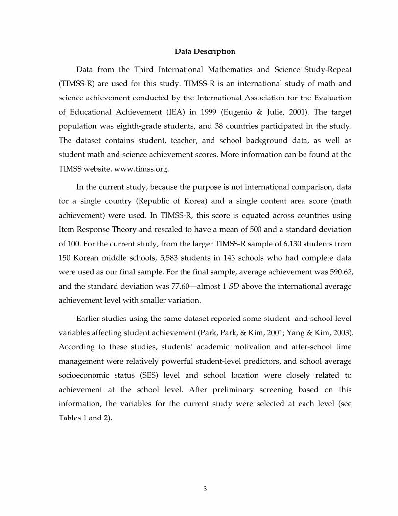
Data Description

Data from the Third International Mathematics and Science Study-Repeat

(TIMSS-R) are used for this study. TIMSS-R is an international study of math and

science achievement conducted by the International Association for the Evaluation

of Educational Achievement (IEA) in 1999 (Eugenio & Julie, 2001). The target

population was eighth-grade students, and 38 countries participated in the study.

The dataset contains student, teacher, and school background data, as well as

student math and science achievement scores. More information can be found at the

TIMSS website, www.timss.org.

In the current study, because the purpose is not international comparison, data

for a single country (Republic of Korea) and a single content area score (math

achievement) were used. In TIMSS-R, this score is equated across countries using

Item Response Theory and rescaled to have a mean of 500 and a standard deviation

of 100. For the current study, from the larger TIMSS-R sample of 6,130 students from

150 Korean middle schools, 5,583 students in 143 schools who had complete data

were used as our final sample. For the final sample, average achievement was 590.62,

and the standard deviation was 77.60—almost 1 SD above the international average

achievement level with smaller variation.

Earlier studies using the same dataset reported some student- and school-level

variables affecting student achievement (Park, Park, & Kim, 2001; Yang & Kim, 2003).

According to these studies, students’ academic motivation and after-school time

management were relatively powerful student-level predictors, and school average

socioeconomic status (SES) level and school location were closely related to

achievement at the school level. After preliminary screening based on this

information, the variables for the current study were selected at each level (see

Tables 1 and 2).

4

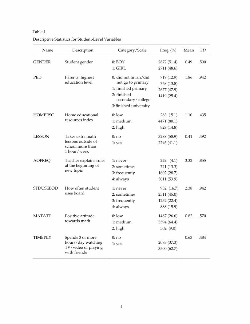
Table 1

Descriptive Statistics for Student-Level Variables

Name Description Category/Scale Freq. (%) Mean SD

GENDER Student gender 0: BOY 1: GIRL

2872 (51.4) 2711 (48.6)

0.49 .500

PED Parents’ highest education level

0: did not finish/did not go to primary

1: finished primary 2: finished

secondary/college 3: finished university

719 (12.9) 768 (13.8)

2677 (47.9) 1419 (25.4)

1.86 .942

HOMERSC Home educational resources index

0: low 1: medium 2: high

283 ( 5.1) 4471 (80.1) 829 (14.8)

1.10 .435

LESSON Takes extra math lessons outside of school more than 1 hour/week

0: no 1: yes

3288 (58.9) 2295 (41.1)

0.41 .492

AOFREQ Teacher explains rules at the beginning of new topic

1: never 2: sometimes 3: frequently 4: always

229 (4.1) 741 (13.3)

1602 (28.7) 3011 (53.9)

3.32 .855

STDUSEBOD How often student uses board

1: never 2: sometimes 3: frequently 4: always

932 (16.7) 2511 (45.0) 1252 (22.4) 888 (15.9)

2.38 .942

MATATT Positive attitude towards math

0: low 1: medium 2: high

1487 (26.6) 3594 (64.4) 502 (9.0)

0.82 .570

TIMEPLY Spends 3 or more hours/day watching TV/video or playing with friends

0: no 1: yes 2083 (37.3)

3500 (62.7)

0.63 .484

5

Table 2

Descriptive Statistics for School-Level Variables

Name Description Category/Scale Freq. (%) Mean SD

URBAN Urban schools 0: no 1: yes

69 (48.3) 74 (51.7)

0.52 .501

SUBURBAN Suburban schools 0: no 1: yes

89 (62.2) 54 (37.8)

0.38 .486

MPED School mean PED Continuous 1.85 .318

USEBOD How often teacher uses board

Continuous (1: never ~ 4: always)

3.05 .167

Note. PED = parents’ highest education level; USEBOD is entered for variance modeling.

For student background characteristics, student gender (GENDER), parents’ highest

education level (PED), and the home educational resources index (HOMERSC) were

used. HOMERSC is a composite variable that IEA calculated based on students’

responses regarding household possessions, such as computers, student’s own desk,

etc. For student’s experience outside school, extra math lessons outside school

(LESSON) and time spent on non-academic activities such as watching TV or

playing with friends (TIMEPLY) were selected. Student responses to the frequency

of teacher’s advance organizer use (AOFREQ) and how often students used the

board (STDUSEBOD) were selected to capture the impact of the classroom

experience. Finally, student’s positive attitude toward mathematics (MATATT) was

selected to check the impact of student motivation.

Some student-level variables are aggregated to the school level to measure

contextual effect and school practice effect. The school mean of parents’ education

level (MPED) can be used to measure the contextual effect of SES, which will be

discussed in the Results section. School location (rural, suburban or urban) is

entered as a dummy variable to estimate the location contrast.

6

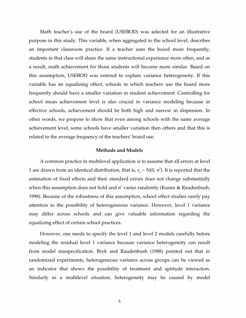
Math teacher’s use of the board (USEBOD) was selected for an illustrative

purpose in this study. This variable, when aggregated to the school level, describes

an important classroom practice. If a teacher uses the board more frequently,

students in that class will share the same instructional experience more often, and as

a result, math achievement for those students will become more similar. Based on

this assumption, USEBOD was entered to explain variance heterogeneity. If this

variable has an equalizing effect, schools in which teachers use the board more

frequently should have a smaller variation in student achievement. Controlling for

school mean achievement level is also crucial in variance modeling because in

effective schools, achievement should be both high and narrow in dispersion. In

other words, we propose to show that even among schools with the same average

achievement level, some schools have smaller variation then others and that this is

related to the average frequency of the teachers’ board use.

Methods and Models

A common practice in multilevel application is to assume that all errors at level

1 are drawn from an identical distribution, that is, rij ~ N(0, σ2). It is reported that the

estimation of fixed effects and their standard errors does not change substantially

when this assumption does not hold and σ2 varies randomly (Kasim & Raudenbush,

1998). Because of the robustness of this assumption, school effect studies rarely pay

attention to the possibility of heterogeneous variance. However, level 1 variance

may differ across schools and can give valuable information regarding the

equalizing effect of certain school practices.

However, one needs to specify the level 1 and level 2 models carefully before

modeling the residual level 1 variance because variance heterogeneity can result

from model misspecification. Bryk and Raudenbush (1988) pointed out that in

randomized experiments, heterogeneous variance across groups can be viewed as

an indicator that shows the possibility of treatment and aptitude interaction.

Similarly in a multilevel situation, heterogeneity may be caused by model

7

misspecification, either by omitting an important level 1 variable or by erroneously

fixing a level 1 predictor slope (Raudenbush & Bryk, 2002). However, it should be

pointed out also that modeling heterogeneous variance does not compensate for

model misspecification. Heterogeneous variance only indicates the possibility of the

misspecification of mean function, and finding a systematic relationship between

level 1 variance and school characteristics does not reduce the bias in fixed effects

estimates caused by the misspecification.

If we find heterogeneity in level 1 variances after establishing the final model,

the next step is to model this residual variance to see whether there is a systematic

pattern. Variance homogeneity can be tested by computing chi-square statistics for

standardized dispersion (see Raudenbush & Bryk, 2002, pp. 263-265, for example).

After checking the variance heterogeneity, the next step would be to examine the

distribution of variances and set up a regression model to find a relationship with

school characteristics. Our specific models and their development are discussed

below.

First, we fit a fully unconditional model to decompose the total variance into

student and school levels. The results showed that the grand mean math

achievement was 590.22, between-school variance was 379.81, and within-school

variance was 5652.50. These results indicate that only about 6.3% of the total

variance is attributable to school differences and the remaining 93.7% of the total

variance comes from individual differences among students within schools. Also,

the test of homogeneous variance rejected the homogeneous variance assumption.

The results are summarized in Table 3.

As noted above, variance heterogeneity could occur by omission of an

important level 1 variable or by fixing the level 1 slope that is in fact varying across

schools. To make sure this was not the case, we fit a series of HM as described below.

We entered all eight level 1 variables were entered in the model and random

variation was allowed only for intercept (Model 1, Random intercept ANCOVA

8

Table 3

Results From Unconditional Model

Fixed effect Estimate SE T-ratio p-value

Grand mean 590.22 1.912 308.64 0.000

Variance components Estimate Chi-square p-value

Between-school variance 379.81 507.70 0.000

Within-school variance 5652.50

Homogeneity of level 1 var. test 177.63 0.02

model). The level 1 homogeneous variance test for this model still rejected the null

hypothesis that level 1 residual errors are drawn from identical distribution.

Following Raudenbush and Bryk (2002), we checked the variability of level 1 slopes

across schools and found that LESSON, AOFREQ, and TIMEPLY effects varied

significantly across schools. Therefore, in Model 2, we allowed random variation for

intercept and the three slopes. Also in this model, school location and the average

education level of parents (MPED) were entered to model the intercept (adjusted

grand mean). The chi-square test for this model also rejected the homogeneous

level 1 variance assumption. In Model 3, school location and MPED were entered for

the three random slopes specified in Model 2, as well as for the intercept. This was

the final mean structure model. The homogeneous variance assumption was again

rejected in this model. Therefore, we moved to the heterogeneous variance model,

keeping the mean structure as specified in Model 3. Results for Models 1 through 3

are summarized in Table 4. The statistics package HLM5 was used to fit the three

models described above.

Table 4

Result Summary for Model 1 to Model 3 With Homogeneity of Level 1 Variance Test

Model 1 Model 2 Model 3 Fixed effects Estimate SE T (p-value) Estimate SE T (p-value) Estimate SE T (p-value)

For adjusted grand mean, β0j Adjusted grand mean, γ00 590.46 1.49 396.24 (0.00) 590.41 1.31 450.69(0.00) 590.94 1.32 447.67 (0.00) Urban schools, γ01 19.73 5.40 3.66 (0.00) 18.44 5.5 3.34 (0.00) Suburban schools, γ02 16.46 5.41 3.04 (0.00) 14.69 5.49 2.67 (0.00) School average parents ed. level, γ03 11.84 4.21 2.81 (0.00) 14.92 4.46 3.33 (0.00)

Gender contrast, γ10 –3.33 3.06 –1.08 (0.27) –2.93 3.10 –0.95 (0.35) –2.77 3.14 –0.88 (0.37) Parent highest ed. slope, γ20 6.92 1.22 5.68 (0.00) 6.24 1.23 5.09 (0.00) 6.12 1.23 4.94 (0.00) Home resource slope, γ30 32.86 2.64 12.44 (0.00) 32.02 2.64 12.11 (0.00) 32.16 2.63 12.21 (0.00) For extra outside lesson slope, β4j Adjusted mean effect, γ40 21.73 2.30 9.44 (0.00) 20.62 2.34 8.81 (0.00) 21.22 2.34 9.06 (0.00) Urban schools, γ41 –10.56 9.66 –1.09 (0.27) Suburban schools, γ42 –4.68 9.78 –0.47 (0.63) School average parents ed. level, γ43 –15.21 7.21 –2.10 (0.03)

For “teacher explains rules at the beginning” slope, β5j Adjusted mean effect, γ50 14.94 1.33 11.22 (0.00) 14.75 1.32 11.17 (0.00) 14.53 1.3 11.17 (0.00) Urban schools, γ51 2.44 7.05 0.34 (0.72) Suburban schools, γ52 2.62 7.05 0.37 (0.71) School average parents ed. level, γ53 –10.25 4.98 –2.05 (0.03)

Students’ board use slope, γ60 6.48 1.12 5.78 (0.00) 6.61 1.11 5.95 (0.00) 6.63 1.09 6.05 (0.00) Positive attitude toward math slope, γ70 27.38 1.68 16.24 (0.00) 27.73 1.69 16.40 (0.00) 27.74 1.69 16.41 (0.00) For “spend more than 3 hrs. playing/TV” slope, β8j Adjusted mean effect, γ80 –12.34 2.05 –5.99 (0.00) –13.18 2.05 –6.42 (0.00) –13.24 2.01 –6.57 (0.00) Urban schools, γ81 –13.92 7.49 –1.85 (0.06) Suburban schools, γ82 –14.27 7.49 –1.90 (0.05) School average parents ed. level, γ83 4.29 6.53 0.65 (0.51) Model 1 Model 2 Model 3

Variance components Estimate Chi-sq p-value Estimate Chi-sq p-value Estimate Chi-sq p-value Within 4417.46 4312.19 4313.77 Between (intercept, τ00) 205.83 397.40 0.000 135.33 284.60 0.000 133.57 283.13 0.000 Between (extra lesson slope, τ44) 198.45 184.12 0.009 169.02 174.50 0.019 Between (teacher explain rules slope, τ55) 65.51 196.90 0.002 61.75 189.59 0.003 Between (3 or more hrs playing slope, z88) 93.86 169.27 0.052 88.07 166.76 0.048 Homogeneity of level-1 var. test 174.37 0.033 175.30 0.030 183.37 0.010

9

10

In the heterogeneous variance model, level 1 variance is assumed to vary across

schools. Therefore, we posed school-specific within-school residual variance, 2jσ for

school j. The first step in our variance modeling was to check whether schools with

higher achievement levels had smaller 2jσ or vice versa. For this we used a latent

variable regression technique (Raudenbush & Bryk, 2002; Seltzer, Choi, & Thum,

2003), which essentially uses the unobserved latent variable (adjusted school mean,

β0 in this study) as a predictor for 2jσ (Model 4).

An effective school, according to our definition, is a school with high

achievement and small variation in achievement among its students. Therefore, to

determine school effectiveness it is crucial to examine school characteristics and

practices that can reduce student achievement variation even after controlling for

school mean achievement. Our final model (Model 5) illustrates this point. Both β0

(average achievement level) and USEBOD were entered to predict jσ . Therefore, a

significant USEBOD effect will indicate that among schools with the same

achievement level, schools in which teachers use the board more frequently have a

smaller gap between high- and low-achieving students. Specification of the final

models are shown in equations (1.1), (1.2), and (1.3).

Note that at the student level, PED, HOMERSC and LESSON are grand mean

centered and other level 1 variables are group mean centered. These grand mean

centered variables are related to either SES or academic input from outside the

school and would be better controlled for in a school effects study because variation

in student achievement due to these variables cannot be attributable to school

practice. This is especially true if, for example, a school’s average achievement is

high because most of its students take extra lessons outside school; then it would be

more reasonable to adjust for the effect of these outside lessons when we evaluate

the school’s performance. By virtue of this level 1 centering, β0j now represents the

average math achievement of school j, holding constant parents’ education, home

educational resources, and extra math lessons. β1j through β8j capture the effect of

11

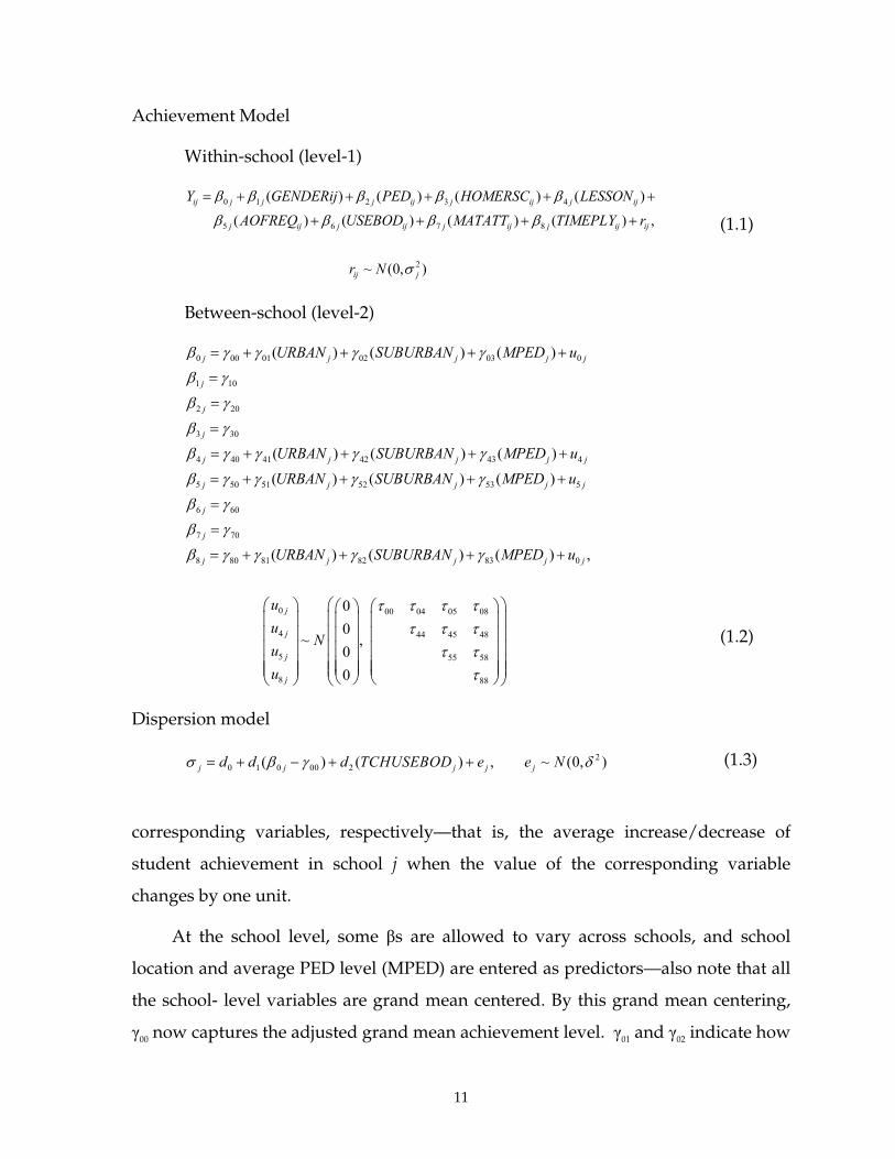
Achievement Model

Within-school (level-1)

0 1 2 3 4

5 6 7 8

2

( ) ( ) ( ) ( )

( ) ( ) ( ) ( ) ,

~ (0, )

ij j j j ij j ij j ij

j ij j ij j ij j ij ij

ij j

Y GENDERij PED HOMERSC LESSON

AOFREQ USEBOD MATATT TIMEPLY r

r N

β β β β β

β β β β

σ

= + + + + +

+ + + + (1.1)

Between-school (level-2)

0 00 01 02 03 0

1 10

2 20

3 30

4 40 41 42 43 4

5 50 51 52 53 5

6 60

7 70

8 80 81

( ) ( ) ( )

( ) ( ) ( )

( ) ( ) ( )

(

j j j j j

j

j

j

j j j j j

j j j j j

j

j

j j

URBAN SUBURBAN MPED u

URBAN SUBURBAN MPED u

URBAN SUBURBAN MPED u

URBAN

β γ γ γ γ

β γ

β γ

β γ

β γ γ γ γ

β γ γ γ γ

β γ

β γ

β γ γ

= + + + +

=

=

=

= + + + +

= + + + +

=

=

= + 82 83 0

0 00 04 05 08

4 44 45 48

5 55 58

8 88

) ( ) ( ) ,

00

~ ,00

j j j

j

j

j

j

SUBURBAN MPED u

uu

Nuu

γ γ

τ τ τ ττ τ τ

τ ττ

+ + +

(1.2)

Dispersion model

20 1 0 00 2( ) ( ) , ~ (0, )j j j j jd d d TCHUSEBOD e e Nσ β γ δ= + − + + (1.3)

corresponding variables, respectively—that is, the average increase/decrease of

student achievement in school j when the value of the corresponding variable

changes by one unit.

At the school level, some βs are allowed to vary across schools, and school

location and average PED level (MPED) are entered as predictors—also note that all

the school- level variables are grand mean centered. By this grand mean centering,

γ00 now captures the adjusted grand mean achievement level. γ01 and γ02 indicate how

12

much urban and suburban schools did better/worse than the grand mean. γ03

requires special attention for interpretation—this fixed effect captures the contextual

effect of parents’ education level. Because we already have adjusted for PED at the

student level, γ03 captures, among students with similar parental education levels,

how much extra advantage students receiving in schools with a one-unit-higher

mean PED level.

Because preliminary analysis found no variability in GENDER, PED, and

HOMERSC effects across schools, these slopes are fixed at the school level. Therefore,

γ10, γ20, and γ30 show overall gender difference (γ10), PED effect (γ20), and HOMERSC

effect (γ30), respectively. LESSON and AOFREQ slopes showed significant variability

across schools, and these slopes are set to vary randomly across schools. γ40 captures

the overall extra lessons effect. γ41 through γ43 show whether extra lessons are more

effective in urban schools (γ41), suburban schools (γ42) or in schools with higher

average SES levels (γ43). γ50 through γ53 can be interpreted the same way as γ40 through

γ43. USEBOD and MATATT slopes are also fixed across schools. Therefore, γ60 and γ70

represent the overall USEBOD effect (γ60) and MATATT effect (γ70), respectively. γ80 is

the overall achievement difference between students spending 3 or more hours

playing/watching TV and students spending less than 3 hours in those non-

academic activities. γ81 and γ82 show whether this difference is larger or smaller in

urban schools (γ81) and suburban schools (γ82), and, if so, how much. Finally, γ83

shows whether the gap gets wider or narrower depending on school mean SES level.

As we specified the level 1 model (equation 1.1) such that each school has its

own within-school residual variance ( 2jσ ), 2

jσ now captures the dispersion of

student achievement in school j after explaining out the effect of student-level

variables.

13

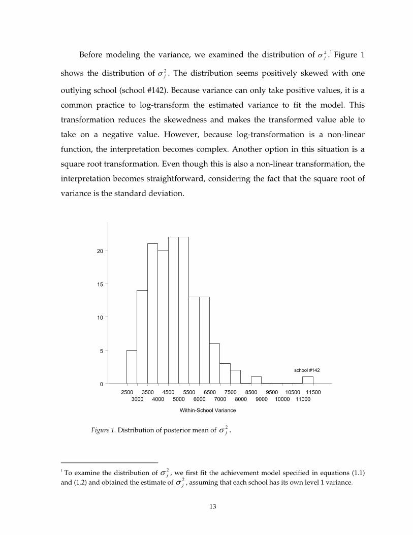
Before modeling the variance, we examined the distribution of 2jσ .1 Figure 1

shows the distribution of 2jσ . The distribution seems positively skewed with one

outlying school (school #142). Because variance can only take positive values, it is a

common practice to log-transform the estimated variance to fit the model. This

transformation reduces the skewedness and makes the transformed value able to

take on a negative value. However, because log-transformation is a non-linear

function, the interpretation becomes complex. Another option in this situation is a

square root transformation. Even though this is also a non-linear transformation, the

interpretation becomes straightforward, considering the fact that the square root of

variance is the standard deviation.

Figure 1. Distribution of posterior mean of 2jσ .

1 To examine the distribution of 2

jσ , we first fit the achievement model specified in equations (1.1) and (1.2) and obtained the estimate of 2

jσ , assuming that each school has its own level 1 variance.

25003000

35004000

45005000

55006000

65007000

75008000

85009000

950010000

10500 11000

11500

Within-School Variance

0

5

10

15

20

school #142

14

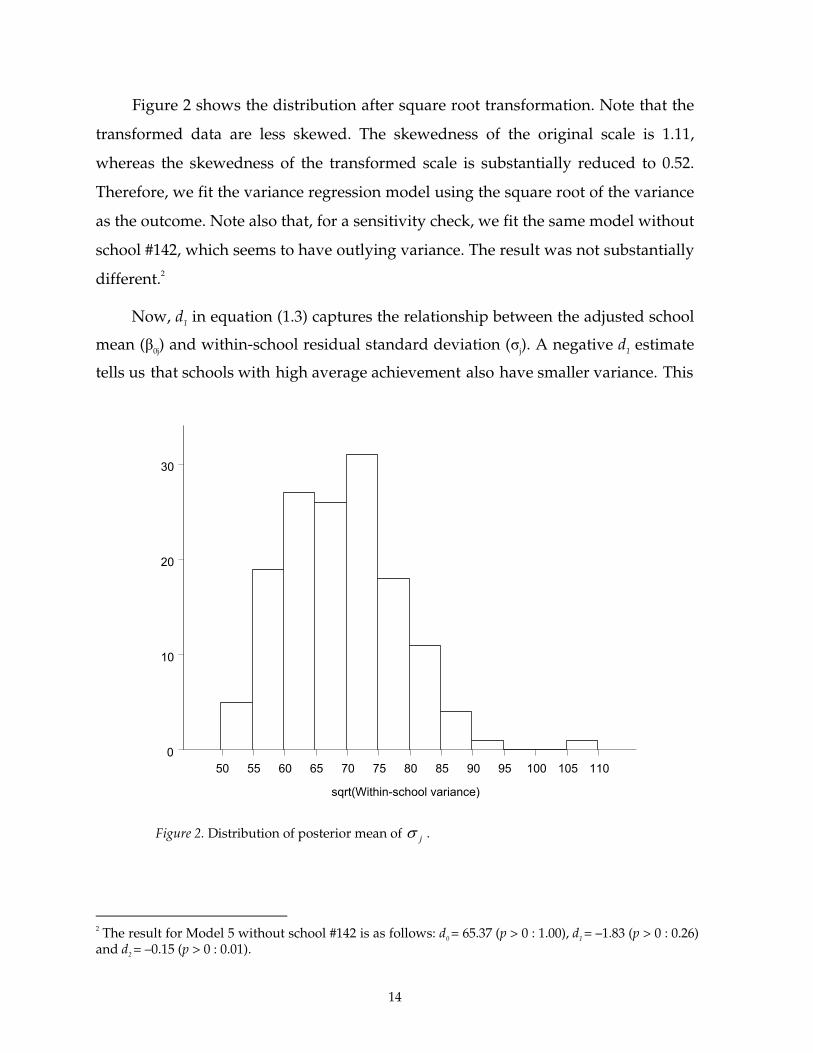
Figure 2 shows the distribution after square root transformation. Note that the

transformed data are less skewed. The skewedness of the original scale is 1.11,

whereas the skewedness of the transformed scale is substantially reduced to 0.52.

Therefore, we fit the variance regression model using the square root of the variance

as the outcome. Note also that, for a sensitivity check, we fit the same model without

school #142, which seems to have outlying variance. The result was not substantially

different.2

Now, d1 in equation (1.3) captures the relationship between the adjusted school

mean (β0j) and within-school residual standard deviation (σj). A negative d1 estimate

tells us that schools with high average achievement also have smaller variance. This

Figure 2. Distribution of posterior mean of jσ .

2 The result for Model 5 without school #142 is as follows: d0 = 65.37 (p > 0 : 1.00), d1 = –1.83 (p > 0 : 0.26) and d2 = –0.15 (p > 0 : 0.01).

50 55 60 65 70 75 80 85 90 95 100 105 110 sqrt(Within-school variance)

0

10

20

30

15

could possibly occur due to a ceiling effect or other successful instructional factors.

Note also that β0j is centered around its grand mean (γ00) so that the intercept (d0) can

represent the average within-school variation of 143 schools. d2 in equation (1.3)

shows whether teachers’ frequent use of the board can reduce σj , even after

controlling for school mean achievement. USEBOD is also grand mean centered.

Results for this variance model (Models 4 and 5) are summarized in Table 5. Note

that Model 4 and Model 5 are analyzed using a fully Bayesian approach via Gibbs

Sampler implemented in WinBUGS (Spiegelhalter, Thomas, Bets, & Lunn, 2003).

Results

The results for Models 1 through 4 are preliminary analyses showing the step-

by- step procedure. Therefore, we will discuss only the results for the final model

(Model 5). General fixed effects in the mean structure model (achievement model)

will be discussed first; then, more importantly, the result for the variance model

(dispersion model) will be discussed.

Achievement Model

After adjusting for the effect of parents’ education level, home educational

resources, and extra outside school math lessons, the grand mean estimate is 591 (γ00).

The mean for urban schools was 18.03 points above average (γ01). The mean for

suburban schools was 14.21 points above average (605.21). The contextual effect of

the aggregate parent education level was 15.33 (γ03). Because the standard deviation

of MPED is .318 (see Table 2), if we compare two students with the same parental

education level in two schools differing by 1 SD MPED level, we would expect the

student in the school in the 1 SD higher MPED level to show 4.87 points (i.e.,

15.33*.318=4.87) higher achievement than the other student in the other school.

We found no gender difference in math achievement (γ10). Parents’ education

level did make a difference in student math achievement (γ20). Note that the possible

difference in math achievement between students in the lowest parents’ education

level and the highest is 18.54 (i.e., 6.183*3=18.54). However, as mentioned above,

16

Table 5

Result Summary for Heterogeneous Variance Modeling

Model 4 Model 5

Mean (SE)

95% interval

Prob. >0

Mean (SE)

95% interval

Prob. >0

Mean model

For adjusted grand mean, β0j Adjusted grand mean, γ00 591.0 (1.36) 588.4, 593.7 1.000 591.0 (1.36) 588.3, 593.7 1.000

Urban schools, γ01 18.08 (5.31) 7.55, 28.38 1.000 18.26 (5.35) 7.69, 28.65 1.000

Suburban schools, γ02 14.27 (5.27) 3.80, 24.45 0.996 14.55 (5.27) 4.18, 24.78 0.997

School average parents ed. level, γ03 15.45 (4.92) 5.87, 25.12 0.999 15.28 (4.93) 5.63, 24.96 0.999

Gender contrast, γ10 –2.60 (3.13) –8.74, 3.55 0.203 –2.44 (3.12) –8.57, 3.68 0.217

Parent highest ed. slope, γ20 6.15 (1.20) 3.79, 8.49 1.000 6.16 (1.20) 3.82, 8.51 1.000

Home resource slope, γ30 31.84 (2.61) 26.71, 36.95 1.000 31.89 (2.61) 26.78, 37.00 1.000

For extra outside lesson slope, β4j

Adjusted average effect, γ40 21.15 (2.35) 16.51, 25.75 1.000 21.01 (2.34) 16.42, 25.60 1.000

Urban schools, γ41 –10.99 (9.52) –30.02, 7.53 0.121 10.86 (9.63) –30.03, 7.99 0.128

Suburban schools, γ42 –4.99 (9.42) –23.54, 13.46 0.299 –4.81 (9.58) –23.60, 14.10 0.305

School average parents ed. level, γ43 –15.33 (8.05) –31.01, 0.49 0.029 14.94 (7.99) –30.69, 0.85 0.031

For “Adv. Org. frequency” slope, β5j

Adjusted average effect, γ50 14.61 (1.33) 12.01, 17.24 1.000 14.63 (1.33) 12.02, 17.25 1.000

Urban schools, γ51 2.32 (5.22) –7.71, 12.63 0.669 2.73 (5.08) –7.19, 12.67 0.706

Suburban schools, γ52 2.27 (5.13) –7.50, 12.38 0.666 2.74 (5.03) –7.15, 12.61 0.705

School average parents ed. level, γ53 –10.53 (4.63) –19.59, –1.49 0.011 10.68 (4.61) –19.76, –1.64 0.011

Students’ board use slope, γ60 6.63 (1.04) 4.61, 8.67 1.000 6.65 (1.04) 4.61, 8.69 1.000

Positive attitude toward math slope, γ70 27.72 (1.63) 24.52, 30.92 1.000 27.74 (1.63) 24.55, 30.94 1.000

For “play time” slope, β8j

Adjusted average effect, γ80 –13.41 (2.16) –17.65, –9.19 0.000 13.43 (2.19) –17.74, –9.14 0.000

Urban schools, γ81 –13.71 (8.54) –30.11, 3.70 0.056 13.95 (8.39) –30.63, 2.35 0.047

Suburban schools, γ82 –13.70 (8.46) –30.10, 3.30 0.054 13.76 (8.30) –30.26, 2.24 0.048

School average parents ed. level, γ83 3.81 (7.51) –10.83, 18.58 0.693 4.15 (7.42) –10.19, 18.90 0.712

Variance model for σj

Average within-school residual SD, d0 65.62 (0.74) 64.18, 67.10 1.000 65.62 (0.73) 64.21, 67.09 1.000

School mean achievement slope, d1 –0.14 (0.06) –0.27, –0.02 0.012 –0.13 (0.06) –0.25, –0.01 0.019 Teachers’ board use slope, d2 –8.57 (4.31) –16.92, –0.05 0.024

Random effects variance matrix (T)

−−

−−−

2.13306.1132.6530.3543.127.20873.1420.773.573.140

−−

−−−

7.13282.1069.6772.3525.115.20223.1368.838.548.139

17

depending on the school’s average PED level, this gap can get wider or narrower.

Home resources had a strong effect on math achievement (the effect estimate is 31.81,

γ30). Because this variable is coded 0 to 2, the expected difference between students

with low and high home resources is 63.62 (i.e., 31.81*2=63.62). However, note that

most of the students (80%, Table 1) had a medium home resources level.

Students who took extra math lessons outside school more than 1 hour per

week scored about 21 points better on average (γ40). However, students in high

MPED level schools got less benefit from extra lessons (γ43). Students’ frequent

exposure to teacher’s advance organizer (AO) did increase students’ achievement

(γ50). Also, in high MPED level schools, this AO effect was smaller than average (γ53).

For example, the average AO effect was 14.60, and the AO effect for schools at 2 SD

above the average MPED level was 7.77 (14.60–(2*.318*10.74)=7.77). The reason for

extra lessons and AO being less effective in high SES schools requires further

investigation. However, one possible explanation might be that in high SES schools,

students could have various other educational resources and different environments

(e.g., peer/family pressure and better classroom instruction) not specified in this

study that contribute to student achievement, compared to low SES schools, in

which students have fewer options to take extra lessons, for example.

Students’ more frequent board use was positively associated with math

achievement (γ60). Also, students reporting a high positive attitude toward math

showed higher math achievement (γ70). These effects did not vary significantly across

schools.

γ80 shows that students who spend more than 3 hours doing non-academic

activities after school scored 13.46 points less on average. Interestingly, this gap gets

wider in both urban (γ81) and suburban schools (γ82). In urban schools, the gap

became 27.49 (–13.46 – 14.03 = –27.49), and in suburban schools, the gap is 27.46

(–13.46 – 14.0 = –27.46). In general, the gap between the two activity groups was

smaller in rural schools than in nonrural schools.

18

Dispersion Model

Variance model results (d0 to d2 in Model 5; see Table 5) tell us that average jσ

was 65.61(d0). School mean achievement was significantly related to smallerjσ (d1 =

–.13). d2, the effect of USEBOD, was –8.57 with prob. > 0 equal to 0.024. This shows

that 97.6% of the posterior distribution of d2 falls below zero—strong evidence of a

negative relationship. Therefore, even after adjusting for school mean, using the

board frequently in classroom instruction seems to reduce the achievement gap

within schools. Table 2 shows that teachers already used the board frequently in the

classroom (mean = 3.05, SD = .167). We expect a 1.43 point (8.57*.167 = 1.43)

decrease in jσ when USEBOD increases by 1 SD. If we compare two schools with a 2

SD difference in USEBOD and the same achievement level, the school with higher

USEBOD will have about 11.2 points smaller 95% interval.3 This interval can

alternatively be interpreted as the gap between upper and lower 2.5% achievement

level in a school. Therefore, the gap between the upper and lower 2.5% students will

also be smaller by 11.2 points in schools with 2 SD above the USEBOD level. This

variance model result is summarized in Figure 3. Each bar in Figure 3 represents the

predicted 95% achievement range in a school.

As noted before, this can be interpreted as the achievement gap between the

highest and lowest 2.5% of students in a school. For Figure 3, we chose three

achievement levels (2 SD below average, average, and 2 SD above average), and

within each achievement level, we selected three USEBOD levels (2 SD below

average, average, and 2 SD above average). This figure clearly shows that high-

achievement schools have a smaller gap, and among schools with the same

achievement level, high USEBOD schools have an even smaller gap.

3 The 95% interval, which captures the middle 95% of the predicted achievement distribution in a school, can be calculated as 0j± 1.96* jσ . This interval becomes smaller in schools with high achievement or with higher USEBOD level because jσ becomes smaller in these schools.

19

Summary and Implications

Our results can be summarized as follows:

1. Student background characteristics, such as family SES level and home

educational resources, do affect student achievement, and the magnitude of

these effects is constant across schools, regardless of school characteristics.

2. Students’ experiences outside school, such as extra lessons and amount of

playtime, are significantly associated with student achievement level.

However, the magnitude of these effects varies depending on which school

a student attends. In rural schools, after-school playtime does not affect

low (=552.02) medium (=590.22) high (=628.42)

400

450

500

550

600

650

700

750

800

teachers’ board use: lowteachers’ board use: mediumteachers’ board use: high

Score

Predicted score forupper 2.5% student

Predicted mean

Predicted score forupper 2.5% student

School Mean Achievement Figure 3. Comparing achievement gap between high- and low-achieving students in schools with different achievement levels and USEBOD levels.

20

student achievement, in contrast to nonrural schools. Also, the effect of

extra after-school lessons is magnified in low SES schools.

3. Students’ classroom experience, such as teacher’s advance organizer use

and students’ board use, is positively related to student achievement. This

is an especially important point regarding school effects because classroom

experience is under the control of the individual school. This result shows

that schools’ practice, not the context, can increase student achievement

level.

4. School context and background characteristics also affect student

achievement in school. Rural schools showed substantially lower

achievement levels than nonrural schools. Also, students in high SES

schools achieved more compared to students with the same SES level in

lower SES schools.

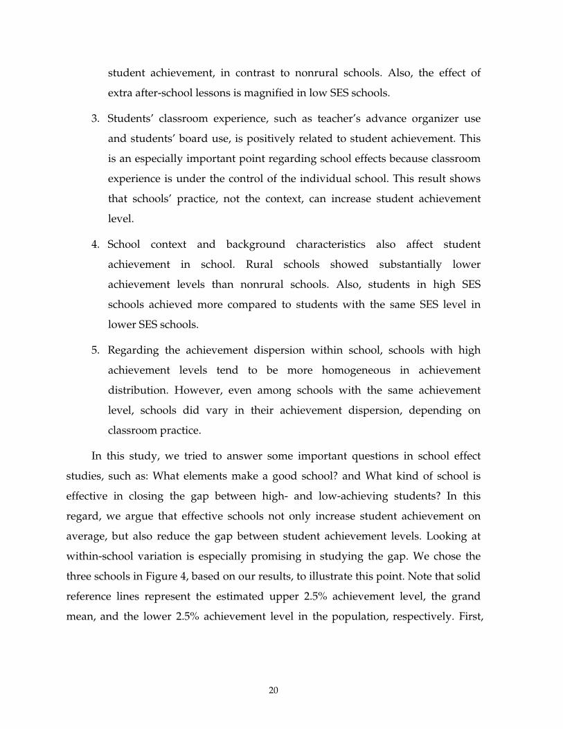
5. Regarding the achievement dispersion within school, schools with high

achievement levels tend to be more homogeneous in achievement

distribution. However, even among schools with the same achievement

level, schools did vary in their achievement dispersion, depending on

classroom practice.

In this study, we tried to answer some important questions in school effect

studies, such as: What elements make a good school? and What kind of school is

effective in closing the gap between high- and low-achieving students? In this

regard, we argue that effective schools not only increase student achievement on

average, but also reduce the gap between student achievement levels. Looking at

within-school variation is especially promising in studying the gap. We chose the

three schools in Figure 4, based on our results, to illustrate this point. Note that solid

reference lines represent the estimated upper 2.5% achievement level, the grand

mean, and the lower 2.5% achievement level in the population, respectively. First,

21

School ID

400

450

500

550

600

650

700

750

800

20 21142

Score

Grand mean(=591)

School #20mean = 606.20high 2.5% = 728.39low 2.5% = 484.01range = 244.38

School #21mean = 572.20high 2.5% = 715.59low 2.5% = 428.81range = 286.78

School #142mean = 603.00high2.5% = 750.61low 2.5% = 455.39range = 295.22

Upper 2.5%(=719.62)

Lower 2.5%(=462.38)

Figure 4. Contrasting three type of schools: high achievement and small gap (#20); high achievement and large gap (#142); and low achievement and large gap (#21).

schools #20 and #142 have similar mean achievement levels (606 and 603). However,

if we compare the predicted gap between the upper and lower 2.5% of students in

the two schools, we see that the gap is about 50 points smaller in school #20.

Therefore, in terms of closing the gap, school #20 is more effective than school #142.

School #21 is an example of a less effective school in dispersion as well as

achievement, that is, low achievement and large gap. (See Appendix for estimated

means and 95% intervals for all 143 sample schools.)

As exemplified above, the advantage of variance modeling is that we can

actually calculate the gap between any two achievement percentile scores within a

school (for example, 25% and 75%), and this can be used as a school indicator along

with school performance level. This study also has an important implication

regarding the No Child Left Behind (NCLB) Act (2002) in that closing the gap is one

of NCLB’s main concerns. In particular, we can study the school characteristics or

practices that reduce or magnify the gap and use the information for school reform

22

to direct as many students as possible towards the achievement goal. Also, for

evaluation purposes, we can utilize more information from large-scale assessment

data to identify effective schools.

23

References

Bryk, A. S., & Raudenbush, S. W. (1988). Heterogeneity of variance in experimental studies: A challenge to conventional interpretations. Psychological Bulletin, 104, 396-404.

Eugenio, J. G., & Julie, A. M. (2001). TIMSS 1999 user guide for the international database. Boston: Boston College, Lynch School of Education, International Study Center.

Lee, V. E., & Bryk, A. S. (1989). A multilevel model of the social distribution of high school achievement. Sociology of Education, 62, 172-192.

Kasim, R., & Raudenbush, S. W. (1998). Application of Gibbs sampling to nested variance components models with heterogeneous within-group variance. Journal of Educational and Behavioral Statistics, 23, 93-116.

No Child Left Behind Act of 2001, Pub. L. No. 107-110, 115 Stat. 1425 (2002).

Park, D., Park, J., & Kim, S. (2001). The effects of school and student background variables on math and science achievements in middle schools. Journal of Educational Evaluation, 14, 127-149.

Raudenbush, S. W., & Bryk, A. S. (2002). Hierarchical linear models: Applications and data analysis methods (2nd ed.). Newbury Park, CA: Sage.

Rumberger, R. W., & Palardy, G. J. (2003). Multilevel models for school effectiveness research. In D. Kaplan (Ed.), Handbook of quantitative methodology for the social sciences (pp. 235-258). Thousand Oaks, CA: Sage.

Seltzer, M., Choi, K., & Thum, Y. (2003). Examining relationship between where students start and how rapidly they progress: Using new developments in growth modeling to gain insight into the distribution of achievement within schools. Education Evaluation and Policy Analysis, 25, 263-286.

Spiegelhalter, D., Thomas, A., Bets, N., & Lunn, D. (2003). WinBUGS: windows version of Bayesian inference using Gibbs sampling, version 1.4, User manual. Cambridge, UK: University of Cambridge, MRC Biostatistics Unit.

Yang, J., & Kim, K. (2003). Effects of middle school organization on academic achievement in Korea: An HLM analysis of TIMSS-R. Korean Journal of Sociology of Education, 13, 165-184.

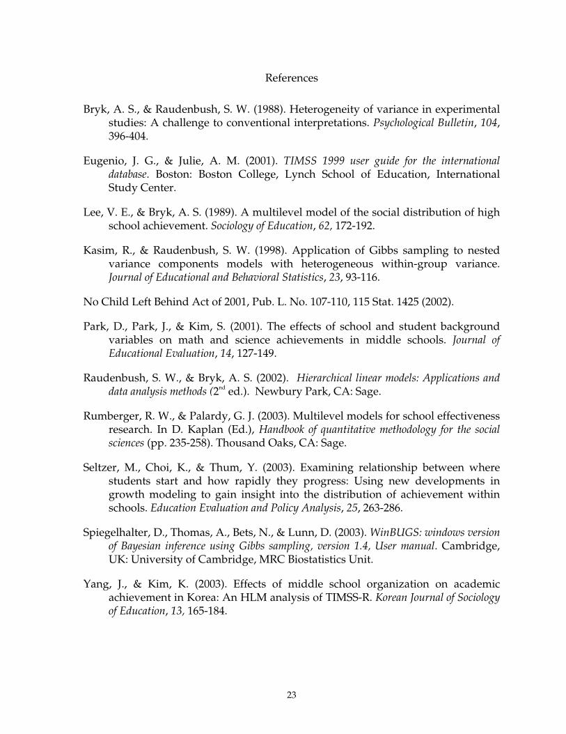
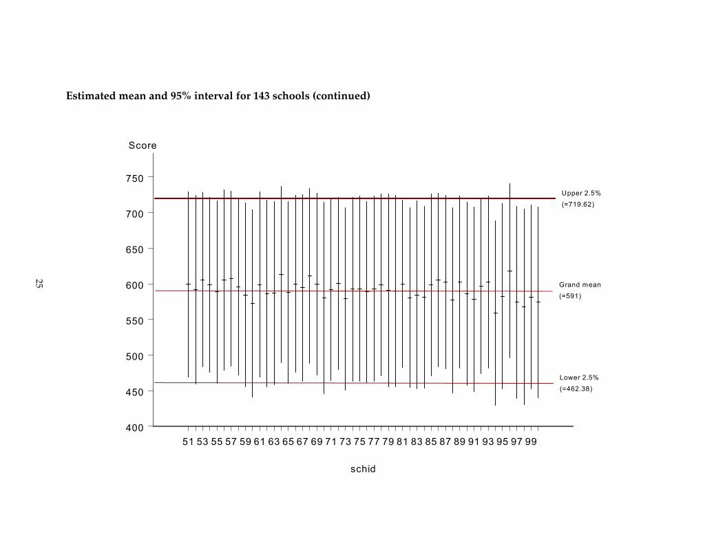
APPENDIX

Estimated mean and 95% document interval for 143 schools

12

34

56

78

910

1112

1314

1516

1718

1920

2122

2324

2526

2728

2930

3132

3334

3536

3738

3940

4142

4344

4546

4748

4950

schid

400

450

500

550

600

650

700

750

Score

Grand mean(=591)

Upper 2.5%(=719.62)

Lower 2.5%(=462.38)

24

Estimated mean and 95% interval for 143 schools (continued)

51 53 55 57 59 61 63 65 67 69 71 73 75 77 79 81 83 85 87 89 91 93 95 97 99

schid

400

450

500

550

600

650

700

750

Score

Grand mean(=591)

Upper 2.5%(=719.62)

Lower 2.5%(=462.38)

25

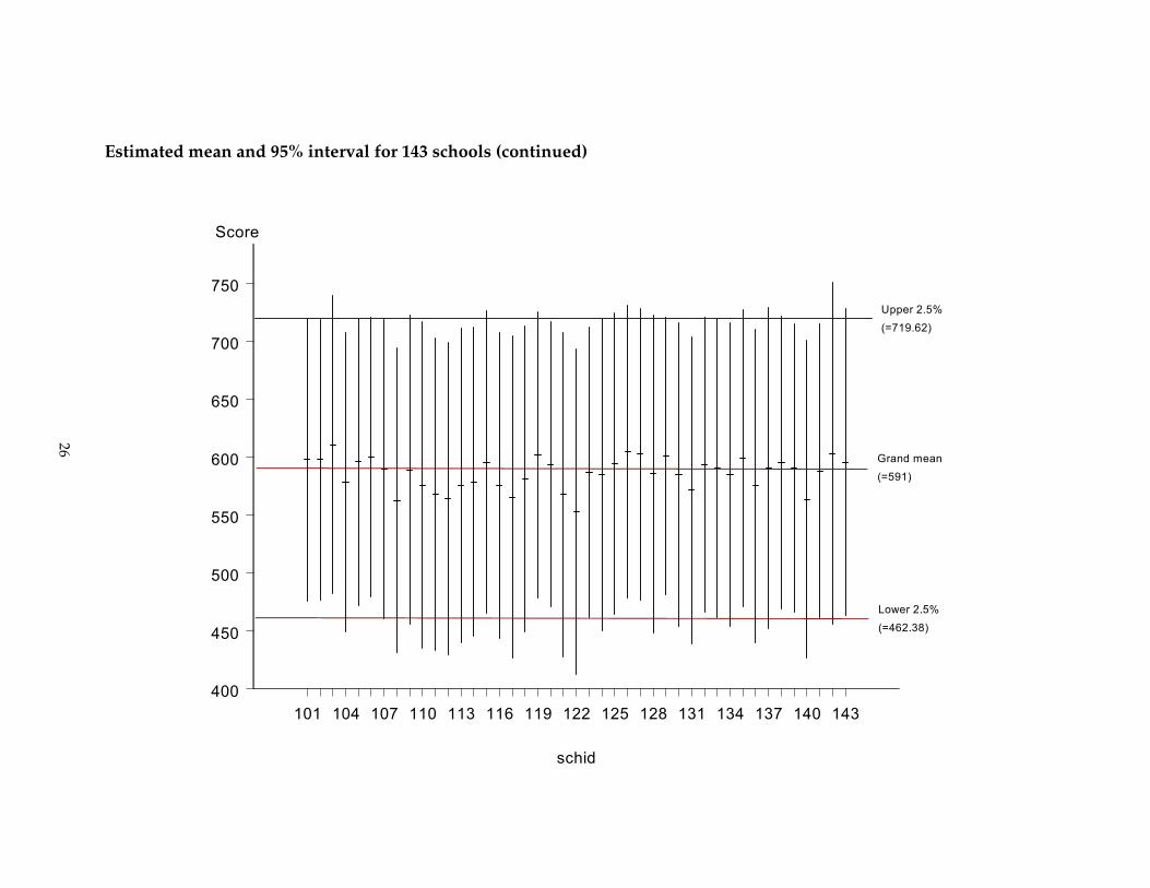
Estimated mean and 95% interval for 143 schools (continued)

101 104 107 110 113 116 119 122 125 128 131 134 137 140 143

schid

400

450

500

550

600

650

700

750

Score

Grand mean(=591)

Upper 2.5%(=719.62)

Lower 2.5%(=462.38)

26