Clock SkewingClock Skewing

EECS 290A EECS 290A Sequential Logic Synthesis and VerificationSequential Logic Synthesis and Verification

OutlineOutline MotivationMotivation GraphsGraphs Algorithms for the shortest path computationAlgorithms for the shortest path computation

Dijkstra and Bellman-FordDijkstra and Bellman-Ford

Optimum cycle ratio computationOptimum cycle ratio computation Howard algorithmHoward algorithm

ASAP and ALAP skewsASAP and ALAP skews Clock skew as the shortest pathClock skew as the shortest path Retiming as discrete clock skewingRetiming as discrete clock skewing

MotivationMotivation

When combinational optimization cannot help, When combinational optimization cannot help, sequential optimization holds some promisesequential optimization holds some promise

Sequential optimization changes one or more of the Sequential optimization changes one or more of the followingfollowing

the clock cycle (the clock cycle (clock skewingclock skewing)) the number and positions of memory elements (the number and positions of memory elements (retimingretiming)) combinational logic (combinational logic (retiming and resynthesisretiming and resynthesis))

Clock skewing is an “easy” way of reducing the clock Clock skewing is an “easy” way of reducing the clock period without moving latches period without moving latches

Moving latches, if done on a mapped and placed netlist, may Moving latches, if done on a mapped and placed netlist, may destroy placement, etcdestroy placement, etc

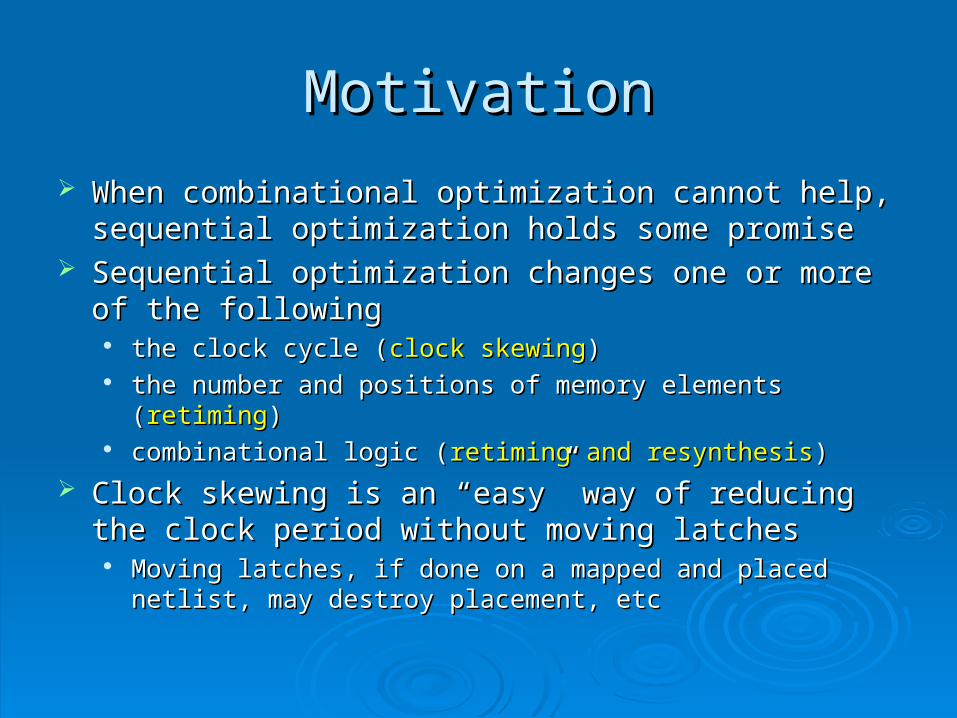
Directed GraphsDirected Graphs GraphGraph is set of vertices and edges is set of vertices and edges G = (V,E)G = (V,E) Each edge is Each edge is directeddirected (has a source and a sink) (has a source and a sink) A A pathpath is the sequence of vertices connected by edges is the sequence of vertices connected by edges A A cyclecycle is the circular path is the circular path Graph is Graph is strongly connectedstrongly connected if there exist a path from any vertex to if there exist a path from any vertex to

any other vertex.any other vertex. For the general formulation of the graph problems, each edge For the general formulation of the graph problems, each edge ee has has

distance, d(e),distance, d(e), and a and a latency, t(e)latency, t(e)

In this lectureIn this lecture Graph is the “latch dependency graph” Graph is the “latch dependency graph”

• Vertices are latchesVertices are latches• Edges are combinational paths between the latchesEdges are combinational paths between the latches

Distance of an edge is its combinational delayDistance of an edge is its combinational delay Latency of an edge is 1Latency of an edge is 1

Graph ProblemsGraph Problems

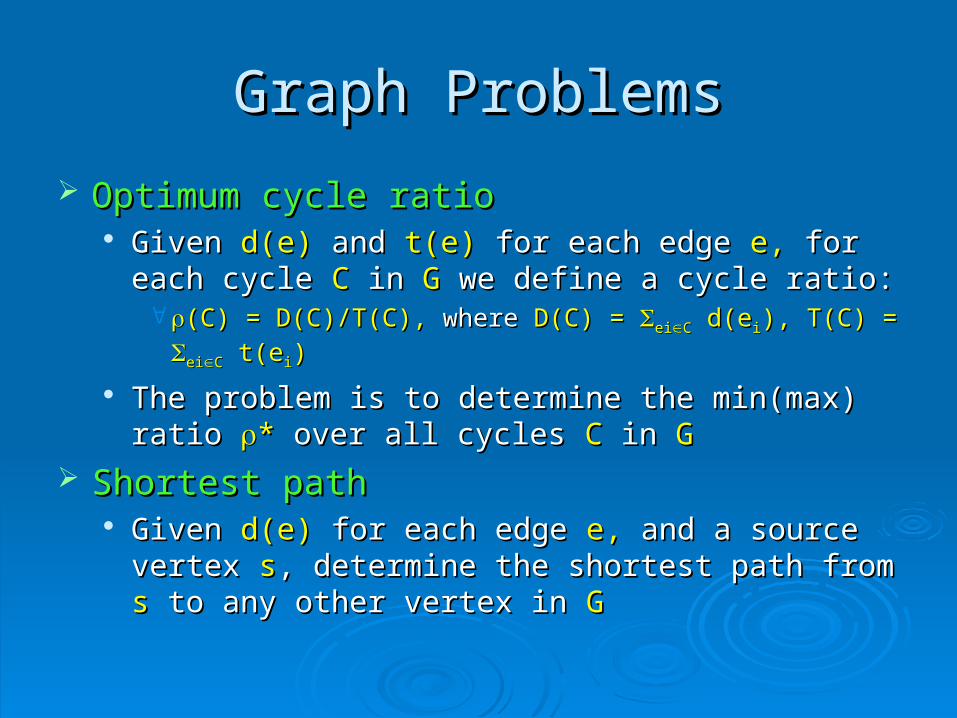
Optimum cycle ratioOptimum cycle ratio Given Given d(e)d(e) and and t(e) t(e) for each edgefor each edge e, e, for each cycle for each cycle CC

in in GG we define a cycle ratio: we define a cycle ratio: (C) = D(C)/T(C),(C) = D(C)/T(C), where where D(C) = D(C) = eieiCC d(e d(eii), T(C) = ), T(C) = eieiCC t(e t(eii))

The problem is to determine the min(max) ratio The problem is to determine the min(max) ratio ** over all cycles over all cycles CC in in GG

Shortest pathShortest path Given Given d(e)d(e) for each edge for each edge e, e, and a source vertex and a source vertex ss, ,

determine the shortest path from determine the shortest path from ss to any other vertex to any other vertex in in GG

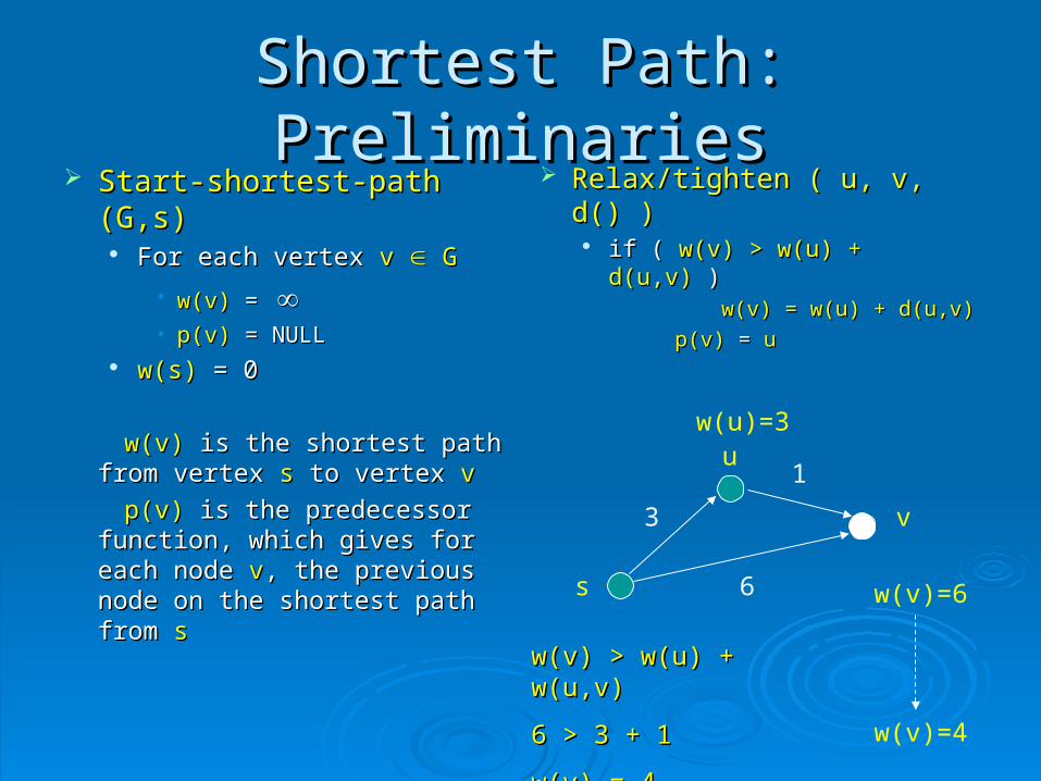
Shortest Path: PreliminariesShortest Path: Preliminaries Start-shortest-path (G,s)Start-shortest-path (G,s)

For each vertex For each vertex v v G G

• w(v)w(v) = = • p(v)p(v) = NULL = NULL

w(s)w(s) = 0 = 0

w(v)w(v) is the shortest path from is the shortest path from vertexvertex s s to vertex to vertex v v

p(v) p(v) is the predecessor is the predecessor function, which gives for each function, which gives for each node node vv, the previous node on , the previous node on the shortest path from the shortest path from ss

Relax/tighten ( u, v, d() )Relax/tighten ( u, v, d() ) if ( if ( w(v) > w(u) + d(u,v)w(v) > w(u) + d(u,v) ) ) w(v) = w(u) + d(u,v)w(v) = w(u) + d(u,v)

p(v)p(v) = = uu

3

1

6

u

s

v

w(u)=3

w(v)=6

w(v)=4

w(v) > w(u) + w(u,v)w(v) > w(u) + w(u,v)

6 > 3 + 16 > 3 + 1

w(v) = 4w(v) = 4

Shortest Path: Dijkstra AlgorithmShortest Path: Dijkstra Algorithm

Start-shortest-path(G,s)Start-shortest-path(G,s) S=S=, Q, Qww = V(G) = V(G) while ( Qwhile ( Qww ) )

U = Extract-Min( QU = Extract-Min( Qww ) ) S = S S = S {u} {u} for each vertexfor each vertex v, v, which is a successor ofwhich is a successor of u u

• Relax( u, v, d() )Relax( u, v, d() )• Update ordering in QUpdate ordering in Qww

Q Q is a priority queue storing vertices by their distanceis a priority queue storing vertices by their distanceS S is the set of vertices, whose shortest path from is the set of vertices, whose shortest path from ss has has

already been foundalready been found

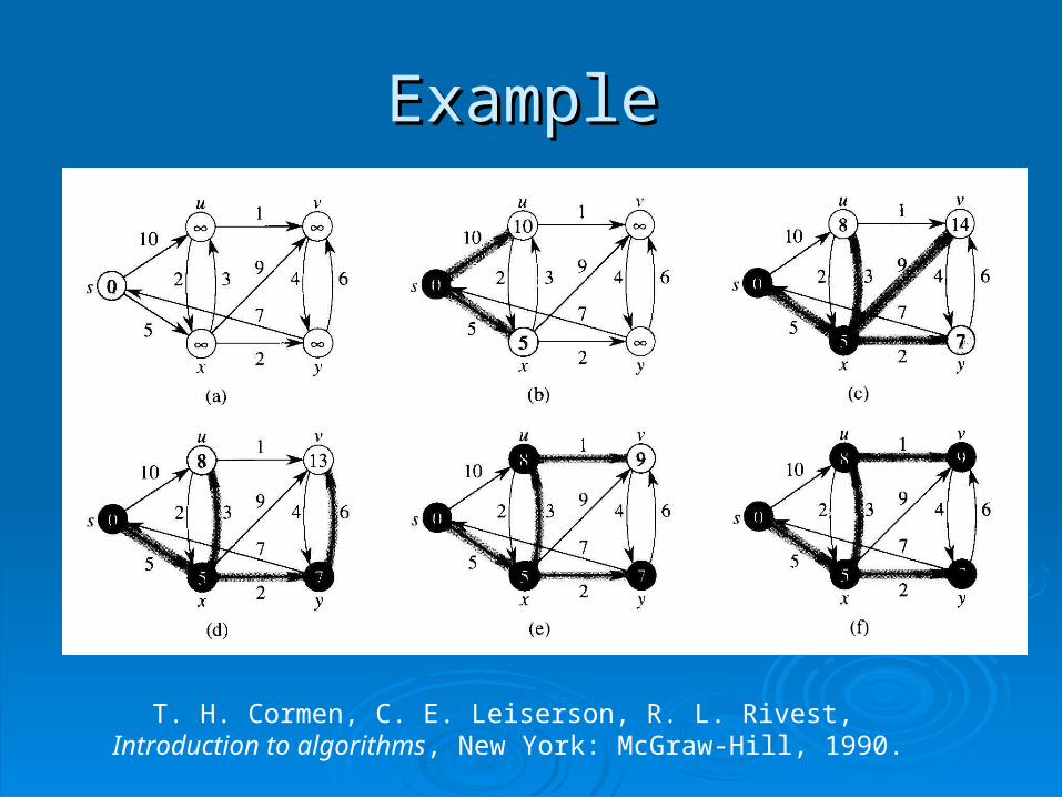
ExampleExample

T. H. Cormen, C. E. Leiserson, R. L. Rivest, Introduction to algorithms, New York: McGraw-Hill, 1990.

Shortest Path: Bellman-Ford Shortest Path: Bellman-Ford

The limitation of Dijkstra is that it only works for positive The limitation of Dijkstra is that it only works for positive distances distances w(u,v)w(u,v)

Bellman-Ford overcomes this limitation and can detect a Bellman-Ford overcomes this limitation and can detect a negative cyclenegative cycle

Start-shortest-path(G,s)Start-shortest-path(G,s) for i = 1 to i < |V(G)|for i = 1 to i < |V(G)|

for each edge (u,v) for each edge (u,v) E(G) E(G)• relax( u, v, d() )relax( u, v, d() )

for each edge (u,v) for each edge (u,v) E(G) E(G) if w(v) > w(u) + d(u,v)if w(v) > w(u) + d(u,v)

• return FALSEreturn FALSE

return TRUEreturn TRUE

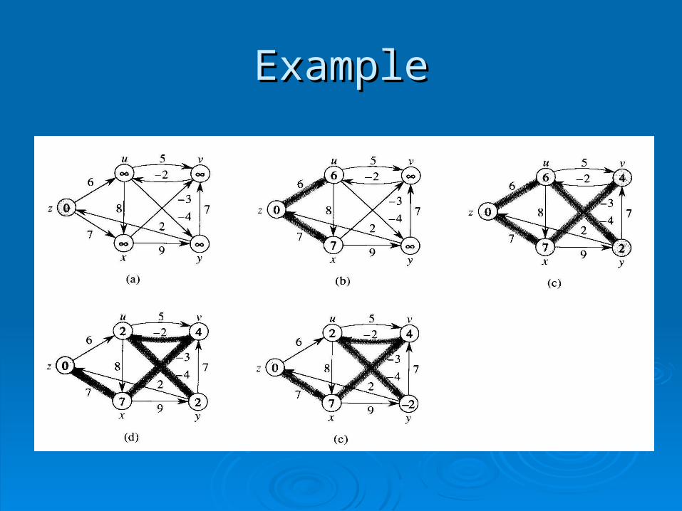
ExampleExample

Efficient Implementation of Efficient Implementation of Bellman-FordBellman-Ford

If If w(u)w(u) is not tightened in the current iteration, is not tightened in the current iteration, u u cannot cannot affect the distances of its successors in the next iterationaffect the distances of its successors in the next iteration

Start-shortest-path(G,s)Start-shortest-path(G,s) Q = {s} /* Q is a FIFO queue */Q = {s} /* Q is a FIFO queue */ while ( Q while ( Q ) )

u = Extract from Q u = Extract from Q for each edge (u,v) for each edge (u,v) E(G) E(G)

• relax( u, v, d() )relax( u, v, d() )

• if ( distance of v has changed )if ( distance of v has changed ) Insert v into QInsert v into Q

Check for negative cycleCheck for negative cycle

Optimum Cycle RatioOptimum Cycle Ratio

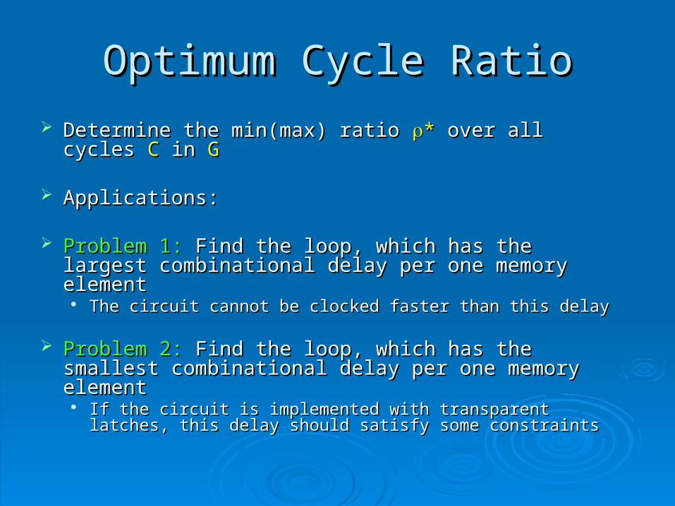
Determine the min(max) ratio Determine the min(max) ratio ** over all cycles over all cycles CC in in GG

Applications:Applications:

Problem 1:Problem 1: Find the loop, which has the largest Find the loop, which has the largest combinational delay per one memory elementcombinational delay per one memory element

The circuit cannot be clocked faster than this delayThe circuit cannot be clocked faster than this delay

Problem 2:Problem 2: Find the loop, which has the smallest Find the loop, which has the smallest combinational delay per one memory elementcombinational delay per one memory element

If the circuit is implemented with transparent latches, this If the circuit is implemented with transparent latches, this delay should satisfy some constraintsdelay should satisfy some constraints

Latch-to-Latch Max DelayLatch-to-Latch Max Delay

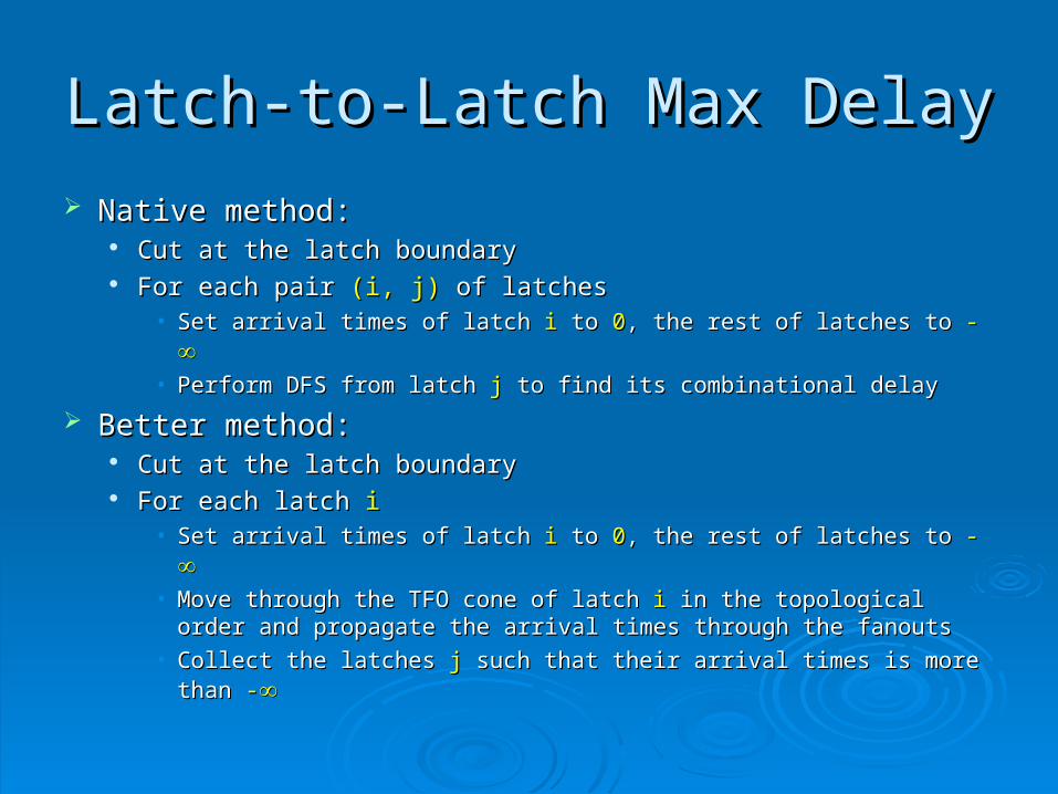
Native method: Native method: Cut at the latch boundaryCut at the latch boundary For each pair For each pair (i, j)(i, j) of latches of latches

• Set arrival times of latch Set arrival times of latch ii to to 00, the rest of latches to , the rest of latches to --• Perform DFS from latchPerform DFS from latch j j to find its combinational delay to find its combinational delay

Better method: Better method: Cut at the latch boundaryCut at the latch boundary For each latch For each latch ii

• Set arrival times of latch Set arrival times of latch ii to to 00, the rest of latches to , the rest of latches to --• Move through the TFO cone of latch Move through the TFO cone of latch ii in the topological order and in the topological order and

propagate the arrival times through the fanoutspropagate the arrival times through the fanouts

• Collect the latches Collect the latches jj such that their arrival times is more than such that their arrival times is more than --

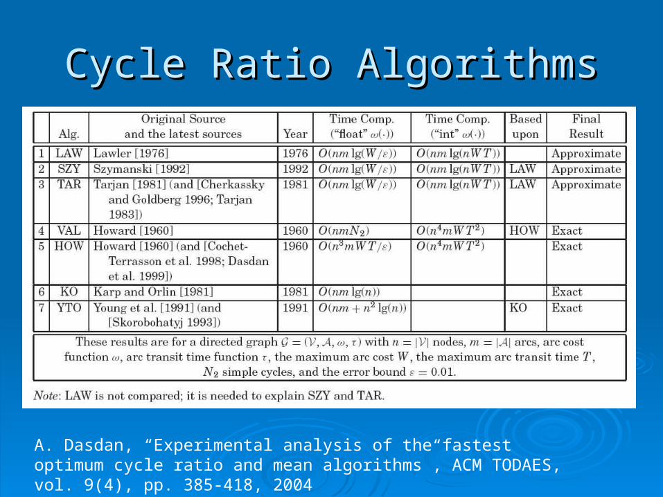
Cycle Ratio AlgorithmsCycle Ratio Algorithms

A. Dasdan, “Experimental analysis of the fastest optimum cycle ratio and mean algorithms”, ACM TODAES, vol. 9(4), pp. 385-418, 2004

Overview of Howard’s AlgorithmOverview of Howard’s Algorithm

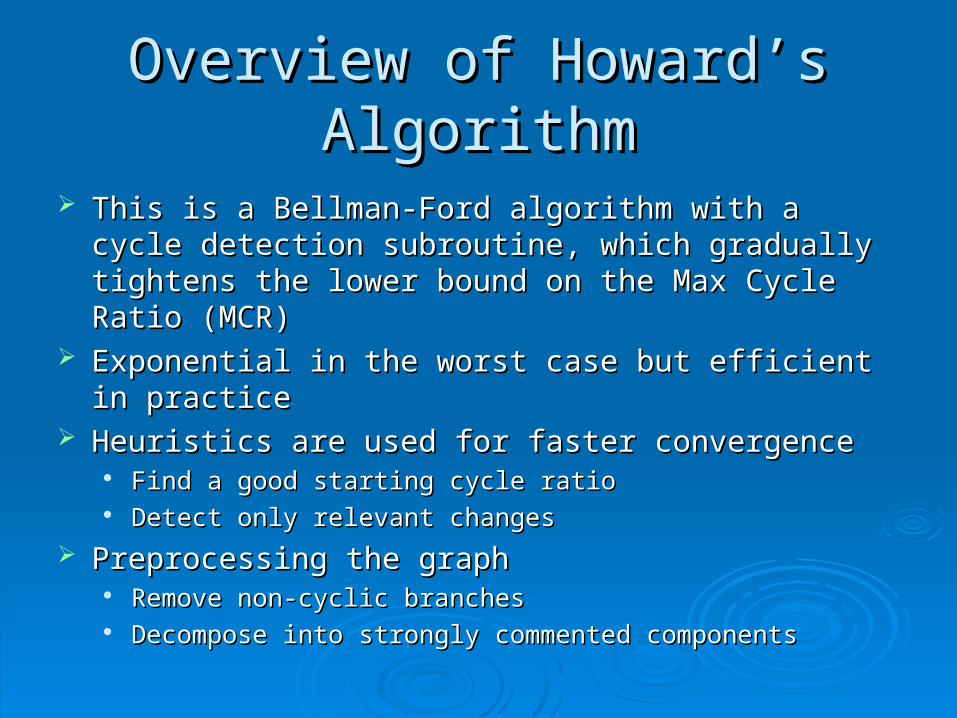
This is a Bellman-Ford algorithm with a cycle detection This is a Bellman-Ford algorithm with a cycle detection subroutine, which gradually tightens the lower bound on subroutine, which gradually tightens the lower bound on the Max Cycle Ratio (MCR)the Max Cycle Ratio (MCR)

Exponential in the worst case but efficient in practiceExponential in the worst case but efficient in practice Heuristics are used for faster convergenceHeuristics are used for faster convergence

Find a good starting cycle ratioFind a good starting cycle ratio Detect only relevant changesDetect only relevant changes

Preprocessing the graphPreprocessing the graph Remove non-cyclic branchesRemove non-cyclic branches Decompose into strongly commented componentsDecompose into strongly commented components

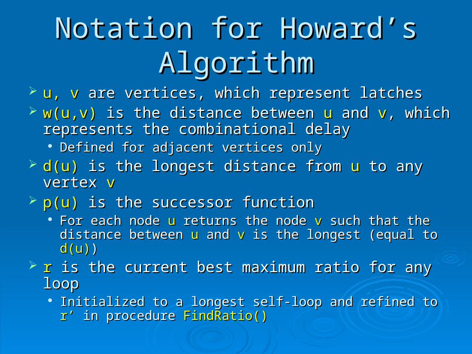
Notation for Howard’s AlgorithmNotation for Howard’s Algorithm

u, vu, v are vertices, which represent latches are vertices, which represent latches w(u,v)w(u,v) is the distance between is the distance between uu and and vv, which , which

represents the combinational delayrepresents the combinational delay Defined for adjacent vertices onlyDefined for adjacent vertices only

d(u)d(u) is the longest distance from is the longest distance from uu to any vertex to any vertex vv p(u)p(u) is the successor function is the successor function

For each nodeFor each node u u returns the node returns the node vv such that the such that the distance between distance between uu and and v v is the longest (equal to is the longest (equal to d(u)d(u)))

r r is the current best maximum ratio for any loopis the current best maximum ratio for any loop Initialized to a longest self-loop and refined to Initialized to a longest self-loop and refined to r’r’ in in

procedure procedure FindRatio()FindRatio()

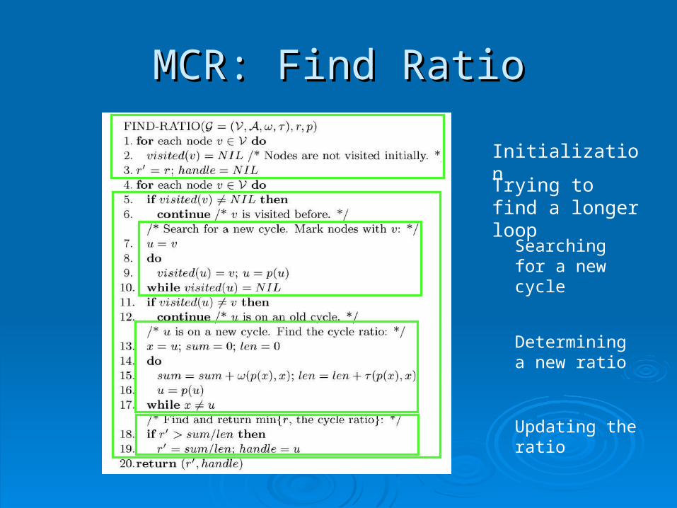
MCR: Find RatioMCR: Find Ratio

Initialization

Searching for a new cycle

Determining a new ratio

Trying to find a longer loop

Updating the ratio

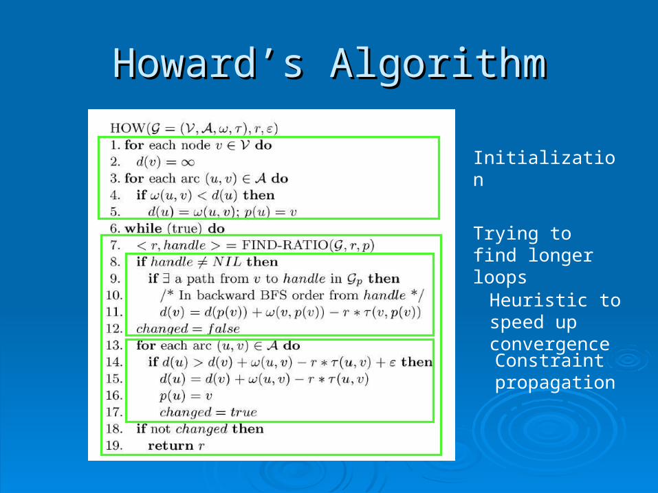
Howard’s AlgorithmHoward’s Algorithm

Initialization

Trying to find longer loops

Heuristic to speed up convergence

Constraint propagation

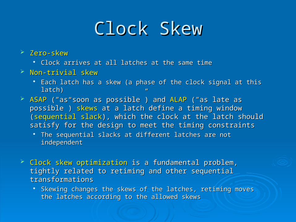
Clock SkewClock Skew Zero-skewZero-skew

Clock arrives at all latches at the same timeClock arrives at all latches at the same time Non-trivial skewNon-trivial skew

Each latch has a skew (a phase of the clock signal at this latch)Each latch has a skew (a phase of the clock signal at this latch) ASAPASAP (“as soon as possible”) and (“as soon as possible”) and ALAPALAP (“as late as possible”) (“as late as possible”)

skewsskews at a latch define a timing window ( at a latch define a timing window (sequential slacksequential slack), ), which the clock at the latch should satisfy for the design to which the clock at the latch should satisfy for the design to meet the timing constraintsmeet the timing constraints

The sequential slacks at different latches are not independentThe sequential slacks at different latches are not independent

Clock skew optimizationClock skew optimization is a fundamental problem, tightly is a fundamental problem, tightly related to retiming and other sequential transformationsrelated to retiming and other sequential transformations

Skewing changes the skews of the latches, retiming moves the Skewing changes the skews of the latches, retiming moves the latches according to the allowed skewslatches according to the allowed skews

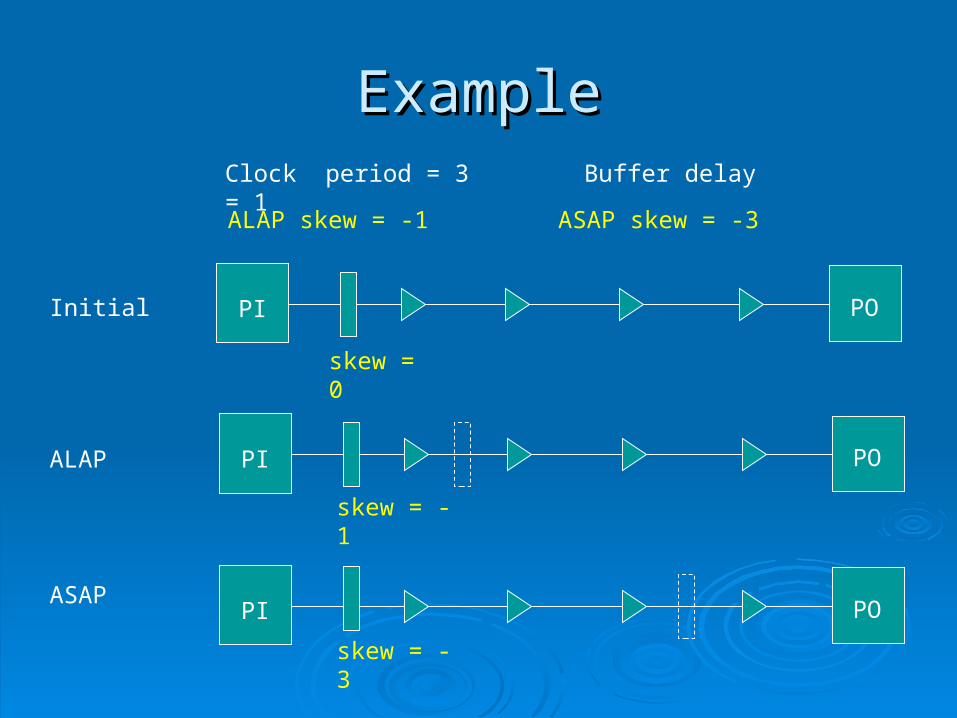
ExampleExample

PI PO

Clock period = 3 Buffer delay = 1

Initial

ALAP

ASAP

ALAP skew = -1 ASAP skew = -3

PI PO

PI PO

skew = 0

skew = -1

skew = -3

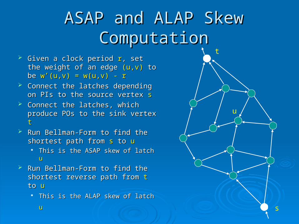
ASAP and ALAP Skew ComputationASAP and ALAP Skew Computation

Given a clock period Given a clock period rr, set the , set the weight of an edge weight of an edge (u,v)(u,v) to be to be w’(u,v) = w(u,v) - rw’(u,v) = w(u,v) - r

Connect the latches depending on Connect the latches depending on PIs to the source vertex PIs to the source vertex s s

Connect the latches, which Connect the latches, which produce POs to the sink vertex produce POs to the sink vertex tt

Run Bellman-Form to find the Run Bellman-Form to find the shortest path from shortest path from ss to to uu

This is the ASAP skew of latch This is the ASAP skew of latch uu Run Bellman-Form to find the Run Bellman-Form to find the

shortest reverse path from shortest reverse path from tt to to uu

This is the ALAP skew of latch This is the ALAP skew of latch uu

t

s

u