EE 290A: Generalized Principal Component Analysis

Lecture 6: Iterative Methods for Mixture-Model Segmentation

Sastry & Yang © Spring, 2011

EE 290A, University of California, Berkeley 1

Last time

PCA reduces dimensionality of a data set while retaining as much as possible the data variation. Statistical view: The leading PCs are given

by the leading eigenvectors of the covariance.

Geometric view: Fitting a d-dim subspace model via SVD

Extensions of PCA Probabilistic PCA via MLE Kernel PCA via kernel functions and kernel

matricesSastry & Yang © Spring, 2011

EE 290A, University of California, Berkeley 2

This lecture

Review basic iterative algorithms Formulation of the subspace

segmentation problem

Sastry & Yang © Spring, 2011

EE 290A, University of California, Berkeley 3

Example 4.1

Euclidean distance-based clustering is not invariant to linear transformation

Distance metric needs to be adjusted after linear transformation

Sastry & Yang © Spring, 2011

EE 290A, University of California, Berkeley 4

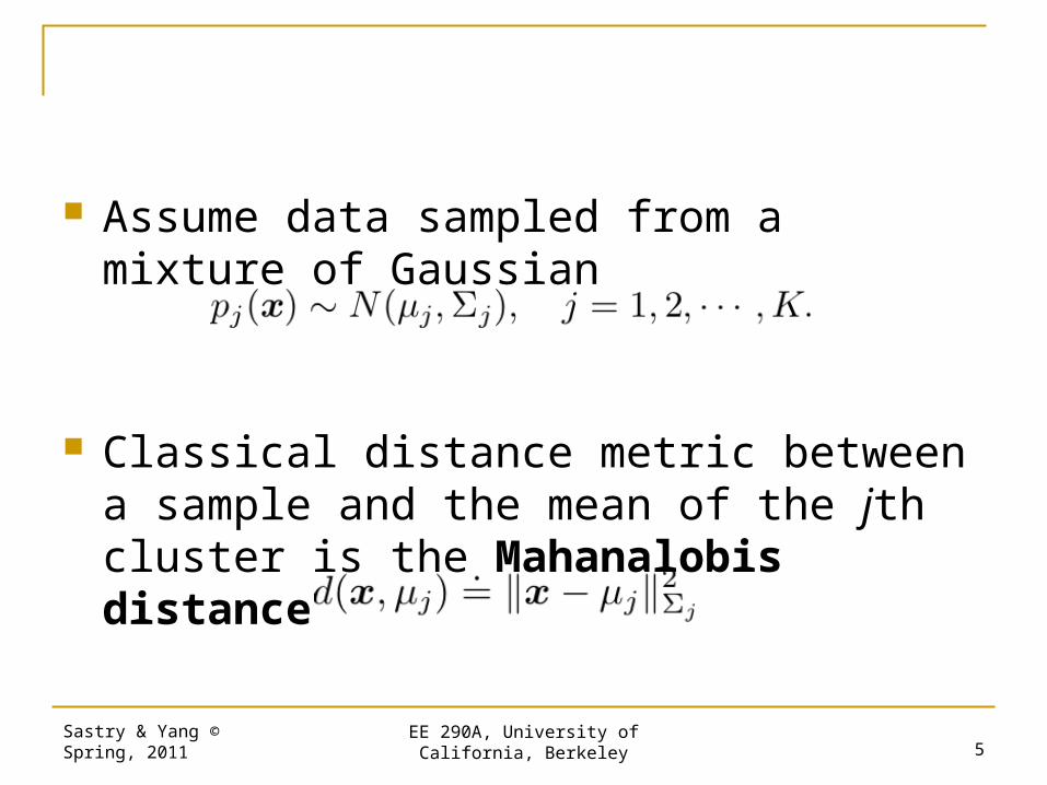
Assume data sampled from a mixture of Gaussian

Classical distance metric between a sample and the mean of the jth cluster is the Mahanalobis distance

Sastry & Yang © Spring, 2011

EE 290A, University of California, Berkeley 5

K-Means

Assume a map function provide each ith sample a label

An optimal clustering minimizes the within-cluster scatter:

i.e., the average distance of all samples to their respective cluster means

Sastry & Yang © Spring, 2011

EE 290A, University of California, Berkeley 6

However, as K is user defined, when each point becomes a cluster itself: K=n.

In this chapter, would assume true K is known.

Sastry & Yang © Spring, 2011

EE 290A, University of California, Berkeley 7

Algorithm

A chicken-and-egg view

Sastry & Yang © Spring, 2011

EE 290A, University of California, Berkeley 8

Two-Step Iteration

Sastry & Yang © Spring, 2011

EE 290A, University of California, Berkeley 9

Example

http://www.paused21.net/off/kmeans/bin/

Sastry & Yang © Spring, 2011

EE 290A, University of California, Berkeley 10

Characteristics of K-Means

It is a greedy algorithm, does not guarantee to converge to the global optimum.

Given fixed initial clusters/ Gaussian models, the iterative process is deterministic.

Result may be improved by running k-means multiple times with different starting conditions.

The segmentation-estimation process can be treated as a generalized expectation-maximization algorithm

Sastry & Yang © Spring, 2011

EE 290A, University of California, Berkeley 11

EM Algorithm [Dempster-Laird-Rubin 1977] EM estimates the model parameters

and the segmentation in a ML sense. Assume samples are independently

drawn from a mixed probabilistic distribution, indicated by a hidden discrete variable z

Cond. dist. can be Gaussian

Sastry & Yang © Spring, 2011

EE 290A, University of California, Berkeley 12

The Maximum-Likelihood Estimation The unknown parameters are The likelihood function:

The optimal solution maximizes the log-likelihood

Sastry & Yang © Spring, 2011

EE 290A, University of California, Berkeley 13

E Step: Compute the Expectation Directly maximize the log-likelihood

function is a high-dimensional nonlinear optimization problem

Sastry & Yang © Spring, 2011

EE 290A, University of California, Berkeley 14

Define a new function:

The first term is called expected complete log-likelihood function;

The second term is the conditional entropy.

Sastry & Yang © Spring, 2011

EE 290A, University of California, Berkeley 15

Observation:

Sastry & Yang © Spring, 2011

EE 290A, University of California, Berkeley 16

M-Step: Maximization

Regard the (incomplete) log-likelihood as a function of two variables:

Maximize g iteratively

Sastry & Yang © Spring, 2011

EE 290A, University of California, Berkeley 17

Iteration converges to a stationary point

Sastry & Yang © Spring, 2011

EE 290A, University of California, Berkeley 18

Prop 4.2: Update

Sastry & Yang © Spring, 2011

EE 290A, University of California, Berkeley 19

Update

Recall

Assume is fixed, then maximize the expected complete log-likelihood

Sastry & Yang © Spring, 2011

EE 290A, University of California, Berkeley 20

To maximize the expected log-likelihood, as an example, assume each cluster is isotropic normal distribution:

Eliminate the constant term in the objective

Sastry & Yang © Spring, 2011

EE 290A, University of California, Berkeley 21

Exer 4.2

Sastry & Yang © Spring, 2011

EE 290A, University of California, Berkeley 22

Compared to k-means, EM assigns the samples “softly” to each cluster according to a set of probabilities.

EM Algorithm

Sastry & Yang © Spring, 2011

EE 290A, University of California, Berkeley 23

Exam 4.3: Global max may not exist

Sastry & Yang © Spring, 2011

EE 290A, University of California, Berkeley 24