Climate Feedback Variance and the Interaction of Aerosol Forcing and Feedbacks

A. GETTELMAN

National Center for Atmospheric Research,a Boulder, Colorado

L. LIN

National Center for Atmospheric Research, Boulder, Colorado, and College of Atmospheric Sciences,

Lanzhou University, Lanzhou, China

B. MEDEIROS AND J. OLSON

National Center for Atmospheric Research, Boulder, Colorado

(Manuscript received 18 February 2016, in final form 16 May 2016)

ABSTRACT

Aerosols can influence cloud radiative effects and, thus, may alter interpretation of how Earth’s radiative

budget responds to climate forcing. Three different ensemble experiments from the same climate model with

different greenhouse gas and aerosol scenarios are used to analyze the role of aerosols in climate feedbacks

and their spread across initial condition ensembles of transient climate simulations. The standard deviation of

global feedback parameters across ensemblemembers is low, typically 0.02Wm22 K21. Feedbacks from high

(8.5Wm22) and moderate (4.5Wm22) year 2100 forcing cases are nearly identical. An aerosol kernel is

introduced to remove effects of aerosol cloud interactions that alias into cloud feedbacks. Adjusted cloud

feedbacks indicate an ‘‘aerosol feedback’’ resulting from changes to climate that increase sea-salt emissions,

mostly in the SouthernOcean. Ensemble simulations also indicate higher tropical cloud feedbackswith higher

aerosol loading. These effects contribute to a difference in cloud feedbacks of nearly 50%between ensembles

of the samemodel. These two effects are also seen in aquaplanet simulations with varying fixed drop number.

Thus aerosols can be a significant modifier of cloud feedbacks, and different representations of aerosols and

their interactions with clouds may contribute to multimodel spread in climate feedbacks and climate

sensitivity in multimodel archives.

1. Introduction

Cloud feedbacks, the cloud response to forced envi-

ronmental (surface temperature) changes, are the larg-

est uncertainty in estimates of the response of the

climate system to radiative forcing (Boucher et al. 2013).

Forcing is an imposed change on the system (or the ra-

diative result of an imposed change) and feedback is the

response of the system to a perturbation, usually the

change in surface temperature DTs.

Aerosol–cloud interactions (ACIs) are the largest

uncertainty in current estimates of anthropogenic radi-

ative forcing of climate (Boucher et al. 2013). Aerosols

affect the number concentration of cloud drops Nc, thus

altering the brightness (albedo) of clouds (Twomey

1977). Aerosols may alter cloud lifetime as fewer pre-

cipitation drops form (Albrecht 1989) and increase liq-

uid water path (LWP).

Cloud feedbacks can be expressed as the change in

cloud radiative effects (CREs) divided by the global

mean surface temperature change (Wm22K21) (Cess

et al. 1990). Because CRE is defined as the difference in

top-of-atmosphere all-sky and clear-sky radiative fluxes,

its change is affected by changes in surface properties or

atmospheric composition (Soden et al. 2008). Correc-

tions for these noncloud changes should be applied to

accurately assess cloud feedbacks. This can be done

using radiative kernels (Soden et al. 2008), known as a

a The National Center for Atmospheric Research is sponsored

by the National Science Foundation.

Corresponding author address: A. Gettelman, National Center

for Atmospheric Research, 3090 Center Green Dr., Boulder, CO

80301.

E-mail: andrew@ucar.edu

15 SEPTEMBER 2016 GETTELMAN ET AL . 6659

DOI: 10.1175/JCLI-D-16-0151.1

� 2016 American Meteorological Society

kernel-adjusted radiative feedback. Gettelman et al.

(2012a) explain this approach using kernels from Shell

et al. (2008) and Soden et al. (2008). Dessler (2010)

discussed the application of the method to try to tease

out climate feedbacks from observations, following

Schneider (1972) and Forster and Gregory (2006).

The kernel approach has been adapted to directly

account for clouds by Zelinka et al. (2012). Cloud feed-

backs play a central role in uncertainty surrounding cli-

mate sensitivity (Bony et al. 2015; Fasullo et al. 2015).

Several assumptions are commonly made about cli-

mate feedbacks. The first assumption is that feedbacks

are not a strong function of the climate state or the

perturbation from present-day climate. This assumption

is distinct from complexities using different methods,

particularly with small perturbations (Klocke et al. 2013).

Jonko et al. (2012) tested this hypothesis and found weak

nonlinearity for moderate radiative forcing. Knutti and

Rugenstein (2015) note that such nonlinearity may con-

tribute to spread in estimates across models.

Second, it is generally assumed that feedbacks have

low internal variability in any given model, even locally

(Armour et al. 2013), and will not vary across different

realizations. This has not been tested with single model

ensembles.

Aerosols may be important for climate feedbacks as

well as for climate forcing. Because ACI alter the mean

state of clouds (LWP and Nc), ACI may also alter cloud

feedbacks. A cloud with high LWP and small drop

concentration could have the same CRE as a cloud with

low LWP and high drop concentration, but these clouds

may respond differently (differentDCRE) to a change in

surface temperature, giving a different cloud feedback.

Thus, an ‘‘aerosol feedback’’ may exist such that envi-

ronmental changes affect aerosol burdens and then the

aerosol changes will alter CRE by changing ACI. In this

manuscript we will explore these interactions, along

with the variance (or internal variability) of climate

feedbacks in ensembles of climate simulations from a

single model.

These potential modifiers to cloud feedbacks by

aerosols are important because the suite of models used

for assessments of climate change contains a diversity of

approaches and complexity of ACI (Boucher et al.

2013). The extent to which aerosols, and not cloud

processes, are contributing to the spread of cloud feed-

back needs to be assessed as more climate models are

including ACI. ACI are usually assessed and quantified

by the change in CRE (Gettelman 2015; Ghan et al.

2013); see the definition in section 2.

Several hypotheses will be tested using the same

methods, taking advantage of several different ensem-

bles of simulations with a single model (section 2). This

extends recent work on multimodel ensembles reviewed

by Fasullo et al. (2015). First, we will explore the hy-

pothesis that feedbacks are independent of climate state

by investigating feedbacks using two different radiative

forcing scenarios with different levels of warming (sec-

tion 3). Second, each of these ensembles enables us to

estimate the spatial variance of the feedbacks across the

ensemblemembers due to internal variability (section 3)

in a single model. There have been many analyses of the

spread of cloud feedbacks across models (Flato et al.

2013), but no analysis of the spread within a singlemodel

ensemble. Third, we will explore how the background

state of clouds affects cloud feedbacks and climate

sensitivity (section 4). We will compare cloud feedbacks

in two different ensembles with the same greenhouse gas

forcing but different levels of forcing due to anthro-

pogenic aerosol emissions. This requires a method to

control for different ACI between simulations. We also

explore analogous climate states and feedbacks in sim-

pler aquaplanet simulations.

This paper builds on previous work to test the extent

to which climate feedbacks are similar for different

levels of greenhouse gas forcing (Jonko et al. 2012;

Klocke et al. 2013). While Klocke et al. (2013) looked at

variance due to short-term climate variability, this work

presents new analysis on the variance of climate states

across ensemble members over long time periods. We

also develop a new approach to removing aerosol effects

from simulations with interactive aerosols and illustrate

the extent to which cloud state affects cloud feedbacks.

Finally, interactive aerosols allow changes to the

aerosol distribution induced by changes to climate. The

aerosol changes then alter the cloud radiative effect.

This is not an aerosol forcing, because it is internal to

the climate system. It is rather an aerosol feedback on

clouds and climate (section 5). The feedbacks will occur

as a result of 1) changes in emissions of natural aero-

sols into the atmosphere, such as changes to sea salt (a

function of surface wind speed over the oceans) or dust

(a function of wind speed and soil moisture), 2) changes

in scavenging and the lifetime of aerosols resulting from

changes in clouds, and/or 3) changes in aerosol direct

optical properties resulting from different ambient hu-

midity. We will use the simulations to isolate and

quantify this effect. A discussion and conclusions are in

section 6.

2. Methods

a. Feedback methodology

To determine climate radiative feedbacks, we employ

the method of radiative kernels developed by Soden

6660 JOURNAL OF CL IMATE VOLUME 29

et al. (2008). The method uses offline kernels that

estimate a climate response ›R/›X, where R is the

shortwave or longwave top-of-atmosphere (TOA) ra-

diative flux in response to a perturbation in state X,

where X is temperature, water vapor, clouds, or surface

albedo. The feedback is then (›R/›X)(DX/DTs), where

DX/DTs is the global annual average surface tempera-

ture change derived from the difference of two simula-

tions. Kernels for single-level quantities such as surface

albedo and surface temperature are monthly 2D (i.e.,

latitude by longitude) fields, while temperature and

water vapor kernels are 3D (i.e., latitude by longitude by

vertical level) monthly fields (Soden et al. 2008). Cloud

feedbacks are estimated by the kernel-adjusted CRE,

where the kernel adjustments account for changes in the

state of water vapor, temperature, and surface albedo

that may affect R, and CRE5 R2 Rclear, where Rclear is

the clear-sky TOA flux. We also include adjustments for

aerosol forcing (see below). Fluxes are calculated sep-

arately for the longwave (LW) and shortwave (SW)

radiation bands.

The cloud feedback [i.e., (›R/›C)(DC/DTs)] cannot

be directly computed because of the intricate links

among clouds, radiation, and the environment. Fol-

lowing Soden et al. (2008) and Shell et al. (2008), the

cloud feedback (CF) is the change in CRE divided by

the change in surface temperature:

CF5DCRE/DTs. (1)

The feedback is adjusted by removing terms for

changes to water vapor Q, surface albedo a and tem-

perature T in the clear sky c and all sky to get the kernel

adjustments to CRE, DCREk:

DCREk5 (K

T2Kc

T)dT1 (KQ2Kc

Q)dQ

1 (Ka2Kc

a)da , (2)

where KX is the all-sky kernel and KcX is the clear-sky

kernel for X 5 T, Q, and a. This yields the kernel-

adjusted cloud feedback CFa:

CFa5 (DCRE2DCRE

k)/DT

s. (3)

Traditionally radiative kernels are run on equilibrium

experiments, but regression methods (Gregory et al.

2004) and comparison tests (Gettelman et al. 2012a) in-

dicate that flux imbalances can be included as part of the

forcing [see also discussion byMedeiros et al. (2015)]. The

use of models with TOA flux imbalances allows applica-

tion of the kernels to transient experiments. In equilib-

rium, the model used here does not have an imbalance.

The method follows the work of Gettelman et al.

(2012a) and Gettelman et al. (2013), who illustrated the

causes of the change in climate sensitivity between dif-

ferent versions of the Community Earth System Model

(CESM). The kernels were originally developed by

Shell et al. (2008) for version 3 of the Community At-

mosphere Model (CAM), but in general the kernels are

stable across models (Soden et al. 2008). The code has

been updated to run on output from the current version

of CESM (CESM1.1). We do not use the cloud property

kernels developed by Zelinka et al. (2012) because the

necessary simulator outputs were not available from the

CESM experiments used (see below).

b. Aerosol kernel adjustment

One of the complexities of estimating feedbacks using

these transient simulations with different aerosols is that

ACI alter CRE. This additional dimension to the feed-

backs may affect the ‘‘efficacy’’ (efficiency) of different

climate forcings (Hansen et al. 2005). To remove the

aerosol forcing effect, we will calculate an ‘‘aerosol

kernel’’ to adjust the cloud forcing for the direct and

indirect effect of aerosols (mostly indirect).

Following Eq. (2) above we add a term for the aerosol

kernel:

DCREk5 (K

T2Kc

T)dT1 (KQ2Kc

Q)dQ

1 (Ka2Kc

a)da1 (KA2Kc

A)dA , (4)

where A is aerosols, and dA is DAOD, the change in

aerosol optical depth (AOD). The aerosol kernel for all

sky KA and clear sky KcA is estimated from

KA5 ›R/›AOD (5)

and

KcA 5 ›R

c/›AOD, (6)

where ›R is the change in all-sky flux and ›Rc is the

change in clear-sky flux due to aerosols. The aerosol

kernel is approximated based on a difference of two

simulations as DR/DAOD and DRc/DAOD at each

horizontal location (x, y): the change in TOA radiation

DR, occurring because of the change in aerosols DAOD.

The aerosol kernel is similar to the other kernels in that

it is a TOA radiative response to a difference to a per-

turbation to the system. It is similar to the surface albedo

kernel as a response to a single-level (column) pertur-

bation. The aerosol kernel is different in that it is not

estimated from a unit perturbation, but rather from

another set of model simulations.

The kernel is applied to remove flux perturbations,

similar to how other kernels (such as surface albedo) are

applied to generate kernel-adjusted cloud feedbacks.

All adjustments, including aerosols, are made at the

15 SEPTEMBER 2016 GETTELMAN ET AL . 6661

same time. As with the other kernels, both clear- and all-

sky kernels are applied. The clear-sky aerosol kernel is

basically the direct effect and all-sky kernels are the

total effect (mostly the cloud effect). The effects shown

in sections 4 and 5 are with aerosol kernels applied with

all other adjustments. For example, a change in surface

albedo will affect the clear-sky TOA flux, which is

aliased into the cloud radiative effects. The adjustment

for surface albedo takes the a change Da between two

simulations, and multiplies this by the surface albedo

kernel ›R/›a at each point to remove this DR from

DCRE [Eqs. (2) and (4)]. Aerosols cause clouds to be

brighter because of a change in drop number (and po-

tentially cloud lifetime). The aerosol kernel adjustment

uses DAOD multiplied by the aerosol kernel KA 5 DR/DAOD to estimate an additional DR to remove from

DCRE [Eq. (2)]. This is done for KA and KcA in the LW

and SW radiation.

Because it uses a difference between two simulations,

for stability a threshold of DAOD . 0.01 locally is ap-

plied. This means that clean regions do not see aerosol

perturbations. Regions where the aerosol kernels are

applied are inside the filled contour in Fig. 1, meaning

most of the Northern Hemisphere. The clean regions

(DAOD , 0.01) are mostly only over the poles and the

Southern Hemisphere oceans. However, they also do

not see large TOA flux perturbations due to aerosols

(e.g., Gettelman 2015, his Fig. 8). The results (and con-

clusions) are not very sensitive to the AOD threshold.

Estimating the aerosol kernel is dependent on the

particular climate model formulation and aerosol dis-

tribution. The aerosol kernel is not strongly dependent

on the climate state (see below). The stability is ex-

pected given themagnitude of the kernel forcing (locally

10Wm22) and the dominance of the effect in the

shortwave radiation, while the greenhouse gas forcing

alters the climate state by the longwave emission of CO2

and H2O, modulated by clouds.

Fortunately, our methodology and ensembles will

minimize these uncertainties. We are using the same

model [CESM1(CAM5)] for all simulations. Further-

more, we will estimate the kernel using a similar pattern

of DAOD, and an appropriate range of DAOD that

brackets the emissions changes in the ensembles. Ac-

cordingly, the aerosol kernel is calculated from two 50-yr

CAM5 simulations with 2000 and 1850 aerosol emissions.

For a 50-yr simulation, the local standard deviation in

annual TOA flux in the Northern Hemisphere storm

track is approximately 3Wm22. Using a 95% confidence

Student’s t test, thismeans local (not global) deviations of

larger than 0.7Wm22 are statistically significant, and the

regions of the aerosol kernel meet this criterion (e.g.,

Gettelman andMorrison 2015, their Fig. 8). These are not

idealized kernels; they are estimated from a similar per-

turbation as the one we are trying to remove, and using

the same model physics. Regions of high aerosol sus-

ceptibility but no change in aerosols have a small aerosol

kernel correction. This limits the analysis to regions with

significant aerosol perturbations based on current distri-

butions of aerosols. In the case of these ensembles of

model runs, these are exactly the perturbations we are

testing. We have also tested the sensitivity of the kernel

by repeating the analysis using alternative kernels from

1) a different model configuration and 2) the same con-

figuration but with a climate reflecting the end of the

representative concentration pathway 8.5 (RCP8.5) cli-

mate of a warmer planet with higher (doubled) CO2.

Perturbations to the aerosol kernel are discussed in

section 4.

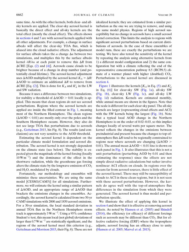
Figure 1 illustrates the kernels [KA in Eq. (5) and KcA

in Eq. (6)] for clear-sky SW (Fig. 1a), all-sky SW

(Fig. 1b), clear-sky LW (Fig. 1c), and all-sky LW

(Fig. 1d) radiation. Kernels are estimated monthly,

while annual means are shown in the figures. Note that

the scale is different for each clear-sky panel. The all-sky

kernels are larger (representing cloud effects and ACI)

with the SW kernels being the largest (Fig. 1b). Note

that a typical local AOD change in the Northern

Hemisphere is on the order of 0.02–0.03, so this implies

changes locally of several watts per square meter. The

kernel reflects the changes in the emissions between

preindustrial and present because the changes to top-of-

atmosphere flux DR tend to be regionally constrained to

regions near where aerosols are changing (DAOD .0.01). The annual mean DAOD, 0.01 line is shown on

each panel in Fig. 1. It also illustrates that this is not a

unit perturbation (perturbing AOD by 0.01 and then

estimating the response) since the effects are not

simple direct radiative calculations but rather involve

nonlinear ACI effects on clouds. In regions over the

oceans far from aerosol sources, there is little effect of

the aerosol kernel. There may still be susceptibility of

clouds to ACI in these clean regions, but it is not seen

with these aerosol perturbations. However, the ker-

nels do agree well with the top-of-atmosphere flux

differences in the simulation from which they were

generated. The aerosol kernel is thus model and per-

turbation specific.

We illustrate the effect of applying this kernel in

section 4 and show that it is effective at removing aerosol

effects. As noted by Hansen et al. (2005) and Shindell

(2014), the efficiency (or efficacy) of different forcings

such as aerosols may be different than CO2. But for ef-

fective radiative forcing (ERF) where the troposphere

adjusts, aerosol forcing has an efficacy close to unity

(Hansen et al. 2005; Marvel et al. 2015).

6662 JOURNAL OF CL IMATE VOLUME 29

c. Models

All experiments use CESM1 simulations, with the

Community Atmosphere Model, version 5 (CAM5;

Neale et al. 2010). CESM1(CAM5) includes a modal

aerosol model (Liu et al. 2012) in the atmosphere with

prognostic aerosols, and physically calculated ACI in

the stratiform cloud regime (Gettelman et al. 2010).

1) ENSEMBLES OF COUPLED SIMULATIONS

The CESMLarge Ensemble (CESM-LE, or LE) of 30

members is described by Kay et al. (2014b). The CESM-

LE follows a RCP emission scenario for greenhouse

gases (GHGs) and aerosols with 8.5Wm22 of forcing in

2100 (van Vuuren et al. 2011). We also use a CESM

Medium Ensemble (CESM-ME, or ME) described by

Sanderson et al. (2016). The CESM-ME has 15 ensem-

ble members that use RCP4.5 with 4.5Wm22 of forcing

in 2100 (van Vuuren et al. 2011). We also use the CESM

Fixed Aerosol Ensemble (CESM-FixA, or FixA). As

described by Xu et al. (2016), the FixA ensemble has 15

members and uses the same RCP8.5 scenario as the LE,

but the FixA ensemble fixes aerosol emissions at con-

stant year 2005 values starting from year 2006. The en-

sembles for ME and FixA were run to 2080. All versions

use the same model code for CESM. The only differ-

ences are the GHG and aerosol forcing.

2) AQUAPLANET EXPERIMENTS

To aid in the interpretation of the ensembles, we also

turn to simpler experiments using an aquaplanet con-

figuration of CESM (Medeiros et al. 2016). This version

uses fixed sea surface temperatures, and the same physi-

cal parameterizations as in the CESM ensembles. To

simulate climate changes, we run CESM-Aqua with a

control case, and a case with doubled carbon dioxide

(367–734ppm) and a uniform increase in SST of 14K.

This is a standard test for producing feedback estimates

from aquaplanet simulations.

To test the sensitivity to aerosols, pairs of experiments

are conducted with different fixed Nc: 50, 100, and

300 cm23 with double-moment microphysics. This is

done so that tests can be performed without aerosols

(which have a land and ocean contrast), but tomimic the

effects of aerosols. The range is chosen to mimic the

effect of anthropogenic aerosols on top of atmosphere

fluxes (see below). A value of Nc 5 100 cm23 is the

baseline, while Nc 5 50 cm23 is typical of marine con-

ditions andNc5 300 cm23 is more typical of continental

or polluted conditions. These simulations are called

FIG. 1. Maps of annual mean KA (Wm22 per unit AOD): (a) clear-sky SW, (b) all-sky SW, (c) clear-sky LW, and

(d) all-sky LW radiation. Black contour indicates the annual mean value of DAOD 5 0.01 (see text).

15 SEPTEMBER 2016 GETTELMAN ET AL . 6663

Nc100, Nc50, and Nc300, respectively. The different

drop numbers result in differences in the SWCRE in the

control case. The net global SW CRE in the aquaplanet

control simulations is 260.6, 264.3, and 270.0Wm22

for simulations Nc50, Nc100, and Nc300 respectively. To

isolate the difference of Nc in the base state, an addi-

tional simulation was conducted where the base state

in the Nc300 simulation was adjusted back to a SW

CRE similar to that in the Nc50 simulation. The ad-

justment was accomplished by reducing the cloud frac-

tion, through an increase in the critical relative humidity

for cloud formation in the cloud macrophysics (Park

2014). The change does not alter the pattern of cloud

forcing appreciably, only its magnitude. This simulation,

called Nc300RH, has a global-mean base state SW CRE

of 261.4Wm22, close to the Nc50 case. The difference

in top-of-atmosphere flux between the Nc300 and Nc50

cases is22.2Wm22, which is similar to the21.5Wm22

change due to anthropogenic aerosols in the full model

calculation.

d. Hypotheses

The different hypotheses to be tested and themethods

of using these ensembles to test them are outlined

below.

1) FEEDBACK VARIANCE

We hypothesize that kernel-adjusted fast feedbacks

have small variability on a global basis across ensemble

members (internal variability), but may have large local

variability. This hypothesis can be tested by estimating

feedbacks from a 100-yr section of the CESM-LE con-

trol and 20 years of each ensemble member at the end of

the twenty-first century (2060–80). We seek to quantify

the variance across the ensemble members of each

feedback and to understand the patterns of variance and

how it varies. We will examine the sensitivity to the

number of members or the years averaged.

2) FEEDBACK LINEARITY

Second, we wish to test if feedbacks are constant be-

tween different ensembles. The forcing and surface

temperature changes are different between the ME

(RCP4.5) and the LE (RCP8.5) simulations. But the

feedbacks are normalized by DTs. To understand if the

different feedbacks are the same we will estimate and

compare kernel-adjusted feedbacks from each ensemble

(average and spread).

3) AEROSOL EFFECTS

Third, we hypothesize that aerosols will alter cloud

state (LWP and Nc), and a different cloud state may

affect climate feedbacks. To test this hypothesis, we will

calculate feedbacks for the FixA simulation (constant

aerosol forcing case) to determine if they are different

than for the LE (RCP8.5). The surface temperature will

be different. The FixA simulation has higher cloud drop

number concentrations, particularly in the Northern

Hemisphere, as a result of anthropogenic aerosols. It

will warm and less than the LE simulation, because of

the continuation of aerosol radiative forcing due to both

direct and indirect effects of aerosols. If the feedbacks

are not dependent on the degree of warming (tested by

comparing LE and ME with similar aerosols as noted

above), then any feedback differences between FixA

and LE simulations should be due to aerosols. To un-

derstand the effects, we analyze the cloud state (mean

column drop number, LWP, etc.) in the LE simulation

and the FixA ensemble. The difficulty is that there are

differences in patterns of the aerosol emissions over

time. We use aerosol kernels to control for changing

aerosol radiative effects.

4) AEROSOL FEEDBACKS

Finally, with interactive aerosols, there can be

changes to the aerosol distribution induced by changes

to climate. We will test the hypothesis that climate-

induced aerosol changes can alter CRE. This is not an

aerosol forcing, because it is internal to the climate

system. It is rather an aerosol feedback on clouds and

climate. As with aerosol radiative forcing, these effects

can be both direct and indirect. As noted above, there

are several possible internal mechanisms that can

change aerosol populations to create this feedback.

e. Aerosols in CESM

To test these hypotheses we perform several analyses.

First, we estimate feedbacks based on a 100-yr section of

the CESM-LE control, and then 20 years of eachCESM-

LE member in the late twenty-first century (2080–60).

So feedbacks are 2060–80 minus the control (1850 forc-

ing). Note that between 1850 and 2060, anthropogenic

aerosols first rise and then fall again, so that past and

future periods have similar but not identical aerosols.

CESM-LE uses RCP8.5 with increased greenhouse gases

and reduced aerosols in the twenty-first century.

We do the same for the CESM-ME (RCP4.5) en-

semble members. The control simulation for the LE and

ME are the same. RCP4.5 has a reduction of aerosols in

the future, similar to RCP8.5. Finally we also estimate

the feedbacks for each member of the FixA (constant

aerosol) ensemble. Since the FixA ensemble was run

from 2006 to 2080 with fixed aerosols, we subtract 2006–

26 from 2060–80 values. This case has high aerosol

loading throughout. Figure 2a illustrates the aerosol

loading by latitude for the different simulations and

6664 JOURNAL OF CL IMATE VOLUME 29

periods. Figure 2b shows the change in AOD be-

tween the analyzed beginning and end points of each

ensemble.

Feedbacks calculated with radiative kernels using

2006–26 (20 yr) as the base period for all three ensem-

bles (LE, ME, and FixA) are qualitatively and quanti-

tatively similar to using the longer control run for ME

and LE. The benefit of using the control simulation for

LE and ME is to minimize the difference in aerosol

loading between time periods. The choice of base period

only impacts the standard deviations: using 20 years

from different ensembles results in larger feedback

spread (by about a factor of 2) than using 100 years of

the same control run. This explains much of the differ-

ence in standard deviation between FixA and ME sim-

ulations, which have more internal variability (larger

standard deviation) than LE because of the smaller

ensemble size.

Figure 2 illustrates that both the latitudinal distribu-

tion of aerosols and the absolute amount are quite dif-

ferent in different time periods. The change in aerosols

between different time periods of each ensemble is due

to both external changes in emissions and aerosol

feedbacks due to climate changes that affect aerosols. In

the FixA ensemble, the emissions changes are elimi-

nated and any change in aerosols is due to a climate

influence on aerosols (aerosol feedbacks). These feed-

backs include changes in winds that influence sea salt

emissions (in the Southern Ocean, peaking at 608S) andchanges in tropical dust (one-third of the change at

308N), as well as internal changes to aerosol transport,

scavenging, and optical properties.

The differences in Fig. 2 for the LE and ME simula-

tions arise mostly from the emissions. Lamarque et al.

(2011, see their Fig. 9) illustrate that AOD in 2080 is

similar between RCP4.5 and RCP8.5 but that it is not

the same as AOD in 1850 (used for the control). It is

more similar to global AOD in 1950–70. Figure 10 in

Lamarque et al. (2011) clearly shows the local SO4

and black carbon column burdens are not the same

because of a shift of aerosols into the tropics. Even if

we looked at the same global AOD, there would be

differences in AOD patterns, consistent with in-

creased AOD in the tropics, and still some at NH

midlatitudes.

To adjust for these different levels and locations of

AOD changes, we will use KA to correct the clear-sky

and all-sky radiative forcing for the changes to aerosols

diagnosed in these simulations. Furthermore, we will

use aquaplanet simulations to understand the global

results.

3. Variance results

Table 1 illustrates a summary of climate feedbacks for

the different ensembles, and the standard deviation

within each ensemble. The feedbacks may differ be-

cause of aerosols or climate forcing, and we will try to

pull this out of the analysis. A comparison of feedbacks

in our Table 1 with those in Table 2 of Gettelman et al.

FIG. 2. Zonal-mean (a)AODat 550-nmwavelength and (b) change inAOD from three ensembles of simulations:

LE (red), ME (black), and FixA (blue). Also shown in (a) are the control simulation for ME and LE (orange) and

the FixA control (2006–26; yellow). The two standard deviation spreads of zonal-meanAOD across each ensemble

are shown by the shaded regions in (b).

15 SEPTEMBER 2016 GETTELMAN ET AL . 6665

(2012a) indicates that these transient experiments yield

results very similar to traditional slab or mixed layer

ocean model feedback experiments, or modified-Cess

(see Cess et al. 1990; fixed sea surface temperature)

experiments. The model here, CESM1.1.1, is very sim-

ilar to the CAM5 experiments in Gettelman et al.

(2012a), and feedbacks are comparable. Water vapor

and lapse rate feedbacks differ by about 0.2Wm22K21

between these experiments and those of Gettelman

et al. (2012a), but the combination of the two feedbacks

is similar (;1.2Wm22K21). Albedo feedback magni-

tudes are also very similar (;0.3Wm22K21). Aerosol

kernels are only applied to cloud feedbacks. The cloud

feedbacks with the aerosol kernel applied are also sim-

ilar to previous versions (;0.5Wm22K21). Two alter-

native estimates of the aerosol kernel (denoted alt and

alt2x) are used to test the sensitivity of the results to the

aerosol kernel. The alt kernel uses simulations with a

revised version of the cloud microphysics (Gettelman

and Morrison 2015) and different cloud tuning. The

ACI are slightly lower. The third kernel (alt2x) was

also estimated using this same model configuration but

with climate conditions (CO2 concentration and sea

surface temperatures) reflecting a doubling of CO2

(720 ppmv). Next we discuss the variance of feedbacks

in more detail.

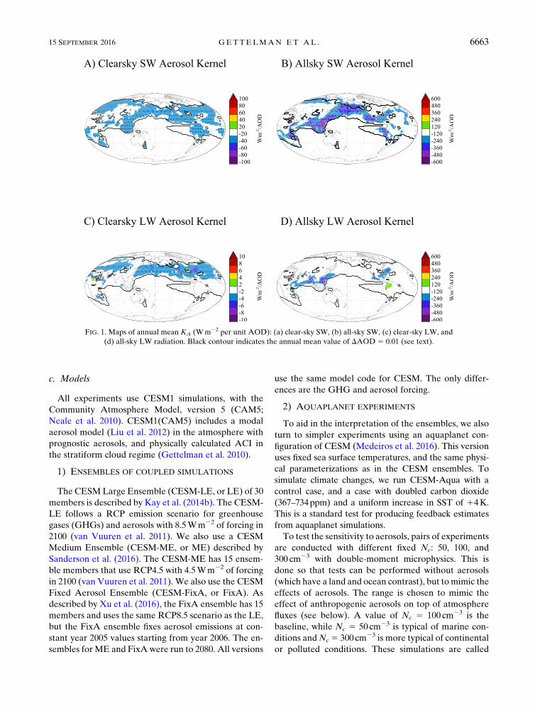
a. Water vapor feedback variance

Figure 3 illustrates the water vapor feedback from the

three ensembles. For this and other zonal mean figures,

the feedback is presented in terms of petawatts (1PW51015W) per degree of latitude. This essentially weights

the feedback by the area of a latitude circle so that the

integral represents the global mean value (Wm22). The

figures give a visual picture of where the feedbacks are

important in the global mean. The feedback is generally

very similar across the ensembles. There is a slight dif-

ference in the water vapor feedback between ensembles

in the Northern Hemisphere. The differences are par-

tially due to surface temperature: the LE simulation is

the warmest, followed by the FixA ensemble (slightly

cooler because of aerosols), and the ME simulation has

the lowest mean surface temperature (because of re-

duced radiative forcing in RCP4.5 vs RCP8.5). This is

consistent with weak nonlinearities in water vapor

feedbacks (Jonko et al. 2012). Regional differences are

largely due to dry subtropical regions of the Sahara and

western Indian Ocean. The ensemble spread and stan-

dard deviation are quite small, only a few percent of the

value, and the differences in the Northern Hemisphere

subtropics are small. Global totals of feedback terms

from each ensemble are in Table 1, and the water vapor

feedback is very similar, with the small difference fol-

lowing the zonal difference in the NH subtropics in

Fig. 3. There is no discernible pattern in the horizontal

distribution of feedback variance. Variance is higher in

the FixA ensemble than the ME or LE simulations, al-

though the global integral is quite small. This is due to

the difference in base period (there is only a single

control simulation, and it is 100 years long). For LE and

ME simulation feedbacks estimated with a 20-yr base

period of 2006–26 (the same as FixA), variance is com-

parable across ensembles.

b. Albedo feedback variance

Zonal-mean surface albedo feedbacks are illustrated

in Fig. 4. Given the large variance in high-latitude cli-

mate, as seen for example in high-latitude surface air

temperature trends in Kay et al. (2014b) for the LE

simulations, it might be expected that snow- and ice-

covered surfaces will exhibit more variance. In Fig. 4,

there is little variance or difference between the en-

sembles in the Southern Hemisphere. However, there

is a difference between the ensembles in the Northern

Hemisphere, and larger variance for the FixA ensemble.

The largest variance occurs at the sea ice edge near

TABLE 1. Temperature change (DTs; K) and feedback terms

(Wm22 K21) for different ensembles. Values in parentheses are

the standard deviation across the ensembles. Regional total cloud

feedback (total cloud) results are area averaged to be representa-

tive of the fraction of the global total. Cloud feedbacks are also

shown with three different aerosol kernel adjustments as described

in the text.

Ensemble LE ME FixA

DTs 3.47 (0.03) 2.26 (0.03) 2.09 (0.05)

Feedback

Planck 22.13 (0.01) 22.09 (0.01) 22.13 (0.02)

Lapse rate 20.49 (0.01) 20.43 (0.01) 20.49 (0.02)

H2O 1.67 (0.01) 1.61 (0.02) 1.65 (0.03)

Albedo 0.32 (0.00) 0.35 (0.01) 0.32 (0.01)

Total cloud 0.18 (0.01) 0.21 (0.01) 0.49 (0.02)

LW cloud 20.10 (0.01) 0.01 (0.01) 20.03 (0.01)

SW cloud 0.28 (0.01) 0.20 (0.01) 0.52 (0.03)

Aerosol kernel KA

Total cloud 0.41 (0.01) 0.47 (0.01) 0.60 (0.02)

LW cloud 20.17 (0.01) 20.03 (0.01) 20.04 (0.02)

SW cloud 0.58 (0.01) 0.50 (0.02) 0.64 (0.03)

Aerosol kernel alt

Total cloud 0.25 (0.01) 0.29 (0.01) 0.52 (0.02)

LW cloud 20.11 (0.01) 0.01 (0.01) 20.02 (0.02)

SW cloud 0.36 (0.01) 0.28 (0.01) 0.55 (0.03)

Aerosol kernel alt2x

Total cloud 0.24 (0.01) 0.27 (0.01) 0.51 (0.02)

LW cloud 20.11 (0.01) 0.02 (0.01) 20.02 (0.01)

SW cloud 0.35 (0.01) 0.25 (0.01) 0.54 (0.03)

Regional

Total cloud, 508–158S 0.07 (0.01) 0.11 (0.01) 0.13 (0.02)

Total cloud, 158S–158N 0.17 (0.01) 0.16 (0.01) 0.24 (0.01)

6666 JOURNAL OF CL IMATE VOLUME 29

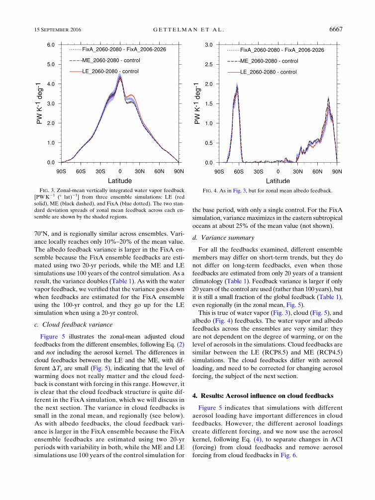
708N, and is regionally similar across ensembles. Vari-

ance locally reaches only 10%–20% of the mean value.

The albedo feedback variance is larger in the FixA en-

semble because the FixA ensemble feedbacks are esti-

mated using two 20-yr periods, while the ME and LE

simulations use 100 years of the control simulation. As a

result, the variance doubles (Table 1). As with the water

vapor feedback, we verified that the variance goes down

when feedbacks are estimated for the FixA ensemble

using the 100-yr control, and they go up for the LE

simulation when using a 20-yr control.

c. Cloud feedback variance

Figure 5 illustrates the zonal-mean adjusted cloud

feedbacks from the different ensembles, following Eq. (2)

and not including the aerosol kernel. The differences in

cloud feedbacks between the LE and the ME, with dif-

ferent DTs are small (Fig. 5), indicating that the level of

warming does not really matter and the cloud feed-

back is constant with forcing in this range. However, it

is clear that the cloud feedback structure is quite dif-

ferent in the FixA simulation, which we will discuss in

the next section. The variance in cloud feedbacks is

small in the zonal mean, and regionally (see below).

As with albedo feedbacks, the cloud feedback vari-

ance is larger in the FixA ensemble because the FixA

ensemble feedbacks are estimated using two 20-yr

periods with variability in both, while the ME and LE

simulations use 100 years of the control simulation for

the base period, with only a single control. For the FixA

simulation, variancemaximizes in the eastern subtropical

oceans at about 25% of the mean value (not shown).

d. Variance summary

For all the feedbacks examined, different ensemble

members may differ on short-term trends, but they do

not differ on long-term feedbacks, even when those

feedbacks are estimated from only 20 years of a transient

climatology (Table 1). Feedback variance is larger if only

20 years of the control are used (rather than 100 years), but

it is still a small fraction of the global feedback (Table 1),

even regionally (in the zonal mean, Fig. 5).

This is true of water vapor (Fig. 3), cloud (Fig. 5), and

albedo (Fig. 4) feedbacks. The water vapor and albedo

feedbacks across the ensembles are very similar: they

are not dependent on the degree of warming, or on the

level of aerosols in the simulations. Cloud feedbacks are

similar between the LE (RCP8.5) and ME (RCP4.5)

simulations. The cloud feedbacks differ with aerosol

loading, and need to be corrected for changing aerosol

forcing, the subject of the next section.

4. Results: Aerosol influence on cloud feedbacks

Figure 5 indicates that simulations with different

aerosol loading have important differences in cloud

feedbacks. However, the different aerosol loadings

create different forcing, and we now use the aerosol

kernel, following Eq. (4), to separate changes in ACI

(forcing) from cloud feedbacks and remove aerosol

forcing from cloud feedbacks in Fig. 6.

FIG. 3. Zonal-mean vertically integrated water vapor feedback

[PWK21 (8 lat)21] from three ensemble simulations: LE (red

solid), ME (black dashed), and FixA (blue dotted). The two stan-

dard deviation spreads of zonal mean feedback across each en-

semble are shown by the shaded regions.

FIG. 4. As in Fig. 3, but for zonal mean albedo feedback.

15 SEPTEMBER 2016 GETTELMAN ET AL . 6667

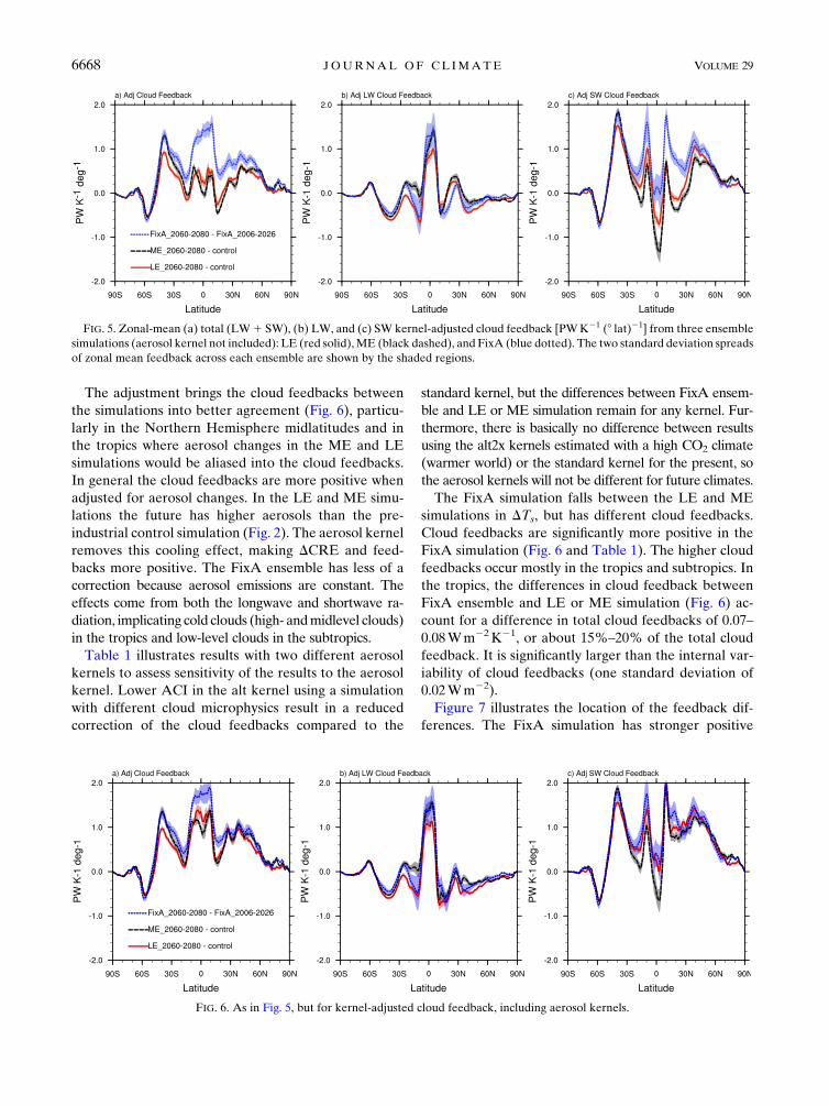
The adjustment brings the cloud feedbacks between

the simulations into better agreement (Fig. 6), particu-

larly in the Northern Hemisphere midlatitudes and in

the tropics where aerosol changes in the ME and LE

simulations would be aliased into the cloud feedbacks.

In general the cloud feedbacks are more positive when

adjusted for aerosol changes. In the LE and ME simu-

lations the future has higher aerosols than the pre-

industrial control simulation (Fig. 2). The aerosol kernel

removes this cooling effect, making DCRE and feed-

backs more positive. The FixA ensemble has less of a

correction because aerosol emissions are constant. The

effects come from both the longwave and shortwave ra-

diation, implicating cold clouds (high- andmidlevel clouds)

in the tropics and low-level clouds in the subtropics.

Table 1 illustrates results with two different aerosol

kernels to assess sensitivity of the results to the aerosol

kernel. Lower ACI in the alt kernel using a simulation

with different cloud microphysics result in a reduced

correction of the cloud feedbacks compared to the

standard kernel, but the differences between FixA ensem-

ble and LE or ME simulation remain for any kernel. Fur-

thermore, there is basically no difference between results

using the alt2x kernels estimated with a high CO2 climate

(warmer world) or the standard kernel for the present, so

the aerosol kernels will not be different for future climates.

The FixA simulation falls between the LE and ME

simulations in DTs, but has different cloud feedbacks.

Cloud feedbacks are significantly more positive in the

FixA simulation (Fig. 6 and Table 1). The higher cloud

feedbacks occur mostly in the tropics and subtropics. In

the tropics, the differences in cloud feedback between

FixA ensemble and LE or ME simulation (Fig. 6) ac-

count for a difference in total cloud feedbacks of 0.07–

0.08Wm22K21, or about 15%–20% of the total cloud

feedback. It is significantly larger than the internal var-

iability of cloud feedbacks (one standard deviation of

0.02Wm22).

Figure 7 illustrates the location of the feedback dif-

ferences. The FixA simulation has stronger positive

FIG. 5. Zonal-mean (a) total (LW1 SW), (b) LW, and (c) SW kernel-adjusted cloud feedback [PWK21 (8 lat)21] from three ensemble

simulations (aerosol kernel not included): LE (red solid),ME (black dashed), and FixA (blue dotted). The two standard deviation spreads

of zonal mean feedback across each ensemble are shown by the shaded regions.

FIG. 6. As in Fig. 5, but for kernel-adjusted cloud feedback, including aerosol kernels.

6668 JOURNAL OF CL IMATE VOLUME 29

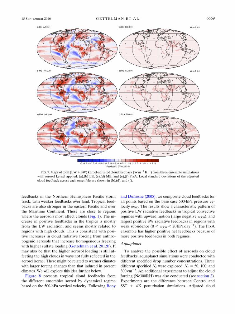
feedbacks in the Northern Hemisphere Pacific storm

track, with weaker feedbacks over land. Tropical feed-

backs are also stronger in the eastern Pacific and over

the Maritime Continent. These are close to regions

where the aerosols most affect clouds (Fig. 1). The in-

crease in positive feedbacks in the tropics is mostly

from the LW radiation, and seems mostly related to

regions with high clouds. This is consistent with posi-

tive increases in cloud radiative forcing from anthro-

pogenic aerosols that increase homogeneous freezing

with higher sulfate loading (Gettelman et al. 2012b). It

may also be that the higher aerosol loading is still af-

fecting the high clouds in ways not fully reflected in the

aerosol kernel. These might be related to warmer climates

with larger forcing changes than that induced in present

climates. We will explore this idea further below.

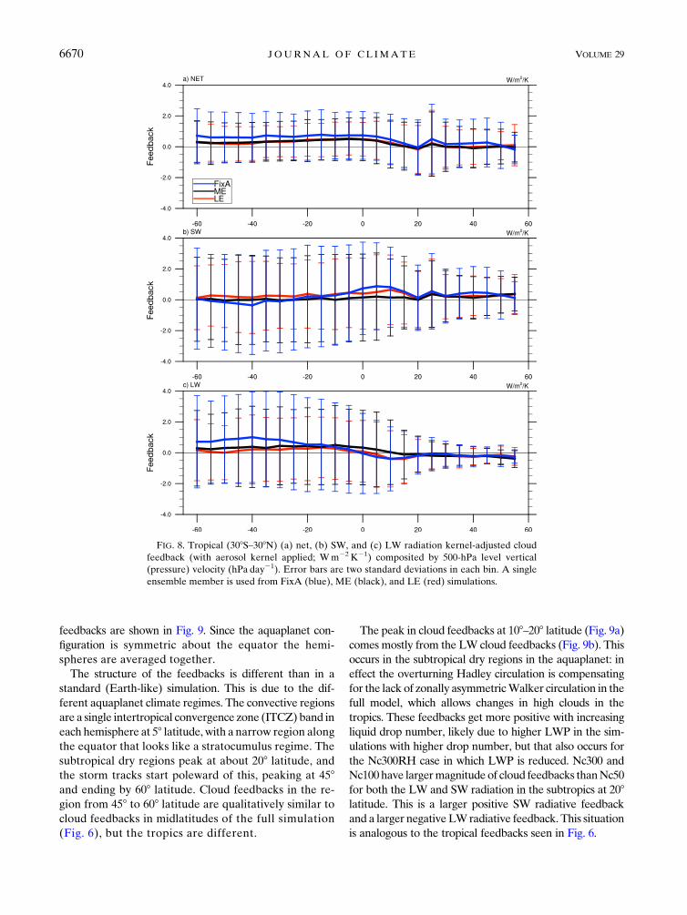
Figure 8 presents tropical cloud feedbacks from

the different ensembles sorted by dynamical regime

based on the 500-hPa vertical velocity. Following Bony

and Dufresne (2005), we composite cloud feedbacks for

all points based on the base case 500-hPa pressure ve-

locity v500. The results show a characteristic pattern of

positive LW radiative feedbacks in tropical convective

regimes with upward motion (large negative v500), and

largest positive SW radiative feedbacks in regions with

weak subsidence (0 , v500 , 20 hPaday21). The FixA

ensemble has higher positive net feedbacks because of

more positive feedbacks in both regimes.

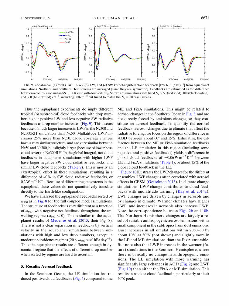
Aquaplanet

To analyze the possible effect of aerosols on cloud

feedbacks, aquaplanet simulations were conducted with

different specified drop number concentrations. Three

different specified Nc were explored: Nc 5 50, 100, and

300 cm23. An additional experiment to adjust the cloud

forcing (Nc300RH) was also conducted (see section 2).

Experiments are the difference between Control and

SST 1 4K perturbation simulations. Adjusted cloud

FIG. 7. Maps of total (LW1 SW) kernel-adjusted cloud feedback (Wm22 K21) from three ensemble simulations

with aerosol kernel applied: (a),(b) LE, (c),(d) ME, and (e),(f) FixA. Local standard deviations of the adjusted

cloud feedback across each ensemble are shown in (b),(d), and (f).

15 SEPTEMBER 2016 GETTELMAN ET AL . 6669

feedbacks are shown in Fig. 9. Since the aquaplanet con-

figuration is symmetric about the equator the hemi-

spheres are averaged together.

The structure of the feedbacks is different than in a

standard (Earth-like) simulation. This is due to the dif-

ferent aquaplanet climate regimes. The convective regions

are a single intertropical convergence zone (ITCZ) band in

each hemisphere at 58 latitude, with a narrow region along

the equator that looks like a stratocumulus regime. The

subtropical dry regions peak at about 208 latitude, andthe storm tracks start poleward of this, peaking at 458and ending by 608 latitude. Cloud feedbacks in the re-

gion from 458 to 608 latitude are qualitatively similar to

cloud feedbacks in midlatitudes of the full simulation

(Fig. 6), but the tropics are different.

The peak in cloud feedbacks at 108–208 latitude (Fig. 9a)comes mostly from the LW cloud feedbacks (Fig. 9b). This

occurs in the subtropical dry regions in the aquaplanet: in

effect the overturning Hadley circulation is compensating

for the lack of zonally asymmetricWalker circulation in the

full model, which allows changes in high clouds in the

tropics. These feedbacks get more positive with increasing

liquid drop number, likely due to higher LWP in the sim-

ulations with higher drop number, but that also occurs for

the Nc300RH case in which LWP is reduced. Nc300 and

Nc100have largermagnitude of cloud feedbacks thanNc50

for both the LW and SW radiation in the subtropics at 208latitude. This is a larger positive SW radiative feedback

and a larger negative LWradiative feedback. This situation

is analogous to the tropical feedbacks seen in Fig. 6.

FIG. 8. Tropical (308S–308N) (a) net, (b) SW, and (c) LW radiation kernel-adjusted cloud

feedback (with aerosol kernel applied; Wm22 K21) composited by 500-hPa level vertical

(pressure) velocity (hPa day21). Error bars are two standard deviations in each bin. A single

ensemble member is used from FixA (blue), ME (black), and LE (red) simulations.

6670 JOURNAL OF CL IMATE VOLUME 29

Thus the aquaplanet experiments do imply different

tropical (or subtropical) cloud feedbacks with drop num-

ber: higher positive LW and less negative SW radiative

feedbacks as drop number increases (Fig. 9). This occurs

because ofmuch larger increases inLWP in theNc300 and

Nc300RH simulation than Nc50. Midlatitude LWP in-

creases 25% more than Nc50. Cloud coverage changes

have a very similar structure, and are very similar between

Nc50 andNc300, but slightly larger (because of lower base

cloud cover) in Nc300RH. In the global integral, net cloud

feedbacks in aquaplanet simulations with higher LWP

have larger negative SW cloud radiative feedbacks, and

similar LW cloud feedbacks (Table 2). This is mostly an

extratropical effect in these simulations, resulting in a

difference of 40% in SW cloud radiative feedbacks, or

0.2Wm22K21. Because of different regime extents in the

aquaplanet these values do not quantitatively translate

directly to the Earth-like configuration.

We have analyzed the aquaplanet feedbacks sorted by

v500 as in Fig. 8 for the full coupled model simulations.

The structure of feedbacks is very different as a function

of v500, with negative net feedback throughout the up-

welling regime (v500 , 0). This is similar to the aqua-

planet results of Medeiros et al. (2015, their Fig. 8).

There is not a clear separation in feedbacks by vertical

velocity in the aquaplanet simulations between sim-

ulations with high and low drop numbers, except in

moderate subsidence regimes (20,v500, 40hPaday21).

Thus the aquaplanet results are different enough in dy-

namical regime that the effects of different drop number

when sorted by regime are hard to ascertain.

5. Results: Aerosol feedback

In the Southern Ocean, the LE simulation has re-

duced positive cloud feedbacks (Fig. 6) compared to the

ME and FixA simulations. This might be related to

aerosol changes in the Southern Ocean in Fig. 2, and are

not directly forced by emissions changes, so they con-

stitute an aerosol feedback. To quantify the aerosol

feedback, aerosol changes due to climate that affect the

radiative forcing, we focus on the region of difference in

AOD between about 608 and 158S. Estimating the dif-

ference between the ME or FixA simulation feedbacks

and the LE simulation in this region (including some

negative and positive feedbacks) yields a difference in

global cloud feedbacks of 20.06Wm22K21 between

LE and FixA simulations (Table 1), or about 15% of the

global cloud feedback in the LE.

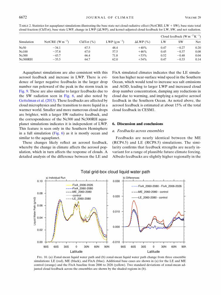
Figure 10 illustrates the LWP changes for the different

ensembles. LWP change is often correlated with aerosol

effects in CESM (Gettelman 2015). In climate change

simulations, LWP change contributes to cloud feed-

backs with midlatitude warming (Kay et al. 2014a).

LWP changes are driven by changes in aerosols and

by changes in climate. Warmer climates have higher

LWP, and increases in aerosols also increase LWP.

Note the correspondence between Figs. 2b and 10b.

The Northern Hemisphere changes are largely a re-

sult of variable anthropogenic aerosol emissions, with a

small component in the subtropics from dust emissions.

Dust increases in all simulations within 2060–80 by

about 10% at 308N (not shown) and slightly more in

the LE and ME simulations than the FixA ensemble.

But note also that LWP increases in the warmer (fu-

ture) simulations in the Southern Hemisphere, where

there is basically no change in anthropogenic emis-

sions. The LE simulation with more warming has

significantly larger changes in AOD (Fig. 2) and LWP

(Fig. 10) than either the FixA or ME simulation. This

results in weaker cloud feedbacks, particularly at their

408S peak.

FIG. 9. Zonal-mean (a) total (LW 1 SW), (b) LW, and (c) SW kernel-adjusted cloud feedback [PWK21 (8 lat)21] from aquaplanet

simulations. Northern and Southern Hemispheres are averaged (since they are symmetric). Feedbacks are estimated as the difference

between a control case and an SST1 4K case with doubledCO2. Shown are simulations with fixedNc of 50 (red solid), 100 (black dashed),

and 300 (blue dotted) cm23, including 300 cm23 but tuned to match the Nc 5 50 case (green).

15 SEPTEMBER 2016 GETTELMAN ET AL . 6671

Aquaplanet simulations are also consistent with this

aerosol feedback and increase in LWP. There is evi-

dence of larger negative feedbacks in the larger drop

number run poleward of the peak in the storm track in

Fig. 9. These are also similar to larger feedbacks due to

the SW radiation seen in Fig. 6, and also noted by

Gettelman et al. (2013). These feedbacks are affected by

cloud microphysics and the transition to more liquid in a

warmer world. Smaller and more numerous cloud drops

are brighter, with a larger SW radiative feedback, and

the correspondence of the Nc300 and Nc300RH aqua-

planet simulations indicates it is independent of LWP.

This feature is seen only in the Southern Hemisphere

in a full simulation (Fig. 6) as it is mostly ocean and

similar to the aquaplanet.

These changes likely reflect an aerosol feedback,

whereby the change in climate affects the aerosol pop-

ulation, which in turn affects the response of clouds. A

detailed analysis of the difference between the LE and

FixA simulated climates indicates that the LE simula-

tion has higher near-surface wind speed in the Southern

Ocean, which would tend to increase sea salt emissions

and AOD, leading to larger LWP and increased cloud

drop number concentration, damping any reductions in

cloud due to warming, and implying a negative aerosol

feedback in the Southern Ocean. As noted above, the

aerosol feedback is estimated at about 15% of the total

cloud feedback in CESM1.

6. Discussion and conclusions

a. Feedbacks across ensembles

Feedbacks are nearly identical between the ME

(RCP4.5) and LE (RCP8.5) simulations. The simi-

larity confirms that feedback strengths are nearly in-

variant for a range of plausible future climate forcing.

Albedo feedbacks are slightly higher regionally in the

TABLE 2. Statistics for aquaplanet simulations illustrating the base state net cloud radiative effect (NetCRE; LW1 SW), base state total

cloud fraction (CldTot), base state LWP, change in LWP (DLWP), and kernel-adjusted cloud feedback for LW, SW, and net radiation.

Simulation NetCRE (Wm22) CldTot (%) LWP (gm22) DLWP (%)

Cloud feedback (Wm22 K21)

LW SW Net

Nc50 234.1 67.5 48.4 140% 0.47 20.27 0.20

Nc100 237.8 67.0 57.5 146% 0.45 20.37 0.08

Nc300 243.7 66.4 71.8 153% 0.52 20.48 0.04

Nc300RH 235.5 64.7 62.0 154% 0.47 20.33 0.14

FIG. 10. (a) Zonal-mean liquid water path and (b) zonal-mean liquid water path change from three ensemble

simulations: LE (red), ME (black), and FixA (blue). Additional base cases are shown in (a) for the LE and ME

control (orange) and the FixA baseline from 2006 to 2026 (yellow). Two standard deviations of zonal-mean ad-

justed cloud feedback across the ensembles are shown by the shaded regions in (b).

6672 JOURNAL OF CL IMATE VOLUME 29

LE (RCP8.5) simulation. This makes sense as high

latitudes experience the largest warming.

The ensemble spread (internal variability) in feed-

backs is very small. This might be expected for water

vapor feedbacks, and possibly even for cloud feedbacks,

but it is also true of albedo feedbacks. All feedbacks are

remarkably stable with respect to internal variability

in a model, even for simulations based on 20 years of

output. Low variability of albedo feedbacks may seem

counterintuitive in light of work showing large differ-

ences in short-term climate trends (Deser et al. 2012;

Kay et al. 2014b). Variability in near-term climate

trends is not caused by varying feedbacks. It implies

that the variability in high-latitude warming trends is

due more to variations in heat transport or absorption

or constant feedback responses of the coupled system

(heat to or from the ocean) than to variations in the

structural nature of ‘‘fast feedbacks’’ in the atmosphere

or at the surface. Even large-scale decadal modes of

variability do not seem to project onto feedbacks.

b. Role of aerosols in feedbacks

The role of aerosols in climate feedbacks is complex.

Aerosols alias into cloud feedbacks, and in simulations

with changing aerosols they must be accounted for. As

an added complication, the efficiency (or efficacy) of

inhomogeneous forcing like aerosols to affect surface

temperature may be larger than that for CO2 (Hansen

et al. 2005; Shindell 2014; Marvel et al. 2015). Different

efficacies may bias the estimates of total response from

historical forcing. Here we have shown a complemen-

tary result: aerosol forcings alter interpretations of fu-

ture climate feedbacks, not just present-day forcing. We

use an equilibrium framework, similar to effective ra-

diative forcing (Marvel et al. 2015), where efficacies for

aerosols are close to 1.

The aerosol kernel method is largely successful at

removing a signal due to aerosols in the different en-

sembles, and the resulting cloud feedbacks including an

aerosol kernel adjustment are quite similar in many re-

gions. However, it is difficult to apply a single aerosol

kernel across models. The aerosol kernel is basically an

expression of the ACI in a particular model. A com-

parison of aerosol kernels across models would be a

useful framework for analyzing multimodel uncertainty

in ACI.

In addition to the spurious changes that aerosols will

have because of ACI from changes in emissions, there

are other changes we have not removed. These changes

in feedbacks remain because they are not present in the

aerosol emissions change experiment from which the

kernel was calculated. There are two effects due to cloud

state changes and aerosol feedbacks.

c. Cloud state changes from aerosols

First, aerosols affect cloud feedbacks through effects

of altering the cloud state. The difference is evident

in the tropics of the CESM simulations, where cloud

feedbacks, adjusted for aerosols, are still higher in

tropics and subtropics in the FixA ensemble than in the

LE and ME simulations. The difference is 0.07–

0.08Wm22K21, or approximately 20% of the total

global cloud feedback. For a typical total feedback pa-

rameter of 1.33Wm22K21, implying a 3-K climate

sensitivity for a 4Wm22 CO2 forcing, the difference

would contribute to about 0.25K of climate sensitivity.

This is much larger than the variance in the feedbacks

within any ensemble, so the difference is not internal

variability of simulations. In general the LW radiative

feedbacks are more positive, and the SW radiation less

negative with higher aerosols. In the tropics the increase

in feedback occurs in most regions. In midlatitudes,

there are offsetting changes between land and ocean:

ocean regions see more positive feedback in the NH in

the FixA ensemble, but the zonal-mean total cloud

feedback is similar.

How certain are these effects, and what is the mech-

anism? The higher feedbacks are seen with and without

the aerosol kernel adjustment. The effects are sub-

stantial in regions of eastern and southeastern Asia,

as well as over the subtropical oceans (Fig. 7), where

higher aerosols in the FixA ensemble brighten clouds

throughout the twenty-first century. The effect may be

through reduced LWP change and different base state

LWP, which may buffer changes in SW radiative cloud

cover and increase SW radiative feedbacks, or in-

crease high clouds in the tropics and affect the ice

phase. A more detailed analysis with cloud property

kernels and using other models with different aerosol

treatments would be valuable for understanding the

mechanisms further.

Altered feedbacks due to different cloud state are seen

in aquaplanet simulations. The different drop number

experiments are an analog for higher aerosol concentra-

tions. The regimes are different than in the full simula-

tions, but the subtropical increase in feedbacks occurs

with higher drop numbers, with LW radiation increases

not quite balanced by SW radiation decreases because

of larger changes in high clouds in the higher drop

number experiments. In full simulations, the main

signal in the tropics is a high cloud effect over land, the

Maritime Continent and some ocean regions. Aqua-

planet simulations have higher LWP with larger drop

numbers (unless LWP limited as in Nc300RH) and

larger cloud feedbacks as LWP increases. Different

drop numbers alter LWP in the aquaplanet simulations,

15 SEPTEMBER 2016 GETTELMAN ET AL . 6673

and the change in LWP seems to alter cloud feedbacks.

Note that LWP is adjusted with the Nc300RH simulation

to be more like Nc50, and the resulting feedbacks are

more like Nc50. The mechanism is consistent with full

simulations where aerosols alter LWP.

d. Aerosol feedback

The second effect of aerosols is an ‘‘aerosol feedback’’

that results from aerosols whose emissions depend on

climate. In the Southern Hemisphere storm tracks there

appears to be a feedback based on increasing wind speed

increasing sea salt, and this increases drop number and

cloud brightness, hence creating a different feedback.

This contributes about 15%of total cloud feedback (0.04–

0.06Wm22K21), and this difference would imply about

0.15K of global mean surface temperature change. No

significant effect is seenwith dust emissions, which affect a

region of the subtropics, but have a smaller perturbation.

e. Conclusions

In summary, climate feedbacks are remarkably stable

across ensemble members, even when estimated using

only 20 years of data (as with the FixA simulation). Var-

iance reaches only 25% of the feedback in highly variable

regions such as the sea ice edge for albedo feedbacks, and

the subtropics for water vapor feedbacks. Cloud feed-

backs have regional variance up to 30% of the local cloud

feedback, but the global variance is very small (5%).

It is possible to calculate feedbacks with transient

simulations, and feedbacks estimated with different

RCPs (LE vs ME simulations) are nearly identical in all

respects. Thus feedbacks are broadly linear for pertur-

bations on the century time scale.

Changing aerosol emissions will change cloud radia-

tive effects and alias into climate feedbacks. These must

be removed to understand what the true cloud feedback

is, which can be accomplished with an ‘‘aerosol kernel.’’

There appears to be a small impact of different cloud

microphysical states (induced by aerosols, and specified

in the aquaplanet simulations) on cloud feedbacks,

mostly through the longwave effect of high clouds in the

tropics, which in CESM is approximately 20% of the

global cloud feedback.

There also appear to be distinct aerosol feedbacks

from aerosol species whose emissions are dependent on

climate. Here the warmer climate of the RCP8.5 LE

simulation has higher wind speeds than in the control

climate, and thus larger AOD from sea salt, leading to a

change in drop number and an impact on clouds. The

Southern Ocean aerosol feedback in CESM is about

15% of the global cloud feedback. In the midlatitudes of

the aquaplanet simulations, cloud feedbacks are simi-

larly altered by specifying higher drop numbers.

Aquaplanet simulations show sensitivity to drop

number, with extratropical SW cloud feedbacks getting

more negative with higher LWP. The regimes are dif-

ferent than in full simulations, making direct attribution

difficult. However, the simulations confirm that cloud

microphysics and aerosol effects on cloud microphysics

may alter cloud feedbacks.

Thus aerosol effects need to be accounted for in

complex Earth systemmodels (ESMs), and comparisons

across models will have uncertainties in cloud feedback

driven by differences in aerosols and aerosol–cloud in-

teractions. In CESM, the combined effects of aerosol

feedback and alterations to cloud feedback contribute

to a nearly 50%difference in total cloud feedback between

the LE (0.41Wm22K21) and FixA (0.60Wm22K21)

simulations (Table 1), regardless of aerosol kernel used.

Aerosols may enhance ensemble spread across multi-

model ensembles due to different treatments of aerosols

and aerosol–cloud interactions. These mechanisms and

effects should be verified in other ESMs with compre-

hensive aerosol treatments, and further detailed and ide-

alized experiments conducted to more completely isolate

and quantify aerosol feedbacks.

Acknowledgments.Thanks toB. Sandersonand J. Fasullo

for comments. L. Lin is supported by the National

Basic Research Program of China (2012CB955303),

NSFC Grant 41275070, the National Science Foun-

dation of China under Grant (41405010), and the

China Scholarship council. B. Medeiros and J. Olson

acknowledge support from the Regional and Global

Climate Modeling Program of the U.S. Department of

Energy’s Office of Science, Cooperative Agreement DE-

FC02-97ER62402.

REFERENCES

Albrecht, B. A., 1989: Aerosols, cloud microphysics and frac-

tional cloudiness. Science, 245, 1227–1230, doi:10.1126/

science.245.4923.1227.

Armour, K. C., C. M. Bitz, and G. H. Roe, 2013: Time-varying

climate sensitivity from regional feedbacks. J. Climate, 26,

4518–4534, doi:10.1175/JCLI-D-12-00544.1.

Bony, S., and J. L. Dufresne, 2005: Marine boundary layer clouds

at the heart of tropical cloud feedback uncertainties in cli-

mate models. Geophys. Res. Lett., 32, L20806, doi:10.1029/

2005GL023851.

——, and Coauthors, 2015: Clouds, circulation and climate sensi-

tivity. Nat. Geosci., 8, 261–268, doi:10.1038/ngeo2398.Boucher, O., and Coauthors, 2013: Clouds and aerosols. Climate

Change 2013: The Physical Science Basis, T. F. Stocker et al.,

Eds., Cambridge University Press, 571–657.

Cess, R. D., and Coauthors, 1990: Intercomparison and in-

terpretation of climate feedback processes in 19 atmospheric

general circulation models. J. Geophys. Res., 95, 16 601–

16 615, doi:10.1029/JD095iD10p16601.

6674 JOURNAL OF CL IMATE VOLUME 29

Deser, C., A. Phillips, V. Bourdette, and H. Teng, 2012: Uncertainty

in climate change projections: The role of internal variability.

Climate Dyn., 38, 527–546, doi:10.1007/s00382-010-0977-x.

Dessler, A. E., 2010: A determination of the cloud feedback from

climate variations over the past decade. Science, 330, 1523–

1527, doi:10.1126/science.1192546.

Fasullo, J. T., B. M. Sanderson, and K. E. Trenberth, 2015: Recent

progress in constraining climate sensitivity with model en-

sembles. Curr. Climate Change Rep., 1, 268–275, doi:10.1007/

s40641-015-0021-7.

Flato, G., and Coauthors, 2013: Evaluation of climate models.

Climate Change 2013: The Physical ScienceBasis, T. F. Stocker

et al., Eds., Cambridge University Press, 741–866.

Forster, P. M. F., and J. M. Gregory, 2006: The climate sensitivity

and its components diagnosed from Earth radiation budget

data. J. Climate, 19, 39–52, doi:10.1175/JCLI3611.1.

Gettelman, A., 2015: Putting the clouds back in aerosol–cloud in-

teractions. Atmos. Chem. Phys., 15, 12 397–12 411, doi:10.5194/

acp-15-12397-2015.

——, and H. Morrison, 2015: Advanced two-moment bulk micro-

physics for globalmodels. Part I: Off-line tests and comparison

with other schemes. J. Climate, 28, 1268–1287, doi:10.1175/

JCLI-D-14-00102.1.

——, and Coauthors, 2010: Global simulations of ice nucleation

and ice supersaturation with an improved cloud scheme in

the Community Atmosphere Model. J. Geophys. Res., 115,

D18216, doi:10.1029/2009JD013797.

——, J. E. Kay, and K. M. Shell, 2012a: The evolution of climate

feedbacks in the Community Atmosphere Model. J. Climate,

25, 1453–1469, doi:10.1175/JCLI-D-11-00197.1.

——, X. Liu, D. Barahona, U. Lohmann, and C. C. Chen, 2012b:

Climate impacts of ice nucleation. J. Geophys. Res., 117,

D20201, doi:10.1029/2012JD017950.

——, H. Morrison, C. R. Terai, and R. Wood, 2013: Microphysical

process rates and global aerosol–cloud interactions. Atmos.

Chem. Phys., 13, 9855–9867, doi:10.5194/acp-13-9855-2013.

Ghan, S. J., and Coauthors, 2013: A simple model of global aerosol

indirect effects. J. Geophys. Res. Atmos., 118, 6688–6707,

doi:10.1002/jgrd.50567.

Gregory, J. M., and Coauthors, 2004: A newmethod for diagnosing

radiative forcing and climate sensitivity. Geophys. Res. Lett.,

31, L03205, doi:10.1029/2003GL018747.

Hansen, J., and Coauthors, 2005: Efficacy of climate forcings.

J. Geophys. Res., 110, D18104, doi:10.1029/2005JD005776.

Jonko, A. K., K. M. Shell, B. M. Sanderson, and G. Danabasoglu,

2012: Climate feedbacks in CCSM3 under changing CO2

forcing. Part I: Adapting the linear radiative kernel technique

to feedback calculations for a broad range of forcings.

J. Climate, 25, 5260–5272, doi:10.1175/JCLI-D-11-00524.1.

Kay, J. E., B.Medeiros, Y.-T. Hwang, A. Gettelman, J. Perket, and

M. Flanner, 2014a: Processes controlling Southern Ocean

shortwave climate feedbacks in CESM. Geophys. Res. Lett.,

41, 616–622, doi:10.1002/2013GL058315.

——, and Coauthors, 2014b: The Community Earth SystemModel

(CESM) Large Ensemble Project: A community resource for

studying climate change in the presence of internal climate

variability.Bull. Amer.Meteor. Soc., 96, 1333–1349, doi:10.1175/

BAMS-D-13-00255.1.

Klocke, D., J. Quaas, and B. Stevens, 2013: Assessment of different

metrics for physical climate feedbacks. Climate Dyn., 41,

1173–1185, doi:10.1007/s00382-013-1757-1.

Knutti, R., and M. A. A. Rugenstein, 2015: Feedbacks, climate

sensitivity and the limits of linear models. Philos. Trans. Roy.

Soc., 373A, doi:10.1098/rsta.2015.0146.

Lamarque, J., G. Kyle, M. Meinshausen, K. Riahi, S. Smith, D. van

Vuuren, A. Conley, and F. Vitt, 2011: Global and regional

evolution of short-lived radiatively-active gases and aerosols

in the representative concentration pathways.Climatic Change,

109, 191–212, doi:10.1007/s10584-011-0155-0.Liu, X., and Coauthors, 2012: Toward a minimal representation of

aerosols in climate models: Description and evaluation in the

Community Atmosphere Model CAM5. Geosci. Model Dev.,

5, 709–739, doi:10.5194/gmd-5-709-2012.

Marvel, K., G. A. Schmidt, R. L. Miller, and L. S. Nazarenko, 2015:

Implications for climate sensitivity from the response to in-

dividual forcings.Nat. Climate Change, 6, 386–389, doi:10.1038/nclimate2888.

Medeiros, B., B. Stevens, and S. Bony, 2015: Using aquaplanets to

understand the robust responses of comprehensive climate

models to forcing. Climate Dyn., 44, 1957–1977, doi:10.1007/s00382-014-2138-0.

——, D. L. Williamson, and J. G. Olson, 2016: Reference aquaplanet

climate in theCommunityAtmosphereModel, version 5. J. Adv.

Model. Earth Syst., 8, 406–424, doi:10.1002/2015MS000593.

Neale, R. B., and Coauthors, 2010: Description of the NCAR

Community Atmosphere Model (CAM5.0). NCAR Tech.

Rep. NCAR/TN-4861STR, 268 pp.

Park, S., 2014: A Unified Convection Scheme (UNICON). Part I:

Formulation. J. Atmos. Sci., 71, 3902–3930, doi:10.1175/

JAS-D-13-0233.1.

Sanderson, B.M., K.W.Oleson,W.G. Strand, F. Lehner, and B. C.

O’Neill, 2016: A new ensemble of GCM simulations to assess

avoided impacts in a climate mitigation scenario. Climatic

Change, doi:10.1007/s10584-015-1567-z, in press.

Schneider, S., 1972: Cloudiness as a global climatic feedback

mechanism: The effects on radiation balance and surface

temperatures of variations in cloudiness. J. Atmos. Sci.,

29, 1413–1422, doi:10.1175/1520-0469(1972)029,1413:

CAAGCF.2.0.CO;2.

Shell, K.M., J. T. Kiehl, andC.A. Shields, 2008:Using the radiative

kernel technique to calculate climate feedbacks in NCAR’s

Community Atmosphere Model. J. Climate, 21, 2269–2282,doi:10.1175/2007JCLI2044.1.

Shindell, D. T., 2014: Inhomogeneous forcing and transient climate

sensitivity. Nat. Climate Change, 4, 274–277, doi:10.1038/

nclimate2136.

Soden, B. J., I.M.Held, R. Colman, K.M. Shell, J. T. Kiehl, andC.A.

Shields, 2008: Quantifying climate feedbacks using radiative

kernels. J. Climate, 21, 3504–3520, doi:10.1175/2007JCLI2110.1.

Twomey, S., 1977: The influence of pollution on the shortwave

albedo of clouds. J. Atmos. Sci., 34, 1149–1152, doi:10.1175/

1520-0469(1977)034,1149:TIOPOT.2.0.CO;2.

van Vuuren, D. P., and Coauthors, 2011: The representative con-

centration pathways: An overview. Climatic Change, 109, 5–31,

doi:10.1007/s10584-011-0148-z.

Xu, Y., J.-F. Lamarque, and B. M. Sanderson, 2016: The impor-

tance of aerosol scenarios in projections of future heat extremes.

Climatic Change, doi:10.1007/s10584-015-1565-1, in press.

Zelinka, M., S. Klein, and D. Hartmann, 2012: Computing and

partitioning cloud feedbacks using cloud property histograms.

Part II: Attribution to changes in cloud amount, altitude, and

optical depth. J. Climate, 25, 3736–3754, doi:10.1175/

JCLI-D-11-00249.1.

15 SEPTEMBER 2016 GETTELMAN ET AL . 6675