Embed Size (px)
Citation preview
Task 636 (387)
Climate Change Research
Research into the Highways Agency’s Water Footprint
April 2010
Research into the Highways Agency’s Water Footprint
Climate Change Portfolio Contract 3/387 – National Framework for Research and Development Services Document Control
Document Control Sheet
Report Title
Final Version: Research into the Highways Agency’s Water Footprint
Document No.
HSR91450AB/001
Originator: Client:
PB Queen Victoria House Redland Hill Bristol BS6 6US
Highways Agency Temple Quay House 2, The Square Temple Quay Bristol, BS1 6HA
Tel: 0117 933 9300
Fax: 0117 933 9251
AUTHORISATION
PB Final Version, Issued by:
Kathryn Vowles
Signature: Date: April 2010
This report has been prepared as part of the Climate Change Portfolio of Projects being undertaken by the PB-WSP consortium on behalf of the Highways Agency. The Delivery Team consists of:
Lead Organisation: PB
Research into the Highways Agency’s Water Footprint
Climate Change Portfolio Contract 3/387 – National Framework for Research and Development Services Page i
CONTENTS
1 Introduction 1
1.1 Background 1
1.2 Research Objective 1
1.3 Interactions with Water 1
2 Context – Water Resource Pressures 3
2.1 Global Water Distribution 3
2.2 Water Stress & Scarcity 3
2.3 UK Water Resource Pressure 4
2.4 Impacts of Climate Change 5
2.5 Summary 6
3 Measures of Water Impact 7
3.1 Corporate Water Risk 7
3.2 Embodied Water, Virtual Water and the Water Footprint 7
3.3 Analysis of UK Water Footprint 8
3.4 Measuring Organisational Water Footprints 9
4 Internal Water Use 10
4.1 Review of Corporate Position on Water 10
4.2 Previous Analysis of Water Use 11
4.3 Office Blue Water Consumption 12
4.4 Meeting Targets 14
4.5 Key Findings 14
5 Supply-Chain Direct Operations 15
5.1 Major Projects 15
5.2 Design-Build-Finance-Operate Schemes 19
5.3 Managing Agent Contractors 20
5.4 Key Findings 21
6 Supply-Chain Indirect (Materials) 23
6.1 Production of Aggregates 23
6.2 Production of Cement & Concrete 24
6.3 Production of Steel 26
6.4 Bitumen & Diesel Production 27
6.5 Key Limitations 28
6.6 Geographic Impacts 28
6.7 Key Findings 29
7 Grey Water Footprint 31
7.1 Methodology 31
7.2 Road Network Coverage 31
7.3 Precipitation Inputs 32
Research into the Highways Agency’s Water Footprint
Climate Change Portfolio Contract 3/387 – National Framework for Research and Development Services Page ii
7.4 Key Findings 33
8 Key Findings from Research 34
8.1 Interpretation of Water Footprint 35
8.2 Conclusions & Future of Water Footprinting 36
9 References 38
APPENDICES
Appendix A Global Water Demands
Appendix B UK Water Trends
Appendix C Global Water & Climate Change Impacts
Appendix D UK Climate Impacts Programme Projections
Appendix E Highways Agency Office Consumption
Appendix F Site Water Use
Appendix G Material Production & Embodied Use
Appendix H UK Mineral Self-Sufficiency & Imports
Appendix I Grey Water Information
Research into the Highways Agency’s Water Footprint
Climate Change Portfolio Contract 3/387 – National Framework for Research and Development Services Page iii
EXECUTIVE SUMMARY
Research Context
All organisations interact with water, either directly or indirectly, and the value of this resource is increasingly being recognised. Available global resources are limited, and in certain regions are being placed under increasing pressures due to population growth, industrial development and climate change. Agriculture is a key influence and driver, although water use in the domestic and industrial sectors is projected to significantly increase in intensity. In the UK, water catchments in certain regions are being exploited unsustainably through over-exploitation, over-licensing and limited additional supply capacity during dryer periods. Population growth of an additional 10 million people by 2033, combined with the seasonal supply and demand impacts of climate change will increasingly threaten the security of supply and the health of UK water environments.
The water footprint concept is emerging as an indicator of impact upon water resources, and is comprised of blue water (extracted surface and groundwater), green water (rainwater stored in the soil and utilised by vegetation) and grey water (polluted water or effluent produced). It also seeks to establish the nature of geographical impacts of water use, both domestically and internationally. The Highways Agency interacts with water in different ways – as a direct and indirect consumer, and through its drainage provisions. All of these different aspects contribute to the Highways Agency’s water footprint. The key areas of impact have been investigated as part of this report, in order to determine how the Highways Agency might best address the emerging water footprint agenda within its sustainability and corporate responsibility efforts.
Key Findings
Internal water use from Highways Agency offices and facilities is estimated at 22,500m3 per year from which a reduction of 515m3 per year will be required to meet the Governments first target in 2016/17. Previous research indicated that water reductions are achievable, although from historic data a concerted effort and delivery strategy will be required. Within a wider context, although Government Departments must demonstrate leadership, it is concluded that the greatest potential to deliver cost-effective water savings lies within the supply-chain rather than the internal estate.
Onsite use by Major Projects, DBFO’s and MACs in 2009/10 is estimated to be from 415-535,000m3. Site use is strongly influenced by the scale and type of works. For example, certain projects avoid the direct use of water through the use of ready-mix concrete whereas others incur this impact through onsite concrete batching plants. Certain areas of the supply chain are more active in addressing water management, and are investigating improvements and changes in practice but on the whole monitoring is relatively low and represents a key area of improvement. There are potentially significant volumes of water being used onsite which are currently unrecorded, coming from un-metered sources, unlicensed abstractions or through the use of water collected onsite which are largely unrecorded.
The ability to accurately estimate the total indirect demand is limited by available data and its reliability, but initial analysis indicates that the estimated volume of water required in the production of selected materials represents a significant proportion of the water footprint (270,000m3 from aggregates, cement, concrete, steel and diesel). With more robust data covering total water inputs of relevant industries, it would be expected that indirect water demand would exceed direct use onsite.
Water quality impacts have historically be a key area of interest for the Highways Agency, and in terms of its water footprint the volume of grey water production is potentially the most significant component. At a high level the volume of highway runoff is substantial at an estimated at 251km3 per annum, prior to treatment. A substantial will receive treatment through silt and oil traps and retention pounds for example, which will significantly reduce the grey water footprint of highway runoff. Assuming that an indicative 1% of runoff enters a water resource with pollutant levels above natural concentrations, would yield a grey water footprint from the network of 2.5 million m3 per annum. The development of a refined model could provide a more accurate estimation, following which measures to address the grey water footprint of specific schemes could follow.
Conclusions
The water footprint concept provides the Highways Agency with an alternative perspective on water use, and, like carbon footprinting, can provide a unified agenda both internally and within the supply chain. The Highways Agency faces challenging targets internally, for which strategy and direction are required. But targets to reduce direct use in offices and supply-chain operations will only address part of the issue, as
Research into the Highways Agency’s Water Footprint
Climate Change Portfolio Contract 3/387 – National Framework for Research and Development Services Page iv
significant volumes of water could also be saved, potentially more cost-effectively, through a focus on resource efficiency.
The indirect water demand of materials is a real contributor to the water footprint, but at present the ability to measure this is limited given the infancy of water footprinting and its data intensive nature. A key theme of the findings for each section is the need for a robust dataset and water management procedures, both internally and from within the supply-chain. In the time water footprinting needs to evolve into a practical process for end-consumer organisations such as the Highways Agency, there is the opportunity to focus upon developing the systems and procedures to measure and manage direct water use, to debate and establish its corporate position, and to engage the supply-chain in both resource and water efficiency.
Research into the Highways Agency’s Water Footprint
Climate Change Portfolio Contract 3/387 – National Framework for Research and Development Services Page 1
1 INTRODUCTION
1.1 BACKGROUND All organisations interact with water, either directly or indirectly, and the value of this resource is increasingly being recognised. Within the UK, there are growing pressures upon water resources, and factors such as the effects of climate change and projected population growth are likely to enhance these. As such, the analysis of water use and consumption is of growing importance for organisations and following the uptake of carbon footprinting, water footprinting is likely to become embedded in organisations corporate reporting over the next few years. The underlying issue for many is that water is a finite resource, as well as a fundamental requirement in material production, and beyond achieving greater efficiency in use, there is no potential substitute.
UK Government Departments are under increasing scrutiny to report on natural resource consumption through the Sustainable Development in Government (SDiG) targets, which include water-related targets to which the Highways Agency must adhere. Furthermore, the 2008 Sustainable Development in Government (SDiG) Report, stated that:
“Government and departments should begin to develop the methodologies to produce water footprints in order to help them understand the water consumption used through their operations and procurement practices, including embedded water in products.”
In addition, the Strategy for Sustainable Construction (2008) establishes a challenging target to reduce water use in the manufacturing and construction phase by 20% by 2012, compared with a 2008 baseline.
Analysis of corporate water use has traditionally focused on direct resource consumption, volumes of discharge, and the impact of pollutant activities. The SDiG Report reflects a broadening of approach; to also begin to understand the wider impacts demands place on water resources for example through corporate procurement and the activities of supply-chains. Furthermore, the links between water efficiency and carbon are increasingly made, as part of a unified agenda.
1.2 RESEARCH OBJECTIVE Following carbon, water is emerging to be the next area of corporate sustainability focus through the concept of the ‘water footprint’. Despite widespread interest, this method is currently at an embryonic stage in that the issues and approach are only now beginning to be tested and debated. Required industry information is therefore limited at the present time. Where information is available, its application is confused by uncertainties surrounding its scope and assumptions, which are not fully or consistently documented. Following experience in carbon footprinting, consistency is a fundamental requirement for success.
Within this context, the primary objective of this research is to be the starting point for promoting a greater awareness of sustainable water use within the Highways Agency, and therefore within its supply-chain. To achieve this, the water footprint concept has been investigated, followed by analysis of available water consumption data, and research into the embodied water contents of selected construction materials.
This approach allows the investigation of the water footprint method in relation to the Highways Agency, in order to establish where the key areas of impact (i.e. water use) are, and to determine how the Highways Agency might best address the emerging water footprint agenda within its sustainability and corporate responsibility efforts.
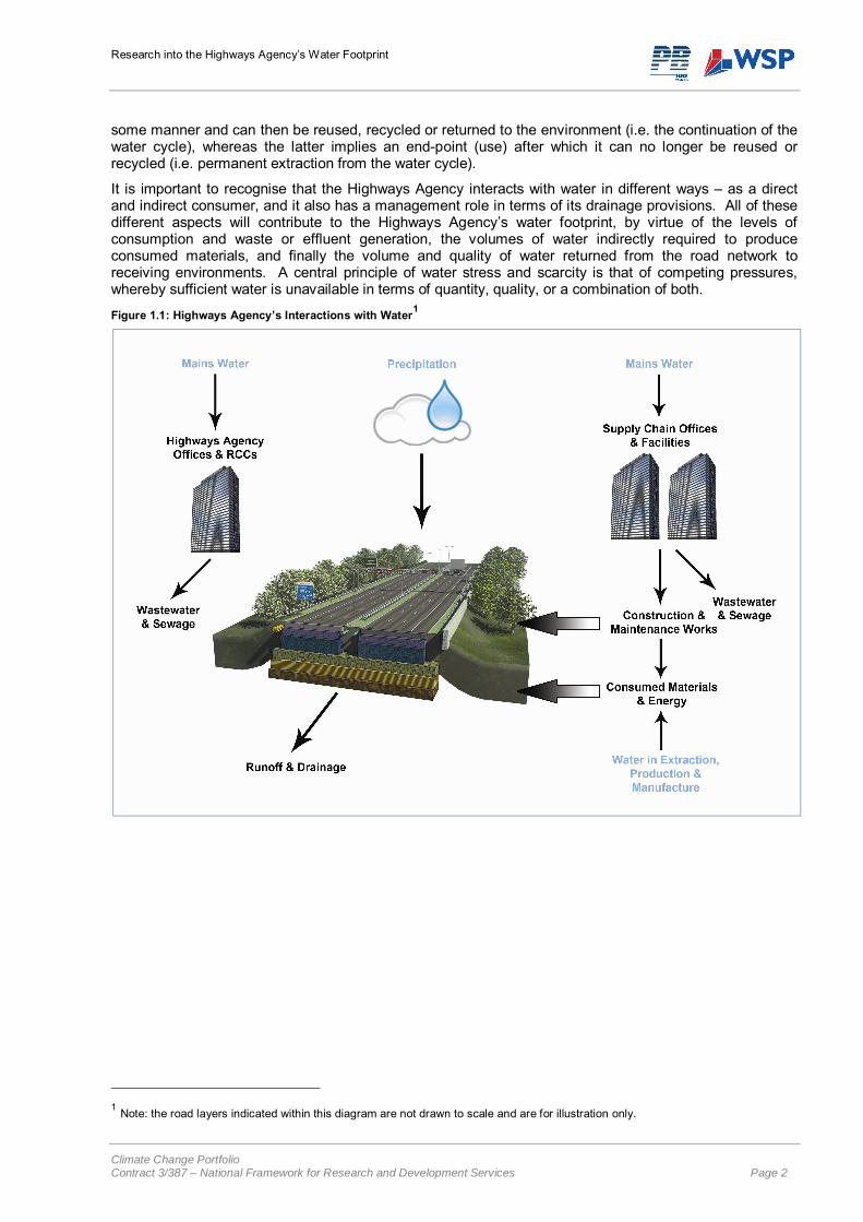
1.3 INTERACTIONS WITH WATER As illustrated within Figure 1.1, the Highways Agency interacts with water and water resources at a number of levels. With reference to the water footprint model in Figure 1.1; operational water will include that used directly within offices and facilities such as Regional Control Centres, and any water intercepted by the network and generated surface runoff. Within the supply chain, water is used within offices and depots, and onsite in construction and maintenance activities. More indirectly, water will be used in the production and supply of consumed goods and services, both internally by the Highways Agency and within the supply chain.
There is an important distinction to be made between ‘water use’ and ‘water consumption’, and within this Report these terms have been used to infer a different meaning. The former implies that water is utilised in
Research into the Highways Agency’s Water Footprint
Climate Change Portfolio Contract 3/387 – National Framework for Research and Development Services Page 2
some manner and can then be reused, recycled or returned to the environment (i.e. the continuation of the water cycle), whereas the latter implies an end-point (use) after which it can no longer be reused or recycled (i.e. permanent extraction from the water cycle).
It is important to recognise that the Highways Agency interacts with water in different ways – as a direct and indirect consumer, and it also has a management role in terms of its drainage provisions. All of these different aspects will contribute to the Highways Agency’s water footprint, by virtue of the levels of consumption and waste or effluent generation, the volumes of water indirectly required to produce consumed materials, and finally the volume and quality of water returned from the road network to receiving environments. A central principle of water stress and scarcity is that of competing pressures, whereby sufficient water is unavailable in terms of quantity, quality, or a combination of both.
Figure 1.1: Highways Agency’s Interactions with Water1
1 Note: the road layers indicated within this diagram are not drawn to scale and are for illustration only.
Research into the Highways Agency’s Water Footprint
Climate Change Portfolio Contract 3/387 – National Framework for Research and Development Services Page 3
2 CONTEXT – WATER RESOURCE PRESSURES
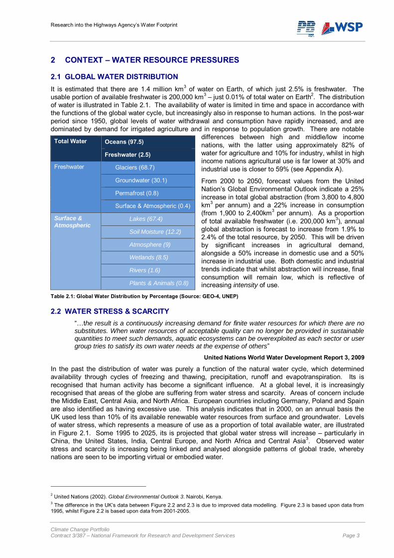
2.1 GLOBAL WATER DISTRIBUTION It is estimated that there are 1.4 million km3 of water on Earth, of which just 2.5% is freshwater. The usable portion of available freshwater is 200,000 km3 – just 0.01% of total water on Earth2. The distribution of water is illustrated in Table 2.1. The availability of water is limited in time and space in accordance with the functions of the global water cycle, but increasingly also in response to human actions. In the post-war period since 1950, global levels of water withdrawal and consumption have rapidly increased, and are dominated by demand for irrigated agriculture and in response to population growth. There are notable
differences between high and middle/low income nations, with the latter using approximately 82% of water for agriculture and 10% for industry, whilst in high income nations agricultural use is far lower at 30% and industrial use is closer to 59% (see Appendix A).
From 2000 to 2050, forecast values from the United Nation’s Global Environmental Outlook indicate a 25% increase in total global abstraction (from 3,800 to 4,800 km3 per annum) and a 22% increase in consumption (from 1,900 to 2,400km3 per annum). As a proportion of total available freshwater (i.e. 200,000 km3), annual global abstraction is forecast to increase from 1.9% to 2.4% of the total resource, by 2050. This will be driven by significant increases in agricultural demand, alongside a 50% increase in domestic use and a 50% increase in industrial use. Both domestic and industrial trends indicate that whilst abstraction will increase, final consumption will remain low, which is reflective of increasing intensity of use.
Table 2.1: Global Water Distribution by Percentage (Source: GEO-4, UNEP)
2.2 WATER STRESS & SCARCITY “…the result is a continuously increasing demand for nite water resources for which there are no substitutes. When water resources of acceptable quality can no longer be provided in sustainable quantities to meet such demands, aquatic ecosystems can be overexploited as each sector or user group tries to satisfy its own water needs at the expense of others”
United Nations World Water Development Report 3, 2009
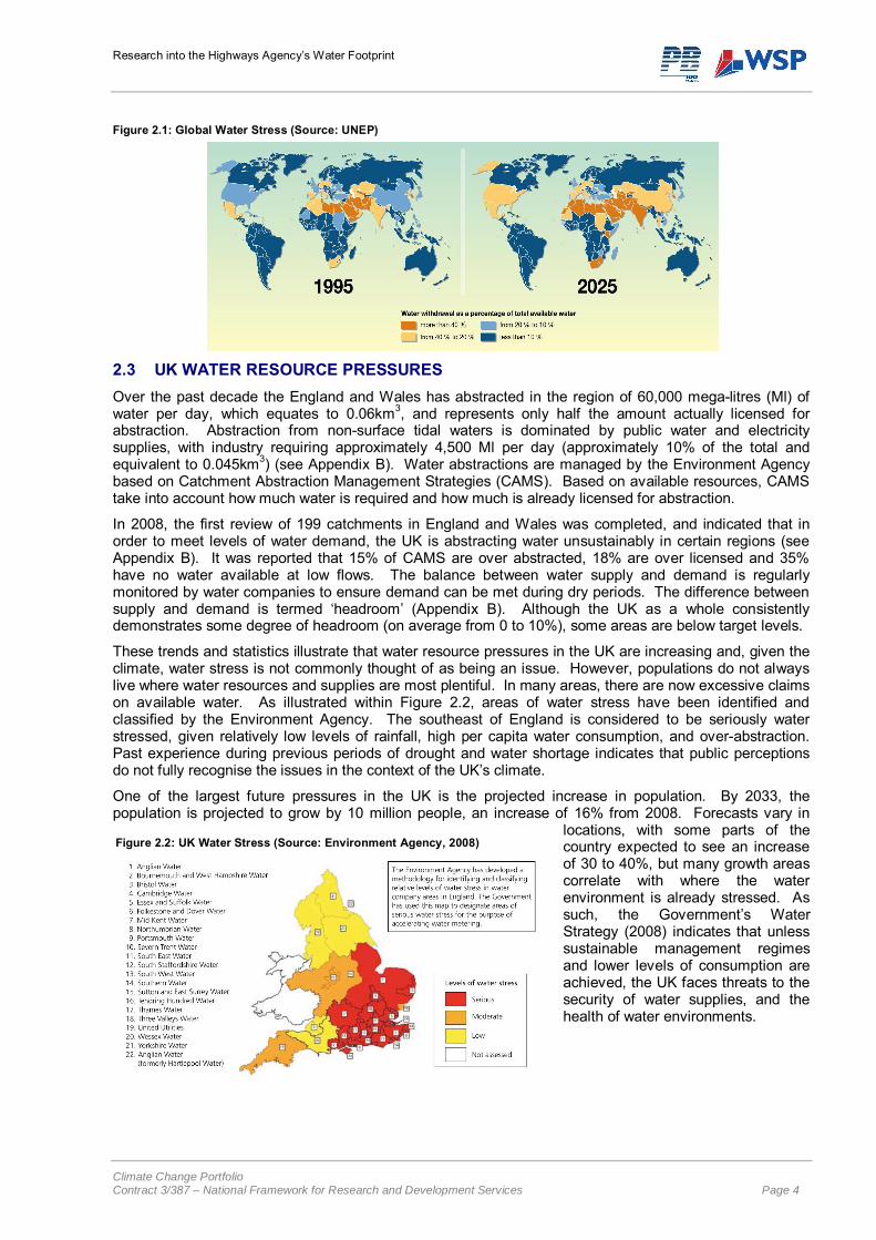
In the past the distribution of water was purely a function of the natural water cycle, which determined availability through cycles of freezing and thawing, precipitation, runoff and evapotranspiration. Its is recognised that human activity has become a significant influence. At a global level, it is increasingly recognised that areas of the globe are suffering from water stress and scarcity. Areas of concern include the Middle East, Central Asia, and North Africa. European countries including Germany, Poland and Spain are also identified as having excessive use. This analysis indicates that in 2000, on an annual basis the UK used less than 10% of its available renewable water resources from surface and groundwater. Levels of water stress, which represents a measure of use as a proportion of total available water, are illustrated in Figure 2.1. Some 1995 to 2025, its is projected that global water stress will increase – particularly in China, the United States, India, Central Europe, and North Africa and Central Asia3. Observed water stress and scarcity is increasing being linked and analysed alongside patterns of global trade, whereby nations are seen to be importing virtual or embodied water.
2 United Nations (2002). Global Environmental Outlook 3. Nairobi, Kenya. 3 The difference in the UK’s data between Figure 2.2 and 2.3 is due to improved data modelling. Figure 2.3 is based upon data from 1995, whilst Figure 2.2 is based upon data from 2001-2005.
Total Water Oceans (97.5)
Freshwater (2.5)
Freshwater Glaciers (68.7)
Groundwater (30.1)
Permafrost (0.8)
Surface & Atmospheric (0.4)
Surface & Atmospheric
Lakes (67.4)
Soil Moisture (12.2)
Atmosphere (9)
Wetlands (8.5)
Rivers (1.6)
Plants & Animals (0.8)
Research into the Highways Agency’s Water Footprint
Climate Change Portfolio Contract 3/387 – National Framework for Research and Development Services Page 4
Figure 2.1: Global Water Stress (Source: UNEP)
2.3 UK WATER RESOURCE PRESSURES Over the past decade the England and Wales has abstracted in the region of 60,000 mega-litres (Ml) of water per day, which equates to 0.06km3, and represents only half the amount actually licensed for abstraction. Abstraction from non-surface tidal waters is dominated by public water and electricity supplies, with industry requiring approximately 4,500 Ml per day (approximately 10% of the total and equivalent to 0.045km3) (see Appendix B). Water abstractions are managed by the Environment Agency based on Catchment Abstraction Management Strategies (CAMS). Based on available resources, CAMS take into account how much water is required and how much is already licensed for abstraction.
In 2008, the first review of 199 catchments in England and Wales was completed, and indicated that in order to meet levels of water demand, the UK is abstracting water unsustainably in certain regions (see Appendix B). It was reported that 15% of CAMS are over abstracted, 18% are over licensed and 35% have no water available at low flows. The balance between water supply and demand is regularly monitored by water companies to ensure demand can be met during dry periods. The difference between supply and demand is termed ‘headroom’ (Appendix B). Although the UK as a whole consistently demonstrates some degree of headroom (on average from 0 to 10%), some areas are below target levels.
These trends and statistics illustrate that water resource pressures in the UK are increasing and, given the climate, water stress is not commonly thought of as being an issue. However, populations do not always live where water resources and supplies are most plentiful. In many areas, there are now excessive claims on available water. As illustrated within Figure 2.2, areas of water stress have been identified and classified by the Environment Agency. The southeast of England is considered to be seriously water stressed, given relatively low levels of rainfall, high per capita water consumption, and over-abstraction. Past experience during previous periods of drought and water shortage indicates that public perceptions do not fully recognise the issues in the context of the UK’s climate.
One of the largest future pressures in the UK is the projected increase in population. By 2033, the population is projected to grow by 10 million people, an increase of 16% from 2008. Forecasts vary in
locations, with some parts of the country expected to see an increase of 30 to 40%, but many growth areas correlate with where the water environment is already stressed. As such, the Government’s Water Strategy (2008) indicates that unless sustainable management regimes and lower levels of consumption are achieved, the UK faces threats to the security of water supplies, and the health of water environments.
Figure 2.2: UK Water Stress (Source: Environment Agency, 2008)
Research into the Highways Agency’s Water Footprint
Climate Change Portfolio Contract 3/387 – National Framework for Research and Development Services Page 5
2.4 IMPACTS OF CLIMATE CHANGE Despite recent media conjecture, there is extensive research and evidence indicating that climate is changing, both globally and in the UK4. According to the Intergovernmental Panel on Climate Change (IPCC), water resources will be affected by climate change by exacerbating current stress placed on water resources from population growth and economic and land-use change5.
Climate change represents the single most important supply-side driver of water availability through direct impacts on the hydrological cycle, in terms of the quantity and quality of freshwater resources. There is consensus that climate change will “…intensify, accelerate or enhance the global hydrological cycle”, in terms of increased evaporation, evapotranspiration, precipitation and stream ow6. Changes in precipitation and temperature will lead to changes in runoff, and therefore water availability, although impacts will vary with location.
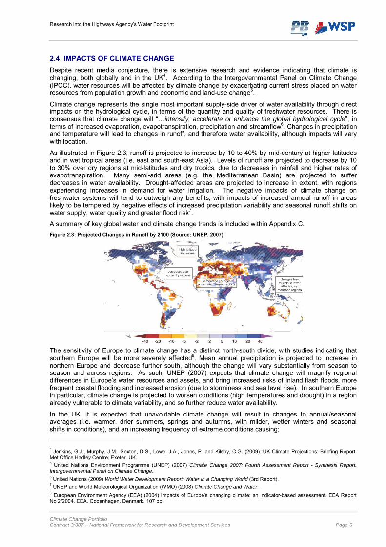
As illustrated in Figure 2.3, runoff is projected to increase by 10 to 40% by mid-century at higher latitudes and in wet tropical areas (i.e. east and south-east Asia). Levels of runoff are projected to decrease by 10 to 30% over dry regions at mid-latitudes and dry tropics, due to decreases in rainfall and higher rates of evapotranspiration. Many semi-arid areas (e.g. the Mediterranean Basin) are projected to suffer decreases in water availability. Drought-affected areas are projected to increase in extent, with regions experiencing increases in demand for water irrigation. The negative impacts of climate change on freshwater systems will tend to outweigh any benefits, with impacts of increased annual runoff in areas likely to be tempered by negative effects of increased precipitation variability and seasonal runoff shifts on water supply, water quality and greater flood risk7.
A summary of key global water and climate change trends is included within Appendix C. Figure 2.3: Projected Changes in Runoff by 2100 (Source: UNEP, 2007)
The sensitivity of Europe to climate change has a distinct north-south divide, with studies indicating that southern Europe will be more severely affected8. Mean annual precipitation is projected to increase in northern Europe and decrease further south, although the change will vary substantially from season to season and across regions. As such, UNEP (2007) expects that climate change will magnify regional differences in Europe’s water resources and assets, and bring increased risks of inland flash floods, more frequent coastal flooding and increased erosion (due to storminess and sea level rise). In southern Europe in particular, climate change is projected to worsen conditions (high temperatures and drought) in a region already vulnerable to climate variability, and so further reduce water availability.
In the UK, it is expected that unavoidable climate change will result in changes to annual/seasonal averages (i.e. warmer, drier summers, springs and autumns, with milder, wetter winters and seasonal shifts in conditions), and an increasing frequency of extreme conditions causing:
4 Jenkins, G.J., Murphy, J.M., Sexton, D.S., Lowe, J.A., Jones, P. and Kilsby, C.G. (2009). UK Climate Projections: Briefing Report. Met Office Hadley Centre, Exeter, UK. 5 United Nations Environment Programme (UNEP) (2007) Climate Change 2007: Fourth Assessment Report - Synthesis Report. Intergovernmental Panel on Climate Change. 6 United Nations (2009) World Water Development Report: Water in a Changing World (3rd Report). 7 UNEP and World Meteorological Organization (WMO) (2008) Climate Change and Water. 8 European Environment Agency (EEA) (2004) Impacts of Europe’s changing climate: an indicator-based assessment. EEA Report No 2/2004, EEA, Copenhagen, Denmark, 107 pp.
Research into the Highways Agency’s Water Footprint
Climate Change Portfolio Contract 3/387 – National Framework for Research and Development Services Page 6
More very hot days;
More intense downpours of rain;
More frequent high water levels along coastlines; and
Uncertain changes in storm frequencies, with possibly an increase in winter9. Projections for the UK Climate Impacts Programme (UKCIP) indicate that (under the medium emissions scenario) towards 2080 a projected average temperature rise of 2-3 degrees Celsius across most of the country in winter. In summer a 4 degrees Celsius increase is projected, with a pronounced north to south gradient (see Appendix D). In terms of average precipitation, increases in winter are estimated to be from +10% to +30% across the country, and against in summer there is a north to south gradient from no change in Shetland to -40% in southwest England.
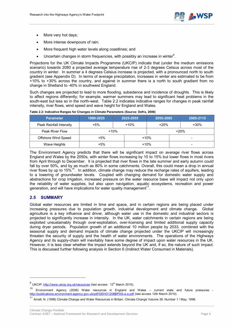
Such changes are projected to lead to more flooding, subsidence and incidence of droughts. This is likely to affect regions differently; for example, warmer summers may lead to significant heat problems in the south-east but less so in the north-west. Table 2.2 indicates indicative ranges for changes in peak rainfall intensity, river flows, wind speed and wave height for England and Wales. Table 2.2: Indicative Ranges for Changes in Climate Parameters (Source: Defra, 2006)
Parameter 1990-2025 2025-2055 2055-2085 2085-2115
Peak Rainfall Intensity +5% +10% +20% +30%
Peak River Flow +10% +20%
Offshore Wind Speed +5% +10% -
Wave Heights +5% +10% -
The Environment Agency predicts that there will be significant impact on average river flows across England and Wales by the 2050s, with winter flows increasing by 10 to 15% but lower flows in most rivers from April through to December. It is projected that river flows in the late summer and early autumn could fall by over 50%, and by as much as 80% in some catchments. Overall, this could mean a drop in annual river flows by up to 15%10. In addition, climate change may reduce the recharge rates of aquifers, leading to a lowering of groundwater levels. Coupled with changing demand for domestic water supply and abstractions for crop irrigation, increased pressure on the water resource base will impact not only upon the reliability of water supplies, but also upon navigation, aquatic ecosystems, recreation and power generation, and will have implications for water quality management11.
2.5 SUMMARY Global water resources are limited in time and space, and in certain regions are being placed under increasing pressures due to population growth, industrial development and climate change. Global agriculture is a key influence and driver, although water use in the domestic and industrial sectors is projected to significantly increase in intensity. In the UK, water catchments in certain regions are being exploited unsustainably through over-exploitation, over-licensing and limited additional supply capacity during dryer periods. Population growth of an additional 10 million people by 2033, combined with the seasonal supply and demand impacts of climate change projected under the UKCIP will increasingly threaten the security of supply and the health of water environments. The operations of the Highways Agency and its supply-chain will inevitably have some degree of impact upon water resources in the UK. However, it is less clear whether the impact extends beyond the UK and, if so, the nature of such impact. This is discussed further following analysis in Section 6 (Indirect Water Consumed in Materials).
9 UKCIP, http://www.ukcip.org.uk/resources (last access: 12th March 2010). 10 Environment Agency (2008) Water resources in England and Wales – current state and future pressures - http://publications.environment-agency.gov.uk/pdf/GEHO1208BPAS-e-e.pdf (last access 12th March 2010). 11 Arnell, N. (1998) Climate Change and Water Resources in Britain. Climate Change Volume 39, Number 1 / May, 1998.
Research into the Highways Agency’s Water Footprint
Climate Change Portfolio Contract 3/387 – National Framework for Research and Development Services Page 7
3 MEASURES OF WATER IMPACT
3.1 CORPORATE WATER RISK “Businesses cannot afford to ignore this trend…it means closer scrutiny of how they, their supply chains, and their markets access and use water, and of how new business risks emerge as they compete with other users.”
Business in the World of Water (2006) World Business Council for Sustainable Development
Globally, organisations are increasingly recognising water risks within their operations and supply chains, where production processes or upstream products / services are reliant upon the availability and quality of resources. Certain industries, including construction, will utilise considerably more water indirectly in the supply chain, rather than for direct onsite use. A review by JPMorgan (2008) highlighted risks posed by sectors considered to have water security issues, including: food and beverages, manufacturing, semiconductor production, power generation, insurance, and extractive industries. As indicated in these sectors, it is increasingly recognised that where there is high dependence on water availability, corporate financial performance may be affected through supply chain disruptions, there will be increasing costs from regulatory pressures, and there will be greater competition for available resources. Furthermore, there are reputation risks in relation to water intensive products and operations. Organisations with direct links to water, particularly those with close links to agriculture, have begun to take this issue seriously.
A recent study by Barton (2010)12 benchmarked 100 companies in terms of approaches to water risk and corporate reporting. This focused on similar sectors to JPMorgan (2008), and concluded that even for companies in high risk sectors, the disclosure of risk and corporate water performance is surprisingly weak. In terms of supply-chain analysis, no companies currently provide comprehensive data on supplier’s performance, although organisations such as SABMiller and Unilever are beginning to provide estimates of water embedded in their supply chains, and a small number demonstrated working with supply-chains to reduce water use. If only small numbers of global organisations involved in the extraction and production of raw materials and input products are currently addressing and disclosing corporate (and supply-chain) water use data, the ability of end-consumers to accurately assess their water footprints will prove limited.
3.2 EMBODIED WATER, VIRTUAL WATER & THE WATER FOOTPRINT The term ‘embodied water’ is used to describe the volume which has been consumed within upstream extraction and production processes, and is comparable to the concept of ‘embodied carbon’ from carbon footprinting. The analysis of water is developing in a similar manner, to measure and analyse levels of embodied water contained within supply chains, although current procedures are far less developed and for organisations towards the top of the supply chain, with complex inputs and supply chains, the analysis of embodied water proves a complex task. It can provide a useful perspective on where volumes of water are required within operations and the supply chain and to help target efficiency and management strategies for improved performance.
‘Virtual water’ relates to embodied water, but is used to symbolise the relative flow of water from one location to another. For example, virtual water flows occur from one nation to another through patterns of global trade and commodity flows. Analysis illustrated below suggests that volumes of virtual water can be significant; the UK has an estimated net virtual-water import of 25-50 Gm3/yr from imported goods and services13 (1 Gm3 is equivalent to 1 billion cubic metres). This suggests that 25 to 50 billion m3 of water is required per year in the production and supply of goods and services to the UK. As Hoekstra (2010) demonstrates, international trade patterns can significantly influence patterns of water availability in producer countries.
Embodied and virtual water both only reflect the volume of water consumed, and so the ‘water footprint’ concept has emerged to refer also to “…the sort of water that was used….and to when and where the water was used” (WFN, 2009). It is a geographically explicit indicator, which recognises that activities influence water resources through pollution, discharge and the production of waste effluent. Within water footprint analysis, blue water describes volumes of extracted surface and groundwater, green water
12 Barton, B. (2010) Murky Waters? Corporate Reporting on Water Risk: A Benchmarking Study of 100 Companies. Boston, USA. 13 Calculated by Hoekstra & Chapagain (2008) based upon data over the period 1997-2001.
Research into the Highways Agency’s Water Footprint
Climate Change Portfolio Contract 3/387 – National Framework for Research and Development Services Page 8
describes volumes from rainwater stored in the soil as soil moisture, and grey water describes the volume of polluted water or effluent produced.
3.3 ANALYSIS OF UK WATER FOOTPRINT The availability of water is an emotive issue, particularly linked to the levels of stress and scarcity experienced within emerging economies and part episodes of drought and famine. The virtual water and water footprint concepts are being used to investigate the scale of impacts that global trade is having on non-domestic water resources.
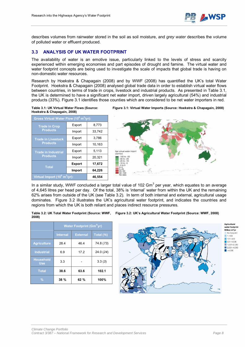
Research by Hoekstra & Chapagain (2008) and by WWF (2008) has quantified the UK’s total Water Footprint. Hoekstra & Chapagain (2008) analysed global trade data in order to establish virtual water flows between countries, in terms of trade in crops, livestock and industrial products. As presented in Table 3.1, the UK is determined to have a significant net water import, driven largely agricultural (54%) and industrial products (33%). Figure 3.1 identifies those counties which are considered to be net water importers in red.
Table 3.1: UK Virtual Water Flows (Source: Hoekstra & Chapagain, 2008)
Figure 3.1: Virtual Water Imports (Source: Hoekstra & Chapagain, 2008)
Gross Virtual Water Flow (106 m3/yr):
Trade in Crop Products
Export 8,773
Import 33,742
Trade in Livestock Products
Export 3,786
Import 10,163
Trade in Industrial Products
Export 5,113
Import 20,321
Total Export 17,672
Import 64,226
Virtual Import (106 m3/yr): 46,554
In a similar study, WWF concluded a larger total value of 102 Gm3 per year, which equates to an average of 4,645 litres per head per day. Of the total, 38% is ‘internal’ water from within the UK and the remaining 62% arises from outside of the UK (see Table 3.2). In term of both internal and external, agricultural usage dominates. Figure 3.2 illustrates the UK’s agricultural water footprint, and indicates the countries and regions from which the UK is both reliant and places indirect resource pressures.
Table 3.2: UK Total Water Footprint (Source: WWF, 2008)
Figure 3.2: UK’s Agricultural Water Footprint (Source: WWF, 2008)
Water Footprint (Gm3/yr)
Internal External Total (%)
Agriculture 28.4 46.4 74.8 (73)
Industrial 6.9 17.2 24.0 (24)
Household Use 3.3 - 3.3 (3)
Total 38.6 63.6 102.1
% 38 % 62 % 100%
Research into the Highways Agency’s Water Footprint
Climate Change Portfolio Contract 3/387 – National Framework for Research and Development Services Page 9
Water Footprint
Operational
Blue Water
Green Water
Grey Water
Supply Chain
Blue Water
Green Water
Grey Water
Water Footprint
Highways Agency Internal
Blue Water
Grey Water
Supply-Chain Direct Operations
Blue Water
Grey Water
Supply Chain Indirect (Materials)
Blue Water
Grey Water
Network Drainage
Grey Water
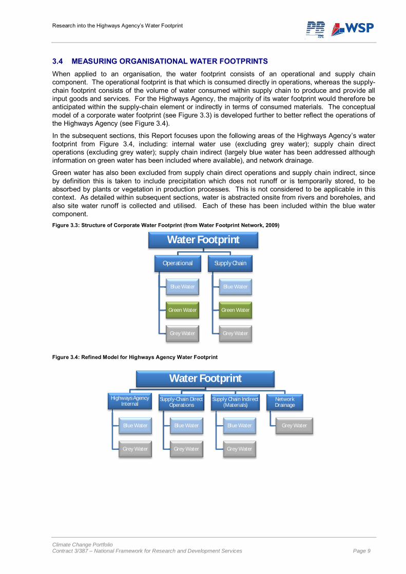
3.4 MEASURING ORGANISATIONAL WATER FOOTPRINTS When applied to an organisation, the water footprint consists of an operational and supply chain component. The operational footprint is that which is consumed directly in operations, whereas the supply-chain footprint consists of the volume of water consumed within supply chain to produce and provide all input goods and services. For the Highways Agency, the majority of its water footprint would therefore be anticipated within the supply-chain element or indirectly in terms of consumed materials. The conceptual model of a corporate water footprint (see Figure 3.3) is developed further to better reflect the operations of the Highways Agency (see Figure 3.4).
In the subsequent sections, this Report focuses upon the following areas of the Highways Agency’s water footprint from Figure 3.4, including: internal water use (excluding grey water); supply chain direct operations (excluding grey water); supply chain indirect (largely blue water has been addressed although information on green water has been included where available), and network drainage.
Green water has also been excluded from supply chain direct operations and supply chain indirect, since by definition this is taken to include precipitation which does not runoff or is temporarily stored, to be absorbed by plants or vegetation in production processes. This is not considered to be applicable in this context. As detailed within subsequent sections, water is abstracted onsite from rivers and boreholes, and also site water runoff is collected and utilised. Each of these has been included within the blue water component. Figure 3.3: Structure of Corporate Water Footprint (from Water Footprint Network, 2009)
Figure 3.4: Refined Model for Highways Agency Water Footprint
Research into the Highways Agency’s Water Footprint
Climate Change Portfolio Contract 3/387 – National Framework for Research and Development Services Page 10
4 INTERNAL WATER USE
“There is a real need to reduce water consumption in the UK. Treatment and supply of water is expensive and energy intensive so by reducing consumption both costs and carbon emissions are reduced. With climate change expected to increase pressure on the UK’s water resources, it is important that government is seen to be leading by example by improving water efficiency and reducing water consumption, which will also help to reduce government’s carbon footprint”
Sustainable Development Commission (2008)
The water used within main offices and other facilities forms the key area of direct water use for the Highways Agency. As indicated by the Sustainable Development Commission there is a role for Government in demonstrating leadership, which begins on with the Government estate. The Sustainable Development in Government (SDiG) targets place two obligations on Government Departments and Executive Agencies, in relation to internal water use in all buildings and non-office estate. Current water targets are outlined below,:
1. Reduce water consumption by 7% in non-office estate by 2016/17, relative to 2010/11 levels;
2. Achieve a water consumption level of 6m3 per full time equivalent (FTE) on office estate by 2016/17; and
3. Contribute to an aspirational target to achieve an average consumption level of 4m3 per FTE on the office estate by 2022.
This Section provides analysis of the Highways Agency’s current level of water use internally, and develops an estimate of total consumption from available data. An illustration of where the Highways Agency needs to be in order to meet its requirements under SDiG is presented.
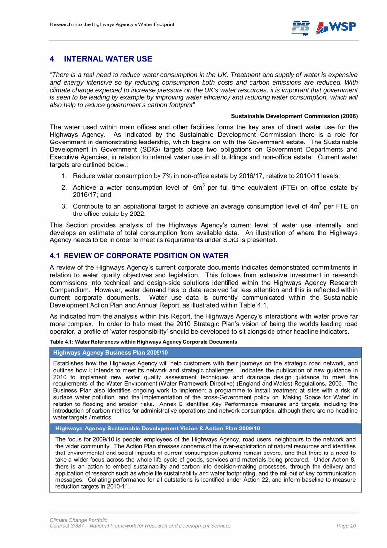
4.1 REVIEW OF CORPORATE POSITION ON WATER A review of the Highways Agency’s current corporate documents indicates demonstrated commitments in relation to water quality objectives and legislation. This follows from extensive investment in research commissions into technical and design-side solutions identified within the Highways Agency Research Compendium. However, water demand has to date received far less attention and this is reflected within current corporate documents. Water use data is currently communicated within the Sustainable Development Action Plan and Annual Report, as illustrated within Table 4.1.
As indicated from the analysis within this Report, the Highways Agency’s interactions with water prove far more complex. In order to help meet the 2010 Strategic Plan’s vision of being the worlds leading road operator, a profile of ‘water responsibility’ should be developed to sit alongside other headline indicators. Table 4.1: Water References within Highways Agency Corporate Documents
Highways Agency Business Plan 2009/10
Establishes how the Highways Agency will help customers with their journeys on the strategic road network, and outlines how it intends to meet its network and strategic challenges. Indicates the publication of new guidance in 2010 to implement new water quality assessment techniques and drainage design guidance to meet the requirements of the Water Environment (Water Framework Directive) (England and Wales) Regulations, 2003. The Business Plan also identifies ongoing work to implement a programme to install treatment at sites with a risk of surface water pollution, and the implementation of the cross-Government policy on ‘Making Space for Water’ in relation to flooding and erosion risks. Annex B identifies Key Performance measures and targets, including the introduction of carbon metrics for administrative operations and network consumption, although there are no headline water targets / metrics.
Highways Agency Sustainable Development Vision & Action Plan 2009/10
The focus for 2009/10 is people; employees of the Highways Agency, road users, neighbours to the network and the wider community. The Action Plan stresses concerns of the over-exploitation of natural resources and identifies that environmental and social impacts of current consumption patterns remain severe, and that there is a need to take a wider focus across the whole life cycle of goods, services and materials being procured. Under Action 8, there is an action to embed sustainability and carbon into decision-making processes, through the delivery and application of research such as whole life sustainability and water footprinting, and the roll out of key communication messages. Collating performance for all outstations is identified under Action 22, and inform baseline to measure reduction targets in 2010-11.
Research into the Highways Agency’s Water Footprint
Climate Change Portfolio Contract 3/387 – National Framework for Research and Development Services Page 11
Highways Agency Annual Report 2008/09
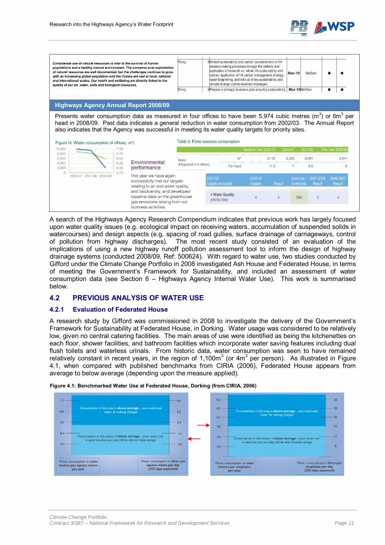
Presents water consumption data as measured in four offices to have been 5,974 cubic metres (m3) or 6m3 per head in 2008/09. Past data indicates a general reduction in water consumption from 2002/03. The Annual Report also indicates that the Agency was successful in meeting its water quality targets for priority sites.
A search of the Highways Agency Research Compendium indicates that previous work has largely focused upon water quality issues (e.g. ecological impact on receiving waters, accumulation of suspended solids in watercourses) and design aspects (e.g. spacing of road gullies, surface drainage of carriageways, control of pollution from highway discharges). The most recent study consisted of an evaluation of the implications of using a new highway runoff pollution assessment tool to inform the design of highway drainage systems (conducted 2008/09, Ref: 500624). With regard to water use, two studies conducted by Gifford under the Climate Change Portfolio in 2008 investigated Ash House and Federated House, in terms of meeting the Government’s Framework for Sustainability, and included an assessment of water consumption data (see Section 6 – Highways Agency Internal Water Use). This work is summarised below.
4.2 PREVIOUS ANALYSIS OF WATER USE 4.2.1 Evaluation of Federated House
A research study by Gifford was commissioned in 2008 to investigate the delivery of the Government’s Framework for Sustainability at Federated House, in Dorking. Water usage was considered to be relatively low, given no central catering facilities. The main areas of use were identified as being the kitchenettes on each floor, shower facilities, and bathroom facilities which incorporate water saving features including dual flush toilets and waterless urinals. From historic data, water consumption was seen to have remained relatively constant in recent years, in the region of 1,100m3 (or 4m3 per person). As illustrated in Figure 4.1, when compared with published benchmarks from CIRIA (2006), Federated House appears from average to below average (depending upon the measure applied).
Figure 4.1: Benchmarked Water Use at Federated House, Dorking (from CIRIA, 2006)
Research into the Highways Agency’s Water Footprint
Climate Change Portfolio Contract 3/387 – National Framework for Research and Development Services Page 12
The study made the following key recommendations with regard to further reduction measures:
As a relatively low cost improvement, a 20% water saving over 2004/05 could be achieved by introducing reduced flow or aerated taps;
Installation of low flow or aerated shower heads;
Investigation of potential to introduce recycling rainwater or grey water as toilet water, with the potential to save 44% or 40% respectively; and
Undertake regular inspections and maintenance for pipe work, and upgrade the building management system to include sub-metering of specific areas of use.
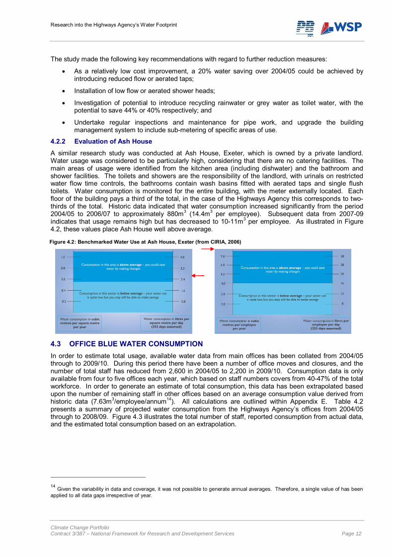
4.2.2 Evaluation of Ash House
A similar research study was conducted at Ash House, Exeter, which is owned by a private landlord. Water usage was considered to be particularly high, considering that there are no catering facilities. The main areas of usage were identified from the kitchen area (including dishwater) and the bathroom and shower facilities. The toilets and showers are the responsibility of the landlord, with urinals on restricted water flow time controls, the bathrooms contain wash basins fitted with aerated taps and single flush toilets. Water consumption is monitored for the entire building, with the meter externally located. Each floor of the building pays a third of the total, in the case of the Highways Agency this corresponds to two-thirds of the total. Historic data indicated that water consumption increased significantly from the period 2004/05 to 2006/07 to approximately 880m3 (14.4m3 per employee). Subsequent data from 2007-09 indicates that usage remains high but has decreased to 10-11m3 per employee. As illustrated in Figure 4.2, these values place Ash House well above average.
Figure 4.2: Benchmarked Water Use at Ash House, Exeter (from CIRIA, 2006)
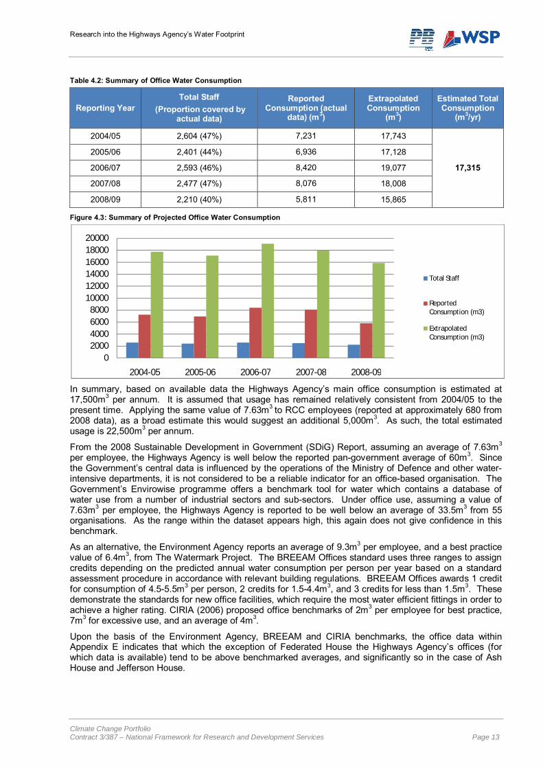
4.3 OFFICE BLUE WATER CONSUMPTION In order to estimate total usage, available water data from main offices has been collated from 2004/05 through to 2009/10. During this period there have been a number of office moves and closures, and the number of total staff has reduced from 2,600 in 2004/05 to 2,200 in 2009/10. Consumption data is only available from four to five offices each year, which based on staff numbers covers from 40-47% of the total workforce. In order to generate an estimate of total consumption, this data has been extrapolated based upon the number of remaining staff in other offices based on an average consumption value derived from historic data (7.63m3/employee/annum14). All calculations are outlined within Appendix E. Table 4.2 presents a summary of projected water consumption from the Highways Agency’s offices from 2004/05 through to 2008/09. Figure 4.3 illustrates the total number of staff, reported consumption from actual data, and the estimated total consumption based on an extrapolation.
14 Given the variability in data and coverage, it was not possible to generate annual averages. Therefore, a single value of has been applied to all data gaps irrespective of year.
Research into the Highways Agency’s Water Footprint
Climate Change Portfolio Contract 3/387 – National Framework for Research and Development Services Page 13
Table 4.2: Summary of Office Water Consumption
Reporting Year Total Staff
(Proportion covered by actual data)
Reported Consumption (actual
data) (m3)
Extrapolated Consumption
(m3)
Estimated Total Consumption
(m3/yr)
2004/05 2,604 (47%) 7,231 17,743
17,315
2005/06 2,401 (44%) 6,936 17,128
2006/07 2,593 (46%) 8,420 19,077
2007/08 2,477 (47%) 8,076 18,008
2008/09 2,210 (40%) 5,811 15,865
Figure 4.3: Summary of Projected Office Water Consumption
In summary, based on available data the Highways Agency’s main office consumption is estimated at 17,500m3 per annum. It is assumed that usage has remained relatively consistent from 2004/05 to the present time. Applying the same value of 7.63m3 to RCC employees (reported at approximately 680 from 2008 data), as a broad estimate this would suggest an additional 5,000m3. As such, the total estimated usage is 22,500m3 per annum.
From the 2008 Sustainable Development in Government (SDiG) Report, assuming an average of 7.63m3 per employee, the Highways Agency is well below the reported pan-government average of 60m3. Since the Government’s central data is influenced by the operations of the Ministry of Defence and other water-intensive departments, it is not considered to be a reliable indicator for an office-based organisation. The Government’s Envirowise programme offers a benchmark tool for water which contains a database of water use from a number of industrial sectors and sub-sectors. Under office use, assuming a value of 7.63m3 per employee, the Highways Agency is reported to be well below an average of 33.5m3 from 55 organisations. As the range within the dataset appears high, this again does not give confidence in this benchmark.
As an alternative, the Environment Agency reports an average of 9.3m3 per employee, and a best practice value of 6.4m3, from The Watermark Project. The BREEAM Offices standard uses three ranges to assign credits depending on the predicted annual water consumption per person per year based on a standard assessment procedure in accordance with relevant building regulations. BREEAM Offices awards 1 credit for consumption of 4.5-5.5m3 per person, 2 credits for 1.5-4.4m3, and 3 credits for less than 1.5m3. These demonstrate the standards for new office facilities, which require the most water efficient fittings in order to achieve a higher rating. CIRIA (2006) proposed office benchmarks of 2m3 per employee for best practice, 7m3 for excessive use, and an average of 4m3.
Upon the basis of the Environment Agency, BREEAM and CIRIA benchmarks, the office data within Appendix E indicates that which the exception of Federated House the Highways Agency’s offices (for which data is available) tend to be above benchmarked averages, and significantly so in the case of Ash House and Jefferson House.
02000400060008000
100001200014000160001800020000
2004-05 2005-06 2006-07 2007-08 2008-09
Total Staff
Reported Consumption (m3)
Extrapolated Consumption (m3)
Research into the Highways Agency’s Water Footprint
Climate Change Portfolio Contract 3/387 – National Framework for Research and Development Services Page 14
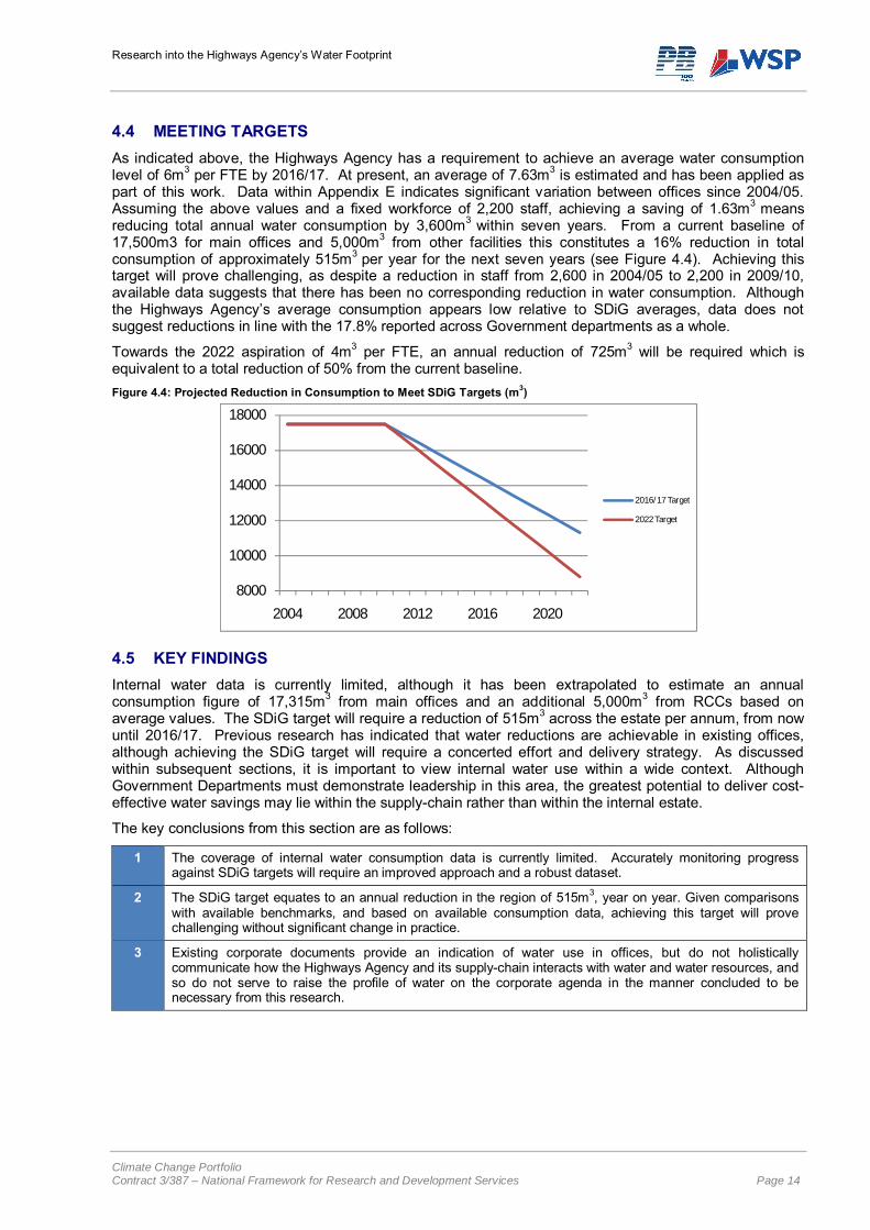
4.4 MEETING TARGETS As indicated above, the Highways Agency has a requirement to achieve an average water consumption level of 6m3 per FTE by 2016/17. At present, an average of 7.63m3 is estimated and has been applied as part of this work. Data within Appendix E indicates significant variation between offices since 2004/05. Assuming the above values and a fixed workforce of 2,200 staff, achieving a saving of 1.63m3 means reducing total annual water consumption by 3,600m3 within seven years. From a current baseline of 17,500m3 for main offices and 5,000m3 from other facilities this constitutes a 16% reduction in total consumption of approximately 515m3 per year for the next seven years (see Figure 4.4). Achieving this target will prove challenging, as despite a reduction in staff from 2,600 in 2004/05 to 2,200 in 2009/10, available data suggests that there has been no corresponding reduction in water consumption. Although the Highways Agency’s average consumption appears low relative to SDiG averages, data does not suggest reductions in line with the 17.8% reported across Government departments as a whole.
Towards the 2022 aspiration of 4m3 per FTE, an annual reduction of 725m3 will be required which is equivalent to a total reduction of 50% from the current baseline. Figure 4.4: Projected Reduction in Consumption to Meet SDiG Targets (m3)
4.5 KEY FINDINGS Internal water data is currently limited, although it has been extrapolated to estimate an annual consumption figure of 17,315m3 from main offices and an additional 5,000m3 from RCCs based on average values. The SDiG target will require a reduction of 515m3 across the estate per annum, from now until 2016/17. Previous research has indicated that water reductions are achievable in existing offices, although achieving the SDiG target will require a concerted effort and delivery strategy. As discussed within subsequent sections, it is important to view internal water use within a wide context. Although Government Departments must demonstrate leadership in this area, the greatest potential to deliver cost-effective water savings may lie within the supply-chain rather than within the internal estate.
The key conclusions from this section are as follows:
1 The coverage of internal water consumption data is currently limited. Accurately monitoring progress against SDiG targets will require an improved approach and a robust dataset.
2 The SDiG target equates to an annual reduction in the region of 515m3, year on year. Given comparisons with available benchmarks, and based on available consumption data, achieving this target will prove challenging without significant change in practice.
3 Existing corporate documents provide an indication of water use in offices, but do not holistically communicate how the Highways Agency and its supply-chain interacts with water and water resources, and so do not serve to raise the profile of water on the corporate agenda in the manner concluded to be necessary from this research.
8000
10000
12000
14000
16000
18000
2004 2008 2012 2016 2020
2016/17 Target
2022 Target
Research into the Highways Agency’s Water Footprint
Climate Change Portfolio Contract 3/387 – National Framework for Research and Development Services Page 15
5 SUPPLY-CHAIN DIRECT OPERATIONS
Onsite water usage has been investigated in terms of the operation of Major Projects, Design-Build-Finance-Operate (DBFO) schemes, and Managing Agent Contractors (MACs). For each data return from the Carbon Calculation Tool have been analysed, followed by consultations to establish the main area of onsite use. As indicated previously, the Sustainable Construction Strategy (2008) establishes a target to reduce water use in the manufacturing and construction phase by 20% by 2012, compared with a 2008 baseline. This is a challenging target within a very short timescale, and the objective of this section is to identify any issues in achieving this, or future targets onsite.
5.1 MAJOR PROJECTS 5.1.1 Reported Water Use
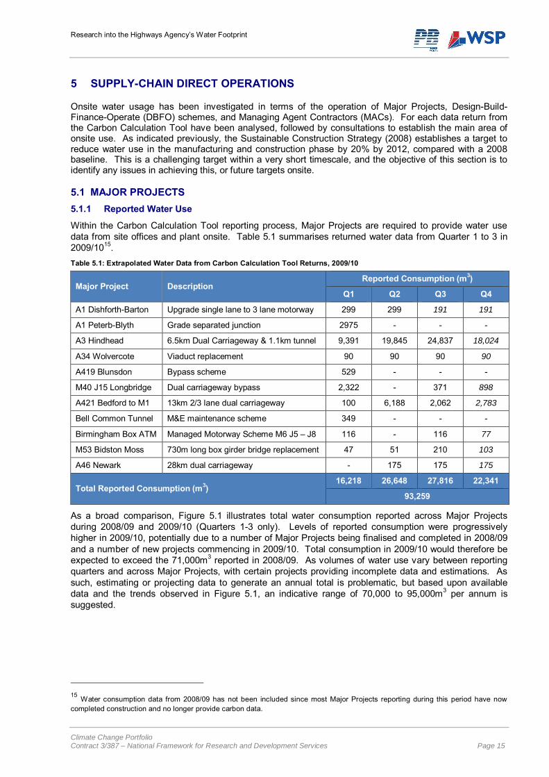
Within the Carbon Calculation Tool reporting process, Major Projects are required to provide water use data from site offices and plant onsite. Table 5.1 summarises returned water data from Quarter 1 to 3 in 2009/1015. Table 5.1: Extrapolated Water Data from Carbon Calculation Tool Returns, 2009/10
Major Project Description Reported Consumption (m3)
Q1 Q2 Q3 Q4
A1 Dishforth-Barton Upgrade single lane to 3 lane motorway 299 299 191 191
A1 Peterb-Blyth Grade separated junction 2975 - - -
A3 Hindhead 6.5km Dual Carriageway & 1.1km tunnel 9,391 19,845 24,837 18,024
A34 Wolvercote Viaduct replacement 90 90 90 90
A419 Blunsdon Bypass scheme 529 - - -
M40 J15 Longbridge Dual carriageway bypass 2,322 - 371 898
A421 Bedford to M1 13km 2/3 lane dual carriageway 100 6,188 2,062 2,783
Bell Common Tunnel M&E maintenance scheme 349 - - -
Birmingham Box ATM Managed Motorway Scheme M6 J5 – J8 116 - 116 77
M53 Bidston Moss 730m long box girder bridge replacement 47 51 210 103
A46 Newark 28km dual carriageway - 175 175 175
Total Reported Consumption (m3) 16,218 26,648 27,816 22,341
93,259
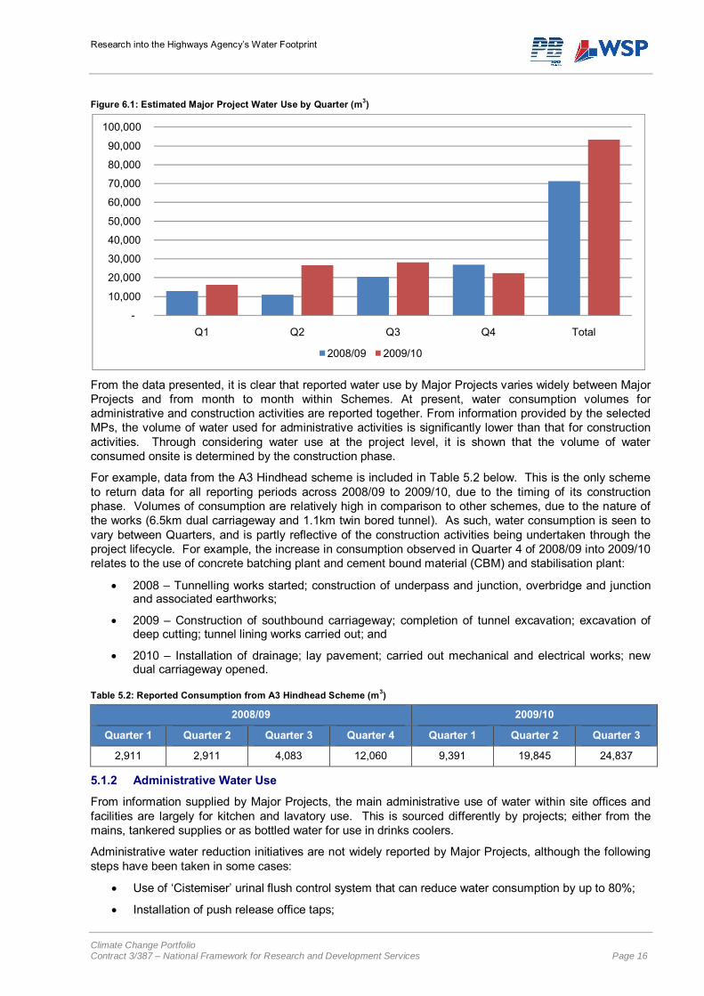
As a broad comparison, Figure 5.1 illustrates total water consumption reported across Major Projects during 2008/09 and 2009/10 (Quarters 1-3 only). Levels of reported consumption were progressively higher in 2009/10, potentially due to a number of Major Projects being finalised and completed in 2008/09 and a number of new projects commencing in 2009/10. Total consumption in 2009/10 would therefore be expected to exceed the 71,000m3 reported in 2008/09. As volumes of water use vary between reporting quarters and across Major Projects, with certain projects providing incomplete data and estimations. As such, estimating or projecting data to generate an annual total is problematic, but based upon available data and the trends observed in Figure 5.1, an indicative range of 70,000 to 95,000m3 per annum is suggested.
15 Water consumption data from 2008/09 has not been included since most Major Projects reporting during this period have now completed construction and no longer provide carbon data.
Research into the Highways Agency’s Water Footprint
Climate Change Portfolio Contract 3/387 – National Framework for Research and Development Services Page 16
Figure 6.1: Estimated Major Project Water Use by Quarter (m3)
From the data presented, it is clear that reported water use by Major Projects varies widely between Major Projects and from month to month within Schemes. At present, water consumption volumes for administrative and construction activities are reported together. From information provided by the selected MPs, the volume of water used for administrative activities is significantly lower than that for construction activities. Through considering water use at the project level, it is shown that the volume of water consumed onsite is determined by the construction phase.
For example, data from the A3 Hindhead scheme is included in Table 5.2 below. This is the only scheme to return data for all reporting periods across 2008/09 to 2009/10, due to the timing of its construction phase. Volumes of consumption are relatively high in comparison to other schemes, due to the nature of the works (6.5km dual carriageway and 1.1km twin bored tunnel). As such, water consumption is seen to vary between Quarters, and is partly reflective of the construction activities being undertaken through the project lifecycle. For example, the increase in consumption observed in Quarter 4 of 2008/09 into 2009/10 relates to the use of concrete batching plant and cement bound material (CBM) and stabilisation plant:
2008 – Tunnelling works started; construction of underpass and junction, overbridge and junction and associated earthworks;
2009 – Construction of southbound carriageway; completion of tunnel excavation; excavation of deep cutting; tunnel lining works carried out; and
2010 – Installation of drainage; lay pavement; carried out mechanical and electrical works; new dual carriageway opened.
Table 5.2: Reported Consumption from A3 Hindhead Scheme (m3)
2008/09 2009/10
Quarter 1 Quarter 2 Quarter 3 Quarter 4 Quarter 1 Quarter 2 Quarter 3
2,911 2,911 4,083 12,060 9,391 19,845 24,837
5.1.2 Administrative Water Use
From information supplied by Major Projects, the main administrative use of water within site offices and facilities are largely for kitchen and lavatory use. This is sourced differently by projects; either from the mains, tankered supplies or as bottled water for use in drinks coolers.
Administrative water reduction initiatives are not widely reported by Major Projects, although the following steps have been taken in some cases:
Use of ‘Cistemiser’ urinal flush control system that can reduce water consumption by up to 80%;
Installation of push release office taps;
-
10,000
20,000
30,000
40,000
50,000
60,000
70,000
80,000
90,000
100,000
Q1 Q2 Q3 Q4 Total
2008/09 2009/10
Research into the Highways Agency’s Water Footprint
Climate Change Portfolio Contract 3/387 – National Framework for Research and Development Services Page 17
Installation of water-saving devices in toilets (e.g. “hippos”);
Specification of low water consumption fixtures in new office facilities (e.g. 6 litre cisterns); and
1 Major Project currently being setting up and is planning to collect water to supply toilets.
One Major Project reported the intention to install waterless urinals within site cabins, although the cabin supplier was unwilling.
5.1.3 Construction Water Use
There are three main sources of water reported to be used on construction sites:
Mains – including either metered or un-metered supply;
Abstracted water – abstractions area permitted up to 20m3 / day without a licence from the Environment Agency. Potential water sources include local rivers/streams, reservoirs, canals, springs, underwater source, borrow pits; and
Surface water runoff collected in temporary attenuation ponds, drainage balancing ponds.
The most significant uses of mains water reported by the A3 Hindhead, M40 Junction 14 and A421 projects include within concrete batching and cement bound material plant (35,000m3 per annum), road sweeping (2,500m3), temperature control (1,000m3), hydro-demolition (300m3), and jet wash facilities (300-450m3). Water abstractions for dust suppression purposes were reported by two Major Projects, at less than 20m3 per day for the A421 Bedford scheme (approximately 13,000m3 to date abstracted from borrow pits) and over 30m3 per day for the M40 scheme which requires an abstraction licence (approximately 1000m3 to date).
The collection and use of surface water reduces the need for mains supplied water or abstractions. As such, those activities which harbour surface water runoff for reuse within construction processes can be recognised as water reduction initiatives.
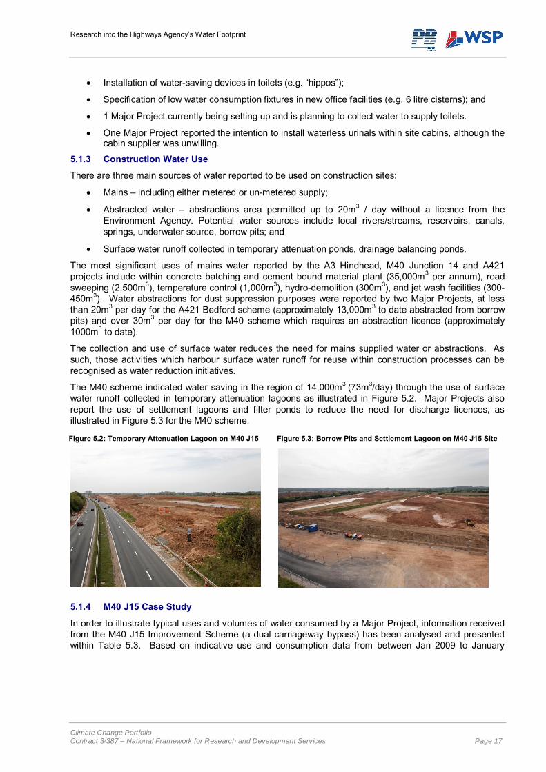
The M40 scheme indicated water saving in the region of 14,000m3 (73m3/day) through the use of surface water runoff collected in temporary attenuation lagoons as illustrated in Figure 5.2. Major Projects also report the use of settlement lagoons and filter ponds to reduce the need for discharge licences, as illustrated in Figure 5.3 for the M40 scheme.
Figure 5.2: Temporary Attenuation Lagoon on M40 J15 Figure 5.3: Borrow Pits and Settlement Lagoon on M40 J15 Site
5.1.4 M40 J15 Case Study
In order to illustrate typical uses and volumes of water consumed by a Major Project, information received from the M40 J15 Improvement Scheme (a dual carriageway bypass) has been analysed and presented within Table 5.3. Based on indicative use and consumption data from between Jan 2009 to January
Research into the Highways Agency’s Water Footprint
Climate Change Portfolio Contract 3/387 – National Framework for Research and Development Services Page 18
201016 (although the project commenced in March 2008), as anticipated water use in construction activities is significantly higher than for administrative activities (18,300m3 and 1,700m3 respectively).
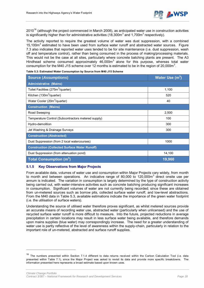
The activity reported to require the greatest volume of water was dust suppression, with a combined 15,100m3 estimated to have been used from surface water runoff and abstracted water sources. Figure 7.3 also indicates that reported water uses tended to be for site maintenance (i.e. dust suppression, wash off and temperature control), rather than being consumed in the process of making/processing materials. This would not be the case at all sites, particularly where concrete batching plants are present. The A3 Hindhead scheme consumed approximately 46,000m3 alone for this purpose, whereas total water consumption for the M40 J15 scheme over 12 months is estimated to be in the region of 20,000m3. Table 5.3: Estimated Water Consumption by Source from M40 J15 Scheme
Source (Assumptions) Water Use (m3) Administrative (Mains)
Toilet Facilities (275m3/quarter) 1,100
Kitchen (130m3/quarter) 520
Water Cooler (20m3/quarter) 40
Construction (Mains)
Road Sweeping 2,500
Temperature Control (Subcontractors metered supply) 100
Hydro-demolition 300
Jet Washing & Drainage Surveys 300
Construction (Abstracted)
Dust Suppression (from 2 local watercourses) 1000
Construction (Collected Surface Water Runoff)
Dust Suppression (from attenuation pond) 14,100
Total Consumption (m3) 19,960
5.1.5 Key Observations from Major Projects
From available data, volumes of water use and consumption within Major Projects vary widely, from month to month and between operations. An indicative range of 80,000 to 120,000m3 direct onsite use per annum is indicated. The variation in consumption is largely determined by the type of construction activity being carried out, with water-intensive activities such as concrete batching producing significant increases in consumption. Significant volumes of water are not currently being recorded; since these are obtained from un-metered sources such as borrow pits, collected surface water runoff, and low-level abstractions. From the M40 data in Table 5.3, available estimations indicate the importance of the green water footprint (i.e. the utilisation of surface waters).
Understanding the source of utilised water therefore proves significant, as whilst metered sources provide an accurate means of recording water use, abstracted water (particularly when unlicensed) and the use of recycled surface water runoff is more difficult to measure. Into the future, projected reductions in average precipitation in certain locations may result in less surface water being available, and therefore demands upon mains supplies (blue water) may correspondingly increase. The need for a greater understanding of water use is partly reflective of the level of awareness within the supply-chain, particularly in relation to the important role of un-metered, abstracted and surface runoff supplies.
16 The numbers presented within Section 7.1.4 different to data returns received within the Carbon Calculation Tool (i.e. data presented within Table 7.1), since the Major Project was asked to revisit its data and provide more specific breakdowns. The information presented here represents a broad estimate based upon known uses.
Research into the Highways Agency’s Water Footprint
Climate Change Portfolio Contract 3/387 – National Framework for Research and Development Services Page 19
5.2 DESIGN-BUILD-FINANCE-OPERATE (DBFO) SCHEMES To gain an understanding of how the DBFO supply chain uses water throughout its operations returned data from the Carbon Calculation Tool has been analysed, in addition with consultation with DBFO organisations. Given data limitations, this section is largely based upon analysis of information from the M25 DBFO, which has provided both qualitative and quantitative data for water used within its administrative activities (i.e. non-construction uses such as kitchen and toilet facilities) and construction activities.
5.2.1 Reported Water Use
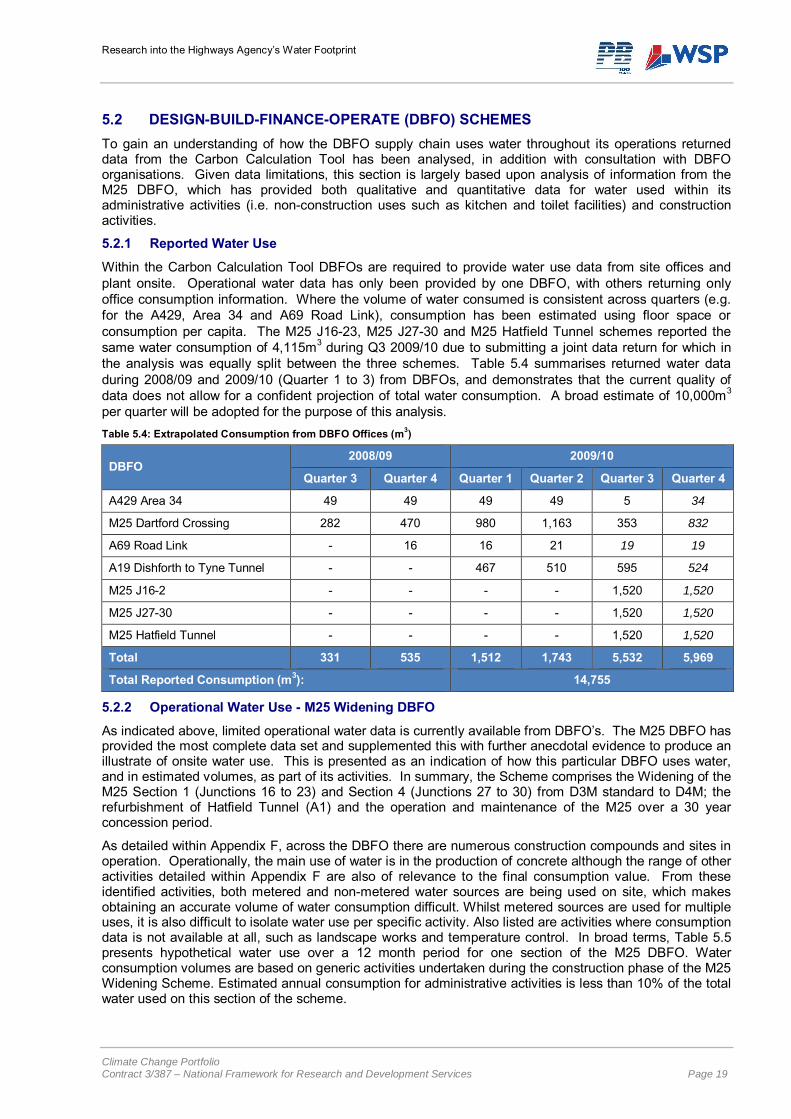
Within the Carbon Calculation Tool DBFOs are required to provide water use data from site offices and plant onsite. Operational water data has only been provided by one DBFO, with others returning only office consumption information. Where the volume of water consumed is consistent across quarters (e.g. for the A429, Area 34 and A69 Road Link), consumption has been estimated using floor space or consumption per capita. The M25 J16-23, M25 J27-30 and M25 Hatfield Tunnel schemes reported the same water consumption of 4,115m3 during Q3 2009/10 due to submitting a joint data return for which in the analysis was equally split between the three schemes. Table 5.4 summarises returned water data during 2008/09 and 2009/10 (Quarter 1 to 3) from DBFOs, and demonstrates that the current quality of data does not allow for a confident projection of total water consumption. A broad estimate of 10,000m3
per quarter will be adopted for the purpose of this analysis. Table 5.4: Extrapolated Consumption from DBFO Offices (m3)
DBFO 2008/09 2009/10
Quarter 3 Quarter 4 Quarter 1 Quarter 2 Quarter 3 Quarter 4
A429 Area 34 49 49 49 49 5 34
M25 Dartford Crossing 282 470 980 1,163 353 832
A69 Road Link - 16 16 21 19 19
A19 Dishforth to Tyne Tunnel - - 467 510 595 524
M25 J16-2 - - - - 1,520 1,520
M25 J27-30 - - - - 1,520 1,520
M25 Hatfield Tunnel - - - - 1,520 1,520
Total 331 535 1,512 1,743 5,532 5,969
Total Reported Consumption (m3): 14,755
5.2.2 Operational Water Use - M25 Widening DBFO
As indicated above, limited operational water data is currently available from DBFO’s. The M25 DBFO has provided the most complete data set and supplemented this with further anecdotal evidence to produce an illustrate of onsite water use. This is presented as an indication of how this particular DBFO uses water, and in estimated volumes, as part of its activities. In summary, the Scheme comprises the Widening of the M25 Section 1 (Junctions 16 to 23) and Section 4 (Junctions 27 to 30) from D3M standard to D4M; the refurbishment of Hatfield Tunnel (A1) and the operation and maintenance of the M25 over a 30 year concession period.
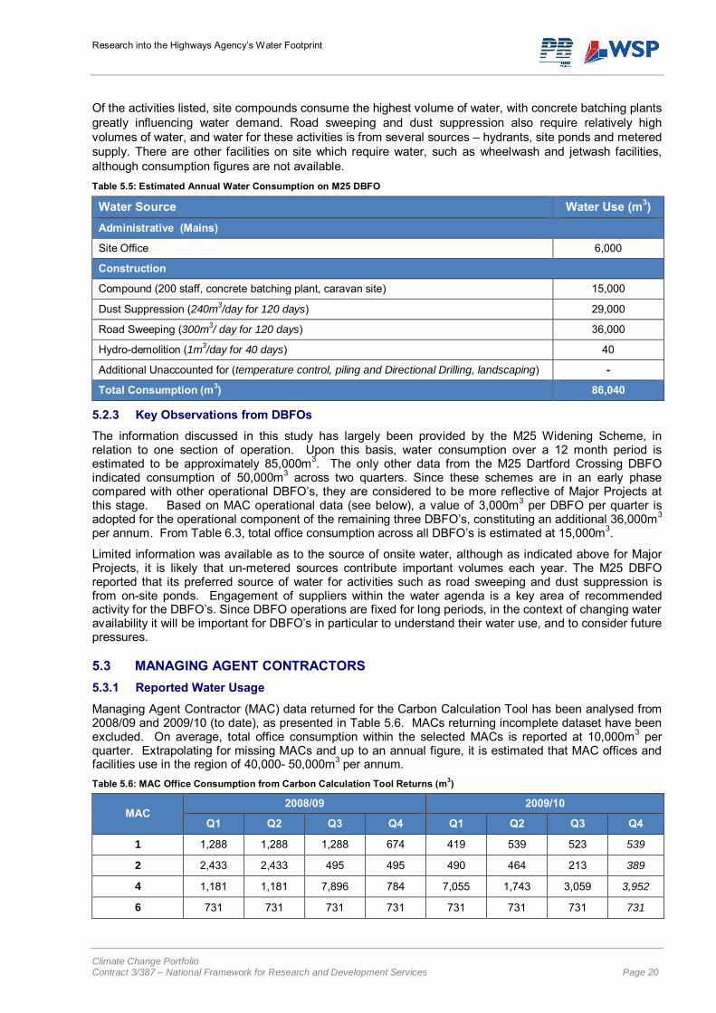
As detailed within Appendix F, across the DBFO there are numerous construction compounds and sites in operation. Operationally, the main use of water is in the production of concrete although the range of other activities detailed within Appendix F are also of relevance to the final consumption value. From these identified activities, both metered and non-metered water sources are being used on site, which makes obtaining an accurate volume of water consumption difficult. Whilst metered sources are used for multiple uses, it is also difficult to isolate water use per specific activity. Also listed are activities where consumption data is not available at all, such as landscape works and temperature control. In broad terms, Table 5.5 presents hypothetical water use over a 12 month period for one section of the M25 DBFO. Water consumption volumes are based on generic activities undertaken during the construction phase of the M25 Widening Scheme. Estimated annual consumption for administrative activities is less than 10% of the total water used on this section of the scheme.
Research into the Highways Agency’s Water Footprint
Climate Change Portfolio Contract 3/387 – National Framework for Research and Development Services Page 20
Of the activities listed, site compounds consume the highest volume of water, with concrete batching plants greatly influencing water demand. Road sweeping and dust suppression also require relatively high volumes of water, and water for these activities is from several sources – hydrants, site ponds and metered supply. There are other facilities on site which require water, such as wheelwash and jetwash facilities, although consumption figures are not available. Table 5.5: Estimated Annual Water Consumption on M25 DBFO
Water Source Water Use (m3) Administrative (Mains)
Site Office 6,000
Construction
Compound (200 staff, concrete batching plant, caravan site) 15,000
Dust Suppression (240m3/day for 120 days) 29,000
Road Sweeping (300m3/ day for 120 days) 36,000
Hydro-demolition (1m3/day for 40 days) 40
Additional Unaccounted for (temperature control, piling and Directional Drilling, landscaping) -
Total Consumption (m3) 86,040
5.2.3 Key Observations from DBFOs
The information discussed in this study has largely been provided by the M25 Widening Scheme, in relation to one section of operation. Upon this basis, water consumption over a 12 month period is estimated to be approximately 85,000m3. The only other data from the M25 Dartford Crossing DBFO indicated consumption of 50,000m3 across two quarters. Since these schemes are in an early phase compared with other operational DBFO’s, they are considered to be more reflective of Major Projects at this stage. Based on MAC operational data (see below), a value of 3,000m3 per DBFO per quarter is adopted for the operational component of the remaining three DBFO’s, constituting an additional 36,000m3 per annum. From Table 6.3, total office consumption across all DBFO’s is estimated at 15,000m3.
Limited information was available as to the source of onsite water, although as indicated above for Major Projects, it is likely that un-metered sources contribute important volumes each year. The M25 DBFO reported that its preferred source of water for activities such as road sweeping and dust suppression is from on-site ponds. Engagement of suppliers within the water agenda is a key area of recommended activity for the DBFO’s. Since DBFO operations are fixed for long periods, in the context of changing water availability it will be important for DBFO’s in particular to understand their water use, and to consider future pressures.
5.3 MANAGING AGENT CONTRACTORS 5.3.1 Reported Water Usage
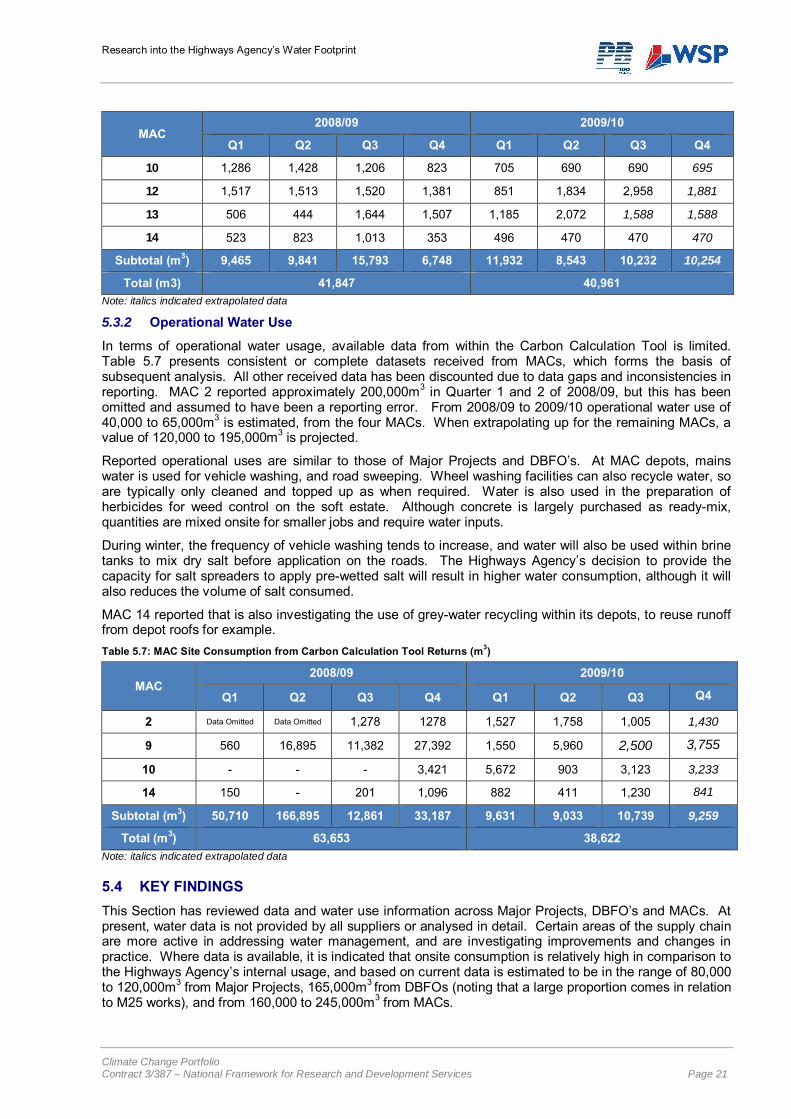
Managing Agent Contractor (MAC) data returned for the Carbon Calculation Tool has been analysed from 2008/09 and 2009/10 (to date), as presented in Table 5.6. MACs returning incomplete dataset have been excluded. On average, total office consumption within the selected MACs is reported at 10,000m3 per quarter. Extrapolating for missing MACs and up to an annual figure, it is estimated that MAC offices and facilities use in the region of 40,000- 50,000m3 per annum. Table 5.6: MAC Office Consumption from Carbon Calculation Tool Returns (m3)
MAC 2008/09 2009/10
Q1 Q2 Q3 Q4 Q1 Q2 Q3 Q4
1 1,288 1,288 1,288 674 419 539 523 539
2 2,433 2,433 495 495 490 464 213 389
4 1,181 1,181 7,896 784 7,055 1,743 3,059 3,952
6 731 731 731 731 731 731 731 731
Research into the Highways Agency’s Water Footprint
Climate Change Portfolio Contract 3/387 – National Framework for Research and Development Services Page 21
MAC 2008/09 2009/10
Q1 Q2 Q3 Q4 Q1 Q2 Q3 Q4
10 1,286 1,428 1,206 823 705 690 690 695
12 1,517 1,513 1,520 1,381 851 1,834 2,958 1,881
13 506 444 1,644 1,507 1,185 2,072 1,588 1,588
14 523 823 1,013 353 496 470 470 470
Subtotal (m3) 9,465 9,841 15,793 6,748 11,932 8,543 10,232 10,254
Total (m3) 41,847 40,961 Note: italics indicated extrapolated data
5.3.2 Operational Water Use
In terms of operational water usage, available data from within the Carbon Calculation Tool is limited. Table 5.7 presents consistent or complete datasets received from MACs, which forms the basis of subsequent analysis. All other received data has been discounted due to data gaps and inconsistencies in reporting. MAC 2 reported approximately 200,000m3 in Quarter 1 and 2 of 2008/09, but this has been omitted and assumed to have been a reporting error. From 2008/09 to 2009/10 operational water use of 40,000 to 65,000m3 is estimated, from the four MACs. When extrapolating up for the remaining MACs, a value of 120,000 to 195,000m3 is projected.
Reported operational uses are similar to those of Major Projects and DBFO’s. At MAC depots, mains water is used for vehicle washing, and road sweeping. Wheel washing facilities can also recycle water, so are typically only cleaned and topped up as when required. Water is also used in the preparation of herbicides for weed control on the soft estate. Although concrete is largely purchased as ready-mix, quantities are mixed onsite for smaller jobs and require water inputs.
During winter, the frequency of vehicle washing tends to increase, and water will also be used within brine tanks to mix dry salt before application on the roads. The Highways Agency’s decision to provide the capacity for salt spreaders to apply pre-wetted salt will result in higher water consumption, although it will also reduces the volume of salt consumed.
MAC 14 reported that is also investigating the use of grey-water recycling within its depots, to reuse runoff from depot roofs for example. Table 5.7: MAC Site Consumption from Carbon Calculation Tool Returns (m3)
MAC 2008/09 2009/10
Q1 Q2 Q3 Q4 Q1 Q2 Q3 Q4
2 Data Omitted Data Omitted 1,278 1278 1,527 1,758 1,005 1,430
9 560 16,895 11,382 27,392 1,550 5,960 2,500 3,755
10 - - - 3,421 5,672 903 3,123 3,233
14 150 - 201 1,096 882 411 1,230 841
Subtotal (m3) 50,710 166,895 12,861 33,187 9,631 9,033 10,739 9,259
Total (m3) 63,653 38,622 Note: italics indicated extrapolated data
5.4 KEY FINDINGS This Section has reviewed data and water use information across Major Projects, DBFO’s and MACs. At present, water data is not provided by all suppliers or analysed in detail. Certain areas of the supply chain are more active in addressing water management, and are investigating improvements and changes in practice. Where data is available, it is indicated that onsite consumption is relatively high in comparison to the Highways Agency’s internal usage, and based on current data is estimated to be in the range of 80,000 to 120,000m3 from Major Projects, 165,000m3 from DBFOs (noting that a large proportion comes in relation to M25 works), and from 160,000 to 245,000m3 from MACs.
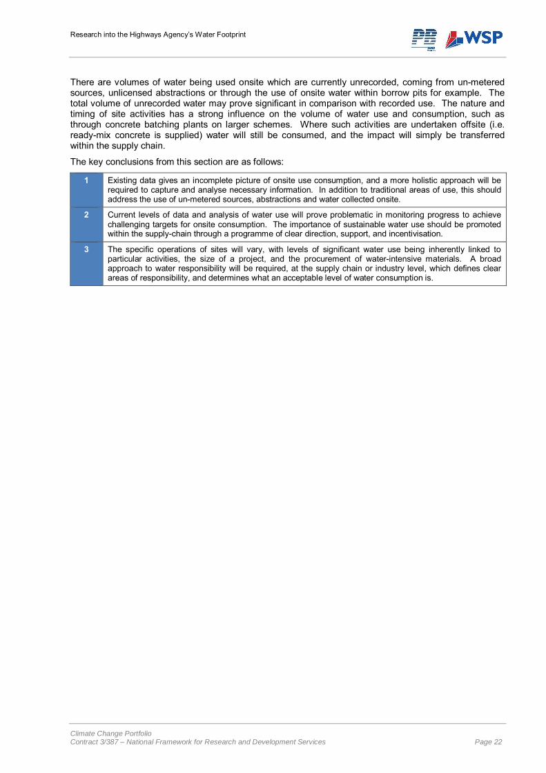
Research into the Highways Agency’s Water Footprint
Climate Change Portfolio Contract 3/387 – National Framework for Research and Development Services Page 22
There are volumes of water being used onsite which are currently unrecorded, coming from un-metered sources, unlicensed abstractions or through the use of onsite water within borrow pits for example. The total volume of unrecorded water may prove significant in comparison with recorded use. The nature and timing of site activities has a strong influence on the volume of water use and consumption, such as through concrete batching plants on larger schemes. Where such activities are undertaken offsite (i.e. ready-mix concrete is supplied) water will still be consumed, and the impact will simply be transferred within the supply chain.
The key conclusions from this section are as follows:
1 Existing data gives an incomplete picture of onsite use consumption, and a more holistic approach will be required to capture and analyse necessary information. In addition to traditional areas of use, this should address the use of un-metered sources, abstractions and water collected onsite.
2 Current levels of data and analysis of water use will prove problematic in monitoring progress to achieve challenging targets for onsite consumption. The importance of sustainable water use should be promoted within the supply-chain through a programme of clear direction, support, and incentivisation.
3 The specific operations of sites will vary, with levels of significant water use being inherently linked to particular activities, the size of a project, and the procurement of water-intensive materials. A broad approach to water responsibility will be required, at the supply chain or industry level, which defines clear areas of responsibility, and determines what an acceptable level of water consumption is.
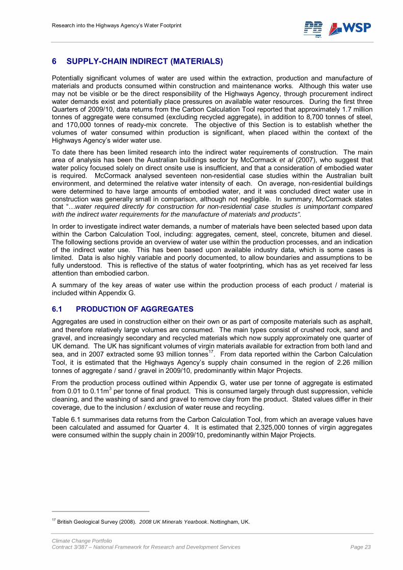
Research into the Highways Agency’s Water Footprint
Climate Change Portfolio Contract 3/387 – National Framework for Research and Development Services Page 23
6 SUPPLY-CHAIN INDIRECT (MATERIALS)
Potentially significant volumes of water are used within the extraction, production and manufacture of materials and products consumed within construction and maintenance works. Although this water use may not be visible or be the direct responsibility of the Highways Agency, through procurement indirect water demands exist and potentially place pressures on available water resources. During the first three Quarters of 2009/10, data returns from the Carbon Calculation Tool reported that approximately 1.7 million tonnes of aggregate were consumed (excluding recycled aggregate), in addition to 8,700 tonnes of steel, and 170,000 tonnes of ready-mix concrete. The objective of this Section is to establish whether the volumes of water consumed within production is significant, when placed within the context of the Highways Agency’s wider water use.
To date there has been limited research into the indirect water requirements of construction. The main area of analysis has been the Australian buildings sector by McCormack et al (2007), who suggest that water policy focused solely on direct onsite use is insufficient, and that a consideration of embodied water is required. McCormack analysed seventeen non-residential case studies within the Australian built environment, and determined the relative water intensity of each. On average, non-residential buildings were determined to have large amounts of embodied water, and it was concluded direct water use in construction was generally small in comparison, although not negligible. In summary, McCormack states that “…water required directly for construction for non-residential case studies is unimportant compared with the indirect water requirements for the manufacture of materials and products”.
In order to investigate indirect water demands, a number of materials have been selected based upon data within the Carbon Calculation Tool, including: aggregates, cement, steel, concrete, bitumen and diesel. The following sections provide an overview of water use within the production processes, and an indication of the indirect water use. This has been based upon available industry data, which is some cases is limited. Data is also highly variable and poorly documented, to allow boundaries and assumptions to be fully understood. This is reflective of the status of water footprinting, which has as yet received far less attention than embodied carbon.
A summary of the key areas of water use within the production process of each product / material is included within Appendix G.
6.1 PRODUCTION OF AGGREGATES Aggregates are used in construction either on their own or as part of composite materials such as asphalt, and therefore relatively large volumes are consumed. The main types consist of crushed rock, sand and gravel, and increasingly secondary and recycled materials which now supply approximately one quarter of UK demand. The UK has significant volumes of virgin materials available for extraction from both land and sea, and in 2007 extracted some 93 million tonnes17. From data reported within the Carbon Calculation Tool, it is estimated that the Highways Agency’s supply chain consumed in the region of 2.26 million tonnes of aggregate / sand / gravel in 2009/10, predominantly within Major Projects.
From the production process outlined within Appendix G, water use per tonne of aggregate is estimated from 0.01 to 0.11m3 per tonne of final product. This is consumed largely through dust suppression, vehicle cleaning, and the washing of sand and gravel to remove clay from the product. Stated values differ in their coverage, due to the inclusion / exclusion of water reuse and recycling.
Table 6.1 summarises data returns from the Carbon Calculation Tool, from which an average values have been calculated and assumed for Quarter 4. It is estimated that 2,325,000 tonnes of virgin aggregates were consumed within the supply chain in 2009/10, predominantly within Major Projects.
17 British Geological Survey (2008). 2008 UK Minerals Yearbook. Nottingham, UK.
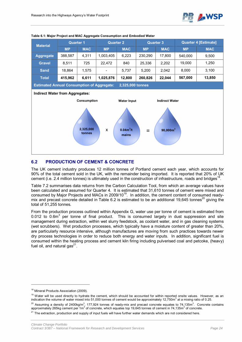
Research into the Highways Agency’s Water Footprint
Climate Change Portfolio Contract 3/387 – National Framework for Research and Development Services Page 24
Table 6.1: Major Project and MAC Aggregate Consumption and Embodied Water
Material Quarter 1 Quarter 2 Quarter 3 Quarter 4 [Estimate]
MP MAC MP MAC MP MAC MP MAC
Aggregate 388,587 4,311 1,003,405 6,223 230,290 17,800 540,000 9,500
Gravel 8,511 725 22,472 840 25,336 2,202 19,000 1,250
Sand 18,864 1,575 - 5,737 5,200 2,042 8,000 3,100
Total 415,962 6,611 1,025,876 12,800 260,826 22,044 567,000 13,850
Estimated Annual Consumption of Aggregate: 2,325,000 tonnes
Indirect Water from Aggregates:
6.2 PRODUCTION OF CEMENT & CONCRETE The UK cement industry produces 12 million tonnes of Portland cement each year, which accounts for 90% of the total cement sold in the UK, with the remainder being imported. It is reported that 20% of UK cement (i.e. 2.4 million tonnes) is ultimately used in the construction of infrastructure, roads and bridges18.
Table 7.2 summarises data returns from the Carbon Calculation Tool, from which an average values have been calculated and assumed for Quarter 4. It is estimated that 31,610 tonnes of cement were mixed and consumed by Major Projects and MACs in 2009/1019. In addition, the cement content of consumed ready-mix and precast concrete detailed in Table 6.2 is estimated to be an additional 19,645 tonnes20 giving the total of 51,255 tonnes.
From the production process outlined within Appendix G, water use per tonne of cement is estimated from 0.012 to 0.6m3 per tonne of final product. This is consumed largely in dust suppression and site management during extraction, within wet slurry feedstock, as coolant water, and in gas cleaning systems (wet scrubbers). Wet production processes, which typically have a moisture content of greater than 20%, are particularly resource intensive, although manufactures are moving from such practices towards newer dry process technologies in order to reduce both energy and water inputs. In addition, significant fuel is consumed within the heating process and cement kiln firing including pulverised coal and petcoke, (heavy) fuel oil, and natural gas21.
18 Mineral Products Association (2009). 19 Water will be used directly to hydrate the cement, which should be accounted for within reported onsite values. However, as an indication the volume of water mixed into 51,000 tonnes of cement would be approximately 12,750m3 at a mixing ratio of 0.25. 20 Assuming a density of 2400kg/m3, 177,924 tonnes of ready-mix and precast concrete equates to 74,135m3. Concrete contains approximately 265kg cement per 1m3 of concrete, which equates top 19,645 tonnes of cement in 74,135m3 of concrete. 21 The extraction, production and supply of input fuels will have further water demands which are not considered here.
Consumption Water Input Indirect Water
2,325,000 tonnes
x 0.04m3/t mains
= 90,000m3
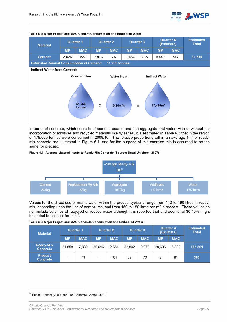
Research into the Highways Agency’s Water Footprint
Climate Change Portfolio Contract 3/387 – National Framework for Research and Development Services Page 25
Table 6.2: Major Project and MAC Cement Consumption and Embodied Water
Material Quarter 1 Quarter 2 Quarter 3 Quarter 4
[Estimate] Estimated
Total
MP MAC MP MAC MP MAC MP MAC
Cement 3,626 827 7,913 78 11,434 736 6,449 547 31,610
Estimated Annual Consumption of Cement: 51,255 tonnes
Indirect Water from Cement:
In terms of concrete, which consists of cement, coarse and fine aggregate and water, with or without the incorporation of additives and recycled materials like fly ashes, it is estimated in Table 6.3 that in the region of 178,000 tonnes were consumed in 2009/10. The relative proportions within an average 1m3 of ready-mix concrete are illustrated in Figure 6.1, and for the purpose of this exercise this is assumed to be the same for precast. Figure 6.1: Average Material Inputs to Ready-Mix Concrete (Source: Buzzi Unichem, 2007)
Values for the direct use of mains water within the product typically range from 140 to 190 litres in ready-mix, depending upon the use of admixtures, and from 150 to 180 litres per m3 in precast. These values do not include volumes of recycled or reused water although it is reported that and additional 30-40% might be added to account for this22. Table 6.3: Major Project and MAC Concrete Consumption and Embodied Water
Material Quarter 1 Quarter 2 Quarter 3 Quarter 4
[Estimate] Estimated
Total
MP MAC MP MAC MP MAC MP MAC
Ready-Mix Concrete 31,858 7,832 36,016 2,654 52,802 9,973 29,606 6,820 177,561
Precast Concrete - 73 - 101 28 70 9 81 363
22 British Precast (2009) and The Concrete Centre (2010).
Average Ready-Mix
1m3
Cement
264kg
Replacement Fly Ash
46kg
Aggregate
1872kg
Additives
1.5 litres
Water
175 litres
Consumption Water Input
x =
Indirect Water
0.34m3/t 51,255 tonnes 17,426m3
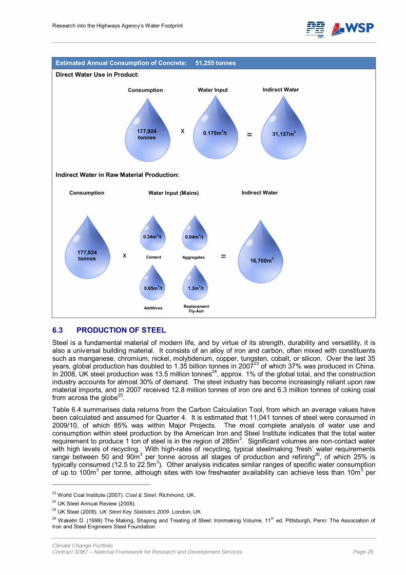
Research into the Highways Agency’s Water Footprint
Climate Change Portfolio Contract 3/387 – National Framework for Research and Development Services Page 26
Estimated Annual Consumption of Concrete: 51,255 tonnes
Direct Water Use in Product: Indirect Water in Raw Material Production:
6.3 PRODUCTION OF STEEL Steel is a fundamental material of modern life, and by virtue of its strength, durability and versatility, it is also a universal building material. It consists of an alloy of iron and carbon, often mixed with constituents such as manganese, chromium, nickel, molybdenum, copper, tungsten, cobalt, or silicon. Over the last 35 years, global production has doubled to 1.35 billion tonnes in 200723 of which 37% was produced in China. In 2008, UK steel production was 13.5 million tonnes24, approx. 1% of the global total, and the construction industry accounts for almost 30% of demand. The steel industry has become increasingly reliant upon raw material imports, and in 2007 received 12.8 million tonnes of iron ore and 6.3 million tonnes of coking coal from across the globe25.
Table 6.4 summarises data returns from the Carbon Calculation Tool, from which an average values have been calculated and assumed for Quarter 4. It is estimated that 11,041 tonnes of steel were consumed in 2009/10, of which 85% was within Major Projects. The most complete analysis of water use and consumption within steel production by the American Iron and Steel Institute indicates that the total water requirement to produce 1 ton of steel is in the region of 285m3. Significant volumes are non-contact water with high levels of recycling. With high-rates of recycling, typical steelmaking ‘fresh’ water requirements range between 50 and 90m3 per tonne across all stages of production and refining26, of which 25% is typically consumed (12.5 to 22.5m3). Other analysis indicates similar ranges of specific water consumption of up to 100m3 per tonne, although sites with low freshwater availability can achieve less than 10m3 per
23 World Coal Institute (2007). Coal & Steel. Richmond, UK. 24 UK Steel Annual Review (2008). 25 UK Steel (2009). UK Steel Key Statistics 2009. London, UK 26 Wakelin D. (1999) The Making, Shaping and Treating of Steel: Ironmaking Volume, 11th ed. Pittsburgh, Penn: The Association of Iron and Steel Engineers Steel Foundation.
Consumption Water Input Indirect Water Indirect Water
x = 0.175m3/t
177,924 tonnes 31,137m3
Water Input (Mains) Consumption Indirect Water
x =
0.34m3/t
177,924 tonnes 16,700m3
0.04m3/t
0.65m3/t
1.3m3/t
Additives Replacement Fly-Ash
Cement Aggregates
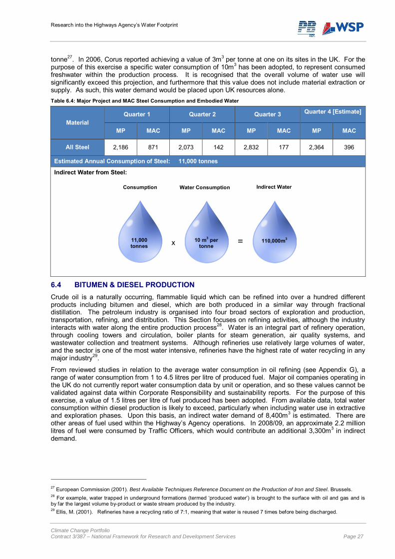
Research into the Highways Agency’s Water Footprint
Climate Change Portfolio Contract 3/387 – National Framework for Research and Development Services Page 27
tonne27. In 2006, Corus reported achieving a value of 3m3 per tonne at one on its sites in the UK. For the purpose of this exercise a specific water consumption of 10m3 has been adopted, to represent consumed freshwater within the production process. It is recognised that the overall volume of water use will significantly exceed this projection, and furthermore that this value does not include material extraction or supply. As such, this water demand would be placed upon UK resources alone. Table 6.4: Major Project and MAC Steel Consumption and Embodied Water
Material Quarter 1 Quarter 2 Quarter 3 Quarter 4 [Estimate]
MP MAC MP MAC MP MAC MP MAC
All Steel 2,186 871 2,073 142 2,832 177 2,364 396
Estimated Annual Consumption of Steel: 11,000 tonnes
Indirect Water from Steel:
6.4 BITUMEN & DIESEL PRODUCTION Crude oil is a naturally occurring, flammable liquid which can be refined into over a hundred different products including bitumen and diesel, which are both produced in a similar way through fractional distillation. The petroleum industry is organised into four broad sectors of exploration and production, transportation, refining, and distribution. This Section focuses on refining activities, although the industry interacts with water along the entire production process28. Water is an integral part of refinery operation, through cooling towers and circulation, boiler plants for steam generation, air quality systems, and wastewater collection and treatment systems. Although refineries use relatively large volumes of water, and the sector is one of the most water intensive, refineries have the highest rate of water recycling in any major industry29.
From reviewed studies in relation to the average water consumption in oil refining (see Appendix G), a range of water consumption from 1 to 4.5 litres per litre of produced fuel. Major oil companies operating in the UK do not currently report water consumption data by unit or operation, and so these values cannot be validated against data within Corporate Responsibility and sustainability reports. For the purpose of this exercise, a value of 1.5 litres per litre of fuel produced has been adopted. From available data, total water consumption within diesel production is likely to exceed, particularly when including water use in extractive and exploration phases. Upon this basis, an indirect water demand of 8,400m3 is estimated. There are other areas of fuel used within the Highway’s Agency operations. In 2008/09, an approximate 2.2 million litres of fuel were consumed by Traffic Officers, which would contribute an additional 3,300m3 in indirect demand.
27 European Commission (2001). Best Available Techniques Reference Document on the Production of Iron and Steel. Brussels. 28 For example, water trapped in underground formations (termed ‘produced water’) is brought to the surface with oil and gas and is by far the largest volume by-product or waste stream produced by the industry. 29 Ellis, M. (2001). Refineries have a recycling ratio of 7:1, meaning that water is reused 7 times before being discharged.
Indirect Water Water Consumption Consumption
x = 11,000 tonnes
10 m3 per tonne
110,000m3

Research into the Highways Agency’s Water Footprint
Climate Change Portfolio Contract 3/387 – National Framework for Research and Development Services Page 28
Table 6.5: Major Project and MAC Steel Consumption and Embodied Water
Material Quarter 1 Quarter 2 Quarter 3 Quarter 4 [Estimate]
MP MAC MP MAC MP MAC MP MAC
Diesel 1,240,101 86,319 1,557,981 92,450 934,512 296,366 1,244,198 158,378
Estimated Annual Consumption of Diesel: 5,610,000 + 2,200,000 litres from Traffic Officers
Indirect Water from Diesel:
6.5 KEY LIMITATIONS Publicly available data for the analysis of embodied water in productions is limited at the time of writing. Publicly available studies have been reviewed, alongside reported industry data within corporate responsibility and sustainability reports. Where necessary, clarifications have been gained from organisations. Estimates for the above materials are limited in terms of coverage of all water inputs to production processes, which are often highly complex and involve significant volumes of non-contact process water which is not consumed and recycled. Organisations in the aggregate, steel, cement and petroleum industries indicate they are currently involved in studies to determine their water inputs and grey water outputs. It is expected that in the next few years far more information will be available for more complete assessments of indirect water requirements. As such, the analysis and data presented within this section provides illustrative trends of indirect water demand from selected materials.
6.6 GEOGRAPHICAL IMPACTS The availability of water is an emotive issue, particularly linked to the levels of stress and scarcity experienced within emerging economies and part episodes of drought and famine. The virtual water and water footprint concepts are being used to investigate the scale of impacts that global trade is having on non-domestic water resources. As indicated within Section 3.3 (Analysis of UK Water Footprint), research into the UK’s virtual water imports and water footprint indicate that through established trade patterns there is a significant net water importer. Analysis of the agricultural sector has focused upon the virtual water impacts of nations such as the UK, since it is recognised that the water intensity of production coupled with the volume of imports means that significant virtual water demands exist. The geographic impact of construction products may differ from agriculture, and not have the same international dimension. For example, the UK is (at the present time) relatively self-sufficient in certain minerals.
A review of European mineral statistics by the British Geological Survey (2010) indicated that in term of bulk construction materials30, the majority of EU countries (including the UK) are self-sufficient in supply. In terms of industrial (non-construction) minerals, typically non-metallic and non-energy minerals used as feedstock in manufacturing or industrial process, at a European level production supplies a high proportion of the continent’s requirements. The UK is indicated to be high supplier to salt and kaolin in this category. In terms of metals, it is determined that all of Europe is now heavily dependant on sources of virtually all metals form outside of Europe, although levels of recycling make an important contribution.
European supply of energy minerals including petroleum and natural gas are dominated by the North Sea and offshore fields exploited by the UK and Norway, whilst coal and uranium has relatively small levels of
30 Including aggregates, clay and shale, gypsum, limestone and dolomite.
Indirect Water Water Consumption Consumption
x = 7,810,000 litres
1.5 litre per litre
11,715m3
Research into the Highways Agency’s Water Footprint
Climate Change Portfolio Contract 3/387 – National Framework for Research and Development Services Page 29
supply (in terms of total global levels) largely from Germany and Poland (coal) and the Czech Republic (uranium). A summary of production, import and export statistics from the British Geological Survey for the UK are included within Appendix H, including observed key trends.
In terms of more specific products, Table 6.6 provides a summary of selected trade data from HM Revenue and Customs for 2009, which amongst others would be of relevance to the activities of the Highways Agency. For certain products such as petroleum oils form bituminous minerals, the UK imports significant volumes from many locations across the globe. For materials such as pig iron, there is strong reliance upon a smaller number of import locations. Imports (by value) can be very large for given products and materials used within the construction sector, and as suggested by WWF (2008), the UK’s internal water footprint may, for certain products or materials, be overshadowed by the external component. Table 6.6: UK Trade Data for 2009 for selected Comcodes
Comcode Description Key Imports by Value
2907 Petroleum oils and oils obtained from bituminous minerals, crude
Norway £10,100m; Russia £1,100m; Nigeria £545m; Libya £533m; Turkey £350m; Algeria: £306m; Angola £256m; Venezuela £217m; Brazil £210m; Tunisia £189m; Iran £165m.
7201 Pig Iron and spiegeleisen in pigs, blocks or other primary forms
South Africa £2.8m; The Netherlands £1.1m; Russia £0.9m.
7301 Sheet piling of iron of steel, whether nor not drilled, punched or made from assembled elements; welded angles, shapes and sections
European Union £38m; Japan £3.8m; China, £2.4m; USA + Puerto Rico £1.2m; South Korea £0.8m
8429 Self-propelled bulldozers, graders, levellers, scrapers, mechanical shovels, excavators, shovel loaders, tamping machines and road rollers
European Union £255m; USA + Puerto Rico £18m; South Korea £14m; Japan £9.9m; Brazil 4.9m
Allocating a spatial or geographical dimension to green, blue and grey water impacts is a key area of focus for the water footprint method. The small number of studies available have each struggled with this issue. It proves easier for organisations closely linked to production or manufacturing, since water demands can be easily identified at particular sites or the sites of subcontractors. SABMiller, one of the world’s largest brewing companies, has been able to develop a number of case studies from particular operations and concluded that “…the complexity of attributing impact to individual users is not straight forward…For now, it is useful for companies to use risk maps for the value chain to assess where the footprint ‘lands’ in relation to scarcity issues on the ground”.
Analysis by Katsoufis (2009) into the water footprint of a petrochemical company also struggled to determine the nature of geographic impacts from supply chain components, and concluded that providing geographically explicit results is an unrealistic ambition of water footprinting. It is considered that given the current status of water footprints and the availability of data, providing a geographical indication of impact is not yet achievable. From experience in carbon footprinting, an overwhelming level of analysis and disclosure may first be required before organisations towards the top of the supply-chain can gain a perspective of the specific geographical impacts of their procurement.
6.7 KEY FINDINGS “There has been little attention to the fact that, in the end, total water consumption and pollution relate to what and how many communities consume and to the structure of the global economy that supplies the various consumer goods and services”
Water Footprint Manual (2009), Water Footprint Network
The estimated embodied water contents of selected materials are presented in Figure 6.2, and if assumed to represent water demand suggest a total volume of demand greater than the combined consumption from Highway Agency’s offices and supply-chain operations onsite. With further investigation, and more reliable data, the indirect water demand within these materials would be expected to increase, and the total indirect water demand would increase dramatically with the inclusion of other consumed products and materials. Certain products are more water-intensive in production than others, but it is important to
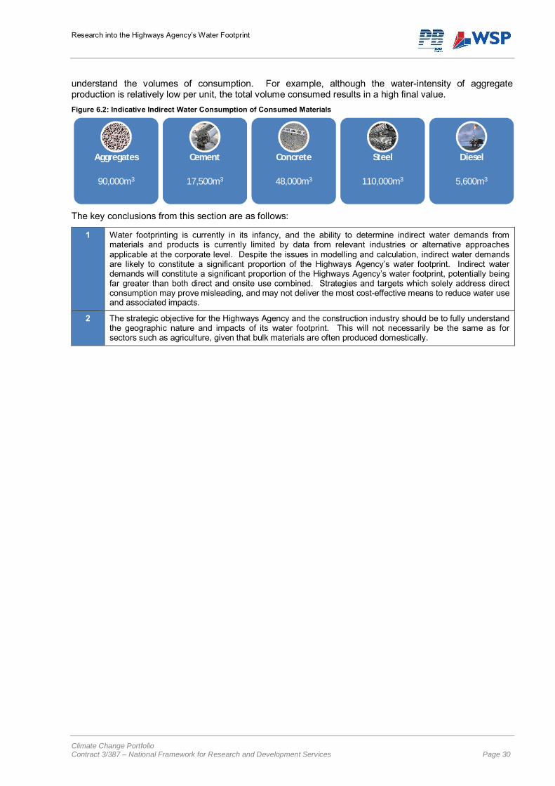
Research into the Highways Agency’s Water Footprint
Climate Change Portfolio Contract 3/387 – National Framework for Research and Development Services Page 30
understand the volumes of consumption. For example, although the water-intensity of aggregate production is relatively low per unit, the total volume consumed results in a high final value. Figure 6.2: Indicative Indirect Water Consumption of Consumed Materials
The key conclusions from this section are as follows:
1 Water footprinting is currently in its infancy, and the ability to determine indirect water demands from materials and products is currently limited by data from relevant industries or alternative approaches applicable at the corporate level. Despite the issues in modelling and calculation, indirect water demands are likely to constitute a significant proportion of the Highways Agency’s water footprint. Indirect water demands will constitute a significant proportion of the Highways Agency’s water footprint, potentially being far greater than both direct and onsite use combined. Strategies and targets which solely address direct consumption may prove misleading, and may not deliver the most cost-effective means to reduce water use and associated impacts.
2 The strategic objective for the Highways Agency and the construction industry should be to fully understand the geographic nature and impacts of its water footprint. This will not necessarily be the same as for sectors such as agriculture, given that bulk materials are often produced domestically.
Aggregates
90,000m3
Cement
17,500m3
Concrete
48,000m3
Steel
110,000m3
Diesel
5,600m3
Research into the Highways Agency’s Water Footprint
Climate Change Portfolio Contract 3/387 – National Framework for Research and Development Services Page 31
7 GREY WATER FOOTPRINT
Highways and roads cover a large surface area in the UK and will therefore intercept large quantities of water. Road drainage is a critical part of the highway infrastructure to ensure that surface water from rainfall is quickly evacuated. But even during short contact periods, rain water will absorb the pollutants present on the surface (oils, hydrocarbons, metals, salts, etc) and become polluted. The polluted water forms the grey water footprint of highways and roads. This is calculated by dividing the pollutant load (L, in mass/time) by the difference between the ambient water quality standard for that pollutant (the maximum acceptable concentration Cmax, in mass/volume) and its natural concentration in the receiving water body (Cnat, in mass/volume):
Grey Water Footprint (GW) = Pollutant Load (L)
Maximum Acceptable Conc. (Cmax) – Natural Conc. (Cnat)
When chemicals are directly released into a surface water body, the load can directly be measured. When a chemical is applied on or put into the soil, like in the case of solid waste or use of fertilisers or pesticides, only a fraction may reach the groundwater or enter a surface water stream. In this case, the pollutant load is the fraction of the total amount of chemicals applied that reaches the ground- or surface water, which requires a further calculation. The pollutant load can be calculated as the effluent volume (Effl, in volume/time) multiplied by the difference between the concentration of the pollutant in the effluent (Ceffl, in mass/volume) and its natural concentration in the receiving water body (Cnat, in mass/volume):
Grey Water Footprint (GW) = Effluent Volume (Effl) x (Conc. of Pollutant (Ceffl) – Natural Conc. (Cnat))
Maximum Acceptable Conc. (Cmax) – Natural Conc. (Cnat)
The pollutant load L is defined as the load that comes on top of the natural concentration in the receiving water body. For human-made substances that naturally do not occur in water, Cnat = 0, so that the final calculation is as follows:
Grey Water Footprint (GW) = Effluent Volume (Effl) x Conc. of Pollutant (Ceffl)
Maximum Acceptable Conc. (Cmax)
7.1 METHODOLOGY As part of this research, it would prove extremely difficult to apply the above, since there would be numerous pollutants being deposited on roads requiring quantification. Water quality information is unlikely to be available at local level to determine the natural concentration of each pollutant. There would also be difficulties in determining other key factors such as the concentration of pollutants absorbed by rainfall and the quantity of pollutants actually present on the road network. This process was considered too onerous as part of this work, and therefore an alternative method has been used to provide a high level overview of the Highways Agency’s grey water footprint. It is assumed that the grey water element is entirely composed of rainwater diluting pollutants present on the roads (i.e. there are no other pollutant inputs), and that the pollutants will not be naturally present (or only in small quantities) in the environment in high concentration. In order to estimate the volume of polluted water run off, the level of rainfall and surface area covered by the roads has been calculated based on available data. No water quality information has been reviewed at this stage31.
7.2 ROAD NETWORK COVERAGE The highway asset stock is composed of motorways, dual and single carriage ways (see Appendix I). The surface covered by each category will vary and is dependant on the width of the road. By using the Highway Agency standards included in the Design Manual for Roads and Bridges (DMRB), Volume 6, TD 31 However, we are aware that the Highways Agency has undertaken extensive research on the water quality of highway runoff. This has been used to inform DMRB Volume 11, Section 3 Part 10. The Highways Agency Water Risk Assessment Tool (HAWRAT) ensures that new assets are developed to eliminate or minimise the pollution risk from highway runoff.
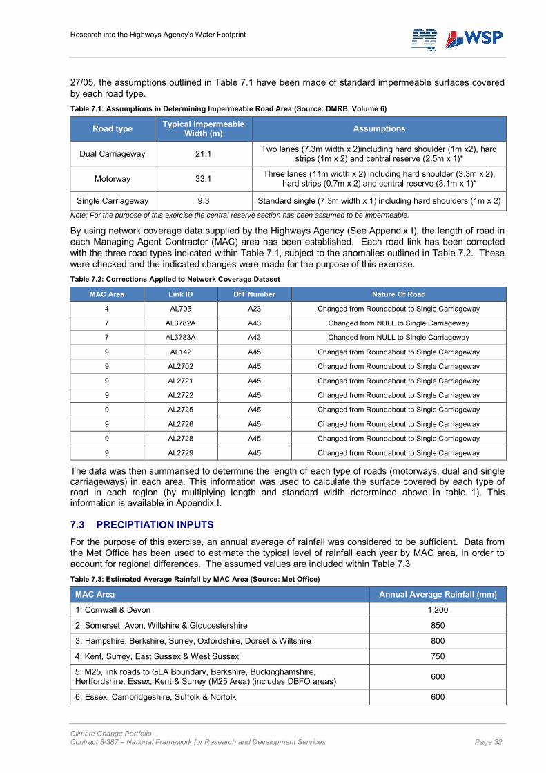
Research into the Highways Agency’s Water Footprint
Climate Change Portfolio Contract 3/387 – National Framework for Research and Development Services Page 32
27/05, the assumptions outlined in Table 7.1 have been made of standard impermeable surfaces covered by each road type. Table 7.1: Assumptions in Determining Impermeable Road Area (Source: DMRB, Volume 6)
Road type Typical Impermeable Width (m) Assumptions
Dual Carriageway 21.1 Two lanes (7.3m width x 2)including hard shoulder (1m x2), hard strips (1m x 2) and central reserve (2.5m x 1)*
Motorway 33.1 Three lanes (11m width x 2) including hard shoulder (3.3m x 2), hard strips (0.7m x 2) and central reserve (3.1m x 1)*
Single Carriageway 9.3 Standard single (7.3m width x 1) including hard shoulders (1m x 2) Note: For the purpose of this exercise the central reserve section has been assumed to be impermeable.
By using network coverage data supplied by the Highways Agency (See Appendix I), the length of road in each Managing Agent Contractor (MAC) area has been established. Each road link has been corrected with the three road types indicated within Table 7.1, subject to the anomalies outlined in Table 7.2. These were checked and the indicated changes were made for the purpose of this exercise. Table 7.2: Corrections Applied to Network Coverage Dataset
MAC Area Link ID DfT Number Nature Of Road
4 AL705 A23 Changed from Roundabout to Single Carriageway
7 AL3782A A43 Changed from NULL to Single Carriageway
7 AL3783A A43 Changed from NULL to Single Carriageway
9 AL142 A45 Changed from Roundabout to Single Carriageway 9 AL2702 A45 Changed from Roundabout to Single Carriageway 9 AL2721 A45 Changed from Roundabout to Single Carriageway 9 AL2722 A45 Changed from Roundabout to Single Carriageway 9 AL2725 A45 Changed from Roundabout to Single Carriageway 9 AL2726 A45 Changed from Roundabout to Single Carriageway 9 AL2728 A45 Changed from Roundabout to Single Carriageway 9 AL2729 A45 Changed from Roundabout to Single Carriageway
The data was then summarised to determine the length of each type of roads (motorways, dual and single carriageways) in each area. This information was used to calculate the surface covered by each type of road in each region (by multiplying length and standard width determined above in table 1). This information is available in Appendix I.
7.3 PRECIPTIATION INPUTS For the purpose of this exercise, an annual average of rainfall was considered to be sufficient. Data from the Met Office has been used to estimate the typical level of rainfall each year by MAC area, in order to account for regional differences. The assumed values are included within Table 7.3 Table 7.3: Estimated Average Rainfall by MAC Area (Source: Met Office)
MAC Area Annual Average Rainfall (mm)
1: Cornwall & Devon 1,200
2: Somerset, Avon, Wiltshire & Gloucestershire 850
3: Hampshire, Berkshire, Surrey, Oxfordshire, Dorset & Wiltshire 800
4: Kent, Surrey, East Sussex & West Sussex 750
5: M25, link roads to GLA Boundary, Berkshire, Buckinghamshire, Hertfordshire, Essex, Kent & Surrey (M25 Area) (includes DBFO areas) 600
6: Essex, Cambridgeshire, Suffolk & Norfolk 600
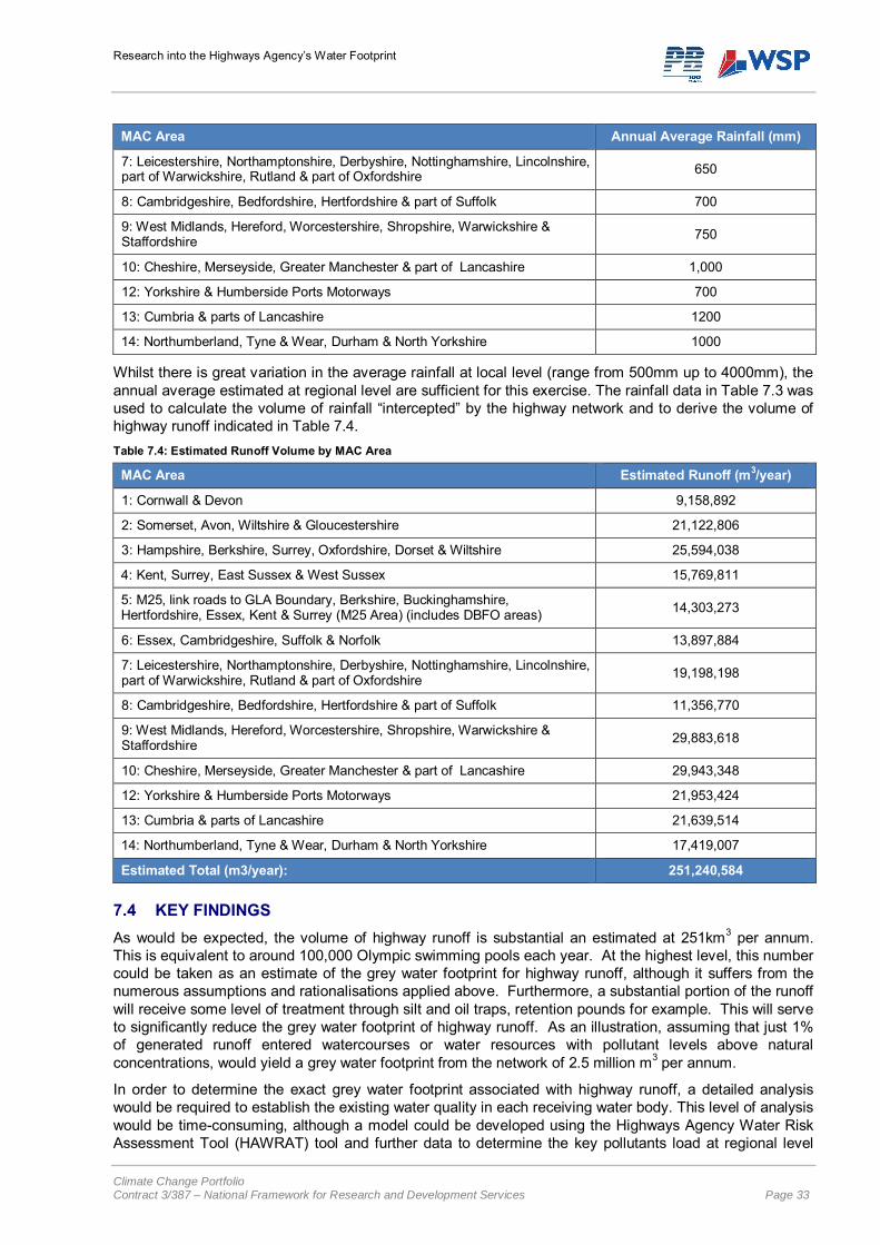
Research into the Highways Agency’s Water Footprint
Climate Change Portfolio Contract 3/387 – National Framework for Research and Development Services Page 33
MAC Area Annual Average Rainfall (mm)
7: Leicestershire, Northamptonshire, Derbyshire, Nottinghamshire, Lincolnshire, part of Warwickshire, Rutland & part of Oxfordshire 650
8: Cambridgeshire, Bedfordshire, Hertfordshire & part of Suffolk 700
9: West Midlands, Hereford, Worcestershire, Shropshire, Warwickshire & Staffordshire 750
10: Cheshire, Merseyside, Greater Manchester & part of Lancashire 1,000
12: Yorkshire & Humberside Ports Motorways 700
13: Cumbria & parts of Lancashire 1200
14: Northumberland, Tyne & Wear, Durham & North Yorkshire 1000
Whilst there is great variation in the average rainfall at local level (range from 500mm up to 4000mm), the annual average estimated at regional level are sufficient for this exercise. The rainfall data in Table 7.3 was used to calculate the volume of rainfall “intercepted” by the highway network and to derive the volume of highway runoff indicated in Table 7.4. Table 7.4: Estimated Runoff Volume by MAC Area
MAC Area Estimated Runoff (m3/year)
1: Cornwall & Devon 9,158,892
2: Somerset, Avon, Wiltshire & Gloucestershire 21,122,806
3: Hampshire, Berkshire, Surrey, Oxfordshire, Dorset & Wiltshire 25,594,038
4: Kent, Surrey, East Sussex & West Sussex 15,769,811
5: M25, link roads to GLA Boundary, Berkshire, Buckinghamshire, Hertfordshire, Essex, Kent & Surrey (M25 Area) (includes DBFO areas) 14,303,273
6: Essex, Cambridgeshire, Suffolk & Norfolk 13,897,884
7: Leicestershire, Northamptonshire, Derbyshire, Nottinghamshire, Lincolnshire, part of Warwickshire, Rutland & part of Oxfordshire 19,198,198
8: Cambridgeshire, Bedfordshire, Hertfordshire & part of Suffolk 11,356,770
9: West Midlands, Hereford, Worcestershire, Shropshire, Warwickshire & Staffordshire 29,883,618
10: Cheshire, Merseyside, Greater Manchester & part of Lancashire 29,943,348
12: Yorkshire & Humberside Ports Motorways 21,953,424
13: Cumbria & parts of Lancashire 21,639,514
14: Northumberland, Tyne & Wear, Durham & North Yorkshire 17,419,007
Estimated Total (m3/year): 251,240,584
7.4 KEY FINDINGS As would be expected, the volume of highway runoff is substantial an estimated at 251km3 per annum. This is equivalent to around 100,000 Olympic swimming pools each year. At the highest level, this number could be taken as an estimate of the grey water footprint for highway runoff, although it suffers from the numerous assumptions and rationalisations applied above. Furthermore, a substantial portion of the runoff will receive some level of treatment through silt and oil traps, retention pounds for example. This will serve to significantly reduce the grey water footprint of highway runoff. As an illustration, assuming that just 1% of generated runoff entered watercourses or water resources with pollutant levels above natural concentrations, would yield a grey water footprint from the network of 2.5 million m3 per annum.
In order to determine the exact grey water footprint associated with highway runoff, a detailed analysis would be required to establish the existing water quality in each receiving water body. This level of analysis would be time-consuming, although a model could be developed using the Highways Agency Water Risk Assessment Tool (HAWRAT) tool and further data to determine the key pollutants load at regional level
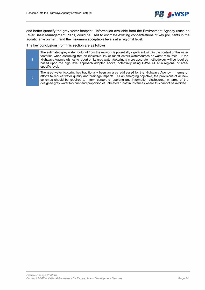
Research into the Highways Agency’s Water Footprint
Climate Change Portfolio Contract 3/387 – National Framework for Research and Development Services Page 34
and better quantify the grey water footprint. Information available from the Environment Agency (such as River Basin Management Plans) could be used to estimate existing concentrations of key pollutants in the aquatic environment, and the maximum acceptable levels at a regional level.
The key conclusions from this section are as follows:
1
The estimated grey water footprint from the network is potentially significant wirthin the context of the water footprint, when assuming that an indicative 1% of runoff enters watercourses or water resources. If the Highways Agency wishes to report on its grey water footprint, a more accurate methodology will be required based upon the high level approach adopted above, potentially using HAWRAT at a regional or area-specific level.
2 The grey water footprint has traditionally been an area addressed by the Highways Agency, in terms of efforts to reduce water quality and drainage impacts. As an emerging objective, the provisions of all new schemes should be required to inform corporate reporting and information disclosures, in terms of the designed grey water footprint and proportion of untreated runoff in instances where this cannot be avoided.
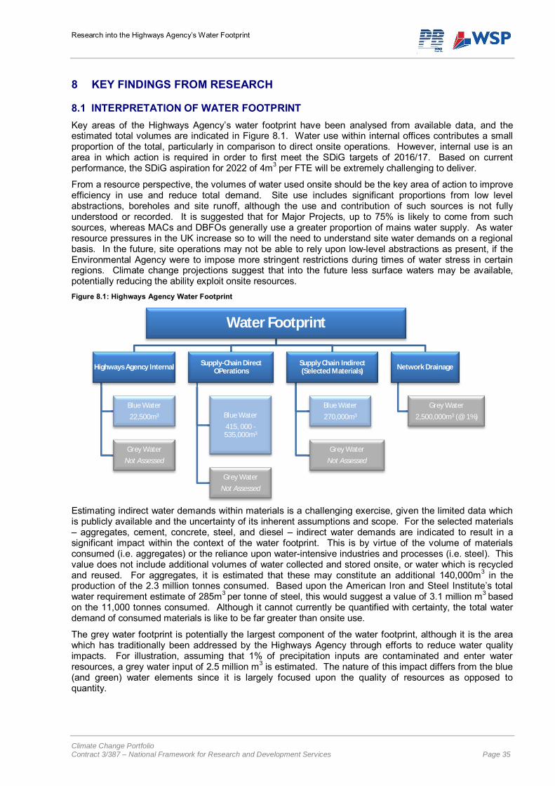
Research into the Highways Agency’s Water Footprint
Climate Change Portfolio Contract 3/387 – National Framework for Research and Development Services Page 35
8 KEY FINDINGS FROM RESEARCH
8.1 INTERPRETATION OF WATER FOOTPRINT Key areas of the Highways Agency’s water footprint have been analysed from available data, and the estimated total volumes are indicated in Figure 8.1. Water use within internal offices contributes a small proportion of the total, particularly in comparison to direct onsite operations. However, internal use is an area in which action is required in order to first meet the SDiG targets of 2016/17. Based on current performance, the SDiG aspiration for 2022 of 4m3 per FTE will be extremely challenging to deliver.
From a resource perspective, the volumes of water used onsite should be the key area of action to improve efficiency in use and reduce total demand. Site use includes significant proportions from low level abstractions, boreholes and site runoff, although the use and contribution of such sources is not fully understood or recorded. It is suggested that for Major Projects, up to 75% is likely to come from such sources, whereas MACs and DBFOs generally use a greater proportion of mains water supply. As water resource pressures in the UK increase so to will the need to understand site water demands on a regional basis. In the future, site operations may not be able to rely upon low-level abstractions as present, if the Environmental Agency were to impose more stringent restrictions during times of water stress in certain regions. Climate change projections suggest that into the future less surface waters may be available, potentially reducing the ability exploit onsite resources. Figure 8.1: Highways Agency Water Footprint
Estimating indirect water demands within materials is a challenging exercise, given the limited data which is publicly available and the uncertainty of its inherent assumptions and scope. For the selected materials – aggregates, cement, concrete, steel, and diesel – indirect water demands are indicated to result in a significant impact within the context of the water footprint. This is by virtue of the volume of materials consumed (i.e. aggregates) or the reliance upon water-intensive industries and processes (i.e. steel). This value does not include additional volumes of water collected and stored onsite, or water which is recycled and reused. For aggregates, it is estimated that these may constitute an additional 140,000m3 in the production of the 2.3 million tonnes consumed. Based upon the American Iron and Steel Institute’s total water requirement estimate of 285m3 per tonne of steel, this would suggest a value of 3.1 million m3 based on the 11,000 tonnes consumed. Although it cannot currently be quantified with certainty, the total water demand of consumed materials is like to be far greater than onsite use.
The grey water footprint is potentially the largest component of the water footprint, although it is the area which has traditionally been addressed by the Highways Agency through efforts to reduce water quality impacts. For illustration, assuming that 1% of precipitation inputs are contaminated and enter water resources, a grey water input of 2.5 million m3 is estimated. The nature of this impact differs from the blue (and green) water elements since it is largely focused upon the quality of resources as opposed to quantity.
Water Footprint
Highways Agency Internal
Blue Water
22,500m3
Grey Water
Not Assessed
Supply-Chain Direct OPerations
Blue Water
415, 000 -535,000m3
Grey Water
Not Assessed
Supply Chain Indirect (Selected Materials)
Blue Water
270,000m3
Grey Water
Not Assessed
Network Drainage
Grey Water
2,500,000m3 (@ 1%)
Research into the Highways Agency’s Water Footprint
Climate Change Portfolio Contract 3/387 – National Framework for Research and Development Services Page 36
8.2 CONCLUSIONS & FUTURE OF WATER FOOTPRINTING “UK industry must show leadership on global water security. Through their global reach, businesses must examine their supply chains and production processes to assess and reduce their water footprint. This should be a core component of their corporate and social responsibility strategies”
Engineering the Future (2010) Global Water Security – An Engineering Perspective
The above quote is taken from a report published in April 2010, which recommends that industry should act upon water issues and take a position of leadership. Alongside carbon, water is likely to become a core component of the corporate responsibility agenda, and there will be increasing pressure for information disclosure. The water footprint concept provides the Highways Agency with an alternative perspective on water use, as it draws together different types of water pressure and impact under one heading and, much like the carbon footprint, it provides a unified agenda.
From the analysis within this Report, if water impact is being measured in terms of the volume of consumption the objective is to reduce total demand. As such, targets to reduce direct use in offices and supply-chain operations will address part of the issue, but significant volumes of water could also be saved, potentially more cost-effectively, through a focus on resource efficiency and lean construction. For example, achieving a nominal 5% reduction in virgin aggregate consumption may yield an indirect water saving or avoidance volume of 4,500m3. For the Highways Agency offices, assuming an annual reduction of 515m3 per year in line with the 2016/17 SDiG target, this would take eight years to achieve.
As with the Highways Agency’s carbon footprint, the indirect component within materials will be a significant contributor. There is clear merit is addressing indirect water demands within materials, but it is recommended that the Highways Agency views this as a strategic objective. Indirect water demands can be reduced immediately through resource efficiency, but whilst water footprinting remains in its infancy the ability to accurately measure and monitor remains limited. In the time it evolves, the Highways Agency has the opportunity to focus upon developing the systems and procedures to measure and manage direct water use, to develop its corporate position, and to engage the supply-chain. A key theme of the findings for each section is the need for a robust dataset and water management procedures, both internally and from within the supply-chain.

Research into the Highways Agency’s Water Footprint
Climate Change Portfolio Contract 3/387 – National Framework for Research and Development Services Page 37
Research into the Highways Agency’s Water Footprint
Climate Change Portfolio Contract 3/387 – National Framework for Research and Development Services Page 38
9 REFERENCES
Argonne National Laboratory (2009). Consumptive Water Use in the Production of Ethanol and Petroleum Gasoline. Illinois, USA.
Arnell, N. (1998) Climate Change and Water Resources in Britain. Climate Change Volume 39, Number 1 / May, 1998.
Barton, B. (2010) Murky Waters? Corporate Reporting on Water Risk – Benchmarking Study of 100 Companies. Boston, USA.
British Geological Survey (2010). European Mineral Statistics. Keyworth, Nottingham.
British Precast (2009). Sustainability Matters: Forth Annual Report on the Precast Industry’s Progress on Sustainability. Leicester, UK.
CH2MHill, 2003, Water Use in Industries of the Future, Report prepared for U.S. Department of Energy.
Ellis, M., Dillich, S. & Margolis, N. (2001). Industrial Water Use and Its Energy Implications. Energetics, USA.
EMEP/EEA (2009). Air Pollutant Emission Inventory Guidebook — Technical report No 6/2009.
Engineering the Future (2010) Global Water Security – An Engineering Perspective. The Royal Academy of Engineering, London.
Environment Agency (2008). Water Resources in England and Wales – Current State and Future Pressures. Bristol, UK.
European Environment Agency (EEA) (2004) Impacts of Europe’s changing climate: an indicator-based assessment. EEA Report No 2/2004, EEA, Copenhagen, Denmark, 107 pp.
HM Government (2008). Future Water – The Government’s Water Strategy for England. London.
Hoekstra, A.Y. (2010) The Relation between International Trade and Freshwater Scarcity. World Trade Organisation Working Paper, Geneva.
Hoekstra, A.Y. & Chapagain, A.K. (2008). Globalization of Water: Sharing the Planet’s Freshwater Resources. Blackwell Publishing, Singapore.
International Water Management Institute (2006). Insights from the Comprehensive Assessment of Water Management in Agriculture. Colombo, Sri Lanka
Jenkins, G.J., Murphy, J.M., Sexton, D.S., Lowe, J.A., Jones, P. and Kilsby, C.G. (2009). UK Climate Projections: Briefing Report. Met Office Hadley Centre, Exeter, UK.
JPMorgan (2008). Watching Water: A Guide to Evaluating Corporate Risks in a Thirsty World. New York.
Katsofis, S. (2009). Cradle-to-Gate Water Footprint Analysis of Borealis Group Polyolefin Value Chain. Stockholm, Sweden.
Mineral Products Association (2009). The UK Cement Industry. Surrey, UK.
Sustainable Development Commission (2008). Sustainable Development in Government – Challenges for Government. London, UK.
The Concrete Centre (2009). The Concrete Industry Sustainability Report – 1st Report. Surrey, UK.
WWF (2008). UK Water Footprint: The Impact of the UK’s Food and Fibre Consumption on Global Water Resources – Volume 1. Godalming, UK.
CIRIA (2006). Key Performance Indicators for Water Use in Offices. London, UK.
Research into the Highways Agency’s Water Footprint
Climate Change Portfolio Contract 3/387 – National Framework for Research and Development Services Page 39
Buzzi Unichem (2007). Cement Environmental Declaration – Environmental Product Declaration. Italy.
The Concrete Centre (2010) Concrete Credentials: Sustainability. Camberley, Surrey.
United Nations (2002). Global Environmental Outlook 3. Nairobi, Kenya.
United Nations (2009) World Water Development Report: Water in a Changing World (3rd Report).
United Nations Environment Programme (UNEP) (2007) Climate Change 2007: Fourth Assessment Report - Synthesis Report. Intergovernmental Panel on Climate Change.
UNEP and World Meteorological Organization (WMO) (2008) Climate Change and Water.
World Coal Institute (2007). Coal & Steel. Richmond, UK.
World Bank Group (1998) Petroleum Refining. Pollution Prevention and Abatement Handbook. World Bank Group.
Wu, M. Mintz, M. Wang, M. & Arora, S. (2009). Water Consumption in the Production of Ethanol and Petroleum Gasoline. Environmental Management, 44(5), 981-997.

APPENDIX A – GLOBAL WATER TRENDS
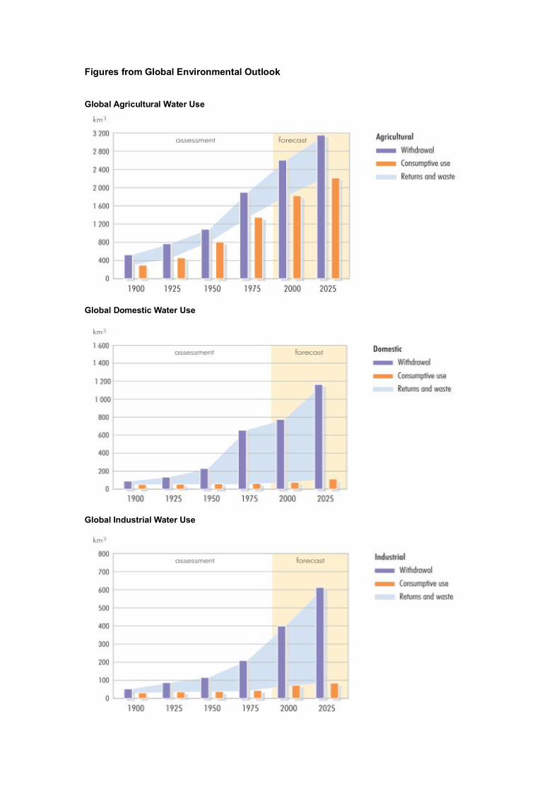
Figures from Global Environmental Outlook
Global Agricultural Water Use
Global Domestic Water Use
Global Industrial Water Use
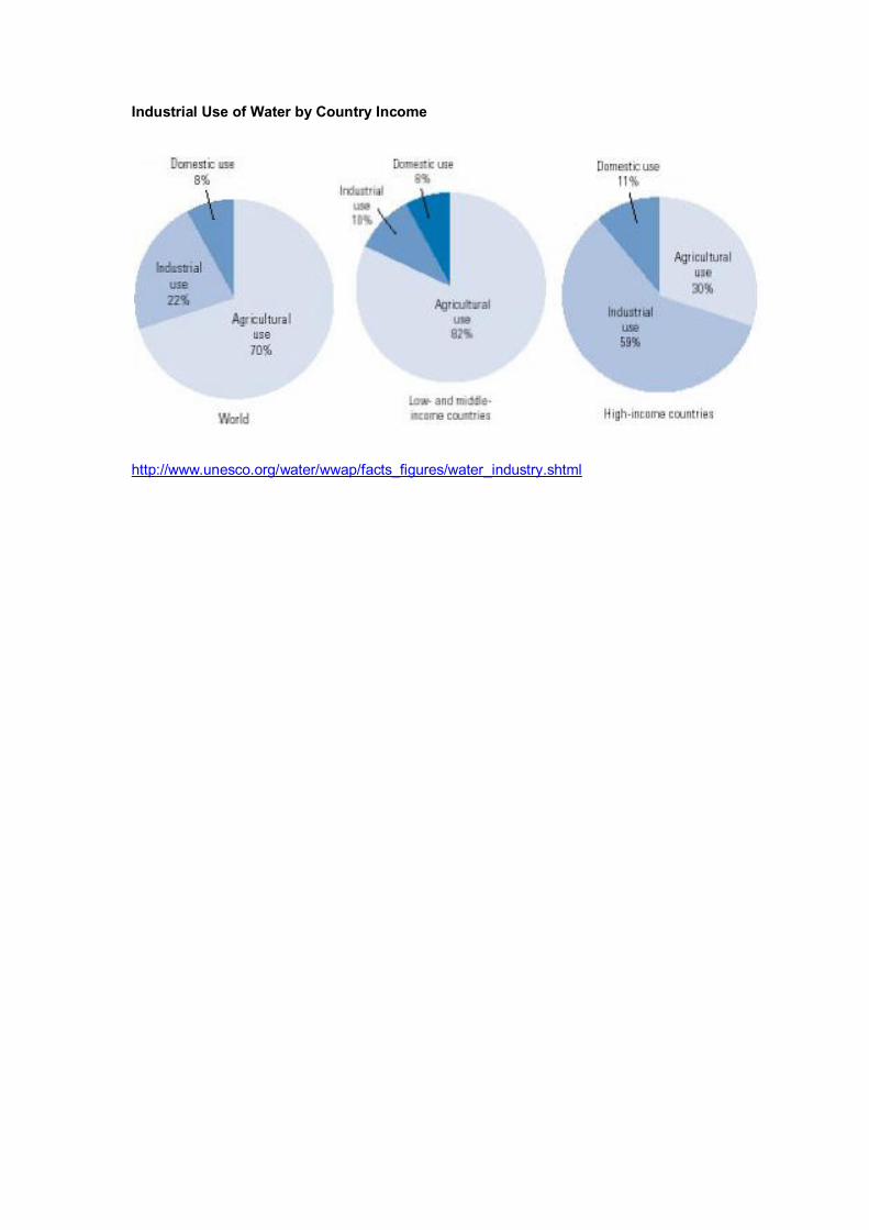
Industrial Use of Water by Country Income
http://www.unesco.org/water/wwap/facts_figures/water_industry.shtml

APPENDIX B – UK WATER TRENDS
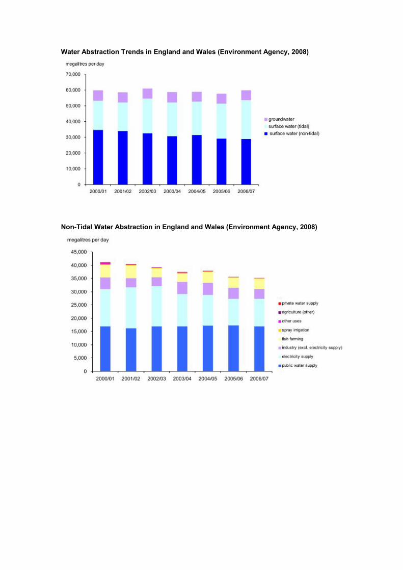
Water Abstraction Trends in England and Wales (Environment Agency, 2008)
Non-Tidal Water Abstraction in England and Wales (Environment Agency, 2008)
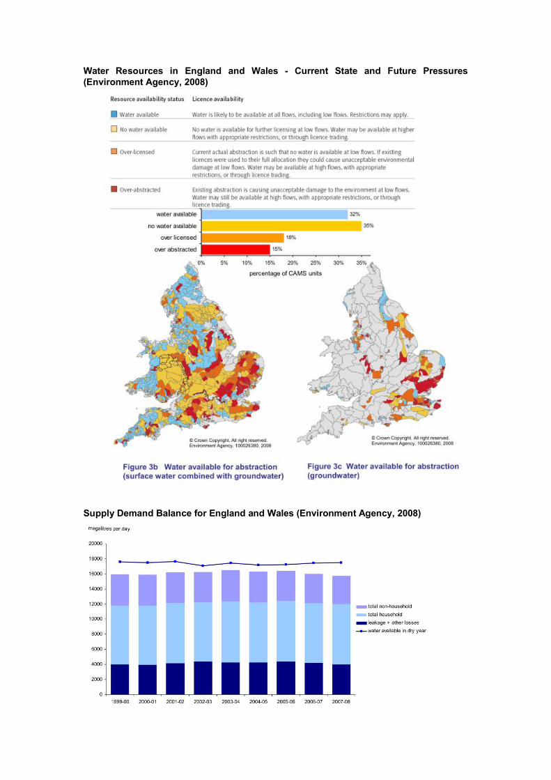
Water Resources in England and Wales - Current State and Future Pressures (Environment Agency, 2008)
Supply Demand Balance for England and Wales (Environment Agency, 2008)

APPENDIX C – WATER & CLIMATE CHANGE IMPACTS
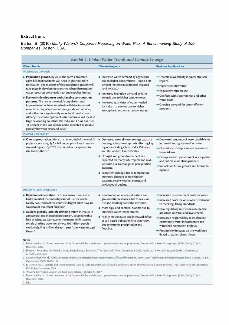
Extract from:
Barton, B. (2010) Murky Waters? Corporate Reporting on Water Risk, A Benchmarking Study of 100 Companies. Boston, USA.

APPENDIX D – UKCIP PROJECTIONS
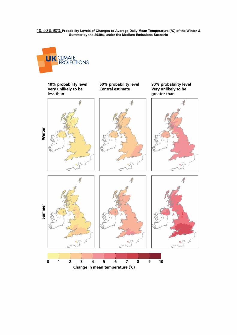
10, 50 & 90% Probability Levels of Changes to Average Daily Mean Temperature (ºC) of the Winter & Summer by the 2080s, under the Medium Emissions Scenario
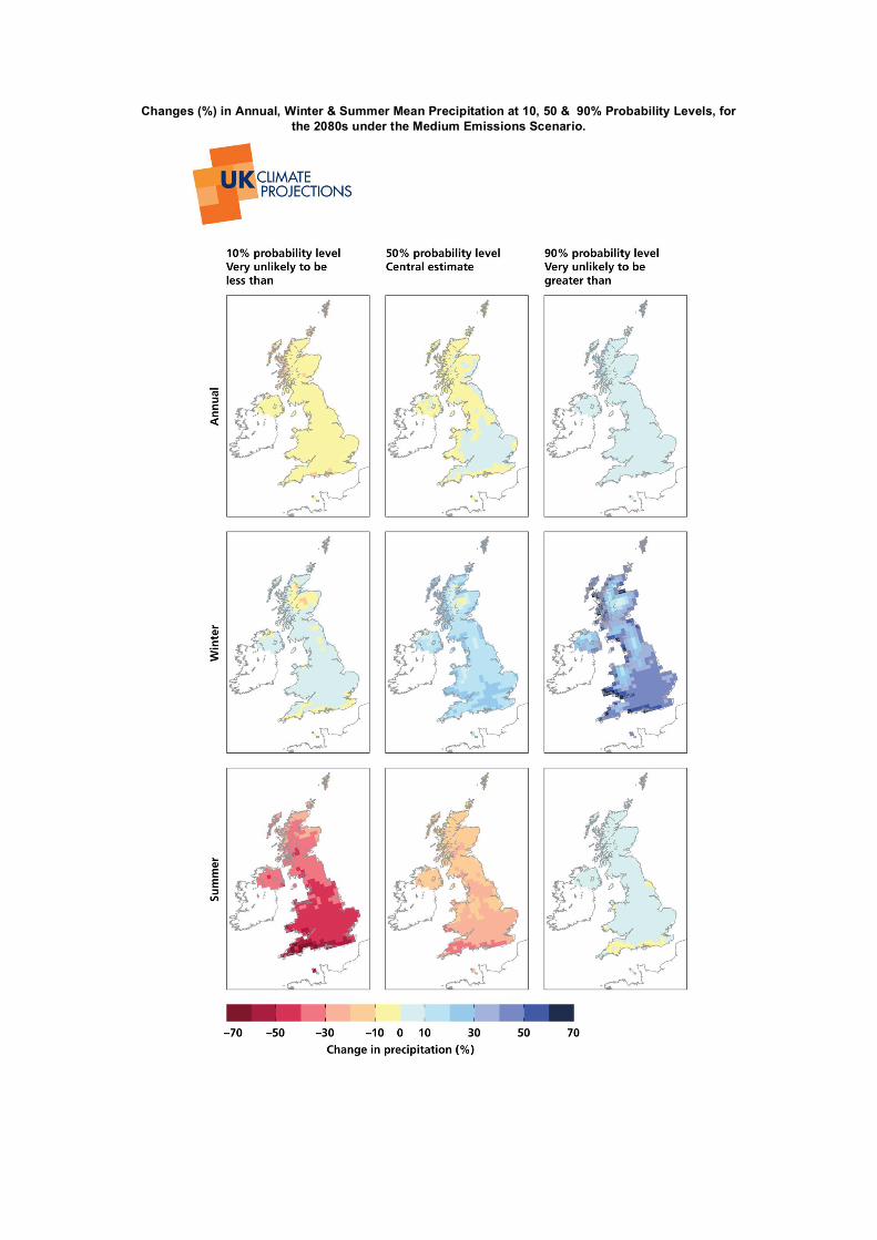
Changes (%) in Annual, Winter & Summer Mean Precipitation at 10, 50 & 90% Probability Levels, for the 2080s under the Medium Emissions Scenario.
APPENDIX E – HIGHWAYS AGENCY OFFICE CONSUMPTION
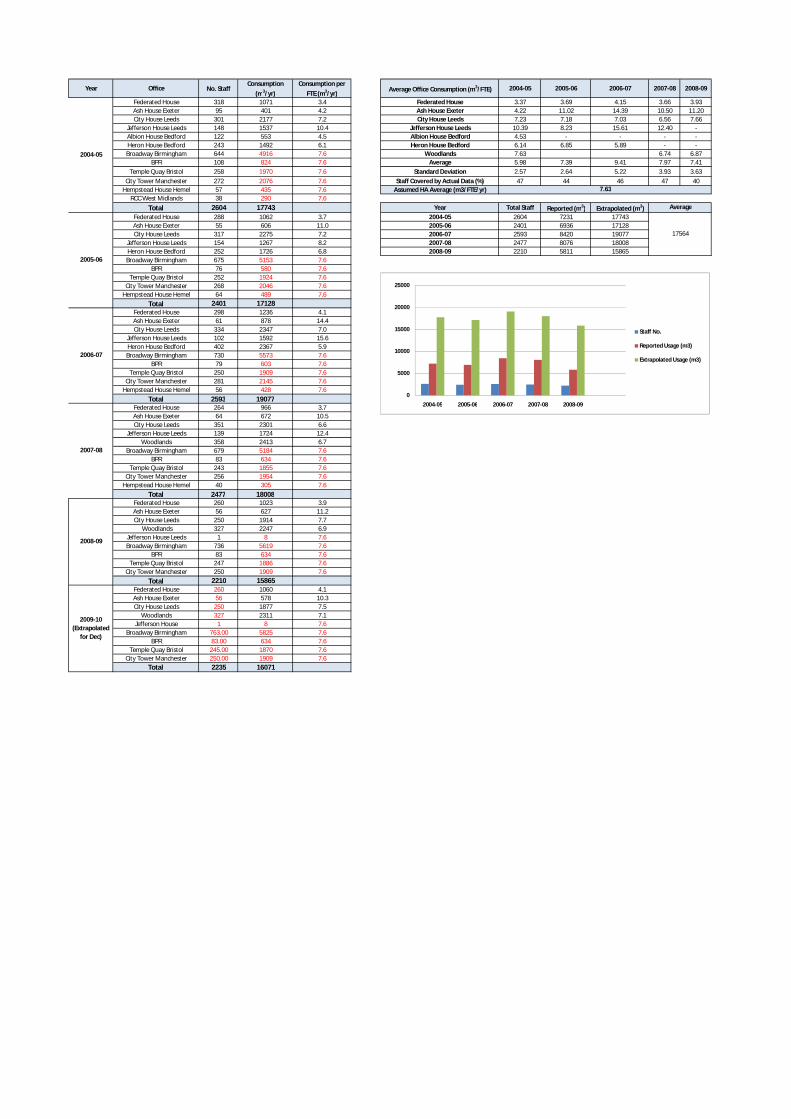
Year Office No. StaffConsumption
(m3/yr)
Consumption per
FTE (m3/yr)Average Office Consumption (m3/FTE) 2004-05 2005-06 2006-07 2007-08 2008-09
Federated House 318 1071 3.4 Federated House 3.37 3.69 4.15 3.66 3.93Ash House Exeter 95 401 4.2 Ash House Exeter 4.22 11.02 14.39 10.50 11.20City House Leeds 301 2177 7.2 City House Leeds 7.23 7.18 7.03 6.56 7.66
Jefferson House Leeds 148 1537 10.4 Jefferson House Leeds 10.39 8.23 15.61 12.40 -Albion House Bedford 122 553 4.5 Albion House Bedford 4.53 - - - -Heron House Bedford 243 1492 6.1 Heron House Bedford 6.14 6.85 5.89 - -Broadway Birmingham 644 4916 7.6 Woodlands 7.63 6.74 6.87
BPR 108 824 7.6 Average 5.98 7.39 9.41 7.97 7.41Temple Quay Bristol 258 1970 7.6 Standard Deviation 2.57 2.64 5.22 3.93 3.63
City Tower Manchester 272 2076 7.6 Staff Covered by Actual Data (%) 47 44 46 47 40Hempstead House Hemel 57 435 7.6 Assumed HA Average (m3/FTE/yr)
RCC West Midlands 38 290 7.6
Total 2604 17743 Year Total Staff Reported (m3) Extrapolated (m3)Federated House 288 1062 3.7 2004-05 2604 7231 17743Ash House Exeter 55 606 11.0 2005-06 2401 6936 17128City House Leeds 317 2275 7.2 2006-07 2593 8420 19077
Jefferson House Leeds 154 1267 8.2 2007-08 2477 8076 18008Heron House Bedford 252 1726 6.8 2008-09 2210 5811 15865Broadway Birmingham 675 5153 7.6
BPR 76 580 7.6Temple Quay Bristol 252 1924 7.6
City Tower Manchester 268 2046 7.6Hempstead House Hemel 64 489 7.6
Total 2401 17128Federated House 298 1236 4.1Ash House Exeter 61 878 14.4City House Leeds 334 2347 7.0
Jefferson House Leeds 102 1592 15.6Heron House Bedford 402 2367 5.9Broadway Birmingham 730 5573 7.6
BPR 79 603 7.6Temple Quay Bristol 250 1909 7.6
City Tower Manchester 281 2145 7.6Hempstead House Hemel 56 428 7.6
Total 2593 19077Federated House 264 966 3.7Ash House Exeter 64 672 10.5City House Leeds 351 2301 6.6
Jefferson House Leeds 139 1724 12.4Woodlands 358 2413 6.7
Broadway Birmingham 679 5184 7.6BPR 83 634 7.6
Temple Quay Bristol 243 1855 7.6City Tower Manchester 256 1954 7.6
Hempstead House Hemel 40 305 7.6
Total 2477 18008Federated House 260 1023 3.9Ash House Exeter 56 627 11.2City House Leeds 250 1914 7.7
Woodlands 327 2247 6.9Jefferson House Leeds 1 8 7.6Broadway Birmingham 736 5619 7.6
BPR 83 634 7.6Temple Quay Bristol 247 1886 7.6
City Tower Manchester 250 1909 7.6
Total 2210 15865Federated House 260 1060 4.1Ash House Exeter 56 578 10.3City House Leeds 250 1877 7.5
Woodlands 327 2311 7.1Jefferson House 1 8 7.6
Broadway Birmingham 763.00 5825 7.6BPR 83.00 634 7.6
Temple Quay Bristol 245.00 1870 7.6City Tower Manchester 250.00 1909 7.6
Total 2235 16071
2009-10 (Extrapolated
for Dec)
7.63
2008-09
2007-08
2004-05
2005-06
2006-07
17564
Average
0
5000
10000
15000
20000
25000
2004-05 2005-06 2006-07 2007-08 2008-09
Staff No.
Reported Usage (m3)
Extrapolated Usage (m3)

APPENDIX F – SITE WATER USE INFORMATION
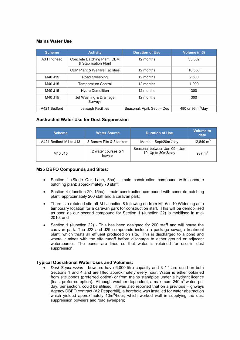
Mains Water Use
Scheme Activity Duration of Use Volume (m3)
A3 Hindhead Concrete Batching Plant, CBM & Stabilisation Plant
12 months 35,562
CBM Plant & Welfare Facilities 12 months 10,558
M40 J15 Road Sweeping 12 months 2,500
M40 J15 Temperature Control 12 months 1,000
M40 J15 Hydro Demolition 12 months 300
M40 J15 Jet Washing & Drainage Surveys
12 months 300
A421 Bedford Jetwash Facilities Seasonal: April, Sept – Dec 480 or 96 m3/day
Abstracted Water Use for Dust Suppression
Scheme Water Source Duration of Use Volume to date
A421 Bedford M1 to J13 3 Borrow Pits & 3 tankers March – Sept:20m3/day 12,840 m3
M40 J15 2 water courses & 1 bowser
Seasonal between Jan 09 – Jan 10: Up to 30m3/day
987 m3
M25 DBFO Compounds and Sites:
Section 1 (Slade Oak Lane, 5ha) – main construction compound with concrete batching plant; approximately 70 staff;
Section 4 (Junction 29, 15ha) – main construction compound with concrete batching plant; approximately 200 staff and a caravan park;
There is a retained site off M1 Junction 8 following on from M1 6a -10 Widening as a temporary location for a caravan park for construction staff. This will be demobilised as soon as our second compound for Section 1 (Junction 22) is mobilised in mid-2010; and
Section 1 (Junction 22) - This has been designed for 200 staff and will house the caravan park. The J22 and J29 compounds include a package sewage treatment plant, which treats all effluent produced on site. This is discharged to a pond and where it mixes with the site runoff before discharge to either ground or adjacent watercourse. The ponds are lined so that water is retained for use in dust suppression.
Typical Operational Water Uses and Volumes: Dust Suppression - bowsers have 6,000 litre capacity and 3 / 4 are used on both
Sections 1 and 4 and are filled approximately every hour. Water is either obtained from site ponds (preferred option) or from mains standpipe under a hydrant licence (least preferred option). Although weather dependent, a maximum 240m3 water, per day, per section, could be utilised. It was also reported that on a previous Highways Agency DBFO contract (A2 Pepperhill), a borehole was installed for water abstraction which yielded approximately 10m3/hour, which worked well in supplying the dust suppression bowsers and road sweepers;

Road Sweeping – road sweepers are used for cleaning mud from the roads close to earthworks activities and for cleaning the road surface in advance of laying pavement. These normally have a capacity of 3 - 5m3. Consumption depends on weather conditions and site activities, and a scheme may have up to 12 sweepers on site at any one time. Sweepers are filled using either a hydrant source or water from the metered supply in the compound. A rough estimate of consumption is approximately 25m3 per sweeper per day, a maximum of 300m3 per day.
Wheel Washes – located at the main exits from earthwork areas onto the motorway / public roads. These are relatively self contained and recirculate water, so are only cleaned out and topped up as required.
Hydrodemolition – used to assist modification of structures. This technique uses approximately 1m3/hour/team. The most intensive use of hydro-demolition was for a viaduct structure which used 3 teams over a 2 month period for each side of the structure;
Temperature Control – small quantities of water are used for cooling of drilling and sawing equipment, although this will amount to a reasonable quantity over the course of the project. Water consumption volumes were not available;
Other – Piling and directional drilling use water mixed with a polymer as a drilling fluid. Drainage works require the drainage network to be jetted to clean out the pipe work. Landscape works includes hydro-seeding of grass / wildflower areas. The ongoing maintenance requires watering to be carried out in dry periods.
APPENDIX G – SUMMARY OF WATER USE IN MATERIAL PRODUCTION
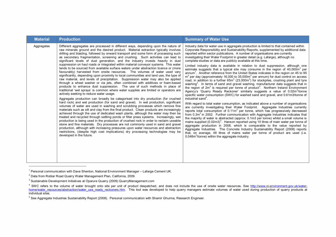
Material Production Summary of Water Use Aggregates Different aggregates are processed in different ways, depending upon the nature of
raw minerals ground and the desired product. Material extraction typically involves drilling and blasting, followed by onward transport and some form of processing such as secondary fragmentation, screening and crushing. Such activities can lead to significant levels of dust generation, and the industry invests heavily in dust suppression on haul roads or integrated within material conveyor systems. This water tends to be sourced from available surface waters under abstraction licence or (more favourably) harvested from onsite resources. The volumes of water used vary significantly, depending upon proximity to local communities and land use, the type of raw material, and levels of precipitation. Suppression water may also be applied through a wheel washer or via jets, often combined with additives or foam-based products to enhance dust suppression. The use of such methods in place of traditional ‘wet sprays’ is common where water supplies are limited or operators are actively seeking to reduce water usage. Aggregate production can broadly be categorised into dry production (for crushed hard rock) and wet production (for sand and gravel). In wet production, significant volumes of water are used in washing and scrubbing processes which remove fine materials such as silt and clay from the final product. Clean products are increasingly achieved through the use of dedicated wash plants, although the water may then be treated and recycled through settling ponds or filter press systems. Increasingly, wet production is being used in the production of crushed rock in order to reclaim useable stone and fine materials. Dry processes are not commonly used in sand and gravel production, although with increasing pressures upon water resources and abstraction restrictions, (despite high cost implications) dry processing technologies may be developed in the future.
Industry data for water use in aggregate production is limited to that contained within Corporate Responsibility and Sustainability Reports, supplemented by additional data reported within sector publications. A number of organisations are currently investigating their Water Footprint in greater detail (e.g. Lafarge), although no complete studies or data are publicly available at this time. Limited industry data is available in relation to dust suppression, although one estimate suggests that a typical site may consume in the region of 40,000m3 per annum1. Another reference from the United States indicates in the region on 45 to 95 m3 per day (approximately 16,000 to 35,000m3 per annum) for dust control on access road, in addition to a further 65m3 (23,000m3) for stockpiles, crushing plant and tyre washing2. In terms of sand and gravel washing, manufacturer data suggests that in the region of 2m3 is required per tonne of product3. Northern Ireland Environment Agency’s ‘Quarry Ready Reckoner’ similarly suggests a value of 0.02m3/tonne specific water consumption (SWC) for washed sand and gravel, and 0.61m3/tonne of industrial sand4. With regard to total water consumption, as indicated above a number of organisations are currently investigating their Water Footprint. Aggregate Industries currently reports total consumption of 0.11m3 per tonne, which has progressively decreased from 0.3m3 in 2002. Further communication with Aggregate Industries indicates that the majority of water is abstracted (approx. 0.1m3 per tonne) whilst a small volume is mains supplied (0.02m3)5. Hanson reported using 10 litres of main water per tonne of aggregate production in 2008, which is comparable to the value reported by Aggregate Industries. The Concrete Industry Sustainability Report (2008) reports that, on average, 48 litres of mains water per tonne of product are used (i.e. 0.048m3/tonne) within the aggregate industry.
1 Personal communication with Dave Shenton, National Environment Manager – Lafarge Cement UK. 2 Data from Roblar Road Quarry Water Management Plan, California, 2009. 3 Sustainable Development Initiatives at Oparure Quarry (2009) QuarryManagement.com 4 SWC refers to the volume of water brought onto site per unit of product despatched, and does not include the use of onsite water resources. See http://www.ni-environment.gov.uk/water-home/water_resources/abstraction/water_use_ready_reckoners.htm. This tool was developed to help quarry managers estimate volumes of water used during production of quarry products at individual sites. 5 See Aggregate Industries Sustainability Report (2008). Personal communication with Shamir Ghurma, Research Engineer.
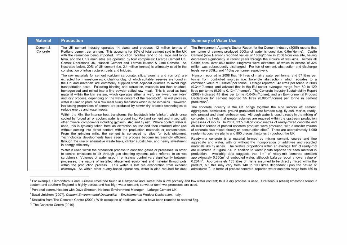
Material Production Summary of Water Use Cement & Concrete
The UK cement industry operates 14 plants and produces 12 million tonnes of Portland cement per annum. This accounts for 90% of total cement sold in the UK with the remainder being imported. Production facilities tend to be large and long-term, and the UK’s main sites are operated by four companies: Lafarge Cement UK, Cemex Operations UK, Hanson Cement and Tarmac Buxton & Lime Cement. As illustrated below, 20% of UK cement (i.e. 2.4 million tonnes) is ultimately used in the construction of infrastructure, roads and bridges. The raw materials for cement (calcium carbonate, silica, alumina and iron ore) are extracted from limestone rock, chalk or clay, of which suitable reserves are found in the UK and materials are commonly supplied from adjacent quarries to avoid high transportation costs. Following blasting and extraction, materials are then crushed, homogenised and milled into a fine powder called raw meal. This is used as feed material within the kiln system, which operates either a ‘wet’, ‘semi-wet’, ‘semi-dry’ and ‘dry’ process, depending on the water content of the feedstock6. In wet process, water is used to produce a raw meal slurry feedstock which is fed into kilns. However, increasing proportions of cement are produced by newer dry process technologies to reduce energy and water inputs. Within the kiln, the intense heat transforms the feedstock into ‘clinker’, which once cooled by forced air or coolant water is ground into Portland cement and mixed with other mineral components including gypsum, slag and fly ash. Where coolant water is used, this is typically taken from an extraction source and then returned after use without coming into direct contact with the production materials or contaminates. From the grinding mills, the cement is conveyed to silos for bulk shipment. Technological developments have seen the process become increasingly efficient, through the use of alternative waste fuels, clinker substitutes, and heavy investment in energy efficiency. Water is used within the production process to condition gases or processes, in order to control emissions to air through gas cleaning systems (also referred to as wet scrubbers). Volumes of water used in emissions control vary significantly between processes, the nature of installed abatement equipment and material throughputs within the production process. This water is lost via evaporation from exhaust chimneys. As within other quarry-based operations, water is also required for dust
The Environment Agency’s Sector Report for the Cement Industry (2005) reports that per tonne of cement produced 600kg of water is used (i.e. 0.6m3/tonne). Castle Cement (now Hanson) reported values of 186kg/tonne in 2006 from one site, having decreased significantly in recent years through the closure of wet-kilns. Across all Castle sites, over 850 million kilograms were extracted, of which in excess of 325 million was subsequently discharged. Per ton of cement, abstraction and discharge levels were 309kg and 116kg per tonne respectively. Hanson reported in 2008 that 19 litres of mains water per tonne, and 67 litres per tonne from controlled sources (i.e. borehole abstraction), which equates to a combined value of 0.086m3 per tonne. Lafarge reported 343 litres per tonne in 2008 (0.34m3/tonne), and advised that in the EU sector averages range from 60 to 120 litres per tonne (0.06 to 0.12m3 / tonne)7. The Concrete Industry Sustainability Report (2008) indicated 45 litres per tonne (0.045m3/tonne), and an Environmental Product Declaration for cement reported 95 litres (0.095m3/tonne) per tonne in cement production8. The concrete industry in the UK brings together the nine sectors of: cement, aggregates, admixtures, ground granulated blast furnace slag, fly ash, mortar, ready-mix, precast and steel reinforcement. Although water is used directly in the mixing of concrete, it is likely that greater volumes are required within the upstream production processes of inputs. In 2007, 23.5 million cubic metres of ready-mixed concrete and 38 million tonnes of precast concrete products were produced, with a smaller volume of concrete also mixed directly on construction sites9. There are approximately 1,000 ready-mix concrete plants and 800 precast factories throughout the UK. Ready-mix concrete is a material formed by mixing cement, coarse and fine aggregate and water, with or without the incorporation of additives and recycled materials like fly ashes. The relative proportions within an average 1m3 of ready-mix are illustrated in Figure 7.4, in addition to water inputs reported for each material in production. Available data suggests that 1m3 of ready-mix concrete contains approximately 0.350m3 of embodied water, although Lafarge report a lower value of 0.284m3. Approximately 165 litres of this is assumed to be directly mixed within the product, but this may vary from 140 to 190 litres dependant upon the nature of admixtures10. In terms of precast concrete, reported water contents range from 150 to
6 For example, Carboniferous and Jurassic limestone found in Derbyshire and Dorset has a low porosity and low water content; thus a dry process is used. Cretaceous (chalk) limestone found in eastern and southern England is highly porous and has high water content; so wet or semi-wet processes are used. 7 Personal communication with Dave Shenton, National Environment Manager – Lafarge Cement UK. 8 Buzzi Unichem (2007). Cement Environmental Declaration – Environmental Product Declaration. Italy. 9 Statistics from The Concrete Centre (2009). With exception of additives, values have been rounded to nearest 5kg. 10 The Concrete Centre (2010).
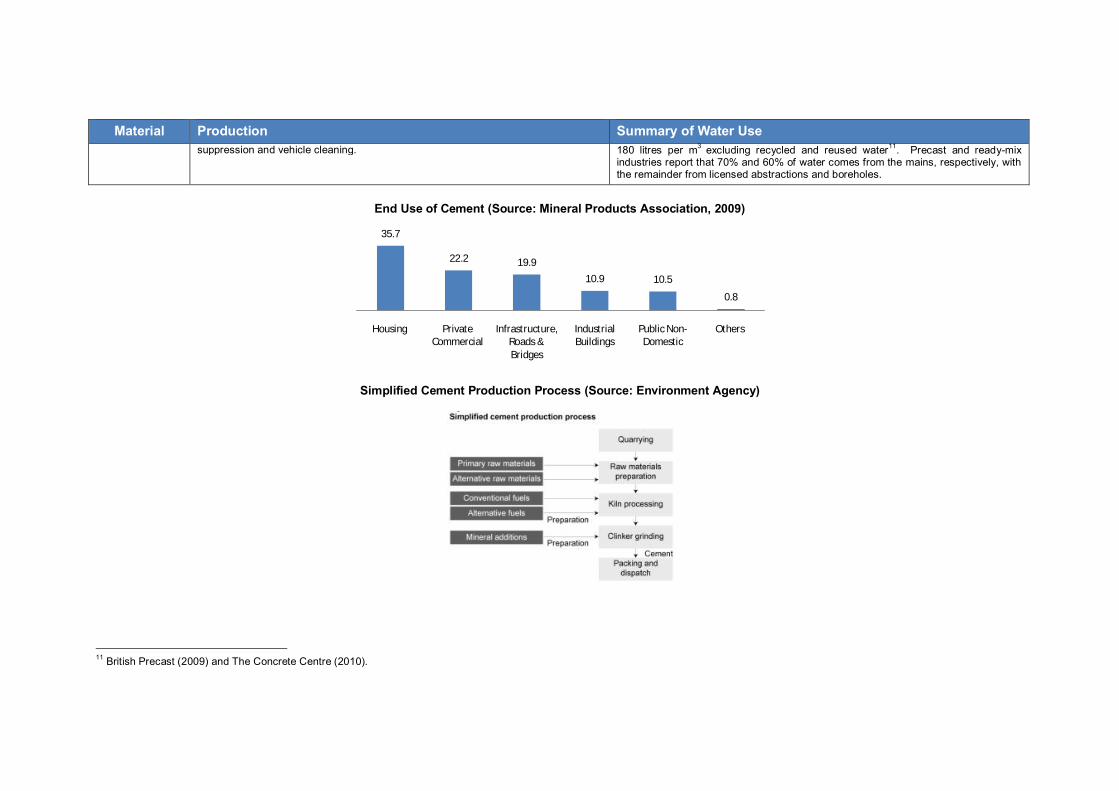
Material Production Summary of Water Use suppression and vehicle cleaning.
180 litres per m3 excluding recycled and reused water11. Precast and ready-mix industries report that 70% and 60% of water comes from the mains, respectively, with the remainder from licensed abstractions and boreholes.
End Use of Cement (Source: Mineral Products Association, 2009)
Simplified Cement Production Process (Source: Environment Agency)
11 British Precast (2009) and The Concrete Centre (2010).
35.7
22.2 19.9
10.9 10.5
0.8
Housing Private Commercial
Infrastructure, Roads & Bridges
Industrial Buildings
Public Non-Domestic
Others
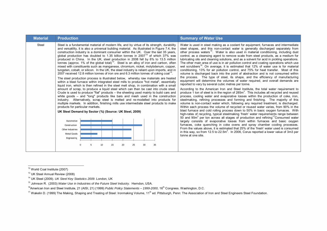
Material Production Summary of Water Use Steel Steel is a fundamental material of modern life, and by virtue of its strength, durability
and versatility, it is also a universal building material. As illustrated in Figure 7.4, the construction industry is a dominant consumer within the UK. Over the last 35 years, global production has doubled to 1.35 billion tonnes in 200712 of which 37% was produced in China. In the UK, steel production in 2008 fell by 6% to 13.5 million tonnes (approx. 1% of the global total)13. Steel is an alloy of iron and carbon, often mixed with constituents such as manganese, chromium, nickel, molybdenum, copper, tungsten, cobalt, or silicon. In the UK, the steel industry is reliant upon imports, and in 2007 received 12.8 million tonnes of iron ore and 6.3 million tonnes of coking coal14. The steel production process is illustrated below, whereby raw materials are heated within a blast furnace within integrated steel mills to produce "hot metal", essentially liquid iron, which is then refined in the steel melt shop, in combination with a small amount of scrap, to produce a liquid steel which can then be cast into crude steel. Crude is used to produce "flat" products – the sheeting used mainly to build cars and white goods – and "long" products like bars and mesh used in the construction industry. Alternatively, scrap steel is melted and re-modelled into products for multiple markets. In addition, finishing mills use intermediate steel products to make products for particular markets. UK Steel Demand by Sector (%) (Source: UK Steel, 2009)
Water is used in steel making as a coolant for equipment, furnaces and intermediate steel shapes, and this non-contact water is generally discharged separately from other process waters15. Water is also used in material conditioning, including dust control, as a cleansing agent to remove scale from steel products, as a medium for lubricating oils and cleaning solutions, and as a solvent for acid in pickling operations. The other main area of use is in air pollution control and coating operations which use wet scrubbers16. On average, it is estimated that 12% of water use is for material conditioning, 13% for air pollution control, and 75% for heat transfer. Most of this volume is discharged back into the point of abstraction and is not consumed within the process. The type of steel, its shape, and the efficiency of manufacturing equipment will determine the volumes of water required, and overall demands are reported to vary by several cubic metres per tonne. According to the American Iron and Steel Institute, the total water requirement to produce 1 ton of steel is in the region of 285m3. This includes all recycled and reused process, cooling water and evaporative losses within the production of coke, iron, steelmaking, refining processes and forming and finishing. The majority of this volume is non-contact water which, following any required treatment, is discharged. Within each process the volume of recycled or reused water varies, from 90% in the blast furnace and cold rolling process down to 50% in basic oxygen furnaces. With high-rates of recycling, typical steelmaking ‘fresh’ water requirements range between 50 and 90m3 per ton across all stages of production and refining17Consumed water largely consists of evaporative losses from within furnaces and basic oxygen furnaces, coke quenching in coke ovens and spray chamber cooling processes. From the values above, it is estimated that 25% of the ‘fresh’ water used is consumed in this way, so from 12.5 to 22.5m3. In 2006, Corus reported a lower value of 3m3 per tonne at one site.
12 World Coal Institute (2007) 13 UK Steel Annual Review (2008) 14 UK Steel (2009). UK Steel Key Statistics 2009. London, UK 15 Johnson R. (2003) Water Use in Industries of the Future Steel Industry. Herndon, USA. 16American Iron and Steel Institute, 21 (AISI, 21) (1999) Public Policy Statements – 1999-2000, 16th Congress. Washington, D.C. 17 Wakelin D. (1999) The Making, Shaping and Treating of Steel: Ironmaking Volume, 11th ed. Pittsburgh, Penn: The Association of Iron and Steel Engineers Steel Foundation.
0 5 10 15 20 25 30 35
Engineering
Metal Goods
Other Industries
Construction
Automotive
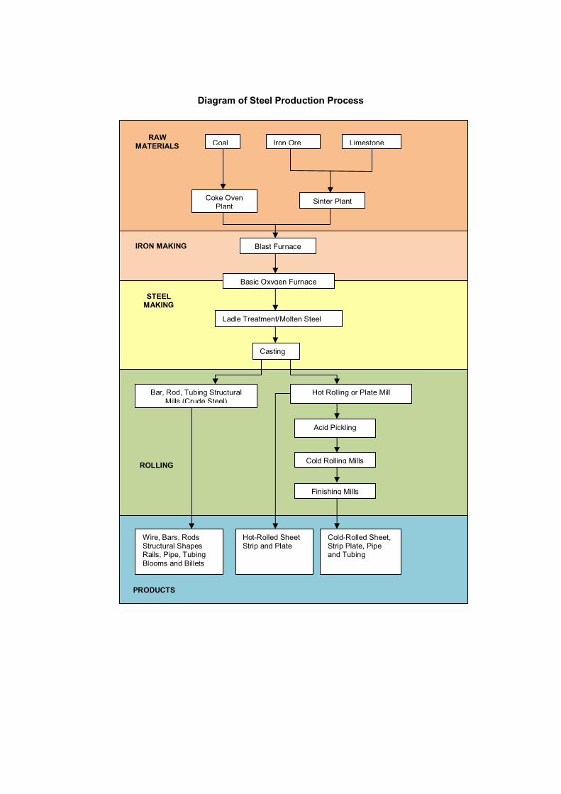
Diagram of Steel Production Process
IRON MAKING
PRODUCTS
STEEL MAKING
ROLLING
RAW MATERIALS
Wire, Bars, Rods Structural Shapes Rails, Pipe, Tubing Blooms and Billets
Hot-Rolled Sheet Strip and Plate
Cold-Rolled Sheet, Strip Plate, Pipe and Tubing
Bar, Rod, Tubing Structural Mills (Crude Steel)
Hot Rolling or Plate Mill
Acid Pickling
Cold Rolling Mills
Finishing Mills
Ladle Treatment/Molten Steel
Casting
Coal
Coke Oven Plant
Iron Ore Limestone
Sinter Plant
Blast Furnace
Basic Oxygen Furnace
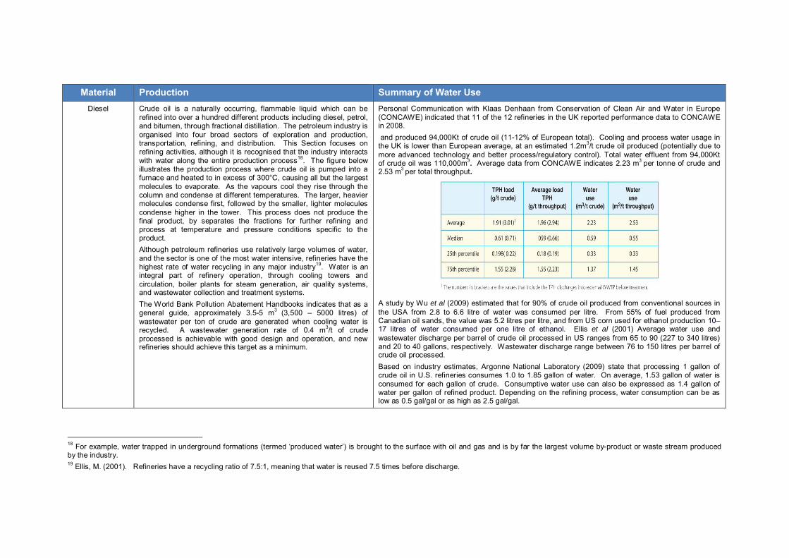
Material Production Summary of Water Use Diesel Crude oil is a naturally occurring, flammable liquid which can be
refined into over a hundred different products including diesel, petrol, and bitumen, through fractional distillation. The petroleum industry is organised into four broad sectors of exploration and production, transportation, refining, and distribution. This Section focuses on refining activities, although it is recognised that the industry interacts with water along the entire production process18. The figure below illustrates the production process where crude oil is pumped into a furnace and heated to in excess of 300°C, causing all but the largest molecules to evaporate. As the vapours cool they rise through the column and condense at different temperatures. The larger, heavier molecules condense first, followed by the smaller, lighter molecules condense higher in the tower. This process does not produce the final product, by separates the fractions for further refining and process at temperature and pressure conditions specific to the product. Although petroleum refineries use relatively large volumes of water, and the sector is one of the most water intensive, refineries have the highest rate of water recycling in any major industry19. Water is an integral part of refinery operation, through cooling towers and circulation, boiler plants for steam generation, air quality systems, and wastewater collection and treatment systems. The World Bank Pollution Abatement Handbooks indicates that as a general guide, approximately 3.5-5 m3 (3,500 – 5000 litres) of wastewater per ton of crude are generated when cooling water is recycled. A wastewater generation rate of 0.4 m3/t of crude processed is achievable with good design and operation, and new refineries should achieve this target as a minimum.
Personal Communication with Klaas Denhaan from Conservation of Clean Air and Water in Europe (CONCAWE) indicated that 11 of the 12 refineries in the UK reported performance data to CONCAWE in 2008. and produced 94,000Kt of crude oil (11-12% of European total). Cooling and process water usage in the UK is lower than European average, at an estimated 1.2m3/t crude oil produced (potentially due to more advanced technology and better process/regulatory control). Total water effluent from 94,000Kt of crude oil was 110,000m3. Average data from CONCAWE indicates 2.23 m3 per tonne of crude and 2.53 m3 per total throughput.
A study by Wu et al (2009) estimated that for 90% of crude oil produced from conventional sources in the USA from 2.8 to 6.6 litre of water was consumed per litre. From 55% of fuel produced from Canadian oil sands, the value was 5.2 litres per litre, and from US corn used for ethanol production 10–17 litres of water consumed per one litre of ethanol. Ellis et al (2001) Average water use and wastewater discharge per barrel of crude oil processed in US ranges from 65 to 90 (227 to 340 litres) and 20 to 40 gallons, respectively. Wastewater discharge range between 76 to 150 litres per barrel of crude oil processed. Based on industry estimates, Argonne National Laboratory (2009) state that processing 1 gallon of crude oil in U.S. refineries consumes 1.0 to 1.85 gallon of water. On average, 1.53 gallon of water is consumed for each gallon of crude. Consumptive water use can also be expressed as 1.4 gallon of water per gallon of refined product. Depending on the refining process, water consumption can be as low as 0.5 gal/gal or as high as 2.5 gal/gal.
18 For example, water trapped in underground formations (termed ‘produced water’) is brought to the surface with oil and gas and is by far the largest volume by-product or waste stream produced by the industry. 19 Ellis, M. (2001). Refineries have a recycling ratio of 7.5:1, meaning that water is reused 7.5 times before discharge.
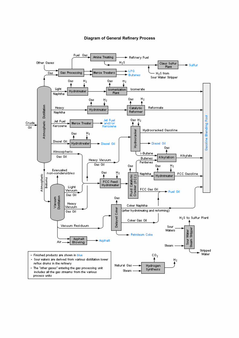
Diagram of General Refinery Process

APPENDIX H – UK MINERAL SELF-SUFFICIENCY & IMPORTS
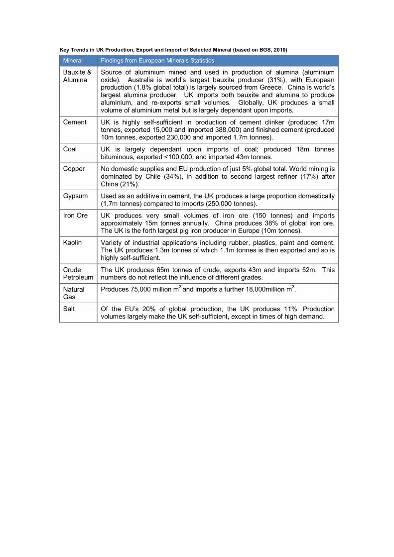
Key Trends in UK Production, Export and Import of Selected Mineral (based on BGS, 2010)
Mineral Findings from European Minerals Statistics
Bauxite & Alumina
Source of aluminium mined and used in production of alumina (aluminium oxide). Australia is world’s largest bauxite producer (31%), with European production (1.8% global total) is largely sourced from Greece. China is world’s largest alumina producer. UK imports both bauxite and alumina to produce aluminium, and re-exports small volumes. Globally, UK produces a small volume of aluminium metal but is largely dependant upon imports.
Cement UK is highly self-sufficient in production of cement clinker (produced 17m tonnes, exported 15,000 and imported 388,000) and finished cement (produced 10m tonnes, exported 230,000 and imported 1.7m tonnes).
Coal UK is largely dependant upon imports of coal; produced 18m tonnes bituminous, exported <100,000, and imported 43m tonnes.
Copper No domestic supplies and EU production of just 5% global total. World mining is dominated by Chile (34%), in addition to second largest refiner (17%) after China (21%).
Gypsum Used as an additive in cement, the UK produces a large proportion domestically (1.7m tonnes) compared to imports (250,000 tonnes).
Iron Ore UK produces very small volumes of iron ore (150 tonnes) and imports approximately 15m tonnes annually. China produces 38% of global iron ore. The UK is the forth largest pig iron producer in Europe (10m tonnes).
Kaolin Variety of industrial applications including rubber, plastics, paint and cement. The UK produces 1.3m tonnes of which 1.1m tonnes is then exported and so is highly self-sufficient.
Crude Petroleum
The UK produces 65m tonnes of crude, exports 43m and imports 52m. This numbers do not reflect the influence of different grades.
Natural Gas
Produces 75,000 million m3 and imports a further 18,000million m3.
Salt Of the EU’s 20% of global production, the UK produces 11%. Production volumes largely make the UK self-sufficient, except in times of high demand.
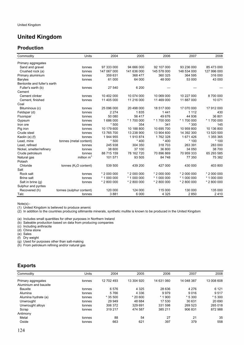
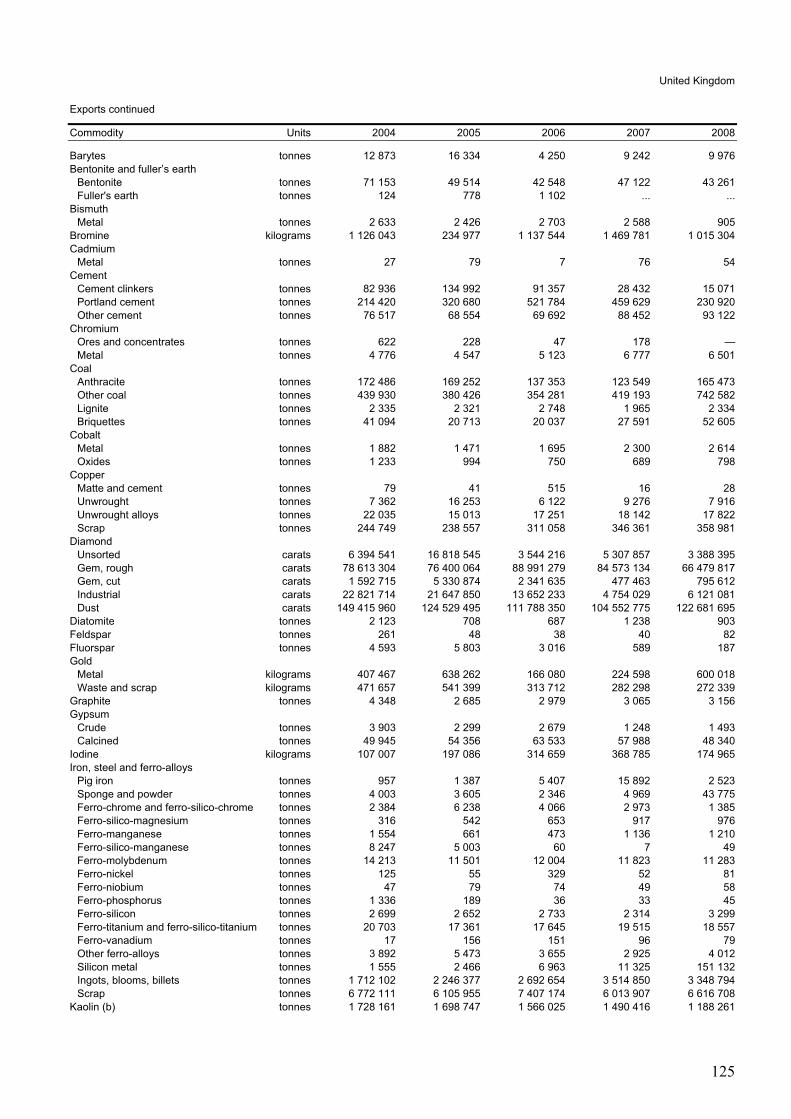

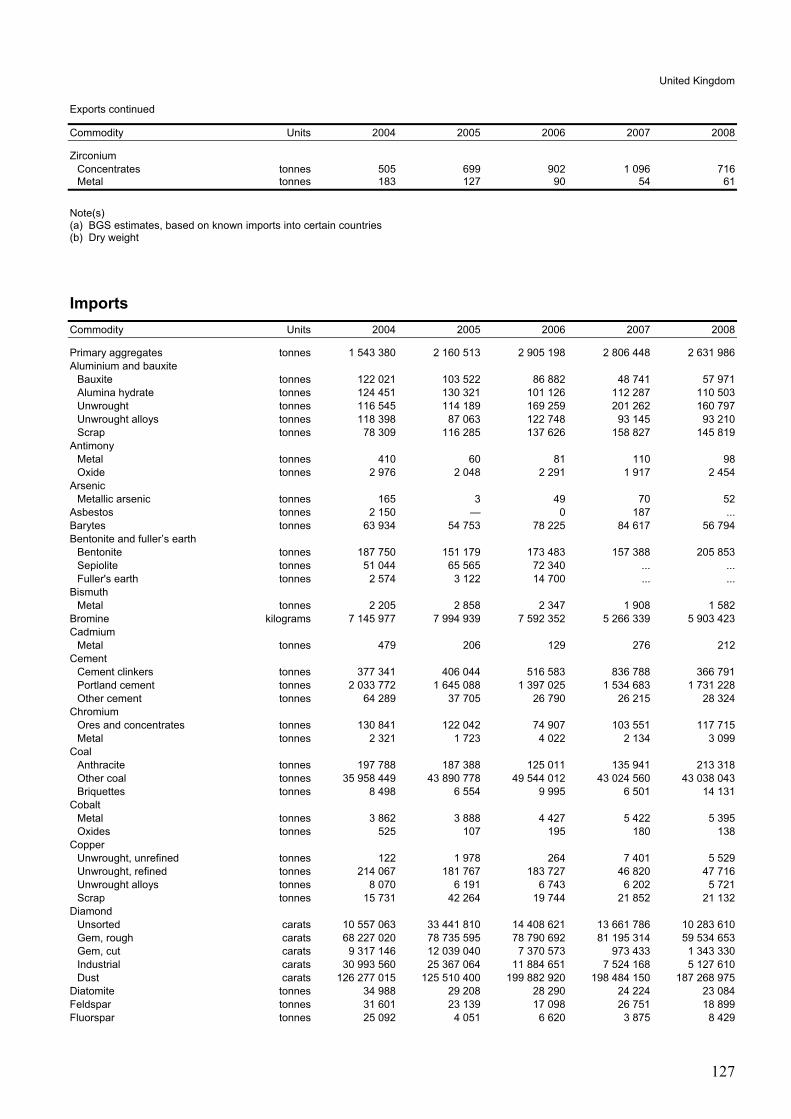
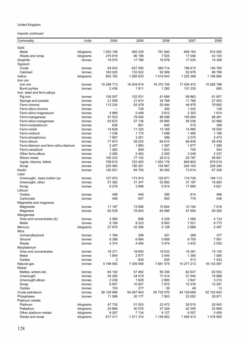
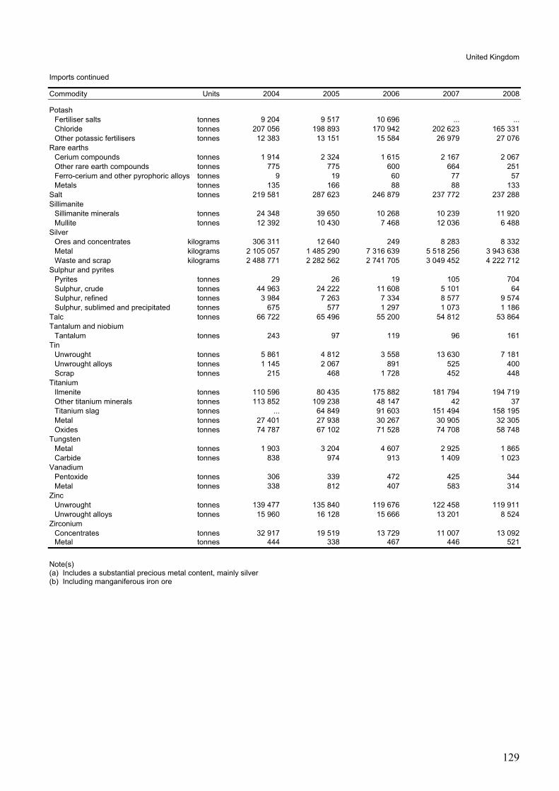

APPENDIX I – GREY WATER INFORMATION
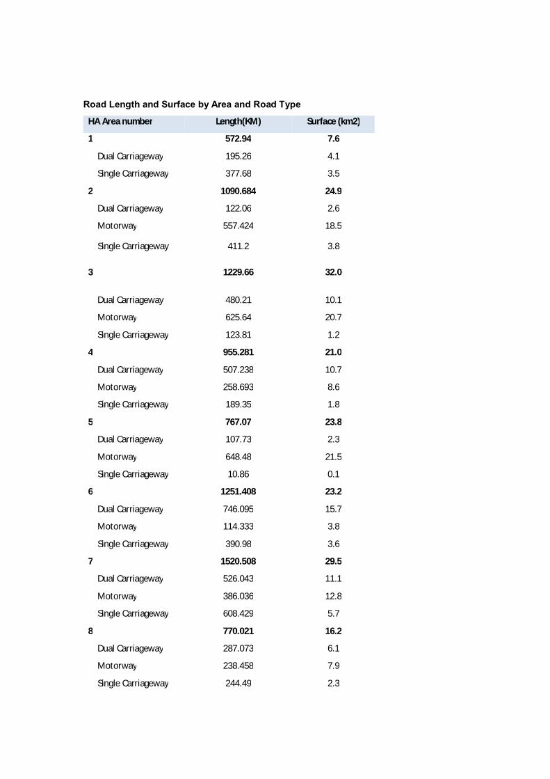
Road Length and Surface by Area and Road Type
HA Area number Length(KM) Surface (km2)
1 572.94 7.6
Dual Carriageway 195.26 4.1
Single Carriageway 377.68 3.5
2 1090.684 24.9
Dual Carriageway 122.06 2.6
Motorway 557.424 18.5
Single Carriageway 411.2 3.8
3 1229.66 32.0
Dual Carriageway 480.21 10.1
Motorway 625.64 20.7
Single Carriageway 123.81 1.2
4 955.281 21.0
Dual Carriageway 507.238 10.7
Motorway 258.693 8.6
Single Carriageway 189.35 1.8
5 767.07 23.8
Dual Carriageway 107.73 2.3
Motorway 648.48 21.5
Single Carriageway 10.86 0.1
6 1251.408 23.2
Dual Carriageway 746.095 15.7
Motorway 114.333 3.8
Single Carriageway 390.98 3.6
7 1520.508 29.5
Dual Carriageway 526.043 11.1
Motorway 386.036 12.8
Single Carriageway 608.429 5.7
8 770.021 16.2
Dual Carriageway 287.073 6.1
Motorway 238.458 7.9
Single Carriageway 244.49 2.3
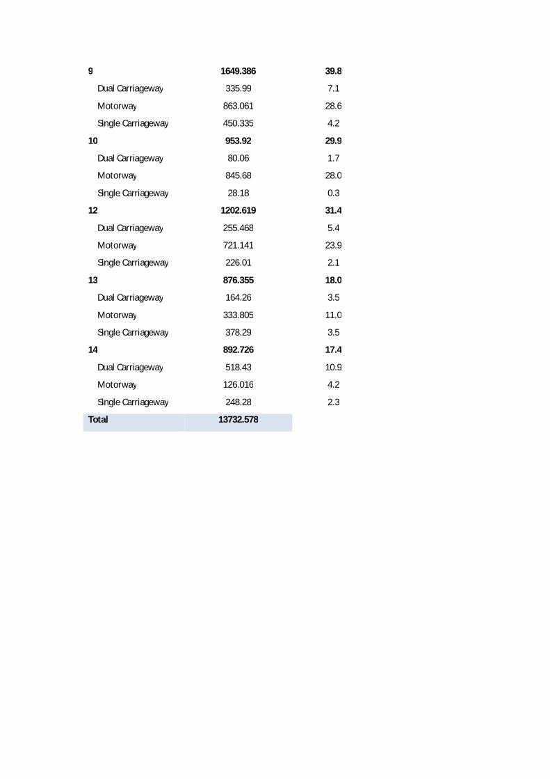
9 1649.386 39.8
Dual Carriageway 335.99 7.1
Motorway 863.061 28.6
Single Carriageway 450.335 4.2
10 953.92 29.9
Dual Carriageway 80.06 1.7
Motorway 845.68 28.0
Single Carriageway 28.18 0.3
12 1202.619 31.4
Dual Carriageway 255.468 5.4
Motorway 721.141 23.9
Single Carriageway 226.01 2.1
13 876.355 18.0
Dual Carriageway 164.26 3.5
Motorway 333.805 11.0
Single Carriageway 378.29 3.5
14 892.726 17.4
Dual Carriageway 518.43 10.9
Motorway 126.016 4.2
Single Carriageway 248.28 2.3
Total 13732.578
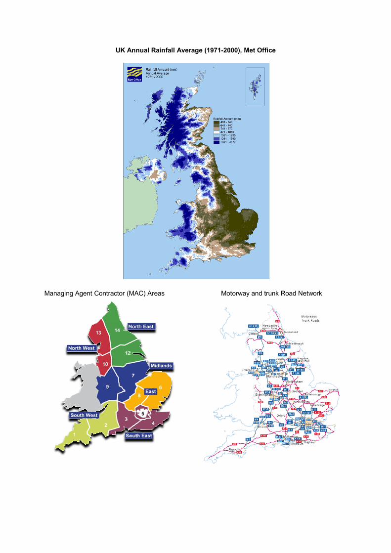
UK Annual Rainfall Average (1971-2000), Met Office
Managing Agent Contractor (MAC) Areas Motorway and trunk Road Network