Embed Size (px)
Citation preview
UNIVERSITY OF HELSINKIDEPARTMENT OF PLANT PRODUCTION
Section of Crop HusbandryPUBLICATION no. 55
CLIMATE CHANGE AND CROP POTENTIAL IN FINLAND:REGIONAL ASSESSMENT OF SPRING WHEAT
Riitta A. Saarikko
Department of Plant ProductionSection of Crop Husbandry
P.O. Box 27FIN-00014 University of Helsinki
Finland
E-mail: [email protected]
ACADEMIC DISSERTATION
To be presented, with the permission of the Faculty of Agriculture and Forestry of theUniversity of Helsinki, for public criticism in Viikki, Auditorium B2,
on 26 November, 1999, at 12 o’clock noon.
HELSINKI 1999
2
Saarikko, R.A. 1999. Climate change and crop potential in Finland: regional assessment
of spring wheat.
Keywords: Triticum aestivum, mapping, crop modelling, upscaling, phenology, thermal
time, photothermal time, climate change scenarios, CERES-Wheat, crop suitability, crop
productivity.
Supervisor: Dr. Timothy R. Carter
Finnish Environment Institute
Helsinki, Finland
Reviewers: Professor Risto Kuittinen
Finnish Geodetic Institute
Kirkkonummi, Finland
Dr. Jouko Kleemola
Kemira-Agro Oy
Espoo, Finland
Opponent: Dr. Ana Iglesias
Dept. Proyectos y Planificacion Rural
E.T.S. Ingenieros Agronomos
Universidad Politecnica
Madrid, Spain
ISBN 951-45-8749-9 (PDF version) Helsingin yliopiston verkkojulkaisut
ISSN 1235-3663
3
CONTENTS
ABSTRACT………………………………………………………………………… 5
LIST OF ORIGINAL PAPERS…………………………………………………… 7
LIST OF ABBREVIATIONS……………………………………………………… 8
1. INTRODUCTION……………………………………………………… ……… 9
1.1. Changing atmospheric composition and climate…………………………. 9
1.2. Climate change impacts on agriculture…………………………………… 10
1.2.1. Research methods and general impact mechanisms………………….. 10
1.2.2. Global implications…………………………………………………… 11
1.2.3. Implications in Finland……………………………………………… . 12
2. OBJECTIVES OF THE STUDY……………………………………………… 14
3. METHODS TO ESTIMATE REGIONAL CROP POTENTIAL…………… 16
3.1. Agroclimatic indices and models………………………………………….. 16
3.2. Different approaches to depict regional patterns………………………… 17
3.3. Methods, data and models………………………………………………… 18
3.3.1. National data base…………………………………………………… 19
3.3.2. Climatological data………………………………………………….. 20
3.3.3. Climate change scenarios…………….……………………………… 20
3.3.4. Models………………….……………………………………………. 22
4. MODELLING CROP PHENOLOGY………………………………………… 23
4.1. Distinction between crop development and growth……………………… 23
4.2. Material and methods……………………………………………………… 24
4.3. Results and discussion……………………………………………………… 26

4
5. CROP THERMAL SUITABILITY…………………………………………… 28
5.1. Methods, models and scenarios…………………………………………… 29
5.1.1. Scenarios of climate change………………………………………….. 30
5.2. Results and discussion…………………………………………………….. 31
5.2.1. Spatial shift in suitability and changes in phase durations…………… 31
5.2.2. Uncertainties in the spatial estimates………………………………… 32
6. UPSCALING A CROP YIELD MODEL TO NATIONAL SCALE………… 34
6.1. Material and methods……………………………………………………… 35
6.1.1. Crop model…………………………………………………………… 35
6.1.2. Data, assumptions and upscaling procedures………………………… 37
6.1.3. Scenarios of climate change…………………………………………… 38
6.2. Results………………………………………………………………………. 39
6.2.1. Model performance at individual locations…………………………… 39
6.2.2. The effects of reduced-form input to the model……………………….. 41
6.2.3. Sensitivity of the model to systematic changes in climate and CO2…… 42
6.2.4. Regional validity of the model under the current climate……………… 42
6.2.5. National yield estimates under variable and changing climate……….. 42
6.3. Discussion…………………………………………………………………… 44
7. CONCLUSIONS………………………………………………………………… 45
8. ACKNOWLEDGEMENTS……………………………………………………. 47
9. REFERENCES………………………………………………………………….. 49
APPENDICES: ORIGINAL PAPERS I-IV

5
ABSTRACT
The present study examines how regional crop potential in Finland may be affected by
possible changes in climate up to the year 2050. Crop potential refers here to two aspects
of crop production: (1) suitability to cultivate a crop and (2) productivity i.e., expectation
of harvestable yield. A regional approach was adopted, since site-based experimental
results and crop model estimates usually fail adequately to describe geographical
variations in crop response. Regional information on crop potential is useful for
agricultural policies concerning e.g., plant breeding, regional agricultural support and
rural development. Here spring wheat was studied as an example crop, but the methods
presented are more generally applicable to other crops and regions.
The first scientific paper describes the geographical analysis system that was developed
and employed. The system included a mapping platform, a geographically referenced
data base, empirical-statistical models and finally, a process-based crop growth model
for wheat (introduced in paper IV). Measures of crop potential were mapped on a regular
10x10 km grid across Finland, although raw data for many attributes (e.g., on current
crop production) were available by different administrative units. Observed climate for
the baseline period 1961-1990 was interpolated to the grid resolution by a kriging
method. Scenarios of climate change were also obtained and either applied directly or
linearly interpolated from global climate model results to the Finnish grid.
Paper II investigated crop phenology using observations from several sites in Finland
during the period 1970-1990. The aim was to select the most appropriate models for
different cultivars of barley, wheat and oats that could be applied in crop zonation and
crop-growth modelling studies. Different mathematical models which relate temperature
to development rate were examined to predict the duration of phenological phases. A
photoperiodic response of plant development before heading was also tested. For all
phases the relationship between temperature and development was approximately linear
and no significant response of plant development to photoperiod was found. This was
explained by consistently long photoperiods in the observational material. Parameters
for a linear model were derived from a regression analysis of mean development rate of
each phase against mean temperature.

6
In the third scientific paper the models developed in paper II were used in conjunction
with indices of growing season length to evaluate the regional thermal suitability for
spring wheat. Thermal suitability was computed using interpolated temperature data for
the baseline period 1961-1990 over the 100 km2 grid. Confidence limits of the
development model were re-interpreted as spatial uncertainties in modelled suitability.
The effects of climatic warming on modelled suitability were investigated by adjusting
the baseline temperatures both systematically and according to climate change scenarios.
The fourth scientific paper describes a method to upscale a site-based crop model to
obtain regional and national estimates of spring wheat productivity under changing
climate. The model, CERES-Wheat, was first calibrated and tested at sites, and second,
yields were computed in the grid and aggregated regionally for comparison to yield
observations in the farm statistics. Finally, the model was run across the grid both for the
baseline climate (1961-1990) and scenarios of future climate and atmospheric CO2
concentrations for 2050. The results indicate that CERES-Wet-Wheat, a modified
version of CERES-Wheat, was able to detect climate-dependent yield variations both at
the site and regional scales, even though the approach did not consider variations in crop
management, pests and diseases and soil dependent differences in initial conditions.
Overall, the results of this study suggest that climatic warming would induce shifts in
the northern limit of spring wheat cultivation of between 160-180 km per each 1 °C
increase in mean annual temperature. The average grain yield of a currently grown
cultivar is estimated to be greater in 2050 than at present over most or all the area of
estimated present-day suitability, and the yearly yield variation is estimated to decrease
markedly. An increasing atmospheric CO2 concentration enhances crop productivity,
while elevated temperatures enhance crop development and tend to reduce the harvested
yield of currently grown crop cultivars. However, without any long term changes in
climate or in cultivation technology, significant multi-decadal variations in mean yield
can occur simply as a result of natural variations in the climate. Such noise in the long-
term climatic record complicates the detection of a greenhouse gas signal, both in the
climate itself and in the response of crop yields.

7
LIST OF ORIGINAL PAPERS
This thesis is based on the following articles, which are referred to by their Roman
numerals
I
Carter, T.R. and Saarikko, R.A. 1996. Estimating regional crop potential under a
changing climate. Agric. For. Met. 79: 301-313.
II
Saarikko, R.A. and Carter, T.R. 1996. Phenological development in spring cereals:
response to temperature and photoperiod under northern conditions. Eur. J. Agron. 5:
59-70.
III
Saarikko, R.A. and Carter, T.R. 1996. Estimating the development and regional
thermal suitability of spring wheat in Finland under climatic warming. Clim. Res. 7:
243-252.
IV
Saarikko, R.A. 1999. Applying a site-based crop model to estimate regional yields
under current and changed climates. (submitted for publication).
In the end of this thesis papers I and II are reprinted with kind permissions from Elsevier
Science. Paper III is reprinted with kind permission from Inter-Reserch.

8
LIST OF ABBREVIATIONS
AERO regional climate change scenario: the first HadCM2 greenhouse
gas and sulphate aerosols simulation approximating the IS92a
emission scenario
CFC chlorofluorocarbon
CH4 methane
CO2 carbon dioxide
cv. cultivar
GCM general circulation model
GFDL Geophysical Fluid Dynamics Laboratory GCM transient climate
change experiment
IPCC Intergovernmental Panel on Climate Change
N2O nitrous oxide
O3 ozone
ppmv parts per million by volume
REF regional climate change scenario: the first HadCM2 simulation
for a greenhouse gas-induced radiative forcing approximating the
IS92a emission scenario
SILMU High national climate change scenario for Finland, high estimate
SILMU Low national climate change scenario for Finland, low estimate
SO2 sulphur dioxide
Tb threshold temperature at which crop development begins (°C)
UKTR the UK Met. Office high resolution GCM transient climate
change experiment

9
1. INTRODUCTION
1.1. Changing atmospheric composition and climate
In the period since industrialisation, and more during recent decades, the Earth’s
atmospheric composition has been changing due to human activities, in particular fossil
fuel combustion, changes in land use and land cover (IPCC, 1996a). Increases have been
measured in the concentration of the so-called greenhouse gases, including carbon
dioxide (CO2), methane (CH4), chlorofluorocarbons (CFCs), and nitrous oxide (N2O), as
well as atmospheric aerosols, especially sulphur compounds. Changes in these
constituents have an effect on the radiative balance of the atmosphere. The greenhouse
gases tend to warm the lower atmosphere by impeding the escape of terrestrial longwave
radiation and re-radiating some back to the surface. In contrast the aerosols have a
counteractive cooling effect both directly, by absorbing incoming solar radiation, and
indirectly by contributing to the formation of clouds which reflect incoming solar
radiation back to space (IPCC, 1996a). Aerosols are likely to continue to affect the
continental-scale patterns of climate change in some regions during the next few
decades. However, they will not completely offset the global long-term warming as their
concentrations are expected to decline during the latter part of the 21st century (IPCC,
1998).
According to the current knowledge changes in atmospheric composition lead to
regional and global changes in temperature, precipitation and other climate variables. On
average, the anticipated rate of global warming has been estimated to be greater than any
other in the past 10 000 years, although the actual annual to decadal rate would include
natural variability and regional changes could differ substantially from the global mean
value. Climate models project that by year 2100 annual global surface temperature will
increase by 1-3.5 °C, precipitation patterns will change both spatially and temporally and
global mean sea level will rise by 15-95 cm (IPCC, 1998). These estimates are based on
a range of sensitivities of climate to changes in greenhouse gas concentrations (IPCC,
1996a) and plausible changes in emissions of the greenhouse gases and aerosols
(emissions scenarios that assume no climate policies, IS92a-f, Leggett et al., 1992).
However, there are still large uncertainties surrounding predictions of future changes.
The potential effects of climate change is a key concern for governments and the

10
environmental science community world-wide. To address this concern, the
Intergovernmental Panel on Climate Change (IPCC) was set up in 1988 to provide an
international statement of scientific opinion on climate change.
1.2. Climate change impacts on agriculture
1.2.1. Research methods and general impact mechanisms
During the last two decades numerous studies have aimed to understand the nature and
magnitude of gains and losses for agricultural production in different places and under
various projections of climatic change (e.g., Parry et al., 1988a and b; Leemans and
Solomon, 1993; Rosenzweig and Parry, 1994; Mela et al., 1996; Rosenzweig and Hillel,
1998; Downing et al., 1999). Regional, national and global studies have been
summarised in the Intergovernmental Panel on Climate Change (IPCC) Working group
II Reports (IPCC, 1990, 1992a and 1996b). The earlier studies sought to isolate the
effects of climate on agricultural activity, whereas lately there has been a growing
emphasis on understanding the interactions of climatic, environmental and social factors
in a wider context (e.g., Rosenzweig and Parry, 1994; Reilly et al., 1996).
Commonly the research has employed three different approaches: experimental research,
climate analogues and mathematical modelling (Carter et al., 1994; Parry and Carter,
1998). In the experimental research, plants (or possibly also pathogens, pests and weeds)
are grown under strictly controlled and monitored environments either in the field, in
greenhouses, in open top chambers or in growth cabinets (e.g., Idso et al., 1987; Lawlor
and Mitchell, 1991; Wheeler et al., 1996; Hakala, 1998). In empirical analogue studies
information is transferred from a different time or place to an area of interest to serve as
an analogy (e.g., Parry and Carter, 1988). Different types of mathematical models can
simulate crop development and growth, pests and pathogens, livestock production and
also socio-economic responses. Integrated agricultural modelling efforts are regarded as
a key research tool when examining climate change impacts on agriculture (Reilly et al.,
1996). With integrated systems models, attempts are made to identify and address all
different components of the problem (Parry and Carter, 1998).

11
The effects of changes in atmospheric composition are both direct, through changes in
concentration of important gases, and indirect, through changes in climatic conditions.
For example, rising concentrations of some of the greenhouse gases (CO2, tropospheric
ozone (O3)) and sulphur dioxide (SO2) have direct effects on plant physiological
processes (e.g., Allen, 1990). Of these, tropospheric ozone is potentially the most
harmful (Allen, 1990).
Many experimental studies have investigated the effect of rising atmospheric CO2
content on the productivity of plants (e.g., Cure and Acock, 1986; Lawlor and Mitchell,
1991; Hakala, 1998). Increasing levels of atmospheric CO2 enhance the growth of
temperate crop species like wheat, i.e., plants which have a so-called C3 photosynthetic
pathway (e.g., Bowes, 1991). The level of atmospheric CO2 affects the growth of crops
through two fundamental mechanisms (Warrick et al., 1986). The first is related to the
reaction of photosynthetic carbon assimilation, and the second to the closure of stomata
at the surface of leaves. Other effects are usually feedbacks related to these two
mechanisms. Annual C3 plants exhibit an increased production averaging about 30 per
cent at doubled (700 ppmv) CO2 concentrations (Cure and Acock, 1986). However,
variations in responsiveness between plant species and conditions persist (-10 % to +80
%) and only gradually is the basis for these differences being resolved (Cure and Acock,
1986; Reilly et al., 1996; Batts et al., 1997).
1.2.2. Global implications
Globally, climate change will be only one of many factors that will affect agriculture.
The broader impacts of climate change on world markets, on hunger, and on resource
degradation will depend on how agriculture meets the demands of a growing population
and threats of further resource degradation (Reilly et al., 1996; Rosenzweig and Hillel,
1998). Population in the world is projected to rise to over 9 billion in the coming
century from the estimated 5.8 billion in 1996 (UN, 1996). On the whole, it has been
concluded that global agricultural production can probably be maintained relative to
current production in the face of the anticipated climate changes over the next century
but that regional effects will vary widely (Rosenzweig and Parry, 1994; Reilly et al.,
1996).

12
It is likely that the pattern of agricultural production will change in a number of regions.
Leemans and Solomon (1993) found that climate change as depicted by one climate
model for doubled levels of atmospheric CO2 would affect the yield and distribution of
world crops, leading to production increases at high latitudes and production decreases
in low latitudes. Rosenzweig and Iglesias (1994) conclude in their international study
that the more favourable effects on yield in temperate regions compared to low-latitudes
depends to a large extent on full realisation of the potentially beneficial direct effects of
CO2 on crop growth. Vulnerability, i.e., the potential for negative consequences of
climate change depends not only on biophysical but also on socio-economic
characteristics. Historically, farming systems have responded to a growing population
and have adapted to changing economic conditions, technology and resource availability
(e.g., Rosenberg, 1992). Adaptation to climate change is likely, the extent depending on
the cost of adaptive measures, technology and biophysical constraints (Reilly et al.,
1996).
1.2.3. Implications in Finland
Under current Finnish conditions climate imposes a significant constraint on agriculture.
Low temperatures in the winter and transition seasons limit the growing season to about
6 months in southern Finland and only 3 months in the far north of Lapland (Kettunen et
al., 1988). In addition, night frosts constrain the production and wet harvest conditions
often reduce the quality and increase the need for artificial drying of cereal grain. The
long winters exert a considerable stress on winterannual and perennial plants (Mela,
1996). For example, about 80 per cent of the cultivated area of wheat is spring sown,
and it is produced only in southern Finland between latitudes 60-63 °N, in some areas up
to latitude 64 °N (Mukula and Rantanen, 1989).
Estimates of possible effects of climate change on Finnish crop production have been
obtained from experiments (e.g., Kleemola and Karvonen, 1996; Hakala, 1998), from
empirical-statistical crop climate models (e.g., Kettunen et al., 1988), from mechanistic
crop models applied at sites (e.g., Laurila, 1995; Kleemola and Karvonen, 1996) and
from regional mapping exercises (Carter et al., 1996a, 1996b). Also climate effects on
some pests and diseases have been studied (e.g., Tiilikkala et al., 1995; Carter et al.,

13
1996b; Kaukoranta, 1996). On the basis of foreign research Carter et al. (1996a)
conclude that the effects of changing climate on livestock production are mainly due to
changes in foodstuffs such as through a lengthened grazing season. When the effects on
crop production are considered, six aspects are important: the length and intensity of
growing season, crop development and productivity, quality and pattern of crop
suitability (Carter, 1992). Below some of these aspects are discussed in the light of the
previous Finnish research.
The growing season is conventionally defined in Finland to cover the period when daily
mean temperature exceeds +5 °C. This period is estimated to lengthen by 9-11 days for
each one degree warming in the annual mean temperature (Carter, 1992; Carter et al.,
1996a). The effect would be greatest in the coastal regions and less in the north and east
of Finland. In all parts except northern Finland, the growing season would lengthen
more in the autumn than in the spring. According to one climate change projection
(SILMU central scenario - Carter et al., 1995) which estimates an average annual
temperature increase of 2.4 °C by 2050, the growing season would lengthen by 3-5
weeks compared to the average for 1961-1990. For example, in 2050 the growing season
in Rovaniemi would resemble that of Jyväskylä today and in Jokioinen that of
Stockholm today (Carter et al., 1996a).
Warming would also lead to an enhanced intensity of the growing season, i.e., crops
would be grown under higher temperatures than today (e.g., Carter, 1992). A
lengthening and intensifying growing season would enable a wider selection of crops to
be cultivated. For example, grain maize could be cultivated reliably in many parts of
southern Finland under the SILMU central scenario by 2050 (Carter et al., 1996b). Also
the year to year variability in spring cereal yields has been estimated to decrease, mainly
attributable to a reduced frequency of poor-yielding cool summers (Kettunen et al.,
1988). However, as already observed in the current climate, warm summers enhance
crop development and the shorter growing time would reduce the harvestable yield of
crops with a determinate growth habit (Carter, 1992; Kleemola and Karvonen, 1996;
Hakala, 1998). New, better adapted crop varieties are required to replace the currently
grown varieties, to take advantage of the longer and intensified growing seasons and
increased CO2 concentrations (Kleemola and Karvonen, 1996; Hakala, 1998).
14
In an experiment at Jokioinen (60°49’N, 23°30’E) atmospheric CO2 concentration was
elevated to an average value of 700 ppmv, resulting in an increase in total above-ground
biomass and grain yield of spring wheat of 5-60 per cent, depending on the year (Hakala,
1998). This increase was mainly due to the increased number of ears per unit area. The
effect of enhanced CO2 concentration on yield also depends on the growing time of the
plant, since the yield depends both on the photosynthesis rate and on the duration of net
photosynthesis, cumulative carbon production in the leaves and the demand of
photosynthates created by the sinks (Farrar and Williams, 1991). Accordingly, the crop
varieties having a long growing time and a high yield capacity benefit most from an
enhanced CO2 level.
On the other hand, new challenges and risks are likely to appear with a changing
climate. Pests and diseases are expected to alter their range and damage potential
(Tiilikkala et al., 1995; Kaukoranta, 1996). For example, the potential distribution of
nematode species expands northwards and additional generations of some species are
likely (Carter et al., 1996b). Furthermore, increased precipitation is often predicted for
the Finnish region and this may have implications for farm operations, quality of the
harvest and overwintering of crops (e.g., Kettunen et al., 1988).
2. OBJECTIVES OF THE STUDY
This study examines how regional crop potential in Finland may change in the future.
The term crop potential is used to refer to two aspects of crop production: (1) regional
suitability for cultivation and (2) productivity i.e., expectation of harvestable yield. A
regional approach is of importance, since site-based experimental results and crop model
estimates usually fail adequately to describe geographical variations in crop response.
Knowledge about possible changes in the regional pattern of crop potential may be of
great value to agricultural decision makers. This study employed spring wheat (Triticum
aestivum L.) as a research crop, but the approach of this study is more generally
applicable to other crops and regions.

15
To produce maps of crop potential under changing climate a geographical analysis
system was developed for Finland (described in paper I). In the analysis system Finland
was covered by a 10x10 km regular grid. The analysis system was developed first by
selecting a geographical information system and gathering a data base on climate,
climate change scenarios, agricultural statistics, landuse and soil types. The system has
also been employed in other related research not described here (e.g., Carter et al.,
1996a, 1996b, Carter et al., 1999).
The research of this thesis was conducted by progressing through three major
milestones:
1) In order to study crop suitability, models to estimate crop phasic development were
constructed. Different approaches were studied using field observations of several
cultivars on all spring cereals grown in Finland: spring wheat, barley and oats, (paper
II).
2) Regional suitability to grow spring wheat was studied both for the baseline climate
(1961-1990) and for scenarios up to 2050, (paper III).
3) A crop yield model, CERES-Wheat, was tested at sites and upscaled to estimate
spring wheat yield across Finland both under the baseline and future (2050) climate,
(paper IV).
This study aimed first, to select existing biophysical models and, where necessary to
develop new ones, to test them at sites and to evaluate upscaling procedures to enable
measures of crop potential to be computed at regional and national scales. The second
aim was to apply the tested measures to estimate changes in the average spring wheat
suitability and productivity and their inter-annual variability both under the baseline
climate (1961-1990) and under scenarios of future climate and carbon dioxide
concentration. Third, uncertainties in the regional estimates due to the crop models and
to the climate change scenarios were addressed.

16
3. METHODS TO ESTIMATE REGIONAL CROP POTENTIAL
3.1. Agroclimatic indices and models
Crop potential can be estimated by using biophysical models which range from simple
agroclimatic indices to complex models (e.g., Carter et al., 1988). Biophysical models
can be grouped in different ways, for example in to empirical-statistical models and
process-based models (Carter et al., 1994). Empirical-statistical models are based on the
statistical relationships between climate and the exposure unit1, and they can be simple
indices, univariate regression models or complex multivariate models. A commonly
used agroclimatic index is a sum of temperature over time, often expressed in degree-
days. This has been used to describe, for example, the intensity of the growing season
and crop suitability in Finland (e.g., Rantanen and Solantie, 1987; Carter et al., 1996a).
A major weakness of empirical-statistical approach is that the models are usually
developed on the basis of present-day climatic variations. Consequently, they have a
limited ability to predict effects of climatic events that lie outside the range of present-
day variability. Process-based models, on the other hand, employ physical laws and
theories to express the interactions between climate and the exposure unit and attempt to
represent understanding of the important mechanisms in the system. In this sense, they
represent processes that can be applied universally to similar systems in different
circumstances (Carter et al., 1994; Parry and Carter, 1998).
When crop potential is to be estimated environmental information is required. This is
most readily available at individual locations. Data availability can impose severe
limitations on the types of indices and models that can be used to evaluate regional
patterns of crop potential. Therefore, when applying a site-specific crop model across
regions the model often needs to be simplified and the input data derived or estimated.
To illustrate this, Harrison and Butterfield (1996) studied regional impacts of climatic
change on agricultural crops in Europe, and they ran simplified crop models based on
mechanistic principles across a regular grid. Alternatively, Iglesias (1997) ran a process-
based crop model at sites and on the basis of the site-specific results developed empirical
agricultural-response functions for use in the evaluation of agricultural changes over
1 An exposure unit is the activity, group, region or resource exposed to significant climatic variations(Carter et al., 1994).

17
wide geographical areas in Spain. One method to obtain spatial data on cultivated crops
is through remote sensing, and information of this kind has begun to be used for model
calibration in climate change studies (e.g., Delecolle and Guérif, 1995; Downing et al.,
1999).
3.2. Different approaches to depict regional patterns
Typically, three ways of creating zones of crop potential have been used. First, the
simplest method of representing zones is to interpolate between site estimates onto a
base map. Here subjective methods can be used to account for local features such as
soils, altitude or proximity to lakes, which are known to influence crop potential. This
approach was applied when a crop zonation was developed for Finland to assist farmers
on the choice of different crops and cultivars (Mukula, 1984; Rantanen and Solantie,
1987). Also future regional spring wheat yields in Finland under a climate change
scenarios have been estimated using this approach (Kettunen et al., 1988).
The second method to estimate regional crop potential is to first interpolate the original
environmental data to a finer resolution, e.g., to a regular grid, and compute the
measures using the gridded data. This method has been applied both for suitability and
productivity purposes in e.g., Finland (including this study), the UK, Denmark, Spain
(Downing et al., 1999), Europe (e.g., Carter et al., 1991; Kenny and Harrison, 1992;
Jones and Carter, 1993; Harrison and Butterfield, 1996; Downing et al., 1999), New-
Zealand (Kenny et al., 1996) and at the global scale (Leemans and Solomon, 1993). This
method can be defended by the argument that individual environmental variables can be
interpolated in a more objective way than the composite measure of crop potential such
as yield.
In the third method a region is divided into contiguous units of varying size depending
on the environmental properties. Crop models are run at sites which are considered
representative of predefined homogenous areas to derive regional changes in crop
production. This method has been employed in some climate change studies (e.g., Wolf
and van Diepen, 1991; Easterling et al., 1993; Iglesias, 1995) and also in an assessment
to evaluate current regional productivity in Europe (van Lanen et al., 1992). The

18
advantage of this approach is that detailed modelling techniques can be applied to the
representative sites. The disadvantage is that little information on the spatial patterns of
change can be determined. To conclude, this approach is most appropriate in regions,
where there is little spatial variability in the environmental factors which affect crop
growth. In Europe such regions are quite small (Orr and Brignall, 1995).
3.3. Methods, data and models
FIGURE 1. Schema of the methodological approach for mapping regional crop
potential in Finland.
19
This study employed a geographical analysis system which was developed to map crop
suitability and productivity on a regular 10x10 km grid across Finland (Figure 1). The
system included a mapping platform, a geographically referenced data base, empirical-
statistical models and a process-based crop growth model for wheat. Prior to the regional
analysis the agroclimatic models were calibrated and tested at individual locations in
Finland.
Standard map specifications were adopted for the Finnish region. The map projection
was Gauss-Krüger, centred on longitude 27 °E and referenced according to the
rectangular national co-ordinate system. The 3827 uniform 100 km2 resolution grid
boxes were the basic units to estimate crop potential, although raw data for many
attributes were available by different administrative units. The mapping was carried out
using IDRISI - a commercial geographical information system.
3.3.1. National data base
All environmental data were referenced according to the national co-ordinate system.
The data base used in this study comprised the following information (sources in
parentheses):
1. National and administrative boundaries, coastlines, major rivers and lakes (National
Board of Survey).
2. Minimum, mean and maximum grid box altitude and standard deviation at 10 km
resolution, derived from a 200 m resolution digital topographic data base (National
Board of Survey and National Board of Waters and Environment).
3. Cultivated crops on an areal basis for the 461 communes in 1990 (National Board of
Agriculture).
4. Regional spring wheat yields for agricultural administrative regions in 1981-1996
(Information Centre of the Ministry of Agriculture and Forestry).
5. Data on spring wheat development and yields at several research stations
(Agricultural Research Centre).
6. Locations of fields (National Board of Survey and National Board of Water and
Environment).

20
7. Topsoil classes including 22 mineral soil types for the 460 communes based on farm
soil samples of which fertility was investigated commercially in 1981-1985 (Kähäri
et al., 1987).
8. Observed climate interpolated to the grid (Finnish Meteorological Institute) and
scenarios of climate change. Since these data and the interpolation methods are
essential in this study, they are described in detail below.
3.3.2. Climatological data
At every grid box monthly means of minimum and maximum temperature, global
radiation and precipitation sum were available for individual years in the period 1961-
1996. The gridded values were interpolated from stations by a kriging method
(Henttonen, 1991; Venäläinen and Heikinheimo, 1997). Since agroclimatic indices and
crop models need daily input data, they were derived from the monthly values. Daily
temperature and radiation were derived from monthly means using a sine curve
interpolation method (Brooks, 1943) and daily precipitation by creating the daily rainfall
distribution according to a frequency distribution at one site, here Jokioinen (60°49’N,
23°30’E) (see justifications below in the context of crop yield model application,
Section 6).
3.3.3. Climate change scenarios
Because of the uncertainties surrounding prediction of climate change, it is common to
employ scenarios to estimate the impacts of climate change on a system like agricultural
production. They represent alternative projections which are meteorologically plausible
(i.e., physically, temporally and geographically realistic) and embrace the best available
estimates of the uncertainties in projections. Scenarios need to be consistent both
temporally and spatially with projections of other related environmental variables such
as atmospheric composition and sea-level (Carter, 1996).
The 10 km grid was used for depicting projected future climate, as a set of regional
climatic scenarios (Carter et al., 1995; Barrow et al., 1999; Carter et al., 1999). The
analysis system provided a common grid both for validating climate model simulations
21
of current climate against observations and for adjusting the observations according to
anticipated climatic change. In the grid the sensitivity of agroclimatic models to changes
in climate was studied by altering the climate first in a systematic way, e.g., by
increasing the temperature by one degree interval +1 °C - +5 °C. Subsequently, the
analysis was repeated for different scenarios of future climate based on outputs from
global climate models (GCMs). These could be divided into two sets: (1) national
”SILMU” scenarios using composite GCM results and (2) regional scenarios using
direct outputs from individual GCMs.
The SILMU scenarios were developed to provide an impression of the range of future
climate projections for Finland; seasonal scenarios applicable to the whole country as
part of the Finnish Research Programme on Climate Change, SILMU (Carter et al.,
1995). These attempted to embrace the range of uncertainty in projections of greenhouse
gas emissions and of global climate sensitivity2 reported by the Intergovernmental Panel
on Climate Change (IPCC, 1992b) by using a set of simple models (MAGICC - Hulme
et al., 1995) combined with regional estimates over Finland from coupled ocean-
atmosphere GCMs. These SILMU temperature scenarios were applied in paper III to
estimate future crop thermal suitability.
GCMs provide the most advanced tool for predicting the potential climatic
consequences of increasing radiatively active trace gases in a consistent manner. GCMs
represent the three-dimensional spatial distribution of atmospheric variables, such as
temperature, pressure, moisture and wind at regular intervals over the entire globe.
These have been reviewed thoroughly by the Intergovernmental Panel on Climate
Change (Gates et al., 1992; Kattenberg et al., 1996). The GCM-based scenarios applied
here were from transient experiments, where greenhouse-gas forcing had been
incorporated time-dependently (Carter, 1996; Barrow et al., 1999). An alternative
method is to study an equilibrium response in GCM experiments, which consider the
steady-state response of the model’s climate to step-function changes (commonly a
doubling) of atmospheric CO2. Temperature changes were linearly interpolated to the
2 The climate sensitivity is defined as the global mean annual equilibrium surface air temperature changethat occurs in response to an equivalent doubling of the atmospheric CO2 concentration (Carter et al.,1994).

22
Finnish 10 km grid from the GCM grid box centres over Finland (e.g., 15 from the
UKTR model and 6 from the GFDL model applied in paper III). More sophisticated
methods of statistical downscaling from the GCM outputs to selected locations in
Europe have been conducted (Barrow et al., 1996), but were not applied here given the
large number of 10 km grid boxes (3827) over Finland. Furthermore, there were doubts
concerning the usefulness and validity of such detailed information (based on outputs
from a single GCM) compared to the other large uncertainties in climate projections.
Table 1 illustrates the temperature and precipitation scenarios that were applied in this
study. Details of each scenario are given together with each individual modelling
exercise (see below).
TABLE 1. Scenarios of May-August climate change relative to the baseline 1961-1990
by 2050. To be comparable the values shown here are averaged for the whole of
Finland in the case of GCM-based regional scenarios.
Scenario acronymMay-August temperature
relative to 1961-1990, (°C increase)
May-August precipitationrelative to 1961-1990,
(% increase)SILMU Low(a, (c 0.5 (Not used in this study)SILMU High(a, (c 2.9 -“-
UKTR 6675(b, (c 2.7 -“-GFDL 5564 (b, (c
REF(b, (d
2.4
1.7
-“-
8AERO(b, (d 2.0 0.8(a National scenario, seasonal temperature change is the same across the whole country.(b Regional scenario based on GCM outputs. Climate change is site (grid box) dependent.(c Scenario applied in Paper III.(d Scenario applied in Paper IV.
3.3.4. Models
The crucial final component of the analysis system was the models and indices to
estimate crop potential. These were developed and tested as independent computer
programs which were subsequently linked to the geographically referenced data base
through input and output protocols.

23
This study considered first the models to estimate crop phenological development and
their application to estimate regional crop suitability and growing time of spring wheat
under different climatic conditions. Subsequently a crop growth model (CERES-Wheat)
was tested and applied to estimate regional yields.
4. MODELLING CROP PHENOLOGY
In order to map regional crop suitability, a phenological model to estimate the growing
time from sowing to seed maturity is required. A phenological model can also estimate
the timing of different phenological events, such as flowering, and the duration of
phenological phases, such as the grain filling phase. Some earlier Finnish studies
(Lallukka et al., 1978; Kontturi, 1979; Kleemola, 1991) had examined crop
phenological development, but all of them had focused on only a few crops and cultivars
or the results were based on a limited sample of crop observations. Furthermore, these
studies had not quantified crop response to photoperiod comprehensively. As a
consequence, in the literature there were no results to indicate which models and
parameter values could be applied in a regional climate change assessment. This study
aimed: (1) to select appropriate phenological models for spring wheat, barley and oats
and (2) to define model parameter values for an early maturing, an average and a late
maturing cultivar of each crop. The models derived here are also applicable for purposes
other than climate change studies, including crop-growth modelling and crop zonation
for advisory purposes under the current climate.
4.1. Distinction between crop development and growth
The simulation of crop development, growth and yield is accomplished through
evaluating the stage of crop development, the growth rate and the partitioning of
biomass into growing organs (Ritchie et al., 1998). Recognising the distinction between
growth and development, growth can be defined as the increase in weight or volume of
the total plant or the various plant organs, while development involves changes in stages
of growth and is almost always associated with major changes in biomass partitioning
patterns (Ritchie et al., 1998). Phenological development is characterised by the order

24
and rate of appearance of vegetative and reproductive organs. Both development and
growth are dynamic processes and often interrelated, and they are affected by
environmental and cultivar specific factors.
Most models to describe crop phenology are of a statistical type, since crop development
does not easily lend itself to mechanistic-type modelling (Robertson, 1983). Many
models correlate the rate of development during a certain phase to temperature and
daylength (e.g., Ritchie, 1991). In high latitude regions a linear temperature model, the
well-known thermal time measure, is widely applied (e.g., Lallukka et al., 1978; Strand,
1987). Here the development rate correlates positively to temperature between a base
and an optimum temperature. Below the base temperature a crop does not develop, and
above the optimum temperature the development rate starts to decline (e.g., Robertson,
1983). During certain phenological phases, usually prior to flowering, increased
photoperiod accelerates the development of long-day plants between a lower threshold
photoperiod and an upper threshold (optimal) photoperiod (Porter et al., 1987). Above
the optimal photoperiod, no further enhancement in development is observed (Porter et
al., 1987; Roberts et al., 1988). There is also some evidence that deficiency of water or
nitrogen can accelerate development towards ripening (e.g., Kontturi, 1979).
4.2. Material and methods
This study tested several models to predict the duration of phenological phases. The
model parameters were derived by relating environmental variables - temperature,
photoperiod and precipitation - to field observations of phenological events. Crop
observations were obtained from ten sites in Finland from official variety trials
conducted during 1970-1990 (cf. Figure 1 and Table 1 in paper II). In all cases the dates
of sowing and yellow ripening, in most cases the dates of heading and in some cases the
dates of plant emergence were available. The different stages were defined as follows:
plant emergence - the first leaf was visible on approximately half of the crop; heading -
50 percent of the spikes were completely out of the boots within a plot; yellow ripening -
the colour of the plants had turned yellow and the moisture content of the grains was
about 35 percent (estimated by eye). Since the experiments were made at several

25
locations under many years, different persons were doing the plant observations. The
average error in the observed dates for different stages is probably 1-2 days.
Daily mean air temperatures and precipitation totals were obtained from Finnish
Meteorological Institute, comprising data from the meteorological stations closest to
each experiment. Photoperiod for a day was computed according to a definition where
the photoperiod starts and ends when the true centre of the sun is 5 ° below the horizon,
an arbitrary selection which included most of the civil twilight period.
Development during a phase is often expressed as a daily rate (e.g., Robertson, 1983),
such that the sum of daily rates equals 1 on the last day of the considered phase. Both
linear and non-linear equations for daily development rate were tested, and they were
expressed either as function of temperature or as a function of temperature and
photoperiod (Angus et al., 1981; Roberts et al., 1988). Temperature models were tested
for all phases: sowing-emergence, emergence-heading, heading-yellow ripening, sowing
heading and sowing-yellow ripening. Photothermal models, which incorporate both
temperature and photoperiod, were tested in the phases sowing-heading and emergence-
heading. Each function included a base temperature (Tb) which represents the threshold
below which development does not occur. Also a method where Tb was fixed at 5 °C
was tested for the linear temperature model, because in Finland the thermal time has
conventionally been calculated as a temperature sum above this threshold (Lallukka et
al., 1978). It should be noted that a linear temperature model can also be expressed in
terms of thermal time, such that a phase is completed when a given accumulation of
daily temperatures or effective temperature sum above a base temperature has been
achieved (Equations 3, 3a and 4 in paper II).
For the purposes of model fitting and testing the phenological observations were divided
into two groups. Model parameters were estimated by a minimisation procedure
(O’Neill, 1971). For the linear temperature model the parameters were defined in three
different ways: (1) minimisation, where Tb = 5 °C, (2) minimisation with no constraints
on any parameter and (3) through regression analysis, where the phasal mean
temperature was the independent variable and the mean development rate of the phase
(reciprocal of the number of days during the phase) as the dependent variable. The best

26
model for each phase and cultivar was selected as those having the lowest value in the
minimised variable (Equation 7 in paper II). Finally, the predictive performance of the
best-fit model and the three linear temperature models were compared by computing
root mean square differences (RMSD) between predictions and observed values of the
duration of development phases. The models were tested using both independent data
and data used to derive the model parameters. In addition, the prediction errors
(observed date-estimated date) were plotted against phasal precipitation to examine the
effect of precipitation on development rate.
4.3. Results and discussion
On the basis of the minimisation procedure the model which described phenological
development best varied from phase to phase and between crop cultivars. In 51 percent
of the cases, including all cereals and phases, a quadratic temperature model (Equation
3d in paper II) turned out to be the best-fit model. However, differences in RMSD
between all the models, both non-linear and linear, were small. Consequently, the linear
temperature model with an optimised base temperature had practically the same
prediction accuracy as the best-fit models for the different phases of development (Table
3 in paper II). Furthermore, parameter values for the linear temperature model could be
defined satisfactorily by regressing the mean phasal temperature and development rate,
since daily temperatures lie predominately above the base temperature. Parameter values
for all cultivars and phases and the linear model are given in paper II (Equations 3 and
3a, Appendix A in paper II).
The base temperatures estimated here should be interpreted as ‘apparent’ values
(Robertson, 1983), because many of them were below 0 °C and therefore have no
physiological meaning. Nonetheless, the results demonstrate that the use of apparent
values is superior to predefining the base temperature to a supposedly physiologically
meaningful value such as Tb = 5 °C. For the whole sowing-yellow ripening phase, a
lower value than Tb = 5 °C may be preferable which is consistent with other results
(Lallukka et al., 1978; Strand, 1987; Kleemola, 1991). A fixed phase temperature can
lead to erroneous conclusions, e.g., on the effect of photoperiod on crop development.
27
The response of plant development to photoperiod was not significant for the early
phases until heading, which may be explained by the extremely long day conditions,
where the upper threshold for delay in development was exceeded. Values of 13-16 hd-1
have been suggested for this threshold (Roberts et al., 1988), whereas photoperiods
generally exceeded 18 hd-1 in this study. However, the method to study the
photoperiodic response was coarse, since the phases sowing to heading or emergence to
heading are long. The length of photoperiod may be important only during a short time
in the development or the signal may change during the development (e.g., Porter et al.,
1987; Summerfield et al., 1991).
Factors other than temperature and photoperiod may also affect the development of
crops grown under non-optimal field conditions. For example, previous studies have
reported that in dry years the base temperature for wheat development is higher than in
wet years (Kontturi, 1979; Strand 1987). However, no relationship between prediction
accuracy and total precipitation was detected in this study. Controlled environment
studies are required to enhance understanding of the effects of different stress factors on
development.
The linear response to temperature that was derived is probably part of a more general
curvilinear or piece-wise function, where development rate is related positively to
temperature between a base temperature and an optimum temperature, but is retarded
above this optimum (e.g., Robertson, 1983; Summerfield et al., 1991). The daily
temperatures analysed here were apparently seldom supra-optimal, otherwise a non-
linear model would have produced more accurate predictions than the linear one and the
optimum temperature could have been defined.
In most cereal-growth simulation models it is necessary to predict the timing of each
development stage sequentially throughout the crop’s lifetime. A probable outcome of
this procedure is the propagation of prediction errors through consecutive phases of
development. In order to quantify this, prediction of yellow ripening was tested with the
linear temperature model using two methods: (a) a single-phase simulation from sowing
to yellow ripening and (b) a two-phase simulation sowing to heading and heading to
yellow ripening. For five of the nine different crop cultivars the first method proved to

28
be more accurate in terms of days, and the difference was marginal for three of the
remaining four cultivars. Comparisons were conducted on the basis of root mean square
differences, excluding cases when the simulated crop failed to achieve yellow ripening
in contrast to the observations. The number of such cases provide a further indicator of
model accuracy: there were only two for the first method compared with eight for the
two-phase approach. To conclude, the results demonstrate that yellow ripening is most
reliably predicted with a single model starting from sowing.
5. CROP THERMAL SUITABILITY
As described above there is a strong dependence of crop development rate on
temperature, and this allows zones of thermal suitability to be delimited by matching the
temperature requirements for crop maturation to the prevailing thermal climate in
different regions. Such zonations are commonly used to advise farmers of the most
appropriate regions in which to cultivate different crop cultivars. However, these
zonations are only valid if the prevailing climate is assumed to be stationary.
Climatic warming induced by the enhanced greenhouse effect could lead to substantial
changes in growing season length, in crop development rate and, hence, in thermal
suitability. One potentially beneficial effect is that crops could complete their life span in
regions that are currently unsuitable (e.g., Carter et al., 1991). Conversely, in zones of
current suitability, a temperature increase may truncate important development phases
and so reduce yield potential (Nonhebel, 1993) or change the timing of developmental
events disadvantageously in relation to damaging frosts or drought (Bindi et al., 1993).
Paper III examined some effects of climatic warming on the regional thermal suitability
of spring wheat. Attention was focused on 3 main aspects: (1) mapping of spring wheat
development and thermal suitability in Finland under present-day climate, (2) possible
changes in the pattern of thermal suitability under scenarios of future climate, and (3)
quantification of a number of sources of uncertainty in these projections. While the
results of this study are specific to wheat in Finland, the approach to mapping thermal
suitability and issues concerning uncertainty are more generally applicable.
29
5.1. Methods, models and scenarios
The thermal suitability of two spring wheat cultivars was examined: cv. Ruso (early
maturing) and cv. Kadett (late maturing). Suitability was estimated using a combination
of crop development models and growing season indices. These were tested and applied
across the whole of Finland and simulations were run for both the baseline climate
(1961-1990) and scenarios of climate in 2050.
Before crop development can be estimated at any location, a period with favourable
growth conditions needs to be identified. The beginning of that period was specified as
the day when smoothed daily mean air temperature (interpolated from monthly mean
temperature by the method of Brooks, 1943) exceeded 8 °C in the spring. This limit was
approximated on basis of sowing date information from 20 years (1971-1990) of official
variety trials at sites in southern Finland (paper I). The favourable period was terminated
when daily mean air temperature fell below 12 °C in the autumn. This autumn cut-off
represented roughly a 25 % risk of the first occurrence of hard frost, when daily
minimum air temperature is below 0 °C (paper I).
The mean temperature during the favourable growing season was computed, and the
linear temperature model (see above, cf., Figure 1 in paper III) was used to infer the
number of days the crop would require to develop from sowing to yellow ripening at that
temperature. A grid box was classified as suitable if the required duration did not exceed
the growing season duration. By computing thermal suitability for each year of the 30-
year baseline period, probabilities of successful crop yellow ripening could be estimated.
In addition, the uncertainty of the suitability classification was also evaluated at each
grid box by computing the respective crop requirements for development from the 95 %
confidence intervals about the linear regression model (e.g., Zar, 1984). In this way, two
types of model uncertainty could be expressed spatially: (1) the uncertainty surrounding
the mean relationship between temperature and suitability, and (2) the uncertainty
surrounding individual predictions of suitability at single grid boxes. It should be noted
that the confidence intervals are applicable only to the temperature range within which
the model was constructed.
30
Finally, the durations of the sowing-heading and heading-yellow ripening phases were
computed in those grid boxes classified as suitable. Conditions during the sowing to
heading phase are known to influence the population density and size of the ear in
wheat, while the grain weight is mainly determined during the grain filling period, which
is a major part of the heading to yellow ripening phase (Hay and Walker, 1989). Thus,
phase durations, and their timing in relation to weather events and light conditions, can
have important effects on the harvestable yield. The duration of the latter phase was
calculated by subtracting the estimated heading date from the estimated yellow ripening
date rather than by using a separate model for the phase heading-yellow ripening. This
was because the date of yellow ripening is most accurately predicted with a single model
starting from sowing (paper II).
5.1.1. Scenarios of climate change
Thermal suitability was first computed for the baseline climate, using both the 30-year
mean climate and data from each individual year to examine the effects of climatic
variability. Next, as a means of testing the sensitivity of suitability zones to changing
temperature, baseline temperatures throughout the year were adjusted systematically by
+1, +2,+3,+4 and +5 °C increments. Subsequently, the analysis was repeated for 2 sets
of scenarios of altered temperatures: first, low and high estimates of temperature change
for Finland by 2050, accounting for different sources of uncertainty (SILMU scenarios)
and second, two regional scenarios of temperature change based on outputs from global
climate models (GCMs), (Table 1, section 3.3.3. above).
In the SILMU scenarios extreme low and high estimates of global temperature change
by 2050 were first obtained with MAGICC for the extreme low IPCC emissions
scenario IS92c and low climate sensitivity assumption (+1.5 °C) and for the respective
extreme high emissions scenario IS92f and high climate sensitivity assumption (+4.5
°C), (Carter et al., 1995). Estimates of the cooling effect of sulphate aerosol
concentrations, consistent with the emissions scenarios, were also included at a global
scale in the simulations with MAGICC. Outputs from 3 transient GCMs (forced with
greenhouse gases but not sulphate aerosols) were then used to identify seasonal
temperature changes over Finland corresponding to the low and high global temperature

31
change estimates. Changes from the 3 GCMs were averaged to produce the SILMU Low
and SILMU High scenarios, giving a range of mean annual warming of between 0.6 and
3.6 °C by 2050 (Carter, 1996). The SILMU scenarios therefore provide a range of
projections that account for a large part of the global uncertainty (due to emissions and
climate sensitivity), but not necessarily encompassing all of the differences between
GCM estimates. As such, formal confidence levels cannot be attached to these climate
change scenarios, but at least the uncertainties they embrace are readily identifiable.
The regional scenarios were based on transient simulations with two coupled ocean-
atmosphere models: the United Kingdom Meteorological Office (UKTR, Murphy and
Mitchell, 1995) and Geophysical Fluid Dynamics Laboratory (GFDL, Manabe et al.,
1991) transient experiments. Decadal mean temperature changes relative to the control
for years 66 to 75 of the UKTR simulation (UKTR6675) and years 55 to 64 of the
GFDL simulation (GFDL 5564) were used. These decades produced a warming of 2.6
°C in GFDL5564 and 3.3 °C in UKTR6675 at Jokioinen as averaged throughout the
year (see details in Table 2 in Paper III). The GCM-based scenarios illustrate some of
the differences between GCM estimates at the regional and monthly level that are not
represented by the SILMU scenarios. The future time periods represented by the two
GCM-based scenarios depend on various assumptions about future rates of radiative
forcing and climate response, and are different from that of the SILMU scenarios (i.e.,
2050). For example, if it is assumed that these scenarios reflect the regional climate
response under the IPCC central estimates of greenhouse gas emissions and climate
sensitivity (IPCC, 1992b) then their timing can be estimated as the mid-2060s (Barrow
et al., 1996).
5.2. Results and discussion
5.2.1. Spatial shift in suitability and changes in phase durations
In line with earlier European wide studies (e.g., Carter et al., 1991; Kenny et al., 1993)
the results of this study show that the thermal suitability of crop cultivation could shift
markedly northwards under the anticipated climatic warming of future decades. The
northernmost regions of actual spring wheat cultivation coincide roughly with the 60 %
probability limit of estimated ripening of cv. Ruso under the baseline climate (Figure 2
32
in paper III). However, in this study, a strict limit of 80 % probability, i.e., crop failure in
no more than 2 years per decade (or 6 in 30 years) was adopted to describe thermal
suitability. This limit was estimated to shift northwards by some 160-180 km per 1 °C
increase in mean temperature. The sensitivity to warming up to 2 °C relative to the
baseline is more marked in western than in eastern Finland. This probably reflects the
combined effects of lower altitude and proximity to the coast in the west. The rate of
northward extension for cv. Kadett is broadly similar to that for cv. Ruso.
Under the two transient scenarios, modelled thermal suitability of cv. Ruso extended
northwards by 580 km in western and 330 km in eastern Finland under the UKTR6675
scenario and 520 km and 330 km, respectively under the GFDL5564 scenario (Figure 6b
in paper III). Bearing in mind the assumptions of greenhouse gas emissions and climate
sensitivity, this would imply rates of northward shift in suitability for both scenarios of
approximately 45 to 75 km per decade. A better impression of the range of uncertainties
attached to future climate projections over Finland can be obtained by applying the
SILMU Low and SILMU High Scenarios. They imply a rate of northward shift of
between 10 and 80 km per decade, an 8-fold difference (Figure 7 in paper III).
Under higher temperatures the timing of crop development is shifted earlier in the year
and there is a shortening of developmental phases in the regions of present-day
suitability. If sowing dates are shifted earlier with climatic warming, this shortening
occurs especially during the phase heading-yellow ripening, while the early development
(sowing-heading phase) is less affected. A marked shortening of the heading to yellow
ripening phase under climatic warming could be expected to curtail grain filling, hence
reducing yield (Nonhebel, 1993). Regionally, the phasal shortening was greatest near the
northern limit of the baseline suitability, where the longest phase durations are found
under the baseline climate.
5.2.2. Uncertainties in the spatial estimates
The spatial expression of uncertainty is a useful device, since it offers a clear visual
method of describing and comparing different sources of uncertainty. This study
considered two sources of spatial uncertainty: one based on the crop phenological model
33
and one based on climate change scenarios. The geographical zones of thermal
suitability have associated uncertainty bounds which are based on the confidence limits
of the development model. These confidence limits can also be expressed geographically
(Figure 3 in paper III). This was done by using three zones: (1) regions in which the
modelled crop is suitable with greater than 97.5 % confidence in at least 24 years of 30
(2) regions within the 95 % confidence limits of the model and (3) regions where the
probability is 2.5 % or less that the crop might ripen in 24 years of 30. This zonation was
done both to describe the uncertainty of the mean suitability limit and the uncertainty of
individual predictions of suitability at a certain grid box. Under the baseline conditions
the 95 % confidence range of the mean limit was approximately 10 km (1 grid box) in
width, while the uncertainty of an individual prediction was some 180 to 220 km in
width.
If it is assumed that a large proportion of the uncertainty in future climate projections is
captured by the SILMU scenarios, then a tentative comparison is possible between the
estimates of crop suitability under the baseline climate showing model uncertainty and
estimates of future average suitability. Clearly, the uncertainties surrounding future
climate projections, when expressed spatially, far exceed the model uncertainty
surrounding the mapped limit of mean suitability, and are greater even than the
uncertainty of individual predictions of suitability.
However, a number of caveats need to be considered in interpreting the results of this
study further. For example, the crop development models were developed on the basis of
observed mean daily temperatures (paper II), and it is inevitable that a climatic warming
will bring high temperatures that lie outside the range used in model construction,
requiring extrapolation of the modelled relationships. In this paper, however, the sowing
date was shifted earlier with climatic warming such that the mean temperature under the
phase sowing to yellow ripening did not increase as much as the anticipated mean
annual temperature. Furthermore, the daily temperatures were smoothed, and the
realistic day-to-day temperature variability with extreme high and low temperature
events were omitted from the analysis. These are precisely the occurrences for which
problems of extrapolation would be expected under a climatic warming. However, even
if the linear relationship does not hold outside the observed range, it seems unlikely that
34
some supra-optimal temperature events would greatly affect the conclusions of this
study. In any case, farmers would be unlikely to use the same cultivars under a
substantially warmer climate, since other cultivars would be better suited to the changed
conditions (e.g., Kleemola and Karvonen, 1996; Hakala, 1998).
The modelling approach of paper III considered suitability only in terms of successful
maturation of the crop, and no account was taken of other factors that might restrict
cultivation. These include physical constraints such as soils, surface waters, terrain and
land cover characteristics, economic considerations of profitability and comparative
advantage, and other constraints on land use. The most important consideration in
economic terms is the amount and quality of the harvested crop. Paper IV studied more
detailed physical constraints on cultivation and estimated crop yield.
6. UPSCALING A CROP MODEL TO NATIONAL SCALE
Paper IV sought to develop methods of upscaling a site-base crop model to be applicable
across the Finnish 10 km grid. The general aim was to estimate crop productivity under
present-day climate and under scenarios of climate change. Estimates of regional
productivity are of interest, for example, in evaluating the comparative performance of
different crops under a range of plausible environmental conditions. Such information
might have a bearing on policies concerning plant breeding, regional support and rural
development.
Physiologically-based mechanistic crop models are frequently employed to estimate
crop yields in climate change studies, as they attempt to represent the major processes of
crop environmental response (e.g., Reilly et al., 1996). Since mechanistic models are
conventionally designed for application at individual sites, there are many questions and
uncertainties to be addressed when upscaling these to regional and national scales (e.g.,
Downing et al., 1999). However, there are advantages to be gained in scaling up, since if
modelled site estimates are averaged to obtain regional mean yield the procedure is
likely to introduce aggregation error that depends on the degree of nonlinearity of the
crop model functions and on the density of sites in the region. Furthermore, in a climate

35
change study the selection of single locations that are representative of present day
conditions may be inappropriate, if the projected future climate is likely to shift the
suitability to grow a crop into new regions.
In paper IV attention was focused on 6 main aspects: (1) to calibrate and test the crop
model at sites with field observations, (2) to study the sensitivity of the model to
changes in climate and soil conditions, (3) to develop upscaling procedures for obtaining
regional yield estimates (4) to test the model regionally for some baseline years, (5) to
obtain yield estimates under a range of climatic scenarios, and (6) to represent
uncertainties attributable to the models and the scenarios.
The research method was build on a previous attempt, where regional barley yields were
simulated with a physiologically based model (Carter et al., 1996b). In that study crop
potential was mapped across the whole of geographical area of Finland on the basis of
climate alone, while here also other constraints such as soils and land cover were
addressed and different methods to aggregate regional yields were studied. This study
was part of a research collaboration, where the upscaling of crop models was a common
theme in different countries, i.e., Denmark, Finland, Hungary, Spain, the UK and at
continental European scale (Downing et al., 1999). As a part of that project, a potato
yield model was also upscaled in Finland (Carter et al., 1999).
6.1. Material and methods
6.1.1. Crop model
A range of mechanistic crop models have been developed to estimate crop growth. The
effectiveness of a model, for whatever purpose it is designed, depends to a large extent
on the nature and validity of its assumptions (Carter et al., 1988). In this study CERES-
Wheat (e.g., Tsuji et al., 1998) was selected. It has been validated over a wide range of
environments (e.g., Otter-Nacke et al., 1986; Chipanshi et al., 1997), and has been
applied in several climate change studies at sites (e.g., Laurila, 1995; Rosenzweig and
Tubiello, 1996), across regions (Iglesias, 1995 and 1997; Brklacich et al., 1996) and in
international studies (Rosenzweig and Iglesias, 1994). Furthermore, it has been tested
against other mechanistic crop models using the same input data (Porter et al., 1993;

36
Jamieson et al., 1998) and some tests have also included conditions of climate change
(Wolf et al., 1995 and 1996; Semenov et al., 1996).
CERES-Wheat (ver. GECER960) employs functions to predict the growth of both
winter and spring wheat as influenced by the major factors that affect yield, i.e., genetic
properties, climate (daily solar radiation, maximum and minimum temperatures and
precipitation), soils and management (Tsuji et al., 1998). Modelled processes include
phenological development, growth of vegetative and reproductive plant parts, extension
growth of leaves and stems, senescence of leaves, biomass production and partitioning
among plant parts and root system dynamics. Potential growth is proportional to the
intercepted light, which depends on the prevailing leaf area and light extinction in the
canopy. When the daytime temperature is either below or above 18 °C, the potential
growth is reduced. CERES-Wheat also has the capability to simulate the effects of
nitrogen deficiency and soil-water deficit on photosynthesis and pathways of
carbohydrate movement in the plant. The effect of altered atmospheric CO2
concentration is estimated by scaling the potential growth and by adjusting the leaf
stomatal resistance based on methods derived from Peart et al. (1989).
To simulate water and nitrogen availability CERES-Wheat simulates a layered soil
profile. The soil water amount increases as a result of precipitation and irrigation and it
decreases through evaporation, root absorption, runoff and drainage. The water content
at certain soil water tensions - wilting point, field drained upper limit and saturated
water content - needs to be specified for each soil layer. The nitrogen submodel
computes leaching, mineralisation, immobilisation, fertiliser applications, nitrification,
denitrification and plant nitrogen uptake (Tsuji et al., 1998).
CERES-Wheat model includes seven crop cultivar related input parameters. Four of
them determine the phenological development and include the effects of vernalisation,
response to photoperiod, phyllochron interval and a parameter defining the length of
grain filling duration. Three parameters define ear and panicle growth, grain filling and
grain number determination (Tsuji et al., 1998).

37
6.1.2. Data, assumptions and upscaling procedures
Detailed data for calibrating CERES-Wheat were obtained from field experiments
conducted at Jokioinen 1994-1995. The model was tested with data from national
variety trials at eight sites across southern Finland and from experiments at Jokioinen in
1996 (Saarikko et al., 1996). In the field experiments crop management followed local
farm recommendations, and the crops were not irrigated. All data comprised grain yield,
fertiliser application, sowing density and topsoil textural class, while in the Jokioinen
experiments e.g., crop biomass was measured several times during the growing time.
The variety trials data included results from three topsoil classes: clay, clay loam and
fine sand. For the model runs the soil parameters were defined to approximate these soil
types, and the entire profiles (0-150 cm) were assumed to be homogenous. No detailed
measurements of soil characteristics (e.g., on water retention) were available. At sowing,
the moisture content of the topsoil (0-15 cm) was assumed to be at 80 % of field
capacity, and it was increased to reach field capacity in the subsoil (45-150 cm).
For regional validation purposes, official statistics on crop yield, harvested area and total
production based on farm surveys were obtained for 20 agricultural advisory districts
during 1981-1991 and for 17 rural business districts during 1992-1997. The annual crop
production estimates are based on a survey of about 12 000 farms, and the sample error
of the regional estimates can be about 4 % (Kuittinen et al., 1998).
The crop model was run for the experimental sites using daily weather data (minimum
and maximum temperature, precipitation and global radiation), while over the grid daily
weather was derived from monthly average values. Daily values of temperature and
global radiation were obtained by the Brooks interpolation routine (Brooks, 1943) and
daily precipitation by allocating the monthly mean total at each grid box according to the
1961-1990 frequency distribution at Jokioinen. The method of using a single site to
distribute precipitation elsewhere was tested with a potato model (Carter et al., 1999),
and it was found to be an effective method when the daily frequency distribution cannot
be obtained from other sources e.g., by a stochastic weather-generator. The sensitivity of
the model to weather data was studied at the Jokioinen site by running the model with
daily observations and from monthly derived data for each year 1961-1990.
38
In the grid sowing and nitrogen fertilisation (100 kg ha-1) was defined to take place when
the derived mean temperature reached +8 °C in the spring. The crop was estimated to
ripen successfully only if it ripened before the derived daily temperature dropped below
+12 °C in the autumn (paper III). A grid box was classified as suitable for spring wheat
cultivation if the modelled crop ripened in at least 80 % of the years (the same measure
as in Paper III). It should be noted, however, that in paper IV the suitability was
computed by the CERES-Wheat model while paper III employed the models described
in paper II. Also the simulated crop cultivars were different in papers III and IV.
At each grid box the crop model was run for three generic soil types: clay, clay loam and
sand. Organic soils were not considered, since they warm up and dry slowly in the
spring and they are not recommended for wheat cultivation today (Mukula and
Rantanen, 1989). The 22 mineral soil types given by communes (Kähäri et al., 1987)
were each sorted to one of the generic classes. Proportions of the three generic soil types
were assigned to each grid box according to the commune that covered greatest
proportion of the grid box in question. The average yield for a grid box was computed
taking into account the proportions of different generic soil classes. Grid boxes that was
covered by less than 1 % of arable land were classified as unsuitable for spring wheat
cultivation. From the gridded yield estimates average yields were computed for different
regions, i.e., for the agricultural administrative districts and the zones of estimated
national suitability.
6.1.3. Scenarios of climate change
Regional and national changes in spring wheat yields were examined for two scenarios
of future climate based on GCM transient outputs from the Hadley Centre HadCM2
model ( Johns et al., 1997) for the period centred on 2050. The first scenario (labelled
the REF scenario) was the first HadCM2 simulation for greenhouse gas-induced
radiative forcing approximating the IS92a emissions scenario (Leggett et al., 1992) and
the second scenario (labelled the AERO scenario) was the first HadCM2 greenhouse gas
+ sulphate aerosols simulation also for an IS92a-type forcing (Barrow et al., 1999).
These GCM-based scenarios were adopted to allow comparison with other agricultural
impact studies in which the same scenarios were also used as a part of a European-wide

39
collaborative research project (CLIVARA - Downing et al., 1999). Both scenarios
assumed a future atmospheric CO2 concentration of 515 ppmv based on the model of
Wigley and Raper (1992) while the concentration during the baseline period was fixed at
353 ppmv. Temperature and precipitation changes for the summer period are shown in
Table 1 (Section 3.3.3. above).
6.2. Results
6.2.1. Model performance at individual locations
CERES-Wheat was originally developed for conditions where excess soil water and
poor aeration do not normally restrict crop growth (Ritchie, 1998). However, poor
aeration can reduce crop growth during wet periods on poorly structured and drained
soils in Finland. During the early growing period of the two years used in model
calibration, 1994 and 1995, the moisture conditions differed. In 1995 the weather was
cool and topsoil was wet after sowing and seedling emergence, and this diminished crop
growth, while the model simulated good growth. Consequently, the model was modified
according to Karvonen and Varis (1992). It was assumed that the potential water uptake
from any soil layer starts to decline if the gas filled porosity drops below an anaerobiosis
point of 0.07 cm3 cm-3. This model version was identified as ”CERES-Wet-Wheat”.
Table 2 compares the modelled yields to the measured ones in Jokioinen 1994-1996.
CERES-Wheat also failed to simulate crop morphological development precisely,
regardless of the input parameters. Although the model simulated the timing of leaf
appearance well, it produced two to three extra leaves after the final observed leaf had
appeared. However, with respect to the estimated grain yield it is important that the
simulated stem and spike weight are correct at the time when stem elongation ceases.
With a suitable set of cultivar related input parameters the model was able to fulfil this
demand, and the internal structure of the model was not changed in this respect.
To verify the applicability of the crop model yield estimates were compared against
independent crop data (cv. Polkka) from seven sites during 1985-1990. The same data
set on cv. Polkka was used earlier in paper II to construct the models of phenological
development. Two aspects of the simulated results were studied: prediction of crop
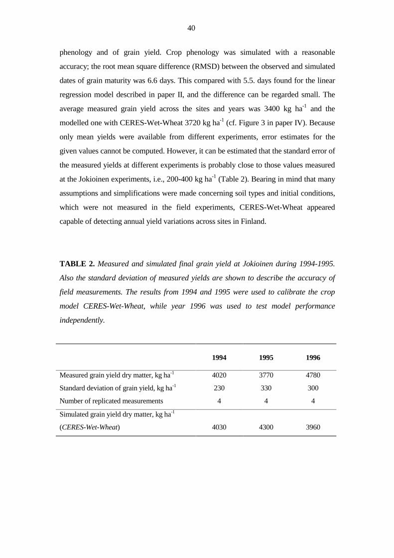
40
phenology and of grain yield. Crop phenology was simulated with a reasonable
accuracy; the root mean square difference (RMSD) between the observed and simulated
dates of grain maturity was 6.6 days. This compared with 5.5. days found for the linear
regression model described in paper II, and the difference can be regarded small. The
average measured grain yield across the sites and years was 3400 kg ha-1 and the
modelled one with CERES-Wet-Wheat 3720 kg ha-1 (cf. Figure 3 in paper IV). Because
only mean yields were available from different experiments, error estimates for the
given values cannot be computed. However, it can be estimated that the standard error of
the measured yields at different experiments is probably close to those values measured
at the Jokioinen experiments, i.e., 200-400 kg ha-1 (Table 2). Bearing in mind that many
assumptions and simplifications were made concerning soil types and initial conditions,
which were not measured in the field experiments, CERES-Wet-Wheat appeared
capable of detecting annual yield variations across sites in Finland.
TABLE 2. Measured and simulated final grain yield at Jokioinen during 1994-1995.
Also the standard deviation of measured yields are shown to describe the accuracy of
field measurements. The results from 1994 and 1995 were used to calibrate the crop
model CERES-Wet-Wheat, while year 1996 was used to test model performance
independently.
1994 1995 1996
Measured grain yield dry matter, kg ha-1 4020 3770 4780
Standard deviation of grain yield, kg ha-1 230 330 300
Number of replicated measurements 4 4 4
Simulated grain yield dry matter, kg ha-1
(CERES-Wet-Wheat) 4030 4300 3960

41
6.2.2. The effects of reduced-form input to the model
The effect of derived daily weather data on simulated crop was studied at Jokioinen
using the weather data from years 1961-1990. When the input weather was derived from
monthly values, yields were 11-26 % higher than those obtained by using daily
measurements. This is due the fact that the extreme high and low daily temperatures
sometimes observed in daily weather are not repeated and the interpolated daytime
temperature is closer to the modelled growth optimum of 18 °C during a greater number
of days. Also yield variability was greater at sites when yield was simulated with the
observed climate than with the derived data.
The three different soil types were compared to each other by simulating yield at
Jokioinen during 1961-1990. The clay loam soil was the highest yielding of the three
soil types, while the lowest yields and greatest yield variations were obtained from the
clay profile. The clay profile appeared susceptible to stress caused by excess soil water,
while drought was the major concern on the sandy soil.
6.2.3. Sensitivity of the model to systematic changes in climate and CO2
The sensitivity of CERES-Wet-Wheat was studied by computing yields with different
modifications of the Jokioinen baseline weather data (1961-1990) and of atmospheric
CO2 concentration. The crop was estimated to ripen successfully in 21 of the 30 baseline
years, and only these ‘suitable’ years were used in subsequent sensitivity tests to
understand the direct physiological response of the modelled crop to changes. Overall,
the temperature and CO2 effects on yield appeared to dominate over the precipitation
and radiation effects across a credible range of future changes in climate. Under
increasing temperature the mean yield at Jokioinen declined, with the greatest decrease
on drought-susceptible sandy soil, due to increased evaporation, and less on the other
two soils. The coefficient of variation (CV) declined with increasing temperatures on
clay, remaining approximately unchanged on clay loam but increased rapidly on the
sand.
42
Higher CO2 concentration led to increased yields, with the lowest mean response on clay
loam, where the yields were least limited by soil water content. The CV rose with
increasing CO2 on clay and was little affected on the two other soil types. Simulations
for combinations of CO2 and temperature change indicate that the positive effect on
mean yield at Jokioinen of a CO2 increase from 353 to 515 ppmv (increase from 1990 to
year 2050 scenario level) is almost entirely offset by a temperature change of 2 °C.
6.2.4. Regional validity of the model under the current climate
To evaluate the performance of CERES-Wet-Wheat regionally annual average spring
wheat yields were computed from the gridded values for each agricultural administrative
district in southern Finland. The simulated regional yields were higher than the recorded
ones, the RMSD ranging from 1350 to 1970 kg ha-1 during 1981-1991 and from 1190 to
1500 kg ha-1 during 1992-1996. Two periods were defined because the regions for
which agricultural statistics were published shifted from agricultural districts to rural
business districts in 1992, and these had somewhat different geographical regions. The
overestimation of modelled yield was probably due to the assumption in the model of
optimal crop management, which is less justified at aggregate farm level than under the
experimental conditions for which the model was calibrated. When the district yields
were aggregated to one annual average value for Finland the relationship between the
observed and modelled yield was strong (R2 = 0.67) in the period 1981-1991 indicating
good model performance in detecting inter-annual variations. However, the relationship
was poorer in the later period 1992-1996, and because of that the positive relationship
was low (R2 = 0.28) across the whole period 1981-1996. The poorer performance over
the longer period may be related, in part, to the contraction in cultivated area to more
productive land after 1990, a consequence of changes in agricultural policy.
Furthermore, at farms a range of crop cultivars are grown while this study simulated the
yield of a single cultivar.
6.2.5. National yield estimates under variable and changing climate
In order to quantify the effects of climate variability and climate change the baseline
gridded weather was altered according to different scenarios. First, the climate was

43
adjusted according to GCM anomalies from the 240-year mean of eight non-overlapping
30-year periods from the HadCM2 control simulation (labelled NOISE scenarios). In
this way it was evaluated how modelled wheat yields are affected by multi-decadal
natural climatic variability as represented by a global climate model. For a range of 30-
year mean May-August temperature anomalies relative to the 240-year mean of -0.4 °C
to +0.3 °C the area of suitability (computed here with the CERES-Wet-Wheat model)
varied between 132 and 929 grid boxes, and national mean yields varied from -3 % to
+5 % relative to the baseline value. This result indicates that significant multi-decadal
variations in mean yield can occur simply as a result of natural variations in the climate,
without any greenhouse gas-induced forcing. Such ”noise” in the long-term climatic
record complicates the detection of a greenhouse gas ”signal”, both in the climate itself
and in the response of crop yields (Hulme et al., 1999). However, this interpretation is
based on the premise that the climate model provides an accurate estimate of natural
climatic variability, an assumption difficult to test due to the absence of long-term
climatic observations that are unaffected by greenhouse gas forcing.
The effects of future climate change on spring wheat yields were examined for the two
GCM-based scenarios (‘REF’ and ‘AERO’) representing the climate of 2050. Under
both scenarios the area of suitability expands northwards (into 1346 and 1400 additional
grid boxes for REF and AERO, respectively), mean yields increase in most (REF
scenario) or in all (AERO scenario) suitable grid boxes, and yield variability decreases
markedly (Figures 6 and 7 in Paper IV). In the zone of baseline suitability the mean yield
of a 30-year period is statistically significantly greater under AERO than REF (4809 kg
ha-1 and 4656 kg ha-1, respectively), and also the annual mean yields are slightly more
reliable as shown in a lower coefficient of variation (CV is 12 % under AERO and 13 %
under REF, compared to 37 % for the baseline). The reason for these differences is not
clear, but is probably related to the beneficial effects of warmer, drier conditions applied
to wet baseline years under AERO outweighing the detrimental effects of this scenario
in warm dry baseline years.

44
6.3. Discussion
This study demonstrated that a rigorously calibrated and tested site-based crop model is
also capable of detecting yield responses to climatic variations at regional level in
Finland under the baseline climate. This result is in line with the study of Kuittinen et al.
(1998), where two crop models were applied to estimate current crop productivity in
different agricultural advisory districts. However, at farm level yields vary considerably
depending on crop management, e.g., pest and disease control, soil conditions and
sowing date. Physiologically based crop models like CERES-Wheat are not developed
for the purpose of mimicking the great variation in a field ecosystem. Since the climate
signal was detected even in the regional yield estimates, the results imply, that under
northern European conditions weather is a more dominant factor determining yield level
than, for example, in the UK, where the weather signal easily disappears within the
noise of management practises and pest and disease effects (Landau et al., 1998;
Jamieson et al., 1999). However, as the climate warms, these confounding effects may
become more important in northern regions too, progressively obscuring the climate
signal - a possible factor of uncertainty to consider when interpreting the results of this
study.
The upscaling method of regional yield prediction offers a number advantages over the
conventional site-based analysis. For instance, a site based analysis is unlikely to
represent the diversity in crop response exhibited for local combinations and gradients of
climate and soil. However, a number of uncertainty sources can be listed in this study.
There are few accurate crop measurements to validate the yield estimates both at
experimental sites and on farm level. Furthermore, the crop model relied on numerous
assumptions about soil initial conditions, soil profile and sowing date. These details,
required by physiologically-based crop models, cannot easily be gathered
comprehensively or estimated objectively. In future, it would be of interest to conduct a
more detailed risk analysis of yields as well as evaluation of model uncertainty at
regional scale.
45
7. CONCLUSIONS
This study developed and tested a number of methods which can be used to evaluate
regional and national crop suitability and yield potential under different climatic
conditions. The study employed spring wheat as a research crop, but the approach is
more generally applicable to other crops and also other regions outside Finland.
Regional information on crop suitability and crop productivity are needed for
agricultural policies concerning e.g., plant breeding, regional agricultural support and
rural development.
The major findings of this study can be summarised as follows:
1) A warming of the climate is estimated to induce shifts in the northern limit of spring
wheat cultivation of between 160-180 km per 1 °C increase in mean annual
temperature. Under the range of uncertainty represented by the SILMU scenarios for
2050, this translates into a mean northward shift of about 10-80 km per decade.
When the suitability is estimated on the basis of two GCM-based scenarios by 2050,
the suitability to grow a relatively early maturing cultivar (cv. Polkka) would expand
to cultivable land within an area covering 1346-1400 grid boxes (i.e., up to 140000
km2).
2) With climatic warming crop development is enhanced in the regions of present-day
suitability. If sowing dates are shifted earlier with climatic warming, the shortening of
development phases is especially marked during the heading-yellow ripening phase,
while the early development (sowing-heading phase) is less affected. An enhanced
development is likely to reduce harvested yield of crop cultivars grown under the
present climate.
3) Average grain yield of a present-day spring-wheat cultivar Polkka in 2050 is
estimated to be greater than at present over most or all the area of the estimated
present-day suitability in southern Finland. The negative or insignificant change is
mostly due to the combined effects of changes in CO2 and temperature. The scenarios
applied in this study assumed a CO2 increase from 353 to 515 ppmv and a mean
summer temperature (May-August) increase of 1.7 °C or 2 °C averaged across
Finland. Crop model simulations of combinations of CO2 and temperature indicate
46
that the positive effect on mean yield at a test site, Jokioinen, of the CO2 increase
from 353 to 515 ppmv is almost entirely offset by a temperature change of 2 °C.
4) The regional year to year variability of crop yield is estimated to decrease markedly in
the estimated current zone of crop suitability.
5) Significant multi-decadal variations in mean yield can occur simply as a result of
natural variations in the climate, without any greenhouse gas-induced forcing. Such
”noise” in the long-term climatic record complicates the detection of a greenhouse
gas ”signal”, both in the climate itself and in the response of crop yields. However,
this interpretation is based on the assumption that the climate model provides an
accurate estimate of climatic variability. There is some support for this assertion from
the proxy climatic record over the past millennium (Jones et al., 1998).
6) Many uncertainties are linked to the regional model estimates, of which many can be
clearly identified and some also quantified. In this study, spatial uncertainty of the
crop phenological model was mapped and compared to estimates of future shifts in
crop suitability under different climate change scenarios. The uncertainties of future
climate projections far exceed the model uncertainty surrounding the mapped limit of
baseline mean suitability. On the other hand, the uncertainties linked to the regional
yield estimates are complicated because of the many non-linear relationships in the
model. Quantification of the uncertainty of mechanistic crop yield models is a major
challenge for the international scientific community.
This study tested and developed some basic key tools, which can be applied to examine
crop potential regionally. Many important factors including crop quality and the risk of
pests and diseases were not considered here. Further research efforts should concentrate
on refining the method of estimating crop potential, and to include aspects of farm-level
adaptation to changing climate. In the next stage, an integrated modelling approach
could be adopted, where environmental pollution and economical aspects are also
modelled, to obtain a better understanding of the whole crop production system at
regional and national level under changing environmental conditions.

47
8. ACKNOWLEDGEMENTS
This study was undertaken as part of the Finnish Research Programme on Climate
Change (SILMU) in 1991-1995 and the research project ‘Climate Change, Climatic
Variability and Agriculture in Europe’ (CLIVARA) under the European Union Fourth
Framework Programme, Environment and Climate (ENV4-CT95-0154) in 1996-1998.
The work was funded by the Academy of Finland, the Agricultural Research Centre of
Finland and the Commission of the European Communities. The thesis was finalised
with personal grants from August Johannes and Aino Tiura’s Agricultural Research
Foundation, University of Helsinki and Scientific Foundation of Academic
Agronomists. I am also grateful for the working facilities provided by the Finnish
Meteorological Institute and for the regional information used in the analysis system
supplied by various government bodies.
I wish to acknowledge my debt to Dr. Timothy Carter (Finnish Environment Institute)
who supervised this study and taught me how to assess climate change impacts on
regional crop production. I would also like to express my gratitude to Professor Timo
Mela (Agricultural Research Centre) for his support of my work and studies, and to
Professor Eija Pehu (University of Helsinki, Department of Plant Production) for her
enthusiastic and encouraging attitude to my thesis.
I am indebted to Professor Risto Kuittinen (Finnish Geodetic Institute) and Dr. Jouko
Kleemola (Kemira Agro Oy) for reviewing a draft of this thesis and giving constructive
criticism. Furthermore, I benefitted a lot from advice and discussions on crop modelling
with Jouko Kleemola during the early years of this work.
I would like to express my thanks to Ms. Marjo Pihala for her initiative and careful work
with our field experiments at Jokioinen. I am grateful to Ms. Sanna Tuovinen, Mr. Matti
Matilainen, Dr. Kaija Hakala, Mr. Timo Kaukoranta, Mr. Jari Poikulainen, Ms. Leila
Salo and Ms. Irma Noppa, Mr. Mikko Vähä-Perttula and Ms. Anneli Partala for their co-
operative assistance in the arrangement of the crop experiments, and I also thank other
colleagues at the Agricultural Research Centre for making available experimental crop
data from different research stations.

48
Many warm thanks to Dr. Kaija Hakala for giving encouraging comments on my work
and Ms. Hannele Sankari for inspirational discussions. The assistance of Ms. Pirkko
Vatka, Ms. Marja-Riitta Juhala, Ms. Mari Topi-Hulmi and Ms. Anneli Hyvönen is also
much appreciated.
I am grateful to the staff of the Finnish Meteorological Institute, especially Mr. Eino
Hellsten, Dr. Ari Venäläinen, Ms. Päivi Junila, Dr. Raino Heino, Dr. Mikko Alestalo
and Dr. Martti Heikinheimo for supporting and advising me in various ways. I would
like to offer special thanks to Ms. Hanna Lappalainen for her friendship and to the staff
of the Meteorological Research for providing a friendly atmosphere in which to work.
Finally, I am especially grateful to my husband Mats Nurmio for his love and
encouragement and our sons Axel and Edvin for helping me to realise what is most
important in life.
49
9. REFERENCES
Allen, L.H., Jr. 1990. Plant responses to rising carbon dioxide and potential interactions
with air pollutants. J. Environ. Qual. 19: 15-34.
Angus, J.F., Mackenzie, D.H., Morton, R. and Schafer, C.A. 1981. Phasic
development in field crops. II. Thermal and photoperiodic responses of spring
wheat. Field Crops Res. 4: 269-283.
Barrow, E., Hulme, M. and Semenov, M. 1996. Effects of using different methods in
the construction of climate change scenarios: examples from Europe. Clim. Res.
7: 195-211.
Barrow, E.M., Hulme, M., Semenov, M.A. and Brooks, R.J. 1999. Climate change
scenarios. In: Downing, T.E., Harrison, P.A., Butterfield, R.E. and Lonsdale, K.G.
(Eds). Climate Change, Climatic Variability and Agriculture in Europe: An
Integrated Assessment. Research Report No. 21, Environmental Change Unit,
University of Oxford, Oxford, UK. (in press)
Batts, G.R., Morison, J.I.L., Ellis, R.H., Hadley, P. and Wheeler, T.R. 1997. Effects
of CO2 and temperature on growth and yield of crops of winter wheat over several
seasons. Eur. J. Agron. 7: 43-52.
Bindi, M., Castellani, M., Maracchi, G. and Miglietta, F. 1993. The ontogenesis of
wheat under scenarios of increased air temperature in Italy: a simulation study.
Eur. J. Agron. 2: 261-280.
Bowes, G. 1991. Growth at elevated CO2: photosynthetic responses mediated through
Rubisco. Plant, Cell and Environ. 14: 869-875.
Brklacich, M., Curran, P. and Brunt, D. 1996. The application of agricultural land
rating and crop models to CO2 and climate change issues in Northern regions: the
Mackenzie Basin case study. Agric. Food Sci. Fin. 5: 351-365.
Brooks, C.E.P. 1943. Interpolation tables for daily values of meteorological elements.
Q. J. R. Meteorol. Soc. 69: 160-162.
Carter, T. 1992. The Greenhouse Effect and Finnish Agriculture. Maatilahallinnon
aikakauskirja (Journal of Farm Administration) 1/1992: 31-57.
Carter, T.R. 1996. Developing scenarios of atmosphere, weather and climate for
northern regions. Agric. Food Sci. Fin. 5: 235-249.

50
Carter, T.R., Konijn, N.T. and Watts, R.G. 1988. The choice of first-order impact
models. In: Parry, M.L., Carter, T.R. and Konijn, N.T. (Eds). The Impact of
Climatic Variations on Agriculture. Vol. 1, Assessments in Cool Temperate an
Cold Regions, Kluwer, Dordrecht, The Netherlands. pp. 97-123.
Carter, T.R., Parry, M.L. and Porter, J.H. 1991. Climatic change and future
agroclimatic potential in Europe. Int. J. Climatol. 11: 251-269.
Carter, T.R., Parry, M.L., Harasawa, H. and Nishioka, S. 1994. IPCC Technical
Guidelines for Assessing Climate Change Impacts and Adaptation.
Intergovernmental Panel on Climate Change, Department of Geography,
University College London, UK and Centre for Global Environmental Research,
Tsukuba, Japan, 59 p.
Carter, T., Posch, M. and Tuomenvirta, H. 1995. SILMUSCEN and CLIGEN User’s
Guide. Guidelines for the construction of climatic scenarios and use of a stochastic
weather generator in the Finnish Research Programme on Climate Change
(SILMU). Publications of the Academy of Finland 5/95. Helsinki, Finland. 62 p +
diskette.
Carter, T., Hakala, K., Kaukoranta, T., Kleemola, J., Laurila, H., Mela, T., Pehu,
E., Saarikko, R. and Tiilikkala, K. 1996a. Maatalous. (Agriculture). In:
Kuusisto, E., Kauppi, L. and Heikinheimo, P. (Eds). Ilmastonmuutos ja Suomi.
(Climate Change and Finland). Helsinki University Press, Helsinki, Finland.
pp.129-143. (in Finnish).
Carter, T.R., Saarikko, R.A. and Niemi, K.J. 1996b. Assessing the risks and
uncertainties of regional crop potential under a changing climate in Finland. Agric.
Food Sci. Fin. 5: 329-350.
Carter, T.R., Saarikko, R.A. and Joukainen, S.K.H. 1999. Modelling climate change
impacts on wheat and potato in Finland. In: Downing, T.E., Harrison, P.A.,
Butterfield, R.E. and Lonsdale, K.G. (Eds). Climate Change, Climatic Variability
and Agriculture in Europe: An Integrated Assessment. Research Report No. 21,
Environmental Change Unit, University of Oxford, Oxford, UK. (in press)
Chipanshi, A.C., Ripley, E.A. and Lawford, R.G. 1997. Early prediction of spring
wheat yields in Saskatchewan from current and historical weather data using the
CERES-Wheat model. Agric. For. Met. 84: 223-232.

51
Cure, J.D. and Acock, B. 1986. Crop responses to carbon dioxide doubling: a literature
survey. Agric. For. Met. 38: 127-145.
Delecolle, R. and Guérif, M.O. 1995. Regional calibration of crop models using
remote sensing data. In: Harrison, P.A., Butterfield, R.E. and Downing, T.E.
(Eds). Climate Change and Agriculture in Europe. Assessment of Impacts and
Adaptations. Research Report No. 9. Environmental Change Unit, University of
Oxford, Oxford, UK. pp. 302-310.
Downing, T.E., Harrison, P.A., Butterfield, R.E. and Lonsdale, K.G. 1999. Climate
Change, Climate Variability and Agriculture in Europe: An Integrated
Assessment. Research Report No. 21, Environmental Change Unit, University of
Oxford, Oxford, UK. (in press)
Easterling, W.E., Crossen, P.R., Rosenberg, N.J., McKenney, M.S., Katz, L.A. and
Lemon, K.M. 1993. Agricultural impacts and responses to climate change in the
Missouri-Iowa-Nebraska-Kansas (MINK) region. Climate Change 24: 23-61.
Farrar, J.F. and Williams, M.L. 1991. The effects of increased atmospheric carbon
dioxide and temperature on carbon partitioning, source-sink relations and
respiration. Plant, Cell and Environ. 14: 819-830.
Gates, W.L., Mitchell, J.F.B., Boer, G.J., Cubasch, U. and Meleshko, V.P. 1992.
Climate modelling, climate prediction and model validation. In Houghton, J.T.,
Callander, B.A. and Varney, S.K. (Eds). Climate change 1992. The supplementary
report to the IPCC scientific assessment. Cambridge University Press, Cambridge,
UK. pp. 97-134.
Hakala, K. 1998. Effects of climate change in the north on growth, yield formation and
photosynthesis of spring wheat and meadow fescue. Academic dissertation. Turku
University Publications, Series AII, No. 110, Turku, Finland.
Harrison, P.A. and Butterfield, R.E. 1996. Effects of climate change on Europe-wide
winter wheat and sunflower productivity. Clim. Res. 7: 225-241.
Hay, R.K.M. and Walker, A.J. 1989. An Introduction to the Physiology of Crop Yield.
Longman, Harlow, UK. 292 p.
Henttonen, H. 1991. Kriging in interpolating July mean temperatures and precipitation
sums. Reports from the Department of Statistics, University of Jyväskylä, Finland,
12/1991, 41 p.
52
Hulme, M., Raper, S.C.B. and Wigley, T.M.L. 1995. An integrated framework to
address climate change (ESCAPE) and further development of the global and
regional climate modules (MAGICC). Energy Policy 23: 347-355.
Hulme, M., Barrow, E.M., Arnell, N.W., Harrison, P.A., Johns, T.C. and Downing,
T.E. 1999. Relative impacts of human-induced climate change and natural climate
variability. Nature 397: 688-691.
Idso, S.B., Kimball, B.A., Anderson, M.G. and Mauney, J.R. 1987. Effects of
atmospheric CO2 enrichment on plant growth: the interactive role of air
temperature. Agriculture, Ecosystems and Environment 20: 1-10.
Iglesias, A. 1995. Modelling the effects of climate change on crops at the regional scale:
Effects on wheat and maize in Spain. In: Harrison, P.A., Butterfield, R.E. and
Downing, T.E. (Eds). Climate Change and Agriculture in Europe. Assessment of
Impacts and Adaptations. Research Report No 9, Environmental Change Unit,
University of Oxford, Oxford, UK. pp. 310-319.
Iglesias, A. 1997. Modelling climate change impacts on wheat and soya bean in Spain.
In: Butterfield, R.E., Lonsdale, K.G. and Downing, T.E. (Eds). Climate Change,
Climatic Variability and Agriculture in Europe: An Integrated Assessment.
Annual Report to the Environment Programme, Comission of the European
Communities, Environmental Change Unit, University of Oxford, Oxford, UK.
pp.243-248.
IPCC, 1990. Climate Change: The IPCC Impacts Assessment. Tegart, W.J.McG.,
Sheldon, G.W. and Griffiths, D.C. (Eds). Report prepared for IPCC by Working
Group II, Australian Government Publishing Service, Canberra, Australia. 210 p.
IPCC, 1992a. Climate Change 1992: the Supplementary Report to the IPCC Impacts
Assessment. Tegart, W.J.McG., Sheldon, G.W. and Griffiths, D.C. (Eds). Report
Prepared for IPCC Working Group II, Australian Government Publishing Service,
Canberra, Australia.
IPCC, 1992b. Climate Change 1992. The Supplementary Report to the IPCC Scientific
Assessment. Houghton, J.T., Callander, B.A. and Varney, S.K. (Eds). Cambridge
University Press, Cambridge, UK. 200 p.
IPCC, 1996a. Climate Change 1995. The Science of Climate Change. Contribution of
Working Group I to the Second Assessment Report of the Intergovernmental
Panel on Climate Change. Houghton, J.T., Meira Filho, L.G., Callander, B.A.,

53
Harris, N., Kattenberg, A. and Maskell, K. (Eds). Cambridge University Press,
Cambridge, UK, 572 p.
IPCC, 1996b. Climate Change 1995. Impacts, Adaptations and Mitigation of Climate
Change: Scientific-Technical Analyses. Contribution of Working Group II to the
Second Assessment Report of the Intergovernmental Panel on Climate Change.
Watson, R.T., Zinyowera, M.C., Moss, R.H. and Dokken, D.J. (Eds). Cambridge
University Press, Cambridge, UK. 878 p.
IPCC, 1998. The Regional Impacts of Climate Change. An Assessment of
Vulnerability. Watson, R.T., Zinyowera, M.C., Moss, R.H. and Dokken, D.J.
(Eds). Cambridge University Press, Cambridge, UK. 517 p.
Jamieson, P.D., Porter, J.R., Goudriaan, J., Ritchie, J.T., van Keulen, H. and Stol,
W. 1998. A comparison of the models AFRCWHEAT2, CERES-Wheat, Sirius,
SUCROS2 and SWHEAT with measurements from wheat grown under drought.
Field Crops Res. 55: 23-44.
Jamieson, P.D., Porter, J.R., Semenov, M.A., Brooks, R.J., Ewert, F. and Ritchie,
J.T. 1999. Comments on ”Testing UK wheat simulation models’ predictions
against observed UK grain yields” by S. Landau et al. (1998). Agric. For. Met. 96:
157-161.
Johns, T.C., Carnell, R.E., Crossley, J.F., Gregory, J.M., Mitchell, J.F.B., Senior,
C.A., Tett, S.F.B. and Wood, R.A. 1997. The second Hadley Centre coupled
ocean-atmosphere GCM: Model description, spinup and validation. Climate
Dynamics 13: 103-134.
Jones, M.B. and Carter, T.R. 1993. European grassland production in a changing
climate. Proceedings of the 14th General Meeting of the European Grassland
Federation, Lahti, Finland. pp. 97-110.
Jones, P.D., Briffa, K.R., Barnett, T.P. and Tett, S.F.B. 1998. High-resolution
palaeoclimatic records for the last millennium: interpretation, integration and
comparison with GCM control-run temperatures. The Holocene 8: 455-471.
Karvonen, T. and Varis, E. 1992. Mathematical models in crop production. University
of Helsinki, Department of Plant Production. Publication N:r 32, Helsinki,
Finland, 218 p.
Kattenberg, A., Giorgi, F., Grassl, H., Meehl, G.A., Mitchell, J.F.B., Stouffer, R.J.,
Tokioka, T., Weaver, A.J. and Wigley, T.M.L. 1996. Climate models -

54
projections of future climate. In: Houghton, J.T., Meira Filho, L.G., Callander,
B.A., Harris, N., Kattenberg, A. and Maskell, K. (Eds). Climate Change 1995. The
Science of Climate Change. Contribution of Working Group I to the Second
Assessment Report of the Intergovernmental Panel on Climate Change.
Cambridge University Press, Cambridge, UK, pp. 285-357.
Kaukoranta, T. 1996. Impact of global warming on potato late blight: risk, yield loss
and control. Agric. Food Sci. Fin. 5: 311-327.
Kenny, G.J. and Harrison, P.A. 1992. The effects of climate variability and change on
grape suitability in Europe. J. Wine Res. 3: 163-183.
Kenny, G.J., Harrison, P.A., Olesen, J.E. and Parry, M.L. 1993. The effects of
climatic change on land suitability of grain maize, winter wheat and cauliflower in
Europe. Eur. J. Agron. 2: 325-338.
Kenny, G.J., Sims, G.C. and Warrick, R.A. 1996. CLIMPACTS 1995/1996: Progress
with development of the CLIMPACTS system. University of Waikato, New-
Zealand. CEARS Report Series No. RP-96-07.
Kettunen, L., Mukula, J., Pohjonen, V., Rantanen, O. and Varjo, U. 1988. The
effects of climatic variations on agriculture in Finland. In: Parry, M.L., Carter,
T.R. and Konijn N.T. (Eds). The Impacts of Climatic Variations on Agriculture.
Volume 1. Assessments in Cool Temperate and Cold Regions, Kluwer, Dordrecht,
The Netherlands, pp. 511-614.
Kleemola, J. 1991. Effect of temperature on phasic development of spring wheat in
northern conditions. Acta Agric. Scand. 41: 275-283.
Kleemola, J. and Karvonen, T. 1996. Modelling growth and nitrogen balance of barley
under ambient and future conditions. Agric. Food Sci. Fin. 5: 299-310.
Kontturi, M. 1979. The effects of weather on yield and development of spring wheat in
Finland. Ann. Agric. Fenn. 18: 263-274.
Kuittinen, R., Ahokas, E., Granqvist, M., Ikäheimo, E., Heikinheimo, M.,
Venäläinen, A., Jänne, S., Keskisarja, V., Parmes, E., Perdigao, V. and van
der Goot, E. 1998. An early crop yield estimation method for Finnish conditions:
the crop growth monitoring system of the Joint Research Centre with and without
remotely sensed and other additional input data. Reports of the Finnish Geodetic
Institute, 98:2. Helsinki, Finland. 114 p.

55
Kähäri, J., Mäntylahti, V. and Rannikko, M. 1987. Soil Fertility of Finnish
Cultivated Soils in 1981-1985. Viljavuuspalvelu Oy. Helsinki, Finland. 105 p. (in
Finnish).
Lallukka, U., Rantanen, O. and Mukula, J. 1978. The temperature sum requirement
of barley varieties in Finland. Ann. Agric. Fenn. 17: 185-191.
Landau, S., Mitchell, R.A.C., Barnett, V., Colls, J.J., Craigon, J., Moore, K.L. and
Payne, R.W. 1998. Testing winter wheat simulation models’ predictions against
observed UK grain yields. Agric. For. Met. 89: 85-99.
Laurila, H. 1995. Modelling the effects of elevated CO2 and temperature on Swedish
and German spring wheat varieties with CERES-Wheat and AFRC-Wheat crop
models. J. Biogeogr. 22: 591-595.
Lawlor, D.W. and Mitchell, A.C. 1991. The effects of increasing CO2 on crop
photosynthesis and productivity: a review of field studies. Plant, Cell and Environ.
14: 807-818.
Leemans, R. and Solomon, A.M. 1993. Modeling the potential change in yield and
distribution of the earth’s crops under a warmed climate. Clim. Res. 3: 79-96.
Leggett, J., Pepper, W.J. and Swart, R.J. 1992. Emissions scenarios for the IPCC: an
update. In: Houghton, J.T., Callander, B.A. and Varney, S.K. (Eds). Climate
Change 1992. The Supplementary Report to the IPCC Scientific Assessment.
Cambridge University Press, Cambridge, UK. pp. 69-95.
Manabe, S., Stouffer, R.J., Spelman, M.J. and Bryan, K. 1991. Transient response of
a coupled ocean-atmosphere model to gradual changes of atmospheric CO2. Part I:
Annual mean response. J. Clim. 4: 785-818.
Mela, T.J.N. 1996. Northern agriculture: constraints and responses to global climate
change. Agric. Food Sci. Fin. 5: 229-234.
Mela, T., Carter, T., Hakala, K., Hannukkala, A., Kaukoranta, T., Laurila, H.,
Niemi, K., Saarikko, R. and Tiilikkala, K. 1996. The effects of climatic change
on crop production: results of a five-year research project. In: Roos, J. (Ed). The
Finnish Research Programme on Climate Change. Final Report. Publications of
the Academy of Finland 4/96. Helsinki, Finland. pp. 324-336.
Mukula, J. 1984. Zones for cultivars of field crops. Maataloushallinnon aikakauskirja
(Journal of Farm Administration) 4: 1-7.

56
Mukula, J. and Rantanen, O. 1989. Climatic risks to yield and quality of field crops in
Finland. V. Spring wheat 1969-1986. Ann. Agric. Fenn. 28: 21-28.
Murphy, J.M. and Mitchell, J.F.B. 1995. Transient response of the Hadley Centre
coupled ocean-atmosphere model to increasing carbon dioxide. Part II: spatial and
temporal structure of the response. J. Clim. 8: 57-80.
Nonhebel, S. 1993. Effects of changes in temperature and CO2 concentrations on
simulated spring wheat yields in the Netherlands. Climate Change 24: 311-329.
O’Neill, R. 1971. Algorithm AS 47. Function minimization using a simplex procedure.
Appl. Stat. 20: 338-345.
Orr, J.L. and Brignall, A.P. 1995. Methods for site and regional scale integration of
crop model results. In: Harrison, P.A., Butterfield, R.E. and Downing, T.E. (Eds).
Climate Change and Agriculture in Europe. Assessment of Impacts and
Adaptations. Research Report No. 9, Environmental Change Unit, University of
Oxford, Oxford, UK. pp. 391-401.
Otter-Nacke, S., Godwin, D.C. and Ritchie, J.T. 1986. Testing and Validating the
CERES-Wheat Model in Diverse Environments. AGRISTARS YM-15-00407.
Johnson Space Center No. 20244. Houston, USA.
Parry. M. and Carter, T. 1988. The assessment of effects of climatic variations on
agriculture: Aims, Methods and Summary of results. In: Parry, M.L., Carter, T.R.
and Konijn N.T. (Eds). The Impact of Climatic Variations on Agriculture. Volume
1. Assessments in Cool Temperate and Cold Regions, Kluwer, Dordrecht, The
Netherlands. pp. 11-95.
Parry, M.L., Carter, T.R. and Konijn, N.T. (Eds). 1988a. The Impact of Climatic
Variations on Agriculture. Volume 1. Assessments in Cool Temperate and Cold
Regions. Kluwer, Dordrecht, The Netherlands. 876 p.
Parry, M.L., Carter, T.R. and Konijn, N.T. (Eds). 1988b. The Impact of Climatic
Variations on Agriculture. Volume 2. Assessments in Semi-Arid Regions.
Kluwer, Dordrecht, The Netherlands.
Parry, M. and Carter, T. 1998. Climate Impact and Adaptation Assessment. A Guide
to the IPCC Approach. Earthscan Publications Ltd, London, UK. 166 p.
Peart, R.M., Jones, J.W., Curry, R.B., Boote, K. and Allen, L.H. Jr. 1989. Impact of
climate change on crop yield in the southeastern USA. In: Smith, J.B. and Tirpak,
D.A. (Eds). The Potential Effects of Global Climate Change on the United States,

57
Appendix C. Report to Congress. US Environmental Protection Agency, EPA-
230-05-89-050, Washington DC, USA.
Porter, J.R., Kirby, E.J.M., Day, W., Adam, J.S., Appleyard, M., Ayling, S., Baker,
C.K., Beale, P., Belford, R.K., Biscoe, P.V., Chapman, A., Fuller, M.P.,
Hampson, J., Hay, R.K.M., Hough, M.N., Matthews, S., Thompson, W.J.,
Weir, A.H., Willington, V.B.A. and Wood, D.W. 1987. An analysis of
morphological development stages in Avalon winter wheat crops with different
sowing dates and at ten sites in England and Scotland. J. Agric. Sci. 109: 107-121.
Porter, J.R., Jamieson, P.D. and Wilson, D.R. 1993. Comparison of the wheat
simulation models AFRCWHEAT2, CERES-Wheat and SWHEAT for non-
limiting conditions of crop growth. Field Crops Res. 33: 131-157.
Rantanen, O. and Solantie, R. 1987. Climatic risks to the yield and quality of field
crops in Finland. II. Cultivation zones and sub-divisions. Ann. Agric. Fenn. 26:
19-37.
Reilly, J., Baethgen, W., Chege, F.E., van de Geijn, S.C., Erda L., Iglesias, A.,
Kenny, G., Patterson, D., Rogasik, J., Rötter, R., Rosenzweig, C., Sombroek,
W., Westbrook, J., Bachelet, D., Brklacich, M., Dämmgen, U., Howden, M.,
Joyce, R.J.V., Lingren, P.D., Schimmelpfennig, D., Singh, U., Sirotenko, O.
and Wheaton, E. 1996. Agriculture in a Changing Climate: Impacts and
Adaptation. In: Watson, R.T., Zinyowera, M.C., Moss, R.H. and Dokken, D.J.
(Eds.). Climate Change 1995. Impacts, Adaptations and Mitigation of Climate
Change: Scientific-Technical Analyses. Contribution of Working Group II to the
Second Assessment Report of the Intergovernmental Panel on Climate Change.
Cambridge University Press, Cambridge, UK. pp. 427- 467.
Ritchie, J.T. 1991. Wheat Phasic Development. In: Hanks, J. and Ritchie, J.T. (Eds).
Modeling Plant and Soil Systems, Agron. No. 31. Madison, Wisconsin, USA. pp.
31-54.
Ritchie, J.T. 1998. Soil water balance and plant water stress. In: Tsuji, G.Y.,
Hoogenboom, G. and Thornton, P.K. (Eds). Understanding Options for
Agricultural Production. Kluwer Academic Publisher in cooperation with ICASA.
Dordrecht, The Netherlands. pp. 41-54.
Ritchie, J.T., Singh, U., Godwin, D.C. and Bowen, W.T. 1998. Cereal growth,
development and yield. In: Tsuji, G.Y., Hoogenboom, G. and Thornton, P.K.

58
(Eds). Understanding Options for Agricultural Production. Kluwer Academic
Publisher in cooperation with ICASA. Dordrecht, The Netherlands. pp. 79-98.
Roberts, E.H., Summerfield, R.J., Cooper, J.P. and Ellis, R.H. 1988. Environmental
control of flowering in barley (Hordeum vulgare L.). I. Photoperiod limits to long-
day responses, photoperiod-insensitive phases and effects of low-temperature and
short-day vernalization. Ann. Bot. 62: 127-144.
Robertson, G.W. 1983. Weather-based mathematical models for estimating
development and ripening of crops. WMO, Geneva, Technical Note No 180, 99 p.
Rosenberg, N.J. 1992. Adaptation of agriculture to climate change. Climate Change 21:
385-405.
Rosenzweig, C. and Iglesias, A. 1994. Implications of Climate Change for International
Agriculture: Crop Modeling Study. EPA 230-B-94-003, Office of Policy Planning
and Evaluation, United States Environmental Protection Agency, Washington,
D.C., USA.
Rosenzweig, C. and Parry, M.L. 1994. Potential impacts of climate change on world
food supply. Nature 367: 133-138.
Rosenzweig, C. and Tubiello, F.N. 1996. Effects of changes in minimum and
maximum temperature on wheat yields in the central US. A simulation study.
Agric. For. Met. 80: 215-230.
Rosenzweig, C. and Hillel, D. 1998. Climate Change and the Global Harvest. Potential
Impacts of the Greenhouse Effect on Agriculture. Oxford University Press, New
York, USA. 324 p.
Saarikko, R.A., Pihala, M.T., Hannukkala, A. and Carter, T.R. 1996. Greenhouse
and field experiments on the effects of increased temperature on wheat, maize and
potato. In: Harrison, P.A., Butterfield, R.E. and Downing, T.E. (Eds). Climate
Change, Climatic Variability and Agriculture in Europe. An Integrated
Assessment. Annual Report to the Environment Programme, Comission of the
European Communities, Environmental Change Unit, University of Oxford,
Oxford, UK, pp. 34-39.
Semenov, M.A., Wolf, J., Evans, L.G., Eckersten, H. and Iglesias, A. 1996.
Comparison of wheat simulation models under climate change. II. Application of
climate change scenarios. Clim. Res. 7: 271-281.
59
Strand, E. 1987. Base temperature levels in heat sum calculations. Acta Agric. Scand.
37: 279-286.
Summerfield, R.J., Roberts, E.H., Ellis, R.H. and Lawn, R.J. 1991. Towards the
reliable prediction of time to flowering in six annual crops. I. The development of
simple models for fluctuating field environments. Exp. Agric. 27: 11-31.
Tiilikkala, K., Carter, T., Heikinheimo, M. and Venäläinen, A. 1995. Pest risk
analysis of Meloidogyne chitwoodi for Finland. EPPO Bulletin 25: 419-435.
Tsuji, G.Y., Hoogenboom, G. and Thornton, P.K. (Eds.) 1998. Understanding
Options for Agricultural Production. Kluwer Academic Publisher in cooperation
with ICASA. Dordrecht, The Netherlands. 399 p.
UN, 1996. World population prospects: the 1996 Revision. United Nations Department
for Economic and Social Information and Policy Analysis Population Division,
New York, USA.
van Lanen, H.A.J., van Diepen, C.A., Reinds, G.H.J., de Koning, G.H.J., Bulens,
J.D. and Bregt, A.K. 1992. Physical land evaluation methods and GIS to explore
the crop potential and its effects within the European Communities. Agric. Syst.,
39: 307-328.
Venäläinen, A. and Heikinheimo, M. 1997. The spatial variation of long-term mean
global radiation in Finland. Int. J. Clim. 17: 415-426.
Warrick, R.A., Gifford, R.M. and Parry, M.L. 1986. CO2, climatic change and
agriculture. In: Bolin, B., Döös, B.R., Jäger. J. and Warrick, R.A. (Eds). The
Greenhouse Effect, Climatic Change and Ecosystems. SCOPE 29, Wiley,
Chichester, UK. pp. 393-474.
Wheeler, T.R, Batts, G.R., Ellis, R.H., Hadley, P. and Morison, J.I.L. 1996. Growth
and yield of winter wheat (Triticum aestivum) crops in response to CO2 and
temperature. J. Agric. Sci. 127: 37-48.
Wigley, T.M.L. and Raper, S.C.B. 1992. Implications for climate and sea level of
revised IPCC emissions scenarios. Nature 357: 293–300.
Wolf, J. and van Diepen, C.A. 1991. Effects of Climate Change on Crop Production in
the Rhine Basin. DLO-The Winand Staring Centre, Wageningen, The
Netherlands.
Wolf, J., Semenov, M.A., Eckersten, H., Evans, L.G., Iglesias, A. and Porter, J.R.
1995. Modelling the effects of climate change and climatic variability on crops at

60
the site scale. Effects on winter wheat: A comparison of five models. In: Harrison,
P.A., Butterfield, R.E. and Downing, T.E. (Eds). Climate Change and Agriculture
in Europe. Assessment of Impacts and Adaptations. Research Report No 9,
Environmental Change Unit, University of Oxford, Oxford, UK. pp. 231-280.
Wolf, J., Evans, L.G., Semenov, M.A., Eckersten, H. and Iglesias, A. 1996.
Comparison of wheat simulation models under climate change. I. Model
calibration and sensitivity analyses. Clim. Res. 7: 253-270.
Zar, J.H. 1984. Biostatistical analysis, 2nd edn. Prentice-Hall, Eaglewood Cliffs, NJ.