Climate Amenities, Climate Change, and American …davidalbouy.net/climatewelfare.pdfClimate Amenities, Climate Change, and American Quality of Life David Albouy, Walter Graf, Ryan

Climate Amenities, Climate Change,

and American Quality of Life

David Albouy, Walter Graf, Ryan Kellogg, Hendrik Wolff

Abstract: We present a hedonic framework to estimate US households’ prefer-ences over local climates, using detailed weather and 2000 Census data. We find thatAmericans favor a daily average temperature of 65 degrees Fahrenheit, that they willpay more on the margin to avoid excess heat than cold, and that damages increaseless than linearly over extreme cold. These preferences vary by location due to sort-ing or adaptation. Changes in climate amenities under business-as-usual predictionsimply annual welfare losses of 1%–4% of income by 2100, holding technology andpreferences constant.

JEL Codes: H49, I39, Q54, R10

Keywords: Amenity valuation, Climate change, Hedonic model, Household sorting,Impact assessment, Quality of life

THE CHEMISTRY OF THE HUMAN BODY makes our health and comfort sensitiveto climate. Every day, climate influences human activity, including diet, chores, recre-ation, and conversation. Households spend considerable amounts on housing, energy,clothing, and travel to protect themselves from extreme climates and to enjoy com-

David Albouy is at the University of Illinois, Department of Economics, and NBER ([email protected]). Walter Graf is at the University of California, Berkeley, Department of Agri-cultural and Resource Economics ([email protected]). Ryan Kellogg (correspondingauthor) is at the University of Michigan, Department of Economics, and NBER ([email protected]). Hendrik Wolff is at Simon Fraser University, Department of Economics([email protected]). Albouy acknowledges financial support from NSF grant SES-0922340.We thank Kenneth Chay, Don Fullerton, Philip Haile, Kai-Uwe Kühn, Matthew Turner,Wolfram Schlenker, the editor Daniel Phaneuf, and three anonymous referees for particularlyhelpful criticisms and suggestions. We are also grateful for comments from seminar partici-pants at Boston, Brown, Calgary, Columbia, CU-Boulder, Duke, EPA, Harvard, Houston,Illinois, Maryland, Michigan, Michigan State, Minnesota, NYU, Olin, Oregon, Princeton, RFF,Rice, Stanford, Texas A&M, TREE, UC Berkeley, UCLA, UNR,Washington,WesternMichigan,and Wisconsin, as well as conference attendees at the American Economic Association, Cowles,

Received July 23, 2014; Accepted October 16, 2015; Published online January 22, 2016.

JAERE, volume 3, number 1. © 2016 by The Association of Environmental and Resource Economists.All rights reserved. 2333-5955/2016/0301-0006$10.00 http://dx.doi.org/10.1086/684573

205

This content downloaded from 144.092.122.212 on March 04, 2016 13:37:47 PMAll use subject to University of Chicago Press Terms and Conditions (http://www.journals.uchicago.edu/t-and-c).

fortable moderation. Geographically, climate affects the desirability of different loca-tions and the quality of life they offer; few seek to live in the freezing tundra or op-pressively hot deserts. Given the undeniable influence climate has on economic de-cisions and welfare, we seek to estimate the dollar value American households placeon climate amenities, with a focus on temperature.

Valuing climate amenities not only helps us to understand how climate affects wel-fare and where people live but also helps to inform policy responses to climate change.Global climate change threatens to alter local climates, most obviously by raising tem-peratures. A priori, the welfare impacts of higher temperatures are ambiguous: house-holds may suffer from hotter summers but benefit from milder winters. Ultimately,these impacts depend on where households are located, the changes in climate ameni-ties they experience, and how much they value these changes.

In this paper, we estimate the value of climate amenities in the United States byexamining how households’ willingness to pay (WTP) to live in different areas varieswith climate in the cross-section. Following the intuition laid out by Rosen (1974,1979) and Roback (1982), and later refined by Albouy (2012), we measure WTP bydeveloping a local quality-of-life (QOL) index based on how much households pay incosts of living relative to the incomes they receive. The United States is a particularlyappropriate setting in which to use this method as it has a large population that ismobile over areas with diverse climates. Globally, the United States lies in a temper-ate zone, with some areas that are quite hot (Arizona) while others are quite cold(Minnesota), and some with extreme seasonality (Missouri) while others are mildyear round (coastal California). This variation allows us to identify preferences over abroad range of habitable climates.

We adopt this hedonic approach as there are no explicit markets for climate ame-nities, only an implicit market based on household location choices. Our estimates ofamenity values primarily reflect impacts of exposure to climate on comfort, activity,and health, including time use (Graff Zivin and Neidell 2012) and mortality risk(Deschênes and Greenstone 2011; Barreca et al. 2015). They exclude costs from res-idential heating, cooling, and insulation. As such, the value of the climate amenitieswe estimate does not appear in national income accounts and so neither would theimpact of climate change on these amenities. Our study therefore complements workthat assesses how climate directly affects national income through agricultural andurban productivity (for a survey of the climate and productivity literature, see Tol2002, 2009).

We adopt a cross-sectional estimation strategy in the tradition of Mendelsohn,Nordhaus, and Shaw (1994) rather than a time-series panel approach for several

North American summer meeting of the Econometric Society, North American Regional Sci-ence Council, National Bureau of Economic Research, Environmental and Energy Economics,Research Seminar in Quantitative Economics, and World Congress of Environmental and Re-source Economists.

206 Journal of the Association of Environmental and Resource Economists March 2016


reasons. First, yearly changes in weather are unlikely to affect households’ WTP tolive in an area: WTP should depend on long-run climate rather than the outcome ofthe weather in the most recent year. Second, low frequency changes are not very in-formative as long-run secular climate changes so far have been slight, particularlyrelative to changes in technology—especially air conditioning (Barreca et al. 2015)—and local economic conditions. Third, Kuminoff and Pope (2014) have shown thattemporal changes in the capitalization of amenities do not typically translate to mea-sures of WTP. Finally, households can mitigate potential damages from climatethrough adaptation—say, by insulating homes, changing wardrobes, or adopting newactivities—which cross-sectional methods account for, thereby making our estimatesmore relevant for assessing the impact of climate change.

An unavoidable drawback of our estimation strategy is that it requires climateamenities to be uncorrelated with the influence unobserved local amenities have onQOL. This untestable assumption is hard to circumvent, as there do not appear tobe any viable instrumental variables for climate. Instead, we examine the potentialfor omitted variable bias by testing the robustness of our estimates to an array of spec-ifications and powerful controls, following the intuition laid out by Altonji, Elder, andTaber (2005) and the literature on agricultural yields and farmland values (Schlen-ker, Hanemann, and Fisher 2006; Deschênes and Greenstone 2007; Schlenker andRoberts 2009; Deschênes and Greenstone 2012; Fisher et al. 2012). While the stabil-ity of our estimates across these specifications is reassuring, we nonetheless acknowl-edge that our research design cannot conclusively rule out the possibility that unob-served factors are influencing our estimates.

Prior hedonic studies investigating US climate preferences have been few and con-flicting. Estimates of WTP for incremental warming range from positive (Hoch andDrake 1974; Moore 1998), to approximately zero (Nordhaus 1996), to negative (Craggand Kahn 1997, 1999; Kahn 2009; Sinha and Cropper 2013).1 Our paper makesthree contributions to the literature on climate amenities by drawing from recent in-novations in the literatures on climate damages to agriculture and health, quality oflife measurement, and hedonic estimation under preference heterogeneity. First, wecharacterize climates using the full distribution of realized daily temperatures ratherthan seasonal or monthly averages, allowing us to explore how households value pro-gressively extreme temperatures. Prior research into climate amenities has ignored theimportance of flexibly modeling temperature profiles, even though other research has

1. Hedonic studies focusing on countries other than the United States include Maddisonand Bigano (2003) in Italy, Rehdanz (2006) in Great Britain, Rehdanz and Maddison (2009)in Germany, and Timmins (2007) in Brazil. In addition, alternative nonhedonic approacheshave been used to estimate the impact of climate change on amenities. Shapiro and Smith(1981) and Maddison (2003) use a household production function approach, Fritjers andVan Praag (1998) use hypothetical equivalence scales, and Rehdanz and Maddison (2005)link a panel of self-reported happiness across 67 countries to temperature and precipitation.

Climate Change and American Quality of Life Albouy et al. 207


shown that extreme temperatures, not averages, are especially harmful to crop yields(Schlenker et al. 2006; Schlenker and Roberts 2009) and health (Deschênes andGreenstone 2011; Barreca 2012). Second, following Albouy and Lue (2015), ourQOL estimates account for commuting costs, local expenditures beyond housing, andfederal taxes on wages. We show that previous work, by ignoring these factors, pro-duced noisy and misleading estimates of climate valuations, while our results are ro-bust to many alternative specifications, such as including controls for every state. Third,we apply methods by Bajari and Benkard (2005) to model unobserved heterogeneity inhouseholds’ preferences, thereby allowing for sorting based on differences in (dis)tastefor cold or heat and for adaptation to local climates.

Our estimates of climate preferences yield four main results. First, we find thatAmericans most prefer daily average temperatures—the average of the daily high anddaily low—near 65 degrees Fahrenheit (°F), agreeing with standard degree-day mod-els that predict little need for heating or cooling at this temperature. Second, on themargin, households pay more to avoid a degree of excess heat than a degree of excesscold. Third, we find that the marginal WTP (MWTP) to avoid extreme cold is notsubstantially greater than the MWTP to avoid moderate cold. Put another way,households will pay more to a turn a moderately cold day into a perfect day than toturn a bitterly cold day into a moderately cold day. This finding is consistent withevidence that households reduce their time outdoors as temperatures become uncom-fortable, reducing their sensitivity to further temperature changes (Graff Zivin andNeidell 2012). Fourth, we find that households in the South are particularly averse tocold. This result is consistent with models of both residential sorting and adaptation.Conversely, we do not find evidence that southern households are less heat aversethan northern households.

We apply our estimated climate preferences by simulating how climate change mayaffect welfare by improving or reducing the value of climate amenities. For our cli-mate change predictions, we rely primarily on the business-as-usual A2 scenario usedin the Intergovernmental Panel on Climate Change fourth assessment report (IPCC2007), which predicts a 7.3 °F increase in US temperatures by 2100. Our simulatedwelfare effects are predicated on technology and preferences remaining constant andare therefore best interpreted as a benchmark case. This assumption is common tomost estimates of climate change damages, including the agricultural and health lit-eratures referenced above. We view endogenizing technology and preferences as be-yond the scope of this paper’s climate change application, and we leave this issue forfuture work.

We project that on average, Americans would pay 1%–4% of their annual incometo avoid predicted climate change. While damages are rather severe in the South, wefind that most areas in the North also suffer because (1) they lose many pleasant sum-mer days in exchange for only moderately warmer winter days and (2) northerners arewilling to pay less to reduce cold than are southerners. Welfare impacts are reducedslightly when we model migration responses.



1. HEDONIC ESTIMATES OF QUALITY OF LIFE

The intuition underlying our approach is that households pay higher prices and ac-cept lower wages to live in areas with desirable climate amenities. Below we discussthe hedonic framework underlying this intuition, how we calculate wage and cost ofliving differences across areas, and how we combine these to create a single-indexQOL measure for each location. Our approach is rooted in the conceptual frame-work of Rosen (1974, 1979) and Roback (1982) and adopts important recent con-tributions to this framework from the hedonic literature. In particular, we followAlbouy (2012) and Albouy and Lue (2015) to properly weight wages and housingprices when creating the QOL measure, and we adopt Bajari and Benkard (2005) toallow for preference heterogeneity. These innovations ultimately prove to be conse-quential in obtaining preferences for climate, as we discuss further below.

1.1. A Model of QOL Using Local Cost of Living and Wage Differentials

The US economy consists of locations, indexed by j, which trade with each otherand share a population of perfectly mobile, price-taking households, indexed by i (wediscuss estimates that relax the perfect mobility assumption in sec. 6). These house-holds have preferences over two consumption goods: a traded numeraire good x anda nontraded “home” good y, with local price pj that determines local cost of living.Households earn wage income wi

j that is location-dependent and own portfolios ofland and capital that pay a combined income of Ri. Gross household income ismi

j = Ri þ wij, out of which households pay federal taxes of τðmi

jÞ. Federal revenuesare rebated lump sum.2

Each location is characterized by a K-dimensional vector of observable amenitiesZj, including climate, and a scalar characteristic ξj that is observable to householdsbut not econometricians.3 We assume a continuum of locations so that the set ofavailable characteristics (Z, ξ ) is a complete, compact subset of ℝKþ1. Each householdi seeks out the location j that maximizes its utility, given by uij =Viðpj;wi

j;Zj; ξ jÞ.This indirect utility function is assumed to be continuous and differentiable in all itsarguments, strictly increasing in wi and ξj, and strictly decreasing in pj. Householdsare permitted to have heterogeneous preferences over (Z, ξ).

2. We also apply adjustments for state taxes and tax benefits to owner occupied housing,discussed in Albouy (2012), which prove to be minor in practice.

3. This set up omits an idiosyncratic unobserved preference shock εij from households’utility function. Relaxing this assumption implies that the QOL measure may depend not juston prices and wages but also on population levels or changes. We allow for such dependencein some of our specifications as discussed below (for example, by adjusting our wage estimatesfor migration per Dahl [2002]), none of which substantially alters our conclusions. See Albouy(2012) for a more general discussion of addressing idiosyncratic preferences in QOL estimates.



On the supply side, we assume that firms face perfectly competitive input and out-put prices and earn zero profits, offering higher wage levels in more productive loca-tions. We model each household i’s wage in location j as ϕiwj, where ϕ

i is household-specific skill and wj is the local wage level.

4

Let pðZj; ξ jÞ and wðZj; ξ jÞ denote the functions relating wages and prices tolocal characteristics. These functions are determined in equilibrium by households’demands for local amenities, firms’ location decisions, and the availability of land. Onthe demand side, household utility maximization implies the following first-ordercondition for each characteristic k:

1

mijλ

�i

∂Viðpj; wj; Zj; ξ jÞ∂Zk

=pjyijmi

j

∂lnpðZj; ξ jÞ∂Zk

–wi

jð1 – τ0Þmi

j

∂lnwðZj; ξ jÞ∂Zk

; ð1Þ

where λi is the marginal utility of income and τ0 is the average marginal tax rate onlabor income. This equation relates household i’s marginal valuation of characteristick, as a fraction of income, to differential changes in the logarithms of the cost of liv-ing and wage differentials at j.

Operationally, we develop a QOL index to indicate the willingness to pay of house-holds, averaged by income, from the right-hand side of (1). This measure at j, denotedQ j, is a weighted combination of pj and wj, the differentials in log housing costs andwages relative to the US income-weighted average, according to the formula

Q j = sypj – ð1 – τ 0Þswwj = 0:33pj – 0:50wj; ð2Þwhere sy denotes the average share of income spent on local goods and sw the averageshare of income from wages. The second equality substitutes in values for these pa-rameters of sy = 0:33, sw = 0:75, and τ 0 = 0:33. For additional details, including theincorporation of local nonhousing expenditures into sy, see Albouy (2012). Section 6considers estimates allowing for heterogeneity in sy and sw.

Let QðZj; ξ jÞ denote QOL as a function of local characteristics, per (2) and thefunctions pðZj; ξ jÞ and wðZj; ξ jÞ. Then, by condition (1), for any household i in j, themarginal willingness to pay (MWTP) for characteristic k is equal to the derivative ofQðZj; ξ jÞ with respect to k:

1mi

jλi

∂Viðpj; wj; Zj; ξ jÞ∂Zk

=∂QðZj; ξ jÞ

∂Zk

: ð3Þ

Condition (3) is illustrated in figure 1 in the case of a single characteristic, aver-age summer temperature Ts. The bold line denotes a hypothetical function QðTsÞ

4. By using a single index of skill, we abstract away from the possibility that some house-holds have a comparative advantage in certain locations. Relaxing this assumption has implica-tions similar to those for allowing an idiosyncratic unobserved preference shock.



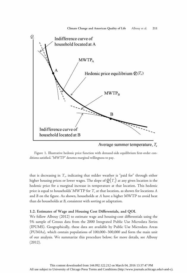
that is decreasing in Ts, indicating that milder weather is “paid for” through eitherhigher housing prices or lower wages. The slope of QðTsÞ at any given location is thehedonic price for a marginal increase in temperature at that location. This hedonicprice is equal to households’MWTP for Ts at that location, as shown for locations Aand B on the figure. As shown, households at A have a higher MWTP to avoid heatthan do households at B, consistent with sorting or adaptation.

1.2. Estimates of Wage and Housing Cost Differentials, and QOL

We follow Albouy (2012) to estimate wage and housing-cost differentials using the5% sample of Census data from the 2000 Integrated Public Use Microdata Series(IPUMS). Geographically, these data are available by Public Use Microdata Areas(PUMAs), which contain populations of 100,000–300,000 and form the main unitof our analysis. We summarize this procedure below; for more details, see Albouy(2012).

Figure 1. Illustrative hedonic price function with demand-side equilibrium first-order con-ditions satisfied. “MWTP” denotes marginal willingness to pay.



We calculate wage differentials by PUMA, wj, using the logarithm of hourly wagesfor full-time workers aged 25–55 and controlling for observable skill and occupationdifferences across workers. Specifically, we regress the log wage of worker i on PUMAindicators μw

j and extensive controls Xwi (each interacted with gender) for education,

experience, race, occupation, and industry, as well as veteran, marital, and immigrantstatus, in an equation of the form lnwij =Xw

i βw þ μw

j þ εwij . The estimates of the μwj are

used as the PUMA wage differentials wj following a refinement, per Albouy and Lue(2015), so that they reflect wages by place of work rather than place of residence,netting out differences in commuting costs.

Our model interprets the wj as the causal effect of a PUMA’s characteristics on aworker’s wage, while the observable and unobservable skill differences across work-ers, the Xw

i and εwij , are an analogue to the ϕi factors in the model. This interpreta-tion requires that any sorting of workers across locations based on unobserved skillsor a spatial match component of wages does not substantially affect observed wagepremia. This assumption receives mixed support in the literature. Glaeser and Maré(2001) and Baum-Snow and Pavan (2012) find that unobserved skill and match-based sorting contribute little to city-size wage premia; however, Gyourko, Mayer,and Sinai (2013) find that a select group of “superstar cities” may disproportionatelyattract high-skilled workers. Dahl (2002) finds that selective migration biases esti-mates of the returns to education (though not the range of returns across states), andKennan and Walker (2011) finds a role for location-specific job matches in migrationdecisions.

In light of the uncertainty in the literature, we address the potential for skill andmatch-based sorting in a series of alternative specifications. First, we adopt the methodused in Dahl (2002) to adjust our wage estimates wj for selective migration by includ-ing a flexible control function of migration probabilities in our wage equation. Second,in a closely related specification, we directly adjust our QOL estimates for each PUMAusing the PUMA’s rate of net in-migration between 1990 and 2000 (in percent) anda mobility cost estimate from Notowidigdo (2013). Finally, we guard against effectsfrom “superstar cities” by estimating a specification in which superstar metropolitanareas (as defined in Gyourko et al. [2013]) are dropped from the sample. These spec-ifications are described in more detail in section 6 and ultimately yield estimates ofclimate preferences and welfare effects that are not qualitatively different from ourbaseline estimates.

To calculate housing cost differentials, we use housing values and gross rents, in-cluding utilities. Following previous studies, we convert housing values to imputedrents at a discount rate of 7.85% (Peiser and Smith 1985) and add in utility costs tomake them comparable to gross rents. This approach follows the standard practicein the QOL literature from Blomquist, Berger, and Hoehn (1988) to Chen and Ro-senthal (2008) and is required by the data because utility costs are included in gross



rents. We then calculate housing-cost differentials with a regression of rents on flex-ible controls Yij (each interacted with renter status) for size, rooms, acreage, commer-cial use, kitchen and plumbing facilities, type and age of building, and the number ofresidents per room. This regression takes the form lnpij =Yijβ

p þ μpj þ ε pij . The esti-

mates of the μpj are then used as PUMA-level housing cost differentials pj. Proper

identification of housing-cost differences requires that they not vary systematicallywith unobserved housing quality across locations.

We incorporate energy and insulation costs in our housing-cost measure becausedoing so allows us to interpret our QOL differentials as solely reflecting the value ofnonmarket climate amenities rather than the effect of climate on utility costs. Hence,our QOL differentials will reflect the disamenity of outdoor exposure to climate andthe disamenity of adverse indoor temperatures to the extent that they are not com-pletely mitigated by insulation and energy use. In addition, the QOL estimates willincorporate any disamenity from spending more time indoors to avoid uncomfort-able outdoor temperatures.

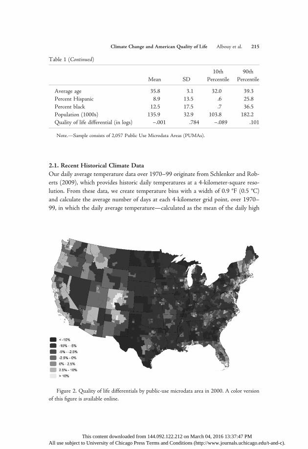
Descriptive statistics for QOL are given at the bottom of table 1,5 and QOLdifferentials across PUMAs for the year 2000 are mapped in figure 2. These esti-mates show that households find the amenities in urban areas, coastal locations, andcertain mountain areas to be quite desirable. Areas in the middle of the country, whereseasons are more extreme, tend to be less desirable, although the variation is consider-able. As discussed in Albouy (2012), our QOL estimates correlate well with noneco-nomic measures of QOL, such as the “livability” rankings in the Places Rated Almanac(Savageau 1999). Moreover, the QOL model correctly predicts the relationship be-tween housing costs and wages, controlling for observable amenities.

2. DATA

We estimate our main specifications at the PUMA level using 2,057 PUMAs cov-ering the contiguous 48 states as of the 2000 census.6 In this section, we summarizeour data set, covering recent historical climate, climate-change projections, and othervariables. Additional details are provided in appendix 2 (available online).

5. The mean QOL differential is not exactly zero in table 1 because the table shows un-weighted data, while QOL differentials are defined so that the income-weighted mean is zero.

6. We have also aggregated our data to the MSA-level and run some of our empiricalspecifications at an MSA-level resolution. The point estimates for preferences and climatechange welfare impacts are similar to those discussed below, with modestly larger standard errors(see appendix table A1.1, col. R13). We believe that the MSA-level results are less precisebecause MSAs are frequently too large to capture important micro-climates, particularly indensely populated coastal areas such as San Francisco.



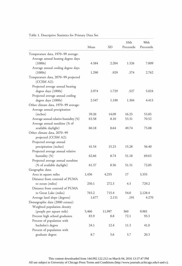
Table 1. Descriptive Statistics for Primary Data Set

Mean SD10th

Percentile90th

Percentile

Temperature data, 1970–99 average:Average annual heating degree days(1000s) 4.384 2.204 1.326 7.009

Average annual cooling degree days(1000s) 1.290 .929 .374 2.762

Temperature data, 2070–99 projected(CCSM A2):

Projected average annual heatingdegree days (1000s) 2.974 1.729 .527 5.024

Projected average annual coolingdegree days (1000s) 2.547 1.190 1.304 4.413

Other climate data, 1970–99 average:Average annual precipitation(inches) 39.26 14.09 16.25 53.85

Average annual relative humidity (%) 63.58 8.10 53.31 70.52Average annual sunshine (% ofavailable daylight) 60.18 8.64 49.74 73.08

Other climate data, 2070–99projected (CCSM A2):

Projected average annualprecipitation (inches) 41.54 15.23 15.28 56.40

Projected average annual relativehumidity (%) 62.66 8.74 51.18 69.63

Projected average annual sunshine(% of available daylight) 61.37 8.56 51.31 72.85

Geographic data:Area in square miles 1,436 4,255 17 3,355Distance from centroid of PUMAto ocean (miles) 250.1 272.3 4.3 729.2

Distance from centroid of PUMAto Great Lake (miles) 763.2 715.4 54.0 2,128.4

Average land slope (degrees) 1.677 2.131 .191 4.270Demographic data (2000 census):

Weighted population density(people per square mile) 5,466 11,997 360 9,981

Percent high school graduates 83.9 8.8 72.1 93.3Percent of population withbachelor’s degree 24.1 12.4 11.3 41.0

Percent of population withgraduate degree 8.7 5.6 3.7 20.3


2.1. Recent Historical Climate Data

Our daily average temperature data over 1970–99 originate from Schlenker and Rob-erts (2009), which provides historic daily temperatures at a 4-kilometer-square reso-lution. From these data, we create temperature bins with a width of 0.9 °F (0.5 °C)and calculate the average number of days at each 4-kilometer grid point, over 1970–99, in which the daily average temperature—calculated as the mean of the daily high

Mean SD10th

Percentile90th

Percentile

Average age 35.8 3.1 32.0 39.3Percent Hispanic 8.9 13.5 .6 25.8Percent black 12.5 17.5 .7 36.5Population (1000s) 135.9 32.9 103.8 182.2Quality of life differential (in logs) –.001 .784 –.089 .101

Note.—Sample consists of 2,057 Public Use Microdata Areas (PUMAs).

Table 1 (Continued)

Figure 2. Quality of life differentials by public-use microdata area in 2000. A color versionof this figure is available online.



and low—fell within each bin.7 Within each PUMA, we average the bin distributionat each grid point to yield a PUMA-level data set.

We obtain monthly precipitation and humidity data from the Parameter elevationRegressions on Independent Slopes Model (PRISM) at the same grid points for 1970–99, averaging them by month of year at the PUMA level. We obtain sunshine data,measured as the percentage of daylight hours for which the sun is not obscured byclouds, by month of year from 156 weather stations from the National Climactic DataCenter. We interpolate PUMA-level data on sunshine from the four closest weatherstations.8

2.2. Projected Climate Data

Predicted climate change data (temperatures, precipitation, humidity, and sunshine)are from the third release of the Community Climate System Model. These datawere also used in the Intergovernmental Panel on Climate Change AssessmentReport 4 (IPCC AR4) released in 2007. We use two business-as-usual scenarios inwhich no actions to reduce greenhouse gas emissions are taken: the A2 scenario andthe A1FI scenario. In both models, data are provided at a resolution of 1.4 degreeslongitude (120 km) by 1.4 degrees latitude (155 km), so we interpolate these data tothe PUMA level.9 The A2 scenario predicts average (population-weighted) US warm-

7. As an alternative specification, we fit a sinusoidal curve to each day’s high and lowtemperature and then find the fraction of each day that falls within each temperature bin,following Schlenker and Roberts (2009). The resulting US population-weighted average tem-perature distribution is plotted in appendix figure A1.3 and is necessarily broader than thatobtained from daily means. Figure A1.3 also presents estimated WTPs for temperature thatuse the procedure discussed in section 3 and are analogous to figure 4 (7th degree spline) andfigure 5 (panel B) in the main text. The estimated WTPs using intraday temperature varia-tion are similar to those in the main text: WTP to avoid heat is greater than WTP to avoidcold, and the WTP curves flatten at extreme temperatures. This flattening occurs at fartherextremes than in the main specification, since extreme low and high temperatures are neces-sarily lower and higher, respectively, than extreme daily mean temperatures. Figure A1.3 doesnot present an analogous distribution of future climate because our climate model data sourcedoes not provide high and low temperature information.

8. Our sunshine data are therefore not as fine scaled as the other variables in our re-gressions and may incorporate prediction error. This concern is at least partially mitigated bythe fact that variation in sunshine is smooth relative to the density of sunshine-measuringweather stations, as shown in appendix figures A2.1 and A2.2, although microclimates maynonetheless not be captured. Fine-scale variation in precipitation and humidity may help toproxy for finer changes in local sunshine, as they are strongly correlated at coarser levels ofgeography.

9. This interpolation may fail to capture localized changes, particularly in coastal areas.



ing of 7.3 °F from the baseline (1970–99) to the end of the century (2070–99), whilethe A1FI scenario predicts warming of 8.6 °F. We focus on the A2 scenario but alsoprovide results for A1FI.

Data for present and projected (A2 model) climate variables are given in the tophalf of table 1, which summarizes temperature distributions using annual heatingdegree days (HDD) and cooling degree days (CDD) statistics. HDD is a measure ofhow cold a location is: it equals the sum, over all days of the year in which it is colderthan 65 °F, of the difference between 65 °F and each day’s mean temperature. CDD,a measure of heat, is defined similarly for temperatures greater than 65 °F. HDD andCDD are often used by engineers as predictors of heating and cooling loads, andsince Graves (1979) they have often been used as measures of climate amenities.

According to the CCSM model predictions, climate change will be manifest pri-marily through changes in temperature, as seen in table 1. The average US PUMAwill see its number of HDDs fall by 32% and its number of CDDs rise by 97% un-der the A2 scenario. In contrast, changes to precipitation, relative humidity, and sun-shine are predicted to be minor on average.10 The predicted temperature changes varyconsiderably by geography, as shown in figure 3. While substantial increases in bothJanuary and July temperatures are predicted nationwide, the interior South is pre-dicted to experience a particularly large increase in days for which the average tempera-ture exceeds 90 °F.

2.3. Other Variables

Table 1 also presents data on the control variables in our econometric specifications.The geographic controls, used in all estimates, include the minimum distances fromeach PUMA’s centroid to an ocean and Great Lakes coastline, as well as the averageslope of the land, to measure hilliness. Demographic data include measures of popula-tion density,11 educational attainment, age, and racial-ethnic composition. Table A1.2in the appendix provides evidence on correlations of these geographic and demographic

10. Some areas are predicted to have appreciable changes, though these average out to besmall. Also note that our study is meant to capture the impact of precipitation on QOL, notwater supply.

11. We use population density rather than population because PUMAs are drawn to havesimilar populations. Our population density measure is “weighted” in the sense that, withineach PUMA, we calculate the population density of each of its census tracts and then take apopulation-weighted average of these densities. This weighted density gives a better senseof the population density immediately around individuals than a conventional unweightedmeasure.



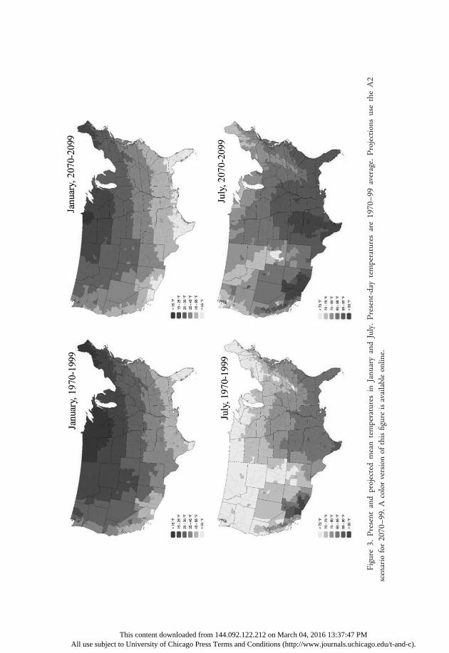
Figure

3.Present

andprojectedmeantemperaturesin

JanuaryandJuly.Present-day

temperaturesare1970–99

average.

Projections

usetheA2

scenario

for2070–99.A

colorversionof

thisfigure

isavailableonline.


control variables with HDD and CDD. Table 1 also provides statistics on the distri-bution of population across PUMAs and on the QOL measure.

3. ESTIMATION OF WTP FOR CLIMATE UNDER

HOMOGENEOUS PREFERENCES

3.1. Specification

We begin by estimating a simple hedonic model in which we assume that climatepreferences are homogeneous across the US population and that factors (includingclimate) affecting QOL enter linearly. While this model is highly restrictive, it pro-vides an intuitive introduction to our approach that resembles the previous literature,and it provides a benchmark against which we can later compare a model that allowsfor preference heterogeneity.

We estimate the impact of marginal changes to climate on QOL using an OLSregression of each PUMA j’s QOL differential Q j on vectors of climate variables Xj

and other local characteristics Dj:

Q j = βXj þ γDj þ ξ j: ð4Þ

The parameters β and γ represent the WTP of households for an additional unitof each element of Xj and Dj, respectively, measured as a fraction of income. Thedisturbance term ξj is a vertical location characteristic that is observed by householdsbut not by the econometrician. We face two substantial challenges in estimating (4).First, we must select a functional form for how the climate variables—and in partic-ular the temperature distribution—enter into Xj. Our goal is to use a form that isboth flexible and capable of providing precise estimates.12 Second, consistent estima-tion of β and γ requires that unobserved factors ξj be uncorrelated with Xj and Dj.In the absence of instrumental variables, orthogonality between ξj and Xj is a neces-sary assumption that cannot be tested. We therefore assess the reliability of our esti-mates of β by studying their sensitivity to a variety of alternative specifications. Ulti-mately, we view the estimates’ robustness across these regressions as arguing in favorof their interpretation as preference parameters, but it is important to caveat thatthese results cannot definitively rule out the presence of confounding factors.

12. We could in principle model rainfall, humidity, and sunshine as flexible distributions,as we do with temperature. We instead simply include these variables as linear regressors, fortwo reasons. First, these three variables are highly collinear even when entered linearly; al-lowing for substantial nonlinearities only exacerbates this problem. Second, we wish to focusprimarily on temperatures, given that in our climate change application only temperatureschange substantially. We have estimated a binned specification for precipitation (6 bins) andhumidity (10 bins), similar to that in Barreca (2012); this specification yields similar results tothose shown here. Results are available upon request.



We model the WTP for exposure to an additional day at temperature t, relativeto a day at 65 °F, as the function f (t).13 The temperature 65 °F is a natural nor-malization point because conventional HDD and CDD calculations treat 65 °F as a“bliss point” at which neither heating nor cooling is required. If discomfort from heatand cold, in terms of WTP, follow HDD and CDD, then f (t) is a two-piece linearfunction with the kink point at 65 °F. One of our objectives is to test whether f (t)follows this functional form.

Given our data, the most flexible possible model for f (t) would include a dummyvariable for each 0.9 °F temperature bin, in which each coefficient would signify aWTP relative to the bin containing 65 °F. This model is impractical, however, as wehave too little data to provide estimates that are precise enough to be meaningful.14

Instead, we model f (t) using cubic splines per (5)

f ðtÞ = oS

s=1

βsSsðtÞ; ð5Þ

in which S1(t) through SS(t) are standard basis functions of a cubic B-spline of degreeS. We space the knots of the basis functions evenly on the cumulative distributionfunction of the population-weighted average temperature distribution.15 This spacing,rather than even spacing over the unweighted temperature support, clusters the nodesin the center of the distribution where the data are richest, improving flexibility in thisregion.

13. This specification, under homogeneous preferences, disallows nonlinear effects of heator cold, in which the WTP to avoid an additional day of extreme temperature increases withthe number of days of extreme temperatures. It also disallows a preference for “seasonality,”which would be manifest as a lower WTP to avoid heat (cold) in a location with severe win-ters (summers). Nonlinear effects and preferences for seasonality are, however, captured byour heterogeneous preference specification, which allows the MWTP for any temperature binto vary with the distribution of realized temperatures. We find that sorting and adaptationeffects outweigh nonlinear damage effects, as discussed in section 4 (especially for cold weather;see panels A and B of fig. 6). Overall, we do not find consistent evidence of a preference forseasons, as shown in appendix figure A1.1, which plots the MWTP for 40 °F and 80 °Fas functions of CDD and HDD. These plots should slope upward when households preferseasons.

14. We have experimented with wider bins and found that bins approximately 10 °F wideare necessary for reasonable precision. In table A1.1 in theappendix, column R12 shows thatsuch a binned specification yields similar qualitative results to those discussed below. The binnedWTPs are plotted in appendix figure A1.8. We find the continuous splines more appealingbecause we do not believe that human comfort changes discontinuously every 10 degrees.

15. The support of the contiguous US temperature distribution ranges from –39.1 °F to111.2 °F, covering 167 0.9 °F bins. For a cubic spline of degree S, there are S – 2 nodes, in-cluding the nodes at the endpoints. In the 7th degree cubic spline that we ultimately focus on,the three interior nodes are located at 44.15, 58.55, and 71.15 °F (these temperatures are thecenters of the relevant bins).



Defining Njt as the average number of days per year at location j for which theaverage temperature is between t and t + 0.9, we flexibly estimate climate preferencesby substituting into (4) the product of the spline function in (5) with Njt, summedover all temperature bins:

Q j = ot

Njt f ðtÞ þ βrRainj þ βhHumidj þ βsSunj þ γ˙Dj þ ξ j

= oS

s = 1

βs

�ot

NjtSsðtÞ�þ βrRainj þ βhHumidj þ βsSunj þ γ˙Dj þ ξ j:

ð6Þ

As a reference case, we include in Dj the “full set” of both geographic and demo-graphic controls described above. In all of our regressions, we weight each PUMA(observation) by its population.16 For inference, we use standard errors that are clus-tered to allow for arbitrary spatial correlation of residuals across PUMAs within eachstate (Arellano 1987; Wooldridge 2003).17

3.2. Homogeneous Preference WTP Estimates

Estimating the Shape of f (t)

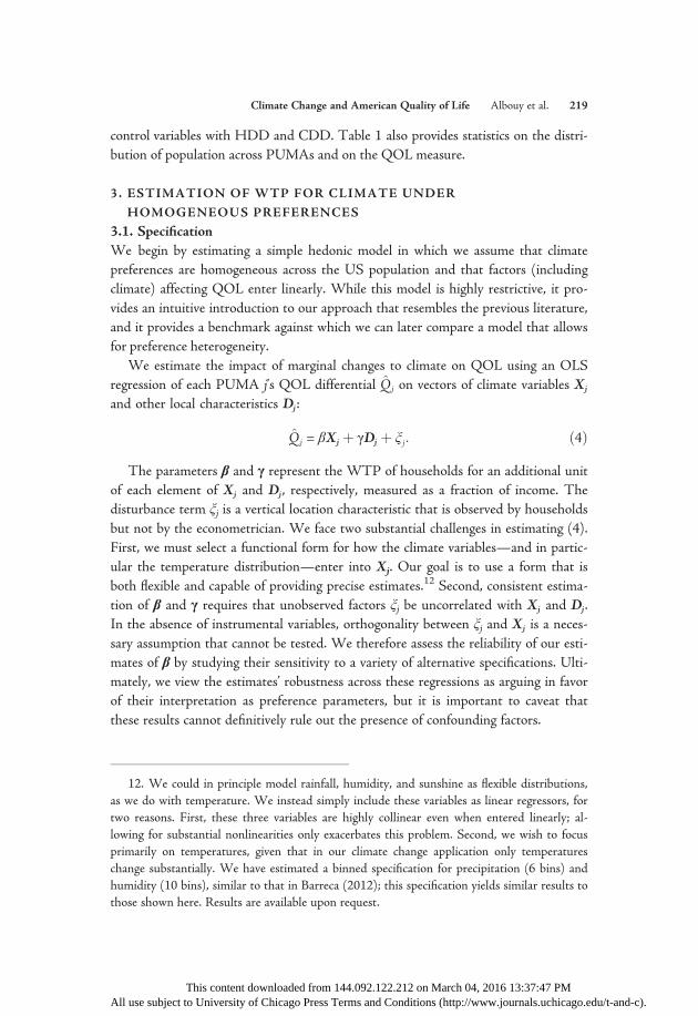
Figure 4 presents our estimates of f (t) using 5th through 10th degree splines, givenour reference case controls described in section 3.1. In each panel, the plotted esti-mate of the f(t) curve is the MWTP for a day at temperature t rather than a day at65 °F, measured as a fraction of income. Each panel also depicts, for reference, thepresent and future (2070–99, A2 scenario) US population-weighted average tempera-ture distributions. While the 5th degree spline appears too restrictive, and the 10th de-gree too noisy, several regularities emerge from the set of plots. First, the WTP curvesconsistently have an interior maximum near 65 °F. We view this result—which isdriven by the data and not “forced” by our QOL variable or functional form—as animportant validation of our model and empirical strategy, since it accords with theintuition underlying HDD and CDD that WTP is maximized at 65 °F. Second,there are too few days with average temperatures over 90 °F to permit precise infer-ence over this range, as evinced by the extremely wide standard error bands. Third, itappears that WTP departs nonlinearly away from 65 °F, undermining the restrictionfrom the HDD/CDD model that f (t) is linear. In particular, the slopes of the WTP

16. As shown in appendix table A1.1, column R11, this weighting does not materiallyaffect the estimates.

17. We have also experimented with clustering at the MSA level (in which PUMAs thatare not part of an MSA are clustered within each state) and census division level. These ap-proaches lead to estimated standard errors that are only slightly smaller and larger, respectively,than those presented here. When clustering on census divisions (of which there are nine) weuse the cluster wild bootstrap to improve small sample performance (Cameron, Gelbach, andMiller 2008). This specification is displayed in column R14 of appendix table A1.1.



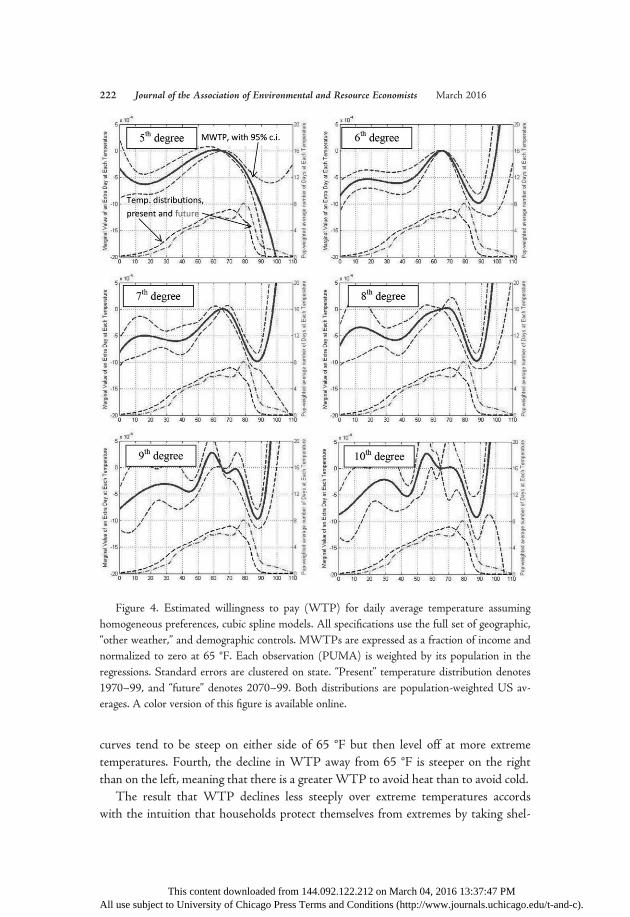
curves tend to be steep on either side of 65 °F but then level off at more extremetemperatures. Fourth, the decline in WTP away from 65 °F is steeper on the rightthan on the left, meaning that there is a greaterWTP to avoid heat than to avoid cold.

The result that WTP declines less steeply over extreme temperatures accordswith the intuition that households protect themselves from extremes by taking shel-

Figure 4. Estimated willingness to pay (WTP) for daily average temperature assuminghomogeneous preferences, cubic spline models. All specifications use the full set of geographic,“other weather,” and demographic controls. MWTPs are expressed as a fraction of income andnormalized to zero at 65 °F. Each observation (PUMA) is weighted by its population in theregressions. Standard errors are clustered on state. “Present” temperature distribution denotes1970–99, and “future” denotes 2070–99. Both distributions are population-weighted US av-erages. A color version of this figure is available online.



ter in climate-controlled environments. Once the temperature is sufficiently uncom-fortable that households spend little time outside, further increases in extreme tem-perature are less important. This result is consistent with research by Graff Zivin andNeidell (2012) that uses time-diary data to show that households spend less timeoutside in cold or hot weather.

The result that, on the margin, increases in heat are worse than increases in coldalso follows intuition. Individuals can adapt to cold by wearing more clothing. How-ever, options for thermoregulation are more limited in hot conditions.

The imprecision of our estimates at the extremes of the temperature distributioninhibit the ability of spline-estimated WTP functions to inform the welfare effects ofclimate change. This is true especially at the high end: days with average (not just high)temperatures exceeding 90 °F are rare at present but common in climate change pro-jections. To address this issue, we examine two functional forms that maintain flexibil-ity in the interior of the temperature distribution while projecting WTP at the farextremes.18 The first is a restricted 7th degree cubic spline, with WTP assumed to beconstant over the extreme 1% of realized temperatures.19 The second is a four-piecelinear spline, with kink points at 45 °F, 65 °F, and 80 °F, allowing for a projectionof decreasing WTP over extreme temperatures.20 This second specification permitsmore straightforward hypothesis testing of how WTP changes over the temperaturedistribution.

Panels A and B of figure 5, and columns I and II of table 2, present results for bothspecifications, controlling for both geography and demographics. The point estimatesin table 2 can be interpreted as the WTP for each characteristic. In both specifica-tions, WTP declines more steeply as temperatures increase away from 65 °F than asthey decrease from 65 °F. With the linear spline, we reject a null hypothesis that the

18. We are not the first to confront the issue of conducting inference at temperatures nearand beyond the limit of what is realized in present-day data. Prior work in the crop yield andhealth literatures has assumed that the damage function is constant beyond the point at whichinference is no longer feasible (Deschênes and Greenstone 2007, 2011; Schlenker and Roberts2009). The first of our two restricted specifications—a 7th degree cubic spline with a restric-tion that MWTP is constant at the extremes—accords with this prior practice.

19. Specifically, we impose constant WTP over the bottom 0.5% and top 0.5% of thepopulation-weighted temperature distribution, covering temperatures less than 4.1 °F andgreater than 87.8 °F. We apply this imposition after estimating the full 7th degree splinerather than beforehand, as reversing the order leads to unstable estimates at the cutoff points.We focus on a 7th degree spline because it visually appears to strike a balance between flex-ibility and precision. Using 6th or 8th degree splines instead does not substantially affect theresults.

20. The choices of 45 °F and 80 °F tend to yield the best fit to the data (per R2) in mostspecifications. Alternative choices such as 50 °F or 75 °F do not substantially affect the pref-erence or welfare estimates.



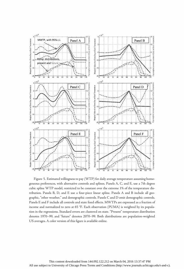
Figure 5. Estimated willingness to pay (WTP) for daily average temperature assuming homo-geneous preferences, with alternative controls and splines. Panels A, C, and E, use a 7th degreecubic spline WTP model, restricted to be constant over the extreme 1% of the temperature dis-tribution. Panels B, D, and E use a four-piece linear spline. Panels A and B include all geo-graphic, “other weather,” and demographic controls. Panels C and D omit demographic controls.Panels E and F include all controls and state fixed effects. MWTPs are expressed as a fraction ofincome and normalized to zero at 65 °F. Each observation (PUMA) is weighted by its popula-tion in the regressions. Standard errors are clustered on state. “Present” temperature distributiondenotes 1970–99, and “future” denotes 2070–99. Both distributions are population-weightedUS averages. A color version of this figure is available online.


magnitudes of the slopes on either side of 65 °F are equal with a p-value of .001. Bothsplines exhibit flatter slopes over the extremes than over the center of the distribution,particularly on the cold side of 65 °F. For the linear spline, the change in slope at the45 °F kink point is statistically significant (p = .005), although the change in slope at80 °F is not (p = .523).

Thus, while we have some confidence in the result that extreme cold is not sub-stantially more disamenable than moderate cold, the lack of statistical power over ex-tremely hot days means that we are less confident in saying that about extreme ver-sus moderate heat.21 The restricted cubic and linear spline specifications can thereforebe viewed as two plausible alternatives. The former is conservative in assessing theWTP to avoid extreme heat because it assumes that WTP is constant over this range,whereas the linear spline model is more aggressive as it extrapolates the (negative)slope of theWTP function outside of the observed temperature range.

Nontemperature Climate Variables, Controls, and Robustness

The results in columns I and II of table 2 indicate that households have a strongpreference for sunshine, a mild preference for precipitation, and no statistically signif-icant taste for humidity. Due to multi-collinearity, it is difficult to disentangle pref-erences for these three climate variables: locations that are very sunny also tend to bedry and nonhumid. Among the geographic control variables, we estimate strong tastesfor hilliness (average land slope), a taste for proximity to the ocean, but no strongpreference for proximity to a Great Lake. The estimated coefficients on the demo-graphic control variables indicate that QOL increases with population density, educa-tional attainment, average age, and percentage Hispanic, while it decreases in percent-age black.

The demographic controls may themselves be endogenous, as demographic groupsmay have different tastes and sort accordingly.22 These variables may also introducean “overcontrolling” problem if they are, at least in part, determined by climate. Thatsaid, we believe that the benefits of controlling for demographics outweigh the costs.

21. The linear spline projection is sufficiently imprecise to the right of 80 °F that we alsocannot reject the hypothesis that WTP is constant over this range (p = .117).

22. The coefficient on population density is particularly difficult to interpret, since it cap-tures unobserved amenities that come with population density (e.g., culture and restaurants) aswell as idiosyncratic household-specific valuations of a location. The former drives the coeffi-cient on population density upward, while the latter drives it downward (because the cost ofliving must fall [or wages must rise] to attract additional households). Empirically, the amenityaspects of population density appear to dominate, since we estimate a positive coefficient on thisvariable. Our estimated WTP for climate is robust to excluding population density from thespecification. In section 6, we discuss the related issue of adjusting our QOL measure to ac-count for changes in population between 1990 and 2000.



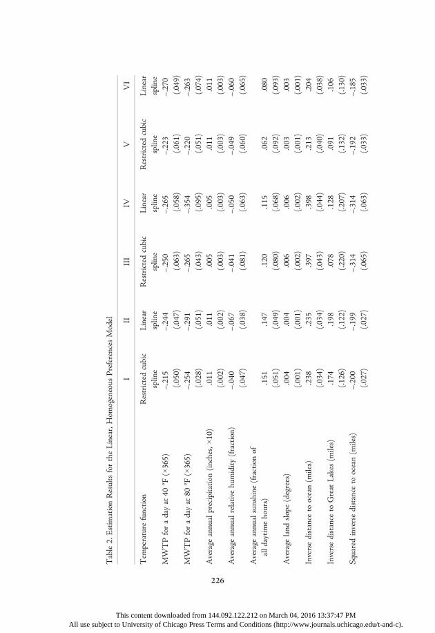
Table2.

EstimationResultsfortheLinear,H

omogeneous

Preferences

Model

III

III

IVV

VI

Tem

perature

functio

nRestrictedcubic

spline

Linear

spline

Restrictedcubic

spline

Linear

spline

Restrictedcubic

spline

Linear

spline

MW

TPforadayat

40°F

(×365)

–.215

–.244

–.250

–.265

–.223

–.270

(.050)

(.047)

(.063)

(.058)

(.061)

(.049)

MW

TPforadayat

80°F

(×365)

–.254

–.291

–.265

–.354

–.220

–.263

(.028)

(.051)

(.043)

(.095)

(.051)

(.074)

Average

annualprecipitatio

n(inches,×10)

.011

.011

.005

.005

.011

.011

(.002)

(.002)

(.003)

(.003)

(.003)

(.003)

Average

annualrelativehu

midity

(fraction)

–.040

–.067

–.041

–.050

–.049

–.060

(.047)

(.038)

(.081)

(.063)

(.060)

(.065)

Average

annualsunshine

(fractionof

alld

aytim

ehours)

.151

.147

.120

.115

.062

.080

(.051)

(.049)

(.080)

(.068)

(.092)

(.093)

Average

land

slope(degrees)

.004

.004

.006

.006

.003

.003

(.001)

(.001)

(.002)

(.002)

(.001)

(.001)

Inversedistance

toocean(m

iles)

.238

.235

.397

.398

.213

.204

(.034)

(.034)

(.043)

(.044)

(.040)

(.038)

Inversedistance

toGreat

Lakes(m

iles)

.174

.198

.078

.128

.091

.106

(.126)

(.122)

(.220)

(.207)

(.132)

(.130)

Squaredinversedistance

toocean(m

iles)

–.200

–.199

–.314

–.314

–.192

–.185

(.027)

(.027)

(.065)

(.063)

(.033)

(.033)

226


Squaredinversedistance

toGreat

Lakes

(miles)

–.158

–.186

.051

–.006

–.088

–.103

(.140)

(.134)

(.240)

(.221)

(.146)

(.144)

Logof

weightedpopulatio

ndensity

.006

.007

...

...

.003

.004

(.003)

(.003)

(.002)

(.002)

Fractio

nhigh

school

graduates

.156

.154

...

...

.134

.131

(.048)

(.046)

(.045)

(.043)

Fractio

nbachelor’sdegrees

.314

.298

...

...

.338

.341

(.059)

(.063)

(.058)

(.059)

Fractio

ngraduate

degrees

–.011

.019

...

...

–.027

–.032

(.095)

(.105)

(.091)

(.095)

Average

age(×100)

.204

.204

...

...

.220

.209

(.040)

(.039)

(.033)

(.036)

Fractio

nHispanic

.089

.082

...

...

.092

.089

(.033)

(.035)

(.027)

(.028)

Fractio

nblack

–.064

–.068

...

...

–.057

–.060

(.008)

(.008)

(.009)

(.008)

Statefixedeffects

NN

NN

YY

Num

berof

observations

2,057

2,057

2,057

2,057

2,057

2,057

R2

.798

.796

.386

.382

.830

.830

Note.—Dependent

variableisquality

oflife(Q

OL)

differentialasfractio

nof

income.The

unitof

observationisaPUMA.A

llregressionsareweightedby

populatio

nin

each

PUMA.T

helinearsplines

arefour

piecewith

breakpointsat45

°F,65°F,and

80°F,and

therestricted

cubicsplineis7thdegree

with

aconstant

MW

TPrestrictionfor

thelower

andupper1%

ofthepopulatio

n-weightedUSaveragetemperature

distributio

n.MW

TPsshow

nforadayat40

°For

80°F

arerelativeto

65°F

andexpressedas

afractio

nof

income.Parentheticalvalues

indicatestandard

errorsclusteredon

state.

227


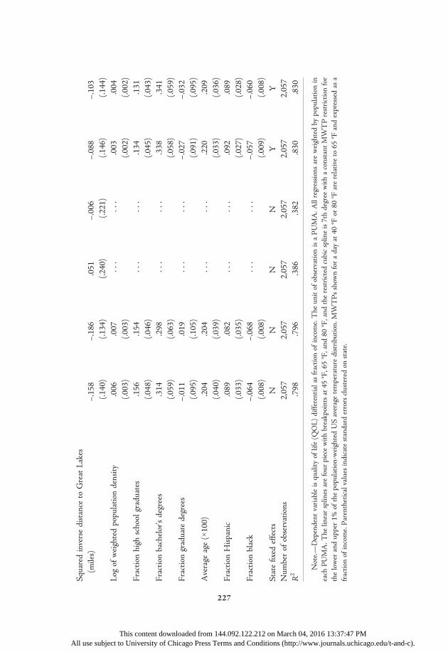
First, their inclusion substantially improves the precision of the estimated WTP forclimate. Panels C and D in figure 5, and columns III and IV of table 2, present esti-mates of specifications that do not include the demographic variables. These speci-fications have notably wider WTP confidence intervals and less than one-half the R2

of those that include demographics (using the cubic spline model, the standard errorson the estimated MWTPs for days at 40 °F and 80 °F are 26% and 55% larger, re-spectively, when the demographic controls are excluded). Second, including demo-graphic variables helps guard against omitted variables bias and, in this case, providesevidence that such bias may not be a substantial concern. Although the demographicvariables are powerful correlates of QOL, as evidenced by their large effect on R2,they have only a modest effect on the estimated WTPs for the climate variables. Nor,as we discuss in section 5, do they substantially affect our estimates of the welfareimpact of climate change. We obtain these results despite evidence of some correla-tion of the demographic covariates—especially the percentage of high school graduatesand the percentages of minorities—with warm weather, as shown in table A1.2.23

Overall, following the logic of Altonji et al. (2005), our results suggest that if unob-served demographics substantially bias our climate preference and welfare estimates,they would have to be more strongly correlated with climate than the “headline” ob-servable demographics included in our regressions.24

Specifications that include state fixed effects (FE) along with demographics areexamined in figure 5 panels E and F, and columns V and VI of table 2.25 These spec-ifications rely solely on within-state variation in climate for identification. Despite

23. As an additional robustness check, we have found that adding squared terms of thedemographic variables does not substantially affect the results. See table A1.1, column R9. Itmay be that the semiparametric temperature functions we use are less susceptible to the rawcorrelations shown in table A1.2, or that the partial correlations after controlling for theother weather variables and geographic controls are relatively small. We have also controlledfor public spending on parks (though data are available for only 1,970 PUMAs) and foundthat these controls do not qualitatively affect our estimates.

24. In other settings for hedonic studies—for example, measurements of the WTP forclean air—it has been shown that estimates are sensitive to the inclusion or exclusion ofdemographic controls (see, e.g., Chay and Greenstone 2005). In such cases, the source ofbias is often intuitive. For example, emitters of pollutants are often concentrated in industrialareas that tend to be populated by lower-income households. With regard to climate, how-ever, a source of omitted variable bias from demographics is less obvious ex ante because awide range of demographic groups and urban vs. rural locations can be found in essentiallyevery climate zone. Our result that adding demographic variables to the specification doesnot substantially affect the estimated WTP for climate accords with this intuition.

25. As shown in appendix table A1.1, specification R10, using census division fixedeffects rather than state fixed effects does not result in a substantial difference relative to thenon-FE estimate.



this substantial change in identifying variation, we still find in panel E that WTP ismaximized near 65 °F. The inclusion of state FE does result in a loss of precision andan increase in the estimated WTP to avoid cold. This increase may arise from the factthat the statistical power of the FE estimates comes from large, populous states with alarge number of PUMAs and a broad range of climates. Thus, states like Californiaand Texas are more influential than states in the Northeast and Midwest. If resi-dents of these large, warm states have sorted because they are more averse to cold—apossibility consistent with our findings in section 4—this may explain the differencebetween the FE and non-FE estimators. Nonetheless, the estimated WTP to avoidcold remains smaller than the estimated WTP to avoid heat, though this difference isno longer statistically significant. The estimates are sufficiently imprecise that the stateFE estimates are not statistically significantly different than those without FE.26

Estimated preferences derived from additional alternative specifications are pre-sented in appendix table A1.1. These regressions explore alternative control variables,specifications for f(t), subsamples of the data (e.g., omitting superstar cities), and weight-ing schemes. This table also provides estimated impacts of climate change on amenityvalues and estimates that allow for preference heterogeneity, as discussed below. Over-all, our conclusions do not qualitatively change across these specifications.

4. ESTIMATION OF WTP FOR CLIMATE WITH

HETEROGENEOUS PREFERENCES

4.1. Empirical Strategy

Section 3 and prior work on climate amenity valuation has assumed that householdsshare homogeneous preferences for climate. Here, we relax this assumption and al-low households to sort into locations that suit their preferences (noting that hetero-geneity may also reflect households’ adaptation to their local climate). Estimationunder these more relaxed conditions is based on the framework developed by Bajariand Benkard (2005) and applied by Bajari and Kahn (2005). The intuition of thisapproach lies in the first-order condition of equation (3) and is illustrated in figure 1,

26. We test the null hypothesis that the state FE are uncorrelated with the climatevariables via block wild bootstrapping, clustering on state (200 repetitions). For each draw, weestimate preferences both with and without state FE. We then use all draws to obtain astandard deviation of the difference between the estimators. This procedure, unlike a tradi-tional Hausman test, does not require that the non-FE estimator be efficient (see Cameronand Trivedi 2005, 718). We find that we cannot reject equality of the WTP for 40 °F acrossthe estimators (the p-values are .858 for the cubic spline and .603 for the linear spline) norequality of the WTP for 80 °F (the p-values are .445 for the cubic spline and .560 for thelinear spline). We do, however, marginally reject equality of the welfare impact of climatechange across the two estimators (the p-values are .086 for the cubic spline and .076 for thelinear spline).



which depicts an equilibrium in which the only characteristic is average summertemperature, Ts. Given a nonlinear hedonic price function QðZj; ξ jÞ, the MWTP ofhouseholds located at j for a characteristic k (e.g., a day in a given temperature bin)is simply given by ∂QðZj; ξ jÞ=∂Zk. Thus, flexible estimation of QðZj; ξ jÞ allows us torecover the distribution of MWTP for each characteristic k across the population ofhouseholds. In figure 1, for example, the depicted equilibrium is consistent with pos-itive sorting in which households with a high MWTP to avoid heat settle in areas withlow summer temperatures. In contrast, a concave equilibrium price function would re-flect nonlinear damages from heat, so that the MWTP to avoid heat would be greaterfor hot locations than for mild locations.

To flexibly estimate QðZj; ξ jÞ, we use local linear regression per Fan and Gijbels(1996). We suppose that, local to location j*, QðZj; ξ jÞ satisfies (7):

Q j = ok

β j�k Zjk þ ξ j: ð7Þ

In (7), the implicit prices β are superscripted by j*, as we estimate a distinct set ofprices at each location. We obtain the β j� at each location via weighted least squaresper (8) and (9):

β j� = arg minβðbQ – ZβÞ0WðbQ –ZβÞ ð8Þ

bQ = bQj

h i;Z = Zj

� �;W = diag KhðZj –Zj�Þ

� �; ð9Þ

where W is a matrix of kernel weights defined so that locations that are similar to j*in characteristics receive the most weight in the regression.27 This approach allowshouseholds in relatively hot or cold locations to have different MWTPs to avoid de-partures from mild climates. To calculate W, we use a normal kernel function witha bandwidth h of 2, per (10) and (11) below.28 The term σk denotes the standarddeviation of characteristic k across the sample:

27. In principle, W can include every characteristic in the model, so that preferences canvary in the cross-section not only with the climate variables but also with the controls. Inpractice, however, we include only the temperature spline basis functions in W, since includingthe controls requires a very large bandwidth in order to avoid collinearity in the weightedcovariate matrix. In addition, when implementing our procedure with the restricted 7th degreespline specifications, we only include a 5th degree cubic spline in W. Including the full 7thdegree cubic spline in W results in very noisy estimates of temperature preferences at extremelocations (such as northwest Minnesota) that have few neighbors in climate space.

28. We follow Bajari and Benkard (2005) and Bajari and Kahn (2005) in choosing a normalkernel and in choosing a bandwidth that yields visually appealing preference estimates, in thesense that estimated MWTP varies smoothly over characteristics space (as in fig. 6). In contrast,using leave-one-out cross-validation we find an “optimal” bandwidth of 0.22 in the cubic splinepreference specification. This small bandwidth leads to very noisy and imprecise preference



KðZÞ = ∏k

NðZk=σkÞ ð10Þ

KhðZÞ =KðZ=hÞ=h: ð11Þ

Ideally, our estimator would allow for heterogeneity in households’ MWTP forall local characteristics, not just the temperature profiles. Were the choice set contin-uous in characteristics, point identification of preferences for all characteristics ateach location would indeed be possible. In our setting, however, there is a discretenumber of 2,057 PUMAs, which implies that households’ preferences are only setidentified. That is, there is a range of MWTPs such that each household wouldprefer to stay in its PUMA rather than move. We study these identified sets using aGibbs sampling method per Bajari and Benkard (2005) and find that they are oftenlarge enough to be uninformative when households are permitted to have heteroge-neous preferences over all characteristics (including the control variables).29 Our mainspecifications therefore maintain the restriction that households share a homogeneousMWTP for nontemperature characteristics.30 With this restriction, we find that theidentified sets of MWTPs for temperature are sufficiently small to closely approxi-mate point identification. The results presented below therefore follow Bajari andKahn (2005) in treating MWTP as point identified at each location. Appendix 4 pre-sents set identified estimates and discusses our set identification procedure in detail.

Finally, we emphasize that we only identify the MWTP of each household foreach temperature at its chosen climate and cannot identify its WTP for a large changein climate, over which MWTP may vary. In figure 1, for instance, the MWTPs atlocations A and B are identified, but the shapes of the indifference curves are not.Estimating the welfare impacts from nonmarginal changes in climate therefore requiresassuming a functional form for households’ utility. We focus on welfare estimates thatassume the indifference curves are linear, with a slope equal to the estimated MWTP.This approach is transparent, permits an apples-to-apples comparison to the homoge-neous preference estimates, and is conservative: allowing for concavity would unambig-

estimates as well as an extremely large estimated amenity loss from climate change (18.5% ofincome under the A2 scenario). In general, the estimated amenity loss increases as the band-width becomes smaller, so our bandwidth choice of 2 is conservative.

29. Bajari and Benkard (2005) find similar results when the number of parameters overwhich preferences may be heterogeneous is permitted to increase, relative to a fixed choice set.

30. Prior to running the local linear regression, we enforce preference homogeneity overthe nontemperature variables by stripping their effects from Q using the OLS estimates fromsection 3 (this approach follows an example given in Bajari and Benkard [2005]). Thus, theonly characteristics involved in the local linear regression are the temperature spline basisfunctions.



uously increase the estimated amenity losses, as the cost of each additional hot daywould rise (and the benefit from each reduction in cold days would fall).

The assumption that households’ utility functions are linear in characteristics cre-ates the problem, however, that the second-order condition for utility maximizationmay not hold if the hedonic price function is not globally convex. Because we ulti-mately find that the QðZj; ξ jÞ function is slightly concave in some dimensions, wehave studied a specification in which households’ utility functions are sufficientlyconcave that their utility is maximized at their present location. Our procedure forestimating this specification is discussed in appendix 3. We find that allowing forconcavity in the utility function increases the estimated losses from climate changeby roughly 0.4 percentage points relative to the results given in section 5 (for thecubic spline model in col. I of tables 3 and 4).

4.2. Heterogeneous Preference MWTP Estimates

Estimated MWTPs for temperature by PUMA are graphed in figure 6: panels Aand C from the restricted cubic spline, panels B and D from the linear spline, allcontrolling for geography and demography, but not state FE. Panels A and B presentthe distribution of MWTP, scaled up by 365, for an additional day at 40 °F relativeto a day at 65 °F, as a function of HDD. Each of the plotted points represents thepreferences of a specific PUMA in the data. The strong upward slope in both panelsindicates that households with the most negative MWTP for cold weather tend to belocated in areas with the fewest HDDs (the reduction in the MWTPs’ magnitudesnear zero HDD or CDD may simply reflect large confidence intervals; see standarddeviations for the MWTP estimates in appendix fig. A1.6). This result is consistentboth with households sorting based on their aversion to cold and with adaptation tocold climates. Panels C and D, in contrast, examine the MWTP for an additional dayat 80 °F as a function of CDD. Panel C, which uses the restricted cubic spline model,exhibits a weak downward slope, consistent with residents of hot areas being more heataverse on the margin and indicating mild concavity in households’ utility functionsrather than sorting. This result also suggests that households have only a limited abilityto adapt to heat, relative to their ability to adapt to cold. The linear spline model inPanel D, however, indicates a positive slope, suggestive of some sorting on willingnessto avoid heat, though the overall heterogeneity in MWTP is still smaller than that forthe willingness to avoid cold.

An alternative depiction of heterogeneous climate preferences is given in appendixfigure A1.2. This figure plots MWTP curves under the cubic spline model at a fewselect cities. Beyond showing that the magnitude of households’ MWTP to avoidcold is negatively correlated with the amount of cold they face, this figure also showsthat the estimated maximum of the MWTP function occurs at slightly higher tem-peratures in warmer locations, again consistent with sorting based on aversion tocold or with adaptation.



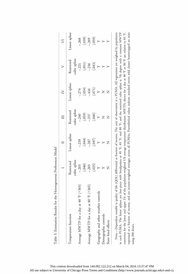
Table3.

EstimationResultsfortheHeterogeneous

Preferences

Model

III

III

IVV

VI

Tem

perature

functio

nRestricted

cubicspline

Linear

spline

Restricted

cubicspline

Linearspline

Restricted

cubicspline

Linear

spline

Average

MW

TPforadayat

40°F

(×365)

–.203

–.239

–.240

–.274

–.221

–.268

(.046)

(.044)

(.059)

(.054)

(.051)

(.039)

Average

MW

TPforadayat

80°F

(×365)

–.265

–.287

–.337

–.416

–.236

–.269

(.025)

(.047)

(.046)

(.071)

(.043)

(.059)

Geography

andotherweather

controls

YY

YY

YY

Dem

ographiccontrols

YY

NN

YY

Statefixedeffects

NN

NN

YY

Note.—Dependent

variableisquality

oflife(Q

OL)

differentialas

fractio

nof

income.The

unitof

observationisaPUMA.A

llregressionsareweightedby

populatio

nin

each

PUMA.The

linearsplines

arefour-piece

with

breakpointsat

45°F,65

°F,and80

°F,andtherestricted

cubicsplineis7thdegree

with

aconstant

MW

TP

restrictionforthelower

andupper1%

ofthepopulatio


distributio

n.MW

TPsshow

nforadayat

40°F

or80

°Farerelativeto

65°F,

expressedas

afractio

nof

income,

andareincome-weightedaverages

across

allPUMAs.Parenthetical

values

indicate

standard

errors

wild

clusterbootstrapped

onstate

using200draw

s.


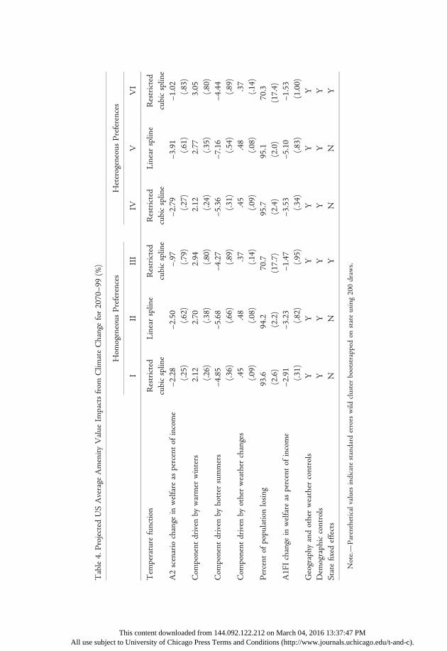
Table4.

Projected

USAverage

Amenity

Value

Impactsfrom

Clim

ateChangefor2070–99

(%)

Hom

ogeneous

Preferences

Heterogeneous

Preferences

III

III

IVV

VI

Tem

perature

functio

nRestricted

cubicspline

Linear

spline

Restricted

cubicspline

Restricted

cubicspline

Linearspline

Restricted

cubicspline

A2scenario

change

inwelfare

aspercentof

income

–2.28

–2.50

–.97

–2.79

–3.91

–1.02

(.25)

(.62)

(.79)

(.27)

(.61)

(.83)

Com

ponent

driven

bywarmer

winters

2.12

2.70

2.94

2.12

2.77

3.05

(.26)

(.38)

(.80)

(.24)

(.35)

(.80)

Com

ponent

driven

byhotter

summers

–4.85

–5.68

–4.27

–5.36

–7.16

–4.44

(.36)

(.66)

(.89)

(.31)

(.54)

(.89)

Com

ponent

driven

byotherweather

changes

.45

.48

.37

.45

.48

.37

(.09)

(.08)

(.14)

(.09)

(.08)

(.14)

Percent

ofpopulatio

nlosing

93.6

94.2

70.7

95.7

95.1

70.3

(2.6)

(2.2)

(17.7)

(2.4)

(2.0)

(17.4)

A1F

Ichange

inwelfare

aspercentof

income

–2.91

–3.23

–1.47

–3.53

–5.10

–1.53

(.31)

(.82)

(.95)

(.34)

(.83)

(1.00)

Geography

andotherweather

controls

YY

YY

YY

Dem

ographiccontrols

YY

YY

YY

Statefixedeffects

NN

YN

NY

Note.—Parentheticalvalues

indicate

standard

errorswild

clusterbootstrapped

onstateusing200draw

s.


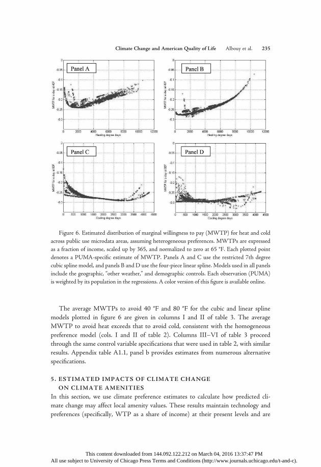
The average MWTPs to avoid 40 °F and 80 °F for the cubic and linear splinemodels plotted in figure 6 are given in columns I and II of table 3. The averageMWTP to avoid heat exceeds that to avoid cold, consistent with the homogeneouspreference model (cols. I and II of table 2). Columns III–VI of table 3 proceedthrough the same control variable specifications that were used in table 2, with similarresults. Appendix table A1.1, panel b provides estimates from numerous alternativespecifications.

5. ESTIMATED IMPACTS OF CLIMATE CHANGE

ON CLIMATE AMENITIES

In this section, we use climate preference estimates to calculate how predicted cli-mate change may affect local amenity values. These results maintain technology andpreferences (specifically, WTP as a share of income) at their present levels and are

Figure 6. Estimated distribution of marginal willingness to pay (MWTP) for heat and coldacross public use microdata areas, assuming heterogeneous preferences. MWTPs are expressedas a fraction of income, scaled up by 365, and normalized to zero at 65 °F. Each plotted pointdenotes a PUMA-specific estimate of MWTP. Panels A and C use the restricted 7th degreecubic spline model, and panels B and D use the four-piece linear spline. Models used in all panelsinclude the geographic, “other weather,” and demographic controls. Each observation (PUMA)is weighted by its population in the regressions. A color version of this figure is available online.



best interpreted as welfare impacts that would occur if changes predicted for the endof the century were to occur now, allowing for spatial adaptation (e.g., households inthe North adopting southern behaviors and levels of air conditioning penetration) tooccur instantly.

We focus first on the reference case model I from table 2, using the restricted cubicspline under homogeneous preferences, with projections from the A2 scenario for2070–99. Table 4 displays estimated changes in welfare for this specification (col. I)and several variants. We project a net welfare loss of 2.28% of personal income, or$195 billion per year (in year 2000 dollars),31 from decreased amenity value of cli-mate. This loss is driven by the result that the WTP to avoid heat exceeds the WTPto avoid cold, so that the welfare loss from hotter summers of –4.85% exceeds the gainfrom warmer winters of 2.12%. These temperature-driven welfare losses are slightlyoffset by increases in amenities from the small predicted changes to precipitation,humidity, and sunshine. Results from the linear spline in column II predict slightlyhigher welfare costs, with higher benefits from warmer winters and greater costs fromhotter summers. Finally, the bottom row of table 4 presents welfare impacts under thealternative A1FI scenario, which predicts more extreme changes in temperature. Thisscenario results in larger welfare effects from milder winters and hotter summers, sothat net welfare losses are roughly 3% of total income.

The geographic distributions of welfare changes for the restricted cubic and linearspline specifications are shown in panels A and B of figure 7. Both maps show a fewareas in the Pacific Northwest, northern Michigan, and the upper Northeast—accounting for about 6% of the population—for which we forecast a minor improve-ment. The rest of the US population will experience losses. These are especially se-vere in the Southeast and Southwest: some areas in Florida, Louisiana, Texas, andCalifornia have expected losses greater than 4% of income. Much of the country, asfar north as the Dakotas, is expected to experience substantial losses as they lose manydays with moderate temperatures, which we estimate are highly valued.

The predictions of the two estimated temperature functions agree less in the centerof the country, where the restricted cubic spline predicts relatively small losses. Thisresult occurs because summer temperatures in this area are already sufficiently hotthat residents are on the flat portion of the WTP curve. In contrast, the linear splinepredicts relatively large welfare losses, as already hot summer days become hotter.These predictions are imprecise as the historical climate record offers too few ex-tremely hot days to allow a precise claim about WTP over such extreme heat.

Appendix table A1.1 presents estimates of amenity losses from several other alter-native specifications with varying control structures, generally finding similar results,

31. The dollar figure is based on year 2000 total personal income of $8.576 trillion inthe 48 contiguous states.



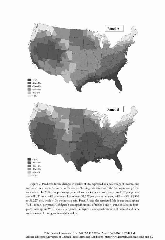
Figure 7. Predicted future changes in quality of life, expressed as a percentage of income, dueto climate amenities. A2 scenario for 2070–99, using estimates from the homogeneous prefer-ence model. In 2014, one percentage point of average income corresponded to $307 per personannually. Thus < –4% connotes a loss of over $1,227 per person per year, –4% – –3% of $920to $1,227, etc., while > 0% connotes a gain. Panel A uses the restricted 7th degree cubic splineWTP model, per panel A of figure 5 and specification I of tables 2 and 4. Panel B uses the four-piece linear spline WTP model, per panel B of figure 5 and specification II of tables 2 and 4. Acolor version of this figure is available online.


with welfare losses of 2% or more of income. Our results are largely unchanged if weremove the demographic controls, although they do become less precise. The greatestchanges occur if we use estimates that include state FE, as seen in column III of table 4.These estimates imply greater welfare gains from warmer winters and smaller lossesfrom hotter summers, resulting in a smaller net welfare loss closer to 1% of income.

Accounting for heterogeneous preferences yields a somewhat larger net amenityloss of 2.79% of income, as shown in column IV of table 4. This difference is pri-marily driven by the finding that households in the North are the least averse tocold. As a result, the predicted reduction in cold days is negatively correlated spatiallywith the MWTP to avoid those cold days, so that those who see the greatest re-duction of winter are those who would benefit from it the least. The spatial distribu-tions of estimated welfare losses for specifications IV and V in table 4 are shown inappendix figure A1.7

For small changes in climate, the estimated welfare effects shown in table 4 provideaccurate first-order approximations, robust to migration via the envelope theorem.However, if climate changes are sufficiently large, the second-order effect of migrationmay be material. We assess the importance of migration with a parsimonious modelunder homogeneous preferences. Intuitively, households will leave areas with worsen-ing climates and migrate toward areas with improving climates. We model the case inwhich mobility responses are proportional to changes in QOL, ΔQ j, and householdsremain within the United States. Thus, changes in the logarithm of population den-sity of location j, ΔNj, depend on changes in QOL at j relative to the average QOLchange in the United States, ΔQavg , per the formula

ΔNj = εN;QðΔQ j – ΔQavgÞ; ð12Þ

where εN;Q is the long-run elasticity of population with respect to changes in quality oflife. Although direct empirical evidence on this elasticity is scant, work by Albouy andStuart (2015) suggests a value of 8.32 In other words, a 1% increase in QOL will leadto an 8% increase in population density, taking into account long-run responses inhousing and migration.

Allowing for adaptive migration per equation (12) we estimate that for our base-line specification I, the average absolute value of the population change across allPUMAs is 10.3%. This migration only modestly changes our estimated aggregate

32. This elasticity incorporates five different responses to a change in QOL: (i) housing pro-ducer substitution away from land; i.e., housing supply elasticity, (ii) traded-good producers’substitution away from land, creating diminishing returns from fixed factors, (iii) consumers’substitution away from housing; i.e., crowding into the existing housing stock, (iv) willingness ofhouseholds to consume less overall (net of housing) in high QOL areas, and (v) endogenousagglomeration economies and congestion effects from changes in population density.



http://www.journals.uchicago.edu/action/showLinks?crossref=10.3386%2Fw14472


welfare loss from 2.28% to 2.01%. Adaptive migration only slightly mitigates welfarelosses because only a few areas actually improve, and migration to these areas is con-strained by crowding.

6. ALTERNATIVE MEASURES OF QOL

In section 1, we emphasized the importance of correctly weighting wage and housing-cost and wage differentials when calculating our QOL measure, while also making acorrection for commuting costs. In table 5, we examine climate-preference and wel-fare estimates based on alternative measures. First, in column II, we use wage dif-ferentials by place of residence rather than place of work, without correcting forcommuting. This change slightly attenuates the WTP estimates, leading to smallerinferred damages. Intuitively, the wage and commuting correction to QOL does notsubstantially affect the WTP estimates because these factors operate on a small geo-graphic scale that is likely orthogonal to climate variation. We next consider the sep-arate roles that wages and housing costs play in determining QOL. In column III, wemeasure QOL using only the additive inverse of wages (so that low wages denotehigher QOL). Without state FE, this change causes extreme temperatures to be valuedpositively; with fixed effects, the specification finds a positive (though statistically in-significant) WTP for heat, recalling the results of Hoch and Drake (1974) and Moore(1998).33 Conversely, when only housing costs are used to measure QOL in col-umn IV, the estimates exaggerate households’ aversion to extreme temperatures anddamages to climate change. Column V uses a QOL measure similar to Roback (1982),Nordhaus (1996), and Sinha and Cropper (2013) that, relative to our measure, puts2.7 times more weight on wages relative to housing costs (by not accounting for tax-ation and nonhousing local costs). Not surprisingly, these results resemble those basedonly on wages, albeit less extremely. The dramatic difference in results between thespecifications with and without fixed effects also evokes the lack of robustness thatNordhaus (1996) finds using his QOLmeasure.

Columns VI and VII of table 5 return to our baseline QOL measures but alterna-tively use wage levels (and income and expenditure shares sw and sy) for workerswithout a college degree or with one, to test whether these two groups value amenitiesdifferently. Our findings suggest that more educated workers may be relatively heataverse.

As discussed in section 1, a potential concern regarding our baseline QOL mea-sures is that our estimates of the PUMA level wage differentials wj are not robust to

33. In the column III state FE specification, the estimated welfare impact is similar to thatobtained with the reference case QOL measure despite the very different MWTPs at 40 °Fand 80 °F. This result occurs only because the estimated MWTP is very large and positiveover extreme cold <30 °F. The estimates in column V with state FE behave similarly.



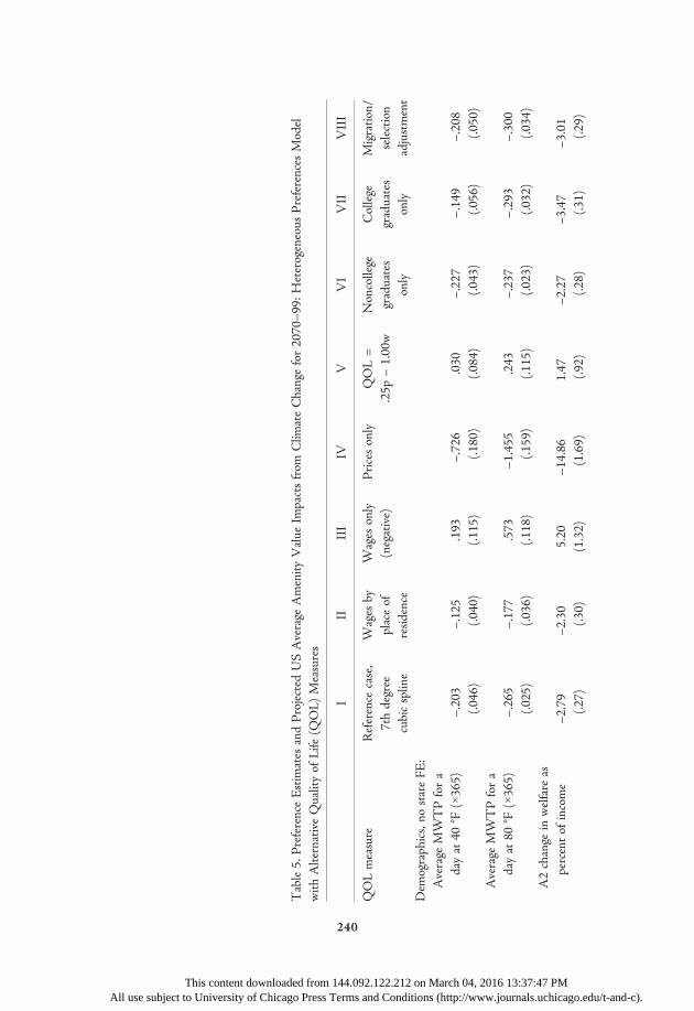
Table5.

PreferenceEstimates

andProjected

USAverage

Amenity

Value

Impactsfrom

Clim

ateChangefor2070–99:H

eterogeneous

Preferences

Model

with

AlternativeQualityof

Life(Q

OL)

Measures

III

III

IVV

VI

VII

VIII

QOLmeasure

Reference

case,

7thdegree

cubicspline

Wages

byplaceof

residence

Wages

only

(negative)

Pricesonly

QOL=

.25p

–1.00w

Noncollege

graduates

only

College

graduates

only

Migratio

n/selection

adjustment

Dem

ographics,no

stateFE

:Average

MW

TPfora

dayat

40°F

(×365)

–.203

–.125

.193

–.726

.030

–.227

–.149

–.208

(.046)

(.040)

(.115)

(.180)

(.084)

(.043)

(.056)

(.050)

Average

MW

TPfora

dayat

80°F

(×365)

–.265

–.177

.573

–1.455

.243

–.237

–.293

–.300

(.025)

(.036)

(.118)

(.159)

(.115)

(.023)

(.032)

(.034)

A2change

inwelfare

aspercentof

income

–2.79

–2.30

5.20

–14.86

1.47

–2.27

–3.47

–3.01

(.27)

(.30)

(1.32)

(1.69)

(.92)

(.28)

(.31)

(.29)

240


Dem

ographics,stateFE

:Average

MW

TPfora

dayat

40°F

(×365)

–.221

–.178

–.147

–.403

–.231

–.242

–.172

–.221

(.051)

(.045)

(.057)

(.196)

(.047)

(.048)

(.063)

(.055)

Average

MW

TPfora

dayat

80°F

(×365)

–.236

–.210

.081

–.747

–.115

–.231

–.207

–.260

(.043)

(.047)

(.084)

(.236)

(.065)

(.038)

(.060)

(.055)

A2change

inwelfare

aspercentof

income

–1.02

–1.82

–.57

–2.95

–2.46

–.96

–.53

–.94

(.83)

(.58)

(1.24)

(3.18)

(.88)

(.77)

(1.00)

(.89)

Note.—The

unitof

observationisaPUMA.Allregressionsareweightedby

populatio

nin

each

PUMA.Allspecificatio

nsusea7thdegree

restricted

cubicsplinewith

aconstant

MW

TPrestrictionforthelower

andupper1%

ofthepopulatio


distributio

n.Allregressionsincludegeographic,o

ther

weather,and

demographiccontrols.M

WTPsshow

nforadayat

40°F

or80

°Farerelativeto

65°F,expressed

asafractio

nof

income,andareincome-weightedaverages

across

allP

UMAs.

Welfare

impactsshow

nassumethat

households’utility

functio

nsarelinearin

characteristics.

Colum

nV

uses

wages

byresidence.

Colum

nVIIIadjustsQOLforselective

migratio

nperDahl(2002),as

discussedin

sections

1.2and6.

Parentheticalvalues

indicate

standard

errorswild

clusterbootstrapped

onstateusing200draw

s.

241


sorting based on unobserved skills or a spatial match component of wages. We ad-dress this concern in several ways. First, column VIII of table 5 presents results froma specification in which we adopt the procedure used in Dahl (2002) to adjust the wj

for selective migration. In our wage equation, we include a flexible control functionfor each individual’s probability of moving from his or her state of birth to the cur-rent state, as well as the probability of staying in the state of birth, based on the in-dividual’s observed demographic characteristics.34 This adjustment will decrease theestimated wj (and therefore increase the estimated Q j) for PUMAs with a relativelyhigh rate of in-migration to the extent that in-migrants earn relatively high wages. Asshown in column VIII, this adjustment to our QOL estimates does not substantiallyaffect our preference and welfare estimates.

As an alternative and closely related approach for addressing selective migration,we have also adjusted our baseline QOL estimates for each PUMA by adding acorrection equal to the PUMA’s rate of net in-migration between 1990 and 2000 (inpercent) multiplied by a mobility cost estimate from Notowidigdo (2013).35 Thisadjustment explicitly increases the estimated QOL for locations that are growingrelatively quickly. We find that this adjustment modestly increases the estimatedaversion to cold and slightly attenuates the estimated welfare loss under the A2 model(by 0.3% of income). Finally, we have estimated a specification that insulates ourestimates from selective migration to “superstar cities” by dropping superstar metropol-itan areas (as defined in Gyourko, Mayer, and Sinai [2013]) from the sample (we drop442 of the 2,057 PUMAs in the sample). We find that doing so also modestly de-creases the estimated MWTPs and welfare impact, without qualitatively affecting ourconclusions (see appendix table A1.1, col. R15).

34. Per Dahl (2002), we estimate these probabilities by category according to various de-mographic characteristics. We use the exact same categories as Dahl (2002) for movers (20 foreach state) and stayers (70). We also add a separate mover category, “birth-state,” for thoseborn outside the United States. As Dahl only used male, white, and ages 25–34, we create12 times the number of original categories to account for female, nonwhite, and age categories35–44 and 45–55. To identify the wage intercepts across states, we constrain the coefficients inthe control function to be the same across states, unlike in Dahl (2002).

35. Notowidigdo (2013) allows for heterogeneity in mobility costs and estimates a mobilitycost elasticity, which dictates how the mobility cost of the marginal migrant increases with thenumber of migrants. This elasticity is appropriate for adjusting our QOL estimates because it isthe marginal migrant that determines market prices and wages. Our calculations use a weightedaverage of Notowidigdo’s (2013) estimated elasticities for high-skill and low-skill workers (0.066and 0.065 respectively; see table 7 in his paper). These estimates are identified from plausiblyexogenous Bartik (1991) labor demand shocks and correspond to migration over a 10-year pe-riod, thereby aligning with our 1990 to 2000 migration rates. We also use Notowidigdo’s (2013)curvature parameters (betas) in specifying the mobility cost function.



7. CONCLUSIONS

This paper illustrates the ability of the Rosen-Roback hedonic framework, whenproperly calibrated, to recover willingness to pay for nonmarket goods such as climate.By using a quality of life measure that is carefully constructed from local wage andhousing price differentials in the contiguous United States and by adopting a flexiblemodel of climate based on local temperature distributions, we obtain estimates ofhouseholds’ valuation of climate amenities that both accord with intuition and aregenerally robust to a wide range of empirical specifications. We find that households(1) place the most value on temperatures near 65 °F, (2) tend to dislike marginal in-creases in heat more than marginal increases in cold, and (3) suffer less from marginalincreases in cold or heat once the temperature is sufficiently cold or hot (althoughinference is weak for hot weather). Finally, we find evidence of heterogeneity in thesepreferences, with households that are most averse to cold living in the South, consis-tent with models of both sorting and adaptation.

When we apply our estimates to value the amenity impacts of climate change, weestimate an average US welfare loss between 1% and 4% of income per year by 2070–99 under “business as usual.” Most areas in the United States are predicted to experi-ence losses, as many pleasantly warm days will be lost while uncomfortably cold dayswill only be moderately abated. These estimates are similar in magnitude to the per-centage losses in GDP (market goods) predicted by Nordhaus (2007) and Stern (2007)for 2100 under business as usual, suggesting that nonmarket amenity benefits alonemay justify the mitigation costs discussed in their studies.36

The greatest limitation to our empirical method is that we have little statisticalpower to make inferences regarding households’ willingness to pay (WTP) to avoidtemperatures beyond the limits of the current temperature distribution. The dataprovide only limited guidance as to how WTP should be extrapolated over extremelyhot temperatures that have yet to be realized. Should the WTP to avoid heat actuallyincrease nonlinearly over the extremes, our damage estimates will be too conservative,particularly in the southern United States.

REFERENCES

Albouy, David. 2012. Are big cities bad places to live? Estimating quality of life across metropolitan areas.

NBER Working paper 14472, National Bureau of Economic Research, Cambridge, MA (original

November 2008, revised May 2012).

Albouy, David, and Bert Lue. 2015. Driving to opportunity: Local wages, commuting, and sub-

metropolitan quality of life. Journal of Urban Economics 89:74–92.

36. The Nordhaus and Stern market damage estimates of 3% and 2.9% apply to world-wide GDP, not US GDP.





http://www.journals.uchicago.edu/action/showLinks?crossref=10.1016%2Fj.jue.2015.03.003

Albouy, David, and Bryan Stuart. 2015. Urban population and amenities: The neoclassical model of

location. NBER Working paper 19919, National Bureau of Economic Research, Cambridge, MA

(original February 2014, revised September 2015).

Altonji, Joseph G., Todd E. Elder, and Christopher R. Taber. 2005. Selection on observed and unob-

served variables: Assessing the effectiveness of Catholic schools. Journal of Political Economy 113 (1):

151–84.

Arellano, M. 1987. Computing robust standard errors for within-groups estimators. Oxford Bulletin of

Economics and Statistics 49 (4): 431–34.

Bajari, Patrick, and C. Lanier Benkard. 2005. Demand estimation with heterogeneous consumers and un-

observed product characteristics: A hedonic approach. Journal of Political Economy 113 (6): 1239–76.

Bajari, Patrick, and Matthew E. Kahn. 2005. Estimating housing demand with an application to ex-

plaining racial segregation in cities. Journal of Business and Economic Statistics 23 (1): 20–33.

Barreca, Alan I. 2012. Climate change, humidity, and mortality in the United States. Journal of Environ-

mental Economics and Management 63 (1): 19–34.

Barreca, Alan, Karen Clay, Olivier Deschênes, Michael Greenstone, and Joseph S. Shapiro. 2015. Adapt-

ing to climate change: The remarkable decline in the U.S. temperature-mortality relationship over the

20th century. NBERWorking paper 18692, National Bureau of Economic Research, Cambridge, MA

(original January 2013, revised March 2015).

Bartik, Timothy J. 1991. Who benefits from state and local economic development policies? W. E. Upjohn

Institute for Employment Research, Kalamazoo, MI.

Baum-Snow, Nathaniel, and Ronni Pavan. 2012. Understanding the city size wage gap. Review of Eco-

nomic Studies 79 (1): 88–127.

Blomquist, Glenn C., Mark C. Berger, and John P. Hoehn. 1988. New estimates of quality of life in urban

areas. American Economic Review 78 (1): 89–107.

Cameron, A. Colin, Jonah B. Gelbach, and Douglas L. Miller. 2008. Bootstrap-based improvements for

inferences with clustered errors. Review of Economics and Statistics 90 (3): 414–27.

Cameron, A. Colin, and Pravin K. Trivedi. 2005. Microeconometrics: Methods and applications. New

York: Cambridge University Press.

Chay, Kenneth Y., and Michael Greenstone. 2005. Does air quality matter? Evidence from the housing

market. Journal of Political Economy 113 (2): 376–424.

Chen, Yong, and Stuart S. Rosenthal. 2008. Local amenities and life-cycle migration: Do people move for

jobs or fun? Journal of Urban Economics 64 (3): 519–37.

Cragg, Michael, and Matthew Kahn. 1997. New estimates of climate demand: Evidence from location

choice. Journal of Urban Economics 42 (2): 261–84.

———. 1999. Climate consumption and climate pricing from 1940 to 1990. Regional Science and Urban

Economics 29 (4): 519–39.

Dahl, Gordon B. 2002. Mobility and the return to education: Testing a Roy model with multiple markets.

Econometrica 70 (6): 2367–2420.

Deschênes, Olivier, andMichael Greenstone. 2007. The economic impacts of climate change: Evidence from

agricultural output and random fluctuations in weather.American Economic Review 97 (1): 354–85.

———. 2011. Climate change, mortality and adaptation: Evidence from annual fluctuations in weather in

the US. American Economic Journal: Applied Economics 3 (4): 152–85.

———. 2012. The economic impacts of climate change: Evidence from agricultural output and random

fluctuations in weather: Reply. American Economic Review 102 (7): 3761–73.



http://www.journals.uchicago.edu/action/showLinks?crossref=10.1257%2Faer.102.7.3761

http://www.journals.uchicago.edu/action/showLinks?system=10.1086%2F498586


http://www.journals.uchicago.edu/action/showLinks?crossref=10.1198%2F073500104000000334

http://www.journals.uchicago.edu/action/showLinks?crossref=10.1016%2Fj.jue.2008.05.005

http://www.journals.uchicago.edu/action/showLinks?crossref=10.1016%2Fj.jeem.2011.07.004

http://www.journals.uchicago.edu/action/showLinks?crossref=10.1016%2Fj.jeem.2011.07.004

http://www.journals.uchicago.edu/action/showLinks?crossref=10.1006%2Fjuec.1996.2027

http://www.journals.uchicago.edu/action/showLinks?crossref=10.1016%2FS0166-0462%2898%2900046-5


http://www.journals.uchicago.edu/action/showLinks?crossref=10.1093%2Frestud%2Frdr022


http://www.journals.uchicago.edu/action/showLinks?crossref=10.1093%2Frestud%2Frdr022


http://www.journals.uchicago.edu/action/showLinks?crossref=10.1111%2F1468-0262.00379



http://www.journals.uchicago.edu/action/showLinks?crossref=10.1162%2Frest.90.3.414

http://www.journals.uchicago.edu/action/showLinks?crossref=10.1111%2Fj.1468-0084.1987.mp49004006.x

http://www.journals.uchicago.edu/action/showLinks?crossref=10.1257%2Fapp.3.4.152

http://www.journals.uchicago.edu/action/showLinks?crossref=10.1111%2Fj.1468-0084.1987.mp49004006.x

Fan, J., and I. Gijbels. 1996. Local polynomial modelling and its applications. London: Chapman & Hall.

Fisher, Anthony C., W. Michael Hanemann, Michael J. Roberts, and Wolfram Schlenker. 2012. The

economic impacts of climate change: Evidence from agricultural output and random fluctuations in

weather: Comment. American Economic Review 102 (7): 3749–60.

Frijters, P., and B. M. S. Van Praag. 1998. The effects of climate on welfare and well-being in Russia.

Climatic Change 39 (1): 61–81.

Glaeser, Edward L., and David C. Maré. 2001. Cities and skills. Journal of Labor Economics 19 (2): 316–

42.

Graff Zivin, Joshua, and Matthew Neidell. 2014. Temperature and the allocation of time: Implications

for climate change. Journal of Labor Economics 32 (1): 1–26.

Graves, Philip E. 1979. A life-cycle empirical analysis of migration and climate, by race. Journal of Urban

Economics 6 (2): 135–47.

Gyourko, Joseph, Christopher Mayer, and Todd Sinai. 2013. Superstar cities. American Economic Jour-

nal: Economic Policy 5 (4): 167–99.

Hoch, Irving, and Judith Drake. 1974. Wages, climate, and the quality of life. Journal of Environmental

Economics and Management 1 (4): 268–96.

IPCC (Intergovernmental Panel on Climate Change), Working Group I. 2007. Climate change 2007:

The physical science basis. In The Fourth Assessment Report of the Intergovernmental Panel on Climate

Change, ed. S. Solomon, D. Qin, M. Manning, Z. Chen, M. Marquis, K. B. Averyt, M. Tignor, and

H. L. Miller. New York: Cambridge University Press.

Kahn, Matthew E. 2009. Urban growth and climate change. Annual Review of Resource Economics 1:333–

50.

Kennan, John, and James R. Walker. 2011. The effect of expected income on individual migration de-

cisions. Econometrica 79 (1): 211–51.

Kuminoff, Nicolai V., and Jaren C. Pope. 2014. Do “capitalization effects” for public goods reveal the

public’s willingness to pay? International Economic Review 55 (4): 1227–50.

Maddison, David. 2003. The amenity value of the climate: The household production function approach.

Resource and Energy Economics 25 (2): 155–75.

Maddison, David, and Andrea Bigano. 2003. The amenity value of the Italian climate. Journal of Environ-

mental Economics and Management 45 (2): 319–32.

Mendelsohn, Robert, William D. Nordhaus, and Daigee Shaw. 1994. The impact of global warming on

agriculture: A Ricardian analysis. American Economic Review 84 (4): 753–71.

Moore, Thomas Gale. 1998. Health and amenity effects of global warming. Economic Inquiry 36 (3): 471–

88.

Nordhaus, William D. 1996. Climate amenities and global warming. In Climate change: Integrating science,

economics, and policy, ed. N. Nakicenovic, W. D. Nordhaus, R. Richels, and F. Toth. Laxenburg:

IIASA.

———. 2007. The challenge of global warming: Economic models and environmental policy. Vol. 4. New

Haven, CT: Yale University.

Notowidigdo, Matthew J. 2013. The incidence of local labor demand shocks. NBER Working paper

17167, National Bureau of Economic Research, Cambridge, MA (original June 2011, revised March

2013).

Peiser, Richard B., and Lawrence B. Smith. 1985. Homeownership returns, tenure choice and inflation.

American Real Estate and Urban Economics Journal 13 (4): 343–60.



http://www.journals.uchicago.edu/action/showLinks?crossref=10.1257%2Fpol.5.4.167

http://www.journals.uchicago.edu/action/showLinks?crossref=10.1257%2Fpol.5.4.167

http://www.journals.uchicago.edu/action/showLinks?crossref=10.1111%2Fj.1465-7295.1998.tb01729.x




http://www.journals.uchicago.edu/action/showLinks?crossref=10.1146%2Fannurev.resource.050708.144249


http://www.journals.uchicago.edu/action/showLinks?crossref=10.3982%2FECTA4657

http://www.journals.uchicago.edu/action/showLinks?crossref=10.1023%2FA%3A1005347721963


http://www.journals.uchicago.edu/action/showLinks?crossref=10.1111%2F1540-6229.00358

http://www.journals.uchicago.edu/action/showLinks?crossref=10.1111%2Fiere.12088




http://www.journals.uchicago.edu/action/showLinks?crossref=10.1016%2F0094-1190%2879%2990001-9



http://www.journals.uchicago.edu/action/showLinks?crossref=10.1016%2F0094-1190%2879%2990001-9

Rehdanz, Katrin. 2006. Hedonic pricing of climate change impacts to households in Great Britain.

Climatic Change 74 (4): 413–34.

Rehdanz, Katrin, and David J. Maddison. 2005. Climate and happiness. Ecological Economics 52 (1): 111–

25.

———. 2009. The amenity value of climate to German households. Oxford Economic Papers 61 (1):

150–67.

Roback, Jennifer. 1982. Wages, rents, and the quality of life. Journal of Political Economy 90 (6): 1257–

78.

Rosen, Sherwin. 1974. Hedonic prices and implicit markets: Product differentiation in pure competi-

tion. Journal of Political Economy 82 (1): 34–55.

———. 1979. Wages-based indexes of urban quality of life. In Current issues in urban economics, ed.

P. Mieszkowski and M. Straszheim. Baltimore: Johns Hopkins University Press.

Savageau, David. 1999. Places rated almanac. Foster City, CA: IDG Books Worldwide.

Schlenker, Wolfram, W. Michael Hanemann, and Anthony C. Fisher. 2006. The impact of global warm-

ing on U.S. agriculture: An econometric analysis of optimal growing conditions. Review of Economics

and Statistics 88 (1): 113–25.

Schlenker, Wolfram, and Michael J. Roberts. 2009. Nonlinear temperature effects indicate severe damages

to U.S. crop yields under climate change. Proceedings of the National Academy of Sciences 106 (37):

15594–98.

Shapiro, P., and T. Smith. 1981. Preferences on non-market goods revealed through market demands.

Advances in Applied Microeconomics: A Research Annual 1:105–22.

Sinha, Paramita, and Maureen L. Cropper. 2013. The value of climate amenities: Evidence from U.S.

migration decisions. NBER Working paper 18756, National Bureau of Economic Research, Cam-

bridge, MA.

Stern, Nicholas. 2007. The economics of climate change: The Stern Review. New York: Cambridge Uni-

versity Press.

Timmins, Christopher. 2007. If you cannot take the heat, get out of the Cerrado . . . : Recovering the

equilibrium amenity cost of nonmarginal climate change in Brazil. Journal of Regional Science 47 (1):

1–25.

Tol, Richard S. J. 2002. Estimates of the damage costs of climate change, Part II. Dynamic estimates.

Environmental and Resource Economics 21 (2): 135–60.

———. 2009. The economic effects of climate change. Journal of Economic Perspectives 23 (2): 29–51.

Wooldridge, Jeffrey M. 2003. Cluster-sample methods in applied econometrics. American Economic Re-

view Papers and Proceedings 93 (2): 133–38.



http://www.journals.uchicago.edu/action/showLinks?crossref=10.1093%2Foep%2Fgpn028


http://www.journals.uchicago.edu/action/showLinks?crossref=10.1111%2Fj.1467-9787.2007.00497.x


http://www.journals.uchicago.edu/action/showLinks?crossref=10.1023%2FA%3A1014539414591

http://www.journals.uchicago.edu/action/showLinks?crossref=10.1257%2Fjep.23.2.29


http://www.journals.uchicago.edu/action/showLinks?crossref=10.1162%2Frest.2006.88.1.113


http://www.journals.uchicago.edu/action/showLinks?crossref=10.1162%2Frest.2006.88.1.113

http://www.journals.uchicago.edu/action/showLinks?crossref=10.1007%2Fs10584-006-3486-5

http://www.journals.uchicago.edu/action/showLinks?crossref=10.1073%2Fpnas.0906865106

http://www.journals.uchicago.edu/action/showLinks?crossref=10.1016%2Fj.ecolecon.2004.06.015

Documents

Climate Amenities, Climate Change, and American …davidalbouy.net/climatewelfare.pdfClimate Amenities, Climate Change, and American Quality of Life David Albouy, Walter Graf, Ryan