Embed Size (px)
Citation preview

DRAFT
Analysis of 30 Years of Pavement Temperatures using the
Enhanced Integrated Climate Model (EICM)
Draft report prepared for the
CALIFORNIA DEPARTMENT OF TRANSPORTATION
By:
A. Ongel, J. Harvey
August 2004
Pavement Research Center Institute of Transportation Studies University of California, Berkeley
University of California, Davis

ii

TABLE OF CONTENTS
Table of Contents........................................................................................................................... iii
List of Figures ................................................................................................................................. v
List of Tables ................................................................................................................................. ix
List of Tables ................................................................................................................................. ix
Executive Summary ....................................................................................................................... xi
1.0 Introduction......................................................................................................................... 1
1.1 Climate and Pavement Distress ...................................................................................... 1
1.2 Evaluation of Structural Condition by Deflections......................................................... 2
1.3 Climate Data for Pavement Design in California ........................................................... 3
1.4 Temperature Prediction Models:..................................................................................... 4
1.5 Research Objectives........................................................................................................ 5
1.6 Scope of this Report........................................................................................................ 6
2.0 Methods............................................................................................................................... 7
2.1 EICM Inputs.................................................................................................................... 9
2.2 EICM Outputs:.............................................................................................................. 10
2.3 Database Development ................................................................................................. 11
3.0 Evaluation of the Use of 5 Years of Climate Data for Pavement Design......................... 13
3.1 Rainfall.......................................................................................................................... 13
3.2 Pavement Temperatures................................................................................................ 18
4.0 New Asphalt Concrete Subsurface Temperature Estimation Equations and Comparison
with the BELLS2 Equation........................................................................................................... 23
4.1 New AC Subsurface Temperature Estimation Equations............................................. 24
4.2 Comparison of Equations.............................................................................................. 26
iii

4.2.1 Temperatures at One-Quarter Depth of the Asphalt Concrete.................................. 27
4.2.2 Temperatures at the Mid-Depth of Asphalt Concrete............................................... 28
5.0 Qualitative Analysis of Climate Effects on Pavement Performance ................................ 31
5.1 Effects of Climate on Flexible Pavements.................................................................... 32
5.1.1 Mix Rutting............................................................................................................... 32
5.1.2 Bottom-Up Fatigue ................................................................................................... 35
5.1.3 Thermal Cracking ..................................................................................................... 39
5.2 Climatic Effects on Rigid Pavement Fatigue................................................................ 41
5.2.1 Faulting ..................................................................................................................... 47
5.3 Unbonded PCC Overlays of PCC (PCC-AC-PCC) ...................................................... 51
5.3.1 Fatigue....................................................................................................................... 51
5.3.2 Faulting ..................................................................................................................... 53
5.4 Climatic Effects on Composite Pavements................................................................... 55
5.4.1 Mix Rutting............................................................................................................... 55
5.4.2 Faulting ..................................................................................................................... 56
5.4.3 Reflection Cracking .................................................................................................. 56
6.0 Conclusions....................................................................................................................... 61
Flexible Pavements................................................................................................................ 61
Rigid Pavements .................................................................................................................... 62
Unbonded Concrete Overlays................................................................................................ 63
Composite Pavements............................................................................................................ 63
7.0 References......................................................................................................................... 65
iv

LIST OF FIGURES
Figure 1. 5 year moving averages of rainfall for the six climate region cities. ........................... 14
Figure 2. Annual and 5 year moving averages of rainfall for Arcata (North Coast region). ....... 15
Figure 3. Annual and 5 year moving averages of rainfall for Daggett (Desert region). .............. 15
Figure 4. Annual and 5 year moving averages of rainfall for Reno (Mountain/High Desert
region). .................................................................................................................................. 16
Figure 5. Annual and 5 year moving averages of rainfall for San Francisco (Bay Area). .......... 16
Figure 6. Annual and 5 year moving averages of rainfall for Sacramento (Valley region). ....... 17
Figure 7. Annual and 5 year moving averages of rainfall for Los Angeles (South Coast region).
............................................................................................................................................... 17
Figure 8. 5-year distributions of asphalt concrete (AC 0-8-6-6) surface temperature (°C) for
Sacramento............................................................................................................................ 19
Figure 9. Annual distributions of asphalt concrete (AC 0-8-6-6) surface temperature (°C) for
Sacramento............................................................................................................................ 19
Figure 10. 5 year distributions of PCC (PCC 0-12-6-6) thermal gradients (°C/m) for
Sacramento............................................................................................................................ 21
Figure 11. Annual distributions of PCC (PCC 0-12-6-6) thermal gradients (°C/m) for
Sacramento............................................................................................................................ 21
Figure 12. Los Angeles AC 0-12-12-6 Temperatures on July 26, 1974 at 4-hour intervals. ....... 23
Figure 13. Comparison of temperatures predicted from BELLS2 and Equation 2 with the
temperatures predicted by EICM at one-quarter depth of the asphalt concrete layer........... 27
Figure 14. Comparison of temperatures predicted by BELLS2 and Equation 3 with the
temperatures predicted by EICM at mid-depth of the asphalt concrete layer....................... 28
Figure 15. Rainfall variability among six climate regions, 1961-1990. ...................................... 32
v
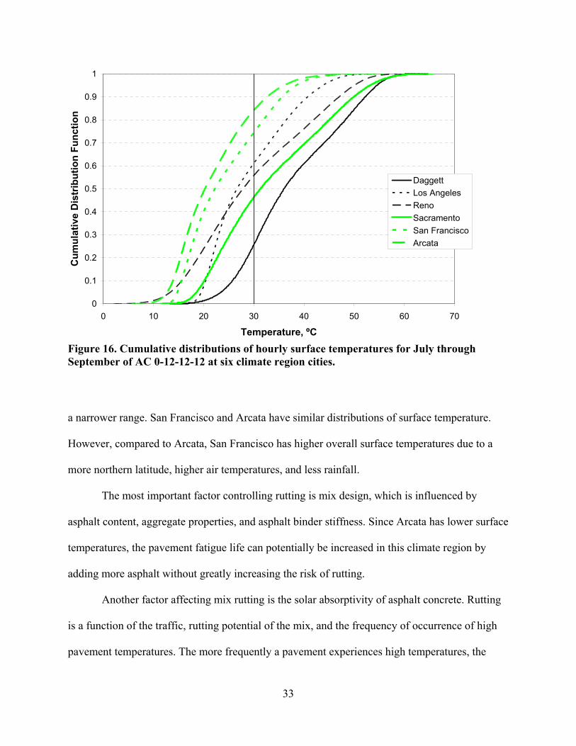
Figure 16. Cumulative distributions of hourly surface temperatures for July through September
of AC 0-12-12-12 at six climate region cities....................................................................... 33
Figure 17. Temperature distribution during a hot week in the 30-year period 1961-1990 for
typical solar absorptivity values............................................................................................ 34
Figure 18. Cumulative distribution of temperatures at the bottom of the AC (0-12-12-12) for six
climate regions. ..................................................................................................................... 37
Figure 19. Temperature variability at the bottom of the AC in a 12-inch. AC layer (0-12-12-12)
for six climate regions........................................................................................................... 37
Figure 20. Cumulative distribution of temperatures at the mid-depth of the 8-inch AC layer (0-8-
12-12) for the six California climate regions........................................................................ 38
Figure 21. Temperature variability at the mid-depth of the AC in an 8-inch layer (0-8-12-12) for
six climate regions. ............................................................................................................... 39
Figure 22. Cumulative temperature distribution at the surface of the 4-inch thick AC (0-4-12-12)
for six climate regions........................................................................................................... 40
Figure 23. Pavement surface temperatures of AC in a 4-inch layer (0-4-12-12) for six climate
regions................................................................................................................................... 40
Figure 24. Temperature distribution for a cold week in 30-year period 1961-1990 for different
absorptivity values. ............................................................................................................... 42
Figure 25. Cumulative distribution of thermal gradients for 16-inch PCC slab (0-16-6-6) with an
absorptivity value of 0.65 for six California climate regions. .............................................. 44
Figure 26. Cumulative distribution of thermal gradients for 16-inch thick PCC (0-16-6-6) with
absorptivity value of 0.8 for the six California climate regions. .......................................... 46
vi

Figure 27. Corner and centerline transverse joint load transfer efficiency versus surface
temperature for undoweled, untrafficked joints and cracks. (1) ........................................... 48
Figure 28. Cumulative temperature distribution at mid-depth of PCC (0-12-12-12) for six climate
regions................................................................................................................................... 50
Figure 29. Temperature variability at mid-depth of 12-inch thick PCC (0-12-12-12) for six
climate regions. ..................................................................................................................... 50
Figure 30. Cumulative distribution of thermal gradients in top slab of PCC-AC-PCC (0-12-2-8-
6-6) for six climate regions. .................................................................................................. 51
Figure 31. Cumulative distribution of bottom PCC thermal gradients of PCC-AC-PCC (0-12-2-
8-6-6) for six climate regions................................................................................................ 53
Figure 32. Cumulative distribution of top PCC layer mid-depth temperatures for PCC-AC-PCC
(0-12-2-8-6-6) for six climate regions. ................................................................................. 54
Figure 33. Cumulative distribution of bottom PCC layer mid-depth temperatures for PCC (0-12-
2-8-6-6) for six climate regions. ........................................................................................... 55
Figure 34. Surface temperature Distribution of PCC composite (0-2-12-6-6) for six climate
regions................................................................................................................................... 56
vii

viii

LIST OF TABLES
Table 1 Weather Station Locations and Climate Regions ....................................................... 7
Table 2 Flexible Pavement Structures Evaluated by EICM .................................................... 8
Table 3 Rigid Pavement Structures Evaluated by EICM......................................................... 9
Table 4 Composite Pavement Structures (Asphalt Concrete Overlays of Portland Cement
Concrete) Evaluated by EICM................................................................................................ 9
Table 5 Unbonded PCC Overlays (PCC-AC-PCC) Thickness Profiles .................................. 9
Table 6 Thermal Gradients at Various Times of the Day for AC 0-16-12-12....................... 25
Table 7 Frequency of Occurrence of Temperatures Above 25ºC at the Bottom of the AC
Layer for the Six Climate Regions........................................................................................ 38
Table 8 Frequency of Occurrence of Temperatures Below 10ºC at Mid-depth in the AC
Layer for the Six Climate Regions........................................................................................ 38
Table 9 Maximum Thermal Gradients over 30-year Period .................................................. 45
Table 10 Minumum Thermal Gradients over 30-year Period.................................................. 45
Table 11 Maximum and Minimum Thermal Gradients for PCC Slabs (0-16-6-6) with
Different Solar Absorptivity Values ..................................................................................... 47
Table 12 Comparison of Thermal Gradients for Conventional PCC and Unbonded PCC
Overlay of PCC Pavement .................................................................................................... 52
Table 13 Yearly Maximum and Minimum Temperatures at AC/PCC Interface of Three
Composite Structures ............................................................................................................ 58
Table 14 Maximum, Minimum, and Average Daily Extreme Temperature Differences at the
AC/PCC Interface of Three Composite Structures............................................................... 59
ix

x

EXECUTIVE SUMMARY
The external factors affecting the structural performance of pavements are traffic, the
environment, and the interaction of the two. The most significant environmental factors affecting
pavement performance are pavement temperature and moisture content. Various climatic
conditions to which the pavements are exposed influence pavement distress mechanisms and
performance.
The incorporation of climatic factors in pavement design is important for developing a
mechanistic-empirical design procedure. In order to account for the climatic variability in the
pavement design, it is essential to develop a database containing the critical pavement
temperatures and rainfall for climate regions over a long time period.
Harvey et al. summarized the effects of pavement temperatures and rainfall on distress
mechanisms of rigid, flexible, and composite pavements. These climate differences were
compared for six climate regions of California which were defined based on rainfall, and
maximum and minimum temperatures. The report concluded that climate regions should be
considered in the design of rigid, flexible, and composite pavement structures. However, the
climate data included in the analysis were averaged over 30 years due to limited time and the
massive amount of data and calculations, and so did not account for climate variability.
The 2002 Design Procedure produced by the National Cooperative Highway Research
Program (NCHRP), also known as the NCHRP 1-37A procedure, takes into account climatic
effects along with traffic and structural data in pavement design and rehabilitation. While this
design procedure allows the user to choose the climate region for the pavement, climate data
available in the software for design spans only 5 years. It is thought that a five-year period may
be insufficient to capture the total variability because climate cycles often last longer than five
years in California.
xi

Pavement temperatures are also important for back-calculating the stiffness of pavement
layers using Falling Weight Deflectometer (FWD) data. This is a reliable method to evaluate
flexible pavement condition. Since asphalt concrete is temperature dependent, FWD test results
are affected by the daily and the seasonal temperature fluctuations. The knowledge of sub-
surface temperatures helps in developing more accurate estimates of in-situ stiffnesses of the
pavement layers.
One of the factors affecting pavement temperatures is the absorptivity of the pavement
surface to solar radiation. Solar absorptivity values change according to the pavement type and
the pavement age.
In this study, databases for rainfall and temperatures were developed for six climate
regions of California. The weather data was obtained from National Climatic Database Center
(NCDC). The pavement temperatures were simulated using Enhanced Integrated Climatic Model
(EICM) software. Hourly pavement temperatures at the critical depths in the pavement layers
were obtained using EICM for six cities, one in each of the identified climate regions.
The objectives of the study presented in this report are:
• Create a database of hourly pavement temperatures predicted using EICM for 30
years (1961–1990) for typical California pavements including hourly averages and
standard deviations of pavement temperatures for each of the six California climate
regions.
• Evaluate the stability of pavement temperatures and rainfall across different 5-year
periods to determine whether 5 years of data is sufficient to characterize a climate
region.
xii
• Qualitatively evaluate the effects of pavement temperatures and rainfall and their
variability as they affect each distress across the climate regions in California.
• Compare the temperatures predicted by the BELLS2 equation with the temperatures
calculated by the EICM and propose new models to predict temperatures at depth in
the asphalt concrete layer in flexible pavements.
• Examine the effects of differences in albedo (reflectivity of solar radiation) on
pavement temperatures and qualitatively evaluate the effect on pavement distresses.
The report includes a brief description of the EICM model and its inputs and outputs, and
identifies the climate regions and the cities from which detailed climate information was used to
represent each region. Pavement temperatures were calculated using EICM for 37 pavement
structures. The structures included 28 different flexible pavements, three different rigid
pavements, four different composite pavements [asphalt (AC) on Portland cement concrete
(PCC)], and three different unbonded concrete overlays (PCC-AC-PCC) for each of the climate
regions over a 30-year period (1961–1990).
Several solar absorptivity values, obtained from measurements by the Lawrence Berkeley
National Laboratory, were used for the calculations. The sufficiency of 5 years of climate data
for pavement design in terms of providing stable inputs for running the EICM model was
evaluated.
The BELLS2 equation, the industry standard for prediction of sub-surface asphalt
concrete temperatures from surface temperatures, is briefly discussed. New models for
predicting pavement temperature developed from EICM-calculated temperatures are presented
and compared with BELLS 2 predictions and with EICM-calculated pavement temperatures. The
new prediction models are based on regression of pavement temperatures below the surface
xiii

calculated using the EICM and EICM calculated surface temperatures, time of day, and other
information available during FWD field operations.
Also included in the report is a qualitative evaluation of the risks of each distress type for
the different pavement types in each climate region, and the evaluation of the effects of solar
absorptivity on pavement temperatures.
The conclusions of the report are as follows:
• Database
1. A database of hourly pavement temperatures has been developed for the 30-year
period 1961–1990 for a range of pavement structures that spans California
highway practice. The temperatures were calculated using the Enhanced
Integrated Climate Model (EICM) version 3.
• Prediction of Subsurface AC Temperatures
2. Comparing database temperatures predicted by EICM with temperatures predicted
by the BELLS2 equation, they give very close results at one-third depth.
However, at mid-depth, BELLS2 equation somewhat overestimates the
temperatures calculated using EICM at high temperatures and underestimates
them at low temperatures.
• Flexible Pavements
3. It is expected that the risk of AC mix rutting would be greater in the desert
(Daggett) and central valley (Sacramento) while being less in the North Coast
(Arcata) climate regions.
4. The South Coast (Los Angeles) may have faster rates of crack initiation for
fatigue based on temperatures at the bottom of the asphalt while the
xiv

mountain/high desert region (Reno) would likely have faster rates of crack
propagation.
5. Thermal cracking is a much greater risk for the mountain/high desert (Reno)
region due to cold temperatures in the winter, some risk in the valley
(Sacramento) and desert (Daggett) regions due to hot summers and cold winters,
and a very low risk for coastal regions of California.
6. The effect of solar absorptivity values becomes significant at higher temperatures.
Higher solar absorptivity values result in pavement surface temperatures
increasing approximately 5ºC, and therefore increased the risk of rutting. Solar
absorptivity values have no effect on surface temperatures at colder temperatures.
• Rigid Pavements
7. Pavements in the desert region are more prone to transverse fatigue cracking due
to positive temperature gradients, while those in the Bay Area are more likely to
experience corner and longitudinal cracking due to negative temperature
gradients.
8. Among the six climate regions, mountain/high desert (Reno), central valley
(Sacramento), and desert (Daggett) are more likely to experience reduced
aggregate interlock and lower load transfer efficiency due to differences in
pavement temperatures between winter and summer.
9. In the case of rigid pavements, solar absorptivity values don’t have any significant
effect on thermal gradients.
• Unbonded Concrete Overlays
xv

10. The surface PCC slab experiences temperatures and gradients similar to other
rigid pavements. The bottom PCC experiences small thermal gradients and lower
temperatures differences throughout the year.
• Composite Pavements
11. Composite pavements experience high temperatures causing mix rutting similar to
flexible pavements.
12. Among the six climate regions, pavements in the mountain/high desert (Reno),
central valley (Sacramento), and desert (Daggett) are more likely to experience
reflection cracking because of differences in temperature between summer and
winter.
13. Daily temperature changes at the AC/PCC interface are similar among climate
regions, and generally small due to the insulating effect of the AC overlay, which
increases with overlay thickness.
xvi

1.0 INTRODUCTION
The external factors affecting the structural performance of pavements are traffic,
environmental conditions, and the interaction of the two. In studying environmental effects on
pavement performance, the most significant factors to be considered are temperature and
moisture content.
Pavements are classified into three types: flexible, rigid, and composite. Flexible
pavements include pavements with bituminous wearing surfaces such as asphalt concrete. Rigid
pavements include those with wearing surfaces constructed of Portland cement concrete.
Composite pavements are defined for this report to have asphalt concrete on top of Portland
cement concrete.
1.1 Climate and Pavement Distress
The primary distresses associated with flexible pavements are fatigue cracking, thermal
cracking, and rutting. In addition to these, reflection cracking is a major distress associated with
asphalt overlays of flexible pavements. The distresses associated with rigid pavements are
cracking (longitudinal, transverse, and corner) and faulting. The primary distresses for composite
pavements (asphalt overlays of Portland cement concrete pavements) are reflection cracking,
rutting, and thermal cracking.
Pavement temperatures are affected by air temperatures as well as precipitation, wind
speed, and solar radiation. The response of a pavement system is highly influenced by the
temperature of the surface layers and moisture content of the unbound soils. Annual, seasonal,
and daily variations in temperature and precipitation have large influences on pavement service
life. Therefore, the variability associated with climatic factors should be included in pavement
design reliability analysis to help ensure desired performance.
1

For flexible pavements, temperature has an effect on the stiffness of the bituminous
layers. Asphalt concrete becomes stiffer at lower temperatures and softer at higher temperatures
and exhibits different material characteristics at different temperatures. The stiffnesses and shear
strengths of unbound soil layers often vary seasonally with changes in moisture content and
suction.
The most important factors affecting rigid pavement systems are the thermally controlled
expansion and contraction, and the vertical thermal and moisture gradients in the concrete slab.
Thermal and/or moisture gradients that cause curling in the slab can create tensile stresses as
large as those caused by heavy traffic loads. The curled shape can also result in larger
deformations under traffic loading than would occur for a flat slab, which increases the rate of
faulting caused by traffic loads. Joint opening/closing and some tensile stresses are controlled by
slab expansion and contraction, and restraint of slab movement by the base.
Support provided to the cement and asphalt bound layers is largely controlled by
moisture content and suction changes, which depend in large part on rainfall.
1.2 Evaluation of Structural Condition by Deflections
The in-situ moduli of pavement layers are excellent indicators of the structural condition
of a pavement. They are important for evaluating a project for the need for maintenance or
rehabilitation, and are needed for mechanistic design. Nondestructive evaluation using a Falling
Weight Deflectometer (FWD) is a reliable and commonly used method for obtaining in-situ
moduli and determining pavement condition. In FWD testing, an impulse load is applied to the
pavement and the measured dynamic response (deflection) of the surface is recorded by
deflection sensors on the device. These measurements are then used to back-calculate pavement
2

material properties. FWDs are also used to measure Load Transfer Efficiency (LTE) across joints
and cracks in rigid pavements.
A deflection measurement and the back-calculated moduli or LTE are a “snapshot” of the
pavement structural condition at the time of the measurement. The properties of the pavement
materials and structure are constantly changing as the temperatures, moisture contents and
suction change. It is important to be able to translate FWD information to the rest of the year,
and to other FWD measurements which may have been obtained under different climatic
conditions, which requires knowledge of the pavement layer temperatures at the time of
measurement. This is especially important for asphalt concrete for which stiffness is controlled
by temperature.
The stiffness of asphalt concrete decreases with increasing temperature, which results in
larger deflections. FWD test results are influenced by temperature due to these properties of
asphalt concrete. It is relatively easy to measure surface temperatures in the field when
performing FWD tests, however it is much more difficult to measure temperatures in the asphalt
concrete below the surface. The temperatures throughout the asphalt concrete influence the
pavement deflections, and the accuracy of back-calculated pavement moduli is greatly improved
with knowledge of subsurface temperatures.
1.3 Climate Data for Pavement Design in California
Harvey et al. summarized the effects of pavement temperatures and rainfall on distress
mechanisms of rigid, flexible, and composite pavements and these climate differences were
compared for six climate regions of California defined in that report based on rainfall, and
maximum and minimum temperatures.(1) The report concluded that climate regions should be
considered in the design of rigid, flexible, and composite pavement structures. However, the
3

climatic data included in the analysis was averaged over 30 years due to limited time and the
massive amount of data and calculations, and so did not account for variability.
The 2002 Design Procedure produced by the National Cooperative Highway Research
Program (NCHRP) takes into account climatic effects along with traffic and structural data in
pavement design and rehabilitation.(2) While this design procedure allows the user to choose the
climate region for the pavement, climate data available in the software for design spans only 5
years. It is thought that a five-year period may be insufficient to capture the total variability
because climate cycles often last longer than five years in California.
Another difficulty with the NCHRP procedure is that it contains no information on which
years are included in the design procedure. Since only a five-year period was selected, the period
could be a particularly hot or cold period or wet or dry period which would introduce bias in the
expected lives of the pavements.
1.4 Temperature Prediction Models:
The temperature prediction model included in the 2002 Design Procedure, and used for
the research presented in this report, is the Enhanced Integrated Climate Model (EICM)
developed by the University of Illinois.(3) EICM is a program capable of modeling climatic
effects on pavements. It can operate in both SI and English units and can accept hourly data for
up to 10 consecutive years. EICM is able to predict the thermal gradient, temperature, pore water
pressure, water content, frost heave, and drainage performance throughout the pavement profile.
Only the pavement temperature models were used for this project. The effects of climate depend
on a detailed knowledge of the pavement structure, which was beyond the scope of this project.
A temperature prediction equation commonly used in practice to estimate subsurface
asphalt concrete temperatures during deflection testing is the BELLS2 equation.(4, 5) It can
4

predict pavement temperatures in flexible pavements at depth using the surface temperature,
average air temperature one day before testing, time of the day, and the depth at which the
temperature is predicted.
The BELLS2 equation was calibrated in the field to predict temperatures at depth. It has
been verified at mid-depth and one-third depth of the asphalt concrete layer.(4) The BELLS2
equation is the standard equation recommended for use in back-calculation of moduli on Long-
Term Pavement Performance (LTPP) test sections.(4)
1.5 Research Objectives
The objectives of the study presented in this report are:
• Create a database of hourly pavement temperatures predicted using EICM for 30
years (1961–1990) for typical California pavements including hourly averages and
standard deviations of pavement temperatures for each of the six California climate
regions.
• Evaluate the stability of pavement temperatures and rainfall across different 5-year
periods to determine whether 5 years of data is sufficient to characterize a climate
region.
• Qualitatively evaluate the effects of pavement temperatures and rainfall and their
variability as they affect each distress across the climate regions in California.
• Compare the temperatures predicted by the BELLS2 equation with the temperatures
calculated by the EICM and propose new models to predict temperatures at depth in
the asphalt concrete layer in flexible pavements.
• Examine the effects of differences in albedo (reflectivity of solar radiation) on
pavement temperatures and qualitatively evaluate the effect on pavement distresses.
5

1.6 Scope of this Report
Chapter 2 of this report describes the EICM model and its inputs and outputs, and
identifies the climate regions and the cities from which detailed climate information was used to
represent each region.
Chapter 3 describes the pavement structures and albedo (its reflectivity, measured in
terms of the portion of the sun’s energy reflected by the pavement surface) values used for the
calculations. The evaluation of the sufficiency of 5 years of climate data for pavement design is
also presented.
Chapter 4 describes the BELLS2 equation and new models for predicting pavement
temperature developed from EICM calculated temperatures, and presents comparison of the new
asphalt concrete prediction equations and the BELLS 2 predictions with EICM calculated
pavement temperatures. The new prediction models are based on regression of pavement
temperatures below the surface calculated using the EICM and EICM calculated surface
temperatures, time of day, and other information available during FWD field operations.
Chapter 5 presents the qualitative evaluation of the risks of each distress type for the
different pavement types in each climate region, and the evaluation of the effects of albedo on
pavement temperatures.
Chapter 6 presents the conclusions and recommendations from the study.
6

2.0 METHODS
Seven climate regions were identified for California based on rainfall and air temperature
data. The Mountain and High Desert regions were combined because of the lack of a major
weather station with data sufficient to operate the EICM model in the Mountain region.
Comparison of available data from Blue Canyon in the Mountain region and Reno in the High
Desert region indicated that the Mountain region most closely corresponded to the High Desert
region.(1)
Six cities, one representing each of the climate regions, were chosen and the weather data
for each location were obtained from the National Climatic Database Center CD-ROMS (6) and
the California Department of Water Resources (7). The weather data includes 30 years (1961-
1990) of daily maximum and minimum temperatures, daily average percent sunshine, daily
average rainfall, daily average wind speed for the locations of Arcata (CA), Daggett (CA),
Sacramento (CA), San Francisco (CA), Los Angeles (CA), and Reno (NV).
Table 1 Weather Station Locations and Climate Regions Location Climate Region Latitude Arcata, CA North Coast 40.98 Sacramento, CA Central Valley 38.52 San Francisco, CA Bay Area 37.62 Daggett, CA Desert 34.87 Los Angeles, CA South Coast 33.93 Reno, NV Mountain, High Desert 39.50 For this study, Enhanced Integrated Climate Model (EICM) version 3 was used to
simulate the pavement temperatures. The EICM program was used to evaluate 28 different
flexible pavements, three different rigid pavements, four different composite pavements [asphalt
(AC) on Portland cement concrete (PCC)], and three different unbonded concrete overlays
(PCC-AC-PCC) for each of the climate regions over a 30-year period (1961–1990). EICM can
7

handle 10 years of data at a time, so the climatic inputs from 1961 to 1990 were divided into
three decades: 1961–1970, 1971–1980, and 1981–1990.
Tables 2 through 4 show the structures that were evaluated by EICM. The thicknesses are
given in both SI and English units and the designation associated with each structure is provided.
(e.g., PCC 0-8-6-6 stands for rigid pavement without any thin surface treatment or overlay
[hence the zero in the first thickness position], 8 inches of Portland cement concrete, 6 inches of
base, and 6 inches of subbase).
Table 2 Flexible Pavement Structures Evaluated by EICM
Layer Thickness, in. (mm) Structure Name Designation Asphalt
Concrete Aggregate Base
Aggregate Subbase Subgrade
AC Structure 1 AC 0-2-6-6 2 (50) 6 (150) 6 (150) 130 (3250) AC Structure 2 AC 0-2-6-12 2 (50) 6 (150) 12 (300) 124 (3100) AC Structure 3 AC 0-2-12-6 2 (50) 12 (300) 6 (150) 124 (3100) AC Structure 4 AC 0-2-12-12 2 (50) 12 (300) 12 (300) 118 (2950) AC Structure 5 AC 0-4-6-6 4 (100) 6 (150) 6 (150) 128 (3200) AC Structure 6 AC 0-4-6-12 4 (100) 6 (150) 12 (300) 122 (3050) AC Structure 7 AC 0-4-12-6 4 (100) 12 (300) 6 (150) 122 (3050) AC Structure 8 AC 0-4-12-12 4 (100) 12 (300) 12 (300) 116 (2900) AC Structure 9 AC 0-8-6-6 8 (200) 6 (150) 6 (150) 124 (3100) AC Structure 10 AC 0-8-6-12 8 (200) 6 (150) 12 (300) 118 (2950) AC Structure 11 AC 0-8-12-6 8 (200) 12 (300) 6 (150) 118 (2950) AC Structure 12 AC 0-8-12-12 8 (200) 12 (300) 12 (300) 112 (2800) AC Structure 13 AC 0-12-6-6 12 (300) 6 (150) 6 (150) 120 (3000) AC Structure 14 AC 0-12-6-12 12 (300) 6 (150) 12 (300) 114 (2850) AC Structure 15 AC 0-12-12-6 12 (300) 12 (300) 6 (150) 114 (2850) AC Structure 16 AC 0-12-12-12 12 (300) 12 (300) 12 (300) 108 (2700) AC Structure 17 AC 0-16-6-6 16 (400) 6 (150) 6 (150) 116 (2900) AC Structure 18 AC 0-16-6-12 16 (400) 6 (150) 12 (300) 110 (2750) AC Structure 19 AC 0-16-12-6 16 (400) 12 (300) 6 (150) 110 (2750) AC Structure 20 AC 0-16-12-12 16 (400) 12 (300) 12 (300) 104 (2600) AC Structure 21 AC 0-22-6-6 22 (550) 6 (150) 6 (150) 110 (2750) AC Structure 22 AC 0-22-6-12 22 (550) 6 (150) 12 (300) 104 (2600) AC Structure 23 AC 0-22-12-6 22 (550) 12 (300) 6 (150) 104 (2600) AC Structure 24 AC 0-22-12-12 22 (550) 12 (300) 12 (300) 98 (2450) AC Structure 25 AC 0-28-6-6 28 (700) 6 (150) 6 (150) 104 (2600) AC Structure 26 AC 0-28-6-12 28 (700) 6 (150) 12 (300) 98 (2450) AC Structure 27 AC 0-28-12-6 28 (700) 12 (300) 6 (150) 98 (2450) AC Structure 28 AC 0-28-12-12 28 (700) 12 (300) 12 (300) 92 (2300)
8

Table 3 Rigid Pavement Structures Evaluated by EICM Layer Thickness, in. (mm)
Structure Name Designation Portland Cement Concrete
Aggregate Base
Aggregate Subbase Subgrade
PCC Structure 1 PCC 0-8-6-6 8 (200) 6 (150) 6 (150) 124 (3100) PCC Structure 2 PCC 0-12-6-6 12 (300) 6 (150) 6 (150) 120 (3000) PCC Structure 3 PCC 0-16-6-6 16 (400) 6 (150) 6 (150) 116 (2900)
Table 4 Composite Pavement Structures (Asphalt Concrete Overlays of Portland Cement Concrete) Evaluated by EICM
Layer Thickness, in. (mm) Structure Name Designation Asphalt
Concrete
Portland Cement Concrete
Aggregate Base
Aggregate Subbase Subgrade
Composite Structure 1
AC-PCC Comp. 0-4-8-6-6 4 (100) 8 (200) 6 (150) 6 (150) 120 (3000)
Composite Structure 2
AC-PCC Comp. 0-4-12-6-6 4 (100) 12 (300) 6 (150) 6 (150) 116 (2900)
Composite Structure 3
AC-PCC Comp. 0-8-8-6-6 8 (200) 8 (200) 6 (150) 6 (150) 116 (2900)
Composite Structure 4
AC-PCC Comp. 0-8-12-6-6 8 (200) 12 (300) 6 (150) 6 (150) 112 (2800)
Table 5 Unbonded PCC Overlays (PCC-AC-PCC) Thickness Profiles Layer Thickness, in. (mm) Structure
Name Designation PCC AC PCC Aggregate Base
Aggregate Subbase Subgrade
PCC Structure 1
PCC-AC-PCC 0-8-2-8-6-6 8 (20) 2 (50) 8 (200) 6 (150) 6 (150) 114 (2850)
PCC Structure 2
PCC-AC-PCC 0-12-2-8-6-6 12 (30) 2 (50) 8 (200) 6 (150) 6 (150) 110 (2750)
2.1 EICM Inputs
The climatic inputs required by the EICM are daily minimum and maximum
temperatures, wind speed, precipitation amount, and cloud cover. In addition to the climatic
inputs, EICM requires the thermal and material properties of the pavement materials as well as
9

drainage and infiltration model inputs. Using these inputs, EICM is able to produce the desired
outputs for each hour at different depths in the pavement being modeled. EICM allows the user
to enter the number of increments for each layer and at the end it generates the temperatures for
the specified nodes.
For the purposes of this research, the surface layers were divided into 1-in. (25-mm)
increments while the base and subbase layers were divided into 2-in. (50-mm) increments. The
subgrade was divided into eight increments regardless of the thickness, since EICM gives
stability errors if the layer is divided into too many fine increments.
Another input which has a significant effect on pavement temperatures is the albedo of a
given pavement surface, or its solar reflectivity. This was included in this study as solar
absorptivity (i.e., 1-albedo). The solar absorptivity value changes according to pavement type
and pavement age. For rigid pavements, this value increases as the concrete ages and darkens
while for the flexible pavements it decreases with time as the pavement lightens in color.
Therefore, solar absorptivity was assumed to be 0.65 for new rigid pavements and 0.8 for old
rigid pavements while it was assumed to be 0.90 or 0.95 for new flexible pavements and 0.80 for
old flexible pavements. These solar absorptivity values are based on field studies conducted by
the Lawrence Berkeley National Laboratory.(8)
2.2 EICM Outputs:
Among the EICM outputs of pore water pressure, water content, frost heave, and
drainage performance, nodal temperatures for each hour and for each node were selected and
used for this study. Since EICM can only handle 10 years of data, it was run 3 times for each
structure (once for each decade studied, as discussed in Section 2.2), and these decades were
10

combined to create 30 years of pavement temperatures. The 30-year data were then imported to a
database.
2.3 Database Development
Databases containing 30 years of nodal-hourly pavement temperatures, mean averages,
and standard deviations of the nodal-hourly temperatures over 30 years were created in
Microsoft Access and will eventually be loaded into an Oracle database.
For rigid pavements, two databases were developed: one for an absorptivity value of 0.65
and one for an absorptivity value of 0.8. Both included all the climate regions. One database was
developed for unbonded concrete overlays (PCC-AC-PCC) with an absorptivity value of 0.65 for
all climate regions. However, because the study included 28 different asphalt concrete structures
and the database cannot handle more than 2 GBytes, separate databases for each climate region
and each solar absorptivity value (0.8, 0.9 and 0.95) were developed for the flexible pavement
structures. For composite pavements, two databases were developed: one for each new pavement
absorptivity value (0.9 and 0.95) for all six climate regions.
The summaries of pavement temperatures presented in this report are based on the
asphalt concrete absorptivity value of 0.9 and Portland cement concrete absorptivity value of
0.65 unless otherwise indicated.
11

12
3.0 EVALUATION OF THE USE OF 5 YEARS OF CLIMATE DATA FOR PAVEMENT DESIGN
The variability of the climate data inputs for the EICM was the subject of some analysis
in Reference (1) and further analysis presented in Chapter 5 of this report.
The 2002 Design Procedure produced by National Cooperative Highway Research
Program Project 1-37A (NCHRP 1-37A) takes into account climatic effects along with traffic
and structural data in pavement design and rehabilitation.(2) The NCHRP 1-37A software runs
EICM during pavement performance calculations, and allows the users to choose the climate
region for the pavement. However, climate data available for design in the software spans only 5
years or less because of the large amounts of input data and computation time required to run
EICM for longer periods of time.
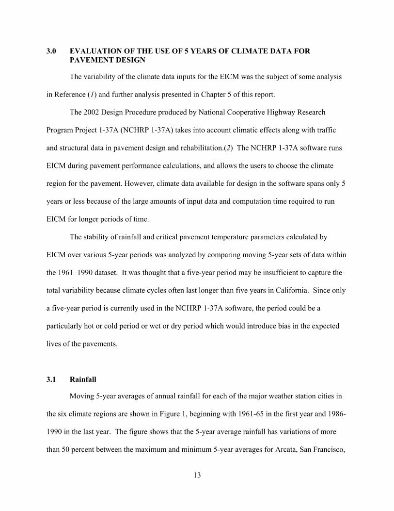
The stability of rainfall and critical pavement temperature parameters calculated by
EICM over various 5-year periods was analyzed by comparing moving 5-year sets of data within
the 1961–1990 dataset. It was thought that a five-year period may be insufficient to capture the
total variability because climate cycles often last longer than five years in California. Since only
a five-year period is currently used in the NCHRP 1-37A software, the period could be a
particularly hot or cold period or wet or dry period which would introduce bias in the expected
lives of the pavements.
3.1 Rainfall
Moving 5-year averages of annual rainfall for each of the major weather station cities in
the six climate regions are shown in Figure 1, beginning with 1961-65 in the first year and 1986-
1990 in the last year. The figure shows that the 5-year average rainfall has variations of more
than 50 percent between the maximum and minimum 5-year averages for Arcata, San Francisco,
13

0
20
40
60
80
100
120
140
1961 1965 1969 1973 1977 1981 1985 1989
Year
Rai
nfal
l (cm
)DaggettLos AngelesRenoSacramentoSan FranciscoArcata
First Year of Data Set
First Year of 5-Year Average
Figure 1. 5 year moving averages of rainfall for the six climate region cities.
Sacramento, and Los Angeles. The moving 5-year averages show less variation for Reno and
Daggett, the two regions with the lowest annual rainfall.
The annual variability that causes the instability in the 5-year moving averages is shown
in Figures 2 through 7. It appears from the data shown in these figures that 5 years is not a
sufficient period to use to obtain a stable best estimate for rainfall for pavement design.
The database of 30-year average rainfalls prepared as part of this study should provide a
more stable best estimate for pavement design, assuming that future rainfall is similar to that 30-
year period. Individual years of rainfall and pavement temperatures are available in the new
database, which permits the pavement designer to select dry or wet periods for sensitivity
analysis of pavement design using mechanistic-empirical pavement design methods, such as
NCHRP 1-37A.
14

0
20
40
60
80
100
120
140
160
180
1960 1965 1970 1975 1980 1985 1990 1995
Year
Rai
nfal
l (cm
)
Yearly Sum5-Year Average
Figure 2. Annual and 5 year moving averages of rainfall for Arcata (North Coast region).
0
20
40
60
80
100
120
140
160
180
1960 1965 1970 1975 1980 1985 1990 1995
Year
Rai
nfal
l (cm
)
Yearly Sum5-Year Average
Figure 3. Annual and 5 year moving averages of rainfall for Daggett (Desert region).
15

0
20
40
60
80
100
120
140
160
180
1960 1965 1970 1975 1980 1985 1990 1995
Year
Rai
nfal
l (cm
)
Yearly Sum5-Year Average
Figure 4. Annual and 5 year moving averages of rainfall for Reno (Mountain/High Desert region).
0
20
40
60
80
100
120
140
160
180
1960 1965 1970 1975 1980 1985 1990 1995
Year
Rai
nfal
l (cm
)
Yearly Sum5-Year Average
Figure 5. Annual and 5 year moving averages of rainfall for San Francisco (Bay Area).
16

0
20
40
60
80
100
120
140
160
180
1960 1965 1970 1975 1980 1985 1990 1995
Year
Rai
nfal
l (cm
)
Yearly Sum5-Year Average
Figure 6. Annual and 5 year moving averages of rainfall for Sacramento (Valley region).
0
20
40
60
80
100
120
140
160
180
1960 1965 1970 1975 1980 1985 1990 1995
Year
Rai
nfal
l (cm
)
Yearly Sum5-Year Average
Figure 7. Annual and 5 year moving averages of rainfall for Los Angeles (South Coast region).
17

3.2 Pavement Temperatures
To evaluate the stability of the 5-year moving average for pavement temperatures, a
flexible structure with an 8-inch asphalt concrete surface (AC 0-8-6-6) and rigid structure with a
12-inch PCC surface (PCC 0-12-6-6) were used as examples. Sacramento was used as the
example city (Valley climate region).
Surface temperatures were evaluated as an example for flexible pavement (results are
similar for composite pavements) because they have a larger variance than subsurface
temperatures, and because they are important for both rutting and thermal cracking. The 5-year
distributions for surface temperature are shown in Figure 8, beginning with 1961-65 in the first
year and 1986-1990 in the last year. The annual distributions over the same period are shown in
Figure 9.
In each of the box plots, the bottom of the box shows the first quartile (25 percent of the
observations) and the top of the box shows the third quartile (75 percent of the observations).
The line with the dot in the middle of the box is the median (50 percent of the observations).
The distance between the first quartile and the third quartile is the inter-quartile range (IQR).
Each of the whiskers (lines that extend above and below the box) has a length of 1.5 times the
IQR. Each of the lines above the upper whisker is an observation that is greater than 1.5 times
the IQR.
It appears from Figure 8 that the 5 year distributions are stable, with variation of about 15
degrees in the extreme maximum temperature events, and about seven degrees in the lower
whisker. The quartiles and median, of importance primarily for fatigue and reflection cracking,
are nearly identical for each 5 year period. The annual distributions, shown in Figure 9, show
variation of about 18 degrees in the extreme maximum temperature events, and about 10 degrees
in the lower whisker.
18

Figure 8. 5-year distributions of asphalt concrete (AC 0-8-6-6) surface temperature (°C) for Sacramento.
Figure 9. Annual distributions of asphalt concrete (AC 0-8-6-6) surface temperature (°C) for Sacramento.
19

Considerable numbers of high temperature events occurred above the upper whisker,
while none occurred below the lower whisker, indicating that the distributions are somewhat
skewed, and that rare high temperature events that can cause rutting are much more likely than
rare low temperature events that would cause thermal cracking. The quartiles and median are
nearly identical for each year. These results indicate that the 5-year period is reasonable for
flexible and composite pavement temperatures. However, the pavement designer may select
particular years from the database to evaluate the effects of temperature distributions with
extreme hot or cold temperatures.
Temperature gradients (difference between the temperatures at the top and bottom of the
PCC divided by the PCC thickness) were evaluated as examples for rigid pavements because
they have a larger variance than subsurface temperatures, and because they are critical for
transverse, longitudinal, and corner cracking, and are important for faulting. The 5-year
distributions for temperature gradient are shown in Figure 10, beginning with 1961-65 in the first
year and 1986-1990 in the last year. The annual distributions over the same period are shown in
Figure 11.
The results shown in Figure 10 indicate that the 5-year distributions are stable, except for
occurrence of rare positive temperature gradient events. Positive temperature gradients are more
critical for bottom-up transverse cracking, and would not be expected to have much effect on
faulting performance. The quartile, median, and negative temperature whiskers are nearly
identical for each 5-year period. No events occurred below the negative temperature gradient
whisker. Negative temperature gradients are critical for longitudinal cracking, corner cracking,
top-down transverse cracking, and faulting. The annual distributions, shown in Figure 11, show
very little variation in the distributions except for the extreme positive temperature gradient
20

Figure 10. 5 year distributions of PCC (PCC 0-12-6-6) thermal gradients (°C/m) for Sacramento.
Figure 11. Annual distributions of PCC (PCC 0-12-6-6) thermal gradients (°C/m) for Sacramento.
21
events. The presence of positive temperature gradients above the upper whisker and lack of
negative temperature gradients below the lower whisker indicates some skew in the distribution.
These results indicate that the 5-year period is reasonable for rigid pavement temperature
gradients. The pavement designer may select particular years from the database to evaluate the
effects of temperature distributions with extreme positive temperature gradients, although they
are generally only critical for bottom-up transverse fatigue cracking.
22

4.0 NEW ASPHALT CONCRETE SUBSURFACE TEMPERATURE ESTIMATION EQUATIONS AND COMPARISON WITH THE BELLS2 EQUATION
Thermal gradients were calculated for the flexible pavement structures to compare with
estimates from the BELLS2 equation and to develop new equations for estimating subsurface
asphalt concrete temperatures that might be better than the BELLS2 equation. For the thermal
gradient calculations, the top pavement layers were divided into three sections: surface to
quarter-depth, quarter-depth to mid-depth, and mid-depth to the bottom. The thermal gradient,
which is the difference between the temperatures at the top and bottom of the pavement layer
divided by the thickness of that layer, was calculated for each of these three subdivisions as well
as for the whole pavement structure. Daytime thermal gradients are positive since the surface is
hotter than the bottom, whereas nighttime gradients are negative since the surface is cooler than
the bottom (Figure 12).
0
20
40
60
80
100
120
140
15 20 25 30 35 40
Temperature (ºC)
Dep
th (c
m)
0:004:008:0012:0016:0020:00
Asphalt Concrete
Aggregate Subbase
Aggregate Base
Subgrade
Time ofDay
Figure 12. Los Angeles AC 0-12-12-6 Temperatures on July 26, 1974 at 4-hour intervals.
23

4.1 New AC Subsurface Temperature Estimation Equations
In order to obtain temperatures at depth in the AC layer, regression equations relating
surface temperature to subsurface temperature were developed using temperatures calculated
from the EICM stored in the database. These equations are similar to the BELLS2 equation:
( ) ( )
( )
××−××
+
××−×+−×+×−
×
+×+=
1825.13sin037.0
1825.15sin29.31626.0487.0
8.17log935.09.2
9
11
π
π
hrIR
hrdayIR
mmdIRT
(1)
where: T = Pavement temperature at depth d, ºC IR = Infrared surface temperature, ºC d = Depth at which temperature is to be predicted, mm 1-day = Average air temperature the day before testing hr = Time of day, in 24-hour (military time) clock system, but calculated using
an 18-hour asphalt concrete (AC) temperature rise and fall time cycle hr11 = is a decimal time between 11:00 and 05:00 hrs. If the actual time is outside
this time range then hr11 = 11. If the actual time is less than 5:00 add 24. (e.g., if time is 13:15 then decimal time is 13.25).
hr9 = is a decimal time between 09:00 and 03:00 hrs. If the actual time is outside this time range then hr9 = 9. If the actual time is less than 3:00 add 24.
However, the new equations are based on EICM results rather than field measurements. Their
main advantage over BELLS2 is that they are simpler to use because they require fewer input
variables.
The following equations were developed for predicting the in-depth pavement
temperatures for thick asphalt concrete layers (16-, 22-, and 28-in. thick AC). Equations 2 and 3
are for pavement surface to quarter-depth and quarter-depth to mid-depth thermal gradients,
respectively.
24

( )[ ]24210sin5.1947.108.27.41 π××−+×−×+−= hourtTTQ (2) R2 (adj.) = 48.5%
TQ = Thermal Gradient from top to quarter, (ºC/m) T = Surface Temperature, (ºC) t = Thickness, (m) hour = time of day, in 24-hour format
( )[ ] tThourtTQH ××−××−+×+×+−= 146.324210sin18.1667278.21.46 π (3) R2 (adj.) = 73.23 %
where: QH = Thermal Gradient from quarter to half, (ºC/m) T = Surface Temperature, (ºC) t = Thickness, (m) hour = time of day, in 24-hour format
Thermal gradients from the pavement surface to quarter-depth, quarter-depth to mid-
depth, and mid-depth to the bottom were predicted using the surface temperature, thickness of
the AC layer, and time of day. Only the equations that can predict the temperatures at the mid-
depth and quarter-depth of the thick AC layers are shown in this report, since the temperature
difference between the mid-depth and bottom of the AC is not significant, as can be seen in
Table 6. Furthermore, compared to thicker AC layers, thin AC layers do not have large
temperature differences between the top and bottom of the AC.
Table 6 Thermal Gradients at Various Times of the Day for AC 0-16-12-12 Time Pavement Surface to
Quarter-Depth (ºC/m) Quarter-Depth to Mid-Depth (ºC/m)
Mid-Depth to Bottom (ºC/m)
5:00 -31 -15 2 6:00 -25 -15 0 7:00 -15 -14 2 8:00 8 -11 -2 9:00 28 -4 -3 10:00 43 3 -2 11:00 54 11 -1 12:00 60 18 1 13:00 61 24 3
25

As can be seen in Table 6, thermal gradients from the pavement surface to quarter-depth
and quarter-depth to mid-depth have quite large values. However, thermal gradients for mid-
depth to the bottom of the asphalt have values very close to zero.
4.2 Comparison of Equations
A random sample of AC surface temperatures was selected and thermal gradients were
calculated using Equations 2 and 3. The results were then compared with the subsurface
temperatures calculated using the EICM. The sample of surface temperatures was also evaluated
using the BELLS2 equation and the results were compared with the EICM subsurface
temperatures. The size of the random sample chosen for the comparison was limited to 1100 so
as not to overwhelm the graphs when comparing the models.
Since the BELLS2 equation was verified at one-third depth and mid-depth of the asphalt
layer, the comparison of the models was conducted for the respective depths. However, the
temperatures of the asphalt layer at one-third depth were not obtained from the EICM. Therefore,
the temperatures at the one-quarter depth of the asphalt layer obtained from EICM was compared
with the temperatures at one-third depth of the asphalt layer obtained from BELLS2 equation,
assuming that the temperature change from the one-quarter and one-third depth of the asphalt
layer wouldn’t be significant. Since Equations 2 and 3 predict thermal gradients rather than
temperatures, the results from these equations were converted to temperatures using surface
temperatures in order to compare them with the temperatures obtained from EICM.
The comparisons of subsurface temperatures predicted using Equations 2 and 3 and the
BELLS2 equation with the EICM calculated temperatures assume that EICM temperatures are
the same as temperatures occurring in the field.
26

4.2.1 Temperatures at One-Quarter Depth of the Asphalt Concrete
In Figure 13, the temperatures at one-quarter depth of asphalt concrete calculated by
EICM are compared with the temperatures predicted from Equation 2 at one-quarter depth and
BELLS2 equation at one-third depth.
For the random sample of 1100 temperatures shown in Figure 13, the correlation
coefficient between EICM temperatures and temperatures predicted from Equation 2 is 0.719,
indicating a fairly good correlation.
The correlation coefficient for the temperatures from EICM and BELLS2 is 0.9027,
indicating that temperature predictions from these two models are very similar. The small
differences between the temperatures predicted from the three equations may be due to the
comparisons conducted at different depths (i.e., one-quarter versus one-third depth).
R2 EICM versus BELLS 2 = 0.9027
R2 EICM versus Equation 2 = 0.7191
-20
-10
0
10
20
30
40
50
60
-10.0 0.0 10.0 20.0 30.0 40.0 50.0
Temperature Predicted by EICM (ºC)
Tem
pera
ture
Pre
dict
ed b
yB
ELLS
2 &
Equ
atio
n 2
(ºC
)
EICM versus Equation 2
EICM versus BELLS2
Figure 13. Comparison of temperatures predicted from BELLS2 and Equation 2 with the temperatures predicted by EICM at one-quarter depth of the asphalt concrete layer.
27

4.2.2 Temperatures at the Mid-Depth of Asphalt Concrete
The temperatures at the mid-depth of asphalt concrete calculated by EICM were
compared with the temperatures predicted from Equation 3 and the BELLS2 equation at the mid-
depth of asphalt concrete (Figure 14).
For the random sample of 1100 temperatures shown in Figure 14, the correlation
coefficient between the temperature predictions from EICM and Equation 3 is 0.622. Equation 3
for the mid-depth temperatures explains the variability of the EICM temperatures better than
Equation 2 does for the quarter-depth temperatures. The better results at mid-depth are probably
due to the greater effect of air temperature and resulting rapid changes in temperature at one-
quarter depth compared to mid-depth.
R2 EICM versus Equation 3 = 0.622
R2 EICM versus BELLS2 = 0.7526
-20
-10
0
10
20
30
40
50
60
-10.0 0.0 10.0 20.0 30.0 40.0 50.0
Temperature Predicted by EICM (ºC)
Tem
pera
ture
Pre
dict
ed b
yB
ELLS
2 &
Equ
atio
n 3
(ºC
)
EICM versus Equation 3
EICM versus BELLS2
Figure 14. Comparison of temperatures predicted by BELLS2 and Equation 3 with the temperatures predicted by EICM at mid-depth of the asphalt concrete layer.
28

The correlation coefficient for the random sample for the EICM and BELLS2 equation is
0.75 at mid-depth while it was 0.9 for quarter-depth. This indicates that the BELLS2 matches
EICM calculated temperatures better for depths nearer the pavement surface. It can also be seen
in Figure 14 that for low temperatures, the BELLS2 equation underpredicts the EICM
temperatures, and that for the high temperatures, the BELLS2 equation overpredicts the EICM
temperatures. Therefore, it can be concluded that the BELLS2 equation predicts a wider range of
temperatures at mid-depth than does the EICM.
29

30

5.0 QUALITATIVE ANALYSIS OF CLIMATE EFFECTS ON PAVEMENT PERFORMANCE
The variability of pavement temperature and rainfall, and their effects on pavement
performance were qualitatively evaluated. The results of these evaluations are presented in this
section.
The major climatic factors affecting the pavement life are pavement temperature and
rainfall. Pavement temperatures change seasonally, daily, and even hourly. As can be seen in
Figure 12, pavement temperatures increase with increasing air temperature during daytime and
decrease with decreasing air temperature during nighttime, indicating that the temperature at any
given time is not independent of previous temperatures. However, pavement temperatures are
evaluated independently of each other in this report since Miner’s Law (hypothesis of cumulative
damage) sums the damage in any given hour, assuming that hourly temperatures are independent
of each other.
Figure 15 shows the variation of the 30-year annual rainfall for the six climate regions. It
can be seen that Arcata has the most rainfall while Daggett has the least rainfall among the six
regions. Also, 1983 appears as an outlier as it was a year with significantly higher rainfall than
all the other years. The black line is the median rainfall, the dark region indicates the range of
25th to 75th percentile, and the bars indicate the total range.
Before the analysis of the pavement temperatures at critical depths, normality checks
were conducted for the asphalt concrete surface temperatures for 6 climate regions. According to
the normality tests, the surface temperatures follow a normal distribution.
31

Figure 15. Rainfall variability among six climate regions, 1961-1990.
5.1 Effects of Climate on Flexible Pavements
5.1.1 Mix Rutting
High temperatures in the upper 100 mm of the asphalt layer contribute to asphalt concrete
rutting. Because temperatures above 30ºC near the surface of the asphalt concrete are important
for predicting rutting, hourly surface temperatures from July through September for 30 years
(1961-1990) were evaluated for the six climate region cities (Figure 16).
From Figure 16, it can be seen that Daggett experiences higher surface temperatures
making it more prone to rutting, while Arcata has lower surfaces temperatures and is therefore a
region where rutting is less likely to occur. In addition, it can be seen that Reno has a wide range
of surface temperatures, whereas in Los Angeles, pavement surface temperatures fluctuate across
32
0
0.1
0.2
0.3
0.4
0.5
0.6
0.7
0.8
0.9
1
0 10 20 30 40 50 60 70
Temperature, ºC
Cum
ulat
ive
Dis
trib
utio
n Fu
nctio
n
DaggettLos AngelesRenoSacramentoSan FranciscoArcata
Figure 16. Cumulative distributions of hourly surface temperatures for July through September of AC 0-12-12-12 at six climate region cities.
a narrower range. San Francisco and Arcata have similar distributions of surface temperature.
However, compared to Arcata, San Francisco has higher overall surface temperatures due to a
more northern latitude, higher air temperatures, and less rainfall.
The most important factor controlling rutting is mix design, which is influenced by
asphalt content, aggregate properties, and asphalt binder stiffness. Since Arcata has lower surface
temperatures, the pavement fatigue life can potentially be increased in this climate region by
adding more asphalt without greatly increasing the risk of rutting.
Another factor affecting mix rutting is the solar absorptivity of asphalt concrete. Rutting
is a function of the traffic, rutting potential of the mix, and the frequency of occurrence of high
pavement temperatures. The more frequently a pavement experiences high temperatures, the
33

more prone a given asphalt concrete is to mix rutting. Since higher solar absorptivity may result
in more frequent high temperatures, this variable can affect the rutting of asphalt concrete.
Figure 17 shows the cumulative distribution of temperatures for asphalt concrete layers
with different solar absorptivity values (0.8, 0.9 and 0.95) during one hot week in the 30-year
period (1961-1990) for Arcata and Daggett.
As shown in Figure 17, pavements with different solar absorptivity values have similar
pavement temperatures at lower temperatures. The effect of the solar absorptivity values
becomes important at high temperatures. The pavement with the highest absorptivity has the
highest pavement temperatures, which makes it more prone to mix rutting. Changing the solar
absorptivity from 0.8 to 0.95 increases the maximum temperature for Daggett by about 5ºC,
0
0.1
0.2
0.3
0.4
0.5
0.6
0.7
0.8
0.9
1
10 20 30 40 50 60 70
Temperature, ºC
Cum
ulat
ive
Dis
tibut
ion
Func
tion
Daggett (0.8)Daggett (0.9)Daggett (0.95)Arcata (0.8)Arcata (0.9)Arcata (0.95)
Figure 17. Temperature distribution during a hot week in the 30-year period 1961-1990 for typical solar absorptivity values.
34
which can significantly increase the risk of rutting. These results indicate that surface treatments
with lower absorptivity may decrease the risk of rutting in AC mixes.
5.1.2 Bottom-Up Fatigue
Bottom-up fatigue is cracking of asphalt concrete due to stress repetitions produced by
heavy traffic. Fatigue cracking is controlled by resistance to bending of the pavement structure,
which is a function of both AC stiffness and thickness. Fatigue of asphalt concrete can be
controlled through mix design and pavement thickness.
At moderate temperatures, AC experiences larger tensile strains compared to low
temperatures, but has lower fatigue resistance than at high temperatures. Thick AC layers
experience lower tensile strains than thin ones. According to these mechanisms, in the case of
thick pavements, i.e., those thicker than 4 in. (100 mm), fatigue damage occurs more frequently
when the AC layer is experiencing moderate to high temperatures (15ºC to 40ºC). For pavements
with less than 4 in. (100 mm) of asphalt concrete, fatigue damage occurs at colder temperatures.
Since few pavements in California have AC layers thinner than four inches, only thick
pavements are evaluated in this report.
Bottom-up fatigue cracking involves two stages which are dependent on pavement
temperatures. The first stage is crack initiation at the bottom of the asphalt concrete and is mostly
associated with moderate to high temperatures at the bottom of the asphalt layer, which result in
greater bending and larger tensile strains at the bottom of the asphalt concrete. The second stage
is crack propagation, which is associated with colder temperatures near the mid-depth of the
asphalt layer due to the thermal contraction and stiffening of asphalt at lower temperatures.
In terms of climatic effects on fatigue, moderate to hot temperatures at the bottom of the
asphalt layer are evaluated for crack initiation, while colder temperatures at the mid-depth of the
35

asphalt layer are evaluated for crack propagation. Figures 18 and 19 show the cumulative
distribution of temperatures and the variability of the temperatures at the bottom of the asphalt
concrete layer, respectively, for the six climate regions studied for the entire 30-year period. In
the box plots shown in Figure 19, the bottom of the shaded box indicates the lower quartile, the
top of the box indicates the upper quartile, and the line across the box indicates the median or
50th percentile. The lines extending above and below the box are the whiskers, which extend 1.5
times the IQR (interquartile region, the distance between the upper and lower quartiles) from the
median.
The critical temperature for crack initiation is typically between 15ºC and 40ºC.(9)
According to Figures 18 and 19, the bottom of the asphalt layer is between 15ºC and 40ºC during
most of a typical year. Reno has the lowest proportion of time in that range, whereas Los
Angeles has the highest proportion.
Table 7 shows the percentage of the temperatures that are above 25ºC over the 30-year
period investigated. According to the table, there is no significant difference in temperatures for
different thickness except in the San Francisco and Arcata regions. However, there are
significant differences among the climate regions. Arcata and San Francisco have lower surface
temperatures and they do not experience temperatures as extreme as those of other regions.
Table 8 shows the percentage of temperatures below 10ºC at the mid-depth of the AC
layer. According to the table, thickness does not have a significant effect on the mid-depth
temperatures.
Figures 20 and 21 show the cumulative distribution and variability of temperatures at the
mid-depth of the asphalt concrete layer, respectively, for the entire 30 year period.
36

0
0.1
0.2
0.3
0.4
0.5
0.6
0.7
0.8
0.9
1
-20 -10 0 10 20 30 40 5
Temperature (ºC)
Cum
ulat
ive
Dis
trib
utio
n Fu
nctio
n
0
DaggettLos AngelesRenoSan FranciscoSacramentoArcata
Figure 18. Cumulative distribution of temperatures at the bottom of the AC (0-12-12-12) for six climate regions.
Figure 19. Temperature variability at the bottom of the AC in a 12-inch. AC layer (0-12-12-12) for six climate regions.
37

Table 7 Frequency of Occurrence of Temperatures Above 25ºC at the Bottom of the AC Layer for the Six Climate Regions
Frequency of Occurrence for Region (Percent) AC Layer Thickness Daggett Los
Angeles Reno Sacramento San Francisco Arcata
4 in. 52 38 29 45 14 6 8 in. 51 35.5 29 45 9 2.5 12 in. 50 33 28 44 5 1.5
Table 8 Frequency of Occurrence of Temperatures Below 10ºC at Mid-depth in the AC Layer for the Six Climate Regions
Frequency of Occurrence for Region (Percent) AC Layer Thickness Daggett Los
Angeles Reno Sacramento San Francisco Arcata
4 in. 4 0.12 30 7.7 3.5 10.5 8 in. 3 0.03 29 7 2.5 9 12 in. 2.3 ~0 28 6 1.7 7.4
0
0.1
0.2
0.3
0.4
0.5
0.6
0.7
0.8
0.9
1
-20 -10 0 10 20 30 40 50
Temperature (ºC)
Cum
ulat
ive
Dis
trib
utio
n Fu
nctio
n
60
DaggettLos AngelesRenoSacramentoSan FranciscoArcata
Figure 20. Cumulative distribution of temperatures at the mid-depth of the 8-inch AC layer (0-8-12-12) for the six California climate regions.
38

Figure 21. Temperature variability at the mid-depth of the AC in an 8-inch layer (0-8-12-12) for six climate regions.
For crack propagation, lower temperatures are thought to be critical, especially below
about 10ºC. As shown in Figures 20 and 21, only Reno experienced mid-depth temperatures
below 10ºC more than about 10 percent of the time, which may result in this region experiencing
faster crack propagation.
5.1.3 Thermal Cracking
Thermal cracking is caused by the contraction of the asphalt surface due to low
temperatures. This type of cracking is primarily associated with cold temperatures (below 10ºC)
at the surface of the asphalt concrete. Thermal cracking is controlled through selection of an
asphalt binder for the expected minimum temperature of the pavement.
Figures 22 and 23 show the cumulative distribution and the variability of the surface
temperatures of the asphalt concrete, respectively, for the entire-30 year period.
39

0
0.1
0.2
0.3
0.4
0.5
0.6
0.7
0.8
0.9
1
-30 -20 -10 0 10 20 30 40 50 60 70 80
Temperature (ºC)
Cum
ulat
ive
Dis
tibut
ion
Func
tion
DaggettLos AngelesRenoSacramentoSan FranciscoArcata
Figure 22. Cumulative temperature distribution at the surface of the 4-inch thick AC (0-4-12-12) for six climate regions.
Figure 23. Pavement surface temperatures of AC in a 4-inch layer (0-4-12-12) for six climate regions.
40

For evaluation of climatic effects on thermal cracking of AC, temperatures below 10ºC
were evaluated for each climate region. As shown in Figures 22 and 23, thermal cracking is not a
major risk in most California climate regions since the pavements in these regions usually have
temperatures above 10ºC. Among the six regions studied, Reno is the one which is most prone to
thermal cracking since it experiences prolonged freezing temperatures and surface temperatures
are below 10ºC nearly 30 percent of the time. High summer temperatures in Reno also
contribute to thermal cracking because they would be expected to increase the rate of aging of
the asphalt which makes it stiffer and more brittle. Daggett and Sacramento also experience
temperatures below 10ºC, though they are of relatively short duration compared to Reno. The
combination of hot summer temperatures in Daggett and Sacramento that increases aging of the
asphalt, and some temperatures below 10ºC and as low as -5ºC indicates some risk of thermal
cracking in these regions as well.
Figure 24 shows the cumulative temperature during a cold week in 30-year period 1961-
1990 for the Arcata, Daggett, and Sacramento regions with solar absorptivities of 0.8, 0.9 and
0.95.
As shown in Figure 24, the temperature difference among the pavements with different
absorptivity values has almost no effect at the lowest temperatures for Sacramento and Daggett,
and about a three degree difference for Arcata. These results indicate that the solar absorptivity
of the surface is not particularly important for thermal cracking.
5.2 Climatic Effects on Rigid Pavement Fatigue
Fatigue in rigid pavements is caused by daily temperature fluctuations, traffic loading,
and the interaction of both of these factors. Concrete slabs are subjected to tensile stresses due to
daily temperature fluctuation. These fluctuations cause non-uniform temperatures in the slabs
41

0
0.1
0.2
0.3
0.4
0.5
0.6
0.7
0.8
0.9
1
-10 -5 0 5 10 15 20 25
Temperature, ºC
Cum
ulat
ive
Dis
tibut
ion
Func
tion
Daggett (0.8)Daggett (0.9)Daggett (0.95)Arcata (0.8)Arcata (0.9)Arcata (0.95)Sacramento (0.8)Sacramento (0.9)Sacramento (0.95)
Figure 24. Temperature distribution for a cold week in 30-year period 1961-1990 for different absorptivity values.
which result in curling of the slabs. Concrete slabs experience tensile stresses at the top during
nighttime and at the bottom during daytime from curling. The magnitude of the thermal gradient
is important because larger gradients result in higher bending stresses in the concrete slabs.
Differential shrinkage also causes tensile stresses. Concrete shrinks while curing, which
results in tensile stresses in the slab. Warping is caused by non-uniform shrinkage of the slab.
Since the top of the concrete is typically drier and cures faster, it shrinks more than the bottom
resulting in tensile stresses at the top of the concrete.
Rigid pavements experience three type of fatigue cracking:
42

1. Transverse Cracking. Traffic loading results in tensile stresses at the bottom of
concrete slabs if the load is at the edge in concrete slabs. Since the tensile stresses
caused by temperature gradient are at the bottom during daytime, they are additive
with edge loading. The critical conditions for transverse cracking are load at the mid-
slab edge and daytime curling. The absence of load transfer at the edge increases the
probability of transverse cracking.
2. Corner Cracking. Load at the corner of the concrete slab results in tensile stresses at
the top of the slab, which are additive with nighttime curling (stresses at the top of the
slab) and warping of the slabs. Critical conditions for corner cracking are load at the
corner, warping, and nighttime curling. Reduced load transfer at the edge increases
the probability of transverse cracking.
3. Longitudinal Cracking: The critical conditions for longitudinal cracking are
nighttime curl, and warping. The critical load location for longitudinal cracking is
away from the edge of the slab.
Figure 25 shows the cumulative distribution of thermal gradients for the six California
climate regions for a 16-in. thick PCC slab with a solar absorptivity value of 0.65, for the 30-year
period. As shown in Figure 25, Daggett experiences positive thermal gradients more frequently
than the other climate regions, which makes pavements in the Daggett (desert) region more
prone to bottom-up transverse cracking. Since positive thermal gradients are additive with mid-
slab edge loading, cracking may result if the tensile strength of the concrete is exceeded by the
combined tensile stresses of a wheel load and a thermal gradient at the critical location.
43

0
0.1
0.2
0.3
0.4
0.5
0.6
0.7
0.8
0.9
1
-60 -40 -20 0 20 40 60 80 100
Thermal Gradients (ºC/m)
Cum
ulat
ive
Dis
trib
utio
n Fu
nctio
n
DaggettLos AngelesRenoSacramentoSan FranciscoArcata
Figure 25. Cumulative distribution of thermal gradients for 16-inch PCC slab (0-16-6-6) with an absorptivity value of 0.65 for six California climate regions.
Pavements in the San Francisco region experience larger negative thermal gradients more
frequently than pavements in the other regions, indicating that top-down corner and longitudinal
cracking are more likely to occur in the San Francisco region. Tables 9 and 10 show the
maximum and minimum thermal gradients occurring in each climate region for three different
rigid structures during the 30-year period. The tables also show the time of year and time of day
at which the extreme thermal gradients occur.
As shown in Tables 9 and 10, Daggett and Sacramento have higher all-time maximum
and minimum thermal gradients than the other climate regions. Los Angeles experiences the
lowest maximum and minimum thermal gradients among the six regions. The tables also show
that thinner pavements experience greater positive and negative thermal gradients than thicker
pavements. In the design of concrete slabs, thermal gradients should be considered.
44

Table 9 Maximum Thermal Gradients over 30-year Period Climate Region Structure Date of
Occurrence Time of Occurrence
Maximum Thermal Gradient, ºC/m
0-8-6-6 05 Apr 1981 14:00 139 0-12-6-6 05 Apr 1981 14:00 99 Daggett 0-16-6-6 05 Apr 1981 14:00 77 0-8-6-6 04 Apr 1989 14:00 111 0-12-6-6 04 Apr 1989 15:00 81 Los Angeles 0-16-6-6 04 Apr 1989 15:00 63 0-8-6-6 02 May 1970 14:00 120 0-12-6-6 02 May 1970 15:00 90 Reno 0-16-6-6 02 May 1970 15:00 71 0-8-6-6 21 June 1988 15:00 156 0-12-6-6 21 June 1988 15:00 111 Sacramento 0-16-6-6 21 June 1988 15:00 84 0-8-6-6 14 June 1961 15:00 125 0-12-6-6 14 June 1961 15:00 94 San Francisco 0-16-6-6 14 June 1961 15:00 73 0-8-6-6 31 May 1970 15:00 116 0-12-6-6 31 May 1970 15:00 86 Arcata 0-16-6-6 31 May 1970 15:00 67
Table 10 Minimum Thermal Gradients over 30-year Period Climate Region Structure Date of
Occurrence Time of Occurrence
Minimum Thermal Gradient, ºC/m
0-8-6-6 03 Oct 1964 04:00 -95 0-12-6-6 03 Oct 1964 04:00 -66 Daggett 0-16-6-6 03 Oct 1964 04:00 -48 0-8-6-6 19 June 1981 04:00 -56 0-12-6-6 19 June 1981 04:00 -37 Los Angeles 0-16-6-6 13 Jan 1963 05:00 -28 0-8-6-6 24 Aug 1970 04:00 -87 0-12-6-6 02 Jan 1972 05:00 -62 Reno 0-16-6-6 02 Jan 1972 05:00 -50 0-8-6-6 17 Jun 1961 04:00 -84 0-12-6-6 23 Jun 1962 04:00 -54 Sacramento 0-16-6-6 14 Jun 1979 04:00 -40 0-8-6-6 10 April 1989 04:00 -65 0-12-6-6 30 June 1976 04:00 -43 San Francisco 0-16-6-6 30 June 1976 04:00 -32 0-8-6-6 29 Aug1967 05:00 -62 0-12-6-6 07 May 1990 04:00 -42 Arcata 0-16-6-6 07 May 1990 04:00 -32
45

Tensile stresses increase for a given temperature gradient with increased slab dimensions.
Since Daggett and Sacramento experience the largest temperature gradients among the climate
regions of California, the length of the concrete slabs should be limited in these regions to reduce
the chance of cracking.
As in the case of asphalt concrete pavements, solar absorptivity affects the temperature of
concrete slabs. For this study, two absorptivity values (0.65 and 0.8) were evaluated to determine
the effect of solar absorptivity on thermal gradient in concrete slabs. The cumulative distribution
of thermal gradients for the absorptivity value of 0.65 for 16-in. thick PCC slabs is presented in
Figure 25. Figure 26 shows the cumulative distribution of the thermal gradients in 16-in. thick
PCC slabs with absorptivity values of 0.8.
0
0.1
0.2
0.3
0.4
0.5
0.6
0.7
0.8
0.9
1
-60 -40 -20 0 20 40 60 80 100
Temperature (ºC/m)
Cum
ulat
ive
Dis
trib
utio
n Fu
nctio
n
Daggett(0.8)Los Angeles(0.8)Reno(0.8)Sacramento(0.8)San Francisco (0.8)Arcata(0.8)
Figure 26. Cumulative distribution of thermal gradients for 16-inch thick PCC (0-16-6-6) with absorptivity value of 0.8 for the six California climate regions.
46

Table 11 shows the maximum and minimum thermal gradients occurring during the 30-
year period in 16-in. thick PCC slabs with solar absorptivity values of 0.65 and 0.8 for the six
climate regions.
Table 11 Maximum and Minimum Thermal Gradients for PCC Slabs (0-16-6-6) with
Different Solar Absorptivity Values Thermal Gradient (ºC/m) for Given Solar AbsorptivityClimate
Region Maximum/Minimum Solar Absorptivity 0.65 Solar Absorptivity 0.8 Minimum -48 -51 Daggett Maximum 77 91 Minimum -28 -29 Los Angeles Maximum 63 68 Minimum -50 -50 Reno Maximum 71 81 Minimum -40 -43 Sacramento Maximum 84 88 Minimum -32 -35 San Francisco Maximum 73 80 Minimum -32 -35 Arcata Maximum 67 75
As shown in Table 11, solar absorptivity does not have a significant effect on minimum
thermal gradient values. However, the maximum thermal gradients of pavements with a solar
absorptivity of 0.8 are approximately 5 to 15 percent greater than the maximum thermal
gradients of pavements with a solar absorptivity of 0.65. The difference in the thermal gradients
becomes more significant in the regions with higher air temperatures. Higher positive thermal
gradients may result in high stresses when combined with edge loading resulting in an increased
risk of bottom-up transverse cracking.
5.2.1 Faulting
Faulting is the difference in elevation across joints between slabs (tilting of the slabs)
caused by loss of support beneath the slab. It is usually associated with undoweled jointed plain
concrete pavements and it results in poor ride quality. It is controlled by the interrelated factors
47

of load transfer across the joints, aggregate interlock at the transverse joints, and sufficient slab
support from base material.
The basic factors increasing the load transfer are dowels, aggregate interlock, and non-
erodible base. Since the pavement temperatures affect the aggregate interlock and rainfall affects
base erosion, these climatic factors indirectly affect the load transfer at the transverse joints. The
erosion of the base results in less support to the slab and may cause cracking.
Temperature also affects aggregate interlock. Aggregate interlock increases with the
increasing temperature, resulting in higher load transfer efficiency.(10) Figure 27 shows the load
transfer efficiency at the corner and mid-joint at different surface temperatures from an
undoweled set of slabs on US101 near Ukiah. It can be seen that the load transfer efficiency
increases with increasing temperature.
y = 1.8295x + 31.944R2 = 0.4808
0
20
40
60
80
100
120
0 5 10 15 20 25 30 35 40 45
Surface Temperature (ºC)
Load
Tra
nsfe
r Effi
cien
cy a
t C
ente
r of J
oint
or C
rack
(%)
Figure 27. Corner and centerline transverse joint load transfer efficiency versus surface temperature for undoweled, untrafficked joints and cracks. (1)
48

Negative thermal gradients cause the slab corners to curl upward and result in larger
deflections and reduced load transfer; positive thermal gradients cause the slab to curl
downwards at the edges and corners resulting in increased support from the underlying layers
and therefore reduced deflections. Negative thermal gradients occurring during rain increase the
hydraulic scouring when heavy loads pass over the joint, which erodes the base material and
results in decreased support, in turn resulting in reduced load transfer efficiency.
As shown in Table 10 and Figure 15, rigid pavements in Arcata and San Francisco do not
experience negative thermal gradients as large as those of other climate regions, but they
experience high annual rainfall indicating that erosion of base material is a major risk in these
climate regions. Sacramento experiences large negative thermal gradients and high annual
rainfall which likely increases the risk of faulting for pavements in this region.
Temperature fluctuations cause slabs to contract and expand. At low temperatures, the
slabs contract and the aggregate interlock decreases resulting in reduced load transfer efficiency.
The critical factor controlling the aggregate interlock, and therefore the load transfer, is the
temperature change at the mid-depth of the PCC layer.
Figures 28 and 29 show mid-slab temperature cumulative distribution and variability,
respectively, for the 30 year period. As shown in these figures, Reno has the largest range of
mid-slab temperatures among the six climate regions. Higher seasonal temperature changes
indicated by the range of temperatures may result in larger slab contractions and therefore lower
load transfer efficiency.
49

0
0.1
0.2
0.3
0.4
0.5
0.6
0.7
0.8
0.9
1
-20 -10 0 10 20 30 40 50
Temperature (ºC)
Cum
ulat
ive
Dis
trib
utio
n Fu
nctio
n
DaggettLos AngelesRenoSan FranciscoSacramentoArcata
Figure 28. Cumulative temperature distribution at mid-depth of PCC (0-12-12-12) for six climate regions.
Figure 29. Temperature variability at mid-depth of 12-inch thick PCC (0-12-12-12) for six climate regions.
50

5.3 Unbonded PCC Overlays of PCC (PCC-AC-PCC)
5.3.1 Fatigue
An unbonded PCC overlay can experience fatigue in the same way rigid pavements do.
The critical factors affecting fatigue are thermal gradients and traffic loading. Both the top and
bottom PCC layers experience tensile stresses due to daily temperature fluctuations. Figure 30
shows the cumulative distribution of thermal gradients in a 12-in. thick unbonded PCC overlay
of an 8-in. PCC pavement.
As shown in Figure 30, pavements in Daggett experience positive thermal gradients more
frequently than those in other regions, making transverse cracking a greater risk for this region.
Pavements in Reno and San Francisco experience negative thermal gradients more frequently
than those in other regions, making them more prone to longitudinal and corner cracking.
0
0.1
0.2
0.3
0.4
0.5
0.6
0.7
0.8
0.9
1
-100 -50 0 50 100 150
Thermal Gradient (ºC/m)
Cum
ulat
ive
Dis
tric
utio
n Fu
nctio
n
Daggett Los Angeles Reno Sacramento San FranciscoArcata
Figure 30. Cumulative distribution of thermal gradients in top slab of PCC-AC-PCC (0-12-2-8-6-6) for six climate regions.
51

Table 12 shows the maximum and minimum thermal gradients for a 12-in. thick PCC
slab and a 12-in. thick PCC overlay occurring in the 30-year period.
Table 12 Comparison of Thermal Gradients for Conventional PCC and Unbonded PCC Overlay of PCC Pavement
Thermal Gradient (ºC/m) Climate Region
Maximum/ Minimum Conventional PCC:
PCC 0-12-6-6 Unbonded PCC Overlay of PCC: PCC-AC-PCC 0-12-2-8-6-6
Minimum -66 -61 Daggett Maximum 99 104 Minimum -37 -35 Los Angeles Maximum 81 87 Minimum -62 -65 Reno Maximum 90 97 Minimum -54 -45 Sacramento Maximum 111 120 Minimum -43 -37 San Francisco Maximum 94 99 Minimum -42 -39 Arcata Maximum 86 91
As shown in Table 12, the positive thermal gradients are higher for the unbonded PCC
overlays than for conventional PCC, while the negative thermal gradients are lower for the
unbonded PCC than for conventional PCC slabs. This is due to the bottom of the PCC overlays
being colder than the conventional PCC slabs. The higher positive thermal gradients make the
PCC overlays more vulnerable to transverse cracking while the higher negative thermal gradients
of the conventional PCC slabs make them more prone to longitudinal and corner cracking.
Figure 31 shows the bottom PCC thermal gradients of the PCC-AC-PCC structure (0-12-
2-8-6-6). The thermal gradients of the bottom PCC range from -13ºC/m to 15ºC/m while the top
PCC thermal gradients range from -65ºC/m to 120ºC/m. The results show that temperature
52

0
0.1
0.2
0.3
0.4
0.5
0.6
0.7
0.8
0.9
1
-15 -10 -5 0 5 10 15 20
Thermal Gradient (ºC/m)
Cum
ulat
ive
Dis
trib
utio
n Fu
nctio
n
DaggettLos AngelesRenoSacramentoSan FranciscoArcata
Figure 31. Cumulative distribution of bottom PCC thermal gradients of PCC-AC-PCC (0-12-2-8-6-6) for six climate regions.
gradients in the underlying PCC are very small, which indicates that curling of the underlying
slabs is not a major problem.
5.3.2 Faulting
Faulting of unbonded PCC overlays occurs in the same way as in rigid pavements. The
factors controlling faulting are aggregate interlock, load transfer efficiency, and slab support
from base material.
Figure 32 shows the mid-depth temperature distribution of the top PCC layer of PCC-
AC-PCC 0-12-2-8-6-6. As shown in the figure, Reno experiences a greater range of temperatures
than any other region. Therefore, concrete slabs in Reno may have less load transfer across the
joints.
53

0
0.1
0.2
0.3
0.4
0.5
0.6
0.7
0.8
0.9
1
-10 0 10 20 30 40 50
Temperature (ºC)
Cum
ulat
ive
Dis
trib
utio
n Fu
nctio
n
DaggettLos AngelesRenoSacramentoSan FranciscoArcata
Figure 32. Cumulative distribution of top PCC layer mid-depth temperatures for PCC-AC-PCC (0-12-2-8-6-6) for six climate regions.
Figure 33 shows the mid-depth temperature at the bottom PCC layer of PCC-AC-PCC 0-
12-2-8-6-6. According to the figure, Reno has the greatest range of temperatures at the mid-depth
of the bottom PCC layer which causes pavements in Reno to experience larger thermal
contractions and therefore decreased load transfer efficiency in the underlying slabs. The mid-
depth temperature of the bottom PCC layer is distributed over a narrower range than the top PCC
layer, however, a fairly large range of temperatures still occurs.
54

0
0.1
0.2
0.3
0.4
0.5
0.6
0.7
0.8
0.9
1
-5 0 5 10 15 20 25 30 35 40
Temperature (ºC)
Cum
ulat
ive
Dis
trib
utio
n Fu
nctio
n
Daggett
Los Angeles
Reno
Sacramento
Figure 33. Cumulative distribution of bottom PCC layer mid-depth temperatures for PCC (0-12-2-8-6-6) for six climate regions.
5.4 Climatic Effects on Composite Pavements
5.4.1 Mix Rutting
Composite structures experience mix rutting in the same way as the flexible pavements.
As with flexible pavements, higher temperatures in the upper region of the asphalt layer (top 100
mm) makes the composite pavement more prone to rutting. As shown in Figure 34, the climate
region most prone to mix rutting is Daggett since the temperatures throughout the year is above
30ºC nearly 40 percent of the time. The coolest surface temperatures occur in Arcata which
makes pavements in this region less prone to rutting.
55

0
0.1
0.2
0.3
0.4
0.5
0.6
0.7
0.8
0.9
1
-20 -10 0 10 20 30 40 50 60 70Temperature (ºC)
Cum
ulat
ive
Dis
trib
utio
n Fu
nctio
n
DaggettLos AngelesRenoSacramentoSan FranciscoArcata
Figure 34. Surface temperature Distribution of PCC composite (0-2-12-6-6) for six climate regions.
5.4.2 Faulting
If concrete slabs in composite pavements are properly cracked and seated, faulting is
typically not a risk.
5.4.3 Reflection Cracking
Reflection cracking is a major distress in asphalt concrete overlays of flexible and rigid
pavements. It is caused by the propagation of cracks in the underlying structure through the
asphalt concrete overlay. The basic mechanisms inducing crack propagation from the underlying
structure are tensile strains caused by temperature changes and thermal gradients, as well as
shear stresses from traffic loads, and the interaction of these two factors.
56

In the case of composite pavements, daily and seasonal thermal contraction/expansion of
the PCC layer causes tensile strains and induces the propagation of cracks and joints through the
AC overlay. The basic mechanism controlling temperature-induced reflection cracking is the
temperature fluctuations at the PCC/AC interface.
Since reflection cracking is caused by daily temperature differentials as well as large
seasonal temperature fluctuations, seasonal and daily temperature differences for 30 years were
evaluated. Table 13 shows the yearly extreme temperatures and the differences between these for
the AC/PCC interface of three composite structures. The extreme values are extracted from the
hourly temperatures averaged over the 30-year period.
According to Table 13, composite structures in Arcata, San Francisco, and Los Angeles
experience the lowest seasonal temperature fluctuation, whereas Reno, Daggett, and Sacramento
experience high temperature differences between seasons. It can be also seen that the thinner
surface layers experience greater temperature differences at the AC/PCC interfaces making them
more prone to reflection cracking.
Table 14 shows the maximum, minimum, and average daily temperature differences at
the AC/PCC interface of composite structures. The temperature differences were calculated
using the hourly temperatures from the 30-year period.
According to Table 14, the maximum and minimum temperature differences as well as
the average temperature differences are very similar for each climate region. Also, it can be seen
from the table that the increasing AC thickness results in decreased daily temperature fluctuation
at the AC/PCC interface. This indicates that thicker overlays have important thermal insulation
properties that should be expected to slow reflection cracking.
57

Table 13 Yearly Maximum and Minimum Temperatures at AC/PCC Interface of Three Composite Structures
Climate Region Structure
Average yearly Maximum Temperature, ºC
Average yearly Minimum Temperature, ºC
Average Seasonal Change (Maximum-Minimum, ºC)
5-cm (2-in.) thick PCC Overlay 44.3 10.1 34.1
10-cm (4-in.) thick PCC Overlay 42.0 11.0 31.0 Daggett
20-cm (8-in.) thick PCC Overlay 39.3 12.1 27.2
5-cm (2-in.) thick PCC Overlay 33.0 14.8 18.1
10-cm (4-in.) thick PCC Overlay 31.2 15.4 15.9 Los Angeles
20-cm (8-in.) thick PCC Overlay 29.2 16.0 13.2
5-cm (2-in.) thick PCC Overlay 38.0 2.1 35.9
10-cm (4-in.) thick PCC Overlay 35.6 3.0 32.5 Reno
20-cm (8-in.) thick PCC Overlay 32.6 4.4 28.2
5-cm (2-in.) thick PCC Overlay 40.6 8.6 32.0
10-cm (4-in.) thick PCC Overlay 37.9 9.2 28.7 Sacramento
20-cm (8-in.) thick PCC Overlay 35.0 10.1 24.8
5-cm (2-in.) thick PCC Overlay 28.6 10.4 18.2
10-cm (4-in.) thick PCC Overlay 26.7 11.0 15.7 San
Francisco 20-cm (8-in.) thick PCC Overlay 24.6 11.7 12.9
5-cm (2-in.) thick PCC Overlay 25.6 9.1 16.5
10-cm (4-in.) thick PCC Overlay 24.2 9.7 14.5 Arcata
20-cm (8-in.) thick PCC Overlay 22.5 10.4 12.1
58

Table 14 Maximum, Minimum, and Average Daily Extreme Temperature Differences at the AC/PCC Interface of Three Composite Structures
Climate Region Structure
Maximum Difference, ºC
Minimum Difference, ºC
Average Difference, ºC
5-cm (2-in.) thick PCC Overlay 9.0 4.6 6.9
10-cm (4-in.) thick PCC Overlay 5.8 3.0 4.4 Daggett
20-cm (8-in.) thick PCC Overlay 2.7 1.3 2.1
5-cm (2-in.) thick PCC Overlay 7.0 3.8 5.5
10-cm (4-in.) thick PCC Overlay 4.6 2.5 3.6 Los
Angeles 20-cm (8-in.) thick PCC Overlay 2.3 1.1 1.7
5-cm (2-in.) thick PCC Overlay 10.4 3.2 6.8
10-cm (4-in.) thick PCC Overlay 6.8 2.1 4.5 Reno
20-cm (8-in.) thick PCC Overlay 3.3 0.9 2.1
5-cm (2-in.) thick PCC Overlay 10.4 2.8 6.7
10-cm (4-in.) thick PCC Overlay 6.8 1.8 4.4 Sacramento
20-cm (8-in.) thick PCC Overlay 3.3 0.8 2.0
5-cm (2-in.) thick PCC Overlay 7.1 3.0 5.1
10-cm (4-in.) thick PCC Overlay 4.8 1.9 3.3 San
Francisco 20-cm (8-in.) thick PCC Overlay 2.3 0.9 1.5
5-cm (2-in.) thick PCC Overlay 6.5 2.6 4.5
10-cm (4-in.) thick PCC Overlay 6.0 2.5 4.2 Arcata
20-cm (8-in.) thick PCC Overlay 2.1 0.8 1.4
59

60

6.0 CONCLUSIONS
Database
1. A database of hourly pavement temperatures has been developed for the 30-year
period 1961–1990 for a range of pavement structures that spans California highway
practice. The temperatures were calculated using the Enhanced Integrated Climate
Model (EICM) version 3.
Prediction of Sub Surface AC Temperatures
2. Regarding prediction of subsurface asphalt temperatures from surface temperatures
for use with FWD testing: The new model for surface to quarter-depth (Equation 2)
can not predict temperatures very well (R2 = 48.5 percent). However, the new model
for quarter to mid-depth temperatures (Equation 3) can predict temperatures well (R2
= 73.23 percent). These models were developed from regressions using the pavement
temperature database.
3. Comparing database temperatures predicted by EICM with temperatures predicted by
the BELLS2 equation, they give very close results at one-third depth. However, at
mid-depth, BELLS2 equation somewhat overestimates the temperatures calculated
using EICM at high temperatures and underestimates them at low temperatures.
Flexible Pavements
4. It is expected that the risk of AC mix rutting would be greater in the desert (Daggett)
and central valley (Sacramento) while being less in the North Coast (Arcata) climate
regions.
61

5. The South Coast (Los Angeles) may have faster rates of crack initiation for fatigue
based on temperatures at the bottom of the asphalt while the mountain/high desert
region (Reno) would likely have faster rates of crack propagation.
6. Thermal cracking is a much greater risk for the mountain/high desert (Reno) region
due to cold temperatures in the winter, some risk in the valley (Sacramento) and
desert (Daggett) regions due to hot summers and cold winters, and a very low risk for
coastal regions of California.
7. The effect of solar absorptivity values becomes significant at higher temperatures.
Higher solar absorptivity values result in pavement surface temperatures increasing
approximately 5ºC, and therefore increased the risk of rutting. Solar absorptivity
values have no effect on surface temperatures at colder temperatures.
Rigid Pavements
8. Pavements in the desert region are more prone to transverse fatigue cracking due to
positive temperature gradients while those in the Bay Area are more likely to
experience corner and longitudinal cracking due to negative temperature gradients.
9. Among the six climate regions, mountain/high desert (Reno), central valley
(Sacramento), and desert (Daggett) are more likely to experience reduced aggregate
interlock and lower load transfer efficiency due to differences in pavement
temperatures between winter and summer.
10. In the case of rigid pavements, solar absorptivity values don’t have any significant
effect on thermal gradients.
62

Unbonded Concrete Overlays
11. The surface PCC slab experiences temperatures and gradients similar to other rigid
pavements. The bottom PCC experiences small thermal gradients and lower
temperatures differences throughout the year.
Composite Pavements
12. Composite pavements experience high temperatures causing mix rutting similar to
flexible pavements.
13. Among the six climate regions, pavements in the mountain/high desert (Reno),
central valley (Sacramento), and desert (Daggett) are more likely to experience
reflection cracking because of differences in temperature between summer and
winter.
14. Daily temperature changes at the AC/PCC interface are similar among climate
regions, and generally small due to the insulating effect of the AC overlay, which
increases with overlay thickness.
63

64

65
7.0 REFERENCES
1. Harvey, J.T., A. Chong, J. Roesler. Climate Regions for Mechanistic-Empirical Pavement Design in California and Expected Effects on Performance. Pavement Research Center, CAL/APT Program, Institute of Transportation Studies, University of California, Berkeley. June 2000.
2. ERES Consultants, ASU, National Cooperative Highway Program (NCHRP) Pavement Analysis and Design Procedure CD.
3. Larson, G. and B. Dempsey. EICM Software. Enhanced Integrated Climatic Model Version 3.0 (EICM). Urbana, Illinois: University of Illinois. 2003.
4. Federal Highway Administration. Temperature Predictions and Adjustment Factors for Asphalt Pavement. Publication No. FHWA-RD-98-085, McLean, VA, June 2000.
5. Baltzer, S., H. J. Ertman-Larson, E. O. Lukanen, and R. N. Stubstad. “Prediction of AC Mat Temperature for Routine Load/Deflection Measurements.” Proceedings, Fourth International Conference on Bearing Capacity of Roads and Airfields, Volume 1. Minnesota Department of Transportation, pp. 401-412.
6. National Climate Data Center (NCDC). Summary of the Day West 1 1994. CD-ROM. Boulder, Colorado: EarthInfo Inc.
7. California Department of Water Resources, http://cdec.water.ca.gov, July 2003.
8. Pomerantz, M., B. Pon. The Effects of Pavements’ Temperatures on Air Temperatures in Large Cities. Berkeley, California, April 2000.
9. Tsai, B-W. High Temperature Fatigue and Fatigue Damage Process of Aggregate-Asphalt Mixes. Draft report prepared for the California Department of Transportation. Pavement Research Center, Institute of Transportation Studies, University of California. February 2003.
10. Harvey, J. T., A. Ali. Construction and Test Results from Dowel Bar Retrofit HVS Test Sections 553FD, 554FD and 555FD: US 101, Ukiah, Mendocino County. Pavement Research Center, Institute of Transportation Studies, University of California, February 2003.


![Forty Years of Numerical Climate Modelling[1]](https://img.pdfslide.us/doc/110x75/563dba00550346aa9aa1d016/forty-years-of-numerical-climate-modelling1.jpg)