Cleansing Indoor RFID Tracking Data

Asif Iqbal Baba† Hua Lu‡ Torben Bach Pedersen‡ Manfred Jaeger‡†Department of Computer Science , Tuskegee University, USA

ababa@mytu.tuskegee.edu‡Department of Computer Science, Aalborg University, Denmark

{luhua, tbp, jaeger}@cs.aau.dk

Abstract

The Radio-Frequency Identification (RFID) technology has been increasingly deployed in indoor en-vironments for object tracking and monitoring. However, the uncertain characteristics of RFID data,including noise and incompleteness hinder RFID data querying and analysis at higher levels. Hence, itis of paramount importance to cleanse the RFID data for such applications. This paper introduces ourcomprehensive research on cleansing RFID data in indoor settings. We focus on two inherent errors insuch RFID data: false positives (unexpected cross readings) and false negatives (missing readings). Inour proposed graph model based approach, we design a probabilistic distance-aware graph to representthe indoor topology, the deployment of RFID readers and their sensing parameters. We also augmentthe graph with transition probabilities that capture how likely objects move from one RFID reader toanother. Based on the proposed graph, we design cleansing algorithms to reduce false positives and re-cover false negatives. In the learning-based approach, we propose an Indoor RFID Multi-variate HiddenMarkov Model (IR-MHMM) to capture the uncertainties of indoor RFID data as well as the correlationof moving object locations and object’s RFID readings. We solely use raw RFID data for the learn-ing of the IR-MHMM parameters. Using the resulting IR-MHMM, the learning-based approach is ableto deliver cleansing performance comparable to and even better than that of the graph model basedapproach, although the former requires much less prior knowledge than the latter.

1 Introduction

A typical RFID based application consists of RFID tags attached to the objects (e.g., a check-in bag at anairport or an item in a store), and the RFID readers that detect the objects within their proximity ranges. EachRFID reader continuously detects objects in its range and generates reports with the frequency determined byits sampling rate. Each such report is a raw RFID reading 〈tagID, readerID, t〉, implying that the object withthe tag tagID is detected by the RFID reader identified by readerID at time point t. In a wide variety ofindoor scenarios, RFID based systems generate 100 to 1,000 times the data generated by conventional bar codesystems. One of the leading retailers, Walmart, is estimated to generate more than 7 terabytes raw RFID dataper day [4]. Such huge amounts of data form a rich mine for data querying and analytics that are intended touncover unique insights about the indoor environments.

However, the errors present in raw RFID data hinder the process of performing high level querying andanalytics on such data. Due to the inconsistent nature of RF signals, the detection range of an RFID reader maychange unexpectedly from time to time, especially in an indoor space where there are various signal reflectingand/or blocking entities like walls as well as changing flows of people. Our research has been focused on

cleansing two types of errors inherent in indoor RFID tracking data. False positives (cross readings) occur whena tag (and the object it is attached to) is unexpectedly detected by multiple readers simultaneously. This mayresult from an unexpected change of the detection range of a reader. Such changes happen due to various reasons,e.g., metal items that reflect the signals, or the re-direction of reader antenna(s). As a result, the object is reportedby multiple readers that are placed at different positions, and thus the object’s position become ambiguous. Falsenegatives (missing readings) occur when a reader fails to read a tag in its detection range. Missing readings arecaused by power failures on readers, tag orientation with respect to the reader, presence of metal, dielectric orwater close to the tag, and other factors.

1

2

8

7

6

8 25Room StaircaseHallway

RFID Reader

13

14

15

9

12

Trajectory

R11

R1710 11

3 5

Person (Tag)

4

R3

R16

R4

R9

R15

R14

R13

R5

R2

R1

R8

R7

R6

R12

R10

tag1

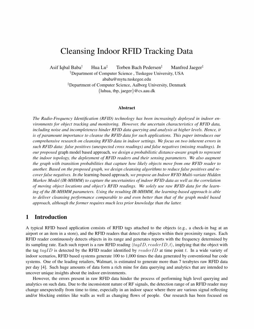
Figure 1: RFID reader deployment example

An indoor RFID deployment is illustrated in Figure 1 andpart of the data generated for a person with tag1 there is given inTable 1. The person was first detected by reader R1 from timepoint t0 to time point t3, yielding four readings by reader R1. Itis noteworthy that the RFID readers altogether do not cover theentire indoor space because otherwise the deployment cost wouldbe too high. Therefore, an object is not continuously detected byRFID readers and for many time points the data does not tellwhere an object is. Due to the unexpected expansion of R4’sdetection range, at time points t13 and t14, tag1 was detected byboth readers R4 and R9. As a result, tag1 seems to be presentin both locations at time points t13 and t14, thus giving rise toa false positive. It is, however, impossible that tag1 can appearin both locations at the same time as the two readers R4 and R9

cover two separate locations and their detection ranges are notconfigured to overlap. Next, tag1 was detected by reader R17

from time point t26 to t29. However, tag1 is not supposed to be detected by R17 before it is detected by readerR10 on its way as shown in Figure 1. Actually, tag1 passed throughR10 but it failed to generate any information,thus giving rise to false negatives.

Table 1: Raw readings table

To effectively and efficiently support high-levelRFID business logic processing, it is necessary to per-form data cleansing to reduce false positives and re-cover false negatives in raw indoor RFID data. Inthis paper, we present two approaches to address thisproblem. The graph-based approach uses a graphmodel to capture detailed domain information includ-ing the deployment of RFID readers, the indoor topol-ogy, the configurations of RFID readers, and the tran-sition probabilities that capture how likely objects move from one RFID reader to another. Utilizing such in-formation in the graph model, algorithms are designed to eliminate false positives in raw RFID data and createcorrect readings for false negatives in the data. In contrast, the learning-based approach assumes considerablyless prior knowledge and employs an Indoor RFID Multi-variate Hidden Markov Model (IR-MHMM) to inferthe most probable observation sequence for an object. Such inferred sequences accordingly reduce false posi-tives and recover false negatives. To learn the parameters for the IR-MHMM, the approach uses raw RFID datawithout any labels.

The rest of this paper is organized as follows. Sections 2 and 3 describe the graph-based indoor RFIDdata cleansing approach and the learning-based approach, respectively. Section 4 draw some conclusions anddiscusses directions for future research on cleansing indoor RFID data.

2 Graph-Based Approach for Cleansing Indoor RFID Data

In the graph-based approach, the raw RFID data is pre-processed and transformed into more meaningful trackingrecords without any information loss. Each tracking record is in the format of 〈tagID, readerID, ts, te, count〉,which means object identified by tagID is detected by reader identified by readerID for count times duringthe time interval [ts, te]. Details can be found in our previous work [3].

2.1 Indoor Graph Model

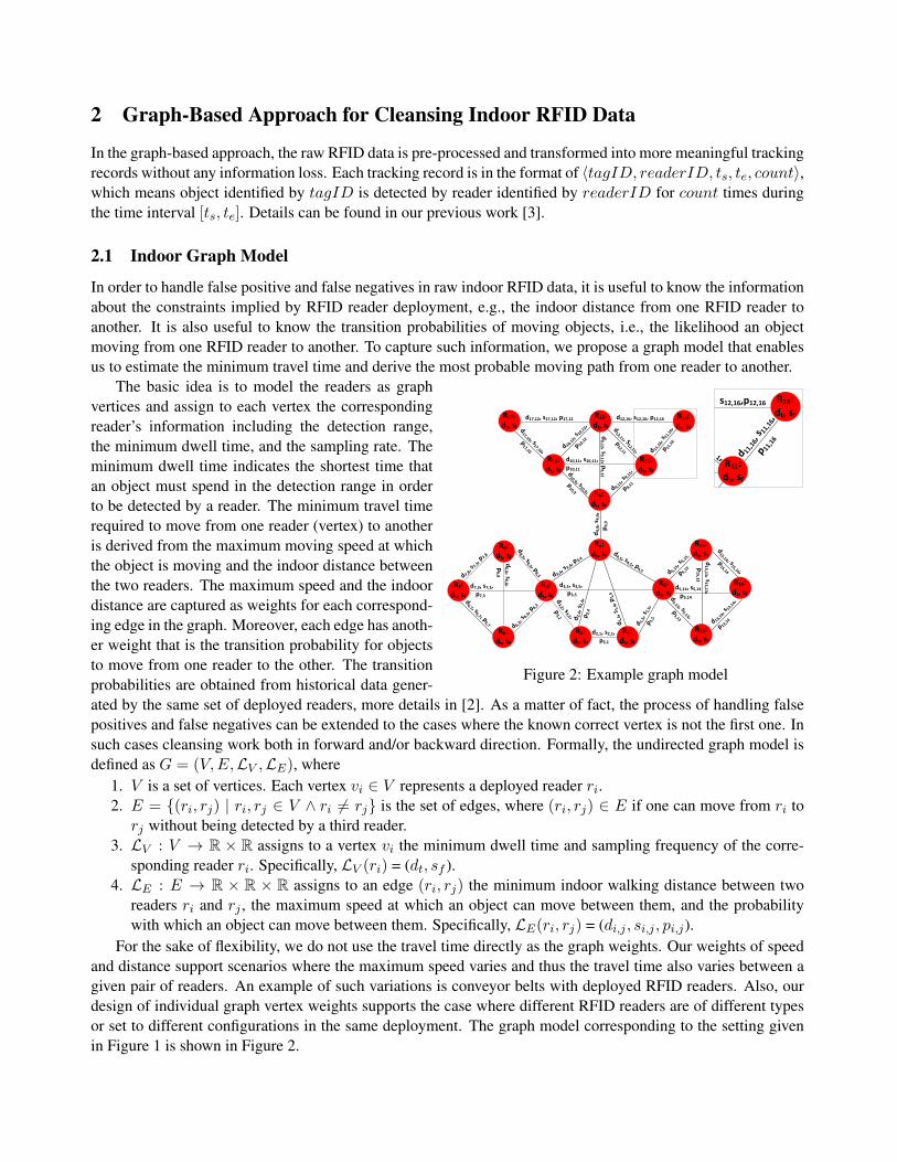
In order to handle false positive and false negatives in raw indoor RFID data, it is useful to know the informationabout the constraints implied by RFID reader deployment, e.g., the indoor distance from one RFID reader toanother. It is also useful to know the transition probabilities of moving objects, i.e., the likelihood an objectmoving from one RFID reader to another. To capture such information, we propose a graph model that enablesus to estimate the minimum travel time and derive the most probable moving path from one reader to another.

d10,9 , s

10,9 , p

10,9

d12,11 , S

12,11 ,

p12,11

d9,1

1, s

9,11,

p9,1

1

d10,1

2, s

10,12,

p10,1

2

d9

,12 , s

9,1

2 , p9

,12

d10,11, s10,11, p10,11

d 11,1

6, s

11,1

6,

p 11,1

6

d17,10 , s

17,10 ,

p17,10

d17,12, s17,12, p17,12 d12,16, s12,16, p12,16

d6,3

, s6,3

, p6,3

d 7,8, s

7,3, p

7,8

d8,3 , s

8,3 , p8,3

d6,7 , s

6,7 , p6,7

d6

,8 , s6

,8 , p

6,8 d 5,1

5, s

5,15,

p 5,15

d 13,1

4, s

13,14,

p 13,14

d5,13 , s

5,13 ,

p5,13

d15,14 , s

15,14 ,

p15,14

d5,14, s5,14 p5,14

d1

5,1

3 , s1

5,1

3 ,p

15

,13

d7,3, s7,3, p7,3

d3,5, s3,5, p3,5

d2,1, s2,1, p2,1

d3,2 , s

3,2 ,

p3,2

d3,4, s3,4

, p3,4

d

1,5, s

1,5,

p1,

5

d 2,

4, s

2,4,

p 2,4

d1,

4, s

1,4,

p1,

4

d4,5 , s4,5 , p

4,5

2

R14: dt, sf

R6: dt, sf

R8: dt, sf

R3: dt, sf

R2: dt, sf

R1: dt, sf

R4: dt, sf

R5: dt, sf

R13: dt, sf

R15: dt, sf

R9: dt, sf

R11: dt, sf

R16: dt, sf

R10: dt, sf

R17:dt, sf

R12: dt, sf

R7: dt, sf

d4

,9, s

4,9

, p

4,9

d 11,1

6, s

11,1

6,

p 11,1

6

R11: dt, sf

R16: dt, sf

1 ,

s12,16,p12,16

Figure 2: Example graph model

The basic idea is to model the readers as graphvertices and assign to each vertex the correspondingreader’s information including the detection range,the minimum dwell time, and the sampling rate. Theminimum dwell time indicates the shortest time thatan object must spend in the detection range in orderto be detected by a reader. The minimum travel timerequired to move from one reader (vertex) to anotheris derived from the maximum moving speed at whichthe object is moving and the indoor distance betweenthe two readers. The maximum speed and the indoordistance are captured as weights for each correspond-ing edge in the graph. Moreover, each edge has anoth-er weight that is the transition probability for objectsto move from one reader to the other. The transitionprobabilities are obtained from historical data gener-ated by the same set of deployed readers, more details in [2]. As a matter of fact, the process of handling falsepositives and false negatives can be extended to the cases where the known correct vertex is not the first one. Insuch cases cleansing work both in forward and/or backward direction. Formally, the undirected graph model isdefined as G = (V,E,LV ,LE), where

1. V is a set of vertices. Each vertex vi ∈ V represents a deployed reader ri.2. E = {(ri, rj) | ri, rj ∈ V ∧ ri 6= rj} is the set of edges, where (ri, rj) ∈ E if one can move from ri torj without being detected by a third reader.

3. LV : V → R × R assigns to a vertex vi the minimum dwell time and sampling frequency of the corre-sponding reader ri. Specifically, LV (ri) = (dt, sf ).

4. LE : E → R × R × R assigns to an edge (ri, rj) the minimum indoor walking distance between tworeaders ri and rj , the maximum speed at which an object can move between them, and the probabilitywith which an object can move between them. Specifically, LE(ri, rj) = (di,j , si,j , pi,j).

For the sake of flexibility, we do not use the travel time directly as the graph weights. Our weights of speedand distance support scenarios where the maximum speed varies and thus the travel time also varies between agiven pair of readers. An example of such variations is conveyor belts with deployed RFID readers. Also, ourdesign of individual graph vertex weights supports the case where different RFID readers are of different typesor set to different configurations in the same deployment. The graph model corresponding to the setting givenin Figure 1 is shown in Figure 2.

2.2 False Positive Cleansing

In this section, we briefly describe how to reduce false positives in the raw data. The details of the process andthe algorithms can be found in our previous work [3]. From the perspective of tracking records, false positivesoccur if two tracking records temporally overlap or are too close to each other. For such cases, we need to checkif the two involved readers are close enough in the deployment. If they are not close enough for the object tomove from one to the other during the time gap, or for it to be seen simultaneously by the two readers, the twotracking records are dirty as they tell wrong information with respect to the reality.

We use the information captured by the graph model (G) to conduct the false positive cleansing. To identifyand reduce the possible false positives involving two RFID readers Rs and Rd, we first compute the minimumtraveling time (min tt(Rs, Rd)) that a moving object needs to reach from Rs to Rd. Specifically, we apply theDijkstra’s algorithm to graph G, expanding the search from Rs until Rt is reached. In the process, we also takeinto account the minimum dwell time of a device Ri, which is captured by the corresponding vertex vi’s weightG.LV (vi), in prioritizing the visiting order of unvisited vertices (readers). Due to the page limit, we omit thedetails of min tt(Rs, Rd) computation.

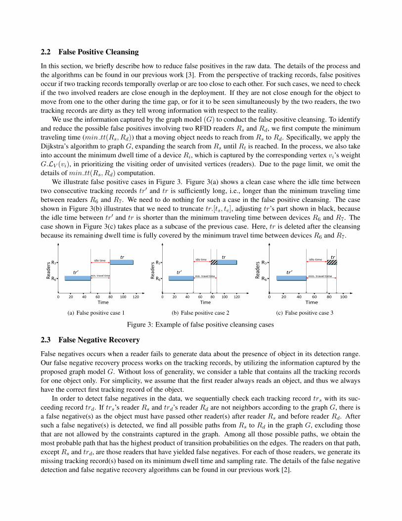
We illustrate false positive cases in Figure 3. Figure 3(a) shows a clean case where the idle time betweentwo consecutive tracking records tr′ and tr is sufficiently long, i.e., longer than the minimum traveling timebetween readers R6 and R7. We need to do nothing for such a case in the false positive cleansing. The caseshown in Figure 3(b) illustrates that we need to truncate tr.[ts, te], adjusting tr’s part shown in black, becausethe idle time between tr′ and tr is shorter than the minimum traveling time between devices R6 and R7. Thecase shown in Figure 3(c) takes place as a subcase of the previous case. Here, tr is deleted after the cleansingbecause its remaining dwell time is fully covered by the minimum travel time between devices R6 and R7.

0 20 40 60 80 100 120

R6

R7

Time

Rea

ders

tr’

tr

min. travel time

idle time

(a) False positive case 1

0 20 40 60 80 100 120

R6

R7

Time

Rea

der

s

tr’

tr

min. travel time

idle time

(b) False positive case 2

0 20 40 60 80 100

R6

R7

Time

Read

ers

tr’

tr

min. travel time

idle time

(c) False positive case 3

Figure 3: Example of false positive cleansing cases

2.3 False Negative Recovery

False negatives occurs when a reader fails to generate data about the presence of object in its detection range.Our false negative recovery process works on the tracking records, by utilizing the information captured by theproposed graph model G. Without loss of generality, we consider a table that contains all the tracking recordsfor one object only. For simplicity, we assume that the first reader always reads an object, and thus we alwayshave the correct first tracking record of the object.

In order to detect false negatives in the data, we sequentially check each tracking record trs with its suc-ceeding record trd. If trs’s reader Rs and trd’s reader Rd are not neighbors according to the graph G, there isa false negative(s) as the object must have passed other reader(s) after reader Rs and before reader Rd. Aftersuch a false negative(s) is detected, we find all possible paths from Rs to Rd in the graph G, excluding thosethat are not allowed by the constraints captured in the graph. Among all those possible paths, we obtain themost probable path that has the highest product of transition probabilities on the edges. The readers on that path,except Rs and trd, are those readers that have yielded false negatives. For each of those readers, we generate itsmissing tracking record(s) based on its minimum dwell time and sampling rate. The details of the false negativedetection and false negative recovery algorithms can be found in our previous work [2].

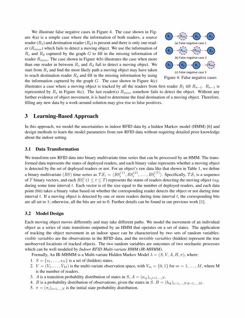
Rd RnRmissRs

RdRmissRs Rmiss

RsR1 RmissR2

(a) False negative case 1

(b) False negative case 2

(c) False negative case 3

Figure 4: False negative cases

We illustrate false negative cases in Figure 4. The case shown in Fig-ure 4(a) is a simple case where the information of both readers, a sourcereader (Rs) and destination reader (Rd) is present and there is only one read-er (Rmiss) which fails to detect a moving object. We use the information ofRs and Rd captured by the graph G to fill in the missing information ofreader Rmiss. The case shown in Figure 4(b) illustrates the case when morethan one reader in between Rs and Rd fail to detect a moving object. Westart from Rs and find the most likely path a moving object may have takento reach destination reader Rd and fill in the missing information by usingthe information captured by the graph G. The case shown in Figure 4(c)illustrates a case where a moving object is tracked by all the readers from first reader R1 till Rn−1. Rn−1 isrepresented by Rs in Figure 4(c). The last reader(s) Rmiss somehow fails to detect the object. Without anyfurther evidence of object movement, it is hard to determine the final destination of a moving object. Therefore,filling any new data by a work-around solution may give rise to false positives.

3 Learning-Based Approach

In this approach, we model the uncertainties in indoor RFID data by a hidden Markov model (HMM) [6] anddesign methods to learn the model parameters from raw RFID data without requiring detailed prior knowledgeabout the indoor setting.

3.1 Data Transformation

We transform raw RFID data into binary multivariate time series that can be processed by an HMM. The trans-formed data represents the states of deployed readers, and each binary value represents whether a moving objectis detected by the set of deployed readers or not. For an object’s raw data like that shown in Table 1, we definea binary multivariate (BS ) time series as T S i = 〈BS (1 )

i ,BS(2 )i , . . . ,BS

(T )i 〉. Specifically, T Si is a sequence

of T binary vectors, and each BS ti (1 ≤ t ≤ T ) represents the status of readers detecting the moving object tagi

during some time interval t. Each vector is of the size equal to the number of deployed readers, and each datapoint (bit) takes a binary value based on whether the corresponding reader detects the object or not during timeinterval t. If a moving object is detected by one or more readers during time interval t, the corresponding bitsare all set to 1; otherwise, all the bits are set to 0. Further details can be found in our previous work [1].

3.2 Model Design

Each moving object moves differently and may take different paths. We model the movement of an individualobject as a series of state transitions outputted by an HMM that operates on a set of states. The applicationof tracking the object movement in an indoor space can be characterized by two sets of random variables:visible variables are the observations in the RFID data, and the invisible variables (hidden) represent the trueunobserved locations of tracked objects. The two random variables are outcomes of two stochastic processeswhich can be well modeled by Indoor RFID Multi-variate HMM (IR-MHMM).

Formally, An IR-MHMM is a Multi-variate Hidden Markov Model λ = (S, V,A,B, π), where:1. S = {s1, . . . , sN} is a set of (hidden) states.2. V = (V1, . . . , VM ) is the multi-variate observation space, with Vm = {0, 1} for m = 1, . . . ,M , where M

is the number of readers.3. A is a transition probability distribution of states in S, A = (aij)i,j=1,...,N .4. B is a probability distribution of observations, given the states in S. B = (bik)i=1,...,N ;k=1,...,M .5. π = (πi)i=1,...,N is the initial state probability distribution.

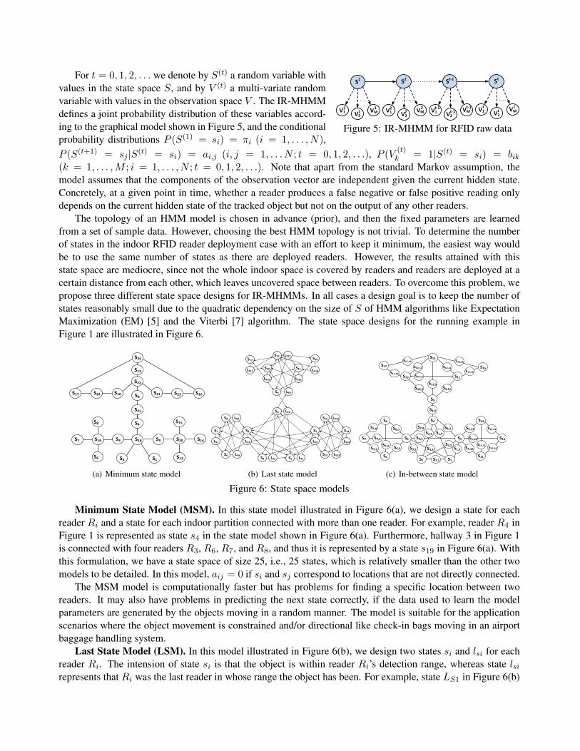
S1 S2 St-1 St

V1 V2VM V1 V2

VM V1 V2 VM V1 V2

VM1

11 2

22 t-1

t-1t-1 t

tt

Figure 5: IR-MHMM for RFID raw data

For t = 0, 1, 2, . . . we denote by S(t) a random variable withvalues in the state space S, and by V (t) a multi-variate randomvariable with values in the observation space V . The IR-MHMMdefines a joint probability distribution of these variables accord-ing to the graphical model shown in Figure 5, and the conditionalprobability distributions P (S(1) = si) = πi (i = 1, . . . , N),P (S(t+1) = sj |S(t) = si) = ai,j (i, j = 1, . . . N ; t = 0, 1, 2, . . .), P (V (t)

k = 1|S(t) = si) = bik(k = 1, . . . ,M ; i = 1, . . . , N ; t = 0, 1, 2, . . .). Note that apart from the standard Markov assumption, themodel assumes that the components of the observation vector are independent given the current hidden state.Concretely, at a given point in time, whether a reader produces a false negative or false positive reading onlydepends on the current hidden state of the tracked object but not on the output of any other readers.

The topology of an HMM model is chosen in advance (prior), and then the fixed parameters are learnedfrom a set of sample data. However, choosing the best HMM topology is not trivial. To determine the numberof states in the indoor RFID reader deployment case with an effort to keep it minimum, the easiest way wouldbe to use the same number of states as there are deployed readers. However, the results attained with thisstate space are mediocre, since not the whole indoor space is covered by readers and readers are deployed at acertain distance from each other, which leaves uncovered space between readers. To overcome this problem, wepropose three different state space designs for IR-MHMMs. In all cases a design goal is to keep the number ofstates reasonably small due to the quadratic dependency on the size of S of HMM algorithms like ExpectationMaximization (EM) [5] and the Viterbi [7] algorithm. The state space designs for the running example inFigure 1 are illustrated in Figure 6.

S7 S3

S8

S6

S19

S4

S2 S1

S18

S5

S15

S13

S20

S10 S9

S22

S23S24 S11

S7 S14

S25

S17 S16

S21

S12

(a) Minimum state model

S7

LS7

S6 LS6

S8 LS8

S3

LS3

S5

LS5

S13 LS13

S15 LS15

S14

LS14

S10

LS10

S9 LS9

S12 LS12

S11

LS11

S4 LS4

S2 LS2 S1 LS1

S16

LS16

S17

LS17

(b) Last state model

S7 S3

S8

S6

S7,3

S2 S1

S16

S17,12

S9,11

S7

S12

S7,8

S7,6 S6,3

S8,3

S7,3

S4,9

S3,5

S1,4

S7 S14

S13

S15

S5,14

S15,14

S13,15

S7,8 S8,3

S2,1

S2,4

S3,2S2,5

S1,5

S5,13 S13,14

S5,15

S4

S12,9

S9

S10,11

S10,12

S10

S12,11S17

S11

S10,9

S12,16

S11,16S17,10

S5

S3,1

(c) In-between state model

Figure 6: State space models

Minimum State Model (MSM). In this state model illustrated in Figure 6(a), we design a state for eachreader Ri and a state for each indoor partition connected with more than one reader. For example, reader R4 inFigure 1 is represented as state s4 in the state model shown in Figure 6(a). Furthermore, hallway 3 in Figure 1is connected with four readers R3, R6, R7, and R8, and thus it is represented by a state s19 in Figure 6(a). Withthis formulation, we have a state space of size 25, i.e., 25 states, which is relatively smaller than the other twomodels to be detailed. In this model, aij = 0 if si and sj correspond to locations that are not directly connected.

The MSM model is computationally faster but has problems for finding a specific location between tworeaders. It may also have problems in predicting the next state correctly, if the data used to learn the modelparameters are generated by the objects moving in a random manner. The model is suitable for the applicationscenarios where the object movement is constrained and/or directional like check-in bags moving in an airportbaggage handling system.

Last State Model (LSM). In this model illustrated in Figure 6(b), we design two states si and lsi for eachreader Ri. The intension of state si is that the object is within reader Ri’s detection range, whereas state lsirepresents that Ri was the last reader in whose range the object has been. For example, state LS1 in Figure 6(b)

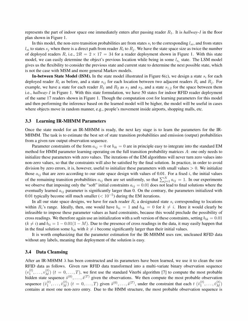
represents the part of indoor space one immediately enters after passing reader R1. It is hallway-1 in the floorplan shown in Figure 1.

In this model, the non-zero transition probabilities are from states si to the corresponding lsi, and from stateslsi to states sj when there is a direct path from readerRi toRj . We have the state space size as twice the numberof deployed readers R, i.e., 2R = 2 × 17 = 34 for a reader deployment shown in Figure 1. With this statemodel, we can easily determine the object’s previous location while being in some lsi state. The LSM modelgives us the flexibility to consider the previous state and current state to determine the next possible state, whichis not the case with MSM and more general Markov models.

In-between State Model (ISM). In the state model illustrated in Figure 6(c), we design a state si for eachdeployed reader Ri as before, and a state sij for each location between two adjacent readers Ri and Rj . Forexample, we have a state for each reader R1 and R2 as s1 and s2, and a state s1,2 for the space between themi.e., hallway-1 in Figure 1. With this state formulation, we have 50 states for indoor RFID reader deploymentof the same 17 readers shown in Figure 1. Though the computation cost for learning parameters for this modeland then performing the inference based on the learned model will be higher, the model will be useful in caseswhere objects move in random manner, e.g., people’s movement inside airports, shopping malls, etc.

3.3 Learning IR-MHMM Parameters

Once the state model for an IR-MHMM is ready, the next key stage is to learn the parameters for the IR-MHMM. The task is to estimate the best set of state transition probabilities and emission (output) probabilitiesfrom a given raw output observation sequence.

Parameter constraints of the form aij = 0 or bik = 0 are in principle easy to integrate into the standard EMmethod for HMM parameter learning operating on the full transition probability matrices A: one only needs toinitialize these parameters with zero values. The iterations of the EM algorithms will never turn zero values intonon-zero values, so that the constraints will also be satisfied by the final solution. In practice, in order to avoiddivision by zero errors, it is, however, useful to initialize these parameters with small values > 0. We initializethose aij that are zero according to our state space design with values of 0.01. For a fixed i, the initial valuesof the remaining transition probabilities aij then are set uniformly, so that

∑Nj=1 aij = 1. In our experiments

we observe that imposing only the “soft” initial constraints aij = 0.01 does not lead to final solutions where theeventually learned aij parameter is significantly larger than 0. On the contrary, the parameters initialized with0.01 typically become still much smaller (< 10−5) during the EM iterations.

In all our state space designs, we have for each reader Ri a designated state si corresponding to locationswithin Ri’s range. Ideally, then, one would have bii = 1 and bik = 0 for k 6= i. Here it would clearly beinfeasible to impose these parameter values as hard constraints, because this would preclude the possibility ofcross readings. We therefore again use an initialization with a soft version of these constraints, setting bik = 0.01(k 6= i) and bii = 1− 0.01(1−M). Due to the presence of cross readings in the data, it may easily happen thatin the final solution some bik with k 6= i become significantly larger than their initial values.

It is worth emphasizing that the parameter estimation for the IR-MHMM uses raw, uncleaned RFID datawithout any labels, meaning that deployment of the solution is easy.

3.4 Data Cleansing

After an IR-MHMM λ has been constructed and its parameters have been learned, we use it to clean the rawRFID data as follows. Given raw RFID data transformed into a multi-variate binary observation sequence(v

(t)1 , . . . , v

(t)M ) (t = 0, . . . , T ), we first use the standard Viterbi algorithm [7] to compute the most probable

hidden state sequence s(0), . . . , s(T ) given the observations. We then compute the most probable observationsequence (v

(t)1 , . . . , v

(t)M ) (t = 0, . . . , T ) given s(0), . . . , s(T ), under the constraint that each t (v(t)1 , . . . , v

(t)M )

contains at most one non-zero entry. Due to the HMM structure, the most probable observation sequence is

determined pointwise for each t by maximizing P (V (t)1 = v

(t)1 , . . . , V

(t)M = v

(t)M |S(t) = s(t)). If s(t) = si, then

this probability is maximized by setting v(t)k = 1 if bik > 0.5, and v(t)k = 0 otherwise. Under the constraint thatv(t)k can be nonzero for at most one k, this is modified to setting v(t)k = 1 if bik > 0.5, and bik > bik′ for allk′ 6= k.

4 Conclusion and Future Work

In this paper we introduce two approaches for cleansing indoor RFID data. The graph model based approachcaptures in a graph detailed prior knowledge: the RFID reader deployment (both topology and distance amongreaders), RFID reader properties, and the transition probabilities for objects to move from one reader to another.Such information is utilized in detecting false positives and false negatives and cleanse them in raw indoor RFIDdata. In contrast, the learning-based approach only needs to know the topology of reader deployment in theindoor space. Instead, it learns information from raw data using a hidden Markov model designed for indoorRFID based object tracking, and applies the model thus obtained to cleanse raw RFID data. Our experimentalstudies [1] show that, when having enough indoor RFID data for learning, the learning-based approach achievesdata cleansing results comparable to or even better than those delivered by the graph-based model.

There are several directions for further research on cleansing indoor RFID tracking data.• It is possible to further enhance the learning-based approach by using a probabilistic timing model to relate

the travel time between readers and the dwell time at each reader. Such information can be integrated intothe proposed IR-MHMM.• It is relevant to design a hybrid, tunable approach that can work with, and adapt to, different availabilities

of prior knowledge in order to maximize the data cleansing effectiveness.• If domain knowledge is available for a particular indoor scenario, both the graph-based approach and the

learning-based approach can be further enhanced to achieve better cleansing results.

AcknowledgmentsThis work was partly sponsored by the NILTEK project funded by European Regional Development Fund andthe BagTrack project funded by the Danish National Advanced Technology Foundation (grant no. 010-2011-1).

References

[1] A. I. Baba, M. Jaeger, H. Lu, T. B. Pedersen, W.-S. Ku, and X. Xie. Learning-based cleansing for indoorRFID data. In SIGMOD, pages 925–936, 2016.

[2] A. I. Baba, H. Lu, T. B. Pedersen, and X. Xie. Handling false negatives in indoor RFID data. In MDM,pages 117–126, 2014.

[3] A. I. Baba, H. Lu, X. Xie, and T. B. Pedersen. Spatiotemporal data cleansing for indoor RFID tracking data.In MDM, pages 187–196, 2013.

[4] Y. Bai, F. Wang, and P. Liu. Efficiently filtering RFID data streams. In CleanDB, 2006.

[5] L. E. Baum and T. Petrie. Statistical inference for probabilistic functions of finite state Markov chains.Annals of Mathematical Statistics, 37:1554–1563, 1966.

[6] L. R. Rabiner and B. H. Juang. An introduction to hidden markov models. IEEE ASSp Magazine, 1986.

[7] A. J. Viterbi. Error bounds for convolutional codes and an asymptotically optimum decoding algorithm.IEEE Trans. Information Theory, 13(2):260–269, 1967.