Chapter-4

CLASSIFICATION USING NEURAL

NETWORK

4.1 IntroductionClassification is one of the most active research and application

area of neural networks. Neural Networks are considered a robust classifier. This chapter summarizes some of the most important developments of neural network in pattern classification and specifically, the Pattern Classification using the polynomial neural network.

The field of Neural Networks has arisen from diverse sources, ranging from the fascination of mankind with understanding and emulating the human brain, to broader issues of copying human abilities such as Classification, it is one of the most frequently encountered decision making tasks of human activity. Classification is an essential feature to separate large datasets into classes for the purpose of Rule generation, Decision Making, Pattern recognition, Dimensionality Reduction, Data Mining etc. The Neural networks have emerged as an important tool for classification.

The recent vast research activities in classification have established that neural networks are a promising alternative to various conventional classification methods. The advantage of neural networks lies in the following theoretical aspects. First, neural networks are data driven self-adaptive methods in that they can adjust themselves to the data without any explicit specification of functional or distributional form for the underlying model. Second, they are universal functional approximators in that neural networks can approximate any function with arbitrary accuracy [42], [77], [78]. Since any classification procedure seeks a functional relationship between the group membership and the attributes of the object, accurate identification of this underlying function is doubtlessly important. Third, neural networks have shown extremely good nonlinear input-output mapping, which makes them flexible in

modeling real world complex relationships. Fourth, neural networks are able to estimate the posterior probability, which provides the basis for establishing classification rule and performing statistical analysis [171]. Finally, neural network is able to work parallel with input variables and consequently handle large sets of data swiftly. The principal strength with the network is its ability to extract the patterns and irregularities as well as detecting multi-dimensional non-linear connections in data. The latter quality is extremely useful for modeling dynamical systems, e.g. the stock market, meteorological department apart from that, neural networks are frequently used for pattern recognition tasks and non-linear regression [19]. Although significant progress has been made in classification related areas of neural networks, a number of issues in applying neural networks still remain to be solved successfully or completely. This chapter provides a quintessence of the most important advances of neural networks in classification and detail description of polynomial neural network. For a good introductory text, see Hertz et al. [73] and Wasserman [220].

4.2 Fundamentals of Biological Neural Network

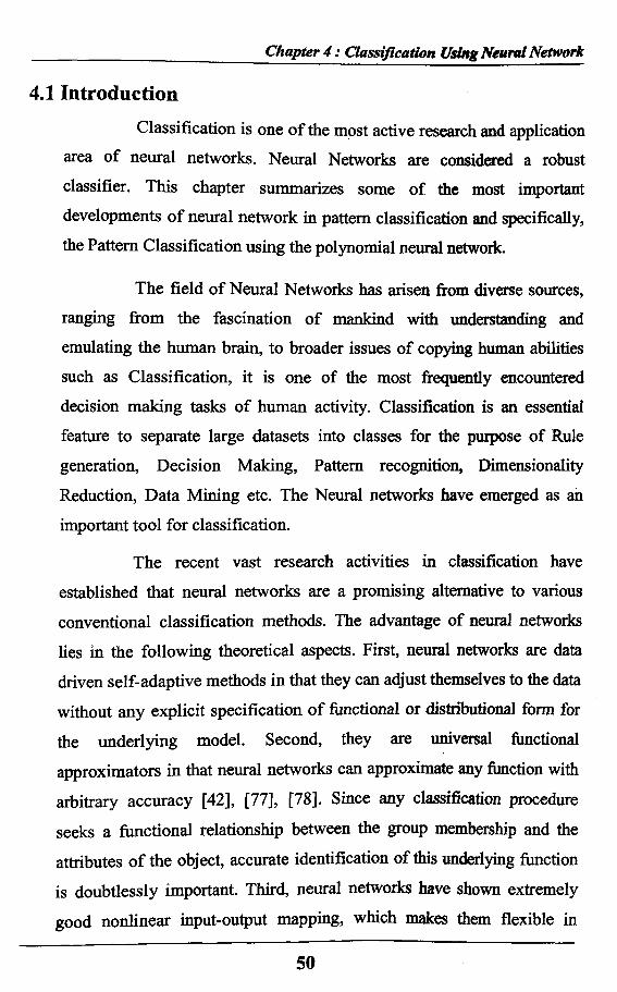
The term neural network inspired from the functioning of the human brain. It’s adopted simplified models of biological neural network [4]. The biological neural network consists of nerve cells (neurons) as in Figure-4.1. The cell body of the neuron, which includes the neuron’s nucleus, is where most of the neural 'computation' takes place. Neural activity passes from one neuron to another in terms of electrical triggers which travel from one cell to the other down the neuron’s axon, by means of an electrochemical process of voltage-gated ion exchange along the axon and of diffusion of neurotransmitter molecules through the membrane over the synaptic gap. The axon can be viewed as a connection wire. However, the mechanism of signal flow is

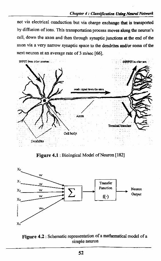
not via electrical conduction but via charge exchange that is transported by diffusion of ions. This transportation process moves along the neuron’s cell, down the axon and then through synaptic junctions at the end of the axon via a very narrow synaptic space to the dendrites and/or soma of the next neuron at an average rate of 3 m/sec [66].

INPUT from otluer neurons O tffPBT to o tlu r m

Figure 4.1: Biological Model of Neuron [182]

Xo

NeuronOutput

Figure 4.2 : Schematic representation of a mathematical model of asimple neuron

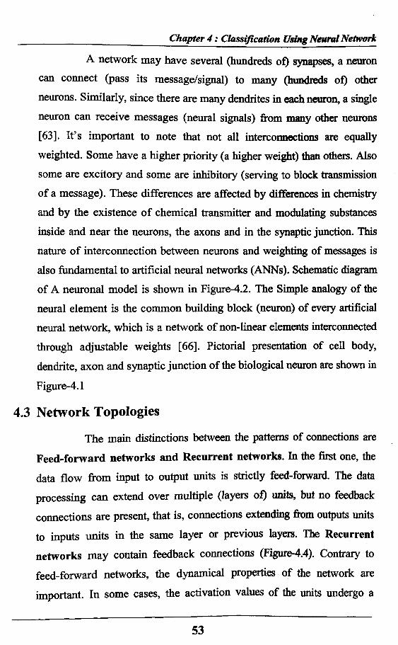
A network may have several (hundreds of) synapses, a neuron can connect (pass its message/signal) to many (hundreds of) other neurons. Similarly, since there are many dendrites in each neuron, a single neuron can receive messages (neural signals) from many other neurons [63]. It’s important to note that not all interconnections are equally weighted. Some have a higher priority (a higher weight) than others. Also some are excitory and some are inhibitory (serving to block transmission of a message). These differences are affected by differences in chemistry and by the existence of chemical transmitter and modulating substances inside and near the neurons, the axons and in the synaptic junction. This nature of interconnection between neurons and weighting of messages is also fundamental to artificial neural networks (ANNs). Schematic diagram of A neuronal model is shown in Figure-4.2. The Simple analogy of the neural element is the common building block (neuron) of every artificial neural network, which is a network of non-linear elements interconnected through adjustable weights [66]. Pictorial presentation of cell body, dendrite, axon and synaptic junction of the biological neuron are shown in

Figure-4.1

4.3 Network Topologies

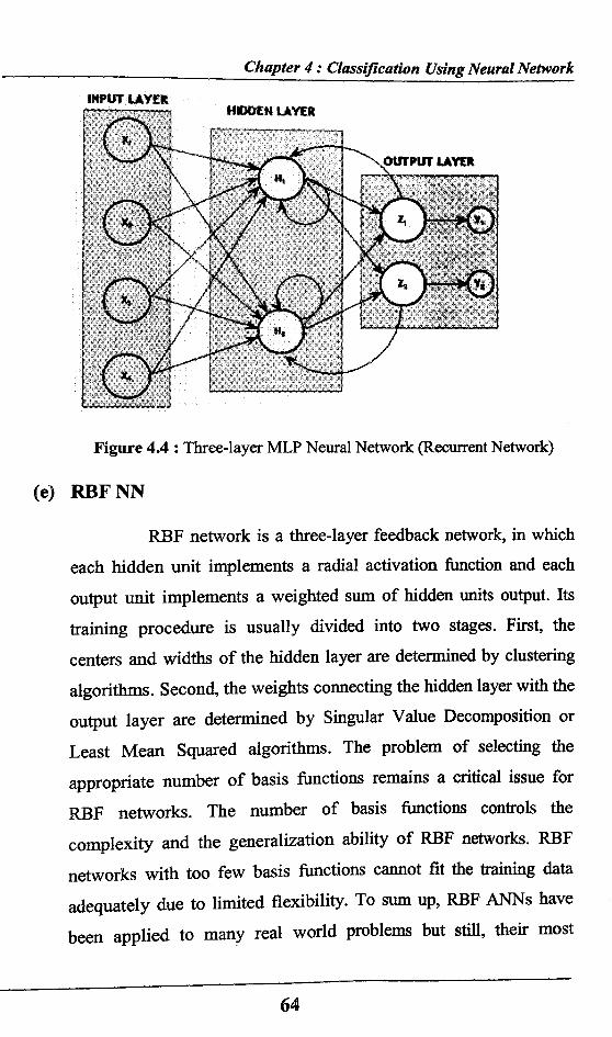
The main distinctions between the patterns of connections are Feed-forward networks and Recurrent networks. In the first one, the data flow from input to output units is strictly feed-forward. The data processing can extend over multiple (layers of) units, but no feedback connections are present, that is, connections extending from outputs units to inputs units in the same layer or previous layers. The Recurrent networks may contain feedback connections (Figure-4.4). Contrary to feed-forward networks, the dynamical properties of the network are important. In some cases, the activation values of the units undergo a

relaxation process such that the network will evolve to a stable state in which these activations do not change anymore. In other applications, the change of the activation values of the output neurons is significant; such that the dynamical behavior constitutes the output of the network [4]. The example of feed-forward networks is perceptron and the examples of recurrent networks have been presented by Anderson, Kohonen and Hopfield are discussed in Section-4.5.

4.4 Brief History and Land Marks of Neural Network

In this section we have focused on a few important

breakthroughs throughout history. In 1943 McCulloch and Pitts describe

the brain functions by mathematical means and used their neural networks

to model logical operators. In 1949 Hebb proposed that the synaptic

connections inside the brain are constantly changing as a person gains

experience. In other words, synapses are either strengthened or weakened

depending on whether neurons on either side of the synapse are activated

simultaneously or not. In the late 1950s Rosenblatt introduced the concept

of the perceptron. Basically, the Perceptron, which works as a pattem-

classifier, is a more sophisticated model of the neuron developed by

McCulloch and Pitts. Depending on the amount of neurons incorporated,

the perceptron can solve classification problems with various numbers of

classes which are linearly separable, which is a major setback. This was

shown by Minsky and Papert in 1969. Minsky and Papert also raised the

issue of the credit-assignment problem related to the multi-layer

perceptron. During the next decade the general interest in neural networks

diminish mainly as a direct consequence of the results reported in the late

sixties. Certainly the lack of powerful experimental equipment

(computers, work stations etc.) also had an influence on the decline.

The interest in neural networks is renewed in 1982 when Kohonen introduced the Self Organizing Map (SOM). SOM use an unsupervised learning algorithm for applications in specifically data mining, image processing and visualization. As a basic description one can say that high-dimensional data is transformed and organized in a low­dimensional output space. The same year Hopfield built a bridge between neural computing and physics. A Hopfield network (which consists of symmetric synaptic connections and multiple feedback loops) which is initialized with random weights eventually reaches a final state of sta­bility. From a physicists point of view a Hopfield network corresponds to a dynamical system falling into a state of minimal energy.

In 1984 the Boltzmann machine was invented by Ludwig

Boltzmann. This neural network utilizes a stochastic learning algorithm

based on properties of the Boltzmann distribution.

Rummelhart, Hinton and Williams, who discovered the

backpropagation algorithm in 1986, proved crucial step for the revival of

neural networks. Rummelhart, Hinton and Williams got the credit but it

showed that Werbos already in 1974 had introduced the error

backpropagation in his PhD thesis. This learning algorithm is

unchallenged as the most influential learning algorithm for training of

multi-layer perceptrons.

The Radial-Basis Function (RBF) was brought forward by Broomhead and Lowe in 1988. The RBF netwoik emerged as an alternative to the multi-layer perception in the search of a solution to the multivariate interpolation problem. By using a set of symmetric non-linear functions in the hidden units of a neural network new properties could be explored. Work by Moody and Darken (presented in 1989) on how to

estimate parameters in the basis functions has contributed significantly to the theory.

One of the first approaches of systematic design of nonlinear relationships comes under the name of a Group Method of Data Handling (GMDH) which was proposed in the late 1960s by Ivakhnenko. The GMDH algorithm generates an optimal structure of the model through successive generations of partial descriptions (PDs) of data being regarded as quadratic regression polynomials with two input variables. It’s identifying the nonlinear relations between input and output variables. In late 1990 this method is improved as Polynomial Neural Network. It was proposed to alleviate the problems associated with the GMDH.

4.5 Architecture of Neural Network

It is useful to make a distinction between different neural network architectures based on the way in which the network is trained and classify the patterns. Such a distinction dictates the approach to a problem at a fundamental level. The Neural Network techniques can be divided into supervised, unsupervised and reinforced techniques. In this study we will concentrate on supervised and unsupervised only.

4.5.1 Supervised Neural Network

The neural network is given the target outputs on to which it should map its inputs, i.e. it is given in paired data of input and output. The error arising from the discrepancy between the network output and the target is used to optimize the network parameters. Once the network has been trained, it is used to produce an output for unseen data.

The neurons are arranged in a layer fashion is referred to as a perceptron. Perceptrons are trained in a supervised learning fashion. This means that one tries to train the net to perform specific, known functions

[147]. We have a target test set where the outputs are known, which is used to train the net

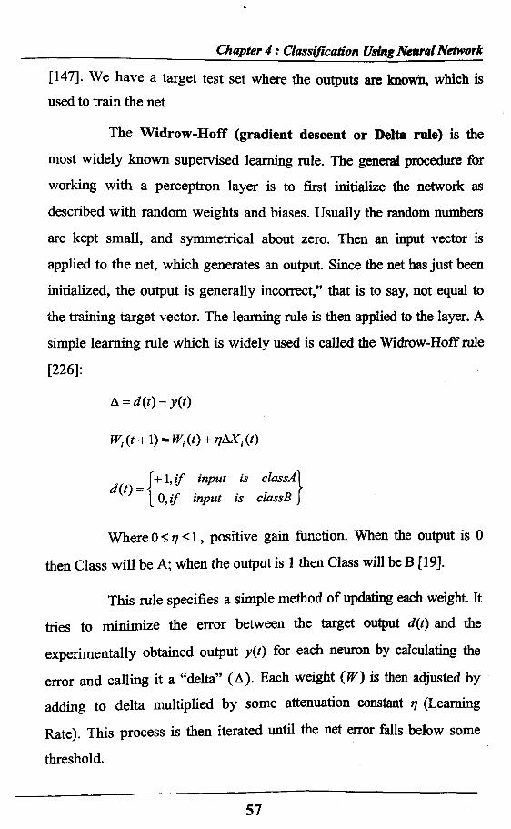
The Widrow-Hoff (gradient descent or Delta rale) is the

most widely known supervised learning rule. The general procedure for working with a perceptron layer is to first initialize the network as

described with random weights and biases. Usually the random numbers

are kept small, and symmetrical about zero. Then an input vector is applied to the net, which generates an output. Since the net has just been

initialized, the output is generally incorrect,” that is to say, not equal to

the training target vector. The learning rule is then applied to the layer. A

simple learning rule which is widely used is called the Widrow-HofF rule

[226]:

A = d { t ) - y ( t )

Wi{t + \) = Wi{t) + v^Xi{t)

+ 1, i f input is classA 0, i f input is classB

Where 0 < 77 < 1, positive gain function. When the output is 0

then Class will be A; when the output is 1 then Class will be B [19].

This rule specifies a simple method of updating each weight. It tries to minimize the error between the target output d(t) and the

experimentally obtained output y(t) for each neuron by calculating the

error and calling it a “delta” (A). Each weight (W) is then adjusted by adding to delta multiplied by some attenuation constant 77 (Learning

Rate). This process is then iterated until the net error falls below some

threshold.

By adding its specific error to each of the weights, we are ensured that the network is being moved towards the position of minimum

error and by using attenuation constant, rather than the foil value of the error, we move it slowly towards this position of minimnm error. When correctly trained, the perceptron exhibits some highly promising behavior. The descriptions of Different models based on the perceptron are given below.

(a) Single Layer Perceptron

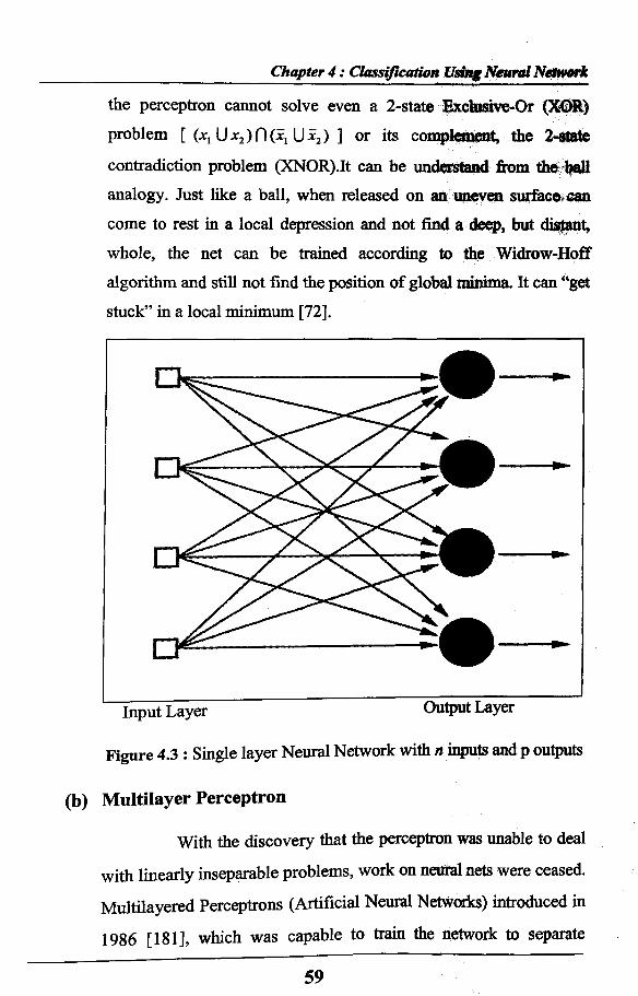
The perceptron’s learning theorem was formulated by Rosenblatt in 1961. The theorem states that a perceptron can learn (solve) anything it can represent (simulate). A single layer perceptron as shown in Figure-4.3 is able to learn to classify objects according to their position in n-dimensional hyperspace defined by the n inputs (Not interconnected) where the problem can be reduced to a linear separable (classification) problem [108].

When perceptrons were first introduced, they seemed revolutionary. It was a mathematical model of a structure which could be taught to classify points in hyperspace, not according to rules, but by being shown which points belonged in which sets. This freed humans from the necessity of determining rules by which the points should be classified. It was thought that they could be trained to solve any problem which could be set up as a classification problem in hyperspace.

In 1969, Minsky and Papert published a book where they pointed out as did E. B. Crane in 1965 in a less-known book, to the grave limitations in the capabilities of the perceptron, as is evident by its representation theorem. They have shown that, for example,

the perceptron cannot solve even a 2-state Exctusive-Or (XGR) problem [ (*, U*2) ] or its complement, the 2-state

contradiction problem (XNOR).It can be understand from the ball analogy. Just like a ball, when released on an uneven surfacecan come to rest in a local depression and not find a deep, but distant, whole, the net can be trained according to the Widrow-Hoff algorithm and still not find the position of global minima. It can “get stuck” in a local minimum [72].

Input Layer Output Layer

Figure 4.3 : Single layer Neural Network with n inputs and p outputs

(b) Multilayer Perceptron

With the discovery that the perceptron was unable to deal

with linearly inseparable problems, work on neural nets were ceased.

Multilayered Perceptrons (Artificial Neural Networks) introduced in

1986 [181], which was capable to train the network to separate

linearly inseparable data. It consists of large number of units

(neurons) joined together in a pattern of connections (Figure-4.5).

Units in a neural net are usually segregated into three classes: input

units, which receive information to be processed; output units, where

the results of the processing are found; and units in between known

as hidden units. There are various models defined based on

Multilayer Perceptron, some of them are defined here.

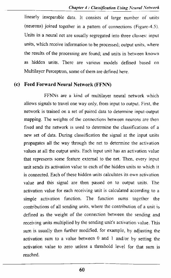
(c) Feed Forward Neural Network (FFNN)

FFNNs are a kind of multilayer neural network which

allows signals to travel one way only, from input to output. First, the

network is trained on a set of paired data to determine input-output

mapping. The weights of the connections between neurons are then

fixed and the network is used to determine the classifications of a

new set of data. During classification the signal at the input units

propagates all the way through the net to determine the activation

values at all the output units. Each input unit has an activation value

that represents some feature external to the net. Then, every input

unit sends its activation value to each of the hidden units to which it

is connected. Each of these hidden units calculates its own activation

value and this signal are then passed on to output units. The

activation value for each receiving unit is calculated according to a

simple activation function. The function sums together the

contributions of all sending units, where the contribution of a unit is

defined as the weight of the connection between the sending and

receiving units multiplied by the sending unit's activation value. This

sum is usually then further modified, for example, by adjusting the

activation sum to a value between 0 and 1 and/or by setting the

activation value to zero unless a threshold level for that sum is

reached.

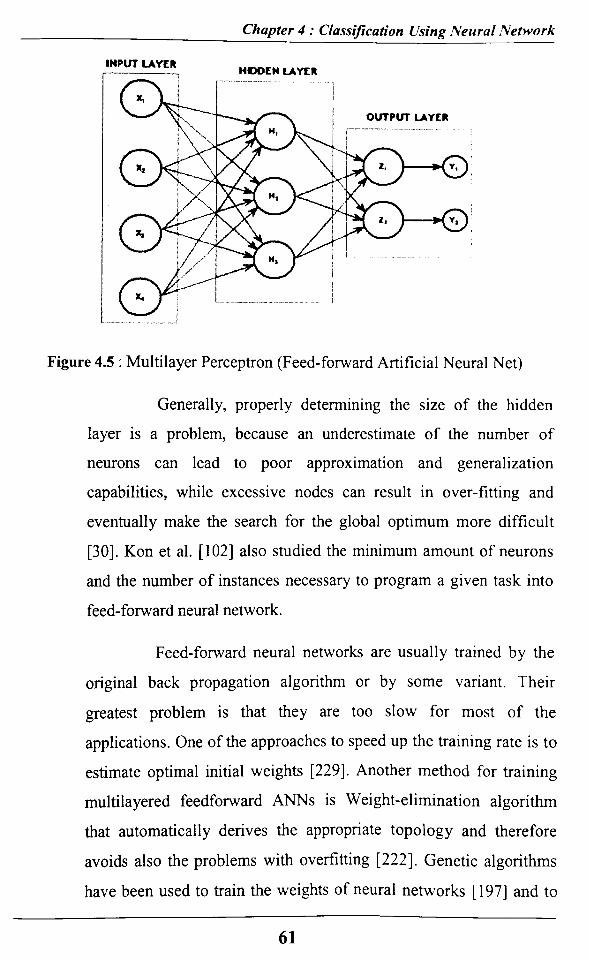
Figure 4.5 : Multilayer Perceptron (Feed-forward Artificial Neural Net)

Generally, properly determining the size of the hidden

layer is a problem, because an underestimate of the number of

neurons can lead to poor approximation and generalization

capabilities, while excessive nodes can result in over-fitting and

eventually make the search for the global optimum more difficult

[30]. Kon et al. [102] also studied the minimum amount of neurons

and the number of instances necessary to program a given task into

feed-forward neural network.

Feed-forward neural networks are usually trained by the

original back propagation algorithm or by some variant. Their

greatest problem is that they are too slow for most of the

applications. One of the approaches to speed up the training rate is to

estimate optimal initial weights [229]. Another method for training

multilayered feedforward ANNs is Weight-elimination algorithm

that automatically derives the appropriate topology and therefore

avoids also the problems with overfitting [222], Genetic algorithms

have been used to train the weights of neural networks [197] and to

find the architecture of neural networks [269]. There are also Bayesian methods in existence which attempt to train neural networks [217]. A number of other techniques have emerged recently which attempt to improve Artificial Neural Nets training algorithms by changing the architecture of the networks as training proceeds. These techniques include pruning useless nodes or weights [32], and constructive algorithms, where extra nodes are added as required [157].

(d) Back Propagation (BP)

BP algorithm is used for training artificial neural networks [229]. Training is usually carried out by iterative updating of weights based on the error signal. The negative gradient of a mean-squared error function is commonly used. In the output layer, the error signal is the difference between the desired and actual output values, multiplied by the slope of a sigmoidal activation function. Then the error signal is back-propagated to the lower layers. BP is a descent algorithm, which attempts to minimize the error at the each iteration. The weights of the network are adjusted by the algorithm such that the error is decreased along a decent direction. Traditionally, two parameters, called learning rate and momentum factor, are used for controlling the weight adjustment along the descent direction and for

dampening oscillations.

The BP algorithm is used for many applications. However, its convergence rate is relatively slow, especially for networks with more than one hidden layer. The reason for this is the saturation behavior of the activation function used for the hidden and output layers. Since the output of a unit exists in the saturation area, the

corresponding descent gradient takes a very small value, even if the output error is large, leading to very little progress in the weight adjustment. The selection of the learning rate and momentum factor is arbitrary, because the error surface usually consists of many flat and steep regions and behaves differently from application to application. Large values of the learning rate and momentum factor are helpful to accelerate learning. However, this increases the possibility of the weight search jumping over steep regions and moving out of the desired regions.

In training by back-propagation algorithm, the target

values of the neuron’s output are set to 1 or 0 but there are no target

values for the hidden neuron’s output. Thus the training is not

efficient. To overcome from this problem several approaches are

developed to train the network layer by layer using [57], [117],

[178], [212], [213], [218], [219], each layer is trained layer by layer

using, as the objective function for each layer, the objective function

for the discriminant analysis that maximizes the between class scatter

while keeping the within class scatter constant. In Wang and Chan

[219] the weights between output and hidden layers and the output of

the previous layers are determined by minimizing the sum of squared

errors. Then the calculated outputs are used as a desired output of the

hidden neurons. This method can be used both for pattern

classification and function approximation [2].

INPUT LAYER

Figure 4.4 : Three-layer MLP Neural Network (Recurrent Network)

(e) RBF NN

RBF network is a three-layer feedback network, in which each hidden unit implements a radial activation function and each output un it implements a weighted sum of hidden units output. Its training procedure is usually divided into two stages. First, the centers and widths of the hidden layer are determined by clustering algorithms. Second, the weights connecting the hidden layer with the output layer are determined by Singular Value Decomposition or Least Mean Squared algorithms. The problem of selecting the appropriate number of basis functions remains a critical issue for RBF networks. The number of basis functions controls the complexity and the generalization ability of RBF networks. RBF networks with too few basis functions cannot fit the training data adequately due to limited flexibility. To sum up, RBF ANNs have been applied to many real world problems but still, their most

striking disadvantage is their lack of ability to reason about their output in a way that can be effectively communicated. For this reason many researchers have tried to address the issue of improving

the comprehensibility of neural networks, where the most attractive solution is to extract symbolic rules from trained neural networks. Setiono and Leow [119] divided the activation values of relevant hidden units into two subintervals and then found the set of relevant connections of those relevant units to construct rules. They are trying to make the network architecture flexible and optimized. Radial Basis Function (RBF) networks have been also widely applied in many sciences and engineering fields [173], [236].

(e) Group Method Data Handling (GMDH)

Prof. A. G. Ivakhnenko in the late 1960s developed Group

Method Data Handling (GMDH) as a means for identifying

nonlinear relations between input and output variables. As described

in [227] the GMDH generates successive layers with complex links

that are individual terms of a polynomial equation. GMDH offers

several advantages over conventional Feedback Neural Networks.

Since it allows a second-order method of convergence to its memory

locations, it approaches equilibrium rapidly. The memories of this

network can be located anywhere in an n-dimensional space rather

than being confined to the comers of a hypercube, as is the case with

Hopfield network and other networks which uses sigmoidal or

similar nonlinearities. The GMDH algorithms better epitomize the

biological complex neurons which are self organized. Only by this

self-organizing method can optimal non-physical models be found

for small, inaccurate or noisy data samples. Non-physical models

usually have a higher accuracy and a simpler model structure than

physical models. In a neuronet with such neurons, we will have a

twofold multilayered structure: neurons themselves are multilayered

and they will be united in a multilayered way into common matrix

[172]. GMDH algorithms are examples of complex active neurons,

because they choose the effective inputs and corresponding

coeficients by themselves during the process of self-organization.

The GMDH is improved as Polynomial Neural Network (PNN)

[146], [149] for classification purposes.

4.5.2 Unsupervised Neural Network

This is used when we have impaired data and we want to find

groupings within the data heuristically. Therefore there is no input output

function to map, as there are no targets. Unsupervised learning produces

groupings of the data based solely on the correlations in the data, and not

on associations with external parameters (the targets in the supervised

case). The Hebbian rule is the most widely known unsupervised learning

rule; it is based on work by the Canadian neuro-psychologist Donald

Hebb, who theorized that neuronal learning (i.e., synaptic change), which

is a local phenomenon which can be express in terms of the temporal

correlation between the activation values of neurons. Specifically, the

synaptic change depends on both pre-synaptic and post-synaptic activities

and states that the change in a synaptic weight is a function of the

temporal correlation between the pre-synaptic and postsynaptic activities.

The value of the synaptic weight between two neurons increases whenever

they are in the same state and decreases when they are in different states.

Unsupervised classification methods could be useful in spotting natural

___________________________________________________________ Chapter 4 : Classification Using Neural Network

groupings within a dataset when we have little knowledge of what the

groupings could be. Examples of unsupervised networks include

Kohonens Self-Organizing Map[100], the Bayesian Auto Class system of

Cheese man [270] and the Adaptive Resonance Theory (ART) [271]. For

example an unsupervised neural Network, the Kohanen’s Self Organizing Map is given below.

Kohonen Neural Network

The Self-Organizing Map [99] is a very popular artificial

neural network (ANN) algorithm based on unsupervised learning. The

SOM is used in various data mining, Pattern Recognition etc tasks. It

provides several very beneficial properties, like vector quantization and

projection. The network consists of output units, typically arranged in a

two-dimensional plane, with weights between each unit and input units.

When an input vector is fed to the network, only one output unit, which

has the best-matching weight i.e. the weight vector is the closest to the

input vector, is selected as a 'winner1. After learning, units in the network

have modified weights such that neighboring units have similar weight

vectors. Hence similar inputs are linked with winner units that are located

close to each other, while winner units for different inputs are located far

away in the network. Thus the feature map is created and inputs to the

network are automatically classified on the map. The advantage of the

feature map is that the weight of each output unit directly shows a

corresponding input vector itself. The main property of the Kohonen

network is the unsupervised learning. That permits to divide the input

vectors set in clusters without prior knowledge about their similarities.

_______________________________________________ ___________________ Chapter 4 : Classification Using Neural Network

4.6 PNN for Pattern Classification

PNN is a flexible neural architecture whose topology is not predetermined or fixed like a conventional ANN but grown through learning layer by layer. The design is based on GMDH which was invented by Prof. A. G. Ivakhnenko in the late 1960s [80], [81], [146], [149]. He developed GMDH as a means for identifying nonlinear relations between input and output variables. As described in [148], the GMDH generates successive layers with complex links that are individual terms of a polynomial equation. The individual terms generated in the layers are partial descriptions (PDs) of data being the quadratic regression polynomials as shown in Figure-3.1 and 4.7 of a basic PNN model and building blocks with all inputs. The first layer is created by computing regressions of the input variables and choosing the best ones for survival. The second layer is created by computing regressions of the values in the previous layer along with the input variables and retaining the best candidates. More layers are built until the network stops getting better based on termination criteria. The selection criterion used in this study penalizes the model that become too complex to prevent overtraining.

In a feed-forward neural network (FNN) [156] to achieve high

classification accuracy, one has to provide in advance, a well defined

structure of FNN, such as, the number of input nodes, hidden and output

neurons, and assume a proper set of relevant features. To alleviate this

drawback of ANN; PNN can be used for classification purposes. Using

this approach during learning, the PNN model generates the new

population of neurons and the number of layers and the complexity of the

network increases [138], [139] until a predefined criterion is met. Such

models can be comprehensively described by a set of short-term

polynomials thereby developing a PNN classifier. Coefficients of PNN

can be estimated by least square fitting. The network architecture grows

depending on the number of input features, PNN model selected, number

of layer required, and the number of PD’s preserved in each layer.

The GMDH belongs to a kind of inductive self-organization

data driven approach. It requires small data samples which are able to

optimize the structure of the models objectively and this relationship

between input-output variables can be well approximated by Volterra

functional series, the discrete form of which is Kolmogorov-Gabor

polynomial [81].

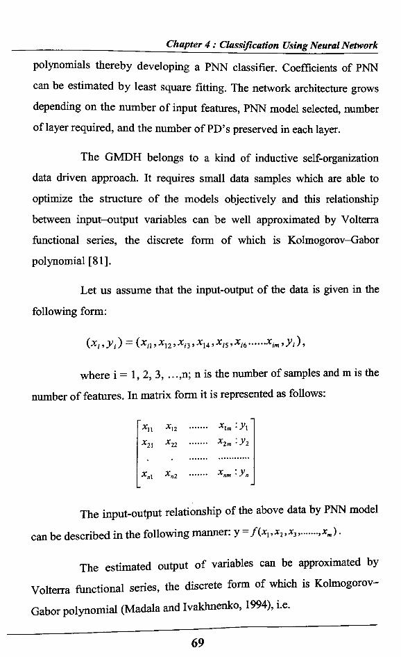
Let us assume that the input-output of the data is given in the

following form:

( X i i ) = ( * , 1 5 X 12 ’ X i3 ’ * 1 4 ’ X iS ’ X i 6 ...........X im ’ -V i ) 5

where i = 1, 2, 3, ...,n; n is the number of samples and m is the

number of features. In matrix form it is represented as follows:

**il 1̂2 ..... X\m * y 1■̂21 '̂ '22 ..... X2m ' y2

Xnl Xn2 ..... Xnm ' ̂ n

The input-output relationship of the above data by PNN model

can be described in the following manner: y =f(xl,x2,xJ,..... ,xm) .

The estimated output o f variables can be approximated by

Volterra functional series, the discrete form of which is Kolmogorov-

Gabor polynomial (Madala and Ivakhnenko, 1994), i.e.

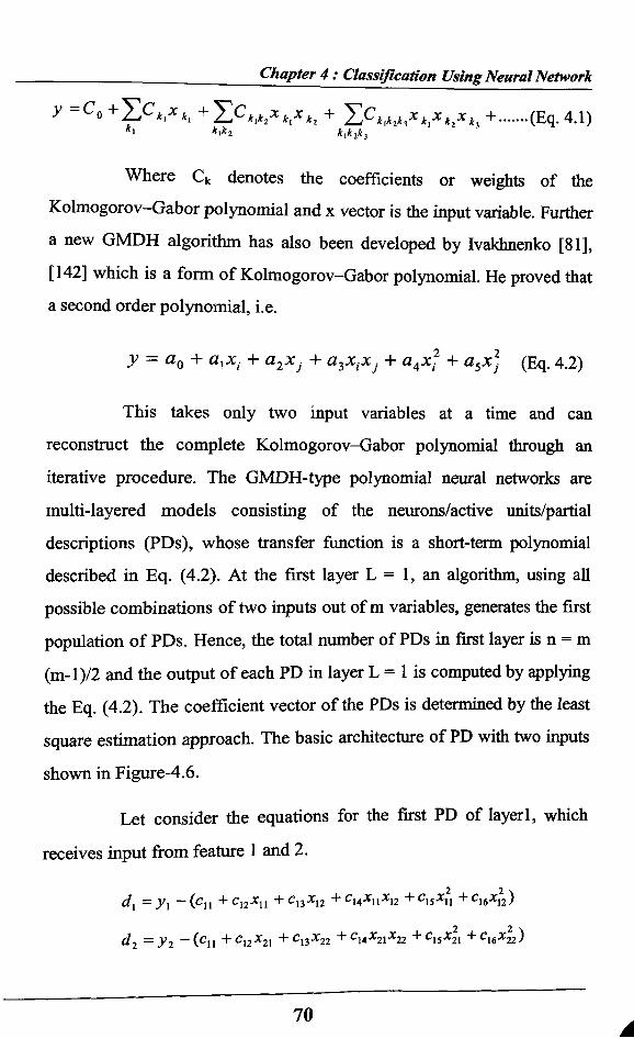
y - Co +'LCk x ki + ' £ c kikx i x k2 + Y,Ckxkikx k x k x k̂ + ..... (Eq. 4.1)k xk

Where denotes the coefficients or weights of the

Kolmogorov—Gabor polynomial and x vector is the input variable. Further

a new GMDH algorithm has also been developed by Ivakhnenko [81],

[142] which is a form of Kolmogorov—Gabor polynomial. He proved that a second order polynomial, i.e.

y = a 0 + alx i + a2Xj + a3x,xj + a 4x,2 + a5x ] (Eq. 4.2)

This takes only two input variables at a time and can

reconstruct the complete Kolmogorov-Gabor polynomial through an

iterative procedure. The GMDH-type polynomial neural networks are

multi-layered models consisting of the neurons/active units/partial

descriptions (PDs), whose transfer function is a short-term polynomial

described in Eq. (4.2). At the first layer L = 1, an algorithm, using all

possible combinations of two inputs out of m variables, generates the first

population of PDs. Hence, the total number of PDs in first layer is n = m

(m-l)/2 and the output of each PD in layer L = 1 is computed by applying

the Eq. (4.2). The coefficient vector of the PDs is determined by the least

square estimation approach. The basic architecture of PD with two inputs

shown in Figure-4.6.

Let consider the equations for the first PD of layerl, which

receives input from feature 1 and 2.

d l = y l — ( C n + Cn X n + ^ 1 3 - ^ 1 2 + £14*1 1 * 1 2 + C 15X U + C 1 6 * 1 2 )

d2 = J 2 — (Cll + C 12X 21 + C 13X 22 + C 1 4 * 2 1 * 2 2 + C 15*21 + C 1 6 * 2 2 )

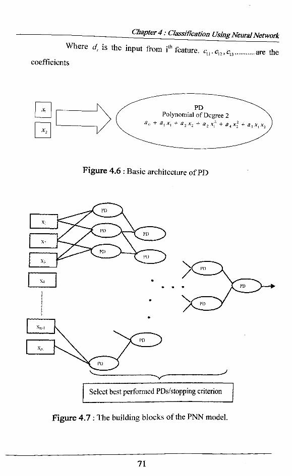
Where d, is the input from i* feature. q „c„,c13,....... are thecoefficients

Figure 4.6 : Basic architecture of PD

Select best performed PDs/stopping criterion

Figure 4.7 : The building blocks of the PNN model.

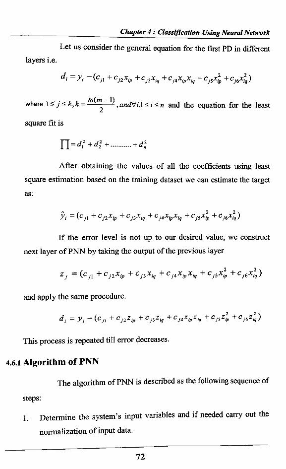
Let us consider the general equation for the first PD in differentlayers i.e.

where 1 < j < k, k = — ——, ancNi, 1 < i < n and the equation for the least

square fit is

U = d? +dl + .........+ d 2n

After obtaining the values of all the coefficients using least square estimation based on the training dataset we can estimate the targetas:

$ 1 = (C,l + C j l X ip + C p X iq + C j 4 X ipX iq + c j 5 x ?P + CJ6X l )

If the error level is not up to our desired value, we construct next layer of PNN by taking the output of the previous layer

and apply the same procedure.

dt = y t — (Cyi + C j 2 Z ip + C j 3 Z iq C j A Z ipZ iq + C j 5 Z ip + C j 6 Z i q )

This process is repeated till error decreases.

4.6.1 Algorithm of PNN

The algorithm of PNN is described as the following sequence of

steps:

1. Determine the system’s input variables and if needed carry out the

normalization of input data.

____________________________ ____________ __ ________________Chapter 4 : Classification Using Neural Network

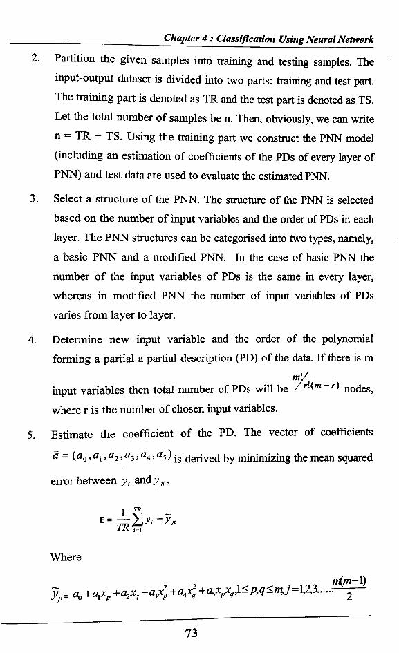
2. Partition the given samples into training and testing samples. The input-output dataset is divided into two parts: training and test part. The training part is denoted as TR and the test part is denoted as TS. Let the total number of samples be n. Then, obviously, we can write n = TR + TS. Using the training part we construct the PNN model (including an estimation of coefficients of the PDs of every layer of PNN) and test data are used to evaluate the estimated PNN.

3. Select a structure of the PNN. The structure of the PNN is selected based on the number of input variables and the order of PDs in each layer. The PNN structures can be categorised into two types, namely, a basic PNN and a modified PNN. In the case of basic PNN the number of the input variables of PDs is the same in every layer, whereas in modified PNN the number of input variables of PDs varies from layer to layer.

4. Determine new input variable and the order of the polynomial form ing a partial a partial description (PD) of the data. If there is m

ml/input variables then total number of PDs will be / r'(m~r) nodes,

where r is the number of chosen input variables.

5. Estimate the coefficient of the PD. The vector of coefficients

a = (aQ, ax, a2, a3, a4, a5) derived by m inim izing the mean squared

error between y t and^,,

| TR

Where

yji= Oq +alXp +a1Xq +a4 ^ +aSXpXq ^-P ’(l - r>1>j = ̂ 2 .... ; 2

_______________________.__________________________ Chapter 4 : Classification Using Neural Network

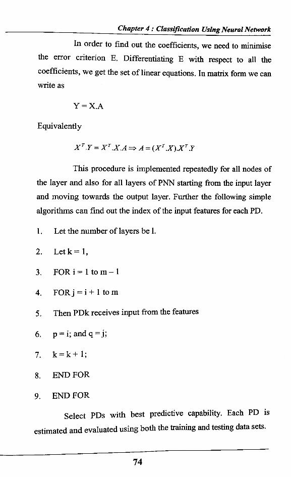
In order to find out the coefficients, we need to minimise the error criterion E. Differentiating E with respect to all the coefficients, we get the set of linear equations. In matrix form we can write as

Y = X.A

Equivalently

X t .Y = X t.X.A =>A = ( X tX ) X t .Y

This procedure is implemented repeatedly for all nodes of the layer and also for all layers of PNN starting from the input layer and moving towards the output layer. Further the following simple algorithms can find out the index of the input features for each PD.

1. Let the number of layers be 1.

2. Let k = 1,

3. FOR i = 1 t o m - 1

4. FOR j = i + 1 to m

5. Then PDk receives input from the features

6. p = i ;andq=j ;

7. k = k + 1;

8. END FOR

9. END FOR

Select PDs with best predictive capability. Each PD is

estimated and evaluated using both the training and testing data sets.

6. Select PDs with the best classification accuracy: The PDs which give the best predictive performance will be chosen for the output variable. Normally a pre specified cutoff value of the performance for all PDs is specified. If the performance of the PD is above the pre specified cutoff value then only they will be remain in the next generation.

7. Check the Stopping Criterion.

7.1 The following stopping condition indicates that an optimal PNN model has been accomplished at the previous layer, and the modeling can be terminated. This condition reads as Ec > Ep, where Ec is a minimal identification error of the current layer and Ep denotes a minimal identification error that occurred at the previous layer

7.2 The PNN algorithm terminates when the number of iterations (predetermined by the designer) is reached. When setting up a stopping (termination) criterion, one should be prudent in achieving a balance between model accuracy and an overall computational complexity associated with the development of

the model.

8. Determine new input variables for the next layer.

If any of the above two criteria fails, then the model will be

expand to the next layer.

4.7 Neural Network Techniques in Pattern Classification -

A Review

Data classification [54], [119], [140] is a core issue in data mining, pattern recognition and forecasting. The goal of classification is to

assign a new object to a class from a given set of predefined classes based on the attribute values of the object. Furthermore, classification is based on some discovered model, which forms an important piece of knowledge about the application domain. There has been wide range of methods for classification task. One of the popular and widely used techniques is artificial neural network (ANN) [156]. The main idea behind an Artificial Neural Network is to use several simple computational units, connected by weighted links through which activation values are transmitted. The units normally have a very simple way to calculate new activation values given the values received through the connections, for example summ ing

their inputs and feeding it through a monotonous transfer function. In a classification task, the pattern which is to classify is typically fed into the network as activation of a set of input units. This activation is then spread through the network via the connections, finally resulting in activation of the output units, which is then interpreted as the classification result. Training of the network consists in showing the patterns of the training set to the network, and letting it adjust its connection weights to obtain the

correct output.

There are a large number of different neural network architectures. One of the most popular neural network architectures used for classification is the Multi-Layer Perceptron. The units are organized into different layers, and the network is said to be feed-forward because the activation values propagate in one direction only, from the units in the input layer, through a number of hidden layers, to end up in the output layer. The multi-layer perceptron is usually trained with the Error Back-

Propagation method [183].

Worth mentioning here is the Single Layer Perceptron which

is a simple perceptron [176] which preceded the multi-layer perceptron.

The original perceptron actually had what could be considered as a hidden

layer of randomly selected “higher order units”. The single layer

perceptron is perhaps more similar in structure to the Adaline [225]. The

single layer of weights between input and output units is trained, just as in

the multi-layer case, with a gradient descent method, which adjusts the

weights a small step in the direction which will make the classification of

the current pattern more correct. The reason to mention this network is

mainly because of its limitations [135] pointed out what could and could

not be done with this simple type of architecture. Since each output unit

can only perform a vector multiplication of the input vector with its

weight vector and feed this through a monotonous transfer function, the

decision boundary between any pair of output units will always be a linear

hyper plane in the input space. This means that it can only solve

classification tasks where the classes are linearly separable. The duo [135]

gave several examples of interesting tasks which have more complex

decision boundaries, and thus can not be solved with this simple

architecture regardless of what method is used to set the weights. These

limitations can be overcome for instance by using one or more hidden

layers in the network.

The idea behind the error back-propagation neural networks

is very different from the other classification methods. Rather than trying

to calculate a probability or similarity or truth value directly, they use

more of an error correcting strategy: start with random weights and adjust

them to make the results better. Still, under certain conditions the output

activities of a multi-layer perceptron, trained with error back-propagation,

can be shown to approach the conditional probabilities of the

corresponding classes [171]. This relates these neural networks to the

statistical methods. The above networks all use supervised training

methods, where the correct class label has to be given when updating the

weights. There is another kind of training called reinforcement learning

[17], in which only a global signal indicating if the answer was wrong or

right is given. This is sometimes useful when e. g. learning to play a

game, and it is only possible to know if a whole sequence of moves was

good or bad (if it lead to a win or a loss), and not exactly what should

have been done in each move [133]. To continue with some different

architecture, there is also a large group of radial basis function (RBF)

neural networks [29], [272], Whereas the units in the hidden layer of the

multi-layer perceptron each responds for inputs on one side of a hyper

plane in the input space, a unit in an RBF network responds in a radially

symmetric region of the input space. In one version there are equally

many hidden units as training samples [164], each with the center of their

radially symmetric function (typically a Gaussian function) in one of the

training samples. Although not usually considered as RBF networks,

related groups are the competitive neural networks e.g. self-organizing

maps [100], [172] and learning vector quantization [101]. Here the

units correspond to prototype patterns; codebook vectors, and responds in

relation to how close a stimulated pattern is. They are usually of the

winner-take-all type; i.e. only the most active unit wins and suppresses all

other units. This is similar to the principles used in generalized nearest

neighbor methods.

The competitive neural networks are usually trained by moving

the codebook vectors closer to the patterns they respond to, using some

scheme [100], [120], [172], Interesting is also the Competitive Selective

Learning [33] method, which includes a way to remove codebook vectors

from regions where they are too dense and add them in regions where they are too sparse.

There is another type of neural network, not primarily

associated with classification. This is the class of recurrent neural

networks, i.e. with feedback connections used to feed the outputs of units

in one layer back into the units of the same or a previous layer. Rather

than sending the pattern through the network from the input units to the

output units, the signals cycle around in the network until the activity

stabilizes. One example of this is the Hopfield Network [76]. An

important concept for Hopfield networks is the energy function, a scalar

function from the activity state of the network. During the recall phase of

the Hopfield network the activity pattern strives to attain as low energy as

possible, causing it to find local minima in the energy landscape,

corresponding to stable patterns of activity. It is possible to prove that the

network will always arrive at a stable state if the weight matrix is

symmetric, since every activity change in the network will decrease the

energy by a certain amount, and there is a minimum possible energy. The

problem of getting stuck in a local minimum, when searching for the

global m inim um , can be a severe obstacle for hill climbing methods in

general. In a neural network context it will typically come in either during

training of the weights with some gradient descent method like error back-

propagation, or during relaxation of the activities in a recurrent neural

network. One way to solve this is to use simulated annealing [97] which

is a method to add a stochastic component to the hill climbing, which

introduces a small probability of locally going in the “wrong direction”.

The amount of randomness introduced is regulated by the temperature. A

high temperature means a high probability of escaping from a local

minimum. If the temperature is initially set to a high value, and then

decreased slowly enough, the probability that the procedure will end up in

the global minimum can be made arbitrarily close to one. Unfortunately,

dependent on the task at hand, “slowly enough” may mean that it will take

exceedingly long time. A recurrent neural network which can be used for

classification tasks is the boltzmann machine [3]. It uses the concepts of

energy function and simulated annealing to represent the probability

distribution over the domain. This is done by representing the probability

distribution in the energy function, and using a dynamics which makes the

probability of a pattern of activity proportional to the represented

probability of that pattern. This type of network will eventually learn the

correct probability distribution over the domain, but both training and

recall may require prohibitively long time.

The bayesian neural network [105], [113], [114] is a network

model in which the activities of units represent probabilities. The idea is

to make the activities of the output units equal to the probabilities of the

corresponding classes given the attributes represented by the stimulated

input units. In its single-layer form it is related to the naive Bayesian

classifier; in that the key assumption is, different input attributes are

independent. The multi-layer version has a hidden layer which

compensates for dependencies between the input attributes. The kinds of

problems handled by this neural network are the same as those which can

be handled by the Bayesian belief networks or the dependency tree

method by Chow and Liu [37].

Out of all other neural network the feed forward neural

network (FNN) is one of the popular and widely used techniques [156].

Although such FNNs can learn to classify wide range of problem domain

well, the classification model cannot be comprehensible due to large

number of synaptic connections. To achieve high classification accuracy

in FNN framework, one has to provide a well defined structure of FNNs,*

such as, the number of input nodes, hidden and output neurons, and

assume a proper set of relevant features. Trial and error methodology is

used to arrive at such kind of structures, which is computationally

expensive. Similarly other methods like rule extraction and decision tree,

which provide comprehensible rule, are based on the trade-off between

the complexity and the classification accuracy of the model. Recently, a

lot of attention has been directed to advanced techniques of system

modeling. The focus of the existing methodologies and detailed

algorithms is confronted with nonlinear systems, high dimensionality of

the problems, a quest for high accuracy and generalization capabilities of

the ensuing models. Nonlinear models can address some of these issues

but they request a large amount of data. The global nonlinear behavior of

the model may also cause undesired effects (the well-known is a

phenomenon of data approximation by high order polynomials where such

approximation leads to unexpected ripples in the overall nonlinear

relationship of the model). When the complexity of the system to be

modeled increases both experimental data and some prior domain

knowledge (conveyed by the model developer) are of importance to

_____________________________ _____ ________________________Chapter 4 : Classification Using Neural Network

complete an efficient design procedure. It is also worth stressing that the

nonlinear form of the model acts as a two-edge sword: while we gain

flexibility to cope with experimental data, we are provided with an

abundance of nonlinear dependencies that need to be exploited in a systematic manner.

As compare to FNN which requires the optimized structure and

improved by trial and error methodology the group method of data

handling (GMDH) approach which is one of the first approach along

systematic design of nonlinear relationships. It was developed to

identifying nonlinear relations between input and output variables. The

GMDH [58], [81], [144], [150] algorithm generates an optimal structure

of the model through successive generations of partial descriptions (PDs)

of data being regarded as quadratic regression polynomials with two input

variables. While providing with a systematic design procedure, GMDH

has some drawbacks. First, it tends to generate quite complex polynomial

for relatively simple systems (data). Second, owing to its limited generic

structure (quadratic two variable polynomial), GMDH also tends to

produce an overly complex network (model) when it comes to highly

nonlinear systems. Third, if there are less than three input variables,

GMDH algorithm does not generate a highly versatile structure.

To alleviate the problems associated with the GMDH,

polynomial neural networks (PNN) is introduced which is useful for

classification purposes. In a nutshell, these networks come with a high

level of flexibility as each node (processing element forming a PD) can

have a different number of input variables as well as exploit a different

order of the polynomial (linear, quadratic, cubic, etc.). In comparison to

well-known neural networks whose topologies are commonly prior to all

detailed (parametric) learning, the PNN architecture is not fixed in

advance but becomes fully optimized (both structurally and

parametrically). Especially, the number of layers of the PNN architecture

can be modified with new layers added, if required. Polynomial networks

have been known in the literature for many years [31], [122], [158]. The

polynomials have powerful approximation properties [158] and excellent

properties as classifiers [31]. Because of the Weierstrass theorem,

polynomial classifiers are universal approximators to the optimal Bayes

classifier [96], [50]. The Weierstrass theorem [180] states that any

continuous function can be approximated to an arbitrary accuracy by

polynomials. The polynomial classifier is also known as higher-order

neural network [180] or functional link net [156]. With binomial

expansion on linear subspace features, the polynomial classifier has

shown superior performance to multilayer neural networks [74], [110],

[122], [196]. PNN generates layers of neurons/simulated units/partial

descriptions (PDs) and then trains and selects those neurons, which

provide the best classification. During learning the PNN model grows the

new population of neurons and the number of layers so that the

complexity of the network increases [136], [139] while a predefined

criterion is met. Due to the complex architecture it requires huge memory

and computation time. To overcome from this problem evolutionary

strategies suggested by [137], [146] where they take only one layer of

PNN model and selected an optimal set from the PD’s generated in the

first layer along with the input features using PSO technique. This optimal

set of features is fed to a single Perceptron like model of ANN. The

weights are also optimized by PSO. We have proposed a unique scheme

using GA with PNN (see Chapter-7). In this scheme GA is been used for

feature selection (see Chapter-5) and the PNN is involved to find out the

fitness of GA. This proposed scheme outperformed than other methods

such as PNN, PNN with Gradient Descent, PNN with PSO etc.