CLASSIFICATION OF SURFACES - University of …may/VIGRE/VIGRE2011/REUPapers/Teo.pdfCLASSIFICATION OF SURFACES CHEN HUI GEORGE TEO Abstract. The sphere, torus, Klein bottle, and the

CLASSIFICATION OF SURFACES

CHEN HUI GEORGE TEO

Abstract. The sphere, torus, Klein bottle, and the projective plane are the

classical examples of orientable and non-orientable surfaces. As with much of

mathematics, it is natural to ask the question: are these all possible surfaces,or, more generally, can we classify all possible surfaces? In this paper, we

examine a result originally due to Seifert and Threlfall that all compact surfaces

are homeomorphic to the sphere, the connect sum of tori, or the connect sumof projective planes; for this paper, we follow a modern proof from Lee [2].

Contents

1. Introduction 12. Surfaces 23. Triangulation 33.1. Euclidean Simplicial Complex 33.2. Triangulation 64. Polygonal Presentation 74.1. Polygons 74.2. The Connect Sum of Surfaces 104.3. Polygonal Presentation 115. The Classification Theorem 166. Concluding Remarks 20Acknowledgments 20References 20

1. Introduction

In this paper, we prove that all compact surfaces are homeomorphic to the sphere,the connect sum of tori, or the connect sum of projective planes. We develop thenotion of Euclidean simplicial complexes to understand the triangulation theorem,and the idea of polygonal presentations as a combinatorial view of a surface. Wethen prove the classification theorem for surfaces by proving that given any surface,we can get to the polygonal presentation of the sphere, the connect sum of tori, orthe connect sum of projective planes via a sequence of elementary transformationswhich preserve the surface up to homeomorphism.

We assume the reader is comfortable with point-set topology from the basicnotions of a topological space and topological continuity to Hausdorffness, com-pactness, connectedness and constructing new spaces via the subspace, product,and quotient topology. Two results from point-set topology that we will use often

Date: DEADLINE AUGUST 26, 2011.

1

2 CHEN HUI GEORGE TEO

deserve special mention: the uniqueness of the quotient topology, which states thatgiven two quotient maps from the same space, if the maps make the same identifi-cations, then the two resultant quotient spaces are homeomorphic, and the closedmap lemma, which states that a map from a compact space to a Hausdorff spaceis a quotient map if it is surjective, and a homeomorphism if it is bijective. Wealso assume the reader is familiar with linear algebra, in particular affine maps andtransformations.

2. Surfaces

We begin by defining our mathematical object of study: the surface.

Definition 2.1. A surface is a 2-manifold, by this we mean a second countableHausdorff space that is locally homeomorphic to R2.

The classic examples of surfaces are the sphere, the torus, the Klein bottle, andthe projective plane.

The torus T2 is the subset of R3 formed by rotating the circle S1 of radius 1centered at 2 in the xz-plane around the z axis.

Figure 1. A torus as the rotation of a circle around the z-axis.

Equivalently, we see that the torus is homeomorphic to the quotient space ofI × I (where I denotes the closed unit interval) modulo the equivalence relationgiven by (x, 0) ∼ (x, 1) for all x ∈ I and (0, y) ∼ (1, y) for all y ∈ I.

Figure 2. The torus as the identification of I × I.

CLASSIFICATION OF SURFACES 3

More generally, given an even sided polygon, identifying edges pairwise will al-ways result in a surface. However, is the converse true?

Question 2.2. Can every surface be constructed from a polygon with the edgesidentified in an appropriate manner?

To answer this question, we shall first prove that every surface can be ‘covered’by finitely many triangles that are connected at an edge, thus by taking the convexpolygon spanned by these triangles, we obtain a polygon whose quotient space isthe surface. To achieve this goal, we shall rigorously define the idea of a complexof triangles.

3. Triangulation

3.1. Euclidean Simplicial Complex. In this section, we introduce the idea of asimplicial complex, which will serve as the triangular building blocks of manifolds.

Definition 3.1. Given points v0, . . . , vk in general position (by which we mean{v1 − v0, . . . , vk − v0} are linearly independent) in Rn, the simplex spanned bythem is the set of points

{x ∈ Rn | x =

k∑i=0

tivi such that 0 ≤ ti ≤ 1 and

k∑i=0

ti = 1}

with the subspace topology.Each point vi is a vertex of the simplex and we sometimes denote the simplexspanned by vertices {v0, . . . , vk} by 〈v0, . . . , vk〉. The dimension of σ is k.

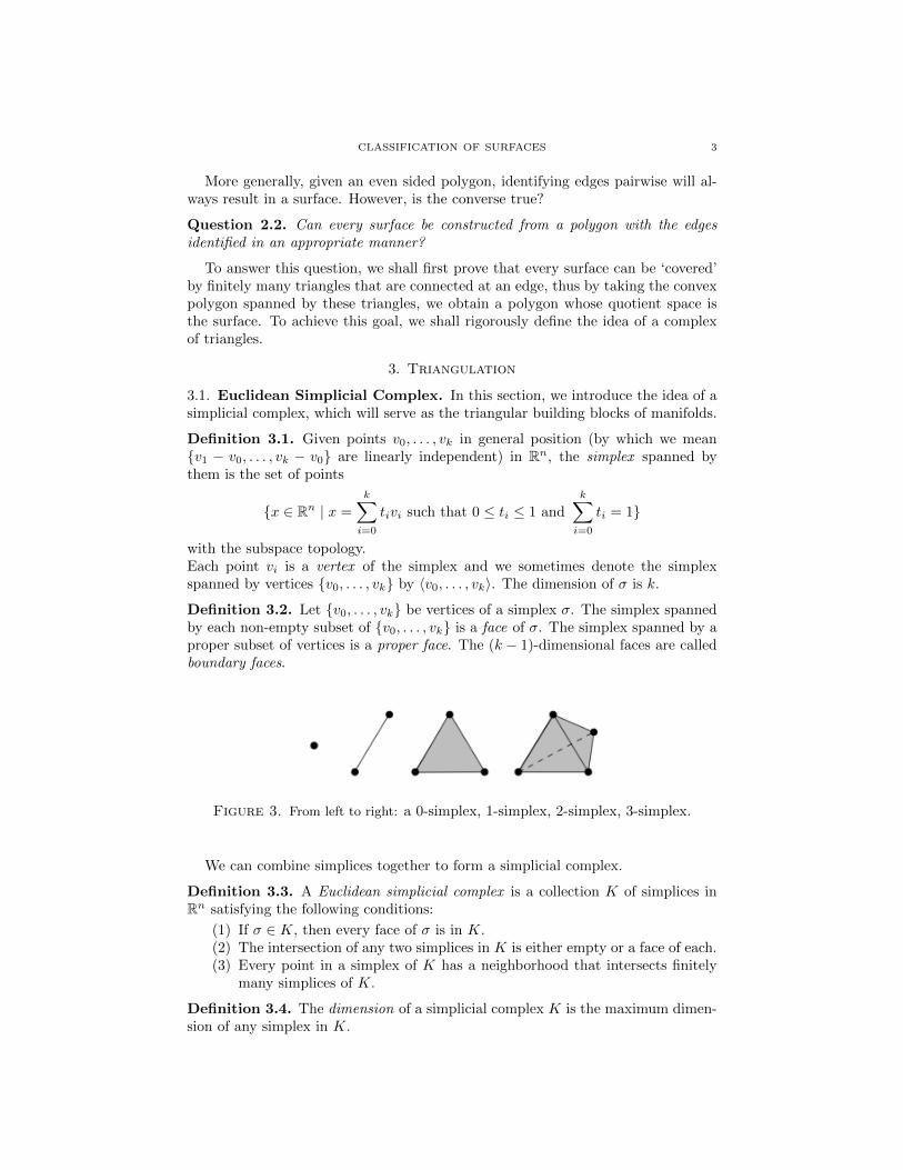
Definition 3.2. Let {v0, . . . , vk} be vertices of a simplex σ. The simplex spannedby each non-empty subset of {v0, . . . , vk} is a face of σ. The simplex spanned by aproper subset of vertices is a proper face. The (k − 1)-dimensional faces are calledboundary faces.

Figure 3. From left to right: a 0-simplex, 1-simplex, 2-simplex, 3-simplex.

We can combine simplices together to form a simplicial complex.

Definition 3.3. A Euclidean simplicial complex is a collection K of simplices inRn satisfying the following conditions:

(1) If σ ∈ K, then every face of σ is in K.(2) The intersection of any two simplices in K is either empty or a face of each.(3) Every point in a simplex of K has a neighborhood that intersects finitely

many simplices of K.

Definition 3.4. The dimension of a simplicial complex K is the maximum dimen-sion of any simplex in K.


The following is an example of a valid simplicial complex.

Figure 4. A 2-dimensional simplicial complex

For 2-dimensional simplicial complexes, like those pictured above, condition 2means that simplicies intersect at either vertices or edges. The following is anexample of condition 2 being broken:

Figure 5. Not a simplicial complex

Definition 3.5. Given a Euclidean complex K, the union of all simplices in K isa topological space denoted |K| with the subspace topology from Rn.

Definition 3.6. Let K be a Euclidean simplicial complex. For any non-negativeinteger k, the subset K(k) ⊂ K, which is the subset of all simplices with dimensionless than or equal to k, is a subcomplex of K called the k-skeleton of K.

Definition 3.7. Further terminology:

(1) The boundary of a simplex is the union of it’s boundary faces. i.e., theunion of all proper faces. We denote the boundary of a simplex σ by ∂σ.

(2) The interior of a simplex is the simplex minus its boundary. We denotethe interior of a simplex σ by Int σ.

Whenever we have mathematical objects, a question that naturally arises is:what are the functions that map between these objects. (e.g., group homomor-phisms in group theory and linear maps in linear algebra.) In this subsection, westudy the maps between Euclidean simplicial complexes. We begin with a motivat-ing proposition.

Proposition 3.8. Let σ = 〈v0, . . . , vk〉 be a k-simplex in Rn. Given k + 1 pointsw0, . . . , wk ∈ Rm, there exists a unique map f : σ → Rm that is the restriction ofan affine map that maps vi to wi for each i.

Proof. We may assume that v0 = 0 and w0 = 0, since we can simply apply theinvertible affine transformations x 7→ x − v0 and y 7→ y − w0. Recall that for ak-simplex, {v1 − v0, . . . , vk − v0} are linearly independent. In our case, we have


{v1, . . . , vk} as linearly independent. We can let f : σ → Rm be the restrictionof any linear map such that vi 7→ wi for 1 ≤ i ≤ k. To prove that f is uniquelydetermined by the map of the vertices, observe that

f(v) = f

(k∑i=0

tivi

)=

k∑i=0

tif(vi),

where v ∈ σ and ti has the usual conditions. �

Using this motivating proposition, we define a simplicial map:

Definition 3.9. Let K and L be two Euclidean simplicial complexes. A continuousmap f : |K| → |L| such that the restriction to each simplex of K maps to somesimplex in L via an affine map is a simplicial map.

Definition 3.10. The restriction of f (from the previous definition) to K(0) yieldsa map f0 : K(0) → L(0) called the vertex map of f .

Definition 3.11. A simplicial map that is also a homeomorphism (recall that |K|and |L| have topological structure) is a simplicial isomorphism.

Lemma 3.12. Let K and L be simplicial complexes. Suppose f0 : K(0) → L(0)

is any map satisfying the following: if {v0, . . . , vk} are vertices of a simplex of K,then {f0(v0), . . . , f0(vk)} are vertices of a simplex of L. Then there is a uniquesimplicial map f : |K| → |L| whose vertex map is f0.

Proof. Let f : |K| → |L| be a map such that the restriction to each simplexσ = 〈v0, . . . , vk〉 maps the vertices of σ to the vertices {f0(v0), . . . , f0(vk)} of asimplex in L via the vertex map f0. The convex hull 〈f0(v0), . . . , f0(vk)〉 is thesimplex in L spanned by {f0(v0), . . . , f0(vk)}. Thus, f is a simplicial map.

To show that f is uniquely determined by f0, notice that for any point v in eachsimplex:

f(v) = f

(k∑t=0

tivi

)=

k∑t=0

tif(vi) =

k∑t=0

tif0(vi),

where ti has the usual conditions. �

Lemma 3.13. Let K and L be simplicial complexes and f0 and f as above. Thefunction f is a simplicial isomorphism if: i) f0 is bijective, and ii) {v0, . . . , vk}are vertices of a simplex of K if and only if {f0(v0), . . . , f0(vk)} are vertices of asimplex of L.

Proof. From the previous lemma, we know that f is a simplicial map, it remainsto show that f is a homeomorphism from |K| to |L|. Since the vertex map f0is bijective, the number of vertices in K equals the number of vertices in L, so{v0, . . . , vk} are vertices in some simplex of K if and only if {f0(v0), . . . , f0(vk)} ={w0, . . . , wk} are distinct vertices in L. So 〈v0, . . . , vk〉 and 〈w0, . . . , wk〉 are k-dimensional simplicies in K and L respectively. Thus, σ is a k-simplex in K if andonly if f0(σ) (the convex hull of f0 applied to each vertex point in σ) is a simplex inL, so |K| and |L| with the subspace topology are homeomorphic, so f is a simplicialisomorphism. �


3.2. Triangulation.

Definition 3.14. A polyhedron is a topological space that is homeomorphic to anEuclidean simplicial complex

Definition 3.15. A triangulation is a particular homeomorphism between a topo-logical space and a Euclidean simplicial complex.Notice that there can be multiple different triangulations for a topological space.

Recall that I × I/ ∼ with the equivalence relation given by (x, 0) ∼ (x, 1) forall x ∈ I and (0, y) ∼ (1, y) for all y ∈ I is homeomorphic to a torus. We can makeI × I into a simplicial complex K as pictured below:

Figure 6. The minimal triangulation of the torus.

The homeomorphism between this simplicial complex with the equivalence rela-tion ∼ from above and the torus is a triangulation of the torus.

The following is a simple example of an invalid triangulation of the torus:

Figure 7. Not a triangulation of the torus.

It fails to be a triangulation, because given the identification of the sides of thesquare region, the two simplexes share 3 edges and 3 vertices, which fails condition2 of a simplicial complex.

The primary purpose of this section is to prove that all surfaces are triangulable.This result was originally proven by Rado in the 1920’s.

Theorem 3.16 (Triangulation Theorem for 2-Manifolds). Every 2-Manifold ishomeomorphic to the polyhedron of a 2-dimensional simplicial complex, in whichevery 1-simplex is a face of exactly two 2-simplices.


Proof. The proof of this result is long and intricate, and, thus, we shall not presentit here. The basic approach is to cover the manifold with regular coordinate disksand show that each disk can be triangulated compatibly. The main lemma that isneeded is the Schonflies Theorem, which states that a topological embedding of thecircle into R2 can be extended to an embedding of the closed disk. A proof of theSchonflies Theorem and the triangulation theorem for surfaces can be obtained inMohar and Thomassen [1]. �

4. Polygonal Presentation

4.1. Polygons. We begin by formally defining a polygon.

Definition 4.1. A subset P of the plane is a polygonal region if it is a compact(not necessarily connected) subset whose boundary is a 1-dimensional Euclideansimplicial complex satisfying the following conditions:

(1) Each point q of an edge that is not a vertex has a neighborhood U ⊂ R2

such that P ∪ U is equal to the intersection of U with a closed half-plane{(x, y) | ax+ by + c ≥ 0}.

(2) Each vertex v has a neighborhood V ⊂ R2 such that P ∪ V is equal tothe intersection of V with two closed half-planes whose boundaries onlyintersect at v.

Condition 1 and 2, illustrated below, define a subset of R2 that is a polygon.

Figure 8. Left: Condition 1. Right: Condition 2.

A polygonal can be made into a surface by identifying pairs of edges.

Theorem 4.2. Let P be a polygonal region in the plane with an even number ofedges and suppose we are given an equivalence relation that identifies each edge withexactly one other edge by means of a (Euclidean) simplicial isomorphism. Then theresultant quotient space is a compact surface.

Proof. Let M be the quotient space P/ ∼ and let π : P →M denote the quotientmap. Since P is compact, f(P ) = M is compact. The equivalence relation identifiesonly edges with edges and vertices with vertices so the points of M are either:

(1) face points - points whose inverse image in P are in IntP .(2) edge points - points whose inverse images are on edges but not vertices.(3) vertex points - points whose inverse images are vertices.

To prove that M is locally Euclidean, it suffices to consider the three types ofpoints.


Face points - Because π is injective on Int P and π, being a quotient map issurjective, π is bijective on Int P . So by the closed map lemma, π is a homeomor-phism on Int P . Since Int P ⊂ R2 is a open set, R2 ∼= Int P ∼= π(Int P ), so everyface point is in a locally Euclidean neighborhood, namely π(Int P ).

Edge points - For any edge point q, pick a sufficiently small neighborhood suchthat there are no vertex points in the neighborhood N . By the definition of apolygonal region, q has two inverse images, q1 and q2 with neighborhoods U1 andU2 such that V1 = U1 ∩ P and V2 = U2 ∩ P are disjoint half planes. Furthermore,notice that π|V1∪V2 is also a quotient map. We construct affine homeomorphismα1 and α2 such that α1 maps V1 to a half disk on the upper half plane and α2

maps V2 to the lower disk on the lower half plane. We can shrink V1 and V2until they are saturated open sets in P ; i.e., for every boundary point of V1, thecorresponding boundary point is in V2 and vice versa. We can now define anotherquotient map ϕ : V1 ∪ V2 → R2 such that ϕ = α1 on V1 and ϕ = α2 on V2.Modulus the equivalence relation r1 ∼ r2, where r1 and r2 are edge points in V1and V2 respectively, whenever ϕ(r1) = ϕ(r2). Notice that ϕ is a quotient map ontoa Euclidean ball centered at the origin and makes the same identifications as π.By the uniqueness of the quotient map, the quotient spaces are homeomorphic, soedge points are locally Euclidean.

Vertex points - Repeat the same process as the edge points, but this time therewill be multiple pieces of the polygon that are identified in a fanning manner in R2.The resultant quotient space is homeomorphic to an open ball, so we may concludeby appealing to the uniqueness of the quotient map. Therefore, we know that Mis locally Euclidean.

To show that M is Hausdorff, simply pick sufficient small balls. Since M isthe quotient space of the quotient map from the polygonal region P , the preimageof any pair of points in M can be separated into disjoint open sets by picking


sufficiently small open balls; the image of these open balls will be open sets in Mthat separate the two points in M . �

The converse of this is also true: every compact surface is the quotient space ofa polygon with sides pairwise identified, but the proof of this is cleaner after wedevelop the notion of a polygonal presentation, so we prove this in the next section.

Example 4.3. The sphere S2 = {(x, y, z) ∈ R3 | x2+y2+z2 = 1} is homeomorphicto the square region S = {(x, y) | |x| + |y| ≤ 1} modulo the equivalence relation(x, y) ∼ (−x, y) for (x, y) ∈ ∂S.

Figure 9. Polygon identification homeomorphism to sphere.

Example 4.4. The torus T2 is homeomorphic to the square region modulo theequivalence relation (x, y) ∼ (−y,−x) for (x, y) ∈ ∂S.

Example 4.5. The Klein bottle K2 is homeomorphic to the square region modulothe equivalence relation (x, y) ∼ (−x,−y) for (x, y) ∈ ∂S such that 0 ≤ x, y ≤ 1 or−1 ≤ x, y ≤ 0, and another equivalence relation (x, y) ∼ (−y,−x) for (x, y) ∈ ∂Ssuch that −1 ≤ x ≤ 0 ≤ y ≤ 1 or −1 ≤ y ≤ 0 ≤ x ≤ 1.

Figure 10. Klein Bottle.

Example 4.6. The projective plane P2 is homeomorphic to the square regionmodulo the equivalence relation (x, y) ∼ (−x,−y) for (x, y) ∈ ∂S.


Figure 11. The identification of the square region that yields aprojective plane.

4.2. The Connect Sum of Surfaces. Given two surfaces, we wish to join themin a natural way such that we end up with another surface. For example, given twotori, the natural gluing process should result in a two hole torus. This operation iscalled the connect sum.

Definition 4.7. Suppose X and Y are topological spaces, A is a closed subset ofY , and f : A→ X is a continuous map, then we define an equivalence relation ∼ onthe disjoint union X q Y such that a ∼ f(a) for all a ∈ A. The resulting quotientspace (X q Y )/ ∼, denoted X ∪f Y is an adjunction space.

The connect sum is the adjunction space given a particular choice for the closedset A.

Definition 4.8. Given surfaces M1 and M2 and regular coordinate balls Bi ⊂Mi,the subspace M ′i := Mi \Bi are surfaces with boundaries homeomorphic to S1. Letf : ∂M ′2 → ∂M ′1 be any homeomorphism, then the adjunction space M ′1 ∪f M ′2 isthe connect sum of M1 and M2 denoted M1#M2.

The connect sum operation basically involves cutting out open balls from surfacesand gluing points along the S1 by an equivalence relation, giving a new manifold.

Figure 12. connect sum of two Surfaces M1 and M2.


So far, we have assumed that the connect sum of two surfaces indeed results ina surface, now we shall prove it.

Theorem 4.9. The connect sum M1#M2 of two connected surfaces M1 and M2

is a connected surface.

Proof. It suffices to show that M1#M2 is locally Euclidean and Hausdorff. Theproof of this is similar to Theorem 4.2, so we only provide a sketch of the proof.Let π : M ′1 qM ′2 → M1#M2 be the quotient map. As with Theorem 4.2, thereare two types of points: points in M1#M2 with preimage in Int M ′1 or Int M ′2, orpoints with primages ∂M ′1 and ∂M ′2. As with Theorem 4.2, the first type of pointsare clearly Euclidean: simply pick a neighborhood small enough such that it isstrictly in the interior M ′i , i = 1, 2, and homeomorphic to R2. For the second typeof points, proceed analogous to the proof for edge points in theorem 4.2. Adjust theneighborhoods such that for each point of ∂M ′1 in one neighborhood, the equivalentpoint in ∂M ′2 is in the other neighborhood, and vice versa. Then map the two halfplanes to R2 with the same identification as the original quotient map. By theuniqueness of quotient maps, since the two maps make the same identifications, thetwo space are homeomorphic, so the second type of points is also locally Euclidean.Hausdorffness follows by picking sufficiently small neighborhoods.

To show that M1#M2 is connected, simply note that M1#M2 is the union oftwo connected sets π(M ′1) and π(M ′2), where π(M ′1) ∩ π(M ′2) 6= Ø. �

4.3. Polygonal Presentation. We begin by defining a polygonal presentation:

Definition 4.10. A polygonal presentation is a finite set S with finitely manywords W1, . . . ,Wk, where Wi is a word in S of length 3 or longer. We denote apolygonal presentation P = 〈S |W1, . . . ,Wk〉.

To explain this definition, we need two other definitions:

Definition 4.11. Given a set S, a word in S is an ordered k-tuple of symbols ofthe form a or a−1 where a ∈ S.

Definition 4.12. The length of a word is the number of elements in the word,where a and a−1 count as distinct elements.

Notation 4.13. As a matter of notation, we leave out the curly braces whendescribing the elements of S and denote words by juxtaposition. So if we had,for example, S = {a, b} and two words W1 = {aba−1b−1} and W2 = {aa}, thenP = 〈a, b | aba−1b−1, aa〉.

As with simplicial complexes, any polygonal presentation determines a topolog-ical space |P| called the geometric realization.

Definition 4.14. The geometric realization of a polygonal presentation, denoted|P| is determined by the following algorithm:

(1) For each word Wi, let Pi denote the convex k-sided polygonal region in theplane that has its center at the origin, side length 1, equal angles, and onevertex on the positive y axis. (k is the length of the word.)

(2) Define a bijective function between the symbols of Wi and the edges of Piin counterclockwise order, starting at the vertex of y-axis.


(3) Let |P| denote the quotient space of∐i Pi determined by identifying edges

that have the same edge symbol by an affine homeomorphism that matchesup the initial vertices and and terminal vertices of edges with labels a anda, or a−1 and a−1, and initial to terminal vertices for edges labeled a anda−1.

Definition 4.15. In the special case where Wi is a word of length 2, we define Pito be a sphere if the word is aa−1 or a−1a and the projective plane if the word isaa or a−1a−1.

Figure 13. Presentation of the two words of length 2.

If we want the geometric realization of a presentation to be a surface, we make theaddition stipulation that each symbol a ∈ S only occurs twice in the presentationP.

Definition 4.16. A surface presentation is a polygonal presentation such that eachsymbol a ∈ S occurs only exactly twice in W1, . . . ,Wk, counting each a or a−1 asone occurrence.

By theorem 4.2, the geometric realization is a compact surface.

Examples 4.17. The common surfaces S2, T2, K and P2 all have presentations:

(1) The sphere: 〈a | aa−1〉 or 〈a, b | abb−1a−1〉(2) The torus: 〈a, b | aba−1b−1〉(3) The projective plane: 〈a | aa〉 or 〈a, b | abab〉(4) The Klein Bottle: 〈a, b | abab−1〉

Figure 14. Polygonal presentation of S2, T2, P2, and K.

Definition 4.18. If two presentations P1 and P2 have homeomorphic geometricrealizations, we say that the are topologically equivalent and write P1

∼= P2.


We are now ready to prove the converse of theorem 4.2.

Theorem 4.19. Every compact surface admits a polygonal presentation.

Proof. Let M be a compact surface. By the triangulation theorem, M is homeo-morphic to a 2-dimension simplicial complex K, in which each 1-simplex is a faceof exactly two 2-simplices.

From this simplicial complex, construct a surface presentation P such that each2-simplex is a word of length 3, where edges are labeled with the same letter if theyare the same 1-simplex. Thus, we have two quotient maps: πK : P → |K| andπP : P → |P|, where the domain P = P1q . . .qPk. It is sufficient to show that thetwo quotient maps make the same identifications.

It is clear by construction that the two quotient maps identify the same edges.Now it remains to show that πK and πP identify vertices with instructions from

the edge identifications. Suppose v ∈ K is any vertex. v must be in some 1-simplex,otherwise it would be an isolated point. By the triangulation theorem, this edgemust be in two 2-simplices σ and σ′. Now we define an equivalence relation on theset of 2-simplices containing v by saying two 2-simplices containing v, σ and σ′,are equivalent if there exists a sequence of 2-simplices σ = σ1, . . . , σk = σ′ suchthat σi shares an edge with σi+1 for i = 1, . . . , k − 1. Thus to prove that the twoquotient maps identify the same vertices, it is sufficient to prove that there is onlyone equivalence class.

Suppose that there were two equivalence classes {σ1, . . . , σk} and {τ1, . . . , τm}such that σi ∼ σj and σi 6∼ τj . Let ε be small enough such that Bε(v) onlyintersects simplices containing v. Bε(v) ∩ |K| is an open subset of |K|, so v has aneighborhood U homeomorphic to R2 that is also a subset of Bε(v)∩|K|. Since thisneighborhood is homeomorphic to R2, U \ {v} is connected. However, if we assumefor contradiction that there are two equivalence classes, then W ∩(σ1∪· · ·∪σk)\{v}and W ∩ (τ1∪· · ·∪τm)\{v} are both open in |K|, since their intersection with eachsimplex is open. Then W \{v} = (W ∩(σ1∪· · ·∪σk)\{v})∪(W ∩(τ1∪· · ·∪τm)\{v})is disconnected, which is a contradiction. �

The following lemma will provide a simpler method of proving that two polygonalpresentations have homeomorphic geometric realizations.

Lemma 4.20. Let P1 and P2 be convex polygons with the same number of edges,and let f : ∂P1 → ∂P2 be a simplicial isomorphism. Then f extends to a homeo-morhism F : P1 → P2.

Proof. Choose any point pi ∈ Int Pi, i = 1, 2. By convexity, the line segment frompi to each vertex of Pi lies entirely in Pi. The convex hull spanned by pi and eachpair of adjacent vertices of Pi is a simplex. The disjoint union of these simplices witheach inner line segment and their attendant endpoints identified form a simplicialcomplex whose polyhedron is Pi. Now simply let F : P1 → P2 be the simplicialmap whose restriction to ∂P1 is f and takes p1 to p2. �

Pictorially, extending the simplicial isomorphism to a homeomorphism F lookslike this:


We will now define a series of elementary transformations of polygonal presen-tations.

Notation 4.21. For the following definitions, we shall adopt the following conven-tion:

(1) e denotes any symbol not in S.(2) W1W2 denotes a word formed by concatenating W1 and W2.(3) (a−1)−1 = a

Definition 4.22. The following operations are elementary transformations of apolygonal presentation.

(1) Reflecting: 〈S | a1 · · · am,W2, . . . ,Wk〉 7→ 〈S | a−1m · · · a−11 ,W2, . . . ,Wk〉.

(2) Rotating: 〈S | a1 · · · am,W2, . . . ,Wk〉 7→ 〈S | a2 · · · ama1,W2, . . . ,Wk〉.

(3) Cutting: If W1 and W2 both have length at least 2, 〈S |W1W2, . . . ,Wk〉 7→〈S, e |W1e, e

−1W2, . . . ,Wk〉.(4) Pasting: IfW1 andW2 both have length at least 2, 〈S, e |W1e, e

−1W2, . . . ,Wk〉 7→〈S |W1W2, . . . ,Wk〉.

Figure 15. Cutting/Pasting.


(5) Folding: If W1 has length at least 3, 〈S, e | W1ee−1,W2, . . . ,Wk〉 7→ 〈S |

W1,W2, . . . ,Wk〉. W1 can have length 2 if the presentation only has oneword.

(6) Unfolding: 〈S |W1,W2, . . . ,Wk〉 7→ 〈S, e |W1ee−1,W − 2, . . . ,Wk〉.

Figure 16. Folding/Unfolding.

Theorem 4.23. Elementary transformations of a polygonal presentation producea topologically equivalent presentation.

Proof. Notice that cutting/pasting and folding/unfolding are symmetric, so we onlyneed to prove that one of the pair presents homeomorphic geometric realizations.

(1) Reflecting: Let P1 be the geometric realization of a1, . . . , am and P ′1 be thegeometric realization of a−1m , . . . , a−11 . Since reflection is a linear transfor-mation, we choose the reflection matrix to be our homeomorphism; clearly,it is bijective and bicontinuous. We can extend the homeomorphism toW2, . . . ,Wk by the identity map.

(2) Rotation: Let P1 be the geometric realization of a1, . . . , am and P ′1 be thegeometric realization of a2, . . . , am, a1. Similar to reflecting, we choose therotation matrix to be our homeomorphism. The reflection linear transfor-mation is clearly bijective and bicontinuous. We can similarly extend tohomeomorphism to W2, . . . ,Wk by the identity map.

(3) Cutting: Let P1 and P2 be polygons labeled W1e and e−1W2 respectively,and let P ′ be the polygon labeled W1W2. Let π : P1 q P2 → S andπ′ : P ′ → S′ be the two quotient maps. Let e be the line segment fromthe terminal to initial vertex of W1 in P ′; by convexity, the edge is in P ′.The continuous map f : P1 q P2 → P ′ takes each edge of P1 or P2 to itscorresponding edge in P ′, and identifies e and e−1. Thus, by the closed maplemma, f is a quotient map. So π′ ◦ f and π make the same identificationsfrom the same domain, so by the uniqueness of the quotient map, S and S′

are homeomorphic. If there are other words, W3, . . . ,Wk in the polygonalpresentation, then extend the homeomorphism by the identity.

(4) Folding: Assume without loss of generality that the W1 has at least length3. (If it has a shorter length, simply introduce a new face, divide an existingface into two parts, labeled with different letters.) First assume that W1 =abc and let P and P ′ be polygons of abcee−1 and abc respectively. Also, letπ : P → S and π′ : P ′ → S′ be the two quotient maps. Transform P into asimplicial complex by adding edges. The resultant words to represent thesimplicial complex are of the form: e−1ad, d−1bf, f−1ce, where sides of thesame letter are identified and the vertex identification is forced by the edgeidentification. Let f : P → P ′ be the simplicial map that takes edges in P


to edges with the same label in P ′. Then π ◦ f and π are quotient mapsthat make the same identifications, so by the uniqueness of the quotientmap, S and S′ are homeomorphic. We can extend the homeomorphism tothe other words W2, . . . ,Wk by the identity.

�

The connect sum of two surfaces can also be expressed as an operation on thepolygonal presentation.

Theorem 4.24. Let M1 and M2 be surfaces that admit presentations 〈S1 | W1〉and 〈S2 | W2〉, in which S1 and S2 are disjoint sets and presentation has a singleface. Then 〈S1, S2 |W1W2〉 is a presentation of the connect sum of M1#M2.

Proof. Given the presentation of M1 as 〈S1 | W1〉, we get 〈S1 | W1〉 ∼= 〈S1, a, b, c |W1c

−1b−1a−1, abc〉 by cutting 3 times. The word abc represents a polygon and itsconvex hull is a 2-simplex, which is homeomorphic to B. Let B1 be the interior ofthe convex hull of the polygon corresponding to the word abc. Thus, the geometricrealization of 〈S1, a, b, c | W1c

−1b−1a−1〉 is homeomorphic to M1 \ B1 := M ′1. Bya similar argument, we get the presentation of M ′2 is 〈S2, a, b, c | abcW2〉. Sothe presentation 〈S1, S2, a, b, c |W1c

−1b−1a−1, abcW2〉, which shows that a, b, c areidentified in a complementary manner, is the presentation of M ′1 qM ′2 where theball represented by abc is identified, which is exactly M ′1#M ′2 Pasting along c andfolding a and b gives a homeomorphic presentation 〈S1, S2 |W1W2〉. �

5. The Classification Theorem

We are now ready to prove the main result of this paper. This theorem was firstproved in 1907 by Max Dehn and Poul Heegaard.

Theorem 5.1. Every non-empty, compact, connected 2-manifold is homeomorphicto one of the following:

(1) S2(2) A connect sum of one or more copies T2

(3) A connect sum of one or more copies of P2.

It might appear that some of the surfaces are absent from the list. In particular,the Klein bottle K and any connect sum involving both tori and projective planes,for example T2#P2.

Lemma 5.2. The Klein bottle is homeomorphic to P2#P2.

Proof. The Klein bottle has a presentation: 〈a, b | abab−1〉. By a sequence ofelementary transformations, we get

〈a, b | abab−1〉 ∼= 〈a, b, c | abc, c−1ab−1〉 (cut along c)

∼= 〈a, b, c | bca, a−1cb〉 (rotate and reflect)

∼= 〈b, c | bbcc〉 (paste along a and rotate).

The final presentation is the connect sum of two projective planes. �

Lemma 5.3. The connect sum of T2#P2 is homeomorphic to P2#P2#P2.


Proof. By the previous corollary, P2#P2#P2 ∼= K#P2 = 〈a, b, c | abab−1cc〉. By asequence of elementary transformations,

〈a, b, c | abab−1cc〉 ∼= 〈a, b, c, d | cabd−1, dab−1c〉 (rotate and cut)

∼= 〈a, b, c, d | abd−1c, c−1ba−1d−1〉 (rotate and reflect)

∼= 〈a, b, d, e | a−1d−1abe, e−1d−1b〉 (paste along c and cut along e)

∼= 〈a, b, d, e | ea−1d−1ab, b−1de〉 (rotate and reflect)

∼= 〈a, c, e | a−1d−1adee〉 (paste along b, rotate, and reflect)

The final presentation is the connect sum of a torus and projective plane. �

Before we begin, we shall give two preliminary definitions that will make expo-sition simpler:

Definition 5.4. A pair of edges that are to be identified is twisted if they bothappear as a, . . . , a or a−1, . . . , a−1.

Definition 5.5. A pair of edges that are to be identified is complementary if itappears as a, . . . , a−1 or a−1, . . . , a.

Given the two preceding lemmas, we are now ready to prove the classificationtheorem for compact 2-manifolds.

Proof of the Classification Theorem. Given any compact surface, this proof willshow that by a sequence of elementary transformations, we get a surface that hasa polygonal presentation homeomorphic to the sphere, the connect sum of tori, orthe connect sum of projective planes.

Step 1 M admits a presentation that has only one face (only one word). Since Mis connected, each word must have a letter in common with another word,so by repeated pasting transformations (with rotations and reflections asnecessary), we get a polygonal presentation with only one word, whichadmits a presentation with one face.

Step 2 M is either a sphere or admits a presentation with no adjacent complemen-tary pairs. If there is an adjacent complementary pair, we may remove itby folding. The only time, when an adjacent complementary pair cannotbe removed is if it is the only pair of letters left. i.e., 〈a, aa−1〉, in whichcase, we have a sphere. Now we assume that the surface is not a sphere.

Step 3 M admits a presentation in which all twisted pairs are adjacent. Supposewe have a non-adjacent twisted pair. Then the word will take the formV aWa, where V and W are non-empty words. By a sequence of elementarytransformations:

〈a, V,W | V aWa〉 ∼= 〈a, b, V,W | V ab, b−1Wa〉∼= 〈a, b, V,W | bV a, a−1W−1b〉∼= 〈b, V,W | VW−1bb〉.


We may have introduced new non-adjacent twisted pairs in the process.However, recall that the set of symbols S is finite, so by repeating the sameprocess, we can transform each non-adjacent twisted pair into adjacentcomplementary pairs without affecting the bb complementary pair. So aftera finite number of iterations, we get a word with no non-adjacent twistedpairs and a string of adjacent complementary pairs. The complementarypairs can be removed by repeating step 2, which does not increase the totalnumber of non-adjacent twisted pairs.

Step 4 M admits a presentation in which all vertices are identified to a singlepoint. Recall that we have an equivalence relation on the set of edges. Theidentification of the edges, as we have seen before, forces an equivalencerelation on the set of vertices; choose some equivalence class of vertices [v].Suppose that there are vertices not in the equivalence class [v]. Then theremust be some edge a that connects [v] to some other vertex class [w]. Sincethis is a polygonal surface, the other edge that touches a at [v] cannot bea−1, or else we would have got rid of it in step 2. The other edge cannot bea, because, if it were, then the initial and terminal ends would be identifiedunder the quotient map, which is not the case. So we label this other edgeb and the other vertex x.

Somewhere else in the polygon, there is another edge labeled either b orb−1. Without loss of generality, assume that it is b−1. The proof if it is b issimilar except for an extra reflection. Thus the presentation is of the formbaXb−1Y . By elementary transformations:

〈a, b,X, Y | baXb−1Y 〉 ∼= 〈a, b, c,X, Y | bac, c−1Xb−1Y 〉∼= 〈a, b, c,X, Y | acb, b−1Y c−1X〉∼= 〈a, c,X, Y | acY c−1X〉.


Recall that the [v] referred to the initial vertex of a and the terminalvertex of b, so by pasting the edges labeled b, we have reduced the numberof distinct vertices in the polygon labeled v. We may have increased thenumber of vertices labeled w and we may have introduced new complemen-tary pairs. To repair the latter, perform step 2 again noticing that step 2does not increase the number of vertices labeled v. Thus, by repeating thisprocess finitely many times, we can eliminate the vertex class [v]. Repeatingthis procedure for each vertex class, we can get the desired result.

Step 5 If the presentation has any complementary pairs a, a−1, then it has an-other complementary pair b, b−1 that occurs intertwined with the first. i.e.,a, . . . , b, . . . , a−1, . . . , b−1. Assume that this is not the case, that is, thepresentation is of the form aXa−1Y , where X and Y only contain matchedcomplementary pairs or adjacent twisted pairs. (By matched, we mean thatthe complementary pairs remain exclusively within X or Y .) Recall thatnon-adjacent twisted pairs and adjacent complementary pairs are not pos-sible by step 2 and 3. Thus each edge in X is identified with another edge inY and similarly for Y . This means the terminal vertices of a and a−1 bothtouch vertices in X and the initial vertices are identified with only verticesin Y . This is a contradiction, since all vertices are within one equivalenceclass by Step 4.

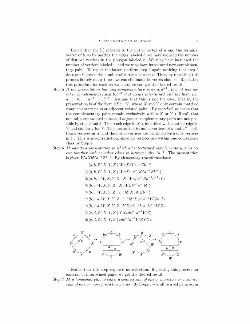
Step 6 M admits a presentation in which all intertwined complementary pairs oc-cur together with no other edges in between: aba−1b−1. The presentationis given WaXbY a−1Zb−1. By elementary transformations:

〈a, b,W,X, Y, Z |WaXbY a−1Zb−1〉∼=〈a, b,W,X, Y, Z |WaXc, c−1bY a−1Zb−1〉∼=〈a, b, c,W,X, Y, Z | XcWa, a−1Zb−1c−1bY 〉∼=〈b, c,W,X, Y, Z | XcWZb−1c−1bY 〉∼=〈b, c,W,X, Y, Z | c−1bY XcWZb−1〉∼=〈b, c, d,W,X, Y, Z | c−1bY Xcd, d−1WZb−1〉∼=〈b, c, d,W,X, Y, Z | Y Xcdc−1b, b−1d−1WZ〉∼=〈c, d,W,X, Y, Z | Y Xcdc−1d−1WZ〉∼=〈c, d,W,X, Y, Z | cdc−1d−1WZY Z〉.

Notice that this step required no reflection. Repeating this process foreach set of intertwined pairs, we get the desired result.

Step 7 M is homeomorphic to either a connect sum of one or more tori or a connectsum of one or more projective planes. By Steps 1−6, all twisted pairs occur


adjacent to each other: aa (projective planes) and all complementary pairsoccur in intertwined groups bcb−1c−1 (tori). If the presentation consistsexclusively of either case, then we are done, since we would either have theconnect sum of tori or connect sum of projective planes. If the presentationcontains both twisted and complementary pairs, then the presentation mustbe one of the following forms: aabcb−1c−1X or bcb−1c−1aaX. In either case,by the previous lemma, T2#P2 ∼= P2#P2#P2. So, if both cases occur in thepresentation, we can eliminate all occurrences of T2 by this transformation,and we get the connect sum of P2.

�

6. Concluding Remarks

In this paper, we proved that all compact surfaces are homeomorphic to thesphere, the connect sum of tori, or the connect sum of projective planes, but thekeen reader may have noticed that we have yet to prove that the surfaces aretopologically distinct. e.g., a sphere is not homeomorphic to a torus. The answerto this non-trivial question lies with other topological invariants such as the EulerCharacteristic and orientibility. The interested reader should refer to Lee [2].

Acknowledgments. It is my pleasure to thank Peter May for organizing the REU,Benson Farb for his excellent introductory lectures on Geometry/Topology, whichattracted my interest in this subject, and my mentors William Lopes and KatieMann for helping me understand and write this paper.

References

[1] B. Mohar and C. Thomassen. Graphs on Surfaces. John Hopkins University Press. 2001.[2] J. M. Lee. Introduction to Topological Manifolds. Springer-Verlag. 2000.

Documents

CLASSIFICATION OF SURFACES - University of …may/VIGRE/VIGRE2011/REUPapers/Teo.pdfCLASSIFICATION OF SURFACES CHEN HUI GEORGE TEO Abstract. The sphere, torus, Klein bottle, and the