REPRESENTTIONSA OF LIE ALGEBRAS, WITH …may/VIGRE/VIGRE2007/REUPapers/FINALFU… · representtionsa of lie algebras, with applications to arpticle physics james marrone university

REPRESENTATIONS OF LIE ALGEBRAS, WITH APPLICATIONS TO

PARTICLE PHYSICS

JAMES MARRONE

UNIVERSITY OF CHICAGO MATHEMATICS REU, AUGUST 2007

Abstract. The structure of Lie groups and the classication of their representations are subjects

undertaken by many an author of mathematics textbooks; Lie algebras are always considered as an

indispensable component of such a study. Yet every author approaches Lie algebras dierently - some

begin axiomatically, some derive the algebra from prior principles, and some barely connect them to

Lie groups at all. The ensuing problem for the student is that the importance of the Lie algebra can

only be deduced by reading between the lines, so to speak; the relationship between a Lie algebra

and a Lie group is not always illuminated (in fact, there isn't always a relationship in the rst place)

and so considering the representations of Lie algebras may appear redundant or at best cloudy. The

approach to Lie algebras in this paper should clarify such problems. Lie algebras are historically a

consequence of Lie groups (namely, they are the tangent space of a Lie group at the identity) which

may be axiomatized so that they stand alone as an algebraic concept. The important correspondence

between representations of Lie algebras and Lie groups, however, makes Lie algebras indispensable

to the study of Lie groups; one example of this is the Eight-Fold Way of particle physics, which is

actually just an 8-dimensional representation of sl3(C) but which has the enlightening property of

corresponding to the strong nuclear interaction, giving a physical manifestation of the action of a

representation and showing just one of the many interesting ramications of mathematics on science

within the past 50 years.

1. Lie Groups and Representations

We begin with

Denition 1. A Lie group is a group such that the map ω : G × G → G sending (x, y) 7→ xy−1 is

C∞.

The important consequence of this is that a Lie group is endowed with a manifold structure. Without

looking very far, we can easily nd Lie groups - just take groups of non-singular n ×n matrices over

a complete metric space, such as R or C. Then this is locally equivalent to working in the nite-

dimensional space Rm or Cm , depending on the number of degrees of freedom characterizing the

matrix group. For example, SLn(R), the group of non-singular real matrices with determinant 1, has

dimension n2 − 1. These are elementary facts from linear algebra, and we might create a complete list1

REPRESENTATIONS OF LIE ALGEBRAS, WITH APPLICATIONS TO PARTICLE PHYSICS 2

of all the classical groups SOn(R), SUn(R), Spp,q(R) and the corresponding complex Lie groups with

their corresponding dimensions. To see how these might have a manifold structure, consider the map

above as a continous map on a vector space. For example, consider any matrix

(a b

c d

)∈ SL2 (R).

Since ad−cb = 1, we have 3 free parameters but the last element is then xed by the other three in order

to get determinant 1. This group consists of many 'components,' one of which is the set of matrices(a b

c 1+cba

)such that a 6= 0. We can map such a matrix to the element

(a, b, c, 1+cb

a

)∈ R4. This

denes a subspace of R4 that gives the local structure that denes a manifold; to get dierentiability,

the map ω : (x, y) 7→ xy−1 can be dened by

((a b

c 1+cba

),

(e f

g 1+fge

))7→

(a b

c 1+cba

)(1+fge −f−g e

)=

(a+afge − bg c+cfg

e − g+gcba

be− af e+ecba − cf

)

corresponding to the map

ωR :(

(a, b, c,1 + cb

a), (e, f, g,

1 + fg

e))7→ (

a+ afg

e− bg,

c+ cfg

e− g + gcb

a, be− af,

e+ ecb

a− cf).

Since any of the six parameters a, b, c, e, f, g can be continuously varied in the reals, we can take ∂ωR∂xi

for xi = a, b, c, etc. Hence ∂ωR∂c = (0, 1+fg

e − gba , 0,

eba − f) and so forth, and we have a smooth map on

the group. This map gives a manifold structure because it provides a local coordinatization for each

element by multiplying The next important concept is

Denition 2. A representation of a group G is a smooth group homomorphism ϕ : G→ GLn(V ) forsome nite-dimensional vector space V .

Hence, a representation assigns to each g ∈ G a linear map ϕg : V → V , and one can say for short that

V is a representation of G . Given V a nite-dimensional vector space over a eld F , it is clear that

if V is an FG-module, V is also a representation of G since we can dene ϕg(v) = g · v. Conversely,if V is a representation of G we can turn it into an FG-module by dening

(∑αigi) · v =

∑αiϕgi(v)

so that there is a one-to-one correspondence between nite-dimensional representations of G and FG-

modules. This is useful in creating a conceptual basis for the idea of a representation, especially since

nite-dimensional representations are the only ones in which we will be interested. Without going into

too many details, two important examples are stated, as these will reappear later:


Example 1. (The Standard Representation): Let G be a permutation group, i.e. G ∼= Sn for some n.

Then g ∈ G acts on elements of Fn : let e1 , e2 , . . . , en be a basis; then g · ei = eg(i). Then the vector

space is a representation of G , as each element of the group is associated with a linear map on the

vector space.

-

Example 2. (The Dual Representation): If V is an arbitrary vector space, take ψ : V → V with its

dual ψ∗ : V ∗ → V ∗ dened by ψ∗(ρ) = ρ ψ in the normal way for a vector space. In matrix form,

ψ∗ is tψ and since t(ψ · φ) =t φ ·t ψ for any two matrices ψ, φ, we have (ψ · φ)∗(ρ) = φ∗(ψ∗(ρ)). If

V is a representation of a group G , we have ϕgfor each g ∈ Gand we see ϕ∗g·h = ϕ∗h ϕ∗gso this is an

anti-homomorphism. By dening, in the case of group representations, ϕ∗g =t ϕg−1 , we get

ϕ∗g·h =t ϕ(g·h)−1 =t(ϕh−1 · ϕg−1

)=t ϕg−1 ·t ϕh−1 = ϕ∗g ϕ∗h

as desired. We have thus described V ∗as a representation of G .

We now turn away from the group structure of a Lie group and explore the implications of its manifold

structure.

2. Lie Algebras

2.1. The Tangent Space at the Identity. Since a Lie group is a nite-dimensional manifold, given

a point go on its surface we may nd the tangent space at go . That is, for G a Lie group we have a

space of all analytic functions (not necessarily linear) G → G . We may take the partial derivatives of

any of these functions at our specied point go . We do this by xing a chart (U , ϕ) and considering

the space of operatorsξi ∂∂xi

, applying them to analytic functions at go . The direction of the partial

derivative is determined by ξi (or, specically, the ratio of ξi to ξj for various coordinates i ,j), and the

space of such operators analyzed at go is the tangent space at go , TgoG . If we have a tangent vector at

each point of the manifold, we have a vector eld. We wish to invest the space of analytic vector elds

A with the structure of a vector space, like its corresponding Lie group G , and so we need to have a

multiplication. Merely taking two tangent vectors ξi ∂∂xi

and ηi ∂∂xi

at a point go and composing them

as operators yields

ξi∂

∂xi

(ηj

∂

∂xj

)= ξiηj

∂2

∂xi∂xj+ ξi

∂ηj

∂xi

∂

∂xj

which is not a tangent vector because of the double partial derivative. However, if we take two such

operators as before, we see that

(ξi

∂

∂xi

)(ηj

∂

∂xj

)−(ηj

∂

∂xj

)(ξi

∂

∂xi

)=(ξi∂ηj

∂xj− ηj

∂ξi

∂xj

)∂

∂xi


which is itself another tangent vector. Hence, we can dene multiplication of two vector elds X,Y ∈ Ato be [X,Y] = XY − YX, which is also known as the commutator.

This is a repetition of results in dierential geometry, but there are some useful results for Lie groups.

In particular, as with any group, we consider the action of a Lie group on itself by right (or left)

multiplication, i.e. for g ∈ G consider the map Φg(g ′) = g · g ′. Any homomorphism of groups ρ :G → H must preserve this action, since

ρ(g · g′) = ρ(g) · ρ(g′) = ρ(g) · ρ(g′) = Φρ(g)(g′).

That a map respects multiplication on the right or left is equivalent to saying that it is a homomorphism.

Hence, nding group representations amounts in some sense to nding maps between groups that

are compatible with right multiplication. Since right multiplication is everywhere continuous, we

can take its dierential at some point go . Let X = ξi ∂∂xi

be a tangent vector at go and consider

XΦg(v) = ξi∂(ϕΦg)(v)

∂vi

∣∣∣v=go

. Letting∂((ϕΦg)(v))k

∂vi

∣∣∣v=go

= Φk,ig (go), we can dene, for an arbitrary

analytic function f , Xg f (v) = X (f Φg)(v) = Xf (g · v) which gives

ξi∂f (g · v)∂vi

∣∣∣∣v=go

= ξi[∂f (g · v)∂(g · v)k

∂(g · v)k∂vi

]v=go

= ξiΦk,ig (go)∂f(g · v)∂(g · v)k

∣∣∣∣v=go

which as a tangent vector ξiΦk,ig (go) ∂∂(g·v) is an element an element of T g·goG . We get a function

between tangent spaces dened by this innitesimal right translation. We can map any tangent

space T goGto T eG by dening a map ω such that

ω(X) = Xg−1o

∈ T go ·g−1o

G = T eG

so that we have pulled back the tangent vector to lie in the tangent space to the identity. Suppose X

were a right-invariant vector eld; then ω must map every tangent vector to the same element, namely

to X(e). But given a tangent vector at the identity, we can construct a right-invariant vector eld

by right-translating it, so these vector elds are in one-to-one correspondence with elements of T eG .

Further, the map ω preserves the commutator of two right-invariant vector elds:

ω([X,Y]i) = ω(Xi∂Yj∂xi

− Yi∂Xj∂xi

) = X(e)∂Y(e)j∂xi

− Y(e)i∂X(e)j∂xi

= [ω(X), ω(Y)]i

.

We have proved:

Proposition 1. The tangent space at the identity TeG is isomorphic to the space of right-invariant

vector elds.


To see that TeG encodes many desired properties of G , we will use this isomorphism to move from

elements of the tangent space to the manifold itself.

2.2. The Exponential Map. Given X ∈ TeG let X be the associated right-invariant vector eld,

i.e. X(e) = X. Then the results of dierential equations allow us to integrate over X, getting a map

φX : U ⊂ R → G such that φX(0) = go for some chosen point go and φ′X(t) = X(φ(t)) for t ∈ U ,

where U is some open ball around the origin. Essentially, we are solving the dierential equation

dφXdt

= X(φX(t))

given φX(0) = go, so we are using the principle of least action and following the tangent vectors.

By the invariance of X and the denition of φX it follows that φX(s + t) = φX(s)φX(t) so φX is a

homomorphism: Fix s and dene αX(t) = φX(s + t), βX(t) = φX(s)φX(t); take the dierential of

both sides to see that, by invariance, X(α(t)) = α′(t) and X(β(t)) = β′(t). Since α(0) = β(0) their

dierentials must be the same at the origin, so by the uniqueness of the integral curve they are equal

for all t . Then φX is a homomorphism of Lie groups and since it is dened around the origin, it extends

uniquely to all of Rn . As there is one such map for each tangent vector X , one might assume that

they will somehow be useful. They do get their own special name:

Denition 3. The homomorphisms φX : R → G are the one-parameter subgroups of G.

Now let go = e and dene a map that will take elements of TeG to the manifold:

Denition 4. The exponential map of a Lie group G is the map sending elements X ∈ TeG to the

corresponding one-parameter subgroup of G.

exp :X 7→ φX(1).

If the Lie group is a real or complex matrix group, the 'usual' properties of the exponential hold (see

below). However, for any group, the exp map gives us the useful result

Proposition 2. The map exp is natural, i.e. for any homomorphism of groups Ψwith dierential

ψ : TeG→ TeG the following diagram commutes:

G Ψ−→ H

exp ↑ exp ↑TeG

G ψ−→ TeH

H

.

Proof. Let X ∈ TeGG and take φX ; then ΨφX : R → H is the one-parameter subgroup corresponding

to ψ(X) ∈ TeHH, so by denition exp(ψ(X)) = (Ψ φX)(1) = Ψ exp(X).


Note that this means exp lifts the tangent space to give a neighborhood of the identity in G; if G is

connected then we generate the whole group from this neighborhood. The connectedness of Lie groups

will be important for the construction of the Lie algebra (see Theorem 1 below). If our Lie group is

indeed a real or complex matrix group, the exponential can be written

exp(X) = I +X +X2

2+X3

6+ · · ·

as with the 'usual' denition of exponential.1 This will always converge; if we are dealing with an

n × n matrix X whose largest value is m then the elements of X i will be at most((ni−1mi)

)and

since m∑∞i=1

(nm)i−1

i! will converge for any number nm, the innite sum I + X + X 2

2 + · · · will alwaysconverge. One can additionally check that if [X,Y ] = 0 then exp(X) exp(Y ) = exp(X + Y ) on a

suciently small neighborhood of the identity. Because exp is injective on a neighborhood of the

identity, we can introduce an inverse on this neighborhood. It will map from a subset of GLn(R) to

the tangent space TeGLn(R):

Denition 5. Dene on a neighborhood of e ∈ GLn(R) the map

log : g 7→ (g − I)−(

(g − I)2

2

)+(

(g − I)3

6

)− · · ·

and on a neighborhood of 0 in TeGLn(R) the binary operation ∗ such that

X ∗Y = log (exp(X ) · exp(Y )).

This is the Campbell-Hausdor Formula.

Careful computation gives the rst few terms of the Campbell-Hausdor formula:

X ∗Y = X + Y +12[X,Y ] +

112

[X, [X,Y ]] + · · ·

The Campbell-Hausdor formula provides a way to expand the binary operation above without the

use of exp or log, i.e. it relies only on the algebraic relations of the elements of the tangent space. We

observe that this series always converges, so that exp(X) · exp(Y ) must always be in the Lie group if

X,Y are in the tangent space. The formula shows how TeG encodes the local group structure of the

manifold while simplifying the topology via a linearization.

As we said earlier, nding homomorphisms of groups is our main goal, and we employed right transla-

tion to aid us in our search. Before we can completely characterize homomorphisms of Lie groups, we

prove a lemma.

1Since R is itself a Lie group, the 'usual' exponential might be seen as a special case of the map described here.


Lemma 1. Let G be a real matrix Lie group with h ≤ TeG a subspace of the tangent space at the

identity of G. Then the subgroup of G obtained via exp(h) is an immersed2 subgroup H with tangent

space TeH = h.

Proof. Let h ∈ H and consider the map ρg : H → TeH taking y 7→ log(g−1 · y). This gives an atlas of

local coordinatization of elements of H because log is dened only on a neighborhood of the identity.

Hence only those elements for which g−1 is suciently near y will map under ρg to the tangent space,

and so we have identied a neighborhood of y in G.

Now we can prove the nal result, showing a correspondence between homomorphisms of Lie groups

and homomorphisms of their tangent spaces at the identity.

Theorem 1. Let G, H be Lie groups with G simply connected. Let TeGG , TeH

H be the corresponding

tangent spaces. Then Ψ : G → H is a (dierentiable) group homomorphism i dΨeG= ψ : TeG

G →TeH

H is a dierentiable homomorphism of the tangent spaces (that is, it preserves the commutator).

Proof. Consider the Lie group G × H, which has tangent space TeGG × TeH

H . Then if ψ is a ho-

momorphism as hypothesized, the graph j of ψ is a subspace of TeGG × TeH

H . By Lemma 1, this

would imply that we have an immersed subgroup J ⊂ G ×H with tangent space TeG×HJ . Consider

the projection map on the rst factor π1 : J → G, which has dierential dπ1 : j→TeG that is an

isomorphism by hypothesis. But since G is simply connected, π1 is also an isomorphism. Hence the

projection on the second factor π2 : J → H must be a homomorphism with dierential at the identity

equal to ψ. The other direction follows from the diagram above; that is, if Ψ is a homomorphism then

its dierential is also.

We used the fact that G is simply connected in order to show that the map Ψ is dened on all of Gwhile preserving its dierentiability. Hopefully it is clear now that the tangent space at the identity

is quite important, because as Theorem 1 shows, any representation of a Lie group will induce a

representation of the tangent space. Although we have seen before now that the tangent space has the

structure of an algebra (bilinearity in its commutator), its importance was not illuminated until now,

and so we nally give the tangent space a special name.

Denition 6. The tangent space at the identity of a Lie group, TeG, is called the Lie algebra of the

group and is labeled g.

Hence we can now name the Lie algebras of the classical Lie groups: for the special linear group SL(n)we have sln, for the symplectic group Sp(2n) we have sp2n, etc.

Note that we may axiomatize Lie algebras:

2The term immersed borrows from [6] and corresponds to what is normally termed a Lie subgroup, not necessarilyclosed.


Denition 7. A Lie algebra is a vector space g over a eld F with a map [·, ·] : g → g satisfying three

axioms:

1. Bilinearity: [aX + bY, Z] = a [X,Z] + b [Y,Z]

2. Anticommutativity: [X,Y ] = − [Y,X]

3. Jacobi identity: [X, [Y, Z]] + [Y, [Z,X]] + [Z, [X,Y ]] = 0

Property 3 was not veried for the tangent space of a Lie group, but it holds. Denition 7 would

imply that perhaps there exist Lie algebras without an associated Lie group - indeed there do, but

they must be innite-dimensional. On the other hand, we could construct an 'abstract' Lie algebra

by taking generators of any vector space such as a Lie group and applying commutation relations to

them to determine what the commutators are. This is the method we use in Section 3 to develop the

Eight-Fold Way. Other instances of a Lie algebra being developed 'from scratch' rather than from a

Lie group would be the Heisenberg group:

h3 = 〈x, y, z : [x, y] = z, [x, z] = 0 = [y, z]〉

which has for elements the upper-triangular matrices with diagonal elements equal to 1. This has

additional applications to quantum mechanics.

Now that Lie algebras have been developed and their relationships to Lie groups and Lie subgroups

have been discussed,3 we describe an example in which representations of a Lie algebra prove useful

in examining a Lie group. Lie algebras will be important in the following exposition because they

are endowed with a commutator. Lacking any other information about how to nd a representation,

we know that any representation of a Lie group must preserve the commutation relations of the Lie

algebra, so we can construct an 'abstract' Lie algebra using the generators of the Lie group and

nd the commutation relations between them, thereby gaining some structure for the action of the

representation.

3. The Eight-Fold Way

3.1. Historical Background. One common method for predicting the potential for certain interac-

tions to occur in physics is to determine what observable quantities must be conserved during the

reaction; if a given interaction conserves all of these quantities, then it is considered possible and can

3Note: One may equivalently develop Lie groups using the adjoint representation of a Lie group. This is perfectlyequivalent to the method outlined above but seems rather articial because one doesn't know a priori that the adjointoperator will be useful. Hence, examining the tangent space, which is a very normal endeavor when dealing withmanifolds, seems to be the most natural method of describing the Lie group, and is also closer to what Sophus Lieoriginally did.


be looked for in an experiment in order to conrm the theory. Most people are familiar with the con-

cepts of conservation of energy and momentum, but there are other quantities that must be conserved,

depending on the reaction. Two of these observable are known as isospin and strangeness. As science

began to uncover the inner structure of the atom, it became clear that some force must be binding the

protons and neutrons together in the nucleus. This force must be stronger over short distances than

the electromagnetic force but ultimately weaker at far distances (where far can mean billionths of a

meter). This so-called strong force is charge-independent, since neutron and proton do not have the

same charge but act the same under the force. Heisenberg postulated in 1932 that these two particles

are just dierent states of a single particle, the nucleon. In fact, this would imply that they could be

transformed from one to the other as matrices might be transformed under the action of a symmetry

group. Heisenberg assumed that the associated group was SU (2) and that the two eigenstates of the

nucleon were |n〉 =

(01

)and |p〉 =

(10

)(the similarity to the spin-up/spin-down states of an elec-

tron caused this nucleon matrix group to be known as isospin, with each particle having an observable

isospin, and the total isospin must be conserved in any interaction).4 Note that the choice of SU (2)

was probably due to the fact that there are generators of SU (2) which take

(10

)to

(01

)and

vice-versa. In addition, a few other particles involved in the strong interaction (baryons, including the

proton and neutron, and mesons, such as pions and kaons) must be related by matrix relations of the

same group, as they are involved in interactions with each other. Then the transformation between the

states of the nucleon would be equivalent to the action of the two-dimensional representation of SU (2).We won't go into the details of this representation - nding generators and so forth - because some of

the reactions that were hypothesized to occur were not found in high-energy accelerator experiments.

Such interactions conserved all the supposedly necessary observables required by the strong interac-

tion. Because these reactions did not occur, Murray Gell-Mann and Nishijima hypothesized that there

must be an additional observable quantity which these unseen reactions did not conserve. Because

this quantity was theretofore unknown, they called it strangeness. By normalizing the strangeness

of the proton and neutron to zero, the strangeness of other particles could be deduced from their

production or decay reactions. A new quantum number, the hypercharge, was introduced and related

to the strangeness S and the baryon number B:

Y = S +B

.

4The |·〉bra-ket notation is a product of Paul Dirac and indicates that the corresponding matrix represents a particle'sstate, in this case the state of the neutron and proton, respectively.


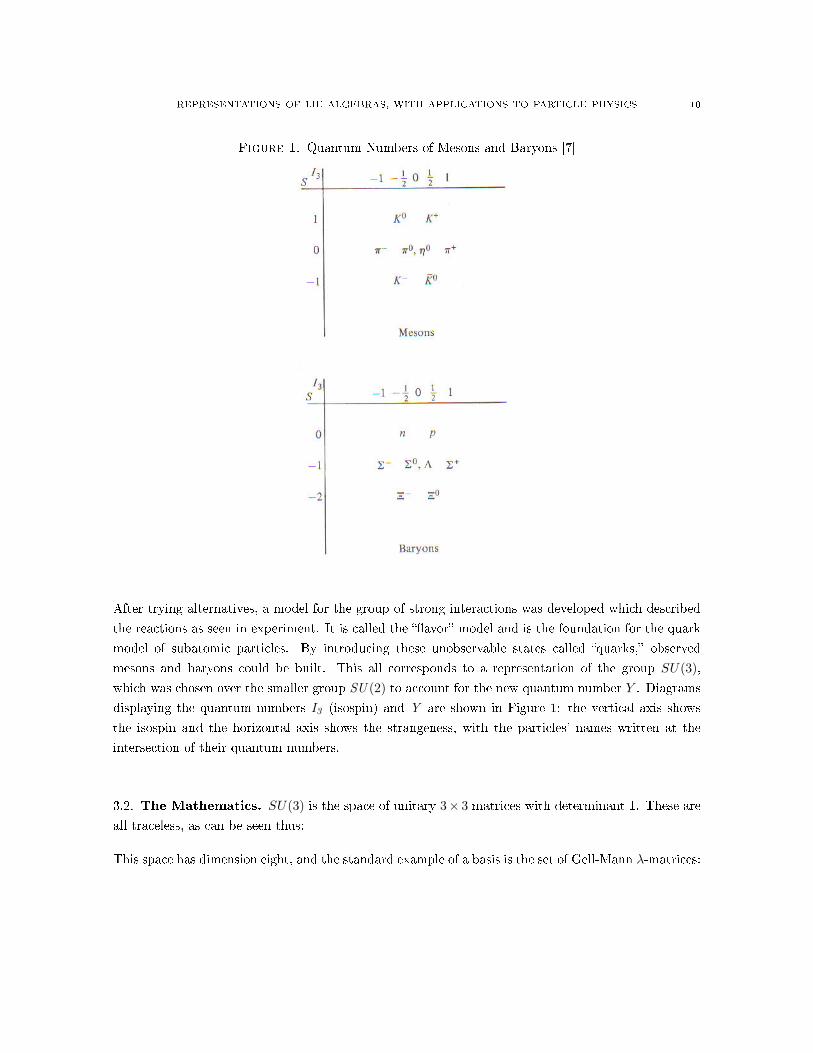
Figure 1. Quantum Numbers of Mesons and Baryons [7]

After trying alternatives, a model for the group of strong interactions was developed which described

the reactions as seen in experiment. It is called the avor model and is the foundation for the quark

model of subatomic particles. By introducing these unobservable states called quarks, observed

mesons and baryons could be built. This all corresponds to a representation of the group SU(3),which was chosen over the smaller group SU (2) to account for the new quantum number Y . Diagrams

displaying the quantum numbers I3 (isospin) and Y are shown in Figure 1: the vertical axis shows

the isospin and the horizontal axis shows the strangeness, with the particles' names written at the

intersection of their quantum numbers.

3.2. The Mathematics. SU(3) is the space of unitary 3× 3 matrices with determinant 1. These are

all traceless, as can be seen thus:

This space has dimension eight, and the standard example of a basis is the set of Gell-Mann λ-matrices:


λ1 =

0 1 01 0 00 0 0

, λ2 =

0 −i 0i 0 00 0 0

, λ3 =

1 0 00 −1 00 0 0

(the Pauli matrices, which generate SU(2), with extra row of zeroes)

λ4 =

0 0 10 0 01 0 0

, λ5 =

0 0 −i0 0 0i 0 0

, λ6 =

0 0 00 0 10 1 0

, λ7 =

0 0 00 0 −i0 i 0

, λ8 =1√3

1 0 00 1 00 0 −2

.

Without actually nding the corresponding Lie algebra, we can construct an abstract version by

implementing the fact that elements of the Lie algebra obey the commutation relation (in fact, the Lie

algebra of SU(3) is isomorphic to that of SL3(C), so we can call it sl3(C)). Out of eventual convenience(and partly to reect the structure of the basis of SU(2) that we didn't consider) we dene some new

matrices (the names are historical artices):

Tx =12λ1, Ty =

12λ2, Tz =

12λ3, Vx =

12λ4, Vy =

12λ5, Ux =

12λ6, Uy =

12λ7, Y =

1√3λ8

and

T± = Tx ± iTy, V± = Vx ± iVy, U± = Ux ± iUy (the so− called “shift′′ operators).

The names should give some hint of what the matrices mean; Y , for instance, corresponds to the

hypercharge and accordingly, Tz , the only other matrix not encoded in a ± relation, corresponds

to isospin (note that these are the only two diagonalizable matrices, and so the only ones with eigen-

vectors). The convenience comes when we consider the commutation relations (in Table 1), so that

all commutators are just scalar multiples of other matrices in the basis. We construct an abstract Lie

algebra by assuming elements tx , ty, tz, etc. whose commutators are the same as the commutators of

the matrices above.

We see that y and tz commute, so they are simultaneously diagonalizable; hence we might write

simultaneous eigenvectors as particle states in the Dirac notation |λ, µ〉 where λ, µ are eigenvalues of

the matrices on that vector. Then the notation |λ, µ〉 would correspond to the state of a particle with

isospin λ and strangeness µ. By examination we see that T+ shifts the eigenstate to |λ+ 1, µ〉, U+

shifts it to∣∣λ− 1

2 , µ+ 1⟩, etc. so that the shift operators (hence the reason for the subscripts) form

a diagram with vectors T+ = (1, 0), U+ = (− 12 , 1), etc. The shift operators, then, actually transform

between particles, which are themselves eigenstates of the isospin and strangeness operators. Figure 2

shows the six vectors (note that in the text from which this came, the operators T are called I ; someone


Table 1. Commutation Relations for Elements of Abstract Lie Algebra

t+ t− tz v+ v− u+ u− yt+ 0 2tz −t+ 0 −u− v+ 0 0t− −2tz 0 t− u+ 0 0 −v− 0tz t+ −t− 0 1

2v+ − 12v− − 1

2u+12uz 0

v+ 0 −u+ − 12v+ 0 3

2y + tz 0 t− −v+v− −u− 0 1

2v− − 32y − tz 0 −t− 0 v−

u+ −v+ 0 12u+ 0 t− 0 3

2y − tz −u+

u− 0 v− − 12uz −t− 0 − 3

2y + tz 0 u−y 0 0 0 v+ −v− u+ −u− 0

Figure 2. Root Diagram for Shift Operators(A2) [7]

with previous background might recognize this chart as the root diagram A2 , which corresponds to

the Lie algebra we are considerinig). A representation of this Lie algebra would be any map from the

generators t+, t−, etc. to a vector space while preserving the commutator relations.

Beginning with the standard representation from Example 1 above, with the vector space V = C3,

we have basis vectors e1 =

100

, e2 =

010

, e3 =

001

. The Lie group acts on these by

multiplying on the left. We (suggestively) write these e1 = u (up quark), e2 = d (downquark), e3 =s (strange quark). Using the denition of the dual representation as stated in Example 2 above, the

basis vectors are u∗ =(−1 0 0

), d∗ =

(0 −1 0

), s∗ =

(0 0 −1

)which are anti-up,

anti-down, and anti-strange. The Lie group acts on these by multiplying on the right by a matrix. For

example,

u∗V+ =(−1 0 0

) 0 0 −10 0 00 0 0

=(

0 0 −1)

= s∗

.


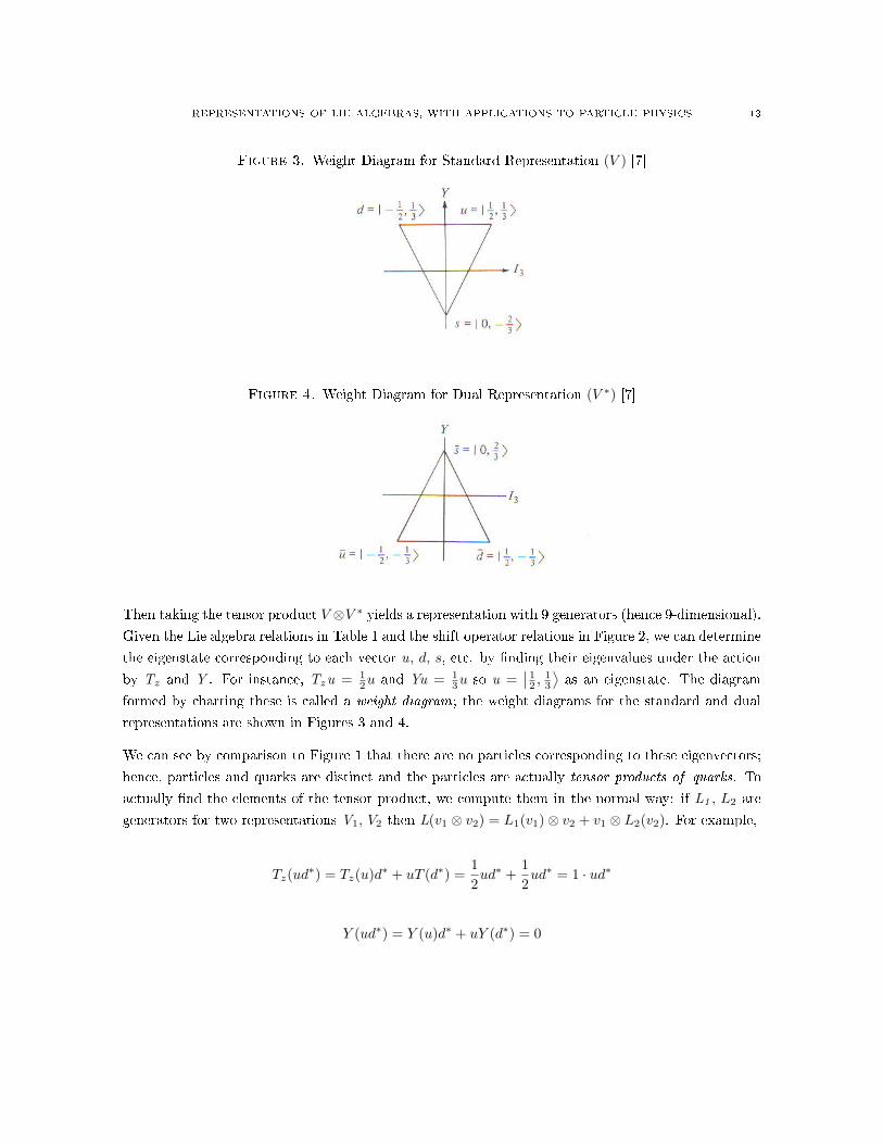
Figure 3. Weight Diagram for Standard Representation (V ) [7]

Figure 4. Weight Diagram for Dual Representation (V ∗) [7]

Then taking the tensor product V ⊗V ∗ yields a representation with 9 generators (hence 9-dimensional).

Given the Lie algebra relations in Table 1 and the shift operator relations in Figure 2, we can determine

the eigenstate corresponding to each vector u, d, s, etc. by nding their eigenvalues under the action

by Tz and Y . For instance, Tzu = 12u and Yu = 1

3u so u =∣∣ 12 ,

13

⟩as an eigenstate. The diagram

formed by charting these is called a weight diagram; the weight diagrams for the standard and dual

representations are shown in Figures 3 and 4.

We can see by comparison to Figure 1 that there are no particles corresponding to these eigenvectors;

hence, particles and quarks are distinct and the particles are actually tensor products of quarks. To

actually nd the elements of the tensor product, we compute them in the normal way: if L1 , L2 are

generators for two representations V1, V2 then L(v1 ⊗ v2) = L1(v1)⊗ v2 + v1 ⊗ L2(v2). For example,

Tz(ud∗) = Tz(u)d∗ + uT (d∗) =12ud∗ +

12ud∗ = 1 · ud∗

Y (ud∗) = Y (u)d∗ + uY (d∗) = 0


Figure 5. The Meson Octet [7]

so ud∗ corresponds to the state |1, 0〉 which, as one can see from Diagram 1, is the same as that of the

pion π+. Further, we can get relationships using the shift operators. For example,

U+ud∗ = us∗ =

∣∣ 12 , 1⟩which is the kaon K+.

From these relationships, we can generate every meson; however, the particle η = uu∗+dd∗+ss∗√6

= |0, 0〉is invariant under the action (one can check that uu∗, dd∗, ss∗ go to zero under the shift operators)

so it cannot be transformed into any other particle. Hence the representation V ⊗V ∗ reduces to the

direct sum of two irreducible representations of degrees 8 and 1.5 The tensor product of the standard

representation and its dual, then, accurately explain the observed interactions of mesons, and the

group of eight mesons generated by the shift operators gives the Eight-Fold Way its name. The meson

octet is shown in Figure 5 (by historical convention, π+ = −ud∗ instead of ud∗ as we determined).

3.3. Physical Re-Interpretation. As stated above, quarks are the basis vectors for the standard

representation of SU(3) and anti-quarks are the basis vectors for the dual representation (although

today there are six quarks in the model of the universe). The tensor product has generators consisting

of quark-anti-quark pairs, and these correspond to the mesons. Therefore, the elementary particles

are the generators for a vector space into which there is a homomorphism from a Lie group. That Lie

group has eight elements for generators; two of them have the particles as eigenvectors, and we can

uniquely identify the particles from their corresponding two eigenvalues. The other six generators of

the Lie group act on the mesons by transforming them, turning them into other mesons. Therefore,

one might say that all mesons are basis vectors for C3⊗C3∗ and meson interactions are characterized

by the action of linear combinations of generators of the Lie group SU(3). Why this should be - why

5Actually, the representation of degree 8 is the adjoint representation mentioned in footnote 2; one may actually beginwith this representation as teh basis for the eight-fold way, but it makes more sense to me to start with the standard anddual representations, as their actions will end up corresponding to the actions of quarks and antiquarks, respectively.


Lie groups should be woven into the background of the universe's fabric - is a question I simply can't

answer.

We have shown that all mesons are composed of one or more quark-antiquark pairs. The baryons

(protons, neutrons, etc.), it turns out, correspond to the triple tensor product representation V ⊗V ⊗Vso each of them have 3 quarks (the proton, for instance, is up-up-down). This splits into a 10-

dimensional irreducible representation, two 8-dimensional ones (the same as the 8-dimensional one

above) and a 1-dimensional representation. The benet of this mathematical model is that given

enough information from the mathematics, one can tell when the physics is incomplete. In 1964,

using a theoretical prediction from the representation theory used here, the baryon Ω− was discovered.

While the number of known elementary particles has grown to several hundred, some are still only

theoretical predictions. That the mathematics of homomorphisms between groups should help in the

endeavor to ascertain the structure of the universe is exciting and gives a unique perspective on just

what the interactions between matter really are.

Lie algebras were indispensable here because, although we did all our work with the matrices of the

Lie group itself, we used the fact that the Lie algebra is endowed with a commutator, and since

homomorphisms between groups must correspond to homomorphisms between algebras, we use the

information of the commutators to guarantee that we are nding workable representations of the

groups at hand. Indeed, in this case one might not even know what vector space V to use as a

representation; what ended up happening was that the Lie algebra itself acted as that vector space,

as we found an 8-dimensional representation corresponding to a map into the Lie algebra.6 Hence the

algebraic structure of Lie algebras are a vital tool in the study of representations of Lie groups.

References

[1] Adams, J. Frank. Lectures on Lie Groups. Chicago: University of Chicago Press, 1969.

[2] Cahn, Robert N. Semisimple Lie Algebras and Their Representations. Accessed online: http://www-

physics.lbl.gov/~rncahn/book.html.

[3] Cohn, P.M. Lie Groups. Cambridge: Cambridge University Press, 1957.

[4] Duistermat, J.J. and J.A.C. Kolk. Lie Groups. New York: Springer-Verlag, 2000.

[5] Dummit, David S. and Richard M. Foote. Abstract Algebra. Hoboken, NJ: John Wiley and Sons, Inc., 2004.

[6] Fulton, William and Joe Harris. Representation Theory: A First Course. New York: Springer Verlag, 1991.

[7] Sattinger, D. H. and O. L. Weaver. Lie Groups and Algebras with Applications to Physics, Geometry, and Mechanics.

New York: Springer-Verlag, 1986.

6A greater elaboration on the adjoint representation would demonstrate immediately that this is true. In short, if Θg

is conjugation by g ∈ G then Ad(g) = (dΘg)e is a map from the Lie group to the space of automorphisms of its Liealgebra, Aut(g).

Documents

REPRESENTTIONSA OF LIE ALGEBRAS, WITH …may/VIGRE/VIGRE2007/REUPapers/FINALFU… · representtionsa of lie algebras, with applications to arpticle physics james marrone university