Embed Size (px)
Citation preview
Classical inference and design efficiency
Zurich SPM Course 2014
Jakob [email protected]
Translational Neuromodeling Unit (TNU) Institute for Biomedical Engineering (IBT)University and ETH Zürich
Many thanks to K. E. Stephan, G. Flandin and others for material
Translational Neuromodeling Unit
Classical Inference and Design Efficiency 2
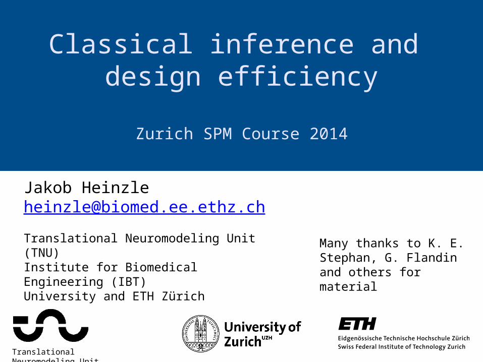
Normalisation
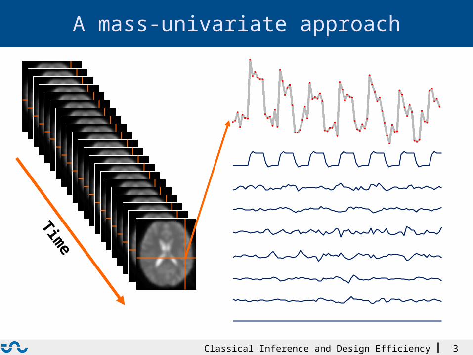
Statistical Parametric MapImage time-series
Parameter estimates
General Linear ModelRealignment Smoothing
Design matrix
Anatomicalreference
Spatial filter
StatisticalInference
RFT
p <0.05
Overview
Classical Inference and Design Efficiency 3
A mass-univariate approach
Time
Classical Inference and Design Efficiency 4
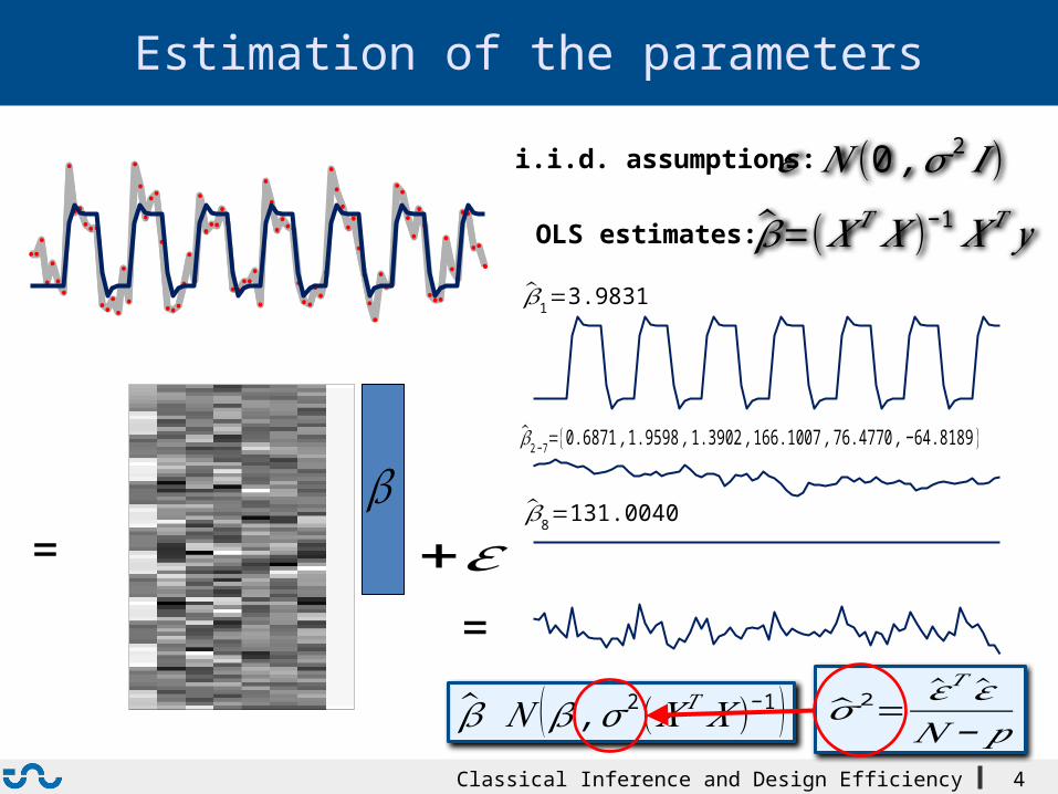
Estimation of the parameters
= +𝜀𝛽
𝜀 𝑁 (0 ,𝜎 2 𝐼 )
��=(𝑋𝑇 𝑋 )−1 𝑋𝑇 𝑦
i.i.d. assumptions:
OLS estimates:
��1=3.9831
��2 −7={0.6871 ,1.9598 , 1.3902 , 166.1007 , 76.4770 ,− 64.8189 }
��8=131.0040
=
�� 2= ��𝑇 ��𝑁−𝑝�� 𝑁 (𝛽 ,𝜎2(𝑋𝑇 𝑋 )−1 )
Classical Inference and Design Efficiency 5
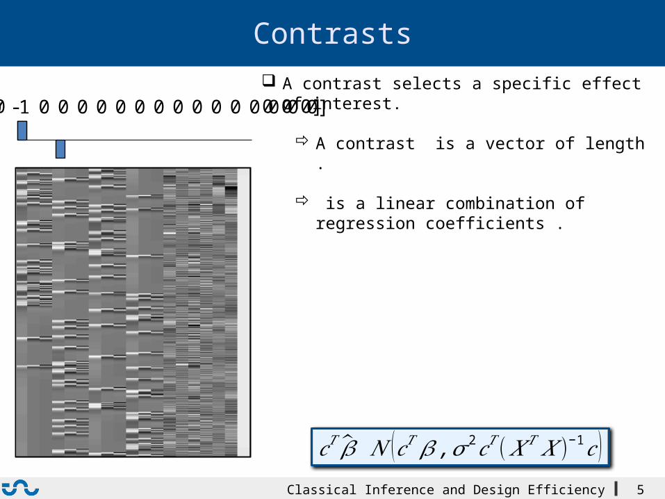
Contrasts
A contrast selects a specific effect of interest.
A contrast is a vector of length .
is a linear combination of regression coefficients .
[1 0 0 0 0 0 0 0 0 0 0 0 0 0 0 0 0 0 0]
𝑐𝑇 �� 𝑁 (𝑐𝑇 𝛽 ,𝜎2𝑐𝑇 (𝑋𝑇 𝑋 )−1𝑐 )
[1 0 0 -1 0 0 0 0 0 0 0 0 0 0 0 0 0 0 0]
Classical Inference and Design Efficiency 6
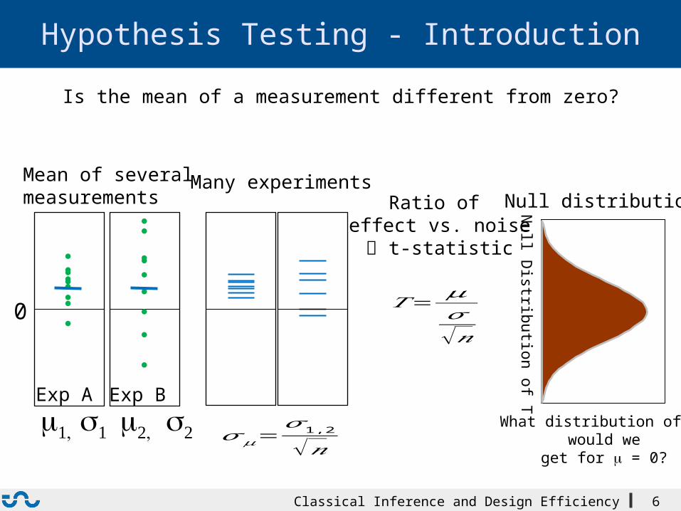
Hypothesis Testing - Introduction
Is the mean of a measurement different from zero?
Mean of severalmeasurements
Many experiments
𝑇=𝜇𝜎√𝑛
Ratio of effect vs. noise
t-statistic Null D
istribution of T
Null distribution
What distribution of T would we
get for m = 0?
𝜎 𝜇=𝜎1,2
√𝑛
0
m1, s1
Exp A
m2, s2
Exp B
Classical Inference and Design Efficiency 7
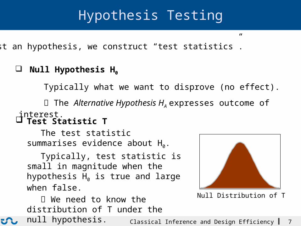
Hypothesis Testing
Null Hypothesis H0
Typically what we want to disprove (no effect).
The Alternative Hypothesis HA expresses outcome of interest.
To test an hypothesis, we construct “test statistics”.
Test Statistic T
The test statistic summarises evidence about H0.
Typically, test statistic is small in magnitude when the hypothesis H0 is true and large when false.
We need to know the distribution of T under the null hypothesis. Null Distribution of T
Classical Inference and Design Efficiency 8
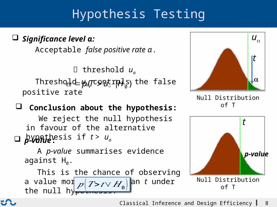
Hypothesis Testing
p-value:
A p-value summarises evidence against H0.
This is the chance of observing a value more extreme than t under the null hypothesis.
Null Distribution of T
Significance level α:
Acceptable false positive rate α.
threshold uα
Threshold uα controls the false positive rate
t
p-value
Null Distribution of T
u
Conclusion about the hypothesis:
We reject the null hypothesis in favour of the alternative hypothesis if t > uα
)|( 0HuTp
𝑝 (𝑇>𝑡∨𝐻0 )
t
Classical Inference and Design Efficiency 9
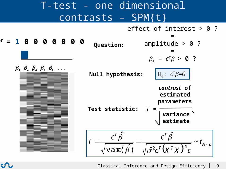
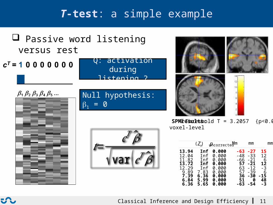
cT = 1 0 0 0 0 0 0 0
T =
contrast ofestimated
parameters
varianceestimate
effect of interest > 0 ?=
amplitude > 0 ?=
b1 = cT b > 0 ?
b1 b2 b3 b4 b5 ...
T-test - one dimensional contrasts – SPM{t}
Question:
Null hypothesis: H0: cTb=0 H0: cTb=0
Test statistic:
pNTT
T
T
T
tcXXc
c
c
cT
~ˆ
ˆ
)ˆvar(
ˆ
12
Classical Inference and Design Efficiency 10
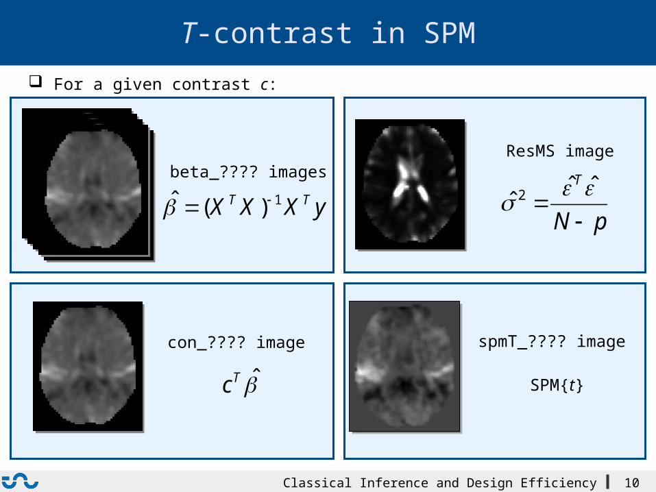
T-contrast in SPM
con_???? image
Tc
ResMS image
pN
T
ˆˆ
ˆ 2
spmT_???? image
SPM{t}
For a given contrast c:
yXXX TT 1)(ˆ beta_???? images
Classical Inference and Design Efficiency 11
T-test: a simple example
Q: activation during listening ?
Null hypothesis: b1 = 0
Passive word listening versus rest
SPMresults: Threshold T = 3.2057 {p<0.001}voxel-level
p uncorrected
T
( Zº) Mm mm mm
13.94 Inf 0.000 -63 -27 15 12.04 Inf 0.000 -48 -33 12 11.82 Inf 0.000 -66 -21 6 13.72 Inf 0.000 57 -21 12 12.29 Inf 0.000 63 -12 -3 9.89 7.83 0.000 57 -39 6 7.39 6.36 0.000 36 -30 -15 6.84 5.99 0.000 51 0 48 6.36 5.65 0.000 -63 -54 -3
𝑡= 𝑐𝑇 ��
√var (𝑐𝑇 ��)
Classical Inference and Design Efficiency 12
T-test: summary
T-test is a signal-to-noise measure (ratio of estimate to standard deviation of estimate).
T-contrasts are simple combinations of the betas; the T-statistic does not depend on the scaling of the regressors or the scaling of the contrast.
H0: 0Tc vs HA: 0Tc
Alternative hypothesis:
Classical Inference and Design Efficiency 13
��=(𝑋𝑇 𝑋 )−1 𝑋𝑇 𝑦
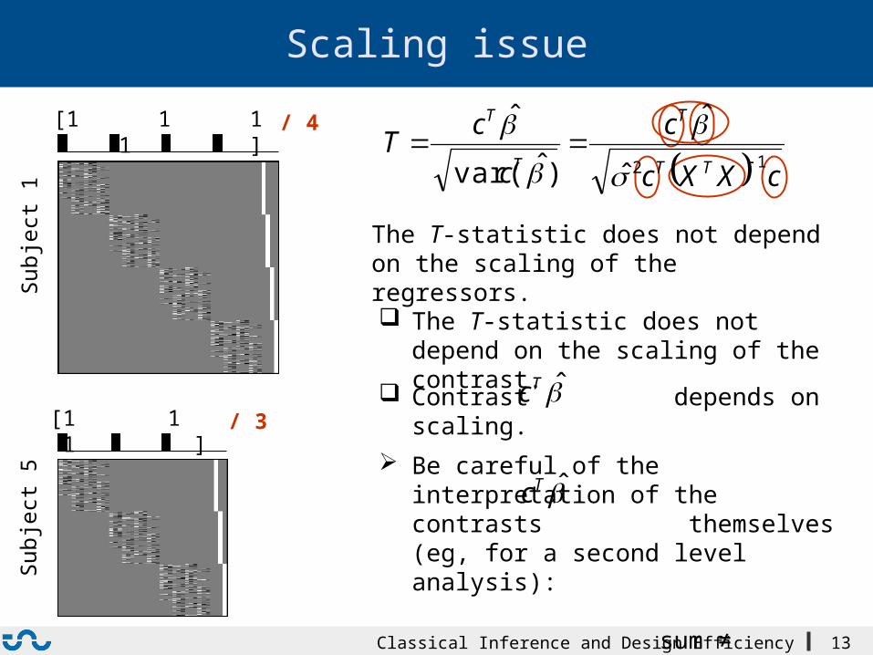
Scaling issue
The T-statistic does not depend on the scaling of the regressors.
cXXc
c
c
cT
TT
T
T
T
12ˆ
ˆ
)ˆvar(
ˆ
[1 1 1 1 ]
Be careful of the interpretation of the contrasts themselves (eg, for a second level analysis):
sum ≠ average
The T-statistic does not depend on the scaling of the contrast.
/ 4
Tc
Sub
ject
1
[1 1 1 ]
Sub
ject
5
Contrast depends on scaling.Tc/ 3
Classical Inference and Design Efficiency 14
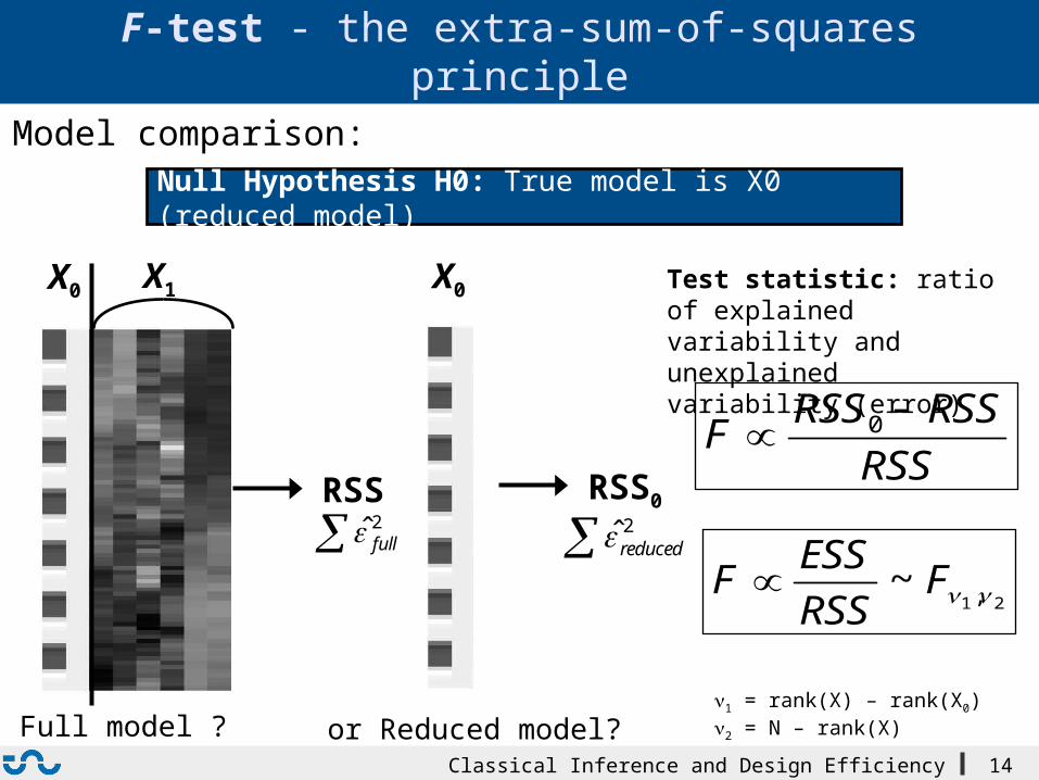
F-test - the extra-sum-of-squares principle
Model comparison:
Full model ?
X1 X0
or Reduced model?
X0 Test statistic: ratio of explained variability and unexplained variability (error)
1 = rank(X) – rank(X0)2 = N – rank(X)
RSS
2ˆ fullRSS0
2ˆreduced
RSS
RSSRSSF
0
21 ,~ FRSS
ESSF
Null Hypothesis H0: True model is X0 (reduced model)
Classical Inference and Design Efficiency 15
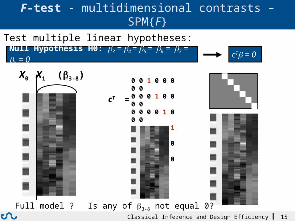
F-test - multidimensional contrasts – SPM{F}
Test multiple linear hypotheses:
Full model ?
Null Hypothesis H0: b3 = b4 = b5 = b6 = b7 = b8 = 0
X1 (b3-8)X0 0 0 1 0 0 0 0 00 0 0 1 0 0 0 00 0 0 0 1 0 0 00 0 0 0 0 1 0 00 0 0 0 0 0 1 00 0 0 0 0 0 0 1
cT =
cTb = 0
Is any of b3-8 not equal 0?
Classical Inference and Design Efficiency 16
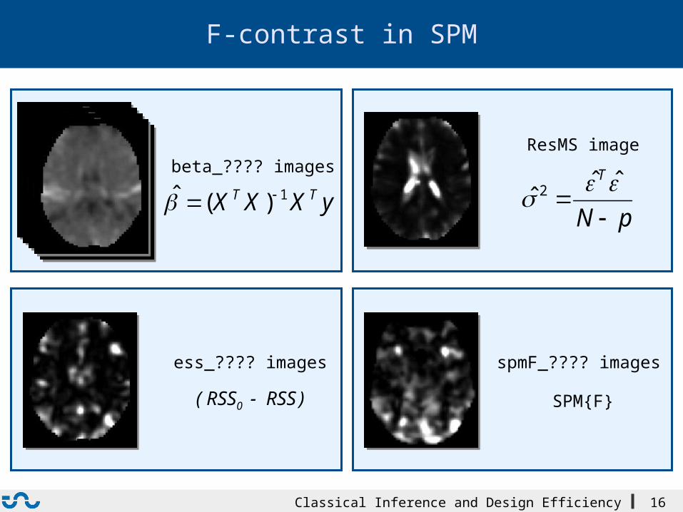
F-contrast in SPM
ResMS image
pN
T
ˆˆ
ˆ 2
spmF_???? images
SPM{F}
ess_???? images
( RSS0 - RSS )
yXXX TT 1)(ˆ beta_???? images
Classical Inference and Design Efficiency 17
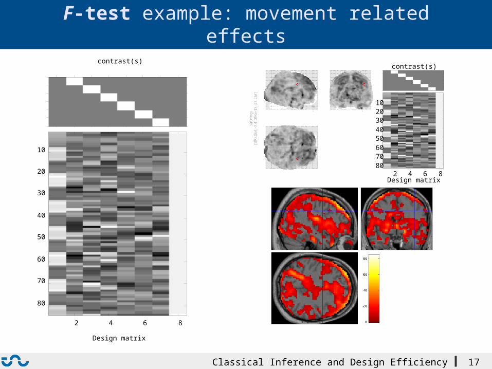
F-test example: movement related effects
Design matrix
2 4 6 8
10
20
30
40
50
60
70
80
contrast(s)
Design matrix2 4 6 8
1020304050607080
contrast(s)
Classical Inference and Design Efficiency 18
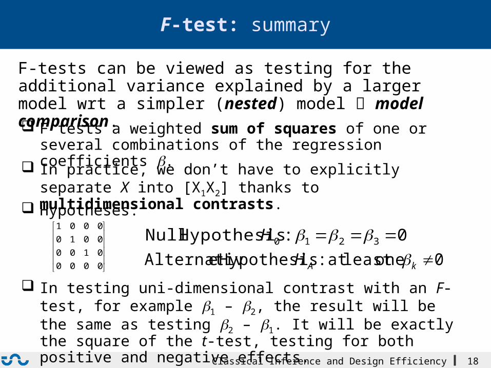
F-test: summary
F-tests can be viewed as testing for the additional variance explained by a larger model wrt a simpler (nested) model model comparison.
0000
0100
0010
0001
In testing uni-dimensional contrast with an F-test, for example b1 – b2, the result will be the same as testing b2 – b1. It will be exactly the square of the t-test, testing for both positive and negative effects.
F tests a weighted sum of squares of one or several combinations of the regression coefficients b.
In practice, we don’t have to explicitly separate X into [X1X2] thanks to multidimensional contrasts.
Hypotheses:
0 : Hypothesis Null 3210 H
0 oneleast at : Hypothesis eAlternativ kAH
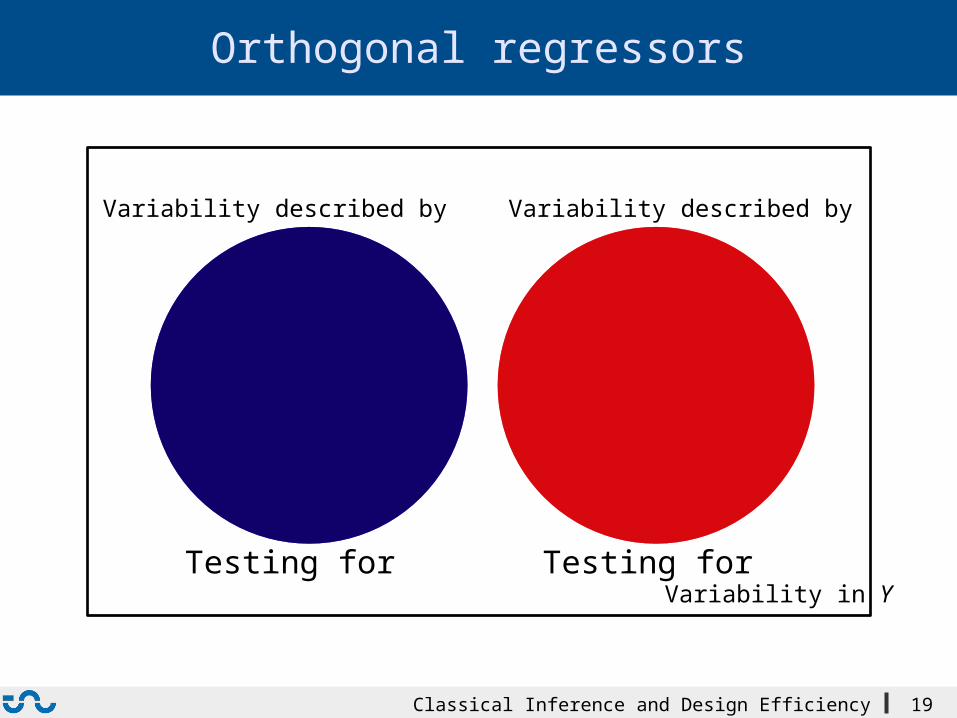
Classical Inference and Design Efficiency 19
Variability described by Variability described by
Orthogonal regressors
Variability in YTesting for Testing for
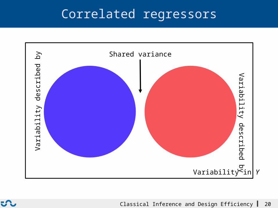
Classical Inference and Design Efficiency 20
Correlated regressors
Var
iabi
lity
desc
ribed
by
Variability described by
Shared variance
Variability in Y
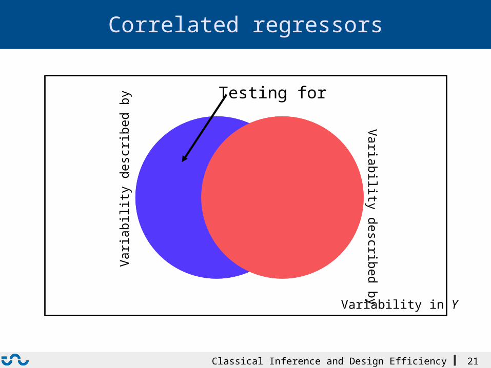
Classical Inference and Design Efficiency 21
Correlated regressors
Var
iabi
lity
desc
ribed
by
Variability described by
Variability in Y
Testing for
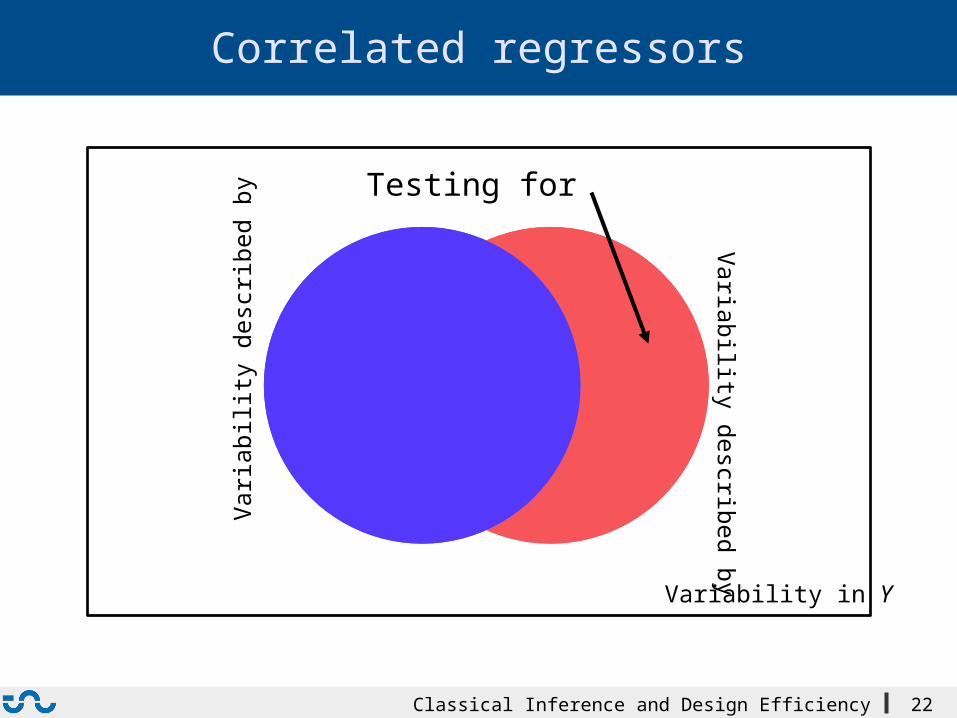
Classical Inference and Design Efficiency 22
Correlated regressors
Var
iabi
lity
desc
ribed
by
Variability described by
Variability in Y
Testing for
Classical Inference and Design Efficiency 23
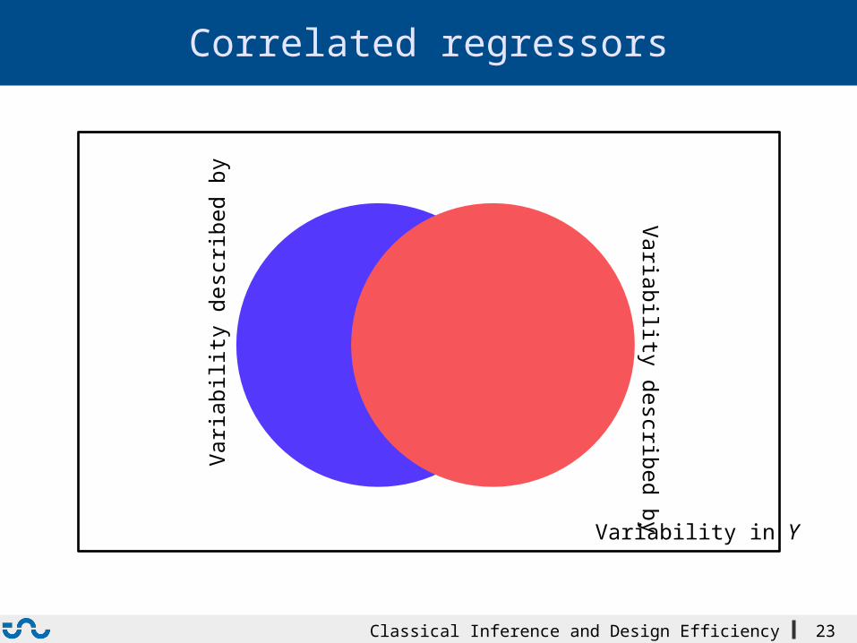
Correlated regressors
Var
iabi
lity
desc
ribed
by
Variability described by
Variability in Y
Classical Inference and Design Efficiency 24
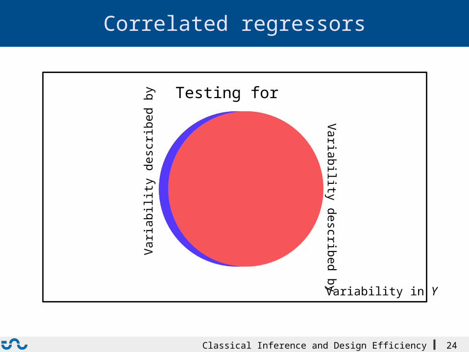
Correlated regressors
Var
iabi
lity
desc
ribed
by
Variability described by
Variability in Y
Testing for
Classical Inference and Design Efficiency 25
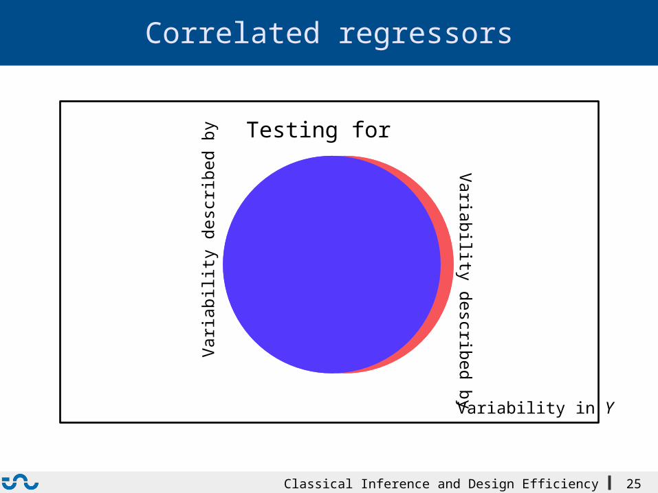
Correlated regressors
Var
iabi
lity
desc
ribed
by
Variability described by
Variability in Y
Testing for
Classical Inference and Design Efficiency 26
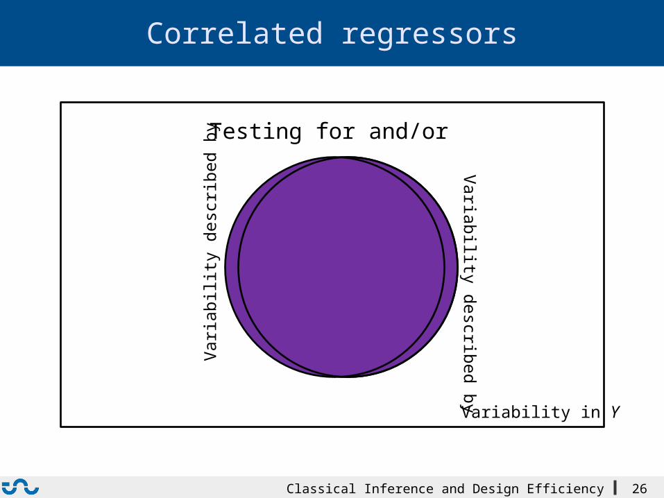
Correlated regressors
Var
iabi
lity
desc
ribed
by
Variability described by
Variability in Y
Testing for and/or
Classical Inference and Design Efficiency 27
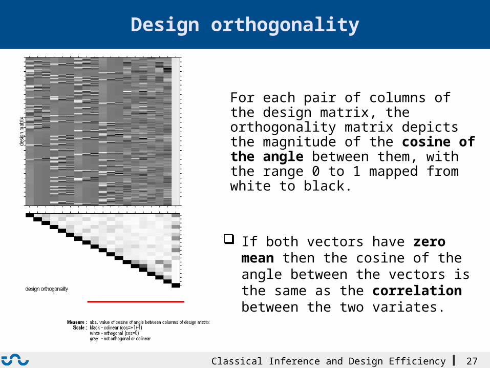
Design orthogonality
For each pair of columns of the design matrix, the orthogonality matrix depicts the magnitude of the cosine of the angle between them, with the range 0 to 1 mapped from white to black.
If both vectors have zero mean then the cosine of the angle between the vectors is the same as the correlation between the two variates.
Classical Inference and Design Efficiency 28
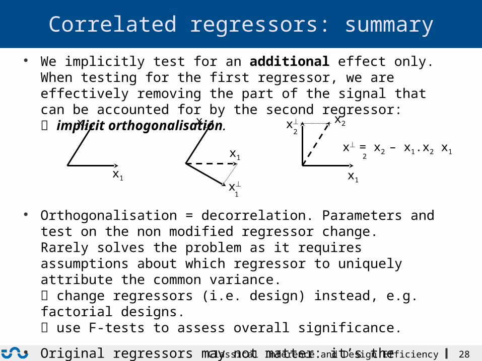
Correlated regressors: summary
● We implicitly test for an additional effect only. When testing for the first regressor, we are effectively removing the part of the signal that can be accounted for by the second regressor: implicit orthogonalisation.
● Orthogonalisation = decorrelation. Parameters and test on the non modified regressor change.Rarely solves the problem as it requires assumptions about which regressor to uniquely attribute the common variance. change regressors (i.e. design) instead, e.g. factorial designs. use F-tests to assess overall significance.
● Original regressors may not matter: it’s the contrast you are testing which should be as decorrelated as possible from the rest of the design matrix
x1
x2
x1
x2
x1
x2x^
x^
2
1
2x^ = x2 – x1.x2 x1
Classical Inference and Design Efficiency 29
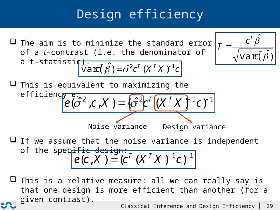
Design efficiency
1122 ))(ˆ(),,ˆ( cXXcXce TT
)ˆvar(
ˆ
T
T
c
cT The aim is to minimize the standard error of a t-contrast
(i.e. the denominator of a t-statistic).
cXXcc TTT 12 )(ˆ)ˆvar( This is equivalent to maximizing the efficiency e:
Noise variance Design variance
If we assume that the noise variance is independent of the specific design:
11 ))((),( cXXcXce TT
This is a relative measure: all we can really say is that one design is more efficient than another (for a given contrast).
Classical Inference and Design Efficiency 30
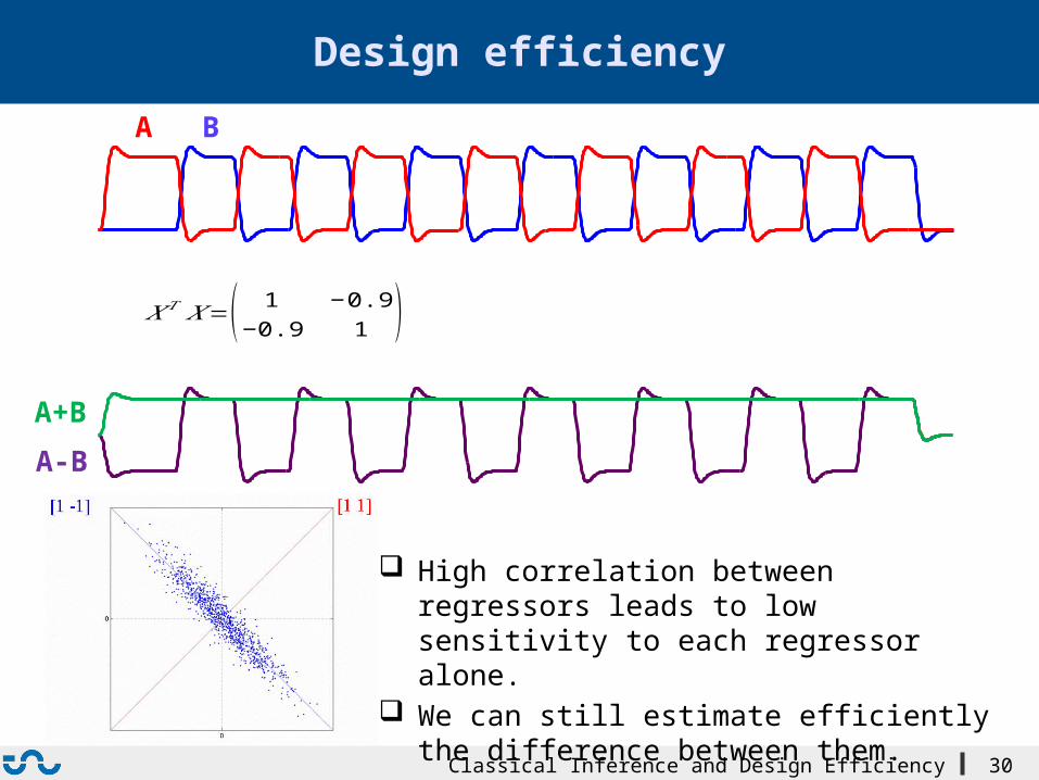
Design efficiency
A B
A+B
A-B
𝑋𝑇 𝑋=( 1 − 0.9− 0.9 1 )
High correlation between regressors leads to low sensitivity to each regressor alone.
We can still estimate efficiently the difference between them.
Classical Inference and Design Efficiency 31
Bibliography:
Statistical Parametric Mapping: The Analysis of Functional Brain Images. Elsevier, 2007.
Plane Answers to Complex Questions: The Theory of Linear Models. R. Christensen, Springer, 1996.
Statistical parametric maps in functional imaging: a general linear approach. K.J. Friston et al, Human Brain Mapping, 1995.
Ambiguous results in functional neuroimaging data analysis due to covariate correlation. A. Andrade et al., NeuroImage, 1999.
Estimating efficiency a priori: a comparison of blocked and randomized designs. A. Mechelli et al., NeuroImage, 2003.