Classical Decomposition Model Revisited

• recall classical decomposition model

Xt = mt + st + Wt (∗)where mt is trend; st is periodic with known period s (i.e.,st−s = st for all t ∈ Z) satisfying

∑sj=1 sj = 0; and Wt is a

zero-mean stationary process

• recall definition of lag-s seasonal differencing operator:

∇sXt = Xt −Xt−s = (1−Bs)Xt• application of this operator to (∗) yields

∇sXt = mt −mt−s + st − st−s + Wt −Wt−s= mt −mt−s + Wt −Wt−s

because {st} has period s

BD: 20, CC: 98, SS: 57 XV–1

Seasonal ARMA Models: I

• assumption of exact repetition of seasonal pattern often dicey

• while differencing eliminates st, also complicatesWt component

• motivates period s seasonal ARMA(p, q)× (P,Q)s model

• time series Xt is said to obey this so-called SARMA model ifXt is a causal ARMA process defined by

φ(B)Φ(Bs)Xt = θ(B)Θ(Bs)Zt, {Zt} ∼WN(0, σ2),

where

φ(z) = 1− φ1z − · · · − φpzp

Φ(z) = 1− Φ1z − · · · − ΦPzP

θ(z) = 1 + θ1z + · · · + θqzq

Θ(z) = 1 + Θ1z + · · · + ΘQzQ

BD: 177–178, CC: 231, SS: 150 XV–2

Seasonal ARMA Models: II

• as an example, consider SARMA(1, 0)× (1, 0)12 model:

φ(B)Φ(B12)Xt = Zt(1− φ1B)(1− Φ1B

12)Xt = Zt(1− φ1B − Φ1B

12 + φ1Φ1B13)Xt = Zt

Xt − φ1Xt−1 − Φ1Xt−12 + φ1Φ1Xt−13 = Zt

• above is a special case of AR(13) model with

− 10 coefficients set to zero

− 3 remaining coefficients set using 2 parameters

• SARMA(p, q) × (P,Q)s models are ARMA(p + Ps, q + Qs)models with certain constraints on AR and MA coefficients

BD: 177–178, CC: 231, SS: 150 XV–3

Seasonal ARIMA Models: I

• can extend SARMA model to include ordinary and/or seasonaldifferencing – leads to seasonal ARIMA(p, d, q) × (P,D,Q)smodel

• time series Xt is said to obey a SARIMA model if

Yt = (1−B)d(1−Bs)DXtis a causal ARMA process defined by

φ(B)Φ(Bs)Yt = θ(B)Θ(Bs)Zt, {Zt} ∼WN(0, σ2)

• as an example, consider SARIMA(0, 1, 1) × (0, 1, 1)12 model,which is a popular model for nonstationary monthly economicdata with a seasonal pattern:

(1−B)(1−B12)Xt = θ(B)Θ(B12)Zt

BD: 177–178, CC: 233, SS: 150 XV–4

Seasonal ARIMA Models: II

• expanding out

(1−B)(1−B12)Xt = θ(B)Θ(B12)Zt

yields

(1−B −B12 + B13)Xt = (1− θ1B)(1− Θ1B12)Zt

(1−B −B12 + B13)Xt = (1− θ1B − Θ1B12 + θ1Θ1B

13)Zt

and hence

Xt = Xt−1 + Xt−12 −Xt−13 + Zt − θ1Zt−1 − Θ1Zt−12 + θ1Θ1Zt−13

BD: 177–178, CC: 233, SS: 150 XV–5

Seasonal ARMA Models: III

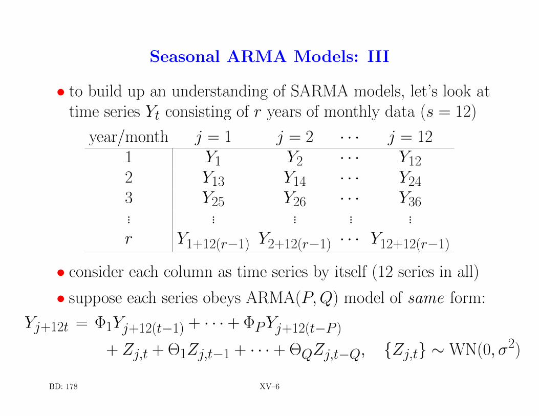
• to build up an understanding of SARMA models, let’s look attime series Yt consisting of r years of monthly data (s = 12)

year/month j = 1 j = 2 · · · j = 121 Y1 Y2 · · · Y122 Y13 Y14 · · · Y243 Y25 Y26 · · · Y36... ... ... ... ...r Y1+12(r−1) Y2+12(r−1) · · · Y12+12(r−1)

• consider each column as time series by itself (12 series in all)

• suppose each series obeys ARMA(P,Q) model of same form:

Yj+12t = Φ1Yj+12(t−1) + · · · + ΦPYj+12(t−P )

+ Zj,t + Θ1Zj,t−1 + · · · + ΘQZj,t−Q, {Zj,t} ∼WN(0, σ2)

BD: 178 XV–6

Seasonal ARMA Models: IV

• interleave Zj,t’s from models for individual months to form

Zj+12t = Zj,t,

using which we can now write

Yj+12t = Φ1Yj+12(t−1) + · · · + ΦPYj+12(t−P )

+ Zj+12t + Θ1Zj+12(t−1) + · · · + ΘQZj+12(t−Q)

• since same equation holds for all j and t, can write

Φ(B12)Yt = Θ(B12)Zt

• while E{Zt} = 0 and var {Zt} = σ2, {Zt} need not be whitenoise: we have E{ZtZt+h} = 0 if h is an nonzero integermultiple of 12, but this need not be zero for other nonzero h

BD: 178 XV–7

Seasonal ARMA Models: V

• between-year (interannual) model Φ(B12)Yt = Θ(B12)Zt nota SARMA(0, 0) × (P,Q)12 model unless we further assumeE{ZtZt+h} = 0 for all h 6= 0, allowing us to write

Φ(B12)Yt = Θ(B12)Zt, {Zt} ∼WN(0, σ2)

• so-called pure SARMA model (i.e., p = q = 0) is instructive,but of questionable practical value: says, e.g., every RV that ispart of February time series is uncorrelated with every RV thatis part of March series (even if months are within same year!)

• keeping still to s = 12, consider ACF, PACF and simulatedseries from following pure SARMA models:

− P = 0, Q = 1 and Θ1 = −0.95

− P = 1, Q = 0 and Φ1 = 0.95

BD: 178–179, CC: 228, SS: 145–146 XV–8

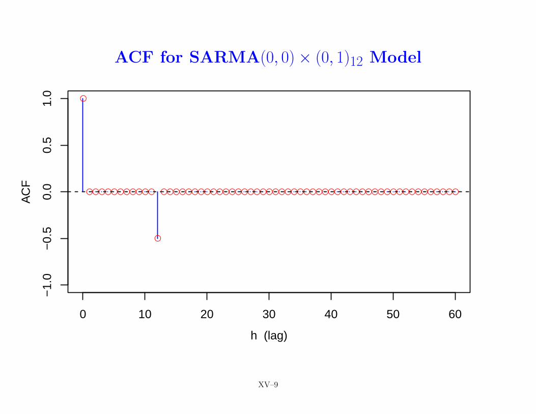
ACF for SARMA(0, 0)× (0, 1)12 Model

●

●●●●●●●●●●●

●

●●●●●●●●●●●●●●●●●●●●●●●●●●●●●●●●●●●●●●●●●●●●●●●●

0 10 20 30 40 50 60

−1.

0−

0.5

0.0

0.5

1.0

h (lag)

AC

F

XV–9

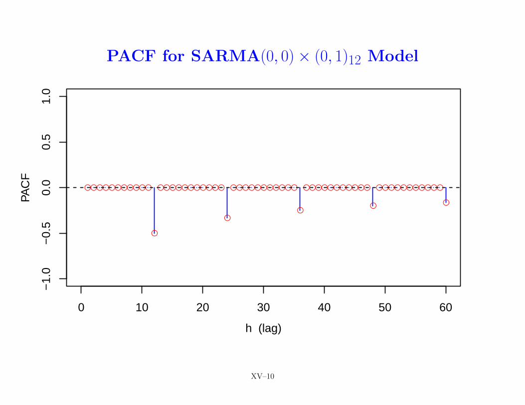
PACF for SARMA(0, 0)× (0, 1)12 Model

●●●●●●●●●●●

●

●●●●●●●●●●●

●

●●●●●●●●●●●

●

●●●●●●●●●●●

●

●●●●●●●●●●●

●

0 10 20 30 40 50 60

−1.

0−

0.5

0.0

0.5

1.0

h (lag)

PAC

F

XV–10

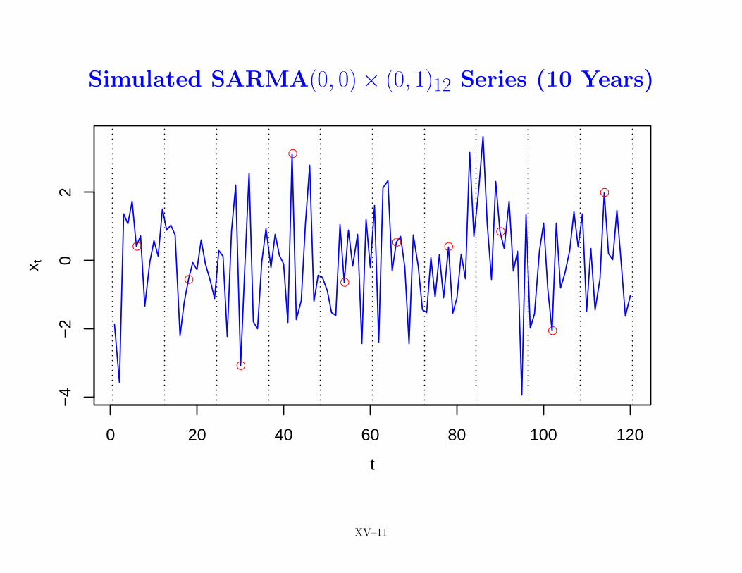
Simulated SARMA(0, 0)× (0, 1)12 Series (10 Years)

●

●

●

●

●

● ●

●

●

●

0 20 40 60 80 100 120

−4

−2

02

t

x t

XV–11

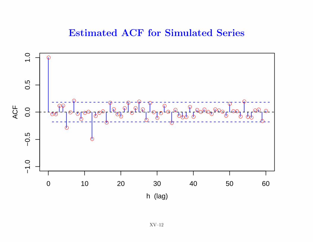
Estimated ACF for Simulated Series

●

●●

●●

●

●

●

●

●

●●

●

●●●

●

●

●●

●

●

●

●●

●

●

●

●

●

●●

●

●

●

●

●●●

●

●

●●●

●●

●●●●

●

●●

●

●

●●

●●

●

●

0 10 20 30 40 50 60

−1.

0−

0.5

0.0

0.5

1.0

h (lag)

AC

F

XV–12

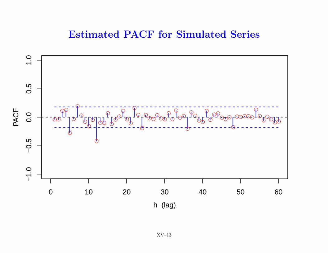
Estimated PACF for Simulated Series

●●

●●

●

●

●

●

●●

●

●

●●

●

●●

●

●

●●

●

●

●

●●●

●●●

●

●

●

●●

●

●●

●●

●

●●●

●●●

●

●●●●●

●

●●

●●

●●

0 10 20 30 40 50 60

−1.

0−

0.5

0.0

0.5

1.0

h (lag)

PAC

F

XV–13

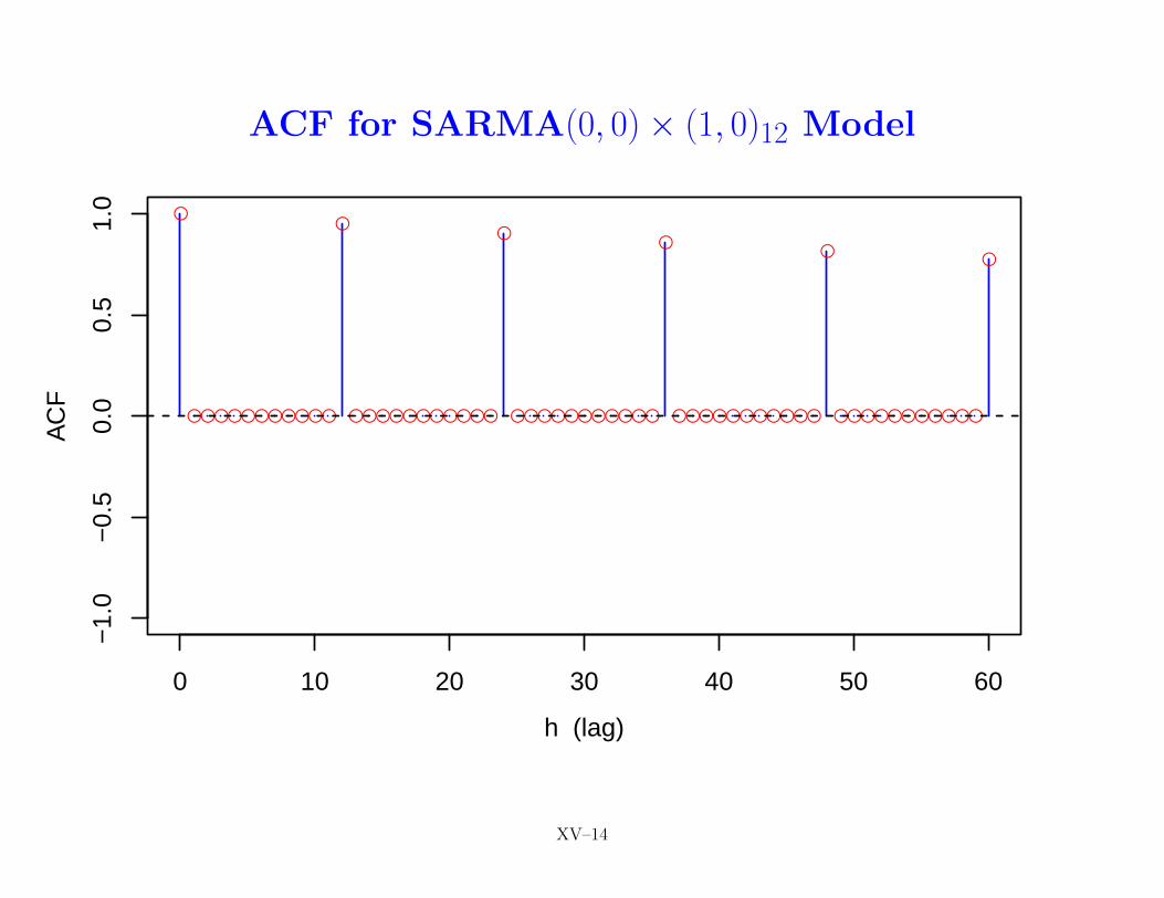
ACF for SARMA(0, 0)× (1, 0)12 Model

●

●●●●●●●●●●●

●

●●●●●●●●●●●

●

●●●●●●●●●●●

●

●●●●●●●●●●●

●

●●●●●●●●●●●

●

0 10 20 30 40 50 60

−1.

0−

0.5

0.0

0.5

1.0

h (lag)

AC

F

XV–14

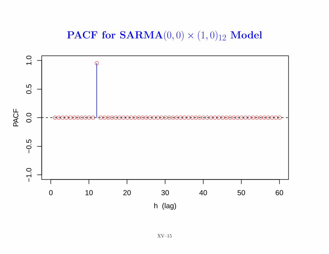
PACF for SARMA(0, 0)× (1, 0)12 Model

●●●●●●●●●●●

●

●●●●●●●●●●●●●●●●●●●●●●●●●●●●●●●●●●●●●●●●●●●●●●●●

0 10 20 30 40 50 60

−1.

0−

0.5

0.0

0.5

1.0

h (lag)

PAC

F

XV–15

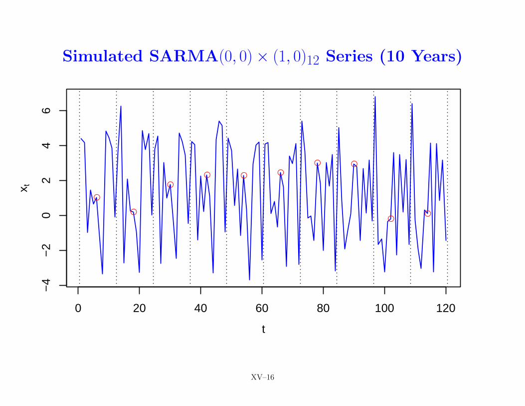
Simulated SARMA(0, 0)× (1, 0)12 Series (10 Years)

●

●

●

● ● ●

● ●

●●

0 20 40 60 80 100 120

−4

−2

02

46

t

x t

XV–16

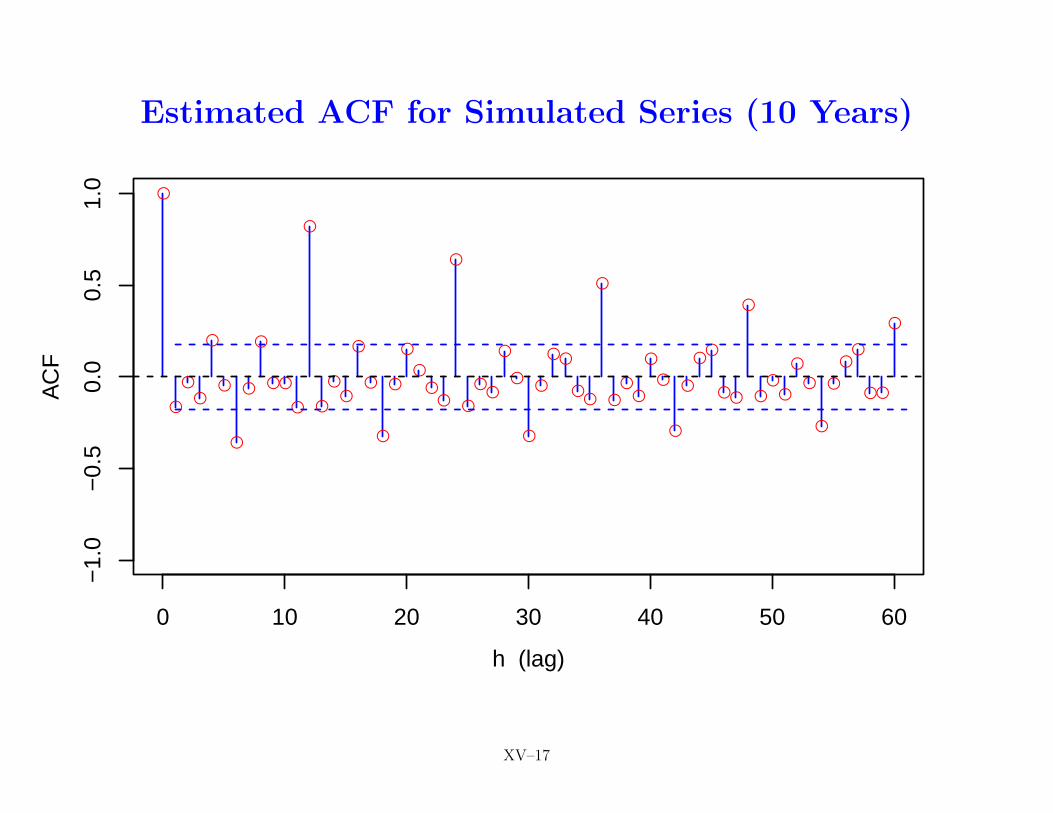
Estimated ACF for Simulated Series (10 Years)

●

●

●●

●

●

●

●

●

●●

●

●

●

●●

●

●

●

●

●

●

●●

●

●

●●

●

●

●

●

●●

●●

●

●●

●

●

●

●

●

●●

●●

●

●●

●

●

●

●

●

●●

●●

●

0 10 20 30 40 50 60

−1.

0−

0.5

0.0

0.5

1.0

h (lag)

AC

F

XV–17

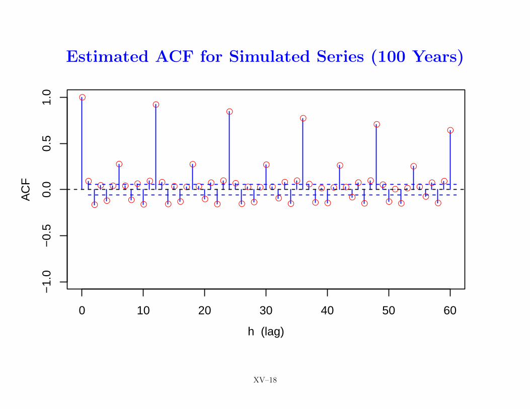
Estimated ACF for Simulated Series (100 Years)

●

●

●

●

●

●

●

●

●

●

●

●

●

●

●

●

●

●

●

●

●

●

●

●

●

●

●

●

●

●

●

●

●

●

●

●

●

●

●

●

●

●

●

●

●

●

●

●

●

●

●

●

●

●

●

●

●

●

●

●

●

0 10 20 30 40 50 60

−1.

0−

0.5

0.0

0.5

1.0

h (lag)

AC

F

XV–18

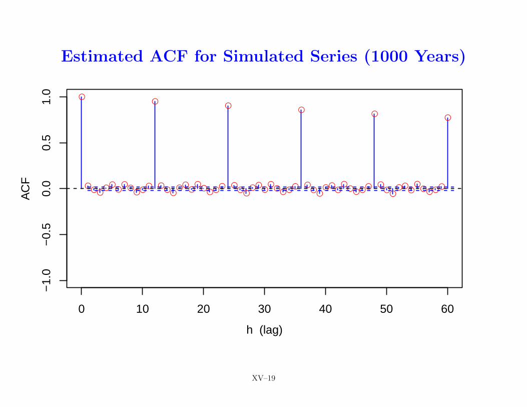
Estimated ACF for Simulated Series (1000 Years)

●

●●●

●●●

●●

●●●

●

●●●

●●●

●●

●●●

●

●●●

●●●

●●●●●

●

●●

●●●

●●

●●●●

●

●●

●●●

●●

●●●●

●

0 10 20 30 40 50 60

−1.

0−

0.5

0.0

0.5

1.0

h (lag)

AC

F

XV–19

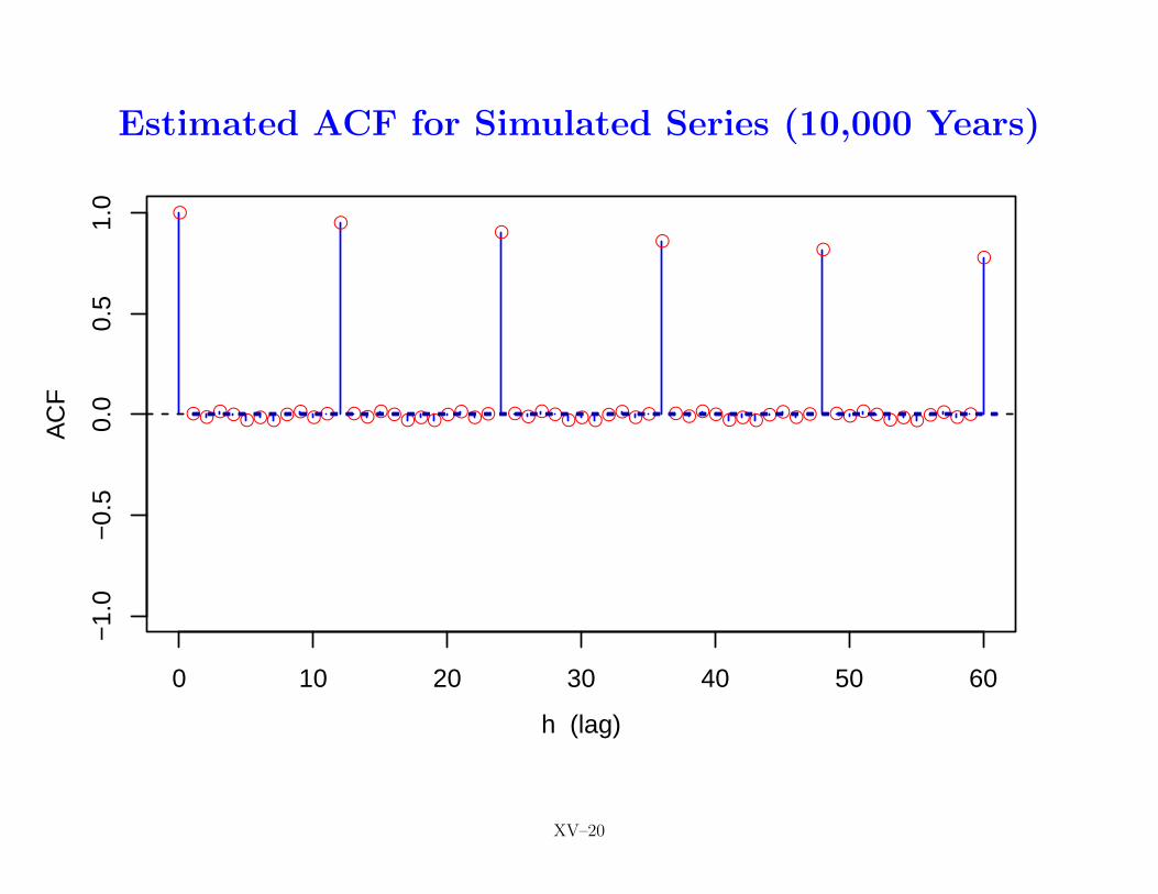
Estimated ACF for Simulated Series (10,000 Years)

●

●●●●●●●●●●●

●

●●●●●●●●●●●

●

●●●●●●●●●●●

●

●●●●●●●●●●●

●

●●●●●●●●●●●

●

0 10 20 30 40 50 60

−1.

0−

0.5

0.0

0.5

1.0

h (lag)

AC

F

XV–20

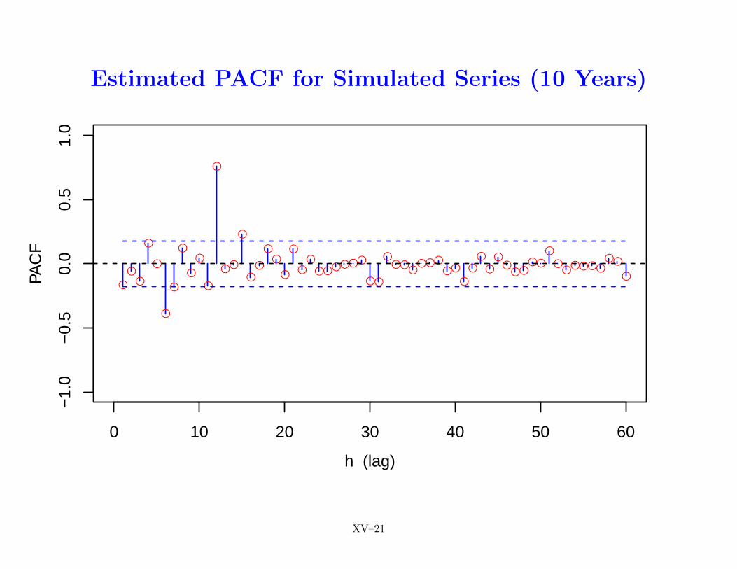
Estimated PACF for Simulated Series (10 Years)

●

●●

●

●

●

●

●

●

●

●

●

●●

●

●●

●●

●

●

●●

●●●●●●

●●

●●●

●●●●

●●

●

●●

●●

●●●

●●

●

●●●●●●

●●

●

0 10 20 30 40 50 60

−1.

0−

0.5

0.0

0.5

1.0

h (lag)

PAC

F

XV–21

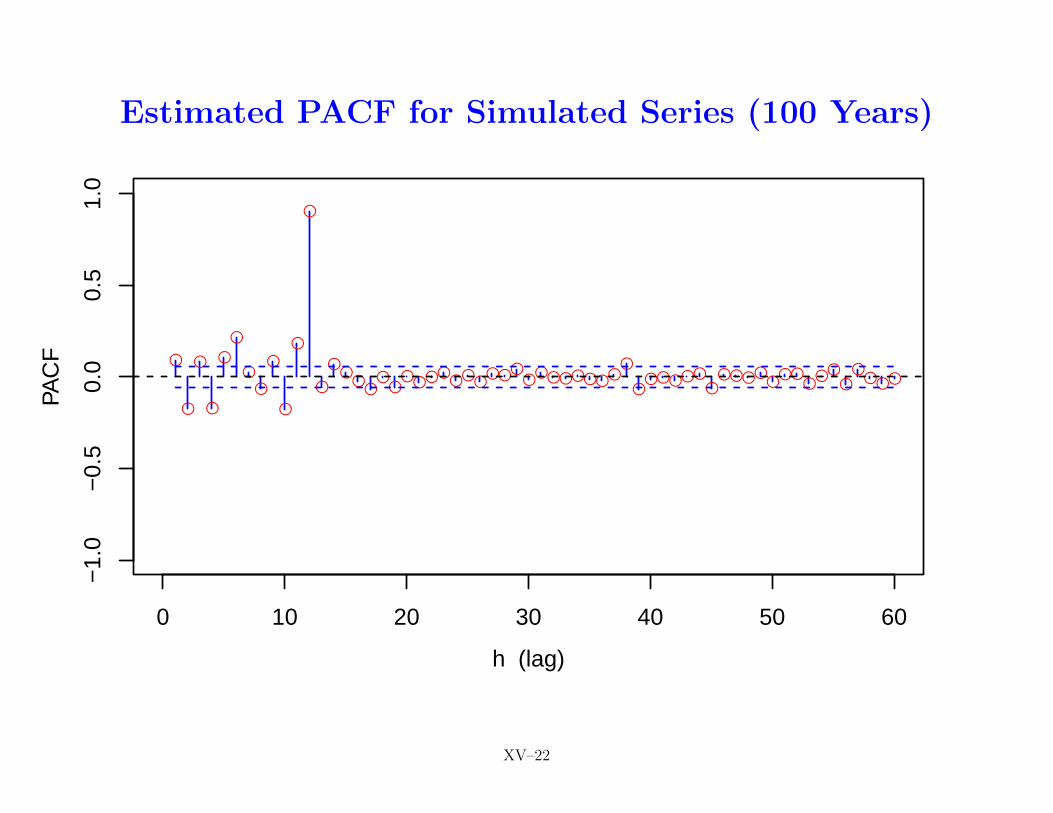
Estimated PACF for Simulated Series (100 Years)

●

●

●

●

●

●

●●

●

●

●

●

●

●●

●●

●●

●●●●●●●

●●●●

●●●●●●●●

●●●●●●

●●●●●

●●●

●●●

●●

●●●

0 10 20 30 40 50 60

−1.

0−

0.5

0.0

0.5

1.0

h (lag)

PAC

F

XV–22

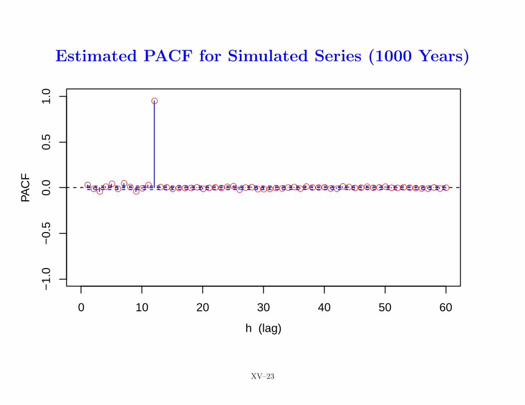
Estimated PACF for Simulated Series (1000 Years)

●●●

●●●

●●

●●●

●

●●●●●●●●●●●●●●●●●●●●●●●●●●●●●●●●●●●●●●●●●●●●●●●●

0 10 20 30 40 50 60

−1.

0−

0.5

0.0

0.5

1.0

h (lag)

PAC

F

XV–23

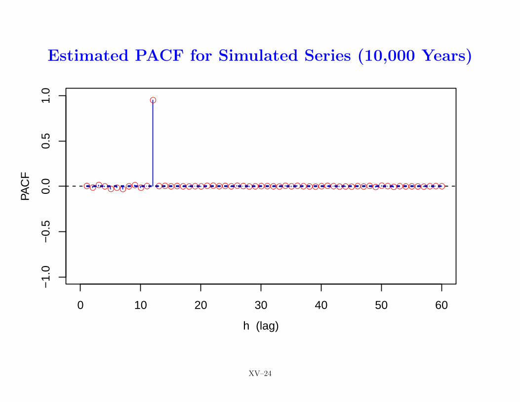
Estimated PACF for Simulated Series (10,000 Years)

●●●●●●●●●●●

●

●●●●●●●●●●●●●●●●●●●●●●●●●●●●●●●●●●●●●●●●●●●●●●●●

0 10 20 30 40 50 60

−1.

0−

0.5

0.0

0.5

1.0

h (lag)

PAC

F

XV–24

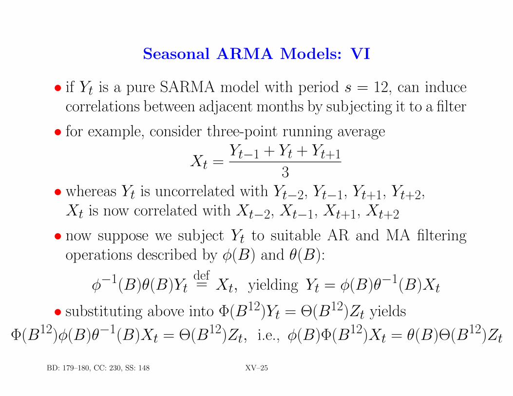
Seasonal ARMA Models: VI

• if Yt is a pure SARMA model with period s = 12, can inducecorrelations between adjacent months by subjecting it to a filter

• for example, consider three-point running average

Xt =Yt−1 + Yt + Yt+1

3• whereas Yt is uncorrelated with Yt−2, Yt−1, Yt+1, Yt+2,Xt is now correlated with Xt−2, Xt−1, Xt+1, Xt+2

• now suppose we subject Yt to suitable AR and MA filteringoperations described by φ(B) and θ(B):

φ−1(B)θ(B)Ytdef= Xt, yielding Yt = φ(B)θ−1(B)Xt

• substituting above into Φ(B12)Yt = Θ(B12)Zt yields

Φ(B12)φ(B)θ−1(B)Xt = Θ(B12)Zt, i.e., φ(B)Φ(B12)Xt = θ(B)Θ(B12)Zt

BD: 179–180, CC: 230, SS: 148 XV–25

Seasonal ARMA Models: VII

• conclusion: in general SARMA model

φ(B)Φ(B12)Xt = θ(B)Θ(B12)Zt,

primary role of

− φ(B) & θ(B) is to model correlations between months withina single year (intra-annual variations)

− Φ(B) & Θ(B) is to model correlations for a given monthacross several years (inter-annual variations)

BD: 179–180, CC: 230, SS: 148 XV–26

Seasonal ARMA Models: VIII

• keeping with s = 12, let’s consider four SARMA models:

− p = 0, P = 0, q = 1, Q = 1, θ1 = 0.9, Θ1 = −0.4

− p = 0, P = 0, q = 1, Q = 1, θ1 = 0.9, Θ1 = 0.4

− p = 1, P = 1, q = 0, Q = 0, φ1 = 0.5, Φ1 = 0.7

− p = 1, P = 1, q = 0, Q = 0, φ1 = 0.9, Φ1 = 0.7

• first two are examples of SARMA(0, 1)× (0, 1)12 model

Xt = Zt + θ1Zt−1 + Θ1Zt−12 + θ1Θ1Zt−13

(special case of MA(13) model)

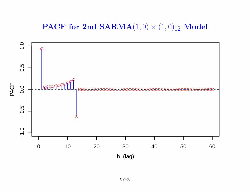
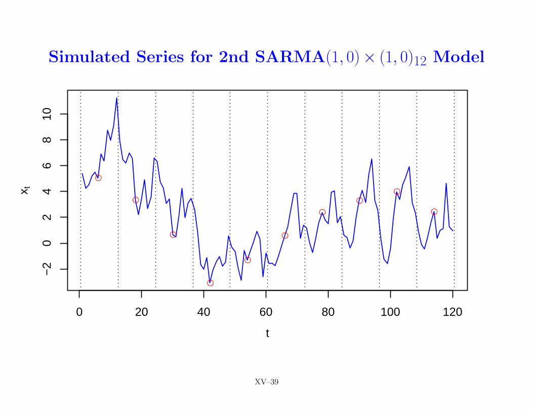
• second two are examples of SARMA(1, 0)× (1, 0)12 model

Xt − φ1Xt−1 − Φ1Xt−12 + φ1Φ1Xt−13 = Zt

(special case of AR(13) model)

BD: 179–180 XV–27

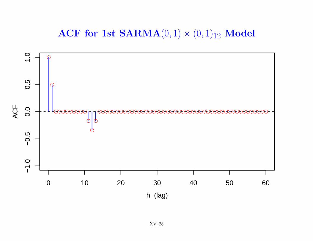
ACF for 1st SARMA(0, 1)× (0, 1)12 Model

●

●

●●●●●●●●●

●

●

●

●●●●●●●●●●●●●●●●●●●●●●●●●●●●●●●●●●●●●●●●●●●●●●●

0 10 20 30 40 50 60

−1.

0−

0.5

0.0

0.5

1.0

h (lag)

AC

F

XV–28

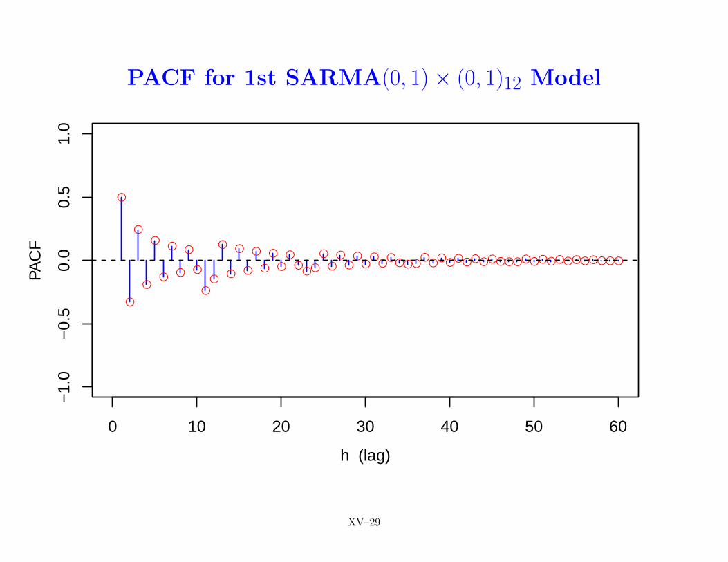
PACF for 1st SARMA(0, 1)× (0, 1)12 Model

●

●

●

●

●

●

●

●

●

●

●●

●

●

●

●

●

●

●

●●

●●●

●

●●

●●

●●

●●

●●●●

●●●●●●●●●●●●●●●●●●●●●●●

0 10 20 30 40 50 60

−1.

0−

0.5

0.0

0.5

1.0

h (lag)

PAC

F

XV–29

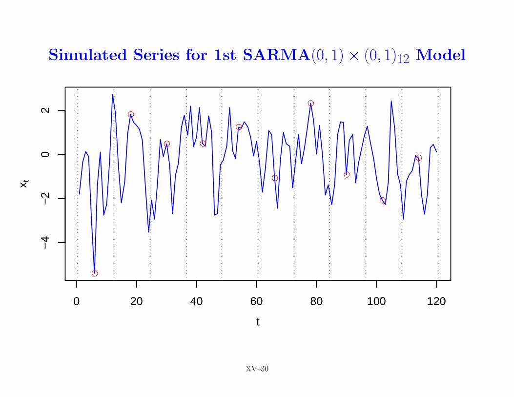
Simulated Series for 1st SARMA(0, 1)× (0, 1)12 Model

●

●

● ●

●

●

●

●

●

●

0 20 40 60 80 100 120

−4

−2

02

t

x t

XV–30

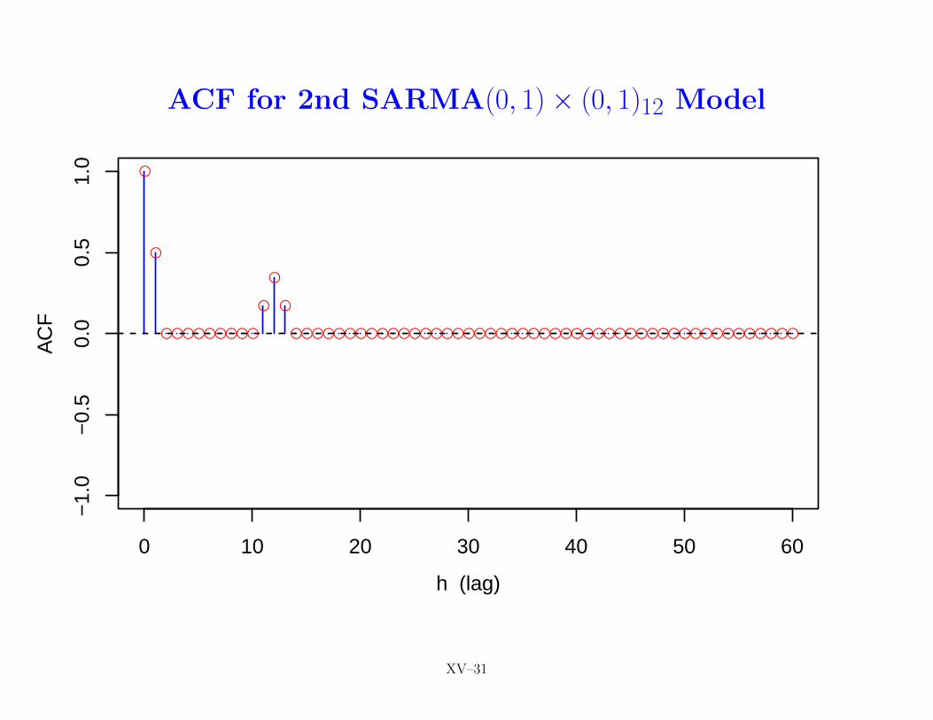
ACF for 2nd SARMA(0, 1)× (0, 1)12 Model

●

●

●●●●●●●●●

●

●

●

●●●●●●●●●●●●●●●●●●●●●●●●●●●●●●●●●●●●●●●●●●●●●●●

0 10 20 30 40 50 60

−1.

0−

0.5

0.0

0.5

1.0

h (lag)

AC

F

XV–31

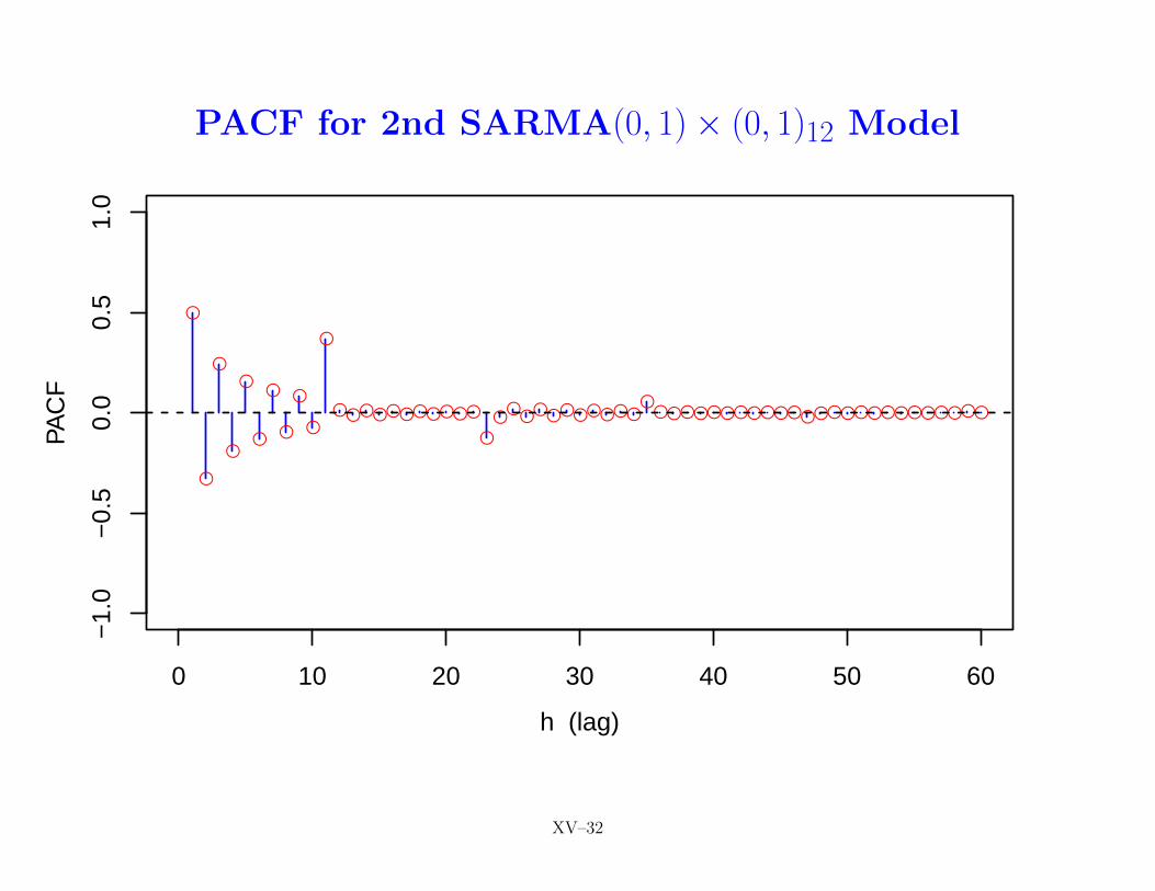
PACF for 2nd SARMA(0, 1)× (0, 1)12 Model

●

●

●

●

●

●

●

●

●

●

●

●●●●●●●●●●●

●

●●●●●●●●●●●

●●●●●●●●●●●●●●●●●●●●●●●●●●

0 10 20 30 40 50 60

−1.

0−

0.5

0.0

0.5

1.0

h (lag)

PAC

F

XV–32

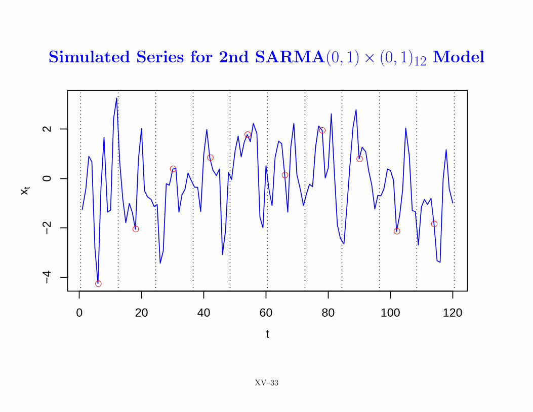
Simulated Series for 2nd SARMA(0, 1)× (0, 1)12 Model

●

●

●

●

●

●

●

●

●●

0 20 40 60 80 100 120

−4

−2

02

t

x t

XV–33

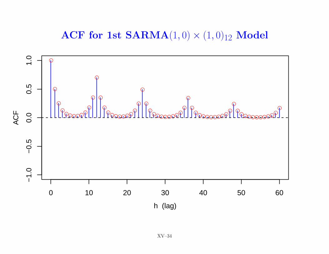
ACF for 1st SARMA(1, 0)× (1, 0)12 Model

●

●

●

●●●●●●

●●

●

●

●

●●

●●●●●●●

●

●

●

●●●●●●●●

●●

●

●●

●●●●●●●●●

●

●●●●●●●●●●

●●

0 10 20 30 40 50 60

−1.

0−

0.5

0.0

0.5

1.0

h (lag)

AC

F

XV–34

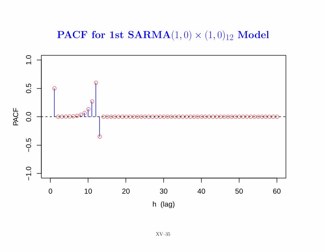
PACF for 1st SARMA(1, 0)× (1, 0)12 Model

●

●●●●●●●●●

●

●

●

●●●●●●●●●●●●●●●●●●●●●●●●●●●●●●●●●●●●●●●●●●●●●●●

0 10 20 30 40 50 60

−1.

0−

0.5

0.0

0.5

1.0

h (lag)

PAC

F

XV–35

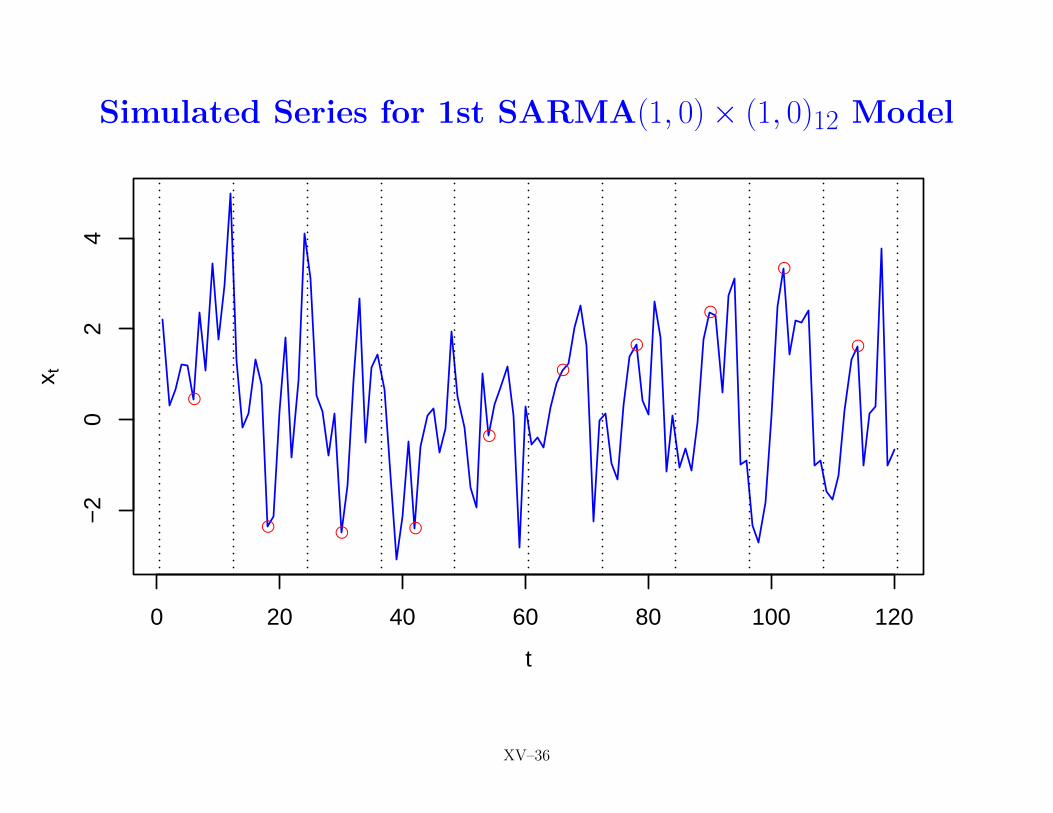
Simulated Series for 1st SARMA(1, 0)× (1, 0)12 Model

●

● ● ●

●

●

●

●

●

●

0 20 40 60 80 100 120

−2

02

4

t

x t

XV–36

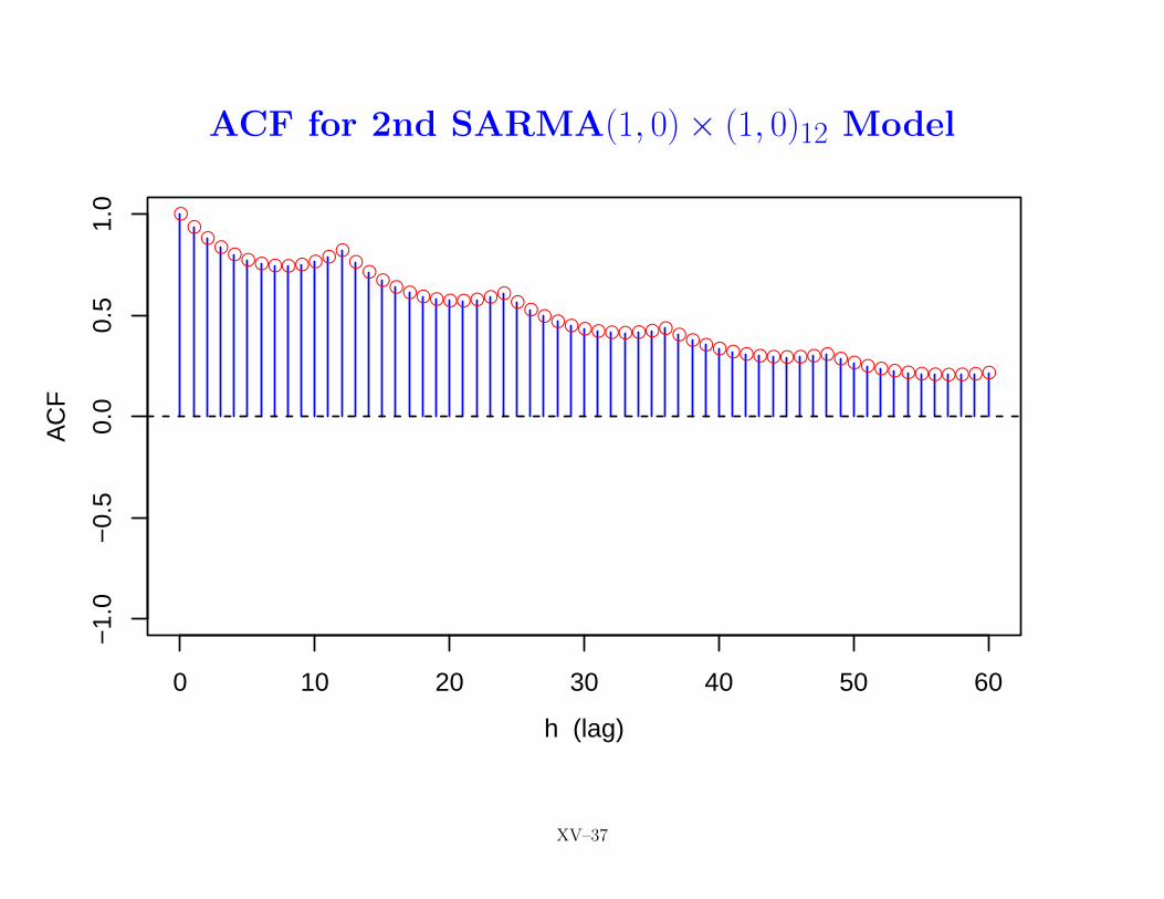
ACF for 2nd SARMA(1, 0)× (1, 0)12 Model

●●

●●●●●●●●●●●

●●

●●●●●●●●●●●●●●●●●●●●●●●●●●●●●●●●●●●●●●●●●●●●●●

0 10 20 30 40 50 60

−1.

0−

0.5

0.0

0.5

1.0

h (lag)

AC

F

XV–37

PACF for 2nd SARMA(1, 0)× (1, 0)12 Model

●

●●●●●●●●●●●

●

●●●●●●●●●●●●●●●●●●●●●●●●●●●●●●●●●●●●●●●●●●●●●●●

0 10 20 30 40 50 60

−1.

0−

0.5

0.0

0.5

1.0

h (lag)

PAC

F

XV–38

Simulated Series for 2nd SARMA(1, 0)× (1, 0)12 Model

●

●

●

●

●

●

●

●

●

●

0 20 40 60 80 100 120

−2

02

46

810

t

x t

XV–39

Seasonal ARIMA Models: III

• recall definition of seasonal differencing:

∇sXt = Xt −Xt−s = (1−Bs)Xt

• in model Xt = mt + st +Wt, where st = st±s is periodic withperiod s, seasonal differencing eliminates st completely

• seasonal differencing also of interest if, rather than deterministicst, Xt has a stochastic component that is quasi-periodic

• with monthly data in mind, consider model

Xt = St + Zt with {Zt} ∼WN(0, σ2Z),

where St is a stochastic component that is slowly varying fromone January to the next, with similar patterns holding for theother 11 months

BD: 179–180, CC: 233, SS: 148–149 XV–40

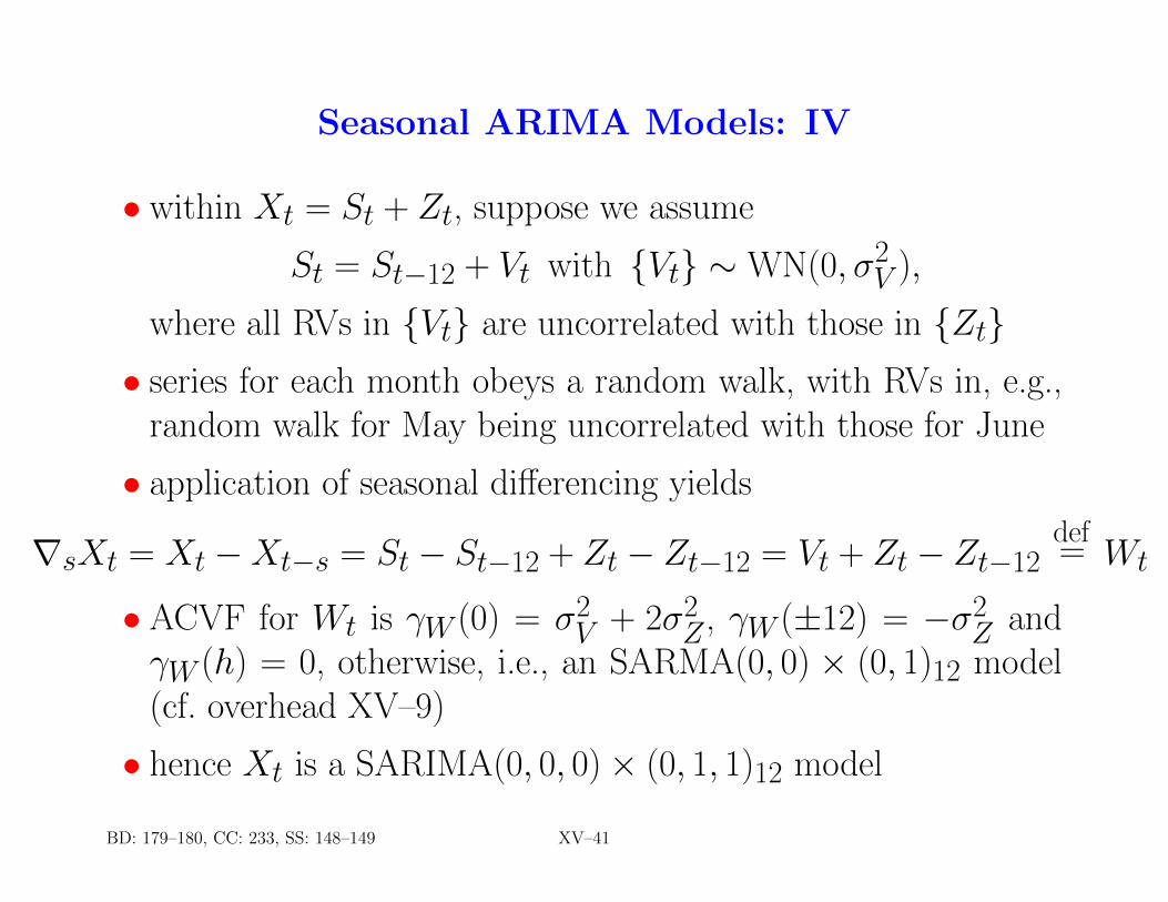
Seasonal ARIMA Models: IV

• within Xt = St + Zt, suppose we assume

St = St−12 + Vt with {Vt} ∼WN(0, σ2V ),

where all RVs in {Vt} are uncorrelated with those in {Zt}• series for each month obeys a random walk, with RVs in, e.g.,

random walk for May being uncorrelated with those for June

• application of seasonal differencing yields

∇sXt = Xt −Xt−s = St − St−12 + Zt − Zt−12 = Vt + Zt − Zt−12def= Wt

• ACVF for Wt is γW (0) = σ2V + 2σ2

Z , γW (±12) = −σ2Z and

γW (h) = 0, otherwise, i.e., an SARMA(0, 0) × (0, 1)12 model(cf. overhead XV–9)

• hence Xt is a SARIMA(0, 0, 0)× (0, 1, 1)12 model

BD: 179–180, CC: 233, SS: 148–149 XV–41

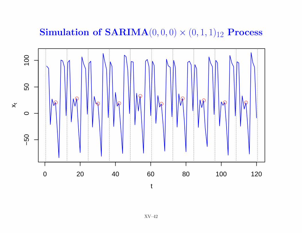
Simulation of SARIMA(0, 0, 0)× (0, 1, 1)12 Process

●●

● ●

●

●

● ●● ●

0 20 40 60 80 100 120

−50

050

100

t

x t

XV–42

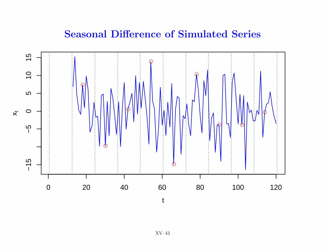
Seasonal Difference of Simulated Series

●

●

●

●

●

●

● ●

●

0 20 40 60 80 100 120

−15

−5

05

1015

t

x t

XV–43

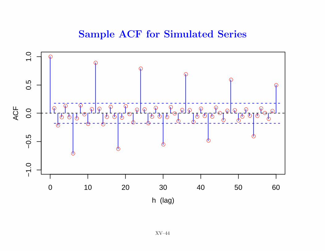
Sample ACF for Simulated Series

●

●

●

●

●

●

●

●

●

●

●

●

●

●

●

●

●

●

●

●

●

●

●

●

●

●

●

●

●

●

●

●

●

●

●

●

●

●

●●

●

●

●

●

●

●

●

●

●

●

●●

●

●

●

●

●●

●

●

●

0 10 20 30 40 50 60

−1.

0−

0.5

0.0

0.5

1.0

h (lag)

AC

F

XV–44

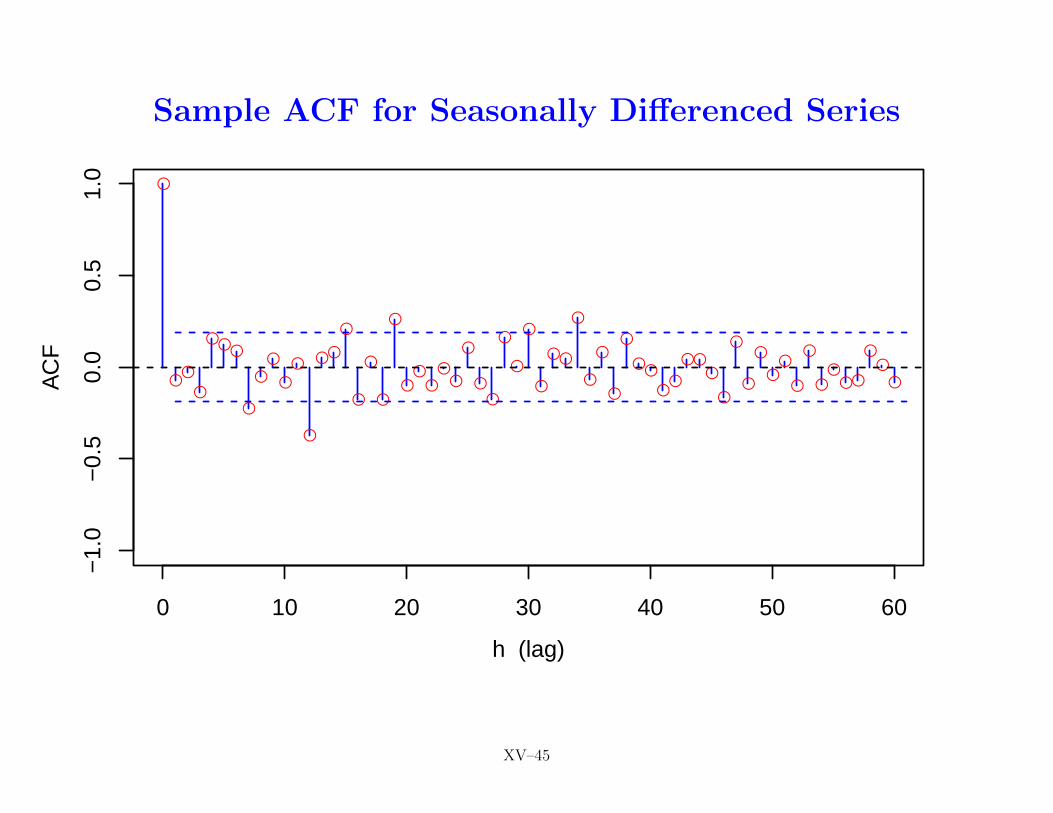
Sample ACF for Seasonally Differenced Series

●

●●

●

●●●

●

●

●

●

●

●

●●

●

●

●

●

●

●●

●●

●

●

●●

●

●

●

●

●●

●

●

●

●

●

●●

●●

●●●

●

●

●

●

●●

●

●

●●

●●

●●

●

0 10 20 30 40 50 60

−1.

0−

0.5

0.0

0.5

1.0

h (lag)

AC

F

XV–45

Seasonal ARIMA Models: V

• identification of SARIMA model for series Xt with known s

1. find d and D such that

Yt = (1−B)d(1−Bs)DXtlooks amenable to modeling by a stationary process

2. examine sample ACF and PACF for Yt at lags s, 2s, 3s,. . . , to select P and Q such that ARMA(P ,Q) model iscompatible with ρ̂(ks) and φ̂ks,ks, k = 1, 2, 3, . . .

3. examine sample ACF and PACF at lags 1, 2, . . . , s − 1 toselect p and q such that ARMA(p,q) model is compatiblewith ρ̂(h) and φ̂h,h, h = 1, 2, . . . , s− 1

• as example, reconsider recruitment time series

BD: 179–180, CC: 234, SS: 150 XV–46

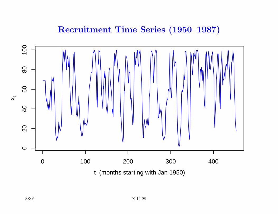
Recruitment Time Series (1950–1987)

0 100 200 300 400

020

4060

8010

0

t (months starting with Jan 1950)

x t

SS: 6 XIII–28

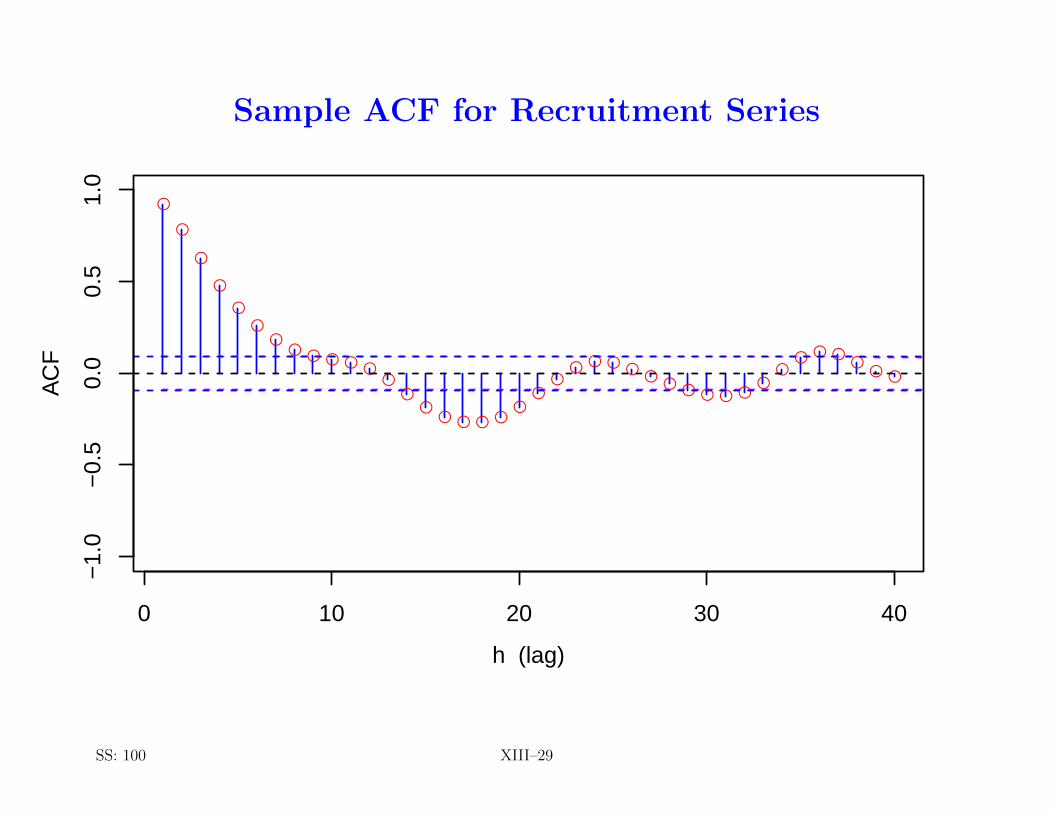
Sample ACF for Recruitment Series

●

●

●

●

●

●●

● ● ● ● ●●

●●

● ● ● ●●

●●

● ● ● ●●

● ● ● ● ●●

●● ● ●

●● ●

0 10 20 30 40

−1.

0−

0.5

0.0

0.5

1.0

h (lag)

AC

F

SS: 100 XIII–29

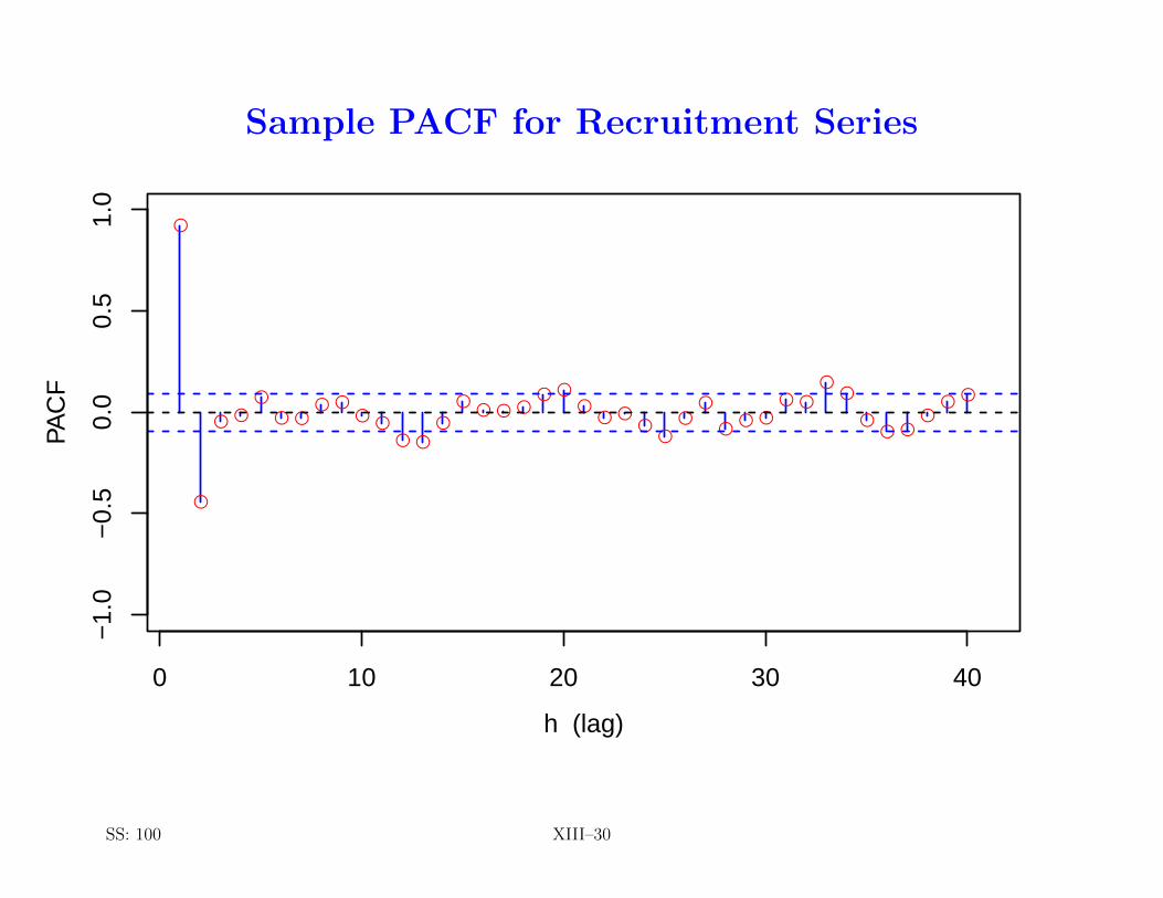
Sample PACF for Recruitment Series

●

●

● ●●

● ●● ●

● ●● ●

●

●● ● ●

● ●●

● ●●

●●

●

●● ●

● ●

●●

●● ●

●● ●

0 10 20 30 40

−1.

0−

0.5

0.0

0.5

1.0

h (lag)

PAC

F

SS: 100 XIII–30

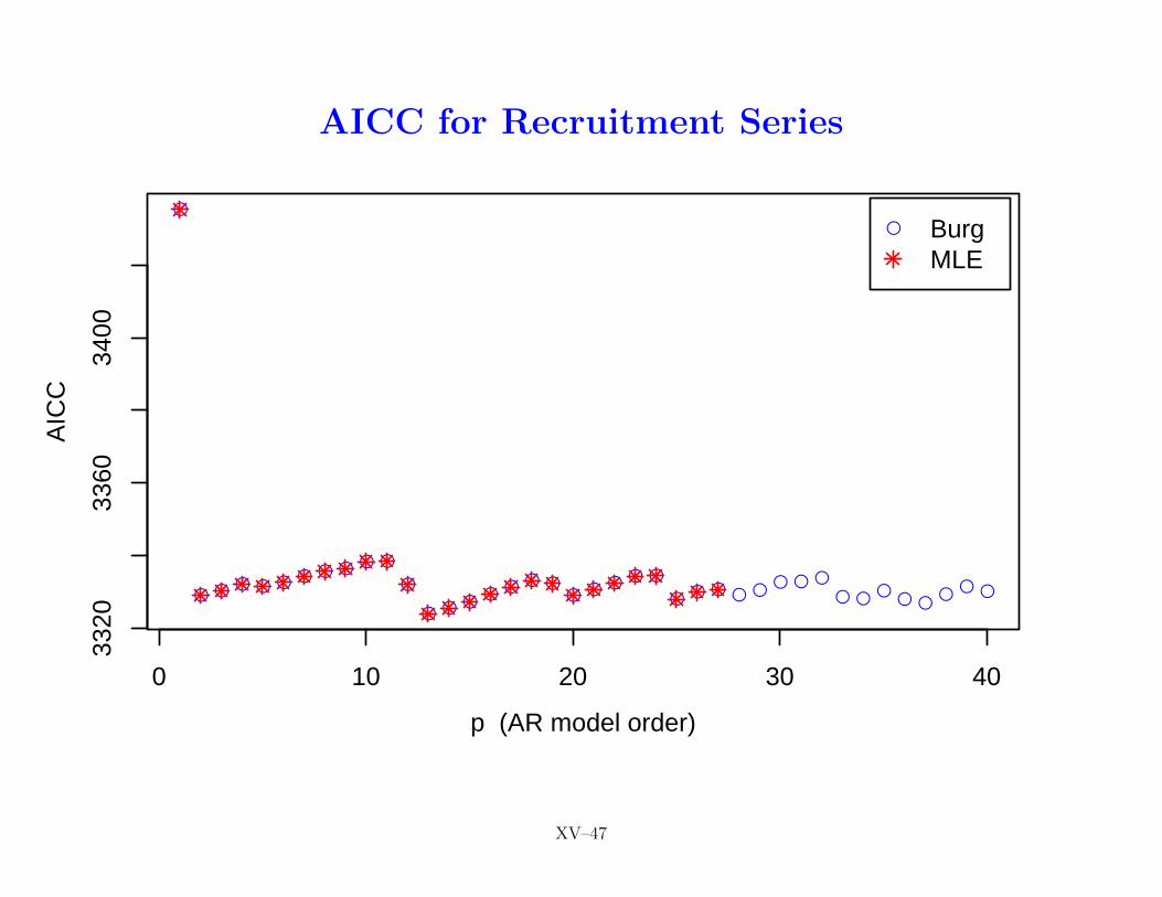
AICC for Recruitment Series

●

● ● ● ● ● ● ● ● ● ●

●

● ● ●● ● ● ●

● ● ● ● ●

● ● ● ● ●● ● ●

● ●●

● ●●

● ●

● Burg MLE

0 10 20 30 40

3320

3360

3400

p (AR model order)

AIC

C

XV–47

SARIMA Model for Recruitment Series: I

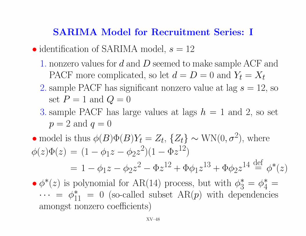
• identification of SARIMA model, s = 12

1. nonzero values for d and D seemed to make sample ACF andPACF more complicated, so let d = D = 0 and Yt = Xt

2. sample PACF has significant nonzero value at lag s = 12, soset P = 1 and Q = 0

3. sample PACF has large values at lags h = 1 and 2, so setp = 2 and q = 0

• model is thus φ(B)Φ(B)Yt = Zt, {Zt} ∼WN(0, σ2), where

φ(z)Φ(z) = (1− φ1z − φ2z2)(1− Φz12)

= 1− φ1z − φ2z2 − Φz12 + Φφ1z

13 + Φφ2z14 def

= φ∗(z)

• φ∗(z) is polynomial for AR(14) process, but with φ∗3 = φ∗4 =· · · = φ∗11 = 0 (so-called subset AR(p) with dependenciesamongst nonzero coefficients)

XV–48

SARIMA Model for Recruitment Series: II

• AICC for AR(13) model is 3324.0

• AICC for SARMA(2, 0)× (1, 0)12 model is 3323.8

• tiny improvement, but # of estimated parameters now just 4

• examination of residuals gives similar results for both models(cannot reject white noise hypothesis), with exception of

− p-value close to 0.05 for h = 5 portmanteau test for SARMA

− p-value of 0.015 from rank test for AR(13) and

− p-value of 0.047 from runs test for SARMA

(for details, see R code for this overhead)

• comparison of sample ACF and PACF with corresponding the-oretical functions shows better visual agreement with AR(13)(but appearances can be deceiving!)

XV–49

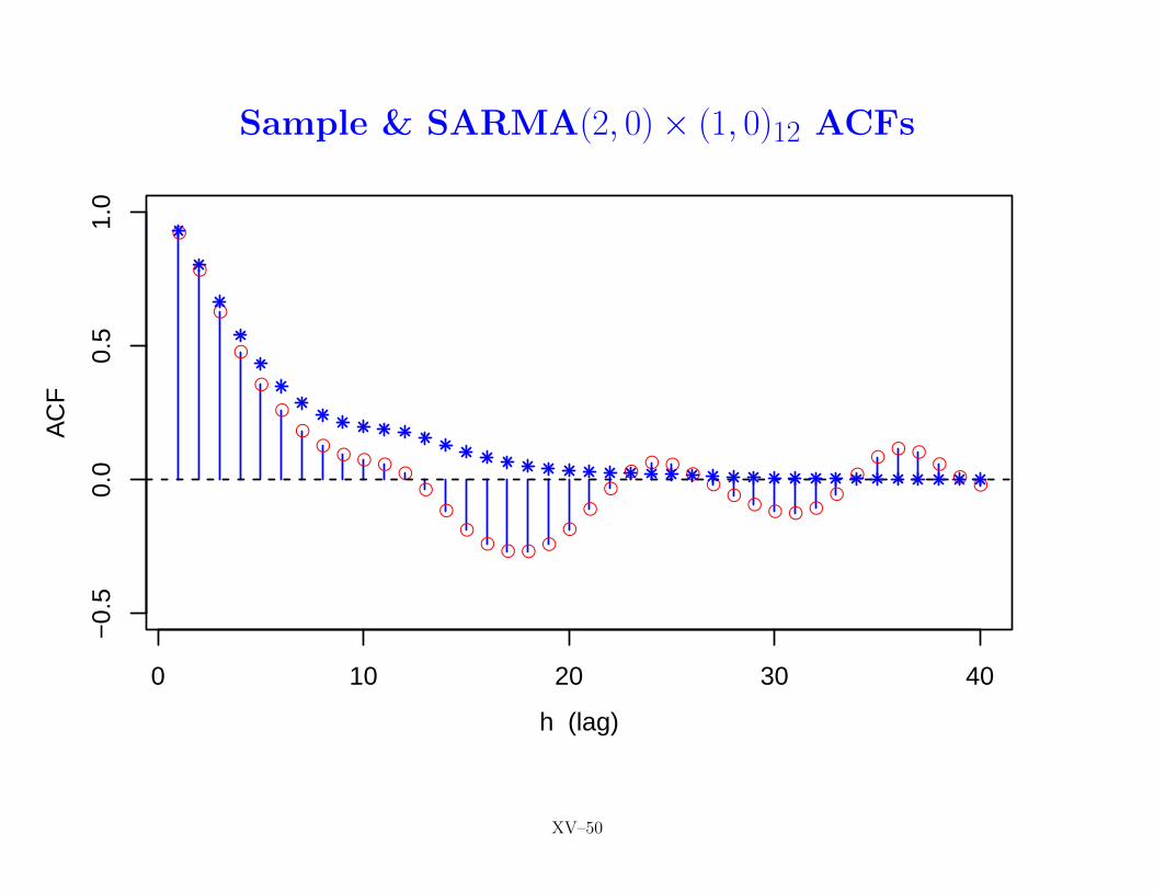
Sample & SARMA(2, 0)× (1, 0)12 ACFs

●

●

●

●

●

●

●●

● ● ●●

●

●

●● ● ● ●

●

●

●●

● ●●

●●

● ● ● ●●

●●

● ●●

●●

0 10 20 30 40

−0.

50.

00.

51.

0

h (lag)

AC

F

XV–50

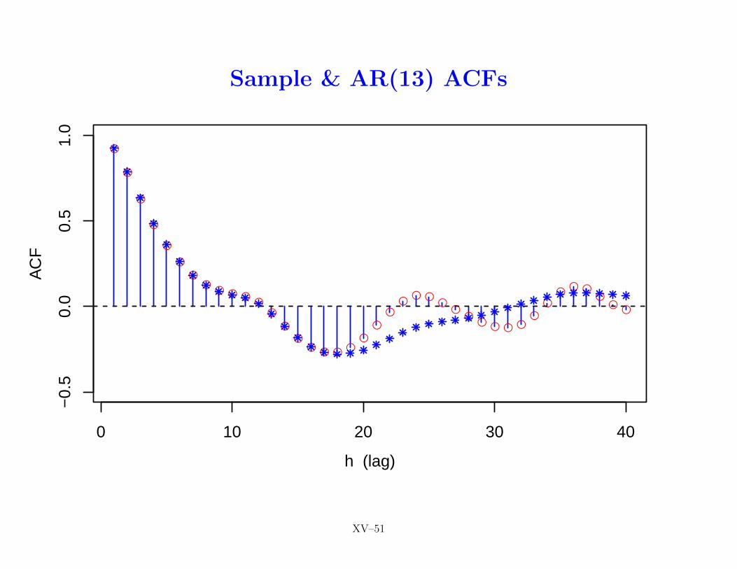
Sample & AR(13) ACFs

●

●

●

●

●

●

●●

● ● ●●

●

●

●● ● ● ●

●

●

●●

● ●●

●●

● ● ● ●●

●●

● ●●

●●

0 10 20 30 40

−0.

50.

00.

51.

0

h (lag)

AC

F

XV–51

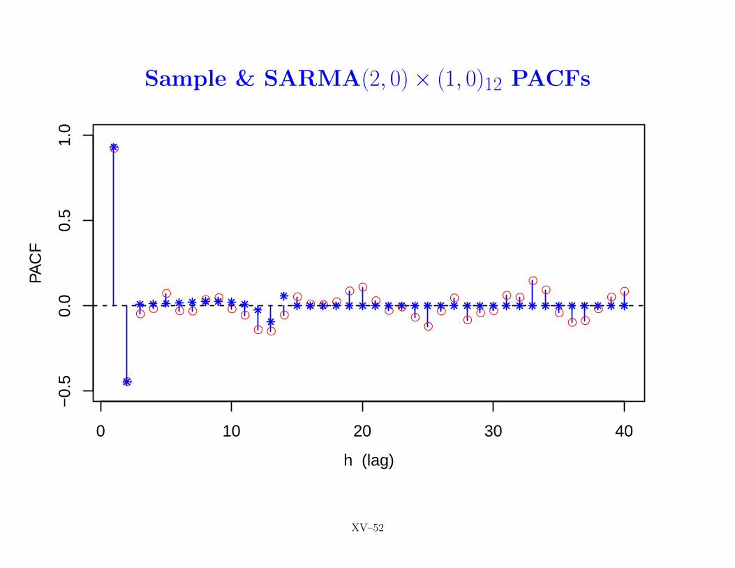
Sample & SARMA(2, 0)× (1, 0)12 PACFs

●

●

●●

●

● ●● ●

●●

● ●

●

●● ● ●

● ●

●● ●

●●

●

●

●● ●

● ●

●●

●● ●

●●

●

0 10 20 30 40

−0.

50.

00.

51.

0

h (lag)

PAC

F

XV–52

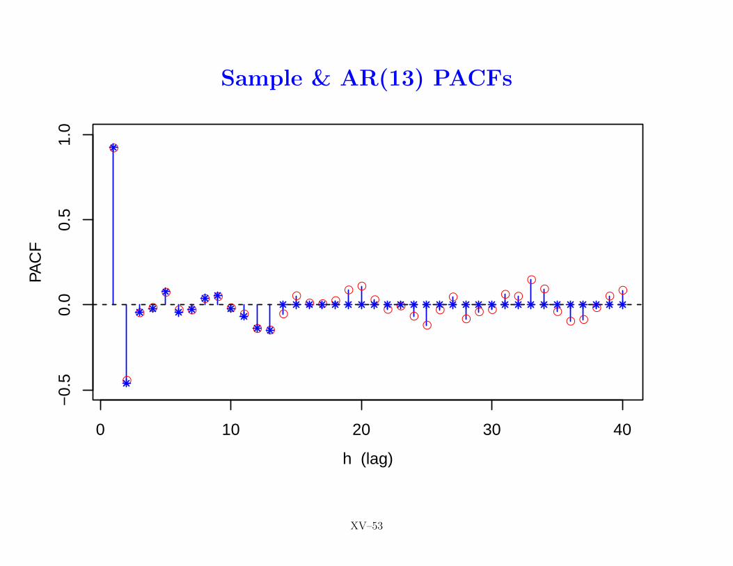
Sample & AR(13) PACFs

●

●

●●

●

● ●● ●

●●

● ●

●

●● ● ●

● ●

●● ●

●●

●

●

●● ●

● ●

●●

●● ●

●●

●

0 10 20 30 40

−0.

50.

00.

51.

0

h (lag)

PAC

F

XV–53

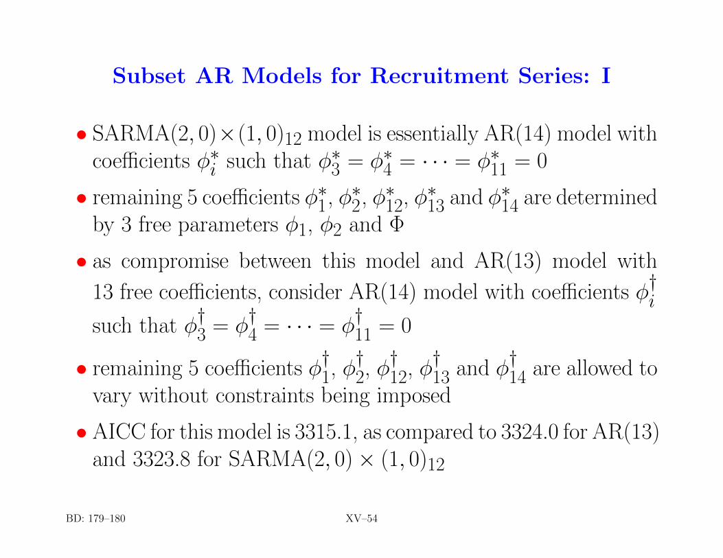
Subset AR Models for Recruitment Series: I

• SARMA(2, 0)×(1, 0)12 model is essentially AR(14) model withcoefficients φ∗i such that φ∗3 = φ∗4 = · · · = φ∗11 = 0

• remaining 5 coefficients φ∗1, φ∗2, φ∗12, φ∗13 and φ∗14 are determinedby 3 free parameters φ1, φ2 and Φ

• as compromise between this model and AR(13) model with

13 free coefficients, consider AR(14) model with coefficients φ†i

such that φ†3 = φ

†4 = · · · = φ

†11 = 0

• remaining 5 coefficients φ†1, φ†2, φ†12, φ

†13 and φ

†14 are allowed to

vary without constraints being imposed

• AICC for this model is 3315.1, as compared to 3324.0 for AR(13)and 3323.8 for SARMA(2, 0)× (1, 0)12

BD: 179–180 XV–54

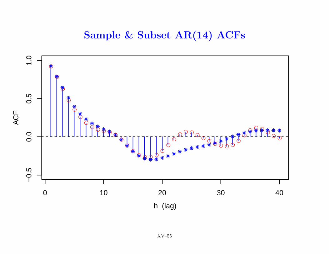
Sample & Subset AR(14) ACFs

●

●

●

●

●

●

●●

● ● ●●

●

●

●● ● ● ●

●

●

●●

● ●●

●●

● ● ● ●●

●●

● ●●

●●

0 10 20 30 40

−0.

50.

00.

51.

0

h (lag)

AC

F

XV–55

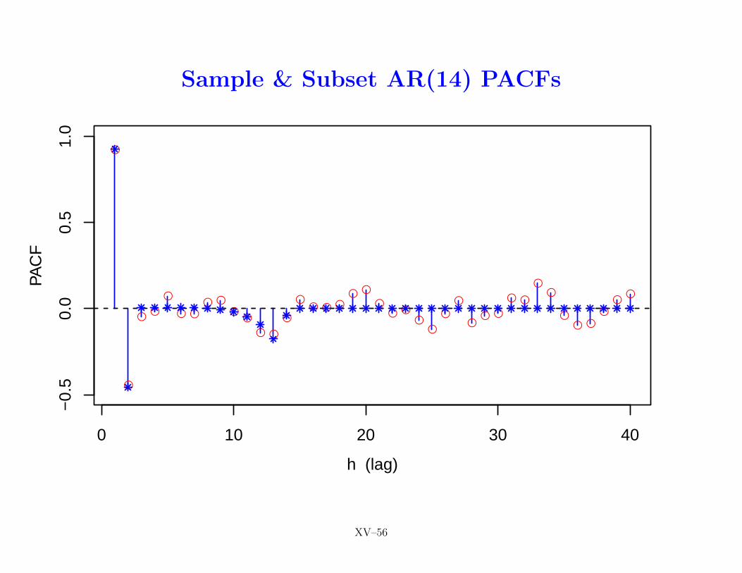
Sample & Subset AR(14) PACFs

●

●

●●

●

● ●● ●

●●

● ●

●

●● ● ●

● ●

●● ●

●●

●

●

●● ●

● ●

●●

●● ●

●●

●

0 10 20 30 40

−0.

50.

00.

51.

0

h (lag)

PAC

F

XV–56

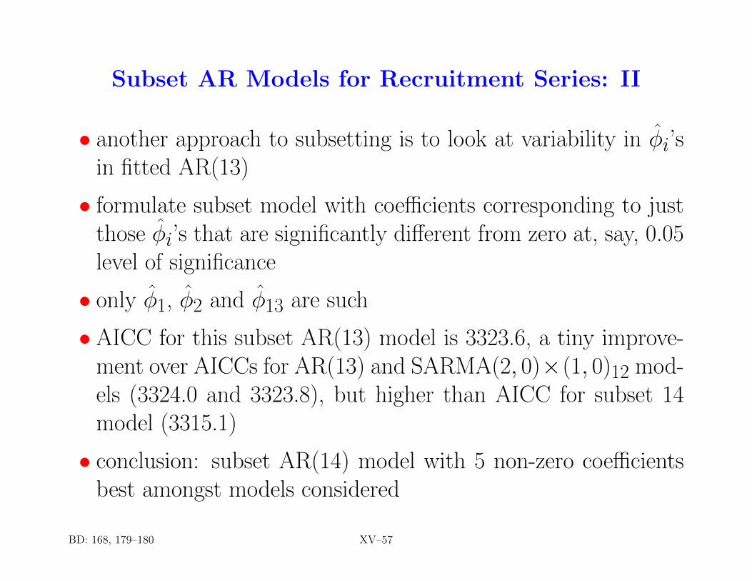
Subset AR Models for Recruitment Series: II

• another approach to subsetting is to look at variability in φ̂i’sin fitted AR(13)

• formulate subset model with coefficients corresponding to justthose φ̂i’s that are significantly different from zero at, say, 0.05level of significance

• only φ̂1, φ̂2 and φ̂13 are such

• AICC for this subset AR(13) model is 3323.6, a tiny improve-ment over AICCs for AR(13) and SARMA(2, 0)×(1, 0)12 mod-els (3324.0 and 3323.8), but higher than AICC for subset 14model (3315.1)

• conclusion: subset AR(14) model with 5 non-zero coefficientsbest amongst models considered

BD: 168, 179–180 XV–57