Embed Size (px)
Citation preview


CLASSICAL AND MODERN METHODOLOGY IN HUMAN GENETICS
(MÉTODOS CLÁSICOS Y MODERNOS PARA EL ANÁLISIS DE
DATOS EN GENÉTICA HUMANA)
PAULO A. OTTO
Departamento de Genética e Biologia Evolutiva Instituto de Biociências Universidade de São Paulo
Caixa Postal 11461 05422-970 São Paulo SP
Curso Teórico Práctico de Post-Grado 4 al 9 de Agosto de 2008 Departamento de Genética
Laboratorio de Citogenética y Genética Humana Facultad de Ciencias Exactas Químicas y Naturales
Universidad Nacional de Misiones Posadas, Misiones, República Argentina
LACyGH – FCEQyN UnaM
2008
EDITORIAL UNIVERSITARIA DE MISIONES
San Luis 1870 Posadas - Misiones – Tel-Fax: (03752) 428601 Correos electrónicos: [email protected] [email protected] [email protected] [email protected] [email protected]
Otto, Paulo Alberto Métodos clásicos y modernos para el análisis de datos en genética humana, 1ª ed. (revisada) – Posadas: EdUNaM – Editorial Universitaria de la Universidad Nacional de Misiones, 2008. 266 p. ISBN 978-950-579-102-6 1. Genética Humana. 2. Variación Genética. I. Título CDD 616.042
ISBN: 978-950-579-102-6 Impreso en Argentina ©Editorial Universitaria Universidad Nacional de Misiones Posadas, 2008
page
HARDY-WEINBERG EQUILIBRIUM AND GENE FREQUENCY ESTIMATION 6
HARDY-WEINBERG EQUILIBRIUM TESTING 29
LINKAGE CALCULATIONS 51
ASSOCIATION ANALYSIS 69
SIB PAIR ANALYSIS (SIB IBD METHOD) 97
SEGREGATION ANALYSIS 109
PENETRANCE RATE ESTIMATION 129
TWIN METHODS 157
FORENSIC GENETIC METHODS 167
REFERENCES 194
6
HARDY-WEINBERG EQUILIBRIUM AND GENE FREQUENCY ESTIMATION
HARDY-WEINBERG EQUILIBRIUM EQUILIBRIUM FOR AUTOSOMAL GENES Generation 0 : {d = P(AA) , h = P(Aa) , r = P(aa)} Generation 0 → Generation 1 :
offspring genotypic frequencies parental crossings
frequencies AA Aa aa
AA × AA d2 d2 0 0
AA × Aa 2dh dh dh 0
AA × aa 2dr 0 2dr 0
Aa × Aa h2 h2/4 h2/2 h2/4
Aa × aa 2hr 0 hr hr
aa × aa r2 0 0 r2
totals (d+h+r)2 = 1 (d+h/2)2 2(d+h/2)(h/2+r) (h/2+r)2
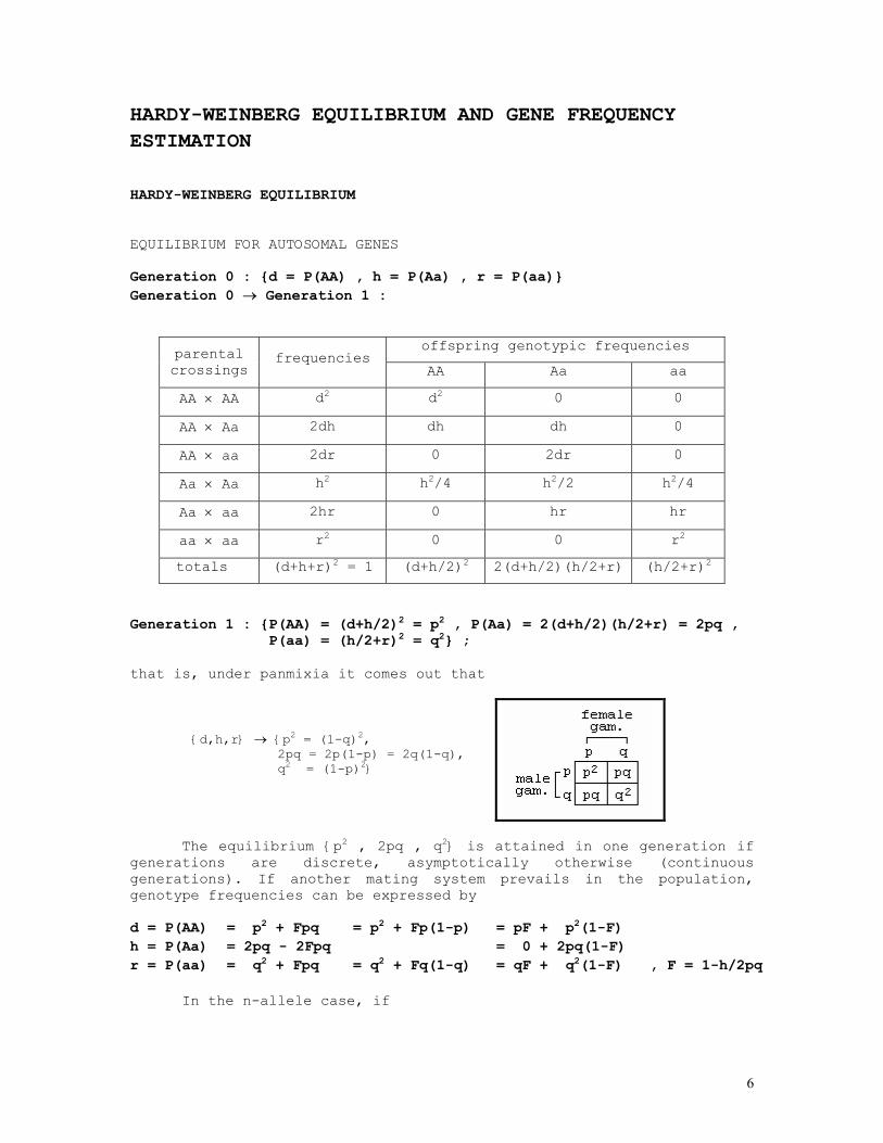
Generation 1 : {P(AA) = (d+h/2)2 = p2 , P(Aa) = 2(d+h/2)(h/2+r) = 2pq , P(aa) = (h/2+r)2 = q2} ; that is, under panmixia it comes out that
{d,h,r} → {p2 = (1-q)2, 2pq = 2p(1-p) = 2q(1-q), q2 = (1-p)2}
The equilibrium {p2 , 2pq , q2} is attained in one generation if generations are discrete, asymptotically otherwise (continuous generations). If another mating system prevails in the population, genotype frequencies can be expressed by
d = P(AA) = p2 + Fpq = p2 + Fp(1-p) = pF + p2(1-F) h = P(Aa) = 2pq - 2Fpq = 0 + 2pq(1-F) r = P(aa) = q2 + Fpq = q2 + Fq(1-q) = qF + q2(1-F) , F = 1-h/2pq
In the n-allele case, if
7
pi = P(Ai) = P(AiAi) + ½ Σj≠iP(AiAj) = pii + ½ Σj≠ipij the formulae above become
pii = P(AiAi) = pi2 pij = P(AiAj) = 2pipj
pij = P(AiAj) = (2-δij)pipj δij = 1 if i=j, δij = 0 if i≠j
and, for any possible mating system, pii = P(AiAi) = pi2 + pi(1-pi)F = piF + pi2(1-F) pij = P(AiAj) = 2pipj(1-F) F = 1 - Σh/Σj≠iP(AiAj) = 1 - Σh/2Σj≥ipipj
pij = δijFpi + (2-δij)(1-F)pipj , δij = 1 if i=j, δij = 0 if i≠j
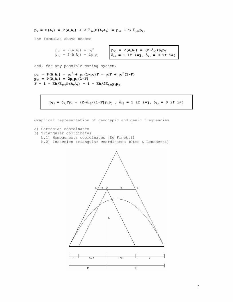
Graphical representation of genotypic and genic frequencies a) Cartesian coordinates b) Triangular coordinates b.1) Homogeneous coordinates (De Finetti) b.2) Isosceles triangular coordinates (Otto & Benedetti)
8
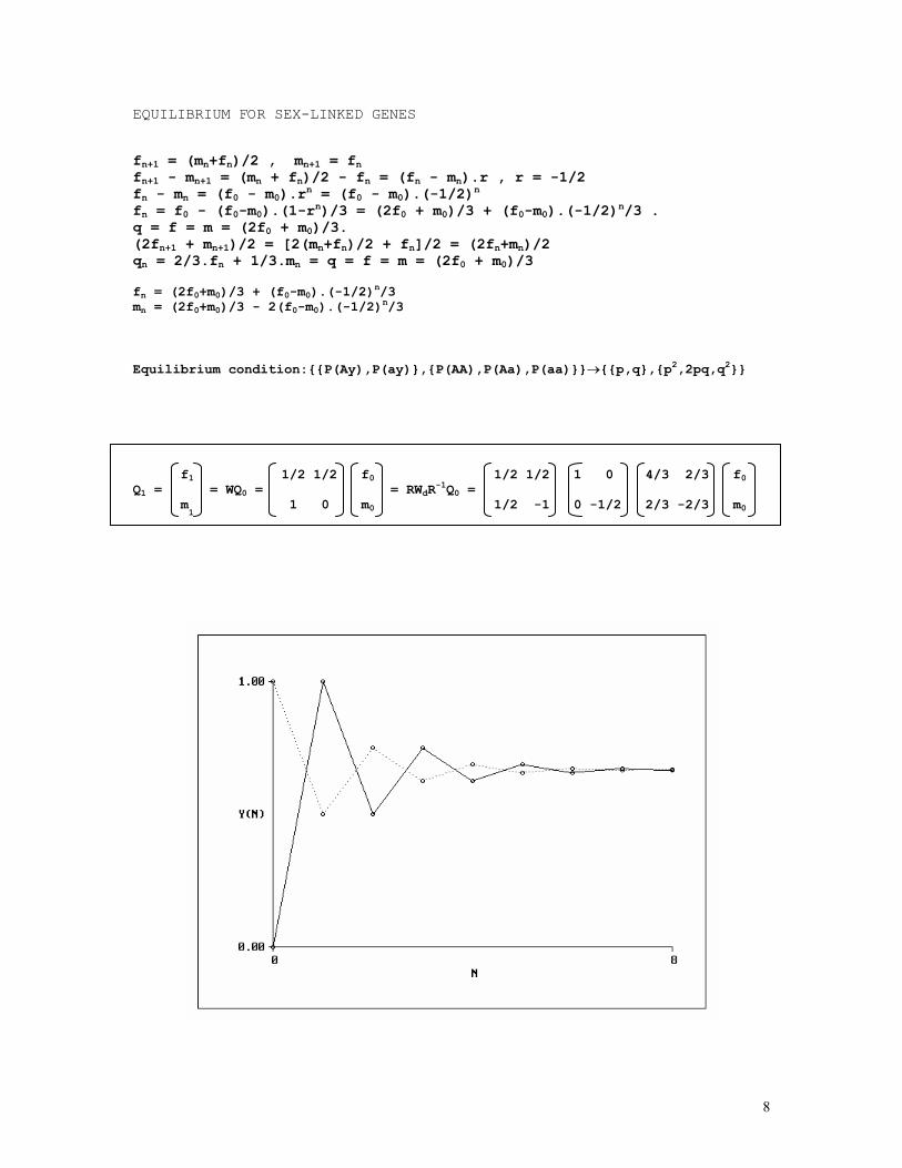
EQUILIBRIUM FOR SEX-LINKED GENES fn+1 = (mn+fn)/2 , mn+1 = fn fn+1 - mn+1 = (mn + fn)/2 - fn = (fn - mn).r , r = -1/2 fn - mn = (f0 - m0).rn = (f0 - m0).(-1/2)n fn = f0 - (f0-m0).(1-rn)/3 = (2f0 + m0)/3 + (f0-m0).(-1/2)n/3 . q = f = m = (2f0 + m0)/3. (2fn+1 + mn+1)/2 = [2(mn+fn)/2 + fn]/2 = (2fn+mn)/2 qn = 2/3.fn + 1/3.mn = q = f = m = (2f0 + m0)/3 fn = (2f0+m0)/3 + (f0-m0).(-1/2)
n/3 mn = (2f0+m0)/3 - 2(f0-m0).(-1/2)
n/3 Equilibrium condition:{{P(Ay),P(ay)},{P(AA),P(Aa),P(aa)}}→{{p,q},{p2,2pq,q2}} f1 1/2 1/2 f0 1/2 1/2 1 0 4/3 2/3 f0 Q1 = = WQ0 = = RWdR
-1Q0 = m
1 1 0 m0 1/2 -1 0 -1/2 2/3 -2/3 m0
9
EQUILIBRIUM FOR LINKED GENES
Let r ( ½ ≤ r ≤ 0) be the recombination fraction between loci A and B and Pt(AiBj) and Pt+1(AiBj) be the frequencies of the haplotype AiBj at generations t and t+1; Pt(Ai) = P(Ai), the frequency of the i-th allele of the A locus in any generation or, for sufficiently large populations, the probability of a given allele of the A locus being the i-th one; Pt(Bj) = P(Bj), the frequency of the j-th allele of the B locus in any generation or, for sufficiently large populations, the probability of a given allele of the B locus being the j-th one; then we get immediately the recursion equation Pt+1(AiBj) = (1-r).Pt(AiBj) + r.P(Ai).P(Bj) , from which we obtain the general solution Pt(AiBj) = P(Ai).P(Bj) + (1-r)t.[P0(AiBj) - P(Ai).P(Bj)] . Since P0(AiBj) – P(Ai).P(Bj) = P0(AiBj) – [P0(AiBj)+P0(Aib)].[P0(AiBj)+P0(aBj)] = P0(AiBj) – {P0(AiBj)[P0(AiBj)+P0(Aib)+P0(aBj)]+P0(Aib).P0(aBj)} = P0(AiBj) – {P0(AiBj)[1-P0(ab)]+P0(Aib).P0(aBj)} = P0(AiBj).P0(ab) - P0(Aib).P0(aBj) , the above expression can be written as Pt(AiBj) = P(Ai).P(Bj) + (1-r)t.[P0(AiBj).P0(ab)-P0(Aib).P0(aBj)] .
The limit of both expressions, as t tends to infinity, is clearly P(AiBj) = P(Ai).P(Bj), that is, at equilibrium the frequency of a given haplotype is the product of the frequencies of the genes contained in the sintenic loci, that become therefore independent at population level. If P(AiBj)-P(Ai).P(Bj) = P(AiBj).P(ab)-P(Aib).P(aBj) = ∆ab ≠ 0 , a situation known as linkage disequilibrium exhists; ∆ab is the so-called linkage disequilibrium value. GENE FREQUENCY ESTIMATION 1) Two autosomal codominant alleles N(AA) = D = n1 , N(Aa) = H = n2 , N(aa) = R = n3 , n1+n2+n3 = N Likelihood function: P = N!/(n1!n2!n3!).(p2)n1.(2pq)n2.(q2)n3 = 2n2.N!/(n1!n2!n3!).p2n1+n2.qn2+2n3 L = log(P) = const. + (2n1+n2).log(p) + (n2+2n3).log(q) Maximum likelihood estimates: dL/dp = (2n1+n2)/p - (n2+2n3)/(1-p) = 0 p = (2n1+n2)/2N = (2D+H)/2N = 2D/2N + H/2N = d + h/2 q = 1-p = (n2+2n3)/2N = (H+2R)/2N = h/2 + r
10
(d2L/dp2)p = -(2n1+n2)/p2 - (n2+2n3)/(1-p)2 = -2Np/p2 – 2Nq/q2 = -2N(1/p + 1/q) = -2N/pq = -I(p) I(p) = I(q) = 2N/pq = 1/var(p) = 1/var(q) var(p) = var(q) = pq/2N = p(1-p)/2N = q(1-q)/2N var(p) = var(d+h/2) = var(d) + var(h/2) + 2cov(d,h/2) = d(1-d)/N + h(1-h)/4N - dh/N = d/N + h/4N - (d+h/2)2/N = d/2N + (d+h/2)/2N - 2p2/2N = (p + d - 2p2)/2N ≈ p(1-p)/2N = pq/2N if d ≈ p2 se(p) = se(q) = √[var(p)] ≈ √[(pq)/2N] ci95%(p) ≈ p ± 1.96 se(p)
The confidence interval above is just an approximation. Exact Bayesian credible intervals can be obtained by finding the area that corresponds to 95% of the total area under the likelihood function. Mathematically the problem reduces to integrating the function y = f(q) between two limits a and b with the same ordinate value such that f(q=a) = f(q=b) and ∫a,b[f(q)dq]/∫0,1[f(q)dq] = 0.95. This is accomplished by programs such as the following one: REM program filename confint6.bas REM calculation of the 95%CI of a binomial estimate p = x/n REM modification of Romberg's osculatory method DEFDBL A-Z: CLS PRINT "Function : p^n1.(1-p)^n2" INPUT "n1 = "; n1 INPUT "n2 = "; n2 PRINT USING "p = n1/(n1+n2) = ### / ### = #.####"; n1; n1 + n2; n1 / (n1 + n2) p0 = 0: pn = 1: GOSUB simpsonsrule: totalarea = area: p0 = .001: niter = 50 repeat: p = p0: GOSUB functsub: pp0 = pp: p1 = 1 FOR j = 1 TO niter p1 = p1 - 1 / niter: p = p1: GOSUB functsub pp1 = pp: IF pp1 >= pp0 THEN GOTO getout NEXT j getout: p0 = p0: pn = p1: GOSUB simpsonsrule IF area / totalarea >= .95 THEN p0 = p0 + 1 / niter: GOTO repeat p0 = p0 - 1 / niter: p1 = p1 + 1 / niter: niter = niter * 5 IF ABS(.95 - area / totalarea) <= .00001 THEN GOTO ENDPRGM ELSE GOTO repeat DO: LOOP WHILE INKEY$ <> " " ENDPRGM: PRINT PRINT USING "lower limit (p) = #.####"; p0 PRINT USING "upper limit (p) = #.####"; pn END simpsonsrule: h = (pn - p0) / 1000: p = p0: GOSUB functsub: s = pp p = pn: GOSUB functsub: s = s + pp: w = 4 FOR j = 1 TO 999 p = p0 + j * h GOSUB functsub s = s + w * pp w = 6 - w NEXT j area = h * s / 3: s = 0 IF p0 <> 0 THEN p = p0: GOSUB functsub: pp0 = pp p = pn: GOSUB functsub: pp1 = pp END IF RETURN
11
functsub: pp = p ^ n1 * (1 - p) ^ n2 RETURN
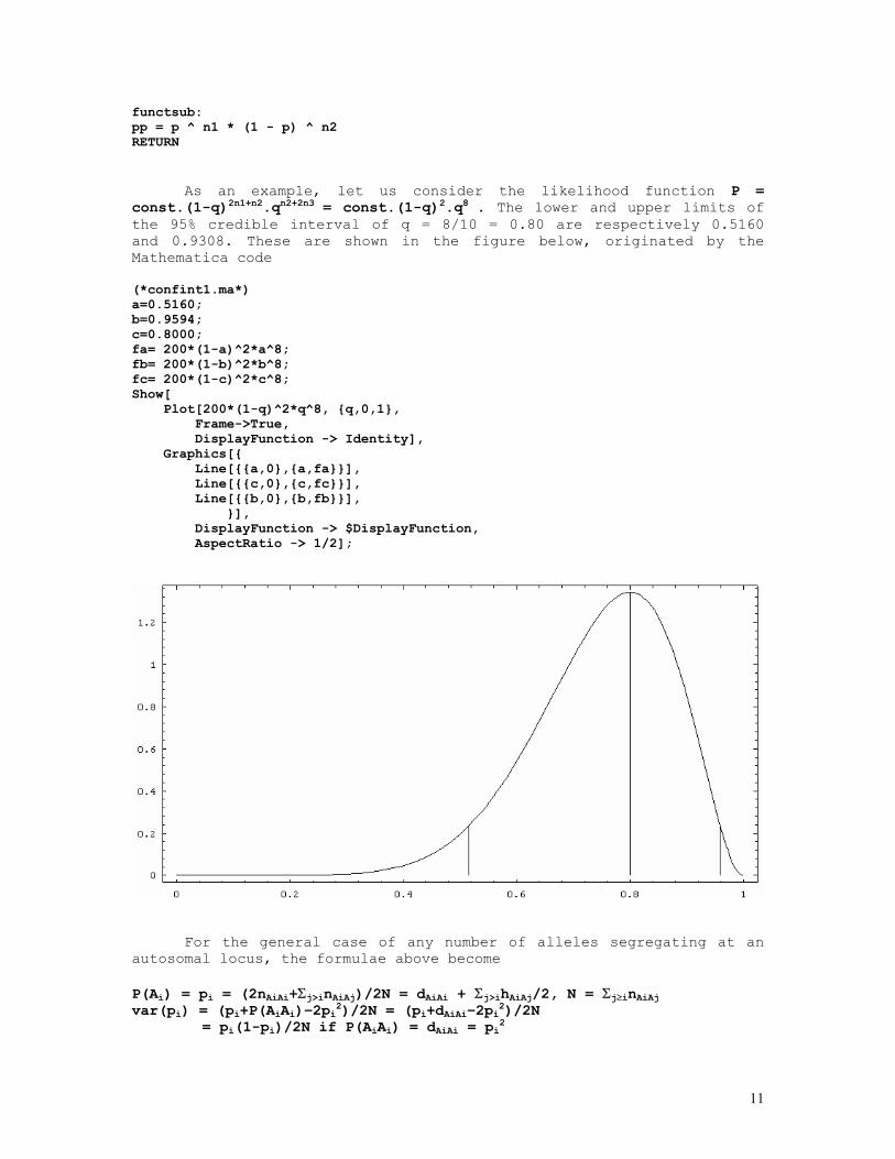
As an example, let us consider the likelihood function P = const.(1-q)2n1+n2.qn2+2n3 = const.(1-q)2.q8 . The lower and upper limits of the 95% credible interval of q = 8/10 = 0.80 are respectively 0.5160 and 0.9308. These are shown in the figure below, originated by the Mathematica code (*confint1.ma*) a=0.5160; b=0.9594; c=0.8000; fa= 200*(1-a)^2*a^8; fb= 200*(1-b)^2*b^8; fc= 200*(1-c)^2*c^8; Show[ Plot[200*(1-q)^2*q^8, {q,0,1}, Frame->True, DisplayFunction -> Identity], Graphics[{ Line[{{a,0},{a,fa}}], Line[{{c,0},{c,fc}}], Line[{{b,0},{b,fb}}], }], DisplayFunction -> $DisplayFunction, AspectRatio -> 1/2];
For the general case of any number of alleles segregating at an autosomal locus, the formulae above become P(Ai) = pi = (2nAiAi+Σj>inAiAj)/2N = dAiAi + Σj>ihAiAj/2, N = Σj≥inAiAj var(pi) = (pi+P(AiAi)–2pi2)/2N = (pi+dAiAi–2pi2)/2N = pi(1-pi)/2N if P(AiAi) = dAiAi = pi2
12
In the k-allele case the likelihood function is given by
P = N!/[Πi=1,kni!].Πi=1,k,j=ipi2nij.2Πi=1,k-1,j=i+1,k(pipj)nij
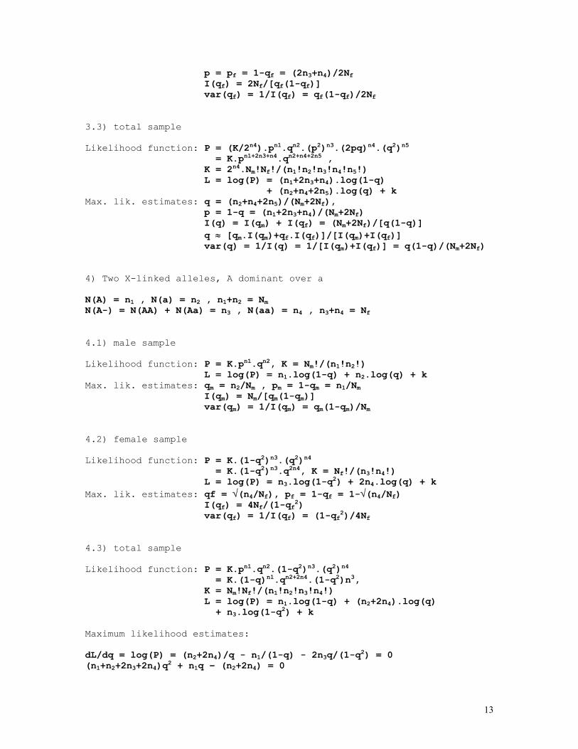
and the allele frequency estimates p1, ... , pk are the solutions of the set of equations {∂L/∂p1 = 0 , ... , ∂L/dpk = 0}, where L = log(P) as before. 2) Two autosomal dominant alleles, A dominant over a N(A-) = N(AA)+N(Aa) = n1 , N(aa) = n2, n1+n2 = N Likelihood function: P = N!/(n1!n2!).(1-q2)n1.(q2)n2 = N!/(n1!n2!).(1-q2)n1.q2n2 L = log(P) = const. + n1.log(1-q2) + 2n2.log(q) Maximum likelihood estimates: dL/dq = 2n2/q - 2n1q/(1-q2) = 0 n2 = (n1+n2)q2 , q2 = n2/(n1+n2) , q = √[n2/(n1+n2)] = √(n2/N) , p = 1-q = 1-√(n2/N) (d2L/dq2)q = - 2n2/q2 - 2n1(1+q2)/(1-q2)2 = - 2Nq2/q2 – 2N(1-q2)(1+q2)/(1-q2)2 = - 2N[1-q2+1+q2]/(1-q2) = -4N/(1-q2) = -I(q) I(q) = I(p) = 4N/(1-q2) = 1/var(p) = 1/var(q) var(q) = (1-q2)/4N var(q2) = q2(1-q2)/N = var(q).(dq2/dq)2 = 4q2var(q) var(q) = 1/I(q) = var(q2)/4q2 = (1-q2)/4N = (p2+2pq)/4N = p2/4N + pq/2N > pq/2N 3) Two X-linked codominant alleles N(A) = n1 , N(a) = n2 , n1+n2 = Nm N(AA) = n3 , N(Aa) = n4 , N(aa) = n5 , n3+n4+n5 = Nf 3.1) male sample Likelihood function: P = K.pn1.qn2, K = Nm!/(n1!n2!) L = log(P) = n1.log(1-q) + n2.log(q) + k Max. lik. estimates: qm = n2/Nm , pm = 1-qm = n1/Nm I(qm) = Nm/[qm(1-qm)] var(qm) = 1/I(qm) = qm(1-qm)/Nm 3.2) female sample Likelihood function: P = (K/2n4).(p2)n3.(2pq)n4.(q2)n5 = K.p2n3+n4.qn4+2n5, K = 2n4.Nf!/(n3!n4!n5!) L = log(P) = (2n3+n4).log(1-q) + (n4+2n5).log(q) + k Max. lik. estimates: q = qf = (n4+2n5)/2Nf ,
13
p = pf = 1-qf = (2n3+n4)/2Nf I(qf) = 2Nf/[qf(1-qf)] var(qf) = 1/I(qf) = qf(1-qf)/2Nf 3.3) total sample Likelihood function: P = (K/2n4).pn1.qn2.(p2)n3.(2pq)n4.(q2)n5 = K.pn1+2n3+n4.qn2+n4+2n5 , K = 2n4.Nm!Nf!/(n1!n2!n3!n4!n5!) L = log(P) = (n1+2n3+n4).log(1-q) + (n2+n4+2n5).log(q) + k Max. lik. estimates: q = (n2+n4+2n5)/(Nm+2Nf), p = 1-q = (n1+2n3+n4)/(Nm+2Nf) I(q) = I(qm) + I(qf) = (Nm+2Nf)/[q(1-q)] q ≈ [qm.I(qm)+qf.I(qf)]/[I(qm)+I(qf)] var(q) = 1/I(q) = 1/[I(qm)+I(qf)] = q(1-q)/(Nm+2Nf) 4) Two X-linked alleles, A dominant over a N(A) = n1 , N(a) = n2 , n1+n2 = Nm N(A-) = N(AA) + N(Aa) = n3 , N(aa) = n4 , n3+n4 = Nf 4.1) male sample Likelihood function: P = K.pn1.qn2, K = Nm!/(n1!n2!) L = log(P) = n1.log(1-q) + n2.log(q) + k Max. lik. estimates: qm = n2/Nm , pm = 1-qm = n1/Nm I(qm) = Nm/[qm(1-qm)] var(qm) = 1/I(qm) = qm(1-qm)/Nm 4.2) female sample Likelihood function: P = K.(1-q2)n3.(q2)n4 = K.(1-q2)n3.q2n4, K = Nf!/(n3!n4!) L = log(P) = n3.log(1-q2) + 2n4.log(q) + k Max. lik. estimates: qf = √(n4/Nf), pf = 1-qf = 1-√(n4/Nf) I(qf) = 4Nf/(1-qf2) var(qf) = 1/I(qf) = (1-qf2)/4Nf 4.3) total sample Likelihood function: P = K.pn1.qn2.(1-q2)n3.(q2)n4 = K.(1-q)n1.qn2+2n4.(1-q2)n3, K = Nm!Nf!/(n1!n2!n3!n4!) L = log(P) = n1.log(1-q) + (n2+2n4).log(q) + n3.log(1-q2) + k Maximum likelihood estimates: dL/dq = log(P) = (n2+2n4)/q - n1/(1-q) - 2n3q/(1-q2) = 0 (n1+n2+2n3+2n4)q2 + n1q – (n2+2n4) = 0
14
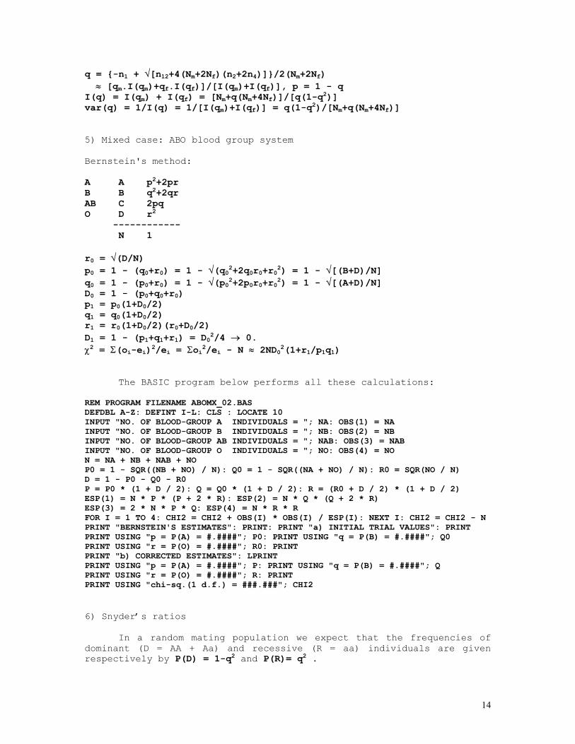
q = {-n1 + √[n12+4(Nm+2Nf)(n2+2n4)]}/2(Nm+2Nf) ≈ [qm.I(qm)+qf.I(qf)]/[I(qm)+I(qf)], p = 1 - q I(q) = I(qm) + I(qf) = [Nm+q(Nm+4Nf)]/[q(1-q2)] var(q) = 1/I(q) = 1/[I(qm)+I(qf)] = q(1-q2)/[Nm+q(Nm+4Nf)] 5) Mixed case: ABO blood group system Bernstein's method: A A p2+2pr B B q2+2qr AB C 2pq O D r2 ------------ N 1 r0 = √(D/N) p0 = 1 - (q0+r0) = 1 - √(q02+2q0r0+r02) = 1 - √[(B+D)/N] q0 = 1 - (p0+r0) = 1 - √(p02+2p0r0+r02) = 1 - √[(A+D)/N] D0 = 1 - (p0+q0+r0) p1 = p0(1+D0/2) q1 = q0(1+D0/2) r1 = r0(1+D0/2)(r0+D0/2) D1 = 1 - (p1+q1+r1) = D02/4 → 0. χ2 = Σ(oi-ei)2/ei = Σoi2/ei - N ≈ 2ND02(1+r1/p1q1)
The BASIC program below performs all these calculations: REM PROGRAM FILENAME ABOMX_02.BAS DEFDBL A-Z: DEFINT I-L: CLS : LOCATE 10 INPUT "NO. OF BLOOD-GROUP A INDIVIDUALS = "; NA: OBS(1) = NA INPUT "NO. OF BLOOD-GROUP B INDIVIDUALS = "; NB: OBS(2) = NB INPUT "NO. OF BLOOD-GROUP AB INDIVIDUALS = "; NAB: OBS(3) = NAB INPUT "NO. OF BLOOD-GROUP O INDIVIDUALS = "; NO: OBS(4) = NO N = NA + NB + NAB + NO P0 = 1 - SQR((NB + NO) / N): Q0 = 1 - SQR((NA + NO) / N): R0 = SQR(NO / N) D = 1 - P0 - Q0 - R0 P = P0 * (1 + D / 2): Q = Q0 * (1 + D / 2): R = (R0 + D / 2) * (1 + D / 2) ESP(1) = N * P * (P + 2 * R): ESP(2) = N * Q * (Q + 2 * R) ESP(3) = 2 * N * P * Q: ESP(4) = N * R * R FOR I = 1 TO 4: CHI2 = CHI2 + OBS(I) * OBS(I) / ESP(I): NEXT I: CHI2 = CHI2 - N PRINT "BERNSTEIN'S ESTIMATES": PRINT: PRINT "a) INITIAL TRIAL VALUES": PRINT PRINT USING "p = P(A) = #.####"; P0: PRINT USING "q = P(B) = #.####"; Q0 PRINT USING "r = P(O) = #.####"; R0: PRINT PRINT "b) CORRECTED ESTIMATES": LPRINT PRINT USING "p = P(A) = #.####"; P: PRINT USING "q = P(B) = #.####"; Q PRINT USING "r = P(O) = #.####"; R: PRINT PRINT USING "chi-sq.(1 d.f.) = ###.###"; CHI2 6) Snyder’s ratios
In a random mating population we expect that the frequencies of dominant (D = AA + Aa) and recessive (R = aa) individuals are given respectively by P(D) = 1-q2 and P(R)= q2 .
15
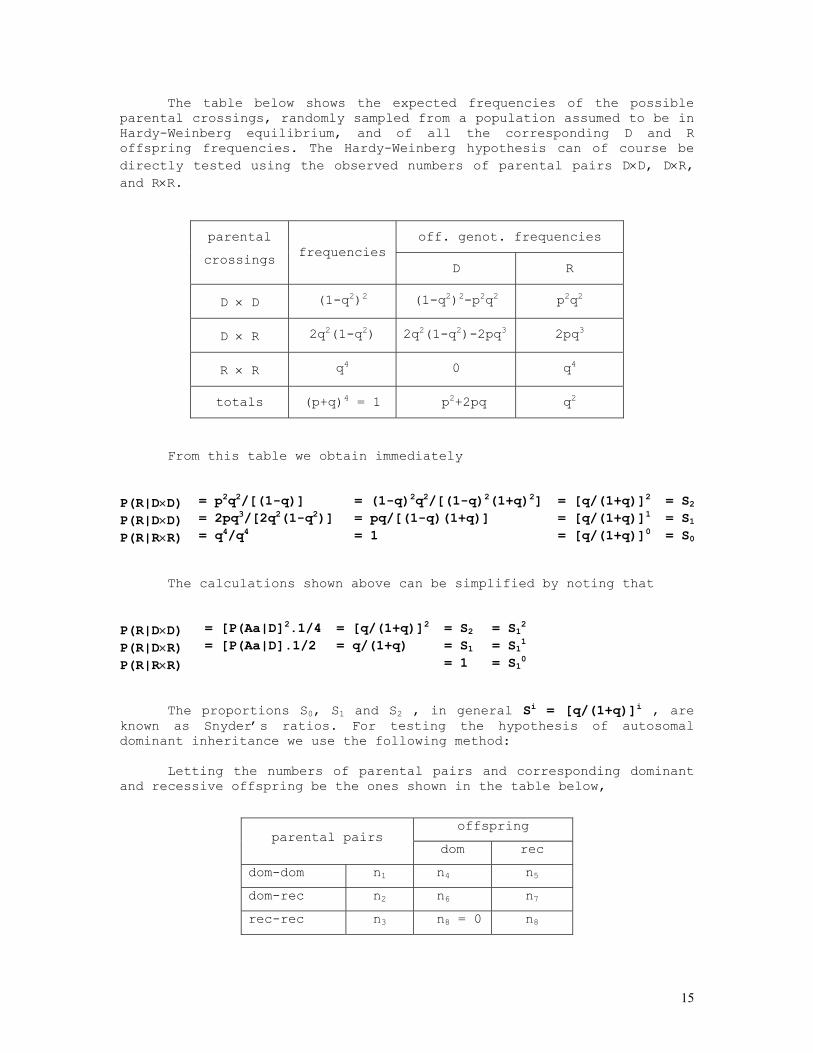
The table below shows the expected frequencies of the possible parental crossings, randomly sampled from a population assumed to be in Hardy-Weinberg equilibrium, and of all the corresponding D and R offspring frequencies. The Hardy-Weinberg hypothesis can of course be directly tested using the observed numbers of parental pairs D×D, D×R, and R×R.
off. genot. frequencies parental
crossings frequencies D R
D × D (1-q2)2 (1-q2)2-p2q2 p2q2
D × R 2q2(1-q2) 2q2(1-q2)-2pq3 2pq3
R × R q4 0 q4
totals (p+q)4 = 1 p2+2pq q2
From this table we obtain immediately P(R|D×D) = p2q2/[(1-q)] = (1-q)2q2/[(1-q)2(1+q)2] = [q/(1+q)]2 = S2 P(R|D×D) = 2pq3/[2q2(1-q2)] = pq/[(1-q)(1+q)] = [q/(1+q)]1 = S1 P(R|R×R) = q4/q4 = 1 = [q/(1+q)]0 = S0
The calculations shown above can be simplified by noting that
P(R|D×D) = [P(Aa|D]2.1/4 = [q/(1+q)]2 = S2 = S12 P(R|D×R) = [P(Aa|D].1/2 = q/(1+q) = S1 = S11 P(R|R×R) = 1 = S10
The proportions S0, S1 and S2 , in general Si = [q/(1+q)]i , are
known as Snyder’s ratios. For testing the hypothesis of autosomal dominant inheritance we use the following method:
Letting the numbers of parental pairs and corresponding dominant and recessive offspring be the ones shown in the table below,
offspring
parental pairs dom rec
dom-dom n1 n4 n5
dom-rec n2 n6 n7
rec-rec n3 n8 = 0 n8
16
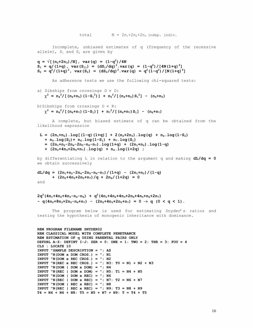
total N = 2n1+2n2+2n3 indep. indiv.
Incomplete, unbiased estimates of q (frequency of the recessive
allele), S1 and S2 are given by q = √[(n2+2n3)/N], var(q) = (1-q2)/4N S1 = q/(1+q), var(S11) = (dS1/dq)2.var(q) = (1-q2)/[4N(1+q)4] S2 = q2/(1+q)2, var(S2) = (dS2/dq)2.var(q) = q2(1-q2)/[N(1+q)6]
As adherence tests we use the following chi-squared tests: a) Sibships from crossings D × D: χ2 = n42/[(n4+n5)(1-S12)] + n52/[(n4+n5)S12] - (n4+n5) b)Sibships from crossings D × R: χ2 = n62/[(n6+n7)(1-S1)] + n72/[(n6+n7)S1] - (n6+n7)
A complete, but biased estimate of q can be obtained from the likelihood expression L = (2n1+n2).log[(1-q)(1+q)] + 2(n2+2n3).log(q) + n4.log(1-S2) + n5.log(S2)+ n6.log(1-S1) + n7.log(S1) = (2n1+n2-2n4-2n5-n6-n7).log(1+q) + (2n1+n2).log(1-q) + (2n2+4n3+2n5+n7).log(q) + n4.log(1+2q) ; by differentiating L in relation to the argument q and making dL/dq = 0 we obtain successively dL/dq = (2n1+n2-2n4-2n5-n6-n7)/(1+q) - (2n1+n2)/(1-q) + (2n2+4n3+2n5+n7)/q + 2n4/(1+2q) = 0 and 2q3(4n1+4n2+4n3-n4-n6) + q2(4n1+4n2+4n3+2n4+4n5+n6+2n7) - q(4n2+8n3+2n5-n6+n7) - (2n2+4n3+2n5+n7) = 0 → q (0 < q < 1).
The program below is used for estimating Snyder’s ratios and testing the hypothesis of monogenic inheritance with dominance. REM PROGRAM FILENAME SNYDER02 REM CLASSICAL MODEL WITH COMPLETE PENETRANCE REM ESTIMATION OF q USING PARENTAL PAIRS ONLY DEFDBL A-Z: DEFINT I-J: ZER = 0: ONE = 1: TWO = 2: THR = 3: FOU = 4 CLS : LOCATE 10 INPUT "SAMPLE DESCRIPTION = "; A$ INPUT "N(DOM x DOM CROS.) = "; N1 INPUT "N(DOM x REC CROS.) = "; N2 INPUT "N(REC x REC CROS.) = "; N3: T0 = N1 + N2 + N3 INPUT "N(DOM | DOM x DOM) = "; N4 INPUT "N(REC | DOM x DOM) = "; N5: T1 = N4 + N5 INPUT "N(DOM | DOM x REC) = "; N6 INPUT "N(REC | DOM x REC) = "; N7: T2 = N6 + N7 INPUT "N(DOM | REC x REC) = "; N8 INPUT "N(REC | REC x REC) = "; N9: T3 = N8 + N9 T4 = N4 + N6 + N8: T5 = N5 + N7 + N9: T = T4 + T5
17
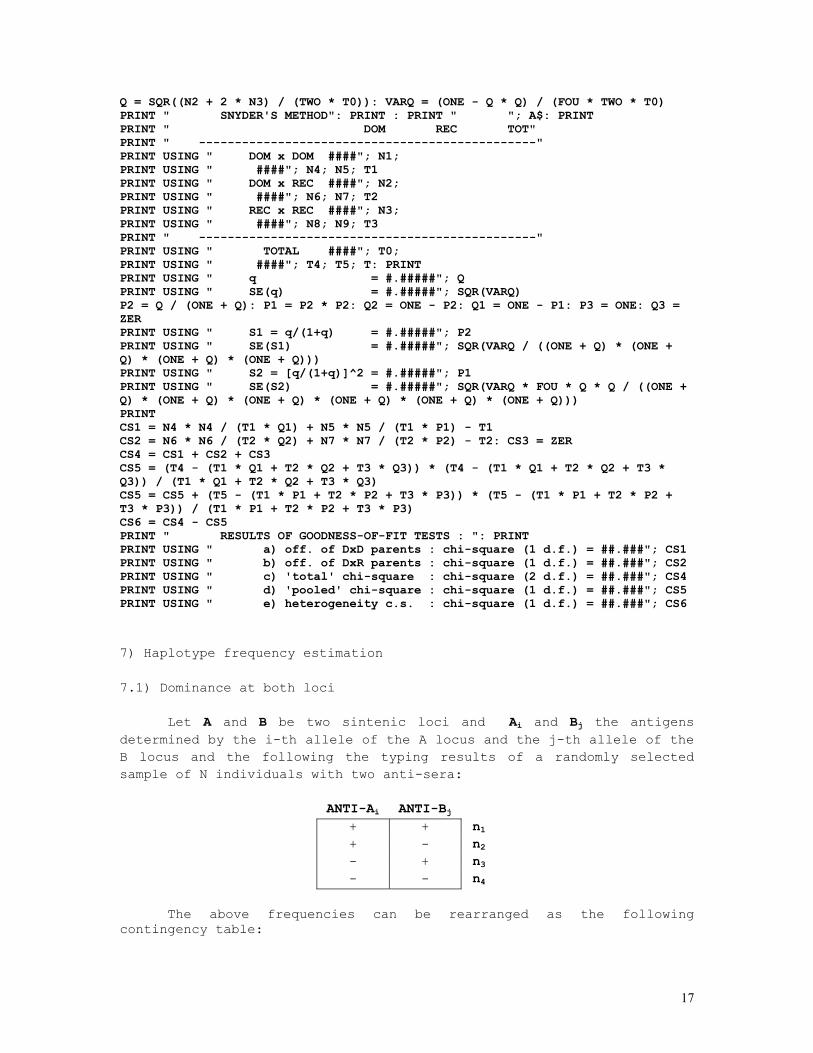
Q = SQR((N2 + 2 * N3) / (TWO * T0)): VARQ = (ONE - Q * Q) / (FOU * TWO * T0) PRINT " SNYDER'S METHOD": PRINT : PRINT " "; A$: PRINT PRINT " DOM REC TOT" PRINT " -----------------------------------------------" PRINT USING " DOM x DOM ####"; N1; PRINT USING " ####"; N4; N5; T1 PRINT USING " DOM x REC ####"; N2; PRINT USING " ####"; N6; N7; T2 PRINT USING " REC x REC ####"; N3; PRINT USING " ####"; N8; N9; T3 PRINT " -----------------------------------------------" PRINT USING " TOTAL ####"; T0; PRINT USING " ####"; T4; T5; T: PRINT PRINT USING " q = #.#####"; Q PRINT USING " SE(q) = #.#####"; SQR(VARQ) P2 = Q / (ONE + Q): P1 = P2 * P2: Q2 = ONE - P2: Q1 = ONE - P1: P3 = ONE: Q3 = ZER PRINT USING " S1 = q/(1+q) = #.#####"; P2 PRINT USING " SE(S1) = #.#####"; SQR(VARQ / ((ONE + Q) * (ONE + Q) * (ONE + Q) * (ONE + Q))) PRINT USING " S2 = [q/(1+q)]^2 = #.#####"; P1 PRINT USING " SE(S2) = #.#####"; SQR(VARQ * FOU * Q * Q / ((ONE + Q) * (ONE + Q) * (ONE + Q) * (ONE + Q) * (ONE + Q) * (ONE + Q))) PRINT CS1 = N4 * N4 / (T1 * Q1) + N5 * N5 / (T1 * P1) - T1 CS2 = N6 * N6 / (T2 * Q2) + N7 * N7 / (T2 * P2) - T2: CS3 = ZER CS4 = CS1 + CS2 + CS3 CS5 = (T4 - (T1 * Q1 + T2 * Q2 + T3 * Q3)) * (T4 - (T1 * Q1 + T2 * Q2 + T3 * Q3)) / (T1 * Q1 + T2 * Q2 + T3 * Q3) CS5 = CS5 + (T5 - (T1 * P1 + T2 * P2 + T3 * P3)) * (T5 - (T1 * P1 + T2 * P2 + T3 * P3)) / (T1 * P1 + T2 * P2 + T3 * P3) CS6 = CS4 - CS5 PRINT " RESULTS OF GOODNESS-OF-FIT TESTS : ": PRINT PRINT USING " a) off. of DxD parents : chi-square (1 d.f.) = ##.###"; CS1 PRINT USING " b) off. of DxR parents : chi-square (1 d.f.) = ##.###"; CS2 PRINT USING " c) 'total' chi-square : chi-square (2 d.f.) = ##.###"; CS4 PRINT USING " d) 'pooled' chi-square : chi-square (1 d.f.) = ##.###"; CS5 PRINT USING " e) heterogeneity c.s. : chi-square (1 d.f.) = ##.###"; CS6 7) Haplotype frequency estimation 7.1) Dominance at both loci
Let A and B be two sintenic loci and Ai and Bj the antigens determined by the i-th allele of the A locus and the j-th allele of the B locus and the following the typing results of a randomly selected sample of N individuals with two anti-sera:
ANTI-Ai ANTI-Bj + + n1 + - n2 - + n3 - - n4
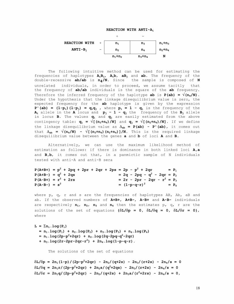
The above frequencies can be rearranged as the following
contingency table:
18
REACTION WITH ANTI-Ai
+ -
+ n1 n3 n1+n3 REACTION WITH
ANTI-Bj - n2 n4 n2+n4
n1+n2 n3+n4 N
The following intuitive method can be used for estimating the frequencies of haplotypes AiBj, Aib, aBj and ab. The frequency of the double-recessive ab/ab is n4/N. Since the sample is composed of N unrelated individuals, in order to proceed, we assume tacitly that the frequency of ab/ab individuals is the square of the ab frequency. Therefore the inferred frequency of the haplotype ab is P(ab) = √(n4/N). Under the hypothesis that the linkage disequilibrium value is zero, the expected frequency for the ab haplotype is given by the expression P'(ab) = (1-pi)(l-pj) = qiqj , where pi = 1 - qi is the frequency of the Ai allele in the A locus and pj = 1 - qj the frequency of the Bj allele in locus B. The values qi and qj are easily estimated from the above contingency table: qi = √[(n3+n4)/N] and qj = √[(n2+n4)/N]. If we define the linkage disequilibrium value as ∆ab = P(ab) - P'(ab), it comes out that ∆ab = √(n4/N) - √[(n3+n4)(n2+n4)]/N. This is the required linkage disequilibrium value between the genes a and b of loci A and B.
Alternatively, we can use the maximum likelihood method of estimation as follows: if there is dominance in both linked loci A,a and B,b, it comes out that, in a panmictic sample of N individuals tested with anti-A and anti-B sera P(A+B+) = p2 + 2pq + 2pr + 2qr + 2ps = 2p - p2 + 2qr = P1 P(A+B-) = q2 + 2qs = 2q - 2pq - q2 - 2qr = P2 P(A-B+) = r2 + 2rs = 2r - 2pr - 2qr - r2 = P3 P(A-B-) = s2 = (1-p-q-r)2 = P4 where p, q, r and s are the frequencies of haplotypes AB, Ab, aB and ab. If the observed numbers of A+B+, A+B-, A-B+ and A-B- individuals are respectively n1, n2, n3 and n4 then the estimates p, q, r are the solutions of the set of equations {δL/δp = 0, δL/δq = 0, δL/δr = 0}, where L = Σni.log(Pi) = n1.log(P1) + n2.log(P2) + n3.log(P3) + n4.log(P4) = n1.log(2p-p2+2qr) + n2.log(2q-2pq-q2-2qr) + n3.log(2r-2pr-2qr-r2) + 2n4.log(1-p-q-r).
The solutions of the set of equations δL/δp = 2n1(1-p)/(2p-p2+2qr) - 2n2/(q+2s) - 2n3/(r+2s) - 2n4/s = 0 δL/δq = 2n1r/(2p-p2+2qr) + 2n2s/(q2+2qs) - 2n3/(r+2s) - 2n4/s = 0 δL/δr = 2n1q/(2p-p2+2qr) - 2n2/(q+2s) + 2n3s/(r2+2rs) - 2n4/s = 0,
19
where s = 1-p-q-r, are: p = P(A) + P(B) + √(n4/N) - 1 = 1 + √(n4/N) - √[(n3+n4)/N] - √[(n2+n4)/N] = 1-q-r-s q = 1 - P(B) - √(n4/N) = √[(n2+n4)/N] - √(n4/N) = √[(q+s)2] - √(s2) r = 1 - P(A) - √ (n4/N) = √[(n3+n4)/N] - √(n4/N) = √[(r+s)2] - √(s2) s = √(n4/N) = √(s2).
The linkage disequilibrium value estimate ∆AB is obtained directly from ∆AB = P(AB)-P(A).P(B) = P(ab)-P(a).P(b) = √(n4/N) - √[(n2+n4)(n3+n4)]/N.
For testing the hypothesis ∆AB = 0 the following chi-squared statistics (with 1 d.f.) is used: χ2 = (n1n4-n2n3)2.N/[(n1+n2)(n1+n3)(n2+n4)(n3+n4)]
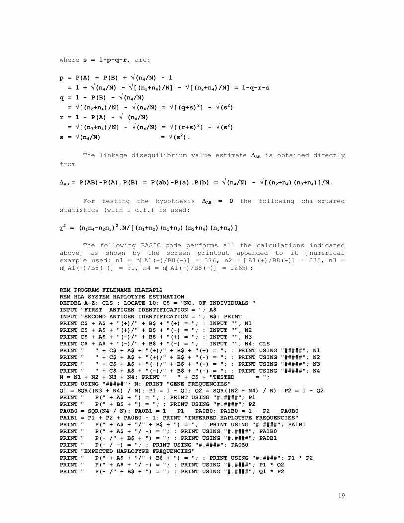
The following BASIC code performs all the calculations indicated above, as shown by the screen printout appended to it {numerical example used: n1 = n[A1(+)/B8(-)] = 376, n2 = [A1(+)/B8(-)] = 235, n3 = n[A1(-)/B8(+)] = 91, n4 = n[A1(-)/B8(-)] = 1265}: REM PROGRAM FILENAME HLAHAPL2 REM HLA SYSTEM HAPLOTYPE ESTIMATION DEFDBL A-Z: CLS : LOCATE 10: C$ = "NO. OF INDIVIDUALS " INPUT "FIRST ANTIGEN IDENTIFICATION = "; A$ INPUT "SECOND ANTIGEN IDENTIFICATION = "; B$: PRINT PRINT C$ + A$ + "(+)/" + B$ + "(+) = "; : INPUT "", N1 PRINT C$ + A$ + "(+)/" + B$ + "(-) = "; : INPUT "", N2 PRINT C$ + A$ + "(-)/" + B$ + "(+) = "; : INPUT "", N3 PRINT C$ + A$ + "(-)/" + B$ + "(-) = "; : INPUT "", N4: CLS PRINT " " + C$ + A$ + "(+)/" + B$ + "(+) = "; : PRINT USING "#####"; N1 PRINT " " + C$ + A$ + "(+)/" + B$ + "(-) = "; : PRINT USING "#####"; N2 PRINT " " + C$ + A$ + "(-)/" + B$ + "(+) = "; : PRINT USING "#####"; N3 PRINT " " + C$ + A$ + "(-)/" + B$ + "(-) = "; : PRINT USING "#####"; N4 N = N1 + N2 + N3 + N4: PRINT " " + C$ + "TESTED = "; PRINT USING "#####"; N: PRINT "GENE FREQUENCIES" Q1 = SQR((N3 + N4) / N): P1 = 1 - Q1: Q2 = SQR((N2 + N4) / N): P2 = 1 - Q2 PRINT " P(" + A$ + ") = "; : PRINT USING "#.####"; P1 PRINT " P(" + B$ + ") = "; : PRINT USING "#.####"; P2 PA0B0 = SQR(N4 / N): PA0B1 = 1 - P1 - PA0B0: PA1B0 = 1 - P2 - PA0B0 PA1B1 = P1 + P2 + PA0B0 - 1: PRINT "INFERRED HAPLOTYPE FREQUENCIES" PRINT " P(" + A$ + "/" + B$ + ") = "; : PRINT USING "#.####"; PA1B1 PRINT " P(" + A$ + "/ -) = "; : PRINT USING "#.####"; PA1B0 PRINT " P(- /" + B$ + ") = "; : PRINT USING "#.####"; PA0B1 PRINT " P(- / -) = "; : PRINT USING "#.####"; PA0B0 PRINT "EXPECTED HAPLOTYPE FREQUENCIES" PRINT " P(" + A$ + "/" + B$ + ") = "; : PRINT USING "#.####"; P1 * P2 PRINT " P(" + A$ + "/ -) = "; : PRINT USING "#.####"; P1 * Q2 PRINT " P(- /" + B$ + ") = "; : PRINT USING "#.####"; Q1 * P2
20
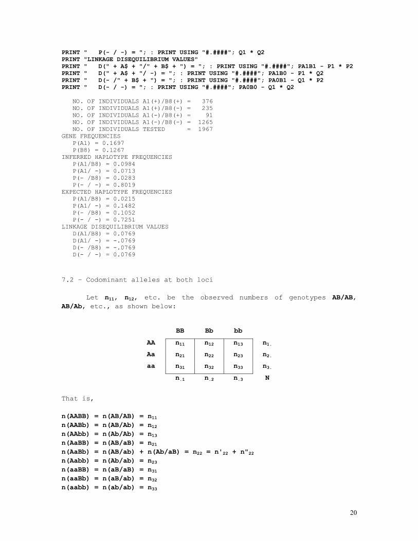
PRINT " P(- / -) = "; : PRINT USING "#.####"; Q1 * Q2 PRINT "LINKAGE DISEQUILIBRIUM VALUES" PRINT " D(" + A$ + "/" + B$ + ") = "; : PRINT USING "#.####"; PA1B1 - P1 * P2 PRINT " D(" + A$ + "/ -) = "; : PRINT USING "#.####"; PA1B0 - P1 * Q2 PRINT " D(- /" + B$ + ") = "; : PRINT USING "#.####"; PA0B1 - Q1 * P2 PRINT " D(- / -) = "; : PRINT USING "#.####"; PA0B0 - Q1 * Q2 NO. OF INDIVIDUALS A1(+)/B8(+) = 376 NO. OF INDIVIDUALS A1(+)/B8(-) = 235 NO. OF INDIVIDUALS A1(-)/B8(+) = 91 NO. OF INDIVIDUALS A1(-)/B8(-) = 1265 NO. OF INDIVIDUALS TESTED = 1967 GENE FREQUENCIES P(A1) = 0.1697 P(B8) = 0.1267 INFERRED HAPLOTYPE FREQUENCIES P(A1/B8) = 0.0984 P(A1/ -) = 0.0713 P(- /B8) = 0.0283 P(- / -) = 0.8019 EXPECTED HAPLOTYPE FREQUENCIES P(A1/B8) = 0.0215 P(A1/ -) = 0.1482 P(- /B8) = 0.1052 P(- / -) = 0.7251 LINKAGE DISEQUILIBRIUM VALUES D(A1/B8) = 0.0769 D(A1/ -) = -.0769 D(- /B8) = -.0769 D(- / -) = 0.0769 7.2 – Codominant alleles at both loci
Let n11, n12, etc. be the observed numbers of genotypes AB/AB, AB/Ab, etc., as shown below:
BB Bb bb
AA n11 n12 n13 n1.
Aa n21 n22 n23 n2.
aa n31 n32 n33 n3.
n.1 n.2 n.3 N
That is, n(AABB) = n(AB/AB) = n11 n(AABb) = n(AB/Ab) = n12 n(AAbb) = n(Ab/Ab) = n13 n(AaBB) = n(AB/aB) = n21 n(AaBb) = n(AB/ab) + n(Ab/aB) = n22 = n'22 + n"22 n(Aabb) = n(Ab/ab) = n23 n(aaBB) = n(aB/aB) = n31 n(aaBb) = n(aB/ab) = n32 n(aabb) = n(ab/ab) = n33
21
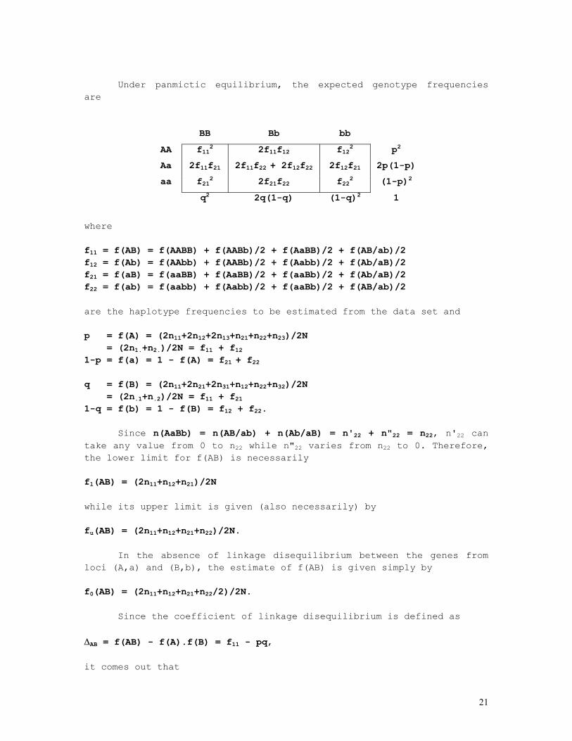
Under panmictic equilibrium, the expected genotype frequencies
are
BB Bb bb
AA f112 2f11f12 f122 p2
Aa 2f11f21 2f11f22 + 2f12f22 2f12f21 2p(1-p)
aa f212 2f21f22 f222 (1-p)2
q2 2q(1-q) (1-q)2 1
where f11 = f(AB) = f(AABB) + f(AABb)/2 + f(AaBB)/2 + f(AB/ab)/2 f12 = f(Ab) = f(AAbb) + f(AABb)/2 + f(Aabb)/2 + f(Ab/aB)/2 f21 = f(aB) = f(aaBB) + f(AaBB)/2 + f(aaBb)/2 + f(Ab/aB)/2 f22 = f(ab) = f(aabb) + f(Aabb)/2 + f(aaBb)/2 + f(AB/ab)/2 are the haplotype frequencies to be estimated from the data set and p = f(A) = (2n11+2n12+2n13+n21+n22+n23)/2N = (2n1.+n2.)/2N = f11 + f12 1-p = f(a) = 1 - f(A) = f21 + f22 q = f(B) = (2n11+2n21+2n31+n12+n22+n32)/2N = (2n.1+n.2)/2N = f11 + f21 1-q = f(b) = 1 - f(B) = f12 + f22.
Since n(AaBb) = n(AB/ab) + n(Ab/aB) = n'22 + n"22 = n22, n'22 can take any value from 0 to n22 while n"22 varies from n22 to 0. Therefore, the lower limit for f(AB) is necessarily fl(AB) = (2n11+n12+n21)/2N while its upper limit is given (also necessarily) by fu(AB) = (2n11+n12+n21+n22)/2N.
In the absence of linkage disequilibrium between the genes from loci (A,a) and (B,b), the estimate of f(AB) is given simply by f0(AB) = (2n11+n12+n21+n22/2)/2N.
Since the coefficient of linkage disequilibrium is defined as
∆AB = f(AB) - f(A).f(B) = f11 - pq, it comes out that

22
∆AB = f11 - (f11+f12)(f11+f21)
= f11(f11+f12+f21+f22) - (f11+f12)(f11+f21) = f11.f22 - f12.f21 = n'22/N - n"22/2N = (n'22-n"22)/2N.
Assuming that the marginal frequencies for both one-locus genoypes [(AA, Aa, aa) and (BB, Bb, bb)] are in Hardy-Weinberg proportions, the likelihood function is given by P = N!/(n11!...n33!).(f112)n11.(2f11f12)n12.(f122)n13 .(2f11f21)n21.(2f11f22+2f12f21)n22.(2f12f22)n23 .(f212)n31.(2f21f22)n32.(f222)n33, so that the frequencies f11, f12 and f21 can be estimated by maximizing the likelihood function in logarithmic form L = log P = const. + ΣXij.log(fij) + n22.log(f11.f22-f12.f21) = const. + X11.log(f11)+ X12.log(f12) + X21.log(f21) + X22.log(f22) + n22.log(f11.f22-f12.f21) = const. + X11.log(f11) + X12.log(f12) + X21.log(f21) + X22.log(1-f11-f12-f21) + n22.log[f11(1-f11-f12-f21)-f12.f21], where X11 = 2n11 + n12 + n21 X12 = 2n13 + n12 + n23 X21 = 2n31 + n21 + n32 X22 = 2n33 + n23 + n32.
The estimates f11, f12 and f21 are obtained by maximizing the function L, that is, they are the solutions of the set of linearly independent equations {∂L/∂f11 = 0, ∂L/∂f12 = 0, ∂L/∂f21 = 0}.
Since it is not possible to obtain explicit solutions for this set of equations, a numerical method as the generalized Newton-Raphson iterative procedure is used: (fij)t+1 = (fij)t + ((-∂(*L/*fij)/∂fij)-1.(∂L/*fij))t = (fij)t + ((-∂2L/∂fij2)-1.(∂L/∂fij))t = (fij)t + ((Vij).(∂L/∂fij))t, where (fij)t is the column vector (at the t-th iteration) (f11, f12, f21)T, (∂L/∂fij)t is the column vector, at iteration t, of partial derivatives
23
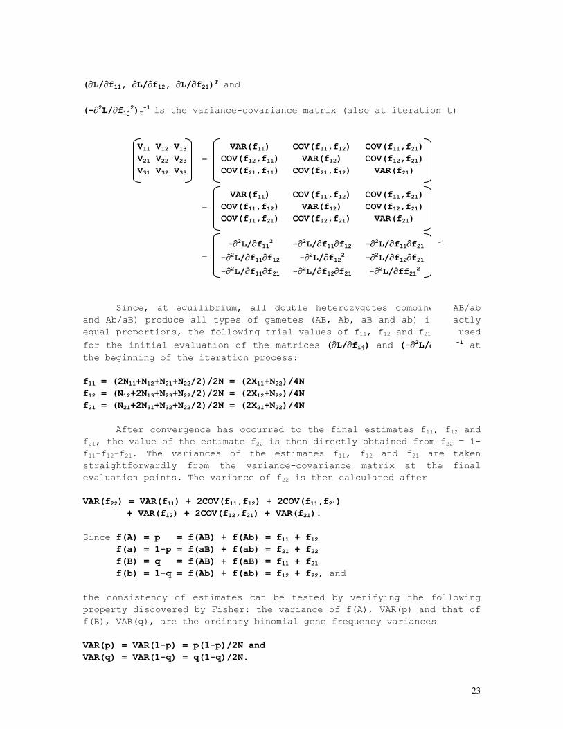
(∂L/∂f11, ∂L/∂f12, ∂L/∂f21)T and (-∂2L/∂fij2)t-1 is the variance-covariance matrix (also at iteration t)
V11 V12 V13 VAR(f11) COV(f11,f12) COV(f11,f21) V21 V22 V23 COV(f12,f11) VAR(f12) COV(f12,f21) V31 V32 V33
= COV(f21,f11) COV(f21,f12) VAR(f21)
VAR(f11) COV(f11,f12) COV(f11,f21) COV(f11,f12) VAR(f12) COV(f12,f21)
= COV(f11,f21) COV(f12,f21) VAR(f21)
-∂2L/∂f112 -∂2L/∂f11∂f12 -∂2L/∂f11∂f21 -∂2L/∂f11∂f12 -∂2L/∂f122 -∂2L/∂f12∂f21
=
-∂2L/∂f11∂f21 -∂2L/∂f12∂f21 -∂2L/∂ff212
Since, at equilibrium, all double heterozygotes combined (AB/ab and Ab/aB) produce all types of gametes (AB, Ab, aB and ab) in exactly equal proportions, the following trial values of f11, f12 and f21 are used for the initial evaluation of the matrices (∂L/∂fij) and (-∂2L/∂fij2)-1 at the beginning of the iteration process: f11 = (2N11+N12+N21+N22/2)/2N = (2X11+N22)/4N f12 = (N12+2N13+N23+N22/2)/2N = (2X12+N22)/4N f21 = (N21+2N31+N32+N22/2)/2N = (2X21+N22)/4N
After convergence has occurred to the final estimates f11, f12 and f21, the value of the estimate f22 is then directly obtained from f22 = 1-f11-f12-f21. The variances of the estimates f11, f12 and f21 are taken straightforwardly from the variance-covariance matrix at the final evaluation points. The variance of f22 is then calculated after VAR(f22) = VAR(f11) + 2COV(f11,f12) + 2COV(f11,f21) + VAR(f12) + 2COV(f12,f21) + VAR(f21). Since f(A) = p = f(AB) + f(Ab) = f11 + f12 f(a) = 1-p = f(aB) + f(ab) = f21 + f22 f(B) = q = f(AB) + f(aB) = f11 + f21 f(b) = 1-q = f(Ab) + f(ab) = f12 + f22, and the consistency of estimates can be tested by verifying the following property discovered by Fisher: the variance of f(A), VAR(p) and that of f(B), VAR(q), are the ordinary binomial gene frequency variances VAR(p) = VAR(1-p) = p(1-p)/2N and VAR(q) = VAR(1-q) = q(1-q)/2N.
-1
24
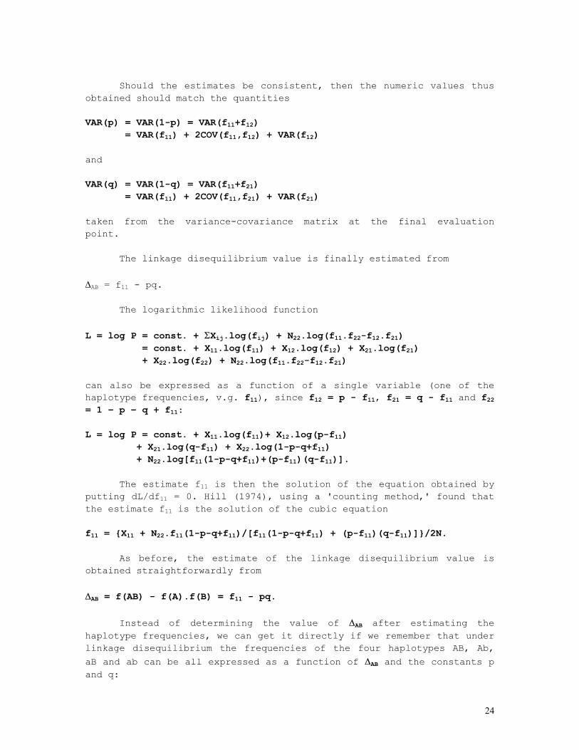
Should the estimates be consistent, then the numeric values thus
obtained should match the quantities VAR(p) = VAR(1-p) = VAR(f11+f12) = VAR(f11) + 2COV(f11,f12) + VAR(f12) and VAR(q) = VAR(1-q) = VAR(f11+f21) = VAR(f11) + 2COV(f11,f21) + VAR(f21) taken from the variance-covariance matrix at the final evaluation point.
The linkage disequilibrium value is finally estimated from
∆AB = f11 - pq.
The logarithmic likelihood function L = log P = const. + ΣXij.log(fij) + N22.log(f11.f22-f12.f21) = const. + X11.log(f11) + X12.log(f12) + X21.log(f21) + X22.log(f22) + N22.log(f11.f22-f12.f21) can also be expressed as a function of a single variable (one of the haplotype frequencies, v.g. f11), since f12 = p - f11, f21 = q - f11 and f22 = 1 – p – q + f11: L = log P = const. + X11.log(f11)+ X12.log(p-f11) + X21.log(q-f11) + X22.log(1-p-q+f11) + N22.log[f11(1-p-q+f11)+(p-f11)(q-f11)].
The estimate f11 is then the solution of the equation obtained by putting dL/df11 = 0. Hill (1974), using a 'counting method,' found that the estimate f11 is the solution of the cubic equation f11 = {X11 + N22.f11(1-p-q+f11)/[f11(1-p-q+f11) + (p-f11)(q-f11)]}/2N.
As before, the estimate of the linkage disequilibrium value is obtained straightforwardly from ∆AB = f(AB) - f(A).f(B) = f11 - pq.
Instead of determining the value of ∆AB after estimating the haplotype frequencies, we can get it directly if we remember that under linkage disequilibrium the frequencies of the four haplotypes AB, Ab, aB and ab can be all expressed as a function of ∆AB and the constants p and q:
25
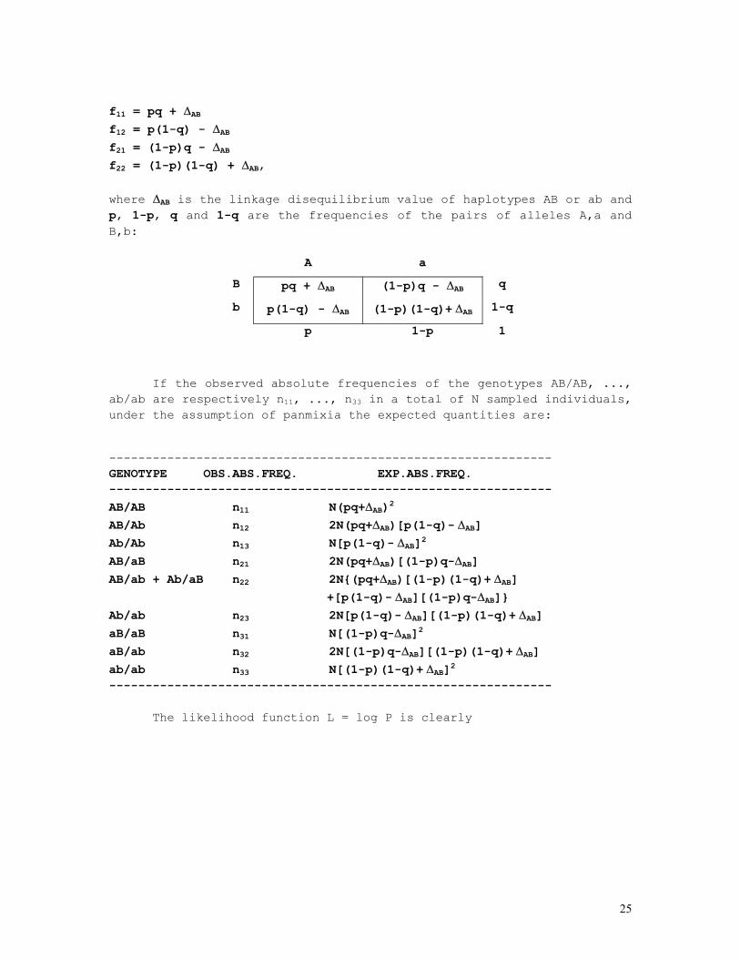
f11 = pq + ∆AB
f12 = p(1-q) - ∆AB
f21 = (1-p)q - ∆AB
f22 = (1-p)(1-q) + ∆AB, where ∆AB is the linkage disequilibrium value of haplotypes AB or ab and p, 1-p, q and 1-q are the frequencies of the pairs of alleles A,a and B,b:
A a
B pq + ∆AB (1-p)q - ∆AB q
b p(1-q) - ∆AB (1-p)(1-q)+ ∆AB 1-q
p 1-p 1
If the observed absolute frequencies of the genotypes AB/AB, ..., ab/ab are respectively n11, ..., n33 in a total of N sampled individuals, under the assumption of panmixia the expected quantities are: ------------------------------------------------------------- GENOTYPE OBS.ABS.FREQ. EXP.ABS.FREQ. ------------------------------------------------------------- AB/AB n11 N(pq+∆AB)2
AB/Ab n12 2N(pq+∆AB)[p(1-q)- ∆AB]
Ab/Ab n13 N[p(1-q)- ∆AB]2
AB/aB n21 2N(pq+∆AB)[(1-p)q-∆AB]
AB/ab + Ab/aB n22 2N{(pq+∆AB)[(1-p)(1-q)+ ∆AB]
+[p(1-q)- ∆AB][(1-p)q-∆AB]}
Ab/ab n23 2N[p(1-q)- ∆AB][(1-p)(1-q)+ ∆AB]
aB/aB n31 N[(1-p)q-∆AB]2
aB/ab n32 2N[(1-p)q-∆AB][(1-p)(1-q)+ ∆AB]
ab/ab n33 N[(1-p)(1-q)+ ∆AB]2 -------------------------------------------------------------
The likelihood function L = log P is clearly

26
L = const. + X11.log(pq+∆AB) + X12.log[p(1-q)- ∆AB]
+ X21.log[(1-p)q-∆AB] + X22.log[(1-p)(1-q)+ ∆AB]
+ N22.log{(pq+∆AB)[(1-p)(1-q)+ ∆AB]
+ [p(1-q)- ∆AB][(1-p)q-∆AB]}, where X11, X12, X21 and X22 are the summary measures already defined. The allelic frequencies can be treated as constants, and they are easily estimated by an independent direct counting method: p = (X11+X12+N22)/2N, 1 - p = (X21+X22+N22)/2N q = (X11+X21+N22)/2N, 1 - q = (X12+X22+N22)/2N .
Putting ∆AB = ∆ , the first derivative dL/d∆ has literal value dL/d∆ = X11/(pq+∆) - X12/[p(1-q)- ∆] - X21/[(1-p)q-∆] + X22/[(1-p)(1-q)+ ∆] + N22[4∆+(1-2p)(1-2q)]/[2∆2+∆(1-2q)(1-2p)+2pq(1-p)(1-q)] whereas the second derivative takes value d2L/d∆2 = - X11/(pq+∆)2 - X12/[p(1-q)- ∆]2 - X21/[(1-p)q-∆]2 - X22/[(1-p)(1-q)+ ∆]2 - N22[8pq(1-p)(1-q)+1-4p(1-q)-4(1-p)q] / [2∆2+∆(1-2q)(1-2p)+2pq(1-p)(1-q)].
The estimate ∆ is the solution of the equation dL/d∆ = 0. Since this equation has no explicit solution, a numerical method such as the Newton-Raphson procedure is used to obtain it, as folows: ∆t+1 = ∆t - f(∆)t/f'(∆)t = ∆t + (dL/d∆)t.[-(d2L/d∆2)t]-1
= ∆t + (dL/d∆)t.VAR(∆)t .
Hill (1974) showed that a suitable starting value for iteration is given by f11 = ∆0 + pq = (X11-X12-X21+X22)/4N + ½ - (1-p)(1-q) and therefore ∆0 = (X11-X12-X21+X22)/4N + ½ - (1-p)(1-q) – pq .
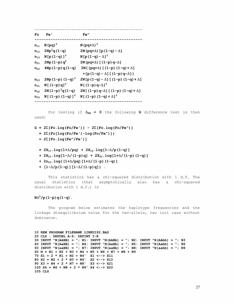
Now, let Fo be the observed numbers and Fe' and Fe" respectively the expected values under the assumptions of ∆ = ∆AB = 0 and ∆ = ∆AB ≠ 0 (estimated after any of the methods just delineated) as follows:
27
----------------------------------------------- Fo Fe' Fe" ----------------------------------------------- n11 N(pq)2 N(pq+∆)2 n12 2Np2q(1-q) 2N(pq+∆)[p(1-q)- ∆] n13 N[p(1-q)]2 N[p(1-q)- ∆]2 n21 2Np(1-p)q2 2N(pq+∆)[(1-p)q-∆] n22 4Np(1-p)q(1-q) 2N{(pq+∆)[(1-p)(1-q)+ ∆] +[p(1-q)- ∆][(1-p)q-∆]} n23 2Np(1-p)(1-q)2 2N[p(1-q)- ∆][(1-p)(1-q)+ ∆] n31 N[(1-p)q]2 N[(1-p)q-∆]2 n32 2N(1-p)2q(1-q) 2N[(1-p)q-∆][(1-p)(1-q)+ ∆] n33 N[(1-p)(1-q)]2 N[(1-p)(1-q)+ ∆]2 -----------------------------------------------
For testing if ∆AB ≠ 0 the following G difference test is then used: G = 2Σ{Fo.log(Fo/Fe')} - 2Σ{Fo.log(Fo/Fe")} = 2Σ{Fo[log(Fo/Fe')-log(Fo/Fe")]} = 2Σ[Fo.log(Fe"/Fe')] = 2X11.log(1+∆/pq) + 2X12.log[1-∆/p(1-q)] + 2X21.log[1-∆/(1-p)q] + 2X22.log[1+∆/(1-p)(1-q)] + 2n22.log{(1+∆/pq)[1+∆/(1-p)(1-q)] + [1-∆/p(1-q)][1-∆/(1-p)q]} .
This statistics has a chi-squared distribution with 1 d.f. The usual statistics (that asymptotically also has a chi-squared distribution with 1 d.f.) is N∆2/p(1-p)q(1-q).
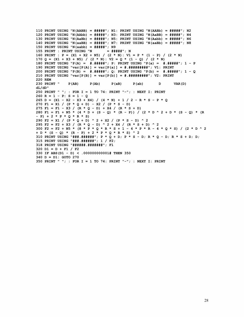
The program below estimates the haplotype frequencies and the linkage disequilibrium value for the two-allele, two loci case without dominance. 10 REM PROGRAM FILENAME LINKDIS2.BAS 20 CLS : DEFDBL A-Z: DEFINT I-K 30 INPUT "N(AABB) = "; N1: INPUT "N(AABb) = "; N2: INPUT "N(AAbb) = "; N3 40 INPUT "N(AaBB) = "; N4: INPUT "N(AaBb) = "; N5: INPUT "N(Aabb) = "; N6 50 INPUT "N(aaBB) = "; N7: INPUT "N(aaBb) = "; N8: INPUT "N(aabb) = "; N9 60 N = N1 + N2 + N3 + N4 + N5 + N6 + N7 + N8 + N9 70 X1 = 2 * N1 + N2 + N4' X1 <--> X11 80 X2 = N2 + 2 * N3 + N6' X2 <--> X12 90 X3 = N4 + 2 * N7 + N8' X3 <--> X21 100 X4 = N6 + N8 + 2 * N9' X4 <--> X22 105 CLS
28
110 PRINT USING "N(AABB) = #####"; N1: PRINT USING "N(AABb) = #####"; N2 120 PRINT USING "N(AAbb) = #####"; N3: PRINT USING "N(AaBB) = #####"; N4 130 PRINT USING "N(AaBb) = #####"; N5: PRINT USING "N(Aabb) = #####"; N6 140 PRINT USING "N(aaBB) = #####"; N7: PRINT USING "N(aaBb) = #####"; N8 150 PRINT USING "N(aabb) = #####"; N9 155 PRINT : PRINT USING "N = #####"; N 160 PRINT : P = (X1 + X2 + N5) / (2 * N): V1 = P * (1 - P) / (2 * N) 170 Q = (X1 + X3 + N5) / (2 * N): V2 = Q * (1 - Q) / (2 * N) 180 PRINT USING "P(A) = #.#####"; P: PRINT USING "P(a) = #.#####"; 1 - P 190 PRINT USING "var[P(A)] = var[P(a)] = #.#########"; V1: PRINT 200 PRINT USING "P(B) = #.#####"; Q: PRINT USING "P(b) = #.#####"; 1 - Q 210 PRINT USING "var[P(B)] = var[P(b)] = #.#########"; V2: PRINT 220 REM 230 PRINT " P(AB) P(Ab) P(aB) P(ab) D VAR(D) dL/dD" 250 PRINT " "; : FOR I = 1 TO 74: PRINT "-"; : NEXT I: PRINT 260 R = 1 - P: S = 1 - Q 265 D = (X1 - X2 - X3 + X4) / (4 * N) + 1 / 2 - R * S - P * Q 270 F1 = X1 / (P * Q + D) - X2 / (P * S - D) 275 F1 = F1 - X3 / (R * Q - D) + X4 / (R * S + D) 280 F1 = F1 + N5 * (4 * D + (S - Q) * (R - P)) / (2 * D ^ 2 + D * (S - Q) * (R - P) + 2 * P * Q * R * S) 290 F2 = X1 / (P * Q + D) ^ 2 + X2 / (P * S - D) ^ 2 295 F2 = F2 + X3 / (R * Q - D) ^ 2 + X4 / (R * S + D) ^ 2 300 F2 = F2 + N5 * (8 * P * Q * R * S + 1 - 4 * P * R - 4 * Q * S) / (2 * D ^ 2 + D * (S - Q) * (R - P) + 2 * P * Q * R * S) ^ 2 310 PRINT USING "###.######"; P * Q + D; P * S - D; R * Q - D; R * S + D; D; 315 PRINT USING "###.######"; 1 / F2; 318 PRINT USING "######.#######"; F1 320 D1 = D + F1 / F2 330 IF ABS(D1 - D) < .000000000001# THEN 350 340 D = D1: GOTO 270 350 PRINT " "; : FOR I = 1 TO 74: PRINT "-"; : NEXT I: PRINT
29
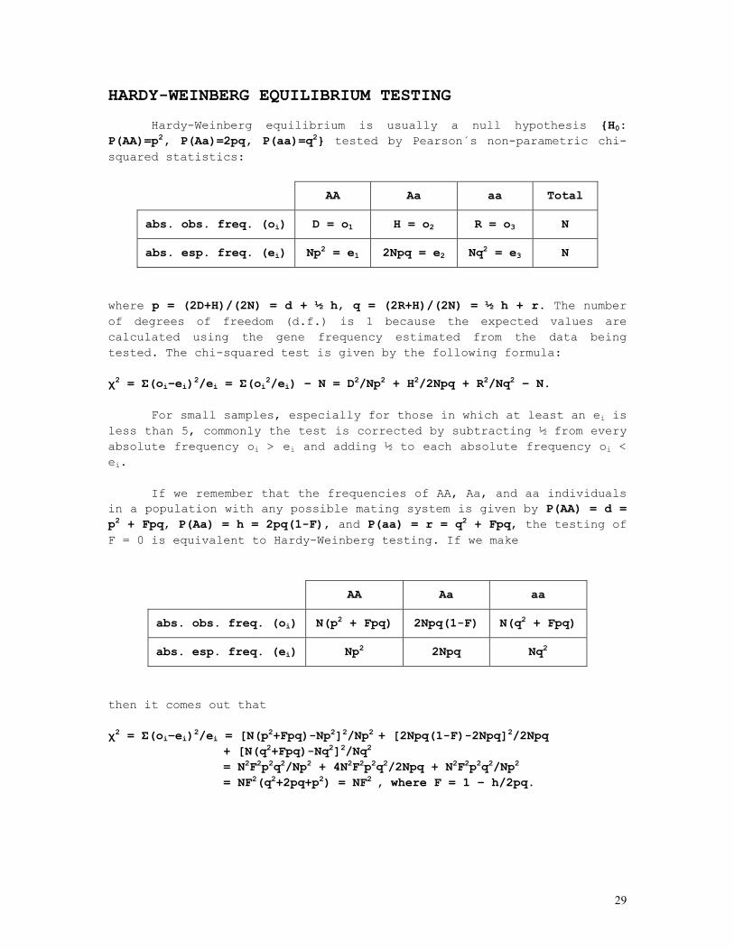
HARDY-WEINBERG EQUILIBRIUM TESTING
Hardy-Weinberg equilibrium is usually a null hypothesis {H0: P(AA)=p2, P(Aa)=2pq, P(aa)=q2} tested by Pearson´s non-parametric chi-squared statistics:
AA Aa aa Total
abs. obs. freq. (oi) D = o1 H = o2 R = o3 N
abs. esp. freq. (ei) Np2 = e1 2Npq = e2 Nq2 = e3 N
where p = (2D+H)/(2N) = d + ½ h, q = (2R+H)/(2N) = ½ h + r. The number of degrees of freedom (d.f.) is 1 because the expected values are calculated using the gene frequency estimated from the data being tested. The chi-squared test is given by the following formula: χ2 = Σ(oi–ei)2/ei = Σ(oi2/ei) – N = D2/Np2 + H2/2Npq + R2/Nq2 – N.
For small samples, especially for those in which at least an ei is less than 5, commonly the test is corrected by subtracting ½ from every absolute frequency oi > ei and adding ½ to each absolute frequency oi < ei.
If we remember that the frequencies of AA, Aa, and aa individuals in a population with any possible mating system is given by P(AA) = d = p2 + Fpq, P(Aa) = h = 2pq(1-F), and P(aa) = r = q2 + Fpq, the testing of F = 0 is equivalent to Hardy-Weinberg testing. If we make
AA Aa aa
abs. obs. freq. (oi) N(p2 + Fpq) 2Npq(1-F) N(q2 + Fpq)
abs. esp. freq. (ei) Np2 2Npq Nq2
then it comes out that χ2 = Σ(oi–ei)2/ei = [N(p2+Fpq)-Np2]2/Np2 + [2Npq(1-F)-2Npq]2/2Npq + [N(q2+Fpq)-Nq2]2/Nq2 = N2F2p2q2/Np2 + 4N2F2p2q2/2Npq + N2F2p2q2/Np2 = NF2(q2+2pq+p2) = NF2 , where F = 1 – h/2pq.

30
There exists an obvious correspondence between the formula χ2 = Σ(oi–ei)2/ei and the one obtained from the contingency table:
D H/2 Np
H/2 R Nq
Np Nq N
since e1 = Np × Np / N = Np2, e’2 = Np × Nq / N = Npq, e”2 = e’2, e2 = e”2 + e’2 = 2Npq, e3 = Nq × Nq / N = Nq2. The formula χ2 = Σ(oi–ei)2/ei can be easily rearranged algebraically as: χ2 = (H2/4–DR)2N / [(D+H/2)2(H/2+R)2] = (H2–4DR)2N / [(2D+H)2(H+2R)2].
If we apply Yates’ continuity correction to this formula, we obtain: χ2 = [|H2/4–DR|2–N/2]2N / [(D+H/2)2(H/2+R)2] = [|H2–4DR|2–2N]2 N / [(2D+H)2(H+2R)2] .
Since the data can be rearranged as the above table, we can use other tests that make use of contingency tables, such as the G (likelihood ratio) test with or without correction and Fisher’s exact test.
In the case of the G test, which has approximately a chi-squared distribution, we apply the formula G = 2[Σoi.log(oi/ei)] = 2[Σoi.log(oi)- Σoi.log(ei)], which in the case of a contingency table takes the form G = 2[ΣiΣjoij.log(oij) - ΣRi.log(Ri) - ΣCj.log(Cj) + N.log(N)], where Cj is the marginal total of column j and Ri is the marginal total of row i. For the case of the contingency table used in the chi-squared test seen above, the formula becomes G ≈ χ2 ≈ 2[D log(D)+H/2 log(H/2)+H/2 log(H/2)+R log(R) – (D+H/2) log(D+H/2)–(R+H/2) log(R+H/2)+N log(N)] ≈ 2{D log(D)+H log(H)+R log(R)–H log(2) – 2N[p log(p)+q log(q)] – N log(N)}.
The same formula is obtained if we let G = 2.log(P1/P0) ,
31
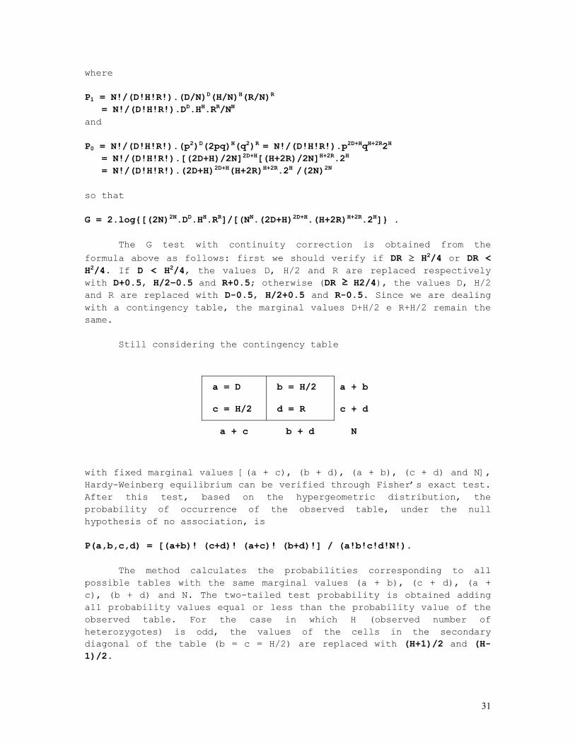
where P1 = N!/(D!H!R!).(D/N)D(H/N)H(R/N)R = N!/(D!H!R!).DD.HH.RR/NN and P0 = N!/(D!H!R!).(p2)D(2pq)H(q2)R = N!/(D!H!R!).p2D+HqH+2R2H = N!/(D!H!R!).[(2D+H)/2N]2D+H[(H+2R)/2N]H+2R.2H = N!/(D!H!R!).(2D+H)2D+H(H+2R)H+2R.2H /(2N)2N so that G = 2.log{[(2N)2N.DD.HH.RR]/[(NN.(2D+H)2D+H.(H+2R)H+2R.2H]} .
The G test with continuity correction is obtained from the formula above as follows: first we should verify if DR ≥ H2/4 or DR < H2/4. If D < H2/4, the values D, H/2 and R are replaced respectively with D+0.5, H/2–0.5 and R+0.5; otherwise (DR ≥ H2/4), the values D, H/2 and R are replaced with D-0.5, H/2+0.5 and R-0.5. Since we are dealing with a contingency table, the marginal values D+H/2 e R+H/2 remain the same.
Still considering the contingency table
a = D b = H/2 a + b
c = H/2 d = R c + d
a + c b + d N
with fixed marginal values [(a + c), (b + d), (a + b), (c + d) and N], Hardy-Weinberg equilibrium can be verified through Fisher’s exact test. After this test, based on the hypergeometric distribution, the probability of occurrence of the observed table, under the null hypothesis of no association, is P(a,b,c,d) = [(a+b)! (c+d)! (a+c)! (b+d)!] / (a!b!c!d!N!).
The method calculates the probabilities corresponding to all possible tables with the same marginal values (a + b), (c + d), (a + c), (b + d) and N. The two-tailed test probability is obtained adding all probability values equal or less than the probability value of the observed table. For the case in which H (observed number of heterozygotes) is odd, the values of the cells in the secondary diagonal of the table (b = c = H/2) are replaced with (H+1)/2 and (H-1)/2.
32
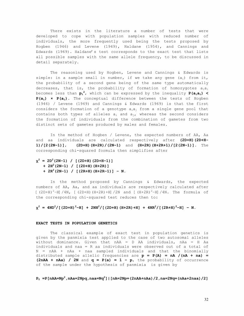
There exists in the literature a number of tests that were developed to cope with population samples with reduced number of individuals, the more frequently used being the tests proposed by Hogben (1946) and Levene (1949), Haldane (1954), and Cannings and Edwards (1969). Haldane’s test corresponds to the exact test that lists all possible samples with the same allele frequency, to be discussed in detail separately.
The reasoning used by Hogben, Levene and Cannings & Edwards is simple: in a sample small in number, if we take any gene (ai) from it, the probability of a second gene being of the same type automatically decreases, that is, the probability of formation of homozygotes aiai becomes less than pi2, which can be expressed by the inequality P(aiai) < P(ai) × P(ai). The conceptual difference between the tests of Hogben (1946) / Levene (1949) and Cannings & Edwards (1969) is that the first considers the formation of a genotype aiaj from a single gene pool that contains both types of alleles ai and aj, whereas the second considers the formation of individuals from the combination of gametes from two distinct sets of gametes produced by males and females.
In the method of Hogben / Levene, the expected numbers of AA, Aa and aa individuals are calculated respectively after (2D+H)(2D+H-1)/[2(2N–1)], (2D+H)(H+2R)/(2N–1) and (H+2R)(H+2R+1)/[2(2N–1)]. The corresponding chi-squared formula then simplifies after χ2 = 2D2(2N–1) / [(2D+H)(2D+H–1)] + 2H2(2N–1) / [(2D+H)(H+2R)] + 2R2(2N–1) / [(2R+H)(H+2R–1)] – N.
In the method proposed by Cannings & Edwards, the expected numbers of AA, Aa, and aa individuals are respectively calculated after [(2D+H)2–H]/4N, [(2D+H)(H+2R)+H]/2N and [(H+2R)2–H]/4N. The formula of the corresponding chi-squared test reduces then to: χ2 = 4ND2/[(2D+H)2–H] + 2NH2/[(2D+H)(H+2R)+H] + 4NR2/[(2R+H)2–H] – N. EXACT TESTS IN POPULATION GENETICS
The classical example of exact test in population genetics is given by the panmixia test applied to the case of two autosomal alleles without dominance. Given that nAA = D AA individuals, nAa = H Aa individuals and naa = R aa individuals were observed out of a total of N = nAA + nAa + naa sampled individuals and that the binomially distributed sample allelic frequencies are p = P(A) = nA /(nA + na) = (2nAA + nAa) / 2N and q = P(a) = 1 – p, the probability of occurrence of the sample under the hypothesis of panmixia is given by
P0 =P[nAA=Np2,nAa=2Npq,naa=Nq2]|[nA=2Np=(2nAA+nAa)/2,na=2Nq=(nAa+2naa)/2]
33
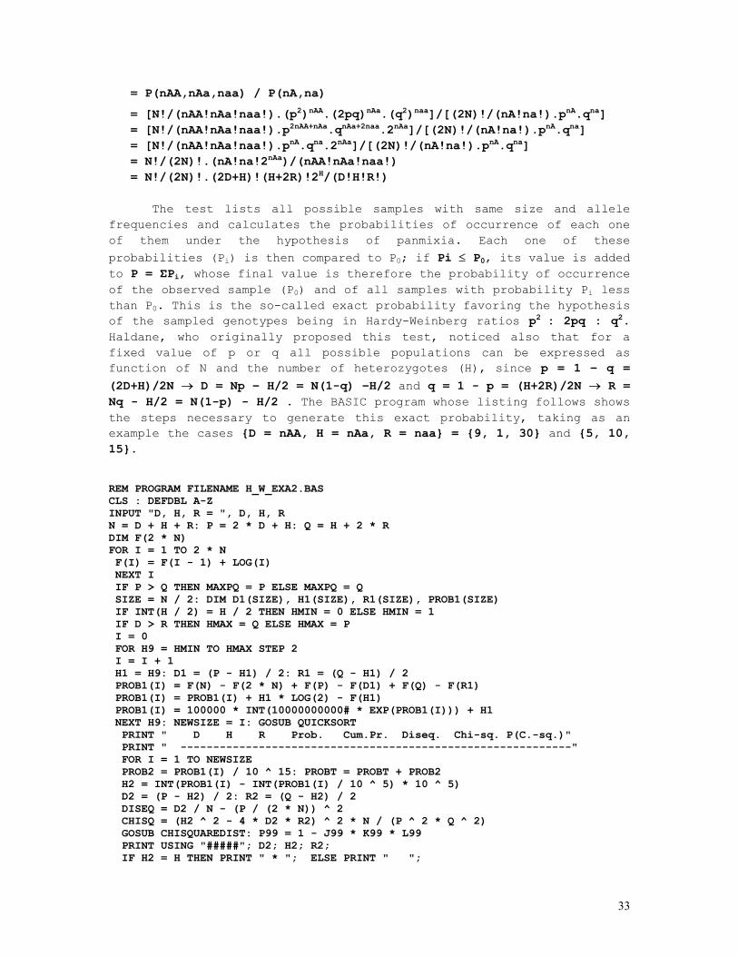
= P(nAA,nAa,naa) / P(nA,na)
= [N!/(nAA!nAa!naa!).(p2)nAA.(2pq)nAa.(q2)naa]/[(2N)!/(nA!na!).pnA.qna] = [N!/(nAA!nAa!naa!).p2nAA+nAa.qnAa+2naa.2nAa]/[(2N)!/(nA!na!).pnA.qna] = [N!/(nAA!nAa!naa!).pnA.qna.2nAa]/[(2N)!/(nA!na!).pnA.qna] = N!/(2N)!.(nA!na!2nAa)/(nAA!nAa!naa!) = N!/(2N)!.(2D+H)!(H+2R)!2H/(D!H!R!)
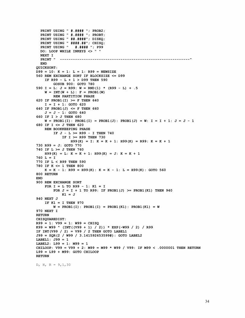
The test lists all possible samples with same size and allele frequencies and calculates the probabilities of occurrence of each one of them under the hypothesis of panmixia. Each one of these probabilities (Pi) is then compared to P0; if Pi ≤ P0, its value is added to P = ΣPi, whose final value is therefore the probability of occurrence of the observed sample (P0) and of all samples with probability Pi less than P0. This is the so-called exact probability favoring the hypothesis of the sampled genotypes being in Hardy-Weinberg ratios p2 : 2pq : q2. Haldane, who originally proposed this test, noticed also that for a fixed value of p or q all possible populations can be expressed as function of N and the number of heterozygotes (H), since p = 1 – q = (2D+H)/2N → D = Np – H/2 = N(1-q) –H/2 and q = 1 - p = (H+2R)/2N → R = Nq - H/2 = N(1-p) - H/2 . The BASIC program whose listing follows shows the steps necessary to generate this exact probability, taking as an example the cases {D = nAA, H = nAa, R = naa} = {9, 1, 30} and {5, 10, 15}. REM PROGRAM FILENAME H_W_EXA2.BAS CLS : DEFDBL A-Z INPUT "D, H, R = ", D, H, R N = D + H + R: P = 2 * D + H: Q = H + 2 * R DIM F(2 * N) FOR I = 1 TO 2 * N F(I) = F(I - 1) + LOG(I) NEXT I IF P > Q THEN MAXPQ = P ELSE MAXPQ = Q SIZE = N / 2: DIM D1(SIZE), H1(SIZE), R1(SIZE), PROB1(SIZE) IF INT(H / 2) = H / 2 THEN HMIN = 0 ELSE HMIN = 1 IF D > R THEN HMAX = Q ELSE HMAX = P I = 0 FOR H9 = HMIN TO HMAX STEP 2 I = I + 1 H1 = H9: D1 = (P - H1) / 2: R1 = (Q - H1) / 2 PROB1(I) = F(N) - F(2 * N) + F(P) - F(D1) + F(Q) - F(R1) PROB1(I) = PROB1(I) + H1 * LOG(2) - F(H1) PROB1(I) = 100000 * INT(10000000000# * EXP(PROB1(I))) + H1 NEXT H9: NEWSIZE = I: GOSUB QUICKSORT PRINT " D H R Prob. Cum.Pr. Diseq. Chi-sq. P(C.-sq.)" PRINT " ------------------------------------------------------------" FOR I = 1 TO NEWSIZE PROB2 = PROB1(I) / 10 ^ 15: PROBT = PROBT + PROB2 H2 = INT(PROB1(I) - INT(PROB1(I) / 10 ^ 5) * 10 ^ 5) D2 = (P - H2) / 2: R2 = (Q - H2) / 2 DISEQ = D2 / N - (P / (2 * N)) ^ 2 CHISQ = (H2 ^ 2 - 4 * D2 * R2) ^ 2 * N / (P ^ 2 * Q ^ 2) GOSUB CHISQUAREDIST: P99 = 1 - J99 * K99 * L99 PRINT USING "#####"; D2; H2; R2; IF H2 = H THEN PRINT " * "; ELSE PRINT " ";
34
PRINT USING " #.#### "; PROB2; PRINT USING " #.#### "; PROBT; PRINT USING " ##.####"; DISEQ; PRINT USING " ####.##"; CHISQ; PRINT USING " #.#### "; P99 DO: LOOP WHILE INKEY$ <> " " NEXT I PRINT " ------------------------------------------------------------" END QUICKSORT: D99 = 10: K = 1: L = 1: R99 = NEWSIZE 560 REM EXCHANGE SORT IF BLOCKSIZE <= D99 IF R99 - L + 1 > D99 THEN 590 GOSUB 900: GOTO 780 590 I = L: J = R99: W = RND(1) * (R99 - L) + .5 W = INT(W + L): F = PROB1(W) REM PARTITION PHASE 620 IF PROB1(I) >= F THEN 640 I = I + 1: GOTO 620 640 IF PROB1(J) <= F THEN 660 J = J - 1: GOTO 640 660 IF I > J THEN 680 W = PROB1(I): PROB1(I) = PROB1(J): PROB1(J) = W: I = I + 1: J = J - 1 680 IF I <= J THEN 620 REM BOOKKEEPING PHASE IF J - L >= R99 - I THEN 740 IF I >= R99 THEN 730 H99(K) = I: K = K + 1: H99(K) = R99: K = K + 1 730 R99 = J: GOTO 770 740 IF L >= J THEN 760 H99(K) = L: K = K + 1: H99(K) = J: K = K + 1 760 L = I 770 IF L < R99 THEN 590 780 IF K <= 1 THEN 800 K = K - 1: R99 = H99(K): K = K - 1: L = H99(K): GOTO 560 800 RETURN END 900 REM EXCHANGE SORT FOR I = L TO R99 - 1: K1 = I FOR J = I + 1 TO R99: IF PROB1(J) >= PROB1(K1) THEN 940 K1 = J 940 NEXT J IF K1 = I THEN 970 W = PROB1(I): PROB1(I) = PROB1(K1): PROB1(K1) = W 970 NEXT I RETURN CHISQUAREDIST: R99 = 1: V99 = 1: W99 = CHISQ K99 = W99 ^ (INT((V99 + 1) / 2)) * EXP(-W99 / 2) / R99 IF INT(V99 / 2) = V99 / 2 THEN GOTO LABEL1 J99 = SQR(2 / W99 / 3.141592653599#): GOTO LABEL2 LABEL1: J99 = 1 LABEL2: L99 = 1: M99 = 1 CHILOOP: V99 = V99 + 2: M99 = M99 * W99 / V99: IF M99 < .0000001 THEN RETURN L99 = L99 + M99: GOTO CHILOOP RETURN D, H, R = 9,1,30
35
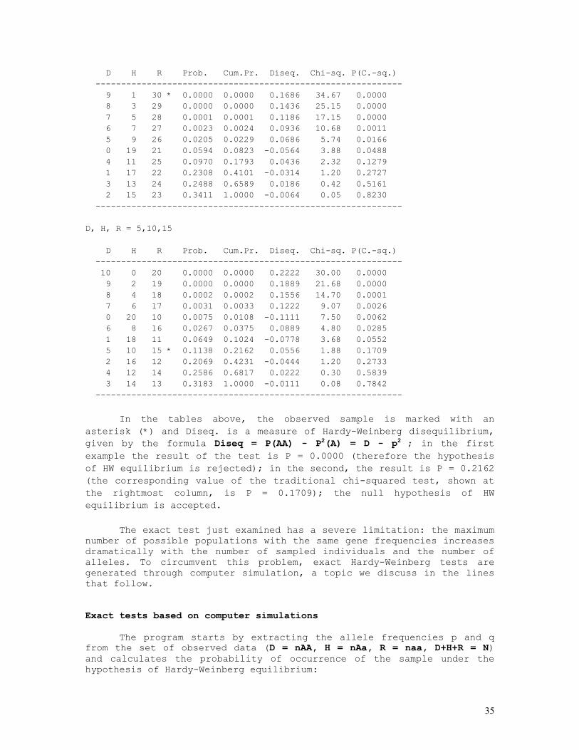
D H R Prob. Cum.Pr. Diseq. Chi-sq. P(C.-sq.) ------------------------------------------------------------ 9 1 30 * 0.0000 0.0000 0.1686 34.67 0.0000 8 3 29 0.0000 0.0000 0.1436 25.15 0.0000 7 5 28 0.0001 0.0001 0.1186 17.15 0.0000 6 7 27 0.0023 0.0024 0.0936 10.68 0.0011 5 9 26 0.0205 0.0229 0.0686 5.74 0.0166 0 19 21 0.0594 0.0823 -0.0564 3.88 0.0488 4 11 25 0.0970 0.1793 0.0436 2.32 0.1279 1 17 22 0.2308 0.4101 -0.0314 1.20 0.2727 3 13 24 0.2488 0.6589 0.0186 0.42 0.5161 2 15 23 0.3411 1.0000 -0.0064 0.05 0.8230 ------------------------------------------------------------ D, H, R = 5,10,15 D H R Prob. Cum.Pr. Diseq. Chi-sq. P(C.-sq.) ------------------------------------------------------------ 10 0 20 0.0000 0.0000 0.2222 30.00 0.0000 9 2 19 0.0000 0.0000 0.1889 21.68 0.0000 8 4 18 0.0002 0.0002 0.1556 14.70 0.0001 7 6 17 0.0031 0.0033 0.1222 9.07 0.0026 0 20 10 0.0075 0.0108 -0.1111 7.50 0.0062 6 8 16 0.0267 0.0375 0.0889 4.80 0.0285 1 18 11 0.0649 0.1024 -0.0778 3.68 0.0552 5 10 15 * 0.1138 0.2162 0.0556 1.88 0.1709 2 16 12 0.2069 0.4231 -0.0444 1.20 0.2733 4 12 14 0.2586 0.6817 0.0222 0.30 0.5839 3 14 13 0.3183 1.0000 -0.0111 0.08 0.7842 ------------------------------------------------------------
In the tables above, the observed sample is marked with an asterisk (*) and Diseq. is a measure of Hardy-Weinberg disequilibrium, given by the formula Diseq = P(AA) - P2(A) = D - p2 ; in the first example the result of the test is P = 0.0000 (therefore the hypothesis of HW equilibrium is rejected); in the second, the result is P = 0.2162 (the corresponding value of the traditional chi-squared test, shown at the rightmost column, is P = 0.1709); the null hypothesis of HW equilibrium is accepted.
The exact test just examined has a severe limitation: the maximum number of possible populations with the same gene frequencies increases dramatically with the number of sampled individuals and the number of alleles. To circumvent this problem, exact Hardy-Weinberg tests are generated through computer simulation, a topic we discuss in the lines that follow. Exact tests based on computer simulations
The program starts by extracting the allele frequencies p and q
from the set of observed data (D = nAA, H = nAa, R = naa, D+H+R = N) and calculates the probability of occurrence of the sample under the hypothesis of Hardy-Weinberg equilibrium:
36
P0 = N!/(2N)!.(nA!na!2nAa) /(nAA!nAa!naa!)
= N!/(2N)!.(2D+H)!(H+2R)!2H /(D!H!R!).
Then the program generates a random number between 0 and 1; if the number is smaller than or equal to p = (2D+H)/2N, this indicates that an A gene was obtained among the 2N of the sample; if the random number is larger than p, an a gene was sampled. The process is repeated 2N-1 times, and in each instance the random number generated is compared to p. A counter registers the number of times (X) the gene A is sampled and the frequency of the gene A in this first set of 2N simulations is therefore given by p’ = P(A) = X/2N; the frequency of the its allele a is calculated after q’ = P(a) = 1 – X/2N. Every two sequentially sampled genes are used for creating the genotypes AA, Aa, and aa. The counters D’, H’, and R’ accumulate the amount of times in which the genotypes AA, Aa and aa were obtained, each one being generated by two consecutive random numbers. Thus the first simulated population of N individuals and 2N genes has been formed. The computer repeats this process t times (t, the number of simulations, is defined by the computer user but generally is a number of the order of magnitude of 10,000). After each simulation the computer calculates the value of the probability Pi of occurrence of the sample under the hypothesis of Hardy-Weinberg equilibrium:
Pi = N!/(2N)!.(2Di’+Hi’)!(Hi’+2Ri’)!2Hi’/(Di’!Hi’!Ri’!).
This probability Pi is then compared to P0, the probability of occurrence of the observed sample under the hypothesis of HW equilibrium. The exact probability P, obtained after t simulations, is given by P = T/t (generally t = 10,000 and P = T/10,000), where T is the number of times in which Pi is smaller than or equal to P0 (Pi ≤ P0). The programs below (h_w_ext7.bas and h_w_ex13.bas), using different algorithms, perform all these calculations, in addition to give the mean values (over the t simulations performed) of p, D, H, and R generated by it.
REM PROGRAM FILENAME H_W_EXT7.BAS DEFDBL A-Z: CLS INPUT "D, H, R = "; D, H, R: N = D + H + R INPUT "NUMBER OF SIMULATIONS = "; T CHDIR "C:\TEMP": FILES "*.DAT" INPUT "FILE NAME FOR STORING DATA (DRIVE:FILENAME.EXT) = "; FILENAME$ CLS : OPEN FILENAME$ FOR OUTPUT AS #1 PRINT #1, FILENAME$ P = 2 * D + H: Q = H + 2 * R: P0 = P / (2 * N): P1 = P: Q1 = Q PRINT #1, D, H, R, N, P0, T TIMEWA$ = TIME$ TIMEWAS = VAL(MID$(TIMEWA$, 1, 2)) * 3600 + VAL(MID$(TIMEWA$, 4, 2)) * 60 TIMEWAS = TIMEWAS + VAL(MID$(TIMEWA$, 7, 2)) D1 = D: H1 = H: R1 = R K = N: GOSUB FACTORIAL: NFAC = FACT K = 2 * N: GOSUB FACTORIAL: N2FAC = FACT CONSTFAC = NFAC - N2FAC: D1 = D: H1 = H: R1 = R: GOSUB FACTPQDHR
37
PROB2 = EXP(CONSTFAC + PFAC + QFAC - DFAC - HFAC - RFAC + H1 * LOG(2)) FOR I = 1 TO T R1 = 0: D1 = 0: H1 = 0 FOR INDIV = 1 TO N A = RND(1): B = RND(1) IF A < P0 AND B < P0 THEN D1 = D1 + 1: GOTO NEXTINDIV IF A >= P0 AND B >= P0 THEN R1 = R1 + 1: GOTO NEXTINDIV H1 = H1 + 1 NEXTINDIV: NEXT INDIV P1 = 2 * D1 + H1: Q1 = H1 + 2 * R1 D1TOT = D1TOT + D1: H1TOT = H1TOT + H1: R1TOT = R1TOT + R1 PTOT = PTOT + P1 / (2 * N) GOSUB FACTPQDHR PROB1 = EXP(CONSTFAC + PFAC + QFAC - DFAC - HFAC - RFAC + H1 * LOG(2)) IF PROB1 <= PROB2 THEN PROBT = PROBT + 1 PRINT #1, P1, H1 LOCATE 6: PRINT USING "PERFORMING SIMULATION NO. ##### "; I; PRINT USING "OUT OF #####"; T NEXT I CLOSE #1 TIMENO$ = TIME$ TIMENOW = VAL(MID$(TIMENO$, 1, 2)) * 3600 + VAL(MID$(TIMENO$, 4, 2)) * 60 TIMENOW = TIMENOW + VAL(MID$(TIMENO$, 7, 2)) CLS : PRINT "NO. OF SIMULATED SAMPLES OF SIZE "; N; " = "; T PRINT "TOTAL ELAPSED TIME (ALL CALCULATIONS) = "; TIMENOW - TIMEWAS; " SEC." PRINT "DATA FROM DATAFILE "; FILENAME$: PRINT PRINT USING "SAMPLE P = #.####"; P0 PRINT USING "SAMPLE D = #####.####"; D PRINT USING "SAMPLE H = #####.####"; H PRINT USING "SAMPLE R = #####.####"; R: PRINT PRINT USING "P MEAN = #.####"; PTOT / T PRINT USING "OBS.D MEAN = #####.####"; D1TOT / T PRINT USING "OBS.H MEAN = #####.####"; H1TOT / T PRINT USING "OBS.R MEAN = #####.####"; R1TOT / T: PRINT PRINT USING "EX. PROB. = #.####"; PROBT / T DO: LOOP WHILE INKEY$ <> " " END FACTPQDHR: K = P1: GOSUB FACTORIAL: PFAC = FACT K = Q1: GOSUB FACTORIAL: QFAC = FACT K = D1: GOSUB FACTORIAL: DFAC = FACT K = H1: GOSUB FACTORIAL: HFAC = FACT K = R1: GOSUB FACTORIAL: RFAC = FACT: RETURN FACTORIAL: FACT = 0: FOR J = 1 TO K: FACT = FACT + LOG(J): NEXT J: RETURN
REM PROGRAM FILENAME H_W_EX13.BAS REM 'EXACT' HARDY-WEINBERG TEST (TWO AUTOSOMAL ALLELES) REM GENERATES T RANDOM SAMPLES OF SIZE N = D + H + R REM WITH GENOTYPE PROBABILITIES d = p^2, h = 2pq, r = q^2 REM p = (2D+H)/2, q = 1-p DEFDBL A-Z: CLS INPUT "D, H, R = "; D, H, R: N = D + H + R INPUT "NUMBER OF SIMULATIONS = "; T CHDIR "C:\TEMP": FILES "*.DAT" INPUT "FILE NAME FOR STORING DATA (DRIVE:FILENAME.EXT) = "; FILENAME$ OPEN FILENAME$ FOR OUTPUT AS #1 PRINT #1, FILENAME$ P = 2 * D + H: Q = H + 2 * R: P0 = P / (2 * N) PRINT #1, D, H, R, N, P0, T CLS FOR I = 1 TO T INDIV = 0: R1 = 0: D1 = 0: H1 = 0 DO WHILE INDIV < N
38
A = RND(1) B = RND(1) IF A < P0 AND B < P0 THEN GENOTYPE = 2 ELSEIF A >= P0 AND B >= P0 THEN GENOTYPE = 0 ELSE GENOTYPE = 1 END IF SELECT CASE GENOTYPE CASE 0 INDIV = INDIV + 1 R1 = R1 + 1 CASE 2 INDIV = INDIV + 1 D1 = D1 + 1 CASE 1 INDIV = INDIV + 1 H1 = H1 + 1 END SELECT LOOP P1 = 2 * D1 + H1: Q1 = H1 + 2 * R1 D1TOT = D1TOT + D1: H1TOT = H1TOT + H1: R1TOT = R1TOT + R1 PTOT = PTOT + P1 PRINT #1, P1, H1 LOCATE 6: PRINT USING "PERFORMING SIMULATION NO. ##### "; I; PRINT USING "OUT OF #####"; T NEXT I CLOSE #1 PRINT : PRINT "DATA FROM DATAFILE "; FILENAME$: PRINT PRINT USING "SAMPLE P = #.####"; P0 PRINT USING "SAMPLE D = #####.####"; D PRINT USING "SAMPLE H = #####.####"; H PRINT USING "SAMPLE R = #####.####"; R: PRINT PRINT USING "P MEAN = #.####"; PTOT / (2 * T * N) PRINT USING "OBS.D MEAN = #####.####"; D1TOT / T PRINT USING "OBS.H MEAN = #####.####"; H1TOT / T PRINT USING "OBS.R MEAN = #####.####"; R1TOT / T: PRINT
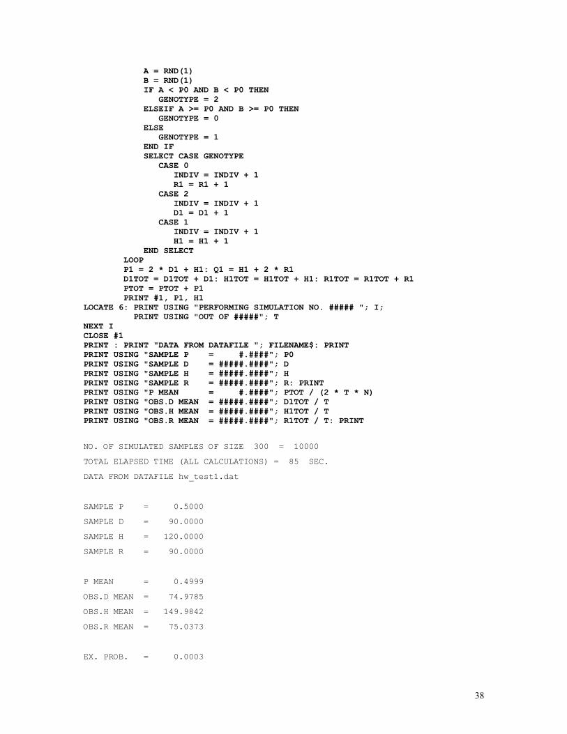
NO. OF SIMULATED SAMPLES OF SIZE 300 = 10000
TOTAL ELAPSED TIME (ALL CALCULATIONS) = 85 SEC.
DATA FROM DATAFILE hw_test1.dat
SAMPLE P = 0.5000
SAMPLE D = 90.0000
SAMPLE H = 120.0000
SAMPLE R = 90.0000
P MEAN = 0.4999
OBS.D MEAN = 74.9785
OBS.H MEAN = 149.9842
OBS.R MEAN = 75.0373
EX. PROB. = 0.0003
39
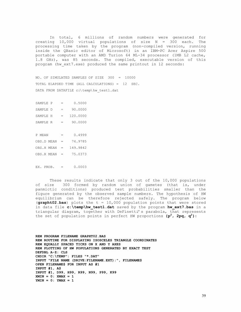
In total, 6 millions of random numbers were generated for creating 10,000 virtual populations of size N = 300 each. The processing time taken by the program (non-compiled version, running inside the QBasic editor of Microsoft) in an IBM-PC Acer Aspire 500 portable computer with an AMD Turion 64 ML-34 processor (1MB L2 cache, 1.8 GHz), was 85 seconds. The compiled, executable version of this program (hw_ext7.exe) produced the same printout in 12 seconds:
NO. OF SIMULATED SAMPLES OF SIZE 300 = 10000
TOTAL ELAPSED TIME (ALL CALCULATIONS) = 12 SEC.
DATA FROM DATAFILE c:\temp\hw_test1.dat
SAMPLE P = 0.5000
SAMPLE D = 90.0000
SAMPLE H = 120.0000
SAMPLE R = 90.0000
P MEAN = 0.4999
OBS.D MEAN = 74.9785
OBS.H MEAN = 149.9842
OBS.R MEAN = 75.0373
EX. PROB. = 0.0003
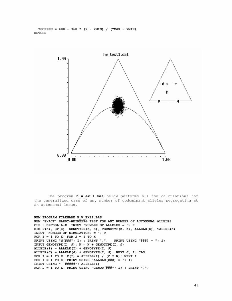
These results indicate that only 3 out of the 10,000 populations of size 300 formed by random union of gametes (that is, under panmictic conditions) produced test probabilities smaller than the figure generated by the observed sample numbers. The hypothesis of HW equilibrium can be therefore rejected safely. The program below (grapht02.bas) plots the t = 10,000 population points that were stored in data file c:\temp\hw_test1.dat saved by the program hw_ext7.bas in a triangular diagram, together with DeFinetti’s parabola, that represents the set of population points in perfect HW proportions {p2, 2pq, q2}:
REM PROGRAM FILENAME GRAPHT02.BAS REM ROUTINE FOR DISPLAYING ISOSCELES TRIANGLE COORDINATES REM EQUALLY SPACED TICKS ON X AND Y AXES REM PLOTTING OF HW POPULATIONS GENERATED BY EXACT TEST DEFDBL A-Z: CLS CHDIR "C:\TEMP": FILES "*.DAT" INPUT "FILE NAME (DRIVE:FILENAME.EXT):", FILENAME$ OPEN FILENAME$ FOR INPUT AS #1 INPUT #1, A$ INPUT #1, D99, H99, R99, N99, P99, K99 XMIN = 0: XMAX = 1 YMIN = 0: YMAX = 1
40
SCREEN 12: REM VGA GRAPHICS MODE RESOLUTION 480 x 640 REM SMALL TRIANGLE WITH EXPLANATIONS LINE (440, 200)-(520, 40) LINE -(600, 200) LINE (440, 200)-(467, 200) LINE (484, 200)-(538, 200) LINE (556, 200)-(600, 200) LINE (506, 136)-(506, 155) LINE (506, 179)-(506, 200) LINE (472, 136)-(482, 136) LINE (499, 136)-(530, 136) LINE (547, 136)-(568, 136) CIRCLE (506, 136), 3 LOCATE 9, 62: PRINT "d" LOCATE 9, 68: PRINT "r" LOCATE 11, 64: PRINT "h" LOCATE 13, 60: PRINT "p" LOCATE 13, 69: PRINT "q" REM GRAPH AXES LINE (130, 40)-(130, 400) LINE (140, 410)-(500, 410) REM SIDES OF ISOSCELES TRIANGLE LINE (140, 400)-(320, 40) LINE -(500, 400) LINE -(140, 400) REM Y-AXIS TICKS FOR I = 40 TO 400 STEP 18 LINE (126, I)-(130, I) NEXT I REM X-AXIS TICKS FOR I = 140 TO 500 STEP 18 LINE (I, 410)-(I, 414) NEXT I FOR X = XMIN TO XMAX STEP 1 / 400 Y = 2 * X * (1 - X) GOSUB PLOTXY IF X = XMIN THEN PSET (XSCREEN, YSCREEN) ELSE LINE -(XSCREEN, YSCREEN) NEXT X X = XMAX Y = 2 * X * (1 - X) GOSUB PLOTXY LINE -(XSCREEN, YSCREEN) FOR I99 = 1 TO K99 INPUT #1, X: X = X / (2 * N99) INPUT #1, Y: Y = Y / N99 GOSUB PLOTXY CIRCLE (XSCREEN, YSCREEN), 1 NEXT I99 CLOSE #1 LOCATE 2, (81 - LEN(A$)) / 2: PRINT A$ LOCATE 3, 9: PRINT USING "####.##"; YMAX 'LOCATE 14, 15: PRINT "h" LOCATE 26, 9: PRINT USING "####.##"; YMIN LOCATE 27, 15: PRINT USING "###.##"; XMIN LOCATE 27, 60: PRINT USING "###.##"; XMAX 'LOCATE 27, 40: PRINT "p" STAYHERE: REM PRESS THE SPACE BAR TO RETURN TO QBASIC IF INKEY$ <> " " THEN GOTO STAYHERE SCREEN 0, 0, 0 END PLOTXY: XSCREEN = 140 + 360 * (X - XMIN) / (XMAX - XMIN)
41
YSCREEN = 400 - 360 * (Y - YMIN) / (YMAX - YMIN) RETURN
The program h_w_ex11.bas below performs all the calculations for the generalized case of any number of codominant alleles segregating at an autosomal locus. REM PROGRAM FILENAME H_W_EX11.BAS REM 'EXACT' HARDY-WEINBERG TEST FOR ANY NUMBER OF AUTOSOMAL ALLELES CLS : DEFDBL A-Z: INPUT "NUMBER OF ALLELES = "; K DIM P(K), SP(K), GENOTYPE(K, K), TGENOTYP(K, K), ALLELE(K), TALLEL(K) INPUT "NUMBER OF SIMULATIONS = "; T FOR I = 1 TO K: FOR J = I TO K PRINT USING "N(###"; I; : PRINT ","; : PRINT USING "###) = "; J; INPUT GENOTYPE(I, J): N = N + GENOTYPE(I, J) ALLELE(I) = ALLELE(I) + GENOTYPE(I, J) ALLELE(J) = ALLELE(J) + GENOTYPE(I, J): NEXT J, I: CLS FOR I = 1 TO K: P(I) = ALLELE(I) / (2 * N): NEXT I FOR I = 1 TO K: PRINT USING "ALLELE(###) = "; I; PRINT USING " #####"; ALLELE(I) FOR J = I TO K: PRINT USING "GENOT(###"; I; : PRINT ",";
42
PRINT USING "###) = "; J; : PRINT USING "####"; GENOTYPE(I, J) DO: LOOP WHILE INKEY$ <> " " NEXT J, I PRINT USING "N = ######"; N DO: LOOP WHILE INKEY$ <> " " CLS K9 = N: GOSUB FACTORIAL: NFAC = FACT K9 = 2 * N: GOSUB FACTORIAL: N2FAC = FACT CONSTFAC = NFAC - N2FAC GOSUB EXACTPROBCALC: PROB2 = EXPROB FOR I = 1 TO K: SSP = SSP + P(I): SP(I) = SP(I) + SSP: NEXT I FOR I = 1 TO T GOSUB CLEARALLVAR FOR INDIV = 1 TO N A = RND(1): B = RND(1) FOR I88 = 1 TO K IF A > SP(I88 - 1) AND A <= SP(I88) THEN AI88 = I88: ALLELE(I88) = ALLELE(I88) + 1 TALLEL(I88) = TALLEL(I88) + 1 END IF IF B > SP(I88 - 1) AND B <= SP(I88) THEN BI88 = I88: ALLELE(I88) = ALLELE(I88) + 1 TALLEL(I88) = TALLEL(I88) + 1 END IF NEXT I88 IF AI88 > BI88 THEN SWAP AI88, BI88 GENOTYPE(AI88, BI88) = GENOTYPE(AI88, BI88) + 1 TGENOTYP(AI88, BI88) = TGENOTYP(AI88, BI88) + 1 NEXT INDIV GOSUB EXACTPROBCALC: PROB1 = EXPROB IF PROB1 <= PROB2 THEN PROBT = PROBT + 1 LOCATE 10: PRINT "SIMULATION NO. "; I NEXT I DO: LOOP WHILE INKEY$ <> " " CLS PRINT "OVERALL RESULTS BASED ON "; T; " SIMULATIONS OF SIZE "; N; " INDIVIDUALS" FOR I77 = 1 TO K PRINT USING "ALLELE(###) = "; I77; : PRINT USING "#####.####"; TALLEL(I77) / T FOR J77 = I77 TO K PRINT USING "GENOTYPE(###"; I77; : PRINT ","; PRINT USING "###) = "; J77; : PRINT USING "#####.####"; TGENOTYP(I77, J77) / T DO: LOOP WHILE INKEY$ <> " " NEXT J77, I77 PRINT : PRINT USING "EXACT PROB. = #.####"; PROBT / T END CLEARALLVAR: HETLOG = 0: ALLELFAC = 0: GENOTFAC = 0 FOR I66 = 1 TO K ALLELE(I66) = 0 FOR J66 = I66 TO K: GENOTYPE(I66, J66) = 0 NEXT J66, I66 RETURN EXACTPROBCALC: GOSUB FACTALLEL: GOSUB FACTGENOT FOR I9 = 1 TO K - 1: FOR J9 = I9 + 1 TO K IF I9 <> J9 THEN HETLOG = HETLOG + GENOTYPE(I9, J9) * LOG(2) NEXT J9, I9 EXPROB = EXP(CONSTFAC + ALLELFAC - GENOTFAC + HETLOG) RETURN
43
FACTALLEL: FOR I9 = 1 TO K K9 = ALLELE(I9): GOSUB FACTORIAL: ALLELFAC = ALLELFAC + FACT NEXT I9 RETURN FACTGENOT: FOR I9 = 1 TO K: FOR J9 = I9 TO K K9 = GENOTYPE(I9, J9): GOSUB FACTORIAL: GENOTFAC = GENOTFAC + FACT NEXT J9, I9 RETURN FACTORIAL: FACT = 0 FOR J = 1 TO K9 FACT = FACT + LOG(J) NEXT J RETURN NUMBER OF ALLELES = ? 4
NUMBER OF SIMULATIONS = ? 10000
N( 1, 1) = ? 1
N( 1, 2) = ? 5
N( 1, 3) = ? 7
N( 1, 4) = ? 8
N( 2, 2) = ? 3
N( 2, 3) = ? 11
N( 2, 4) = ? 16
N( 3, 3) = ? 8
N( 3, 4) = ? 25
N( 4, 4) = ? 16
ALLELE( 1) = 22
GENOT( 1, 1) = 1
GENOT( 1, 2) = 5
GENOT( 1, 3) = 7
GENOT( 1, 4) = 8
ALLELE( 2) = 38
GENOT( 2, 2) = 3
GENOT( 2, 3) = 11
GENOT( 2, 4) = 16
ALLELE( 3) = 59
GENOT( 3, 3) = 8
GENOT( 3, 4) = 25
ALLELE( 4) = 81
GENOT( 4, 4) = 16
N = 100
44
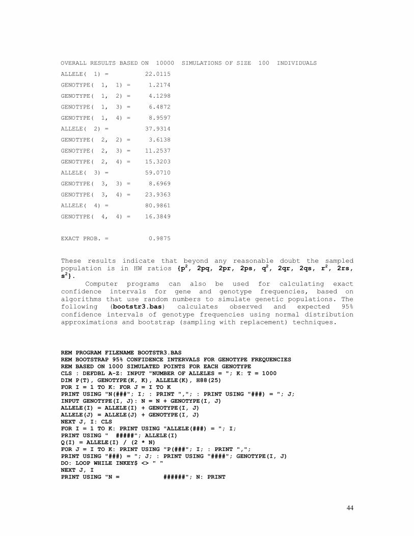
OVERALL RESULTS BASED ON 10000 SIMULATIONS OF SIZE 100 INDIVIDUALS
ALLELE( 1) = 22.0115
GENOTYPE( 1, 1) = 1.2174
GENOTYPE( 1, 2) = 4.1298
GENOTYPE( 1, 3) = 6.4872
GENOTYPE( 1, 4) = 8.9597
ALLELE( 2) = 37.9314
GENOTYPE( 2, 2) = 3.6138
GENOTYPE( 2, 3) = 11.2537
GENOTYPE( 2, 4) = 15.3203
ALLELE( 3) = 59.0710
GENOTYPE( 3, 3) = 8.6969
GENOTYPE( 3, 4) = 23.9363
ALLELE( 4) = 80.9861
GENOTYPE( 4, 4) = 16.3849
EXACT PROB. = 0.9875
These results indicate that beyond any reasonable doubt the sampled population is in HW ratios {p2, 2pq, 2pr, 2ps, q2, 2qr, 2qs, r2, 2rs, s2}.
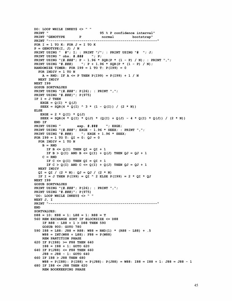
Computer programs can also be used for calculating exact confidence intervals for gene and genotype frequencies, based on algorithms that use random numbers to simulate genetic populations. The following (bootstr3.bas) calculates observed and expected 95% confidence intervals of genotype frequencies using normal distribution approximations and bootstrap (sampling with replacement) techniques.
REM PROGRAM FILENAME BOOTSTR3.BAS REM BOOTSTRAP 95% CONFIDENCE INTERVALS FOR GENOTYPE FREQUENCIES REM BASED ON 1000 SIMULATED POINTS FOR EACH GENOTYPE CLS : DEFDBL A-Z: INPUT "NUMBER OF ALLELES = "; K: T = 1000 DIM P(T), GENOTYPE(K, K), ALLELE(K), H88(25) FOR I = 1 TO K: FOR J = I TO K PRINT USING "N(###"; I; : PRINT ","; : PRINT USING "###) = "; J; INPUT GENOTYPE(I, J): N = N + GENOTYPE(I, J) ALLELE(I) = ALLELE(I) + GENOTYPE(I, J) ALLELE(J) = ALLELE(J) + GENOTYPE(I, J) NEXT J, I: CLS FOR I = 1 TO K: PRINT USING "ALLELE(###) = "; I; PRINT USING " #####"; ALLELE(I) Q(I) = ALLELE(I) / (2 * N) FOR J = I TO K: PRINT USING "P(###"; I; : PRINT ","; PRINT USING "###) = "; J; : PRINT USING "####"; GENOTYPE(I, J) DO: LOOP WHILE INKEY$ <> " " NEXT J, I PRINT USING "N = ######"; N: PRINT
45
DO: LOOP WHILE INKEY$ <> " " PRINT " 95 % P confidence interval" PRINT "GENOTYPE P normal bootstrap" PRINT "-----------------------------------------------------" FOR I = 1 TO K: FOR J = I TO K P = GENOTYPE(I, J) / N PRINT USING " #"; I; : PRINT "/"; : PRINT USING "# "; J; PRINT USING " obs. #.### "; P; PRINT USING "{#.###"; P - 1.96 * SQR(P * (1 - P) / N); : PRINT ","; PRINT USING "#.###} "; P + 1.96 * SQR(P * (1 - P) / N); RANDOMIZE TIMER: FOR I99 = 1 TO T: P(I99) = 0 FOR INDIV = 1 TO N A = RND: IF A <= P THEN P(I99) = P(I99) + 1 / N NEXT INDIV NEXT I99 GOSUB SORTVALUES PRINT USING "{#.###"; P(26); : PRINT ","; PRINT USING "#.###}"; P(975) IF I = J THEN EXGE = Q(I) * Q(J) SEEX = SQR(4 * Q(I) ^ 3 * (1 - Q(I)) / (2 * N)) ELSE EXGE = 2 * Q(I) * Q(J) SEEX = SQR(4 * Q(I) * Q(J) * (Q(I) + Q(J) - 4 * Q(I) * Q(J)) / (2 * N)) END IF PRINT USING " exp. #.### "; EXGE; PRINT USING "{#.###"; EXGE - 1.96 * SEEX; : PRINT ","; PRINT USING "#.###} "; EXGE + 1.96 * SEEX; FOR I99 = 1 TO T: QI = 0: QJ = 0 FOR INDIV = 1 TO N B = RND IF B <= Q(I) THEN QI = QI + 1 IF B > Q(I) AND B <= Q(I) + Q(J) THEN QJ = QJ + 1 C = RND IF C <= Q(I) THEN QI = QI + 1 IF C > Q(I) AND C <= Q(I) + Q(J) THEN QJ = QJ + 1 NEXT INDIV QI = QI / (2 * N): QJ = QJ / (2 * N) IF I = J THEN P(I99) = QI ^ 2 ELSE P(I99) = 2 * QI * QJ NEXT I99 GOSUB SORTVALUES PRINT USING "{#.###"; P(26); : PRINT ","; PRINT USING "#.###}"; P(975) 'DO: LOOP WHILE INKEY$ <> " " NEXT J, I PRINT "-----------------------------------------------------" END SORTVALUES: D88 = 10: K88 = 1: L88 = 1: R88 = T 560 REM EXCHANGE SORT IF BLOCKSIZE <= D88 IF R88 - L88 + 1 > D88 THEN 590 GOSUB 900: GOTO 780 590 I88 = L88: J88 = R88: W88 = RND(1) * (R88 - L88) + .5 W88 = INT(W88 + L88): F88 = P(W88) REM PARTITION PHASE 620 IF P(I88) >= F88 THEN 640 I88 = I88 + 1: GOTO 620 640 IF P(J88) <= F88 THEN 660 J88 = J88 - 1: GOTO 640 660 IF I88 > J88 THEN 680 W88 = P(I88): P(I88) = P(J88): P(J88) = W88: I88 = I88 + 1: J88 = J88 - 1 680 IF I88 <= J88 THEN 620 REM BOOKKEEPING PHASE
46
IF J88 - L88 >= R88 - I88 THEN 740 IF I88 >= R88 THEN 730 H88(K88) = I88: K88 = K88 + 1: H88(K88) = R88: K88 = K88 + 1 730 R88 = J88: GOTO 770 740 IF L88 >= J88 THEN 760 H88(K88) = L88: K88 = K88 + 1: H88(K88) = J88: K88 = K88 + 1 760 L88 = I88 770 IF L88 < R88 THEN 590 780 IF K88 <= 1 THEN 800 K88 = K88 - 1: R88 = H88(K88): K88 = K88 - 1: L88 = H88(K88): GOTO 560 800 RETURN 900 REM EXCHANGE SORT FOR I88 = L88 TO R88 - 1: K1 = I88 FOR J88 = I88 + 1 TO R88: IF P(J88) >= P(K1) THEN 940 K1 = J88 940 NEXT J88 IF K1 = I88 THEN 970 W88 = P(I88): P(I88) = P(K1): P(K1) = W88 970 NEXT I88 RETURN NUMBER OF ALLELES = ? 2 N( 1, 1) = ? 10 N( 1, 2) = ? 15 N( 2, 2) = ? 20 ALLELE( 1) = 35
P( 1, 1) = 10
P( 1, 2) = 15
ALLELE( 2) = 55
P( 2, 2) = 20
N = 45
95 % P confidence interval
GENOTYPE P normal bootstrap
-----------------------------------------------------
1/1 obs. 0.222 {0.101,0.344} {0.111,0.356}
exp. 0.151 {0.073,0.230} {0.083,0.239}
1/2 obs. 0.333 {0.196,0.471} {0.200,0.467}
exp. 0.475 {0.431,0.520} {0.411,0.499}
2/2 obs. 0.444 {0.299,0.590} {0.311,0.578}
exp. 0.373 {0.250,0.497} {0.261,0.506}
-----------------------------------------------------
NUMBER OF ALLELES = ? 3
N( 1, 1) = ? 5
N( 1, 2) = ? 6
N( 1, 3) = ? 7
N( 2, 2) = ? 8
N( 2, 3) = ? 9
47
N( 3, 3) = ? 10
ALLELE( 1) = 23
P( 1, 1) = 5
P( 1, 2) = 6
P( 1, 3) = 7
ALLELE( 2) = 31
P( 2, 2) = 8
P( 2, 3) = 9
ALLELE( 3) = 36
P( 3, 3) = 10
N = 45
95 % P confidence interval
GENOTYPE P normal bootstrap
-----------------------------------------------------
1/1 obs. 0.111 {0.019,0.203} {0.022,0.200}
exp. 0.065 {0.019,0.111} {0.028,0.119}
1/2 obs. 0.133 {0.034,0.233} {0.044,0.244}
exp. 0.176 {0.115,0.237} {0.117,0.237}
1/3 obs. 0.156 {0.050,0.261} {0.067,0.267}
exp. 0.204 {0.139,0.270} {0.137,0.268}
2/2 obs. 0.178 {0.066,0.289} {0.067,0.289}
exp. 0.119 {0.051,0.186} {0.060,0.198}
2/3 obs. 0.200 {0.083,0.317} {0.089,0.311}
exp. 0.276 {0.208,0.343} {0.204,0.344}
3/3 obs. 0.222 {0.101,0.344} {0.111,0.356}
exp. 0.160 {0.079,0.241} {0.090,0.250}
-----------------------------------------------------
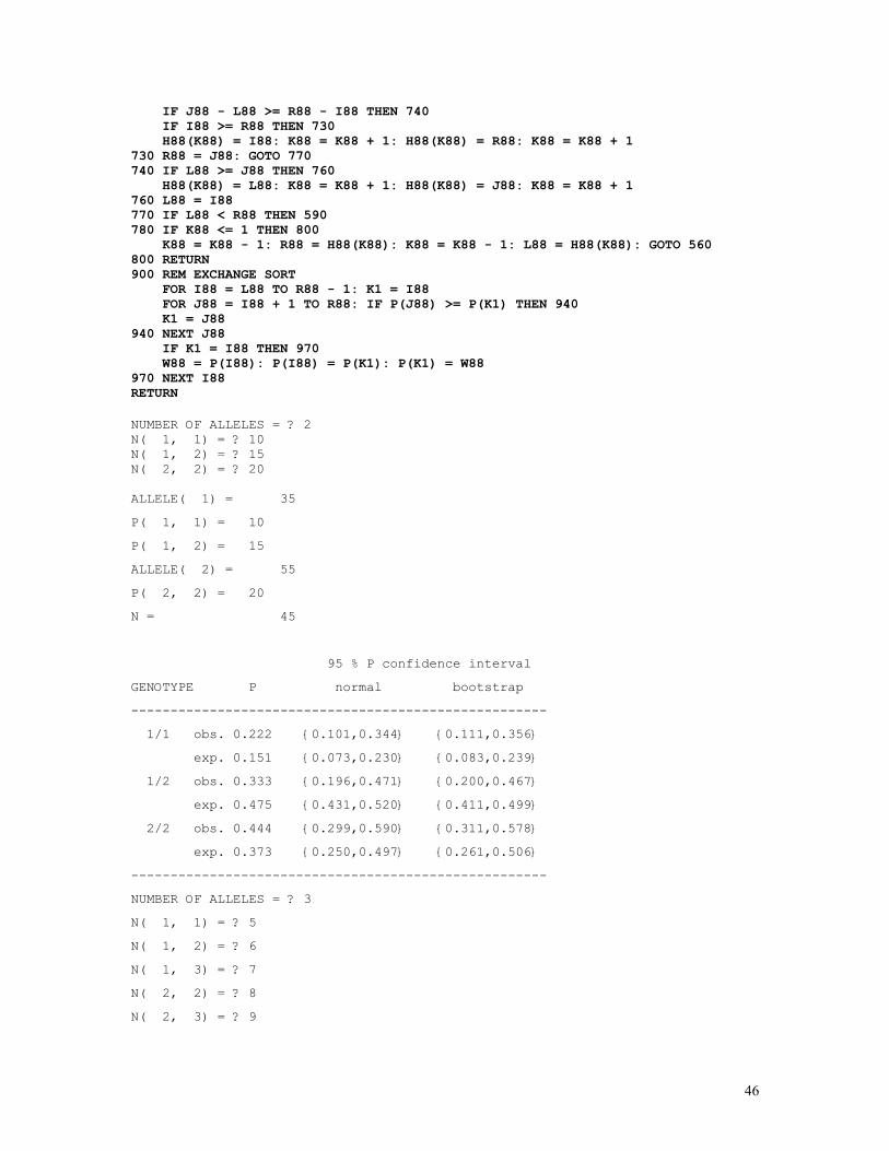
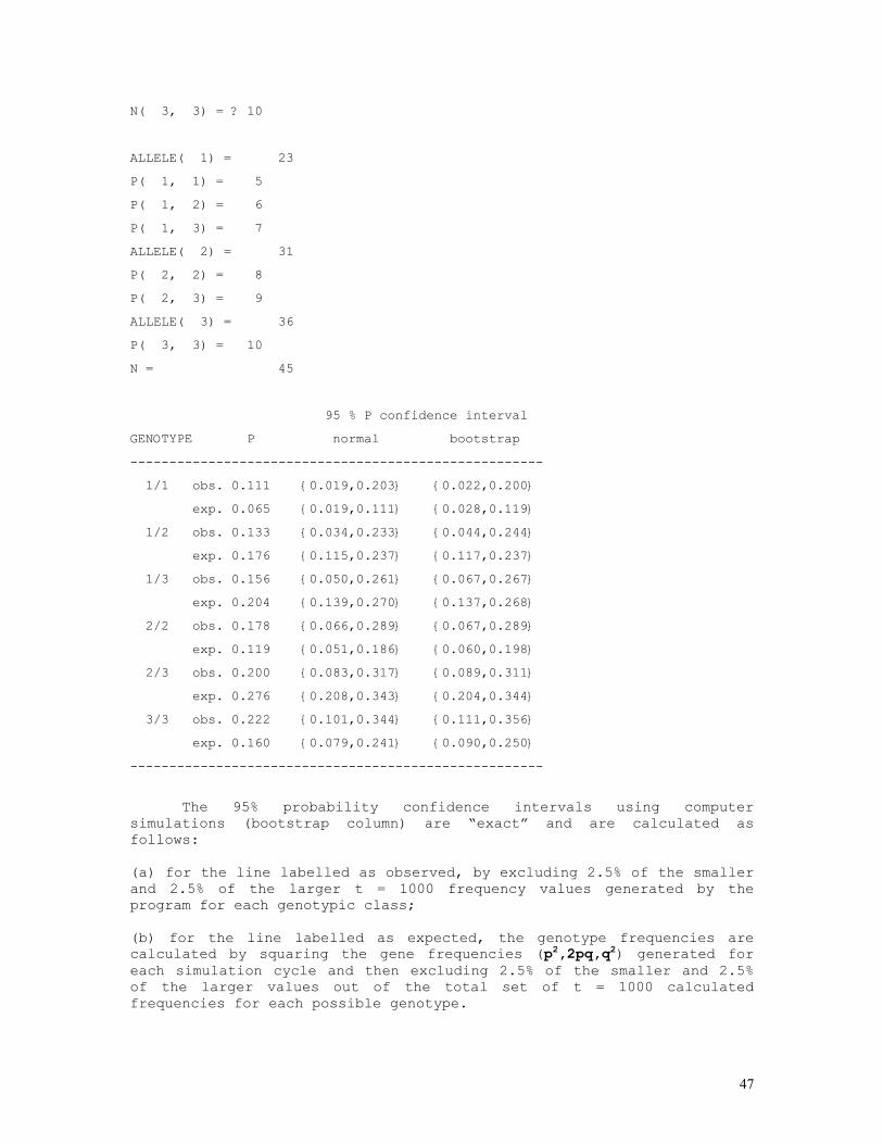
The 95% probability confidence intervals using computer
simulations (bootstrap column) are “exact” and are calculated as follows:
(a) for the line labelled as observed, by excluding 2.5% of the smaller and 2.5% of the larger t = 1000 frequency values generated by the program for each genotypic class; (b) for the line labelled as expected, the genotype frequencies are calculated by squaring the gene frequencies (p2,2pq,q2) generated for each simulation cycle and then excluding 2.5% of the smaller and 2.5% of the larger values out of the total set of t = 1000 calculated frequencies for each possible genotype.

48
The normal approximations to these confidence intervals are constructed:
(a) for the line labelled as observed the confidence intervals are obtained directly from the sampled observed values of P(AA), P(AB), P(AC), etc.: pij = P(AiAj), s.e.(pij) = pij(1-pij)/N, 95% c.i. = pij ± 1.96 s.e.(pij); (b) for the line labelled as expected, the same procedure is applied but the standard errors are calculated after s.e.[P(AiAj)] = s.e.(pij) = √[4pi3(1-pi)/2N] if i=j, s.e.[P(AiAj)] = s.e.(pij) = √[4pipj(pi+pj-4pipj)/2N] otherwise.
All the simulation methods that we have just reviewed generate exact probabilities using models that permit random fluctuations in gene frequencies and that therefore are not strictly correspondent to Haldane’s exact test, which assumes that gene frequencies are fixed. The program below (h_wex13a.bas) takes this into account, using a model of generation of genotype frequencies conditional to constant gene frequency, equivalent to a system in which the alleles are randomly drawn from a genic pool of finite size 2N without replacement. The method circumvents the difficulties that normally arise in Haldane’s method with the increasing of the sample number and of the allele number, as we show below: REM PROGRAM FILENAME H_WEX13A.BAS REM 'EXACT' HARDY-WEINBERG TEST (TWO AUTOSOMAL ALLELES) REM GENERATES T RANDOM SAMPLES OF SIZE N = D + H + R REM WITH GENOTYPE PROBABILITIES d = p^2, h = 2pq, r = q^2 REM p = (2D+H)/2, q = 1-p REM WITHOUT REPLACEMENT DEFDBL A-Z: CLS INPUT "D, H, R = "; D, H, R: N = D + H + R: P = 2 * D + H: DIM NH(P + 2), PROB1(P + 2), AUX(P + 2) INPUT "NUMBER OF SIMULATIONS = "; T: CHDIR "C:\TEMP": FILES "*.DAT" INPUT "FILE NAME FOR STORING DATA (DRIVE:FILENAME.EXT) = "; FILENAME$ OPEN FILENAME$ FOR OUTPUT AS #1: PRINT #1, FILENAME$ PRINT #1, D, H, R, P, N, T CLS FOR I = 1 TO T INDIV = 0: R1 = 0: D1 = 0: H1 = 0: N1 = N: P1 = P DO WHILE INDIV < N A = RND(1): B = RND(1): GENOT = 3 IF A < P1 / (2 * N1) AND B < (P1 - 1) / (2 * N1 - 1) THEN GENOT = 2 IF A >= P1 / (2 * N1) AND B >= P1 / (2 * N1 - 1) THEN GENOT = 0 IF GENOT = 3 THEN GENOT = 1 N1 = N1 - 1: P1 = P1 - GENOT SELECT CASE GENOT CASE 0: R1 = R1 + 1 CASE 2: D1 = D1 + 1 CASE 1: H1 = H1 + 1 END SELECT INDIV = INDIV + 1 LOOP D1TOT = D1TOT + D1: H1TOT = H1TOT + H1: R1TOT = R1TOT + R1 PTOT = PTOT + 2 * D1 + H1: NH(H1) = NH(H1) + 1 LOCATE 6: PRINT USING "PERFORMING SIMULATION NO. ##### "; I; PRINT USING "OUT OF #####"; T NEXT I:
49
PRINT : PRINT "DATA FROM DATAFILE "; FILENAME$: PRINT PRINT USING "SAMPLE P = #.####"; P / (2 * N) PRINT USING "SAMPLE D = #####.####"; D PRINT USING "SAMPLE H = #####.####"; H PRINT USING "SAMPLE R = #####.####"; R: PRINT PRINT USING "SIM.P MEAN = #.####"; PTOT / (2 * T * N) PRINT USING "SIM.D MEAN = #####.####"; D1TOT / T PRINT USING "SIM.H MEAN = #####.####"; H1TOT / T PRINT USING "SIM.R MEAN = #####.####"; R1TOT / T: PRINT FOR I = 0 TO P + 1 IF NH(I) <> 0 THEN PROB1(I) = NH(I): AUX(I) = I END IF NEXT I GOSUB QUICKSORT PRINT #1, " D H R f(x) F(x)" PRINT #1, "-----------------------------" FOR H1 = 0 TO P + 1 IF PROB1(H1) <> 0 THEN AC = AC + PROB1(H1) / T PRINT #1, USING "#### "; (P - AUX(H1)) / 2; AUX(H1); N - (P + AUX(H1)) / 2; IF AUX(H1) = H THEN PRINT #1, "*"; ELSE PRINT #1, " "; PRINT #1, USING " #.###"; PROB1(H1) / T; PRINT #1, USING " #.###"; AC END IF NEXT H1 PRINT #1, "-----------------------------" CLOSE #1 END QUICKSORT: D99 = 10: K = 1: L = 1: R99 = P + 1 560 REM EXCHANGE SORT IF BLOCKSIZE <= D99 IF R99 - L + 1 > D99 THEN 590 GOSUB 900: GOTO 780 590 I = L: J = R99: W = RND(1) * (R99 - L) + .5 W = INT(W + L): F = PROB1(W) REM PARTITION PHASE 620 IF PROB1(I) >= F THEN 640 I = I + 1: GOTO 620 640 IF PROB1(J) <= F THEN 660 J = J - 1: GOTO 640 660 IF I > J THEN 680 W = PROB1(I): PROB1(I) = PROB1(J): PROB1(J) = W W = AUX(I): AUX(I) = AUX(J): AUX(J) = W: I = I + 1: J = J - 1 680 IF I <= J THEN 620 REM BOOKKEEPING PHASE IF J - L >= R99 - I THEN 740 IF I >= R99 THEN 730 H99(K) = I: K = K + 1: H99(K) = R99: K = K + 1 730 R99 = J: GOTO 770 740 IF L >= J THEN 760 H99(K) = L: K = K + 1: H99(K) = J: K = K + 1 760 L = I 770 IF L < R99 THEN 590 780 IF K <= 1 THEN 800 K = K - 1: R99 = H99(K): K = K - 1: L = H99(K): GOTO 560 800 RETURN 900 REM EXCHANGE SORT FOR I = L TO R99 - 1: K1 = I FOR J = I + 1 TO R99: IF PROB1(J) >= PROB1(K1) THEN 940 K1 = J 940 NEXT J

50
IF K1 = I THEN 970 W = PROB1(I): PROB1(I) = PROB1(K1): PROB1(K1) = W W = AUX(I): AUX(I) = AUX(K1): AUX(K1) = W 970 NEXT I RETURN DATA FROM DATAFILE hw_new1.dat SAMPLE P = 0.3333 SAMPLE D = 5.0000 SAMPLE H = 10.0000 SAMPLE R = 15.0000 SIM.P MEAN = 0.3333 SIM.D MEAN = 3.2323 SIM.H MEAN = 13.5354 SIM.R MEAN = 13.2323 D H R f(x) F(x) ----------------------------- 8 4 18 0.000 0.000 7 6 17 0.004 0.004 0 20 10 0.007 0.011 6 8 16 0.029 0.040 1 18 11 0.062 0.102 5 10 15 * 0.115 0.217 2 16 12 0.209 0.426 4 12 14 0.255 0.681 3 14 13 0.319 1.000 -----------------------------
The printout generated by the program that applies Haldane’s method, with figures rounded to three decimal places, is D H R f(x) F(x) ----------------------------- 8 4 18 0.000 0.000 7 6 17 0.003 0.003 0 20 10 0.007 0.011 6 8 16 0.027 0.037 1 18 11 0.065 0.102 5 10 15 * 0.114 0.216 2 16 12 0.207 0.423 4 12 14 0.259 0.682 3 14 13 0.318 1.000 ----------------------------- ,
showing that the simulation method is efficient: in effect, absolute and relative errors, when we compare the “simulated” (first table) to the “exact” (second table) probability values, are respectively 0.003 and 0.014, therefore negligible.
51
LINKAGE CALCULATIONS
Since at equilibrium P(AiBj) = P(Ai).P(Bj), where AiBj denotes a haplotype formed by the i-th allele at the A locus and the j-th allele at the B locus situated in the same chromosome (A and B are syntenic loci), it comes out that linkage (with exception of course to closely linked loci) cannot be detected in random population samples but only from a set of informative nuclear families.
We will start by defining some useful parameters. The map distance (m) is defined as the average number of crossovers occurring in a given length of a single chromatid and this measurement is correlated to the physical length of this interval. The recombination fraction (r or θ) between two syntenic loci is the probability that the alleles contained in these loci originated from distinct parental chromosomes (in other words, it is the frequency with which a given chromosome contained in the gametes of an individual will be recombinant in relation to the same parental chromosome pair, that is, the chromosome pair present in his or her diploid cells). If p0 is the probability of no chiasma between these two loci, it comes out that θ = (1-p0)/2, thus demonstrating the intuitive fact that the maximum value θ may take is ½. If we assume, as Haldane correctly did, that crossovers occur at random independently from each other, the number of crossovers that take place between two syntenic loci follows a Poisson distribution. Since the probability of occurrence of a chiasma in a distance of m map units is 2m (the quantity m is doubled because at the time of occurrence of chiasmas the chromatids are at tetrad stage), it comes out that the probability of no chiasma in the interval is p0 = e-2m and θ = (1-p0)/2 = (1-e-2m)/2 . Taking the logarithms of both sides of this last equation we obtain the inverse function of θ = (1-e-2m)/2 : m = -log(1-2θ)/2 , that is Haldane’s map function. Other map functions are presently used as well, such as Kosambi’s, which has the form m = ¼ log[(1+2θ)/(1-2θ)], whose inverse function is θ = ½ (e4m-1)/(e4m+1) . This last formula was derived taking into account the fact that for tightly linked loci Haldane’s map function is inaccurate because the probability of occurrence of two crossovers in close proximity to each other is generally less than that predicted by chance (interference phenomenon).
Genetic markers are used for linkage studies and to be reliable in such studies they should be easily detectable and highly polymorphic in the population in order to maximize the probability that unrelated individuals have different alleles at their loci. Classical markers (blood groups and serum proteins) have limited use in linkage studies because their number of alleles is generally low and many exhibit a dominant pattern of inheritance and presently the only reliable classical polymorphism still used in linkage studies is that of the HLA system. Currently most linkage studies are performed using molecular (DNA) markers, such as RFLP and hypervariable markers. To measure the usefulness of genetic (classical or molecular) markers one commonly uses two indices. The first one is the heterozygosity or diversity index, given by the formula , where pi is the population frequency of the i-th allele at a polymorphic autosomal locus and n is the total number of alleles at this loci; it is simply the expected frequency of all possible heterozygotes in relation to an
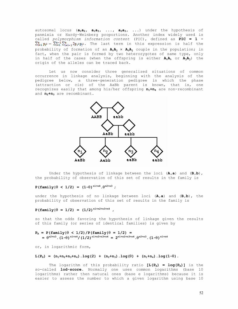
52
autosomal locus (a1a2, a1a3, ..., a2a3, ...) under the hypothesis of panmixia or Hardy-Weinberg proportions. Another index widely used is called polymorphism information content (PIC), defined as PIC = 1 -
. The last term in this expression is half the
probability of formation of an AiAj × AiAj couple in the population; in fact, when the pair is formed by two heterozygotes of same type, only in half of the cases (when the offspring is either AiAi or AjAj) the origin of the alleles can be traced back.
Let us now consider three generalized situations of common occurrence in linkage analysis, beginning with the analysis of the pedigree below, a three-generation pedigree in which the phase (attraction or cis) of the AaBb parent is known, that is, one recognizes easily that among his/her offspring n1+n4 are non-recombinant and n2+n3 are recombinant.
Under the hypothesis of linkage between the loci (A,a) and (B,b),
the probability of observation of this set of results in the family is P(family|θ < 1/2) = (1-θ)n1+n4.θn2+n3 ; under the hypothesis of no linkage between loci (A,a) and (B,b), the probability of observation of this set of results in the family is P(family|θ = 1/2) = (1/2)n1+n2+n3+n4 , so that the odds favoring the hypothesis of linkage given the results of this family (or series of identical families) is given by PR = P(family|θ < 1/2)/P(family|θ = 1/2) = = θn2+n3.(1-θ)n1+n4/(1/2)n1+n2+n3+n4 = 2n1+n2+n3+n4.θn2+n3.(1-θ)n1+n4 or, in logarithmic form, L(PR) = (n1+n2+n3+n4).log(2) + (n2+n3).log(θ) + (n1+n4).log(1-θ).
The logarithm of this probability ratio [L(PR) = log(PR)] is the so-called lod-score. Normally one uses common logarithms (base 10 logarithms) rather then natural ones (base e logarithms) because it is easier to assess the number to which a given logarithm using base 10
53
corresponds. An odds ratio of 1000 (that corresponds to number 3 on a scale of base 10 logarithms) or greater is generally used for granting the state of linkage between two loci beyond any reasonable doubt.
The maximum likelihood estimate of θ is the solution of equation dL(PR)/ dθ = (n2+n3)/θ - (n1+n4)/(1-θ) = 0 → θ = (n2+n3)/(n1+n2+n3+n4); evidently this same quantity is obtained by direct counting, since the quantity of recombinants is (n2+n3) and that of non-recombinants is (n1+n4).
We will now consider the following example of numerical application to this situation: n1 = 17, n2 = 1, n3 = 1, n4 = 2, so that n1+n4 = 19, n2+n3 = 2 and n1+n2+n3+n4 = 21. We obtain successively P(family|θ < 1/2) = θ2.(1-θ)19 P(family|θ = 1/2) = (1/2)21 and PR = P(family|θ < 1/2)/P(family|θ = 1/2) = 2097152.θ2.(1-θ)19 .
The next step is to verify which value of θ maximizes the likelihood function PR. This can be performed manually, consulting ready-to-use tables or calculating the value of PR for any specific value of θ, as the program below does: REM PROGRAM FILENAME LINKAG00.BAS CLS PRINT " r P(r) Le(r) L10(r)" PRINT "-----------------------------------" FOR I = 2 TO 50 STEP 1.25 R = (I + .5) / 100 P = 2097152 * R ^ 2 * (1 - R) ^ 19 L1 = LOG(P): L2 = LOG(P) / LOG(10) PRINT USING "#.#### ####.## ##.## ##.##"; R; P; L1; L2 DO: LOOP WHILE INKEY$ <> " " NEXT I PRINT "-----------------------------------" r P(r) Le(r) L10(r) ---------------------------------- 0.0250 810.21 6.70 2.91 0.0375 1426.61 7.26 3.15 0.0500 1978.42 7.59 3.30 0.0625 2403.50 7.78 3.38 0.0750 2681.92 7.89 3.43 0.0875 2818.84 7.94 3.45 0.1000 2832.94 7.95 3.45 0.1125 2748.74 7.92 3.44 0.1250 2591.81 7.86 3.41 0.1375 2385.93 7.78 3.38 0.1500 2151.65 7.67 3.33 0.1625 1905.67 7.55 3.28 0.1750 1660.85 7.42 3.22 0.1875 1426.52 7.26 3.15
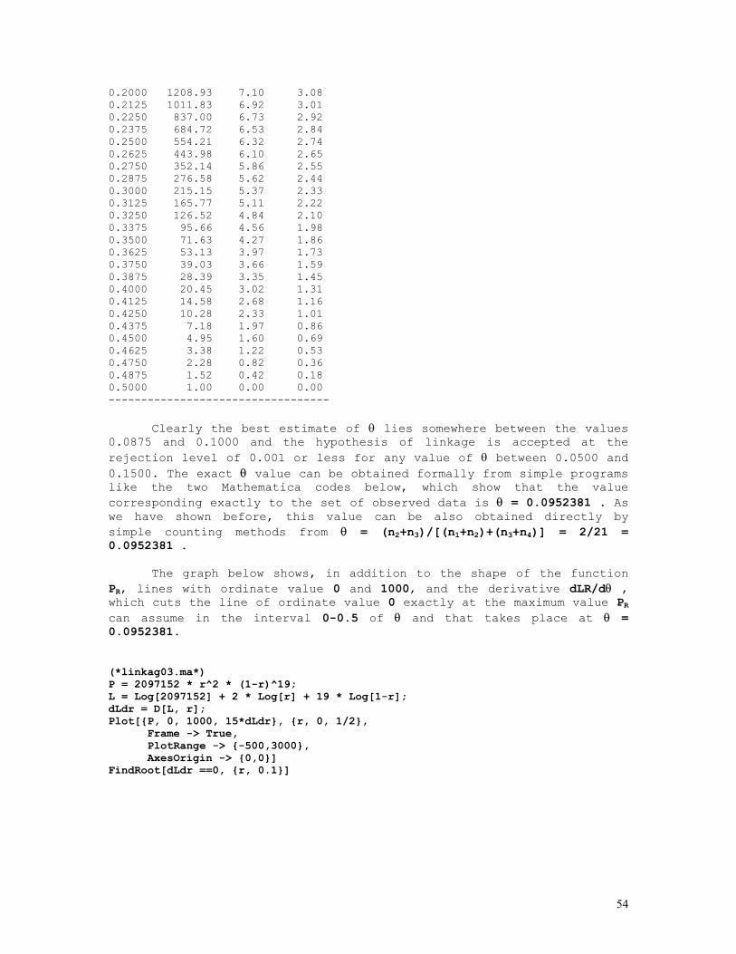
54
0.2000 1208.93 7.10 3.08 0.2125 1011.83 6.92 3.01 0.2250 837.00 6.73 2.92 0.2375 684.72 6.53 2.84 0.2500 554.21 6.32 2.74 0.2625 443.98 6.10 2.65 0.2750 352.14 5.86 2.55 0.2875 276.58 5.62 2.44 0.3000 215.15 5.37 2.33 0.3125 165.77 5.11 2.22 0.3250 126.52 4.84 2.10 0.3375 95.66 4.56 1.98 0.3500 71.63 4.27 1.86 0.3625 53.13 3.97 1.73 0.3750 39.03 3.66 1.59 0.3875 28.39 3.35 1.45 0.4000 20.45 3.02 1.31 0.4125 14.58 2.68 1.16 0.4250 10.28 2.33 1.01 0.4375 7.18 1.97 0.86 0.4500 4.95 1.60 0.69 0.4625 3.38 1.22 0.53 0.4750 2.28 0.82 0.36 0.4875 1.52 0.42 0.18 0.5000 1.00 0.00 0.00 ----------------------------------
Clearly the best estimate of θ lies somewhere between the values 0.0875 and 0.1000 and the hypothesis of linkage is accepted at the rejection level of 0.001 or less for any value of θ between 0.0500 and 0.1500. The exact θ value can be obtained formally from simple programs like the two Mathematica codes below, which show that the value corresponding exactly to the set of observed data is θ = 0.0952381 . As we have shown before, this value can be also obtained directly by simple counting methods from θ = (n2+n3)/[(n1+n2)+(n3+n4)] = 2/21 = 0.0952381 .
The graph below shows, in addition to the shape of the function PR, lines with ordinate value 0 and 1000, and the derivative dLR/dθ , which cuts the line of ordinate value 0 exactly at the maximum value PR can assume in the interval 0-0.5 of θ and that takes place at θ = 0.0952381. (*linkag03.ma*) P = 2097152 * r^2 * (1-r)^19; L = Log[2097152] + 2 * Log[r] + 19 * Log[1-r]; dLdr = D[L, r]; Plot[{P, 0, 1000, 15*dLdr}, {r, 0, 1/2}, Frame -> True, PlotRange -> {-500,3000}, AxesOrigin -> {0,0}] FindRoot[dLdr ==0, {r, 0.1}]
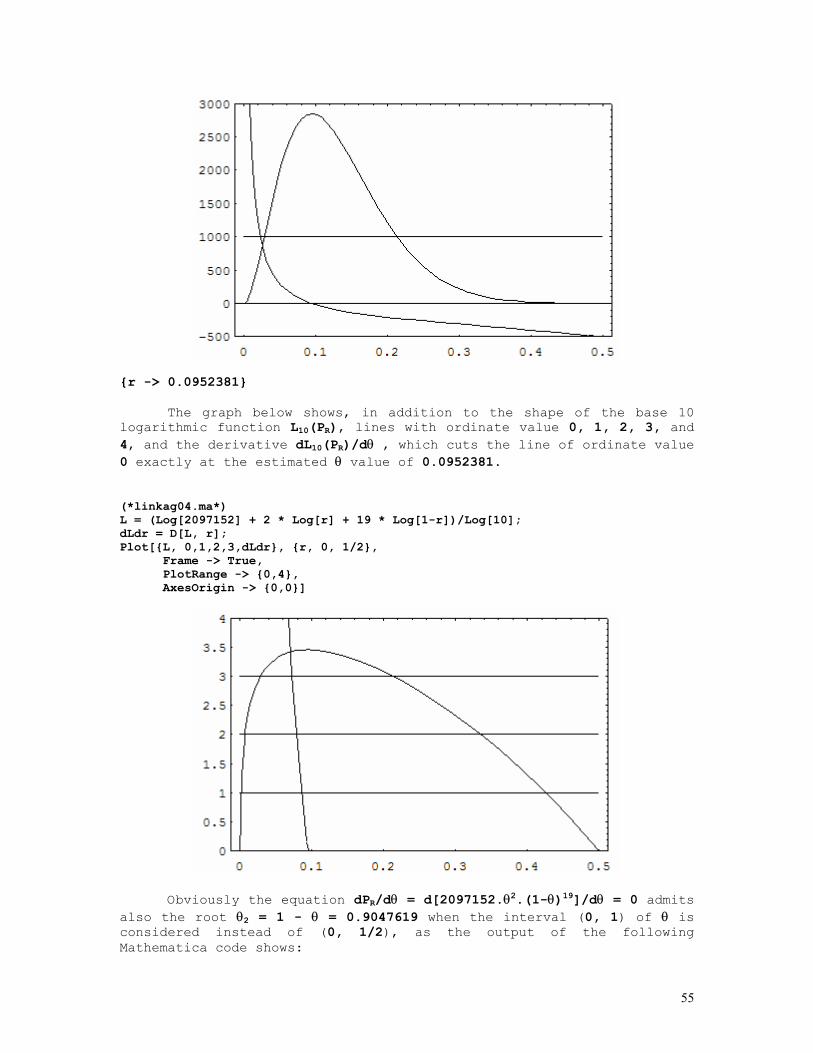
55
{r -> 0.0952381}
The graph below shows, in addition to the shape of the base 10 logarithmic function L10(PR), lines with ordinate value 0, 1, 2, 3, and 4, and the derivative dL10(PR)/dθ , which cuts the line of ordinate value 0 exactly at the estimated θ value of 0.0952381. (*linkag04.ma*) L = (Log[2097152] + 2 * Log[r] + 19 * Log[1-r])/Log[10]; dLdr = D[L, r]; Plot[{L, 0,1,2,3,dLdr}, {r, 0, 1/2}, Frame -> True, PlotRange -> {0,4}, AxesOrigin -> {0,0}]
Obviously the equation dPR/dθ = d[2097152.θ2.(1-θ)19]/dθ = 0 admits also the root θ2 = 1 - θ = 0.9047619 when the interval (0, 1) of θ is considered instead of (0, 1/2), as the output of the following Mathematica code shows:
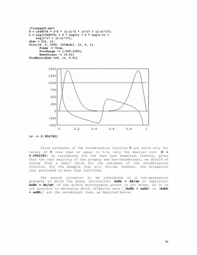
56
(*linkag05.ma*) P = 1048576 * r^2 * (1-r)^2 * (r^17 + (1-r)^17); L = Log[1048576] + 2 * Log[r] + 2 * Log[1-r] + Log[r^17 + (1-r)^17]; dLdr = D[L, r]; Plot[{P, 0, 1000, 15*dLdr}, {r, 0, 1}, Frame -> True, PlotRange -> {-500,1500}, AxesOrigin -> {0,0}] FindRoot[dLdr ==0, {r, 0.9}]
{r -> 0.904762}
Since estimates of the recombination fraction θ are valid only for values of θ less than or equal to 0.5, only the smaller root (θ = 0.0952381) is considered. For the case just examined, however, given that the vast majority of the progeny was non-recombinant, we should of course find a small value for the estimate of the recombination fraction. For the example that will follow, however, the divagation just performed is more than justified.
The second situation to be considered is a two-generation pedigree in which the phase (attraction: AaBb = AB/ab or repulsion: AaBb = Ab/aB) of the double heterozygous parent is not known, so it is not possible to determine which offspring sets [(AaBb + aabb) or (Aabb + aaBb)] are the recombinant ones, as depicted below:
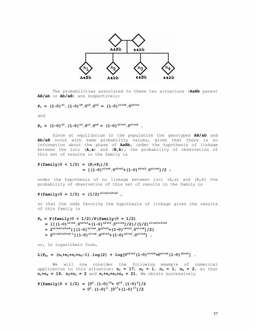
57
The probabilities associated to these two situations (AaBb parent AB/ab or Ab/aB) are respectively: P1 = (1-θ)n1.(1-θ)n4.θn2.θn3 = (1-θ)n1+n4.θn2+n3 and P2 = (1-θ)n2.(1-θ)n3.θn1.θn4 = (1-θ)n2+n3.θn1+n4 .
Since at equilibrium in the population the genotypes AB/ab and Ab/aB occur with same probability values, given that there is no information about the phase of AaBb, under the hypothesis of linkage between the loci (A,a) and (B,b), the probability of observation of this set of results in the family is P(family|θ < 1/2) = (P1+P2)/2 = [(1-θ)n1+n4.θn2+n3+(1-θ)n2+n3.θn1+n4]/2 ; under the hypothesis of no linkage between loci (A,a) and (B,b) the probability of observation of this set of results in the family is P(family|θ = 1/2) = (1/2)n1+n2+n3+n4 , so that the odds favoring the hypothesis of linkage given the results of this family is PR = P(family|θ < 1/2)/P(family|θ = 1/2) = {[(1-θ)n1+n4.θn2+n3+(1-θ)n2+n3.θn1+n4]/2}/(1/2)n1+n2+n3+n4 = 2n1+n2+n3+n4{[(1-θ)n1+n4.θn2+n3+(1-θ)n2+n3.θn1+n4]/2} = 2n1+n2+n3+n4-1[(1-θ)n1+n4.θn2+n3+(1-θ)n2+n3.θn1+n4] , or, in logarithmic form, L(PR) = (n1+n2+n3+n4-1).log(2) + log[θn2+n3(1-θ)n1+n4+θn1+n4(1-θ)n2+n3] .
We will now consider the following example of numerical application to this situation: n1 = 17, n2 = 1, n3 = 1, n4 = 2, so that n1+n4 = 19, n2+n3 = 2 and n1+n2+n3+n4 = 21. We obtain successively P(family|θ < 1/2) = [θ2.(1-θ)19+ θ19.(1-θ)2]/2 = θ2.(1-θ)2.[θ17+(1-θ)17]/2
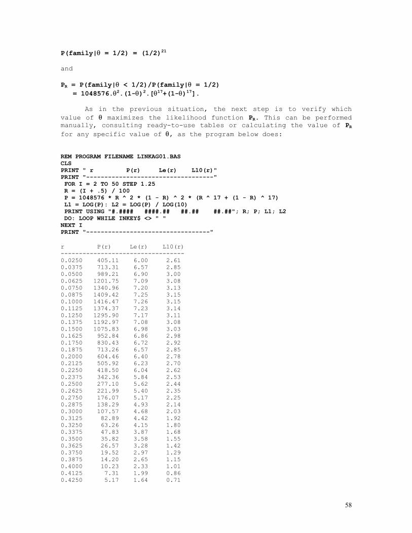
58
P(family|θ = 1/2) = (1/2)21 and PR = P(family|θ < 1/2)/P(family|θ = 1/2) = 1048576.θ2.(1-θ)2.[θ17+(1-θ)17].
As in the previous situation, the next step is to verify which value of θ maximizes the likelihood function PR. This can be performed manually, consulting ready-to-use tables or calculating the value of PR for any specific value of θ, as the program below does: REM PROGRAM FILENAME LINKAG01.BAS CLS PRINT " r P(r) Le(r) L10(r)" PRINT "-----------------------------------" FOR I = 2 TO 50 STEP 1.25 R = (I + .5) / 100 P = 1048576 * R ^ 2 * (1 - R) ^ 2 * (R ^ 17 + (1 - R) ^ 17) L1 = LOG(P): L2 = LOG(P) / LOG(10) PRINT USING "#.#### ####.## ##.## ##.##"; R; P; L1; L2 DO: LOOP WHILE INKEY$ <> " " NEXT I PRINT "----------------------------------" r P(r) Le(r) L10(r) ---------------------------------- 0.0250 405.11 6.00 2.61 0.0375 713.31 6.57 2.85 0.0500 989.21 6.90 3.00 0.0625 1201.75 7.09 3.08 0.0750 1340.96 7.20 3.13 0.0875 1409.42 7.25 3.15 0.1000 1416.47 7.26 3.15 0.1125 1374.37 7.23 3.14 0.1250 1295.90 7.17 3.11 0.1375 1192.97 7.08 3.08 0.1500 1075.83 6.98 3.03 0.1625 952.84 6.86 2.98 0.1750 830.43 6.72 2.92 0.1875 713.26 6.57 2.85 0.2000 604.46 6.40 2.78 0.2125 505.92 6.23 2.70 0.2250 418.50 6.04 2.62 0.2375 342.36 5.84 2.53 0.2500 277.10 5.62 2.44 0.2625 221.99 5.40 2.35 0.2750 176.07 5.17 2.25 0.2875 138.29 4.93 2.14 0.3000 107.57 4.68 2.03 0.3125 82.89 4.42 1.92 0.3250 63.26 4.15 1.80 0.3375 47.83 3.87 1.68 0.3500 35.82 3.58 1.55 0.3625 26.57 3.28 1.42 0.3750 19.52 2.97 1.29 0.3875 14.20 2.65 1.15 0.4000 10.23 2.33 1.01 0.4125 7.31 1.99 0.86 0.4250 5.17 1.64 0.71
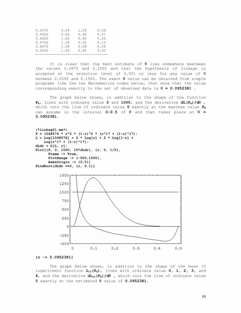
59
0.4375 3.64 1.29 0.56 0.4500 2.56 0.94 0.41 0.4625 1.82 0.60 0.26 0.4750 1.35 0.30 0.13 0.4875 1.08 0.08 0.04 0.5000 1.00 0.00 0.00 ----------------------------------
It is clear that the best estimate of θ lies somewhere beetween the values 0.0875 and 0.1000 and that the hypothesis of linkage is accepted at the rejection level of 0.001 or less for any value of θ between 0.0500 and 0.1500. The exact θ value can be obtained from simple programs like the two Mathematica codes below, that show that the value corresponding exactly to the set of observed data is θ = 0.0952381 .
The graph below shows, in addition to the shape of the function PR, lines with ordinate value 0 and 1000, and the derivative dL(PR)/dθ , which cuts the line of ordinate value 0 exactly at the maximum value PR can assume in the interval 0-0.5 of θ and that takes place at θ = 0.0952381. (*linkag01.ma*) P = 1048576 * r^2 * (1-r)^2 * (r^17 + (1-r)^17); L = Log[1048576] + 2 * Log[r] + 2 * Log[1-r] + Log[r^17 + (1-r)^17]; dLdr = D[L, r]; Plot[{P, 0, 1000, 15*dLdr}, {r, 0, 1/2}, Frame -> True, PlotRange -> {-500,1500}, AxesOrigin -> {0,0}] FindRoot[dLdr ==0, {r, 0.1}]
{r -> 0.0952381}
The graph below shows, in addition to the shape of the base 10 logarithmic function L10(PR), lines with ordinate value 0, 1, 2, 3, and 4, and the derivative dL10(PR)/dθ , which cuts the line of ordinate value 0 exactly at the estimated θ value of 0.0952381.
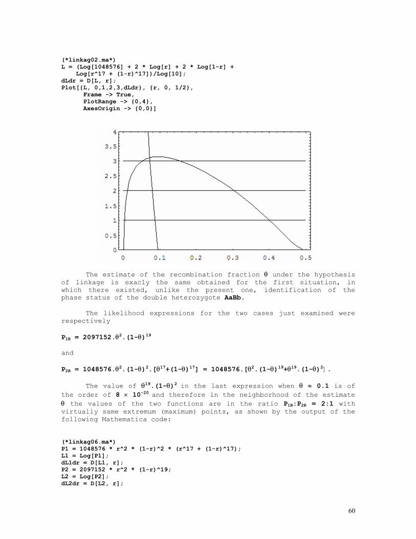
60
(*linkag02.ma*) L = (Log[1048576] + 2 * Log[r] + 2 * Log[1-r] + Log[r^17 + (1-r)^17])/Log[10]; dLdr = D[L, r]; Plot[{L, 0,1,2,3,dLdr}, {r, 0, 1/2}, Frame -> True, PlotRange -> {0,4}, AxesOrigin -> {0,0}]
The estimate of the recombination fraction θ under the hypothesis of linkage is exacly the same obtained for the first situation, in which there existed, unlike the present one, identification of the phase status of the double heterozygote AaBb.
The likelihood expressions for the two cases just examined were respectively P1R = 2097152.θ2.(1-θ)19 and P2R = 1048576.θ2.(1-θ)2.[θ17+(1-θ)17] = 1048576.[θ2.(1-θ)19+θ19.(1-θ)2].
The value of θ19.(1-θ)2 in the last expression when θ ≈ 0.1 is of the order of 8 × 10-20 and therefore in the neighborhood of the estimate θ the values of the two functions are in the ratio P1R:P2R = 2:1 with virtually same extremum (maximum) points, as shown by the output of the following Mathematica code: (*linkag06.ma*) P1 = 1048576 * r^2 * (1-r)^2 * (r^17 + (1-r)^17); L1 = Log[P1]; dL1dr = D[L1, r]; P2 = 2097152 * r^2 * (1-r)^19; L2 = Log[P2]; dL2dr = D[L2, r];
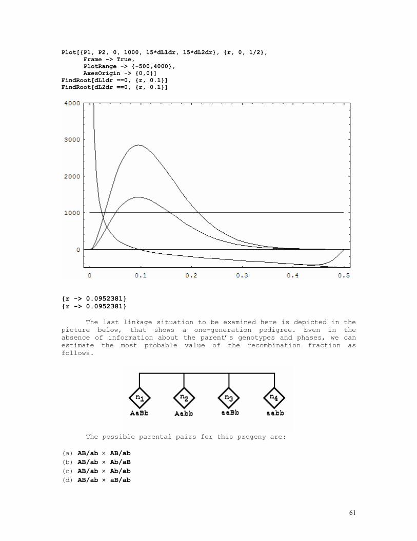
61
Plot[{P1, P2, 0, 1000, 15*dL1dr, 15*dL2dr}, {r, 0, 1/2}, Frame -> True, PlotRange -> {-500,4000}, AxesOrigin -> {0,0}] FindRoot[dL1dr ==0, {r, 0.1}] FindRoot[dL2dr ==0, {r, 0.1}]
{r -> 0.0952381} {r -> 0.0952381}
The last linkage situation to be examined here is depicted in the picture below, that shows a one-generation pedigree. Even in the absence of information about the parent’s genotypes and phases, we can estimate the most probable value of the recombination fraction as follows.
The possible parental pairs for this progeny are:
(a) AB/ab × AB/ab (b) AB/ab × Ab/aB (c) AB/ab × Ab/ab (d) AB/ab × aB/ab
62
(e) AB/ab × ab/ab (f) Ab/aB × Ab/aB (g) Ab/aB × Ab/ab (h) Ab/aB × aB/ab (i) Ab/aB × ab/ab (j) Ab/ab × aB/ab . (a) Parental mating AB/ab × AB/ab
If no recombination occurs in both parental meioses, the offspring genotypes will be AABB, AaBb, and aabb, with probabilities 1/4, 1/2, and 1/4. If recombination takes place in one meiosis but not in the other, offspring genotypes will be AABb, AaBB, Aabb, and aaBb, each with probability 1/4. If recombination takes place in both meioses, the offspring genotypes will be AAbb, AaBb, and aaBB, with probabilities 1/4, 1/2, and 1/4. The probabilities associated with these three events are respectively (1-θ)2, 2θ(1-θ) and θ2 . Therefore, given the parental mating pair AB/ab × AB/ab, the probabilities of progenies AaBb, Aabb, aaBb, and aabb are respectively P(AaBb|AB/ab × AB/ab) = [(1-θ)2+θ2]/2 P(Aabb|AB/ab × AB/ab) = θ(1-θ)/2 P(aaBb|AB/ab × AB/ab) = θ(1-θ)/2 P(aabb|AB/ab × AB/ab) = (1-θ)2/4 .
Since the frequency of AB/ab genotypes in the population is 2p1q1p2q2, where p1 and q1 are the frequencies of alleles A and a at locus (A, a) and p2 and q2 the frequencies of alleles B and b at locus (B, b), the frequency of the mating type AB/ab × AB/ab is (2p1q1p2q2)2 and the likelihood function of the set of offspring genotypes is given by P(a) = (2p1q1p2q2)2.[(1-θ)2/2+θ2/2]n1.[θ(1-θ)/2]n2+n3.[(1-θ)2/4]n4 .
This is the partial contribution of matings AB/ab × AB/ab that should be added, together with the contribution of other possible nine mating types, to the final (overall) likelihood function under the hypothesis of linkage with θ < 1/2. (b) Parental mating AB/ab × Ab/aB
If no recombination occurs in both parental meioses, the offspring genotypes will be AABb, Aabb, AaBB, and aaBb, with equal probabilities (1/4). If recombination occurs in the meiosis of individual AB/ab but not in the meiosis of individual Ab/aB, the offspring genotypes will be AAbb, AaBb, and aaBB, with probabilities 1/4, 1/2, and 1/4. If recombination occurs in the meiosis of individual Ab/aB but not in the meiosis of individual AB/ab, the offspring genotypes will be AABB, AaBb, and aabb, with probabilities 1/4, 1/2, and 1/4. If recombination takes place in both meioses, the offspring genotypes will be AABb, Aabb, AaBB, and aaBb, with equal probabilities (1/4), that is, the offspring genotypes will be the same as in the case of no recombination in both meiosis. The probabilities associated with
63
these four events are respectively (1-θ)2, θ(1-θ), θ(1-θ), and θ2. Therefore, given the parental mating pair AB/ab × Ab/aB, the probabilities of progenies AaBb, Aabb, aaBb, and aabb are respectively P(AaBb|AB/ab × Ab/aB) = θ(1-θ) P(Aabb|AB/ab × Ab/aB) = [(1-θ)2+θ2]/4 P(aaBb|AB/ab × Ab/aB) = [(1-θ)2+θ2]/4 P(aabb|AB/ab × Ab/aB) = θ(1-θ)/4 .
Since the frequency of either AB/ab or Ab/aB genotypes in the population is 2p1q1p2q2, the frequency of the mating type AB/ab × Ab/Ab is 2(2p1q1p2q2)2 = 8(p1q1p2q2)2 and the likelihood function of the set of offspring genotypes is given by P(b) = 8(p1q1p2q2)2.[θ(1-θ)]n1.[(1-θ)2/4+θ2/4]n2+n3.[θ(1-θ)/4]n4. (c) Parental mating AB/ab × Ab/ab
If no recombination occurs in the meiosis of the double heterozygote, the offspring genotypes will be AABb, AaBb, Aabb, and aabb, with equal probabilities (1/4). If recombination takes place in the meiosis of the AaBb individual, the offspring genotypes will be AAbb, Aabb, AaBb, and aaBb, also with equal probabilities (1/4). Since the probabilities associated with these two events are (1-θ) and θ respectively, given the parental pair AB/ab × Ab/ab, the probabilities of progenies AaBb, Aabb, aaBb, and aabb are respectively P(AaBb|AB/ab × Ab/ab) = 1/4 P(Aabb|AB/ab × Ab/ab) = 1/4 P(aaBb|AB/ab × Ab/ab) = θ/4 P(aabb|AB/ab × Ab/ab) = (1-θ)/4 .
Since the frequency of AB/ab genotypes in the population is 2p1q1p2q2, and the frequency of Ab/ab genotypes is 2p1q1q22, the frequency of the mating type AB/ab × Ab/ab is 2 × 2p1q1p2q2 × 2p1q1q22 = 8p12q12p2q23 and the likelihood function of the set of offspring genotypes is given by P(c) = 8p12q12p2q23.(1/4)n1+n2.(θ/4)n3.[(1-θ)/4]n4 . (d) Parental mating AB/ab × aB/ab
If no recombination occurs in the meiosis of the double heterozygote, the offspring genotypes will be AaBB, AaBb, aaBb, and aabb, with equal probabilities (1/4). If recombination takes place in the meiosis of the AaBb individual, the offspring genotypes will be AaBb, Aabb, aaBB, and aaBb, also with equal probabilities (1/4). Since the probabilities associated with these two events are (1-θ) and θ respectively, given the parental pair AB/ab × aB/ab, the probabilities of progenies AaBb, Aabb, aaBb, and aabb are respectively
64
P(AaBb|AB/ab × aB/ab) = 1/4 P(Aabb|AB/ab × aB/ab) = θ/4 P(aaBb|AB/ab × aB/ab) = 1/4 P(aabb|AB/ab × aB/ab) = (1-θ)/4 .
Since the frequency of AB/ab genotypes in the population is 2p1q1p2q2, and the frequency of aB/ab genotypes is 2q12p2q2, the frequency of the mating type AB/ab × aB/ab is 2 × 2p1q1p2q2 × 2q12p2q2 = 8p1q13p22q22 and the likelihood function of the set of offspring genotypes is given by P(d) = 8p1q13p22q22.(1/4)n1+n3.(θ/4)n2.[(1-θ)/4]n4 . (e) Parental mating AB/ab × ab/ab
If no recombination occurs in the meiosis of the double heterozygote, the offspring genotypes will be AaBb and aabb, with equal probabilities (1/2). If recombination takes place in the meiosis of the AaBb individual, the offspring genotypes will be Aabb and aaBb, also with equal probabilities (1/2). Since the probabilities associated with these two events are (1-θ) and θ respectively, given the parental pair AB/ab × ab/ab, the probabilities of progenies AaBb, Aabb, aaBb, and aabb are respectively P(AaBb|AB/ab × ab/ab) = (1-θ)/2 P(Aabb|AB/ab × ab/ab) = θ/2 P(aaBb|AB/ab × ab/ab) = θ/2 P(aabb|AB/ab × ab/ab) = (1-θ)/2 .
Since the frequency of AB/ab genotypes in the population is 2p1q1p2q2, and the frequency of ab/ab genotypes is q12q22, the frequency of the mating type AB/ab × ab/ab is 2 × 2p1q1p2q2 × q12q22 = 4p1q13p2q23 and the likelihood function of the set of offspring genotypes is given by P(e) = 4p1q13p2q23.[(1-θ)/2]n1+n4.(θ/2)n2+n3 . (f) Parental mating Ab/aB × Ab/aB
If no recombination occurs in both parental meioses, the offspring genotypes will be AAbb, AaBb, and aaBB, with probabilities 1/4, 1/2, and 1/4. If recombination takes place in one meiosis but not in the other, offspring genotypes will be AABb, AaBB, Aabb, and aaBb, each with probability 1/4. If recombination takes place in both meioses, the offspring genotypes will be AABB, AaBb, and aabb, with probabilities 1/4, 1/2, and 1/4. The probabilities associated with these three events are respectively (1-θ)2, 2θ(1-θ) and θ2 . Therefore, given the parental mating pair Ab/aB × Ab/aB, the probabilities of progenies AaBb, Aabb, aaBb, and aabb are respectively P(AaBb|Ab/aB × Ab/aB) = [(1-θ)2+θ2]/2 P(Aabb|Ab/aB × Ab/aB) = θ(1-θ)/2
65
P(aaBb|Ab/aB × Ab/aB) = θ(1-θ)/2 P(aabb|Ab/aB × Ab/aB) = θ2/4 .
Since the frequency of Ab/aB genotypes in the population is 2p1q1p2q2, the frequency of the mating type Ab/aB × Ab/aB is (2p1q1p2q2)2 and the likelihood function of the set of offspring genotypes is given by P(f) = (2p1q1p2q2)2.[(1-θ)2/2+θ2/2]n1.[θ(1-θ)/2]n2+n3.(θ2/4)n4 . (g) Parental mating Ab/aB × Ab/ab
If no recombination occurs in the meiosis of the double heterozygote, the offspring genotypes will be AAbb, Aabb, AaBb, and aaBb, with equal probabilities (1/4). If recombination takes place in the meiosis of the AaBb individual, the offspring genotypes will be AABb, AaBb, Aabb, and aabb, also with equal probabilities (1/4). Since the probabilities associated with these two events are (1-θ) and θ respectively, given the parental pair Ab/aB × Ab/ab, the probabilities of progenies AaBb, Aabb, aaBb, and aabb are respectively P(AaBb|Ab/aB × Ab/ab) = 1/4 P(Aabb|Ab/aB × Ab/ab) = 1/4 P(aaBb|Ab/aB × Ab/ab) = (1-θ)/4 P(aabb|Ab/aB × Ab/ab) = θ/4 .
Since the frequency of Ab/aB genotypes in the population is 2p1q1p2q2, and the frequency of Ab/ab genotypes is 2p1q1q22, the frequency of the mating type AB/ab × Ab/ab is 2 × 2p1q1p2q2 × 2p1q1q22 = 8p12q12p2q23 and the likelihood function of the set of offspring genotypes is given by P(g) = 8p12q12p2q23.(1/4)n1+n2.[(1-θ)/4]n3.(θ/4)n4. (h) Parental mating Ab/aB × aB/ab
If no recombination occurs in the meiosis of the double heterozygote, the offspring genotypes will be AaBb, Aabb, aaBB, and aaBb, with equal probabilities (1/4). If recombination takes place in the meiosis of the AaBb individual, the offspring genotypes will be AaBB, AaBb, aaBb, and aabb, also with equal probabilities (1/4). Since the probabilities associated with these two events are (1-θ) and θ respectively, given the parental pair Ab/aB × aB/ab, the probabilities of progenies AaBb, Aabb, aaBb, and aabb are respectively P(AaBb|Ab/aB × aB/ab) = 1/4 P(Aabb|Ab/aB × aB/ab) = (1-θ)/4 P(aaBb|Ab/aB × aB/ab) = 1/4 P(aabb|Ab/aB × aB/ab) = θ/4 .
Since the frequency of Ab/aB genotypes in the population is 2p1q1p2q2, and the frequency of aB/ab genotypes is 2q12p2q2, the frequency
66
of the mating type AB/ab × aB/ab is 2 × 2p1q1p2q2 × 2q12p2q2 = 8p1q13p22q22 and the likelihood function of the set of offspring genotypes is given by P(h) = 8p1q13p22q22.(1/4)n1+n3.[(1-θ)/4]n2.(θ/4)n4 . (i) Parental mating Ab/aB × ab/ab
If no recombination occurs in the meiosis of the double heterozygote, the offspring genotypes will be Aabb and aaBb, with equal probabilities (1/2). If recombination takes place in the meiosis of the AaBb individual, the offspring genotypes will be AaBb and aabb, also with equal probabilities (1/2). Since the probabilities associated with these two events are (1-θ) and θ respectively, given the parental pair Ab/aB × ab/ab, the probabilities of progenies AaBb, Aabb, aaBb, and aabb are respectively P(AaBb|Ab/aB × ab/ab) = θ/2 P(Aabb|Ab/aB × ab/ab) = (1-θ)/2 P(aaBb|Ab/aB × ab/ab) = (1-θ)/2 P(aabb|Ab/aB × ab/ab) = θ/2 .
Since the frequency of AB/ab genotypes in the population is 2p1q1p2q2, and the frequency of ab/ab genotypes is q12q22, the frequency of the mating type AB/ab × ab/ab is 2 × 2p1q1p2q2 × q12q22 = 4p1q13p2q23 and the likelihood function of the set of offspring genotypes is given by P(i) = 4p1q13p2q23.(θ/2)n1+n4.[(1-θ)/2]n2+n3 . (j) Parental mating Ab/ab × aB/ab
If the parental mating is Ab/ab × aB/ab, independenly of occurring recombination or not in one or in both individuals, the offspring genotypes AaBb, Aabb, aaBb, and aabb will occur with equal probabilities (1/4): P(AaBb|AB/ab × Ab/aB) = 1/4 P(Aabb|AB/ab × Ab/aB) = 1/4 P(aaBb|AB/ab × Ab/aB) = 1/4 P(aabb|AB/ab × Ab/aB) = 1/4 .
Since the frequency of Ab/ab genotypes in the population is 2p1q1q22 and that of aB/ab genotypes is 2q12p2q2, the frequency of the mating type Ab/ab × aB/ab is 2 × 2p1q1q22 × 2q12p2q2 = 8p1q13p2q23 and the likelihood function of the set of offspring genotypes is given by P(j) = 8p1q13p2q23.(1/4)n1+n2+n3+n4 .
The likelihood function under the hypothesis of linkage is then P(family|θ < 1/2) = [P(a) + ... + P(j)]/16p1q12p2q22 ,
67
where 16p1q12p2q22 = (2p1q1p2q2)2 + 8(p1q1p2q2)2 + 8p12q12p2q23 + 8p1q13p22q22 + 4p1q13p2q23 + (2p1q1p2q2)2 + 8p12q12p2q23 + 8p1q13p22q22 + 4p1q13p2q23 + 8p1q13p2q23 = = 16p12q12p22q22 + 16p12q12p2q23 + 16p1q13p22q22 + 16p1q13p2q23 = 16p1q1p2q22(p1q1p2+p1q1q2+q12p2+q12q2) = 16p1q1p2q22[p1q1(p2+q2)+q12(p2+q2)] = 16p1q1p2q22(p1q1+q12) = 16p1q1p2q22[q1(p1+q1)] = 16p1q12p2q22 .
The likelihood function under the hypothesis of no linkage is obtained from each expression P(a), ... , P(j) by replacing θ by 1/2: P(family|θ = 1/2) = [P’(a) + ... + P’(j)]/16p1q12p2q22 , where P’(a) = P’(f) = (2p1q1p2q2)2.(1/4)n1.(1/8)n2+n3.(1/16)n4 P’(b) = 8(p1q1p2q2)2.(1/4)n1.(1/8)n2+n3.(1/16)n4 P’(c) = P’(g) = 8p12q12p2q23.(1/4)n1+n2.(1/8)n3+n4 P’(d) = P’(h) = 8p1q13p22q22.(1/4)n1+n3.(1/8)n2+n4 P’(e) = P’(i) = ½P’(j) = 4p1q13p2q23.(1/4)n1+n4+n2+n3 .
The odds ratio favoring the hypothesis of linkage is (finally!) obtained from PR = P(family|θ < 1/2)/P(family|θ = 1/2), and, as in the previous situations, the next step is to verify which value of θ maximizes the likelihood function PR. This is performed through computer programs like the Mathematica code below. The allele frequencies for genes in loci (A,a) and (B,b) used by the program can be taken from the literature describing the corresponding polymorphims. (*linkag07.ma*) p1 = 0.96; q1 = 1 - p1; p2 = 0.95; q2 = 1 - p2; n1 = 17; n2 = 1; n3 = 1; n4 = 2; P1a = (2*p1*q1*p2*q2)^2*((1-r)^2/2+r^2/2)^n1*(r*(1-r)/2)^(n2+n3)* ((1-r)^2/4)^n4; P1b = 8*(p1*q1*p2*q2)^2*(r*(1-r))^n1*((1-r)^2/4+r^2/4)^(n2+n3)*(r*(1-r)/4)^n4; P1c = 8*p1^2*q1^2*p2*q2^3*(1/4)^(n1+n2)*(r/4)^n3*((1-r)/4)^n4; P1d = 8*p1*q1^3*p2^2*q2^2*(1/4)^(n1+n3)*(r/4)^n2*((1-r)/4)^n4; P1e = 4*p1*q1^3*p2*q2^3*((1-r)/2)^(n1+n4)*(r/2)^(n2+n3); P1f = (2*p1*q1*p2*q2)^2*((1-r)^2/2+r^2/2)^n1*(r*(1-r)/2)^(n2+n3)*(r^2/4)^n4; P1g = 8*p1^2*q1^2*p2*q2^3*(1/4)^(n1+n2)*((1-r)/4)^n3*(r/4)^n4; P1h = 8*p1*q1^3*p2^2*q2^2*(1/4)^(n1+n3)*((1-r)/4)^n2*(r/4)^n4; P1i = 4*p1*q1^3*p2*q2^3*(r/2)^(n1+n4)*((1-r)/2)^(n2+n3); P1j = 8*p1*q1^3*p2*q2^3*(1/4)^(n1+n2+n3+n4); P2a = (2*p1*q1*p2*q2)^2*(1/4)^n1*(1/8)^(n2+n3)*(1/16)^n4; P2b = 8*(p1*q1*p2*q2)^2*(1/4)^n1*(1/8)^(n2+n3)*(1/16)^n4; P2c = 8*p1^2*q1^2*p2*q2^3*(1/4)^(n1+n2)*(1/8)^(n3+n4); P2d = 8*p1*q1^3*p2^2*q2^2*(1/4)^(n1+n3)*(1/8)^(n2+n4); P2e = 4*p1*q1^3*p2*q2^3*(1/4)^(n1+n4+n2+n3); P2f = P2a; P2g = P2c; P2h = P2d; P2i = P2e; P2j = 2*P2e; P3 = 16*p1*q1^2*p2*q2^2; Plink = (P1a+P1b+P1c+P1d+P1e+P1f+P1g+P1h+P1i+P1j)/P3; Pnlin = (P2a+P2b+P2c+P2d+P2e+P2f+P2g+P2h+P2i+P2j)/P3; P = Plink/Pnlin; L = Log[P]; dLdr = D[L,r]; Plot [{P, 0, 1000, 15*dLdr},{r,0,1/2}, Frame -> True,
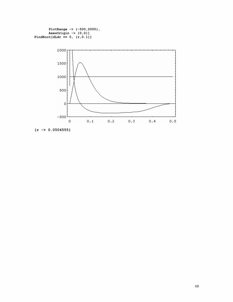
68
PlotRange -> {-500,2000}, AxesOrigin -> {0,0}] FindRoot[dLdr == 0, {r,0.1}]
{r -> 0.0504555}
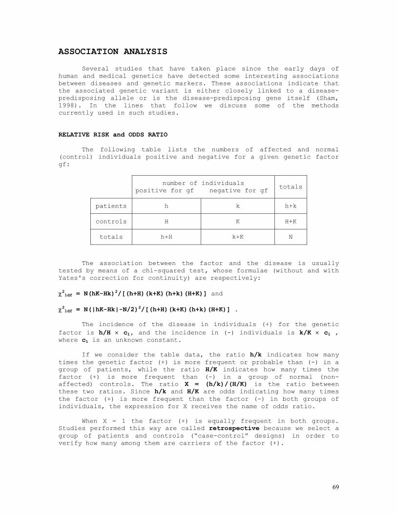
69
ASSOCIATION ANALYSIS
Several studies that have taken place since the early days of human and medical genetics have detected some interesting associations between diseases and genetic markers. These associations indicate that the associated genetic variant is either closely linked to a disease-predisposing allele or is the disease-predisposing gene itself (Sham, 1998). In the lines that follow we discuss some of the methods currently used in such studies. RELATIVE RISK and ODDS RATIO
The following table lists the numbers of affected and normal (control) individuals positive and negative for a given genetic factor gf:
number of individuals positive for gf negative for gf totals
patients h k h+k
controls H K H+K
totals h+H k+K N
The association between the factor and the disease is usually tested by means of a chi-squared test, whose formulae (without and with Yates's correction for continuity) are respectively: χ2
1df = N(hK-Hk)2/[(h+H)(k+K)(h+k)(H+K)] and χ2
1df = N(|hK-Hk|-N/2)2/[(h+H)(k+K)(h+k)(H+K)] .
The incidence of the disease in individuals (+) for the genetic factor is h/H × c1, and the incidence in (-) individuals is k/K × c1 , where c1 is an unknown constant.
If we consider the table data, the ratio h/k indicates how many times the genetic factor (+) is more frequent or probable than (-) in a group of patients, while the ratio H/K indicates how many times the factor (+) is more frequent than (-) in a group of normal (non-affected) controls. The ratio X = (h/k)/(H/K) is the ratio between these two ratios. Since h/k and H/K are odds indicating how many times the factor (+) is more frequent than the factor (-) in both groups of individuals, the expression for X receives the name of odds ratio.
When X = 1 the factor (+) is equally frequent in both groups. Studies performed this way are called retrospective because we select a group of patients and controls (“case-control” designs) in order to verify how many among them are carriers of the factor (+).
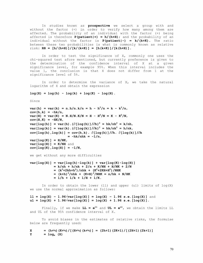
70
In studies known as prospective we select a group with and without the factor (+) in order to verify how many among them are affected. The probability of an individual with the factor (+) being affected is therefore P(patient|+) = h/(h+H); and the probability of an individual without the factor is P(patient|-) = k/(k+K). The ratio between these two probabilities is what is commonly known as relative risk: RR = [h/(h+H)]/[k/(k+K)] = [h(k+K)]/[k(h+H)].
In order to test the significance of X, commonly one uses the chi-squared test afore mentioned, but currently preference is given to the determination of the confidence interval of X at a given significance level, for example 95%. When this interval includes the value 1, the conclusion is that X does not differ from 1 at the significance level of 5%.
In order to determine the variance of X, we take the natural logarithm of X and obtain the expression
log(X) = log(h) - log(k) + log(K) - log(H). Since var(h) = var(k) = n.h/n.k/n = h - h2/n = k - k2/n, cov(h,k) = -hk/n, var(H) = var(K) = N.H/N.K/N = H - H2/N = K - K2/N, cov(H,K) = -HK/N, var[log(h)] = var(h).{∂[log(h)]/∂h}2 = hk/nh2 = k/nh, var[log(k)] = var(k).{∂[log(k)]/∂k}2 = hk/nk2 = h/nk, cov[log(h),log(k)] = cov(h,k). ∂[log(h)]/∂h. ∂[log(k)]/∂k = -hk/nhk = -1/n, var[log(K)] = H/NK, var[log(H)] = K/NH and cov[log(K),log(H)] = -1/N, we get without any more difficulties var[log(X)] = var[log(h)-log(k)] + var[log(K)-log(H)] = k/nh + h/nk + 2/n + K/NH + H/NK + 2/N = (k2+2kh+h2)/nhk + (K2+2KH+H2)/NHK = (k+h)2/nhk + (K+H)2/NHK = n/hk + N/HK = 1/h + 1/k + 1/H + 1/K.
In order to obtain the lower (ll) and upper (ul) limits of log(X) we use the normal approximation as follows:
ll = log(X) – 1.96√var[log(X)] = log(X) – 1.96 s.e.[log(X)] and ul = log(X) + 1.96√var[log(X)] = log(X) + 1.96 s.e.[log(X)].
Finally, if we make LL = ell and UL = eul, we obtain the limits LL and UL of the 95% confidence interval of X.
To avoid biases in the estimates of relative risks, the formulae below are frequently used: X = (h+½)(K+½)/[(H+½)(k+½)] = (2h+1)(2K+1)/[(2H+1)(2k+1)] Y = loge (X)
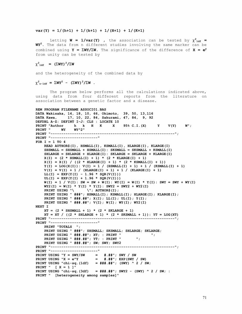
71
var(Y) = 1/(h+1) + 1/(k+1) + 1/(H+1) + 1/(K+1)
Letting W = 1/var(Y) , the association can be tested by χ21df =
WY2. The data from n different studies involving the same marker can be combined using Y = ΣWY/ΣW. The significance of the difference of X = ey from unity can be tested by χ2
1df = (ΣWY)2/ΣW and the heterogeneity of the combined data by χ2
n-1df = ΣWY2 - (ΣWY)2/ΣW .
The program below performs all the calculations indicated above, using data from four different reports from the literature on association between a genetic factor and a disease. REM PROGRAM FILENAME ASSOCI01.BAS DATA Wakisaka, 14, 18, 10, 66, Okimoto, 39, 50, 13,116 DATA Kawa, 17, 10, 22, 84, Sakurami, 47, 84, 9, 92 DEFDBL A-Z: DEFINT I-J: CLS : LOCATE 10 PRINT "Author h k H K X 95% C.I.(X) Y V(Y) W"; PRINT " WY WY^2" PRINT "----------------------------------------------------------"; PRINT "----------------------" FOR I = 1 TO 4 READ AUTHOR$(I), HSMALL(I), KSMALL(I), HLARGE(I), KLARGE(I) SHSMALL = SHSMALL + HSMALL(I): SKSMALL = SKSMALL + KSMALL(I) SHLARGE = SHLARGE + HLARGE(I): SKLARGE = SKLARGE + KLARGE(I) X(I) = (2 * HSMALL(I) + 1) * (2 * KLARGE(I) + 1) X(I) = X(I) / ((2 * HLARGE(I) + 1) * (2 * KSMALL(I) + 1)) Y(I) = LOG(X(I)): V(I) = 1 / (HSMALL(I) + 1) + 1 / (KSMALL(I) + 1) V(I) = V(I) + 1 / (HLARGE(I) + 1) + 1 / (KLARGE(I) + 1) LL(I) = EXP(Y(I) - 1.96 * SQR(V(I))) UL(I) = EXP(Y(I) + 1.96 * SQR(V(I))) W(I) = 1 / V(I): SW = SW + W(I): WY(I) = W(I) * Y(I): SWY = SWY + WY(I) WY2(I) = W(I) * Y(I) * Y(I): SWY2 = SWY2 + WY2(I) PRINT USING "\ \"; AUTHOR$(I); PRINT USING " ###"; HSMALL(I); KSMALL(I); HLARGE(I); KLARGE(I); PRINT USING " ###.##"; X(I); LL(I); UL(I); Y(I); PRINT USING " ###.##"; V(I); W(I); WY(I); WY2(I) NEXT I XT = (2 * SHSMALL + 1) * (2 * SKLARGE + 1) XT = XT / ((2 * SHLARGE + 1) * (2 * SKSMALL + 1)): YT = LOG(XT) PRINT "----------------------------------------------------------"; PRINT "----------------------" PRINT "TOTALS "; PRINT USING " ###"; SHSMALL; SKSMALL; SHLARGE; SKLARGE; PRINT USING " ###.##"; XT; : PRINT " "; PRINT USING " ###.##"; YT; : PRINT " "; PRINT USING " ###.##"; SW; SWY; SWY2 PRINT "----------------------------------------------------------"; PRINT "----------------------" PRINT USING "Y = SWY/SW = #.##"; SWY / SW PRINT USING "X = e^Y = #.##"; EXP(SWY / SW) PRINT USING "chi-sq.(1df) = ###.##"; (SWY) ^ 2 / SW; PRINT " [ X = 1 ]" PRINT USING "chi-sq.(3df) = ###.##"; SWY2 - (SWY) ^ 2 / SW; : PRINT " [heterogeneity among samples]"
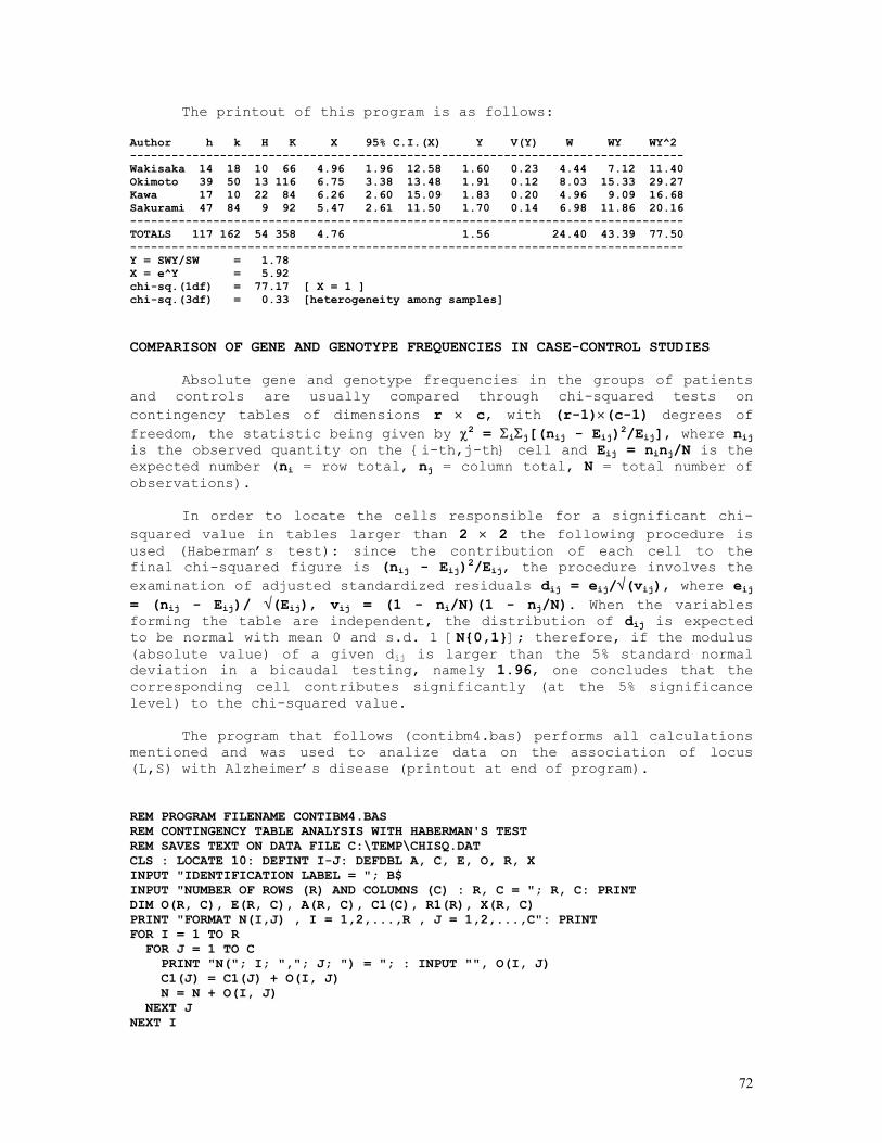
72
The printout of this program is as follows: Author h k H K X 95% C.I.(X) Y V(Y) W WY WY^2 -------------------------------------------------------------------------------- Wakisaka 14 18 10 66 4.96 1.96 12.58 1.60 0.23 4.44 7.12 11.40 Okimoto 39 50 13 116 6.75 3.38 13.48 1.91 0.12 8.03 15.33 29.27 Kawa 17 10 22 84 6.26 2.60 15.09 1.83 0.20 4.96 9.09 16.68 Sakurami 47 84 9 92 5.47 2.61 11.50 1.70 0.14 6.98 11.86 20.16 -------------------------------------------------------------------------------- TOTALS 117 162 54 358 4.76 1.56 24.40 43.39 77.50 -------------------------------------------------------------------------------- Y = SWY/SW = 1.78 X = e^Y = 5.92 chi-sq.(1df) = 77.17 [ X = 1 ] chi-sq.(3df) = 0.33 [heterogeneity among samples] COMPARISON OF GENE AND GENOTYPE FREQUENCIES IN CASE-CONTROL STUDIES
Absolute gene and genotype frequencies in the groups of patients and controls are usually compared through chi-squared tests on contingency tables of dimensions r × c, with (r-1)×(c-1) degrees of freedom, the statistic being given by χ2 = ΣiΣj[(nij - Eij)2/Eij], where nij is the observed quantity on the {i-th,j-th} cell and Eij = ninj/N is the expected number (ni = row total, nj = column total, N = total number of observations).
In order to locate the cells responsible for a significant chi-squared value in tables larger than 2 × 2 the following procedure is used (Haberman’s test): since the contribution of each cell to the final chi-squared figure is (nij - Eij)2/Eij, the procedure involves the examination of adjusted standardized residuals dij = eij/√(vij), where eij = (nij - Eij)/ √(Eij), vij = (1 - ni/N)(1 - nj/N). When the variables forming the table are independent, the distribution of dij is expected to be normal with mean 0 and s.d. 1 [N{0,1}]; therefore, if the modulus (absolute value) of a given dij is larger than the 5% standard normal deviation in a bicaudal testing, namely 1.96, one concludes that the corresponding cell contributes significantly (at the 5% significance level) to the chi-squared value.
The program that follows (contibm4.bas) performs all calculations mentioned and was used to analize data on the association of locus (L,S) with Alzheimer’s disease (printout at end of program). REM PROGRAM FILENAME CONTIBM4.BAS REM CONTINGENCY TABLE ANALYSIS WITH HABERMAN'S TEST REM SAVES TEXT ON DATA FILE C:\TEMP\CHISQ.DAT CLS : LOCATE 10: DEFINT I-J: DEFDBL A, C, E, O, R, X INPUT "IDENTIFICATION LABEL = "; B$ INPUT "NUMBER OF ROWS (R) AND COLUMNS (C) : R, C = "; R, C: PRINT DIM O(R, C), E(R, C), A(R, C), C1(C), R1(R), X(R, C) PRINT "FORMAT N(I,J) , I = 1,2,...,R , J = 1,2,...,C": PRINT FOR I = 1 TO R FOR J = 1 TO C PRINT "N("; I; ","; J; ") = "; : INPUT "", O(I, J) C1(J) = C1(J) + O(I, J) N = N + O(I, J) NEXT J NEXT I
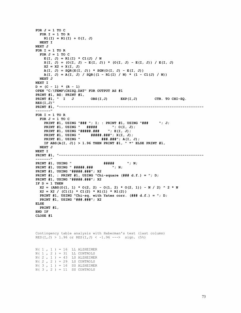
73
FOR J = 1 TO C FOR I = 1 TO R R1(I) = R1(I) + O(I, J) NEXT I NEXT J FOR I = 1 TO R FOR J = 1 TO C E(I, J) = R1(I) * C1(J) / N X(I, J) = (O(I, J) - E(I, J)) * (O(I, J) - E(I, J)) / E(I, J) X2 = X2 + X(I, J) A(I, J) = SQR(X(I, J)) * SGN(O(I, J) - E(I, J)) A(I, J) = A(I, J) / SQR((1 - R1(I) / N) * (1 - C1(J) / N)) NEXT J NEXT I D = (C - 1) * (R - 1) OPEN "C:\TEMP\CHISQ.DAT" FOR OUTPUT AS #1 PRINT #1, B$: PRINT #1, PRINT #1, " I J OBS(I,J) EXP(I,J) CTR. TO CHI-SQ. RES(I,J)" PRINT #1, "---------------------------------------------------------------------------" FOR I = 1 TO R FOR J = 1 TO C PRINT #1, USING "### "; I; : PRINT #1, USING "### "; J; PRINT #1, USING " ##### "; O(I, J); PRINT #1, USING "#####.### "; E(I, J); PRINT #1, USING " #####.###"; X(I, J); PRINT #1, USING " ###.###"; A(I, J); IF ABS(A(I, J)) > 1.96 THEN PRINT #1, " *" ELSE PRINT #1, NEXT J NEXT I PRINT #1, "---------------------------------------------------------------------------" PRINT #1, USING " ##### "; N; PRINT #1, USING " #####.### "; N; PRINT #1, USING "#####.###"; X2 PRINT #1, : PRINT #1, USING "Chi-square (### d.f.) = "; D; PRINT #1, USING "#####.###"; X2 IF D = 1 THEN X2 = (ABS(O(1, 1) * O(2, 2) - O(1, 2) * O(2, 1)) - N / 2) ^ 2 * N X2 = X2 / (C1(1) * C1(2) * R1(1) * R1(2)) PRINT #1, USING "Chi-sq. with Yates corr. (### d.f.) = "; D; PRINT #1, USING "###.###"; X2 ELSE PRINT #1, END IF CLOSE #1 Contingency table analysis with Haberman's test (last column) RES(I,J) > 1.96 or RES(I,J) < -1.96 ---> sign. (5%) N( 1 , 1 ) = 16 LL ALZHEIMER N( 1 , 2 ) = 31 LL CONTROLS N( 2 , 1 ) = 43 LS ALZHEIMER N( 2 , 2 ) = 29 LS CONTROLS N( 3 , 1 ) = 16 SS ALZHEIMER N( 3 , 2 ) = 11 SS CONTROLS
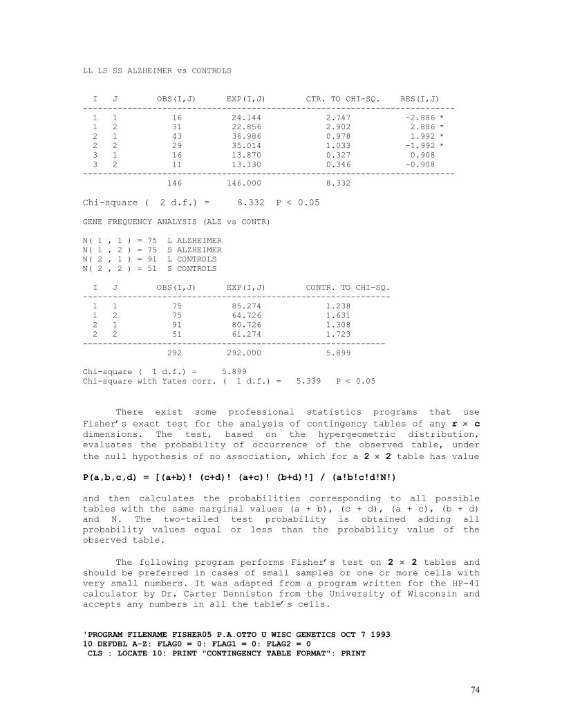
74
LL LS SS ALZHEIMER vs CONTROLS I J OBS(I,J) EXP(I,J) CTR. TO CHI-SQ. RES(I,J) --------------------------------------------------------------------------- 1 1 16 24.144 2.747 -2.886 * 1 2 31 22.856 2.902 2.886 * 2 1 43 36.986 0.978 1.992 * 2 2 29 35.014 1.033 -1.992 * 3 1 16 13.870 0.327 0.908 3 2 11 13.130 0.346 -0.908 --------------------------------------------------------------------------- 146 146.000 8.332 Chi-square ( 2 d.f.) = 8.332 P < 0.05 GENE FREQUENCY ANALYSIS (ALZ vs CONTR) N( 1 , 1 ) = 75 L ALZHEIMER N( 1 , 2 ) = 75 S ALZHEIMER N( 2 , 1 ) = 91 L CONTROLS N( 2 , 2 ) = 51 S CONTROLS I J OBS(I,J) EXP(I,J) CONTR. TO CHI-SQ. -------------------------------------------------------------- 1 1 75 85.274 1.238 1 2 75 64.726 1.631 2 1 91 80.726 1.308 2 2 51 61.274 1.723 ------------------------------------------------------------- 292 292.000 5.899 Chi-square ( 1 d.f.) = 5.899 Chi-square with Yates corr. ( 1 d.f.) = 5.339 P < 0.05
There exist some professional statistics programs that use Fisher’s exact test for the analysis of contingency tables of any r × c dimensions. The test, based on the hypergeometric distribution, evaluates the probability of occurrence of the observed table, under the null hypothesis of no association, which for a 2 × 2 table has value P(a,b,c,d) = [(a+b)! (c+d)! (a+c)! (b+d)!] / (a!b!c!d!N!) and then calculates the probabilities corresponding to all possible tables with the same marginal values (a + b), (c + d), (a + c), (b + d) and N. The two-tailed test probability is obtained adding all probability values equal or less than the probability value of the observed table.
The following program performs Fisher’s test on 2 × 2 tables and should be preferred in cases of small samples or one or more cells with very small numbers. It was adapted from a program written for the HP-41 calculator by Dr. Carter Denniston from the University of Wisconsin and accepts any numbers in all the table’s cells. 'PROGRAM FILENAME FISHER05 P.A.OTTO U WISC GENETICS OCT 7 1993 10 DEFDBL A-Z: FLAG0 = 0: FLAG1 = 0: FLAG2 = 0 CLS : LOCATE 10: PRINT "CONTINGENCY TABLE FORMAT": PRINT
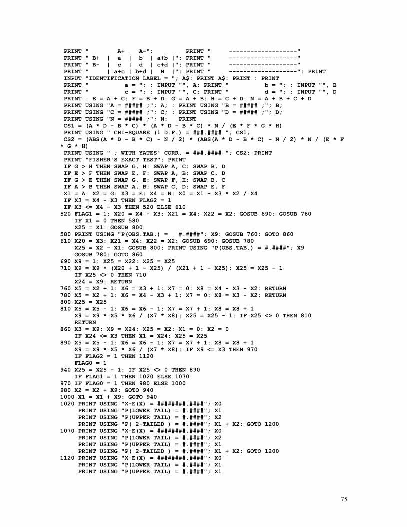
75
PRINT " A+ A-": PRINT " -------------------" PRINT " B+ | a | b | a+b |": PRINT " -------------------" PRINT " B- | c | d | c+d |": PRINT " -------------------" PRINT " | a+c | b+d | N |": PRINT " -------------------": PRINT INPUT "IDENTIFICATION LABEL = "; A$: PRINT A$: PRINT : PRINT PRINT " a = "; : INPUT "", A: PRINT " b = "; : INPUT "", B PRINT " c = "; : INPUT "", C: PRINT " d = "; : INPUT "", D PRINT : E = A + C: F = B + D: G = A + B: H = C + D: N = A + B + C + D PRINT USING "A = ##### ;"; A; : PRINT USING "B = ##### ;"; B; PRINT USING "C = ##### ;"; C; : PRINT USING "D = ##### ;"; D; PRINT USING "N = ##### ;"; N: PRINT CS1 = (A * D - B * C) * (A * D - B * C) * N / (E * F * G * H) PRINT USING " CHI-SQUARE (1 D.F.) = ###.#### "; CS1; CS2 = (ABS(A * D - B * C) - N / 2) * (ABS(A * D - B * C) - N / 2) * N / (E * F * G * H) PRINT USING " ; WITH YATES' CORR. = ###.#### "; CS2: PRINT PRINT "FISHER'S EXACT TEST": PRINT IF G > H THEN SWAP G, H: SWAP A, C: SWAP B, D IF E > F THEN SWAP E, F: SWAP A, B: SWAP C, D IF G > E THEN SWAP G, E: SWAP F, H: SWAP B, C IF A > B THEN SWAP A, B: SWAP C, D: SWAP E, F X1 = A: X2 = G: X3 = E: X4 = N: X0 = X1 - X3 * X2 / X4 IF X3 = X4 - X3 THEN FLAG2 = 1 IF X3 <= X4 - X3 THEN 520 ELSE 610 520 FLAG1 = 1: X20 = X4 - X3: X21 = X4: X22 = X2: GOSUB 690: GOSUB 760 IF X1 = 0 THEN 580 X25 = X1: GOSUB 800 580 PRINT USING "P(OBS.TAB.) = #.####"; X9: GOSUB 760: GOTO 860 610 X20 = X3: X21 = X4: X22 = X2: GOSUB 690: GOSUB 780 X25 = X2 - X1: GOSUB 800: PRINT USING "P(OBS.TAB.) = #.####"; X9 GOSUB 780: GOTO 860 690 X9 = 1: X25 = X22: X25 = X25 710 X9 = X9 * (X20 + 1 - X25) / (X21 + 1 - X25): X25 = X25 - 1 IF X25 <> 0 THEN 710 X24 = X9: RETURN 760 X5 = X2 + 1: X6 = X3 + 1: X7 = 0: X8 = X4 - X3 - X2: RETURN 780 X5 = X2 + 1: X6 = X4 - X3 + 1: X7 = 0: X8 = X3 - X2: RETURN 800 X25 = X25 810 X5 = X5 - 1: X6 = X6 - 1: X7 = X7 + 1: X8 = X8 + 1 X9 = X9 * X5 * X6 / (X7 * X8): X25 = X25 - 1: IF X25 <> 0 THEN 810 RETURN 860 X3 = X9: X9 = X24: X25 = X2: X1 = 0: X2 = 0 IF X24 <= X3 THEN X1 = X24: X25 = X25 890 X5 = X5 - 1: X6 = X6 - 1: X7 = X7 + 1: X8 = X8 + 1 X9 = X9 * X5 * X6 / (X7 * X8): IF X9 <= X3 THEN 970 IF FLAG2 = 1 THEN 1120 FLAG0 = 1 940 X25 = X25 - 1: IF X25 <> 0 THEN 890 IF FLAG1 = 1 THEN 1020 ELSE 1070 970 IF FLAG0 = 1 THEN 980 ELSE 1000 980 X2 = X2 + X9: GOTO 940 1000 X1 = X1 + X9: GOTO 940 1020 PRINT USING "X-E(X) = ########.####"; X0 PRINT USING "P(LOWER TAIL) = #.####"; X1 PRINT USING "P(UPPER TAIL) = #.####"; X2 PRINT USING "P( 2-TAILED ) = #.####"; X1 + X2: GOTO 1200 1070 PRINT USING "X-E(X) = ########.####"; X0 PRINT USING "P(LOWER TAIL) = #.####"; X2 PRINT USING "P(UPPER TAIL) = #.####"; X1 PRINT USING "P( 2-TAILED ) = #.####"; X1 + X2: GOTO 1200 1120 PRINT USING "X-E(X) = ########.####"; X0 PRINT USING "P(LOWER TAIL) = #.####"; X1 PRINT USING "P(UPPER TAIL) = #.####"; X1
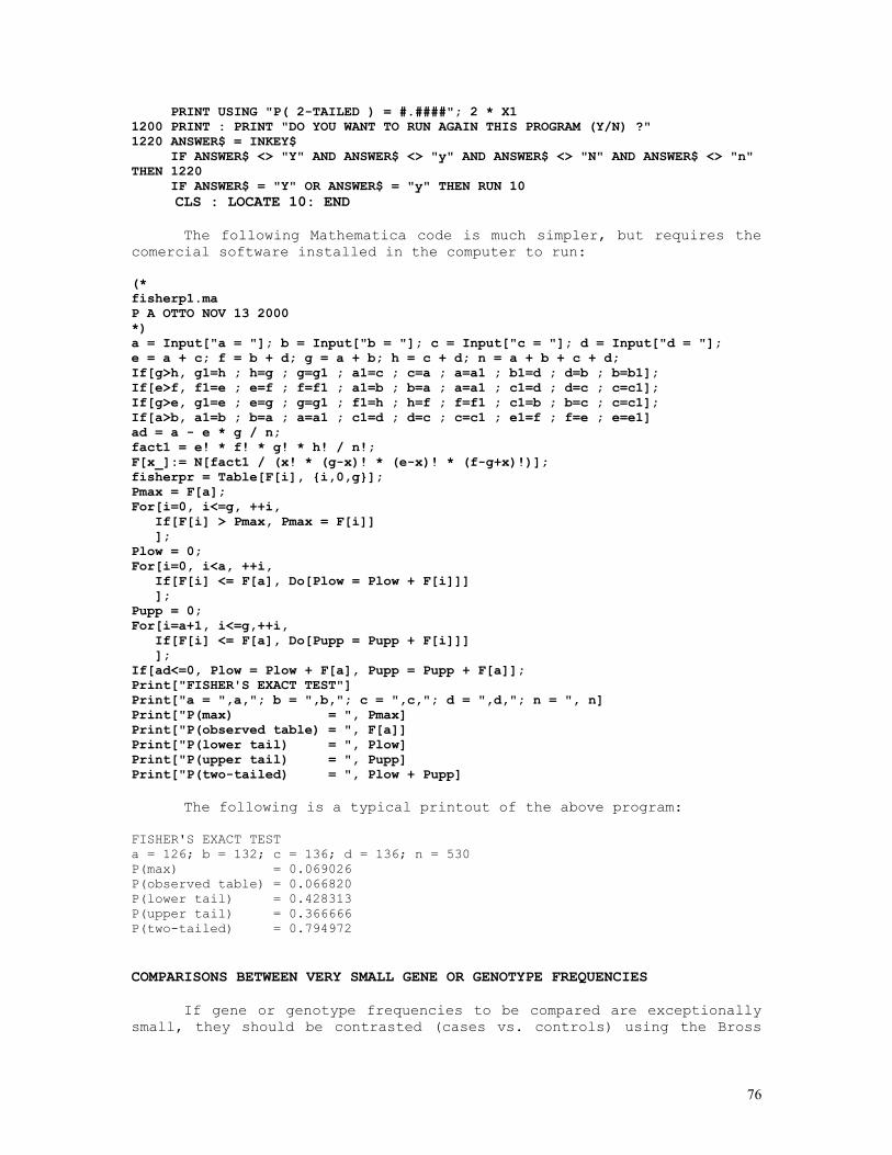
76
PRINT USING "P( 2-TAILED ) = #.####"; 2 * X1 1200 PRINT : PRINT "DO YOU WANT TO RUN AGAIN THIS PROGRAM (Y/N) ?" 1220 ANSWER$ = INKEY$ IF ANSWER$ <> "Y" AND ANSWER$ <> "y" AND ANSWER$ <> "N" AND ANSWER$ <> "n" THEN 1220 IF ANSWER$ = "Y" OR ANSWER$ = "y" THEN RUN 10 CLS : LOCATE 10: END
The following Mathematica code is much simpler, but requires the comercial software installed in the computer to run: (* fisherp1.ma P A OTTO NOV 13 2000 *) a = Input["a = "]; b = Input["b = "]; c = Input["c = "]; d = Input["d = "]; e = a + c; f = b + d; g = a + b; h = c + d; n = a + b + c + d; If[g>h, g1=h ; h=g ; g=g1 ; a1=c ; c=a ; a=a1 ; b1=d ; d=b ; b=b1]; If[e>f, f1=e ; e=f ; f=f1 ; a1=b ; b=a ; a=a1 ; c1=d ; d=c ; c=c1]; If[g>e, g1=e ; e=g ; g=g1 ; f1=h ; h=f ; f=f1 ; c1=b ; b=c ; c=c1]; If[a>b, a1=b ; b=a ; a=a1 ; c1=d ; d=c ; c=c1 ; e1=f ; f=e ; e=e1] ad = a - e * g / n; fact1 = e! * f! * g! * h! / n!; F[x_]:= N[fact1 / (x! * (g-x)! * (e-x)! * (f-g+x)!)]; fisherpr = Table[F[i], {i,0,g}]; Pmax = F[a]; For[i=0, i<=g, ++i, If[F[i] > Pmax, Pmax = F[i]] ]; Plow = 0; For[i=0, i<a, ++i, If[F[i] <= F[a], Do[Plow = Plow + F[i]]] ]; Pupp = 0; For[i=a+1, i<=g,++i, If[F[i] <= F[a], Do[Pupp = Pupp + F[i]]] ]; If[ad<=0, Plow = Plow + F[a], Pupp = Pupp + F[a]]; Print["FISHER'S EXACT TEST"] Print["a = ",a,"; b = ",b,"; c = ",c,"; d = ",d,"; n = ", n] Print["P(max) = ", Pmax] Print["P(observed table) = ", F[a]] Print["P(lower tail) = ", Plow] Print["P(upper tail) = ", Pupp] Print["P(two-tailed) = ", Plow + Pupp]
The following is a typical printout of the above program: FISHER'S EXACT TEST a = 126; b = 132; c = 136; d = 136; n = 530 P(max) = 0.069026 P(observed table) = 0.066820 P(lower tail) = 0.428313 P(upper tail) = 0.366666 P(two-tailed) = 0.794972 COMPARISONS BETWEEN VERY SMALL GENE OR GENOTYPE FREQUENCIES
If gene or genotype frequencies to be compared are exceptionally small, they should be contrasted (cases vs. controls) using the Bross
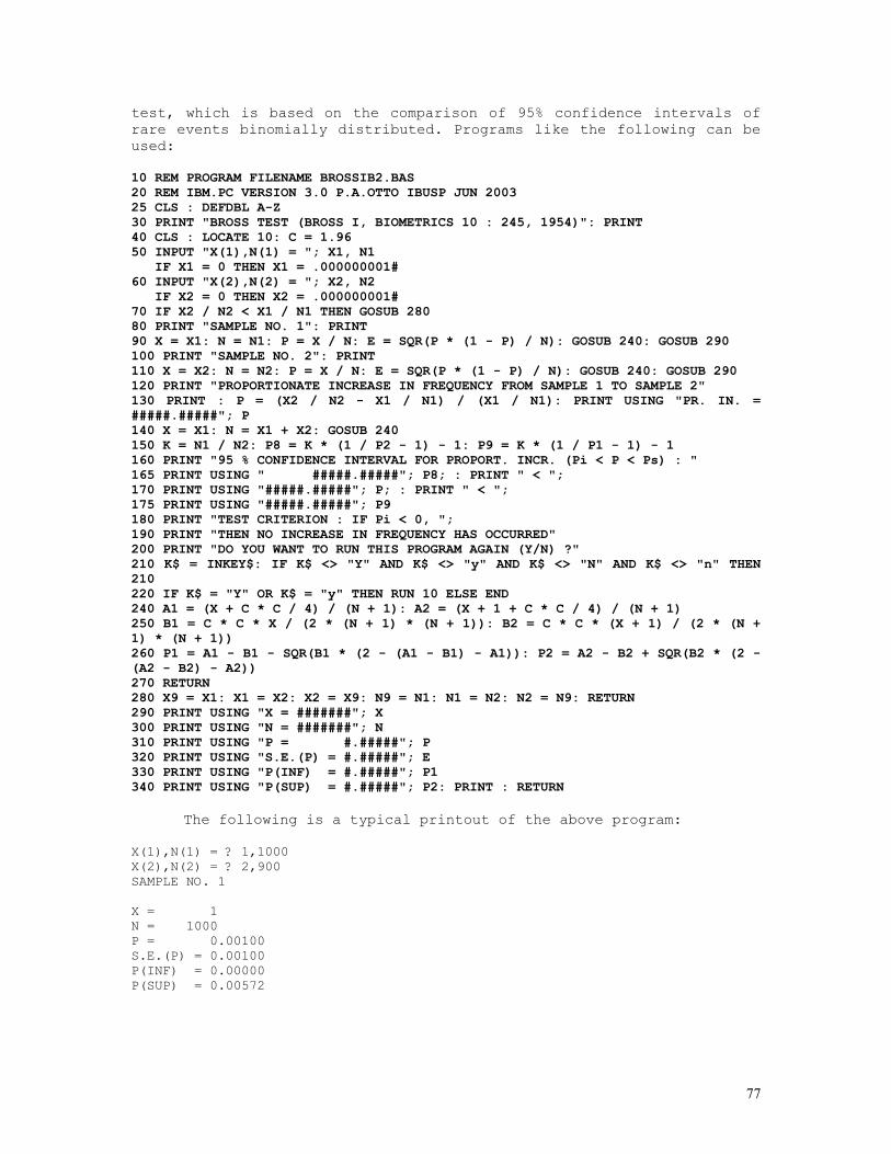
77
test, which is based on the comparison of 95% confidence intervals of rare events binomially distributed. Programs like the following can be used: 10 REM PROGRAM FILENAME BROSSIB2.BAS 20 REM IBM.PC VERSION 3.0 P.A.OTTO IBUSP JUN 2003 25 CLS : DEFDBL A-Z 30 PRINT "BROSS TEST (BROSS I, BIOMETRICS 10 : 245, 1954)": PRINT 40 CLS : LOCATE 10: C = 1.96 50 INPUT "X(1),N(1) = "; X1, N1 IF X1 = 0 THEN X1 = .000000001# 60 INPUT "X(2),N(2) = "; X2, N2 IF X2 = 0 THEN X2 = .000000001# 70 IF X2 / N2 < X1 / N1 THEN GOSUB 280 80 PRINT "SAMPLE NO. 1": PRINT 90 X = X1: N = N1: P = X / N: E = SQR(P * (1 - P) / N): GOSUB 240: GOSUB 290 100 PRINT "SAMPLE NO. 2": PRINT 110 X = X2: N = N2: P = X / N: E = SQR(P * (1 - P) / N): GOSUB 240: GOSUB 290 120 PRINT "PROPORTIONATE INCREASE IN FREQUENCY FROM SAMPLE 1 TO SAMPLE 2" 130 PRINT : P = (X2 / N2 - X1 / N1) / (X1 / N1): PRINT USING "PR. IN. = #####.#####"; P 140 X = X1: N = X1 + X2: GOSUB 240 150 K = N1 / N2: P8 = K * (1 / P2 - 1) - 1: P9 = K * (1 / P1 - 1) - 1 160 PRINT "95 % CONFIDENCE INTERVAL FOR PROPORT. INCR. (Pi < P < Ps) : " 165 PRINT USING " #####.#####"; P8; : PRINT " < "; 170 PRINT USING "#####.#####"; P; : PRINT " < "; 175 PRINT USING "#####.#####"; P9 180 PRINT "TEST CRITERION : IF Pi < 0, "; 190 PRINT "THEN NO INCREASE IN FREQUENCY HAS OCCURRED" 200 PRINT "DO YOU WANT TO RUN THIS PROGRAM AGAIN (Y/N) ?" 210 K$ = INKEY$: IF K$ <> "Y" AND K$ <> "y" AND K$ <> "N" AND K$ <> "n" THEN 210 220 IF K$ = "Y" OR K$ = "y" THEN RUN 10 ELSE END 240 A1 = (X + C * C / 4) / (N + 1): A2 = (X + 1 + C * C / 4) / (N + 1) 250 B1 = C * C * X / (2 * (N + 1) * (N + 1)): B2 = C * C * (X + 1) / (2 * (N + 1) * (N + 1)) 260 P1 = A1 - B1 - SQR(B1 * (2 - (A1 - B1) - A1)): P2 = A2 - B2 + SQR(B2 * (2 - (A2 - B2) - A2)) 270 RETURN 280 X9 = X1: X1 = X2: X2 = X9: N9 = N1: N1 = N2: N2 = N9: RETURN 290 PRINT USING "X = #######"; X 300 PRINT USING "N = #######"; N 310 PRINT USING "P = #.#####"; P 320 PRINT USING "S.E.(P) = #.#####"; E 330 PRINT USING "P(INF) = #.#####"; P1 340 PRINT USING "P(SUP) = #.#####"; P2: PRINT : RETURN
The following is a typical printout of the above program: X(1),N(1) = ? 1,1000 X(2),N(2) = ? 2,900 SAMPLE NO. 1 X = 1 N = 1000 P = 0.00100 S.E.(P) = 0.00100 P(INF) = 0.00000 P(SUP) = 0.00572

78
SAMPLE NO. 2 X = 2 N = 900 P = 0.00222 S.E.(P) = 0.00157 P(INF) = 0.00021 P(SUP) = 0.00815 PROPORTIONATE INCREASE IN FREQUENCY FROM SAMPLE 1 TO SAMPLE 2 PR. IN. = 1.22222 95 % CONFIDENCE INTERVAL FOR PROPORT. INCR. (Pi < P < Ps) : -0.91269 < 1.22222 < 8386.70358 TEST CRITERION : IF Pi < 0, THEN NO INCREASE IN FREQUENCY HAS OCCURRED ASSOCIATION ANALYSIS USING A CASE-CONTROL DESIGN: ASSOCIATION BETWEEN A DISEASE AND A SET OF MARKER LOCI
Sham (1998) describes in detail a method for assessing linkage disequilibrium, in a control/case study, between a disease and a set of marker loci, using log-likelihood tests that compare a model that assumes linkage disequilibrium between all loci (disease and markers) with a model that assumes disequilibrium between the marker loci but equilibrium between the marker loci and the disease locus (Terwilliger and Ott, 1994). In the lines that follow we adapt their method to a generalized X-linked case that uses data collected from male individuals.
Let (A, a) and (B, b) be two diallelic X-linked loci. In a control/case study, the genotypes were determined in a random sample of N1 nonaffected male individuals, with the following results:
A a
B n11 n21 N31
b n31 n41 N41
N11 N21 N1
and in a random sample of N2 affected male individuals having a rare X-linked disease, with the following results:
A a
B n12 n22 N32
b n32 n42 N42
N12 N22 N2
Among nonaffected individuals, gene frequencies, haplotype
frequencies, and linkage disequilibrium values are estimated respectively after P1(A) = p1 = N11/N1 P1(a) = 1-p1 = N21/N1
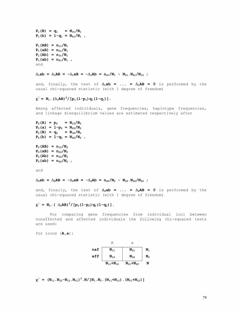
79
P1(B) = q1 = N31/N1 P1(b) = 1-q1 = N41/N1 , P1(AB) = n11/N1 P1(aB) = n21/N1 P1(Ab) = n31/N1 P1(ab) = n41/N1 , and ∆1ab = ∆1AB = -∆1aB = -∆1Ab = n41/N1 - N21.N41/N12 ; and, finally, the test of ∆1ab = ... = ∆1AB = 0 is performed by the usual chi-squared statistic (with 1 degree of freedom) χ2 = N1.(∆1AB)2/[p1(1-p1)q1(1-q1)]. Among affected individuals, gene frequencies, haplotype frequencies, and linkage disequilibrium values are estimated respectively after P2(A) = p2 = N12/N2 P2(a) = 1-p2 = N22/N2 P2(B) = q2 = N32/N2 P2(b) = 1-q2 = N42/N2 , P2(AB) = n12/N2 P2(aB) = n22/N2 P2(Ab) = n32/N2 P2(ab) = n42/N2 , and ∆2ab = ∆2AB = -∆2aB = -∆2Ab = n42/N2 - N22.N42/N22 ; and, finally, the test of ∆2ab = ... = ∆2AB = 0 is performed by the usual chi-squared statistic (with 1 degree of freedom) χ2 = N2.( ∆2AB)2/[p2(1-p2)q2(1-q2)].
For comparing gene frequencies from individual loci between nonaffected and affected individuals the following chi-squared tests are used: for locus (A,a):
A a
naf N11 N21 N1
aff N12 N22 N2
N11+N12 N21+N22 N
χ2 = (N11.N22-N12.N21)2.N/[N1.N2.(N11+N12).(N21+N22)]
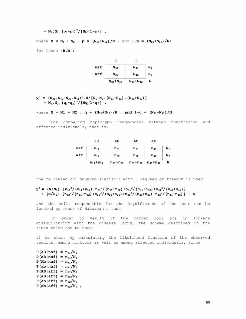
80
= N1.N2.(p1-p2)2/[Np(1-p)] , where N = N1 + N2 , p = (N11+N12)/N , and 1-p = (N21+N22)/N; for locus (B,b):
B b
naf N31 N41 N1
aff N32 N42 N2
N31+N32 N41+N42 N
χ2 = (N31.N42-N32.N41)2.N/[N1.N2.(N31+N32).(N41+N42)] = N1.N2.(q1-q2)2/[Nq(1-q)] , where N = N1 + N2 , q = (N31+N32)/N , and 1-q = (N41+N42)/N.
For comparing haplotype frequencies between nonaffected and affected individuals, that is,
AB aB Ab ab
naf n11 n21 n31 n41 N1
aff n12 n22 n32 n42 N2
n11+n12 n21+n22 n31+n32 n41+n42 N
the following chi-squared statistic with 3 degrees of freedom is used: χ2 = (N/N1).[n112/(n11+n12)+n212/(n21+n22)+n312/(n31+n32)+n412/(n41+n42)] + (N/N2).[n122/(n11+n12)+n222/(n21+n22)+n322/(n31+n32)+n422/(n41+n42)] - N and the cells responsible for the significance of the test can be located by means of Haberman's test.
In order to verify if the marker loci are in linkage disequilibrium with the disease locus, the scheme described in the lines below can be used. a) we start by calculating the likelihood function of the observed results, among controls as well as among affected individuals; since P(AB|naf) = n11/N1 P(aB|naf) = n21/N1 P(Ab|naf) = n31/N1 P(ab|naf) = n41/N1 P(AB|aff) = n12/N2 P(aB|aff) = n22/N2 P(Ab|aff) = n32/N2 P(ab|aff) = n42/N2 ,
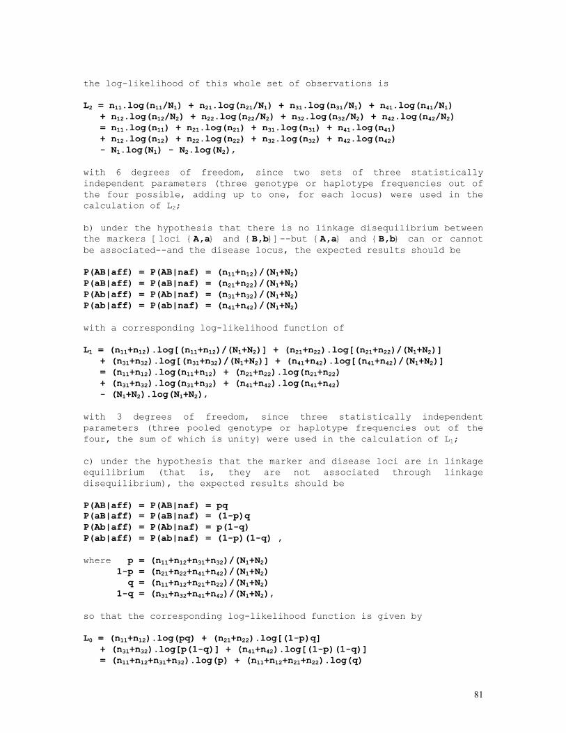
81
the log-likelihood of this whole set of observations is L2 = n11.log(n11/N1) + n21.log(n21/N1) + n31.log(n31/N1) + n41.log(n41/N1) + n12.log(n12/N2) + n22.log(n22/N2) + n32.log(n32/N2) + n42.log(n42/N2) = n11.log(n11) + n21.log(n21) + n31.log(n31) + n41.log(n41) + n12.log(n12) + n22.log(n22) + n32.log(n32) + n42.log(n42) - N1.log(N1) - N2.log(N2), with 6 degrees of freedom, since two sets of three statistically independent parameters (three genotype or haplotype frequencies out of the four possible, adding up to one, for each locus) were used in the calculation of L2; b) under the hypothesis that there is no linkage disequilibrium between the markers [loci {A,a} and {B,b}]--but {A,a} and {B,b} can or cannot be associated--and the disease locus, the expected results should be P(AB|aff) = P(AB|naf) = (n11+n12)/(N1+N2) P(aB|aff) = P(aB|naf) = (n21+n22)/(N1+N2) P(Ab|aff) = P(Ab|naf) = (n31+n32)/(N1+N2) P(ab|aff) = P(ab|naf) = (n41+n42)/(N1+N2) with a corresponding log-likelihood function of L1 = (n11+n12).log[(n11+n12)/(N1+N2)] + (n21+n22).log[(n21+n22)/(N1+N2)] + (n31+n32).log[(n31+n32)/(N1+N2)] + (n41+n42).log[(n41+n42)/(N1+N2)] = (n11+n12).log(n11+n12) + (n21+n22).log(n21+n22) + (n31+n32).log(n31+n32) + (n41+n42).log(n41+n42) - (N1+N2).log(N1+N2), with 3 degrees of freedom, since three statistically independent parameters (three pooled genotype or haplotype frequencies out of the four, the sum of which is unity) were used in the calculation of L1; c) under the hypothesis that the marker and disease loci are in linkage equilibrium (that is, they are not associated through linkage disequilibrium), the expected results should be P(AB|aff) = P(AB|naf) = pq P(aB|aff) = P(aB|naf) = (1-p)q P(Ab|aff) = P(Ab|naf) = p(1-q) P(ab|aff) = P(ab|naf) = (1-p)(1-q) , where p = (n11+n12+n31+n32)/(N1+N2) 1-p = (n21+n22+n41+n42)/(N1+N2) q = (n11+n12+n21+n22)/(N1+N2) 1-q = (n31+n32+n41+n42)/(N1+N2), so that the corresponding log-likelihood function is given by L0 = (n11+n12).log(pq) + (n21+n22).log[(1-p)q] + (n31+n32).log[p(1-q)] + (n41+n42).log[(1-p)(1-q)] = (n11+n12+n31+n32).log(p) + (n11+n12+n21+n22).log(q)
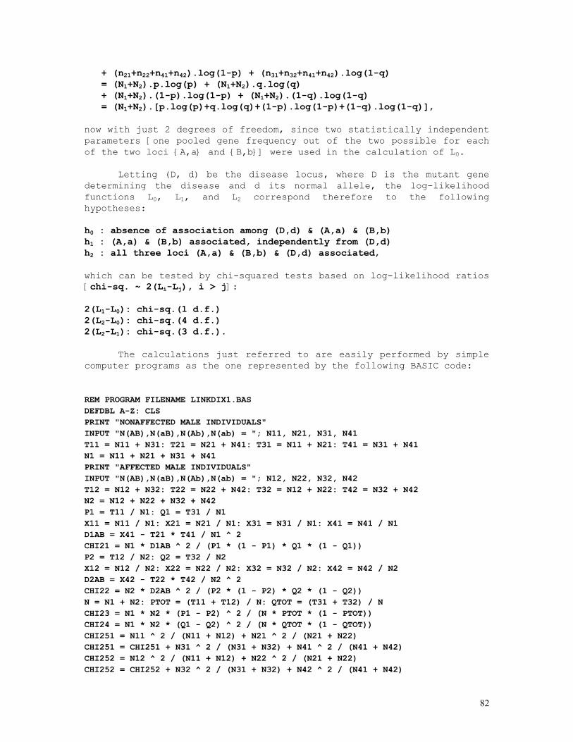
82
+ (n21+n22+n41+n42).log(1-p) + (n31+n32+n41+n42).log(1-q) = (N1+N2).p.log(p) + (N1+N2).q.log(q) + (N1+N2).(1-p).log(1-p) + (N1+N2).(1-q).log(1-q) = (N1+N2).[p.log(p)+q.log(q)+(1-p).log(1-p)+(1-q).log(1-q)], now with just 2 degrees of freedom, since two statistically independent parameters [one pooled gene frequency out of the two possible for each of the two loci {A,a} and {B,b}] were used in the calculation of L0.
Letting (D, d) be the disease locus, where D is the mutant gene determining the disease and d its normal allele, the log-likelihood functions L0, L1, and L2 correspond therefore to the following hypotheses: h0 : absence of association among (D,d) & (A,a) & (B,b) h1 : (A,a) & (B,b) associated, independently from (D,d) h2 : all three loci (A,a) & (B,b) & (D,d) associated, which can be tested by chi-squared tests based on log-likelihood ratios [chi-sq. ~ 2(Li-Lj), i > j]: 2(L1-L0): chi-sq.(1 d.f.) 2(L2-L0): chi-sq.(4 d.f.) 2(L2-L1): chi-sq.(3 d.f.).
The calculations just referred to are easily performed by simple computer programs as the one represented by the following BASIC code:
REM PROGRAM FILENAME LINKDIX1.BAS DEFDBL A-Z: CLS PRINT "NONAFFECTED MALE INDIVIDUALS" INPUT "N(AB),N(aB),N(Ab),N(ab) = "; N11, N21, N31, N41 T11 = N11 + N31: T21 = N21 + N41: T31 = N11 + N21: T41 = N31 + N41 N1 = N11 + N21 + N31 + N41 PRINT "AFFECTED MALE INDIVIDUALS" INPUT "N(AB),N(aB),N(Ab),N(ab) = "; N12, N22, N32, N42 T12 = N12 + N32: T22 = N22 + N42: T32 = N12 + N22: T42 = N32 + N42 N2 = N12 + N22 + N32 + N42 P1 = T11 / N1: Q1 = T31 / N1 X11 = N11 / N1: X21 = N21 / N1: X31 = N31 / N1: X41 = N41 / N1 D1AB = X41 - T21 * T41 / N1 ^ 2 CHI21 = N1 * D1AB ^ 2 / (P1 * (1 - P1) * Q1 * (1 - Q1)) P2 = T12 / N2: Q2 = T32 / N2 X12 = N12 / N2: X22 = N22 / N2: X32 = N32 / N2: X42 = N42 / N2 D2AB = X42 - T22 * T42 / N2 ^ 2 CHI22 = N2 * D2AB ^ 2 / (P2 * (1 - P2) * Q2 * (1 - Q2)) N = N1 + N2: PTOT = (T11 + T12) / N: QTOT = (T31 + T32) / N CHI23 = N1 * N2 * (P1 - P2) ^ 2 / (N * PTOT * (1 - PTOT)) CHI24 = N1 * N2 * (Q1 - Q2) ^ 2 / (N * QTOT * (1 - QTOT)) CHI251 = N11 ^ 2 / (N11 + N12) + N21 ^ 2 / (N21 + N22) CHI251 = CHI251 + N31 ^ 2 / (N31 + N32) + N41 ^ 2 / (N41 + N42) CHI252 = N12 ^ 2 / (N11 + N12) + N22 ^ 2 / (N21 + N22) CHI252 = CHI252 + N32 ^ 2 / (N31 + N32) + N42 ^ 2 / (N41 + N42)
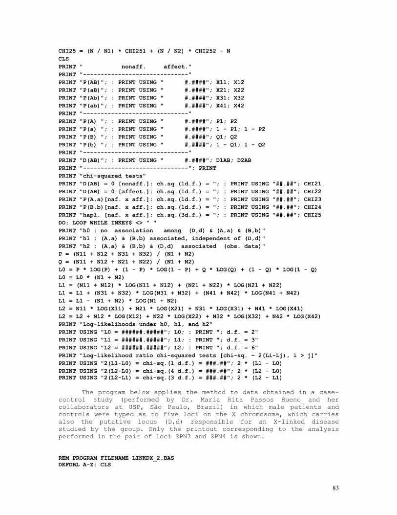
83
CHI25 = (N / N1) * CHI251 + (N / N2) * CHI252 - N CLS PRINT " nonaff. affect." PRINT "------------------------------" PRINT "P(AB)"; : PRINT USING " #.####"; X11; X12 PRINT "P(aB)"; : PRINT USING " #.####"; X21; X22 PRINT "P(Ab)"; : PRINT USING " #.####"; X31; X32 PRINT "P(ab)"; : PRINT USING " #.####"; X41; X42 PRINT "------------------------------" PRINT "P(A) "; : PRINT USING " #.####"; P1; P2 PRINT "P(a) "; : PRINT USING " #.####"; 1 - P1; 1 - P2 PRINT "P(B) "; : PRINT USING " #.####"; Q1; Q2 PRINT "P(b) "; : PRINT USING " #.####"; 1 - Q1; 1 - Q2 PRINT "------------------------------" PRINT "D(AB)"; : PRINT USING " #.####"; D1AB; D2AB PRINT "------------------------------": PRINT PRINT "chi-squared tests" PRINT "D(AB) = 0 [nonaff.]: ch.sq.(1d.f.) = "; : PRINT USING "##.##"; CHI21 PRINT "D(AB) = 0 [affect.]: ch.sq.(1d.f.) = "; : PRINT USING "##.##"; CHI22 PRINT "P(A,a)[naf. x aff.]: ch.sq.(1d.f.) = "; : PRINT USING "##.##"; CHI23 PRINT "P(B,b)[naf. x aff.]: ch.sq.(1d.f.) = "; : PRINT USING "##.##"; CHI24 PRINT "hapl. [naf. x aff.]: ch.sq.(3d.f.) = "; : PRINT USING "##.##"; CHI25 DO: LOOP WHILE INKEY$ <> " " PRINT "h0 : no association among (D,d) & (A,a) & (B,b)" PRINT "h1 : (A,a) & (B,b) associated, independent of (D,d)" PRINT "h2 : (A,a) & (B,b) & (D,d) associated (obs. data)" P = (N11 + N12 + N31 + N32) / (N1 + N2) Q = (N11 + N12 + N21 + N22) / (N1 + N2) L0 = P * LOG(P) + (1 - P) * LOG(1 - P) + Q * LOG(Q) + (1 - Q) * LOG(1 - Q) L0 = L0 * (N1 + N2) L1 = (N11 + N12) * LOG(N11 + N12) + (N21 + N22) * LOG(N21 + N22) L1 = L1 + (N31 + N32) * LOG(N31 + N32) + (N41 + N42) * LOG(N41 + N42) L1 = L1 - (N1 + N2) * LOG(N1 + N2) L2 = N11 * LOG(X11) + N21 * LOG(X21) + N31 * LOG(X31) + N41 * LOG(X41) L2 = L2 + N12 * LOG(X12) + N22 * LOG(X22) + N32 * LOG(X32) + N42 * LOG(X42) PRINT "Log-likelihoods under h0, h1, and h2" PRINT USING "L0 = ######.#####"; L0; : PRINT "; d.f. = 2" PRINT USING "L1 = ######.#####"; L1; : PRINT "; d.f. = 3" PRINT USING "L2 = ######.#####"; L2; : PRINT "; d.f. = 6" PRINT "Log-likelihood ratio chi-squared tests [chi-sq. ~ 2(Li-Lj), i > j]" PRINT USING "2(L1-L0) = chi-sq.(1 d.f.) = ###.##"; 2 * (L1 - L0) PRINT USING "2(L2-L0) = chi-sq.(4 d.f.) = ###.##"; 2 * (L2 - L0) PRINT USING "2(L2-L1) = chi-sq.(3 d.f.) = ###.##"; 2 * (L2 - L1)
The program below applies the method to data obtained in a case-control study (performed by Dr. Maria Rita Passos Bueno and her collaborators at USP, São Paulo, Brazil) in which male patients and controls were typed as to five loci on the X chromosome, which carries also the putative locus (D,d) responsible for an X-linked disease studied by the group. Only the printout corresponding to the analysis performed in the pair of loci SPN3 and SPN4 is shown. REM PROGRAM FILENAME LINKDX_2.BAS DEFDBL A-Z: CLS
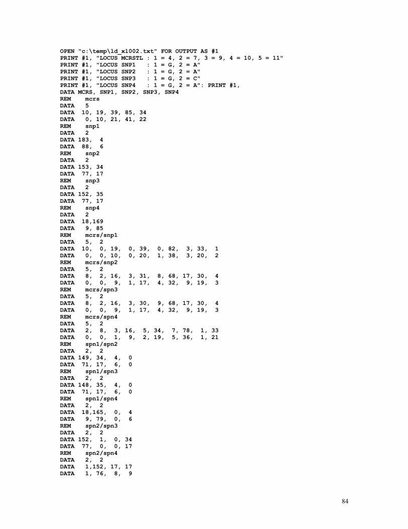
84
OPEN "c:\temp\ld_xl002.txt" FOR OUTPUT AS #1 PRINT #1, "LOCUS MCRSTL : 1 = 4, 2 = 7, 3 = 9, 4 = 10, 5 = 11" PRINT #1, "LOCUS SNP1 : 1 = G, 2 = A" PRINT #1, "LOCUS SNP2 : 1 = G, 2 = A" PRINT #1, "LOCUS SNP3 : 1 = G, 2 = C" PRINT #1, "LOCUS SNP4 : 1 = G, 2 = A": PRINT #1, DATA MCRS, SNP1, SNP2, SNP3, SNP4 REM mcrs DATA 5 DATA 10, 19, 39, 85, 34 DATA 0, 10, 21, 41, 22 REM snp1 DATA 2 DATA 183, 4 DATA 88, 6 REM snp2 DATA 2 DATA 153, 34 DATA 77, 17 REM snp3 DATA 2 DATA 152, 35 DATA 77, 17 REM snp4 DATA 2 DATA 18,169 DATA 9, 85 REM mcrs/snp1 DATA 5, 2 DATA 10, 0, 19, 0, 39, 0, 82, 3, 33, 1 DATA 0, 0, 10, 0, 20, 1, 38, 3, 20, 2 REM mcrs/snp2 DATA 5, 2 DATA 8, 2, 16, 3, 31, 8, 68, 17, 30, 4 DATA 0, 0, 9, 1, 17, 4, 32, 9, 19, 3 REM mcrs/spn3 DATA 5, 2 DATA 8, 2, 16, 3, 30, 9, 68, 17, 30, 4 DATA 0, 0, 9, 1, 17, 4, 32, 9, 19, 3 REM mcrs/spn4 DATA 5, 2 DATA 2, 8, 3, 16, 5, 34, 7, 78, 1, 33 DATA 0, 0, 1, 9, 2, 19, 5, 36, 1, 21 REM spn1/spn2 DATA 2, 2 DATA 149, 34, 4, 0 DATA 71, 17, 6, 0 REM spn1/spn3 DATA 2, 2 DATA 148, 35, 4, 0 DATA 71, 17, 6, 0 REM spn1/spn4 DATA 2, 2 DATA 18,165, 0, 4 DATA 9, 79, 0, 6 REM spn2/spn3 DATA 2, 2 DATA 152, 1, 0, 34 DATA 77, 0, 0, 17 REM spn2/spn4 DATA 2, 2 DATA 1,152, 17, 17 DATA 1, 76, 8, 9

85
REM spn3/spn4 DATA 2, 2 DATA 1,151, 17, 18 DATA 1, 76, 8, 9 K9 = 20: L9 = 20 DIM AB1(K9, L9), AB2(K9, L9), A1(K9), A2(K9), B1(L9), B2(L9) DIM FAB1(K9, L9), FAB2(K9, L9), FA1(K9), FA2(K9), FB1(L9), FB2(L9) DIM DAB1(K9, L9), DAB2(K9, L9), AA(K9), BB(L9) DIM A(2, K9 * L9), X(2, K9 * L9), E(2, K9 * L9) DIM O(K9 * L9, 2), R1(2), C1(K9 * L9) FOR I = 1 TO 5: READ LOCUS$(I): NEXT I FOR K99 = 1 TO 5 PRINT #1, "ALLELE (= GENOTYPE) ABSOLUTE AND RELATIVE FREQUENCIES : LOCUS "; PRINT #1, LOCUS$(K99) PRINT #1, " controls patients" PRINT #1, "all. obs. freq. obs. freq." PRINT #1, " i abs. rel. abs. rel." PRINT #1, "------------------------------------" READ K FOR I = 1 TO K: READ ALC(I): N99 = N99 + ALC(I): NEXT I FOR I = 1 TO K: READ ALP(I): N88 = N88 + ALP(I): NEXT I FOR I = 1 TO K PRINT #1, USING "## "; I; PRINT #1, USING "### ###.#### "; ALC(I); ALC(I) / N99; PRINT #1, USING "### ###.####"; ALP(I); ALP(I) / N88 NEXT I PRINT #1, "------------------------------------" PRINT #1, USING " ### ###"; N99; N88: PRINT #1, FOR J = 1 TO K: C1(J) = ALC(J) + ALP(J): NEXT J R1(1) = N99: R1(2) = N88: N = N99 + N88 FOR I = 1 TO 2: FOR J = 1 TO K E(I, J) = R1(I) * C1(J) / N IF I = 1 THEN AA(J) = ALC(J) ELSE AA(J) = ALP(J) X(I, J) = (AA(J) - E(I, J)) * (AA(J) - E(I, J)) / E(I, J) X2 = X2 + X(I, J) A(I, J) = SQR(X(I, J)) * SGN(AA(J) - E(I, J)) A(I, J) = A(I, J) / SQR((1 - R1(I) / N) * (1 - C1(J) / N)) NEXT J, I d = K - 1 PRINT #1, "CONTROLS vs. PATIENTS : LOCUS "; LOCUS$(K99) PRINT #1, "i = 1 (controls), i = 2 (patients); j = 1,2,... = "; LOCUS$(K99); PRINT #1, " alleles": PRINT #1, PRINT #1, " i j obs(i,j) exp(i,j) ctr. to chi-sq. res(i,j)" PRINT #1, "---------------------------------------"; PRINT #1, "------------------------------------" FOR J = 1 TO K: FOR I = 1 TO 2 PRINT #1, USING "### "; I; : PRINT #1, USING "### "; J; IF I = 1 THEN PRINT #1, USING " ##### "; ALC(J); IF I = 2 THEN PRINT #1, USING " ##### "; ALP(J); PRINT #1, USING "#####.### "; E(I, J); PRINT #1, USING " #####.###"; X(I, J); PRINT #1, USING " ###.###"; A(I, J); IF ABS(A(I, J)) > 1.96 THEN PRINT #1, " *" ELSE PRINT #1, NEXT I, J PRINT #1, "---------------------------------------"; PRINT #1, "------------------------------------" PRINT #1, USING " ##### "; N; PRINT #1, USING " #####.### "; N; PRINT #1, USING "#####.###"; X2 PRINT #1, : PRINT #1, USING "Chi-square (### d.f.) = "; d; PRINT #1, USING "#####.###"; X2: X2 = 0: N88 = 0: N99 = 0: PRINT #1, NEXT K99
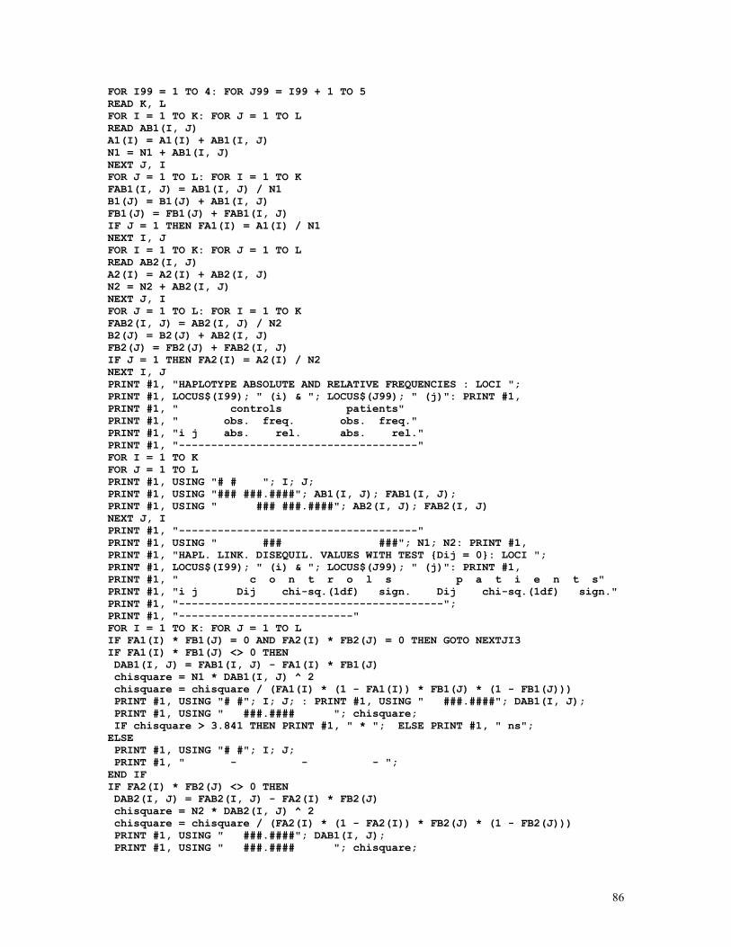
86
FOR I99 = 1 TO 4: FOR J99 = I99 + 1 TO 5 READ K, L FOR I = 1 TO K: FOR J = 1 TO L READ AB1(I, J) A1(I) = A1(I) + AB1(I, J) N1 = N1 + AB1(I, J) NEXT J, I FOR J = 1 TO L: FOR I = 1 TO K FAB1(I, J) = AB1(I, J) / N1 B1(J) = B1(J) + AB1(I, J) FB1(J) = FB1(J) + FAB1(I, J) IF J = 1 THEN FA1(I) = A1(I) / N1 NEXT I, J FOR I = 1 TO K: FOR J = 1 TO L READ AB2(I, J) A2(I) = A2(I) + AB2(I, J) N2 = N2 + AB2(I, J) NEXT J, I FOR J = 1 TO L: FOR I = 1 TO K FAB2(I, J) = AB2(I, J) / N2 B2(J) = B2(J) + AB2(I, J) FB2(J) = FB2(J) + FAB2(I, J) IF J = 1 THEN FA2(I) = A2(I) / N2 NEXT I, J PRINT #1, "HAPLOTYPE ABSOLUTE AND RELATIVE FREQUENCIES : LOCI "; PRINT #1, LOCUS$(I99); " (i) & "; LOCUS$(J99); " (j)": PRINT #1, PRINT #1, " controls patients" PRINT #1, " obs. freq. obs. freq." PRINT #1, "i j abs. rel. abs. rel." PRINT #1, "-------------------------------------" FOR I = 1 TO K FOR J = 1 TO L PRINT #1, USING "# # "; I; J; PRINT #1, USING "### ###.####"; AB1(I, J); FAB1(I, J); PRINT #1, USING " ### ###.####"; AB2(I, J); FAB2(I, J) NEXT J, I PRINT #1, "-------------------------------------" PRINT #1, USING " ### ###"; N1; N2: PRINT #1, PRINT #1, "HAPL. LINK. DISEQUIL. VALUES WITH TEST {Dij = 0}: LOCI "; PRINT #1, LOCUS$(I99); " (i) & "; LOCUS$(J99); " (j)": PRINT #1, PRINT #1, " c o n t r o l s p a t i e n t s" PRINT #1, "i j Dij chi-sq.(1df) sign. Dij chi-sq.(1df) sign." PRINT #1, "-----------------------------------------"; PRINT #1, "---------------------------" FOR I = 1 TO K: FOR J = 1 TO L IF FA1(I) * FB1(J) = 0 AND FA2(I) * FB2(J) = 0 THEN GOTO NEXTJI3 IF FA1(I) * FB1(J) <> 0 THEN DAB1(I, J) = FAB1(I, J) - FA1(I) * FB1(J) chisquare = N1 * DAB1(I, J) ^ 2 chisquare = chisquare / (FA1(I) * (1 - FA1(I)) * FB1(J) * (1 - FB1(J))) PRINT #1, USING "# #"; I; J; : PRINT #1, USING " ###.####"; DAB1(I, J); PRINT #1, USING " ###.#### "; chisquare; IF chisquare > 3.841 THEN PRINT #1, " * "; ELSE PRINT #1, " ns"; ELSE PRINT #1, USING "# #"; I; J; PRINT #1, " - - - "; END IF IF FA2(I) * FB2(J) <> 0 THEN DAB2(I, J) = FAB2(I, J) - FA2(I) * FB2(J) chisquare = N2 * DAB2(I, J) ^ 2 chisquare = chisquare / (FA2(I) * (1 - FA2(I)) * FB2(J) * (1 - FB2(J))) PRINT #1, USING " ###.####"; DAB1(I, J); PRINT #1, USING " ###.#### "; chisquare;
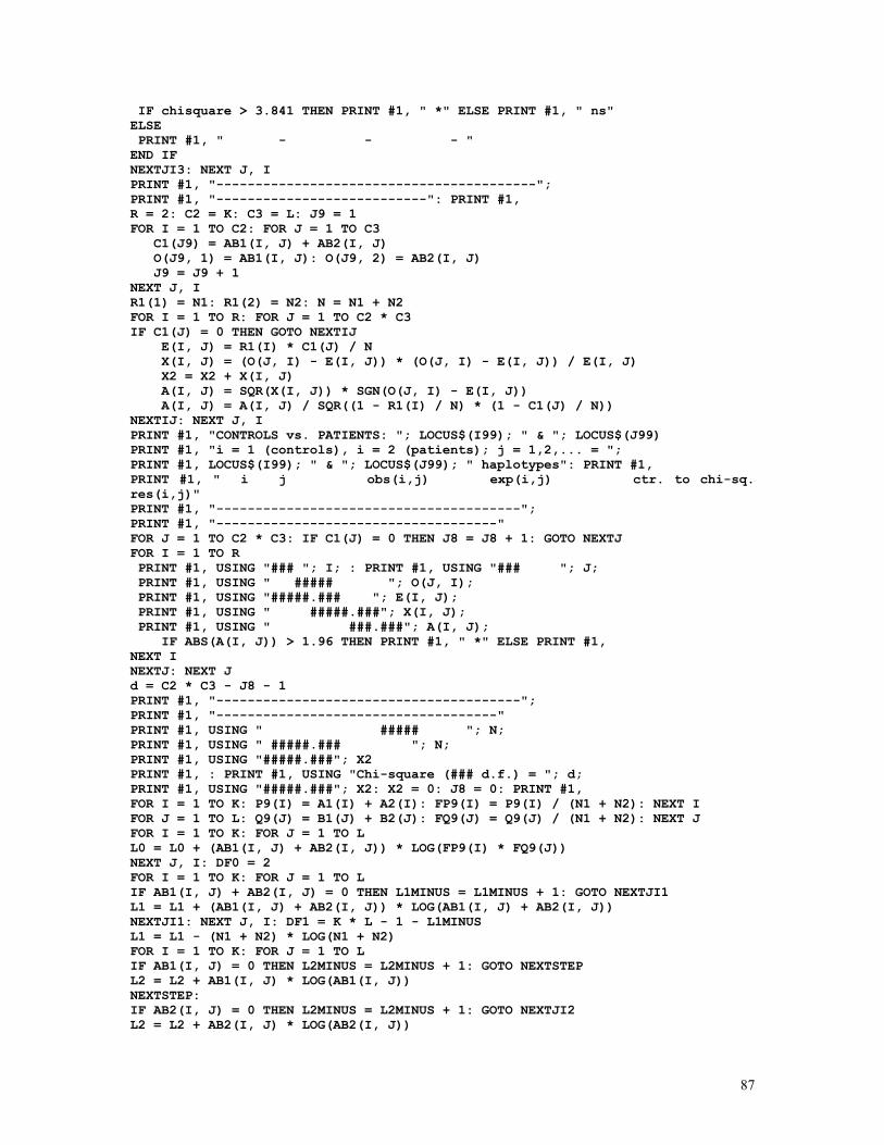
87
IF chisquare > 3.841 THEN PRINT #1, " *" ELSE PRINT #1, " ns" ELSE PRINT #1, " - - - " END IF NEXTJI3: NEXT J, I PRINT #1, "-----------------------------------------"; PRINT #1, "---------------------------": PRINT #1, R = 2: C2 = K: C3 = L: J9 = 1 FOR I = 1 TO C2: FOR J = 1 TO C3 C1(J9) = AB1(I, J) + AB2(I, J) O(J9, 1) = AB1(I, J): O(J9, 2) = AB2(I, J) J9 = J9 + 1 NEXT J, I R1(1) = N1: R1(2) = N2: N = N1 + N2 FOR I = 1 TO R: FOR J = 1 TO C2 * C3 IF C1(J) = 0 THEN GOTO NEXTIJ E(I, J) = R1(I) * C1(J) / N X(I, J) = (O(J, I) - E(I, J)) * (O(J, I) - E(I, J)) / E(I, J) X2 = X2 + X(I, J) A(I, J) = SQR(X(I, J)) * SGN(O(J, I) - E(I, J)) A(I, J) = A(I, J) / SQR((1 - R1(I) / N) * (1 - C1(J) / N)) NEXTIJ: NEXT J, I PRINT #1, "CONTROLS vs. PATIENTS: "; LOCUS$(I99); " & "; LOCUS$(J99) PRINT #1, "i = 1 (controls), i = 2 (patients); j = 1,2,... = "; PRINT #1, LOCUS$(I99); " & "; LOCUS$(J99); " haplotypes": PRINT #1, PRINT #1, " i j obs(i,j) exp(i,j) ctr. to chi-sq. res(i,j)" PRINT #1, "---------------------------------------"; PRINT #1, "------------------------------------" FOR J = 1 TO C2 * C3: IF C1(J) = 0 THEN J8 = J8 + 1: GOTO NEXTJ FOR I = 1 TO R PRINT #1, USING "### "; I; : PRINT #1, USING "### "; J; PRINT #1, USING " ##### "; O(J, I); PRINT #1, USING "#####.### "; E(I, J); PRINT #1, USING " #####.###"; X(I, J); PRINT #1, USING " ###.###"; A(I, J); IF ABS(A(I, J)) > 1.96 THEN PRINT #1, " *" ELSE PRINT #1, NEXT I NEXTJ: NEXT J d = C2 * C3 - J8 - 1 PRINT #1, "---------------------------------------"; PRINT #1, "------------------------------------" PRINT #1, USING " ##### "; N; PRINT #1, USING " #####.### "; N; PRINT #1, USING "#####.###"; X2 PRINT #1, : PRINT #1, USING "Chi-square (### d.f.) = "; d; PRINT #1, USING "#####.###"; X2: X2 = 0: J8 = 0: PRINT #1, FOR I = 1 TO K: P9(I) = A1(I) + A2(I): FP9(I) = P9(I) / (N1 + N2): NEXT I FOR J = 1 TO L: Q9(J) = B1(J) + B2(J): FQ9(J) = Q9(J) / (N1 + N2): NEXT J FOR I = 1 TO K: FOR J = 1 TO L L0 = L0 + (AB1(I, J) + AB2(I, J)) * LOG(FP9(I) * FQ9(J)) NEXT J, I: DF0 = 2 FOR I = 1 TO K: FOR J = 1 TO L IF AB1(I, J) + AB2(I, J) = 0 THEN L1MINUS = L1MINUS + 1: GOTO NEXTJI1 L1 = L1 + (AB1(I, J) + AB2(I, J)) * LOG(AB1(I, J) + AB2(I, J)) NEXTJI1: NEXT J, I: DF1 = K * L - 1 - L1MINUS L1 = L1 - (N1 + N2) * LOG(N1 + N2) FOR I = 1 TO K: FOR J = 1 TO L IF AB1(I, J) = 0 THEN L2MINUS = L2MINUS + 1: GOTO NEXTSTEP L2 = L2 + AB1(I, J) * LOG(AB1(I, J)) NEXTSTEP: IF AB2(I, J) = 0 THEN L2MINUS = L2MINUS + 1: GOTO NEXTJI2 L2 = L2 + AB2(I, J) * LOG(AB2(I, J))
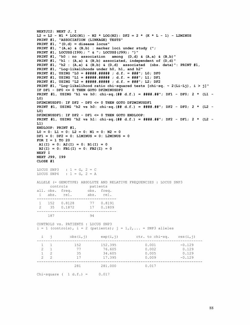
88
NEXTJI2: NEXT J, I L2 = L2 - N1 * LOG(N1) - N2 * LOG(N2): DF2 = 2 * (K * L - 1) - L2MINUS PRINT #1, "ASSOCIATION (LINKAGE) TESTS" PRINT #1, "(D,d) = disease locus" PRINT #1, "(A,a) & (B,b) : marker loci under study ("; PRINT #1, LOCUS$(I99); " & "; LOCUS$(J99); ")" PRINT #1, "h0 : no association among (D,d) & (A,a) & (B,b)" PRINT #1, "h1 : (A,a) & (B,b) associated, independent of (D,d)" PRINT #1, "h2 : (A,a) & (B,b) & (D,d) associated (obs. data)": PRINT #1, PRINT #1, "Log-likelihoods under h0, h1, and h2" PRINT #1, USING "L0 = #####.##### ; d.f. = ###"; L0; DF0 PRINT #1, USING "L1 = #####.##### ; d.f. = ###"; L1; DF1 PRINT #1, USING "L2 = #####.##### ; d.f. = ###"; L2; DF2 PRINT #1, "Log-likelihood ratio chi-squared tests [chi-sq. ~ 2(Li-Lj), i > j]" IF DF1 - DF0 <= 0 THEN GOTO DF2MINUSDF0 PRINT #1, USING "h1 vs h0: chi-sq.(## d.f.) = ####.##"; DF1 - DF0; 2 * (L1 - L0) DF2MINUSDF0: IF DF2 - DF0 <= 0 THEN GOTO DF2MINUSDF1 PRINT #1, USING "h2 vs h0: chi-sq.(## d.f.) = ####.##"; DF2 - DF0; 2 * (L2 - L0) DF2MINUSDF1: IF DF2 - DF1 <= 0 THEN GOTO ENDLOOP: PRINT #1, USING "h2 vs h1: chi-sq.(## d.f.) = ####.##"; DF2 - DF1; 2 * (L2 - L1) ENDLOOP: PRINT #1, L0 = 0: L1 = 0: L2 = 0: N1 = 0: N2 = 0 DF1 = 0: DF2 = 0: L1MINUS = 0: L2MINUS = 0 FOR I = 1 TO 20 A1(I) = 0: A2(I) = 0: B1(I) = 0 B2(I) = 0: FB1(I) = 0: FB2(I) = 0 NEXT I NEXT J99, I99 CLOSE #1 LOCUS SNP3 : 1 = G, 2 = C LOCUS SNP4 : 1 = G, 2 = A ALLELE (= GENOTYPE) ABSOLUTE AND RELATIVE FREQUENCIES : LOCUS SNP3 controls patients all. obs. freq. obs. freq. i abs. rel. abs. rel. ------------------------------------ 1 152 0.8128 77 0.8191 2 35 0.1872 17 0.1809 ------------------------------------ 187 94 CONTROLS vs. PATIENTS : LOCUS SNP3 i = 1 (controls), i = 2 (patients); j = 1,2,... = SNP3 alleles i j obs(i,j) exp(i,j) ctr. to chi-sq. res(i,j) --------------------------------------------------------------------------- 1 1 152 152.395 0.001 -0.129 2 1 77 76.605 0.002 0.129 1 2 35 34.605 0.005 0.129 2 2 17 17.395 0.009 -0.129 --------------------------------------------------------------------------- 281 281.000 0.017 Chi-square ( 1 d.f.) = 0.017
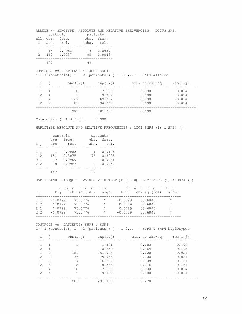
89
ALLELE (= GENOTYPE) ABSOLUTE AND RELATIVE FREQUENCIES : LOCUS SNP4 controls patients all. obs. freq. obs. freq. i abs. rel. abs. rel. ------------------------------------ 1 18 0.0963 9 0.0957 2 169 0.9037 85 0.9043 ------------------------------------ 187 94 CONTROLS vs. PATIENTS : LOCUS SNP4 i = 1 (controls), i = 2 (patients); j = 1,2,... = SNP4 alleles i j obs(i,j) exp(i,j) ctr. to chi-sq. res(i,j) --------------------------------------------------------------------------- 1 1 18 17.968 0.000 0.014 2 1 9 9.032 0.000 -0.014 1 2 169 169.032 0.000 -0.014 2 2 85 84.968 0.000 0.014 --------------------------------------------------------------------------- 281 281.000 0.000 Chi-square ( 1 d.f.) = 0.000 HAPLOTYPE ABSOLUTE AND RELATIVE FREQUENCIES : LOCI SNP3 (i) & SNP4 (j) controls patients obs. freq. obs. freq. i j abs. rel. abs. rel. ------------------------------------- 1 1 1 0.0053 1 0.0106 1 2 151 0.8075 76 0.8085 2 1 17 0.0909 8 0.0851 2 2 18 0.0963 9 0.0957 ------------------------------------- 187 94 HAPL. LINK. DISEQUIL. VALUES WITH TEST {Dij = 0}: LOCI SNP3 (i) & SNP4 (j) c o n t r o l s p a t i e n t s i j Dij chi-sq.(1df) sign. Dij chi-sq.(1df) sign. -------------------------------------------------------------------- 1 1 -0.0729 75.0776 * -0.0729 33.6806 * 1 2 0.0729 75.0776 * 0.0729 33.6806 * 2 1 0.0729 75.0776 * 0.0729 33.6806 * 2 2 -0.0729 75.0776 * -0.0729 33.6806 * -------------------------------------------------------------------- CONTROLS vs. PATIENTS: SNP3 & SNP4 i = 1 (controls), i = 2 (patients); j = 1,2,... = SNP3 & SNP4 haplotypes i j obs(i,j) exp(i,j) ctr. to chi-sq. res(i,j) --------------------------------------------------------------------------- 1 1 1 1.331 0.082 -0.498 2 1 1 0.669 0.164 0.498 1 2 151 151.064 0.000 -0.021 2 2 76 75.936 0.000 0.021 1 3 17 16.637 0.008 0.161 2 3 8 8.363 0.016 -0.161 1 4 18 17.968 0.000 0.014 2 4 9 9.032 0.000 -0.014 --------------------------------------------------------------------------- 281 281.000 0.270
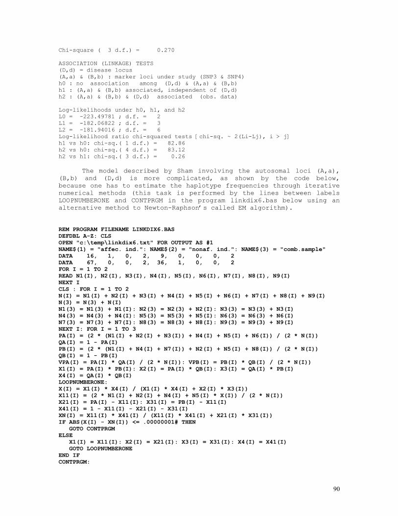
90
Chi-square ( 3 d.f.) = 0.270 ASSOCIATION (LINKAGE) TESTS (D,d) = disease locus (A,a) & (B,b) : marker loci under study (SNP3 & SNP4) h0 : no association among (D,d) & (A,a) & (B,b) h1 : (A,a) & (B,b) associated, independent of (D,d) h2 : (A,a) & (B,b) & (D,d) associated (obs. data) Log-likelihoods under h0, h1, and h2 L0 = -223.49781 ; d.f. = 2 L1 = -182.06822 ; d.f. = 3 L2 = -181.94016 ; d.f. = 6 Log-likelihood ratio chi-squared tests [chi-sq. ~ 2(Li-Lj), i > j] h1 vs h0: chi-sq.( 1 d.f.) = 82.86 h2 vs h0: chi-sq.( 4 d.f.) = 83.12 h2 vs h1: chi-sq.( 3 d.f.) = 0.26
The model described by Sham involving the autosomal loci (A,a), (B,b) and (D,d) is more complicated, as shown by the code below, because one has to estimate the haplotype frequencies through iterative numerical methods (this task is performed by the lines between labels LOOPNUMBERONE and CONTPRGM in the program linkdix6.bas below using an alternative method to Newton-Raphson’s called EM algorithm). REM PROGRAM FILENAME LINKDIX6.BAS DEFDBL A-Z: CLS OPEN "c:\temp\linkdix6.txt" FOR OUTPUT AS #1 NAME$(1) = "affec. ind.": NAME$(2) = "nonaf. ind.": NAME$(3) = "comb.sample" DATA 16, 1, 0, 2, 9, 0, 0, 0, 2 DATA 67, 0, 0, 2, 36, 1, 0, 0, 2 FOR I = 1 TO 2 READ N1(I), N2(I), N3(I), N4(I), N5(I), N6(I), N7(I), N8(I), N9(I) NEXT I CLS : FOR I = 1 TO 2 N(I) = N1(I) + N2(I) + N3(I) + N4(I) + N5(I) + N6(I) + N7(I) + N8(I) + N9(I) N(3) = N(3) + N(I) N1(3) = N1(3) + N1(I): N2(3) = N2(3) + N2(I): N3(3) = N3(3) + N3(I) N4(3) = N4(3) + N4(I): N5(3) = N5(3) + N5(I): N6(3) = N6(3) + N6(I) N7(3) = N7(3) + N7(I): N8(3) = N8(3) + N8(I): N9(3) = N9(3) + N9(I) NEXT I: FOR I = 1 TO 3 PA(I) = (2 * (N1(I) + N2(I) + N3(I)) + N4(I) + N5(I) + N6(I)) / (2 * N(I)) QA(I) = 1 - PA(I) PB(I) = (2 * (N1(I) + N4(I) + N7(I)) + N2(I) + N5(I) + N8(I)) / (2 * N(I)) QB(I) = 1 - PB(I) VPA(I) = PA(I) * QA(I) / (2 * N(I)): VPB(I) = PB(I) * QB(I) / (2 * N(I)) X1(I) = PA(I) * PB(I): X2(I) = PA(I) * QB(I): X3(I) = QA(I) * PB(I) X4(I) = QA(I) * QB(I) LOOPNUMBERONE: X(I) = X1(I) * X4(I) / (X1(I) * X4(I) + X2(I) * X3(I)) X11(I) = (2 * N1(I) + N2(I) + N4(I) + N5(I) * X(I)) / (2 * N(I)) X21(I) = PA(I) - X11(I): X31(I) = PB(I) - X11(I) X41(I) = 1 - X11(I) - X21(I) - X31(I) XN(I) = X11(I) * X41(I) / (X11(I) * X41(I) + X21(I) * X31(I)) IF ABS(X(I) - XN(I)) <= .00000001# THEN GOTO CONTPRGM ELSE X1(I) = X11(I): X2(I) = X21(I): X3(I) = X31(I): X4(I) = X41(I) GOTO LOOPNUMBERONE END IF CONTPRGM:
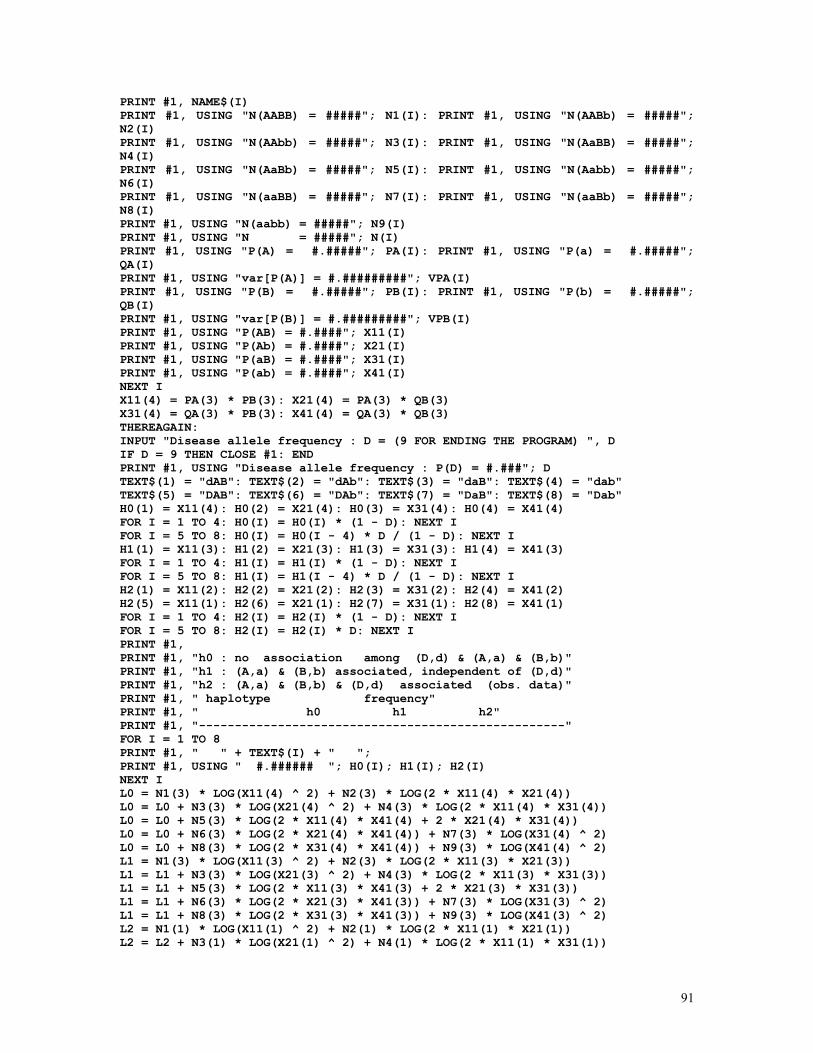
91
PRINT #1, NAME$(I) PRINT #1, USING "N(AABB) = #####"; N1(I): PRINT #1, USING "N(AABb) = #####"; N2(I) PRINT #1, USING "N(AAbb) = #####"; N3(I): PRINT #1, USING "N(AaBB) = #####"; N4(I) PRINT #1, USING "N(AaBb) = #####"; N5(I): PRINT #1, USING "N(Aabb) = #####"; N6(I) PRINT #1, USING "N(aaBB) = #####"; N7(I): PRINT #1, USING "N(aaBb) = #####"; N8(I) PRINT #1, USING "N(aabb) = #####"; N9(I) PRINT #1, USING "N = #####"; N(I) PRINT #1, USING "P(A) = #.#####"; PA(I): PRINT #1, USING "P(a) = #.#####"; QA(I) PRINT #1, USING "var[P(A)] = #.#########"; VPA(I) PRINT #1, USING "P(B) = #.#####"; PB(I): PRINT #1, USING "P(b) = #.#####"; QB(I) PRINT #1, USING "var[P(B)] = #.#########"; VPB(I) PRINT #1, USING "P(AB) = #.####"; X11(I) PRINT #1, USING "P(Ab) = #.####"; X21(I) PRINT #1, USING "P(aB) = #.####"; X31(I) PRINT #1, USING "P(ab) = #.####"; X41(I) NEXT I X11(4) = PA(3) * PB(3): X21(4) = PA(3) * QB(3) X31(4) = QA(3) * PB(3): X41(4) = QA(3) * QB(3) THEREAGAIN: INPUT "Disease allele frequency : D = (9 FOR ENDING THE PROGRAM) ", D IF D = 9 THEN CLOSE #1: END PRINT #1, USING "Disease allele frequency : P(D) = #.###"; D TEXT$(1) = "dAB": TEXT$(2) = "dAb": TEXT$(3) = "daB": TEXT$(4) = "dab" TEXT$(5) = "DAB": TEXT$(6) = "DAb": TEXT$(7) = "DaB": TEXT$(8) = "Dab" H0(1) = X11(4): H0(2) = X21(4): H0(3) = X31(4): H0(4) = X41(4) FOR I = 1 TO 4: H0(I) = H0(I) * (1 - D): NEXT I FOR I = 5 TO 8: H0(I) = H0(I - 4) * D / (1 - D): NEXT I H1(1) = X11(3): H1(2) = X21(3): H1(3) = X31(3): H1(4) = X41(3) FOR I = 1 TO 4: H1(I) = H1(I) * (1 - D): NEXT I FOR I = 5 TO 8: H1(I) = H1(I - 4) * D / (1 - D): NEXT I H2(1) = X11(2): H2(2) = X21(2): H2(3) = X31(2): H2(4) = X41(2) H2(5) = X11(1): H2(6) = X21(1): H2(7) = X31(1): H2(8) = X41(1) FOR I = 1 TO 4: H2(I) = H2(I) * (1 - D): NEXT I FOR I = 5 TO 8: H2(I) = H2(I) * D: NEXT I PRINT #1, PRINT #1, "h0 : no association among (D,d) & (A,a) & (B,b)" PRINT #1, "h1 : (A,a) & (B,b) associated, independent of (D,d)" PRINT #1, "h2 : (A,a) & (B,b) & (D,d) associated (obs. data)" PRINT #1, " haplotype frequency" PRINT #1, " h0 h1 h2" PRINT #1, "---------------------------------------------------" FOR I = 1 TO 8 PRINT #1, " " + TEXT$(I) + " "; PRINT #1, USING " #.###### "; H0(I); H1(I); H2(I) NEXT I L0 = N1(3) * LOG(X11(4) ^ 2) + N2(3) * LOG(2 * X11(4) * X21(4)) L0 = L0 + N3(3) * LOG(X21(4) ^ 2) + N4(3) * LOG(2 * X11(4) * X31(4)) L0 = L0 + N5(3) * LOG(2 * X11(4) * X41(4) + 2 * X21(4) * X31(4)) L0 = L0 + N6(3) * LOG(2 * X21(4) * X41(4)) + N7(3) * LOG(X31(4) ^ 2) L0 = L0 + N8(3) * LOG(2 * X31(4) * X41(4)) + N9(3) * LOG(X41(4) ^ 2) L1 = N1(3) * LOG(X11(3) ^ 2) + N2(3) * LOG(2 * X11(3) * X21(3)) L1 = L1 + N3(3) * LOG(X21(3) ^ 2) + N4(3) * LOG(2 * X11(3) * X31(3)) L1 = L1 + N5(3) * LOG(2 * X11(3) * X41(3) + 2 * X21(3) * X31(3)) L1 = L1 + N6(3) * LOG(2 * X21(3) * X41(3)) + N7(3) * LOG(X31(3) ^ 2) L1 = L1 + N8(3) * LOG(2 * X31(3) * X41(3)) + N9(3) * LOG(X41(3) ^ 2) L2 = N1(1) * LOG(X11(1) ^ 2) + N2(1) * LOG(2 * X11(1) * X21(1)) L2 = L2 + N3(1) * LOG(X21(1) ^ 2) + N4(1) * LOG(2 * X11(1) * X31(1))
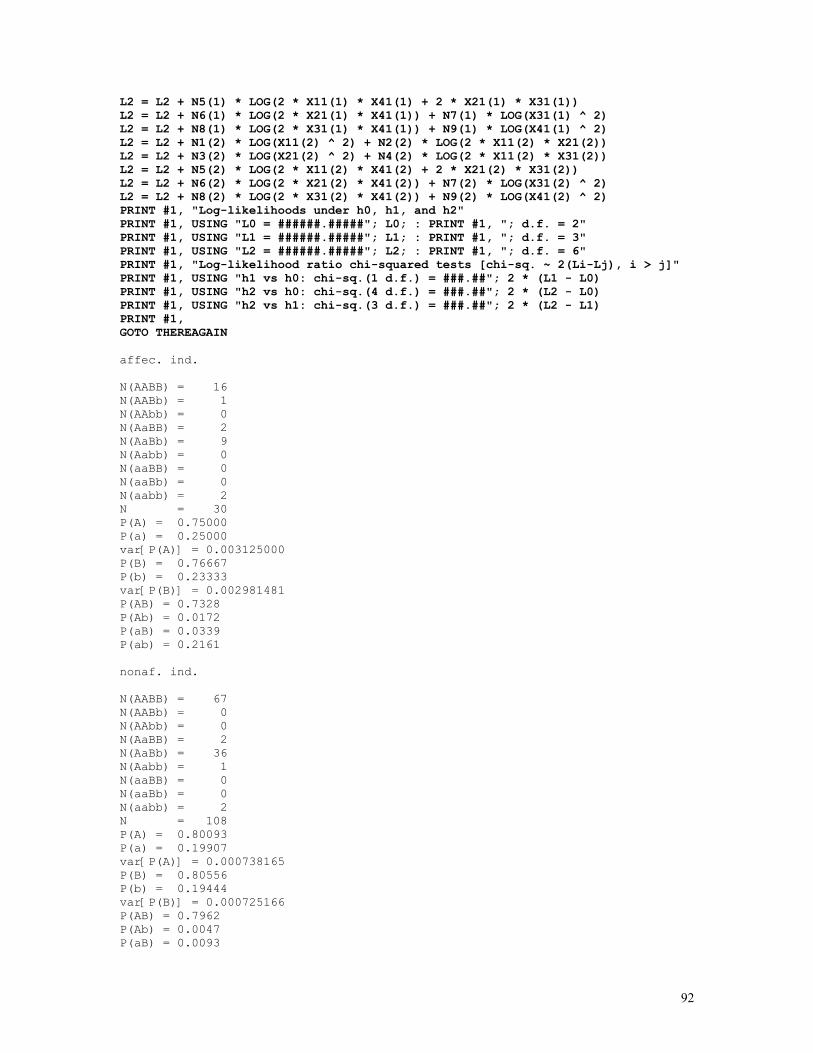
92
L2 = L2 + N5(1) * LOG(2 * X11(1) * X41(1) + 2 * X21(1) * X31(1)) L2 = L2 + N6(1) * LOG(2 * X21(1) * X41(1)) + N7(1) * LOG(X31(1) ^ 2) L2 = L2 + N8(1) * LOG(2 * X31(1) * X41(1)) + N9(1) * LOG(X41(1) ^ 2) L2 = L2 + N1(2) * LOG(X11(2) ^ 2) + N2(2) * LOG(2 * X11(2) * X21(2)) L2 = L2 + N3(2) * LOG(X21(2) ^ 2) + N4(2) * LOG(2 * X11(2) * X31(2)) L2 = L2 + N5(2) * LOG(2 * X11(2) * X41(2) + 2 * X21(2) * X31(2)) L2 = L2 + N6(2) * LOG(2 * X21(2) * X41(2)) + N7(2) * LOG(X31(2) ^ 2) L2 = L2 + N8(2) * LOG(2 * X31(2) * X41(2)) + N9(2) * LOG(X41(2) ^ 2) PRINT #1, "Log-likelihoods under h0, h1, and h2" PRINT #1, USING "L0 = ######.#####"; L0; : PRINT #1, "; d.f. = 2" PRINT #1, USING "L1 = ######.#####"; L1; : PRINT #1, "; d.f. = 3" PRINT #1, USING "L2 = ######.#####"; L2; : PRINT #1, "; d.f. = 6" PRINT #1, "Log-likelihood ratio chi-squared tests [chi-sq. ~ 2(Li-Lj), i > j]" PRINT #1, USING "h1 vs h0: chi-sq.(1 d.f.) = ###.##"; 2 * (L1 - L0) PRINT #1, USING "h2 vs h0: chi-sq.(4 d.f.) = ###.##"; 2 * (L2 - L0) PRINT #1, USING "h2 vs h1: chi-sq.(3 d.f.) = ###.##"; 2 * (L2 - L1) PRINT #1, GOTO THEREAGAIN affec. ind. N(AABB) = 16 N(AABb) = 1 N(AAbb) = 0 N(AaBB) = 2 N(AaBb) = 9 N(Aabb) = 0 N(aaBB) = 0 N(aaBb) = 0 N(aabb) = 2 N = 30 P(A) = 0.75000 P(a) = 0.25000 var[P(A)] = 0.003125000 P(B) = 0.76667 P(b) = 0.23333 var[P(B)] = 0.002981481 P(AB) = 0.7328 P(Ab) = 0.0172 P(aB) = 0.0339 P(ab) = 0.2161 nonaf. ind. N(AABB) = 67 N(AABb) = 0 N(AAbb) = 0 N(AaBB) = 2 N(AaBb) = 36 N(Aabb) = 1 N(aaBB) = 0 N(aaBb) = 0 N(aabb) = 2 N = 108 P(A) = 0.80093 P(a) = 0.19907 var[P(A)] = 0.000738165 P(B) = 0.80556 P(b) = 0.19444 var[P(B)] = 0.000725166 P(AB) = 0.7962 P(Ab) = 0.0047 P(aB) = 0.0093
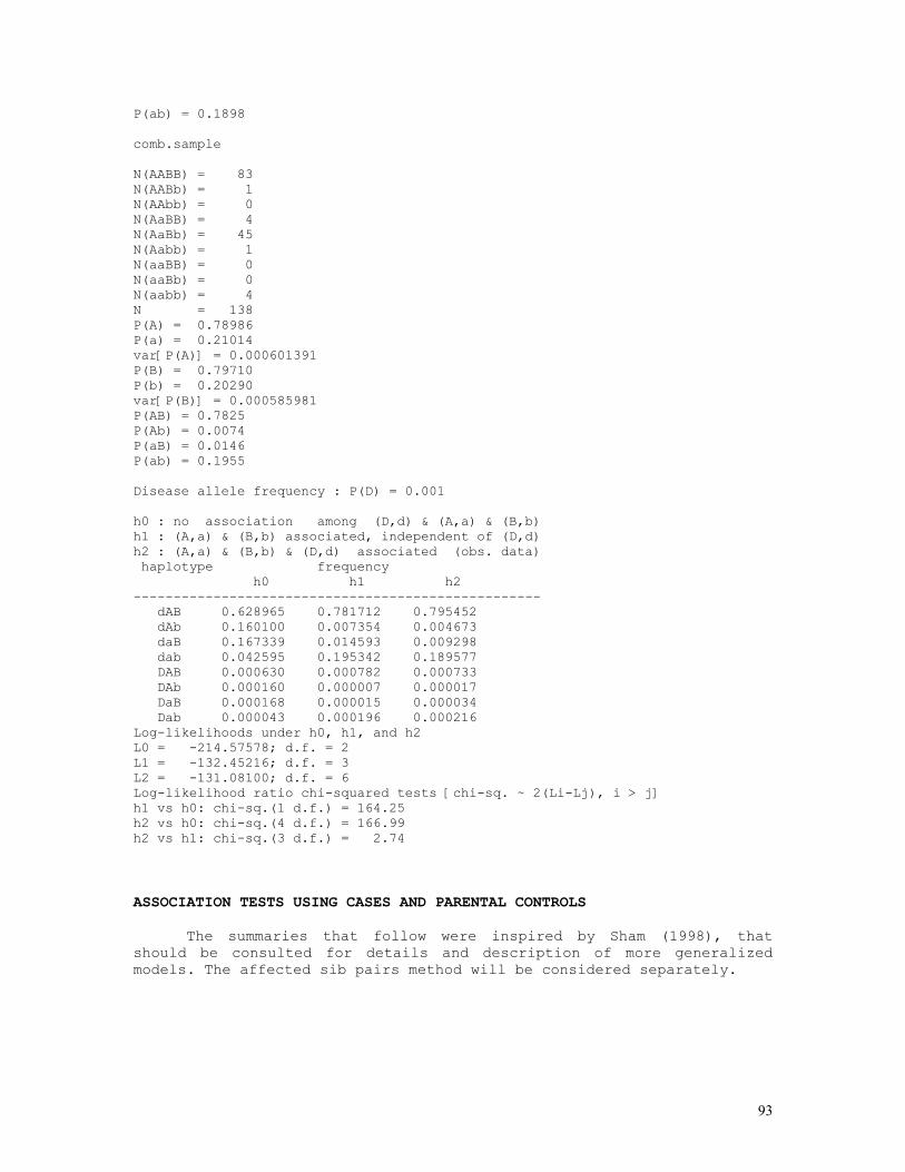
93
P(ab) = 0.1898 comb.sample N(AABB) = 83 N(AABb) = 1 N(AAbb) = 0 N(AaBB) = 4 N(AaBb) = 45 N(Aabb) = 1 N(aaBB) = 0 N(aaBb) = 0 N(aabb) = 4 N = 138 P(A) = 0.78986 P(a) = 0.21014 var[P(A)] = 0.000601391 P(B) = 0.79710 P(b) = 0.20290 var[P(B)] = 0.000585981 P(AB) = 0.7825 P(Ab) = 0.0074 P(aB) = 0.0146 P(ab) = 0.1955 Disease allele frequency : P(D) = 0.001 h0 : no association among (D,d) & (A,a) & (B,b) h1 : (A,a) & (B,b) associated, independent of (D,d) h2 : (A,a) & (B,b) & (D,d) associated (obs. data) haplotype frequency h0 h1 h2 --------------------------------------------------- dAB 0.628965 0.781712 0.795452 dAb 0.160100 0.007354 0.004673 daB 0.167339 0.014593 0.009298 dab 0.042595 0.195342 0.189577 DAB 0.000630 0.000782 0.000733 DAb 0.000160 0.000007 0.000017 DaB 0.000168 0.000015 0.000034 Dab 0.000043 0.000196 0.000216 Log-likelihoods under h0, h1, and h2 L0 = -214.57578; d.f. = 2 L1 = -132.45216; d.f. = 3 L2 = -131.08100; d.f. = 6 Log-likelihood ratio chi-squared tests [chi-sq. ~ 2(Li-Lj), i > j] h1 vs h0: chi-sq.(1 d.f.) = 164.25 h2 vs h0: chi-sq.(4 d.f.) = 166.99 h2 vs h1: chi-sq.(3 d.f.) = 2.74
ASSOCIATION TESTS USING CASES AND PARENTAL CONTROLS
The summaries that follow were inspired by Sham (1998), that should be consulted for details and description of more generalized models. The affected sib pairs method will be considered separately.
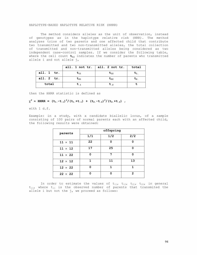
94
HAPLOTYPE-BASED HAPLOTYPE RELATIVE RISK (HHRR)
The method considers alleles as the unit of observation, instead
of genotypes as in the haplotype relative risk (HRR). The method analyzes trios of two parents and one affected child that contribute two transmitted and two non-transmitted alleles, the total collection of transmitted and non-transmitted alleles being considered as two independent case-control samples. If we consider the following table, where the cell count tij indicates the number of parents who transmitted allele i and not allele j,
all. 1 not tr. all. 2 not tr. total
all. 1 tr. t11 t12 t1.
all. 2 tr. t21 t22 t2.
total t.1 t.2 t
then the HHRR statistic is defined as χ2 ≈ HHRR = (t1.-t.1)2/(t1.+t.1) + (t2.-t.2)2/(t2.+t.2) , with 1 d.f. Example: in a study, with a candidate biallelic locus, of a sample consisting of 100 pairs of normal parents each with an affected child, the following results were obtained:
offspring parents
1/1 1/2 2/2
11 × 11 22 0 0
11 × 12 17 25 0
11 × 22 0 7 0
12 × 12 1 11 13
12 × 22 0 1 1
22 × 22 0 0 2
In order to estimate the values of t11, t12, t21, t22, in general
tij, where tij is the observed number of parents that transmited the allele i but not the j, we proceed as follows:
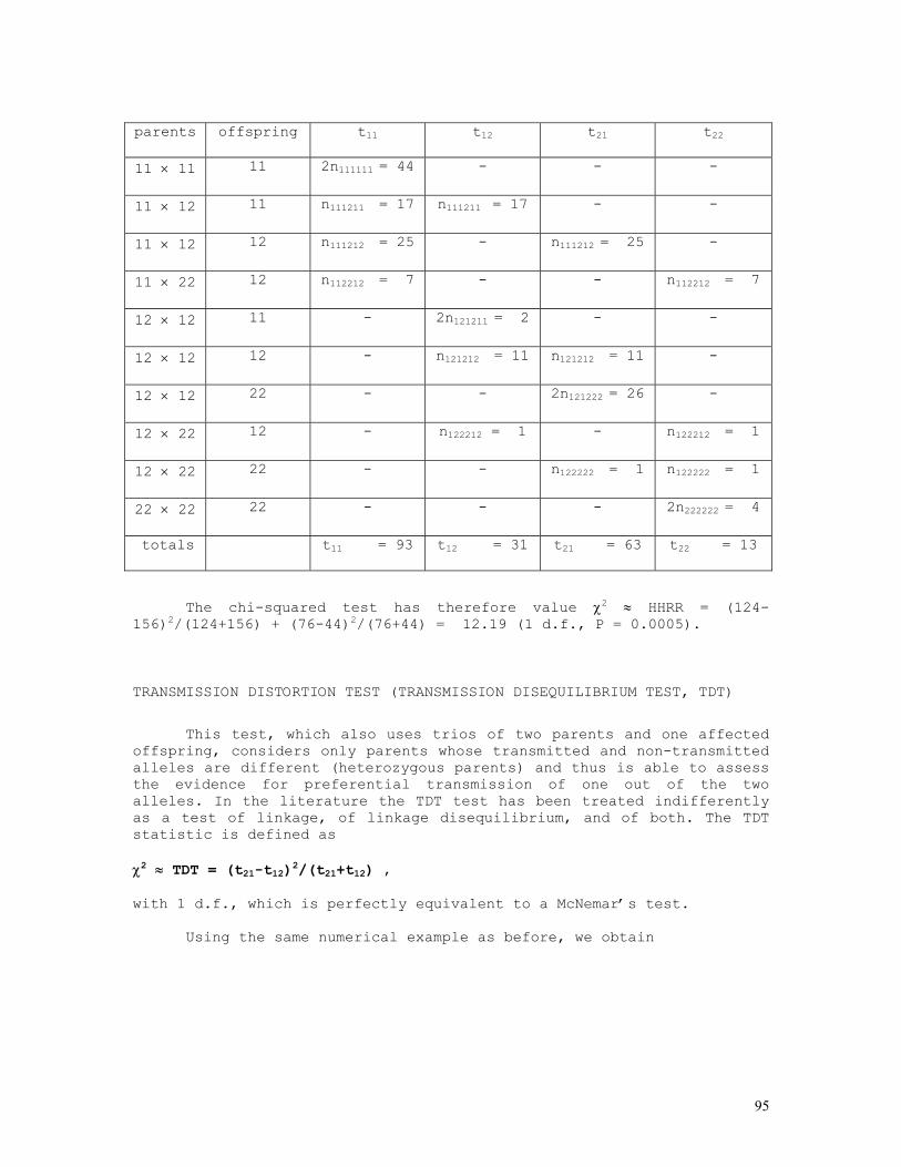
95
parents offspring t11 t12 t21 t22
11 × 11 11 2n111111 = 44 - - -
11 × 12 11 n111211 = 17 n111211 = 17 - -
11 × 12 12 n111212 = 25 - n111212 = 25 -
11 × 22 12 n112212 = 7 - - n112212 = 7
12 × 12 11 - 2n121211 = 2 - -
12 × 12 12 - n121212 = 11 n121212 = 11 -
12 × 12 22 - - 2n121222 = 26 -
12 × 22 12 - n122212 = 1 - n122212 = 1
12 × 22 22 - - n122222 = 1 n122222 = 1
22 × 22 22 - - - 2n222222 = 4
totals t11 = 93 t12 = 31 t21 = 63 t22 = 13
The chi-squared test has therefore value χ2 ≈ HHRR = (124-156)2/(124+156) + (76-44)2/(76+44) = 12.19 (1 d.f., P = 0.0005).
TRANSMISSION DISTORTION TEST (TRANSMISSION DISEQUILIBRIUM TEST, TDT)
This test, which also uses trios of two parents and one affected
offspring, considers only parents whose transmitted and non-transmitted alleles are different (heterozygous parents) and thus is able to assess the evidence for preferential transmission of one out of the two alleles. In the literature the TDT test has been treated indifferently as a test of linkage, of linkage disequilibrium, and of both. The TDT statistic is defined as χ2 ≈ TDT = (t21-t12)2/(t21+t12) , with 1 d.f., which is perfectly equivalent to a McNemar’s test.
Using the same numerical example as before, we obtain
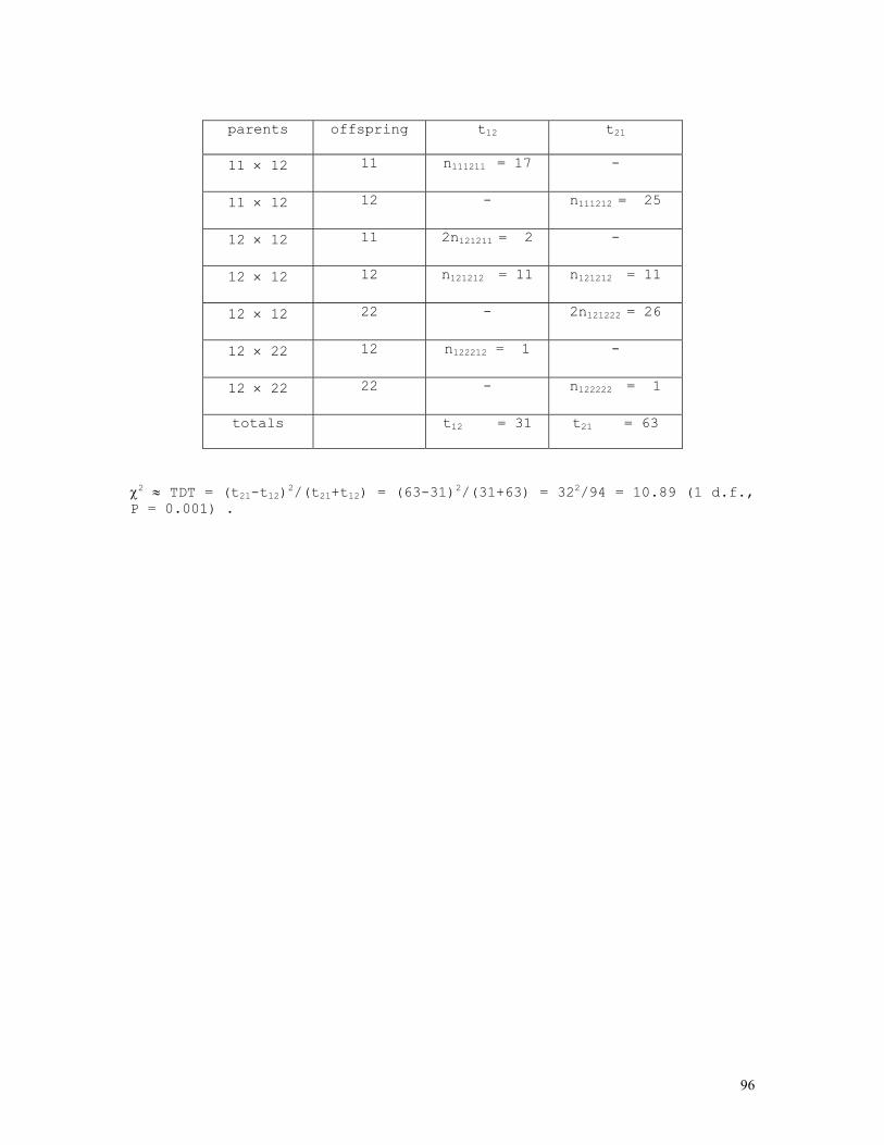
96
parents offspring t12 t21
11 × 12 11 n111211 = 17 -
11 × 12 12 - n111212 = 25
12 × 12 11 2n121211 = 2 -
12 × 12 12 n121212 = 11 n121212 = 11
12 × 12 22 - 2n121222 = 26
12 × 22 12 n122212 = 1 -
12 × 22 22 - n122222 = 1
totals t12 = 31 t21 = 63
χ2 ≈ TDT = (t21-t12)2/(t21+t12) = (63-31)2/(31+63) = 322/94 = 10.89 (1 d.f., P = 0.001) .
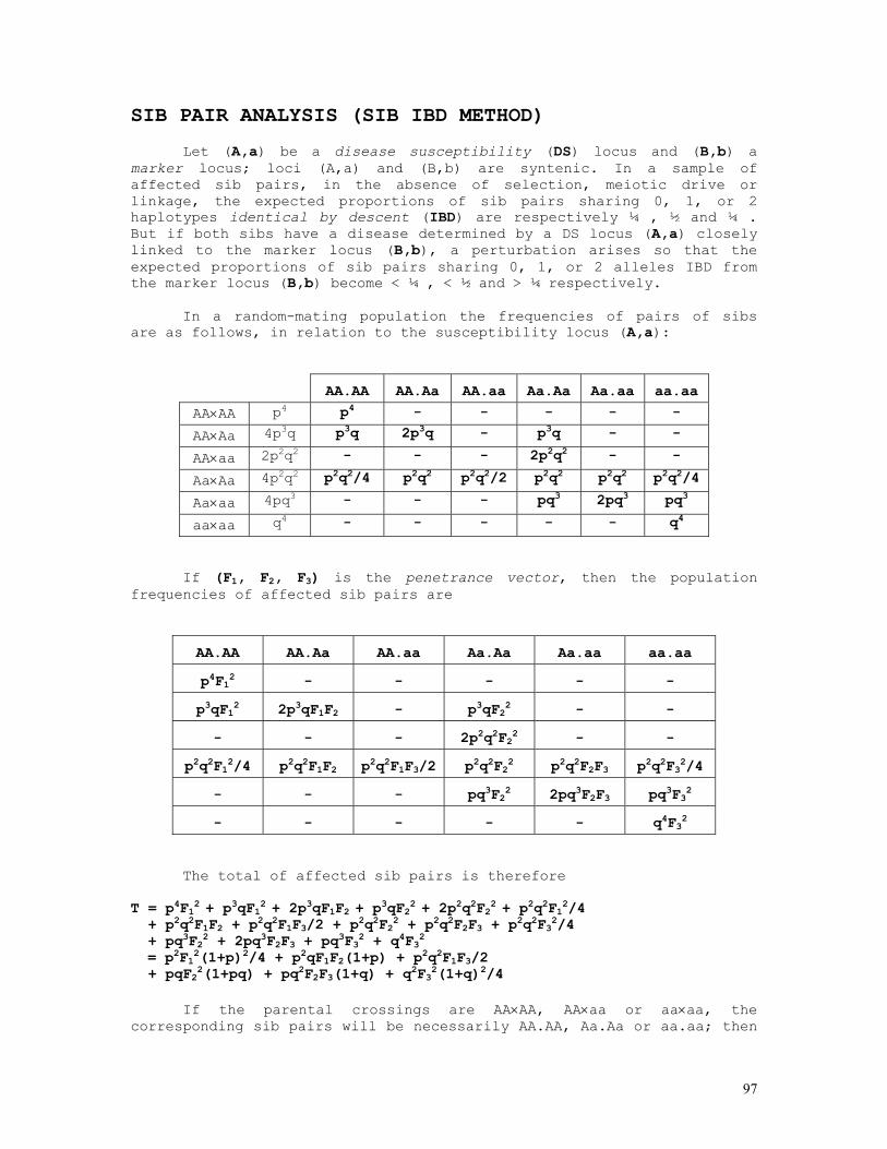
97
SIB PAIR ANALYSIS (SIB IBD METHOD)
Let (A,a) be a disease susceptibility (DS) locus and (B,b) a marker locus; loci (A,a) and (B,b) are syntenic. In a sample of affected sib pairs, in the absence of selection, meiotic drive or linkage, the expected proportions of sib pairs sharing 0, 1, or 2 haplotypes identical by descent (IBD) are respectively ¼ , ½ and ¼ . But if both sibs have a disease determined by a DS locus (A,a) closely linked to the marker locus (B,b), a perturbation arises so that the expected proportions of sib pairs sharing 0, 1, or 2 alleles IBD from the marker locus (B,b) become < ¼ , < ½ and > ¼ respectively.
In a random-mating population the frequencies of pairs of sibs are as follows, in relation to the susceptibility locus (A,a):
AA.AA AA.Aa AA.aa Aa.Aa Aa.aa aa.aa
AA×AA p4 p4 - - - - -
AA×Aa 4p3q p3q 2p3q - p3q - -
AA×aa 2p2q2 - - - 2p2q2 - -
Aa×Aa 4p2q2 p2q2/4 p2q2 p2q2/2 p2q2 p2q2 p2q2/4
Aa×aa 4pq3 - - - pq3 2pq3 pq3
aa×aa q4 - - - - - q4
If (F1, F2, F3) is the penetrance vector, then the population frequencies of affected sib pairs are
AA.AA AA.Aa AA.aa Aa.Aa Aa.aa aa.aa
p4F12 - - - - -
p3qF12 2p3qF1F2 - p3qF22 - -
- - - 2p2q2F22 - -
p2q2F12/4 p2q2F1F2 p2q2F1F3/2 p2q2F22 p2q2F2F3 p2q2F32/4
- - - pq3F22 2pq3F2F3 pq3F32
- - - - - q4F32
The total of affected sib pairs is therefore T = p4F12 + p3qF12 + 2p3qF1F2 + p3qF22 + 2p2q2F22 + p2q2F12/4 + p2q2F1F2 + p2q2F1F3/2 + p2q2F22 + p2q2F2F3 + p2q2F32/4 + pq3F22 + 2pq3F2F3 + pq3F32 + q4F32 = p2F12(1+p)2/4 + p2qF1F2(1+p) + p2q2F1F3/2 + pqF22(1+pq) + pq2F2F3(1+q) + q2F32(1+q)2/4
If the parental crossings are AA×AA, AA×aa or aa×aa, the corresponding sib pairs will be necessarily AA.AA, Aa.Aa or aa.aa; then
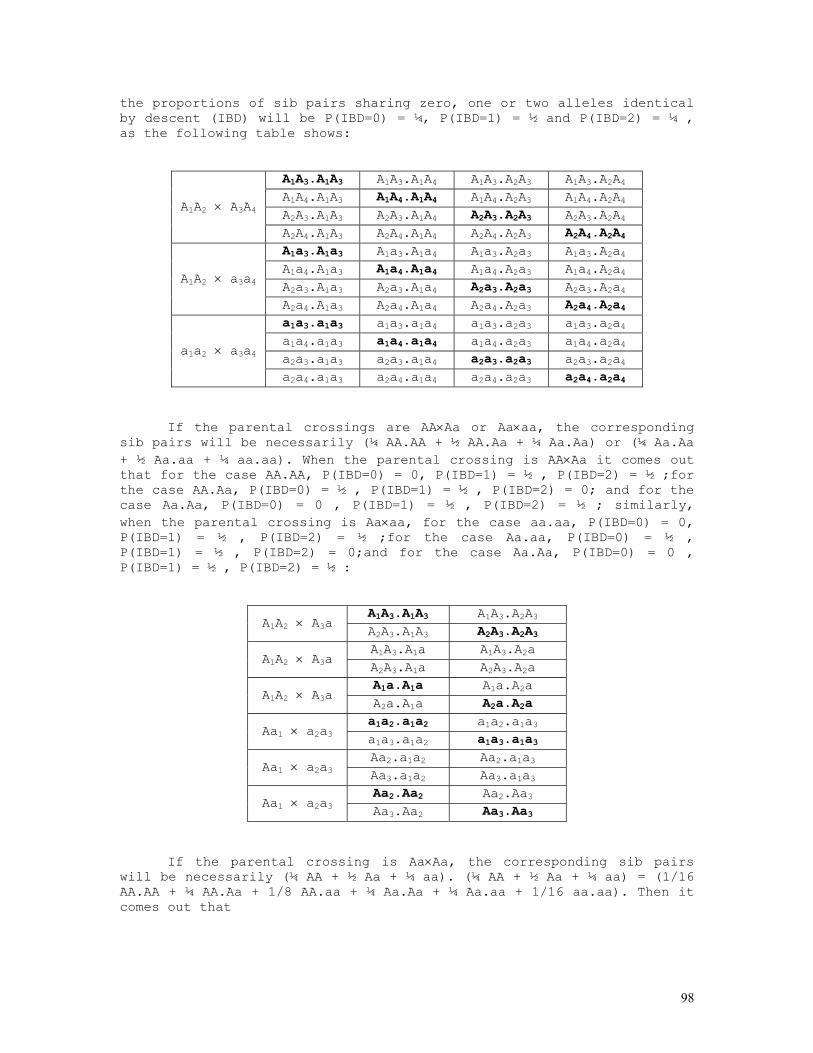
98
the proportions of sib pairs sharing zero, one or two alleles identical by descent (IBD) will be P(IBD=0) = ¼, P(IBD=1) = ½ and P(IBD=2) = ¼ , as the following table shows:
A1A3.A1A3 A1A3.A1A4 A1A3.A2A3 A1A3.A2A4 A1A4.A1A3 A1A4.A1A4 A1A4.A2A3 A1A4.A2A4 A2A3.A1A3 A2A3.A1A4 A2A3.A2A3 A2A3.A2A4
A1A2 × A3A4
A2A4.A1A3 A2A4.A1A4 A2A4.A2A3 A2A4.A2A4 A1a3.A1a3 A1a3.A1a4 A1a3.A2a3 A1a3.A2a4 A1a4.A1a3 A1a4.A1a4 A1a4.A2a3 A1a4.A2a4 A2a3.A1a3 A2a3.A1a4 A2a3.A2a3 A2a3.A2a4
A1A2 × a3a4
A2a4.A1a3 A2a4.A1a4 A2a4.A2a3 A2a4.A2a4 a1a3.a1a3 a1a3.a1a4 a1a3.a2a3 a1a3.a2a4 a1a4.a1a3 a1a4.a1a4 a1a4.a2a3 a1a4.a2a4 a2a3.a1a3 a2a3.a1a4 a2a3.a2a3 a2a3.a2a4
a1a2 × a3a4
a2a4.a1a3 a2a4.a1a4 a2a4.a2a3 a2a4.a2a4
If the parental crossings are AA×Aa or Aa×aa, the corresponding sib pairs will be necessarily (¼ AA.AA + ½ AA.Aa + ¼ Aa.Aa) or (¼ Aa.Aa + ½ Aa.aa + ¼ aa.aa). When the parental crossing is AA×Aa it comes out that for the case AA.AA, P(IBD=0) = 0, P(IBD=1) = ½ , P(IBD=2) = ½ ;for the case AA.Aa, P(IBD=0) = ½ , P(IBD=1) = ½ , P(IBD=2) = 0; and for the case Aa.Aa, P(IBD=0) = 0 , P(IBD=1) = ½ , P(IBD=2) = ½ ; similarly, when the parental crossing is Aa×aa, for the case aa.aa, P(IBD=0) = 0, P(IBD=1) = ½ , P(IBD=2) = ½ ;for the case Aa.aa, P(IBD=0) = ½ , P(IBD=1) = ½ , P(IBD=2) = 0;and for the case Aa.Aa, P(IBD=0) = 0 , P(IBD=1) = ½ , P(IBD=2) = ½ :
A1A3.A1A3 A1A3.A2A3 A1A2 × A3a A2A3.A1A3 A2A3.A2A3 A1A3.A1a A1A3.A2a A1A2 × A3a A2A3.A1a A2A3.A2a A1a.A1a A1a.A2a A1A2 × A3a A2a.A1a A2a.A2a a1a2.a1a2 a1a2.a1a3 Aa1 × a2a3 a1a3.a1a2 a1a3.a1a3 Aa2.a1a2 Aa2.a1a3 Aa1 × a2a3 Aa3.a1a2 Aa3.a1a3 Aa2.Aa2 Aa2.Aa3 Aa1 × a2a3 Aa3.Aa2 Aa3.Aa3
If the parental crossing is Aa×Aa, the corresponding sib pairs will be necessarily (¼ AA + ½ Aa + ¼ aa). (¼ AA + ½ Aa + ¼ aa) = (1/16 AA.AA + ¼ AA.Aa + 1/8 AA.aa + ¼ Aa.Aa + ¼ Aa.aa + 1/16 aa.aa). Then it comes out that
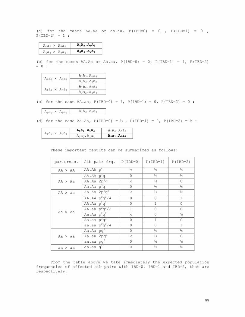
99
(a) for the cases AA.AA or aa.aa, P(IBD=0) = 0 , P(IBD=1) = 0 , P(IBD=2) = 1 :
A1a2 × A3a4 A1A3.A1A3
A1a2 × A3a4 a2a4.a2a4
(b) for the cases AA.Aa or Aa.aa, P(IBD=0) = 0, P(IBD=1) = 1, P(IBD=2) = 0 :
A1A3.A1a4 A1a2 × A3a4 A1A3.A3a2 A1a4.a2a4 A1a2 × A3a4 A3a2.a2a4
(c) for the case AA.aa, P(IBD=0) = 1, P(IBD=1) = 0, P(IBD=2) = 0 :
A1a2 × A3a4 A1A3.a2a4 (d) for the case Aa.Aa, P(IBD=0) = ½ , P(IBD=1) = 0, P(IBD=2) = ½ :
A1a4.A1a4 A1a4.A3a2 A1a2 × A3a4 A3a2.A1a4 A3a2.A3a2
These important results can be summarized as follows:
par.cross. Sib pair frq. P(IBD=0) P(IBD=1) P(IBD=2)
AA × AA AA.AA p4 ¼ ½ ¼
AA.AA p3q 0 ½ ½ AA.Aa 2p3q ½ ½ 0 AA × Aa Aa.Aa p3q 0 ½ ½
AA × aa Aa.Aa 2p2q2 ¼ ½ ¼
AA.AA p2q2/4 0 0 1 AA.Aa p2q2 0 1 0 AA.aa p2q2/2 1 0 0 Aa.Aa p2q2 ½ 0 ½ Aa.aa p2q2 0 1 0
Aa × Aa
aa.aa p2q2/4 0 0 1 Aa.Aa pq3 0 ½ ½ Aa.aa 2pq3 ½ ½ 0 Aa × aa aa.aa pq3 0 ½ ½
aa × aa aa.aa q4 ¼ ½ ¼
From the table above we take immediately the expected population frequencies of affected sib pairs with IBD=0, IBD=1 and IBD=2, that are respectively:
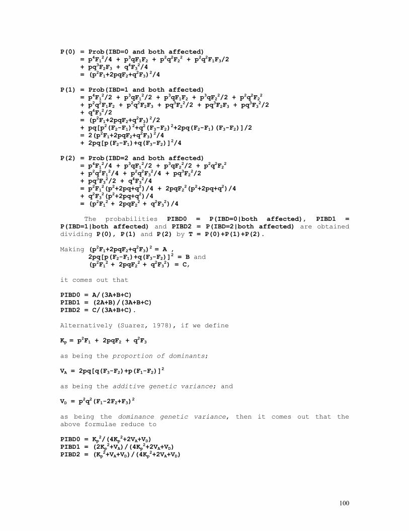
100
P(0) = Prob(IBD=0 and both affected) = p4F12/4 + p3qF1F2 + p2q2F22 + p2q2F1F3/2 + pq3F2F3 + q4F32/4 = (p2F1+2pqF2+q2F3)2/4 P(1) = Prob(IBD=1 and both affected) = p4F12/2 + p3qF12/2 + p3qF1F2 + p3qF22/2 + p2q2F22 + p2q2F1F2 + p2q2F2F3 + pq3F22/2 + pq3F2F3 + pq3F32/2 + q4F32/2 = (p2F1+2pqF2+q2F3)2/2 + pq[p2(F2-F1)2+q2(F3-F2)2+2pq(F2-F1)(F3-F2)]/2 = 2(p2F1+2pqF2+q2F3)2/4 + 2pq[p(F2-F1)+q(F3-F2)]2/4 P(2) = Prob(IBD=2 and both affected) = p4F12/4 + p3qF12/2 + p3qF22/2 + p2q2F22 + p2q2F12/4 + p2q2F32/4 + pq3F22/2 + pq3F32/2 + q4F32/4 = p2F12(p2+2pq+q2)/4 + 2pqF22(p2+2pq+q2)/4 + q2F32(p2+2pq+q2)/4 = (p2F12 + 2pqF22 + q2F32)/4
The probabilities PIBD0 = P(IBD=0|both affected), PIBD1 = P(IBD=1|both affected) and PIBD2 = P(IBD=2|both affected) are obtained dividing P(0), P(1) and P(2) by T = P(0)+P(1)+P(2). Making (p2F1+2pqF2+q2F3)2 = A , 2pq[p(F2-F1)+q(F3-F2)]2 = B and (p2F12 + 2pqF22 + q2F32) = C, it comes out that PIBD0 = A/(3A+B+C) PIBD1 = (2A+B)/(3A+B+C) PIBD2 = C/(3A+B+C). Alternatively (Suarez, 1978), if we define Kp = p2F1 + 2pqF2 + q2F3
as being the proportion of dominants; VA = 2pq[q(F3-F2)+p(F1-F2)]2 as being the additive genetic variance; and VD = p2q2(F1-2F2+F3)2 as being the dominance genetic variance, then it comes out that the above formulae reduce to PIBD0 = Kp2/(4Kp2+2VA+VD) PIBD1 = (2Kp2+VA)/(4Kp2+2VA+VD) PIBD2 = (Kp2+VA+VD)/(4Kp2+2VA+VD)
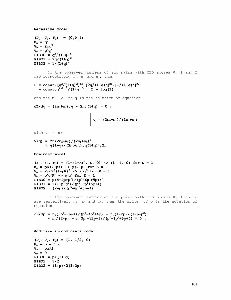
101
Recessive model: (F1, F2, F3) = (0,0,1) Kp = q2 VA = 2pq3 VD = p2q2 PIBD0 = q2/(1+q)2 PIBD1 = 2q/(1+q)2 PIBD2 = 1/(1+q)2
If the observed numbers of sib pairs with IBD scores 0, 1 and 2 are respectively n0, n1 and n2, then P = const.[q2/(1+q)2]n0.[2q/(1+q)2]n1.[1/(1+q)2]n2 = const.q2n0+n1/(1+q)2n , L = log(P) and the m.l.e. of q is the solution of equation dL/dq = (2n0+n1)/q - 2n/(1+q) = 0 :
q = (2n0+n1)/(2n2+n1)
with variance V(q) = 2n(2n0+n1)/(2n2+n1)3 = q(1+q)/(2n2+n1).q(1+q)2/2n Dominant model: (F1, F2, F3) = (1-(1-K)2, K, 0) -> (1, 1, 0) for K = 1 Kp = pK(2-pK) -> p(2-p) for K = 1 VA = 2pqK2(1-pK)2 -> 2pq3 for K = 1 VD = p2q2K4 -> p2q2 for K = 1 PIBD0 = p(4-4p+p2)/(p3-6p2+5p+4) PIBD1 = 2(1+p-p2)/(p3-6p2+5p+4) PIBD2 = (2-p)/(p3-6p2+5p+4)
If the observed numbers of sib pairs with IBD scores 0, 1 and 2 are respectively n0, n1 and n2, then the m.l.e. of p is the solution of equation dL/dp = n0(3p2-8p+4)/(p3-4p2+4p) + n1(1-2p)/(1-p-p2) - n2/(2-p) - n(3p2-12p+5)/(p3-6p2+5p+4) = 0 . Additive (codominant) model: (F1, F2, F3) = (1, 1/2, 0) Kp = p = 1-q VA = pq/2 VD = 0 PIBD0 = p/(1+3p) PIBD1 = 1/2 PIBD2 = (1+p)/2(1+3p)
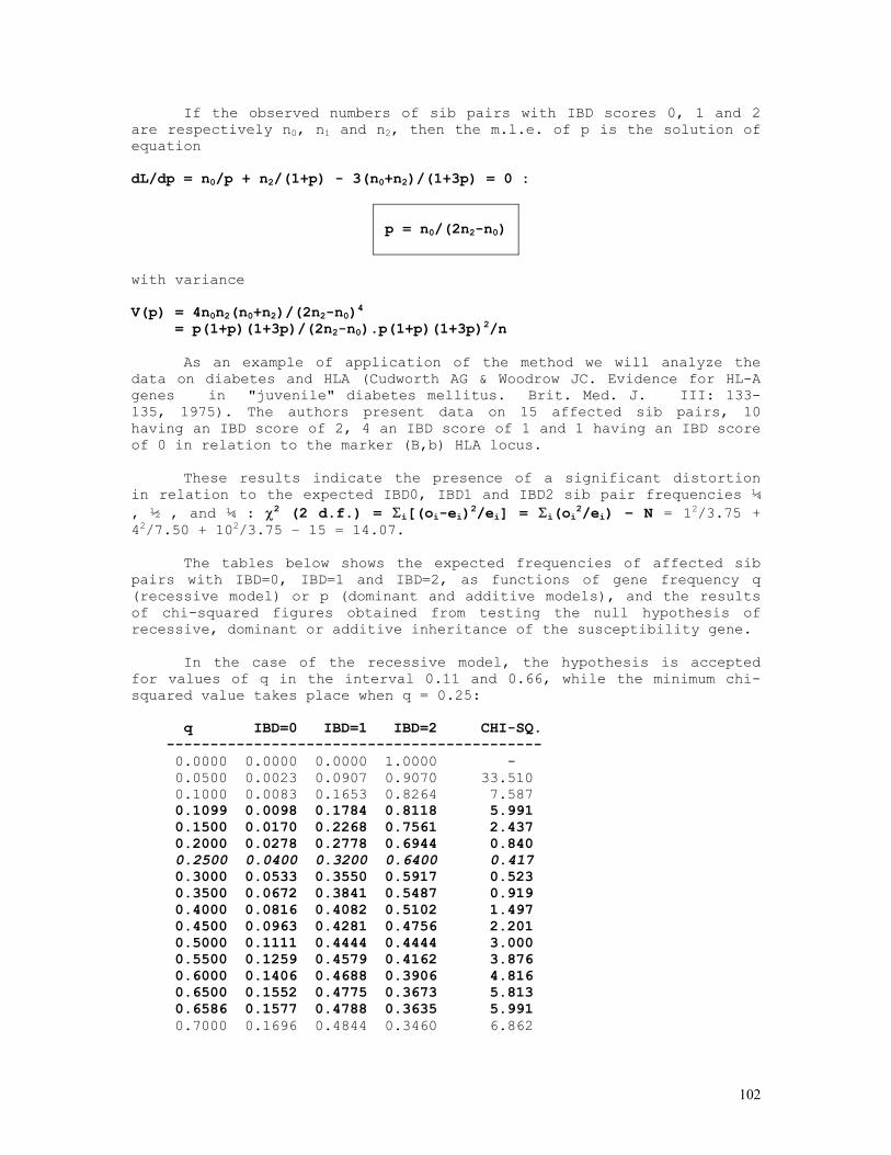
102
If the observed numbers of sib pairs with IBD scores 0, 1 and 2 are respectively n0, n1 and n2, then the m.l.e. of p is the solution of equation dL/dp = n0/p + n2/(1+p) - 3(n0+n2)/(1+3p) = 0 :
p = n0/(2n2-n0)
with variance V(p) = 4n0n2(n0+n2)/(2n2-n0)4 = p(1+p)(1+3p)/(2n2-n0).p(1+p)(1+3p)2/n
As an example of application of the method we will analyze the data on diabetes and HLA (Cudworth AG & Woodrow JC. Evidence for HL-A genes in "juvenile" diabetes mellitus. Brit. Med. J. III: 133-135, 1975). The authors present data on 15 affected sib pairs, 10 having an IBD score of 2, 4 an IBD score of 1 and 1 having an IBD score of 0 in relation to the marker (B,b) HLA locus.
These results indicate the presence of a significant distortion in relation to the expected IBD0, IBD1 and IBD2 sib pair frequencies ¼ , ½ , and ¼ : χ2 (2 d.f.) = Σi[(oi-ei)2/ei] = Σi(oi2/ei) – N = 12/3.75 + 42/7.50 + 102/3.75 – 15 = 14.07.
The tables below shows the expected frequencies of affected sib pairs with IBD=0, IBD=1 and IBD=2, as functions of gene frequency q (recessive model) or p (dominant and additive models), and the results of chi-squared figures obtained from testing the null hypothesis of recessive, dominant or additive inheritance of the susceptibility gene.
In the case of the recessive model, the hypothesis is accepted for values of q in the interval 0.11 and 0.66, while the minimum chi-squared value takes place when q = 0.25: q IBD=0 IBD=1 IBD=2 CHI-SQ. ------------------------------------------- 0.0000 0.0000 0.0000 1.0000 - 0.0500 0.0023 0.0907 0.9070 33.510 0.1000 0.0083 0.1653 0.8264 7.587 0.1099 0.0098 0.1784 0.8118 5.991 0.1500 0.0170 0.2268 0.7561 2.437 0.2000 0.0278 0.2778 0.6944 0.840 0.2500 0.0400 0.3200 0.6400 0.417 0.3000 0.0533 0.3550 0.5917 0.523 0.3500 0.0672 0.3841 0.5487 0.919 0.4000 0.0816 0.4082 0.5102 1.497 0.4500 0.0963 0.4281 0.4756 2.201 0.5000 0.1111 0.4444 0.4444 3.000 0.5500 0.1259 0.4579 0.4162 3.876 0.6000 0.1406 0.4688 0.3906 4.816 0.6500 0.1552 0.4775 0.3673 5.813 0.6586 0.1577 0.4788 0.3635 5.991 0.7000 0.1696 0.4844 0.3460 6.862
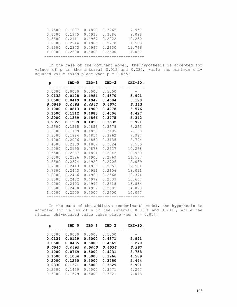
103
0.7500 0.1837 0.4898 0.3265 7.957 0.8000 0.1975 0.4938 0.3086 9.098 0.8500 0.2111 0.4967 0.2922 10.280 0.9000 0.2244 0.4986 0.2770 11.503 0.9500 0.2373 0.4997 0.2630 12.766 1.0000 0.2500 0.5000 0.2500 14.067 -------------------------------------------
In the case of the dominant model, the hypothesis is accepted for values of p in the interval 0.013 and 0.235, while the minimum chi-squared value takes place when p = 0.055: p IBD=0 IBD=1 IBD=2 CHI-SQ. ------------------------------------------ 0.0000 0.0000 0.5000 0.5000 - 0.0132 0.0128 0.4984 0.4570 5.991 0.0500 0.0449 0.4947 0.4604 3.120 0.0549 0.0488 0.4942 0.4570 3.113 0.1000 0.0813 0.4909 0.4278 3.576 0.1500 0.1112 0.4883 0.4006 4.427 0.2000 0.1359 0.4866 0.3775 5.342 0.2355 0.1509 0.4858 0.3632 5.991 0.2500 0.1565 0.4856 0.3578 6.253 0.3000 0.1739 0.4853 0.3409 7.138 0.3500 0.1884 0.4854 0.3262 7.987 0.4000 0.2006 0.4859 0.3135 8.794 0.4500 0.2109 0.4867 0.3024 9.555 0.5000 0.2195 0.4878 0.2927 10.268 0.5500 0.2267 0.4891 0.2842 10.930 0.6000 0.2326 0.4905 0.2769 11.537 0.6500 0.2374 0.4920 0.2706 12.089 0.7000 0.2413 0.4936 0.2651 12.581 0.7500 0.2443 0.4951 0.2606 13.011 0.8000 0.2466 0.4966 0.2568 13.374 0.8500 0.2482 0.4979 0.2539 13.667 0.9000 0.2493 0.4990 0.2518 13.884 0.9500 0.2498 0.4997 0.2505 14.020 1.0000 0.2500 0.5000 0.2500 14.067 ------------------------------------------
In the case of the additive (codominant) model, the hypothesis is accepted for values of p in the interval 0.0134 and 0.2330, while the minimum chi-squared value takes place when p = 0.054:
p IBD=0 IBD=1 IBD=2 CHI-SQ. ------------------------------------------ 0.0000 0.0000 0.5000 0.5000 - 0.0134 0.0129 0.5000 0.4871 5.991 0.0500 0.0435 0.5000 0.4565 3.270 0.0540 0.0465 0.5000 0.4536 3.267 0.1000 0.0769 0.5000 0.4231 3.758 0.1500 0.1034 0.5000 0.3966 4.589 0.2000 0.1250 0.5000 0.3750 5.444 0.2330 0.1371 0.5000 0.3629 5.991 0.2500 0.1429 0.5000 0.3571 6.267 0.3000 0.1579 0.5000 0.3421 7.043
104
0.3500 0.1707 0.5000 0.3293 7.771 0.4000 0.1818 0.5000 0.3182 8.452 0.4500 0.1915 0.5000 0.3085 9.091 0.5000 0.2000 0.5000 0.3000 9.689 0.5500 0.2075 0.5000 0.2925 10.250 0.6000 0.2143 0.5000 0.2857 10.778 0.6500 0.2203 0.5000 0.2797 11.274 0.7000 0.2258 0.5000 0.2742 11.742 0.7500 0.2308 0.5000 0.2692 12.184 0.8000 0.2353 0.5000 0.2647 12.602 0.8500 0.2394 0.5000 0.2606 12.997 0.9000 0.2432 0.5000 0.2568 13.372 0.9500 0.2468 0.5000 0.2532 13.728 1.0000 0.2500 0.5000 0.2500 14.067 ------------------------------------------
The graphs obtained by the Mathematica code below show the chi-squared values generated under the dominant, recessive and additive hypotheses, for all possible frequency values of gene A from the DS locus. (* IBD01.MA data on diabetes x HLA n(ibd=0) = 1, n(ibd=1) = 4, n(ibd=2) = 10 [Cudworth AG & Woodrow JC. Evidence for HL-A genes in "juvenile" diabetes mellitus. Brit. Med. J. III: 133-135, 1975] dominant model : (f1, f2, f3) = (1, 1, 0) recessive model : (f1, f2, f3) = (0, 0, 1) additive model : (f1, f2, f3) = (1, 1/2, 0) *) f1 = 1; f2 = 1; f3 = 0; (* f1 = 0; f2 = 0; f3 = 1; *) (* f1 = 1; f2 = 0.5; f3 = 0; *) lbl = "Chi-squared values - dom. hyp."; (* lbl = "Chi-squared values - rec. hyp."; *) (* lbl = "Chi-squared values - add. hyp."; *) kp = x^2*f1+2*x*(1-x)*f2+(1-x)^2*f3; va = 2*x*(1-x)*((1-x)*(f3-f2)+x*(f2-f1))^2; vd = x^2*(1-x)^2*(f1-2*f2+f3)^2; pibd0 = kp^2/(4*kp^2+2*va+vd); pibd1 = (2*kp^2+va)/(4*kp^2+2*va+vd); pibd2 = (kp^2+va+vd)/(4*kp^2+2*va+vd); epibd0 = 15*pibd0; epibd1 = 15*pibd1; epibd2 = 15*pibd2; f = 1/epibd0 + 16/epibd1 + 100/epibd2 - 15; Plot[{f, 5.99}, {x, 0, 1}, PlotRange -> {0, 20}, Frame -> True, PlotLabel -> FontForm[lbl, {"ZapfChancery-MediumItalic", 12}], FrameLabel -> {FontForm["p",{"Palatino-Italic", 10}], FontForm["Chi-sq. val.", {"Palatino-Italic", 10}]}, DefaultFont -> {"Helvetica-Oblique", 8}]

105
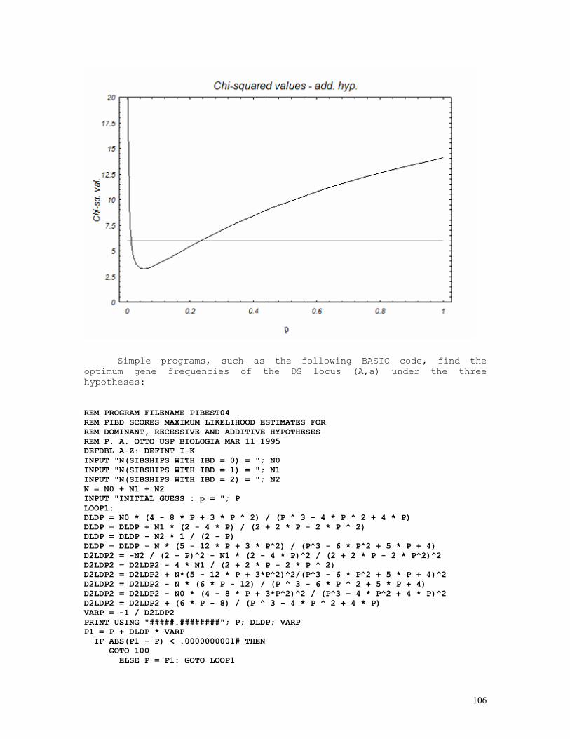
106
Simple programs, such as the following BASIC code, find the optimum gene frequencies of the DS locus (A,a) under the three hypotheses: REM PROGRAM FILENAME PIBEST04 REM PIBD SCORES MAXIMUM LIKELIHOOD ESTIMATES FOR REM DOMINANT, RECESSIVE AND ADDITIVE HYPOTHESES REM P. A. OTTO USP BIOLOGIA MAR 11 1995 DEFDBL A-Z: DEFINT I-K INPUT "N(SIBSHIPS WITH IBD = 0) = "; N0 INPUT "N(SIBSHIPS WITH IBD = 1) = "; N1 INPUT "N(SIBSHIPS WITH IBD = 2) = "; N2 N = N0 + N1 + N2 INPUT "INITIAL GUESS : p = "; P LOOP1: DLDP = N0 * (4 - 8 * P + 3 * P ^ 2) / (P ^ 3 - 4 * P ^ 2 + 4 * P) DLDP = DLDP + N1 * (2 - 4 * P) / (2 + 2 * P - 2 * P ^ 2) DLDP = DLDP - N2 * 1 / (2 - P) DLDP = DLDP - N * (5 - 12 * P + 3 * P^2) / (P^3 - 6 * P^2 + 5 * P + 4) D2LDP2 = -N2 / (2 - P)^2 - N1 * (2 - 4 * P)^2 / (2 + 2 * P - 2 * P^2)^2 D2LDP2 = D2LDP2 - 4 * N1 / (2 + 2 * P - 2 * P ^ 2) D2LDP2 = D2LDP2 + N*(5 - 12 * P + 3*P^2)^2/(P^3 - 6 * P^2 + 5 * P + 4)^2 D2LDP2 = D2LDP2 - N * (6 * P - 12) / (P ^ 3 - 6 * P ^ 2 + 5 * P + 4) D2LDP2 = D2LDP2 - N0 * (4 - 8 * P + 3*P^2)^2 / (P^3 – 4 * P^2 + 4 * P)^2 D2LDP2 = D2LDP2 + (6 * P - 8) / (P ^ 3 - 4 * P ^ 2 + 4 * P) VARP = -1 / D2LDP2 PRINT USING "#####.########"; P; DLDP; VARP P1 = P + DLDP * VARP IF ABS(P1 - P) < .0000000001# THEN GOTO 100 ELSE P = P1: GOTO LOOP1
107
END IF 100 PRINT USING "N(SIBSHIPS WITH IBD = 0) = ### "; N0 PRINT USING "N(SIBSHIPS WITH IBD = 1) = ### "; N1 PRINT USING "N(SIBSHIPS WITH IBD = 2) = ### "; N2 PRINT : PRINT " 1) RECESSIVE HYPOTHESIS" Q = (2 * N0 + N1) / (2 * N2 + N1) VARQ = 2 * (N0 + N1 + N2) * (2 * N0 + N1) / (2 * N2 + N1) ^ 3 PRINT USING "q = #.########"; Q PRINT USING "var(q) = #.########"; VARQ E1 = N * (Q / (1 + Q)) ^ 2 E2 = N * 2 * Q / (1 + Q) ^ 2 E3 = N * (1 / (1 + Q)) ^ 2 CHISQ = N0 ^ 2 / E1 + N1 ^ 2 / E2 + N2 ^ 2 / E3 - N PRINT USING "chi-sq. (1 d.f.) = ###.####"; CHISQ PRINT : PRINT " 2) DOMINANT HYPOTHESIS" PRINT USING "p = #.########"; P PRINT USING "var(p) = #.########"; VARP E1 = N * P * (4 - 4 * P + P ^ 2) / (P ^ 3 - 6 * P ^ 2 + 5 * P + 4) E2 = N * 2 * (1 + P - P ^ 2) / (P ^ 3 - 6 * P ^ 2 + 5 * P + 4) E3 = N * (2 - P) / (P ^ 3 - 6 * P ^ 2 + 5 * P + 4) CHISQ = N0 ^ 2 / E1 + N1 ^ 2 / E2 + N2 ^ 2 / E3 - N PRINT USING "chi-sq. (1 d.f.) = ###.####"; CHISQ PRINT : PRINT " 3) ADDITIVE HYPOTHESIS" P = N0 / (2 * N2 - N0) VARP = P * (1 + P) * (1 + 3 * P) / (2 * N2 - N0) PRINT USING "p = #.########"; P PRINT USING "var(p) = #.########"; VARP E1 = N * P / (1 + 3 * P) E2 = N / 2 E3 = N * (1 + P) / (2 * (1 + 3 * P)) CHISQ = N0 ^ 2 / E1 + N1 ^ 2 / E2 + N2 ^ 2 / E3 – N PRINT USING "chi-sq. (1 d.f.) = ###.####"; CHISQ N(SIBSHIPS WITH IBD = 0) = ? 1 N(SIBSHIPS WITH IBD = 1) = ? 4 N(SIBSHIPS WITH IBD = 2) = ? 10 INITIAL GUESS : p = ? .01 0.01000000 79.77356276 0.00010052 0.01801849 35.67688499 0.00032999 0.02979143 14.31651608 0.00092654 0.04305621 4.58875483 0.00202295 0.05233903 0.88092095 0.00311055 0.05507918 0.04916321 0.00349034 0.05525078 0.00017334 0.00351509 0.05525139 0.00000000 0.00351518 N(SIBSHIPS WITH IBD = 0) = 1 N(SIBSHIPS WITH IBD = 1) = 4 N(SIBSHIPS WITH IBD = 2) = 10 1) RECESSIVE HYPOTHESIS q = 0.25000000 var(q) = 0.01302083 chi-sq. (1 d.f.) = 0.4167 2) DOMINANT HYPOTHESIS p = 0.05525139 var(p) = 0.00351518 chi-sq. (1 d.f.) = 3.1138 3) ADDITIVE HYPOTHESIS p = 0.05263158 var(p) = 0.00337628 chi-sq. (1 d.f.) = 3.2667
108
As these results clearly show the observed data are compatible
with the three models here presented, especially the recessive one. Actually, it is possible to obtain population estimates of Kp, VA and VD , in order to restrict the parameters {q = 1-p, F1, F2, F3} to the constraints Kp = p2F1 + 2pqF2 + q2F3, VA = 2pq[q(F3-F2)+p(F1-F2)]2 and VD = p2q2(F1-2F2+F3)2, but the constraints { Kp , VA , VD } are consistent with an infinite number of parameter sets {q = 1-p, F1, F2, F3}. Some minimum, maximum and intermediate gene frequencies (and their corresponding penetrance vectors), consistent with the population parameters Kp = 0.0058 (population incidence of juvenile diabetes) and VA = 3.85 × 10⁻⁴ and VD = 4.27 × 10⁻⁴ (additive and dominance genetic variances inferred from population data), are shown below (modified from Suarez, 1978):
q F1 F2 F3 χ2
0.03 0.0016 0.0616 0.8316 1.250
0.04 0.0010 0.0503 0.6376 1.275
0.05 0.0005 0.0424 0.5193 1.291
0.06 0.0001 0.0365 0.4208 1.264
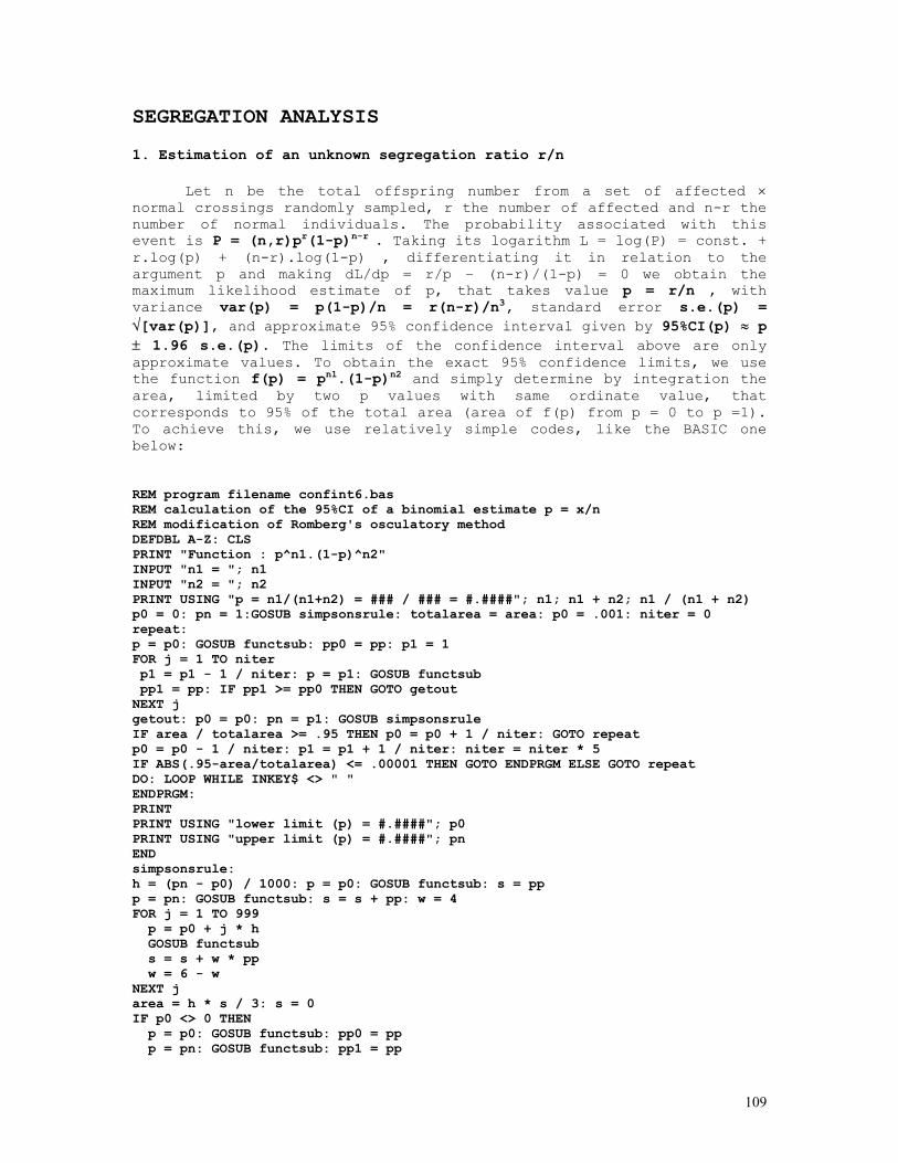
109
SEGREGATION ANALYSIS
1. Estimation of an unknown segregation ratio r/n
Let n be the total offspring number from a set of affected × normal crossings randomly sampled, r the number of affected and n-r the number of normal individuals. The probability associated with this event is P = (n,r)pr(1-p)n-r . Taking its logarithm L = log(P) = const. + r.log(p) + (n-r).log(1-p) , differentiating it in relation to the argument p and making dL/dp = r/p – (n-r)/(1-p) = 0 we obtain the maximum likelihood estimate of p, that takes value p = r/n , with variance var(p) = p(1-p)/n = r(n-r)/n3, standard error s.e.(p) = √[var(p)], and approximate 95% confidence interval given by 95%CI(p) ≈ p ± 1.96 s.e.(p). The limits of the confidence interval above are only approximate values. To obtain the exact 95% confidence limits, we use the function f(p) = pn1.(1-p)n2 and simply determine by integration the area, limited by two p values with same ordinate value, that corresponds to 95% of the total area (area of f(p) from p = 0 to p =1). To achieve this, we use relatively simple codes, like the BASIC one below: REM program filename confint6.bas REM calculation of the 95%CI of a binomial estimate p = x/n REM modification of Romberg's osculatory method DEFDBL A-Z: CLS PRINT "Function : p^n1.(1-p)^n2" INPUT "n1 = "; n1 INPUT "n2 = "; n2 PRINT USING "p = n1/(n1+n2) = ### / ### = #.####"; n1; n1 + n2; n1 / (n1 + n2) p0 = 0: pn = 1:GOSUB simpsonsrule: totalarea = area: p0 = .001: niter = 0 repeat: p = p0: GOSUB functsub: pp0 = pp: p1 = 1 FOR j = 1 TO niter p1 = p1 - 1 / niter: p = p1: GOSUB functsub pp1 = pp: IF pp1 >= pp0 THEN GOTO getout NEXT j getout: p0 = p0: pn = p1: GOSUB simpsonsrule IF area / totalarea >= .95 THEN p0 = p0 + 1 / niter: GOTO repeat p0 = p0 - 1 / niter: p1 = p1 + 1 / niter: niter = niter * 5 IF ABS(.95-area/totalarea) <= .00001 THEN GOTO ENDPRGM ELSE GOTO repeat DO: LOOP WHILE INKEY$ <> " " ENDPRGM: PRINT PRINT USING "lower limit (p) = #.####"; p0 PRINT USING "upper limit (p) = #.####"; pn END simpsonsrule: h = (pn - p0) / 1000: p = p0: GOSUB functsub: s = pp p = pn: GOSUB functsub: s = s + pp: w = 4 FOR j = 1 TO 999 p = p0 + j * h GOSUB functsub s = s + w * pp w = 6 - w NEXT j area = h * s / 3: s = 0 IF p0 <> 0 THEN p = p0: GOSUB functsub: pp0 = pp p = pn: GOSUB functsub: pp1 = pp
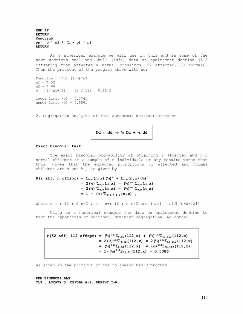
110
END IF RETURN functsub: pp = p ^ n1 * (1 - p) ^ n2 RETURN
As a numerical example we will use in this and in some of the next sections Neel and Shull (1954) data on opalescent dentine (112 offspring from affected × normal crossings, 52 affected, 60 normal). Then the printout of the program above will be: Function : p^n1.(1-p)^n2 n1 = ? 52 n2 = ? 60 p = n1/(n1+n2) = 52 / 112 = 0.4643 lower limit (p) = 0.3741 upper limit (p) = 0.5561 2. Segregation analysis of rare autosomal dominant diseases
Dd × dd → ½ Dd + ½ dd
Exact binomial test
The exact binomial probability of obtaining r affected and n-r normal children in a sample of n individuals or any results worse than this, given that the expected proportions of affected and normal children are ½ and ½ , is given by P(r aff, n offspr) = Σ0,c(n,x)(½)n + Σc,n(n,x)(½)n = 2(½)nΣ0,c(n,x) = (½)n-1Σ0,c(n,x) = 2(½)nΣc,n(n,x) = (½)n-1Σc,n(n,x) = 1 - (½)nΣr+1,n-r-1(n,x) , where c = r if r ≤ n/2 , c = n-r if r > n/2 and (n,x) = n!/[(n-x)!x!]
Using as a numerical example the data on opalescent dentine to test the hypothesis of autosomal dominant segregation, we obtan:
P(52 aff, 112 offspr) = (½)112Σ0,52(112,x) + (½)112Σ60,112(112,x) = 2(½)112Σ0,52(112,x) = 2(½)112Σ60,112(112,x) = (½)111Σ0,52(112,x) = (½)111Σ60,112(112,x) = 1-(½)112Σ53,61(112,x) = 0.5086
as shown in the printout of the following BASIC program REM BINPROB4.BAS CLS : LOCATE 5: DEFDBL A-Z: DEFINT I-N
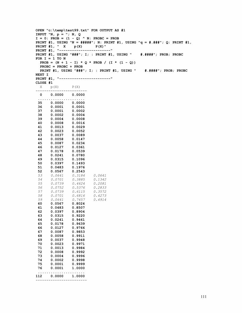
111
OPEN "c:\temp\test99.txt" FOR OUTPUT AS #1 INPUT "N, p = "; N, Q I = 0: PROB = (1 - Q) ^ N: PROBC = PROB PRINT #1, USING "N = #####"; N: PRINT #1, USING "q = #.###"; Q: PRINT #1, PRINT #1, " X p(X) P(X)" PRINT #1, "------------------------" PRINT #1, USING "###"; I; : PRINT #1, USING " #.####"; PROB; PROBC FOR I = 1 TO N PROB = (N + 1 - I) * Q * PROB / (I * (1 - Q)) PROBC = PROBC + PROB PRINT #1, USING "###"; I; : PRINT #1, USING " #.####"; PROB; PROBC NEXT I PRINT #1, "------------------------" CLOSE #1 X p(X) P(X) ------------------------ 0 0.0000 0.0000 ...................... 35 0.0000 0.0000 36 0.0001 0.0001 37 0.0001 0.0002 38 0.0002 0.0004 39 0.0004 0.0008 40 0.0008 0.0016 41 0.0013 0.0029 42 0.0023 0.0052 43 0.0037 0.0089 44 0.0058 0.0147 45 0.0087 0.0234 46 0.0127 0.0361 47 0.0178 0.0539 48 0.0241 0.0780 49 0.0315 0.1096 50 0.0397 0.1493 51 0.0483 0.1976 52 0.0567 0.2543 53 0.0641 0.3184 0.0641 54 0.0701 0.3885 0.1342 55 0.0739 0.4624 0.2081 56 0.0752 0.5376 0.2833 57 0.0739 0.6115 0.3572 58 0.0701 0.6816 0.4273 59 0.0641 0.7457 0.4914 60 0.0567 0.8024 61 0.0483 0.8507 62 0.0397 0.8904 63 0.0315 0.9220 64 0.0241 0.9461 65 0.0178 0.9639 66 0.0127 0.9766 67 0.0087 0.9853 68 0.0058 0.9911 69 0.0037 0.9948 70 0.0023 0.9971 71 0.0013 0.9984 72 0.0008 0.9992 73 0.0004 0.9996 74 0.0002 0.9998 75 0.0001 0.9999 76 0.0001 1.0000 ...................... 112 0.0000 1.0000 ------------------------

112
Standard normal test
Using the standard normal deviate z = (x-µ)/σ → N{0,1} we get the following test, that is based therefore on the normal approximation to the binomial distribution [µ = np, σ2 = np(1-p)] : z = (r-np)/√[np(1-p)] = (r-n/2)/√(n/4)
z = (52-56)/ √(28) = -4/√28 = -0.7559 → P = 0.4496
Chi-squared test
The data can also be analyzed by the usual chi-squared statistics, that in this special case takes the form Z2 ≈ χ2 = (x-np)2/[np(1-p)] = (x-np)2/np + [(n-x)-n(1-p)]2/[n(1-p)] = Σ(oi-ei)2/ei = Σ(oi2/ei) – n = (r-n/2)2/(n/4)
χ2 = (52-56)2/ 28 = 0.5714 → P = 0.4496
Log-likelihood test
The test that follows is asymptotically equivalent to the chi-squared test detailed above: L(p) = (n,r)pr(1-p)n-r L1(p) = (n,r)(52/112)52(60/112)60 L2(p) = (n,r)(1/2)52(1/2)60 2[log L1(p) – log L2(p)] ≈ χ2
χ2 = 2[52.log(52/112) + 60.log(60/112) – 112.log(1/2)] = 0.5719 → P = 0.4495
3. Segregation analysis of autosomal codominant loci
The usual situation is the analysis of the offspring of a known mating cross, vg. Aa vs. Aa. As a numerical example we will consider the genotypes of 275 offspring resulting from matings MN × MN: 71 MM, 141 MN, 63 NN. To test the hypothesis of monogenic codominant inheritance we apply a chi-squared or a log-likelihood test as follows:
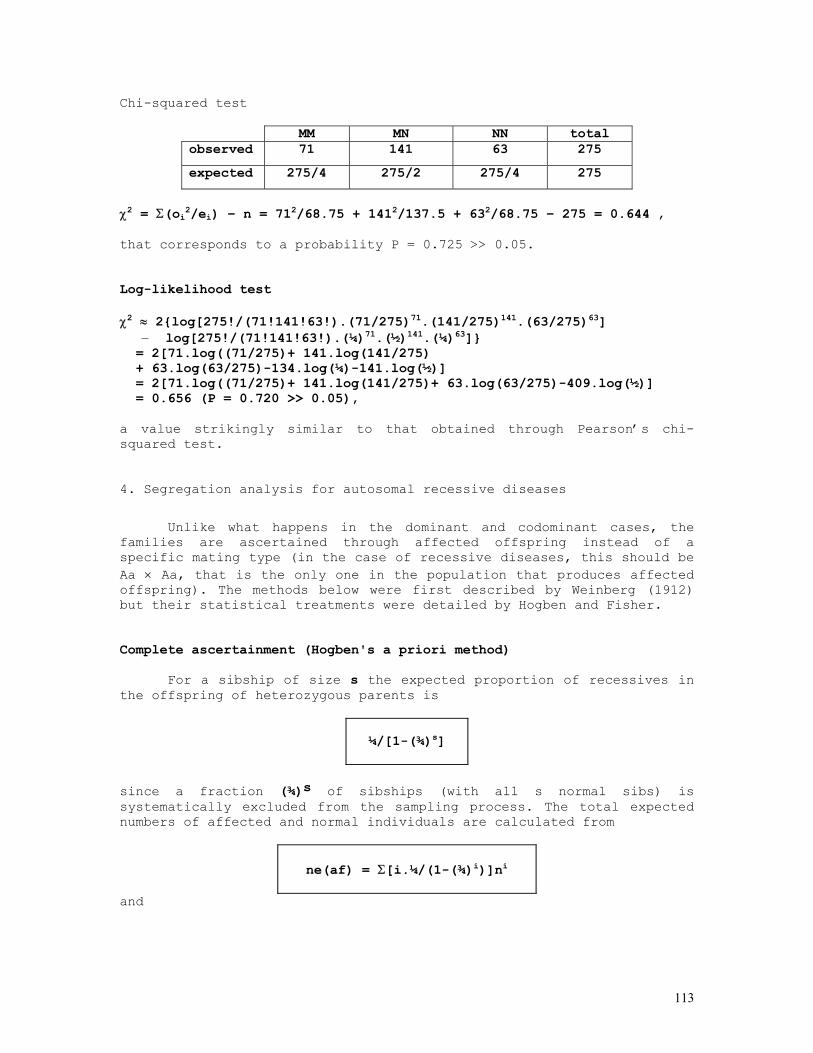
113
Chi-squared test
MM MN NN total observed 71 141 63 275
expected 275/4 275/2 275/4 275
χ2 = Σ(oi2/ei) – n = 712/68.75 + 1412/137.5 + 632/68.75 – 275 = 0.644 , that corresponds to a probability P = 0.725 >> 0.05. Log-likelihood test χ2 ≈ 2{log[275!/(71!141!63!).(71/275)71.(141/275)141.(63/275)63]
– log[275!/(71!141!63!).(¼)71.(½)141.(¼)63]} = 2[71.log((71/275)+ 141.log(141/275) + 63.log(63/275)-134.log(¼)-141.log(½)] = 2[71.log((71/275)+ 141.log(141/275)+ 63.log(63/275)-409.log(½)] = 0.656 (P = 0.720 >> 0.05), a value strikingly similar to that obtained through Pearson’s chi-squared test. 4. Segregation analysis for autosomal recessive diseases
Unlike what happens in the dominant and codominant cases, the
families are ascertained through affected offspring instead of a specific mating type (in the case of recessive diseases, this should be Aa × Aa, that is the only one in the population that produces affected offspring). The methods below were first described by Weinberg (1912) but their statistical treatments were detailed by Hogben and Fisher. Complete ascertainment (Hogben's a priori method)
For a sibship of size s the expected proportion of recessives in the offspring of heterozygous parents is
¼/[1-(¾)s]
since a fraction (¾)s of sibships (with all s normal sibs) is systematically excluded from the sampling process. The total expected numbers of affected and normal individuals are calculated from
ne(af) = Σ[i.¼/(1-(¾)i)]ni
and
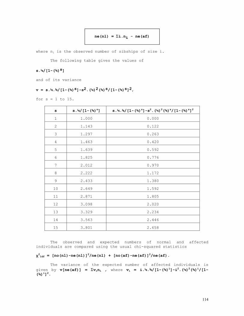
114
ne(nl) = Σi.ni - ne(af)
where ni is the observed number of sibships of size i.
The following table gives the values of
s.¼/[1-(¾)s] and of its variance v = s.¼.¾/[1-(¾)s]-s2.(¼)2(¾)s/[1-(¾)s]2, for s = 1 to 15.
s s.¼/[1-(¾)s] s.¼.¾/[1-(¾)s]-s2.(¼)2(¾)s/[1-(¾)s]2
1 1.000 0.000
2 1.143 0.122
3 1.297 0.263
4 1.463 0.420
5 1.639 0.592
6 1.825 0.776
7 2.012 0.970
8 2.222 1.172
9 2.433 1.380
10 2.649 1.592
11 2.871 1.805
12 3.098 2.020
13 3.329 2.234
14 3.563 2.446
15 3.801 2.658
The observed and expected numbers of normal and affected individuals are compared using the usual chi-squared statistics χ21df = [no(nl)-ne(nl)]2/ne(nl) + [no(af)-ne(af)]2/ne(af).
The variance of the expected number of affected individuals is given by v[ne(af)] = Σvini , where vi = i.¼.¾/[1-(¾)i]-i2.(¼)2(¾)i/[1-(¾)i]2.
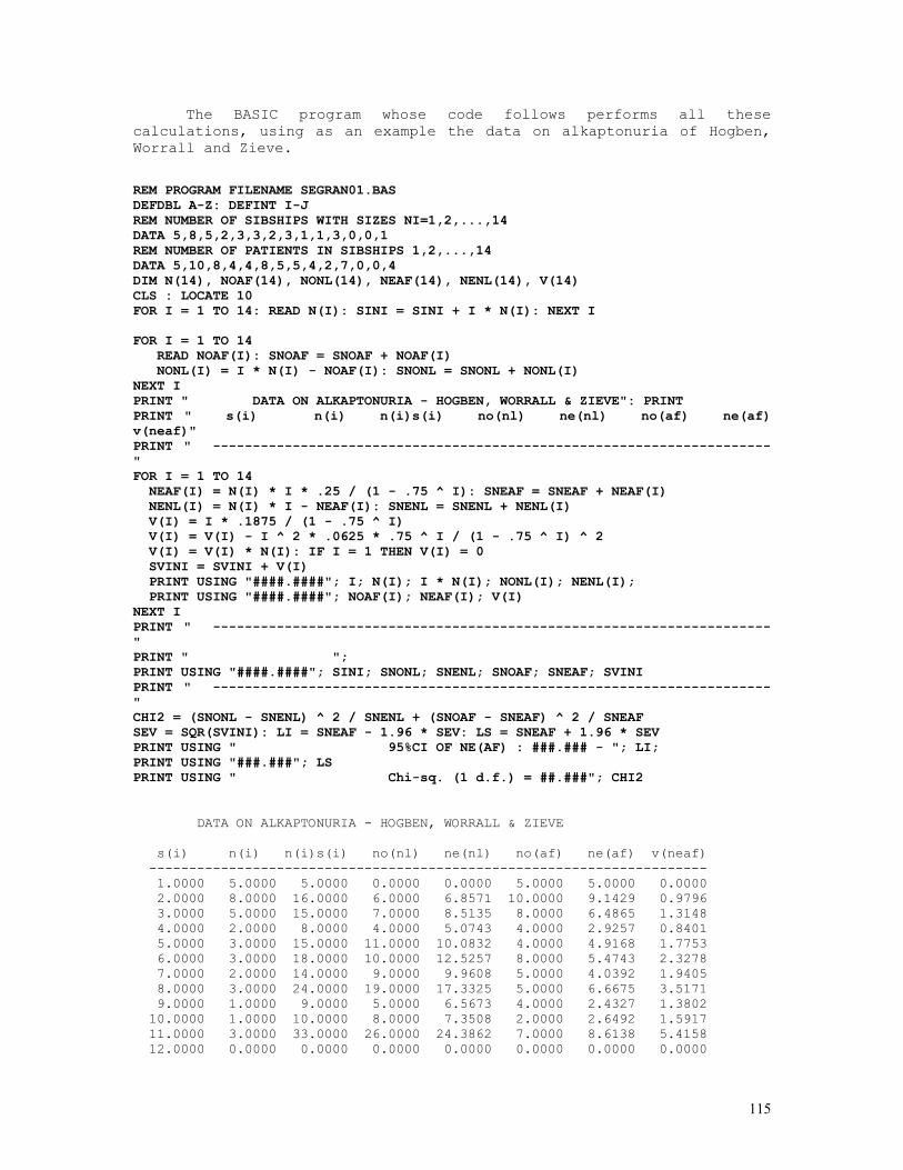
115
The BASIC program whose code follows performs all these calculations, using as an example the data on alkaptonuria of Hogben, Worrall and Zieve. REM PROGRAM FILENAME SEGRAN01.BAS DEFDBL A-Z: DEFINT I-J REM NUMBER OF SIBSHIPS WITH SIZES NI=1,2,...,14 DATA 5,8,5,2,3,3,2,3,1,1,3,0,0,1 REM NUMBER OF PATIENTS IN SIBSHIPS 1,2,...,14 DATA 5,10,8,4,4,8,5,5,4,2,7,0,0,4 DIM N(14), NOAF(14), NONL(14), NEAF(14), NENL(14), V(14) CLS : LOCATE 10 FOR I = 1 TO 14: READ N(I): SINI = SINI + I * N(I): NEXT I
FOR I = 1 TO 14 READ NOAF(I): SNOAF = SNOAF + NOAF(I) NONL(I) = I * N(I) - NOAF(I): SNONL = SNONL + NONL(I) NEXT I PRINT " DATA ON ALKAPTONURIA - HOGBEN, WORRALL & ZIEVE": PRINT PRINT " s(i) n(i) n(i)s(i) no(nl) ne(nl) no(af) ne(af) v(neaf)" PRINT " ----------------------------------------------------------------------" FOR I = 1 TO 14 NEAF(I) = N(I) * I * .25 / (1 - .75 ^ I): SNEAF = SNEAF + NEAF(I) NENL(I) = N(I) * I - NEAF(I): SNENL = SNENL + NENL(I) V(I) = I * .1875 / (1 - .75 ^ I) V(I) = V(I) - I ^ 2 * .0625 * .75 ^ I / (1 - .75 ^ I) ^ 2 V(I) = V(I) * N(I): IF I = 1 THEN V(I) = 0 SVINI = SVINI + V(I) PRINT USING "####.####"; I; N(I); I * N(I); NONL(I); NENL(I); PRINT USING "####.####"; NOAF(I); NEAF(I); V(I) NEXT I PRINT " ----------------------------------------------------------------------" PRINT " "; PRINT USING "####.####"; SINI; SNONL; SNENL; SNOAF; SNEAF; SVINI PRINT " ----------------------------------------------------------------------" CHI2 = (SNONL - SNENL) ^ 2 / SNENL + (SNOAF - SNEAF) ^ 2 / SNEAF SEV = SQR(SVINI): LI = SNEAF - 1.96 * SEV: LS = SNEAF + 1.96 * SEV PRINT USING " 95%CI OF NE(AF) : ###.### - "; LI; PRINT USING "###.###"; LS PRINT USING " Chi-sq. (1 d.f.) = ##.###"; CHI2 DATA ON ALKAPTONURIA - HOGBEN, WORRALL & ZIEVE s(i) n(i) n(i)s(i) no(nl) ne(nl) no(af) ne(af) v(neaf) ---------------------------------------------------------------------- 1.0000 5.0000 5.0000 0.0000 0.0000 5.0000 5.0000 0.0000 2.0000 8.0000 16.0000 6.0000 6.8571 10.0000 9.1429 0.9796 3.0000 5.0000 15.0000 7.0000 8.5135 8.0000 6.4865 1.3148 4.0000 2.0000 8.0000 4.0000 5.0743 4.0000 2.9257 0.8401 5.0000 3.0000 15.0000 11.0000 10.0832 4.0000 4.9168 1.7753 6.0000 3.0000 18.0000 10.0000 12.5257 8.0000 5.4743 2.3278 7.0000 2.0000 14.0000 9.0000 9.9608 5.0000 4.0392 1.9405 8.0000 3.0000 24.0000 19.0000 17.3325 5.0000 6.6675 3.5171 9.0000 1.0000 9.0000 5.0000 6.5673 4.0000 2.4327 1.3802 10.0000 1.0000 10.0000 8.0000 7.3508 2.0000 2.6492 1.5917 11.0000 3.0000 33.0000 26.0000 24.3862 7.0000 8.6138 5.4158 12.0000 0.0000 0.0000 0.0000 0.0000 0.0000 0.0000 0.0000
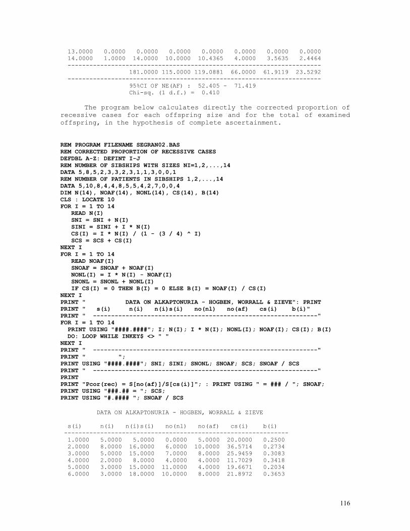
116
13.0000 0.0000 0.0000 0.0000 0.0000 0.0000 0.0000 0.0000 14.0000 1.0000 14.0000 10.0000 10.4365 4.0000 3.5635 2.4464 ---------------------------------------------------------------------- 181.0000 115.0000 119.0881 66.0000 61.9119 23.5292 ---------------------------------------------------------------------- 95%CI OF NE(AF) : 52.405 - 71.419 Chi-sq. (1 d.f.) = 0.410
The program below calculates directly the corrected proportion of recessive cases for each offspring size and for the total of examined offspring, in the hypothesis of complete ascertainment. REM PROGRAM FILENAME SEGRAN02.BAS REM CORRECTED PROPORTION OF RECESSIVE CASES DEFDBL A-Z: DEFINT I-J REM NUMBER OF SIBSHIPS WITH SIZES NI=1,2,...,14 DATA 5,8,5,2,3,3,2,3,1,1,3,0,0,1 REM NUMBER OF PATIENTS IN SIBSHIPS 1,2,...,14 DATA 5,10,8,4,4,8,5,5,4,2,7,0,0,4 DIM N(14), NOAF(14), NONL(14), CS(14), B(14) CLS : LOCATE 10 FOR I = 1 TO 14 READ N(I) SNI = SNI + N(I) SINI = SINI + I * N(I) CS(I) = I * N(I) / (1 - (3 / 4) ^ I) SCS = SCS + CS(I) NEXT I FOR I = 1 TO 14 READ NOAF(I) SNOAF = SNOAF + NOAF(I) NONL(I) = I * N(I) - NOAF(I) SNONL = SNONL + NONL(I) IF CS(I) = 0 THEN B(I) = 0 ELSE B(I) = NOAF(I) / CS(I) NEXT I PRINT " DATA ON ALKAPTONURIA - HOGBEN, WORRALL & ZIEVE": PRINT PRINT " s(i) n(i) n(i)s(i) no(nl) no(af) cs(i) b(i)" PRINT " --------------------------------------------------------------" FOR I = 1 TO 14 PRINT USING "####.####"; I; N(I); I * N(I); NONL(I); NOAF(I); CS(I); B(I) DO: LOOP WHILE INKEY$ <> " " NEXT I PRINT " --------------------------------------------------------------" PRINT " "; PRINT USING "####.####"; SNI; SINI; SNONL; SNOAF; SCS; SNOAF / SCS PRINT " --------------------------------------------------------------" PRINT PRINT "Pcor(rec) = S[no(af)]/S[cs(i)]"; : PRINT USING " = ### / "; SNOAF; PRINT USING "###.## = "; SCS; PRINT USING "#.#### "; SNOAF / SCS DATA ON ALKAPTONURIA - HOGBEN, WORRALL & ZIEVE s(i) n(i) n(i)s(i) no(nl) no(af) cs(i) b(i) -------------------------------------------------------------- 1.0000 5.0000 5.0000 0.0000 5.0000 20.0000 0.2500 2.0000 8.0000 16.0000 6.0000 10.0000 36.5714 0.2734 3.0000 5.0000 15.0000 7.0000 8.0000 25.9459 0.3083 4.0000 2.0000 8.0000 4.0000 4.0000 11.7029 0.3418 5.0000 3.0000 15.0000 11.0000 4.0000 19.6671 0.2034 6.0000 3.0000 18.0000 10.0000 8.0000 21.8972 0.3653
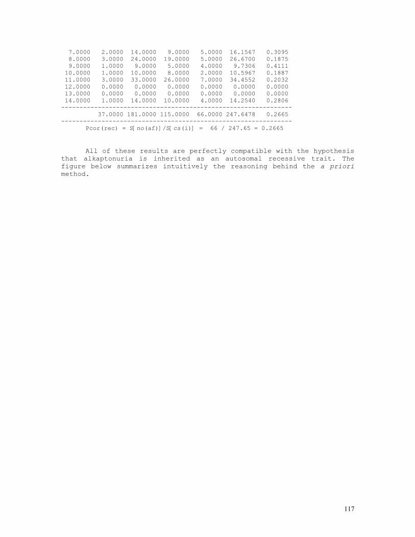
117
7.0000 2.0000 14.0000 9.0000 5.0000 16.1567 0.3095 8.0000 3.0000 24.0000 19.0000 5.0000 26.6700 0.1875 9.0000 1.0000 9.0000 5.0000 4.0000 9.7306 0.4111 10.0000 1.0000 10.0000 8.0000 2.0000 10.5967 0.1887 11.0000 3.0000 33.0000 26.0000 7.0000 34.4552 0.2032 12.0000 0.0000 0.0000 0.0000 0.0000 0.0000 0.0000 13.0000 0.0000 0.0000 0.0000 0.0000 0.0000 0.0000 14.0000 1.0000 14.0000 10.0000 4.0000 14.2540 0.2806 --------------------------------------------------------------- 37.0000 181.0000 115.0000 66.0000 247.6478 0.2665 ---------------------------------------------------------------
Pcor(rec) = S[no(af)]/S[cs(i)] = 66 / 247.65 = 0.2665
All of these results are perfectly compatible with the hypothesis that alkaptonuria is inherited as an autosomal recessive trait. The figure below summarizes intuitively the reasoning behind the a priori method.
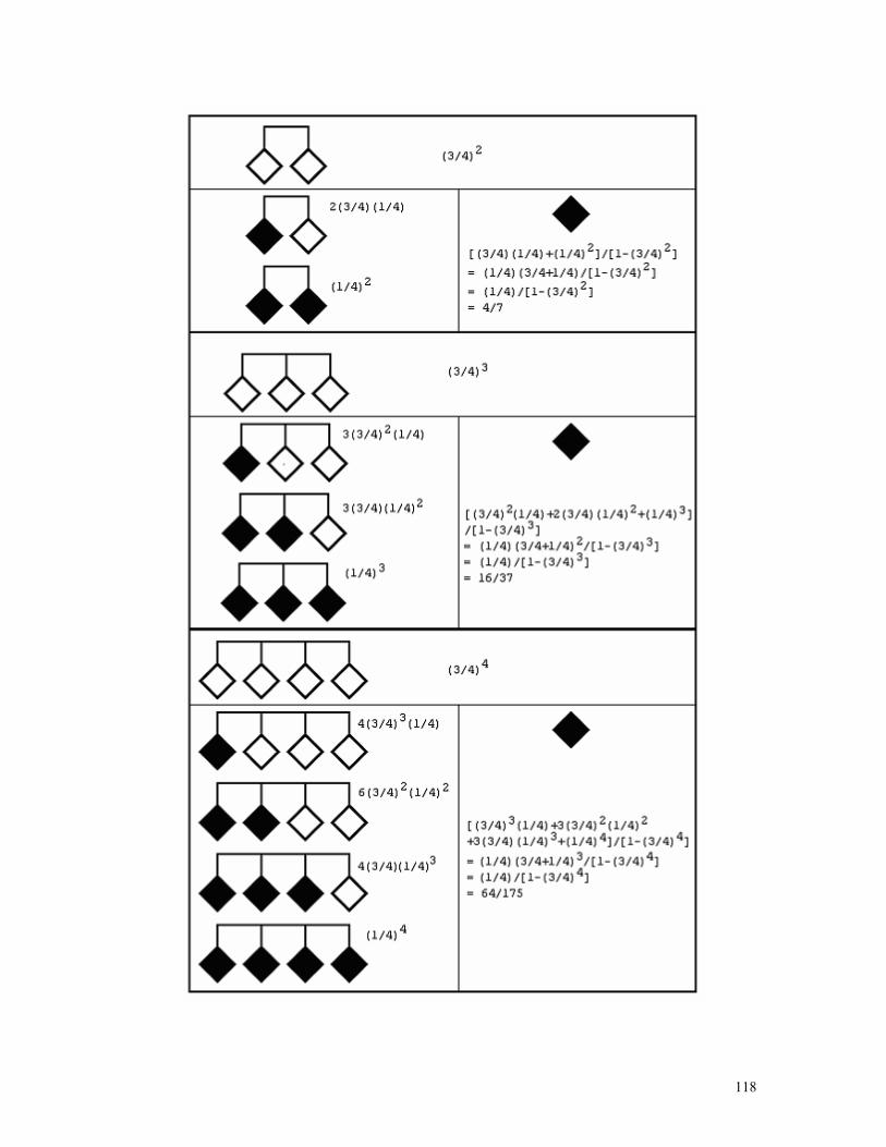
118
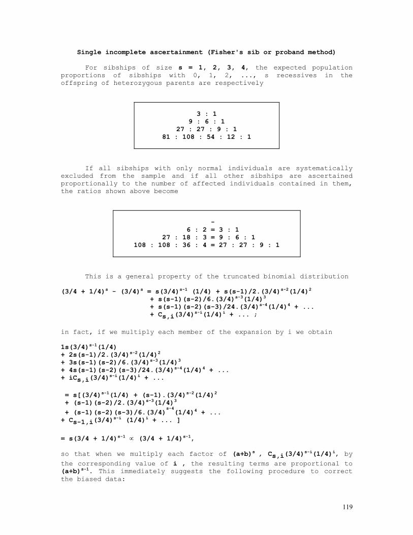
119
Single incomplete ascertainment (Fisher's sib or proband method)
For sibships of size s = 1, 2, 3, 4, the expected population proportions of sibships with 0, 1, 2, ..., s recessives in the offspring of heterozygous parents are respectively
3 : 1
9 : 6 : 1 27 : 27 : 9 : 1
81 : 108 : 54 : 12 : 1
If all sibships with only normal individuals are systematically excluded from the sample and if all other sibships are ascertained proportionally to the number of affected individuals contained in them, the ratios shown above become
-
6 : 2 = 3 : 1 27 : 18 : 3 = 9 : 6 : 1
108 : 108 : 36 : 4 = 27 : 27 : 9 : 1
This is a general property of the truncated binomial distribution (3/4 + 1/4)s - (3/4)s = s(3/4)s-1 (1/4) + s(s-1)/2.(3/4)s-2(1/4)2 + s(s-1)(s-2)/6.(3/4)s-3(1/4)3 + s(s-1)(s-2)(s-3)/24.(3/4)s-4(1/4)4 + ... + Cs,i(3/4)
s-i(1/4)i + ... ; in fact, if we multiply each member of the expansion by i we obtain 1s(3/4)s-1(1/4) + 2s(s-1)/2.(3/4)s-2(1/4)2 + 3s(s-1)(s-2)/6.(3/4)s-3(1/4)3 + 4s(s-1)(s-2)(s-3)/24.(3/4)s-4(1/4)4 + ... + iCs,i(3/4)
s-i(1/4)i + ... = s[(3/4)s-1(1/4) + (s-1).(3/4)s-2(1/4)2 + (s-1)(s-2)/2.(3/4)s-3(1/4)3
+ (s-1)(s-2)(s-3)/6.(3/4)s-4(1/4)4 + ...
+ Cs-1,i(3/4)s-i (1/4)i + ... ]
= s(3/4 + 1/4)s-1 ∝ (3/4 + 1/4)s-1, so that when we multiply each factor of (a+b)s
, Cs,i(3/4)
s-i(1/4)i, by the corresponding value of i , the resulting terms are proportional to (a+b)s-1. This immediately suggests the following procedure to correct the biased data:
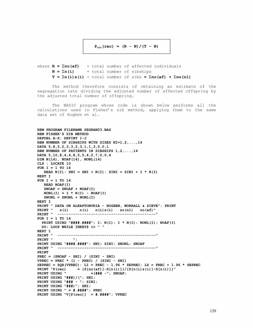
120
Pcor(rec) = (R - N)/(T - N)
where R = Σno(af) = total number of affected individuals N = Σn(i) = total number of sibships T = Σn(i)s(i) = total number of sibs = Σno(af) + Σno(nl)
The method therefore consists of obtaining an estimate of the segregation rate dividing the adjusted number of affected offspring by the adjusted total number of offspring.
The BASIC program whose code is shown below performs all the calculations used in Fisher’s sib method, applying them to the same data set of Hogben et al. REM PROGRAM FILENAME SEGRAN03.BAS REM FISHER'S SIB METHOD DEFDBL A-Z: DEFINT I-J REM NUMBER OF SIBSHIPS WITH SIZES NI=1,2,...,14 DATA 5,8,5,2,3,3,2,3,1,1,3,0,0,1 REM NUMBER OF PATIENTS IN SIBSHIPS 1,2,...,14 DATA 5,10,8,4,4,8,5,5,4,2,7,0,0,4 DIM N(14), NOAF(14), NONL(14) CLS : LOCATE 10 FOR I = 1 TO 14 READ N(I): SNI = SNI + N(I): SINI = SINI + I * N(I) NEXT I FOR I = 1 TO 14 READ NOAF(I) SNOAF = SNOAF + NOAF(I) NONL(I) = I * N(I) - NOAF(I) SNONL = SNONL + NONL(I) NEXT I PRINT " DATA ON ALKAPTONURIA - HOGBEN, WORRALL & ZIEVE": PRINT PRINT " s(i) n(i) n(i)s(i) no(nl) no(af)" PRINT " --------------------------------------------" FOR I = 1 TO 14 PRINT USING "####.####"; I; N(I); I * N(I); NONL(I); NOAF(I) DO: LOOP WHILE INKEY$ <> " " NEXT I PRINT " --------------------------------------------" PRINT " "; PRINT USING "####.####"; SNI; SINI; SNONL; SNOAF PRINT " --------------------------------------------" PRINT PREC = (SNOAF - SNI) / (SINI - SNI) VPREC = PREC * (1 - PREC) / (SINI - SNI) SEPREC = SQR(VPREC): LI = PREC - 1.96 * SEPREC: LS = PREC + 1.96 * SEPREC PRINT "P(rec) = {S[no(af)]-S[n(i)]}/{S[n(i)s(i)]-S[n(i)]}" PRINT USING " =(### -"; SNOAF; PRINT USING "###)/("; SNI; PRINT USING "### - "; SINI; PRINT USING "###)"; SNI; PRINT USING " = #.####"; PREC PRINT USING "V[P(rec)] = #.####"; VPREC
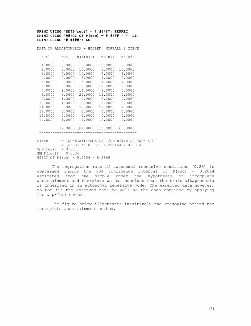
121
PRINT USING "SE[P(rec)] = #.####"; SEPREC PRINT USING "95%CI OF P(rec) = #.#### - "; LI; PRINT USING "#.####"; LS DATA ON ALKAPTONURIA - HOGBEN, WORRALL & ZIEVE s(i) n(i) n(i)s(i) no(nl) no(af) -------------------------------------------- 1.0000 5.0000 5.0000 0.0000 5.0000 2.0000 8.0000 16.0000 6.0000 10.0000 3.0000 5.0000 15.0000 7.0000 8.0000 4.0000 2.0000 8.0000 4.0000 4.0000 5.0000 3.0000 15.0000 11.0000 4.0000 6.0000 3.0000 18.0000 10.0000 8.0000 7.0000 2.0000 14.0000 9.0000 5.0000 8.0000 3.0000 24.0000 19.0000 5.0000 9.0000 1.0000 9.0000 5.0000 4.0000 10.0000 1.0000 10.0000 8.0000 2.0000 11.0000 3.0000 33.0000 26.0000 7.0000 12.0000 0.0000 0.0000 0.0000 0.0000 13.0000 0.0000 0.0000 0.0000 0.0000 14.0000 1.0000 14.0000 10.0000 4.0000 -------------------------------------------- 37.0000 181.0000 115.0000 66.0000 -------------------------------------------- P(rec) = {S[no(af)]-S[n(i)]}/{S[n(i)s(i)]-S[n(i)]} = (66-37)/(181-37) = 29/144 = 0.2014 V[P(rec)] = 0.0011 SE[P(rec)] = 0.0334 95%CI OF P(rec) = 0.1359 - 0.2669
The segregation rate of autosomal recessive conditions (0.25) is contained inside the 95% confidence interval of P(rec) = 0.2014 estimated from the sample under the hypothesis of incomplete ascertainment and therefore we can conclude that the trait alkaptonuria is inherited in an autosomal recessive mode. The expected data,however, do not fit the observed ones so well as the ones obtained by applying the a priori method.
The figure below illustrates intuitively the reasoning behind the incomplete ascertainment method.
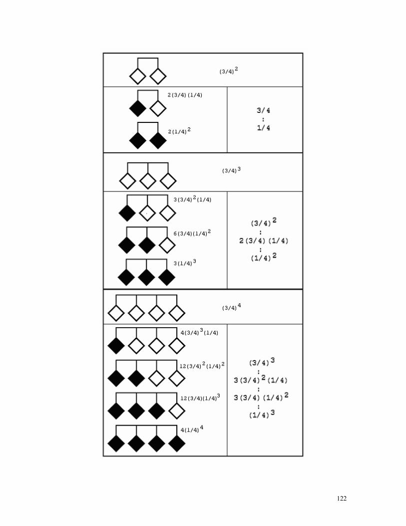
122
123
The a priori (complete ascertainment) and single or proband
(incomplete ascertainment) methods are actually incomplete selection cases because the families are ascertained through affected children (if the families were obtained through random sampling of heterozygous parents the selection would be complete). The methods just detailed receive also the names of truncate selection and single selection respectively, corresponding to situations in which (1) the distribution of affected children among families is binomial with the omission of sibships with none affected or (2) the probability of inclusion of a family is proportional to the number of children affected, unlike in case (1), where the probability of inclusion of a family is independent of the number of children affected. These two extreme cases are actually special cases included in a general situation called multiple selection. The vocabulary truncate, single and multiple selection was introduced by Morton (1959) and much of the section that follows was based on Crow (1965) and on Cavalli-Sforza and Bodmer (1971).
Multiple selection of autosomal recessive diseases
When the number of probands of each sibship is known, we use the method below, in whose formulae the following symbols will be used throughout: p = probability of an affected child (p = ¼ for a fully penetrant recessive trait in the case of heterozygous parents); q = 1-p π = probability of an affected child being independently ascertained (π = 0 in the single selection case, π = 1 in the truncate selection case) s = sibship size r = number of affected children in a sibship a = number of probands (affected children independently ascertained) in the sibship n = total number of families T = total number of children R = total number of affected children The formula for obtaining an initial estimate of the true proportion of affected children is p0 = Σa(r-1) / Σa(s-1) while the variance of the estimate from a single sibship of size s is v(p) = p(1-p)[1+π+pπ(s-3)] / a(s-1) and the variance of the estimate from all sibships of size s is v(p) = p(1-p)[1+π+pπ(s-3)] / Σa(s-1), where π is estimated as π = Σa(a-1) / Σa(r-1) ; for obtaining a pooled estimate of p for all sibships, we weigh the p values obtained from sibships of size s by the reciprocals of their
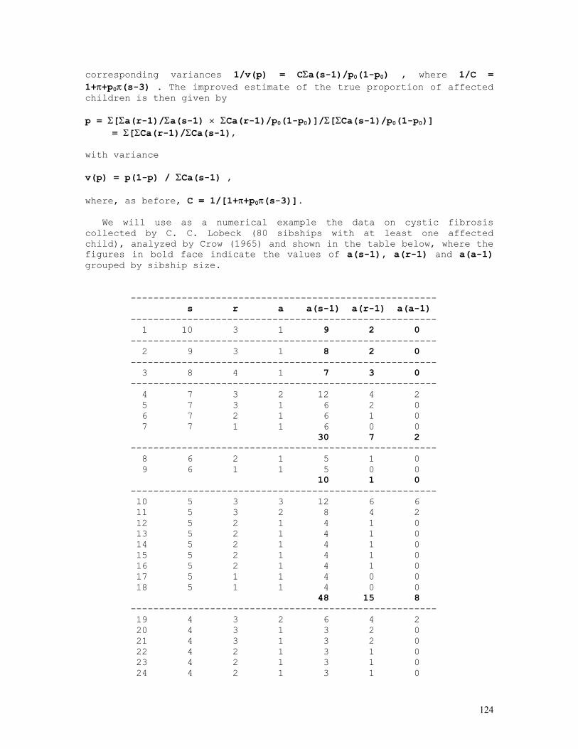
124
corresponding variances 1/v(p) = CΣa(s-1)/p0(1-p0) , where 1/C = 1+π+p0π(s-3) . The improved estimate of the true proportion of affected children is then given by p = Σ[Σa(r-1)/Σa(s-1) × ΣCa(r-1)/p0(1-p0)]/Σ[ΣCa(s-1)/p0(1-p0)]
= Σ[ΣCa(r-1)/ΣCa(s-1),
with variance v(p) = p(1-p) / ΣCa(s-1) , where, as before, C = 1/[1+π+p0π(s-3)].
We will use as a numerical example the data on cystic fibrosis collected by C. C. Lobeck (80 sibships with at least one affected child), analyzed by Crow (1965) and shown in the table below, where the figures in bold face indicate the values of a(s-1), a(r-1) and a(a-1) grouped by sibship size.
------------------------------------------------------ s r a a(s-1) a(r-1) a(a-1) ------------------------------------------------------ 1 10 3 1 9 2 0 ------------------------------------------------------ 2 9 3 1 8 2 0 ------------------------------------------------------ 3 8 4 1 7 3 0 ------------------------------------------------------ 4 7 3 2 12 4 2 5 7 3 1 6 2 0 6 7 2 1 6 1 0 7 7 1 1 6 0 0 30 7 2 ------------------------------------------------------ 8 6 2 1 5 1 0 9 6 1 1 5 0 0 10 1 0 ------------------------------------------------------ 10 5 3 3 12 6 6 11 5 3 2 8 4 2 12 5 2 1 4 1 0 13 5 2 1 4 1 0 14 5 2 1 4 1 0 15 5 2 1 4 1 0 16 5 2 1 4 1 0 17 5 1 1 4 0 0 18 5 1 1 4 0 0 48 15 8 ------------------------------------------------------ 19 4 3 2 6 4 2 20 4 3 1 3 2 0 21 4 3 1 3 2 0 22 4 2 1 3 1 0 23 4 2 1 3 1 0 24 4 2 1 3 1 0
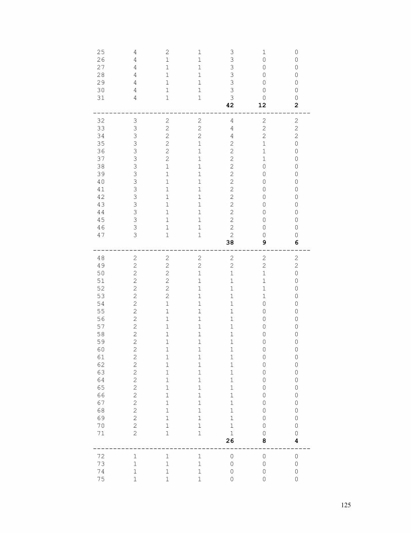
125
25 4 2 1 3 1 0 26 4 1 1 3 0 0 27 4 1 1 3 0 0 28 4 1 1 3 0 0 29 4 1 1 3 0 0 30 4 1 1 3 0 0 31 4 1 1 3 0 0 42 12 2 ------------------------------------------------------ 32 3 2 2 4 2 2 33 3 2 2 4 2 2 34 3 2 2 4 2 2 35 3 2 1 2 1 0 36 3 2 1 2 1 0 37 3 2 1 2 1 0 38 3 1 1 2 0 0 39 3 1 1 2 0 0 40 3 1 1 2 0 0 41 3 1 1 2 0 0 42 3 1 1 2 0 0 43 3 1 1 2 0 0 44 3 1 1 2 0 0 45 3 1 1 2 0 0 46 3 1 1 2 0 0 47 3 1 1 2 0 0 38 9 6 ------------------------------------------------------ 48 2 2 2 2 2 2 49 2 2 2 2 2 2 50 2 2 1 1 1 0 51 2 2 1 1 1 0 52 2 2 1 1 1 0 53 2 2 1 1 1 0 54 2 1 1 1 0 0 55 2 1 1 1 0 0 56 2 1 1 1 0 0 57 2 1 1 1 0 0 58 2 1 1 1 0 0 59 2 1 1 1 0 0 60 2 1 1 1 0 0 61 2 1 1 1 0 0 62 2 1 1 1 0 0 63 2 1 1 1 0 0 64 2 1 1 1 0 0 65 2 1 1 1 0 0 66 2 1 1 1 0 0 67 2 1 1 1 0 0 68 2 1 1 1 0 0 69 2 1 1 1 0 0 70 2 1 1 1 0 0 71 2 1 1 1 0 0 26 8 4 ------------------------------------------------------ 72 1 1 1 0 0 0 73 1 1 1 0 0 0 74 1 1 1 0 0 0 75 1 1 1 0 0 0
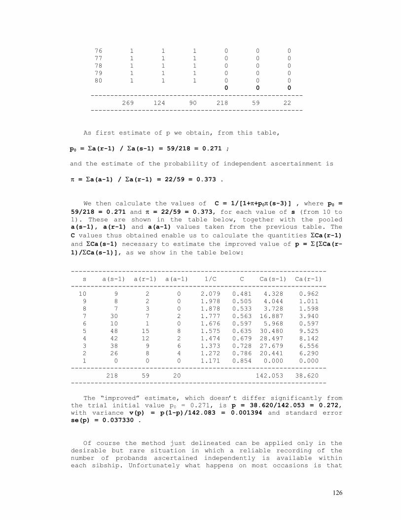
126
76 1 1 1 0 0 0 77 1 1 1 0 0 0 78 1 1 1 0 0 0 79 1 1 1 0 0 0 80 1 1 1 0 0 0 0 0 0 ------------------------------------------------------ 269 124 90 218 59 22 ------------------------------------------------------
As first estimate of p we obtain, from this table, p0 = Σa(r-1) / Σa(s-1) = 59/218 = 0.271 ; and the estimate of the probability of independent ascertainment is π = Σa(a-1) / Σa(r-1) = 22/59 = 0.373 .
We then calculate the values of C = 1/[1+π+p0π(s-3)] , where p0 = 59/218 = 0.271 and π = 22/59 = 0.373, for each value of s (from 10 to 1). These are shown in the table below, together with the pooled a(s-1), a(r-1) and a(a-1) values taken from the previous table. The C values thus obtained enable us to calculate the quantities ΣCa(r-1) and ΣCa(s-1) necessary to estimate the improved value of p = Σ[ΣCa(r-1)/ΣCa(s-1)], as we show in the table below:
----------------------------------------------------------------- s a(s-1) a(r-1) a(a-1) 1/C C Ca(s-1) Ca(r-1) ----------------------------------------------------------------- 10 9 2 0 2.079 0.481 4.328 0.962 9 8 2 0 1.978 0.505 4.044 1.011 8 7 3 0 1.878 0.533 3.728 1.598 7 30 7 2 1.777 0.563 16.887 3.940 6 10 1 0 1.676 0.597 5.968 0.597 5 48 15 8 1.575 0.635 30.480 9.525 4 42 12 2 1.474 0.679 28.497 8.142 3 38 9 6 1.373 0.728 27.679 6.556 2 26 8 4 1.272 0.786 20.441 6.290 1 0 0 0 1.171 0.854 0.000 0.000 ----------------------------------------------------------------- 218 59 20 142.053 38.620 -----------------------------------------------------------------
The “improved” estimate, which doesn’t differ significantly from the trial initial value p0 = 0.271, is p = 38.620/142.053 = 0.272, with variance v(p) = p(1-p)/142.083 = 0.001394 and standard error se(p) = 0.037330 .
Of course the method just delineated can be applied only in the desirable but rare situation in which a reliable recording of the number of probands ascertained independently is available within each sibship. Unfortunately what happens on most occasions is that
127
the information is either missing or inaccurate. In those cases we should use the general method that follows.
The probability that a sibship of size s contains r affected children of which a are probands is
(r,a)πa(1-π)r-a(s,r)pr(1-p)s-r , where (x,y) = Cx,y = x!/y!(x-y)! ;
if a is not known, the probability of a family of size s with r affected is the sum of the above expression over all values of a from 1 to r :
Σa=1,r(r,a)πa(1-π)r-a(s,r)pr(1-p)s-r = [1-(1-π)r](s,r)pr(1-p)s-r ,
where [1-(1-π)r] is the probability that a ≥ 1 (probability of the family being independently ascertained at least once).
The proportion of families of size s that are not ascertained is
Σr=0,s(s,r)pr(1-p)s-r (1-π)r = [1-p+p(1-π)]s = (1-pπ)s ,
where pπ is the probability of an affected child in a segregating family becoming a proband.
Therefore, among families of size s that are ascertained at least once, the proportion with r affected is
(s,r)pr(1-p)s-r[1-(1-π)r]/[1-(1-pπ)s] ;
when π = 1, this likelihood function becomes the complete ascertainment case
(s,r)pr(1-p)s-r/[1-(1-p)s];
when π = 0, it simplifies to the single ascertainment case
(s-1,r-1)pr-1(1-p)s-r .
In relation to the total of n families sampled the likelihood function (s,r)pr(1-p)s-r[1-(1-π)r]/[1-(1-pπ)s] becomes
128
Σi=1,n{(si,ri)pri(1-p)si-ri[1-(1-π)ri]/[1-(1-pπ)si]} ;
taking the natural logarithm of the likelihood of a family of size r with r affected,
P = (s,r)pr(1-p)s-r[1-(1-π)r]/[1-(1-pπ)s] ,
we obtain
L = log(P) = log[s!/(s-r)!r!] + r.log(p) – (s-r).log(1-p)
+ log[1-(1-π)r] - log[1-(1-pπ)s] .
The parameters p and π are then obtained from the set of equations {∂L/∂p = 0, ∂L/∂π = 0}, where
∂L/∂p = r/p - (s-r)/(1-p) - πs(1-πp)s-1/[1-(1-πp)s]
∂L/∂π = r(1-π)r-1/[1-(1-π)r] - ps(1-πp)s-1/[1-(1-πp)s] .
For the whole set of n sampled families the equations above clearly take the form
∂L/∂p = Σi=1,n{ri/p - (si-ri)/(1-p) - πsi(1-πp)si-1/[1-(1-πp)si]}
∂L/∂π = Σi=1,n{ri(1-π)ri-1/[1-(1-π)ri] - psi(1-πp)si-1/[1-(1-πp)si]} .
129
PENETRANCE RATE ESTIMATION
Andréa R. V. Russo Horimoto
Paulo A. Otto
Penetrance rate is the conditional probability pij that a genotype aiaj expresses itself phenotypically. As any probability, the penetrance rate can take any value in the interval (0,1); when the penetrance rate has value 1, it is said to be complete; when assuming any value larger than 0 and smaller than 1, it is said to be incomplete. Inversely, the non-penetrance of a genetic trait, that takes place with a probability 1-pij, is the lack of phenotypic manifestation due exclusively or predominantly to environmental or to random factors (such as mutation) associated only to the aiaj genotype.
In the generalized case, the penetrance rate can be represented
by the transitional matrix pij (Rogatko, 1983, 1986):
f1 f2 f3
a1a1 p11 p12 p13 a1a2 p21 p22 p23 a2a2 p31 p32 p33
that is, the conditional probability p(fk|aiaj) of an individual presenting the phenotype fk, given that his/her genotype is aiaj, is the penetrance rate pij. In the cases of dominance and codominance with complete penetrance, the above transitional matrix reduces to
f1 f2 f3
a1a1 1 0 0 a1a2 1 0 0 a2a2 0 0 1
and
f1 f2 f3
a1a1 1 0 0 a1a2 0 1 0 a2a2 0 0 1
respectively (Rogatko, 1983).
The penetrance values pij in all possible cases of dominance with incomplete penetrance can be reduced to a single parameter pij = K and used to define five different penetrance models, as the following table shows:
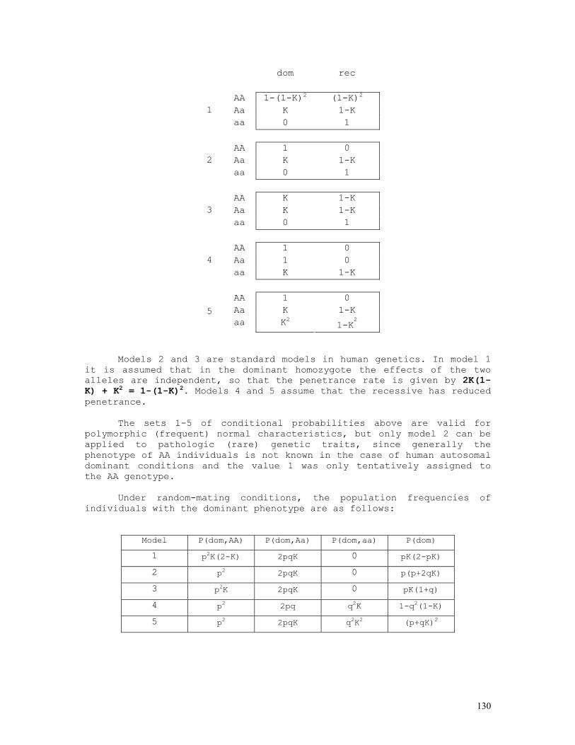
130
dom rec
AA 1-(1-K)2 (1-K)2 Aa K 1-K 1 aa 0 1
AA 1 0 Aa K 1-K 2 aa 0 1
AA K 1-K Aa K 1-K 3 aa 0 1
AA 1 0 Aa 1 0 4 aa K 1-K
AA 1 0 Aa K 1-K 5 aa K2 1-K
2
Models 2 and 3 are standard models in human genetics. In model 1
it is assumed that in the dominant homozygote the effects of the two alleles are independent, so that the penetrance rate is given by 2K(1-K) + K2 = 1-(1-K)2. Models 4 and 5 assume that the recessive has reduced penetrance.
The sets 1-5 of conditional probabilities above are valid for
polymorphic (frequent) normal characteristics, but only model 2 can be applied to pathologic (rare) genetic traits, since generally the phenotype of AA individuals is not known in the case of human autosomal dominant conditions and the value 1 was only tentatively assigned to the AA genotype.
Under random-mating conditions, the population frequencies of
individuals with the dominant phenotype are as follows:
Model P(dom,AA) P(dom,Aa) P(dom,aa) P(dom)
1 p2K(2-K) 2pqK 0 pK(2-pK)
2 p2 2pqK 0 p(p+2qK)
3 p2K 2pqK 0 pK(1+q)
4 p2 2pq q2K 1-q2(1-K)
5 p2 2pqK q2K2 (p+qK)2
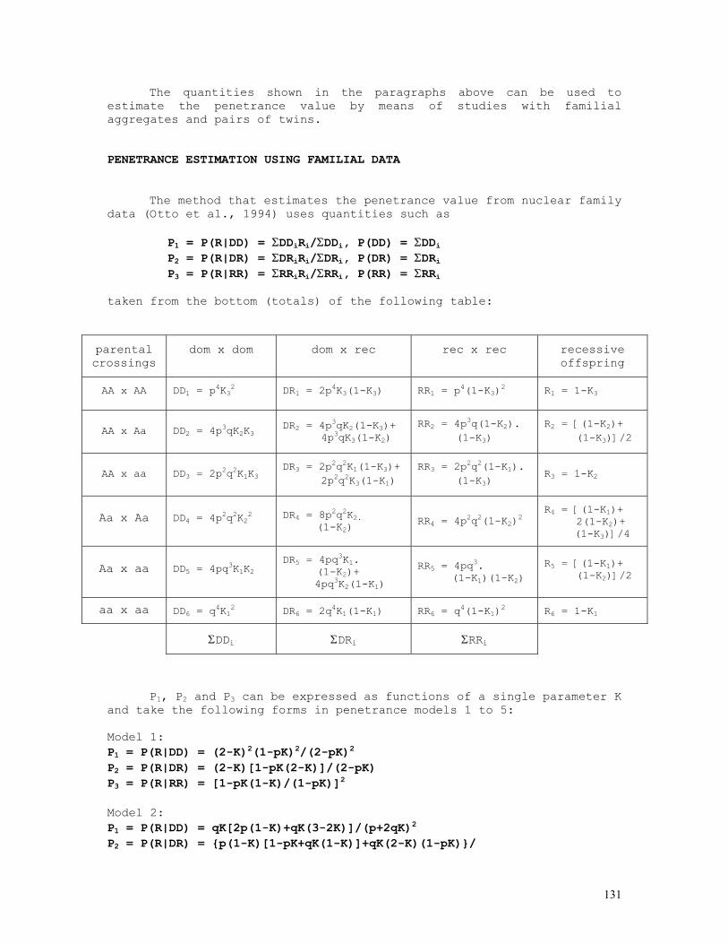
131
The quantities shown in the paragraphs above can be used to estimate the penetrance value by means of studies with familial aggregates and pairs of twins. PENETRANCE ESTIMATION USING FAMILIAL DATA The method that estimates the penetrance value from nuclear family data (Otto et al., 1994) uses quantities such as
P1 = P(R|DD) = ΣDDiRi/ΣDDi, P(DD) = ΣDDi P2 = P(R|DR) = ΣDRiRi/ΣDRi, P(DR) = ΣDRi P3 = P(R|RR) = ΣRRiRi/ΣRRi, P(RR) = ΣRRi
taken from the bottom (totals) of the following table:
parental crossings
dom x dom dom x rec rec x rec recessive offspring
AA x AA DD1 = p4K3
2 DR1 = 2p4K3(1-K3) RR1 = p
4(1-K3)2 R1 = 1-K3
AA x Aa DD2 = 4p3qK2K3
DR2 = 4p3qK2(1-K3)+
4p3qK3(1-K2) RR2 = 4p
3q(1-K2). (1-K3)
R2 = [(1-K2)+ (1-K3)]/2
AA x aa DD3 = 2p2q2K1K3
DR3 = 2p2q2K1(1-K3)+
2p2q2K3(1-K1) RR3 = 2p
2q2(1-K1). (1-K3)
R3 = 1-K2
Aa x Aa DD4 = 4p2q2K2
2 DR4 = 8p2q2K2.
(1-K2) RR4 = 4p
2q2(1-K2)2
R4 = [(1-K1)+ 2(1-K2)+ (1-K3)]/4
Aa x aa DD5 = 4pq3K1K2
DR5 = 4pq3K1.
(1-K2)+ 4pq3K2(1-K1)
RR5 = 4pq3.
(1-K1)(1-K2) R5 = [(1-K1)+ (1-K2)]/2
aa x aa DD6 = q4K12 DR6 = 2q4K1(1-K1) RR6 = q4(1-K1)
2 R6 = 1-K1
ΣDDi ΣDRi ΣRRi
P1, P2 and P3 can be expressed as functions of a single parameter K and take the following forms in penetrance models 1 to 5: Model 1: P1 = P(R|DD) = (2-K)2(1-pK)2/(2-pK)2 P2 = P(R|DR) = (2-K)[1-pK(2-K)]/(2-pK) P3 = P(R|RR) = [1-pK(1-K)/(1-pK)]2
Model 2: P1 = P(R|DD) = qK[2p(1-K)+qK(3-2K)]/(p+2qK)2 P2 = P(R|DR) = {p(1-K)[1-pK+qK(1-K)]+qK(2-K)(1-pK)}/

132
{(p+2qK)[2p(1-K)+q]} P3 = P(R|RR) = {p(1-K)[p(1-K)(3-2K)+2q(2-K)]+q2}/ [2p(1-K)+q]2 Model 3: P1 = P(R|DD) = 1-K + q2K/(1+q)2 P2 = P(R|DR) = [p(1-K)2(1+q)2+pq2(1-K2)+q3(2-K)]/{(1+q)[1-pK(1+q)]} P3 = P(R|RR) = {(1-pK)4+pK(1-K)[p3(1-K)2-3pq2(1-K)-2q3]}/[1-pK(1+q)]2 Model 4: P1 = P(R|DD) = (1-K){q(p+qK)/[1-q2(1-K)]}2 P2 = P(R|DR) = (1-K)q(p+qK)/[1-q2(1-K)] P3 = P(R|RR) = 1-K Model 5: P1 = P(R|DD) = qK(1-K)[2-q(1-K)(2+K)]/[1-q(1-K)]2 P2 = P(R|DR) = (1-K)[(1-q)2+(1-q)2qK(4+K)+ (1-q)q2K(2+K)(1+2K)+q3K2(1+K)2]/{[1-q(1-K)]2[2-q(1-K)]} P3 = P(R|RR) = (1-K)[(1-q)2(3+K)+2q(1-q)(1+K)(2+K)+ q2(1+K)3]/[2-q(1-K)]2
Let us suppose that, from the familial analysis of n1 + n2 + n3 couples with N1 + N2 + N3 children, we observe the following set of quantities:
offspring parents
dom rec total dom x dom n1 n4 n5 N1 dom x rec n2 n6 n7 N2 rec x rec n3 n8 n9 N3
total N4 N5 N
Under the hypothesis of dominant monogenic inheritance with incomplete penetrance, the (log) likelihood function is given by the expression: L = n1.log[P(DD)] + n2.log[P(DR)] + n3.log[P(RR)] + n4.log[P(D|DD)] + n5.logP[(R|DD)] + n6.log[P(D|DR)] + n7.log[P(R|DR)] + n8.logP[(D|RR)] + n9.log[P(R|RR)] = (2n1+n2).log[P(D)] + (n2+2n3).log[P(R)] + n4.log(Q1) + n5.log(P1)+ n6.log(Q2)+ n7.log(P2)+ n8.log(Q3)+ n9.log(P3), where Qi = 1-Pi (i = 1, 2, 3).
The adherence of observed to expected values can be tested by the following tests:
1) in the offspring of dom x dom crossings: χ2 = (n4-N1Q1)2/N1Q1 + (n5-N1P1)2/N1P1 = n4
2/N1Q1 + n52/N1P1 – N1
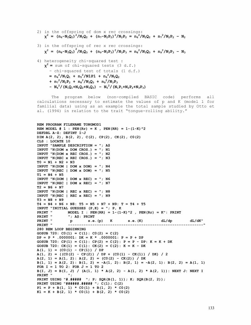
133
2) in the offspring of dom x rec crossings: χ2 = (n6-N2Q2)2/N2Q2 + (n7-N2P2)2/N2P2 = n62/N2Q2 + n72/N2P2 – N2 3) in the offspring of rec x rec crossings: χ2 = (n8-N3Q3)
2/N3Q3 + (n9-N3P3)2/N3P3 = n82/N3Q3 + n92/N3P3 – N3
4) heterogeneity chi-squared test : χ2 = sum of chi-squared tests (3 d.f.) – chi-squared test of totals (1 d.f.) = n42/N1Q1 + n52/N1P1 + n62/N2Q2 + n72/N2P2 + n8
2/N3Q3 + n92/N3P3 - N42/(N1Q1+N2Q2+N3Q3) – N52/(N1P1+N2P2+N3P3)
The program below (non-compiled BASIC code) performs all calculations necessary to estimate the values of p and K (model 1 for familial data) using as an example the total sample studied by Otto et al. (1994) in relation to the trait “tongue-rolling ability.” REM PROGRAM FILENAME TONGMOD1 REM MODEL # 1 : PEN(Rr) = K , PEN(RR) = 1-(1-K)^2 DEFDBL A-Z: DEFINT I-J DIM A(2, 2), B(2, 2), C(2), CP(2), CK(2), C0(2) CLS : LOCATE 10 INPUT "SAMPLE DESCRIPTION = "; A$ INPUT "N(DOM x DOM CROS.) = "; N1 INPUT "N(DOM x REC CROS.) = "; N2 INPUT "N(REC x REC CROS.) = "; N3 T0 = N1 + N2 + N3 INPUT "N(DOM | DOM x DOM) = "; N4 INPUT "N(REC | DOM x DOM) = "; N5 T1 = N4 + N5 INPUT "N(DOM | DOM x REC) = "; N6 INPUT "N(REC | DOM x REC) = "; N7 T2 = N6 + N7 INPUT "N(DOM | REC x REC) = "; N8 INPUT "N(REC | REC x REC) = "; N9 T3 = N8 + N9 T4 = N4 + N6 + N8: T5 = N5 + N7 + N9: T = T4 + T5 INPUT "INITIAL GUESSES (P,K) = "; P, K PRINT " MODEL I : PEN(RR) = 1-(1-K)^2 , PEN(Rr) = K": PRINT PRINT " "; A$: PRINT PRINT " p s.e.(p) K s.e.(K) dL/dp dL/dK" PRINT " -------------------------------------------------------------" 280 REM LOOP BEGINNING GOSUB 720: C0(1) = C(1): C0(2) = C(2) DP = P * .0000001: DK = K * .0000001: P = P + DP GOSUB 720: CP(1) = C(1): CP(2) = C(2): P = P - DP: K = K + DK GOSUB 720: CK(1) = C(1): CK(2) = C(2): K = K - DK A(1, 1) = (C0(1) - CP(1)) / DP A(1, 2) = ((C0(2) - CP(2)) / DP + (C0(1) - CK(1)) / DK) / 2 A(2, 1) = A(1, 2): A(2, 2) = (C0(2) - CK(2)) / DK B(1, 1) = A(2, 2): B(1, 2) = -A(1, 2): B(2, 1) = -A(2, 1): B(2, 2) = A(1, 1) FOR I = 1 TO 2: FOR J = 1 TO 2 B(I, J) = B(I, J) / (A(1, 1) * A(2, 2) - A(1, 2) * A(2, 1)): NEXT J: NEXT I PRINT " "; PRINT USING "#.##### "; P; SQR(B(1, 1)); K; SQR(B(2, 2)); PRINT USING "######.##### "; C(1); C(2) P1 = P + B(1, 1) * C0(1) + B(1, 2) * C0(2) K1 = K + B(2, 1) * C0(1) + B(2, 2) * C0(2)
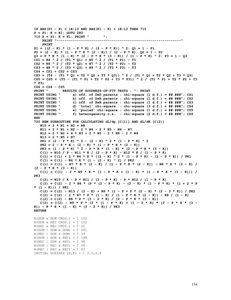
134
IF ABS(P1 - P) < 1E-12 AND ABS(K1 - K) < 1E-12 THEN 710 P = P1: K = K1: GOTO 280 710 P = P1: K = K1: PRINT " "; PRINT "-------------------------------------------------------------" PRINT P1 = ((2 - K) * (1 - P * K) / (2 - P * K)) ^ 2: Q1 = 1 - P1 P2 = (2 - K) * (1 - P * K * (2 - K)) / (2 - P * K): Q2 = 1 - P2 Q3 = P * K * (1 - K) * (2 - P * K * (3 - K)) / (1 - P * K) ^ 2: P3 = 1 - Q3 CS1 = N4 ^ 2 / (T1 * Q1) + N5 ^ 2 / (T1 * P1) - T1 CS2 = N6 ^ 2 / (T2 * Q2) + N7 ^ 2 / (T2 * P2) - T2 CS3 = N8 ^ 2 / (T3 * Q3) + N9 ^ 2 / (T3 * P3) - T3 CS4 = CS1 + CS2 + CS3 CS5 = (T4 - (T1 * Q1 + T2 * Q2 + T3 * Q3)) ^ 2 / (T1 * Q1 + T2 * Q2 + T3 * Q3) CS5 = CS5 + (T5 - (T1 * P1 + T2 * P2 + T3 * P3)) ^ 2 / (T1 * P1 + T2 * P2 + T3 * P3) CS6 = CS4 - CS5 PRINT " RESULTS OF GOODNESS-OF-FIT TESTS : ": PRINT PRINT USING " a) off. of DxD parents : chi-square (1 d.f.) = ##.###"; CS1 PRINT USING " b) off. of DxR parents : chi-square (1 d.f.) = ##.###"; CS2 PRINT USING " c) off. of RxR parents : chi-square (1 d.f.) = ##.###"; CS3 PRINT USING " d) 'total' chi-square : chi-square (3 d.f.) = ##.###"; CS4 PRINT USING " e) 'pooled' chi-square : chi-square (1 d.f.) = ##.###"; CS5 PRINT USING " f) heterogeneity c.s. : chi-square (2 d.f.) = ##.###"; CS6 END 720 REM SUBROUTINE FOR CALCULATING dL/dp [C(1)] AND dL/dK [C(2)] N10 = 2 * N1 + N2 + N8 N11 = 2 * N1 + N2 - 2 * N4 - 2 * N5 - N6 - N7 N12 = 2 * N2 + 4 * N3 + 2 * N5 - 2 * N8 - 2 * N9 N13 = 2 * N5 + N7 PK1 = (2 - P * K) ^ 2 - (2 - K) ^ 2 * (1 - P * K) ^ 2 PK2 = 2 - P * K - (2 - K) * (1 - P * K * (2 - K)) PK3 = (1 - P * K) ^ 2 - P * K * (1 - K) * (2 - P * K * (3 - K)) C(1) = N10 / P - N11 * K / (2 - P * K) - N12 * K / (1 - P * K) C(1) = C(1) + 2 * N4 * K * ((2 - K) ^ 2 * (1 - P * K) - (2 - P * K)) / PK1 C(1) = C(1) - N6 * K * (1 - (2 - K) ^ 2) / PK2 C(1) = C(1) - N7 * K * (2 - K) / (1 - P * K * (2 - K)) - N8 * K * (3 - K) / (2 - P * K * (3 - K)) C(1) = C(1) - 2 * N9 * K * (1 - P * K + (1 - K) * (1 - P * K * (3 - K))) / PK3 C(2) = N10 / K - P * N11 / (2 - P * K) - P * N12 / (1 - P * K) C(2) = C(2) - 2 * N4 * (P * (2 - P * K) - (2 - K) * (1 - P * K) * (1 + 2 * P * (1 - K))) / PK1 C(2) = C(2) - N13 / (2 - K) + N6 * (1 - P + P * (2 - K) * (2 - 3 * K)) / PK2 C(2) = C(2) - 2 * N7 * P * (1 - K) / (1 - P * K * (2 - K)) - N8 / (1 - K) C(2) = C(2) - N8 * P * (3 - 2 * K) / (2 - P * K * (3 - K)) C(2) = C(2) - N9 * P * (2 * (1 - P * K) + (1 - 2 * K) * (2 - P * K * (3 - K)) - P * K * (1 - K) * (3 - 2 * K)) / PK3 RETURN N(DOM x DOM CROS.) = ? 102 N(DOM x REC CROS.) = ? 102 N(REC x REC CROS.) = ? 22 N(DOM | DOM x DOM) = ? 241 N(REC | DOM x DOM) = ? 39 N(DOM | DOM x REC) = ? 198 N(REC | DOM x REC) = ? 98 N(DOM | REC x REC) = ? 24 N(REC | REC x REC) = ? 43 INITIAL GUESSES (P,K) = ? 0.5,0.8
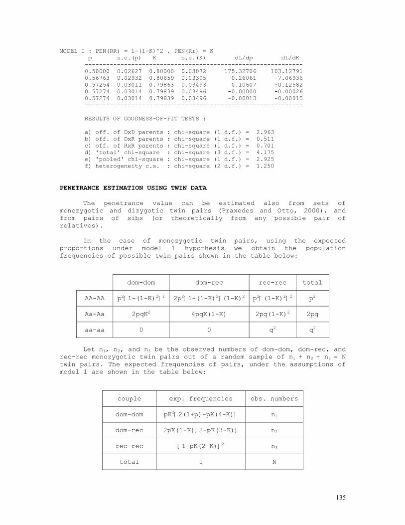
135
MODEL I : PEN(RR) = 1-(1-K)^2 , PEN(Rr) = K p s.e.(p) K s.e.(K) dL/dp dL/dK ------------------------------------------------------------- 0.50000 0.02627 0.80000 0.03072 175.32706 103.12791 0.56763 0.02932 0.80659 0.03395 -0.26061 -7.06936 0.57254 0.03011 0.79863 0.03493 0.10607 -0.12582 0.57274 0.03014 0.79839 0.03496 -0.00000 -0.00026 0.57274 0.03014 0.79839 0.03496 -0.00013 -0.00015 ------------------------------------------------------------- RESULTS OF GOODNESS-OF-FIT TESTS : a) off. of DxD parents : chi-square (1 d.f.) = 2.963 b) off. of DxR parents : chi-square (1 d.f.) = 0.511 c) off. of RxR parents : chi-square (1 d.f.) = 0.701 d) 'total' chi-square : chi-square (3 d.f.) = 4.175 e) 'pooled' chi-square : chi-square (1 d.f.) = 2.925 f) heterogeneity c.s. : chi-square (2 d.f.) = 1.250 PENETRANCE ESTIMATION USING TWIN DATA
The penetrance value can be estimated also from sets of monozygotic and dizygotic twin pairs (Praxedes and Otto, 2000), and from pairs of sibs (or theoretically from any possible pair of relatives).
In the case of monozygotic twin pairs, using the expected
proportions under model 1 hypothesis we obtain the population frequencies of possible twin pairs shown in the table below:
dom-dom dom-rec rec-rec total
AA-AA p2[1-(1-K)2]2 2p2[1-(1-K)2](1-K)2 p2[(1-K)2]2 p2
Aa-Aa 2pqK2 4pqK(1-K) 2pq(1-K)2 2pq
aa-aa 0 0 q2 q2
Let n1, n2, and n3 be the observed numbers of dom-dom, dom-rec, and
rec-rec monozygotic twin pairs out of a random sample of n1 + n2 + n3 = N twin pairs. The expected frequencies of pairs, under the assumptions of model 1 are shown in the table below:
couple exp. frequencies obs. numbers
dom-dom pK2[2(1+p)-pK(4-K)] n1
dom-rec 2pK(1-K)[2-pK(3-K)] n2
rec-rec [1-pK(2-K)]2 n3
total 1 N
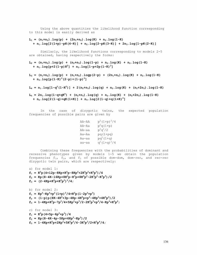
136
Using the above quantities the likelihood function corresponding to this model is easily derived as L1 = (n1+n2).log(p) + (2n1+n2).log(K) + n2.log(1-K) + n1.log[2(1+p)-pK(4-K)] + n2.log[2-pK(3-K)] + 2n3.log[1-pK(2-K)]
Similarly, the likelihood functions corresponding to models 2-5 are obtained, having respectively the forms: L2 = (n1+n2).log(p) + (n2+n3).log(1-p) + n2.log(K) + n2.log(1-K) + n1.log[p+2(1-p)K2] + n3.log[1-p+2p(1-K)2] L3 = (n1+n2).log(p) + (n1+n2).logp(2-p) + (2n1+n2).log(K) + n2.log(1-K) + n3.log[p(1-K)2(2-p)+(1-p)2] L4 = n1.log[1-q2(1-K2)] + 2(n2+n3).log(q) + n2.log(K) + (n2+2n3).log(1-K) L5 = 2n1.log(1-q+qK2) + (n2+n3).log(q) + n2.log(K) + (n2+2n3).log(1-K) + n2.log[2(1-q)+qK(1+K)] + n3.log[2(1-q)+q(1+K)2]
In the case of dizygotic twins, the expected population frequencies of possible pairs are given by
AA-AA p2(1+p)2/4 AA-Aa p2q(1+p) AA-aa p2q2/2 Aa-Aa pq(1+pq) Aa-aa pq2(1+q) aa-aa q2(1+q)2/4
Combining these frequencies with the probabilities of dominant and
recessive phenotypes given by models 1-5 we obtain the population frequencies f1, f2, and f3 of possible dom-dom, dom-rec, and rec-rec dizygotic twin pairs, which are respectively: a) for model 1: f1 = K2p(4+12p-8Kp+K2p-8Kp2+2K2p2+K2p3)/4 f2 = Kp(8-4K-16Kp+8K2p-K3p+8K2p2-2K3p2-K3p3)/2 f3 = (2-4Kp+K2p+K2p2)2/4; b) for model 2: f1 = Kp2-Kp4+p2(1+p)2/4+K2p(1-2p2+p3) f2 = (1-p)p(8K-4K2+3p-4Kp-4K2p+p2-4Kp2+4K2p2)/2 f3 = 1-4Kp+K2p-7p2/4+5Kp2+p3/2-2K2p3+p4/4-Kp4+K2p4;
c) for model 3: f1 = K2p(4+5p-6p2+p3)/4 f2 = Kp(8-4K-4p-5Kp+6Kp2-Kp3)/2 f3 = 1-4Kp+K2p+2Kp2+5K2p2/4-3K2p3/2+K2p4/4;
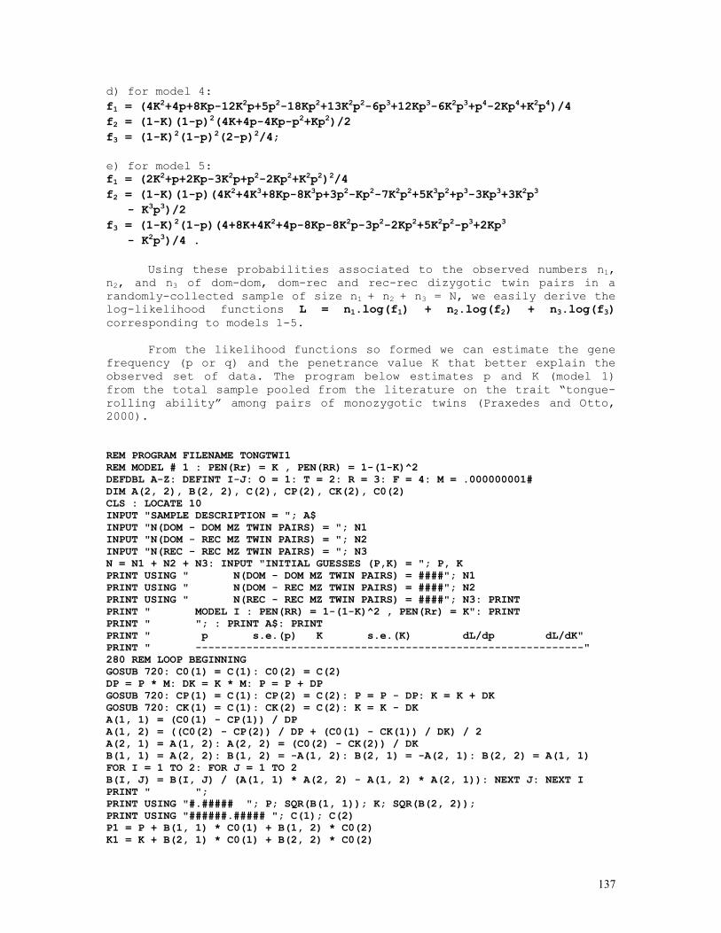
137
d) for model 4: f1 = (4K2+4p+8Kp-12K2p+5p2-18Kp2+13K2p2-6p3+12Kp3-6K2p3+p4-2Kp4+K2p4)/4 f2 = (1-K)(1-p)2(4K+4p-4Kp-p2+Kp2)/2 f3 = (1-K)2(1-p)2(2-p)2/4; e) for model 5: f1 = (2K2+p+2Kp-3K2p+p2-2Kp2+K2p2)2/4 f2 = (1-K)(1-p)(4K2+4K3+8Kp-8K3p+3p2-Kp2-7K2p2+5K3p2+p3-3Kp3+3K2p3
- K3p3)/2 f3 = (1-K)2(1-p)(4+8K+4K2+4p-8Kp-8K2p-3p2-2Kp2+5K2p2-p3+2Kp3 - K2p3)/4 .
Using these probabilities associated to the observed numbers n1, n2, and n3 of dom-dom, dom-rec and rec-rec dizygotic twin pairs in a randomly-collected sample of size n1 + n2 + n3 = N, we easily derive the log-likelihood functions L = n1.log(f1) + n2.log(f2) + n3.log(f3) corresponding to models 1-5.
From the likelihood functions so formed we can estimate the gene
frequency (p or q) and the penetrance value K that better explain the observed set of data. The program below estimates p and K (model 1) from the total sample pooled from the literature on the trait “tongue-rolling ability” among pairs of monozygotic twins (Praxedes and Otto, 2000). REM PROGRAM FILENAME TONGTWI1 REM MODEL # 1 : PEN(Rr) = K , PEN(RR) = 1-(1-K)^2 DEFDBL A-Z: DEFINT I-J: O = 1: T = 2: R = 3: F = 4: M = .000000001# DIM A(2, 2), B(2, 2), C(2), CP(2), CK(2), C0(2) CLS : LOCATE 10 INPUT "SAMPLE DESCRIPTION = "; A$ INPUT "N(DOM - DOM MZ TWIN PAIRS) = "; N1 INPUT "N(DOM - REC MZ TWIN PAIRS) = "; N2 INPUT "N(REC - REC MZ TWIN PAIRS) = "; N3 N = N1 + N2 + N3: INPUT "INITIAL GUESSES (P,K) = "; P, K PRINT USING " N(DOM - DOM MZ TWIN PAIRS) = ####"; N1 PRINT USING " N(DOM - REC MZ TWIN PAIRS) = ####"; N2 PRINT USING " N(REC - REC MZ TWIN PAIRS) = ####"; N3: PRINT PRINT " MODEL I : PEN(RR) = 1-(1-K)^2 , PEN(Rr) = K": PRINT PRINT " "; : PRINT A$: PRINT PRINT " p s.e.(p) K s.e.(K) dL/dp dL/dK" PRINT " -------------------------------------------------------------" 280 REM LOOP BEGINNING GOSUB 720: C0(1) = C(1): C0(2) = C(2) DP = P * M: DK = K * M: P = P + DP GOSUB 720: CP(1) = C(1): CP(2) = C(2): P = P - DP: K = K + DK GOSUB 720: CK(1) = C(1): CK(2) = C(2): K = K - DK A(1, 1) = (C0(1) - CP(1)) / DP A(1, 2) = ((C0(2) - CP(2)) / DP + (C0(1) - CK(1)) / DK) / 2 A(2, 1) = A(1, 2): A(2, 2) = (C0(2) - CK(2)) / DK B(1, 1) = A(2, 2): B(1, 2) = -A(1, 2): B(2, 1) = -A(2, 1): B(2, 2) = A(1, 1) FOR I = 1 TO 2: FOR J = 1 TO 2 B(I, J) = B(I, J) / (A(1, 1) * A(2, 2) - A(1, 2) * A(2, 1)): NEXT J: NEXT I PRINT " "; PRINT USING "#.##### "; P; SQR(B(1, 1)); K; SQR(B(2, 2)); PRINT USING "######.##### "; C(1); C(2) P1 = P + B(1, 1) * C0(1) + B(1, 2) * C0(2) K1 = K + B(2, 1) * C0(1) + B(2, 2) * C0(2)
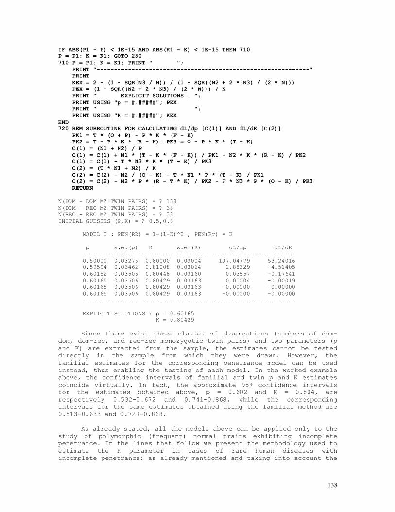
138
IF ABS(P1 - P) < 1E-15 AND ABS(K1 - K) < 1E-15 THEN 710 P = P1: K = K1: GOTO 280 710 P = P1: K = K1: PRINT " "; PRINT "-------------------------------------------------------------" PRINT KEX = 2 - (1 - SQR(N3 / N)) / (1 - SQR((N2 + 2 * N3) / (2 * N))) PEX = (1 - SQR((N2 + 2 * N3) / (2 * N))) / K PRINT " EXPLICIT SOLUTIONS : "; PRINT USING "p = #.#####"; PEX PRINT " "; PRINT USING "K = #.#####"; KEX END 720 REM SUBROUTINE FOR CALCULATING dL/dp [C(1)] AND dL/dK [C(2)] PK1 = T * (O + P) - P * K * (F - K) PK2 = T - P * K * (R - K): PK3 = O - P * K * (T - K) C(1) = (N1 + N2) / P C(1) = C(1) + N1 * (T - K * (F - K)) / PK1 - N2 * K * (R - K) / PK2 C(1) = C(1) - T * N3 * K * (T - K) / PK3 C(2) = (T * N1 + N2) / K C(2) = C(2) - N2 / (O - K) - T * N1 * P * (T - K) / PK1 C(2) = C(2) - N2 * P * (R - T * K) / PK2 - F * N3 * P * (O - K) / PK3 RETURN N(DOM - DOM MZ TWIN PAIRS) = ? 138 N(DOM - REC MZ TWIN PAIRS) = ? 38 N(REC - REC MZ TWIN PAIRS) = ? 38 INITIAL GUESSES (P,K) = ? 0.5,0.8 MODEL I : PEN(RR) = 1-(1-K)^2 , PEN(Rr) = K p s.e.(p) K s.e.(K) dL/dp dL/dK ------------------------------------------------------------- 0.50000 0.03275 0.80000 0.03004 107.04779 53.24016 0.59594 0.03462 0.81008 0.03064 2.88329 -4.51405 0.60152 0.03505 0.80448 0.03160 0.03857 -0.17641 0.60165 0.03506 0.80429 0.03163 0.00004 -0.00019 0.60165 0.03506 0.80429 0.03163 -0.00000 -0.00000 0.60165 0.03506 0.80429 0.03163 -0.00000 -0.00000 ------------------------------------------------------------- EXPLICIT SOLUTIONS : p = 0.60165 K = 0.80429
Since there exist three classes of observations (numbers of dom-dom, dom-rec, and rec-rec monozygotic twin pairs) and two parameters (p and K) are extracted from the sample, the estimates cannot be tested directly in the sample from which they were drawn. However, the familial estimates for the corresponding penetrance model can be used instead, thus enabling the testing of each model. In the worked example above, the confidence intervals of familial and twin p and K estimates coincide virtually. In fact, the approximate 95% confidence intervals for the estimates obtained above, p = 0.602 and K = 0.804, are respectively 0.532-0.672 and 0.741-0.868, while the corresponding intervals for the same estimates obtained using the familial method are 0.513-0.633 and 0.728-0.868.
As already stated, all the models above can be applied only to the
study of polymorphic (frequent) normal traits exhibiting incomplete penetrance. In the lines that follow we present the methodology used to estimate the K parameter in cases of rare human diseases with incomplete penetrance; as already mentioned and taking into account the
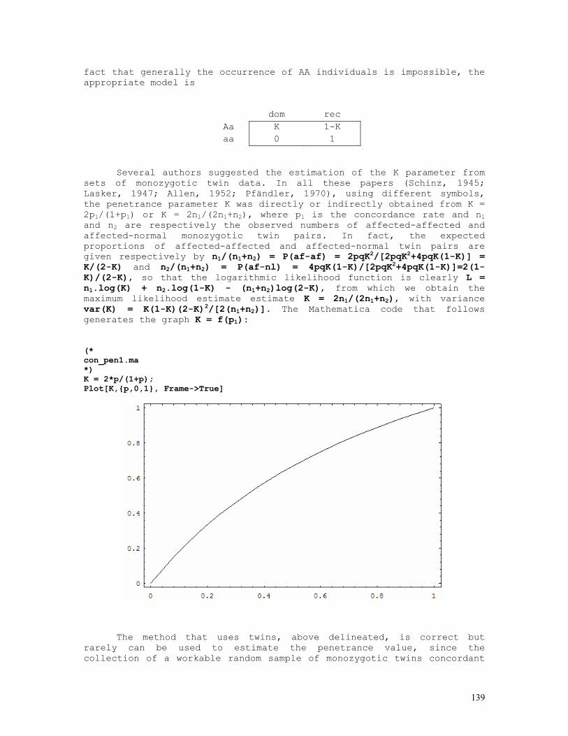
139
fact that generally the occurrence of AA individuals is impossible, the appropriate model is
dom rec Aa K 1-K aa 0 1
Several authors suggested the estimation of the K parameter from sets of monozygotic twin data. In all these papers (Schinz, 1945; Lasker, 1947; Allen, 1952; Pfändler, 1970), using different symbols, the penetrance parameter K was directly or indirectly obtained from K = 2p1/(1+p1) or K = 2n1/(2n1+n2), where p1 is the concordance rate and n1 and n2 are respectively the observed numbers of affected-affected and affected-normal monozygotic twin pairs. In fact, the expected proportions of affected-affected and affected-normal twin pairs are given respectively by n1/(n1+n2) = P(af-af) = 2pqK2/[2pqK2+4pqK(1-K)] = K/(2-K) and n2/(n1+n2) = P(af-nl) = 4pqK(1-K)/[2pqK2+4pqK(1-K)]=2(1-K)/(2-K), so that the logarithmic likelihood function is clearly L = n1.log(K) + n2.log(1-K) - (n1+n2)log(2-K), from which we obtain the maximum likelihood estimate estimate K = 2n1/(2n1+n2), with variance var(K) = K(1-K)(2-K)2/[2(n1+n2)]. The Mathematica code that follows generates the graph K = f(p1): (* con_pen1.ma *) K = 2*p/(1+p); Plot[K,{p,0,1}, Frame->True]
The method that uses twins, above delineated, is correct but rarely can be used to estimate the penetrance value, since the collection of a workable random sample of monozygotic twins concordant

140
and discordant as to rare autosomal dominant conditions is really troublesome and even impossible on practical grounds. For instance, bilateral retinoblastom is an autsomal dominant condition with incomplete penetrance and its population frequency among infants has been estimated in less than 1/10,000; taking into account that twin births occur in most populations with a frequency of about 1/100, one expects that the frequency of twins presenting the tumor would be of the order of 1/1,000,000 or l0-6.
The analysis of genealogies with familial cases of dominant
conditions, on the other hand, allows the calculation of reliable estimates of the penetrance value, as we show in the lines that follows.
PENETRANCE ESTIMATION FOR RARE DOMINANT CONDITIONS USING GENEALOGICAL INFORMATION
The methodology described below was developed by Rogatko et al. (1983, 1986) and detailed in several aspects by Horimoto (PhD thesis); other more sophisticated methods, including models that consider different penetrance rate values in the various generations (Horimoto et al., 2007; Horimoto, Pearson & Otto, manuscript in press) are not discussed here due to their complexity and because they interest only to professional specialists.
The first step of the method consists in filtering the genealogy information, that is, replacing the original genealogy by one containing only individuals informative or relevant as to the penetrance estimation.
The figure below represents the full genealogy of a family with
several individuals affected by a rare autosomal dominant condition:
The corresponding filtered genealogy is
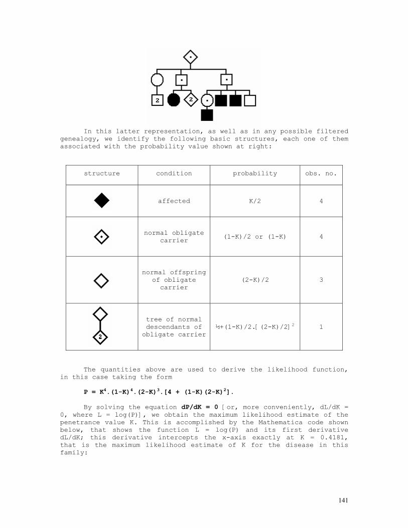
141
In this latter representation, as well as in any possible filtered genealogy, we identify the following basic structures, each one of them associated with the probability value shown at right:
structure condition probability obs. no.
affected K/2 4
normal obligate carrier (1-K)/2 or (1-K) 4
normal offspring of obligate carrier
(2-K)/2 3
tree of normal descendants of obligate carrier
½+(1-K)/2.[(2-K)/2]2 1
The quantities above are used to derive the likelihood function, in this case taking the form
P = K4.(1-K)4.(2-K)3.[4 + (1-K)(2-K)2]. By solving the equation dP/dK = 0 [or, more conveniently, dL/dK =
0, where L = log(P)], we obtain the maximum likelihood estimate of the penetrance value K. This is accomplished by the Mathematica code shown below, that shows the function L = log(P) and its first derivative dL/dK; this derivative intercepts the x-axis exactly at K = 0.4181, that is the maximum likelihood estimate of K for the disease in this family:
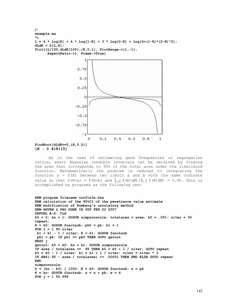
142
(* example.ma *) L = 4 * Log[K] + 4 * Log[1-K] + 3 * Log[2-K] + Log[4+(1-K)*(2-K)^2]; dLdK = D[L,K]; Plot[{L/100,dLdK/100},{K,0,1}, PlotRange->{1,-1}, AspectRatio->1, Frame->True]
FindRoot[dLdK==0,{K,0.5}] {K → 0.418115}
As in the case of estimating gene frequencies or segregation ratios, exact Bayesian credible intervals can be obtained by finding the area that corresponds to 95% of the total area under the likelihood function. Mathematically the problem is reduced to integrating the function y = f(K) between two limits a and b with the same ordinate value so that f(K=a) = f(K=b) and ∫a,b[f(K)dK]/∫0,1[f(K)dK] = 0.95. This is accomplished by programs as the following one: REM program filename confin3a.bas REM calculation of the 95%CI of the penetrance value estimate REM modification of Romberg's osculatory method REM ARVRH & PAO DGBE IB USP FEB 22 2007 DEFDBL A-Z: CLS k0 = 0: kn = 1: GOSUB simpsonsrule: totalarea = area: k0 = .001: niter = 50 repeat: K = k0: GOSUB functsub: pk0 = pk: k1 = 1 FOR j = 1 TO niter k1 = k1 - 1 / niter: K = k1: GOSUB functsub pk1 = pk: IF pk1 >= pk0 THEN GOTO getout NEXT j getout: k0 = k0: kn = k1: GOSUB simpsonsrule IF area / totalarea >= .95 THEN k0 = k0 + 1 / niter: GOTO repeat k0 = k0 - 1 / niter: k1 = k1 + 1 / niter: niter = niter * 5 IF ABS(.95 - area / totalarea) <= .00001 THEN END ELSE GOTO repeat END simpsonsrule: h = (kn - k0) / 1000: K = k0: GOSUB functsub: s = pk K = kn: GOSUB functsub: s = s + pk: w = 4 FOR j = 1 TO 999
143
K = k0 + j * h GOSUB functsub s = s + w * pk w = 6 - w NEXT j area = h * s / 3: s = 0 IF k0 <> 0 THEN 'LOCATE 10 PRINT USING "#.###### #.###### #.###### "; k0; kn; area / totalarea; K = k0: GOSUB functsub: pk0 = pk K = kn: GOSUB functsub: pk1 = pk PRINT USING "####.###### "; pk0; pk1 END IF RETURN functsub: pk = K ^ 4 * (1 - K) ^ 4 * (2 - K) ^ 3 * (4 + (1 - K) * (2 - K) ^ 2) RETURN
The upper and lower limits of the exact 95% confidence interval for the estimate K = 0.418115, obtained by running the above program, are respectively 0.162786 and 0.724774 (see also the graph generated by the Mathematica code below). (*confint2.ma*) a=0.16279; b=0.72477; c=0.41811; fa= a^4*(1-a)^4*(2-a)^3*(4+(1 - a)*(2 - a)^2); fb= b^4*(1-b)^4*(2-b)^3*(4+(1 - b)*(2 - b)^2); fc= c^4*(1-c)^4*(2-c)^3*(4+(1 - c)*(2 - c)^2); Show[ Plot[K^4*(1-K)^4*(2-K)^3*(4+(1 - K)*(2 - K)^2), {K,0,1}, Frame->True, DisplayFunction -> Identity], Graphics[{ Line[{{a,0},{a,fa}}], Line[{{c,0},{c,fc}}], Line[{{b,0},{b,fb}}], }], DisplayFunction -> $DisplayFunction, AspectRatio -> 1/2];
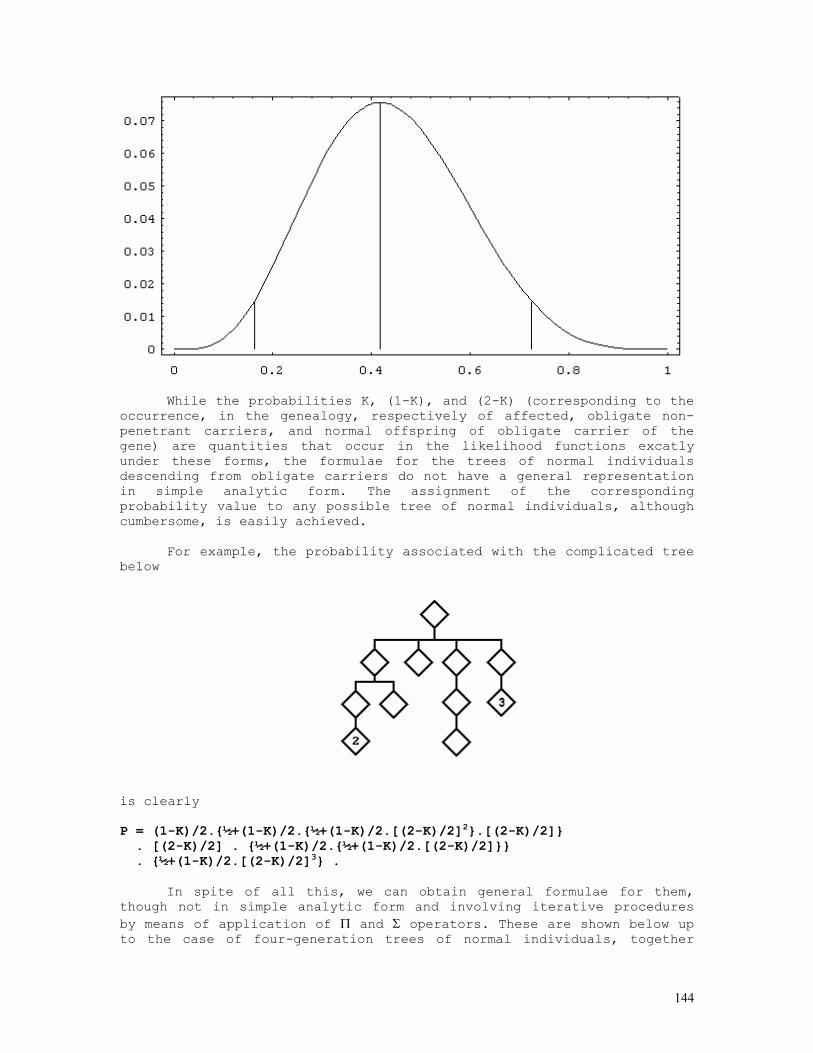
144
While the probabilities K, (1-K), and (2-K) (corresponding to the
occurrence, in the genealogy, respectively of affected, obligate non-penetrant carriers, and normal offspring of obligate carrier of the gene) are quantities that occur in the likelihood functions excatly under these forms, the formulae for the trees of normal individuals descending from obligate carriers do not have a general representation in simple analytic form. The assignment of the corresponding probability value to any possible tree of normal individuals, although cumbersome, is easily achieved.
For example, the probability associated with the complicated tree
below
is clearly P = (1-K)/2.{½+(1-K)/2.{½+(1-K)/2.[(2-K)/2]2}.[(2-K)/2]} . [(2-K)/2] . {½+(1-K)/2.{½+(1-K)/2.[(2-K)/2]}} . {½+(1-K)/2.[(2-K)/2]3} .
In spite of all this, we can obtain general formulae for them,
though not in simple analytic form and involving iterative procedures by means of application of Π and Σ operators. These are shown below up to the case of four-generation trees of normal individuals, together
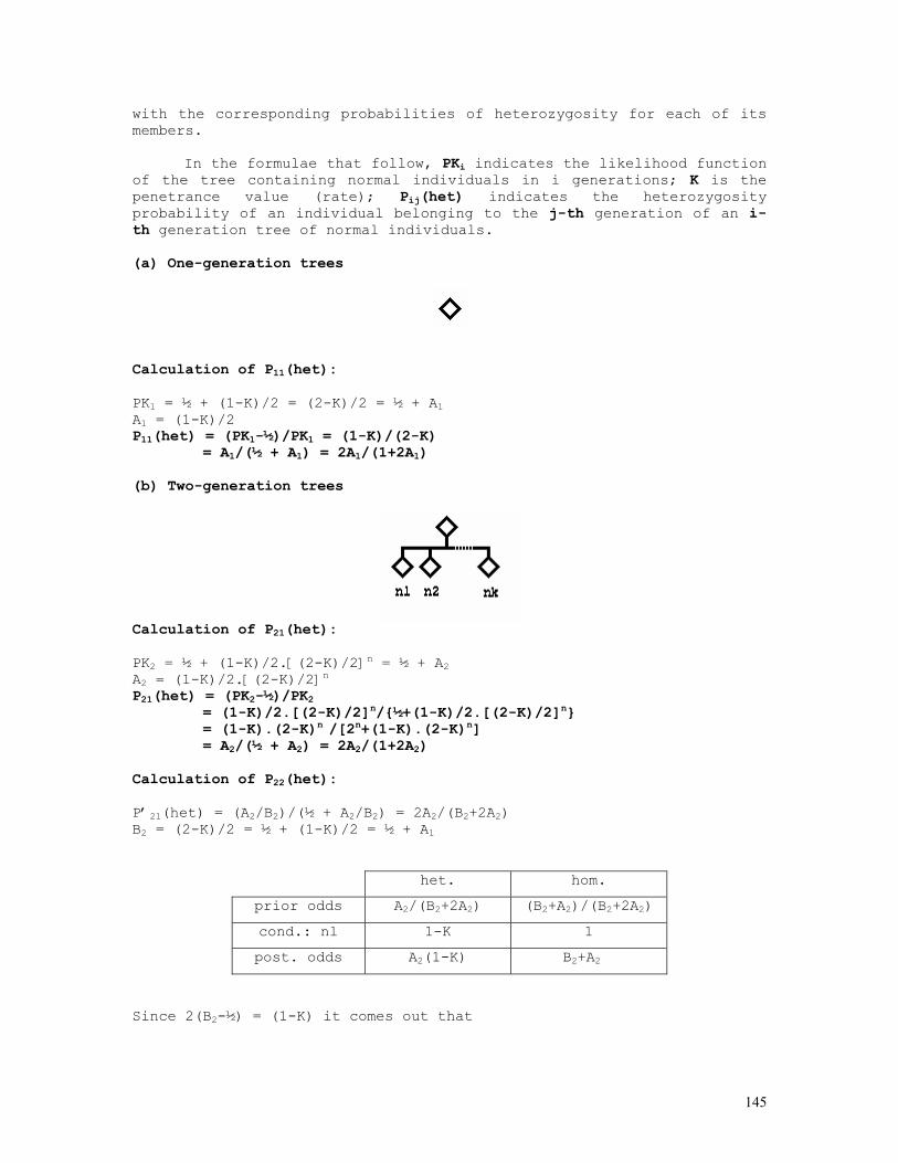
145
with the corresponding probabilities of heterozygosity for each of its members.
In the formulae that follow, PKi indicates the likelihood function of the tree containing normal individuals in i generations; K is the penetrance value (rate); Pij(het) indicates the heterozygosity probability of an individual belonging to the j-th generation of an i-th generation tree of normal individuals. (a) One-generation trees
Calculation of P11(het): PK1 = ½ + (1-K)/2 = (2-K)/2 = ½ + A1 A1 = (1-K)/2 P11(het) = (PK1-½)/PK1 = (1-K)/(2-K) = A1/(½ + A1) = 2A1/(1+2A1) (b) Two-generation trees
Calculation of P21(het): PK2 = ½ + (1-K)/2.[(2-K)/2]n = ½ + A2 A2 = (1-K)/2.[(2-K)/2]n P21(het) = (PK2-½)/PK2 = (1-K)/2.[(2-K)/2]n/{½+(1-K)/2.[(2-K)/2]n} = (1-K).(2-K)n /[2n+(1-K).(2-K)n] = A2/(½ + A2) = 2A2/(1+2A2) Calculation of P22(het): P’21(het) = (A2/B2)/(½ + A2/B2) = 2A2/(B2+2A2) B2 = (2-K)/2 = ½ + (1-K)/2 = ½ + A1
het. hom.
prior odds A2/(B2+2A2) (B2+A2)/(B2+2A2)
cond.: nl 1-K 1
post. odds A2(1-K) B2+A2
Since 2(B2-½) = (1-K) it comes out that
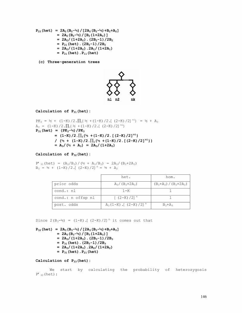
146
P22(het) = 2A2(B2-½)/[2A2(B2-½)+B2+A2] = 2A2(B2-½)/[B2(1+2A2)] = 2A2/(1+2A2).(2B2-1)/2B2 = P21(het).(2B2-1)/2B2 = 2A2/(1+2A2).2A1/(1+2A1) = P21(het).P11(het) (c) Three-generation trees
Calculation of P31(het): PK3 = ½ + (1-K)/2.∏i{½ +(1-K)/2.[(2-K)/2]ni} = ½ + A3 A3 = (1-K)/2.∏i{½ +(1-K)/2.[(2-K)/2]ni} P31(het) = (PK3-½)/PK3 = (1-K)/2.∏i{½ +(1-K)/2.[(2-K)/2]ni} / {½ + (1-K)/2.∏i{½ +(1-K)/2.[(2-K)/2]ni}} = A3/(½ + A3) = 2A3/(1+2A3) Calculation of P32(het): P’31(het) = (A3/B3)/(½ + A3/B3) = 2A3/(B3+2A3) B3 = ½ + (1-K)/2.[(2-K)/2]n = ½ + A2
het. hom.
prior odds A3/(B3+2A3) (B3+A3)/(B3+2A3)
cond.: nl 1-K 1
cond.: n offsp nl [(2-K)/2]n 1
post. odds A3(1-K).[(2-K)/2]n B3+A3
Since 2(B3-½) = (1-K).[(2-K)/2]n it comes out that P32(het) = 2A3(B3-½)/[2A3(B3-½)+B3+A3] = 2A3(B3-½)/[B3(1+2A3)] = 2A3/(1+2A3).(2B3-1)/2B3 = P31(het).(2B3-1)/2B3 = 2A3/(1+2A3).2A2/(1+2A2) = P31(het).P21(het) Calculation of P33(het):
We start by calculating the probability of heterozygosis P’32(het):
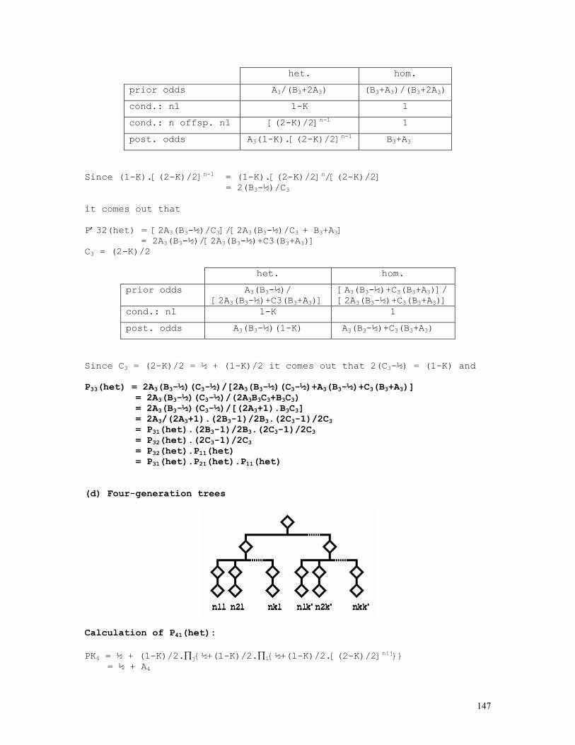
147
het. hom.
prior odds A3/(B3+2A3) (B3+A3)/(B3+2A3)
cond.: nl 1-K 1
cond.: n offsp. nl [(2-K)/2]n-1 1
post. odds A3(1-K).[(2-K)/2]n-1 B3+A3
Since (1-K).[(2-K)/2]n-1 = (1-K).[(2-K)/2]n/[(2-K)/2] = 2(B3-½)/C3 it comes out that P’32(het) = [2A3(B3-½)/C3]/[2A3(B3-½)/C3 + B3+A3] = 2A3(B3-½)/[2A3(B3-½)+C3(B3+A3)] C3 = (2-K)/2
het. hom.
prior odds A3(B3-½)/ [2A3(B3-½)+C3(B3+A3)]
[A3(B3-½)+C3(B3+A3)]/ [2A3(B3-½)+C3(B3+A3)]
cond.: nl 1-K 1
post. odds A3(B3-½)(1-K) A3(B3-½)+C3(B3+A3)
Since C3 = (2-K)/2 = ½ + (1-K)/2 it comes out that 2(C3-½) = (1-K) and P33(het) = 2A3(B3-½)(C3-½)/[2A3(B3-½)(C3-½)+A3(B3-½)+C3(B3+A3)] = 2A3(B3-½)(C3-½)/(2A3B3C3+B3C3) = 2A3(B3-½)(C3-½)/[(2A3+1).B3C3] = 2A3/(2A3+1).(2B3-1)/2B3.(2C3-1)/2C3 = P31(het).(2B3-1)/2B3.(2C3-1)/2C3 = P32(het).(2C3-1)/2C3 = P32(het).P11(het) = P31(het).P21(het).P11(het) (d) Four-generation trees
Calculation of P41(het): PK4 = ½ + (1-K)/2.∏j{½+(1-K)/2.∏i{½+(1-K)/2.[(2-K)/2]nij}} = ½ + A4
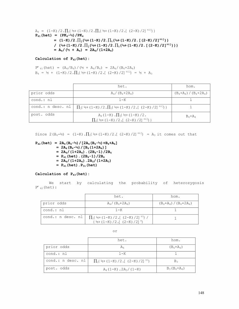
148
A4 = (1-K)/2.∏j{½+(1-K)/2.∏i{½+(1-K)/2.[(2-K)/2]nij}} P41(het) = (PK4-½)/PK4 = (1-K)/2.∏j{½+(1-K)/2.∏i{½+(1-K)/2.[(2-K)/2]nij}} / {½+(1-K)/2.∏j{½+(1-K)/2.∏i{½+(1-K)/2.[(2-K)/2]nij}}} = A4/(½ + A4) = 2A4/(1+2A4) Calculation of P42(het): P’41(het) = (A4/B4)/(½ + A4/B4) = 2A4/(B4+2A4) B4 = ½ + (1-K)/2.∏i{½+(1-K)/2.[(2-K)/2]nij} = ½ + A3
het. hom.
prior odds A4/(B4+2A4) (B4+A4)/(B4+2A4)
cond.: nl 1-K 1
cond.: n desc. nl ∏j{½+(1-K)/2.∏i{½+(1-K)/2.[(2-K)/2]nij}} 1
post. odds A4(1-K).∏j{½+(1-K)/2. ∏i{½+(1-K)/2.[(2-K)/2]nij}}
B4+A4
Since 2(B4-½) = (1-K).∏i{½+(1-K)/2.[(2-K)/2]nij} = A3 it comes out that P42(het) = 2A4(B4-½)/[2A4(B4-½)+B4+A4] = 2A4(B4-½)/[B4(1+2A4)] = 2A4/(1+2A4).(2B4-1)/2B4 = P41(het).(2B4-1)/2B4 = 2A4/(1+2A4).2A3/(1+2A3) = P41(het).P31(het) Calculation of P43(het):
We start by calculating the probability of heterozygosis P’42(het):
het. hom.
prior odds A4/(B4+2A4) (B4+A4)/(B4+2A4)
cond.: nl 1-K 1
cond.: n desc. nl ∏i{½+(1-K)/2.[(2-K)/2]ni}/ {½+(1-K)/2.[(2-K)/2]n}
1
or
het. hom.
prior odds A4 (B4+A4)
cond.: nl 1-K 1
cond.: n desc. nl ∏i{½+(1-K)/2.[(2-K)/2]ni} B3
post. odds A4(1-K).2A3/(1-K) B3(B4+A4)
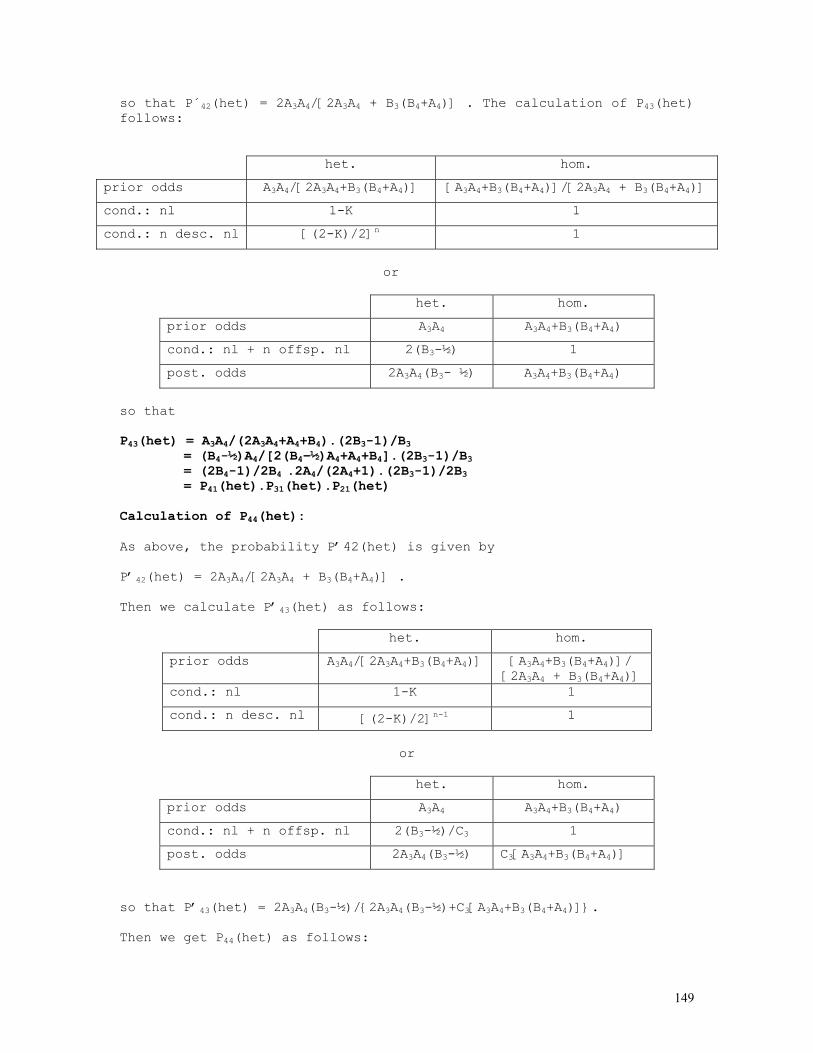
149
so that P´42(het) = 2A3A4/[2A3A4 + B3(B4+A4)] . The calculation of P43(het) follows:
het. hom.
prior odds A3A4/[2A3A4+B3(B4+A4)] [A3A4+B3(B4+A4)]/[2A3A4 + B3(B4+A4)]
cond.: nl 1-K 1
cond.: n desc. nl [(2-K)/2]n 1
or
het. hom.
prior odds A3A4 A3A4+B3(B4+A4)
cond.: nl + n offsp. nl 2(B3-½) 1
post. odds 2A3A4(B3- ½) A3A4+B3(B4+A4)
so that P43(het) = A3A4/(2A3A4+A4+B4).(2B3-1)/B3 = (B4-½)A4/[2(B4–½)A4+A4+B4].(2B3-1)/B3 = (2B4-1)/2B4 .2A4/(2A4+1).(2B3-1)/2B3 = P41(het).P31(het).P21(het)
Calculation of P44(het): As above, the probability P’42(het) is given by P’42(het) = 2A3A4/[2A3A4 + B3(B4+A4)] . Then we calculate P’43(het) as follows:
het. hom.
prior odds A3A4/[2A3A4+B3(B4+A4)] [A3A4+B3(B4+A4)]/ [2A3A4 + B3(B4+A4)]
cond.: nl 1-K 1
cond.: n desc. nl [(2-K)/2]n-1 1
or
het. hom.
prior odds A3A4 A3A4+B3(B4+A4)
cond.: nl + n offsp. nl 2(B3-½)/C3 1
post. odds 2A3A4(B3-½) C3[A3A4+B3(B4+A4)]
so that P’43(het) = 2A3A4(B3-½)/{2A3A4(B3-½)+C3[A3A4+B3(B4+A4)]}. Then we get P44(het) as follows:
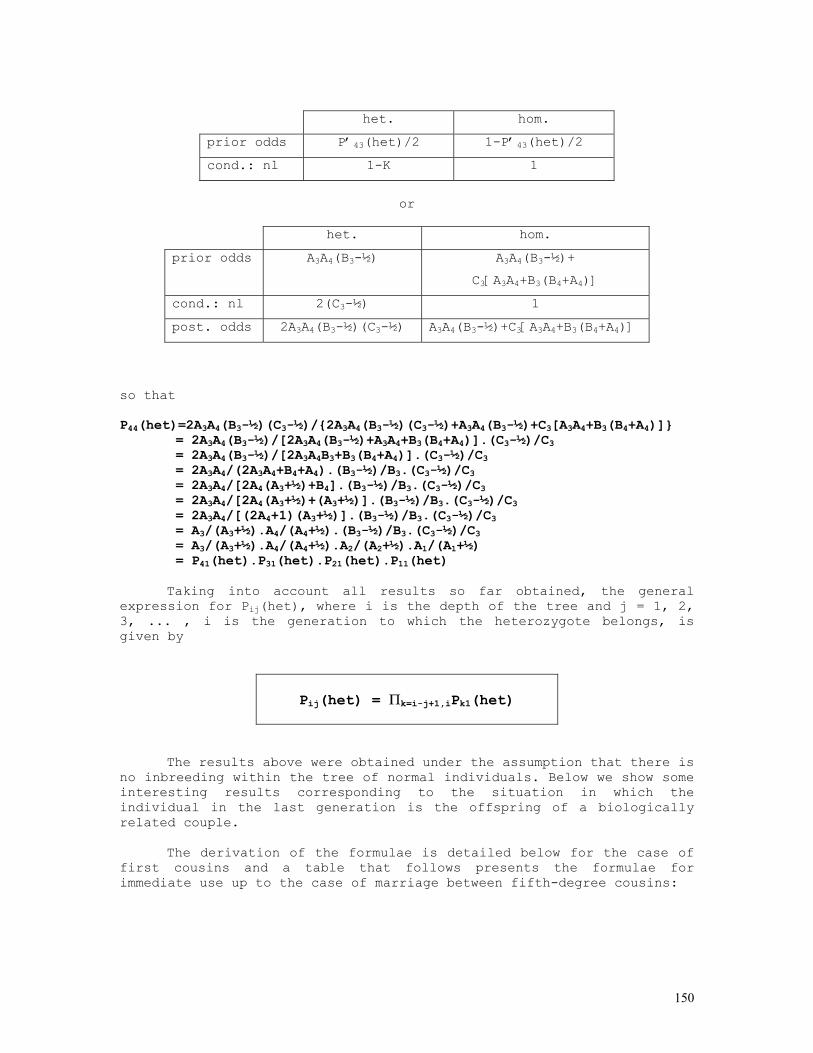
150
het. hom.
prior odds P’43(het)/2 1-P’43(het)/2
cond.: nl 1-K 1
or
het. hom.
prior odds A3A4(B3-½) A3A4(B3-½)+
C3[A3A4+B3(B4+A4)]
cond.: nl 2(C3-½) 1
post. odds 2A3A4(B3-½)(C3-½) A3A4(B3-½)+C3[A3A4+B3(B4+A4)]
so that P44(het)=2A3A4(B3-½)(C3-½)/{2A3A4(B3-½)(C3-½)+A3A4(B3-½)+C3[A3A4+B3(B4+A4)]} = 2A3A4(B3-½)/[2A3A4(B3-½)+A3A4+B3(B4+A4)].(C3-½)/C3 = 2A3A4(B3-½)/[2A3A4B3+B3(B4+A4)].(C3-½)/C3 = 2A3A4/(2A3A4+B4+A4).(B3-½)/B3.(C3-½)/C3 = 2A3A4/[2A4(A3+½)+B4].(B3-½)/B3.(C3-½)/C3 = 2A3A4/[2A4(A3+½)+(A3+½)].(B3-½)/B3.(C3-½)/C3 = 2A3A4/[(2A4+1)(A3+½)].(B3-½)/B3.(C3-½)/C3 = A3/(A3+½).A4/(A4+½).(B3-½)/B3.(C3-½)/C3 = A3/(A3+½).A4/(A4+½).A2/(A2+½).A1/(A1+½) = P41(het).P31(het).P21(het).P11(het)
Taking into account all results so far obtained, the general expression for Pij(het), where i is the depth of the tree and j = 1, 2, 3, ... , i is the generation to which the heterozygote belongs, is given by
Pij(het) = Πk=i-j+1,iPk1(het)
The results above were obtained under the assumption that there is
no inbreeding within the tree of normal individuals. Below we show some interesting results corresponding to the situation in which the individual in the last generation is the offspring of a biologically related couple.
The derivation of the formulae is detailed below for the case of
first cousins and a table that follows presents the formulae for immediate use up to the case of marriage between fifth-degree cousins:

151
P(1) = (1/2)2 P(2) = 2(1-K)/2.(1/2)2 P(3) = [(1-K)/2]2.(1/2)2 P(4) = 2[(1-K)/2]2.(1/2)2 P(5) = 2[(1-K)/2]3.(1/2)2 P(6) = [(1-K)/2]4.1/3 P(7) = 2[(1-K)/2]3.1/2 P(8) = 2[(1-K)/2]4.1/2 P(9)= [(1-K)/2]4.2(1-K)/3 ΣP(i) = P(1) + ... + P(9) = 1/4 + (1-K)(5-K)/16 + (1-K)2.(2-K)(3-K)/16 + (1-K)4.(3-2K)/48 = (48-83K+80K2-45K3+14K4-2K5)/48 = P3K P(III-1 = nl aa) = [P(1)+P(2)+P(3)+P(4)+P(5)+P(6)]/ΣP(i) = {[12+12(1-K)+9(1-K)^2+3(1-K)^3 + (1-K)4]/48}/P3K = (37-43K+24K2-7K3+K4) / (48-83K+80K2-45K3+14K4-2K5) P(III-1 = nl Aa) = [P(7)+P(8)+P(9)]/ΣP(i) = {[6(1-K)3+3(1-K)4+2(1-K)5]/48}/P3K = (11-40K+56K2-38K3+13K4-2K5) / (48-83K+80K2-45K3+14K4-2K5)
The tables below show the likelihood functions (C = A + B) and probabilities of non-penetrant heterozygosis P(het,nl) = A/C and normal homozygosis P(hom,nl) = B/C for the offspring of consanguineous unions 1-11 (1 – brother-sister incest; 2 – uncle-niece union; 3 to 11 – first- to fifth-degree cousins (odd numbers: first-, second-, third-, fourth- and fifth-degree cousins; even numbers : first-, second-, third-, and fourth-degree cousins once removed):
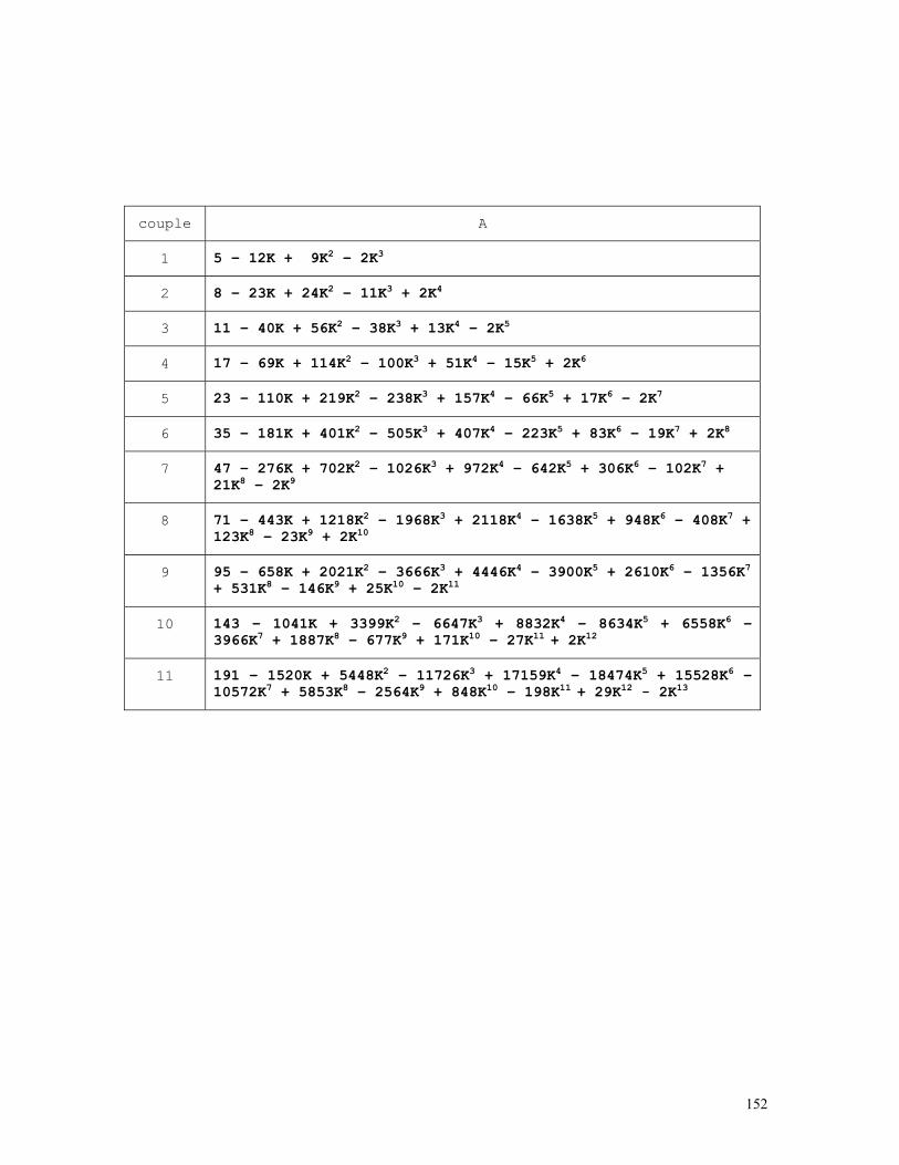
152
couple A
1 5 – 12K + 9K2 – 2K3
2 8 – 23K + 24K2 – 11K3 + 2K4
3 11 – 40K + 56K2 – 38K3 + 13K4 – 2K5
4 17 – 69K + 114K2 – 100K3 + 51K4 – 15K5 + 2K6
5 23 – 110K + 219K2 – 238K3 + 157K4 – 66K5 + 17K6 – 2K7
6 35 – 181K + 401K2 – 505K3 + 407K4 – 223K5 + 83K6 – 19K7 + 2K8
7 47 – 276K + 702K2 – 1026K3 + 972K4 – 642K5 + 306K6 – 102K7 + 21K8 – 2K9
8 71 – 443K + 1218K2 – 1968K3 + 2118K4 – 1638K5 + 948K6 – 408K7 + 123K8 – 23K9 + 2K10
9 95 – 658K + 2021K2 – 3666K3 + 4446K4 – 3900K5 + 2610K6 – 1356K7 + 531K8 – 146K9 + 25K10 – 2K11
10 143 – 1041K + 3399K2 – 6647K3 + 8832K4 – 8634K5 + 6558K6 –3966K7 + 1887K8 – 677K9 + 171K10 – 27K11 + 2K12
11 191 – 1520K + 5448K2 – 11726K3 + 17159K4 – 18474K5 + 15528K6 –10572K7 + 5853K8 – 2564K9 + 848K10 – 198K11 + 29K12 - 2K13
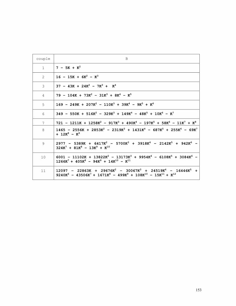
153
couple B
1 7 – 5K + K2
2 16 – 15K + 6K2 – K3
3 37 – 43K + 24K2 – 7K3 + K4
4 79 – 104K + 73K2 – 31K3 + 8K4 – K5
5 169 – 249K + 207K2 – 110K3 + 39K4 – 9K5 + K6
6 349 – 550K + 516K2 – 329K3 + 149K4 – 48K5 + 10K6 – K7
7 721 – 1211K + 1258K2 – 917K3 + 490K4 – 197K5 + 58K6 – 11K7 + K8
8 1465 – 2556K + 2853K2 – 2319K3 + 1431K4 – 687K5 + 255K6 – 69K7
+ 12K8 – K9
9 2977 – 5389K + 6417K2 – 5700K3 + 3918K4 – 2142K5 + 942K6 –324K7 + 81K8 – 13K9 + K10
10 6001 – 11102K + 13822K2 – 13173K3 + 9954K4 – 6108K5 + 3084K6 –1266K7 + 405K8 – 94K9 + 14K10 – K11
11 12097 – 22863K + 29676K2 – 30067K3 + 24519K4 – 16446K5 + 9240K6 – 43506K7 + 1671K8 – 499K9 + 108K10 – 15K11 + K12
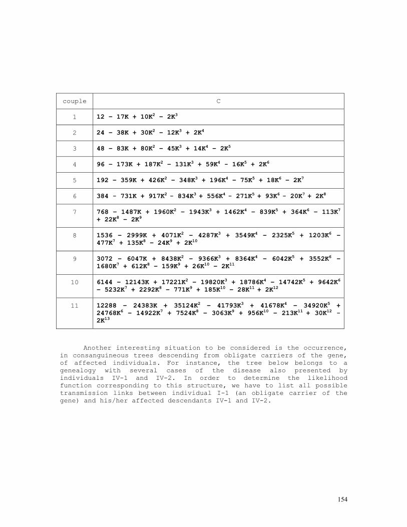
154
couple C
1 12 – 17K + 10K2 – 2K3
2 24 – 38K + 30K2 – 12K3 + 2K4
3 48 – 83K + 80K2 – 45K3 + 14K4 – 2K5
4 96 – 173K + 187K2 – 131K3 + 59K4 - 16K5 + 2K6
5 192 – 359K + 426K2 – 348K3 + 196K4 – 75K5 + 18K6 – 2K7
6 384 - 731K + 917K2 - 834K3 + 556K4 - 271K5 + 93K6 - 20K7 + 2K8
7 768 – 1487K + 1960K2 – 1943K3 + 1462K4 – 839K5 + 364K6 – 113K7
+ 22K8 – 2K9
8 1536 – 2999K + 4071K2 – 4287K3 + 3549K4 – 2325K5 + 1203K6 –477K7 + 135K8 – 24K9 + 2K10
9 3072 – 6047K + 8438K2 – 9366K3 + 8364K4 – 6042K5 + 3552K6 –1680K7 + 612K8 – 159K9 + 26K10 – 2K11
10 6144 – 12143K + 17221K2 – 19820K3 + 18786K4 – 14742K5 + 9642K6
– 5232K7 + 2292K8 – 771K9 + 185K10 – 28K11 + 2K12
11 12288 – 24383K + 35124K2 – 41793K3 + 41678K4 – 34920K5 + 24768K6 – 14922K7 + 7524K8 – 3063K9 + 956K10 – 213K11 + 30K12 -2K13
Another interesting situation to be considered is the occurrence, in consanguineous trees descending from obligate carriers of the gene, of affected individuals. For instance, the tree below belongs to a genealogy with several cases of the disease also presented by individuals IV-1 and IV-2. In order to determine the likelihood function corresponding to this structure, we have to list all possible transmission links between individual I-1 (an obligate carrier of the gene) and his/her affected descendants IV-1 and IV-2.
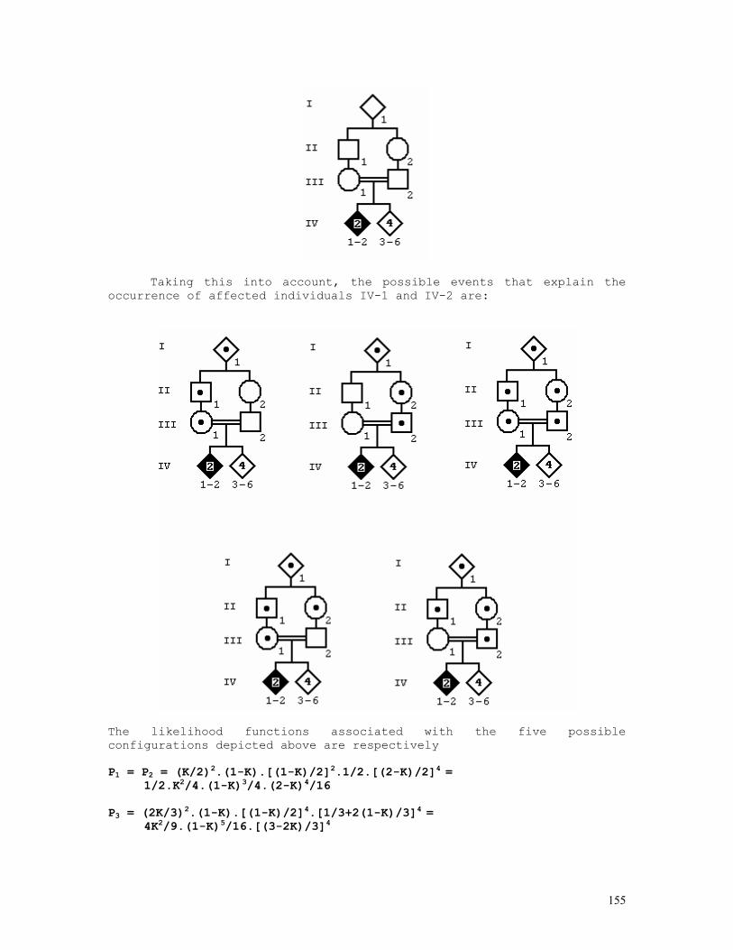
155
Taking this into account, the possible events that explain the occurrence of affected individuals IV-1 and IV-2 are:
The likelihood functions associated with the five possible configurations depicted above are respectively P1 = P2 = (K/2)2.(1-K).[(1-K)/2]2.1/2.[(2-K)/2]4 = 1/2.K2/4.(1-K)3/4.(2-K)4/16 P3 = (2K/3)2.(1-K).[(1-K)/2]4.[1/3+2(1-K)/3]4 = 4K2/9.(1-K)5/16.[(3-2K)/3]4
156
P4 = P5 = (K/2)2.(1-K).[(1-K)/2]3.1/2.[(2-K)/2]4 = 1/2.K2/4.(1-K)4/8.(2-K)4/16 The likelihood function for this particular consanguineous tree is therefore PK = P1 + P2 + P3 + P4 + P5 PK = 2.1/2.K2/4.(1-K)3/4.(2-K)4/16 + 4K2/9.(1-K)5/16.[(3-2K)/3]4 + 2.1/2.K2/4.(1-K)4/8.(2-K)4/16, or, ignoring constant quantities, PK = K2.(1-K)3.[1458.(2-K)4+128.(1-K)2.(3-2K)4+729.(1-K).(2-K)4], with a corresponding maximum likelihood estimate of K = 0.276. REFERENCES ALLEN G. The meaning of concordance and discordance in estimation of penetrance and gene frequency. Am. J. Hum. Genet. 4: 155-172, 1952. HORIMOTO ARVR, LEZIROVITZ K, PEARSON PL, OTTO PA. Maximum likelihood estimates of penetrance: a pilot study using the ectrodactyly-hemimelia
syndrome. 53o Congresso Nacional de Genética (Águas de Lindóia, SP).
CDROM de Resumos do 53o Congresso Nacional de Genética, 2007 (gh42.pdf, p. 42). LASKER GW. Penetrance estimated by frequency of unilateral occurences and by discordance in monozygotic twins. Hum. Biol. 19: 217-230, 1947. OTTO PA, FROTA-PESSOA O, POLCAN SP. Snyder’s ratios with incomplete penetrance. J. Hered. 85: 331-335, 1994. PFÄNDLER U. La signification statistique de la concordance chez les jumeaux MZ et DZ. Acta Genet. Med. Gemellol 19: 160-164, 1970. PRAXEDES LA, OTTO PA. Estimation of penetrance from twin data. Twin Research 3: 294-298, 2000. ROGATKO A, PEREIRA CAB, FROTA-PESSOA O. A Bayesian method for the estimation of penetrance: application to mandibulofacial and frontonasal dysostoses. Am. J. Med. Genet. 24: 231-246, 1986. ROGATKO A. Solução bayesiana para dois problemas clássicos em genética: penetrância e equilíbrio de Hardy-Weinberg. 1983. 113f. Tese (Doutorado), Instituto de Biociências, Universidade de São Paulo, São Paulo, 1983. SCHINZ HR. Konkordanz, Diskordanz und Penetranz bei eineiigen Zwillingen (Versuch einer elementaren Darstellung). Arch. Julius-Klaus Stift. 20: 2-25, 1945.
157
TWIN METHODS 1) PROPORTIONS OF MZ AND DZ TWINS IN A RANDOM SAMPLE OF TWIN PAIRS No(mm) = observed number of male twin pairs No(mf) = observed number of unlike-sexed twin pairs No(ff) = observed number of female twin pairs N = total number of twin pairs m = frequency of males in the sample = [2.No(mm)+No(mf)]/{2[No(mm)+No(mf)+No(ff)]} = [2.No(mm)+No(mf)]/2N f = frequency of females in the sample = [No(mf)+2.No(ff)]/{2[No(mm)+No(mf)+No(ff)]} = [No(mf)+2.No(ff)]/2N = 1-m x = P(MZ), y = 1-x = P(DZ) Ne(mm) = N(xm + ym2) = N[xm + (1-x)m2] Ne(mf) = 2Nmfy = 2Nm(1-m)(1-x) Ne(ff) = N[xf + yf2] = N[x(1-m) + (1-x)(1-m)2] Ne(mf) = No(mf) → 1-x = No(mf)/[2Nm(1-m)] If m = f = 1/2 → 1-x = 2No(mf)/N, that is, the proportion of DZ twins in the sample is twice the frequency of unlike-sexed twins. Maximum likelihood method: P = [xm + (1-x)m2]n1.[2m(1-m)(1-x)]n2.[(x(1-m) + (1-x)(1-m)2]n3 L = n1.log[xm+(1-x)m2]+n2.log[2m(1-m)(1-x)]+n3.log[(x(1-m)+(1-x)(1-m)2] ∂L/∂m = n1[x + 2m(1-x)]/[xm + (1-x)m2] + n2[1/m - 1/(1-m)] - n3[x + 2(1-x)(1-m)]/[(x(1-m) + (1-x)(1-m)2] ∂L/∂x = n1m(1-m)/[xm + (1-x)m2] - n2/(1-x) + n3m(1-m)/[(x(1-m) + (1-x)(1-m)2] {∂L/∂m = 0 , ∂L/∂x = 0} → {m, x} REM PROGRAM FILENAME TWINME01.BAS DEFDBL A-Z: CLS : LOCATE 10: INPUT "IDENTIFICATION LABEL = "; LABEL$ INPUT "N(mm) = "; n1: INPUT "N(mf) = "; n2: INPUT "N(ff) = "; n3 n = n1 + n2 + n3: REM direct estimates male = (2 * n1 + n2) / (2 * n): vmal = male * (1 - male) / (2 * n) xmon = 1 - n2 / (2 * n * male * (1 - male)): PRINT LABEL$ PRINT USING "N(mm) = ######"; n1: PRINT USING "N(mf) = ###### "; n2 PRINT USING "N(ff) = ######"; n3: PRINT USING "N = ######"; n PRINT "DIRECT ESTIMATES": PRINT USING "m = #.####"; male
158
PRINT USING "v(m) = #.########"; vmal: PRINT USING "x = #.####"; xmon PRINT "MAXIMUM LIKELIHOOD ESTIMATES" PRINT "-------------------------------------------------------------------------" PRINT " m x dL/dm dL/dx var(m) var(x)" PRINT "-------------------------------------------------------------------------" m = 1 / 2: x = 1 / 3 LARGELOOP: d1 = .00001: d2 = .00002 m0 = m: x0 = x: m1 = m + m * d1: x1 = x + x * d1: m2 = m + m * d2 x2 = x + x * d2: m = m0: x = x0: GOSUB 670: L1 = F' L1 = L(m,x) m = m1: GOSUB 670: L2 = F' L2 = L(m+dm,x) m = m0: x = x1: GOSUB 670: L3 = F' L3 = L(m,x+dx) x = x0: m = m2: GOSUB 670: L4 = F' L4 = L(m+2dm,x) m = m0: x = x2: GOSUB 670: L5 = F' L5 = L(m,x+2dx) m = m1: x = x1: GOSUB 670: L6 = F' L6 = L(m+dm,x+dx) x = x0: m = m0: I = (L2 - L1) / (m * d1)' I = dL/dm J = (L3 - L1) / (x * d1)' J = dL/dx K = ((L4 - L2) / (m * d1) - I) / (m * d1)' K = dL2/dm2 L = ((L5 - L3) / (x * d1) - J) / (x * d1)' L = dL2/dx2 R = ((L6 - L3) / (m * d1) - I) / (x * d1)' R = dL2/dmdx R = R + ((L6 - L2) / (x * d1) - J) / (m * d1)' O = det R = R / 2: O = K * L - R * R' S = var(m) S = -L / O: T = -K / O' T = var(x) U = R / O' U = cov(m,x) ' printout routine PRINT USING "#.######## "; m; x; : PRINT USING "#####.######## "; I; J; PRINT USING "#.######## "; S; T ' generalized Newton-Raphson method m3 = m + S * I + U * J: x3 = x + U * I + T * J: Z = .000000001# IF ABS(m3 - m) >= Z OR ABS(x3 - x) >= Z THEN m = m3: x = x3: GOTO LARGELOOP PRINT "-------------------------------------------------------------------------" DO: LOOP WHILE INKEY$ <> " " END 670 ' subroutine for calculating L1,...,L6 F = n1 * LOG(ABS(x * m + (1 - x) * m * m)) F = F + n2 * LOG(ABS(m)) + n2 * LOG(ABS(1 - m)) + n2 * LOG(ABS(1 - x)) F = F + n3 * LOG(ABS(x * (1 - m) + (1 - x) * (1 - m) * (1 - m))): RETURN TWIN DATA (CAUCASOIDS) N(mm) = 7251 N(mf) = 6911 N(ff) = 6852 N = 21014 DIRECT ESTIMATES m = 0.5095 v(m) = 0.00000595 x = 0.3420 MAXIMUM LIKELIHOOD ESTIMATES ------------------------------------------------------------------------- m x dL/dm dL/dx var(m) var(x) ------------------------------------------------------------------------- 0.50000000 0.33333333 1196.68549272 210.71086290 0.00000795 0.00004260 0.50945093 0.34194489 5.05743415 1.54038869 0.00000798 0.00004204 0.50949113 0.34200913 0.00010354 -0.00007233 0.00000798 0.00004203 0.50949113 0.34200913 0.00000000 0.00000106 0.00000798 0.00004203 -------------------------------------------------------------------------
159
REM PROGRAM FILENAME TWINME02.BAS DEFDBL A-Z: CLS : LOCATE 10: INPUT "IDENTIFICATION LABEL = "; LABEL$ INPUT "N(mm) = "; n1: INPUT "N(mf) = "; n2: INPUT "N(ff) = "; n3 n = n1 + n2 + n3: m = (2 * n1 + n2) / (2 * n): vm = m * (1 - m) / (2 * n) PRINT LABEL$: PRINT PRINT USING "N(mm) = ######"; n1: PRINT USING "N(mf) = ###### "; n2 PRINT USING "N(ff) = ######"; n3: PRINT USING "N = ######"; n: PRINT PRINT "DIRECT ESTIMATE OF m": PRINT PRINT USING "m = [2N(mm)+N(mf)]/2N = #.####"; m PRINT USING "v(m) = m(1-m)/2N = #.########"; vm: PRINT PRINT "MAXIMUM LIKELIHOOD ESTIMATE OF x": PRINT ONE = 1: TTHOU = 100000: TWO = 2: INPUT "x(0) = "; x PRINT " x dL/dx d2L/dx2 var(x)" PRINT " -------------------------------------------------------------" 100 D1 = CDBL(ONE / TTHOU): D2 = CDBL(TWO / TTHOU) x0 = CDBL(x): x1 = CDBL(x + x * D1): x2 = CDBL(x + x * D2) x = x0: GOSUB LKLFUNC: L0 = F ' L0 = L(x) x = x1: GOSUB LKLFUNC: L1 = F ' L1 = L(x+Dx) x = x2: GOSUB LKLFUNC: L2 = F ' L2 = L(x+2Dx) x = x0: DLDx = CDBL((L1 - L0) / (x * D1)) D2LDx2 = CDBL(((L2 - L1) / (x * D1) - DLDx) / (x * D1)) xONE = CDBL(x - DLDx / D2LDx2): PRINT " "; PRINT USING "######.######## "; x; DLDx; D2LDx2; CDBL(-ONE / D2LDx2) IF ABS(xONE - x) < 1E-08 THEN GOTO EXACT ELSE x = xONE: GOTO 100 LKLFUNC: F = CDBL(n1 * LOG(x * m + (ONE - x) * m * m)) F = F + CDBL(n2 * LOG(TWO * m * (ONE - m) * (ONE - x))) F = F + CDBL(n3 * LOG((x * (ONE - m) + (ONE - x) * (ONE - m) * (ONE - m)))) RETURN EXACT: PRINT " -------------------------------------------------------------" TWIN DATA (caucasoids) N(mm) = 7251 N(mf) = 6911 N(ff) = 6852 N = 21014 DIRECT ESTIMATE OF m m = [2N(mm)+N(mf)]/2N = 0.5095 v(m) = m(1-m)/2N = 0.00000595 MAXIMUM LIKELIHOOD ESTIMATE OF x x dL/dx d2L/dx2 var(x) ------------------------------------------------------------- 0.40000000 -1450.32211094 -26390.35301400 0.00003789 0.34504347 -72.36236642 -23903.92423572 0.00004183 0.34201626 -0.17034611 -23791.53276572 0.00004203 0.34200910 -0.00000106 -23791.28485567 0.00004203 -------------------------------------------------------------
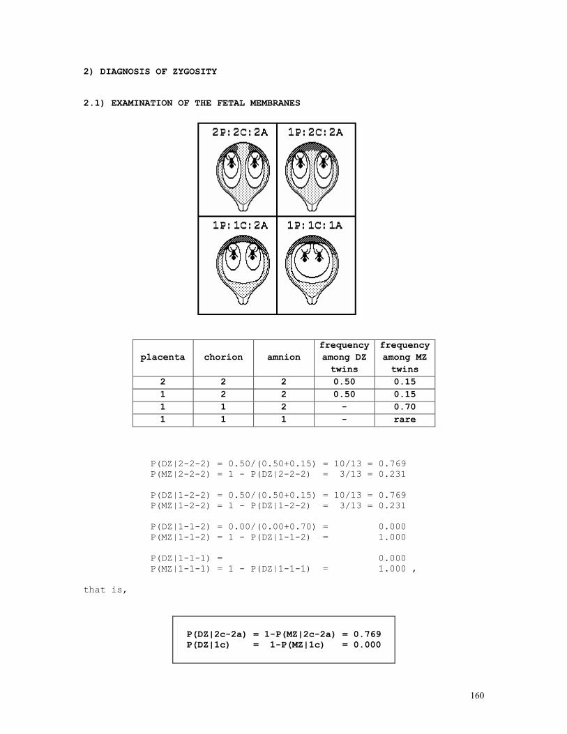
160
2) DIAGNOSIS OF ZYGOSITY 2.1) EXAMINATION OF THE FETAL MEMBRANES
placenta
chorion
amnion
frequencyamong DZ twins
frequency among MZ twins
2 2 2 0.50 0.15 1 2 2 0.50 0.15 1 1 2 - 0.70 1 1 1 - rare
P(DZ|2-2-2) = 0.50/(0.50+0.15) = 10/13 = 0.769 P(MZ|2-2-2) = 1 - P(DZ|2-2-2) = 3/13 = 0.231 P(DZ|1-2-2) = 0.50/(0.50+0.15) = 10/13 = 0.769 P(MZ|1-2-2) = 1 - P(DZ|1-2-2) = 3/13 = 0.231 P(DZ|1-1-2) = 0.00/(0.00+0.70) = 0.000 P(MZ|1-1-2) = 1 - P(DZ|1-1-2) = 1.000 P(DZ|1-1-1) = 0.000 P(MZ|1-1-1) = 1 - P(DZ|1-1-1) = 1.000 , that is,
P(DZ|2c-2a) = 1-P(MZ|2c-2a) = 0.769 P(DZ|1c) = 1-P(MZ|1c) = 0.000
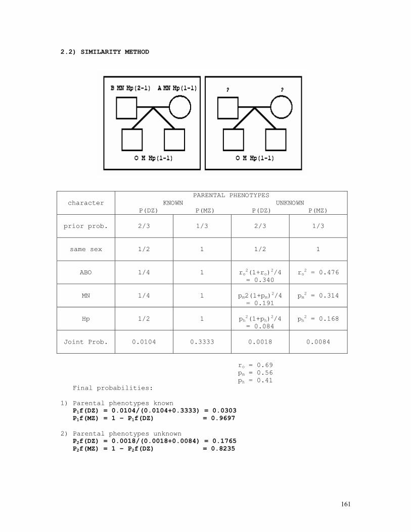
161
2.2) SIMILARITY METHOD
character PARENTAL PHENOTYPES
KNOWN UNKNOWN P(DZ) P(MZ) P(DZ) P(MZ)
prior prob.
2/3
1/3
2/3
1/3
same sex
1/2
1
1/2
1
ABO
1/4
1
ro2(1+ro)2/4 = 0.340
ro2 = 0.476
MN
1/4
1
pm2(1+pm)2/4 = 0.191
pm2 = 0.314
Hp
1/2
1
ph2(1+ph)2/4 = 0.084
ph2 = 0.168
Joint Prob.
0.0104
0.3333
0.0018
0.0084
ro = 0.69 pm = 0.56 ph = 0.41 Final probabilities: 1) Parental phenotypes known P1f(DZ) = 0.0104/(0.0104+0.3333) = 0.0303 P1f(MZ) = 1 – P1f(DZ) = 0.9697 2) Parental phenotypes unknown P2f(DZ) = 0.0018/(0.0018+0.0084) = 0.1765 P2f(MZ) = 1 – P2f(DZ) = 0.8235
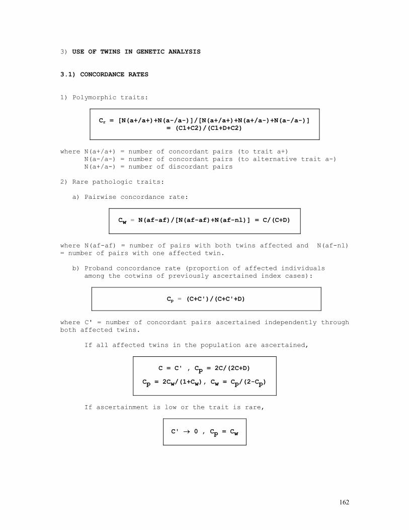
162
3) USE OF TWINS IN GENETIC ANALYSIS 3.1) CONCORDANCE RATES 1) Polymorphic traits:
Cr = [N(a+/a+)+N(a-/a-)]/[N(a+/a+)+N(a+/a-)+N(a-/a-)]
= (C1+C2)/(C1+D+C2)
where N(a+/a+) = number of concordant pairs (to trait a+) N(a-/a-) = number of concordant pairs (to alternative trait a-) N(a+/a-) = number of discordant pairs 2) Rare pathologic traits: a) Pairwise concordance rate:
Cw = N(af-af)/[N(af-af)+N(af-nl)] = C/(C+D)
where N(af-af) = number of pairs with both twins affected and N(af-nl) = number of pairs with one affected twin. b) Proband concordance rate (proportion of affected individuals among the cotwins of previously ascertained index cases):
Cp = (C+C')/(C+C'+D)
where C' = number of concordant pairs ascertained independently through both affected twins.
If all affected twins in the population are ascertained,
C = C' , Cp = 2C/(2C+D)
Cp = 2Cw/(1+Cw), Cw = Cp/(2-Cp)
If ascertainment is low or the trait is rare,
C' → 0 , Cp = Cw
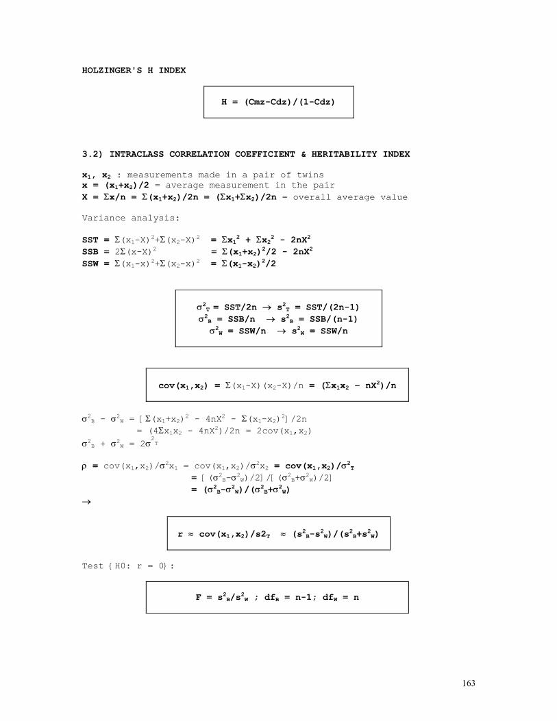
163
HOLZINGER'S H INDEX
H = (Cmz-Cdz)/(1-Cdz)
3.2) INTRACLASS CORRELATION COEFFICIENT & HERITABILITY INDEX x1, x2 : measurements made in a pair of twins x = (x1+x2)/2 = average measurement in the pair X = Σx/n = Σ(x1+x2)/2n = (Σx1+Σx2)/2n = overall average value Variance analysis: SST = Σ(x1-X)2+Σ(x2-X)2 = Σx12 + Σx22 - 2nX2 SSB = 2Σ(x-X)2 = Σ(x1+x2)2/2 - 2nX2 SSW = Σ(x1-x)2+Σ(x2-x)2 = Σ(x1-x2)2/2
σ2
T = SST/2n → s2T = SST/(2n-1) σ2
B = SSB/n → s2B = SSB/(n-1) σ2
W = SSW/n → s2W = SSW/n
cov(x1,x2) = Σ(x1-X)(x2-X)/n = (Σx1x2 – nX2)/n
σ2
B - σ2W = [Σ(x1+x2)2 - 4nX2 - Σ(x1-x2)2]/2n
= (4Σx1x2 - 4nX2)/2n = 2cov(x1,x2) σ2
B + σ2W = 2σ
2T
ρ = cov(x1,x2)/σ2x1 = cov(x1,x2)/σ2x2 = cov(x1,x2)/σ2
T = [(σ2
B-σ2W)/2]/[(σ2
B+σ2W)/2]
= (σ2B-σ2
W)/(σ2B+σ2
W) →
r ≈ cov(x1,x2)/s2T ≈ (s2B-s2W)/(s2B+s2W)
Test {H0: r = 0}:
F = s2B/s2W ; dfB = n-1; dfW = n
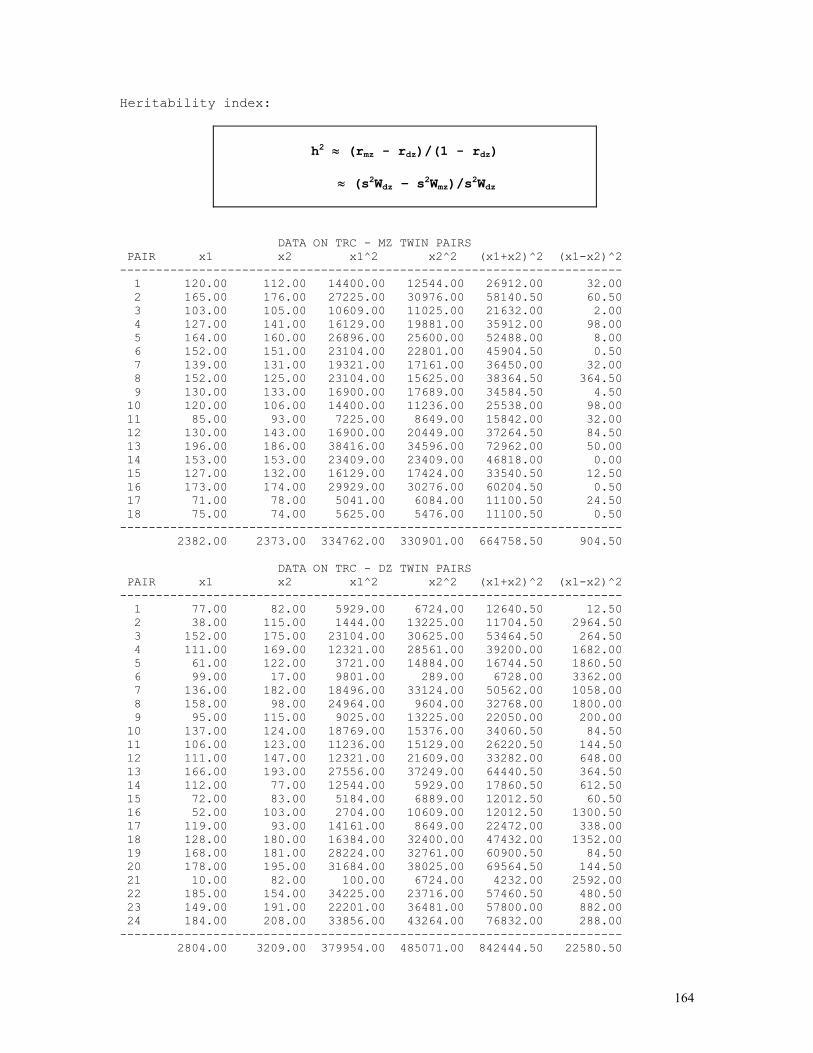
164
Heritability index:
h2 ≈ (rmz - rdz)/(1 - rdz)
≈ (s2Wdz – s2Wmz)/s2Wdz
DATA ON TRC - MZ TWIN PAIRS PAIR x1 x2 x1^2 x2^2 (x1+x2)^2 (x1-x2)^2 ---------------------------------------------------------------------- 1 120.00 112.00 14400.00 12544.00 26912.00 32.00 2 165.00 176.00 27225.00 30976.00 58140.50 60.50 3 103.00 105.00 10609.00 11025.00 21632.00 2.00 4 127.00 141.00 16129.00 19881.00 35912.00 98.00 5 164.00 160.00 26896.00 25600.00 52488.00 8.00 6 152.00 151.00 23104.00 22801.00 45904.50 0.50 7 139.00 131.00 19321.00 17161.00 36450.00 32.00 8 152.00 125.00 23104.00 15625.00 38364.50 364.50 9 130.00 133.00 16900.00 17689.00 34584.50 4.50 10 120.00 106.00 14400.00 11236.00 25538.00 98.00 11 85.00 93.00 7225.00 8649.00 15842.00 32.00 12 130.00 143.00 16900.00 20449.00 37264.50 84.50 13 196.00 186.00 38416.00 34596.00 72962.00 50.00 14 153.00 153.00 23409.00 23409.00 46818.00 0.00 15 127.00 132.00 16129.00 17424.00 33540.50 12.50 16 173.00 174.00 29929.00 30276.00 60204.50 0.50 17 71.00 78.00 5041.00 6084.00 11100.50 24.50 18 75.00 74.00 5625.00 5476.00 11100.50 0.50 ---------------------------------------------------------------------- 2382.00 2373.00 334762.00 330901.00 664758.50 904.50 DATA ON TRC - DZ TWIN PAIRS PAIR x1 x2 x1^2 x2^2 (x1+x2)^2 (x1-x2)^2 ---------------------------------------------------------------------- 1 77.00 82.00 5929.00 6724.00 12640.50 12.50 2 38.00 115.00 1444.00 13225.00 11704.50 2964.50 3 152.00 175.00 23104.00 30625.00 53464.50 264.50 4 111.00 169.00 12321.00 28561.00 39200.00 1682.00 5 61.00 122.00 3721.00 14884.00 16744.50 1860.50 6 99.00 17.00 9801.00 289.00 6728.00 3362.00 7 136.00 182.00 18496.00 33124.00 50562.00 1058.00 8 158.00 98.00 24964.00 9604.00 32768.00 1800.00 9 95.00 115.00 9025.00 13225.00 22050.00 200.00 10 137.00 124.00 18769.00 15376.00 34060.50 84.50 11 106.00 123.00 11236.00 15129.00 26220.50 144.50 12 111.00 147.00 12321.00 21609.00 33282.00 648.00 13 166.00 193.00 27556.00 37249.00 64440.50 364.50 14 112.00 77.00 12544.00 5929.00 17860.50 612.50 15 72.00 83.00 5184.00 6889.00 12012.50 60.50 16 52.00 103.00 2704.00 10609.00 12012.50 1300.50 17 119.00 93.00 14161.00 8649.00 22472.00 338.00 18 128.00 180.00 16384.00 32400.00 47432.00 1352.00 19 168.00 181.00 28224.00 32761.00 60900.50 84.50 20 178.00 195.00 31684.00 38025.00 69564.50 144.50 21 10.00 82.00 100.00 6724.00 4232.00 2592.00 22 185.00 154.00 34225.00 23716.00 57460.50 480.50 23 149.00 191.00 22201.00 36481.00 57800.00 882.00 24 184.00 208.00 33856.00 43264.00 76832.00 288.00 ---------------------------------------------------------------------- 2804.00 3209.00 379954.00 485071.00 842444.50 22580.50
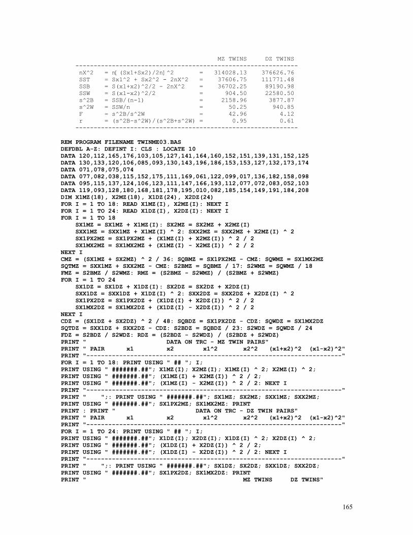
165
MZ TWINS DZ TWINS ------------------------------------------------------------- nX^2 = n[(Sx1+Sx2)/2n]^2 = 314028.13 376626.76 SST = Sx1^2 + Sx2^2 - 2nX^2 = 37606.75 111771.48 SSB = S(x1+x2)^2/2 - 2nX^2 = 36702.25 89190.98 SSW = S(x1-x2)^2/2 = 904.50 22580.50 s^2B = SSB/(n-1) = 2158.96 3877.87 s^2W = SSW/n = 50.25 940.85 F = s^2B/s^2W = 42.96 4.12 r = (s^2B-s^2W)/(s^2B+s^2W) = 0.95 0.61 ------------------------------------------------------------- REM PROGRAM FILENAME TWINME03.BAS DEFDBL A-Z: DEFINT I: CLS : LOCATE 10 DATA 120,112,165,176,103,105,127,141,164,160,152,151,139,131,152,125 DATA 130,133,120,106,085,093,130,143,196,186,153,153,127,132,173,174 DATA 071,078,075,074 DATA 077,082,038,115,152,175,111,169,061,122,099,017,136,182,158,098 DATA 095,115,137,124,106,123,111,147,166,193,112,077,072,083,052,103 DATA 119,093,128,180,168,181,178,195,010,082,185,154,149,191,184,208 DIM X1MZ(18), X2MZ(18), X1DZ(24), X2DZ(24) FOR I = 1 TO 18: READ X1MZ(I), X2MZ(I): NEXT I FOR I = 1 TO 24: READ X1DZ(I), X2DZ(I): NEXT I FOR I = 1 TO 18 SX1MZ = SX1MZ + X1MZ(I): SX2MZ = SX2MZ + X2MZ(I) SXX1MZ = SXX1MZ + X1MZ(I) ^ 2: SXX2MZ = SXX2MZ + X2MZ(I) ^ 2 SX1PX2MZ = SX1PX2MZ + (X1MZ(I) + X2MZ(I)) ^ 2 / 2 SX1MX2MZ = SX1MX2MZ + (X1MZ(I) - X2MZ(I)) ^ 2 / 2 NEXT I CMZ = (SX1MZ + SX2MZ) ^ 2 / 36: SQBMZ = SX1PX2MZ - CMZ: SQWMZ = SX1MX2MZ SQTMZ = SXX1MZ + SXX2MZ - CMZ: S2BMZ = SQBMZ / 17: S2WMZ = SQWMZ / 18 FMZ = S2BMZ / S2WMZ: RMZ = (S2BMZ - S2WMZ) / (S2BMZ + S2WMZ) FOR I = 1 TO 24 SX1DZ = SX1DZ + X1DZ(I): SX2DZ = SX2DZ + X2DZ(I) SXX1DZ = SXX1DZ + X1DZ(I) ^ 2: SXX2DZ = SXX2DZ + X2DZ(I) ^ 2 SX1PX2DZ = SX1PX2DZ + (X1DZ(I) + X2DZ(I)) ^ 2 / 2 SX1MX2DZ = SX1MX2DZ + (X1DZ(I) - X2DZ(I)) ^ 2 / 2 NEXT I CDZ = (SX1DZ + SX2DZ) ^ 2 / 48: SQBDZ = SX1PX2DZ - CDZ: SQWDZ = SX1MX2DZ SQTDZ = SXX1DZ + SXX2DZ - CDZ: S2BDZ = SQBDZ / 23: S2WDZ = SQWDZ / 24 FDZ = S2BDZ / S2WDZ: RDZ = (S2BDZ - S2WDZ) / (S2BDZ + S2WDZ) PRINT " DATA ON TRC - MZ TWIN PAIRS" PRINT " PAIR x1 x2 x1^2 x2^2 (x1+x2)^2 (x1-x2)^2" PRINT "----------------------------------------------------------------------" FOR I = 1 TO 18: PRINT USING " ## "; I; PRINT USING " #######.##"; X1MZ(I); X2MZ(I); X1MZ(I) ^ 2; X2MZ(I) ^ 2; PRINT USING " #######.##"; (X1MZ(I) + X2MZ(I)) ^ 2 / 2; PRINT USING " #######.##"; (X1MZ(I) - X2MZ(I)) ^ 2 / 2: NEXT I PRINT "----------------------------------------------------------------------" PRINT " ";: PRINT USING " #######.##"; SX1MZ; SX2MZ; SXX1MZ; SXX2MZ; PRINT USING " #######.##"; SX1PX2MZ; SX1MX2MZ: PRINT PRINT : PRINT " DATA ON TRC - DZ TWIN PAIRS" PRINT " PAIR x1 x2 x1^2 x2^2 (x1+x2)^2 (x1-x2)^2" PRINT "----------------------------------------------------------------------" FOR I = 1 TO 24: PRINT USING " ## "; I; PRINT USING " #######.##"; X1DZ(I); X2DZ(I); X1DZ(I) ^ 2; X2DZ(I) ^ 2; PRINT USING " #######.##"; (X1DZ(I) + X2DZ(I)) ^ 2 / 2; PRINT USING " #######.##"; (X1DZ(I) - X2DZ(I)) ^ 2 / 2: NEXT I PRINT "----------------------------------------------------------------------" PRINT " ";: PRINT USING " #######.##"; SX1DZ; SX2DZ; SXX1DZ; SXX2DZ; PRINT USING " #######.##"; SX1PX2DZ; SX1MX2DZ: PRINT PRINT " MZ TWINS DZ TWINS"

166
PRINT " -------------------------------------------------------------" PRINT " nX^2 = n[(Sx1+Sx2)/2n]^2 = "; PRINT USING "########.## "; CMZ / 2; CDZ / 2 PRINT " SST = Sx1^2 + Sx2^2 - 2nX^2 = "; PRINT USING "########.## "; SQTMZ; SQTDZ PRINT " SSB = S(x1+x2)^2/2 - 2nX^2 = "; PRINT USING "########.## "; SQBMZ; SQBDZ PRINT " SSW = S(x1-x2)^2/2 = "; PRINT USING "########.## "; SQWMZ; SQWDZ PRINT " s^2B = SSB/(n-1) = "; PRINT USING "########.## "; S2BMZ; S2BDZ PRINT " s^2W = SSW/n = "; PRINT USING "########.## "; S2WMZ; S2WDZ PRINT " F = s^2B/s^2W = "; PRINT USING "########.## "; FMZ; FDZ PRINT " r = (s^2B-s^2W)/(s^2B+s^2W) = "; PRINT USING "########.## "; RMZ; RDZ PRINT " -------------------------------------------------------------"
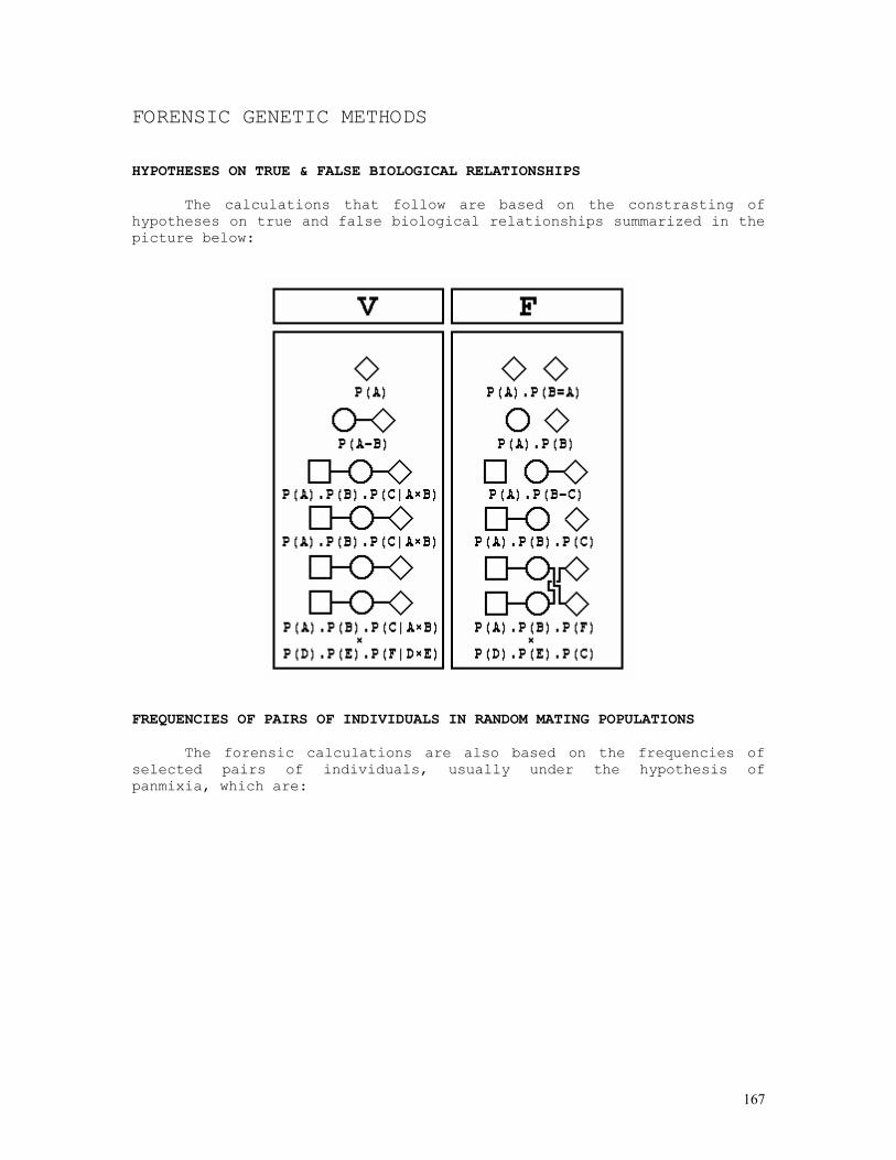
167
FORENSIC GENETIC METHODS
HYPOTHESES ON TRUE & FALSE BIOLOGICAL RELATIONSHIPS
The calculations that follow are based on the constrasting of hypotheses on true and false biological relationships summarized in the picture below:
FREQUENCIES OF PAIRS OF INDIVIDUALS IN RANDOM MATING POPULATIONS
The forensic calculations are also based on the frequencies of
selected pairs of individuals, usually under the hypothesis of panmixia, which are:
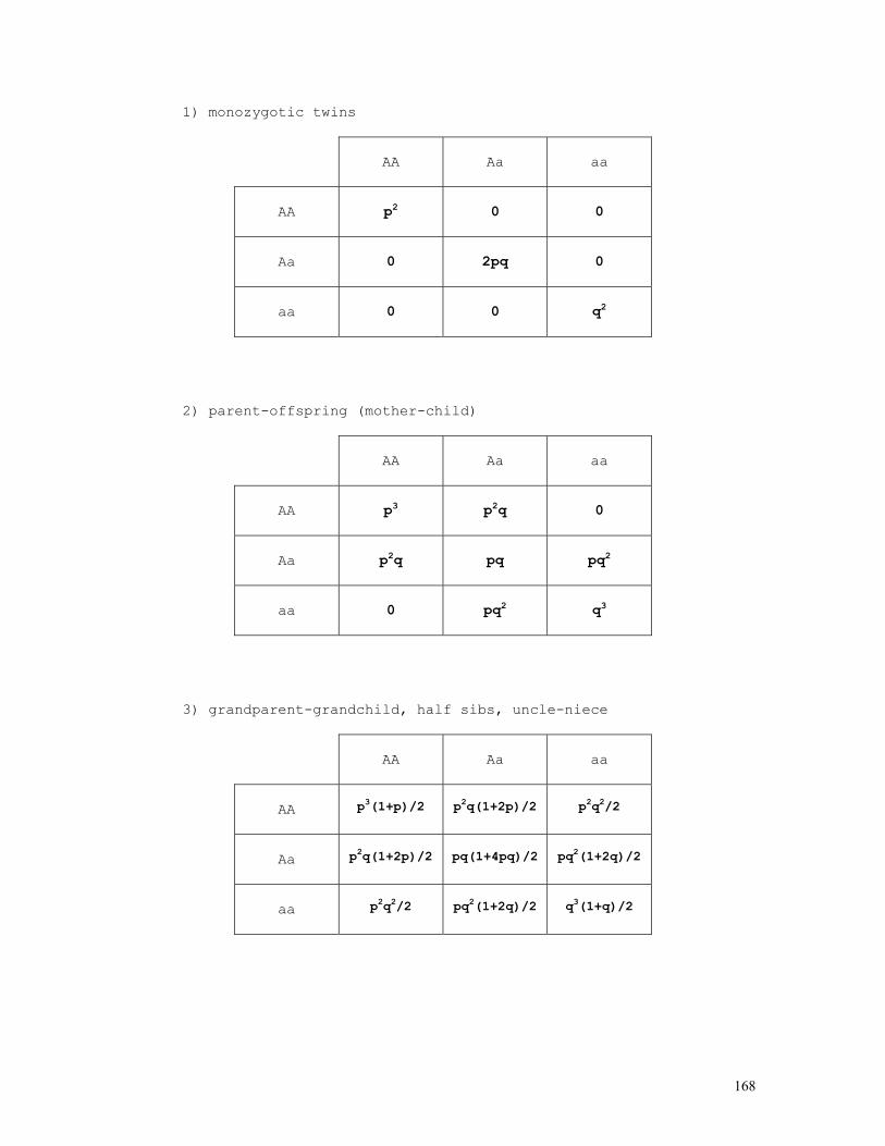
168
1) monozygotic twins
AA
Aa
aa
AA
p2
0
0
Aa
0
2pq
0
aa
0
0
q2
2) parent-offspring (mother-child)
AA Aa
aa
AA
p3
p2q
0
Aa
p2q
pq
pq2
aa
0
pq2
q3
3) grandparent-grandchild, half sibs, uncle-niece
AA Aa
aa
AA
p3(1+p)/2
p2q(1+2p)/2
p2q2/2
Aa
p2q(1+2p)/2
pq(1+4pq)/2
pq2(1+2q)/2
aa
p2q2/2
pq2(1+2q)/2
q3(1+q)/2

169
4) full sibs
AA
Aa
aa
AA
p2(1+p)2/4
p2q(1+p)/2
p2q2/4
Aa
p2q(1+p)/2
pq(1+pq)
pq2(1+q)/2
aa
p2q2/4
pq2(1+q)/2
q2(1+q)2/4
5) first cousins
AA
Aa
aa
AA
p3(1+3p)/4
p2q(1+6p)/4
3p2q2/4
Aa
p2q(1+6p)/4
pq(1+12pq)/4
pq2(1+6q)/4
aa
3p2q2/4
pq2(1+6q)/4
q3(1+3q)/4
6) unrelated persons
AA
Aa
aa
AA
p4
2p3q
p2q2
Aa
2p3q
4p2q2
2pq3
aa
p2q2
2pq3
q4
Probability of Identity Exclusion [P(E1)]
For the case of two alleles segregating in an autosomal locus, the probability of identity exclusion is taken straightforwardly from the following table:
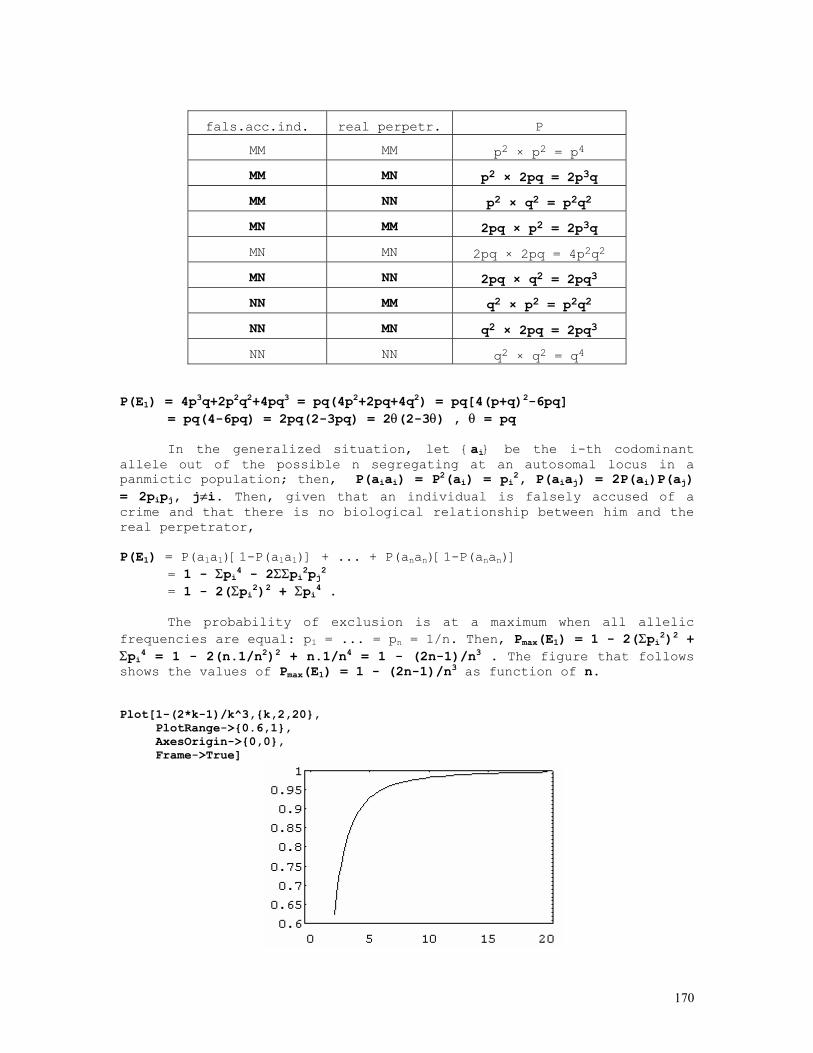
170
fals.acc.ind. real perpetr. P
MM MM p2 × p2 = p4
MM MN p2 × 2pq = 2p3q
MM NN p2 × q2 = p2q2
MN MM 2pq × p2 = 2p3q
MN MN 2pq × 2pq = 4p2q2
MN NN 2pq × q2 = 2pq3
NN MM q2 × p2 = p2q2
NN MN q2 × 2pq = 2pq3
NN NN q2 × q2 = q4 P(E1) = 4p3q+2p2q2+4pq3 = pq(4p2+2pq+4q2) = pq[4(p+q)2-6pq] = pq(4-6pq) = 2pq(2-3pq) = 2θ(2-3θ) , θ = pq
In the generalized situation, let {ai} be the i-th codominant allele out of the possible n segregating at an autosomal locus in a panmictic population; then, P(aiai) = P2(ai) = pi2, P(aiaj) = 2P(ai)P(aj) = 2pipj, j≠i. Then, given that an individual is falsely accused of a crime and that there is no biological relationship between him and the real perpetrator, P(E1) = P(a1a1)[1-P(a1a1)] + ... + P(anan)[1-P(anan)] = 1 - Σpi4 - 2ΣΣpi2pj2 = 1 - 2(Σpi2)2 + Σpi4 .
The probability of exclusion is at a maximum when all allelic frequencies are equal: p1 = ... = pn = 1/n. Then, Pmax(E1) = 1 - 2(Σpi2)2 + Σpi4 = 1 - 2(n.1/n2)2 + n.1/n4 = 1 - (2n-1)/n3 . The figure that follows shows the values of Pmax(E1) = 1 - (2n-1)/n3 as function of n. Plot[1-(2*k-1)/k^3,{k,2,20}, PlotRange->{0.6,1}, AxesOrigin->{0,0}, Frame->True]
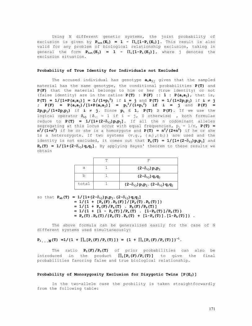
171
Using N different genetic systems, the joint probability of
exclusion is given by Ptot(E1) = 1 - Πi[1-Pi(E1)]. This result is also valid for any problem of biological relationship exclusion, taking in general the form Ptot(Ej) = 1 - Πi[1-Pi(Ej)], where j denotes the exclusion situation. Probability of True Identity for Individuals not Excluded
The accused individual has genotype aiaj; given that the sampled material has the same genotype, the conditional probabilities P(T) and P(F) that the material belongs to him or her (true identity) or not (false identity) are in the ratios P(T) : P(F) :: 1 : P(aiaj), that is, P(T) = 1/[1+P(aiaj)] = 1/(1+pi2) if i = j and P(T) = 1/(1+2pipj) if i ≠ j ; P(F) = P(aiaj)/[1+P(aiaj)] = pi2/(1+pi2) if i = j and P(F) = 2pipj/(1+2pipj) if i ≠ j. Since pi ≤ 1, P(T) ≥ P(F). If we use the logical operator δij {δij = 1 if i = j, 0 otherwise} , both formulae reduce to P(T) = 1/[1+(2-δij)pipj]. If all the n codominant alleles segregating at this locus occur with equal frequencies, pi = 1/n, P(T) = n2/(1+n2) if he or she is a homozygote and P(T) = n2/(2+n2) if he or she is a heterozygote. If two systems (v.g., {ai},{bi}) are used and the identity is not excluded, it comes out that Pa(T) = 1/[1+(2-δij)pipj] and Pb(T) = 1/[1+(2-δij)qiqj]. By applying Bayes' theorem to these results we obtain
T F
a 1 (2-δij)pipj
b 1 (2-δij)qiqj
total 1 (2-δij)pipj.(2-δij)qiqj
so that Pab(T) = 1/[1+(2-δij)pipj.(2-δij)qiqj] = 1/{1 + [Pa(F).Pb(F)]/[Pa(T).Pb(T)]} = 1/[1 + Pa(F)/Pa(T) . Pb(F)/Pb(T)] = 1/{1 + [1 - Pa(T)]/Pa(T) . [1-Pb(T)]/Pb(T)} = Pa(T).Pb(T)/{Pa(T).Pb(T) + [1-Pa(T)].[1-Pb(T)]} .
The above formula can be generalized easily for the case of N different systems used simultaneously: P1...N(T) =1/{1 + ∏i[Pi(F)/Pi(T)]} = {1 + ∏i[Pi(F)/Pi(T)]}-1.
The ratio P0(F)/P0(T) of prior probabilities can also be introduced in the product ∏i[Pi(F)/Pi(T)] to give the final probabilities favoring false and true biological relationship. Probability of Monozygosity Exclusion for Dizygotic Twins [P(E2)]
In the two-allele case the probility is taken straightforwardly from the following table:
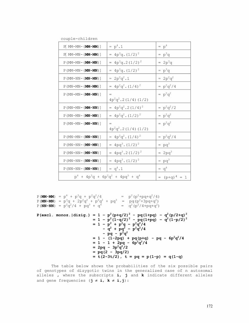
172
couple-children
P[MM-MM-(MM-MM)] = p4.1 = p4
P[MM-MN-(MM-MM)] = 4p3q.(1/2)2 = p3q
P(MM-MN-(MM-MN)] = 4p3q.2(1/2)2 = 2p3q
P(MM-MN-(MN-MN)] = 4p3q.(1/2)2 = p3q
P(MM-NN-(MN-MN)] = 2p2q2.1 = 2p2q2
P(MN-MN-(MM-MM)] = 4p2q2.(1/4)2 = p2q2/4
P(MN-MN-(MM-MN)] = 4p2q2.2(1/4)(1/2)
= p2q2
P(MN-MN-(MM-NN)] = 4p2q2.2(1/4)2 = p2q2/2
P(MN-MN-(MN-MN)] = 4p2q2.(1/2)2 = p2q2
P(MN-MN-(MN-NN)] = 4p2q2.2(1/4)(1/2)
= p2q2
P(MN-MN-(NN-NN)] = 4p2q2.(1/4)2 = p2q2/4
P(MN-NN-(MN-MN)] = 4pq3.(1/2)2 = pq3
P(MN-NN-(MN-NN)] = 4pq3.2(1/2)2 = 2pq3
P(MN-NN-(NN-NN)] = 4pq3.(1/2)2 = pq3
P(NN-NN-(NN-NN)] = q4.1 = q4
p4 + 4p3q + 6p2q2 + 4pq3 + q4 = (p+q)4 = 1 P(MM-MM) = p4 + p3q + p2q2/4 = p2(p2+pq+q2/4) P(MN-MN) = p3q + 2p2q2 + p2q2 + pq3 = pq(p2+3pq+q2) P(NN-NN) = p2q2/4 + pq3 + q4 = q2(p2/4+pq+q2) P(excl. monoz.|dizig.) = 1 – p2(p+q/2)2 - pq(1+pq) – q2(p/2+q)2 = 1 – p2(1-q/2)2 - pq(1+pq) – q2(1-p/2)2 = 1 – p2 + p2q – p2q2/4 - q2 + pq2 – p2q2/4 - pq - p2q2 = 1 - (1-2pq) + pq(p+q) - pq - 6p2q2/4 = 1 - 1 + 2pq - 6p2q2/4 = 2pq - 3p2q2/2 = pq(2 - 3pq/2) = t(2-3t/2), t = pq = p(1-p) = q(1-q)
The table below shows the probabilities of the six possible pairs of genotypes of dizygotic twins in the generalized case of n autosomal alleles , where the subscripts i, j and k indicate different alleles and gene frequencies (j ≠ i, k ≠ i,j):
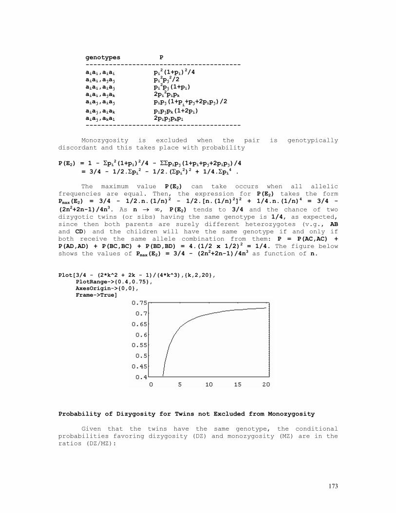
173
genotypes P ---------------------------------------- aiai,aiai pi2(1+pi)2/4 aiai,ajaj pi2pj2/2 aiai,aiaj pi2pj(1+pi) aiai,ajak 2pi
2pipk aiaj,aiaj pipj(1+pi+pj+2pipj)/2 aiaj,aiak pipjpk(1+2pi) aiaj,akal 2pipjpkpl ----------------------------------------
Monozygosity is excluded when the pair is genotypically discordant and this takes place with probability P(E2) = 1 - Σpi2(1+pi)2/4 - ΣΣpipj(1+pi+pj+2pipj)/4 = 3/4 - 1/2.Σpi2 - 1/2.(Σpi2)2 + 1/4.Σpi4 .
The maximum value P(E2) can take occurs when all allelic frequencies are equal. Then, the expression for P(E2) takes the form Pmax(E2) = 3/4 - 1/2.n.(1/n)2 - 1/2.[n.(1/n)2]2 + 1/4.n.(1/n)4 = 3/4 - (2n2+2n-1)/4n3. As n → ∞, P(E2) tends to 3/4 and the chance of two dizygotic twins (or sibs) having the same genotype is 1/4, as expected, since then both parents are surely different heterozygotes (v.g., AB and CD) and the children will have the same genotype if and only if both receive the same allele combination from them: P = P(AC,AC) + P(AD,AD) + P(BC,BC) + P(BD,BD) = 4.(1/2 x 1/2)2 = 1/4. The figure below shows the values of Pmax(E2) = 3/4 - (2n2+2n-1)/4n3 as function of n. Plot[3/4 - (2*k^2 + 2k - 1)/(4*k^3),{k,2,20}, PlotRange->{0.4,0.75}, AxesOrigin->{0,0}, Frame->True]
Probability of Dizygosity for Twins not Excluded from Monozygosity
Given that the twins have the same genotype, the conditional probabilities favoring dizygosity (DZ) and monozygosity (MZ) are in the ratios (DZ/MZ):
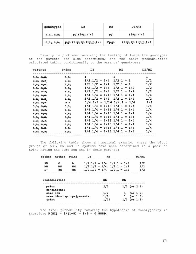
174
genotypes DZ MZ DZ/MZ
aiai,aiai pi2(1+pi)2/4 pi2 (1+pi)2/4
aiaj,aiaj pipj(1+pi+pj+2pipj)/2 2pipj (1+pi+pj+2pipj)/4
Usually in problems involving the testing of twins the genotypes of the parents are also determined, and the above probabilities calculated taking conditionally to the parents' genotypes: parents twins DZ MZ DZ/MZ ---------------------------------------------------------------- aiai,aiai aiai 1 1 1 aiai,aiaj aiai 1/2.1/2 = 1/4 1/2.1 = 1 1/2 aiai,aiaj aiaj 1/2.1/2 = 1/4 1/2.1 = 1 1/2 aiai,ajak aiaj 1/2.1/2 = 1/4 1/2.1 = 1/2 1/2 aiai,ajak aiak 1/2.1/2 = 1/4 1/2.1 = 1/2 1/2 aiaj,aiaj aiai 1/4.1/4 = 1/16 1/4.1 = 1/4 1/4 aiaj,aiaj aiaj 1/2.1/2 = 1/4 1/2.1 = 1/4 1/2 aiaj,aiaj ajaj 1/4.1/4 = 1/16 1/4.1 = 1/4 1/4 aiaj,aiak aiai 1/4.1/4 = 1/16 1/4.1 = 1/4 1/4 aiaj,aiak aiak 1/4.1/4 = 1/16 1/4.1 = 1/4 1/4 aiaj,aiak aiaj 1/4.1/4 = 1/16 1/4.1 = 1/4 1/4 aiaj,aiak ajak 1/4.1/4 = 1/16 1/4.1 = 1/4 1/4 aiaj,akal aiak 1/4.1/4 = 1/16 1/4.1 = 1/4 1/4 aiaj,akal ajak 1/4.1/4 = 1/16 1/4.1 = 1/4 1/4 aiaj,akal aial 1/4.1/4 = 1/16 1/4.1 = 1/4 1/4 aiaj,akal ajal 1/4.1/4 = 1/16 1/4.1 = 1/4 1/4 ----------------------------------------------------------------
The following table shows a numerical example, where the blood groups of ABO, MN and Rh systems have been determined in a pair of twins having the same sex and in their parents: father mother twins DZ MZ DZ/MZ ------------------------------------------------------------- AB O A 1/2.1/2 = 1/4 1/2.1 = 1/2 1/2 MM MN MM 1/2.1/2 = 1/4 1/2.1 = 1/2 1/2 D- dd dd 1/2.1/2 = 1/4 1/2.1 = 1/2 1/2 ------------------------------------------------------------- Probabilities DZ MZ ----------------------------------------------------------- prior 2/3 1/3 (or 2:1) conditional same sex 1/2 1 (or 1:2) same blood groups|parents 1/8 1 (or 1:8) joint 1/24 1/3 (or 1:8) -----------------------------------------------------------
The final probability favoring the hypothesis of monozygosity is therefore P(MZ) = 8/(1+8) = 8/9 = 0.8889.
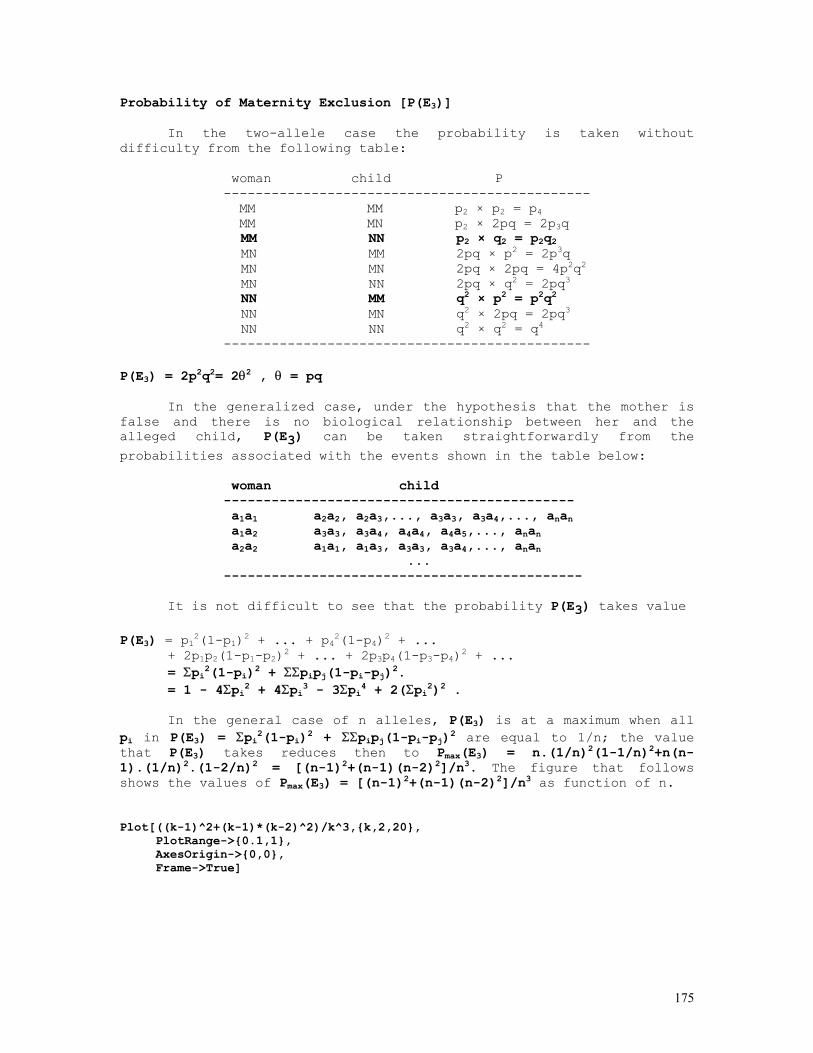
175
Probability of Maternity Exclusion [P(E3)]
In the two-allele case the probability is taken without difficulty from the following table: woman child P ---------------------------------------------- MM MM p2 × p2 = p4 MM MN p2 × 2pq = 2p3q
MM NN p2 × q2 = p2q2 MN MM 2pq × p2 = 2p3q MN MN 2pq × 2pq = 4p2q2 MN NN 2pq × q2 = 2pq3 NN MM q2 × p2 = p2q2 NN MN q2 × 2pq = 2pq3 NN NN q2 × q2 = q4
---------------------------------------------- P(E3) = 2p2q2= 2θ2 , θ = pq
In the generalized case, under the hypothesis that the mother is false and there is no biological relationship between her and the alleged child, P(E3) can be taken straightforwardly from the
probabilities associated with the events shown in the table below: woman child -------------------------------------------- a1a1 a2a2, a2a3,..., a3a3, a3a4,..., anan a1a2 a3a3, a3a4, a4a4, a4a5,..., anan a2a2 a1a1, a1a3, a3a3, a3a4,..., anan ... ---------------------------------------------
It is not difficult to see that the probability P(E3) takes value P(E3) = p12(1-p1)2 + ... + p42(1-p4)2 + ... + 2p1p2(1-p1-p2)2 + ... + 2p3p4(1-p3-p4)2 + ... = Σpi2(1-pi)2 + ΣΣpipj(1-pi-pj)2. = 1 - 4Σpi2 + 4Σpi3 - 3Σpi4 + 2(Σpi2)2 .
In the general case of n alleles, P(E3) is at a maximum when all pi in P(E3) = Σpi2(1-pi)2 + ΣΣpipj(1-pi-pj)2 are equal to 1/n; the value that P(E3) takes reduces then to Pmax(E3) = n.(1/n)2(1-1/n)2+n(n-1).(1/n)2.(1-2/n)2 = [(n-1)2+(n-1)(n-2)2]/n3. The figure that follows shows the values of Pmax(E3) = [(n-1)2+(n-1)(n-2)2]/n3 as function of n. Plot[((k-1)^2+(k-1)*(k-2)^2)/k^3,{k,2,20}, PlotRange->{0.1,1}, AxesOrigin->{0,0}, Frame->True]
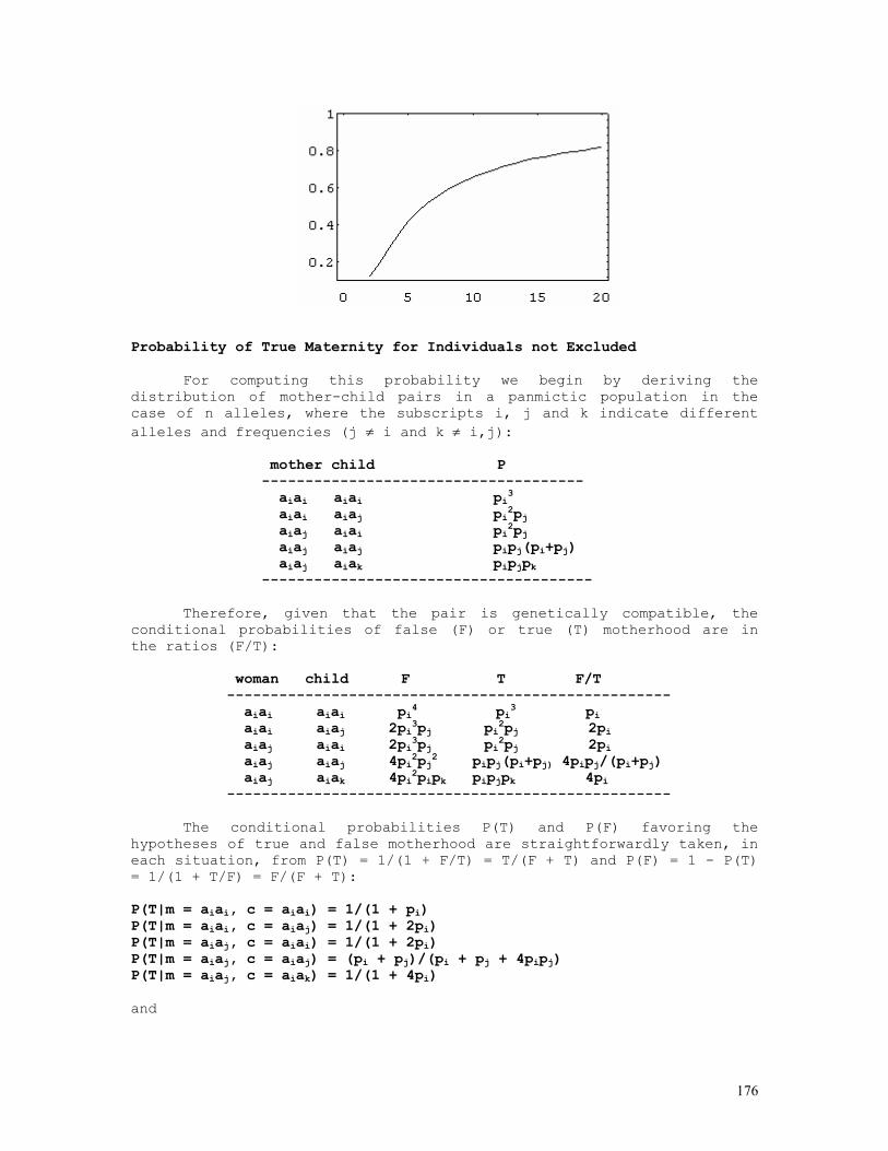
176
Probability of True Maternity for Individuals not Excluded
For computing this probability we begin by deriving the distribution of mother-child pairs in a panmictic population in the case of n alleles, where the subscripts i, j and k indicate different alleles and frequencies (j ≠ i and k ≠ i,j): mother child P ------------------------------------- aiai aiai pi3 aiai aiaj pi2pj aiaj aiai pi2pj aiaj aiaj pipj(pi+pj) aiaj aiak pipjpk --------------------------------------
Therefore, given that the pair is genetically compatible, the conditional probabilities of false (F) or true (T) motherhood are in the ratios (F/T): woman child F T F/T --------------------------------------------------- aiai aiai pi4 pi3 pi aiai aiaj 2pi3pj pi2pj 2pi aiaj aiai 2pi3pj pi2pj 2pi aiaj aiaj 4pi2pj2 pipj(pi+pj) 4pipj/(pi+pj) aiaj aiak 4pi2pipk pipjpk 4pi ---------------------------------------------------
The conditional probabilities P(T) and P(F) favoring the hypotheses of true and false motherhood are straightforwardly taken, in each situation, from P(T) = 1/(1 + F/T) = T/(F + T) and P(F) = 1 - P(T) = 1/(1 + T/F) = F/(F + T):
P(T|m = aiai, c = aiai) = 1/(1 + pi) P(T|m = aiai, c = aiaj) = 1/(1 + 2pi) P(T|m = aiaj, c = aiai) = 1/(1 + 2pi) P(T|m = aiaj, c = aiaj) = (pi + pj)/(pi + pj + 4pipj) P(T|m = aiaj, c = aiak) = 1/(1 + 4pi) and
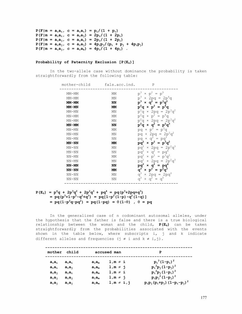
177
P(F|m = aiai, c = aiai) = pi/(1 + pi) P(F|m = aiai, c = aiaj) = 2pi/(1 + 2pi) P(F|m = aiaj, c = aiai) = 2pi/(1 + 2pi) P(F|m = aiaj, c = aiaj) = 4pipj/(pi + pj + 4pipj) P(F|m = aiaj, c = aiak) = 4pi/(1 + 4pi) . Probability of Paternity Exclusion [P(E4)]
In the two-allele case without dominance the probability is taken straightforwardly from the following table: mother-child fals.acc.ind. P -------------------------------------------------- MM-MM MM p3 × p2 = p5 MM-MM MN p3 × 2pq = 2p4q MM-MM NN p3 × q2 = p3q2 MM-MN MM p2q × p2 = p4q MM-MN MN p2q × 2pq = 2p3q2 MN-MM MM p2q × p2 = p4q MN-MM MN p2q × 2pq = 2p3q2 MN-MM NN p2q × q2 = p2q3 MN-MN MM pq × p2 = p3q MN-MN MN pq × 2pq = 2p2q2 MN-MN NN pq × q2 = pq3 MN-NN MM pq2 × p2 = p3q2 MN-NN MN pq2 × 2pq = 2p2q3 MN-NN NN pq2 × q2 = pq4 NN-MN MM pq2 × p2 = p3q2 NN-MN MN pq2 × 2pq = 2p2q3 NN-MN NN pq2 × q2 = pq4 NN-NN MM q3 × p2 = p2q3 NN-NN MN q3 × 2pq = 2pq4 NN-NN NN q3 × q2 = q5 ------------------------------------------------ P(E4) = p4q + 2p3q2 + 2p2q3 + pq4 = pq(p3+2pq+q3) = pq(p3+1-p2-q2+q3) = pq[1-p2(1-p)-q2(1-q)] = pq(1-p2q-pq2) = pq(1-pq) = θ(1-θ) , θ = pq
In the generalized case of n codominant autosomal alleles, under the hypothesis that the father is false and there is a true biological relationship between the woman and the child, P(E4) can be taken straightforwardly from the probabilities associated with the events shown in the table below, where subscripts i, j and k indicate different alleles and frequencies (j ≠ i and k ≠ i,j). -------------------------------------------------------------- mother child accused man P -------------------------------------------------------------- aiai aiai alam l,m ≠ i pi3(1-pi)2 aiai aiaj alam l,m ≠ j pi2pj(1-pj)2 aiaj aiai alam l,m ≠ i pi2pj(1-pi)2 aiaj aiaj alam l,m ≠ j pipj2(1-pj)2 aiaj aiaj alam l,m ≠ i,j pipj(pi+pj)(1-pi-pj)2
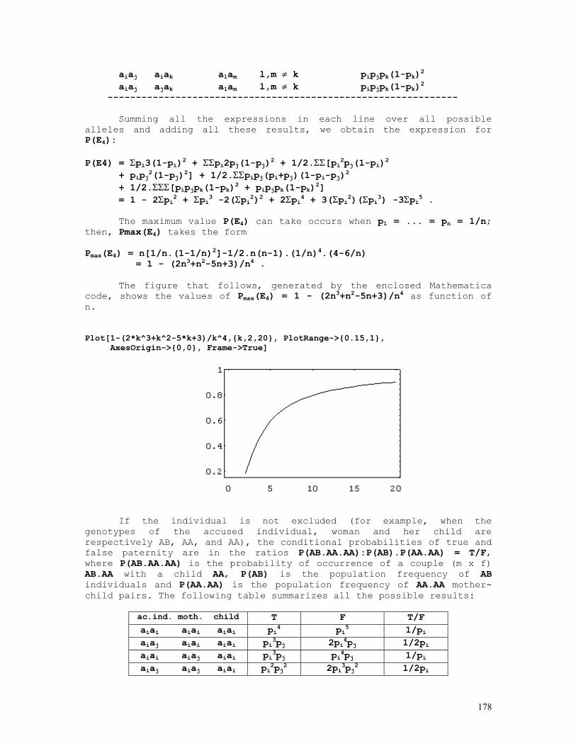
178
aiaj aiak alam l,m ≠ k pipjpk(1-pk)2 aiaj ajak alam l,m ≠ k pipjpk(1-pk)2 --------------------------------------------------------------
Summing all the expressions in each line over all possible alleles and adding all these results, we obtain the expression for P(E4):
P(E4) = Σpi3(1-pi)2 + ΣΣpi2pj(1-pj)2 + 1/2.ΣΣ[pi2pj(1-pi)2 + pipj2(1-pj)2] + 1/2.ΣΣpipj(pi+pj)(1-pi-pj)2 + 1/2.ΣΣΣ[pipjpk(1-pk)2 + pipjpk(1-pk)2] = 1 - 2Σpi2 + Σpi3 -2(Σpi2)2 + 2Σpi4 + 3(Σpi2)(Σpi3) -3Σpi5 .
The maximum value P(E4) can take occurs when p1 = ... = pn = 1/n; then, Pmax(E4) takes the form
Pmax(E4) = n[1/n.(1-1/n)2]-1/2.n(n-1).(1/n)4.(4-6/n) = 1 - (2n3+n2-5n+3)/n4 .
The figure that follows, generated by the enclosed Mathematica code, shows the values of Pmax(E4) = 1 - (2n3+n2-5n+3)/n4 as function of n. Plot[1-(2*k^3+k^2-5*k+3)/k^4,{k,2,20}, PlotRange->{0.15,1}, AxesOrigin->{0,0}, Frame->True]
If the individual is not excluded (for example, when the genotypes of the accused individual, woman and her child are respectively AB, AA, and AA), the conditional probabilities of true and false paternity are in the ratios P(AB.AA.AA):P(AB).P(AA.AA) = T/F, where P(AB.AA.AA) is the probability of occurrence of a couple (m x f) AB.AA with a child AA, P(AB) is the population frequency of AB individuals and P(AA.AA) is the population frequency of AA.AA mother-child pairs. The following table summarizes all the possible results:
ac.ind. moth. child T F T/F aiai aiai aiai pi4 pi5 1/pi aiaj aiai aiai pi3pj 2pi4pj 1/2pi aiai aiaj aiai pi3pj pi4pj 1/pi aiaj aiaj aiai pi2pj2 2pi3pj2 1/2pi
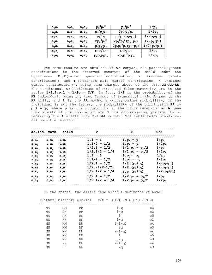
179
aiaj aiai aiaj pi2pj2 pi2pj3 1/pj ajak aiai aiaj pi2pjpk 2pi2pj2pk 1/2pj aiai aiaj aiaj pi3pj pi3pj(pi+pj) 1/(pi+pj) aiaj aiaj aiaj 2pi2pj2 2pi2pj2(pi+pj) 1/(pi+pj) ajak aiaj aiaj pipj2pk 2pipj2pk(pi+pj) 1/2(pi+pj) ajaj aiak aiaj pipj2pk pipj3pk 1/pj ajal aiak aiaj pipjpkpl 2pipj2pkpl 1/2pj
The same results are obtained if we compare the parental gamete contributions to the observed genotype of the child under the hypotheses T:{P(father gametic contribution) × P(mother gamete contribution)} and F:{P(random male gamete contribution) × P(mother gamete contribution)}. Using same example above of the trio AB-AA-AA, the conditional probabilities of true and false paternity are in the ratios 1/2.1:p.1 = 1/2p = T/F. In fact, 1/2 is the probability of the AB individual, being the true father, of transmitting the A gene to the AA child, and 1 is the AA mother's corresponding probability; if the individual is not the father, the probability of the child being AA is p.1 = p, where p is the probability of the child receiving an A gene from a male of the population and 1 the corresponding probability of receiving the A allele from his AA mother. The table below summarizes all possible results: --------------------------------------------------------------------- ac.ind. moth. child T F T/F --------------------------------------------------------------------- aiai aiai aiai 1.1 = 1 1.pi = pi 1/pi aiaj aiai aiai 1.1/2 = 1/2 1.pi = pi 1/2pi aiai aiaj aiai 1/2.1 = 1/2 1/2.pi = pi/2 1/pi aiaj aiaj aiai 1/2.1/2 = 1/4 1/2.pi = pi/2 1/2pi ajaj aiai aiaj 1.1 = 1 1.pj = pj 1/pj ajak aiai aiaj 1.1/2 = 1/2 1.pj = pj 1/2pj aiai aiaj aiaj 1/2.1 = 1/2 1/2.(pi+pj) 1/(pi+pj) aiaj aiaj aiaj 1/2.(1/2+1/2) 1/2.(pi+pj) 1/(pi+pj) ajak aiaj aiaj 1/2.1/2 = 1/4 1/2.(pi+pj) 1/2(pi+pj) ajaj aiak aiaj 1/2.1 = 1/2 1/2.pj = pj/2 1/pj ajal aiak aiaj 1/2.1/2 = 1/4 1/2.pj = pj/2 1/2pj ----------------------------------------------------------------------
In the special two-allele case without dominance we have: F(ather) M(other) C(hild) f/t = P[(F)-(M-C)]/P[F-M-C] --------------------------------------------------------- MM MM MM 1-q e2 MM MN MM 1-q e2 MM MN MN 1 e5 MM NN MN 1-q e2 MN MM MM 2(1-q) e4 MN MM MN 2q e3 MN MN MM 2(1-q) e4 MN MN MN 1 e5 MN MN NN 2q e3 MN NN MN 2(1-q) e4 MN NN NN 2q e3
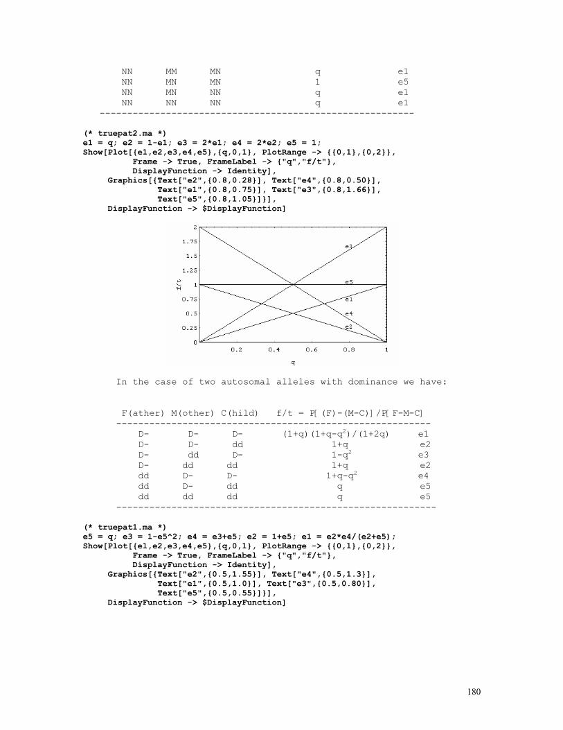
180
NN MM MN q e1 NN MN MN 1 e5 NN MN NN q e1 NN NN NN q e1 --------------------------------------------------------- (* truepat2.ma *) e1 = q; e2 = 1-e1; e3 = 2*e1; e4 = 2*e2; e5 = 1; Show[Plot[{e1,e2,e3,e4,e5},{q,0,1}, PlotRange -> {{0,1},{0,2}}, Frame -> True, FrameLabel -> {"q","f/t"}, DisplayFunction -> Identity], Graphics[{Text["e2",{0.8,0.28}], Text["e4",{0.8,0.50}], Text["e1",{0.8,0.75}], Text["e3",{0.8,1.66}], Text["e5",{0.8,1.05}]}], DisplayFunction -> $DisplayFunction]
In the case of two autosomal alleles with dominance we have: F(ather) M(other) C(hild) f/t = P[(F)-(M-C)]/P[F-M-C] --------------------------------------------------------- D- D- D- (1+q)(1+q-q2)/(1+2q) e1 D- D- dd 1+q e2 D- dd D- 1-q2 e3 D- dd dd 1+q e2 dd D- D- 1+q-q2 e4 dd D- dd q e5 dd dd dd q e5 ---------------------------------------------------------- (* truepat1.ma *) e5 = q; e3 = 1-e5^2; e4 = e3+e5; e2 = 1+e5; e1 = e2*e4/(e2+e5); Show[Plot[{e1,e2,e3,e4,e5},{q,0,1}, PlotRange -> {{0,1},{0,2}}, Frame -> True, FrameLabel -> {"q","f/t"}, DisplayFunction -> Identity], Graphics[{Text["e2",{0.5,1.55}], Text["e4",{0.5,1.3}], Text["e1",{0.5,1.0}], Text["e3",{0.5,0.80}], Text["e5",{0.5,0.55}]}], DisplayFunction -> $DisplayFunction]
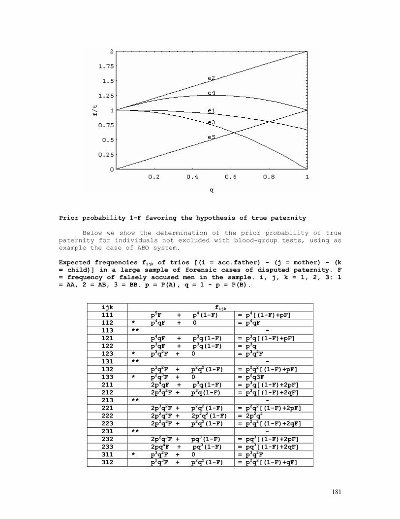
181
Prior probability 1-F favoring the hypothesis of true paternity
Below we show the determination of the prior probability of true paternity for individuals not excluded with blood-group tests, using as example the case of ABO system. Expected frequencies fijk of trios [(i = acc.father) - (j = mother) - (k = child)] in a large sample of forensic cases of disputed paternity. F = frequency of falsely accused men in the sample. i, j, k = 1, 2, 3: 1 = AA, 2 = AB, 3 = BB. p = P(A), q = 1 - p = P(B).
ijk fijk 111 p5F + p4(1-F) = p4[(1-F)+pF] 112 * p4qF + 0 = p4qF 113 ** - 121 p4qF + p3q(1-F) = p3q[(1-F)+pF] 122 p3qF + p3q(1-F) = p3q 123 * p3q2F + 0 = p3q2F 131 ** - 132 p3q2F + p2q2(1-F) = p2q2[(1-F)+pF] 133 * p2q3F + 0 = p2q3F 211 2p4qF + p3q(1-F) = p3q[(1-F)+2pF] 212 2p3q2F + p3q(1-F) = p3q[(1-F)+2qF] 213 ** - 221 2p3q2F + p2q2(1-F) = p2q2[(1-F)+2pF] 222 2p2q2F + 2p2q2(1-F) = 2p2q2 223 2p2q3F + p2q2(1-F) = p2q2[(1-F)+2qF] 231 ** - 232 2p2q3F + pq3(1-F) = pq3[(1-F)+2pF] 233 2pq4F + pq3(1-F) = pq3[(1-F)+2qF] 311 * p3q2F + 0 = p3q2F 312 p2q3F + p2q2(1-F) = p2q2[(1-F)+qF]
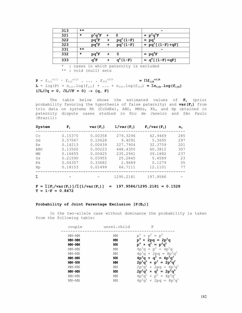
182
313 ** - 321 * p2q3F + 0 = p2q3F 322 pq3F + pq3(1-F) = pq3 323 pq4F + pq3(1-F) = pq3[(1-F)+qF] 331 ** - 332 * pq4F + 0 = pq4F
333 q5F + q4(1-F) = q4[(1-F)+qF]
* : cases in which paternity is excluded ** : void (null) sets P = f111n111 . f112n112 . ... . f333n333 = Πfijknijk L = log(P) = n111.log(f111) + ... + n333.log(f333) = Σnijk.log(fijk) {∂L/∂q = 0, ∂L/∂F = 0} → {q, F}
The table below shows the estimated values of Fi (prior probability favoring the hypothesis of false paternity) and var(Fi) from trio data on systems Rh (CcDdEe), ABO, MNSs, Kk, and Hp obtained in paternity dispute cases studied in Rio de Janeiro and São Paulo (Brazil): System Fi var(Fi) 1/var(Fi) Fi/var(Fi) ni --------------------------------------------------------------- Cc 0.15375 0.00358 279.3296 42.9469 285 Dd 0.57067 0.10628 9.4091 5.3695 297 Ee 0.14213 0.00439 227.7904 32.3759 201 ABO 0.13500 0.00223 448.4305 60.3812 307 MN 0.16655 0.00425 235.2941 39.1882 237 Ss 0.21590 0.03955 25.2845 5.4589 23 Kk 0.04307 0.33682 2.9689 0.1279 55 Hp 0.18153 0.01499 66.7111 12.1101 77 --------------------------------------------------------------- Σ - - 1295.2181 197.9586 - F = Σ[Fi/var(Fi)]/Σ[1/var(Fi)] = 197.9586/1295.2181 = 0.1528 T = 1-F = 0.8472 Probability of Joint Parentage Exclusion [P(E5)]
In the two-allele case without dominance the probability is taken from the following table:
couple unrel.child P ------------------------------------------------ MM-MM MM p4 × p2 = p6 MM-MM MN p4 × 2pq = 2p5q MM-MM NN p4 × q2 = p4q2 MM-MN MM 4p3q × p2 = 4p5q MM-MN MN 4p3q × 2pq = 8p4q2 MM-MN NN 4p3q × q2 = 4p3q3 MM-NN MM 2p2q2 × p2 = 2p4q2 MM-MN MN 2p2q2 × 2pq = 4p3q3 MM-MN NN 2p2q2 × q2 = 2p2q4 MN-MN MM 4p2q2 × p2 = 4p4q2 MN-MN MN 4p2q2 × 2pq = 8p3q3
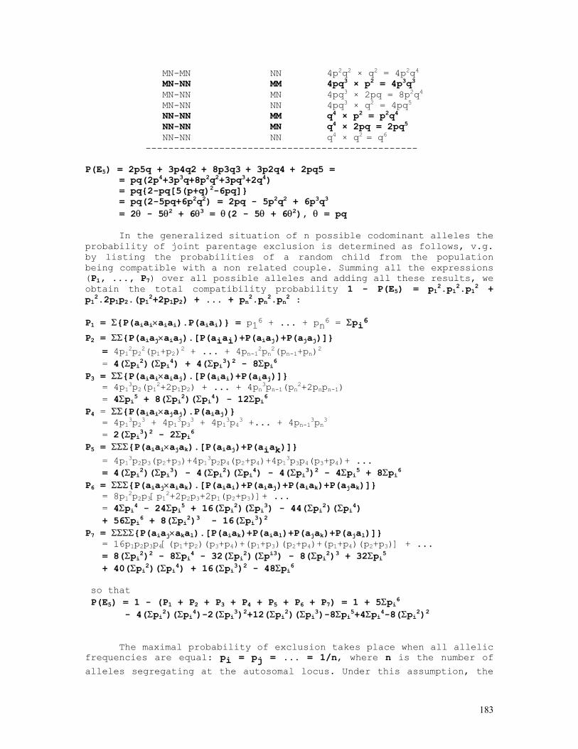
183
MN-MN NN 4p2q2 × q2 = 4p2q4 MN-NN MM 4pq3 × p2 = 4p3q3 MN-NN MN 4pq3 × 2pq = 8p2q4 MN-NN NN 4pq3 × q2 = 4pq5 NN-NN MM q4 × p2 = p2q4 NN-NN MN q4 × 2pq = 2pq5 NN-NN NN q4 × q2 = q6 ------------------------------------------------
P(E5) = 2p5q + 3p4q2 + 8p3q3 + 3p2q4 + 2pq5 = = pq(2p4+3p3q+8p2q2+3pq3+2q4) = pq{2-pq[5(p+q)2-6pq]} = pq(2-5pq+6p2q2) = 2pq - 5p2q2 + 6p3q3 = 2θ - 5θ2 + 6θ3 = θ(2 - 5θ + 6θ2), θ = pq
In the generalized situation of n possible codominant alleles the probability of joint parentage exclusion is determined as follows, v.g. by listing the probabilities of a random child from the population being compatible with a non related couple. Summing all the expressions (P1, ..., P7) over all possible alleles and adding all these results, we obtain the total compatibility probability 1 - P(E5) = p12.p12.p12 + p12.2p1p2.(p12+2p1p2) + ... + pn2.pn2.pn2 : P1 = Σ{P(aiai×aiai).P(aiai)} = p16 + ... + pn6 = Σpi6
P2 = ΣΣ{P(aiaj×aiaj).[P(aiai)+P(aiaj)+P(ajaj)]} = 4p12p22(p1+p2)2 + ... + 4pn-12pn2(pn-1+pn)2 = 4(Σpi2)(Σpi4) + 4(Σpi3)2 - 8Σpi6 P3 = ΣΣ{P(aiai×aiaj).[P(aiai)+P(aiaj)]} = 4p13p2(p12+2p1p2) + ... + 4pn3pn-1(pn2+2pnpn-1) = 4Σpi5 + 8(Σpi2)(Σpi4) - 12Σpi6 P4 = ΣΣ{P(aiai×ajaj).P(aiaj)} = 4p13p23 + 4p13p33 + 4p13p43 +... + 4pn-13pn3 = 2(Σpi3)2 - 2Σpi6 P5 = ΣΣΣ{P(aiai×ajak).[P(aiaj)+P(aiak)]} = 4p13p2p3(p2+p3)+4p13p2p4(p2+p4)+4p13p3p4(p3+p4)+ ... = 4(Σpi2)(Σpi3) - 4(Σpi2)(Σpi4) - 4(Σpi3)2 - 4Σpi5 + 8Σpi6 P6 = ΣΣΣ{P(aiaj×aiak).[P(aiai)+P(aiaj)+P(aiak)+P(ajak)]} = 8p12p2p3[p12+2p2p3+2p1(p2+p3)]+ ... = 4Σpi4 - 24Σpi5 + 16(Σpi2)(Σpi3) - 44(Σpi2)(Σpi4) + 56Σpi6 + 8(Σpi2)3 - 16(Σpi3)2 P7 = ΣΣΣΣ{P(aiaj×akal).[P(aiak)+P(aial)+P(ajak)+P(ajal)]} = 16p1p2p3p4[(p1+p2)(p3+p4)+(p1+p3)(p2+p4)+(p1+p4)(p2+p3)] + ... = 8(Σpi2)2 - 8Σpi4 - 32(Σpi2)(Σpi3) - 8(Σpi2)3 + 32Σpi5 + 40(Σpi2)(Σpi4) + 16(Σpi3)2 - 48Σpi6 so that P(E5) = 1 - (P1 + P2 + P3 + P4 + P5 + P6 + P7) = 1 + 5Σpi6 - 4(Σpi2)(Σpi4)-2(Σpi3)2+12(Σpi2)(Σpi3)-8Σpi5+4Σpi4-8(Σpi2)2
The maximal probability of exclusion takes place when all allelic frequencies are equal: pi = pj = ... = 1/n, where n is the number of alleles segregating at the autosomal locus. Under this assumption, the
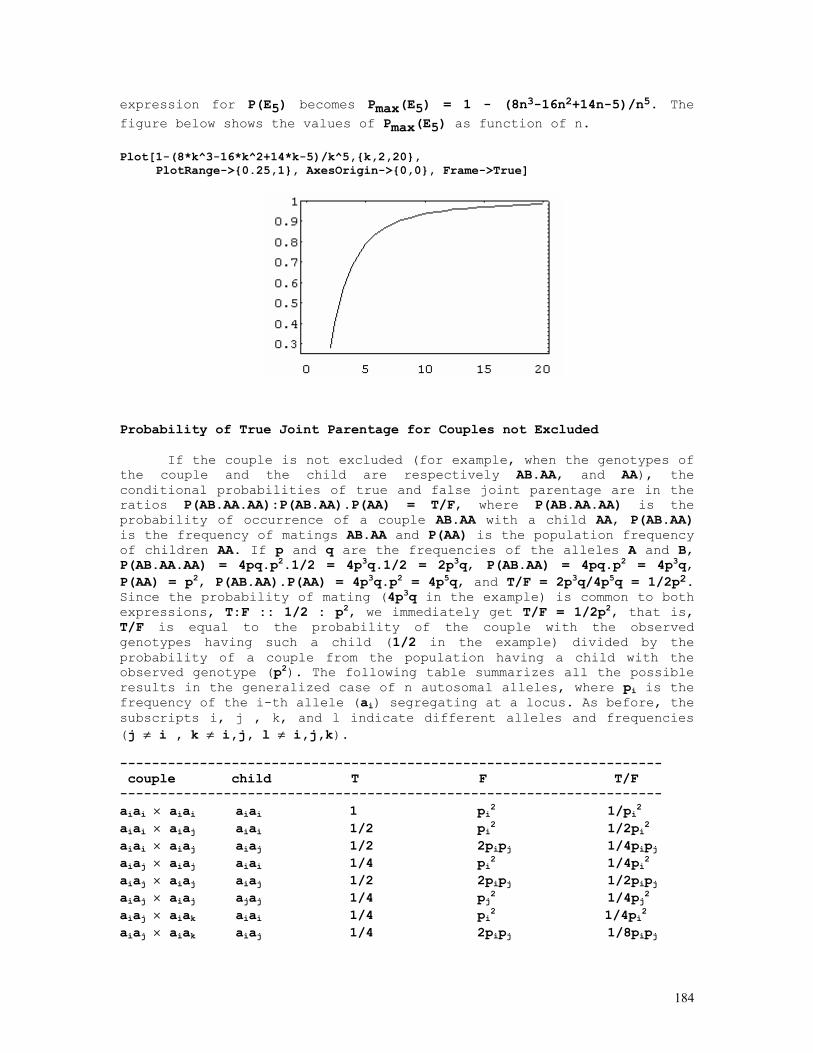
184
expression for P(E5) becomes Pmax(E5) = 1 - (8n3-16n2+14n-5)/n5. The figure below shows the values of Pmax(E5) as function of n. Plot[1-(8*k^3-16*k^2+14*k-5)/k^5,{k,2,20}, PlotRange->{0.25,1}, AxesOrigin->{0,0}, Frame->True]
Probability of True Joint Parentage for Couples not Excluded
If the couple is not excluded (for example, when the genotypes of the couple and the child are respectively AB.AA, and AA), the conditional probabilities of true and false joint parentage are in the ratios P(AB.AA.AA):P(AB.AA).P(AA) = T/F, where P(AB.AA.AA) is the probability of occurrence of a couple AB.AA with a child AA, P(AB.AA) is the frequency of matings AB.AA and P(AA) is the population frequency of children AA. If p and q are the frequencies of the alleles A and B, P(AB.AA.AA) = 4pq.p2.1/2 = 4p3q.1/2 = 2p3q, P(AB.AA) = 4pq.p2 = 4p3q, P(AA) = p2, P(AB.AA).P(AA) = 4p3q.p2 = 4p5q, and T/F = 2p3q/4p5q = 1/2p2. Since the probability of mating (4p3q in the example) is common to both expressions, T:F :: 1/2 : p2, we immediately get T/F = 1/2p2, that is, T/F is equal to the probability of the couple with the observed genotypes having such a child (1/2 in the example) divided by the probability of a couple from the population having a child with the observed genotype (p2). The following table summarizes all the possible results in the generalized case of n autosomal alleles, where pi is the frequency of the i-th allele (ai) segregating at a locus. As before, the subscripts i, j , k, and l indicate different alleles and frequencies (j ≠ i , k ≠ i,j, l ≠ i,j,k). -------------------------------------------------------------------- couple child T F T/F -------------------------------------------------------------------- aiai × aiai aiai 1 pi2 1/pi2 aiai × aiaj aiai 1/2 pi2 1/2pi2 aiai × aiaj aiaj 1/2 2pipj 1/4pipj aiaj × aiaj aiai 1/4 pi2 1/4pi2 aiaj × aiaj aiaj 1/2 2pipj 1/2pipj aiaj × aiaj ajaj 1/4 pj2 1/4pj2 aiaj × aiak aiai 1/4 pi2 1/4pi2 aiaj × aiak aiaj 1/4 2pipj 1/8pipj
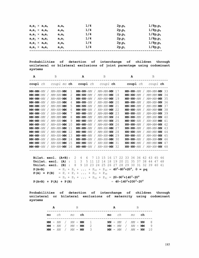
185
aiaj × aiak aiak 1/4 2pipk 1/8pipk aiaj × aiak ajak 1/4 2pjpk 1/8pjpk aiaj × akal aiak 1/4 2pipk 1/8pipk aiaj × akal aial 1/4 2pipl 1/8pipl aiaj × akal ajak 1/4 2pjpk 1/8pjpk aiaj × akal ajal 1/4 2pjpl 1/8pjpl -------------------------------------------------------------------- Probabilities of detection of interchange of children through unilateral or bilateral exclusions of joint parentage using codominant systems
A B A B A B ----------------------------------------------------------------------- coupl ch coupl mo ch coupl ch coupl ch coupl ch coupl ch ----------------------------------------------------------------------- MM-MM-MN / MM-MN-MM 1 MM-NN-MM / MM-MM-MN 17 MN-NN-MM / MM-MM-MN 33 MM-MM-MN / MM-NN-MM 2 MM-NN-MM / MM-MN-MN 18 MN-NN-MM / MM-MM-NN 34 MM-MM-MN / MN-MN-MM 3 MM-NN-MM / MN-MN-MN 19 MN-NN-MM / MM-MN-MN 35 MM-MM-MN / MN-NN-MM 4 MM-NN-NN / MN-MN-MN 20 MN-NN-MM / MM-MN-NN 36 MM-MM-NN / MN-MN-MM 5 MM-NN-NN / MN-NN-MN 21 MN-NN-MM / MN-MN-MN 37 MM-MM-NN / MN-NN-MM 6 MM-NN-NN / NN-NN-MN 22 MN-NN-MM / MN-MN-NN 38 MM-MM-NN / NN-NN-MM 7 MN-MN-MM / MM-MM-MN 23 MN-NN-MN / MM-MN-NN 39 MM-MN-MM / MM-MM-MN 8 MN-MN-MM / MM-MM-NN 24 MN-NN-MN / MM-NN-NN 40 MM-MN-MN / MM-NN-MM 9 MN-MN-MM / MM-MN-NN 25 MN-NN-NN / NN-NN-MN 41 MM-MN-MN / MN-NN-MM 10 MN-MN-MN / MM-MN-NN 26 NN-NN-MM / MM-MM-NN 42 MM-MN-NN / MN-MN-MM 11 MN-MN-MN / MM-NN-MM 27 NN-NN-MM / MM-MN-NN 43 MM-MN-NN / MN-MN-MN 12 MN-MN-MN / MM-NN-NN 28 NN-NN-MM / MN-MN-NN 44 MM-MN-NN / MN-NN-MM 13 MN-MN-MN / MN-NN-MM 29 NN-NN-MN / MM-MN-NN 45 MM-MN-NN / MN-NN-MN 14 MN-MN-NN / MN-NN-MM 30 NN-NN-MN / MM-NN-NN 46 MM-MN-NN / NN-NN-MM 15 MN-MN-NN / NN-NN-MM 31 NN-NN-MN / MN-MN-NN 47 MM-MN-NN / NN-NN-MN 16 MN-MN-NN / NN-NN-MN 32 NN-NN-MN / MN-NN-NN 48 ----------------------------------------------------------------------- Bilat. excl. (A+B): 2 4 6 7 13 15 16 17 22 33 34 36 42 43 45 46 Unilat. excl. (A) : 1 3 5 11 12 14 18 19 20 21 35 37 38 44 47 48 Unilat. excl. (B) : 8 9 10 23 24 25 26 27 28 29 30 31 32 39 40 41 P(A+B) = P2 + P4 + ... + P45 + P46 = 4θ2-8θ3+2θ4, θ = pq P(A) = P(B) = P1 + P3 + ... + P47 + P48 = P8 + P9 + ... + P40 + P41 = 2θ-9θ2+14θ3-2θ4 P(A+B) + P(A) + P(B) = 4θ-14θ2+20θ3-2θ4 Probabilities of detection of interchange of children through unilateral or bilateral exclusions of maternity using codominant systems A B A B ------------------------------------------------------ mo ch mo ch mo ch mo ch ------------------------------------------------------ MM - NN / NN - MM 1 NN - MM / MM - NN 8 MM - NN / MN - MM 2 MM - MN / NN - MM 9 MM - NN / MN - MN 3 MN - MM / MM - NN 10
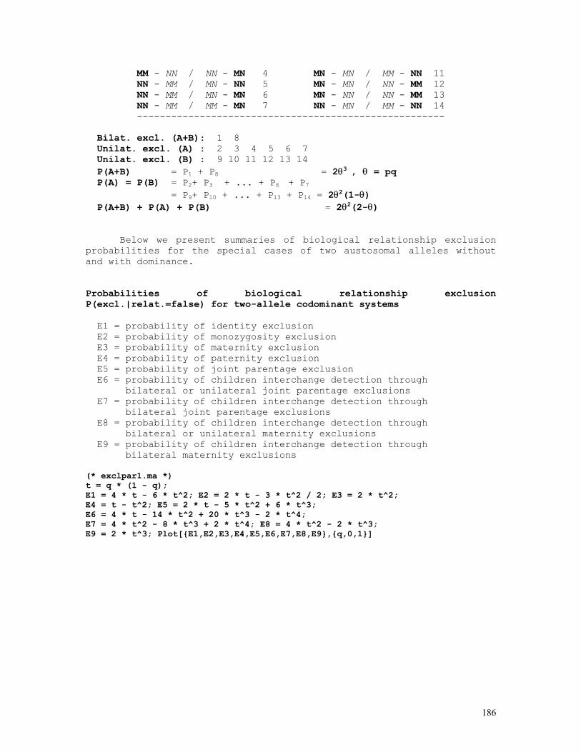
186
MM - NN / NN - MN 4 MN - MN / MM - NN 11 NN - MM / MN - NN 5 MN - MN / NN - MM 12 NN - MM / MN - MN 6 MN - NN / NN - MM 13 NN - MM / MM - MN 7 NN - MN / MM - NN 14 ------------------------------------------------------ Bilat. excl. (A+B): 1 8 Unilat. excl. (A) : 2 3 4 5 6 7 Unilat. excl. (B) : 9 10 11 12 13 14 P(A+B) = P1 + P8 = 2θ3 , θ = pq P(A) = P(B) = P2+ P3 + ... + P6 + P7 = P9+ P10 + ... + P13 + P14 = 2θ2(1-θ) P(A+B) + P(A) + P(B) = 2θ2(2-θ)
Below we present summaries of biological relationship exclusion probabilities for the special cases of two austosomal alleles without and with dominance. Probabilities of biological relationship exclusion P(excl.|relat.=false) for two-allele codominant systems E1 = probability of identity exclusion E2 = probability of monozygosity exclusion E3 = probability of maternity exclusion E4 = probability of paternity exclusion E5 = probability of joint parentage exclusion E6 = probability of children interchange detection through bilateral or unilateral joint parentage exclusions E7 = probability of children interchange detection through bilateral joint parentage exclusions E8 = probability of children interchange detection through bilateral or unilateral maternity exclusions E9 = probability of children interchange detection through bilateral maternity exclusions (* exclpar1.ma *) t = q * (1 - q); E1 = 4 * t - 6 * t^2; E2 = 2 * t - 3 * t^2 / 2; E3 = 2 * t^2; E4 = t - t^2; E5 = 2 * t - 5 * t^2 + 6 * t^3; E6 = 4 * t - 14 * t^2 + 20 * t^3 - 2 * t^4; E7 = 4 * t^2 - 8 * t^3 + 2 * t^4; E8 = 4 * t^2 - 2 * t^3; E9 = 2 * t^3; Plot[{E1,E2,E3,E4,E5,E6,E7,E8,E9},{q,0,1}]
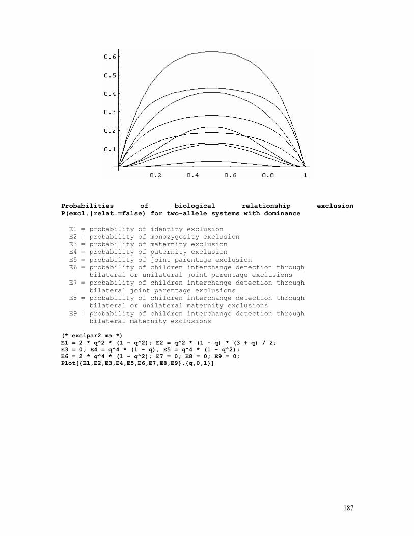
187
Probabilities of biological relationship exclusion P(excl.|relat.=false) for two-allele systems with dominance E1 = probability of identity exclusion E2 = probability of monozygosity exclusion E3 = probability of maternity exclusion E4 = probability of paternity exclusion E5 = probability of joint parentage exclusion E6 = probability of children interchange detection through bilateral or unilateral joint parentage exclusions E7 = probability of children interchange detection through bilateral joint parentage exclusions E8 = probability of children interchange detection through bilateral or unilateral maternity exclusions E9 = probability of children interchange detection through bilateral maternity exclusions (* exclpar2.ma *) E1 = 2 * q^2 * (1 - q^2); E2 = q^2 * (1 - q) * (3 + q) / 2; E3 = 0; E4 = q^4 * (1 - q); E5 = q^4 * (1 - q^2); E6 = 2 * q^4 * (1 - q^2); E7 = 0; E8 = 0; E9 = 0; Plot[{E1,E2,E3,E4,E5,E6,E7,E8,E9},{q,0,1}]
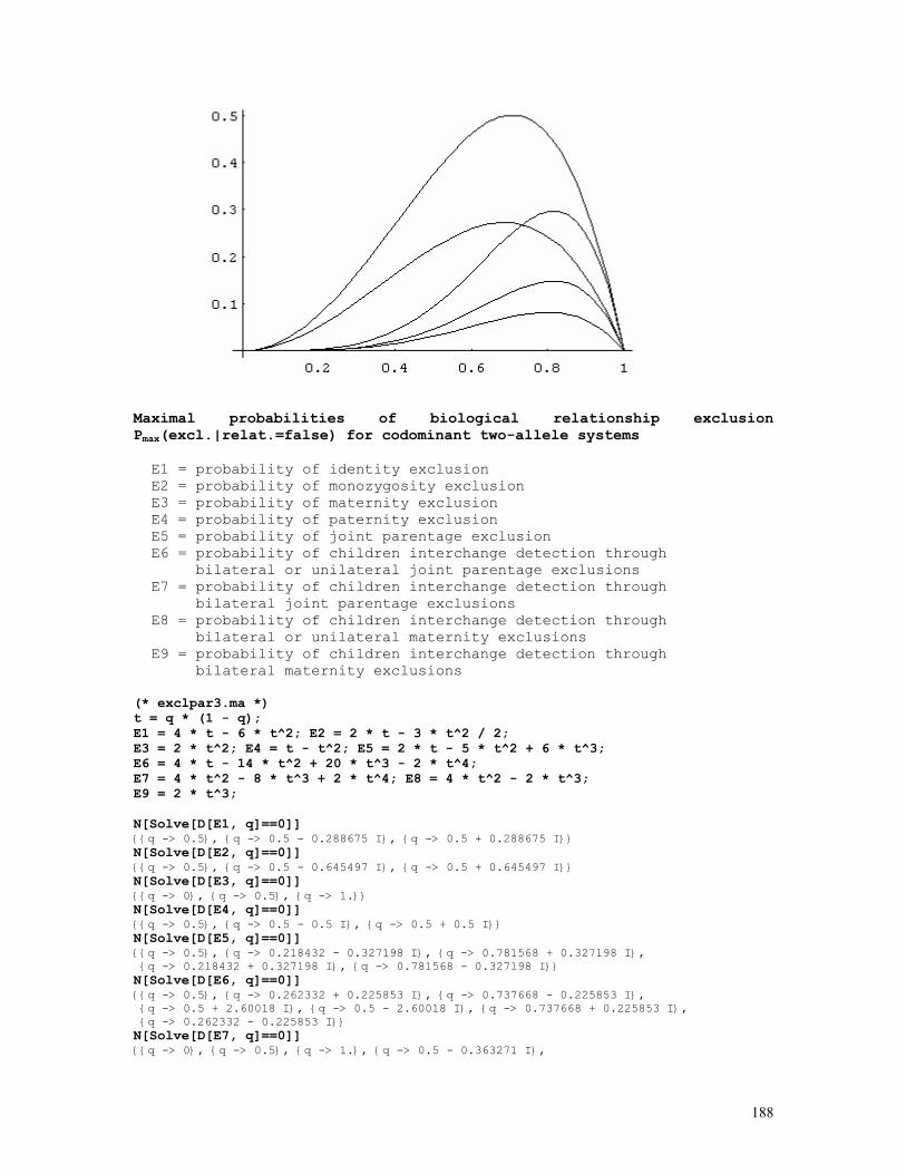
188
Maximal probabilities of biological relationship exclusion Pmax(excl.|relat.=false) for codominant two-allele systems E1 = probability of identity exclusion E2 = probability of monozygosity exclusion E3 = probability of maternity exclusion E4 = probability of paternity exclusion E5 = probability of joint parentage exclusion E6 = probability of children interchange detection through bilateral or unilateral joint parentage exclusions E7 = probability of children interchange detection through bilateral joint parentage exclusions E8 = probability of children interchange detection through bilateral or unilateral maternity exclusions E9 = probability of children interchange detection through bilateral maternity exclusions (* exclpar3.ma *) t = q * (1 - q); E1 = 4 * t - 6 * t^2; E2 = 2 * t - 3 * t^2 / 2; E3 = 2 * t^2; E4 = t - t^2; E5 = 2 * t - 5 * t^2 + 6 * t^3; E6 = 4 * t - 14 * t^2 + 20 * t^3 - 2 * t^4; E7 = 4 * t^2 - 8 * t^3 + 2 * t^4; E8 = 4 * t^2 - 2 * t^3; E9 = 2 * t^3; N[Solve[D[E1, q]==0]] {{q -> 0.5}, {q -> 0.5 - 0.288675 I}, {q -> 0.5 + 0.288675 I}} N[Solve[D[E2, q]==0]] {{q -> 0.5}, {q -> 0.5 - 0.645497 I}, {q -> 0.5 + 0.645497 I}} N[Solve[D[E3, q]==0]] {{q -> 0}, {q -> 0.5}, {q -> 1.}} N[Solve[D[E4, q]==0]] {{q -> 0.5}, {q -> 0.5 - 0.5 I}, {q -> 0.5 + 0.5 I}} N[Solve[D[E5, q]==0]] {{q -> 0.5}, {q -> 0.218432 - 0.327198 I}, {q -> 0.781568 + 0.327198 I}, {q -> 0.218432 + 0.327198 I}, {q -> 0.781568 - 0.327198 I}} N[Solve[D[E6, q]==0]] {{q -> 0.5}, {q -> 0.262332 + 0.225853 I}, {q -> 0.737668 - 0.225853 I}, {q -> 0.5 + 2.60018 I}, {q -> 0.5 - 2.60018 I}, {q -> 0.737668 + 0.225853 I}, {q -> 0.262332 - 0.225853 I}} N[Solve[D[E7, q]==0]] {{q -> 0}, {q -> 0.5}, {q -> 1.}, {q -> 0.5 - 0.363271 I},
189
{q -> 0.5 + 0.363271 I}, {q -> 0.5 - 1.53884 I}, {q -> 0.5 + 1.53884 I}} N[Solve[D[E8, q]==0]] {{q -> 0}, {q -> 0.5}, {q -> 1.}, {q -> 0.5 - 1.04083 I}, {q -> 0.5 + 1.04083 I}} N[Solve[D[E9, q]==0]] {{q -> 0}, {q -> 0}, {q -> 0.5}, {q -> 1.}, {q -> 1.}} Maximal probabilities of biological relationship exclusion Pmax(excl.|relat.=false) for codominant two-allele systems E1 = probability of identity exclusion E2 = probability of monozygosity exclusion E3 = probability of maternity exclusion E4 = probability of paternity exclusion E5 = probability of joint parentage exclusion E6 = probability of children interchange detection through bilateral or unilateral joint parentage exclusions E7 = probability of children interchange detection through bilateral joint parentage exclusions E8 = probability of children interchange detection through bilateral or unilateral maternity exclusions E9 = probability of children interchange detection through bilateral maternity exclusions (* exclpar5.ma *) q = 0.5; t = q * (1 - q); E1 = 4 * t - 6 * t^2 E2 = 2 * t - 3 * t^2 / 2 E3 = 2 * t^2 E4 = t - t^2 E5 = 2 * t - 5 * t^2 + 6 * t^3 E6 = 4 * t - 14 * t^2 + 20 * t^3 - 2 * t^4 E7 = 4 * t^2 - 8 * t^3 + 2 * t^4 E8 = 4 * t^2 - 2 * t^3 E9 = 2 * t^3 0.625 0.40625 0.125 0.1875 0.28125 0.429687 0.132813 0.21875 0.03125 Maximal probabilities of biological relationship exclusion Pmax(excl.|relat.=false) for two-allele systems with dominance E1 = probability of identity exclusion E2 = probability of monozygosity exclusion E3 = probability of maternity exclusion E4 = probability of paternity exclusion E5 = probability of joint parentage exclusion E6 = probability of children interchange detection through bilateral or unilateral joint parentage exclusions E7 = probability of children interchange detection through bilateral joint parentage exclusions E8 = probability of children interchange detection through bilateral or unilateral maternity exclusions
190
E9 = probability of children interchange detection through bilateral maternity exclusions (* exclpar6.ma *) q = 0.707107; E1 = 2 * q^2 * (1 - q^2) q = 0.686141; E2 = q^2 * (1 - q) * (3 + q) / 2 E3 = 0; q = 0.8; E4 = q^4 * (1 - q) q = 0.816497; E5 = q^4 * (1 - q^2) E6 = 2 * q^4 * (1 - q^2) E7 = 0; E8 = 0; E9 = 0; 0.5 0.272335 0.08192 0.148148 0.296296
Below we present some results obtained in Brazil using some molecular genetic (DNA) systems currently used for solving forensic situations. (a) from : Soares-Vieira JA, Billerbeck AE, Iwamura ESM, Otto PA. Brazilian population data on the polymerase chain reaction-based loci LDLR, GYPA, HBGG, D7S8, and Gc. Amer. J. For. Med. Pathol. 24: 283-287, 2003.
WHITES (SAO PAULO) ---------------------------------------------------------------------- genotype frequencies allele n p se(p) χ2(HW) d.f. P heteroz. val. ---------------------------------------------------------------------- LD(A) 235 0.470 ± 0.023 (0.022) 1.470 1 n.s. e.: 0.498 ± 0.003 LD(B) 265 0.530 ± 0.023 (0.022) 1.459 1 n.s. o.: 0.460 ± 0.032 ---------------------------------------------------------------------- GY(A) 272 0.544 ± 0.021 (0.022) 1.032 1 n.s. e.: 0.496 ± 0.004 GY(B) 228 0.456 ± 0.021 (0.022) 1.016 1 n.s. o.: 0.528 ± 0.032 ---------------------------------------------------------------------- HG(A) 229 0.458 ± 0.023 (0.022) 0.683 3 n.s. e.: 0.525 ± 0.007 HG(B) 257 0.514 ± 0.023 (0.022) 0.299 1 n.s. o.: 0.508 ± 0.032 HG(C) 14 0.028 ± 0.007 (0.007) ---------------------------------------------------------------------- D7(A) 312 0.624 ± 0.022 (0.022) 0.009 1 n.s. e.: 0.469 ± 0.011 D7(B) 188 0.376 ± 0.022 (0.022) 0.008 1 n.s. o.: 0.472 ± 0.032 ---------------------------------------------------------------------- GC(A) 113 0.226 ± 0.018 (0.019) 5.702 3 n.s. e.: 0.570 ± 0.017 GC(B) 94 0.188 ± 0.018 (0.017) 0.680 1 n.s. o.: 0.596 ± 0.031 GC(C) 293 0.586 ± 0.021 (0.022) ----------------------------------------------------------------------
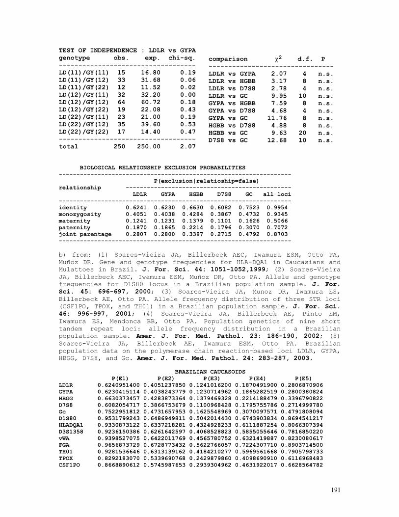
191
TEST OF INDEPENDENCE : LDLR vs GYPA genotype obs. exp. chi-sq. ----------------------------------- LD(11)/GY(11) 15 16.80 0.19 LD(11)/GY(12) 33 31.68 0.06 LD(11)/GY(22) 12 11.52 0.02 LD(12)/GY(11) 32 32.20 0.00 LD(12)/GY(12) 64 60.72 0.18 LD(12)/GY(22) 19 22.08 0.43 LD(22)/GY(11) 23 21.00 0.19 LD(22)/GY(12) 35 39.60 0.53 LD(22)/GY(22) 17 14.40 0.47 ----------------------------------- total 250 250.00 2.07
comparison χ2 d.f. P -------------------------------- LDLR vs GYPA 2.07 4 n.s. LDLR vs HGBB 3.17 8 n.s. LDLR vs D7S8 2.78 4 n.s. LDLR vs GC 9.95 10 n.s. GYPA vs HGBB 7.59 8 n.s. GYPA vs D7S8 4.68 4 n.s. GYPA vs GC 11.76 8 n.s. HGBB vs D7S8 4.88 8 n.s. HGBB vs GC 9.63 20 n.s. D7S8 vs GC 12.68 10 n.s.
BIOLOGICAL RELATIONSHIP EXCLUSION PROBABILITIES ------------------------------------------------------------------ P(exclusion|relatioship=false) relationship ----------------------------------------------- LDLR GYPA HGBB D7S8 GC all loci ------------------------------------------------------------------ identity 0.6241 0.6230 0.6630 0.6082 0.7523 0.9954 monozygosity 0.4051 0.4038 0.4284 0.3867 0.4732 0.9345 maternity 0.1241 0.1231 0.1379 0.1101 0.1626 0.5066 paternity 0.1870 0.1865 0.2214 0.1796 0.3070 0.7072 joint parentage 0.2807 0.2800 0.3397 0.2715 0.4792 0.8703 ------------------------------------------------------------------ b) from: (1) Soares-Vieira JA, Billerbeck AEC, Iwamura ESM, Otto PA, Muñoz DR. Gene and genotype frequencies for HLA-DQA1 in Caucasians and Mulattoes in Brazil. J. For. Sci. 44: 1051-1052,1999; (2) Soares-Vieira JA, Billerbeck AEC, Iwamura ESM, Muñoz DR, Otto PA. Allele and genotype frequencies for D1S80 locus in a Brazilian population sample. J. For. Sci. 45: 696-697, 2000; (3) Soares-Vieira JA, Munoz DR, Iwamura ES, Billerbeck AE, Otto PA. Allele frequency distribution of three STR loci (CSF1PO, TPOX, and TH01) in a Brazilian population sample. J. For. Sci. 46: 996-997, 2001; (4) Soares-Vieira JA, Billerbeck AE, Pinto EM, Iwamura ES, Mendonca BB, Otto PA. Population genetics of nine short tandem repeat loci: allele frequency distribution in a Brazilian population sample. Amer. J. For. Med. Pathol. 23: 186-190, 2002; (5) Soares-Vieira JA, Billerbeck AE, Iwamura ESM, Otto PA. Brazilian population data on the polymerase chain reaction-based loci LDLR, GYPA, HBGG, D7S8, and Gc. Amer. J. For. Med. Pathol. 24: 283-287, 2003. BRAZILIAN CAUCASOIDS P(E1) P(E2) P(E3) P(E4) P(E5) LDLR 0.6240951400 0.4051237850 0.1241016200 0.1870491900 0.2806870906 GYPA 0.6230415114 0.4038243779 0.1230714962 0.1865282519 0.2800380824 HBGG 0.6630373457 0.4283873364 0.1379469328 0.2214188479 0.3396790822 D7S8 0.6082054717 0.3866753679 0.1100968428 0.1795755786 0.2714999780 Gc 0.7522951812 0.4731657953 0.1625548969 0.3070097571 0.4791808094 D1S80 0.9531799243 0.6486949811 0.5042014430 0.6743903834 0.8694541217 HLADQA1 0.9330873122 0.6337218281 0.4324928233 0.6111887254 0.8066307394 D3S1358 0.9236150386 0.6261642597 0.4068528823 0.5855055646 0.7816850220 vWA 0.9398527075 0.6422011769 0.4565780752 0.6321419887 0.8230080617 FGA 0.9656873729 0.6728773432 0.5622766057 0.7224307710 0.8903714500 TH01 0.9281536646 0.6313139162 0.4184210277 0.5969561668 0.7905798733 TPOX 0.8292183070 0.5339690768 0.2429879860 0.4098690910 0.6116968483 CSF1PO 0.8668890612 0.5745987653 0.2939304962 0.4631922017 0.6628564782
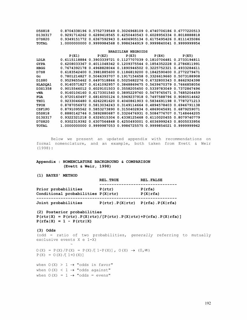
192
D5S818 0.8704338196 0.5752739549 0.3026968109 0.4740706186 0.6777220513 D13S317 0.9291714262 0.6289418565 0.4250440543 0.6028956334 0.8018888818 D7S820 0.9349151772 0.6367592943 0.4406905134 0.6175495426 0.8111435086 TOTAL 1.0000000000 0.9999984568 0.9986344919 0.9999840041 0.9999999954 BRAZILIAN NEGROIDS P(E1) P(E2) P(E3) P(E4) P(E5) LDLR 0.6115118884 0.3903339721 0.1127707039 0.1810706481 0.2733194811 GYPA 0.6208033367 0.4011048342 0.1209375544 0.1854352228 0.2786811991 HBGG 0.7674392178 0.4968828044 0.1890946502 0.3225752321 0.4933284611 D7S8 0.6183542400 0.3981885600 0.1186819200 0.1842590400 0.2772279471 Gc 0.7801214827 0.5046393707 0.1917154658 0.3326619660 0.5073188908 D1S80 0.9529655462 0.6497518866 0.5025682276 0.6732800343 0.8662924398 HLADQA1 0.9140571827 0.6141092957 0.3848869475 0.5639670379 0.7666858056 D3S1358 0.9015546012 0.6029101503 0.3558205450 0.5339783049 0.7372867496 vWA 0.9160106160 0.6173301540 0.3895229760 0.5679765671 0.7685204459 FGA 0.9720160497 0.6816050124 0.5969237918 0.7497588796 0.9080514642 TH01 0.9233046480 0.6262281620 0.4040861903 0.5834691198 0.7787271213 TPOX 0.8787056972 0.5813034243 0.3149114664 0.4894578403 0.6946791138 CSF1PO 0.8791095562 0.5853273890 0.3150402834 0.4869045691 0.6879259071 D5S818 0.8880142746 0.5892880687 0.3326476931 0.5084776707 0.7148444205 D13S317 0.9322321218 0.6326515304 0.4338125468 0.6110020455 0.8079740779 D7S820 0.9302319392 0.6307564848 0.4250493001 0.6036999243 0.8005033956 TOTAL 1.0000000000 0.9999987053 0.9986725575 0.9999854021 0.9999999962
Below we present an updated appendix with recommendations on formal nomenclature, and an example, both taken from Evett & Weir (1998): Appendix : NOMENCLATURE BACKGROUND & COMPARISON (Evett & Weir, 1998) (1) BAYES' METHOD REL.TRUE REL.FALSE -------------------------------- Prior probabilities P(rtr) P(rfa) Conditional probabilities P(X|rtr) P(X|rfa) ---------------------------------------------------------- Joint probabilities P(rtr).P(X|rtr) P(rfa).P(X|rfa) (2) Posterior probabilities P(rtr|X) = P(rtr).P(X|rtr)/[P(rtr).P(X|rtr)+P(rfa).P(X|rfa)] P(rfa|X) = 1 - P(rtr|X) (3) Odds (odd = ratio of two probabilities, generally referring to mutually exclusive events X e 1-X) ~
O(X) = P(X)/P(X) = P(X)/[1-P(X)], O(X) → (0,∞) P(X) = O(X)/[1+O(X)] when O(X) > 1 → "odds in favor" when O(X) < 1 → "odds against" when O(X) = 1 → "odds = evens"
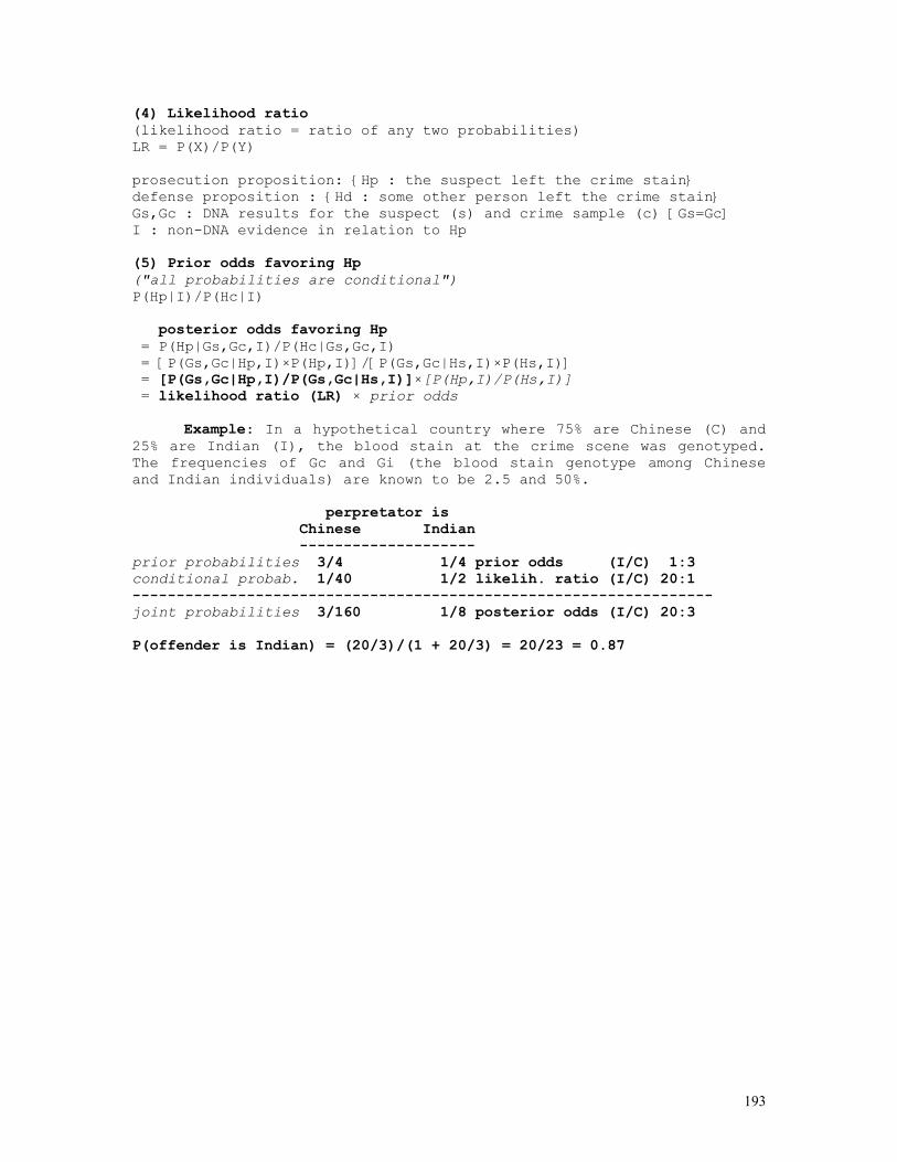
193
(4) Likelihood ratio (likelihood ratio = ratio of any two probabilities) LR = P(X)/P(Y) prosecution proposition: {Hp : the suspect left the crime stain} defense proposition : {Hd : some other person left the crime stain} Gs,Gc : DNA results for the suspect (s) and crime sample (c) [Gs=Gc] I : non-DNA evidence in relation to Hp (5) Prior odds favoring Hp ("all probabilities are conditional") P(Hp|I)/P(Hc|I) posterior odds favoring Hp = P(Hp|Gs,Gc,I)/P(Hc|Gs,Gc,I) = [P(Gs,Gc|Hp,I)×P(Hp,I)]/[P(Gs,Gc|Hs,I)×P(Hs,I)] = [P(Gs,Gc|Hp,I)/P(Gs,Gc|Hs,I)]×[P(Hp,I)/P(Hs,I)] = likelihood ratio (LR) × prior odds
Example: In a hypothetical country where 75% are Chinese (C) and 25% are Indian (I), the blood stain at the crime scene was genotyped. The frequencies of Gc and Gi (the blood stain genotype among Chinese and Indian individuals) are known to be 2.5 and 50%. perpretator is Chinese Indian -------------------- prior probabilities 3/4 1/4 prior odds (I/C) 1:3 conditional probab. 1/40 1/2 likelih. ratio (I/C) 20:1 ------------------------------------------------------------------ joint probabilities 3/160 1/8 posterior odds (I/C) 20:3 P(offender is Indian) = (20/3)/(1 + 20/3) = 20/23 = 0.87
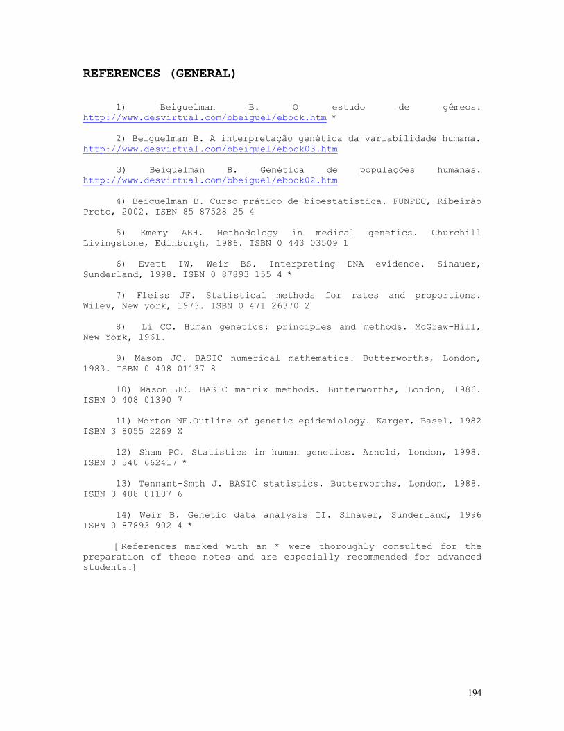
194
REFERENCES (GENERAL)
1) Beiguelman B. O estudo de gêmeos. http://www.desvirtual.com/bbeiguel/ebook.htm *
2) Beiguelman B. A interpretação genética da variabilidade humana.
http://www.desvirtual.com/bbeiguel/ebook03.htm 3) Beiguelman B. Genética de populações humanas. http://www.desvirtual.com/bbeiguel/ebook02.htm
4) Beiguelman B. Curso prático de bioestatística. FUNPEC, Ribeirão Preto, 2002. ISBN 85 87528 25 4
5) Emery AEH. Methodology in medical genetics. Churchill Livingstone, Edinburgh, 1986. ISBN 0 443 03509 1
6) Evett IW, Weir BS. Interpreting DNA evidence. Sinauer,
Sunderland, 1998. ISBN 0 87893 155 4 * 7) Fleiss JF. Statistical methods for rates and proportions.
Wiley, New york, 1973. ISBN 0 471 26370 2 8) Li CC. Human genetics: principles and methods. McGraw-Hill,
New York, 1961.
9) Mason JC. BASIC numerical mathematics. Butterworths, London, 1983. ISBN 0 408 01137 8
10) Mason JC. BASIC matrix methods. Butterworths, London, 1986. ISBN 0 408 01390 7
11) Morton NE.Outline of genetic epidemiology. Karger, Basel, 1982
ISBN 3 8055 2269 X
12) Sham PC. Statistics in human genetics. Arnold, London, 1998. ISBN 0 340 662417 *
13) Tennant-Smth J. BASIC statistics. Butterworths, London, 1988.
ISBN 0 408 01107 6 14) Weir B. Genetic data analysis II. Sinauer, Sunderland, 1996
ISBN 0 87893 902 4 * [References marked with an * were thoroughly consulted for the
preparation of these notes and are especially recommended for advanced students.]
195
CLASSICAL AND MODERN METHODOLOGY IN HUMAN GENETICS
(MÉTODOS CLÁSICOS Y MODERNOS PARA EL ANÁLISIS DE
DATOS EN GENÉTICA HUMANA)
PAULO A. OTTO
CLASS EXERCISES
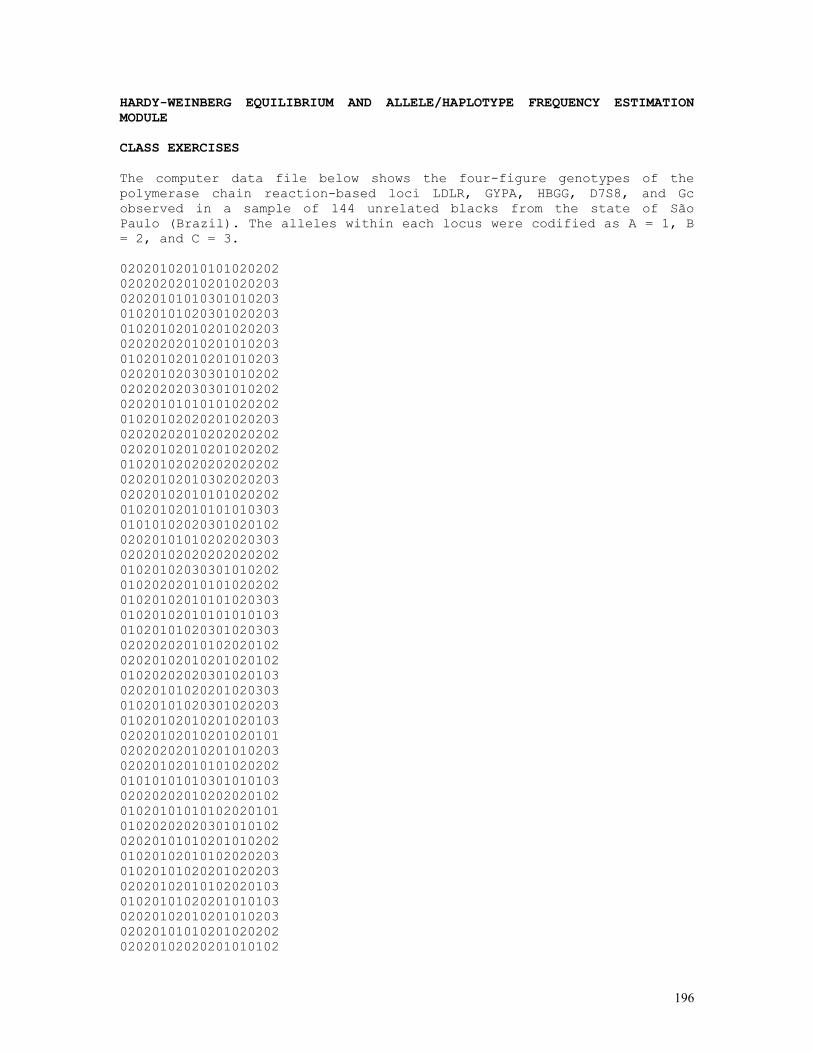
196
HARDY-WEINBERG EQUILIBRIUM AND ALLELE/HAPLOTYPE FREQUENCY ESTIMATION MODULE CLASS EXERCISES The computer data file below shows the four-figure genotypes of the polymerase chain reaction-based loci LDLR, GYPA, HBGG, D7S8, and Gc observed in a sample of 144 unrelated blacks from the state of São Paulo (Brazil). The alleles within each locus were codified as A = 1, B = 2, and C = 3. 02020102010101020202 02020202010201020203 02020101010301010203 01020101020301020203 01020102010201020203 02020202010201010203 01020102010201010203 02020102030301010202 02020202030301010202 02020101010101020202 01020102020201020203 02020202010202020202 02020102010201020202 01020102020202020202 02020102010302020203 02020102010101020202 01020102010101010303 01010102020301020102 02020101010202020303 02020102020202020202 01020102030301010202 01020202010101020202 01020102010101020303 01020102010101010103 01020101020301020303 02020202010102020102 02020102010201020102 01020202020301020103 02020101020201020303 01020101020301020203 01020102010201020103 02020102010201020101 02020202010201010203 02020102010101020202 01010101010301010103 02020202010202020102 01020101010102020101 01020202020301010102 02020101010201010202 01020102010102020203 01020101020201020203 02020102010102020103 01020101020201010103 02020102010201010203 02020101010201020202 02020102020201010102
197
01020102010302020102 02020102020301010203 02020102010202020202 01020102020302020202 01020102030301020202 02020101020301020102 01020101010301010203 01020202020201020202 01020102030301020103 01020101010301020202 02020101010101020102 02020101010201010202 02020202020301010202 02020101020301020202 02020101010101020202 01020102010301020202 02020102010201010203 02020102020302020202 02020102020201020202 02020102010202020303 02020102030301020102 02020101010101010202 02020102030301010202 02020101010201020303 01010102020201020102 01020101010201010202 01020102010301020102 01010101010301020203 02020101030301010102 02020202010101010202 01020101010102020103 02020101010302020202 01020202020201020303 02020101020301010203 02020102010302020202 02020102020301020102 02020101010301010103 02020102010301020202 01020102020302020202 02020102010102020303 01010102010202020203 02020102010301010203 02020101030301010202 01020101030301010102 01020202010201020102 01010102010201020203 02020102010201010202 02020102020201020102 02020102010201020203 01020101030301020202 01020102030301020203 01020101010301010202 02020102020201010103 01010102010301010203 02020202010201020202 01020102020301010303 02020102020301010202

198
02020102010301010103 02020202010101010202 01020202010302020203 01020102010201020202 02020102020301020202 02020102010101010102 01020102010101010203 02020101020301010203 02020101020301010102 01010202020201020102 02020102020301020102 01020102010102020202 02020102020301010101 01020102020202020203 02020102010201020202 01010102010101020202 02020102010301020202 01020101020301020203 01010101010201020102 01020101010101020102 02020101020301020102 02020102010202020203 01010102010201010102 02020202010301020202 01020202030301010203 02020202010102020203 02020202010101020202 01010102010101020101 01020102010101010203 01020102010201020103 02020101010101010203 02020101010301010103 01020102020202020203 01020102010201010102 02020101020201010103 01020202010202020202 01020102010101010101 01020102010101020202 01020202020301020203 02020102010202020202 01020102010302020102 (1) Using the data set above, estimate the allele frequencies (A and B for loci LDLR, GYPA, D7S8, and A, B and C for loci HBGG and GC) and their corresponding standard errors, under the assumptions of panmixia present and absent. Determine also the approximate (binomial) 95% confidence intervals of these estimates. Explain how "exact" (Bayesian) 95% credible intervals can be constructed from the corresponding likelihood functions. (2) Using the same data set, estimate the genotype frequencies for each locus and test if these frequencies are in Hardy-Weinberg ratios using the tests listed below (for the 2-allele cases; for the 3-allele cases perform just a chi-squared test without continuity correction): 2a. chi-squared tests with and without continuity correction;
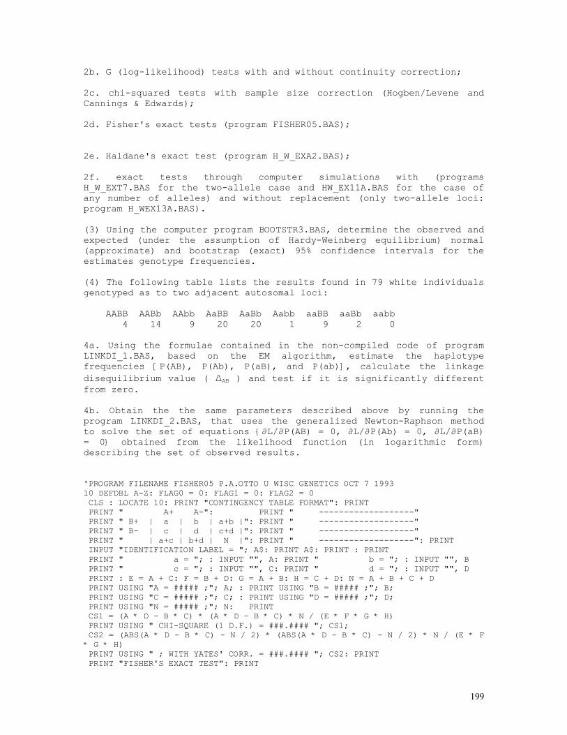
199
2b. G (log-likelihood) tests with and without continuity correction; 2c. chi-squared tests with sample size correction (Hogben/Levene and Cannings & Edwards); 2d. Fisher's exact tests (program FISHER05.BAS); 2e. Haldane's exact test (program H_W_EXA2.BAS); 2f. exact tests through computer simulations with (programs H_W_EXT7.BAS for the two-allele case and HW_EX11A.BAS for the case of any number of alleles) and without replacement (only two-allele loci: program H_WEX13A.BAS). (3) Using the computer program BOOTSTR3.BAS, determine the observed and expected (under the assumption of Hardy-Weinberg equilibrium) normal (approximate) and bootstrap (exact) 95% confidence intervals for the estimates genotype frequencies. (4) The following table lists the results found in 79 white individuals genotyped as to two adjacent autosomal loci: AABB AABb AAbb AaBB AaBb Aabb aaBB aaBb aabb 4 14 9 20 20 1 9 2 0 4a. Using the formulae contained in the non-compiled code of program LINKDI_1.BAS, based on the EM algorithm, estimate the haplotype frequencies [P(AB), P(Ab), P(aB), and P(ab)], calculate the linkage disequilibrium value ( ∆AB ) and test if it is significantly different from zero. 4b. Obtain the the same parameters described above by running the program LINKDI_2.BAS, that uses the generalized Newton-Raphson method to solve the set of equations {∂L/∂P(AB) = 0, ∂L/∂P(Ab) = 0, ∂L/∂P(aB) = 0} obtained from the likelihood function (in logarithmic form) describing the set of observed results. 'PROGRAM FILENAME FISHER05 P.A.OTTO U WISC GENETICS OCT 7 1993 10 DEFDBL A-Z: FLAG0 = 0: FLAG1 = 0: FLAG2 = 0 CLS : LOCATE 10: PRINT "CONTINGENCY TABLE FORMAT": PRINT PRINT " A+ A-": PRINT " -------------------" PRINT " B+ | a | b | a+b |": PRINT " -------------------" PRINT " B- | c | d | c+d |": PRINT " -------------------" PRINT " | a+c | b+d | N |": PRINT " -------------------": PRINT INPUT "IDENTIFICATION LABEL = "; A$: PRINT A$: PRINT : PRINT PRINT " a = "; : INPUT "", A: PRINT " b = "; : INPUT "", B PRINT " c = "; : INPUT "", C: PRINT " d = "; : INPUT "", D PRINT : E = A + C: F = B + D: G = A + B: H = C + D: N = A + B + C + D PRINT USING "A = ##### ;"; A; : PRINT USING "B = ##### ;"; B; PRINT USING "C = ##### ;"; C; : PRINT USING "D = ##### ;"; D; PRINT USING "N = ##### ;"; N: PRINT CS1 = (A * D - B * C) * (A * D - B * C) * N / (E * F * G * H) PRINT USING " CHI-SQUARE (1 D.F.) = ###.#### "; CS1; CS2 = (ABS(A * D - B * C) - N / 2) * (ABS(A * D - B * C) - N / 2) * N / (E * F * G * H) PRINT USING " ; WITH YATES' CORR. = ###.#### "; CS2: PRINT PRINT "FISHER'S EXACT TEST": PRINT
200
IF G > H THEN SWAP G, H: SWAP A, C: SWAP B, D IF E > F THEN SWAP E, F: SWAP A, B: SWAP C, D IF G > E THEN SWAP G, E: SWAP F, H: SWAP B, C IF A > B THEN SWAP A, B: SWAP C, D: SWAP E, F X1 = A: X2 = G: X3 = E: X4 = N: X0 = X1 - X3 * X2 / X4 IF X3 = X4 - X3 THEN FLAG2 = 1 IF X3 <= X4 - X3 THEN 520 ELSE 610 520 FLAG1 = 1: X20 = X4 - X3: X21 = X4: X22 = X2: GOSUB 690: GOSUB 760 IF X1 = 0 THEN 580 X25 = X1: GOSUB 800 580 PRINT USING "P(OBS.TAB.) = #.####"; X9: GOSUB 760: GOTO 860 610 X20 = X3: X21 = X4: X22 = X2: GOSUB 690: GOSUB 780 X25 = X2 - X1: GOSUB 800: PRINT USING "P(OBS.TAB.) = #.####"; X9 GOSUB 780: GOTO 860 690 X9 = 1: X25 = X22: X25 = X25 710 X9 = X9 * (X20 + 1 - X25) / (X21 + 1 - X25): X25 = X25 - 1 IF X25 <> 0 THEN 710 X24 = X9: RETURN 760 X5 = X2 + 1: X6 = X3 + 1: X7 = 0: X8 = X4 - X3 - X2: RETURN 780 X5 = X2 + 1: X6 = X4 - X3 + 1: X7 = 0: X8 = X3 - X2: RETURN 800 X25 = X25 810 X5 = X5 - 1: X6 = X6 - 1: X7 = X7 + 1: X8 = X8 + 1 X9 = X9 * X5 * X6 / (X7 * X8): X25 = X25 - 1: IF X25 <> 0 THEN 810 RETURN 860 X3 = X9: X9 = X24: X25 = X2: X1 = 0: X2 = 0 IF X24 <= X3 THEN X1 = X24: X25 = X25 890 X5 = X5 - 1: X6 = X6 - 1: X7 = X7 + 1: X8 = X8 + 1 X9 = X9 * X5 * X6 / (X7 * X8): IF X9 <= X3 THEN 970 IF FLAG2 = 1 THEN 1120 FLAG0 = 1 940 X25 = X25 - 1: IF X25 <> 0 THEN 890 IF FLAG1 = 1 THEN 1020 ELSE 1070 970 IF FLAG0 = 1 THEN 980 ELSE 1000 980 X2 = X2 + X9: GOTO 940 1000 X1 = X1 + X9: GOTO 940 1020 PRINT USING "X-E(X) = ########.####"; X0 PRINT USING "P(LOWER TAIL) = #.####"; X1 PRINT USING "P(UPPER TAIL) = #.####"; X2 PRINT USING "P( 2-TAILED ) = #.####"; X1 + X2: GOTO 1200 1070 PRINT USING "X-E(X) = ########.####"; X0 PRINT USING "P(LOWER TAIL) = #.####"; X2 PRINT USING "P(UPPER TAIL) = #.####"; X1 PRINT USING "P( 2-TAILED ) = #.####"; X1 + X2: GOTO 1200 1120 PRINT USING "X-E(X) = ########.####"; X0 PRINT USING "P(LOWER TAIL) = #.####"; X1 PRINT USING "P(UPPER TAIL) = #.####"; X1 PRINT USING "P( 2-TAILED ) = #.####"; 2 * X1 1200 PRINT : PRINT "DO YOU WANT TO RUN AGAIN THIS PROGRAM (Y/N) ?" 1220 ANSWER$ = INKEY$ IF ANSWER$ <> "Y" AND ANSWER$ <> "y" AND ANSWER$ <> "N" AND ANSWER$ <> "n" THEN 1220 IF ANSWER$ = "Y" OR ANSWER$ = "y" THEN RUN 10 CLS : LOCATE 10: END REM PROGRAM FILENAME H_W_EXA2.BAS CLS : DEFDBL A-Z INPUT "D, H, R = ", D, H, R N = D + H + R: P = 2 * D + H: Q = H + 2 * R DIM F(2 * N) FOR I = 1 TO 2 * N F(I) = F(I - 1) + LOG(I) NEXT I
201
IF P > Q THEN MAXPQ = P ELSE MAXPQ = Q SIZE = N / 2: DIM D1(SIZE), H1(SIZE), R1(SIZE), PROB1(SIZE) IF INT(H / 2) = H / 2 THEN HMIN = 0 ELSE HMIN = 1 IF D > R THEN HMAX = Q ELSE HMAX = P I = 0 FOR H9 = HMIN TO HMAX STEP 2 I = I + 1 H1 = H9: D1 = (P - H1) / 2: R1 = (Q - H1) / 2 PROB1(I) = F(N) - F(2 * N) + F(P) - F(D1) + F(Q) - F(R1) PROB1(I) = PROB1(I) + H1 * LOG(2) - F(H1) PROB1(I) = 100000 * INT(10000000000# * EXP(PROB1(I))) + H1 NEXT H9: NEWSIZE = I: GOSUB QUICKSORT PRINT " D H R Prob. Cum.Pr. Diseq. Chi-sq. P(C.-sq.)" PRINT " ------------------------------------------------------------" FOR I = 1 TO NEWSIZE PROB2 = PROB1(I) / 10 ^ 15: PROBT = PROBT + PROB2 H2 = INT(PROB1(I) - INT(PROB1(I) / 10 ^ 5) * 10 ^ 5) D2 = (P - H2) / 2: R2 = (Q - H2) / 2 DISEQ = D2 / N - (P / (2 * N)) ^ 2 CHISQ = (H2 ^ 2 - 4 * D2 * R2) ^ 2 * N / (P ^ 2 * Q ^ 2) GOSUB CHISQUAREDIST: P99 = 1 - J99 * K99 * L99 PRINT USING "#####"; D2; H2; R2; IF H2 = H THEN PRINT " * "; ELSE PRINT " "; PRINT USING " #.#### "; PROB2; PRINT USING " #.#### "; PROBT; PRINT USING " ##.####"; DISEQ; PRINT USING " ####.##"; CHISQ; PRINT USING " #.#### "; P99 DO: LOOP WHILE INKEY$ <> " " NEXT I PRINT " ------------------------------------------------------------" END QUICKSORT: D99 = 10: K = 1: L = 1: R99 = NEWSIZE 560 REM EXCHANGE SORT IF BLOCKSIZE <= D99 IF R99 - L + 1 > D99 THEN 590 GOSUB 900: GOTO 780 590 I = L: J = R99: W = RND(1) * (R99 - L) + .5 W = INT(W + L): F = PROB1(W) REM PARTITION PHASE 620 IF PROB1(I) >= F THEN 640 I = I + 1: GOTO 620 640 IF PROB1(J) <= F THEN 660 J = J - 1: GOTO 640 660 IF I > J THEN 680 W = PROB1(I): PROB1(I) = PROB1(J): PROB1(J) = W: I = I + 1: J = J - 1 680 IF I <= J THEN 620 REM BOOKKEEPING PHASE IF J - L >= R99 - I THEN 740 IF I >= R99 THEN 730 H99(K) = I: K = K + 1: H99(K) = R99: K = K + 1 730 R99 = J: GOTO 770 740 IF L >= J THEN 760 H99(K) = L: K = K + 1: H99(K) = J: K = K + 1 760 L = I 770 IF L < R99 THEN 590 780 IF K <= 1 THEN 800 K = K - 1: R99 = H99(K): K = K - 1: L = H99(K): GOTO 560 800 RETURN END 900 REM EXCHANGE SORT FOR I = L TO R99 - 1: K1 = I FOR J = I + 1 TO R99: IF PROB1(J) >= PROB1(K1) THEN 940
202
K1 = J 940 NEXT J IF K1 = I THEN 970 W = PROB1(I): PROB1(I) = PROB1(K1): PROB1(K1) = W 970 NEXT I RETURN CHISQUAREDIST: R99 = 1: V99 = 1: W99 = CHISQ K99 = W99 ^ (INT((V99 + 1) / 2)) * EXP(-W99 / 2) / R99 IF INT(V99 / 2) = V99 / 2 THEN GOTO LABEL1 J99 = SQR(2 / W99 / 3.141592653599#): GOTO LABEL2 LABEL1: J99 = 1 LABEL2: L99 = 1: M99 = 1 CHILOOP: V99 = V99 + 2: M99 = M99 * W99 / V99: IF M99 < .0000001 THEN RETURN L99 = L99 + M99: GOTO CHILOOP RETURN REM PROGRAM FILENAME H_W_EXT7.BAS DEFDBL A-Z: CLS INPUT "D, H, R = "; D, H, R: N = D + H + R INPUT "NUMBER OF SIMULATIONS = "; T INPUT "FILE NAME FOR STORING DATA (DRIVE:FILENAME.EXT) = "; FILENAME$ CLS : OPEN FILENAME$ FOR OUTPUT AS #1 PRINT #1, FILENAME$ P = 2 * D + H: Q = H + 2 * R: P0 = P / (2 * N): P1 = P: Q1 = Q PRINT #1, D, H, R, N, P0, T TIMEWA$ = TIME$ TIMEWAS = VAL(MID$(TIMEWA$, 1, 2)) * 3600 + VAL(MID$(TIMEWA$, 4, 2)) * 60 TIMEWAS = TIMEWAS + VAL(MID$(TIMEWA$, 7, 2)) D1 = D: H1 = H: R1 = R K = N: GOSUB FACTORIAL: NFAC = FACT K = 2 * N: GOSUB FACTORIAL: N2FAC = FACT CONSTFAC = NFAC - N2FAC: D1 = D: H1 = H: R1 = R: GOSUB FACTPQDHR PROB2 = EXP(CONSTFAC + PFAC + QFAC - DFAC - HFAC - RFAC + H1 * LOG(2)) FOR I = 1 TO T R1 = 0: D1 = 0: H1 = 0 FOR INDIV = 1 TO N A = RND(1): B = RND(1) IF A < P0 AND B < P0 THEN D1 = D1 + 1: GOTO NEXTINDIV IF A >= P0 AND B >= P0 THEN R1 = R1 + 1: GOTO NEXTINDIV H1 = H1 + 1 NEXTINDIV: NEXT INDIV P1 = 2 * D1 + H1: Q1 = H1 + 2 * R1 D1TOT = D1TOT + D1: H1TOT = H1TOT + H1: R1TOT = R1TOT + R1 PTOT = PTOT + P1 / (2 * N) GOSUB FACTPQDHR PROB1 = EXP(CONSTFAC + PFAC + QFAC - DFAC - HFAC - RFAC + H1 * LOG(2)) IF PROB1 <= PROB2 THEN PROBT = PROBT + 1 PRINT #1, P1, H1 LOCATE 6: PRINT USING "PERFORMING SIMULATION NO. ##### "; I; PRINT USING "OUT OF #####"; T NEXT I CLOSE #1 TIMENO$ = TIME$ TIMENOW = VAL(MID$(TIMENO$, 1, 2)) * 3600 + VAL(MID$(TIMENO$, 4, 2)) * 60 TIMENOW = TIMENOW + VAL(MID$(TIMENO$, 7, 2)) CLS : PRINT "NO. OF SIMULATED SAMPLES OF SIZE "; N; " = "; T PRINT "TOTAL ELAPSED TIME (ALL CALCULATIONS) = "; TIMENOW - TIMEWAS; " SEC." PRINT "DATA FROM DATAFILE "; FILENAME$: PRINT PRINT USING "SAMPLE P = #.####"; P0 PRINT USING "SAMPLE D = #####.####"; D PRINT USING "SAMPLE H = #####.####"; H PRINT USING "SAMPLE R = #####.####"; R: PRINT

203
PRINT USING "P MEAN = #.####"; PTOT / T PRINT USING "OBS.D MEAN = #####.####"; D1TOT / T PRINT USING "OBS.H MEAN = #####.####"; H1TOT / T PRINT USING "OBS.R MEAN = #####.####"; R1TOT / T: PRINT PRINT USING "EX. PROB. = #.####"; PROBT / T DO: LOOP WHILE INKEY$ <> " " END FACTPQDHR: K = P1: GOSUB FACTORIAL: PFAC = FACT K = Q1: GOSUB FACTORIAL: QFAC = FACT K = D1: GOSUB FACTORIAL: DFAC = FACT K = H1: GOSUB FACTORIAL: HFAC = FACT K = R1: GOSUB FACTORIAL: RFAC = FACT: RETURN FACTORIAL: FACT = 0: FOR J = 1 TO K: FACT = FACT + LOG(J): NEXT J: RETURN REM PROGRAM FILENAME HW_EX11A.BAS REM 'EXACT' HARDY-WEINBERG TEST FOR ANY NUMBER OF AUTOSOMAL ALLELES CLS : DEFDBL A-Z: INPUT "NUMBER OF ALLELES = "; K DIM P(K), SP(K), GENOTYPE(K, K), TGENOTYP(K, K), ALLELE(K), TALLEL(K) INPUT "NUMBER OF SIMULATIONS = "; T FOR I = 1 TO K: FOR J = I TO K PRINT USING "N(###"; I; : PRINT ","; : PRINT USING "###) = "; J; INPUT GENOTYPE(I, J): N = N + GENOTYPE(I, J) ALLELE(I) = ALLELE(I) + GENOTYPE(I, J) ALLELE(J) = ALLELE(J) + GENOTYPE(I, J): NEXT J, I: CLS FOR I = 1 TO K: P(I) = ALLELE(I) / (2 * N): NEXT I FOR I = 1 TO K: PRINT USING "ALLELE(###) = "; I; PRINT USING " #####"; ALLELE(I) FOR J = I TO K: PRINT USING "GENOT(###"; I; : PRINT ","; PRINT USING "###) = "; J; : PRINT USING "####"; GENOTYPE(I, J) 'DO: LOOP WHILE INKEY$ <> " " NEXT J, I PRINT USING "N = ######"; N DO: LOOP WHILE INKEY$ <> " " CLS TIMEWA$ = TIME$ TIMEWAS = VAL(MID$(TIMEWA$, 1, 2)) * 3600 + VAL(MID$(TIMEWA$, 4, 2)) * 60 TIMEWAS = TIMEWAS + VAL(MID$(TIMEWA$, 7, 2)) K9 = N: GOSUB FACTORIAL: NFAC = FACT K9 = 2 * N: GOSUB FACTORIAL: N2FAC = FACT CONSTFAC = NFAC - N2FAC GOSUB EXACTPROBCALC: PROB2 = EXPROB FOR I = 1 TO K: SSP = SSP + P(I): SP(I) = SP(I) + SSP: NEXT I FOR I = 1 TO T GOSUB CLEARALLVAR FOR INDIV = 1 TO N A = RND(1): B = RND(1) FOR I88 = 1 TO K IF A > SP(I88 - 1) AND A <= SP(I88) THEN AI88 = I88: ALLELE(I88) = ALLELE(I88) + 1 TALLEL(I88) = TALLEL(I88) + 1 END IF IF B > SP(I88 - 1) AND B <= SP(I88) THEN BI88 = I88: ALLELE(I88) = ALLELE(I88) + 1 TALLEL(I88) = TALLEL(I88) + 1 END IF NEXT I88 IF AI88 > BI88 THEN SWAP AI88, BI88 GENOTYPE(AI88, BI88) = GENOTYPE(AI88, BI88) + 1 TGENOTYP(AI88, BI88) = TGENOTYP(AI88, BI88) + 1 NEXT INDIV GOSUB EXACTPROBCALC: PROB1 = EXPROB IF PROB1 <= PROB2 THEN PROBT = PROBT + 1

204
LOCATE 10: PRINT "SIMULATION NO. "; I NEXT I 'DO: LOOP WHILE INKEY$ <> " " CLS TIMENO$ = TIME$ TIMENOW = VAL(MID$(TIMENO$, 1, 2)) * 3600 + VAL(MID$(TIMENO$, 4, 2)) * 60 TIMENOW = TIMENOW + VAL(MID$(TIMENO$, 7, 2)) PRINT "OVERALL RESULTS BASED ON "; T; " SIMULATIONS OF SIZE "; N; " INDIVIDUALS" PRINT "TOTAL ELAPSED TIME (ALL CALCULATIONS) = "; TIMENOW - TIMEWAS; " SEC." FOR I77 = 1 TO K PRINT USING "ALLELE(###) = "; I77; : PRINT USING "#####.####"; TALLEL(I77) / T FOR J77 = I77 TO K PRINT USING "GENOTYPE(###"; I77; : PRINT ","; PRINT USING "###) = "; J77; : PRINT USING "#####.####"; TGENOTYP(I77, J77) / T 'DO: LOOP WHILE INKEY$ <> " " NEXT J77, I77 PRINT : PRINT USING "EXACT PROB. = #.####"; PROBT / T END CLEARALLVAR: HETLOG = 0: ALLELFAC = 0: GENOTFAC = 0 FOR I66 = 1 TO K ALLELE(I66) = 0 FOR J66 = I66 TO K: GENOTYPE(I66, J66) = 0 NEXT J66, I66 RETURN EXACTPROBCALC: GOSUB FACTALLEL: GOSUB FACTGENOT FOR I9 = 1 TO K - 1: FOR J9 = I9 + 1 TO K IF I9 <> J9 THEN HETLOG = HETLOG + GENOTYPE(I9, J9) * LOG(2) NEXT J9, I9 EXPROB = EXP(CONSTFAC + ALLELFAC - GENOTFAC + HETLOG) RETURN FACTALLEL: FOR I9 = 1 TO K K9 = ALLELE(I9): GOSUB FACTORIAL: ALLELFAC = ALLELFAC + FACT NEXT I9 RETURN FACTGENOT: FOR I9 = 1 TO K: FOR J9 = I9 TO K K9 = GENOTYPE(I9, J9): GOSUB FACTORIAL: GENOTFAC = GENOTFAC + FACT NEXT J9, I9 RETURN FACTORIAL: FACT = 0 FOR J = 1 TO K9 FACT = FACT + LOG(J) NEXT J RETURN REM PROGRAM FILENAME H_WEX13A.BAS REM 'EXACT' HARDY-WEINBERG TEST (TWO AUTOSOMAL ALLELES) REM GENERATES T RANDOM SAMPLES OF SIZE N = D + H + R REM WITH GENOTYPE PROBABILITIES d = p^2, h = 2pq, r = q^2 REM p = (2D+H)/2, q = 1-p REM WITHOUT REPLACEMENT DEFDBL A-Z: CLS DIM H99(100) INPUT "D, H, R = "; D, H, R: N = D + H + R: P = 2 * D + H: DIM NH(P + 2), PROB1(P + 2), AUX(P + 2) INPUT "NUMBER OF SIMULATIONS = "; T
205
CLS FOR I = 1 TO T INDIV = 0: R1 = 0: D1 = 0: H1 = 0: N1 = N: P1 = P DO WHILE INDIV < N A = RND(1): B = RND(1): GENOT = 3 IF A < P1 / (2 * N1) AND B < (P1 - 1) / (2 * N1 - 1) THEN GENOT = 2 IF A >= P1 / (2 * N1) AND B >= P1 / (2 * N1 - 1) THEN GENOT = 0 IF GENOT = 3 THEN GENOT = 1 N1 = N1 - 1: P1 = P1 - GENOT SELECT CASE GENOT CASE 0: R1 = R1 + 1 CASE 2: D1 = D1 + 1 CASE 1: H1 = H1 + 1 END SELECT INDIV = INDIV + 1 LOOP D1TOT = D1TOT + D1: H1TOT = H1TOT + H1: R1TOT = R1TOT + R1 PTOT = PTOT + 2 * D1 + H1: NH(H1) = NH(H1) + 1 LOCATE 6: PRINT USING "PERFORMING SIMULATION NO. ##### "; I; PRINT USING "OUT OF #####"; T NEXT I: PRINT PRINT USING "SAMPLE P = #.####"; P / (2 * N) PRINT USING "SAMPLE D = #####.####"; D PRINT USING "SAMPLE H = #####.####"; H PRINT USING "SAMPLE R = #####.####"; R: PRINT PRINT USING "SIM.P MEAN = #.####"; PTOT / (2 * T * N) PRINT USING "SIM.D MEAN = #####.####"; D1TOT / T PRINT USING "SIM.H MEAN = #####.####"; H1TOT / T PRINT USING "SIM.R MEAN = #####.####"; R1TOT / T: PRINT FOR I = 0 TO P + 1 IF NH(I) <> 0 THEN PROB1(I) = NH(I): AUX(I) = I END IF NEXT I GOSUB QUICKSORT PRINT " D H R f(x) F(x)" PRINT "-----------------------------" FOR H1 = 0 TO P + 1 IF PROB1(H1) <> 0 THEN AC = AC + PROB1(H1) / T PRINT USING "#### "; (P - AUX(H1)) / 2; AUX(H1); N - (P + AUX(H1)) / 2; IF AUX(H1) = H THEN PRINT "*"; ELSE PRINT " "; PRINT USING " #.###"; PROB1(H1) / T; PRINT USING " #.###"; AC END IF NEXT H1 PRINT "-----------------------------" END QUICKSORT: D99 = 10: K = 1: L = 1: R99 = P + 1 560 REM EXCHANGE SORT IF BLOCKSIZE <= D99 IF R99 - L + 1 > D99 THEN 590 GOSUB 900: GOTO 780 590 I = L: J = R99: W = RND(1) * (R99 - L) + .5 W = INT(W + L): F = PROB1(W) REM PARTITION PHASE 620 IF PROB1(I) >= F THEN 640 I = I + 1: GOTO 620 640 IF PROB1(J) <= F THEN 660 J = J - 1: GOTO 640 660 IF I > J THEN 680 W = PROB1(I): PROB1(I) = PROB1(J): PROB1(J) = W
206
W = AUX(I): AUX(I) = AUX(J): AUX(J) = W: I = I + 1: J = J - 1 680 IF I <= J THEN 620 REM BOOKKEEPING PHASE IF J - L >= R99 - I THEN 740 IF I >= R99 THEN 730 H99(K) = I: K = K + 1: H99(K) = R99: K = K + 1 730 R99 = J: GOTO 770 740 IF L >= J THEN 760 H99(K) = L: K = K + 1: H99(K) = J: K = K + 1 760 L = I 770 IF L < R99 THEN 590 780 IF K <= 1 THEN 800 K = K - 1: R99 = H99(K): K = K - 1: L = H99(K): GOTO 560 800 RETURN 900 REM EXCHANGE SORT FOR I = L TO R99 - 1: K1 = I FOR J = I + 1 TO R99: IF PROB1(J) >= PROB1(K1) THEN 940 K1 = J 940 NEXT J IF K1 = I THEN 970 W = PROB1(I): PROB1(I) = PROB1(K1): PROB1(K1) = W W = AUX(I): AUX(I) = AUX(K1): AUX(K1) = W 970 NEXT I RETURN REM PROGRAM FILENAME BOOTSTR3.BAS REM BOOTSTRAP 95% CONFIDENCE INTERVALS FOR GENOTYPE FREQUENCIES REM BASED ON 1000 SIMULATED POINTS FOR EACH GENOTYPE CLS : DEFDBL A-Z: INPUT "NUMBER OF ALLELES = "; K: T = 1000 DIM P(T), GENOTYPE(K, K), ALLELE(K), H88(25) FOR I = 1 TO K: FOR J = I TO K PRINT USING "N(###"; I; : PRINT ","; : PRINT USING "###) = "; J; INPUT GENOTYPE(I, J): N = N + GENOTYPE(I, J) ALLELE(I) = ALLELE(I) + GENOTYPE(I, J) ALLELE(J) = ALLELE(J) + GENOTYPE(I, J) NEXT J, I: CLS FOR I = 1 TO K: PRINT USING "ALLELE(###) = "; I; PRINT USING " #####"; ALLELE(I) Q(I) = ALLELE(I) / (2 * N) FOR J = I TO K: PRINT USING "P(###"; I; : PRINT ","; PRINT USING "###) = "; J; : PRINT USING "####"; GENOTYPE(I, J) DO: LOOP WHILE INKEY$ <> " " NEXT J, I PRINT USING "N = ######"; N: PRINT DO: LOOP WHILE INKEY$ <> " " PRINT " 95 % P confidence interval" PRINT "GENOTYPE P normal bootstrap" PRINT "-----------------------------------------------------" FOR I = 1 TO K: FOR J = I TO K P = GENOTYPE(I, J) / N PRINT USING " #"; I; : PRINT "/"; : PRINT USING "# "; J; PRINT USING " obs. #.### "; P; PRINT USING "{#.###"; P - 1.96 * SQR(P * (1 - P) / N); : PRINT ","; PRINT USING "#.###} "; P + 1.96 * SQR(P * (1 - P) / N); RANDOMIZE TIMER: FOR I99 = 1 TO T: P(I99) = 0 FOR INDIV = 1 TO N A = RND: IF A <= P THEN P(I99) = P(I99) + 1 / N NEXT INDIV NEXT I99 GOSUB SORTVALUES PRINT USING "{#.###"; P(26); : PRINT ","; PRINT USING "#.###}"; P(975)
207
IF I = J THEN EXGE = Q(I) * Q(J) SEEX = SQR(4 * Q(I) ^ 3 * (1 - Q(I)) / (2 * N)) ELSE EXGE = 2 * Q(I) * Q(J) SEEX = SQR(4 * Q(I) * Q(J) * (Q(I) + Q(J) - 4 * Q(I) * Q(J)) / (2 * N)) END IF PRINT USING " exp. #.### "; EXGE; PRINT USING "{#.###"; EXGE - 1.96 * SEEX; : PRINT ","; PRINT USING "#.###} "; EXGE + 1.96 * SEEX; FOR I99 = 1 TO T: QI = 0: QJ = 0 FOR INDIV = 1 TO N B = RND IF B <= Q(I) THEN QI = QI + 1 IF B > Q(I) AND B <= Q(I) + Q(J) THEN QJ = QJ + 1 C = RND IF C <= Q(I) THEN QI = QI + 1 IF C > Q(I) AND C <= Q(I) + Q(J) THEN QJ = QJ + 1 NEXT INDIV QI = QI / (2 * N): QJ = QJ / (2 * N) IF I = J THEN P(I99) = QI ^ 2 ELSE P(I99) = 2 * QI * QJ NEXT I99 GOSUB SORTVALUES PRINT USING "{#.###"; P(26); : PRINT ","; PRINT USING "#.###}"; P(975) 'DO: LOOP WHILE INKEY$ <> " " NEXT J, I PRINT "-----------------------------------------------------" END SORTVALUES: D88 = 10: K88 = 1: L88 = 1: R88 = T 560 REM EXCHANGE SORT IF BLOCKSIZE <= D88 IF R88 - L88 + 1 > D88 THEN 590 GOSUB 900: GOTO 780 590 I88 = L88: J88 = R88: W88 = RND(1) * (R88 - L88) + .5 W88 = INT(W88 + L88): F88 = P(W88) REM PARTITION PHASE 620 IF P(I88) >= F88 THEN 640 I88 = I88 + 1: GOTO 620 640 IF P(J88) <= F88 THEN 660 J88 = J88 - 1: GOTO 640 660 IF I88 > J88 THEN 680 W88 = P(I88): P(I88) = P(J88): P(J88) = W88: I88 = I88 + 1: J88 = J88 - 1 680 IF I88 <= J88 THEN 620 REM BOOKKEEPING PHASE IF J88 - L88 >= R88 - I88 THEN 740 IF I88 >= R88 THEN 730 H88(K88) = I88: K88 = K88 + 1: H88(K88) = R88: K88 = K88 + 1 730 R88 = J88: GOTO 770 740 IF L88 >= J88 THEN 760 H88(K88) = L88: K88 = K88 + 1: H88(K88) = J88: K88 = K88 + 1 760 L88 = I88 770 IF L88 < R88 THEN 590 780 IF K88 <= 1 THEN 800 K88 = K88 - 1: R88 = H88(K88): K88 = K88 - 1: L88 = H88(K88): GOTO 560 800 RETURN 900 REM EXCHANGE SORT FOR I88 = L88 TO R88 - 1: K1 = I88 FOR J88 = I88 + 1 TO R88: IF P(J88) >= P(K1) THEN 940 K1 = J88 940 NEXT J88 IF K1 = I88 THEN 970 W88 = P(I88): P(I88) = P(K1): P(K1) = W88

208
970 NEXT I88 RETURN REM PROGRAM FILENAME LINKDI_1.BAS REM EM ALGORITHM P. A. OTTO DEFDBL A-Z: CLS INPUT "N(AABB) = "; n1: INPUT "N(AABb) = "; n2: INPUT "N(AAbb) = "; n3 INPUT "N(AaBB) = "; n4: INPUT "N(AaBb) = "; n5: INPUT "N(Aabb) = "; n6 INPUT "N(aaBB) = "; n7: INPUT "N(aaBb) = "; n8: INPUT "N(aabb) = "; n9 CLS N = n1 + n2 + n3 + n4 + n5 + n6 + n7 + n8 + n9 PAA = (n1 + n2 + n3) / N: PBB = (n1 + n4 + n7) / N PA = (2 * (n1 + n2 + n3) + n4 + n5 + n6) / (2 * N): QA = 1 - PA PB = (2 * (n1 + n4 + n7) + n2 + n5 + n8) / (2 * N): QB = 1 - PB PRINT USING "N(AABB) = #####"; n1: PRINT USING "N(AABb) = #####"; n2 PRINT USING "N(AAbb) = #####"; n3: PRINT USING "N(AaBB) = #####"; n4 PRINT USING "N(AaBb) = #####"; n5: PRINT USING "N(Aabb) = #####"; n6 PRINT USING "N(aaBB) = #####"; n7: PRINT USING "N(aaBb) = #####"; n8 PRINT USING "N(aabb) = #####"; n9 PRINT USING "N = #####"; N: PRINT PRINT USING "P(A) = #.#####"; PA: PRINT USING "P(a) = #.#####"; QA PRINT USING "P(B) = #.#####"; PB: PRINT USING "P(b) = #.#####"; QB PRINT : PRINT " P(AB) P(Ab) P(aB) P(ab) D(AB)" X1 = PA * PB: X2 = PA * QB: X3 = QA * PB: X4 = QA * QB: I = 0 LOOPNUMBERONE: X = X1 * X4 / (X1 * X4 + X2 * X3) DAB = X1 - PA * PB PRINT USING "## "; I; : PRINT USING "#.##### "; X1; X2; X3; X4; DAB X11 = (2 * n1 + n2 + n4 + n5 * X) / (2 * N) X21 = (n2 + 2 * n3 + n5 * (1 - X) + n6) / (2 * N) X31 = (n4 + n5 * (1 - X) + 2 * n7 + n8) / (2 * N) X41 = (n5 * X + n6 + n8 + 2 * n9) / (2 * N) REM X21 = PA - X11: X31 = PB - X11: X41 = 1 - X11 - X21 - X31 XN = X11 * X41 / (X11 * X41 + X21 * X31) IF ABS(X - XN) <= .0000001# THEN PRINT PRINT USING "chi-sq.(1 d.f.) = ##.###"; N * DAB ^ 2 / (PA * QA * PB * QB) END ELSE X1 = X11: X2 = X21: X3 = X31: X4 = X41 I = I + 1: GOTO LOOPNUMBERONE END IF REM PROGRAM FILENAME LINKDI_2.BAS DIM A(3, 3), B(3, 3), C(3) CLS : LOCATE 10 INPUT "N(AABB) = "; N1: INPUT "N(AABb) = "; N2: INPUT "N(AAbb) = "; N3 INPUT "N(AaBB) = "; N4: INPUT "N(AaBb) = "; N5: INPUT "N(Aabb) = "; N6 INPUT "N(aaBB) = "; N7: INPUT "N(aaBb) = "; N8: INPUT "N(aabb) = "; N9 CLS N = N1 + N2 + N3 + N4 + N5 + N6 + N7 + N8 + N9 X1 = 2 * N1 + N2 + N4: X2 = N2 + 2 * N3 + N6 X3 = N4 + 2 * N7 + N8: X4 = N6 + N8 + 2 * N9 PRINT PRINT USING "N(AABB) = ######"; N1 PRINT USING "N(AABb) = ######"; N2 PRINT USING "N(AAbb) = ######"; N3 PRINT USING "N(AaBB) = ######"; N4 PRINT USING "N(AaBb) = ######"; N5 PRINT USING "N(Aabb) = ######"; N6 PRINT USING "N(aaBB) = ######"; N7
209
PRINT USING "N(aaBb) = ######"; N8 PRINT USING "N(aabb) = ######"; N9: PRINT PRINT USING "N = ######"; N PRINT P3 = (2 * (N1 + N2 + N3) + N4 + N5 + N6) / (2 * N): Q3 = 1 - P3 P4 = (2 * (N1 + N4 + N7) + N2 + N5 + N8) / (2 * N): Q4 = 1 - P4 PRINT USING "P(A) = #.#####"; P3 PRINT USING "P(a) = #.#####"; Q3 PRINT USING "P(B) = #.#####"; P4 PRINT USING "P(b) = #.#####"; Q4: PRINT P = (X1 - X2 - X3 + X4) / (4 * N) + 1 / 2 - Q3 * Q4 240 F1 = X1 / P - X2 / (P3 - P) - X3 / (P4 - P) + X4 / (1 - P3 - P4 + P) F1 = F1 + N5 * (1 + 4 * P - 2 * (P3 + P4)) / (P * (1 - P3 - P4 + P) + (P3 - P) * (P4 - P)) F2 = X1 / P ^ 2 + X2 / (P3 - P) ^ 2 + X3 / (P4 - P) ^ 2 + X4 / (1 - P3 - P4 + P) ^ 2 F2 = F2 + N5 * ((1 + 4 * P - 2 * (P3 + P4)) / (P * (1 - P3 - P4 + P) + (P3 - P) * (P4 - P))) ^ 2 F2 = F2 - 4 * N5 / (P * (1 - P3 - P4 + P) + (P3 - P) * (P4 - P)) P1 = P + F1 / F2 IF ABS(P1 - P) < .00001 THEN 310 ELSE P = P1: GOTO 240 310 P = P1: Q = P3 - P: R = P4 - P: S = Q3 - R 320 C(1) = X1 / P + N5 * (S - P) / (P * S + Q * R) - X4 / S C(2) = X2 / Q + N5 * (R - P) / (P * S + Q * R) - X4 / S C(3) = X3 / R + N5 * (Q - P) / (P * S + Q * R) - X4 / S A(1, 1) = X1 / P ^ 2 + X4 / S ^ 2 + N5 * (P ^ 2 + 2 * Q * R + S ^ 2) / (P * S + Q * R) ^ 2 A(2, 2) = X2 / Q ^ 2 + X4 / S ^ 2 + N5 * (R - P) ^ 2 / (P * S + Q * R) ^ 2 A(3, 3) = X3 / R ^ 2 + X4 / S ^ 2 + N5 * (Q - P) ^ 2 / (P * S + Q * R) ^ 2 A(1, 2) = X4 / S ^ 2 + N5 * (P ^ 2 - P * R + Q * R + R * S) / (P * S + Q * R) ^ 2 A(1, 3) = X4 / S ^ 2 + N5 * (P ^ 2 - P * Q + Q * R + Q * S) / (P * S + Q * R) ^ 2 A(2, 3) = X4 / S ^ 2 + N5 * P * (2 * P - 1) / (P * S + Q * R) ^ 2 A(2, 1) = A(1, 2): A(3, 1) = A(1, 3): A(3, 2) = A(2, 3) GOSUB MATRINV V = 0: FOR I = 1 TO 3: FOR J = 1 TO 3: V = V + B(I, J): NEXT J: NEXT I P1 = P + B(1, 1) * C(1) + B(1, 2) * C(2) + B(1, 3) * C(3) Q1 = Q + B(2, 1) * C(1) + B(2, 2) * C(2) + B(2, 3) * C(3) R1 = R + B(3, 1) * C(1) + B(3, 2) * C(2) + B(3, 3) * C(3): S1 = 1 - P1 - Q1 - R1: W9 = 9.999999999999999D-12 IF ABS(P1 - P) < W9 AND ABS(Q1 - Q) < W9 AND ABS(R1 - R) < W9 THEN 490 P = P1: Q = Q1: R = R1: S = S1: GOTO 320 490 PRINT USING "P(AB) = #.#####"; P1 PRINT USING "P(Ab) = #.#####"; Q1 PRINT USING "P(aB) = #.#####"; R1 PRINT USING "P(ab) = #.#####"; S1 PRINT : PRINT USING "var[P(AB)] = #.#########"; B(1, 1) PRINT USING "var[P(Ab)] = #.#########"; B(2, 2) PRINT USING "var[P(aB)] = #.#########"; B(3, 3) PRINT USING "var[P(ab)] = #.#########"; V: PRINT : D1 = P1 - P3 * P4 PRINT USING "LINKAGE DISEQUILIBRIUM VALUE = #.#####"; D1: PRINT END 5000 MATRINV: 5010 FOR J = 1 TO 3 5020 B(J, J) = 1 5030 NEXT J 5040 FOR J = 1 TO 3 5050 I = J - 1 5060 I = I + 1 5070 IF A(I, J) <> 0 THEN 5090 5080 GOTO 5060 5090 FOR K = 1 TO 3
210
5100 SWAP A(J, K), A(I, K) 5110 SWAP B(J, K), B(I, K) 5120 NEXT K 5130 TT = 1 / A(J, J) 5140 FOR K = 1 TO 3 5150 A(J, K) = TT * A(J, K) 5160 B(J, K) = TT * B(J, K) 5170 NEXT K 5180 FOR L = 1 TO 3 5190 IF L = J THEN 5250 5200 TT = -A(L, J) 5210 FOR K = 1 TO 3 5220 A(L, K) = A(L, K) + TT * A(J, K) 5230 B(L, K) = B(L, K) + TT * B(J, K) 5240 NEXT K 5250 NEXT L 5260 NEXT J 5270 RETURN
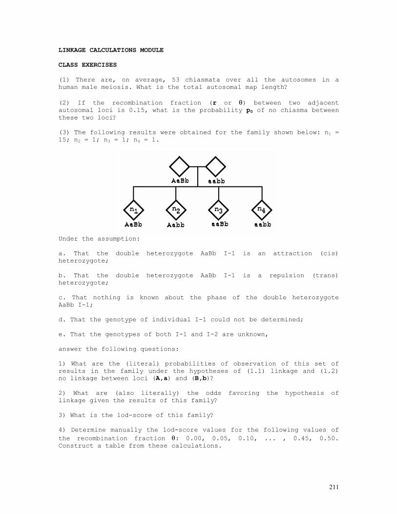
211
LINKAGE CALCULATIONS MODULE CLASS EXERCISES (1) There are, on average, 53 chiasmata over all the autosomes in a human male meiosis. What is the total autosomal map length? (2) If the recombination fraction (r or θ) between two adjacent autosomal loci is 0.15, what is the probability p0 of no chiasma between these two loci? (3) The following results were obtained for the family shown below: n1 = 15; n2 = 1; n3 = 1; n4 = 1.
Under the assumption: a. That the double heterozygote AaBb I-1 is an attraction (cis) heterozygote; b. That the double heterozygote AaBb I-1 is a repulsion (trans) heterozygote; c. That nothing is known about the phase of the double heterozygote AaBb I-1; d. That the genotype of individual I-1 could not be determined; e. That the genotypes of both I-1 and I-2 are unknown, answer the following questions: 1) What are the (literal) probabilities of observation of this set of results in the family under the hypotheses of (1.1) linkage and (1.2) no linkage between loci (A,a) and (B,b)? 2) What are (also literally) the odds favoring the hypothesis of linkage given the results of this family? 3) What is the lod-score of this family? 4) Determine manually the lod-score values for the following values of the recombination fraction θ: 0.00, 0.05, 0.10, ... , 0.45, 0.50. Construct a table from these calculations.

212
5) Try to locate the maximum value the lod-score can take in the interval (0,0.5) of possible recombination fraction values. 6) By modifying the following Mathematica code (*linkag03.ma*) P = 2097152 * r^2 * (1-r)^19; L = Log[2097152] + 2 * Log[r] + 19 * Log[1-r]; dLdr = D[L, r]; Plot[{P, 0, 1000, 15*dLdr}, {r, 0, 1/2}, Frame -> True, PlotRange -> {-500,3000}, AxesOrigin -> {0,0}] FindRoot[dLdr ==0, {r, 0.1}] check your calculations. Is the value of lod-score suggestive of linkage between loci (A,a) and (B,b)?
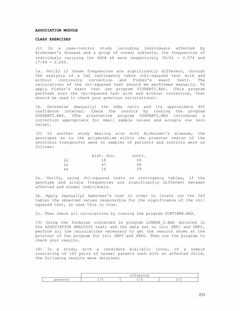
213
ASSOCIATION MODULE CLASS EXERCISES (1) In a case-control study including individuals affected by Alzheimer's disease and a group of normal subjects, the frequencies of individuals carrying the APOE ε4 were respectively 35/61 = 0.574 and 17/64 = 0.266. 1a. Verify if these frequencies are significantly different, through the analysis of a 2x2 contingency table (chi-squared test with and without continuity correction and Fisher's exact test). The calculations of the chi-squared test should be performed manually. To apply Fisher's exact test use program FISHER05.BAS. (This program performs also the chi-squared test with and without correction, that should be used to check your previous calculations). 1b. Determine (manually) the odds ratio and its approximate 95% confidence interval. Check the results by running the program ODDSRAT2.BAS. (The alternative program ODDSRAT3.BAS introduces a correction appropriate for small sample values and accepts one zero value). (2) In another study dealing also with Alzheimer's disease, the genotypes as to the polymorphism within the promoter region of the serotonin transporter gene in samples of patients and controls were as follows: Alzh. dis. contr. LL 18 69 Ls 47 68 ss 16 29 2a. Verify, using chi-squared tests on contingency tables, if the genotype and allele frequencies are significantly different between affected and normal individuals. 2b. Apply (manually) Haberman's test in order to locate (on the 2x3 table) the observed values responsible for the significance of the chi-squared test, in case this is true. 2c. Then check all calculations by running the program CONTIBM4.BAS. (3) Using the formulae contained in program LINKDX_2.BAS (printed in the ASSOCIATION ANALYSIS text) and the data set on loci SNP1 and SNP2, perform all the calculations necessary to get the results shown at the printout of the program for loci SNP3 and SNP4. Then run the program to check your results. (4) In a study, with a candidate biallelic locus, of a sample consisting of 100 pairs of normal parents each with an affected child, the following results were obtained:
offspring parents 1/1 1/2 2/2

214
11 × 11 17 0 0
11 × 12 18 26 0
11 × 22 0 8 0
12 × 12 1 13 13
12 × 22 0 1 1
22 × 22 0 0 2 4a. Estimate the values of t11, t12, t21, t22, in general tij, where tij is the observed number of parents that transmited the allele i but not the j, placing the the results in the corresponding cells of the table below:
parents offspring t11 t12 t21 t22 11 × 11 11
11 × 12 11
11 × 12 12
11 × 22 12
12 × 12 11
12 × 12 12
12 × 12 22
12 × 22 12
12 × 22 22
22 × 22 22 totals 4b. Using the values labeled as “totals” at the bottom of the table, construct the contingency table
all. 1 not tr. all. 2 not tr. total all. 1 tr. t11 t12 t1. all. 2 tr. t21 t22 t2.
total t.1 t.2 t and apply the chi-squared tests appropriate for (4c) the haplotype-based haplotype relative risk (HHRR) and (4d) the transmission disequilibrium (distortion) test (TDT). (5) The determination of HLA haplotypes in a sample of 20 sib pairs with both affected by juvenile diabetes mellitus showed the following results: IBD no. of pairs 2 12 1 6 0 2 5a. Does the distribution of IBD scores among the affected pairs indicate an association (linkage) of the susceptibility gene at the disease locus with the HLA locus? 5b. Determine manually the optimum gene frequencies of the disease susceptibility gene under the hypotheses of recessive and additive model. Use program PIBEST04.BAS to check your calculations and to
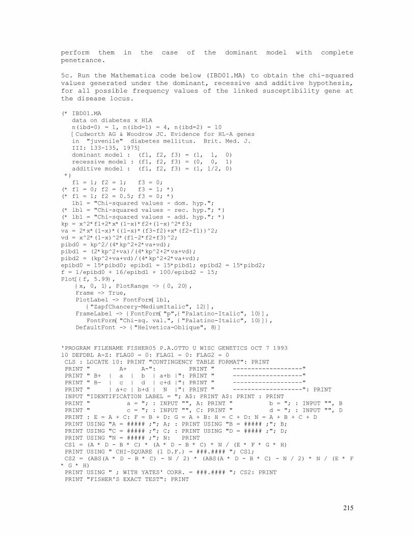
215
perform them in the case of the dominant model with complete penetrance. 5c. Run the Mathematica code below (IBD01.MA) to obtain the chi-squared values generated under the dominant, recessive and additive hypothesis, for all possible frequency values of the linked susceptibility gene at the disease locus. (* IBD01.MA data on diabetes x HLA n(ibd=0) = 1, n(ibd=1) = 4, n(ibd=2) = 10 [Cudworth AG & Woodrow JC. Evidence for HL-A genes in "juvenile" diabetes mellitus. Brit. Med. J. III: 133-135, 1975] dominant model : (f1, f2, f3) = (1, 1, 0) recessive model : (f1, f2, f3) = (0, 0, 1) additive model : (f1, f2, f3) = (1, 1/2, 0) *) f1 = 1; f2 = 1; f3 = 0; (* f1 = 0; f2 = 0; f3 = 1; *) (* f1 = 1; f2 = 0.5; f3 = 0; *) lbl = "Chi-squared values - dom. hyp."; (* lbl = "Chi-squared values - rec. hyp."; *) (* lbl = "Chi-squared values - add. hyp."; *) kp = x^2*f1+2*x*(1-x)*f2+(1-x)^2*f3; va = 2*x*(1-x)*((1-x)*(f3-f2)+x*(f2-f1))^2; vd = x^2*(1-x)^2*(f1-2*f2+f3)^2; pibd0 = kp^2/(4*kp^2+2*va+vd); pibd1 = (2*kp^2+va)/(4*kp^2+2*va+vd); pibd2 = (kp^2+va+vd)/(4*kp^2+2*va+vd); epibd0 = 15*pibd0; epibd1 = 15*pibd1; epibd2 = 15*pibd2; f = 1/epibd0 + 16/epibd1 + 100/epibd2 - 15; Plot[{f, 5.99}, {x, 0, 1}, PlotRange -> {0, 20}, Frame -> True, PlotLabel -> FontForm[lbl, {"ZapfChancery-MediumItalic", 12}], FrameLabel -> {FontForm["p",{"Palatino-Italic", 10}], FontForm["Chi-sq. val.", {"Palatino-Italic", 10}]}, DefaultFont -> {"Helvetica-Oblique", 8}] 'PROGRAM FILENAME FISHER05 P.A.OTTO U WISC GENETICS OCT 7 1993 10 DEFDBL A-Z: FLAG0 = 0: FLAG1 = 0: FLAG2 = 0 CLS : LOCATE 10: PRINT "CONTINGENCY TABLE FORMAT": PRINT PRINT " A+ A-": PRINT " -------------------" PRINT " B+ | a | b | a+b |": PRINT " -------------------" PRINT " B- | c | d | c+d |": PRINT " -------------------" PRINT " | a+c | b+d | N |": PRINT " -------------------": PRINT INPUT "IDENTIFICATION LABEL = "; A$: PRINT A$: PRINT : PRINT PRINT " a = "; : INPUT "", A: PRINT " b = "; : INPUT "", B PRINT " c = "; : INPUT "", C: PRINT " d = "; : INPUT "", D PRINT : E = A + C: F = B + D: G = A + B: H = C + D: N = A + B + C + D PRINT USING "A = ##### ;"; A; : PRINT USING "B = ##### ;"; B; PRINT USING "C = ##### ;"; C; : PRINT USING "D = ##### ;"; D; PRINT USING "N = ##### ;"; N: PRINT CS1 = (A * D - B * C) * (A * D - B * C) * N / (E * F * G * H) PRINT USING " CHI-SQUARE (1 D.F.) = ###.#### "; CS1; CS2 = (ABS(A * D - B * C) - N / 2) * (ABS(A * D - B * C) - N / 2) * N / (E * F * G * H) PRINT USING " ; WITH YATES' CORR. = ###.#### "; CS2: PRINT PRINT "FISHER'S EXACT TEST": PRINT
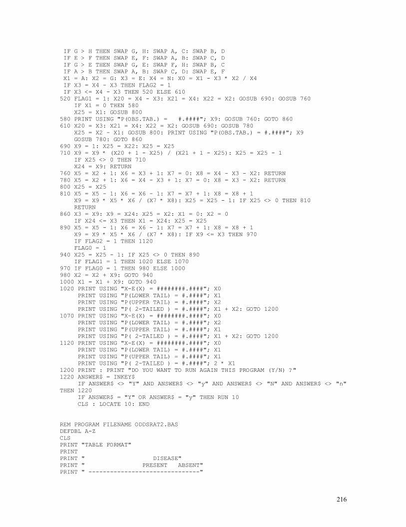
216
IF G > H THEN SWAP G, H: SWAP A, C: SWAP B, D IF E > F THEN SWAP E, F: SWAP A, B: SWAP C, D IF G > E THEN SWAP G, E: SWAP F, H: SWAP B, C IF A > B THEN SWAP A, B: SWAP C, D: SWAP E, F X1 = A: X2 = G: X3 = E: X4 = N: X0 = X1 - X3 * X2 / X4 IF X3 = X4 - X3 THEN FLAG2 = 1 IF X3 <= X4 - X3 THEN 520 ELSE 610 520 FLAG1 = 1: X20 = X4 - X3: X21 = X4: X22 = X2: GOSUB 690: GOSUB 760 IF X1 = 0 THEN 580 X25 = X1: GOSUB 800 580 PRINT USING "P(OBS.TAB.) = #.####"; X9: GOSUB 760: GOTO 860 610 X20 = X3: X21 = X4: X22 = X2: GOSUB 690: GOSUB 780 X25 = X2 - X1: GOSUB 800: PRINT USING "P(OBS.TAB.) = #.####"; X9 GOSUB 780: GOTO 860 690 X9 = 1: X25 = X22: X25 = X25 710 X9 = X9 * (X20 + 1 - X25) / (X21 + 1 - X25): X25 = X25 - 1 IF X25 <> 0 THEN 710 X24 = X9: RETURN 760 X5 = X2 + 1: X6 = X3 + 1: X7 = 0: X8 = X4 - X3 - X2: RETURN 780 X5 = X2 + 1: X6 = X4 - X3 + 1: X7 = 0: X8 = X3 - X2: RETURN 800 X25 = X25 810 X5 = X5 - 1: X6 = X6 - 1: X7 = X7 + 1: X8 = X8 + 1 X9 = X9 * X5 * X6 / (X7 * X8): X25 = X25 - 1: IF X25 <> 0 THEN 810 RETURN 860 X3 = X9: X9 = X24: X25 = X2: X1 = 0: X2 = 0 IF X24 <= X3 THEN X1 = X24: X25 = X25 890 X5 = X5 - 1: X6 = X6 - 1: X7 = X7 + 1: X8 = X8 + 1 X9 = X9 * X5 * X6 / (X7 * X8): IF X9 <= X3 THEN 970 IF FLAG2 = 1 THEN 1120 FLAG0 = 1 940 X25 = X25 - 1: IF X25 <> 0 THEN 890 IF FLAG1 = 1 THEN 1020 ELSE 1070 970 IF FLAG0 = 1 THEN 980 ELSE 1000 980 X2 = X2 + X9: GOTO 940 1000 X1 = X1 + X9: GOTO 940 1020 PRINT USING "X-E(X) = ########.####"; X0 PRINT USING "P(LOWER TAIL) = #.####"; X1 PRINT USING "P(UPPER TAIL) = #.####"; X2 PRINT USING "P( 2-TAILED ) = #.####"; X1 + X2: GOTO 1200 1070 PRINT USING "X-E(X) = ########.####"; X0 PRINT USING "P(LOWER TAIL) = #.####"; X2 PRINT USING "P(UPPER TAIL) = #.####"; X1 PRINT USING "P( 2-TAILED ) = #.####"; X1 + X2: GOTO 1200 1120 PRINT USING "X-E(X) = ########.####"; X0 PRINT USING "P(LOWER TAIL) = #.####"; X1 PRINT USING "P(UPPER TAIL) = #.####"; X1 PRINT USING "P( 2-TAILED ) = #.####"; 2 * X1 1200 PRINT : PRINT "DO YOU WANT TO RUN AGAIN THIS PROGRAM (Y/N) ?" 1220 ANSWER$ = INKEY$ IF ANSWER$ <> "Y" AND ANSWER$ <> "y" AND ANSWER$ <> "N" AND ANSWER$ <> "n" THEN 1220 IF ANSWER$ = "Y" OR ANSWER$ = "y" THEN RUN 10 CLS : LOCATE 10: END REM PROGRAM FILENAME ODDSRAT2.BAS DEFDBL A-Z CLS PRINT "TABLE FORMAT" PRINT PRINT " DISEASE" PRINT " PRESENT ABSENT" PRINT " -------------------------------"
217
PRINT " |PRESENT a b" PRINT " FACTOR +-----------------------" PRINT " |ABSENT c d" PRINT " -------------------------------" PRINT INPUT "IDENTIFICATION LABEL = "; A$ INPUT "a, b, c, d = "; A, B, C, D N = A + B + C + D CHI2 = (ABS(A * D - B * C) - N / 2) ^ 2 * N CHI2 = CHI2 / ((A + B) * (C + D) * (A + C) * (B + D)) R = (A * D) / (B * C) LR = LOG(R) VLR = 1 / A + 1 / B + 1 / C + 1 / D SLR = SQR(VLR) LLL = LR - 1.96 * SLR LUL = LR + 1.96 * SLR RLL = EXP(LLL) RUL = EXP(LUL) PRINT PRINT USING " ####.##"; R PRINT USING " ####.##"; RLL PRINT USING " ####.##"; RUL PRINT USING "chi-sq.(1df) = ###.###"; CHI2 REM PROGRAM FILENAME ODDSRAT3.BAS REM WITH CORRECTION [+ 1/2] (accepts zero cells) DEFDBL A-Z CLS PRINT "TABLE FORMAT" PRINT PRINT " DISEASE" PRINT " PRESENT ABSENT" PRINT " -------------------------------" PRINT " |PRESENT a b" PRINT " FACTOR +-----------------------" PRINT " |ABSENT c d" PRINT " -------------------------------" PRINT INPUT "IDENTIFICATION LABEL = "; A$ INPUT "a, b, c, d = "; A, B, C, D R = ((A + 1 / 2) * (D + 1 / 2)) / ((B + 1 / 2) * (C + 1 / 2)) LR = LOG(R) VLR = 1 / (A + 1) + 1 / (B + 1) + 1 / (C + 1) + 1 / (D + 1) SLR = SQR(VLR) LLL = LR - 1.96 * SLR LUL = LR + 1.96 * SLR RLL = EXP(LLL) RUL = EXP(LUL) PRINT PRINT USING " ####.##"; R PRINT USING " ####.##"; RLL PRINT USING " ####.##"; RUL REM PROGRAM FILENAME CONTIBM4.BAS REM CONTINGENCY TABLE ANALYSIS WITH HABERMAN'S TEST REM SAVES TEXT ON DATA FILE C:\TEMP\CHISQ.DAT CLS : LOCATE 10: DEFINT I-J: DEFDBL A, C, E, O, R, X INPUT "IDENTIFICATION LABEL = "; B$ INPUT "NUMBER OF ROWS (R) AND COLUMNS (C) : R, C = "; R, C: PRINT DIM O(R, C), E(R, C), A(R, C), C1(C), R1(R), X(R, C) PRINT "FORMAT N(I,J) , I = 1,2,...,R , J = 1,2,...,C": PRINT
218
FOR I = 1 TO R FOR J = 1 TO C PRINT "N("; I; ","; J; ") = "; : INPUT "", O(I, J) C1(J) = C1(J) + O(I, J) N = N + O(I, J) NEXT J NEXT I FOR J = 1 TO C FOR I = 1 TO R R1(I) = R1(I) + O(I, J) NEXT I NEXT J FOR I = 1 TO R FOR J = 1 TO C E(I, J) = R1(I) * C1(J) / N X(I, J) = (O(I, J) - E(I, J)) * (O(I, J) - E(I, J)) / E(I, J) X2 = X2 + X(I, J) A(I, J) = SQR(X(I, J)) * SGN(O(I, J) - E(I, J)) A(I, J) = A(I, J) / SQR((1 - R1(I) / N) * (1 - C1(J) / N)) NEXT J NEXT I D = (C - 1) * (R - 1) OPEN "C:\TEMP\CHISQ.DAT" FOR OUTPUT AS #1 PRINT #1, B$: PRINT #1, PRINT #1, " I J OBS(I,J) EXP(I,J) CTR. TO CHI-SQ. RES(I,J)" PRINT #1, "---------------------------------------------------------------------------" FOR I = 1 TO R FOR J = 1 TO C PRINT #1, USING "### "; I; : PRINT #1, USING "### "; J; PRINT #1, USING " ##### "; O(I, J); PRINT #1, USING "#####.### "; E(I, J); PRINT #1, USING " #####.###"; X(I, J); PRINT #1, USING " ###.###"; A(I, J); IF ABS(A(I, J)) > 1.96 THEN PRINT #1, " *" ELSE PRINT #1, NEXT J NEXT I PRINT #1, "---------------------------------------------------------------------------" PRINT #1, USING " ##### "; N; PRINT #1, USING " #####.### "; N; PRINT #1, USING "#####.###"; X2 PRINT #1, : PRINT #1, USING "Chi-square (### d.f.) = "; D; PRINT #1, USING "#####.###"; X2 IF D = 1 THEN X2 = (ABS(O(1, 1) * O(2, 2) - O(1, 2) * O(2, 1)) - N / 2) ^ 2 * N X2 = X2 / (C1(1) * C1(2) * R1(1) * R1(2)) PRINT #1, USING "Chi-sq. with Yates corr. (### d.f.) = "; D; PRINT #1, USING "###.###"; X2 ELSE PRINT #1, END IF CLOSE #1 REM PROGRAM FILENAME PIBEST04 REM PIBD SCORES MAXIMUM LIKELIHOOD ESTIMATES FOR REM DOMINANT, RECESSIVE AND ADDITIVE HYPOTHESES REM P. A. OTTO USP BIOLOGIA MAR 11 1995 DEFDBL A-Z: DEFINT I-K INPUT "N(SIBSHIPS WITH IBD = 0) = "; N0 INPUT "N(SIBSHIPS WITH IBD = 1) = "; N1
219
INPUT "N(SIBSHIPS WITH IBD = 2) = "; N2 N = N0 + N1 + N2 INPUT "INITIAL GUESS : p = "; P LOOP1: DLDP = N0 * (4 - 8 * P + 3 * P ^ 2) / (P ^ 3 - 4 * P ^ 2 + 4 * P) DLDP = DLDP + N1 * (2 - 4 * P) / (2 + 2 * P - 2 * P ^ 2) DLDP = DLDP - N2 * 1 / (2 - P) DLDP = DLDP - N * (5 - 12 * P + 3 * P^2) / (P^3 - 6 * P^2 + 5 * P + 4) D2LDP2 = -N2 / (2 - P)^2 - N1 * (2 - 4 * P)^2 / (2 + 2 * P - 2 * P^2)^2 D2LDP2 = D2LDP2 - 4 * N1 / (2 + 2 * P - 2 * P ^ 2) D2LDP2 = D2LDP2 + N*(5 - 12 * P + 3*P^2)^2/(P^3 - 6 * P^2 + 5 * P + 4)^2 D2LDP2 = D2LDP2 - N * (6 * P - 12) / (P ^ 3 - 6 * P ^ 2 + 5 * P + 4) D2LDP2 = D2LDP2 - N0 * (4 - 8 * P + 3*P^2)^2 / (P^3 – 4 * P^2 + 4 * P)^2 D2LDP2 = D2LDP2 + (6 * P - 8) / (P ^ 3 - 4 * P ^ 2 + 4 * P) VARP = -1 / D2LDP2 PRINT USING "#####.########"; P; DLDP; VARP P1 = P + DLDP * VARP IF ABS(P1 - P) < .0000000001# THEN GOTO 100 ELSE P = P1: GOTO LOOP1 END IF 100 PRINT USING "N(SIBSHIPS WITH IBD = 0) = ### "; N0 PRINT USING "N(SIBSHIPS WITH IBD = 1) = ### "; N1 PRINT USING "N(SIBSHIPS WITH IBD = 2) = ### "; N2 PRINT : PRINT " 1) RECESSIVE HYPOTHESIS" Q = (2 * N0 + N1) / (2 * N2 + N1) VARQ = 2 * (N0 + N1 + N2) * (2 * N0 + N1) / (2 * N2 + N1) ^ 3 PRINT USING "q = #.########"; Q PRINT USING "var(q) = #.########"; VARQ E1 = N * (Q / (1 + Q)) ^ 2 E2 = N * 2 * Q / (1 + Q) ^ 2 E3 = N * (1 / (1 + Q)) ^ 2 CHISQ = N0 ^ 2 / E1 + N1 ^ 2 / E2 + N2 ^ 2 / E3 - N PRINT USING "chi-sq. (1 d.f.) = ###.####"; CHISQ PRINT : PRINT " 2) DOMINANT HYPOTHESIS" PRINT USING "p = #.########"; P PRINT USING "var(p) = #.########"; VARP E1 = N * P * (4 - 4 * P + P ^ 2) / (P ^ 3 - 6 * P ^ 2 + 5 * P + 4) E2 = N * 2 * (1 + P - P ^ 2) / (P ^ 3 - 6 * P ^ 2 + 5 * P + 4) E3 = N * (2 - P) / (P ^ 3 - 6 * P ^ 2 + 5 * P + 4) CHISQ = N0 ^ 2 / E1 + N1 ^ 2 / E2 + N2 ^ 2 / E3 - N PRINT USING "chi-sq. (1 d.f.) = ###.####"; CHISQ PRINT : PRINT " 3) ADDITIVE HYPOTHESIS" P = N0 / (2 * N2 - N0) VARP = P * (1 + P) * (1 + 3 * P) / (2 * N2 - N0) PRINT USING "p = #.########"; P PRINT USING "var(p) = #.########"; VARP E1 = N * P / (1 + 3 * P) E2 = N / 2 E3 = N * (1 + P) / (2 * (1 + 3 * P)) CHISQ = N0 ^ 2 / E1 + N1 ^ 2 / E2 + N2 ^ 2 / E3 – N PRINT USING "chi-sq. (1 d.f.) = ###.####"; CHISQ

220
SEGREGATION ANALYSIS MODULE CLASS EXERCISES (1) The analysis of the offspring of matings affected vs. normal for a rare disease (nail-patella syndrome) suspected to be transmitted in an autosomal dominant mode showed the following results:
sex affected normal total masculine 11 13 24 feminine 7 10 17 total 18 23 41
1a. Verify if the proportions of affected and normals are the same among male and female children. In case the hypothesis is accepted, use the total numbers to solve the questions 1b. - 1d. that follow. 1b. Estimate the segregation rate of the disease and its approximate (normal) 95% binomial confidence interval. 1c. Using the likelihood function corresponding to the observed data set and the program CONFINT6.BAS, determine the exact 95% credible interval for the estimate of the segregation rate. 1d. Test if the segregation rate is compatible with that of an autosomal dominant mode with complete penetrance using the exact binomial test (program BINPROB4.BAS), the chi-squared test, and the log-likelihood test. (2) The structure of the following pedigree suggests that the disease segregating in it (dark symbols) is determined by an autosomal dominant mode of inheritance with incomplete penetrance.
2a. If K is the penetrance value of the disease, what is the likelihood function of this family? 2b. Find the maximum likelihood estimate of the penetrance value K. 2c. Use a chi-squared test to verify if the offspring data from item (1) are compatible with autosomal dominant inheritance with incomplete penetrance, using the K value estimated above. (3) The table below lists the observed offspring genotype numbers in 529 English families analyzed in relation to MN blood groups. Are the

221
genotype offspring numbers compatible with the hypothesis of codominant inheritance?
parents children type no. M MN N total M × M 40 98 - - 98 M × N 62 - 132 - 132 M × MN 162 203 182 - 385 MN × MN 124 57 143 79 279 MN × N 111 - 116 122 238 N × N 30 - - 67 67 total 529 358 573 268 1199
(4) The data that follow on phenylketonuria were collected from sibships containing at least one affected child, all produced by couples of normal parents. Test (manually) if the data are compatible with an autosomal recessive mode of inheritance assuming:
s(i) n(i) no(nl) no(af) 1 6 - 6 2 7 6 8 3 6 8 10 4 5 12 8 5 7 22 13 6 5 18 12 7 2 10 4 8 3 16 8 9 1 7 2 10 2 15 5 11 1 9 2 12 1 9 3 13 1 9 4
totals 47 141 85 4a. a truncate selection mode (in which the distribution of affected children among families is binomial with the omission of sibships with none affected); 4b. a single selection mode (in which the probability of inclusion of a family is proportional to the number of children affected). 4c. check your results by running programs SEGRAN01.BAS and SEGRAN03.BAS (the enclosed codes should be adapted to the current data set). (5) The table below lists the results of Rh typing (by means of anti-serum D alone) of 100 American families:
parental matings children no. Rh(+) Rh(-) total
Rh(+) × Rh(+) 73 248 16 264 Rh(+) × Rh(-) 20 54 23 77 Rh(-) × Rh(-) 7 - 34 34
222
total 100 302 73 375 5a. Verify (manually) if the data agree with the hypothesis of monogenic recessive inheritance. 5b. Check your results by running programs SNYDER02.BAS and SNYDER01.BAS. What is the difference between these two programs? REM program filename confint6.bas REM calculation of the 95%CI of a binomial estimate p = x/n REM modification of Romberg's osculatory method DEFDBL A-Z: CLS PRINT "Function : p^n1.(1-p)^n2" INPUT "n1 = "; n1 INPUT "n2 = "; n2 PRINT USING "p = n1/(n1+n2) = ### / ### = #.####"; n1; n1 + n2; n1 / (n1 + n2) p0 = 0: pn = 1:GOSUB simpsonsrule: totalarea = area: p0 = .001: niter = 0 repeat: p = p0: GOSUB functsub: pp0 = pp: p1 = 1 FOR j = 1 TO niter p1 = p1 - 1 / niter: p = p1: GOSUB functsub pp1 = pp: IF pp1 >= pp0 THEN GOTO getout NEXT j getout: p0 = p0: pn = p1: GOSUB simpsonsrule IF area / totalarea >= .95 THEN p0 = p0 + 1 / niter: GOTO repeat p0 = p0 - 1 / niter: p1 = p1 + 1 / niter: niter = niter * 5 IF ABS(.95-area/totalarea) <= .00001 THEN GOTO ENDPRGM ELSE GOTO repeat DO: LOOP WHILE INKEY$ <> " " ENDPRGM: PRINT PRINT USING "lower limit (p) = #.####"; p0 PRINT USING "upper limit (p) = #.####"; pn END simpsonsrule: h = (pn - p0) / 1000: p = p0: GOSUB functsub: s = pp p = pn: GOSUB functsub: s = s + pp: w = 4 FOR j = 1 TO 999 p = p0 + j * h GOSUB functsub s = s + w * pp w = 6 - w NEXT j area = h * s / 3: s = 0 IF p0 <> 0 THEN p = p0: GOSUB functsub: pp0 = pp p = pn: GOSUB functsub: pp1 = pp END IF RETURN functsub: pp = p ^ n1 * (1 - p) ^ n2 RETURN REM BINPROB4.BAS CLS : LOCATE 5: DEFDBL A-Z: DEFINT I-N OPEN "c:\temp\test99.txt" FOR OUTPUT AS #1 INPUT "N, p = "; N, Q I = 0: PROB = (1 - Q) ^ N: PROBC = PROB PRINT #1, USING "N = #####"; N: PRINT #1, USING "q = #.###"; Q: PRINT #1, PRINT #1, " X p(X) P(X)" PRINT #1, "------------------------"

223
PRINT #1, USING "###"; I; : PRINT #1, USING " #.####"; PROB; PROBC FOR I = 1 TO N PROB = (N + 1 - I) * Q * PROB / (I * (1 - Q)) PROBC = PROBC + PROB PRINT #1, USING "###"; I; : PRINT #1, USING " #.####"; PROB; PROBC NEXT I PRINT #1, "------------------------" CLOSE #1 REM PROGRAM FILENAME SEGRAN01.BAS DEFDBL A-Z: DEFINT I-J REM NUMBER OF SIBSHIPS WITH SIZES NI=1,2,...,14 DATA 5,8,5,2,3,3,2,3,1,1,3,0,0,1 REM NUMBER OF PATIENTS IN SIBSHIPS 1,2,...,14 DATA 5,10,8,4,4,8,5,5,4,2,7,0,0,4 DIM N(14), NOAF(14), NONL(14), NEAF(14), NENL(14), V(14) CLS : LOCATE 10 FOR I = 1 TO 14: READ N(I): SINI = SINI + I * N(I): NEXT I FOR I = 1 TO 14 READ NOAF(I): SNOAF = SNOAF + NOAF(I) NONL(I) = I * N(I) - NOAF(I): SNONL = SNONL + NONL(I) NEXT I PRINT " DATA ON ALKAPTONURIA - HOGBEN, WORRALL & ZIEVE": PRINT PRINT " s(i) n(i) n(i)s(i) no(nl) ne(nl) no(af) ne(af) v(neaf)" PRINT " ----------------------------------------------------------------------" FOR I = 1 TO 14 NEAF(I) = N(I) * I * .25 / (1 - .75 ^ I): SNEAF = SNEAF + NEAF(I) NENL(I) = N(I) * I - NEAF(I): SNENL = SNENL + NENL(I) V(I) = I * .1875 / (1 - .75 ^ I) V(I) = V(I) - I ^ 2 * .0625 * .75 ^ I / (1 - .75 ^ I) ^ 2 V(I) = V(I) * N(I): IF I = 1 THEN V(I) = 0 SVINI = SVINI + V(I) PRINT USING "####.####"; I; N(I); I * N(I); NONL(I); NENL(I); PRINT USING "####.####"; NOAF(I); NEAF(I); V(I) NEXT I PRINT " ----------------------------------------------------------------------" PRINT " "; PRINT USING "####.####"; SINI; SNONL; SNENL; SNOAF; SNEAF; SVINI PRINT " ----------------------------------------------------------------------" CHI2 = (SNONL - SNENL) ^ 2 / SNENL + (SNOAF - SNEAF) ^ 2 / SNEAF SEV = SQR(SVINI): LI = SNEAF - 1.96 * SEV: LS = SNEAF + 1.96 * SEV PRINT USING " 95%CI OF NE(AF) : ###.### - "; LI; PRINT USING "###.###"; LS PRINT USING " Chi-sq. (1 d.f.) = ##.###"; CHI2
REM PROGRAM FILENAME SEGRAN03.BAS REM FISHER'S SIB METHOD DEFDBL A-Z: DEFINT I-J REM NUMBER OF SIBSHIPS WITH SIZES NI=1,2,...,14 DATA 5,8,5,2,3,3,2,3,1,1,3,0,0,1 REM NUMBER OF PATIENTS IN SIBSHIPS 1,2,...,14

224
DATA 5,10,8,4,4,8,5,5,4,2,7,0,0,4 DIM N(14), NOAF(14), NONL(14) CLS : LOCATE 10 FOR I = 1 TO 14 READ N(I): SNI = SNI + N(I): SINI = SINI + I * N(I) NEXT I FOR I = 1 TO 14 READ NOAF(I) SNOAF = SNOAF + NOAF(I) NONL(I) = I * N(I) - NOAF(I) SNONL = SNONL + NONL(I) NEXT I PRINT " DATA ON ALKAPTONURIA - HOGBEN, WORRALL & ZIEVE": PRINT PRINT " s(i) n(i) n(i)s(i) no(nl) no(af)" PRINT " --------------------------------------------" FOR I = 1 TO 14 PRINT USING "####.####"; I; N(I); I * N(I); NONL(I); NOAF(I) DO: LOOP WHILE INKEY$ <> " " NEXT I PRINT " --------------------------------------------" PRINT " "; PRINT USING "####.####"; SNI; SINI; SNONL; SNOAF PRINT " --------------------------------------------" PRINT REM PROGRAM FILENAME SNYDER01 REM P.A.OTTO U WISCONSIN GENETICS MAY 13 1993 REM CLASSICAL MODEL WITH COMPLETE PENETRANCE DEFDBL A-Z: DEFINT I-J: ZER = 0: ONE = 1: TWO = 2: THR = 3: FOU = 4 CLS : LOCATE 10 INPUT "SAMPLE DESCRIPTION = "; A$ INPUT "N(DOM x DOM CROS.) = "; N1 INPUT "N(DOM x REC CROS.) = "; N2 INPUT "N(REC x REC CROS.) = "; N3 T0 = N1 + N2 + N3 INPUT "N(DOM | DOM x DOM) = "; N4 INPUT "N(REC | DOM x DOM) = "; N5 T1 = N4 + N5 INPUT "N(DOM | DOM x REC) = "; N6 INPUT "N(REC | DOM x REC) = "; N7 T2 = N6 + N7 INPUT "N(DOM | REC x REC) = "; N8 INPUT "N(REC | REC x REC) = "; N9 T3 = N8 + N9 T4 = N4 + N6 + N8: T5 = N5 + N7 + N9: T = T4 + T5 INPUT "INITIAL GUESS (q) = "; Q PRINT " SNYDER'S METHOD": PRINT PRINT " "; A$: PRINT PRINT " DOM REC TOT" PRINT " -----------------------------------------------" PRINT USING " DOM x DOM ####"; N1; PRINT USING " ####"; N4; N5; T1 PRINT USING " DOM x REC ####"; N2; PRINT USING " ####"; N6; N7; T2 PRINT USING " REC x REC ####"; N3; PRINT USING " ####"; N8; N9; T3 PRINT " -----------------------------------------------" PRINT USING " TOTAL ####"; T0; PRINT USING " ####"; T4; T5; T

225
PRINT PRINT " q s.e.(q) dL/dq" PRINT " ------------------------------------------------------" 280 REM LOOP BEGINNING A = TWO * N1 + N2 - TWO * N4 - TWO * N5 - N6 - N7 B = TWO * N1 + N2 c = TWO * N2 + FOU * N3 + TWO * N5 + N7 D = TWO * N4 DLDQ = A / (ONE + Q) - B / (ONE - Q) + c / Q + D / (ONE + TWO * Q) D2LDQ2 = -A / ((ONE + Q) * (ONE + Q)) - B / ((ONE - Q) * (ONE - Q)) D2LDQ2 = D2LDQ2 - c / (Q * Q) D2LDQ2 = D2LDQ2 - TWO * D / ((ONE + TWO * Q) * (ONE + TWO * Q)) VARQ = -ONE / D2LDQ2 Q1 = Q + DLDQ * VARQ PRINT USING "#####.############ "; Q; SQR(VARQ); DLDQ IF ABS(Q1 - Q) < 1E-15 THEN 300 ELSE Q = Q1: GOTO 280 300 PRINT " ------------------------------------------------------" PRINT P2 = Q / (ONE + Q): P1 = P2 * P2: Q2 = ONE - P2: Q1 = ONE - P1: P3 = ONE: Q3 = ZER CS1 = N4 * N4 / (T1 * Q1) + N5 * N5 / (T1 * P1) - T1 CS2 = N6 * N6 / (T2 * Q2) + N7 * N7 / (T2 * P2) - T2 CS3 = ZER CS4 = CS1 + CS2 + CS3 CS5 = (T4 - (T1 * Q1 + T2 * Q2 + T3 * Q3)) * (T4 - (T1 * Q1 + T2 * Q2 + T3 * Q3)) / (T1 * Q1 + T2 * Q2 + T3 * Q3) CS5 = CS5 + (T5 - (T1 * P1 + T2 * P2 + T3 * P3)) * (T5 - (T1 * P1 + T2 * P2 + T3 * P3)) / (T1 * P1 + T2 * P2 + T3 * P3) CS6 = CS4 - CS5 PRINT " RESULTS OF GOODNESS-OF-FIT TESTS : ": PRINT PRINT USING " a) off. of DxD parents : chi-square (1 d.f.) = ##.###"; CS1 PRINT USING " b) off. of DxR parents : chi-square (1 d.f.) = ##.###"; CS2 PRINT USING " c) 'total' chi-square : chi-square (2 d.f.) = ##.###"; CS4 PRINT USING " d) 'pooled' chi-square : chi-square (1 d.f.) = ##.###"; CS5 PRINT USING " e) heterogeneity c.s. : chi-square (1 d.f.) = ##.###"; CS6 END REM PROGRAM FILENAME SNYDER02 REM P.A.OTTO U WISCONSIN GENETICS MAY 18 1993 REM CLASSICAL MODEL WITH COMPLETE PENETRANCE REM ESTIMATION OF q USING PARENTAL PAIRS ONLY DEFDBL A-Z: DEFINT I-J: ZER = 0: ONE = 1: TWO = 2: THR = 3: FOU = 4 CLS : LOCATE 10 INPUT "SAMPLE DESCRIPTION = "; A$ INPUT "N(DOM x DOM CROS.) = "; N1 INPUT "N(DOM x REC CROS.) = "; N2 INPUT "N(REC x REC CROS.) = "; N3: T0 = N1 + N2 + N3 INPUT "N(DOM | DOM x DOM) = "; N4 INPUT "N(REC | DOM x DOM) = "; N5: T1 = N4 + N5 INPUT "N(DOM | DOM x REC) = "; N6 INPUT "N(REC | DOM x REC) = "; N7: T2 = N6 + N7 INPUT "N(DOM | REC x REC) = "; N8 INPUT "N(REC | REC x REC) = "; N9: T3 = N8 + N9 T4 = N4 + N6 + N8: T5 = N5 + N7 + N9: T = T4 + T5 Q = SQR((N2 + 2 * N3) / (TWO * T0)): VARQ = (ONE - Q * Q) / (FOU * TWO * T0) PRINT " SNYDER'S METHOD": PRINT : PRINT " "; A$: PRINT PRINT " DOM REC TOT" PRINT " -----------------------------------------------" PRINT USING " DOM x DOM ####"; N1; PRINT USING " ####"; N4; N5; T1 PRINT USING " DOM x REC ####"; N2; PRINT USING " ####"; N6; N7; T2
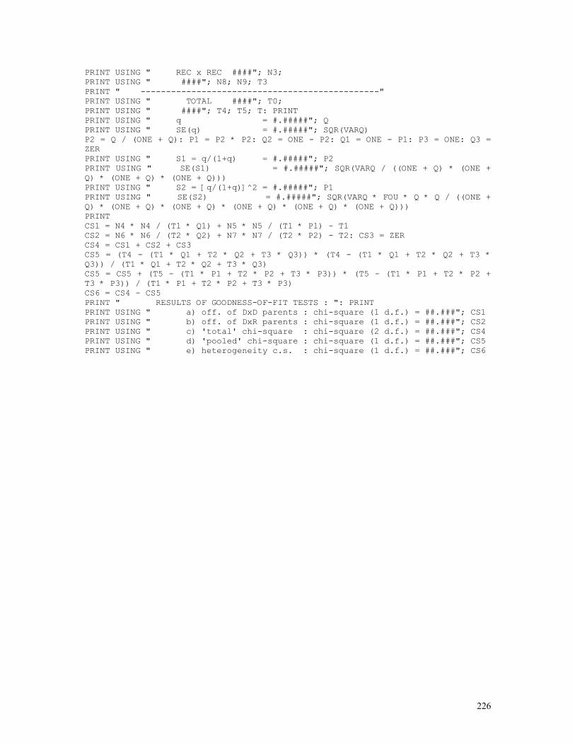
226
PRINT USING " REC x REC ####"; N3; PRINT USING " ####"; N8; N9; T3 PRINT " -----------------------------------------------" PRINT USING " TOTAL ####"; T0; PRINT USING " ####"; T4; T5; T: PRINT PRINT USING " q = #.#####"; Q PRINT USING " SE(q) = #.#####"; SQR(VARQ) P2 = Q / (ONE + Q): P1 = P2 * P2: Q2 = ONE - P2: Q1 = ONE - P1: P3 = ONE: Q3 = ZER PRINT USING " S1 = q/(1+q) = #.#####"; P2 PRINT USING " SE(S1) = #.#####"; SQR(VARQ / ((ONE + Q) * (ONE + Q) * (ONE + Q) * (ONE + Q))) PRINT USING " S2 = [q/(1+q)]^2 = #.#####"; P1 PRINT USING " SE(S2) = #.#####"; SQR(VARQ * FOU * Q * Q / ((ONE + Q) * (ONE + Q) * (ONE + Q) * (ONE + Q) * (ONE + Q) * (ONE + Q))) PRINT CS1 = N4 * N4 / (T1 * Q1) + N5 * N5 / (T1 * P1) - T1 CS2 = N6 * N6 / (T2 * Q2) + N7 * N7 / (T2 * P2) - T2: CS3 = ZER CS4 = CS1 + CS2 + CS3 CS5 = (T4 - (T1 * Q1 + T2 * Q2 + T3 * Q3)) * (T4 - (T1 * Q1 + T2 * Q2 + T3 * Q3)) / (T1 * Q1 + T2 * Q2 + T3 * Q3) CS5 = CS5 + (T5 - (T1 * P1 + T2 * P2 + T3 * P3)) * (T5 - (T1 * P1 + T2 * P2 + T3 * P3)) / (T1 * P1 + T2 * P2 + T3 * P3) CS6 = CS4 - CS5 PRINT " RESULTS OF GOODNESS-OF-FIT TESTS : ": PRINT PRINT USING " a) off. of DxD parents : chi-square (1 d.f.) = ##.###"; CS1 PRINT USING " b) off. of DxR parents : chi-square (1 d.f.) = ##.###"; CS2 PRINT USING " c) 'total' chi-square : chi-square (2 d.f.) = ##.###"; CS4 PRINT USING " d) 'pooled' chi-square : chi-square (1 d.f.) = ##.###"; CS5 PRINT USING " e) heterogeneity c.s. : chi-square (1 d.f.) = ##.###"; CS6
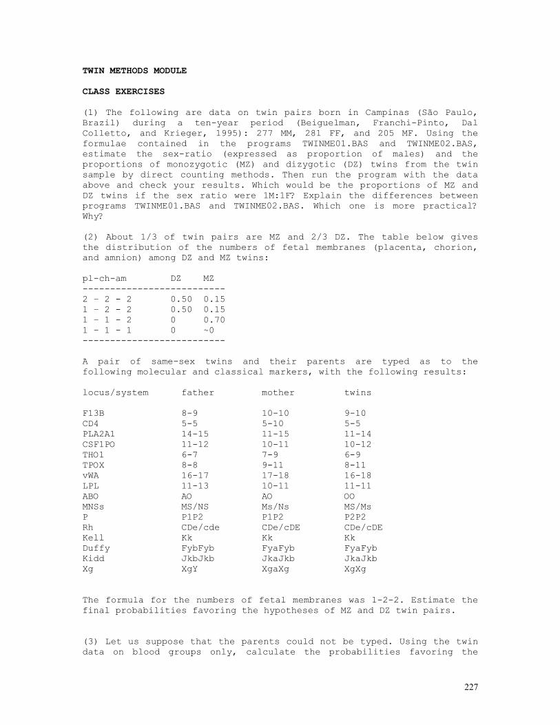
227
TWIN METHODS MODULE CLASS EXERCISES (1) The following are data on twin pairs born in Campinas (São Paulo, Brazil) during a ten-year period (Beiguelman, Franchi-Pinto, Dal Colletto, and Krieger, 1995): 277 MM, 281 FF, and 205 MF. Using the formulae contained in the programs TWINME01.BAS and TWINME02.BAS, estimate the sex-ratio (expressed as proportion of males) and the proportions of monozygotic (MZ) and dizygotic (DZ) twins from the twin sample by direct counting methods. Then run the program with the data above and check your results. Which would be the proportions of MZ and DZ twins if the sex ratio were 1M:1F? Explain the differences between programs TWINME01.BAS and TWINME02.BAS. Which one is more practical? Why? (2) About 1/3 of twin pairs are MZ and 2/3 DZ. The table below gives the distribution of the numbers of fetal membranes (placenta, chorion, and amnion) among DZ and MZ twins: pl-ch-am DZ MZ -------------------------- 2 – 2 - 2 0.50 0.15 1 – 2 - 2 0.50 0.15 1 – 1 - 2 0 0.70 1 – 1 - 1 0 ~0 -------------------------- A pair of same-sex twins and their parents are typed as to the following molecular and classical markers, with the following results: locus/system father mother twins
F13B 8-9 10-10 9-10 CD4 5-5 5-10 5-5 PLA2A1 14-15 11-15 11-14 CSF1PO 11-12 10-11 10-12 THO1 6-7 7-9 6-9 TPOX 8-8 9-11 8-11 vWA 16-17 17-18 16-18 LPL 11-13 10-11 11-11 ABO AO AO OO MNSs MS/NS Ms/Ns MS/Ms P P1P2 P1P2 P2P2 Rh CDe/cde CDe/cDE CDe/cDE Kell Kk Kk Kk Duffy FybFyb FyaFyb FyaFyb Kidd JkbJkb JkaJkb JkaJkb Xg XgY XgaXg XgXg The formula for the numbers of fetal membranes was 1-2-2. Estimate the final probabilities favoring the hypotheses of MZ and DZ twin pairs. (3) Let us suppose that the parents could not be typed. Using the twin data on blood groups only, calculate the probabilities favoring the
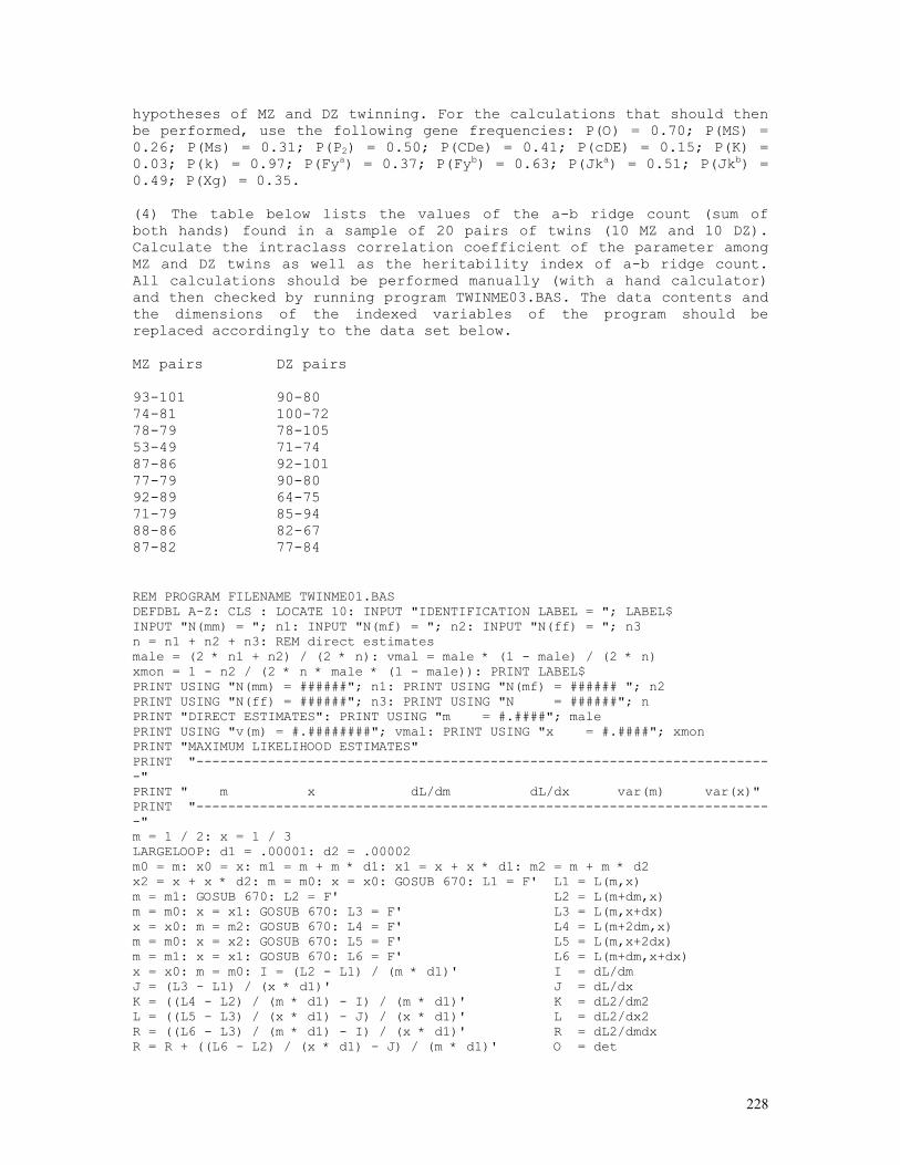
228
hypotheses of MZ and DZ twinning. For the calculations that should then be performed, use the following gene frequencies: P(O) = 0.70; P(MS) = 0.26; P(Ms) = 0.31; P(P2) = 0.50; P(CDe) = 0.41; P(cDE) = 0.15; P(K) = 0.03; P(k) = 0.97; P(Fya) = 0.37; P(Fyb) = 0.63; P(Jka) = 0.51; P(Jkb) = 0.49; P(Xg) = 0.35. (4) The table below lists the values of the a-b ridge count (sum of both hands) found in a sample of 20 pairs of twins (10 MZ and 10 DZ). Calculate the intraclass correlation coefficient of the parameter among MZ and DZ twins as well as the heritability index of a-b ridge count. All calculations should be performed manually (with a hand calculator) and then checked by running program TWINME03.BAS. The data contents and the dimensions of the indexed variables of the program should be replaced accordingly to the data set below. MZ pairs DZ pairs
93-101 90-80 74-81 100-72 78-79 78-105 53-49 71-74 87-86 92-101 77-79 90-80 92-89 64-75 71-79 85-94 88-86 82-67 87-82 77-84 REM PROGRAM FILENAME TWINME01.BAS DEFDBL A-Z: CLS : LOCATE 10: INPUT "IDENTIFICATION LABEL = "; LABEL$ INPUT "N(mm) = "; n1: INPUT "N(mf) = "; n2: INPUT "N(ff) = "; n3 n = n1 + n2 + n3: REM direct estimates male = (2 * n1 + n2) / (2 * n): vmal = male * (1 - male) / (2 * n) xmon = 1 - n2 / (2 * n * male * (1 - male)): PRINT LABEL$ PRINT USING "N(mm) = ######"; n1: PRINT USING "N(mf) = ###### "; n2 PRINT USING "N(ff) = ######"; n3: PRINT USING "N = ######"; n PRINT "DIRECT ESTIMATES": PRINT USING "m = #.####"; male PRINT USING "v(m) = #.########"; vmal: PRINT USING "x = #.####"; xmon PRINT "MAXIMUM LIKELIHOOD ESTIMATES" PRINT "-------------------------------------------------------------------------" PRINT " m x dL/dm dL/dx var(m) var(x)" PRINT "-------------------------------------------------------------------------" m = 1 / 2: x = 1 / 3 LARGELOOP: d1 = .00001: d2 = .00002 m0 = m: x0 = x: m1 = m + m * d1: x1 = x + x * d1: m2 = m + m * d2 x2 = x + x * d2: m = m0: x = x0: GOSUB 670: L1 = F' L1 = L(m,x) m = m1: GOSUB 670: L2 = F' L2 = L(m+dm,x) m = m0: x = x1: GOSUB 670: L3 = F' L3 = L(m,x+dx) x = x0: m = m2: GOSUB 670: L4 = F' L4 = L(m+2dm,x) m = m0: x = x2: GOSUB 670: L5 = F' L5 = L(m,x+2dx) m = m1: x = x1: GOSUB 670: L6 = F' L6 = L(m+dm,x+dx) x = x0: m = m0: I = (L2 - L1) / (m * d1)' I = dL/dm J = (L3 - L1) / (x * d1)' J = dL/dx K = ((L4 - L2) / (m * d1) - I) / (m * d1)' K = dL2/dm2 L = ((L5 - L3) / (x * d1) - J) / (x * d1)' L = dL2/dx2 R = ((L6 - L3) / (m * d1) - I) / (x * d1)' R = dL2/dmdx R = R + ((L6 - L2) / (x * d1) - J) / (m * d1)' O = det
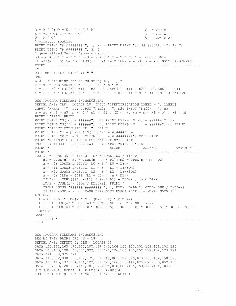
229
R = R / 2: O = K * L - R * R' S = var(m) S = -L / O: T = -K / O' T = var(x) U = R / O' U = cov(m,x) ' printout routine PRINT USING "#.######## "; m; x; : PRINT USING "#####.######## "; I; J; PRINT USING "#.######## "; S; T ' generalized Newton-Raphson method m3 = m + S * I + U * J: x3 = x + U * I + T * J: Z = .000000001# IF ABS(m3 - m) >= Z OR ABS(x3 - x) >= Z THEN m = m3: x = x3: GOTO LARGELOOP PRINT "-------------------------------------------------------------------------" DO: LOOP WHILE INKEY$ <> " " END 670 ' subroutine for calculating L1,...,L6 F = n1 * LOG(ABS(x * m + (1 - x) * m * m)) F = F + n2 * LOG(ABS(m)) + n2 * LOG(ABS(1 - m)) + n2 * LOG(ABS(1 - x)) F = F + n3 * LOG(ABS(x * (1 - m) + (1 - x) * (1 - m) * (1 - m))): RETURN REM PROGRAM FILENAME TWINME02.BAS DEFDBL A-Z: CLS : LOCATE 10: INPUT "IDENTIFICATION LABEL = "; LABEL$ INPUT "N(mm) = "; n1: INPUT "N(mf) = "; n2: INPUT "N(ff) = "; n3 n = n1 + n2 + n3: m = (2 * n1 + n2) / (2 * n): vm = m * (1 - m) / (2 * n) PRINT LABEL$: PRINT PRINT USING "N(mm) = ######"; n1: PRINT USING "N(mf) = ###### "; n2 PRINT USING "N(ff) = ######"; n3: PRINT USING "N = ######"; n: PRINT PRINT "DIRECT ESTIMATE OF m": PRINT PRINT USING "m = [2N(mm)+N(mf)]/2N = #.####"; m PRINT USING "v(m) = m(1-m)/2N = #.########"; vm: PRINT PRINT "MAXIMUM LIKELIHOOD ESTIMATE OF x": PRINT ONE = 1: TTHOU = 100000: TWO = 2: INPUT "x(0) = "; x PRINT " x dL/dx d2L/dx2 var(x)" PRINT " -------------------------------------------------------------" 100 D1 = CDBL(ONE / TTHOU): D2 = CDBL(TWO / TTHOU) x0 = CDBL(x): x1 = CDBL(x + x * D1): x2 = CDBL(x + x * D2) x = x0: GOSUB LKLFUNC: L0 = F ' L0 = L(x) x = x1: GOSUB LKLFUNC: L1 = F ' L1 = L(x+Dx) x = x2: GOSUB LKLFUNC: L2 = F ' L2 = L(x+2Dx) x = x0: DLDx = CDBL((L1 - L0) / (x * D1)) D2LDx2 = CDBL(((L2 - L1) / (x * D1) - DLDx) / (x * D1)) xONE = CDBL(x - DLDx / D2LDx2): PRINT " "; PRINT USING "######.######## "; x; DLDx; D2LDx2; CDBL(-ONE / D2LDx2) IF ABS(xONE - x) < 1E-08 THEN GOTO EXACT ELSE x = xONE: GOTO 100 LKLFUNC: F = CDBL(n1 * LOG(x * m + (ONE - x) * m * m)) F = F + CDBL(n2 * LOG(TWO * m * (ONE - m) * (ONE - x))) F = F + CDBL(n3 * LOG((x * (ONE - m) + (ONE - x) * (ONE - m) * (ONE - m)))) RETURN EXACT: PRINT " -------------------------------------------------------------" REM PROGRAM FILENAME TWINME03.BAS REM MZ TWIN PAIRS TRC (N = 18) DEFDBL A-Z: DEFINT I: CLS : LOCATE 10 DATA 120,112,165,176,103,105,127,141,164,160,152,151,139,131,152,125 DATA 130,133,120,106,085,093,130,143,196,186,153,153,127,132,173,174 DATA 071,078,075,074 DATA 077,082,038,115,152,175,111,169,061,122,099,017,136,182,158,098 DATA 095,115,137,124,106,123,111,147,166,193,112,077,072,083,052,103 DATA 119,093,128,180,168,181,178,195,010,082,185,154,149,191,184,208 DIM X1MZ(18), X2MZ(18), X1DZ(24), X2DZ(24) FOR I = 1 TO 18: READ X1MZ(I), X2MZ(I): NEXT I
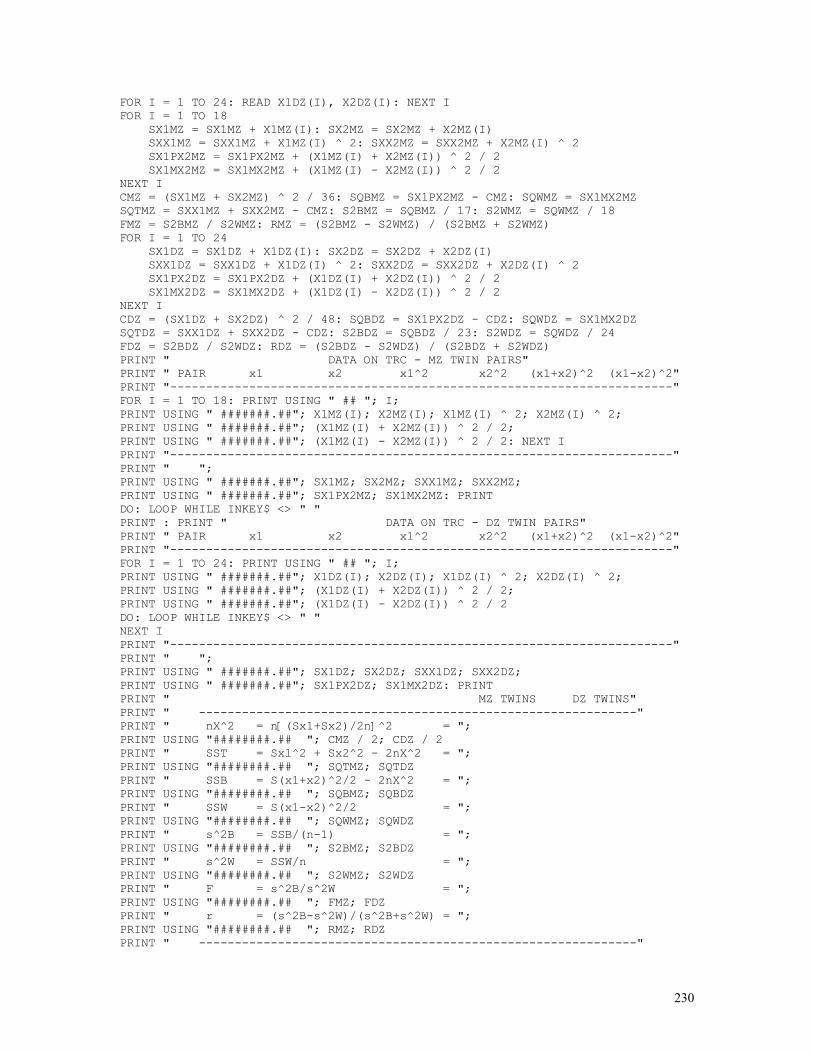
230
FOR I = 1 TO 24: READ X1DZ(I), X2DZ(I): NEXT I FOR I = 1 TO 18 SX1MZ = SX1MZ + X1MZ(I): SX2MZ = SX2MZ + X2MZ(I) SXX1MZ = SXX1MZ + X1MZ(I) ^ 2: SXX2MZ = SXX2MZ + X2MZ(I) ^ 2 SX1PX2MZ = SX1PX2MZ + (X1MZ(I) + X2MZ(I)) ^ 2 / 2 SX1MX2MZ = SX1MX2MZ + (X1MZ(I) - X2MZ(I)) ^ 2 / 2 NEXT I CMZ = (SX1MZ + SX2MZ) ^ 2 / 36: SQBMZ = SX1PX2MZ - CMZ: SQWMZ = SX1MX2MZ SQTMZ = SXX1MZ + SXX2MZ - CMZ: S2BMZ = SQBMZ / 17: S2WMZ = SQWMZ / 18 FMZ = S2BMZ / S2WMZ: RMZ = (S2BMZ - S2WMZ) / (S2BMZ + S2WMZ) FOR I = 1 TO 24 SX1DZ = SX1DZ + X1DZ(I): SX2DZ = SX2DZ + X2DZ(I) SXX1DZ = SXX1DZ + X1DZ(I) ^ 2: SXX2DZ = SXX2DZ + X2DZ(I) ^ 2 SX1PX2DZ = SX1PX2DZ + (X1DZ(I) + X2DZ(I)) ^ 2 / 2 SX1MX2DZ = SX1MX2DZ + (X1DZ(I) - X2DZ(I)) ^ 2 / 2 NEXT I CDZ = (SX1DZ + SX2DZ) ^ 2 / 48: SQBDZ = SX1PX2DZ - CDZ: SQWDZ = SX1MX2DZ SQTDZ = SXX1DZ + SXX2DZ - CDZ: S2BDZ = SQBDZ / 23: S2WDZ = SQWDZ / 24 FDZ = S2BDZ / S2WDZ: RDZ = (S2BDZ - S2WDZ) / (S2BDZ + S2WDZ) PRINT " DATA ON TRC - MZ TWIN PAIRS" PRINT " PAIR x1 x2 x1^2 x2^2 (x1+x2)^2 (x1-x2)^2" PRINT "----------------------------------------------------------------------" FOR I = 1 TO 18: PRINT USING " ## "; I; PRINT USING " #######.##"; X1MZ(I); X2MZ(I); X1MZ(I) ^ 2; X2MZ(I) ^ 2; PRINT USING " #######.##"; (X1MZ(I) + X2MZ(I)) ^ 2 / 2; PRINT USING " #######.##"; (X1MZ(I) - X2MZ(I)) ^ 2 / 2: NEXT I PRINT "----------------------------------------------------------------------" PRINT " "; PRINT USING " #######.##"; SX1MZ; SX2MZ; SXX1MZ; SXX2MZ; PRINT USING " #######.##"; SX1PX2MZ; SX1MX2MZ: PRINT DO: LOOP WHILE INKEY$ <> " " PRINT : PRINT " DATA ON TRC - DZ TWIN PAIRS" PRINT " PAIR x1 x2 x1^2 x2^2 (x1+x2)^2 (x1-x2)^2" PRINT "----------------------------------------------------------------------" FOR I = 1 TO 24: PRINT USING " ## "; I; PRINT USING " #######.##"; X1DZ(I); X2DZ(I); X1DZ(I) ^ 2; X2DZ(I) ^ 2; PRINT USING " #######.##"; (X1DZ(I) + X2DZ(I)) ^ 2 / 2; PRINT USING " #######.##"; (X1DZ(I) - X2DZ(I)) ^ 2 / 2 DO: LOOP WHILE INKEY$ <> " " NEXT I PRINT "----------------------------------------------------------------------" PRINT " "; PRINT USING " #######.##"; SX1DZ; SX2DZ; SXX1DZ; SXX2DZ; PRINT USING " #######.##"; SX1PX2DZ; SX1MX2DZ: PRINT PRINT " MZ TWINS DZ TWINS" PRINT " -------------------------------------------------------------" PRINT " nX^2 = n[(Sx1+Sx2)/2n]^2 = "; PRINT USING "########.## "; CMZ / 2; CDZ / 2 PRINT " SST = Sx1^2 + Sx2^2 - 2nX^2 = "; PRINT USING "########.## "; SQTMZ; SQTDZ PRINT " SSB = S(x1+x2)^2/2 - 2nX^2 = "; PRINT USING "########.## "; SQBMZ; SQBDZ PRINT " SSW = S(x1-x2)^2/2 = "; PRINT USING "########.## "; SQWMZ; SQWDZ PRINT " s^2B = SSB/(n-1) = "; PRINT USING "########.## "; S2BMZ; S2BDZ PRINT " s^2W = SSW/n = "; PRINT USING "########.## "; S2WMZ; S2WDZ PRINT " F = s^2B/s^2W = "; PRINT USING "########.## "; FMZ; FDZ PRINT " r = (s^2B-s^2W)/(s^2B+s^2W) = "; PRINT USING "########.## "; RMZ; RDZ PRINT " -------------------------------------------------------------"
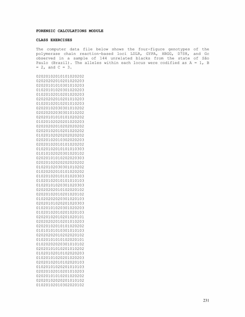
231
FORENSIC CALCULATIONS MODULE CLASS EXERCISES The computer data file below shows the four-figure genotypes of the polymerase chain reaction-based loci LDLR, GYPA, HBGG, D7S8, and Gc observed in a sample of 144 unrelated blacks from the state of São Paulo (Brazil). The alleles within each locus were codified as A = 1, B = 2, and C = 3. 02020102010101020202 02020202010201020203 02020101010301010203 01020101020301020203 01020102010201020203 02020202010201010203 01020102010201010203 02020102030301010202 02020202030301010202 02020101010101020202 01020102020201020203 02020202010202020202 02020102010201020202 01020102020202020202 02020102010302020203 02020102010101020202 01020102010101010303 01010102020301020102 02020101010202020303 02020102020202020202 01020102030301010202 01020202010101020202 01020102010101020303 01020102010101010103 01020101020301020303 02020202010102020102 02020102010201020102 01020202020301020103 02020101020201020303 01020101020301020203 01020102010201020103 02020102010201020101 02020202010201010203 02020102010101020202 01010101010301010103 02020202010202020102 01020101010102020101 01020202020301010102 02020101010201010202 01020102010102020203 01020101020201020203 02020102010102020103 01020101020201010103 02020102010201010203 02020101010201020202 02020102020201010102 01020102010302020102
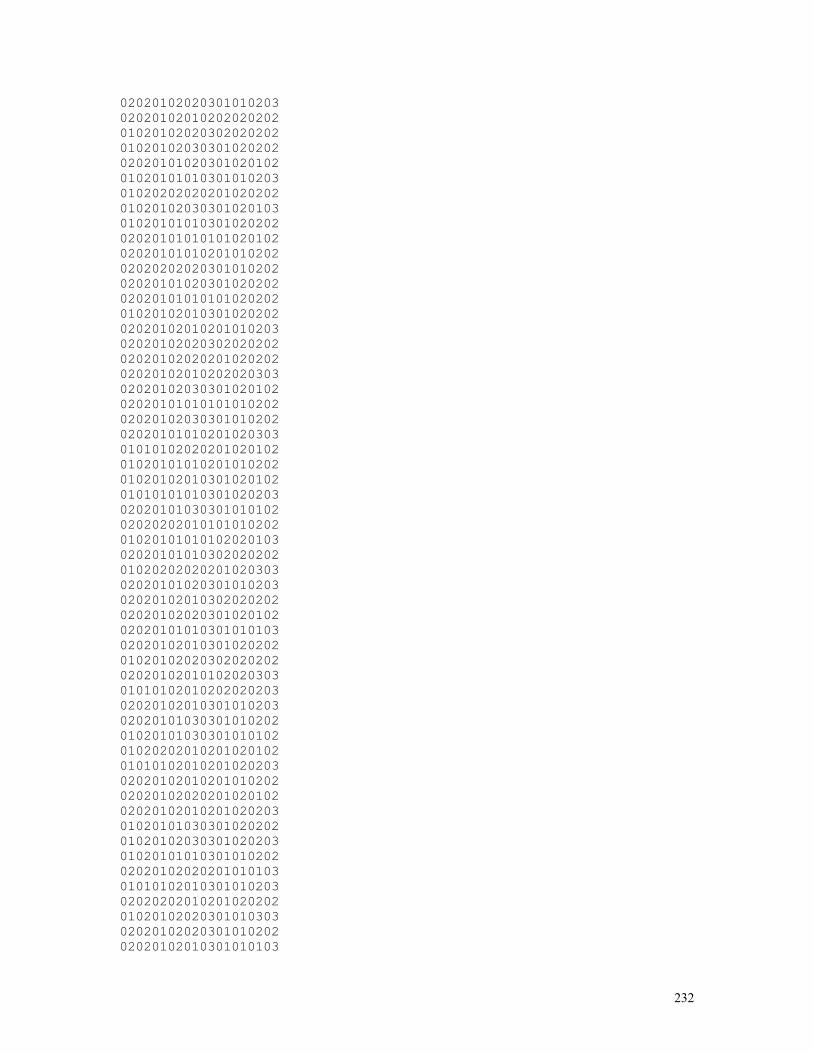
232
02020102020301010203 02020102010202020202 01020102020302020202 01020102030301020202 02020101020301020102 01020101010301010203 01020202020201020202 01020102030301020103 01020101010301020202 02020101010101020102 02020101010201010202 02020202020301010202 02020101020301020202 02020101010101020202 01020102010301020202 02020102010201010203 02020102020302020202 02020102020201020202 02020102010202020303 02020102030301020102 02020101010101010202 02020102030301010202 02020101010201020303 01010102020201020102 01020101010201010202 01020102010301020102 01010101010301020203 02020101030301010102 02020202010101010202 01020101010102020103 02020101010302020202 01020202020201020303 02020101020301010203 02020102010302020202 02020102020301020102 02020101010301010103 02020102010301020202 01020102020302020202 02020102010102020303 01010102010202020203 02020102010301010203 02020101030301010202 01020101030301010102 01020202010201020102 01010102010201020203 02020102010201010202 02020102020201020102 02020102010201020203 01020101030301020202 01020102030301020203 01020101010301010202 02020102020201010103 01010102010301010203 02020202010201020202 01020102020301010303 02020102020301010202 02020102010301010103
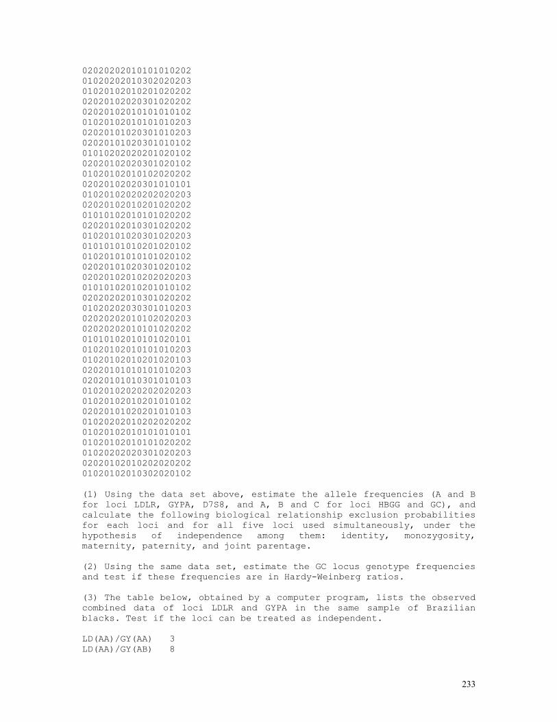
233
02020202010101010202 01020202010302020203 01020102010201020202 02020102020301020202 02020102010101010102 01020102010101010203 02020101020301010203 02020101020301010102 01010202020201020102 02020102020301020102 01020102010102020202 02020102020301010101 01020102020202020203 02020102010201020202 01010102010101020202 02020102010301020202 01020101020301020203 01010101010201020102 01020101010101020102 02020101020301020102 02020102010202020203 01010102010201010102 02020202010301020202 01020202030301010203 02020202010102020203 02020202010101020202 01010102010101020101 01020102010101010203 01020102010201020103 02020101010101010203 02020101010301010103 01020102020202020203 01020102010201010102 02020101020201010103 01020202010202020202 01020102010101010101 01020102010101020202 01020202020301020203 02020102010202020202 01020102010302020102 (1) Using the data set above, estimate the allele frequencies (A and B for loci LDLR, GYPA, D7S8, and A, B and C for loci HBGG and GC), and calculate the following biological relationship exclusion probabilities for each loci and for all five loci used simultaneously, under the hypothesis of independence among them: identity, monozygosity, maternity, paternity, and joint parentage. (2) Using the same data set, estimate the GC locus genotype frequencies and test if these frequencies are in Hardy-Weinberg ratios. (3) The table below, obtained by a computer program, lists the observed combined data of loci LDLR and GYPA in the same sample of Brazilian blacks. Test if the loci can be treated as independent. LD(AA)/GY(AA) 3 LD(AA)/GY(AB) 8
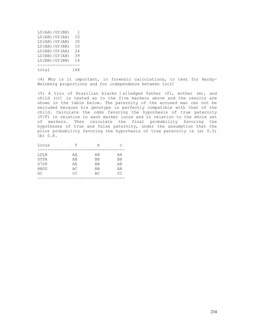
234
LD(AA)/GY(BB) 1 LD(AB)/GY(AA) 15 LD(AB)/GY(AB) 30 LD(AB)/GY(BB) 10 LD(BB)/GY(AA) 24 LD(BB)/GY(AB) 39 LD(BB)/GY(BB) 14 ----------------- total 144 (4) Why is it important, in forensic calculations, to test for Hardy-Weinberg proportions and for independence between loci? (5) A trio of Brazilian blacks [alledged father (f), mother (m), and child (c)] is tested as to the five markers above and the results are shown in the table below. The paternity of the accused man can not be excluded because his genotype is perfectly compatible with that of the child. Calculate the odds favoring the hypothesis of true paternity (T/F) in relation to each marker locus and in relation to the whole set of markers. Then calculate the final probability favoring the hypotheses of true and false paternity, under the assumption that the prior probability favoring the hypothesis of true paternity is (a) 0.5; (b) 0.8. Locus f m c ----------------------------------- LDLR AA AB AA GYPA AB BB BB D7S8 AA BB AB HBGG AC BB AB GC CC BC CC -----------------------------------
235
CLASSICAL AND MODERN METHODOLOGY IN HUMAN GENETICS
(MÉTODOS CLÁSICOS Y MODERNOS PARA EL ANÁLISIS DE
DATOS EN GENÉTICA HUMANA)
PAULO A. OTTO
SOLVED CLASS EXERCISES
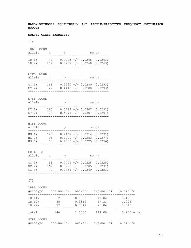
236
HARDY-WEINBERG EQUILIBRIUM AND ALLELE/HAPLOTYPE FREQUENCY ESTIMATION MODULE SOLVED CLASS EXERCISES (1) LDLR LOCUS allele n p se(p) ------------------------------------------- LD(1) 79 0.2743 +/- 0.0268 (0.0263) LD(2) 209 0.7257 +/- 0.0268 (0.0263) ------------------------------------------- GYPA LOCUS allele n p se(p) ------------------------------------------- GY(1) 161 0.5590 +/- 0.0280 (0.0293) GY(2) 127 0.4410 +/- 0.0280 (0.0293) ------------------------------------------- D7S8 LOCUS allele n p se(p) ------------------------------------------- D7(1) 165 0.5729 +/- 0.0307 (0.0291) D7(2) 123 0.4271 +/- 0.0307 (0.0291) ------------------------------------------- HGBB LOCUS allele n p se(p) ------------------------------------------- HG(1) 120 0.4167 +/- 0.0314 (0.0291) HG(2) 95 0.3299 +/- 0.0283 (0.0277) HG(3) 73 0.2535 +/- 0.0273 (0.0256) ------------------------------------------- GC LOCUS allele n p se(p) ------------------------------------------- GC(1) 51 0.1771 +/- 0.0228 (0.0225) GC(2) 167 0.5799 +/- 0.0305 (0.0291) GC(3) 70 0.2431 +/- 0.0260 (0.0253) ------------------------------------------- (2) LDLR LOCUS genotype obs.no.(o) obs.fr. exp.no.(e) (o-e)^2/e --------------------------------------------------------- LD(11) 12 0.0833 10.84 0.125 LD(12) 55 0.3819 57.33 0.095 LD(22) 77 0.5347 75.84 0.018 --------------------------------------------------------- total 144 1.0000 144.00 0.238 = csq GYPA LOCUS genotype obs.no.(o) obs.fr. exp.no.(e) (o-e)^2/e
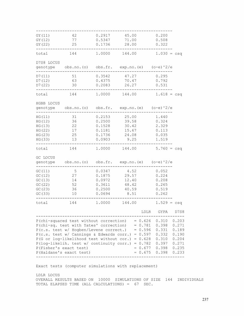
237
--------------------------------------------------------- GY(11) 42 0.2917 45.00 0.200 GY(12) 77 0.5347 71.00 0.508 GY(22) 25 0.1736 28.00 0.322 --------------------------------------------------------- total 144 1.0000 144.00 1.030 = csq D7S8 LOCUS genotype obs.no.(o) obs.fr. exp.no.(e) (o-e)^2/e --------------------------------------------------------- D7(11) 51 0.3542 47.27 0.295 D7(12) 63 0.4375 70.47 0.792 D7(22) 30 0.2083 26.27 0.531 --------------------------------------------------------- total 144 1.0000 144.00 1.618 = csq HGBB LOCUS genotype obs.no.(o) obs.fr. exp.no.(e) (o-e)^2/e --------------------------------------------------------- HG(11) 31 0.2153 25.00 1.440 HG(12) 36 0.2500 39.58 0.324 HG(13) 22 0.1528 30.42 2.329 HG(22) 17 0.1181 15.67 0.113 HG(23) 25 0.1736 24.08 0.035 HG(33) 13 0.0903 9.25 1.519 --------------------------------------------------------- total 144 1.0000 144.00 5.760 = csq GC LOCUS genotype obs.no.(o) obs.fr. exp.no.(e) (o-e)^2/e --------------------------------------------------------- GC(11) 5 0.0347 4.52 0.052 GC(12) 27 0.1875 29.57 0.224 GC(13) 14 0.0972 12.40 0.208 GC(22) 52 0.3611 48.42 0.265 GC(23) 36 0.2500 40.59 0.519 GC(33) 10 0.0694 8.51 0.262 --------------------------------------------------------- total 144 1.0000 144.00 1.529 = csq LDLR GYPA D7S8 -------------------------------------------------------------- P(chi-squared test without correction) = 0.626 0.310 0.203 P(chi-sq. test with Yates' correction) = 0.781 0.398 0.271 P(c.s. test w/ Hogben/Levene correct.) = 0.596 0.331 0.189 P(c.s. test w/ Cannings & Edwards corr.) = 0.597 0.332 0.190 P(G or log-likelihood test without cor.) = 0.628 0.310 0.204 P(log-likelih. test w/ continuity corr.) = 0.782 0.397 0.271 P(Fisher's exact test) = 0.677 0.398 0.235 P(Haldane's exact test) = 0.675 0.398 0.233 -------------------------------------------------------------- Exact tests (computer simulations with replacement) LDLR LOCUS OVERALL RESULTS BASED ON 10000 SIMULATIONS OF SIZE 144 INDIVIDUALS TOTAL ELAPSED TIME (ALL CALCULATIONS) = 67 SEC.
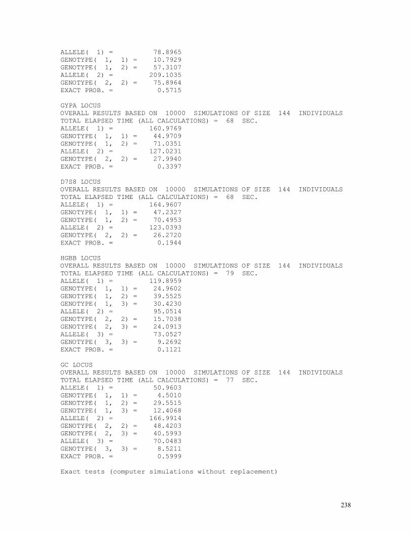
238
ALLELE( 1) = 78.8965 GENOTYPE( 1, 1) = 10.7929 GENOTYPE( 1, 2) = 57.3107 ALLELE( 2) = 209.1035 GENOTYPE( 2, 2) = 75.8964 EXACT PROB. = 0.5715 GYPA LOCUS OVERALL RESULTS BASED ON 10000 SIMULATIONS OF SIZE 144 INDIVIDUALS TOTAL ELAPSED TIME (ALL CALCULATIONS) = 68 SEC. ALLELE( 1) = 160.9769 GENOTYPE( 1, 1) = 44.9709 GENOTYPE( 1, 2) = 71.0351 ALLELE( 2) = 127.0231 GENOTYPE( 2, 2) = 27.9940 EXACT PROB. = 0.3397 D7S8 LOCUS OVERALL RESULTS BASED ON 10000 SIMULATIONS OF SIZE 144 INDIVIDUALS TOTAL ELAPSED TIME (ALL CALCULATIONS) = 68 SEC. ALLELE( 1) = 164.9607 GENOTYPE( 1, 1) = 47.2327 GENOTYPE( 1, 2) = 70.4953 ALLELE( 2) = 123.0393 GENOTYPE( 2, 2) = 26.2720 EXACT PROB. = 0.1944 HGBB LOCUS OVERALL RESULTS BASED ON 10000 SIMULATIONS OF SIZE 144 INDIVIDUALS TOTAL ELAPSED TIME (ALL CALCULATIONS) = 79 SEC. ALLELE( 1) = 119.8959 GENOTYPE( 1, 1) = 24.9602 GENOTYPE( 1, 2) = 39.5525 GENOTYPE( 1, 3) = 30.4230 ALLELE( 2) = 95.0514 GENOTYPE( 2, 2) = 15.7038 GENOTYPE( 2, 3) = 24.0913 ALLELE( 3) = 73.0527 GENOTYPE( 3, 3) = 9.2692 EXACT PROB. = 0.1121 GC LOCUS OVERALL RESULTS BASED ON 10000 SIMULATIONS OF SIZE 144 INDIVIDUALS TOTAL ELAPSED TIME (ALL CALCULATIONS) = 77 SEC. ALLELE( 1) = 50.9603 GENOTYPE( 1, 1) = 4.5010 GENOTYPE( 1, 2) = 29.5515 GENOTYPE( 1, 3) = 12.4068 ALLELE( 2) = 166.9914 GENOTYPE( 2, 2) = 48.4203 GENOTYPE( 2, 3) = 40.5993 ALLELE( 3) = 70.0483 GENOTYPE( 3, 3) = 8.5211 EXACT PROB. = 0.5999 Exact tests (computer simulations without replacement)
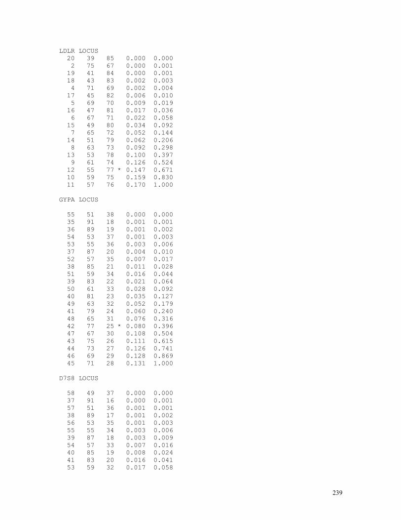
239
LDLR LOCUS 20 39 85 0.000 0.000 2 75 67 0.000 0.001 19 41 84 0.000 0.001 18 43 83 0.002 0.003 4 71 69 0.002 0.004 17 45 82 0.006 0.010 5 69 70 0.009 0.019 16 47 81 0.017 0.036 6 67 71 0.022 0.058 15 49 80 0.034 0.092 7 65 72 0.052 0.144 14 51 79 0.062 0.206 8 63 73 0.092 0.298 13 53 78 0.100 0.397 9 61 74 0.126 0.524 12 55 77 * 0.147 0.671 10 59 75 0.159 0.830 11 57 76 0.170 1.000 GYPA LOCUS 55 51 38 0.000 0.000 35 91 18 0.001 0.001 36 89 19 0.001 0.002 54 53 37 0.001 0.003 53 55 36 0.003 0.006 37 87 20 0.004 0.010 52 57 35 0.007 0.017 38 85 21 0.011 0.028 51 59 34 0.016 0.044 39 83 22 0.021 0.064 50 61 33 0.028 0.092 40 81 23 0.035 0.127 49 63 32 0.052 0.179 41 79 24 0.060 0.240 48 65 31 0.076 0.316 42 77 25 * 0.080 0.396 47 67 30 0.108 0.504 43 75 26 0.111 0.615 44 73 27 0.126 0.741 46 69 29 0.128 0.869 45 71 28 0.131 1.000 D7S8 LOCUS 58 49 37 0.000 0.000 37 91 16 0.000 0.001 57 51 36 0.001 0.001 38 89 17 0.001 0.002 56 53 35 0.001 0.003 55 55 34 0.003 0.006 39 87 18 0.003 0.009 54 57 33 0.007 0.016 40 85 19 0.008 0.024 41 83 20 0.016 0.041 53 59 32 0.017 0.058
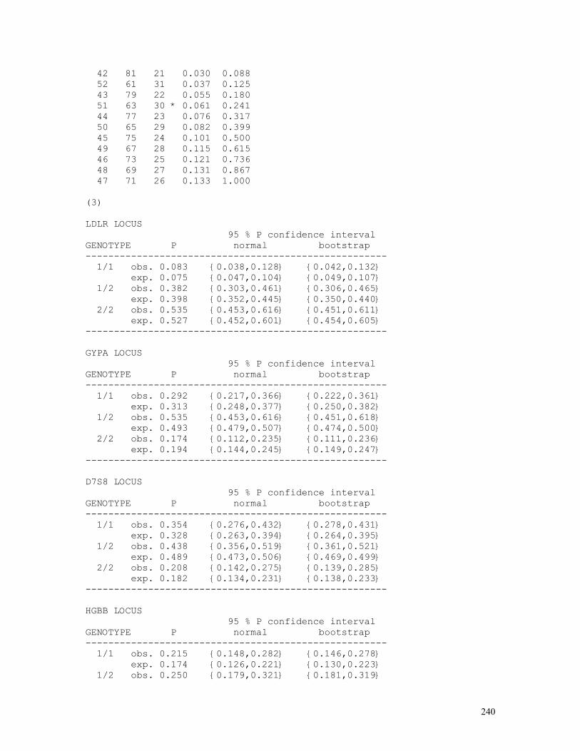
240
42 81 21 0.030 0.088 52 61 31 0.037 0.125 43 79 22 0.055 0.180 51 63 30 * 0.061 0.241 44 77 23 0.076 0.317 50 65 29 0.082 0.399 45 75 24 0.101 0.500 49 67 28 0.115 0.615 46 73 25 0.121 0.736 48 69 27 0.131 0.867 47 71 26 0.133 1.000 (3) LDLR LOCUS 95 % P confidence interval GENOTYPE P normal bootstrap ----------------------------------------------------- 1/1 obs. 0.083 {0.038,0.128} {0.042,0.132} exp. 0.075 {0.047,0.104} {0.049,0.107} 1/2 obs. 0.382 {0.303,0.461} {0.306,0.465} exp. 0.398 {0.352,0.445} {0.350,0.440} 2/2 obs. 0.535 {0.453,0.616} {0.451,0.611} exp. 0.527 {0.452,0.601} {0.454,0.605} ----------------------------------------------------- GYPA LOCUS 95 % P confidence interval GENOTYPE P normal bootstrap ----------------------------------------------------- 1/1 obs. 0.292 {0.217,0.366} {0.222,0.361} exp. 0.313 {0.248,0.377} {0.250,0.382} 1/2 obs. 0.535 {0.453,0.616} {0.451,0.618} exp. 0.493 {0.479,0.507} {0.474,0.500} 2/2 obs. 0.174 {0.112,0.235} {0.111,0.236} exp. 0.194 {0.144,0.245} {0.149,0.247} ----------------------------------------------------- D7S8 LOCUS 95 % P confidence interval GENOTYPE P normal bootstrap ----------------------------------------------------- 1/1 obs. 0.354 {0.276,0.432} {0.278,0.431} exp. 0.328 {0.263,0.394} {0.264,0.395} 1/2 obs. 0.438 {0.356,0.519} {0.361,0.521} exp. 0.489 {0.473,0.506} {0.469,0.499} 2/2 obs. 0.208 {0.142,0.275} {0.139,0.285} exp. 0.182 {0.134,0.231} {0.138,0.233} ----------------------------------------------------- HGBB LOCUS 95 % P confidence interval GENOTYPE P normal bootstrap ----------------------------------------------------- 1/1 obs. 0.215 {0.148,0.282} {0.146,0.278} exp. 0.174 {0.126,0.221} {0.130,0.223} 1/2 obs. 0.250 {0.179,0.321} {0.181,0.319}
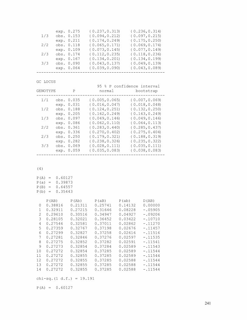
241
exp. 0.275 {0.237,0.313} {0.236,0.314} 1/3 obs. 0.153 {0.094,0.212} {0.097,0.215} exp. 0.211 {0.174,0.249} {0.175,0.250} 2/2 obs. 0.118 {0.065,0.171} {0.069,0.174} exp. 0.109 {0.073,0.145} {0.077,0.149} 2/3 obs. 0.174 {0.112,0.235} {0.118,0.236} exp. 0.167 {0.134,0.201} {0.134,0.199} 3/3 obs. 0.090 {0.043,0.137} {0.049,0.139} exp. 0.064 {0.039,0.090} {0.043,0.089} ----------------------------------------------------- GC LOCUS 95 % P confidence interval GENOTYPE P normal bootstrap ----------------------------------------------------- 1/1 obs. 0.035 {0.005,0.065} {0.007,0.069} exp. 0.031 {0.016,0.047} {0.018,0.048} 1/2 obs. 0.188 {0.124,0.251} {0.132,0.250} exp. 0.205 {0.162,0.249} {0.163,0.249} 1/3 obs. 0.097 {0.049,0.146} {0.049,0.146} exp. 0.086 {0.062,0.110} {0.064,0.113} 2/2 obs. 0.361 {0.283,0.440} {0.285,0.437} exp. 0.336 {0.270,0.402} {0.275,0.404} 2/3 obs. 0.250 {0.179,0.321} {0.188,0.319} exp. 0.282 {0.238,0.326} {0.235,0.322} 3/3 obs. 0.069 {0.028,0.111} {0.035,0.111} exp. 0.059 {0.035,0.083} {0.038,0.083} ----------------------------------------------------- (4) P(A) = 0.60127 P(a) = 0.39873 P(B) = 0.64557 P(b) = 0.35443 P(AB) P(Ab) P(aB) P(ab) D(AB) 0 0.38816 0.21311 0.25741 0.14132 0.00000 1 0.32911 0.27215 0.31646 0.08228 -.05905 2 0.29610 0.30516 0.34947 0.04927 -.09206 3 0.28105 0.32021 0.36452 0.03422 -.10710 4 0.27546 0.32581 0.37011 0.02862 -.11270 5 0.27359 0.32767 0.37198 0.02676 -.11457 6 0.27299 0.32827 0.37258 0.02616 -.11516 7 0.27281 0.32846 0.37276 0.02597 -.11535 8 0.27275 0.32852 0.37282 0.02591 -.11541 9 0.27273 0.32854 0.37284 0.02589 -.11543 10 0.27272 0.32854 0.37285 0.02589 -.11544 11 0.27272 0.32855 0.37285 0.02589 -.11544 12 0.27272 0.32855 0.37285 0.02588 -.11544 13 0.27272 0.32855 0.37285 0.02588 -.11544 14 0.27272 0.32855 0.37285 0.02588 -.11544 chi-sq.(1 d.f.) = 19.191 P(A) = 0.60127
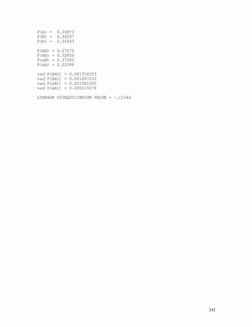
242
P(a) = 0.39873 P(B) = 0.64557 P(b) = 0.35443 P(AB) = 0.27272 P(Ab) = 0.32855 P(aB) = 0.37285 P(ab) = 0.02588 var[P(AB)] = 0.001316323 var[P(Ab)] = 0.001457225 var[P(aB)] = 0.001541055 var[P(ab)] = 0.000219376 LINKAGE DISEQUILIBRIUM VALUE = -.11544
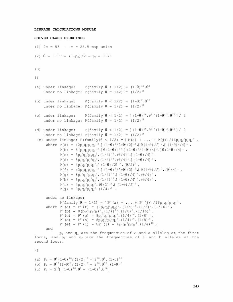
243
LINKAGE CALCULATIONS MODULE SOLVED CLASS EXERCISES (1) 2m = 53 → m = 26.5 map units (2) θ = 0.15 = (1-p0)/2 → p0 = 0.70 (3)
1) (a) under linkage: P(family|θ < 1/2) = (1-θ)16.θ2
under no linkage: P(family|θ = 1/2) = (1/2)18 (b) under linkage: P(family|θ < 1/2) = (1-θ)2.θ16 under no linkage: P(family|θ = 1/2) = (1/2)18 (c) under linkage: P(family|θ < 1/2) = [(1-θ)16.θ2 +(1-θ)2.θ16 ]/ 2 under no linkage: P(family|θ = 1/2) = (1/2)18 (d) under linkage: P(family|θ < 1/2) = [(1-θ)16.θ2 +(1-θ)2.θ16 ]/ 2 under no linkage: P(family|θ = 1/2) = (1/2)18 (e) under linkage: P(family|θ < 1/2) = [P(a) + ... + P(j)]/16p1q12p2q22 , where P(a) = (2p1q1p2q2)2.[(1-θ)2/2+θ2/2]15.[θ(1-θ)/2]2.[(1-θ)2/4]1 , P(b) = 8(p1q1p2q2)2.[θ(1-θ)]15.[(1-θ)2/4+θ2/4]2.[θ(1-θ)/4]1 , P(c) = 8p12q12p2q23.(1/4)16.(θ/4)1.[(1-θ)/4]1 , P(d) = 8p1q13p22q22.(1/4)16.(θ/4)1.[(1-θ)/4]1 , P(e) = 4p1q13p2q23.[(1-θ)/2]16.(θ/2)2 , P(f) = (2p1q1p2q2)2.[(1-θ)2/2+θ2/2]15.[θ(1-θ)/2]2.(θ2/4)1 , P(g) = 8p12q12p2q23.(1/4)16.[(1-θ)/4]1.(θ/4)1 , P(h) = 8p1q13p22q22.(1/4)16.[(1-θ)/4]1.(θ/4)1 , P(i) = 4p1q13p2q23.(θ/2)16.[(1-θ)/2]2 , P(j) = 8p1q13p2q23.(1/4)18 . under no linkage: P(family|θ = 1/2) = [P’(a) + ... + P’(j)]/16p1q12p2q22 , where P’(a) = P’(f) = (2p1q1p2q2)2.(1/4)15.(1/8)2.(1/16)1 , P’(b) = 8(p1q1p2q2)2.(1/4)15.(1/8)2.(1/16)1 , P’(c) = P’(g) = 8p12q12p2q23.(1/4)16.(1/8)2 , P’(d) = P’(h) = 8p1q13p22q22.(1/4)16.(1/8)2 , P’(e) = P’(i) = ½P’(j) = 4p1q13p2q23.(1/4)18 , and p1 and q1 are the frequencies of A and a alleles at the first locus, and p2 and q2 are the frequencies of B and b alleles at the second locus. 2) (a) PR = θ2(1-θ)16/(1/2)18 = 218.θ2.(1-θ)16 (b) PR = θ16(1-θ)2/(1/2)18 = 218.θ16.(1-θ)2 (c) PR = 217[(1-θ)16.θ2 + (1-θ)2.θ16]
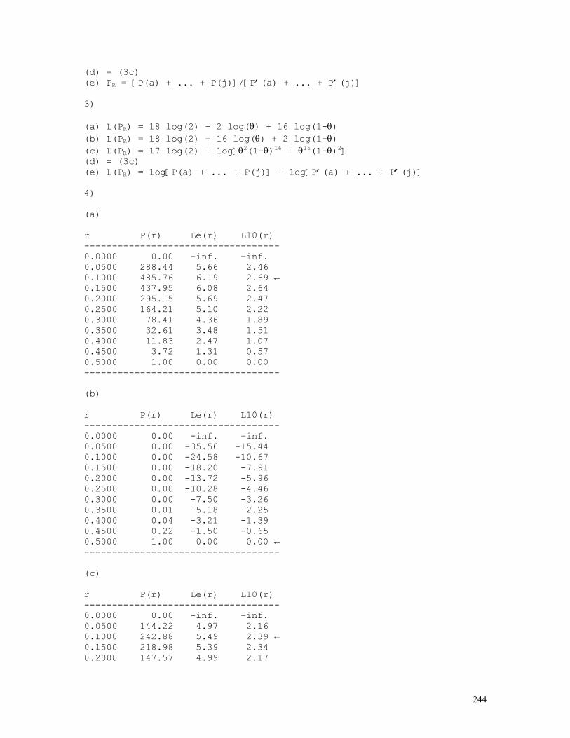
244
(d) = (3c) (e) PR = [P(a) + ... + P(j)]/[P’(a) + ... + P’(j)] 3) (a) L(PR) = 18 log(2) + 2 log(θ) + 16 log(1-θ) (b) L(PR) = 18 log(2) + 16 log(θ) + 2 log(1-θ) (c) L(PR) = 17 log(2) + log[θ2(1-θ)16 + θ16(1-θ)2] (d) = (3c) (e) L(PR) = log[P(a) + ... + P(j)] - log[P’(a) + ... + P’(j)] 4) (a) r P(r) Le(r) L10(r) ----------------------------------- 0.0000 0.00 -inf. –inf. 0.0500 288.44 5.66 2.46 0.1000 485.76 6.19 2.69 ← 0.1500 437.95 6.08 2.64 0.2000 295.15 5.69 2.47 0.2500 164.21 5.10 2.22 0.3000 78.41 4.36 1.89 0.3500 32.61 3.48 1.51 0.4000 11.83 2.47 1.07 0.4500 3.72 1.31 0.57 0.5000 1.00 0.00 0.00 ----------------------------------- (b) r P(r) Le(r) L10(r) ----------------------------------- 0.0000 0.00 -inf. –inf. 0.0500 0.00 -35.56 -15.44 0.1000 0.00 -24.58 -10.67 0.1500 0.00 -18.20 -7.91 0.2000 0.00 -13.72 -5.96 0.2500 0.00 -10.28 -4.46 0.3000 0.00 -7.50 -3.26 0.3500 0.01 -5.18 -2.25 0.4000 0.04 -3.21 -1.39 0.4500 0.22 -1.50 -0.65 0.5000 1.00 0.00 0.00 ← ----------------------------------- (c) r P(r) Le(r) L10(r) ----------------------------------- 0.0000 0.00 -inf. –inf. 0.0500 144.22 4.97 2.16 0.1000 242.88 5.49 2.39 ← 0.1500 218.98 5.39 2.34 0.2000 147.57 4.99 2.17

245
0.2500 82.11 4.41 1.91 0.3000 39.20 3.67 1.59 0.3500 16.31 2.79 1.21 0.4000 5.94 1.78 0.77 0.4500 1.97 0.68 0.30 0.5000 1.00 0.00 0.00 ----------------------------------- (d) = (c) (e) r P(r) Le(r) L10(r) ----------------------------------- 0.0000 0.00 -inf. –inf. 0.0500 171.45 5.14 2.23 ← 0.1000 128.77 4.86 2.11 0.1500 57.22 4.05 1.76 0.2000 21.88 3.09 1.34 0.2500 8.31 2.12 0.92 0.3000 3.44 1.23 0.54 0.3500 1.72 0.54 0.23 0.4000 1.15 0.14 0.06 0.4500 1.02 0.02 0.01 0.5000 1.00 0.00 0.00 ----------------------------------- (5) The arrows at right of tables shown in items 4a to 4e indicate the approximate maximum values the lod-score can take in the interval (0,0.5) of possible recombination fraction values for each situation (a – e). (6) (a) r = 0.1111
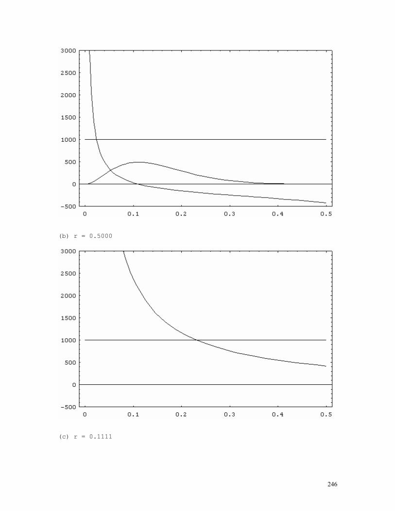
246
(b) r = 0.5000
(c) r = 0.1111
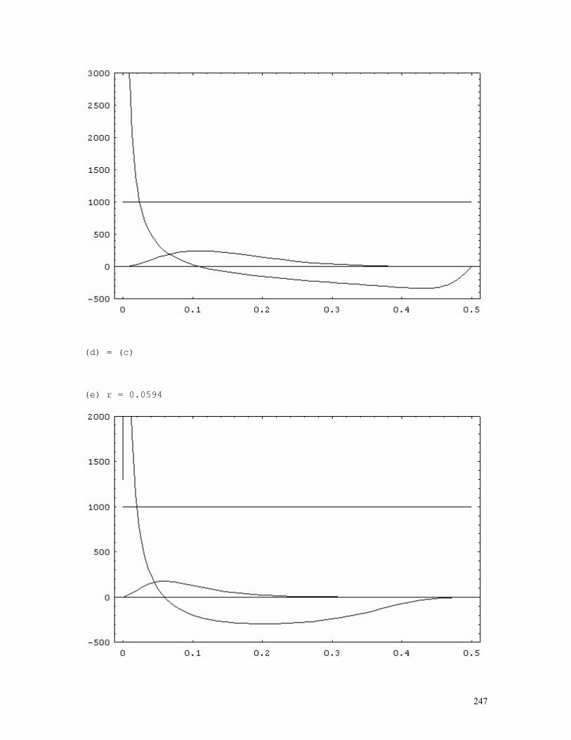
247
(d) = (c) (e) r = 0.0594
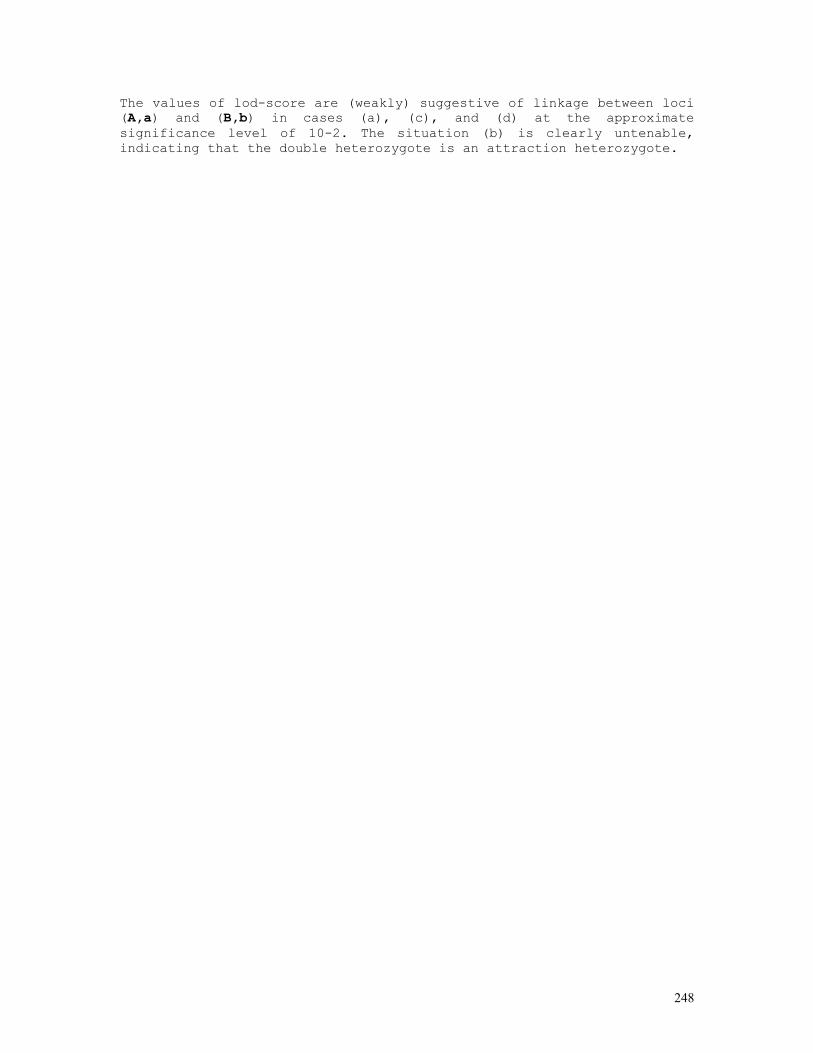
248
The values of lod-score are (weakly) suggestive of linkage between loci (A,a) and (B,b) in cases (a), (c), and (d) at the approximate significance level of 10-2. The situation (b) is clearly untenable, indicating that the double heterozygote is an attraction heterozygote.
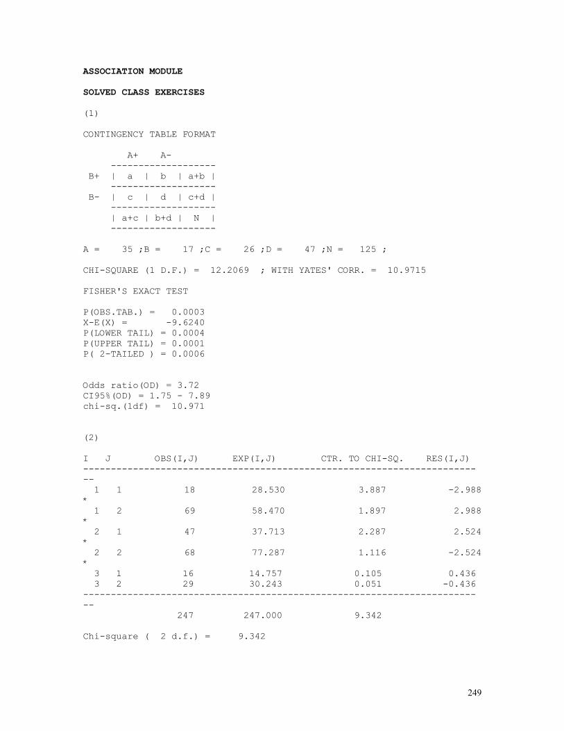
249
ASSOCIATION MODULE SOLVED CLASS EXERCISES (1) CONTINGENCY TABLE FORMAT A+ A- ------------------- B+ | a | b | a+b | ------------------- B- | c | d | c+d | ------------------- | a+c | b+d | N | ------------------- A = 35 ;B = 17 ;C = 26 ;D = 47 ;N = 125 ; CHI-SQUARE (1 D.F.) = 12.2069 ; WITH YATES' CORR. = 10.9715 FISHER'S EXACT TEST P(OBS.TAB.) = 0.0003 X-E(X) = -9.6240 P(LOWER TAIL) = 0.0004 P(UPPER TAIL) = 0.0001 P( 2-TAILED ) = 0.0006 Odds ratio(OD) = 3.72 CI95%(OD) = 1.75 - 7.89 chi-sq.(1df) = 10.971 (2) I J OBS(I,J) EXP(I,J) CTR. TO CHI-SQ. RES(I,J) ------------------------------------------------------------------------- 1 1 18 28.530 3.887 -2.988 * 1 2 69 58.470 1.897 2.988 * 2 1 47 37.713 2.287 2.524 * 2 2 68 77.287 1.116 -2.524 * 3 1 16 14.757 0.105 0.436 3 2 29 30.243 0.051 -0.436 ------------------------------------------------------------------------- 247 247.000 9.342 Chi-square ( 2 d.f.) = 9.342
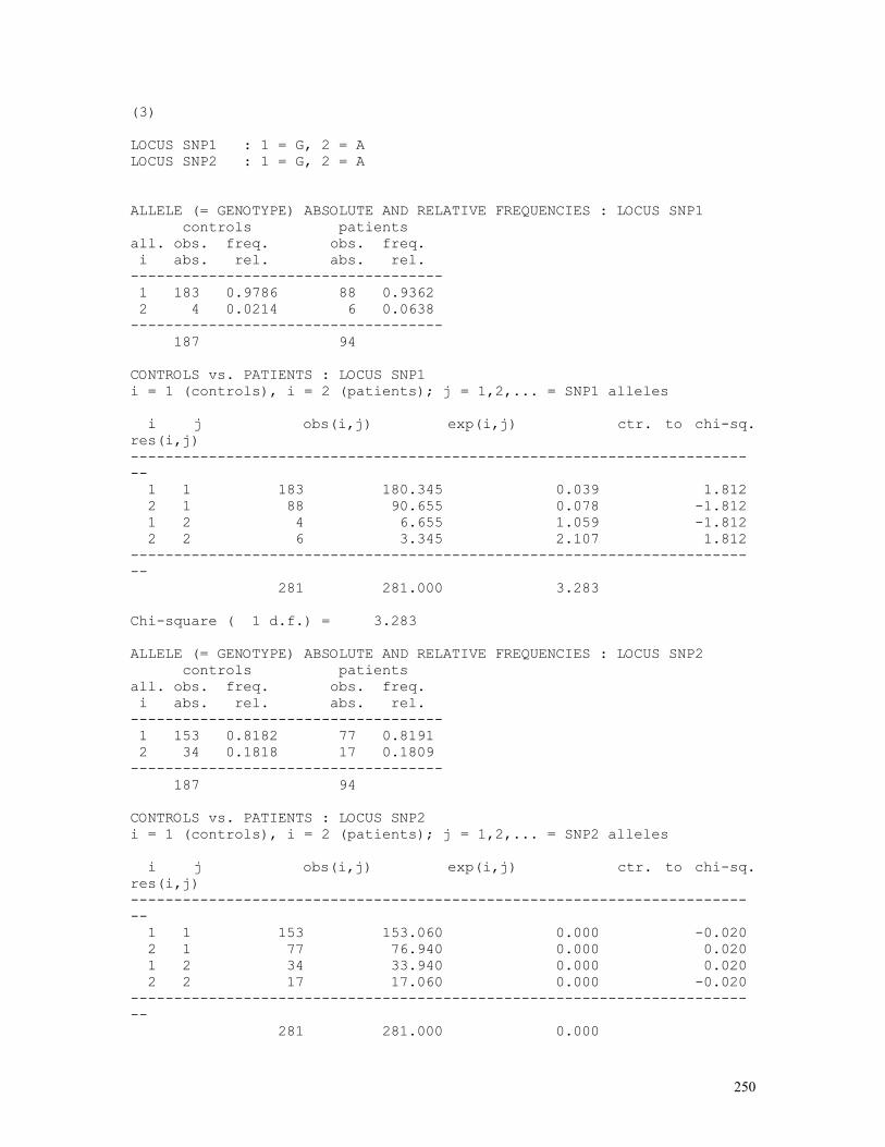
250
(3) LOCUS SNP1 : 1 = G, 2 = A LOCUS SNP2 : 1 = G, 2 = A ALLELE (= GENOTYPE) ABSOLUTE AND RELATIVE FREQUENCIES : LOCUS SNP1 controls patients all. obs. freq. obs. freq. i abs. rel. abs. rel. ------------------------------------ 1 183 0.9786 88 0.9362 2 4 0.0214 6 0.0638 ------------------------------------ 187 94 CONTROLS vs. PATIENTS : LOCUS SNP1 i = 1 (controls), i = 2 (patients); j = 1,2,... = SNP1 alleles i j obs(i,j) exp(i,j) ctr. to chi-sq. res(i,j) ------------------------------------------------------------------------- 1 1 183 180.345 0.039 1.812 2 1 88 90.655 0.078 -1.812 1 2 4 6.655 1.059 -1.812 2 2 6 3.345 2.107 1.812 ------------------------------------------------------------------------- 281 281.000 3.283 Chi-square ( 1 d.f.) = 3.283 ALLELE (= GENOTYPE) ABSOLUTE AND RELATIVE FREQUENCIES : LOCUS SNP2 controls patients all. obs. freq. obs. freq. i abs. rel. abs. rel. ------------------------------------ 1 153 0.8182 77 0.8191 2 34 0.1818 17 0.1809 ------------------------------------ 187 94 CONTROLS vs. PATIENTS : LOCUS SNP2 i = 1 (controls), i = 2 (patients); j = 1,2,... = SNP2 alleles i j obs(i,j) exp(i,j) ctr. to chi-sq. res(i,j) ------------------------------------------------------------------------- 1 1 153 153.060 0.000 -0.020 2 1 77 76.940 0.000 0.020 1 2 34 33.940 0.000 0.020 2 2 17 17.060 0.000 -0.020 ------------------------------------------------------------------------- 281 281.000 0.000
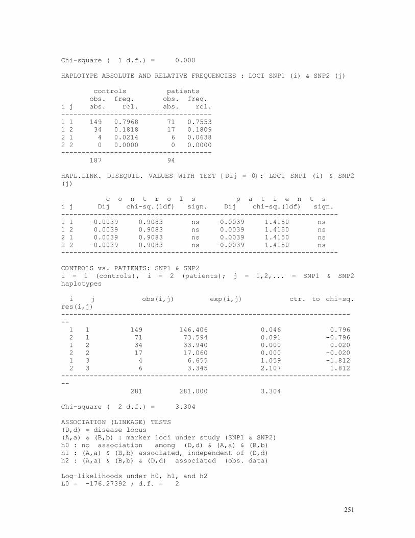
251
Chi-square ( 1 d.f.) = 0.000 HAPLOTYPE ABSOLUTE AND RELATIVE FREQUENCIES : LOCI SNP1 (i) & SNP2 (j) controls patients obs. freq. obs. freq. i j abs. rel. abs. rel. ------------------------------------- 1 1 149 0.7968 71 0.7553 1 2 34 0.1818 17 0.1809 2 1 4 0.0214 6 0.0638 2 2 0 0.0000 0 0.0000 ------------------------------------- 187 94 HAPL.LINK. DISEQUIL. VALUES WITH TEST {Dij = 0}: LOCI SNP1 (i) & SNP2 (j) c o n t r o l s p a t i e n t s i j Dij chi-sq.(1df) sign. Dij chi-sq.(1df) sign. -------------------------------------------------------------------- 1 1 -0.0039 0.9083 ns -0.0039 1.4150 ns 1 2 0.0039 0.9083 ns 0.0039 1.4150 ns 2 1 0.0039 0.9083 ns 0.0039 1.4150 ns 2 2 -0.0039 0.9083 ns -0.0039 1.4150 ns -------------------------------------------------------------------- CONTROLS vs. PATIENTS: SNP1 & SNP2 i = 1 (controls), i = 2 (patients); j = 1,2,... = SNP1 & SNP2 haplotypes i j obs(i,j) exp(i,j) ctr. to chi-sq. res(i,j) ------------------------------------------------------------------------- 1 1 149 146.406 0.046 0.796 2 1 71 73.594 0.091 -0.796 1 2 34 33.940 0.000 0.020 2 2 17 17.060 0.000 -0.020 1 3 4 6.655 1.059 -1.812 2 3 6 3.345 2.107 1.812 ------------------------------------------------------------------------- 281 281.000 3.304 Chi-square ( 2 d.f.) = 3.304 ASSOCIATION (LINKAGE) TESTS (D,d) = disease locus (A,a) & (B,b) : marker loci under study (SNP1 & SNP2) h0 : no association among (D,d) & (A,a) & (B,b) h1 : (A,a) & (B,b) associated, independent of (D,d) h2 : (A,a) & (B,b) & (D,d) associated (obs. data) Log-likelihoods under h0, h1, and h2 L0 = -176.27392 ; d.f. = 2
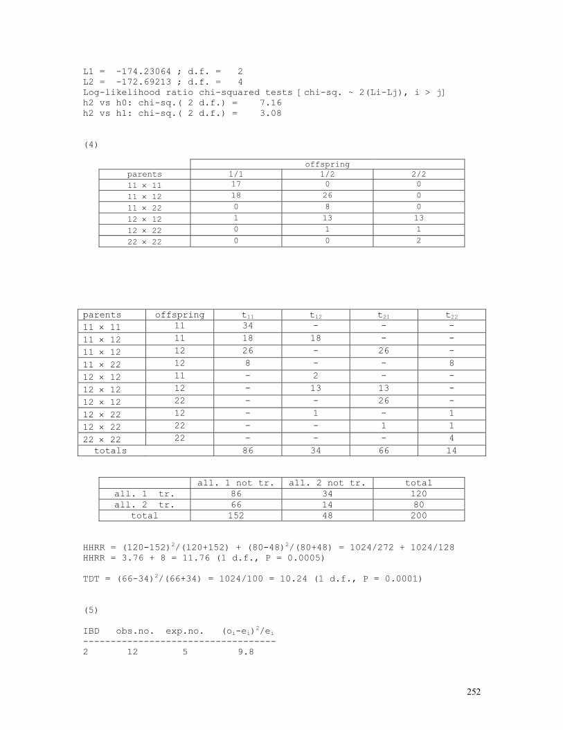
252
L1 = -174.23064 ; d.f. = 2 L2 = -172.69213 ; d.f. = 4 Log-likelihood ratio chi-squared tests [chi-sq. ~ 2(Li-Lj), i > j] h2 vs h0: chi-sq.( 2 d.f.) = 7.16 h2 vs h1: chi-sq.( 2 d.f.) = 3.08 (4)
offspring parents 1/1 1/2 2/2 11 × 11 17 0 0
11 × 12 18 26 0
11 × 22 0 8 0
12 × 12 1 13 13
12 × 22 0 1 1
22 × 22 0 0 2
parents offspring t11 t12 t21 t22 11 × 11 11 34 - - -
11 × 12 11 18 18 - -
11 × 12 12 26 - 26 -
11 × 22 12 8 - - 8
12 × 12 11 - 2 - -
12 × 12 12 - 13 13 -
12 × 12 22 - - 26 -
12 × 22 12 - 1 - 1
12 × 22 22 - - 1 1
22 × 22 22 - - - 4 totals 86 34 66 14
all. 1 not tr. all. 2 not tr. total all. 1 tr. 86 34 120 all. 2 tr. 66 14 80
total 152 48 200 HHRR = (120-152)2/(120+152) + (80-48)2/(80+48) = 1024/272 + 1024/128 HHRR = 3.76 + 8 = 11.76 (1 d.f., P = 0.0005) TDT = (66-34)2/(66+34) = 1024/100 = 10.24 (1 d.f., P = 0.0001) (5) IBD obs.no. exp.no. (oi-ei)2/ei ----------------------------------- 2 12 5 9.8
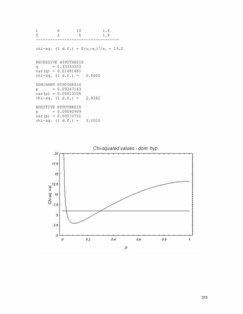
253
1 6 10 1.6 0 2 5 1.8 ----------------------------------- chi-sq. (1 d.f.) = Σ(oi-ei)2/ei = 13.2 RECESSIVE HYPOTHESIS q = 0.33333333 var(q) = 0.01481481 chi-sq. (1 d.f.) = 0.8000 DOMINANT HYPOTHESIS p = 0.09247143 var(p) = 0.00613556 chi-sq. (1 d.f.) = 2.9382 ADDITIVE HYPOTHESIS p = 0.09090909 var(p) = 0.00573731 chi-sq. (1 d.f.) = 3.2000
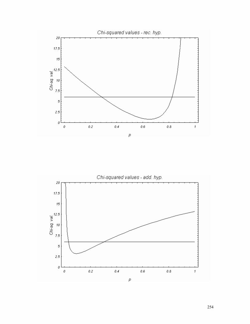
254
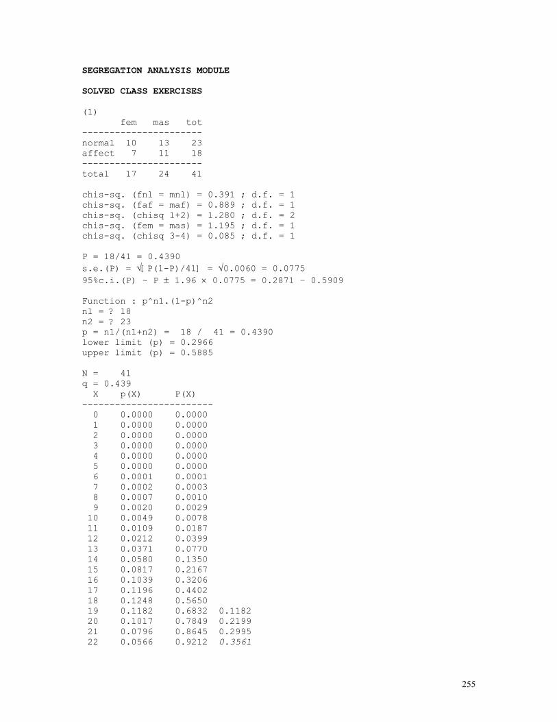
255
SEGREGATION ANALYSIS MODULE SOLVED CLASS EXERCISES (1) fem mas tot ---------------------- normal 10 13 23 affect 7 11 18 ---------------------- total 17 24 41 chis-sq. (fnl = mnl) = 0.391 ; d.f. = 1 chis-sq. (faf = maf) = 0.889 ; d.f. = 1 chis-sq. (chisq 1+2) = 1.280 ; d.f. = 2 chis-sq. (fem = mas) = 1.195 ; d.f. = 1 chis-sq. (chisq 3-4) = 0.085 ; d.f. = 1 P = 18/41 = 0.4390 s.e.(P) = √[P(1-P)/41] = √0.0060 = 0.0775 95%c.i.(P) ~ P ± 1.96 × 0.0775 = 0.2871 – 0.5909 Function : p^n1.(1-p)^n2 n1 = ? 18 n2 = ? 23 p = n1/(n1+n2) = 18 / 41 = 0.4390 lower limit (p) = 0.2966 upper limit (p) = 0.5885 N = 41 q = 0.439 X p(X) P(X) ------------------------ 0 0.0000 0.0000 1 0.0000 0.0000 2 0.0000 0.0000 3 0.0000 0.0000 4 0.0000 0.0000 5 0.0000 0.0000 6 0.0001 0.0001 7 0.0002 0.0003 8 0.0007 0.0010 9 0.0020 0.0029 10 0.0049 0.0078 11 0.0109 0.0187 12 0.0212 0.0399 13 0.0371 0.0770 14 0.0580 0.1350 15 0.0817 0.2167 16 0.1039 0.3206 17 0.1196 0.4402 18 0.1248 0.5650 19 0.1182 0.6832 0.1182 20 0.1017 0.7849 0.2199 21 0.0796 0.8645 0.2995 22 0.0566 0.9212 0.3561
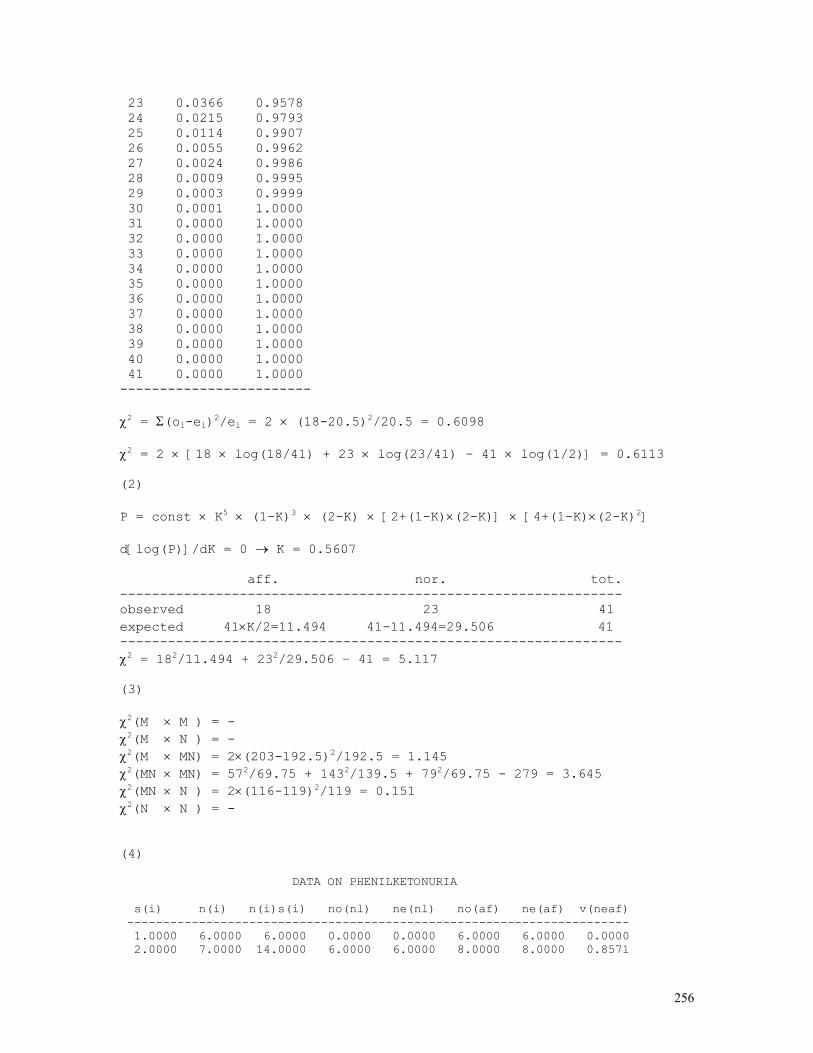
256
23 0.0366 0.9578 24 0.0215 0.9793 25 0.0114 0.9907 26 0.0055 0.9962 27 0.0024 0.9986 28 0.0009 0.9995 29 0.0003 0.9999 30 0.0001 1.0000 31 0.0000 1.0000 32 0.0000 1.0000 33 0.0000 1.0000 34 0.0000 1.0000 35 0.0000 1.0000 36 0.0000 1.0000 37 0.0000 1.0000 38 0.0000 1.0000 39 0.0000 1.0000 40 0.0000 1.0000 41 0.0000 1.0000 ------------------------ χ2 = Σ(oi-ei)2/ei = 2 × (18-20.5)2/20.5 = 0.6098 χ2 = 2 × [18 × log(18/41) + 23 × log(23/41) – 41 × log(1/2)] = 0.6113 (2) P = const × K5 × (1-K)3 × (2-K) × [2+(1-K)×(2-K)] × [4+(1-K)×(2-K)2] d[log(P)]/dK = 0 → K = 0.5607 aff. nor. tot. --------------------------------------------------------------- observed 18 23 41 expected 41×K/2=11.494 41-11.494=29.506 41 --------------------------------------------------------------- χ2 = 182/11.494 + 232/29.506 – 41 = 5.117 (3) χ2(M × M ) = - χ2(M × N ) = - χ2(M × MN) = 2×(203-192.5)2/192.5 = 1.145 χ2(MN × MN) = 572/69.75 + 1432/139.5 + 792/69.75 - 279 = 3.645 χ2(MN × N ) = 2×(116-119)2/119 = 0.151 χ2(N × N ) = - (4) DATA ON PHENILKETONURIA s(i) n(i) n(i)s(i) no(nl) ne(nl) no(af) ne(af) v(neaf) ---------------------------------------------------------------------- 1.0000 6.0000 6.0000 0.0000 0.0000 6.0000 6.0000 0.0000 2.0000 7.0000 14.0000 6.0000 6.0000 8.0000 8.0000 0.8571
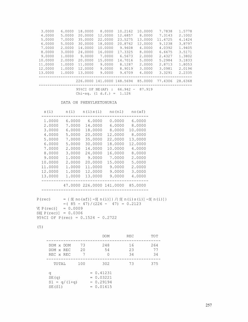
257
3.0000 6.0000 18.0000 8.0000 10.2162 10.0000 7.7838 1.5778 4.0000 5.0000 20.0000 12.0000 12.6857 8.0000 7.3143 2.1002 5.0000 7.0000 35.0000 22.0000 23.5275 13.0000 11.4725 4.1424 6.0000 5.0000 30.0000 18.0000 20.8762 12.0000 9.1238 3.8797 7.0000 2.0000 14.0000 10.0000 9.9608 4.0000 4.0392 1.9405 8.0000 3.0000 24.0000 16.0000 17.3325 8.0000 6.6675 3.5171 9.0000 1.0000 9.0000 7.0000 6.5673 2.0000 2.4327 1.3802 10.0000 2.0000 20.0000 15.0000 14.7016 5.0000 5.2984 3.1833 11.0000 1.0000 11.0000 9.0000 8.1287 2.0000 2.8713 1.8053 12.0000 1.0000 12.0000 9.0000 8.9019 3.0000 3.0981 2.0196 13.0000 1.0000 13.0000 9.0000 9.6709 4.0000 3.3291 2.2335 ---------------------------------------------------------------------- 226.0000 141.0000 148.5694 85.0000 77.4306 28.6368 ---------------------------------------------------------------------- 95%CI OF NE(AF) : 66.942 - 87.919 Chi-sq. (1 d.f.) = 1.126 DATA ON PHENYLKETONURIA s(i) n(i) n(i)s(i) no(nl) no(af) -------------------------------------------- 1.0000 6.0000 6.0000 0.0000 6.0000 2.0000 7.0000 14.0000 6.0000 8.0000 3.0000 6.0000 18.0000 8.0000 10.0000 4.0000 5.0000 20.0000 12.0000 8.0000 5.0000 7.0000 35.0000 22.0000 13.0000 6.0000 5.0000 30.0000 18.0000 12.0000 7.0000 2.0000 14.0000 10.0000 4.0000 8.0000 3.0000 24.0000 16.0000 8.0000 9.0000 1.0000 9.0000 7.0000 2.0000 10.0000 2.0000 20.0000 15.0000 5.0000 11.0000 1.0000 11.0000 9.0000 2.0000 12.0000 1.0000 12.0000 9.0000 3.0000 13.0000 1.0000 13.0000 9.0000 4.0000 -------------------------------------------- 47.0000 226.0000 141.0000 85.0000 -------------------------------------------- P(rec) = {S[no(af)]-S[n(i)]}/{S[n(i)s(i)]-S[n(i)]} =( 85 - 47)/(226 - 47) = 0.2123 V[P(rec)] = 0.0009 SE[P(rec)] = 0.0306 95%CI OF P(rec) = 0.1524 - 0.2722 (5) DOM REC TOT ----------------------------------------------- DOM x DOM 73 248 16 264 DOM x REC 20 54 23 77 REC x REC 7 0 34 34 ----------------------------------------------- TOTAL 100 302 73 375 q = 0.41231 SE(q) = 0.03221 S1 = q/(1+q) = 0.29194 SE(S1) = 0.01615
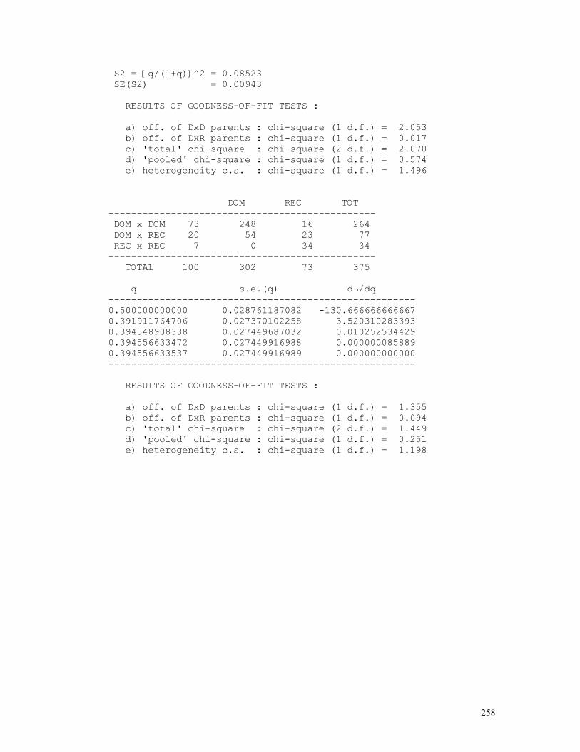
258
S2 = [q/(1+q)]^2 = 0.08523 SE(S2) = 0.00943 RESULTS OF GOODNESS-OF-FIT TESTS : a) off. of DxD parents : chi-square (1 d.f.) = 2.053 b) off. of DxR parents : chi-square (1 d.f.) = 0.017 c) 'total' chi-square : chi-square (2 d.f.) = 2.070 d) 'pooled' chi-square : chi-square (1 d.f.) = 0.574 e) heterogeneity c.s. : chi-square (1 d.f.) = 1.496 DOM REC TOT ----------------------------------------------- DOM x DOM 73 248 16 264 DOM x REC 20 54 23 77 REC x REC 7 0 34 34 ----------------------------------------------- TOTAL 100 302 73 375 q s.e.(q) dL/dq ------------------------------------------------------ 0.500000000000 0.028761187082 -130.666666666667 0.391911764706 0.027370102258 3.520310283393 0.394548908338 0.027449687032 0.010252534429 0.394556633472 0.027449916988 0.000000085889 0.394556633537 0.027449916989 0.000000000000 ------------------------------------------------------ RESULTS OF GOODNESS-OF-FIT TESTS : a) off. of DxD parents : chi-square (1 d.f.) = 1.355 b) off. of DxR parents : chi-square (1 d.f.) = 0.094 c) 'total' chi-square : chi-square (2 d.f.) = 1.449 d) 'pooled' chi-square : chi-square (1 d.f.) = 0.251 e) heterogeneity c.s. : chi-square (1 d.f.) = 1.198
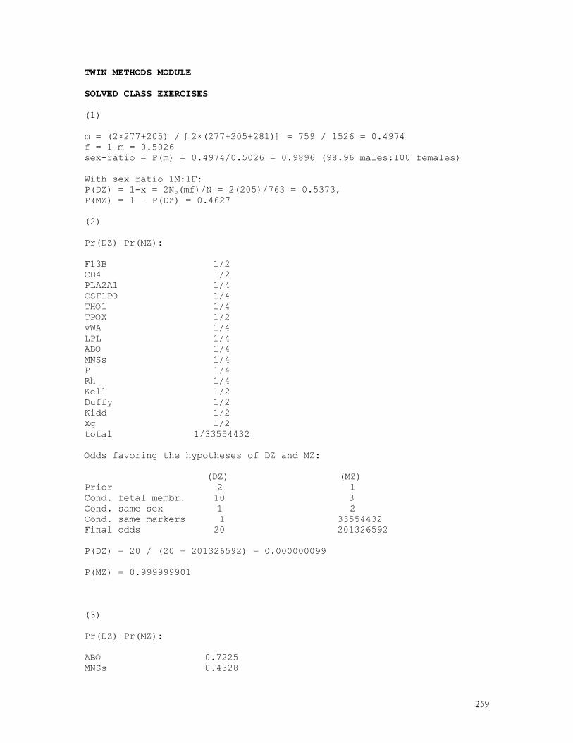
259
TWIN METHODS MODULE SOLVED CLASS EXERCISES (1) m = (2×277+205) / [2×(277+205+281)] = 759 / 1526 = 0.4974 f = 1-m = 0.5026 sex-ratio = P(m) = 0.4974/0.5026 = 0.9896 (98.96 males:100 females) With sex-ratio 1M:1F: P(DZ) = 1-x = 2No(mf)/N = 2(205)/763 = 0.5373, P(MZ) = 1 – P(DZ) = 0.4627 (2) Pr(DZ)|Pr(MZ): F13B 1/2 CD4 1/2 PLA2A1 1/4 CSF1PO 1/4 THO1 1/4 TPOX 1/2 vWA 1/4 LPL 1/4 ABO 1/4 MNSs 1/4 P 1/4 Rh 1/4 Kell 1/2 Duffy 1/2 Kidd 1/2 Xg 1/2 total 1/33554432 Odds favoring the hypotheses of DZ and MZ: (DZ) (MZ) Prior 2 1 Cond. fetal membr. 10 3 Cond. same sex 1 2 Cond. same markers 1 33554432 Final odds 20 201326592 P(DZ) = 20 / (20 + 201326592) = 0.000000099 P(MZ) = 0.999999901 (3) Pr(DZ)|Pr(MZ): ABO 0.7225 MNSs 0.4328
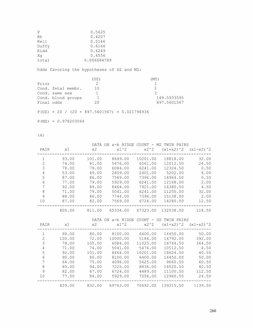
260
P 0.5625 Rh 0.4207 Kell 0.5146 Duffy 0.6166 Kidd 0.6249 Xg 0.4556 total 0.006684789 Odds favoring the hypotheses of DZ and MZ: (DZ) (MZ) Prior 2 1 Cond. fetal membr. 10 3 Cond. same sex 1 2 Cond. blood groups 1 149.5933595 Final odds 20 897.5601567 P(DZ) = 20 / (20 + 897.5601567) = 0.021796936 P(MZ) = 0.978203064 (4) DATA ON a-b RIDGE COUNT - MZ TWIN PAIRS PAIR x1 x2 x1^2 x2^2 (x1+x2)^2 (x1-x2)^2 ---------------------------------------------------------------------- 1 93.00 101.00 8649.00 10201.00 18818.00 32.00 2 74.00 81.00 5476.00 6561.00 12012.50 24.50 3 78.00 79.00 6084.00 6241.00 12324.50 0.50 4 53.00 49.00 2809.00 2401.00 5202.00 8.00 5 87.00 86.00 7569.00 7396.00 14964.50 0.50 6 77.00 79.00 5929.00 6241.00 12168.00 2.00 7 92.00 89.00 8464.00 7921.00 16380.50 4.50 8 71.00 79.00 5041.00 6241.00 11250.00 32.00 9 88.00 86.00 7744.00 7396.00 15138.00 2.00 10 87.00 82.00 7569.00 6724.00 14280.50 12.50 ---------------------------------------------------------------------- 800.00 811.00 65334.00 67323.00 132538.50 118.50 DATA ON a-b RIDGE COUNT - DZ TWIN PAIRS PAIR x1 x2 x1^2 x2^2 (x1+x2)^2 (x1-x2)^2 ---------------------------------------------------------------------- 1 90.00 80.00 8100.00 6400.00 14450.00 50.00 2 100.00 72.00 10000.00 5184.00 14792.00 392.00 3 78.00 105.00 6084.00 11025.00 16744.50 364.50 4 71.00 74.00 5041.00 5476.00 10512.50 4.50 5 92.00 101.00 8464.00 10201.00 18624.50 40.50 6 90.00 80.00 8100.00 6400.00 14450.00 50.00 7 64.00 75.00 4096.00 5625.00 9660.50 60.50 8 85.00 94.00 7225.00 8836.00 16020.50 40.50 9 82.00 67.00 6724.00 4489.00 11100.50 112.50 10 77.00 84.00 5929.00 7056.00 12960.50 24.50 ---------------------------------------------------------------------- 829.00 832.00 69763.00 70692.00 139315.50 1139.50
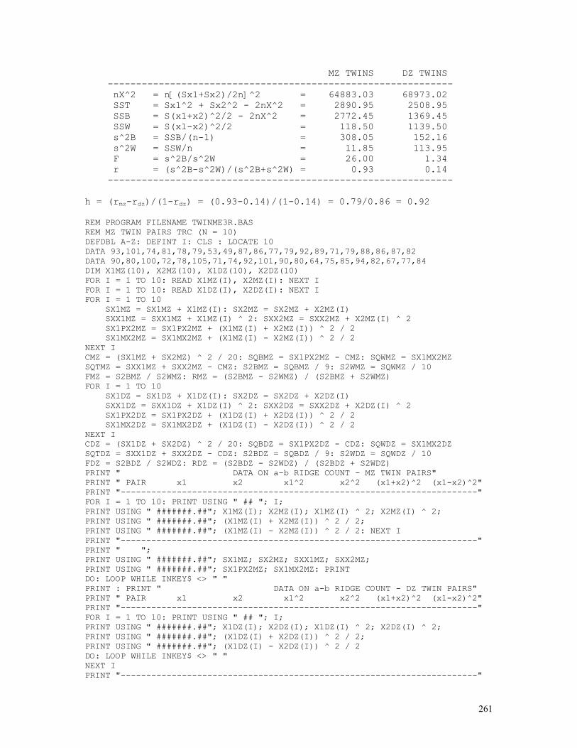
261
MZ TWINS DZ TWINS ------------------------------------------------------------- nX^2 = n[(Sx1+Sx2)/2n]^2 = 64883.03 68973.02 SST = Sx1^2 + Sx2^2 - 2nX^2 = 2890.95 2508.95 SSB = S(x1+x2)^2/2 - 2nX^2 = 2772.45 1369.45 SSW = S(x1-x2)^2/2 = 118.50 1139.50 s^2B = SSB/(n-1) = 308.05 152.16 s^2W = SSW/n = 11.85 113.95 F = s^2B/s^2W = 26.00 1.34 r = (s^2B-s^2W)/(s^2B+s^2W) = 0.93 0.14 ------------------------------------------------------------- h = (rmz-rdz)/(1-rdz) = (0.93-0.14)/(1-0.14) = 0.79/0.86 = 0.92 REM PROGRAM FILENAME TWINME3R.BAS REM MZ TWIN PAIRS TRC (N = 10) DEFDBL A-Z: DEFINT I: CLS : LOCATE 10 DATA 93,101,74,81,78,79,53,49,87,86,77,79,92,89,71,79,88,86,87,82 DATA 90,80,100,72,78,105,71,74,92,101,90,80,64,75,85,94,82,67,77,84 DIM X1MZ(10), X2MZ(10), X1DZ(10), X2DZ(10) FOR I = 1 TO 10: READ X1MZ(I), X2MZ(I): NEXT I FOR I = 1 TO 10: READ X1DZ(I), X2DZ(I): NEXT I FOR I = 1 TO 10 SX1MZ = SX1MZ + X1MZ(I): SX2MZ = SX2MZ + X2MZ(I) SXX1MZ = SXX1MZ + X1MZ(I) ^ 2: SXX2MZ = SXX2MZ + X2MZ(I) ^ 2 SX1PX2MZ = SX1PX2MZ + (X1MZ(I) + X2MZ(I)) ^ 2 / 2 SX1MX2MZ = SX1MX2MZ + (X1MZ(I) - X2MZ(I)) ^ 2 / 2 NEXT I CMZ = (SX1MZ + SX2MZ) ^ 2 / 20: SQBMZ = SX1PX2MZ - CMZ: SQWMZ = SX1MX2MZ SQTMZ = SXX1MZ + SXX2MZ - CMZ: S2BMZ = SQBMZ / 9: S2WMZ = SQWMZ / 10 FMZ = S2BMZ / S2WMZ: RMZ = (S2BMZ - S2WMZ) / (S2BMZ + S2WMZ) FOR I = 1 TO 10 SX1DZ = SX1DZ + X1DZ(I): SX2DZ = SX2DZ + X2DZ(I) SXX1DZ = SXX1DZ + X1DZ(I) ^ 2: SXX2DZ = SXX2DZ + X2DZ(I) ^ 2 SX1PX2DZ = SX1PX2DZ + (X1DZ(I) + X2DZ(I)) ^ 2 / 2 SX1MX2DZ = SX1MX2DZ + (X1DZ(I) - X2DZ(I)) ^ 2 / 2 NEXT I CDZ = (SX1DZ + SX2DZ) ^ 2 / 20: SQBDZ = SX1PX2DZ - CDZ: SQWDZ = SX1MX2DZ SQTDZ = SXX1DZ + SXX2DZ - CDZ: S2BDZ = SQBDZ / 9: S2WDZ = SQWDZ / 10 FDZ = S2BDZ / S2WDZ: RDZ = (S2BDZ - S2WDZ) / (S2BDZ + S2WDZ) PRINT " DATA ON a-b RIDGE COUNT - MZ TWIN PAIRS" PRINT " PAIR x1 x2 x1^2 x2^2 (x1+x2)^2 (x1-x2)^2" PRINT "----------------------------------------------------------------------" FOR I = 1 TO 10: PRINT USING " ## "; I; PRINT USING " #######.##"; X1MZ(I); X2MZ(I); X1MZ(I) ^ 2; X2MZ(I) ^ 2; PRINT USING " #######.##"; (X1MZ(I) + X2MZ(I)) ^ 2 / 2; PRINT USING " #######.##"; (X1MZ(I) - X2MZ(I)) ^ 2 / 2: NEXT I PRINT "----------------------------------------------------------------------" PRINT " "; PRINT USING " #######.##"; SX1MZ; SX2MZ; SXX1MZ; SXX2MZ; PRINT USING " #######.##"; SX1PX2MZ; SX1MX2MZ: PRINT DO: LOOP WHILE INKEY$ <> " " PRINT : PRINT " DATA ON a-b RIDGE COUNT - DZ TWIN PAIRS" PRINT " PAIR x1 x2 x1^2 x2^2 (x1+x2)^2 (x1-x2)^2" PRINT "----------------------------------------------------------------------" FOR I = 1 TO 10: PRINT USING " ## "; I; PRINT USING " #######.##"; X1DZ(I); X2DZ(I); X1DZ(I) ^ 2; X2DZ(I) ^ 2; PRINT USING " #######.##"; (X1DZ(I) + X2DZ(I)) ^ 2 / 2; PRINT USING " #######.##"; (X1DZ(I) - X2DZ(I)) ^ 2 / 2 DO: LOOP WHILE INKEY$ <> " " NEXT I PRINT "----------------------------------------------------------------------"
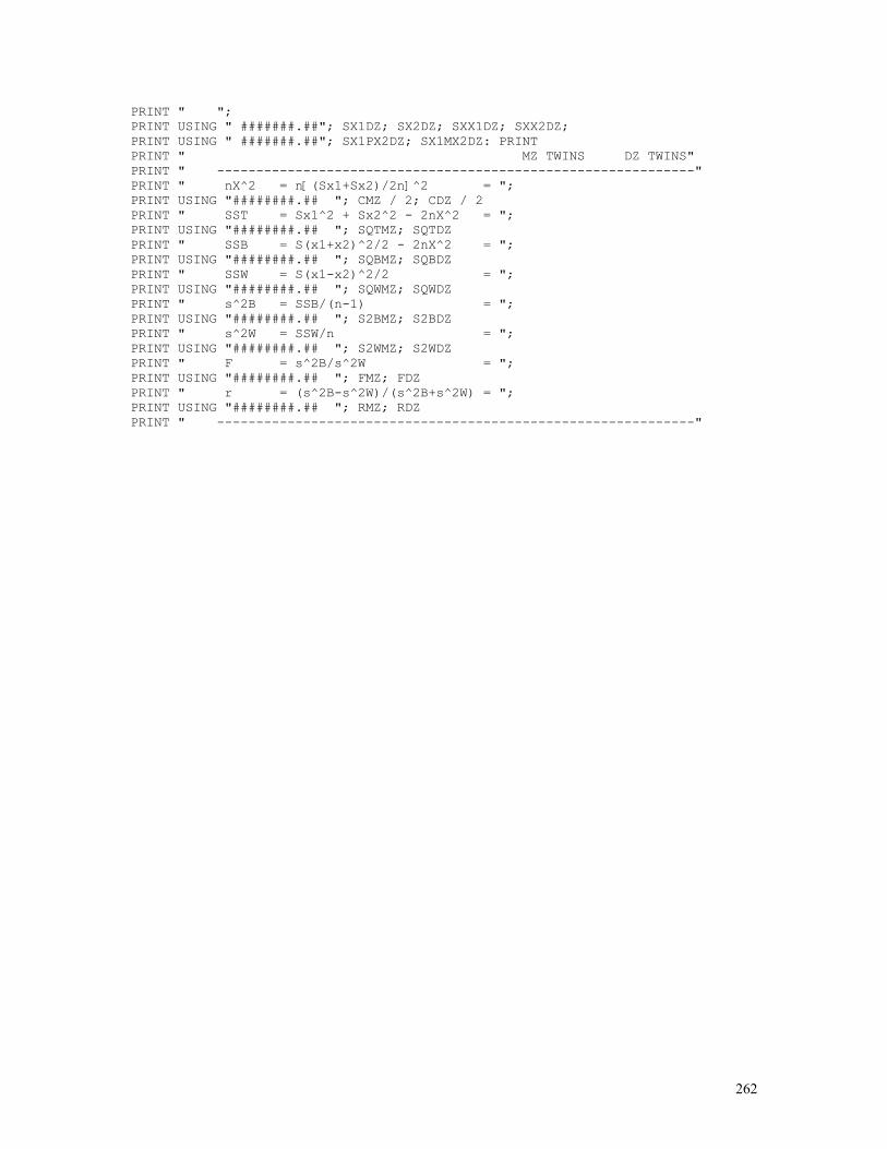
262
PRINT " "; PRINT USING " #######.##"; SX1DZ; SX2DZ; SXX1DZ; SXX2DZ; PRINT USING " #######.##"; SX1PX2DZ; SX1MX2DZ: PRINT PRINT " MZ TWINS DZ TWINS" PRINT " -------------------------------------------------------------" PRINT " nX^2 = n[(Sx1+Sx2)/2n]^2 = "; PRINT USING "########.## "; CMZ / 2; CDZ / 2 PRINT " SST = Sx1^2 + Sx2^2 - 2nX^2 = "; PRINT USING "########.## "; SQTMZ; SQTDZ PRINT " SSB = S(x1+x2)^2/2 - 2nX^2 = "; PRINT USING "########.## "; SQBMZ; SQBDZ PRINT " SSW = S(x1-x2)^2/2 = "; PRINT USING "########.## "; SQWMZ; SQWDZ PRINT " s^2B = SSB/(n-1) = "; PRINT USING "########.## "; S2BMZ; S2BDZ PRINT " s^2W = SSW/n = "; PRINT USING "########.## "; S2WMZ; S2WDZ PRINT " F = s^2B/s^2W = "; PRINT USING "########.## "; FMZ; FDZ PRINT " r = (s^2B-s^2W)/(s^2B+s^2W) = "; PRINT USING "########.## "; RMZ; RDZ PRINT " -------------------------------------------------------------"
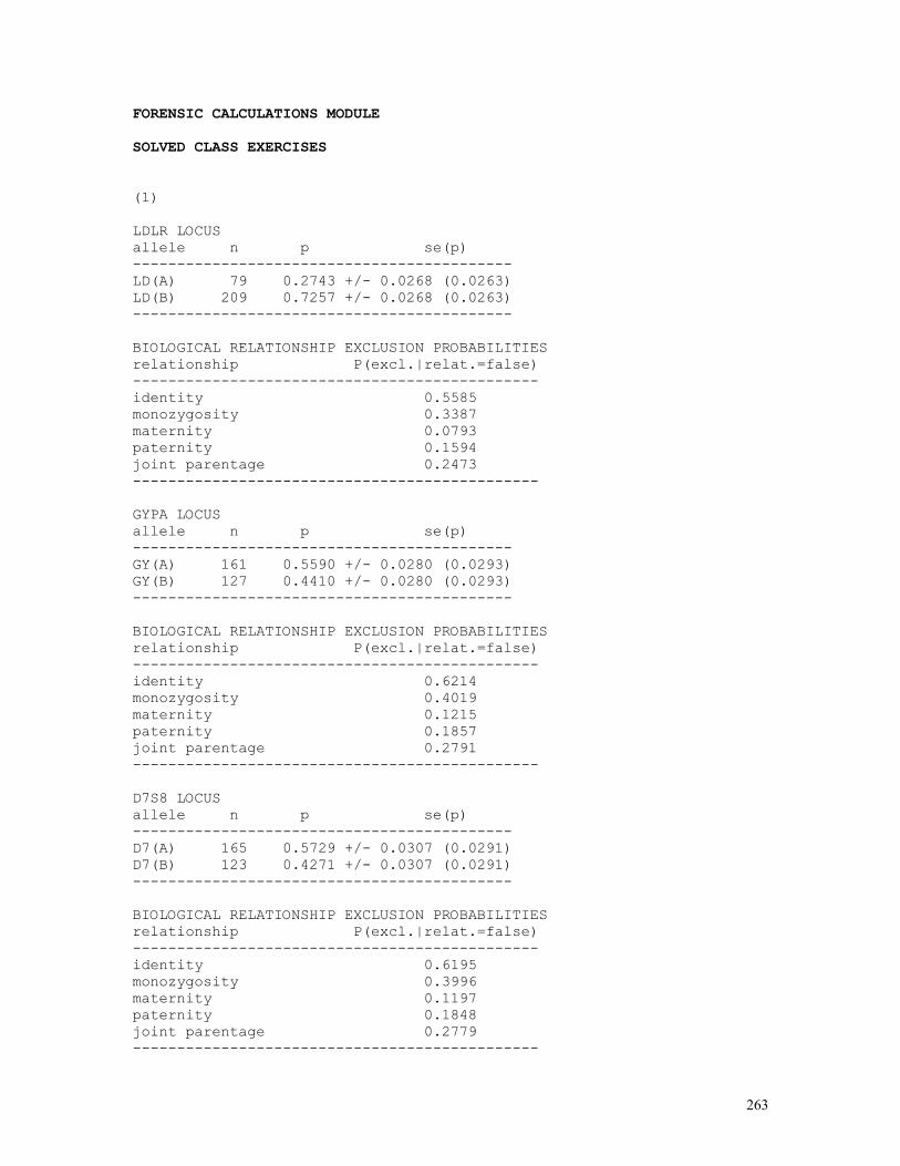
263
FORENSIC CALCULATIONS MODULE SOLVED CLASS EXERCISES (1) LDLR LOCUS allele n p se(p) ------------------------------------------- LD(A) 79 0.2743 +/- 0.0268 (0.0263) LD(B) 209 0.7257 +/- 0.0268 (0.0263) ------------------------------------------- BIOLOGICAL RELATIONSHIP EXCLUSION PROBABILITIES relationship P(excl.|relat.=false) ---------------------------------------------- identity 0.5585 monozygosity 0.3387 maternity 0.0793 paternity 0.1594 joint parentage 0.2473 ---------------------------------------------- GYPA LOCUS allele n p se(p) ------------------------------------------- GY(A) 161 0.5590 +/- 0.0280 (0.0293) GY(B) 127 0.4410 +/- 0.0280 (0.0293) ------------------------------------------- BIOLOGICAL RELATIONSHIP EXCLUSION PROBABILITIES relationship P(excl.|relat.=false) ---------------------------------------------- identity 0.6214 monozygosity 0.4019 maternity 0.1215 paternity 0.1857 joint parentage 0.2791 ---------------------------------------------- D7S8 LOCUS allele n p se(p) ------------------------------------------- D7(A) 165 0.5729 +/- 0.0307 (0.0291) D7(B) 123 0.4271 +/- 0.0307 (0.0291) ------------------------------------------- BIOLOGICAL RELATIONSHIP EXCLUSION PROBABILITIES relationship P(excl.|relat.=false) ---------------------------------------------- identity 0.6195 monozygosity 0.3996 maternity 0.1197 paternity 0.1848 joint parentage 0.2779 ----------------------------------------------
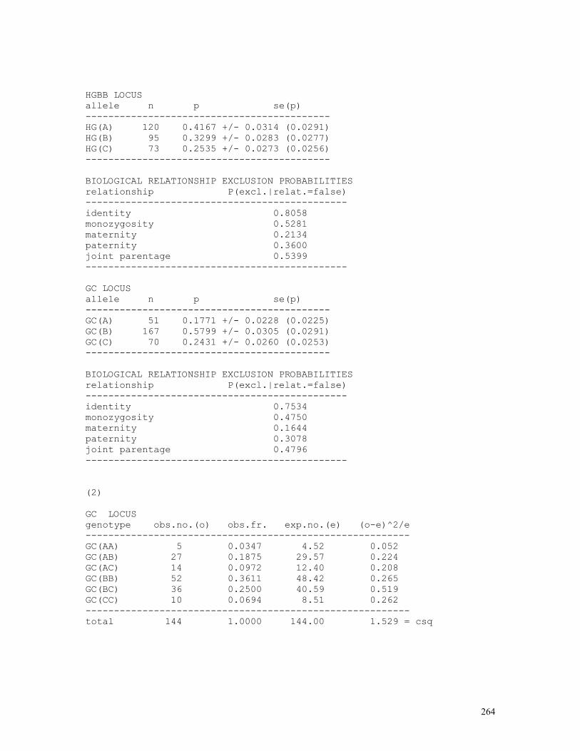
264
HGBB LOCUS allele n p se(p) ------------------------------------------- HG(A) 120 0.4167 +/- 0.0314 (0.0291) HG(B) 95 0.3299 +/- 0.0283 (0.0277) HG(C) 73 0.2535 +/- 0.0273 (0.0256) ------------------------------------------- BIOLOGICAL RELATIONSHIP EXCLUSION PROBABILITIES relationship P(excl.|relat.=false) ---------------------------------------------- identity 0.8058 monozygosity 0.5281 maternity 0.2134 paternity 0.3600 joint parentage 0.5399 ---------------------------------------------- GC LOCUS allele n p se(p) ------------------------------------------- GC(A) 51 0.1771 +/- 0.0228 (0.0225) GC(B) 167 0.5799 +/- 0.0305 (0.0291) GC(C) 70 0.2431 +/- 0.0260 (0.0253) ------------------------------------------- BIOLOGICAL RELATIONSHIP EXCLUSION PROBABILITIES relationship P(excl.|relat.=false) ---------------------------------------------- identity 0.7534 monozygosity 0.4750 maternity 0.1644 paternity 0.3078 joint parentage 0.4796 ---------------------------------------------- (2) GC LOCUS genotype obs.no.(o) obs.fr. exp.no.(e) (o-e)^2/e --------------------------------------------------------- GC(AA) 5 0.0347 4.52 0.052 GC(AB) 27 0.1875 29.57 0.224 GC(AC) 14 0.0972 12.40 0.208 GC(BB) 52 0.3611 48.42 0.265 GC(BC) 36 0.2500 40.59 0.519 GC(CC) 10 0.0694 8.51 0.262 --------------------------------------------------------- total 144 1.0000 144.00 1.529 = csq
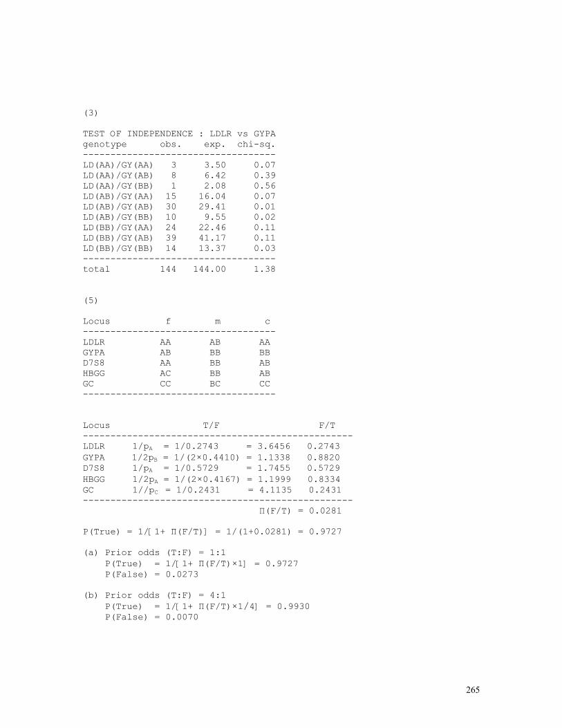
265
(3) TEST OF INDEPENDENCE : LDLR vs GYPA genotype obs. exp. chi-sq. ----------------------------------- LD(AA)/GY(AA) 3 3.50 0.07 LD(AA)/GY(AB) 8 6.42 0.39 LD(AA)/GY(BB) 1 2.08 0.56 LD(AB)/GY(AA) 15 16.04 0.07 LD(AB)/GY(AB) 30 29.41 0.01 LD(AB)/GY(BB) 10 9.55 0.02 LD(BB)/GY(AA) 24 22.46 0.11 LD(BB)/GY(AB) 39 41.17 0.11 LD(BB)/GY(BB) 14 13.37 0.03 ----------------------------------- total 144 144.00 1.38 (5) Locus f m c ----------------------------------- LDLR AA AB AA GYPA AB BB BB D7S8 AA BB AB HBGG AC BB AB GC CC BC CC ----------------------------------- Locus T/F F/T ------------------------------------------------- LDLR 1/pA = 1/0.2743 = 3.6456 0.2743 GYPA 1/2pB = 1/(2×0.4410) = 1.1338 0.8820 D7S8 1/pA = 1/0.5729 = 1.7455 0.5729 HBGG 1/2pA = 1/(2×0.4167) = 1.1999 0.8334 GC 1//pC = 1/0.2431 = 4.1135 0.2431 ------------------------------------------------- Π(F/T) = 0.0281 P(True) = 1/[1+ Π(F/T)] = 1/(1+0.0281) = 0.9727 (a) Prior odds (T:F) = 1:1 P(True) = 1/[1+ Π(F/T)×1] = 0.9727 P(False) = 0.0273 (b) Prior odds (T:F) = 4:1 P(True) = 1/[1+ Π(F/T)×1/4] = 0.9930 P(False) = 0.0070