Quantitative Genetics in the Age of Genomics

QuickTime™ and aTIFF (Uncompressed) decompressorare needed to see this picture.QuickTime™ and aTIFF (Uncompressed) decompressorare needed to see this picture.

Classical Quantitative Genetics• Quantitative genetics deals with the observed variation in a

trait both within and between populations• Basic model (Fisher 1918): The phenotype (z) is the sum of

(unseen) genetic (g) and environmental values (e)

• z = g + e • The genetic value needs to be further decomposed into an

additive part A passed for parent to offspring, separate from dominance (D) and epistatic effects (I) that are only fully passed along in clones

• g = A + D + I• Var(g)/Var(z) is quantitative measure of nature vs. nurture

– fraction of all trait variation due to genetic differences

Fisher’s great insight: Phenotypic covariances between relatives can estimate the variances of g,

e, etc.• For example, in the simplest settings,

– Cov(parent,offspring) = Var(A)/2– Cov(Full sibs) = Var(A)/2 + Var(D)/4– Cov(clones) = Var(g) = Var(A)+Var(D)+Var(I)

• Random-effects model– Interest is in estimating variances

• Thus, in classical quantitative genetics, a few statistical descriptors describe the underlying complex genetics– This leaves an uneasy feeling among most of my

molecular colleagues.– Does the age of genomics usher in the death knell of

Quantitative Genetics?

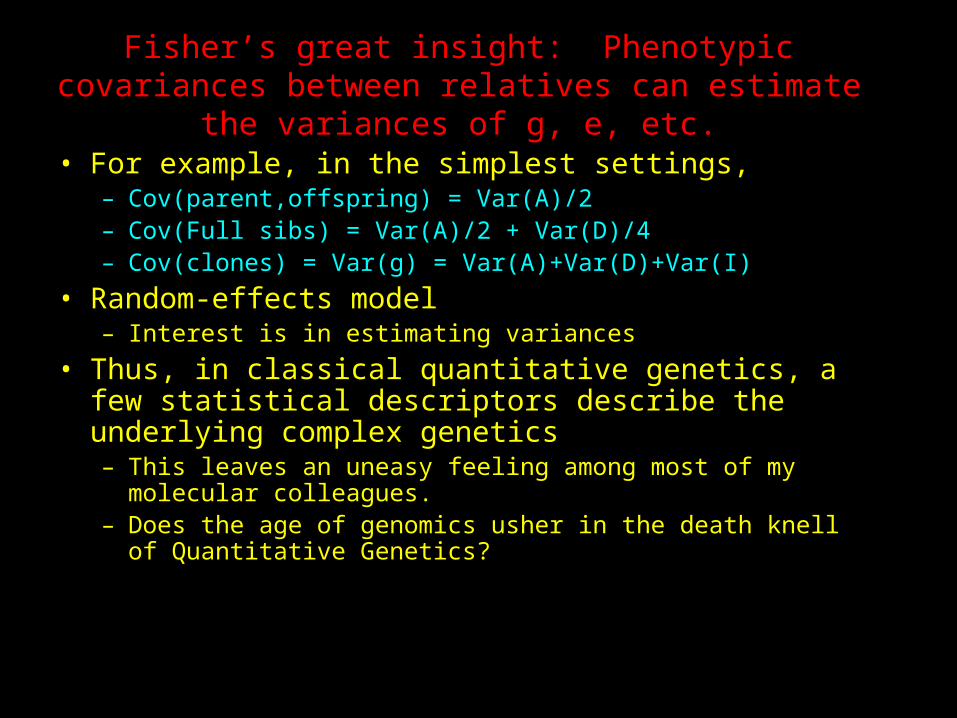
Approximate costs of genome projects

• Arabidopsis Genome Project ... $500 million

• Drosophila Genome Project ... $1 billion

• Human Genome Project ... $10 billion

• Working knowledge of multivariate statistics ... Priceless

Model systems

QuickTime™ and aPhoto - JPEG decompressor

are needed to see this picture.

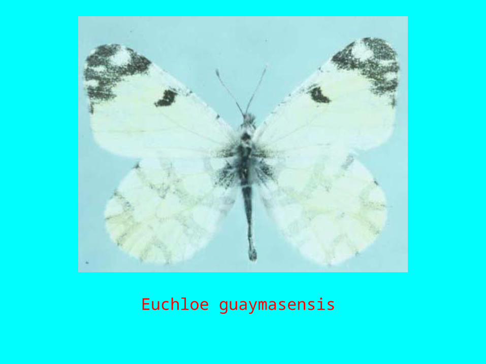
Euchloe guaymasensis

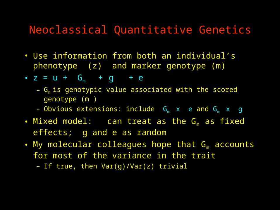
Neoclassical Quantitative Genetics

• Use information from both an individual’s phenotype (z) and marker genotype (m)

• z = u + Gm + g + e– Gm is genotypic value associated with the scored

genotype (m )

– Obvious extensions: include Gm x e and Gm x g

• Mixed model: can treat as the Gm as fixed effects; g and e as random

• My molecular colleagues hope that Gm accounts for most of the variance in the trait– If true, then Var(g)/Var(z) trivial

Limitations on Gm

• The importance of particular genotypes may be quite fleeting– can easily change as populations evolve and as the biotic

and abiotic environments change– If epistasis and/or genotype-environment interactions are

significant, any particular genotype may be a good, but not exceptional, predictor of phenotype

• Quantitative genetics provides the machinery necessary for managing all this uncertainty in the face of some knowledge of important genotypes– e.g., proper accounting of correlations between relatives

in the unmeasured genetic values (g)

The importance of even rather imperfect marker information

• Suppose an F1 is segregating favorable alleles at n loci, and we inbred to fixation before selecting among pure lines– Pr (fixation favorable allele) = 1/2

• What are the required number of lines for Pr (at least one line fixed for n favorable alleles) = 0.9?

• For n = 10: 2,360 lines• For n = 20: 2,400,000 lines

• Suppose marker information increases the probability of fixation by 50% (to 0.75)

• Required number of lines for Prob(at least one line fixed for n favorable alleles) = 0.9

• For n = 10: 40 lines (60-fold reduction)• For n = 20: 725 lines (3,300-fold reduction)

How do we obtain Gm?• Ideally, we screen a number of candidate loci• QTL (Quantitative trait locus) mapping

• Uses molecular markers to follow which chromosome

segments are common between individuals • This allows construction of a likelihood function, e.g.,

Estimated from marker informationKnown from pedigree relationships

Estimated QTL effect Background genetic effects

(̀zjπ;æ2A;æ2A§;æ2e)=1p(2º)njVjexp∑°12(z°π)TV°1(z°π)∏whereV=Ræ2A+Aæ2A§+Iæ2eandRij=Ω1fori=jRijfori6=j;Aij=Ω1fori=j2£ijfori6=j

A typical QTL map from a likelihood analysis

Estimated QTL location

Support interval

SignificanceThreshold

Genomics and candidate loci

• Typical QTL confidence interval 20-50 cM

• The big question: how do we find suitable candidates?

• The hope is that a genomic sequence will suggest candidates

Genomics tools to probe for candidates

• Dense marker maps

• Complete genome sequence

– Expression data (microarrays)

– Proteomics

– Metablomics

The accelerating pace of genomics

• Faster and cheaper sequencing

• Rapid screening of thousands of loci via DNA chips

• “Phylogenetic bootstrapping” from model systems to distant relatives

A

B

CD

EG

F

H

I

J

L

N

M

Q O

K

Prediction of Candidate Genes

• Try homologous candidates from other species• Examine all Open Reading Frames (ORFs) within

a QTL confidence interval– Expression array analysis of these ORFs– Lack of tissue-specific expression does not exclude a

gene

• Proteomics– Specific protein motifs may provide functional clues

• Cracking the regulatory code (in silico genetics)• Analysis of networks and pathways

Searching for Natural Variation

• This may be the area where genomics has the largest payoff

• Source (natural and/or weakly domesticated) populations contain more variation than the current highly domesticated lines

• Key is to first detect and localize importance variants, then introgress them into elite lines

Impact of other biotechnologies • Cloning, other reproductive technologies

– Maintain elite lines as cell cultures?– Embryo transplation into elite maternal lines?

• Transgenics– Important tool in both breeding and evolutionary biology

• Complications: – Silencing of multiple copies in some species

– Strong position effects– Currently restricted to major genes

• Major genes can have deleterious effects on other characters• Importance of quantitative genetics for selecting for background

polygenic modifiers

Useful Tools for Quantitative Genetic analysis

• Four subfields of Quantitative Genetics– Plant breeding– Animal breeding (forest genetics)– Evolutionary Genetics– Human Genetics

• Restricted communications between fields

• Important tools often unknown outside a field

Tools from Plant Breeding• Special features dealt with by plant breeders

– Diversity of mating systems (esp. selfing)– Sessile individuals

• Issues– Creation and selection of inbred lines– Hybridization between lines– Genotype x Environment interactions– Competition

• Plant breeding tools useful in other fields– Field-plot designs – G x E analysis models: AMMI and biplots

• These designs are also excellent candidates for the analysis of microarray expression data

– Covariance between inbred relatives– Line cross analysis

Animal Breeding• Special features

– Complex pedigrees– Large half-sib (more rarely full-sib) families– Long life spans– Overlapping generations

• Tree breeders face many of these same issues• Animal breeding tools useful in other fields

– BLUP (best linear unbiased predictors) for genotypic values

– REML (restricted maximum likelihood) for variance components

• BLUP/REML allow for arbitrary pedigrees, very complex models

– Maternal effects designs• Endosperm work of Shaw and Waser

– Selection response in structured populations

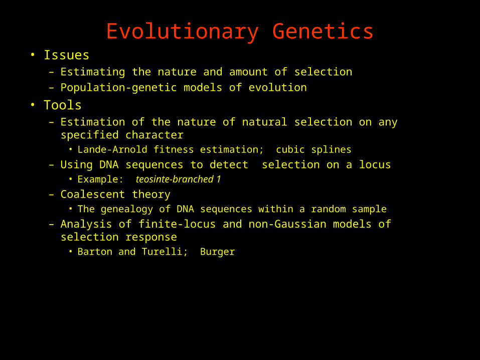
Evolutionary Genetics• Issues

– Estimating the nature and amount of selection– Population-genetic models of evolution

• Tools– Estimation of the nature of natural selection on any specified

character• Lande-Arnold fitness estimation; cubic splines

– Using DNA sequences to detect selection on a locus• Example: teosinte-branched 1

– Coalescent theory• The genealogy of DNA sequences within a random sample

– Analysis of finite-locus and non-Gaussian models of selection response

• Barton and Turelli; Burger

Human Genetics

• Issues– Very small family sizes– Lack of controlled mating designs

• Tools of potential use– Sib-pair approaches for QTL mapping

• QTL mapping in populations

– Transmission-disequilibrium test (TDT)• Account for population structure

– Linkage-disequilibrium mapping• Use historical recombinations to fine-map genes

– Random-effects models for QTL mapping• BLUP/REML-type analysis over arbitrary pedigrees

A Bayesian Future?

• 1970s saw the start of a shift in QG from methods-of moments approaches (i.e., estimators based on sample means and

variance) to likelihood approaches that use the entire distribution of the data– Initial objections to having to specify a likelihood function,

• L(u | data)

– As these methods became computationally feasible, they started to supplant their method-of-moments counterparts.

• Similarly, Bayesian approaches have become much more computationally feasible recently because of both advances in computational power and a greater appreciation of the power of resampling methods (MCMC and Gibbs samplers)

prior

0 100 200 300 400

0.0025

0.005

0.0075

0.01

0.0125

0.015

0.0175

0.02

Posterior ( u | data ) = C* Likelihood ( u | data) * prior (u)

0 100 200 300 400

0.0025

0.005

0.0075

0.01

0.0125

0.015

0.0175

0.02

posterior

Why Bayesian?

• Marginal posteriors– The effects of the uncertainty in estimating

nuisance parameters (those not of interest) are fully accounted for.

• Exact for small sample size• Powerful interative sampling methods (MCMC,

Gibbs) allow Bayesian analysis to work on problems with a very large number of parameters and relative few actual data points (vectors)

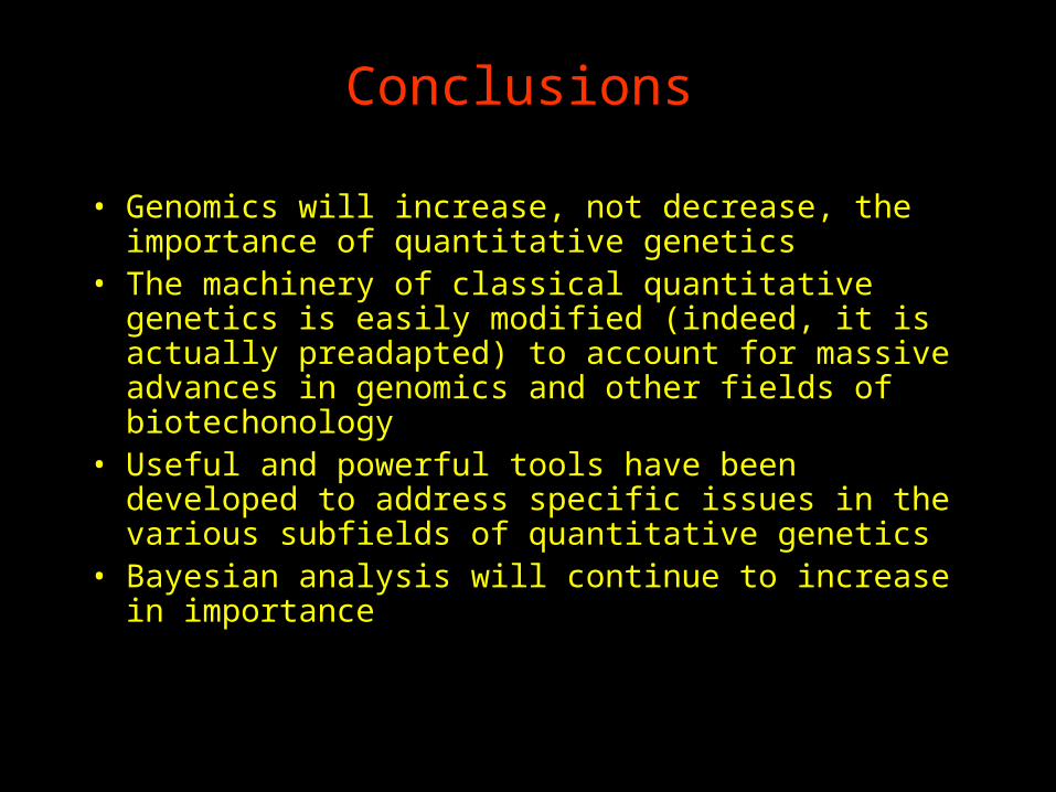
Conclusions

• Genomics will increase, not decrease, the importance of quantitative genetics

• The machinery of classical quantitative genetics is easily modified (indeed, it is actually preadapted) to account for massive advances in genomics and other fields of biotechonology

• Useful and powerful tools have been developed to address specific issues in the various subfields of quantitative genetics

• Bayesian analysis will continue to increase in importance