Classic HPC Development using Visual C++ - vscht.czdsp.vscht.cz/konference_matlab/MATLAB08/prispevky/Sprinx... · Web viewTitle Classic HPC Development using Visual C++ Subject Windows

Microsoft HPC Pack 2008 SDK

Classic HPC Development using Visual C++

Developed by Pluralsight LLC, in partnership with Microsoft Corp.

All rights reserved, ©2008© 2008 Microsoft Corporation

Developed by Pluralsight LLC

Page 2 of 89

Table of Contents

Preface………………………………………………………………………………………………………………………………………………………………………………………………………….41. Problem Domain52. Data Parallelism and Contrast Stretching 73. A Sequential Version of the Contrast Stretching Application 10

3.1 Architecture of Sequential Version 103.2 Allocating Efficient 2D Arrays 133.3 Lab Exercise! 14

4. Working with Windows HPC Server 2008 154.1 Submitting a Job to the Cluster 154.2 Lab Exercise! 20

5. A Shared-Memory Parallel Version using OpenMP 205.1 Working with OpenMP in Visual Studio 2005/2008 235.2 Lab Exercise! 23

6. A Distributed-Memory Parallel Version using MPI 286.1 Installing and Configuring MS-MPI 306.2 Working with MS-MPI in Visual Studio 2005/2008 306.3 MS-MPI and Windows HPC Server 2008 366.4 Lab Exercise! 37

7. MPI Debugging, Profiling and Event Tracing 487.1 Profiling with ETW 487.2 Local vs. Cluster Profiling 507.3 Lab Exercise! 517.4 Don’t have Administrative Rights? Need targeted tracing? 53

Page 3 of 89

7.5 MPI Debugging 537.6 Lab Exercise! 567.7 Remote MPI Debugging on the Cluster 567.8 Lab Exercise! 597.9 Other Debugging Tools 60

8. Using MPI’s Collective and Asynchronous Functions for an Improved Distributed-Memory Solution 608.1 Example 608.2 Lab Exercise! 64

9. Hybrid OpenMP + MPI Designs 6510. Managed Solutions with MPI.NET 66

10.1 Lab Exercise! 6911. Conclusions 70

11.1 References 7011.2 Resources 71

Appendix A: Summary of Cluster and Developer Setup for Windows HPC Server 2008 72Appendix B: Troubleshooting Windows HPC Server 2008 Job Execution 75Appendix C: Screen Snapshots 77

Feedback…………………………………………………………………………………………………………………………………………………………………………………………………….79More Information and Downloads 79

Page 4 of 89

Preface

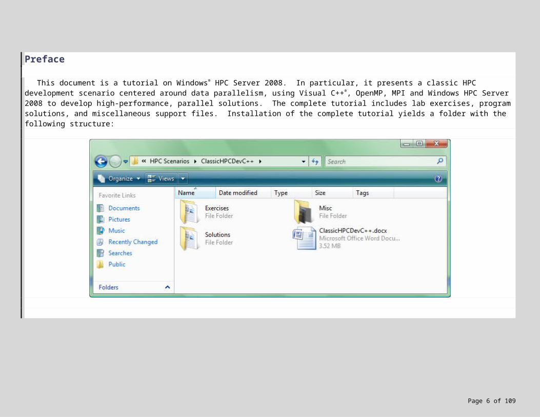
This document is a tutorial on Windows® HPC Server 2008. In particular, it presents a classic HPC development scenario centered around data parallelism, using Visual C++®, OpenMP, MPI and Windows HPC Server 2008 to develop high-performance, parallel solutions. The complete tutorial includes lab exercises, program solutions, and miscellaneous support files. Installation of the complete tutorial yields a folder with the following structure:

Page 5 of 89

This document presents a classic HPC development scenario — data parallelism in the context of image processing. Written for the C and C++ developer, this tutorial walks you through the steps of designing, writing, debugging and profiling a parallel application for Windows HPC Server 2008, and is designed to provide you with the skills and expertise necessary to deliver high-performance, cluster-wide applications for Windows HPC Server 2008.

1. Problem Domain

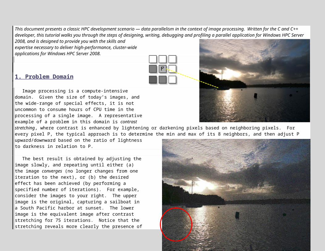
Image processing is a compute-intensive domain. Given the size of today’s images, and the wide-range of special effects, it is not uncommon to consume hours of CPU time in the processing of a single image. A representative example of a problem in this domain is contrast stretching, where contrast is enhanced by lightening or darkening pixels based on neighboring pixels. For every pixel P, the typical approach is to determine the min and max of its 8 neighbors, and then adjust P upward/downward based on the ratio of lightness to darkness in relation to P.

The best result is obtained by adjusting the image slowly, and repeating until either (a) the image converges (no longer changes from one iteration to the next), or (b) the desired effect has been achieved (by performing a specified number of iterations). For example, consider the images to your right. The upper image is the original, capturing a sailboat in a South Pacific harbor at sunset. The lower image is the equivalent image after contrast stretching for 75 iterations. Notice that the stretching reveals more clearly the presence of other boats in the harbor, in particular their white masts. Contrast stretching is one of the many techniques used to enhance images.

Programmatically, images are most easily treated as two-dimensional arrays of integers. For simplicity, we’ll work with bitmaps (.bmp), where each pixel is stored as

Page 6 of 89

3 distinct integers (0..255) representing the amount of blue, green and red at that pixel. Thus, an M-by-N image contains M*N pixels, M*N*3 integers, and will be represented by a 2D array with N rows and M columns. In this approach, each element of the array denotes a single pixel, which we’ll represent using a structure containing 3 fields, each field an unsigned char since the range is 0..255:

typedef struct {uchar blue; // amount of blue at this pixel (0..255, 0 => no blue/black, 255 => max blue/white)uchar green; // amount of green (0..255)uchar red; // amount of red (0..255)

} PIXEL_T;

PIXEL_T image[N][M];

For example, an 800x600 bitmap contains 480,000 pixels, 1,440,000 bytes, and will be represented by an array of PIXEL_T with 600 rows and 800 columns.

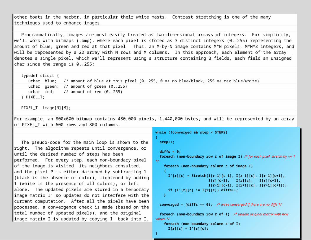
The pseudo-code for the main loop is shown to the right. The algorithm repeats until convergence, or until the desired number of steps has been performed. For every step, each non-boundary pixel of the image is visited, its neighbors consulted, and the pixel P is either darkened by subtracting 1 (black is the absence of color), lightened by adding 1 (white is the presence of all colors), or left alone. The updated pixels are stored in a temporary image matrix I' so updates do not interfere with the current computation. After all the pixels have been processed, a convergence check is made (based on the total number of updated pixels), and the original image matrix I is updated by copying I' back into I.

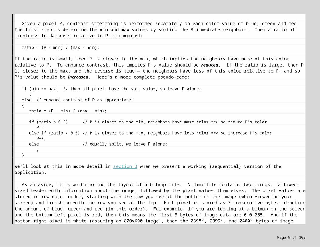
Given a pixel P, contrast stretching is performed separately on each color value of blue, green and red. The first step is determine the min and max values by sorting the 8 immediate neighbors. Then a ratio of lightness to darkness relative to P is computed:

ratio = (P – min) / (max – min);

If the ratio is small, then P is closer to the min, which implies the neighbors have more of this color relative to P. To enhance contrast, this implies P’s value should be reduced. If the ratio is large, then P is closer to the max, and the reverse is true — the neighbors have less of this color relative to P, and so P’s value should be increased. Here’s a more complete pseudo-code:

if (min == max) // then all pixels have the same value, so leave P alone:

;else // enhance contrast of P as appropriate:

Page 7 of 89

while (!converged && step < STEPS){ step++;

diffs = 0; foreach (non-boundary row r of image I) /* for each pixel, stretch by +/- 1 */ foreach (non-boundary column c of image I) { I'[r][c] = Stretch(I[r-1][c-1], I[r-1][c], I[r-1][c+1], I[r][c-1], I[r][c], I[r][c+1], I[r+1][c-1], I[r+1][c], I[r+1][c+1]); if (I'[r][c] != I[r][c]) diffs++; }

converged = (diffs == 0); /* we’ve converged if there are no diffs */

foreach (non-boundary row r of I) /* update original matrix with new values */ foreach (non-boundary column c of I) I[r][c] = I'[r][c];}

{ratio = (P – min) / (max – min);

if (ratio < 0.5) // P is closer to the min, neighbors have more color ==> so reduce P's colorP--;

else if (ratio > 0.5) // P is closer to the max, neighbors have less color ==> so increase P's colorP++;

else // equally split, we leave P alone:;

}

We’ll look at this in more detail in section 3 when we present a working (sequential) version of the application.

As an aside, it is worth noting the layout of a bitmap file. A .bmp file contains two things: a fixed-sized header with information about the image, followed by the pixel values themselves. The pixel values are stored in row-major order, starting with the row you see at the bottom of the image (when viewed on your screen) and finishing with the row you see at the top. Each pixel is stored as 3 consecutive bytes, denoting the amount of blue, green and red (in this order). For example, if you are looking at a bitmap on the screen and the bottom-left pixel is red, then this means the first 3 bytes of image data are 0 0 255. And if the bottom-right pixel is white (assuming an 800x600 image), then the 2398th, 2399th, and 2400th bytes of image data are 255 255 255. Finally, if the top-right pixel is yellow, then the last 3 bytes in the image (and the file) are 0 255 255.

2. Data Parallelism and Contrast Stretching

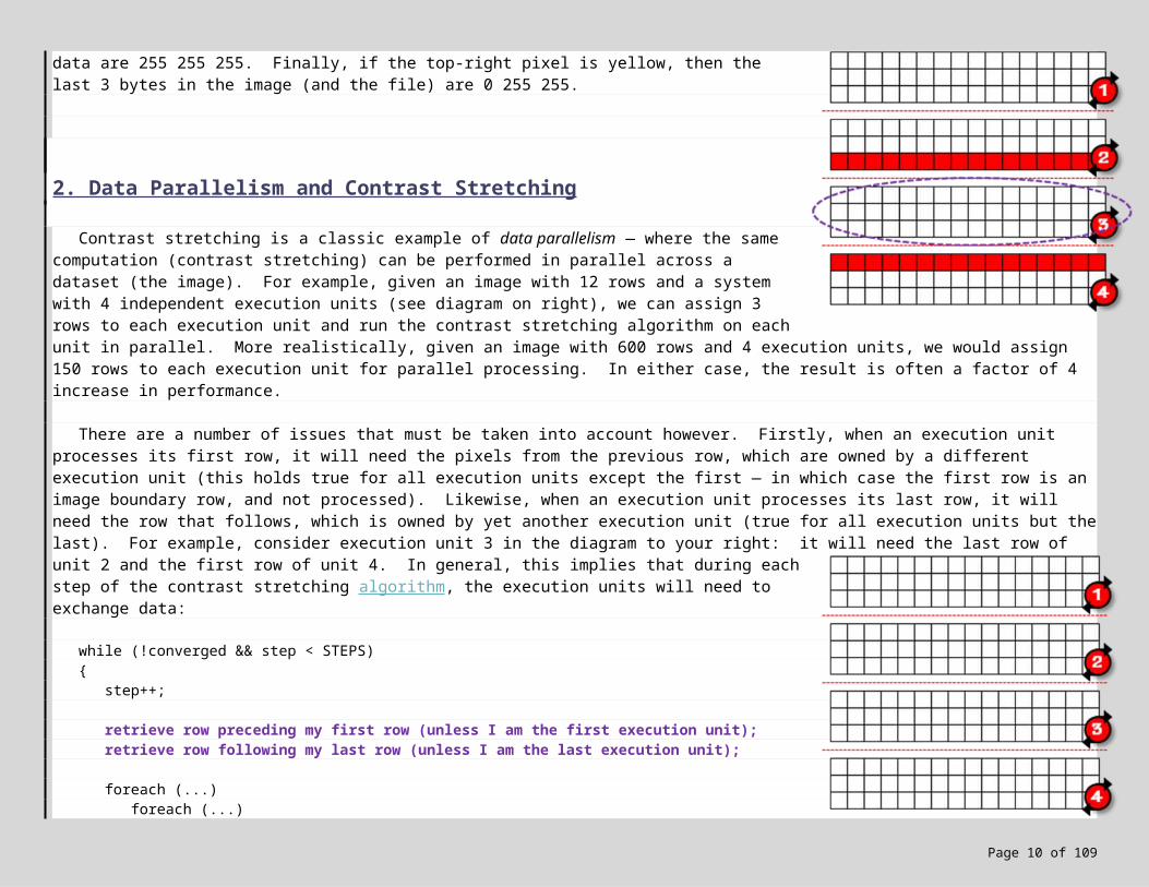
Contrast stretching is a classic example of data parallelism — where the same computation (contrast stretching) can be performed in parallel across a dataset (the image). For example, given an image with 12 rows and a system with 4 independent execution units (see diagram on right), we can assign 3 rows to each execution unit and run the contrast stretching algorithm on each unit in parallel. More realistically, given an image with 600 rows and 4 execution units, we would assign 150 rows to each execution unit for parallel processing. In either case, the result is often a factor of 4 increase in performance.

There are a number of issues that must be taken into account however. Firstly, when an execution unit processes its first row, it will need the pixels from the previous row, which are owned by a different execution unit (this holds true for all execution units except the first — in which case the first row is an image boundary row, and not processed). Likewise, when an execution unit processes its last row, it will need the row that follows, which is owned by yet another execution unit (true for all execution units but the last). For example, consider execution unit 3 in the diagram to your right: it will need the last row of unit 2 and the first row of unit 4. In general, this implies that during each step of the contrast stretching algorithm, the execution units will need to exchange data:

Page 8 of 89

while (!converged && step < STEPS){

step++;

retrieve row preceding my first row (unless I am the first execution unit);retrieve row following my last row (unless I am the last execution unit);

foreach (...)foreach (...){

I'[r][c] = Stretch(...);if (I'[r][c] != I[r][c]) localDiffs++;

}

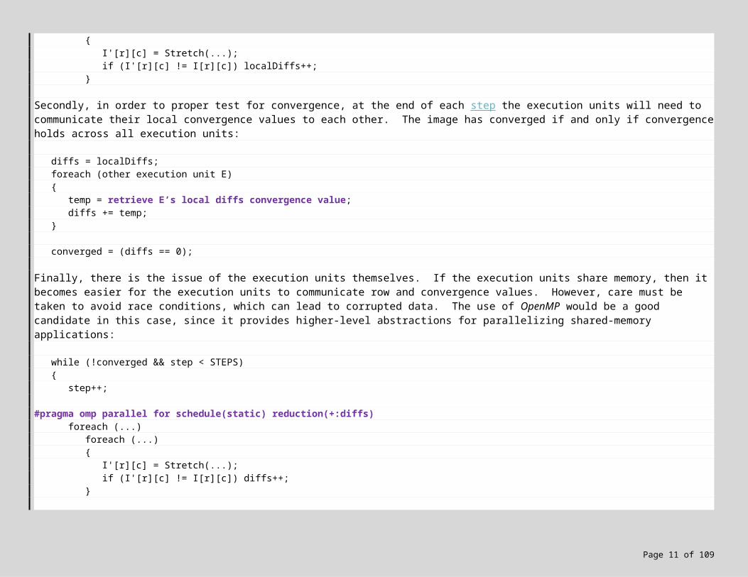
Secondly, in order to proper test for convergence, at the end of each step the execution units will need to communicate their local convergence values to each other. The image has converged if and only if convergence holds across all execution units:

diffs = localDiffs;foreach (other execution unit E){

temp = retrieve E’s local diffs convergence value;diffs += temp;

}

converged = (diffs == 0);

Finally, there is the issue of the execution units themselves. If the execution units share memory, then it becomes easier for the execution units to communicate row and convergence values. However, care must be taken to avoid race conditions, which can lead to corrupted data. The use of OpenMP would be a good candidate in this case, since it provides higher-level abstractions for parallelizing shared-memory applications:


step++;

#pragma omp parallel for schedule(static) reduction(+:diffs)foreach (...)

foreach (...){

I'[r][c] = Stretch(...);if (I'[r][c] != I[r][c]) diffs++;

}

Page 9 of 89

The parallel algorithm is unchanged from the original except for the addition of an OpenMP-based pragma. The pragma tells the compiler to parallelize the outer loop, which effectively parallelizes the algorithm by row; a static schedule splits the outer loop (rows) evenly across available threads, and the reduction clause tells the compiler to safely parallelize the otherwise unsafe computation of diffs. OpenMP is enabled in Visual C++ via a simple compiler switch, and is supported in both Visual Studio® 2005 and 2008.

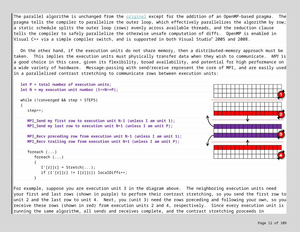
On the other hand, if the execution units do not share memory, then a distributed-memory approach must be taken. This implies the execution units must physically transfer data when they wish to communicate. MPI is a good choice in this case, given its flexibility, broad availability, and potential for high performance on a wide variety of hardware. Message-passing with send/receive represent the core of MPI, and are easily used in a parallelized contrast stretching to communicate rows between execution units:

let P = total number of execution units;let N = my execution unit number (1<=N<=P);


step++;

MPI_Send my first row to execution unit N-1 (unless I am unit 1); MPI_Send my last row to execution unit N+1 (unless I am unit P);

MPI_Recv preceding row from execution unit N-1 (unless I am unit 1);MPI_Recv trailing row from execution unit N+1 (unless I am unit P);

foreach (...)foreach (...){

I'[r][c] = Stretch(...);if (I'[r][c] != I[r][c]) localDiffs++;

}

For example, suppose you are execution unit 3 in the diagram above. The neighboring execution units need your first and last rows (shown in purple) to perform their contrast stretching, so you send the first row to unit 2 and the last row to unit 4. Next, you (unit 3) need the rows preceding and following your own, so you receive these rows (shown in red) from execution units 2 and 4, respectively. Since every execution unit is running the same algorithm, all sends and receives complete, and the contrast stretching proceeds in parallel. Once all pixels have been processed, the execution units will need to communicate their convergence values to determine if the image has converged. While this can be done through a series of sends and receives, MPI offers a much more efficient, safer and readable collective operation for summing across the execution units:

MPI_Allreduce(localDiffs, diffs, ..., MPI_SUM, ...); // sum all the localDiffs, and distribute final diffsconverged = (diffs == 0);

Page 10 of 89

Microsoft® MPI (MSMPI) is a complete implementation of MPI-2, offering both C and FORTRAN bindings. MS-MPI is an integral component of Windows HPC Server 2008, with support for low-latency Network Direct message passing, event tracing for windows (ETW), and remote MPI cluster debugging (in conjunction with Visual Studio).

Other parallel approaches on the Windows platform include the .NET Parallel Framework (PFx) for shared-memory programming1, and MPI.NET for distributed-memory programming2. These offer managed approaches to HPC from languages such as C#, F# and VB.

3. A Sequential Version of the Contrast Stretching Application

An important first step in developing a parallel version of an application is to create a sequential version. A sequential version allows us to gain a better understanding of the problem, provides a vehicle for correctness testing against the parallel versions, and forms the basis for performance measurements. Performance is often measured in terms of speedup, i.e. how much faster the parallel version executed in comparison to the sequential version. More precisely:

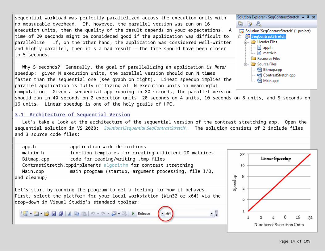
For example, if the sequential version runs in 80 seconds and the parallel version runs in 20 seconds, then the speedup is 4. If the parallel version was run on 4 execution units, this is a very good result — the sequential workload was perfectly parallelized across the execution units with no measurable overhead. If, however, the parallel version was run on 16 execution units, then the quality of the result depends on your expectations. A time of 20 seconds might be considered good if the application was difficult to parallelize. If, on the other hand, the application was considered well-written and highly-parallel, then it’s a bad result — the time should have been closer to 5 seconds.

Why 5 seconds? Generally, the goal of parallelizing an application is linear speedup: given N execution units, the parallel version should run N times faster than the sequential one (see graph on right). Linear speedup implies the parallel application is fully utilizing all N execution units in meaningful computation. Given a sequential app running in 80 seconds, the parallel version should run in 40 seconds on 2 execution units, 20 seconds on 4 units, 10 seconds on 8 units, and 5 seconds on 16 units. Linear speedup is one of the holy grails of HPC.

1 http://msdn2.microsoft.com/en-us/concurrency/default.aspx 2 http://osl.iu.edu/research/mpi.net/

Page 11 of 89

3.1 Architecture of Sequential Version Let’s take a look at the architecture of the sequential version of

the contrast stretching app. Open the sequential solution in VS 2008: Solutions\Sequential\SeqContrastStretch\. The solution consists of 2 include files and 3 source code files:

app.h application-wide definitionsmatrix.h function templates for creating efficient 2D

matricesBitmap.cpp code for reading/writing .bmp filesContrastStretch.cpp implements algorithm for contrast stretchingMain.cpp main program (startup, argument processing, file I/O, and cleanup)

Let’s start by running the program to get a feeling for how it behaves. First, select the platform for your local workstation (Win32 or x64) via the drop-down in Visual Studio’s standard toolbar:

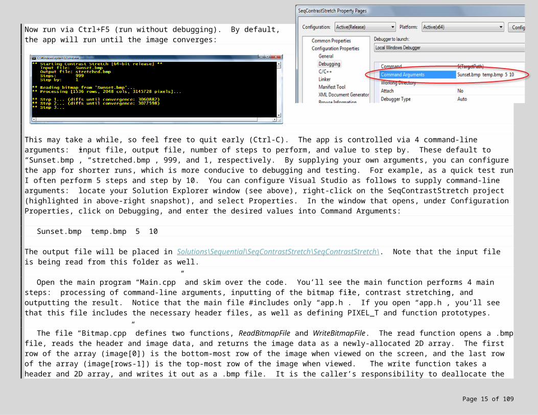
Now run via Ctrl+F5 (run without debugging). By default, the app will run until the image converges:

This may take a while, so feel free to quit early (Ctrl-C). The app is controlled via 4 command-line arguments: input file, output file, number of steps to perform, and value to step by. These default to “Sunset.bmp”, “stretched.bmp”, 999, and 1, respectively. By supplying your own arguments, you can configure the app for shorter runs, which is more conducive to debugging and testing. For example, as a quick test run I often perform 5 steps and step by 10. You can configure Visual Studio as follows to supply command-line arguments: locate your Solution Explorer window (see above), right-click on the SeqContrastStretch project (highlighted in above-right snapshot), and select Properties. In the window that opens, under Configuration Properties, click on Debugging, and enter the desired values into Command Arguments:

Sunset.bmp temp.bmp 5 10

Page 12 of 89

The output file will be placed in Solutions\Sequential\SeqContrastStretch\SeqContrastStretch\. Note that the input file is being read from this folder as well.

Open the main program “Main.cpp” and skim over the code. You’ll see the main function performs 4 main steps: processing of command-line arguments, inputting of the bitmap file, contrast stretching, and outputting the result. Notice that the main file #includes only “app.h”. If you open “app.h”, you’ll see that this file includes the necessary header files, as well as defining PIXEL_T and function prototypes.

The file “Bitmap.cpp” defines two functions, ReadBitmapFile and WriteBitmapFile. The read function opens a .bmp file, reads the header and image data, and returns the image data as a newly-allocated 2D array. The first row of the array (image[0]) is the bottom-most row of the image when viewed on the screen, and the last row of the array (image[rows-1]) is the top-most row of the image when viewed. The write function takes a header and 2D array, and writes it out as a .bmp file. It is the caller’s responsibility to deallocate the 2D array of image data.

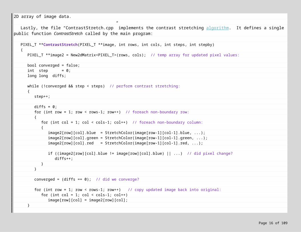
Lastly, the file “ContrastStretch.cpp” implements the contrast stretching algorithm. It defines a single public function ContrastStretch called by the main program:

PIXEL_T **ContrastStretch(PIXEL_T **image, int rows, int cols, int steps, int stepby){

PIXEL_T **image2 = New2dMatrix<PIXEL_T>(rows, cols); // temp array for updated pixel values:

bool converged = false;int step = 0;long long diffs;

while (!converged && step < steps) // perform contrast stretching:{

step++;

diffs = 0;for (int row = 1; row < rows-1; row++) // foreach non-boundary row:{

for (int col = 1; col < cols-1; col++) // foreach non-boundary column:{

image2[row][col].blue = StretchColor(image[row-1][col-1].blue, ...);image2[row][col].green = StretchColor(image[row-1][col-1].green, ...);image2[row][col].red = StretchColor(image[row-1][col-1].red, ...);

if ((image2[row][col].blue != image[row][col].blue) || ...) // did pixel change?diffs++;

}}

converged = (diffs == 0); // did we converge?

Page 13 of 89

for (int row = 1; row < rows-1; row++) // copy updated image back into original:for (int col = 1; col < cols-1; col++)

image[row][col] = image2[row][col];}

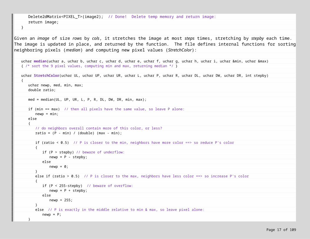
Delete2dMatrix<PIXEL_T>(image2); // Done! Delete temp memory and return image:return image;

}

Given an image of size rows by cols, it stretches the image at most steps times, stretching by stepby each time. The image is updated in place, and returned by the function. The file defines internal functions for sorting neighboring pixels (median) and computing new pixel values (StretchColor):

uchar median(uchar a, uchar b, uchar c, uchar d, uchar e, uchar f, uchar g, uchar h, uchar i, uchar &min, uchar &max){ /* sort the 9 pixel values, computing min and max, returning median */ }

uchar StretchColor(uchar UL, uchar UP, uchar UR, uchar L, uchar P, uchar R, uchar DL, uchar DW, uchar DR, int stepby){

uchar newp, med, min, max;double ratio;

med = median(UL, UP, UR, L, P, R, DL, DW, DR, min, max);

if (min == max) // then all pixels have the same value, so leave P alone:newp = min;

else{

// do neighbors overall contain more of this color, or less?ratio = (P - min) / (double) (max - min);

if (ratio < 0.5) // P is closer to the min, neighbors have more color ==> so reduce P's color{

if (P > stepby) // beware of underflow:newp = P - stepby;

else newp = 0;

}else if (ratio > 0.5) // P is closer to the max, neighbors have less color ==> so increase P's color{

if (P < 255-stepby) // beware of overflow:newp = P + stepby;

else newp = 255;

}else // P is exactly in the middle relative to min & max, so leave pixel alone:

newp = P;}

return newp;}

Page 14 of 89

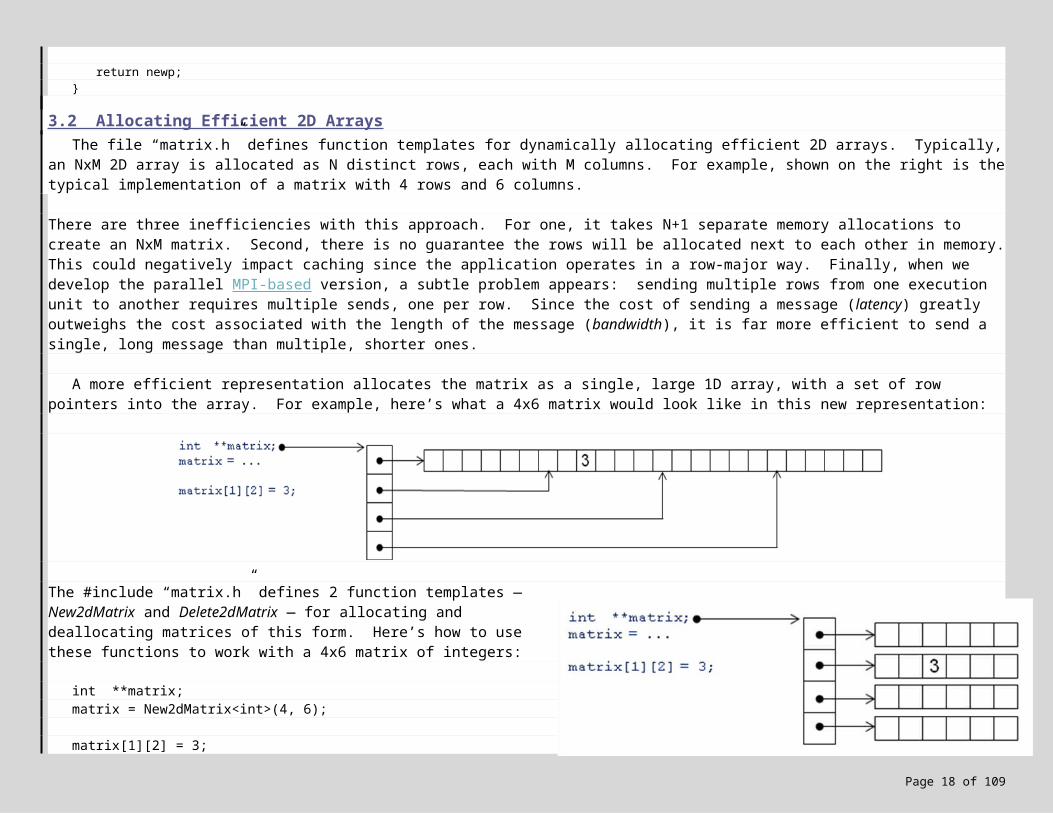
3.2 Allocating Efficient 2D Arrays The file “matrix.h” defines function templates for dynamically allocating efficient 2D arrays. Typically, an NxM 2D array is

allocated as N distinct rows, each with M columns. For example, shown on the right is the typical implementation of a matrix with 4 rows and 6 columns.

There are three inefficiencies with this approach. For one, it takes N+1 separate memory allocations to create an NxM matrix. Second, there is no guarantee the rows will be allocated next to each other in memory. This could negatively impact caching since the application operates in a row-major way. Finally, when we develop the parallel MPI-based version, a subtle problem appears: sending multiple rows from one execution unit to another requires multiple sends, one per row. Since the cost of sending a message (latency) greatly outweighs the cost associated with the length of the message (bandwidth), it is far more efficient to send a single, long message than multiple, shorter ones.

A more efficient representation allocates the matrix as a single, large 1D array, with a set of row pointers into the array. For example, here’s what a 4x6 matrix would look like in this new representation:

The #include “matrix.h” defines 2 function templates — New2dMatrix and Delete2dMatrix — for allocating and deallocating matrices of this form. Here’s how to use these functions to work with a 4x6 matrix of integers:

int **matrix;matrix = New2dMatrix<int>(4, 6);

matrix[1][2] = 3;

Delete2dMatrix<int>(matrix);

3.3 Lab Exercise! This is a good time to take a break and experiment with the

sequential version of the application. A copy of the application can be found in Exercises\01 Sequential\SeqContrastStretch\. Open the application, and select your target platform (Win32 or x64). One optimization is to consider replacing the doubly-nested loop at the end of the contrast stretch, i.e.

Page 15 of 89

for (int row = 1; row < rows-1; row++) // copy updated image back into original:for (int col = 1; col < cols-1; col++)

image[row][col] = image2[row][col];

with one or more calls to memcpy (or the safe version memcpy_s). Note that one call to memcpy is not sufficient since the boundary rows of image2 are empty. If you make changes to the application, you can check your work by comparing your resulting images to those in Misc\:

Sunset-75-by-1.bmp: contrast stretch of “Sunset.bmp”, 75 steps, stepping by 1Sunset-convergence-260-by-1.bmp:contrast stretch of “Sunset.bmp” until

convergence (260 steps, stepping by 1)

Use a tool like WinDiff to compare your result to the supplied .bmp files; a copy of WinDiff can be found in Misc\WinDiff\. Your goal in this exercise is to record the average execution time of 3 sequential runs on your local workstation. We need this result to accurately compute speedup values for the upcoming parallel versions. Stretch the supplied image “Sunset.bmp”, and run until convergence; this should take on the order of 260 steps. Make sure you time the release version of your application. When you are done, record the time here:

Sequentialtime on local workstation for convergence run:______________________

4. Working with Windows HPC Server 2008

Let’s assume you have a working Windows HPC Server 2008 cluster at your disposal (if not, you can safely skip this section, or if you need help setting one up, see Appendix A). Jobs are submitted to the cluster in a variety of ways: through an MMC plug-in such as the Microsoft® HPC Pack 2008 Job Manager, through Windows PowerShell™ or a console window (“black screen”), or through custom scripts / programs using the cluster’s API. We’ll focus here on using the MMC plug-ins to submit jobs from your local workstation.

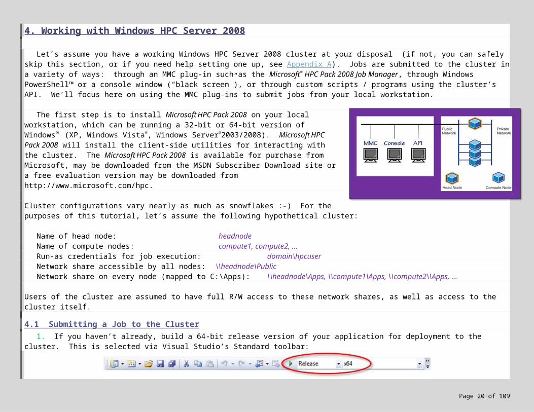
The first step is to install Microsoft HPC Pack 2008 on your local workstation, which can be running a 32-bit or 64-bit version of Windows® (XP, Windows Vista®, Windows Server®2003/2008). Microsoft HPC Pack 2008 will install the client-side utilities for interacting with the cluster. The Microsoft HPC Pack 2008 is available for purchase from Microsoft, may be downloaded from the MSDN Subscriber Download site or a free evaluation version may be downloaded from http://www.microsoft.com/hpc.

Cluster configurations vary nearly as much as snowflakes :-) For the purposes of this tutorial, let’s assume the following hypothetical cluster:

Page 16 of 89

Name of head node: headnodeName of compute nodes: compute1, compute2, …Run-as credentials for job execution: domain\hpcuserNetwork share accessible by all nodes: \\headnode\Public Network share on every node (mapped to C:\Apps): \\headnode\Apps, \\compute1\Apps, \\compute2\\Apps, …

Users of the cluster are assumed to have full R/W access to these network shares, as well as access to the cluster itself.

4.1 Submitting a Job to the Cluster 1. If you haven’t already, build a 64-bit release version of your application for deployment to the cluster. This is selected via

Visual Studio’s Standard toolbar:

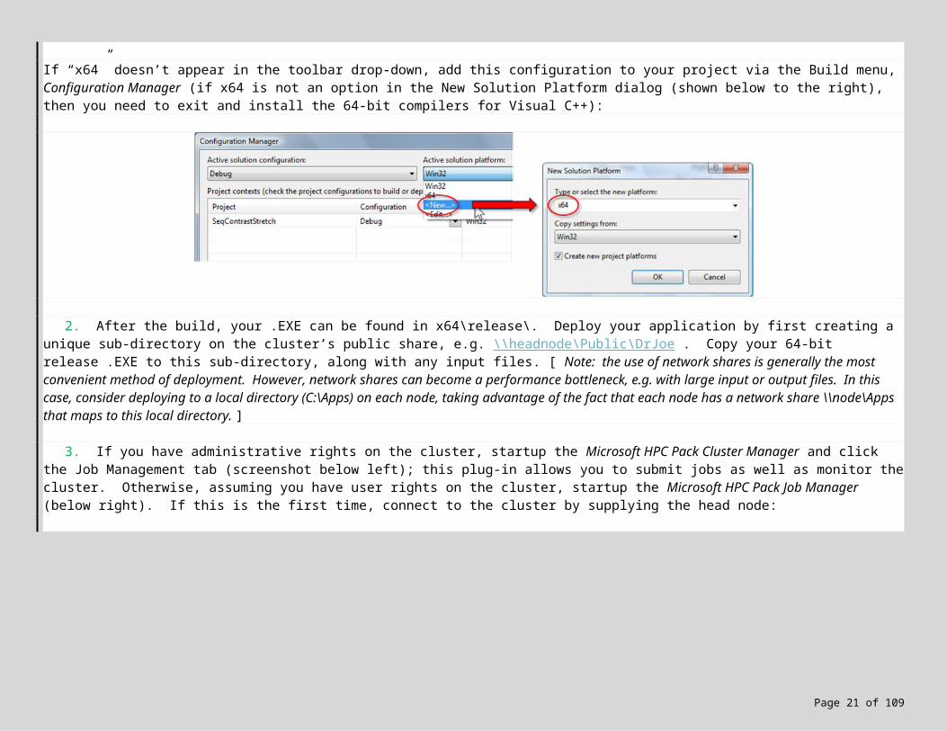
If “x64” doesn’t appear in the toolbar drop-down, add this configuration to your project via the Build menu, Configuration Manager (if x64 is not an option in the New Solution Platform dialog (shown below to the right), then you need to exit and install the 64-bit compilers for Visual C++):

2. After the build, your .EXE can be found in x64\release\. Deploy your application by first creating a unique sub-directory on the cluster’s public share, e.g. \\headnode\Public\DrJoe . Copy your 64-bit release .EXE to this sub-directory, along with any input files. [ Note: the use of network shares is generally the most convenient method of deployment. However, network shares can become a performance bottleneck, e.g. with large input or output files. In this case, consider deploying to a local directory (C:\Apps) on each node, taking advantage of the fact that each node has a network share \\node\Apps that maps to this local directory. ]

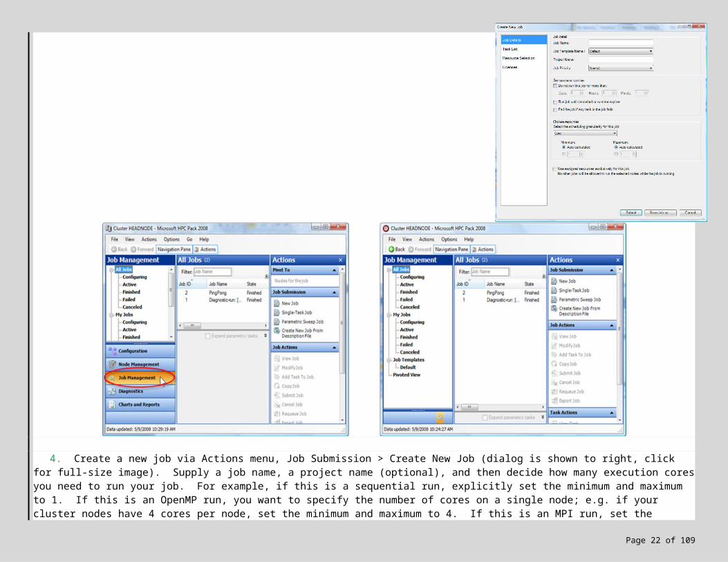
3. If you have administrative rights on the cluster, startup the Microsoft HPC Pack Cluster Manager and click the Job Management tab (screenshot below left); this plug-in allows you to submit jobs as well as monitor the cluster. Otherwise,

Page 17 of 89

assuming you have user rights on the cluster, startup the Microsoft HPC Pack Job Manager (below right). If this is the first time, connect to the cluster by supplying the head node:

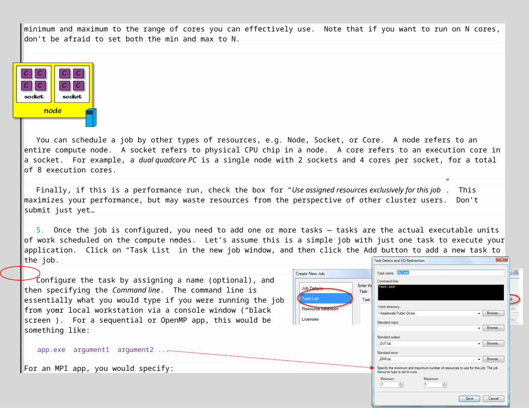
4. Create a new job via Actions menu, Job Submission > Create New Job (dialog is shown to right, click for full-size image). Supply a job name, a project name (optional), and then decide how many execution cores you need to run your job. For example, if this is a sequential run, explicitly set the minimum and maximum to 1. If this is an OpenMP run, you want to specify the number of cores on a single node; e.g. if your cluster nodes have 4 cores per node, set the minimum and maximum to 4. If this is an MPI run, set the minimum and maximum to the range of cores you can effectively use. Note that if you want to run on N cores, don’t be afraid to set both the min and max to N.

Page 18 of 89

You can schedule a job by other types of resources, e.g. Node, Socket, or Core. A node refers to an entire compute node. A socket refers to physical CPU chip in a node. A core refers to an execution core in a socket. For example, a dual quadcore PC is a single node with 2 sockets and 4 cores per socket, for a total of 8 execution cores.

Finally, if this is a performance run, check the box for “Use assigned resources exclusively for this job”. This maximizes your performance, but may waste resources from the perspective of other cluster users. Don’t submit just yet…

5. Once the job is configured, you need to add one or more tasks — tasks are the actual executable units of work scheduled on the compute nodes. Let’s assume this is a simple job with just one task to execute your application. Click on “Task List” in the new job window, and then click the Add button to add a new task to the job.

Configure the task by assigning a name (optional), and then specifying the Command line. The command line is essentially what you would type if you were running the job from your local workstation via a console window (“black screen”). For a sequential or OpenMP app, this would be something like:

app.exe argument1 argument2 ...

For an MPI app, you would specify:

mpiexec mpiapp.exe argument1 argument2 ...

Note that you drop the –n argument to mpiexec when executing on the cluster. Next, set the Working directory to the location where you deployed the .EXE (e.g. \\headnode\Public\DrJoe, or C:\Apps if you deployed locally on each node). Redirect Standard output and error to text files; these capture program output and error messages, and will be created in the working directory (these files are very handy when troubleshooting). Finally, select the minimum and maximum number of execution cores to use for executing this task. The range is constrained by the values set for the overall job: use a min/max of

Page 19 of 89

1 for sequential apps, the number of cores on a node for OpenMP apps, and a range of cores for MPI apps. Click Save to save the configuration.

6. You should now be back at the job creation window, with a job ready for submission. First, let’s save the job as an XML-based template so it’s easier to resubmit if need be: click the “Save Job as…” button, provide a name for the generated description file, and save.

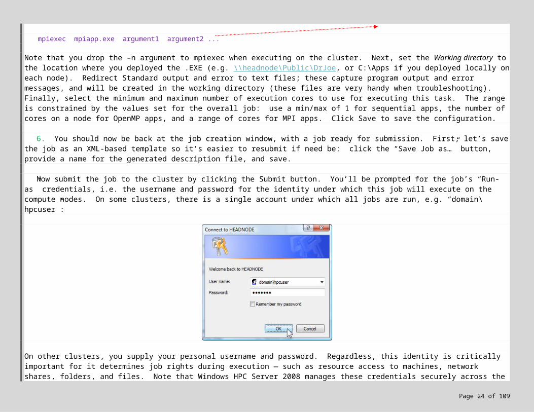
Now submit the job to the cluster by clicking the Submit button. You’ll be prompted for the job’s “Run-as” credentials, i.e. the username and password for the identity under which this job will execute on the compute nodes. On some clusters, there is a single account under which all jobs are run, e.g. “domain\hpcuser”:

On other clusters, you supply your personal username and password. Regardless, this identity is critically important for it determines job rights during execution — such as resource access to machines, network shares, folders, and files. Note that Windows HPC Server 2008 manages these credentials securely across the cluster. [ Note that you also have the option to securely cache these credentials on your local workstation by checking the “Remember my password” option. Later, if you need to clear this cache (e.g. when the password changes), select Options menu, Clear Credential Cache in the HPC Cluster or Job Manager. ]

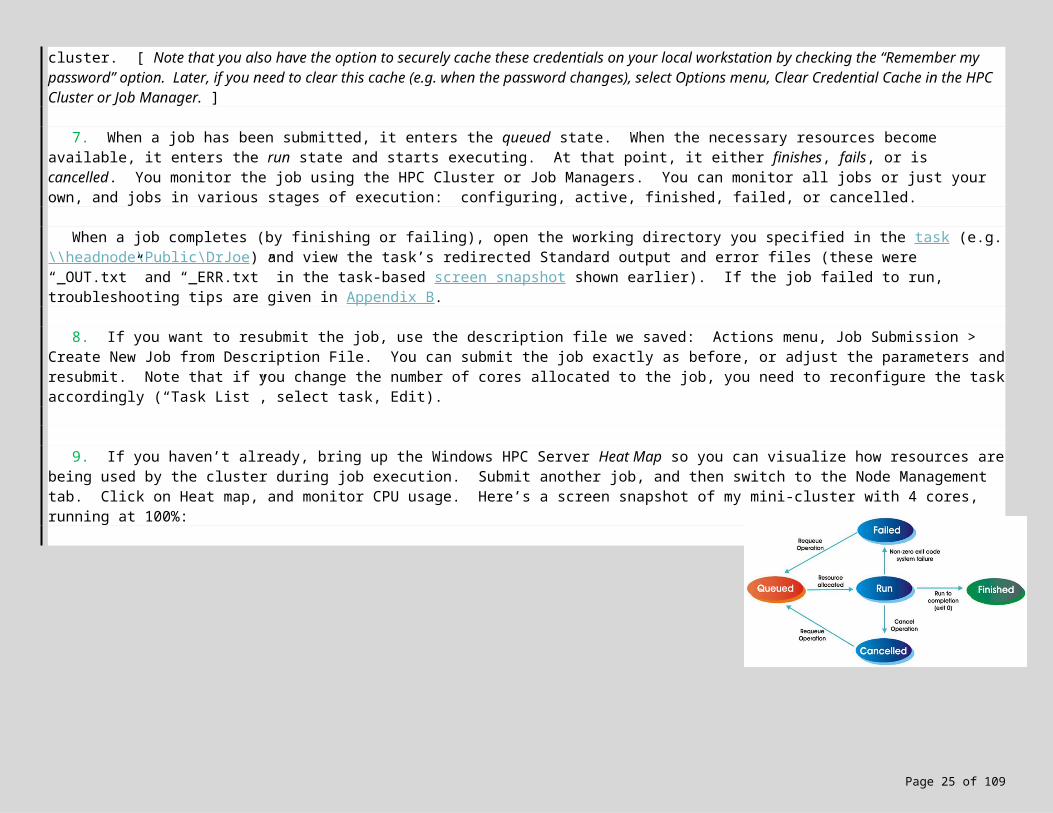
7. When a job has been submitted, it enters the queued state. When the necessary resources become available, it enters the run state and starts executing. At that point, it either finishes, fails, or is cancelled. You monitor the job using the HPC Cluster or Job Managers. You can monitor all jobs or just your own, and jobs in various stages of execution: configuring, active, finished, failed, or cancelled.

Page 20 of 89

When a job completes (by finishing or failing), open the working directory you specified in the task (e.g. \\headnode\Public\DrJoe) and view the task’s redirected Standard output and error files (these were “_OUT.txt” and “_ERR.txt” in the task-based screen snapshot shown earlier). If the job failed to run, troubleshooting tips are given in Appendix B.

8. If you want to resubmit the job, use the description file we saved: Actions menu, Job Submission > Create New Job from Description File. You can submit the job exactly as before, or adjust the parameters and resubmit. Note that if you change the number of cores allocated to the job, you need to reconfigure the task accordingly (“Task List”, select task, Edit).

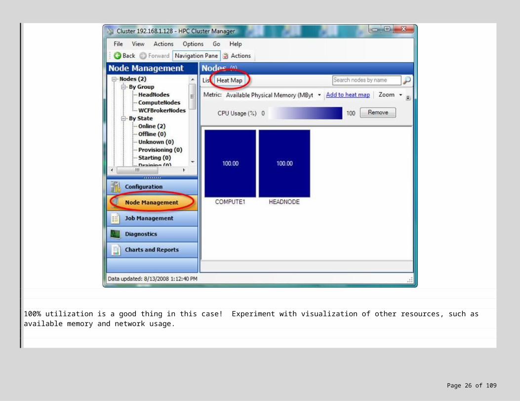
9. If you haven’t already, bring up the Windows HPC Server Heat Map so you can visualize how resources are being used by the cluster during job execution. Submit another job, and then switch to the Node Management tab. Click on Heat map, and monitor CPU usage. Here’s a screen snapshot of my mini-cluster with 4 cores, running at 100%:

Page 21 of 89

100% utilization is a good thing in this case! Experiment with visualization of other resources, such as available memory and network usage.

Page 22 of 89

10. Finally, try using Windows PowerShell or a console window to submit your jobs (or likewise automate with a script), here are two examples. First, submitting the sequential version of the contrast stretching app via a console window (Start, cmd.exe):

> job submit /scheduler:headnode /jobname:MyJob /numprocessors:1-1 /exclusive:true /workdir:\\headnode\Public\DrJoe /stdout:_OUT.txt /stderr:_ERR.txt /user:domain\hpcuser SeqContrastStretch.exe Sunset.bmp result.bmp 75 1

Again, this time via Windows PowerShell (Start, Microsoft HPC Pack 2008 > Windows PowerShell):

> $job = new-hpcjob –scheduler "headnode" –name "MyJob" –numprocessors "1-1" –exclusive 1> add-hpctask –scheduler "headnode" –job $job –workdir "\\headnode\Public\DrJoe" –stdout "_OUT.txt" –stderr

"_ERR.txt" –command "SeqContrastStretch.exe Sunset.bmp result.bmp 75 1"> submit-hpcjob –scheduler "headnode" –job $job –credential "domain\hpcuser"

For more info, type “job submit /?” in your console window or “get-help submit-hpcjob” in Windows PowerShell.

4.2 Lab Exercise! Revisit your sequential application in Exercises\01 Sequential\SeqContrastStretch\. Your goal in this exercise

is to record the average execution time of 3 sequential runs on one node of your cluster. We need this result to accurately compute speedup values for the upcoming parallel versions. Stretch the supplied image “Sunset.bmp”, and run until convergence; this should take on the order of 260 steps. Make sure you are running the 64-bit release version on the cluster. When you are done, record the time here:

Sequentialtime on one node of cluster for convergence run: ______________________

5. A Shared-Memory Parallel Version using OpenMP

Let’s take a look at parallelizing the contrast stretching algorithm for execution on a shared-memory machine. This machine can be your local workstation, or a single node in the Windows HPC Server 2008 cluster. Assuming it is multi-core / multi-socket, the resulting speedup should be linear (or nearly so) for the number of cores / sockets.

Page 23 of 89

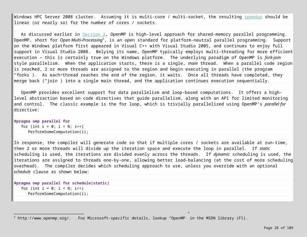
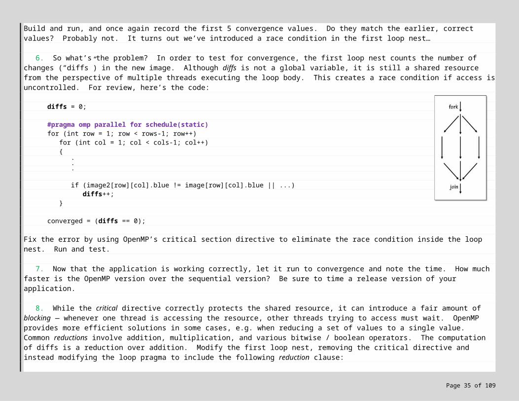
As discussed earlier in Section 2, OpenMP is high-level approach for shared-memory parallel programming. OpenMP, short for Open Multi-Processing3, is an open standard for platform-neutral parallel programming. Support on the Windows platform first appeared in Visual C++ with Visual Studio 2005, and continues to enjoy full support in Visual Studio 2008. Belying its name, OpenMP typically employs multi-threading for more efficient execution — this is certainly true on the Windows platform. The underlying paradigm of OpenMP is fork-join style parallelism. When the application starts, there is a single, main thread. When a parallel code region is reached, 2 or more threads are assigned to the region and begin executing in parallel (the program “forks”). As each thread reaches the end of the region, it waits. Once all threads have completed, they merge back (“join”) into a single main thread, and the application continues execution sequentially.

OpenMP provides excellent support for data parallelism and loop-based computations. It offers a high-level abstraction based on code directives that guide parallelism, along with an API for limited monitoring and control. The classic example is the for loop, which is trivially parallelized using OpenMP’s parallel for directive:

#pragma omp parallel forfor (int i = 0; i < N; i++)

PerformSomeComputation(i);

In response, the compiler will generate code so that if multiple cores / sockets are available at run-time, then 2 or more threads will divide up the iteration space and execute the loop in parallel. If static scheduling is used, the iterations are divided evenly across the threads. If dynamic scheduling is used, the iterations are assigned to threads one-by-one, allowing better load-balancing (at the cost of more scheduling overhead). The compiler decides which scheduling approach to use, unless you override with an optional schedule clause as shown below:

#pragma omp parallel for schedule(static)for (int i = 0; i < N; i++)


Note that parallel for is really just a special case of OpenMP’s more general concept of a parallel region, in which threads are forked off to execute the region in parallel. Here is the equivalent version using an OpenMP parallel region:

#pragma omp parallel {

#pragma omp for schedule(static)for (int i = 0; i < N; i++)

PerformSomeComputation(i); }

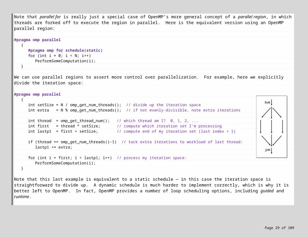
We can use parallel regions to assert more control over parallelization. For example, here we explicitly divide the iteration space:

#pragma omp parallel {

3 http://www.openmp.org/. For Microsoft-specific details, lookup “OpenMP” in the MSDN library (F1).

Page 24 of 89

int setSize = N / omp_get_num_threads(); // divide up the iteration spaceint extra = N % omp_get_num_threads(); // if not evenly-divisible, note extra iterations

int thread = omp_get_thread_num(); // which thread am I? 0, 1, 2, ...int first = thread * setSize; // compute which iteration set I'm processingint lastp1 = first + setSize; // compute end of my iteration set (last index + 1)

if (thread == omp_get_num_threads()-1) // tack extra iterations to workload of last thread:lastp1 += extra;

for (int i = first; i < lastp1; i++) // process my iteration space:PerformSomeComputation(i);

}

Note that this last example is equivalent to a static schedule — in this case the iteration space is straightforward to divide up. A dynamic schedule is much harder to implement correctly, which is why it is better left to OpenMP. In fact, OpenMP provides a number of loop scheduling options, including guided and runtime.

More importantly, note that shared variables, and race conditions that may result from parallel access to shared variables, are the responsibility of the programmer, not OpenMP. For example, let’s revisit our original example:

#pragma omp parallel for schedule(static)for (int i = 0; i < N; i++)


Suppose that PerformSomeComputation adds the parameter i to a global variable (this could just as easily be a global data structure):

int global = 0;

void PerformSomeComputation(int i){

global += i;}

The sequential version of this program computes N*(N-1)/2. The parallel version as shown above has a race condition, and computes a value somewhere between 0 and N*(N-1)/2, inclusive. The solution is to control access to the shared resource, e.g. with an OpenMP critical section:

void PerformSomeComputation(int i){

#pragma omp critical{

global += i;}

Page 25 of 89

}

Race conditions are the single, largest problem in parallel applications.

Finally, OpenMP provides a simple API for obtaining run-time information, and for modifying some aspects of the run-time environment. Here are the most commonly used functions:

omp_get_num_procs( ) returns number of processors currently available at time of call

omp_get_max_threads( ) returns maximum number of threads available for execution of a parallel region

omp_get_num_threads( ) returns number of threads currently executing in the parallel region

omp_get_thread_num( ) returns thread number of calling thread (0 .. omp_get_num_threads( )-1)omp_in_parallel( ) returns a nonzero value if called from within a parallel regionomp_set_num_threads(N) sets the number N of threads to use in subsequent parallel regions

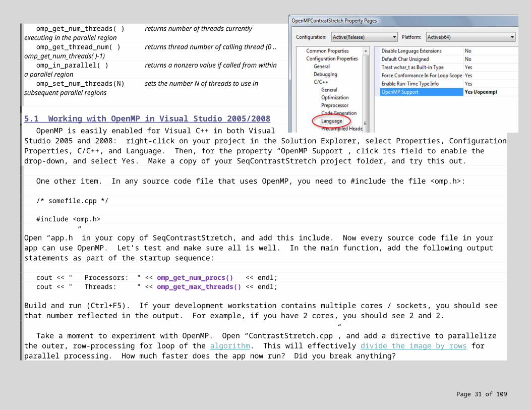
5.1 Working with OpenMP in Visual Studio 2005/2008 OpenMP is easily enabled for Visual C++ in both Visual Studio 2005 and 2008: right-click on your project in the Solution

Explorer, select Properties, Configuration Properties, C/C++, and Language. Then, for the property “OpenMP Support”, click its field to enable the drop-down, and select Yes. Make a copy of your SeqContrastStretch project folder, and try this out.

One other item. In any source code file that uses OpenMP, you need to #include the file <omp.h>:

/* somefile.cpp */

#include <omp.h>

Open “app.h” in your copy of SeqContrastStretch, and add this include. Now every source code file in your app can use OpenMP. Let’s test and make sure all is well. In the main function, add the following output statements as part of the startup sequence:

cout << " Processors: " << omp_get_num_procs() << endl;cout << " Threads: " << omp_get_max_threads() << endl;

Build and run (Ctrl+F5). If your development workstation contains multiple cores / sockets, you should see that number reflected in the output. For example, if you have 2 cores, you should see 2 and 2.

Page 26 of 89

Take a moment to experiment with OpenMP. Open “ContrastStretch.cpp”, and add a directive to parallelize the outer, row-processing for loop of the algorithm. This will effectively divide the image by rows for parallel processing. How much faster does the app now run? Did you break anything?

5.2 Lab Exercise! Okay, time for a lab exercise, and a more focused exploration of OpenMP. What you’re going to find is that in the context of

data parallel applications (and others), OpenMP is a very effective approach for single-node, shared-memory parallelism. Note that a solution to the lab exercise is provided in Solutions\OpenMP\OpenMPContrastStretch\.

1. Start by opening the application in Exercises\02 OpenMP\OpenMPContrastStretch\. This is a copy of the sequential contrast stretching application. Switch to the target platform appropriate for your workstation (Win32 or x64), and enable OpenMP. Modify “app.h” to #include <omp.h>, and build to make sure all is well. Modify the main function’s startup sequence to output information about your runtime environment:

cout << " Processors: " << omp_get_num_procs() << endl;cout << " Threads: " << omp_get_max_threads() << endl;

Build and run (Ctrl+F5). Record the first 5 convergence values; make note that these are the correct values.

2. How many processors and threads were reported? If either of these values is 1, you will not see any speedup on your workstation from OpenMP (nor any of the errors that might occur if you use OpenMP incorrectly). In this case, run your app solely on the cluster. If both of the reported values are 2 or more, feel free to run your app locally (Ctrl+F5), then deploy and run on the cluster for additional results.

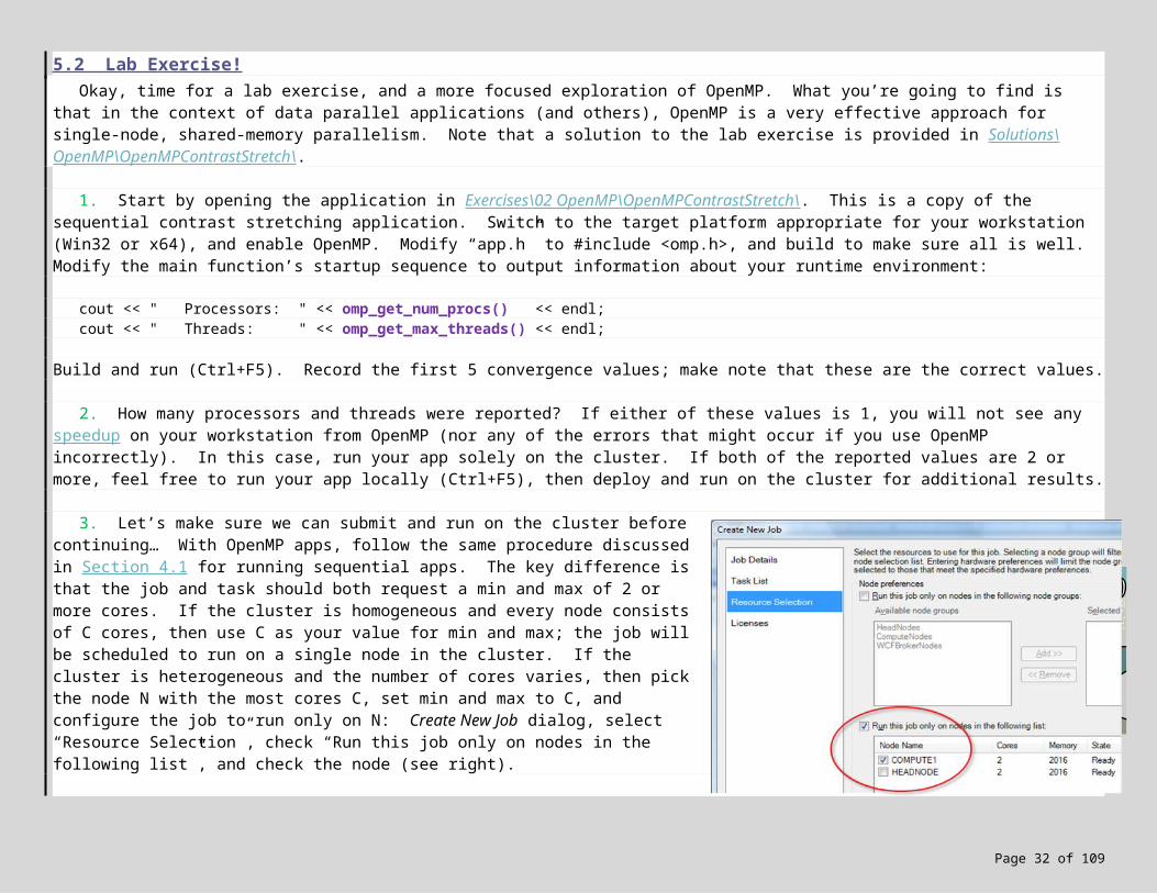
3. Let’s make sure we can submit and run on the cluster before continuing… With OpenMP apps, follow the same procedure discussed in Section 4.1 for running sequential apps. The key difference is that the job and task should both request a min and max of 2 or more cores. If the cluster is homogeneous and every node consists of C cores, then use C as your value for min and max; the job will be scheduled to run on a single node in the cluster. If the cluster is heterogeneous and the number of cores varies, then pick the node N with the most cores C, set min and max to C, and configure the job to run only on N: Create New Job dialog, select “Resource Selection”, check “Run this job only on nodes in the following list”, and check the node (see right).

Save the job configuration as an XML-based description file, then submit. When the job finishes, view the standard output (did you capture in a text file?), and confirm that the first 5 convergence values match those recorded earlier. Next time you want to run on the cluster, simply use the description file: Actions menu, Job Submission > Create New Job from Description File. Of course, if the app has changed, be sure to rebuild and redeploy to the cluster before submitting a new job.

Page 27 of 89

4. Now let’s start experimenting with OpenMP. While there are many places you could add OpenMP directives, the goal is to use the fewest number of directives that maximize the amount of parallelism. For example, we could try to parallelize the median( ) sorting function in “ContrastStretch.cpp”, but the array contains only 9 elements, and not worth the overhead of multi-threading. StretchColor( ) is likewise too trivial to parallelize.

The obvious candidate is ContrastStretch( ), which contains triply-nested loops and calls upon median( ) and StretchColor( ). In a perfect world, you would parallelize the outer-most loop, and be done4:

#pragma omp parallel{

while (!converged && step < steps){

...}

}

Go ahead and try it — OpenMP is happy to oblige :-) But does this make sense? Absolutely not. The above directive parallelizes the steps of the algorithm, which maximizes parallelism but at the cost of correctness (not only does this break the algorithm, but it also causes a race condition on the global image array). On the conservative side, we could parallelize the inner-most loops, for example:

// copy updated image back into original:for (int row = 1; row < rows-1; row++)

#pragma omp parallel forfor (int col = 1; col < cols-1; col++)


This preserves correctness and provides a performance boost, but does not maximize parallelism — we process the columns in parallel, but we advance from row to row sequentially. The end result is that we’ll start with row 1, fork off a set of threads to process the columns in parallel, join, advance to the next row, fork off a set of threads to process those columns in parallel, join, advance, fork, join, advance, and so on. Given N rows, this approach will cause N forks and N joins.

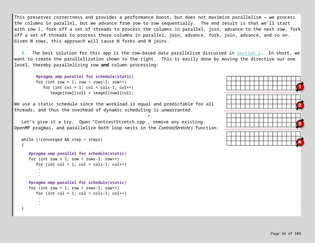
5. The best solution for this app is the row-based data parallelism discussed in Section 2. In short, we want to create the parallelization shown to the right. This is easily done by moving the directive out one level, thereby parallelizing row and column processing:

#pragma omp parallel for schedule(static)for (int row = 1; row < rows-1; row++)

for (int col = 1; col < cols-1; col++)

4 In general, if you were given an application and had no idea where to start, profile the application to see where time is being spent, and then look to parallelize the outer-most loop(s) in that time-intensive code.

Page 28 of 89


We use a static schedule since the workload is equal and predictable for all threads, and thus the overhead of dynamic scheduling is unwarranted.

Let’s give it a try. Open “ContrastStretch.cpp”, remove any existing OpenMP pragmas, and parallelize both loop nests in the ContrastStretch( ) function:

while (!converged && step < steps){


for (int col = 1; col < cols-1; col++) . . .


for (int col = 1; col < cols-1; col++) . . .

}

Build and run, and once again record the first 5 convergence values. Do they match the earlier, correct values? Probably not. It turns out we’ve introduced a race condition in the first loop nest…

6. So what’s the problem? In order to test for convergence, the first loop nest counts the number of changes (“diffs”) in the new image. Although diffs is not a global variable, it is still a shared resource from the perspective of multiple threads executing the loop body. This creates a race condition if access is uncontrolled. For review, here’s the code:

diffs = 0;


for (int col = 1; col < cols-1; col++){

.

.

.

if (image2[row][col].blue != image[row][col].blue || ...)diffs++;

}

converged = (diffs == 0);

Page 29 of 89

Fix the error by using OpenMP’s critical section directive to eliminate the race condition inside the loop nest. Run and test.

7. Now that the application is working correctly, let it run to convergence and note the time. How much faster is the OpenMP version over the sequential version? Be sure to time a release version of your application.

8. While the critical directive correctly protects the shared resource, it can introduce a fair amount of blocking — whenever one thread is accessing the resource, other threads trying to access must wait. OpenMP provides more efficient solutions in some cases, e.g. when reducing a set of values to a single value. Common reductions involve addition, multiplication, and various bitwise / boolean operators. The computation of diffs is a reduction over addition. Modify the first loop nest, removing the critical directive and instead modifying the loop pragma to include the following reduction clause:

#pragma omp parallel for schedule(static) reduction(+:diffs)for (int row = 1; row < rows-1; row++) . . .

Since + is associative5, the compiler can create a local diffs variable for each thread — eliminating any contention for the shared variable. After the threads have joined, the main thread sums the local variables and produces the final sum. The end result is faster execution while maintaining correctness. Let’s confirm. First, run and convince yourself that the application is still working correctly. Now run to convergence and note the time. Did the application run faster? It should! This optimization should cut a number of seconds off the execution time…

9. Speaking of optimizations, try dynamic scheduling. Does it improve performance? How about guided scheduling? [ Lookup “OpenMP” in the MSDN library (F1) for more information about scheduling options. ]

10. If you are running the app locally on your workstation, bring up the Task Manager (Ctrl-Alt-Del). Switch to the Performance tab, and confirm that you are utilizing each core / socket 100%.

11. Now that the application is working and somewhat optimized, deploy to the cluster and record the average time for a set of convergence runs. What kind of speedup are you seeing? It should be close to linear (if not, make sure you are timing a release version). If your local workstation has multiple sockets / cores, record the average time across a few local convergence runs. Record your times here:

OpenMP Paralleltime on local workstation for convergence run: ______________, number of cores = ______, speedup = ________

OpenMP Paralleltime on one cluster node for convergence run: ______________, number of cores = ______, speedup = ________

5 Ignoring round-off errors that can occur with floating-point values.

Page 30 of 89

OPTIONAL1. Let’s modify the program to convince ourselves that multiple threads are in fact executing the loop nests. Currently the

program outputs to stdout as each step of the algorithm unfolds:

** Step 1... (diffs until convergence: 3060882)** Step 2... (diffs until convergence: 3077598)...

Modify the program so that each thread outputs its id followed by the step. For example:

1: Step 1...0: Step 1...** Diffs until convergence: 30608820: Step 2...1: Step 2...** Diffs until convergence: 3077598...

Use omp_get_thread_num( ) to retrieve a thread’s id; you must be inside an OpenMP parallel region for this call to work. Define a parallel region surrounding the output statement and the first loop nest, modify the output statement(s), update the pragma on the loop nest, and run. Make sure the first 5 convergence values are correct. If not, did you drop the parallel keyword from the loop nest (since the loop is already inside a parallel region)?

2. The compiler switch /FAs (Configuration Properties, C/C++, Output Files, Assembler Output, Assembly with Source Code) can be used to see the generated code from the OpenMP directives, such as calls to fork off threads (“_vcomp_fork”). While helpful, the output is assembly language and difficult to read. Can you find a better way to see the generated source code?

3. Here’s an optimization to ponder… The loop nests are parallelized separately, which causes a fork-join followed by another fork-join. Can we eliminate the first join, thereby speeding up the program by eliminating an unnecessary synchronization step? Is correctness maintained? You can test this optimization as follows: move the second loop nest into the parallel region, delete parallel from the loop nest pragma, and then add OpenMP’s nowait clause to the end of the pragma on the first loop nest. Now, when a thread finishes the first loop nest, it will immediately start the second without waiting. What happens? Even if the convergence values are the same, and even if WinDiff reports no differences, is this optimization safe in all cases?

6. A Distributed-Memory Parallel Version using MPI

Page 31 of 89

When designing sequential applications, we generally give little thought to the physical location of RAM. As good designers we try to minimize memory usage, and to improve caching by optimizing memory layout. However, we also make an implicit assumption — that memory is directly accessible from anywhere in our program. Given a global array A with N > 0 elements, the expression A[0] always refers to the same array, and the same first element. Taking this a step further, if we parallelize the program with OpenMP, we continue to program under this same assumption. For example, if multiple threads read A[0] at time T, we assume the same value will be read by all. This is shared memory.

The advantage of shared memory is that it’s familiar. The disadvantage is that it limits you to execution on one node of the cluster. To take advantage of multiple compute nodes, the designer is faced with a distributed memory6. MPI (Message Passing Interface7) is by far the most common approach for programming distributed-memory applications, given its flexibility, broad availability, and potential for high performance on a wide variety of hardware.

In an MPI application, multiple processes run concurrently, one per execution unit. This is known as the MIMD paradigm: Multiple Instruction, Multiple Data. Each process has its own private address space, with no sharing of memory. In order to communicate, processes must send and receive data using MPI operations. The fundamental operations are MPI_Send and MPI_Recv, prototyped as follows:

int MPI_Send(void *buf, int count, MPI_Datatype datatype, int dest, int tag, MPI_Comm comm);

int MPI_Recv(void *buf, int count, MPI_Datatype datatype, int src, int tag, MPI_Comm comm, MPI_Status *status);

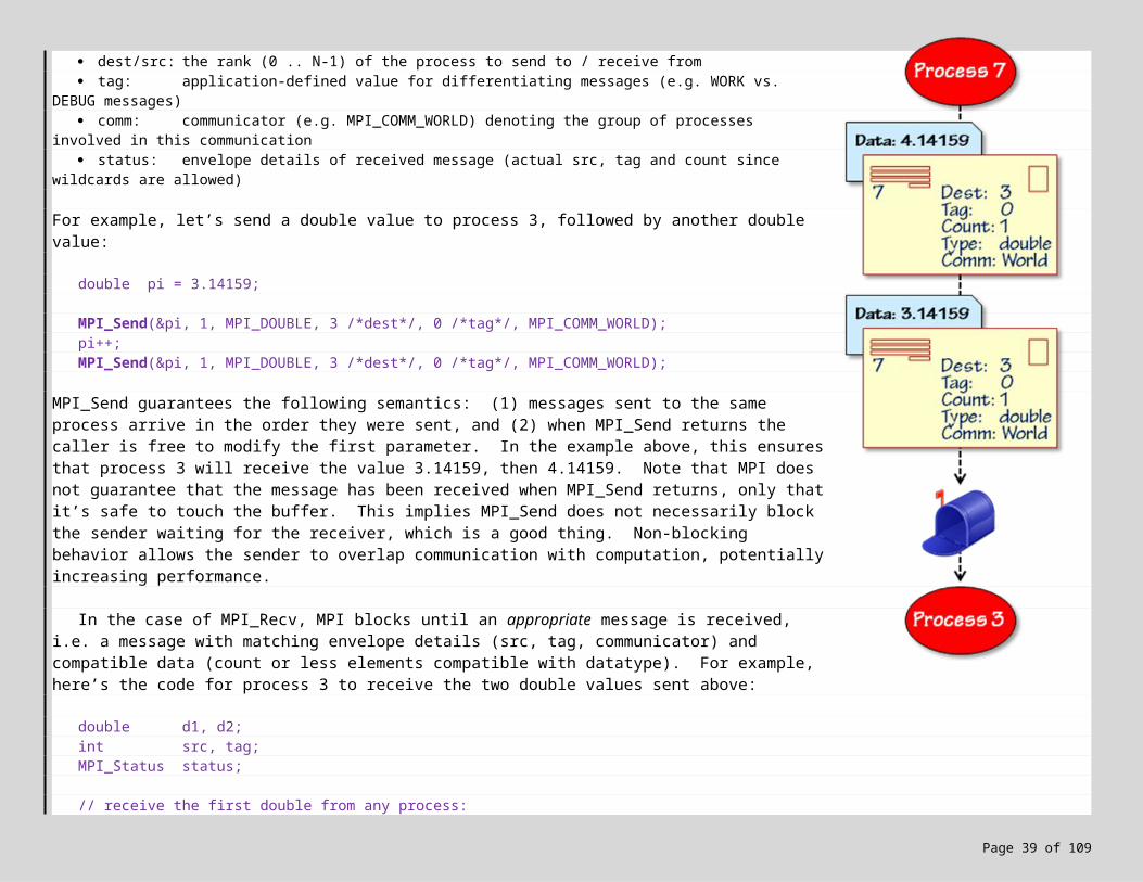
A message in MPI consists of an envelope and the data, analogous to postal mail (see diagram on next page). The data is specified by the first parameter, denoting the address of a memory buffer. In the case of MPI_Send, this buffer contains the data to send; in MPI_Recv, this buffer will hold the received data. The envelope controls addressing, and is specified via the remaining parameters:

count: number of buffer elements to send / maximum number of buffer elements to receive datatype: the type of buffer elements (character, integer, float, etc.) dest/src: the rank (0 .. N-1) of the process to send to / receive from tag: application-defined value for differentiating messages (e.g. WORK vs. DEBUG messages) comm: communicator (e.g. MPI_COMM_WORLD) denoting the group of processes involved in this communication status: envelope details of received message (actual src, tag and count since wildcards are allowed)

6 An active area of ongoing research is distributed virtual shared memory, which presents a shared memory to the programmer even though memory is physically distributed. Cluster OpenMP is a commercial implementation of this approach based on a relaxed memory consistency model.7 http://www.mpi-forum.org/.

Page 32 of 89

For example, let’s send a double value to process 3, followed by another double value:

double pi = 3.14159;

MPI_Send(&pi, 1, MPI_DOUBLE, 3 /*dest*/, 0 /*tag*/, MPI_COMM_WORLD);pi++;MPI_Send(&pi, 1, MPI_DOUBLE, 3 /*dest*/, 0 /*tag*/, MPI_COMM_WORLD);

MPI_Send guarantees the following semantics: (1) messages sent to the same process arrive in the order they were sent, and (2) when MPI_Send returns the caller is free to modify the first parameter. In the example above, this ensures that process 3 will receive the value 3.14159, then 4.14159. Note that MPI does not guarantee that the message has been received when MPI_Send returns, only that it’s safe to touch the buffer. This implies MPI_Send does not necessarily block the sender waiting for the receiver, which is a good thing. Non-blocking behavior allows the sender to overlap communication with computation, potentially increasing performance.

In the case of MPI_Recv, MPI blocks until an appropriate message is received, i.e. a message with matching envelope details (src, tag, communicator) and compatible data (count or less elements compatible with datatype). For example, here’s the code for process 3 to receive the two double values sent above:

double d1, d2;int src, tag;MPI_Status status;

// receive the first double from any process:MPI_Recv(&d1, 1, MPI_DOUBLE, MPI_ANY_SOURCE, MPI_ANY_TAG, MPI_COMM_WORLD, &status);

// receive the second double from the same process:src = status.MPI_SOURCE;tag = status.MPI_TAG;MPI_Recv(&d2, 1, MPI_DOUBLE, src, tag, MPI_COMM_WORLD, &status);

The optional wildcards MPI_ANY_SOURCE and MPI_ANY_TAG allow reception from any sending process. The first call to MPI_Recv causes process 3 to wait until a message arrives containing at most 1 double; the second call initiates a wait until another message arrives, from that same process and tag, containing at most 1 double.

While Send and Receive form the basis of any message-passing system, MPI contains nearly 200 functions for designing more powerful and higher-performing communication strategies8.

8 Two good books on the subject of MPI: Parallel Programming with MPI, by Peter Pacheco, and Using MPI : Portable Parallel Programming with the Message-Passing Interface (2nd edition), by W. Gropp, E. Lusk and A. Skjellum.

Page 33 of 89

6.1 Installing and Configuring MS-MPI Microsoft® MPI (MS-MPI) is the Microsoft implementation of MPI-2 that ships with Windows HPC Server 2008. MS-MPI

offers both C and FORTRAN bindings, and is a optimized port of Argonne’s well-regarded MPICH implementation (pronounced “M-Pitch”). To develop MPI applications for Windows, you need only do 2 things:

1. Install the SDK for Microsoft HPC Pack 20082. Configure Visual Studio 2005/2008

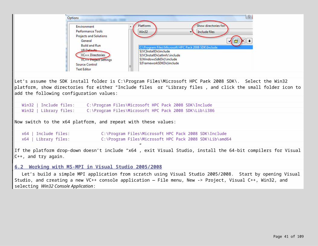
The SDK is installed on your local development workstation, which can be running a 32-bit or 64-bit version of Windows (XP, Windows Vista, Windows Server 2003/2008). Download the SDK from http://go.microsoft.com/fwlink/?linkID= 127031 . During installation, make note of the SDK’s install folder. The second step is to configure Visual Studio to locate MS-MPI during compilation and linking; this needs to be done only once. Startup Visual Studio, Tools menu, Options, Projects and Solutions, and select VC++ Directories:

Let’s assume the SDK install folder is C:\Program Files\Microsoft HPC Pack 2008 SDK\. Select the Win32 platform, show directories for either “Include files” or “Library files”, and click the small folder icon to add the following configuration values:

Win32 | Include files: C:\Program Files\Microsoft HPC Pack 2008 SDK\Include Win32 | Library files: C:\Program Files\Microsoft HPC Pack 2008 SDK\Lib\i386

Now switch to the x64 platform, and repeat with these values:

x64 | Include files: C:\Program Files\Microsoft HPC Pack 2008 SDK\Include x64 | Library files: C:\Program Files\Microsoft HPC Pack 2008 SDK\Lib\amd64

If the platform drop-down doesn’t include “x64”, exit Visual Studio, install the 64-bit compilers for Visual C++, and try again.

Page 34 of 89

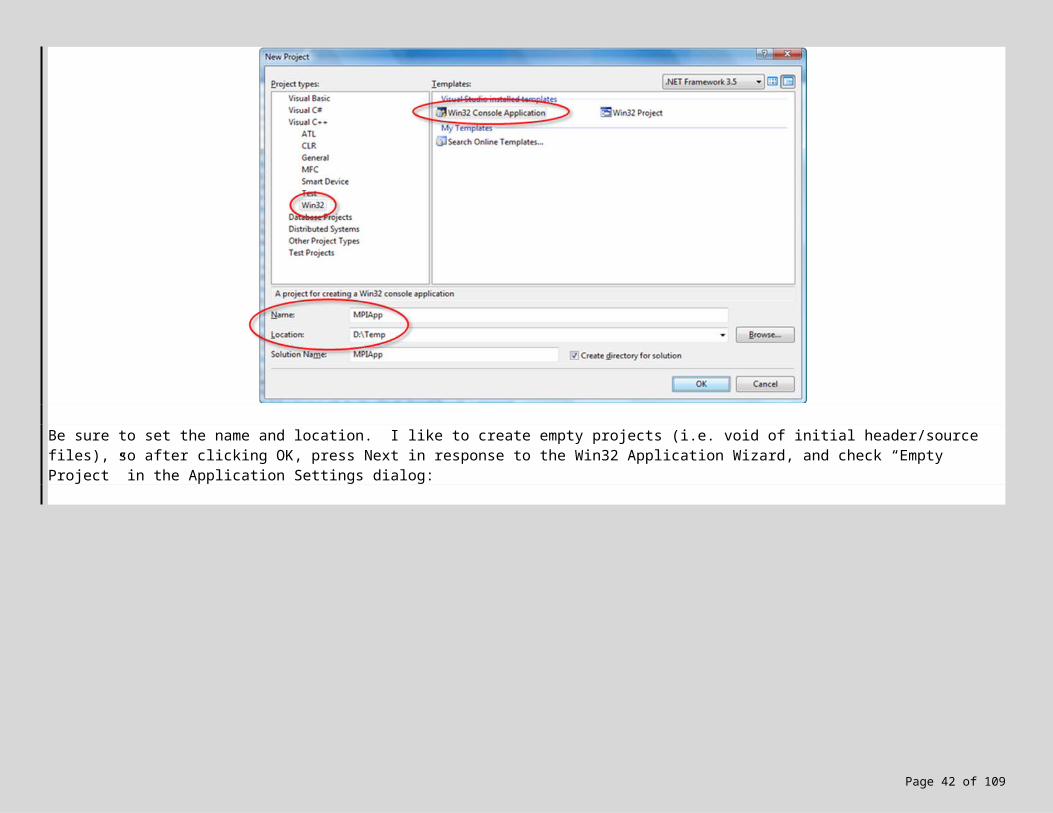
http://go.microsoft.com/fwlink/?linkID=%20127031%20

6.2 Working with MS-MPI in Visual Studio 2005/2008 Let’s build a simple MPI application from scratch using Visual Studio 2005/2008. Start by opening Visual Studio, and

creating a new VC++ console application — File menu, New -> Project, Visual C++, Win32, and selecting Win32 Console Application:

Be sure to set the name and location. I like to create empty projects (i.e. void of initial header/source files), so after clicking OK, press Next in response to the Win32 Application Wizard, and check “Empty Project” in the Application Settings dialog:

Page 35 of 89

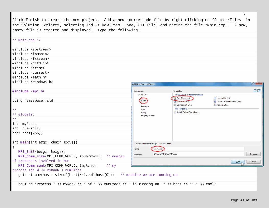
Click Finish to create the new project. Add a new source code file by right-clicking on “Source Files” in the Solution Explorer, selecting Add -> New Item, Code, C++ File, and naming the file “Main.cpp”. A new, empty file is created and displayed. Type the following:

/* Main.cpp */

#include <iostream>#include <iomanip>#include <fstream>#include <cstdlib>#include <ctime>#include <cassert>#include <math.h>#include <windows.h>

#include <mpi.h>

using namespace::std;

// // Globals://int myRank;int numProcs;char host[256];

int main(int argc, char* argv[]){

MPI_Init(&argc, &argv);MPI_Comm_size(MPI_COMM_WORLD, &numProcs); // number

of processes involved in runMPI_Comm_rank(MPI_COMM_WORLD, &myRank); // my

process id: 0 <= myRank < numProcsgethostname(host, sizeof(host)/sizeof(host[0])); //

machine we are running on

cout << "Process " << myRank << " of " << numProcs << " is running on '" << host << "'." << endl;

MPI_Finalize();return 0;

}

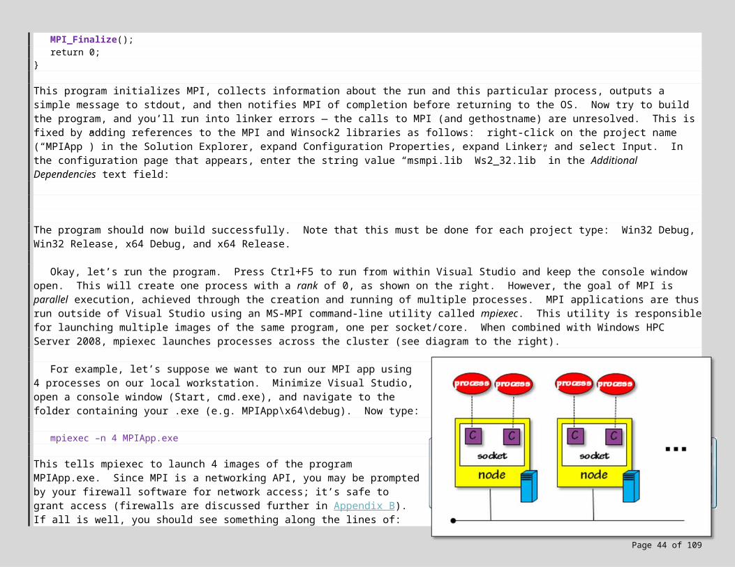
This program initializes MPI, collects information about the run and this particular process, outputs a simple message to stdout, and then notifies MPI of completion before returning to the OS. Now try to build the program, and you’ll run into linker errors

Page 36 of 89

— the calls to MPI (and gethostname) are unresolved. This is fixed by adding references to the MPI and Winsock2 libraries as follows: right-click on the project name (“MPIApp”) in the Solution Explorer, expand Configuration Properties, expand Linker, and select Input. In the configuration page that appears, enter the string value “msmpi.lib Ws2_32.lib” in the Additional Dependencies text field:

The program should now build successfully. Note that this must be done for each project type: Win32 Debug, Win32 Release, x64 Debug, and x64 Release.

Okay, let’s run the program. Press Ctrl+F5 to run from within Visual Studio and keep the console window open. This will create one process with a rank of 0, as shown on the right. However, the goal of MPI is parallel execution, achieved through the creation and running of multiple processes. MPI applications are thus run outside of Visual Studio using an MS-MPI command-line utility called mpiexec. This utility is responsible for launching multiple images of the same program, one per socket/core. When combined with Windows HPC Server 2008, mpiexec launches processes across the cluster (see diagram to the right).

For example, let’s suppose we want to run our MPI app using 4 processes on our local workstation. Minimize Visual Studio, open a console window (Start, cmd.exe), and navigate to the folder containing your .exe (e.g. MPIApp\x64\debug). Now type:

mpiexec –n 4 MPIApp.exe

Page 37 of 89

This tells mpiexec to launch 4 images of the program MPIApp.exe. Since MPI is a networking API, you may be prompted by your firewall software for network access; it’s safe to grant access (firewalls are discussed further in Appendix B). If all is well, you should see something along the lines of:

Process 1 of 4 is running on 'crispix-t61p'.Process 0 of 4 is running on 'crispix-t61p'.Process 2 of 4 is running on 'crispix-t61p'.Process 3 of 4 is running on 'crispix-t61p'.

[ Note that if mpiexec hangs and appears to do nothing, you may have multiple versions of the SDK installed. See Appendix B for troubleshooting help. ] Run the application a few more times using mpiexec. The output should remain roughly the same, though the order may differ based on how the processes are scheduled by the OS. To convince yourself that mpiexec is in fact creating Windows processes, add the following line of code to the body of main:

Sleep(20000); // sleep for 20 seconds

Build, run via mpiexec, and open the Windows Task Manager (Ctrl+Alt+Del) to view the list of running processes — you will see multiple processes running MPIApp.exe.

Let’s make the application more realistic by having the processes communicate with one another. First, let’s divide the processes into two sets: the master, and the workers. By convention, the master process is the one of rank 0, and the remaining processes (1..numProcs-1) are the workers. The workers will startup, initialize MPI, send a message to the master consisting of their rank and hostname, and terminate:

MPI_Init(&argc, &argv);MPI_Comm_size(MPI_COMM_WORLD, &numProcs);MPI_Comm_rank(MPI_COMM_WORLD, &myRank);gethostname(host, sizeof(host)/sizeof(host[0]));

char msg[256];sprintf_s(msg, 256, "Process %d of %d is running on '%s'.", myRank, numProcs, host);

int dest = 0; // process 0int tag = 0; // any value will doMPI_Send(msg, (int) strlen(msg)+1, MPI_CHAR, dest, tag, MPI_COMM_WORLD);


The master will startup, initialize MPI, receive and echo the messages, and terminate:

Page 38 of 89


cout << "Master process 0 is running on '" << host << "'." << endl;

char msg[256];MPI_Status status;int src = MPI_ANY_SOURCE; // receive from any workerint tag = MPI_ANY_TAG; // tag is being ignored

for (int proc = 1; proc < numProcs; proc++) // for each of the workers:{

MPI_Recv(msg, 256, MPI_CHAR, src, tag, MPI_COMM_WORLD, &status);cout << msg << endl;

}


To simplify program launching via mpiexec, these individual “programs” are typically merged into a single application. With a master-worker design, the process’s rank is used to determine which execution path to follow. Here’s the layout of the resulting application:

int main(int argc, char* argv[]){


if (myRank > 0){

.

. // code for workers:

.}else{

.

. // code for master:

.}

MPI_Finalize();

Page 39 of 89

return 0;}

This approach is a special case of MIMD known as SPMD: Single Program, Multiple Data. For a complete solution, see Solutions\MPI\MPIApp\. Build and run your app, launching say 6 processes:

mpiexec –n 6 MPIApp.exe

The output:

Master process 0 is running on 'crispix-t61p'.Process 5 of 6 is running on 'crispix-t61p'.Process 1 of 6 is running on 'crispix-t61p'.Process 2 of 6 is running on 'crispix-t61p'.Process 3 of 6 is running on 'crispix-t61p'.Process 4 of 6 is running on 'crispix-t61p'.

6.3 MS-MPI and Windows HPC Server 2008 So far we’ve been running MPI locally on our development workstation. Let’s look at how we use

Windows HPC Server 2008 to execute MPI applications on the cluster. Recall that Section 4 discusses how to build, deploy, submit, and monitor jobs under Windows HPC Server 2008, including MPI-based jobs. In short, the steps are as follows:

1. Install Microsoft HPC Pack 20082. Build a 64-bit release version of the application3. Deploy 64-bit release .EXE to the cluster4. Create a new job via the HPC Cluster or Job Manager MMC plug-ins5. Add a task to execute the .EXE6. Submit and monitor execution7. Harvest results

With MPI applications, the key is step 5 — adding and configuring the task correctly for MPI execution. In particular, when specifying the task’s Command line, be sure to include mpiexec in order to launch the app across the cluster (see snapshot on right). Additionally, drop the –n argument to mpiexec, since it’s the job of Windows HPC Server 2008 to decide the number of processes to create on your behalf.

Go ahead and execute the MPI app on your cluster. Configure your job to run on as many nodes as possible, forcing MPI to use network communication from worker to master. For example, if your cluster has 8 nodes with 4 cores per node, then configure the job to request a min of 8 cores and a max of 32. Configure the task similarly. After the job has finished execution, open the redirected stdout file (e.g. “_OUT.txt”), and the output should be similar to the following:

Master process 0 is running on 'compute1'.Process 1 of 8 is running on 'compute1'.

Page 40 of 89

Process 2 of 8 is running on 'compute1'.Process 3 of 8 is running on 'compute1'.Process 6 of 8 is running on 'compute2'.Process 5 of 8 is running on 'compute2'.Process 7 of 8 is running on 'compute2'.Process 4 of 8 is running on 'compute2'.

Note where each process is running. If your MPI app fails to execute, see Appendix B for help with troubleshooting. The most common issues are related to cluster configuration and security.

How exactly does Windows HPC Server 2008 creates processes across the cluster? This is accomplished by a combination of mpiexec and background services running on the cluster nodes. When the head node schedules a task for execution, it allocates resources (nodes, cores, etc.) and then reflects this allocation via a number of environment variables. When the MPI-based task starts execution, mpiexec uses these environment variables to determine on what nodes to launch processes, and how many. For each node, mpiexec communicates with a background service called the HPC MPI Service and requests the launching of the .EXE on that remote node, socket, and core. As each process starts up and calls MPI_Init, the processes locate each other and open up channels of communication.

6.4 Lab Exercise! Okay, time for a lab exercise, and a more focused exploration of MPI. Let’s revisit the Contrast Stretching

application, and use MPI to build a cluster-wide parallel solution. In the context of data parallel applications (and others), you’ll find that MPI is a very effective approach for multi-node, distributed-memory parallelism. A solution to this lab exercise is provided in Solutions\MPI\MPIContrastStretch\.

1. Start by opening the application in Exercises\03 MPI\MPIContrastStretch\. This is a copy of the sequential contrast stretching application. Switch to the target platform appropriate for your workstation (Win32 or x64), modify “app.h” to #include <mpi.h>, and build to make sure all is well. If the build fails, Visual Studio is not configured properly to locate MS-MPI.

At the start of main (before any of the command-lines arguments are processed), add calls to MPI_Init, MPI_Comm_size, MPI_Comm_rank, and gethostname. For ease of debugging, declare the associated variables as globals. You should end up with something that looks like the following:

int myRank;int numProcs;char host[256];

Page 41 of 89

int main(int argc, char *argv[]){

MPI_Init(...);MPI_Comm_size(...);MPI_Comm_rank(...);gethostname(...);

.

.

.


}

At the end of main (i.e. just before the return), add the call to MPI_Finalize. Build, fix any syntax errors, and build again — now you’ll encounter linker errors. As discussed in the sub-section Working with MS-MPI in Visual Studio, add additional linker dependencies to the libraries “msmpi.lib Ws2_32.lib”. Now modify the startup sequence to output information about your run-time environment:

cout << " Processes: " << numProcs << endl;cout << " Process " << myRank << " is running on '"

<< host << "'" << endl;

Build and run from within Visual Studio (Ctrl+F5), creating just one MPI process. Record the first 5 convergence values; make note that these are the correct values.

2. The MPI version will follow a standard data parallel design: (1) distribute the data, (2) process the data in parallel (communicating only when necessary), and (3) collect the results. Applying this design to our Contrast Stretching application (see diagram to right), the master process reads the image file and evenly distributes the image matrix to the worker processes, keeping a chunk to itself for processing. All processes then stretch their image chunk in parallel. As a worker completes, it sends its chunk back to the master, who inserts the chunk into the proper location of the resulting image. Finally, after all chunks have been collected, the master writes the newly stretched image back to disk.

Page 42 of 89

In a perfect world, parallel applications are developed step-by-step, starting with a correct solution and maintaining correctness as we go. We’ll take this approach here, using WinDiff to compare the resulting image with the expected image.

The first step is to distribute the image among the workers. To test for correctness, we’ll skip the contrast stretching, and simply collect the image back on the master. If all is well, the resulting image file will be byte-for-byte identical to the original image file.

The master and workers will use MPI_Send and MPI_Recv to distribute and collect the image matrix. Recall that one of the parameters to MPI_Send / Recv is a datatype, conveying the type of elements being sent and received. This type is the struct PIXEL_T, defined in “app.h”. To use structured types with MPI_Send / Recv, the type must first be defined as an MPI_Datatype by all processes. For simplicity, a function to perform this duty is defined at the bottom of “Main.cpp”. Somewhere after the call to MPI_Init, add a call to this function CreateMPIPixelDatatype to define a new MPI datatype called MPI_PIXEL_T:

// Create an MPI-based datatype to represent our PIXEL_T struct:MPI_Datatype MPI_PIXEL_T = CreateMPIPixelDatatype();

Just before the call to MPI_Finalize, all processes should free this datatype with a call to MPI_Type_free:

MPI_Type_free(&MPI_PIXEL_T);MPI_Finalize();return 0;

For more information about MPI datatypes, see one of the references listed in Conclusions.

3. We are now ready to distribute the image matrix across the worker processes. Start by locating in main the call to ContrastStretch(…). Immediately above this line, we’re going to add code to call a function to distribute the matrix. Immediately after, we’re going to call a function to collect the results. Finally, we’ll comment out the call to ContrastStretch to skip this step for now. Here’s what you should enter:

PIXEL_T **chunk = NULL;int myrows = 0;int mycols = 0;

chunk = DistributeImage(image, rows, cols, myrows, mycols, MPI_PIXEL_T); // distribute image, get back a chunk:

assert(chunk != NULL); // every process should have work to do now:assert(rows > 0); assert(cols > 0);assert(myrows > 0); assert(mycols > 0);

// chunk = ContrastStretch(chunk, myrows, mycols, steps, stepby, MPI_PIXEL_T);

image = CollectImage(image, rows, cols, chunk, myrows, mycols, MPI_PIXEL_T); // collect chunks to get image:

Page 43 of 89

Even though it is commented out, note that the call to ContrastStretch is now parameterized in terms of a chunk, not the entire matrix.

Next, add two source code files to your project, “Distribute.cpp” and “Collect.cpp”. In “Distribute.cpp”, stub out a definition of our DistributeImage function:

#include "app.h"

PIXEL_T **DistributeImage(PIXEL_T **image, int &rows, int &cols, int &myrows, int &mycols, MPI_Datatype MPI_PIXEL_T){

return NULL;}

In “Collect.cpp”, stub out our CollectImage function:

#include "app.h"

PIXEL_T **CollectImage(PIXEL_T **image, int rows, int cols, PIXEL_T **chunk, int myrows, int mycols, MPI_Datatype MPI_PIXEL_T)

{return NULL;

}

Finally, define prototypes for these functions by adding the following declarations to “app.h”:

PIXEL_T **DistributeImage(PIXEL_T **image, int &rows, int &cols, int &myrows, int &mycols, MPI_Datatype MPI_PIXEL_T);PIXEL_T **CollectImage(PIXEL_T **image, int rows, int cols, PIXEL_T **chunk, int myrows, int mycols, MPI_Datatype MPI_PIXEL_T);

Build, and fix any syntax errors.

4. Before we start implementing these functions, let’s finish our modifications to the main function. The crucial observation is that N processes are now executing the program, 1 master and N-1 workers. Do we really want all N processes opening and reading the input file? Outputting to stdout? Starting and stopping the clock? Writing the output file? No. Generally, these tasks are performed by the master process only9. By convention, the master process is the first process launched — the rank 0 process. Go back through main line by line, and decide whether all processes should execute a particular line of code, or just the master process. For example, all processes must initialize MPI, process the command-line arguments, and define the MPI datatype MPI_PIXEL_T. On the other hand, only the master process should read the input file:

BITMAPFILEHEADER bitmapFileHeader;BITMAPINFOHEADER bitmapInfoHeader;

9 This is certainly not the only possible design. For example, we could have all processes read the input file and thus avoid the data distribution step. The potential disadvantage is that if the input file is on a network share, the share becomes a bottleneck. We could solve this by assuming the input file is local to each process, but then we complicate application deployment to the cluster. Common trade-offs in the design of cluster-wide, HPC applications.

Page 44 of 89

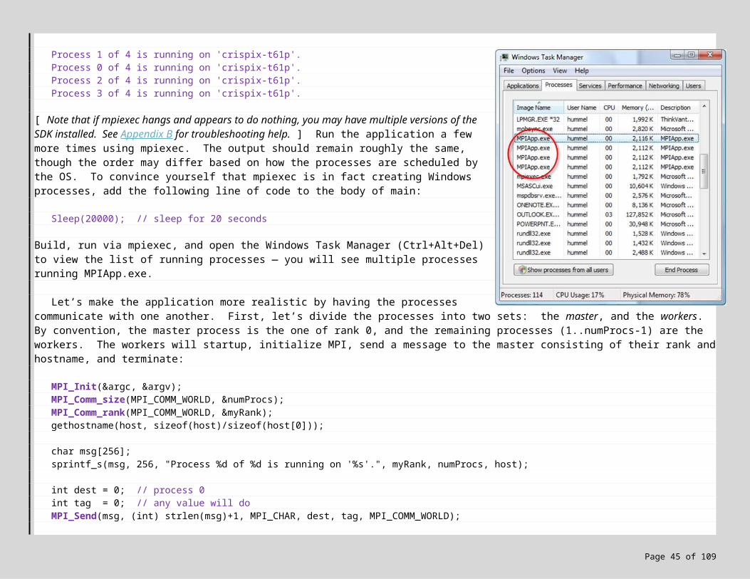
PIXEL_T **image = NULL;int rows = 0, cols = 0;

if (myRank == 0){

cout << "** Reading bitmap from '" << infile << "'..." << endl;image = ReadBitmapFile(infile, bitmapFileHeader, bitmapInfoHeader, rows, cols);if (image == NULL){

cout << endl;cout << "** Failed to open image file, halting..." << endl;return 1;

}}

Work your way through main, thinking carefully about which processes are involved in which tasks. When in doubt, don’t forget a complete solution is available for your review in Solutions\MPI\MPIContrastStretch\. When you’re done, build and eliminate any syntax errors.

5. The problem of distributing the image matrix is now encapsulated within DistributeImage. This function takes the image and its size (rows and cols), and returns the chunk (of size myrows and mycols) that the calling process should stretch:

chunk = DistributeImage(image, rows, cols, myrows, mycols, MPI_PIXEL_T);

All processes are involved in this step, and should be calling this function from main. However, the role that a process plays during distribution depends on whether they are the master or a worker. More subtle is the fact that the validity of the parameters to DistributeImage depends on the process. Since the master process reads the input file, when the master calls DistributeImage, the parameters image, rows and cols contain meaningful values. For the worker processes, these parameters reflect their initialized values of NULL, 0, and 0, respectively.

Within DistributeImage, the master process is responsible for first distributing the size of the matrix, since this is unknown to the workers. Then it distributes the individual chunks to each of the workers. This is accomplished through a series of calls to MPI_Send. Finally, the master makes a copy of the chunk it is supposed to process — the first chunk of the original matrix. Here we go:

PIXEL_T **chunk = NULL; // best practice with MPI: initialize all variablesint tag = 0;int params[2] = {0, 0};

cout << myRank << " (" << host << "): Distributing image..." << endl;

if (myRank == 0) // Master:{

int rowsPerProc = rows / numProcs;int leftOverRows = rows % numProcs;

Page 45 of 89

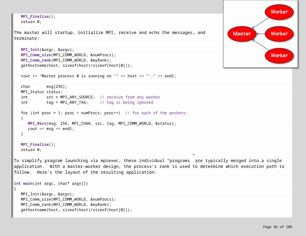
params[0] = rows;params[1] = cols;

for (int dest=1; dest < numProcs; dest++) // send each worker the size of the image:MPI_Send(params, sizeof(params)/sizeof(params[0]), MPI_INT, dest, tag, MPI_COMM_WORLD);

for (int dest=1; dest < numProcs; dest++) // now send the actual data chunk (skip over first chunk + leftover):MPI_Send(image[leftOverRows + dest*rowsPerProc], rowsPerProc*cols, MPI_PIXEL_T, dest, tag, MPI_COMM_WORLD);

// okay, master is responsible for the first chunk + any leftover rows:myrows = rowsPerProc + leftOverRows;mycols = cols;chunk = New2dMatrix<PIXEL_T>(myrows+2, mycols); // why 2 extra rows? See contrast stretching functionmemcpy_s(chunk[1], myrows*mycols*sizeof(PIXEL_T), image[0], myrows*mycols*sizeof(PIXEL_T));

}

The master retains the first chunk for itself to process, including any extra rows if the number of processes does not evenly divide the size of the matrix. You’ll notice the allocated chunk contains 2 extra rows; I’ll explain when we discuss the MPI-based Contrast Stretching algorithm.

6. During distribution, the worker processes receive the size of the image, compute their chunk size, allocate memory, and then receive the actual chunk data. This can be coded as follows:

else // Workers:{

MPI_Status status;

MPI_Recv(params, sizeof(params)/sizeof(params[0]), MPI_INT, 0 /*master*/, tag, MPI_COMM_WORLD, &status);

rows = params[0];cols = params[1];myrows = rows / numProcs; // size of our chunk to process:mycols = cols;

chunk = New2dMatrix<PIXEL_T>(myrows+2, mycols); // why 2 extra rows? See contrast stretching function

MPI_Recv(chunk[1], myrows*mycols, MPI_PIXEL_T, 0 /*master*/, tag, MPI_COMM_WORLD, &status);}

return chunk;

All processes finish the distribution step by returning their chunk back to the caller. Build and fix any syntax errors. If you get errors complaining of undefined symbols for myRank, numProcs, or host, recall these are defined in “Main.cpp” but you also need to inform the compiler. Define these as external symbols by adding the following to “app.h”:

Page 46 of 89

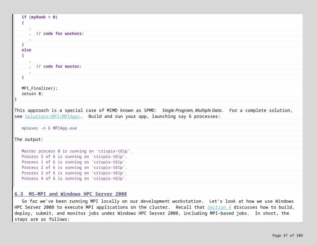
extern int myRank;extern int numProcs;extern char host[256];

The build should now succeed without error.

7. We are almost ready to run and test our handiwork. What remains is to implement the CollectImage function, in which the workers send their chunks to the master, and the master collects and builds the resulting image. I’m going to leave the details to you, but in short the idea is to reverse the steps you performed in DistributeImage. The workers are simple: they send their chunk back to the master process, though keep in mind the data starts at chunk[1], not chunk[0] (due to those 2 extra rows we haven’t explained yet). The master is likewise straightforward: it receives each worker chunk back into image, the location of which depends on the worker’s rank. The master must also copy their own chunk back into image (likewise starting at chunk[1]). Once the image is complete, the master returns the image back to the caller; the workers should return NULL. If you need help, recall a complete solution is available in Solutions\MPI\MPIContrastStretch\.

8. Now it’s time to run and see what happens. To adequately test our work, we need to run with multiple processes — first with say 2, then 4, and then 7 (an odd number of processes will trigger the case of the image not dividing evenly and thus leftover rows). As discussed earlier, we’ll need to minimize Visual Studio, open a console window (“black screen”), and launch the app using mpiexec. Go ahead and open a console window (Start, cmd.exe), and navigate to the directory containing your .exe (e.g. Exercises\MPI\MPIContrastStretch\x64\release). You’ll need an image to process, so copy “sunset.bmp” from the MPIContrastStretch\ sub-directory. Now run and launch 2 processes, the app will run quickly since we commented out the stretching step:

Page 47 of 89

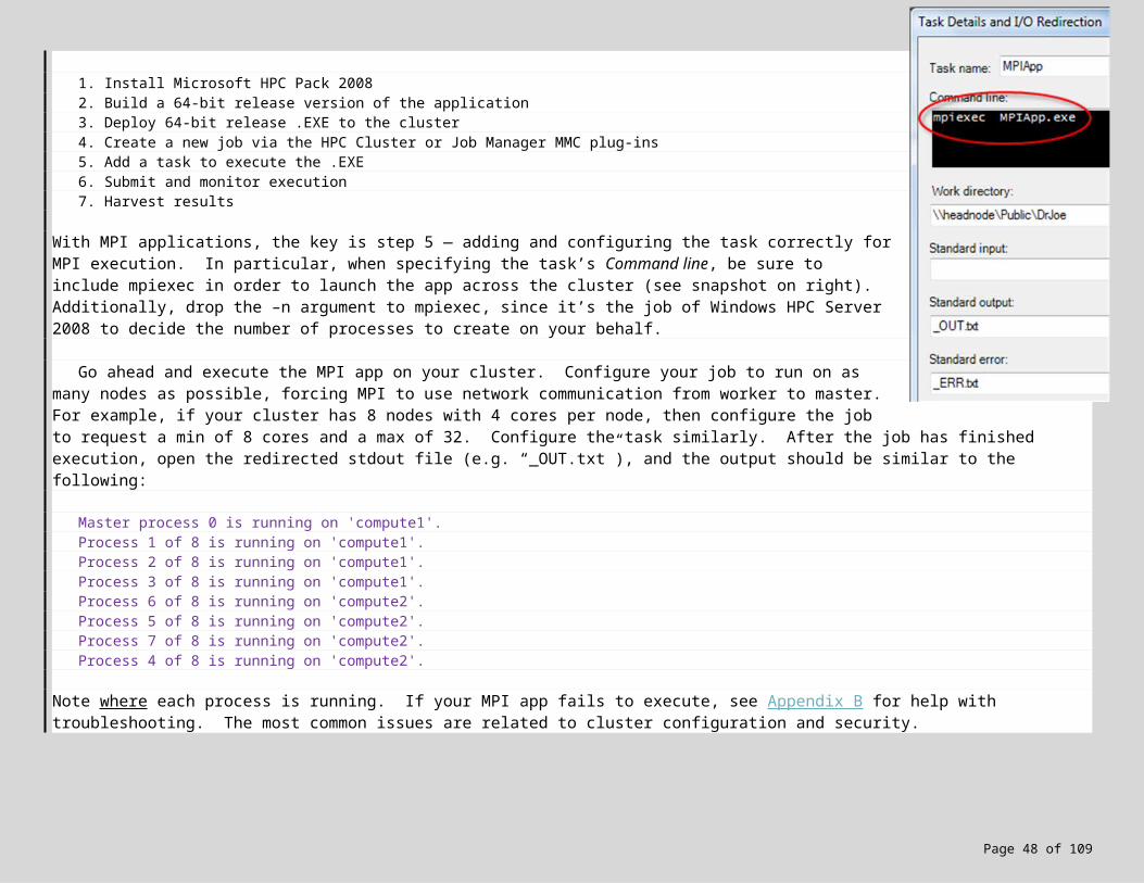
To ensure the distribution and collection are working properly, compare the input file “sunset.bmp” to the output file “stretched.bmp”. Do a byte-for-byte comparison, using a tool such as WinDiff (available in Misc\). There should be no reported differences. Repeat for 4 and 7 processes.

9. The last step of the conversion to MPI is the contrast stretching portion of the application. In main, uncomment the call to ContrastStretch, yielding:

chunk = ContrastStretch(chunk, myrows, mycols, steps, stepby, MPI_PIXEL_T);

Fix the function prototype in “app.h” to match the new definition (note the additional parameter at the end):

PIXEL_T **ContrastStretch(PIXEL_T **image, int rows, int cols, int steps, int stepby, MPI_Datatype MPI_PIXEL_T);

Now we’ll focus our attention on the implementation in “ContrastStretch.cpp”. Open the source code file, and update the function header to match the new prototype. Add an output statement for debugging purposes, and update the allocation of the temporary matrix to include 2 extra rows:

PIXEL_T **ContrastStretch(PIXEL_T **image, int rows, int cols, int steps, int stepby, MPI_Datatype MPI_PIXEL_T)

{cout << myRank << " (" << host << "): Processing " << rows << " rows, " << cols << "

cols..." << endl;PIXEL_T **image2 = New2dMatrix<PIXEL_T>(rows+2, cols);

Okay, so why the 2 extra rows? Recall the basics of the Contrast Stretching algorithm: for each pixel P, we update P based on its 8 surrounding neighbors. Based on this algorithm, the first row must be treated as a special case, since the first row has no neighbors to the North. Likewise, the last row has no neighbors to the South, the first column no neighbors to the West, and the last column no neighbors to the East. The

solution is to ignore processing of these rows and columns.

When we distribute the image matrix, we run into the same problem with each *chunk*. In particular, for each process P, P is unable to process their first and last rows since the neighboring rows are in other processes. And unlike the first and last columns, processing of the first and last rows cannot be skipped without changing the semantics of the algorithm. This holds true for all processes except the first (rank 0) and the last (rank numProcs-1). The implication is that during each step of the algorithm, processes must swap their first and last rows with their neighboring processes.

For example, consider process 2 in a run with 4 processes. As shown to the right, process 2 will need to send its first row to process 1, and its last row to process 3. Likewise, process 2 will need to receive the last row from process 1, and the first row from

Page 48 of 89

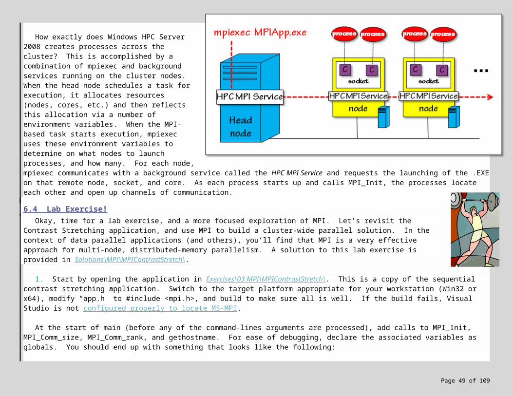
process 3. These two extra rows are typically referred to as ghost rows, and will need to be stored locally on process 2. Thus, when we allocate the memory for process 2’s chunk, we include room for the 2 ghost rows; likewise for allocation of the matching temporary matrix. For example, if process 2 was responsible for 2 rows and 6 columns of data, its chunk would be 4x6 in size (as shown to the left), with the data starting in row 1.

10. Locate the while loop, and add code at the top of the loop body to exchange ghost rows. First, for each process, send its last row “down” and receive the corresponding row from its neighbor as its upper ghost row:

if (myRank < numProcs-1) // everyone send last row down (except last):MPI_Send(image[rows], cols, MPI_PIXEL_T, myRank+1, 0 /*tag*/, MPI_COMM_WORLD);

if (myRank > 0) // now everyone receive that ghost row from above (except first):MPI_Recv(image[0], cols, MPI_PIXEL_T, myRank-1, 0 /*tag*/, MPI_COMM_WORLD, &status);

The second step is for each process to send its first row “up” and receive the corresponding row from its neighbor as its lower ghost row

if (myRank > 0) // everyone send first row up (except first):MPI_Send(image[1], cols, MPI_PIXEL_T, myRank-1, 0 /*tag*/, MPI_COMM_WORLD);

if (myRank < numProcs-1) // and everyone receive that ghost row from below (except last):MPI_Recv(image[rows+1], cols, MPI_PIXEL_T, myRank+1, 0 /*tag*/, MPI_COMM_WORLD, &status);

Add the necessary variable declarations (e.g. status), and build. But don’t run just yet.

11. With the ghost rows now set, we are ready to perform one pass of the Contrast Stretching algorithm. However, the nested for loops that process each pixel require a subtle update. Every process should start processing at the first data row of their chunk — i.e. row 1 — *except* the first process. The first process has no data in row 0 (its upper ghost row), since row 1 is the start of the image. So the first process should start processing at row 2. Similarly, every process should process up to and including the last row of their chunk — i.e. up to and including the index rows. The last process, however, should stop processing at rows-1, since rows denotes the last row of the image. Let’s compute this explicitly for each process, and update the for loops accordingly:

int firstRow = 1; // this holds true for everyone but master & last worker:int lastRow = rows;

if (myRank == 0) // master: does not process first rowfirstRow = 2;

// NOTE: master & last worker could be the same if numProcs == 1, so don’t tie if tests together.

if (myRank == numProcs-1) // last worker: does not process last rowlastRow = rows-1;

for (int row = firstRow; row <= lastRow; row++) // from first row to last row, inclusive:{

Page 49 of 89

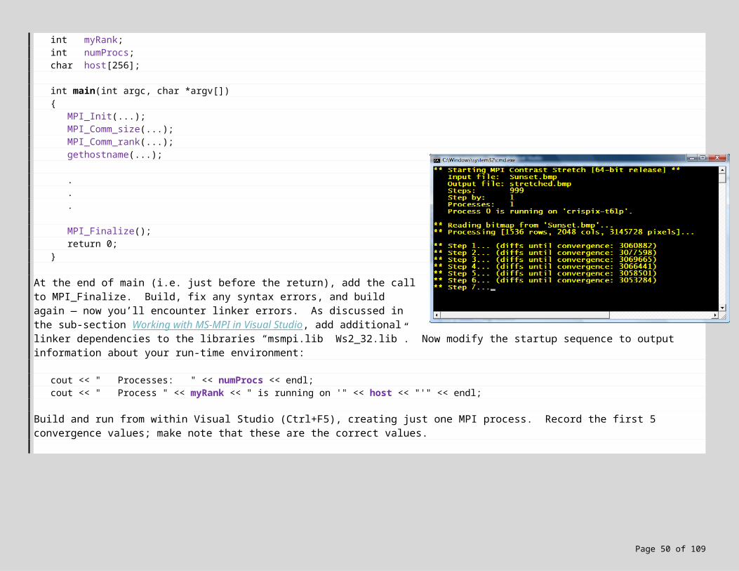
for (int col = 1; col < cols-1; col++){

Okay, just one more issue before we run and test… When the for loops end, a convergence test is performed to see if the stretching has reached a steady state (in which case the algorithm can terminate):

}}

cout << " (diffs until convergence: " << diffs << ")" << endl;converged = (diffs == 0);

Since the image is distributed, the computed diffs is now a local value. But the algorithm calls for a global value, terminating if and only if the total number of differences is 0. This implies the processes need to communicate their local diffs to the master, who will sum and redistribute the total value. This is going to require a number of sends and receives:

if (myRank > 0) // workers:{

MPI_Send(&diffs, 1, MPI_LONG_LONG, 0 /*master*/, 0 /*tag*/, MPI_COMM_WORLD);MPI_Recv(&diffs, 1, MPI_LONG_LONG, 0 /*master*/, 0 /*tag*/, MPI_COMM_WORLD, &status);

}else // master:{

long long temp;

for (int src=1; src < numProcs; src++) // receive from workers:{

MPI_Recv(&temp, 1, MPI_LONG_LONG, MPI_ANY_SOURCE, 0 /*tag*/, MPI_COMM_WORLD, &status);diffs += temp; // add to our own diffs

}

for (int dest=1; dest < numProcs; dest++) // now send out total diffs to workers:MPI_Send(&diffs, 1, MPI_LONG_LONG, dest, 0 /*tag*/, MPI_COMM_WORLD);

}

cout << " (diffs until convergence: " << diffs << ")" << endl;converged = (diffs == 0);

Finally, since the nested for loops changed, we also need to update the corresponding nested for loops which copy the contents of the temporary matrix back into the image matrix. In particular, the rows to copy have changed:

for (int row = firstRow; row <= lastRow; row++)for (int col = 1; col < cols-1; col++)


Page 50 of 89

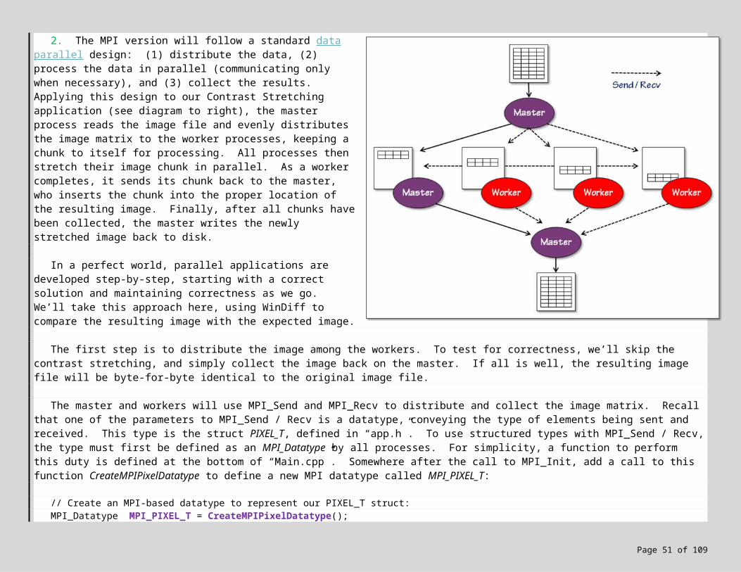
Build and fix any syntax errors. If you haven’t already, you should also update the output statements to include process rank and hostname.

12. We now have a complete, MPI-based, Contrast Stretching application. Let’s run and test. Minimize Visual Studio, open up a console window, and launch the app with mpiexec. Start with 2 processes, and run for 75 steps:

First, make sure the first 5 convergence values reported are the same as the sequentially-generated values (you wrote them down, right? :-). Then, when the run finishes, compare your output file “stretched.bmp” to the sequentially-generated image file “Sunset-75-by-1.bmp” in Misc\. There should be no differences. Repeat for 4 processes, 7 processes, and 1 process. Why test against a single MPI process? If possible, it’s generally a good idea for your MPI application to run correctly with just one process; this allows correct execution if the app is run on hardware with only a single core or a cluster with only 1 core/socket/node available.

13. Congratulations on developing a non-trivial MPI application! In a later section I’ll suggest some ways to improve the application using more advanced features of MPI, but for now let’s experiment a bit more with the current version…

14. Does your developer workstation have multiple cores/sockets? Call this number N. If N > 1, launch the app with N processes, bring up the Task Manager (Ctrl-Alt-Del), switch to the Performance tab, and confirm that you are utilizing each core / socket 100%. Now let’s record the average time across a few local convergence runs. Be sure you are timing a release build of your .EXE, and record your data here:

Page 51 of 89

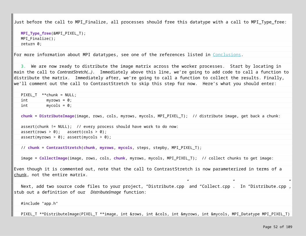
MPI Paralleltime on local workstation for convergence run: ______________, number of cores = ______, speedup = ________

Refer back to the local execution time for an OpenMP convergence run. How well does MPI compare, i.e. is it slower, faster, or about the same? You should find the times roughly the same, which speaks well of MPI-based solutions. While MPI has more overhead in comparison to multi-threaded solutions due to its use of processes and messages, MPI optimizes using shared memory when message-passing on the same node. And MPI-based solutions typically expose more parallelism, since problem decomposition and communication must be explicitly designed in from the start. The trade-off is that MPI applications are generally more difficult to develop.

14. Now let’s run the application on the cluster. This is where MPI really shines, since it can potentially utilize every core, socket and node in the cluster — whereas shared-memory solutions are limited to a single node. Recall that Section 4 discusses how to build, deploy, submit, and monitor jobs under Windows HPC Server 2008, and Section 6.3 goes into the details of running MPI-based applications on the cluster. In short, build a 64-bit release version of your application, and deploy both the application and the input file (“sunset.bmp”) to a public network share. Create a new job, request exclusive use of all the cores/sockets/nodes in your cluster, add a task as shown to the right (requesting the same number of resources), and save the job configuration as an XML-based description file. Now submit, and when the job finishes, grab the output file “stretched.bmp”. Compare this to the correct version “Sunset-convergence-260-by-1.bmp” in Misc\, and confirm the application is working correctly. Assuming all is well, view the standard output and record the execution time. Perform a few more runs to collect an average execution time, using the saved description file to resubmit (Actions menu, Job Submission > Create New Job from Description File). Record your data here:

MPIParalleltime on cluster for convergence run: ____________, number of cores = ______, speedup = ________

What kind of speedup are you seeing? Are we taking advantage of the entire cluster? If not, run again using fewer cores/sockets/nodes, and see where the speedup starts to fall from linear.

15. Excellent work, well done!

7. MPI Debugging, Profiling and Event Tracing

Debugging and profiling are important aspects of any software development project. This is especially true with MPI, given the distributed nature of the applications, and the focus on high performance. Let’s take a look at the MPI-based debugging and profiling options available with Windows HPC Server 2008 and Visual Studio 2005/2008.

Page 52 of 89

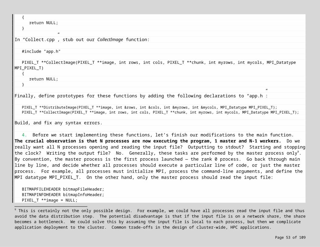
7.1 Profiling with ETW Since an MPI application is really a set of cooperating processes, there are two levels of profiling: the individual processes,

and the communication infrastructure. Profiling of the individual processes is much like profiling any application, using traditional tools such as Visual Studio’s Profiler, AMD’s CodeAnalyst, or the Windows Performance Toolkit (“xperf”). Since this is familiar territory for most developers, and well-documented elsewhere, we’ll skip the discussion of traditional profiling and simply provide a few references:

VS Profiler: “Find Application Bottlenecks with Visual Studio Profiler”, H. Pulapaka and B. Vidolov, MSDN Magazine, March 2008 (available online at http://msdn.microsoft.com/en-us/magazine/cc337887.aspx)

CodeAnalyst: available tool for x86 and x64 processors, http://developer.amd.com/CPU/Pages/default.aspx xperf: a tool used internally by Microsoft, now available at

http://www.microsoft.com/whdc/system/sysperf/perftools.mspx

Profiling of the communication infrastructure is not typical, and highly-dependent on the technology used. Windows HPC Server 2008 provides excellent support for profiling MPI applications by integrating with Event Tracing for Windows. ETW is the tracing strategy used by the Windows OS, and nearly all Microsoft applications.

In Windows HPC Server, the MS-MPI library has been instrumented with ETW-based calls. This makes it a snap to profile communications within an MPI application: launch your app with tracing enabled, let it run, and then visualize the results. The trace contains detailed information about every process’s communication behavior, including calls to MPI, and the duration of each call. The latter measures not only the cost of an MPI call, but also how long a given process had to wait in order to communicate with another process. This helps reveal bottlenecks, unbalanced workloads, and designs that hinder parallelism.

To launch an MPI app with tracing enabled, you must have administrative rights or membership in the Performance Log Users group. Given the appropriate permissions, simply run mpiexec with the -tracefile option:

mpiexec -tracefile mytrace.etl ... MPIApp.exe ...

This creates an event trace file “mytrace.etl” in the current directory (or the working directory when run on the cluster). In fact, this creates a set of trace files, one for each node hosting MPI processes. Since each trace may be collected on a different machine with a different clock, the next step is to synchronize the traces to a single clock by computing offsets from a base clock. This is performed by the mpicsync tool, itself an MPI program shipped with Windows HPC Server 2008:

mpiexec -cores 1 mpicsync mytrace.etl

This runs one instance of mpicsync on each node, processing the trace file on that node. The result is a clock offset / trace info file named “mytrace.etl.info”, one per node. The last step is to merge the traces into a single trace file, while also converting to

Page 53 of 89

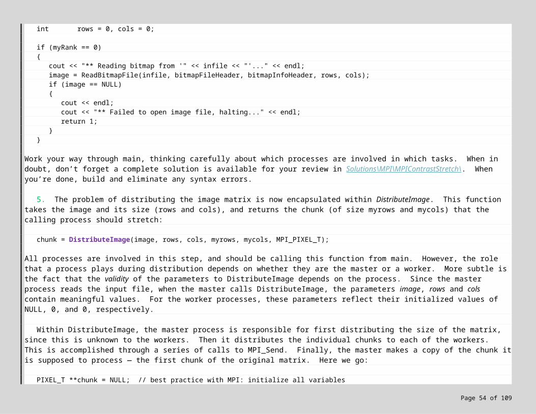
a format suitable for visualization. For example, Windows HPC Server 2008 ships with the MPI-based etl2clog tool for converting ETW-based traces to the CLOG format10, a standard developed by Argonne National Labs:

mpiexec -cores 1 etl2clog mytrace.etl

This yields a single CLOG file named “mytrace.etl.clog2”.

There are a number of ways to visualize the trace and analyze the communication characteristics of your MPI application. Jumpshot is an available11 Java-based tool for visualization of CLOG and SLOG trace files. The main window is shown to the right; use the File menu to open your CLOG trace file. You’ll be asked if you want to convert to the SLOG-2 format (Yes), click “Convert” to perform the conversion (see snapshot bottom-right), and then click “OK” to view the trace. You’ll see something like the following:

In Jumpshot, boxes represent MPI function calls, and arrows depict communication. Time moves from left-to-right, with each process depicted on the timeline. Initially the time span covers the entire program execution; insight is gained by zooming into the timeline at

10 http://www.mcs.anl.gov/perfvis/software/log_format/index.htm .11 See the Misc\ sub-folder, or download from ftp://ftp.mcs.anl.gov/pub/mpi/slog2/slog2rte.tar.gz . You’ll also need to install the Java RTE before running JumpShot, see http://www.java.com/getjava/ .

Page 54 of 89

http://www.java.com/getjava/

ftp://ftp.mcs.anl.gov/pub/mpi/slog2/slog2rte.tar.gz

http://www.mcs.anl.gov/perfvis/software/log_format/index.htm

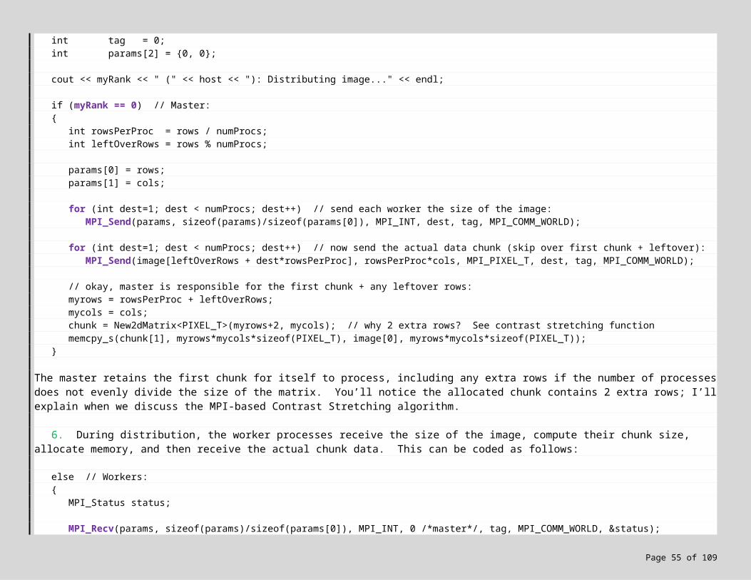
various points (+ zooms in, and – zooms out). Right-clicking on a box or arrow yields additional information, such as the MPI function that was called and its duration. You can also right-click and select a region of the timeline:

This yields various statistics about the selected region, e.g. the “Statistics” button yields a histogram-based summary. For more information about Jumpshot and its usage, see the online user manual or the .pdf provided in Misc\Jumpshot. As a general rule of thumb, “big boxes are bad”, since this means your app is spending more time communicating and less time computing.

7.2 Local vs. Cluster Profiling The same process is followed whether you profile on the cluster, or locally on your development workstation. When you

profile locally, don’t be surprised if the trace reveals lots of “big boxes” — you can expect waiting for communications to complete if the number of processes in your app > number of cores/sockets in your workstation.

When you profile on the cluster, configure the job to request exactly N cores/sockets/nodes (by setting min and max to N), and request exclusive access to these resources. Next, add 3 tasks, one for each profiling step: (1) execution, (2) clock sync, and (3) aggregation & conversion. Then add a 4th task to copy the final CLOG trace file to a known location such as the cluster’s Public network share. For completeness, here are the 4 tasks:

mpiexec -tracefile mytrace.etl ... MPIApp.exe ...mpiexec -cores 1 mpicsync mytrace.etl

Page 55 of 89

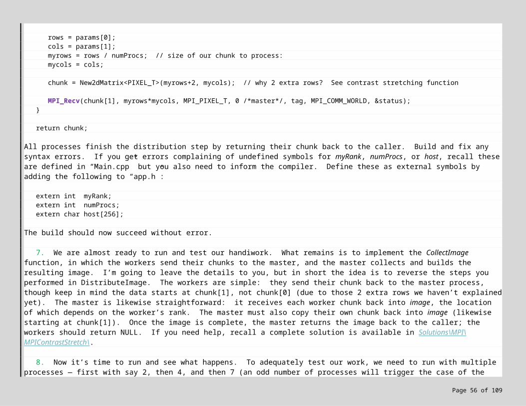
http://www.mcs.anl.gov/perfvis/software/viewers/jumpshot-4/usersguide.html

mpiexec -cores 1 etl2clog mytrace.etlmpiexec -n 1 cmd /C copy /Y mytrace.etl.clog2 \\headnode\Public

Be sure to configure each task identically, e.g. if the execution task requests N resources, then the other tasks must also request N resources. You’ll also need to add dependencies between these tasks so that task i+1 does not start until task i finishes. See the screen snapshot to the right.

In terms of deployment, this is a situation in which you do *not* want to deploy to a network share — if the working directory for the tasks is a network share, then each process tries to create a trace file in the same location. Since the trace files all have the same name, execution fails. The solution is to deploy to the same local folder on each node, e.g. C:\Apps, and set the working directory of each task to this local folder (see snapshot, middle-right). To simplify deployment in this case, each node in the typical cluster has an Apps network share that maps to C:\Apps. Finally, when you submit the job for execution, be sure to supply Run-as credentials for a user account that either has administrative rights, or is a member of the Performance Log Users group. Otherwise you’ll get an “access denied” error when you launch with mpiexec.

Once the job completes, the CLOG trace file will reside in the cluster’s Public network share. Copy this file to your local workstation, and visualize with Jumpshot.

7.3 Lab Exercise!

Page 56 of 89

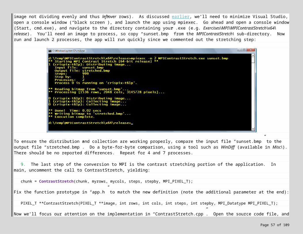
Let’s put our new MPI profiling skills into practice. In the previous lab exercise you developed a working MPI application for Contrast Stretching. Let’s profile this app locally on your development workstation, and then on the cluster. If you were unable to complete the lab exercise, 32-bit and 64-bit executables are provided for you to profile.

1. If you have a working MPI-based Contrast Stretching application, build a release version and copy the .EXE to a temporary folder. If you don’t, copy one of the provided .EXEs from Exercises\04 ETW\. Now copy an image file to your temp folder, e.g. “Sunset.bmp” from Misc\.

If your user account is a member of the Performance Log Users group, simply open a console window (“black screen”). If not, you’ll need administrative rights to either add yourself to this group (in which case you need to logout and log back in), or to open a console window as administrator (Start, type “cmd”, right-click on “cmd.exe” at top of search, run as administrator). Navigate to your temp folder, and launch the app without tracing to make sure all is well.

2. Now re-run the app, this time with tracing enabled. If you have N cores/sockets on your development machine, then launch with N processes:

mpiexec -tracefile mytrace.etl -n N MPIContrastStretch.exe Sunset.bmp out.bmp 25 1

The app will run for 25 time steps, long enough to generate a reasonable trace. List your directory contents to confirm that the trace file “mytrace.etl” has been generated. How big is the file? Now sync the clock and convert the trace to CLOG format:

mpiexec -cores 1 mpicsync mytrace.etlmpiexec -cores 1 etl2clog mytrace.etl

List the directory contents, and confirm you now have 3 trace-related files: “mytrace.etl”, “mytrace.etl.info”, and “mytrace.etl.clog2”.

3. Launch Jumpshot by double-clicking on Misc\Jumpshot\Jumpshot\jumpshot_launcher.jar. If this fails to launch Jumpshot, make sure you have the Java RTE installed (available from http://www.java.com/getjava/). Use the File menu, Select… command to open your .clog2 file. Click “Yes” when prompted to convert to SLOG format, and in the dialog that appears, click “Convert” to actually perform the conversion. When the conversion finishes, click “OK” to visualize the trace. Explore the trace as discussed earlier.

Page 57 of 89

http://www.java.com/getjava/

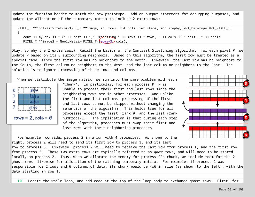
4. To see what a “bad” trace might look like, trace an execution with 4N or 8N processes. Since your workstation has only N cores/sockets, the majority of processes will experience some waiting, increasing communication time.

5. Now let’s generate a realistic trace by running on the cluster. If necessary, build a 64-bit release version of your application. Start by deciding how many compute nodes you are going to run on, and deploy the .EXE and .bmp files to each node locally. You must deploy to the same folder on each node, e.g. C:\Apps. Create a new job, and request the desired number N of cores/sockets/nodes by setting both min & max to N. Request exclusive access to these resources. If you deployed to a subset of compute nodes, request these compute nodes explicitly via the “Resource Selection” tab.

6. Add a task to the job with the following command-line:

mpiexec -tracefile mytrace.etl MPIContrastStretch.exe Sunset.bmp out.bmp 25 1

Make sure the requested number of resources (both min and max) is set to N, and set the working directory to the deployment directory (C:\Apps?). Redirect stdin and stdout. Now add 3 more tasks, each configured exactly the same way, to execute the following command lines:

mpiexec -cores 1 mpicsync mytrace.etlmpiexec -cores 1 etl2clog mytrace.etlmpiexec -n 1 cmd /C copy /Y mytrace.etl.clog2 \\headnode\Public\

DrJoe

As discussed earlier, click the “Dependency” button on the job page to add dependencies between these tasks so that task i+1 does not start until task i finishes.

7. Before you submit, click the “Save Job as…” button to save your job configuration in a description file.

8. Now submit your job for execution, supplying Run-as credentials with either administrative rights, or membership in the Performance Log Users group. When the job is complete, the CLOG trace file “mytrace.etl.clog2” should reside in the cluster’s Public network share. Copy to your local workstation and visualize in Jumpshot.

7.4 Don’t have Administrative Rights? Need targeted tracing? What if you want to trace your app right now, and don’t have the appropriate permissions? Another approach is to use

MPE12, which collects an event trace much like ETW. MPE is a complete replacement for MPI, intercepting every MPI call to collect trace information. To use MPE, the first step is to modify your Visual Studio project settings to link against “msmpe.lib” instead of “msmpi.lib” (available in Misc\MPE\). Build, deploy locally to each compute node, and launch the app normally (i.e. without the -tracefile option). You do not need special permissions. MPE generates a set of trace files, then automatically clock

12 http://www.mcs.anl.gov/perfvis/download/index.htm .

Page 58 of 89

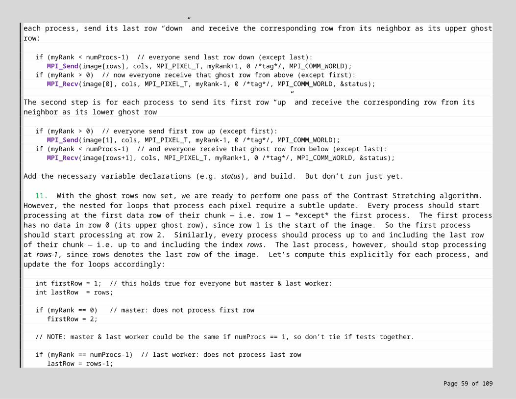
http://www.mcs.anl.gov/perfvis/download/index.htm

syncs and merges to produce a single .clog2 file. Locate the trace file (it will reside on the compute node that ran the rank 0 process), copy to your local workstation, and view with Jumpshot.

If you want to trace a specific MPI function, or generate other types of statistics (failure rates, message sizes, etc.), then you can take the same approach as MPE — intercept the MPI call(s) of interest and collect whatever data you want. MPI was designed with call interception in mind. For example, to intercept all calls to MPI_Send, define your own MPI_Send function, calling MPI’s internal PMPI_Send to do the actual work:

int MPIAPI MPI_Send(void *buf, int count, MPI_Datatype datatype, int dest, int tag, MPI_Comm comm)

{... ; // pre-process:

int rc = PMPI_Send(buf, count, datatype, dest, tag, comm);

... ; // post-process:

return rc; }

Link against “msmpi.lib” (not “msmpe.lib”), build, ignore any link errors (just rebuild), and run normally. Intercept the call to MPI_Finalize to output your trace data.

7.5 MPI Debugging Of course, debugging is another important component of software development. In fact, debugging usually precedes

profiling :-) The good news is that Visual Studio 2005 and 2008 both ship will full support for source-level, MPI debugging. You can debug locally on your development workstation, or configure jobs in Windows HPC Server 2008 to enable remote debugging on the cluster itself.

Given the long-running nature of many HPC applications, note that print-style debugging is still a viable and common option for debugging. Debug-related code is often conditionally compiled for easy removal from release builds:

#ifdef _Debugcout << "..." << endl;

#endif

The symbol “_Debug” is automatically defined by Visual Studio whenever you build a debug version of your application. MPI takes care of collecting all stdout (and stderr) output on the master (rank 0) process.

Page 59 of 89

Of course, Visual Studio’s source-level debugger offer a much more powerful debugging experience. We can run via F5, set breakpoints, inspect and edit variables, conditionally break execution, and so on. To debug MPI applications using Visual Studio’s source-level debugger, it’s mostly a matter of configuring VS — the application itself does not change. Let’s start by looking at local debugging on your development workstation.

Open one of your MPI apps in Visual Studio, switch to the debug version, and bring up the project properties page. Click on the Debugging tab, and select “MPI Cluster Debugger” from the “Debugger to launch” drop-down. Now we configure the debugger to launch the app via mpiexec as we normally would. For Visual Studio 2008, we configure as follows:

MPIRun Command: mpiexec MPIRun Arguments: args to mpiexec such as -n 4 to launch 4 processes MPIRun Working directory: the directory containing the debug .EXE (e.g. x64\debug), denoted by the macro $

(TargetDir) Application Command: the full pathname of the debug .EXE, denoted by the macro $(TargetPath) Application Arguments: args to the application itself (e.g. Sunset.bmp output.bmp 25 1) MPIShim Location: the location of the .EXE that acts as shim between the VS debugger and our MPI processes

32-bit application: C:\Program Files\Microsoft Visual Studio 9.0\Common7\IDE\Remote Debugger\x86\mpishim.exe 64-bit application: C:\Program Files\Microsoft Visual Studio 9.0\Common7\IDE\Remote Debugger\x64\mpishim.exe

Save your property settings. Next, copy any input files (such as “Sunset.bmp”) to the folder containing the debug .EXE (e.g. x64\debug). That’s it, you are ready to debug! Set one or more breakpoints, and press F5 to run.

Now the fun begins :-) Keep in mind that MPI applications consist of one or more running processes. This means you are now debugging N instances of the same program — N processes — at the same time. Let’s suppose you configure VS to launch 4 processes. When you press F5 to run with debugging, 4 processes will launch behind the scenes (as you would expect). This becomes readily apparent from the 4 console windows that open, one per MPI process:

Page 60 of 89

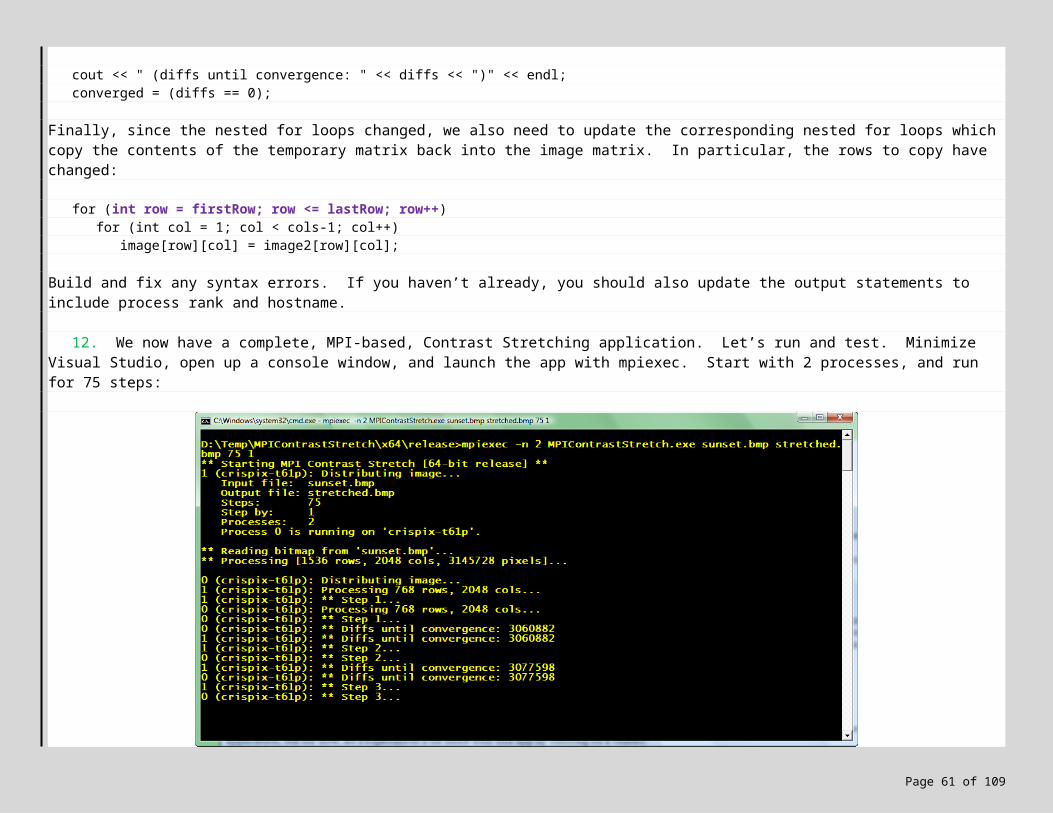
You can also see the processes listed in Visual Studio. When you reach a breakpoint, select Debug menu, Windows, Processes — VS will list the running processes involved in the debug session (large circled area in snapshot above). How do you know which process reached the breakpoint? A common trick is to define the process’s rank as a global variable (“myRank”), and then add a watch on this variable (small circled area above). Each time a breakpoint is reached, the watch reveals the process.

By default, when any process reaches a breakpoint, all processes are stopped in their tracks. This is generally what you want, since it gives you time to explore the stopped process without worrying about the impact on other processes. To confirm this setting (or change it), see Tools menu, Options, Debugging tab, General, “Break all processes when one process breaks” — this option should be checked.

Page 61 of 89

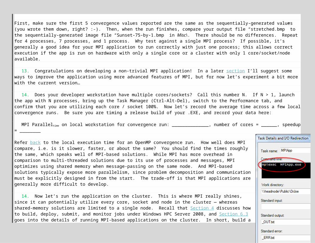
7.6 Lab Exercise! Let’s take a moment (if you haven’t already) to become familiar with the MPI Cluster Debugger on your local

development workstation.

1. If you have a working MPI-based Contrast Stretching application, open this solution in Visual Studio (this is most likely in Exercises\03 MPI\MPIContrastStretch\). If you don’t, open the solution provided in Solutions\MPI\MPIContrastStretch\. Switch to debug mode, and configure the MPI Cluster Debugger as discussed. Copy an image file such as Misc\Sunset.bmp to the folder containing your debug .EXE (e.g. x64\debug).

2. Before you run, make sure Visual Studio is configured to break all processes when one process breaks. Now set a breakpoint at the top of the DistributeImage function, and start debugging (F5). When the breakpoint is reached, list the processes in Visual Studio (Debug menu, Windows, Processes). Add a watch on the variable “myRank” — which process reached the breakpoint first? Press F5 to continue execution, and see which process hits the breakpoint next. Press F5 twice more, and now the 4th and final process will have reached the breakpoint. Assuming no other breakpoints have been set, when you press F5 again, the app will run to completion.

3. As the app runs, organize the console windows so you can view the output from each process. When the app completes, there may be a lingering console window you need to close. Run again, and experiment with single-stepping through the program. Does it work as expected?

4. Right-click on a breakpoint you’ve set, and set the condition to myRank == 0. Run, and now the breakpoint will trigger only for the master process.

5. That’s it, take a well-deserved break!

7.7 Remote MPI Debugging on the Cluster Remote debugging is another reality of software development. Programs may work correctly on a developer’s workstation

or a small test cluster, but then fail when deployed to the HPC cluster. Often remote debugging is the only way to determine the cause of the failure. The good news is that Visual Studio and Windows HPC Server support remote debugging of MPI apps on the cluster — in a manner identical to local debugging!

Before we start, there are a few hardware and software prerequisites to remote debugging. First, the compute nodes involved in the debugging session must be accessible on the network, either through a public network or by providing the developer workstations with access to the cluster’s private network. Second, the firewalls on these network connections must be disabled / opened to debug traffic, as well as the firewalls on the developer workstations13. Third, each compute node must have the Visual C++ 2008 Debug Runtimes installed, as well as the VS 2008 Remote Debugger. Fourth, the compute nodes need to support remote desktop access for HPC users. See Appendix A for details on software setup.

13 For more information, see http://msdn.microsoft.com/en-us/library/bb385831.aspx .

Page 62 of 89

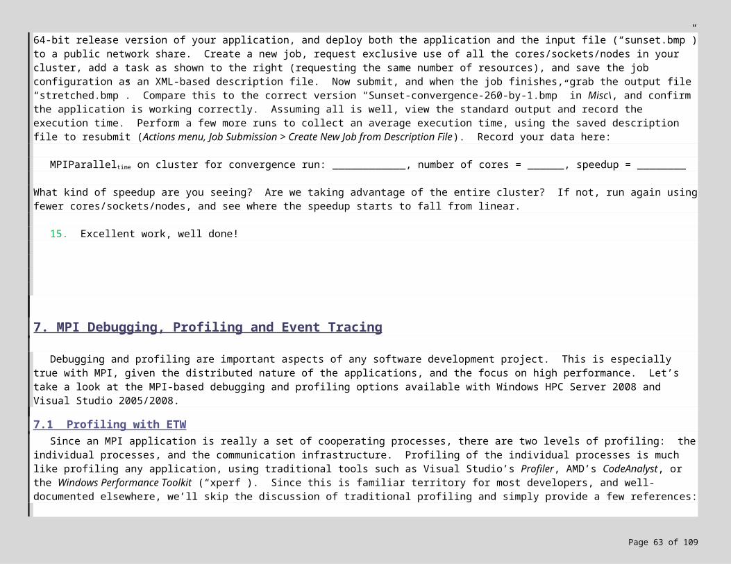
http://msdn.microsoft.com/en-us/library/bb385831.aspx

Let’s assume the cluster has been setup so that each compute node has a local deployment folder named C:\Apps. Also, we’ll assume the remote debugger has been installed in the folder C:\RDB on each compute node. Finally, let’s debug across 4 compute nodes named C1, C2, C3, and C4, each of which has 2 cores, using Visual Studio 2008.

To begin remote debugging, the first step is to build and deploy a 64-bit, debug version of your application on the cluster. Be sure to deploy both the .EXE and the associated .PDB, as well as any input files. To avoid a registry hack associated with the use of network shares and remote debugging, I recommend deploying to a local folder on each compute node, in our case C:\Apps. If your development machine is 32-bit, have no fear: build and deploy a 64-bit version, but then switch back to 32-bit mode in Visual Studio when you start debugging.

Assuming you deployed a 64-bit .EXE, the next step is to start the 64-bit Visual Studio Remote Debugging Monitor on each of the compute nodes involved in the debugging session (if you deployed a 32-bit .EXE, then you’ll want to start the 32-bit remote debugger). While there are various ways to do this, I recommend that you remote desktop into each compute node, login as yourself (i.e. using the same credentials as your development workstation), and start the monitor manually: Start menu, All Programs, Visual Studio 2008, Visual Studio Tools, Visual Studio 2008 Remote Debugger (x64). As you proceed, leave the remote desktop sessions open. While tedious, this approach has 2 distinct advantages. First, the monitors are a great aid in troubleshooting connection problems. Second, as you debug, you can switch to the various remote desktops and view the console windows associated with the MPI processes (identical to the console windows that appear when debugging locally).

At this point we are ready to go. In a normal remote debugging scenario, we would startup Visual Studio on our development workstation, configure the debugger to remotely launch the app, and run (F5). But in the case of MPI, mpiexec coordinates with Windows HPC Server to launch remote processes on the cluster. And from a scheduling perspective, Windows HPC Server allocates resources *before* running applications. The implication is that we cannot simply configure VS to launch our app on the compute nodes. Instead we must configure VS to submit a job requesting these nodes, and then launch within the context of this job. On your development workstation, switch to Visual Studio and bring up the project properties. Click on the Debugging tab, select “MPI Cluster Debugger” from the “Debugger to launch” drop-down, and configure as follows:

Page 63 of 89

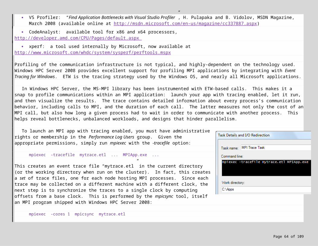
As you can see, when we start debugging, we actually run “job”, a program shipped with Windows HPC Server 2008 for submitting jobs from the command-line. The second field contains the arguments to job, and are nearly identical to the example shown earlier in Section 4.1, “Submitting a Job to the Cluster”. Here is the contents of that second field, representing one long set of arguments:

submit /scheduler:headnode /jobname:DEBUG /requestednodes:C1,C2,C3,C4 /numcores:8-8 /exclusive:true /workdir:C:\Apps /stdout:_OUT.txt /stderr:_ERR.txt mpiexec

Save the settings, and you are ready to debug. Set one or more breakpoints, and press F5 to run. After a few seconds, a new job is submitted to Windows HPC Server, which you can view using the HPC Cluster or Job Manager. When the resources become available and the job starts running, Visual Studio becomes responsive and you can begin debugging. The experience is then identical to that of local MPI debugging — when one process breaks all processes break, etc. The difference is that the console windows are only visible on the compute nodes themselves, since this is where the processes are actually running. Whenever you want to see the state of execution, switch to one or more of the remote desktops and view the console windows (there will be multiple windows, one per core). To keep the console windows open when the application completes, add a breakpoint at the end of main.

Page 64 of 89

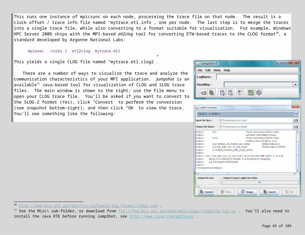
When the application completes, or if you stop debugging, Visual Studio halts and breaks the remote debugging connections. This in turn terminates any running processes, and signifies the completion of the job from the perspective of Windows HPC Server. Windows HPC Server then reclaims the associated resources, and schedules the next job. The debugging session is over.

Granted, there are a lot of moving parts to remote debugging on an HPC cluster. Here are some troubleshooting ideas if you cannot get remote debugging to work. In order:

Startup HPC Cluster or Job Manager and check the status of your DEBUG job; did it submit successfully? Did it fail? Is it queued waiting for execution? Your debugging session will not start until the job is running… If your job never runs, perhaps you requested more resources than your cluster provides? If your job failed, check the redirected stderr (“_ERR.txt”?) for error messages.

Reduce the scope of the debugging scenario to just one compute node. Does it work? If not, disable the firewall on this compute node, as well as on your development workstation. Does it work now?

Test a simpler scenario by remotely debugging a single instance of the application; configure as shown on the right.

Confirm that the remote debugger has been started on each compute node. If you deployed a 64-bit .EXE, make sure you started the x64-based version of the debugger, otherwise you must start the x86-based version. Finally, under what user credentials was the remote debugger started? Confirm that the user account which started the remote debugger is identical to the user account trying to debug — i.e. your account. In other words, when you remote desktop into a compute node to start the remote debugger, you must login as yourself.

Open a console window on your development workstation and confirm that you can submit the job via the command line. Build the command line from the same values you used to configure Visual Studio:

job submit /scheduler:headnode ... mpiexec C:\Apps\MPIContrastStretch.exe Sunset.bmp ...

If the job / app fails to run, does the error message offer any insight? Remote desktop into one of the compute nodes and confirm that you can run the app with mpiexec:

mpiexec C:\Apps\MPIContrastStretch.exe Sunset.bmp ...

Page 65 of 89

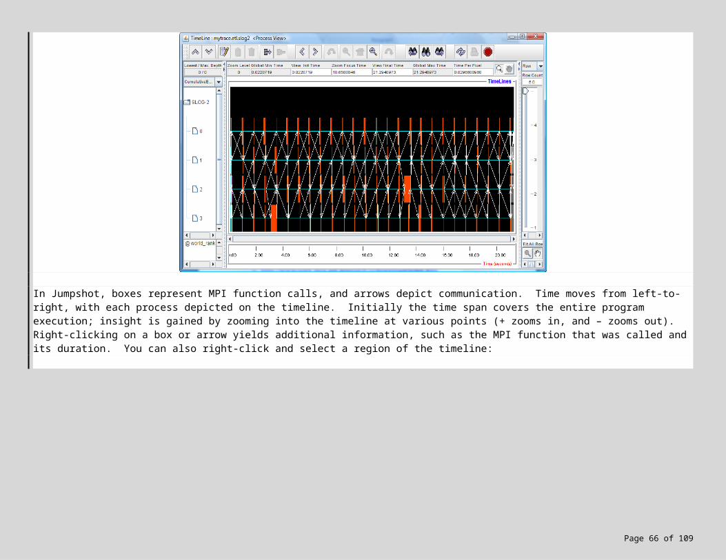
If the app fails to run, the most likely cause is the debug runtimes are not installed. See Appendix B. See the more general troubleshooting ideas presented in Appendix B.

7.8 Lab Exercise! Let’s take a moment (if you haven’t already) to experiment with remote MPI debugging on the cluster.

1. If you have a working MPI-based Contrast Stretching application, open this solution in Visual Studio (this is most likely in Exercises\03 MPI\MPIContrastStretch\). If you don’t, open the solution provided in Solutions\MPI\MPIContrastStretch\. Use the configuration manager to switch to 64-bit debug mode, and build. Copy an image file such as Misc\Sunset.bmp to the x64\debug folder containing your .EXE. Select the compute nodes for your debugging session, and deploy the .EXE, .PDB, and .bmp files to a local folder on each compute node (let’s assume C:\Apps).

2. Remote desktop into each of the compute nodes, login using your current user credentials, and start Visual Studio’s 64-bit remote debugger: Start menu, All Programs, Visual Studio 2008, Visual Studio Tools, Visual Studio 2008 Remote Debugger (x64). Leave these remote desktop sessions open.

3. Make sure Visual Studio is configured to break all processes when one process breaks. Switch back to 32-bit mode if appropriate, and configure Visual Studio for remote MPI debugging as discussed in the previous section. Adjust as necessary (names of compute nodes, total number of cores requested, etc.). Set a breakpoint at the start of main, and run (F5). After a few seconds, Visual Studio should start debugging, and the first process will trigger the breakpoint. Success!

[ If nothing happens… First, wait 30 seconds, and then use HPC Cluster or Job Manager to check the status of your DEBUG job — perhaps it is still queued? If so, you’ll have to wait, or stop debugging & resubmit with fewer resources. Next, check to see if one of the processes has crashed — look at the console windows in each of the remote desktops. Otherwise, it may be a more subtle problem, in which case please review the troubleshooting tips and cluster prerequisites presented in the previous section. ]

4. Assuming all is well, press F5 a few times to allow other processes to reach the breakpoint. Switch to the remote desktops and confirm the presence of console windows representing your MPI processes. Startup the HPC Cluster or Job Manager, and confirm that your DEBUG job is running. Set more breakpoints, continue execution, and view the state of the various processes as these new breakpoints are reached.

5. Allow the application to run to completion, monitoring progress via the remote desktop console windows. When the app completes, confirm that Visual Studio and Windows HPC Server clean up correctly — the job finished execution, the console windows are closed, and Visual Studio stops debugging.

7.9 Other Debugging Tools For completeness, here are some additional tools available for debugging MPI applications in Windows HPC Server 2008:

Allinea DDTLite: plug-in for Visual Studio 2008, http://www.allinea.com/

Page 66 of 89

http://www.allinea.com/

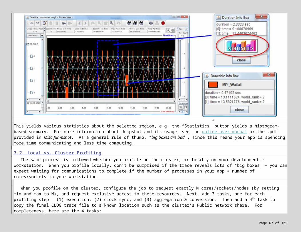
Intel Cluster Debugger: stand-alone toolset, http://www.intel.com/cd/software/products/asmo-na/eng/index.htm Portland Group Cluster Kit: stand-along toolset, http://www.pgroup.com/products/cdkindex.htm

8. Using MPI’s Collective and Asynchronous Functions for an Improved Distributed-Memory Solution

If you are new to MPI, we need to discuss (at least briefly) the additional functionality offered by the API. MPI_Send and Recv, while critically important, are just 2 of more than 170 functions available in MPI-2. For example, there are asynchronous versions of MPI_Send / Recv for greater concurrency, collective (i.e. group) operations for more efficient data distribution and collection, and support for cluster-wide reductions such as sum, min and max.

8.1 Example In the MPI-based Contrast Stretching application, the master process distributes the size of the image — the number of rows

and columns — to the worker processes. The obvious approach is using a sequence of sends by the master, and receives by the workers:

int params[2] = {0, 0};

if (myRank == 0) // Master:{

params[0] = rows;params[1] = cols;

for (int dest=1; dest < numProcs; dest++) // send each worker the size of their chunk:MPI_Send(params, 2, MPI_INT, dest, 0 /*tag*/, MPI_COMM_WORLD);

}else // Workers:{

MPI_Status status;MPI_Recv(params, 2, MPI_INT, 0 /*src*/, 0 /*tag*/, MPI_COMM_WORLD, &status);

rows = params[0];cols = params[1];

}

Semantically, this is a broadcast operation from the master to the workers. We can express this directly using MPI’s MPI_Bcast function:

int params[2] = {0, 0};

if (myRank == 0) // Master preps data for bcast:

Page 67 of 89

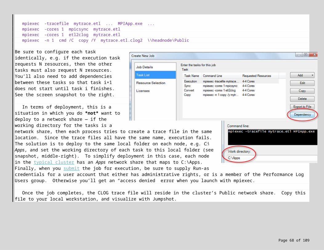
http://www.pgroup.com/products/cdkindex.htm

http://www.intel.com/cd/software/products/asmo-na/eng/index.htm

{params[0] = rows;params[1] = cols;

}

// EVERYONE participates in broadcast (one sends, rest receive):MPI_Bcast(params, 2, MPI_INT, 0 /*master broadcasts*/, MPI_COMM_WORLD);

// EVERYONE now knows the size of the image:rows = params[0];cols = params[1];

The result is more readable, more efficient, and safer (MPI avoids possible deadlock situations involving MPI_Send and Recv). Similarly, when the master

needs to distribute the image matrix amongst the workers, MPI_Scatter offers a more efficient approach:

int rowsPerProc = rows / numProcs;int leftOverRows = rows % numProcs;

void *sendbuf = (myRank == 0) ? image[leftOverRows] : NULL; // master does the sending, worker NULLvoid *recvbuf = (myRank == 0) ? chunk[1+leftOverRows] : chunk[1]; // we all receive into chunkint count = rowsPerProc * cols;

MPI_Scatter(sendbuf, count, MPI_PIXEL_T, recvbuf, count, MPI_PIXEL_T, 0 /*master scatters*/, MPI_COMM_WORLD);

// master has to copy over leftover rows since they weren’t scattered:if (myRank == 0 && leftOverRows > 0)

memcpy_s(chunk[1], leftOverRows*cols*sizeof(PIXEL_T), image[0], leftOverRows*cols*sizeof(PIXEL_T));

MPI_Bcast and MPI_Scatter are examples of MPI’s collective operations (versus MPI_Send / Recv, which are point-to-point operations). Collective operations are executed by all processes involved in the communication, with 1 or more processes sending data while the others receive. One of the subtleties of using the collective operations is ensuring that values are valid for all processes. For example, in the call to MPI_Scatter, the value of count must be the same for both master and workers. This implies that the values of rowsPerProc and cols must be the same on all processes. On the other hand, only the master process is sending data as part of the scatter, so sendbuf only has meaning for the master; the workers simply initialize sendbuf to NULL (which is the best they can do since image is NULL on the workers).

Support for asynchronous operations is another important feature of MPI. These allow the design of applications that attempt to hide communication latency by overlapping communication and computation. For example, suppose your application needs to swap some data before performing work:

MPI_Send(...);MPI_Recv(...);

for (int i = 0; i < N; i++) // working...

Page 68 of 89

{...

}

Your app may block on the send (depending on how buffering is done), but it will definitely block on the recv until the data arrives. If the sending and receiving processes are out of sync, the receiver may block for quite some time. This wait can be mitigated / eliminated by starting the send / recv and then immediately going to work:

MPI_Isend(...);MPI_Irecv(...);

for (int i = 0; i < N; i++) // working...{ ... }

MPI_Isend / Irecv are asynchronous versions of Send / Recv. In this case, the for loop will start execution before the send & receive have necessarily completed. The trade-off is that you must redesign your application to remove any dependences on the data in the send & receive. You can test for completion with the MPI_Test function; you wait for completion by calling MPI_Wait. When testing or waiting on multiple sends / recvs, use MPI_Testall or MPI_Waitall.

For example, these asynchronous operations work well with a simple redesign of the MPI-based Contrast Stretching application. At the start of each step of the algorithm, the processes must swap ghost rows with their neighbors. This was done using 2 calls to MPI_Send and 2 calls to MPI_Recv:

// send my last row "down" and receive corresponding row from above:if (myRank < numProcs-1) // everyone send last row down (except last):

MPI_Send(image[rows], cols, MPI_PIXEL_T, myRank+1, 0 /*tag*/, MPI_COMM_WORLD);if (myRank > 0) // now everyone receive that ghost row from above (except first):

MPI_Recv(image[0], cols, MPI_PIXEL_T, myRank-1, 0 /*tag*/, MPI_COMM_WORLD, &status);

// send my first row "up" and receive corresponding row from below:if (myRank > 0) // everyone send first row up (except first):

MPI_Send(image[1], cols, MPI_PIXEL_T, myRank-1, 0 /*tag*/, MPI_COMM_WORLD);if (myRank < numProcs-1) // and everyone receive that ghost row from below (except last):

MPI_Recv(image[rows+1], cols, MPI_PIXEL_T, myRank+1, 0 /*tag*/, MPI_COMM_WORLD, &status);

We can hide the cost of this communication by making it asynchronous, and then working on the non-ghost rows of the image until these calls complete. The general rule is to initiate IRecvs first, then ISends:

MPI_Request sreqs[2], rreqs[2];

// all receive except the first process, store into top row:src = (myRank > 0) ? myRank - 1 : MPI_PROC_NULL;MPI_Irecv(image[0], cols, MPI_PIXEL_T, src, 0 /*tag*/, MPI_COMM_WORLD, &rreqs[0]);

// all receive except the last process, store in bottom row:

Page 69 of 89

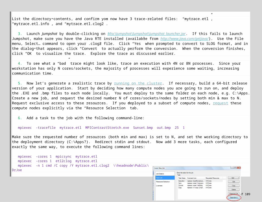
src = (myRank < numProcs-1) ? myRank + 1 : MPI_PROC_NULL;MPI_Irecv(image[rows+1], cols, MPI_PIXEL_T, src, 0 /*tag*/, MPI_COMM_WORLD, &rreqs[1]);

// all send except the last process:dest = (myRank < numProcs-1) ? myRank + 1 : MPI_PROC_NULL;MPI_Isend(image[rows], cols, MPI_PIXEL_T, dest, 0 /*tag*/, MPI_COMM_WORLD, &sreqs[0]);

// all send except the first process:dest = (myRank > 0) ? myRank - 1 : MPI_PROC_NULL;MPI_Isend(image[1], cols, MPI_PIXEL_T, dest, 0 /*tag*/, MPI_COMM_WORLD, &sreqs[1]);

// SKIP FIRST AND LAST ROWS while communication takes place...for (int row = firstRow+1; row <= lastRow-1; row++){ ... }

Once the bulk of the image has been stretched, the processes wait for the earlier communication to complete, and then set about processing the last two rows of their image chunk:

// wait for reception of ghost rows before processing first and last row:MPI_Status rstats[2];MPI_Waitall(2, rreqs, rstats);

row = 1;...

row = rows;...

Finally, we wait for the sends to complete before updating the original image matrix:

MPI_Status sstats[2];MPI_Waitall(2, sreqs, sstats);

for (int row = firstRow; row <= lastRow; row++)for (int col = 1; col < cols-1; col++)


Note that this wait is technically unnecessary, since the sends must have completed in order for the receives to complete. For more information on these and other features of MPI, see “Using MPI: Portable Parallel Programming with the Message-Passing Interface (2nd edition)”, by W. Gropp, E. Lusk and A. Skjellum. MS-MPI actually supports the more recent MPI-2 standard, which contains even more functionality. For info on MPI-2, see “Using MPI-2: Advanced Features of the Message-Passing Interface”, by W. Gropp, E. Lusk and R. Thakur.

Page 70 of 89

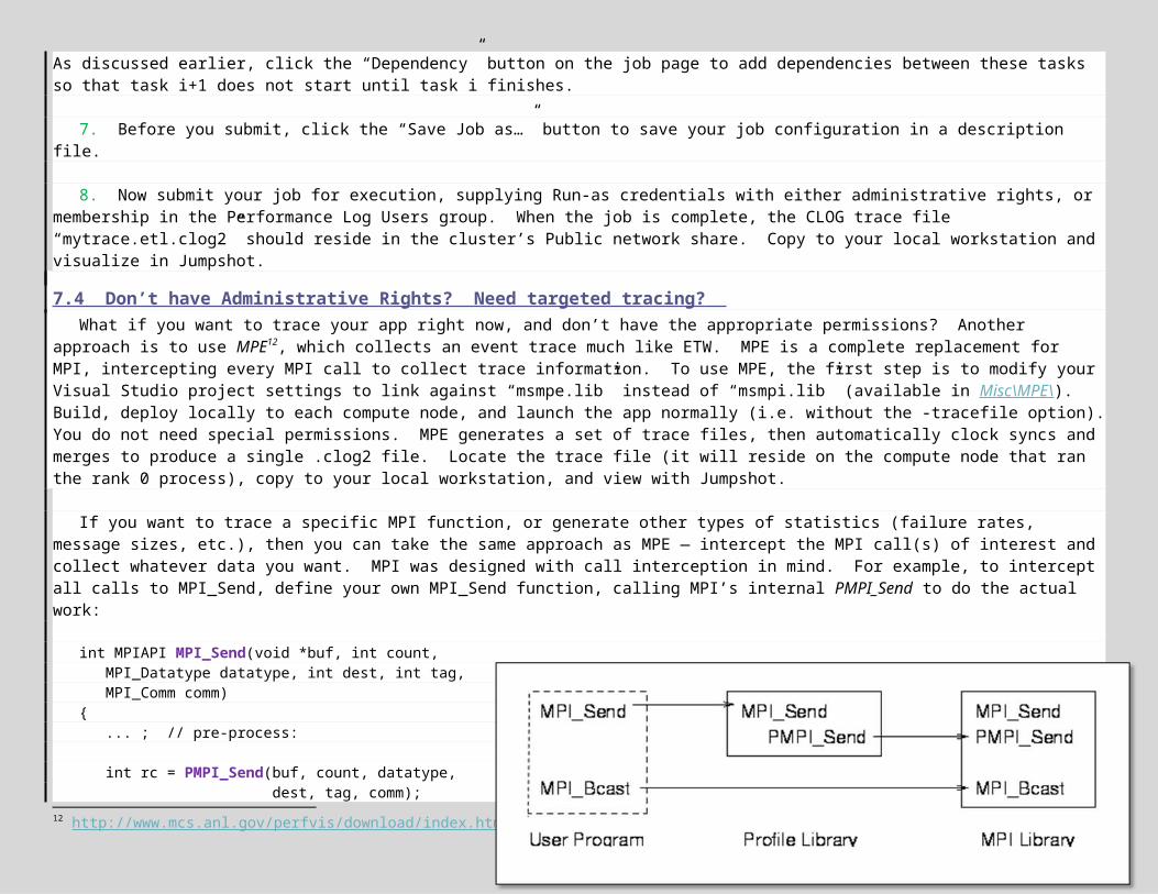
8.2 Lab Exercise! Let’s apply MPI’s collective and asynchronous functionality to our Contrast Stretching application. I’ll provide

fewer details in this exercise, giving you more room to design and experiment on your own. A solution to this lab exercise is provided in Solutions\MPI\AdvMPIContrastStretch\.

1. Start by opening a working, MPI-based, Contrast Stretching application. This might be your own version from the earlier MPI lab exercise, e.g. Exercises\03 MPI\MPIContrastStretch\. Or you can work from the provided skeleton in Exercises\05 AdvMPI\AdvMPIContrastStretch\ (which is just a copy of my solution to the earlier MPI exercise). Build, open a console window, navigate to the folder containing the .EXE, and copy over an image file to process (the Misc\ folder contains an image file, e.g. “Misc\Sunset.bmp”). Now run with say 7 processes to make sure all is well (using 7 processes checks to make sure leftover rows are handled properly):

mpiexec -n 7 MPIContrastStretch.exe Sunset.bmp out.bmp 75 1

or

mpiexec -n 7 AdvMPIContrastStretch.exe Sunset.bmp out.bmp 75 1

Use WinDiff (available in Misc\WinDiff) to confirm that your output image “out.bmp” is identical to “Misc\Sunset-75-by-1.bmp”. Another indicator that things are working is to confirm the first 5 convergence values match those reported for the sequential version (3060882, 3077598, …).

2. Rewrite the DistributeImage function to use MPI_Bcast and MPI_Scatter as discussed earlier. Run and test with 1, 4 and 7 processes. Confirm correctness with WinDiff. Online documentation for all MPI functions is available here: http://www.mcs.anl.gov/mpi/www/www3/.

3. Now rewrite the CollectImage function using MPI_Gather (synopsis available at http://www.mcs.anl.gov/mpi/www/www3/). Run and test with 1, 4 and 7 processes. Confirm correctness with WinDiff.

4. The last step is the ContrastStretch function, for which we can make 2 improvements. First, learn about the MPI_Allreduce function. This is the perfect function for calculating the globals diffs value needed for convergence testing — it reduces all the local values to a single global value, and then distributes this final value back out to all the processes. The only non-obvious requirement about calling MPI_Allreduce is that sendbuf and recvbuf must be disjoint memory locations. So you’ll want to copy the local diffs value into a temporary before calling. Find the send/recv code for summing and distributing diffs, and replace with this:

temp = diffs;MPI_Allreduce(&temp, &diffs, 1, MPI_LONG_LONG, MPI_SUM, MPI_COMM_WORLD);

Note that by default, this buffer restriction is true for all MPI functions. Build, run and test. The second improvement is to swap the ghost rows asynchronously as discussed earlier. Build, run and test (with 1, 4 and 7 processes). Confirm with WinDiff.

Page 71 of 89

http://www.mcs.anl.gov/mpi/www/www3/

http://www.mcs.anl.gov/mpi/www/www3/

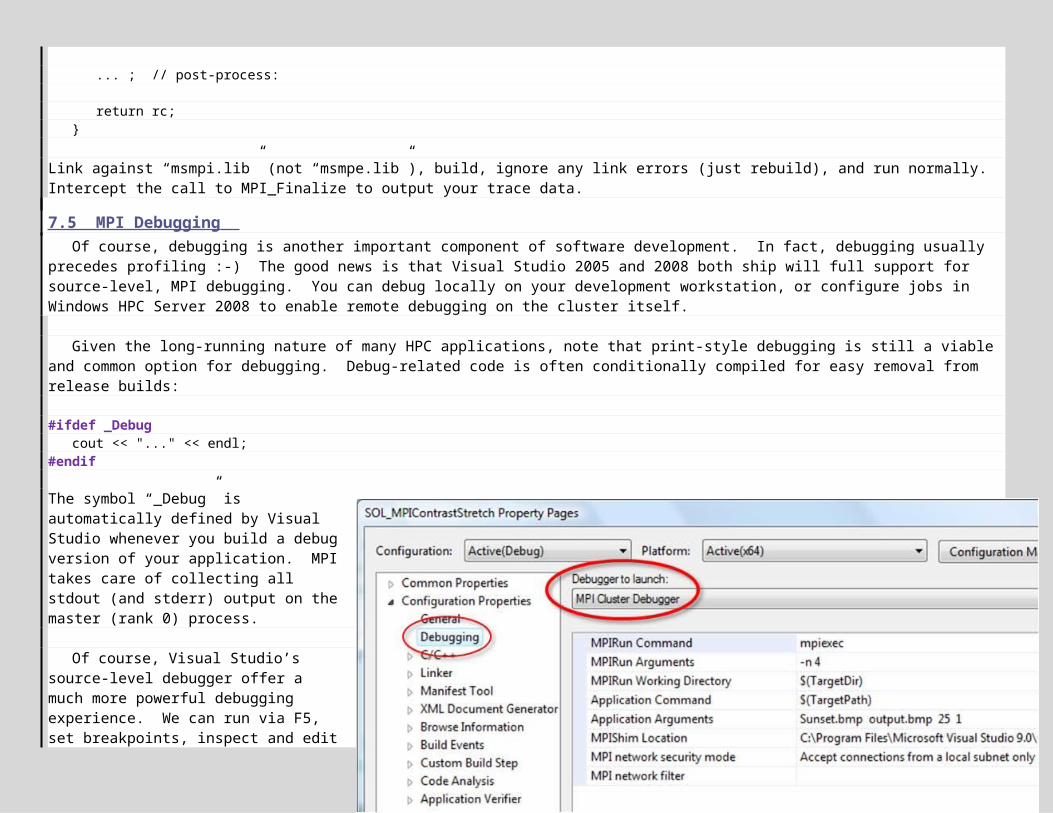
5. Have our changes improved performance? Run and time, both locally and on the cluster:

MPI Paralleltime on local workstation for convergence run: ______________, number of cores = ______, speedup = ________

MPI Paralleltime on cluster for convergence run: ______________, number of cores = ______, speedup = ________

Compare these to your earlier results. You should see a small improvement locally, and a larger improvement on the cluster.

9. Hybrid OpenMP + MPI Designs

It is generally accepted that multi-threading is more efficient than multi-processing — threads are cheaper to create than processes, and threads communicate via shared-memory while processes require some form of message-passing. In the case of cluster-wide applications, this implies the highest-performing design would be a hybrid one, employing multi-threading (OpenMP) within a node and multi-processing (MPI) across the nodes. Interestingly, research does not support this approach14. Hybrid designs rarely outperformed pure MPI designs, and when they did, required significant development effort.

The rationale is two-fold. First, the MPI library is not fully thread-safe, and so care must be taken when calling MPI functions from multiple threads. MS-MPI offers a high-degree of thread safety from the standpoint of MPI libraries: MPI_THREAD_SERIALIZED. However, this means that even though multiple threads can make MPI calls, you are limited to only one thread at a time. This forces you into more complicated designs where one thread communicates, while the rest compute.

Second, pure MPI encourages you to think in terms of decomposition and communication from the start, potentially exposing more parallelism than approaches based on more familiar, shared-memory techniques. Combined with MPI’s internal, shared-memory optimization of intra-node communication, MPI generally performs quite well in comparison to multi-threaded solutions.

The moral of the story? When in doubt, prefer pure MPI over hybrid solutions for multi-node / cluster-wide applications. And there’s growing evidence this may also hold true for apps targeting manycore hardware. If you want to experiment with hybrid designs in Windows HPC Server, start with an MPI design, rewrite the computation kernels using OpenMP, and configure the job to request exclusive access to a set of nodes. Finally, assuming you requested exclusive access to the compute nodes C1, C2, C3 and C4, launch your app as follows:

mpiexec -hosts 4 C1 1 C2 1 C3 1 C4 1 MPIApp.exe ...

14 “Hybrid OpenMP and MPI Parallel Programming”, R. Rabenseifner, G. Hager, G. Jost and R. Keller, half-day tutorial, Supercomputing 2007.

Page 72 of 89

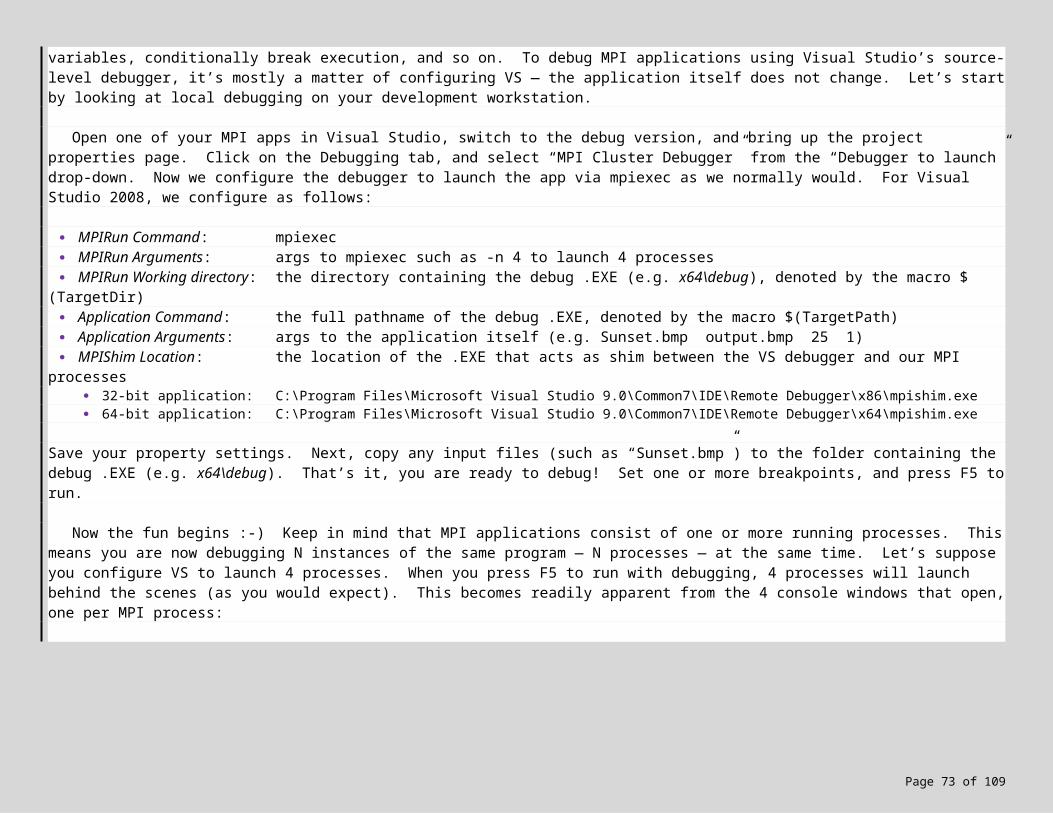
This launches 1 process on each of C1 – C4, leaving the execution cores open for multi-threading. The Contrast Stretching application is a good candidate for testing out a hybrid design.

10. Managed Solutions with MPI.NET

Speaking of alternative approaches, an exciting technology looming on the horizon is MPI.NET — a managed MPI library for languages such as C# and VB.NET. In theory, MPI.NET is simply a managed wrapper around MS-MPI. In reality, MPI.NET offers a slew of advantages, from better support for object-oriented programming to fewer memory and pointer errors.

MPI.NET is a research project from the University of Indiana15, which should RTM around the same time as Windows HPC Server 2008. MPI.NET is currently in beta (version 0.80), with solid support for MPI’s point-to-point and collective operations, asynchronous processing, and MPI topologies. For example, here’s a simple program in MPI.NET and C# that broadcasts a string to all processes:

class Program{

static void Main(string[] args){

using (new MPI.Environment(ref args)){

MPI.Communicator comm = MPI.Communicator.world;

string msg = "";

if (comm.Rank == 0)msg = "Master process says hello!";

comm.Broadcast<string>(ref msg, 0 /*master*/);

Console.WriteLine("{0} on {1}: {2}", comm.Rank, MPI.Environment.ProcessorName, msg);}

}}

A copy of this program is available in Solutions\MPI.NET\BcastHello\. To use MPI.NET, you need to: (1) install MS-MPI, (2) install MPI.NET, and (3) reference the managed assembly MPI.dll (which can be found in C:\Program Files (x86)\MPI.NET\Lib) from your .NET project in Visual Studio. To run an MPI.NET application, launch as you normally would with mpiexec:

mpiexec –n N MPIdotnetApp.exe ...

15 http://osl.iu.edu/research/mpi.net/software/ .

Page 73 of 89

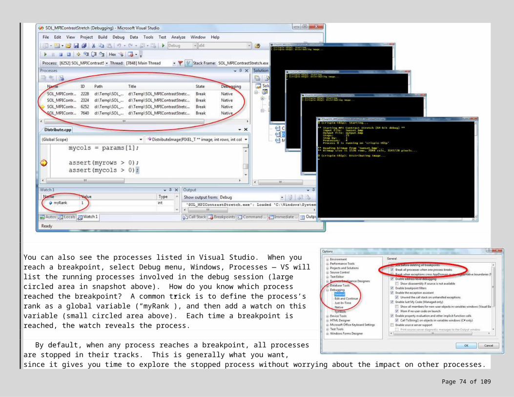
http://osl.iu.edu/research/mpi.net/software/


To run on the cluster, deploy the MPI.NET run-time to each of the compute nodes, and submit to Windows HPC Server like any other MPI job.

One of MPI.NET’s most compelling features is the ability to send and receive objects in a type-safe, intuitive manner. First, recall that MPI traditionally works in terms of memory addresses. Here are the C prototypes for MPI_Send and Recv:

int MPI_Send(void *buf, int count, MPI_Datatype datatype, int dest, int tag, MPI_Comm comm);int MPI_Recv(void *buf, int count, MPI_Datatype datatype, int src, int tag, MPI_Comm comm, MPI_Status *status);

Now consider MPI.NET’s declarations of Send and Recv16:

public abstract class Communicator{

public void Send<T>(T value, int dest, int tag)public T Receive<T>(int src, int tag)...

}

MPI.NET defines Send and Receive in terms of a generic type T. This means you can send any type of data to another process, including objects such as arrays:

int[,] matrix = new int[1000,1000]; // create a new 2D matrix objectFillWithData(matrix); // fill with data

comm.Send<int[,]>(matrix, dest, tag); . . .matrix = comm.Receive<int[,]>(src, tag);

And DataSets (database-like objects):

DataSet ds = new DataSet(); // create an empty dataset objectFillWithData(ds); // fill with data

comm.Send<DataSet>(ds, dest, tag); . . .ds = comm.Receive<DataSet>(src, tag);

16 In reality these methods are overloaded with additional declarations. For simplicity, I present only two.

Page 74 of 89

This also includes user-defined objects, e.g. our own Customer class:

Customer c;c = new Customer(...);

comm.Send<Customer>(c, dest, tag); . . .c = comm.Receive<Customer>(src, tag);

Contrast this with the effort required to use structured data in MPI, where the developer must first define a C struct, and then construct an MPI_Datatype to mirror this struct. The only restriction in MPI.NET is that the class must be Serializable so the objects can be marshaled from one process to another:

[System.Serializable]public class Customer{

...}

When an object is sent from process A to process B, its data is serialized into a byte-stream on A, transmitted in message format to B, and then recreated on B by instantiating a new object from the deserialized data. Note that an object’s code is never marshaled, only its data.

One of the trade-offs in using MPI.NET is the potential performance penalty as objects are marshaled during the send/recv process. In comparisons with native code, the designers of MPI.NET report a worst-case performance hit of 12% on small benchmarks17; an MPI.NET version of the Contrast Stretching application is running 4x slower with the 0.80 beta release (which is most likely a non-optimized debug release). This cost should be weighed carefully against the expected gain in programmer productivity offered by .NET in general, and MPI.NET in particular. For example, in C/C++ you can allocate large 1D arrays and treat them as 2D arrays — as long as you get the pointer manipulations correct. This makes for efficient Scatter and Gather operations. In .NET, by default you are not given direct access to memory nor memory addresses. You must either switch to unsafe (i.e. unmanaged) code, or redesign your object hierarchy. In MPI.NET, in order to scatter a 2D array, the managed solution is to create an *array* of 2D arrays. Let’s assume we need to distribute a 1000-by-1000 integer matrix across 4 processors. We would create an array of 4 2D arrays, each 250-by-250 in size, and then scatter:

int[][,] data;data = new int[4][,];

for (int i = 0; i < 4; i++) {

data[i] = new int[250,250];FillWithData(data[i]);

17 http://www.osl.iu.edu/research/mpi.net/faq/?category=performance.

Page 75 of 89

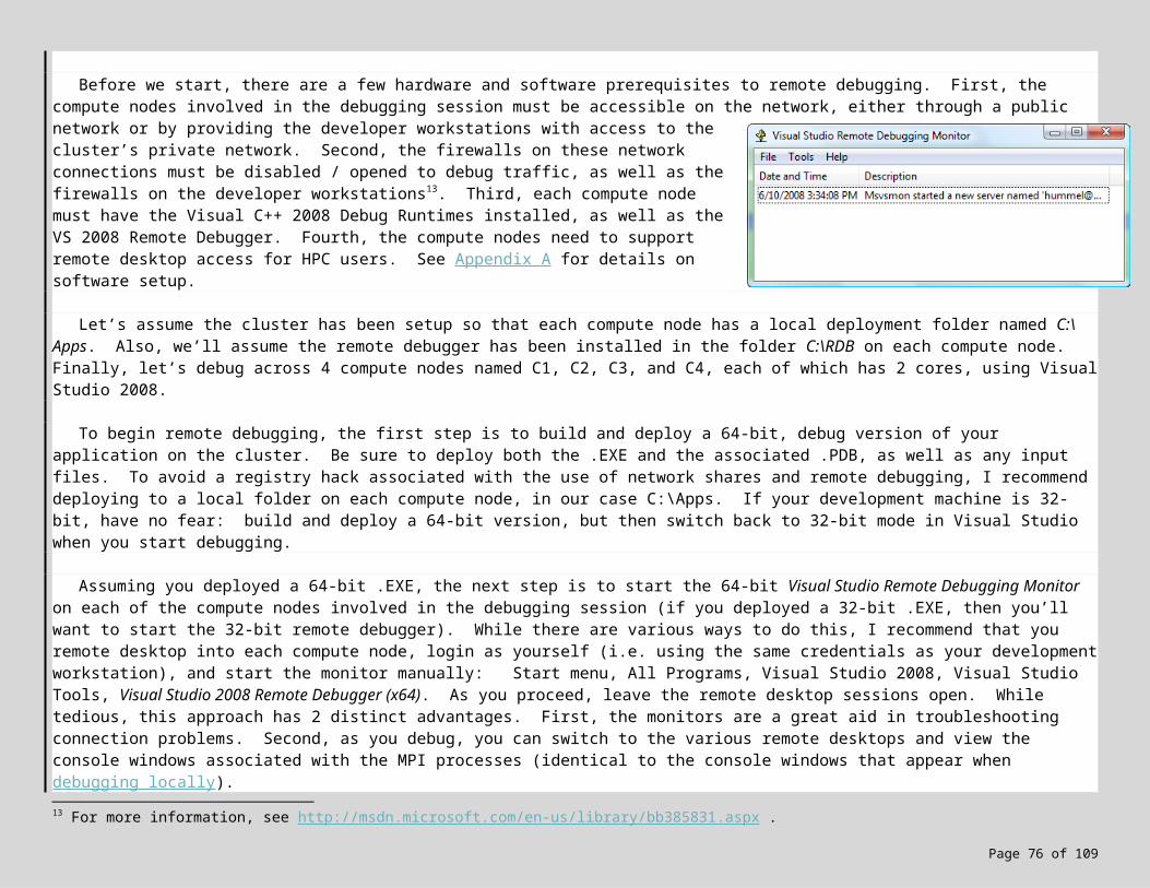
http://www.osl.iu.edu/research/mpi.net/faq/?category=performance

}

int[,] chunk;chunk = comm.Scatter<int[,]>(data, root);

We are effectively partitioning the data ourselves through the creation of additional objects, which adds overhead during (a) creation, and (b) the marshalling process. But we are also working at a higher-level of abstraction, and significantly reducing the possibility of memory errors.

10.1 Lab Exercise! Let’s take a look at MPI.NET in the context of our Contrast Stretching application. This will be less of a step-by-

step lab exercise, and more of a look at how the application can be redesigned for use with MPI.NET. Note that a solution to this exercise is available in Solutions\MPI.NET\AdvMPIContrastStretch\.

1. Start by installing the MPI.NET SDK on your development machine: http://osl.iu.edu/research/mpi.net/software/. Now open the provided MPI.NET version of the Contrast Stretching app given in Exercises\06 MPI.NET\AdvMPIContrastStretch\. Add a reference (via Project menu) to the managed assembly “MPI.dll”, which can be found in C:\Program Files (x86)\MPI.NET\Lib. The program should now build without error.

2. Open a console window, navigate to the folder containing your .EXE (bin\debug or bin\release), and copy an image file to process (the Misc\ folder contains an image to process, e.g. “Misc\Sunset.bmp”). Now run with say 7 processes to make sure all is well (using 7 processes checks to make sure leftover rows are handled properly):

mpiexec -n 7 AdvMPIContrastStretch.exe Sunset.bmp out.bmp 75 1

Use WinDiff (available in Misc\WinDiff) to confirm that your output image “out.bmp” is identical to “Misc\Sunset-75-by-1.bmp”. Another indicator that things are working is to confirm the first 5 convergence values match those reported for the sequential version (3060882, 3077598, …).

3. Now skim the source code in Visual Studio. Start by looking at the object design. First, the definition of a Pixel in “Pixel.cs”. Notice the use of a struct instead of a class; structs are value types in .NET like int and double, which means they do not require individual object instantiation — creating an array of N structs requires just 1 object instantiation, while creating an array of N objects requires 1+N object instantiations. For performance, when in doubt use structs, not classes.

Next, review the definition of an ImageChunk in “ImageChunk.cs”. This represents the chunk of data each process will receive, stretch, and return (see diagram to right). As noted earlier, MPI.NET encourages us to explicitly design our data distribution, versus the unmanaged approach of distributing data based on memory buffers and pointer arithmetic. Finally, the entire image is represented by the ImageData object defined in “ImageData.cs”.

Page 76 of 89


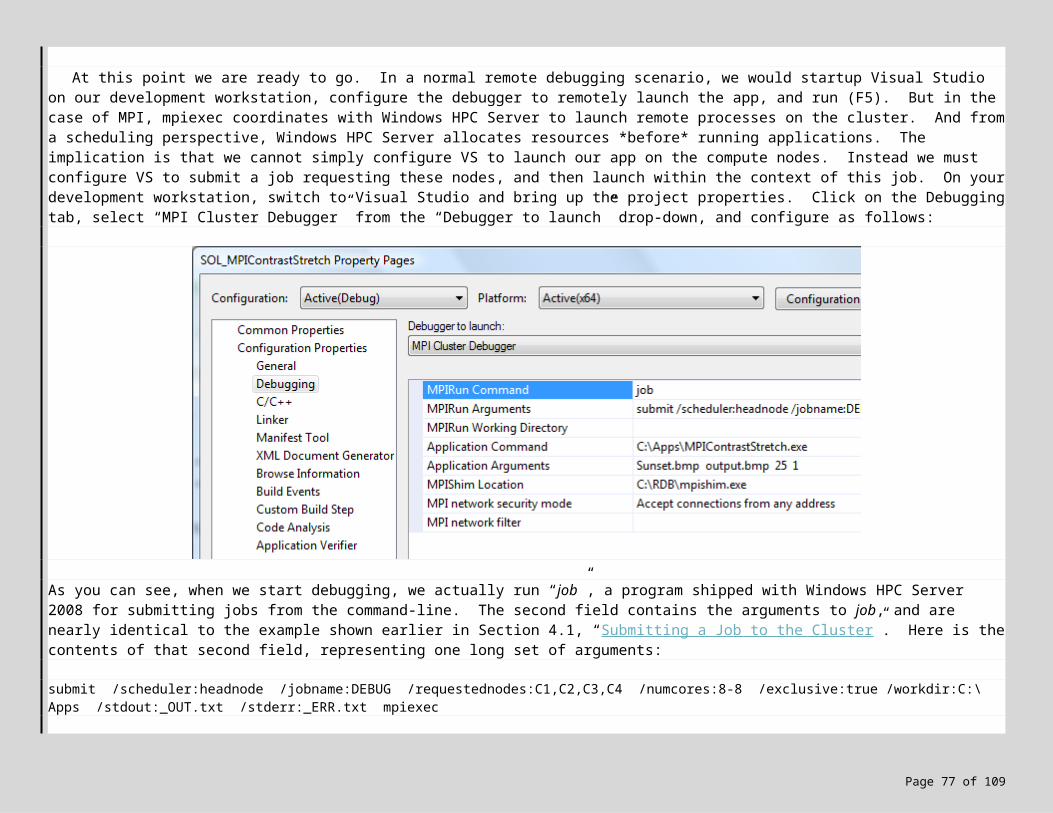
4. Now skim the main method defined in “Program.cs”. The code follows the same design as our previous MPI versions, consisting of master / worker processes and 3 main processing steps: (1) distribute, (2) stretch, and (3) collect. Scroll down to see the DistributeImage and CollectImage methods. Given the upfront design of the data hierarchy, distribution and collection are straightforward:

myChunk = Communicator.world.Scatter<ImageChunk>(chunks, 0 /*master scatters*/);...results = Communicator.world.Gather<ImageChunk>(myChunk, 0 /*master gathers*/);

5. Let’s collect some performance data on the MPI.NET version. First, build a release version of your application, and time it locally:

MPI.NET Paralleltime on local workstation for convergence run: ______________, number of cores = ______, speedup = ________

How does this compare to the unmanaged result recorded in the previous lab exercise? Keep in mind this is a beta release of MPI.NET. Now let’s time on the cluster. First, deploy your app to the cluster. If you deploy to a public share, you’ll need to install the MPI.NET runtime on each compute node. If you deploy locally to each compute node, you can simply deploy your app + MPI.dll. Once configured, submit a job to Windows HPC Server and record the time:

MPI.NET Paralleltime on cluster for convergence run: ______________, number of cores = ______, speedup = ________

How does this compare to the result with unmanaged code?

6. If you want to experiment with MPI.NET, try modifying the contrast stretching algorithm (Algorithms.ContrastStretch) to use asynchronous communication. I was unable to get this to work with the 0.80 beta release, perhaps you will have better luck (or access to a newer release). If so, does this help performance?

11. Conclusions

Windows HPC Server 2008 provides a framework for developing and executing high-performance applications. This tutorial presented a classic HPC development scenario where data parallelism is exploited using both shared-memory (OpenMP) and distributed-memory (MPI) techniques. Combined with Visual Studio, Visual C++, VisuC#, and .NET, the result is a powerful environment for developing high-performing, cluster-wide applications.

Other tutorials are available on Windows HPC Server 2008, including scenarios for the sequential developer, the enterprise developer, and those new to HPC. The following are also good references and resources on HPC. Cheers!

Page 77 of 89

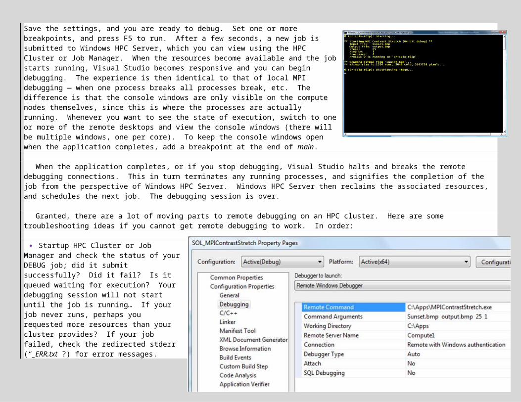
http://go.microsoft.com/fwlink/?LinkId=124941




11.1 References Windows HPC Server 2008 homepage: http://www.microsoft.com/HPC/

Windows HPC Server 2008 resources, blogs, forums: http://windowshpc.net/Pages/Default.aspx

OpenMP: http://openmp.org/

MPI: http://www.mpi-forum.org/, http://www.mcs.anl.gov/mpi/

General HPC news: http://www.hpcwire.com/

11.2 Resources “Multi-Core Programming”, by S. Akhter and J. Roberts (Intel Press)

“Using MPI : Portable Parallel Programming with the Message-Passing Interface (2nd edition)”, by W. Gropp, E. Lusk and A. Skjellum

“Using MPI-2: Advanced Features of the Message-Passing Interface”, by W. Gropp, E. Lusk and R. Thakur

“Patterns for Parallel Programming”, by T. Mattson, B. Sanders and B. Massingill

“Parallel Programming with MPI”, by P. Pacheco

“Parallel Programming in C with MPI and OpenMP”, by M. Quinn

Page 78 of 89

http://www.hpcwire.com/

http://www.mcs.anl.gov/mpi/

http://www.mpi-forum.org/

http://openmp.org/

http://windowshpc.net/Pages/Default.aspx

http://www.microsoft.com/HPC/

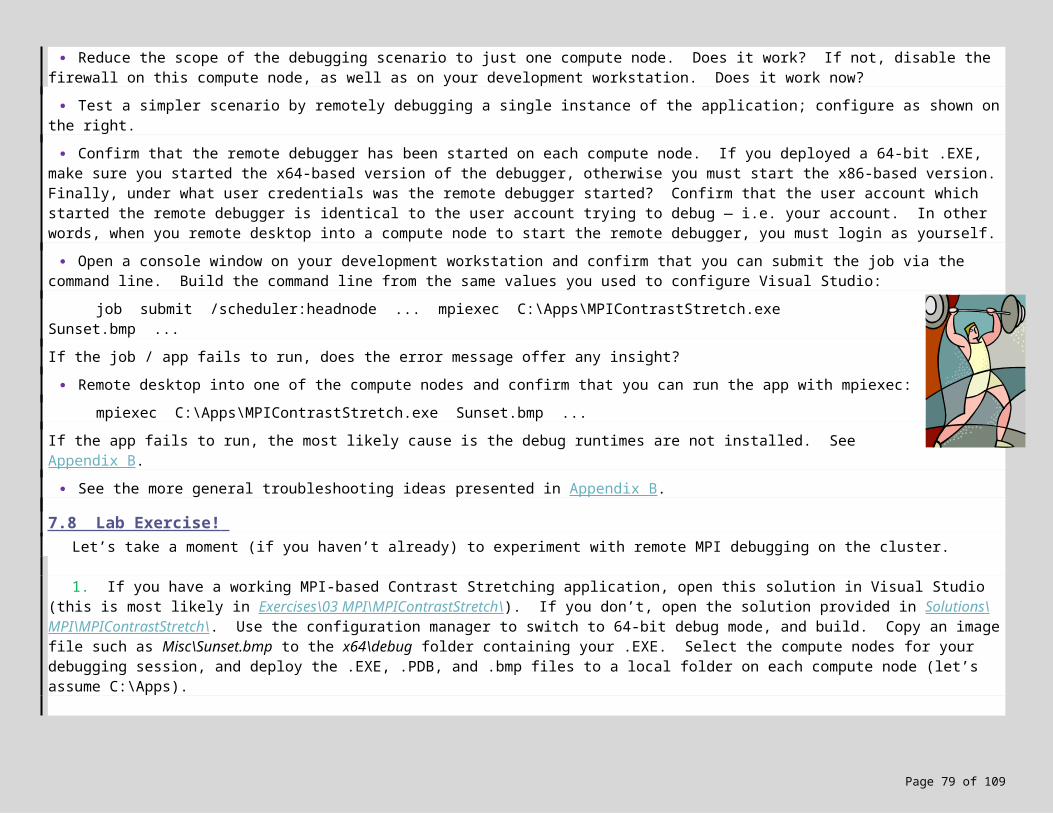
Appendix A: Summary of Cluster and Developer Setup for Windows HPC Server 2008

This appendix serves as a brief summary of how to setup an Windows HPC Server 2008 cluster. It outlines the main software components you need, and the major steps to perform. I use this summary when setting up small personal clusters; this summary is not appropriate for setting up large, production-ready clusters.

Hardware requirementsOne or more 64-bit capable machines; network interconnect.

Software requirementsWindows Server® 2008 64-bit, standard or enterprise edition. Microsoft HPC Pack 2008. Developers will need Visual Studio

2008, SDK for Microsoft HPC Pack 2008, and Windows PowerShell. The Microsoft HPC Pack 2008 is available for purchase from Microsoft, may be downloaded from the MSDN Subscriber Download site or a free evaluation version may be downloaded from http://www.microsoft.com/hpc. Download the SDK from http://go.microsoft.com/fwlink/?linkID= 127031 .

Developer Workstation SetupInstall Visual Studio 2008 (full install), Windows PowerShell, Microsoft HPC Pack 2008 (client-side utilities), and SDK for

Microsoft HPC Pack 2008. Note that unlike cluster nodes, a developer machine can be running 32-bit or 64-bit Windows. In the 32-bit case, you build and test locally in 32-bit, then rebuild as 64-bit and deploy to cluster.

Cluster Setup1. Install Windows Server 2008 64-bit on each machine. Assign admin pwd, enable remote desktop. Activate Windows if

necessary via Control Panel System applet. Add roles: Web Server, App Server (in particular ASP.NET). Windows update.

2. Install latest release of .NET framework (http://msdn.microsoft.com/en-us/netframework/aa569263.aspx), and Visual C++ runtimes on each machine. At the very least, you want to install 64-bit release runtimes for Visual Studio 2008. Download here: http://www.microsoft.com/downloads/details.aspx?familyid=bd2a6171-e2d6-4230-b809-9a8d7548c1b6&displaylang=en . Now ask yourself, do you plan to run debug versions on the cluster (e.g. to do remote debugging)? 32-bit release / debug versions? Apps built with Visual Studio 2005? If you answered yes to any of these, you have more runtimes to install. I’ve written a more detailed set of instructions on what you need, where to get it, and how to install it. See Misc\VC++ Runtimes\Readme.docx. The release runtimes are easy; the debug runtimes are not.

3. Decide which machine is going to be the head node, when in doubt pick the one with the largest capacity hard disk. The head node can also act as a compute node, which is typical for small clusters. Have this machine join an existing domain, or if not, add role: Active Directory® Domain Services. Create the following groups in the domain: HPCUsers, HPCAdmins. Create

Page 79 of 89

http://www.microsoft.com/downloads/details.aspx?familyid=bd2a6171-e2d6-4230-b809-9a8d7548c1b6&displaylang=en

http://msdn.microsoft.com/en-us/netframework/aa569263.aspx

http://go.microsoft.com/fwlink/?linkID=%20127031%20

http://www.microsoft.com/hpc

the following users in the domain: hpcuser, hpcadmin. Add both users to HPCUsers group, add hpcadmin to HPCAdmins group. Add yourself and others to these groups as appropriate.

4. On head node, create directories C:\Apps and C:\Public. Give everyone read access, give HPCUsers and HPCAdmins full access. Now share both C:\Apps and C:\Public, giving everyone read access, HPCUsers and HPCAdmins full access.

5. On remaining nodes of cluster, join domain. Create directory C:\Apps. Give everyone read access, give HPCUsers and HPCAdmins full access. Now share C:\Apps, giving everyone read access, HPCUsers and HPCAdmins full access.

6. Back on head node, install Microsoft HPC Pack 2008 to setup a new cluster. Follow step-by-step “To do” list to configure network, firewalls, etc. When it comes to “node template”, create an empty template since we will configure the compute nodes manually. Add HPCUsers as a cluster user, add HPCAdmins as a cluster admin. If necessary, change head node role to include acting as a compute node. Bring head node online via Node Management tab, right-click. When you are done, make sure firewall if off (if you have exactly one NIC then it has to be off, if you have multiple NICs then make sure it’s off for the private network MPI will use).

7. On remaining nodes, install Microsoft HPC Pack 2008 to join an existing cluster. When you are done, make sure firewall if off (if you have exactly one NIC then it has to be off, if you have multiple NICs then make sure it’s off for the private network MPI will use).

8. Back on head node, startup the Microsoft HPC Pack Cluster Manager MMC plug-in, and select Node Management tab. For each of the remaining nodes, right-click and apply empty node template. Then right-click and bring online. When you’re done, the cluster is ready for testing! Run the pingpong diagnostic from the HPC Cluster Manager, which sends messages between every pair of execution cores in the cluster. This may take a few minutes (to a few hours based on the size and complexity of the cluster).

9. If you plan to develop software on any of the nodes (e.g. sometimes you might want to recompile apps on the head node), install Visual Studio 2008 and the SDK for Microsoft HPC Pack 2008.

10. If you want to enable remote desktop connections for non-administrative users, add HPCUsers and HPCAdmins as members of the “Remote Desktop Users” group. Also, make sure that “Remote Desktop Users” have been granted access through Terminal Services: Security Settings, Local Policies, User Rights Assignment, Allow log on through Terminal Services. Repeat on each node you want to support remote access.

11. If you want to enable ETW tracing for non-administrative users, add HPCUsers and HPCAdmins as members of the “Performance Log Users” group. Repeat on each node you want to support tracing.

12. If you want to enable remote debugging on the cluster, install Visual Studio’s Remote Debugger on each compute node. Locate your Visual Studio 2008 install disk, and copy Remote Debugger\x64\rdbgsetup.exe to the cluster’s Public share. For each compute node, including the head node if it also serves as a compute node, do the following: (1) run rdbgsetup.exe, and (2) copy the contents of C:\Program Files\Microsoft Visual Studio 9.0\Common7\UDE\Remote Debugging\x64 to C:\RDB. Note

Page 80 of 89

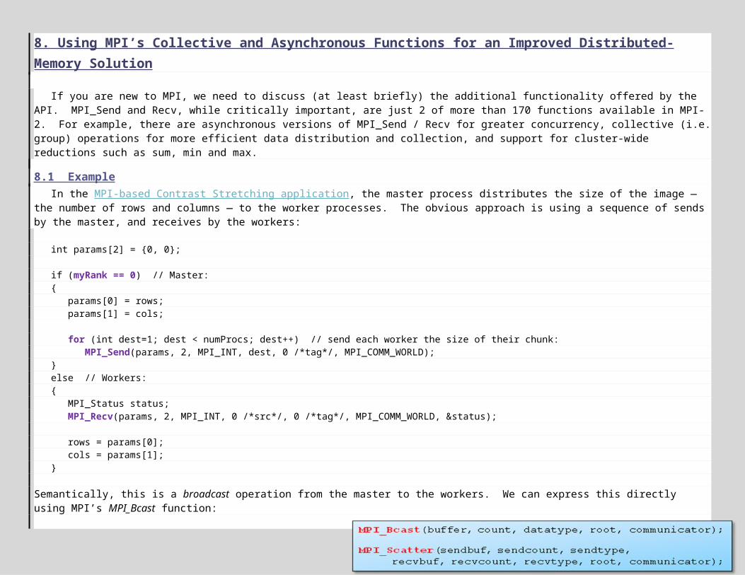
that you can use a different target directory for step 2, but make sure the path does not contain spaces, and use the same path on each node.

13. If you plan to support MPI.NET on the cluster, install the MPI.NET runtime on each compute node: download from http://osl.iu.edu/research/mpi.net/software/.

ShutdownWhen shutting down the cluster, first shutdown the compute nodes via the remote desktop and then shutdown the head

node.

StartupWhen booting the cluster, boot the head node first, give it 5+ minutes (especially if it’s a domain controller), then boot the

compute nodes. Check (via HPC Cluster Manager) to make sure each machine is online. Finally, check the head node and one of the compute nodes (via remote desktop) to make sure the firewall is turned off (if you have exactly one NIC then it has to be off, if you have multiple NICs then make sure it’s off for the private network MPI will use).

Page 81 of 89


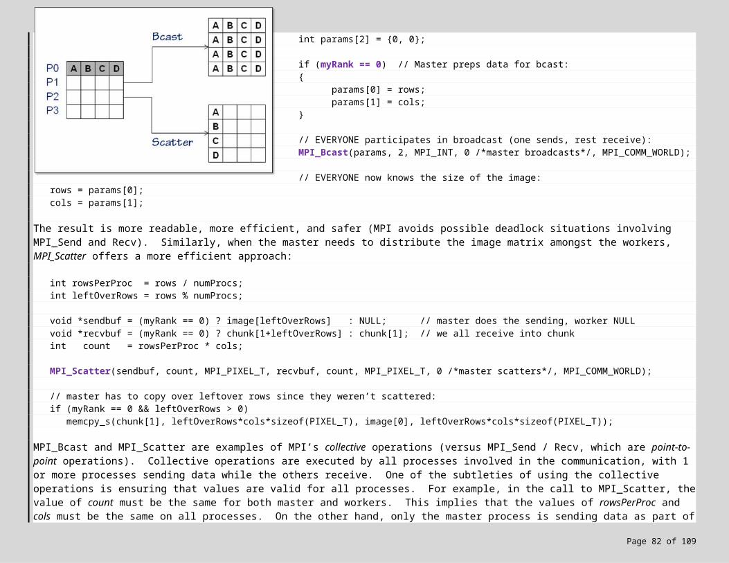
Appendix B: Troubleshooting Windows HPC Server 2008 Job Execution

Are you submitting a job and getting nothing in return? Here’s what I do to troubleshoot execution failures on the cluster. The symptoms range from submitting a job that never runs (e.g. remains queued forever) to error messages such as “execution failed”.

Step 1: It’s a Local ProblemThe best way to troubleshoot a failure of any kind is to deploy the app as you normally would, and then remote desktop into

one of the compute nodes, open a console window (Start, cmd.exe), and run the .EXE directly. If you deployed locally, navigate to the working directory you specified in the job configuration, and type “appname.exe” to run it. If you deployed to a network share and set the network share as your working directory, then run by concatenating the network share and the .EXE name, e.g. “\\headnode\public\appname.exe”. What happens? If the application failed to start, the most common problem with VC++ is that you deployed a debug version of the app, and the debug runtimes are not installed (or you deployed a 32-bit app and the 32-bit runtimes are not installed, etc.). The simplest fix in this case is to build a 64-bit release version of your application, redeploy, and test this version of the .EXE. The other fix is to deploy the necessary runtimes to the cluster; see Appendix A on cluster setup (step 2). For .NET applications, make sure the latest release of .NET is installed; e.g. MPI.NET requires .NET 3.5 (see http://msdn.microsoft.com/en-us/netframework/aa569263.aspx). Also, are you trying to run a .NET app from a network share or other remote location? Note that by default, .NET is configured for security reasons to prevent the execution of non-local code; if you get a security exception when you run the .EXE, this is most likely the problem. The solution is to deploy the .EXE locally to each node, or configure .NET on each node to make the public network share a trusted location.

Once the .EXE at least loads and starts, type the command-line as given in the task that failed (e.g. “mpiexec MPIApp.exe …”). Now what happens? The most common problems include forgetting to specify mpiexec at the start of an MPI run, misspelling the share or application name, omitting required command-line arguments to the app, or missing input files. Also, make sure you are specifying a working directory in your task configuration — this might explain why the .EXE and input files cannot be found. Once the application runs locally on a compute node, resubmit the job and see what happens.

Are you trying to run an MPI application, and mpiexec just hangs? In other words, you correctly type “mpiexec MPIApp.exe …”, but execution just hangs? I’ve seen this problem if both Microsoft® Compute Cluster Pack and Microsoft HPC Pack are installed. In particular, echo the PATH environment variable from a console window (“echo %path%”) and see if it contains “C:\Program Files\Microsoft Compute Cluster Pack\...”. If so, you need to delete any references to WCCS from the PATH variable (Control Panel, System, Advanced Settings, Environment Variables). Close the console window, reopen, and try running again.

Step 2: It’s a Global ProblemAssuming the app runs locally on a compute node, the next most common problem is a global one, typically firewall or

security. Security problems appear as jobs that fail immediately, or jobs that queue but never finish. Firewall problems typically result in MPI failures along the lines of “unable to open connection”.

Page 82 of 89

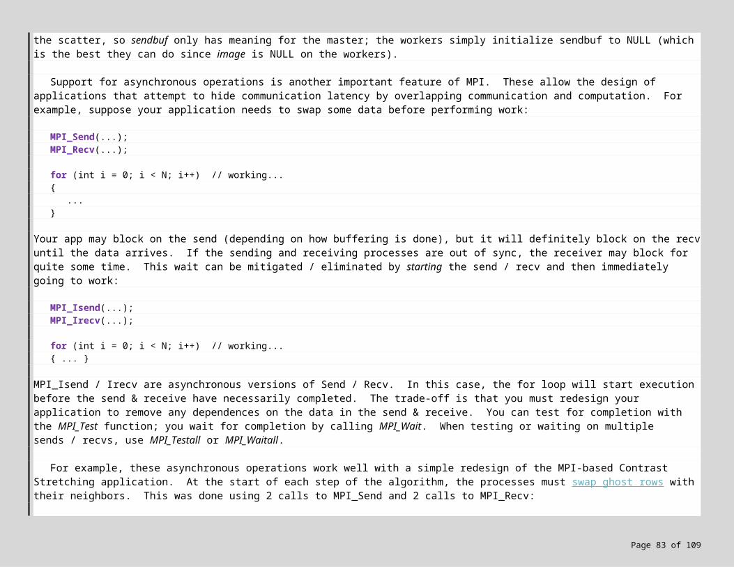
http://msdn.microsoft.com/en-us/netframework/aa569263.aspx

In terms of security, keep in mind there are two distinct logins needed: one to connect to the head node for submitting a job, and one for job execution (“run-as”). When you connect to the head node to submit a job, you are using the credentials of your personal login on your local workstation; if you were able to open the Windows HPC Job Manager and connect to the head node, you have the proper permissions to use the cluster. The more common problem are the “run-as” credentials. You are prompted for these credentials when you submit a job. Does this login have permission to access the .EXE? Access the input files? Execute the .EXE? Write the output file(s)? The simplest way to find out is to use a known administrator account for the run-as credentials. Start by clearing the credential cache on the machine you have been submitting jobs from: open the HPC Job Manager, Options menu, and select Clear Credential Cache. This will ensure that you are prompted for run-as credentials the next time you submit a job. Now submit your job once again, entering a known administrator login and password for the cluster when prompted. If the job runs, you know it’s a security problem related to the login you were trying to use.

To collect more data about what the security problem might be, remote desktop into one of the compute nodes and login with the credentials you are specifying for the run-as credentials. Can you login? Try to run the application. Do you have permission? If all this works, the last step is to repeat this exercise on the head node. If the head node is a domain controller, note that logins need explicit permission to login, and this is most likely the source of the problem.

If security does not appear to be the cause of the problem, are you trying to execute MPI programs? In this case, make sure the firewall is off on all the nodes: if nodes have exactly one NIC then it has to be off, if they have multiple NICs then make sure it’s off for the private network MPI will use. A quick way to determine firewall status on the cluster is to open the Microsoft HPC Pack Cluster Manager MMC plug-in and run the diagnostic FirewallConfigurationReport. This will take a few seconds, then you can view the completed test results to see the status of the firewall on every node. If you are not sure whether this is the problem, turn the firewall completely off on 2 nodes, and resubmit the job configured to run on just those nodes. If the job now runs, it’s a firewall problem; fix the other machines to match the firewall configuration of the working machines.

If you are running MPI programs and absolutely require compute nodes to have their firewalls on, then the next best solution is to limit MPI to a range of ports, and configure your firewall software to open these ports. You specify the range of MPI ports via the environment variable MPICH_PORT_RANGE in the format min,max (e.g. 9500,9999). You then configure the firewall to open this range of ports. Repeat on each compute node. The alternative is to grant each individual MPI program full access to the network on each compute node.

Step 3: Job Submission TweaksMake sure you are specifying a working directory in your task configuration, otherwise the .EXE and input files may not be

found. Likewise, be sure to redirect stdout and stderr to capture error messages you might be missing. Are you resubmitting jobs from a template? Note that if you change the number of processors for the job (such as reducing the maximum number of processes requested), you also need to adjust the number of processors requested for the individual tasks — changing job configuration parameters does not necessarily update the underlying task configurations. For example, you might change a job to request a max of 4 processors, but one of the tasks is still requesting 5..8 processors, so the job never runs. When in doubt, submit a new, simpler job from scratch.

Step 4: Okay, I’m Really Stuck

Page 83 of 89

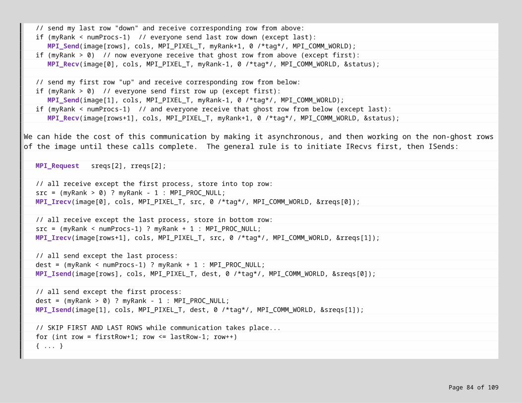
If you’ve come this far, then you’re really stuck, and the problem is not one of the more common ones. So now what? First, abandon the program you are trying to run, and run a much simpler application — try to submit and run a trivial, sequential “Hello world” type of application. If you need such an app, use Misc\VC++ Runtimes\VS2008\Hello-64r.exe. Start the troubleshooting process over with this trivial application. Second, try running one of the diagnostics in the HPC Cluster Manager, such as pingpong. This can identify nodes that are not working properly, at least with respect to the network infrastructure. Third, try Microsoft’s HPC Community forums, you might find a solution listed there. Or worst-case, post your problem as a new thread and see what unfolds. Start here: http://www.windowshpc.net/Pages/Default.aspx . The forums can be found here: http://forums.microsoft.com/WindowsHPC/default.aspx .

Good luck!

Page 84 of 89

http://forums.microsoft.com/WindowsHPC/default.aspx

http://www.windowshpc.net/Pages/Default.aspx

Appendix C: Screen Snapshots

HPC Cluster Manager / HPC Job Manager : Create New Job dialog

Page 85 of 89

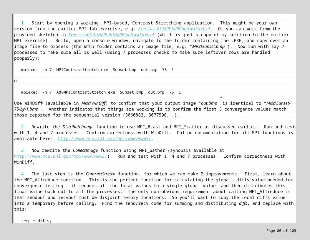
Page 86 of 89

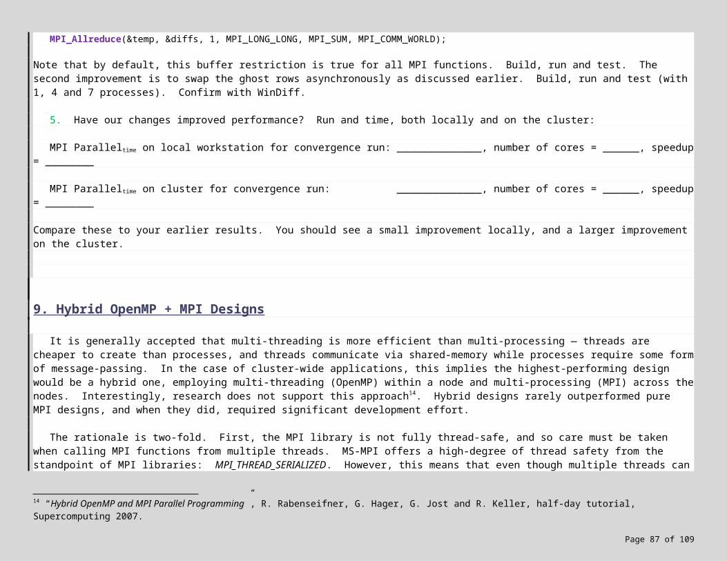
HPC Cluster Manager / HPC Job Manager : Add Task dialog

Page 87 of 89

Page 88 of 89

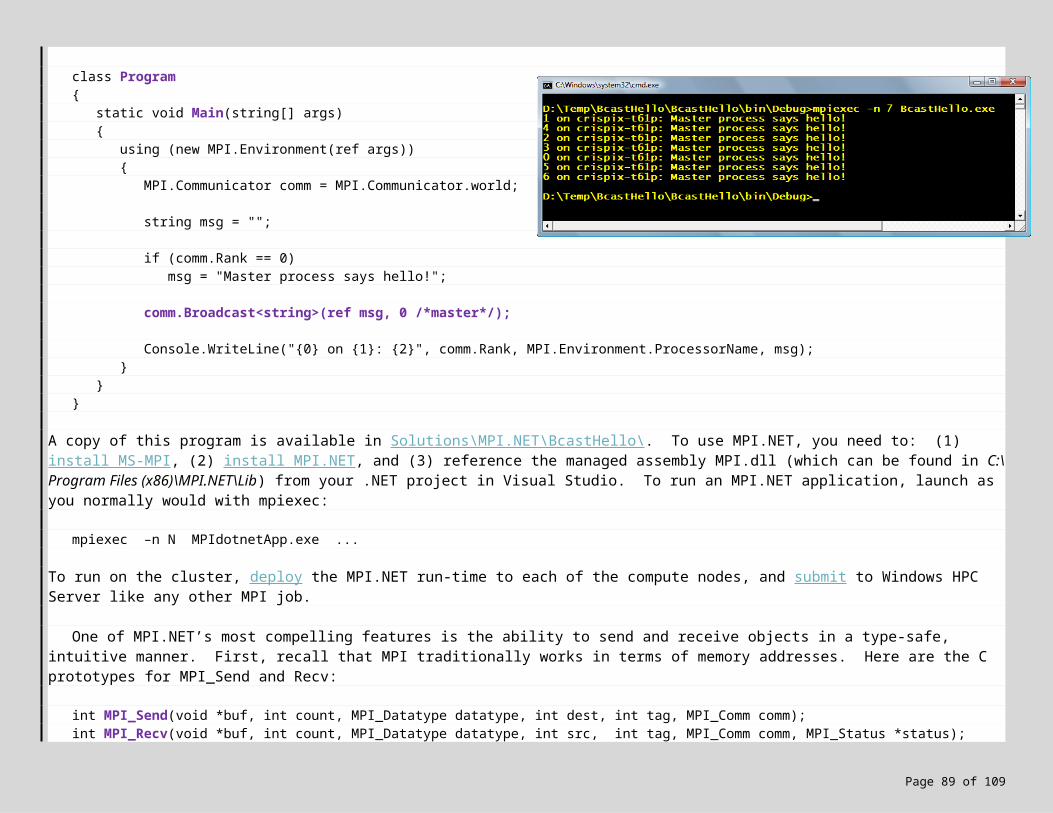
Feedback Did you find problems with this tutorial? Do you have suggestions that would improve it? Send us your feedback or report a bug on the Microsoft HPC developer forum.

More Information and Downloads

Allinea DDTLite http://www.allinea.com/Intel Cluster Debugger http://www.intel.com/cd/software/products/asmo-na/eng/index.htmPortland Group Cluster Kit http://www.pgroup.com/products/cdkindex.htmMPI.NET http://osl.iu.edu/research/mpi.net/software/OpenMP http://openmp.org/MPI http://www.mpi-forum.org/, http://www.mcs.anl.gov/mpi/ Windows HPC Server 2008 homepage http://www.microsoft.com/HPC/Windows HPC Server 2008 developer resource page http://www.microsoft.com/hpc/dev

This document was developed prior to the product’s release to manufacturing, and as such, we cannot guarantee that all details included herein will be exactly as what is found in the shipping product.

The information contained in this document represents the current view of Microsoft Corporation on the issues discussed as of the date of publication. Because Microsoft must respond to changing market conditions, it should not be interpreted to be a commitment on the part of Microsoft, and Microsoft cannot guarantee the accuracy of any information presented after the date of publication.This White Paper is for informational purposes only. MICROSOFT MAKES NO WARRANTIES, EXPRESS, IMPLIED, OR STATUTORY, AS TO THE INFORMATION IN THIS DOCUMENT.

Complying with all applicable copyright laws is the responsibility of the user. Without limiting the rights under copyright, no part of this document may be reproduced, stored in or introduced into a retrieval system, or transmitted in any form or by any means (electronic, mechanical, photocopying, recording, or otherwise), or for any purpose, without the express written permission of Microsoft Corporation. Microsoft may have patents, patent applications, trademarks, copyrights, or other intellectual property rights covering subject matter in this document. Except as expressly provided in any written license agreement from Microsoft, the furnishing of this document does not give you any license to these patents, trademarks, copyrights, or other intellectual property.

© 2008 Microsoft Corporation. All rights reserved.

Microsoft, Active Directory, Visual C++, Visual C#, Visual Studio, Windows, the Windows logo, Windows PowerShell, Windows Server, and Windows Vista are trademarks of the Microsoft group of companies.

All other trademarks are property of their respective owners.

Page 89 of 89

http://www.microsoft.com/hpc/dev

http://www.microsoft.com/HPC/

http://www.mcs.anl.gov/mpi/

http://openmp.org/


http://www.pgroup.com/products/cdkindex.htm

http://www.intel.com/cd/software/products/asmo-na/eng/index.htm

http://www.allinea.com/

http://forums.community.microsoft.com/en-US/windowshpcdevs/threads/

Documents

Classic HPC Development using Visual C++ - vscht.czdsp.vscht.cz/konference_matlab/MATLAB08/prispevky/Sprinx... · Web viewTitle Classic HPC Development using Visual C++ Subject Windows