2D CORRELATION SPECTROSCOPY AND ITSAPPLICATION IN VIBRATIONAL SPECTROSCOPY

USING MATLAB

T. Pazderka, V. Kopecky Jr.

Institute of Physics, Faculty of Mathematics and Physics, Charles University, Ke Karlovu 5,Prague 2, 121 16, Czech Republic

Abstract

Two dimensional correlation spectroscopy is a powerfull tool for spectral analysis.It is able to reveal correlations between spectral changes and to deconvolveoverlapping peaks. It is easily applicable in a study of biomolecules. Herepresented program was created for easy accessibility of all necessary operations.Presented algorithm was deeply tested on regular spectra as well as on a spectraof vibrational optical activity. Basic mathematics needed for understanding andperforming two-dimensional correlation spectroscopy was also presented.

1 Two dimensional correlation spectroscopy

Two dimensional correlation spectroscopy (2DCoS) originated in a NMR spectroscopy. Therewere efforts to use it in different methods of optical spectroscopy since its development. Themain reason is that 2DCos has an ability to determine an order of bands and also has superiordeconvolution abilities. This effort has run into troubles with a time scale because very shortlight pulses are needed for excitation. That wasn’t possible until construction of femtosecondlasers and therefore existed an effort for creating a generalised form of 2DCoS. Practical useof so called Generalised 2DCoS was enabled in 1986 when Noda [1] utilised its basic theory.In Generalised 2DCos external impulses (pH, temperature, concentration etc.) are used tostimulate the system instead of short excitation pulses. Excited system is then analysed by oneor more spectroscopic techniques. This spectra are then processed by a correlation function intoa 2D spectra.

This method allows us to study the response of our system on different physical-chemicalimpulses with use of conventional spectrometers and without need of femtosecond lasers andoptical stimulation [2]. It also provides information about order of spectral bands in dependencyon external impulse and has very strong deconvoluting abilities.

The first part of this spectra (so called synchronous) is representing simultaneous or co-incidental changes of measured spectral series. This spectrum is allways symetrical along thediagonal and has peaks on the diagonal. Intensity of these peaks (also called autocorrelation) isrepresenting a strength of the band. The peaks off the diagonal are called cross-peaks and arerepresenting a degree of correlation. When this peak is positive then both peaks are changing inthe same direction (both increasing or both decreasing). When negative, peaks are changing inthe different way (one is decreasing and the other is increasing). These rules are reversed whenthese peaks have different signs.

Second part of this spectra (asynchronous) is representing sequential or successive changesof measured spectral series. It is always antisymetrical along the diagonal and there are no peakson the diagonal. When the cross-peak is positive then a band from the first spectra is growingearlier or more intensive then a band from second spectra and vice versa.

2DCoS can be performed in two ways. First of them is called homospectral correlationand there are two identical assemblies of data (spectra) on the input. This method can be usedto deconvolve and to determine correlations between bands in the spectra. The second one iscalled heterospectral correlation and there are two different sets of data on the input. They

are obtained by measuring the system with different spectroscopic techniques. This is the mostpowerfull variant because when we know the explanation of some peaks in one type of spectraand we see that this band is strongly correlated with another band in the second spectra it ismost probable that these two bands have the same origin.

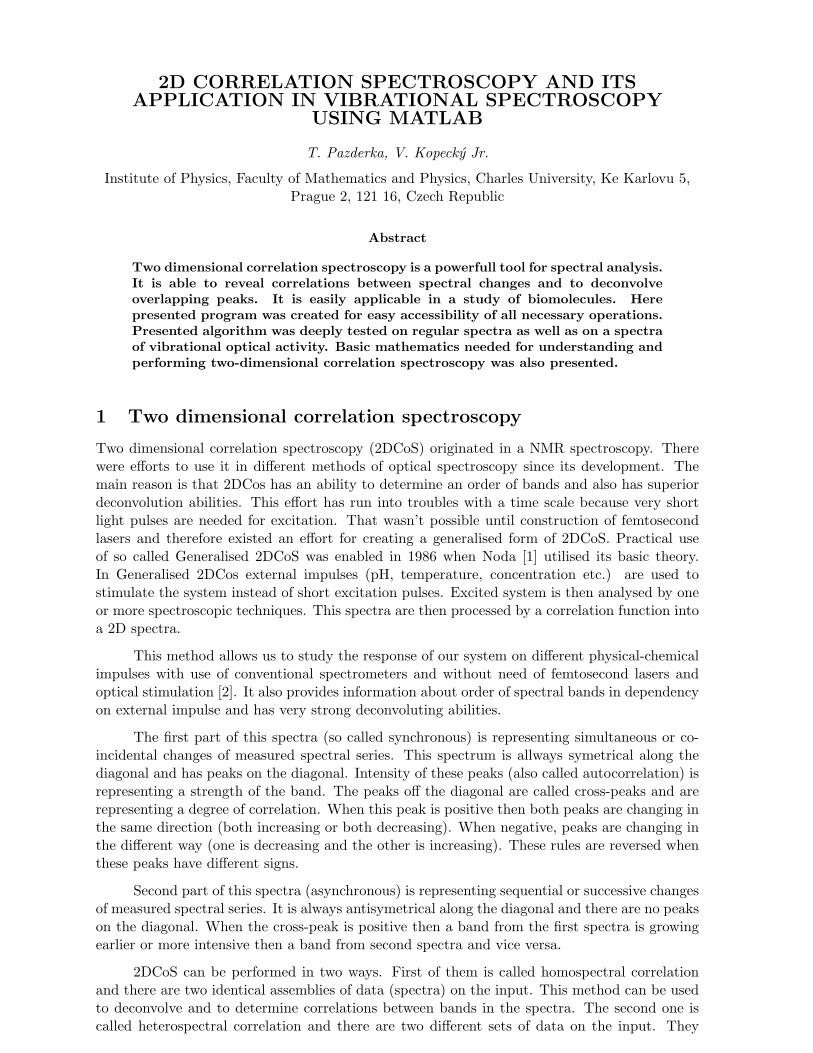
Figure 1: Synchronous (A) and asynchronous (B) spectra with marked correlation squares andpeaks.

Some basic properties of correlation spectra are marked on figure 1. We can see diagonalpeaks in the synchronous part and a symetrical positive cross-peak which indicates that bothbands are changing in the same way. There are no diagonal peaks in the asynchronous partand from negative peak in the lower right corner we can say that band on 70 is changing slowerthan band on 30 (positive peak in the upper left corner is saying the same). In both cases wecan draw so called correlation square which is connecting all peaks belonging to two correlatingbands.

2 Computation of 2D spectra

First of all we need a set of spectra measured on a system which was induced by some externalimpulse. Spectral intensities of this set can be expressed as I(ν, t) where ν is a spectral charac-teristic (wavenumber, wavelength or Raman shift) and t is a parameter of an external impulse.That can be an evolution in time, temperature, pH, concentration etc. Only certain range of tcan be measured and therefore a dynamical spectrum is implemented as [3]:

y(ν, t) =

{y(ν, t)− y(ν) if Tmin ≤ t ≤ Tmax,0 otherwise

(1)

where y(ν) is a reference spectrum of the system. An average spectrum is usually picked as areference spectrum but any reasonable spectrum can be chosen. Correlation spectrum is thendefined as:

χ(ν1, ν2) = 〈y(ν1, t) · y(ν2, t)〉 (2)

where the symbol 〈〉 is a crosscorrelation function defined as:

C(t, τ) = 〈Φ(τ)|Ψ(t)〉 (3)

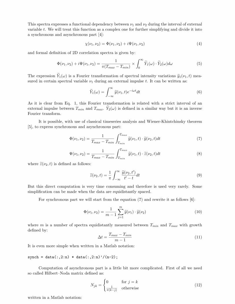
This spectra expresses a functional dependency between ν1 and ν2 during the interval of externalvariable t. We will treat this function as a complex one for further simplifying and divide it intoa synchronous and asynchronous part [4]:

χ(ν1, ν2) = Φ(ν1, ν2) + iΨ(ν1, ν2) (4)

and formal definition of 2D correlation spectra is given by:

Φ(ν1, ν2) + iΨ(ν1, ν2) =1

π(Tmax − Tmin)×

∫ ∞0

Y1(ω) · Y2(ω)dω (5)

The expression Y1(ω) is a Fourier transformation of spectral intensity variations y1(ν1, t) mea-sured in certain spectral variable ν1 during an external impulse t. It can be written as:

Y1(ω) =∫ ∞−∞

y(ν1, t)e−iωtdt (6)

As it is clear from Eq. 1, this Fourier transformation is related with a strict interval of anexternal impulse between Tmin and Tmax. Y2(ω) is defined in a similar way but it is an inverseFourier transform.

It is possible, with use of classical timeseries analysis and Wiener-Khintchinsky theorem[5], to express synchronous and asynchronous part:

Φ(ν1, ν2) =1

Tmax − Tmin

∫ Tmax

Tmin

y(ν1, t) · y(ν2, t)dt (7)

Ψ(ν1, ν2) =1

Tmax − Tmin

∫ Tmax

Tmin

y(ν1, t) · z(ν2, t)dt (8)

where z(ν2, t) is defined as follows:

z(ν2, t) =1π

∫ ∞−∞

y(ν2, t′)

t′ − tdt (9)

But this direct computation is very time consuming and therefore is used very rarely. Somesimplification can be made when the data are equidistantly spaced.

For synchronous part we will start from the equation (7) and rewrite it as follows [6]:

Φ(ν1, ν2) =1

m− 1

m∑j=1

y(ν1) · y(ν2) (10)

where m is a number of spectra equidistantly measured between Tmin and Tmax with growthdefined by:

∆t =Tmax − Tmin

m− 1(11)

It is even more simple when written in a Matlab notation:

synch = data(:,2:n) * data(:,2:n)’/(n-2);

Computation of asynchronous part is a little bit more complicated. First of all we needso called Hilbert–Noda matrix defined as:

Njk =

{0 for j = k

1π(k−j) otherwise

(12)

written in a Matlab notation:

N = zeros(n-1);for i=2:(n-1)

N(1,i) = 1/(pi * (i-1));endfor i=2:(n-2)

for j=i:(n-1)N(i,j) = N(i-1,j-1);

end;endfor i=2:(n-1)

for j=1:iN(i,j) = -N(j,i);

end;end

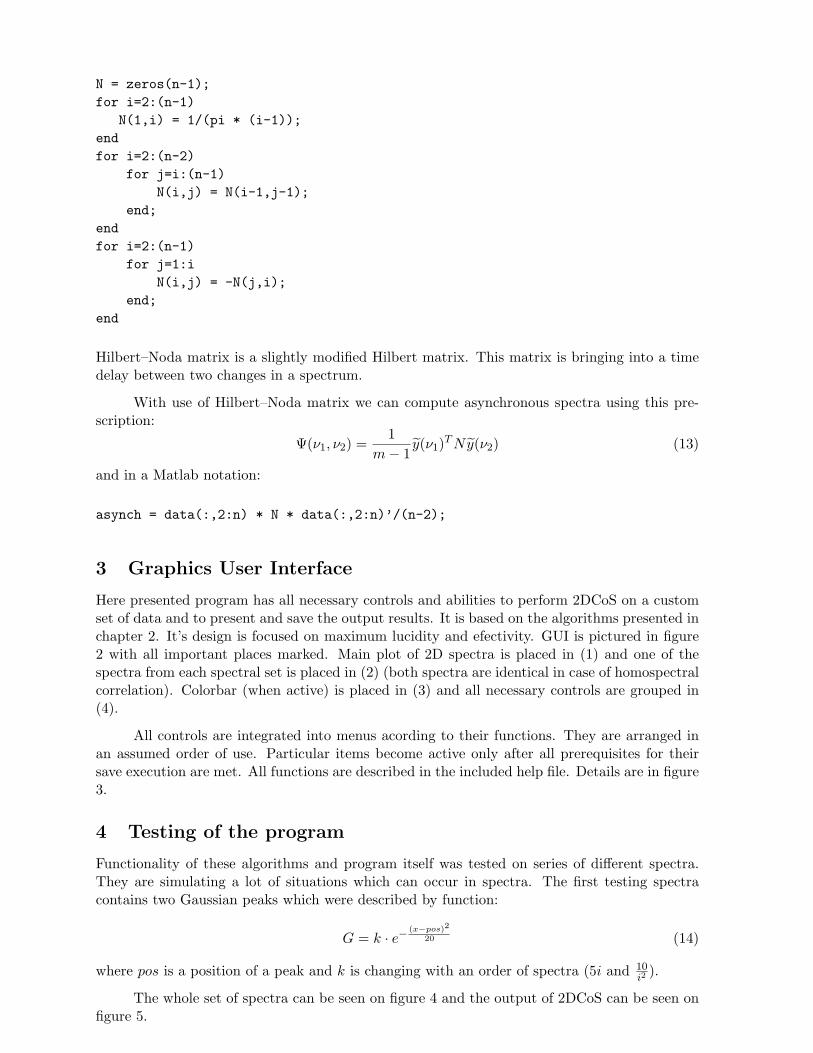
Hilbert–Noda matrix is a slightly modified Hilbert matrix. This matrix is bringing into a timedelay between two changes in a spectrum.

With use of Hilbert–Noda matrix we can compute asynchronous spectra using this pre-scription:

Ψ(ν1, ν2) =1

m− 1y(ν1)TNy(ν2) (13)

and in a Matlab notation:

asynch = data(:,2:n) * N * data(:,2:n)’/(n-2);

3 Graphics User Interface

Here presented program has all necessary controls and abilities to perform 2DCoS on a customset of data and to present and save the output results. It is based on the algorithms presented inchapter 2. It’s design is focused on maximum lucidity and efectivity. GUI is pictured in figure2 with all important places marked. Main plot of 2D spectra is placed in (1) and one of thespectra from each spectral set is placed in (2) (both spectra are identical in case of homospectralcorrelation). Colorbar (when active) is placed in (3) and all necessary controls are grouped in(4).

All controls are integrated into menus acording to their functions. They are arranged inan assumed order of use. Particular items become active only after all prerequisites for theirsave execution are met. All functions are described in the included help file. Details are in figure3.

4 Testing of the program

Functionality of these algorithms and program itself was tested on series of different spectra.They are simulating a lot of situations which can occur in spectra. The first testing spectracontains two Gaussian peaks which were described by function:

G = k · e−(x−pos)2

20 (14)

where pos is a position of a peak and k is changing with an order of spectra (5i and 10i2

).

The whole set of spectra can be seen on figure 4 and the output of 2DCoS can be seen onfigure 5.

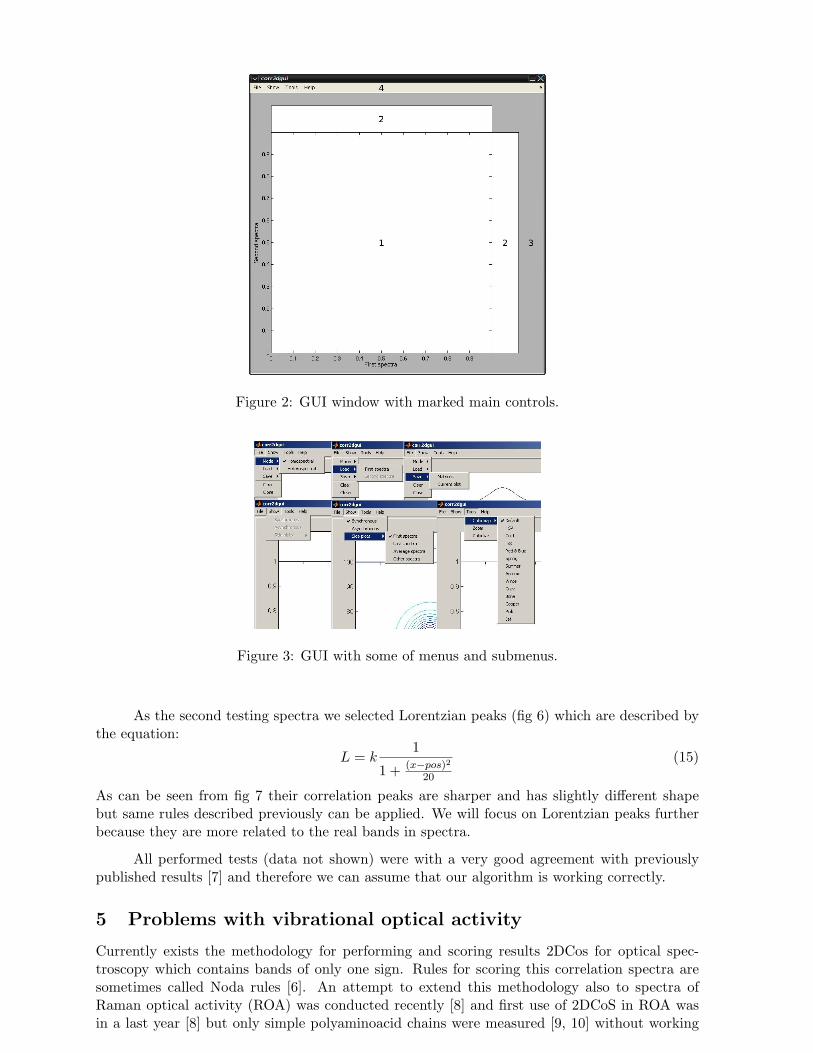
Figure 2: GUI window with marked main controls.

Figure 3: GUI with some of menus and submenus.

As the second testing spectra we selected Lorentzian peaks (fig 6) which are described bythe equation:

L = k1

1 + (x−pos)220

(15)

As can be seen from fig 7 their correlation peaks are sharper and has slightly different shapebut same rules described previously can be applied. We will focus on Lorentzian peaks furtherbecause they are more related to the real bands in spectra.

All performed tests (data not shown) were with a very good agreement with previouslypublished results [7] and therefore we can assume that our algorithm is working correctly.

5 Problems with vibrational optical activity

Currently exists the methodology for performing and scoring results 2DCos for optical spec-troscopy which contains bands of only one sign. Rules for scoring this correlation spectra aresometimes called Noda rules [6]. An attempt to extend this methodology also to spectra ofRaman optical activity (ROA) was conducted recently [8] and first use of 2DCoS in ROA wasin a last year [8] but only simple polyaminoacid chains were measured [9, 10] without working

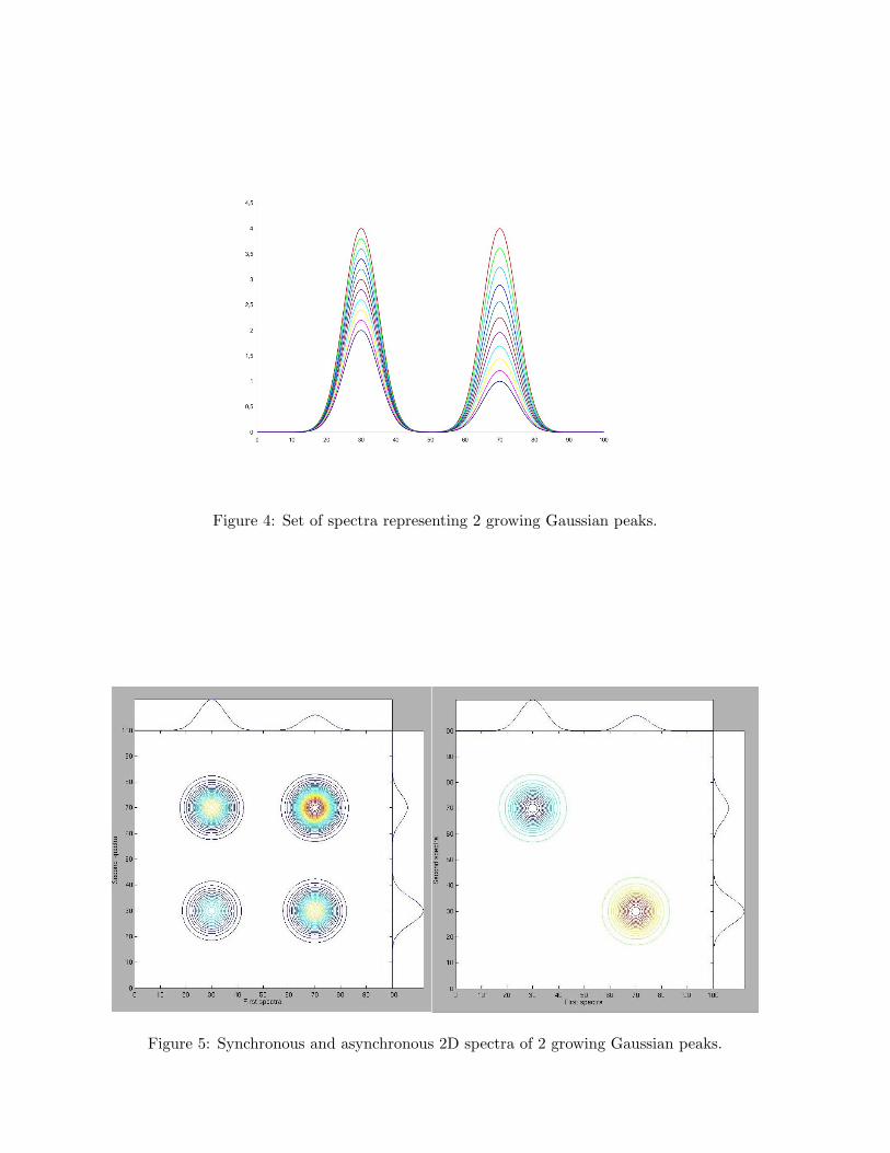
Figure 4: Set of spectra representing 2 growing Gaussian peaks.

Figure 5: Synchronous and asynchronous 2D spectra of 2 growing Gaussian peaks.

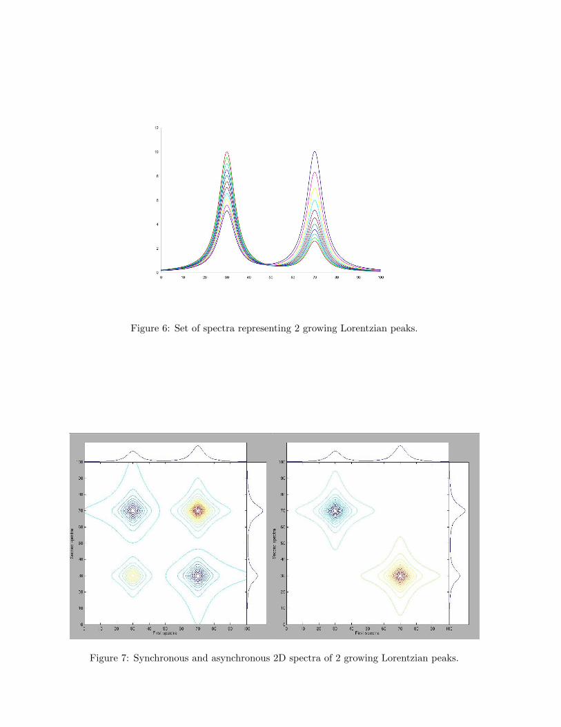
Figure 6: Set of spectra representing 2 growing Lorentzian peaks.

Figure 7: Synchronous and asynchronous 2D spectra of 2 growing Lorentzian peaks.

out a detailed methodology. ROA and vibrational circular dichroism (VCD) are different fromother spectroscopic techniques because they are differential methods and so they have bands ofboth polarity in spectra. The final methodology is a little bit different from the original rulesand is listed in [8].

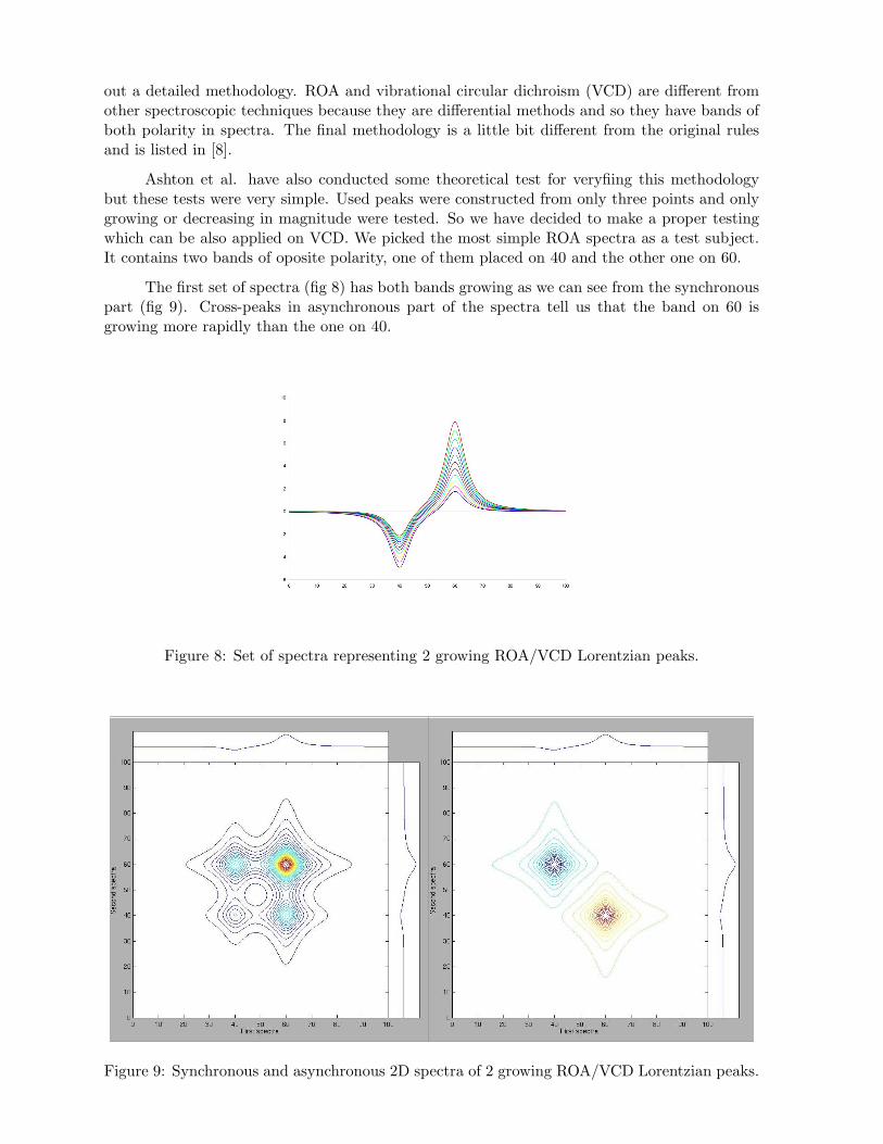
Ashton et al. have also conducted some theoretical test for veryfiing this methodologybut these tests were very simple. Used peaks were constructed from only three points and onlygrowing or decreasing in magnitude were tested. So we have decided to make a proper testingwhich can be also applied on VCD. We picked the most simple ROA spectra as a test subject.It contains two bands of oposite polarity, one of them placed on 40 and the other one on 60.

The first set of spectra (fig 8) has both bands growing as we can see from the synchronouspart (fig 9). Cross-peaks in asynchronous part of the spectra tell us that the band on 60 isgrowing more rapidly than the one on 40.

Figure 8: Set of spectra representing 2 growing ROA/VCD Lorentzian peaks.

Figure 9: Synchronous and asynchronous 2D spectra of 2 growing ROA/VCD Lorentzian peaks.

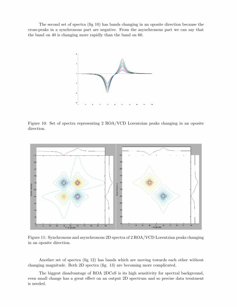
The second set of spectra (fig 10) has bands changing in an oposite direction because thecross-peaks in a synchronous part are negative. From the asynchronous part we can say thatthe band on 40 is changing more rapidly than the band on 60.

Figure 10: Set of spectra representing 2 ROA/VCD Lorentzian peaks changing in an opositedirection.

Figure 11: Synchronous and asynchronous 2D spectra of 2 ROA/VCD Lorentzian peaks changingin an oposite direction.

Another set of spectra (fig 12) has bands which are moving towards each other withoutchanging magnitude. Both 2D spectra (fig. 13) are becoming more complicated.

The biggest disadvantage of ROA 2DCoS is its high sensitivity for spectral background,even small change has a great effect on an output 2D spectrum and so precise data treatmentis needed.

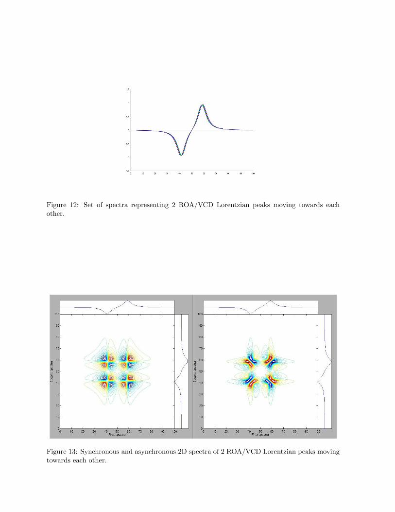
Figure 12: Set of spectra representing 2 ROA/VCD Lorentzian peaks moving towards eachother.

Figure 13: Synchronous and asynchronous 2D spectra of 2 ROA/VCD Lorentzian peaks movingtowards each other.

6 Conclusions and future work

Two-dimensional correlation spectroscopy is a usefull tool in studying dynamic changes in spec-tra or for deconvolving overlapping peaks. It can analyze a spectral set under some perturbationand find any correlations or coincidences between spectral changes. It can also analyze differentspectra under the same type of perturbation and then transfer explanation from one type ofspectra to another type of spectra. This method is applicable on study of biomolecules andtheir interactions.

Future work will be focused on optimalizing the code and on expanding capabilities of thisprogram to cover even some simple data treatment methods and to enhance its current abilities.We will also focus on practical use of this program in studying protein dynamics.

Acknowledgments: The Grant Agency of the Czech Republic and the Ministry of Educa-tion of the Czech Republic are gratefully acknowledged for support (No. 202/06/P208, No.GA202/07/0732 and No. MSM 0021620835, respectively).

References

[1] Noda, I. (1986) Two-dimensional infrared (2-D IR) spectroscopy of synthetic and biopoly-mer. Bull. Am. Phys. Soc., 31, 520

[2] Noda, I. (1990) Two-dimensional infrared (2DIR) spectroscopy: theory and applications,Appl. Spectrosc., 44, 550–561

[3] Noda, I. (1993) Generalized two-dimensional correlation method applicable to infrared,Raman, and other types of spectroscopy, Appl. Spectrosc., 47, 1329–1336

[4] Noda, I.; Dowrey, A. E.; Marcott, C. (1993) Recent developments in two-dimensional in-frared (2D IR) correlation spectroscopy, Appl. Spectrosc., 47, 1317–1323

[5] Noda, I. (2000) Determination of two-dimensional correlation spectra using Hilbert trans-form, Appl. Spectrosc. 54, 994–999

[6] Noda, I. (2002) General theory of two-dimensional (2D) analysis, in Handbook of vibrationalspectroscopy (Eds. Chalmers, J. M., Griffiths, P. R.), vol. 3, 2123–2134

[7] Noda, I.; Ozaki, Y. (2004) Two-dimensional correlation spectroscopy: Applications in vi-brational and optical spectroscopy, John Wiley and Sons

[8] Ashton, L.; Czarnik-Matusewicz, B.; Blanxh, E. W. (2006) Application of two-dimensionalcorrelation analysis to Raman optical activity, J. Mol. Struc., 799, 61–71

[9] Ashton, L; Barron, L. D.; Hecht, L; Hydec, J.; Blanch, E. W. (2007) Two-dimensional Ra-man and Raman optical activity correlation analysis of the α-helix-to-disordered transitionin poly(L-glutamic acid), Analyst, 132, 468–479

[10] Ashton, L.; Barron, L. D.; Czarnik-Matusewicz, B.; Hecht, L.; Hyde, J.; Blanch, E. W.(2006) Two-dimensional correlation analysis of Raman optical activity data on the α-helix-to-β-sheet transition in poly(L-lysine), Molecular Physics, 104, 1429–1445

Vladimır Kopecky Jr.Adress:Institute of Physics of Charles UniversityFaculty of Mathematics and Physics

Charles University in PragueKe Karlovu 5, 121 16 Praha 2Czech RepublicE-mail:kopecky@karlov.mff.cuni.cz