Embed Size (px)
Citation preview
Class Imbalance and Active Learning
Josh AttenbergEtsy
Brooklyn, NY [email protected]
Seyda ErtekinMIT Sloan School of Management
Massachusetts Institute of TechnologyCambridge, MA 02142
1 IntroductionThe rich history of predictive modeling has culminated in a diverse set of techniquescapable of making accurate predictions on many real-world problems. Many of thesetechniques demand training, whereby a set of instances with ground-truth labels(values of a dependent variable) are observed by a model-building process that attemptsto capture, at least in part, the relationship between the features of the instances andtheir labels. The resultant model can be applied to instances for which the label is notknown, to estimate or predict the labels. These predictions depend not only on thefunctional structure of the model itself, but on the particular data with which the modelwas trained. The accuracy of the predicted labels depends highly on the model’s abilityto capture an unbiased and sufficient understanding of the characteristics of differentclasses; in problems where the prevalence of classes is imbalanced, it is necessary toprevent the resultant model from being skewed towards the majority class and to ensurethat the model is capable of reflecting the true nature of the minority class.
Another consequence of class imbalance is observed in domains where the groundtruth labels in the dataset are not available beforehand and need to be gathered on-demand at some cost. The costs associated with collecting labels may be due tohuman labor or as a result of costly incentives, interventions or experiments. Inthese settings, simply labeling all available instances may not be practicable, dueto budgetary constraints or simply a strong desire to be cost efficient. In a similarfashion to predictive modeling with imbalanced classes, the goal here is to ensure thatthe budget is not predominantly expended on getting the labels of the majority classinstances, and to make sure that the set of instances to be labeled have comparablenumber of minority class instances as well.
In the context of learning from imbalanced datasets, the role of active learning canbe viewed from two different perspectives. The first perspective considers the casewhere the labels for all the examples in a reasonably large, imbalanced dataset arereadily available. The role of active learning in this case is to reduce, and potentiallyeliminate, any adverse effects that the class imbalance can have on the model’sgeneralization performance. The other perspective addresses the setting where we haveprior knowledge that the dataset is imbalanced, and we would like to employ active
1
learning to select informative examples both from the majority and minority classesfor labeling, subject to the constraints of a given budget. The first perspective focuseson active learning’s ability to address class imbalance, whereas the second perspectiveis concerned with the impact of class imbalance on the sampling performance of theactive learner. The intent of this chapter is to present a comprehensive analysis ofthis interplay of active learning and class imbalance. In particular, we first presenttechniques for dealing with the class imbalance problem using active learning anddiscuss how active learning can alleviate the issues that stem from class imbalance.We show that active learning, even without any adjustments to target class imbalance,is an effective strategy to have a balanced view of the dataset in most cases. It is alsopossible to further improve the effectiveness of active learning by tuning its samplingstrategy in a class-specific way. Additionally, we will focus on dealing with highlyskewed datasets and their impact on the selections performed by an active learningstrategy. Here, we discuss the impact significant class imbalance has on active learning,and illustrate alternatives to traditional active learning that may be considered whendealing with the most difficult, highly skewed problems.
2 Active Learning for Imbalanced ProblemsThe intent of this section is to provide the reader with some background on theactive learning problem in the context of building cost-effective classification models.We then discuss challenges encountered by active learning heuristics in settings withsignificant class imbalance. We then discuss strategies specialized in overcoming thedifficulties imposed by this setting.
2.1 Background on Active LearningActive Learning is specialized set of machine learning techniques developed forreducing the annotation costs associated with gathering the training data required forbuilding predictive statistical models. In many applications, unlabeled data comesrelatively cheaply when compared to the costs associated with the acquisition of aground-truth value of the target variable of that data. For instance, the textual contentof a particular web page may be crawled readily, or the actions of a user in a socialnetwork may be collected trivially by mining the web logs in that network. However,knowing with some degree of certainty the topical categorization of a particular webpage, or identifying any malicious activity of a user in a social network is likely torequire costly editorial review. These costs restrict the number of examples that maybe labeled, typically to a small fraction of the overall population. Because of thesepractical constraints typically placed on the overall number of ground truth labelsavailable, and the tight dependence of the performance of a predictive model on theexamples in its training set, the benefits of careful selection of the examples areapparent. This importance is further evidenced by the vast research literature on thetopic.
While an in-depth literature review is beyond the scope of this chapter, for contextwe provide a brief overview of some of the more broadly cited approaches in active
2
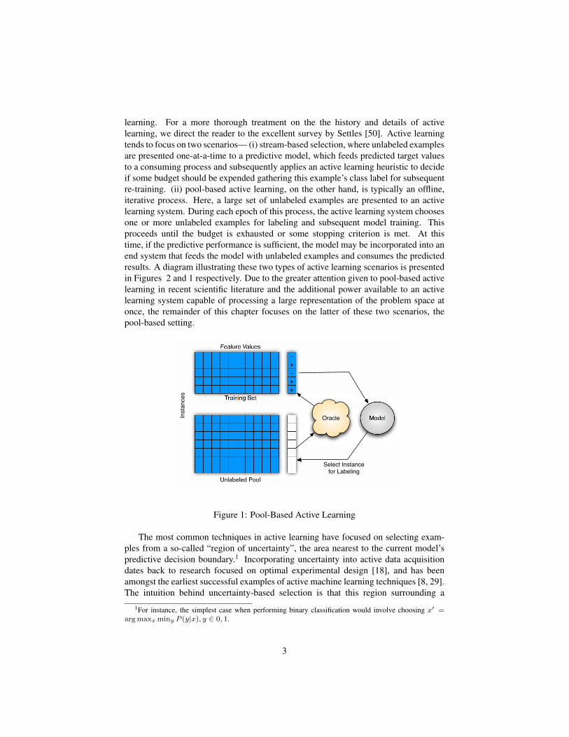
learning. For a more thorough treatment on the the history and details of activelearning, we direct the reader to the excellent survey by Settles [50]. Active learningtends to focus on two scenarios— (i) stream-based selection, where unlabeled examplesare presented one-at-a-time to a predictive model, which feeds predicted target valuesto a consuming process and subsequently applies an active learning heuristic to decideif some budget should be expended gathering this example’s class label for subsequentre-training. (ii) pool-based active learning, on the other hand, is typically an offline,iterative process. Here, a large set of unlabeled examples are presented to an activelearning system. During each epoch of this process, the active learning system choosesone or more unlabeled examples for labeling and subsequent model training. Thisproceeds until the budget is exhausted or some stopping criterion is met. At thistime, if the predictive performance is sufficient, the model may be incorporated into anend system that feeds the model with unlabeled examples and consumes the predictedresults. A diagram illustrating these two types of active learning scenarios is presentedin Figures 2 and 1 respectively. Due to the greater attention given to pool-based activelearning in recent scientific literature and the additional power available to an activelearning system capable of processing a large representation of the problem space atonce, the remainder of this chapter focuses on the latter of these two scenarios, thepool-based setting.
+
+
-
+
-
Instances
Feature Values
Training Set
Model
Unlabeled Pool
Oracle
Select Instancefor Labeling
Figure 1: Pool-Based Active Learning
The most common techniques in active learning have focused on selecting exam-ples from a so-called “region of uncertainty”, the area nearest to the current model’spredictive decision boundary.1 Incorporating uncertainty into active data acquisitiondates back to research focused on optimal experimental design [18], and has beenamongst the earliest successful examples of active machine learning techniques [8, 29].The intuition behind uncertainty-based selection is that this region surrounding a
1For instance, the simplest case when performing binary classification would involve choosing x′ =argmaxx miny P (y|x), y ∈ 0, 1.
3
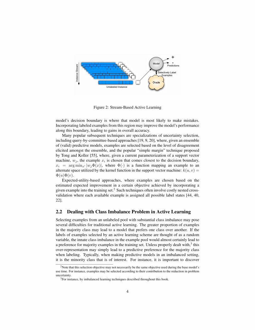
Instance Stream
Oracle
Model
Unlabeled Instance
+
-
Selectively Label Examples
Predictions
Figure 2: Stream-Based Active Learning
model’s decision boundary is where that model is most likely to make mistakes.Incorporating labeled examples from this region may improve the model’s performancealong this boundary, leading to gains in overall accuracy.
Many popular subsequent techniques are specializations of uncertainty selection,including query-by-committee-based approaches [19, 9, 20], where, given an ensembleof (valid) predictive models, examples are selected based on the level of disagreementelicited amongst the ensemble, and the popular “simple margin” technique proposedby Tong and Koller [55], where, given a current parameterization of a support vectormachine, wj , the example xi is chosen that comes closest to the decision boundary,xi = arg minx′ |wjΦ(x)|, where Φ(·) is a function mapping an example to analternate space utilized by the kernel function in the support vector machine: k(u, v) =Φ(u)Φ(v).
Expected-utility-based approaches, where examples are chosen based on theestimated expected improvement in a certain objective achieved by incorporating agiven example into the training set.2 Such techniques often involve costly nested cross-validation where each available example is assigned all possible label states [44, 40,22].
2.2 Dealing with Class Imbalance Problem in Active LearningSelecting examples from an unlabeled pool with substantial class imbalance may poseseveral difficulties for traditional active learning. The greater proportion of examplesin the majority class may lead to a model that prefers one class over another. If thelabels of examples selected by an active learning scheme are thought of as a randomvariable, the innate class imbalance in the example pool would almost certainly lead toa preference for majority examples in the training set. Unless properly dealt with,3 thisover-representation may simply lead to a predictive preference for the majority classwhen labeling. Typically, when making predictive models in an imbalanced setting,it is the minority class that is of interest. For instance, it is important to discover
2Note that this selection objective may not necessarily be the same objective used during the base model’suse time. For instance, examples may be selected according to their contribution to the reduction in problemuncertainty.
3For instance, by imbalanced learning techniques described throughout this book.
4
patients who have a rare but dangerous ailment based on the results of a blood test,or infrequent but costly fraud in a credit card company’s transaction history. Thisdifference in class preferences between an end-system’s needs and a model’s tendenciescauses a serious problem for active learning (and predictive systems in general) inimbalanced settings. Even if the problem of highly imbalanced (though correct interms of base rate) training set problem can be dealt with, the tendency for a selectionalgorithm to gather majority examples creates other problems. The nuances of theminority set may be poorly represented in the training data, leading to a “predictivemisunderstanding” in certain regions of the problem space; while a model may be ableto accurately identify large regions of the minority-space, portions of this space mayget mislabeled, or labeled with poor quality, due to underrepresentation in the trainingset. At the extreme, disjunctive sub-regions may get missed entirely. Both of theseproblems are particularly acute as the class imbalance increases, and are discussed ingreater detail in Section 6. Finally, in the initial stages of active learning, when thebase model is somewhat naïve, the minority class may get missed entirely as an activelearning heuristic probes the problem space for elusive but critical minority examples.
2.3 Addressing the Class Imbalance Problem with Active LearningAs we will demonstrate in Section 3, active learning presents itself as an effec-tive strategy for dealing with moderate class imbalance even, without any specialconsiderations for the skewed class distribution. However, the previously discusseddifficulties imposed by more substantial class imbalance on the selective abilitiesof active learning heuristics have led to the development of several techniques thathave been specially adapted to imbalanced problem settings. These skew-specializedactive learning techniques incorporate an innate preference for the minority class,leading to more balanced training sets and better predictive performance in imbalancedsettings. Additionally, there exists a category of density-sensitive active learningtechniques, techniques that explicitly incorporate the geometry of the problem space.By incorporating knowledge of independent dimensions of the unlabeled example pool,there exists a potential for better exploration, resulting in improved resolution of raresub-regions of the minority class. We detail these two broad classes of active learningtechniques below.
2.3.1 Density-Sensitive Active Learning
Utility-based selection strategies for active learning attribute some score, U(·), to eachinstance x encapsulating how much improvement can be expected from training onthat instance. Typically, the examples offering a maximum U(x) are selected forlabeling. However, the focus on individual examples may expose the selection heuristicto outliers, individual examples that achieve a high utility score, but do not represent asizable portion of the problem space. Density-sensitive active learning heuristics seekto alleviate this problem by leveraging the entire unlabeled pool of examples availableto the active learner. By explicitly incorporating the geometry of the input space whenattributing some selection score to a given example, outliers, noisy examples, and
5
sparse areas of the problem space may be avoided. Below are some exemplary activelearning heuristics that leverage density sensitivity.
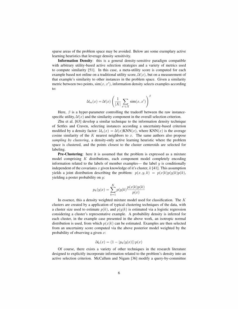
Information Density: this is a general density-sensitive paradigm compatiblewith arbitrary utility-based active selection strategies and a variety of metrics usedto compute similarity [51]. In this case, a meta-utility score is computed for eachexample based not online on a traditional utility score, U(x), but on a measurement ofthat example’s similarity to other instances in the problem space. Given a similaritymetric between two points, sim(x, x′), information density selects examples accordingto:
Um(x) = U(x)
(1
|X|∑x′∈X
sim(x, x′)
)βHere, β is a hyper-parameter controlling the tradeoff between the raw instance-
specific utility, U(x) and the similarity component in the overall selection criterion.Zhu et al. [63] develop a similar technique to the information density technique
of Settles and Craven, selecting instances according a uncertainty-based criterionmodified by a density factor: Un(x) = U(x)KNN(x), where KNN(x) is the averagecosine similarity of the K nearest neighbors to x. The same authors also proposesampling by clustering, a density-only active learning heuristic where the problemspace is clustered, and the points closest to the cluster centeroids are selected forlabeling.
Pre-Clustering: here it is assumed that the problem is expressed as a mixturemodel comprising K distributions, each component model completely encodinginformation related to the labels of member examples— the label y is conditionallyindependent of the covariates x given knowledge of it’s cluster, k [41]. This assumptionyields a joint distribution describing the problem: p(x, y, k) = p(x|k)p(y|k)p(k),yielding a poster probability on y:
pk(y|x) =
K∑k=1
p(y|k)p(x|k)p(k)
p(x)
In essence, this a density weighted mixture model used for classification. The Kclusters are created by a application of typical clustering techniques of the data, witha cluster size used to estimate p(k), and p(y|k) is estimated via a logistic regressionconsidering a cluster’s representative example. A probability density is inferred foreach cluster, in the example case presented in the above work, an isotropic normaldistribution is used, from which p(x|k) can be estimated. Examples are then selectedfrom an uncertainty score computed via the above posterior model weighted by theprobability of observing a given x:
Uk(x) = (1− |pk(y|x)|) p(x)
Of course, there exists a variety of other techniques in the research literaturedesigned to explicitly incorporate information related to the problem’s density into anactive selection criterion. McCallum and Nigam [36] modify a query-by-committee
6
to use an exponentiated KL-divergence-based uncertainty metric and combine thiswith semi-supervised learning in the form of an expectation maximization procedure.This combined semi-supervised active learning has the benefit of ignoring regions thatcan be reliably “filled in” by a semi-supervised procedure, while also selecting thoseexamples that may benefit this EM process.
Donmez et al. [12] propose a modification of the density-weighted technique ofNguyen and Smeulders. This modification simply selects examples according to theconvex combination of the density weighted technique and traditional uncertaintysampling. This hybrid approach is again incorporated into a so-called dual activelearner, where uncertainty sampling is only incorporated once the benefits of puredensity sensitive sampling seem to be diminishing.
Alternate Density-Sensitive Heuristics: Donmez and Carbonell [11] incorporatedensity into active label selection by performing a change of coordinates into a spacewhose metric expresses not only euclidian similarity but also density. Examplesare then chosen based on a density-weighted uncertainty metric designed to selectexamples in pairs— one member of the pair from each side of the current decisionboundary. The motivation is that sampling from both sides of the decision boundarymay yield better results than selecting from one side in isolation.
Through selection based on an “unsupervised” heuristic estimating the utility oflabel acquisition on the pool of unlabeled instances, Roy and McCallum incorporatethe geometry of the problem space into active selection implicitly [44]. This approachattempts to quantify the improvement in model performance attributable to eachunlabeled example, taken in expectation over all label assignments:
UE =∑y′∈Y
p(y′|x)∑x′ 6=X
Ue(x′;x, y = y′)
Here, the probability of class membership in the above expectation comes fromthe base model’s current posterior estimates. The utility value on the right side of theabove equation, Ue(x′;x, y = y′), comes from assuming a label of y′ for examplex, and incorporating this pseudo-labeled example into the training set temporarily.The improvement in model performance with the inclusion of this new example isthen measured. Since a selective label acquisition procedure may result in a small orarbitrarily biased set of examples, accurate evaluation through nested cross validationdifficult. To accommodate this, Roy and McCallum propose two uncertainty measurestaken over the pool of unlabeled examples, x′ 6= x. Specifically, they look at theentropy of the posterior probabilities of examples in the pool, and the magnitude ofthe maximum posterior as utility measures, both estimated after the inclusion of the“new” example. Both metrics favor “sharp” posteriors, an optimization minimizinguncertainty rather than model performance; instances are selected by their reduction inuncertainty taken in expectation over the entire example pool.
2.3.2 Skew-Specialized Active Learning
Additionally, there exists a body of research literature on active learning specificallyto deal with class imbalance problem. Tomanek [54] investigates query-by-committee-based approaches to sampling labeled sentences for the task of named entity recog-
7
nition. The goal of their selection strategy is to encourage class-balanced selectionsby incorporating class-specific costs. Unlabeled instances are ordered by a class-weighted, entropy-based disagreement measure, −
∑j∈{0,1} bj
V (kj)|C| log
V (kj)|C| , where
V (kj) is the number of votes from a committee of size |C| that an instance belongsto a class kj . bj is a weight corresponding to the importance of including a certainclass; a larger value of bj corresponds to a increased tendency to include examplesthat are thought to belong to this class. From a window W of examples with highestdisagreement, instances are selected greedily based on the model’s estimated classmembership probabilities so that the batch selected from the window has the highestprobability of having a balanced class membership.
SVM-based active learning has been shown [17] to be a highly effective strategy foraddressing class imbalance without any skew-specific modifications to the algorithm.Bloodgood and Shanker [5] extend the benefits of SVM-based active learning byproposing an approach that incorporates class specific costs. That is, the typical Cfactor describing an SVM’s misclassification penalty is broken up into C+ and C−,describing costs associated with misclassification of positive and negative examples,respectively, a common approach for improving the performance of support vectormachines in cost-sensitive settings. Additionally, cost sensitive support vector ma-chines is known to yield predictive advantages in imbalanced settings by offeringsome preference to an otherwise overlooked class, often using the heuristic for settingclass specific costs: C+
C−= |{x|x∈−}||{x|x∈+}| , a ratio in inverse proportion to the number of
examples in each class. However, in the active learning setting, the true class ratiois unknown, and the quantity C+
C−must be estimated by the active learning system.
Bloodgood and Shanker show that it is advantageous to use a preliminary stage ofrandom selection in order to establish some estimate of the class ratio, and then proceedwith example selection according to the uncertainty-based “simple margin” criterionusing the appropriately tuned cost-sensitive SVM.
Active learning has also been studied as a way to improve the generalizationperformance of resampling strategies that address class imbalance. In these settings,active learning is used to choose a set of instances for labeling, with sampling strategiesused to improve the class distribution. Ertekin [16] presented VIRTUAL, a hybridmethod of oversampling and active learning that forms an adaptive technique forresampling of the minority class instances. The learner selects the most informativeexample xi for oversampling, and the algorithm creates a synthetic instance along thedirection of xi’s one of k neighbors. The algorithm works in an online fashion andbuilds the classifier incrementally without the need to retrain on the entire labeleddataset after creating a new synthetic example. This approach, which we present indetail in Section 4, yields an efficient and scalable learning framework.
Zhu and Hovy [62] describe a bootstrap-based oversampling strategy (BootOS)that, given an example to be resampled, generates a bootstrap example based on all thek neighbors of that example. At each epoch, the examples with the greatest uncertaintyare selected for labeling and incorporated into a labeled set, L. From L, the proposedoversampling strategy is applied, yielding a more balanced data set, L′ , a data setthat is used to retrain the base model. The selection of the examples with the highestuncertainty for labeling at each iteration involves resampling the labeled examples
8
and training a new classifier with the resampled dataset, therefore, scalability of thisapproach may be a concern for large scale datasets.
In the next section, we demonstrate that the principles of active learning arenaturally suited to address the class imbalance problem and that active learning canin fact be an effective strategy to have construct a balanced view of an otherwiseimbalanced dataset, without the need to resort to resampling techniques. It is worthnoting that the goal of the next section is not to cast active learning as a replacementfor resampling strategies. Rather, our main goal is to demonstrate how active learningcan alleviate the issues that stem from class imbalance, and to present active learningas an alternate technique that should be considered in case a resampling approach isimpractical, inefficient or ineffective. In problems where resampling is the preferredsolution, we show in Section 4 that the benefits of active learning can still be leveragedto address class imbalance. In particular, we present an adaptive oversamplingtechnique that uses active learning to determine which examples to resample in anonline setting. These two different approaches show the versatility of active learningand the importance of selective sampling to address the class imbalance problem.
3 Active Learning for Imbalanced Data ClassificationAs outlined in Section 2.1, active learning is primarily considered as a technique toreduce the number of training samples that need to be labeled for a classification task.From a traditional perspective, the active learner has access to a vast pool of unlabeledexamples, and it aims to make a clever choice to select the most informative example toobtain its label. However, even in the cases where the labels of training data are alreadyavailable, active learning can still be leveraged to obtain the informative examplesthrough training sets [49, 6, 24]. For example, in large-margin classifiers such asSupport Vector Machines (SVM), the informativeness of an example is synonymouswith its distance to the hyperplane. The farther an example is to the hyperplane, themore the learner is confident about its true class label; hence there is little, if any,benefit that the learner can gain by asking for the label of that example. On the otherhand, the examples close to the hyperplane are the ones that yield the most informationto the learner. Therefore, the most commonly used active learning strategy in SVMsis to check the distance of each unlabeled example to the hyperplane and focus onthe examples that lie closest to the hyperplane, as they are considered to be the mostinformative examples to the learner [55].
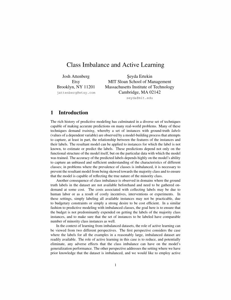
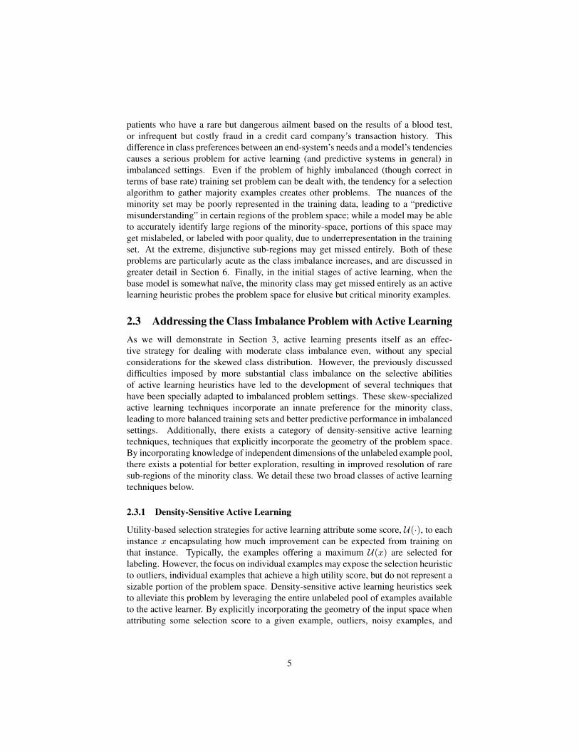
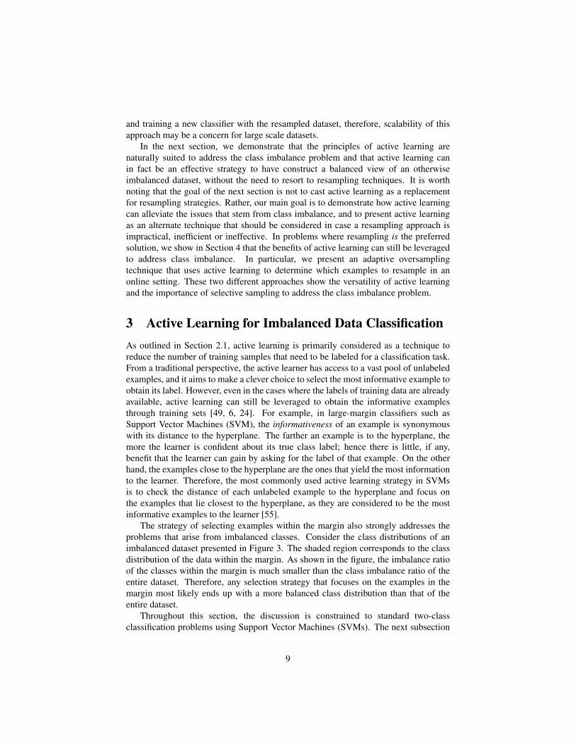
The strategy of selecting examples within the margin also strongly addresses theproblems that arise from imbalanced classes. Consider the class distributions of animbalanced dataset presented in Figure 3. The shaded region corresponds to the classdistribution of the data within the margin. As shown in the figure, the imbalance ratioof the classes within the margin is much smaller than the class imbalance ratio of theentire dataset. Therefore, any selection strategy that focuses on the examples in themargin most likely ends up with a more balanced class distribution than that of theentire dataset.
Throughout this section, the discussion is constrained to standard two-classclassification problems using Support Vector Machines (SVMs). The next subsection
9
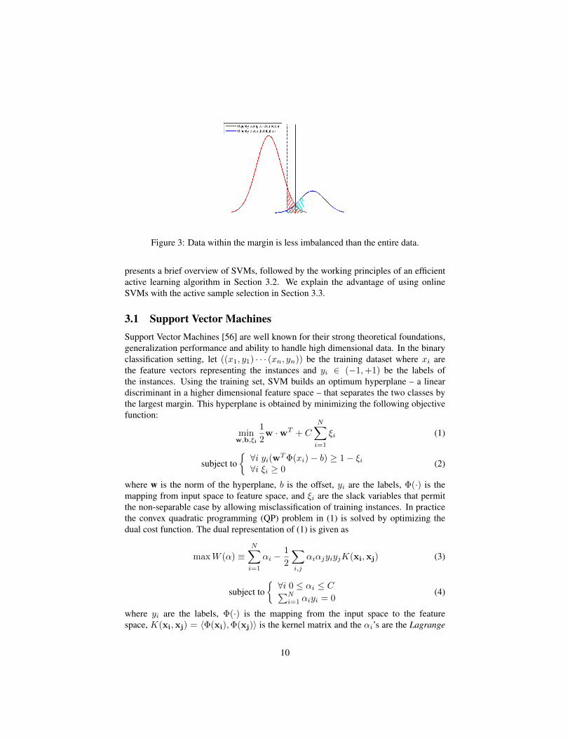
Figure 3: Data within the margin is less imbalanced than the entire data.
presents a brief overview of SVMs, followed by the working principles of an efficientactive learning algorithm in Section 3.2. We explain the advantage of using onlineSVMs with the active sample selection in Section 3.3.
3.1 Support Vector MachinesSupport Vector Machines [56] are well known for their strong theoretical foundations,generalization performance and ability to handle high dimensional data. In the binaryclassification setting, let ((x1, y1) · · · (xn, yn)) be the training dataset where xi arethe feature vectors representing the instances and yi ∈ (−1,+1) be the labels ofthe instances. Using the training set, SVM builds an optimum hyperplane – a lineardiscriminant in a higher dimensional feature space – that separates the two classes bythe largest margin. This hyperplane is obtained by minimizing the following objectivefunction:
minw,b,ξi
1
2w ·wT + C
N∑i=1
ξi (1)
subject to{∀i yi(wTΦ(xi)− b) ≥ 1− ξi∀i ξi ≥ 0
(2)
where w is the norm of the hyperplane, b is the offset, yi are the labels, Φ(·) is themapping from input space to feature space, and ξi are the slack variables that permitthe non-separable case by allowing misclassification of training instances. In practicethe convex quadratic programming (QP) problem in (1) is solved by optimizing thedual cost function. The dual representation of (1) is given as
maxW (α) ≡N∑i=1
αi −1
2
∑i,j
αiαjyiyjK(xi,xj) (3)
subject to{∀i 0 ≤ αi ≤ C∑Ni=1 αiyi = 0
(4)
where yi are the labels, Φ(·) is the mapping from the input space to the featurespace, K(xi,xj) = 〈Φ(xi),Φ(xj)〉 is the kernel matrix and the αi’s are the Lagrange
10
multipliers which are non-zero only for the training instances which fall in the margin.Those training instances are called support vectors and they define the position ofthe hyperplane. After solving the QP problem, the norm of the hyperplane w canbe represented as
w =
n∑i=1
αiΦ(xi) (5)
3.2 Margin-based Active Learning with SVMsNote that in (5), only the support vectors affect the SVM solution. This means that ifSVM is retrained with a new set of data which only consist of those support vectors,the learner will end up finding the same hyperplane. This emphasizes the fact that notall examples are equally important in training sets. Then the question becomes howto select the most informative examples for labeling from the set of unlabeled trainingexamples. This section focuses on a form of selection strategy called margin-basedactive learning. As was highlighted earlier, in SVMs the most informative exampleis believed to be the closest one to the hyperplane since it divides the version spaceinto two equal parts. The aim is to reduce the version space as fast as possible toreach the solution faster in order to avoid certain costs associated with the problem.For the possibility of a non-symmetric version space, there are more complex selectionmethods suggested by [55], but it has been observed that the advantage of those are notsignificant, considering their high computational costs.
Active Learning with Small Pools: The basic working principle of margin-basedactive learning with SVMs is: i) train an SVM on the existing training data, ii) selectthe closest example to the hyperplane, and iii) add the new selected example to thetraining set and train again. In classical active learning [55], the search for the mostinformative example is performed over the entire dataset. Note that, each iteration ofactive learning involves the recomputation of each training example’s distance to thenew hyperplane. Therefore, for large datasets, searching the entire training set is a verytime consuming and computationally expensive task.
One possible remedy for this performance bottleneck is to use the “59 trick”[53], which alleviates a full search through the entire dataset, approximating themost informative examples by examining a small constant number of randomlychosen samples. The method picks L (L � # training examples) random trainingsamples in each iteration and selects the best (closest to the hyperplane) amongthem. Suppose, instead of picking the closest example among all the training samplesXN = (x1, x2, · · · , xN ) at each iteration, we first pick a random subset XL, L � Nand select the closest sample xi from XL based on the condition that xi is among thetop p% closest instances in XN with probability (1− η). Any numerical modificationto these constraints can be met by varying the size of L, and is independent of N . Todemonstrate, the probability that at least one of the L instances is among the closest pis 1− (1− p)L. Due to the requirement of (1− η) probability, we have
1− (1− p)L = 1− η (6)
11
which follows the solution of L in terms of η and p
L = log η / log(1− p) (7)
For example, the active learner will pick one example, with 95% probability, that isamong the top 5% closest instances to the hyperplane, by randomly sampling onlydlog(.05)/ log(.95)e = 59 examples regardless of the training set size. This approachscales well since the size of the subset L is independent of the training set size N ,requires significantly less training time and does not have an adverse effect on theclassification performance of the learner.
3.3 Active Learning with Online LearningOnline learning algorithms are usually associated with problems where the completetraining set is not available. However, in cases where the complete training set isavailable, the computational properties of these algorithms can be leveraged for fasterclassification and incremental learning. Online learning techniques can process newdata presented one at a time, either as the result of active learning or random selection,and can integrate the information of the new data to the system without training on allpreviously seen data, thereby allowing models to be constructed incrementally. Thisworking principle of online learning algorithms leads to speed improvements and areduced memory footprint, making the algorithm applicable to very large datasets.More importantly, this incremental learning principle suits the nature of active learningin a much more naturally than the batch algorithms. Empirical evidence indicates thata single presentation of each training example to the algorithm is sufficient to achievetraining errors comparable to those achieved by the best minimization of the SVMobjective [6].
3.4 Performance MetricsClassification accuracy is not a good metric to evaluate classifiers in applications facingclass imbalance problems. SVMs have to achieve a tradeoff between maximizingthe margin and minimizing the empirical error. In the non-separable case, if themisclassification penalty C is very small, the SVM learner simply tends to classifyevery example as negative. This extreme approach maximizes the margin while makingno classification errors on the negative instances. The only error is the cumulative errorof the positive instances which are already few in numbers. Considering an imbalanceratio of 99 to 1, a classifier that classifies everything as negative, will be 99% accurate.Obviously, such a scheme would not have any practical use as it would be unable toidentify positive instances.
For the evaluation of these results, it is useful to consider several other pre-diction performance metrics such as g-means, AUC and PRBEP which are com-monly used in imbalanced data classification. g-means [27] is denoted as g =√sensitivity · specificity where sensitivity is the accuracy on the positive instances
given as TruePos./(TruePos. + FalseNeg.) and specificity is the accuracy on thenegative instances given as TrueNeg./(TrueNeg.+ FalsePos.).
12
The Receiver Operating Curve (ROC) displays the relationship between sensitivityand specificity at all possible thresholds for a binary classification scoring model, whenapplied to independent test data. In other words, ROC curve is a plot of the true positiverate against the false positive rate as the decision threshold is changed. The area underthe ROC curve (AUC) is a numerical measure of a model’s discrimination performanceand shows how successfully and correctly the model ranks and thereby separates thepositive and negative observations. Since the AUC metric evaluates the classifier acrossthe entire range of decision thresholds, it gives a good overview about the performancewhen the operating condition for the classifier is unknown or the classifier is expectedto be used in situations with significantly different class distributions.
Precision Recall Break-Even Point (PRBEP) is another commonly used perfor-mance metric for imbalanced data classification. PRBEP is the accuracy of thepositive class at the threshold where precision equals to recall. Precision is defined asTruePos./(TruePos.+FalsePos.) and recall is defined as TruePos./(TruePos.+FalseNeg.)
3.5 Experiments and Empirical EvaluationWe study the performance of the algorithm on various benchmark real-world datasets,including MNIST, USPS, several categories of Reuters-21578 collection, five topicsfrom CiteSeer, and three datasets from the UCI repository. The characteristics of thedatasets are outlined in [17]. In the experiments, an early stopping heuristic for active
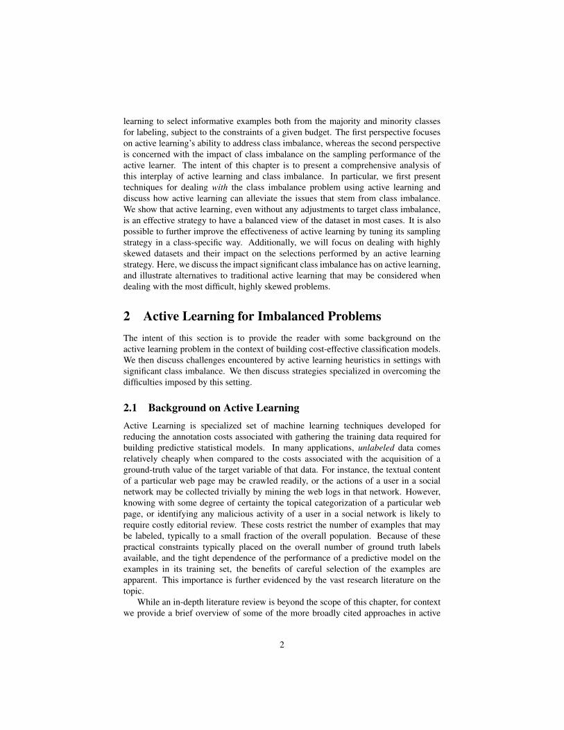
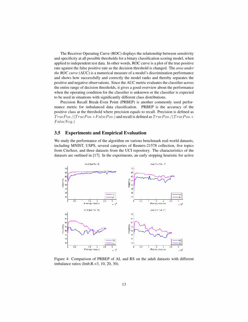
Figure 4: Comparison of PRBEP of AL and RS on the adult datasets with differentimbalance ratios (Imb.R.=3, 10, 20, 30).
13
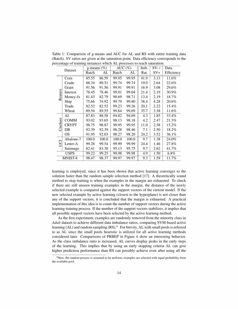
Table 1: Comparison of g-means and AUC for AL and RS with entire training data(Batch). SV ratios are given at the saturation point. Data efficiency corresponds to thepercentage of training instances which AL processes to reach saturation.
Dataset g-means (%) AUC (%) Imb. SV- / DataEfficiencyBatch AL Batch AL Rat. SV+
Reu
ters
Corn 85.55 86.59 99.95 99.95 41.9 3.13 11.6%Crude 88.34 89.51 99.74 99.74 19.0 2.64 22.6%Grain 91.56 91.56 99.91 99.91 16.9 3.08 29.6%Interest 78.45 78.46 99.01 99.04 21.4 2.19 30.9%Money-fx 81.43 82.79 98.69 98.71 13.4 2.19 18.7%Ship 75.66 74.92 99.79 99.80 38.4 4.28 20.6%Trade 82.52 82.52 99.23 99.26 20.1 2.22 15.4%Wheat 89.54 89.55 99.64 99.69 35.7 3.38 11.6%
Cite
Seer
AI 87.83 88.58 94.82 94.69 4.3 1.85 33.4%COMM 93.02 93.65 98.13 98.18 4.2 2.47 21.3%CRYPT 98.75 98.87 99.95 99.95 11.0 2.58 15.2%DB 92.39 92.39 98.28 98.46 7.1 2.50 18.2%OS 91.95 92.03 98.27 98.20 24.2 3.52 36.1%
UC
I Abalone-7 100.0 100.0 100.0 100.0 9.7 1.38 24.0%Letter-A 99.28 99.54 99.99 99.99 24.4 1.46 27.8%Satimage 82.41 83.30 95.13 95.75 9.7 2.62 41.7%USPS 99.22 99.25 99.98 99.98 4.9 1.50 6.8%
MNIST-8 98.47 98.37 99.97 99.97 9.3 1.59 11.7%
learning is employed, since it has been shown that active learning converges to thesolution faster than the random sample selection method [17]. A theoretically soundmethod to stop training is when the examples in the margin are exhausted. To checkif there are still unseen training examples in the margin, the distance of the newlyselected example is compared against the support vectors of the current model. If thenew selected example by active learning (closest to the hyperplane) is not closer thanany of the support vectors, it is concluded that the margin is exhausted. A practicalimplementation of this idea is to count the number of support vectors during the activelearning training process. If the number of the support vectors stabilizes, it implies thatall possible support vectors have been selected by the active learning method.
As the first experiment, examples are randomly removed from the minority class inAdult dataset to achieve different data imbalance ratios, comparing SVM-based activelearning (AL) and random sampling (RS).4 For brevity, AL with small pools is referredto as AL since the small pools heuristic is utilized for all active learning methodsconsidered later. Comparisons of PRBEP in Figure 4 show an interesting behavior.As the class imbalance ratio is increased, AL curves display peaks in the early stepsof the learning. This implies that by using an early stopping criteria AL can givehigher prediction performance than RS can possibly achieve even after using all the
4Here, the random process is assumed to be uniform; examples are selected with equal probability fromthe available pool.
14
0 1000 2000 3000 4000 5000 6000 7000 80000
0.1
0.2
0.3
0.4
0.5
0.6
0.7
0.8
0.9
1
crude7770
AL SV+:SV−
RS SV+:SV−
data ratio: 0.0527
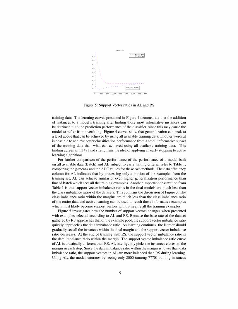
Figure 5: Support Vector ratios in AL and RS
training data. The learning curves presented in Figure 4 demonstrate that the additionof instances to a model’s training after finding those most informative instances canbe detrimental to the prediction performance of the classifier, since this may cause themodel to suffer from overfitting. Figure 4 curves show that generalization can peak toa level above that can be achieved by using all available training data. In other words,itis possible to achieve better classification performance from a small informative subsetof the training data than what can achieved using all available training data. Thisfinding agrees with [49] and strengthens the idea of applying an early stopping to activelearning algorithms.
For further comparison of the performance of the performance of a model builton all available data (Batch) and AL subject to early halting criteria, refer to Table 1,comparing the g-means and the AUC values for these two methods. The data efficiencycolumn for AL indicates that by processing only a portion of the examples from thetraining set, AL can achieve similar or even higher generalization performance thanthat of Batch which sees all the training examples. Another important observation fromTable 1 is that support vector imbalance ratios in the final models are much less thanthe class imbalance ratios of the datasets. This confirms the discussion of Figure 3. Theclass imbalance ratio within the margins are much less than the class imbalance ratioof the entire data and active learning can be used to reach those informative exampleswhich most likely become support vectors without seeing all the training examples.
Figure 5 investigates how the number of support vectors changes when presentedwith examples selected according to AL and RS. Because the base rate of the datasetgathered by RS approaches that of the example pool, the support vector imbalance ratioquickly approaches the data imbalance ratio. As learning continues, the learner shouldgradually see all the instances within the final margin and the support vector imbalanceratio decreases. At the end of training with RS, the support vector imbalance ratio isthe data imbalance ratio within the margin. The support vector imbalance ratio curveof AL is drastically different than RS. AL intelligently picks the instances closest to themargin in each step. Since the data imbalance ratio within the margin is lower than dataimbalance ratio, the support vectors in AL are more balanced than RS during learning.Using AL, the model saturates by seeing only 2000 (among 7770) training instances
15
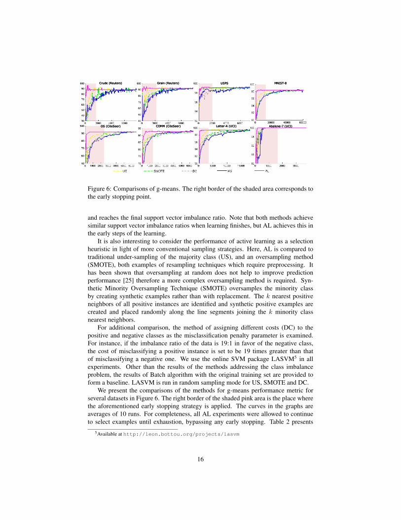
Figure 6: Comparisons of g-means. The right border of the shaded area corresponds tothe early stopping point.
and reaches the final support vector imbalance ratio. Note that both methods achievesimilar support vector imbalance ratios when learning finishes, but AL achieves this inthe early steps of the learning.
It is also interesting to consider the performance of active learning as a selectionheuristic in light of more conventional sampling strategies. Here, AL is compared totraditional under-sampling of the majority class (US), and an oversampling method(SMOTE), both examples of resampling techniques which require preprocessing. Ithas been shown that oversampling at random does not help to improve predictionperformance [25] therefore a more complex oversampling method is required. Syn-thetic Minority Oversampling Technique (SMOTE) oversamples the minority classby creating synthetic examples rather than with replacement. The k nearest positiveneighbors of all positive instances are identified and synthetic positive examples arecreated and placed randomly along the line segments joining the k minority classnearest neighbors.
For additional comparison, the method of assigning different costs (DC) to thepositive and negative classes as the misclassification penalty parameter is examined.For instance, if the imbalance ratio of the data is 19:1 in favor of the negative class,the cost of misclassifying a positive instance is set to be 19 times greater than thatof misclassifying a negative one. We use the online SVM package LASVM5 in allexperiments. Other than the results of the methods addressing the class imbalanceproblem, the results of Batch algorithm with the original training set are provided toform a baseline. LASVM is run in random sampling mode for US, SMOTE and DC.
We present the comparisons of the methods for g-means performance metric forseveral datasets in Figure 6. The right border of the shaded pink area is the place wherethe aforementioned early stopping strategy is applied. The curves in the graphs areaverages of 10 runs. For completeness, all AL experiments were allowed to continueto select examples until exhaustion, bypassing any early stopping. Table 2 presents
5Available at http://leon.bottou.org/projects/lasvm
16
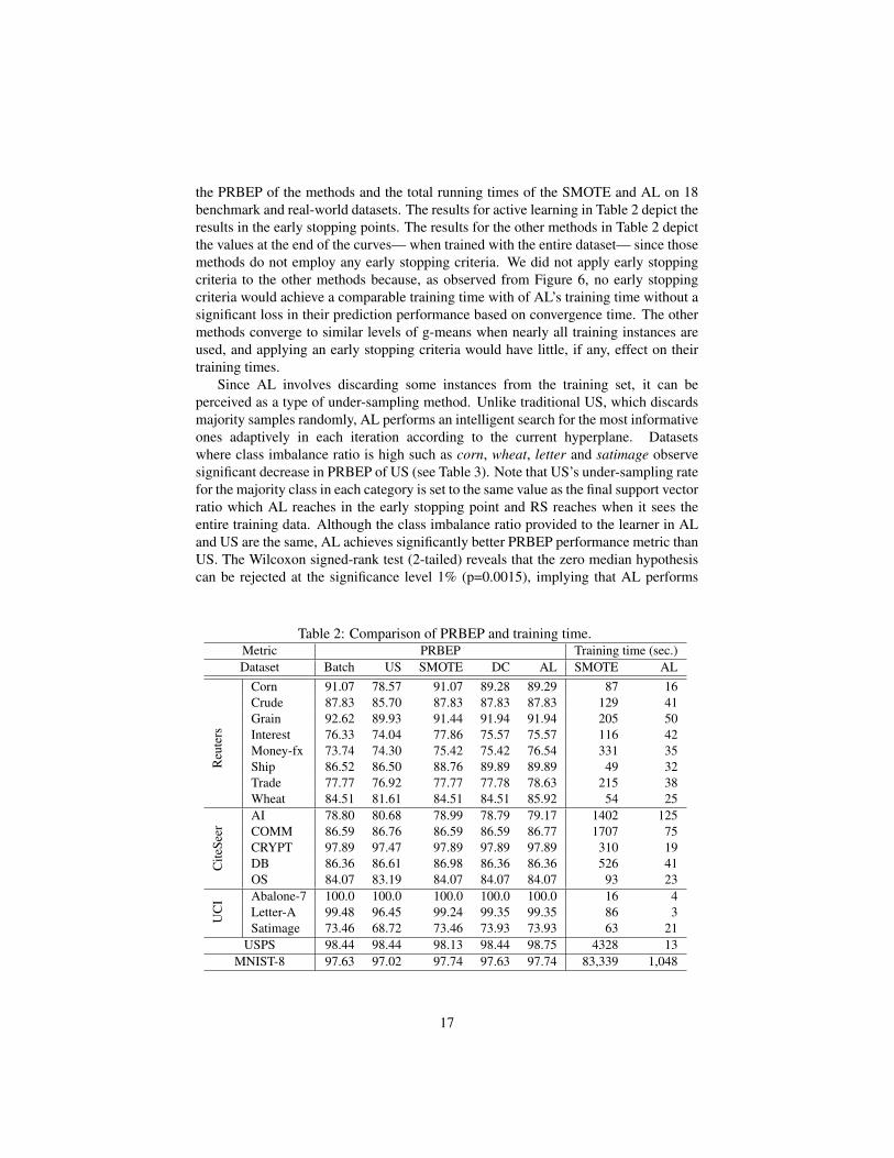
the PRBEP of the methods and the total running times of the SMOTE and AL on 18benchmark and real-world datasets. The results for active learning in Table 2 depict theresults in the early stopping points. The results for the other methods in Table 2 depictthe values at the end of the curves— when trained with the entire dataset— since thosemethods do not employ any early stopping criteria. We did not apply early stoppingcriteria to the other methods because, as observed from Figure 6, no early stoppingcriteria would achieve a comparable training time with of AL’s training time without asignificant loss in their prediction performance based on convergence time. The othermethods converge to similar levels of g-means when nearly all training instances areused, and applying an early stopping criteria would have little, if any, effect on theirtraining times.
Since AL involves discarding some instances from the training set, it can beperceived as a type of under-sampling method. Unlike traditional US, which discardsmajority samples randomly, AL performs an intelligent search for the most informativeones adaptively in each iteration according to the current hyperplane. Datasetswhere class imbalance ratio is high such as corn, wheat, letter and satimage observesignificant decrease in PRBEP of US (see Table 3). Note that US’s under-sampling ratefor the majority class in each category is set to the same value as the final support vectorratio which AL reaches in the early stopping point and RS reaches when it sees theentire training data. Although the class imbalance ratio provided to the learner in ALand US are the same, AL achieves significantly better PRBEP performance metric thanUS. The Wilcoxon signed-rank test (2-tailed) reveals that the zero median hypothesiscan be rejected at the significance level 1% (p=0.0015), implying that AL performs
Table 2: Comparison of PRBEP and training time.Metric PRBEP Training time (sec.)Dataset Batch US SMOTE DC AL SMOTE AL
Reu
ters
Corn 91.07 78.57 91.07 89.28 89.29 87 16Crude 87.83 85.70 87.83 87.83 87.83 129 41Grain 92.62 89.93 91.44 91.94 91.94 205 50Interest 76.33 74.04 77.86 75.57 75.57 116 42Money-fx 73.74 74.30 75.42 75.42 76.54 331 35Ship 86.52 86.50 88.76 89.89 89.89 49 32Trade 77.77 76.92 77.77 77.78 78.63 215 38Wheat 84.51 81.61 84.51 84.51 85.92 54 25
Cite
Seer
AI 78.80 80.68 78.99 78.79 79.17 1402 125COMM 86.59 86.76 86.59 86.59 86.77 1707 75CRYPT 97.89 97.47 97.89 97.89 97.89 310 19DB 86.36 86.61 86.98 86.36 86.36 526 41OS 84.07 83.19 84.07 84.07 84.07 93 23
UC
I Abalone-7 100.0 100.0 100.0 100.0 100.0 16 4Letter-A 99.48 96.45 99.24 99.35 99.35 86 3Satimage 73.46 68.72 73.46 73.93 73.93 63 21
USPS 98.44 98.44 98.13 98.44 98.75 4328 13MNIST-8 97.63 97.02 97.74 97.63 97.74 83,339 1,048
17
statistically better than US in these 18 datasets. These results reveal the importance ofusing the informative instances for learning.
Table 2 gives the comparison of the computation times of the AL and SMOTE.Note that SMOTE requires significantly long preprocessing time which dominates thetraining time in large datasets, e.g., MNIST-8 dataset. The low computation cost,scalability and high prediction performance of AL suggest that AL can efficientlyhandle the class imbalance problem.
4 Adaptive Resampling with Active LearningThe analysis in Section 3.5 shows the effectiveness of active learning on imbalanceddatasets without employing any resampling techniques. This section extends thediscussion on the effectiveness of active learning for imbalanced data classification,and demonstrates that even in cases where resampling is the preferred approach, activelearning can still be used to significantly improve the classification performance.
In supervised learning, a common strategy to overcome the rarity problem is toresample the original dataset to decrease the overall level of class imbalance. Resam-pling is done either by oversampling the minority (positive) class and/or undersamplingthe majority (negative) class until the classes are approximately equally represented[7, 26, 27, 31]. Oversampling, in its simplest form, achieves a more balanced classdistribution either by duplicating minority class instances, or introducing new syntheticinstances that belong to the minority class [7]. No information is lost in oversamplingsince all original instances of the minority and the majority classes are retained inthe oversampled dataset. The other strategy to reduce the class imbalance is under-sampling, which eliminates some majority class instances mostly by random sampling.
Even though both approaches address the class imbalance problem, they alsosuffer some drawbacks. The under-sampling strategy can potentially sacrifice theprediction performance of the model, since it is possible to discard informativeinstances that the learner might benefit. Oversampling strategy, on the other hand,can be computationally overwhelming in cases with large training sets— if a complexoversampling method is used, a large computational effort must be expended duringpreprocessing of the data. Worse, oversampling causes longer training time duringthe learning process due to the increased number of training instances. In additionto suffering from increased runtime due to added computational complexity, it alsonecessitates an increased memory footprint due to the extra storage requirements ofartificial instances. Other costs associated with the learning process (i.e., extendedkernel matrix in kernel classification algorithms) further increase the burden ofoversampling.
4.1 VIRTUAL: Virtual Instance Resampling Technique UsingActive Learning
In this section, the focus is on the oversampling strategy for imbalanced dataclassification and investigate how it can benefit from the principles of active learning.Our goal is to remedy the efficiency drawbacks of oversampling in imbalanced data
18
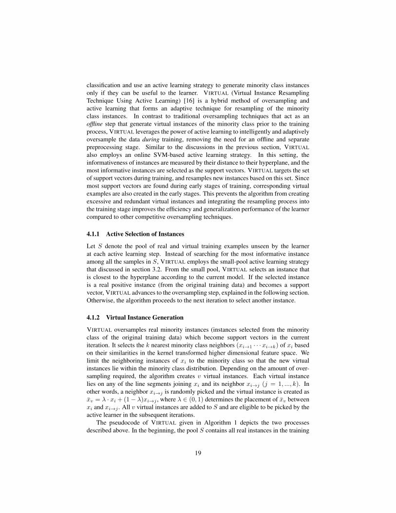
classification and use an active learning strategy to generate minority class instancesonly if they can be useful to the learner. VIRTUAL (Virtual Instance ResamplingTechnique Using Active Learning) [16] is a hybrid method of oversampling andactive learning that forms an adaptive technique for resampling of the minorityclass instances. In contrast to traditional oversampling techniques that act as anoffline step that generate virtual instances of the minority class prior to the trainingprocess, VIRTUAL leverages the power of active learning to intelligently and adaptivelyoversample the data during training, removing the need for an offline and separatepreprocessing stage. Similar to the discussions in the previous section, VIRTUALalso employs an online SVM-based active learning strategy. In this setting, theinformativeness of instances are measured by their distance to their hyperplane, and themost informative instances are selected as the support vectors. VIRTUAL targets the setof support vectors during training, and resamples new instances based on this set. Sincemost support vectors are found during early stages of training, corresponding virtualexamples are also created in the early stages. This prevents the algorithm from creatingexcessive and redundant virtual instances and integrating the resampling process intothe training stage improves the efficiency and generalization performance of the learnercompared to other competitive oversampling techniques.
4.1.1 Active Selection of Instances
Let S denote the pool of real and virtual training examples unseen by the learnerat each active learning step. Instead of searching for the most informative instanceamong all the samples in S, VIRTUAL employs the small-pool active learning strategythat discussed in section 3.2. From the small pool, VIRTUAL selects an instance thatis closest to the hyperplane according to the current model. If the selected instanceis a real positive instance (from the original training data) and becomes a supportvector, VIRTUAL advances to the oversampling step, explained in the following section.Otherwise, the algorithm proceeds to the next iteration to select another instance.
4.1.2 Virtual Instance Generation
VIRTUAL oversamples real minority instances (instances selected from the minorityclass of the original training data) which become support vectors in the currentiteration. It selects the k nearest minority class neighbors (xi→1 · · ·xi→k) of xi basedon their similarities in the kernel transformed higher dimensional feature space. Welimit the neighboring instances of xi to the minority class so that the new virtualinstances lie within the minority class distribution. Depending on the amount of over-sampling required, the algorithm creates v virtual instances. Each virtual instancelies on any of the line segments joining xi and its neighbor xi→j (j = 1, ..., k). Inother words, a neighbor xi→j is randomly picked and the virtual instance is created asxv = λ · xi + (1− λ)xi→j , where λ ∈ (0, 1) determines the placement of xv betweenxi and xi→j . All v virtual instances are added to S and are eligible to be picked by theactive learner in the subsequent iterations.
The pseudocode of VIRTUAL given in Algorithm 1 depicts the two processesdescribed above. In the beginning, the pool S contains all real instances in the training
19

set. At the end of each iteration, the instance selected is removed from S, and anyvirtual instances generated are included in the pool S. In this pseudocode, VIRTUALterminates when there are no instances in S.
4.2 Remarks on VIRTUALWe compare VIRTUAL with a popular oversampling technique SMOTE. Figure 7shows the different behavior of how SMOTE and VIRTUAL create virtual instancesfor the minority class. SMOTE creates virtual instance(s) for each positive example(see Figure 7(a)), whereas VIRTUAL creates the majority of virtual instances aroundthe positive canonical hyperplane (shown with a dashed line in Figure 7(b)). Notethat a large portion of virtual instances created by SMOTE are far away from the
Algorithm 1 VIRTUALDefine:X = {x1, x2, · · · , xn} : training instancesX+
R : positive real training instancesS : pool of training instances for SVMv : # virtual instances to create in each iterationL : size of the small set of randomly picked samples
for active sample selection
1. Initialize S ← X2. while S 6= ∅3. // Active sample selection step4. dmin ←∞5. for i← 1 to L6. xj ← RandomSelect(S)7. If d(xj , hyperplane) < dmin
8. dmin ← d(xj , hyperplane)9. candidate← xj10. end11. end12. xs ← candidate13. // Virtual Instance Generation14. If xs becomes SV and xs ∈ X+
R
15. K ← k nearest neighbors of xs16. for i← 1 to v17. xm ← RandomSelect(K)18. // Create a virtual positive instance xvs,m between xs and xm19. λ=random number between 0 and 120. xvs,m = λ · xs + (1− λ)xm21. S ← S ∪ xvs,m22. end23. end24. S ← S − xs25. end
20
(a) Oversampling with SMOTE (b) Oversampling with VIRTUAL
Figure 7: Comparison of oversampling the minority class with SMOTE and VIRTUAL.
hyperplane and thus are not likely to be selected as support vectors. VIRTUAL, on theother hand, generates virtual instances near the real positive support vectors adaptivelyin the learning process. Hence the virtual instances are near the hyperplane and thusare more informative.
We further analyze the computation complexity of SMOTE and VIRTUAL. Thecomputation complexity of VIRTUAL is O(|SV (+)| · v · C), where v is the number ofvirtual instances created for a real positive support vector in each iteration, |SV (+)| isthe number of positive support vectors and C is the cost of finding k nearest neighbors.The computation complexity of SMOTE isO(
∣∣X+R
∣∣·v·C), where∣∣X+
R
∣∣ is the number ofpositive training instances. C depends on the approach for finding k nearest neighbors.The naive implementation searches all N training instances for the nearest neighborsand thus C = kN . Using advanced data structure such as kd-tree, C = k logN .Since |SV (+)| is typically much less than
∣∣X+R
∣∣, VIRTUAL incurs lower computationoverhead than SMOTE. Also, with fewer virtual instances created, the learner is lessburdened with VIRTUAL. We demonstrate with empirical results that the virtualinstances created with VIRTUAL are more informative and the prediction performanceis also improved.
4.3 ExperimentsWe conduct a series of experiments on Reuters-21578 and four UCI datasets todemonstrate the efficacy of VIRTUAL. The characteristics of the datasets are detailedin [16]. We compare VIRTUAL with two systems, Active Learning (AL) and SMOTE.AL adopts the traditional active learning strategy without preprocessing or creating anyvirtual instances during learning. SMOTE, on the other hand, preprocesses the databy creating virtual instances before training and uses random sampling in learning.Experiments elicit the advantages of adaptive virtual sample creation in VIRTUAL.
In Figures 8 and 9 provide details on the behavior of the three algorithms, SMOTE,AL and VIRTUAL. For the Reuters datasets (Figure 9), note that in all the 10 categoriesVIRTUAL outperforms AL in g-means metric after saturation. The difference in
21
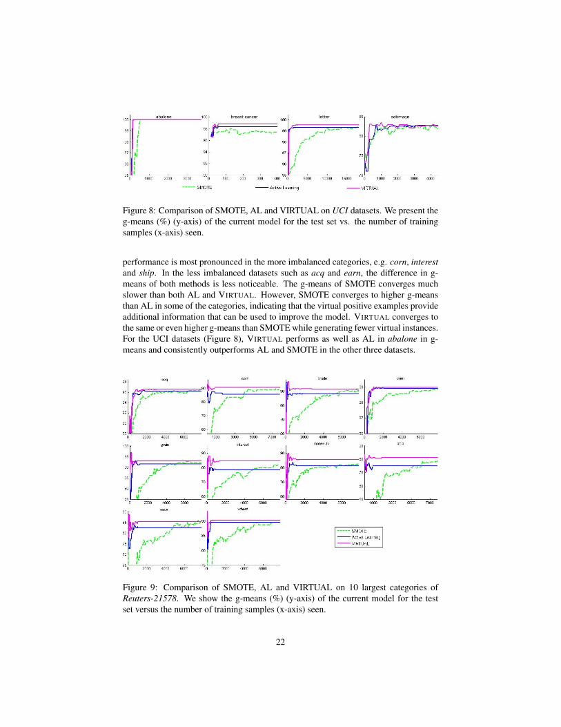
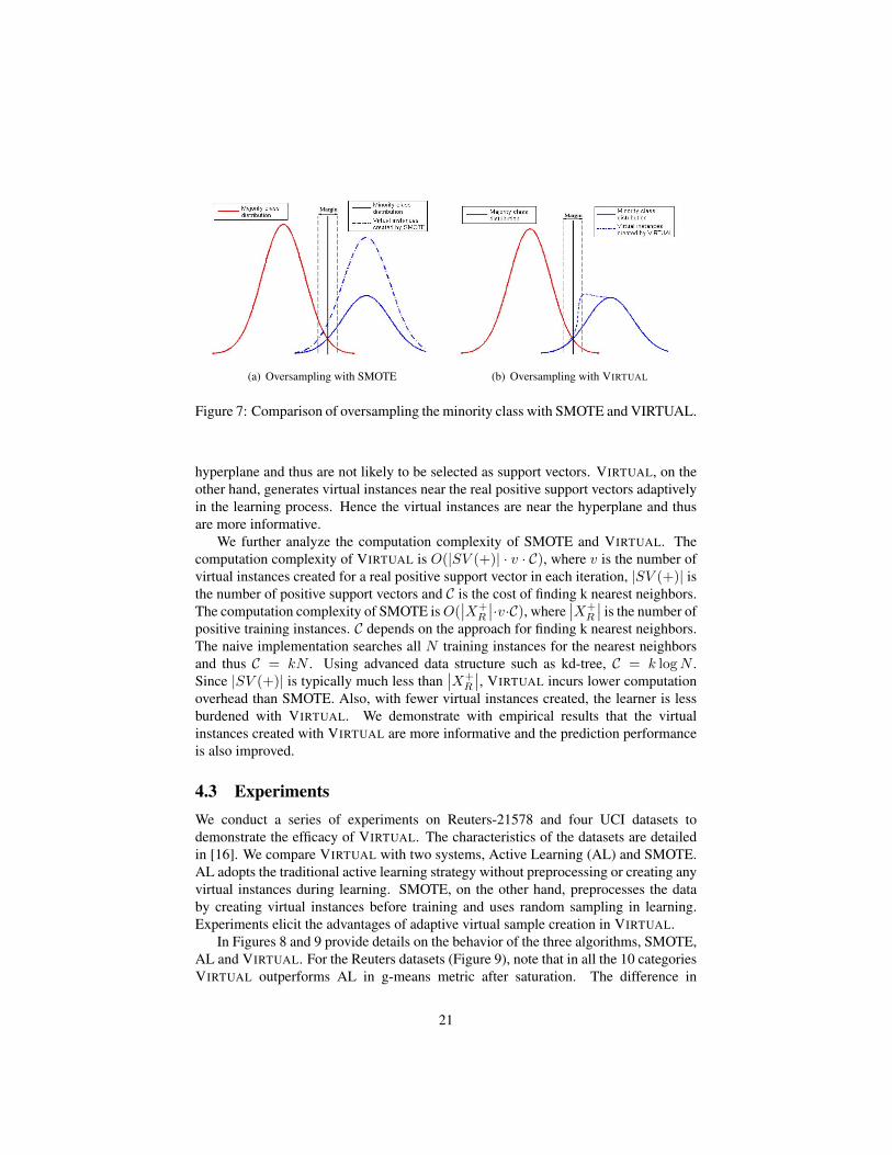
Figure 8: Comparison of SMOTE, AL and VIRTUAL on UCI datasets. We present theg-means (%) (y-axis) of the current model for the test set vs. the number of trainingsamples (x-axis) seen.
performance is most pronounced in the more imbalanced categories, e.g. corn, interestand ship. In the less imbalanced datasets such as acq and earn, the difference in g-means of both methods is less noticeable. The g-means of SMOTE converges muchslower than both AL and VIRTUAL. However, SMOTE converges to higher g-meansthan AL in some of the categories, indicating that the virtual positive examples provideadditional information that can be used to improve the model. VIRTUAL converges tothe same or even higher g-means than SMOTE while generating fewer virtual instances.For the UCI datasets (Figure 8), VIRTUAL performs as well as AL in abalone in g-means and consistently outperforms AL and SMOTE in the other three datasets.
Figure 9: Comparison of SMOTE, AL and VIRTUAL on 10 largest categories ofReuters-21578. We show the g-means (%) (y-axis) of the current model for the testset versus the number of training samples (x-axis) seen.
22
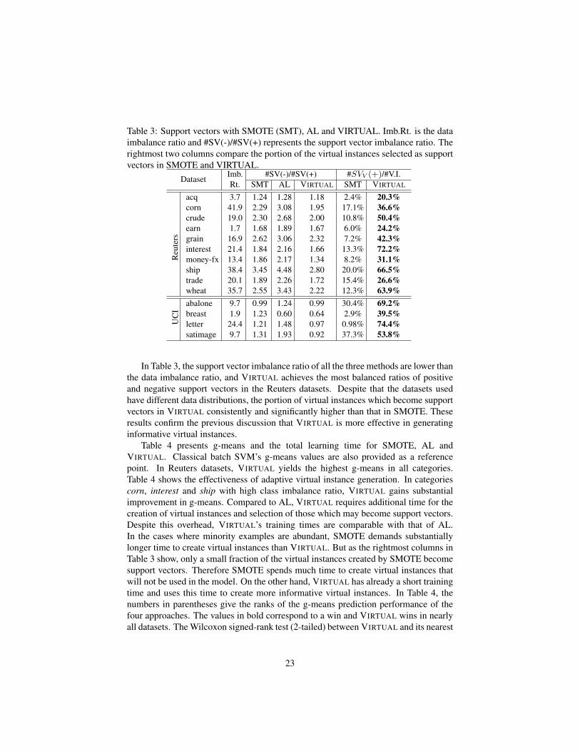
Table 3: Support vectors with SMOTE (SMT), AL and VIRTUAL. Imb.Rt. is the dataimbalance ratio and #SV(-)/#SV(+) represents the support vector imbalance ratio. Therightmost two columns compare the portion of the virtual instances selected as supportvectors in SMOTE and VIRTUAL.
DatasetImb. #SV(-)/#SV(+) #SVV (+)/#V.I.Rt. SMT AL VIRTUAL SMT VIRTUAL
Reu
ters
acq 3.7 1.24 1.28 1.18 2.4% 20.3%corn 41.9 2.29 3.08 1.95 17.1% 36.6%crude 19.0 2.30 2.68 2.00 10.8% 50.4%earn 1.7 1.68 1.89 1.67 6.0% 24.2%grain 16.9 2.62 3.06 2.32 7.2% 42.3%interest 21.4 1.84 2.16 1.66 13.3% 72.2%money-fx 13.4 1.86 2.17 1.34 8.2% 31.1%ship 38.4 3.45 4.48 2.80 20.0% 66.5%trade 20.1 1.89 2.26 1.72 15.4% 26.6%wheat 35.7 2.55 3.43 2.22 12.3% 63.9%
UC
I
abalone 9.7 0.99 1.24 0.99 30.4% 69.2%breast 1.9 1.23 0.60 0.64 2.9% 39.5%letter 24.4 1.21 1.48 0.97 0.98% 74.4%satimage 9.7 1.31 1.93 0.92 37.3% 53.8%
In Table 3, the support vector imbalance ratio of all the three methods are lower thanthe data imbalance ratio, and VIRTUAL achieves the most balanced ratios of positiveand negative support vectors in the Reuters datasets. Despite that the datasets usedhave different data distributions, the portion of virtual instances which become supportvectors in VIRTUAL consistently and significantly higher than that in SMOTE. Theseresults confirm the previous discussion that VIRTUAL is more effective in generatinginformative virtual instances.
Table 4 presents g-means and the total learning time for SMOTE, AL andVIRTUAL. Classical batch SVM’s g-means values are also provided as a referencepoint. In Reuters datasets, VIRTUAL yields the highest g-means in all categories.Table 4 shows the effectiveness of adaptive virtual instance generation. In categoriescorn, interest and ship with high class imbalance ratio, VIRTUAL gains substantialimprovement in g-means. Compared to AL, VIRTUAL requires additional time for thecreation of virtual instances and selection of those which may become support vectors.Despite this overhead, VIRTUAL’s training times are comparable with that of AL.In the cases where minority examples are abundant, SMOTE demands substantiallylonger time to create virtual instances than VIRTUAL. But as the rightmost columns inTable 3 show, only a small fraction of the virtual instances created by SMOTE becomesupport vectors. Therefore SMOTE spends much time to create virtual instances thatwill not be used in the model. On the other hand, VIRTUAL has already a short trainingtime and uses this time to create more informative virtual instances. In Table 4, thenumbers in parentheses give the ranks of the g-means prediction performance of thefour approaches. The values in bold correspond to a win and VIRTUAL wins in nearlyall datasets. The Wilcoxon signed-rank test (2-tailed) between VIRTUAL and its nearest
23
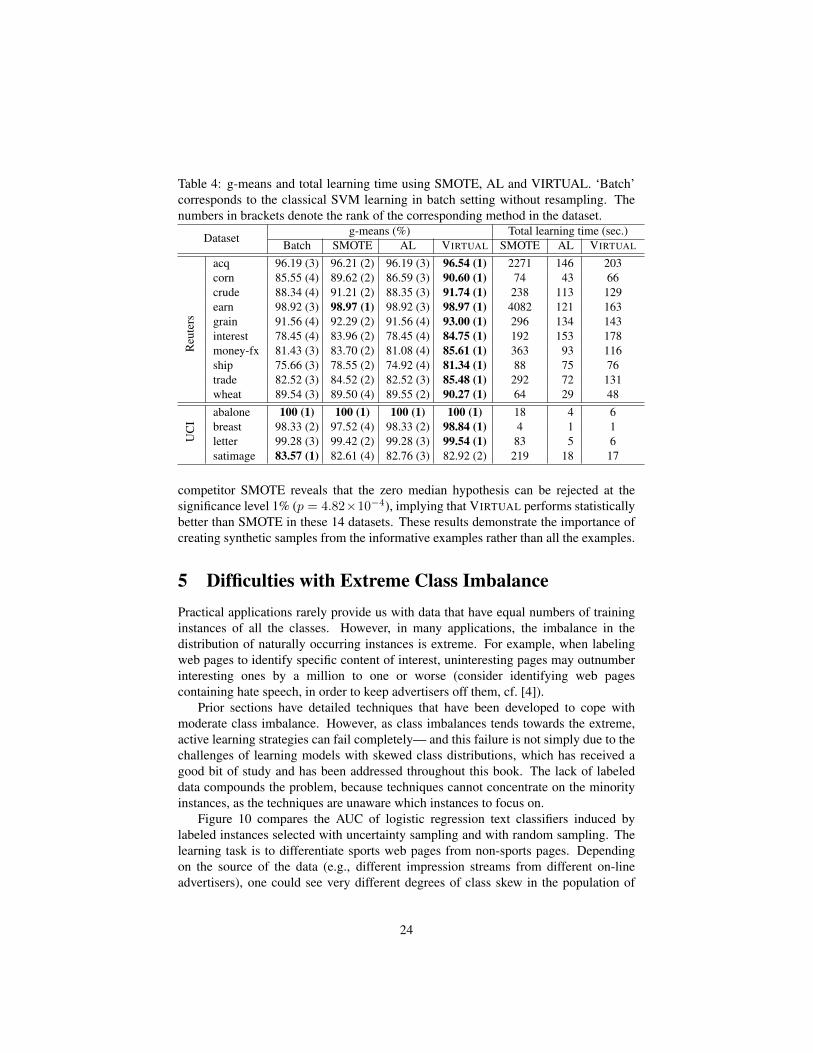
Table 4: g-means and total learning time using SMOTE, AL and VIRTUAL. ‘Batch’corresponds to the classical SVM learning in batch setting without resampling. Thenumbers in brackets denote the rank of the corresponding method in the dataset.
Datasetg-means (%) Total learning time (sec.)
Batch SMOTE AL VIRTUAL SMOTE AL VIRTUAL
Reu
ters
acq 96.19 (3) 96.21 (2) 96.19 (3) 96.54 (1) 2271 146 203corn 85.55 (4) 89.62 (2) 86.59 (3) 90.60 (1) 74 43 66crude 88.34 (4) 91.21 (2) 88.35 (3) 91.74 (1) 238 113 129earn 98.92 (3) 98.97 (1) 98.92 (3) 98.97 (1) 4082 121 163grain 91.56 (4) 92.29 (2) 91.56 (4) 93.00 (1) 296 134 143interest 78.45 (4) 83.96 (2) 78.45 (4) 84.75 (1) 192 153 178money-fx 81.43 (3) 83.70 (2) 81.08 (4) 85.61 (1) 363 93 116ship 75.66 (3) 78.55 (2) 74.92 (4) 81.34 (1) 88 75 76trade 82.52 (3) 84.52 (2) 82.52 (3) 85.48 (1) 292 72 131wheat 89.54 (3) 89.50 (4) 89.55 (2) 90.27 (1) 64 29 48
UC
I
abalone 100 (1) 100 (1) 100 (1) 100 (1) 18 4 6breast 98.33 (2) 97.52 (4) 98.33 (2) 98.84 (1) 4 1 1letter 99.28 (3) 99.42 (2) 99.28 (3) 99.54 (1) 83 5 6satimage 83.57 (1) 82.61 (4) 82.76 (3) 82.92 (2) 219 18 17
competitor SMOTE reveals that the zero median hypothesis can be rejected at thesignificance level 1% (p = 4.82×10⁻⁴), implying that VIRTUAL performs statisticallybetter than SMOTE in these 14 datasets. These results demonstrate the importance ofcreating synthetic samples from the informative examples rather than all the examples.
5 Difficulties with Extreme Class ImbalancePractical applications rarely provide us with data that have equal numbers of traininginstances of all the classes. However, in many applications, the imbalance in thedistribution of naturally occurring instances is extreme. For example, when labelingweb pages to identify specific content of interest, uninteresting pages may outnumberinteresting ones by a million to one or worse (consider identifying web pagescontaining hate speech, in order to keep advertisers off them, cf. [4]).
Prior sections have detailed techniques that have been developed to cope withmoderate class imbalance. However, as class imbalances tends towards the extreme,active learning strategies can fail completely— and this failure is not simply due to thechallenges of learning models with skewed class distributions, which has received agood bit of study and has been addressed throughout this book. The lack of labeleddata compounds the problem, because techniques cannot concentrate on the minorityinstances, as the techniques are unaware which instances to focus on.
Figure 10 compares the AUC of logistic regression text classifiers induced bylabeled instances selected with uncertainty sampling and with random sampling. Thelearning task is to differentiate sports web pages from non-sports pages. Dependingon the source of the data (e.g., different impression streams from different on-lineadvertisers), one could see very different degrees of class skew in the population of
24
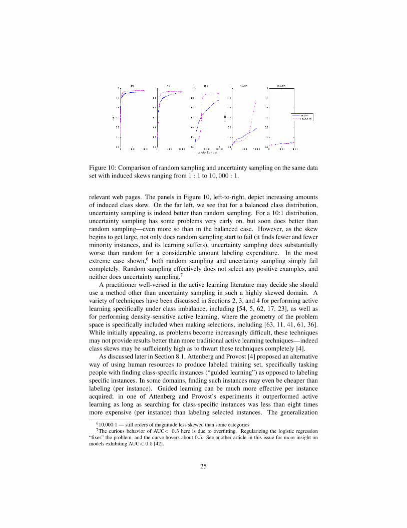
Figure 10: Comparison of random sampling and uncertainty sampling on the same dataset with induced skews ranging from 1 : 1 to 10, 000 : 1.
relevant web pages. The panels in Figure 10, left-to-right, depict increasing amountsof induced class skew. On the far left, we see that for a balanced class distribution,uncertainty sampling is indeed better than random sampling. For a 10:1 distribution,uncertainty sampling has some problems very early on, but soon does better thanrandom sampling—even more so than in the balanced case. However, as the skewbegins to get large, not only does random sampling start to fail (it finds fewer and fewerminority instances, and its learning suffers), uncertainty sampling does substantiallyworse than random for a considerable amount labeling expenditure. In the mostextreme case shown,6 both random sampling and uncertainty sampling simply failcompletely. Random sampling effectively does not select any positive examples, andneither does uncertainty sampling.7
A practitioner well-versed in the active learning literature may decide she shoulduse a method other than uncertainty sampling in such a highly skewed domain. Avariety of techniques have been discussed in Sections 2, 3, and 4 for performing activelearning specifically under class imbalance, including [54, 5, 62, 17, 23], as well asfor performing density-sensitive active learning, where the geometry of the problemspace is specifically included when making selections, including [63, 11, 41, 61, 36].While initially appealing, as problems become increasingly difficult, these techniquesmay not provide results better than more traditional active learning techniques—indeedclass skews may be sufficiently high as to thwart these techniques completely [4].
As discussed later in Section 8.1, Attenberg and Provost [4] proposed an alternativeway of using human resources to produce labeled training set, specifically taskingpeople with finding class-specific instances (“guided learning”) as opposed to labelingspecific instances. In some domains, finding such instances may even be cheaper thanlabeling (per instance). Guided learning can be much more effective per instanceacquired; in one of Attenberg and Provost’s experiments it outperformed activelearning as long as searching for class-specific instances was less than eight timesmore expensive (per instance) than labeling selected instances. The generalization
610,000:1 — still orders of magnitude less skewed than some categories7The curious behavior of AUC< 0.5 here is due to overfitting. Regularizing the logistic regression
“fixes” the problem, and the curve hovers about 0.5. See another article in this issue for more insight onmodels exhibiting AUC< 0.5 [42].
25
performance of guided learning is shown in Figure 12, discussed below in Section 8.1for the same setting as Figure 10.
6 Dealing with disjunctive classesEven more subtly still, certain problem spaces may not have such an extreme classskew, but may still be particularly difficult because they possess important but verysmall disjunctive sub-concepts, rather than simple continuously dense regions ofminority and majority instances. Prior research has shown that such “small disjuncts”can comprise a large portion of a target class in some domains [59]. For active learning,these small subconcepts act like rare classes: if a learner has seen no instances of thesubconcept, how can it “know” which instances to label? Note that this is not simply aproblem of using the wrong loss function: in an active learning setting, the learner doesnot even know that the instances of the subconcept are misclassified if no instances ofa subconcept have yet been labeled. Nonetheless, in a research setting (where we knowall the labels) using an undiscriminative loss function, such as classification accuracyor even the area under the ROC curve (AUC), may result in the researcher not evenrealizing that an important subconcept has been missed.
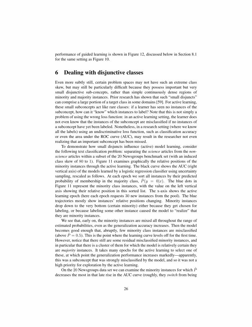
To demonstrate how small disjuncts influence (active) model learning, considerthe following text classification problem: separating the science articles from the non-science articles within a subset of the 20 Newsgroups benchmark set (with an inducedclass skew of 80 to 1). Figure 11 examines graphically the relative positions of theminority instances through the active learning. The black curve shows the AUC (rightvertical axis) of the models learned by a logistic regression classifier using uncertaintysampling, rescaled as follows. At each epoch we sort all instances by their predictedprobability of membership in the majority class, P (y = 0|x). The blue dots inFigure 11 represent the minority class instances, with the value on the left verticalaxis showing their relative position in this sorted list. The x-axis shows the activelearning epoch (here each epoch requests 30 new instances from the pool). The bluetrajectories mostly show instances’ relative positions changing. Minority instancesdrop down to the very bottom (certain minority) either because they get chosen forlabeling, or because labeling some other instance caused the model to “realize” thatthey are minority instances.
We see that, early on, the minority instances are mixed all throughout the range ofestimated probabilities, even as the generalization accuracy increases. Then the modelbecomes good enough that, abruptly, few minority class instances are misclassified(above P = 0.5). This is the point where the learning curve levels off for the first time.However, notice that there still are some residual misclassified minority instances, andin particular that there is a cluster of them for which the model is relatively certain theyare majority instances. It takes many epochs for the active learning to select one ofthese, at which point the generalization performance increases markedly—apparently,this was a subconcept that was strongly misclassified by the model, and so it was not ahigh priority for exploration by the active learning.
On the 20 Newsgroups data set we can examine the minority instances for which Pdecreases the most in that late rise in the AUC curve (roughly, they switch from being
26
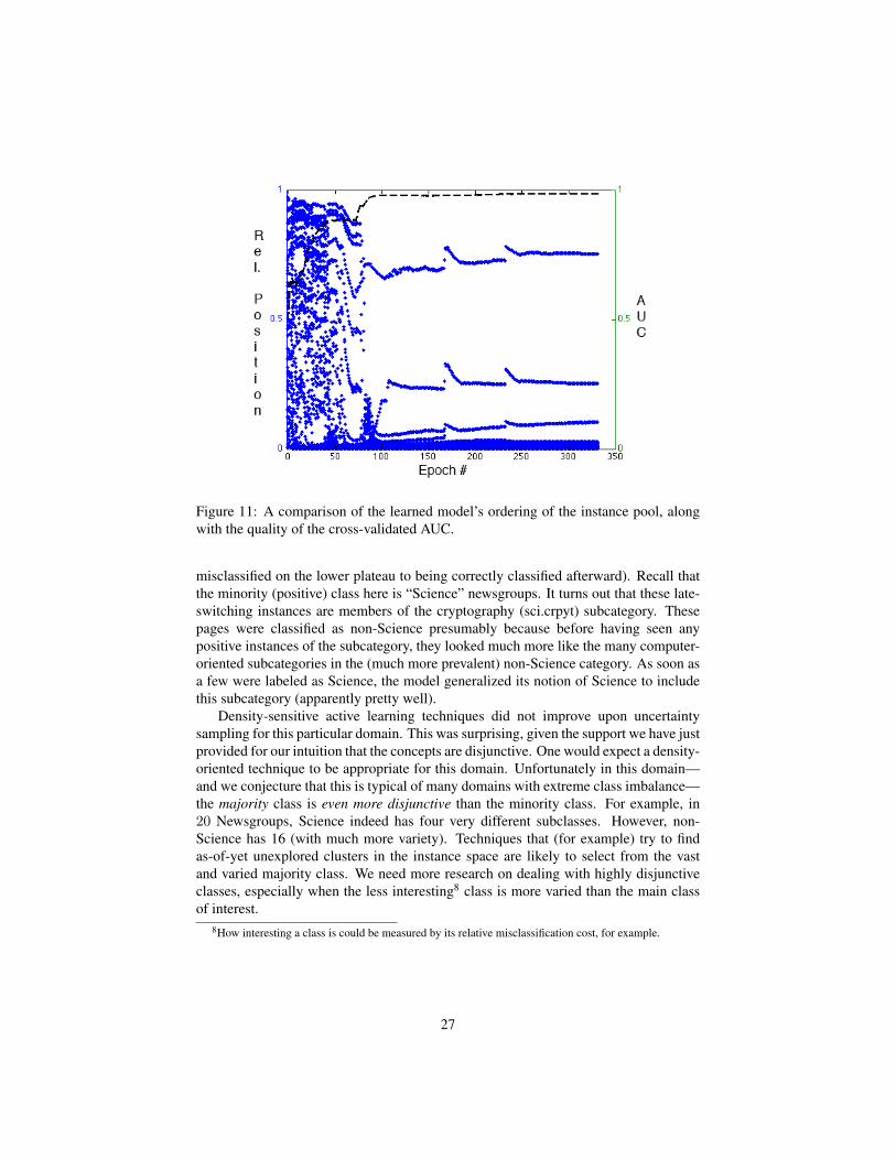
Figure 11: A comparison of the learned model’s ordering of the instance pool, alongwith the quality of the cross-validated AUC.
misclassified on the lower plateau to being correctly classified afterward). Recall thatthe minority (positive) class here is “Science” newsgroups. It turns out that these late-switching instances are members of the cryptography (sci.crpyt) subcategory. Thesepages were classified as non-Science presumably because before having seen anypositive instances of the subcategory, they looked much more like the many computer-oriented subcategories in the (much more prevalent) non-Science category. As soon asa few were labeled as Science, the model generalized its notion of Science to includethis subcategory (apparently pretty well).
Density-sensitive active learning techniques did not improve upon uncertaintysampling for this particular domain. This was surprising, given the support we have justprovided for our intuition that the concepts are disjunctive. One would expect a density-oriented technique to be appropriate for this domain. Unfortunately in this domain—and we conjecture that this is typical of many domains with extreme class imbalance—the majority class is even more disjunctive than the minority class. For example, in20 Newsgroups, Science indeed has four very different subclasses. However, non-Science has 16 (with much more variety). Techniques that (for example) try to findas-of-yet unexplored clusters in the instance space are likely to select from the vastand varied majority class. We need more research on dealing with highly disjunctiveclasses, especially when the less interesting8 class is more varied than the main classof interest.
8How interesting a class is could be measured by its relative misclassification cost, for example.
27
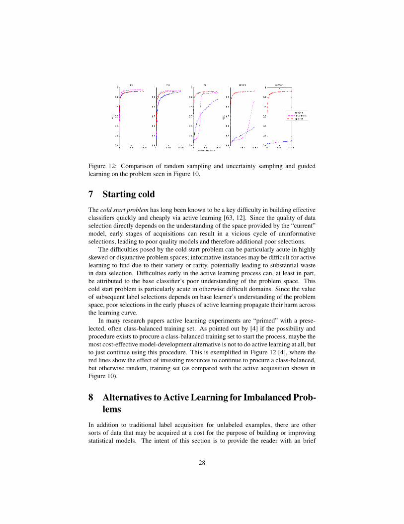
Figure 12: Comparison of random sampling and uncertainty sampling and guidedlearning on the problem seen in Figure 10.
7 Starting coldThe cold start problem has long been known to be a key difficulty in building effectiveclassifiers quickly and cheaply via active learning [63, 12]. Since the quality of dataselection directly depends on the understanding of the space provided by the “current”model, early stages of acquisitions can result in a vicious cycle of uninformativeselections, leading to poor quality models and therefore additional poor selections.
The difficulties posed by the cold start problem can be particularly acute in highlyskewed or disjunctive problem spaces; informative instances may be difficult for activelearning to find due to their variety or rarity, potentially leading to substantial wastein data selection. Difficulties early in the active learning process can, at least in part,be attributed to the base classifier’s poor understanding of the problem space. Thiscold start problem is particularly acute in otherwise difficult domains. Since the valueof subsequent label selections depends on base learner’s understanding of the problemspace, poor selections in the early phases of active learning propagate their harm acrossthe learning curve.
In many research papers active learning experiments are “primed” with a prese-lected, often class-balanced training set. As pointed out by [4] if the possibility andprocedure exists to procure a class-balanced training set to start the process, maybe themost cost-effective model-development alternative is not to do active learning at all, butto just continue using this procedure. This is exemplified in Figure 12 [4], where thered lines show the effect of investing resources to continue to procure a class-balanced,but otherwise random, training set (as compared with the active acquisition shown inFigure 10).
8 Alternatives to Active Learning for Imbalanced Prob-lems
In addition to traditional label acquisition for unlabeled examples, there are othersorts of data that may be acquired at a cost for the purpose of building or improvingstatistical models. The intent of this section is to provide the reader with an brief
28
overview of some alternative techniques for active data acquisition for predictive modelconstruction in a cost-restrictive setting. We begin this setting with a discussion ofclass-conditional example acquisition, a paradigm related to active learning whereexamples are drawn from some available unlabeled pool in accordance to somepredefined class-proportion. We then go on in Section 8.2 to touch on active featurelabeling and active dual supervision. These two paradigms attempt to to replace orsupplement traditional supervised learning with class-specific associations on certainfeature values. While this set of techniques require specialized models, significantgeneralization performance can often be achieved at a reasonable cost by leveragingexplicit feature/class relationships. This is often appealing in the active setting, whereit is occasionally less challenging to identify class-indicative feature values than it is tofind quality training data for labeling, particularly in the imbalanced setting.
8.1 Class-Conditional Example AcquisitionImagine as an alternative to the traditional active learning problem setting, where anoracle is queried in order to assign examples to specially selected unlabeled examples,a setting where an oracle is charged with selecting exemplars from the underlayingproblem space in accordance to some predefined class ratio. Consider as a motivationalexample, the problem of building predictive models based on data collected throughan “artificial nose” with the intent of “sniffing out” explosive or hazardous chemicalcompounds [33, 35, 34]. In this setting, the reactivity of a large number of chemicals isalready known, representing label-conditioned pools of available instances. However,producing these chemicals in a laboratory setting and running the resultant compoundthrough the artificial nose may be an expensive, time-consuming process. While thisproblem may seem quite unique, many data acquisition tasks may be cast into a similarframework.
A much more general issue in selective data acquisition is the amount of controlceded to the “oracle” doing the acquisition. The work discussed so far assumes that anoracle will be queried for some specific value, and the oracle simply returns that value.However, if the oracle is actually a person, he or she may be able to apply considerableintelligence and other resources to “guide” the selection. Such guidance is especiallyhelpful in situations where some aspect of the data is rare—where purely data-drivenstrategies are particularly challenged.
As discussed throughout this work, in many practical settings, one class isquite rare. As an example motivating the application of class-conditional exampleacquisition in practice, consider building a predictive model from scratch designedto classify web pages containing a particular topic of interest. While large absolutenumbers of such web pages may be present on the web, they may be outnumbered byuninteresting pages by a million to one or worse (take, for instance, the task of detectingand removing hate speech from the web [4]). As discussed in Section 5, such extremelyimbalanced problem settings present a particularly insidious difficulty for traditionalactive learning techniques. In a setting with a 10, 000 : 1 class ratio, a reasonably largelabeling budget could be expended with out observing a single minority example.9
9Note that in practice, such extremely imbalanced problem settings may actually be quite common.
29
-
+
-
+
-
+
-
+
-
Instances
Feature Values
InstanceSpace
Oracle
New Instance
Training Set
Seek OutUseful Instances
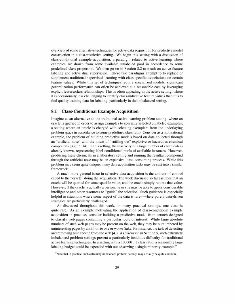
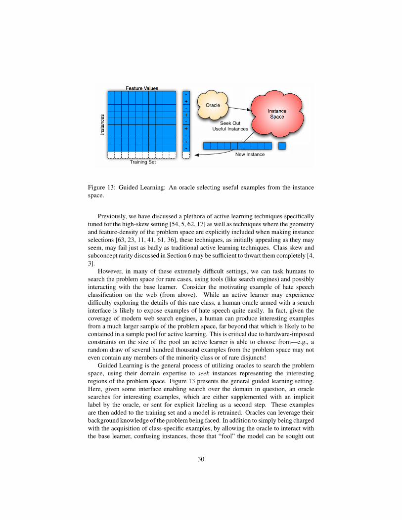
Figure 13: Guided Learning: An oracle selecting useful examples from the instancespace.
Previously, we have discussed a plethora of active learning techniques specificallytuned for the high-skew setting [54, 5, 62, 17] as well as techniques where the geometryand feature-density of the problem space are explicitly included when making instanceselections [63, 23, 11, 41, 61, 36], these techniques, as initially appealing as they mayseem, may fail just as badly as traditional active learning techniques. Class skew andsubconcept rarity discussed in Section 6 may be sufficient to thwart them completely [4,3].
However, in many of these extremely difficult settings, we can task humans tosearch the problem space for rare cases, using tools (like search engines) and possiblyinteracting with the base learner. Consider the motivating example of hate speechclassification on the web (from above). While an active learner may experiencedifficulty exploring the details of this rare class, a human oracle armed with a searchinterface is likely to expose examples of hate speech quite easily. In fact, given thecoverage of modern web search engines, a human can produce interesting examplesfrom a much larger sample of the problem space, far beyond that which is likely to becontained in a sample pool for active learning. This is critical due to hardware-imposedconstraints on the size of the pool an active learner is able to choose from—e.g., arandom draw of several hundred thousand examples from the problem space may noteven contain any members of the minority class or of rare disjuncts!
Guided Learning is the general process of utilizing oracles to search the problemspace, using their domain expertise to seek instances representing the interestingregions of the problem space. Figure 13 presents the general guided learning setting.Here, given some interface enabling search over the domain in question, an oraclesearches for interesting examples, which are either supplemented with an implicitlabel by the oracle, or sent for explicit labeling as a second step. These examplesare then added to the training set and a model is retrained. Oracles can leverage theirbackground knowledge of the problem being faced. In addition to simply being chargedwith the acquisition of class-specific examples, by allowing the oracle to interact withthe base learner, confusing instances, those that “fool” the model can be sought out
30
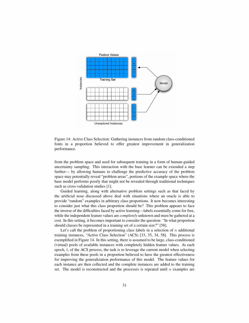
+
+
-
+
-
Instances
Feature Values
+
+
+
-
-
-
-
Training Set
Model
Unexplored Instances
Figure 14: Active Class Selection: Gathering instances from random class-conditionedfonts in a proportion believed to offer greatest improvement in generalizationperformance.
from the problem space and used for subsequent training in a form of human-guideduncertainty sampling. This interaction with the base learner can be extended a stepfurther— by allowing humans to challenge the predictive accuracy of the problemspace may potentially reveal “problem areas”, portions of the example space where thebase model performs poorly that might not be revealed through traditional techniquessuch as cross-validation studies [1].
Guided learning, along with alternative problem settings such as that faced bythe artificial nose discussed above deal with situations where an oracle is able toprovide “random” examples in arbitrary class proportions. It now becomes interestingto consider just what this class proportion should be? This problem appears to facethe inverse of the difficulties faced by active learning—labels essentially come for free,while the independent feature values are completely unknown and must be gathered at acost. In this setting, it becomes important to consider the question: “In what proportionshould classes be represented in a training set of a certain size?” [58].
Let’s call the problem of proportioning class labels in a selection of n additionaltraining instances, “Active Class Selection" (ACS) [33, 35, 34, 58]. This process isexemplified in Figure 14. In this setting, there is assumed to be large, class-conditioned(virtual) pools of available instances with completely hidden feature values. At eachepoch, t, of the ACS process, the task is to leverage the current model when selectingexamples from these pools in a proportion believed to have the greatest effectivenessfor improving the generalization performance of this model. The feature values foreach instance are then collected and the complete instances are added to the trainingset. The model is reconstructed and the processes is repeated until n examples are
31
obtained (because the budget is exhausted or some other stopping criterion is met, suchas a computational limit). Note that this situation can be considered to be a specialcase of the instance completion setting of Active Feature-Value Acquisition (cf. [38]).It is a degenerate special case because, prior to selection, there is no information at allabout the instances other than their classes.
For the specific problem at the heart of ACS, the extreme lack of information toguide selection leads to the development of unique uncertainty and utility estimators,which, in the absence of predictive covariates, require unique approximations.10 Whilealternative approaches to active class selection have emerged, for thematic clarity,uncertainty-based and expected utility-based approaches will be presented first. Notethat because effective classification requires that both sides of a prediction boundary berepresented, unlike typical active learning techniques, active class selection typicallysamples classes from their respective score distributions [45, 46].
8.1.1 Uncertainty-based approaches
This family of techniques for performing active class selection is based on the volatilityin the predictions made about certain classes—those classes whose cross-validatedpredictions are subject to the most change between successive epochs of instanceselection are likely to be based upon an uncertain predictor, and amenable to refinementby the incorporation of additional training data [33, 34]. Analogous to the case of moretraditional uncertainty-based data acquisition, several heuristics have been devised tocapture the notion of variability.
One measure of the uncertainty of a learned model is how volatile its predictiveperformance is in the face of new training data. Take a typical learning curve, forinstance, those presented in Figure 6. Notice that the modeling is much more volatile atthe left side of the figure, showing large changes in generalization performance for thesame amount of new training data. We can think that as the predictor gains knowledgeof the problem space, it tends to solidify in the face of data, exhibiting less changeand greater certainty. For ACS, we might wonder if the learning curves will be equallysteep regardless of the class of the training data [33, 35, 34]. With this in mind, wecan select instances at epoch t from the classes in proportion to their improvements inaccuracy at t − 1 and t − 2. For example, we could use cross-validation to estimatethe generalization performance of the classifier with respect to each class, A(c); classc can then be sampled according to:
ptA(c) ∝max
{0,At−1(c)−At−2(c)
}∑c′ max {0,At−1(c′)−At−2(c′)}
,
Alternatively, we could consider general volatility in class members’ predictedlabels, beyond improvement in the model’s ability to predict the class. Again, by usingcross-validated predictions at successive epochs, it is possible to isolate members ofeach class, and observe changes in the predicted class for each instance. For example,when the predicted label of a given instance changes between successive epochs, we
10In realistic settings, for instance, such as potential application for ACS, guided learning, this lack ofinformation assumption may be softened.
32
can deem the instance to have been redistricted [33, 35, 34]. Again considering thelevel of volatility in a model’s predictions to be a measurement of uncertainty, wecan sample classes at epoch t according to each classes’ proportional measure ofredistricting:
ptR(c) ∝1|c|∑x∈c I(f t−1(x) 6= f t−2(x))∑
c′1|c′|∑x∈c′ I(f t−1(x) 6= f t−2(x))
,
where I(·) is an indicator function taking the value of 1 if its argument is true and 0otherwise. f t−1(x) and f t−2(x) are the predicted labels for instance x from the modelstrained at epoch t− 1 and t− 2, respectively [33, 35, 34].
8.1.2 Expected Class Utility
The previously described active class selection heuristics are reliant on the assumptionthat adding examples belonging to a particular class will improve the predictiveaccuracy with respect to that class. This does not directly estimate the utility of addingmembers of a particular class to a model’s overall performance. Instead, it may bepreferable to select classes whose instances’ presence in the training set will reduce amodel’s misclassification cost by the greatest amount in expectation.
Let cost(ci|cj) be the cost of predicting ci on an instance x whose true label is cj .Then the expected empirical misclassification cost over a sample dataset, D, is:
R =1
|D|∑x∈D
∑i
P (ci|x)cost(ci|y),
Where y is the correct class for a given x. Typically in the active class selection setting,this expectation would be taken over the training set (e.g. D = T ), preferably usingcross-validation. In order to reduce this risk, we would like to select examples fromclass c leading to the greatest reduction in this expected risk [35].
Consider a predictive model PT∪c(·|x), a model built on the training set, T ,supplemented with an arbitrary example belonging to class c. Given the opportunity tochoose an additional class-representative example to the training pool, we would liketo select the class that reduces expected risk by the greatest amount:
c = arg maxcU(c),
Where
U(c) =1
|D|∑x∈D
∑i
PT (ci|x)cost(ci|y)− 1
|D|∑x∈D
∑i
PT∪c(ci|x)cost(ci|y).
Of course the benefit of adding additional examples on a test dataset is unknown.Furthermore, the impact of a particular class’s examples may vary depending on thefeature values of particular instances. In order to cope with these issues, we canestimate via cross-validation on the training set. Using sampling, we can try various
33
class-conditional additions and compute the expected benefit of a class across thatclass’s representatives in T , assessed on the testing folds. The above utility thenbecomes:
U(c) = Ex∈c
[1
|D|∑x∈D
∑i
PT (ci|x)cost(ci|y)− 1
|D|∑x∈D
∑i
PT∪c(ci|x)cost(ci|y)
].
Note that it is often preferred to add examples in batch. In this case, we may wishto sample from the classes in proportion to their respective utilities:
ptU
(c) ∝ U(c)∑c′ U(c′)
.
Further, diverse class-conditional acquisition costs can be incorporated, utilizingU(c)ωc
in place of U(c), where ωc is the (expected) cost of acquiring the feature vectorof an example in class c.
8.1.3 Alternative Approaches to ACS
In addition to uncertainty-based and utility-based techniques, there are several alterna-tive techniques for performing active class selection. Motivated by empirical resultsshowing that barring any domain-specific information, when collecting examples for atraining set of size n, a balanced class distribution tends to offer reasonable AUC ontest data [57, 58], a reasonable baseline approach to active class selection is simply toselect classes in balanced proportion.
Search strategies may alternately be employed in order to reveal the most effectiveclass ratio at each epoch. Utilizing a nested cross-validation on the training set, thespace of class ratios can be explored, with the most favorable ratio being utilized ateach epoch. Note that it is not possible to explore all possible class ratios in all epochs,without eventually spending too much on one class or another. Thus, as we approach nwe can narrow the range of class ratios, assuming that there is a problem-optimal classratio that will become more apparent as we obtain more data [58].
It should be noted that many techniques employed for building classificationmodels assume an identical or similar training and test distribution. Violating thisassumption may lead to biased predictions on test data where classes preferentiallyrepresented in the training data are predicted more frequently. In particular increasingthe prior probability of a class increases the posterior probability of the class, movingthe classification boundary for that class so that more cases are classified into thatclass" [47, 43]. Thus in settings where instances are selected specifically in proportionsdifferent from those seen in the wild, posterior probability estimates should be properlycalibrated to be aligned with the test data, if possible [43, 15, 58].
Prior work has repeatedly demonstrated the benefits of performing active classselection beyond simply selecting random examples from an example pool for
34
acquisition or simply using uniformly balanced selection. However, in many cases,simply casting what would typically be an active learning problem into an ACSproblem, and selecting examples uniformly amongst the classes can provide resultsfar better than what would be possible with active learning alone. For instance, thelearning curves presented in Figure 12 compare such uniform guided learning withactive learning and simple random selection. Providing the model with an essentiallyrandom but class-balanced training set far exceeds the generalization performancepossible for an active learning strategy or by random selection once the class skewbecomes substantial. More intelligent ACS strategies may make this difference evenmore pronounced, and should be considered if the development effort associated withincorporating such strategies would be outweighed by the savings coming from reduceddata acquisition costs.
8.2 Feature-Based Learning and Active Dual SupervisionWhile traditional supervised learning is by far the most prevalent classificationparadigm encountered in the research literature, it is not the only approach forincorporating human knowledge into a predictive system. By leveraging, for instance,class associations with certain feature values, predictive systems can be trained thatoffer potentially excellent generalization performance without requiring the assignmentof class labels to individual instances. Consider, the example domain of predictingthe sentiment of movie reviews. In this context it is clear that the presence of wordslike “amazing” and “thrilling” carry an association with the positive class, while termslike “boring” and ”disappointing” evoke negative sentiment [2]. Gathering this kindof annotation leverages an oracle’s prior experience with the class polarity of certainfeature values— in this case, the emotion that certain terms tend to evoke. Thesystematic selection of feature-values for labeling by a machine learning system isreferred to as Active Feature-Value Labeling,11 (AFL). The general setting where classassociations are actively sought for both feature-values and particular examples isknown as Active Dual Supervisions (ADS). The process of selection for AFL and ADScan be seen in Figures 15 and 16 respectively.
Of course, incorporating the class polarities associated with certain feature-values typically requires specialized models who’s functional form has been designedto leverage feature-based background knowledge. While a survey of models forincorporating such feature-value/class polarities is beyond the scope of this chapter,an interested reader is advised to seek any number of related papers (cf. [37, 48,60, 32, 10, 28, 13]). However, while sophisticated models of this type have beendevised, practical, yet very simple solutions are easy to imagine. Consider at themost basic extreme class assignment rules, where the presence of certain feature-values (or combinations of feature-values) connect an example with a particular class.A rudimentary “dual” model can also be constructed by simply averaging the classpredictions of a traditional supervised machine learning model with a model based onfeature-value/class relationships.
11For brevity, this is often shortened to Active Feature Labeling, a moniker that is best suited for domainswith binary features
35
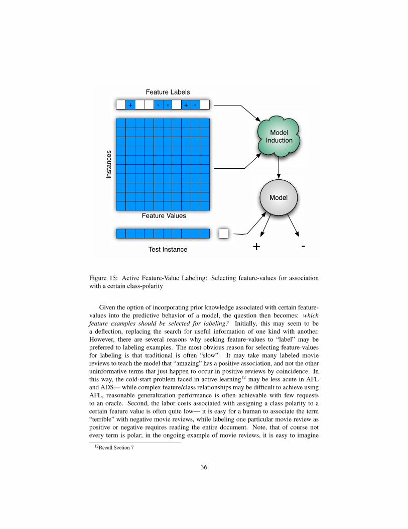
+ - - + -Instances
Test Instance
Feature Labels
Model
Model
Induction
+ -
Feature Values
Figure 15: Active Feature-Value Labeling: Selecting feature-values for associationwith a certain class-polarity
Given the option of incorporating prior knowledge associated with certain feature-values into the predictive behavior of a model, the question then becomes: whichfeature examples should be selected for labeling? Initially, this may seem to bea deflection, replacing the search for useful information of one kind with another.However, there are several reasons why seeking feature-values to “label” may bepreferred to labeling examples. The most obvious reason for selecting feature-valuesfor labeling is that traditional is often “slow”. It may take many labeled moviereviews to teach the model that “amazing” has a positive association, and not the otheruninformative terms that just happen to occur in positive reviews by coincidence. Inthis way, the cold-start problem faced in active learning12 may be less acute in AFLand ADS— while complex feature/class relationships may be difficult to achieve usingAFL, reasonable generalization performance is often achievable with few requeststo an oracle. Second, the labor costs associated with assigning a class polarity to acertain feature value is often quite low— it is easy for a human to associate the term“terrible” with negative movie reviews, while labeling one particular movie review aspositive or negative requires reading the entire document. Note, that of course notevery term is polar; in the ongoing example of movie reviews, it is easy to imagine
12Recall Section 7
36
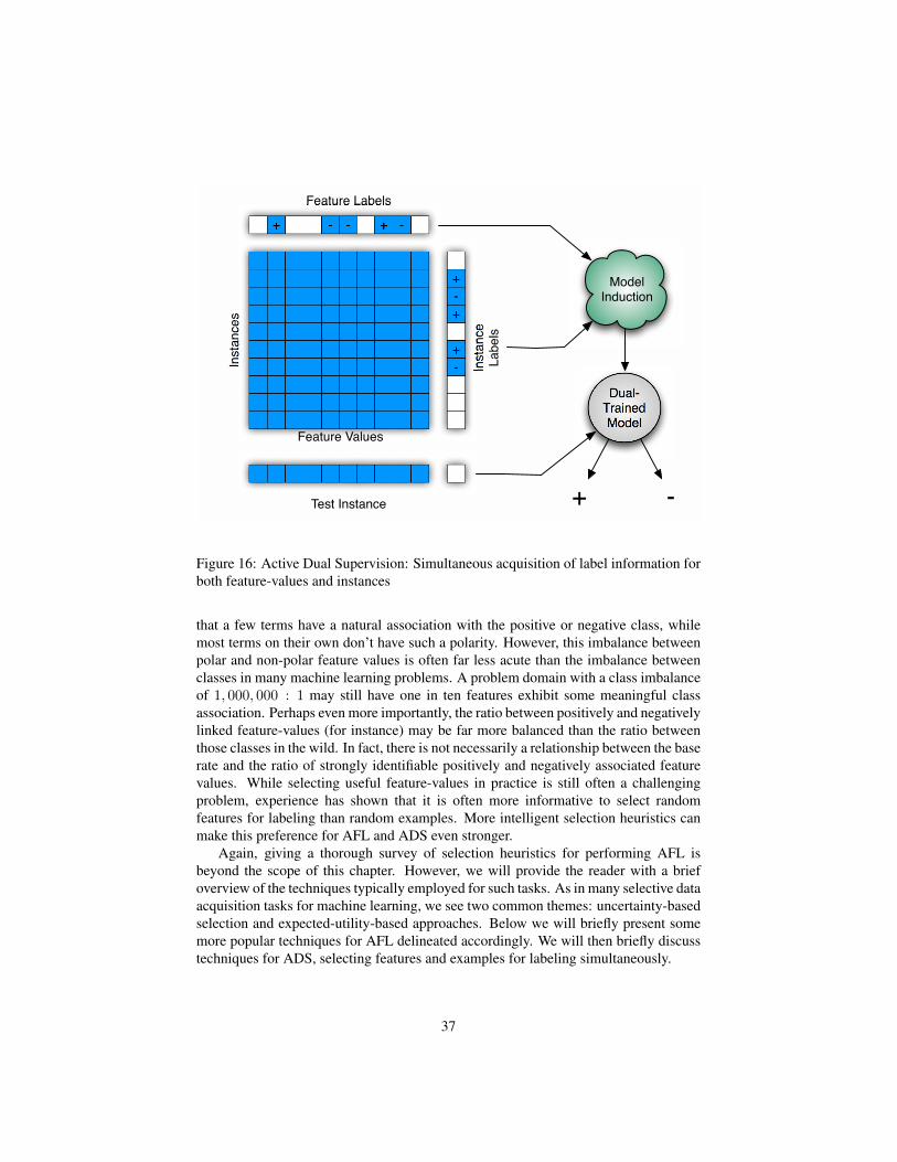
-
+
+
-
+
+ - - + -Instances
Instance
Labels
Test Instance
Feature Labels
Dual-
Trained
Model
Model
Induction
+ -
Feature Values
Figure 16: Active Dual Supervision: Simultaneous acquisition of label information forboth feature-values and instances
that a few terms have a natural association with the positive or negative class, whilemost terms on their own don’t have such a polarity. However, this imbalance betweenpolar and non-polar feature values is often far less acute than the imbalance betweenclasses in many machine learning problems. A problem domain with a class imbalanceof 1, 000, 000 : 1 may still have one in ten features exhibit some meaningful classassociation. Perhaps even more importantly, the ratio between positively and negativelylinked feature-values (for instance) may be far more balanced than the ratio betweenthose classes in the wild. In fact, there is not necessarily a relationship between the baserate and the ratio of strongly identifiable positively and negatively associated featurevalues. While selecting useful feature-values in practice is still often a challengingproblem, experience has shown that it is often more informative to select randomfeatures for labeling than random examples. More intelligent selection heuristics canmake this preference for AFL and ADS even stronger.
Again, giving a thorough survey of selection heuristics for performing AFL isbeyond the scope of this chapter. However, we will provide the reader with a briefoverview of the techniques typically employed for such tasks. As in many selective dataacquisition tasks for machine learning, we see two common themes: uncertainty-basedselection and expected-utility-based approaches. Below we will briefly present somemore popular techniques for AFL delineated accordingly. We will then briefly discusstechniques for ADS, selecting features and examples for labeling simultaneously.
37
8.2.1 Uncertainty-based AFL
By far the most prevalent class of active learning heuristics, uncertainty-basedapproaches do not have a direct analogue to the selection problem faced in ADS;feature-value/class associations factor quite differently into the formation and trainingof machine learning models than more traditional example labels. Nonetheless,thematically similar approaches to the ADS problem have been developed, wherefeatures are selected to labeling according to some notion of stability within the currentmodel. As in traditional uncertainty selection in active learning, the primary differenceamongst these uncertainty-based ADS techniques is the manner by which featureuncertainty is estimated. In the simplest case, using a linear model, the coefficientson particular feature values may be interpreted as a measure of uncertainty, with lowercoefficient magnitude corresponding to a greater degree of uncertainty [52]. The NaíveBayes-like model used presented in [37] presents a more appealing option— feature-value label uncertainty can be measured by looking at the magnitude of the log-oddsof the feature-value likelihoods:
∣∣∣log p(f |+)p(f |−)
∣∣∣ for feature-value f and classes + and −.Again, a smaller value corresponds to increased uncertainty.
A range of other techniques for Uncertainty-based AFL exist. Through thecreation of one-term pseudo-documents Godbole et al [21] coerce the notion offeature label uncertainty into a more traditional instance uncertainty framework fortext classification tasks. By incorporating label information on each feature-valuewith unlabeled examples, Druck et al. [13] create a corresponding GeneralizedExpectation term that rates the model’s predicted class distribution conditioned onthe presence of the particular feature. This rating penalizes these predicted classdistributions according to their KL-divergence from reference distributions constructedusing labeled features. Similarly, Liang et al. [30] learn from labeled examplesand actively selected constraints in the form of expectations with some associatednoise from particular examples. Druck et al. [14] analyze several uncertainty-basedselection techniques for gathering feature labels when training conditional randomfields. Finding that the total uncertainty (measured as the sum of the marginalentropies) tends to favor more frequent features. As a remedy, they propose anuncertainty scheme where the mean uncertainty is weighted by the log of the counts ofthe associated feature values.
Interestingly, even for reasonable uncertainty estimators, feature/class uncertaintymay not be a desirable criterion for selection. Consider the above discussion regardingthe preponderance of uninformative features. Clearly, in the case of documentclassification, terms like “of” and “the” will seldom have any class polarity. Atthe same time, these terms are likely to have a high degree of uncertainty, leavinguncertainty-based approaches to perform poorly in practice. Preferring to selectfeatures based on certainty, that is, selecting those features with the least uncertaintyseems to work much better in practice [52, 39].
8.2.2 Expected Utility-based AFL
As with traditional uncertainty (and certainty) sampling for active learning, the querycorresponding to the greatest level of uncertainty my not necessarily be the query
38
offering the greatest level of information to the model. This is particularly true innoisy or complex environments. Instead of using a heuristic to estimate the informationvalue of a particular feature label, it is possible to estimate this quantity directly. Letq enumerate over all possible feature-values that may be queried for labels. We canestimate the expected utility of such a query by: EU(q) =
∑Kk=1 P (q = ck)U(q=ck)ωq
,where P (q = ck) is the probability of the instance or feature queried being associatedwith class ck, ωq is the cost of query q and U is some measure of the utility of q.13 Thisresults in the decision-theoretic optimal policy, which is to ask for feature labels which,once incorporated into the data, will result in the highest increase in classificationperformance in expectation [2, 39].
8.2.3 Active Dual Supervision
Active dual supervision is concerned with situations where it is possible to query anoracle for labels associated with both feature-values and examples. Even though sucha paradigm is concerned with the simultaneous acquisition of feature and examplelabels, the simplest approach is treating each acquisition problem separately, and thenmixing selections somehow. Active interleaving is performs a separate (un)certinaty-based ordering on features and on examples, and chooses selections from the topof each ordering according to some predefined proportion. The different nature offeature-value and example uncertainty values lead to incompatible quantities existingon different scales, preventing a single, unified ordering. However, expected utility canbe used to compute a single unified metric encapsulating the value of both types ofdata acquisition. As above, we are estimating the utility of a certain feature of examplequery q as: EU(q) =
∑Kk=1 P (q = ck)U(q=ck)ωq
. Using a single utility function forboth features and examples and incorporating label acquisition costs, costs and benefitsof the different types of acquisition can be optimized directly [2].
9 ConclusionThis chapter presents a broad perspective on the relationship between active learning— the selective acquisition of labeled examples for training statistical models — andimbalanced data classification tasks where at least one of the classes in the training setis represented with much fewer instances than the other classes. Our comprehensiveanalysis of this relationship leads to the identification of two common associations,namely, (i) the ability of active learning to deal with the data imbalance problem that,when manifested in a training set, typically degrades the generalization performanceof an induced model, and (ii) the impact class imbalance may have on the abilitiesof an otherwise reasonable active learning scheme to select informative examples, aphenomenon that is particularly acute as the imbalance tends towards the extreme.
Mitigating the impact of class imbalance on the generalization performance of ana predictive model, in Sections 3 and 4 we present active learning as an alternativeto more conventional resampling strategies. An active learning strategy may select a
13For instance, cross-validated accuracy or log-gain may be used.
39
data set that is both balanced and extremely informative in terms of model training.Early stopping criteria for halting the selection process of active learning can furtherimprove the generalization of induced models. That is, a model trained on a small butinformative subsample often offers performance far exceeding what can be achievedby training on a large dataset drawn from the natural, skewed base rate. The abilities ofactive learning to provide small, balanced training from large, but imbalanced problemsare enhanced further by VIRTUAL, introduced in Section 4. Here, artificially generatedinstances supplement the pool of examples available to the active selection mechanism.
Additionally, it is noted throughout that abilities of an active learning system tendto degrade as the imbalance of the underlying distribution increases. While at moremoderate imbalances, the quality of the resulting training set may still be sufficientto provide usable statistical models, but at more substantial class imbalances, it maybe difficult for a system based upon active learning to produce accurate models.Throughout Sections 2, 3, and 4, we illustrate a variety of active learning techniquesspecially adapted for imbalanced settings, techniques that may be considered bypractitioners facing difficult problems. In Sections 5 and 6, we note that as a problem’sclass imbalance tends towards the extreme, the selective abilities of an active learningheuristic may fail completely. We present several alternative approaches for dataacquisition in Section 8, mechanisms that may alleviate the difficulties active learningfaces in problematic domains. Among these alternatives are guided learning and activeclass selection in Subsection 8.1, and using associations between specific feature valuesand certain classes in Subsection 8.2.
Class imbalance presents a challenge to statistical models and to machine learningsystems in general. Because the abilities of these models are so tightly coupled withthe data used for training, it is crucial to consider the selection process that generatesthis data. This chapter discusses specifically this problem. It is clear that whenbuilding models for challenging imbalanced domains, active learning is an aspect ofthe approach that shouldn’t be ignored.
References[1] Josh Attenberg, Panagiotis Ipeirotis, and Foster Provost. Beat the machine:
Challenging workers to find the unknown unknowns. In Proceedings of the 3rdHuman Computation Workshop (HCOMP 2011), August 2011.
[2] Josh Attenberg, Prem Melville, and Foster J. Provost. A unified approach to activedual supervision for labeling features and examples. In European Conference onMachine Learning, 2010.
[3] Josh Attenberg and Foster Provost. Inactive Learning? Difficulties EmployingActive Learning in Practice. SIGKDD Explorations, 12(2):36–41, 2010.
[4] Josh Attenberg and Foster Provost. Why label when you can search? Strategiesfor applying human resources to build classification models under extreme classimbalance. In KDD, 2010.
40
[5] Michael Bloodgood and K. Vijay Shanker. Taking into account the differencesbetween actively and passively acquired data: the case of active learning withsupport vector machines for imbalanced datasets. In NAACL ’09, 2009.
[6] Antoine Bordes, Seyda Ertekin, Jason Weston, and Léon Bottou. Fast kernelclassifiers with online and active learning. Journal of Machine Learning Research(JMLR), 6:1579–1619, 2005.
[7] N. V. Chawla, K. W. Bowyer., L. O. Hall, and W. P. Kegelmeyer. Smote: Syntheticminority over-sampling technique. Journal of Artificial Intelligence Research(JAIR), 16:321–357, 2002.
[8] David Cohn, Les Atlas, and Richard Ladner. Improving generalization with activelearning. Mach. Learn., 15(2):201–221, May 1994.
[9] Ido Dagan and Sean P. Engelson. Committee-based sampling for trainingprobabilistic classifiers. In In Proceedings of the Twelfth InternationalConference on Machine Learning, pages 150–157. Morgan Kaufmann, 1995.
[10] A. Dayanik, D. Lewis, D. Madigan, V. Menkov, and A. Genkin. Constructinginformative prior distributions from domain knowledge in text classification. InSIGIR, 2006.
[11] P. Donmez and J. Carbonell. Paired Sampling in Density-Sensitive ActiveLearning. In Proc. 10 ths International Symposium on Artificial Intelligence andMathematics, 2008.
[12] Pinar Donmez, Jaime G. Carbonell, and Paul N. Bennett. Dual strategy activelearning. In ECML ’07, 2007.
[13] G. Druck, G. Mann, and A. McCallum. Learning from labeled features usinggeneralized expectation criteria. In Special Interest Group in InformationRetrieval (SIGIR), 2008.
[14] G. Druck, B. Settles, and A. McCallum. Active learning by labeling features.In Conference on Empirical Methods in Natural Language Processing (EMNLP’09), pages 81–90. Association for Computational Linguistics, 2009.
[15] Charles Elkan. The foundations of cost-sensitive learning. In Proceedings ofthe Seventeenth International Joint Conference on Artificial Intelligence, pages973–978, 2001.
[16] Seyda Ertekin. Learning in Extreme Conditions: Online and Active Learningwith Massive, Imbalanced and Noisy Data. PhD thesis, The Pennsylvania StateUniversity, 2009.
[17] Seyda Ertekin, Jian Huang, Leon Bottou, and C. Lee Giles. Learning on theborder: Active learning in imbalanced data classification. In Proc. of the 16thACM Conference on Information and Knowledge Management (CIKM), pages127–136, Lisbon, Portugal, 2007.
41
[18] V. V. Federov. Theory of optimal experiments, 1972.
[19] Yoav Freund. Sifting informative examples from a random source. In In WorkingNotes of the Workshop on Relevance, AAAI Fall Symposium Series, pages 85–89,1994.
[20] Yoav Freund, H. Sebastian Seung, Eli Shamir, and Naftali Tishby. Information,prediction, and query by committee. In Advances in Neural InformationProcessing Systems 5, [NIPS Conference], pages 483–490, San Francisco, CA,USA, 1993. Morgan Kaufmann Publishers Inc.
[21] S. Godbole, A. Harpale, S. Sarawagi, and S. Chakrabarti. Document classificationthrough interactive supervision of document and term labels. In Practice ofKnowledge Discovery in Databases (PKDD), 2004.
[22] Yuhong Guo and Russ Greiner. Optimistic active learning using mutualinformation. In Proceedings of the 20th international joint conference on Artificalintelligence, IJCAI’07, pages 823–829, 2007.
[23] Jingrui He and Jaime G. Carbonell. Nearest-neighbor-based active learning forrare category detection. In NIPS, 2007.
[24] Jian Huang, Seyda Ertekin, and C. Lee Giles. Efficient name disambiguation forlarge scale datasets. In Proc. of European Conference on Principles and Practiceof Knowledge Discovery in Databases (ECML/PKDD), volume 4213/2006, pages536–544, 2006.
[25] N. Japkowicz and S. Stephen. The class imbalance problem: A systematic study.Intelligent Data Analysis, 6(5):429–449, 2002.
[26] Nathalie Japkowicz. The class imbalance problem: Significance and strategies. InProc. of 2000 Int. Conference on Artificial Intelligence (IC-AI’2000), volume 1,pages 111–117, 2000.
[27] M. Kubat and S. Matwin. Addressing the curse of imbalanced training datasets:One sided selection. Proc. of 14th Int. Conference on Machine Learning (ICML),30(2-3):195–215, 1997.
[28] Gautam Kunapuli, Kristin P. Bennett, Amina Shabbeer, Richard Maclin, and JudeShavlik. Online knowledge-based support vector machines. In JosO L. BalcGzar,Francesco Bonchi, Aristides Gionis, and MichRle Sebag, editors, ECML/PKDD(2), volume 6322, 2010.
[29] David D. Lewis and William A. Gale. A sequential algorithm for training textclassifiers. In SIGIR ’94: Proceedings of the 17th annual international ACMSIGIR conference on Research and development in information retrieval, pages3–12, New York, NY, USA, 1994. Springer-Verlag New York, Inc.
[30] Percy Liang, Michael I. Jordan, and Dan Klein. Learning from measurements inexponential families. In ICML, 2009.
42
[31] C. X. Ling and C. Li. Data mining for direct marketing: Problems and solutions.In Knowledge Discovery and Data Mining, pages 73–79, 1998.
[32] Bing Liu, Xiaoli Li, Wee Sun Lee, and Philip Yu. Text classification by labelingwords. In AAAI, 2004.
[33] R. Lomasky, C. Brodley, M. Aernecke, D. Walt, and M. Friedl. Active ClassSelection. In Machine Learning: ECML, volume 4701, pages 640–647, 2007.
[34] R. Lomasky, C. E. Brodley, S. Bencic, M. Aernecke, and D Walt. Guiding classselection for an artificial nose. In NIPS Workshop on Testing of DeployableLearning and Decision Systems, 2006.
[35] Rachel Lomasky. Active Acquisition of Informative Training Data. PhD thesis,Tufts University, 2010.
[36] Andrew K. Mccallum and Kamal Nigam. Employing em in pool-based activelearning for text classification. In ICML, 1998.
[37] Prem Melville, Wojciech Gryc, and Richard Lawrence. Sentiment analysis ofblogs by combining lexical knowledge with text classification. In KDD, 2009.
[38] Prem Melville, Foster J. Provost, and Raymond J. Mooney. An expected utilityapproach to active feature-value acquisition. In International Conference on DataMining, pages 745–748, 2005.
[39] Prem Melville and Vikas Sindhwani. Active dual supervision: Reducing the costof annotating examples and features. In Proceedings of the NAACL HLT 2009Workshop on Active Learning for Natural Language Processing, 2009.
[40] Robert Moskovitch, Nir Nissim, Dima Stopel, Clint Feher, Roman Englert, andYuval Elovici. Improving the detection of unknown computer worms activityusing active learning. In Proceedings of the 30th annual German conference onAdvances in Artificial Intelligence, KI ’07, pages 489–493, Berlin, Heidelberg,2007. Springer-Verlag.
[41] Hieu T. Nguyen and Arnold Smeulders. Active learning using pre-clustering. InICML, 2004.
[42] Claudia Perlich and Grzegorz Swirszcz. On cross-validation and stacking:Building seemingly predictive models on random data. SIGKDD Explorations,12(2):This issue, 2010.
[43] F. Provost. Machine learning from imbalanced data sets 101. In Proceedings ofthe AAAI Workshop on Imbalanced Data Sets, 2000.
[44] Nicholas Roy and Andrew McCallum. Toward optimal active learning throughsampling estimation of error reduction. In ICML, 2001.
43
[45] Maytal Saar-tsechansky and Foster Provost. Active learning for class probabilityestimation and ranking. In In Proc of the Seventeenth Int Joint Fonf on ArtificialIntelligence (IJCAI-2001, pages 911–920, 2001.
[46] Maytal Saar-Tsechansky and Foster Provost. Active sampling for classprobability estimation and ranking. Machine Learning, 54(2):153–178, 2004.
[47] SAS Institute Inc. Getting Started with SAS Enterprise Miner. SAS Institute Inc,Cary, NC, 2001.
[48] Robert E. Schapire, Marie Rochery, Mazin G. Rahim, and Narendra Gupta.Incorporating prior knowledge into boosting. In International Conference onMachine Learning (ICML), 2002.
[49] Greg Schohn and David Cohn. Less is more: Active learning with support vectormachines. In Proc. of the 17th Int. Conference on Machine Learning (ICML),pages 839–846, 2000.
[50] Burr Settles. Active learning literature survey. Computer Sciences TechnicalReport 1648, University of Wisconsin–Madison, 2009.
[51] Burr Settles and Mark Craven. An analysis of active learning strategies forsequence labeling tasks. In Proceedings of the Conference on Empirical Methodsin Natural Language Processing, EMNLP ’08, pages 1070–1079, Stroudsburg,PA, USA, 2008. Association for Computational Linguistics.
[52] Vikas Sindhwani, Prem Melville, and Richard Lawrence. Uncertainty samplingand transductive experimental design for active dual supervision. In Proceedingsof the 26th International Conference on Machine Learning (ICML-09), 2009.
[53] Alex J. Smola and Bernhard Schölkopf. Sparse greedy matrix approximation formachine learning. In Proc. of 17th Int. Conference on Machine Learning (ICML),pages 911–918, 2000.
[54] Katrin Tomanek and Udo Hahn. Reducing class imbalance during active learningfor named entity annotation. In K-CAP ’09, 2009.
[55] Simon Tong and Daphne Koller. Support vector machine active learning withapplications to text classification. J. Mach. Learn. Res., 2:45–66, 2002.
[56] V. Vapnik. The Nature of Statistical Learning Theory. Springer, New York, 1995.
[57] G. Weiss and F. Provost. The effect of class distribution on classifier learning,2001.
[58] Gary M. Weiss and Foster Provost. Learning when training data are costly: theeffect of class distribution on tree induction. J. Artif. Int. Res., 19:315–354, 2003.
[59] Weiss, Gary M. The Impact of Small Disjuncts on Classifier Learning. Annals ofInformation Systems, 8:193–226, 2010.
44

[60] Xiaoyun Wu and Rohini Srihari. Incorporating prior knowledge with weightedmargin support vector machines. In Conference on Knowledge Discovery andData Mining (KDD), 2004.
[61] Zhao Xu, Kai Yu, Volker Tresp, Xiaowei Xu, and Jizhi Wang. Representativesampling for text classification using support vector machines. In ECIR, 2003.
[62] Jingbo Zhu and Eduard Hovy. Active learning for word sense disambiguationwith methods for addressing the class imbalance problem. In EMNLP-CoNLL2007, 2007.
[63] Jingbo Zhu, Huizhen Wang, Tianshun Yao, and Benjamin K. Tsou. Activelearning with sampling by uncertainty and density for word sense disambiguationand text classification. In COLING ’08, 2008.
45

![A LOGISTIC REGRESSION BASED HYBRID MODEL FOR ...2006/11/20 · and Rani, (2018)]. A major problem with disease datasets is the class imbalance present in them, Class imbalance occurs](https://img.pdfslide.us/doc/110x75/60da54a8c67b4821c54391d9/a-logistic-regression-based-hybrid-model-for-20061120-and-rani-2018.jpg)


![OKSUZ et al.: IMBALANCE PROBLEMS IN OBJECT ...balance point of view, these surveys only consider class imbalance problem with a limited provision. Additionally, Zou et al. [32] provide](https://img.pdfslide.us/doc/110x75/5eb72818847da72fd258619e/oksuz-et-al-imbalance-problems-in-object-balance-point-of-view-these-surveys.jpg)