Class Imbalance andThe Curse of Minority Hubs

Nenad Tomasev, Dunja Mladenic

aInstitute Jozef StefanArtificial Intelligence Laboratory

Jamova 39, 1000 Ljubljana, Slovenianenad.tomasev@ijs.si, dunja.mladenic@ijs.si

Abstract

Most machine learning tasks involve learning from high-dimensional data, which is often quite difficult to handle.Hubnessis an aspect of thecurse of dimensionalitythat was shown to be highly detrimental tok-nearest neighbormethods in high-dimensional feature spaces.Hubs, very frequent nearest neighbors, emerge as centers of influencewithin the data and often act as semantic singularities. This paper deals with evaluating the impact of hubness onlearning under class imbalance withk-nearest neighbor methods. Our results suggest that, contrary to the commonbelief, minority class hubs might be responsible for most misclassification in many high-dimensional datasets. Thestandard approaches to learning under class imbalance usually clearly favor the instances of the minority class andare not well suited for handling such highly detrimental minority points. In our experiments, we have evaluatedseveral state-of-the-art hubness-awarekNN classifiers that are based on learning from the neighbor occurrence modelscalculated from the training data. The experiments included learning under severe class imbalance, class overlap andmislabeling and the results suggest that the hubness-awaremethods usually achieve promising results on the examinedhigh-dimensional datasets. The improvements seem to be most pronounced when handling the difficult point types:borderline points, rare points and outliers. On most examined datasets, the hubness-aware approaches improve theclassification precision of the minority classes and the recall of the majority class, which helps with reducing thenegative impact of minority hubs. We argue that it might prove beneficial to combine the extensible hubness-awarevoting frameworks with the existing class imbalancedkNN classifiers, in order to properly handle class imbalanceddata in high-dimensional feature spaces.

Keywords: class imbalance, class overlap, classifica-tion, k-nearest neighbor, hubness, curse of dimension-ality

1. Introduction

Nearest-neighbor methods form an important groupof techniques involved in solving various types of ma-chine learning tasks. They are based on a simple as-sumption that neighboring points share certain commonproperties. Often enough, they also share the same la-bel, which is why so many differentk-nearest neighborclassification algorithms have been developed over theyears [28][54][36][64][53][90].

0This paper was published by Elsevier in theKnowledge-Based Systems journal in 2013. DOI:”http://dx.doi.org/10.1016/j.knosys.2013.08.031”.

The basick-nearest neighbor algorithm (kNN) [19]is quite simple. The label in the point of interest is de-rived from itsk-nearest neighbors by a majority vote.The kNN rule has some favorable asymptotic proper-ties [11].

Under the basickNN approach, no model is gener-ated in the training phase and the target function is in-ferred locally when the query is made to the system.Methods with this property are said to performlazylearning.

Algorithms which induce classification models usu-ally adopt the maximum generality bias [33]. In con-trast, thek-nearest neighbor classifier exhibits highspecificity bias, since it retains all the examples. Thespecificity bias is considered a desired property of al-gorithms designed for handling highly imbalanced data.Not surprisingly,kNN has been advocated as one wayof handling such imbalanced data sets [84][33].

Preprint submitted to Elsevier November 3, 2014

Data sets with significant class imbalance often posedifficulties for learning algorithms [87], especially thosewith a high generality bias. Such algorithms tend toover-generalize on the majority class, which in turnleads to a lower performance on the minority class. De-signing good methods capable of coping with highly im-balanced data still remains a daunting task.

Certain concerns have recently been raised about theapplicability of the basickNN approach in imbalancedscenarios [23]. The method requires high densities todeliver good probability estimates. These densities areoften closely related to class size, which makeskNNsomewhat sensitive to the imbalance level. The differ-ence among the densities between the classes becomescritical in the overlap regions. Data points from thedenser class (usually themajority class) are often en-countered as neighbors of points from the less dense cat-egory (usually theminority class). In high-dimensionaldata the task is additionally complicated by the wellknowncurse of dimensionality.

High dimensionality often exhibits a detrimental in-fluence on classification, since all data is sparse anddensity estimates tend to become less meaningful. Italso gives rise to the phenomenon ofhubness[59],which greatly affects nearest neighbor methods in high-dimensional data. The distribution of neighbor occur-rences becomes skewed to the right and most points ei-ther never occur ink-neighbor sets or occur very rarely.A small number of points,hubs, account for most of theobserved neighbor occurrences. Hubs are very frequentnearest neighbors1 and, as such, exhibit a substantial in-fluence on subsequent reasoning.

The hubness issue first emerged in music retrieval andrecommendation systems, where some songs were be-ing too frequently retrieved, even in such cases whereit was impossible to discern some reasonable seman-tic correlation to the queries [3][2]. Such song hubswere detrimental to the system performance. It wasinitially thought that this was merely a consequenceof the discrepancies between the perceptual similar-ity and the specific similarity measures employed bythe systems. It was later demonstrated thatintrin-sically high-dimensional data with finite and well-defined means has a certain tendency for exhibiting hub-ness [59][51][60][61] and that changing the similaritymeasure can only reduce, but not entirely eliminate theproblem. Boundary-less high-dimensional data does not

1Formally, in accordance with the existing definitions in theliter-ature [59], we will say thathubsare points that have an occurrencecount exceeding the mean (k) by more than two standard deviationsof the neighbor occurrence distribution.

necessarily exhibit hubness [47], but this case does notarise often in practical applications. The phenomenonof hubness will be discussed in more detail in Section 3.

The fact that neighbor occurrence distributions as-sume a certain shape in high-dimensional data givesus additional information which can be taken into ac-count in algorithm design. Several simplehubness-awarekNN classification methods have recently beenproposed in an attempt to tackle this problem explic-itly. An instance-weighting scheme was first proposedin [59], which reduces the bad influence of hubs duringvoting. An extension of the fuzzyk-nearest neighborframework was shown to be somewhat better on aver-age [81], introducing the concept ofclass-conditionalhubnessof neighbor points and building an occurrencemodel which is used in classification. This approachwas further improved by considering the informationcontent of each neighbor occurrence [75]. An alter-native approach in treating each occurrence as a ran-dom event was explored in [79], where it was shownthat some form of Bayesian reasoning might be yet an-other feasible way of dealing with changes in the occur-rence distribution. More details on the algorithms willbe given in Section 3.4.

1.1. Project goalThe phenomenon of hubness has not been stud-

ied under the assumption of class imbalance in high-dimensional data and its impact on learning withkNNmethods in skewed label distributions was unknown.This raises some concerns, as most real-world data is in-trinsically high-dimensional and many important prob-lems are also class-imbalanced.

The goal of this project was to examine the influenceof hubness on learning under class imbalance, as wellas test the performance and robustness of the existinghubness-awarekNN classification methods in order toevaluate whether they might be appropriate for handlingsuch highly complex classification tasks.

Most misclassification is known to occur in border-line regions, where different classes meet and over-lap. Class imbalance poses a problem only if a signifi-cant class overlap is present [56], so both of these fac-tors must be considered carefully. In our experiments,we have generated several synthetic imbalanced high-dimensional data sets with severe overlap between dif-ferent distributions in order to see if the hubness-awarealgorithms are able to overcome this obstacle by relyingon their occurrence models.

Real-world data labels are not always very reliable.Data is usually labeled by people and people make mis-takes. This is why we decided to examine the influence

2

of very high levels of artificially induced mislabeling onthe classification process.

1.2. Contributions

This research is the first attempt to correlate hubnessas an aspect of the dimensionality curse with the prob-lem of learning under class imbalance. Our analysisshows some surprising results, as our tests suggest thatthe minority class induces high misclassification of themajority class in many high-dimensional datasets, con-trary to the low-dimensional case. We do not imply thatthis would always be the case, but it is an entirely newpossibility that has so far been overlooked in algorithmdesign and needs to be carefully considered and takeninto account.

We have performed an extensive experimental eval-uation and shown that the recently proposed hubness-aware neighbor occurrence models achieve promisingperformance in several difficult types of classificationproblems: learning under class imbalance, mislabelingand class overlap in intrinsically high-dimensional data.

Our experiments suggest that the observed improve-ments stem from being able to better handle the difficultpoint types: borderline points, rare points and outliers.Additionally, the analysis reveals that, in most cases, thehubness-aware methods improve the recall of the ma-jority class and the precision of the minority classes.This helps in improving the classification performancein presence of minority hubs.

Based on these encouraging results and the extensi-bility of the hubness-aware voting frameworks, we ar-gue that it might be beneficial to combine them with theexisting techniques for class imbalanced data classifica-tion, in order to improve system performance in high-dimensional data under the assumption of hubness.

2. Related work

2.1. Class imbalanced data classification

The problem of learning from imbalanced datahas recently attracted attention of both industry andacademia alike. Many classification algorithms usedin real-world systems and applications fail to meetthe performance requirements when faced with se-vere class distribution skews [31][18][39][5] and over-lapping data distributions [56]. Various approacheshave been developed in order to deal with this is-sue, including some forms of class under-samplingor over-sampling [9][24][30][45][91][4][25][46][93], ,synthetic data generation [67], misclassification cost-sensitive techniques [49][68], decision trees [44], rough

sets [42], kernel methods [89][34], ensembles [21][22]or active learning [15][14]. Novel classifier designs arestill being proposed [48].

Many classification approaches for handling class im-balanced data are extensions of the basickNN rule. In-troducing an explicit bias towards the minority classis a standard strategy, either by introducing instanceweights [65][86] or in some other way [92]. Eventhough such a bias might help in handling some mi-nority classes in some datasets, global weighting ap-proaches are known to face certain problems. Namely,performance depends mostly on the levels of imbal-ance in certain regions of the data space where differentclasses overlap, which often varies and is not constantthroughout the data volume. Taking the local class dis-tributions into account seems to be a somewhat moreflexible approach [12].

The examplar-basedkNN [41] introduces the conceptof pivot minority points that are expanded to Gaussianballs, which makes them closer to other minority exam-ples.

It has been suggested that the main problem whenworking with kNN under class imbalance lies in try-ing to estimate the prior class probabilities in the pointsof interest [43] and that somewhat more complex prob-abilistic models are required. When not much trainingdata is available, semi-supervised approaches might beemployed [26].

2.2. Hubness-aware methods

Hubness of the data is known to be detrimental tovarious machine learning and data mining tasks [59].Several robust hubness-aware methods have recentlybeen proposed for classification [59][81][79][75][76],instance selection for time series analysis [8], cluster-ing [80][82], information retrieval [70], bug duplicatedetection [69] and metric learning [73][74][63].

3. The hubness phenomenon

3.1. Emergence of hubs

Let D = (x1, y1), (x2, y2), ..(xn, yn) be the data set,where eachxi ∈ Rd resides in a high-dimensional Eu-clidean space2 andyi ∈ c1, c2, ..cC are instance labels.Denote byDk(xi) the k-neighborhood defined by the

2For the sake of simplicity, we will restrict our discussion on theEuclidean case, as this is where the hubness phenomenon has beenshown to arise as a consequence of distance concentration. It is, ofcourse, possible for hubs to emerge in categorical or mixed datasetsas well.

3

nearest neighbors ofxi. Also, letNk(xi) be the num-ber of k-occurrences (occurrences ink-neighbor sets)of xi and byNk,c(xi) the number of such occurrencesin neighborhoods of elements from classc. We will alsorefer toNk,c asclass-conditional occurrence frequency.

The phenomenon ofhubnessis expressed as an in-creasedskewnessof the k-neighbor occurrence distri-bution in high dimensions. This is illustrated in Fig-ure 1 for the Gaussian mixture data. A certain number ofhub-points occur very frequently and permeate mostk-neighbor sets, while most other points occur very rarely.This constitutes a sort of an information loss, as mostavailable information is very poorly utilized. We willrefer to the rarely occurring points asanti-hubsor or-phans.

Figure 1: The change in the distribution shape of 10-occurrences(N10) in i.i.d. Gaussian data with increasing dimensionality whenusing the Euclidean distance. The graph was obtained by averag-ing over 50 randomly generated data sets. Hub-points exist also withN10 > 60, so the graph displays only a restriction of the actual dataoccurrence distribution.

Dimensionality reduction can not entirely eliminatethe problem [60]. Only by reducing the dimensionalitywell below the intrinsic dimensionality of the data it ispossible to achieve a significant decrease in data hub-ness. This leads to an information loss that might alsohurt system performance. It seems that taking the hub-ness into account while working with high-dimensionaldata might be a better practical decision.

Hubness is related to the distance concentration phe-nomenon, which is another well-known aspect of thedimensionality curse. The relative contrast betweenthe maximal and the minimal distance observed on thedata decreases with increasing dimensionality, therebymaking it harder to distinguish between relevant andirrelevant points [20] [1]. Some researchers haveeven been inclined to question whether the concept ofnearest neighbors is meaningful in high dimensionalspaces [13].

Due to the concentration of distances, high-dimensional data lies approximately on hyper-spherescentered around cluster means. Data points closer to themeans have a much higher probability of being includedin k-neighbor sets. Most hubs emerge precisely in thecentral cluster regions and the neighbor occurrence fre-quency can be used as a good indicator of local pointcentrality in intrinsically high-dimensional data [82].

3.2. Good and bad hubness

In labeled data, somek-occurrences aregood andsome arebad. Occurrences are bad when there is la-bel mismatch - when an observed point and its neighbordo not share the same label. Bad occurrences are, nat-urally, detrimental tokNN classification. Hub-pointsthat frequently occur as bad neighbors are referred to asbad hubsand their overall bad occurrence frequency asbad hubness. So, byNk(xi) = GNk(xi) + BNk(xi),hubness of a point is decomposed into good and badhubness.

3.3. ”How bad can it be?”: motivating examples

All misclassification in nearest-neighbor methods isultimately a result of label mismatches ink-neighborsets. In very high dimensional data, bad hubness of in-dividual points becomes more important, as hubs be-come more influential and have a higher impact on theclassification process. We will illustrate the increasedinfluence of hubs by considering a peculiar data set de-scribed in [71].

The data comprised a set of 2731 quantized imagerepresentations based on Haar wavelet features, belong-ing to 3 different categories, with some imbalance. Anunexpected problem was encountered while varying thedimensionality in order to determine the optimal sizeof the visual word vocabulary. ThekNN classificationperformance deteriorated significantly in higher dimen-sions and even ended up being worse than zero-rule.The results are shown in Table 1.

Table 1: Classification accuracy ofkNN and four hubness-awarekNNalgorithms (hw-kNN, NHBNN, h-FNN, HIKNN) on one compro-mised high dimensional 3-category image dataset.

Data set 5-NN hw-kNN NHBNN h-FNN HIKNN

ImNet3Err 21.2± 2.1 27.1± 11.3 59.5± 3.2 ◦ 59.5 ± 3.2 ◦ 59.6 ± 3.2 ◦

Subsequent analysis of the data had revealed the un-derlying causes behind the apparent drop in classifierperformance. It turned out that exactly 5 images had

4

been assigned empty representations (zero vectors) dueto an I/O error. Removing these 5 points was enoughto raise thekNN classification accuracy from21.2% toaround90%. It was astonishing that only 5 erroneouspoints (out of 2731) were enough to renderkNN use-less. It was determined that this was a consequence ofhubness.

An increase in data dimensionality had resulted inthese 5 points becoming prominent hubs in a clearlypathological way, due to an interplay of certain prop-erties of the metric and the feature representation. Thisis illustrated in Figure 2. Most observed occurrences in-duced label mismatches, since the hub points belongedto the minority class.

Figure 2: The 5 major hub-points in the data from the example an-alyzed in Table 1. We see that most of their hubness is in factbadhubness. Hubs are not necessarily bad, but that is indeed often thecase in practice.

This extreme example was a consequence of erro-neous data processing and it might be argued that it doesnot reflect well the phenomena that occur in error-freedata. However, it is usually not the erroneous pointsthat become hubs in practice [58]. It is very difficult topredict where the hubs would emerge for a given dataset.

In order to better illustrate that the minority classpoints might pose certain problems when they becomehubs in high-dimensional data, we will briefly mentionanother real-world example, on WIKImage data [55,78], a set of publicly available Wikipedia images. Thedistribution of bad hubs for a binary ”person detection”problem (WM-l1) is shown in Figure 3. The majorityclass accounts for79.5% of the data, yet it contains onlya small portion of the bad hubs within the data, underseveral different feature representations: SIFT, SURFand ORB. This phenomenon will be discussed in moredetail in Section 4.2, as it has significant consequencesfor data analysis.

An image data visualization tool has recently become

Figure 3: The proportion of bad image hubs in the majority andtheminority class, for several different feature representations: SIFT,SURF and ORB.

available [77] that allows for quick and easy detection ofcritical hub points in the data and can be used to exam-ine the nature of their influence. This allows the devel-opers to detect and correct similar issues in their imagesearch and object detection systems.

3.4. Hubness-aware classification

Several hubness-awarek-nearest neighbor meth-ods have recently been proposed for robust high-dimensional data classification.

• hw-kNN: This weighting algorithm [59] is thesimplest way to reduce the influence of bad hubs- they are simply assigned lower voting weights.Each neighbor vote is weighted bye−hb(xi), wherehb(xi) is the neighbor’s standardized bad hubnessscore. All neighbors still vote by their own la-bel (unlike in the algorithms considered below),which might prove disadvantageous sometimes, asimplied by the example in Table 1.

• h-FNN: uc(xi) =Nk,c(xi)Nk(xi)

(relative class hubness)can be interpreted as the fuzziness of the event thatxi had occurred as a neighbor. Hence, h-FNN [81]integrates class hubness into a fuzzyk-nearest-neighbor voting framework [38]. This means thatthe label probabilities in the point of interest areestimated as:

uc(x) =

∑

xi∈Dk(x)uc(xi)

∑

xi∈Dk(x)

∑

c∈C uc(xi)(1)

Special care has to be given to anti-hubs and theiroccurrence fuzziness is estimated as the averagefuzziness of points from the same class. Optionaldistance-based vote weighting is possible.

• NHBNN: Eachk-occurrence can be treated as arandom event. What NHBNN [79] does is that

5

it essentially performs a Naive-Bayesian inferencefrom thesek events.

p(yi = c|Dk(xi)) ∝

p(yi = c)k∏

t=1

p(xit ∈ Dk(xi)|yi = c).(2)

Even thoughk-occurrences are highly correlated,NHBNN still offers some improvement over thebasickNN. Anti-hubs are, again, treated as a spe-cial case.

• HIKNN: Recently, class-hubness was also ex-ploited in an information-theoretic approach tok-nearest neighbor classification [75]. Rare occur-rences have higher self-information (Equation 3)and are favored by the algorithm. Hubs, on theother hand, lie closer to cluster centers and carryless local information relevant for the particularquery.

p(xit ∈ Dk(x)) ≈Nk(xit)

N

Ixit= log

1

p(xit ∈ Dk(x))

(3)

Occurrence self-information is used to define theabsolute and relative relevance factors in the fol-lowing way:

α(xit) =Ixit

−minxj∈D Ixj

log n−minxj∈D Ixj

, β(xit) =Ixit

logN(4)

The final fuzzy vote combines the information con-tained in the neighbor’s label with the informationcontained in its occurrence profile. The relative rel-evance factor is used for weighting the two infor-mation sources. This is shown in Equation 5

pk(yi = c|xit ∈ Dk(xi)) =Nk,c(xit)

Nk(xit)= pk,c(xit)

pk(yi = c|xit) ≈

{

α(xit) + (1 − α(xit)) · pk,c(xit), yit = c

(1 − α(xit)) · pk,c(xit), yit 6= c

(5)

The final class assignments are given by theweighted sum of these fuzzy votes, as shown inEquation 6. The distance weighting factordw(xit)

yields mostly minor improvements and can be leftout in practice.

uc(xi) ∝k

∑

t=1

β(xit) · dw(xit) · pk(yi = c|xit)

(6)

NHBNN, HIKNN and h-FNN utilize class-conditional occurrence frequency estimates to performclassification based on the neighbor occurrence models.In high-dimensional data, this might be somewhatbetter than voting by label [75].

Computing all thek-neighbor sets accurately in thetraining phase could sometimes become overly time-consuming when working with big data. In suchcases, approximatekNN graph construction methodscan be considered instead. One such approach [10]was analyzed in [75] and it was shown that hubness-aware algorithms outperform thekNN baseline on high-dimensional data even if the entire graph is approxi-mated in linear time (instead ofΘ(dn2)) and that verygood approximations are usually available with a mod-est time investment (Θ(dn1.2) orΘ(dn1.4)).

4. Hypotheses and Methodology

4.1. Bad hubness in mislabeled data

Obviously, mislabeled and noisy instances both con-tribute to the overall bad hubness of the data. The casediscussed in Table 1 and Figure 2 is a rather extremeexample of how much damage can be caused by noisymeasurements in many dimensions. The impact of erro-neous labels and inaccurate numeric values is the high-est precisely when they are present in hub-points. Hubscan easily spread both correct and incorrect/corruptedinformation.

Unfortunately, as we have already seen, there is noguarantee that errors will be contained among the rarelyoccurring examples. The exact distribution of hubnessamong data points depends heavily on the particularchoice of feature representation and similarity measureand is, in general, very hard to predict.

Hypothesis: By using the neighbor occurrence mod-els learned on the training data, the hubness-awarekNNalgorithms should in most cases be able to cope with badhubness caused by mislabeling and/or noisy data.

A neighbor occurrence model is any model thatcan be used for predicting the probability of a certainpoint occurring as a neighbor in akNN set of a query

6

point that belongs to a specific class. In our experi-ments, these probabilities are directly estimated fromthekNN graph on the training data, based on the class-conditional occurrence frequencies of all the trainingpoints.

In our experiments we have focused on the former,as it is easier to evaluate. Noise, on the other hand,can take various forms (Gaussian, non-Gaussian), bepresent in various intensities and distributed in variousways across the data.

An illustrative example explaining how the class-conditional occurrence information can be used in orderto help with dealing with mislabeled data points is givenin Figure 4.

Figure 4: An illustrative example. Point under consideration ismarked by ”x” and NN(x) = xb. However,xb is a mislabeled point.Reasoning by the1-NN rule, we would conclude thaty = 1, which isprobably wrong, looking at the data. On the other hand, if we were toreason according toclass hubness, we would infery = 0, becausexb

was previously a neighbor of instances labeled ”0”. This shows howlearning from previous occurrences can help in making the nearestneighbor classifiers less prone to errors in mislabeled datasets.

Mislabeled examples are not uncommon in large,complex systems. Detecting and correcting such datapoints is not an easy task and many correction algo-rithms have been proposed in an attempt to solve theproblem [29][27][83]. Regardless, some errors alwaysremain in the data. This is why robustness to mislabel-ing is very important in classification algorithms.

4.2. Bad hubness under class imbalance

The usual interpretation of the bad influence of classimbalanced data onkNN classification is that the ma-jority class points would often become neighbors of theminority class examples, due to the relative differencein densities between different categories. As neighbors,they would often cause misclassification of the minor-ity class. Consequently, the methods which are being

proposed for imbalanced data classification and (brieflyoutlined in Section 2.1), are focused primarily on rec-tifying this by improving the overall classifier perfor-mance on the minority class. Naturally, something hasto be sacrificed in return and usually it is the recall ofthe majority class.

This is certainly reasonable. In many real-worldproblems the misclassification cost is much higher forthe minority class. Some well known examples includecancer diagnosis, oil spill recognition, earthquake pre-diction, terrorist detection, etc. However, things are notso simple as they might seem. Often enough, the costof misclassifying the majority class is almost equallyhigh. In fraud detection [16][17], accusing innocentpeople of fraud might lose customers for the compa-nies involved and incur a significant financial loss. Evenin breast cancer detection it has recently been shownthat the current diagnostic techniques lead to significantover-diagnosis of cancer cases [37]. This leads to manyotherwise healthy women being admitted for treatmentand subjected to various drug courses and/or operatingprocedures.

In Section 3.3, we have seen how things may go awryif the minority instances turn into bad hubs. This can becaused by noise or mislabeling, but it is not necessarilythe case in practice. Problems might arise in completely’clean’ datasets as well.

Hypothesis: The examples outlined in Section 3.3had led us to hypothesize that, in intrinsically high-dimensional data, the primary concern should be themi-nority class hubs causing misclassification of the major-ity class pointsinstead of the other way around.

This is exactly the opposite of what most imbalanceddata classification algorithms are trying to solve. It isa very important observation, especially because mostof the data that is being automatically processed andmined is in fact high-dimensional and exhibits hub-ness, whether it is text, images, video, time series,etc. [59][60][71][62]

If our hypothesis were to hold, this would pose a newchallenge for the imbalanced data classification algo-rithm design, as future algorithms would need to incor-porate mechanisms of improving both the minority andthe majority class recall at the same time. This is non-trivial problem.

Such a phenomenon is easy to overlook, as it is highlycounterintuitive. In lower dimensional data, most mis-classification in imbalanced data sets occurs in borderregions where classes overlap and have different densi-ties. As the minority classes usually have a lower den-sity in those regions, they get misclassified more often.However, most misclassification in high-dimensional

7

data is caused by bad hubs - and they can emerge in un-predictable places. As point-wise occurrence frequen-cies depend heavily on the choice of metric and fea-ture representation, the arising structure of influencedoes not necessarily reflect the semantics of the datawell. In fact, hubs often become semantic singularitiesand places where the semantic consistency of thekNNstructure becomes most compromised [59][60][61].

With that in mind, consider a simplified examplegiven in Figure 5. The 1-NN misclassification rate fora particular hub-point would trivially be maximized ifits label were to match the minority class in its occur-rence profile. In the more general case ofkNN, theselabel mismatches do not necessarily induce misclassifi-cation, but a cumulative effect of several co-occurringhub points would have the same negative outcome. Ifwe were to think of hubness as a purely geometric prop-erty that is not well aligned with data semantics, wewould expect the distribution of classes in the occur-rence profiles of major hubs to tend towards the (local)class priors. In those cases, the minority class in the oc-currence profile would often match the overall minorityclass. This means that most label mismatches would becaused by the minority hubs.

Figure 5: An illustrative example.xh is a hub, neighbor to manyother points. There is a certain label distribution among its reversenearest neighbors, defining the occurrence profile ofxh. It is obviousthat most damage would be done to the classification process by xh

if it were to share the label of the minority part of its reverse neighborset. On average, we would expect this to equal the overall minorityclass in the data. This suggests that minority hubs might have a higheraverage tendency to become bad hubs and that this might proveto be,in general, quite detrimental to classifier performance.

4.3. Methodology

We propose to analyze the interplay between hub-ness and class imbalance in several steps. First, weperform a detailed analysis of class-to-class occurrencedistributions and thekNN confusion matrices in order

to detect the principal gradients of misclassification.We proceed by examining the distributions of differenttypes of points among different classes. This includesa characterization of points into hubs, regulars and anti-hubs [59], as well as the characterization of points intosafe, borderline, rare and outliers [52]. Points are con-sidered safe if 4 or 5 of their 5-NNs belong to their class,borderline if it is 2 or 3, rare if only 1 neighbor share thesame label and outliers otherwise. Finally, we evaluatethe performance of the hubness-aware classification ap-proaches by comparisons to the baselinekNN and char-acterize the nature of their improvements by examiningthe improvements in the precision and recall of both themajority and minority class or classes. Both the accu-racy and theF1-score [88] will be used to evaluate theoverall aggregate classifier performance.

We propose to analyze the influence of misla-beling on the hubness-aware classification processby randomly introducing mislabeling into the train-ing data during the cross-validation folds while test-ing the algorithms on existing real-world datasets.By observing how the classification performancechanges for different mislabeling levels, we are ableto estimate the robustness of different approaches.This testing functionality is fully supported in theHub Miner library (http://ailab.ijs.si/nenad_tomasev/hub-miner-library/), which we haveused in our experiments.

A general approach to hubness-aware classification isoutlined in Figure 6.

5. Experiments and Discussion

In order to test the above stated hypotheses, we per-formed extensive experimental evaluation.

The results have been structured in the followingway: Section 5.2 examines the role of minority hubsin class imbalancedkNN classification and presents aseries of experiments that support our initial hypothe-sis stated in Section 4.2. Section 5.3 deals with robust-ness to high mislabeling levels and confirms our hypoth-esis that the neighbor occurrence models learned on thetraining data can increase thekNN classification perfor-mance under high mislabeling levels. Section 5.4 exam-ines algorithm performance under severe class overlapin high-dimensional class imbalanced Gaussian mix-tures.

5.1. Data OverviewIn our experiments we have used both low

hubness data sets (mostly balanced) and high-hubness image data sets (mostly imbalanced).

8

Figure 6: The hubness-aware analytic framework: learning from past neighbor occurrences.

Table 2: Summary of the real-world data sets. Each data set isde-scribed by the following set of properties: size, number of features(d), number of classes (c), skewness of the5-occurrence distribution(SN5

), the percentage ofbad5-occurrences (BN5), the degree of thelargest hub-point (maxN5), relative imbalance of the label distribu-tion (RImb) and the size of the majority class (p(cM ))

Data set size d C SN5BN5 maxN5 RImb p(cM)

diabetes 768 8 2 0.19 32.3% 14 0.30 65.1%ecoli 336 7 8 0.15 20.7% 13 0.41 42.6%glass 214 9 6 0.26 25.0% 13 0.34 35.5%iris 150 4 3 0.32 5.5% 13 0 33.3%mfeat-factors 2010 216 10 0.83 7.8% 25 0 10%mfeat-fourrier 2000 76 10 0.93 19.6% 27 0 10%ovarian 2534 72 2 0.50 15.3% 16 0.28 64%segment 2310 19 7 0.33 5.3% 15 0 14.3%sonar 208 60 2 1.28 21.2% 22 0.07 53.4%vehicle 846 18 4 0.64 35.9% 14 0.02 25.8%

ImNet3 2731 416 3 8.38 21.0% 213 0.40 50.2%ImNet4 6054 416 4 7.69 40.3% 204 0.14 35.1%ImNet5 6555 416 5 14.72 44.6% 469 0.20 32.4%ImNet6 6010 416 6 8.42 43.4% 275 0.26 30.9%ImNet7 10544 416 7 7.65 46.2% 268 0.09 19.2%ImNet3Imb 1681 416 3 3.48 17.2% 75 0.72 81.5%ImNet4Imb 3927 416 4 7.39 38.2% 191 0.39 54.1%ImNet5Imb 3619 416 5 9.35 41.4% 258 0.48 58.7%ImNet6Imb 3442 416 6 4.96 41.3% 122 0.46 54%ImNet7Imb 2671 416 7 6.44 42.8% 158 0.46 52.1%

The former were taken from the UCI reposi-tory (http://archive.ics.uci.edu/ml/datasets.html),the latter from the ImageNet public collection(http://www.image-net.org/). More info on the imagedata feature representation is available in [75][71].

From the first five image data sets we removed a ran-dom subset of instances from all the minority classes inorder to make the data even more imbalanced for theexperiments. The relevant properties of the data setsare given in Table 2. The listed UCI data sets weremostly not imbalanced and we included the results inTable 3 only for comparison with the mislabeled casewhich follows in Section 5.3. The classification accura-cies given in Table 3 have already been reported in ourearlier work [75][73] and will serve as a starting pointfor further analysis.

All classification tests were performed as10-times10-fold cross-validation. Corrected re-sampledt-test

Table 3: Experiments on UCI and ImageNet data. Classification accu-racy is given forkNN, hubness-weightedkNN (hw-kNN), hubness-based fuzzy nearest neighbor (h-FNN), naive hubness-Bayesian k-nearest neighbor (NHBNN) and hubness informationk-nearest neigh-bor (HIKNN). All experiments were performed fork = 5. Thesymbols•/◦ denote statistically significant worse/better performance(p < 0.05) compared tokNN. The best result in each line is in bold.

Data set kNN hw-kNN h-FNN NHBNN HIKNN

diabetes 67.8 ± 3.7 75.6 ± 3.7 ◦ 75.4 ± 3.2 ◦ 73.9 ± 3.4 ◦ 75.8 ± 3.6 ◦

ecoli 82.7 ± 4.2 86.9 ± 4.1 ◦ 87.6 ± 4.1 ◦ 86.5 ± 4.1 ◦ 87.0 ± 4.0 ◦

glass 61.5 ± 7.3 65.8 ± 6.7 67.2 ± 7.0 ◦ 59.1 ± 7.5 67.9 ± 6.7 ◦

iris 95.3 ± 4.1 95.8 ± 3.7 95.3 ± 3.8 95.6 ± 3.7 95.4 ± 3.8mfeat-factors 94.7 ± 1.1 96.1 ± 0.8 ◦ 95.9 ± 0.8 ◦ 95.7 ± 0.8 ◦ 96.2 ± 0.8 ◦

mfeat-fourier 77.1 ± 2.2 81.3 ± 1.8 ◦ 82.0 ± 1.6 ◦ 82.1 ± 1.7 ◦ 82.1 ± 1.7 ◦

ovarian 91.4 ± 3.6 92.5 ± 3.5 93.2 ± 3.5 93.5 ± 3.3 93.8 ± 2.9segment 87.6 ± 1.5 88.2 ± 1.3 88.8 ± 1.3 ◦ 87.8 ± 1.3 91.2 ± 1.1 ◦

sonar 82.7 ± 5.5 83.4 ± 5.3 82.0 ± 5.8 81.1 ± 5.6 85.3 ± 5.5vehicle 62.5 ± 3.8 65.9 ± 3.2 ◦ 64.9 ± 3.6 63.7 ± 3.5 67.2 ± 3.6 ◦

ImNet3 72.0 ± 2.7 80.8 ± 2.3 ◦ 82.4 ± 2.2 ◦ 81.8 ± 2.3 ◦ 82.2 ± 2.0 ◦

ImNet4 56.2 ± 2.0 63.3 ± 1.9 ◦ 65.2 ± 1.7 ◦ 64.6 ± 1.9 ◦ 64.7 ± 1.9 ◦

ImNet5 46.6 ± 2.0 56.3 ± 1.7 ◦ 61.9 ± 1.7 ◦ 61.8 ± 1.9 ◦ 60.8 ± 1.9 ◦

ImNet6 60.1 ± 2.2 68.1 ± 1.6 ◦ 69.3 ± 1.7 ◦ 69.4 ± 1.7 ◦ 69.9 ± 1.9 ◦

ImNet7 43.4 ± 1.7 55.1 ± 1.5 ◦ 59.2 ± 1.5 ◦ 58.2 ± 1.5 ◦ 56.9 ± 1.6 ◦

ImNet3Imb 72.8 ± 2.4 87.7 ± 1.7 ◦ 87.6 ± 1.6 ◦ 84.9 ± 1.9 ◦ 88.3 ± 1.6 ◦

ImNet4Imb 63.0 ± 1.8 68.8 ± 1.5 ◦ 69.9 ± 1.4 ◦ 69.4 ± 1.5 ◦ 70.3 ± 1.4 ◦

ImNet5Imb 59.7 ± 1.5 63.9 ± 1.8 ◦ 64.7 ± 1.8 ◦ 63.9 ± 1.8 ◦ 65.5 ± 1.8 ◦

ImNet6Imb 62.4 ± 1.7 69.0 ± 1.7 ◦ 70.9 ± 1.8 ◦ 68.4 ± 1.8 ◦ 70.2 ± 1.8 ◦

ImNet7Imb 55.8 ± 2.2 63.4 ± 2.0 ◦ 64.1 ± 2.3 ◦ 63.1 ± 2.1 ◦ 64.3 ± 2.1 ◦

AVG 69.77 75.40 76.38 75.23 76.75

was used to detect statistical significance [6]. Man-hattan metric was used in all real-world experiments,while the Euclidean distance was used for dealing withGaussian mixtures in Section 5.4. All feature values inUCI and ImageNet data were normalized to the[0, 1]range. All the hubness-aware algorithms were testedunder their default parameter configurations, accordingto what was specified in the respective papers.

5.2. Class imbalanced data

While analyzing the connection between hubness andclass imbalance we will focus on the image datasetsshown in the lower half of Table 2. To measurethe imbalance of a particular dataset, we will ob-serve two quantities:p(cM ), which is the relativesize of the majority class - and relative imbalance(RImb) of the label distribution which we define asthe normalized standard deviation of the class prob-abilities from the absolutely homogenous mean valueof 1/c for each class. In other words,RImb =

9

√

(∑

c∈C (p(c)− 1/C)2)/((C − 1)/C)).Unbalancing the original five datasets (ImNet3-

ImNet7) seems not to have increased the overall dif-ficulty in terms of the achieved classification accuracyand the total induced bad hubness (Table 2). As badhubness is not directly caused by class imbalance andresults as an interplay of various contributing factors,this is not altogether surprising.

ImNetImb data sets were selected via random un-dersampling and it is always difficult to predict the ef-fects of data reduction on hubness. Removing anti-hubsmakes nearly no difference, but removing hub-pointscertainly does. After a hub is removed and all neighborlists are recalculated, the occurrence profiles of manyother hub-points change, as they fill in the thereby re-leased ’empty spaces’ in neighbor lists where the re-moved hub participated.

5.2.1. Correlating bad hubness and class imbalanceConsider a class-to-classk-occurrence matrix for the

ImNet7Imb dataset that is given in Table 4. Each rowcontains average outgoing hubness from one categoryto another. On the diagonal we are able to see the per-centage of occurrences of points from each category inneighborhoods of points from the same category (i.e.good hubness). We see that in ImNet7Imb the majorityclass has highest relative good hubness. It also seemsthat most of the bad hubness expressed by the minorityclasses is directed towards the majority class. We cansee this more clearly by observing the graph ofincom-ing hubness, shown in Figure 7. In this case, most badhubness is generated by the minority classes and most ofthis bad influence is directed towards the majority class(c5).

Table 4: Class-to-class hubness between different classesin Im-Net7Imb fork = 5. Each row contains the outgoing occurrence ratetowards other categories. For instance, in the first row we see thatonly 56% of all neighbor occurrences of points from the first classare in the neighborhoods of elements from the same class. Thediago-nal elements (self-hubness) are given in bold, as well as themajorityclass.

p(c) c1 c2 c3 c4 c5 c6 c7c1 0.05 0.56 0.05 0.04 0.12 0.11 0.05 0.07c2 0.08 0.05 0.48 0.11 0.03 0.17 0.09 0.07c3 0.05 0.06 0.140.32 0.06 0.25 0.12 0.05c4 0.08 0.04 0.06 0.040.62 0.15 0.02 0.07c5 0.52 0.01 0.02 0.02 0.010.85 0.08 0.01c6 0.17 0.05 0.07 0.05 0.01 0.390.42 0.01c7 0.05 0.02 0.10 0.02 0.05 0.13 0.020.66

Since individual label mismatches do not necessarilycause misclassification, analyzing the class-to-classk-

occurrence matrix is in itself not sufficient. ThekNNconfusion matrix helps in analyzing the actual misclas-sification gradients and the confusion matrix for Im-Net7Imb data is given in Table 5, generated by aver-aging after 10 runs of 10-fold cross validation.

(a) incoming hubness

(b) class distribution

Figure 7: Theincoming hubnesstowards each category expressed byother categories in the data shown for ImNet7Imb data set. The 7 barsin each group represent columns of the class-to-classk-occurrenceTable 4. Neighbor sets were computed fork = 5. We see that mosthubness expressed by the minority classes is directed towards the ma-jority class. This gives some justification to our hypothesis that inhigh-dimensional data with hubness it is mostly the minority class in-stances that cause misclassification of the majority class and not theother way around.

Several things in Table 5 are worth noting. First ofall, the majority class FP rate is lower than its FN rate,which means that more errors are made on average bymisclassifying the majority class points than by misclas-sifying the minority class points into the majority class.Also, the highest FP rate is not achieved by the majorityclass, but rather by one of the minority classes -c6. Bothof these observations are very important, as we have al-ready mentioned that there are various scenarios wherethe cost of misclassifying the majority class points isquite high. [16][17][37]

The previously discussed correlation between rel-ative class size and bad hubness can be establishedalso by inspecting a collection of imbalanced data sets(ImNet3Imb-ImNet7Imb) at the same time. Pearsoncorrelation between class size and class-conditional bad

10

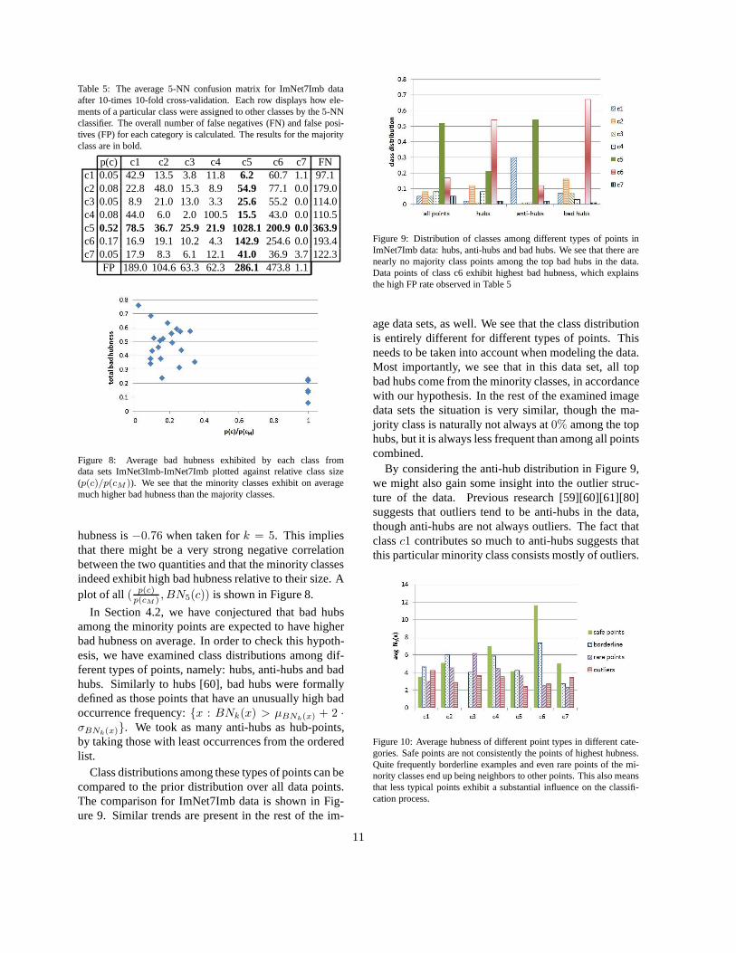
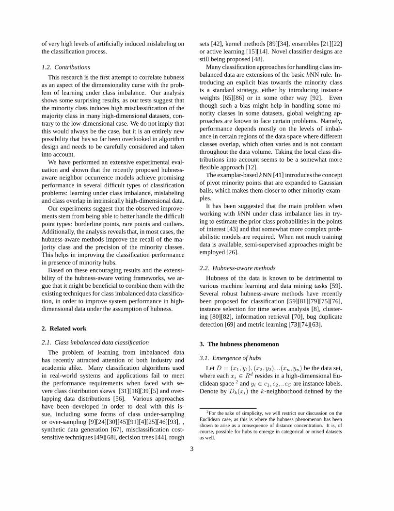
Table 5: The average5-NN confusion matrix for ImNet7Imb dataafter 10-times 10-fold cross-validation. Each row displays how ele-ments of a particular class were assigned to other classes bythe5-NNclassifier. The overall number of false negatives (FN) and false posi-tives (FP) for each category is calculated. The results for the majorityclass are in bold.

p(c) c1 c2 c3 c4 c5 c6 c7 FNc1 0.05 42.9 13.5 3.8 11.8 6.2 60.7 1.1 97.1c2 0.08 22.8 48.0 15.3 8.9 54.9 77.1 0.0179.0c3 0.05 8.9 21.0 13.0 3.3 25.6 55.2 0.0114.0c4 0.08 44.0 6.0 2.0 100.5 15.5 43.0 0.0110.5c5 0.52 78.5 36.7 25.9 21.9 1028.1 200.9 0.0 363.9c6 0.17 16.9 19.1 10.2 4.3 142.9 254.6 0.0193.4c7 0.05 17.9 8.3 6.1 12.1 41.0 36.9 3.7122.3

FP 189.0 104.6 63.3 62.3286.1 473.8 1.1

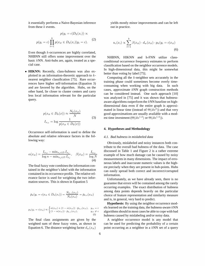
Figure 8: Average bad hubness exhibited by each class fromdata sets ImNet3Imb-ImNet7Imb plotted against relative class size(p(c)/p(cM )). We see that the minority classes exhibit on averagemuch higher bad hubness than the majority classes.

hubness is−0.76 when taken fork = 5. This impliesthat there might be a very strong negative correlationbetween the two quantities and that the minority classesindeed exhibit high bad hubness relative to their size. Aplot of all ( p(c)

p(cM ) , BN5(c)) is shown in Figure 8.

In Section 4.2, we have conjectured that bad hubsamong the minority points are expected to have higherbad hubness on average. In order to check this hypoth-esis, we have examined class distributions among dif-ferent types of points, namely: hubs, anti-hubs and badhubs. Similarly to hubs [60], bad hubs were formallydefined as those points that have an unusually high badoccurrence frequency:{x : BNk(x) > µBNk(x) + 2 ·σBNk(x)}. We took as many anti-hubs as hub-points,by taking those with least occurrences from the orderedlist.

Class distributions among these types of points can becompared to the prior distribution over all data points.The comparison for ImNet7Imb data is shown in Fig-ure 9. Similar trends are present in the rest of the im-

Figure 9: Distribution of classes among different types of points inImNet7Imb data: hubs, anti-hubs and bad hubs. We see that there arenearly no majority class points among the top bad hubs in the data.Data points of class c6 exhibit highest bad hubness, which explainsthe high FP rate observed in Table 5

age data sets, as well. We see that the class distributionis entirely different for different types of points. Thisneeds to be taken into account when modeling the data.Most importantly, we see that in this data set, all topbad hubs come from the minority classes, in accordancewith our hypothesis. In the rest of the examined imagedata sets the situation is very similar, though the ma-jority class is naturally not always at0% among the tophubs, but it is always less frequent than among all pointscombined.

By considering the anti-hub distribution in Figure 9,we might also gain some insight into the outlier struc-ture of the data. Previous research [59][60][61][80]suggests that outliers tend to be anti-hubs in the data,though anti-hubs are not always outliers. The fact thatclassc1 contributes so much to anti-hubs suggests thatthis particular minority class consists mostly of outliers.

Figure 10: Average hubness of different point types in different cate-gories. Safe points are not consistently the points of highest hubness.Quite frequently borderline examples and even rare points of the mi-nority classes end up being neighbors to other points. This also meansthat less typical points exhibit a substantial influence on the classifi-cation process.

11

Figure 11: Average5-NN bad hubness of different point types shownboth for ImNet and high-dimensional synthetic Gaussian mixturesgiven in Table 9, Section 5.4. We give both bad hubness distribu-tions here for easier comparison. It is clear that they are quite dif-ferent. In the analyzed image data, most bad influence is exhibitedby atypical class points (borderline examples, rare points, outliers),while most bad influence in the Gaussian mixture data is generatedby safe points. The latter is quite counterintuitive, as we usually ex-pect for such typical points to be located in the inner regions of classdistributions.

In Figure 10 we can see the distribution of occurrencefrequencies among safe points, borderline points, rarepoints and outliers given separately for each category ofthe ImNet7Imb data set. The results indicate a strongviolation of the cluster assumption, as point hubnessis closely linked to within-cluster centrality [80][82].High hubness of borderline points indicates that dataclusters are not homogenous with respect to the labelspace. Indeed, our initial tests have shown that this datadoes not cluster well. Another thing worth noting is thatpoints that we usually think of as reliable might havea detrimental influence on the classification process,which is clear from examining the hubness/bad hubnessdistribution across different point types forc6, whichhas a high overall bad hubness and FP rate. It is pre-cisely the safe points that exhibit both the highest hub-ness (AVG. 11.66) and the highest bad hubness (AVG.6.63). This is yet another good illustration of the differ-ences between low-dimensional and high-dimensionaldata. Intuitively, we would expect the safe points tobe located in the innermost part of the class distribu-tion space and not to become neighbors tomanyotherpoints from different categories. This is precisely whathappens here and is yet another slightly counterintuitiveresult.

Bad occurrence distributions summarized in Fig-ure 11 illustrate that different underlying bad hub struc-tures exist in different types of data. In the analyzed im-age data (ImNet3-7, ImNetImb3-7), the previously de-scribed pathological case of safe/inner points arising astop bad hubs in the data is still more an exception than

a rule, while in high-dimensional Gaussian mixtures itbecomes a dominating feature. Further analysis of thesynthetic datasets is given in Section 5.4, where classoverlap is discussed.

5.2.2. Hubness-aware classification under class imbal-ance

In order to learn more about the way in which thehubness-aware classifiers handle the minority and themajority class points, we have performed an in-depthanalysis of the classification results summarized in Ta-ble 3, by focusing on certain imbalanced image datasets.

Unbalancing the original five datasets (ImNet3-ImNet7) seems not to have increased the overall dif-ficulty in terms of the achieved classification accuracyand the total induced bad hubness (Table 2). As badhubness is not directly caused by class imbalance andresults as an interplay of various contributing factors,this is not altogether surprising.

ImNetImb data sets were selected via random un-dersampling and it is always difficult to predict the ef-fects of data reduction on hubness. Removing anti-hubsmakes nearly no difference, but removing hub-pointscertainly does. After a hub is removed and all neighborlists are recalculated, the occurrence profiles of manyother hub-points change, as they fill in the thereby re-leased ’empty spaces’ in neighbor lists where the re-moved hub participated.

An analysis of precision and recall for each class sep-arately is shown in Table 6, for the ImNet7Imb dataset.It can be see that all hubness-aware algorithms improveon average both precision and recall for most individualcategories.

Table 6: Precision and recall for each class and each method sepa-rately on ImNet7Imb data set. Values greater or equal to the scoreachieved bykNN are given as bold. The last column represents theSpearman correlation between the improvement overkNN in preci-sion or recall and the size of the class. In other words,corrImp =

corr(p(c)

max p(c), improvement).

method measure c1 c2 c3 c4 c5 c6 c7priors: 0.05 0.08 0.05 0.08 0.52 0.17 0.05 AVG corrImp

kNNprecision0.20 0.32 0.18 0.62 0.78 0.35 0.31 0.39recall 0.31 0.21 0.10 0.47 0.74 0.57 0.03 0.35

hw-kNNprecision 0.46 0.39 0.28 0.72 0.79 0.41 0.58 0.52 -0.96recall 0.30 0.30 0.19 0.73 0.81 0.59 0.17 0.44 -0.43

h-FNNprecision 0.65 0.46 0.37 0.72 0.69 0.44 0.76 0.58 -0.86recall 0.18 0.19 0.09 0.73 0.92 0.43 0.12 0.38 -0.07

NHBNNprecision 0.36 0.37 0.22 0.62 0.79 0.47 0.45 0.47 -0.39recall 0.43 0.22 0.22 0.80 0.81 0.50 0.20 0.45 -0.68

HIKNNprecision 0.55 0.45 0.30 0.74 0.78 0.40 0.67 0.55 -0.75recall 0.24 0.23 0.14 0.74 0.84 0.61 0.17 0.42 0.0

To further analyze the structure of this improvement,an analysis of the correlation between class size and

12

the improvement in precision or recall was performedfor each tested algorithm. As it turns out, hubness-aware algorithms improve precision much more con-sistently than recall - and this improvement has highnegative correlation with relative class size. In otherwords,hubness-aware classification improves the preci-sion of minority class categorization, and the improve-ment grows for smaller and smaller classes. Actually,NHBNN is an exception, as it soon becomes clear thatit behaves differently. A closer examination reveals thatthe recall of the majority class is improved in all the im-balanced data sets, except when NHBNN is used. Thisis shown in Figure 12. On the contrary, NHBNN is bestat improving the minority class recall, which is not al-ways improved by other hubness-aware algorithms, asshown in Figure 13.

HIKNN is essentially an extension of the basic h-FNN algorithm, so it is interesting to observe such aclear difference between the two. h-FNN is always bet-ter at improving the majority class recall, while HIKNNachieves better overall minority class recall. Both algo-rithms rely on neighbor occurrence models, but HIKNNderives more information directly from a neighbor’s la-bel and this is why it has a higher specificity bias, whichis reflected in the results. The results of NHBNN, on theother hand, are not so easy to interpret. It seems that theBayesian modeling of the neighbor-relation differs fromthe fuzzy model in some subtle way.

Figure 12: A comparison of majority class recall achieved bybothkNN and the hubness-aware classification algorithms on five imbal-anced image data sets. Improvements are clear in hw-kNN, h-FNNand HIKNN.

Observing precision and recall separately does not al-low us to rank the algorithms according to their relativeperformance, so we will rank them according to theF1-measure scores [88]. We report the micro- and macro-averagedF1-measure (Fµ

1 andFM1 , respectivelly) for

each algorithm over the imbalanced data sets in Table 7.Micro-averaging is affected by class imbalance, so themacro-averagedF1 scores ought to be preferred. In thiscase it makes no difference. The results show that all

Figure 13: A comparison of the cumulative minority class recall(micro-averaged) achieved by bothkNN and the hubness-aware clas-sification algorithms on five imbalanced image data sets. NHBNNseems undoubtedly the best in raising the minority class recall. Otherhubness-aware algorithms offer some improvements on ImNetImb4-7, but under-perform at ImNet3Imb data. In this case, HIKNN is bet-ter than h-FNN on all data sets, just as h-FNN was constantly slightlybetter than HIKNN when raising the majority class recall.

of the hubness-aware approaches improve on the basickNN in terms of bothFµ

1 andFM1 . NHBNN achieves

the bestF1-score, followed by HIKNN and hw-kNN,while h-FNN is, in this case, the least balanced of allthe considered hubness-aware approaches.

Table 7: Micro- and macro-averagedF1 scores of the classifiers onthe imbalanced data sets. The best score in each line is in bold.

kNN hw-kNN h-FNN NHBNN HIKNNF

µ1 0.61 0.68 0.66 0.70 0.69

FM1 0.43 0.52 0.47 0.57 0.53

In order to see if the hubness-aware approaches actu-ally achieve their improvements by utilizing the learnedoccurrence information about the minority hubs, wehave performed additional tests. We have tracked whichpoint-wise class predictions improve over the baselinekNN and which predictions end up being worse, av-eraged over the 10-times 10-fold cross-validation. Inboth cases, we checked for presence of hubs of differ-ent classes in thekNN sets of individual points for eachtest run separately. For each hub point, all the improve-ments and deteriorations in prediction quality over theset of its reverse neighbors have been summed in or-der to estimate the overall change in prediction qualityin thekNN sets where the hub point occurs. The resultsfor the ImNet7Imb dataset are shown in Figure 14. Sim-ilarly, we can focus on bad hubs specifically and the dis-tribution of average improvements in prediction qualityin presence of bad hubs is shown in Figure 15.

In both cases, the improvements are most pronouncedfor classc6, which is not the majority class and is theclass with highest bad hubness on the dataset. This sug-gests that the improvements are indeed obtained by ex-

13

Figure 14: The average number of improvements in predictionqualityamong the reverse neighbors of hubs points, on ImNet7Imb data.

Figure 15: The average number of improvements in predictionqualityamong the reverse neighbors of bad hubs points, on ImNet7Imbdata.

ploiting the relevant hubness information.The property of hw-kNN, h-FNN and HIKNN of sig-

nificantly raising the recall of the majority class is a veryuseful one, especially since they are able to do so with-out harming the minority class recall. This helps withhandling class imbalanced data under the assumption ofhubness.

As most standard approaches to learning under classimbalance aim in the opposite direction, it might beuseful to consider hybrid approaches in the future, bycombining both types of prediction strategies. As thehubness-aware classification methods mostly modifythe final voting, they can easily be combined with over-sampling/under-sampling [9][30][45][91][4][40], in-stance weighting [66] or examplar-based learning [41].They can also, in principle, support cost-sensitive learn-ing, unlike many otherkNN methods. This is madepossible by the occurrence model, as not every occur-rence has to be given the same weight when calculatingNk,c(x). Distance-weighted occurrence models werealready considered [72], but cost-sensitive occurrencemodels are certainly an option that we wish to explorein our future work.

5.3. Robustness to mislabeling

Instance mislabeling is not unrelated to class imbal-ance. [35] Algorithm performance depends on the dis-tribution of mislabeling across the categories in the data.Even more importantly, the impact of mislabeling on al-gorithm performance in high-dimensional data dependsheavily on the average hubness of mislabeled exam-ples. Mislabeling anti-hubs makes no difference what-soever. Mislabeling even a couple of hub-points shouldbe enough to cause significant misclassification.

In our experiments, mislabeling was distributed uni-formly across different categories and only the train-ing data on each cross-validation fold was mislabeled.Evaluation was performed on the original labels. Anoverview of algorithm performance under30% misla-beling rate is shown in Table 8. The results confirmour hypothesis that the hubness-aware algorithms ex-hibit much higher robustnessto mislabeling thankNN.

Table 8: Experiments on mislabeled data. 30% mislabeling was arti-ficially introduced to each data set at random. All experiments wereperformed fork = 5. The symbols•/◦ denote statistically significantworse/better performance (p < 0.05) compared tokNN. The bestresult in each line is in bold.

Data set kNN hw-kNN h-FNN NHBNN HIKNN

diabetes 54.1 ± 3.7 64.7 ± 3.9 ◦ 66.2 ± 3.4 ◦ 66.1 ± 3.4 ◦ 65.4 ± 3.9 ◦

ecoli 68.1 ± 5.6 80.2 ± 4.7 ◦ 85.8 ± 4.1 ◦ 79.3 ± 4.8 ◦ 81.7 ± 4.6 ◦

glass 50.6 ± 7.3 61.6 ± 7.3 ◦ 62.8 ± 6.8 ◦ 56.8 ± 6.6 61.5 ± 6.7 ◦

iris 71.1 ± 8.5 88.2 ± 6.0 ◦ 90.7 ± 5.4 ◦ 93.2 ± 4.6 ◦ 87.8 ± 6.3 ◦

mfeat-factors 70.7 ± 2.3 91.4 ± 1.5 ◦ 94.9 ± 1.1 ◦ 94.7 ± 1.2 ◦ 93.9 ± 1.2 ◦

mfeat-fourier 57.1 ± 2.5 75.0 ± 2.1 ◦ 81.0 ± 1.7 ◦ 80.7 ± 1.9 ◦ 78.7 ± 1.7 ◦

ovarian 58.1 ± 6.6 76.3 ± 6.1 ◦ 81.1 ± 5.6 ◦ 79.4 ± 5.6 ◦ 78.3 ± 5.5 ◦

segment 62.7 ± 2.2 81.1 ± 1.9 ◦ 84.3 ± 1.7 ◦ 83.8 ± 1.6 ◦ 80.8 ± 1.7 ◦

sonar 61.5 ± 7.7 70.8 ± 6.8 ◦ 72.4 ± 6.4 ◦ 72.9 ± 6.3 ◦ 71.4 ± 6.8 ◦

vehicle 48.2 ± 3.9 57.5 ± 3.9 ◦ 58.1 ± 4.0 ◦ 56.8 ± 4.0 ◦ 59.2 ± 3.8 ◦

ImNet3 51.0 ± 2.3 69.9 ± 2.2 ◦ 81.2 ± 1.8 ◦ 80.6 ± 1.6 ◦ 75.3 ± 2.0 ◦

ImNet4 44.6 ± 1.4 52.5 ± 1.3 ◦ 63.3 ± 1.3 ◦ 63.1 ± 1.2 ◦ 57.6 ± 1.3 ◦

ImNet5 40.0 ± 1.4 47.2 ± 1.4 ◦ 60.6 ± 1.2 ◦ 60.0 ± 1.2 ◦ 53.1 ± 1.3 ◦

ImNet6 49.5 ± 1.7 55.1 ± 1.4 ◦ 68.0 ± 1.3 ◦ 67.4 ± 1.3 ◦ 62.8 ± 1.4 ◦

ImNet7 33.1 ± 1.1 44.8 ± 1.1 ◦ 57.6 ± 1.1 ◦ 56.8 ± 1.1 ◦ 51.0 ± 1.1 ◦

ImNet3Imb 56.7 ± 3.0 78.7 ± 2.2 ◦ 87.0 ± 1.6 ◦ 81.1 ± 2.2 ◦ 83.2 ± 2.1 ◦

ImNet4Imb 51.8 ± 1.7 55.0 ± 1.7 ◦ 68.7 ± 1.7 ◦ 67.3 ± 1.8 ◦ 63.9 ± 1.7 ◦

ImNet5Imb 50.7 ± 2.1 53.5 ± 2.0 ◦ 64.2 ± 2.0 ◦ 60.5 ± 1.8 ◦ 60.6 ± 1.2 ◦

ImNet6Imb 54.7 ± 2.1 55.8 ± 2.0 ◦ 69.7 ± 1.7 ◦ 66.6 ± 1.9 ◦ 62.8 ± 2.0 ◦

ImNet7Imb 33.1 ± 2.3 52.0 ± 1.9 ◦ 62.9 ± 1.9 ◦ 61.1 ± 1.9 ◦ 58.6 ± 1.7 ◦

AVG 53.37 65.57 73.03 71.41 69.38

Out of the compared hubness-aware algorithms, h-FNN dominates in this experimental setup. On manydatasets h-FNN is no more than 1-2% less accurate thanbefore, which is astounding considering the level ofmislabeling in the data. On the other hand, the hubness-weighting approach (hw-kNN) fails in this case and isnot able to cope with such high mislabeling rates.

Similarly, Figure 16 shows the drop in accuracy asmislabeling is slowly introduced in the data. ThekNNperformance seems to be decreasing at a linear rate withincreasing noise. At the same time, hubness-aware ap-proaches retain most of their accuracy as the mislabel-ing rate goes all the way up to40% − 50%. This can

14

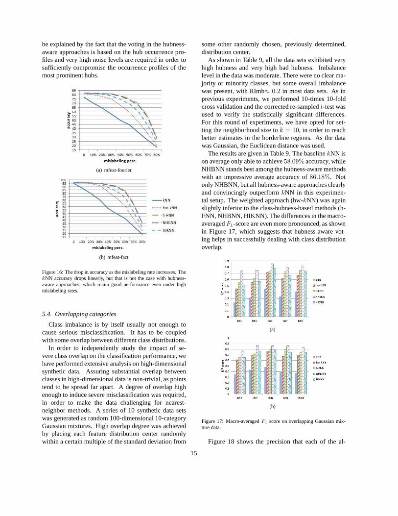
be explained by the fact that the voting in the hubness-aware approaches is based on the hub occurrence pro-files and very high noise levels are required in order tosufficiently compromise the occurrence profiles of themost prominent hubs.

(a) mfeat-fourier

(b) mfeat-fact

Figure 16: The drop in accuracy as the mislabeling rate increases. ThekNN accuracy drops linearly, but that is not the case with hubness-aware approaches, which retain good performance even underhighmislabeling rates.

5.4. Overlapping categories

Class imbalance is by itself usually not enough tocause serious misclassification. It has to be coupledwith some overlap between different class distributions.

In order to independently study the impact of se-vere class overlap on the classification performance, wehave performed extensive analysis on high-dimensionalsynthetic data. Assuring substantial overlap betweenclasses in high-dimensional data is non-trivial, as pointstend to be spread far apart. A degree of overlap highenough to induce severe misclassification was required,in order to make the data challenging for nearest-neighbor methods. A series of 10 synthetic data setswas generated as random 100-dimensional 10-categoryGaussian mixtures. High overlap degree was achievedby placing each feature distribution center randomlywithin a certain multiple of the standard deviation from

some other randomly chosen, previously determined,distribution center.

As shown in Table 9, all the data sets exhibited veryhigh hubness and very high bad hubness. Imbalancelevel in the data was moderate. There were no clear ma-jority or minority classes, but some overall imbalancewas present, with RImb≈ 0.2 in most data sets. As inprevious experiments, we performed 10-times 10-foldcross validation and the corrected re-sampledt-test wasused to verify the statistically significant differences.For this round of experiments, we have opted for set-ting the neighborhood size tok = 10, in order to reachbetter estimates in the borderline regions. As the datawas Gaussian, the Euclidean distance was used.

The results are given in Table 9. The baselinekNN ison average only able to achieve58.09% accuracy, whileNHBNN stands best among the hubness-aware methodswith an impressive average accuracy of86.18%. Notonly NHBNN, but all hubness-aware approaches clearlyand convincingly outperformkNN in this experimen-tal setup. The weighted approach (hw-kNN) was againslightly inferior to the class-hubness-based methods (h-FNN, NHBNN, HIKNN). The differences in the macro-averagedF1-score are even more pronounced, as shownin Figure 17, which suggests that hubness-aware vot-ing helps in successfully dealing with class distributionoverlap.

(a)

(b)

Figure 17: Macro-averagedF1 score on overlapping Gaussian mix-ture data.

Figure 18 shows the precision that each of the al-

15

Table 9: Classification accuracies on synthetic Gaussian mixture data fork = 10. For each data set, the skewness of theN10 distribution is givenalong with the bad occurrence rate (BN10). The symbols•/◦ denote statistically significant worse/better performance (p < 0.01) compared tokNN. The best result in each line is in bold.

Data set sizeSN10 BN10 kNN hw-kNN h-FNN NHBNN HIKNN

DS1 1244 6.68 53.5% 43.8 ± 3.1 64.4 ± 5.3◦ 72.6 ± 2.8◦ 80.7 ± 2.4 ◦ 65.8 ± 3.0◦DS2 1660 4.47 49.2% 48.4 ± 2.8 73.6 ± 6.9◦ 79.3 ± 2.2◦ 83.9 ± 2.2 ◦ 73.1 ± 2.5◦DS3 1753 5.50 42.0% 67.3 ± 2.3 85.3 ± 2.6◦ 86.8 ± 1.7◦ 90.0 ± 1.4 ◦ 86.7 ± 1.9◦DS4 1820 3.45 51% 52.2 ± 2.6 72.8 ± 2.3◦ 78.4 ± 2.2◦ 81.9 ± 2.0 ◦ 72.2 ± 2.3◦DS5 1774 4.39 46.3% 59.2 ± 2.7 80.2 ± 3.4◦ 84.6 ± 1.8◦ 87.2 ± 1.5 ◦ 81.1 ± 2.1◦DS6 1282 3.98 45.6% 58.6 ± 3.3 80.0 ± 3.3◦ 81.7 ± 2.5◦ 86.6 ± 2.2 ◦ 79.4 ± 2.5◦DS7 1662 4.64 41.5% 65.0 ± 2.4 84.6 ± 2.4◦ 85.4 ± 1.9◦ 90.1 ± 1.5 ◦ 84.5 ± 2.0◦DS8 1887 4.19 40.0% 71.0 ± 2.3 82.7 ± 2.5◦ 85.9 ± 1.9◦ 88.4 ± 1.8 ◦ 83.9 ± 2.3◦DS9 1661 5.02 47.5% 57.9 ± 2.7 76.3 ± 3.3◦ 82.3 ± 2.0◦ 87.5 ± 1.7 ◦ 77.7 ± 2.4◦DS10 1594 4.82 46.9% 57.5 ± 2.9 78.1 ± 3.3◦ 81.1 ± 2.3◦ 85.5 ± 1.9 ◦ 77.7 ± 2.2◦

AVG 58.09 77.80 81.81 86.18 78.21

gorithms achieves on safe points, borderline examples,rare points and outliers, separately [52]. Not surpris-ingly, kNN is completely incapable of dealing with rarepoints and outliers - and performs badly even on border-line points. We should point out that the reason why theprecision isn’t100% on safe points is thatk = 5 is used(as described in [52]) to determine point types, but herewe are observing10-NN classification. Hubness-awaremethods achieve higher precision on all point types, safepoints included. The difference in performance is mostpronounced for more difficult point types and this iswhere most of the improvement stems from. Also, weare able to see why NHBNN scores better than the otherhubness-aware algorithms on this data. It performs bet-ter when classifying all the difficult point types in theoverlap regions. On average, NHBNN manages to cor-rectly assign the labels to more than90% of borderlinepoints, about75% of rare points and35% of outliers.We have verified that this is indeed true for all10 ex-amined Gaussian mixtures. It is interesting to note thatthe same trend is not detected in ImgNet data that wasdiscussed in Section 5.2. Bad hubness in ImgNet data isnot exclusively due to class overlap, so it is a differentstory altogether.

As a final remark, we report the performance ofsome other well-known algorithms on class overlapdata. Table 10 contains a summary of results given forthe fuzzyk-nearest-neighbor (FNN) [38], probabilisticnearest neighbor (PNN) [32], neighbor-weightedkNN(NWKNN) [65], adaptivekNN (AKNN) [85], J48 (aWEKA [88] implementation of the Quinlan’s C4.5 al-gorithm [57]), random forest classifier [7] and NaiveBayes [50]. Default parameter configurations were usedfor the Weka implementations of the tree-based algo-

Figure 18: Classification precision on certain types of points onDS0:safe points, borderline points, rare examples and outliers. We seethat the baselinekNN is completely unable to deal with rare pointsand outliers and this is precisely where the improvements inhubness-aware approaches stem from.

rithms.The first thing to notice is that FNN scores much

worse than its hubness-aware counterpart h-FNN. Thisshows that there is a large difference in semantics be-tween the fuzziness derived from direct and reversek-nearest neighbor sets. The best performance among allthe tested hubness-unawarekNN methods is attainedby the adaptivekNN (AKNN), which is not surprisingsince it was designed specifically for handling class-overlap data [85]. Its performance is still, however,somewhat inferior to that of NHBNN, at least in thisexperimental setup.

Decision trees, on the other hand, seem to have beenheavily affected by the induced class overlap, as usingeither C4.5 or random forest classifiers results in lowoverall accuracy rates. Naive Bayes was the best amongthe tested approaches on these Gaussian Mixtures.

Figure 19 shows how both NHBNN and Naive Bayes

16

Table 10: Classification accuracy of a selection of algorithms on Gaussian mixture data. The results are given for fuzzyk-nearest-neighbor (FNN),probabilistic nearest neighbor (PNN), neighbor-weightedkNN (NWKNN), adaptivekNN (AKNN), J48 implementation of the Quinlan’s C4.5algorithm, random forest classifier and Naive Bayes, respectivelly. A neighborhood size ofk = 10 was used in the nearest-neighbor-basedapproaches, where applicable. Results better than than theones of NHBNN in Table 9 are given in bold.

Data set FNN PNN NWKNN AKNN J48 R. Forest Naive Bayes

DS1 36.6 ± 3.0 39.8 ± 3.5 46.5 ± 3.3 79.5 ± 2.6 42.4 ± 4.3 59.5 ± 3.7 95.6 ± 1.3DS2 40.5 ± 2.9 35.9 ± 3.2 54.0 ± 2.6 82.7 ± 2.1 47.3 ± 3.9 65.4 ± 3.9 97.1 ± 0.9DS3 61.5 ± 2.7 71.3 ± 2.4 67.4 ± 2.5 88.7 ± 1.7 48.9 ± 3.9 69.2 ± 3.1 98.6 ± 0.2DS4 46.6 ± 2.4 43.4 ± 4.6 56.5 ± 2.9 84.7 ± 1.7 44.0 ± 3.7 59.7 ± 3.7 98.4 ± 0.2DS5 52.3 ± 2.9 54.1 ± 4.3 61.8 ± 2.6 83.2 ± 2.1 45.6 ± 2.9 64.1 ± 3.2 98.3 ± 0.1DS6 51.5 ± 3.0 51.5 ± 3.5 62.2 ± 3.0 78.6 ± 3.2 52.1 ± 4.2 67.2 ± 3.1 97.3 ± 1.1DS7 59.0 ± 2.7 60.0 ± 4.0 66.9 ± 2.6 90.1 ± 1.5 51.0 ± 3.7 70.7 ± 2.6 98.3 ± 0.7DS8 67.8 ± 2.6 72.6 ± 2.6 71.5 ± 2.5 85.2 ± 1.9 50.2 ± 3.7 67.1 ± 3.1 98.7 ± 0.4DS9 51.9 ± 2.7 48.9 ± 4.6 61.7 ± 2.6 84.5 ± 2.0 43.9 ± 3.6 64.5 ± 3.7 98.3 ± 0.7DS10 51.0 ± 2.7 47.8 ± 4.2 62.1 ± 2.5 79.6 ± 2.0 46.2 ± 3.8 64.0 ± 3.1 97.9 ± 0.8

AVG 51.87 52.53 61.06 83.68 47.16 65.14 97.85

Figure 19: Misclassification towards the class c1 that exhibits highestoverall bad hubness onDS0. NHBNN and NB clearly outperformkNN here.

outperform thekNN baseline by reducing the misclas-sification caused by a class with high bad hubness.

An ROC curve that maps the TP rate against the FPrate is shown in Figure 20 forDS0, wherec5 is takenas the negative class and all other points are treated aspositives. The area under the ROC curve (AUC) in thiscase is 0.923 forkNN, 0.974 for NWKNN, 0.965 forhw-kNN, 0.989 for NHBNN and 0.998 for Naive Bayes.Of course, the ROC analysis in the multi-class case is abit more complex, but Figure 20 illustrates the commontrends in this high-dimensional Gaussian Mixture data.

What these comparisons reveal is that the currentlyavailable hubness-awarek-nearest neighbor approachesrank rather well when compared to the otherkNN-basedmethods, but there is also some room for improvement.

6. Conclusions and Future Work

Hubness is an important aspect of the curse of dimen-sionality related tok-nearest neighbor methods. It has

Figure 20: A one-vs-all ROC curve where one of the classes with alower TP rate (c5) is taken as the negative class, onDS0.

a negative impact on the performance of many informa-tion systems, as it allows the errors to easily propagatethrough the data. In this paper, we have shown that itfurther complicates the issues concerning learning un-der class imbalance in high-dimensional data.

Class imbalance poses great difficulties for most ma-chine learning methods and has been a focus of manyserious studies. In low-to-medium-dimensional data,the majority class is known to often cause misclassifi-cation of the minority class.

Surprisingly, we have shown that this intuitive con-sequence of the difference in average relative densitygradients does not necessarily hold in intrinsically high-dimensional data, under the assumption of hubness. Insuch cases, minority classes frequently exhibit high badhubness and have the capacity to induce severe misclas-sification of the majority class. In high-dimensionaldata, most misclassification is caused by the classeswhich have the majority among the bad hubs. We haveshown that the minority classes often achieve this bad

17

hub majority and become the principal sources of mis-classification.

High-dimensional geometry allows for some moreunexpected results, as we have shown that bad hubnessis not expressed only by borderline points, but also bypoints expected to lie in the interiors of class distribu-tions. This represents a strong violation of the clusterassumption.

In order to see if the arising problems can be solvedby utilizing the neighbor occurrence models in orderto predict and rectify the detrimental hub point occur-rences, we have performed an extensive evaluation ofseveral state-of-the-art hubness-awarek-nearest neigh-bor classifiers: hw-kNN, h-FNN, NHBNN and HIKNN.The methods were compared on high-dimensional prob-lems involving class imbalance, mislabeling and classoverlap. The results suggest that the tested approachesexhibit promising levels of robustness and tolerance tothe arising problems. The Naive Bayesian way of han-dling the occurrence models was able to achieve veryhigh precision when handling borderline examples, rarepoints and outliers.

A high misclassification rate caused by the minorityclass examples in many high-dimensional datasets sug-gests that the traditionalkNN approaches to handlingclass imbalanced data that involve adopting an explicitbias towards the minority points are not in general wellsuited for the high-dimensional case. The design ofthese methods should be extended to support the mod-eling of minority-induced misclassification, in order toreduce the negative impact of bad hubs. One way todo this would be to employ the neighbor occurrencemodeling within the class imbalancedkNN methods,by combining them with the existing hubness-aware ap-proaches.

In future work we intend to investigate the possibil-ities for cost-sensitive learning and boosting in build-ing the occurrence models for hubness-aware classifi-cation. We also plan on extending and improving theexisting algorithms now that we have gained a deeperunderstanding of their advantages and disadvantages.Additionally, we will investigate various hubness-awaredata preprocessing schemes for filtering out the misla-beled/noisy data.

Acknowledgments

This work was supported by the Slovenian Re-search Agency, the ICT Programme of the EC un-der XLike (ICT-STREP-288342), and RENDER (ICT-257790-STREP).

References

[1] Aggarwal, C. C., Hinneburg, A., and Keim, D. A. (2001). Onthesurprising behavior of distance metrics in high dimensional spaces.In Proc. 8th Int. Conf. on Database Theory, pages 420–434.

[2] Aucouturier, J. (2006). Ten experiments on the modelling of poly-phonic timbre. Technical report, Doct. dissert., Univ. of Paris 6.

[3] Aucouturier, J. and Pachet, F. (2004). Improving timbresimilar-ity: How high is the sky? Journal of Negative Results in Speechand Audio Sciences, 1.

[4] Batista, G. E. A. P. A., Prati, R. C., and Monard, M. C. (2004).A study of the behavior of several methods for balancing machinelearning training data.SIGKDD Explor. Newsl., 6(1):20–29.

[5] Batuwita, R. and Palade, V. (2009). Micropred: effective classifi-cation of pre-miRNAs for human miRNA gene prediction.Bioin-formatics, 25(8):989–995.

[6] Bouckaert, R. and Frank, E. (2004). Evaluating the replicabilityof significance tests for comparing learning algorithms. InDai, H.,Srikant, R., and Zhang, C., editors,Advances in Knowledge Dis-covery and Data Mining, pages 3–12. Springer Berlin Heidelberg.

[7] Breiman, L. (2001). Random forests.Mach. Learn., 45(1):5–32.[8] Buza, K., Nanopoulos, A., and Schmidt-Thieme, L. (2011). In-

sight: efficient and effective instance selection for time-series clas-sification. InAdvances in knowledge discovery and data mining,PAKDD’11, pages 149–160, Berlin, Heidelberg. Springer-Verlag.

[9] Chawla, N. V., Bowyer, K. W., Hall, L. O., and Kegelmeyer,W. P.(2002). Smote: Synthetic minority over-sampling technique. Jour-nal of Artificial Intelligence Research, 16:321–357.

[10] Chen, J., Fang, H., and Saad, Y. (2009). Fast approximate kNNgraph construction for high dimensional data via recursiveLanczosbisection.Journal of Machine Learning Research, 10:1989–2012.

[11] C.J.Stone (1977). Consistent nonparametric regression. Annalsof Statistics, 5:595–645.

[12] Dubey, H. and Pudi, V. (2013). Class based weighted k-nearestneighbor over imbalance dataset. In Pei, J., Tseng, V., Cao,L., Mo-toda, H., and Xu, G., editors,Advances in Knowledge Discoveryand Data Mining, pages 305–316. Springer Berlin Heidelberg.

[13] Durrant, R. J. and Kaban, A. (2009). When is ‘nearest neigh-bour’ meaningful: A converse theorem and implications.Journalof Complexity, 25(4):385–397.

[14] Ertekin, S., Huang, J., and Giles, C. L. (2007a). Activelearningfor class imbalance problem. InProceedings of the 30th ACMSIGIR conference, pages 823–824, New York, NY, USA. ACM.

[15] Ertekin, S. E., Huang, J., Bottou, L., and Giles, C. L. (2007b).Learning on the border: Active learning in imbalanced data classi-fication. InIn Proc. of CIKM conference.

[16] Ezawa, K., Singh, M., and Norton, S. W. (1996). Learninggoaloriented Bayesian networks for telecommunications risk manage-ment. InIn Proceedings of the 13th International Conference onMachine Learning, pages 139–147. Morgan Kaufmann.

[17] Ezawa, K. J. and Schuermann, T. (1995). Fraud/uncollectibledebt detection using a bayesian network based learning system: arare binary outcome with mixed data structures. InProc. of the11th conf. on Uncertainty in AI, pages 157–166, San Francisco,CA, USA. Morgan Kaufmann Publishers Inc.

[18] Fernandez, A., Garcia, S., and Herrera, F. (2011). Addressingthe classification with imbalanced data: Open problems and newchallenges on class distribution. InIn proc. of HAIS conference,pages 1–10. Springer Berlin Heidelberg.

[19] Fix, E. and Hodges, J. (1951). Discriminatory analysis, non-parametric discrimination: consistency properties. Technical re-port, USAF School of Aviation Medicine, Randolph Field.

[20] Francois, D., Wertz, V., and Verleysen, M. (2007). Theconcen-tration of fractional distances.IEEE Transactions on Knowledgeand Data Engineering, 19(7):873–886.

18

[21] Galar, M., Fernandez, A., Barrenechea, E., Bustince, H., andHerrera, F. (2012). A review on ensembles for the class imbalanceproblem: Bagging-, boosting-, and hybrid-based approaches. Sys-tems, Man, and Cybernetics, Part C: Applications and Reviews,IEEE Transactions on, 42(4):463–484.

[22] Garca-Pedrajas, N. and Garca-Osorio, C. (2013). Boostingfor class-imbalanced datasets using genetically evolved supervisednon-linear projections.Progress in Artificial Intelligence, 2(1):29–44.

[23] Garcia, V., Mollineda, R. A., and Sanchez, J. S. (2008).Onthe k-nn performance in a challenging scenario of imbalanceandoverlapping.Pattern Anal. Appl., 11:269–280.

[24] Garcia, V., Sanchez, J., Martn-Flez, R., and Mollineda, R.(2012). Surrounding neighborhood-based smote for learning fromimbalanced data sets.Progress in Artificial Intelligence, 1(4):347–362.

[25] Garcia-Pedrajas, N., Perez-Rodriguez, J., and de Haro-Garcia,A. (2013). Oligois: Scalable instance selection for class-imbalanced data sets. Cybernetics, IEEE Transactions on,43(1):332–346.

[26] Ghosh, A. K. (2012). A probabilistic approach for semi-supervised nearest neighbor classification.Pattern Recogn. Lett.,33(9):1127–1133.

[27] Guan, D., Yuan, W., Lee, Y.-K., and Lee, S. (2011). Identifyingmislabeled training data with the aid of unlabeled data.AppliedIntelligence, 35:345–358.

[28] Hastie, T. and Tibshirani, R. (1996). Discriminant adaptive near-est neighbor classification.IEEE Trans. Pattern Anal. Mach. In-tell., 18(6):607–616.

[29] Hayashi, K. (2012). A simple extension of boosting for asym-metric mislabeled data.Statistics and Prob. Letters, 82:348–356.

[30] He, H., Bai, Y., Garcia, E. A., and Li, S. (2008). Adasyn:Adaptive synthetic sampling approach for imbalanced learning. InIJCNN’08, pages 1322–1328.

[31] He, H. and Garcia, E. A. (2009). Learning from imbalanceddata. IEEE Transactions on knowledge and data engineering,21(9):1263–1284.

[32] Holmes, C. C. and Adams, N. M. (2002). A probabilistic nearestneighbor method for statistical pattern recognition.J R Stat Soc B,64:295–306.

[33] Holte, R. C., Acker, L. E., and Porter, B. W. (1989). Conceptlearning and the problem of small disjuncts. InProc. 11th Int.Conf. AI - Volume 1, pages 813–818. Morgan Kaufmann PublishersInc.

[34] Hong, X., Chen, S., and Harris, C. J. (2007). A kernel-basedtwo-class classifier for imbalanced data sets.IEEE Transactionson Neural Networks, pages 28–41.

[35] Hulse, J. V., Khoshgoftaar, T. M., and Napolitano, A. (2007).Skewed class distributions and mislabeled examples. InProceed-ings of the Seventh IEEE International Conference on Data MiningWorkshops, ICDMW ’07, pages 477–482, Washington, DC, USA.IEEE Computer Society.

[36] Jensen, R. and Cornelis, C. (2008). A new approach to fuzzy-rough nearest neighbour classification. InProceedings of the6th International Conference on Rough Sets and Current Trendsin Computing, RSCTC ’08, pages 310–319, Berlin, Heidelberg.Springer-Verlag.

[37] Kalager, M., Adami, H., Bretthauer, M., and Tamimi, R. (2012).Overdiagnosis of invasive breast cancer due to mammographyscreening: results from the norwegian screening program.Annalsof Internal Medicine, 156:491–499.

[38] Keller, J. E., Gray, M. R., and Givens, J. A. (1985). A fuzzyk-nearest-neighbor algorithm. InIEEE Transactions on Systems,Man and Cybernetics, pages 580–585.

[39] Kuang, D., Ling, C., and Du, J. (2012). Foundation of mining

class-imbalanced data. In Tan, P.-N., Chawla, S., Ho, C., and Bai-ley, J., editors,Advances in Knowledge Discovery and Data Min-ing, volume 7301 ofLecture Notes in Computer Science, pages219–230. Springer Berlin Heidelberg.

[40] Kubat, M. and Matwin, S. (1997). Addressing the curse ofim-balanced training sets: One-sided selection. InIn Proceedingsof the Fourteenth International Conference on Machine Learning,pages 179–186. Morgan Kaufmann.

[41] Li, Y. and Zhang, X. (2011). Improving k-nearest neighbor withexemplar generalization for imbalanced classification. InAdvancesin Knowledge Disc. and Data Mining, pages 321–332. Springer.

[42] Liu, J., Hu, Q., and Yu, D. (2008). A comparative study onroughset based class imbalance learning.Knowledge-Based Systems,21(8):753 – 763.

[43] Liu, W. and Chawla, S. (2011). Class confidence weightedknn algorithms for imbalanced data sets. InAdvances in Knowl-edge Discovery and Data Mining, volume 6635, pages 345–356.Springer.

[44] Liu, W., Chawla, S., Cieslak, D. A., and Chawla, N. V. (2010).A Robust Decision Tree Algorithm for Imbalanced Data Sets. InSDM, pages 766–777. SIAM.

[45] Liu, X.-Y., Wu, J., and Zhou, Z.-H. (2006). Exploratoryunder-sampling for class-imbalance learning. InProceedings of the SixthInternational Conference on Data Mining, ICDM ’06, pages 965–969, Washington, DC, USA. IEEE Computer Society.

[46] Lopez, V., Fernndez, A., Moreno-Torres, J. G., and Herrera, F.(2012). Analysis of preprocessing vs. cost-sensitive learning forimbalanced classification. open problems on intrinsic datacharac-teristics.Expert Systems with Applications, 39(7):6585 – 6608.

[47] Low, T., Borgelt, C., Stober, S., and Nrnberger, A. (2013).The hubness phenomenon: Fact or artifact? In Borgelt, C., Gil,M. n., Sousa, J. M., and Verleysen, M., editors,Towards AdvancedData Analysis by Combining Soft Computing and Statistics, vol-ume 285 ofStudies in Fuzziness and Soft Computing, pages 267–278. Springer Berlin Heidelberg.

[48] Martino, M. D., FernaNdez, A., Iturralde, P., and Lecumberry, F.(2013). Novel classifier scheme for imbalanced problems.PatternRecogn. Lett., 34(10):1146–1151.

[49] McCarthy, K., Zabar, B., and Weiss, G. (2005). Does cost-sensitive learning beat sampling for classifying rare classes? InProceedings of the 1st int. workshop on Utility-based data mining,UBDM ’05, pages 69–77, New York, NY, USA. ACM.

[50] Mitchell, T. M. (1997).Machine Learning. McGraw-Hill.[51] Nanopoulos, A., Radovanovic, M., and Ivanovic, M. (2009).

How does high dimensionality affect collaborative filtering? InProceedings of the third ACM conference on Recommender sys-tems, RecSys ’09, pages 293–296, New York, NY, USA. ACM.

[52] Napierala, K. and Stefanowski, J. (2012). Identification of dif-ferent types of minority class examples in imbalanced data.In Inproc. of. HAIS conference, pages 139–150. Springer Berlin.

[53] Ougiaroglou, S., Nanopoulos, A., Papadopoulos, A. N.,Manolopoulos, Y., and Welzer-druzovec, T. (2007). Adaptive k-nearest neighbor classification based on a dynamic number ofnear-est neighbors. InProceedings of ADBIS Conference, ADBIS 2007.

[54] Peng, J., Heisterkamp, D. R., and Dai, H. K. (2004). Adaptivequasiconformal kernel nearest neighbor classification.IEEE Trans.Pattern Anal. Mach. Intell., 26(5):656–661.

[55] Pracner, D., Tomasev, N., Radovanovic, M., Mladeni´c, D., andIvanovic, M. (2011). WIKImage: Correlated image and textdatasets. InProc. of the 14th International Multiconference on In-formation Society (IS 2011), volume A, pages 141–144, Ljubljana,Slovenia.

[56] Prati, R., Batista, G., and Monard, M. (2004). Class imbalancesversus class overlapping: An analysis of a learning system behav-ior. In Proceedings of the Mexican International Conference on

19

Artificial Intelligence, RSCTC ’08, pages 312–321.[57] Quinlan, R. (1993). C4.5: Programs for Machine Learning.

Morgan Kaufmann Publishers.[58] Radovanovic, M. (2011).Representations and Metrics in High-

Dimensional Data Mining. Izdavacka knjizarnica Zorana Sto-janovica, Novi Sad, Serbia.

[59] Radovanovic, M., Nanopoulos, A., and Ivanovic, M. (2009).Nearest neighbors in high-dimensional data: The emergenceandinfluence of hubs. InProc. 26th Int. Conf. on Machine Learning(ICML), pages 865–872.

[60] Radovanovic, M., Nanopoulos, A., and Ivanovic, M. (2010a).Hubs in space: Popular nearest neighbors in high-dimensionaldata.Journal of Machine Learning Research, 11:2487–2531.

[61] Radovanovic, M., Nanopoulos, A., and Ivanovic, M. (2010b).On the existence of obstinate results in vector space models. InProc. 33rd Annual Int. ACM SIGIR Conf. on Research and Devel-opment in Information Retrieval, pages 186–193.

[62] Radovanovic, M., Nanopoulos, A., and Ivanovic, M. (2010).Time-series classification in many intrinsic dimensions. In SDM,pages 677–688. SIAM.

[63] Schnitzer, D., Flexer, A., Schedl, M., and Widmer, G. (2012).Local and global scaling reduce hubs in space.Journal of MachineLearning Research, pages 2871–2902.

[64] Song, Y., Huang, J., Zhou, D., Zha, H., and Giles, C. L. (2007).Iknn: Informative k-nearest neighbor pattern classification. InPro-ceedings of the 11th European conference on Principles and Prac-tice of Knowledge Discovery in Databases, PKDD 2007, pages248–264, Berlin, Heidelberg. Springer-Verlag.

[65] Tan, S. (2005a). Neighbor-weighted k-nearest neighbor for un-balanced text corpus.Expert Syst. Appl., 28:667–671.

[66] Tan, S. (2005b). Neighbor-weighted k-nearest neighbor for un-balanced text corpus.Expert Syst. Appl., 28:667–671.

[67] Thanathamathee, P. and Lursinsap, C. (2013). Handlingim-balanced data sets with synthetic boundary data generationusingbootstrap re-sampling and adaboost techniques.Pattern Recogni-tion Letters, 34(12):1339 – 1347.

[68] Ting, K. M. (2002). An instance-weighting method to in-duce cost-sensitive trees.IEEE Trans. on Knowl. and Data Eng.,14(3):659–665.

[69] Tomasev, N., , Leban, G., and Mladenic, D. (2013a). Exploitinghubs for self-adaptive secondary re-ranking in bug report duplicatedetection. InProceedings of the ITI conference, ITI 2013.

[70] Tomasev, N., , Rupnik, J., and Mladenic, D. (2013b). The role ofhubs in cross-lingual supervised document retrieval. InProceed-ings of the PAKDD Conference, PAKDD 2013.

[71] Tomasev, N., Brehar, R., Mladenic, D., and Nedevschi, S.(2011a). The influence of hubness on nearest-neighbor methods inobject recognition. InProceedings of the 7th IEEE InternationalConference on Intelligent Computer Communication and Process-ing (ICCP), pages 367–374.

[72] Tomasev, N. and Mladenic, D. (2011). The influence of weight-ing the k-occurrences on hubness-aware classification methods. InProceedings of the SiKDD conference.

[73] Tomasev, N. and Mladenic, D. (2012a). Hubness-awaresharedneighbor distances for high-dimensional k-nearest neighbor clas-sification. InProceedings of the 7th International Conference onHybrid Artificial Intelligence Systems, HAIS ’12.

[74] Tomasev, N. and Mladenic, D. (2012b). Hubness-awaresharedneighbor distances for high-dimensional k-nearest neighbor clas-sification. Knowledge and Information Systems.

[75] Tomasev, N. and Mladenic, D. (2012c). Nearest neighbor votingin high dimensional data: Learning from past occurrences.Com-puter Science and Information Systems, 9:691–712.

[76] Tomasev, N. and Mladenic, D. (2013a). Hub co-occurrencemodeling for robust high-dimensional knn classification. In Pro-

ceedings of the ECML/PKDD Conference. Springer.[77] Tomasev, N. and Mladenic, D. (2013b). Image hub explorer:

Evaluating representations and metrics for content-basedimage re-trieval and object recognition. InProceedings of the ECML/PKDDConference. Springer.

[78] Tomasev, N., Pracner, D., Brehar, R., Radovanovic, M.,Mladenic, D., Ivanovic, M., and Nedevshi, S. (2013c). Objectrecognition in wikimage data based on local invariant imagefea-tures. InProceedings of the IEEE ICCP Conference. IEEE.

[79] Tomasev, N., Radovanovic, M., Mladenic, D., and Ivanovic, M.(2011b). A probabilistic approach to nearest neighbor classifica-tion: Naive hubness bayesian k-nearest neighbor. InProceeding ofthe CIKM conference.

[80] Tomasev, N., Radovanovic, M., Mladenic, D., and Ivanovic, M.(2011c). The role of hubness in clustering high-dimensional data.In Advances in Knowledge Discovery and Data Mining, volume6634, pages 183–195. Springer.

[81] Tomasev, N., Radovanovic, M., Mladenic, D., and Ivanovic, M.(2013d). Hubness-based fuzzy measures for high-dimensional k-nearest neighbor classification.International Journal of MachineLearning and Cybernetics.

[82] Tomasev, N., Radovanovic, M., Mladenic, D., and Ivanovic,M. (2013e). The role of hubness in clustering high-dimensionaldata. IEEE Transactions on Knowledge and Data Engineering,99(PrePrints).

[83] Valizadegan, H. and Tan, P.-N. (2007). Kernel based detectionof mislabeled training examples. InSDM. SIAM.

[84] van den Bosch, A., Weijters, T., Herik, H. J. V. D., and Daele-mans, W. (1997). When small disjuncts abound, try lazy learning:A case study.

[85] Wang, J., Neskovic, P., and Cooper, L. N. (2007). Improvingnearest neighbor rule with a simple adaptive distance measure.Pat-tern Recogn. Lett., 28:207–213.

[86] Wang, S., Li, X., Xia, J.-F., and Zhang, X.-P. (2010). Weightedneighborhood classifier for the classification of imbalanced tumordataset.Journal of Circuits, Systems, and Computers, pages 259–273.

[87] Weiss, G. M. (2004). Mining with rarity: a unifying framework.SIGKDD Explor. Newsl., 6:7–19.

[88] Witten, I. H. and Frank, E. (2005).Data Mining: PracticalMachine Learning Tools and Techniques. Morgan Kaufmann Pub-lishers, second edition.

[89] Wu, G. and Chang, E. Y. (2005). KBA: kernel boundary align-ment considering imbalanced data distribution.Knowledge andData Engineering, IEEE Transactions on, 17(6):786–795.

[90] Zhang, H., Berg, A. C., Maire, M., and Malik, J. (2006). Svm-knn: Discriminative nearest neighbor classification for visual cat-egory recognition. InProceedings of the 2006 IEEE ComputerSociety Conference on Computer Vision and Pattern Recognition -Volume 2, CVPR ’06, pages 2126–2136, Washington, DC, USA.IEEE Computer Society.

[91] Zhang, J. and Mani, I. (2003). KNN Approach to UnbalancedData Distributions: A Case Study Involving Information Extrac-tion. In Proceedings of the ICML’2003 Workshop on Learningfrom Imbalanced Datasets.

[92] Zhang, X. and Li, Y. (2013). A positive-biased nearest neigh-bour algorithm for imbalanced classification. In Pei, J., Tseng,V., Cao, L., Motoda, H., and Xu, G., editors,Advances in Knowl-edge Discovery and Data Mining, volume 7819 ofLecture Notesin Computer Science, pages 293–304. Springer Berlin Heidelberg.

[93] Zhou, L. (2013). Performance of corporate bankruptcy predic-tion models on imbalanced dataset: The effect of sampling meth-ods.Know.-Based Syst., 41:16–25.

20