Embed Size (px)
Citation preview

Class 7: Thurs., Sep. 30

Outliers and Influential Observations
• Outlier: Any really unusual observation.• Outlier in the X direction (called high leverage point):
Has the potential to influence the regression line.• Outlier in the direction of the scatterplot: An
observation that deviates from the overall pattern of relationship between Y and X. Typically has a residual that is large in absolute value.
• Influential observation: Point that if it is removed would markedly change the statistical analysis. For simple linear regression, points that are outliers in the x direction are often influential.

Housing Prices and Crime Rates
• A community in the Philadelphia area is interested in how crime rates are associated with property values. If low crime rates increase property values, the community might be able to cover the costs of increased police protection by gains in tax revenues from higher property values.
• The town council looked at a recent issue of Philadelphia Magazine (April 1996) and found data for itself and 109 other communities in Pennsylvania near Philadelphia. Data is in philacrimerate.JMP. House price = Average house price for sales during most recent year, Crime Rate=Rate of crimes per 1000 population.
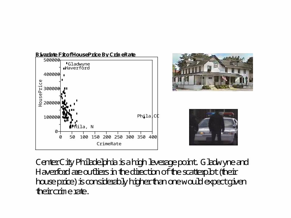
Bivariate Fit of HousePrice By CrimeRate
0
100000
200000
300000
400000
500000
Ho
us
eP
ric
e
GladwyneHaverford
Phila, N
Phila,CC
0 50 100 150 200 250 300 350 400
CrimeRate
Center City Philadelphia is a high leverage point. Gladwyne and Haverford are outliers in the direction of the scatterplot (their house price) is considerably higher than one would expect given their crime rate.

Which points are influential?B iv a r i a t e F i t o f H o u s e P r ic e B y C r im e R a t e
0
1 0 0 0 0 0
2 0 0 0 0 0
3 0 0 0 0 0
4 0 0 0 0 0
5 0 0 0 0 0
Ho
us
eP
rice
G la d w y n eH a v e rfo rd
P h ila , N
P h ila ,C C
0 5 0 1 0 0 1 5 0 2 0 0 2 5 0 3 0 0 3 5 0 4 0 0
C rime R a te
L in e a r F it
L in e a r F it
L in e a r F it
A l l o b s e r v a t i o n s L i n e a r F i t H o u s e P r ic e = 1 7 6 6 2 9 .4 1 - 5 7 6 . 9 0 8 1 3 C r im e R a te
W i t h o u t C e n t e r C i t y P h i l a d e l p h i a L i n e a r F i t H o u s e P r ic e = 2 2 5 2 3 3 .5 5 - 2 2 8 8 . 6 8 9 4 C r im e R a te
W i t h o u t G l a d w y n e L i n e a r F i t H o u s e P r ic e = 1 7 3 1 1 6 . 4 3 - 5 6 7 . 7 4 5 0 8 C r im e R a te
Center City Philadelphia is influential; Gladwyne is not. In general, points that have high leverage are more likely to be influential.

Excluding Observations from Analysis in JMP
• To exclude an observation from the regression analysis in JMP, go to the row of the observation, click Rows and then click Exclude/Unexclude. A red circle with a diagonal line through it should appear next to the observation.
• To put the observation back into the analysis, go to the row of the observation, click Rows and then click Exclude/Unexclude. The red circle should no longer appear next to the observation.

Formal measures of leverage and influence
• Leverage: “Hat values” (JMP calls them hats)• Influence: Cook’s Distance (JMP calls them Cook’s D
Influence).• To obtain them in JMP, click Analyze, Fit Model, put Y
variable in Y and X variable in Model Effects box. Click Run Model box. After model is fit, click red triangle next to Response. Click Save Columns and then Click Hats for Leverages and Click Cook’s D Influences for Cook’s Distances.
• To sort observations in terms of Cook’s Distance or Leverage, click Tables, Sort and then put variable you want to sort by in By box.

Distributions Cook's D Influence HousePrice
HaverfordGladwyne Phila,CC
0 5 1015202530
h HousePrice
Phila,CC
0 .1.2.3.4.5.6.7.8.9
Center City Philadelphia has both influence (Cook’s Distance much Greater than 1 and high leverage (hat value > 3*2/99=0.06). No otherobservations have high influence or high leverage.
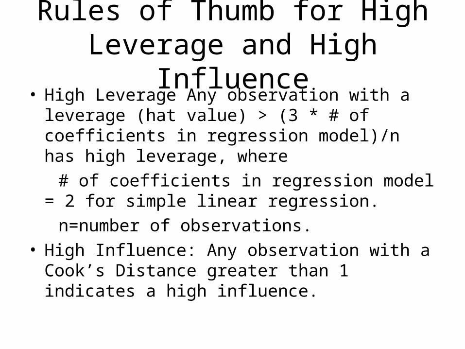
Rules of Thumb for High Leverage and High Influence
• High Leverage Any observation with a leverage (hat value) > (3 * # of coefficients in regression model)/n has high leverage, where
# of coefficients in regression model = 2 for simple linear regression.
n=number of observations. • High Influence: Any observation with a Cook’s
Distance greater than 1 indicates a high influence.

What to Do About Suspected Influential Observations?
See flowchart handout.
Does removing the observation change the
substantive conclusions?• If not, can say something like “Observation x
has high influence relative to all other observations but we tried refitting the regression without Observation x and our main conclusions didn’t change.”

• If removing the observation does change substantive conclusions, is there any reason to believe the observation belongs to a population other than the one under investigation?– If yes, omit the observation and proceed.– If no, does the observation have high leverage
(outlier in explanatory variable).• If yes, omit the observation and proceed. Report that
conclusions only apply to a limited range of the explanatory variable.
• If no, not much can be said. More data (or clarification of the influential observation) are needed to resolve the questions.

General Principles for Dealing with Influential Observations
• General principle: Delete observations from the analysis sparingly – only when there is good cause (observation does not belong to population being investigated or is a point with high leverage). If you do delete observations from the analysis, you should state clearly which observations were deleted and why.

The Question of Causation
• The community that ran this regression would like to increase property values. If low crime rates increase property values, the community might be able to cover the costs of increased police protection by gains in tax revenue from higher property values.
• The regression without Center City Philadelphia is Linear Fit HousePrice = 225233.55 - 2288.6894 CrimeRate• The community concludes that if it can cut its crime rate
from 30 down to 20 incidents per 1000 population, it will increase its average house price by $2288.6894*10=$22,887.
• Is the community’s conclusion justified?

Potential Outcomes Model
• Let Yi30 denote what the house price for
community i would be if its crime rate was 30 and Yi
20 denote what the house price for community i would be if its crime rate was 20.
• X (crime rate) causes a change in Y (house price) for community i if . A decrease in crime rate causes an increase in house price for community i if
2030ii YY
3020ii YY

Association is Not Causation
• A regression model tells us about how the mean of Y|X is associated with changes in X. A regression model does not tell us what would happen if we actually changed X.
• Possible Explanations for an Observed Association Between Y and X
1. Y causes X2. X causes Y3. There is a confounding variable Z that is associated
with changes in both X and Y. Any combination of the three explanations may apply
to an observed association.

X Causes YBivariate Fit of CrimeRate By HousePrice
10
20
30
40
50
60
70
Crim
eRat
e
0 100000 200000 300000 400000 500000
HousePrice
Linear Fit
Linear Fit CrimeRate = 41.929126 - 0.0000805 HousePrice
Perhaps it is changes in house price that cause changes in crime rate. When houseprices increase, the residents of a community have more to lose by engaging in criminal actives; this is called the economic theory of crime.

Confounding Variables
• Confounding variable for the causal relationship between X and Y: A variable Z that is associated with both X and Y.
• Example of confounding variable in Philadelphia crime rate data: Level of education. Level of education may be associated with both house prices and crime rate.
• The effect of crime rate on house price is confounded with the effect of education on house price. If we just look at data on house price and crime rate, we can’t distinguish between the effect of crime rate on house price and the effect of education on house price.

Note on Confounding Variables and Lurking Variables
• The book’s distinction between lurking variable and confounding variable is confusing and the term “lurking variable” is not standard in statistics, whereas “confounding variable” is. So I will just use the term confounding variable in the rest of the course.

Examples of Confounding Variables
• Many studies have found that people who are active in their religion live longer than nonreligious people. Potential confounding variables?

Weekly Wages (Y) and Education (X) in March 1988 CPS
Bivariate Fit of wage By educ
0
2000
4000
6000
8000
10000
12000
14000
16000
18000w
age
0 1 2 3 4 5 6 7 8 9 10 1213 15 1718
educ
Linear Fit
Linear Fit wage = -19.06983 + 50.414381 educ
Will getting an extra year of education cause an increase of $50.41 on averagein your weekly wage? What are some potential confounding variables?
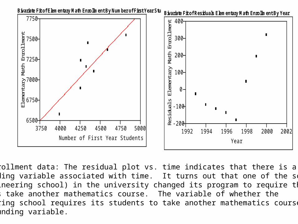
Bivariate Fit of Elementary Math Enrollment By Number of First Year Stu
6500
6750
7000
7250
7500
7750El
emen
tary
Mat
h En
rollm
ent
3750 4000 4250 4500 4750 5000
Number of First Year Students
Bivariate Fit of Residuals Elementary Math Enrollment By Year
-200
-100
0
100
200
300
400
Resid
uals
Elem
enta
ry M
ath
Enro
llmen
t
1992 1994 1996 1998 2000 2002
Year
Math enrollment data: The residual plot vs. time indicates that there is a confounding variable associated with time. It turns out that one of the schools (saythe engineering school) in the university changed its program to require that entering students take another mathematics course. The variable of whether the engineering school requires its students to take another mathematics course isa confounding variable.

Establishing Causation
• Best method is an experiment, but many times that is not ethically or practically possible (e.g., smoking and cancer, education and earnings).

• Main strategy for learning about causation when we can’t do an experiment: Consider all confounding variables you can think of. Try to take them into account (we’ll see how to do this when we study multiple regression in Chapter 11) and see if association between Y and X remains once the known confounding variables have been accounted for.

Other Criteria for Establishing Causation When We Can’t Do An
Experiment1. The association is strong.
2. The association is consistent.
3. Higher doses are associated with stronger responses.
4. The alleged cause precedes the effect in time.
5. The alleged cause is plausible.


![Research Article Outlier Detection in Adaptive Functional ...for detecting additive outliers in bilinear time series, which belong to the family of fractal time series models [ ]](https://img.pdfslide.us/doc/110x75/60a9e87271d831308534b17c/research-article-outlier-detection-in-adaptive-functional-for-detecting-additive.jpg)


![A comparative evaluation of outlier detection algorithms: experiments and analyses · 2020-06-20 · tify outliers. Local outlier factor (LOF) described in [4] is a well-known dis-tance](https://img.pdfslide.us/doc/110x75/5f0d2d0b7e708231d4390b95/a-comparative-evaluation-of-outlier-detection-algorithms-experiments-and-2020-06-20.jpg)


![No Longer the Outlier - Air University › Portals › 10 › ASPJ › journals › Volu… · Outliers: The Story of Success Having served on a COCOM [combatant command] operations](https://img.pdfslide.us/doc/110x75/5f1db640e030fd02105d14f4/no-longer-the-outlier-air-university-a-portals-a-10-a-aspj-a-journals.jpg)
![Distancebased Outlier Detection in Data Streams · outlier de nition have been proposed in [4, 11, 12], by con-sidering a xed number of outliers present in the dataset [11], a probability](https://img.pdfslide.us/doc/110x75/5f4178698a31a4664d3bc531/distancebased-outlier-detection-in-data-streams-outlier-de-nition-have-been-proposed.jpg)
![Distributed Local Outlier Detection in Big Datapeople.csail.mit.edu/lcao/papers/kdd17-ddlof.pdf · Local Outlier Factor (LOF) [7] introduces the notion of local outliers based on](https://img.pdfslide.us/doc/110x75/5f0d2d0c7e708231d4390b9e/distributed-local-outlier-detection-in-big-local-outlier-factor-lof-7-introduces.jpg)


![Angle-Based Outlier Detection in High-dimensional Data · complexity. The distance based notion of outliers uni es distribution based approaches [17, 18]. An object x 2Dis an outlier](https://img.pdfslide.us/doc/110x75/5f8834782feaf023fa448be3/angle-based-outlier-detection-in-high-dimensional-data-complexity-the-distance.jpg)