Class 12

The Behavior of Sums and AveragesAmore Frozen Foods

EMBS 7.3-7.6 (selections from)

Review Class 11. chi-squared test of independence

• H0: The Categorical variables are independent• Ha: They are not.• Pivot Table to create contingency table.• Excel to create Expected Counts• CHITEST() to calculate p-value.

– or Excel to get distances and calculated chi-squared statistic, =chidist with dof = (#rows-1)(#col-1) to get p-value

There is often another way

• H0: Athlete and HSStat are independent• H0: P1=P2

– P1 is probability an athlete took HSStat– P2 is the probability a non-athlete took HSStat

• You can use the method of section 11.1 to test H0. (check out equation 11.7 to see what’s involved)– And you get exactly the same p-value!!

• So, the chi-squared test of independence tests the equality of two probabilities (for a 2x2) and more! That’s why we learned it.

Amore

• At a target of 8.22, Amore’s filling machine fills mac and cheese tins with an amount N(8.22,0.22)– Resulting in about 16% of tins (pies) being

underweight• The FDA requires Amore to test each 20-minute

batch using a random sample of five tins. The entire batch must be rejected if the 5-pie sample averages less than 8 ounces.

• What is the probability a batch will be rejected?

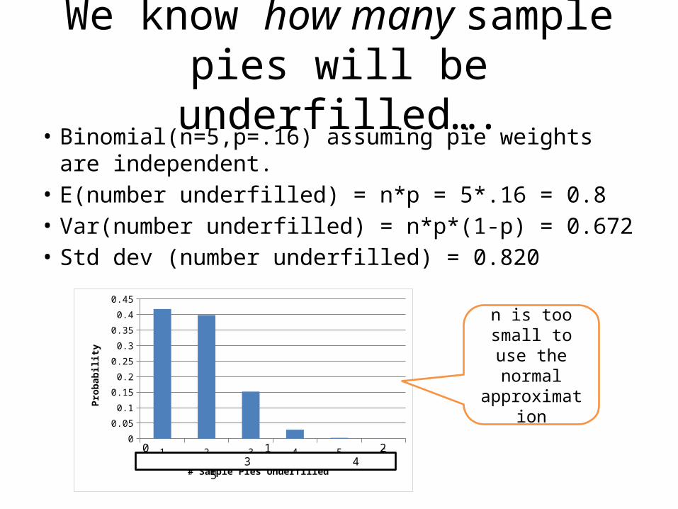
We know how many sample pies will be underfilled….

• Binomial(n=5,p=.16) assuming pie weights are independent.

• E(number underfilled) = n*p = 5*.16 = 0.8• Var(number underfilled) = n*p*(1-p) = 0.672• Std dev (number underfilled) = 0.820

1 2 3 4 5 60

0.05

0.1

0.15

0.2

0.25

0.3

0.35

0.4

0.45

# Sample Pies Underfilled

Prob

abili

ty

0 1 2 3 4 5

n is too small to use the normal approximation

But the fate of the batch rests on the total (average) weight of the

five sampled pies.

We need to figure out what the probability distribution of either the

total or the average of five is.

For Amore….

𝑋=𝑋 1+ 𝑋 2+   𝑋 3+  𝑋 4+  𝑋 5

5

“X-bar”The sample mean

We can work our problem either way.

The sample mean is just

the total times 0.2.

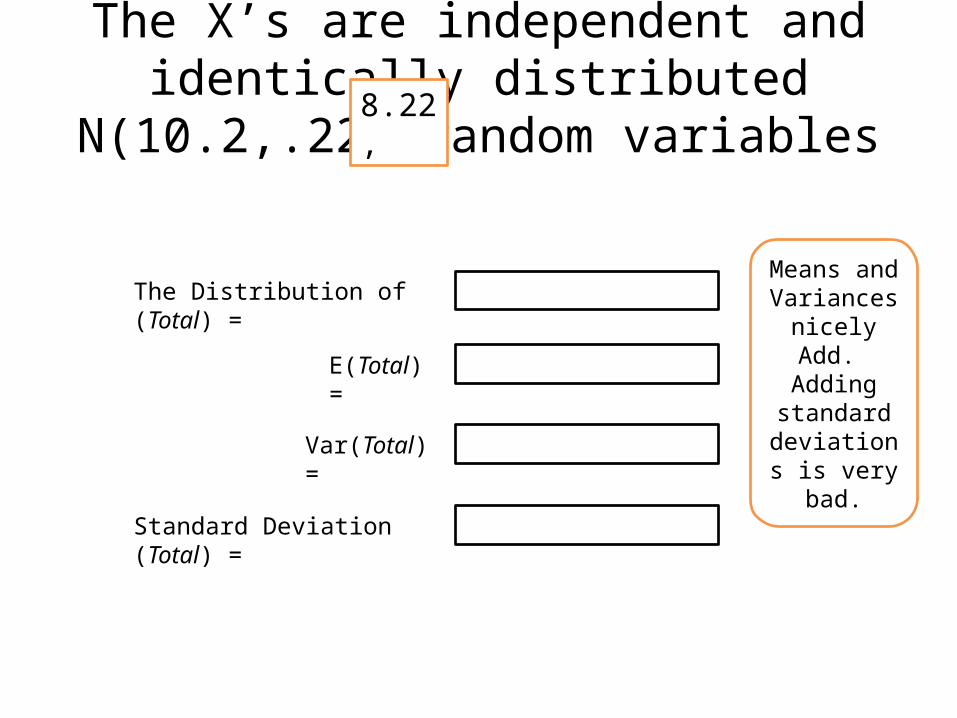
The X’s are independent and identically distributed N(10.2,.22) random variables

E(Total) =

Var(Total) =

Standard Deviation (Total) =

The Distribution of (Total) = Means and Variances

nicely Add. Adding

standard deviations is

very bad.

8.22,

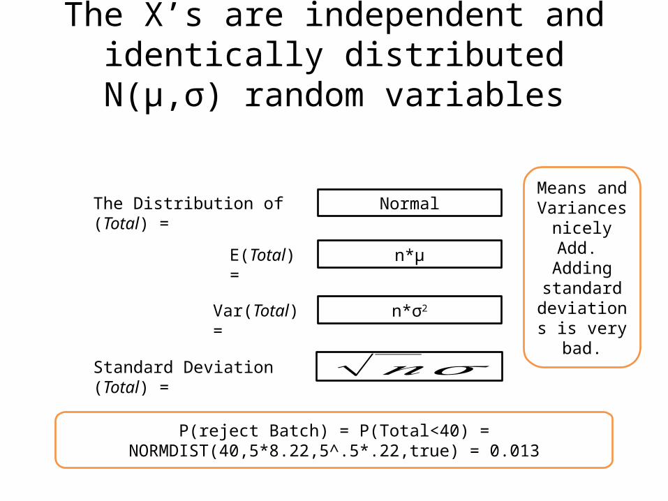
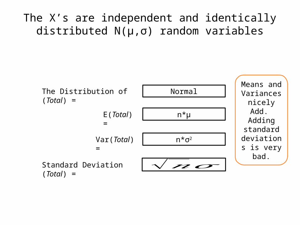
The X’s are independent and identically distributed N(μ,σ) random variables

E(Total) = n*μ

Var(Total) = n*σ2

Standard Deviation (Total) = √𝑛𝜎

The Distribution of (Total) = Normal Means and Variances

nicely Add. Adding

standard deviations is

very bad.

P(reject Batch) = P(Total<40) = NORMDIST(40,5*8.22,5^.5*.22,true) = 0.013

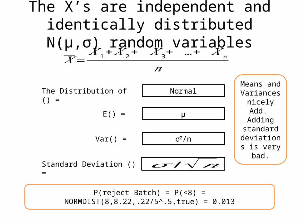
The X’s are independent and identically distributed N(μ,σ) random variables

E() = μ

Var() = σ2/n

Standard Deviation () = 𝜎 /√𝑛

The Distribution of () = Normal Means and Variances

nicely Add. Adding

standard deviations is

very bad.

𝑋=𝑋 1+ 𝑋 2+   𝑋 3+  …+  𝑋𝑛

𝑛

P(reject Batch) = P(<8) = NORMDIST(8,8.22,.22/5^.5,true) = 0.013

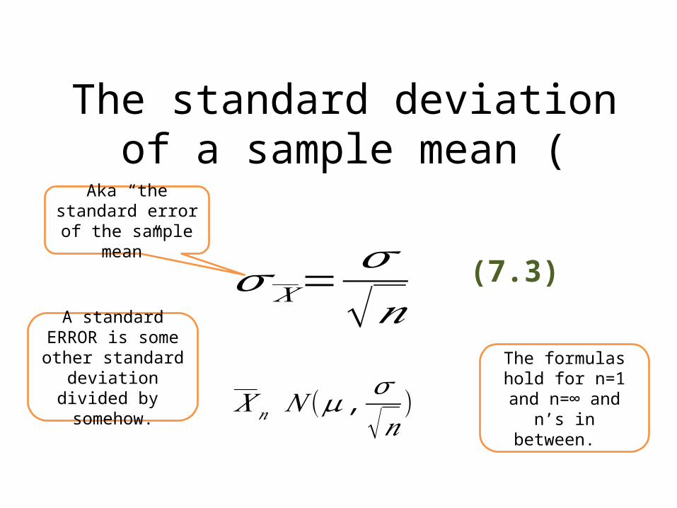
The standard deviation of a sample mean (

𝜎 𝑋=𝜎√𝑛

(7.3)

𝑋𝑛 𝑁 (𝜇 ,𝜎√𝑛

)The formulas hold

for n=1 and n=∞ and n’s in between.

Aka “the standard error of the sample

mean”

A standard ERROR is some other standard deviation divided by

somehow.

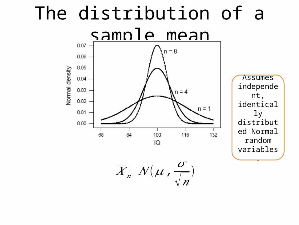
The distribution of a sample mean

𝑋𝑛 𝑁 (𝜇 ,𝜎√𝑛

)

Assumes independent,

identically distributed

Normal random

variables.

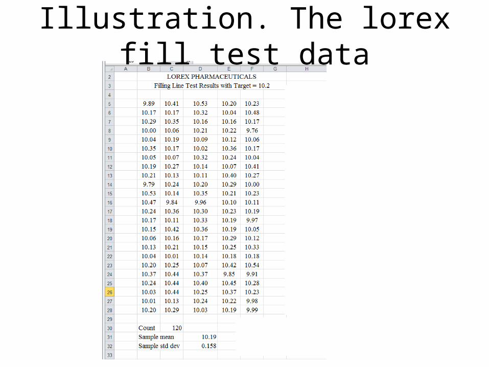
Illustration. The lorex fill test data

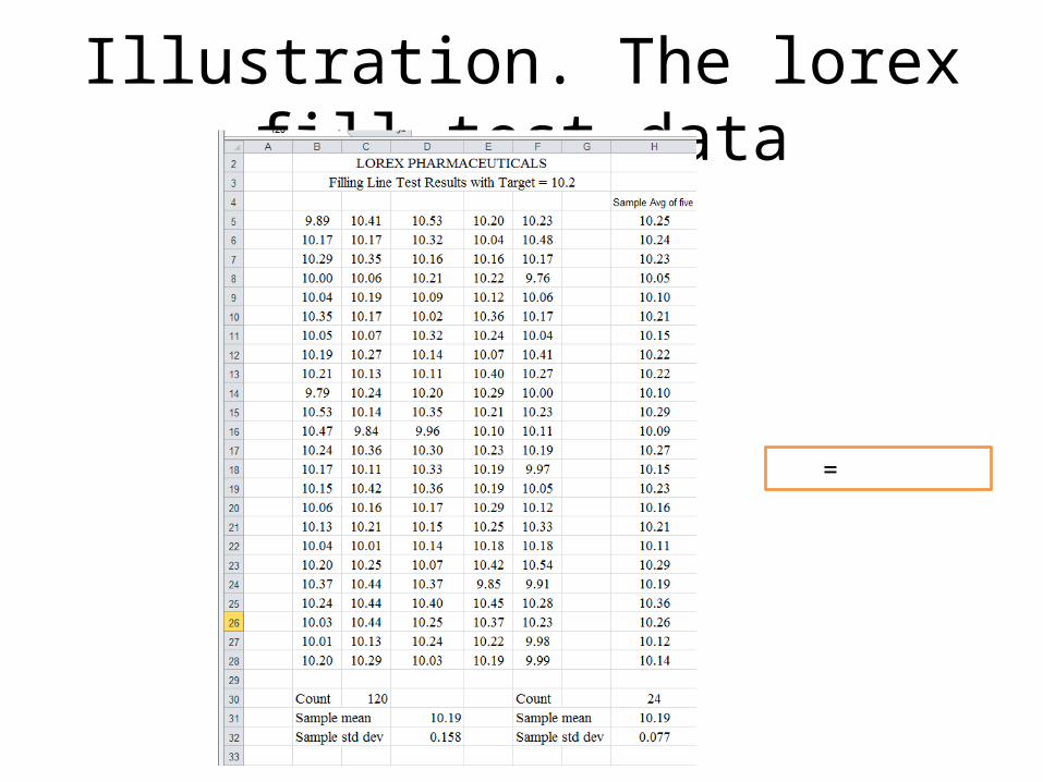
Illustration. The lorex fill test data

=

Small Schools are Better?Did Bill Gates waste a billion dollars because he failed to understand the formula for the standard deviation of the sample mean?

The Gates Foundation certainly spent a lot of money, along with many others, pushing for smaller schools and a lot of the push came because people jumped to the wrong conclusion when they discovered that the smallest schools were consistently among the best performing schools.

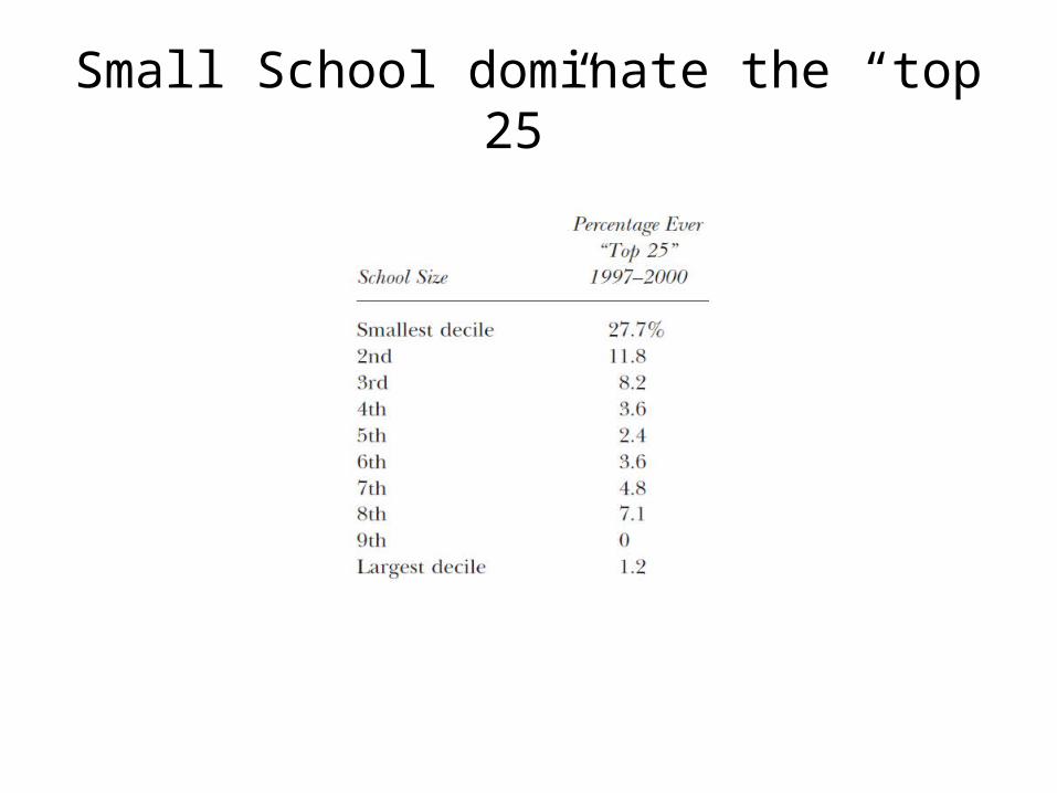
Small School dominate the “top 25”

….and the bottom!

In recent years Bill Gates and the Gates Foundation have acknowledged that their earlier emphasis on small schools was misplaced.

He should have taken “Statistics in Business”

The X’s are independent and identically distributed N(μ,σ) random variables

E(Total) = n*μ

Var(Total) = n*σ2

Standard Deviation (Total) = √𝑛𝜎

The Distribution of (Total) = Normal Means and Variances

nicely Add. Adding

standard deviations is

very bad.

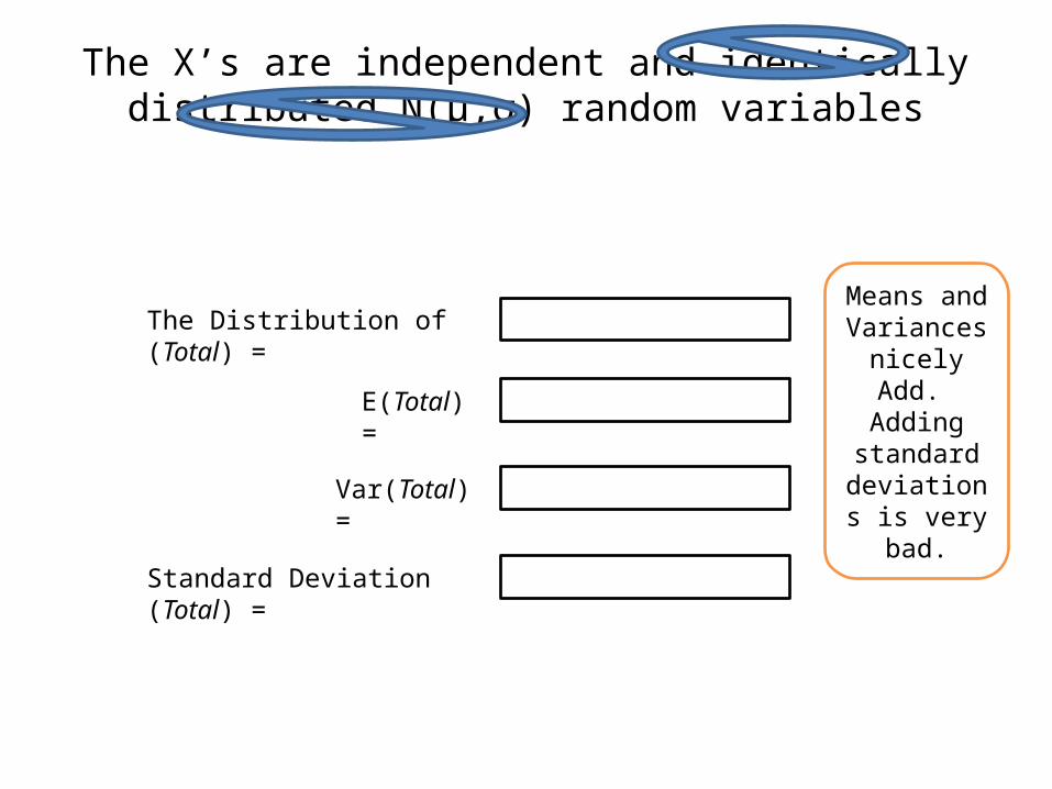
The X’s are independent and identically distributed N(μ,σ) random variables

E(Total) =

Var(Total) =

Standard Deviation (Total) =

The Distribution of (Total) = Means and Variances

nicely Add. Adding

standard deviations is

very bad.

The X’s are independent and identically distributed N(μ,σ) random variables

E(Total) = μ1 + μ2 + … μn

Var(Total) = σ21+ σ2

2+…. σ2n

Standard Deviation (Total) = √𝑉𝑎𝑟

The Distribution of (Total) = ?? Means and Variances

nicely Add. Adding

standard deviations is

very bad.

Illustration: Suppose Wunderdog did five sports

Sport nNumber correct if

guessingExpected #

correct Variance Std Dev1 149 X1 74.5 37.25 6.102 85 X2 42.5 21.25 4.613 133 X3 66.5 33.25 5.774 209 X4 104.5 52.25 7.235 311 X5 155.5 77.75 8.82

Total 887 sum of the Xs 443.5 221.75 14.89

Means and Variances nicely add. Adding

standard deviations is very bad.

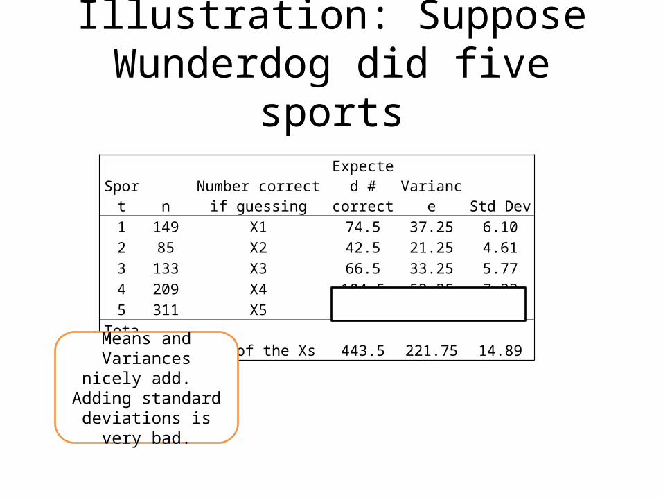
Illustration: Suppose Wunderdog did five sports

Sport nNumber correct if

guessingExpected #

correct Variance Std Dev1 149 X1 74.5 37.25 6.102 85 X2 42.5 21.25 4.613 133 X3 66.5 33.25 5.774 209 X4 104.5 52.25 7.235 311 X5 155.5 77.75 8.82

Total 887 sum of the Xs 443.5 221.75 14.89

Means and Variances nicely add. Adding

standard deviations is very bad.

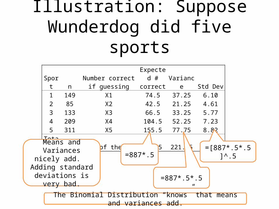
=887*.5

=887*.5*.5

=[887*.5*.5]^.5

The Binomial Distribution “knows” that means and variances add.

Example ProblemEMBS 40 p 306.

• A large BW survey of MBA’s ten years out found mean dining out spending to be $115.5 (per week) and population standard deviation of $35. You will do a follow-up study and survey a random sample of 40 of the MBA alums.– What sample mean will you get?– What is the probability your sample mean will be

within $10 of the population mean?– What is the probability your sample mean will be less

than $100?

Summary

• If we know the X’s are independent, identically distributed N(μ,σ) random variables…– The total of n X’s will be N(nμ,σ)– The sample mean of n X’s is written as– will be N(μ,σ/)

• Means and variances nicely add (if the X’s are independent). Adding standard deviations is very bad.– The BINOMIAL knows this…..

𝑋𝑛

𝑋𝑛

Exam1

• Complete answers have been posted• The Binomial works for small n.

– P(Cubs Win) = BINOMDIST(3,3,.5,false)– P(2Gin4) = BINOMIDIST(2,4,p,false)

• Whether p is 0.5 or 0.48

– P(2P l noD) = BINOMDIST(2,2,.2,false)– P(1P l noD) = BINOMDIST(1,2,.2,false)– P(0P l noD) = BINOMDIST(0,2,.2,false)– #correctly filled is B(n=144,p=.92775)