CL’s Handy Formula Sheet

(Useful formulas from Marcel Finan’s FM/2 Book) Compiled by Charles Lee 8/19/2010

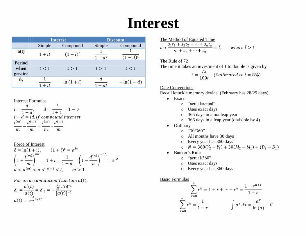
Interest

Interest Discount

Simple Compound Simple Compound

a(t)

Period

when

greater

Interest Formulas

Force of Interest

The Method of Equated Time

The Rule of 72

The time it takes an investment of 1 to double is given by

Date Conventions

Recall knuckle memory device. (February has 28/29 days)

Exact

o “actual/actual”

o Uses exact days

o 365 days in a nonleap year

o 366 days in a leap year (divisible by 4)

Ordinary

o “30/360”

o All months have 30 days

o Every year has 360 days

o

Banker’s Rule

o “actual/360”

o Uses exact days

o Every year has 360 days

Basic Formulas

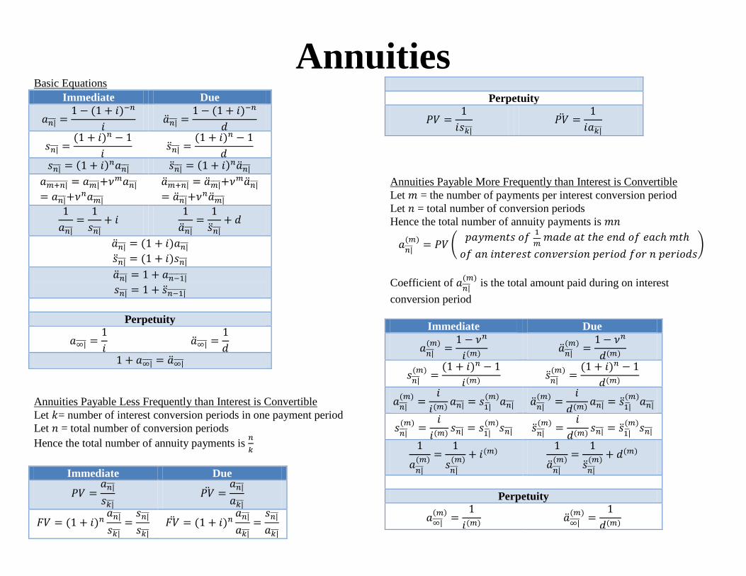
Annuities Basic Equations

Immediate Due

Perpetuity

Annuities Payable Less Frequently than Interest is Convertible

Let = number of interest conversion periods in one payment period

Let = total number of conversion periods

Hence the total number of annuity payments is

Immediate Due

Perpetuity

Annuities Payable More Frequently than Interest is Convertible

Let = the number of payments per interest conversion period

Let = total number of conversion periods

Hence the total number of annuity payments is

Coefficient of

is the total amount paid during on interest

conversion period

Immediate Due

Perpetuity

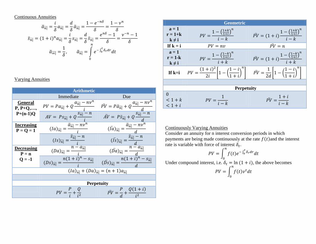
Continuous Annuities

Varying Annuities

Arithmetic

Immediate Due

General

P, P+Q,…,

P+(n-1)Q

Increasing

P = Q = 1

Decreasing

P = n

Q = -1

Perpetuity

Geometric

a = 1

r = 1+k

k ≠ i

If k = i

a = 1

r = 1-k

k ≠ i

If k=i

Perpetuity

Continuously Varying Annuities

Consider an annuity for n interest conversion periods in which

payments are being made continuously at the rate and the interest

rate is variable with force of interest .

Under compound interest, i.e. , the above becomes

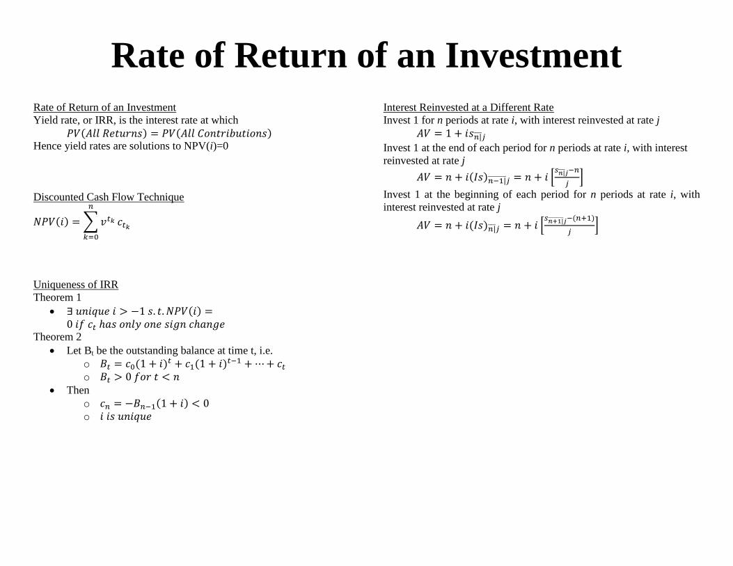
Rate of Return of an Investment

Rate of Return of an Investment

Yield rate, or IRR, is the interest rate at which

Hence yield rates are solutions to NPV(i)=0

Discounted Cash Flow Technique

Uniqueness of IRR

Theorem 1

Theorem 2

Let Bt be the outstanding balance at time t, i.e.

o

o

Then

o

o

Interest Reinvested at a Different Rate

Invest 1 for n periods at rate i, with interest reinvested at rate j

Invest 1 at the end of each period for n periods at rate i, with interest

reinvested at rate j

Invest 1 at the beginning of each period for n periods at rate i, with

interest reinvested at rate j

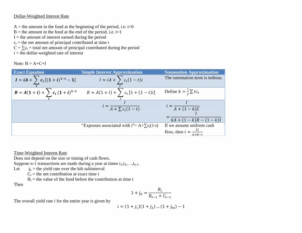
Dollar-Weighted Interest Rate

A = the amount in the fund at the beginning of the period, i.e. t=0

B = the amount in the fund at the end of the period, i.e. t=1

I = the amount of interest earned during the period

ct = the net amount of principal contributed at time t

C = ∑ct = total net amount of principal contributed during the period

i = the dollar-weighted rate of interest

Note: B = A+C+I

Time-Weighted Interest Rate

Does not depend on the size or timing of cash flows.

Suppose n-1 transactions are made during a year at times t1,t2,…,tn-1.

Let jk = the yield rate over the kth subinterval

Ct = the net contribution at exact time t

Bt = the value of the fund before the contribution at time t

Then

The overall yield rate i for the entire year is given by

Exact Equation Simple Interest Approximation Summation Approximation

The summation term is tedious.

Define

“Exposure associated with i"= A+∑ct(1-t) If we assume uniform cash

flow, then

Bonds

Notation

P = the price paid for a bond

F = the par value or face value

C = the redemption value

r = the coupon rate

Fr = the amount of a coupon payment

g = the modified coupon rate, defined by Fr/C

i = the yield rate

n = the number of coupons payment periods

K = the present value, compute at the yield rate, of the

redemption value at maturity, i.e. K=Cvn

G = the base amount of a bond, defined as G=Fr/i. Thus, G is

the amount which, if invested at the yield rate i, would produce

periodic interest payments equal to the coupons on the bond

Quoted yields associated with a bond

1) Nominal Yield

a. Ratio of annualized coupon rate to par value

2) Current Yield

a. Ratio of annualized coupon rate to original price of the

bond

3) Yield to maturity

a. Actual annualized yield rate, or IRR

Pricing Formulas

Basic Formula

o

Premium/Discount Formula

o

Base Amount Formula

o

Makeham Formula

o

Yield rate and Coupon rate of Different Frequencies

Let n be the total number of yield rate conversion periods.

Case 1: Each coupon period contains k yield rate periods

o

Case 2: Each yield period contains m coupon periods

o

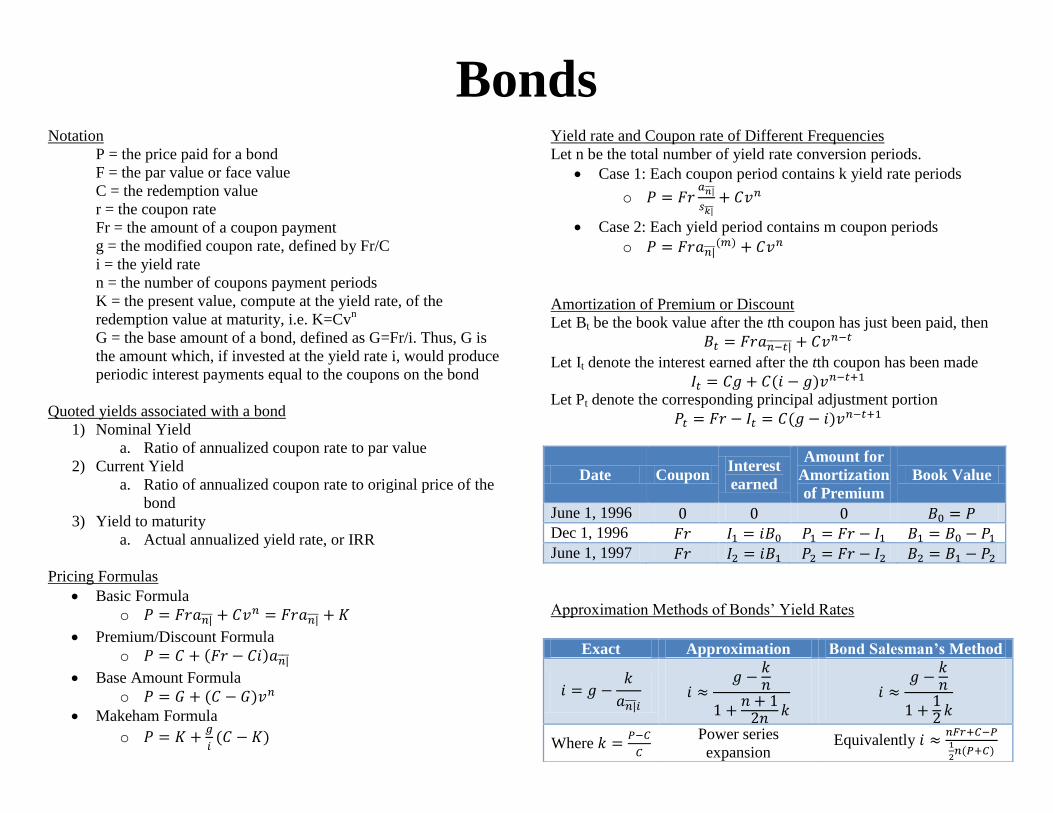
Amortization of Premium or Discount

Let Bt be the book value after the tth coupon has just been paid, then

Let It denote the interest earned after the tth coupon has been made

Let Pt denote the corresponding principal adjustment portion

Date Coupon Interest

earned

Amount for

Amortization

of Premium

Book Value

June 1, 1996

Dec 1, 1996

June 1, 1997

Approximation Methods of Bonds’ Yield Rates

Exact Approximation Bond Salesman’s Method

Where

Power series

expansion Equivalently

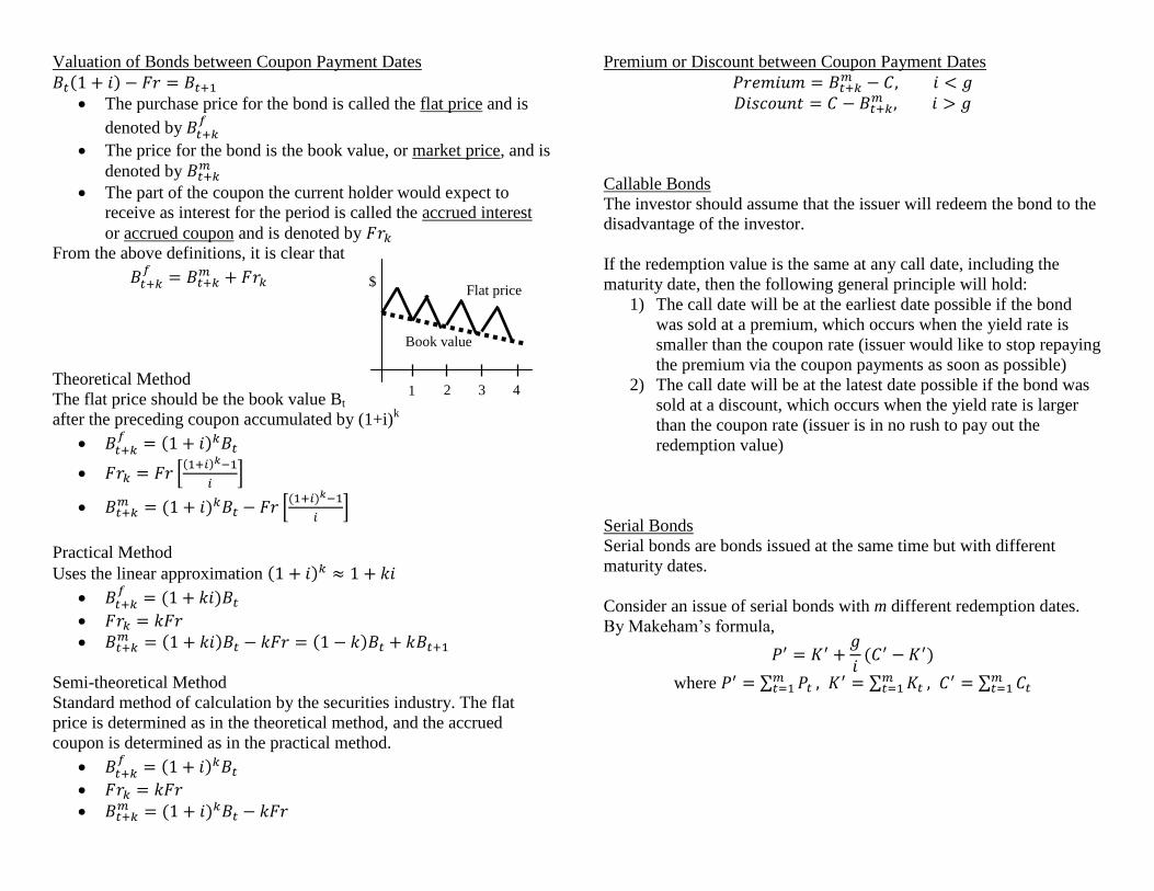
Valuation of Bonds between Coupon Payment Dates

The purchase price for the bond is called the flat price and is

denoted by

The price for the bond is the book value, or market price, and is

denoted by

The part of the coupon the current holder would expect to

receive as interest for the period is called the accrued interest

or accrued coupon and is denoted by

From the above definitions, it is clear that

Theoretical Method

The flat price should be the book value Bt

after the preceding coupon accumulated by (1+i)k

Practical Method

Uses the linear approximation

Semi-theoretical Method

Standard method of calculation by the securities industry. The flat

price is determined as in the theoretical method, and the accrued

coupon is determined as in the practical method.

Premium or Discount between Coupon Payment Dates

Callable Bonds

The investor should assume that the issuer will redeem the bond to the

disadvantage of the investor.

If the redemption value is the same at any call date, including the

maturity date, then the following general principle will hold:

1) The call date will be at the earliest date possible if the bond

was sold at a premium, which occurs when the yield rate is

smaller than the coupon rate (issuer would like to stop repaying

the premium via the coupon payments as soon as possible)

2) The call date will be at the latest date possible if the bond was

sold at a discount, which occurs when the yield rate is larger

than the coupon rate (issuer is in no rush to pay out the

redemption value)

Serial Bonds

Serial bonds are bonds issued at the same time but with different

maturity dates.

Consider an issue of serial bonds with m different redemption dates.

By Makeham’s formula,

where

Book value

Flat price

1 2 3 4

$

Loan Repayment Methods

Amortization Method

Prospective Method

o The outstanding loan balance at any time is equal to the

present value at that time of the remaining payments

Retrospective Method

o The outstanding loan balance at any time is equal to the

original amount of the loan accumulated to that time

less the accumulated value at that time of all payments

previously made

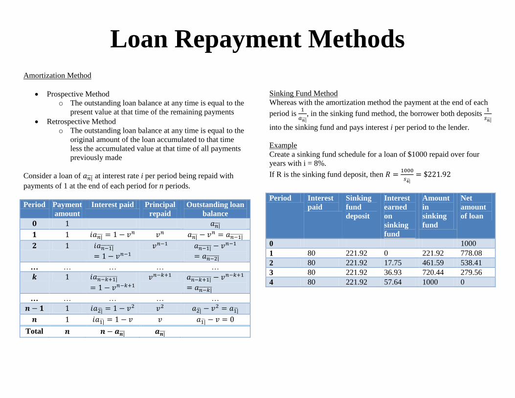
Consider a loan of at interest rate i per period being repaid with

payments of 1 at the end of each period for n periods.

Period Payment

amount

Interest paid Principal

repaid

Outstanding loan

balance

… … … … …

… … … … …

Total

Sinking Fund Method

Whereas with the amortization method the payment at the end of each

period is

, in the sinking fund method, the borrower both deposits

into the sinking fund and pays interest i per period to the lender.

Example

Create a sinking fund schedule for a loan of $1000 repaid over four

years with i = 8%.

If R is the sinking fund deposit, then

Period Interest

paid

Sinking

fund

deposit

Interest

earned

on

sinking

fund

Amount

in

sinking

fund

Net

amount

of loan

0 1000

1 80 221.92 0 221.92 778.08

2 80 221.92 17.75 461.59 538.41

3 80 221.92 36.93 720.44 279.56

4 80 221.92 57.64 1000 0

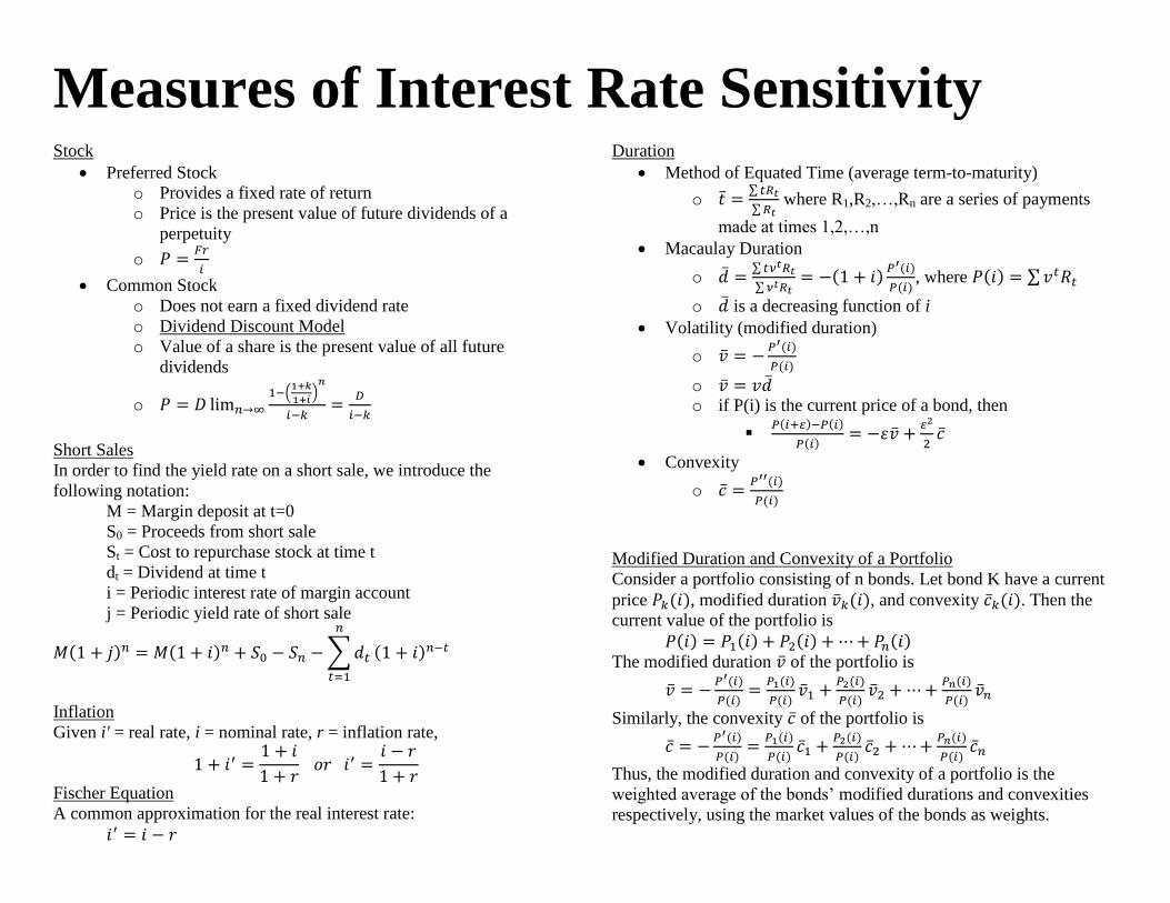
Measures of Interest Rate Sensitivity

Stock

Preferred Stock

o Provides a fixed rate of return

o Price is the present value of future dividends of a

perpetuity

o

Common Stock

o Does not earn a fixed dividend rate

o Dividend Discount Model

o Value of a share is the present value of all future

dividends

o

Short Sales

In order to find the yield rate on a short sale, we introduce the

following notation:

M = Margin deposit at t=0

S0 = Proceeds from short sale

St = Cost to repurchase stock at time t

dt = Dividend at time t

i = Periodic interest rate of margin account

j = Periodic yield rate of short sale

Inflation

Given i' = real rate, i = nominal rate, r = inflation rate,

Fischer Equation

A common approximation for the real interest rate:

Duration

Method of Equated Time (average term-to-maturity)

o

where R1,R2,…,Rn are a series of payments

made at times 1,2,…,n

Macaulay Duration

o

, where

o is a decreasing function of i

Volatility (modified duration)

o

o o if P(i) is the current price of a bond, then

Convexity

o

Modified Duration and Convexity of a Portfolio

Consider a portfolio consisting of n bonds. Let bond K have a current

price , modified duration , and convexity . Then the

current value of the portfolio is

The modified duration of the portfolio is

Similarly, the convexity of the portfolio is

Thus, the modified duration and convexity of a portfolio is the

weighted average of the bonds’ modified durations and convexities

respectively, using the market values of the bonds as weights.

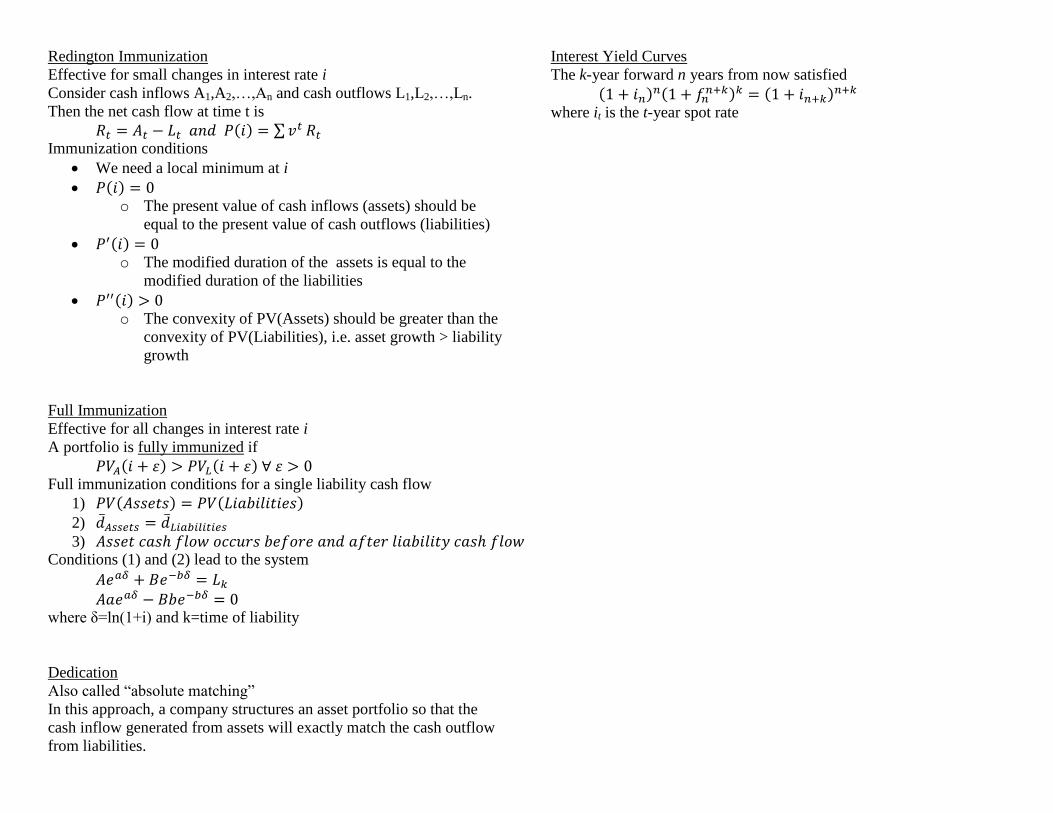
Redington Immunization

Effective for small changes in interest rate i

Consider cash inflows A1,A2,…,An and cash outflows L1,L2,…,Ln.

Then the net cash flow at time t is

Immunization conditions

We need a local minimum at i

o The present value of cash inflows (assets) should be

equal to the present value of cash outflows (liabilities)

o The modified duration of the assets is equal to the

modified duration of the liabilities

o The convexity of PV(Assets) should be greater than the

convexity of PV(Liabilities), i.e. asset growth > liability

growth

Full Immunization

Effective for all changes in interest rate i

A portfolio is fully immunized if

Full immunization conditions for a single liability cash flow

1) 2) 3)

Conditions (1) and (2) lead to the system

where δ=ln(1+i) and k=time of liability

Dedication

Also called “absolute matching”

In this approach, a company structures an asset portfolio so that the

cash inflow generated from assets will exactly match the cash outflow

from liabilities.

Interest Yield Curves

The k-year forward n years from now satisfied

where it is the t-year spot rate

Price at Maturity

Payoff Profit

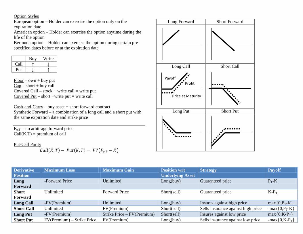
Option Styles

European option – Holder can exercise the option only on the

expiration date

American option – Holder can exercise the option anytime during the

life of the option

Bermuda option – Holder can exercise the option during certain pre-

specified dates before or at the expiration date

Buy Write

Call ↑ ↓

Put ↓ ↑

Floor – own + buy put

Cap – short + buy call

Covered Call – stock + write call = write put

Covered Put – short +write put = write call

Cash-and-Carry – buy asset + short forward contract

Synthetic Forward – a combination of a long call and a short put with

the same expiration date and strike price

Fo,T = no arbitrage forward price

Call(K,T) = premium of call

Put-Call Parity

Long Forward Short Forward

Long Call Short Call

Long Put Short Put

Derivative

Position

Maximum Loss Maximum Gain Position wrt

Underlying Asset

Strategy Payoff

Long

Forward

-Forward Price Unlimited Long(buy) Guaranteed price PT-K

Short

Forward

Unlimited Forward Price Short(sell) Guaranteed price K-PT

Long Call -FV(Premium) Unlimited Long(buy) Insures against high price max{0,PT-K}

Short Call Unlimited FV(Premium) Short(sell) Sells insurance against high price -max{0,PT-K}

Long Put -FV(Premium) Strike Price – FV(Premium) Short(sell) Insures against low price max{0,K-PT}

Short Put FV(Premium) – Strike Price FV(Premium) Long(buy) Sells insurance against low price -max{0,K-PT}

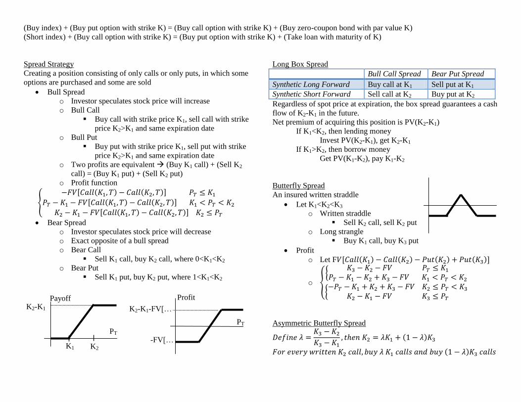
(Buy index) + (Buy put option with strike K) = (Buy call option with strike K) + (Buy zero-coupon bond with par value K)

(Short index) + (Buy call option with strike K) = (Buy put option with strike K) + (Take loan with maturity of K)

Spread Strategy

Creating a position consisting of only calls or only puts, in which some

options are purchased and some are sold

Bull Spread

o Investor speculates stock price will increase

o Bull Call

Buy call with strike price K1, sell call with strike

price K2>K1 and same expiration date

o Bull Put

Buy put with strike price K1, sell put with strike

price K2>K1 and same expiration date

o Two profits are equivalent (Buy K1 call) + (Sell K2

call) = (Buy K1 put) + (Sell K2 put)

o Profit function

Bear Spread

o Investor speculates stock price will decrease

o Exact opposite of a bull spread

o Bear Call

Sell K1 call, buy K2 call, where 0<K1<K2

o Bear Put

Sell K1 put, buy K2 put, where 1<K1<K2

Long Box Spread

Bull Call Spread Bear Put Spread

Synthetic Long Forward Buy call at K1 Sell put at K1

Synthetic Short Forward Sell call at K2 Buy put at K2

Regardless of spot price at expiration, the box spread guarantees a cash

flow of K2-K1 in the future.

Net premium of acquiring this position is PV(K2-K1)

If K1<K2, then lending money

Invest PV(K2-K1), get K2-K1

If K1>K2, then borrow money

Get PV(K1-K2), pay K1-K2

Butterfly Spread

An insured written straddle

Let K1<K2<K3

o Written straddle

Sell K2 call, sell K2 put

o Long strangle

Buy K1 call, buy K3 put

Profit

o Let F

o

Asymmetric Butterfly Spread

K2-K1

Payoff

PT

K2 K1

Profit

K2-K1-FV[…

-FV[…

PT

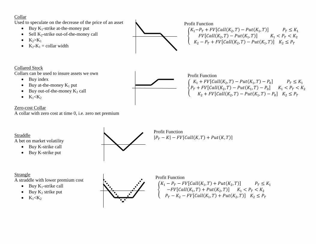
Collar

Used to speculate on the decrease of the price of an asset

Buy K1-strike at-the-money put

Sell K2-strike out-of-the-money call

K2>K1

K2-K1 = collar width

Collared Stock

Collars can be used to insure assets we own

Buy index

Buy at-the-money K1 put

Buy out-of-the-money K2 call

K1<K2

Zero-cost Collar

A collar with zero cost at time 0, i.e. zero net premium

Straddle

A bet on market volatility

Buy K-strike call

Buy K-strike put

Strangle

A straddle with lower premium cost

Buy K1-strike call

Buy K2 strike put

K1<K2

Profit Function

Profit Function

Profit Function

Profit Function

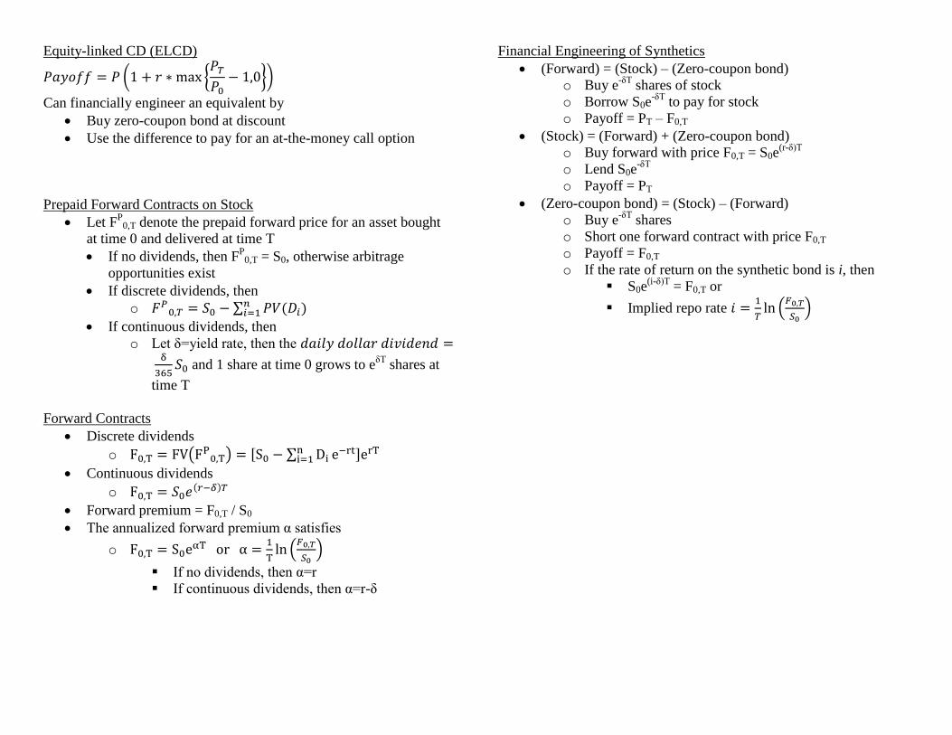
Equity-linked CD (ELCD)

Can financially engineer an equivalent by

Buy zero-coupon bond at discount

Use the difference to pay for an at-the-money call option

Prepaid Forward Contracts on Stock

Let FP

0,T denote the prepaid forward price for an asset bought

at time 0 and delivered at time T

If no dividends, then FP

0,T = S0, otherwise arbitrage

opportunities exist

If discrete dividends, then

o

If continuous dividends, then

o Let δ=yield rate, then the

and 1 share at time 0 grows to e

δT shares at

time T

Forward Contracts

Discrete dividends

o

Continuous dividends

o

Forward premium = F0,T / S0

The annualized forward premium α satisfies

o

If no dividends, then α=r

If continuous dividends, then α=r-δ

Financial Engineering of Synthetics

(Forward) = (Stock) – (Zero-coupon bond)

o Buy e-δT

shares of stock

o Borrow S0e-δT

to pay for stock

o Payoff = PT – F0,T

(Stock) = (Forward) + (Zero-coupon bond)

o Buy forward with price F0,T = S0e(r-δ)T

o Lend S0e-δT

o Payoff = PT

(Zero-coupon bond) = (Stock) – (Forward)

o Buy e-δT

shares

o Short one forward contract with price F0,T

o Payoff = F0,T

o If the rate of return on the synthetic bond is i, then

S0e(i-δ)T

= F0,T or

Implied repo rate