Embed Size (px)
Citation preview
Vortices in favorable pressure gradients
Assessment of Vortex behavior in Formula 1 Underbody conditions
C.K. van Steenbergen November 2004
Supervisors
Ir. L.L.M. Boermans, TU Delft, Department of Aerospace Engineering
Prof. K.P. Garry, Cranfield University, College of Aeronautics
In cooperation with
Abstract
This report covers a ten-month experimental aerodynamics MSC thesis research into vortex
behavior in Formula 1 underbody conditions. This study was divided into two main themes:
an experimental investigation into the effect of a simplified Formula 1 underbody pressure
distribution on vortices generated by vortex generators, and a theoretical investigation into the
effect all other underbody factors, such as the moving ground surface and ground clearance.
The experimental investigation into the effect of a favorable pressure gradient on vortices was
carried out in the Atmospheric Boundary Layer Wind Tunnel, at Cranfield University,
College of Aeronautics, using hot-wire anemometry (HWA) probes to map the vortex flow
field. A two-dimensional Formula 1 underbody pressure distribution was generated by means
of a purpose-built bump. The first arrangement incorporated a single, full-width bump placed
on the floor of the tunnel with a single vortex generated in front of the bump using a Sub
Boundary Layer Vortex Generator(SBVG). Device height Reynolds number for the tests was
Reh = 4.3 ·104, using an SBVG with a device height of h = 42 mm (h/δ = 0.35). When
subjected to the favorable pressure gradient the vortex showed an increase in vortex strength
decay and a decrease in peak vorticity, with the decreased distance between the vortex core
and the single bump surface increases vortex strength decay to such a degree that the peak
vorticity decreases. The HWA measurements limited the size of the data set, and thus the
accuracy of the calculated variables, due to the time-consuming nature and fragility of the
HWA measurements.
The investigation into the effect of ground effect factors on underbody vortices was carried
out in order to generate a test arrangement in which full flow mapping was possible using PIV,
whilst incorporating all ground effect factors. Vortices in underbody conditions are expected
to feature higher vortex strength decrease and vorticity decrease compared to the bump tests,
due to the close proximity to the body surface and the additional interaction between the
vortex and the moving ground surface. The vortex strength decay increases with decreasing
ground clearance, due to the ever decreasing distance to both body and ground surface.
A test arrangement was devised for use in the 8’X 6’ Moving Ground wind tunnel at
Cranfield College of Aeronautics, incorporating a back-face mirror placed on one of the
chamfered bottom corners, to reflect the laser sheet into the underbody region, with a single
CCD camera positioned downstream of the moving ground at a distance of 1200 mm from the
laser sheet, whilst using a 100 mm lens. This distance combines both the lowest overall
measurement error and getting the most out of the camera’s resolution.
1

Acknowledgements
This report represents my Master Thesis as part of my graduation at the Aerodynamics
section of the Department of Aerospace Engineering, at Delft University of Technology. The
graduation work was carried out at Cranfield University, College of Aeronautics, between
September 2003 and July 2004.
I would like to thank my supervisors Prof. K.P. Garry, Cranfield University, and Ir. L.M.M.
Boermans, TU Delft, for their advice and support. I much appreciate the trust and freedom
given to me by both.
Additionally I would like to thank Jennifer Holt and the entire crew at the College of
Aeronautics workshop for their support and hard work constructing and setting up my tests.
Furthermore, I would like to thank Prof. Frans Nieuwstadt, Dr. Fulvio Scarano, Dr. Nick
Lawson and Peter Elleray, for advice and ideas.
Cornelis van Steenbergen
Cranfield, July 2004
2
Nomenclature
A Aspect ratio [-]
b Clauser’s parameter [-]
CL Lift coefficient [-]
CD Drag coefficient [-]
c reference chord length [-]
D Drag force [N]
d Diameter [m]
di Image distance [m]
dO Object distance [m]
dOmin Minimum object distance [m]
dOmax Maximum object distance [m]
f Lens focal distance [-]
H Shape factor [-]
h Device height [m]
h+ Device Reynolds number [-]
I Light power intensity [W]
i Inclination angle [o]
K Relaminarization coefficient [-]
k Turbulent kinetic energy [m2/s2]
L Lift force [N]
l Bump length [m]
M Mach number [-]
n Engine rpm [min-1]
P Power [W]
p Static pressure [N/m2]
p0 Static reference pressure [N/m2]
Re Reynolds number [-]
rR Equivalent rankine vortex radius [m]
S Reference area [m2]
U0 Reference speed [m/s]
Ue Local speed at boundary layer edge [m/s]
Vq Tangential velocity [m/s]
Vr Radial velocity [m/s]
3
u Streamwise velocity component [m/s]
uτ Wall friction velocity [m/s]
v Crossflow velocity component [m/s]
w Vertical velocity component [m/s]
X Streamwise object distance [m]
x X-coordinate (streamwise) [m]
x0 Reference X-coordinate [m]
x* scaled X-coordinate [-]
Y Crossflow object distance [m]
y Y-coordinate (crossflow) [m]
Z Vertical object distance [m]
z Z-coordinate (vertical) [m]
α Angle of attack [o]
β Clauer’s equilibrium parameter [-]
Γ Local vortex circulation/strength [m2/s2]
Γ0 Reference vortex circulation [m2/s2]
δ Boundary layer thickness [m]
δ* Displacement thickness [m]
ε Error [-]
θ Momentum loss thickness [m]
ι Inclination angle [o]
λ Sweep angle [o]
µ Kinetic Viscosity [kg/m s]
ν Dynamic Viscosity [m2/s]
ξ Local vorticity [1/s]
ρ Density [kg/m3]
σ Normal stress [N/m2]
τw Shear Stress at wall [N/m2]
ω Angular velocity [s-1]
ωx Local angular velocity in y-z plane [s-1]
Ω Scaled local vorticity [-]
4
Table of contents
ABSTRACT ............................................................................................................................................1
ACKNOWLEDGEMENTS ...................................................................................................................2
NOMENCLATURE ...............................................................................................................................3
TABLE OF CONTENTS .......................................................................................................................5
CHAPTER 1 - INTRODUCTION ........................................................................................................8
1.1 AERODYNAMICS AND FORMULA 1 ..................................................................................................8 1.2 UNDERBODY SIMULATION PROBLEMS.............................................................................................9 1.3 GOAL DEFINITION .........................................................................................................................10 1.4 REPORT STRUCTURE .....................................................................................................................11
CHAPTER 2 - FLOW THEORY AND PREVIOUS STUDIES.......................................................13
2.1 BOUNDARY LAYER THEORY..........................................................................................................13 2.2 VORTEX BEHAVIOR.......................................................................................................................15
2.2.1. General vortex behavior .....................................................................................................15 2.2.2 Vortex development..............................................................................................................18 2.2.3 Vortex generator theory .......................................................................................................20
CHAPTER 3 - AVAILABLE WIND TUNNEL AND MEASUREMENT FACILITIES ..............24
3.1 FLOW MEASUREMENT METHODS...................................................................................................24 3.1.1 Intrusive methods .................................................................................................................24 3.1.2 Non-intrusive methods .........................................................................................................26
3.2 WIND TUNNEL FACILITIES.............................................................................................................27 3.2.1 Smoke wind tunnel ...............................................................................................................27 3.2.2 Donington wind tunnel.........................................................................................................27 3.2.3 Atmospheric Boundary Layer wind tunnel...........................................................................28
3.2.4 MOVING GROUND WIND TUNNEL ...............................................................................................29
CHAPTER 4 - WIND TUNNEL TEST ARRANGEMENT .............................................................31
4.1 ARRANGEMENT CONCEPTS ...........................................................................................................31 4.2 VORTEX GENERATOR SELECTION..................................................................................................33 4.3 TESTING CONDITIONS ...................................................................................................................35 4.4 HYPOTHESIS .................................................................................................................................36
CHAPTER 5 - BUMP DESIGN IN CFD AND VERIFICATION ...................................................38
5.1 DESIGN PRESSURE DISTRIBUTION..................................................................................................38
5
5.2 CALCULATIONS WITH FLUENT – TURBULENCE MODELING ...........................................................40 5.3 FLUENT RESULTS FOR SINGLE BUMP FLOW ...................................................................................42
5.3.1 Fluent configuration ............................................................................................................42 5.3.2 Velocity distribution data for single bump...........................................................................44 5.3.3 Pressure distribution results for single bump ......................................................................46 5.3.4 Skin friction coefficient and separation results for a single bump.......................................48 5.3.5 Cavity error evaluation........................................................................................................49
5.4 DOUBLE BUMP ARRANGEMENT CALCULATIONS............................................................................51 5.5 WIND TUNNEL TEST RESULTS FOR BUMP FLOWS ...........................................................................53 5.6 COMPARISON AND DISCUSSION.....................................................................................................54
CHAPTER 6 - TEST RESULTS FOR STATIONARY GROUND MEASUREMENTS ..............56
6.1 TEST EVALUATION PRIOR TO FLOW MAPPING................................................................................56 6.2 RESULTS FOR ZERO PRESSURE GRADIENT ARRANGEMENT ............................................................57 6.3 RESULTS FOR SINGLE, FLOOR-MOUNTED BUMP ARRANGEMENT....................................................60 6.4 RESULTS FOR DOUBLE, WALL-MOUNTED BUMP ARRANGEMENT ...................................................63
CHAPTER 7 - TESTING CONCLUSIONS ......................................................................................65
7.1 TEST PROCEDURE AND MEASUREMENT EVALUATION ...................................................................65 7.2 VORTEX BEHAVIOR CONCLUSIONS................................................................................................65 7.3 DISCUSSION AND RECOMMENDATIONS .........................................................................................68
7.3.1 Error and accuracy evaluation ............................................................................................68 7.3.2 Measurement Recommendations..........................................................................................69 7.3.3 Simulation Recommendations ..............................................................................................70 7.3.4 Underbody application ........................................................................................................71
CHAPTER 8 - FORMULA 1 GEOMETRY AND UNDERBODY AERODYNAMICS................72
8.1 FORMULA 1 GEOMETRY AND AERODYNAMICS ..............................................................................72 8.1.1 Front wing............................................................................................................................73 8.1.2 Rear wing.............................................................................................................................73 8.1.3 Wheels and suspension.........................................................................................................73 8.1.4 Bodywork .............................................................................................................................74 8.1.5 Underbody............................................................................................................................74 8.1.6 Interactions ..........................................................................................................................75
8.2 GROUND PROXIMITY AERODYNAMICS ..........................................................................................76 8.3 UNDERBODY CONDITIONS.............................................................................................................79
8.3.1 Underbody geometry analysis..............................................................................................79 8.3.2 Underbody pressure distribution .........................................................................................79 8.3.3 Underbody flow conditions ..................................................................................................83
CHAPTER 9 - GROUND PROXIMITY VORTEX INTERACTION.............................................84
CHAPTER 10 - WIND TUNNEL ARRANGEMENTS FOR GROUND SIMULATION .............87
6
10.1 STATIONARY GROUND PLANE METHODS .....................................................................................87 10.2 BOUNDARY LAYER CONTROL METHODS ON STATIONARY GROUND PLANES................................88 10.3 MOVING GROUND PLANE METHOD..............................................................................................89 10.4 GROUND SIMULATION EVALUATION FOR FLOW MAPPING .........................................................90 10.5 MOVING GROUND ARRANGEMENTS ............................................................................................91
10.5.1 Bump geometry arrangement.............................................................................................91 10.5.2 Underbody model arrangement .........................................................................................92
10.6 FLOW MAPPING MEASUREMENT TECHNIQUES .............................................................................93
CHAPTER 11 - PARTICLE IMAGE VELOCIMETRY IN A MOVING GROUND
ARRANGEMENT................................................................................................................................95
11.1 DETAILED WIND TUNNEL ARRANGEMENT ...................................................................................95 11.2 CAMERA POSITIONING AND ERROR EVALUATION........................................................................97 11.3 PIV ARRANGEMENTS IN AUTOMOTIVE WIND TUNNELS .............................................................100
CHAPTER 12 - OVERALL CONCLUSIONS AND DISCUSSION..............................................103
12.1 CONCLUSIONS...........................................................................................................................103 12.2 DISCUSSION ..............................................................................................................................104
REFERENCES ...................................................................................................................................106
APPENDICES ....................................................................................................................................108
APPENDIX A – TUNNEL SPECIFICATIONS..........................................................................................108 APPENDIX B – TEST ARRANGEMENT SPECIFICATIONS.......................................................................109 APPENDIX C – FLUENT CFD RESULTS ..............................................................................................111 APPENDIX D – HOT-WIRE MEASUREMENT RESULTS .........................................................................113 APPENDIX E – FORMULA 1 GEOMETRY.............................................................................................120 APPENDIX F – 8’ X 6’ PIV ARRANGEMENT FIGURES.........................................................................121
7
Chapter 1
Introduction
1.1 Aerodynamics and Formula 1
Aerodynamic developments play a vital role in modern autosport, either in reducing drag or
generating downforce. This downforce, or negative lift, generated by the car increases the
vertical load on the tires, thus increasing tire friction. This increased tire friction enables a
racing car to take corners at speeds unobtainable without downforce. In recent years, the rules
relating to aerodynamics have changed, primarily for safety reasons. In the late sixties, wings
first appeared on cars, and were progressively integrated into the design of the top
motorsports category, Formula 1. In 1977, Lotus first applied profiled underbodies, making
use of close ground proximity aerodynamics, or ground effect. This lead to a rapid
development of underbodies shaped in the form of airfoils, combined with moveable side-
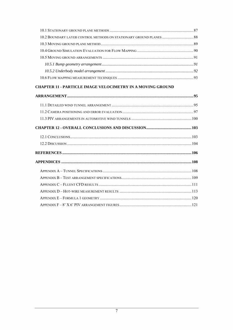
skirts to seal the underbody region from the outer flow as illustrated in Figure 1.1. This
development lead to the generation unprecedented amounts of downforce and a sharp increase
in cornering speeds.
Figure 1.1: Side-skirt assisted Formula underbodies in the late seventies. Left image from Racecar Aerodynamics[14], right image courtesy of Autorensport, 1981.
For safety reasons profiled underbodies were banned from Formula 1 at the end of 1982,
mandating the underbody to form a flat surface between the front and rear wheel axle, with a
diffuser permitted behind the rear axle. This rule initially decreased downforce by a huge
margin, but advances in technology and aerodynamics saw cornering capabilities ride to the
same levels as before. One of these advances was active suspension, a system in which
8
computer-controlled hydraulics replacing the traditional ‘passive’ suspension, with springs
and dampers. This system was able to guarantee ideal aerodynamic pitch and ride-height
under all racing conditions, thus allowing the application of pitch sensitive underbody designs.
This technology was banned in 1993 however, and after a disastrous 1994 season the
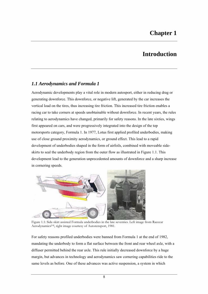
underbody of Formula cars was to change dramatically. The underbody was to form a stepped
bottom, with an additional plank to limit the minimum ride-height even further, illustrated in
Figure 1.2. This regulatory measure decreased the downforce generated by the underbody by
as much as 40% and decreased ride height and pitch sensitivity significantly, making the cars
more predictable and safer.
Figure 1.2: Stepped bottom underbodies on current Formula 1 cars. Left image courtesy of www.F1-Live.com, right image courtesy of G. Piola[24].
The rules governing the rest of the Formula 1 geometry have also been tightened severely
over the years, leaving little room for big changes. Painstaking development delivers
relatively small gains compared to the great strides made in the past. Each area of the car is
under scrutiny for further improvement in order to gain a vital aerodynamic advantage over
the competitors, resulting in hundreds of hours of wind tunnel tests and simulations.
1.2 Underbody simulation problems
The Formula 1 underbody, and in particular the interaction between the underbody and the
preceding elements such as the front wing, remains a somewhat unknown area, as flow
visualization during wind tunnel tests is practically not possible due to the small ride heights.
The small ground clearances cause great difficulties for measuring the actual underbody flow,
by means of either laser equipment or measurement probes.
Computational Fluid Dynamics (CFD) falls short in predicting underbody conditions, as the
vortices generated by the elements in front of the underbody are not reproduced accurately
with the current generation of CFD codes. The current state of computer technology does not
9
allow complete solving of the governing instantaneous Navier-Stokes equations under normal
engineering circumstances, due to the extremely fine meshes required in order to incorporate
the smallest eddy vortices generated by the geometry. This Direct Numerical Simulation
would thus require huge computational resources and calculation times that would be
unacceptable for engineering purposes.
Simplified equations like the Reynolds Averaged Navier Stokes equations (RANS) are used
in current commercial packages such a Fluent. The application of RANS has several
drawbacks concerning simulation of flows: convergence and dissipation. Vortices in
particular are affected by the additional dissipation in RANS methods, present to guarantee a
converging solution. Much can be gained from improving the current calculation methods for
the Formula 1 case, as most elements generate vortices with which the rest of the body
interacts in a certain way.
1.3 Goal definition
The relation between the underbody and the front elements is relatively unknown due to the
unknown interaction between the wakes of the front elements and the underbody. The physics
of the vortices generated by the front elements that pass through the underbody region of the
Formula 1 car are an unknown quantity, as can be seen in Section 1.2, due to the lack of
simulation capabilities and measurement difficulties.
The incoming underbody flow is non-uniform, as the front wing and rotating wheels in
particular generate vortices which are shed into the underbody region. These vortices will be
subjected to a favorable pressure gradient when passing through the underbody region.
This study will focus on two main themes:
• Vortex behavior in underbody pressure distribution, focusing on behavior in
accelerating flow
• Capabilities of recreating vortex behavior in actual underbody conditions, whilst
maintaining full flow mapping capabilities
The first section of this report, Chapters 2 to 7 will focus on the first theme, the vortex
behavior in accelerating flow, or a favorable pressure gradient. There is very little data on
favorable pressure gradients from previous studies, as the focus was primarily on the
decelerating flow region. This area of pressure recovery is of particular interest for aerospace
applications, as application of vortex generators can delay flow separation of airfoils.
10
These tests for this first section of this report were conducted in a wind tunnel with a
stationary floor, using a purpose built bump placed on the floor of the test section to generate
the required axial pressure distribution. Hot-wire probes were used to map the flow field
across the bump, whilst the single vortex is generated by a half-delta wing vortex generator
placed on the floor of the working section upstream of the bump. This arrangement is
simplified compared to the real Formula 1 underbody, but it will allow for complete flow
field mapping and thus provide insight into the effect of the favorable pressure gradient on
vortex behavior.
The second section of this report, Chapters 8-11, will focus on generating an arrangement
containing more real life factors and flow interactions, such as ground proximity
aerodynamics and a moving ground arrangement. Using the results for vortex behavior in
favorable pressure gradient from the first part of this study, the effects of the additional
factors and interactions present in a real underbody case on vortex behavior are evaluated.
1.4 Report structure
As mentioned in section 1.3, this report is divided into two sections, each covering one theme.
The first theme, the study of vortex behavior in a boundary layer under a favorable pressure
gradient, covers Chapters 2 to 7. Chapter 2 represents literature review into boundary layer
theory, general vortex theory, with emphasis on vortex decay, as well as results from previous
studies into vortex behavior. The available test facilities are presented in Chapter 3, followed
by the wind tunnel selection and test arrangement design in Chapter 4. Chapter 5 will present
the design process of the pressure gradient bump by means of CFD, along with CFD
verification using wind tunnel results. The results from the wind tunnel tests are presented in
Chapter 6, followed by conclusions and discussion in Chapter 7.
Chapter 8 marks the start of the second theme, which is the study into creating an
arrangement that will allow for full flow field mapping, incorporating all the ground
proximity aerodynamic elements and interactions present in underbody flows. Chapter 8
presents an analysis of Formula 1 underbody aerodynamics and ground proximity
aerodynamics. The possible test arrangements for recreating moving ground aerodynamics is
discussed in Chapter 9, followed by the effects of ground proximity aerodynamics on vortex
behavior and vortex decay in Chapter 10. A wind tunnel arrangement allowing underbody
flow mapping is generated as well in Chapter 10, which incorporates as many ground
proximity elements as possible, whilst still maintaining full flow mapping capabilities. The
details of the test arrangement and error evaluation are presented in Chapter 11.
11
Overall conclusions for both themes are presented in Chapter 12, along with
recommendations for future research and possible applications.
12
Chapter 2
Flow theory and previous studies
This chapter will present boundary layer and vortex theory, as well as results from previous
studies done into Sub-Boundary layer Vortex Generators (SBVGs) and favorable pressure
gradients. The results of this literature review will be applied to a stationary-ground wind
tunnel arrangement to generate a hypothesis for the first research goal: mapping the behavior
of a vortex in a boundary layer under a favorable pressure gradient.
2.1 Boundary layer theory
In order to gain insight into vortex behavior within a boundary layer, the behavior and physics
of the boundary layer itself has to be understood.
For this study, an understanding of boundary layer behavior in favorable pressure gradient is
required. Zero pressure gradient cases are well known, and can be analyzed using similarity
flows. Boundary layer behavior in adverse pressure gradients, which occurs at decelerating
flow conditions, has been widely studied within aerospace research, as separation and
transition are both stimulated by adverse pressure gradients. Favorable pressure gradients
have been studied to a lesser extent. However, the important features of these conditions are
well known.
In order to determine the effect of a pressure gradient on a boundary layer, Clauser’s
equilibrium parameter is frequently used[1]:
e
w
dpdx
δβτ
∗
=
For a constant value of β, the boundary layer will be in equilibrium, exhibiting self-similarity.
This is the case for all boundary layers under a zero pressure gradient, as Clauser’s parameter
will have a value of β = 0. However, equilibrium boundary layers are not common within
practical applications such as airfoils and underbodies. Clauser’s equilibrium parameter is
thus more useful as a means of comparing boundary layers and conditions for practical
applications.
13
In this study, the emphasis was on vortex behavior in underbody conditions, so no attempt
was made to generate conditions for an equilibrium boundary layer.
When comparing zero pressure gradient conditions with negative (favorable) pressure
gradient conditions, several distinct differences can be observed. The displacement thickness,
defined as δ* of the boundary layer is much smaller than for a zero pressure gradient case.
The boundary layer profile under favorable gradient is fuller, corresponding to a lower shape
factor H, defined as the ratio between the displacement thickness δ and the momentum
thickness θ. The effect of a favorable pressure gradient on the boundary layer thickness is a
decrease in boundary layer thickness growth. When the gradient is large enough, the local
boundary layer thickness will decrease, as observed in a previous study by Li et al[2].
Due to the fuller velocity profile the wall shear stress will increase when applying a favorable
pressure gradient, thus increasing the skin friction coefficient cf.
Another characteristic of a favorable pressure gradient is the effect it has on existing
boundary layers, able to significantly affect the boundary layer profile, as observed by Li et
al[2]. For sufficiently high favorable pressure gradients, a fully turbulent boundary layer can
relaminarize the flow. This effect was also investigated for this thesis study, as the pressure
gradient of an underbody might be able to relaminarize the turbulent incoming flow,
depending on the following parameter K:
2e
e
dUKU dsν
=
In this equation, Ue is the velocity at the edge of the boundary layer, ν is the dynamic
viscosity, and ds represents the local coordinate over the surface in streamwise direction,
defined as ( ) ( ) ( )2 2ds dx dy dz= + + 2.
Experiments in wind tunnels at low Reynolds numbers show that flow relaminarization
occurs for values of , although this relation for K is solely based on the inviscid
outer flow. The fact that boundary layer parameters and the duration to which a turbulent
boundary layer is exposed to the gradient are not present in this relation, leads to the
conclusion that K cannot predict relaminarization with 100% under all conditions.
63.0 10K ≥ ⋅
Even though the absolute turbulence levels will remain practically constant throughout the
test section, due to the increasing mean velocity the turbulence intensity decreases over the
favorable pressure gradient area. Thus for a sufficient length, the integral parameters for an
initially turbulent boundary layer can approach those for a fully laminar boundary layer.
14
Due to the full boundary layer profile and the small thickness, a boundary layer under a
favorable pressure gradient is very sensitive to surface roughness, as observed by Li et al[2].
Surface roughness counters the relaminarization effect by the favorable gradient, as the
roughness is larger compared to the boundary layer thickness. These tests also conclude that
the combined application of roughness and pressure gradient results in similar behavior to
when each is applied separately.
From experiences with wind tunnel contractions, a region of favorable pressure gradient, axial
velocity component fluctuations decrease with a factor of 21 N , in which N represents the
contraction ratio. The lateral and vertical velocity fluctuations on the other hand typically
increase by a factor of N . This increase is due to the stretching and spin-up of the axial
vortices, after Batchelor[3]. This will be discussed further in the following Section.
2.2 Vortex behavior
2.2.1. General vortex behavior
Two distinct vortex cases exist: the two-dimensional vortex case and the three-dimensional
case. For a two dimensional vortex, the vortex core axis runs parallel with the body axis. An
example of a 2D vortex is an eddy vortex in a two-dimensional plane. For the three-
dimensional vortex case is the vortex axis is not aligned to a body axis, covering the vast
majority of vortices.
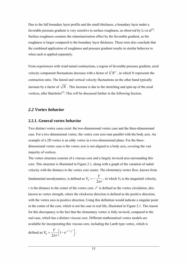
The vortex structure consists of a viscous core and a largely inviscid area surrounding this
core. This structure is illustrated in Figure 2.1, along with a graph of the variation of radial
velocity with the distance to the vortex core center. The elementary vortex flow, known from
fundamental aerodynamics, is defined as 2
Vrθ π
Γ= − , in which Vθ is the tangential velocity,
r is the distance to the center of the vortex core. Γ is defined as the vortex circulation, also
known as vortex strength, where the clockwise direction is defined as the positive direction,
with the vortex axis in positive direction. Using this definition would indicate a singular point
in the center of the core, which is not the case in real life, illustrated in Figure 2.1. The reason
for this discrepancy is the fact that the elementary vortex is fully inviscid, compared to the
real case, which has a distinct viscous core. Different mathematical vortex models are
available for incorporating this viscous core, including the Lamb type vortex, which is
defined as:2 2/1
2cr rV e
rθ π−Γ ⎡ ⎤= −⎣ ⎦ .
15
In this equation rc is the viscous vortex core radius.
As can be seen from Figure 2.1, the Lamb type vortex represents a more adequate model for a
real, viscous vortex, simulating the viscous core.
0
0.5
1
1.5
2
0 0.5 1 1.5 2 2.5 3
r/rc [-]
V θ/V
θmax
[-]
Inviscid vortex model Lamb-type vortex model
Figure 2.1: Vortex structure in radial direction, inviscid and viscid.
A well-known example of a three-dimensional vortex is the wing tip vortex, where a vortex is
generated due the air from the pressure side of the wing spilling over the tip of the wing to the
low-pressure suction side of the wing. A second example is the delta wing vortex under a high
angle of attack, where air spills over the sharp leading edge into the suction side of the wing.
In both cases, the key to the generation of these vortices is the geometry separating the
pressure from the suction side of the wing.
Vortex generators are available in various types, generating single and double vortices. These
vortex generators work under the same principle, with air spilling over a sharp edge in the
geometry. Positioned within the shear layer, the generated vortex enhances the mixing
between the retarded fluid in the boundary layer and the ‘inviscid’ outer flow, increasing the
average surface shear stress downstream of these vortex generators. The generated vortex
results in a boundary layer with increased resistance to separation, which in turn prolongs
flow attachment in a region of pressure recovery.
A series of ESDU papers on vortex generators[4] suggests that vortices suppress boundary
layer turbulence to a certain degree, as this could be the reason for the persistence of vortices
over remarkably long distances in turbulent flows. This paper also reports on observations
showing reductions in the rate of growth of the mean boundary layer when vortex generators
16
are applied, which can be attributed to the possible turbulence suppression capabilities of
vortices.
Four parameters or ‘vortex descriptors’ have been identified in order to quantify vortex
evolution within the boundary layer. These are:
1) peak angular velocity, ωx,max
2) vortex circulation, Γ
3) vortex core center location
4) equivalent Rankine vortex radius
These parameters are defined as follows:
1) The peak streamwise angular velocity ωx,.max is an indicator for vortex concentration,
and is used to identify the center of the vortex core, defined as 12x
w vy z
ω⎛ ⎞∂ ∂
= −⎜ ⎟∂ ∂⎝ ⎠. The
vorticity ξ, equal to the curl of a velocity field, is twice the angular velocity:
2 x xw vy z
ω ξ⎛ ⎞∂ ∂
= = −⎜ ⎟∂ ∂⎝ ⎠.
2) Vortex circulation Γ indicates vortex strength, generally calculated
using . For calculating the circulation in the cross-flow plane
the first equation is used by integrating measured velocities over a rectangular contour. This
contour must encompass the entire viscous vortex core region at least in order to provide
reliable results. The selection of both the position and size of the contour is thus limited: the
center of the contour positioned as closely as possible to the center viscous vortex core,
whereas the height and width of the contour have to be larger than the viscous core.
( )C s
V ds V dsΓ = − = − ∇×∫ ∫∫i i
3) The position and resulting vortex core trajectory are defined by the vortex core center
location at a number of streamwise positions. This position is determined using the velocity
measurement results for the crossflow speeds and vertical speeds.
4) Dynamic similarity of flows requires that when a vortex is generated in the inner
layer of a turbulent boundary layer, the circulation Γ at a certain streamwise position
correlates with the height of the vortex generator h, and the wall friction velocity uτ. The latter
is defined as 2e fu U Cτ = , in which Cf and Ue are the local skin friction coefficient and
17
boundary layer outer edge velocity respectively, measured without the vortex generator in
place. This value is expressed as:
( )u h G hτ+Γ = , in which h+ is the device Reynolds number defined as h u hτ ν+ = .
Equally, the maximum streamwise vorticity is scaled by the uτ and h by the same principle:
( ) MAXh h uτω+Ω = . This scaling is of importance for the definition of the Rankine vortex
radius, but also for comparison with results for vortex strength development from
DERA/Qinetiq studies into Sub-Boundary Layer Vortex Generators[5,6].
In order to attach a scale to the vortex size, the definition for the equivalent Rankine vortex
radius is used:
R
Gr
hπΩ
=
In this equation, G represents the scaled vortex circulation u hτΓ and Ω is the scaled
maximum streamwise vorticity. The Rankine radius is an idealization of a vortex where the
vorticity is assumed to be constant within the Rankine radius, and zero outside.
The advantage of selecting the equivalent Rankine vortex radius as vortex size scale is the
fact that it is independent of the shape of the vortex itself. This is significant as the viscous
vortex core is not always circular nor is the radius of the core constant.
2.2.2 Vortex development
For aerospace applications such as airfoils and bodies in free-stream conditions, six factors
are documented by ESDU[4] that influence vortex development.
These are:
1. Interaction between the main vortex and the secondary vortex that is generated as
reaction on the body surface.
2. Interaction between the vortex and the main surface boundary layer.
3. The initial core turbulence level, affected by the vortex formation. This is a function
of the leading edge radius and Reynolds effects.
4. Dissipation due to interaction with outer stream turbulence.
5. Dissipation in the viscous core of the main vortex.
6. The pressure gradient imposed onto the vortex by the outer stream.
The interaction between the main vortex and secondary vortex depends on the distance
between the generated vortex and the body surface, increasing as the distance decreases. The
vortex-induced lateral velocity on the body surface increases, resulting in a stronger
18
reactionary vortex. The increased strength of the secondary vortex will cause an increase in
vortex strength decay of the primary vortex, due to viscosity.
Increased fluctuations in boundary layers will increase the interaction between the vortex and
the boundary layer, increasing vortex strength decay. This holds for increases in both the axial
and lateral fluctuations.
The interaction between the main surface boundary layer and the vortex is an area of interest
for this study, as the favorable pressure gradient might be able to re-laminarize a turbulent
boundary layer. Freestone presents the following relation to approximate vortex strength
dissipation in an ESDU paper on vortex generator characteristics[4]:
fcddx z
ΓΓ= −
fcd dxz
Γ= −
Γ
where Γ is the local vortex strength, z is the distance between the vortex core and the surface
and cf is the local skin friction coefficient.
For cases in which cf and z vary only slowly with x, the following relation can be derived:
( ) ( )0
0
fcx x
zx
e− −Γ
=Γ
where Γ0 and x0 are the initial vortex strength and position respectively.
The drawback of this approximation is the fact that it only holds for vortices that have not
grown to such an extent that it actually reaches the surface. The effect of the vortex on the
boundary layer and thus skin friction coefficient is not taken into account either.
As cf generally decreases with increasing Reynolds number, scale model testing will thus lead
to higher vortex decay than is the case for the full scale model.
For the inviscid case, vortex strength remains constant, thus complying with Kelvin’s
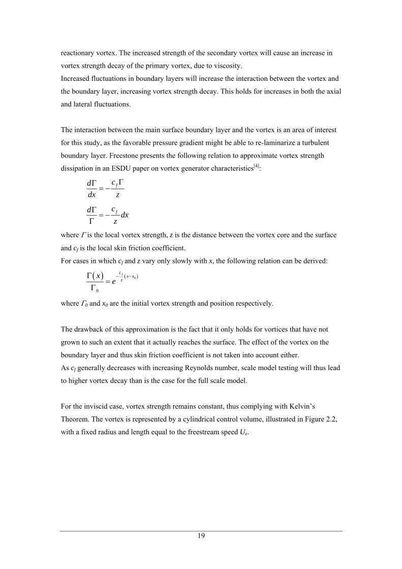
Theorem. The vortex is represented by a cylindrical control volume, illustrated in Figure 2.2,
with a fixed radius and length equal to the freestream speed Ue.
19
12 1
2
e
e
US SU
=
Figure 2.2: Stretching of vortex control volumes in accelerating flow
A vortex will be stretched in accelerating flow, decreasing the radius of the vortex in order to
maintain the same control volume size. The vorticity in the crossflow plane for this vortex
with smaller radius will have to increase to maintain constant vortex strength, following:
( )C s s
w vV ds V ds dsy z
⎛ ⎞∂ ∂Γ = − = − ∇× = − −⎜ ⎟∂ ∂⎝ ⎠
∫ ∫∫ ∫∫i i i
The effect of increased streamwise vorticity with increasing freestream speed is known as the
spin-up of the vortex.
2.2.3 Vortex generator theory
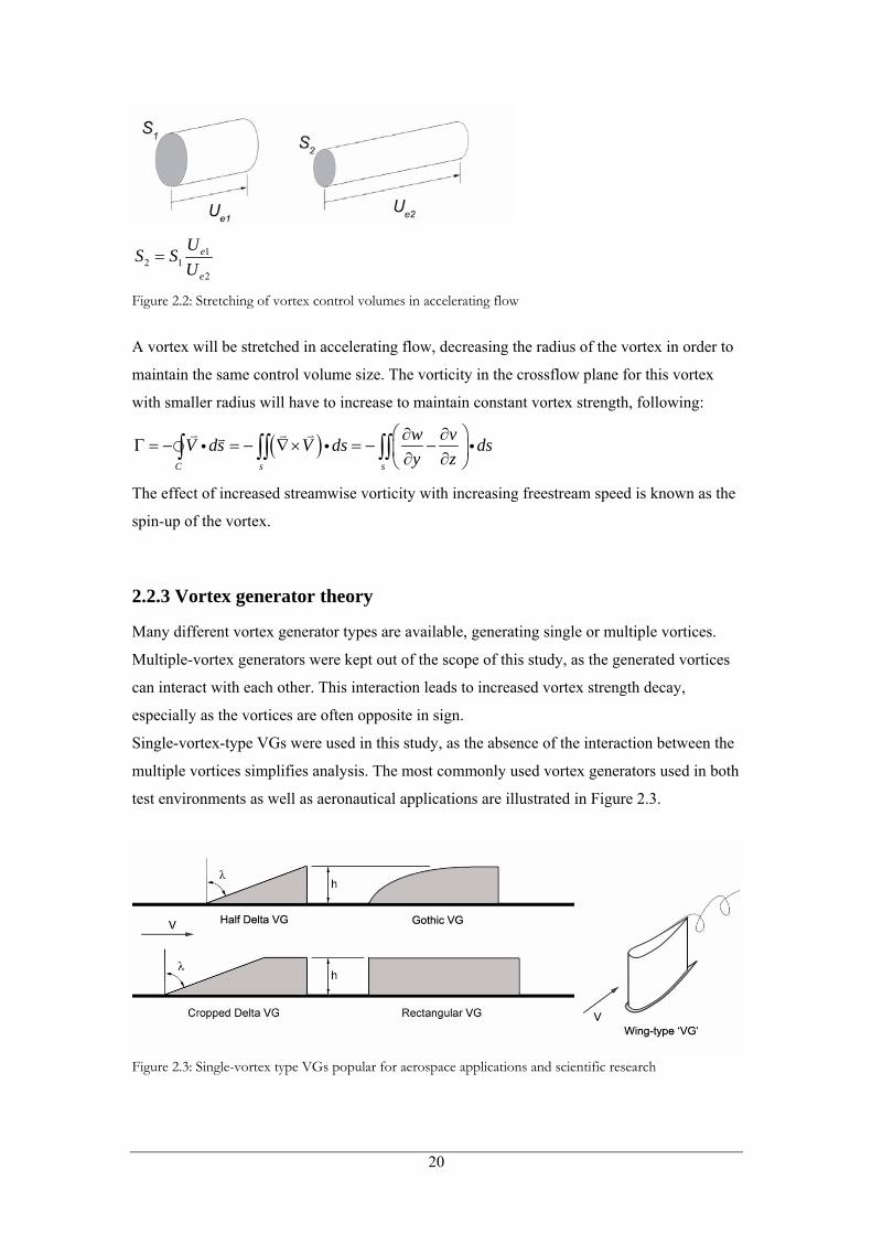
Many different vortex generator types are available, generating single or multiple vortices.
Multiple-vortex generators were kept out of the scope of this study, as the generated vortices
can interact with each other. This interaction leads to increased vortex strength decay,
especially as the vortices are often opposite in sign.
Single-vortex-type VGs were used in this study, as the absence of the interaction between the
multiple vortices simplifies analysis. The most commonly used vortex generators used in both
test environments as well as aeronautical applications are illustrated in Figure 2.3.
Figure 2.3: Single-vortex type VGs popular for aerospace applications and scientific research
20
The following factors influence the characteristics of the vortices generated by vortex
generators:
• Incoming flow characteristics
• (Leading) Edge radius
• Incidence angle (for delta wing type)
• Sweep angle (for delta wing type)
• Device height
The Reynolds number of the incoming flow is one of the factors that determine whether the
flow is capable of generating a vortex. The dependency of the vortex to the Reynolds number
decreases with a sharper VG leading edge, and has been observed in previous studies[5,6].
Vortex generators with a sharp leading edge are less dependent on the Reynolds number than
a wing-tip, as the latter requires a higher Reynolds number for flow attachment along the
airfoil. Increased flow attachment will result in an increased pressure difference between the
suction and pressure side of the wing.
In addition to the Reynolds number, the sweep angle and angle of attack are key factors for
vortices generated by delta wings and vortex generators. As most experiments are carried out
in uniform incoming flow conditions, most previous studies tend to refer to the angle of attack
α of the vortex generator as the incidence angle i.
Sweep and incidence angle are linked as far as vortex generation is concerned. For smaller
sweep angles, vortex breakdown will occur at lower incidence angles, whereas larger sweep
angles feature vortex breakdown at higher angles. Vortex breakdown is a phenomenon in
which vortex instability has risen to such an extent, that the viscous vortex core is unable to
sustain itself, and collapses. Vortex instability is stimulated further by adverse pressure
gradients, which is the case for decelerating flow under normal conditions (with no additional
heating or boundary layer suction/blowing). Vortex breakdown is of significant importance to
jet-fighters equipped with delta wings or strakes, as the vortices are used to produce
additional lift at high angles of attack. Vortex breakdown on the wing surface would thus
cause a loss of the additional ‘vortex lift’.
For increasing incidence angles, the circulation at a given axial location increases up to the
onset of vortex breakdown. Increasing the incidence angle beyond this point will result in a
forward movement of this breakdown point, whilst still increasing vorticity in the area ahead
of the breakdown. In the case of a delta wing with a leading edge sweep angle of λ = 70o
vortex breakdown does not occur on the wing surface for incidence angles less than ι = 30o.
For a sweep angle of λ = 60o breakdown on the wing surface starts to occur at angles
21
exceeding approximately ι = 10o. These values were obtained from a study into development
of vortex breakdown by Bruckner[7]. The exact incidence angles where vortex breakdown
occurs differs significantly per study, even when using the exact same delta wing geometry.
The mentioned incidence angles are therefore an approximate value.
The size of the vortex generator is a key factor in determining the strength of the generated
vortex by a VG and the development downstream. With a constant geometry, the size of the
vortex generator is expressed in the device height h. The strength of the generated vortex is
linearly dependent on the size of the vortex generator.
Vortex generators are distinguished between Sub-Boundary Layer Vortex Generators
(SBVGs), with device heights smaller than the local boundary layer thickness δ, and ordinary
Vortex Generators (VGs), with typical device heights larger than δ, thus protruding into the
outer flow region. SBVGs have a typical device height 20% than the local boundary layer
thickness. An ordinary VG will thus generate a stronger vortex, but this vortex will be at a
larger distance from the body surface, on which the VG is positioned. The vortex will thus be
shed initially into the outer flow rather than the boundary layer. In the case of an SBVG, the
vortex strength will be smaller, but the vortex will be shed primarily into the turbulent
boundary layer. The vortex strength development downstream of the device will thus depend
on the device height.
During the review of previous studies into three-dimensional vortices, focus was on vortices
generated by SBVGs. With a device height typically less than 35% of the local boundary
layer thickness, these SBVGs are substantially smaller than their ordinary VG counterparts,
which protrude into the ‘inviscid’ outer flow. The drag penalty of an SBVG is thus
significantly lower than an ordinary VG.
The geometries used for SBVGs are the same as used for ordinary VGs: rectangular, half
delta, cropped delta and the gothic geometry, as illustrated in Figure 2.2. The choice for
SBVGs over ordinary VGs was made in order to compare results for streamwise vortex
development with results from recent SBVG studies [4,5,8] carried with laser equipment.
These measurement techniques will be discussed in Section 3.1.
Qinetiq UK, formerly known as DERA, has carried out research into vortex behavior of
several multiple-vortex SBVG types as well as a single-vortex half-delta type SBVG [5,6]. The
measurement technique used was Laser Doppler Anemometry. These studies focused on the
effectiveness of each SBVG type to generate a vortex, by measuring vortex strength and
vortex decay in zero pressure gradient and adverse pressure gradient conditions. Adverse
pressure gradient measurements were carried out with a bump-generated flow with the vortex
22
generators placed in the zero pressure gradient area at the apex of the bump, just before the
start of the adverse gradient area. Using a single-vane SBVGs with a device height of 30 mm
the vortex strength decreased by 64% over a length of 50 device heights in a zero pressure
gradient case, whereas the adverse pressure gradient case shows a decrease of 59% over the
same distance. The lower vortex strength decay for the adverse pressure gradient case was
predicted in the approximation presented in Section 2.2.2. The device height Reynolds
number for these tests was Reh = 6.0 ·104.
Particle Laser Velocimetry (PIV) measurements of SBVG and VG generated vortices on a flat
plate were carried out at NASA Langley by Yao et al[8], in order to gain insight into the
physics of vortex generation and propagation over a flat plate. Focus was on the difference
between the ordinary VG and the SBVG, with the VG generating its maximum vorticity at a
smaller incidence angle than the SBVG. Both vortex generator types were tested at three very
different incidence angles, where the VG exhibited vortex breakdown for the two larger
angles. However, a more refined incidence angle selection would have given more insight
into how the vorticity development depends on the incidence angle. The current incidence
angles are too coarse to be able to make genuine conclusions.
The measured maximum local vorticity for the SBVG decreased exponentially to ∆x, the
distance from the trailing edge of the vortex generator. Vortex strength decay on the other
hand was found to be more linearly proportional to ∆x. The device height for the SBVGs was
h = 7 mm (h/δ = 0.20), for the VG this was h = 35 mm, thus making the device height
Reynolds number for the SBVG case Red = 1.6 ·104.
23
Chapter 3
Available wind tunnel and measurement facilities
As this study was carried out at Cranfield University, College of Aeronautics, various
facilities and measurement methods were available. Section 3.1 presents the available
measurement methods, both intrusive and non-intrusive, followed by an evaluation of the
different wind tunnel facilities at Cranfield University in Section 3.2, along with the
advantages and drawbacks of each of these facilities.
3.1 Flow measurement methods
3.1.1 Intrusive methods
For flow mapping purposes, two main methods are available: intrusive and non-intrusive
measurements. Intrusive measurements make use of a probe to measure the flow locally,
whereas non-intrusive measurements have the measurement equipment placed outside of the
flow, thus having no significant effect on the flow.
For intrusive testing Cranfield College of Aeronautics makes use of a fully integrated traverse
gear mounted in the ceiling of the 8’ X 4’ wind tunnel, where both pitot-static measurements
as well as hot-wire measurements can be taken. The workings of Hot-Wire Anemometry is
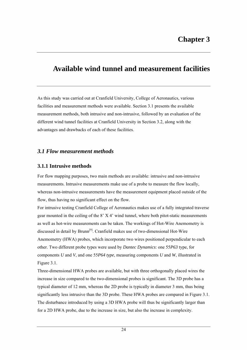
discussed in detail by Brunn[9]. Cranfield makes use of two-dimensional Hot-Wire
Anemometry (HWA) probes, which incorporate two wires positioned perpendicular to each
other. Two different probe types were used by Dantec Dynamics: one 55P63 type, for
components U and V, and one 55P64 type, measuring components U and W, illustrated in
Figure 3.1.
Three-dimensional HWA probes are available, but with three orthogonally placed wires the
increase in size compared to the two-dimensional probes is significant. The 3D probe has a
typical diameter of 12 mm, whereas the 2D probe is typically in diameter 3 mm, thus being
significantly less intrusive than the 3D probe. These HWA probes are compared in Figure 3.1.
The disturbance introduced by using a 3D HWA probe will thus be significantly larger than
for a 2D HWA probe, due to the increase in size, but also the increase in complexity.
24
Three-dimensional HWA probes were thus not an option, due to the increased disturbance to
the flow, but also costs. Due to the complexity of the 3D HWA probe, the cost of such a
probe is significantly higher than a 2D probe.
Diameter 3 mm Diameter 12 mm
Figure 3.1: Comparison between 2D HWA probes used at Cranfield (left) and a typical 3D HWA probe (right) by the same manufacturer
The advantages of HWA probes are the relative simplicity of the arrangement, the ability to
take measurements at very close distance to surfaces and increased accuracy compared to a
pitot-static probe measurements. The latter advantage is because the HWA probes can be
sampled at frequencies up to 10 kHz.
The main drawbacks are the intrusiveness of the probe and the pointwise nature of the
measurements: in order to map a vortex a large number of points will have to be measured at
each streamwise position, with an average measurement taking up to 30 seconds including
probe traversing.
Even though probe intrusiveness is a generally accepted fact, evidence is mixed, with a
number of studies presenting results supporting this fact[10,11]. Other studies clearly present
results where probe intrusiveness does not pose any problems, supported by flow
visualization results[12]. However, these results strongly depend on the testing conditions and
geometry, as the test arrangements for these studies were fairly straight-forward, without
vortices generated well outside of the wall boundary layers and without displacing the vortex
of applying a pressure gradient.
The primary mechanism for vortex/probe interaction is the penetration of the vortex core by
the probe. Previous experiments by Lundgren and Ashurst [10] into the effects of area-varying
waves on vortices, show that penetration of the vortex core will locally increase the radius on
the core as it passes the probe, before decreasing after passing the probe.
25
3.1.2 Non-intrusive methods
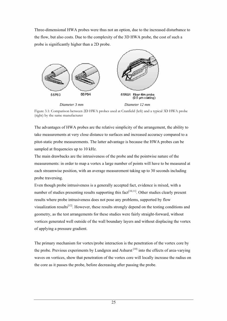
Non-intrusive measurements are carried out without disturbing the flow itself, done generally
by means of laser equipment. The most practical method for laser measurements is Digital
Particle Image Velocimetry (DPIV), generally known as PIV. This method makes use of
seeded particles, injected into the flow well upstream of the measurement position and is
illustrated in Figure 3.2.
Figure 3.2: Particle Image Velocimetry principle
The laser light sheet will have to be generated from a position in the direct cross-flow plane of
the measurement position, depending on the geometry of the model, as reflection has to be
minimized in relation to the current study.
The CCD camera recording the two images will have to be placed downstream of the
measurement position, with a good view of the laser light sheet i.e. not obstructed by the
geometry. The preferred position of the camera is in the forward scatter range rather than
backward scatter. For measurements involving general flow behavior and trends comparing
different cases a single camera will suffice. However, for the accurate determination of actual
flow values two cameras will be required, thus creating a stereoscopic image of the
measurement, also known as Stereo Digital Image Velocimetry (SDPIV). For the current
research, trends in the vortex measurements are of prime importance rather than the actual
determination of quantitative data. Therefore, a single camera arrangement will suffice,
provided the entire PIV equipment positions, including the laser equipment, the camera
26
position and seeding, will remain constant for the duration of the measurements in order to be
able to compare results.
3.2 Wind tunnel facilities
3.2.1 Smoke wind tunnel
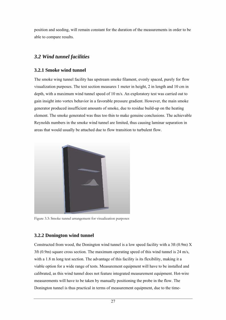
The smoke wing tunnel facility has upstream smoke filament, evenly spaced, purely for flow
visualization purposes. The test section measures 1 meter in height, 2 in length and 10 cm in
depth, with a maximum wind tunnel speed of 10 m/s. An exploratory test was carried out to
gain insight into vortex behavior in a favorable pressure gradient. However, the main smoke
generator produced insufficient amounts of smoke, due to residue build-up on the heating
element. The smoke generated was thus too thin to make genuine conclusions. The achievable
Reynolds numbers in the smoke wind tunnel are limited, thus causing laminar separation in
areas that would usually be attached due to flow transition to turbulent flow.
Figure 3.3: Smoke tunnel arrangement for visualization purposes
3.2.2 Donington wind tunnel
Constructed from wood, the Donington wind tunnel is a low speed facility with a 3ft (0.9m) X
3ft (0.9m) square cross section. The maximum operating speed of this wind tunnel is 24 m/s,
with a 1.8 m long test section. The advantage of this facility is its flexibility, making it a
viable option for a wide range of tests. Measurement equipment will have to be installed and
calibrated, as this wind tunnel does not feature integrated measurement equipment. Hot-wire
measurements will have to be taken by manually positioning the probe in the flow. The
Donington tunnel is thus practical in terms of measurement equipment, due to the time-
27
consuming nature of the manual positioning. The short test section does not allow for
significant boundary layer development prior to the test section. SBVG tests will be
complicated, as device height for SBVGs has to be smaller than the local boundary layer
thickness δ. For SBVG tests the boundary layer will have to be thickened by means of
roughness upstream of the SBVG, or small device heights will have to be chosen, resulting in
lower vortex strength
3.2.3 Atmospheric Boundary Layer wind tunnel
Designed to replicate the atmospheric boundary layer for civil and off-shore engineering
purposes, the 8 ft (2.4m width) X 4 ft (1.2m height) wind tunnel incorporates a fully
integrated, computer controlled traverse system, to which a number of instruments can be
attached in order to take measurements. These range from pitot-static tubes, for pressure and
velocity measurements, to Hot-Wire Anemometry (HWA) probes. The wind tunnel features a
turntable mounted moving ground plane, with boundary layer control. The maximum
allowable speed of the electromotor driving the wind tunnel is 600 rpm, which corresponds to
a speed through the test section of approximately 16 m/s.
The traverse gear is positioned in a cavity in the ceiling of the test section, starting at a
distance of 6.0 meters downstream of the start of the test section, measuring 1.5 meters in
length, 2.0 meters wide and a depth of 1.2 meters. This cavity can be sealed, but will have to
remain open when the traverse gear is used. The traverse gear is able to translate across the
full cavity opening, as well as the full height of the test section.
Measurements can thus be taken right up to the floor surface using HWA probes, but a
minimum clearance of 10 mm is usually applied due to the fragility and cost of the probes.
The 8’X 4’ wind tunnel was selected for the flow mapping HWA experiments, because of the
integrated three-dimensional traverse gear. The flow through the test section in the
measurement region of the wind tunnel is fully developed.
PIV measurements are possible, mounting the necessary laser equipment on rails inside the
tunnel rather than placing it outside the tunnel. For PIV measurement the cavity can be sealed,
thus eliminating the effect of the cavity on the flow through the test section.
The boundary layer thickness δ on the test section floor is typically 120 mm, measured at
axial position of the leading edge of cavity.
28
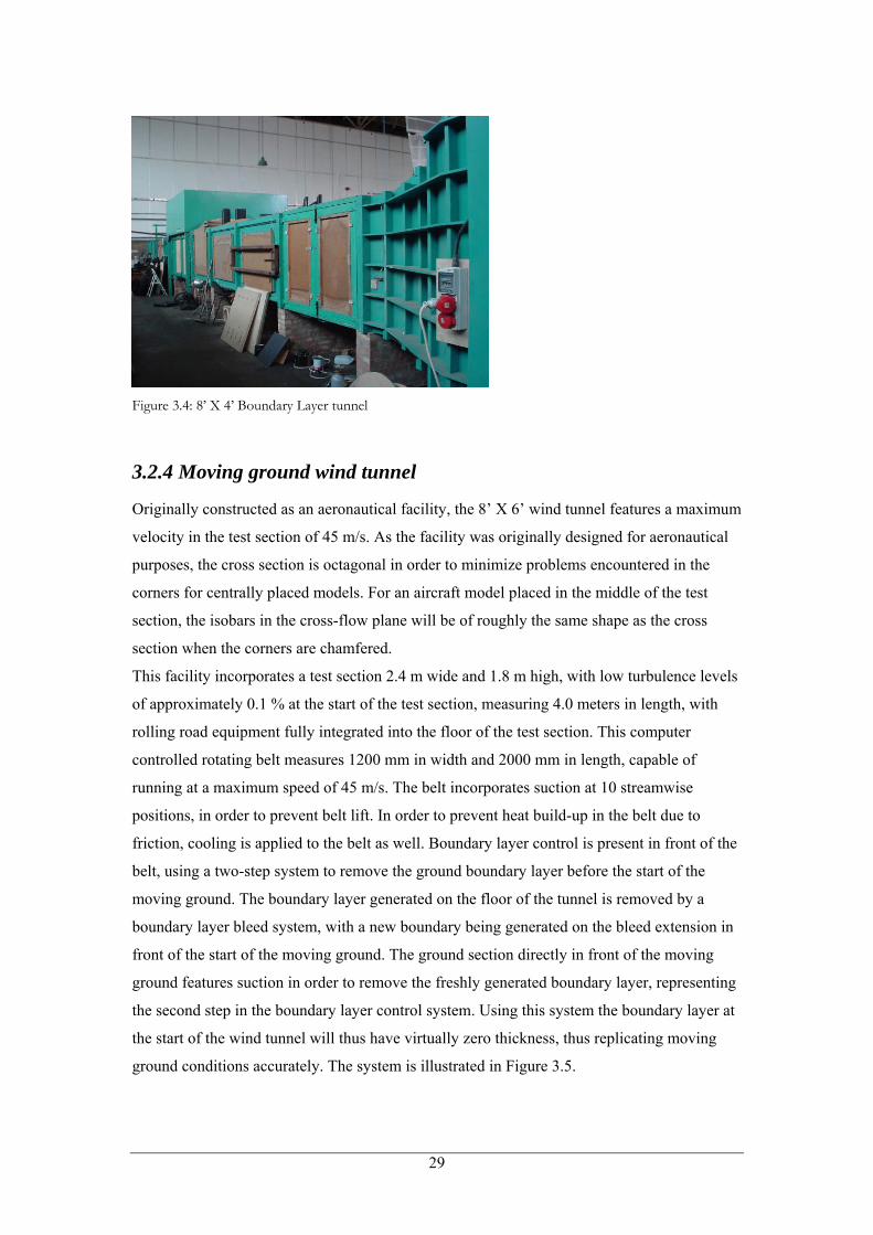
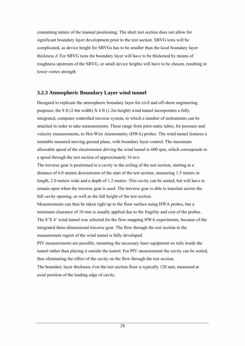
Figure 3.4: 8’ X 4’ Boundary Layer tunnel
3.2.4 Moving ground wind tunnel
Originally constructed as an aeronautical facility, the 8’ X 6’ wind tunnel features a maximum
velocity in the test section of 45 m/s. As the facility was originally designed for aeronautical
purposes, the cross section is octagonal in order to minimize problems encountered in the
corners for centrally placed models. For an aircraft model placed in the middle of the test
section, the isobars in the cross-flow plane will be of roughly the same shape as the cross
section when the corners are chamfered.
This facility incorporates a test section 2.4 m wide and 1.8 m high, with low turbulence levels
of approximately 0.1 % at the start of the test section, measuring 4.0 meters in length, with
rolling road equipment fully integrated into the floor of the test section. This computer
controlled rotating belt measures 1200 mm in width and 2000 mm in length, capable of
running at a maximum speed of 45 m/s. The belt incorporates suction at 10 streamwise
positions, in order to prevent belt lift. In order to prevent heat build-up in the belt due to
friction, cooling is applied to the belt as well. Boundary layer control is present in front of the
belt, using a two-step system to remove the ground boundary layer before the start of the
moving ground. The boundary layer generated on the floor of the tunnel is removed by a
boundary layer bleed system, with a new boundary being generated on the bleed extension in
front of the start of the moving ground. The ground section directly in front of the moving
ground features suction in order to remove the freshly generated boundary layer, representing
the second step in the boundary layer control system. Using this system the boundary layer at
the start of the wind tunnel will thus have virtually zero thickness, thus replicating moving
ground conditions accurately. The system is illustrated in Figure 3.5.
29
Figure 3.5: Two-step boundary layer control ahead of the moving ground
The 8’ X 6’ wind tunnel is primarily a facility for flow visualization as well as force and
pressure measurements, with a fully integrated servo-driven active strut system, allowing
rapid and accurate model pitch and ride height changes. There is no fixed probe traverse
system in the 8’ X 6’ wind tunnel, making an array of hot-wire measurements impractical.
30
Chapter 4
Wind Tunnel Test Arrangement
Concepts for the 8’X 4 Boundary Layer Tunnel are presented in Section 4.1, followed by a
discussion of the available flow measurement methods, listing advantages and drawbacks for
each of the methods, culminating in a measurement method selection in Section 4.2.
Section 4.3 covers the selection of vortex generators, leading to the selection of the vortex
generators used for this study.
4.1 Arrangement concepts
Several methods are available for generating a pressure gradient similar to that of a Formula 1
underbody in the 8’X 4’ wind tunnel. The simplest and cheapest method is by creating a
purpose-built single bump, placed on the floor of the test section. The vortex generator is
placed on the floor of the test section, in front of the leading edge of the bump. Placement on
either of the side walls is not preferred, as the height-to-width ratio of the tunnel is 1:2. The
risk of interaction between the vortex and corners of the test section will thus be greater than
for a placement on the floor. These test section corners have to be avoided as much as
possible, as the flow is no longer two-dimensional in this region.
The ceiling is not an option for placement when using HWA probes, as the ceiling cavity
would have a significant effect on the vortex. The ceiling cavity can be sealed for PIV
measurements though, thus making vortex generator placement on the ceiling of the test
section an option when using PIV.
An additional method of generating the require pressure gradient would be to create two
identical bumps, placed on both sidewalls of the test section. The advantage of such an
arrangement is the fact that the spanwise pressure gradient in the middle of the test section is
virtually constant, due to the mirroring effect of both ramps. The acceleration will be highest
in the proximity of the bump surface. The advantage of this arrangement is the symmetric
velocity distribution in the XZ-plane.
31
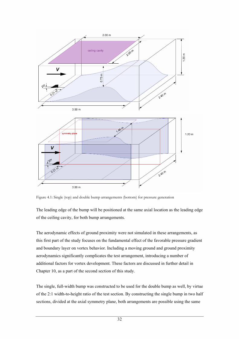
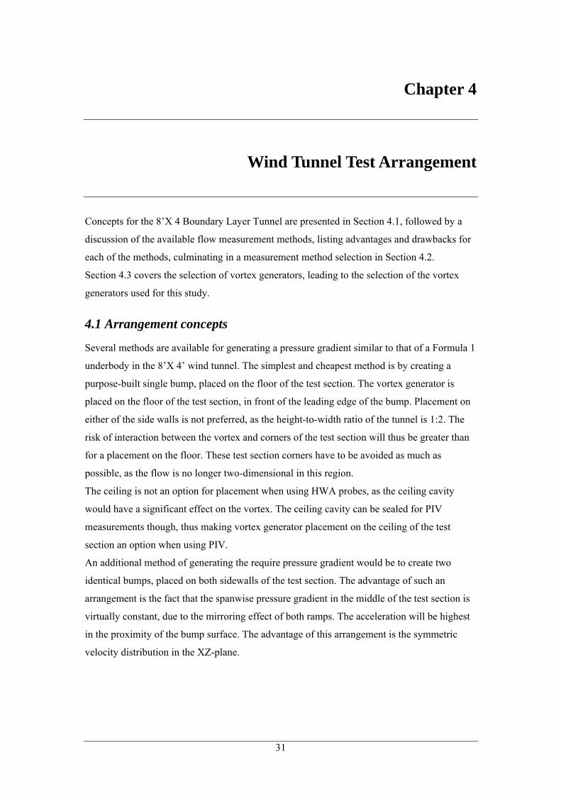
Figure 4.1: Single (top) and double bump arrangements (bottom) for pressure generation
The leading edge of the bump will be positioned at the same axial location as the leading edge
of the ceiling cavity, for both bump arrangements.
The aerodynamic effects of ground proximity were not simulated in these arrangements, as
this first part of the study focuses on the fundamental effect of the favorable pressure gradient
and boundary layer on vortex behavior. Including a moving ground and ground proximity
aerodynamics significantly complicates the test arrangement, introducing a number of
additional factors for vortex development. These factors are discussed in further detail in
Chapter 10, as a part of the second section of this study.
The single, full-width bump was constructed to be used for the double bump as well, by virtue
of the 2:1 width-to-height ratio of the test section. By constructing the single bump in two half
sections, divided at the axial symmetry plane, both arrangements are possible using the same
32
basic construction. The bump was thus constructed in two 4 ft wide sections, equal to the
height of the test section.
Figure 4.2: Bump construction, allowing for both single and double bump arrangement
The suction peak in the middle of the test section for the double bump arrangement will be
lower than the suction single bump setup. In order to achieve the same pressure distribution
for the double bump as for the single bump arrangement, the bumps can be inclined with
respect to the sidewalls, increasing the local velocity. The initial inclination angle was
determined with the use of CFD in Chapter 5, but no inclination was applied for the
experiments, due to time restrictions as well as difficulties with securing the bumps when not
placed flush against the sidewalls.
4.2 Vortex generator selection
Vortex generators are available in a large number of variations, with suitability depending on
the application. As mentioned before, vortex generators can be subdivided into two main
categories:
- Vortex generators generating multiple vortices
- Vortex generators generating one single vortex
Selecting a vortex generator from the first category is not favorable, as the generated vortices
will interact with each other. This additional factor for vortex circulation decay will make
evaluation of the effect of a favorable pressure gradient more complicated. The single vortex
generated by the second VG category will limit the amount of interactions, thus making
evaluation less complicated.
Of these single vortex generators, the single vane type bears most resemblance to vortices
generated by delta wings, with a number of variations within this theme. The most commonly
33
used single-vane vortex generator geometries are illustrated in Figure 2.2. The initial
geometry selection for this study was the rectangular type, the half-delta type and the cropped
delta type, for both VG and SBVG sizes.
However, the available wind tunnel time limited the number of vortex generator types to one.
The selected device was of the cropped-delta SBVG type, selected over the rectangular type
in order to compare the vortex strength development with the DERA/Qinetiq results. The
SBVG sheds the vortex at a closer distance to the surface, thus giving a good indication of the
magnitude of the vortex interaction. The cropped delta was selected over the half-delta as
these are used more frequently in aerospace applications.
The device was positioned at five device heights upstream of the leading edge of the bump.
The device height was set at 42 mm, which is 35 % of the boundary layer thickness at the
position of the device, which was 120 mm. This incoming boundary layer will be analyzed in
Section 5.1. The device is thus of the SBVG type, selected over the ordinary VG to compare
the results with recent SBVG studies.
The advantage of selecting a vortex generator with a swept leading edge is the fact that results
from full-span delta wings can be used. As mentioned in Chapter 3.2, the strength of the
vortex depends on the sweep angle λ, incidence angle α and the leading edge radius. For a
sharp leading edge radius, Reynolds numbers will have significantly less influence on vortex
generation. Sweep angle λ and incidence angle α have to be selected in order to prevent
vortex breakdown, especially when testing in a shear layer. This is because the turbulent
motions within the boundary layer will increase vortex strength dissipation. Previous research
by NASA3 indicates vortex breakdown onset on the vortex generator starts at incidence
angles of α = 10o for a sweep angle of λ = 60o, and an incidence angle of α = 30o for a sweep
angle of λ = 70o. Initial vortex strength increases with increasing incidence angle as well as
for smaller sweep angles. The two cases for sweep and incidence angle mentioned above
produce vortices of roughly the same strength.
The cropped delta VG has a sweep angle of λ = 70o, as this sweep angle provides more
flexibility in incidence angle before the onset of vortex breakdown.
Rectangular vortex generators are often used as well, however with no obvious similarity to
delta wings and thus no possibility of using delta wing test results for reference. However the
NASA Langley PIV study by Yao et al[8], makes use of rectangular vortex generators, both
the ordinary and sub-boundary layer type. For the ordinary type, the height of which is larger
than the local boundary layer thickness, maximum vorticity occurs at an incidence angle of α
= 10o, whereas for the sub-boundary layer type this occurs at α = 23o. It has to be stated that
34
only three incidence angles were measured, α = 10o, 16o and 23o, so genuine conclusions
cannot be drawn from these three points.
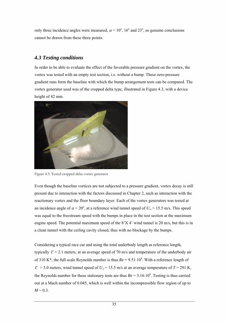
4.3 Testing conditions
In order to be able to evaluate the effect of the favorable pressure gradient on the vortex, the
vortex was tested with an empty test section, i.e. without a bump. These zero-pressure
gradient runs form the baseline with which the bump arrangement tests can be compared. The
vortex generator used was of the cropped delta type, illustrated in Figure 4.3, with a device
height of 42 mm.
Figure 4.3: Tested cropped-delta vortex generator
Even though the baseline vortices are not subjected to a pressure gradient, vortex decay is still
present due to interaction with the factors discussed in Chapter 2, such as interaction with the
reactionary vortex and the floor boundary layer. Each of the vortex generators was tested at
an incidence angle of α = 20o, at a reference wind tunnel speed of U∞ = 15.5 m/s. This speed
was equal to the freestream speed with the bumps in place in the test section at the maximum
engine speed. The potential maximum speed of the 8’X 4’ wind tunnel is 20 m/s, but this is in
a clean tunnel with the ceiling cavity closed, thus with no blockage by the bumps.
Considering a typical race car and using the total underbody length as reference length,
typically c = 2.1 meters, at an average speed of 70 m/s and temperature of the underbody air
of 310 K*, the full scale Reynolds number is thus Re = 9.51⋅106. With a reference length of
c = 3.0 meters, wind tunnel speed of U∞ = 15.5 m/s at an average temperature of T = 291 K,
the Reynolds number for these stationary tests are thus Re = 3.16⋅106. Testing is thus carried
out at a Mach number of 0.045, which is well within the incompressible flow region of up to
M = 0.3.
35
The vortex generated by the cropped-delta vortex generator was measured for an empty test
section, a single, floor-mounted arrangement and the side-wall mounted arrangement. For
both the single and double bump arrangement, flow visualization by means of smoke was
used to gain insight into the vortex core trajectory along the test section before programming
the measurement grid for the HWA probes.
4.4 Hypothesis
As discussed in Chapter 2, a favorable pressure gradient decreases the axial fluctuations in the
boundary layer, but increases the mean fluctuations in the lateral and vertical components.
From these experiences from wind tunnel contractions, it can be reasoned that the lateral and
vertical components of the generated vortex increase over the favorable pressure gradient,
thus increasing the vorticity in the vortex.
The total circulation in the vortex, the vortex strength, will decrease due to viscous effects.
Boundary layer thickness will decrease when subjected to a favorable pressure gradient. The
vortex core trajectory will remain virtually unchanged in the vertical XZ plane when applying
a favorable pressure gradient, as is the case between zero and adverse pressure gradient cases.
Compared to the zero pressure gradient case the vortex will remain within this boundary layer
for a shorter period, thus decreasing the vortex strength decay due to the interaction with this
boundary layer.
However, for the single bump case, the vortex will not be able to clear the bump without
being displaced by it. The vortex will thus run along the bump surface, increasing interaction
with the secondary, reactionary vortex on this surface of the bump. This displacement and
resulting interaction will deform the vortex core, as was observed in a study into two-
dimensional vortices by Conlisk[13], illustrated in Figure 4.4. Even though these two-
dimensional vortices, defined in Section 2.2.1, are of a different nature than the vortices in
this current study, an analogy can be drawn between the two cases concerning the effect of
the displacement on the vortex core shape.
36
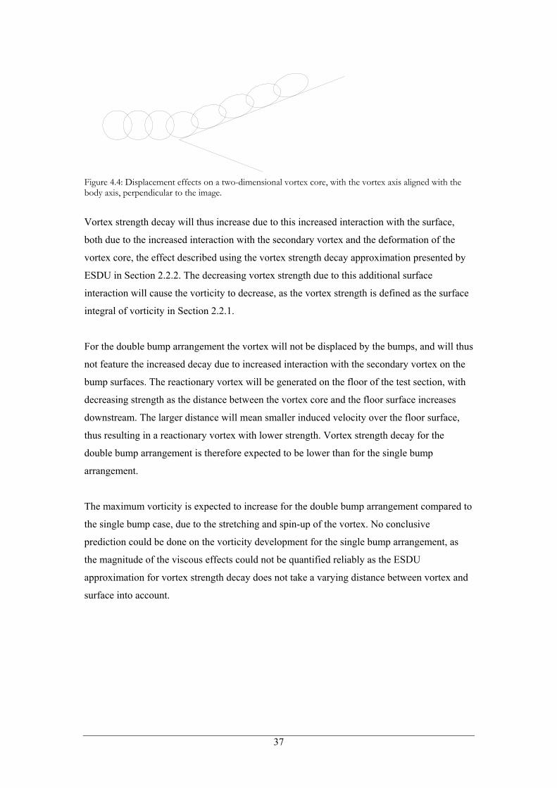
Figure 4.4: Displacement effects on a two-dimensional vortex core, with the vortex axis aligned with the body axis, perpendicular to the image.
Vortex strength decay will thus increase due to this increased interaction with the surface,
both due to the increased interaction with the secondary vortex and the deformation of the
vortex core, the effect described using the vortex strength decay approximation presented by
ESDU in Section 2.2.2. The decreasing vortex strength due to this additional surface
interaction will cause the vorticity to decrease, as the vortex strength is defined as the surface
integral of vorticity in Section 2.2.1.
For the double bump arrangement the vortex will not be displaced by the bumps, and will thus
not feature the increased decay due to increased interaction with the secondary vortex on the
bump surfaces. The reactionary vortex will be generated on the floor of the test section, with
decreasing strength as the distance between the vortex core and the floor surface increases
downstream. The larger distance will mean smaller induced velocity over the floor surface,
thus resulting in a reactionary vortex with lower strength. Vortex strength decay for the
double bump arrangement is therefore expected to be lower than for the single bump
arrangement.
The maximum vorticity is expected to increase for the double bump arrangement compared to
the single bump case, due to the stretching and spin-up of the vortex. No conclusive
prediction could be done on the vorticity development for the single bump arrangement, as
the magnitude of the viscous effects could not be quantified reliably as the ESDU
approximation for vortex strength decay does not take a varying distance between vortex and
surface into account.
37
Chapter 5
Bump design in CFD and verification
In order to be able to evaluate vortex behavior under Formula 1 type underbody conditions,
the pressure distribution have to be determined prior to the construction of the wind tunnel
test arrangement. The desired design pressure distribution for the 8’ X 4’ wind tunnel tests is
given in Chapter 5.1, along with other design and construction considerations, which will
form the baseline for the CFD bump calculations. The CFD package, Fluent, is discussed in
Section 5.2, followed by a numerical analysis of the final bump design in Section 5.3, using
different turbulence models. The single bump provides the initial, baseline condition and
values, providing the conditions for which the shape of the bump was designed using Fluent.
The double bump arrangement uses the same single bump construction, but divided along the
axial centerline to provide the two halves required. The consequences of this method will be
discussed in Section 5.4, presented with the results of the CFD results for the double bump
arrangement.
Section 5.5 will present the results from testing both arrangements within the 8’ X 4’ wind
tunnel without the presence of vortices or vortex generators. A comparison with the CFD
results for both arrangements from Section 5.3 will be presented in Section 5.6.
5.1 Design pressure distribution
As mentioned in Chapter 2, the goal of this part of the study is to gain insight into vortex
behavior in a region of favorable pressure gradient. In view of this, a single bump was
constructed to generate a pressure distribution similar to a simplified Formula underbody. The
Formula 1 underbody is discussed in detail in Chapter 8; however, a brief outline is presented
here in order to generate a design pressure distribution.
A simplified Formula 1 underbody geometry consists of a flat horizontal plate, with a diffuser
attached to the end of this plate. A 2:1 ratio was established between the flat plate and the
maximum diffuser length based on a Formula 1 underbody dimension study. The maximum
diffuser length was selected, as the central diffuser generates the highest acceleration over the
flat plate. The Formula 1 underbody, geometry and underbody flow will be discussed in
further detail in Chapter 8.
38
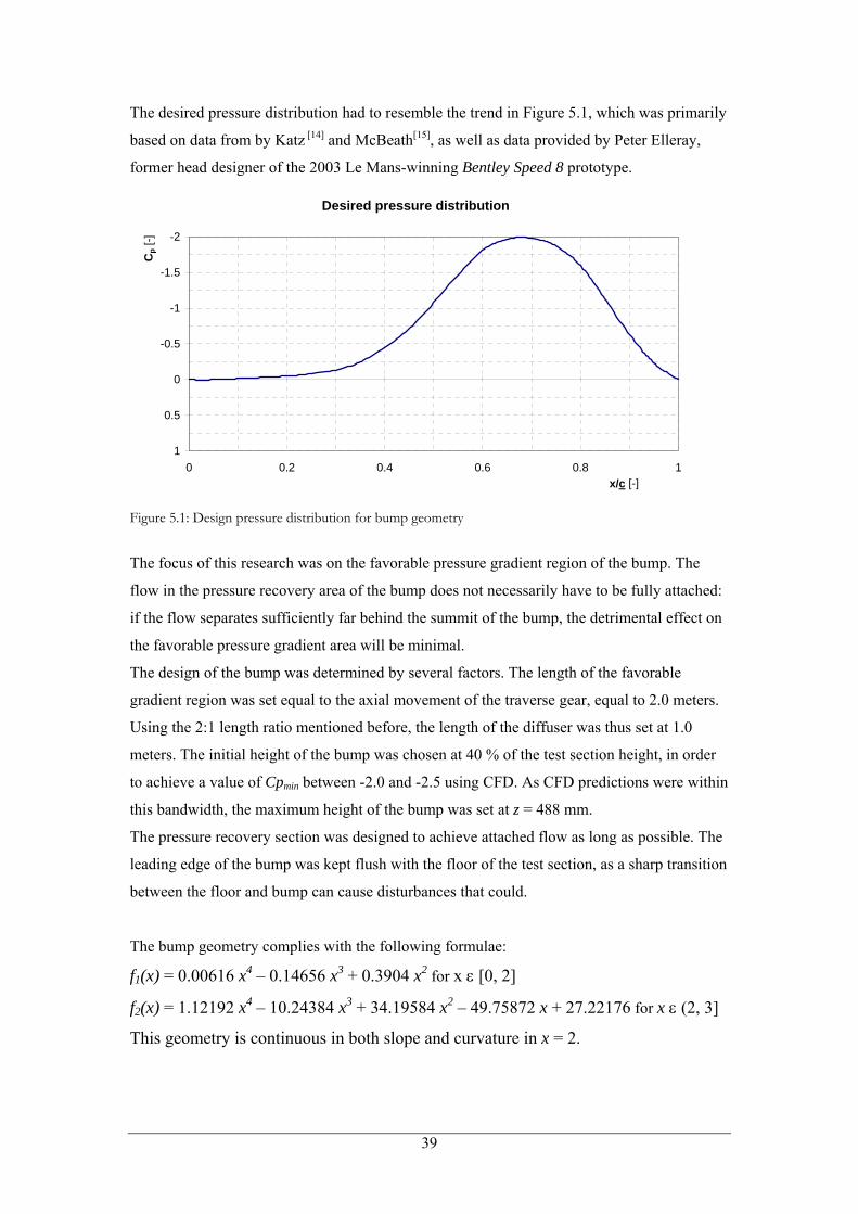
The desired pressure distribution had to resemble the trend in Figure 5.1, which was primarily
based on data from by Katz [14] and McBeath[15], as well as data provided by Peter Elleray,
former head designer of the 2003 Le Mans-winning Bentley Speed 8 prototype.
Desired pressure distribution
-2
-1.5
-1
-0.5
0
0.5
10 0.2 0.4 0.6 0.8
x/c1
[-]
Cp [
-]
Figure 5.1: Design pressure distribution for bump geometry
The focus of this research was on the favorable pressure gradient region of the bump. The
flow in the pressure recovery area of the bump does not necessarily have to be fully attached:
if the flow separates sufficiently far behind the summit of the bump, the detrimental effect on
the favorable pressure gradient area will be minimal.
The design of the bump was determined by several factors. The length of the favorable
gradient region was set equal to the axial movement of the traverse gear, equal to 2.0 meters.
Using the 2:1 length ratio mentioned before, the length of the diffuser was thus set at 1.0
meters. The initial height of the bump was chosen at 40 % of the test section height, in order
to achieve a value of Cpmin between -2.0 and -2.5 using CFD. As CFD predictions were within
this bandwidth, the maximum height of the bump was set at z = 488 mm.
The pressure recovery section was designed to achieve attached flow as long as possible. The
leading edge of the bump was kept flush with the floor of the test section, as a sharp transition
between the floor and bump can cause disturbances that could.
The bump geometry complies with the following formulae:
f1(x) = 0.00616 x4 – 0.14656 x3 + 0.3904 x2 for x ε [0, 2]
f2(x) = 1.12192 x4 – 10.24384 x3 + 34.19584 x2 – 49.75872 x + 27.22176 for x ε (2, 3]
This geometry is continuous in both slope and curvature in x = 2.
39
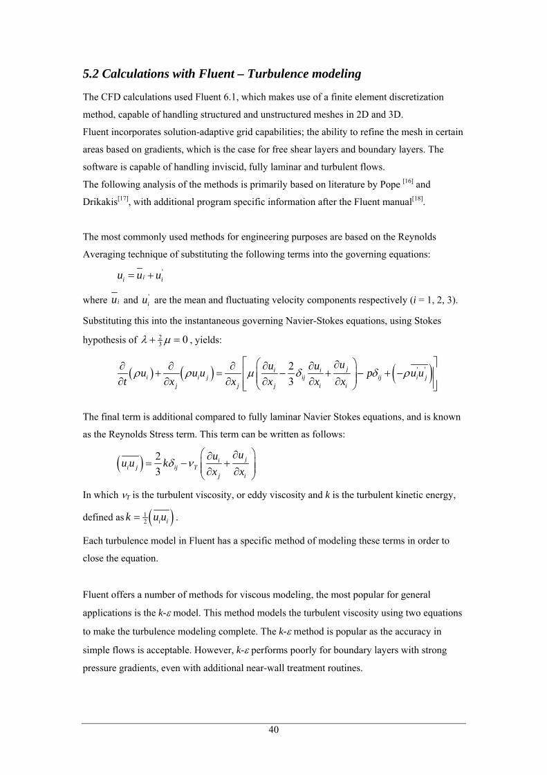
5.2 Calculations with Fluent – Turbulence modeling
The CFD calculations used Fluent 6.1, which makes use of a finite element discretization
method, capable of handling structured and unstructured meshes in 2D and 3D.
Fluent incorporates solution-adaptive grid capabilities; the ability to refine the mesh in certain
areas based on gradients, which is the case for free shear layers and boundary layers. The
software is capable of handling inviscid, fully laminar and turbulent flows.
The following analysis of the methods is primarily based on literature by Pope [16] and
Drikakis[17], with additional program specific information after the Fluent manual[18].
The most commonly used methods for engineering purposes are based on the Reynolds
Averaging technique of substituting the following terms into the governing equations: '
ii iu u u= +
where iu and are the mean and fluctuating velocity components respectively (i = 1, 2, 3). 'iu
Substituting this into the instantaneous governing Navier-Stokes equations, using Stokes
hypothesis of 23 0λ µ+ = , yields:
( ) ( ) ( )' '23
ji ii i j ij ij i
j j j i i
uu uu u u p ut x x x x x
ρ ρ µ δ δ ρ ju⎡ ⎤⎛ ⎞∂∂ ∂∂ ∂ ∂
+ = − + − + −⎢ ⎥⎜ ⎟⎜ ⎟∂ ∂ ∂ ∂ ∂ ∂⎢ ⎥⎝ ⎠⎣ ⎦
The final term is additional compared to fully laminar Navier Stokes equations, and is known
as the Reynolds Stress term. This term can be written as follows:
( ) 23
jii j ij T
j i
uuu u kx x
δ ν⎛ ⎞∂∂
= − +⎜ ⎟⎜ ⎟∂ ∂⎝ ⎠
In which νT is the turbulent viscosity, or eddy viscosity and k is the turbulent kinetic energy,
defined as ( )12 i ik u u= .
Each turbulence model in Fluent has a specific method of modeling these terms in order to
close the equation.
Fluent offers a number of methods for viscous modeling, the most popular for general
applications is the k-ε model. This method models the turbulent viscosity using two equations
to make the turbulence modeling complete. The k-ε method is popular as the accuracy in
simple flows is acceptable. However, k-ε performs poorly for boundary layers with strong
pressure gradients, even with additional near-wall treatment routines.
40
The second-most-popular two-equation turbulent viscosity model is the k-ω model. This
model offers improved performance for boundary layer flows under strong pressure gradients,
making it a superior method to k-ε for many flows. However, non-turbulent free-stream
boundaries are problematic for the k-ω method, which lead to the development of the k-ω
Shear Stress Transport (SST) model, blending the accurate near-wall region formulation of
the k-ω method and the free-stream independence of k-ε. The k-ω SST method is thus more
accurate and reliable for a wider range of applications than the k-ω and k-ε methods, whilst
still using two equations to make the turbulent viscosity modeling complete.
The Spalart-Allmaras method represents a different, more practical approach to turbulence
modeling. Whereas the trend in turbulence modeling development is aimed towards increased
accuracy, involving more equations to represent the eddy viscosity, Spalart-Allmaras uses one
equation to complete the turbulence model, developed for improving costs and ease of use
rather than improving accuracy. The Spalart-Allmaras model was designed specifically for
aerospace applications involving wall-bounded flows. This method has proven to provide
good, reliable results for boundary layers subjected to adverse pressure gradients, making it a
valuable, practical tool for stall prediction, also due to its solution convergence behavior.
Accuracy in free flow situations is less than other methods however.
The previously mentioned methods all make use of the same Boussinesq principle. This
principle is based on the turbulent-viscosity hypothesis, presenting a proportional relation
between Reynolds Stress and the mean rate of strain, resulting in the turbulent viscosity
equation. The most elaborate method available in Fluent, the Reynolds Stress Method (RSM),
abandons this Boussinesq approach and instead solves transport equations for Reynolds
stresses, together with an additional equation for dissipation rate. This means an additional
four equations for a 2D simulation and seven additional equations for the 3D case. Comparing
this to the single Spalart-Allmaras equation and the two equations for the k-ε and k-ω methods
for both 2D and 3D, it comes as no surprise that the RSM method requires significantly more
resources and more iterations to reach a satisfactory solution.
All previously discussed methods rely on the Reynolds Averaging technique, where all
turbulent motions are modeled, holding for the entire range of eddy scales. The suitability and
accuracy of these RANS methods will be discussed in Section 5.6, as well as conclusions and
recommendations for CFD calculations.
41
The Spalart-Allmaras and k-ω SST models were the turbulence routines selected for the
following CFD analysis. The latter method was selected for its accuracy in pressure gradients
as well as free stream, combining the advantages of both the k-ε and k-ω routines. The
Spalart-Allmaras routine was selected for its robustness and short calculation times. Both
methods are currently popular for engineering purposes for these same reasons.
5.3 Fluent results for single bump flow
5.3.1 Fluent configuration
An initial three-dimensional simulation was done using Fluent. For flow separation evaluation,
the boundary layer has to be sufficiently densely meshed, with the boundary layer including a
minimum of 50 points in vertical direction. The general rule-of-thumb on boundary layer
mesh size tells that the element size on the boundary itself should be in the order of 10-4. For a
reliable 3D simulation of the test configuration, even without the SBVG modeled the
available computational resources on a standard engineering PC at Cranfield University was
not sufficient. A two-dimensional simulation, taking the vertical symmetry plane in the
middle of the test section, allows for a much more refined mesh, with reduced calculation
times and resource requirements, allowing it to run on a standard engineering PC.
Selecting a 2D simulation over a 3D simulation in this case without a vortex is a valid choice.
The flow in the center of the test section is less influenced by the boundary layers generated
on the sidewalls than those on the ceiling and floor of the tunnel, due to the 2:1 ratio between
section width and height. The boundary layers generated on the floor and ceiling of the tunnel
are of primary importance, due to the presence of the bump.
The mesh used for the 2D calculations is partially illustrated in Figure 5.2, as the actual mesh
extents 2 meters in front of the start of the bump, and extends 3 meters behind the end of the
bump. The figure shows a preliminary boundary layer shape, where the mesh is more refined
than in the outer region. This preliminary structured boundary layer mesh meets the
requirement of at least 50 points vertically in the boundary layer, with approximately 100
points. The mesh outside the boundary layer is unstructured.
Using the mesh-refining capabilities of Fluent based on the velocity gradient the mesh of the
boundary layers on both the ceiling and the floor surface was refined. This is because the
local boundary layer in favorable pressure gradient has a fuller profile than the laminar inlet
profile, resulting in larger gradients near the wall. Additionally the wall elements were refined
with the Y+/Y routine until a maximum value of Y+/Y = 30 was reached. These routines are
discussed in further detail in the Fluent manual.
42
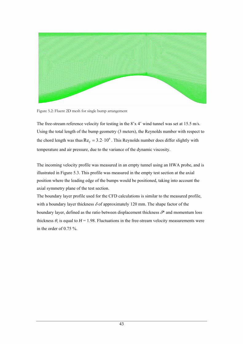
Figure 5.2: Fluent 2D mesh for single bump arrangement
The free-stream reference velocity for testing in the 8’x 4’ wind tunnel was set at 15.5 m/s.
Using the total length of the bump geometry (3 meters), the Reynolds number with respect to
the chord length was thus 6Re 3.2 10c = ⋅ . This Reynolds number does differ slightly with
temperature and air pressure, due to the variance of the dynamic viscosity.
The incoming velocity profile was measured in an empty tunnel using an HWA probe, and is
illustrated in Figure 5.3. This profile was measured in the empty test section at the axial
position where the leading edge of the bumps would be positioned, taking into account the
axial symmetry plane of the test section.
The boundary layer profile used for the CFD calculations is similar to the measured profile,
with a boundary layer thickness δ of approximately 120 mm. The shape factor of the
boundary layer, defined as the ratio between displacement thickness δ* and momentum loss
thickness θ, is equal to H = 1.98. Fluctuations in the free-stream velocity measurements were
in the order of 0.75 %.
43
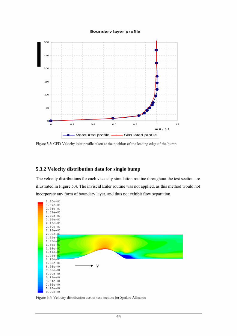
Boundary layer profile
0
50
100
150
200
250
300
0 0.2 0.4 0.6 0.8 1 1.2
u/ U 0 [ - ]
Measured profile Simulated profile
Figure 5.3: CFD Velocity inlet profile taken at the position of the leading edge of the bump
5.3.2 Velocity distribution data for single bump
The velocity distributions for each viscosity simulation routine throughout the test section are
illustrated in Figure 5.4. The inviscid Euler routine was not applied, as this method would not
incorporate any form of boundary layer, and thus not exhibit flow separation.
V
Figure 5.4: Velocity distribution across test section for Spalart-Allmaras
44
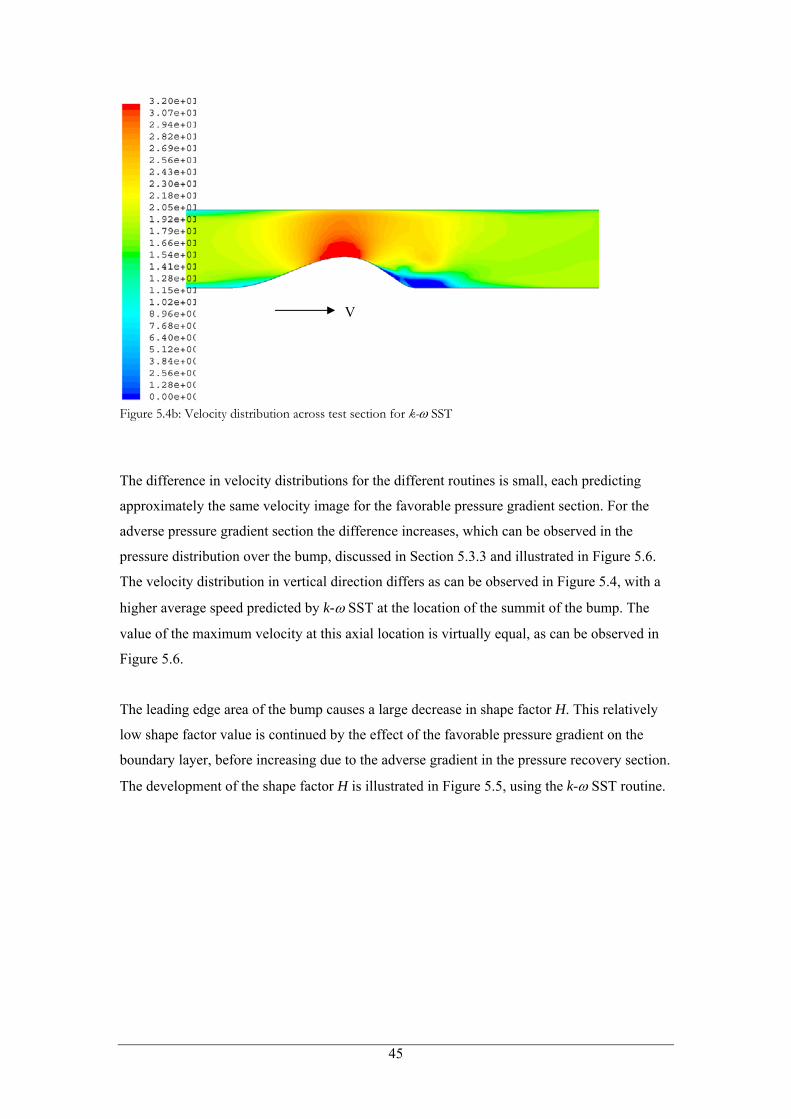
V
Figure 5.4b: Velocity distribution across test section for k-ω SST
The difference in velocity distributions for the different routines is small, each predicting
approximately the same velocity image for the favorable pressure gradient section. For the
adverse pressure gradient section the difference increases, which can be observed in the
pressure distribution over the bump, discussed in Section 5.3.3 and illustrated in Figure 5.6.
The velocity distribution in vertical direction differs as can be observed in Figure 5.4, with a
higher average speed predicted by k-ω SST at the location of the summit of the bump. The
value of the maximum velocity at this axial location is virtually equal, as can be observed in
Figure 5.6.
The leading edge area of the bump causes a large decrease in shape factor H. This relatively
low shape factor value is continued by the effect of the favorable pressure gradient on the
boundary layer, before increasing due to the adverse gradient in the pressure recovery section.
The development of the shape factor H is illustrated in Figure 5.5, using the k-ω SST routine.
45
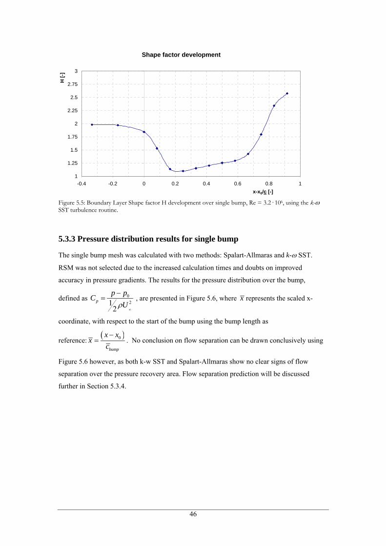
Shape factor development
1
1.25
1.5
1.75
2
2.25
2.5
2.75
3
-0.4 -0.2 0 0.2 0.4 0.6 0.8 1x-x0/c [-]
H [-
]
Figure 5.5: Boundary Layer Shape factor H development over single bump, Re = 3.2· 106, using the k-ω SST turbulence routine.
5.3.3 Pressure distribution results for single bump
The single bump mesh was calculated with two methods: Spalart-Allmaras and k-ω SST.
RSM was not selected due to the increased calculation times and doubts on improved
accuracy in pressure gradients. The results for the pressure distribution over the bump,
defined as 021
2p
p pCUρ
∞
−= , are presented in Figure 5.6, where x represents the scaled x-
coordinate, with respect to the start of the bump using the bump length as
reference:( )0
bump
x xx
c−
= . No conclusion on flow separation can be drawn conclusively using
Figure 5.6 however, as both k-w SST and Spalart-Allmaras show no clear signs of flow
separation over the pressure recovery area. Flow separation prediction will be discussed
further in Section 5.3.4.
46
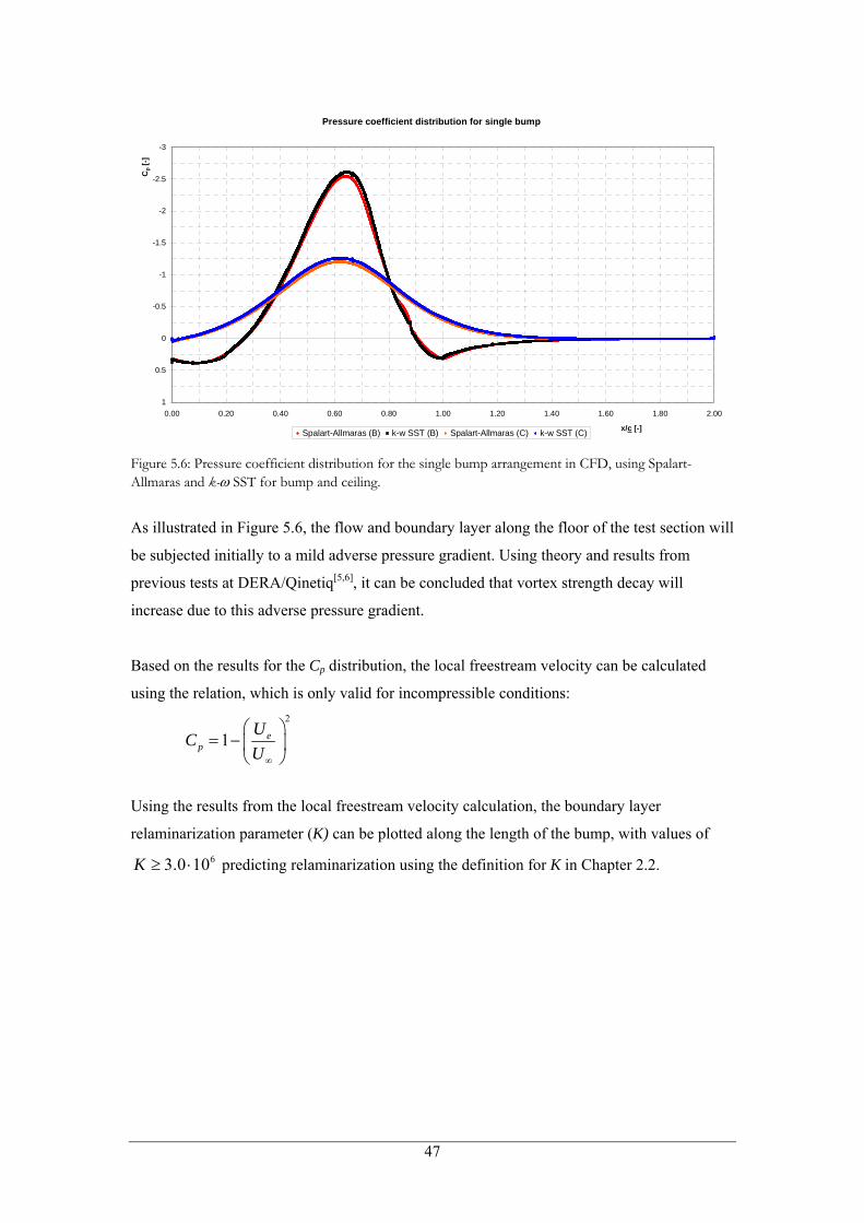
Pressure coefficient distribution for single bump
-3
-2.5
-2
-1.5
-1
-0.5
0
0.5
10.00 0.20 0.40 0.60 0.80 1.00 1.20 1.40 1.60 1.80 2.00
x/c [-]
Cp [
-]
Spalart-Allmaras (B) k-w SST (B) Spalart-Allmaras (C) k-w SST (C) Figure 5.6: Pressure coefficient distribution for the single bump arrangement in CFD, using Spalart-Allmaras and k-ω SST for bump and ceiling.
As illustrated in Figure 5.6, the flow and boundary layer along the floor of the test section will
be subjected initially to a mild adverse pressure gradient. Using theory and results from
previous tests at DERA/Qinetiq[5,6], it can be concluded that vortex strength decay will
increase due to this adverse pressure gradient.
Based on the results for the Cp distribution, the local freestream velocity can be calculated
using the relation, which is only valid for incompressible conditions: 2
1 ep
UCU∞
⎛ ⎞= − ⎜ ⎟
⎝ ⎠
Using the results from the local freestream velocity calculation, the boundary layer
relaminarization parameter (K) can be plotted along the length of the bump, with values of
predicting relaminarization using the definition for K in Chapter 2.2. 63.0 10K ≥ ⋅
47
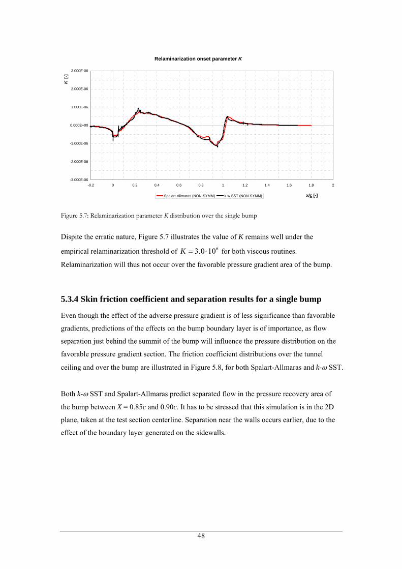
Relaminarization onset parameter K
-3.000E-06
-2.000E-06
-1.000E-06
0.000E+00
1.000E-06
2.000E-06
3.000E-06
-0.2 0 0.2 0.4 0.6 0.8 1 1.2 1.4 1.6 1.8 2
x/c [-]
K [-
]
Spalart-Allmaras (NON-SYMM) k-w SST (NON-SYMM)
Figure 5.7: Relaminarization parameter K distribution over the single bump
Dispite the erratic nature, Figure 5.7 illustrates the value of K remains well under the
empirical relaminarization threshold of 63.0 10K = ⋅ for both viscous routines.
Relaminarization will thus not occur over the favorable pressure gradient area of the bump.
5.3.4 Skin friction coefficient and separation results for a single bump
Even though the effect of the adverse pressure gradient is of less significance than favorable
gradients, predictions of the effects on the bump boundary layer is of importance, as flow
separation just behind the summit of the bump will influence the pressure distribution on the
favorable pressure gradient section. The friction coefficient distributions over the tunnel
ceiling and over the bump are illustrated in Figure 5.8, for both Spalart-Allmaras and k-ω SST.
Both k-ω SST and Spalart-Allmaras predict separated flow in the pressure recovery area of
the bump between X = 0.85c and 0.90c. It has to be stressed that this simulation is in the 2D
plane, taken at the test section centerline. Separation near the walls occurs earlier, due to the
effect of the boundary layer generated on the sidewalls.
48
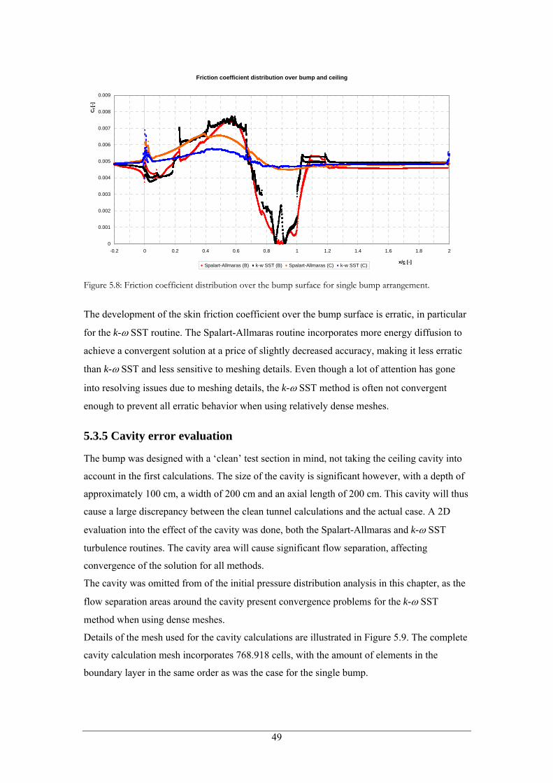
Friction coefficient distribution over bump and ceiling
0
0.001
0.002
0.003
0.004
0.005
0.006
0.007
0.008
0.009
-0.2 0 0.2 0.4 0.6 0.8 1 1.2 1.4 1.6 1.8 2
x/c [-]
Cf [
-]
Spalart-Allmaras (B) k-w SST (B) Spalart-Allmaras (C) k-w SST (C)
Figure 5.8: Friction coefficient distribution over the bump surface for single bump arrangement.
The development of the skin friction coefficient over the bump surface is erratic, in particular
for the k-ω SST routine. The Spalart-Allmaras routine incorporates more energy diffusion to
achieve a convergent solution at a price of slightly decreased accuracy, making it less erratic
than k-ω SST and less sensitive to meshing details. Even though a lot of attention has gone
into resolving issues due to meshing details, the k-ω SST method is often not convergent
enough to prevent all erratic behavior when using relatively dense meshes.
5.3.5 Cavity error evaluation
The bump was designed with a ‘clean’ test section in mind, not taking the ceiling cavity into
account in the first calculations. The size of the cavity is significant however, with a depth of
approximately 100 cm, a width of 200 cm and an axial length of 200 cm. This cavity will thus
cause a large discrepancy between the clean tunnel calculations and the actual case. A 2D
evaluation into the effect of the cavity was done, both the Spalart-Allmaras and k-ω SST
turbulence routines. The cavity area will cause significant flow separation, affecting
convergence of the solution for all methods.
The cavity was omitted from of the initial pressure distribution analysis in this chapter, as the
flow separation areas around the cavity present convergence problems for the k-ω SST
method when using dense meshes.
Details of the mesh used for the cavity calculations are illustrated in Figure 5.9. The complete
cavity calculation mesh incorporates 768.918 cells, with the amount of elements in the
boundary layer in the same order as was the case for the single bump.
49
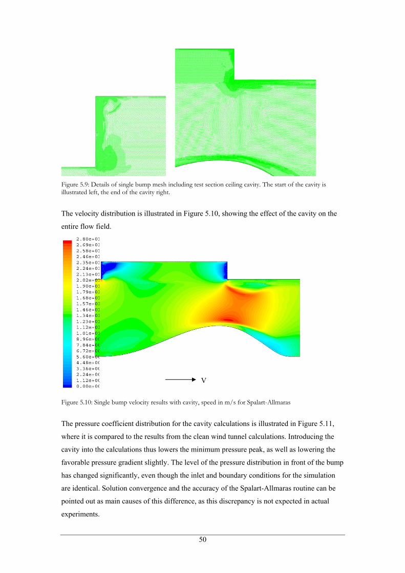
Figure 5.9: Details of single bump mesh including test section ceiling cavity. The start of the cavity is illustrated left, the end of the cavity right.
The velocity distribution is illustrated in Figure 5.10, showing the effect of the cavity on the
entire flow field.
V
Figure 5.10: Single bump velocity results with cavity, speed in m/s for Spalart-Allmaras
The pressure coefficient distribution for the cavity calculations is illustrated in Figure 5.11,
where it is compared to the results from the clean wind tunnel calculations. Introducing the
cavity into the calculations thus lowers the minimum pressure peak, as well as lowering the
favorable pressure gradient slightly. The level of the pressure distribution in front of the bump
has changed significantly, even though the inlet and boundary conditions for the simulation
are identical. Solution convergence and the accuracy of the Spalart-Allmaras routine can be
pointed out as main causes of this difference, as this discrepancy is not expected in actual
experiments.
50
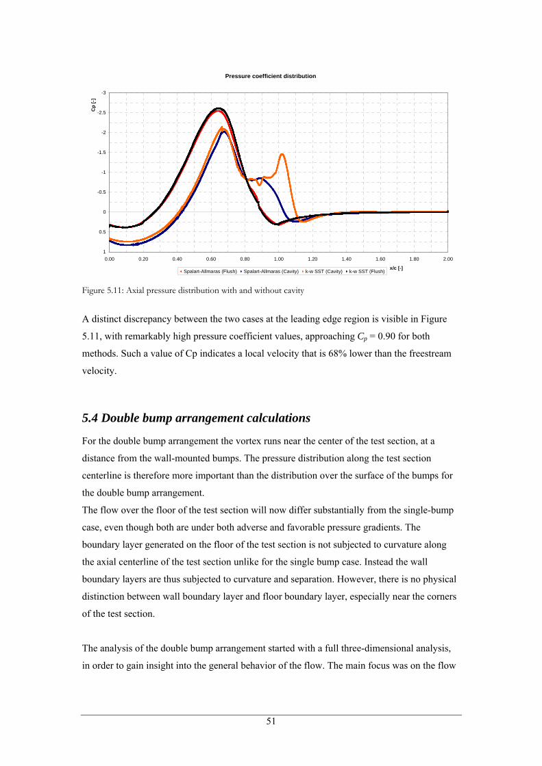
Pressure coefficient distribution
-3
-2.5
-2
-1.5
-1
-0.5
0
0.5
10.00 0.20 0.40 0.60 0.80 1.00 1.20 1.40 1.60 1.80 2.00
x/c [-]
Cp
[-]
Spalart-Allmaras (Flush) Spalart-Allmaras (Cavity) k-w SST (Cavity) k-w SST (Flush) Figure 5.11: Axial pressure distribution with and without cavity
A distinct discrepancy between the two cases at the leading edge region is visible in Figure
5.11, with remarkably high pressure coefficient values, approaching Cp = 0.90 for both
methods. Such a value of Cp indicates a local velocity that is 68% lower than the freestream
velocity.
5.4 Double bump arrangement calculations
For the double bump arrangement the vortex runs near the center of the test section, at a
distance from the wall-mounted bumps. The pressure distribution along the test section
centerline is therefore more important than the distribution over the surface of the bumps for
the double bump arrangement.
The flow over the floor of the test section will now differ substantially from the single-bump
case, even though both are under both adverse and favorable pressure gradients. The
boundary layer generated on the floor of the test section is not subjected to curvature along
the axial centerline of the test section unlike for the single bump case. Instead the wall
boundary layers are thus subjected to curvature and separation. However, there is no physical
distinction between wall boundary layer and floor boundary layer, especially near the corners
of the test section.
The analysis of the double bump arrangement started with a full three-dimensional analysis,
in order to gain insight into the general behavior of the flow. The main focus was on the flow
51
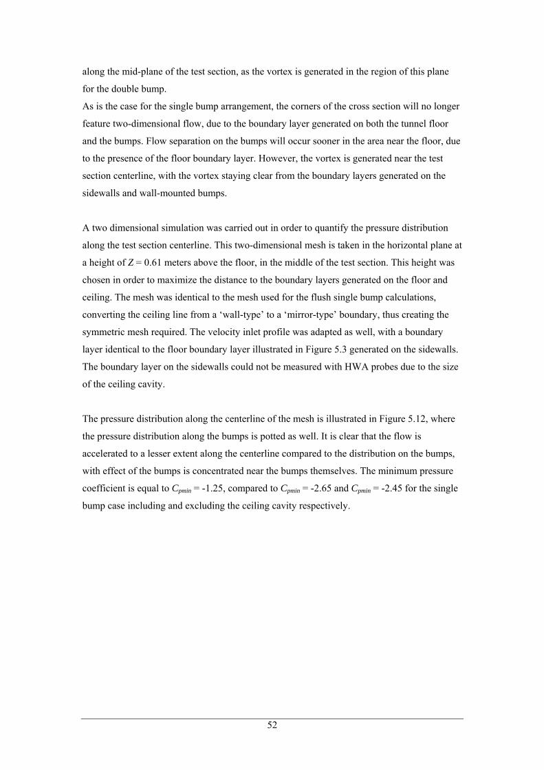
along the mid-plane of the test section, as the vortex is generated in the region of this plane
for the double bump.
As is the case for the single bump arrangement, the corners of the cross section will no longer
feature two-dimensional flow, due to the boundary layer generated on both the tunnel floor
and the bumps. Flow separation on the bumps will occur sooner in the area near the floor, due
to the presence of the floor boundary layer. However, the vortex is generated near the test
section centerline, with the vortex staying clear from the boundary layers generated on the
sidewalls and wall-mounted bumps.
A two dimensional simulation was carried out in order to quantify the pressure distribution
along the test section centerline. This two-dimensional mesh is taken in the horizontal plane at
a height of Z = 0.61 meters above the floor, in the middle of the test section. This height was
chosen in order to maximize the distance to the boundary layers generated on the floor and
ceiling. The mesh was identical to the mesh used for the flush single bump calculations,
converting the ceiling line from a ‘wall-type’ to a ‘mirror-type’ boundary, thus creating the
symmetric mesh required. The velocity inlet profile was adapted as well, with a boundary
layer identical to the floor boundary layer illustrated in Figure 5.3 generated on the sidewalls.
The boundary layer on the sidewalls could not be measured with HWA probes due to the size
of the ceiling cavity.
The pressure distribution along the centerline of the mesh is illustrated in Figure 5.12, where
the pressure distribution along the bumps is potted as well. It is clear that the flow is
accelerated to a lesser extent along the centerline compared to the distribution on the bumps,
with effect of the bumps is concentrated near the bumps themselves. The minimum pressure
coefficient is equal to Cpmin = -1.25, compared to Cpmin = -2.65 and Cpmin = -2.45 for the single
bump case including and excluding the ceiling cavity respectively.
52
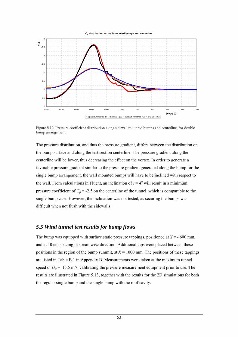
Cp distribution on wall-mounted bumps and centerline
-3
-2.5
-2
-1.5
-1
-0.5
0
0.5
10.00 0.20 0.40 0.60 0.80 1.00 1.20 1.40 1.60 1.80 2.00
(x-x0)/c [-]
Cp [
-]
Spalart-Allmaras (B) k-w SST (B) Spalart-Allmaras (C) k-w SST (C)
Figure 5.12: Pressure coefficient distribution along sidewall mounted bumps and centerline, for double bump arrangement
The pressure distribution, and thus the pressure gradient, differs between the distribution on
the bump surface and along the test section centerline. The pressure gradient along the
centerline will be lower, thus decreasing the effect on the vortex. In order to generate a
favorable pressure gradient similar to the pressure gradient generated along the bump for the
single bump arrangement, the wall mounted bumps will have to be inclined with respect to
the wall. From calculations in Fluent, an inclination of ι = 4o will result in a minimum
pressure coefficient of Cp = -2.5 on the centerline of the tunnel, which is comparable to the
single bump case. However, the inclination was not tested, as securing the bumps was
difficult when not flush with the sidewalls.
5.5 Wind tunnel test results for bump flows
The bump was equipped with surface static pressure tappings, positioned at Y = - 600 mm,
and at 10 cm spacing in streamwise direction. Additional taps were placed between these
positions in the region of the bump summit, at X = 1000 mm. The positions of these tappings
are listed in Table B.1 in Appendix B. Measurements were taken at the maximum tunnel
speed of U0 = 15.5 m/s, calibrating the pressure measurement equipment prior to use. The
results are illustrated in Figure 5.13, together with the results for the 2D simulations for both
the regular single bump and the single bump with the roof cavity.
53
The maximum value of the measure favorable pressure gradient was 3406p x N∂ ∂ = − m ,
or ( ) 7.0pCx c
∂= −∂ .
Bump pressure distribution
-3
-2.5
-2
-1.5
-1
-0.5
0
0.5
10 0.2 0.4 0.6 0.8 1
x/c [-]
Cp
[-]
Calculated single bump (SA) Calculated single bump (kwSST) Measured single bump Calculated single bump + Cavity (SA)
Figure 5.13: Pressure distribution for single bump arrangement, measured and calculated for
5.6 Comparison and discussion
The results from the CFD calculations are of two-dimensional test arrangements, rather than
the full three-dimensional case. The results for the favorable pressure gradient show relatively
good correlation for the minimum pressure coefficient and the magnitude of the favorable
pressure gradient. However, the flow in the actual wind tunnel features distinct three-
dimensional flow effects; it is assumed that this is the primary reason for the discrepancy
between the measurements and the calculated flow. The good correlation between the
simulations and the actual pressure distribution has to be downplayed, as the three-
dimensional effects cause a span-wise variation of the pressure distribution over the bump. A
full 3D simulation would give more insight into the span-wise variation of the calculations.
Discrepancies are most visible in the pressure recovery area, where flow separation occurs.
Flow separation is a distinctly three-dimensional, unsteady phenomenon, which cannot be
taken into account by in the 2D simulations nor the pressure measurements, as the latter were
also taken at one lateral position.
54
The presence of the cavity changes flow pattern, with separated flow in the cavity. Even
though the effects of this separated flow will not strongly influence the flow over the bump
itself, the pressure distribution will differ from the closed-cavity arrangement. Due to the
separation in the cavity area, solution convergence for all methods is poor as well, especially
for the two-equation methods like k-ω SST.
An additional explanation for the discrepancy between pressure measurements and the 2D
simulation results is the use of Reynolds-Averaging Navier Stokes routines. Turbulent flows
are characterized by eddy vortices with a wide range of length and time scales. The eddy
vortices with the smallest scale are responsible for the dissipation of turbulent kinetic energy,
whereas the largest eddies are typically of the same size as the characteristic length of the
mean flow. The Reynolds-Averaging Navier Stokes methods model all turbulent motions,
resulting is relatively low computational resources.
The level of energy diffusion incorporated into each viscous routine differs, the accuracy of
the solution depending on the scheme used. Commercial packages like Fluent incorporate
conservative schemes with overestimated energy diffusion in order to obtain convergent
solutions, thus sacrificing on accuracy. Spalart-Allmaras delivers good results for
convergence due to the highly diffusive scheme, but is less accurate than less convergent
routines like k-ω SST, which incorporates less energy diffusion.
A further drawback of the full turbulent motion modeling is the fact that large flow structures
are also taken into account by both the modeling and the numeric mesh.
With more computational resources a three-dimensional calculation can be carried out, using
more accurate methods like Large Eddy Simulation or Direct Numerical Simulations, which
will both be discussed in Chapter 7.
55
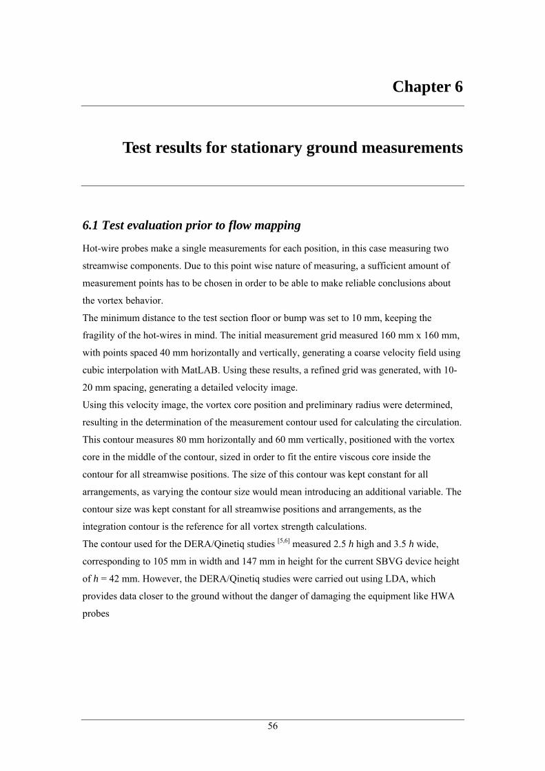
Chapter 6
Test results for stationary ground measurements
6.1 Test evaluation prior to flow mapping
Hot-wire probes make a single measurements for each position, in this case measuring two
streamwise components. Due to this point wise nature of measuring, a sufficient amount of
measurement points has to be chosen in order to be able to make reliable conclusions about
the vortex behavior.
The minimum distance to the test section floor or bump was set to 10 mm, keeping the
fragility of the hot-wires in mind. The initial measurement grid measured 160 mm x 160 mm,
with points spaced 40 mm horizontally and vertically, generating a coarse velocity field using
cubic interpolation with MatLAB. Using these results, a refined grid was generated, with 10-
20 mm spacing, generating a detailed velocity image.
Using this velocity image, the vortex core position and preliminary radius were determined,
resulting in the determination of the measurement contour used for calculating the circulation.
This contour measures 80 mm horizontally and 60 mm vertically, positioned with the vortex
core in the middle of the contour, sized in order to fit the entire viscous core inside the
contour for all streamwise positions. The size of this contour was kept constant for all
arrangements, as varying the contour size would mean introducing an additional variable. The
contour size was kept constant for all streamwise positions and arrangements, as the
integration contour is the reference for all vortex strength calculations.
The contour used for the DERA/Qinetiq studies [5,6] measured 2.5 h high and 3.5 h wide,
corresponding to 105 mm in width and 147 mm in height for the current SBVG device height
of h = 42 mm. However, the DERA/Qinetiq studies were carried out using LDA, which
provides data closer to the ground without the danger of damaging the equipment like HWA
probes
56
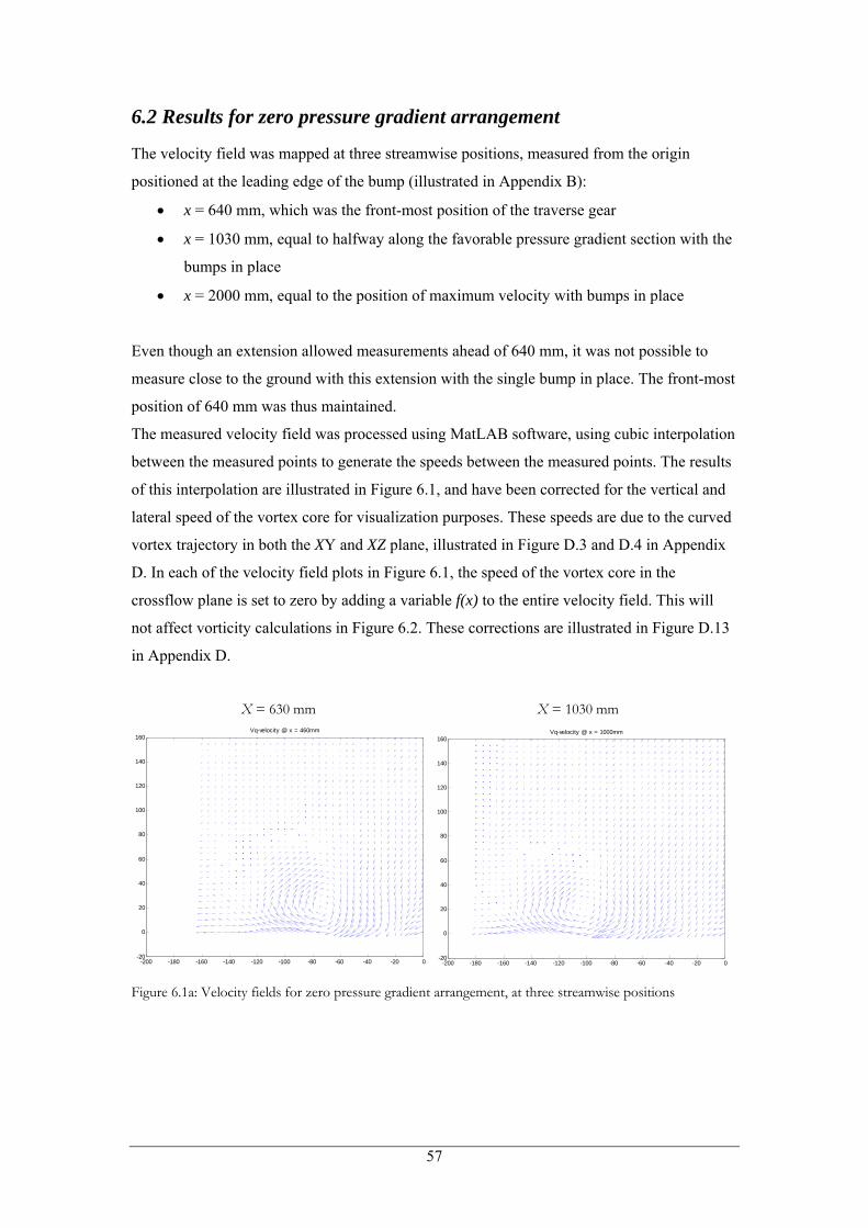
6.2 Results for zero pressure gradient arrangement
The velocity field was mapped at three streamwise positions, measured from the origin
positioned at the leading edge of the bump (illustrated in Appendix B):
• x = 640 mm, which was the front-most position of the traverse gear
• x = 1030 mm, equal to halfway along the favorable pressure gradient section with the
bumps in place
• x = 2000 mm, equal to the position of maximum velocity with bumps in place
Even though an extension allowed measurements ahead of 640 mm, it was not possible to
measure close to the ground with this extension with the single bump in place. The front-most
position of 640 mm was thus maintained.
The measured velocity field was processed using MatLAB software, using cubic interpolation
between the measured points to generate the speeds between the measured points. The results
of this interpolation are illustrated in Figure 6.1, and have been corrected for the vertical and
lateral speed of the vortex core for visualization purposes. These speeds are due to the curved
vortex trajectory in both the XY and XZ plane, illustrated in Figure D.3 and D.4 in Appendix
D. In each of the velocity field plots in Figure 6.1, the speed of the vortex core in the
crossflow plane is set to zero by adding a variable f(x) to the entire velocity field. This will
not affect vorticity calculations in Figure 6.2. These corrections are illustrated in Figure D.13
in Appendix D.
X = 630 mm X = 1030 mm
-200 -180 -160 -140 -120 -100 -80 -60 -40 -20 0-20
0
20
40
60
80
100
120
140
160Vq-velocity @ x = 460mm
-200 -180 -160 -140 -120 -100 -80 -60 -40 -20 0-20
0
20
40
60
80
100
120
140
160Vq-velocity @ x = 1000mm
Figure 6.1a: Velocity fields for zero pressure gradient arrangement, at three streamwise positions
57
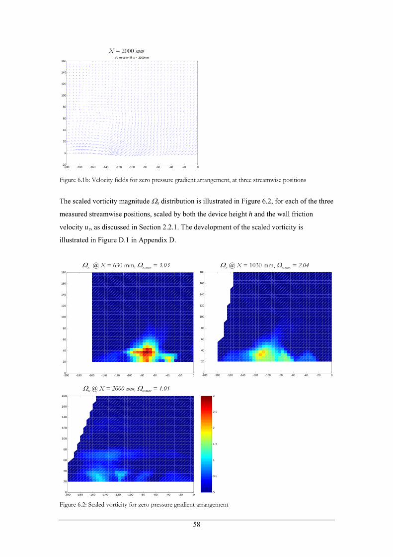
X = 2000 mm
-200 -180 -160 -140 -120 -100 -80 -60 -40 -20 0-20
0
20
40
60
80
100
120
140
160Vq-velocity @ x = 2000mm
Figure 6.1b: Velocity fields for zero pressure gradient arrangement, at three streamwise positions
The scaled vorticity magnitude Ωx distribution is illustrated in Figure 6.2, for each of the three
measured streamwise positions, scaled by both the device height h and the wall friction
velocity uτ, as discussed in Section 2.2.1. The development of the scaled vorticity is
illustrated in Figure D.1 in Appendix D.
Ωx @ X = 630 mm, Ωx,max = 3.03 Ωx @ X = 1030 mm, Ωx,max = 2.04
-200 -180 -160 -140 -120 -100 -80 -60 -40 -20 00
20
40
60
80
100
120
140
160
180
-200 -180 -160 -140 -120 -100 -80 -60 -40 -20 00
20
40
60
80
100
120
140
160
180
Ωx @ X = 2000 mm, Ωx,max = 1.01
-200 -180 -160 -140 -120 -100 -80 -60 -40 -20 00
20
40
60
80
100
120
140
160
180
0
0.5
1
1.5
2
2.5
3
Figure 6.2: Scaled vorticity for zero pressure gradient arrangement
58
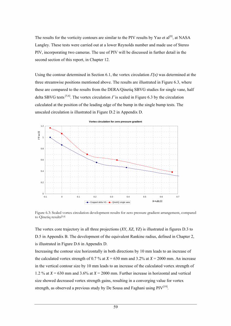
The results for the vorticity contours are similar to the PIV results by Yao et al[8], at NASA
Langley. These tests were carried out at a lower Reynolds number and made use of Stereo
PIV, incorporating two cameras. The use of PIV will be discussed in further detail in the
second section of this report, in Chapter 12.
Using the contour determined in Section 6.1, the vortex circulation Γ(x) was determined at the
three streamwise positions mentioned above. The results are illustrated in Figure 6.3, where
these are compared to the results from the DERA/Qinetiq SBVG studies for single vane, half
delta SBVG tests [5,6]. The vortex circulation Γ is scaled in Figure 6.3 by the circulation
calculated at the position of the leading edge of the bump in the single bump tests. The
unscaled circulation is illustrated in Figure D.2 in Appendix D.
Vortex circulation for zero pressure gradient
0
0.2
0.4
0.6
0.8
1
1.2
-0.1 0 0.1 0.2 0.3 0.4 0.5 0.6 0.7
(x-x0)/c [-]
Γ/ Γ
460
[-]
Cropped delta VG QinetiQ single vane
Figure 6.3: Scaled vortex circulation development results for zero pressure gradient arrangement, compared to Qinetiq results[5,6]
The vortex core trajectory in all three projections (XY, XZ, YZ) is illustrated in figures D.3 to
D.5 in Appendix B. The development of the equivalent Rankine radius, defined in Chapter 2,
is illustrated in Figure D.6 in Appendix D.
Increasing the contour size horizontally in both directions by 10 mm leads to an increase of
the calculated vortex strength of 0.7 % at X = 630 mm and 3.2% at X = 2000 mm. An increase
in the vertical contour size by 10 mm leads to an increase of the calculated vortex strength of
1.2 % at X = 630 mm and 3.6% at X = 2000 mm. Further increase in horizontal and vertical
size showed decreased vortex strength gains, resulting in a converging value for vortex
strength, as observed a previous study by De Sousa and Faghani using PIV[19].
59
Vertical size increase in both directions was not possible, as the measurements were taken up
to 10 mm above the tunnel floor. A larger vertical contour size would thus not have been
possible without endangering the probes.
The standard deviations of the V and W component measurements are illustrated in figures
D.7 and D.8 in Appendix D. These figures clearly illustrate that the deviation is highest
around the position of the viscous vortex core. This is explained by the fact that a vortex is a
far from steady phenomenon; vortex will wander in the cross-flow plane. This vortex
wandering can be observed at each axial measurement position, the magnitude of the
wandering increasing significantly as the distance to the vortex generator increases, which is
to be expected. Vortex wandering will thus cause measurement errors, as the measured speed
is averaged over the measurement time of 4.0 seconds per component at a sampling rate of
4000 Hz.
The dynamic pressure was monitored using the wind tunnel contraction static rings, providing
more reliable results compared to a pitot-static tube. The sampling frequency for the dynamic
pressure was 2000 Hz, with a sampling time of 4 seconds.
6.3 Results for single, floor-mounted bump arrangement
The measurements for the single bump were taken at four streamwise positions; at X = 630,
830, 1030 and 2000 mm downstream of the leading edge of the bump. The absolute minimum
distance to the bump/tunnel floor was fixed at Z = 10 mm to prevent probe failure.
Measurement times and sampling rates remained unchanged compared to the zero pressure
gradient case.
The measured velocity profiles are illustrated in Figure 6.4 for the four measured positions.
The velocity fields in Figure 6.4 have been corrected for both the vortex path and the fact that
the vortex is not aligned with the probe components at all time. The latter correction was
carried out by assuming that the vortex would remain aligned with the bump surface, using
the bump surface inclination at each of the measured positions. Both corrections are
illustrated in Figure D.13 in Appendix D.
The vertical axis in Figure 6.4 represents the distance to the local bump surface, rather than
the absolute distance to the test section floor.
The standard deviation for each measurement position is illustrated in figures D.9 - D.10 in
Appendix D.
60
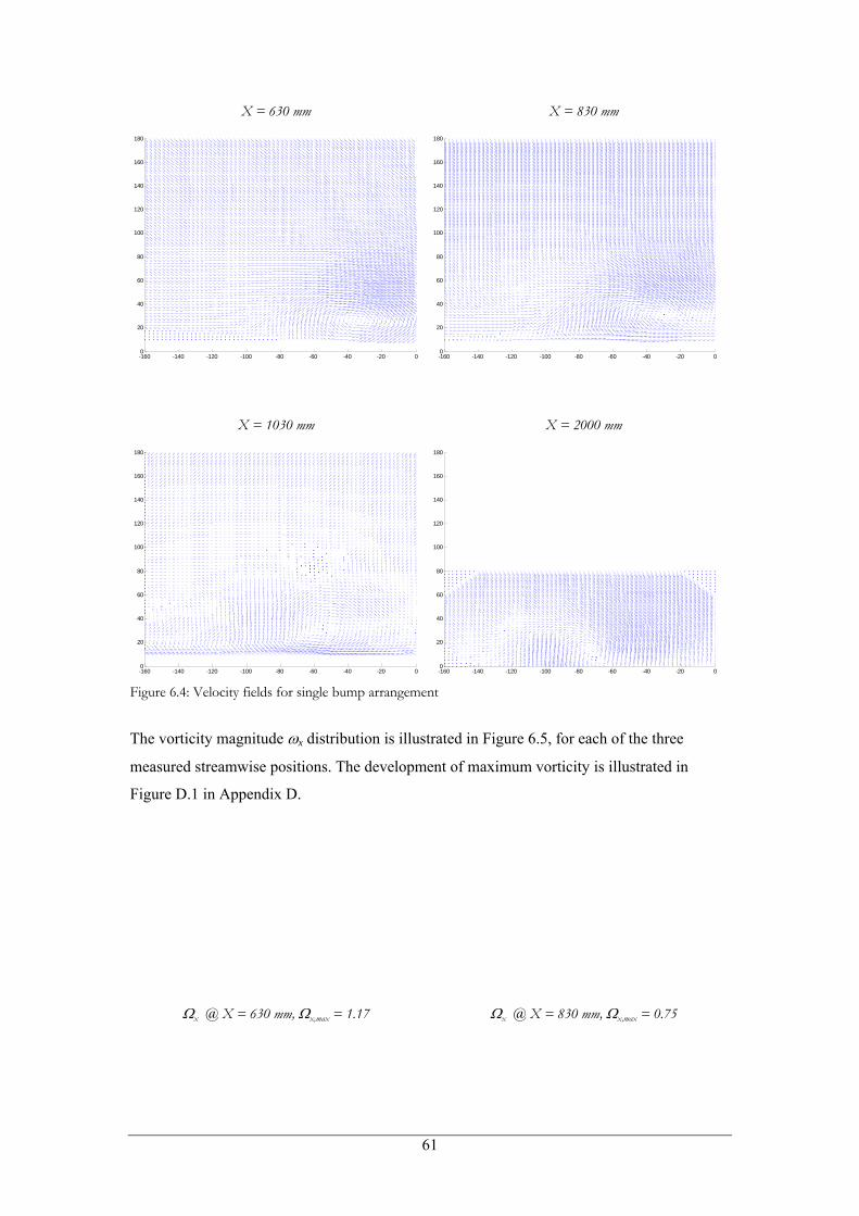
X = 630 mm X = 830 mm
-160 -140 -120 -100 -80 -60 -40 -20 00
20
40
60
80
100
120
140
160
180
-160 -140 -120 -100 -80 -60 -40 -20 00
20
40
60
80
100
120
140
160
180
X = 1030 mm X = 2000 mm
-160 -140 -120 -100 -80 -60 -40 -20 00
20
40
60
80
100
120
140
160
180
-160 -140 -120 -100 -80 -60 -40 -20 00
20
40
60
80
100
120
140
160
180
Figure 6.4: Velocity fields for single bump arrangement
The vorticity magnitude ωx distribution is illustrated in Figure 6.5, for each of the three
measured streamwise positions. The development of maximum vorticity is illustrated in
Figure D.1 in Appendix D.
Ωx @ X = 630 mm, Ωx,max = 1.17 Ωx @ X = 830 mm, Ωx,max = 0.75
61
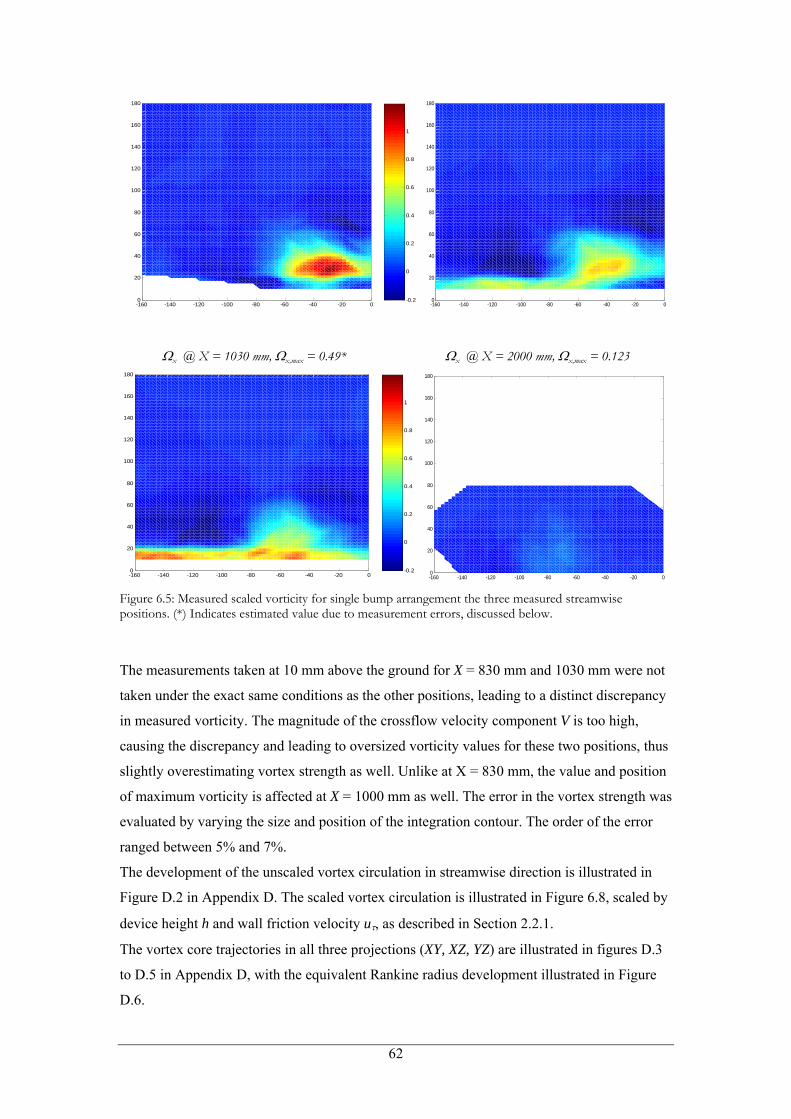
-160 -140 -120 -100 -80 -60 -40 -20 00
20
40
60
80
100
120
140
160
180
-0.2
0
0.2
0.4
0.6
0.8
1
-160 -140 -120 -100 -80 -60 -40 -20 00
20
40
60
80
100
120
140
160
180
Ωx @ X = 1030 mm, Ωx,max = 0.49* Ωx @ X = 2000 mm, Ωx,max = 0.123
-160 -140 -120 -100 -80 -60 -40 -20 00
20
40
60
80
100
120
140
160
180
-0.2
0
0.2
0.4
0.6
0.8
1
-160 -140 -120 -100 -80 -60 -40 -20 00
20
40
60
80
100
120
140
160
180
Figure 6.5: Measured scaled vorticity for single bump arrangement the three measured streamwise positions. (*) Indicates estimated value due to measurement errors, discussed below.
The measurements taken at 10 mm above the ground for X = 830 mm and 1030 mm were not
taken under the exact same conditions as the other positions, leading to a distinct discrepancy
in measured vorticity. The magnitude of the crossflow velocity component V is too high,
causing the discrepancy and leading to oversized vorticity values for these two positions, thus
slightly overestimating vortex strength as well. Unlike at X = 830 mm, the value and position
of maximum vorticity is affected at X = 1000 mm as well. The error in the vortex strength was
evaluated by varying the size and position of the integration contour. The order of the error
ranged between 5% and 7%.
The development of the unscaled vortex circulation in streamwise direction is illustrated in
Figure D.2 in Appendix D. The scaled vortex circulation is illustrated in Figure 6.8, scaled by
device height h and wall friction velocity uτ, as described in Section 2.2.1.
The vortex core trajectories in all three projections (XY, XZ, YZ) are illustrated in figures D.3
to D.5 in Appendix D, with the equivalent Rankine radius development illustrated in Figure
D.6.
62
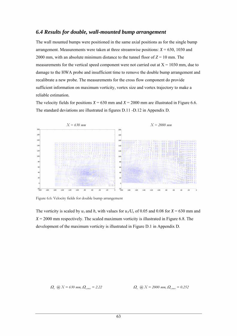
6.4 Results for double, wall-mounted bump arrangement
The wall mounted bumps were positioned in the same axial positions as for the single bump
arrangement. Measurements were taken at three streamwise positions: X = 630, 1030 and
2000 mm, with an absolute minimum distance to the tunnel floor of Z = 10 mm. The
measurements for the vertical speed component were not carried out at X = 1030 mm, due to
damage to the HWA probe and insufficient time to remove the double bump arrangement and
recalibrate a new probe. The measurements for the cross flow component do provide
sufficient information on maximum vorticity, vortex size and vortex trajectory to make a
reliable estimation.
The velocity fields for positions X = 630 mm and X = 2000 mm are illustrated in Figure 6.6.
The standard deviations are illustrated in figures D.11 -D.12 in Appendix D.
X = 630 mm X = 2000 mm
-200 -180 -160 -140 -120 -100 -80 -60 -40 -20 0-20
0
20
40
60
80
100
120
140
160
180
200
-200 -180 -160 -140 -120 -100 -80 -60 -40 -20 0-20
0
20
40
60
80
100
120
140
160
180
200
Figure 6.6: Velocity fields for double bump arrangement
The vorticity is scaled by uτ and h, with values for uτ/Ue of 0.05 and 0.08 for X = 630 mm and
X = 2000 mm respectively. The scaled maximum vorticity is illustrated in Figure 6.8. The
development of the maximum vorticity is illustrated in Figure D.1 in Appendix D.
Ωx @ X = 630 mm, Ωx,max = 2.22 Ωx @ X = 2000 mm, Ωx,max = 0.252
63
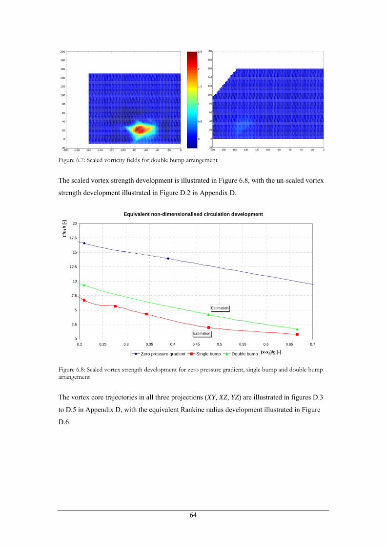
-200 -180 -160 -140 -120 -100 -80 -60 -40 -20 0-20
0
20
40
60
80
100
120
140
160
180
200
0
0.5
1
1.5
2
2.5
-200 -180 -160 -140 -120 -100 -80 -60 -40 -20 0-20
0
20
40
60
80
100
120
140
160
180
200
Figure 6.7: Scaled vorticity fields for double bump arrangement
The scaled vortex strength development is illustrated in Figure 6.8, with the un-scaled vortex
strength development illustrated in Figure D.2 in Appendix D.
Equivalent non-dimensionalised circulation development
Estimation
Estimation0
2.5
5
7.5
10
12.5
15
17.5
20
0.2 0.25 0.3 0.35 0.4 0.45 0.5 0.55 0.6 0.65 0.7
(x-x0)/c [-]
Γ/u τ
h [-]
Zero pressure gradient Single bump Double bump
Figure 6.8: Scaled vortex strength development for zero pressure gradient, single bump and double bump arrangement
The vortex core trajectories in all three projections (XY, XZ, YZ) are illustrated in figures D.3
to D.5 in Appendix D, with the equivalent Rankine radius development illustrated in Figure
D.6.
64
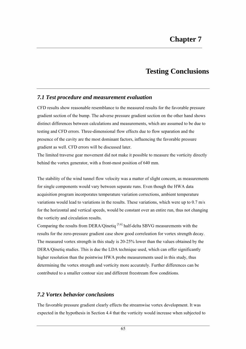
Chapter 7
Testing Conclusions
7.1 Test procedure and measurement evaluation
CFD results show reasonable resemblance to the measured results for the favorable pressure
gradient section of the bump. The adverse pressure gradient section on the other hand shows
distinct differences between calculations and measurements, which are assumed to be due to
testing and CFD errors. Three-dimensional flow effects due to flow separation and the
presence of the cavity are the most dominant factors, influencing the favorable pressure
gradient as well. CFD errors will be discussed later.
The limited traverse gear movement did not make it possible to measure the vorticity directly
behind the vortex generator, with a front-most position of 640 mm.
The stability of the wind tunnel flow velocity was a matter of slight concern, as measurements
for single components would vary between separate runs. Even though the HWA data
acquisition program incorporates temperature variation corrections, ambient temperature
variations would lead to variations in the results. These variations, which were up to 0.7 m/s
for the horizontal and vertical speeds, would be constant over an entire run, thus not changing
the vorticity and circulation results.
Comparing the results from DERA/Qinetiq [5,6] half-delta SBVG measurements with the
results for the zero-pressure gradient case show good correleation for vortex strength decay.
The measured vortex strength in this study is 20-25% lower than the values obtained by the
DERA/Qinetiq studies. This is due the LDA technique used, which can offer significantly
higher resolution than the pointwise HWA probe measurements used in this study, thus
determining the vortex strength and vorticity more accurately. Further differences can be
contributed to a smaller contour size and different freestream flow conditions.
7.2 Vortex behavior conclusions
The favorable pressure gradient clearly effects the streamwise vortex development. It was
expected in the hypothesis in Section 4.4 that the vorticity would increase when subjected to
65
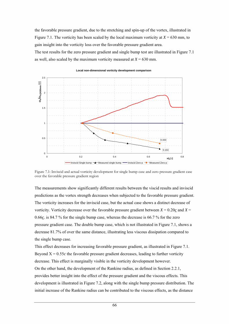
the favorable pressure gradient, due to the stretching and spin-up of the vortex, illustrated in
Figure 7.1. The vorticity has been scaled by the local maximum vorticity at X = 630 mm, to
gain insight into the vorticity loss over the favorable pressure gradient area.
The test results for the zero pressure gradient and single bump test are illustrated in Figure 7.1
as well, also scaled by the maximum vorticity measured at X = 630 mm.
Local non-dimensional vorticity development comparison
0.153
0.333
0
0.5
1
1.5
2
2.5
0 0.2 0.4 0.6 0.8x/c [-]
ωx/ ω
x@63
0mm
[-]
Inviscid Single bump Measured single bump Inviscid Zero-p Measured Zero-p
Figure 7.1: Inviscid and actual vorticity development for single bump case and zero pressure gradient case over the favorable pressure gradient region
The measurements show significantly different results between the viscid results and inviscid
predictions as the vortex strength decreases when subjected to the favorable pressure gradient.
The vorticity increases for the inviscid case, but the actual case shows a distinct decrease of
vorticity. Vorticity decrease over the favorable pressure gradient between X = 0.20c and X =
0.66c. is 84.7 % for the single bump case, whereas the decrease is 66.7 % for the zero
pressure gradient case. The double bump case, which is not illustrated in Figure 7.1, shows a
decrease 81.7% of over the same distance, illustrating less viscous dissipation compared to
the single bump case.
This effect decreases for increasing favorable pressure gradient, as illustrated in Figure 7.1.
Beyond X = 0.55c the favorable pressure gradient decreases, leading to further vorticity
decrease. This effect is marginally visible in the vorticity development however.
On the other hand, the development of the Rankine radius, as defined in Section 2.2.1,
provides better insight into the effect of the pressure gradient and the viscous effects. This
development is illustrated in Figure 7.2, along with the single bump pressure distribution. The
initial increase of the Rankine radius can be contributed to the viscous effects, as the distance
66
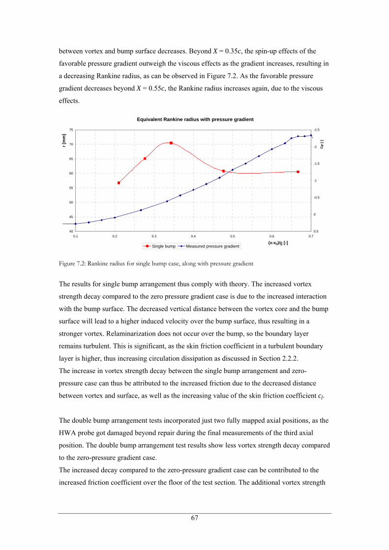
between vortex and bump surface decreases. Beyond X = 0.35c, the spin-up effects of the
favorable pressure gradient outweigh the viscous effects as the gradient increases, resulting in
a decreasing Rankine radius, as can be observed in Figure 7.2. As the favorable pressure
gradient decreases beyond X = 0.55c, the Rankine radius increases again, due to the viscous
effects.
Equivalent Rankine radius with pressure gradient
40
45
50
55
60
65
70
75
0.1 0.2 0.3 0.4 0.5 0.6 0.7
(x-x0)/c [-]
r [m
m]
-2.5
-2
-1.5
-1
-0.5
0
0.5
Cp
[-]
Single bump Measured pressure gradient
Figure 7.2: Rankine radius for single bump case, along with pressure gradient
The results for single bump arrangement thus comply with theory. The increased vortex
strength decay compared to the zero pressure gradient case is due to the increased interaction
with the bump surface. The decreased vertical distance between the vortex core and the bump
surface will lead to a higher induced velocity over the bump surface, thus resulting in a
stronger vortex. Relaminarization does not occur over the bump, so the boundary layer
remains turbulent. This is significant, as the skin friction coefficient in a turbulent boundary
layer is higher, thus increasing circulation dissipation as discussed in Section 2.2.2.
The increase in vortex strength decay between the single bump arrangement and zero-
pressure case can thus be attributed to the increased friction due to the decreased distance
between vortex and surface, as well as the increasing value of the skin friction coefficient cf.
The double bump arrangement tests incorporated just two fully mapped axial positions, as the
HWA probe got damaged beyond repair during the final measurements of the third axial
position. The double bump arrangement test results show less vortex strength decay compared
to the zero-pressure gradient case.
The increased decay compared to the zero-pressure gradient case can be contributed to the
increased friction coefficient over the floor of the test section. The additional vortex strength
67
decay between the single and double bump arrangement can be contributed to the decreased
distance between the vortex and surface for the single bump case.
However, the number of positions for the double bump arrangement is not sufficient to be
able to gain insight into the effect of the magnitude of the pressure gradient, unlike for the
single bump case. More axial positions will have to be measured for the double bump
arrangement.
The results for the single bump case on the other hand show plausible results for vortex
strength decay and Rankine radius. The increased interaction between the bump surface and
the boundary layer causes a decrease in vortex circulation, canceling the effects of the
stretching and spin-up due to the pressure gradient.
Even though each case will differ, it can be concluded that when a vortex is generated and/or
shed in close proximity to a body surface, the viscous effects can outweigh the spin-up effects
of a favorable pressure gradient. In the case of the single bump, the vortex strength decay due
to the interaction with the bump surface cancels out the increased vorticity due to the
favorable pressure gradient, leading to decreasing vorticity over the entire favorable pressure
gradient area.
7.3 Discussion and recommendations
7.3.1 Error and accuracy evaluation
In order to evaluate the accuracy of the results, all errors will have to be evaluated. These
errors range from tunnel speed variations and three-dimensional flow effects to the effect of
hot-wire probe measurements itself.
As mentioned in Chapter 4, HWA is an intrusive method that influences the flow. However,
previous studies show no definitive conclusion on probe intrusiveness, as different
applications, probes and test arrangements yield different results. Therefore in order to be able
to genuinely determine the effect of the hot-wires in a particular arrangement, non-intrusive
measurements will have to be taken of the hot-wire in the wind tunnel, using PIV. Even
though this would seem extravagant to use two measurement methods simultaneously, the
PIV measurements will be able to quantify the effect of the probes on the flow. This is
particularly important for hot-wire measurements of the viscous vortex core, as this area of
the vortex is the most sensitive area for disturbances.
The position of the vortex core is accurate up to 2-2.5 mm, which is equal to an error 3-5%
with respect to the local equivalent Ranking radius.
68
Time-dependent effects like vortex wandering are filtered out of the final results, due to
averaging of the measured signal. The raw measurement data from each point provides
insight into the variation of the signal, but cannot give insight into actual time-dependant
motions, as the independently measured points cannot be linked to each other. Laser
techniques like PIV can provide some insight into this behavior, as the entire flow field
picture is measured instantaneously, although only for low frequency phenomena.
7.3.2 Measurement Recommendations
The use of hot-wires for vortex measurements has a number of drawbacks. These include:
• Time averaged solution
• Flow intrusion
• Probe sensitivity
• Low resolution compared to laser measurements
• Temperature sensitivity
As discussed in Section 4.2, the viscous core is the most sensitive part of the vortex. Probe
intrusion into the core will cause destabilization, thus lower the local vorticity and circulation.
The measured vertical and crossflow components due to the vortex will thus be lower than the
actual components. This effect will decrease with a decreasing value of the probe
diameter/Rankine radius ratio, as the probe will relatively smaller compared to the viscous
vortex core.
Probe sensitivity covers both the probe fragility and temperature sensitivity, as temperature
fluctuations during and between runs have influence on the measurement results.
By increasing the number of points measured per streamwise position, the accuracy and
reliability of the vortex results increases, but so will measurement times. Not only will the
increased measurement times lead to higher costs, but the measurements will be subjected to
changing conditions over a longer period, as heat generated by the electromotor enters the test
section.
Using a laser based measurement system, like LDA or PIV, would allow for higher resolution
and significantly less intrusion into the flow, with decreased sensitivity to measurement
conditions. Resolution and accuracy of laser based measurement is discussed in chapter 12.
Even though the hot-wire data acquisition program incorporates temperature variation
corrections, temperature variations in the test section due to changeable weather caused
measurements to vary by up to 1.0 m/s across the entire array of measured points. In order to
minimize this effect, the latter half of the tests were carried out at night.
69
7.3.3 Simulation Recommendations
A full CFD simulation of the arrangement, including the vortex generator, was not carried out,
due to calculation times and doubts concerning the accuracy of the eventual solution using
Fluent. The computational resources were simply not sufficient to run a three-dimensional
mesh with sufficient density. However, with sufficient resources in a CFD-focused study,
vortex simulations can be carried out, using different, more fundamental techniques. As
mentioned in Chapter 5, the Reynolds Averaging technique uses turbulence models to model
all turbulent motions, irrespective of their scale. A large-scale turbulent motion can thus be
calculated twice in a RANS calculation, doubling the dissipation effects, increasing the error.
Additionally, commercial packages make use of highly dissipative discretization schemes, in
order to improve convergence and thus practicality, at the cost of a loss in accuracy. A study
into underbody vortices using CFD will thus require a different method than RANS in order
to produce more accurate results and conclusions. Two main methods are available: Direct
Numerical Simulation and Large Eddy Simulation.
Direct Numerical Simulation is an option for scientific purposes, incorporating full
discretization of both the large and the small eddies. Considering that the ratio between the
energy-containing large scales and the energy-dissipating small scale is proportional to
(after Pope3/ 4Returbulent[16]), the three-dimensional case is thus proportional to ,
illustrating the small mesh size needed for the smallest eddies at high Reynolds numbers. Vast
amounts of computational resources are thus required for DNS, ruling it out as an option for
engineering purposes, as the required resources and computational times are too great.
9 / 4Returbulent
Large Eddy Simulation provides a more practical alternative to DNS, whilst still representing
an improvement over RANS for turbulence modeling. The principle of LES lies in the fact
that nearly all of the computational effort in DNS is expended on solving the smallest,
dissipative eddies, whereas the energy is basically contained in the larger scales. LES thus
uses turbulence models for simulating the small eddy scales, whereas the large eddies are
directly resolved in the mesh, like in DNS. The minimum mesh sizes for LES calculations are
typically one order larger than for DNS, as the small eddies are modeled instead of discretized,
decreasing the computational resources required. The LES method is optional in Fluent 6.1,
but as with the RANS methods, the level of dissipation incorporated into this routine is
considerably higher than actual dissipation levels, for improved convergence.
70
7.3.4 Underbody application
Focusing on underbody applications, additional factors influencing vortex behavior like a
moving ground and ground proximity were not present in these measurements. These were
not included in order to simplify the test, thus limiting the different variables and influences
on vortex behavior.
With the results for the influence of a favorable pressure gradient on vortex behavior, the
additional aerodynamic underbody conditions can be included into a test arrangement. This
arrangement is the subject of the second section of this report.
71
Chapter 8
Formula 1 geometry and underbody aerodynamics
Formula 1 aerodynamics will be analyzed in this chapter. The complete aerodynamics of the
open-wheeled Formula 1 car is too complicated to analyze completely, but focus in this
section shall be on the elements and factors that interact and influence the underbody flow.
Section 8.2 will present an analysis of ground proximity aerodynamics, followed by an
analysis of the underbody conditions in Section 8.3.
8.1 Formula 1 geometry and aerodynamics
Predicting the exact flow behavior in the underbody region of a Formula 1 racecar is difficult,
due to the complicated geometry of the undertray and the complexity and vorticity of the
incoming flow.
In order to design a generic test arrangement suitable for scientific research into vortex
behavior in underbody flows, the actual underbody has to be simplified. In order to identify
the main influences and elements of the underbody flow, a general Formula 1 model is
examined in this section.
The modern Formula 1 car can be divided into the following main aerodynamic ‘components’:
- Front Wing
- Rear wing
- Wheels and suspension
- Bodywork
- Underbody
Their interaction with the underbody will be discussed in the following sections, using the
FIA technical regulations for the 2004 Formula 1 season[21].
72
8.1.1 Front wing
The front wing of a Formula 1 car is a multi-element high-lift wing, which runs in close
proximity to the ground, the minimum clearance set in the FIA regulations. As most of the car
runs in the wake of this front wing, the front wing design is constantly tuned in order to
achieve the best overall car performance. The front wing is designed to generate a range of
downforce levels, adjustable in a number of settings. The wake of this front wing influences
the underbody in particular. The underbody will thus have to cope with this same range of
wing settings, as each setting results in a different wake and thus different underbody inlet
conditions.
The front wing is highly influenced by the rotating front wheels, in particular when the front
wheels are under a steering angle, resulting in the creation of a vortices as air is squeezed
between the front wing endplates and the wheels.
Sophisticated front wing endplates, shaped in order to minimize wing tip and wheel effects,
also contributing to the generation of vortices. These are illustrated in figure E.3 in Appendix
E.
8.1.2 Rear wing
The multi-element, twin-tiered rear wing operates in the wake of the entire car, with both tiers
performing different functions. The top tier consists of a maximum of two airfoil elements,
and performs similar to a wing on an aircraft: the top tier generates downforce running in
relatively clean air. The bottom tier, consisting of two airfoil elements, is situated close to the
underbody exit: the diffuser. In addition to generating downforce the bottom tier serves as
augmentation of the diffuser, accelerating the flow through the diffuser. As a result, the entire
underbody flow is accelerated due to the suction from the lower tier, thus generating more
downforce from the entire underbody.
Even though the rear wing falls beyond the scope of this research, its influence on the
underbody flow is significant. The presence of the lower tier is causes additional acceleration,
thus causing a larger favorable pressure gradient
8.1.3 Wheels and suspension
The main elements responsible for making the flow around a Formula 1 car so complex are
the exposed, rotating wheels, producing 40% of the total drag of the car as well as generating
positive lift. Additionally, the rotating wheels cause strong cross flows when under a yaw
angle, generating vortices in the process. In addition to the rotating wheels, the front
suspension is another main source of vorticity for the incoming underbody flow, as well as
73
the protruding front wheel brake cooling ducts. The rear wheel suspension has less effect on
the underbody flow, as the suspension is positioned above the underbody exits.
8.1.4 Bodywork
The bodywork itself does not contribute as much to the total downforce level compared to the
wings and underbody. However, due to ever-tightening regulations governing these elements,
the search for increased performance has lead designers to use various ways to augment the
wings and underbody, as well as generating more downforce from the body using additional
elements. Augmenting the performance of the wings and underbody is done by channeling the
flow to optimize incoming flow conditions. Examples of such elements are turning vanes and
winglets, illustrated in Appendix E.
These elements are relatively inefficient in generating downforce compared to the underbody
and wings, but are valuable for improving the performance of the car within the ever-
tightening regulations. Practically all the bodywork and additional elements in front of the
underbody inlet influence the incoming underbody flow, as the underbody operates within the
wake of these elements. The most prominent influence on the incoming underbody flow
within this category are the front wing supports, required to provide as ‘clean’ as possible
flow for the front wing by raising the nose, and barge boards/turning vanes, channeling the
flow into specific regions of the body.
8.1.5 Underbody
The FIA rules clearly define the shape of the Formula 1 underbody: the underbody area must
extend from 330 mm behind the front wheel centerline to the centre line of the rear wheels
and must form a flat surface, known as the reference surface. The reference surface is to have
a minimum and maximum width of 300 mm and 500 mm respectively. Additionally, a step
plane has to be situated 50mm above reference plane, and has to form a flat surface between
330 mm behind the front wheel axle and 330 mm in front of the rear wheel axle.
Behind this reference and step plane, the underbody is allowed to incorporate a central
diffuser with a maximum width of 300 mm and a maximum diffuser height of 300 mm, with
additional lateral diffusers allowed up to the centre line of the rear wheels. The central
diffuser is allowed to run up to 500 mm behind the rear wheel centerline.
Additionally a rectangular skid block has to be fitted from the start of the underbody region to
the centre line of the rear wheels with a thickness of 10 mm and width of 330 mm. The
underbody geometry and dimensions are illustrated in figures E.1 and E.2 in Appendix E.
This stepped bottom design, together with the skid block, limits the effective ground
clearance of the underbody, drastically decreasing the downforce levels generated by the
74
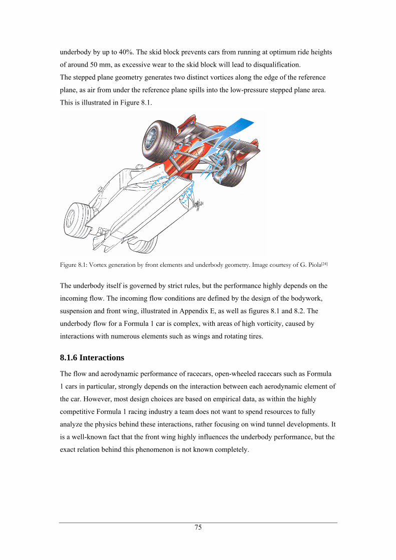
underbody by up to 40%. The skid block prevents cars from running at optimum ride heights
of around 50 mm, as excessive wear to the skid block will lead to disqualification.
The stepped plane geometry generates two distinct vortices along the edge of the reference
plane, as air from under the reference plane spills into the low-pressure stepped plane area.
This is illustrated in Figure 8.1.
Figure 8.1: Vortex generation by front elements and underbody geometry. Image courtesy of G. Piola[24]
The underbody itself is governed by strict rules, but the performance highly depends on the
incoming flow. The incoming flow conditions are defined by the design of the bodywork,
suspension and front wing, illustrated in Appendix E, as well as figures 8.1 and 8.2. The
underbody flow for a Formula 1 car is complex, with areas of high vorticity, caused by
interactions with numerous elements such as wings and rotating tires.
8.1.6 Interactions
The flow and aerodynamic performance of racecars, open-wheeled racecars such as Formula
1 cars in particular, strongly depends on the interaction between each aerodynamic element of
the car. However, most design choices are based on empirical data, as within the highly
competitive Formula 1 racing industry a team does not want to spend resources to fully
analyze the physics behind these interactions, rather focusing on wind tunnel developments. It
is a well-known fact that the front wing highly influences the underbody performance, but the
exact relation behind this phenomenon is not known completely.
75
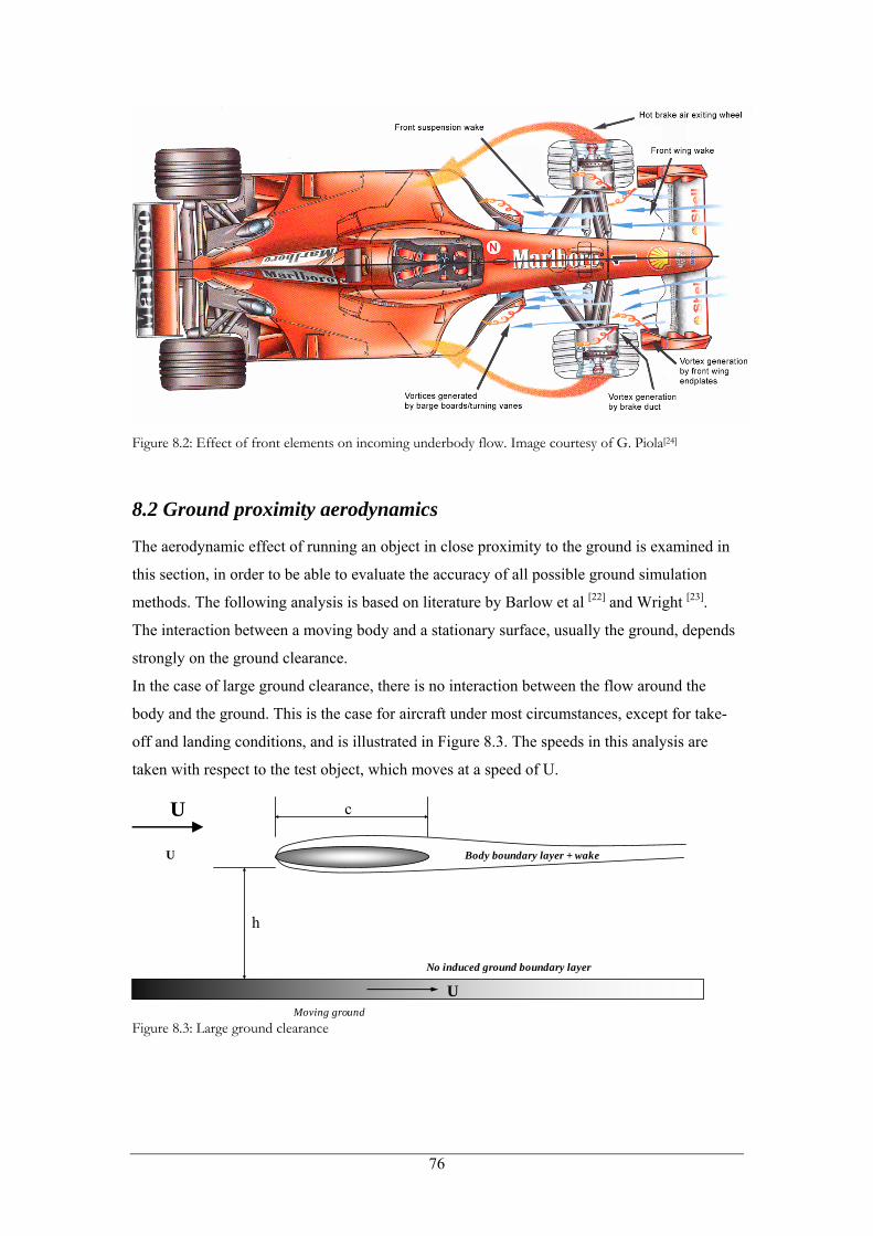
Figure 8.2: Effect of front elements on incoming underbody flow. Image courtesy of G. Piola[24]
8.2 Ground proximity aerodynamics
The aerodynamic effect of running an object in close proximity to the ground is examined in
this section, in order to be able to evaluate the accuracy of all possible ground simulation
methods. The following analysis is based on literature by Barlow et al [22] and Wright [23].
The interaction between a moving body and a stationary surface, usually the ground, depends
strongly on the ground clearance.
In the case of large ground clearance, there is no interaction between the flow around the
body and the ground. This is the case for aircraft under most circumstances, except for take-
off and landing conditions, and is illustrated in Figure 8.3. The speeds in this analysis are
taken with respect to the test object, which moves at a speed of U.
Moving ground
h
U
U
No induced ground boundary layer
Body boundary layer + wake
U
c
Figure 8.3: Large ground clearance
76
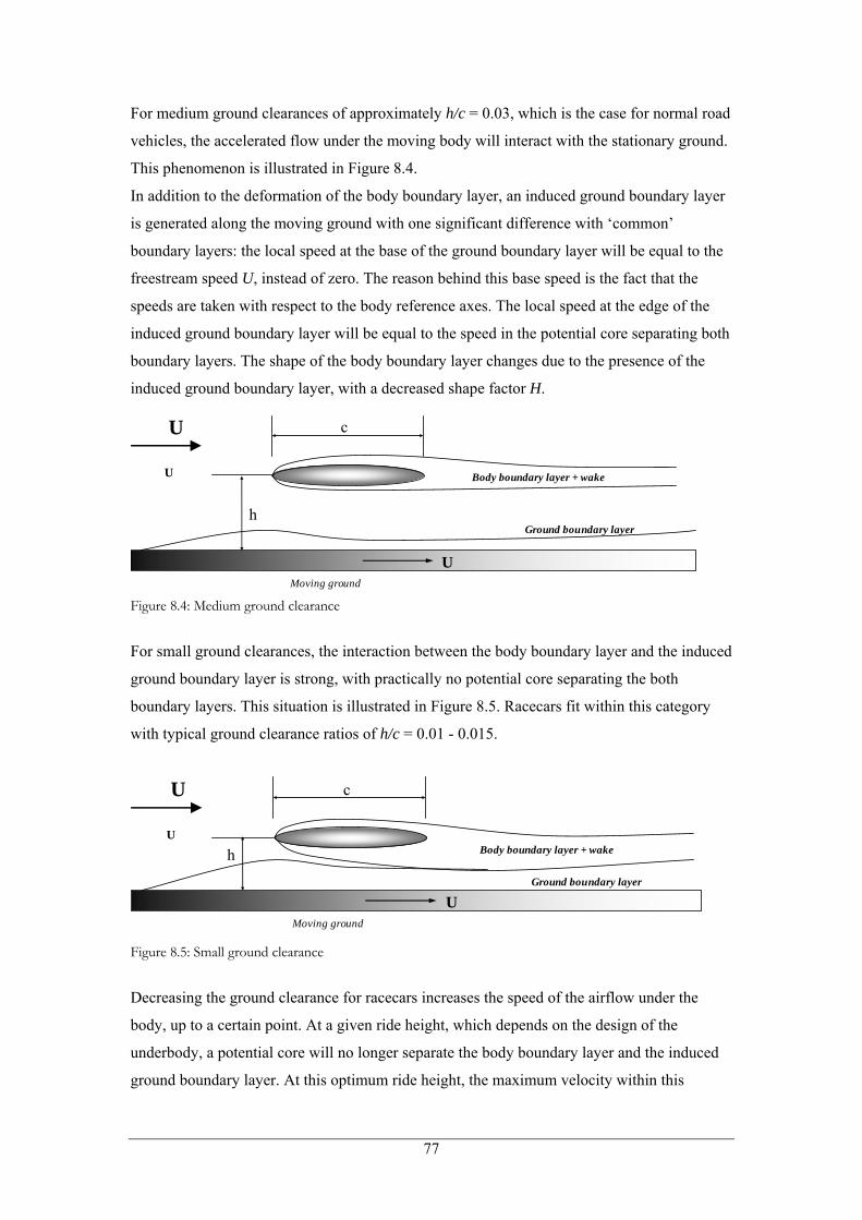
For medium ground clearances of approximately h/c = 0.03, which is the case for normal road
vehicles, the accelerated flow under the moving body will interact with the stationary ground.
This phenomenon is illustrated in Figure 8.4.
In addition to the deformation of the body boundary layer, an induced ground boundary layer
is generated along the moving ground with one significant difference with ‘common’
boundary layers: the local speed at the base of the ground boundary layer will be equal to the
freestream speed U, instead of zero. The reason behind this base speed is the fact that the
speeds are taken with respect to the body reference axes. The local speed at the edge of the
induced ground boundary layer will be equal to the speed in the potential core separating both
boundary layers. The shape of the body boundary layer changes due to the presence of the
induced ground boundary layer, with a decreased shape factor H. U
U
c
h
U Moving ground
Ground boundary layer
Body boundary layer + wake
Figure 8.4: Medium ground clearance
For small ground clearances, the interaction between the body boundary layer and the induced
ground boundary layer is strong, with practically no potential core separating the both
boundary layers. This situation is illustrated in Figure 8.5. Racecars fit within this category
with typical ground clearance ratios of h/c = 0.01 - 0.015.
c
Moving ground
U
U
h Body boundary layer + wake
U Ground boundary layer
Figure 8.5: Small ground clearance
Decreasing the ground clearance for racecars increases the speed of the airflow under the
body, up to a certain point. At a given ride height, which depends on the design of the
underbody, a potential core will no longer separate the body boundary layer and the induced
ground boundary layer. At this optimum ride height, the maximum velocity within this
77
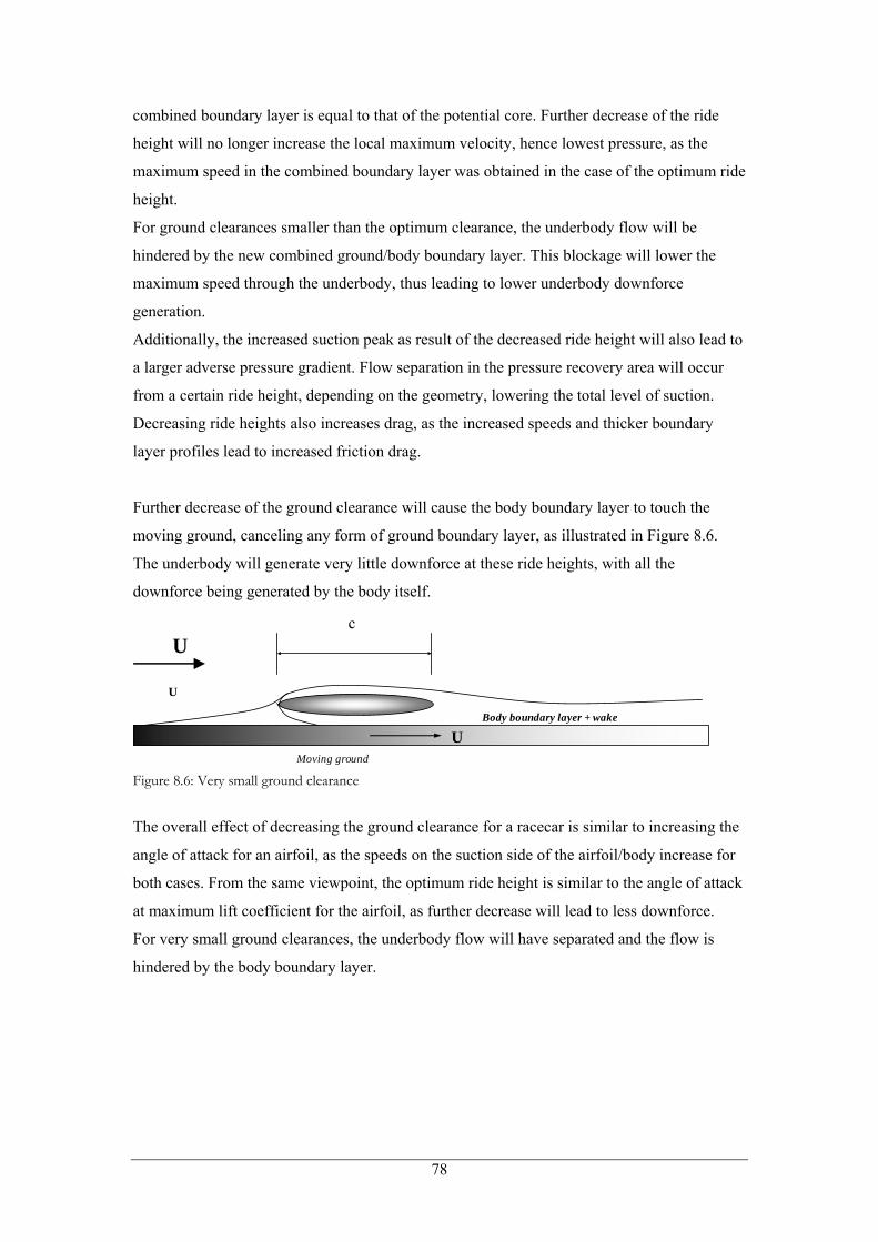
combined boundary layer is equal to that of the potential core. Further decrease of the ride
height will no longer increase the local maximum velocity, hence lowest pressure, as the
maximum speed in the combined boundary layer was obtained in the case of the optimum ride
height.
For ground clearances smaller than the optimum clearance, the underbody flow will be
hindered by the new combined ground/body boundary layer. This blockage will lower the
maximum speed through the underbody, thus leading to lower underbody downforce
generation.
Additionally, the increased suction peak as result of the decreased ride height will also lead to
a larger adverse pressure gradient. Flow separation in the pressure recovery area will occur
from a certain ride height, depending on the geometry, lowering the total level of suction.
Decreasing ride heights also increases drag, as the increased speeds and thicker boundary
layer profiles lead to increased friction drag.
Further decrease of the ground clearance will cause the body boundary layer to touch the
moving ground, canceling any form of ground boundary layer, as illustrated in Figure 8.6.
The underbody will generate very little downforce at these ride heights, with all the
downforce being generated by the body itself.
U Moving ground
c U
U
Body boundary layer + wake
Figure 8.6: Very small ground clearance
The overall effect of decreasing the ground clearance for a racecar is similar to increasing the
angle of attack for an airfoil, as the speeds on the suction side of the airfoil/body increase for
both cases. From the same viewpoint, the optimum ride height is similar to the angle of attack
at maximum lift coefficient for the airfoil, as further decrease will lead to less downforce.
For very small ground clearances, the underbody flow will have separated and the flow is
hindered by the body boundary layer.
78
8.3 Underbody conditions
8.3.1 Underbody geometry analysis
The modern Formula 1 underbody consists of the following four main elements, illustrated in
Figure E.1 in Appendix E:
- The flat underbody reference plane with a width between 300 and 500 mm,
centrally placed, with the skid plate mounted on it.
- The stepped plane, elevated 50 mm above the reference plane, running over the
remaining width of the car.
- Central diffuser, permitted to run along the full remaining length of the car, with
a maximum width of 300 mm.
- Lateral diffusers, attached to the reference plane, allowed to run up to the rear
axle of the car.
The current Formula 1 type stepped plane underbody was introduced in 1995 in order to
lower the overall downforce level as well as pitch and ride height sensitivity. The optimum
ride height for a Formula 1 car with a flat underbody is approximately 40-50 mm, a ride
height that cannot be achieved with the stepped underbody geometry. This is because the
stepped plane is elevated 50 mm above the reference plane and at least 60 mm above the
ground, due to the presence of the mandatory 10 mm thick skid plate. The lateral and central
diffusers are directly connected to the stepped plane rather than to the reference plane, as the
skid plank geometry renders the reference plane useless for generating significant downforce,
especially compared to the elevated plane. This rule forces designers to design the underbody
and diffusers of the car for the stepped plane, with ride heights (with respect to the stepped
plane in this case) of approximately 80 mm. The additional distance with respect to the
practical minimum is required for suspension travel, as excessive wear to the wooden skid
plate will result in immediate disqualification. This increased ride height has decreased pitch
and ride height sensitivity, as it has moved away from the optimum ride height.
The flow between the ground and the reference plane/skid plate will thus be blocked flow or a
borderline case of low ground clearance, as discussed in Section 8.2.
8.3.2 Underbody pressure distribution
From the description of the Formula 1 underbody in the preceding section it can be concluded
that the underbody conditions and pressure distribution are far from uniform in both lateral
and streamwise direction.
79
The underbody flow can be divided into four categories:
• Flow over the reference plane and skid plate
• Flow over stepped plane, accelerated directly by the central diffuser
• Flow over stepped plane, accelerated directly by the lateral diffusers
• Outer flow over stepped plane, not directly accelerated by either lateral or central
diffusers
The outer flow category is the case for the flow on the edge of the stepped bottom, exiting
directly in front of the rear wheels. Even though not directly connected to the lateral or central
diffusers, this region does feature a pressure distribution due to the accelerating air of the
adjacent ‘lateral diffuser region’. As the flow acceleration is indirect, the suction will be
significantly lower, also due to interaction with the external flow. The flow over the body,
wings and rotating wheels can interact with the outer region of the underbody by spilling into
this region of low-pressure. This will lead to a decrease in suction in the outer region, similar
to the flow around the tip of an aircraft wing. Additionally, the exit of this region is directly in
front of the rear wheels, separated by a gap of a few millimeters. The airflow around the
rotating rear wheels will thus have a significant impact on this outer flow region.
The highest velocity in the underbody region is achieved by the flow accelerated by the
central diffuser, as the central diffuser incorporates the largest pressure recovery due to its
length. The lower tier of the rear wing will further increase the velocity through the
underbody, similar to the effect of flaps on aircraft wings.
The flow accelerated primarily by the lateral diffusers, features lower acceleration due to the
shorter diffuser length, with the lateral diffusers being permitted to run up to the rear wheel
axle. The lateral diffusers are not designed to maximum permitted width, due to the
detrimental effect of the rotating rear wheels on the performance of the diffuser. The lateral
diffusers are equipped with horizontal fences, to minimize the effect of the rotating wheels.
Often these horizontal vanes are equipped with an additional vertical vane, to further limit
external flow from spilling into the lateral diffusers, illustrated in Figure 8.7. The lateral
diffusers themselves are equipped with vortex generators, or strakes, in order to increase
mixing between the retarded boundary layer and the inviscid outer flow, at the cost of slightly
increased drag. The geometry of both the later diffusers and the strakes are often highly
curved, in order to maximize mixing inside the diffuser, thus allowing for a more aggressive
diffuser angle.
80
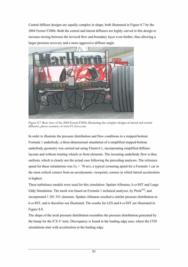
Central diffuser designs are equally complex in shape, both illustrated in Figure 8.7 by the
2004 Ferrari F2004. Both the central and lateral diffusers are highly curved in this design to
increase mixing between the inviscid flow and boundary layer even further, thus allowing a
larger pressure recovery and a more aggressive diffuser angle.
Figure 8.7: Rear view of the 2004 Ferrari F2004, illustrating the complex designs in lateral and central diffusers, photo courtesy of www.F1-Live.com
In order to illustrate the pressure distribution and flow conditions in a stepped-bottom
Formula 1 underbody, a three-dimensional simulation of a simplified stepped-bottom
underbody geometry was carried out using Fluent 6.1, incorporating simplified diffuser
layouts and without rotating wheels or front elements. The incoming underbody flow is thus
uniform, which is clearly not the actual case following the preceding analyses. The reference
speed for these simulations was U0 = 70 m/s, a typical cornering speed for a Formula 1 car in
the most critical corners from an aerodynamic viewpoint; corners in which lateral acceleration
is highest.
Three turbulence models were used for this simulation: Spalart-Allmaras, k-ω SST and Large
Eddy Simulation. The mesh was based on Formula 1 technical analyses, by Piola[24], and
incorporated 1 201 351 elements. Spalart-Allmaras resulted a similar pressure distribution as
k-ω SST, and is therefore not illustrated. The results for LES and k-ω SST are illustrated in
Figure 8.8.
The shape of the axial pressure distribution resembles the pressure distribution generated by
the bump for the 8’X 4’ tests. Discrepancy is found in the leading edge area, where the CFD
simulations start with acceleration at the leading edge.
81
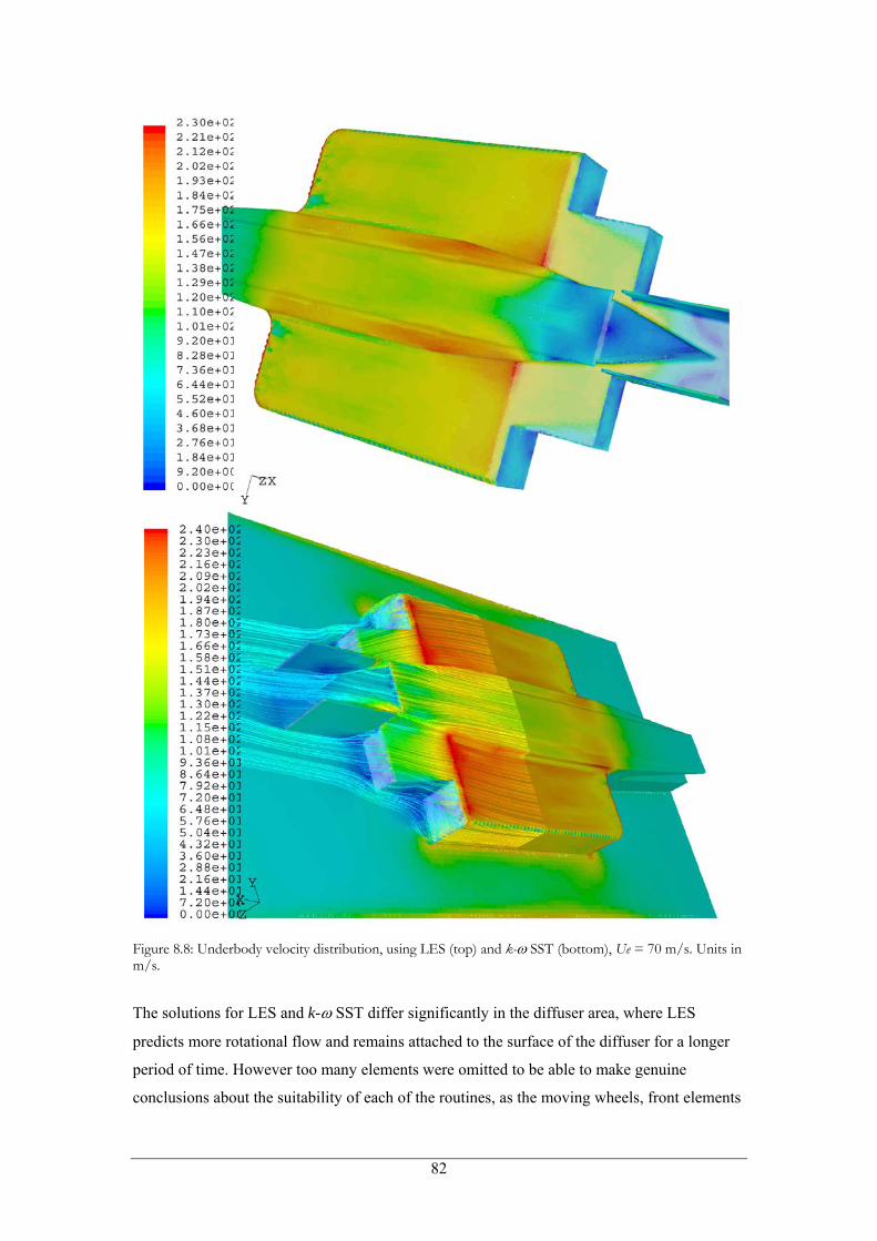
Figure 8.8: Underbody velocity distribution, using LES (top) and k-ω SST (bottom), Ue = 70 m/s. Units in m/s.
The solutions for LES and k-ω SST differ significantly in the diffuser area, where LES
predicts more rotational flow and remains attached to the surface of the diffuser for a longer
period of time. However too many elements were omitted to be able to make genuine
conclusions about the suitability of each of the routines, as the moving wheels, front elements
82
and rear wing are not present, each having a strong influence on the underbody flow and
pressure distribution.
8.3.3 Underbody flow conditions
As mentioned before, underbodies have to be designed in order to cope with a range of
conditions: pitch angles, ride heights, yaw angles and front wing settings. If a change in any
of these factors causes a sudden drop or increase in downforce, or a sudden/dramatic shift in
aerodynamic balance, the design has to be re-evaluated. When car shows large aerodynamic
variation over the normal operating range for these factors, the design is deemed non-drivable
as the car must perform constantly so the driver has confidence in the car. Increasing spring
stiffness can limit the pitch and ride height range, at the price of decreased drivability over
bumps and increasing tire wear.
The quality of the incoming airflow is of vital importance to the underbody, particularly from
a designer’s point of view. The underbody is an integral part of the entire car design, as its
performance depends on the performance of many other elements. The Formula 1 underbody
will thus have to cope with the full range of front and rear ride heights, as well as the full
range of front wing settings. The effect of the front elements on the underbody flow is
illustrated in Figure 8.2.
The incoming underbody flow will thus be turbulent, the intensity and length scale of the
turbulence depending on the design and setting of the preceding elements. The underbody
pressure distribution is comparable to the pressure distribution generated by the bump in the
first part of this report. Using the results for the single bump tests, the vortex entering the
underbody region is expected to decrease in vorticity, due to the close ground proximity to
both the underbody and ground surface. As discussed in Chapter 4 and 7, vortex strength
decay increases with the increasing skin friction coefficient. This is the case for the turbulent
underbody flow as the local skin friction coefficient increases under favorable pressure
gradients.
Vortices in the favorable pressure gradient section of the underbody are generated by the
preceding elements as well as the underbody geometry itself. The pressure jump between the
blocked flow under the skid plate and the lower-pressure stepped plane flow will result in the
generation of a vortex along the reference plane edge, as illustrated in Figure 8.2. These latter
vortices react in a distinctly different manner than the vortices studied in the first part of this
report. As the flow accelerates throughout the stepped plane surface, the pressure jump
between the skid plate and stepped plane increases in magnitude, thus increasing the strength
of the generated vortex.
83
Chapter 9
Ground proximity vortex interaction
In Chapter 2, the following factors were introduced that influence the characteristics of the
vortex generated by a vortex generator:
- Incoming flow characteristics
- (Leading) Edge radius
- Incidence angle (for delta wing type)
- Sweep angle (for delta wing type)
In addition, six known factors for vortex decay were presented, based on ESDU data[4]. These
were:
1. Interaction between the main vortex and the secondary vortex, generated as reaction
on the body surface.
2. Interaction between the vortex and the body boundary layer.
3. The initial core turbulence level, affected by the vortex formation. This is down to
(leading) edge radius and Reynolds effects.
4. Dissipation due to interaction with outer stream turbulence.
5. Dissipation in the viscous core of the main vortex.
6. The pressure gradient imposed onto the vortex by the outer stream.
This chapter will present additional factors for vortex behavior and vortex strength decay
associated with ground proximity aerodynamics, along with a hypothesis on the effect of
these factors on vortex behavior.
From the underbody conditions analysis in Section 8.3, the following additional factors are
introduced compared to the stationary arrangement used in the first section of this study:
• Moving ground plane
• Induced ground boundary layer
84
The effect of a ground plane in combination with a close proximity body on vortices has been
studied the trapped vortex study by Garcia and Katz[20]. This study incorporated a flat,
stationary plate arrangement with four rectangular vortex generators mounted onto this plate.
Ground proximity and ground simulation were achieved by means of a plate, parallel to the
test plate. Results for vortex behavior were obtained by means of force measurements,
whereas qualitative results were obtained for vortex core trajectory by means of smoke
visualization and water tunnel tests.
With decreasing ground clearance, both the aerodynamic downforce and negative pitching
moment due to the vortex increase in magnitude. The increase in aerodynamic downforce is
due to the additional velocity component in the streamwise plane introduced by the vortex,
leading to a higher effective velocity over the surface, as the vortex runs closer to the surface.
The result of the decreased ground clearance is two-fold: the suction generated by the vortex
increases aft of the vortex generator, but vortex strength decay increases as well, due to the
increased interaction with both the ground plane as well as the surface of the body. The higher
velocity along the body surface will not only lead to increased suction, but will also lead to
greater circulation loss due to interaction with the surfaces.
A forward shift in the aerodynamic balance of the model is observed in the Katz/Garcia study,
indicating a decrease in vortex strength and vorticity downstream. Decreasing ground
clearance thus causes vortex decay due to surface interaction to move forwards, whilst
initially increasing the total suction on the flat plate. Suction will increase up to a certain point
however. From this point onwards, decreasing ride height will result in a decrease in suction
due to increasing vortex circulation decay.
This study by Garcia and Katz is one of the first generally available studies into vortex
behavior in ground effect, however with a few drawbacks. The ground is represented by an
elevated, stationary plate, where no-slip conditions apply. The velocity at the base of the
ground boundary layer is thus equal to zero, not equal to the free-stream velocity U0. As
discussed in Chapter 8, the discrepancy between a stationary ground boundary layer and a
moving ground has quite significant influence on the pressure distribution of an underbody.
This test arrangement is thus not applicable for an underbody that generates a pressure
distribution, as the ground boundary layer in the case of a stationary ground does not allow
the pressure recoveries that a moving ground setup would allow.
The effect of interaction with the moving ground on the vortex is in principle similar to the
interaction with the body surface. However, the main difference is the speed difference
between the vortex and the surface. In the case of a minimum pressure coefficient
85
of , the local velocity free-stream velocity Umin 2.0pC = − e(x) will be the 1.73 times the
reference speed U0, which is the speed of the car in this case. The maximum velocity at which
the vortex will be shed is slightly lower than Ue(x). For a stationary ground arrangement, the
maximum speed in streamwise direction of the vortex with respect to the ground will thus be
slightly lower than Ue(x), or 1.73U0 in the case of min 2.0pC = − .
For the moving ground case the vortex is shed at the same velocity with respect to the model,
but the relative speed with respect to the ground is significantly lower, as the road itself
moves along with U0. The maximum streamwise velocity component of the vortex with
respect to the moving ground will thus be slightly lower than 0.73 U0, which is a significantly
smaller difference than with a stationary ground. As the local skin friction on the moving
ground surface will thus be lower, the vortex strength decay with the moving ground is lower
after the approximation for vortex strength development in Section 2.2.2:
fcd dxh
Γ= −
Γ
Interaction between the vortex and moving ground will thus lead to less energy loss compared
to a stationary ground surface, as the skin friction coefficient on the moving ground plane is
lower than on the body surface.
Using the results from the current study and the Katz/Garcia study, combined with
assumptions moving ground interactions, the following hypothesis can be made for vortex
behavior in underbody conditions:
Vortex strength decay due to interaction with both the body and induced ground boundary
layer will increase for decreasing ride heights, as skin friction on both body and ground
surface increases with the increasing velocity that accompanies the decreasing ground
clearance. Vortex interaction with the moving ground will thus also lead to an increase in
vortex decay, however to a lesser extent as interaction with the body surface. This is due to
the lower skin friction coefficient on the moving ground surface, as the velocity at the base of
the induced ground boundary layer is non-zero.
The vortices entering the underbody region will interact with both the body surface and the
moving ground surface. With the results for vorticity development for the stationary ground
tests, presented in Chapter 6, it can thus be argued that a vortex in the underbody region
features decreased vorticity for the vortices entering the underbody. The additional interaction
with the moving ground and the induced boundary layer will cause the viscous effects to
outweigh the spin-up effects of the pressure gradient even more than was the case for the
bump tests in the first part of this report.
86
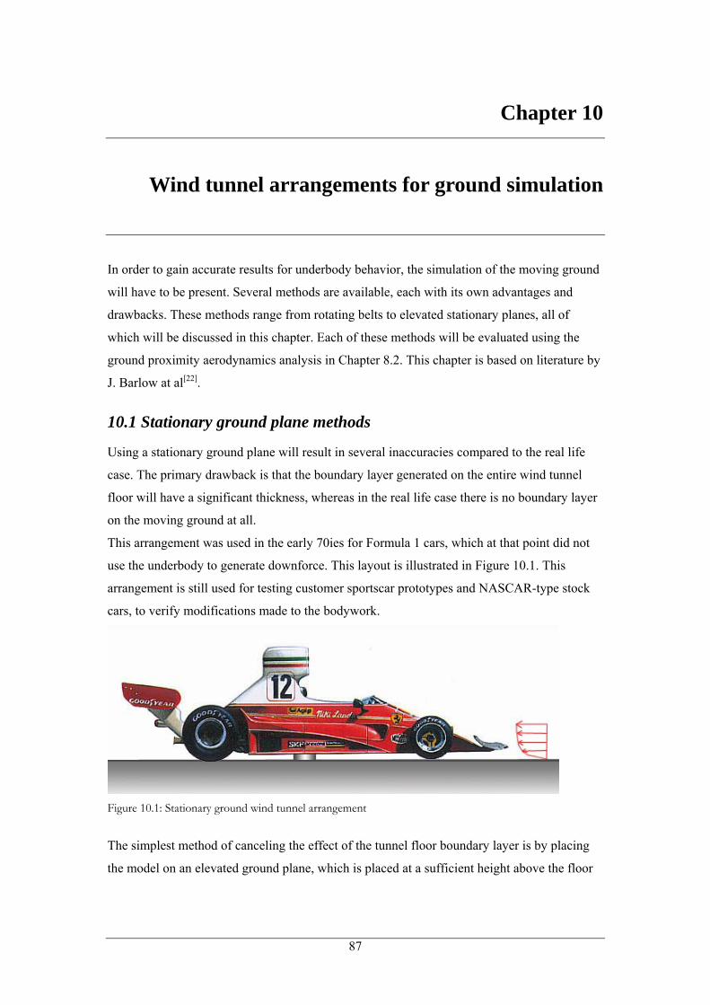
Chapter 10
Wind tunnel arrangements for ground simulation
In order to gain accurate results for underbody behavior, the simulation of the moving ground
will have to be present. Several methods are available, each with its own advantages and
drawbacks. These methods range from rotating belts to elevated stationary planes, all of
which will be discussed in this chapter. Each of these methods will be evaluated using the
ground proximity aerodynamics analysis in Chapter 8.2. This chapter is based on literature by
J. Barlow at al[22].
10.1 Stationary ground plane methods
Using a stationary ground plane will result in several inaccuracies compared to the real life
case. The primary drawback is that the boundary layer generated on the entire wind tunnel
floor will have a significant thickness, whereas in the real life case there is no boundary layer
on the moving ground at all.
This arrangement was used in the early 70ies for Formula 1 cars, which at that point did not
use the underbody to generate downforce. This layout is illustrated in Figure 10.1. This
arrangement is still used for testing customer sportscar prototypes and NASCAR-type stock
cars, to verify modifications made to the bodywork.
Figure 10.1: Stationary ground wind tunnel arrangement
The simplest method of canceling the effect of the tunnel floor boundary layer is by placing
the model on an elevated ground plane, which is placed at a sufficient height above the floor
87
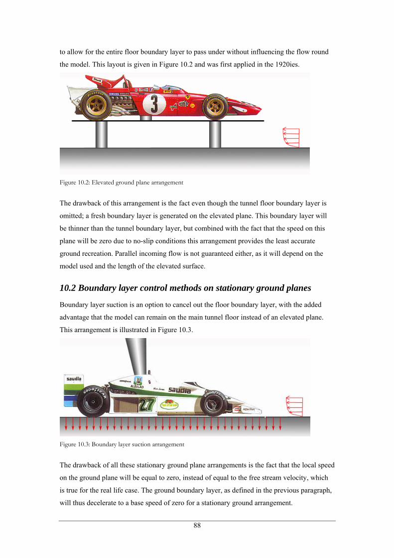
to allow for the entire floor boundary layer to pass under without influencing the flow round
the model. This layout is given in Figure 10.2 and was first applied in the 1920ies.
Figure 10.2: Elevated ground plane arrangement
The drawback of this arrangement is the fact even though the tunnel floor boundary layer is
omitted; a fresh boundary layer is generated on the elevated plane. This boundary layer will
be thinner than the tunnel boundary layer, but combined with the fact that the speed on this
plane will be zero due to no-slip conditions this arrangement provides the least accurate
ground recreation. Parallel incoming flow is not guaranteed either, as it will depend on the
model used and the length of the elevated surface.
10.2 Boundary layer control methods on stationary ground planes
Boundary layer suction is an option to cancel out the floor boundary layer, with the added
advantage that the model can remain on the main tunnel floor instead of an elevated plane.
This arrangement is illustrated in Figure 10.3.
Figure 10.3: Boundary layer suction arrangement
The drawback of all these stationary ground plane arrangements is the fact that the local speed
on the ground plane will be equal to zero, instead of equal to the free stream velocity, which
is true for the real life case. The ground boundary layer, as defined in the previous paragraph,
will thus decelerate to a base speed of zero for a stationary ground arrangement.
88
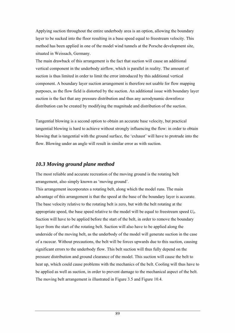
Applying suction throughout the entire underbody area is an option, allowing the boundary
layer to be sucked into the floor resulting in a base speed equal to freestream velocity. This
method has been applied in one of the model wind tunnels at the Porsche development site,
situated in Weissach, Germany.
The main drawback of this arrangement is the fact that suction will cause an additional
vertical component in the underbody airflow, which is parallel in reality. The amount of
suction is thus limited in order to limit the error introduced by this additional vertical
component. A boundary layer suction arrangement is therefore not usable for flow mapping
purposes, as the flow field is distorted by the suction. An additional issue with boundary layer
suction is the fact that any pressure distribution and thus any aerodynamic downforce
distribution can be created by modifying the magnitude and distribution of the suction.
Tangential blowing is a second option to obtain an accurate base velocity, but practical
tangential blowing is hard to achieve without strongly influencing the flow: in order to obtain
blowing that is tangential with the ground surface, the ‘exhaust’ will have to protrude into the
flow. Blowing under an angle will result in similar error as with suction.
10.3 Moving ground plane method
The most reliable and accurate recreation of the moving ground is the rotating belt
arrangement, also simply known as ‘moving ground’.
This arrangement incorporates a rotating belt, along which the model runs. The main
advantage of this arrangement is that the speed at the base of the boundary layer is accurate.
The base velocity relative to the rotating belt is zero, but with the belt rotating at the
appropriate speed, the base speed relative to the model will be equal to freestream speed U0.
Suction will have to be applied before the start of the belt, in order to remove the boundary
layer from the start of the rotating belt. Suction will also have to be applied along the
underside of the moving belt, as the underbody of the model will generate suction in the case
of a racecar. Without precautions, the belt will be forces upwards due to this suction, causing
significant errors to the underbody flow. This belt suction will thus fully depend on the
pressure distribution and ground clearance of the model. This suction will cause the belt to
heat up, which could cause problems with the mechanics of the belt. Cooling will thus have to
be applied as well as suction, in order to prevent damage to the mechanical aspect of the belt.
The moving belt arrangement is illustrated in Figure 3.5 and Figure 10.4.
89
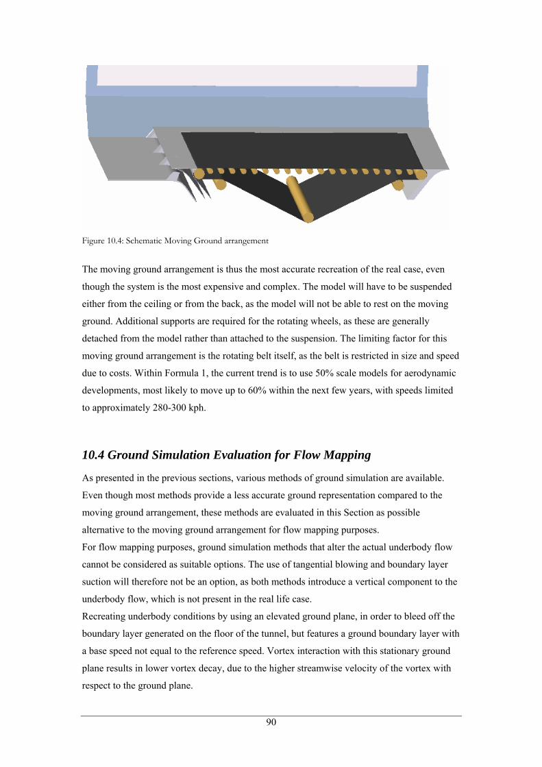
Figure 10.4: Schematic Moving Ground arrangement
The moving ground arrangement is thus the most accurate recreation of the real case, even
though the system is the most expensive and complex. The model will have to be suspended
either from the ceiling or from the back, as the model will not be able to rest on the moving
ground. Additional supports are required for the rotating wheels, as these are generally
detached from the model rather than attached to the suspension. The limiting factor for this
moving ground arrangement is the rotating belt itself, as the belt is restricted in size and speed
due to costs. Within Formula 1, the current trend is to use 50% scale models for aerodynamic
developments, most likely to move up to 60% within the next few years, with speeds limited
to approximately 280-300 kph.
10.4 Ground Simulation Evaluation for Flow Mapping
As presented in the previous sections, various methods of ground simulation are available.
Even though most methods provide a less accurate ground representation compared to the
moving ground arrangement, these methods are evaluated in this Section as possible
alternative to the moving ground arrangement for flow mapping purposes.
For flow mapping purposes, ground simulation methods that alter the actual underbody flow
cannot be considered as suitable options. The use of tangential blowing and boundary layer
suction will therefore not be an option, as both methods introduce a vertical component to the
underbody flow, which is not present in the real life case.
Recreating underbody conditions by using an elevated ground plane, in order to bleed off the
boundary layer generated on the floor of the tunnel, but features a ground boundary layer with
a base speed not equal to the reference speed. Vortex interaction with this stationary ground
plane results in lower vortex decay, due to the higher streamwise velocity of the vortex with
respect to the ground plane.
90
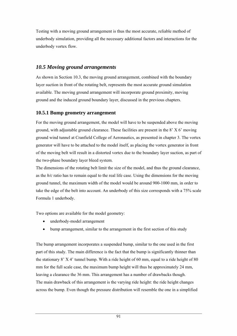
Testing with a moving ground arrangement is thus the most accurate, reliable method of
underbody simulation, providing all the necessary additional factors and interactions for the
underbody vortex flow.
10.5 Moving ground arrangements
As shown in Section 10.3, the moving ground arrangement, combined with the boundary
layer suction in front of the rotating belt, represents the most accurate ground simulation
available. The moving ground arrangement will incorporate ground proximity, moving
ground and the induced ground boundary layer, discussed in the previous chapters.
10.5.1 Bump geometry arrangement
For the moving ground arrangement, the model will have to be suspended above the moving
ground, with adjustable ground clearance. These facilities are present in the 8’ X 6’ moving
ground wind tunnel at Cranfield College of Aeronautics, as presented in chapter 3. The vortex
generator will have to be attached to the model itself, as placing the vortex generator in front
of the moving belt will result in a distorted vortex due to the boundary layer suction, as part of
the two-phase boundary layer bleed system.
The dimensions of the rotating belt limit the size of the model, and thus the ground clearance,
as the h/c ratio has to remain equal to the real life case. Using the dimensions for the moving
ground tunnel, the maximum width of the model would be around 900-1000 mm, in order to
take the edge of the belt into account. An underbody of this size corresponds with a 75% scale
Formula 1 underbody.
Two options are available for the model geometry:
• underbody-model arrangement
• bump arrangement, similar to the arrangement in the first section of this study
The bump arrangement incorporates a suspended bump, similar to the one used in the first
part of this study. The main difference is the fact that the bump is significantly thinner than
the stationary 8’ X 4’ tunnel bump. With a ride height of 60 mm, equal to a ride height of 80
mm for the full scale case, the maximum bump height will thus be approximately 24 mm,
leaving a clearance the 36 mm. This arrangement has a number of drawbacks though.
The main drawback of this arrangement is the varying ride height: the ride height changes
across the bump. Even though the pressure distribution will resemble the one in a simplified
91
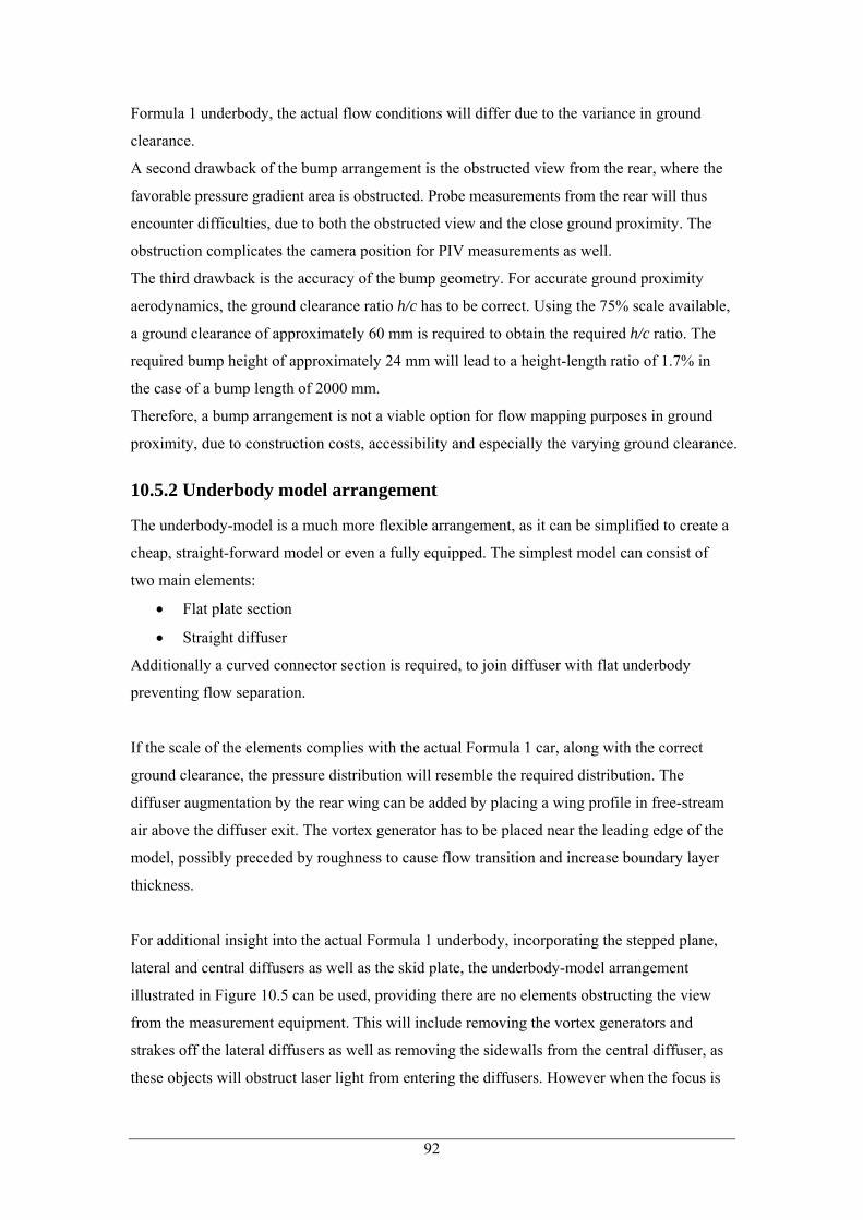
Formula 1 underbody, the actual flow conditions will differ due to the variance in ground
clearance.
A second drawback of the bump arrangement is the obstructed view from the rear, where the
favorable pressure gradient area is obstructed. Probe measurements from the rear will thus
encounter difficulties, due to both the obstructed view and the close ground proximity. The
obstruction complicates the camera position for PIV measurements as well.
The third drawback is the accuracy of the bump geometry. For accurate ground proximity
aerodynamics, the ground clearance ratio h/c has to be correct. Using the 75% scale available,
a ground clearance of approximately 60 mm is required to obtain the required h/c ratio. The
required bump height of approximately 24 mm will lead to a height-length ratio of 1.7% in
the case of a bump length of 2000 mm.
Therefore, a bump arrangement is not a viable option for flow mapping purposes in ground
proximity, due to construction costs, accessibility and especially the varying ground clearance.
10.5.2 Underbody model arrangement
The underbody-model is a much more flexible arrangement, as it can be simplified to create a
cheap, straight-forward model or even a fully equipped. The simplest model can consist of
two main elements:
• Flat plate section
• Straight diffuser
Additionally a curved connector section is required, to join diffuser with flat underbody
preventing flow separation.
If the scale of the elements complies with the actual Formula 1 car, along with the correct
ground clearance, the pressure distribution will resemble the required distribution. The
diffuser augmentation by the rear wing can be added by placing a wing profile in free-stream
air above the diffuser exit. The vortex generator has to be placed near the leading edge of the
model, possibly preceded by roughness to cause flow transition and increase boundary layer
thickness.
For additional insight into the actual Formula 1 underbody, incorporating the stepped plane,
lateral and central diffusers as well as the skid plate, the underbody-model arrangement
illustrated in Figure 10.5 can be used, providing there are no elements obstructing the view
from the measurement equipment. This will include removing the vortex generators and
strakes off the lateral diffusers as well as removing the sidewalls from the central diffuser, as
these objects will obstruct laser light from entering the diffusers. However when the focus is
92
primarily on the favorable pressure gradient area, which precedes the diffuser area, these
elements are best kept in place, as they are vital for the performance of the diffusers.
Figure 10.5: Underbody model consisting of stepped plane, lateral and central diffusers.
The flexibility of the model arrangement and accurate flow conditions make the underbody-
model arrangement the method of choice for flow mapping tests in moving ground conditions.
Dimensions of the simplified underbody shown above are illustrated in Figure F.4 in
Appendix F.
10.6 Flow mapping measurement techniques
The only way of getting HWA measurements would be if these were taken from the behind
the model or through the model from the top. The latter method would require gaps in the
model at each measurement position, which would influence the flow significantly. When
taking hot-wire measurements from behind the model, the probe length will have to be at least
equal to the model length. Probe flutter can lead to probe failure, especially taking the small
ground clearances into account.
A laser-based measurement technique will thus be the only available method to achieve flow
mapping. The main drawback of Laser Doppler Anemometry is the need to have uniform
particle distribution throughout the entire test section, whereas PIV requires only local
seeding for accurate results. Particle Image Velocimetry is thus the most suitable flow
mapping tool available, also as the PIV equipment is considerably more mobile.
Application of PIV in the Cranfield 8’ X 6’ moving ground tunnel will present difficulties,
due to the octagonal shape of the test section, as illustrated in Figure F.1 in Appendix F.
Placing the laser equipment outside an un-modified 8’ X 6’ tunnel will not meet the straight
angle requirement, as mentioned in Chapter 4. Placing the laser on the wind tunnel floor will
not be possible as there is not enough space available between the moving belt and the
chamfered lower corners.
93
PIV can be applied in a modified wind tunnel, using two approaches. The first approach
features the laser equipment placed on one of the sidewalls of the tunnel, with the laser light
aiming in negative Z-direction. The laser light will be deflected into the underbody flow by
means of a mirror, placed on the chamfered bottom corner. This arrangement is illustrated in
Figure F.1 in Appendix F.
The second approach incorporates the drilling of a hole through the chamfered corner,
through which the dispersing element, placed inside the tunnel, is connected with the laser
equipment outside of the tunnel. This method will thus require a major modification to the
wind tunnel test section itself, and is unlikely to be chosen over the first method incorporating
the mirror.
The arrangement featuring the reflected laser light is evaluated and discussed in further detail
in Chapter 12.
94
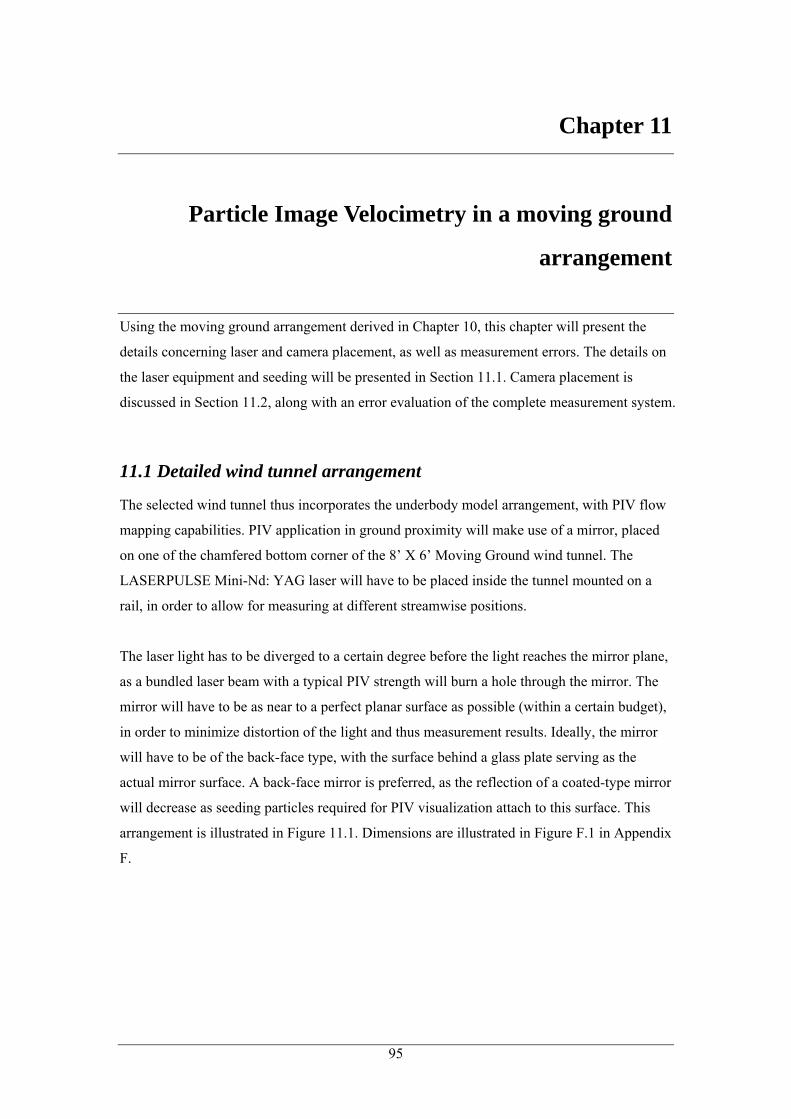
Chapter 11
Particle Image Velocimetry in a moving ground
arrangement
Using the moving ground arrangement derived in Chapter 10, this chapter will present the
details concerning laser and camera placement, as well as measurement errors. The details on
the laser equipment and seeding will be presented in Section 11.1. Camera placement is
discussed in Section 11.2, along with an error evaluation of the complete measurement system.
11.1 Detailed wind tunnel arrangement
The selected wind tunnel thus incorporates the underbody model arrangement, with PIV flow
mapping capabilities. PIV application in ground proximity will make use of a mirror, placed
on one of the chamfered bottom corner of the 8’ X 6’ Moving Ground wind tunnel. The
LASERPULSE Mini-Nd: YAG laser will have to be placed inside the tunnel mounted on a
rail, in order to allow for measuring at different streamwise positions.
The laser light has to be diverged to a certain degree before the light reaches the mirror plane,
as a bundled laser beam with a typical PIV strength will burn a hole through the mirror. The
mirror will have to be as near to a perfect planar surface as possible (within a certain budget),
in order to minimize distortion of the light and thus measurement results. Ideally, the mirror
will have to be of the back-face type, with the surface behind a glass plate serving as the
actual mirror surface. A back-face mirror is preferred, as the reflection of a coated-type mirror
will decrease as seeding particles required for PIV visualization attach to this surface. This
arrangement is illustrated in Figure 11.1. Dimensions are illustrated in Figure F.1 in Appendix
F.
95
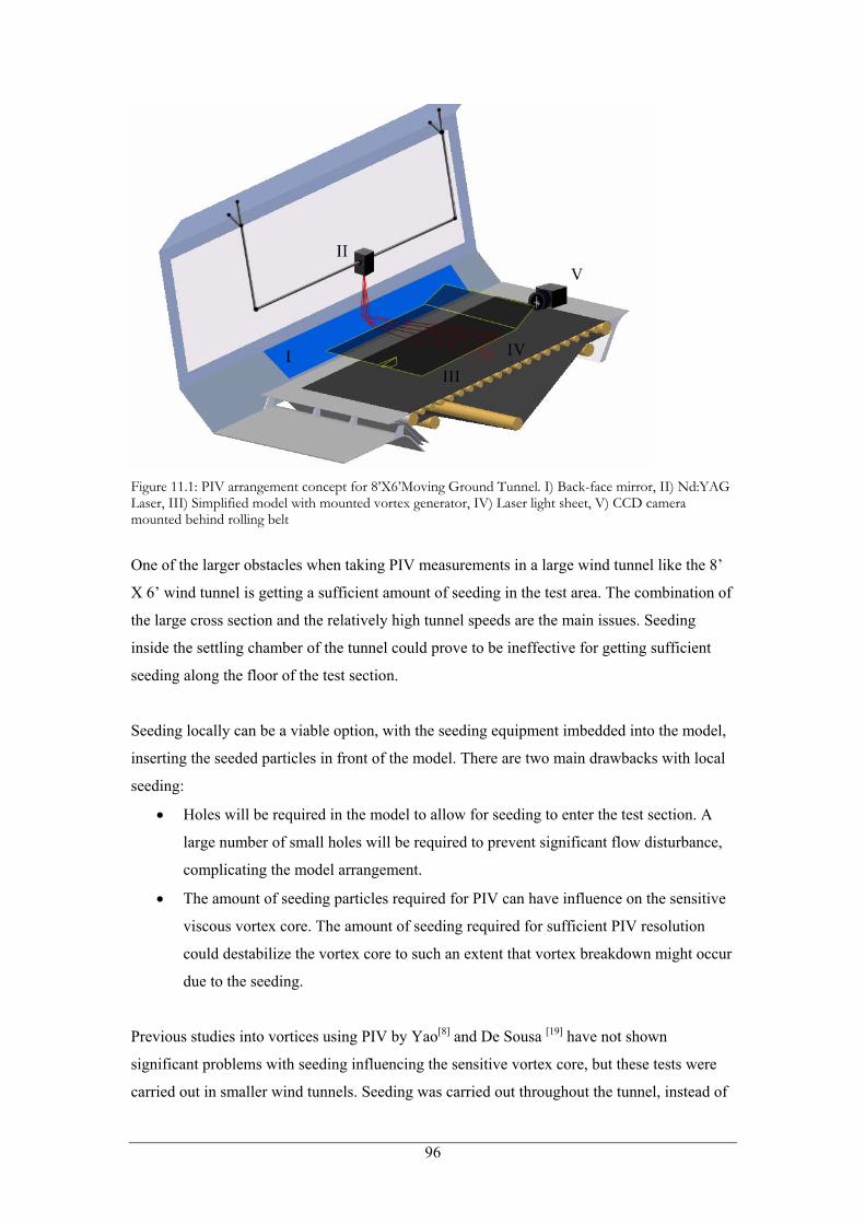
Figure 11.1: PIV arrangement concept for 8’X6’Moving Ground Tunnel. I) Back-face mirror, II) Nd:YAG Laser, III) Simplified model with mounted vortex generator, IV) Laser light sheet, V) CCD camera mounted behind rolling belt
One of the larger obstacles when taking PIV measurements in a large wind tunnel like the 8’
X 6’ wind tunnel is getting a sufficient amount of seeding in the test area. The combination of
the large cross section and the relatively high tunnel speeds are the main issues. Seeding
inside the settling chamber of the tunnel could prove to be ineffective for getting sufficient
seeding along the floor of the test section.
Seeding locally can be a viable option, with the seeding equipment imbedded into the model,
inserting the seeded particles in front of the model. There are two main drawbacks with local
seeding:
• Holes will be required in the model to allow for seeding to enter the test section. A
large number of small holes will be required to prevent significant flow disturbance,
complicating the model arrangement.
• The amount of seeding particles required for PIV can have influence on the sensitive
viscous vortex core. The amount of seeding required for sufficient PIV resolution
could destabilize the vortex core to such an extent that vortex breakdown might occur
due to the seeding.
Previous studies into vortices using PIV by Yao[8] and De Sousa [19] have not shown
significant problems with seeding influencing the sensitive vortex core, but these tests were
carried out in smaller wind tunnels. Seeding was carried out throughout the tunnel, instead of
96
locally. However, the device height of the SBVGs used in these studies was 7 mm, thus
generating a relatively weak vortex compared to the 8’X 4’ tests.
11.2 Camera positioning and error evaluation
Ideally, a PIV arrangement would use a stereoscopic arrangement, incorporating two CCD
cameras placed on either side of the measured light sheet. A twin-camera arrangement would
decrease in-plane errors caused by perspective by an order of magnitude compared to a single
camera arrangement. However, stereoscopic equipment was not available at Cranfield at the
time of writing. A single camera arrangement is available, by TSI Incorporated.
The camera uses a standard F-mount lens mount, allowing the camera to be equipped with a
wide range of lenses. Cranfield University has a 100 mm available lens for this system, which
will be used to the following error analysis.
Assuming that the vortex is generated in the middle of the tunnel, the lateral distance to the
camera is taken at 600 mm. This distance is necessary because the camera will have to be
placed beside the 1200 mm wide moving belt in order to minimize influence on the flow. A
range of streamwise camera positions was calculated for three in-plane errors:
• Error due to measuring the object at an angle, causing a light intensity discrepancy
• Position uncertainty: Lens error due to deflecting light at the edges of the lens
• Error due to decreasing light intensity at increased object distance
The first error is a perspective error, in addition to the fact that the camera is not viewing the
laser sheet perpendicularly. The light intensity of the measured area received by the camera
depends on the distance to the camera, which varies throughout the measurement area. The
error estimation is based on the fact that light intensity decreases with the squared distance to
the light source, which is the measurement area in this case. This error is best approximated
as follows:
( )max
2 22 2 20
2 2 20
424100360000
d X Y y z Xd X Y X
ε+ + ∆ + ∆⎛ ⎞ +
= = =⎜ ⎟ + +⎝ ⎠
In this equation, d0 is the object distance, whereas X, Y and Z are the axial, crossflow and
vertical object distance components respectively.
The second error, position uncertainty due to the lens, is estimated using the following
formula, after Lawson and Reeves[25].
97
2
2
50360000
40360000
yo
zo
yd Xzd X
ε
ε
∗
∗
= =+
= =+
In these equations, εy and εz are the position errors in crossflow and vertical direction. y* and
z* are the distances from the point of focus within the object plane to the extremes of the
measured object, illustrated in Figure F.3 in Appendix F.
The third error can be attributed to the sensitivity of the camera, and decreasing light intensity
at increasing distance. As light intensity decreases squared with the object distance, the
minimum light sensitivity of the CCD camera limits the phenomena that can be recorded.
When measuring at larger distance, the overall light intensity decreases, causing errors due to
the 12-bit recording depth of the camera. The entire brightness spectrum of the CCD camera
will not be able to distinct the subtle differences in light intensity at the larger distance. This
error will also depend on the lens mounted on the camera, as well as the lens settings.
Conservative assumptions were made for both settings, assuming a measurement error due to
this effect of 4% at an axial camera distance of 400 mm.
Two additional factors will cause errors in the measurements. These are laser reflections and
errors due to imperfections on the mirror surface. Both the model surface and the moving
ground cause the reflection. Even though reflection on the body can be treated using specific
surface treatments, typically the first row of pixels adjacent to the body on the CCD image
has to be removed. However, reflection on the moving ground belt is practically impossible to
treat, due to the entire nature of the system. The three pixel rows most adjacent to the belt will
have to be removed from the resulting image. In order to evaluate the size of the removed
areas, a resolution calculation was carried out.
Using the magnification factor di/do and a lens with a focal distance of f = 100 mm, a relation
was found between streamwise camera distance and number of pixels required, using a
measurement area 100 mm wide and 80 mm high. This is illustrated in Figure 11.2.
98
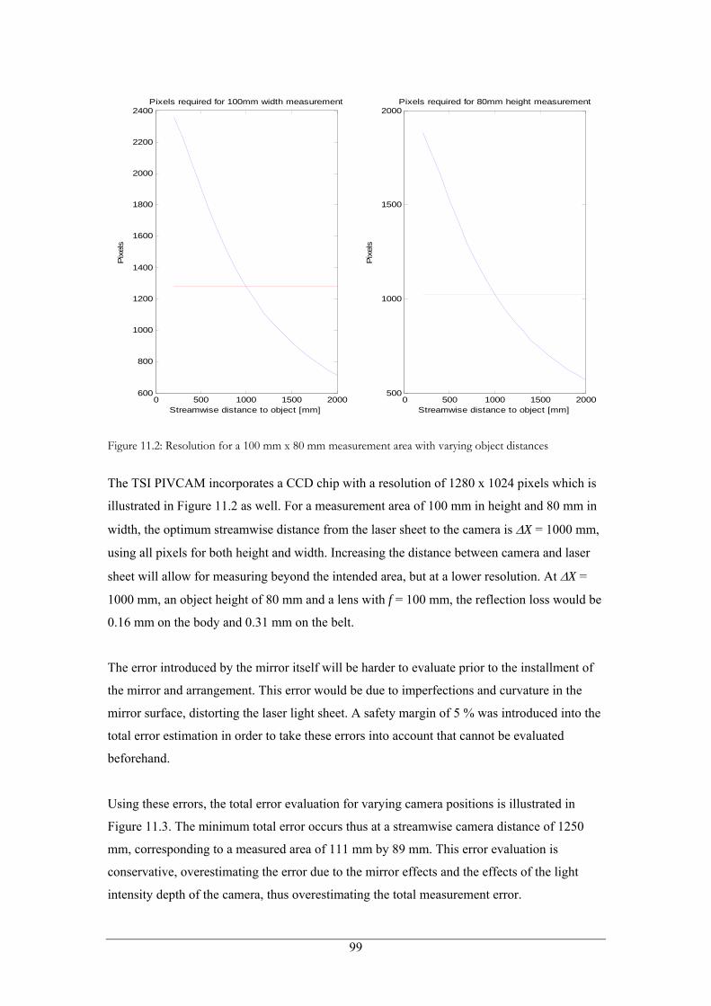
0 500 1000 1500 2000600
800
1000
1200
1400
1600
1800
2000
2200
2400Pixels required for 100mm width measurement
Streamwise distance to object [mm]
Pix
els
0 500 1000 1500 2000500
1000
1500
2000Pixels required for 80mm height measurement
Streamwise distance to object [mm]
Pix
els
Figure 11.2: Resolution for a 100 mm x 80 mm measurement area with varying object distances
The TSI PIVCAM incorporates a CCD chip with a resolution of 1280 x 1024 pixels which is
illustrated in Figure 11.2 as well. For a measurement area of 100 mm in height and 80 mm in
width, the optimum streamwise distance from the laser sheet to the camera is ∆X = 1000 mm,
using all pixels for both height and width. Increasing the distance between camera and laser
sheet will allow for measuring beyond the intended area, but at a lower resolution. At ∆X =
1000 mm, an object height of 80 mm and a lens with f = 100 mm, the reflection loss would be
0.16 mm on the body and 0.31 mm on the belt.
The error introduced by the mirror itself will be harder to evaluate prior to the installment of
the mirror and arrangement. This error would be due to imperfections and curvature in the
mirror surface, distorting the laser light sheet. A safety margin of 5 % was introduced into the
total error estimation in order to take these errors into account that cannot be evaluated
beforehand.
Using these errors, the total error evaluation for varying camera positions is illustrated in
Figure 11.3. The minimum total error occurs thus at a streamwise camera distance of 1250
mm, corresponding to a measured area of 111 mm by 89 mm. This error evaluation is
conservative, overestimating the error due to the mirror effects and the effects of the light
intensity depth of the camera, thus overestimating the total measurement error.
99
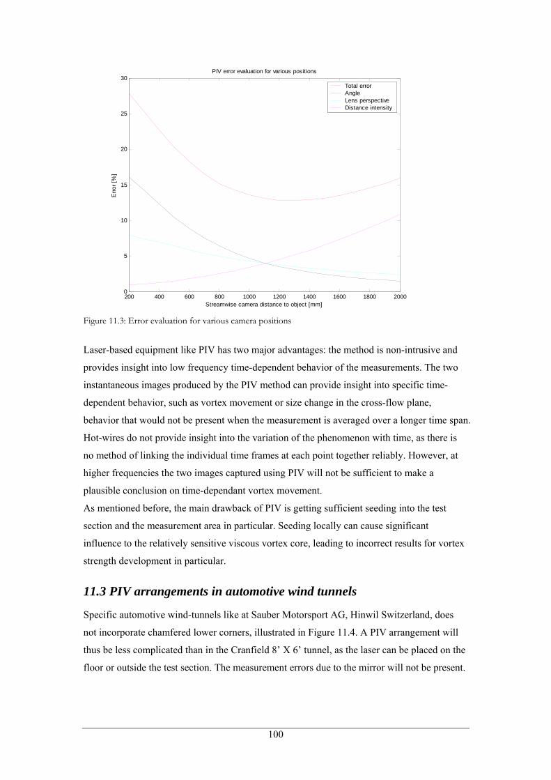
200 400 600 800 1000 1200 1400 1600 1800 20000
5
10
15
20
25
30PIV error evaluation for various positions
Streamwise camera distance to object [mm]
Erro
r [%
]
Total errorAngleLens perspectiveDistance intensity
Figure 11.3: Error evaluation for various camera positions
Laser-based equipment like PIV has two major advantages: the method is non-intrusive and
provides insight into low frequency time-dependent behavior of the measurements. The two
instantaneous images produced by the PIV method can provide insight into specific time-
dependent behavior, such as vortex movement or size change in the cross-flow plane,
behavior that would not be present when the measurement is averaged over a longer time span.
Hot-wires do not provide insight into the variation of the phenomenon with time, as there is
no method of linking the individual time frames at each point together reliably. However, at
higher frequencies the two images captured using PIV will not be sufficient to make a
plausible conclusion on time-dependant vortex movement.
As mentioned before, the main drawback of PIV is getting sufficient seeding into the test
section and the measurement area in particular. Seeding locally can cause significant
influence to the relatively sensitive viscous vortex core, leading to incorrect results for vortex
strength development in particular.
11.3 PIV arrangements in automotive wind tunnels
Specific automotive wind-tunnels like at Sauber Motorsport AG, Hinwil Switzerland, does
not incorporate chamfered lower corners, illustrated in Figure 11.4. A PIV arrangement will
thus be less complicated than in the Cranfield 8’ X 6’ tunnel, as the laser can be placed on the
floor or outside the test section. The measurement errors due to the mirror will not be present.
100
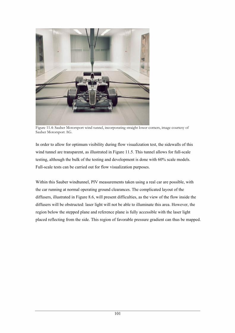
Figure 11.4: Sauber Motorsport wind tunnel, incorporating straight lower corners, image courtesy of Sauber Motorsport AG.
In order to allow for optimum visibility during flow visualization test, the sidewalls of this
wind tunnel are transparent, as illustrated in Figure 11.5. This tunnel allows for full-scale
testing, although the bulk of the testing and development is done with 60% scale models.
Full-scale tests can be carried out for flow visualization purposes.
Within this Sauber windtunnel, PIV measurements taken using a real car are possible, with
the car running at normal operating ground clearances. The complicated layout of the
diffusers, illustrated in Figure 8.6, will present difficulties, as the view of the flow inside the
diffusers will be obstructed: laser light will not be able to illuminate this area. However, the
region below the stepped plane and reference plane is fully accessible with the laser light
placed reflecting from the side. This region of favorable pressure gradient can thus be mapped.
101
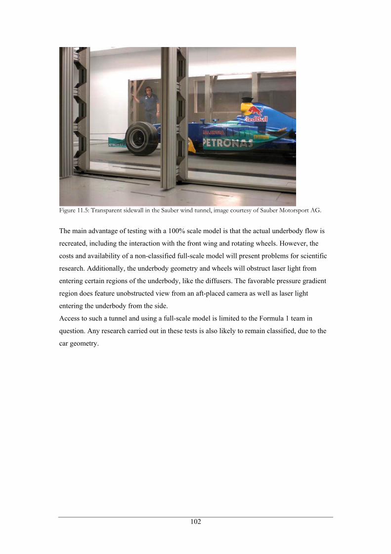
Figure 11.5: Transparent sidewall in the Sauber wind tunnel, image courtesy of Sauber Motorsport AG.
The main advantage of testing with a 100% scale model is that the actual underbody flow is
recreated, including the interaction with the front wing and rotating wheels. However, the
costs and availability of a non-classified full-scale model will present problems for scientific
research. Additionally, the underbody geometry and wheels will obstruct laser light from
entering certain regions of the underbody, like the diffusers. The favorable pressure gradient
region does feature unobstructed view from an aft-placed camera as well as laser light
entering the underbody from the side.
Access to such a tunnel and using a full-scale model is limited to the Formula 1 team in
question. Any research carried out in these tests is also likely to remain classified, due to the
car geometry.
102
Chapter 12
Overall conclusions and discussion
12.1 Conclusions
Inviscid theory predicts increased vorticity when subjected to a favorable pressure gradient,
due to the stretching and spin-up of the vortex. Viscous effects lead to a decrease in vortex
strength, with the vorticity development depending on the magnitude of this effect.
Testing was carried out using a cropped-delta SBVG with a device height of h = 42 mm, at a
device height Reynolds number of Reh = 4.3 ·104, with a local boundary layer thickness of δ =
120 mm. Tests in a bump-generated pressure distribution with a maximum favorable pressure
gradient of ( ) 7.0pCx c
∂= −∂ and a maximum bump height of 488 mm, showed a vorticity
decrease of 85 % over 1.4 m of favorable pressure gradient section compared to 67 % for the
zero pressure gradient measurements. The viscous effects for the single bump tests
outweighed the spin-up effects, illustrated by the vorticity decrease. The increase in skin
friction coefficient due to the favorable pressure gradient and the decreasing distance between
vortex and bump surface are the main factors behind the increased viscous effects.
Double bump tests were carried out, mounting two halves of the single bump on the sidewalls
of the test section. Results showed less vortex strength and vorticity decrease than was the
case for the single bump. The increased distance between the vortex and the test section floor
is the main factor behind the decreased loss in vortex strength and vorticity, as the wall-
mounted bumps allowed for a flat floor surface for the vortex.
Vortex behavior in underbody conditions is reasoned to have increased vortex strength decay
compared to the bump tests, due to the presence of the extra ground surface. Additionally the
small ground clearance of approximately 80 mm for the F1 car results in a small distance
between the vortex and both body and ground surface, thus increasing vortex strength decay.
Vortex strength decay due to interaction with the moving ground surface is expected to be
lower than for interaction with the body surface, as the skin friction coefficient on the moving
ground is significantly smaller.
103
The second goal of this study was to generate an arrangement that will allow for the mapping
of a vortex through the underbody region of a Formula 1 car, incorporating as many
aerodynamic factors as possible. The proposed arrangement incorporates a simplified
underbody model suspended at a variable height above a rotating belt, using a moving ground
wind tunnel.
Taking the facilities at Cranfield University into consideration, the 8’ X 6’ Moving Ground
tunnel would be the tunnel of choice, with a number of modifications to facilitate PIV
measurements. This is because the chamfered, non-transparent corners of the test section
prevent laser measurements from being taken from the side of the model. The laser will have
to be placed on the side walls next to the control room, with the diverged laser light being
reflected by means of a back-face mirror. The laser light will have to be diverged prior to
reaching the mirror, in order to prevent permanent damage to the mirror. The mirror will have
to be as smooth as possible, to prevent distortions to the laser light and thus cause
measurement errors. The CCD camera recording the laser light sheet will be positioned
behind the rotating belt, at an axial distance of 1200 mm from the measured position to
minimize measurement errors.
For further research into vortex behavior in pressure gradients, a laser-based system like PIV
is preferred over HWA measurements. PIV will allow for vortex mapping at significantly
higher resolution then the pointwise HWA measurements, thus resulting in improved
accuracy regarding both vorticity and vortex strength. Additionally the reliability of the
results increases, as the entire flow field is mapped practically instantaneous per streamwise
location, rather than long period required for the HWA measurement array. Conditions for
PIV measurements will be significantly more constant than for HWA measurements, which is
sensitive to temperature changes in particular.
PIV measurements can also provide insight into the effect of the HWA probe on the flow
itself, as the probe protrudes into the flow.
12.2 Discussion
For the Formula 1 underbody case, vortex strength decay will increase when the ride height
decreases. The smaller distance between the vortex and both surfaces, in addition to the
further acceleration, will cause increased vortex strength decay. Vorticity development will
depend on the magnitude of the pressure gradient at that particular ride height.
For aerospace applications, the results can be applied to the application of ‘cove’ Sub
Boundary Layer Vortex Generator devices. These cove devices are designed for placement on
104
the pressure side of slats or the leading edge of the main airfoil, generating vortices to
increase mixing over the main element once the slat is extended.
For the cove device case, vorticity is expected to increase when subjected to the favorable
pressure gradient. This is due to two reasons: the thin, predominantly laminar boundary layer
at the leading edge of the main element and the magnitude of the favorable pressure gradient.
The magnitude of the favorable pressure gradient at the leading edge is significantly higher
than for the single bump case, and is therefore expected to outweigh the viscous effects.
It remains to be seen if cove devices prove to be more effective at augmenting the wing’s
performance at high angles of attack than SBVGs placed in ‘traditional’ positions ahead of
the adverse pressure gradient, as vortex strength will still decrease due to the viscous effects,
regardless of the increased vorticity due to the favorable pressure gradient.
The results for both vortex strength and vorticity development from this study provide
verification data to future CFD code improvements. Improved CFD methods can provide
designers with more powerful tools to design racecars, as vortex development results will
resemble the real case closer compared to the current commercial packages. Wind tunnel tests
are still considered the main tool to develop the aerodynamic package of a racecar, illustrated
by the fact that over 600 separate parts were tested in the wind tunnel development of the
2003 Lister LMP sportscar, after Thorby [26]. Improved CFD methods could provide designers
with more reliable insight into the effect of these pieces prior to testing, which in turn can
reduce the amount of pieces tested, lowering costs for both manufacturing and testing.
105
References
[1] J.D. Anderson, “Fundamentals of Aerodynamics”, McGraw-Hill Inc, Third Edition, 2001
[2] W. Li, R.K. Decker, J.W. Lew and J.W.Naughton, “Characteristics of Turbulent Boundary
Layers on Rough Surfaces with Favorable Pressure Gradients” AIAA Paper No. 2001-2915,
2001
[3] Batchelor, "Theory of Homogeneous Turbulence", Cambridge University Press, 1953
[4] ESDU 93024 “Vortex Generators for Control of Shock-Induced Separation - Part 1:
Introduction and Aerodynamics”, 1995.
[5] P.R. Ashill, J.L. Fulker and K.C. Hackett, “Research at DERA on Sub Boundary Layer
Vortex Generators (SBVGs)” AIAA Paper No. 2001-0887, 2001
[6] P.R. Ashill, J.L. Fulker and K.C. Hackett, “Studies of flows induced by Sub Boundary
Layer Vortex Generators (SBVGs)” AIAA Paper No. 2002-0968, 2002
[7] C. Bruckner, “Development and structural changes of vortex breakdown” AIAA Paper No.
95/2305, 1995
[8] C-S Yao, J.C. Lin and B.G Allan, “Flow-Field Measurement of Device-Induced
Embedded Streamwise Vortex on a Flat Plate” AIAA Paper No. 2002-3162, 2002
[9] H.H. Brunn, “Hot-wire anemometry : principles and signal analysis”, Oxford University
Press, 1995
[10] T. S. Lundgren and W. T. Ashurst. “Area-varying waves on curved vortex tubes with
application to vortex breakdown” Journal of Fluid Mechanics, Vol. 200, 1989, pp.283-307
[11] C.J. Doolan, F.N. Coton and R.A. McD. Galbraith, “Measurement of Three-Dimensional
Vortices using a Hot Wire Anemometer” AIAA Paper No. 99-3810, 1999
[12] W.J. Devenport, M.C. Rife, S.I. Liapis and G.J. Follin, “The structure and development
of a wing-tip vortex” Journal of Fluid Mechanics, Vol. 312, 1996, pp.67-106
[13] A.T. Conlisk, “A Theory of Vortex-Surface Collisions” AIAA Paper No. 98-2858, 1998
[14] J. Katz, “Race Car Aerodynamics: Designing for Speed”, Bentley Publishers, 1996
[15] S. McBeath, “Competitoin Car Downforce”, Haynes Publishing, 1998
[16] S.B. Pope, “Turbulent Flows”, Cambridge University Press, 2000
[17] D. Drikakis, “Advanced in Turbulent Flow Computations Using High-resolution
Methods”, Newton Institute Paper No. 03018, 2003
[18] Fluent 6.1 manual, Fluent Corporation, 2003
[19] F. De Sousa and D. Faghani, “Near-Field Wing Tip Vortex Measurement via PIV”,
AIAA Paper No. 2001-2452, 2001
106
[20] D.L. Garcia and J. Katz, “Trapped-Vortex in Ground Effect”, AIAA Paper No. 2002-
3307, 2002
[21] Federation International de l’Automobile, 2004 Formula 1 Technical Regulations,
http://www.fia.com, 2004
[22] J.B. Barlow, W.H. Rae Jr., A. Pope, “Low-Speed Wind Tunnel Testing”, John Wiley &
Sons Inc, Third Edition, 1999
[23] P. Wright, “Formula 1 Technology”, SAE International, 2001
[24] G. Piola, “Formula 1 2002 Technical Analysis”, Giorgio Nada Editore S.r.l. 2003
[25] N.J. Lawson, M. Reeves, “Evaluation and correction of perspective errors in endoscopic
PIV”, Experiments in Fluids No. 36, 2004, pp 701-705
[26] A. Thorby, “The design of a Le Mans prototype”, Race Tech No. 49-50, 2003
107
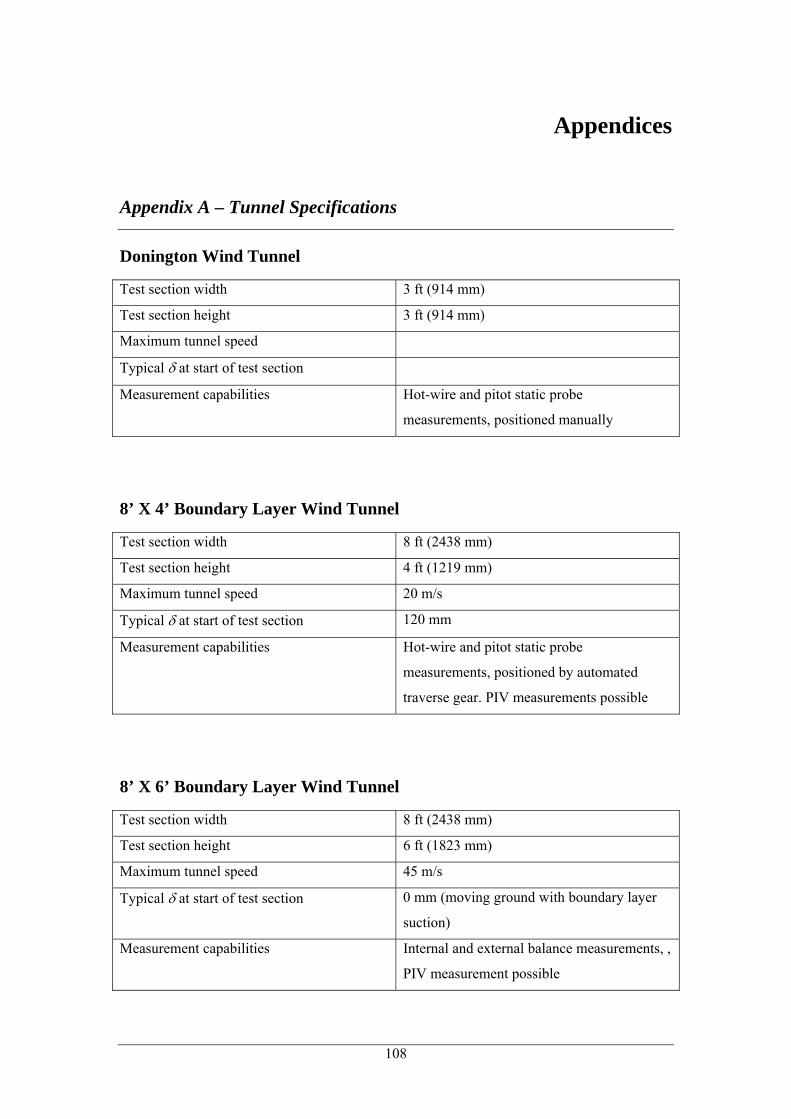
Appendices
Appendix A – Tunnel Specifications
Donington Wind Tunnel
Test section width 3 ft (914 mm)
Test section height 3 ft (914 mm)
Maximum tunnel speed
Typical δ at start of test section
Measurement capabilities Hot-wire and pitot static probe
measurements, positioned manually
8’ X 4’ Boundary Layer Wind Tunnel
Test section width 8 ft (2438 mm)
Test section height 4 ft (1219 mm)
Maximum tunnel speed 20 m/s
Typical δ at start of test section 120 mm
Measurement capabilities Hot-wire and pitot static probe
measurements, positioned by automated
traverse gear. PIV measurements possible
8’ X 6’ Boundary Layer Wind Tunnel
Test section width 8 ft (2438 mm)
Test section height 6 ft (1823 mm)
Maximum tunnel speed 45 m/s
Typical δ at start of test section 0 mm (moving ground with boundary layer
suction)
Measurement capabilities Internal and external balance measurements, ,
PIV measurement possible
108
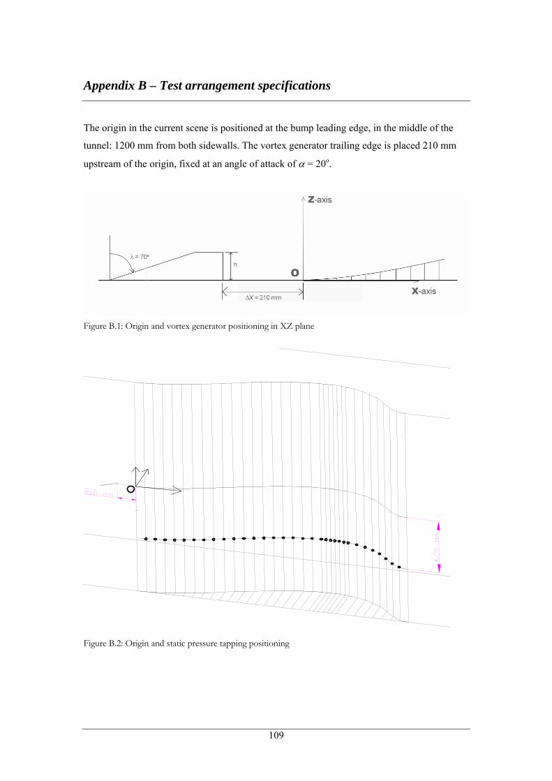
Appendix B – Test arrangement specifications
The origin in the current scene is positioned at the bump leading edge, in the middle of the
tunnel: 1200 mm from both sidewalls. The vortex generator trailing edge is placed 210 mm
upstream of the origin, fixed at an angle of attack of α = 20o.
Figure B.1: Origin and vortex generator positioning in XZ plane
Figure B.2: Origin and static pressure tapping positioning
109
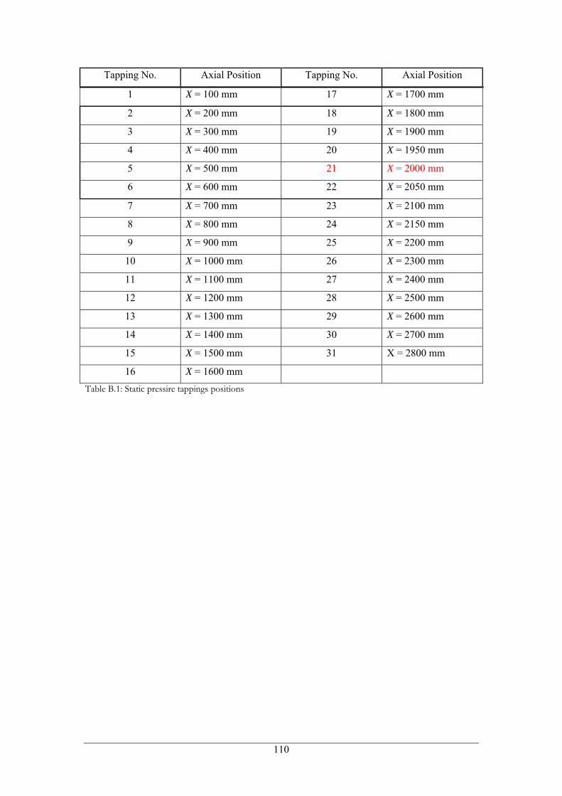
Tapping No. Axial Position Tapping No. Axial Position
1 X = 100 mm 17 X = 1700 mm
2 X = 200 mm 18 X = 1800 mm
3 X = 300 mm 19 X = 1900 mm
4 X = 400 mm 20 X = 1950 mm
5 X = 500 mm 21 X = 2000 mm
6 X = 600 mm 22 X = 2050 mm
7 X = 700 mm 23 X = 2100 mm
8 X = 800 mm 24 X = 2150 mm
9 X = 900 mm 25 X = 2200 mm
10 X = 1000 mm 26 X = 2300 mm
11 X = 1100 mm 27 X = 2400 mm
12 X = 1200 mm 28 X = 2500 mm
13 X = 1300 mm 29 X = 2600 mm
14 X = 1400 mm 30 X = 2700 mm
15 X = 1500 mm 31 X = 2800 mm
16 X = 1600 mm Table B.1: Static pressire tappings positions
110
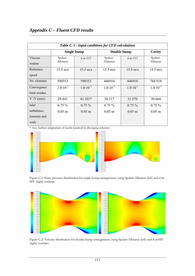
Appendix C – Fluent CFD results
Table C. I : Input conditions for CFD calculations
Single bump Double bump Cavity
Viscous
routine
Spalart-Allmaras
k-ω SST Spalart-Allmaras
k-ω SST Spalart-Allmaras
Reference
speed 15.5 m/s 15.5 m/s 15.5 m/s 15.5 m/s 15.5 m/s
No. elements 590553 590553 446910 446910 768 918
Convergence
limit residue 1.0⋅10-3 1.0⋅10-3 1.0⋅10-3 1.0⋅10-3 1.0⋅10-3
Y+/Y (max) 29.441 41.101* 34.117 31.570 30.664
Inlet
turbulence,
intensity and
scale
0.75 %
0.05 m
0.75 %
0.05 m
0.75 %
0.05 m
0.75 %
0.05 m
0.75 %
0.05 m
* Any further adaptation of mesh resulted in diverging solution
Figure C.1: Static pressure distribution for single bump arrangement, using Spalart-Allmaras (left) and k-ω SST (right) routines.
Figure C.2: Velocity distribution for double bump arrangement, using Spalart-Allmaras (left) and k-ω SST (right) routines.
111
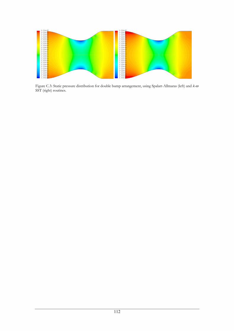
Figure C.3: Static pressure distribution for double bump arrangement, using Spalart-Allmaras (left) and k-ω SST (right) routines.
112
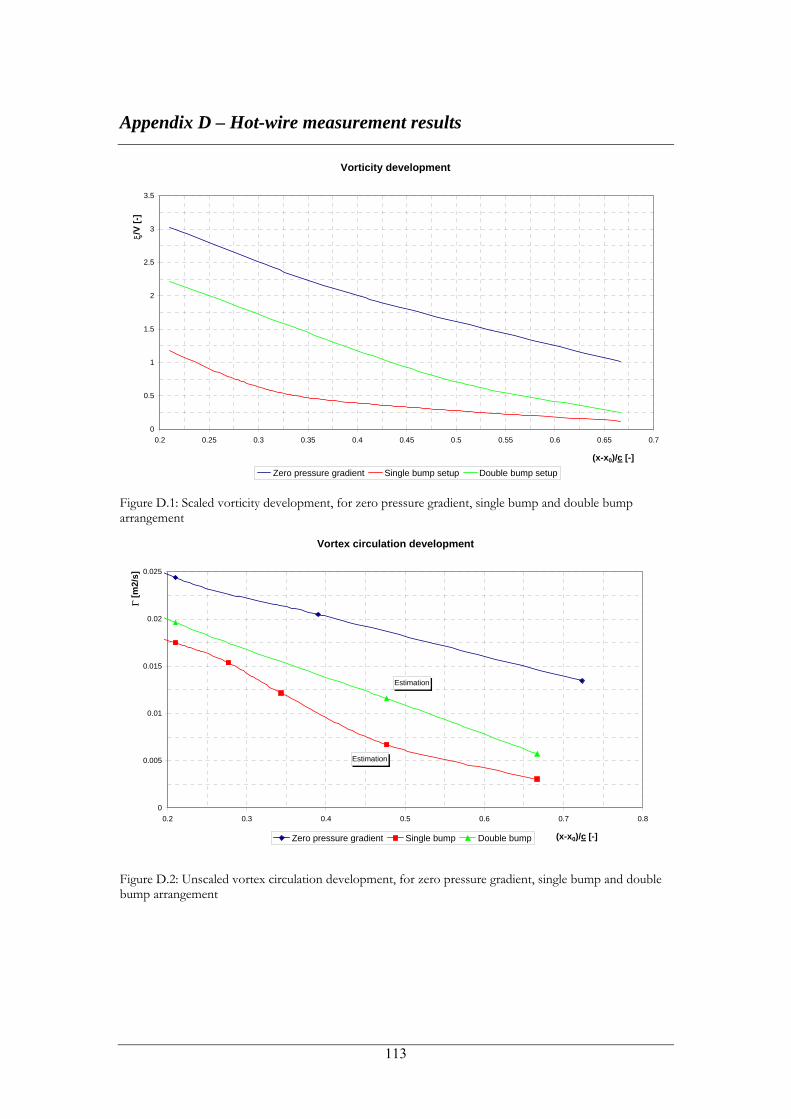
Appendix D – Hot-wire measurement results
Vorticity development
0
0.5
1
1.5
2
2.5
3
3.5
0.2 0.25 0.3 0.35 0.4 0.45 0.5 0.55 0.6 0.65 0.7
(x-x0)/c [-]
ξ/V
[-]
Zero pressure gradient Single bump setup Double bump setup
Figure D.1: Scaled vorticity development, for zero pressure gradient, single bump and double bump arrangement
Vortex circulation development
Estimation
Estimation
0
0.005
0.01
0.015
0.02
0.025
0.2 0.3 0.4 0.5 0.6 0.7 0.8
(x-x0)/c [-]
Γ [m
2/s]
Zero pressure gradient Single bump Double bump
Figure D.2: Unscaled vortex circulation development, for zero pressure gradient, single bump and double bump arrangement
113
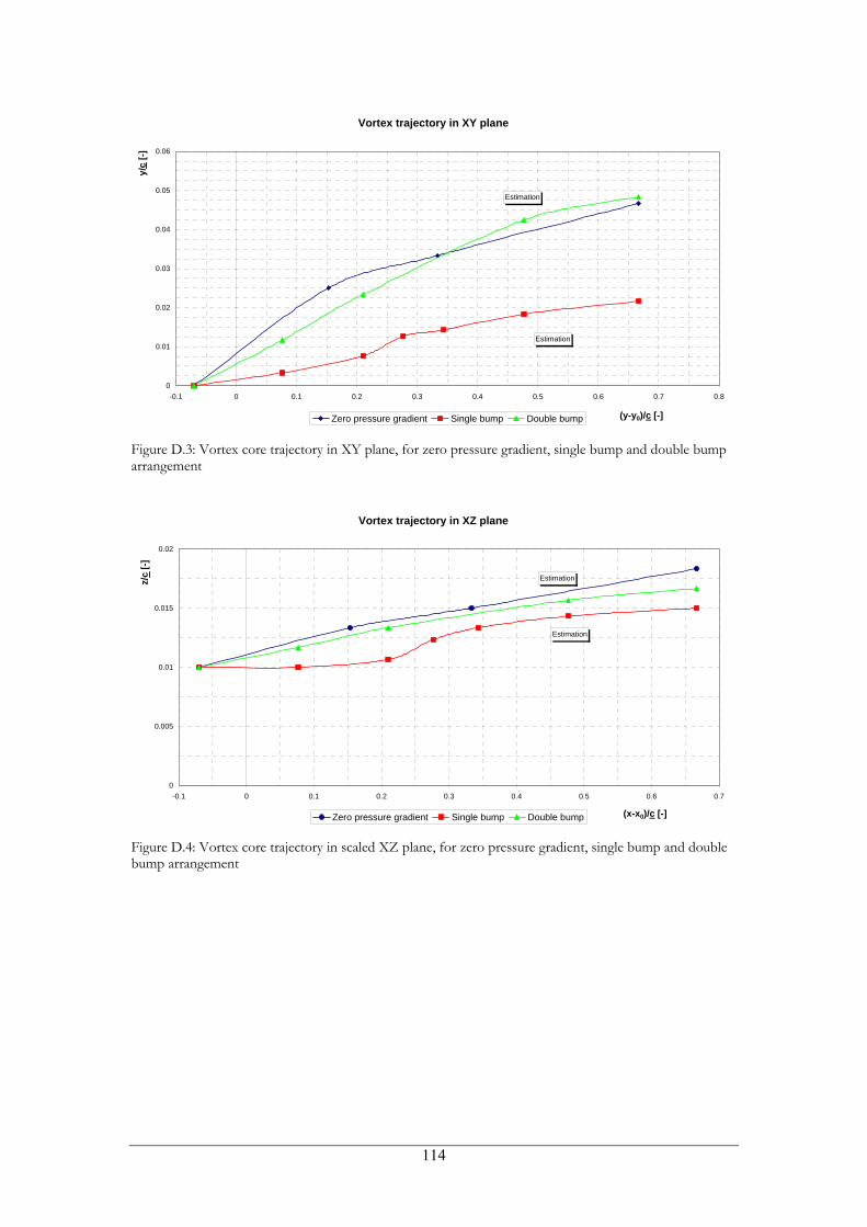
Vortex trajectory in XY plane
Estimation
Estimation
0
0.01
0.02
0.03
0.04
0.05
0.06
-0.1 0 0.1 0.2 0.3 0.4 0.5 0.6 0.7 0.8
(y-y0)/c [-]
y/c
[-]
Zero pressure gradient Single bump Double bump Figure D.3: Vortex core trajectory in XY plane, for zero pressure gradient, single bump and double bump arrangement
Vortex trajectory in XZ plane
Estimation
Estimation
0
0.005
0.01
0.015
0.02
-0.1 0 0.1 0.2 0.3 0.4 0.5 0.6 0.7
(x-x0)/c [-]
z/c
[-]
Zero pressure gradient Single bump Double bump Figure D.4: Vortex core trajectory in scaled XZ plane, for zero pressure gradient, single bump and double bump arrangement
114
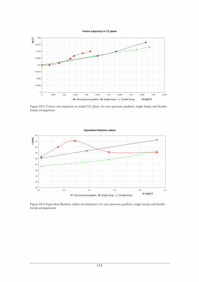
Vortex trajectory in YZ plane
0
0.0025
0.005
0.0075
0.01
0.0125
0.015
0.0175
0.02
0 0.005 0.01 0.015 0.02 0.025 0.03 0.035 0.04 0.045 0.05 0.055
(y-y0)/c [-]
z/c
[-]
Zero pressure gradient Single bump Double bump Figure D.5: Vortex core trajectory in scaled YZ plane, for zero pressure gradient, single bump and double bump arrangement
Equivalent Rankine radius
30
35
40
45
50
55
60
65
70
75
0.2 0.3 0.4 0.5 0.6 0.7
(x-x0)/c [-]
r [m
m]
Zero pressure gradient Single bump Double bump
Figure D.6: Equivalent Rankine radius development, for zero pressure gradient, single bump and double bump arrangements
115
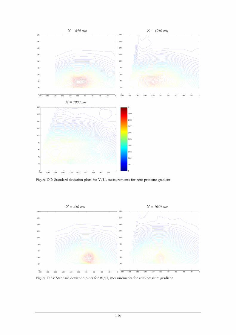
X = 640 mm X = 1040 mm
-200 -180 -160 -140 -120 -100 -80 -60 -40 -20 00
20
40
60
80
100
120
140
160
180
-200 -180 -160 -140 -120 -100 -80 -60 -40 -20 00
20
40
60
80
100
120
140
160
180
X = 2000 mm
-200 -180 -160 -140 -120 -100 -80 -60 -40 -20 00
20
40
60
80
100
120
140
160
180
0
0.01
0.02
0.03
0.04
0.05
0.06
0.07
0.08
0.09
0.1
Figure D.7: Standard deviation plots for V/U0 measurements for zero pressure gradient
X = 640 mm X = 1040 mm
-200 -180 -160 -140 -120 -100 -80 -60 -40 -20 00
20
40
60
80
100
120
140
160
180
-200 -180 -160 -140 -120 -100 -80 -60 -40 -20 00
20
40
60
80
100
120
140
160
180
Figure D.8a: Standard deviation plots for W/U0 measurements for zero pressure gradient
116
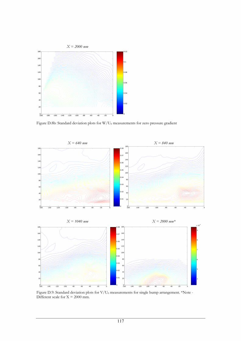
X = 2000 mm
-200 -180 -160 -140 -120 -100 -80 -60 -40 -20 00
20
40
60
80
100
120
140
160
180
0
0.02
0.04
0.06
0.08
0.1
0.12
Figure D.8b: Standard deviation plots for W/U0 measurements for zero pressure gradient
X = 640 mm X = 840 mm
-160 -140 -120 -100 -80 -60 -40 -20 00
20
40
60
80
100
120
140
160
180
0
0.01
0.02
0.03
0.04
0.05
0.06
0.07
0.08
-160 -140 -120 -100 -80 -60 -40 -20 00
20
40
60
80
100
120
140
160
180
X = 1040 mm X = 2000 mm*
-160 -140 -120 -100 -80 -60 -40 -20 00
20
40
60
80
100
120
140
160
180
0
0.01
0.02
0.03
0.04
0.05
0.06
0.07
0.08
-160 -140 -120 -100 -80 -60 -40 -20 00
20
40
60
80
100
120
140
160
180
4
5
6
7
8
9
x 10-3
Figure D.9: Standard deviation plots for V/U0 measurements for single bump arrangement. *Note - Different scale for X = 2000 mm.
117
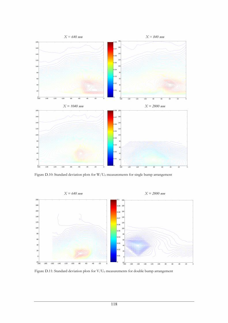
X = 640 mm X = 840 mm
-160 -140 -120 -100 -80 -60 -40 -20 00
20
40
60
80
100
120
140
160
180
0
0.01
0.02
0.03
0.04
0.05
0.06
0.07
0.08
-160 -140 -120 -100 -80 -60 -40 -20 00
20
40
60
80
100
120
140
160
180
X = 1040 mm X = 2000 mm
-160 -140 -120 -100 -80 -60 -40 -20 00
20
40
60
80
100
120
140
160
180
0
0.01
0.02
0.03
0.04
0.05
0.06
0.07
0.08
-160 -140 -120 -100 -80 -60 -40 -20 00
20
40
60
80
100
120
140
160
180
Figure D.10: Standard deviation plots for W/U0 measurements for single bump arrangement
X = 640 mm X = 2000 mm
-200 -180 -160 -140 -120 -100 -80 -60 -40 -20 0-20
0
20
40
60
80
100
120
140
160
180
200
0
0.01
0.02
0.03
0.04
0.05
0.06
0.07
0.08
0.09
0.1
-200 -180 -160 -140 -120 -100 -80 -60 -40 -20 0-20
0
20
40
60
80
100
120
140
160
180
200
Figure D.11: Standard deviation plots for V/U0 measurements for double bump arrangement
118
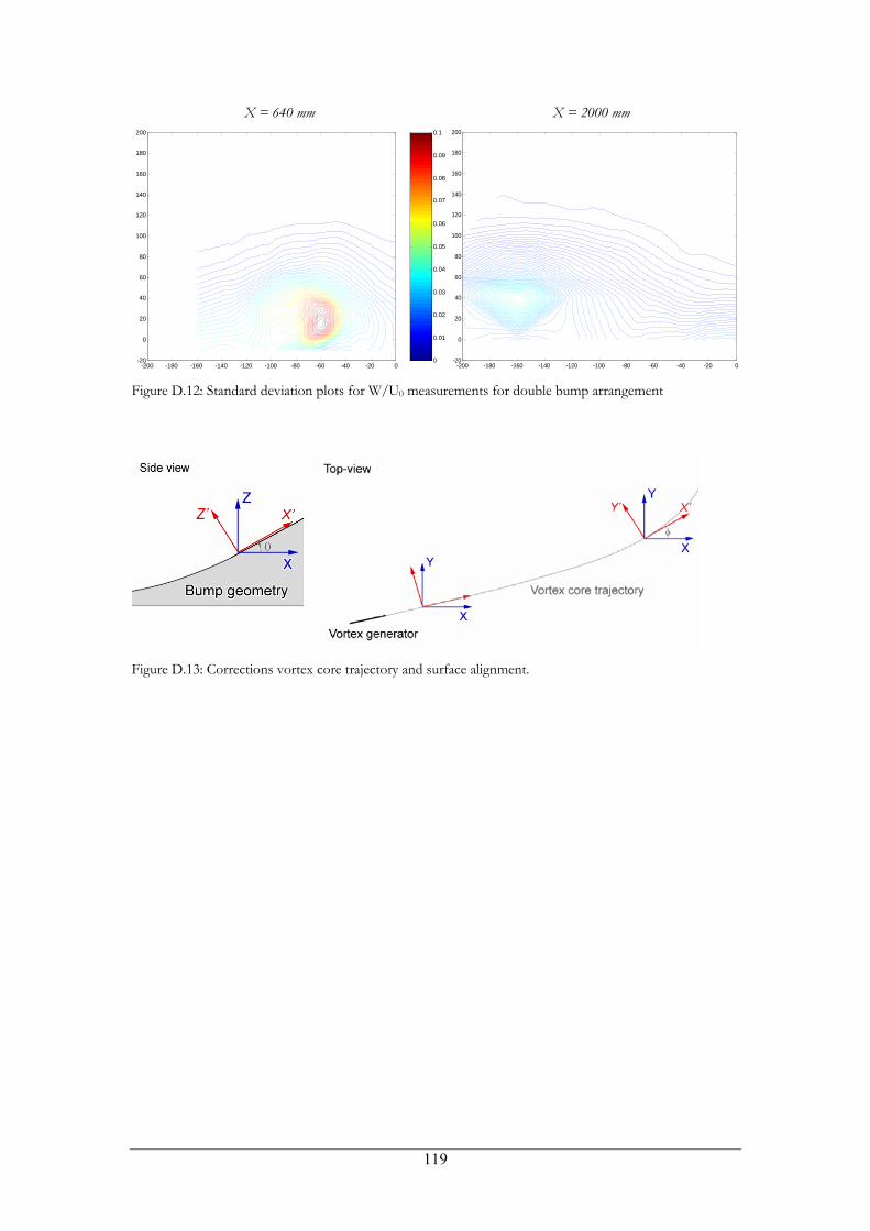
X = 640 mm X = 2000 mm
-200 -180 -160 -140 -120 -100 -80 -60 -40 -20 0-20
0
20
40
60
80
100
120
140
160
180
200
0
0.01
0.02
0.03
0.04
0.05
0.06
0.07
0.08
0.09
0.1
-200 -180 -160 -140 -120 -100 -80 -60 -40 -20 0-20
0
20
40
60
80
100
120
140
160
180
200
Figure D.12: Standard deviation plots for W/U0 measurements for double bump arrangement
Figure D.13: Corrections vortex core trajectory and surface alignment.
119
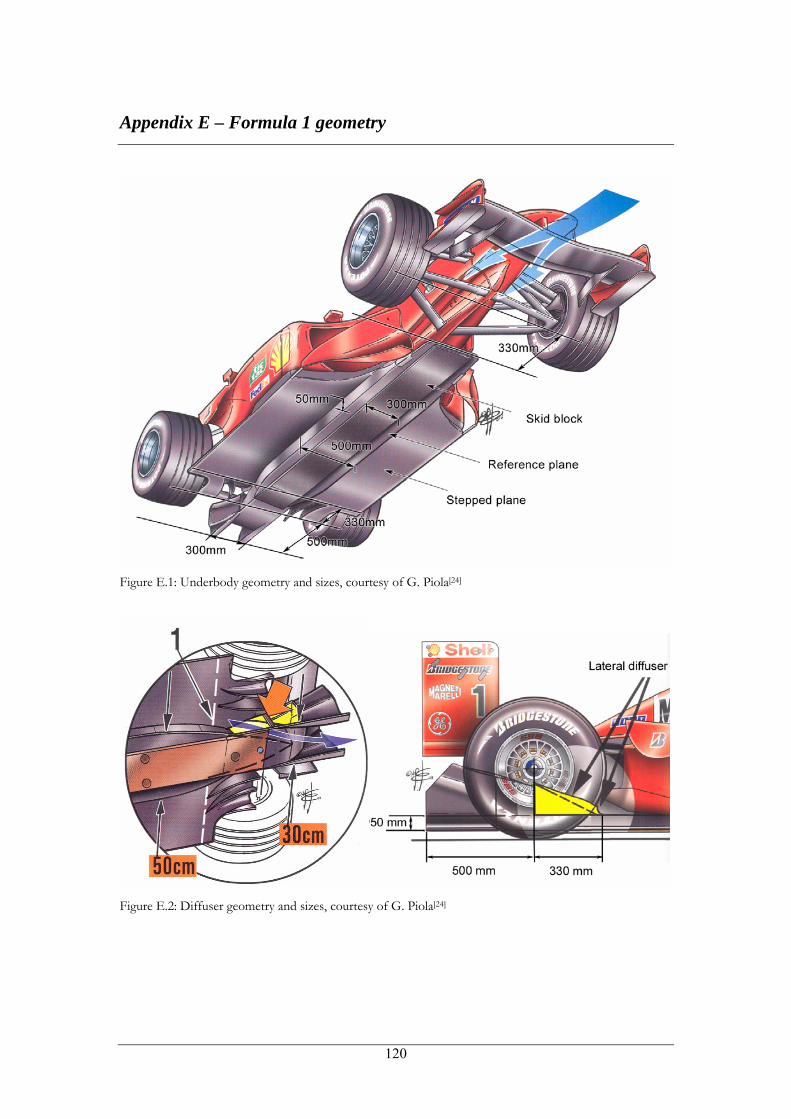
Appendix E – Formula 1 geometry
Figure E.1: Underbody geometry and sizes, courtesy of G. Piola[24]
Figure E.2: Diffuser geometry and sizes, courtesy of G. Piola[24]
120
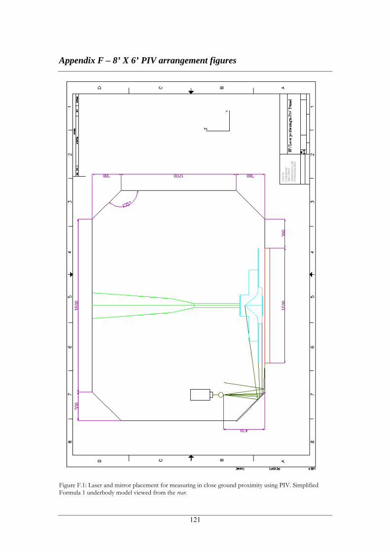
Appendix F – 8’ X 6’ PIV arrangement figures
Figure F.1: Laser and mirror placement for measuring in close ground proximity using PIV. Simplified Formula 1 underbody model viewed from the rear.
121
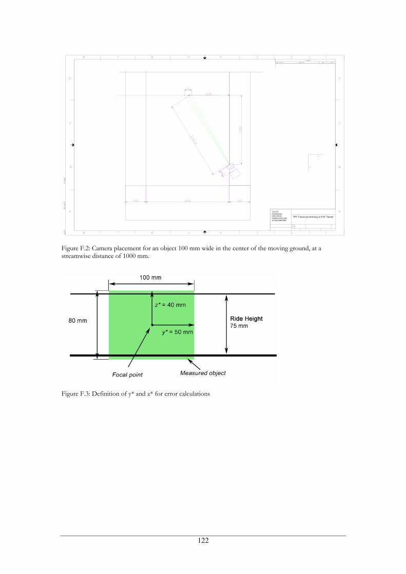
PIV Camera positioning in 8'x6' Tunnel
UNLESS OTHERWISE SPECIFIED, DIMENSIONS ARE IN MILLIMETERS
Figure F.2: Camera placement for an object 100 mm wide in the center of the moving ground, at a streamwise distance of 1000 mm.
Figure F.3: Definition of y* and z* for error calculations
122
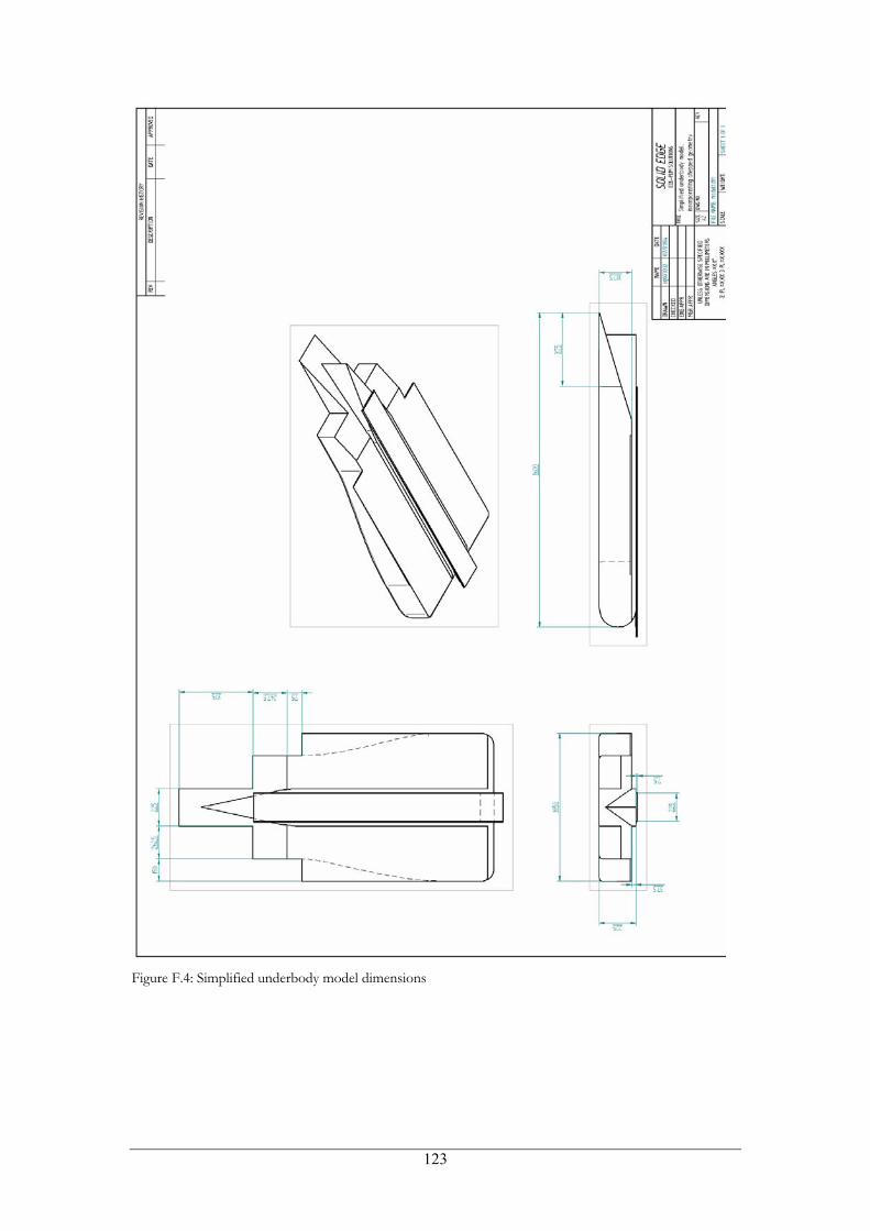
Figure F.4: Simplified underbody model dimensions
123