Embed Size (px)
Citation preview

CITS 4402 Computer Vision
Ajmal Mian
Lecture 09 – Projective Geometry

The University of Western Australia
Overview of this lecture
Computer Vision - Lecture 09 – Projective Geometry 2
Vanishing points and lines
Projective invariants
Cross-ratio
Measuring the height of objects from a single image
Homography
Image rectification
CNN demo and discussion about the Project

The University of Western Australia
Can you work out the geometry of this image?
Computer Vision - Lecture 09 – Projective Geometry 3

The University of Western Australia
Notice the pattern of the trees in this 1460 A.D. painting
Computer Vision - Lecture 09 – Projective Geometry 4

The University of Western Australia
Can you work out the geometry of this image?
Computer Vision - Lecture 09 – Projective Geometry 5

The University of Western Australia
Vanishing points
Computer Vision - Lecture 09 – Projective Geometry 6
In perspective image, all parallel lines meet at a single point.
This point is called the “Vanishing Point”.
Multiple sets of parallel lines will give multiple vanishing points.

The University of Western Australia
Single vanishing point
Computer Vision - Lecture 09 – Projective Geometry 7

The University of Western Australia
Ancient painters were perhaps aware of this concept
Computer Vision - Lecture 09 – Projective Geometry 8
Carpaccio 1514
The University of Western Australia
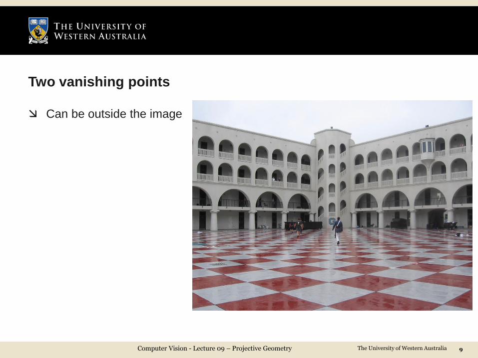
Two vanishing points
Computer Vision - Lecture 09 – Projective Geometry 9
Can be outside the image

The University of Western Australia
Vanishing points and vanishing line
Computer Vision - Lecture 09 – Projective Geometry 10
Joining two vanishing points give a vanishing line
Vertical parallel lines give a
vertical vanishing point
Vertical vanishing point
is at infinity here

The University of Western Australia
Points at infinity
Computer Vision - Lecture 09 – Projective Geometry 11
What are the image coordinates of the point at infinity on the X-axis?
A point at infinity on the X-axis is represented by
1000
.
Where will this appear in the image?
𝑠𝑢𝑠𝑣𝑠
=𝑞11 𝑞12 𝑞13 𝑞14𝑞21 𝑞22 𝑞23 𝑞24𝑞31 𝑞32 𝑞33 𝑞34
1000
=
𝑞11𝑞21𝑞31
Similarly, points at infinity on the y-axis and z-axis are represented by the 2nd and 3rd columns.
The projection of origin of the world coordinates is given by the last column.

The University of Western Australia
Vanishing points and vanishing lines
Computer Vision - Lecture 09 – Projective Geometry 12
Notice how the parallel lines become
non-parallel when projected on the
image plane
Vanishing points are often outside
the image boundary

The University of Western Australia
Vanishing points and vanishing lines
Computer Vision - Lecture 09 – Projective Geometry 13
Notice how the parallel lines become
non-parallel when projected on the
image plane
Vanishing points are often outside
the image boundary

The University of Western Australia
The horizon
Computer Vision - Lecture 09 – Projective Geometry 14
Parallel lines that are not orthogonal to
the optical axis meet at a vanishing point
Two sets of parallel lines on
the ground plane will give
two vanishing points.
Joining the vanishing points
gives the vanishing line or
“horizon”

The University of Western Australia
Vanishing lines
Computer Vision - Lecture 09 – Projective Geometry 15
A set of parallel planes that are not
parallel to the image plane intersect
the image plane at a vanishing line.
The horizon is a special vanishing
line when the set of parallel planes
are parallel to the ground reference.
Anything in the scene that is above the camera will be projected above the horizon in the image.

The University of Western Australia
How to calculate vanishing points and lines
Computer Vision - Lecture 09 – Projective Geometry 16
A point in image is defined by its (u,v) coordinates
Two points determine a line
Intersection of two parallel lines will give us a vanishing point
Two vanishing points will give us the corresponding vanishing line
Two clicks on each parallel line will solve the problem
For automatic solution: Edge detection + Hough lines will solve the problem

The University of Western Australia
Points and lines in Homogeneous coordinates
Computer Vision - Lecture 09 – Projective Geometry 17
Points in 2D are represented in homogeneous coordinates as a 3-vector
𝑥𝑦1
.
Points and lines are dual in 2D, so lines are represented in homogeneous
coordinates as 3-vector also:
𝑎𝑏𝑐
.
Homogeneous coordinates contain redundant information – the representation includes an arbitrary scale!
e.g., 2 3 1 𝑇 and 4 6 2 𝑇 represent the same point 2 3 𝑇 in inhomogeneous coordinates.
e.g., 4 7 −3 𝑇 and 2 3.5 −1.5 𝑇 represent the same line – as 4𝑥 + 7𝑦 −3 = 0 and 2𝑥 + 3.5𝑦 − 1.5 = 0 denote the same line.
To determine if a line 𝒍 = 𝑎 𝑏 𝑐 𝑇 passes through a point 𝒑 = 𝑥 𝑦 1 𝑇
check if their dot product is 0. That is, 𝒍𝑇𝒑 = 0 ⇒ 𝒍 passes through 𝒑. Example: Line 2 4 5 𝑇contains the point 1.5 −2 1 𝑇 since 2 4 5 ∙1.5 −2 1 = 2 ∗ 1.5 − 4 ∗ 2 + 5 ∗ 1 = 0.

The University of Western Australia
Equation of a line given two points
Computer Vision - Lecture 09 – Projective Geometry 18
The line 𝒍 that passes through two points 𝒑1 =𝑥1𝑦11
and 𝒑𝟐 =𝑥2𝑦21
is obtained via
the cross product
𝒍 = 𝒑1 × 𝒑2.
Example: the line 𝒍 passing through the points 0 2 1 𝑇 and 3 0 1 𝑇 is:
021
×301
=23−6
.
Thus, the equation of the line is 2𝑥 + 3𝑦 − 6 = 0.

The University of Western Australia
Finding the intersection of two lines
Computer Vision - Lecture 09 – Projective Geometry 19
Since lines and points are dual in 2D, we obtain the line coordinates the same
way as before. The point of intersection 𝒑 of two given lines 𝒍1 = 𝑎1 𝑏1 𝑐1𝑇
and 𝒍2 = 𝑎2 𝑏2 𝑐2𝑇 is obtained via the cross product
𝒑 = 𝒍1 × 𝒍2.
Example: The lines 4 6 2 𝑇 and 2 0 1 𝑇 intersection at 6 0 −12 𝑇
which corresponds to the point −1
20
𝑇in inhomogeneous coordinates.
Exercise: What are the coordinates of the intersection point of lines 3 1 2 𝑇 and 6 2 2 𝑇 ?

The University of Western Australia
𝒍1
𝒍2
𝒑
Can you find the equation of the vanishing line in this image?
Computer Vision - Lecture 09 – Projective Geometry 20
Click on red points to get the first line
Click on the green points to get the second line
Find their intersection
Repeat the process for another
set of parallel lines
Cross produce of the two
vanishing points will give the
equation of the vanishing line

The University of Western Australia
What can we find from the vanishing points and lines?
Computer Vision - Lecture 09 – Projective Geometry 21
Given the horizon, the vertical vanishing point and one
reference height.
The height of any point (from the ground plane) can be
computed by specifying the point and its projection on the
ground plane in the image.
Criminisi et al 1998.

The University of Western Australia
Human height measurement - example
Computer Vision - Lecture 09 – Projective Geometry 22
If we know the height of one object in the scene
We can find the height of a person using vanishing
points

The University of Western Australia
Representation of various transformations
Computer Vision - Lecture 09 – Projective Geometry 23
Euclidean transformation:
2D: 𝑟11 𝑟12 𝑡1𝑟12 𝑟22 𝑡20 0 1
3D:
𝑟11 𝑟12 𝑟13 𝑡1𝑟21 𝑟22 𝑟23 𝑡2𝑟310
𝑟320
𝑟330
𝑡31
Similarity transformation:
2D: 𝑟11 𝑟12 𝑡1𝑟12 𝑟22 𝑡20 0 𝑠
3D:
𝑟11 𝑟12 𝑟13 𝑡1𝑟21 𝑟22 𝑟23 𝑡2𝑟310
𝑟320
𝑟330
𝑡3𝑠
Affine transformation:
2D: × × ×× × ×0 0 1
3D:
× × × ×× × × ××0
×0
×0
×1
Projective transformation:
2D: × × ×× × ×× × 1
3D:
× × × ×× × × ×××
××
××
×1

The University of Western Australia
Geometric invariants
Computer Vision - Lecture 09 – Projective Geometry 24
Preserves
ratios of lengths
ratios of areas
parallelism
concurrency
collinearity
cross-ratio
Preserves
concurrency
collinearity
cross-ratio
Preserves
angles
ratios of lengths
ratios of areas
parallelism
concurrency
collinearity
cross-ratio

The University of Western Australia
Cross-ratio
Computer Vision - Lecture 09 – Projective Geometry 25
Most important geometric invariant for projective transformation is the cross-ratio
of 4 points on a line.
The cross-ratio is the ratio of two ratios of lengths
• Given 4 points on a line, say A, B, C and 𝐷.
• Take 𝑥1 as the 1st reference point, compute 𝑟1 = 𝐴𝐶 𝐴𝐷 .
• Take 𝑥2 as the 2nd reference point, compute 𝑟2 = 𝐵𝐶 𝐵𝐷 .
• Cross-ratio is defined as 𝑟 = 𝑟1 𝑟2 .
The two reference points and the ratios can also be arbitrary chosen
e.g. 𝑟1 can be set to 𝐶𝐷 𝐶𝐵 , 𝑟2 can be set to 𝐴𝐷 𝐴𝐵 , and 𝑟 = 𝑟2 𝑟1 .
There are 4! = 24 permutations of possible cross-ratio values however, these
values are repeated leaving only 6 unique cross-ratio possibilities

The University of Western Australia Computer Vision - Lecture 09 – Projective Geometry 26

The University of Western Australia
Cross-ratio of equidistant points
Computer Vision - Lecture 09 – Projective Geometry 27
A B C D
1 1 1

The University of Western Australia
Let us measure it from an image with known equidistant points
Computer Vision - Lecture 09 – Projective Geometry 28
Measurements from an
image…
Cross-ratio can always be calculated
from an image.
This cross-ratio will be exactly the same
as in real world.
If one of the measurements is unknown
in the real world, it can be calculated
using the cross ratio

The University of Western Australia
Back to the human height measurement problem
Computer Vision - Lecture 09 – Projective Geometry 29
If we know the height of one object in the scene
We can find the height of a person using vanishing
points

The University of Western Australia
Height measurement with cross-ratio
Computer Vision - Lecture 09 – Projective Geometry 30
All distances are signed distances

The University of Western Australia
Algorithm for calculating height
Computer Vision - Lecture 09 – Projective Geometry 31
Calculate vertical vanishing point
Calculate vanishing line of the reference plane
Select top and base points of the reference object
Compute metric factor
Repeat
• Select top and base points of the object to measure
• Compute the height of the object
A. Criminisi, “Single View Metrology: Algorithms and Applications” 1999.

The University of Western Australia
For precise measurement
Computer Vision - Lecture 09 – Projective Geometry 32
Radial distortion needs to be removed first
Robust detection of parallel lines
Vanishing point detection based on
multiple parallel lines
Heights are not always vertical. Ideally,
the vertical lines should meet at the
vertical vanishing point.

The University of Western Australia
More on cross-ratios
Computer Vision - Lecture 09 – Projective Geometry 33
The 6 possible cross-ratios are: 𝑟, 1
𝑟 , 1 − 𝑟,
𝑟−1
𝑟 ,
1
1−𝑟 ,
𝑟
𝑟−1.
Example of a special case: When 𝑟 =1
2. Then the 6 cross-ratios are not unique:
1
2, 2,
1
2, −1, 2, −1.
This corresponds to the situation where one point is the mid-point of the other
two points while the 4th point is a point at infinity:
X1 X2 X3
𝑋4 = ∞
X2 is the mid-point between X1 and X3, i.e., X3 - X2 = X2 - X1 .

The University of Western Australia
Homography
Images of the same planar surface are related by homography
Homography is used for image rectification (making parallel lines parallel in
images)
Homography is also useful for
• Image registration
• Calculation of camera motion (robot navigation, structure from motion)
• Placing 3D objects in images or videos (augmented reality)
• Inserting new images such as advertisements in movies
Computer Vision - Lecture 09 – Projective Geometry 34

The University of Western Australia
Image rectification
Computer Vision - Lecture 09 – Projective Geometry 35
It is possible to remove perspective distortion of a plane in a scene if
• We can find the vanishing line of the plane
• We have two reference measurements of known lengths and angles
We need to identify 4 points on the plane such that
The University of Western Australia
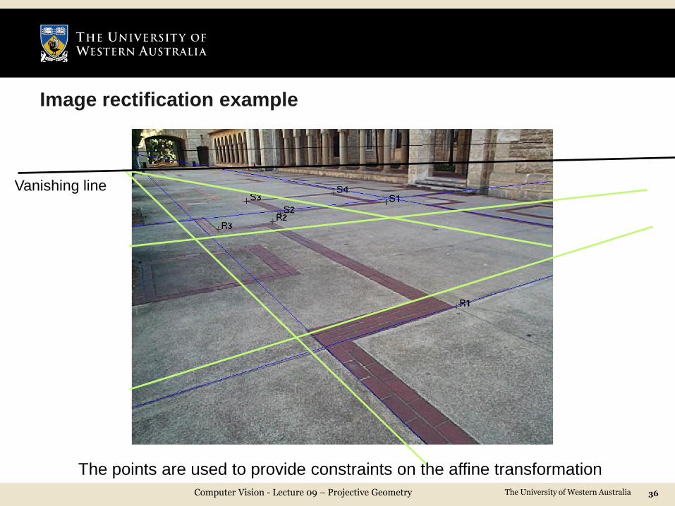
Image rectification example
Computer Vision - Lecture 09 – Projective Geometry 36
Vanishing line
The points are used to provide constraints on the affine transformation

The University of Western Australia
Rectified image
Computer Vision - Lecture 09 – Projective Geometry 37
Cannot include points that are too close to the vanishing line as they are at infinity.

The University of Western Australia
Image rectification
Computer Vision - Lecture 09 – Projective Geometry 38
In general, we need four points for rectifying a plane that has been distorted
by a perspective projection.
Recall the perspective projection equation from Lecture 08
where
We can expand the above equation
The University of Western Australia
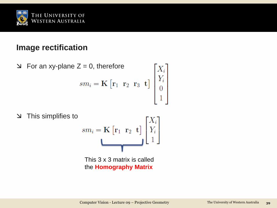
Image rectification
Computer Vision - Lecture 09 – Projective Geometry 39
For an xy-plane Z = 0, therefore
This simplifies to
This 3 x 3 matrix is called
the Homography Matrix

The University of Western Australia
Calculating the homography matrix H
Computer Vision - Lecture 09 – Projective Geometry 40
The homography matrix has 9 unknowns and is defined up to an unknown
scale
We get
Writing it as a system of linear equations
This has for form 𝐴ℎ = 0 and the solution is the right singular vector corresponding to the
smallest singular value of 𝐴 i.e. 𝑠𝑣𝑑 𝐴 = 𝑈𝑆𝑉𝑇 , the last column of 𝑉 is equal to ℎ.

The University of Western Australia
Homography
Homography has 8 degrees of freedom, but generally all entries of the 3x3
matrix are treated as unknowns instead of setting one entry to 1
4 corresponding are minimum required but generally a large number of
correspondences are found automatically (e.g. using the SIFT descriptor)
Some incorrect correspondences are unavoidable
Thus, robust estimation such as RANSAC is used to compute the
homography matrix
Computer Vision - Lecture 09 – Projective Geometry 41
We need ≥ 4 correspondences, so the matrix 𝐴 will have ≥ 8 rows

The University of Western Australia
Homography – Image mosaicing
Explained quite well by Thomas Opsahl http://www.uio.no/studier/emner/matnat/its/UNIK4690/v16/forelesninger/lecture_4_3-estimating-homographies-from-feature-
correspondences.pdf
Mosaicing is used to stich aerial images
• Translate one image to make a bigger image
(with black surroundings so we can stick other images there)
• Find point correspondences between the two images
• Calculate homography between the two images using a robust method
• Transform the smaller image to overlay on the bigger one
• Use smoothing/blending etc to so that individual image edges are not
obvious and the lighting is consistent
Computer Vision - Lecture 09 – Projective Geometry 42

The University of Western Australia
Affine homography
Computer Vision - Lecture 09 – Projective Geometry 43
Affine homography is a more appropriate model if the image region in which the homography is computed is small or the image has been acquired with a large focal length.
Affine homography is a special type of homography whose last row is fixed to
Useful Matlab functions are
• maketform
• imtransform
• estimateGeometricTransform
• imwarp
• Also see homography2d.m on www.peterkovesi.com

The University of Western Australia
Image rectification example
Computer Vision - Lecture 09 – Projective Geometry 44

The University of Western Australia
Image rectification example
Computer Vision - Lecture 09 – Projective Geometry 45

The University of Western Australia
Constructing 3D models from single views
Computer Vision - Lecture 09 – Projective Geometry 46
Extract planes and their relative distances
Segment scene
Remove unwanted objects
Fill occluded area
The 3D scene mode
can be rotated
Note how every segment is approximated with a plane
A. Criminisi, “Signle view metrology: Algorithms and Applications”, 1999.

The University of Western Australia
3D reconstruction of historical paintings
Computer Vision - Lecture 09 – Projective Geometry 47
A. Criminisi, “Signle view metrology: Algorithms and Applications”, 1999.

The University of Western Australia
Convolutional Neural Networks for Feature Extraction
Computer Vision - Lecture 09 – Projective Geometry 48
• This is the vgg-f CNN architecture
• Trained to classify 1000 object classes
Feature maps
Classification

The University of Western Australia
Pedestrian Detection Project
We have two classes i.e. pedestrian and non-pedestrian
The CNN is trained to classify 1000 object classes and pedestrian may not be one of them
Training a CNN from scratch for pedestrian detection requires a very large training dataset.
How can we use a pre-trained CNN for our task?
We can use a pre-trained CNN to extract image features i.e. output of any feature map (generally the last layer)
And train another classifier to differentiate pedestrians from non-pedestrians
Computer Vision - Lecture 09 – Projective Geometry 49

The University of Western Australia
Demonstration of using CNN
Matconvnet installation
Download a pre-trained CNN model
There are many options to chose from
Let us try it out to classify some images from the Internet
Now let us look at the feature maps
Computer Vision - Lecture 09 – Projective Geometry 50

The University of Western Australia
Summary
Vanishing points and lines
Projective invariants
Cross-ratio
Measuring the height of objects from a single image
Homography
Image rectification
51
Acknowledgements: Material for this lecture was taken from Criminisi’s papers, Wickipedia and previous
lectures delivered by Du Huynh and Peter Kovesi.
Computer Vision - Lecture 09 – Projective Geometry