Embed Size (px)
Citation preview

Circuit Simulation of All-Spin Logic
Thesis by
Meshal Alawein
In Partial Fulfillment of the RequirmentsFor the Degree ofMaster of Science
King Abdullah University of Science and TechnologyThuwal, Kingdom of Saudi Arabia
© May 2016Meshal Alawein
All Rights Reserved
The thesis of Meshal Alawein is approved by the examination committee.
Committee Chairperson: Dr. Hossein Fariborzi
Committee Member: Dr. Aurelien Manchon
Committee Member: Dr. Jürgen Kosel

ABSTRACT
Circuit Simulation of All-Spin LogicMeshal Alawein
With the aggressive scaling of complementary metal-oxide semiconductor (CMOS) near-
ing an inevitable physical limit and its well-known power crisis, the quest for an alter-
native/augmenting technology that surpasses the current semiconductor electronics is
needed for further technological progress. Spintronic devices emerge as prime candidates
for Beyond CMOS era by utilizing the electron spin as an extra degree of freedom to de-
crease the power consumption and overcome the velocity limit connected with the charge.
By using the nonvolatility nature of magnetization along with its direction to represent a
bit of information and then manipulating it by spin-polarized currents, routes are opened
for combined memory and logic. This would not have been possible without the recent
discoveries in the physics of nanomagnetism such as spin-transfer torque (STT) whereby
a spin-polarized current can excite magnetization dynamics through the transfer of spin
angular momentum. STT have expanded the available means of switching the magne-
tization of magnetic layers beyond old classical techniques, promising to fulfill the need
for a new generation of dense, fast, and non-volatile logic and storage devices.
All-spin logic (ASL) is among the most promising spintronic logic switches due to its
low power consumption, logic-in-memory structure, and operation on pure spin currents.
The device is based on a lateral nonlocal spin valve and STT switching. It utilizes two
nanomagnets (whereby information is stored) that communicate with pure spin currents
through a spin-coherent nonmagnetic channel. By using the well-known spin physics
and the recently proposed four-component spin circuit formalism, ASL devices can be
thoroughly studied and simulated. Previous attempts to model ASL in the linear and
diffusive regime either neglect the dynamic characteristics of transport or do not provide
a scalable and robust platform for full micromagnetic simulations and inclusion of other
effects like spin Hall effect and spin-orbit torque. In this thesis, we propose an improved
stochastic magnetization dynamics/time-dependent spin transport model based on a
finite-difference scheme of both the temporal and spatial derivatives to capture the key
features of ASL. The approach yields new finite-difference conductance matrices, which,
in addition to recovering the steady-state results, captures the dynamic behavior. The
new conductance matrices are general in that the discretization framework can be readily
applied and extended to other spintronic devices. Also, we provide a stable algorithm
that can be used to simulate a generic ASL switch using the developed model.
ACKNOWLEDGEMENT
I would like to express my gratitude to everyone I met during my journey, especially my
advisor, Dr. Hossein Fariborzi, for whom I would like to express my deepest appreciation
and thanks for his advice, patience, continuous support, and insightful comments.
5
TABLE OF CONTENTS
Examination Committee Approvals Form 2
Abstract 3
Acknowledgement 4
List of Abbreviations 9
List of Symbols 12
List of Physical Constants 14
List of Figures 15
List of Tables 18
1 Introduction 191.1 Motivation . . . . . . . . . . . . . . . . . . . . . . . . . . . . . . . . . . . . 19
1.1.1 Post-CMOS Era . . . . . . . . . . . . . . . . . . . . . . . . . . . . 191.1.2 Novel Switching Mechanisms . . . . . . . . . . . . . . . . . . . . . 22
1.2 All-Spin Logic (ASL) . . . . . . . . . . . . . . . . . . . . . . . . . . . . . . 231.3 Contribution of This Work . . . . . . . . . . . . . . . . . . . . . . . . . . . 251.4 Outline of the Thesis . . . . . . . . . . . . . . . . . . . . . . . . . . . . . . 27
2 Nanomagnetism and Spintronics 282.1 Concepts in Spintronics . . . . . . . . . . . . . . . . . . . . . . . . . . . . 29
2.1.1 Ferromagnets and Spin Polarization . . . . . . . . . . . . . . . . . 292.1.2 Spin Current . . . . . . . . . . . . . . . . . . . . . . . . . . . . . . 312.1.3 Spin-Dependent Transport: The Two-Current Model . . . . . . . . 352.1.4 Spin Injection and Spin Accumulation . . . . . . . . . . . . . . . . 372.1.5 Magnetoresistance (MR) . . . . . . . . . . . . . . . . . . . . . . . . 40
2.1.5.1 Giant Magnetoresistance (GMR) . . . . . . . . . . . . . . 412.1.5.2 Tunneling Magnetoresistance (TMR) . . . . . . . . . . . . 44
2.1.6 Spin-Transfer Torque (STT) . . . . . . . . . . . . . . . . . . . . . . 452.2 Basics of Magnetism . . . . . . . . . . . . . . . . . . . . . . . . . . . . . . 49
2.2.1 Atomic Origin of Magnetism . . . . . . . . . . . . . . . . . . . . . 492.2.2 Brief Review of Magnetostatics . . . . . . . . . . . . . . . . . . . . 51

6
2.2.2.1 Breakthroughs in the History of Magnetism . . . . . . . . 512.2.2.2 Maxwell’s Equations for Magnetostatics . . . . . . . . . . 532.2.2.3 Biot-Savart’s Law, Flux, and Flux Density . . . . . . . . 542.2.2.4 Magnetic Scalar Potential . . . . . . . . . . . . . . . . . . 542.2.2.5 Magnetic Vector Potential . . . . . . . . . . . . . . . . . . 552.2.2.6 Magnetic Forces and Torques . . . . . . . . . . . . . . . . 572.2.2.7 Magnetic Dipoles . . . . . . . . . . . . . . . . . . . . . . . 58
2.2.3 Magnetism in Condensed Matter . . . . . . . . . . . . . . . . . . . 602.2.3.1 Magnetization . . . . . . . . . . . . . . . . . . . . . . . . 602.2.3.2 Classes of Magnetic Materials . . . . . . . . . . . . . . . . 62
2.2.4 Magnetic Domains . . . . . . . . . . . . . . . . . . . . . . . . . . . 632.2.4.1 Formation of Domains: Energy Considerations . . . . . . 652.2.4.2 Domain Walls . . . . . . . . . . . . . . . . . . . . . . . . 66
2.2.5 Characteristic Length Scales—The Big Picture . . . . . . . . . . . 672.3 Micromagnetism . . . . . . . . . . . . . . . . . . . . . . . . . . . . . . . . 70
2.3.1 Assumptions and Definitions . . . . . . . . . . . . . . . . . . . . . 712.3.2 Micromagnetic Energy . . . . . . . . . . . . . . . . . . . . . . . . . 73
2.3.2.1 Thermodynamics . . . . . . . . . . . . . . . . . . . . . . . 732.3.2.2 Energy Terms . . . . . . . . . . . . . . . . . . . . . . . . 782.3.2.3 Brown’s Equation . . . . . . . . . . . . . . . . . . . . . . 87
2.4 Deterministic Dynamic Equations . . . . . . . . . . . . . . . . . . . . . . . 912.4.1 Landau-Lifshitz (LL) . . . . . . . . . . . . . . . . . . . . . . . . . . 912.4.2 Landau-Lifshitz-Gilbert (LLG) . . . . . . . . . . . . . . . . . . . . 972.4.3 Dimensionless Equations . . . . . . . . . . . . . . . . . . . . . . . . 1012.4.4 Toward the Nanoscale—The Macrospin Approximation . . . . . . . 105
2.4.4.1 Statics: The Stoner-Wohlfarth Model . . . . . . . . . . . 1052.4.4.2 Dynamics . . . . . . . . . . . . . . . . . . . . . . . . . . . 109
2.4.5 Landau-Lifshitz-Gilbert-Slonczewski (LLGS) . . . . . . . . . . . . 1102.5 Stochastic Dynamic Equations . . . . . . . . . . . . . . . . . . . . . . . . 112
2.5.1 Thermal Noise in Nanomagnets . . . . . . . . . . . . . . . . . . . . 1122.5.2 Stochastic LLG (sLLG) . . . . . . . . . . . . . . . . . . . . . . . . 1152.5.3 Stochastic LLGS (sLLGS) . . . . . . . . . . . . . . . . . . . . . . . 1222.5.4 Numerical Scheme: Heun’s Method . . . . . . . . . . . . . . . . . . 1242.5.5 Randomizing The Initial Angle . . . . . . . . . . . . . . . . . . . . 125
3 Spin Circuit Theory 1273.1 Magnetoelectronics . . . . . . . . . . . . . . . . . . . . . . . . . . . . . . . 1283.2 Carrier Transport . . . . . . . . . . . . . . . . . . . . . . . . . . . . . . . . 1303.3 Four-Component Circuit Formalism . . . . . . . . . . . . . . . . . . . . . . 135
3.3.1 Total Voltage and Current . . . . . . . . . . . . . . . . . . . . . . . 1353.3.2 Generalized Ohm’s Law . . . . . . . . . . . . . . . . . . . . . . . . 1363.3.3 Generalized Kirchoff’s Circuit Laws . . . . . . . . . . . . . . . . . . 1363.3.4 Generalized Modified Nodal Analysis . . . . . . . . . . . . . . . . . 137
4 Circuit Modeling of ASL 1404.1 Motivation . . . . . . . . . . . . . . . . . . . . . . . . . . . . . . . . . . . . 1414.2 All-Spin Logic (ASL) . . . . . . . . . . . . . . . . . . . . . . . . . . . . . . 142

7
4.2.1 Device Operation . . . . . . . . . . . . . . . . . . . . . . . . . . . . 1434.2.2 Basic Elements of ASL . . . . . . . . . . . . . . . . . . . . . . . . . 1464.2.3 Viability of ASL (The Tenets of Logic) . . . . . . . . . . . . . . . . 147
4.3 Modeling & Simulations of ASL . . . . . . . . . . . . . . . . . . . . . . . . 1504.3.1 Finite-Difference Circuit Model for a Spintronic Device . . . . . . . 151
4.3.1.1 FM/NM Interface . . . . . . . . . . . . . . . . . . . . . . 1524.3.1.2 NM . . . . . . . . . . . . . . . . . . . . . . . . . . . . . . 157
4.3.2 Resulting ASL Model . . . . . . . . . . . . . . . . . . . . . . . . . 1634.3.2.1 Stochastic Magnetization Dynamics . . . . . . . . . . . . 1634.3.2.2 Spin Circuit . . . . . . . . . . . . . . . . . . . . . . . . . 166
4.3.3 Simulations . . . . . . . . . . . . . . . . . . . . . . . . . . . . . . . 1684.3.4 Results and Discussion . . . . . . . . . . . . . . . . . . . . . . . . . 170
5 Summary and Outlook 178
A Mathematical Review 180A.1 Tensor Calculus in Curvilinear Coordinates . . . . . . . . . . . . . . . . . 180
A.1.1 Some Preliminary Notions . . . . . . . . . . . . . . . . . . . . . . . 181A.1.1.1 Suffixes and Einstein’s Convention . . . . . . . . . . . . . 181A.1.1.2 Delta and Epsilon . . . . . . . . . . . . . . . . . . . . . . 182
A.1.2 General Considerations . . . . . . . . . . . . . . . . . . . . . . . . 183A.1.2.1 Coordinate Transformation . . . . . . . . . . . . . . . . . 183A.1.2.2 Contravariant and Covariant Vectors . . . . . . . . . . . . 186
A.1.3 Skew (Oblique) Curvilinear Coordinates in R3 . . . . . . . . . . . . 190A.1.3.1 Base Vectors . . . . . . . . . . . . . . . . . . . . . . . . . 191A.1.3.2 Metric Tensor . . . . . . . . . . . . . . . . . . . . . . . . 194A.1.3.3 Scale Factors . . . . . . . . . . . . . . . . . . . . . . . . . 196A.1.3.4 Components of a Vector . . . . . . . . . . . . . . . . . . . 196A.1.3.5 Scalar and Vector Products . . . . . . . . . . . . . . . . . 197A.1.3.6 Differential Length, Surface, and Volume Elements . . . . 198
A.1.4 Orthogonal Curvilinear System in R3 . . . . . . . . . . . . . . . . . 199A.1.4.1 The Del-Operator ∇ . . . . . . . . . . . . . . . . . . . . . 200A.1.4.2 Special Orthogonal Curvilinear Coordinates . . . . . . . . 203
A.1.5 Mathematical Theorems and Identities . . . . . . . . . . . . . . . . 206A.1.5.1 Definitions and Theorems . . . . . . . . . . . . . . . . . . 206A.1.5.2 List of Vector Identities . . . . . . . . . . . . . . . . . . . 207
A.2 Stochastic Differential Equations (SDEs) . . . . . . . . . . . . . . . . . . . 209A.2.1 Gaussian Process . . . . . . . . . . . . . . . . . . . . . . . . . . . . 209A.2.2 Brownian Motion . . . . . . . . . . . . . . . . . . . . . . . . . . . . 209A.2.3 A Heuristic Introduction to SDEs . . . . . . . . . . . . . . . . . . . 212
A.2.3.1 Itô Calculus . . . . . . . . . . . . . . . . . . . . . . . . . 214A.2.3.2 Stratonovich Calculus . . . . . . . . . . . . . . . . . . . . 216
A.2.4 Langevin Equation . . . . . . . . . . . . . . . . . . . . . . . . . . . 217A.2.5 Fokker-Planck Equation . . . . . . . . . . . . . . . . . . . . . . . . 218
B Multipole Expansion 219
8
C Box-Muller Transform 228
List of Submitted Publications 232
Bibliography 233

9
LIST OF ABBREVIATIONS
AFM Antiferromagnet
AMR Anisotropic Magnetoresistance
AP Antiparallel
ASL All-Spin Logic
BE Backward Euler
BisFET Bilayer Pseudo-Spin Field-Effect Transistor
BMR Ballistic Magnetoresistance
CAD Computer-Aided Design
CIP Current-in-Plane
CLT Central Limit Theorem
CMOS Complementary Metal-Oxide Semiconductor
CNTFET Carbon Nanotubes Field-Effect Transistor
CPP Current-Perpendicular-to-Plane
CPU Central Processing Unit
DOS Density of States
DSA Directed Self-Assembly
DW Domain Wall
EUV Extreme Ultraviolet
ExFET Exciton Field-Effect Transistor
FD-SOI Fully-Depleted Silicon-on-Insulator
FET Field-Effect Transistor
FinFET Fin Field-Effect Transistor
FM Ferromagnet
GAA Gate-All-Around
GMR Giant Magnetoresistance

10
IC Integrated Circuit
IMOS Ionization Metal-Oxide Semiconductor
ITRS International Technology Roadmap for Semiconductors
KCL Kirchoff’s Current Law
KVL Kirchoff’s Voltage Law
LL Landau-Lifshitz
LLG Landau-Lifshitz-Gilbert
LLGS Landau-Lifshitz-Gilbert-Slonczewski
LLSV Lateral Local Spin Valve
LNLSV Lateral Nonlocal Spin Valve
LSDA Local Spin Density Approximation
LSV Lateral Spin Valve
MEMS Microelectromechanical Systems
MNA Modified Nodal Analysis
MR Magnetoresistance
MTJ Magnetic Tunnel Junction
NEGF Nonequilibrium Green’s Function
NEMS Nanoelectromechanical Systems
NIL Nanoimprint Lithography
NM Nonmagnet
NML Nanomagnet Logic
P Parallel
RKKY Ruderman-Kittel-Kasuya-Yosida
RMS Root-Mean-Square
RTD Resonant Tunneling Diode
SD Source-Drain
SDDE Spin Drift-Diffusion Equation
SET Single Electron Transistor
SHE Spin Hall Effect
sLLG Stochastic Landau-Lifshitz-Gilbert
sLLGS Stochastic Landau-Lifshitz-Gilbert-Slonczewski
SO Spin-Orbit
SOI Spin-Orbit Interaction

11
SOT Spin-Orbit Torque
spinFET Spin Field-Effect Transistor
SS Subthreshold Slope
STT Spin-Transfer Torque
SV Spin Valve
SW Stoner-Wohlfarth
TFET Tunneling Field-Effect Transistor
TMR Tunnel Magnetoresistance
TR Trapezoidal Rule

12
LIST OF SYMBOLS
A Magnetic Vector Potential V · s ·m−1
B Magnetic Flux Density Wb ·m−2
C Electrostatic Capacitance F
Cq Quantum Capacitance F ·m−3
χc Charge Compressibility Factor J−1 ·m−3
D Electric Flux Density C ·m−2
D Diffusion Coefficient m2 · s−1
E Electric Field Intensity V ·m−1
EF , µ Fermi Energy J
fF Fermi-Dirac Distribution −
g Density of States J−1 ·m−3
GL Landau-Gibbs Free Energy J
Gσ Spin-Dependent Conductance S
Gσ,−σ Spin-Mixing Conductance S
H Magnetic Field Intensity A ·m−1
I Electric/Total Current A
Im Magnetic Current V
IC Charge Current A
IS Spin Current A
J Electric/Total Current Density A ·m−2
Jm Magnetic Current Density V ·m−2
JC Charge Current Density A ·m−2
JS Spin Current Density A ·m−2
Kn Knudsen Number −
Keff Effective Anisotropy Constant J ·m−3

13
lsf Spin-Diffusion Length m
λ Mean-Free Path m
λsf Spin-Flip Mean-Free Path m
λt Total Mean-Free Path m
λF Fermi Wavelength m
m Magnetic Moment A ·m2
M Magnetization A ·m−1
µ Mobility m2 ·V−1 · s−1
µ Electrochemical Potential J
n Particle Concentration m−3
N Total Number of Particles −
ρ Resistivity Ω ·m
ρv Volume Electric Charge Density C ·m−3
ρmv Volume Magnetic Charge Density Wb ·m−3
ψ Electric Flux C
ψm Magnetic Flux Wb
σ Conductivity S ·m−1
τ Mean-Free Time s
τsf Spin-Diffusion Time s
τt Transit Time by Diffusion s
τsw Switching Time s
τd Dielectric Relaxation Time s
τm Magnetic Torque N ·m
T Temperature K
TF Fermi Temperature K
V Electric/Total Voltage V
Vm Magnetic Voltage A
VC Charge Voltage V
VS Spin Voltage V
v Velocity m · s−1
vF Fermi Velocity m · s−1
W Electric Work J
Wm Magnetic Work J

14
LIST OF PHYSICAL CONSTANTS
Speed of Light c = 2.997 924 580× 108 m · s−1
Permeability of Vacuum µ0 = 1.256 637 061× 10−6 N ·A−2
Permittivity of Vacuum ε0 ≡ 1/µ0c2 = 8.854 187 817× 10−12 F ·m−1
Planck Constant h = 6.626 070 04(81)× 10−34 J · s
Reduced Planck Constant ℏ ≡ h/2π = 1.054 571 800(13)× 10−34 J · s
Boltzmann Constant kB = 1.380 648 8(13)× 10−23 J ·K−1
Electron Charge Magnitude e = 1.602 176 565(35)× 10−19 C
Electron Mass me = 9.109 382 91(40)× 10−31 kg
Proton Mass mp = 1.167 621 777(74)× 10−27 kg
Bohr Magneton µB ≡ eℏ/2me = 9.274 009 68(20)× 10−24 J · T−1
Nuclear Magneton µN ≡ eℏ/2mp = 5.050 783 53(11)× 10−27 J · T−1
Orbital Gyromagnetic Ratio γL ≡ −gLµB/ℏ = −8.794 100 745× 1010 rad · s−1 · T−1
Spin Gyromagnetic Ratio γS ≡ −gSµB/ℏ ∼= −1.758 820 149× 1011 rad · s−1 · T−1
Fine-Structure Constant α ≡ e2/4πε0ℏc = 7.297 352 5698(24)× 10−3
Conductance Quantum G0 ≡ 2e2/h = 7.748 091 7346(25)× 10−5 S
Magnetic Flux Quantum ϕ0 ≡ h/2e = 2.067 833 758(46)× 10−15 Wb
15
LIST OF FIGURES
1.1 Five decades of Moore’s law. . . . . . . . . . . . . . . . . . . . . . . . . . . 201.2 Extending CMOS vs Beyond CMOS. . . . . . . . . . . . . . . . . . . . . . 211.3 Electron spin as a binary information entity. . . . . . . . . . . . . . . . . . 221.4 Schematics showing the difference between local and nonlocal STT in a
lateral spin valve. . . . . . . . . . . . . . . . . . . . . . . . . . . . . . . . . 241.5 A generic ASL switch. . . . . . . . . . . . . . . . . . . . . . . . . . . . . . 241.6 Coupled magnetization dynamics/spin transport simulation framework. . . 26
2.1 The periodic table of chemical elements. . . . . . . . . . . . . . . . . . . . 292.2 Schematic band structures for the Stoner model of ferromagnetism. . . . . 312.3 Illustration of pure charge and spin currents. . . . . . . . . . . . . . . . . 332.4 Nearly-perfect spin filtering process at a FM/NM interface. . . . . . . . . 342.5 Mott’s two-current model. . . . . . . . . . . . . . . . . . . . . . . . . . . . 352.6 Spin accumulation at a FM/NM interface. . . . . . . . . . . . . . . . . . . 382.7 Illustration of the different ways of measurements in NLSV and LSV. . . . 392.8 Simple FM/NM multilayer. . . . . . . . . . . . . . . . . . . . . . . . . . . 412.9 Illustration of CIP-MR and CPP-MR. . . . . . . . . . . . . . . . . . . . . 412.10 Exchange coupling in NM metals. . . . . . . . . . . . . . . . . . . . . . . . 422.11 Spin-dependent scattering in a spin valve (SV). . . . . . . . . . . . . . . . 432.12 Spin-dependent tunneling in a magnetic tunnel junction (MTJ). . . . . . . 462.13 Back-Switching (stabilizing) state by transmission through a NM/FM in-
terface. . . . . . . . . . . . . . . . . . . . . . . . . . . . . . . . . . . . . . . 472.14 Switching (destabilizing) state by reflection from a NM/FM interface. . . 472.15 Classical models of a magnetic dipole. . . . . . . . . . . . . . . . . . . . . 582.16 Materials with non-cooperative (statistical) magnetic behavior. . . . . . . 632.17 Materials with cooperative magnetic behavior. . . . . . . . . . . . . . . . . 642.18 M -H hysteresis curves of a ferromagnet in an initially unmagnetized, vir-
gin state. . . . . . . . . . . . . . . . . . . . . . . . . . . . . . . . . . . . . 652.19 The demagnetizing field of a uniformly magnetized ferromagnet. . . . . . . 662.20 A schematic showing how the formation of magnetic domains reduces the
magnetostatic energy. . . . . . . . . . . . . . . . . . . . . . . . . . . . . . 672.21 A closure domain. . . . . . . . . . . . . . . . . . . . . . . . . . . . . . . . 672.22 Descriptive hierarchy of magnetically ordered materials. . . . . . . . . . . 692.23 The differential volume dΩ over which the magnetization is uniform. . . . 712.24 Ferromagnetic body of volume Ω. . . . . . . . . . . . . . . . . . . . . . . . 732.25 Interaction between magnetic, mechanical, and thermal processes. . . . . . 752.26 Stable, unstable and metastable states of equilibrium. . . . . . . . . . . . 772.27 Four common types of magnetic energy. . . . . . . . . . . . . . . . . . . . 78

16
2.28 Symmetric and antisymmetric wavefunctions. . . . . . . . . . . . . . . . . 792.29 Exchange coupling between spins as a function of their spacing-to-size ratio. 802.30 Ellipsoid. . . . . . . . . . . . . . . . . . . . . . . . . . . . . . . . . . . . . 852.31 Different spheroid shapes. . . . . . . . . . . . . . . . . . . . . . . . . . . . 862.32 Cylinder. . . . . . . . . . . . . . . . . . . . . . . . . . . . . . . . . . . . . 862.33 Sheet. . . . . . . . . . . . . . . . . . . . . . . . . . . . . . . . . . . . . . . 872.34 Magnetization precession and damping torques. . . . . . . . . . . . . . . . 952.35 Magnetization precession and damping torques in the LL equation. . . . . 962.36 Possible trajectories for damped motion. . . . . . . . . . . . . . . . . . . . 972.37 Magnetization precession and damping torques in the LLG equation. . . . 982.38 Geometry of the Stoner-Wohlfarth (SW) problem. . . . . . . . . . . . . . . 1062.39 SW switching astroid. . . . . . . . . . . . . . . . . . . . . . . . . . . . . . 1092.40 Magnetization precession and damping torques in the LLGS equation. . . 1102.41 Illustration of possible switching modes. . . . . . . . . . . . . . . . . . . . 1112.42 Possible stochastic trajectories for damped motion. . . . . . . . . . . . . . 1132.43 Energy landscape of a single domain FM with uniaxial anisotropy. . . . . 114
3.1 Noncollinear FM/NM/FM trilayer with voltage difference applied acrossthe structure. . . . . . . . . . . . . . . . . . . . . . . . . . . . . . . . . . . 128
4.1 Schematics showing the difference between local and nonlocal STT in alateral spin valve. . . . . . . . . . . . . . . . . . . . . . . . . . . . . . . . . 141
4.2 FM with isolated input and output sides. . . . . . . . . . . . . . . . . . . 1424.3 A generic ASL device with its constituent elements. . . . . . . . . . . . . . 1424.4 ASL switch in operation. . . . . . . . . . . . . . . . . . . . . . . . . . . . . 1434.5 ASL switch: P → AP . . . . . . . . . . . . . . . . . . . . . . . . . . . . . 1444.6 ASL switch: AP → P . . . . . . . . . . . . . . . . . . . . . . . . . . . . . 1454.7 Alternative ASL structure in which the voltage is applied to both FMs. . . 1484.8 An ASL device with a tunnel barrier inserted beneath the injecting sides
of the FMs. . . . . . . . . . . . . . . . . . . . . . . . . . . . . . . . . . . . 1484.9 State diagram describing the transition of information of interacting FMs. 1504.10 Coupled magnetization dynamics/spin transport simulation framework. . . 1514.11 Geometrical definitions of a volume element. . . . . . . . . . . . . . . . . . 1524.12 Collinear FM/NM/FM trilayer with a voltage applied across the structure. 1524.13 Noncollinear FM/NM/FM trilayer with a voltage applied across the struc-
ture. . . . . . . . . . . . . . . . . . . . . . . . . . . . . . . . . . . . . . . . 1534.14 A NM element with voltage applied across it. . . . . . . . . . . . . . . . . 1574.15 Distributed circuit model for 1D charge transport through ∆z. . . . . . . 1584.16 Distributed circuit model for 1D spin transport through ∆z. . . . . . . . . 1604.17 Finite-difference model of a capacitor. . . . . . . . . . . . . . . . . . . . . 1614.18 ASL switch to be modeled. . . . . . . . . . . . . . . . . . . . . . . . . . . 1634.19 ASL equivalent circuit. . . . . . . . . . . . . . . . . . . . . . . . . . . . . . 1664.20 Simplified flowchart of the algorithm developed to simulate ASL on MATLAB®.1684.21 Magnetization trajectories on the unit sphere S2. . . . . . . . . . . . . . . 1724.22 Time evolution of magnetization showing ASL inverter switching charac-
teristics. . . . . . . . . . . . . . . . . . . . . . . . . . . . . . . . . . . . . . 1734.23 Time evolution ofm1z &m2z showing ASL inverter switching characteristics.1744.24 Time evolution of IS,1z & IS,2z. . . . . . . . . . . . . . . . . . . . . . . . . 174

17
4.25 Time evolution of P1 & P2. . . . . . . . . . . . . . . . . . . . . . . . . . . 1754.26 Time evolution of spin currents with varying parasitic capacitance. . . . . 1764.27 Time evolution of magnetization with varying parasitic capacitance. . . . 177
A.1 Mapping between two sets. . . . . . . . . . . . . . . . . . . . . . . . . . . 184A.2 A smooth trajectory on an arbitrary coordinate line generated by varying
one curvilinear coordinate. . . . . . . . . . . . . . . . . . . . . . . . . . . . 185A.3 Network of coordinate curves and surfaces in a three-dimensional curvi-
linear coordinate system. . . . . . . . . . . . . . . . . . . . . . . . . . . . . 191A.4 Curvilinear coordinate system with the associated tangent (covariant) and
normal (contravariant) bases. . . . . . . . . . . . . . . . . . . . . . . . . . 192A.5 Cylindrical coordinates system. . . . . . . . . . . . . . . . . . . . . . . . . 203A.6 Spherical coordinates system. . . . . . . . . . . . . . . . . . . . . . . . . . 205A.7 Sample random walk trajectories in two dimensions. . . . . . . . . . . . . 210
B.1 Vectors used in the multipole expansion. . . . . . . . . . . . . . . . . . . . 220B.2 Current-carrying loop representation of a magnetic dipole. . . . . . . . . . 223B.3 Magnetic poles representation of a magnetic dipole . . . . . . . . . . . . . 224B.4 The law of cosines . . . . . . . . . . . . . . . . . . . . . . . . . . . . . . . 225
C.1 Transformation method that maps a random deviate y from a given dis-tribution p (y). . . . . . . . . . . . . . . . . . . . . . . . . . . . . . . . . . 229

18
LIST OF TABLES
2.1 Comparison between charge and spin. . . . . . . . . . . . . . . . . . . . . 34
3.1 Dimensions of variables in the MNA. . . . . . . . . . . . . . . . . . . . . . 139
4.1 ASL simulation parameters. . . . . . . . . . . . . . . . . . . . . . . . . . . 169
19
Chapter 1
Introduction
1.1 Motivation
1.1.1 Post-CMOS Era
The successful scaling of planar complementary metal-oxide semiconductor (CMOS) over
the last five decades at an exponential pace in what is commonly known as Moore’s law
[1] is astonishing. Driven by the power of human invention and high demand of the
market, the scaling sustained and has spanned more than two orders of magnitude in
both feature size and speed and has made CMOS the technology of choice for memory
and logic. With the ever-increasing volume of information, the shrinking continues in
the deep nanometer regime and has now reached the 14 nm node [2].
Although Moore’s law has a habit of defying the skeptics,1 the law is undoubtedly
experiencing asperities and is running out of steam as CMOS is approaching an in-
evitable physical (atomistic) limit. In fact, even if we can push the physics further,
other serious challenges accompany scaled transistors. For example, we expect scaled
transistors to provide us with higher performance, lower power, and lower cost per func-
tion, but the benefits of scaling have been decreasing for some time whereas the cost
has been rising [4, 5]. In fact, the clock frequencies of high-end chips have plateaued
around 2005. CMOS, in general, is confronted by the intractable physics of thermionic
emission and resulting source-drain (SD) subthreshold leakage that limits the scaling of
the supply voltage. The steady increase in power density in recent years lowered the
energy-efficiency and heat-dissipation capabilities of the integrated circuit (IC) chips.1“The number of people predicting the death of Moore’s law doubles every two years”, jokes Peter
Lee, a vice-president at Microsoft Research.

20
....
.
.
1960
.
65
.
70
.75
.80
.
85
.
90
.
95
.
2000
.
5
.
10
.
15
.100 .101
.
102
.
103
.
104
.
105
.
106
.
107
.
108
.
109
.
1010
.
1011
.
1012
.
Moore’s Law Defined
.
Year
.
Num
ber
ofTr
ansi
stor
s
Figure 1.1: Moore’s law, which states that computer power doubles every two years at thesame cost. The figure represents the number of transistors in a central processing unit (CPU)
manufactured by Intel [3].
As a result, CMOS is facing a “power crisis”, a fact believed to be the main roadblock
for further downscaling. These and other issues such as material/performance-related
(gate stack reliability, interconnects delay, channel mobility degradation), economical
(high cost of production and testing), and fabrication (lithography, device variability)
might limit the miniaturization and scalability of next generations of CMOS devices, as
identified by the International Technology Roadmap for Semiconductors (ITRS) [6].
Although novel transistor structures (FD-SOI, FinFET, GAA), dopant and material
engineering (SiGe, III-V), and lithography techniques (EUV, multi-patterning) can ex-
tend CMOS for a longer period in what is known as “Extending CMOS”,2 there is no
guarantee that Moore’s law will not hit a brick wall. It is apparent that we also need
new frontier devices that are, preferably, compatible with the current semiconductor
chips. Novel “Beyond CMOS” device proposals targeted toward revolutionizing the cur-
rent semiconductor technology have been extensively addressed recently, and there are
serious attempts to reinvent the transistor [4]. In fact, “Beyond CMOS” have been added
by the ITRS committee to the list of seven focus topics announced in 2014. The list
consists of both charge- and noncharge-based devices. Some of these devices are shown
in Fig. 1.2.2For example, chip manufacturers have plans for a new 10 nm process (likely to be realized by multiple
patterning) and also 7 nm (that may require 3D packaging). In fact, Intel [3] claims that it can sustainMoore’s law for another ten years, aiming to reach 5 nm, a size that is about the thickness of a cellmembrane.

21
PossibleSolutions
Extending CMOS
Non-Traditional CMOSDopant & MaterialEngineering
Novel Lithogra-phy Techniques
Beyond CMOS
Charge-Based
Steep SS Devices UnconventionalMechanism
Noncharge-Based
Spintronics Other NonchargeState VariablesFD-SOI
FinFET
GAA
Tri-gate
CNTFET
GrapheneFET
SiGe
III-V
EUV
Multi-Patterning
NIL
DSA
TFET
IMOS
NEMS
Neg-Cg
RTD
SET
Mott FET
QCA
Atomic Switch
spinFET
All-Spin Logic
STT Logic
SOT Logic
Spin Wave Logic
NML
DW Logic
ExFET
BisFET
Figure 1.2: Device options to extend the CMOS paradigm or go beyond it. Figure adaptedby the author from [7].
A radical approach to tackle the intractable physics of CMOS is to replace the entire
charge-based architecture with one based on a noncharge state variable. Spintronics (or
spin-based electronics) [8–11] are one of the most promising candidates for Beyond CMOS
technologies to sustain the advancements of Moore’s law. Those are devices that enable
the control of a noncharge computational state variable, namely the intrinsic electron
spin. The extra degree of freedom in electron, just like the charge, is of binary nature
(e.g., “1” = spin up, “0” = spin down, see Fig. 1.3) and thus can carry and process
magnetic information in a digital manner and hence function for logic and memory with
the extra advantage of being nonvolatile. In addition, using spin, one can overcome the
limitations of the velocity of charge and also reduce the energy consumption [8, 12].
In fact, it has been shown that at room temperature one can switch the spins in a
nanomagnet with an energy as low as 40kBT ≈ 0.17 aJ, where kB is Boltzmann constant
[13]. Thus, in addition to providing zero stand-by power (due to nonvolatility), spintronic
devices also consume low switching energies. Such properties have greater and farther-
reaching implications as it coincides with the current trend of normally-off and instant-on
computing for hopefully a greener world. Moreover, spintronic devices contribute toward
long-term prospects in applications to quantum information processing and quantum
cryptography [12, 14, 15]. Hence, by exploiting the esoteric quantum features of electrons,
spintronics offers an unprecedented opportunity for further technological progress.

22
(a) (b)
Figure 1.3: In spintronics, information is stored in the alignment of spins. The quantummechanically “digitized” angular momentum allows the spin to be viewed as a binary entity.For example, if (a) up-spin electron can be considered “1”, then (b) down-spin electron is
considered “0”.
1.1.2 Novel Switching Mechanisms
The concept of magnetic devices for information processing and storage is widely used,
with the latter typically done through the use of the material anisotropy (e.g., mag-
netocrystalline anisotropy) for data retention. The method by which the magnetization
direction of a magnetic layer is reversed has been through the use of applied fields, e.g. by
passing dc currents through (usually mutually perpendicular) small coils or wires to gen-
erate Oersted fields that will reorient the magnetization through a torque τm = m×B,
driving the magnetic potential energy into its lowest configuration [16]. Though simple,
this concept is still (though decreasingly) being used in some of today’s applications such
as in the read-write heads used in hard drives, in addition to some of the conventional
nonvolatile magnetic random access memories (MRAMs) which are known for their high
speed, low power consumption, immunity to radiation, and nearly infinite endurance [17–
21].3 In such memories, the switching (writing) mechanism, “0” and “1” separation, and
unselected bits disturbance are all key considerations in the design [23]. The first is of
prominent importance as problems arises with shrinking of technology. The stray fields
that surround wires decay slowly in space, and hence can limit storage density and result
in magnetic-bits-coupling problems in which a magnetic bit experiences magnetic fields
from neighboring wires [15, 24]. Moreover, the stray fields depend on the geometrical
shape of the cell [25], and the current used in these wires increases as the demagnetizing
field increases, and the latter is inversely proportional to the bit size (magnetic device
volume), which implies that higher currents are needed for smaller bits, and this brings
about write-energy and scalability problems [15, 16, 18, 23, 25, 26]. This is also true when
considering the magnetic element coercivity that must be increased as the cell shrinks to3The first prototype of a magnetic memory using such a switching mechanism used a cross-point
architecture and achieved speeds of few nanoseconds where, interestingly, the limitations were due tothe CMOS itself [22].

23
prevent erroneous thermal reversal, which consequently result in higher currents [15, 16].
All of these issues have been major hurdles in the commercialization of MRAMs and
brings questions about its potential to function as a future universal memory.
Given the issues of switching with applied fields, and in conjuction with the recent
interest of the magnetoelectronic community in current-induced switching of magnetic
elements by local application of electric currents [12, 26–29], recent discoveries in the
physics of nanomagnetism, such as spin-transfer torque (STT) [30, 31], have expanded
the known methods of switching the magnetization of magnetic layers beyond the old
classical techniques. It has been found that in multilayer thin films a spin-polarized
current injected from a nonmagnet (NM) into a ferromagnet (FM) can interact with the
local magnetization in the FM and induce magnetization precession, which, for large
enough currents, can overcome the intrinsic layer damping and induce a total magneti-
zation reversal [21, 30–32]. STT can fulfill the need for new generations of dense, fast,
and nonvolatile information processing/storage devices, and is more power efficient than
classical switching methods [17, 21]. In fact, since it has been found that switching cur-
rents merely depends on the energy barrier between “1” and “0” states, once a threshold
current density meets the criteria at one feature size, the required switching current will
scale down with smaller nodes [16]. Also, with STT one can make devices with no mov-
ing mechanical parts as opposed to hard-disk drives [16]. Furthermore, devices based on
STT can be CMOS compatible, especially those based on tunnel junctions since they can
be impedance-matched and thus easily integrated and augmented with the current IC
chips, permitting the ultimate miniaturization of MRAMs and logic devices [16, 21]. In
fact, the applications of STT are not limited to only logic and memory but extend even
to designing oscillators, detectors, mixers, and phase shifters [21, 29] as STT can excite
long-term oscillations of a nanomagnet [33–35]. The research in this field is ongoing, and
recent demonstrations clearly show the potential of STT to deliver a new generation of
switching devices.
1.2 All-Spin Logic (ASL)
The success of planar CMOS has naturally triggered extensive research on spintronic
structures that resembles the field-effect transistor (FET). Namely, lateral structures
made up of conducting channels and at least two terminals that act as the source and
drain of carriers. Fig. 1.4 shows two examples of such devices. Fig. 1.4a shows a
lateral local spin valve (LLSV) that switches due to the locally injected spin currents,
whereas Fig. 1.4b shows a lateral nonlocal spin valve (LNLSV) that switches due to the
nonlocally injected spin currents [36–42]. Although both devices work on the principles

24
of STT switching, the nonlocal device is rather preferred. This is because the LNLSV
decouples charge from spin, generating pure spin currents. This is advantageous because
it eliminates the spurious effects accompanying spin-polarized (and pure charge) currents
[37, 43].
...
+
.
−
....
IC
..(a)
...
+
.
−
....
IC
..(b)
Figure 1.4: Schematics showing the difference between local and nonlocal spin-transfer torque(STT) in a lateral spin valve (LSV). (a) Local STT. (b) Nonlocal STT.
Among the most promising spintronic logic switches is a device called all-spin logic
(ASL) [44–46] that is based on a LNLSV structure with isolations between the input
and output sides (Fig. 1.5). The device has recently attracted increasing interest due to
its low power operation and logic-in-memory structure.4 In addition, the device utilizes
pure spin currents throughout every stage of its operation, eliminating the need for
repeated spin-to-charge conversion and thus any extra hardware [44, 46]. This is in
contrast to most spintronic logic switches which uses spins internally but have logic
gates with charge-based terminals [44]. The latter property has also the extra advantage
of eliminating the spurious effects accompanying charge currents.
.....
FM
.
NM
.
NM
.(lead)
.
Spacer
Figure 1.5: A generic all-spin logic (ASL) switch is made up of two ferromagnets (FM), anonmagnetic (NM) channel, contacts, and two spacers.
4Less voltage operation also means less parasitic capacitance and stray charge [47]. Moreover, non-volatility ideally implies zero stand-by power.

25
1.3 Contribution of This Work
To assess the feasibility of ASL as a new generation switch, equivalent circuit modeling is
important for rapid computer-aided design (CAD) and verification. Previous successful
attempts have been made to model ASL with circuit components, and most fall into one
of two categories:
1. Self-consistently solving the magnetization dynamics (governed by the Landau-
Lifshitz-Gilbert-Slonczewski (LLGS) equation) and the spin transport model (gov-
erned by the steady-state spin drift-diffusion equation (SDDE) represented in the
four-component spin circuit formalism), as in [45, 47–57].
2. Simulations solely based on circuit models of the LLGS and the time-dependent
SDDE for implementation in SPICE and similar software as performed in [58].
As pointed out in [47, 52], the framework of simultaneously solving the magnetization
dynamics and the steady-state spin transport (Fig. 1.6) is accurate as long as the transit
time of carrier diffusion in the transport section is much shorter than the dynamics of the
nanomagnets, i.e. for τt ≪ τsw, where the transit time by diffusion can be estimated as
τt = L2/2D, with L being the section length and D the diffusion coefficient. Although
this condition holds sufficiently well for metals of a few 100’s of nm [59], these times
might become comparable as we advance in technology where magnetization switching
becomes faster and/or in the case of moderately long channel devices. In fact, we are
not restricted to all-metallic structures and might use semiconducting channels, which,
in addition to modifying the diffusion coefficient, brings up the advantage of longer
spin-diffusion lengths. Moreover, parasitics can be present in the transport section due
to different reasons, and the effects of energy storing elements have to be taken into
account. In any of the previous scenarios, a dynamical description of carrier transport
is necessary. Although the second model provides the necessary tools to capture the
dynamics in the transport section, it lacks the freedom provided by the first model and
the ability to program in common languages as it was meant for SPICE implementation.
In addition, it assumes a macrospin magnet, and thus neglects any spatial variations in
magnetization. It might also be difficult to augment or modify to include other interesting
phenomena like spin Hall effect (SHE) and spin-orbit torque (SOT). These considerations
suggest an extension of the currently available models.
Starting from the theory introduced throughout the thesis, and based on the four-
component spin circuit formalism, we present our improved stochastic magnetization

26
..Magnetization Dynamics (LLGS).
• input: IS1, IS2, . . .
• output: m1,m2, . . .
. Spin Circuit (Spin Circuit).
• input: m1,m2, . . .
• output: IS1, IS2, . . .
.
m1,m2, . . .
.
IS1, IS2, . . .
.Magnetization Dynamics (LLGS).
• input: IS1, IS2, . . .
• output: m1,m2, . . .
. Spin Circuit (SDDE).
• input: m1,m2, . . .
• output: IS1, IS2, . . .
Figure 1.6: Coupled magnetization dynamics/spin transport simulation framework. Figureadapted by the author from [45–47, 52, 55, 56].
dynamics/time-dependent spin transport model based on new finite-difference conduc-
tance matrices which can capture both the dissipative and dynamic behavior of spins in
the channel of spintronic devices in general, and ASL in particular.
In short, our contribution in this thesis is two fold:
• We propose an enhanced magnetization dynamics/spin transport model that can
capture any introduced dynamics in the transport section, and present new finite-
difference conductance matrices.
• Provide a simple, stable, and robust algorithm to obtain the magnetization trajec-
tories from the stochastically perturbed dynamic equations that are coupled to the
spin circuit model.
Our work follows in the spirit of [47, 48, 60], but using our model and algorithm.
Throughout the thesis, we describe the principles in details and present the full deriva-
tions for most of the results (with some twists, modifications, and additions) in the hopes
that it will be a useful startup material for newcomers and a reference for researchers.
27
1.4 Outline of the Thesis
Below, we give a brief outline of the thesis and its organization:
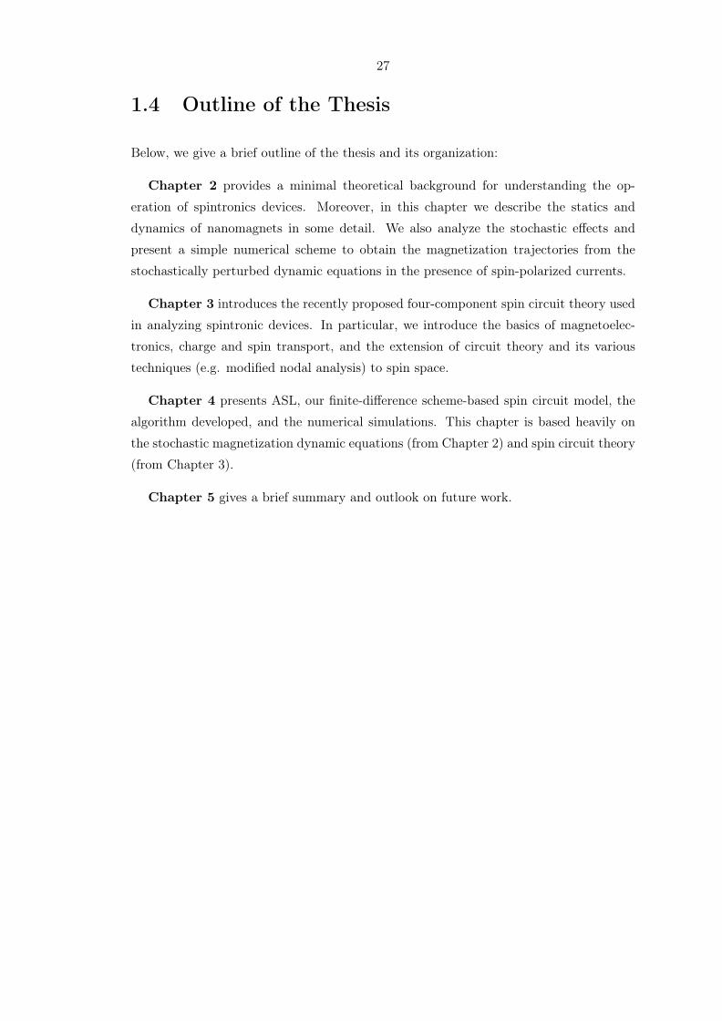
Chapter 2 provides a minimal theoretical background for understanding the op-
eration of spintronics devices. Moreover, in this chapter we describe the statics and
dynamics of nanomagnets in some detail. We also analyze the stochastic effects and
present a simple numerical scheme to obtain the magnetization trajectories from the
stochastically perturbed dynamic equations in the presence of spin-polarized currents.
Chapter 3 introduces the recently proposed four-component spin circuit theory used
in analyzing spintronic devices. In particular, we introduce the basics of magnetoelec-
tronics, charge and spin transport, and the extension of circuit theory and its various
techniques (e.g. modified nodal analysis) to spin space.
Chapter 4 presents ASL, our finite-difference scheme-based spin circuit model, the
algorithm developed, and the numerical simulations. This chapter is based heavily on
the stochastic magnetization dynamic equations (from Chapter 2) and spin circuit theory
(from Chapter 3).
Chapter 5 gives a brief summary and outlook on future work.

28
Chapter 2
Nanomagnetism and Spintronics
In this chapter, we heuristically introduce the basic concepts of spintronics and follow
that with a more detailed and rigor treatment of nanomagnetism. In particular, after in-
troducing spintronics, we review magnetostatics, and talk about domains, domain walls,
and present the typical length scales involved in the description of magnetic behavior.
We then delve into the description of the static character of a ferromagnet by formally
presenting the definitions and postulates of micromagnetism along with the boundary
conditions and energy terms involved. We then describe the deterministic dynamics of
magnetization starting from the Landau-Lifshitz (LL) equation, and present the mathe-
matically equivalent Landau-Lifshitz-Gilbert equation (LLG) equation, which is usually
the preferred form for large damping. Following that, we include the spin-transfer torque
(STT) term in the dynamics, which is of utmost importance in our modeling of ASL and
current-induced switching in general. The introduction of STT leads to a generaliza-
tion of the LLG equation to the so-called Landau-Lifshitz-Gilbert-Slonczewski (LLGS)
equation. We conclude this chapter with a brief discussion about the stochastic LLG
(sLLG) and stochastic LLGS (sLLGS) equations and present a simple and stable numer-
ical scheme to solve such equations.

29
2.1 Concepts in Spintronics
Below we give a heuristic introduction to the essential concepts of spintronics. We try
to be qualitative for the most part and leave the quantitative treatment for the (more
relevant) description of magnetization dynamics later.
2.1.1 Ferromagnets and Spin Polarization
In contrast to mainstream electronics which exploit charge only, spintronic devices utilize
both charge and spin [8, 9]. Spin, being a fundamental property of electrons (in addition
to mass and charge),1 is defined as the intrinsic angular momentum [15]. It is intimately
related to magnetism, and therefore, magnetism is inherently quantum mechanical in
nature. In conventional electronic circuits, an electric current is unpolarized and consists
of an equal number of up- and down-spin electrons, and thus spin has been ignored in
these circuits [21, 63]. However, when ferromagnets (FMs) are incorporated, spins can
polarize along a certain direction, allowing information to be stored in the system and
for magnetism to affect electrical transport (and vice versa) [21, 64, 65]. Typically, FMs
such as the itinerant “delocalized” electron systems: Fe, Co, and Ni are usually what
we mean when we talk about the magnetic behavior (Fig. 2.1). FMs in general are
characterized by a spontaneous magnetization and a very strong attraction to magnetic
fields, in contrast to paramagnets (weak attraction) and diamagnets (weak repulsion)
[66, 67].
1 1.0079
H
Hydrogen
3 6.941
Li
Lithium
11 22.990
Na
Sodium
19 39.098
K
Potassium
37 85.468
Rb
Rubidium
55 132.91
Cs
Caesium
87 223
Fr
Francium
4 9.0122
Be
Beryllium
12 24.305
Mg
Magnesium
20 40.078
Ca
Calcium
38 87.62
Sr
Strontium
56 137.33
Ba
Barium
88 226
Ra
Radium
21 44.956
Sc
Scandium
39 88.906
Y
Yttrium
57-71
La-Lu
Lanthanide
89-103
Ac-Lr
Actinide
22 47.867
Ti
Titanium
40 91.224
Zr
Zirconium
72 178.49
Hf
Halfnium
104 261
Rf
Rutherfordium
23 50.942
V
Vanadium
41 92.906
Nb
Niobium
73 180.95
Ta
Tantalum
105 262
Db
Dubnium
24 51.996
Cr
Chromium
42 95.94
Mo
Molybdenum
74 183.84
W
Tungsten
106 266
Sg
Seaborgium
25 54.938
Mn
Manganese
43 96
Tc
Technetium
75 186.21
Re
Rhenium
107 264
Bh
Bohrium
26 55.845
Fe
Iron
44 101.07
Ru
Ruthenium
76 190.23
Os
Osmium
108 277
Hs
Hassium
27 58.933
Co
Cobalt
45 102.91
Rh
Rhodium
77 192.22
Ir
Iridium
109 268
Mt
Meitnerium
28 58.693
Ni
Nickel
46 106.42
Pd
Palladium
78 195.08
Pt
Platinum
110 281
Ds
Darmstadtium
29 63.546
Cu
Copper
47 107.87
Ag
Silver
79 196.97
Au
Gold
111 280
Rg
Roentgenium
30 65.39
Zn
Zinc
48 112.41
Cd
Cadmium
80 200.59
Hg
Mercury
112 285
Uub
Ununbium
31 69.723
Ga
Gallium
13 26.982
Al
Aluminium
5 10.811
B
Boron
49 114.82
In
Indium
81 204.38
Tl
Thallium
113 284
Uut
Ununtrium
6 12.011
C
Carbon
14 28.086
Si
Silicon
32 72.64
Ge
Germanium
50 118.71
Sn
Tin
82 207.2
Pb
Lead
114 289
Uuq
Ununquadium
7 14.007
N
Nitrogen
15 30.974
P
Phosphorus
33 74.922
As
Arsenic
51 121.76
Sb
Antimony
83 208.98
Bi
Bismuth
115 288
Uup
Ununpentium
8 15.999
O
Oxygen
16 32.065
S
Sulphur
34 78.96
Se
Selenium
52 127.6
Te
Tellurium
84 209
Po
Polonium
116 293
Uuh
Ununhexium
9 18.998
F
Flourine
17 35.453
Cl
Chlorine
35 79.904
Br
Bromine
53 126.9
I
Iodine
85 210
At
Astatine
117 292
Uus
Ununseptium
10 20.180
Ne
Neon
2 4.0025
He
Helium
18 39.948
Ar
Argon
36 83.8
Kr
Krypton
54 131.29
Xe
Xenon
86 222
Rn
Radon
118 294
Uuo
Ununoctium
1
2
3
4
5
6
7
1 IA
2 IIA
3 IIIA 4 IVB 5 VB 6 VIB 7 VIIB 8 VIIIB 9 VIIIB 10 VIIIB 11 IB 12 IIB
13 IIIA 14 IVA 15 VA 16 VIA 17 VIIA
18 VIIIA
57 138.91
La
Lanthanum
58 140.12
Ce
Cerium
59 140.91
Pr
Praseodymium
60 144.24
Nd
Neodymium
61 145
Pm
Promethium
62 150.36
Sm
Samarium
63 151.96
Eu
Europium
64 157.25
Gd
Gadolinium
65 158.93
Tb
Terbium
66 162.50
Dy
Dysprosium
67 164.93
Ho
Holmium
68 167.26
Er
Erbium
69 168.93
Tm
Thulium
70 173.04
Yb
Ytterbium
71 174.97
Lu
Lutetium
89 227
Ac
Actinium
90 232.04
Th
Thorium
91 231.04
Pa
Protactinium
92 238.03
U
Uranium
93 237
Np
Neptunium
94 244
Pu
Plutonium
95 243
Am
Americium
96 247
Cm
Curium
97 247
Bk
Berkelium
98 251
Cf
Californium
99 252
Es
Einsteinium
100 257
Fm
Fermium
101 258
Md
Mendelevium
102 259
No
Nobelium
103 262
Lr
Lawrencium
Alkali Metal
Alkaline Earth Metal
Metal
Metalloid
Non-metal
Halogen
Noble Gas
Lanthanide/Actinide
Z mass
Symbol
Name
man-made
The Periodic Table of the Elements
Figure 2.1: The periodic table of chemical elements. The elements in red are the 3d transitionmetal ferromagnets (FMs).
1“Electron spin” is in fact a misnomer. Although it could be useful to think of an electron as aspinning sphere, this classical picture bears no resemblance to reality [61] (see [62] for an interestingargument).
30
The magnetism of FMs originates almost always from the spin angular momentum
of electrons.2 The ferromagnetic order arises from the electron-electron interaction. In
particular, from the interplay between exchange interaction (which favors parallel spins)
and Pauli exclusion principle (which states that no identical fermions may occupy the
same quantum state simultaneously) [14, 15, 21, 61, 69–71]. When metal atoms condense
to form a bulk metal, the electronic energy levels from atoms combine to form bands of
finite energy width [61, 72]. The result is that, the electronic distribution, called density
of states (DOS), changes. Exchange interaction [73], which is a purely quantum effect,
will force all uncompensated spins to align parallel to lower the system energy. However,
since the kinetic energy cost (which increases with the principal and orbital quantum
numbers) to maintain the atomic magnetic moment with spins aligned on each atom
increases,3 at some point the spin angular momentum will be traded for kinetic energy
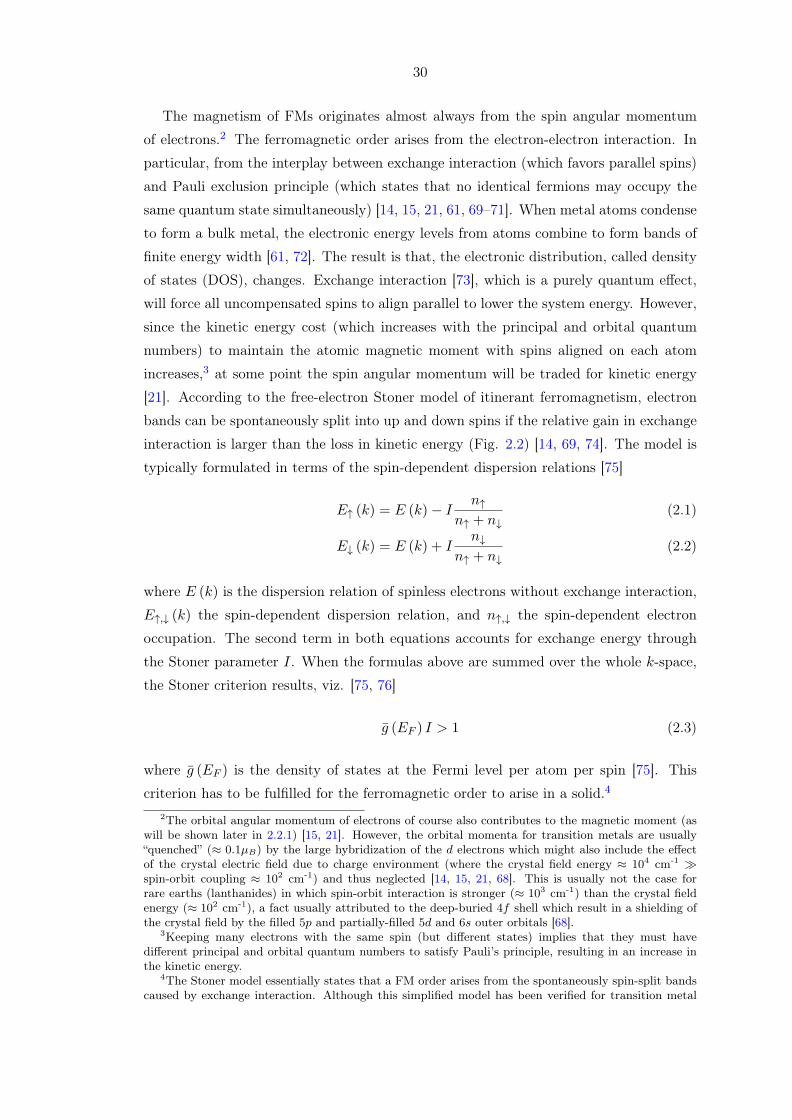
[21]. According to the free-electron Stoner model of itinerant ferromagnetism, electron
bands can be spontaneously split into up and down spins if the relative gain in exchange
interaction is larger than the loss in kinetic energy (Fig. 2.2) [14, 69, 74]. The model is
typically formulated in terms of the spin-dependent dispersion relations [75]
E↑ (k) = E (k)− In↑
n↑ + n↓(2.1)
E↓ (k) = E (k) + In↓
n↑ + n↓(2.2)
where E (k) is the dispersion relation of spinless electrons without exchange interaction,
E↑,↓ (k) the spin-dependent dispersion relation, and n↑,↓ the spin-dependent electron
occupation. The second term in both equations accounts for exchange energy through
the Stoner parameter I. When the formulas above are summed over the whole k-space,
the Stoner criterion results, viz. [75, 76]
g (EF ) I > 1 (2.3)
where g (EF ) is the density of states at the Fermi level per atom per spin [75]. This
criterion has to be fulfilled for the ferromagnetic order to arise in a solid.4
2The orbital angular momentum of electrons of course also contributes to the magnetic moment (aswill be shown later in 2.2.1) [15, 21]. However, the orbital momenta for transition metals are usually“quenched” (≈ 0.1µB) by the large hybridization of the d electrons which might also include the effectof the crystal electric field due to charge environment (where the crystal field energy ≈ 104 cm-1 ≫spin-orbit coupling ≈ 102 cm-1) and thus neglected [14, 15, 21, 68]. This is usually not the case forrare earths (lanthanides) in which spin-orbit interaction is stronger (≈ 103 cm-1) than the crystal fieldenergy (≈ 102 cm-1), a fact usually attributed to the deep-buried 4f shell which result in a shielding ofthe crystal field by the filled 5p and partially-filled 5d and 6s outer orbitals [68].
3Keeping many electrons with the same spin (but different states) implies that they must havedifferent principal and orbital quantum numbers to satisfy Pauli’s principle, resulting in an increase inthe kinetic energy.
4The Stoner model essentially states that a FM order arises from the spontaneously spin-split bandscaused by exchange interaction. Although this simplified model has been verified for transition metal
31
g↓ (E) g↑ (E)
E
EF
d band
s-p band
(a)
g↓ (E) g↑ (E)
E
EF
d band
s-p band
∆
(b)
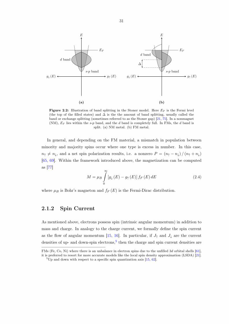
Figure 2.2: Illustration of band splitting in the Stoner model. Here EF is the Fermi level(the top of the filled states) and ∆ is the the amount of band splitting, usually called theband or exchange splitting (sometimes referred to as the Stoner gap) [21, 75]. In a nonmagnet(NM), EF lies within the s-p band, and the d band is completely full. In FMs, the d band is
split. (a) NM metal. (b) FM metal.
In general, and depending on the FM material, a mismatch in population between
minority and majority spins occur where one type is excess in number. In this case,
n↑ = n↓, and a net spin polarization results, i.e. a nonzero P = (n↑ − n↓) / (n↑ + n↓)
[65, 69]. Within the framework introduced above, the magnetization can be computed
as [77]
M = µB
∞∫0
[g↓ (E)− g↑ (E)] fF (E) dE (2.4)
where µB is Bohr’s magneton and fF (E) is the Fermi-Dirac distribution.
2.1.2 Spin Current
As mentioned above, electrons possess spin (intrinsic angular momentum) in addition to
mass and charge. In analogy to the charge current, we formally define the spin current
as the flow of angular momentum [15, 16]. In particular, if J↑ and J↓ are the current
densities of up- and down-spin electrons,5 then the charge and spin current densities are
FMs (Fe, Co, Ni) where there is an unbalance in electron spins due to the unfilled 3d orbital shells [61],it is preferred to resort for more accurate models like the local spin density approximation (LSDA) [21].
5Up and down with respect to a specific spin quantization axis [15, 62].

32
defined as6,7 [71, 78, 79]
JC = J↑ + J↓ (2.7)
JS = J↑ − J↓ (2.8)
Given the above equations, three types of currents can result:-
• Pure Charge Current: JC = 0 and JS = 0.
• Pure Spin Current: JC = 0 and JS = 0.
• Spin-Polarized Current: JC = 0 and JS = 0.
The first two are illustrated in Fig. 2.3.
Interestingly, and in contrast to charge currents, spin currents behave in some unusual
(and counter intuitive) ways. For example, a current will pass more easily if electron spins
line up with, rather than opposite to, the magnetization of a FM. This is what happens in
a process called spin filtering at a NM/FM interface, whereby a FM transmits electrons
of different spin orientations at different rates (roughly shown in Fig. 2.4) [15, 21, 75, 80].
This occurs because near a NM/FM interface, the potential experienced by the electrons
changes and becomes spin dependent and inside the FM the spin-split DOS causes a
spin-dependent transmission and reflection [21, 75]. This process is ultimately governed
by the s-d exchange interaction between the magnetic moments of the magnetization
and the conduction electrons [80]. The electrons that passes easily are usually called
“majority”, and the electrons that scatter are called “minority”.8 Conduction in FMs
therefore depends on the magnetization orientation in addition to the bulk properties [71].6In this section we neglect any noncollinear components in spins/magnetizations and assume spins
to be collinear to magnetization (except for the discussion regarding spin-transfer torque). The generalformalism will be given in Chapter 3.
7In general, for a single electron, the charge current density is the vector given by JC = q ℏm
Im(ψ†∇ψ
)[77], which has to satisfy the following conservation law∫∫
⃝Σ
JC · dS = −∫∫∫
Ω
∂ρ
∂tdV (2.5)
where ρ = qψ†ψ is the charge density. The spin current density, on the other hand, is a tensor (in particu-lar, a second-order pseudo-tensor); a quantity with both a direction of charge flow and a direction of spinpolarization [71]. The spin current density is given by the outer product JS = v⊗s = ℏ2
2mIm
(ψ†σ ⊗∇ψ
)[21, 77], where v is the average electron velocity, s = ℏ
2σ, and σ the Pauli spin vector. An element J ij
S
refers to the component of the spin current flowing in the i-th direction with a spin polarization alongthe j-th direction. If no torques are applied, the spin current satisfies the conservation equation [77]∫∫
⃝Σ
JS · dS = −∫∫∫
Ω
∂S
∂tdV (2.6)
where S = ℏ2ψ†σψ is the spin density.
8Some authors [79] define the majority spin as the spin species of the larger electronic density, andthe one with the smaller electronic density as the minority spin.

33
..Spin Current
.Charge Current
(a)
.
(b)
.
(c)
Figure 2.3: Illustration of pure charge and spin currents. (a) Charge and spin as two degreesof freedom. (b) Up- and down-spin electrons of equal amount cancel in spin when moving inthe same direction, effectively creating a pure charge current. (c) Up- and down-spin electronsof equal amount cancel in charge when moving in opposite directions, effectively creating a
pure spin current.
NM metals, on the other hand, have an equal number of electrons with up and down spins
and their conduction is thus merely determined by the bulk properties (with a resistance
possibly disordered on a microscopic scale) [65]. Moreover, because of spin relaxation
processes, spin currents cannot transmit for long distances9 (whether in FMs or NMs) as
opposed to charge currents [15, 64]. This essentially means that spin is not a conserved
quantity (again, in contrast to charge) [15, 65, 84]. Despite these disadvantages, spin
have the advantages over charge in that it requires less energy to process and is faster to
manipulate. In addition, not only can a spin exist in the classical “0” and “1” states, it can
also be in a coherent superposition of both, forming the so-called quantum bit (qubit)
[62]. This allows for combinatorial calculations, something that cannot be performed
with normal computers. A rough comparison between charge and spin is shown in Table
2.1.
Spin currents can be generated from nonequilibrium spin states, i.e., spin accumu-
lation and spin dynamics. For example, by temperature gradient (spin Seebeck effect)
[85], sound waves (acoustic spin pumping) [86–88], optical orientation [89], mechanical9Longer than the spin-flip mean-free path λsf , which is the mean distance between spin-flipping
collisions [65, 81]. However, due to scattering events, the length over which an electron travels withfixed spin orientation is typically smaller than λsf , and one usually uses a different length scale. Thealternative length scale is the spin-diffusion length lsf , defined as the length over which an electron“diffuses” before losing its spin memory due to spin-flipping collisions [14, 21, 64, 65, 71, 82]. If onedefines the mean-free path λ = vF τ and the spin-flip mean-free path λsf = vF τsf , then the spin-diffusionlength is given by the the geometric mean lsf =
√λλsf [76, 83]. If, instead of λ (related to momentum
exchange), we used the total mean-free path λt = vF τt (related to collision of all kinds whether spinconserving or not), then lsf =
√(1/3)λλt [81]. In general, lsf follows a diffusion equation, can be
written in terms of the diffusion constant lsf =√Dτsf , and obeys (most of the time) the inequality
λF < λt < λ < lsf < λsf [65, 81].
34
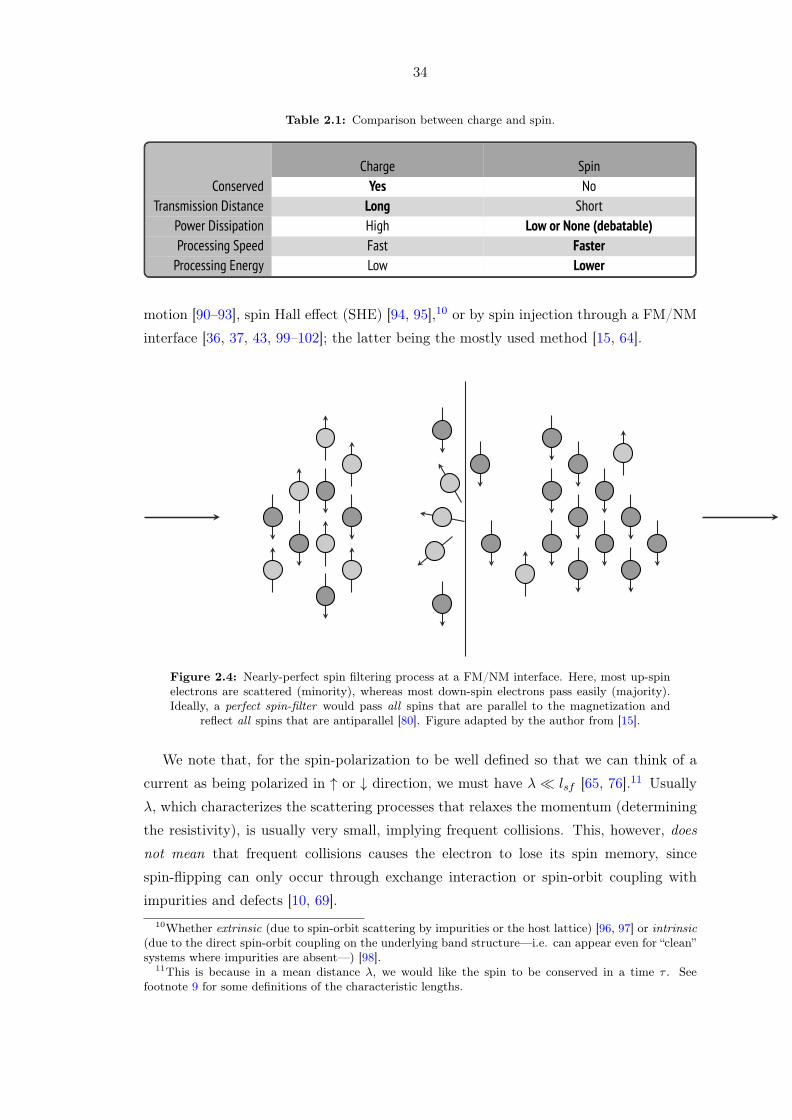
Table 2.1: Comparison between charge and spin.
Charge SpinConserved Yes No
Transmission Distance Long ShortPower Dissipation High Low or None (debatable)Processing Speed Fast FasterProcessing Energy Low Lower
motion [90–93], spin Hall effect (SHE) [94, 95],10 or by spin injection through a FM/NM
interface [36, 37, 43, 99–102]; the latter being the mostly used method [15, 64].
.
Figure 2.4: Nearly-perfect spin filtering process at a FM/NM interface. Here, most up-spinelectrons are scattered (minority), whereas most down-spin electrons pass easily (majority).Ideally, a perfect spin-filter would pass all spins that are parallel to the magnetization and
reflect all spins that are antiparallel [80]. Figure adapted by the author from [15].
We note that, for the spin-polarization to be well defined so that we can think of a
current as being polarized in ↑ or ↓ direction, we must have λ≪ lsf [65, 76].11 Usually
λ, which characterizes the scattering processes that relaxes the momentum (determining
the resistivity), is usually very small, implying frequent collisions. This, however, does
not mean that frequent collisions causes the electron to lose its spin memory, since
spin-flipping can only occur through exchange interaction or spin-orbit coupling with
impurities and defects [10, 69].10Whether extrinsic (due to spin-orbit scattering by impurities or the host lattice) [96, 97] or intrinsic
(due to the direct spin-orbit coupling on the underlying band structure—i.e. can appear even for “clean”systems where impurities are absent—) [98].
11This is because in a mean distance λ, we would like the spin to be conserved in a time τ . Seefootnote 9 for some definitions of the characteristic lengths.

35
2.1.3 Spin-Dependent Transport: The Two-Current Model
The simplest formula for the electrical conductivity is given by Drude’s formula [14, 61,
65]
σ =e2nτ
m∗e
(2.9)
where e is the electron charge, n the electron number density, τ the elastic scattering
time, and m∗e the effective mass of the band. Within the framework of Drude’s transport
theory, the concept of the Fermi surface plays a central role. Due to exchange splitting
between the up- and down-spin bands in FMs, the nature of up- and down-spin electronic
states at the Fermi surface and their coupling to scattering potentials will be different
[14, 15, 65]. Consequently, in FMs the DOSs and Fermi velocities for the majority and
minority spins are different. This transcends to n, τ and m∗e being different (i.e., spin-
dependent) [71, 79]. Therefore one will require an extension of Drude’s model to FMs.
In the mid-1930s, N. F. Mott [103] proposed that at sufficiently low temperatures
(where electron-magnon scattering can be neglected [104]), up- and down-spin electrons
in FM metals carry current independently, corresponding to two current channels con-
nected in parallel (Fig. 2.5) [78]. That is, the total resistivity is given by the parallel
combination
ρ =ρσρ−σ
ρσ + ρ−σ(2.10)
where ρσ is the spin-dependent resistivity and σ =↑, ↓.12 Mott’s model can be thought
as the first understanding of spin-polarized transport.
...
ρ↑
..
ρ↓
Figure 2.5: Mott’s two-current model.
In this model, the conduction is mainly contributed by s electrons.13 Moreover, due to
the large density of states of 3d bands at EF [75], s-d scattering via s-d mixing is assumed12Here σ is not the conductivity, but rather the spin index.13In FMs, both of s and d bands electrons participate in conduction [65]. However, the s bands are
wide, whereas the d bands are narrow (Fig. 2.2b). Thus electrons in the d bands have a large effectivemass (and thus low mobility), in contrast to the ones in s bands; this is evident from the relationsm∗ = ℏ2
(∂2E/∂k2
)−1
EFand µ = eτ/m∗ [61, 69, 74].

36
to occur much more frequently than s-s scattering [12]. This model [105] assumes that
the resistivity is merely determined by interband scattering from 4s to 3d bands (and
vice versa). The probability of scattering is thus proportional to the DOS at the Fermi
level in 3d bands [12, 14, 74]
ρσ ∝ gσ (EF ) (2.11)
Given the picture above, Mott’s model implies that spins have different distribution
functions fσ and relaxation times τσ [14, 69]. Implicit in the “independence” condition
of current channels is the main assumption that spin-flip events are rare (or negligible)
so that one can disregard any transition (or mixing) between the channels. This means
that the spin-angular momentum along the spin quantization axis is conserved by the
single-particle Hamiltonian [14]. This is true in general for 3d transition metals where the
probability of spin-flip scattering is small compared to the conserving scattering events
(e.g., electron-phonon scattering) and where spin-orbit interaction (which mixes spin and
orbital angular momenta) is small [14, 59]. If one includes spin-flip scattering processes
(e.g., the non-conserving electron-magnon scattering at temperatures close to the Curie
point, fluctuating magnetic field, lose spins due to magnetic impurities, or hyperfine
coupling with nuclei), a relaxation time τ↑↓ appears [14, 15, 59, 62, 69, 71, 106]. In
this case, and within the free-electron model, Boltzmann’s equation has an extra spin-
relaxation term due to spin-flip scattering (in addition to the usual momentum-relaxation
term due to lattice defects and vibrations) [59]. Namely, the coupled equations [69, 76]
eE · v∂f0∂E
= −fσ − f0τσ
− fσ − f−σ
τσ,−σ(2.12)
where f0 is the equilibrium distribution function, fσ the spin-dependent distriubtion
function, E the applied electric field, v the velocity, τσ the spin-dependent transport
relaxation time, and τσ,−σ (τ−σ,σ) the spin-flip relaxation time from σ to −σ (−σ to σ).
Since τσ ≪ τσ,−σ, momentum relaxation occurs first, followed by slow spin-relaxation.
In late-1960s, I. A. Campbell and A. Fert [107, 108] investigated the two-current
model. They solved (2.12) and obtained the total resistivity [76]
ρ =ρσρ−σ + ρσ,−σ (ρσ + ρ−σ)
ρσ + ρ−σ + 4ρσ,−σ(2.13)

37
where, in the nondegenerate limit14
ρσ =m∗
nσe2τσ(2.14)
ρσ,−σ =m∗
ne2τσ,−σ(2.15)
When spin-flip scattering is neglected, (2.13) reduces to the two-current model (2.10).
We note that the two-current model generally holds if λ ≪ lsf , whether L > lsf or
L < lsf [43, 65]. However, some FMs (e.g., Py) have short lsf that can in fact be
comparable to λ [110–112]. In the latter case, one has to include spin-mixing effects.
2.1.4 Spin Injection and Spin Accumulation
From thermodynamics, the chemical potential µ is defined as the variation of the ther-
modynamic potential of the system when one particle is added at constant entropy and
constant volume [61, 78, 84].15,16 For particles obeying the Fermi-Dirac statistics and in
the framework of the free-electron model, the chemical potential is given by the Som-
merfeld expansion (assuming kBT ≪ EF17) [61, 109]
µ = EF
[1− π2
12
(kBT
EF
)2
+ · · ·
](2.17)
where EF is the Fermi energy and kB is Boltzmann’s constant. From this equation, it is
apparent that at T = 0 K, one has µ = EF . For a metal, µ is constant.18 If a voltage is
applied the electrochemical potential µ = µ − eVC varies along the conductor and as a
result, a charge current density flows according to Ohm’s law [61, 78, 84]
JC =σ
e∇µ (2.18)
At an interface between two conductors, µ varies in such a way that it presents no
discontinuity at the interface [61, 78].14In the degenerate limit, one has ρσ = 1/nσEF,σe
2gσ [109].15This follows from the differential form of the combined 1st and 2nd laws (sometimes called Gibbs
fundamental form) [84]du = TdS − PdV + µdn (2.16)
16For charged particles (in the absence of magnetic fields), one speaks of an electrochemical potentialµ = µ + qVC , defined as the work done against chemical composition plus internal and/or externalpotential when adding a particle, opposed to the chemical potential µ which is concerned only with thework done against chemical interaction when adding a particle. The two coincide for uncharged species.
17Since the Fermi temperature is given by TF = EF /kB , the condition can be restated as T ≪ TF .Thus it is obvious that this holds for most metals. For example, for a metal with EF = 5 eV, one hasT ≈ 58000 K, which is 10 times higher than the temperature of the Sun.
18Because the density n is almost fixed. However, for semiconductors n varies considerably in spaceand thus µ has to be taken as a function of position [84].

38
In the same way, one may define an electrochemical potential for each spin carrying
particle so that electrons with different spins have different electrochemical potentials.
In this way, the out of equilibrium spin electrochemical potential µs is defined as the
half-difference between the electrochemical potentials of up- and down-spin electrons,
viz. [71, 78, 104]
µs =1
2(µ↑ − µ↓) (2.19)
and is sometimes referred to as the spin accumulation.19 The spin accumulation is related
to the out of equilibrium spin density δs = δn↑ − δn↓ through
µs =1
2e
g↑ (EF ) + g↓ (EF )
g↑ (EF ) g↓ (EF )δs (2.20)
and thus sometimes one might also refer to δs as the spin accumulation. Unlike µ, the
spin accumulation undergoes a discontinuity at the FM/NM interface by an amount
given by µFM − µNM .20 In fact, the drop at the interface is eVS , where VS is known as
the spin accumulation voltage (or just spin voltage) [61]. This quantity arises whenever
there is a discontinuity in conductance between the two spin channels.
..
m
.lFMsf
.lNMsf
.
µ
.
µ↑
.
µ↓
.
∆µ
(a)
..
m
.lFMsf
.lNMsf
.
JS
(b)
Figure 2.6: Schematic showing the spin accumulation at a FM/NM interface. The dashedlines enclose the zone of spin accumulation. In the figure, electrons are assumed to be injectedfrom the NM to the FM (i.e., current is flowing from FM to NM). (a) Spatial variation of thespin-dependent electrochemical potentials. (b) At each point in the multilayer, a difference inthe electrochemical potentials determines a spin current. Figure adapted by the author from
[113].
In 1976, Aronov [99] theoretically predicted the possibility of injecting a spin-polarized
current from a FM to a NM metal attached to it, effectively establishing a nonequilibrium
magnetization in the NM region (i.e., magnetizing the NM region) within a spin-coherent19A semiclassical quantity [71].20In particular, the average spin accumulation is discontinuous at the interface. The individual chem-
ical potentials for the two spin channels is continuous at the FM/NM interface (if one neglects interfaceconductance) [61, 104].

39
distance phenomenologically determined by the spin-diffusion length [71].21 The nonequi-
librium magnetization is equivalent to a nonequilibrium spin-accumulation in the NM
region [71, 78]; in other words, the build-up of spin polarization at the FM/NM interface
when there is a current flowing across the interface [61]. This prediction was proved later
in 1985 by the pioneering studies of Johnson and Silsbee [36, 101, 102] in a structure
similar to that in Fig. 2.7a. This structure is called a nonlocal spin valve (NLSV), since
a current injected in one electrode can be nonlocally detected as a voltage difference
in the other electrode (i.e., without passing the current directly from one end to the
other as in Fig. 2.7b). The nonlocal voltage detected is attributed to the nonequilibrium
magnetization (spin accumulation) established in the NM region after injecting the spin-
polarized current [71, 106]. For this reason, the two electrodes are appropriately named
injector and detector. The main advantage of using a NLSV is the generation of a pure
spin current, in contrast to the LSV in which the pure spin current is associated with a
charge current [21].
The spin transport and spin injection across FM/NM junctions have then been exten-
sively studied, for example in [37, 43]. It is worth noting that in contrast to NMs (which
can have spin-diffusion lengths in the micron range), FMs have very small spin-diffusion
lengths and thus spin-accumulation is mainly an interface property in these materials
(although a spin-current persist in the bulk, recall Fig. 2.6) [71].
.
.
...
V
.
m1
.
m2
(a)
....
A
.
.
m1
.
m2
(b)
Figure 2.7: Illustration of nonlocal spin valve (NLSV) and local spin valve (LSV). Thenonequilibrium magnetization of the spin accumulation injected from FM1 to NM decays overthe spin-diffusion length ℓNM
sd . The spin accumulation in FM1 has been ignored since it islocalized at the interface because ℓFM
sd ≪ ℓNMsd [71]. (a) NLSV. (b) LSV.
21Aronov and Pikus also suggested a similar procedure to be carried in a NM semiconductor [100].

40
2.1.5 Magnetoresistance (MR)
The term magnetoresistance (MR) refers to the dependency of electrical resistance of a
FM/NM multilayer on the relative magnetization orientation of the adjacent FMs [14].
The MR is typically given as the ratio [65, 82]
MR =RAP −RP
RP× 100% (2.21)
where RP and RAP are the resistances in the parallel and antiparallel states, respec-
tively.22 Magnetoresistive structures can be made of several layers of different materials
like FM, AFM, and NM (whether metal, insulator, semiconductor, or even organic)
[15, 114].23 In its simplest form, an MR device is made up of two FMs sandwiching an
NM spacer (usually a metal or an insulator). As shown in Fig. 2.8, one of the FM layers
is called “free”, “switching”, “sensing”, or “soft”, in that its magnetization is free to rotate
in the plane of the layer. The other layer is “fixed” or “hard” by either being naturally
hard, or by virtue of being thicker24 or by exchange bias coupling [115] (i.e., by “pinning”
it to an AFM “pinning layer” such that the hysteresis loop is shifted); the latter implies
that the hard layer is usually comprised of two or more layers25 [15, 21, 26, 61, 114]. The
hard layer is also sometimes called a “polarizer” or a “reference” layer, especially in the
context of current-induced switching and spin-filtering processes (Fig. 2.4). To obtain
high MR ratios, the multilayer is chosen/engineered in a way that the FMs are highly
spin-polarized and the spin scattering of electrons in the NM is low.
Typically, MR structures come in two flavors: either as a current-in-plane (CIP) or a
current-perpendicular-to-plane (CPP) (Fig. 2.9), with the latter being most widely used
nowadays [21, 119].22Some authors define the MR as
MR =RAP −RP
RAP× 100% (2.22)
and typically call it the “pessimistic” definition (in contrast to the “optimistic” one we used), due to thelower MRs since most of the time RAP > RP [65].
23Usually the FMs used are the transition FM materials (Fe, Co, Ni) and their alloys (Py, CoFe,CoFeB, FePt, SmCo, NdFeB). The conducting NMs are usually transition metals (Cr or Ru) or noblemetals (Cu, Ag, and Au). The insulating NMs are usually oxides (Al2O3, MgO). AFMs, on the otherhand, are usually Mn-based alloys (PtMn, PdMn, IrMn, RhMn, FeMn, NiMn, CrMn) and oxides (CoO,NiO).
24This also breaks the “inversion” symmetry of the stack [16].25More layers are generally needed for different purposes like increasing spin polarization, minimization
of stray fields, etc. [26]. In fact, simply pinning a soft FM by depositing it on top of an AFM and makinguse of the exchange coupling at the interface will not prevent errenous events that may occur in somestructures due to the stray fields surrounding the FMs. That is, the FMs can couple via the strayfields, which prefers an antiparallel alignment of the free FM to the reference FM, causing a shift in theswitching curve of the free FM, precluding information storage [114]. To avoid this effect, one can cancelthe unwanted stray fields [116] by using the so-called artificial or synthetic AFM structures. These aremade by two FMs sandwiching a thin NM such as Cu or Ru, and it makes use of the oscillatory behavior

41
m1 m2
Fixed Spacer Free
Figure 2.8: Simple FM/NM multilayer.
...
V
..
A
..
m1
.
m2
(a)
...
V
..
A
..
m1
.
m2
(b)
Figure 2.9: Illustration of CIP-MR and CPP-MR. (a) CIP-MR. (b) CPP-MR.
Below we discuss the most widely used MR structures, namely the GMR and TMR.
2.1.5.1 Giant Magnetoresistance (GMR)
In 1988 and influenced by the discovery of the antiferromagnetic Heisenberg (or bilin-
ear) exchange coupling [120] between ultrathin films came the groundbreaking discovery
of giant magnetoresistance (GMR) from the pioneering work of both Fert’s [121] and
Grünberg’s [122] groups. On the same line, and after the striking GMR measurements,
Parkin and collaborators [117, 118] have observed an oscillatory (or alternating) AFM-
FM behavior of the exchange coupling in metallic multilayers as a function of the NM
spacer (Fig. 2.10) [21].26 The GMR discovery marked the beginning of a new era in data
storage technology, an impact that was later recognized by Fert and Grünberg sharing
of exchange coupling [117, 118] so that one can select an optimal NM thickness to make them oppositelymagnetized (Fig. 2.10), canceling their stray fields.
26The origin of this behavior has been accounted to the Ruderman-Kittel-Kasuya-Yosida (RKKY)interaction mediated by a spin-polarized cloud of electrons [78, 82, 123].

42
the 2007 Nobel Prize in Physics. It is not an exaggeration to say that GMR kicked off
the start of spintronics as a new scientific field.
Thickness
Exchange Coupling
m1 m2
m1 m2
m1 m2
m1 m2
m1 m2
m1 m2
Figure 2.10: Exchange coupling in NM metals.
GMR is an effect that manifests itself in metallic structures whereby the MR of
an ultra-thin multilayer experiences a giant change when the magnetization direction
changes [21].27 The effect is based on spin-dependent scattering of electrons traveling
across metallic thin films [15, 65, 80, 82, 124]. As one injects an electric current, the
spins parallel to the magnetization of the FM will pass through quite easily while those
antiparallel will scatter. Thus, the device acts as a spin filter (or a “spin valve”), letting
more electrons with certain spins; hence the name. Figs. 2.11a and 2.11b illustrate the
scattering picture. The scattering process can also be understood in the Stoner picture
(Fig. 2.2) of FMs as follows. For P alignment, majority-spin electrons are located within
the s-p band and their conduction is similar to those in the NM. For minority-spin
electrons, on the other hand, the s-p bands are hybridized and EF lies within the d
band. Because of the higher DOS of the hybridized band, minority spins scatter more
than the majority, implying shorter mean-free path for minority-spin electrons. For AP
alignment, the former argument applies to either spin in at least one layer.
When both magnetizations are parallel (P), spins of one orientation passes easily, and
the resistance is low. When they are antiparallel (AP), both spins are scattered in at
least one layer, and the multilayer presents a high resistance. The measure of change of27Although ordinary MR effect had been known for more than 100 years ago by William Thomson—
better known as Lord Kelvin—the MR measured was typically low [61, 65, 82, 123].

43
resistances is given by the GMR ratio
GMR =RAP −RP
RP× 100% (2.23)
..
m1
.
m2
(a)..
m1
.
m2
(b)
...
R↑
..
R↓
..
R↑
..
R↓
(c)
...
R↑
..
R↓
..
R↓
..
R↑
(d)
Figure 2.11: Spin-dependent scattering in a spin valve (SV). (a) P alignment. (b) APalignment. (c) Two-current model for P Alignment. (d) Two-current model for AP Alignment.
For negligible spin-flip events, the two-current model is adequate (Figs. 2.11c and
2.11d) [71]. If we consider scattering in the bulk only (i.e., neglecting scattering at the
interface), we can express the resistance of the P and AP alignments as
RP = 2R↑R↓R↑ +R↓
(2.24)
RAP =1
2(R↑ +R↓) (2.25)
from which we write the GMR as [78]
GMR =1
4
(R↑ −R↓)2
R↑R↓(2.26)
As mentioned previously, the CPP geometry is nowadays preferred. This is usu-
ally because of the higher symmetry, the greater MR ratios, and its importance for
spin-transfer torque applications (although CIP geometry is experimentally simpler to
implement) [21, 65, 78, 82, 119]. In addition to the geometry used, there are certain
factors that control the value of GMR. Some of these factors are the spin-dependent
random potential at FM/NM interfaces and band matching/mismatching between the

44
FM and NM layers [65]. The GMR effect technically occurs when t (the layer thickness
of magnetic multilayers) satisfies t <∼ λ [10, 65].
In many cases, spin-relaxation effects cannot be disregarded and one has to resort
to more accurate formalisms. The theory of CPP-GMR structures is known as the
Valet-Fert theory, in honor of Valet and Fert who extensively analyzed this structure
in 1993. Their analysis is based on the diffusive spin-dependent Boltzmann equations.
The quantum formalism of CPP-GMR has been applied by using the quantum Kubo
formula [125, 126]. The results of both Boltzmann and Kubo description turned out to
be equivalent since the band structure was assumed to be parabolic. The more realistic
band structure have been employed in [127–129] using models based on both pictures.28
2.1.5.2 Tunneling Magnetoresistance (TMR)
Tunneling magnetoresistance (TMR) in its simplest form is observed in trilayers made up
of two FMs sandwiching an insulating NM spacer, a structure called a magnetic tunnel
junction (MTJ). The idea is that, for sufficiently thin insulating spacers (≈ 1–2 nm),
electrons can tunnel through [14, 16]. The measure of resistance change in MTJs is given
by the TMR ratio
TMR =RAP −RP
RAP× 100% (2.27)
where we have swapped the roles of RP and RAP in the denominator, adopting the
convention used in most TMR experiments [65].
Although TMR was well-known [132, 133] before the discovery of GMR, the observed
MRs were rather small. However, the discovery of GMR (and the advances of thin
film techniques) has triggered extensive research on tunnel junctions again, first in (the
heavily disordered [21]) Al2O3 tunnel barriers [134–136] and later in (the potentially well-
ordered [21]) MgO barriers [137, 138]. TMR is typically far larger than the GMR, and
this explains the shift in attention from GMRs to TMRs, especially in the implementation
of memory cells and commercial recording heads [16, 65]. High TMRs can generally be
obtained by choosing materials with different symmetries of the wavefunction for both
electrons spins so that the resistance (which depends on the overlap) is high in the AP
state [16]. The TMR ratio, in general, depends on many factors like the shape of the
Fermi surface of the electrodes, electron scattering at the FM/NM interface, symmetry of
the wave functions, and spin-slip tunneling [65]. Additionally, it varies with temperature
and also with the barrier’s height, width, and impurities [15, 65].28For CIP-GMR, see [130] for classical and [131] quantum formalisms.
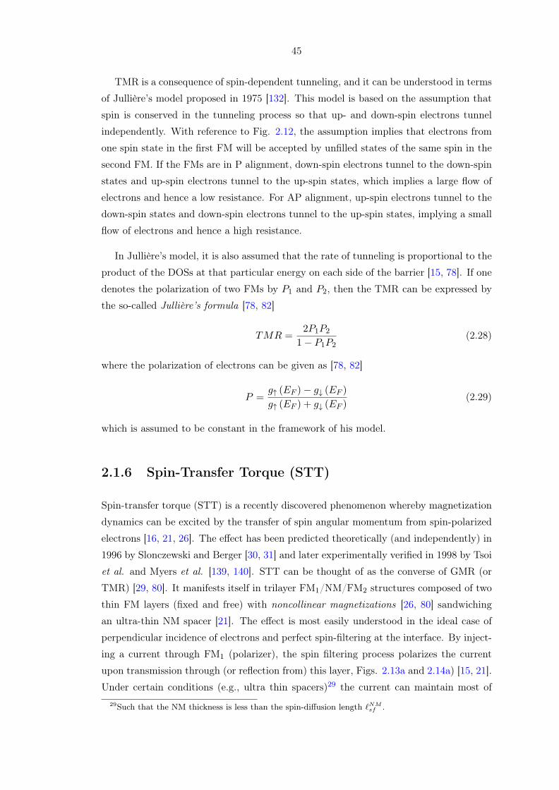
45
TMR is a consequence of spin-dependent tunneling, and it can be understood in terms
of Jullière’s model proposed in 1975 [132]. This model is based on the assumption that
spin is conserved in the tunneling process so that up- and down-spin electrons tunnel
independently. With reference to Fig. 2.12, the assumption implies that electrons from
one spin state in the first FM will be accepted by unfilled states of the same spin in the
second FM. If the FMs are in P alignment, down-spin electrons tunnel to the down-spin
states and up-spin electrons tunnel to the up-spin states, which implies a large flow of
electrons and hence a low resistance. For AP alignment, up-spin electrons tunnel to the
down-spin states and down-spin electrons tunnel to the up-spin states, implying a small
flow of electrons and hence a high resistance.
In Jullière’s model, it is also assumed that the rate of tunneling is proportional to the
product of the DOSs at that particular energy on each side of the barrier [15, 78]. If one
denotes the polarization of two FMs by P1 and P2, then the TMR can be expressed by
the so-called Jullière’s formula [78, 82]
TMR =2P1P2
1− P1P2(2.28)
where the polarization of electrons can be given as [78, 82]
P =g↑ (EF )− g↓ (EF )
g↑ (EF ) + g↓ (EF )(2.29)
which is assumed to be constant in the framework of his model.
2.1.6 Spin-Transfer Torque (STT)
Spin-transfer torque (STT) is a recently discovered phenomenon whereby magnetization
dynamics can be excited by the transfer of spin angular momentum from spin-polarized
electrons [16, 21, 26]. The effect has been predicted theoretically (and independently) in
1996 by Slonczewski and Berger [30, 31] and later experimentally verified in 1998 by Tsoi
et al. and Myers et al. [139, 140]. STT can be thought of as the converse of GMR (or
TMR) [29, 80]. It manifests itself in trilayer FM1/NM/FM2 structures composed of two
thin FM layers (fixed and free) with noncollinear magnetizations [26, 80] sandwiching
an ultra-thin NM spacer [21]. The effect is most easily understood in the ideal case of
perpendicular incidence of electrons and perfect spin-filtering at the interface. By inject-
ing a current through FM1 (polarizer), the spin filtering process polarizes the current
upon transmission through (or reflection from) this layer, Figs. 2.13a and 2.14a) [15, 21].
Under certain conditions (e.g., ultra thin spacers)29 the current can maintain most of29Such that the NM thickness is less than the spin-diffusion length ℓNM
sf .
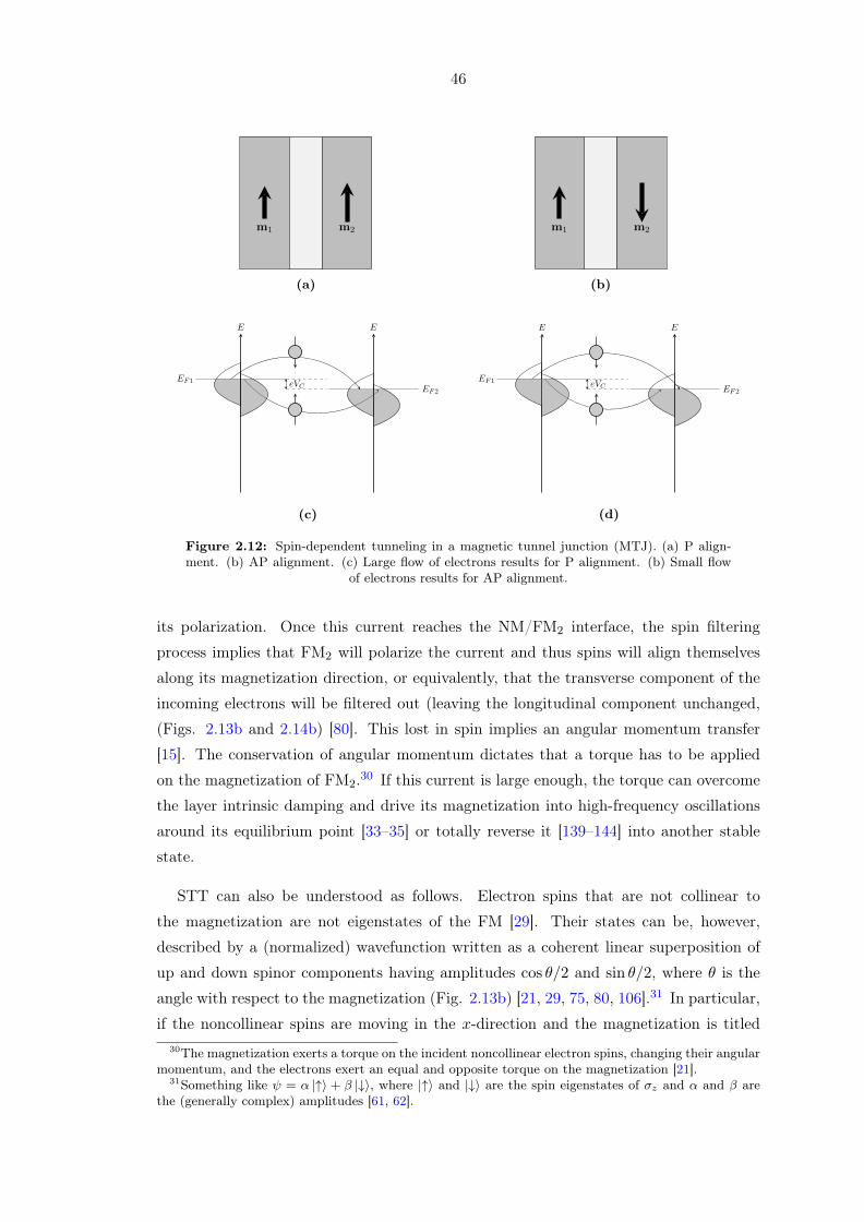
46
m1 m2
(a)
m1 m2
(b)
..
E
.
EF1
.
eVC
.
E
.
EF2
(c)
E
EF1 eVC
E
EF2
(d)
Figure 2.12: Spin-dependent tunneling in a magnetic tunnel junction (MTJ). (a) P align-ment. (b) AP alignment. (c) Large flow of electrons results for P alignment. (b) Small flow
of electrons results for AP alignment.
its polarization. Once this current reaches the NM/FM2 interface, the spin filtering
process implies that FM2 will polarize the current and thus spins will align themselves
along its magnetization direction, or equivalently, that the transverse component of the
incoming electrons will be filtered out (leaving the longitudinal component unchanged,
(Figs. 2.13b and 2.14b) [80]. This lost in spin implies an angular momentum transfer
[15]. The conservation of angular momentum dictates that a torque has to be applied
on the magnetization of FM2.30 If this current is large enough, the torque can overcome
the layer intrinsic damping and drive its magnetization into high-frequency oscillations
around its equilibrium point [33–35] or totally reverse it [139–144] into another stable
state.
STT can also be understood as follows. Electron spins that are not collinear to
the magnetization are not eigenstates of the FM [29]. Their states can be, however,
described by a (normalized) wavefunction written as a coherent linear superposition of
up and down spinor components having amplitudes cos θ/2 and sin θ/2, where θ is the
angle with respect to the magnetization (Fig. 2.13b) [21, 29, 75, 80, 106].31 In particular,
if the noncollinear spins are moving in the x-direction and the magnetization is titled30The magnetization exerts a torque on the incident noncollinear electron spins, changing their angular
momentum, and the electrons exert an equal and opposite torque on the magnetization [21].31Something like ψ = α |↑⟩ + β |↓⟩, where |↑⟩ and |↓⟩ are the spin eigenstates of σz and α and β are
the (generally complex) amplitudes [61, 62].

47
..
m1
.
m2
(a)
..
m2
.
STT
.
θ
(b)
Figure 2.13: Back-Switching (stabilizing) state by transmission through a NM/FM interface.(a) Spins that are noncollinear to the magnetization will lose their transverse components at theFM/NM interface. (b) STT in action; the absorption (loss) of the transverse component of spinis equivalent to a torque applied on the magnetization “conservation of angular momentum”.
..
m1
.
m2
(a)
..
m2
.
STT
.θ − π
2
(b)
Figure 2.14: Switching (destabilizing) state by reflection from a NM/FM interface. (a)Spins that are noncollinear to the magnetization will lose their transverse components at theFM/NM interface. (b) STT in action; the absorption (loss) of the transverse component of spinis equivalent to a torque applied on the magnetization “conservation of angular momentum”.
from z-axis by an angle θ (and thus spins are polarized in the xz-plane), then we have
incident spinors of the form [21]
ψi =
(cos
θ
2|↑⟩+ sin
θ
2|↓⟩)eikx =
[cos θ
2
sin θ2
]eikx (2.30)
We can write the reflected and transmitted spinors as
ψr =
(r↑ cos
θ
2|↑⟩+ r↓ sin
θ
2|↓⟩)e−ikx =
[r↑ cos
θ2
r↓ sinθ2
]e−ikx (2.31)
ψt =
(t↑ cos
θ
2|↑⟩+ t↓ sin
θ
2|↓⟩)eikx =
[t↑ cos
θ2
t↓ sinθ2
]eikx (2.32)
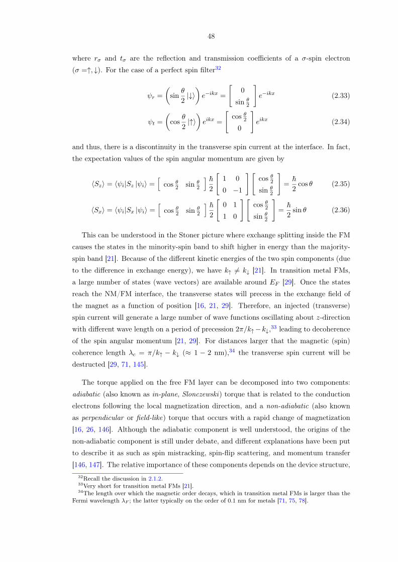
48
where rσ and tσ are the reflection and transmission coefficients of a σ-spin electron
(σ =↑, ↓). For the case of a perfect spin filter32
ψr =
(sin
θ
2|↓⟩)e−ikx =
[0
sin θ2
]e−ikx (2.33)
ψt =
(cos
θ
2|↑⟩)eikx =
[cos θ
2
0
]eikx (2.34)
and thus, there is a discontinuity in the transverse spin current at the interface. In fact,
the expectation values of the spin angular momentum are given by
⟨Sz⟩ = ⟨ψi|Sz |ψi⟩ =[cos θ
2 sin θ2
] ℏ2
[1 0
0 −1
][cos θ
2
sin θ2
]=
ℏ2cos θ (2.35)
⟨Sx⟩ = ⟨ψi|Sx |ψi⟩ =[cos θ
2 sin θ2
] ℏ2
[0 1
1 0
][cos θ
2
sin θ2
]=
ℏ2sin θ (2.36)
This can be understood in the Stoner picture where exchange splitting inside the FM
causes the states in the minority-spin band to shift higher in energy than the majority-
spin band [21]. Because of the different kinetic energies of the two spin components (due
to the difference in exchange energy), we have k↑ = k↓ [21]. In transition metal FMs,
a large number of states (wave vectors) are available around EF [29]. Once the states
reach the NM/FM interface, the transverse states will precess in the exchange field of
the magnet as a function of position [16, 21, 29]. Therefore, an injected (transverse)
spin current will generate a large number of wave functions oscillating about z-direction
with different wave length on a period of precession 2π/k↑−k↓,33 leading to decoherence
of the spin angular momentum [21, 29]. For distances larger that the magnetic (spin)
coherence length λc = π/k↑ − k↓ (≈ 1 − 2 nm),34 the transverse spin current will be
destructed [29, 71, 145].
The torque applied on the free FM layer can be decomposed into two components:
adiabatic (also known as in-plane, Slonczewski) torque that is related to the conduction
electrons following the local magnetization direction, and a non-adiabatic (also known
as perpendicular or field-like) torque that occurs with a rapid change of magnetization
[16, 26, 146]. Although the adiabatic component is well understood, the origins of the
non-adiabatic component is still under debate, and different explanations have been put
to describe it as such as spin mistracking, spin-flip scattering, and momentum transfer
[146, 147]. The relative importance of these components depends on the device structure,32Recall the discussion in 2.1.2.33Very short for transition metal FMs [21].34The length over which the magnetic order decays, which in transition metal FMs is larger than the
Fermi wavelength λF ; the latter typically on the order of 0.1 nm for metals [71, 75, 78].

49
geometry, and material [16]. Both components determine important design parameters
like threshold currents for switching and the oscillation frequency. In general, for metallic
structures, the non-adiabatic torque is assumed to be weaker than the adiabatic [148–
150].
STT is important in most magnetic materials, including dilute and oxide semicon-
ductors, transition-metal/rare-earth and oxide ferromagnets. Its importance also stems
from the fact that it is a local effect in that it occurs only where spin currents flow and
thus can be directed for applications [16]. Moreover, it is in interface effect, and it occurs
in structures of lateral dimensions of about < 250 nm so that STT dominates over the
Oersted fields produced by the passing current [21, 151].
2.2 Basics of Magnetism
2.2.1 Atomic Origin of Magnetism
Magnetism arises from the properties and arrangements of electrons in materials [15, 61,
68, 70]. In accordance with Hund’s rule, all isolated atoms (ions) with odd number of
electrons and unfilled orbital shells (e.g., 3d, 4f , or 5f) will always possess magnetic
moments [15, 21, 61, 68, 152, 153]. That is, a necessary condition for the appearance of
a nonzero magnetic moment is the existence of partially filled shells (i.e. unpaired elec-
trons) [70]. In condensed matter systems, a magnetic moment generally originates from
both the spin and orbital angular momenta that are coupled by spin-orbit interaction
[61].35
In the language of quantum mechanics, the orbital and spin magnetic moment oper-
ators mL and mS (corresponding to the observables mL and mS) are given in terms of
the orbital and spin operators L and S as [21, 61, 70, 155, 156]
mL = −gLµBℏ
L (2.37)
mS = −gSµBℏ
S (2.38)
35A magnetic moment also arises from nucleons (the constituents of the atomic nucleus), and itsinteraction with the electron magnetic moment results in the so-called hyperfine interaction [152, 153].However, the nuclear magnetic moment is three orders of magnitude smaller than the electron magneticmoment (see Physical Constants) and thus usually neglected, except for special applications (e.g., NMR)[61, 154].

50
where µB = eℏ/2me is the Bohr magneton, ℏ = h/2π the reduced Planck constant,
gL = 1 the orbital g-factor, and gS ∼= 2 the spin g-factor.36 The minus sign arises
from the negative charge of the electron and it indicates that the orbital (spin) magnetic
moment is opposite to the orbital (spin) angular momentum. Moreover, the operator
relations implies that the magnetic moment is quantized the same way angular momen-
tum is quantized. One cannot measure neither the magnetic moment nor the angular
momentum directly, but rather along a specific axis [62, 70]. In fact, since the sizes and
z-components of the angular momenta are given by [62, 68]
|L| =√ℓ (ℓ+ 1)ℏ, ℓ = 0, 1, 2, . . . (2.39)
Lz = mℓℏ, mℓ = −ℓ,−ℓ+ 1, . . . , 0, . . . .ℓ− 1, ℓ (2.40)
|S| =√s (s+ 1)ℏ, s =
1
2(2.41)
Sz = msℏ, ms = −1
2,1
2(2.42)
the corresponding quantities for the magnetic moments are given by [68]
|mL| =√ℓ (ℓ+ 1)µB, ℓ = 0, 1, 2, . . . (2.43)
mL,z = −mℓµB, mℓ = −ℓ,−ℓ+ 1, . . . , 0, . . . .ℓ− 1, ℓ (2.44)
|mS | ∼= 2√s (s+ 1)µB, s =
1
2(2.45)
mS,z∼= −2msµB, ms = −
1
2,1
2(2.46)
For many low electron atoms (typically in periods 1-4 [159]) and as long as external
fields are weak (in comparison to the system’s internal field), Russel-Saunders (LS) cou-
pling holds where inter-electronic repulsion is much greater than spin-orbit interaction,37
in which the latter is treated as a perturbation [159]. In this case, the electron orbital
and spins momenta interact independently so one can write S =∑isi, L =
∑iℓi and
couple the two momenta together, forming a total angular momentum J = L + S [61].
The total angular momentum will give rise to a total magnetic moment
mJ = −gJµBℏ
J (2.47)
36The g-factor for a free electron can only be explained in the framework of the relativistic Diracequation. For solids, this factor might slightly (or largely) vary around this value as it depends on thematerial and is strongly affected by spin-orbit interaction due to the lattice ions (and thus one mightexpect dramatic changes in semiconductors) [62, 79, 157]. The value 2 is just an approximation; thequantum field theory correction to the spin g-factor is given by gS = 2 (1 + α/2π + · · ·) = 2.0023192 . . .where α = e2/4πε0ℏc is the fine-structure constant [61, 79, 158].
37For heavier atoms atoms (elements of the 5th and 6th periods like actinides [61, 159]), spin-orbitinteraction is larger than the electronic repulsion [159] and another scheme of coupling, called jj coupling,applies. In this case, each ℓi combines first with si to give j, and then the total angular momentum iswritten as J =
∑i
ji.

51
where gJ , the g-factor of total angular momentum, is typically called the Landé g-factor
and is given by [15, 61, 76]
gJ = 1 +J (J + 1) + S (S + 1)− L (L+ 1)
2J (J + 1)(2.48)
which only depends on L, S, and J . For a given configuration, J and gJ follows Hund’s
rules [61]. Similar to the arguments above, one can write [68]
|J| =√j (j + 1)ℏ, j = ℓ− 1
2, ℓ+
1
2(2.49)
Jz = −mjℏ, j = ℓ− 1
2, ℓ+
1
2(2.50)
from which we write the corresponding quantities for the magnetic moment [68]
|mJ | = gJ√j (j + 1)µB, j = ℓ− 1
2, ℓ+
1
2(2.51)
mJ,z = −gJmjµB, j = ℓ− 1
2, ℓ+
1
2(2.52)
2.2.2 Brief Review of Magnetostatics
In this section, we briefly review the classical theory of magnetism on the bases of
Maxwell’s equations. Some of the results below will be used throughout the chapter.
2.2.2.1 Breakthroughs in the History of Magnetism
Magnetism were known since antiquity. Its history dates back to few millennia when the
attractive properties of mineral lodestone—a naturally occurring form of magnetite38—
were discovered by Ancient Greeks and Chinese between 500 and 1200 B.C. [160–163].
Though the phenomenon has been known for too long (for example magnets were used
in compasses since early days by Chinese [162, 164]) and systematic experiments and
theoretical investigations of both magnetism and electricity have been made by many
scientists such as Petrus Peregrinus [160, 162], William Gilbert [165], Carl Gauss [162],
John Michell and Charles-Augustin Coulomb [162], the deep understanding of magnetism
and its connection to electricity did not begin until a revolutionary experiment in the
19th century [166]. In Denmark in 1820, Hans Oersted linked magnetism to electricity
by showing that a current-carrying wire caused a deflection of a nearby compass needle,
suggesting the association of a magnetic field with the electric current [66].39 This
was remarkable because it linked electricity to magnetism and hence unified the two38A mineral with chemical formula Fe3O4 [160].39Believed by some people to be a mere 'chance' event or an accident [164].

52
sciences into what is now known as electromagnetism [67]. Shortly thereafter in 1820,
and influenced by Oersted’s discovery, scientists over all Europe started investigating
the astonishing result of his experiment and tried to reproduce it [164]. In particular,
Andre-Marie Ampere experimentally verified his conjecture that just as a wire exerts
a kind of 'force at a distance' on a compass needle, two current-carrying wires should
interact in a similar manner [161]. He showed that the two wires attract each other
when the currents flow in the same direction and repel each other when the currents
flow in opposite directions [161, 164]. He formulated the relation between the electric
currents and forces between the wires mathematically and this has led to his force law,
which some consider the first theory in electrodynamics. More importantly, Ampere
also hypothesized that a small current loop acts as a tiny magnet, and a macroscopic
specimen is dynamically alive and is composed of such microscopic currents, leading
him to coin the term electrodynamics [161]. He also observed that the magnetic field
generated by a current loop depends on both the shape of the loop and the amount
of current being carried, and this has led to his famous circuit law [161, 164]. In fact,
Ampere correctly hypothesized that all magnetic phenomena are due to moving electric
charges [166]. At the same time in France, Jean-Baptise Biot and Felix Savart [66]
derived another relationship between electric current and the magnetic field it produces
in a law now called Biot-Savart’s law. Another fundamental law has also been attributed
to Carl Gauss and now famously referred to as Gauss’s law of magnetism, which is
more of a conservation law and implicitly states that there can be no isolated magnetic
charges (monopoles) as opposed to electric charges [66]. The ingenious results made by
scientists (particularly Ampere) has laid the theoretical foundations for electromagnetism
and furnished the way for new theories in electromagnetics such as Faraday’s law of
electromagnetic induction in 1831 [161], the latter who also speculated that light is
electrical in nature [166].
All of the previous work on magnetism has finally put the theory of electromagnetics
on solid ground, and investigations on both electric and magnetic phenomena contin-
ued until 1961, when the Scottish scientist James Maxwell—with his keen mathematical
skills—reduced all of the current knowledge at his time to 20 simultaneous differential
equations in 20 variables [66, 161, 164, 167]. Maxwell also rederived Ampere’s law using
a different approach and from this came his major contribution: the addition of dis-
placement current which made the propagation of electromagnetic waves possible (later
verified by Heinrich Hertz in 1888) [66, 164]. Maxwell’s equations were later reformulated
in a more convenient (and compact) vector form. The 4 celebrated Maxwell equations
are given in differential and integral forms as40 [66, 166, 168]40Usually one carries the differential form around since it is more mathematically convenient. The
integral form, however, is better in describing the underlying physical law. The latter can be obtained

53
(Differential Form) (Integral Form)
∇ ·D = ρ
∫∫⃝
ΣD · dS =
∫∫∫ΩρdV (2.53a)
∇ ·B = ρmv
∫∫⃝
ΣB · dS =
∫∫∫ΩρmvdV (2.53b)
∇×E = −∂B∂t− Jm
∮LE · dℓ = − ∂
∂t
∫∫ΣB · dS−
∫∫ΣJm · dS (2.53c)
∇×H =∂D
∂t+ J
∮LH · dℓ =
∂
∂t
∫∫ΣD · dS+
∫∫ΣJ · dS (2.53d)
where D and B are the electric and magnetic flux densities, E and H the electric and
magnetic field intensities, ρ and ρmv are the electric and magnetic volume charge densi-
ties, and J and Jm are electric and magnetic current densities.41
2.2.2.2 Maxwell’s Equations for Magnetostatics
From Maxwell’s equation (2.53d), it is apparent that magnetic fields are produced by
two means: Either by a time-varying electric field or by a DC current. Under stationary
conditions (when time-varying fields vanish), magnetic fields are also stationary and are
thus solely produced by charges moving with constant velocity [66, 166]. If this is the
case, Maxwell’s equations for stationary magnetic fields becomes
∇ ·B = 0 (2.54a)
∇×H = J (2.54b)
where we ignored the fictitious magnetic sources for the time being. Since now the current
density satisfies ∇ · J = 0, Maxwell’s equations are decoupled.42 The decoupling of
Maxwell’s equations under static conditions is the reason why magnetostatic phenomena
can be studied separately from electrostatics [160].
from the former by invoking two important theorems from vector calculus: Stokes’ (A.138) and Gauss’(A.139) theorems.
41The fictitious magnetic sources have been introduced to make Maxwell’s equations symmetric. More-over, those concepts facilitate certain mathematical computations, especially when solving electromag-netic boundary-value problems applying field equivalence principles [168].
42Maxwell’s equation are generally not independent and are in fact coupled through the continuityequation for electric and magnetic current densities [168]
∇ · J = −∂ρ∂t
(2.55)
∇ · Jm = −∂ρmv
∂t(2.56)
.

54
2.2.2.3 Biot-Savart’s Law, Flux, and Flux Density
Biot-Savart’s law is the general law of magnetostatics (analogous to Coulomb’s law for
electrostatics) and is given as the vector integral [66, 166]
H =
∫L
Idℓ× aR4πR2
(2.57)
where Idℓ is the current element and aR is a unit vector in the direction of the separation
vector R = r − r′. One can formulate this law for other current distributions by using
the equivalence relation of the differential line, surface, and volume current elements
(analogous to the line, surface, and volume charge configurations in electrostatics) [66,
166]
Idℓ ≡ KdS ≡ JdV (2.58)
which yields the three relations
H =
∫L
Idℓ× aR4πR2
(2.59a)
H =
∫∫Σ
KdS × aR4πR2
(2.59b)
H =
∫∫∫Ω
JdV × aR4πR2
(2.59c)
Having found the magnetic field H by either (2.54b) or (2.59), we define the magnetic
flux density B in free space by
B = µ0H (2.60)
where µ0 is the permeability of free space. The magnetic flux density is sometimes
known as the magnetic induction, since it quantifies the response of the material to the
application of H [67]. The magnetic flux through a surface Σ is given by
ψm =
∫∫ΣB · dS (2.61)
2.2.2.4 Magnetic Scalar Potential
For a current-free region, J = 0, and Ampere’s law (2.54b) becomes
∇×H = 0 (2.62)
One can then write the magnetic field H using (A.142) in terms of a magnetic scalar
potential Vm as
H = −∇Vm (2.63)

55
By plugging in the last relation into (2.54a) after using (2.60) and the vector identity
(A.156), the scalar potential can be written as
∇2Vm = 0 (2.64)
which is Laplace’s equation. The equation holds only in a current-free region.
2.2.2.5 Magnetic Vector Potential
Following an approach similar to that made for the scalar potential, we start from Gauss’
law for magnetostatics (2.54a) and use (A.143) to write the magnetic flux density B in
terms of a magnetic vector potential A as
B = ∇×A (2.65)
To find A, we follow a similar approach to that made in [66, 166, 169]. We start from
Biot-Savart’s law
B =µ04π
∫L
Idℓ′ ×R
R3(2.66)
where the prime denotes source coordinates and R = r − r′ is the separation vector.
We would like to introduce the del operator inside the integral so that we can use an
appropriate vector identity to represent the whole thing as a curl, in particular, a form
similar to (2.65). If we use the definition of gradient (A.103)
∇ (Rn) =∂
∂xRnax+
∂
∂yRnay+
∂
∂zRnaz = nxRn−2ax+nyR
n−2ay+nzRn−2az = nRn−2R
we find, for n = −1
∇(1
R
)= − R
R3(2.67)
which yields the following form of Biot-Savart’s law
B = −µ04π
∫LIdℓ′ ×∇
(1
R
)(2.68)
Now, using the vector identity (A.160) by taking V = 1/R, A = dℓ′, we obtain
∇×(dℓ′
R
)=
1
R:0∇× dℓ′ +
(∇ 1
R
)× dℓ′

56
where the term ∇× dℓ′ vanishes since ∇ operates with respect to the unprimed coordi-
nates (x, y, z) while dℓ′ is a function of (x′, y′, z′). Thus
∇×(dℓ′
R
)= −dℓ′ ×
(∇ 1
R
)(2.69)
And (2.68) becomes
B = ∇×∫L
µ0Idℓ′
4πR(2.70)
which when compared with (2.65) yields
A =
∫L
µ0Idℓ′
4πR(2.71)
or more generally (using (2.58))
A =
∫L
µ0Idℓ′
4πR(2.72a)
A =
∫∫Σ
µ0KdS′
4πR(2.72b)
A =
∫∫∫Ω
µ0JdV′
4πR(2.72c)
If fields go to zero at infinity, then Helmholtz’s theorem guarantees that every vector
field is uniquely specified if both its divergence and curl are given at each point [66, 166,
169]. We already know the curl, but we have to specify the divergence. This process
(i.e., specifying the divergence) is known as choosing a gauge. A proper choice for the
magnetostatic problem is the so-called Coulomb gauge [66, 166]
∇ ·A = 0 (2.73)
Now, since we are in free space, we use (2.60) in (2.54b) along with (2.65) to obtain
∇× (∇×A) = µ0J
where we can invoke the vector identity (A.162) and the Coulomb gauge (2.73) to obtain
∇2A = −µ0J (2.74)
which is the vector Poisson equation which has the same solution (2.72a) under appropri-
ate boundary conditions [169]. Moreover, by invoking Stokes’ theorem (A.138) in (2.61)
and using the result (2.65), one obtains a relation between the magnetic vector potential
and the magnetic flux
ψm =
∮LA · dℓ (2.75)
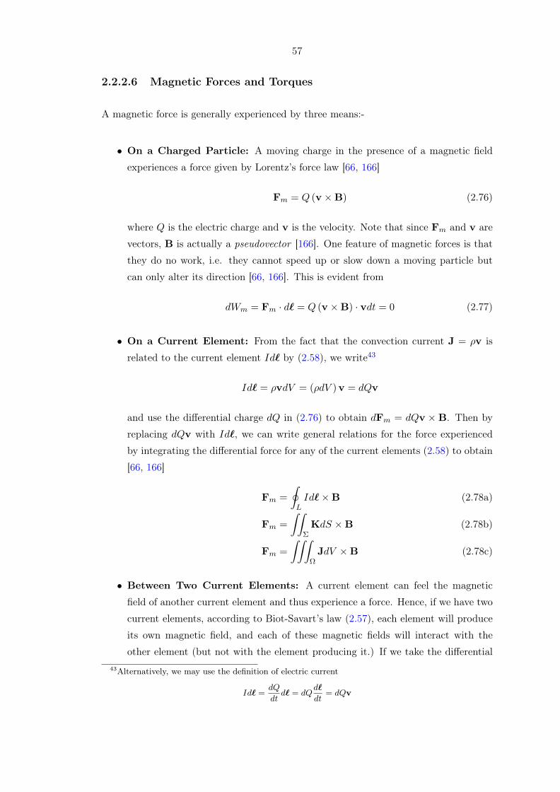
57
2.2.2.6 Magnetic Forces and Torques
A magnetic force is generally experienced by three means:-
• On a Charged Particle: A moving charge in the presence of a magnetic field
experiences a force given by Lorentz’s force law [66, 166]
Fm = Q (v ×B) (2.76)
where Q is the electric charge and v is the velocity. Note that since Fm and v are
vectors, B is actually a pseudovector [166]. One feature of magnetic forces is that
they do no work, i.e. they cannot speed up or slow down a moving particle but
can only alter its direction [66, 166]. This is evident from
dWm = Fm · dℓ = Q (v ×B) · vdt = 0 (2.77)
• On a Current Element: From the fact that the convection current J = ρv is
related to the current element Idℓ by (2.58), we write43
Idℓ = ρvdV = (ρdV )v = dQv
and use the differential charge dQ in (2.76) to obtain dFm = dQv ×B. Then by
replacing dQv with Idℓ, we can write general relations for the force experienced
by integrating the differential force for any of the current elements (2.58) to obtain
[66, 166]
Fm =
∮LIdℓ×B (2.78a)
Fm =
∫∫ΣKdS ×B (2.78b)
Fm =
∫∫∫ΩJdV ×B (2.78c)
• Between Two Current Elements: A current element can feel the magnetic
field of another current element and thus experience a force. Hence, if we have two
current elements, according to Biot-Savart’s law (2.57), each element will produce
its own magnetic field, and each of these magnetic fields will interact with the
other element (but not with the element producing it.) If we take the differential43Alternatively, we may use the definition of electric current
Idℓ =dQ
dtdℓ = dQ
dℓ
dt= dQv

58
of (2.78a) twice, we obtain d (dFm) = Idℓ× dB. Then upon using the differential
of (2.66) in the last relation, we obtain, for example, the force F1 on current loop
1 due to current loop 2 as the double integral
F1 =µ0I1I24π
∮L1
∮L2
dℓ1 × (dℓ2 × aR21)
R221
(2.79)
Now that we considered the forces, we can define the magnetic torque classically as
the cross product
τm = r× Fm (2.80)
where r is the moment arm.
2.2.2.7 Magnetic Dipoles
The concept of magnetic moment (or dipole) is central to the study of magnetostatics.
This is because in the absence of magnetic monopoles (see footnote 52), the most funda-
mental source and building block of magnetism is the magnetic dipole [160]. In brief, the
magnetic dipole moment is defined through a torque relation, and we typically model it
classically44 as either an infinitesimal current loop (the physicists’s way) or as a pair of
oppositely charged magnetic poles in juxtaposition (the engineer’s way) [67]. The two
models are shown in Fig. 2.15 below.
(a) (b)
Figure 2.15: Classical representations of a magnetic dipole. For the current loop, the direc-tion of the magnetic moment is determined by the right-hand rule. For the piece of magnet,the magnetic moment points from S to N. (a) Current loop model. (b) Magnetic poles model.
Current Loop: Referring to Fig. B.2, we define the magnetic dipole moment in terms
of a planar current-carrying loop as
m = IS (2.81)44We say classically because magnetism is a purely quantum mechanical phenomenon.

59
where I is the current and S is an areal vector which points in the normal direction in
accordance with the right-hand rule . In the limit as |S| → 0 while I →∞, |m| is finite
and the result is an ideal point dipole. The magnetic field produced by this dipole45
B =µ04π
[3 (r ·m) r−m
r3+
8π
3mδ (r)
](2.82)
When the magnetic field is non-uniform, there will be a force given by [61]
Fm = ∇ (m ·B) (2.83)
Magnetic Poles: Referring to Fig. B.3, we define the magnetic dipole moment in terms
of two opposite Gilbertian charges as
m = Qmℓ (2.84)
where Qm is the magnetic charge strength and ℓ the distance vector which points from S
to N. The field lines originate from the positive magnetic charge (source) and terminate
at the negative magnetic charge (sink). This is analogous to the definition of the electric
dipole in electrostatics.46 In the limit as |ℓ| → 0 while Qm → ∞, |m| is finite and the
result is an ideal point dipole. The magnetic field produced by this dipole is
B =µ04π
[3 (r ·m) r−m
r3− 4π
3mδ (r)
](2.85)
When the magnetic field is non-uniform, there will be a force given by
Fm = (∇ ·m)B (2.86)
Looking at the force relations above, one can immediately notice that the force be-
tween the two models are related by [61]
m× (∇×B) = ∇ (m ·B)− (∇ ·m)B (2.87)
which implies that the forces in both models are identical when there are no free currents
(J = 0) or time varying electric fields (∂D/∂t = 0), see (2.53d).45Readers who are interested in the derivations of both models are referred to Appendix B.46One should not take this analogy too far since magnetic dipoles are fundamentally different and are
related to angular momentum.
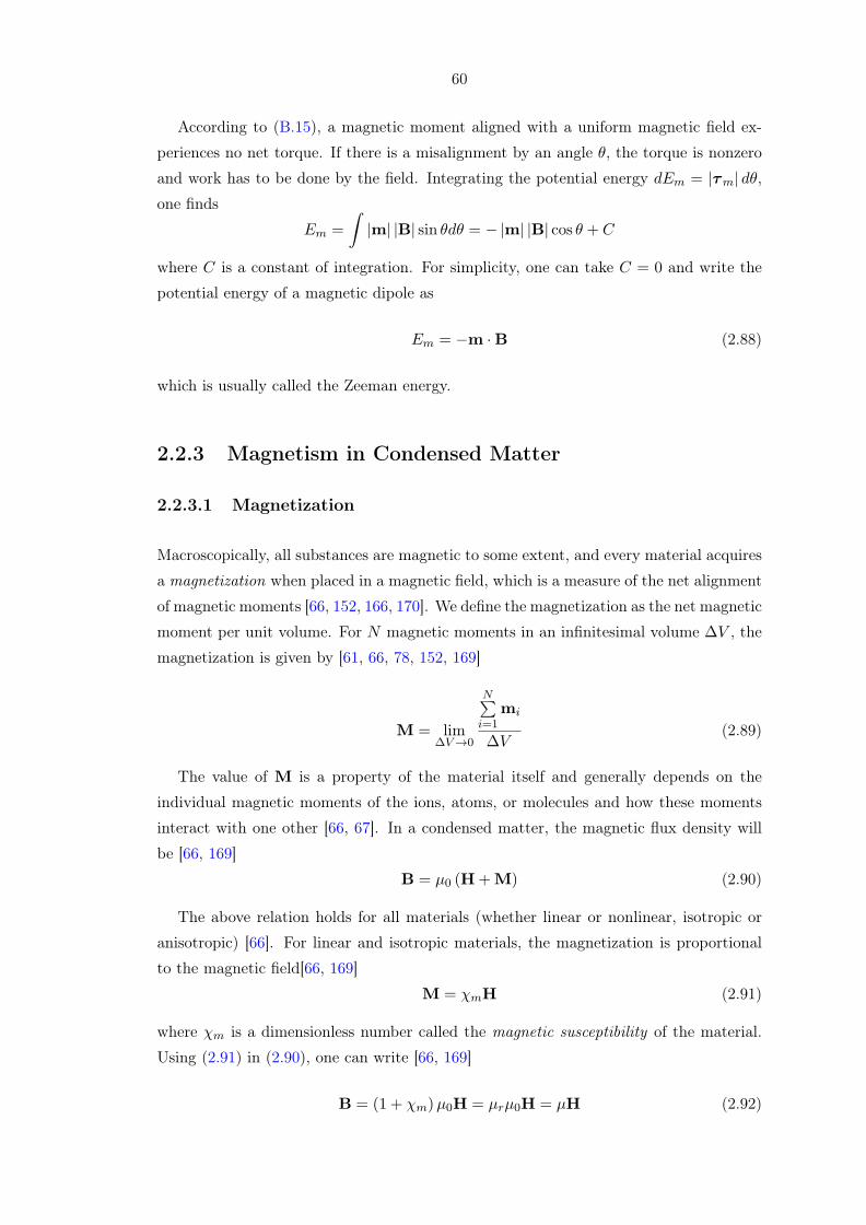
60
According to (B.15), a magnetic moment aligned with a uniform magnetic field ex-
periences no net torque. If there is a misalignment by an angle θ, the torque is nonzero
and work has to be done by the field. Integrating the potential energy dEm = |τm| dθ,one finds
Em =
∫|m| |B| sin θdθ = − |m| |B| cos θ + C
where C is a constant of integration. For simplicity, one can take C = 0 and write the
potential energy of a magnetic dipole as
Em = −m ·B (2.88)
which is usually called the Zeeman energy.
2.2.3 Magnetism in Condensed Matter
2.2.3.1 Magnetization
Macroscopically, all substances are magnetic to some extent, and every material acquires
a magnetization when placed in a magnetic field, which is a measure of the net alignment
of magnetic moments [66, 152, 166, 170]. We define the magnetization as the net magnetic
moment per unit volume. For N magnetic moments in an infinitesimal volume ∆V , the
magnetization is given by [61, 66, 78, 152, 169]
M = lim∆V→0
N∑i=1
mi
∆V(2.89)
The value of M is a property of the material itself and generally depends on the
individual magnetic moments of the ions, atoms, or molecules and how these moments
interact with one other [66, 67]. In a condensed matter, the magnetic flux density will
be [66, 169]
B = µ0 (H+M) (2.90)
The above relation holds for all materials (whether linear or nonlinear, isotropic or
anisotropic) [66]. For linear and isotropic materials, the magnetization is proportional
to the magnetic field[66, 169]
M = χmH (2.91)
where χm is a dimensionless number called the magnetic susceptibility of the material.
Using (2.91) in (2.90), one can write [66, 169]
B = (1 + χm)µ0H = µrµ0H = µH (2.92)

61
where µ is the magnetic permeability and µr the relative permeability of the material.
For anisotropic media (e.g., crystals), the vector fields are not parallel, and we speak of
susceptibility and permeability tensors47
χm =
χ11m χ12
m χ13m
χ21m χ22
m χ23m
χ31m χ32
m χ33m
(2.93)
µ =
µ11 µ12 µ13
µ21 µ22 µ23
µ31 µ32 µ33
(2.94)
where each component of the vector now obeys the relations
Mi = χijmHj (2.95)
Bi = µijHj (2.96)
If we wish to define a magnetic scalar potential Vm inside a material, we can still follow
the approach in 2.2.2.4. However, the divergence equation (2.54a) is now modified. In
particular, if we use (2.90) in Maxwell’s equations for magnetostatics (2.54) while still
assuming a current-free region (J = 0), we obtain
∇ ·H = −∇ ·M (2.97a)
∇×H = 0 (2.97b)
where we have eliminated µ0 since it is a scalar. Then from (2.97b), we can use (A.142),
to write H = −∇Vm so that (2.97a) becomes ∇ · (∇Vm) = ∇ ·M. Thus we obtain
∇2Vm (r) =
∇ ·M, r ∈ Ω
0, r ∈ R3\Ω(2.98)
together with the jump conditions
Vm|in = Vm|out (2.99)
∂Vm∂n
∣∣∣∣in
− ∂Vm∂n
∣∣∣∣out
= M · an (2.100)
The equation has the well-known solution [61, 163, 169]
Vm =1
4π
[−∫∫∫
Ω
∇′ ·M (r′)
|r− r′|dV ′ +
∫∫Σ
M (r′) · an|r− r′|
dS′]
(2.101)
47See A.1.2.2 for a brief overview of tensors.

62
where the integrands, in fact, play the role of source volume and surface magnetic charges
ρmv = −∇′ ·M(r′)
(2.102)
ρmS = M(r′)· an (2.103)
Using a similar approach but for the vector potential A (which can be the natural
approach when source currents are present), one can show that the general solution of
the vector Poisson equation (2.74) is given by [66, 169]
A =µ04π
[∫∫∫Ω
∇′ ×M (r′)
|r− r′|dV ′ +
∫∫Σ
M (r′)× an|r− r′|
dS′]
(2.104)
where the integrands now play the role of volume and surface magnetization currents
Jm = ∇′ ×M(r′)
(2.105)
Km = M(r′)× an (2.106)
2.2.3.2 Classes of Magnetic Materials
The magnetic behavior depends not only on the type of atom (ion) and unpaired spins
but also on the lattice symmetry and cell size. This essentially means that every material
responds to a magnetic field differently [153]. Phenomenologically, a magnetic material
can be characterized by a magnetic susceptibility [15, 78]. Some materials show a non-
cooperative magnetic behavior; examples are diamagnetic and paramagnetic materials
(Fig. 2.16) [61, 78]. In diamagnetic materials, χm is reversible, small, and negative,
and as a result M is slightly repelled by H [153, 171]. Diamagnetism is a fundamental
property of all materials (although often masked by stronger effects) and is temperature
independent [15, 66, 67]. It is essentially observed in materials with filled orbital shells,
i.e. atoms with no unpaired electrons [15, 66, 67, 153]. In paramagnetic materials,
χm is reversible, small, and positive, and M is thus slightly attracted by H [66, 67].
Unlike diamagnetism, paramagnetism results from unpaired spins which align with the
application of a magnetic field and reorient randomly once the field is removed due to
the thermal disorder and is thus temperature dependent [67, 78, 171].
Because of electron-electron interaction, another class of materials show a cooper-
ative (or collective) magnetic behavior (i.e. magnetic order) below certain ordering
temperatures, even in the absence of magnetic fields; e.g. ferromagnetism, antiferro-
magnetism, and ferrimagnetism (Fig. 2.17) [61, 68, 70, 78, 153, 171]. In contrast to
paramagnets, in which individual spins of atoms or ions respond independently to an ex-
ternal field, electron spins of the atoms constituting a ferromagent are more coupled [67].
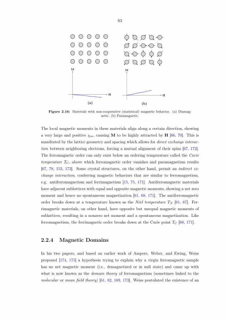
63
..
H
.
M
(a)
..
H
.
M
(b)
Figure 2.16: Materials with non-cooperative (statistical) magnetic behavior. (a) Diamag-netic. (b) Paramagnetic.
The local magnetic moments in these materials align along a certain direction, showing
a very large and positive χm, causing M to be highly attracted by H [66, 70]. This is
manifested by the lattice geometry and spacing which allows for direct exchange interac-
tion between neighboring electrons, forcing a mutual alignment of their spins [67, 172].
The ferromagnetic order can only exist below an ordering temperature called the Curie
temperature TC , above which ferromagnetic order vanishes and paramagnetism results
[67, 78, 153, 173]. Some crystal structures, on the other hand, permit an indirect ex-
change interaction, conferring magnetic behaviors that are similar to ferromagnetism,
e.g. antiferromagnetism and ferrimagnetism [15, 75, 171]. Antiferromagnetic materials
have adjacent sublattices with equal and opposite magnetic moments, showing a net zero
moment and hence no spontaneous magnetization [61, 68, 171]. The antiferromagnetic
order breaks down at a temperature known as the Néel temperature TN [61, 67]. Fer-
rimagnetic materials, on other hand, have opposite but unequal magnetic moments of
sublattices, resulting in a nonzero net moment and a spontaneous magnetization. Like
ferromagnetism, the ferrimagnetic order breaks down at the Curie point TC [68, 171].
2.2.4 Magnetic Domains
In his two papers, and based on earlier work of Ampere, Weber, and Ewing, Weiss
proposed [174, 175] a hypothesis trying to explain why a virgin ferromagnetic sample
has no net magnetic moment (i.e., demagnetized or in null state) and came up with
what is now known as the domain theory of ferromagnetism (sometimes linked to the
molecular or mean field theory) [61, 82, 169, 173]. Weiss postulated the existence of an
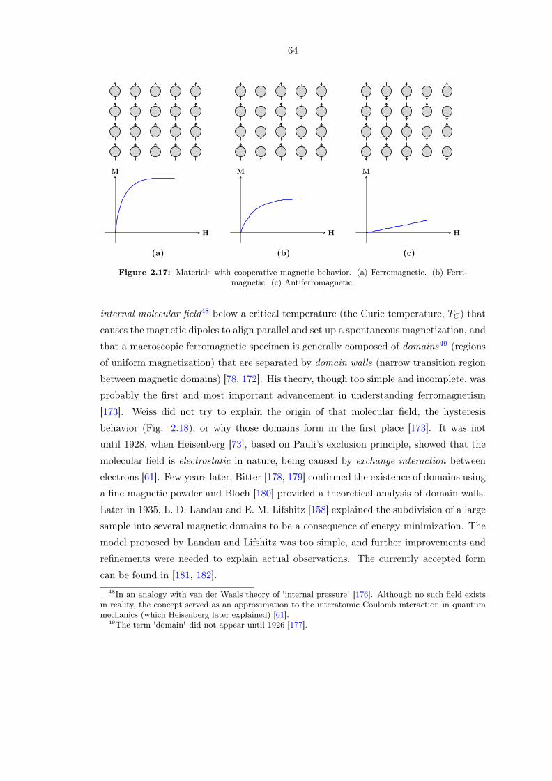
64
..
H
.
M
(a)
..
H
.
M
(b)
..
H
.
M
(c)
Figure 2.17: Materials with cooperative magnetic behavior. (a) Ferromagnetic. (b) Ferri-magnetic. (c) Antiferromagnetic.
internal molecular field48 below a critical temperature (the Curie temperature, TC) that
causes the magnetic dipoles to align parallel and set up a spontaneous magnetization, and
that a macroscopic ferromagnetic specimen is generally composed of domains49 (regions
of uniform magnetization) that are separated by domain walls (narrow transition region
between magnetic domains) [78, 172]. His theory, though too simple and incomplete, was
probably the first and most important advancement in understanding ferromagnetism
[173]. Weiss did not try to explain the origin of that molecular field, the hysteresis
behavior (Fig. 2.18), or why those domains form in the first place [173]. It was not
until 1928, when Heisenberg [73], based on Pauli’s exclusion principle, showed that the
molecular field is electrostatic in nature, being caused by exchange interaction between
electrons [61]. Few years later, Bitter [178, 179] confirmed the existence of domains using
a fine magnetic powder and Bloch [180] provided a theoretical analysis of domain walls.
Later in 1935, L. D. Landau and E. M. Lifshitz [158] explained the subdivision of a large
sample into several magnetic domains to be a consequence of energy minimization. The
model proposed by Landau and Lifshitz was too simple, and further improvements and
refinements were needed to explain actual observations. The currently accepted form
can be found in [181, 182].48In an analogy with van der Waals theory of 'internal pressure' [176]. Although no such field exists
in reality, the concept served as an approximation to the interatomic Coulomb interaction in quantummechanics (which Heisenberg later explained) [61].
49The term 'domain' did not appear until 1926 [177].

65
H
M
Mr
−Mr
Ms
−Ms
Hc−Hc
(a)
H
M
Mr
−Mr
Ms
−Ms
Hc−Hc
(b)
Figure 2.18: M -H hysteresis curves of a ferromagnet in an initially unmagnetized, virginstate. Here Hc is the coercivity, Mr the remanence, and Ms is the saturation magnetization.
(a) Hard magnet. (b) Soft magnet.
2.2.4.1 Formation of Domains: Energy Considerations
In general, magnetic domains form due to different interactions present in the material
such as exchange interaction (favoring parallel alignment of spins), anisotropy50 (favoring
the alignment of spins along certain preferential axes), dipolar (favoring antiparallel
alignment of spins), and Zeeman (favoring alignment of spins with the external field)51
[15, 78, 82, 169, 183]. The formation of domains does not seem to have a common origin as
it could arise from the necessity to reduce stray fields or the adoption of some anisotropy
(determined by the crystal structure, shape, and material parameters) [176]. However, it
is intuitive to explain the phenomenon using arguments concerning energy minimization.
Consider the scenario in Fig. 2.19a, which shows a large, uniformly magnetized (initially
single domain) ferromagnet with no applied magnetic fields in the space surrounding
it. It is useful to associate the magnet with pseudo-surface magnetic monopoles that
are 'smeared' around each end of the sample (Fig. 2.19b).52 In an analogy with electric
charges, magnetic charges act like sources and sinks. That is, magnetic flux lines (whether
inside or outside the sample) will originate from the positive magnetic charge (radially
outward) and terminate on the negative magnetic charge (radially inward). Hence, the
poles at the surface contribute by producing a stray magnetic field that extends into
the space outside the sample (Fig. 2.19c) [82]. Moreover, inside the sample, the poles
themselves produce another field that is opposite in direction to the field outside. This
field is called the demagnetizing field, since it reflects the tendency of that field to reduce50Anisotropy generally refers to the dependence of magnetization/magnetic properties on direction.
A good anisotropy is a prerequisite for hard magnets, whereas near-zero anisotropy is a prerequisite forsoft ones [61].
51The energy terms will be discussed in detail later.52We said 'pseudo' because there are no known magnetic charges; they are fictitious elements. In
contrast to electric charges, isolated magnetic charge do not exist [66, 67]. This follows from Gauss’law of magnetostatics (2.54a). However, one can think of dipoles or equivalently, two oppositely chargedmonopoles (see 2.2.2.7). For example, inside the material the flux density is given by B = µ0 (Hm +M).From (2.97) and the boundary conditions, one can associate the magnetic field Hm with volume andsurface magnetic charge densities ρmv = −∇ ·M and ρmS = M · an .
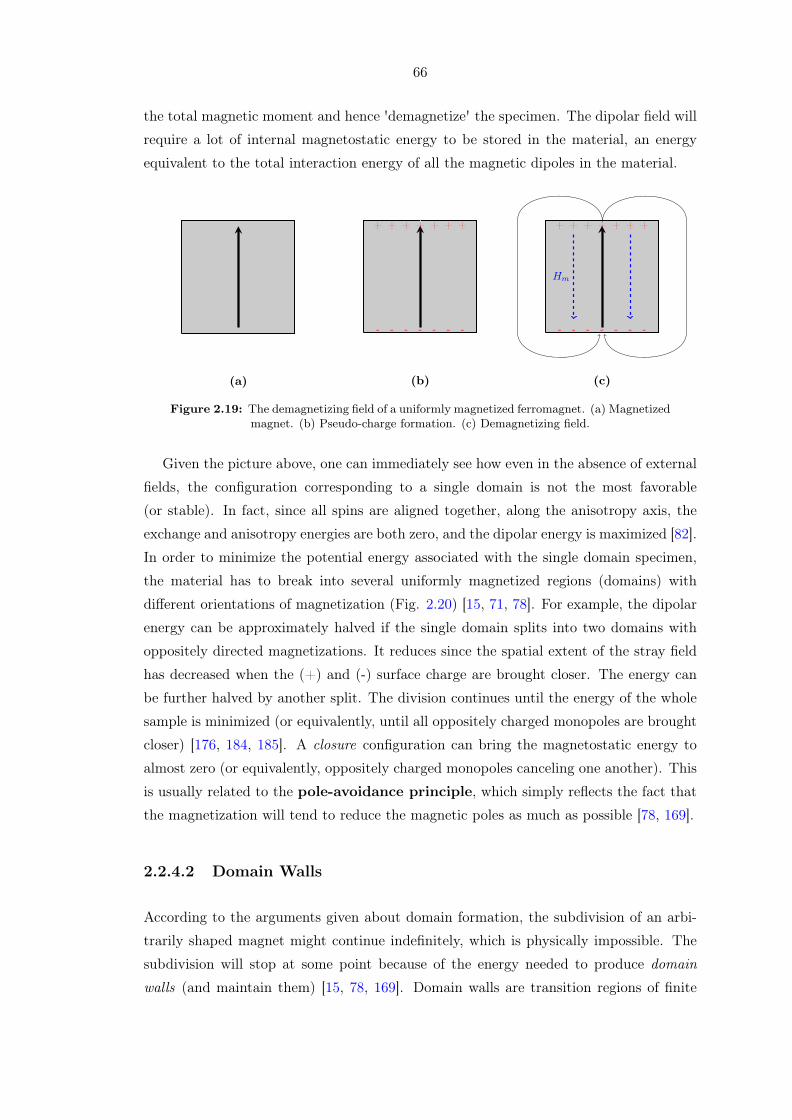
66
the total magnetic moment and hence 'demagnetize' the specimen. The dipolar field will
require a lot of internal magnetostatic energy to be stored in the material, an energy
equivalent to the total interaction energy of all the magnetic dipoles in the material.
(a)
+ ++ ++ ++
- -- -- --
(b)
+ ++ ++ ++
- -- -- --
Hm
(c)
Figure 2.19: The demagnetizing field of a uniformly magnetized ferromagnet. (a) Magnetizedmagnet. (b) Pseudo-charge formation. (c) Demagnetizing field.
Given the picture above, one can immediately see how even in the absence of external
fields, the configuration corresponding to a single domain is not the most favorable
(or stable). In fact, since all spins are aligned together, along the anisotropy axis, the
exchange and anisotropy energies are both zero, and the dipolar energy is maximized [82].
In order to minimize the potential energy associated with the single domain specimen,
the material has to break into several uniformly magnetized regions (domains) with
different orientations of magnetization (Fig. 2.20) [15, 71, 78]. For example, the dipolar
energy can be approximately halved if the single domain splits into two domains with
oppositely directed magnetizations. It reduces since the spatial extent of the stray field
has decreased when the (+) and (-) surface charge are brought closer. The energy can
be further halved by another split. The division continues until the energy of the whole
sample is minimized (or equivalently, until all oppositely charged monopoles are brought
closer) [176, 184, 185]. A closure configuration can bring the magnetostatic energy to
almost zero (or equivalently, oppositely charged monopoles canceling one another). This
is usually related to the pole-avoidance principle, which simply reflects the fact that
the magnetization will tend to reduce the magnetic poles as much as possible [78, 169].
2.2.4.2 Domain Walls
According to the arguments given about domain formation, the subdivision of an arbi-
trarily shaped magnet might continue indefinitely, which is physically impossible. The
subdivision will stop at some point because of the energy needed to produce domain
walls (and maintain them) [15, 78, 169]. Domain walls are transition regions of finite
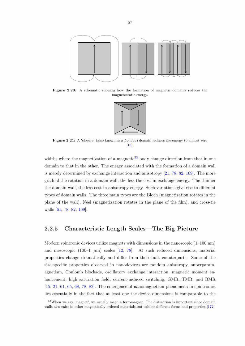
67
Figure 2.20: A schematic showing how the formation of magnetic domains reduces themagnetostatic energy.
Figure 2.21: A 'closure' (also known as a Landau) domain reduces the energy to almost zero[15].
widths where the magnetization of a magnetic53 body change direction from that in one
domain to that in the other. The energy associated with the formation of a domain wall
is merely determined by exchange interaction and anisotropy [21, 78, 82, 169]. The more
gradual the rotation in a domain wall, the less the cost in exchange energy. The thinner
the domain wall, the less cost in anisotropy energy. Such variations give rise to different
types of domain walls. The three main types are the Bloch (magnetization rotates in the
plane of the wall), Néel (magnetization rotates in the plane of the film), and cross-tie
walls [61, 78, 82, 169].
2.2.5 Characteristic Length Scales—The Big Picture
Modern spintronic devices utilize magnets with dimensions in the nanoscopic (1–100 nm)
and mesoscopic (100–1 µm) scales [12, 78]. At such reduced dimensions, material
properties change dramatically and differ from their bulk counterparts. Some of the
size-specific properties observed in nanodevices are random anisotropy, superparam-
agnetism, Coulomb blockade, oscillatory exchange interaction, magnetic moment en-
hancement, high saturation field, current-induced switching, GMR, TMR, and BMR
[15, 21, 61, 65, 68, 78, 82]. The emergence of nanomagnetism phenomena in spintronics
lies essentially in the fact that at least one the device dimensions is comparable to the53When we say 'magnet', we usually mean a ferromagnet. The distinction is important since domain
walls also exist in other magnetically ordered materials but exhibit different forms and properties [172].

68
so-called characteristic lengths54 of the sample, below which interesting phenomena are
observed [68]. By transcending these length scales, the observed magnetic (and elec-
tric) properties can either be enhanced or suppressed. Moreover, these length scales will
determine the ultimate limits on the performance of the device [82].
Many of the defining length scales in magnetism are determined from considerations
regarding energy minimization [82, 184].55,56 In particular, by a competition between
different energy terms [68]. The length scales will determine the “most appropriate
description” of the magnetic sample. For example, consider a large macroscopic magnet.
The stray (or dipolar) fields will cause splitting of the sample into many domains that
are separated by domain walls. The macroscopic average magnetization (determined by
the alignment of domains) adequately describe the character of the magnet as a function
of the applied magnetic field (top of Fig. 2.22). As the size reduces, one has to include
other forms of energy (e.g. exchange and magnetocrystalline anisotropy) and describe
the structure of domains and domain walls [15]. There exist two models for that matter:
the domain theory, which deals with the microstructure of discrete domains and domain
walls, while assuming vanishing walls widths and thus discontinuous magnetization at the
boundaries; and micromagnetism, which invokes a continuum hypothesis and assumes
continuous magnetic moments distribution [183]. As we reduce the size even further,
atomic description is necessary and one has to deal with the structure of spins and their
arrangement in the crystal lattice [183].
Some of the typical length scales are the exchange length lex, domain wall width
parameter dDW , and critical single domain diameter dsd, respectively given by [21, 61,
68, 78, 169]
lex =
√2A
µ0M2s
dDW =
√A
K1
dsd = 72
√AK1
µ0M2s
where A is the exchange coefficient within a grain and K1 is the bulk anisotropy constant.
The exchange length separates the zone where exchange interaction dominates (L < lex,54Plus broken translational symmetry, and the fact that nanoscopic objects contain higher proportion
of surface/interfacial atoms and low coordination numbers [61, 68, 78].55See the discussion in 2.2.4.1 and 2.2.4.2.56Other length scales like the spin-diffusion length ℓsf and the spin-precession length ℓsp could result
from the diffusion processes of energy, momentum or magnetization [61, 82].

69
Magnetic Hysteresis (> 0.1mm)Describes the average magnetization vectorof a sample as a function of the applied field
Domain Theory (1−1000µm)Describes the magnetic microstructure of a sample
with details about the domains and domain boundaries
Micromagnetic Analysis (1−1000 nm)Describes the internal structure and substruc-ture of domain walls using a continuum theory
Atomic Theory (< 1 nm)Describes the origin, the interaction, and the sta-
tistical thermodynamics of magnetic moments
Figure 2.22: Descriptive hierarchy of magnetically ordered materials. The levels are roughlydistinguished with length scales. Figure adapted by the author from [176, 183].
where magnetization is uniform and coherent reversal takes place)57 from that where
dipolar interaction dominates (L > lex, where incoherent reversal of magnetization takes
place through different processes like curling, buckling, and fanning), and can be in
the range 1–100 nm [21, 68, 78, 169].58 The domain wall width parameter dDW59 is
determined by a competition of exchange and anisotropy, or exchange and dipolar (when
anisotropy is weak), and depends on the sample geometry [82]. It usually falls in the
range 1–100 nm [68, 78]. This parameter corresponds to the width of a Bloch wall that is
found in materials where the main source of anisotropy is magnetocrystalline anisotropy
(e.g., hard materials) [68]. In thin films of soft magnetic materials where surface charges
are large (and are replaced by volume charges as suggested by Néel), the domain wall
width parameter corresponds to a Néel wall. Finally, the critical single domain size dsdcan range from 5 nm for soft materials up to 1000 nm for hard ones [78]. Below this
length, the magnet is single domain, whereas above it can exhibit a multidomain, or even
vortex60 configuration. In general, the above parameters follow the inequalities below57A reversal is coherent (or homogeneous) when the moments remain strictly parallel throughout the
process, independent of r [61, 78]. An incoherent (or inhomogeneous) reversal, on the other hand, mightinvolve an intermediate state which is not uniformly magnetized.
58Some authors [61, 78, 169] use a more strict measure for coherence reversal, a parameter called thecoherence radius, given roughly by the expression Rcoh = βlex, where β varies between 5.2 and 7.2. Thisgives the maximum size (i.e., upper bound) of coherent reversal of a uniformly magnetized particle andgenerally depends on the detailed shape as well as material parameters.
59The domain wall width is given by πdDW [76, 78].60Also known as a swirl; a circular arrangement of magnetic moments.
70
[78, 169]
Soft Material:
dsd ∼ lex ≪ dDW (2.107)
Hard Material:
dsd ≫ lex >∼ dDW (2.108)
2.3 Micromagnetism
Micromagnetism is a continuum theory to describe the magnetization distribution in
mesoscopic magnetic structures [21].61,62 Because the spintronic devices of interest are
too small, a model solely based on Maxwell’s electrodynamics, though simple, is however
inaccurate since it does not take into account many of the coupled mechanisms such as
exchange interaction or anisotropy [187–189]. On the other hand, the devices are still
too large for them to be considered 'atomistic', and hence, a pure quantum mechanical
approach is of prohibitive difficulty and computationally expensive (and, in fact, would
seem 'utopic') [189]. Micromagnetics is an intermediate solution; way beyond the range
of classical electromagnetic theory, yet far from being considered an atomic scale theory.
It includes effects on different spatial scales such as the long-range dipolar interaction
and the short-range exchange interaction. Although it usually leads to complex nonlinear
equations—for which only a few idealized cases result in analytic solutions—it bridges
the gap and smoothly interpolates between the two approaches. It assumes a continuum
magnetization configuration while, at the same time, uses results that have been derived
from a quantum mechanical treatment (with a formalism appropriate for the limit of
continuous material).63 The latter fact, coupled with an energy minimization approach
and a dynamic formalism [158], forms the basic principles of micromagnetism.
The theory was originally developed in 1935 by Landau and Lifshitz [158] based
on a variational principle, and later heavily contributed to by Brown with the rise of
computational science in the 1940s [186, 190]. Brown coined the term 'Micromagnetics'
in 1958 [190].64 A classical treatment micromagnetics can be found in Brown’s early
[191, 192] and late [193] books.61Within the framework of the continuum theory in mechanics, a magnetizable specimen is composed
of two interacting continua: lattice continuum and the spin continuum.62As long as any characteristic length is much larger than the size of a unit cell, the assumption of a
continuous material is valid [186].63In particular, a semiclassical approach is invoked in which spins are replaced by classical vectors and
quantum mechanical exchange interaction in the Heisenberg Hamiltonian by a classical exchange energyterm [186].
64This name could be misleading because in micromagnetism the microscopic structure (i.e., atomicnature of the material) is ignored.
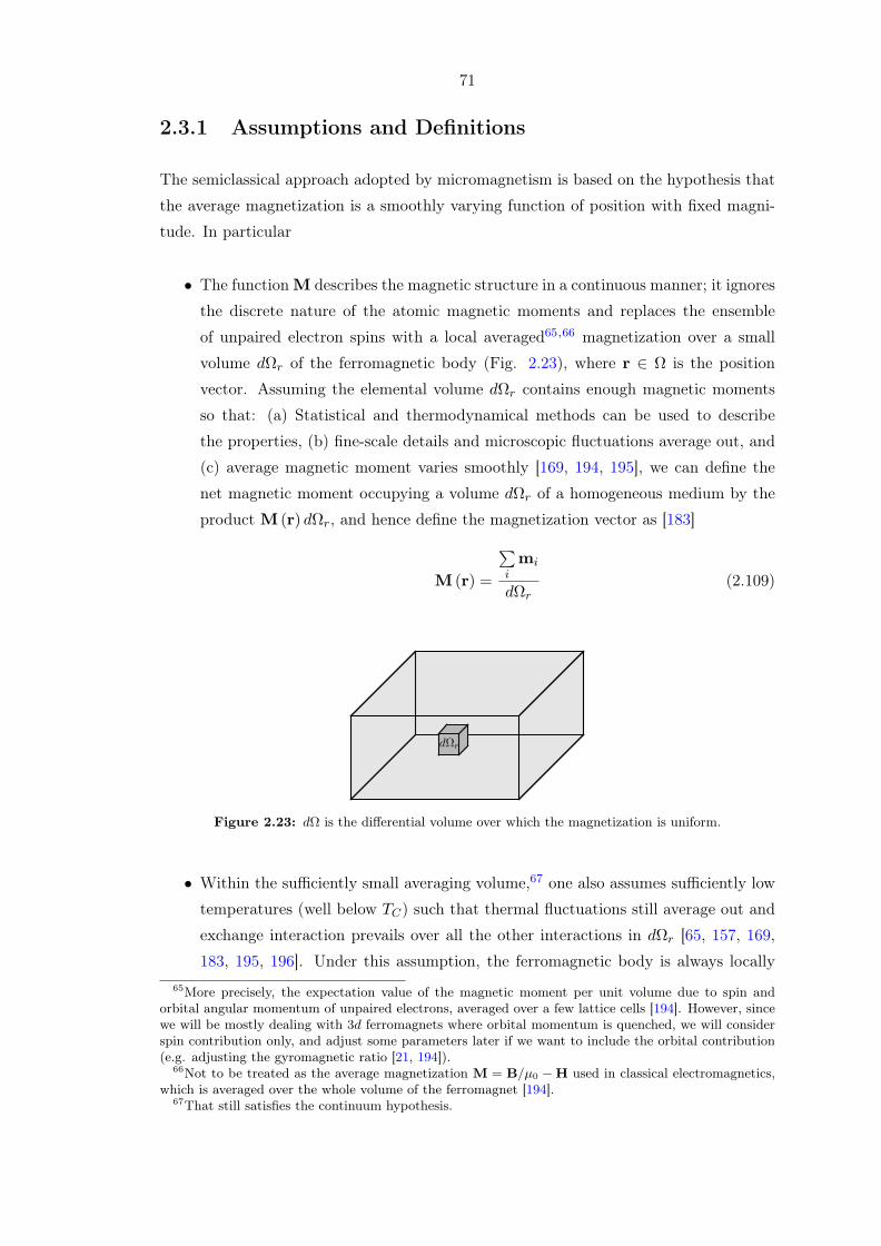
71
2.3.1 Assumptions and Definitions
The semiclassical approach adopted by micromagnetism is based on the hypothesis that
the average magnetization is a smoothly varying function of position with fixed magni-
tude. In particular
• The function M describes the magnetic structure in a continuous manner; it ignores
the discrete nature of the atomic magnetic moments and replaces the ensemble
of unpaired electron spins with a local averaged65,66 magnetization over a small
volume dΩr of the ferromagnetic body (Fig. 2.23), where r ∈ Ω is the position
vector. Assuming the elemental volume dΩr contains enough magnetic moments
so that: (a) Statistical and thermodynamical methods can be used to describe
the properties, (b) fine-scale details and microscopic fluctuations average out, and
(c) average magnetic moment varies smoothly [169, 194, 195], we can define the
net magnetic moment occupying a volume dΩr of a homogeneous medium by the
product M (r) dΩr, and hence define the magnetization vector as [183]
M (r) =
∑imi
dΩr(2.109)
dΩr
Figure 2.23: dΩ is the differential volume over which the magnetization is uniform.
• Within the sufficiently small averaging volume,67 one also assumes sufficiently low
temperatures (well below TC) such that thermal fluctuations still average out and
exchange interaction prevails over all the other interactions in dΩr [65, 157, 169,
183, 195, 196]. Under this assumption, the ferromagnetic body is always locally65More precisely, the expectation value of the magnetic moment per unit volume due to spin and
orbital angular momentum of unpaired electrons, averaged over a few lattice cells [194]. However, sincewe will be mostly dealing with 3d ferromagnets where orbital momentum is quenched, we will considerspin contribution only, and adjust some parameters later if we want to include the orbital contribution(e.g. adjusting the gyromagnetic ratio [21, 194]).
66Not to be treated as the average magnetization M = B/µ0 −H used in classical electromagnetics,which is averaged over the whole volume of the ferromagnet [194].
67That still satisfies the continuum hypothesis.

72
saturated [157, 196], and we obtain the so-called fundamental constraint of micro-
magnetism
|M (r, t)| =Ms(T ) ↔ |m (r, t)| = 1 (2.110)
where Ms is the saturation magnetization which depends on both the material and
temperature.68
Consider a ferromagnetic body (Fig. 2.24) at a temperature T occupying a bounded
domain Ω ⊂ R3 with a smooth boundary ∂Ω. From the previous assumptions, we can
formally define the local magnetization at every point inside the body by the differentiable
vector field M (r, t) given as the map
M : (0, T )× Ω→x ∈ R3 : |x| =Ms
(2.111D)
where Ms > 0 is the constant saturation magnetization at the temperature T . The
magnetization is assumed to vanish on R3\Ω and for T ⩾ Tc. Although the magnitude
of M is constant in space, its direction is allowed to vary. Thus we can write M =Msm,
from which we define the reduced magnetization (or magnetic moment)69
m (r, t) =M (r, t)
Ms(2.112)
which can then formally be defined as
m : (0, T )× Ω→x ∈ R3 : |x| = 1
(2.113D)
Sometimes, one may write m as
m : (0, T )× Ω→ S2 (2.114D)
where S2 denotes the unit sphere of R3.68The saturation magnetization vanishes above the Curie temperature TC where phase transition
takes place (a characteristic of each crystal type) [61, 71, 171, 173]. However, since we usually work withferromagnets way below the Curie point and assume temperature to be uniform in space and constantin time, Ms can be taken as a material-dependent constant and therefore a single number when workingwith a single-crystal ferromagnet.
69This is not the magnetic moment of the atom.

73
Ω
Figure 2.24: Ferromagnetic body of volume Ω.
2.3.2 Micromagnetic Energy
2.3.2.1 Thermodynamics
A model of a magnetic medium is generally analyzed within a thermodynamic framework
where the body is characterized in terms of its internal energy, and the temporal evolution
of the involved variables (e.g., magnetization) is then determined under the goal of “total
energy” minimization. For a unit volume dΩ of a material that is in contact with a
thermal bath at temperature T , the principal thermodynamic laws are:-
1st law of thermodynamics (energy conservation): When work δW is performed on the
system and heat δQ is absorbed by it, the change in internal energy is given by the sum70
dU = δW + δQ (2.115)
For a state (i.e., extensive) variable X describing some property of the system, and its
conjugate (i.e., intensive) variable YX describing some external action exerted on the
system, one can always express the differential work as
δW = YXdX (2.116)
2nd law of thermodynamics (irreversible process): For an irreversible transformation in
a non-isolated system, the entropy changes as
dS ⩾ δQ
T(2.117)
70The symbol δ usually denotes an inexact differential, a quantity which has a circulation that is notnecessary zero, viz. ∮
δA = 0
On the other hand, the special symbol d is usually reserved for exact differentials (i.e., path-independentquantities) ∮
dA = 0

74
Under a reversible transformation, the equality holds and one has
δQ = TdS (2.118)
which in fact reveals that T and S are extensive and intensive variables, respectively
(i.e., conjugate variables)71. The 2nd law can also be formulated as
dS =δQ
T+ dSirr (2.119)
where dSirr is the amount of entropy generated by the irreversibility of the transforma-
tion. It is obvious that dSirr ≥ 0, where dSirr = 0 holds for a reversible process.
Consider the general set of magnetic, mechanical, and thermal processes shown in
Fig. 2.25. As pioneered by Massieu and Gibbs, one can analyze the static properties
of any physical system by what we call thermodynamic potentials, which are state func-
tions controlling how a transformation will evolve [84, 169]. There are four potentials of
interest, each defined by fixing two variables and leaving the other two [61]. The poten-
tials are: Internal Energy u (X,S), Enthalpy h (YX , S), Helmholtz Free Energy f (X,T ),
and Gibbs Free Energy g (YX , T ); all in units of J·m−3 and each reaching a minimum
at thermodynamic equilibrium and never increases under any transformation when the
respective arguments are fixed [61, 169]. According to Fig. 2.25, the extensive variables
are X = M, ε, S, and the intensive variables are YX = Ha, σ, T .
Consider an object in internal thermodynamic equilibrium at temperature T . Al-
though u (M, ε, S) is useful for studying adiabatic (isentropic) processes, in our case T
is fixed and it is better to make a Legendre transformation to the variables (M, ε, T )
and (Ha, σ, T ). Thus the relevant potentials in this case are f (M, ε, T ) and g (Ha, σ, T ).
With these potentials, we would measure the system’s ability to do work, i.e. find its
free energy. The Helmholtz free energy density is given by the Legendre transformation
f (M, ε, T ) = u (M, ε, S)− TS (2.120)
where the first term is related to all interaction energy terms within a magnet and
the second term is constant at a given temperature [163]. In our case, the internal
energy is determined by exchange interaction, crystalline anisotropy, magnetostatic, and
magnetoelastic72 [199]. In fact, since the change in magnetomechanical work (due to71Equations (2.116) and (2.118) in fact reveal the symmetry between the extensive (X,S) and intensive
(YX , T ) variables involved: T and S are conjugate variables with respect to thermal energy, whereas YX
and X are conjugate variables with respect to external work.72A change in magnetization may produce a deformation in the crystal lattice (and vice versa), a
phenomenon known as magnetostriction [61, 82, 198].
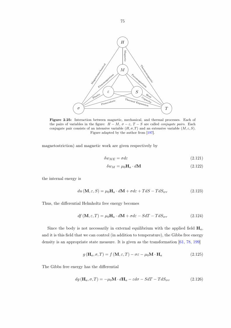
75
H
σ T
M
ε SM
agne
tomec
hani
cal T
hermom
agnetic
Magn
etic
Piezom
agne
tism Pyrom
agnetism
Elastic
Thermal Expansion
HeatCapacityPiezoc
aloric
Figure 2.25: Interaction between magnetic, mechanical, and thermal processes. Each ofthe pairs of variables in the figure: H −M , σ − ε, T − S are called conjugate pairs. Eachconjugate pair consists of an intensive variable (H,σ, T ) and an extensive variable (M, ε, S).
Figure adapted by the author from [197].
magnetostriction) and magnetic work are given respectively by
δwME = σdε (2.121)
δwM = µ0Ha · dM (2.122)
the internal energy is
du (M, ε, S) = µ0Ha · dM+ σdε+ TdS − TdSirr (2.123)
Thus, the differential Helmholtz free energy becomes
df (M, ε, T ) = µ0Ha · dM+ σdε− SdT − TdSirr (2.124)
Since the body is not necessarily in external equilibrium with the applied field Ha,
and it is this field that we can control (in addition to temperature), the Gibbs free energy
density is an appropriate state measure. It is given as the transformation [61, 78, 199]
g (Ha, σ, T ) = f (M, ε, T )− σε− µ0M ·Ha (2.125)
The Gibbs free energy has the differential
dg (Ha, σ, T ) = −µ0M · dHa − εdσ − SdT − TdSirr (2.126)

76
which is a non-increasing function when its arguments are fixed, viz.
dg (Ha, σ, T ) = −TdSirr ≤ 0 (2.127)
since TdSirr ⩾ 0. The minima of g gives the values M, ε, S to which the material
converges as equilibria. The equilibrium equations are given by
∂g (Ha, σ, T )
∂M= 0 (2.128)
∂g (Ha, σ, T )
∂ε= 0 (2.129)
∂g (Ha, σ, T )
∂S= 0 (2.130)
The above conditions are in fact equivalent to
M = − 1
µ0
[∂g (Ha, σ, T )
∂Ha
]σ,T
(2.131)
ε = −[∂g (Ha, σ, T )
∂σ
]Ha,T
(2.132)
S = −[∂g (Ha, σ, T )
∂T
]Ha,σ
(2.133)
The first equation in fact reveals that M has to be expressed with the equation of state
[61]
M = M (Ha, σ, T ) (2.134)
which, at thermodynamic equilibrium, and for a given (Ha, σ, T ), is uniquely determined.
However, this is not the case for a ferromagnetic body: the variables (Ha, σ, T ) are not
sufficient to uniquely determine the state of M. This is because the free energy will
have many local minima (metastable equilibria, Fig. 2.26) [78]; a framework known as
nonequilibrium thermodynamics [169]. This can be analyzed by a generalization of the
Gibbs energy to the Landau-Gibbs free energy gL, given by [169]
gL (M;Ha, σ, T ) = f (M, ε, T )− σε− µ0M ·Ha (2.135)
= u (M, ε, S)− TS − σε− µ0M ·Ha (2.136)
which coincides with the Gibbs energy (2.125) at thermodynamic equilibrium (except
for the fact that gL explicitly uses M, forcing it to take certain values and thus acting
as if it was an external constraint) [61]. At equilibrium, gL is at extremum [169][∂gL (M;Ha, σ, T )
∂M
]Ha,T,σ
= 0 (2.137)
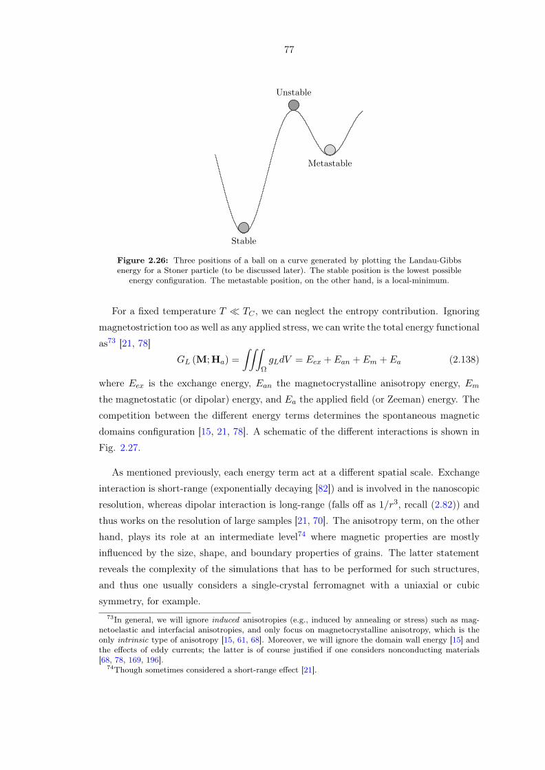
77
Stable
Unstable
Metastable
Figure 2.26: Three positions of a ball on a curve generated by plotting the Landau-Gibbsenergy for a Stoner particle (to be discussed later). The stable position is the lowest possible
energy configuration. The metastable position, on the other hand, is a local-minimum.
For a fixed temperature T ≪ TC , we can neglect the entropy contribution. Ignoring
magnetostriction too as well as any applied stress, we can write the total energy functional
as73 [21, 78]
GL (M;Ha) =
∫∫∫ΩgLdV = Eex + Ean + Em + Ea (2.138)
where Eex is the exchange energy, Ean the magnetocrystalline anisotropy energy, Em
the magnetostatic (or dipolar) energy, and Ea the applied field (or Zeeman) energy. The
competition between the different energy terms determines the spontaneous magnetic
domains configuration [15, 21, 78]. A schematic of the different interactions is shown in
Fig. 2.27.
As mentioned previously, each energy term act at a different spatial scale. Exchange
interaction is short-range (exponentially decaying [82]) and is involved in the nanoscopic
resolution, whereas dipolar interaction is long-range (falls off as 1/r3, recall (2.82)) and
thus works on the resolution of large samples [21, 70]. The anisotropy term, on the other
hand, plays its role at an intermediate level74 where magnetic properties are mostly
influenced by the size, shape, and boundary properties of grains. The latter statement
reveals the complexity of the simulations that has to be performed for such structures,
and thus one usually considers a single-crystal ferromagnet with a uniaxial or cubic
symmetry, for example.73In general, we will ignore induced anisotropies (e.g., induced by annealing or stress) such as mag-
netoelastic and interfacial anisotropies, and only focus on magnetocrystalline anisotropy, which is theonly intrinsic type of anisotropy [15, 61, 68]. Moreover, we will ignore the domain wall energy [15] andthe effects of eddy currents; the latter is of course justified if one considers nonconducting materials[68, 78, 169, 196].
74Though sometimes considered a short-range effect [21].

78
......
θ
(a)
..
ean
..
θ
(b)
.....(c)
..
Ha
..
θ
(d)
Figure 2.27: Four common types of magnetic energy. (a) Exchange. (b) Anisotropy. (c)Magnetostatic. (d) Zeeman.
2.3.2.2 Energy Terms
Below, we discuss each energy term. Thermal effects will be included later.
• Exchange Energy Eex
In a solid, the electronic orbitals of contiguous atoms overlap, leading to a corre-
lation between electrons. The result is that the “interatomic interaction” affects
the total energy, introducing a dependency on the relative orientation of localized
spins in neighboring atoms. Exchange energy is the energy required to rotate one
spin with respect to its neighbors (overcoming the Pauli principle) [82, 173]. The
interaction results from the electrostatic Coulomb repulsion between electrons, and
the spin-dependency of the interaction arises from the requirement that the wave
function of a pair of electrons is antisymmetric with respect to the interchange of
electron coordinates and spin (Fig. 2.28) [70, 75, 76, 82].75 That is, when the
electron spins are parallel, the wave function is antisymmetric in the coordinate
part
ψσσ (r1, r2) = −ψσσ (r2, r1) (2.139)75This comes from the indistinguishability of electrons which implies that exchange of two electrons
should keep the total density of the electrons unchanged: |ψσσ (r1, r2)|2 = |ψσσ (r2, r1)|2 [61].

79
which simply means the probability that two electrons are in close proximity is
small (compared to the other case). This is in agreement with Pauli’s exclusion
principle which essentially states that electrons with parallel spins tend to avoid
each other spatially so that their wavefunctions do not overlap (i.e. not being in the
same place) [14, 15]. As a consequence, the repulsive Coulomb energy is lowered,
and this reduction in Coulomb energy is the exchange energy [15, 21, 75].
....
(a)
....
(b)
Figure 2.28: Symmetric and antisymmetric wavefunctions.
The “direct” exchange interaction is the sum of all of the different interactions:
spin-spin, spin-orbit, etc. [82]. Usually, one only considers the spin-spin interaction
between two contiguous spins and refer to it as a “direct” exchange interaction. In
this case, the exchange energy is defined as the energy difference between parallel
and antiparallel spin configuration. The exchange energy is typically given as the
expectation value of the Heisenberg Hamiltonian. The latter, for example, is given
for a two-spin system as [61, 78]
H = −2J s1 · s2 (2.140)
where J is the exchange parameter which is positive for parallel spins (ferro-
magnetism) and negative for antiparallel spins (antiferromagnetism or ferrimag-
netism)76 [68, 123]. The sign of J depends on the interatomic distances (i.e. orbital
overlap), being negative if the atoms are closely spaced, and positive otherwise (Fig.
2.29).77 Here, s1 and s2 represent the localized electrons spins of adjacent atoms
(in units of ℏ). The interaction is bilinear in spins and isotropic under rotation
(guaranteed by the dot product).76Depending on the topology of the crystal lattice [61].77In the intermediate case, like in γ-Fe2O3 and ferrites, the inter-atomic distance to the atomic size
will result in ferrimagnetism [123].

80
Inter-Atomic Distance—————————–
Atomic Diameter
Cr
Mn
Fe
Co
Ni
Exchange
FM
+
AFM
−
Figure 2.29: Exchange coupling between spins as a function of their spacing-to-size ratio.Figure adapted by the author from [123].
The above expression is quantum mechanical. The classical counterpart can be
written by replacing the operators with classical vectors. For many-electron system
in a lattice, one can write [68, 78, 82]
Eex = −2Jijsi · sj (2.141)
where Jij is the exchange parameter linking the i-th and j-th spins. Here Einstein’s
summation convention is assumed.
The spin-spin exchange interaction penalizes spatial variations in M and leads
to a preferential for large regions of uniform magnetization (magnetic domains)
separated by thin transition regions (domain walls) [68, 196]. Exchange interaction
is believed to be the main cause of ferromagnetism [78]. For small variations of M
from point to point, one can expand the energy as a function of ∇M. Assuming a
cubic crystal, a continuum (micromagnetic scale) approximation, and limiting to
nearest neighbors, the exchange energy can be written by dropping the high order
terms as [78, 82, 169, 196]
Eex =A
M2s
∫∫∫Ω
[(∇Mx)
2 + (∇My)2 + (∇Mz)
2]dV (2.142)
where A = nJS2/a is the exchange stiffness constant for a cubic crystal with one
nonequivalent atom; a phenomenological positive material parameter that sum-
marizes the (usually very) short-range exchange interaction. Here a is the lattice
spacing, and n = 1 for simple cubic lattice, n = 2 for body-centered cubic (bcc) lat-
tice, and n = 4 for face-centered cubic (fcc) [78]. Equation (2.142) can be written

81
more compactly as
Eex =A
M2s
∫∫∫Ω(∇M)2dV (2.143)
In the general case of a non-cubic and anisotropic medium, A is a tensor and
one has
Eex =1
M2s
∫∫∫ΩAkl
∂Mi
∂xk
∂Mi
∂xldV (2.144)
• Magnetocrystalline Anisotropy Energy Ean
Magnetocrystalline anisotropy is related to the competition between spin-orbit cou-
pling, and the local crystal electric field (single-ion) or the dipole-dipole interaction
(two-ion), and thus manifests itself as the energy needed to overcome spin-orbit
coupling78 [15, 21, 61, 68, 70, 82, 169]. The electronic structure induces M to lie
along certain preferred crystallographic directions, so-called easy-axes [15, 68]. The
crystal anisotropy is generally determined by a globally non-negative anisotropy en-
ergy density functional, fan (M) : R3 → R+ that depends on material parameters
and symmetry of the crystalline lattice microstructure [21, 171]. The functional
is globally Lipschitz continuous and vanishes (i.e., achieves its minima) on the set
of unit vectors known as the easy-axes79 [15, 82, 171]. Using the energy density
functional, the anisotropy energy is written as
Ean =
∫∫∫Ωfan (M) dV (2.145)
The functional is typically a polynomial possessing certain symmetry properties. In
general, fan (m) is invariant under inversion of m [169]. We consider two examples
below.
Uniaxial Anisotropy: For uniaxial anisotropy, it is convenient to first express
the magnetization components in spherical coordinates
Mx =Ms sin θ cosϕ (2.146)
My =Ms sin θ sinϕ (2.147)
Mz =Ms cos θ (2.148)
78This might also lead to surface anisotropy—breaking of inversion symmetry at the surface orinterface—in very thin films [68, 78, 200]. Such anisotropy yields an energy of the form fan,s (m) =Ks (1−m · an) [61, 78].
79Saddle-points and maxima of fan (M) are attained at the medium-hard- and hard-axes, respectively[169].
82
This gives the rescaled magnetization
mx = sin θ cosϕ (2.149)
my = sin θ sinϕ (2.150)
mz = cos θ (2.151)
which only depends on direction. Now, since the anisotropy is symmetric with
respect to the easy-axis (i.e., rotationally symmetric), we can write the anisotropy
energy density as an even expansion in sin θ [78, 169]
fan (m) = K1sin2θ +K2sin
4θ +K3sin6θ + · · · (2.152)
where now fan (m) : S2 → R+, since we used the rescaled magnetization. Here θ
is angle between m and the easy-axis ean, and Ki’s are the anisotropy constants.
For simplicity, let us truncate the expansion and consider the first term [61, 68]
fan (m) ≃ K1sin2θ (2.153)
For K1 > 0, the energy minima are located on the easy-axis (for θ = 0 and θ = π)
whereas for K1 < 0, the minima are located on the easy-plane (for θ = π/2). The
uniaxial energy functional can also be written as
fan (m) ≃ K1sin2θ (2.154)
= K1
[1− cos2θ
](2.155)
= K1
[1− (ean ·m)2
](2.156)
Under the hypothesis of uniaxial anisotropy, (2.145) becomes
Ean ≃ K1
∫∫∫Ω
[1− (ean ·m)2
]dV (2.157)
Cubic Anisotropy: For cubic anisotropy, we recall that the anisotropy energy
density functional must satisfy the symmetry conditions. Namely, for this case it
must be: (a) Invariant under any change of any two axes; (b) unaffected by any
reversal of M (which means it will be an expansion in the direction cosines). A
function that satisfies these requirements is the expansion [76–78, 78]
fan (m) = K1
(m2
xm2y +m2
ym2z +m2
zm2x
)+K2m
2xm
2ym
2z + . . . (2.158)
To lowest order
fan (m) ≃ K1
(m2
xm2y +m2
ym2z +m2
zm2x
)(2.159)

83
For K1 > 0, one has six energy minima corresponding to x-, y-, and z-directions
(both positive and negative) [169]. In fact, in total we have: cube edges ⟨100⟩ as
easy-axes (minima), ⟨110⟩ as medium-hard-axes (saddle), and cube diagonals ⟨111⟩as hard-axes (maxima). For K1 < 0, a more complex situation results.80
• Magnetostatic energy Em
A magnetized sample generates its own magnetic field, which can be obtained by
solving Maxwell’s equations (2.97) [198]. This 'self-induced' field is given different
names in literature: stray field, demagnetizing field,81 dipolar field, or magnetostatic
field. The energy associated with this field describes the nonlocal dipolar field term
that favors a divergence-free configuration. The magnetostatic energy is given by
[61, 78, 82, 169, 196, 198]
Em = −µ02
∫∫∫ΩM ·HmdV =
µ02
∫∫∫R3
|Hm|2dV (2.160)
where H = −∇Vm in a current-free region with Vm computed using the general
solution (2.101). The factor 12 accounts for the fact that this energy arises from the
interaction of the magnetization with the magnetic field it produces, thus avoiding
double counting the contribution of each differential δm (as a source and as a
moment) [61, 78].
The calculation of the magnetostatic field is usually the most computationally
difficult and time consuming task in the micromagnetic problem. Fortunately, one
can simplify things when the sample is uniformly magnetized. This can be the
case, for example, in nanoscopic particles where magnets are mostly single domain,
or for ellipsoidal82 particles (and its degenerate shapes: spheroid, long rod, disk,
etc.) or perpendicularly magnetized infinite thin films. In this special case, M is
divergenceless and the first integral in (2.101) vanishes, yielding [82, 169]
Vm =1
4πM ·
∫∫Σ
an|r− r′|
dS′ (2.161)
where one can immediately see the proportionality between the potential and the
magnetization. Moreover, the potential is merely determined by the geometrical
shape of the body [169]. In fact, this is a character of the dipolar field which,
due to its long-range interaction, generally depends on the shape. For example, if
one considered a spherical particle with no magnetocrystalline anisotropy, then the
magnetization has no preferred direction. However, for an ellipsoidal particle, the80It can be shown that the roles interchange: there are now eight easy-axes, e.g. along ⟨111⟩. The ⟨110⟩
now correspond to medium-hard-axes (saddle points) whereas ⟨100⟩ are now the hard-axes (maxima)[169].
81Although most people use the two names interchangably, some authors [61] technically refer to thefield outside the sample as a stray field, and the one inside as a demagnetizing field.
82Sometimes called a tri-axial or scalene ellipsoid.
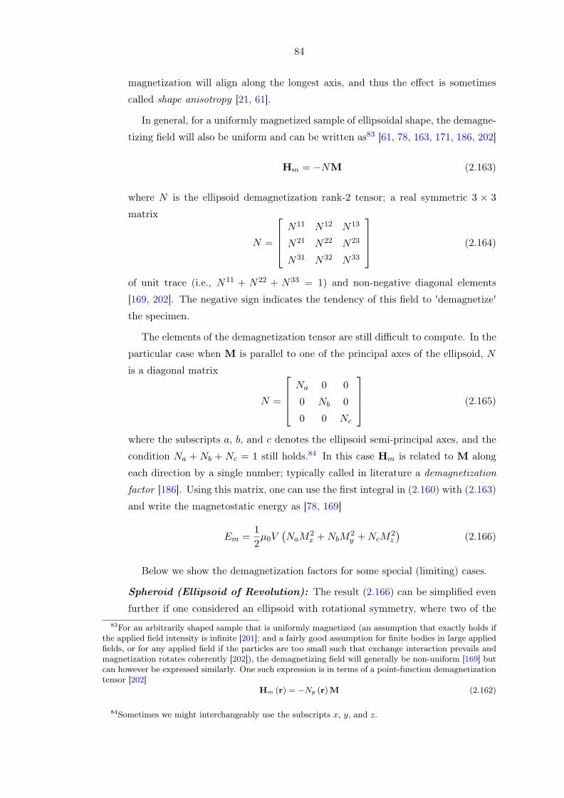
84
magnetization will align along the longest axis, and thus the effect is sometimes
called shape anisotropy [21, 61].
In general, for a uniformly magnetized sample of ellipsoidal shape, the demagne-
tizing field will also be uniform and can be written as83 [61, 78, 163, 171, 186, 202]
Hm = −NM (2.163)
where N is the ellipsoid demagnetization rank-2 tensor; a real symmetric 3 × 3
matrix
N =
N11 N12 N13
N21 N22 N23
N31 N32 N33
(2.164)
of unit trace (i.e., N11 + N22 + N33 = 1) and non-negative diagonal elements
[169, 202]. The negative sign indicates the tendency of this field to 'demagnetize'
the specimen.
The elements of the demagnetization tensor are still difficult to compute. In the
particular case when M is parallel to one of the principal axes of the ellipsoid, N
is a diagonal matrix
N =
Na 0 0
0 Nb 0
0 0 Nc
(2.165)
where the subscripts a, b, and c denotes the ellipsoid semi-principal axes, and the
condition Na + Nb + Nc = 1 still holds.84 In this case Hm is related to M along
each direction by a single number; typically called in literature a demagnetization
factor [186]. Using this matrix, one can use the first integral in (2.160) with (2.163)
and write the magnetostatic energy as [78, 169]
Em =1
2µ0V
(NaM
2x +NbM
2y +NcM
2z
)(2.166)
Below we show the demagnetization factors for some special (limiting) cases.
Spheroid (Ellipsoid of Revolution): The result (2.166) can be simplified even
further if one considered an ellipsoid with rotational symmetry, where two of the83For an arbitrarily shaped sample that is uniformly magnetized (an assumption that exactly holds if
the applied field intensity is infinite [201]; and a fairly good assumption for finite bodies in large appliedfields, or for any applied field if the particles are too small such that exchange interaction prevails andmagnetization rotates coherently [202]), the demagnetizing field will generally be non-uniform [169] butcan however be expressed similarly. One such expression is in terms of a point-function demagnetizationtensor [202]
Hm (r) = −Np (r)M (2.162)
84Sometimes we might interchangeably use the subscripts x, y, and z.

85
..
a
.
x
. b. y.
c
.
z
Figure 2.30: Ellipsoid.
principal axes are equal (e.g., a = b), representing the transverse axes, and the third
(i.e., c), representing the rotation symmetry axis. In this case, the demagnetization
factors of the transverse and symmetry axes are respectively written as Na = Nb =
N⊥ and Nc = N∥. With this notation, we write the demagnetization tensor as
N =
N⊥ 0 0
0 N⊥ 0
0 0 N∥
(2.167)
where N∥ + 2N⊥ = 1 [61]. Using this matrix, we can write (2.166) as [78, 169]
Em =1
2µ0M
2s V(N⊥sin
2θ +N∥cos2θ)
(2.168)
where θ is the angle between the magnetization and the rotational symmetry axis.
The factors can be found in terms of the ratio r = ca > 1 for the three special
spheroids as [78, 169]
Prolate (Elongated) Spheroid: r > 1, which means the ellipse is rotated about its
major axis.
N∥ =1
r2 − 1
[r√
r2 − 1ln(r +
√r2 − 1
)− 1
](2.169)
which, for r ≫ 1, can be approximated as
N∥ ∼=ln (2r)− 1
r2(2.170)
Here, N∥ <13 , N⊥ > N∥, and we have an easy-axis anisotropy along the symmetry
axis of the spheroid.
Oblate (Flattened) Spheroid: r < 1, which means the ellipse is rotated about its
minor axis.
N∥ =1
1− r2
[1− r√
1− r2sin−1
(√1− r2
)](2.171)
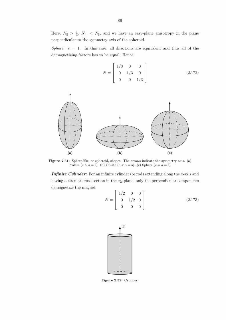
86
Here, N∥ > 13 , N⊥ < N∥, and we have an easy-plane anisotropy in the plane
perpendicular to the symmetry axis of the spheroid.
Sphere: r = 1. In this case, all directions are equivalent and thus all of the
demagnetizing factors has to be equal. Hence
N =
1/3 0 0
0 1/3 0
0 0 1/3
(2.172).
(a)
.
(b)
.
(c)
Figure 2.31: Sphere-like, or spheroid, shapes. The arrows indicate the symmetry axis. (a)Prolate (c > a = b). (b) Oblate (c < a = b). (c) Sphere (c = a = b).
Infinite Cylinder: For an infinite cylinder (or rod) extending along the z-axis and
having a circular cross-section in the xy-plane, only the perpendicular components
demagnetize the magnet
N =
1/2 0 0
0 1/2 0
0 0 0
(2.173)
...
z
Figure 2.32: Cylinder.
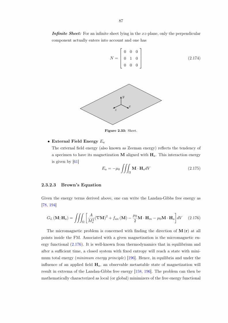
87
Infinite Sheet: For an infinite sheet lying in the xz-plane, only the perpendicular
component actually enters into account and one has
N =
0 0 0
0 1 0
0 0 0
(2.174)..
y
.
z
.
x
Figure 2.33: Sheet.
• External Field Energy Ea
The external field energy (also known as Zeeman energy) reflects the tendency of
a specimen to have its magnetization M aligned with Ha. This interaction energy
is given by [61]
Ea = −µ0∫∫∫
ΩM ·HadV (2.175)
2.3.2.3 Brown’s Equation
Given the energy terms derived above, one can write the Landau-Gibbs free energy as
[78, 194]
GL (M;Ha) =
∫∫∫Ω
[A
M2s
(∇M)2 + fan (M)− µ02M ·Hm − µ0M ·Ha
]dV (2.176)
The micromagnetic problem is concerned with finding the direction of M (r) at all
points inside the FM. Associated with a given magnetization is the micromagnetic en-
ergy functional (2.176). It is well-known from thermodynamics that in equilibrium and
after a sufficient time, a closed system with fixed entropy will reach a state with mini-
mum total energy (minimum energy principle) [196]. Hence, in equilibria and under the
influence of an applied field Ha, an observable metastable state of magnetization will
result in extrema of the Landau-Gibbs free energy [158, 196]. The problem can then be
mathematically characterized as local (or global) minimizers of the free energy functional
88
subject to the constraint (2.110) [198].85 The micromagnetic equilibrium condition will
result in a set of equations known as Brown’s equations.
As stated above, the equilibrium distribution of magnetization will result in extrema
of (2.176). By means of variational calculus, one can find the set of local extrema. At
each point inside the FM, the magnetization vector M (r) will be varied, and we denote
this variation by the small quantity δM (r) (subject to the constraint (2.110), namely
that |M+ δM| = Ms). In response to that, the energy functional will vary, and we
denote this variation by δGL (M;Ha). We want the equilibrium distribution that will
result in the minimum value of energy. From variational calculus, we know that the
sufficient conditions are: for the first variation to be zero δGL (M;Ha) = 0 and for the
second variation to be strongly positive δ2GL (M (·) ,Ha) > 0 [169]. Applying the rules
of variational calculus, one finds the first variation in the energies as follows:-
• Variation in the Exchange Energy δEex:
δEex = Eex (M+ δM)− Eex (M) =2A
M2s
∫∫∫Ω∇M · ∇δMdV (2.177)
Consider the i-th component Mi∫∫∫Ω∇Mi · ∇δMidV =
∫∫∫Ω∇ · (δMi∇Mi) dV −
∫∫∫ΩδMi∇ · (∇Mi) dV
=
∫∫⃝
ΣδMi
∂Mi
∂ndS −
∫∫∫ΩδMi∇ · (∇Mi) dV (2.178)
where we have used (A.155) and (A.139). Thus the variation becomes
δEex = − 2A
M2s
∫∫∫Ω∇ · (∇M) · δMdV +
2A
M2s
∫∫⃝
Σ
∂M
∂n· δMdS (2.179)
• Variation in the Anisotropy Energy δEan:
δEan = Ean (M+ δM)− Ean (M) =
∫∫∫Ω
∂fan (M)
∂M· δMdV (2.180)
• Variation in the Magnetostatic Energy δEm:
δEm = Em (M+ δM)−Em (M) = −µ02
∫∫∫ΩδM ·HmdV −
µ02
∫∫∫ΩM · δHmdV
(2.181)
However, by the reciprocity theorem [166], the two integrals are identical. Thus
δEm = −µ0∫∫∫
ΩδM ·HmdV (2.182)
85One of the difficulties is that the minimization will be carried out in an infinite-dimensional functionalspace of all possible vector fields [169].

89
• Variation in the Zeeman Energy δEa:
δEa = Ea (M+ δM)− Ea (M) = −µ0∫∫∫
ΩδM ·HadV (2.183)
Combining the first-order variations above, one finds
δGL (M;Ha) =δEex + δEan + δEm + δEa
=− µ0[∫∫∫
Ω
(2A
µ0M2s
∇ · (∇M)− 1
µ0
∂fan (M)
∂M+Hm +Ha
)· δMdV
− 2A
µ0M2s
∫∫⃝
Σ
∂M
∂n· δMdS
](2.184)
which can be written as [196]
δGL (M;Ha) = −µ0[∫∫∫
ΩHeff · δMdV − 2A
µ0M2s
∫∫⃝
Σ
∂M
∂n· δMdS
](2.185)
where the local effective field Heff is given by86
Heff = − 1
µ0
δ2GL
δMδV=
2
µ0M2s
∇ · (A∇M)− 1
µ0
∂fan (M)
∂M+Hm +Ha (2.186)
The field can then be written as the sum
Heff = Hex +Han +Hm +Ha (2.187)
where each term is given by [196]
– Exchange field Hex [194]:
Hex =2A
µ0M2s
∇2M (2.188)
– Anisotropy field Han:
Han = − 1
µ0
∂fan (M)
∂M(2.189)
If we consider uniaxial anisotropy
fan (M) ≃ K1
[1− (ean ·M)2
M2s
](2.190)
then the anisotropy field is given by
Han =HK
Ms(ean ·M) ean (2.191)
where HK = 2K1/µ0Ms [78].86Not to be interpreted as a magnetic field in the sense of Maxwell’s equations [169].
90
– Magnetostatic field Hm: Can be found by solving the magnetostatic Maxwell equa-
tions [196]
∇ ·Hm =
∇ ·M, r ∈ Ω
0, r ∈ R3\Ω(2.192)
∇×Hm = 0 (2.193)
subject to following boundary conditions at the FM surface
an ·Hm = an ·M (2.194)
an ·Hm = 0 (2.195)
In the special case of uniform magnetization (e.g., ellipsoidal particles) or perpen-
dicularly magnetized infinite thin films, one can write
Hm = −NM (2.196)
where N is the demagnetization tensor which satisfies Nx +Ny +Nz = 1.
– Applied field Ha: Produced by external sources and can be assumed to be a given
vector field of space and time.
Now, δM is always perpendicular to M (since the magnitude of M is conserved)
[158], and thus we can write the variation as the rotation δM = M × δW, where W
is a space-dependent vector; this is the most general variation compatible with (2.110)
[169, 196]. Plugging this in (2.185) and using (A.145) for both integrands, one finds
δGL (M;Ha) = −µ0[∫∫∫
ΩδW · (Heff ×M)dV − 2A
µ0M2s
∫∫⃝
ΣδW ·
(∂M
∂n×M
)dS
](2.197)
At equilibrium, δGL (M;Ha) = 0 for any arbitrary δM consistent with (2.110) [158, 196].
This means that any term multiplying δM has to be zero. Imposing this condition in
(2.197), we obtain two important equations. The first, known as Brown’s equation
M×Heff = 0, ∀r ∈ Ω (2.198)
essentially states that the magnetization vector experiences zero torque at equilibrium
[191, 192]. The second is the homogeneous boundary condition
M× ∂M
∂n= 0⇔ ∂M
∂n= 0, ∀r onΣ (2.199)

91
where ⇔ indicates an equivalence (resulting from the constraint (2.110)) [78]. The Neu-
mann boundary condition above is valid only when no surface anisotorpy is present [196].
Brown’s equation (2.198) determine all possible magnetization equilibria, regardless
of their stability [169, 196]. That is, the extrema are not necessarily minima of (2.176)
(corresponding to metastable equilibria). The nature of the equilibria can be found by
computing the second variation of (2.176) or checking δGL ⩾ 0 for an arbitrary small
variation of the solution [169].
2.4 Deterministic Dynamic Equations
Ferromagnets are typically bistable [198], and one can switch between magnetization
states using either applied magnetic fields or the more novel solution so-called spin-
transfer torque (STT). In this section, we briefly describe the dynamics of a FM subject
to external excitations.
When M ×Heff = 0, the magnetization experiences a local torque exerted by the
effective field and will evolve in time according to a dynamic equation [21, 196]. The
state of a FM will now be, of course, a function of both space and time M (r, t). The
most used magnetization evolution equation is the Landau-Lifshitz (LL) equation and
Landau-Lifshitz-Gilbert (LLG) equations, both of which adequately model the dynamics
under low-energy excitations (i.e., spin waves or magnons) [29].
2.4.1 Landau-Lifshitz (LL)
The undamped dynamic equation of a magnetic moment is a simple first order partial
differential equation describing the precession of M (r, t) as a 'free' moment about Heff
[61, 158, 196]∂M
∂t= −γLLM×Heff , M (r, 0) = M0 (r) (2.200)
where γLL is the LL gyromagnetic ratio, usually taken to be the gyromagnetic ratio
associated with the electron spin (i.e., γLL≃ 2.21× 10⁵ mA·s)
87 [158]. Such a precession
is typically called Larmor precession and is characterized by the Larmor frequency ω =
87In particular, if one considers spins only
γLL = µ0 |γS | = µ0
∣∣∣−gS µB
ℏ
∣∣∣ ≃ µ0
∣∣∣−2µB
ℏ
∣∣∣ ≈ 221019 = 2.21× 10⁵m
A · s
where gS ≃ 2 is g-factor of a free electron (see footnote 36). On the other hand, the gyromagnetic ratioof orbital momentum is (almost) half this value
γLL = µ0 |γL| = µ0
∣∣∣−gL µB
ℏ
∣∣∣ = µ0
∣∣∣−1µB
ℏ
∣∣∣ ≈ 110509 = 1.10× 10⁵m
A · s

92
µ0γHeff . Before delving further, we present a brief account of the phenomenological
derivation of the undamped equation.
Classical picture: From mechanics, we know that the angular momentum of an object
with a moment of inertia tensor I and angular velocity ω is given by L = Iω = r × p,
where r the moment arm and p the linear momentum. Taking the temporal derivative
of LdL
dt=
d
dt(r× p) =
dr
dt× p+ r× dp
dt(2.201)
If the axis of rotation is fixed, dr/dt = v and thus dr/dt× p = v × p = v × (mv) = 0.
Hence (2.201) becomesdL
dt= r× dp
dt= r× F = τ (2.202)
where we used Newton’s 2nd law of motion dp/dt = F with F being the force and τ
the torque experienced. If we consider (semi-classically) an electron orbiting the nucleus,
then we can associate the electron with the dipole moment given by (2.81). However, a
magnetic moment m immersed in a magnetic field Beff = µ0Heff experiences a torque
given by (B.15). Plugging this relation into (2.202) and using the definition of classical
orbital gyromagnetic ratio m = γLL, one finds
dm
dt= µ0γLm×Heff (2.203)
Usually, we would like to see a negative sign in front. Since γL < 0, we use |γL| and
invoke the relation γLL = µ0 |γL| to obtain
dm
dt= −γLLm×Heff (2.204)
which can be written in terms of the volume averaged magnetization M to obtain the
desired result.
Quantum picture: Consider the spin operator S = Sxax + Syay + Szaz. The equation
of motion can be derived from the quantum-mechanical commutator [21, 203]
dSαdt
= − iℏ
[Sα, H
](2.205)
where α ∈ x, y, z and H is the Hamiltonian of the system. To first order in ℏ, one can
write the equation of motion as
dSαdt
= − iℏdHSβ
[Sα, Sβ
]+O (ℏ) (2.206)
In general, instead of using either of the g-factors alone, one can use an effective g-factor g∗ that includesboth and which in general depends on the material [21, 29, 194].

93
where Einstein’s summation convention is implied (see A.1.1.1). From the properties of
the spin operator, we can write [203][Sα, Sβ
]= iℏεαβγSγ (2.207)
where εαβγ is the antisymmetrical unit tensor (Levi-Civita symbol (A.5)). Invoking the
last property in the equation of motion, one obtains
dSαdt
=dHSβ
εαβγSγ +O (ℏ) (2.208)
However, from the properties of the Levi-Civita symbol, we know that
[A×B]α = εαβγAβBγ (2.209)
Therefore, we can write (2.208) as
dS
dt= −S× dH
dS+O (ℏ) (2.210)
In the semiclassical limit as ℏ→ 0 [200]
d⟨S⟩
dt= −
⟨S⟩×Heff (2.211)
where
Heff =1
µ0|γS |
⟨dHdS
⟩(2.212)
or in the semiclassical approximation
Heff =1
µ0
dE
dm(2.213)
The last two equations imply that m = −gSµB⟨S⟩/ℏ, where we have used |γS | =
gSµB/ℏ. Hence, for classical spins
dm
dt= −γLLm×Heff (2.214)
where γLL = µ0 |γS |. The last equation can be written in terms of the volume averaged
magnetization M to obtain the desired result.
The above approach can in fact be simplified: In analogy with the relation between
the magnetic moment m and the orbital angular momentum L of a moving electron, one
can relate the magnetic moment with the spin angular momentum. In fact, (2.202) still

94
holds if we interpret every quantity as an operator in Hilbert space (i.e., L and τ ) [194].
Thus one can extend this to spin systems by merely replacing L with S in (2.202) so that
dS
dt= τ (2.215)
Then the analogy between the classical and quantum pictures can be applied if one
takes the expectation value of the spin angular momentum operator S using appropriate
quantum states or a density matrix [194]. The equation can then be converted into a
dynamic equation for magnetization by using the definition m = γSS along with (B.15)
so that upon using m = ⟨m⟩ we obtain
dm
dt= −γLLm×Heff (2.216)
where we have used γLL = µ |γS |. The equation can again be written in terms of the
volume averaged magnetization M to obtain the desired result.
The dynamic equation (2.200) has to be consistent with the micromagnetic constraint
(2.110). Dotting both sides of (2.200) with M
M · ∂M∂t
= −γLLM · (M×Heff )
and using the fact that M·(∂M/∂t) = (1/2) d|M|2/dt along with the invariance property
of triple scalar product under cyclic permutation (A.145), we obtain
1
2
∂
∂t|M|2 = −γLLHeff · (M×M) = 0 (2.217)
from which we conclude that the magnitude is conserved.
Experimentally, a precession decays in time towards an energy minimum. The dy-
namic equation (2.200) is not dissipative and thus cannot describe any approach to
equilibrium [196]. This can be shown by taking the temporal derivative of (2.185) and
using (2.199) for the second term to obtain88
dGL
dt= −µ0
∫∫∫ΩHeff ·
∂M
∂tdV − µ0
∫∫∫ΩM · ∂Ha
∂tdV (2.219)
88Alternatively
dGL (M,Ha)
dt=
∫∫∫Ω
[δGL
δM· ∂M∂t
+δGL
δHa· ∂Ha
∂t
]dV = −µ0
∫∫∫Ω
Heff · ∂M∂t
dV−µ0
∫∫∫Ω
M · ∂Ha
∂tdV
(2.218)

95
Substituting (2.200) and assuming a DC external field (so that ∂Ha/∂t = 0), one finds
dGL
dt= µ0γLL
∫∫∫ΩHeff · (M×Heff ) dV = µ0γLL
∫∫∫ΩM · (Heff ×Heff ) dV = 0
(2.220)
where we used the identity (A.145). Thus, the dynamics are non-dissipative but in fact
conservative [198]. Therefore, a damping term has to be added to the equation for it
to describe a realistic situation. The damping term will take into account the transfer
(or loss) of energy from the macroscopic local magnetization to the microscopic thermal
motion (i.e., thermal bath) [194, 196]. However, due to the complexity in describing
the interactions between the magnetic moment and the crystal lattice vibration, crystal
defects (e.g., voids, interstitial atoms, etc.), magnons, or eddy currents, the damping is
usually added as a phenomenological term since it is difficult to separately account for
these mechanisms or even connect it with the energy dissipation rate measured experi-
mentally (e.g., using FMR) [157, 194].
..
Heff
.
Damping
.
Precession
.
M
Figure 2.34: Magnetization precession and damping torques.
In 1935, Landau and Lifshitz introduced the basic damped dynamics equation for
magnetization in their pioneering work about the phenomenological evaluational of the
permeability tensor in FMs [158]. Landau and Lifshitz originally described damping in
a phenomenological approach by adding a term directed toward Heff and perpendicular
to M
∂M
∂t= −γLLM×Heff + γLLλMs
(Heff −
M ·Heff
M2s
M
), M (r, 0) = M0 (r)
(2.221)
where λ is a dimensionless phenomenological damping constant.
The form above is rarely used in literature. In fact, one may notice that the second
term can be obtained by using the identity (A.146) as follows
M× (M×Heff ) = (M ·Heff )M− (M ·M)Heff = (M ·Heff )M−M2sHeff

96
which implies
Heff −(M ·Heff )
M2s
M = − 1
M2s
M× (M×Heff ) (2.222)
Hence we can rewrite the LL equation (2.221) in the more admissible form [78, 196]
∂M
∂t= −γLLM×Heff − γLL
λ
MsM× (M×Heff ) , M (r, 0) = M0 (r) (2.223)
The precession and damping terms are schematically shown in Fig. 2.35 below.
..
Heff
.
−M× (M×Heff )
.
−M×Heff
.
M
Figure 2.35: Magnetization precession and damping torques in the LL equation.
Now we check if the dynamics are dissipative. Using (2.223) in the general relation
(2.219) while still assuming DC external fields, we obtain
dGL
dt= −µ0
∫∫∫ΩHeff ·
[−γLLM×Heff − γLL
λ
MsM× (M×Heff )
]dV
= µ0γLL
∫∫∫ΩHeff · (M×Heff ) dV + µ0γLL
λ
Ms
∫∫∫ΩHeff · [M× (M×Heff )] dV
= 0 + µ0γLLλ
Ms
∫∫∫Ω(M×H) · (H×M) dV
= −µ0γLLλ
Ms
∫∫∫Ω|M×H|2dV (2.224)
where we have used (2.220) and (A.145) throughout. The last equation shows that energy
is a decreasing function of time and thus dissipative. In fact, by numerically integrating
the LL equation, we can plot the damped motion of the moment as in Fig. 2.36.
Before concluding the subsection, we write the LL equation (2.223) in terms of the
rescaled magnetization by dividing both sides by Ms to obtain
∂m
∂t= −γLLm×Heff − γLLλm× (m×Heff ) , m (r, 0) = m0 (r) (2.225)

97
(a) (b) (c)
Figure 2.36: Possible trajectories for damped motion obtained by numerically integratingthe LL equation. (a) λ = 0.01. (b) λ = 0.1. (c) λ = 0.5.
2.4.2 Landau-Lifshitz-Gilbert (LLG)
In 1955, and based on a Lagrangian formalism of the precession equation with damping
added using the so-called Rayleigh dissipation function, Gilbert [194]89 introduced a
viscous damping term into the undamped LL equation. In particular, he started with
a Lagrangian formulation of the damped equation of motion starting from the Euler-
Lagrange equation for conservative dynamics
d
dt
δL[M, M
]δM
−δL[M, M
]δM
= 0 (2.226)
where L[M, M
]is the Lagrangian. He then included a nonconservative force using the
Rayleigh dissipation function
d
dt
δL[M, M
]δM
−δL[M, M
]δM
+dR[M]
dM= 0 (2.227)
where the Rayleigh dissipation functional R[M]
is given by
R[M]=η
2
∫∫∫Ω
∣∣∣M (t, r)∣∣∣2dV (2.228)
where α = ηγGMs is the Gilbert damping, η is a damping paramater, and γG is the
Gilbert gyromagnetic ratio. The Gilbert damping depends on temperature and the
impurity/defect composition of the material [151] and can be a tensor in general [29].
Using the dissipation functional, the LLG can be shown to be [78, 194, 196]
∂M
∂t= −γGM×Heff +
α
MsM× ∂M
∂t, M (r, 0) = M0 (r) (2.229)
The precession and damping terms are schematically shown in Fig. 2.37 below.89Although I should probably refer to [204], Gilbert’s original paper was never published, I believe.
However, Gilbert later published his Ph.D. thesis, and [194] is based on chapters II and III of his thesis,with little modifications.

98
..
Heff
.
M× ∂M/∂t
.
−M×Heff
.
M
Figure 2.37: Magnetization precession and damping torques in the LLG equation.
The LLG equation was the first phenomenological equation to describe the magne-
tization dynamics in the whole dissipation range [157]. The Gilbert form of damping
was merely introduced since the damped LL equation encountered problems for large
damping, producing unphysical solutions [157, 194]. If one considers λ in (2.223) as a
parameter proportional to the energy dissipation in the system, then in the overdamped
regime (λ ≥ 1) the dissipation term dominates and the equation will predict faster re-
laxation for larger damping, an obvious contradiction to the physical picture of damping
[157]. In fact, it was pointed by Landau and Lifshitz themselves [158] that the damping
term introduced by them is neither the only possible nor most general and one may use
their equation in the precession-dominated regime (λ≪ 1) only [157].
To check if the dynamics are dissipative. It is convenient to rewrite (2.229) as
∂M
∂t= −γGM×
(Heff −
α
γGMs
∂M
∂t
)(2.230)
which in fact reveals the nature of the damping term: Directly subtracted from the
effective field, and having a magnitude proportional to the relaxation speed (analogous
to a hydrodynamical viscous damping) [157, 196].
The LLG equation can straightforwardly be shown to be magnitude conserving. To
check if it is dissipative, we dot both sides of (2.230) by (Heff − (α/γGMs) ∂M/∂t)(Heff −
α
γGMs
∂M
∂t
)·∂M∂t
= −γG(Heff −
α
γGMs
∂M
∂t
)[M×
(Heff −
α
γGMs
∂M
∂t
)]= 0
(2.231)
where the second term vanishes as evident from (A.145). Therefore from (2.231), it is
obvious that
Heff ·∂M
∂t=
α
γGMs
∣∣∣∣∂M∂t∣∣∣∣2 (2.232)

99
Using (2.232) in (2.219) while assuming static external field Ha, we obtain
dGL
dt= −µ0
∫∫∫ΩHeff ·
∂M
∂tdV = − µ0α
γGMs
∫∫∫Ω
∣∣∣∣∂M∂t∣∣∣∣2dV (2.233)
which implies that the LLG dynamics are always decreasing and thus dissipative. The
last equation expresses the so-called Lyapunov structure of the LLG equation.
The native form of the LLG equation (2.229) is an implicit differential equation, which
is inconvenient to implement in numerical computations. Fortunately, it can be casted
into an explicit form. Taking the cross product of M with the LL equation (2.223)
M× ∂M
∂t= −γLLM×M×Heff − γLL
λ
MsM× [M× (M×Heff )] (2.234)
But from the identities (A.145) and (A.146), we find M×[M× (M×Heff )] = −M2sM×
Heff . Therefore
M× ∂M
∂t= −γLLM× (M×Heff ) + γLLλMsM×Heff (2.235)
or equivalently
γLLM× (M×Heff ) = −M×∂M
∂t+ γLLλMsM×Heff (2.236)
Substituting (2.236) back into (2.223) and collecting like terms, we obtain
∂M
∂t= −γLL
(1 + λ2
)M×Heff +
λ
MsM× ∂M
∂t, M (r, 0) = M0 (r) (2.237)
where the last equation transforms into the LLG equation upon substituting [21]
γLL =γG
1 + α2(2.238)
λ = α (2.239)
The relations above can also be used in (2.223) to cast the Gilbert equation into the
archetypal LL form (which, from now on, we call the combined LLG equation or just
LLG equation)
∂M
∂t= − γG
1 + α2M×Heff−
γG1 + α2
α
MsM×(M×Heff ) , M (r, 0) = M0 (r) (2.240)
The last equation for zero damping (α = 0) is related to the symplectic flow of harmonic
maps and is also known as the Schrödinger map equation [198]. For high damping
(α→∞), the equation is related to the heat flow of harmonics maps [198].

100
The equivalence between (2.223) and (2.229) is not a coincidence; it turned out that
the LL equation is universal and is the most general equation of damped motion for
magnetic moments [157, 196]. Consider the 1st-order dynamic equation
∂M
∂t= F (M,Heff ) , M (r, 0) = M0 (r) (2.241)
At every instant of time, one can decompose the vector field F (M,Heff ) along three
mutually orthogonal vectors and hence write it as a linear combination of the basis
vectors. In particular, one can write [196]
∂M
∂t= c1M+ c2M× a+ c3M× (M× a) (2.242)
where a is some unknown vector. We can then determine the unknowns by using the fun-
damental micromagnetic constraint (2.110) and Brown’s equation (2.198) at equilibria.
The former can be utilized by dotting both sides of (2.242) by M to obtain
1
2
∂|M|2
∂t= c1|M|2 (2.243)
where the other terms vanishes after one uses (A.145) and (A.146). For (2.110) to hold,
we must have c1 = 0. This should not be surprising since the restriction (2.110) implies
that M can only rotate and that any change ∆M must be perpendicular to M [157]. In
this sense, the equation
∂M
∂t= c2M× a+ c3M× (M× a) , M (r, 0) = M0 (r) (2.244)
can be thought as the general equation of magnetization dynamics; an expansion of
∂M/∂t over the two orthogonal vectors M× a and M× (M× a) which span the plane
perpendicular to M over which ∂M/∂t lies [157]. Now at equilibrium, (2.244) becomes
0 = c2M× a+ c3M× (M× a) (2.245)
which implies that M × a = 0 (since the two terms on the right are mutually orthogo-
nal). This equation is equivalent to Brown’s condition when a = Heff . In fact, (2.242)
reduces to the LL equation (2.200) with c2 = −γLL, c3 = −γLL λMs
and to the combined
LLG equation (2.240) with c2 = − γG1+α2 , c3 = − γG
1+α2αMs
. This implies that all dynamic
equations are reducible to the LL equation (having the general form (2.244)), with the
possibility of having different coefficients [196]. Although (2.223) and (2.229) are in this
sense mathematically equivalent (as also evident from the resulting equation: (2.240)),
they may not be regarded as physically equivalent when one tries to interpret the pre-
cession and damping terms [157, 194, 196]. The two equation have identical damping

101
terms, and only differ in the dimensionless damping parameter [194]. For α2 ≪ 1, (2.240)
obviously coincides with (2.223) [194], and one can then safely interpret α as a damping
parameter proportional to the dissipation energy in the LL form as well (which is not
true for large damping) [157]. It is worth noting at this point that the coefficients γLL,
λ, etc. need not to be constant or time-independent, and can be functions of the state
of the system and can also be tensors [157, 196].
Before concluding, we write the LLG equation (2.229) and the combined LLG equation
(2.240) in terms of the rescaled magnetization by dividing both sides by Ms to obtain
∂m
∂t= −γGm×Heff + αm× ∂m
∂t, m (r, 0) = m0 (r) (2.246)
and
∂m
∂t= − γG
1 + α2m×Heff −
γG1 + α2
αm× (m×Heff ) , m (r, 0) = m0 (r) (2.247)
2.4.3 Dimensionless Equations
It is instructive to write (2.176) and (2.187) in a normalized (dimensionless) form. If the
magnetization and magnetic fields are normalized in units of Ms
m =M
Ms(2.248)
heff =Heff
Ms= hex + han + hm + ha (2.249)
then the free energy (2.176) can be normalized as follows [78, 196]
gL (m (·) ,ha) =GL (M (·) ,Ha)
µ0M2s V
=1
V
∫∫∫Ω
[A
µ0M2s
(∇m)2 +1
µ0M2s
fan (M)− 1
2m · hm −m · ha
]dV
(2.250)
This can also be rewritten in terms of the exchange length lex =√
2Aµ0M2
s[21, 78] and the
normalized anisotropy energy φan (m) = fan(M)µ0M2
sas [196]
gL (m (·) ,ha) =1
V
∫∫∫Ω
[l2ex2(∇m)2 + φan (m)− 1
2m · hm −m · ha
]dV (2.251)
If we normalize r in units of lex, we can write
gL (m (·) ,ha) =1
V
∫∫∫Ω
[1
2(∇m)2 + φan (m)− 1
2m · hm −m · ha
]dV (2.252)
102
where now ∇ operates with respect to the normalized position vector r/lex. In this case,
the first variation (2.185) becomes
δgL (m (·) ,ha) = −1
V
∫∫∫Ωheff · δmdV +
lexV
∫∫⃝
Σ
∂m
∂n· δmdS (2.253)
where the normalized local effective field heff is given by
heff = −δgLδm
= ∇ · (∇m)− ∂ϕan (m)
∂m+ hm + ha (2.254)
The field can then be written as sum
heff = hex + han + hm + ha (2.255)
where each term is given by [196]
– Normalized exchange field hex:
hex = ∇2m (2.256)
– Normalized anisotropy field han:
han = −∂φan (m)
∂m(2.257)
If we consider uniaxial anisotropy
φan (M) ≃ K1
µ0M2s
[1− (ean ·m)2
](2.258)
then the normalized anisotropy field is given by
han =HK
Ms(ean ·m) ean (2.259)
where HK = 2K1µ0Ms
[78].
– Normalized magnetostatic field hm: Can be found by solving the magnetostatic
Maxwell equations [196]
∇ · hm =
∇ ·m, r ∈ Ω
0, r ∈ R3\Ω(2.260)
∇× hm = 0 (2.261)

103
subject to following boundary conditions at the FM surface
an · hm = an ·m (2.262)
an · hm = 0 (2.263)
In the special case of uniform magnetization (e.g., ellipsoidal particles) or perpen-
dicularly magnetized infinite thin films, one can write
hm = −Nm (2.264)
where N is the demagnetization tensor which satisfies Nx +Ny +Nz = 1.
– Normalized Applied field ha: Produced by external sources and can be assumed to
be a given vector field of space and time.
Using a similar approach to that in 2.3.2, we write the variation in m as δm = m×δw,
where w is a space-dependent vector. Plugging this in (2.253) and using (A.145) for both
integrands, we find
δgL (m (·) ,ha) = −µ0[∫∫∫
Ωδw · (heff ×m)dV − 2A
µ0M2s
∫∫⃝
Σδw ·
(∂m
∂n×m
)dS
](2.265)
At equilibrium, δgL (m (·) ,aa) = 0 for any arbitrary δm consistent with (2.110). Im-
posing this condition in (2.265), we obtain two important equations. The first is the
normalized Brown equation [196]
m× heff = 0, ∀r ∈ Ω (2.266)
The second is the normalized homogeneous boundary condition [196]
m× ∂m
∂n= 0⇔ ∂m
∂n= 0, ∀r onΣ (2.267)
which is valid only when no surface anisotropy is present [196].
In the dimensionless case, the dynamics are governed by normalized forms of the LL
(2.225) and LLG (2.246) equations. By noting that µ0 |γ|Ms has the units mA·s
Am = 1
s ,
we identify the reciprocal 1µ0|γ|Ms
as a time constant, and we denote it by τ . Therefore
we can write the time constants of the LL and LLG equations as
τLL =1
γLLMs(2.268)
τG =1
γGMs(2.269)

104
Multiplying each of (2.225) and (2.229) by its own time constant, we obtain
τLL∂m
∂t= −m× heff − αm× (m× heff ) (2.270)
τG∂m
∂t= −m× heff + ατGm×
∂m
∂t(2.271)
If we define the normalized time-spans tLL = tτLL
and tG = tτG
, then their differentials
are given by
∂tLL =∂t
τLL↔ ∂t = τLL∂tLL (2.272)
∂tG =∂t
τG↔ ∂t = τG∂tG (2.273)
Plugging these in (2.270) and (2.271), respectively, one obtains
∂m
∂tLL= −m× heff − αm× (m× heff ) (2.274)
∂m
∂tG= −m× heff + αm× ∂m
∂tG(2.275)
or just simply (after dropping the time subscripts)
∂m
∂t= −m× heff − αm× (m× heff ) , m (r, 0) = m0 (r) (2.276)
∂m
∂t= −m× heff + αm× ∂m
∂t, m (r, 0) = m0 (r) (2.277)
Following a similar approach to that in 2.4.1 and 2.4.2, the associated energy balance
equations for the normalized LL and LLG equations above are given respectively by [196]
dgLdt
= −αV
∫∫∫Ω|m× heff |2dV −
1
V
∫∫∫Ωm · ∂ha
∂tdV (2.278)
dgLdt
= −αV
∫∫∫Ω
∣∣∣∣∂m∂t∣∣∣∣2dV − 1
V
∫∫∫Ωm · ∂ha
∂tdV (2.279)
which are, of course, decreasing functions of time at equilibrium.
If one prefers the combined LLG equation (2.247), then a renormalization of (2.247)
can be applied by using the procedure above but with the time constant τG,c =1+α2
γGMsto
arrive at (2.276) with ∂t = τG,c∂tG,c.

105
2.4.4 Toward the Nanoscale—The Macrospin Approxima-
tion
As discussed in 2.2.5, modern spintronic devices involve magnets with dimensions in
the nanoscopic (1 − 100 nm) scale [68, 78]. At such reduced dimensions, magnetostatic
interaction is weak, and at temperatures well below the Curie point, the strong exchange
interaction aligns all spins together so that spins rotate in unison,90,91 effectively creating
a spatially uniform magnetization, i.e. a giant macrospin [21, 29, 78, 196, 205, 206]. In
this case, a magnetic sample is said to be single domain (or monodomain)92; this is the
case where L < dsd [82].
As we ignore spatial variations of magnetization, ∇M = 0 and thus the exchange field
(2.256) does not play a role anymore [29, 76].93 That is, one now has the effective field
Heff = Han +Hm +Ha (2.280)
In general, one has a spatially uniform solution when the following hold [78, 196, 208]:
1. The initial distribution is given by m (r, 0) = m0, where m0 is a spatially uniform
(i.e., space-independent) vector;
2. The magnet is of some special shape, for example ellipsoidal;
3. The effective field Heff is spatially uniform.
2.4.4.1 Statics: The Stoner-Wohlfarth Model
The first static model (and the one mostly used) to describe the magnetization of small
particles is the Stoner-Wohlfarth model developed in 1948 [209]. This model is valid
for T = 0 K only, but can be generalized for any temperature [78]. In this model, the
main character of a single domain particle is hysteresis (through magnetization reversal),
in which the magnetization of the so-called Stoner particle coherently reverses and can
achieve a maximum coercivity [68, 78].94
90Strictly when L < Rcoh, where Rcoh = βlex. Otherwise, magnetization reversal may not necessarilybe coherent [61], but can exhibit curling, buckling, and fanning.
91In what is sometimes known as Néel rotation. Small particles that are free to rotate as a whole aresaid to exhibit Brown rotation [78].
92This was first suggested by Dorfman [207] in 1930.93This is also obvious as there are no domain walls to form [82].94The coercivity in a single domain particle is larger than in multidomain particle since it is energeti-
cally more difficult to overcome the anisotropy energy than to nucleate (on inhomogeneities and defects)or move a DW [61]. Thus, single domain particles are magnetically hard due to their high coercivityand remanence.

106
The model assumes a homogeneously magnetized, single domain, elongated rotation-
ally symmetric ellipsoid, with uniaxial anisotropy along some axis. For simplicity, we
take the z-axis as the easy-axis. In this case, the Landau-Gibbs free energy becomes
GL (M;Ha) = V
K1
[1− (ean ·M)2
M2s
]+µ02M · (NM)− µ0M ·Ha
= V
K1
[1−m2
z
]+µ0M
2s
2
[N⊥
(1−m2
z
)+N∥m
2z
]− µ0Msm ·Ha
= V
K1 +
µ0M2s
2N⊥ +
[µ0M
2s
2
(N∥ −N⊥
)−K1
]m2
z − µ0Msm ·Ha
(2.281)
where we have used (2.110). If θ is the angle between the M and the easy-axis (which
coincides with the major axis of the ellipse),95 ϕ the angle between Ha (which lies on
the xz-plane) and the easy-axis, and ψ the angle the projection of M makes on xy-plane
with the x-axis, then
GL (M;Ha) =V
K1 +
µ0M2s
2N⊥ +
[µ0M
2s
2
(N∥ −N⊥
)−K1
]cos2θ
− µ0MsHa (sin θ cosψ sinϕ+ cos θ cosϕ)
(2.282)
..
M
.
Ha > 0
.
Ha < 0
.
θ
.
ϕ
Figure 2.38: Geometry of the Stoner-Wohlfarth (SW) problem.
95Which could result from the shape, or the sum of crystal and shape effects [68, 78]. In general,anisotropy is determined from shape (magnetostatic), crystalline structure (magnetocrystalline), residualstrain (magnetoelastic), and various surface/interface effects due to the broken translation symmetry atan interface.

107
When Ha = 0, M points along the anisotropy axis. When Ha = 0, M rotates away from
the easy-axis (toward Ha). Because of symmetry, M will lie on the plane containing ean
and Ha, and one has ψ = 0 (planar problem on the xz-plane) [169]. Thus [78]
GL (M;Ha) = V
[K1sin
2θ +µ0M
2s
2
(N⊥sin
2θ +N∥cos2θ)− µ0MsHa cos (ϕ− θ)
](2.283)
or
GL (M;Ha) = V
[K1sin
2θ +µ0M
2s
2
(N⊥sin
2θ +N∥ −N∥sin2θ)− µ0MsHa cos (ϕ− θ)
]= V
[K1 +
µ0M2s
2
(N⊥ −N∥
)]sin2θ +
µ0M2s
2N∥ − µ0MsHa cos (ϕ− θ)
= V
[K1 +Kd] sin
2θ +µ0M
2s
2N∥ − µ0MsHa cos (ϕ− θ)
= V
[Keff sin
2θ +µ0M
2s
2N∥ − µ0MsHa cos (ϕ− θ)
](2.284)
where Keff = K1 +Kd = K1 + µ0M2s
(N⊥ −N∥
)/2 is the effective anisotropy constant
which takes both magnetocrystalline and shape anisotropy into account [78, 169, 210].
The direction of equilibrium magnetization is determined by the condition [77, 78, 210]
∂GL
∂θ= 0 (2.285)
Imposing this condition, one finds
∂GL
∂θ= V [2Keff sin θ cos θ − µ0MsHa sin (ϕ− θ)] = 0 (2.286)
or2Keff
µ0Mssin θ cos θ −Ha sin (ϕ− θ) = 0 (2.287)
or even more compactly as
HK,eff sin θ cos θ −Ha sin (ϕ− θ) = 0 (2.288)
where HK,eff = 2Keff/µ0Ms is the effective anisotropy field, also known as the Stoner-
Wohlfarth field (or the negative of the nucleation field in this context)96 [78]. A magnetic
field of intensity HK,eff is sufficient to rotate the magnetization, and thus, it is also equal
to the coercivity of the material.97 The above equation can be used to find the height of
the energy barrier separating the two anisotropy energy minima. For example, for ϕ = 0,96Nucleation of magnetization reversal refers to the formation of a regions of reversed magnetization in
a saturated magnet. With this in mind, the nucleation field is defined as H for which the first deviationfrom the uniformly saturated state appears [61].
97In real samples (which are generally inhomogeneous), the coercive field is reduced by imperfectionsthat favor nucleation of reverse domains at bulk defects, surface asperities, or even spontaneous thermal
108
and in the absence of the demagnetizing field
[HK cos θ +Ha] sin θ = 0 (2.290)
where HK = 2K1/µ0Ms. The equation has the three solutions
θ = 0 (2.291)
θ = π (2.292)
θ = cos−1
(− Ha
HK
)(2.293)
The first two solutions correspond to GL,min, whereas the third solution correspond to
GL,max when Ha/HK ⩽ 1. Since cos (Ha/HK) ⩽ 1, a field of intensity HK is sufficient
to rotate the magnetization. The height of the energy barrier can be found from the
difference
Eb = GL,max −GL,min = K1V
(1− Ha
HK
)2
(2.294)
which disappears at Ha = HK .
Now, stable equilibrium is ensured only if the second derivative is strongly positive,
viz. [77, 78, 210]∂2GL
∂θ2> 0 (2.295)
This derivative can be found and set to zero (since switching occurs when the energy
minimum becomes unstable [61])
HK,eff cos 2θ +Ha cos (ϕ− θ) = 0 (2.296)
Thus equations (2.288) and (2.296) give the system
1
2HK,eff sin 2θ −Ha sin (ϕ− θ) = 0 (2.297)
HK,eff cos 2θ +Ha cos (ϕ− θ) = 0 (2.298)
which, after defining Hz = Ha cosϕ,Hx = Ha sinϕ, can be rewritten as
1
2HK,eff sin 2θ −Hx cos θ +Hz sin θ = 0 (2.299)
HK,eff cos 2θ +Hx sin θ +Hz cos θ = 0 (2.300)
fluctuations, resulting in what is commonly known as Brown’s Paradox [61, 68, 78]. In general, Brown’sTheorem in micromagnetics states that the coercive field satisfies the inequality [61, 169]
Hc ⩾ HK −NMs = −HN (2.289)

109
The two equations can be manipulated to get the parametric expressions
Hx = HK,eff sin3θ (2.301)
Hz = −HK,effcos3θ (2.302)
which can be combined (by taking the cubic root and summing the squares) to give the
equation of an asteroid
H2/3x +H2/3
z = H2/3K,eff (2.303)
This asteroid separates the region where the system has one single minimum from that
with two stable minima [77].
−1 −0.5 0.5 1
−1
−0.5
0.5
1
hz
hx
Figure 2.39: Switching astroid obtained by plotting (2.303).
2.4.4.2 Dynamics
The dynamics of a macrospin can be computed from the LLG equation
dm
dt= − γG
1 + α2m×Heff −
γG1 + α2
αm× (m×Heff ) , m (r, 0) = m0 (2.304)
To find the form of the effective field, we write Landau-Gibbs free energy
GL (m;Ha) = V
K1 −K1(ean ·m)2 +
µ0M2s
2m · (Nm)− µ0Msm ·Ha
(2.305)
The effective field can be found from the derivative
Heff = − 1
µ0VMs
δGL
δm= − 1
µ0Ms
δ
δm
[K1 −K1(ean ·m)2 +
µ0M2s
2m · (Nm)− µ0Msm ·Ha
](2.306)

110
But from the rules of matrix calculus
δ
δm(ean ·m)2 = 2 (ean ·m) ean (2.307)
δ
δmm · (Nm) =
δ
δmmTNm =
(N +NT
)m = 2Nm (2.308)
δ
δmm ·Ha =
δ
δmmTHa = Ha (2.309)
where we used the fact that N is symmetric. Thus
Heff = HK (ean ·m) ean −MsNm+Ha (2.310)
where HK = 2K1/µ0Ms.
2.4.5 Landau-Lifshitz-Gilbert-Slonczewski (LLGS)
The Landau-Lifshitz-Gilbert-Slonczewski (LLGS) is the LLG equation (2.246) with the
STT term added.
..
Heff
.
Damping
.
STT
.
Precession
.
M
Figure 2.40: Magnetization precession and damping torques in the LLGS equation.
From our discussion in 2.1.6, we know that for each electron (with q = −e and a
spin angular momentum ±ℏ/2), the loss in the transverse spin angular momentum at a
NM/FM interface is [29]
− 1
e
ℏ2IS,⊥ = −1
e
ℏ2[IS − (IS ·m)m] (2.311)
where IS is the spin current (in units of A). For sufficiently small nanomagnets, the
macrospin approximation holds and all spins rotate in unison. In this case, the torque
has to be shared with all the spins and thus can simply be divided by MsV [21, 29]. In
addition, this torque has to be scaled by the appropriate gyromagnetic ratio (γS in this

111
case) for it to be included in the equation of dynamics,98 namely
− γSMsV
1
e
ℏ2[IS − (IS ·m)m] (2.312)
However, γS = −gSµB/ℏ ∼= −2µB/ℏ and thus we can write the STT torque as
τSTT = − γSMsV
1
e
ℏ2[IS − (IS ·m)m] =
1
e
µBMsV
[IS − (IS ·m)m] =1
eNs[IS − (IS ·m)m]
where we identified Ns = MsV/µB as the number of Bohr magnetons comprising the
FM [47]. Now, using (A.146), we can write
m× (IS ×m) = (m ·m) IS − (IS ·m)m = IS − (IS ·m)m (2.313)
and the STT torque becomes
τSTT =1
eNsm× (IS ×m) (2.314)
The LLGS equation thus reads
dm
dt= −γGm×Heff + αm× dm
dt+ τSTT , m (r, 0) = m0 (2.315)
where τSTT = (1/eNs)m× (IS ×m). The competition between the damping and STT
terms is shown in Fig. 2.41.
(a) (b) (c)
Figure 2.41: Illustration of possible switching modes obtained by numerically integratingthe LLGS equation. (a) Switching. (b) Precession. (c) Damping.
98Something likedm
dt= γτ

112
The LLGS equation is a transcendental equation. It can be casted in the LL form by
plugging the derivative in the right-hand side
dm
dt= −γG (m×Heff ) + α
(m×
[−γµ0 (m×Heff ) + α
(m× dm
dt
)+ τSTT
])+ τSTT
= −γG (m×Heff )− αγG [m× (m×Heff )] + α2
[m×
(m× dm
dt
)]+ α (m× τSTT ) + τSTT
(2.316)
However, from (A.146), we can write
m×(m× dm
dt
)= m
(m · dm
dt
)− dm
dt(m ·m) = 0− dm
dt|m|2 = −dm
dt(2.317)
where we have used (2.110). Therefore
dm
dt= −γG (m×Heff )− γGα [m× (m×Heff )]− α2dm
dt+ α (m× τSTT ) + τSTT
(2.318)
or, after collecting like terms, the LLGS finally becomes
dm
dt=− γG
1 + α2m×Heff −
γG1 + α2
αm× (m×Heff )
+1
1 + α2αm× τSTT +
1
1 + α2τSTT , m (r, 0) = m0 (2.319)
where τSTT = (1/eNs)m× (IS ×m) and m× τSTT = (1/eNs)m× IS .99
2.5 Stochastic Dynamic Equations
2.5.1 Thermal Noise in Nanomagnets
The equations discussed so far model the magnetization dynamics at 0 K [198]. When
T = 0, a ferromagnet will experience the unavoidable thermal noise due to the interaction
with the thermal bath [211]. In modern magnetized media (which lie in the mesoscopic
or nanoscopic scale), thermal agitation is significant, and magnetization (though macro-
scopically have constant magnitude) fluctuates in direction [78, 196, 199]. Fig. 2.42
shows the effect of temperature on magnetization trajectories. In general, this thermal99Easily obtained from
m× τSTT =1
eNsm× [IS − (IS ·m)m] =
1
eNs[m× IS − (IS ·m)m×m] =
1
eNsm× IS

113
fluctuation is caused by the coupling of the magnetic moment with the microscopic de-
grees of freedom of its environment such as phonons, conducting electrons, nuclear spins,
etc. [206, 212].
(a) (b) (c)
Figure 2.42: Possible stochastic trajectories for damped motion obtained by numericallyintegrating the stochastic LLG equation. (a) T = 4.2 K. (b) T = 77 K. (c) T = 300 K.
As discussed previously, modern spintronic devices utilize FMs which tend to be
monodomain. The magnetic energy of these small magnets depends on the magnetic
moment orientation, which, because of anisotropy, has a number of preferred stable
directions or energy minima (defined by the easy-axes), separated by an energy barrier
Eb100 that is in general proportional to the effective anisotropy and volume of the sample.
Namely, Eb = KeffV in the absence of an applied field, or in general [16, 78, 198, 206]
Eb = KeffV
(1− Ha
HK
)2
(2.320)
At T = 0 K, one has the anisotropy field HK,eff = 2Keff/µ0Ms, whereas at T = 0 K,
one has [78, 169]
HK,eff =2Keff
µ0Ms
[1−
(dspd
)3/2]=
2Keff
µ0Ms
[1−
(25kBT
KeffV
)1/2]
(2.321)
where dsp = (25kBT/αKeff )3 is the critical superparamagnetic diameter,101 V = αd3 is
the volume of the particle, and α is a geometrical factor that depends on the shape of
the particle [78, 169]. The above anisotropy field formula is valid in the range 0 ⩽ T ⩽KeffV/25kB.
Using the concept of an energy barrier, one can quantify the stability of the magnet
under thermal fluctuations by the ratio of the energy barrier to the thermal activation100Defined as the difference between the energies at the saddle and minimum points.101A superparamagnet behaves like a Langevin paramagnet; presenting a giant classical moment (104
times larger than individual atomic moment), hence the name [61].

114
energy, ∆ = Eb/kBT , usually called the thermal stability factor [15, 16].102 If the ther-
mal energy is comparable to or larger than the energy barrier, the system is unstable and
will oscillate between energy minima, presenting superparamagnetism [15, 61, 68, 78, 82].
Superparamagnetism is typically characterized by zero coercivity, zero remanence, and
a blocking temperature TB above which a FM order disappears [68]. If the thermal
energy is smaller than the energy barrier, the system behaves as a paramagnet, and
the magnetization will stay in a local minimum and will precess for many periods until
thermal fluctuations cause magnetization reversal from one stable state to another by
surmounting the energy crest separating the two valleys (Fig. 2.43) [68]. This switching
phenomenon occurs on physically relevant timescales and is known as the thermal fluc-
tuation after-effect (or just thermal-activation), one of the after-effects inherent to FMs
[61, 206].
Eb
AttemptFrequency
Switching
Figure 2.43: Energy landscape of a single domain FM with uniaxial anisotropy, where theenergy is a function of the angle between the easy-axis and the magnetization direction. Fora superparamagnet, the thermal energy is comparable to the energy barrier, and thermalagitation can result in surmounting the energy barrier, resulting in magnetization reversal.
Assume Ha = 0. Most of the time, one has Eb/kBT ≫ 1, and switching due to
thermal fluctuations rarely occurs. However, there is still a finite probability of such
unwanted events, and one can calculate the mean time between two flips. In literature,
this retention time is called the Néel relaxation time [213] of magnetization, and it can
be approximated in the high-barrier regime using the Néel-Brown law103 [68, 199]
τN = τ0eEb
kBT (2.322)102For example, the thermal stability limit for magnetic recording is typically taken as ∆ > 25. This
is usually considered the limit at which transition to superparamagnetism in most particles takes place(although it could vary between 20 – 25) [61, 68, 78].
103Sometimes called the Arrhenius-Néel law, since it resembles an Arrhenius type activation law.
115
where τ0 is the attempt time, a characteristic of the material that usually falls in the
range 10−12–10−9 s [78]. The relaxation time τN is the inverse of the relaxation frequency
(frequency of jumps or inversions), whereas τ0 is inverse of the attempt frequency (the
number of attempts to surmount the energy barrier). If one denotes the measurement
time (or time window) by tm, then for tm ≫ τN the magnetization will flip several
time during the measurement, and the magnet is in a superparamagnetic state with zero
average magnetization [78, 206]. If, on the other hand, tm ≪ τN , the magnetization
will not flip during the measurment and will be blocked in its initial state, resulting in
nonzero spontaneous magnetization [78, 206]. In between, a nonequilibrium phenomena
accompanied with magnetic relaxation occurs [206]. The blocking temperature is defined
as the temperature at which tm = τN . Imposing this condition in (2.322), one finds [169]
TB =Eb
kB ln(τNτ0
) (2.323)
Under this temperature, the particle is blocked (ferromagnet): hysteresis will appear
and superparamagnetism will disappear; while above it, the particle is unblocked and
the information is lost [68, 78, 82].
2.5.2 Stochastic LLG (sLLG)
The dynamic equations associated with a thermally disturbed system are the stochasti-
cally perturbed dynamic equations [192]. The effect of thermal noise can be added as
an extra random thermal field to the effective field given by (2.187) [199, 206, 214, 215].
The thermal field will be assumed to be Gaussian because m interacts with a large
number of independent (or weakly coupled) microscopic degrees of freedom with equiv-
alent statistical properties [196, 206].104 The stochastically perturbed LLG equation is
a stochastic differential equation (SDE) of the Langevin type with multiplicative noise,
namely [198, 199, 212]
dm
dt= − γG
1 + α2m× (Heff +HT )−
γG1 + α2
αm× [m× (Heff +HT )] , m (r, 0) = m0
(2.324)
where HT is the thermal field defined as HT = σW. Here, W is the derivative of a
Wiener process that represents the effect of thermal fluctuations. It is an uncorrelated104Central limit theorem [196, 211, 216].

116
and independent Gaussian white noise105 characterized by the two moments106 [198, 199]⟨Wi (t)
⟩= 0 (2.325)⟨
Wi (t) Wj (t+ τ)⟩= 2Dδijδ (τ) (2.326)
where D is a measure of the fluctuating field strength (typically determined by the
fluctuation-dissipation theorem). Here σ2 = 2D is the variance. In addition, ⟨ ⟩ denotes
an average taken over different realizations of the thermal field [206, 212]. The zero
first moment expresses the fact the average thermal field taken over different realizations
vanishes in all directions i ∈ x, y, z. In the second moment, the Kronecker delta δijexpresses the assumption that the different components of the thermal field are uncorre-
lated, whereas the Dirac delta δ (τ) expresses the assumption that the correlation time
of the thermal field is much shorter then the response time of the system, i.e. the noise
has negligible correlation time (“white noise”) [196, 212].
The magnetization trajectory can be obtained by integrating (2.324), which now has
a stochastic contribution in addition to the deterministic one. In the stochastic term,
the thermal field HT enters in a multiplicative way (through the cross product m× (·)),which needs a little extra care when handling since for a white multiplicative noise any
Langevin equation must be supplemented by an interpretation rule to properly define it
[206, 217]. The two dominant interpretations will lead to either Itô [218] or Stratonovich
[219] calculus, which, due to different drift terms, will yield different dynamical properties
[212]. The Itô interpretation relies upon the Markovian and Martingale properties and is
usually used when one wants to employ general results of probability theory, whereas the
Stratonovich interpretation (which does not invoke the Martingale property) is typically
preferred in physical applications since it preserves the standard rules of ordinary calculus
(e.g., chain rule) [206, 217, 220]. Regarding the equation at hand, it turned out that
(2.324) should be interpreted in the Stratonovich sense since in the Itô interpretation
the magnetization would not only not be preserved in magnitude but will also blow up
in a finite time [198].107 The Stratonovich interpretation of the LLG equation will thus
lead to correct thermal properties, in contrast to the Itô interpretation [196, 206]. In
general, the white noise interpretation of at least scalar SDEs should be handled in the
Stratonovich sense [217, 220].
From a numerical integration point of view, the multiplicative white noise in the
Langevin equation also introduces difficulties in developing high-order schemes [221].105Formally defined as the derivative of a Wiener process, see A.2.106Recall that the first two moments determine a Gaussian process.107Brown [199] who first described the spins dynamics using Langevin equations (and others; e.g. Kubo
[215] who on the other hand considered generic classical spins) have in general employed the Stratonovichcalculus.

117
This presents an issue since, in addition to the fact that a mere translation of a numerical
scheme in the deterministic case might not be convergent in the stochastic case (to either
calculus), the order of convergence is typically lower than in the deterministic scheme
[206].
To analyze the problem and find an expression for D, let us start by separating the
deterministic and stochastic parts of (2.324) as
dm
dt=− γG
1 + α2m×Heff −
γG1 + α2
αm× (m×Heff )
− γG1 + α2
m×HT −γG
1 + α2αm× (m×HT ) (2.327)
which in fact reveals that it is a Langevin type SDE with multiplicative noise (cf. A.2.4).
The dynamic equation can be casted into the form of a general system of Langevin
equations
dm = a (t,m) dt+B (t,m) HT (t) dt, m (t0) = m0 (2.328)
where the symbol “” indicates a Stratonovich interpretation (cf. A.2). The equation
can be written component-wise, viz.
dmi = ai (t,m) dt+ bik (t,m) HT,k (t) dt, mi (t0) = mi,0 (2.329)
for i ∈ x, y, z. Now, if we use the antisymmetrical unit tensor εijk (Levi-Civita symbol
(A.5)), we can write
[A×B]i = εijkAjBk (2.330)
and108
[A× (B×C)]i = εijnAjεnmkBmCk
= εijnεnmkAjBmCk
= εijnεmknAjBmCk
= (δimδjk − δikδjm)AjBmCk
= (δimAmδjkBj − δikδjmAjBm)Ck
= (AiBk − δikAmBm)Ck (2.331)
108It might be also easy use (A.146).

118
where Einstein summation convention is assumed throughout (see A.1.1.1). Using (2.335)
and (2.330) with A = m,B = m,C = Heff , we obtain
[m×Heff ]i = εijkmjHeff,k (2.332)
[m× (m×Heff )]i =(mimk − δikm2
m
)Heff,k = (mimk − δik)Heff,k (2.333)
Using the last equations, we find [206, 212]
ai (t,m) = − γG1 + α2
[εijkmj + α (mimk − δik)]Heff,k (2.334)
bik (t,m)HT,k = − γG1 + α2
[εijkmj + α (mimk − δik)]HT,k (2.335)
Now, to find D, we use the Fokker-Planck equation (FPE) which describes the tempo-
ral evolution of the probability density of a stochastic process expressed by the Langevin
equation (2.329) [206, 222]. The equation describes the evolution of the entire distribu-
tion function on the spherical surface rather than the evolution under individual thermal
kicks. The FPE reads [199]
∂p
∂t= − ∂
∂mi
[(ai +Dbjk
∂bik∂mj
)p
]+
∂2
∂mi∂mj[(Dbikbjk) p] (2.336)
By taking the mj derivatives on the right-hand side, one can cast the FPE in the form
of a continuity equation for the probability distribution [206]
∂p
∂t= − ∂
∂mi
[(ai −Dbik
∂bjk∂mj
−Dbikbjk∂
∂mj
)p
](2.337)
Let us start by considering the second term. Using (2.335), we write
∂bik∂mj
=∂
∂mj
[− γG1 + α2
[εijkmj + α (mimk − δik)]HT,k
]= − γG
1 + α2
∂
∂mj[εijkmj + α (mimk − δik)]
= − γG1 + α2
∂
∂mj[εijkmj + α (mimk − δik)]
= − γG1 + α2
[εijk + α (δijmk +miδjk − 2δikmj)] (2.338)
Contracting the index i
∂bjk∂mj
= − γG1 + α2
[εjjk + α (δjjmk +mjδjk − 2δjkmj)]
= − γG1 + α2
[0 + α (3mk +mk − 2mk)]
= − γG1 + α2
(2αmk) (2.339)

119
Therefore
bik∂bjk∂mj
=
− γG1 + α2
[εijkmj + α (mimk − δik)]− γG1 + α2
(2αmk)
=
(γG
1 + α2
)2
2α [εijkmj + α (mimk − δik)]mk
=
(γG
1 + α2
)2
2α [εijkmjmk + α (mimkmk − δikmk)]
=
(γG
1 + α2
)2
2α [0 + α (mi −mi)]
= 0 (2.340)
and thus the second term vanishes. Consider the third term
bikbjk =
− γG1 + α2
[εijkmj + α (mimk − δik)]− γG1 + α2
[εjjkmj + α (mjmk − δjk)]
=
(γG
1 + α2
)2
α [εijkmj + α (mimk − δik)] (mjmk − δjk)
=
(γG
1 + α2
)2
α [εijkmjmjmk − εijkmjδjk + αmimkmjmk − αmimkδjk − αmjmkδik + αδikδjk]
=
(γG
1 + α2
)2
α [εijkmk − εijkmk + αmimj − αmimj − αmjmi + αδij ]
=
(γG
1 + α2
)2
α2 [−mjmi + δij ] (2.341)
which can be compared to (2.333) to reveal that
bikbjk∂p
∂mj= −
(γG
1 + α2
)2 (1 + α2
) [m×
(m× ∂p
∂mj
)]i
(2.342)
Finally, using (2.334), (2.340) and (2.342) in (2.337), one can write the FPE as
∂p
∂t= − ∂
∂mi
[([− γG1 + α2
m×Heff −γG
1 + α2αm× (m×Heff )
]i
+DγG
2
1 + α2
[m×
(m× ∂
∂mj
)]i
)p
](2.343)
or
∂p (t,m)
∂t= − ∂
∂m·[− γG1 + α2
m×Heff −γG
1 + α2αm× (m×Heff )
+1
2τNm×
(m× ∂
∂m
)]p
(2.344)
where1
τN= 2D
γG2
1 + α2(2.345)

120
is the reciprocal of the Néel relaxation time.109 Now, in order to ensure that the sta-
tionary properties coincide with the proper thermal equilibrium properties, the FPE
is forced to have the Boltzmann distribution as a stationary solution [206], namely
p (0,m) = p0 (m), where
p0 (m) ∝ e−E/kBT (2.346)
so that the FPE (2.344) becomes
0 = − ∂
∂m·[− γG1 + α2
m×Heff −γG
1 + α2αm× (m×Heff )
+1
2τNm×
(m× ∂
∂m
)]p0
(2.347)
where we we have set ∂p0 (m) /∂t = 0. Moreover
∂p0∂m
= − 1
kBT
∂E
∂mp0 (2.348)
However, for a magnet of volume V , the energy is given by
E = (−µ0M ·Heff )V = −µ0VMSm ·Heff (2.349)
Thus∂E
∂m= −µ0VMSHeff (2.350)
from which we find∂p0∂m
=µ0VMS
kBTHeffp0 (2.351)
And thus the first term of the FPE becomes
∂
∂m·[− γG1 + α2
m×Heffp0
]= − γG
1 + α2m× (Heffp0)
= − γG1 + α2
∂
∂m·[m×
(kBT
µ0VMS
∂p0∂m
)]= − γG
1 + α2
kBT
µ0VMS
∂
∂m·[m×
(∂p0∂m
)](2.352)
which has the i-th component[∂
∂m·(m× ∂p0
∂m
)]i
=∂
∂mi
(εijkmj
∂p0∂mk
)= 0 (2.353)
109Also known as the free-diffusion time [206].

121
Thus the FPE (2.347) becomes
0 = − ∂
∂m·[− γG1 + α2
αm× (m×Heff ) p0 +1
2τNm×
(m× ∂
∂m
)p0
]= − ∂
∂m·[− γG1 + α2
αm× (m×Heff ) p0 +1
2τNm×
(m× ∂p0
∂m
)]= − ∂
∂m·[− γG1 + α2
αm× (m×Heff ) p0 +1
2τNm×
(m× µ0VMS
kBTHeffp0
)]= − ∂
∂m·[− γG1 + α2
αm× (m×Heffp0) +µ0VMS
kBT
1
2τNm× (m×Heffp0)
]= − ∂
∂m·[− γG1 + α2
α+µ0VMS
kBT
1
2τN
m× (m×Heffp0)
]= −
(− γG1 + α2
α+µ0VMS
kBT
1
2τN
)∂
∂m· [m× (m×Heffp0)] (2.354)
One can then see that it suffice to set
− γG1 + α2
α+µ0VMS
kBT
1
2τN= 0 (2.355)
from which we find1
τN= 2
γG1 + α2
αkBT
µ0VMS(2.356)
Comparing this to (2.345), we obtain the strength of the thermal field
D =αkBT
γGµ0VMS(2.357)
which is the well-known fluctuation-dissipation relation. The above expression is for the
LLG formulation. If one wishes to use the LL form, the substitution (2.238) is needed.
In fact, using this we obtain the field strength for the LL and LLG equations [206, 222]
DLL =1
1 + λ2λkBT
γLLµ0VMs(2.358)
DG =αkBT
γGµ0VMs(2.359)
Although these quantities will definitely yield different trajectories for the magnetization,
the averaged quantities obtained from either the LL or LLG are the same [206].

122
2.5.3 Stochastic LLGS (sLLGS)
The stochastic LLGS (sLLGS) is the stochastically perturbed LLGS equation [223–225],
viz.
dm
dt=− γG
1 + α2m× (Heff +HT )−
γG1 + α2
αm× [m× (Heff +HT )]
+1
1 + α2αm× τSTT +
1
1 + α2τSTT , m (r, 0) = m0 (2.360)
where τSTT = (1/eNs)m × (IS ×m) and m × τSTT = (1/eNs)m × IS . Here, the
thermal field is again given by HT = σW, where⟨Wi (t)
⟩= 0 (2.361)⟨
Wi (t) Wj (t+ τ)⟩= 2Dδijδ (τ) (2.362)
The main assumption in the above formulation is that the STT term does not contain
a fluctuating field, which is a good assumption considering the fact that the transport
properties of the conduction electrons are less affected by the thermal field since they
have much higher Fermi level than the thermal energy [225].
Similar to the previous subsection, one may start by casting the sLLGS into a vector
Langevin equation
dm = a (t,m) dt+B (t,m) HT (t) dt, m (t0) = m0 (2.363)
and write the FPE
∂p (t,m)
∂t=− ∂
∂m·[− γG1 + α2
m×Heff −γG
1 + α2αm× (m×Heff ) +
1
1 + α2αm× τSTT
+1
1 + α2τSTT +D
γG2
1 + α2m×
(m× ∂
∂m
)]p
(2.364)
where now only the deterministic term is altered. If IS = 0 (i.e., no STT action), then
we are in the same situation arrived at the previous subsection: p takes the form of
the Boltzmann distribution, and one can find the strength of the fluctuating field, D.
However, when IS = 0, one can show that the Boltzmann distribution is no more a
solution of the FPE. The reason is that the system is now out of equilibrium; it is
open (due to the applied current) with no minimum free energy, which breaks down the
concept of thermal equilibrium [225].

123
However, following [225], we can still try to obtain a stationary solution of the equa-
tion, namely, setting ∂p0 (m) /∂t = 0 so that
0 =− ∂
∂m·[− γG1 + α2
m×Heff −γG
1 + α2αm× (m×Heff ) +
1
1 + α2αm× τSTT +
1
1 + α2τSTT
+ DγG
2
1 + α2m×
(m× ∂
∂m
)]p
(2.365)
Now, we impose
p0 (m) ∝ e−E/kBT ∗(2.366)
where T ∗ is an effective temperature (different from T ). Then we can immediately note
∂p0∂m
= − 1
kBT ∗∂E
∂mp0 =
1
kBT ∗Heffp0 (2.367)
which, by a similar manipulation as in the previous subsection, result in a vanishing first
term in (2.365). However, even when this term vanishes, the equation is difficult or may
not even have a solution for an arbitrary Heff [225]. Assuming a high barrier regime
so that the probability density is very small when m is away from the easy-axis, and
considering the simple case in which the effective field is of the form
Heff = Han +Hm +Ha (2.368)
where the components are given by
Han = HK (ean ·m) ean (2.369)
Hm = −N (Msm) (2.370)
Ha = Haean (2.371)
and N is that of a thin film, one can find [225]
T ∗ = T
(1− I
Icr
)−1
(2.372)
where Icr is the critical current. As pointed out in [225], the concept of an effective
temperature should be understood as follows: The averaged magnetization behaves as
if the system was at T ∗, but the magnetic temperature (defined through the thermal
fluctuations) remains T . In general, a disadvantage of this phenomenological approach
is that it is only applicable for I < Icr since T ∗ < 0 will result.
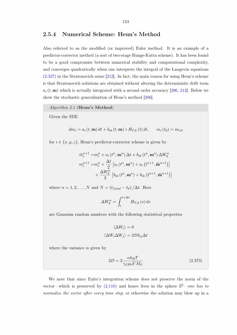
124
2.5.4 Numerical Scheme: Heun’s Method
Also referred to as the modified (or improved) Euler method. It is an example of a
predictor-corrector method (a sort of two-stage Runge-Kutta scheme). It has been found
to be a good compromise between numerical stability and computational complexity,
and converges quadratically when one interprets the integral of the Langevin equations
(2.327) in the Stratonovich sense [212]. In fact, the main reason for using Heun’s scheme
is that Stratonovich solutions are obtained without altering the deterministic drift term
ai (t,m) which is actually integrated with a second order accuracy [206, 212]. Below we
show the stochastic generalization of Heun’s method [206].
Algorithm 2.1 (Heun’s Method)
Given the SDE
dmi = ai (t,m) dt+ bik (t,m) HT,k (t) dt, mi (t0) = mi,0
for i ∈ x, y, z, Heun’s predictor-corrector scheme is given by
mn+1i =mn
i + ai (tn,mn)∆t+ bik (t
n,mn)∆Wnk
mn+1i =mn
i +∆t
2
[ai (t
n,mn) + ai(tn+1, mn+1
)]+
∆Wnk
2
[bik (t
n,mn) + bik(tn+1, mn+1
)]where n = 1, 2, . . . , N and N = (tfinal − t0) /∆t. Here
∆Wnk =
∫ t+∆t
tHT,k (s) ds
are Gaussian random numbers with the following statistical properties
⟨∆Wi⟩ = 0
⟨∆Wi∆Wj⟩ = 2Dδij∆t
where the variance is given by
2D = 2αkBT
γGµ0VMS(2.373)
We note that since Euler’s integration scheme does not preserve the norm of the
vector—which is preserved by (2.110) and hence lives in the sphere S2—one has to
normalize the vector after every time step, or otherwise the solution may blow up in a

125
finite time.110,111 Moreover, for an efficient algorithm to generate the Gaussian random
numbers the reader is referred to Appendix C.
2.5.5 Randomizing The Initial Angle
Since the initial angle of a FM is thermally distributed, then for consistency one has to
randomize this angle before starting the integration scheme. To find the most probable
angle deviation under thermal perturbation, we follow [123] and use the equipartition the-
orem from statistical mechanics.112 Consider the total energy of a uniformly magnetized
FM in the absence of external fields
E = −µ0M ·HeffV
=
K1
[1− (ean ·M)2
M2s
]+µ02M · (NM)
V
=
(Keff sin
2θ0 +µ0M
2s
2N∥
)V (2.374)
where Keff = K1 +Kd = K1 + µ0M2s
(N⊥ −N∥
)/2 is the effective anisotropy constant
which takes both magnetocrystalline and shape anisotropy into account (see 2.4.4.1).
Here, θ0 is the initial angle in root-mean-square (RMS). Since we care about energy
changes, we can drop the constant term for now and just write
E = KeffV sin2θ0 (2.375)
Now, the equipartition theorem states that in thermal equilibrium, every degree of free-
dom of a system has,113,114 most probably, an average energy equal to (1/2) kBT .115
Therefore [123]
KeffV sin2θ0 =1
2kBT (2.376)
110In, general, it is well-known that first-order methods fail to describe the magnetization dynamics[226].
111Although this naive approach is sometimes criticized because it changes the time evolution of mag-netization in a nonlinear manner.
112Also known as the law of equipartition, equipartition of energy, or just equipartition. It is a generalformula that relates the average energies of a system to its temperature. One of its original statementswas that in thermal equilibrium, energy is shared equally among all of its various forms.
113A degree of freedom is any part of the system that is able to store energy.114In general, for a FM there are two degrees of freedom: (1) Rotation out of the plane, and (2) rotation
in the plane. However, due to the large demagnetizing fields, which tend to keep the magnetization inthe plane, the out of plane component is usually small compared to the latter and thus most of the timeneglected [123].
115In fact, for quadratic energies AX2, where A is a constant and X the degree of freedom, theequipartition theorem states that in thermal equilibrium, the average energy is equal to (1/2) kBT .For example, for an LC-circuit in thermal equilibrium, the energies stored in the components are mostprobably (1/2)CV 2
N = (1/2) kBT and (1/2)LI2N = (1/2) kBT , where VN and IN are the RMS noisevoltage and current, respectively [123].
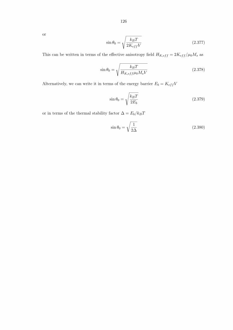
126
or
sin θ0 =
√kBT
2KeffV(2.377)
This can be written in terms of the effective anisotropy field HK,eff = 2Keff/µ0Ms as
sin θ0 =
√kBT
HK,effµ0MsV(2.378)
Alternatively, we can write it in terms of the energy barrier Eb = KeffV
sin θ0 =
√kBT
2Eb(2.379)
or in terms of the thermal stability factor ∆ = Eb/kBT
sin θ0 =
√1
2∆(2.380)
127
Chapter 3
Spin Circuit Theory
In this chapter, we discuss the elementary concepts of magnetoelectronics and diffusive
spin transport for the general case of noncollinear spins. In addition, we introduce the
four-component spin circuit formalism which naturally extends Kirchhoff’s laws, circuit
variables, and circuit techniques to Pauli spin space.

128
3.1 Magnetoelectronics
Magnetoelectronics deals with the transport in circuits when FM elements are incorpo-
rated [71, 227, 228]. The magnetoelectronic problem is best treated with the unified
semiclassical circuit theory pioneered by Brataas et al. [124, 145] which assumes diffu-
sive transport in the bulk and applies quantum mechanical boundary conditions at the
interfaces [29]. Consider the FM/NM multilayer shown in Fig. 3.1.
..
m1
.
m2
.
V1
.
V2
Figure 3.1: Noncollinear FM/NM/FM trilayer with voltage applied across the structure.
The formal procedure is to divide the FM/NM multilayer into [71, 106, 124, 145]:-
1. Nodes (Low Impedance Interconnectors): Each node can be a FM or a
NM, and is characterized by a generalized distribution function, namely a 2 × 2
distribution matrix in spin space f .1 One can assume the nodes to be large and/or
irregular in shape with a sufficient number of randomly distributed scatterers so
that the distribution matrix is isotropic in k-space and therefore depends only on
energy (i.e., f ≡ f (E)) [71, 124, 145]. Otherwise, if, say, the node size is larger the
spin-diffusion length, one has to use spatially-dependent spin distribution functions
[106, 124, 145]. Finally, the charge and spin conservation laws have to be applied
at each node, viz. [145] ∑i
Iij =
(∂fj∂t
)relaxation
(3.1)
where Iij is the current matrix from node (or reservoir) α to node (or reservoir) β.
The term on the right-hand side describes the spin-relaxation, and can be set to
zero when the current is conserved (e.g., when t≪ τsf ) [145].
2. Reservoirs (Voltage Sources): A reservoir can be a FM or a NM, and is char-
acterized by a chemical potential µ. The reservoirs are assumed to be large and in
thermal equilibrium with µ so that the 2×2 distribution matrix is diagonal in spin
space with each component of the matrix given by the Fermi-Dirac distribution,
that is f ≡ 1fF (E, µ) where 1 is the unit matrix and fF (E, µ) is the Fermi-Dirac
distribution.1The hat 'ˆ' denotes a 2× 2 matrix in spin-space.

129
3. Contacts (Resistive Elements): The current-limiting elements. They connect
the nodes to each other and to the reservoirs and are characterized by the mi-
croscopic scattering matrices of the Landauer-Büttiker formalism [229–232]. The
contacts are assumed to have much higher resistance than the nodes, that is
Rcontact ≫ Rnode (3.2)
which is clearly satisfied when the contact have a much smaller cross-sectional area
or when it is are in the tunneling regime [124]. The above simple theory above will
fail when (3.2) does not hold [106].
As mentioned, a contact can be described in terms of the scattering matrices.
In particular, in terms of the 2× 2 conductance tensor composed of [71]
Gσ =e2
h
[M −
∑nm
|rnmσ |2
]=e2
h
[∑nm
|tnmσ |2
](3.3)
Gσ,−σ =e2
h
[M −
∑nm
rnmσ(rnm−σ
)∗] (3.4)
where Gσ is the spin-dependent conductance and Gσ,−σ is the spin-mixing conduc-
tance. Here rnmσ (rnm−σ ) is the reflection coefficient between the transverse modes
n and m at the Fermi level of an electron with spin σ (−σ) in the NM that is
connected to the FM. In addition, M is the number of modes at the NM side and
is given by M = kfA/4π, where kf is the wave-vector in the NM. The spin-mixing
conductance is only relevant for the noncollinear case and is responsible for the
rotation of spins around the magnetization axis [106, 124]. That is, the transport
of spins that are noncollinear to the magnetization is determined by Gσ,−σ, and
hence the spin-transfer torque is only determined by it [150]. For the collinear case,
the transport of spins is only determined by Gσ [106, 124]. The spin-mixing and
spin-dependent conductances can be shown to satisfy the inequality [145]
Re Gσ,−σ ⩽Gσ +G−σ
2(3.5)
The conductances can be computed for diffusive, ballistic, and a tunnel contacts
[145]. Some calculations of Gσ,−σ can be found in [150, 151].

130
3.2 Carrier Transport
Below we show the carrier transport model in diffusive samples, i.e. those for which L >
λ, where λ is the mean-free path between scattering events.2 In particular, we employ the
drift-diffusion model derived from the transparent and coherent thermodynamic approach
as presented in [84], and also make use of the derivations in [43, 79, 109] regarding charge
and spin transport along with the classical works of Valet-Fert [104] and Johnson-Silsbee
[113]. In our formalism, we assume high enough temperatures to dispel the question of
diffusion, and also ignore spin-orbit (SO) coupling3. We assume all transport is governed
by differences in electric fields (drift) or density gradients (diffusion). Moreover, we
assume particles cannot be created or destroyed4; a fact summarized in the normalization
condition [79]
N0 =
∫∫∫R3
n (t, r) dV (3.6)
where N0 is the total number of particles, which is fixed. However, we will allow for slow
spin relaxation processes to establish correct equilibrium polarization [109].
Let X be a balanceable5 quantity that is associated with a local density x and a local
current density Jx. Every such quantity has to obey a continuity equation [84]
∂x (t, r)
∂t+∇ · Jx (t, r) = Σx (t, r) (3.7)
where Σx is the X-generation rate per volume. For conserved quantities, Σx = 0. For
charged particles (in the absence of external magnetic fields), we do not use the local
chemical potential µ,6,7 but rather the local electrochemical potential µ = µ + qVC to
quantify energy changes required for adding or removing charged particles. Thus VCgives the electrostatic contribution to the energy term for the local increase in charge
2In other words, those for which the Knudsen number satisfies
Kn =λ
L< 1
3Otherwise, full quantum transport formalisms like the nonequilibrium Green’s function (NEGF)[233] or scattering theory [71] has to be applied.
4Unless in semiconductors where electrons can recombine with holes.5Not necessarily conserved (e.g., spin).6The key point behind the assumption of “local equilibrium” is that carriers are in equilibrium with
the other carriers in the same local region. This assumption generally holds as long as the subvolumeconsidered is greater than λ3 [84].
7Measured relative to Ec (bottom of conduction band) for electrons, or relative to Ev (top of valenceband) for holes.

131
density from n0 (µ) .8 Thus, for the transport of electric charges we choose µ as an
independent variable and this parameter should enter all the thermodynamic relations
(instead of µ). In the linear low-field regime, one has the current density9
Jx = −D∇x (t, r) + σ
qE (t, r) (3.9)
where E = −∇VC , D is the diffusivity (or diffusion coefficient), and is the σ the conduc-
tivity. The first term represents diffusion, whereas the second term represents drift.
Charge Transport: Letting X = N , we obtain the continuity equation
∂n
∂t+∇ · Jn = 0 (3.10)
where we have set Σn = 0. The particle current density is given by
Jn = −D∇n− σ
eE (3.11)
where σ = eµn, µ being the mobility. The charge current density can be found from
JC = −eJn as
JC = eD∇n+ σE (3.12)
= eD∂n0∂µ∇µ− σ∇VC (3.13)
where we have used the fact that we are in near-equilibrium (i.e., |eVC | < kBT ) so that
we can write ∇n (r) = ∂n0∂µ ∇µ = ∂n0
∂µ ∇ (µ+ eVC) [79, 109]. Under global equilibrium, µ
is constant and the current vanishes [79, 84, 109]. Thus
0 = eD∂n0∂µ
(0 + e∇VC)− σ∇VC (3.14)
or
σ = e2D∂n0∂µ
(3.15)
which is the general form of Einstein’s Relation. The factor ∂n0/∂µ is called the charge
compressibility (also known as the thermodynamic DOS ) and is usually denoted by χc
8Recall that at equilibrium n0 =∞∫0
g (E) fF (E − µ) dE (if the minimum energy of the band energy
is E = 0), where g (E) is the DOS and fF (E − µ) the Fermi-Dirac distribution given by
fF (E − µ) =1
1 + eE−µkBT
(3.8)
9This can be derived from the classical Boltzmann equation in the limit where the density and externalpotentials are slowly varying on the scale of λ [79, 84, 104, 109].

132
[84, 109].10,11 Using Einstein’s relation [61, 78, 84, 109]
JC =σ
e∇µ (3.16)
where we clearly see that current flow is driven by a gradient in the electrochemical
potential [61].12 Note that authors sometimes call the electrochemical potential µ the
quasi-chemical potential. In fact, in the same way as one calls the “equilibrium” chemical
potential the Fermi level, one can also call the quasi-chemical potential (the electrochem-
ical potential) the quasi-Fermi level. Moreover, we note that both (3.16) and (3.12) are
equivalent in the linear regime and can be used to find the current density. The two are
related by Einstein’s relation (3.15).
Spin Transport: Labeling electrons with up- and down-spin with the spin index σ =↑, ↓,we write the total electron density as
n = n↑+n↓ = (n0,↑ + δn↑)+(n0,↓ + δn↓) = (n0,↑ + n0,↓)+(δn↑ + δn↓) = n0+δn (3.17)
where δn↑ = n↑ − n0,↑ and δn↓ = n↓ − n0,↓ are the deviations of the up- and down-densities from their equilibrium values, respectively. The continuity equations can then
be simply extended as [65, 109]
∂n↑∂t− 1
e∇ · J↑ = −
(δn↑τ↑↓−δn↓τ↓↑
)(3.18)
∂n↓∂t− 1
e∇ · J↓ = −
(δn↓τ↓↑−δn↑τ↑↓
)(3.19)
where 1/τ↑↓ is the rate at which a spin ↑ is flipped to ↓, and 1/τ↓↑ the rate at which
spin ↓ is flipped to ↑.13 The terms on the right-hand side represent the generation rates
Σn↑ and Σn↓ which are now nonzero due to the non-conserving spin scattering events
(e.g., electron-magnon collisions, or spin-orbit interactions on defects and impurities10This quantity is related to the microscopic length scale in a Mott insulator known as the screening
length, given by δ =(
e2
εχc
)−1/2
. This is the length over which any charge imbalance is effectivelyscreened out [109]. The spreading of the local charge accumulation roughly occurs during the very shorttime scale known as the dielectric relaxation time given by τd = ε/σ [66]. This is the reason diffusionis usually neglected in metals. In contrast to metals, in doped semiconductors the electron-hole packetsare charge-neutral and can therefore be long-lived and result in density inhomogeneity, making diffusionimportant.
11For degenerate Fermi gas (µ ≈ EF ), g (EF ) ≈ 32
nEF
∝ n1/3 where EF =ℏ2(3π2n)2/3
2m∗ , yieldingχc = g (EF ). This can also be obtained from fact that the Fermi-Dirac distribution for a degenerateFermi gas resembles a step function ∂f
∂µ≈ δ (E − µ) so that ∂n
∂µ= g (EF ). For a nondegenerate Fermi
gas (E − µ≫ kBT ), one has χc = nkBT
[79, 84].12Note that in general σ ≡ σ (µ). Thus for low carrier density materials (e.g., semiconductors) where
large deviations of the local charge density can occur, it is better to separate σ into the carrier densityand mobility, as the latter depends less on µ and thus can be better analyzed [109].
13For degenerate Fermi gas (µ ≈ EF ), τ↑↓g↓ (EF ) = τ↓↑g↑ (EF ). For a nondegenerate Fermigas (E − µ≫ kBT ), one has τ↑↓n↓ = τ↓↑n↑ [65].
133
[76, 104]). Adding the above two equation yields the charge continuity equation (3.10).
On the other, we can define the spin density as the difference
s = n↑−n↓ = (n0,↑ + δn↑)− (n0,↓ + δn↓) = (n0,↑ − n0,↓)+(δn↑ − δn↓) = s0+ δs (3.20)
where δs = n↑ − n↓ = δn↑ − δn↓ is the spin accumulation.14 Now subtracting the
equations yields the continuity equation for the spin current density
∂s
∂t− 1
e∇ · JS = −2
(δn↑τ↑↓−δn↓τ↓↑
)(3.21)
For times t > τd, the system can be considered locally charge neutral, namely n = n0
so that δn = δn↑ + δn↓ = 0 (giving for a system that is charge-neutral at equilibrium
ρ = −eδn a divergenceless electric field ∇ ·E = ρ/ε = 0) [109]. The last fact implies the
only the spin accumulation matters. In fact, now we have δn↑ = −δn↓ = δs2 . Thus
∂s
∂t− 1
e∇ · JS = − δs
τsf(3.22)
where τsf = (1/τ↓↑ + 1/τ↑↓)−1 is the average spin-flip (or spin-relaxation) time [71].
In a FM conductor, the different DOSs at the Fermi level along with the different Fermi
velocities of majority and minority spins result in spin-dependent properties. Thus, now
we may define the spin-resolved properties, for example, as [79, 109]
g = g↑ + g↓ gs = g↑ − g↓ (3.23)
σ = σ↑ + σ↓ σs = σ↑ − σ↓ (3.24)
D =1
2(D↑ +D↓) Ds =
1
2(D↑ −D↓) (3.25)
In addition, by allowing for spin-dependent quasi-chemical potentials, we may write
µ↑ = µ↑ − eVC , µ↑ = µ+ µs (3.26)
µ↓ = µ↓ − eVC , µ↓ = µ− µs (3.27)
we can write the charge and spin quasi-chemical potentials as
µ =1
2(µ↑ + µ↓) µs =
1
2(µ↑ − µ↓) (3.28)
14Although this name sometimes refers to the half-difference in the quasi-chemical potentials [79].Recall the discussion in 2.1.4.

134
The charge current densities for the two spin species in the linear regime can be found
from the simple extension [79, 109]
J↑ = eD↑∇n↑ + σ↑E
= eD↑∂n0,↑∂µ↑
∇µ↑ − σ↑∇VC (3.29)
J↓ = eD↓∇n↓ + σ↓E
= eD↓∂n0,↓∂µ↓
∇µ↓ − σ↓∇VC (3.30)
where we have used ∇n↑ =∂n0,↑∂µ↑∇µ↑ and ∇n↑ =
∂n0,↑∂µ↑∇µ↑.15 Similarly, Einstein’s
relation can be generalized in a non-homogeneous equilibrium state (where the spin
currents vanish and electrochemical potentials are constant [84]), yielding16,17 [109]
σ↑ = e2D↑∂n0,↑∂µ↑
(3.34)
σ↓ = e2D↓∂n0,↓∂µ↓
(3.35)
These relations allow us to write the spin current densities more compactly as [104]
J↑ =σ↑e∇µ↑ (3.36)
J↓ =σ↓e∇µ↓ (3.37)
which is just an extension of the charge transport result by allowing for different quasi-
chemical potentials. Using the last two equations along with the definitions stated at
the beginning, and after some algebra, we can write the current densities as [79]
JC = J↑ + J↓ =σ
e∇µ+
σse∇µs (3.38)
JS = J↑ − J↓ =σse∇µ+
σ
e∇µs (3.39)
15For degenerate Fermi gas (µ ≈ EF ), ∇n↑ = g↑ (EF )∇µ↑ and ∇n↓ = g↓ (EF )∇µ↓. For anondegenerate Fermi gas (E − µ≫ kBT ), one has ∇n↑ =
n↑kBT
∇µ↑ and ∇n↓ =n↓
kBT∇µ↓ [65].
16If one includes electron-electron interactions between different spin populations (i.e. spin Coulombdrag [234]), then σ, D and other spin-dependent parameters like the susceptibility χc all extend to 2× 2tensors in spin space. For example [109]
e, ecJ↑ = e (D↑↑∇n↑ +D↑↓∇n↓) + (σ↑↑ + σ↑↓)E (3.31)J↓ = e (D↓↑∇n↑ +D↓↓∇n↓) + (σ↓↑ + σ↓↓)E (3.32)
and Einstein’s relation would be[σ↑↑ σ↑↓σ↓↑ σ↓↓
]= e2
[D↑↑ D↑↓D↓↑ D↓↓
][ ∂n0,↑∂µ↑
∂n0,↑∂µ↓
∂n0,↓∂µ↑
∂n0,↓∂µ↓
](3.33)
Thus the Coulomb interaction is responsible for the appearance of the off-diagonal elements.17In a simple two-band modelD↑ = 1
dvF↑λ↑ = 1
dvF↑
2τ↑ andD↓ = 1dvF↓λ↓ = 1
dvF↓
2τ↓, where d = 1, 2, 3is the spatial dimension [71].
135
which in fact reveals that a spin current can be generated even in a NM (σs = 0) as long
as there is an accumulation of spins.
The above formulation is for spins along a single axis (i.e., collinear spins). For the
general case in a systems consisting of noncollinear spins, one can write the transport
equation for each spin component, viz.
∂sk∂t− 1
e∇ · JS,k = −δsk
τsf(3.40)
where k is used to denote the spin-polarization along the k-th axis. The current density
along each spin-polarization direction is given by
JS,k = eD∇δsk + eµskE (3.41)
The equations can be combined (while still assuming local charge neutrality) to obtain
the spin drift-diffusion equation (SDDE)
∂s
∂t−D∇2δs− µ (E · ∇) s = − δs
τsf(3.42)
3.3 Four-Component Circuit Formalism
3.3.1 Total Voltage and Current
Following [47] and the similar implementation in [45, 48, 52, 60], we generalize the current
and voltage circuit variables as follows
I =
[IC
IS
]=
IC
IS,x
IS,y
IS,z
(3.43)
V =
[VC
VS
]=
VC
VS,x
VS,y
VS,z
(3.44)
136
where IC is the charge current, IS the vector spin current, VC the charge voltage, VS
the vector spin voltage18.
3.3.2 Generalized Ohm’s Law
Assuming a linear relationship between the total voltage and current,19 the two can be
related by a conductance tensor [45, 47, 48, 52, 60]IC
IS,x
IS,y
IS,z
=
G11 G12 G13 G14
G21 G22 G23 G24
G31 G32 G33 G34
G41 G42 G43 G44
VC
VS,x
VS,y
VS,z
(3.45)
Thus Ohm’s law naturally generalizes to
I = GV (3.46)
where G = R−1, the inverse of the resistance matrix.
3.3.3 Generalized Kirchoff’s Circuit Laws
In spin circuits, Kirchoff’s conservation laws should take spin dissipation (due to spin-
flipping events) into account [47, 48, 52, 124, 145].
Kirchoff’s Current Law (KCL): At any node (junction) in a spin circuit, the sum of
the vector currents flowing into the node is equal to total dissipated vector spin current
at that node. That isn∑
k=1
Ik = Idissipated (3.47)
where Ik is the vector current flowing from branch k into the node, n the total number
of branches, and Idissipated the dissipated vector spin current in that node.20
18This relation is for 1D flow. Recall that the spin current is a tensor of the form
JS =
JxxS Jxy
S JxzS
JyxS Jyy
S JyzS
JzxS Jzy
S JzzS
so the spin circuit variables we will define could correspond to any of the rows of this matrix (whichcorrespond to different directions of flow and not spin quantization).
19The assumption of a linear relationship between voltage and current is valid at least in metals whereelectron density is high and E varies slower than the scattering time; for a better accuracy, one can takethe branches/nodes on which computation is performed to be sufficiently small [48, 79].
20This is essentially an equation of the form (3.1). The dissipated spin current is handled by sinkingit to a “virtual” ground terminal [45, 52].
137
Kirchoff’s Voltage Law (KVL): The sum of the vector voltage differences around
any closed circuit is zero. That isn∑
k=1
Vk = 0 (3.48)
where Vk is the k-th voltage difference and n the total number of voltages.
3.3.4 Generalized Modified Nodal Analysis
In circuit theory, the nodal analysis is a widely used method to obtain the unknown
voltages using KCL. Though simple, the method has some shortcomings, in particular
for algorithm implementation and when handling voltage sources, current-dependent
elements, and the direct evaluation of branch currents. The modified nodal analysis
(MNA) [235] is an extension of the nodal analysis, which, in contrast to the latter, also
determines some branch currents. Although it results in a larger system to be solved, it is
more systematic and better suited for computer implementation. Below we briefly state
the rules of MNA and definitions of the matrices/vectors involved and then naturally
extend MNA to spin space as made in [48].
Given a linear circuit with n nodes (excluding ground) and m voltage sources, the
MNA algorithm proceeds as follows:
1. Select a reference node (usually ground).
2. Label the variables: (i) The nodal voltages V1, V2, . . . , Vn, and (ii) the currents
through the voltages sources as Isource,1, Isource,2, . . . , Isource,m.
3. Write KCL at every node.
4. Write an equation for the voltage of each voltage source.
5. Solve for the n+m unknowns.
In general, the algorithm above will result in the linear system
Ax = b (3.49)
where A ∈ R(n+m)×(n+m), x ∈ R(n+m)×1, and b ∈ R(n+m)×1. The definitions and entires
of the matrix and vectors are as follows:-
• A: Related to the connection of the passive elements. It can generally be written
in terms of some block matrices as
A =
[G B
C D
](3.50)

138
where
G ∈ Rn×n: Related to the interconnection between the passive elements where
the entries can be found as follows
Gij =
negative the conductance between nodes i and j, i = j
sum of the conductances connected to node i (j), i = j(3.51)
The definition clearly implies that G = GT .
B ∈ Rn×m: Related to the connection between the passive elements and the
voltage sources where the entries can be found as follows
Bij =
1, if node i is connected to the positive terminal of the j-th voltage source
−1, if node i is connected to the negative terminal of the j-th voltage source
0, if node i is not connected to the j-th voltage source(3.52)
C ∈ Rm×n: In the special case in which the circuit has only independent
voltage sources, the matrix is related to B by C = BT .21
D ∈ Rm×m: In the special case in which the circuit has only independent
voltage sources, the matrix is the zero matrix, i.e. D = O.
• b: Composed of the known node voltages and branch currents and it has the form
b =
[i
e
](3.53)
where
i ∈ Rn×1: Related to the independent current sources where the entries can
be found as follows
ik =
0, if no current into node k
Iindependent,k, if the independent current Iindependent,k is going into node k(3.54)
e ∈ Rm×1: Related to the independent voltage sources where the entries can
be found as follows
ek = Vindependent,k (3.55)21We will only consider this case here. For the more general case the reader is referred to [236].

139
• x: Composed of the unknown quantities; i.e. node voltages & currents through the
voltage sources. It can be easily be found as
x = A−1b (3.56)
which has the form
x =
[v
j
](3.57)
where
v ∈ Rn×1: Unknowns node voltages.
j ∈ Rm×1: Unknown currents through the voltage sources.
In general, the MNA will result in a matrix with unsymmetric sparse coeffi-
cient matrices with identical nonzero pattern, and thus matrix inversion will be
computationally inefficient. In fact, for O(n2)
entries the system is highly sparse
with O (n) nonzero entries. This, in fact, means that approximately 99% of the
entries in A are zeros [237]. Thus, for medium matrices, one can use the sparse LU
factorization whereas for large matrices one can resort to iterative scheme (e.g.,
conjugate gradient).
For a spintronic circuit, the rules of MNA hold, but everything has to be extended to
spin space, i.e. by replacing n← 4n and m← 4m [48]. This implies that all the matrix
entries now extend to 4× 4 block matrices. Table 3.1 below summarizes the dimensions
of the matrices and vectors in the classical and generalized MNA.
Table 3.1: Dimensions of variables in the MNA. Table adapted by the author from [48].
MNA Generalized MNAx (n+m)× 1 (4n+ 4m)× 1
v n× 1 4n× 1
j m× 1 4m× 1
A (n+m)× (n+m) (4n+ 4m)× (4n+ 4m)
G n× n 4n× 4n
B n×m 4n× 4m
C m× n 4m× 4n
D m×m 4m× 4m
b (n+m)× 1 (4n+ 4m)× 1
i n× 1 4n× 1
e m× 1 4m× 1

140
Chapter 4
Circuit Modeling of ASL
In this chapter, we introduce all-spin logic (ASL), discuss its basic operation principles,
describe the general modeling procedure, and simulate a basic ASL switch. The modeling
and simulations will be based on our finite-difference model using the algorithm we
developed.

141
4.1 Motivation
Spintronic devices [8, 9] are prime candidates for Beyond CMOS technologies to sustain
the advancements of Moore’s law [1] due to their potential for low power consumption
and high-density computation and storage. The success of planar CMOS has naturally
triggered extensive research on spintronic structures that resembles the FET. Namely,
lateral structures made up of conducting channels and at least two terminals that act as
the source and drain of carriers. Fig. 4.1 shows two examples of such devices. Fig. 4.1a
shows a lateral local spin valve (LLSV) that switches due to the locally injected spin
currents, whereas Fig. 4.1b shows a lateral nonlocal spin valve (LNLSV) that switches
due to the nonlocally injected spin currents1 [36–42]. Although both devices work on the
principles of STT switching, the nonlocal device is rather preferred. This is because the
LNLSV decouples charge from spin, generating pure spin currents. This is advantageous
because it eliminates the spurious effects accompanying spin-polarized (and pure charge)
currents [37, 43].
...+
.−
....
IC
..(a)
...+
.−
....
IC
..(b)
Figure 4.1: Schematics showing the difference between local and nonlocal STT in a lateralspin valve (LSV). (a) In local STT, the information is read from the input FM by translatingVsource to IS , whereas information is written to the output FM through local STT due to theinteraction with the spin-polarized current IS . (b) In nonlocal STT, information is read fromthe input FM by translating Vsource to IS , whereas information is written to the output FM
through nonlocal STT due to the interaction with the pure spin current IS .
Although the device in Fig. 4.1b is certainly an attractive candidate for logic switch-
ing, there are some limitations that prevents using it in an integrated circuit. One
issue is that one cannot prevent crosstalking between concatenated stages of these de-
vices. That is, there are no isolations between the different stages to prevent diffusion of
injected/back-injected currents. Fortunately, this problem can be easily solved by insert-
ing a spacer beneath every FM such that each has isolated input and output sides (Fig.
4.2). The beauty of this solution is that both of the exposed sides of the FM are identical,
and thus every FM can act as an injector/detector. The latter is one requirement for a
proper logic operation.1Performing nonlocal STT [238–242].

142
IC
Figure 4.2: Every FM can act as an injector and as a detector. The left side is the write,detect or receive side that acts as the input of the FM where information sent from the previousstage is received. This side is also referred to as the sense side since it senses the pure spincurrents diffusing from the previous stage. The right side is the read, inject or transmit sidethat acts as the output of the FM where information to the next stage is sent. This side isalso referred to as the polarize side since it polarizes the DC current injected from the energy
source Vsource. Figure adapted by the author from [52, 55, 56]
4.2 All-Spin Logic (ASL)
Among the most promising spintronic logic switches is a device called all-spin logic (ASL)
[44–46] that is based on a LNLSV structure and STT switching (Fig. 4.3). The device has
recently attracted increasing interest due to its low power operation and logic-in-memory
structure.2 In addition, the device utilizes pure spin currents throughout every stage of
its operation, eliminating the need for repeated spin-to-charge conversion and thus any
extra hardware [44, 46]. This is in contrast to most spintronic logic switches which uses
spins internally but have logic gates with charge-based terminals [44].3 Moreover, as
discussed in the previous section, using pure spin currents eliminates the spurious effects
accompanying charge currents, which is certainly advantageous.
.....
FM
.
NM
.
NM
.(lead)
.
Spacer
Figure 4.3: A generic ASL device with its constituent elements labeled.
2Less voltage operation also means less parasitic capacitance and stray charge [47]. Moreover, non-volatility ideally implies zero stand-by power.
3Other examples of devices that do not require spin-to-charge conversion: Magnetic quantum cellularautomata (MQCA) [243–245] and domain wall (DW) logic [246]. However, these devices use the Oerstedfields generated by the passing DC currents to switch the FMs, i.e. preforming nanomagnetic logic(NML). ASL, on the other hand, utilizes spin currents directly to switch using nonlocal STT, and is thusnot limited to nearest-neighbor communication like MQCA (i.e., not limited to cellular architectures)[46].

143
4.2.1 Device Operation
ASL utilizes two bistable FMs whereby binary information is stored (e.g., “0” = left,
“1” = right) that communicate with pure spin currents through a spin-coherent NM
channel. The main principle behind the operation of the device is the accumulation of
spins beneath the input FM upon the passage of a charge current. This occurs due to the
spin filtering process at the FM/NM interface which creates a difference in population
of spin density across the NM channel, driving diffusion of up- and down-spins in both
directions4. If sufficient amount of noncollinear spins reaches the output FM, enough
torque can then be exerted on the nanomagnet, switching it into another stable state.
With reference to Figs. 4.5 and 4.6, we can summarize the operation of ASL shown
in Fig. 4.4 as follows5 [52, 55]:
• Positive voltage (NOT operation): Extracts majority spins, and injects mi-
nority spins. Thus a positive Vsource makes the input FM a sink of majority spins.
• Negative voltage (COPY operation): Extracts minority spins, and injects
majority spins. Thus a negative Vsource makes the input FM a source of majority
spins.
...
+
.
−
....
IC
..
(a)
...
+
.
−
....
IC
..
(b)
Figure 4.4: ASL inverter in operation. (a) P → AP (NOT ) . (b) AP → P (COPY ).
We note that while the operation of ASL is reciprocal in that reversing the direction
of the current will cause a spin current of the opposite polarization to reach the output
FM, the currents are not necessarily equal in magnitude, i.e the current required for
switching P → AP and AP → P are not necessarily equal and neither are the switching
times. This will be shown later in the simulations.
4For them to bring the electrochemical potential into equilibrium. Recall the discussion in 2.1.4.5Here, recall that we refer to the spins that are parallel to the magnetization as majority spins,
whereas those antiparallel are referred to as minority spins.

144
..
IC
(a)
.
(b)
..
+
.
−
....
IC
.
(c)
..
+
.−
....
IC
...
(d)
...
+
.
−
....
IC
..
(e)
Figure 4.5: P → AP (NOT ). (a) A charge current is injected from the FM to the NM. (b)Electrons are injected from the NM to the FM. Majority spins are most likely to transmit,whereas minority spins are most likely to reflect and accumulate beneath the FM. (c) Theresult is that the passage of a charge current from the FM to the NM accumulates minorityspins beneath the FM. (d) The difference in population of spin density across the channeldrives diffusion of opposite spins in both directions to bring the electrochemical potential intoequilibrium. Minority spins will diffuse to the right and majority spins will diffuse to the left.(e) Majority spins diffusing to the left are equivalent to minority spins diffusing to the right.Thus, the result is that a total spin current of minority spins will diffuse to the right, switching
the output FM antiparallel through STT.
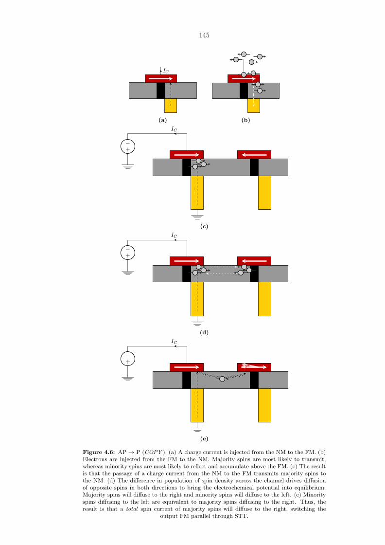
145
..
IC
(a).
(b)
..
+
.
−
....
IC
.
(c)
..
+
.
−
....
IC
...
(d)
...
+
.
−
....
IC
..
(e)
Figure 4.6: AP → P (COPY ). (a) A charge current is injected from the NM to the FM. (b)Electrons are injected from the FM to the NM. Majority spins are most likely to transmit,whereas minority spins are most likely to reflect and accumulate above the FM. (c) The resultis that the passage of a charge current from the NM to the FM transmits majority spins tothe NM. (d) The difference in population of spin density across the channel drives diffusionof opposite spins in both directions to bring the electrochemical potential into equilibrium.Majority spins will diffuse to the right and minority spins will diffuse to the left. (e) Minorityspins diffusing to the left are equivalent to majority spins diffusing to the right. Thus, theresult is that a total spin current of majority spins will diffuse to the right, switching the
output FM parallel through STT.

146
4.2.2 Basic Elements of ASL
• FMs (Input/Output)
Role: Used to store the information represented in the magnetizations (e.g.,
“0” = left, “1” = right) in a nonvolatile manner. For a single ASL device (Fig.
4.3), the left FM is the injector, whereas the right FM is the detector.
Material: Usually transition metal FMs like Fe, Co, Ni, and their alloys such
as Py (Ni80Fe20), CoFeB, CoPd, CoNi, CoPtCr, Co3Pt, FePd, FePt, CoPt,
Fe14Nd2B, or even MnAl6 [46].
• NM Channel (Interconnect)
Role: Connects the input FM to both the output FM and to the ground,
effectively creating two paths to route two types of currents in the device:
1. The pure spin current diffusing from the injecting FM to the detecting
FM;
2. The spin-polarized current flowing from the injecting FM the ground ter-
minal.
Material: Could be either a metal or a semiconductor [44]. For the former,
noble metals such as Cu, Ag , and Au are usually used [37, 40, 247–250]. For
the latter, degenerately doped Si and GaAs channels are possible or even the
novel zero band gap semiconductor, Graphene [251]. In general, the advantage
of using semiconducting channel is the longer spin-diffusion length obtained
[62, 65, 252–256].7 However, when using a semiconductor, one has to overcome
the conductance mismatch problem across a FM/NM interface for the case of
metallic FM and use the solution proposed by Rashba [257] (and later by Fert
and Jaffres [258]) which suggests using a spin-dependent interface resistance;
a tunnel barrier [132–134] in particular.8,9,10
6For more possible FMs, see footnote 23.7Note that moderately doped semiconductors usually have long spin-diffusion lengths. However,
highly doping a semiconductor could decrease the spin-diffusion length [252] whereas lightly doping ithave no major effect [255].
8For an all-semiconductor structure, this is not a problem and spin injection will be efficient.9Schmidt et al. [259] provided an explanation for the conductance mismatch across a
FM(metal)/NM(semiconductor) interface: For diffusive electrons, the spin polarization of the injectedcarriers is β
(ρFM/ρNM
) (lFMsf /lNM
sf
), where β is the spin polarization of the FM. The problem in injec-
tion is the low ratio of ρFM/ρNM which reduces the spin polarization in the NM drastically.10The enhancement of spin injection from FM(metal)/NM(semiconductor) with tunnel barriers have
only been recently (experimentally) demonstrated in normal semiconductors [253, 260–262], few yearsafter it has been demonstrated in all-metallic structures [249].

147
• Spacers (Isolation Layers)
Role: Used to ensure that the communication between the two FMs is limited
to the channel and no unwanted crosstalk occurs between the different stages
[45, 46].
Material: Could comprise electrostatic barriers (e.g. oppositely doped semi-
conductor), deposited oxides (SiO2, Al2O3, or HfO2), or physical cuts [44, 46,
52].
4.2.3 Viability of ASL (The Tenets of Logic)
For a proper logic operation, a solid-state device has to fulfill five indispensable require-
ments “tenets” [263]:
1. Nonlinearity (SNR): [3]
Satisfied because of the nonlinearity of the FMs which corrects any error in the
magnetization direction (self-correcting feature) [46]. This is because the FMs are
bistable with two states separated by an energy barrier (Fig. 2.43) which imply
that information will inherently be digitized from any weak perturbation to one of
the two binary states, correcting any error and increasing the SNR [44].
2. Power Amplification (gain > 1 ): [7]
An essential feature to ensure good signal level during logic operation over a long
chain of gates [44]. This is unfortunately not satisfied with the ASL of the type
shown in Fig. 4.3. The problem is that the voltage developed between the output
FM and the NM channel (i.e., the nonlocal voltage) is relatively low, probably
several orders of magnitude smaller than that at the input and thus insufficient to
drive subsequent stages [52].11
The problem can be solved if the switching energy came from one unclocked
Vsource and not the input FM [44, 46, 52]. That is, instead of conveying both
the information (provided by the input FM) and the energy (provided by Vsource)
through the channel, one can employ an alternative scheme that applies Vsourceto both FMs, and thus only convey the information through the channel, where
the energy is provided to both FMs by Vsource as in Fig. 4.7.12 This might be
in fact an advantage since it is easier to apply the same voltage to closely spaced
structures and will also minimize the associated capacitive charges [45]. However,11Unless intervened with a CMOS circuitry to perform amplification and/or clocking, resulting in a
CMOS-dependent logic [52].12This was suggested in the original paper [44] and also in [52].

148
these advantages come at the expense of requiring a sophisticated clocking scheme
[44].
......
FM
.
NM
.
NM
.(lead)
.
Spacer
Figure 4.7: An alternative ASL structure in which the voltage is applied to both FMs.
3. Concatenability (output of one device can drive another): [3]
Readily ensured since the input and output information are of the same form (i.e.,
magnetization) [46] and the FMs are identical where each act as an injector/detec-
tor [44, 45].
4. Feedback Prevention (output does not drive input): [3]
The directivity of a signal in one direction (and not the other) can be achieved by
various means, for example:
(i) Using a tunnel barrier below the injecting side of the input FM as proposed
in [44–46], which can enhance spin injection into the channel. In addition,
the absence of the tunneling layer in the detecting side of the output FM
will create an Ohmic contact, efficiently sinking spins and suppressing back-
injection [44, 46]. The barriers can be oxides or Schottky [44].13
......
FM
.
NM
.
NM
.
(lead)
. Spacer.
Tunnel
Figure 4.8: An ASL device with a tunnel barrier inserted beneath the injecting sides of theFMs.
13As mentioned in the Supplementary Material of the original paper [44], the height of the Schottkybarrier can be lowered by degenerately doping the channel and can also be tuned by using a low work-function metal like the rare-earth FM, Gd.
149
(ii) Placing the ground lead closer to one FM which then causes the side of the
FM exposed to the ground to act as the injector [46]. In this way, every inject-
ing/detecting FM has two sides (separated by the spacer) that are electrically
distinguished due to the ground placement [45, 46]. This solution was already
implemented in Figs. 4.3 and 4.7 introduced previously.14
(iii) Using nonidentical FMs, for example (a) fixed and free layers for the input and
output FMs, respectively, or (b) FMs of different sizes where the output FM
is smaller than the input FM [45]. However, these solutions are not suitable
for logic implementation since every FM has to act as an injector/detector
(i.e., they have to be identical).
(iv) Using nonidentical sides for the FMs, for example by using different injection
polarizations for each side of the FM such that the FM injects more spin
current than it can receive [55]. One way to achieve this is to employ solution
(i). Other solutions are also possible; for example, using nonidentical interface
areas for the input and output FMs [45].
(v) Using a clocking circuitry (e.g., Bennett clocking) [44–46].
(vi) Applying different voltages to the FMs, for example by grounding the output
FM and applying the signal to the input FM [46, 47]. However, as demon-
strated in [45, 46], this will not yield a stable state and the FMs will keep
switching between all states (though in a well-known fashion, i.e. a determin-
istic oscillation, which might have some applications).
Fig. 4.9b illustrates the state diagram for an ASL with nonreciprocal operation
[45].
5. A Complete Set of Boolean operations (AND and NOT, or OR and NOT ):
[3]
A well-known functionally complete set of Boolean operators is AND & NOT (OR
& NOT), which can be used to construct every possible logic gate. In particular,
these gates can be assembled to make the universal gate, NAND (NOR). Demon-
stration of this property using ASL is shown in [45, 46, 52, 56].14For the latter design, an important point has to be asserted: There is a path from FMout to the
ground underneath FMin, allowing charge current to flow and for spins to accumulate underneath FMout
too. However, due to the asymmetric ground placement, the spin current injected by FMout is smallcompared to the one injected by FMin, and thus the torque τSTT,in = (1/eNs)min × (IS,out ×min) issmaller than τSTT,out = (1/eNs)mout × (IS,in ×mout) [45]. Indeed, this can be roughly seen from theinequality (Rin,ground ∝ Lin,ground) < (Rout,g ∝ Lout,ground).

150
..01. 11.
00
.
10
(a)
..01. 11.
00
.
10
(b)
Figure 4.9: State diagram describing the transition of information of interacting FMs. Here,“0” and “1” represents the magnetization direction (e.g., “0” = left, “1” = right). The direc-tionality of signal results in suppression of some transitions (shown with the semi-transparentgray arrows). In addition, for every scenario, the output will be inverted (for negative volt-age)/copied (for positive voltage) according to the input, and not the other way around. Thegray circles represents the stable states. (a) P → AP (NOT ): A positive voltage will invertthe output, depending on the initial state. If we start from 00, then 00 → 01 (and not 10). Ifwe start from 11, then 11 → 10 (and not 01). (b) AP → P (COPY ): A negative voltage willcopy the input, depending on the initial state. If we start from 01, then 01 → 00 (and not 11).If we start from 10, then 10 → 11 (and not 00). Figure adapted by the author from [45, 46].
4.3 Modeling & Simulations of ASL
Previous successful attempts have been made to model ASL with circuit components,
and most fall into one of two categories: (1) Self-consistently solving the magnetization
dynamics (governed by the LLGS) and the spin transport model (governed by the steady-
state SDDE represented in the four-component spin circuit formalism), as in [45, 47–57];
(2) Simulations solely based on circuit models of the LLGS and the time-dependent SDDE
for implementation in SPICE and similar software as performed in [58]. As pointed out
in [47, 52], the framework of simultaneously solving the magnetization dynamics and
the steady-state transport is accurate as long as the transit time of carrier diffusion in
the transport section is much shorter than the dynamics of the nanomagnets, i.e. for
τt ≪ τsw, where the transit time by diffusion can be estimated as τt = L2/2D, with L
being the section length and D the diffusion coefficient. Although this condition holds
sufficiently well for metals of a few 100’s of nm [59], these times might become comparable
as we advance in technology where magnetization switching becomes faster and/or in
the case of moderately long-channel devices. In fact, we are not restricted to all-metallic
structures and might use semiconducting channels, which, in addition to modifying the
diffusion coefficient, brings up the advantage of longer spin-diffusion lengths. Moreover,
some parasitic capacitances will be present in the transport section due to the interaction
between the thin films [264] and they must taken into account as they are the most
significant contributers to the dynamic power dissipation (especially at high frequencies).
In any of the previous scenarios, a dynamical description of carrier transport is necessary.

151
Although the second model provides the necessary tools to capture the dynamics in
the transport section, it lacks the freedom provided by the first model and the ability
to program in common languages since it was meant for SPICE implementation. In
addition, it assumes a macrospin magnet, and thus neglects any spatial variations in
magnetization. It might also be difficult to augment or modify to include other interesting
phenomena like spin Hall effect (SHE) and spin-orbit torque (SOT). These considerations
suggest an extension of the currently available models.
..Magnetization Dynamics (LLGS).
• input: IS1, IS2, . . .
• output: m1,m2, . . .
. Spin Circuit (Spin Circuit).
• input: m1,m2, . . .
• output: IS1, IS2, . . .
.
m1,m2, . . .
.
IS1, IS2, . . .
.Magnetization Dynamics (LLGS).
• input: IS1, IS2, . . .
• output: m1,m2, . . .
. Spin Circuit (SDDE).
• input: m1,m2, . . .
• output: IS1, IS2, . . .
Figure 4.10: Coupled magnetization dynamics/spin transport simulation framework. Figureadapted by the author from [45–47, 52, 55, 56].
Starting from the theory introduced throughout the thesis, and based on the four-
component spin circuit formalism, we present our improved stochastic magnetization
dynamics/time-dependent spin transport model based on new finite-difference conduc-
tance matrices, which can capture both the dissipative and dynamic behavior of spins
in the channel of spintronic devices in general, and ASL in particular. The derivation of
the model goes in the spirit of:
1. Coupled Magnetization Dynamics/Carrier Transport [45, 47, 52, 55]15
2. Circuit-Based Model [58].
In addition, we also use some of the ideas/derivations scattered throughout [48, 60, 71].
4.3.1 Finite-Difference Circuit Model for a Spintronic De-
vice
In this subsection, we derive new 4× 4 finite-difference conductance matrices for a non-
collinear FM/NM multilayer in a spintronic device and then apply it to ASL. To avoid
ambiguities, the geometrical definitions of each section/wire are as shown below.15Which was based on the work of Brataas et al. [71, 150, 265].

152
..
L
. W.
t
Figure 4.11: Geometrical definitions of a volume element.
4.3.1.1 FM/NM Interface
Collinear Magnetizations: FMs have spin-dependent transport properties. In the
absence of strong spin-flip scattering one can use the two-current model in analyzing a
collinear FM/NM multilayer similar to the one shown below.
..
m1
.
m2
.
V1
.
V2
Figure 4.12: Collinear FM/NM/FM trilayer with a voltage applied across the structure.
In the two-current model model, we define the charge and spin currents as
IC = I↑ + I↓ (4.1)
IS = I↑ − I↓ (4.2)
Similarly, the charge and spin conductances are defined by
GC = G↑ +G↓ (4.3)
GS = G↑ −G↓ (4.4)
Using the two-current model for the FM/NM, one can write the following equations
[71]
IC = I↑ + I↓ = G↑(V NMC + V NM
S − V FMC
)+G↓
(V NMC − V NM
S − V FMC
)(4.5)
IS = I↑ − I↓ = G↑(V NMC + V NM
S − V FMC
)−G↓
(V NMC − V NM
S − V FMC
)(4.6)

153
where V FMC is the charge voltage on the FM, V NM
C the charge voltage on the NM, and
V NMS the spin voltage on the NM.16 If we introduce the polarization [71, 106]
P =G↑ −G↓G↑ +G↓
(4.7)
then the two equations can be rewritten as17
IC = G(V NMC − V FM
C + PV NMS
)(4.8)
IS = G(P(V NMC − V FM
C
)+ V NM
S
)(4.9)
or in matrix form [IC
IS
]=
[G PG
PG G
][V NMC − V FM
C
V NMS
](4.10)
or
I = GFM/NMV (4.11)
where
GFM/NM =
[G PG
PG G
](4.12)
is the FM/NM interface matrix in a collinear FM/NM/FM structure.
Noncollinear Magnetizations: In the noncollinear case, the two-current model is
not applicable anymore and one has to take the vectorial nature of spins into account
[71, 106].
..
m1
.
m2
.
V1
.
V2
Figure 4.13: Noncollinear FM/NM/FM trilayer with a voltage applied across the structure.
16Notice how the spin voltage is projected (on the spin quantization axis) for the down-spins. Thiswill be easily seen in the noncollinear case later.
17The equations in fact reveal that a spin current can be generated by a spin accumulation even fora zero voltage drop. It is instructive to compare these to (3.38) and (3.39).

154
It can be shown that a generalization of the above equations for the transport across
a FM/NM interface in a noncollinear FM/NM/NM multilayer is given by [71]
IC = G↑(V NMC +VNM
S ·m− V FMC
)+G↓
(V NMC −VNM
S ·m− V FMC
)(4.13)
IS,∥ =[G↑(V NMC +VNM
S ·m− V FMC
)−G↓
(V NMC −VNM
S ·m− V FMC
)]m (4.14)
IS,⊥ = 2Re G↑↓m×(VNM
S ×m)+ 2 Im G↑↓VNM
S ×m (4.15)
where IS,∥ and IS,⊥ are the longitudinal and transverse spin currents, respectively. Using
the polarization P , we can rewrite (4.13)–(4.15) as18
IC = G(V NMC − V FM
C + PVNMS
)(4.18)
IS,∥ = G(P(V NMC − V FM
C
)+VNM
S ·m)m (4.19)
IS,⊥ = 2Re G↑↓m×(VNM
S ×m)+ 2 Im G↑↓VNM
S ×m (4.20)
Now, to obtain the interface conductance matrix, we can start by considering a simple
case in which the magnetization coincides with a single axis, say m0 = ax (later we will
generalize to any arbitrary direction). Since IS,∥ = (IS ·m)m, we can write
IS,∥ = G(P(V NMC − V FM
C
)+VNM
S · ax)ax = G
(P(V NMC − V FM
C
)+ V NM
S,x
)ax
(4.21)
IS,⊥ = IS − IS,∥ = (IS,xax + IS,yay + IS,zaz)− (IS,xax) = IS,yay + IS,zaz (4.22)
Moreover, the cross products in (4.20) are given by
VNMS ×m = V NM
S,z ay − V NMS,y az (4.23)
m×(VNM
S ×m)= V NM
S,y ay + V NMS,z az (4.24)
Therefore
IS,⊥ = 2Re G↑↓(V NMS,y ay + V NM
S,z az)+ 2 Im G↑↓
(V NMS,z ay − V NM
S,y az)
=(2Re G↑↓V NM
S,y + 2 Im G↑↓V NMS,z
)ay +
(2Re G↑↓V NM
S,z − 2 Im G↑↓V NMS,y
)az
= IS,y + IS,z (4.25)
18Sometimes written more compactly as [71]
IC = G (VC,N + PVS,N ·m− VC,F ) (4.16)IS = G [(VS,N ·m+ P (VC,N − VC,F ))m+ ηRm× (VS,N ×m) + ηIVS,N ×m] (4.17)
where ηR = 2Re G↑↓ /G and ηI = 2 Im G↑↓/G are the real and imaginary parts of reduced mixingconductance (scaled by 2), 2G↑↓/G.

155
where the orthogonal spin current components are given by
IS,y =(2Re G↑↓V NM
S,y + 2 Im G↑↓V NMS,z
)ay (4.26)
IS,z =(2Re G↑↓V NM
S,z − 2 Im G↑↓V NMS,y
)az (4.27)
Hence we can write the charge and spin components as
IC = G(V NMC − V FM
C
)+GPV NM
S,x (4.28)
IS,x = GP(V NMC − V FM
C
)+GV NM
S,x (4.29)
IS,y = 2Re G↑↓V NMS,y + 2 Im G↑↓V NM
S,z (4.30)
IS,z = −2 Im G↑↓V NMS,y + 2Re G↑↓V NM
S,z (4.31)
and then cast the previous equations in matrix formIC
IS,x
IS,y
IS,z
=
G PG 0 0
PG G 0 0
0 0 2Re G↑↓ 2 Im G↑↓0 0 −2 Im G↑↓ 2Re G↑↓
V NMC − V FM
C
V NMS,x
V NMS,y
V NMS,z
(4.32)
or equivalently
I = GFM/NM (m0)V (4.33)
where
GFM/NM (m0) =
G PG 0 0
PG G 0 0
0 0 2Re G↑↓ 2 Im G↑↓0 0 −2 Im G↑↓ 2Re G↑↓
(4.34)
is the FM/NM interface matrix for a noncollinear FM/NM/FM structure. The upper-
left 2×2 matrix is equivalent to (4.10). The lower-right 2×2 matrix, on the other hand,
is related to the noncollinear components, and is related to the action of STT, where,
in this context, the diagonal and off-diagonal terms are related to the Slonczewski and
field-like torques, respectively. For a metallic structure (i.e., Ohmic contacts) the field-
like terms can be neglected [71, 148–150]. In addition, if the interface is clean, one can
assume the interface conductance to be close to the ballistic limit [52]. For non-Ohmic
interfaces (e.g., tunnel), more complex treatment is needed [150].
The conductance matrix above was obtained for a fixed magnetization orientation.
Although this would not matter for a single magnet, when working with multiple non-
collinear magnets one has to write all the matrices in a single uniform basis. In general,

156
the matrix above can be transformed to any arbitrary basis by a unitary rotation oper-
ation using an extended rotation matrix belonging to SO(3)—the group of all rotation
matrices—under the constraint of keeping the charge component invariant.
Let us assume we have a unitary rotation matrix R that relates the vectors in the
new (primed) and old (unprimed) coordinates as
I′ = RI (4.35)
V′ = RV (4.36)
Using these relations, we can write Ohm’s law in the new coordinate frame
R−1I′ = GFM/NM (m0)R−1V′ (4.37)
or
I′ = GFM/NM (m)V′ (4.38)
where the rotated matrix is given by the quaternion formulaGFM/NM (m) = RGFM/NM (m0)R−1.
Since the matrix is unitary, we can equivalently writeGFM/NM (m) = RGFM/NM (m0)RT .
The rotation matrix of interest to us, in general, belongs to the subgroup of SO(4)
consisting of matrices of the form
R =
1 0 0 0
0 r′11 r′12 r′13
0 r′21 r′22 r′23
0 r′31 r′32 r′33
(4.39)
which leaves one component invariant under rotation (e.g. charge in our case). The
components of the block 3 × 3 matrix R′ in R can found by using Rodrigues’ rotation
formula, which efficiently computes a rotation matrix in SO(3) of R3 corresponding to
a rotation by an angle θ (anticlockwise) about a fixed axis specified by the unit vector
m0 = (mx0,my0,mz0). The formula is given as the exponential map
R′ = eM0θ = I + sin θM0 + (1− cos θ)M02 (4.40)
where M0 is the skew-symmetric matrix of the Lie algebra so(3) of SO(3) given by
M0 =
0 −mz0 my0
mz0 0 −mx0
−my0 mx0 0
(4.41)

157
Using Rodrigues’ formula, we find
R′ =
1 0 0
0 1 0
0 0 1
+sin θ
0 −mz0 my0
mz0 0 −mx0
−my0 mx0 0
+(1− cos θ)
−m2
z0 −m2y0 mx0my0 mx0mz0
mx0my0 −m2z0 −m2
x0 my0mz0
mx0mz0 my0mz0 −m2y0 −m2
x0
(4.42)
or
R′ =
1− (1− cos θ)
(m2
z0 +m2y0
)(1− cos θ)mx0my0 −mz0 sin θ (1− cos θ)mx0mz0 +my0 sin θ
(1− cos θ)mx0my0 +mz0 sin θ 1− (1− cos θ)(m2
z0 +m2x0
)(1− cos θ)my0mz0 −mx0 sin θ
(1− cos θ)mx0mz0 −my0 sin θ (1− cos θ)my0mz0 +mx0 sin θ 1− (1− cos θ)(m2
y0 +m2x0
)
(4.43)
which is equivalent to
R′ =
(1−m2
z0 −m2y0
)+
(m2
z0 +m2y0
)cos θ (1− cos θ)mx0my0 −mz0 sin θ (1− cos θ)mx0mz0 +my0 sin θ
(1− cos θ)mx0my0 +mz0 sin θ(1−m2
z0 −m2x0
)+
(m2
z0 +m2x0
)cos θ (1− cos θ)my0mz0 −mx0 sin θ
(1− cos θ)mx0mz0 −my0 sin θ (1− cos θ)my0mz0 +mxy sin θ(1−m2
y0 −m2x0
)+
(m2
y0 +m2x0
)cos θ
(4.44)
Now, from the micromagnetic constraint (2.110) we know that m2x0 +m2
y0 +m2z0 = 1.
Therefore
R′ =
m2
x0 +(1−m2
x0
)cos θ (1− cos θ)mx0my0 −mz0 sin θ (1− cos θ)mx0mz0 +my0 sin θ
(1− cos θ)mx0my0 +mz0 sin θ m2y0 +
(1−m2
y0
)cos θ (1− cos θ)my0mz0 −mx0 sin θ
(1− cos θ)mx0mz0 −my0 sin θ (1− cos θ)my0mz0 +mx0 sin θ m2z0 +
(1−m2
z0
)cos θ
(4.45)
Hence R becomes
R =
1 0 0 0
0 m2x0 +
(1−m2
x0
)cos θ mx0my0 (1− cos θ)−mz0 sin θ mx0mz0 (1− cos θ) +my0 sin θ
0 mx0my0 (1− cos θ) +mz0 sin θ m2y0 +
(1−m2
y0
)cos θ my0mz0 (1− cos θ)−mx0 sin θ
0 mx0mz0 (1− cos θ)−my0 sin θ my0mz0 (1− cos θ) +mx0 sin θ m2z0 +
(1−m2
z0
)cos θ
(4.46)
4.3.1.2 NM
Here, we derive the conductance matrices that models the 1D transport of charge and
spin in a NM section.
..
V1
.
V2
Figure 4.14: A NM element with voltage applied across it.

158
Charge Transport: In a 1D diffusive wire, the continuity and current density equations
are given by
∂n
∂t− 1
e
∂JC∂z
= 0 (4.47)
JC = eD∂n
∂z+ σE (4.48)
Ignoring diffusion current and using the relation ρv = −en, we can write
∂JC∂z
= −∂ρv∂t
(4.49)
JC = σE (4.50)
For a uniform cross-section A we have IC = JCA and ρℓ = ρvA. Also, E = −∂VC/∂z.Thus
∂IC∂z
= −∂ρℓ∂t
(4.51)
IC = −σA∂VC∂z
(4.52)
In addition, the relation Q = CVC on a per length basis is given by ρℓ = CℓVC , where
Cℓ is the capacitance per unit length. This yields
∂IC∂z
= −Cℓ∂VC∂t
(4.53)
IC = −σA∂VC∂z
(4.54)
Now, employing a first-order finite-difference for a finite section ∆z, we obtain
IC (z)− IC (z +∆z) = Cℓ∆z∂VC∂t
(4.55)
IC =σA
∆z[VC (z)− VC (z +∆z)] (4.56)
which yields the typical RC network with G = σA/∆z and C = Cℓ∆z. The π- and
T -model networks are shown in 4.15.
C/2
G
C/2
(a)
C
2G 2G
(b)
Figure 4.15: Distributed circuit model for 1D charge transport through ∆z. (a) π-network.(b) T -network.

159
Spin Transport: As with the charge transport, the transport of spins starts from the
1D continuity and current density equations. Taking the fact that spins can, in general,
be noncollinear, one has [109]
∂s
∂t− 1
e∇ · JS = − δs
τsf(4.57)
JS = eD∂δs
∂z+ eµEs (4.58)
Following [58], we use the relation sk = µs,k∂n0∂µ for each spin component to obtain
∂n0∂µ
∂µs,k∂t
=1
e
∂JS,k∂z
− ∂n0∂µ
µs,kτsf
(4.59)
JS,k = e∂n0∂µ
D∂µs,k∂z
+ e∂n0∂µ
µEµs,k (4.60)
Then using the relation between the spin quasi-chemical potential and the spin voltage,
µs,k = eVS,k, we obtain
e∂n0∂µ
∂VS,k∂t
=1
e
∂JS,k∂z
− e∂n0∂µ
VS,kτsf
(4.61)
JS,k = e2∂n0∂µ
D∂VS,k∂z
+ e2∂n0∂µ
µEVS,k (4.62)
Now we recognize that e2 ∂n0∂µ is the quantum capacitance per unit volume. Indeed Cq =
eskVS,k
= e2 ∂n0∂µ = σ
D , where the last equality results from Einstein’s relation. The quantum
capacitance can be used along with IS,k = JS,kA to write
CqA∂VS,k∂t
=∂IS,k∂z− CqA
VS,kτsf
(4.63)
IS,k = CqDA∂VS,k∂z
+ CqµEAVS,k (4.64)
Now, we notice that CqEA = σEA/D = JCA/D = IC/D and CqDA = σA. Therefore19
CqA∂VS,k∂t
=∂IS,k∂z− CqA
VS,kτsf
(4.67)
IS,k = σA∂VS,k∂z
+µICD
VS,k (4.68)
19In vector notation
CqA∂VS
∂t=∂IS∂z
− CqAVS
τsf(4.65)
IS = σA∂VS
∂z+µICD
VS (4.66)

160
Employing finite-differences for each component of spin, we obtain
IS,k (z)− IS,k (z +∆z)− CqA∆zVS,kτsf
= CqA∆z∂VS,k∂t
(4.69)
IS,k =σA
∆z[VS,k (z)− VS,k (z +∆z)] +
µICD
VS,k (4.70)
which result in the equivalent circuit shown in Fig. 4.16. In the figure, G = σA/∆z,
GS = CqA∆z/τsf , CS = CqA∆z, and I (VS,k) = µICVS,k/D. The last term would vanish
in the ASL channel.
GS CS
I(VS,k)
2G
I(VS,k)
2G
Figure 4.16: Distributed circuit model for 1D spin transport through ∆z.
Now that we found the circuit representations of charge and spin transport in the
NM, we employ finite-differences again, but for the time derivatives. In particular, using
finite-differences in the relation I = C ∂V∂t , we obtain, using:-
• Backward Euler (BE):
In+1 =C
∆t
(V n+1 − V n
)(4.71)
=C
∆tV n+1 − C
∆tV n (4.72)
= G0Vn+1 + I0 (4.73)
• Trapezoidal Rule (TR):
In+1 =2C
∆t
(V n+1 − V n
)− InC (4.74)
=2C
∆tV n+1 − 2C
∆tV n − InC (4.75)
= G0Vn+1 + I0 (4.76)
both suggesting the finite-difference capacitor model shown below.

161
G0 I0≡C
Figure 4.17: Finite-difference model of a capacitor.
Now we use the finite-difference model above for (4.55) and (4.69). Using BE
In+1C (z)− In+1
C (z +∆z) =Cℓ∆z
∆t
(V n+1C − V n
C
)=Cℓ∆z
∆tV n+1C − Cℓ∆z
∆tV nC (4.77)
In+1S,k (z)− In+1
S,k (z +∆z) =CqA∆z
∆t
(V n+1S,k − V
nS,k
)+CqA∆z
τsfV n+1S,k
= CqA∆z
(1
∆t+
1
τsf
)V n+1S,k −
CqA∆z
∆tV nS,k (4.78)
Similarly, one can use the TR
In+1C (z)− In+1
C (z +∆z) =2Cℓ∆z
∆t
(V n+1C − V n
C
)− [InC (z)− InC (z +∆z)]
=2Cℓ∆z
∆tV n+1C − 2Cℓ∆z
∆tV nC − [InC (z)− InC (z +∆z)]
In+1S,k (z)− In+1
S,k (z +∆z) =2CqA∆z
∆t
(V n+1S,k − V
nS,k
)+CqA∆z
τsf
(V n+1S,k + V n
S,k
)−[InS,k (z)− InS,k (z +∆z)
]=CqA∆z
(2
∆t+
1
τsf
)V n+1S,k − CqA∆z
(2
∆t− 1
τsf
)V nS,k
−[InS,k (z)− InS,k (z +∆z)
](4.79)
Both obviously result in relations of the form
In+1C (z)− In+1
C (z +∆z) = GC,0Vn+1C + IC,0 (V
nC ) (4.80)
In+1S,k (z)− In+1
S,k (z +∆z) = GS,0Vn+1S + IS,0
(V nS,k
)(4.81)
implying that we can approximate the capacitors in Figs. 4.15 and 4.16 with the one in
Fig. 4.17.

162
As with the FM/NM interface, we can now represent every T -model20 with the fol-
lowing series and shunt finite-difference conductance matrices
GNM,se =
GC,se 0 0 0
0 GS,se 0 0
0 0 GS,se 0
0 0 0 GS,se
(4.84)
GNM,sh =
GC,sh 0 0 0
0 GS,sh 0 0
0 0 GS,sh 0
0 0 0 GS,sh
(4.85)
along with the vector current
INM,0 (Vn) =
IC,0 (V
nC )
IS,x,0
(V nS,x
)IS,y,0
(V nS,y
)IS,z,0
(V nS,z
)
(4.86)
where the components are given by:-
• For BE:
GC,se = GS,se =2σA
∆z(4.87)
GC,sh =Cℓ∆z
∆t(4.88)
GS,sh = CqA∆z
(1
∆t+
1
τsf
)(4.89)
IC,0 (VnC ) = −Cℓ∆z
∆tV nC (4.90)
IS,k(V nS,k
)= −CqA∆z
∆tV nS,k (4.91)
20The π- and T -networks are related by the following transformations [48]
Gse,T = 2Gse,π +Gsh,π (4.82)
Gsh,T = Gsh,πG−1se,πGsh,π + 2Gsh,π (4.83)

163
• For TR:
GC,se = GS,se =2σA
∆z(4.92)
GC,sh =2Cℓ∆z
∆t(4.93)
GS,sh = CqA∆z
(2
∆t+
1
τsf
)(4.94)
IC,0 (VnC ) = −2Cℓ∆z
∆tV nC − [InC (z)− InC (z +∆z)] (4.95)
IS,k(V nS,k
)= −CqA∆z
(2
∆t− 1
τsf
)V nS,k − [InC (z)− InC (z +∆z)] (4.96)
4.3.2 Resulting ASL Model
Consider the ASL device shown below. As mentioned in [47, 52], modeling ASL involves
coupling the magnetization dynamics of the FMs (described by the sLLGS equation)
with a spin transport model (described by the SDDE equation). Below we show how
each of these models apply to the device below.
......
FM
.
NM
.
NM
.(lead)
.
Spacer
Figure 4.18: ASL switch to be modeled.
4.3.2.1 Stochastic Magnetization Dynamics
Here, we assume single domain, identical FMs in the macrospin limit. The FMs are
assumed to be rectangular prisms lying in the xz plane with an easy-axis along the z-
axis. In the presence of STT and thermal effects, the dynamics of each FM are governed
164
by the sLLGS equation
dm1
dt=− γG
1 + α2[m1 × (Heff,1 +HT,1)]−
γG1 + α2
α m1 × [m1 × (Heff,1 +HT,1)]
+1
1 + α2αm1 × τSTT,1 +
1
1 + α2τSTT,1, m1 (r, 0) = m0,1 (4.97)
dm2
dt=− γG
1 + α2[m2 × (Heff,2 +HT,2)]−
γG1 + α2
α m2 × [m2 × (Heff,2 +HT,2)]
+1
1 + α2αm2 × τSTT,2 +
1
1 + α2τSTT,2, m2 (r, 0) = m0,2 (4.98)
where τSTT,1 = (1/eNs)m1 × (IS,1 ×m1), m1 × τSTT,1 = (1/eNs)m1 × IS,1, τSTT,2 =
(1/eNs)m2 × (IS,2 ×m2), and m2 × τSTT,2 = (1/eNs)m2 × IS,2. Here, it is assumed
that the STT term does not contain a fluctuating field, which is a good assumption
considering the fact that the transport properties of the conduction electrons are less
affected by the thermal field since they have much higher Fermi level than the thermal
energy [225]. The thermal field of each FM is an uncorrelated and independent Gaussian
white noise, formally defined as the derivative of a Wiener process, i.e. HT,1 = σ1W1,
HT,2 = σ1W2. Each white noise is characterized by the following two moments⟨Wi (t)
⟩= 0 (4.99)⟨
Wi (t) Wj (t+ τ)⟩= 2Dδijδ (τ) (4.100)
for i ∈ x, y, z, where the measure of the fluctuating fields is given by D1 = D2 =
αkBT/γGµ0VMS . Since every component of the white noise vector follows a Gaussian
distribution, i.e. Wi ∼ N (1, 0), then for numerical simulations one has to generate
Gaussian random numbers (and not uniformly distributed ones). An efficient and easy
algorithm to generate such numbers is the Box-Muller transform (see Appendix C).
Now, the effective fields for uniformly magnetized specimens with uniaxial anisotropy
(in the absence of external fields) are given by
Heff,1 = HK (ean ·m1) ean −MsNm1 (4.101)
Heff,2 = HK (ean ·m2) ean −MsNm2 (4.102)
where HK,1 = HK,2 = 2K1/µ0Ms is the anisotropy field and N is the demagnetization
tensor for a thin film. The latter in our case is written as
N =
0 0 0
0 Ny 0
0 0 0
(4.103)
For an infinite thin film, Ny = 1. However, for a finite size thin film, Ny < 1 and Nx = 0,

165
Nz = 0, as expected. Fortunately, Ny can be computed analytically using the result
derived by Aharoni [266]
Ny =b2 − c2
2bcln
(√a2 + b2 + c2 − a√a2 + b2 + c2 + a
)+a2 − c2
2acln
(√a2 + b2 + c2 − b√a2 + b2 + c2 + b
)+
b
2cln
(√a2 + b2 + a√a2 + b2 − a
)
+a
2cln
(√a2 + b2 + b√a2 + b2 − b
)+
c
2aln
(√b2 + c2 − b√b2 + c2 + b
)+
c
2bln
(√a2 + c2 − a√a2 + c2 + a
)
+ 2tan−1
(ab
c√a2 + b2 + c2
)+a3 + b3 − 2c3
3abc+a2 + b2 − 2c2
3abc
√a2 + b2 + c2
+c
ab
(√a2 + c2 +
√b2 + c2
)−
(√a2 + b2
)3+(√
b2 + c2)3
+(√
a2 + c2)3
3abc(4.104)
where, in terms of our geometrical definition: a = 2L, b = 2t, and c = 2W . The
other components can be found from the same equation by applying twice the cyclic
permutation c→ a→ b→ c, and it can be readily shown that Nx +Ny +Nz = 1.
Owing to thermal agitation, the initial angle is also thermally distributed, and for
consistency one has to randomize it with the most probable angle. Using the equipartition
theorem from statistical mechanics, one can use the average value
⟨θ0⟩ =
√kBT
2KeffV(4.105)
where Keff = K1 +Kd = K1 + µ0M2s
(N⊥ −N∥
)/2 is the effective anisotropy constant
which takes both magnetocrystalline and shape anisotropy into account.
To obtain the stochastic magnetization trajectories, one can use a generalized form
of Heun’s predictor-corrector scheme. By casting the SDE into a system of Langevin
equations
dmi = ai (t,m) dt+ bik (t,m) HT,k (t) dt, mi (t0) = mi,0
for i ∈ x, y, z, Heun’s predictor-corrector scheme is given by
mn+1i =mn
i + ai (tn,mn)∆t+ bik (t
n,mn)∆Wnk
mn+1i =mn
i +∆t
2
[ai (t
n,mn) + ai(tn+1, mn+1
)]+
∆Wnk
2
[bik (t
n,mn) + bik(tn+1, mn+1
)]where n = 1, 2, . . . , N and N = (tfinal − t0) /∆t. The i-th component of the determin-
istic and stochastic terms can be found by using Levi-Civita symbol.

4.3.2.2 Spin Circuit
Using the spatially (and temporally) finite-difference model derived in 4.3.1, we can
represent an ASL with the equivalent circuit shown in Fig. 4.19 below.
....
V1
.
Vsource
.
GFM1/NM1
.V2
.
GFM2/NM1
.V4
.GNM1,se
.GNM1,se
.
GNM1,sh
..V3
...
INM1,0
..GNM2,se
.GNM2,se
.
GNM2,sh
....
INM2,0
..V5
..
FM
.
NM
.
NM
.(lead)
.
Isource
Figure 4.19: ASL equivalent circuit.
To analyze the circuit, we invoke the MNA algorithm, extended to spin space. Since
we have n = 5 nodes (excluding ground), we labeled the node voltages with the vectors
V1,V2, . . . ,V5. Moreover, we have m = 1 independent voltage source and have labeled
the charge current through it with Isource. Node 5 was introduced to facilitate compu-
tations since GFM/NM has in general non-zero off-diagonal entries and thus any conduc-
tance in series with it does not make use of the simple rule(G−1
NM1,se +G−1FM2/NM1
)−1.
The generalized MNA algorithm generates the linear system
Ax = b (4.106)
where A ∈ R24×24, x ∈ R24×1, b ∈ R24×1. The linear system can be decomposed as[G B
C D
][v
j
]=
[i
e
](4.107)
where v ∈ R20×1, j ∈ R4×1, G ∈ R20×20, B ∈ R20×4, C ∈ R4×20, D ∈ R4×4, i ∈ R20×1, and
e ∈ R4×1. Using the rules of MNA, one can easily find the entries of each matrix. The
resulting system is shown on the next page.

167
A=
GFM
1/N
M1+G
FM
2/N
M1
−G
FM
1/N
M1
O−G
FM
2/N
M1
OI
−G
FM
1/N
M1
GFM
1/N
M1+G
NM
1,se+G
NM
2,se
−G
NM
1,se
O−G
NM
2,se
O
O−G
NM
1,se
2GNM
1,se+G
NM
1,sh
−G
NM
1,se
OO
−G
FM
2,N
M1
O−G
NM
1,se
GFM
2/N
M1+G
NM
1,se
OO
O−G
NM
2,se
OO
2GNM
2,se+G
NM
2,sh
O
IO
OO
OO
x=
V1
V2
V3
V4
V5
I source
b=
0 0
−I N
M1,0
0
−I N
M2,0
Vso
urce

168
4.3.3 Simulations
With the model introduced above, namely the stochastic magnetization dynamics and
the spin circuit matrix, one can start simulating the circuit and obtain the magnetization
trajectories. For algorithm implementation, we have made 9 scripts on MATLAB®21 that
can also be easily translated to other programming languages. A simplified flow chart of
the algorithm is also shown. The simulation has been performed with a time-step ∆t = 1
ps with the parameters shown in Table 4.1 on the next page.
..Start . main.m. Fetch Device Parameters.
parameters.m
.
Randomize the initial angle ⟨θ0⟩ and set p = 0.
.
Set ICs.
.
Compute I & V
.
spinTransport.m
.
rotateG.m
.
Compute W
.
BoxMuller.m
.
Compute Heff
.
Set n = n+ 1.
.
Compute the deterministic & stochastic parts: a & b
.
computeaibi.m
.
leviCivitaSymbol.m
.
kroneckerDelta.m
.
permutationCount.m
.
p = 0?
.
Predictor step: Compute mp and set p = p+ 1.
.
Corrector step: Compute mc and set p = 0.
.
n = N?
.
Plot output data.
.
Stop
.
Yes
.
No
.
Yes
.
No
Figure 4.20: Simplified flowchart of the algorithm developed to simulate ASL on MATLAB®.
21For questions/suggestions about the algorithm and MATLAB® scripts, please contact the authoron [email protected].
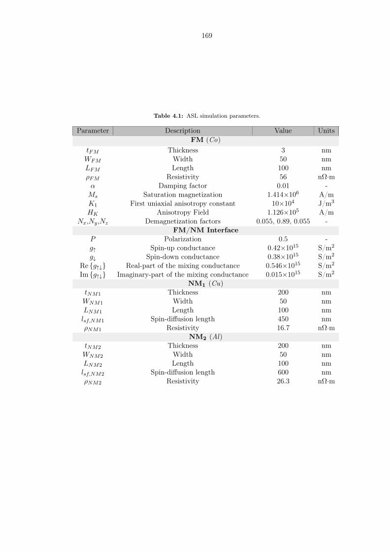
169
Table 4.1: ASL simulation parameters.
Parameter Description Value UnitsFM (Co)
tFM Thickness 3 nmWFM Width 50 nmLFM Length 100 nmρFM Resistivity 56 nΩ·mα Damping factor 0.01 -Ms Saturation magnetization 1.414×10⁶ A/mK1 First uniaxial anisotropy constant 10×104 J/m3
HK Anisotropy Field 1.126×10⁵ A/mNx,Ny,Nz Demagnetization factors 0.055, 0.89, 0.055 -
FM/NM InterfaceP Polarization 0.5 -g↑ Spin-up conductance 0.42×10¹⁵ S/m2
g↓ Spin-down conductance 0.38×10¹⁵ S/m2
Re g↑↓ Real-part of the mixing conductance 0.546×10¹⁵ S/m2
Im g↑↓ Imaginary-part of the mixing conductance 0.015×10¹⁵ S/m2
NM1 (Cu)tNM1 Thickness 200 nmWNM1 Width 50 nmLNM1 Length 100 nmlsf,NM1 Spin-diffusion length 450 nmρNM1 Resistivity 16.7 nΩ·m
NM2 (Al)tNM2 Thickness 200 nmWNM2 Width 50 nmLNM2 Length 100 nmlsf,NM2 Spin-diffusion length 600 nmρNM2 Resistivity 26.3 nΩ·m

170
4.3.4 Results and Discussion
The simulations were performed with the following in mind: (i) To show that our model
works, we first simulated ASL assuming no dynamics in the transport section. Figs. 4.22
& 4.23, 4.24, and 4.25 shows the transient simulations of magnetization, spin current,
and injected power, respectively. Fig. 4.21, on the other hand, shows the 3D trajectory
of the magnetization tip on the unit sphere. (ii) We introduced some dynamics in the
transport section to check if our model is able to capture it and also study the dependency
on capacitance. Such dynamics can occur due to the presence of, say, some parasitics
or loading effect.22 By varying the capacitance between 0.1 pF and 100 pF (which are
reasonable values [264]),23 we generated Figs. 4.26 and 4.27, the transient spin currents
and magnetizations, respectively.
First, we discuss Fig. 4.23, which shows the switching character of ASL. The device
was driven by a 5 mV pulse with a frequency 0.25 × 10⁹ GHz. It is apparent that the
device functions as NOT for positive voltages, and as COPY for negative voltages. The
device roughly switches P → AP after 0.7 − 0.8 ns, and AP → P after 1.3 − 1.4 ns. In
addition, from Fig. 4.24 one can see that the spin currents flow only when switching
occurs, as also pointed out in [46, 47]. This is also the case with the injected power
shown in 4.25. The transient response above is expected and conforms with the results
in literature (e.g., in [48, 60]), and thus our model correctly reduces to the steady-state
case and recovers the expected results.
Second, from 4.21, we see that FM1 is effectively fixed in its position, though it
fluctuates around its easy-axis. The fluctuations occur due to the different interactions
present such as thermal perturbations or torques exerted by the spin current injected
from the passage of IC from FM2 to the ground terminal. FM2, on the other hand,
switches between the two stable states due to the pulsed current injected.
Finally, we introduce some parasitics in the transport section to see if our model
captures the dynamics and responds to the effects of energy storage elements. Figs. 4.26
and 4.27 show the transients spin currents and magnetizations, respectively. Although
there is apparently some overshoot “spiking” due to the increase in the parasitic, one
might wonder why is not there a notable charging/discharging character on time scales
G/C. We recall that we are using an all-metallic structure for which voltage swings
on the capacitors are on the order of ∆µs = 1 µeV, which would imply a very large
capacitor to be used for the transient current C (∂∆µs/∂t) to be significantly altered22Or a Schottky contact in the case of semiconductors.23In general, a 100 pF is very large and the parasitics will probably be must less, say something in the
range 0.1 – 10 pF, as we learned from CMOS. However, for the sake of observing the dependency on thecapacitance we chose an upper bound of 100 pF rather than 10 pF as was also done in [264].

171
with significant finite rise and fall times [59]. In fact, by deliberately adding a large
parasitic capacitance C = 100 pF, the currents are clearly affected by the energy storage
element. Now regarding the magnetization, we can immediately see that there is no
major effect on the switching event P → AP , but a strong one on AP → P . In fact, for
C = 1 pF (a moderate capacitance), the magnetization does not keep up with the pulse
and yields improper switching behavior. However, it is interesting that for even larger
values, the switching behavior is recovered. This might be an oscillatory dependence of
the switching character on capacitance which one can use to find an optimal value to
reduce the switching time. Further discussions about this peculiar dependency can be
found in [264].
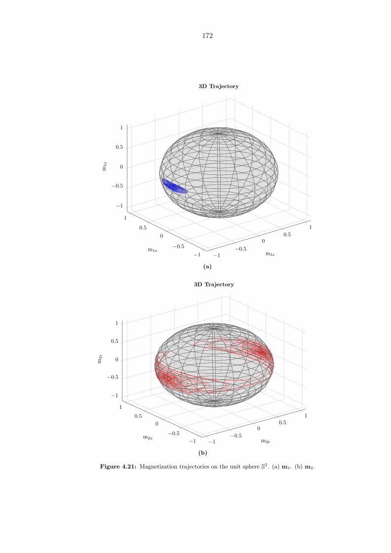
172
−1−0.5
00.5
1
−1
−0.5
0
0.5
1
−1
−0.5
0
0.5
1
m1zm1x
m1y
3D Trajectory
(a)
−1−0.5
00.5
1
−1
−0.5
0
0.5
1
−1
−0.5
0
0.5
1
m2zm2x
m2y
3D Trajectory
(b)
Figure 4.21: Magnetization trajectories on the unit sphere S2. (a) m1. (b) m2.

173
0 0.5 1 1.5 2 2.5 3 3.5 4 4.5 5 5.5 6
−1
−0.8
−0.6
−0.4
−0.2
0
0.2
0.4
0.6
0.8
1
Time (ns)
m1
Time Evolution (T = 300.00 K)
Icm1xm1ym1z
(a)
0 0.5 1 1.5 2 2.5 3 3.5 4 4.5 5 5.5 6
−1
−0.8
−0.6
−0.4
−0.2
0
0.2
0.4
0.6
0.8
1
Time (ns)
m2
Time Evolution (T = 300.00 K)
Icm2xm2ym2z
(b)
Figure 4.22: Time evolution of magnetization showing ASL inverter switching characteristics.(a) m1 vs t. (b) m2 vs t.
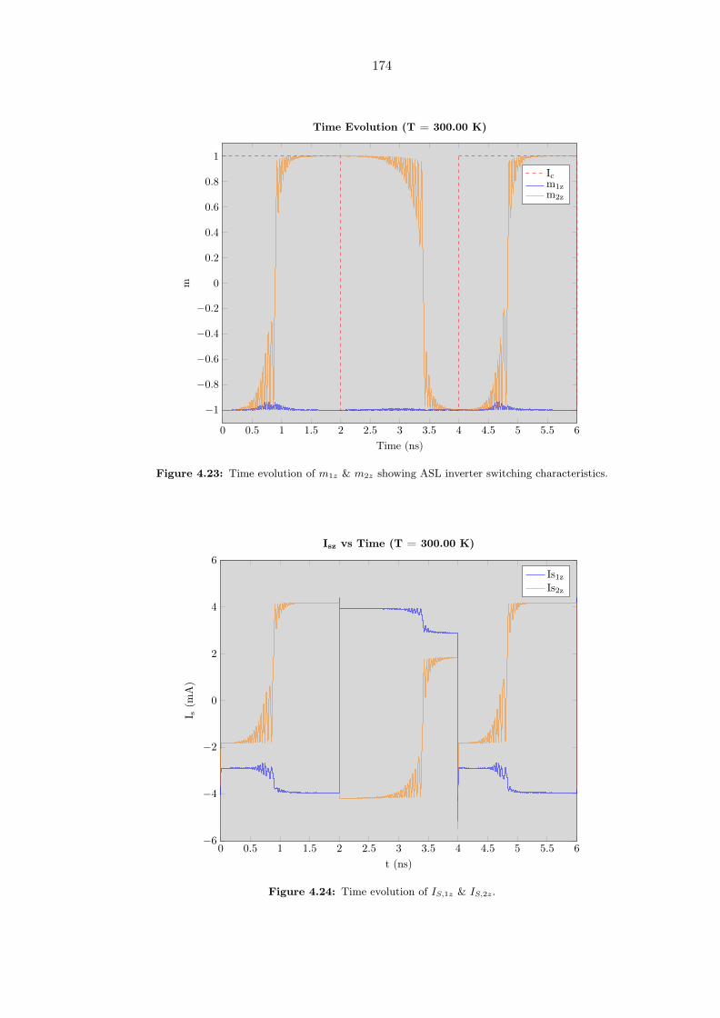
174
0 0.5 1 1.5 2 2.5 3 3.5 4 4.5 5 5.5 6
−1
−0.8
−0.6
−0.4
−0.2
0
0.2
0.4
0.6
0.8
1
Time (ns)
m
Time Evolution (T = 300.00 K)
Icm1zm2z
Figure 4.23: Time evolution of m1z & m2z showing ASL inverter switching characteristics.
0 0.5 1 1.5 2 2.5 3 3.5 4 4.5 5 5.5 6−6
−4
−2
0
2
4
6
t (ns)
I s(m
A)
Isz vs Time (T = 300.00 K)
Is1zIs2z
Figure 4.24: Time evolution of IS,1z & IS,2z.

175
0 0.5 1 1.5 2 2.5 3 3.5 4 4.5 5 5.5 60
5
10
15
20
25
30
35
40
t (ns)
P(u
W)
P vs Time (T = 300.00 K)
P1P2Ptotal
Figure 4.25: Time evolution of P1 & P2.

176
0 0.5 1 1.5 2 2.5 3 3.5 4 4.5 5 5.5 6−20
−15
−10
−5
0
5
10
15
t (ns)
I s(m
A)
Isz vs Time (T = 300.00 K)
Is1zIs2z
(a)
0 0.5 1 1.5 2 2.5 3 3.5 4 4.5 5 5.5 6−20
−15
−10
−5
0
5
10
15
t (ns)
I s(m
A)
Isz vs Time (T = 300.00 K)
Is1zIs2z
(b)
0 0.5 1 1.5 2 2.5 3 3.5 4 4.5 5 5.5 6−20
−15
−10
−5
0
5
10
15
t (ns)
I s(m
A)
Isz vs Time (T = 300.00 K)
Is1zIs2z
(c)
0 0.5 1 1.5 2 2.5 3 3.5 4 4.5 5 5.5 6−20
−15
−10
−5
0
5
10
15
t (ns)
I s(m
A)
Isz vs Time (T = 300.00 K)
Is1zIs2z
(d)
0 0.5 1 1.5 2 2.5 3 3.5 4 4.5 5 5.5 6−20
−15
−10
−5
0
5
10
15
t (ns)
I s(m
A)
Isz vs Time (T = 300.00 K)
Is1zIs2z
(e)
Figure 4.26: Time evolution of spin currents with varying parasitic capacitance. (a) C = 0.1pF. (b) C = 1 pF. (c) C = 10 pF. (d) C = 50 pF. (e) C = 100 pF.

177
0 0.5 1 1.5 2 2.5 3 3.5 4 4.5 5 5.5 6
−1
−0.8
−0.6
−0.4
−0.2
0
0.2
0.4
0.6
0.8
1
Time (ns)
m
Time Evolution (T = 300.00 K)
Icm1zm2z
(a)
0 0.5 1 1.5 2 2.5 3 3.5 4 4.5 5 5.5 6
−1
−0.8
−0.6
−0.4
−0.2
0
0.2
0.4
0.6
0.8
1
Time (ns)
m
Time Evolution (T = 300.00 K)
Icm1zm2z
(b)
0 0.5 1 1.5 2 2.5 3 3.5 4 4.5 5 5.5 6
−1
−0.8
−0.6
−0.4
−0.2
0
0.2
0.4
0.6
0.8
1
Time (ns)
m
Time Evolution (T = 300.00 K)
Icm1zm2z
(c)
0 0.5 1 1.5 2 2.5 3 3.5 4 4.5 5 5.5 6
−1
−0.8
−0.6
−0.4
−0.2
0
0.2
0.4
0.6
0.8
1
Time (ns)
m
Time Evolution (T = 300.00 K)
Icm1zm2z
(d)
0 0.5 1 1.5 2 2.5 3 3.5 4 4.5 5 5.5 6
−1
−0.8
−0.6
−0.4
−0.2
0
0.2
0.4
0.6
0.8
1
Time (ns)
m
Time Evolution (T = 300.00 K)
Icm1zm2z
(e)
Figure 4.27: Time evolution of magnetization with varying parasitic capacitance. (a) C = 0.1pF. (b) C = 1 pF. (c) C = 10 pF. (d) C = 50 pF. (e) C = 100 pF.

178
Chapter 5
Summary and Outlook
With CMOS miniaturization and energy-efficiency rapidly approaching an inevitable
physical limit, a search for an alternative technology is accelerating. Spintronic devices
are one of the prime candidates for Beyond CMOS technologies due to their low-power
operation, nonvolatile nature, and high density computation and storage. In the cat-
egory of promising spintronic switches is a device called all-spin logic (ASL) that has
recently attracted increasing interest due to its low-power operation and built-in mem-
ory structure. In addition, the device utilizes pure spin currents throughout every stage,
eliminating the need for repeated spin-to-charge conversion and any spurious effects ac-
companying charge currents. To assess the feasibility of spintronic devices in general and
ASL in particular to function as logic and memory elements, we presented in this thesis
a dynamic circuit model for rapid computer-aided design and verification.
In chapters 2 and 3, we reviewed some of the essential concepts in nanomagnetism and
spintronics. Following that, we discussed the statics and dynamics of a nanomagnet and
presented an algorithm to compute the trajectories from the stochastically perturbed
dynamic equations in the presence of spin-polarized currents. We then discussed the
basics of spin circuit theory and magnetoelectronics. In particular, the four-component
circuit variables; a novel circuit framework to analyze spintronic devices in a way analogue
to the well-known circuit theory.
In chapter 4, we invoked the well-known physics of nanomagnetism and spin, in partic-
ular, the stochastic Landau-Lifshitz-Gilbert-Slonczewski (sLLGS) and spin drift-diffusion
equation (SDDE) as bases formalisms for our ASL model. Using the recently proposed
four-component spin circuit theory and a finite-difference scheme for both the spatial and
temporal derivatives, we modeled ASL with new finite-difference conductance matrices.
By applying a self-consistent algorithm that passes the solution back-and-forth between

179
the “spin circuit” and the “stochastic nanomagnet dynamics”, we simulated an ASL in-
verter. While in the steady-state limit, the results match the ones in literature, for a finite
channel parasitic capacitance, the transient currents exhibit finite charging/discharging
time which is captured by our model.
Although the model adequately captures any introduced dynamics in the transport
channel, there are still limitations and challenges that one must be aware of. For example,
the model neglects spin dissipation associated with spin-flipping events occurring in the
FM. In other words, we modeled the spin transport in the NM and the scattering at
the FM/NM interface, but neglected spin relaxation inside the FM. For a more accurate
model, one has to invoke the SDDE in the FM and apply the same spatial- and temporal-
discretization to obtain a dynamic circuit model. Despite the minor limitation, the
model generally encompasses a discretization framework that we believe can be used for
improved dynamic circuit modeling for ASL and other emerging spintronic devices.

180
Appendix A
Mathematical Review
Many excellent graduate-level texts provide detailed and thorough treatment of the ma-
terial in this appendix. The aim here is not to discuss the concepts in detail or proof
every statement, but rather introduce the notation used in the thesis and provide a ref-
erence for some of the results used in proofs and derivations. Readers who are interested
in more rigor and in-depth discussions are referred to [267–270].
A.1 Tensor Calculus in Curvilinear Coordinates
In a differentiable manifold such as En,1 the Cartesian coordinates are arguably the most
intuitive and easy handle, but by no means the only possible option. Physical problems
are generally approached by choosing an appropriate coordinate system that fits the given
problem symmetry, which in some cases can be non-Cartesian or even global, common
examples being the famous cylindrical and spherical coordinates. The previous three
coordinates are just a subset of the so-called curvilinear coordinates.
For the sake of generality, a brief glimpse through tensor analysis is introduced in ar-
bitrary curvilinear coordinates. The formalism provides a unified and general description
of the standard coordinate systems. Throughout the discussion, we assume all coordinate
frames to be right-handed trihedrals.1A differentiable manifold is a topological Hausdorff space locally homeomorphic to En.

181
A.1.1 Some Preliminary Notions
A.1.1.1 Suffixes and Einstein’s Convention
We start by introducing the very useful index notation for tensor algebra. Let v ∈ Vbe a vector, where V is a vector space over the reals with dimension n. Moreover, let
S = e1, e2, . . . , en be a basis for V . We can then uniquely write the vector v as a
linear combination of the the basis vectors
v = v1e1 + v2e2 + · · ·+ vnen (A.1)
where (v1, v2, · · · , vn) are the coordinates of v relative to the basis S. Assume we were
given a transformation matrix A associated with the linear map T : Rn → Rn, and would
like to find the coordinates in terms of a new basis S′ =e1
′, e2′, . . . , en
′. For examplev1
′
v2′
...
vn′
=
a11 a12 · · · a1n
a21 a22 · · · a2n...
.... . .
...
an1 an2 · · · ann
v1
v2...
vn
(A.2)
Using suffixes, we can refer to the i-th component of the vector v′ as vi′. Similarly,
the (i, j)-th entry of the matrix A is written as aij . According to the rules of matrix
multiplication, one can write the i-th component of the transformed vector as
vi′ =
n∑j
aijvj , i = 1, 2, · · · , n
In such formulae, we call the suffix i (that appears once) the running index (also
known as the free index ), and the suffix j (that appears twice) the dummy index. A
way to avoid the tedium of writing summation signs, especially for matrix products
and complex equations, is to use a short-cut notation given by the rules of Einstein
summation convention, which we summarize below:
1. Omit summation signs;
2. A suffix appearing twice (i.e., dummy index) implies summation;
3. A suffix appearing once (i.e. free index) can take any value in a specified subset of
integers and is not summed over;
4. A suffix cannot appear more than twice.

182
Example A.1. Let v,u,w,x,y ∈ V , α ∈ R, and A the transformation matrix given
above. Then according to the convention presented we can write the following operations
as
α = v · u↔ α = viui
y = Av↔ yi = aijvj
y = (v · u)w↔ yi = vjujwi
y = x+ |v|2|u|2w↔ yi = xi + vjvjukukwi
where we notice that the free index i appears only once in each term.
A.1.1.2 Delta and Epsilon
The suffix notation can be made easier by introducing two important functions. The
first is the Kronecker delta
δij =
1, i = j
0, i = j(A.3)
The delta function is symmetric δij = δji, and has the sifting property
δijvj = vi (A.4)
The second is the three-dimensional Levi-Civita symbol2
εijk =
1, if (i, j, k) is (1, 2, 3) , (2, 3, 1) , (3, 1, 2)
−1, if (i, j, k) is (3, 2, 1) , (2, 1, 3) , (1, 3, 2)
0, if i = j, j = k, k = i
(A.5)
Example A.2. Let v,u ∈ V , α ∈ R, and A the transformation matrix given above.
Then we can use the functions introduced to write the following operations using suffixes
y = u× b↔ yi = εijkujvk
α = det (A)↔ α = εijkA1iA2jA3k
2Also known as the permutation, antisymmetric or alternating symbol.

183
A.1.2 General Considerations
A.1.2.1 Coordinate Transformation
Two different coordinate systems are related by a coordinate transformation. Consider
the open domain X ⊂ Rn endowed with the Cartesian coordinates x1, x2, · · · , xn.3,4
Assigning each point p ∈ X a set of n real numbers, we define n scalar-valued functions
f1 (p) , f2 (p) , · · · , fn (p) on the region X, which we shall use to define the curvilinear
coordinates patch. Thus we consider another open subset U ⊂ Rn5 that represents the
curvilinear coordinates u1, u2, · · · , un. This allow us to define continuous coordinate
system in a region X ⊂ Rn as the n-tuple of continuous functions(u1, u2, · · · , un
)given
by
u1 = f1(x1, x2, · · · , xn
)u2 = f2
(x1, x2, · · · , xn
)...
un = fn(x1, x2, · · · , xn
)where each ui = fi
(x1, x2, · · · , xn
)maps X both bijectively and continuously in both
directions into some domain U ⊂ Rn. In other words, the function is a bi-continuous
bijection and we say that for each point p, the map
f (p) = (f1 (p) , f2 (p) , · · · , fn (p))
is a homeomorphism6 of X onto U , and the spaces are said to be homeomorphic. Fig.
A.1 shows a rough sketch of the map action.
The values f1 (p) , f2 (p) , · · · , fn (p) are called the coordinates of p relative to the co-
ordinate map f : X → U , and the scalar-valued functions (the components) themselves
f1, f2, · · · , fn are called the coordinate functions. In the category of continuous maps,
we are merely interested in smooth ones, namely those for which the component func-
tions (and their inverses) are continuously differentiable of all orders; that is, functions
belonging to the class C∞.3A set X ⊂ Rn is open if ∀x ∈ X, there is an open ε-neighborhood entirely contained in X. That is,
∃ε > 0 such that Xε(x) ⊂ X, where Xε (x) = y ∈ Rn| |x− y| < ε. In other words, Xε (x) is in openball of radius ε with center x.
4Note how we use superscripts for coordinates, which are the contravariant components of vectors(more about this later). We stick to this policy (borrowed from differential geometry) for nonorthogonalcoordinate systems, which will prove useful. Later for orthogonal systems we drop superscripts and usesubscripts all the way.
5Rn here is another copy of the Euclidean space.6Not to be confused with homomorphism, which is not a topological term but an algebraic one.
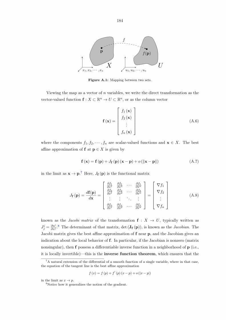
184
pf(p)
f
X Ux1, x2, · · · , xn u1, u2, · · · , un
Figure A.1: Mapping between two sets.
Viewing the map as a vector of n variables, we write the direct transformation as the
vector-valued function f : X ⊂ Rn → U ⊂ Rn, or as the column vector
f (x) =
f1 (x)
f2 (x)...
fn (x)
(A.6)
where the components f1, f2, · · · , fn are scalar-valued functions and x ∈ X. The best
affine approximation of f at p ∈ X is given by
f (x) = f (p) + Jf (p) (x− p) + o (∥x− p∥) (A.7)
in the limit as x→ p.7 Here, Jf (p) is the functional matrix
Jf (p) =df(p)
dx=
∂f1∂x1
∂f1∂x2 · · · ∂f1
∂xn
∂f2∂x1
∂f2∂x2 · · · ∂f2
∂xn
......
. . ....
∂fn∂x1
∂fn∂x2 · · · ∂fn
∂xn
=
∇f1∇f2
...
∇fn
(A.8)
known as the Jacobi matrix of the transformation f : X → U , typically written as
J ij =
∂ui
∂xj .8 The determinant of that matrix, det (Jf (p)), is known as the Jacobian. The
Jacobi matrix gives the best affine approximation of f near p, and the Jacobian gives an
indication about the local behavior of f . In particular, if the Jacobian is nonzero (matrix
nonsingular), then f possess a differentiable inverse function in a neighborhood of p (i.e.,
it is locally invertible)—this is the inverse function theorem, which ensures that the7A natural extension of the differential of a smooth function of a single variable, where in that case,
the equation of the tangent line is the best affine approximation
f (x) = f (p) + f ′ (p) (x− p) + o (|x− p|)
in the limit as x→ p.8Notice how it generalizes the notion of the gradient.

185
inverse map g : U → X is also smooth with the Jacobi matrix
Jg (p) = Jf (p)−1 (A.9)
and thus det (Jf (p)) det (Jg (p)) = 1. A vanishing Jacobian implies that f1, f2, · · · , fnare not independent functions, but rather connected by a relationship F (f1, f2, · · · , fn) =0.
The Jacobi matrix locally describes the amount by which f imposes stretching, com-
pressing, rotating, etc. If det (Jf (p)) > 0, then f preserves the orientation near p, and
otherwise if det (Jf (p)) < 0. The absolute value of the Jacobian |det (Jf (p))| indicates
the amount by which f shrinks or expands a volume. The Jacobi matrix also maps tan-
gent vectors from one frame to the other. To see this, consider the direct transformation
f : X → U . For p ∈ X, the map gives the n-tuple u = f (p). Taking the temporal
derivativedu
dt=df (p)
dt
and applying the chain rule and using (A.8), one finds df(p)dt = df(p)
dxdxdt = Jf (p)
dxdt , or
du
dt= Jf (p)
dx
dt(A.10)
Similarly, for the inverse transformation g : U → X, one can show
dx
dt= Jg (p)
du
dt(A.11)
Under the conditions stated above, we call our curvilinear system regular, and we say
the regular curvilinear coordinates are generated by a diffeomorphism.9 The system of
curvilinear coordinates determines a family of n coordinate lines at each point in the
region (Fig. A.2).
Figure A.2: The smooth trajectory from point P to P0 on an arbitrary coordinate linegenerated by varying one curvilinear coordinate while fixing the rest.
9 A diffeomorphism is a one-to-one onto map which is smooth and has a smooth inverse.
186
Definition A.1 (Regular Smooth Coordinate System). 10 In a region X, a regular
smooth coordinate system is a family of smooth functions fi (x1, x2, · · · , xn) determining
a bijection map from X ⊂ Rn onto a region U ⊂ Rn, and such that the Jacobian of the
map f : X → U is nonzero at all points of the region.
Lemma A.2. Suppose the Jacobian of a family of smooth functions f1 (p) , f2 (p) , · · · , fn (p)is nonzero at all points of the region. Then for each point there exists an open neighbor-
hood in which these functions determine a regular (local) coordinate system. At the same
time, this family of functions may fail to determine the global curvilinear coordinates in
the entire region.
A.1.2.2 Contravariant and Covariant Vectors
Although we typically would like to perform our computations on an orthogonal three-
dimensional curvilinear coordinate system, physical laws and quantities should be inde-
pendent of any particular coordinate system. A point on a map should remain invariant
under a change of coordinates; we should get the same point whether we use Cartesian or
spherical coordinates, for example. Tensors introduce invariant (i.e., coordinate indepen-
dent) formulation. A good tensor transformation leaves the quantities invariant in either
a covariant of contravariant manner (more about this later). Assume we were given a
multi-component object with coefficients vi, i = 1, 2, · · · , n, representing the components
in some coordinate system. The coefficients by themselves have no meaning; they only
acquire it upon relating them to a certain basis (which spans the coordinate space).
Moreover, under a change of coordinate frame, such as rotation or dilation, we must be
able to describe the vector in the other coordinate frame. For the vector to properly
represent an object, it must remain unchanged under transformation. This means that
the components of the vector will transform in a certain way when we apply a coordinate
transformation. The concepts of contravariance and covariance essentially describes how
would a physical entity change with a change of basis.
Consider an n-dimensional manifold with two different frames given by the coordinates
x1, x2, · · · , xn and u1, u2, · · · , un. Under a change of coordinates, the coordinates are
governed by the transformation f : X → U
ui = fi(x1, x2, · · · , xn
)(A.12)
Depending on the transformation, we will have two kind of vectors (i.e., tensor objects
of rank-1):-10Also called a curvilinear coordinate system.

187
1. Contravariant vectors11: Quantities that transform like the coordinate differen-
tials
dui =∂ui
∂xjduj (A.13)
which we can write by letting dui = v′i and duj = vj as
v′i=∂ui
∂xjvj (A.14)
or with the use of J ij =
∂ui
∂xj as
v′i= J i
jvj (A.15)
In general, most of the vectors we deal with are contravariant, with common
examples being the displacement vector and any quantity involving its temporal
derivative (e.g., velocity, acceleration, force, momentum, etc.) From the transfor-
mation rule (A.14), the contravariant components “transform inversely to the old
coordinates”. That is, for the contravariant vectors to be independent of the co-
ordinate system, the components of the vector contra-vary, and we say the vector
components are contravariant components. In linear algebra, we represent such
vectors by column vectors. The contravariant components are distinguished with
superscripts,12 and using Einstein’s notation, we write
v =
v1
v2...
vn
↔ v = viei (A.16)
where ei’s are the bases vectors.
2. Covariant vectors13: Quantities that transform like the derivatives of a scalar
ϕ14
∂ϕ
∂ui=∂xj
∂ui∂ϕ
∂xj(A.17)
which we can write by letting v′i = ∂ϕ∂ui and vi = ∂ϕ
∂xj as
v′i =∂xj
∂uivj (A.18)
11Also called tensors of order (1,0).12Assuming no danger of confusion with exponents.13Also known as a covectors, dual vectors, tensors of order (0,1), or 1-forms.14An object characterized by the identical transformation
ϕ′ (u) = ϕ (x)
is called a scalar, or a tensor of rank-0, which is invariant with respect to coordinate transformation.

188
or with the use of(J−1
)ji= ∂xj
∂ui as
v′i =(J−1
)jivj (A.19)
An example of a covariant vector is the gradient operator. From the transfor-
mation rule (A.18), the covariant components “transform as the old coordinates
do”. That is, for the covariant vector to be independent of the coordinate system,
the components of the vector co-vary, and we say the vector components are co-
variant components. In linear algebra, we represent such vectors by row vectors.
The covariant components are distinguished with subscripts, and using Einstein’s
notation, we write
v =[v1 v2 · · · vn
]↔ v = vie
i (A.20)
where ei’s are the dual bases, which is the reciprocal set of standard bases,15 and
are only important for nonorthogonal coordinate systems.
When a vector space V is equipped with an inner product, then for vectors v,u ∈ V ,
the dot product is given by16
v · v =[v1 v2 · · · vn
]v1
v2...
vn
= vivi (A.22)
Moreover, on this inner product space (also called metric in this context), one can convert
a covariant vector into a contravariant vector, and vice versa. Such operations can be
accomplished through the use of the so-called metric tensor and one of the fundamental
operations for tensors, called contraction.17 The metric tensor can be either contravariant
of covariant. For example, multiplying a covariant metric tensor by a contravariant vector15Given three noncoplanar (i.e., not linearly dependent) vectors A, B and C, the vectors A′, B′ and
C′ given by
A′ =B×C
A · (B×C), B′ =
C×A
A · (B×C), C′ =
A×B
A · (B×C)(A.21)
are called the reciprocal set of vectors. The sets satisfy
A′ ·A = B′ ·B = C′ ·C = 1
A′ ·B = A′ ·C = 0, B′ ·A = B′ ·C = 0, C′ ·A = C′ ·B = 0
16Those who are familiar with the language of quantum mechanics will notice that contravariantvectors vi are associated with kets |v⟩, while covariant vectors vi are associated with bras ⟨v|. As such,the dot product is given by ⟨v| v⟩ = viv
i.17Contraction simply means setting one free index equal to another so that we can perform the sum.
For example, the contraction of vij is vii, which is just equivalent to multiplying by a Kronecker deltasince vijδij = vii.

189
and contracting results in a covariant vector
vi = gijvj (A.23)
Similarly, multiplying a contravariant metric tensor by a covariant vector and contracting
results in a contravariant vector
vi = gijvj (A.24)
The above can be thought as mere operations for “lowering” or “raising” the index.
Thus one might suspect that raising and then lowering the index (or the converse) are
inverse operations, and it is indeed the case. In fact
gijgjk = δik (A.25)
gkjgji = δki (A.26)
where δik = δki is the mixed Kronecker delta, a mixed tensor of rank-2.
The concepts introduced above for rank-1 tensors can be easily generalized to tensors
of rank ≥ 2. For example, a rank-2 covariant tensor (or two-form) results from the
product of two covariant vectors
G′ij =
∂xk
∂ui∂xℓ
∂ujGkℓ
whereas a rank-2 contravariant tensor results from the product of of two contravariant
vectors
G′ij =∂ui
∂xk∂uj
∂xℓGkℓ
Also, in this case we have a mixed tensor
G′ij =
∂ui
∂xk∂xℓ
∂ujGk
ℓ
From now on, and in addition to Einstein’s summation convention, we conform to
the notation of tensor calculus in differentiating between vectors and covectors by using
superscripts and subscripts for their components, respectively (with the only exception
in denoting coordinates). This distinction is especially important if one is dealing with
nonorthogonal coordinate systems or coordinate transformation and mixed tensor anal-
ysis.18
18That is, when dealing with orthogonal coordinates or when there is a fixed coordinate basis, onemay omit the distinction of index position and use subscripts for all components.

190
A.1.3 Skew (Oblique) Curvilinear Coordinates in R3
Consider the three-dimensional Euclidean space, R3. The curvilinear coordinates may be
derived from a set of Cartesian coordinates by using a locally invertible transformation.
Let f : X → U be a C∞ bijective mapping between the open connected regions X ⊂ R3
and U ⊂ R3 on which we respectively prescribe the Cartesian (x1, x2, x3) and curvilinear
(u1, u2, u3) coordinates to a point P . A general point P is referred in the two coordinate
systems through the bijection19
ui = fi(x1, x2, x3
)↔ xi = gi
(u1, u2, u3
)(A.27)
where i = 1, 2, 3. Automatically, the Jacobi matrix is invertible and the Jacobian is
nonvanishing. For the transformation f : X → U , the Jacobi and its inverse are given by
Jf (p) =
∂f1∂x1
∂f1∂x2
∂f1∂x3
∂f2∂x1
∂f2∂x2
∂f2∂x3
∂f3∂x1
∂f3∂x2
∂f3∂x3
↔ Jf (p)−1 =
∂x1
∂f1∂x1
∂f2∂x1
∂f3∂x2
∂f1∂x2
∂f2∂x2
∂f3∂x3
∂f1∂x3
∂f2∂x3
∂f3
(A.28)
which is equivalent if someone started from g : U → X20
Jg (p) =
∂g1∂u1
∂g1∂u2
∂g1∂u3
∂g2∂u1
∂g2∂u2
∂g2∂u3
∂g3∂u1
∂g3∂u2
∂g3∂u3
↔ Jg(p)−1 =
∂u1
∂g1∂u1
∂g2∂u1
∂g3∂u2
∂g1∂u2
∂g2∂u2
∂g3∂u3
∂g1∂u3
∂g2∂u3
∂g3
(A.29)
Fig. A.3 shows a general three-dimensional curvilinear coordinate system where a
point P in a region U is determined by the 3-tuple (u1, u2, u3). The three family of
surfaces u1 = c1, u2 = c2, and u3 = c3 are called the coordinate surfaces. Each
coordinate surface can be generated by fixing one coordinate and varying the other two.
To define a coordinate system, the three surfaces must obviously be noncoplanar. When
the surfaces meet at right-angles, the resulting coordinate system is orthogonal, otherwise
it is called skew (or oblique). The intersection each pair of these surfaces generates a
coordinate line, which is now curved. When the three surfaces intersect, the tangents
along the coordinate lines at the point of intersection generates the coordinate axes,
which are generally allowed to vary in direction from point to point.19The exact function expressions can be written only when we know expressions for coordinate surfaces.20Equivalent in the sense of (A.9), equipped with (A.27).
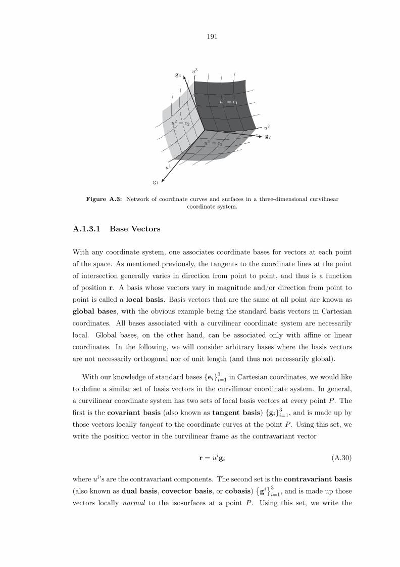
191
u2
u3
u1
g2
g3
g1
u1= c1
u2= c2
u3= c3
Figure A.3: Network of coordinate curves and surfaces in a three-dimensional curvilinearcoordinate system.
A.1.3.1 Base Vectors
With any coordinate system, one associates coordinate bases for vectors at each point
of the space. As mentioned previously, the tangents to the coordinate lines at the point
of intersection generally varies in direction from point to point, and thus is a function
of position r. A basis whose vectors vary in magnitude and/or direction from point to
point is called a local basis. Basis vectors that are the same at all point are known as
global bases, with the obvious example being the standard basis vectors in Cartesian
coordinates. All bases associated with a curvilinear coordinate system are necessarily
local. Global bases, on the other hand, can be associated only with affine or linear
coordinates. In the following, we will consider arbitrary bases where the basis vectors
are not necessarily orthogonal nor of unit length (and thus not necessarily global).
With our knowledge of standard bases ei3i=1 in Cartesian coordinates, we would like
to define a similar set of basis vectors in the curvilinear coordinate system. In general,
a curvilinear coordinate system has two sets of local basis vectors at every point P . The
first is the covariant basis (also known as tangent basis) gi3i=1, and is made up by
those vectors locally tangent to the coordinate curves at the point P . Using this set, we
write the position vector in the curvilinear frame as the contravariant vector
r = uigi (A.30)
where ui’s are the contravariant components. The second set is the contravariant basis
(also known as dual basis, covector basis, or cobasis)gi3i=1
, and is made up those
vectors locally normal to the isosurfaces at a point P . Using this set, we write the

192
position vector in the curvilinear frame as the covariant vector
r = uigi (A.31)
where ui’s are the covariant components. The two sets constitutes reciprocal (also known
as dual) systems of vectors and have reciprocal units. They become identical in the case
of orthogonal coordinates (which is of special interest to us). As stated above, unlike in
Cartesian coordinates, in which the standard bases are of fixed direction, it is generally
not the case for curvilinear bases. Moreover, the curvilinear bases are generally not of
unit length and thus not unit base vectors (they are called unitary base vectors).
x1
x2
x3
e1
e2
e3
u2
u3
u1
g2
g3
g1
g2
g3
g1
g1⊥g2,g3
g2⊥g1,g3
g3⊥g1,g2
Figure A.4: Curvilinear coordinate system with the associated tangent (covariant) and nor-mal (contravariant) bases.
• Covariant Basis Vectors g1,g2,g3
If r = xiei is the position vector of a point P in the Cartesian frame, then the standard
basis ei3i=1 can be found by taking the derivative of r = xiei at the point P with
respect to the local coordinates xi
ei =∂r
∂xi, i = 1, 2, 3 (A.32)
In the curvilinear coordinates frame, the same point P is given by the position vector
r = uigi. Applying the same definition we used for ei3i=1 locally at the point P , we

193
obtain the triple of vectors21
gi =∂r
∂ui=∂xj
∂uiej , i = 1, 2, 3 (A.34)
having the direction of the tangents to the coordinate lines (Fig. A.4). The basis vectors
may not be of unit length and may not also be orthogonal.
To gain more insight into the construction of the covariant basis, consider the position
vector in the Cartesian coordinates frame, r = g1(u1, u2, u3
)e1 + g2
(u1, u2, u3
)e2 +
g3(u1, u2, u3
)e3. Let us rewrite the system (A.34) explicitly
g1 =∂g1∂u1
e1 +∂g2∂u1
e2 +∂g3∂u1
e3 (A.35)
g2 =∂g1∂u2
e1 +∂g2∂u2
e2 +∂g3∂u2
e3 (A.36)
g3 =∂g1∂u3
e1 +∂g2∂u3
e2 +∂g3∂u3
e3 (A.37)
Similarly, from (A.32)
e1 =∂u1
∂g1b1 +
∂u2
∂g2b2 +
∂u3
∂g3b3
e2 =∂u1
∂g1b1 +
∂u2
∂g2b2 +
∂u3
∂g3b3
e3 =∂u1
∂g1b1 +
∂u2
∂g2b2 +
∂u3
∂g3b3
The coefficient matrix of the first and second systems are just the transpose of (A.29),
the Jacobi of the transformation g, and its inverse, respectively. For the basis to be well-
defined at every point P , there must exists one and only one set of basis vectors. This
condition is ensured if the system has a unique nontrivial solution, which is equivalent
to ensuring that the system is nonsingular (i.e., Jacobian is nonvanishing). Note that we
could have derived this directly from the scalar triple product
g1 · (g2 × g3) =
∣∣∣∣∣∣∣∣(g1)1 (g1)2 (g1)3
(g2)1 (g2)2 (g2)3
(g3)1 (g3)2 (g3)3
∣∣∣∣∣∣∣∣ =∣∣∣∣∣∣∣∣
∂x1
∂u1∂x2
∂u1∂x3
∂u1
∂x1
∂u2∂x2
∂u2∂x3
∂u2
∂x1
∂u3∂x2
∂u3∂x3
∂u3
∣∣∣∣∣∣∣∣ = det (Jg (p)) (A.38)
and a nonvanishing Jacobian then ensures that the set of vectors is linearly independent
and thus can form a basis.21This can also be seen as follows: Just like we related the position vector in both frames through
r = uigi = xiei, we can relate the increment of the position vector dr in both frames by using thedefinition of total differential to obtain
dr =∂r
∂ui︸︷︷︸gi
dui =∂r
∂xi︸︷︷︸ei
dxi (A.33)

194
Finally, we assert that unlike the case in Cartesian coordinate in which the standard
basis form an orthonormal set
ei · ej = δij =
1, i = j
0, i = j(A.39)
it is not necessarily the case for the covariant basis. That is, gi · gj = δij . This is in
fact the main motivation for introducing the other contravariant basis vectors, which we
discuss next.
• Contravariant Basis Vectorsg1,g2,g3
As mentioned in the introduction, the contravariant basis vectors are normal to the level
surfaces (see also A.4), and we thus can define them by using the gradient operator as
follows
gi = ∇ui = ∂ui
∂xjej , i = 1, 2, 3 (A.40)
Using the triple scalar product, we find
g1·(g2 × g3
)=
∣∣∣∣∣∣∣∣(g1)1
(g1)2
(g1)3(
g2)1
(g2)2
(g2)3(
g3)1
(g3)2
(g3)3
∣∣∣∣∣∣∣∣ =∣∣∣∣∣∣∣∣
∂u1
∂x1∂u1
∂x2∂u1
∂x3
∂u2
∂x1∂u2
∂x2∂u2
∂x3
∂u3
∂x1∂u3
∂x2∂u3
∂x3
∣∣∣∣∣∣∣∣ = det(Jg(p)
−1)= det (Jf (p))
(A.41)
which again implies that for the set of vector to be linearly independent (and hence form
a basis), the determinant has to be nonzero.
A.1.3.2 Metric Tensor
From the definition of the covariant (A.34) and contravariant (A.40) bases and the or-
thonormallity condition of the standard basis and its dual (A.20), one can show
gi · gj = δij =
1, i = j
0, i = j(A.42)
where δij is now appropriately called the mixed Kronecker delta. The last relation essen-
tially states that each contravariant vector gi is orthogonal to the other two covariant
vectors gj (see Fig. A.4); this is the main reason for introducing the contravariant basis.

195
Just as with the covariant bases, the contravariant bases do not form an orthonormal
set, and thus the dot product between the different pairs is nonzero.22 In fact
gij = gi · gj =∂xk
∂ui∂xk
∂uj(A.43)
gij = gi · gj =∂ui
∂xk∂uj
∂xk(A.44)
are defined as the metric coefficients. Since the dot product is commutative, the
metric coefficients are symmetric gij = gji, gij = gji. Using the previously developed
relations, one can easily show the following properties
gi = gijgj (A.45)
gi = gijgj (A.46)
and
gijgkj = δik =
1, i = k
0, i = k(A.47)
The metric coefficients constitute the metric tensors23
Gij =
g11 g12 g13
g21 g22 g23
g31 g32 g33
(A.48)
Gij =
g11 g12 g13
g21 g22 g23
g31 g32 g33
(A.49)
which we can rewrite by using (A.43) and (A.44) as
Gij =
∂xk
∂u1∂xk
∂u1∂xk
∂u1∂xk
∂u2∂xk
∂u1∂xk
∂u3
∂xk
∂u2∂xk
∂u1∂xk
∂u2∂xk
∂u2∂xk
∂u2∂xk
∂u3
∂xk
∂u3∂xk
∂u1∂xk
∂u3∂xk
∂u2∂xk
∂u3∂xk
∂u3
=
∂x1
∂u1∂x1
∂u2∂x1
∂u3
∂x2
∂u1∂x2
∂u2∂x2
∂u3
∂x3
∂u1∂x3
∂u2∂x3
∂u3
T
∂x1
∂u1∂x1
∂u2∂x1
∂u3
∂x2
∂u1∂x2
∂u2∂x2
∂u3
∂x3
∂u1∂x3
∂u2∂x3
∂u3
(A.50)
Gij =
∂u1
∂xk∂u1
∂xk∂u1
∂xk∂u2
∂xk∂u1
∂xk∂u3
∂xk
∂u2
∂xk∂u1
∂xk∂u2
∂xk∂u2
∂xk∂u2
∂xk∂u3
∂xk
∂u3
∂xk∂u1
∂xk∂u3
∂xk∂u2
∂xk∂u3
∂xk∂u3
∂xk
=
∂u1
∂x1∂u1
∂x2∂u1
∂x3
∂u2
∂x1∂u2
∂x2∂u2
∂x3
∂u3
∂x1∂u3
∂x2∂u3
∂x3
∂u1
∂x1∂u1
∂x2∂u1
∂x3
∂u2
∂x1∂u2
∂x2∂u2
∂x3
∂u3
∂x1∂u3
∂x2∂u3
∂x3
T
(A.51)
22Unless in orthogonal coordinate system, which we discuss later.23Called metric because it determines the square of the length, as will be shown later.

196
which are nothing but Jacobi’s matrices. Therefore we can compactly define the metric
tensors as
Gij = Jg(p)TJg (p) (A.52)
Gij = Jg(p)−1(Jg(p)
−1)T
(A.53)
which has the determinants
det (Gij) = det(Jg(p)
TJg (p))= det (Jg (p))
2 = G (A.54)
det(Gij)= det
(Jg(p)
−1(Jg(p)
−1)T)
= det(Jg(p)
−1)2
=1
det (Jg (p))2 =
1
G
(A.55)
that are related by G = det (Gij) =1
det(Gij).
A.1.3.3 Scale Factors
Since the covariant and contravariant base vectors are not of unit length, we can nor-
malize them to obtain the unit bases
gi =gi|gi|
=gi√gii
gi =gi
|gi|=
gi√gii
The normalizing factors are given special names: The covariant scale factor (or just
scale factor)
hi = |gi| =√gii (no sum) (A.56)
and the contravariant scale factor
hi =∣∣gi∣∣ =√gii (no sum) (A.57)
A.1.3.4 Components of a Vector
Having introduced the two sets of bases, we can write the position vector in two ways;
either as a covariant vector
r = uigi = uih
igi = ui√giigi = u⟨i⟩g
i (A.58)

197
that is composed of a covariant component and contravariant basis, or as a contravariant
vector
r = uigi = uihigi = ui√giigi = u⟨i⟩gi (A.59)
made up of a contravariant component and a covariant basis. Most importantly, we call
u⟨i⟩ and u⟨i⟩ the physical components of the vector.
The contravariant and covariant components can be related through the metric coeffi-
cients
ui = gijuj (A.60)
ui = gijuj (A.61)
A.1.3.5 Scalar and Vector Products
Given two vectors u and v, their dot product can be found as
u · v = uivi = uivi (A.62)
From the determinant relation (A.54) and the scalar triple products (A.38) and (A.41),
we can find
G = (g1 · g2 × g3)2 =
1
(g1 · g2 × g3)2(A.63)
Now, with the help of the Levi-Civita permutation symbol (A.5), we can write the triple
scalar product as
gi · gj × gk = εijk√G (A.64)
gi · gj × gk = εijk1√G
(A.65)
Moreover, we can show that the cross product of the basis vectors is given by
gi × gj = εijk√Ggk (A.66)
gi × gj = εijk1√Ggk (A.67)
which we can use to find the cross product of two vectors as
u× v =√G
∣∣∣∣∣∣∣∣g1 g2 g3
u1 u2 u3
v1 v2 v3
∣∣∣∣∣∣∣∣ =1√G
∣∣∣∣∣∣∣∣g1 g2 g3
u1 u2 u3
v1 v2 v3
∣∣∣∣∣∣∣∣ (A.68)

198
A.1.3.6 Differential Length, Surface, and Volume Elements
In the curvilinear frame, the position vector r = uigi has the differential displacement
dr = duigi. We use this incremental displacement to find the square of the differential
length element (also known as the metric or fundamental quadratic form of the
space), which is the distance between two infinitesimally close points
(dℓ)2 = dr · dr =(duigi
)·(dujgj
)= (gi · gj) duiduj = gijdu
iduj (A.69)
or
dℓi =√gijduidujdgi (A.70)
Now consider an infinitesimal surface element. Using the geometrical interpretation
of the cross product of the tangent vectors (which are normal to that small surface), we
can write
dSi = |drj × drk| (A.71)
=∣∣∣(dujgj)× (dukgk)∣∣∣ (A.72)
= |gj × gk| dujduk (A.73)
=√
(gj × gk) · (gj × gk)dujduk (A.74)
=√
(gj · gj) (gk · gk)− (gj · gk) (gj · gk)dujduk (A.75)
=√Ggiidujduk (A.76)
Hence we obtain
dSi =√Ggiidujdukgi (no sum) (A.77)
where i = j = k.
Finally, it is well-known that the scalar triple product of three vectors gives the volume
of the parallelopiped formed by the three vectors as its sides. Taking the vector compo-
nents of the differential vector dr as the three sides of the skew-angled parallelepiped,
we obtain the differential volume
dV = dri · (drj × drk) (A.78)
= gi · (gj × gk) duidujduk (A.79)
= εijk√Gduidujduk (A.80)

199
Hence24
dV =√Gduidujduk (no sum) (A.81)
where i = j = k.
A.1.4 Orthogonal Curvilinear System in R3
In the case of an orthogonal trihedron of basis vectors, the contravariant and covariant
bases become collinear, and we obtain
gi = gi (A.82)
Thus from now on for orthogonal coordinates we drop all superscripts and use subscripts
instead. The unit vectors, though have fixed magnitudes, do not have a fixed direction
and can point in different directions from point to point (in contrast to the Cartesian
standard basis). Moreover, since the coordinate lines are everywhere orthogonal, the
orthogonal trihedron of the unit base vectors satisfy
gi · gj = δij =
1, i = j
0, i = j(A.83)
and are always normal to the coordinate surfaces. The last result can be easily used to
show that hi = 1hi , ∀i. In the orthogonal case, the scale factors hi are sometimes called
Lame’s coefficients. The fact that hi = 1hi implies that the vectors themselves (not
the unit base vectors) are not identical but rather of different magnitudes
gi = higi (A.84)
gi =1
higi (A.85)
and thus we represent the unit vector as
gi =gihi
= higi (A.86)
Then we can use (A.58) or (A.59) (which are now identical) to express the contravariant
and covariant components of a vector r = uigi = uigi in terms of the physical components
24Notice how the permutation is irrelevant here and thus ignored.

200
and Lame’s coefficients
ui =u⟨i⟩
hi(A.87)
ui = hiu⟨i⟩ (A.88)
Using the last results, we obtain the metric coefficients
gij = gi · gj = hihj (gi · gj) = hihjδij =
hi2, i = i
0, i = j(A.89)
gij = gi · gj =1
hihj(gi · gj) =
1
hihjδij =
1
hi2 , i = i
0, i = j
(A.90)
where the metric tensors Gij and Gij become diagonal
Gij =
h1
2 0 0
0 h22 0
0 0 h32
(A.91)
Gij =
1
h12 0 0
0 1h2
2 0
0 0 1h3
2
(A.92)
and has the determinants
det (Gij) = (hihjhk)2 = G (A.93)
det(Gij)=
1
(hihjhk)2 =
1
G(A.94)
where i = j = k. Finally, the differential elements become
dℓ = hiduigi (A.95)
dSi = hjhkdujdukgi (no sum) (A.96)
dV = hihjhkduidujduk (no sum) (A.97)
where again i = j = k.
A.1.4.1 The Del-Operator ∇
To be able to use vector calculus on a general curvilinear system, one must represent the
del (also called nabla) operator in the local basis. The form taken by the operator ∇
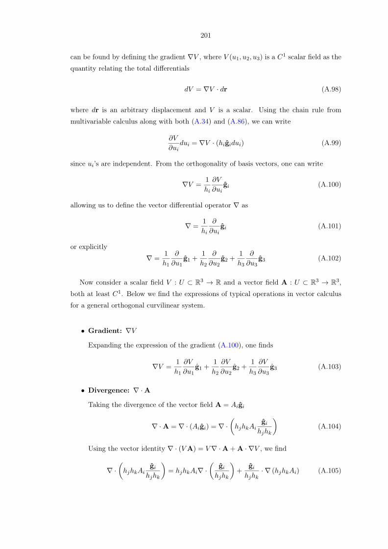
201
can be found by defining the gradient ∇V , where V (u1, u2, u3) is a C1 scalar field as the
quantity relating the total differentials
dV = ∇V · dr (A.98)
where dr is an arbitrary displacement and V is a scalar. Using the chain rule from
multivariable calculus along with both (A.34) and (A.86), we can write
∂V
∂uidui = ∇V · (higidui) (A.99)
since ui’s are independent. From the orthogonality of basis vectors, one can write
∇V =1
hi
∂V
∂uigi (A.100)
allowing us to define the vector differential operator ∇ as
∇ =1
hi
∂
∂uigi (A.101)
or explicitly
∇ =1
h1
∂
∂u1g1 +
1
h2
∂
∂u2g2 +
1
h3
∂
∂u3g3 (A.102)
Now consider a scalar field V : U ⊂ R3 → R and a vector field A : U ⊂ R3 → R3,
both at least C1. Below we find the expressions of typical operations in vector calculus
for a general orthogonal curvilinear system.
• Gradient: ∇V
Expanding the expression of the gradient (A.100), one finds
∇V =1
h1
∂V
∂u1g1 +
1
h2
∂V
∂u2g2 +
1
h3
∂V
∂u3g3 (A.103)
• Divergence: ∇ ·A
Taking the divergence of the vector field A = Aigi
∇ ·A = ∇ · (Aigi) = ∇ ·(hjhkAi
gihjhk
)(A.104)
Using the vector identity ∇ · (VA) = V∇ ·A+A · ∇V , we find
∇ ·(hjhkAi
gihjhk
)= hjhkAi∇ ·
(gihjhk
)+
gihjhk
· ∇ (hjhkAi) (A.105)

202
But for a right-handed trihedron εijkgi = gj × gk and from (A.40), we can rewrite
∇ ·(
gi
hjhk
)as
∇ ·(
gihjhk
)= ∇ · (∇uj ×∇uk) = 0
where we used the identities ∇ · (A×B) = B · (∇×A) −A · (∇×B) and ∇ ×(∇V ) = 0. Thus (A.105) equipped with the definition (A.102) yields
∇·(hjhkAi
gihjhk
)=
gihjhk
·∇ (hjhkAi) =gihjhk
·[1
hi
∂
∂ui(hjhkAi) gi
]=
1
hihjhk
∂
∂ui(hjhkAi)
(A.106)
where i = j = k. By explicitly summing the coefficients, we obtain (A.104) in the
form
∇ ·A =1
h1h2h3
[∂
∂u1(h2h3A1) +
∂
∂u2(h3h1A2) +
∂
∂u3(h1h2A3)
](A.107)
• Curl: ∇×A
Taking the curl of the vector field A = Akgk
∇×A = ∇× (Aigk) = ∇×(hkAk
gkhk
)(A.108)
and using the identity ∇× (VA) = ∇V ×A+ V (∇×A), we obtain
∇×(hkAk
gkhk
)= ∇ (hkAk)×
(gkhk
)+ (hkAk)∇×
(gkhk
)=
1
hk∇ (hkAk)× gk
(A.109)
where we used the fact that ∇×(gkhk
)= ∇×(∇uk) = 0. Using the definition of the
del operator and the fact that for a right-handed coordinate system εijkgi = gj×gk,we get
1
hk∇ (hkAk)× gk =
1
hk
1
hj
∂
∂uk(hkAk) (gj × gk)
=1
hk
1
hj
∂
∂uk(hkAk) εijkgi
= εijkhi
hihjhk
∂
∂uk(hkAk) gi (A.110)
which can be casted in a matrix form and thus (A.108) can be written as
∇×A =1
h1h2h3
∣∣∣∣∣∣∣∣h1g1 h2g2 h3g3
∂∂u1
∂∂u2
∂∂u3
h1A1 h2A2 h3A3
∣∣∣∣∣∣∣∣ (A.111)

203
• Laplacian: ∇2V
By definition, the Laplacian is given by ∇2V = ∇·∇V . Thus we can directly make
use of the divergence formula (A.107) to obtain the Laplacian, merely by writing
A = Aigi =(
1hi
∂V∂ui
)gi to obtain
∇2V =1
h1h2h3
[∂
∂u1
(h2h3h1
∂V
∂u1
)+
∂
∂u2
(h3h1h2
∂V
∂u2
)+
∂
∂u3
(h1h2h3
∂V
∂u3
)](A.112)
A.1.4.2 Special Orthogonal Curvilinear Coordinates
We now consider two examples of orthogonal curvilinear coordinate systems. From now
on, we denote the unit bases vectors (gi and gi) with the symbol aui , where ui is the
i-th curvilinear coordinate.
Example A.3 (Cylindrical Coordinates). With reference to Fig. A.5, the cylindri-
cal coordinates(u1, u2, u3
)= (ρ, ϕ, z) maps a point P to the Cartesian coordinates(
x1, x2, x3)= (x, y, z) through the transformation g : R+ × [0, 2π) × R → R3 and its
inverse
ρ =√x2 + y2 x = ρ cosϕ (A.113)
φ = tan−1(yx
)y = ρ sinϕ (A.114)
z = z z = z (A.115)
x
y
z
P (ρ, φ, z)
ρ
z
φ
Figure A.5: Cylindrical coordinates system.
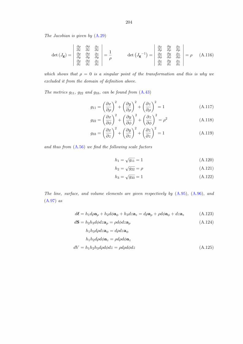
204
The Jacobian is given by (A.29)
det (Jg) =
∣∣∣∣∣∣∣∣∂ρ∂x
∂ϕ∂x
∂z∂x
∂ρ∂y
∂ϕ∂y
∂z∂y
∂ρ∂z
∂ϕ∂z
∂z∂z
∣∣∣∣∣∣∣∣ =1
ρdet(Jg
−1)=
∣∣∣∣∣∣∣∣∂x∂ρ
∂y∂ρ
∂z∂ρ
∂x∂ϕ
∂y∂ϕ
∂z∂ϕ
∂x∂z
∂y∂z
∂z∂z
∣∣∣∣∣∣∣∣ = ρ (A.116)
which shows that ρ = 0 is a singular point of the transformation and this is why we
excluded it from the domain of definition above.
The metrics g11, g22 and g33, can be found from (A.43)
g11 =
(∂x
∂ρ
)2
+
(∂y
∂ρ
)2
+
(∂z
∂ρ
)2
= 1 (A.117)
g22 =
(∂x
∂ϕ
)2
+
(∂y
∂ϕ
)2
+
(∂z
∂ϕ
)2
= ρ2 (A.118)
g33 =
(∂x
∂z
)2
+
(∂y
∂z
)2
+
(∂z
∂z
)2
= 1 (A.119)
and thus from (A.56) we find the following scale factors
h1 =√g11 = 1 (A.120)
h2 =√g22 = ρ (A.121)
h3 =√g33 = 1 (A.122)
The line, surface, and volume elements are given respectively by (A.95), (A.96), and
(A.97) as
dℓ = h1dρaρ + h2dϕaϕ + h3dzaz = dρaρ + ρdϕaϕ + dzaz (A.123)
dS = h2h3dϕdzaρ = ρdϕdzaρ (A.124)
h1h3dρdzaϕ = dρdzaϕ
h1h2dρdϕaz = ρdρdϕaz
dV = h1h2h3dρdϕdz = ρdρdϕdz (A.125)

205
Example A.4 (Spherical Coordinates). With reference to Fig. A.6, the spherical coor-
dinates(u1, u2, u3
)= (r, θ, ϕ) maps a point P to the Cartesian coordinates
(x1, x2, x3
)=
(x, y, z) through the transformation g : R+ × [0, π]× [0, 2π)→ R3 and its inverse
r =√x2 + y2 + z2 x = r sin θ cosϕ (A.126)
θ = tan−1
(√x2 + y2
z
)y = r sin θ sinϕ (A.127)
φ = tan−1(yx
)z = r cos θ (A.128)
x
y
z
r
P (r, θ, φ)
φ
θ
Figure A.6: Spherical coordinates system.
The Jacobian is given by (A.29)
det (Jg) =
∣∣∣∣∣∣∣∣∂r∂x
∂θ∂x
∂ϕ∂x
∂r∂y
∂θ∂y
∂ϕ∂y
∂r∂z
∂θ∂z
∂ϕ∂z
∣∣∣∣∣∣∣∣ =1
r2 sin θdet(Jg
−1)=
∣∣∣∣∣∣∣∣∂x∂r
∂y∂r
∂z∂r
∂x∂θ
∂y∂θ
∂z∂θ
∂x∂ϕ
∂y∂ϕ
∂z∂ϕ
∣∣∣∣∣∣∣∣ = r2 sin θ
which shows that r = 0 is a singular point of the transformation and this is why we
excluded it from the domain of definition above.
The metrics g11, g22 and g33, can be found from (A.43)
g11 =
(∂x
∂r
)2
+
(∂y
∂r
)2
+
(∂z
∂r
)2
= 1 (A.129)
g22 =
(∂x
∂θ
)2
+
(∂y
∂θ
)2
+
(∂z
∂θ
)2
= r2 (A.130)
g33 =
(∂x
∂ϕ
)2
+
(∂y
∂ϕ
)2
+
(∂z
∂ϕ
)2
= r2sin2 θ (A.131)

206
and thus from (A.56) we find the following scale factors
h1 =√g11 = 1 (A.132)
h2 =√g22 = r (A.133)
h3 =√g33 = rsin θ (A.134)
The line, surface, and volume elements are given respectively by (A.95), (A.96), and
(A.97) as
dℓ = h1drar + h2dθaθ + h3dϕaϕ = drar + rdθaθ + r sin θdϕaϕ (A.135)
dS = h2h3dθdϕar = r2 sin θdθdϕar (A.136)
h1h3drdϕaθ = r sin θdrdϕaθ
h1h2drdθaϕ = rdrdθaϕ
dV = h1h2h3drdθdϕ = r2 sin θdrdθdϕ (A.137)
A.1.5 Mathematical Theorems and Identities
A.1.5.1 Definitions and Theorems
Theorem A.3 (Stokes’ (or curl) Theorem). Consider a smooth vector field A : X ⊂R3 → R3 that is C1 on a domain X such that the piecewise smooth surface Σ with
boundary L is completely contained in X. Then we find∮LA · dℓ =
∫∫Σ∇×A · dS (A.138)
where dS points in the direction of the outward normal to the closed boundary Σ of Ω.
Theorem A.4 (Gauss’ (or divergence) Theorem). Consider a vector field A : X ⊂R3 → R3 that is C1 on a domain X such that the volume Ω with piecewise smooth closed
boundary Σ is completely contained in X. Then we find∫∫⃝
ΣA · dS =
∫∫∫Ω∇ ·AdV (A.139)
where dS points in the direction of the outward normal to the closed boundary Σ of Ω.
Theorem A.5 (Gauss’ 1st and 2nd Theorems). Consider the scalar fields ϕ, ψ : X ⊂R3 → R defined on a domain X such that the volume Ω with piecewise smooth closed
boundary Σ is completely contained in X. Then Gauss’ 1st and 2nd theorems are given

207
respectively by ∫∫∫Ω
(ϕ∇2ψ +∇ϕ · ∇ψ
)dV =
∫∫⃝
Σϕ∇ψ · dS (A.140)∫∫∫
Ω
(ϕ∇2ψ − ψ∇2ϕ
)dV =
∫∫⃝
Σ(ϕ∇ψ − ψ∇ϕ) · dS (A.141)
where dS points in the direction of the outward normal to the closed boundary Σ of Ω.
Definition A.6 (Irrotational Field). A vector field A : X ⊂ R3 → R3 with X open is
called irrotational (or curl-free) if
∇×A = 0 (A.142)
Under this condition, one can express A in terms of a scalar field V : X ⊂ R3 → R as
A = −∇V .
Definition A.7 (Solenoidal Field). A vector field A : X ⊂ R3 → R3 with X open is
called solenoidal (or divergence-free) if
∇ ·A = 0 (A.143)
Under this condition, one can express A in terms of a vector field B : X ⊂ R3 → R3 as
A = ∇×B.
A.1.5.2 List of Vector Identities
For the following, let the vector fields A and B and the scalar fields U and V be suffi-
ciently smooth. For more properties and details, see [66, 166].
General:
A · (B×C) =
∣∣∣∣∣∣∣∣Ax Ay Az
Bx By Bz
Cx Cy Cz
∣∣∣∣∣∣∣∣ (A.144)
A · (B×C) = B · (C×A) = C · (A×B) (A.145)
A× (B×C) = B (A ·C)−C (A ·B) (A.146)
A× (B×C) +B× (C×A) +C× (A×B) = 0 (A.147)

208
Gradient:
∇ (U + V ) = ∇U +∇V (A.148)
∇ (UV ) = U∇V + V∇U (A.149)
∇[U
V
]=V (∇U)− U (∇V )
V 2(A.150)
∇V n = nV n−1∇V, n ∈ Z (A.151)
∇ (A ·B) = (A · ∇)B+ (B · ∇)A+A× (∇×B) +B× (∇×A) (A.152)
Divergence:
∇ · (A+B) = ∇ ·A+∇ ·B (A.153)
∇ · (A×B) = B · (∇×A)−A · (∇×B) (A.154)
∇ · (VA) = V∇ ·A+A · ∇V (A.155)
∇ · (∇V ) = ∇2V (A.156)
∇ · (∇×A) = 0 (A.157)
Curl:
∇× (A+B) = ∇×A+∇×B (A.158)
∇× (A×B) = A (∇ ·B)−B (∇ ·A) + (B · ∇)A− (A · ∇)B (A.159)
∇× (VA) = ∇V ×A+ V (∇×A) (A.160)
∇× (∇V ) = 0 (A.161)
∇× (∇×A) = ∇ (∇ ·A)−∇2A (A.162)
Integral: ∮LV dℓ = −
∫∫Σ∇V × dS (A.163)∫∫
⃝ΣV dS =
∫∫∫Ω∇V dV (A.164)∫∫
⃝ΣA× dS = −
∫∫∫Ω∇×AdV (A.165)
209
A.2 Stochastic Differential Equations (SDEs)
Stochastic differential equations (SDEs) can be heuristically defined as those differential
equations where the exogenous driving term is a stochastic process, producing solu-
tions that are also stochastic processes. Below, we briefly introduce SDEs. We will
typically represent SDEs as first-order differential equations since higher-order equa-
tions can almost always be reduced into a system of first-order differential equations
by introducing new unknowns. For more in-depth discussion, the reader is referred to
[196, 214, 216, 220, 271, 272].
A.2.1 Gaussian Process
Definition A.8 (Gaussian Process). A stochastic process Xt is a Gaussian process if
(Xt1 , Xt2 , . . . , Xtn) is jointly normally distributed for all n and every 0 ⩽ t1 ⩽ t2 ⩽ . . . ⩽tn.
If Xt is a Gaussian process, then it is represented by its mean and variance
µ = E [Xt] (A.166)
σ2 = E[Xt
2]− E[Xt]
2 (A.167)
A.2.2 Brownian Motion
Brownian motion refers to the mathematical model of the random movement of par-
ticles immersed in a fluid (or gas). Such motion was first observed by the biologist
Robert Brown in 1828, and later treated statistically in 1905 in the fundamental work of
Einstein and Smoluchowski. In 1923, Norbert Wiener rigorously described the stochas-
tic processes of Brownian motion and thus such processes are interchangeably called
Wiener process. Wiener process is a Gaussian process, and thus can be completely
characterized by the first two moments.
Definition A.9 (Wiener Process as a Gaussian Process). The Wiener process is a Gaus-
sian process with the following mean and covariance
µ = E [Wt] = 0 (A.168)
σ2 = E[Wt
2]− E[Wt]
2 = t (A.169)

210
. . . .
Figure A.7: Sample random walk (or Brownian motion) trajectories in two dimensions.
for all t ≥ 0. This also implies that the Wiener process has the covariance
C (t, s) = E [(Wt − µ) (Ws − µ)] = min(t, s) (A.170)
for all t, s ≥ 0.
One can formally define a Wiener process as that process possessing the following
properties.
Definition A.10 (Wiener Process). A stochastic process Wt : R+ → R is a Wiener
process if
1. W0 = 0;
2. With probability 1, it has continuous sample paths t → Wt for t ≥ 0 that are
nowhere differentiable;
3. The increments Wt − Ws are normally distributed with the following mean and
variance
µ = E [Wt −Ws] = 0 (A.171)
σ2 = E[(Wt −Ws)
2]= t− s (A.172)
on 0 ≤ s < t. That is, Wt −Ws ∼ N (0, t− s) for 0 ≤ s < t.
4. The increments are uncorrelated.25 That is
E [(Wt1 −Ws1) (Wt2 −Ws2)] = E [Wt1 −Ws1 ]E [Wt2 −Ws2 ] = 0 (A.173)
when 0 ≤ s2 ≤ t2 ≤ s1 < t1.
25Because it is a martingale.

211
Notice that by using property 2. (Gaussian character of the Wiener process) along
with property 4., we can restate 4. by saying that the increments are independent. The
nondifferentiability of the trajectory paths follows directly from property 3. by noting
that
limt→s
E
[(Wt −Ws
t− s
)2]= lim
t→s
1
(t− s)2E[(Wt −Ws)
2]=∞ (A.174)
In fact, as opposed to differentiable functions of time (which are first-order in dt), for
Wiener process
E[dWt
2]= dt (A.175)
Definition A.11 (n-dimensional Wiener Process). The vector Wt : R+ → Rn is an
n-dimensional Wiener process if
1. W it is a Wiener process, for all i = 1, 2, . . . , n.
2. W it are independent Wiener processes, for all i = 1, 2, . . . , n.
Using the last definition, we can extend (A.175) to an isotropic Wiener process vector
E[dW i
t dWjt
]= δijdt (A.176)
The reason Wiener process is introduced is that typically SDEs contain a driving
Gaussian white noise term that is calculated as the formal derivative of a Wiener process.
That is
ηt =dWt
dt↔Wt =
∫ t
0ηsds (A.177)
where Wt is a Wiener process, and ηt is a Gaussian white noise process. Using definition
(A.177) along with the properties of a Wiener process and (A.175), one can find
E[ηt
2]= 0 (A.178)
E [ηt1ηt2 ] = δ (t1 − t2) (A.179)
or more generally for an isotropic vector white noise ηt by utilizing (A.176)
E[ηt
2]= 0 (A.180)
E[ηt1
iηt2j]= δijδ (t1 − t2) (A.181)
Notice from the above definition that the white noise process is stationary.

212
From a SDE point of view, it is well-known fact that any diffusion process can be
expressed in terms of a Wiener process. For example, consider the following SDE
dXt
dt= a (t,Xt) + b (t,Xt)
dWt
dt(A.182)
where the white noise appears as a driving term on the right-hand side. The equation
has the obvious problem that the Wiener process is nowhere differentiable (resulting
in irregularity in time of the white noise) and thus solving it requires its own rules of
calculus.
A.2.3 A Heuristic Introduction to SDEs
SDEs are usually interpretted in two ways, depending on which calculus on uses; Itô or
Stratonovich. Before discussing the two calculi, let us first motivate their introduction
by introducing the concept of a stochastic integral. Consider the n-dimensional SDE in
the differential form
dXt = a (t,Xt) dt+B (t,Xt)ηtdt (A.183)
where Xt ∈ Rn is the vector of unknowns and η ∈ Rm is a delta correlated Gaussian
white noise with zero mean. Here, the vector a (t,Xt) ∈ Rn and matrix B (t,Xt) ∈ Rn×m
have arbitrary functions as components. The term a (t,at) dt is called the “drift” term,
whereas the term B (t,Xt)ηtdt is called the “noise” term. If the second term is zero, Xt
will be a martingale. In other words, any change in E [Xt] is actually due to the drift
term. That isdE [Xt]
dt= E [a (t,Xt)] (A.184)
The SDE above is not a differential equation in the normal sense since in the classical
theory of differential equations one cannot permit discontinuous functions such as η.26
In fact, the differential form is actually just a pointer, and the equation acquires its
meaning when one expresses it in the integral form. Thus the differential form (A.183)
is an informal way of representing
Xt −Xt0 =
∫ t
t0
a (s,Xs) ds+
∫ t
t0
B (s,Xs)ηsds (A.185)
The first integral on the right-hand side is just an ordinary integral, and can be, for
example, a Riemann integral, or a Lebesgue integral with respect to the Lebesgue measure
(if more generality is desired). The second integral is a stochastic integral, and thus26In fact, η cannot even be considered a function in the strictest sense, but rather a generalized
function.

213
problematic. It is not Riemann integrable since η is unbounded and discontinuous, viz.∫ t
t0
B (s,Xs)ηsds = limn→∞
∑k
B(t∗k,Xt∗k
)ηt∗k
(tk+1 − tk) (A.186)
where t0 < t1 < . . . < tn = t and t∗k ∈ [tk, tk+1], is not convergent. One could also attempt
to generalize the Riemann integral by using the Stieltjes integral (by first absorbing ηtdt
in dWt) so that we can write (A.185) as
Xt −Xt0 =
∫ t
t0
a (s,Xs) ds+
∫ t
t0
B (s,Xs) dWs (A.187)
which in fact motivates our introduction of Wiener processes above (with dW/dt = ηt;
i.e. the white noise is formally interpreted as the derivative of a Wiener process).27
However, the problem is not solved even after the introduction of Brownian increments
since Wt is no where differentiable and in fact the white noise it represents fluctuates
infinitely with infinite variance. That is, the sum in the definition of the Stieltjes (or
Lebesgue) integral∫ t
t0
B (s,Xs) dWs = limn→∞
∑k
B(t∗k,Xt∗k
) [Wtk+1
−Wtk
](A.189)
where t0 < t1 < . . . < tn = t and t∗k ∈ [tk, tk+1], diverges. The problem here is that the
limit should be independent of the position of t∗k in the interval [tk, tk+1]. The choice
of the evaluation point is actually the crux of the so-called “Itô-Stratonovich dilemma”
which originated from the second integral on the right-hand side of (A.187) (i.e., the
integral of the Wiener process).
Before presenting the calculi needed to solve this issue, we point out that the process
Xt appearing in equation (A.187) has a special name.
Definition A.12 (Itô Process). A process Xt represented as
Xt −Xt0 =
∫ t
t0
a (s,Xs) ds+
∫ t
t0
B (s,Xs) dWs (A.190)
where Xt ∈ Rn, a (t,Xt) ∈ Rn, B (t,Xt) ∈ Rn×m, and W ∈ Rm is a vector of Wiener
processes, is said to be an Itô process.27Wiener first introduced integrals of the form∫ t
t0
b (s) dWs (A.188)
where b(t) is a deterministic function and Ws is a Brownian process. Such integrals are called Wienerintegrals. Itô later generalized this to the case where b(t) is also a random function, giving rise to theso-called stochastic integrals.

214
A.2.3.1 Itô Calculus
Itô stochastic integral solves the previous problem by choosing the evaluation point as
t∗k = tk. This choice maintains the Martingale property in that the expectation value
of a future event is equivalent to that of the present value in the sub-interval [tk, tk+1].
With this choice, the Itô integral is defined as the limit∫ t
t0
B (s,Xs) dWs = limn→∞
∑k
B (tk,Xtk)[Wtk+1
−Wtk
](A.191)
which allows us to define the SDE with the following Itô integral equation
Xt −Xt0 =
∫ t
t0
a (s,Xs) ds+
∫ t
t0
B (s,Xs) dWs (A.192)
Now, if we change the limits to t← t+ dt, t0 ← t and allow dt to be small, we can write
the integral equation in the differential form
dXt = a (t,Xt) dt+B (t,Xt)Wt (A.193)
which after dividing by dt yields the differential equation
dXt
dt= a (t,Xt) +B (t,Xt)
dWt
dt(A.194)
in which we can also interpret the white noise as the derivative ηt =dWtdt .
Now, we present Itô’s Lemma, the cornerstone of the theory of stochastic calculus.
Theorem A.13 (Itô’s Lemma). Let Xt be an n-dimensional Itô process satisfying the
SDE
dXt = a (t,Xt) dt+B (t,Xt) dWt (A.195)
where Xt ∈ Rn, a (t,Xt) ∈ Rn, B (t,Xt) ∈ Rn×m, and W ∈ Rm is a vector of Wiener
processes. If f (t,Xt) : [0,∞) × Rn → R is an arbitrary C1,2 scalar function and Yt :=
f (t,Xt) then
dFt =∂f
∂tdt+
∂f
∂xjdXi
t +1
2
∂2f
∂xi∂xjdXi
tdXjt (A.196)
=∂f
∂tdt+ (∇f)TdXt +
1
2tr(∇∇T f
)dXtdX
Tt
(A.197)

215
where the mixed differentials are combined according to the rules
dXtdt = 0 (A.198)
dtdWt = 0 (A.199)
Itô’s is in essence the Taylor series
f (t+ dt,Xt + dXt) = f (t,Xt) +∂f (t,Xt)
∂tdt+
∂f (t,Xt)
∂xidXi
t +1
2
∂2f
∂xi∂xjdXi
tdXjt + · · ·
≈ f (t,Xt) +∂f (t,Xt)
∂tdt+
∂f (t,Xt)
∂xidXi
t +1
2
∂2f
∂xi∂xjdXi
tdXjt
(A.200)
where we retained terms up to first-order in dt and second-order in dXt. Then if we
define dYt := f (t+ dt,Xt + dXt)− f (t,Xt), we obtain
dYt ≈∂f (t,Xt)
∂tdt+
∂f (t,Xt)
∂xidXi
t +1
2
∂2f
∂xi∂xjdXi
tdXjt (A.201)
Now, in the deterministic case (ordinary calculus), the second-order terms are zero since
dXtdXTt would be of order dt2 (whereas they would be of order dt in the stochastic case).
The fact that the processes have nonzero quadratic variation and thus do not go away is
one main character of stochastic calculus.
As in the classical theory of differential equations, existence and uniqueness are central
topics and are usually related to the coefficients appearing in the equation.
Theorem A.14. Consider the SDE
Xt −Xt0 =
∫ t
t0
a (s,Xs) ds+
∫ t
t0
B (s,Xs) dWs (A.202)
If ai (t,Xt) and bij (t,Xt) are locally Lipschitz continuous in Xt, that is, if ∀α ∈ Z, ∃Cα
and |t| ⩽ |α|
|ai (t,Xt)− ai (t,Yt)| ⩽ Cα |Xt −Yt| ,∀t ∈ R, ∀Xt, Yt ∈ Rn (A.203)
|bij (t,Xt)− bij (t,Yt)| ⩽ Cα |Xt −Yt| ,∀t ∈ R, ∀Xt, Yt ∈ Rn (A.204)
Then ∀Xt0 ∈ Rn, there is at most one solution.
The previous theorem does not guarantee the existence of the solution for all t. How-
ever, the next theorem gives sufficient conditions.

216
Theorem A.15. Consider the SDE
Xt −Xt0 =
∫ t
t0
a (s,Xs) ds+
∫ t
t0
B (s,Xs) dWs (A.205)
If ai (t,Xt) and bij (t,Xt) satisfy the following global Lipschitz continuity and growth
conditions for C <∞
|ai (t,Xt)− ai (t,Yt)| ⩽ C |Xt −Yt| ,∀t ∈ R,∀Xt,Yt ∈ Rn (A.206)
|bij (t,Xt)− bij (t,Yt)| ⩽ C |Xt −Yt| ,∀t ∈ R,∀Xt,Yt ∈ Rn |t| ⩽ |α| (A.207)
|ai (t,Xt)| ⩽ C |Xt| ,∀t ∈ R, ∀Xt ∈ Rn (A.208)
|bij (t,Xt)| ⩽ C |Xt| ,∀t ∈ R, ∀Xt ∈ Rn (A.209)
Then ∀Xt0 ∈ Rn, there is a unique solution.
A.2.3.2 Stratonovich Calculus
In contrast to Itô’s integral, Stratonovich’s integral uses the evaluation point t∗k =tk+tk+1
2
(midpoint), which abandons the Martingale property. With this choice, the Stratonovich
integral is defined as the limit∫ t
t0
B (s,Xs) dWs = limn→∞
∑k
B(t∗k,Xt∗k
) [Wtk+1
− dWtk
](A.210)
The special choice for the evaluation point makes the chain rule of ordinary calculus
valid [220]. The Stratonovich SDE is similar to the Itô SDE but with integrals interpreted
in the Stratonovich sense. In general, we distiniguish the Stratonovich interpretation with
the circle symbol “” before the Wiener process. The Stratonovich SDE is then written
as
dXt = a (t,Xt) dt+B (t,Xt) dWt (A.211)
The disadvantage of Stratonovich’s integral over Itô’s integral is that it is not a mar-
tingale (i.e., integrand not independent of integrator) and thus its analysis is harder. The
advantage, however, is that Stratonovich’s calculus do not require changing the rules of
standard calculus. In general, one can convert between Stratonovich SDE and Itô SDE
by using the following theorems.
Theorem A.16 (Conversion from Stratonovich SDE to Itô SDE). If one has the Stratonovich
SDE
dXt = a (t,Xt) dt+B (t,Xt) dWt (A.212)

217
then the Itô SDE is given by
dXt = a (t,Xt) dt+B (t,Xt) dWt (A.213)
where
a (t,Xt) = a (t,Xt) +1
2
∂bij (t,Xt)
∂xkbkj (t,Xt) (A.214)
Theorem A.17 (Conversion from Itô SDE to Stratonovich SDE). If one has the Itô
SDE
dXt = a (t,Xt) dt+B (t,Xt) dWt (A.215)
then the Stratonovich SDE is given by
dXt = a (t,Xt) dt+B (t,Xt) dWt (A.216)
where
a (t,Xt) = a (t,Xt)−1
2
∂bij (t,Xt)
∂xkbkj (t,Xt) (A.217)
A.2.4 Langevin Equation
There are many different ways to deal with stochastic processes. SDEs such as Langevin
equations are one of the most popular approaches in which the right-hand term of the
differential equation is the sum of a deterministic and a random white noise term. A
Langevin equation describes the motion of a diffusive particle. A system of Langevin
equations is written as
dXit (t)
dt= ai (t,Xt (t)) + bik (t,Xt (t))W
kt (t) (A.218)
where the “Langevin” sources W kt are independent Gaussian processes satisfying
⟨W i
t
⟩= 0 (A.219)⟨
W itW
js
⟩= 2Dδijδ (t− s) (A.220)
where 2D is the variance with D being a measure of the noise fluctuation. The noise
above is multiplicative, since bik is a function of Xt. If ∂bik/∂Xj = 0 (i.e., bik’s are
constants), the noise is additive and in this case the Itô and Stratonovich calculi coincide
and in fact one can use ordinary calculus to treat the problem. Otherwise (i.e., for the
multiplicative noise case) one has to interpret the equation in either calculus.

218
A.2.5 Fokker-Planck Equation
Another equivalent formalism for SDEs is the Fokker-Planck equation. The equation
represents the time evolution of the nonequilibrium probability distribution p (t,Xt) of
an Itô process Xt. In the Stratonovich sense the equation is given by
∂p
∂t= − ∂
∂xi
[(ai +Dbjk
∂bik∂xj
)p
]+
∂2
∂xi∂xj[(Dbikbjk) p] (A.221)
In the Itô sense, the noise-induced drift coefficient Dbjk∂bik/∂xj is omitted and one
obtains∂p
∂t= − ∂
∂xi(aip) +
∂2
∂xi∂xj[(Dbikbjk) p] (A.222)
By taking the xj derivatives on the right-hand side, one can cast the Fokker-Planck
equation in the form of continuity equation for the probability distribution
∂p
∂t=
∂
∂xi
[(ai −Dbik
∂bjk∂xj
−Dbikbjk∂
∂xj
)p
](A.223)

219
Appendix B
Multipole Expansion
Current Loop Model
The result (2.81) is merely a special case for planar loops (of any arbitrary shape) carrying
uniform stationary currents [166]. To gain more insight and understand the reason behind
the assumption of a 'small' current loop, we derive the result for a general current source
and deduce (2.81). Moreover, we will derive expressions for the fields produced by the
dipoles.
Let us assume we were given an arbitrary current distribution. Then we can use (2.72)
to find the magnetic vector potential from which we can find the magnetic field using
(2.65). However, most of the time calculations of the vector potential can be complex, and
one is usually more interested in the 'dominant' feature of the magnetic field produced
by the current distribution and not so much about high-order approximations and fine
details. This is especially the case for evaluations at points far away from the source. It
is thus instructive to find the fields produced in the far-field approximation.
Consider the localized current distribution in Fig. B.1, with the origin of space co-
ordinates set at some point inside the distribution volume Ω. Let us denote the source
position vector by r′ and the evaluation point position vector by r, and define the sepa-
ration vector as R = r− r′. We can write (2.72c) as [169]
A (r) =µ04π
∫∫∫Ω
J (r′) dV ′
|r− r′|(B.1)
To find an approximate expression for far fields r≫ r′, we find the multipole expansion
of 1/ |r− r′| and truncate the series. We start by rewriting the term 1/ |r− r′| as [166]
1
|r− r′|=
1√r2 + r′2 − 2r · r′
=1
r
1√1 +
(r′
r
)2 − 2r·r′r2
=1
r
1√1 + x
(B.2)
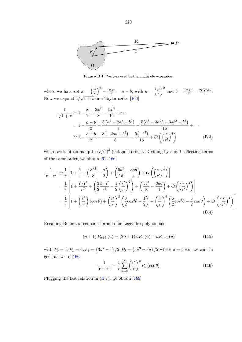
220
r′
R
r
Ω
P
Figure B.1: Vectors used in the multipole expansion.
where we have set x =(r′
r
)2− 2r·r′
r2= a − b, with a =
(r′
r
)2and b = 2r·r′
r2= 2r′ cos θ
r .
Now we expand 1/√1 + x in a Taylor series [166]
1√1 + x
= 1− x
2+
3x2
8− 5x3
16+ · · ·
= 1− a− b2
+3(a2 − 2ab+ b2
)8
−5(a3 − 3a2b+ 3ab2 − b3
)16
+ · · ·
≃ 1− a− b2
+3(−2ab+ b2
)8
−5(−b3
)16
+O
(( rr′
)4)(B.3)
where we kept terms up to (r/r′)3 (octapole order). Dividing by r and collecting terms
of the same order, we obtain [61, 166]
1
|r− r′|≃ 1
r
[1 +
b
2+
(3b2
8− a
2
)+
(5b3
16− 3ab
4
)+O
(( rr′
)4)]=
1
r
[1 +
r · r′
r2+
(3
2
r · r′
r2− 1
2
(r′
r
)2)
+
(5b3
16− 3ab
4
)+O
(( rr′
)4)]
=1
r
[1 +
(r′
r
)(cos θ) +
(r′
r
)2(3
2cos2θ − 1
2
)+
(r′
r
)3(5
2cos3θ − 3
2cos θ
)+O
(( rr′
)4)](B.4)
Recalling Bonnet’s recursion formula for Legendre polynomials
(n+ 1)Pn+1 (u) = (2n+ 1)uPn (u)− nPn−1 (u) (B.5)
with P0 = 1, P1 = u, P2 =(3u2 − 1
)/2, P3 =
(5u3 − 3u
)/2 where u = cos θ, we can, in
general, write [166]1
|r− r′|=
1
r
∞∑n=0
(r′
r
)n
Pn (cos θ) (B.6)
Plugging the last relation in (B.1), we obtain [169]

221
A (r) =µ04π
1r∫∫∫
ΩJ(r′)dV ′︸ ︷︷ ︸
Monopole
+1
r2
∫∫∫Ωr′ cos θJ
(r′)dV ′︸ ︷︷ ︸
Dipole
+1
r3
∫∫∫Ωr′
2(3
2cos2θ − 1
2
)J(r′)dV ′︸ ︷︷ ︸
Quadrupole
+ · · ·
= A(r)Monopole +A(r)Dipole +A(r)Quadrupole + · · · (B.7)
Now, since J is solenoidal (i.e., divergenceless) for static conditions and is confined to Ω,
the monopole term vanishes.1,2 For points far away from the source, we have r′/r ≪ 1
and thus we can approximate the vector potential as3
A (r) ≃ A(r)Dipole =µ04π
1
r2
∫∫∫Ωr′ cos θJ
(r′)dV ′ =
µ04π
1
r3
∫∫∫Ω
(r · r′
)J(r′)dV ′
(B.8)
However, from the vector identity (A.146), we can write (r · r′)J (r′) = (r · J (r′)) r′ −r× (r′ × J (r′)), and thus (B.8) becomes
A (r) ≃ µ04π
1
r3
[∫∫∫Ω
(r · J
(r′))
r′dV ′ − r×∫∫∫
Ω
(r′ × J
(r′))dV ′
](B.9)
Consider the i-th component of the first integral
∫∫∫Ω
(r · J
(r′))ri
′dV ′ =3∑
j=1
∫∫∫ΩrjJj
(r′)ri
′dV ′ =3∑
j=1
rj
∫∫∫Ω
(∇′rj
′ · J(r′))ri
′dV ′
(B.10)
where we used the fact that ∇′rj′ = r′j . Using the vector identity (A.155), we find
∇′ · (rj ′J (r′)) = rj′: 0(∇′ · J (r′)) + J (r′) · (∇′rj
′), where we used the fact that J is
solenoidal under stationary conditions. This allows us to write
3∑j=1
rj
∫∫∫Ω∇′ ·
(rj
′J(r′))ri
′dV ′ = −3∑
j=1
rj
∫∫∫Ωrj
′J(r′)·(∇′ri
′) dV ′ = −∫∫∫
Ω
(r · r′
)Ji(r′)dV ′
1This is not surprising giving the fact that there are (apparently) no isolated magnetic monopoles.See footnote 52.
2If this is not obvious, consider the i-th component of the following integral
0 =
∫∫∫Ω
ri∇ · JdV =
∫∫∫Ω
[∇ · (riJ)− J · ∇ri] dV =
∫∫∫Ω
∇ · (riJ) dV −∫∫∫
Ω
J · ∇ridV
Then from the divergence theorem (A.139) and ∇ri = ri, we find∫∫⃝
Σ
(riJ) · dS−∫∫∫
Ω
JidV = 0
Since the current is localized (i.e., confined to a finite volume), we can take the surface of integrationoutside this volume. Taking the surface to infinity (where there are no current densities), we obtain∫∫∫
ΩJidV = 0 [166]. Generalizing to all three components yields∫∫∫
Ω
JdV = 0
which is the desired result.3In condensed matter, this assumption is generally valid whenever r ≫ ℓs, where ℓs is the character-
istic system size [160].
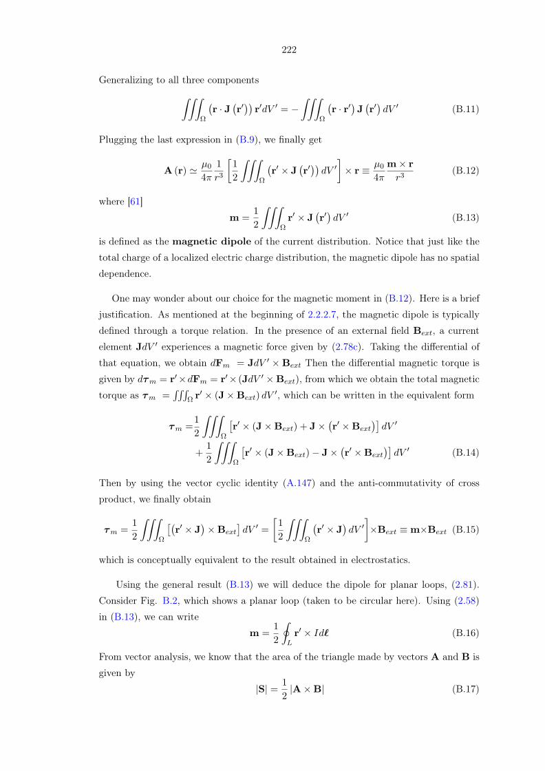
222
Generalizing to all three components∫∫∫Ω
(r · J
(r′))
r′dV ′ = −∫∫∫
Ω
(r · r′
)J(r′)dV ′ (B.11)
Plugging the last expression in (B.9), we finally get
A (r) ≃ µ04π
1
r3
[1
2
∫∫∫Ω
(r′ × J
(r′))dV ′
]× r ≡ µ0
4π
m× r
r3(B.12)
where [61]
m =1
2
∫∫∫Ωr′ × J
(r′)dV ′ (B.13)
is defined as the magnetic dipole of the current distribution. Notice that just like the
total charge of a localized electric charge distribution, the magnetic dipole has no spatial
dependence.
One may wonder about our choice for the magnetic moment in (B.12). Here is a brief
justification. As mentioned at the beginning of 2.2.2.7, the magnetic dipole is typically
defined through a torque relation. In the presence of an external field Bext, a current
element JdV ′ experiences a magnetic force given by (2.78c). Taking the differential of
that equation, we obtain dFm = JdV ′ ×Bext Then the differential magnetic torque is
given by dτm = r′×dFm = r′× (JdV ′ ×Bext), from which we obtain the total magnetic
torque as τm =∫∫∫
Ω r′ × (J×Bext) dV′, which can be written in the equivalent form
τm =1
2
∫∫∫Ω
[r′ × (J×Bext) + J×
(r′ ×Bext
)]dV ′
+1
2
∫∫∫Ω
[r′ × (J×Bext)− J×
(r′ ×Bext
)]dV ′ (B.14)
Then by using the vector cyclic identity (A.147) and the anti-commutativity of cross
product, we finally obtain
τm =1
2
∫∫∫Ω
[(r′ × J
)×Bext
]dV ′ =
[1
2
∫∫∫Ω
(r′ × J
)dV ′
]×Bext ≡m×Bext (B.15)
which is conceptually equivalent to the result obtained in electrostatics.
Using the general result (B.13) we will deduce the dipole for planar loops, (2.81).
Consider Fig. B.2, which shows a planar loop (taken to be circular here). Using (2.58)
in (B.13), we can write
m =1
2
∮Lr′ × Idℓ (B.16)
From vector analysis, we know that the area of the triangle made by vectors A and B is
given by
|S| = 1
2|A×B| (B.17)

223
Letting A = r′ and B = dℓ, we obtain the differential area dℓ as |dS| = 12 |r
′ × dℓ|.Hence we can write (B.16) as a surface integral
|m| = I
∣∣∣∣∫∫⃝ΣdS
∣∣∣∣where we have taken I outside the integral since it is uniform. Since the loop is planar,
the dipole moment is perpendicular to the plane of the loop and thus we can write the
last integral as
m = I
∫∫⃝
ΣdS = IS (B.18)
which is the desired result.
x
y
z
I
r
P
θ
r′
dℓ
Figure B.2: Current-carrying loop representation of a magnetic dipole.
To find the field produced by the source in the dipolar approximation, we start by
taking the curl of (B.12)
B (r) ≡ ∇×A (r) =µ04π∇×
(m× r
r3
)(B.19)
To that end, we invoke the vector identity (A.160) to obtain
∇×(m× r
r3
)= m
(∇ · r
r3
)−:0r
r3(∇ ·m) +:0( r
r3· ∇)m −(m · ∇) r
r3= m
(∇ · r
r3
)−(m · ∇) r
r3
where we used the fact that m is constant for a give current configuration. Moreover,
since r =√x2 + y2 + z2 = 0, we can write
∇ ·( r
r3
)=
∂
∂x
( xr3
)+
∂
∂y
( yr3
)+
∂
∂z
( zr3
)=
(−3
2
2x2
r5+
1
r3
)+
(−3
2
2y2
r5+
1
r3
)+
(−3
2
2z2
r5+
1
r3
)= 0 (B.20)

224
Also
(m · ∇) r
r3= mx
[∂
∂x
r
r3
]+my
[∂
∂y
r
r3
]+mz
[∂
∂z
r
r3
]= mx
[(−3
2
2x2
r5+
1
r3
)ax −
3
2
2xy
r5ay −
3
2
2xz
r5az
]+my [· · · ] +mz [· · · ]
= −3xmx
r5r+
mx
r3ax − 3
ymy
r5r+
my
r3ay − 3
zmz
r5r+
mz
r3az
=1
r3[−3 (m · r) r+m] (B.21)
Using the last three results in (B.19) yields the important expression of the dipolar field
outside the current distribution
B =µ04π
[3 (r ·m) r−m
r3
](B.22)
Magnetic Poles Model
To derive the dipolar field expression, consider Fig. B.3, which shows two oppositely
charged monopoles of magnitude Qm centered around the origin with a separation vector
ℓ.
x
y
z
r
r1
r2ℓ
Qm
−Qm
P
θ
Figure B.3: Magnetic poles representation of a magnetic dipole.
Outside the dipole, there are no free currents and thus H is irrotational and we can use
the results in 2.2.2.4. In particular
H = −∇Vm (B.23)
∇2Vm = 0 (B.24)

225
We may then define the magnetic scalar potential in the same way as in electrostatics
Vm (r) = CQm
r(B.25)
where C is a constant to be determined. From the principle of superposition, the potential
at point P is the sum of both potentials
Vm (r) = CQm
[1
r1− 1
r2
](B.26)
where r1 and r2 are the distances between P and +Qm and −Qm, respectively. Now,
we try to find expressions in terms of ℓ and the angle θ. The law of cosines (Fig. B.4)
allows us to write
r1 =
√r2 +
(ℓ
2
)2
− 2r
(ℓ
2
)cos θ = r
√1 +
ℓ2
4r2− ℓ
rcos θ = r
√1 + x1 (B.27)
r2 =
√r2 +
(ℓ
2
)2
− 2r
(ℓ
2
)cos (π − θ) = r
√1 +
ℓ2
4r2+ℓ
rcos θ = r
√1 + x2 (B.28)
where x1 = ℓ2
4r2− ℓ
r cos θ and x2 = ℓ2
4r2+ ℓ
r cos θ. Then (B.26) becomes
Vm (r) = CQm
r
[1√
1 + x1− 1√
1 + x2
](B.29)
b
ca
A C
B
a2 = b2 + c2 − 2bc cosAb2 = a2 + c2 − 2ac cosBc2 = a2 + b2 − 2ab cosC
Figure B.4: The law of cosines for calculating one side of a triangle when the opposite angleand the other two sides are known.
Since we are mostly interested in far field behavior, we will try to approximate the
results and arrive at a simpler expression. One way is to use the Binomial expansion
(1 + x)n = 1 + nx+n (n− 1)
2x2 +
n (n− 1) (n− 2)
6x3 + · · · (B.30)
which converges for n < 0 if |x| < 1. The series can then be truncated for very small
value of x to obtain
(1 + x)n ∼= 1 + nx (B.31)

226
Using the last relation in (B.29) with n = −1/2
Vm (r) = CQm
r
[(1− 1
2x1
)−(1− 1
2x2
)]= C
Qm
r
[1
2(x2 − x1)
]= C
Qm
r
[1
2
(ℓ2
4r2+ℓ
rcos θ −
ℓ2
4r2+ℓ
rcos θ
)]
= CQm
r
[ℓ
rcos θ
]= C
Qmℓ cos θ
r2(B.32)
Since ℓ cos θ = ℓ · ar = ℓ · (r/r), we can rewrite the last result as
Vm (r) =CQmℓ · r
r3= C
m · rr3
(B.33)
where
m = Qmℓ (B.34)
is defined as the magnetic dipole. Using the scalar potential expression (B.33) along
with (B.23) and (2.60), we can show that
B = −µ0∇(Cm · rr3
)= −µ0C
3 (r ·m) r−m
r3(B.35)
which is consistent with (B.22) if and only if C = 14π . Under this choice we obtain the
scalar potential4
Vm (r) =m · r4πr3
(B.36)
which we can use along with both (B.23) and (2.60) to find the dipolar field
B =µ04π
[3 (r ·m) r−m
r3
](B.37)
Before concluding this appendix, we point a subtle issue concerning the interior fields.
By looking at the expression of the dipolar fields (B.22) and (B.37), one might conclude
that both models are identical. However, one should not jump to such conclusions so fast
as the expressions give the dipolar fields outside the dipoles, and not everywhere. Looking
at the current loop model (Fig. 2.15a), the field lines internal to the dipole point in the
same direction as those external to it. However, for the magnetic poles (Fig. 2.15b), the
field lines between the magnetic poles point in the opposite direction as those outside.
Apparently there is a discrepancy, and in contrast to the expression of the external fields,4It can be easily shown that it indeed satisfies Laplace’s equation (2.64).
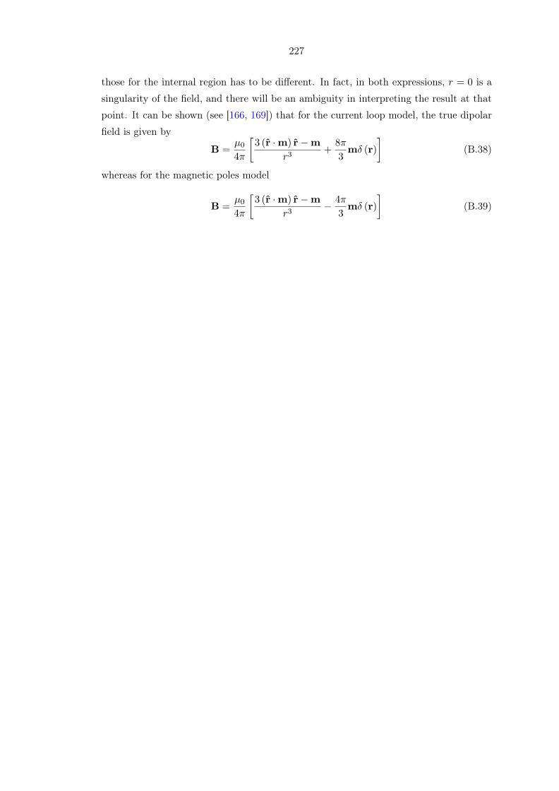
227
those for the internal region has to be different. In fact, in both expressions, r = 0 is a
singularity of the field, and there will be an ambiguity in interpreting the result at that
point. It can be shown (see [166, 169]) that for the current loop model, the true dipolar
field is given by
B =µ04π
[3 (r ·m) r−m
r3+
8π
3mδ (r)
](B.38)
whereas for the magnetic poles model
B =µ04π
[3 (r ·m) r−m
r3− 4π
3mδ (r)
](B.39)

228
Appendix C
Box-Muller Transform
Computer generated random numbers are crucial elements in computer simulations and
they occur in many applications including stochastic physical processes, protecting pri-
vate messages (cryptography), finance, or even video games. Almost all random number
generation on computers is done using algorithms to produce a stream of numbers from
U (0, 1), i.e. from a uniform distribution on the interval (0, 1). However, in many physical
processes, one might need to generate random numbers with Gaussian (normal) distri-
bution. Although one could use some approximate methods based on the Central Limit
Theorem (CLT) [216] to approximate the normal distribution N (0, 1), it is better to
resort for more accurate and computationally-efficient methods. Box-Muller transform
[273] provides an efficient algorithm to generate Gaussian pseudo-random numbers1 given
a source of uniform pseudo-random numbers. It is a brilliant method to overcome the
difficulty that arises when using the inverse transform sampling, i.e. when trying to
invert the distribution function to obtain a normal distribution from a standard uniform
F (x) =
∫ x
−∞
1√2πe−
x′22 dx′ (C.1)
which has no closed form. Box-Muller transform solves this by producing a two-dimensional
bivariate normal distribution from a two-dimensional uniform distribution. It is based on
the premise that, given a distribution function, one can use the fundamental transforma-
tion law of probabilities [274] to obtain a transformation function for the distributions,
i.e. a transformation that maps the random numbers from distribution to the other (Fig.
C.1).1In reality, most random numbers used in computer programs are pseudo-random, which means they
are generated in a predictable fashion using a mathematical formula.

229
..y
.
1
.
x
.0.
Uniform
.
Deviate In
.
Transformed
.
Deviate Out
.
F (y) =∫ y
0p (y) dy
.
p (y)
Figure C.1: Transformation method that maps a random deviate y from a given distributionp (y). The integral
∫p (y) dy must be known and invertible. From a deviate x between 0 and
1, the desired value of y lies on the definite-integral curve. Figure adapted by the author from[274].
Let X be a random variable with a random deviate x ∈ R whose probability density
is pX (x), and let f : X → Y by a map such that another random variable Y is given by
Y = f (X) (C.2)
The fundamental transformation law of probabilities yields
|pY (y) dy| = |pX (x) dx| (C.3)
or
pY (y) = pX (x)
∣∣∣∣dxdy∣∣∣∣ (C.4)
which is the desired probability density of y.
The idea above can be generalized to more than one dimension. In particular, in
two dimensions, one has the two-dimensional random variable X = (X1, X2), having the
random deviates x = (x1, x2) ∈ R2, whose probability density is given by pX (x). If
another random variable is given by the transformation f : X→ Y, viz.
Y1 = f1 (X1, X2) (C.5)
Y2 = f2 (X1, X2) (C.6)

230
obeying
dy1 = df1 (x1, x2) =∂f1∂x1
dx1 +∂f1∂x2
dx2 (C.7)
dy2 = df2 (x1, x2) =∂f2∂x1
dx1 +∂f2∂x2
dx2 (C.8)
then fundamental transformation law of probabilities yields
|pY (y1, y2) dy1dy2| = |pX (x1, x2) dx1dx2| (C.9)
or
pY (y1, y2) = pX (x1, x2)dx1dx2dy1dy2
(C.10)
which is the desired joint probability density of y. The volume elements in the two-
dimensional space given above are related by dy1dy2 = det (Jf ) dx1dx2, where Jf is the
Jacobi of the map f : X→ Y given by
Jf =
[∂f1∂x1
∂f1∂x2
∂f2∂x1
∂f2∂x2
](C.11)
Now, consider the two uniform deviates x1, x2 ∈ U (0, 1) and the transformations
y1 =√−2 lnx1 cos (2πx2) (C.12)
y2 =√−2 lnx1 sin (2πx2) (C.13)
To find the Jacobian, we start by calculating the partial derivatives
∂f1∂x1
=−1
x1√−2 lnx1
cos (2πx2) ,∂f1∂x2
= −2π√−2 lnx1 sin (2πx2) (C.14)
∂f2∂x1
=−1
x1√−2 lnx1
sin (2πx2) ,∂f2∂x2
= −2π√−2 lnx1 cos (2πx2) (C.15)
which yields the Jacobian
det (Jf ) = det
[∂f1∂x1
∂f1∂x2
∂f2∂x1
∂f2∂x2
]= 2πe
y21+y222 (C.16)
Now, on the basis of the fundamental transformation law of probabilities, one has to
consider the inverse of the Jacobian, viz.
1
det (Jf )=
1
2πey21+y22
2
=1
2πe−(
y21+y222
)=
1√2πe−
y212
1√2πe−
y222 (C.17)

231
which clearly shows (in one-dimension) that y1 and y2 are independently distributed
according to the normal distribution.

232
LIST OF SUBMITTED PUBLICATIONS
[1] M. Alawein and H. Fariborzi, “Improved Circuit Model for All-Spin Logic”, in IEEE/ACM
International Symposium on Nanoscale Architectures, Beijing, China, 2016.
[2] M. Alawein and H. Fariborzi, “Dynamic Circuit Model for Spintronic Devices”, in
Eurosensors XXX, Budapest, Hungary, 2016.

233
BIBLIOGRAPHY
[1] I PRESENT. Cramming more components onto integrated circuits. Readings in
computer architecture, 56, 2000.
[2] S Natarajan, M Agostinelli, S Akbar, M Bost, A Bowonder, V Chikarmane,
S Chouksey, A Dasgupta, K Fischer, and Q Fu. A 14nm logic technology featur-
ing 2 nd-generation finfet, air-gapped interconnects, self-aligned double patterning
and a 0.0588 ţm 2 sram cell size. In Electron Devices Meeting (IEDM), 2014 IEEE
International, pages 3.7. 1–3.7. 3. IEEE, 2014.
[3] Intel.
[4] Thomas N Theis and Paul M Solomon. Its time to reinvent the transistor! Science,
327(5973):1600–1601, 2010.
[5] Howard Huff. Into the nano era: Moore’s law beyond planar silicon CMOS, volume
106. Springer Science & Business Media, 2008.
[6] International Technology Roadmap of Semiconductors (ITRS). ITRS, 2013 edition.
[7] Tomasz Brozek. Micro-and Nanoelectronics: Emerging Device Challenges and So-
lutions. CRC Press, 2014.
[8] SA Wolf, DD Awschalom, RA Buhrman, JM Daughton, S Von Molnar, ML Roukes,
A Yu Chtchelkanova, and DM Treger. Spintronics: a spin-based electronics vision
for the future. Science, 294(5546):1488–1495, 2001.
[9] Igor uti, Jaroslav Fabian, and S Das Sarma. Spintronics: Fundamentals and ap-
plications. Reviews of modern physics, 76(2):323, 2004.
[10] Gary A Prinz. Spin-polarized transport. Physics today, 48:58–63, 1995.
[11] Gary A Prinz. Magnetoelectronics. Science, 282(5394):1660–1663, 1998.
[12] A. Hirohata and K. Takanashi. Future perspectives for spintronic devices. Journal
of Physics D-Applied Physics, 47(19), 2014.

234
[13] Behtash Behin-Aein, Sayeef Salahuddin, and Supriyo Datta. Switching energy of
ferromagnetic logic bits. Nanotechnology, IEEE Transactions on, 8(4):505–514,
2009.
[14] M. Ventra, S. Evoy, and J.R. Heflin. Introduction to Nanoscale Science and Tech-
nology. Springer US, 2006.
[15] C.G. Stefanita. Magnetism: Basics and Applications. Springer Berlin Heidelberg,
2012.
[16] Arne Brataas, Andrew D Kent, and Hideo Ohno. Current-induced torques in
magnetic materials. Nature materials, 11(5):372–381, 2012.
[17] M Hosomi, H Yamagishi, T Yamamoto, K Bessho, Y Higo, K Yamane, H Ya-
mada, M Shoji, H Hachino, and C Fukumoto. A novel nonvolatile memory with
spin torque transfer magnetization switching: Spin-ram. In International Electron
Devices Meeting, pages 459–462, 2005.
[18] Tetsuya Yamamoto, Hiroshi Kano, Yutaka Higo, Kazuhiro Ohba, Tetsuya
Mizuguchi, Masanori Hosomi, Kazuhiro Bessho, Minoru Hashimoto, Hiroyuki
Ohmori, and Takeyuki Sone. Magnetoresistive random access memory operation
error by thermally activated reversal. Journal of applied physics, 97(10):10P503,
2005.
[19] Naoki Nishimura, Tadahiko Hirai, Akio Koganei, Takashi Ikeda, Kazuhisa Okano,
Yoshinobu Sekiguchi, and Yoshiyuki Osada. Magnetic tunnel junction device with
perpendicular magnetization films for high-density magnetic random access mem-
ory. Journal of applied physics, 91(8):5246–5249, 2002.
[20] Satishchandra B Ogale. Thin films and heterostructures for oxide electronics.
Springer Science & Business Media, 2006.
[21] DC Ralph and Mark D Stiles. Spin transfer torques. Journal of Magnetism and
Magnetic Materials, 320(7):1190–1216, 2008.
[22] SSP Parkin, KP Roche, MG Samant, PM Rice, RB Beyers, RE Scheuerlein,
EJ Osullivan, SL Brown, J Bucchigano, and DW Abraham. Exchange-biased
magnetic tunnel junctions and application to nonvolatile magnetic random access
memory. Journal of Applied Physics, 85(8):5828–5833, 1999.
[23] M Motoyoshi, I Yamamura, W Ohtsuka, M Shouji, H Yamagishi, M Nakamura,
H Yamada, K Tai, T Kikutani, and T Sagara. A study for 0.18 m high-density
mram. In VLSI Technology, 2004. Digest of Technical Papers. 2004 Symposium
on, pages 22–23. IEEE, 2004.

235
[24] AD Kent, B Özyilmaz, and E Del Barco. Spin-transfer-induced precessional mag-
netization reversal. Applied Physics Letters, 84(19):3897–3899, 2004.
[25] Xiaochun Zhu and Jian-Gang Zhu. Spin torque and field-driven perpendicular
mram designs scalable to multi-gb/chip capacity. Magnetics, IEEE Transactions
on, 42(10):2739–2741, 2006.
[26] Pietro Gambardella and Ioan Mihai Miron. Current-induced spinorbit torques.
Philosophical Transactions of the Royal Society of London A: Mathematical, Phys-
ical and Engineering Sciences, 369(1948):3175–3197, 2011.
[27] Georg Schmidt. Concepts for spin injection into semiconductorsa review. Journal
of Physics D: Applied Physics, 38(7):R107, 2005.
[28] Koichiro Inomata. Present and future of magnetic ram technology. IEICE trans-
actions on electronics, 84(6):740–746, 2001.
[29] Gerrit E. W. Bauer. Paul J. Kelly Arne Brataas, Yaroslav Tserkovnyak. Spin
pumping and spin transfer. Spin current, 17:87, 2012.
[30] L Berger. Emission of spin waves by a magnetic multilayer traversed by a current.
Physical Review B, 54(13):9353, 1996.
[31] John C Slonczewski. Current-driven excitation of magnetic multilayers. Journal
of Magnetism and Magnetic Materials, 159(1):L1–L7, 1996.
[32] JA Katine, FJ Albert, RA Buhrman, EB Myers, and DC Ralph. Current-driven
magnetization reversal and spin-wave excitations in co/cu/co pillars. Physical Re-
view Letters, 84(14):3149, 2000.
[33] S Il Kiselev, JC Sankey, IN Krivorotov, NC Emley, RJ Schoelkopf, RA Buhrman,
and DC Ralph. Microwave oscillations of a nanomagnet driven by a spin-polarized
current. Nature, 425(6956):380–383, 2003.
[34] WH Rippard, MR Pufall, S Kaka, SE Russek, and TJ Silva. Direct-current induced
dynamics in c o 90 f e 10/n i 80 f e 20 point contacts. Physical Review Letters, 92
(2):027201, 2004.
[35] IN Krivorotov, NC Emley, JC Sankey, SI Kiselev, DC Ralph, and RA Buhrman.
Time-domain measurements of nanomagnet dynamics driven by spin-transfer
torques. Science, 307(5707):228–231, 2005.
[36] Mark Johnson and Robert H Silsbee. Interfacial charge-spin coupling: Injection
and detection of spin magnetization in metals. Physical Review Letters, 55(17):
1790, 1985.
236
[37] Friso Jacobus Jedema, AT Filip, and BJ Van Wees. Electrical spin injection and
accumulation at room temperature in an all-metal mesoscopic spin valve. Nature,
410(6826):345–348, 2001.
[38] FJ Jedema, HB Heersche, AT Filip, JJA Baselmans, and BJ Van Wees. Electrical
detection of spin precession in a metallic mesoscopic spin valve. Nature, 416(6882):
713–716, 2002.
[39] T Kimura, J Hamrle, Y Otani, K Tsukagoshi, and Y Aoyagi. Spin-dependent
boundary resistance in the lateral spin-valve structure. Applied physics letters, 85
(16):3501–3503, 2004.
[40] Y Ji, A Hoffmann, JS Jiang, and SD Bader. Spin injection, diffusion, and detection
in lateral spin-valves. Applied physics letters, 85(25):6218–6220, 2004.
[41] SO Valenzuela and M Tinkham. Spin-polarized tunneling in room-temperature
mesoscopic spin valves. Applied physics letters, 85(24):5914–5916, 2004.
[42] Ryan Godfrey and Mark Johnson. Spin injection in mesoscopic silver wires: Exper-
imental test of resistance mismatch. Physical review letters, 96(13):136601, 2006.
[43] FJ Jedema, MS Nijboer, AT Filip, and BJ Van Wees. Spin injection and spin
accumulation in all-metal mesoscopic spin valves. Physical Review B, 67(8):085319,
2003.
[44] Behtash Behin-Aein, Deepanjan Datta, Sayeef Salahuddin, and Supriyo Datta.
Proposal for an all-spin logic device with built-in memory. Nature nanotechnology,
5(4):266–270, 2010.
[45] Sudarshan Srinivasan, Anirban Sarkar, Behtash Behin-Aein, and Soupayan Datta.
All-spin logic device with inbuilt nonreciprocity. Magnetics, IEEE Transactions
on, 47(10):4026–4032, 2011.
[46] B. Behin-Aein, S. Srinivasan, A. Sarkar, S. Datta, and S. Salahuddin. All-spin logic
devices, 2012.
[47] Behtash Behin-Aein, Angik Sarkar, Srikant Srinivasan, and Supriyo Datta. Switch-
ing energy-delay of all spin logic devices. Applied Physics Letters, 98(12):123510,
2011.
[48] Sasikanth Manipatruni, Dmitri E Nikonov, and Ian A Young. Modeling and design
of spintronic integrated circuits. Circuits and Systems I: Regular Papers, IEEE
Transactions on, 59(12):2801–2814, 2012.

237
[49] Sou-Chi Chang, Sasikanth Manipatruni, Dmitri E Nikonov, Ian A Young, and Azad
Naeemi. Design and analysis of si interconnects for all-spin logic. Magnetics, IEEE
Transactions on, 50(9):1–13, 2014.
[50] Sou-Chi Chang, Sourav Dutta, Sasikanth Manipatruni, Dmitri E Nikonov, Ian A
Young, and Azad Naeemi. Interconnects for all-spin logic using automotion of
domain walls. Exploratory Solid-State Computational Devices and Circuits, IEEE
Journal on, 1:49–57, 2015.
[51] Charles Augustine, Georgios Panagopoulos, Behtash Behin-Aein, Srikant Srini-
vasan, Angik Sarkar, and Kaushik Roy. Low-power functionality enhanced
computation architecture using spin-based devices. In Nanoscale Architectures
(NANOARCH), 2011 IEEE/ACM International Symposium on, pages 129–136.
IEEE, 2011.
[52] Srikant Srinivasan, Vinh Diep, Behtash Behin-Aein, Angik Sarkar, Supriyo Datta,
D Awschalom, J Nitta, and Y Xu. Modeling multi-magnet networks interacting
via spin currents. arXiv preprint arXiv:1304.0742, 2013.
[53] Mrigank Sharad, Karthik Yogendra, Arun Gaud, Kon-Woo Kwon, and Kaushik
Roy. Ultra-high density, high-performance and energy-efficient all spin logic. arXiv
preprint arXiv:1308.2280, 2013.
[54] Z Liang and S Sapatnekar. Energy/delay tradeoffs in all-spin logic circuits.
[55] Srikant Srinivasan. Unidirectional information transfer with cascaded all spin logic
devices: A ring oscillator. In Device Research Conference (DRC), 2011 69th An-
nual, 2011.
[56] Angik Sarkar, Srikant Srinivasan, Behtash Behin-Aein, and Supriyo Datta. Model-
ing all spin logic: Multi-magnet networks interacting via spin currents. In Electron
Devices Meeting (IEDM), 2011 IEEE International, pages 11.1. 1–11.1. 4. IEEE,
2011.
[57] Behtash Behin-Aein, Angik Sarkar, and Supriyo Datta. Modeling circuits with
spins and magnets for all-spin logic. In Solid-State Device Research Conference
(ESSDERC), 2012 Proceedings of the European, pages 36–40. IEEE, 2012.
[58] Phillip Bonhomme, Sasikanth Manipatruni, Rouhollah M Iraei, Shaloo Rakheja,
Sou-Chi Chang, Dmitri E Nikonov, Ian A Young, and Azad Naeemi. Circuit
simulation of magnetization dynamics and spin transport. Electron Devices, IEEE
Transactions on, 61(5):1553–1560, 2014.

238
[59] E. Y. Tsymbal and Igor Zutic. Handbook of spin transport and magnetism. CRC
Press, Boca Raton, FL, 2012.
[60] Vehbi Calayir, Dmitri E Nikonov, Sasikanth Manipatruni, and Ian A Young. Static
and clocked spintronic circuit design and simulation with performance analysis
relative to cmos. Circuits and Systems I: Regular Papers, IEEE Transactions on,
61(2):393–406, 2014.
[61] J.M.D. Coey. Magnetism and Magnetic Materials. Cambridge University Press,
2010.
[62] S. Bandyopadhyay and M. Cahay. Introduction to Spintronics. Taylor & Francis,
2008.
[63] Michael Ziese and Martin J Thornton. Spin electronics. 2001.
[64] Jaroslav Fabian and S Das Sarma. Spin relaxation of conduction electrons. Journal
of Vacuum Science & Technology B, 17(4):1708–1715, 1999.
[65] T. Shinjo. Nanomagnetism and Spintronics. Elsevier Science, 2009.
[66] Matthew N. O. Sadiku. Elements of electromagnetics. Oxford University Press,
New York, 5th edition, 2011.
[67] N.A. Spaldin. Magnetic Materials: Fundamentals and Device Applications. Cam-
bridge University Press, 2003.
[68] R. Vajtai. Springer Handbook of Nanomaterials. Springer Berlin Heidelberg, 2013.
[69] D. Feng and G. Jin. Introduction to Condensed Matter Physics. World Scientific,
2005.
[70] R.A. Lukaszew. Handbook of Nanomagnetism: Applications and Tools. Pan Stan-
ford Publishing, 2015.
[71] Arne Brataas, Gerrit EW Bauer, and Paul J Kelly. Non-collinear magnetoelec-
tronics. Physics Reports, 427(4):157–255, 2006.
[72] Donald A Neamen. Semiconductor physics and devices. 1992, 2010.
[73] W. Heisenberg. On the theory of ferromagnetism. Zeitschrift Fur Physik, 49(9-10):
619–636, 1928.
[74] HAM Van den Berg, Reinder Coehoorn, MAM Gijs, P Grünberg, T Rasing, K Röll,
and U Hartmann. Magnetic multilayers and giant magnetoresistance: fundamentals
and industrial applications, volume 37. Springer Science & Business Media, 2013.
239
[75] H. Lüth. Solid Surfaces, Interfaces and Thin Films. Springer International Pub-
lishing, 2014.
[76] Eric Beaurepaire, Fabrice Scheurer, Gérard Krill, and Jean-Paul Kappler. Mag-
netism and synchrotron radiation, volume 34. Springer, 2001.
[77] Daniel D Stancil and Anil Prabhakar. Spin waves. Springer, 2009.
[78] A.P. Guimarães. Principles of Nanomagnetism. Springer Berlin Heidelberg, 2009.
[79] Jaroslav Fabian, Alex Matos-Abiague, Christian Ertler, Peter Stano, and Igor Zu-
tic. Semiconductor spintronics. arXiv preprint arXiv:0711.1461, 2007.
[80] Xavier Waintal, Edward B Myers, Piet W Brouwer, and DC Ralph. Role of spin-
dependent interface scattering in generating current-induced torques in magnetic
multilayers. Physical Review B, 62(18):12317, 2000.
[81] Jack Bass and William P Pratt Jr. Spin-diffusion lengths in metals and alloys,
and spin-flipping at metal/metal interfaces: an experimentalists critical review.
Journal of Physics: Condensed Matter, 19(18):183201, 2007.
[82] C. L. Dennis, R. P. Borges, L. D. Buda, U. Ebels, J. F. Gregg, M. Hehn,
E. Jouguelet, K. Ounadjela, I. Petej, I. L. Prejbeanu, and M. J. Thornton. The
defining length scales of mesomagnetism: A review. Journal of Physics-Condensed
Matter, 14(49):R1175–R1262, 2002.
[83] Robert M White and Bradford Bayne. Quantum theory of magnetism, volume 1.
Springer, 1983.
[84] C Strunk. Thermodynamics and the quantum transport of particles and entropy.
arXiv preprint arXiv:1210.0344, 2012.
[85] K Uchida, S Takahashi, K Harii, J Ieda, W Koshibae, K Ando, S Maekawa, and
E Saitoh. Observation of the spin seebeck effect. Nature, 455(7214):778–781, 2008.
[86] Ken-ichi Uchida, Hiroto Adachi, T An, T Ota, M Toda, B Hillebrands, S Maekawa,
and E Saitoh. Long-range spin seebeck effect and acoustic spin pumping. Nature
materials, 10(10):737–741, 2011.
[87] Ken-ichi Uchida, Toshu An, Yosuke Kajiwara, Masaya Toda, and Eiji Saitoh.
Surface-acoustic-wave-driven spin pumping in y3fe5o12/pt hybrid structure. Ap-
plied Physics Letters, 99(21):212501, 2011.
[88] K Uchida, H Adachi, T An, H Nakayama, M Toda, B Hillebrands, S Maekawa,
and E Saitoh. Acoustic spin pumping: Direct generation of spin currents from

240
sound waves in pt/y3fe5o12 hybrid structures. Journal of Applied Physics, 111(5):
053903, 2012.
[89] R Fiederling, M Keim, Get al Reuscher, W Ossau, G Schmidt, A Waag, and
LW Molenkamp. Injection and detection of a spin-polarized current in a light-
emitting diode. Nature, 402(6763):787–790, 1999.
[90] Mamoru Matsuo, Jun’ichi Ieda, Kazuya Harii, Eiji Saitoh, and Sadamichi
Maekawa. Mechanical generation of spin current by spin-rotation coupling. Phys-
ical Review B, 87(18):180402, 2013.
[91] Mamoru Matsuo, Junichi Ieda, Eiji Saitoh, and Sadamichi Maekawa. Spin-
dependent inertial force and spin current in accelerating systems. Physical Review
B, 84(10):104410, 2011.
[92] Mamoru Matsuo, Junichi Ieda, Eiji Saitoh, and Sadamichi Maekawa. Spin cur-
rent generation due to mechanical rotation in the presence of impurity scattering.
Applied Physics Letters, 98(24):242501, 2011.
[93] Mamoru Matsuo, Junichi Ieda, Eiji Saitoh, and Sadamichi Maekawa. Effects of
mechanical rotation on spin currents. Physical review letters, 106(7):076601, 2011.
[94] MI D’yakonov and VI Perel. Possibility of orienting electron spins with current.
Soviet Journal of Experimental and Theoretical Physics Letters, 13:467, 1971.
[95] MI Dyakonov and VI Perel. Current-induced spin orientation of electrons in semi-
conductors. Physics Letters A, 35(6):459–460, 1971.
[96] YK Kato, RC Myers, AC Gossard, and DD Awschalom. Observation of the spin
hall effect in semiconductors. science, 306(5703):1910–1913, 2004.
[97] Joerg Wunderlich, Bernd Kaestner, Jairo Sinova, and Tomas Jungwirth. Experi-
mental observation of the spin-hall effect in a two-dimensional spin-orbit coupled
semiconductor system. Physical review letters, 94(4):047204, 2005.
[98] Shuichi Murakami, Naoto Nagaosa, and Shou-Cheng Zhang. Dissipationless quan-
tum spin current at room temperature. Science, 301(5638):1348–1351, 2003.
[99] AG Aronov. Spin injection in metals and polarization of nuclei. Jetp Lett, 24(1):
32–34, 1976.
[100] A. G. Aronov and G. E. Pikus. Spin injection into semiconductors. Soviet Physics
Semiconductors-Ussr, 10(6):698–700, 1976.
[101] Mark Johnson and RH Silsbee. Spin-injection experiment. Physical Review B, 37
(10):5326, 1988.
241
[102] Mark Johnson and RH Silsbee. Coupling of electronic charge and spin at a
ferromagnetic-paramagnetic metal interface. Physical Review B, 37(10):5312, 1988.
[103] NF Mott. The electrical conductivity of transition metals. In Proceedings of the
Royal Society of London A: Mathematical, Physical and Engineering Sciences, vol-
ume 153, pages 699–717. The Royal Society, 1936.
[104] T Valet and A Fert. Theory of the perpendicular magnetoresistance in magnetic
multilayers. Physical Review B, 48(10):7099, 1993.
[105] Nevill F Mott. Electrons in transition metals. Advances in Physics, 13(51):325–422,
1964.
[106] Daniel Huertas Hernando, Yu V Nazarov, Arne Brataas, and Gerrit EW Bauer.
Conductance modulation by spin precession in noncollinear ferromagnet normal-
metal ferromagnet systems. Physical Review B, 62(9):5700, 2000.
[107] IA Campbell, A Fert, and R Pomeroy. Evidence for two current conduction iron.
Philosophical Magazine, 15(137):977–983, 1967.
[108] A Fert and IA Campbell. Two-current conduction in nickel. Physical Review
Letters, 21(16):1190, 1968.
[109] Michael E Flatté and Ionel Tifrea. Manipulating quantum coherence in solid state
systems, volume 244. Springer Science & Business Media, 2007.
[110] Sylvain Dubois, Luc Piraux, JM George, K Ounadjela, JL Duvail, and A Fert.
Evidence for a short spin diffusion length in permalloy from the giant magnetore-
sistance of multilayered nanowires. Physical Review B, 60(1):477, 1999.
[111] SD Steenwyk, SY Hsu, R Loloee, J Bass, and WP Pratt. Perpendicular-current
exchange-biased spin-valve evidence for a short spin-diffusion lenght in permalloy.
Journal of magnetism and magnetic materials, 170(1):L1–L6, 1997.
[112] P Holody, WC Chiang, R Loloee, J Bass, WP Pratt Jr, and PA Schroeder. Giant
magnetoresistance of copper/permalloy multilayers. Physical Review B, 58(18):
12230, 1998.
[113] Mark Johnson and RH Silsbee. Thermodynamic analysis of interfacial transport
and of the thermomagnetoelectric system. Physical Review B, 35(10):4959, 1987.
[114] Satishchandra B Ogale. Thin films and heterostructures for oxide electronics.
Springer Science & Business Media, 2006.
[115] William H Meiklejohn and Charles P Bean. New magnetic anisotropy. Physical
review, 102(5):1413, 1956.
242
[116] William J Gallagher and Stuart SP Parkin. Development of the magnetic tunnel
junction mram at ibm: from first junctions to a 16-mb mram demonstrator chip.
IBM Journal of Research and Development, 50(1):5–23, 2006.
[117] SSP Parkin, N More, and KP Roche. Oscillations in exchange coupling and mag-
netoresistance in metallic superlattice structures: Co/ru, co/cr, and fe/cr. Physical
Review Letters, 64(19):2304, 1990.
[118] SSP Parkin and D Mauri. Spin engineering: Direct determination of the ruderman-
kittel-kasuya-yosida far-field range function in ruthenium. Physical Review B, 44
(13):7131, 1991.
[119] K Xia, PJ Kelly, Ge EW Bauer, I Turek, J Kudrnovský, and V Drchal. Interface
resistance of disordered magnetic multilayers. Physical Review B, 63(6):064407,
2001.
[120] PETER Grünberg, R Schreiber, Y Pang, MB Brodsky, and H Sowers. Layered
magnetic structures: evidence for antiferromagnetic coupling of fe layers across cr
interlayers. Physical Review Letters, 57(19):2442, 1986.
[121] Mario Norberto Baibich, Jean Marc Broto, Albert Fert, F Nguyen Van Dau,
Frédéric Petroff, P Etienne, G Creuzet, A Friederich, and J Chazelas. Giant mag-
netoresistance of (001) fe/(001) cr magnetic superlattices. Physical review letters,
61(21):2472, 1988.
[122] Grünberg Binasch, Peter Grünberg, F Saurenbach, and W Zinn. Enhanced mag-
netoresistance in layered magnetic structures with antiferromagnetic interlayer ex-
change. Physical review B, 39(7):4828, 1989.
[123] John C Mallinson. Magneto-resistive and spin valve heads: fundamentals and ap-
plications. Academic Press, 2001.
[124] Arne Brataas, Yu V Nazarov, and Gerrit EW Bauer. Finite-element theory of
transport in ferromagnetnormal metal systems. Physical Review Letters, 84(11):
2481, 2000.
[125] Shufeng Zhang and Peter M Levy. Conductivity perpendicular to the plane of
multilayered structures. Journal of Applied Physics, 69(8):4786–4788, 1991.
[126] Peter M Levy and Shufeng Zhang. Our current understanding of giant magne-
toresistance in transition-metal multilayers. Journal of magnetism and magnetic
materials, 151(3):315–323, 1995.
[127] X-G Zhang and WH Butler. Conductivity of metallic films and multilayers. Physical
Review B, 51(15):10085, 1995.

243
[128] P Zahn, I Mertig, M Richter, and H Eschrig. Ab initio calculations of the giant
magnetoresistance. Physical review letters, 75(16):2996, 1995.
[129] Martin AM Gijs and Gerrit EW Bauer. Perpendicular giant magnetoresistance of
magnetic multilayers. Advances in Physics, 46(3-4):285–445, 1997.
[130] Robert E Camley and J Barna. Theory of giant magnetoresistance effects in mag-
netic layered structures with antiferromagnetic coupling. Physical review letters,
63(6):664, 1989.
[131] Peter M Levy, Shufeng Zhang, and Albert Fert. Electrical conductivity of magnetic
multilayered structures. Physical review letters, 65(13):1643, 1990.
[132] Michel Julliere. Tunneling between ferromagnetic films. Physics letters A, 54(3):
225–226, 1975.
[133] S Maekawa and U Gfvert. Electron tunneling between ferromagnetic films. Mag-
netics, IEEE Transactions on, 18(2):707–708, 1982.
[134] Jagadeesh Subbaiah Moodera, Lisa R Kinder, Terrilyn M Wong, and R Meservey.
Large magnetoresistance at room temperature in ferromagnetic thin film tunnel
junctions. Physical review letters, 74(16):3273, 1995.
[135] Terunobu Miyazaki and N Tezuka. Giant magnetic tunneling effect in fe/al 2 o
3/fe junction. Journal of Magnetism and Magnetic Materials, 139(3):L231–L234,
1995.
[136] Jagadeesh S Moodera, Janusz Nowak, and Rene JM van de Veerdonk. Interface
magnetism and spin wave scattering in ferromagnet-insulator-ferromagnet tunnel
junctions. Physical Review Letters, 80(13):2941, 1998.
[137] WH Butler, X-G Zhang, TC Schulthess, and JM MacLaren. Spin-dependent tun-
neling conductance of fe| mgo| fe sandwiches. Physical Review B, 63(5):054416,
2001.
[138] J Mathon and A Umerski. Theory of tunneling magnetoresistance of an epitaxial
fe/mgo/fe (001) junction. Physical Review B, 63(22):220403, 2001.
[139] M Tsoi, AGM Jansen, J Bass, W-C Chiang, M Seck, V Tsoi, and P Wyder. Exci-
tation of a magnetic multilayer by an electric current. Physical Review Letters, 80
(19):4281, 1998.
[140] EB Myers, DC Ralph, JA Katine, RN Louie, and RA Buhrman. Current-induced
switching of domains in magnetic multilayer devices. Science, 285(5429):867–870,
1999.
244
[141] J-E Wegrowe, D Kelly, Y Jaccard, Ph Guittienne, and J-Ph Ansermet. Current-
induced magnetization reversal in magnetic nanowires. EPL (Europhysics Letters),
45(5):626, 1999.
[142] JZ Sun. Current-driven magnetic switching in manganite trilayer junctions. Journal
of Magnetism and Magnetic Materials, 202(1):157–162, 1999.
[143] JA Katine, FJ Albert, RA Buhrman, EB Myers, and DC Ralph. Current-driven
magnetization reversal and spin-wave excitations in co/cu/co pillars. Physical Re-
view Letters, 84(14):3149, 2000.
[144] Julie Grollier, Vincent Cros, A Hamzic, Jean-Marie George, Henri Jaffrès, Albert
Fert, Giancarlo Faini, J Ben Youssef, and H Legall. Spin-polarized current induced
switching in co/cu/co pillars. Applied Physics Letters, 78(23):3663–3665, 2001.
[145] Arne Brataas, Yu V Nazarov, and Gerrit EW Bauer. Spin-transport in multi-
terminal normal metal-ferromagnet systems with non-collinear magnetizations.
The European Physical Journal B-Condensed Matter and Complex Systems, 22
(1):99–110, 2001.
[146] P Chureemart, RFL Evans, I D’Amico, and RW Chantrell. Influence of uniaxial
anisotropy on domain wall motion driven by spin torque. Physical Review B, 92
(5):054434, 2015.
[147] C Burrowes, AP Mihai, D Ravelosona, J-V Kim, C Chappert, L Vila, A Marty,
Y Samson, F Garcia-Sanchez, and LD Buda-Prejbeanu. Non-adiabatic spin-torques
in narrow magnetic domain walls. Nature Physics, 6(1):17–21, 2010.
[148] David Claudio-Gonzalez, André Thiaville, and Jacques Miltat. Domain wall dy-
namics under nonlocal spin-transfer torque. Physical review letters, 108(22):227208,
2012.
[149] R Wieser, EY Vedmedenko, and R Wiesendanger. Indirect control of antiferro-
magnetic domain walls with spin current. Physical review letters, 106(6):067204,
2011.
[150] K Xia, PJ Kelly, GEW Bauer, A Brataas, and I Turek. Spin torques in
ferromagnetic/normal-metal structures. Physical Review B, 65(22):220401, 2002.
[151] Maciej Zwierzycki, Yaroslav Tserkovnyak, Paul J Kelly, Arne Brataas, and Ger-
rit EW Bauer. First-principles study of magnetization relaxation enhancement and
spin transfer in thin magnetic films. Physical Review B, 71(6):064420, 2005.

245
[152] R.P. Feynman, Feynman Richard P Sands Matthew L Leighton Robert B, R.B.
Leighton, and M. Sands. The Feynman Lectures on Physics, Desktop Edition Vol-
ume II: The New Millennium Edition. Basic Books, 2013.
[153] Unconventional and exotic magnetism in carbon-based structures and related ma-
terials. Intern. J. Modern Phys, V.B 27, N 11, p.1330007 (40 pages); DOI:
10.1142/S0217979213300077.
[154] W.D. Brewer, H. Haken, and H.C. Wolf. The Physics of Atoms and Quanta:
Introduction to Experiments and Theory. Springer Berlin Heidelberg, 2012.
[155] M. S. Dresselhaus. Solid state physics - part iii. Magnetic Properties of Solids.
[156] Jun Yamauchi. Fundamentals of magnetism. In Nitroxides: Applications in Chem-
istry, Biomedicine, and Materials Science. Wiley, 2008.
[157] Dmitri V Berkov. Magnetization dynamics including thermal fluctuations: Basic
phenomenology, fast remagnetization processes and transitions over highenergy
barriers. Handbook of Magnetism and Advanced Magnetic Materials, 2007.
[158] Lev D Landau and Es Lifshitz. On the theory of the dispersion of magnetic per-
meability in ferromagnetic bodies. Phys. Z. Sowjetunion, 8(153):101–114, 1935.
[159] Wai-Kee Li and SM Blinder. Atomic electronic states: the ls and jj coupling
schemes and their correlation. arXiv preprint arXiv:1409.2032, 2014.
[160] W. Andrä and H. Nowak. Magnetism in Medicine: A Handbook. Wiley, 2007.
[161] S. Blundell. Magnetism: A Very Short Introduction. OUP Oxford, 2012.
[162] S. Newcomb. The World in a Crucible: Laboratory Practice and Geological Theory
at the Beginning of Geology. Geological Society of America, 2009.
[163] C. Vittoria. Magnetics, Dielectrics, and Wave Propagation with MATLABő Codes.
Taylor & Francis, 2011.
[164] D. Hainesworth. Understanding the Properties and Behavior of the Cosmos: A
Historical Perspective. Author Solutions, 2011.
[165] William Gilbert. De magnete. Dover Publications, New York„ 1958.
[166] David Jeffrey Griffiths and Reed College. Introduction to electrodynamics, vol-
ume 3. prentice Hall Upper Saddle River, NJ, 1999.
[167] James Clerk Maxwell. A treatise on electricity and magnetism. Dover Publications,
New York, unabridged 3rd edition, 1954.

246
[168] J.M. Jin. Theory and Computation of Electromagnetic Fields. Wiley, 2011.
[169] G. Bertotti. Hysteresis in Magnetism: For Physicists, Materials Scientists, and
Engineers. Academic Press, 1998.
[170] M. Lakshmanan. The fascinating world of the landaulifshitzgilbert equation: an
overview. Philosophical Transactions of the Royal Society of London A: Mathemat-
ical, Physical and Engineering Sciences, 369(1939):1280–1300, 2011.
[171] William Lowrie. Fundamentals of geophysics. Cambridge university press, 2007.
[172] D.C. Jiles. Introduction to Magnetism and Magnetic Materials, Second Edition.
Taylor &Francis, 1998.
[173] John H Van Vleck. A survey of the theory of ferromagnetism. Reviews of Modern
Physics, 17(1):27, 1945.
[174] P. Weiss. The variation of ferromagnetism with temperature. Comptes Rendus
Hebdomadaires Des Seances De L Academie Des Sciences, 143:1136–1139, 1906.
[175] Pierre Weiss. L’hypothèse du champ moléculaire et la propriété ferromagnétique.
J. Phys. Theor. Appl., 6(1):661–690, 1907.
[176] A. Hubert and R. Schäfer. Magnetic Domains: The Analysis of Magnetic Mi-
crostructures. Springer, 1998.
[177] Pierre Weiss and Gabriel Foex. Le Magnetisme. A. Colin, Paris„ 1926.
[178] F. Bitter. Experiments on the nature of ferromagnetism. Physical Review, 41(4):
507–515, 1932.
[179] F. Bitter. On inhomogeneities in the magnetization of ferromagnetic materials.
Physical Review, 38(10):1903–1905, 1931.
[180] F. Bloch. Zur theorie der austausch problems und der remanenzerscheinung der
feromagnetika. Z. Phys, 74(295), 1932.
[181] C. Kittel and J. K. Galt. Ferromagnetic domain theory. Solid State Physics-
Advances in Research and Applications, 3:437–564, 1956.
[182] C. Kittel. Physical theory of ferromagnetic domains. Reviews of Modern Physics,
21(4):541–583, 1949.
[183] Giancarlo Consolo Bruno Azzerboni and Giovanni Finocchio. Chapter 8. Micro-
magnetic Modeling of Nanoscale Spin Valves. Handbook of Nanophysics: Nano-
electronics and Nanophotonics. CRC Press, 2010.

247
[184] A. Kaiser. Magnetization Dynamics in Magnetically Coupled Heterostructures.
Forschungszentrum Jülich, Zentralbibliothek, 2009.
[185] J. Stöhr and H.C. Siegmann. Magnetism: From Fundamentals to Nanoscale Dy-
namics. Springer, 2006.
[186] A. Aharoni. Introduction to the Theory of Ferromagnetism. Oxford University
Press, 2000.
[187] Florian Bruckner, Michael Feischl, Thomas Führer, Petra Goldenits, Marcus Page,
Dirk Praetorius, Michele Ruggeri, and Dieter Suess. Multiscale modeling in micro-
magnetics: existence of solutions and numerical integration. ArXiv e-prints, 1209,
2012.
[188] K. Eason and Georgia Institute of Technology. Numerical Investigation of Micro-
macro Coupling in Magneto-impedance Sensors for Weak Field Measurements.
Georgia Institute of Technology, 2008.
[189] H. Rogge. In-Silico Analysis of Superparamagnetic Nanoparticles: Physics of the
Contrast Agent in Magnetic Particle Imaging. Infinite Science Publishing, 2015.
[190] D. Wei. Micromagnetics and Recording Materials. Springer Berlin Heidelberg,
2012.
[191] W.F. Brown. Magnetostatic Principles in Ferromagnetism. North-Holland Pub-
lishing Company, 1962.
[192] William Fuller Brown. Micromagnetics. Interscience Publishers, New York, 1963.
[193] W. F. Brown. Domains, micromagnetics, and beyond - reminiscences and assess-
ments. Journal of Applied Physics, 49(3):1937–1942, 1978.
[194] T. L. Gilbert. A phenomenological theory of damping in ferromagnetic materials.
Ieee Transactions on Magnetics, 40(6):3443–3449, 2004.
[195] Giorgio Bertotti and I. D. Mayergoyz. Chapter 1 Thermodynamics, Hysteresis, and
Micromagnetics, volume II of The Science of Hysteresis. Academic, Amsterdam ;
Boston, 1st edition, 2006.
[196] Giorgio Bertotti, I. D. Mayergoyz, and Claudio Serpico. Nonlinear magnetization
dynamics in nanosystems. Elsevier series in electromagnetism. Elsevier, Amster-
dam ; Boston, 2009.
[197] 2. model development for ferroelectric compounds. In Smart Material Systems,
pages 43–137.

248
[198] Carlos J. Garcia-Cervera. Numerical micromagnetics: A review. Boletín de la
Sociedad Española de Matemática Aplicada, 39:103 – 135, 2007.
[199] William Fuller Brown Jr. Thermal fluctuations of a singledomain particle. Journal
of Applied Physics, 34(4):1319–1320, 1963.
[200] Pavel Balaz. Current-induced dynamics in magnetic nanopillars. 2011.
[201] L Kraus. The demagnetization tensor of a cylinder. Czechoslovak Journal of Physics
B, 23(5):512–519, 1973.
[202] R Moskowitz and E Della Torre. Theoretical aspects of demagnetization tensors.
Magnetics, IEEE Transactions on, 2(4):739–744, 1966.
[203] Paul Adrien Maurice Dirac. The principles of quantum mechanics. Oxford univer-
sity press, 1981.
[204] TL Gilbert. A lagrangian formulation of the gyromagnetic equation of the magne-
tization field. Phys. Rev., 100:1243, 1955.
[205] J.P. Liu, E. Fullerton, O. Gutfleisch, and D.J. Sellmyer. Nanoscale Magnetic Ma-
terials and Applications. Springer US, 2010.
[206] José Luis García-Palacios and Francisco J Lázaro. Langevin-dynamics study of
the dynamical properties of small magnetic particles. Physical Review B, 58(22):
14937, 1998.
[207] J Frenkel and J Dorfman. Spontaneous and induced magnetisation in ferromagnetic
bodies. Nature, 126(3173):274–275, 1930.
[208] F. Giesen. Magnetization Dynamics of Nanostructured Ferromagnetic Rings and
Rectangular Elements. Cuvillier, 2005.
[209] Edmund C Stoner and EP Wohlfarth. A mechanism of magnetic hysteresis in
heterogeneous alloys. Philosophical Transactions of the Royal Society of London
A: Mathematical, Physical and Engineering Sciences, 240(826):599–642, 1948.
[210] C Tannous and J Gieraltowski. The stonerwohlfarth model of ferromagnetism.
European journal of physics, 29(3):475, 2008.
[211] Werner Horsthemke. Noise induced transitions. Springer, 1984.
[212] Werner Scholz, Thomas Schrefl, and Josef Fidler. Micromagnetic simulation of
thermally activated switching in fine particles. Journal of Magnetism and Magnetic
Materials, 233(3):296–304, 2001.

249
[213] Nicholas Kurti. Selected Works of Louis Neel. CRC Press, 1988.
[214] G. Da Prato and J. Zabczyk. Stochastic Equations in Infinite Dimensions. Cam-
bridge University Press, 2014.
[215] Ryogo Kubo and Natsuki Hashitsume. Brownian motion of spins. Progress of
Theoretical Physics Supplement, 46:210–220, 1970.
[216] C.W. Gardiner. Handbook of stochastic methods for physics, chemistry, and the
natural sciences. Springer-Verlag, 1985.
[217] W Moon and JS Wettlaufer. On the interpretation of stratonovich calculus. New
Journal of Physics, 16(5):055017, 2014.
[218] Kiyosi Itô. 109. stochastic integral. Proceedings of the Imperial Academy, 20(8):
519–524, 1944.
[219] RL Stratonovich. A new representation for stochastic integrals and equations.
SIAM Journal on Control, 4(2):362–371, 1966.
[220] Simo Särkkä. Applied stochastic differential equations. 2012.
[221] P.E. Kloeden and E. Platen. Numerical Solution of Stochastic Differential Equa-
tions. Springer Berlin Heidelberg, 2011.
[222] JL Garcia-Palacios. On the statics and dynamics of magnetoanisotropic nanopar-
ticles. Advances in Chemical Physics, 112:1–210, 2000.
[223] Jiang Xiao, A Zangwill, and MD Stiles. Macrospin models of spin transfer dynam-
ics. Physical Review B, 72(1):014446, 2005.
[224] MD Stiles and A Zangwill. Anatomy of spin-transfer torque. Physical Review B,
66(1):014407, 2002.
[225] Z Li and S Zhang. Thermally assisted magnetization reversal in the presence of a
spin-transfer torque. Physical Review B, 69(13):134416, 2004.
[226] Jan Awrejcewicz. Numerical Simulations of Physical and Engineering Processes.
InTech, 2011.
[227] Gerrit EW Bauer, Yaroslav Tserkovnyak, Daniel Huertas-Hernando, and Arne
Brataas. Universal angular magnetoresistance and spin torque in ferromagnet-
ic/normal metal hybrids. Physical Review B, 67(9):094421, 2003.
[228] Dmitri E Nikonov, George I Bourianoff, and Paolo A Gargini. Power dissipation in
spintronic devices out of thermodynamic equilibrium. Journal of superconductivity
and novel magnetism, 19(6):497–513, 2006.

250
[229] M Büttiker. Four-terminal phase-coherent conductance. Physical review letters, 57
(14):1761, 1986.
[230] M Büttiker, Y Imry, R Landauer, and S Pinhas. Generalized many-channel con-
ductance formula with application to small rings. Physical Review B, 31(10):6207,
1985.
[231] Gerrit EW Bauer. Perpendicular transport through magnetic multilayers. Physical
review letters, 69(11):1676, 1992.
[232] Martin AM Gijs and Gerrit EW Bauer. Perpendicular giant magnetoresistance of
magnetic multilayers. Advances in Physics, 46(3-4):285–445, 1997.
[233] Supriyo Datta. Quantum transport: atom to transistor. Cambridge University
Press, 2005.
[234] Irene DAmico and Giovanni Vignale. Theory of spin coulomb drag in spin-polarized
transport. Physical Review B, 62(8):4853, 2000.
[235] Chung-Wen Ho, Albert E Ruehli, and Pierce A Brennan. The modified nodal
approach to network analysis. Circuits and Systems, IEEE Transactions on, 22(6):
504–509, 1975.
[236] V. Litovski and M. Zwolinski. VLSI Circuit Simulation and Optimization. Springer,
1996.
[237] Farid N Najm. Circuit simulation. John Wiley & Sons, 2010.
[238] Tao Yang, Takashi Kimura, and Yoshichika Otani. Giant spin-accumulation signal
and pure spin-current-induced reversible magnetization switching. Nature Physics,
4(11):851–854, 2008.
[239] JZ Sun, MC Gaidis, EJ OSullivan, EA Joseph, G Hu, DW Abraham, JJ Nowak,
PL Trouilloud, Yu Lu, and SL Brown. A three-terminal spin-torque-driven mag-
netic switch. Applied physics letters, 95(8):083506, 2009.
[240] T Kimura, Y Otani, and J Hamrle. Switching magnetization of a nanoscale fer-
romagnetic particle using nonlocal spin injection. Physical review letters, 96(3):
037201, 2006.
[241] H Zou, XJ Wang, and Y Ji. Nonlocal spin valves with thin co electrodes for
spin-transfer. Journal of Applied Physics, 108(3):3905, 2010.
[242] Han Zou and Yi Ji. Temperature evolution of spin-transfer switching in nonlocal
spin valves with dipolar coupling. Journal of Magnetism and Magnetic Materials,
323(20):2448–2452, 2011.

251
[243] RP Cowburn and ME Welland. Room temperature magnetic quantum cellular
automata. Science, 287(5457):1466, 2000.
[244] Alexandra Imre, G Csaba, L Ji, A Orlov, GH Bernstein, and W Porod. Majority
logic gate for magnetic quantum-dot cellular automata. Science, 311(5758):205–
208, 2006.
[245] David B Carlton, Nathan C Emley, Eduard Tuchfeld, and Jeffrey Bokor. Simulation
studies of nanomagnet-based logic architecture. Nano letters, 8(12):4173–4178,
2008.
[246] Dan A Allwood, Gang Xiong, CC Faulkner, D Atkinson, D Petit, and RP Cowburn.
Magnetic domain-wall logic. Science, 309(5741):1688–1692, 2005.
[247] T Kimura, T Sato, and Y Otani. Temperature evolution of spin relaxation in a
nife/cu lateral spin valve. Physical review letters, 100(6):066602, 2008.
[248] T Kimura and Y Otani. Large spin accumulation in a permalloy-silver lateral spin
valve. Physical review letters, 99(19):196604, 2007.
[249] FJ Jedema, HB Heersche, AT Filip, JJA Baselmans, and BJ Van Wees. Electrical
detection of spin precession in a metallic mesoscopic spin valve. Nature, 416(6882):
713–716, 2002.
[250] Yasuhiro Fukuma, Le Wang, Hiroshi Idzuchi, Saburo Takahashi, Sadamichi
Maekawa, and YoshiChika Otani. Giant enhancement of spin accumulation and
long-distance spin precession in metallic lateral spin valves. Nature materials, 10
(7):527–531, 2011.
[251] Nikolaos Tombros, Csaba Jozsa, Mihaita Popinciuc, Harry T Jonkman, and Bart J
Van Wees. Electronic spin transport and spin precession in single graphene layers
at room temperature. Nature, 448(7153):571–574, 2007.
[252] Jaroslav Fabian, Alex Matos-Abiague, Christian Ertler, Peter Stano, and Igor Zu-
tic. Semiconductor spintronics. Acta Physica Slovaca, 57:565–907, 2007.
[253] Ian Appelbaum, Biqin Huang, and Douwe J Monsma. Electronic measurement and
control of spin transport in silicon. Nature, 447(7142):295–298, 2007.
[254] Biqin Huang, Douwe J Monsma, and Ian Appelbaum. Coherent spin transport
through a 350 micron thick silicon wafer. Physical Review Letters, 99(17):177209,
2007.
[255] Hyuk-Jae Jang, Jing Xu, Jing Li, Biqin Huang, and Ian Appelbaum. Non-ohmic
spin transport in n-type doped silicon. Physical Review B, 78(16):165329, 2008.

252
[256] Biqin Huang and Ian Appelbaum. Spin dephasing in drift-dominated semiconduc-
tor spintronics devices. Physical Review B, 77(16):165331, 2008.
[257] EI Rashba. Theory of electrical spin injection: Tunnel contacts as a solution of the
conductivity mismatch problem. Physical Review B, 62(24):R16267, 2000.
[258] A Fert and H Jaffres. Conditions for efficient spin injection from a ferromagnetic
metal into a semiconductor. Physical Review B, 64(18):184420, 2001.
[259] G Schmidt, D Ferrand, LW Molenkamp, AT Filip, and BJ Van Wees. Fundamental
obstacle for electrical spin injection from a ferromagnetic metal into a diffusive
semiconductor. Physical Review B, 62(8):R4790, 2000.
[260] Berend T Jonker, George Kioseoglou, Aubrey T Hanbicki, Connie H Li, and
Phillip E Thompson. Electrical spin-injection into silicon from a ferromagnetic
metal/tunnel barrier contact. Nature Physics, 3(8):542–546, 2007.
[261] Xiaohua Lou, Christoph Adelmann, Scott A Crooker, Eric S Garlid, Jianjie Zhang,
KS Madhukar Reddy, Soren D Flexner, Chris J Palmstrøm, and Paul A Crowell.
Electrical detection of spin transport in lateral ferromagnetsemiconductor devices.
Nature Physics, 3(3):197–202, 2007.
[262] Saroj P Dash, Sandeep Sharma, Ram S Patel, Michel P de Jong, and Ron Jansen.
Electrical creation of spin polarization in silicon at room temperature. Nature, 462
(7272):491–494, 2009.
[263] Rainer Waser. Nanoelectronics and information technology. John Wiley & Sons,
2012.
[264] Tui Zeng, Yan Zhou, Chi Wah Leung, Peter PT Lai, and Philip WT Pong. Capac-
itance effect on the oscillation and switching characteristics of spin torque oscilla-
tors. Nanoscale research letters, 9(1):1–8, 2014.
[265] Alexey A Kovalev, Arne Brataas, and Gerrit EW Bauer. Spin transfer in diffusive
ferromagnetnormal metal systems with spin-flip scattering. Physical Review B, 66
(22):224424, 2002.
[266] Amikam Aharoni. Demagnetizing factors for rectangular ferromagnetic prisms.
Journal of applied physics, 83(6):3432–3434, 1998.
[267] Loring W Tu. An introduction to manifolds. Springer Science & Business Media,
2010.
[268] Anatolij T Fomenko. Visual geometry and topology. Springer Science & Business
Media, 2012.

253
[269] William D D’haeseleer, William NG Hitchon, James D Callen, and J Leon Shohet.
Flux coordinates and magnetic field structure: a guide to a fundamental tool of
plasma theory. Springer Science & Business Media, 2012.
[270] Kees Dullemond and Kasper Peeters. Introduction to tensor calculus. Kees Dulle-
mond and Kasper Peeters, 1991.
[271] Bernt Oksendal. Stochastic differential equations: an introduction with applica-
tions. Springer Science & Business Media, 2013.
[272] Mike Crampin and Felix Arnold Edward Pirani. Applicable differential geometry,
volume 59. Cambridge University Press, 1986.
[273] George EP Box and Mervin E Muller. A note on the generation of random normal
deviates. The annals of mathematical statistics, 29(2):610–611, 1958.
[274] William H Press. Numerical recipes 3rd edition: The art of scientific computing.
Cambridge university press, 2007.
[275] S. Chikazumi and C.D. Graham. Physics of Ferromagnetism. Clarendon Press,
1997.
[276] I. Prigogine and S.A. Rice. Advances in Chemical Physics: Classical and Quantum
Magnetization Reversal Studied in Nanometer-Sized Particles and Clusters. Wiley,
2009.
[277] Andrew D. Kent. Spins dynamics in nanomagnets.
[278] L.M. Liz-Marzán and M. Giersig. Low-Dimensional Systems: Theory, Preparation,
and Some Applications. Springer Netherlands, 2012.
[279] S.N. Lyle and H. Alloul. Introduction to the Physics of Electrons in Solids. Springer
Berlin Heidelberg, 2010.
[280] Helmut Kronmüller. General micromagnetic theory. In Handbook of Magnetism
and Advanced Magnetic Materials. John Wiley & Sons, Ltd, 2007.
[281] C. Andreas. Multiscale Multimodel Simulation of Micromagnetic Singularities.
Forschungszentrum Jülich, 2014.
[282] D.J. Sellmyer and R. Skomski. Advanced Magnetic Nanostructures. Springer US,
2006.
[283] C. Carstensen, S. Funken, W. Hackbusch, R.W. Hoppe, and P. Monk. Computa-
tional Electromagnetics: Proceedings of the GAMM Workshop on Computational
Electromagnetics, Kiel, Germany, January 2628, 2001. Springer Berlin Heidelberg,
2012.

254
[284] 4. model development for ferromagnetic compounds. In Smart Material Systems,
pages 159–240.
[285] Andreas Prohl. Computational micromagnetism. Springer, 2001.
[286] Rep Kubo. The fluctuation-dissipation theorem. Reports on progress in physics,
29(1):255, 1966.
[287] Horst Czichos, Tetsuya Saito, and Leslie E Smith. Springer handbook of materials
measurement methods. Springer Science & Business Media, 2007.
[288] Camille Aron, Daniel G Barci, Leticia F Cugliandolo, Zochil González Arenas,
and Gustavo S Lozano. Magnetization dynamics: path-integral formalism for the
stochastic landaulifshitzgilbert equation. Journal of Statistical Mechanics: Theory
and Experiment, 2014(9):P09008, 2014.
[289] Werner Scholz. Micromagnetic Simulation of Thermally Activated Switching in
Fine Particles. PhD thesis, 1999.
[290] Joseph L Doob. The brownian movement and stochastic equations. Annals of
Mathematics, pages 351–369, 1942.
[291] Emerson M Pugh. Band model for hall effect, magnetization, and resistivity of
magnetic metals. Physical Review, 97(3):647, 1955.
[292] L Berger. Prediction of a domain-drag effect in uniaxial, non-compensated, fer-
romagnetic metals. Journal of Physics and Chemistry of Solids, 35(8):947–956,
1974.
[293] Luc Berger. Lowfield magnetoresistance and domain drag in ferromagnets. Journal
of Applied Physics, 49(3):2156–2161, 1978.
[294] Luc Berger. Domain drag effect in the presence of variable magnetic field or variable
transport current. Journal of Applied Physics, 50(B3):2137–2139, 1979.
[295] PP Freitas and Luc Berger. Observation of sd exchange force between domain walls
and electric current in very thin permalloy films. Journal of Applied Physics, 57
(4):1266–1269, 1985.
[296] CY Hung and Luc Berger. Exchange forces between domain wall and electric
current in permalloy films of variable thickness. Journal of applied physics, 63(8):
4276–4278, 1988.
[297] CY Hung, L Berger, and CY Shih. Observation of a currentinduced force on bloch
lines in nife thin films. Journal of Applied Physics, 67(9):5941–5943, 1990.
255
[298] E Salhi and L Berger. Currentinduced displacements and precession of a bloch wall
in nife thin films. Journal of applied physics, 73(10):6405–6407, 1993.
[299] E Salhi and L Berger. Currentinduced displacements of bloch walls in nife films of
thickness 120740 nm. Journal of applied physics, 76(8):4787–4792, 1994.
[300] L Berger. Exchange interaction between ferromagnetic domain wall and electric
current in very thin metallic films. Journal of Applied Physics, 55(6):1954–1956,
1984.
[301] L Berger. Motion of a magnetic domain wall traversed by fastrising current pulses.
Journal of applied physics, 71(6):2721–2726, 1992.
[302] Alain Schuhl and Daniel Lacour. Spin dependent transport: Gmr & tmr. Comptes
Rendus Physique, 6(9):945–955, 2005.
[303] Yong-Bin Kim. Challenges for nanoscale mosfets and emerging nanoelectronics.
transactions on electrical and electronic materials, 11(3):93–105, 2010.
[304] Paul Michael Haney. Spintronics in ferromagnets and antiferromagnets from first
principles. ProQuest, 2007.
[305] Ralph Skomski, GC Hadjipanayis, and David J Sellmyer. Effective demagnetizing
factors of complicated particle mixtures. 2007.
[306] Andrew J Newell, Wyn Williams, and David J Dunlop. A generalization of the
demagnetizing tensor for nonuniform magnetization. Journal of Geophysical Re-
search: Solid Earth, 98(B6):9551–9555, 1993.
[307] F Meier and BP Zakharchenya. Optical orientation, modern problems in condensed
matter sciences. Meier, and BP Zakharchenya Eds, 8, 1984.
[308] Jonathan Z Sun. Spin angular momentum transfer in current-perpendicular nano-
magnetic junctions. IBM journal of research and development, 50(1):81–100, 2006.
[309] JZ Sun. Spin-current interaction with a monodomain magnetic body: A model
study. Physical Review B, 62(1):570, 2000.
[310] Samir Garzon, Igor uti, and Richard A Webb. Temperature-dependent asymmetry
of the nonlocal spin-injection resistance: Evidence for spin nonconserving interface
scattering. Physical review letters, 94(17):176601, 2005.
[311] James E Morris and Krzysztof Iniewski. Nanoelectronic device applications hand-
book. CRC Press, 2013.