Chromatic discrimination of natural objectsDepartment of Psychology, Justus-Liebig-University,

Giessen, GermanyThorsten Hansen

Department of Psychology, Justus-Liebig-University,Giessen, GermanyMartin Giesel

Department of Psychology, Justus-Liebig-University,Giessen, GermanyKarl R. Gegenfurtner

Studies of chromatic discrimination are typically based on homogeneously colored patches. Surfaces of natural objects,however, cannot be characterized by a single color. Instead, they have a chromatic texture, that is, a distribution of differentchromaticities. Here we study chromatic discrimination for natural images and synthetic stimuli with a distribution of differentchromaticities under various states of adaptation. Discrimination was measured at the adaptation point, where the meanchromaticity of the test stimuli was the same as the chromaticity of the adapting background, and away from the adaptationpoint. At the adaptation point, discrimination for natural objects resulted in threshold contours that were selectivelyelongated in a direction of color space matching the chromatic variation of the colors within the natural object. Similar effectsoccurred for synthetic stimuli. Away from the adaptation point, discrimination thresholds increased and threshold ellipseswere elongated along the contrast axis connecting adapting color and test color. Away from the adaptation point, nosignificant differences between the different stimulus classes were found. The effect of the chromatic texture ondiscrimination seemed to be masked by the overall increase in discrimination thresholds. Our results show thatdiscrimination of chromatic textures, either synthetic or natural, differs from that of simple uniform patches when thechromatic variation is centered at the adaptation point.

Keywords: chromatic discrimination, natural objects, chromatic textures, chromatic distribution, spatial frequency

Citation: Hansen, T., Giesel, M., & Gegenfurtner, K. R. (2008). Chromatic discrimination of natural objects. Journal of Vision,8(1):2, 1–19, http://journalofvision.org/8/1/2/, doi:10.1167/8.1.2.

Introduction

The study of chromatic discrimination has a longhistory (MacAdam, 1942; Schrodinger, 1920; Stiles,1959; von Helmholtz, 1867; Wright, 1941). It has beenin the focus of interest not only to elucidate themechanisms underlying color vision, but also to predictwhether two colors can be discriminated by an averageobserver or not. For a long time, the data set collected byMacAdam (1942) has guided the effort to find equationsfor an easy, straightforward calculation of color differ-ences. MacAdam measured chromatic discriminationbased on the standard deviation of color matches. In hisstudy, observers viewed a bipartite field. The color of onehalf-field was fixed and defined the test or the referencecolor. The color of the other half-field had to be adjustedalong one of several lines defined in the 1931 CIEchromaticity diagram until it matched the test color.Discrimination contours were then determined based onthe variability of the matches along these lines. Thecontours derived by MacAdam were elliptical and becameknown as “MacAdam ellipses.” MacAdam measured 25of such ellipses for test colors sampling the whole CIEchromaticity diagram. A detailed mathematical analysis of

the ellipses revealed that no geometric transformationexists that simultaneously renders all ellipses into circles,which is a prerequisite for a uniform color space (Brown,1957; Brown & MacAdam, 1949; MacAdam, 1944;Wyszecki & Fielder, 1971a, 1971b). Nevertheless, numer-ous attempts have been made in the past to find trans-formations that might roughly approximate a uniformcolor space (Godlove, 1952; Huertas, Melgosa, & Oleari,2006; Moon & Spencer, 1943; Newhall, Nickerson, &Judd, 1943; Saunderson & Milner, 1944, 1946; Wyszecki,1963). The most prominent and most widely used ofthese transformations were defined in 1978Vmore than35 years after MacAdam’s seminal studyVas the CIELab and the CIE Luv color spaces (CIE, 1978). Sincethen, more complex color appearance models have beenrecommended by the CIE such as the CIECAM97s (CIE,1998; Fairchild, 1998), and uniform color spaces havebeen proposed based on the CIECAM02 color appearancemodel (CIE, 2004; Luo, Cui, & Li, 2006; Moroney, et al.,2002).More recently, several groups have pointed out that

adaptation contributes significantly to the complicatedpattern of results obtained by MacAdam (1942). InMacAdam’s paradigm, the observer looked at the testcolor for extended periods while producing the required

Journal of Vision (2008) 8(1):2, 1–19 http://journalofvision.org/8/1/2/ 1

doi: 10 .1167 /8 .1 .2 Received January 19, 2007; published January 4, 2008 ISSN 1534-7362 * ARVO

match. Therefore, the state of adaptation was fullydetermined by the test color, and as a result, eachmeasurement for each test color was made under adifferent state of adaptation. Recent studies have tried todecouple chromatic discrimination at a particular testcolor from the state of adaptation (Hillis & Brainard,2005; Kawamoto, Inamura, & Shioiri, 2003; Kiener, 1997;Krauskopf & Gegenfurtner, 1992; Loomis & Berger,1979; Miyahara, Smith, & Pokorny, 1993; Rinner &Gegenfurtner, 2000; Shapiro, Beere, & Zaidi, 2001, 2003;Shapiro & Zaidi, 1992; Smith & Pokorny, 1996; Smith,Pokorny, & Sun, 2000; Zaidi, Shapiro, & Hood, 1992;Zele, Smith, & Pokorny, 2006). In these studies, the stateof adaptation is typically determined by a constantbackground of a certain color. The test stimuli are thenpresented on the adapting background only briefly, not todisturb the state of adaptation. A common result of thesestudies is that the discrimination thresholds for a fixed testcolor differ considerably with the state of adaptation. To afirst approximation, the difference between adapting colorand comparison color determines discriminability. Ananalysis of MacAdam’s data by LeGrand (1968) revealedthat some directions of color space seem to play a specialrole (Boynton & Kambe, 1980; MacLeod & Boynton,1979), and these now seem to be the “cardinal directionsof color space” (Krauskopf, Williams, & Heeley, 1982).These cardinal directions of color space correspond toindependent mechanisms whose neuronal substrate origi-nates in the cone-opponent cells in the retina and the lateralgeniculate nucleus (Derrington, Krauskopf, & Lennie, 1984).Krauskopf and Gegenfurtner (1992) measured chromaticdiscrimination in the isoluminant plane of the DKL colorspace under rigorously controlled adaptation conditions.Along each cardinal line, increasing the difference betweenadapting and standard color increased thresholds fordetecting differences in the same cardinal direction, just aspredicted by Weber’s Law. At the same time, thresholds fordifferences in the other cardinal directions were unaffected.Unfortunately, if both cardinal mechanisms were activated,the pattern of color difference thresholds was still rathercomplex (Krauskopf & Gegenfurtner, 1992).Controlling for the state of chromatic adaptation was a

big step forward in understanding chromatic discrimi-nation. However, the typical experimental situationsinvestigated still differ considerably from those in ournatural environment. Rather than the color of uniformspots of light, we usually judge the color of objects on avariegated background. Moreover, in natural scenes, bothobjects and backgrounds do not consist of a single colorbut are characterized by a whole distribution of colorsthat vary systematically in chromaticity. It has beenshown that color sensitivity and appearance is influencedby adaptation to the color distribution of natural images(Webster & Mollon, 1997). Few studies have inves-tigated chromatic discrimination for stimuli that have achromatic distribution. In one of these, Zaidi, Spehar,and DeBonet (1998) showed that adaptation to a textured

background influences subsequent chromatic discriminationof homogeneous colors. In the other, te Pas and Koenderink(2004) investigated discrimination thresholds for texturedstimuli that varied along different dimensions in RGB colorspace. The different chromatic textures were chosen tomodel changes due to shading, specular reflectance, ormaterial. They found elevated discrimination thresholds forthe chromatic textures compared with those for uniformcolors.Here we studied chromatic discrimination for digitized

photographs of natural fruit and vegetable objects. Theseobjects were chosen because of their ecological validity,easy recognition, and significance. The ability to discrim-inate ripe fruits from foliage is one of the benefits of colorvision and may have played a decisive role in theevolution of trichromacy (e.g., Sumner & Mollon, 2000;Walls, 1942). As demonstrated by te Pas and Koenderink(2004) and Zaidi et al. (1998), chromatic discriminationmight be influenced by the chromatic distributions of thechosen objects. Further, chromatic discrimination mightalso be affected by the familiarity of these objects, all ofwhich have a typical or a memory color associated withthem. In particular, Hansen, Olkkonen, Walter, andGegenfurtner (2006) have shown that the appearance ofnatural objects is influenced by memory color. In otherwords, previous knowledge of the chromatic properties ofthese objects modifies how they are perceived. A similareffect might also influence chromatic discrimination. Todisentangle the potential contributions of low-level andhigh-level effects, we paralleled the discrimination experi-ments with natural objects by experiments using syntheticchromatic textures. The synthetic textures were chosen toresemble the chromatic and the spatial properties of thenatural objects. We find that at the adaptation point, thedistribution of chromaticities in natural objects produces aspecific increase in discrimination threshold along the axisof maximal chromatic variation. A similar effect occursfor the synthetic textures, suggesting that the increase indiscrimination threshold can be attributed to low-levelfeatures alone, namely, the chromatic distribution and thespatial frequency content of the stimulus.

Methods

Apparatus

The software for stimulus presentation was pro-grammed in C using the SDL library. The stimuli weredisplayed on a SONY GDM-20se II color CRT monitor.The monitor resolution was set to 1,280 � 1,024 pixelswith a refresh rate of 120 Hz noninterlaced. The monitorwas controlled by a PC with a color graphics card with8-bit intensity resolution for each of the three monitorprimaries. The nonlinear relationship between voltage

Journal of Vision (2008) 8(1):2, 1–19 Hansen, Giesel, & Gegenfurtner 2

output and luminance was linearized by a color look-uptable for each primary. To generate the three RGB look-up tables, we measured the luminance of each phosphorat various voltage levels using a Graseby Optronics Model307 radiometer with a model 265 photometric filter, and asmooth function was used to interpolate between themeasured data. The spectrum of each of the three primariesat its maximum intensity was measured with a PhotoResearch PR 650 spectroradiometer. The obtained spectrawere then multiplied with the Judd-revised CIE 1931 colormatching functions (Judd, 1951; Wyszecki and Stiles,1982) to derive CIE xyY coordinates of the monitorphosphors. The xyY coordinates of the monitor primariesat maximum intensity are given by R = (0.613, 0.349,20.289), G = (0.283, 0.605, 64.055), and B = (0.157,0.071, 8.631). The xyY coordinates were then used toconvert between RGB and DKL color space.

Color space

All stimuli were described in the isoluminant plane ofthe DKL color space (Derrington et al., 1984; Krauskopfet al., 1982). The DKL color space is a second stage cone-opponent color space, which reflects the preferences ofretinal ganglion cells and LGN neurons. It is spanned by anachromatic luminance axis, the L + M axis, and twochromatic axes, the L j M axis, and S j (L + M) axis. The

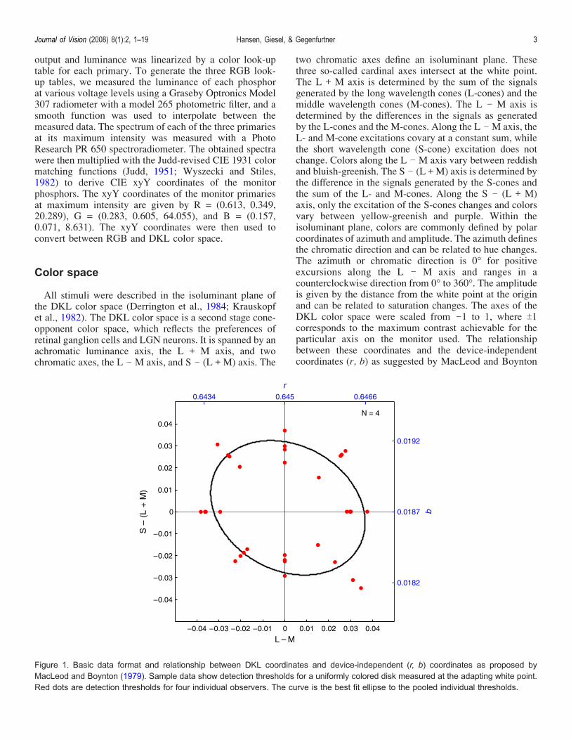
two chromatic axes define an isoluminant plane. Thesethree so-called cardinal axes intersect at the white point.The L + M axis is determined by the sum of the signalsgenerated by the long wavelength cones (L-cones) and themiddle wavelength cones (M-cones). The L j M axis isdetermined by the differences in the signals as generatedby the L-cones and the M-cones. Along the L j M axis, theL- and M-cone excitations covary at a constant sum, whilethe short wavelength cone (S-cone) excitation does notchange. Colors along the L j M axis vary between reddishand bluish-greenish. The S j (L + M) axis is determined bythe difference in the signals generated by the S-cones andthe sum of the L- and M-cones. Along the S j (L + M)axis, only the excitation of the S-cones changes and colorsvary between yellow-greenish and purple. Within theisoluminant plane, colors are commonly defined by polarcoordinates of azimuth and amplitude. The azimuth definesthe chromatic direction and can be related to hue changes.The azimuth or chromatic direction is 0- for positiveexcursions along the L j M axis and ranges in acounterclockwise direction from 0- to 360-. The amplitudeis given by the distance from the white point at the originand can be related to saturation changes. The axes of theDKL color space were scaled from j1 to 1, where T1corresponds to the maximum contrast achievable for theparticular axis on the monitor used. The relationshipbetween these coordinates and the device-independentcoordinates (r, b) as suggested by MacLeod and Boynton

Figure 1. Basic data format and relationship between DKL coordinates and device-independent (r, b) coordinates as proposed byMacLeod and Boynton (1979). Sample data show detection thresholds for a uniformly colored disk measured at the adapting white point.Red dots are detection thresholds for four individual observers. The curve is the best fit ellipse to the pooled individual thresholds.

Journal of Vision (2008) 8(1):2, 1–19 Hansen, Giesel, & Gegenfurtner 3

(1979) are depicted in Figure 1, with sample data showingdetection thresholds for a uniform disk at the white point,measured for four observers.

Stimuli

Three types of stimuli were used: uniform coloreddisks, digital photographs of fruits or vegetables, orsynthetic chromatic textures. All stimuli were displayedon top of a uniform background whose color defined theadaptation point.The main purpose of this study was to investigate

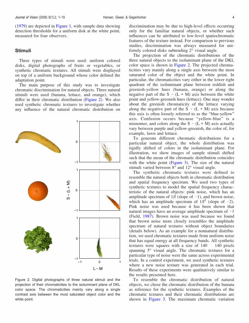
chromatic discrimination for natural objects. Three naturalstimuli were used (banana, lettuce, and orange), whichdiffer in their chromatic distribution (Figure 2). We alsoused synthetic chromatic textures to investigate whetherany influence of the natural chromatic distribution on

discrimination may be due to high-level effects occurringonly for the familiar natural objects, or whether suchinfluences can be attributed to low-level spatiochromaticfeatures of the texture instead. For comparison to previousstudies, discrimination was always measured for uni-formly colored disks subtending 2- visual angle.The projection of the chromatic distributions of the

three natural objects to the isoluminant plane of the DKLcolor space is shown in Figure 2. The projected chroma-ticities vary mainly along a single axis between the mostsaturated color of the object and the white point. Inparticular, the chromaticities vary either in the lower rightquadrant of the isoluminant plane between reddish andgreenish-yellow hues (banana, orange) or along thenegative part of the S j (L + M) axis between the whitepoint and yellow-greenish hues (lettuce). One may wonderabout the greenish chromaticity of the lettuce varyingalong the negative part of the S j (L + M) axis becausethis axis is often loosely referred to as the “blue-yellow”axis. Confusion occurs because “yellow-blue” is amisnomer, and colors along the S j (L + M) axis actuallyvary between purple and yellow-greenish, the color of, forexample, lawn and lettuce.To generate different chromatic distributions for a

particular natural object, the whole distribution wasrigidly shifted of colors in the isoluminant plane. Forillustration, we show images of sample stimuli shiftedsuch that the mean of the chromatic distribution coincideswith the white point (Figure 3). The size of the naturalstimuli varied between 8- and 12- visual angle.The synthetic chromatic textures were defined to

resemble the natural objects both in chromatic distributionand spatial frequency spectrum. We used two types ofsynthetic textures to model the spatial frequency charac-teristic of the natural objects: pink noise, which has anamplitude spectrum of 1/f (slope of j1), and brown noise,which has an amplitude spectrum of 1/f2 (slope of j2).Pink noise was used because it has been shown thatnatural images have an average amplitude spectrum of j1(Field, 1987). Brown noise was used because we foundthat brown noise more closely resembles the amplitudespectrum of natural textures without object boundaries(details below). As an example for a nonnatural distribu-tion, we used chromatic textures made from uniform noisethat has equal energy at all frequency bands. All synthetictextures were squares with a size of 140 � 140 pixelsspanning 5- visual angle. The chromatic textures for aparticular type of noise were the same across experimentaltrials. In a control experiment, we used synthetic textureswhere a new noise texture was generated in each trial.Results of these experiments were qualitatively similar tothe results presented here.To resemble the chromatic distribution of natural

objects, we chose the chromatic distribution of the bananaas reference for the synthetic textures. Examples of thechromatic textures and their chromatic distributions areshown in Figure 3. The maximum chromatic variation

Figure 2. Digital photographs of three natural stimuli and theprojection of their chromaticities to the isoluminant plane of DKLcolor space. The chromaticities mainly vary along a singlecontrast axis between the most saturated object color and thewhite point.

Journal of Vision (2008) 8(1):2, 1–19 Hansen, Giesel, & Gegenfurtner 4

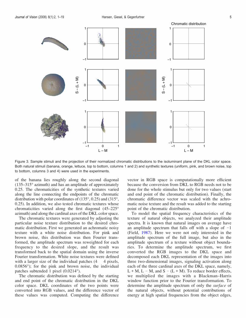
of the banana lies roughly along the second diagonal(135–315- azimuth) and has an amplitude of approximately0.25. The chromaticities of the synthetic textures variedalong the line connecting the endpoints of the chromaticdistribution with polar coordinates of (135-, 0.25) and (315-,0.25). In addition, we also tested chromatic textures whosechromaticities varied along the first diagonal (45–225-azimuth) and along the cardinal axes of the DKL color space.The chromatic textures were generated by adjusting the

particular noise texture distribution to the desired chro-matic distribution. First we generated an achromatic noisytexture with a white noise distribution. For pink andbrown noise, this distribution was then Fourier trans-formed, the amplitude spectrum was reweighted for eachfrequency to the desired slope, and the result wastransformed back to the spatial domain using the inverseFourier transformation. White noise textures were definedwith a larger size of the individual patches (4 � 4 pixels,0.0856-); for the pink and brown noise, the individualpatches subtended 1 pixel (0.0214-).The chromatic distribution was defined by the starting

and end point of the chromatic distribution in the DKLcolor space. DKL coordinates of the two points wereconverted into RGB values, and the difference vector ofthese values was computed. Computing the difference

vector in RGB space is computationally more efficientbecause the conversion from DKL to RGB needs not to bedone for the whole stimulus but only for two values (startand end point of the chromatic distribution). Finally, thechromatic difference vector was scaled with the achro-matic noise texture and the result was added to the startingpoint of the chromatic distribution.To model the spatial frequency characteristics of the

texture of natural objects, we analyzed their amplitudespectra. It is known that natural images on average havean amplitude spectrum that falls off with a slope of j1(Field, 1987). Here we were not only interested in theamplitude spectrum of the full image, but also in theamplitude spectrum of a texture without object bounda-ries. To determine the amplitude spectrum, we firstconverted the RGB images to the DKL space anddecomposed each DKL representation of the images intothree two-dimensional images, signaling activation alongeach of the three cardinal axes of the DKL space, namely,L + M, L j M, and S j (L + M). To reduce border effects,we multiplied the images with a Blackman–Harriswindow function prior to the Fourier transformation. Todetermine the amplitude spectrum of only the surface ofthe natural objects, without potential contributions ofenergy at high spatial frequencies from the object edges,

Figure 3. Sample stimuli and the projection of their normalized chromatic distributions to the isoluminant plane of the DKL color space.Both natural stimuli (banana, orange, lettuce, top to bottom, columns 1 and 2) and synthetic textures (uniform, pink, and brown noise, topto bottom, columns 3 and 4) were used in the experiments.

Journal of Vision (2008) 8(1):2, 1–19 Hansen, Giesel, & Gegenfurtner 5

we evaluated the amplitude spectra in a series of over-lapping cutouts. Each cutout subtended 30 � 30 pixelsand amplitude spectra were evaluated for cutouts at anypossible location where the cutout covered only thesurface of the object, without inclusion of any objectborders. The size of 30 � 30 pixels of the cutout waschosen as the maximum size that could be fitted into allobjects. The slope for each of the natural stimuli wasdetermined as the average slope of the amplitude spectraof all cutouts. The mean slope across all stimuli wasj1.93 T 0.20 SD for all three cardinal axes. This is steeperthan a slope around j1 usually found for natural imagesbecause we analyzed only the object surfaces without thehigh-spatial frequency information at the edges. Theaverage slope of the amplitude spectrum of the full imageswas in the normal range (j0.81 T 0.17 SD). We alsomeasured the slope of the amplitude spectrum for thesynthetic textures using 30 � 30 cutouts. By definition, theslopes should be 0 for white noise, j1 for pink noise, andj2 for brown noise. The average slopes measured within 30� 30 cutouts were in the desired range: slopes were forwhite noise 0.04 T 0.14 SD, for pink noise j1.04 T 0.15 SD,and for brown noise j2.32 T 0.16 SD.

Subjects

Four observers (C.H., D.P., M.G., and M.O.) participatedin the experiments. All observers except one of the authors(M.G.) were naive as to the purpose of the experiment. Allobservers were experienced psychophysical observers whohad participated in previous experiments.

Procedure

The procedure was similar to the one employed byKrauskopf and Gegenfurtner (1992). Observers wereseated in front of the monitor at a distance of 0.60 m ina dimly lit room and instructed to fixate the center of thescreen, which was uniformly colored. In each experimen-tal trial, four stimuli were presented for 500 ms in a 2 � 2arrangement. The bounding box of each stimulus had aconstant distance of 1- visual angle from the center of thescreen. Three of the presented stimuli were identical (teststimuli) whereas the fourth one (comparison stimulus)differed slightly in chromaticity. The position of thecomparison stimulus in the 2 � 2 arrangement wasrandomly varied in each trial. The observer’s task was toindicate the position of the comparison stimulus (odd oneout) by pressing the appropriate one of four buttons.Feedback was given after each response. For each testcolor, discrimination thresholds were measured in eightdifferent comparison directions (0-, 45-, 90-, 135-, 180-,225-, 270-, and 315-) relative to the mean chromaticity ofthe test stimulus. Test and comparison chromaticities werespecified in the isoluminant plane of the DKL color space.

The chromaticities of the comparison stimulus werevaried by a rigid shift of the whole chromatic distributionin the isoluminant plane in the comparison direction. Thistransformation shifts the mean of the distribution to thecomparison color but keeps the position of the chromatic-ities relative to the mean chromaticity constant. Theamount or amplitude of this shift necessary for a correctdiscrimination at 79% of the trials was determined using anadaptive double-random staircase procedure. After threeconsecutive correct responses, the comparison amplitudewas decreased; after an incorrect response, it was increased.In each session, one up- and one down-staircase for each ofthe eight comparison directions were randomly interleaved.Each staircase terminated after four reversals.Discrimination thresholds were measured under two

different conditions of adaptation, as defined by thechromaticity of the background. In the first condition,chromatic discrimination was measured at the adaptationpoint; in the second condition, discrimination was meas-ured at test locations away from the adaptation point.In the first condition, discrimination was investigated at

the location in color space to which the observer wasadapted; that is, the test color was the same as thebackground color (test amplitude of zero) and thecomparison stimuli were excursions from the chromaticityof the background. For the homogeneously colored disk,this condition corresponds to a detection task. For thenatural stimuli and the chromatic textures, the meanchromaticity of the stimuli was the same as the chroma-ticity of the background. Discrimination at nine differentadaptation points was investigated by changing the back-ground color. The adapting background color was eitherthe white point or one out of eight equally spaced colorsin the isoluminant plane. These eight colors all had thesame amplitude of 0.5, but different chromatic directionsof 0-, 45-, 90-, 135-, 180-, 225-, 270-, or 315-. In thiscondition, the mean chromaticity of the test stimuluscoincided with the chromaticity of the adaptation point.In the second regime, the background was always gray;

that is, the adaptation point was fixed at the white pointand the test stimuli were excursions from this point ineight test directions (0-, 45-, 90-, 135-, 180-, 225-, 270-,315-) with a test amplitude of 0.5. In this condition, themean chromaticity of all stimuli differed from thechromaticity of the adaptation point.

Data analysis

To determine thresholds, we pooled the observers’responses for the up- and the down-staircase for eachcomparison direction. Psychometric functions were fittedto the individual observer’s data using the psignifittoolbox for Matlab (Wichmann & Hill, 2001) to derive79% difference thresholds for each of the eight compar-ison directions. To summarize the data, we fitted ellipsesto the eight thresholds using a direct least squares

Journal of Vision (2008) 8(1):2, 1–19 Hansen, Giesel, & Gegenfurtner 6

procedure (Halı r & Flusser, 1998). As in previous studies(Poirson, Wandell, Varner, & Brainard, 1990), we foundthat the ellipses describe the data well. To account forsmall asymmetries, we allowed the centers of the ellipsesto vary. To obtain ellipses for data averaged acrossobservers, we fitted ellipses to the pooled thresholds ofall observers, as suggested by some authors as beingthe most robust method (Wyszecki & Fielder, 1971a;Wyszecki & Stiles, 1982; Xu, Yaguchi, & Shioiri, 2002).Alternatively, we fitted ellipses to the thresholds averagedacross observers. As a third alternative, we also fittedellipses to the thresholds of the individual observers andthen averaged across the parameters of ellipses. All ofthese methods provided similar results.To determine the reliability of the orientation of the

discrimination ellipses, we employed a bootstrap proce-dure similar to the method described by Alder (1981). Foreach threshold measured in the eight comparison direc-tions, 1,000 simulated thresholds were drawn from normaldistributions centered at the measured thresholds. Thestandard deviation of these distributions was estimated

from the bootstrap confidence intervals of each thresholdprovided by the psignifit toolbox for Matlab (Wichmann& Hill, 2001). Ellipses were then fitted to the simulatedthresholds and the 95% confidence interval for theorientation of the major axis was computed.

Results

The results are organized in two sections. In the firstsection, we present results for discrimination at theadaptation point; and in the second section, we presentresults for discrimination away from the adaptation point.

Discrimination at the adaptation point

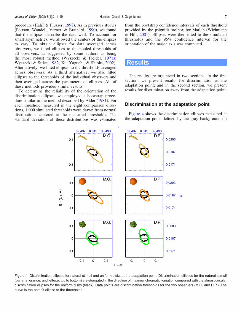
Figure 4 shows the discrimination ellipses measured atthe adaptation point defined by the gray background on

Figure 4. Discrimination ellipses for natural stimuli and uniform disks at the adaptation point. Discrimination ellipses for the natural stimuli(banana, orange, and lettuce, top to bottom) are elongated in the direction of maximal chromatic variation compared with the almost circulardiscrimination ellipses for the uniform disks (black). Data points are discrimination thresholds for the two observers (M.G. and D.P.). Thecurve is the best fit ellipse to the thresholds.

Journal of Vision (2008) 8(1):2, 1–19 Hansen, Giesel, & Gegenfurtner 7

which the stimuli were presented. Discrimination ellipsesfor two observers are shown for natural stimuli (banana,orange, and lettuce) and are compared with discriminationellipses obtained for a uniformly colored disk.The discrimination ellipses for all natural stimuli show

a distinct elongation different from the almost circularellipses obtained for the uniform disks. For example, theellipse for the banana shows a clear elongation along thesecond diagonal, which is the same direction along whichthe chromaticities of the banana vary most (Figure 3).Overall, the direction of the major axis of the ellipses forthe natural stimuli seems to follow the direction ofmaximal chromatic variation. This means that shifts ofthe chromatic distribution in directions where there wasalready considerable chromatic variation in the stimuluswere harder to detect than shifts in those directions wherethere was little variation in the stimulus. In contrast,thresholds for comparison directions away from thedirection of maximal variation were similar to those forthe uniformly colored disk.Next we measured chromatic discrimination at the

adaptation point with synthetic textures. The objective ofusing synthetic textures was twofold. First we wanted toisolate characteristic features of the natural stimuli toclarify whether the differences in threshold contours mightbe attributed to higher or lower level visual effects.Second, we wanted to investigate whether the observedelongation always follows the direction of maximalvariation in the stimulus. This can be tested with synthetictextures whose chromatic distribution can be rotated toarbitrary angles.In the first set of experiments, we used synthetic

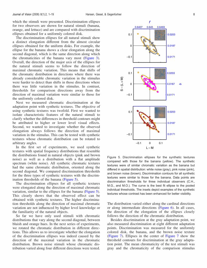
textures with spatial frequency distributions that resemblethe distributions found in natural objects (pink and brownnoise) as well as a distribution with a flat amplitudespectrum (white noise). All synthetic chromatic textureshad the same chromatic distribution, oriented along thesecond diagonal. We compared discrimination thresholdsfor the three types of synthetic textures with the discrim-ination thresholds of the banana (Figure 5).The discrimination ellipses for all synthetic textures

were elongated along the direction of maximal chromaticvariation, similar to the ellipses for the banana (Figure 5).This clearly shows that the observed effect can beobtained with synthetic textures. The higher discrimina-tion thresholds along the direction of maximal chromaticvariation are not influenced by higher level knowledge orthe familiarity of the natural objects.So far we have only used stimuli with chromatic

distributions that vary along the second diagonal, betweenbluish and orange hues. In the next series of experiments,we rotated the chromatic distribution in different direc-tions. This allows us to investigate whether the elongationof the discrimination ellipses was indeed caused by thedirection of the maximal variation in the chromaticdistribution. Brown noise stimuli whose chromatic dis-tribution varied along four different directions were tested.

The distribution varied either along the cardinal directionsor along intermediate directions (Figure 6). In all cases,the direction of the elongation of the ellipses closelyfollows the direction of the chromatic distribution.Besides discrimination at the gray adaptation point, we

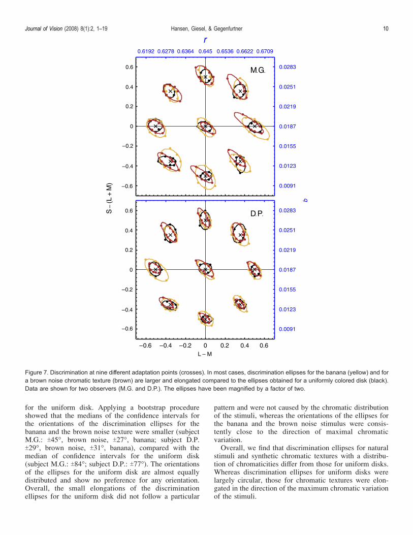
also measured discrimination at eight different adaptationpoints. Discrimination was measured for the uniformlycolored disk, the banana, and the brown noise texture(Figure 7). Ellipses in the center of Figure 7 show thethreshold contours for discrimination at the gray adapta-tion point. The mean chromaticity of the test stimuli wasgray and the chromaticity of the comparison stimulus

Figure 5. Discrimination ellipses for the synthetic texturescompared with those for the banana (yellow). The synthetictextures were of similar chromatic variation as the banana butdiffered in spatial distribution: white noise (gray), pink noise (pink),and brown noise (brown). Discrimination contours for all synthetictextures were similar to those for the banana. Data points arediscrimination thresholds for three individual observers (C.H.,M.G., and M.O.). The curve is the best fit ellipse to the pooledindividual thresholds. The insets depict examples of the synthetictextures whose contrast has been enhanced for better visibility.

Journal of Vision (2008) 8(1):2, 1–19 Hansen, Giesel, & Gegenfurtner 8

was an excursion from the adaptation point in one ofeight comparison directions. For the eight differentadaptation points, the mean chromaticities of the teststimuli were identical to the location indicated by thecrosses in Figure 7. We found at most adaptation points apattern of results similar to the results at the grayadaptation point: Discrimination ellipses for the bananaand for a brown noise chromatic texture were larger andelongated compared to the ellipses obtained for auniformly colored disk.To further quantify the data, we determined the area and

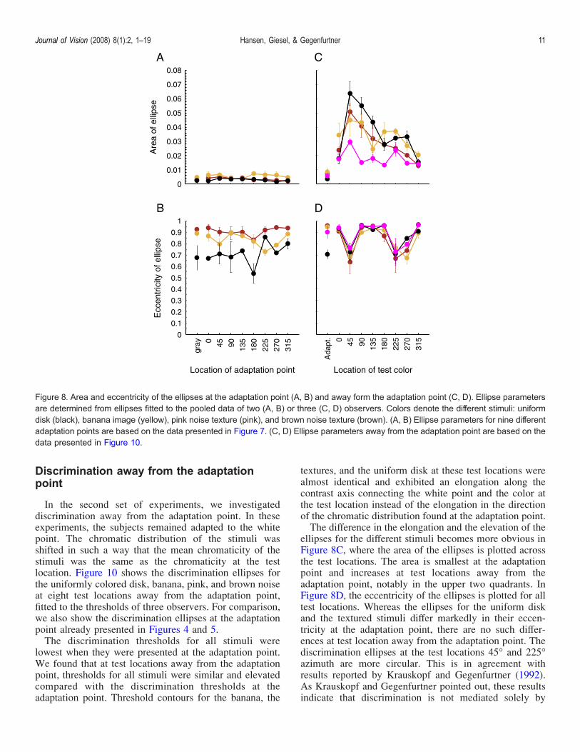
the eccentricity of each discrimination ellipse. We plottedthe area and the eccentricity of the ellipses, averagedacross subjects, for each of the nine adaptation points.Discriminability, quantified as the area of the discrim-ination ellipse, was almost constant for all adaptationpoints and all stimuli (Figure 8A). In contrast to thealmost identical area for all stimuli, the eccentricitiesdiffered considerably for the different stimuli (Figure 8B):For all but one adaptation point (225-), the eccentricity of

the discrimination ellipses for the banana and the brownnoise texture was higher than for the uniform disks. Thisshows that discrimination at the adaptation point isdifferent for chromatic textures compared to uniformdisks, largely independent of the adapting color.Figures 7 and 8A show that not only the chromatic

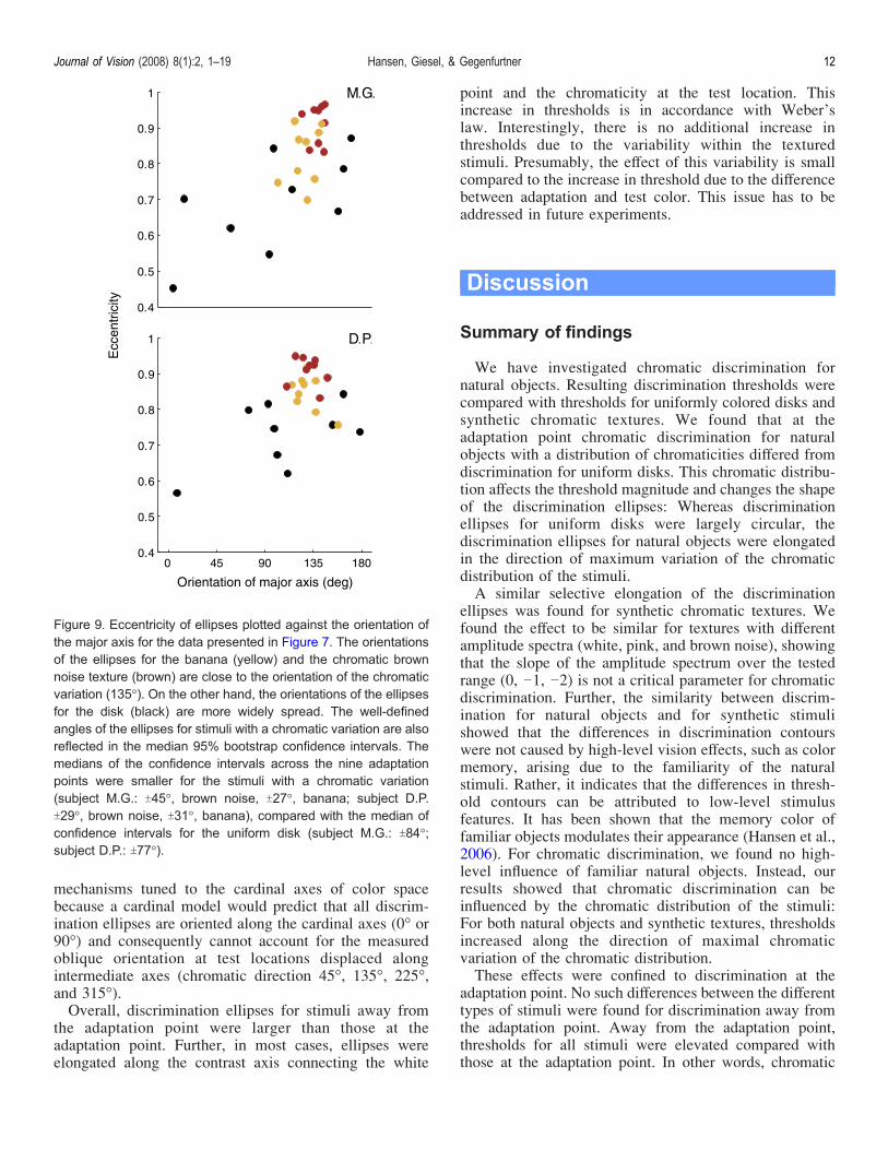
textures had elongated discrimination ellipses of ratherhigh eccentricity, but that elongated ellipses also occur forthe uniform disk, in particular at one adaptation point(225-). To further analyze whether only the ellipses forthe chromatic textures show a distinctive elongation in thedirection of the chromatic distribution, we plot in Figure 9eccentricity versus orientation of the ellipses. Data areshown for the individual observers’ ellipses for theadaptation points presented in Figure 7.The orientations of the major axis of the ellipses for the

banana and the brown noise stimuli clustered between120- and 135- azimuth close to the direction of maximalvariation of the chromatic distribution. The orientationsfor the chromatic textures were better defined than those

Figure 6. Discrimination ellipses for brown noise stimuli are elongated in the direction of maximal chromatic variation. Chromatic directionsof 0- (top left), 135- (top right), 90- (bottom left), and 45- (bottom right) were tested, depicted by the top left inset. Data points arediscrimination thresholds for three individual observers (C.H., M.G., and M.O.). Format is identical to the previous figure.

Journal of Vision (2008) 8(1):2, 1–19 Hansen, Giesel, & Gegenfurtner 9

for the uniform disk. Applying a bootstrap procedureshowed that the medians of the confidence intervals forthe orientations of the discrimination ellipses for thebanana and the brown noise texture were smaller (subjectM.G.: T45-, brown noise, T27-, banana; subject D.P.T29-, brown noise, T31-, banana), compared with themedian of confidence intervals for the uniform disk(subject M.G.: T84-; subject D.P.: T77-). The orientationsof the ellipses for the uniform disk are almost equallydistributed and show no preference for any orientation.Overall, the small elongations of the discriminationellipses for the uniform disk did not follow a particular

pattern and were not caused by the chromatic distributionof the stimuli, whereas the orientations of the ellipses forthe banana and the brown noise stimulus were consis-tently close to the direction of maximal chromaticvariation.Overall, we find that discrimination ellipses for natural

stimuli and synthetic chromatic textures with a distribu-tion of chromaticities differ from those for uniform disks.Whereas discrimination ellipses for uniform disks werelargely circular, those for chromatic textures were elon-gated in the direction of the maximum chromatic variationof the stimuli.

Figure 7. Discrimination at nine different adaptation points (crosses). In most cases, discrimination ellipses for the banana (yellow) and fora brown noise chromatic texture (brown) are larger and elongated compared to the ellipses obtained for a uniformly colored disk (black).Data are shown for two observers (M.G. and D.P.). The ellipses have been magnified by a factor of two.

Journal of Vision (2008) 8(1):2, 1–19 Hansen, Giesel, & Gegenfurtner 10

Discrimination away from the adaptationpoint

In the second set of experiments, we investigateddiscrimination away from the adaptation point. In theseexperiments, the subjects remained adapted to the whitepoint. The chromatic distribution of the stimuli wasshifted in such a way that the mean chromaticity of thestimuli was the same as the chromaticity at the testlocation. Figure 10 shows the discrimination ellipses forthe uniformly colored disk, banana, pink, and brown noiseat eight test locations away from the adaptation point,fitted to the thresholds of three observers. For comparison,we also show the discrimination ellipses at the adaptationpoint already presented in Figures 4 and 5.The discrimination thresholds for all stimuli were

lowest when they were presented at the adaptation point.We found that at test locations away from the adaptationpoint, thresholds for all stimuli were similar and elevatedcompared with the discrimination thresholds at theadaptation point. Threshold contours for the banana, the

textures, and the uniform disk at these test locations werealmost identical and exhibited an elongation along thecontrast axis connecting the white point and the color atthe test location instead of the elongation in the directionof the chromatic distribution found at the adaptation point.The difference in the elongation and the elevation of the

ellipses for the different stimuli becomes more obvious inFigure 8C, where the area of the ellipses is plotted acrossthe test locations. The area is smallest at the adaptationpoint and increases at test locations away from theadaptation point, notably in the upper two quadrants. InFigure 8D, the eccentricity of the ellipses is plotted for alltest locations. Whereas the ellipses for the uniform diskand the textured stimuli differ markedly in their eccen-tricity at the adaptation point, there are no such differ-ences at test location away from the adaptation point. Thediscrimination ellipses at the test locations 45- and 225-azimuth are more circular. This is in agreement withresults reported by Krauskopf and Gegenfurtner (1992).As Krauskopf and Gegenfurtner pointed out, these resultsindicate that discrimination is not mediated solely by

Figure 8. Area and eccentricity of the ellipses at the adaptation point (A, B) and away form the adaptation point (C, D). Ellipse parametersare determined from ellipses fitted to the pooled data of two (A, B) or three (C, D) observers. Colors denote the different stimuli: uniformdisk (black), banana image (yellow), pink noise texture (pink), and brown noise texture (brown). (A, B) Ellipse parameters for nine differentadaptation points are based on the data presented in Figure 7. (C, D) Ellipse parameters away from the adaptation point are based on thedata presented in Figure 10.

Journal of Vision (2008) 8(1):2, 1–19 Hansen, Giesel, & Gegenfurtner 11

mechanisms tuned to the cardinal axes of color spacebecause a cardinal model would predict that all discrim-ination ellipses are oriented along the cardinal axes (0- or90-) and consequently cannot account for the measuredoblique orientation at test locations displaced alongintermediate axes (chromatic direction 45-, 135-, 225-,and 315-).Overall, discrimination ellipses for stimuli away from

the adaptation point were larger than those at theadaptation point. Further, in most cases, ellipses wereelongated along the contrast axis connecting the white

point and the chromaticity at the test location. Thisincrease in thresholds is in accordance with Weber’slaw. Interestingly, there is no additional increase inthresholds due to the variability within the texturedstimuli. Presumably, the effect of this variability is smallcompared to the increase in threshold due to the differencebetween adaptation and test color. This issue has to beaddressed in future experiments.

Discussion

Summary of findings

We have investigated chromatic discrimination fornatural objects. Resulting discrimination thresholds werecompared with thresholds for uniformly colored disks andsynthetic chromatic textures. We found that at theadaptation point chromatic discrimination for naturalobjects with a distribution of chromaticities differed fromdiscrimination for uniform disks. This chromatic distribu-tion affects the threshold magnitude and changes the shapeof the discrimination ellipses: Whereas discriminationellipses for uniform disks were largely circular, thediscrimination ellipses for natural objects were elongatedin the direction of maximum variation of the chromaticdistribution of the stimuli.A similar selective elongation of the discrimination

ellipses was found for synthetic chromatic textures. Wefound the effect to be similar for textures with differentamplitude spectra (white, pink, and brown noise), showingthat the slope of the amplitude spectrum over the testedrange (0, j1, j2) is not a critical parameter for chromaticdiscrimination. Further, the similarity between discrim-ination for natural objects and for synthetic stimulishowed that the differences in discrimination contourswere not caused by high-level vision effects, such as colormemory, arising due to the familiarity of the naturalstimuli. Rather, it indicates that the differences in thresh-old contours can be attributed to low-level stimulusfeatures. It has been shown that the memory color offamiliar objects modulates their appearance (Hansen et al.,2006). For chromatic discrimination, we found no high-level influence of familiar natural objects. Instead, ourresults showed that chromatic discrimination can beinfluenced by the chromatic distribution of the stimuli:For both natural objects and synthetic textures, thresholdsincreased along the direction of maximal chromaticvariation of the chromatic distribution.These effects were confined to discrimination at the

adaptation point. No such differences between the differenttypes of stimuli were found for discrimination away fromthe adaptation point. Away from the adaptation point,thresholds for all stimuli were elevated compared withthose at the adaptation point. In other words, chromatic

Figure 9. Eccentricity of ellipses plotted against the orientation ofthe major axis for the data presented in Figure 7. The orientationsof the ellipses for the banana (yellow) and the chromatic brownnoise texture (brown) are close to the orientation of the chromaticvariation (135-). On the other hand, the orientations of the ellipsesfor the disk (black) are more widely spread. The well-definedangles of the ellipses for stimuli with a chromatic variation are alsoreflected in the median 95% bootstrap confidence intervals. Themedians of the confidence intervals across the nine adaptationpoints were smaller for the stimuli with a chromatic variation(subject M.G.: T45-, brown noise, T27-, banana; subject D.P.T29-, brown noise, T31-, banana), compared with the median ofconfidence intervals for the uniform disk (subject M.G.: T84-;subject D.P.: T77-).

Journal of Vision (2008) 8(1):2, 1–19 Hansen, Giesel, & Gegenfurtner 12

discrimination is best at the adaptation points, in agreementwith earlier studies (Krauskopf & Gegenfurtner, 1992).Highest thresholds were measured at the test location with45- azimuth (Figure 10). In general, thresholds in theupper two quadrants were elevated compared with thresh-olds in the lower two quadrants, indicating that colorvision is less sensitive at discriminating bluish hues andhues along the purple line.Discrimination ellipses for stimuli with a chromatic

distribution were determined by the amplitude and thedirection of both the chromatic distribution and the shiftaway from the adaptation point. An increase of thedistance between the adaptation point and the test locationelevated discrimination thresholds. Depending on theamplitude of the shift, this threshold elevation was sobig that it masked the effect of the chromatic distribution.Another reason that we have not found any effect of the

chromatic distribution away from the adaptation pointmight be due to the particular choice of the chromatictexture, as discussed in the following.

No effect of the chromatic distribution awayfrom the adaptation point?

For chromatic discrimination away from the adaptationpoint, we found no effect of the chromatic texture, whichmight be partly caused by the particular orientation of thechromatic distributions we employed. In our experiments,the variation of the chromatic distribution was along thesecond diagonal, from 135- to 315-. For shifts of the testcolor in these directions, ellipses for homogeneous disksalready had the largest variation along this axis, and theadditional chromatic variation of the stimulus may

Figure 10. Discrimination away from the adaptation point. Ellipses for a uniformly colored disk (black), a digitized banana image (yellow),and a pink (pink) and brown (brown) noise textures at the gray adaptation point and at eight test locations away from the adaptation point.The crosses indicate the chromaticity at the test location. Data points are discrimination thresholds for three individual observers (C.H.,M.G., and M.O.). The curve is the best fit ellipse to the pooled individual thresholds.

Journal of Vision (2008) 8(1):2, 1–19 Hansen, Giesel, & Gegenfurtner 13

consequently be masked. On the other hand, one mayexpect effects for shifts of the test color orthogonal to thechromatic distribution of the stimulus, that is, along themain diagonal. However, discrimination ellipses forhomogeneous disks were already relatively large androunded away from the adaptation point along thesedirections (45- and 225-). Following this argument,effects away from the adaptation point should occur forchromatic distributions varying along the first diagonal attest locations shifted along the second diagonal. In a pilotstudy, we have found evidence for effects away from theadaptation point.Given that the main purpose of our study was to

determine discrimination thresholds for natural stimuli,and given that these stimuli were rather limited in theirchromatic variation, we cannot draw any firm conclusionsabout the interaction of the chromatic variation withineach test object with the variation due to changes inadaptation. Therefore, in future studies using synthetictextures, we plan to investigate the interaction betweenorientation and amplitude of the chromatic distributionand the test locations in more detail.

Comparison to previous work

Traditionally, chromatic discrimination has beenstudied with uniform, homogeneous colors (Brown &MacAdam, 1949; MacAdam, 1942), and only a singleprevious study has investigated chromatic discriminationof stimuli having a chromatic distribution (te Pas &Koenderink, 2004). In their study, te Pas and Koenderink(2004) investigated discrimination for different chromaticdistributions that were specified in RGB space. Observershad to report the orientation of two half-fields of differenttextures, which could be oriented either horizontally orvertically. They found higher discrimination thresholdsfor textured stimuli than for uniform stimuli. Thresholdsdiffered for different test colors of the stimuli, but thesedifferences were attributed to variations in luminancebetween the stimuli. In general, the results of te Pas andKoenderink are difficult to compare to our findingsbecause the stimuli were specified in RGB space, whichconfounds luminance and pure chromatic variation.Further, thresholds were measured only in one direction,and the chromatic distribution was not only rigidly shiftedin color space, as in this study. Instead, the extent of thechromatic distribution was changed during the thresholdmeasurement. It was either broadened to white (i.e., in adirection of the highest luminance of the monitorprimaries), to model changes due to specular reflectance,or rotated, to model changes in material.A more indirect effect of the chromatic distribution on

discrimination was investigated by Zaidi et al. (1998).Observers adapted either to a uniform background or to avariegated background made of randomly arrangedsquares having one of two colors along the cardinal

L j M axis. After the adaptation interval, chromaticdiscrimination was measured. The screen was dividedeither vertically or horizontally, resulting in homogene-ously colored halves that differed in chromaticities. Thechromaticities were picked from the endpoints of variousintervals on the L j M axis that differed in length but werecentered at a fixed point. When the observers were adaptedto a textured background, thresholds were higher thanwhen they were adapted to a uniform background. Thresh-olds for the textured background were highest when thetest color was the same as the spatial average of thebackground textures and decreased when the test colormoved away from the average. For uniform adapting fields,discrimination was best at the adaptation point andincreased with increasing distance of the test chromaticityfrom the adaptation point. In our study, we used ahomogeneous background and measured discriminationfor chromatic textures. We find that discrimination at theadaptation point was determined by the amplitude and thedirection of the chromatic variation.Various authors have studied the segmentation of

chromatic textures (D’Zmura & Knoblauch, 1998;Gegenfurtner & Kiper, 1992; Goda & Fujii, 2001; Hansen& Gegenfurtner, 2006; Li & Lennie, 1997; Webster &Mollon, 1991, 1994). In these studies, textured targetswere embedded in a textured background and not spatiallyseparated by a homogeneous background, as in this study.Also, previous studies differ in their schemes used tomodulate the target texture compared to the backgroundtexture. Despite these differences, all studies found thatthresholds are elevated considerably when backgroundand target distributions were modulated along similardirections in color space. In agreement with thesefindings, we have found the largest threshold elevationswhen the chromatic distribution was shifted along the axisof maximal variation of the chromaticities in the stimulus,such that the chromaticities of the test and the comparisonstimuli mostly varied along the same direction. Because ofthe different stimuli that vary both in layout and definitionof the chromatic distributions, other aspects are difficult tocompare across studies.

Models and mechanisms for chromatictexture discrimination

Unfortunately, none of the elaborate models that areavailable for spatial vision extends to the color domain.Typical “back-pocket-models” for spatial pattern sensitiv-ity contain three main stages (Bergen & Adelson, 1988;Bergen & Landy, 1991; Watson & Ahumada, 1989;Wilson & Reagan, 1984): At the first stage, the image isconvolved with a set of filters that differ in orientation andscale. At the second stage, these filters undergo a staticnonlinearity. Finally, noise may be added to the non-linearly transformed response of the filter bank, andresponses are fed into a final decision stage. Such models

Journal of Vision (2008) 8(1):2, 1–19 Hansen, Giesel, & Gegenfurtner 14

are based on a wide variety of experimental data that havebeen replicated in many different laboratories understandardized conditions (Carney et al., 1999, 2000; Chen& Tyler, 2000; Klein, 1993; Watson, 2000; Watson &Ahumada, 2005; Watson & Ramirez, 1999). These modelspredict performance in simple luminance detection anddiscrimination experiments, as well as for complex texturepatterns.In the color domain, discrimination data have been

frequently obtained under highly different conditions, andthe results are presented in many different color spaces.Although it is possible, in principle, to convert betweendifferent color spaces, there are other aspects such as thesampling of the stimuli that make it difficult to comparesuch data.Existing models of chromatic difference prediction

often transform the image into an opponent color spacewith three channels (black–white, red–green, yellow–blue), sometimes in multiple spatial frequencies andorientations, and then compute the point-by-point differ-ence between a test and a reference image for two-dimensional planes in all channels. In the next step, thesedifference planes may be combined to a single two-dimensional difference image or a single differencenumber (Daly, 1993; Lovell, Parraga, Troscianko,Ripamonti, & Tolhurst, 2006; Zhang & Wandell, 1996,1998). The common feature of these models is the stagewhere a local, point-by-point difference is computed. Forexample, the spatial extension of CIE Lab into S-CIELAB(Zhang & Wandell, 1996, 1998) uses a spatial blurring ofthree color-opponent planes and then computes the pixelwise difference between images. Another class of modelsstarts with a number of global image descriptions, such ascolor histograms or Fourier spectra. Image differences arethen determined based on the difference in these globaldescriptors. Models of this type are frequently used in thedomain of content-based image retrieval to determinedifferences between images (e.g., Neumann&Gegenfurtner,2006). These models were designed to globally evaluatesuprathreshold differences and may not be ideally suitedfor evaluating threshold-level differences between smalltextured patches. A particular subclass of global modelsmay be better suited, which have been proposed to predictdetection and discrimination thresholds for patterns thatvary in color or luminance (Chen, Foley, & Brainard,2000; Goda & Fuji, 2001; Hansen & Gegenfurtner, 2006).These models first compute the global response of a setof chromatic detection mechanisms to the image chroma-ticities. Mechanism responses are computed for twoimages, and the response difference is used as a measureof discriminability. Whereas global models leave out thespatial aspects of the stimuli, local models take the spatialand chromatic aspects into account, but not the second-order color statistics of the chromatic distributions of thestimuli.As outlined above, for chromatic texture discrimination,

one may distinguish between two different types of

conceptual models, which are based on either local orglobal processing. Local models imply that thresholds aredetermined by local information and not from thechromatic distribution. Global models, on the other hand,assume that observers cannot precisely match the spatiallocations between any two images, and that the globalchromatic distribution determines discriminability. Globalmodels are in accordance with findings that chromaticdiscrimination across eye movements is poor (Sachtler &Zaidi, 1992). In the following, we argue that globalmodels of chromatic texture discrimination are bettersuited to account for the effect of the chromaticdistribution on discrimination as studied in the presentarticle.In local models, discrimination thresholds are deter-

mined from the local comparison of matched individualelements in the texture. In global models, spatial reso-lution and localization of individual texture elements arepoor, and discrimination depends on the amount ofoverlap between the chromatic distributions (as could beformalized by the Mahalanobis distance). Both types ofconceptual models make fundamentally different predic-tions about how the chromatic distribution in a chromatictexture influences discrimination. In local models, twotextures could be discriminated if two matching localpatches are sufficiently different, no matter how differentall other patches in the stimulus are and how thechromaticities of these patches are distributed. Conse-quently, for local models, the chromatic distribution,which is a global property, does not affect discrimination.Note that a spatial blurring as often used in local modelsdoes not take the distribution into account, as it only shiftsthe response toward the mean of the distribution. In globalmodels, on the other hand, two textures can be discrimi-nated when the two distributions are sufficiently different,that is, when there are many colors in the comparisonstimulus that are not present in the test stimulus. Likewise,global models predict that two textures cannot bediscriminated if the individual patches are drawn fromlargely overlapping chromatic distributions, even if thechromatic contrast between any two matching patches isthe same above discrimination threshold. The results ofthis study provide evidence for a global model: Observerscannot match individual spatial locations of, for example,the test banana to the comparison banana. Instead themeasured threshold elevation depends on the chromaticdistribution and is largest along the direction of maximalchromatic variation, as predicted by global models.The global model can be detailed in terms of responses

of a set of higher order mechanisms to the stimulus. Forillustration, consider the response of a set of higher ordermechanisms to a comparison banana which is shifted bythe same amount % either along or orthogonal to thedirection of maximal chromatic variation (Figure 11).The distribution of responses for the mechanism tuned tothe “banana direction” will have a mean 2 and standarddeviation sigma A, and the distribution of the responses to

Journal of Vision (2008) 8(1):2, 1–19 Hansen, Giesel, & Gegenfurtner 15

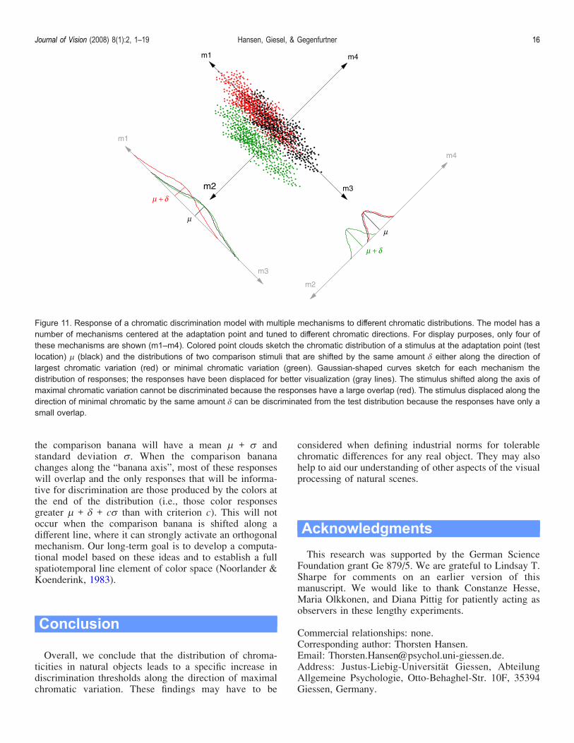
the comparison banana will have a mean 2 + A andstandard deviation A. When the comparison bananachanges along the “banana axis”, most of these responseswill overlap and the only responses that will be informa-tive for discrimination are those produced by the colors atthe end of the distribution (i.e., those color responsesgreater 2 + % + cA than with criterion c). This will notoccur when the comparison banana is shifted along adifferent line, where it can strongly activate an orthogonalmechanism. Our long-term goal is to develop a computa-tional model based on these ideas and to establish a fullspatiotemporal line element of color space (Noorlander &Koenderink, 1983).

Conclusion

Overall, we conclude that the distribution of chroma-ticities in natural objects leads to a specific increase indiscrimination thresholds along the direction of maximalchromatic variation. These findings may have to be

considered when defining industrial norms for tolerablechromatic differences for any real object. They may alsohelp to aid our understanding of other aspects of the visualprocessing of natural scenes.

Acknowledgments

This research was supported by the German ScienceFoundation grant Ge 879/5. We are grateful to Lindsay T.Sharpe for comments on an earlier version of thismanuscript. We would like to thank Constanze Hesse,Maria Olkkonen, and Diana Pittig for patiently acting asobservers in these lengthy experiments.

Commercial relationships: none.Corresponding author: Thorsten Hansen.Email: Thorsten.Hansen@psychol.uni-giessen.de.Address: Justus-Liebig-Universitat Giessen, AbteilungAllgemeine Psychologie, Otto-Behaghel-Str. 10F, 35394Giessen, Germany.

Figure 11. Response of a chromatic discrimination model with multiple mechanisms to different chromatic distributions. The model has anumber of mechanisms centered at the adaptation point and tuned to different chromatic directions. For display purposes, only four ofthese mechanisms are shown (m1–m4). Colored point clouds sketch the chromatic distribution of a stimulus at the adaptation point (testlocation) 2 (black) and the distributions of two comparison stimuli that are shifted by the same amount % either along the direction oflargest chromatic variation (red) or minimal chromatic variation (green). Gaussian-shaped curves sketch for each mechanism thedistribution of responses; the responses have been displaced for better visualization (gray lines). The stimulus shifted along the axis ofmaximal chromatic variation cannot be discriminated because the responses have a large overlap (red). The stimulus displaced along thedirection of minimal chromatic by the same amount % can be discriminated from the test distribution because the responses have only asmall overlap.

Journal of Vision (2008) 8(1):2, 1–19 Hansen, Giesel, & Gegenfurtner 16

References

Alder, C. (1981). A Monte Carlo method for thevalidation of discrimination ellipse data. Journal ofthe Society of Dyers and Colourists, 97, 514–517.

Bergen, J. R., & Adelson, E. H. (1988). Early vision andtexture perception. Nature, 333, 363–364. [PubMed]

Bergen, J. R., & Landy, M. S. (1991). Computationalmodeling of visual texture segregation. In M. S.Landy, & J. A. Movshon (Eds.), Computationalmodels of visual processing. Cambridge, MA: MITPress.

Boynton, R. M., & Kambe, N. (1980). Chromatic differ-ence steps of moderate size measured along theoret-ically critical axes. Color Research and Application,5, 13–23.

Brown, W. R. (1957). Color discrimination of twelveobservers. Journal of the Optical Society of America,47, 137–143. [PubMed]

Brown, W. R., & MacAdam, D. L. (1949). Visualsensitivities to combined chromaticity and luminancedifferences. Journal of the Optical Society of Amer-ica, 39, 808–834.

Carney, T., Klein, S. A., Tyler, C. W., Silverstein, A. D.,Beutter, B., Levi, D., et al. (1999). The developmentof an image/threshold database for designing andtesting human vision models. In B. Rogowitz, &T. Pappas (Eds.), Human vision, visual processing, anddigital display IV (vol. 3644, pp. 542–551). Belling-ham, WA: SPIE.

Carney, T., Tyler, C. W., Watson, A. B., Makous, W.,Beutter, B., Chen, C.-C., et al. (2000). ModelFest:Year one results and plans for future years. InB. Rogowitz, & T. Pappas (Eds.), Human vision,visual processing, and digital display V (vol. 3959,pp. 140–151). Bellingham, WA: SPIE.

Chen, C.-C., Foley, J. M., & Brainard, D. H. (2000).Detection of chromoluminance patterns on chromo-luminance pedestals II: Model. Vision Research, 40,789–803. [PubMed]

Chen, C.-C., & Tyler, C. W. (2000). ModelFest: Imagingthe underlying channel structure. In B. Rogowitz, &T. Pappas (Eds.), Human vision, visual processing,and digital display V (vol. 3959, pp. 152–159).Bellingham, WA: SPIE.

CIE (1978), Recommendations on uniform color spaces,color-difference equations, psychometric color terms.Supplement No. 2 of CIE Publ. No. 15 (E-1.3.1)1971, Bureau Central de la CIE, Paris, 1978.

CIE (1998). The CIE 1997 Interim Colour AppearanceModel (Simple Version), CIECAM97s (Publication116–198). Paris: Bureau Central de la CIE.

CIE (2004). A Colour Appearance Model for ColourManagement Systems: CIECAM02 (Publication 159).Paris: Bureau Central de la CIE.

Daly, S. (1993). The visible difference predictor: Analgorithm for the assessment of image fidelity. InA. B. Watson (Ed.), Digital images and humanvision (pp. 179–206). Cambridge, MA: MIT Press.

Derrington, A. M., Krauskopf, J., & Lennie, P. (1984).Chromatic mechanisms in lateral geniculate nucleus ofmacaque. The Journal of Physiology, 357, 241–265.[PubMed] [Article]

D’Zmura, M., & Knoblauch, K. (1998). Spectral band-width for the detection of color. Vision Research, 38,3117–3128. [PubMed]

Fairchild, M. D. (1998). Color appearance models. Read-ing, MA: Addison-Wesley.

Field, D. J. (1987). Relations between the statistics ofnatural images and the response properties of corticalcells. Journal of the Optical Society of America A,Optics and image science, 4, 2379–2394. [PubMed]

Gegenfurtner, K. R., & Kiper, D. C. (1992). Contrastdetection in luminance and chromatic noise. Journalof the Optical Society of America A, Optics and imagescience, 9, 1880–1888. [PubMed]

Goda, N., & Fujii, M. (2001). Sensitivity to modulation ofcolor distribution in multicolored textures. VisionResearch, 41, 2475–2485. [PubMed]

Godlove, I. H. (1952). Near-circular Adams chromaticitydiagrams. Journal of the Optical Society of America,42, 204–212.

Halı r R., & Flusser J. (1998). Numerically stable directleast squares fitting of ellipses. In Proceedings of the6th International Conference in Central Europe onComputer Graphics and Visualization (pp. 125–132).WSCG ’98. CZ, Plzen.

Hansen, T., & Gegenfurtner, K. R. (2006). Higher levelchromatic mechanisms for image segmentation. Jour-nal of Vision, 6(3):5, 239–259, http://journalofvision.org/6/3/5/, doi:10.1167/6.3.5. [PubMed] [Article]

Hansen, T., Olkkonen,M.,Walter, S., &Gegenfurtner, K. R.(2006). Memory modulates color appearance. NatureNeuroscience, 9, 1367–1368. [PubMed]

Hillis, J. M., & Brainard, D. H. (2005). Do commonmechanisms of adaptationmediate color discriminationand appearance? Uniform backgrounds. Journal of theOptical Society of America A, Optics, image science,and vision, 22, 2090–2106. [PubMed] [Article]

Huertas, R., Melgosa, M., & Oleari, C. (2006). Perform-ance of a color-difference formula based on OSA-UCS space using small–medium color differences.Journal of the Optical Society of America A, Optics,image science, and vision, 23, 2077–2084. [PubMed]

Journal of Vision (2008) 8(1):2, 1–19 Hansen, Giesel, & Gegenfurtner 17

Judd, D. B. (1951). Report of U. S. secretariat committeeon colorimetry and artificial daylight. In Proceedingsof the Twelfth Session of the CIE, Stockholm. Paris:Bureau Central de la CIE.

Kawamoto, K., Inamura, T., & Shioiri, S. (2003). Colordiscrimination characteristics depending on the back-ground color in the (L, M) plane of a cone space.Optical Review, 10, 391–397.

Kiener, S. (1997). On the relationship between two typesof effects caused by color adaptation: Changes incolor appearance and color discriminability. Journalof Mathematical Psychology, 41, 107–121.

Klein, S. A. (1993). Image quality and image compres-sion: A psychophysicist’s viewpoint. In A. B. Watson(Ed.), Digital images and human vision (pp. 73–88).Cambridge, MA: MIT Press.

Krauskopf, J., & Gegenfurtner, K. (1992). Color dis-crimination and adaptation. Vision Research, 32,2165–2175. [PubMed]

Krauskopf, J., Williams, D. R., & Heeley, D. W. (1982).Cardinal directions of color space. Vision Research,22, 1123–1131. [PubMed]

Li, A., & Lennie, P. (1997). Mechanisms underlyingsegmentation of colored textures. Vision Research,37, 83–97. [PubMed]

Loomis, J. M., & Berger, T. (1979). Effects of chromaticadaptation on color discrimination and color appear-ance. Vision Research, 19, 891–901. [PubMed]

Lovell, P. G., Parraga, C. A., Troscianko, T., Ripamonti, C.,& Tolhurst, D. J. (2006). Evaluation of a multiscalecolor model for visual difference prediction. ACMTransactions on Applied Perception, 3, 155–178.

Luo, M. R., Cui, G., & Li, C. (2006). Uniform colourspaces based on CIECAM02 colour appearancemodel. Color Research and Application, 31, 320–330.

MacAdam, D. L. (1942). Visual sensitivities to colordifferences in daylight. Journal of the Optical Societyof America, 32, 247–274.

MacAdam, D. L. (1944). On the geometry of color space.Journal of the Franklin Institute, 238, 195–210.

MacLeod, D. I., & Boynton, R. M. (1979). Chromaticitydiagram showing cone excitation by stimuli of equalluminance. Journal of the Optical Society of America,69, 1183–1186. [PubMed]

Miyahara, E, Smith, V. C., & Pokorny, J. (1993). Howsurround affect chromaticity discrimination. Journalof the Optical Society of America A, Optics andimage science, 69, 1183–1186. [PubMed]

Moon, P., & Spencer, D. E. (1943). Metric for colorspace. Journal of the Optical Society of America, 33,260–269.

Moroney, N., Fairchild, M. D., Hunt, R. W. G., Li, C.,Luo, M. R., & Newmann, T. (2002). The CIECAM02Color Appearance Model. In Proceedings of theTenth Color Imaging Conference: Color Science,Systems and Applications (pp. 23–27).

Neumann, D., & Gegenfurtner, K. R. (2006). Imageretrieval and perceptual similarity. ACM Transactionson Applied Perception, 3, 31–47.

Newhall, S. M., Nickerson D., & Judd D. B. (1943). Finalreport of the O. S. A. subcommittee on spacing of theMunsell colors. Journal of the Optical Society ofAmerica, 33, 385–418.

Noorlander, C., & Koenderink, J. J. (1983). Spatial andtemporal discrimination ellipsoids in color space.Journal of the Optical Society of America, 73,1533–1543. [PubMed]

Poirson, A. B., Wandell, B. A., Varner, D. C., & Brainard,D. H. (1990). Surface characterizations of colorthresholds. Journal of the Optical Society of AmericaA, Optics and image science, 7, 783–789. [PubMed]

Rinner, O., & Gegenfurtner, K. R. (2000). Time course ofchromatic adaptation for color appearance and dis-crimination. Vision Research, 40, 1813–1826.[PubMed]

Sachtler, W. L., & Zaidi, Q. (1992). Chromatic andluminance signals in visual memory. Journal of theOptical Society of America A, Optics and imagescience, 9, 877–894. [PubMed]

Saunderson, J. L., & Milner, B. I. (1944). Further study ofomega space. Journal of the Optical Society ofAmerica, 34, 167–173.

Saunderson, J. L., & Milner, B. I. (1946). Modifiedchromatic value space. Journal of the Optical Societyof America, 36, 36–42.

Schrodinger, E. (1920). Grundlinien einer Theorie derFarbenmetrik im Tagessehen. Annalen der Physik, 4,397–426.

Shapiro, A. G., Beere, J. L., & Zaidi, Q. (2001). Timecourse of adaptation along the RG cardinal axis.Color Research and Application, 26, 43–47.

Shapiro, A. G., Beere, J. L., & Zaidi, Q. (2003). Time-courseof S-cone system adaptation to simple and complexfields. Vision Research, 43, 1135–1147. [PubMed]

Shapiro, A. G., & Zaidi, Q. (1992). The effect ofprolonged temporal modulation on the differentialresponse of color mechanisms. Vision Research, 32,2065–2075. [PubMed]

Smith, V. C., & Pokorny, J. (1996). Color contrast undercontrolled chromatic adaptation reveals opponent rec-tification. Vision Research, 36, 3087–3105. [PubMed]

Smith, V. C., Pokorny, J., & Sun, H. (2000). Chromaticcontrast discrimination: Data and prediction for

Journal of Vision (2008) 8(1):2, 1–19 Hansen, Giesel, & Gegenfurtner 18

stimuli varying in L and M cone excitation. ColorResearch and Application, 25, 105–115.

Stiles, W. S. (1959). Colour vision: The approach throughincrement-threshold sensitivity. Proceedings of theNational Academy of Sciences of the United States ofAmerica, 45, 100–114.

Sumner, P., & Mollon, J. D. (2000). Chromaticity as asignal of ripeness in fruits taken by primates. Journalof Experimental Biology, 203, 1987–2000. [PubMed][Article]

te Pas, S. F., & Koenderink, J. J. (2004). Visualdiscrimination of spectral distributions. Perception,33, 1483–1497. [PubMed]

von Helmholtz, H. L. F. (1867). Handbuch der physiolo-gischen Optik. Hamburg und Leipzig: Voss.

Walls, G. L. (1942). The vertebrate eye and its adaptiveradiation. Bloomfield Hills, MI: The CranbrookInstitute of Science.

Watson, A. B. (2000). Visual detection of spatial contrastpatterns: Evaluation of five simple models. OpticsExpress, 6, 12–33. [PubMed]

Watson, A. B., & Ahumada, A. J., Jr. (1989). A hexagonalorthogonal-oriented pyramid as a model of imagesrepresentation in visual cortex. IEEE Transactions onBiomedical Engineering, 36, 97–106. [PubMed]

Watson, A. B., & Ahumada, A. J., Jr. (2005). A standardmodel for foveal detection of spatial contrast. Journalof Vision, 5(9):6, 717–740, http://journalofvision.org/5/9/6/, doi:10.1167/5.9.6. [PubMed] [Article]

Watson, A. B., & Ramirez, C. (1999). A standardobserver for spatial vision based on ModelFestdataset. Optical Society of America Annual Meeting,Digest of Technical Papers, SuC6.

Webster, M. A., & Mollon, J. D. (1991). Changes incolour appearance following post-receptoral adapta-tion. Nature, 349, 235–238. [PubMed]

Webster, M. A., & Mollon, J. D. (1994). The influence ofcontrast adaptation on color appearance. VisionResearch, 34, 1993–2020. [PubMed]

Webster, M. A., & Mollon, J. D. (1997). Adaptation andthe color statistics of natural images. Vision Research,37, 3283–3298. [PubMed]

Wichmann, F. A., & Hill, N. J. (2001). The psychometricfunction: I. Fitting, sampling and goodness of fit.Perception & Psychophysics, 63, 1293–1313.[PubMed] [Article]

Wilson, H. R., & Regan, D. (1984). Spatial-frequencyadaptation and grating discrimination: Predictions of aline-element model. Journal of the Optical Society ofAmerica A, Optics and image science, 1, 1091–1096.[PubMed]

Wright, W. D. (1941). The sensitivity of the eye to smallcolour differences. Proceedings of the PhysicalSociety of London, 53, 93–112.

Wyszecki, G. (1963). Proposal for a new colour-differenceformula. Journal of the Optical Society of America,53, 1318–1319.

Wyszecki, G., & Fielder, G. H. (1971a). Color differencematches. Journal of the Optical Society of America,61, 1501–1513. [PubMed]

Wyszecki, G., & Fielder, G. H. (1971b). New color-matching ellipses. Journal of the Optical Society ofAmerica, 61, 1135–1152. [PubMed]

Wyszecki, G., & Stiles, W. S. (1982). Color science.Concepts and methods, quantitative data and for-mulae (2nd ed.). New York: Wiley.

Xu, H., Yaguchi, H., & Shioiri, S. (2002). Correlationbetween visual and colorimetric scales ranging fromthreshold to large color difference. Color Researchand Application, 27, 349–359.

Zaidi, Q., Shapiro, A., & Hood, D. (1992). The effect ofadaptation on the differential sensitivity of the S-conecolor system. Vision Research, 32, 1297–1318.[PubMed]

Zaidi, Q., Spehar, B., & DeBonet, J. (1998). Adaptation totextured chromatic fields. Journal of the OpticalSociety of America A, Optics, image science, andvision, 15, 23–32. [PubMed]

Zele, A. J., Smith, V. C., & Pokorny, J. (2006). Spatialand temporal chromatic contrast: Effects on chro-matic discrimination for stimuli varying in L- and M-cone excitation. Visual Neuroscience, 23, 495–501.[PubMed]

Zhang, X. M., & Wandell, B. A. (1996). A spatialextension to CIELAB for digital color image repro-duction. Proceedings of the Society for InformationDisplay, 96, 731–734.

Zhang, X. M., & Wandell, B. A. (1998). Color imagefidelity metrics evaluated using image distortionmaps. Signal Processing, 70, 201–214.

Journal of Vision (2008) 8(1):2, 1–19 Hansen, Giesel, & Gegenfurtner 19