Chromatic detection and discrimination

18Chromatic detection and discrimination

Rhea T. Eskew Jr., James S. McLellan, and Franco Giulianini

In Gegenfurtner, K., & Sharpe, L.T. (Eds.), (1999). Color vision:from molecular genetics to perception. Cambridge: Cambridge UniversityPress. Chapter 18: pp. 345-368.

c(dtobsasca&Bserwoptwccn

c

18Chromatic detection and discrimination

Rhea T. Eskew Jr., James S. McLellan, and Franco Giulianini

The modern history of the study of chromatic dis-rimination begins with the work of Yves LeGrand1949/1994). Using MacAdam’s (1942) chromaticiscrimination ellipses, LeGrand showed that, for

hese constant-luminance conditions, a large fractionf thevariation among theellipsescould beexplainedy considering two dimensions: one in which thehort-wave–sensitive or S-cone signals varied alone,nd another in which thelong- and middle-wave–sen-itive cone signals traded off against one another atonstant sum. Rodieck (1973) performed a similarnalysis, and Boynton, in aseries of papers (Boynton

Kambe, 1980; Boynton, Nagy, & Olson, 1983;oynton, Nagy, & Eskew, 1986) collected new datainupport of ideassimilar to LeGrand’s. In avery influ-ntial paper, Krauskopf, Williams, and Heeley (1982)eferred to these two dimensions, plus one alonghich luminance varied, as the “cardinal directions”f color space. In this chapter we continue down theath that LeGrand started, analyzing chromatic detec-

ion and discrimination in terms of cone signals. Weil l emphasize the representation of stimuli in cone-ontrast space and focus on the roles of “first-site” orone-specific adaptation and “second-site” or cone-onspecific desensitization.

Color spaces

We begin by defining an important direction inolor space: the direction in which all three cone sig-

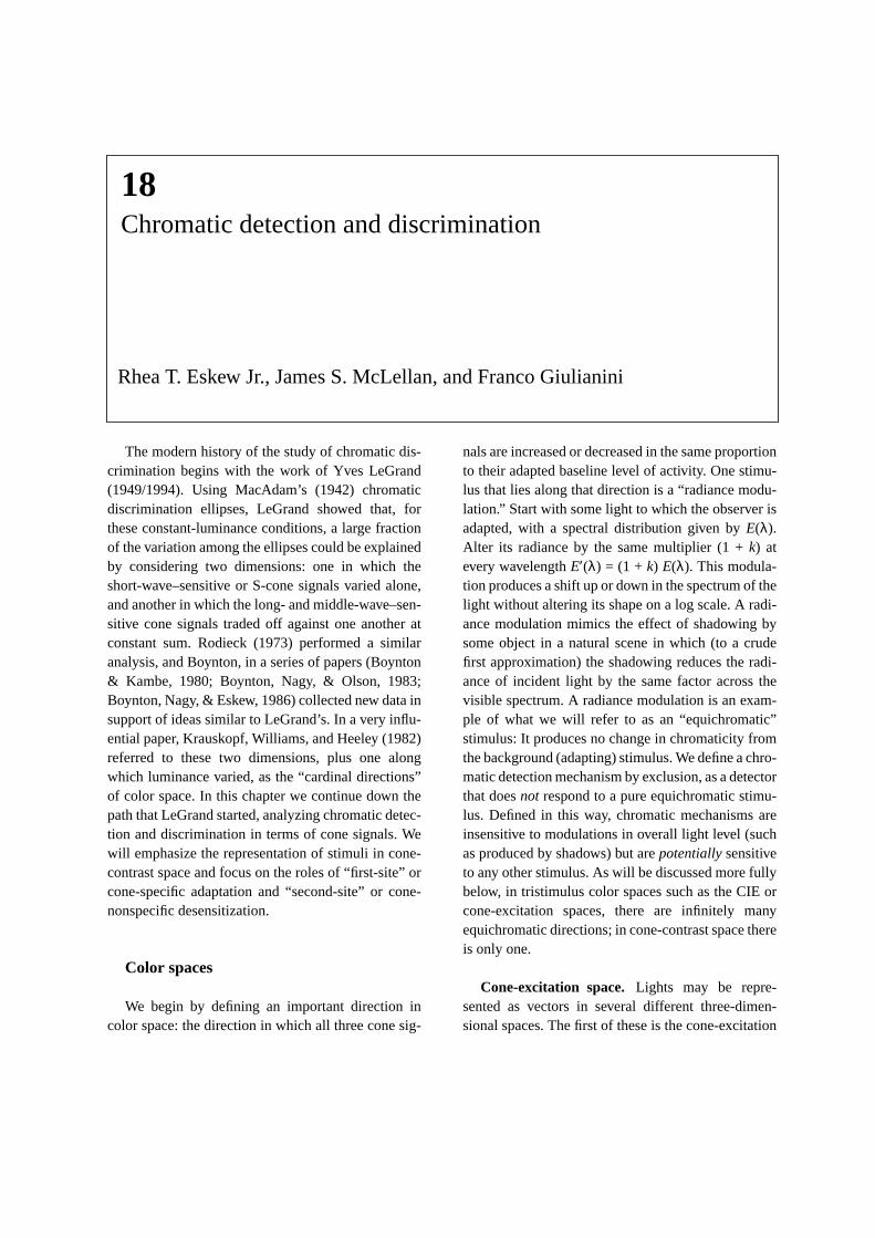
nalsareincreased or decreased in thesameproportionto their adapted baseline level of activity. One stimu-lus that lies along that direction is a “radiance modu-lation.” Start with some light to which the observer isadapted, with a spectral distribution given by E(λ).Alter its radiance by the same multiplier (1 + k) atevery wavelength E′(λ) = (1 + k) E(λ). This modula-tion produces ashift up or down in thespectrum of thelight without altering its shape on a log scale. A radi-ance modulation mimics the effect of shadowing bysome object in a natural scene in which (to a crudefirst approximation) the shadowing reduces the radi-ance of incident light by the same factor across thevisible spectrum. A radiance modulation is an exam-ple of what we wil l refer to as an “equichromatic”stimulus: It produces no change in chromaticity fromthebackground (adapting) stimulus. Wedefine achro-maticdetectionmechanismby exclusion, asadetectorthat does not respond to apure equichromatic stimu-lus. Defined in this way, chromatic mechanisms areinsensitive to modulations in overall light level (suchas produced by shadows) but are potentially sensitiveto any other stimulus. Aswil l bediscussed morefullybelow, in tristimulus color spaces such as the CIE orcone-excitation spaces, there are infinitely manyequichromatic directions; in cone-contrast spacethereis only one.

Cone-excitation space. Lights may be repre-sented as vectors in several different three-dimen-sional spaces. The first of these is the cone-excitation

344 Chromatic detection and discrimination

space (Fig. 18.1A). The three axes of this space areproportional to the quantal catch rates in the three pho-toreceptor classes (L, M, S), and thus this space is alinear transformation of a color-matching space suchas the CIE tristimulus space. The popular MacLeod–Boynton chromaticity diagram (MacLeod & Boynton,1979) is a plane within this space (Fig. 18.1B). Thecone-excitation space is most useful for specifying theadaptive state of the visual system, given by the vectorof cone excitations produced by the adapting light:A =

{ La, Ma, Sa}. The filled dots in the two insets to Fig.18.1A represent the tips of two different adapting vec-tors. To represent test modulations around the adaptingfield, we subtract the adapting vector to make localcone-excitation coordinates (∆L = Ltest−La, ∆M =Mtest−Ma, ∆S= Stest−Sa). Here each of the three axesrepresents the change in cone excitation from theadapting stimulus (insets in Fig. 18.1A). A test stimu-lus that isaddedto an adapting field, such as used is inan increment threshold spectral sensitivity experiment,will be represented in the first octant of a local cone-excitation space, because none of the three cone sig-nals is reduced below their adapted level by such a testlight. The influential space used by Derrington,Krauskopf, and Lennie (1984) is a linear transforma-tion of the axes of local cone-excitation space, so thatthey no longer lie along the cone-excitation coordi-nates but are along the cardinal directions mentionedabove: (∆L−∆M, ∆S, and∆L + ∆M + ∆S).

The cone fundamentals used to define cone spacesare a special set of color matching functions (seeChapter 2). These color matching functions are arbi-trarily scaled, so distances and angles in either of thesecone-excitation spaces have no extrinsic meaning.However, it is conventional to define the units alongthe axes in luminance terms. The Smith–Pokorny(1975) cone fundamentals are designed such that theL- and M-cone fundamentals sum to a modified ver-sion of the CIE photopic luminosity function,V(λ)(Judd, 1951; Vos, 1978). Boynton and Kambe (1980)partitioned the luminance of the light, in cd/m2 or tro-lands (Td), into L- and M-components (e.g., L Td andM Td), such that L+M is the luminance of the light.Because the S-cone fundamental is not a component ofV(λ) in the Smith-Pokorny system, S-cone excitationmust be defined differently: Boynton and Kambechose a new unit that they called a “blue troland”(which will be referred to here as an “S troland”) thatthey defined as the S-cone excitation produced by 1 Tdof equal-energy white. A test presentation at constantluminance [as defined byV(λ)] requires that∆L = −∆Min the local cone-excitation space; there is no suchrestriction on∆S.

M

L

S

∆M

∆L

∆S

AA

∆M

∆L

∆S

∆M/M

∆L/L

∆S/S

M

L

S

W400

450520

650

A

B

C

Figure 18.1: Color spaces. (A) Cone excitation space. Thesmall coordinate axes represent local cone-excitation coordi-nates centered on the adapting condition (solid dot) at twodifferent positions in cone space. The dashed lines connect-ing the origin with the adapting light are equichromaticdirections. (B) The MacLeod–Boynton chromaticity planelocated within cone space. Photopic luminance is constant inthis plane and planes that are parallel to it.W represents anequal-energy white. (C) Cone-contrast space resulting fromdividing the local cone-excitation coordinates (e.g.,∆L) bythe corresponding cone space coordinate (e.g.,L) of theadaping field. All adapting fields plot at the origin in cone-contrast space, and the equichromatic direction is±{1,1,1}(dashed line) for all adapting chromaticities.

Rhea T. Eskew Jr., James S. McLellan, and Franco Giulianini 345

Cone-contrast space.The representation of mostinterest to us is the cone-contrast space (Fig. 18.1C).The first explicit use of cone-contrast space was byNoorlander and Koenderink (1983), although the basicideas that underlie this representation are much older.In this space, the local cone-excitation coordinates ofFig. 18.1A (e.g.,∆L) are divided by the components ofthe adapting vector (La) to produce contrasts (∆L/La orsimply∆L/L) that mimick the sensitivity scaling effectof adaptation occurring in cone-specific pathways.Because contrasts are dimensionless, questions aboutthe relative scaling of cone fundamentals are immate-rial.

In cone-contrast space, like local cone-excitationspace, the origin always represents the adapting condi-tion. Note that, in general, cone-contrast space isnotlinearly related to cone-excitation space. The denomi-nators of the cone contrasts are the coefficients of thetransformation from the cone-excitation space to thecone-contrast space; and if the adapting state is notheld constant, the coefficients are not constant. Thus aset of data collected under various adapting conditionswill be nonlinearly mapped into cone-contrast space(there is a different, linear, mapping for each adaptingcondition, making the transformation of the entire setnonlinear). If the adapting state is constant, there isonly a single, linear relationship.

In cone-contrast space, a radiance modulation bythe factor (1 +k) produces a cone-contrast triplet of{ ∆L/L, ∆M/M, ∆S/S} = { k, k, k} (with a conventionalluminance contrast ofk) that is independent of theadapting condition. Any other means of producingequal cone contrasts (using stimuli that are metamericto a radiance modulation) also produces cone-contrastvectors along this “main diagonal” direction (dashedline in Fig. 18.1C). Thus, in cone-contrast space thereis a fixed equichromatic direction. On the other hand,in cone-excitation space an equichromatic modulationmoves along the line connecting the origin of the spaceto the adapting field [radiance modulation by (1 +k)produces the vector (1 +k) { La, Ma, Sa}], and so is dif-ferent for each adapting field (dashed lines in Fig.18.1A). Just as each of the infinite number of adaptingvectors in cone-excitation space maps to the origin of

the cone-contrast space, each of the infinite number ofequichromatic directions in cone-excitation spacemaps to the same±{1,1,1} direction in cone-contrastspace. As in the cone-excitation space, an incrementaltest light will be represented in the first octant of cone-contrast space. For calculating cone contrasts, see Coleand Hine (1992); Brainard (1996) provides a usefulreview and comparison of cone-contrast space and theDerrington, Krauskopf, and Lennie (1984) version ofthe cone-excitation space.

In the remainder of this chapter we use cone con-trasts to represent stimuli. It is important to rememberthat most conclusions drawn in cone-contrast spaceapply to local cone-excitation space as well – they aresimple linear transformations of one another – as longas the adapting state is held constant; however, acrossdifferent adapting states the relationship is nonlinear.

Chromatic detection

Linear chromatic detection mechanisms.Classi-cal opponent-color mechanisms are often modeled asapproximately linear combinations of cone signals.For example, a red/green detection mechanism mightbe represented as:

(1) RG = γRG (WRG,L∆L/L + WRG,M∆M/M +

WRG,S∆S/S) + N(0,σRG)

= γRG ( ) + N(0, σRG),

where WRG = {WRG,L, WRG,M, WRG,S} and xT ={ ∆L/L, ∆M/M, ∆S/S}.

RG is the number representing the mechanism’sresponse (withRG > 0 meaning “green”, arbitrarily);∆L/L, ∆M/M, ∆S/S are the contrasts produced by thetest stimulus in the three cone classes;WRG,L, WRG,M,andWRG,S are weights that may be positive or nega-tive; andγRGis a positive number representing the gainof the opponent mechanism.N refers to the probabilitydensity of a stochastic process, with zero mean andstandard deviationσRG, that is added to the mecha-

WRG x⋅


nism to model all of the noise sources that corrupt itssignal, viz., quantum light fluctuations, neural noisesin cone-independent pathways, and neural noises atstages after cone signals have been combined. If we let

= γRG ( ) be the deterministic portion ofEqn. (1), then is the mean of the mechanismresponse to a particular stimulus, and on any given pre-sentation the expected response will differ from thatmean by an amount determined byσRG. Definedthusly,RG = N( , σRG).

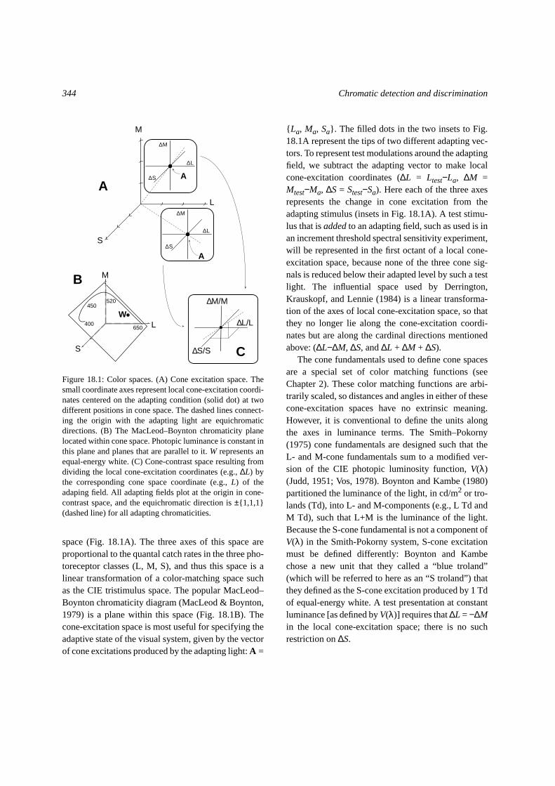
The vector of weights will be referred to hereas the “mechanism vector.” It points in the direction ofmaximum (positive) responsivity of the mechanism incone-contrast space (Fig. 18.2) and is required to haveunit length (so only two of the three weights are inde-pendently determined). The stimulus is represented bythe vector of cone contrasts that it produces, . Theresponse of this hypothetical linear mechanism to anystimulus vector is proportional to the projection of

onto the mechanism vector; because the mechanismresponse is the dot product of the stimulus and mecha-nism vectors, the strength of the response falls off asthe cosine of the angle in color space away from themechanism vector direction (Derrington, Krauskopf,& Lennie, 1984).

In the context of a linear model it is natural to definethreshold as the length of a stimulus vector =[(∆L/L)2 + (∆M/M)2 + (∆S/S)2]0.5producing a constantcriterion response,θ. When the stimulus lies along themechanism vector direction we define the threshold ofthemechanism, T, to be

(2) .

The set of all threshold vectors lies on two planesthat are perpendicular to the mechanism vector, sincethese all produce the same projection onto the mecha-nism vector (Fig. 18.2); the planes represent the tworesponse polarities.T is thus the smallest of the possi-ble cone-contrast thresholds – the shortest Euclideandistance from the origin of the cone-contrast space tothe mechanism’s threshold plane. Similarly, we maydefine the yellow-blue detection mechanism as

(3) YB = γYB ( ) + N(0, σYB) = N( ,σYB),

where = {WYB,L, WYB,M, WYB,S} and xT = {∆L/L,∆M/M, ∆S/S}, and we let “blue” be represented byYB> 0. For the mechanisms to span the cone-contrastspace efficiently, the two mechanism vectorsand will be at right angles, but there is no a priorirestriction that this be so. Although we are using colornames (e.g.,RGandYB) to denote these mechanisms,we emphasize that this is a model of chromatic dis-crimination and detection, not of color appearance.

Additional mechanism vectors would be required torepresent additional linear mechanisms in cone-con-trast space. For instance, a third mechanism vectorcould be defined for the achromatic or luminancemechanism (Lum). The formalism would be identicalfor this nonopponent mechanism; we will let its mech-

RG WRG x⋅RG

RG

WRG

x

xx

x

x TRG≡θRG

γ RG----------=

∆S/S

∆L/L

∆M/M

RG =

WRGRG = 0

-WRG

(null plane)

RG = RGθ

RG−θ

RGθ

Figure 18.2: A mechanism vector and its negative inthree-dimensional cone-contrast space. points in thedirection of maximum responsivity of theRG detectionmechanism. The three planes, all of which are at right anglesto , represent constant-response planes for this hypo-thetical mechanism. The central plane is the null plane of themechanism; stimuli lying in this plane produce no responsein RG. The two outer planes are threshold planes.TRG is theshortest distance from the origin to a threshold plane, andthus it represents the stimulus that most efficiently stimulatesthe mechanism – the mechanism threshold.

WRGWRG

WRG

WYB x⋅ YB

WYB

WRGWYB


anism vector be = {WLum,L, WLum,M, WLum,S}and its gain beγLum. If there arebroadband, “higherorder” chromatic mechanisms (see Chapters 13 and16), these would be represented by still more linearmechanisms.

Assuming that the observer is unbiased and there-fore sets detection criteria atRG = 0 andYB = 0, thedetection probabilities in a 2AFC task are given by:

(4)

.

The standard deviations are divided by becausewe are considering two alternative forced-choice(2AFC) tasks; in a single-interval procedure such as aYes–No experiment, the unmodified standard devia-tions would be used (Green & Swets, 1974). We willdefine the 2AFC threshold to be wherePRG or PYBequals 0.816 (because of its convenience when usingthe Weibull psychometric function). Intuitively, onemay think of a univariate noise distributionN centeredon the origin in cone-contrast space; the signal + noisedistribution is a copy ofN that has been moved out-ward, sliding along the mechanism vector direction, bythe distance . Threshold is reached when 81.6%of the distribution has been moved past the origin.[Actually, N is a multivariate probability distributionwith standard deviations (σRG, σYB, σLum…) taken ineach of the mechanism vector directions.]

The weights {WRG,L, WRG,M, WRG,S} and {WYB,L,WYB,M, WYB,S} [Eqns. (1) and (3)] are interpretable asrelative gains, in signal-to-noise or d′ units. For exam-ple, suppose thatγRG = 100 andWRG,M = 0.2 [Eqn.(1)]. This would indicate that an M-cone–isolating teststimulus with contrast of +5% would produce 100×0.2 × 0.05 = 1 d′ unit of RG signal in the “greenish”direction. If we assume that the noiseN is Gaussian,Eqn. (4) implies that at the 2AFC threshold,

(5)

(because the z-score corresponding toP = 0.816 is

0.90). In other words, at the 2AFC threshold the mag-nitude of the constantRG signal is

(6) .

Thus the mechanism threshold (the cone-contrastthreshold vector along the mechanism direction) is

(7)

[cf. Eqn. 2]. As the postreceptoral gainγ decreases (athigher spatial or temporal frequencies, for example),the mechanism thresholdT increases. If the noise isnot Gaussian, the constant of proportionality betweenT andσ/γ is some number other than 0.636, dependingon the form of the probability density function.

The formalism needs one additional component, acombination rule that specifies how the mechanismsinteract. The usual assumption is that the mechanismsare stochastically independent and their outputs com-bine by probability summation. The detection contour– that is, the locus of threshold cone-contrast vectors –formed by the “inner envelope” of themeans ,

, and of three detection mechanisms is a par-allelepiped, each face of which is an isoresponse sur-face for one polarity of one mechanism. The two outerplanes in Fig. 18.2 represent two of the faces of such aparallelepiped. When the noise is considered, however,the shape of the contour becomes more rounded andsmaller in the corners than the parallelepiped. If thenoise in each mechanism is Gaussian, the probabilitysum of these three linear mechanisms creates an ellip-soidal contour, because an isoprobability surface of ann-dimensional multivariate Gaussian probability dis-tribution is ellipsoidal (Silberstein & MacAdam,1945).

We may approximate the operation of probabilitysummation by use of the following combination rule:At threshold,

(8) .

If the exponentβ is unity, the mechanisms sum (a“city block” rule); when the exponent is large, then the

WLum

PRG N RG σRG 2⁄( , ) d RG( )0

∞

∫=

PYB N YBσYB 2⁄( , )d YB( )0

∞

∫=

2

W x⋅

RG

σRG 2⁄------------------- 2 d' 0.90= =

RG θRG 0.636σRG= =

TRG 0.636σRG

γ RG----------=

RGYB Lum

RGβ

YBβ

Lumβ

+ + 1=


largest signal dominates (a “winner takes all” rule) anda parallelepiped results; for intermediate values ofβ,the equation behaves like a probability summation.This sort of contour has frequently been used to modelprobability summation between chromatic mecha-nisms (Cole, Hine, & McIlhagga, 1993, 1994; Sanker-alli & Mullen, 1996); a somewhat different approach istaken in the influential model of Guth and colleagues(Guth, Massof, & Benzschawel, 1980; Guth, 1991).

The Quick (1974) model of visual summation iden-tifies the combination exponentβ with the slope of theWeibull psychometric function (Graham, 1989). Esti-mates of the psychometric slope for isolatedRGvaryfrom about 1.6 to about 2.1 (Eskew et al., 1991; Eskew,Stromeyer, & Kronauer, 1994);YBprobably also has apsychometric slope in this range (Watanabe, Smith, &Pokorny, 1997). However,Lum has a consistentlyhigher slope, of about 2.2 (Stromeyer, Lee, & Eskew,1992; Eskew, Stromeyer, & Kronauer, 1994; see alsothe foveal data of Vingrys & Metha, 1997).

Rather than assuming the Quick model and usingpsychometric slopes to estimateβ, Eqn. (8) may be fitdirectly to detection data usingβ as a free parameter.When this is done, the estimates ofβ are often higherthan the slopes of psychometric functions (e.g., 3–5;Cole, Hine, & McIlhagga, 1993, 1994). This discrep-ancy between psychometric slopes and fittedβs mightindicate that some of the theoretical assumptions of theQuick approach, such as the high-threshold assump-tion (known to be wrong in detail, on other grounds),fail critically in these experiments. A value ofβ = 4works well in many applications of this model.

Null planes and isolation of mechanisms.Theplane through the origin that is orthogonal to the mech-anism vector is the “null plane” of the mechanism (Fig.18.2; Derrington, Krauskopf, & Lennie, 1984). Thenull plane comprises all of the stimuli (cone triplets)that do not affect the opponent mechanism, becausetheir projection onto the mechanism vector is zero.One of the advantages of using vectors to representthese mechanisms is that doing so immediately revealsthat these linear mechanisms are broadly tuned – theyhave some response to all stimuli except those in the

null plane. To get narrowly-tuned mechanisms – forexample, a higher order mechanism that responds wellto orange and hardly at all to red or yellow – the conesignals must be combined nonlinearly.

The null plane of the luminance mechanism is par-ticularly important in the history of chromatic discrim-ination. This plane is called theequiluminant plane,and many studies of chromatic detection and discrimi-nation restrict themselves to this plane; in practice,heterochromatic flicker photometry or minimally dis-tinct borders are often used to find it. Some of theadvantages and disadvantages of restricting attentionto equiluminant stimuli are discussed in a subsequentsection.

It is important to distinguish between mechanismdirections and mechanism-isolating directions. To iso-late one mechanism, stimuli are presented that liewithin the null planes of the other mechanisms. Forexample, assume that there are three linear mecha-nisms,RG, YB, andLum. To isolate one of them, forexample,RG, one finds the intersection of the nullplanes ofYBandLum. These two null planes meet in aline going through the origin of the cone-contrastspace; the only stimulus vectors that do not stimulateYB andLum, and thus isolate theRG mechanism, liealong that line. The key point is that thisRG isolatingdirection is the same as theRG mechanism directiononly if the three mechanisms are mutually orthogonal;otherwise, theRG isolating direction stimulates theRG mechanism uniquely, but does so less efficientlythan stimulation along the mechanism direction. Ifthere are more than three linear mechanisms (e.g., ifthere are broadly tuned, higher order mechanisms;Krauskopf, see Chapter 16), there may be no colordirection that isolates any one of them, since more thantwo null planes need not meet in a single line. Kno-blauch (1995) discusses relationships between mecha-nism directions and mechanism-isolating directions.

Sometimes the null plane is used to characterize amechanism (Derrington, Krauskopf, & Lennie, 1984),but specifying the null plane alone gives no informa-tion about the sensitivity of the mechanism. Specifyingthe mechanism vector allows the gain of each mecha-nism to be defined. Of course, these gains [theγ’s,


Eqns. (1) and (3)] will vary depending on the spatialand temporal characteristics of the stimuli, but for afixed stimulus condition the specification of the gains,the mechanism vectors, and some combination rule(e.g., probability summation) allows a prediction ofdetection performance.

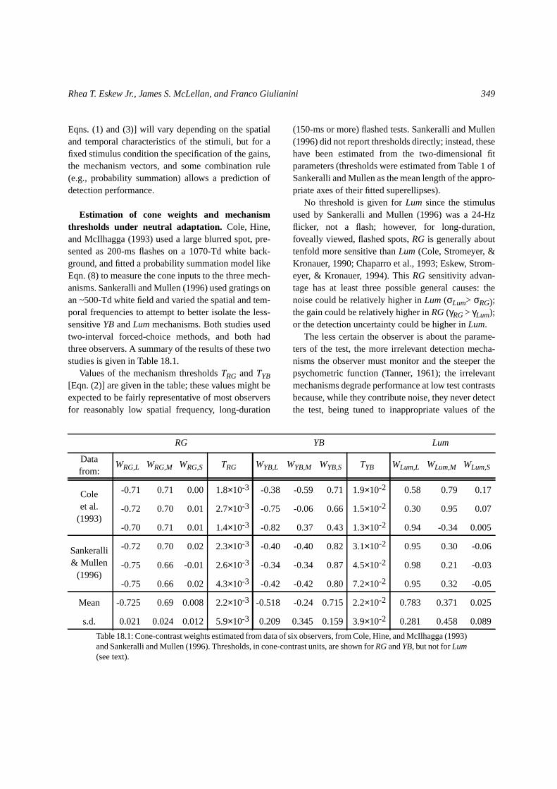
Estimation of cone weights and mechanismthresholds under neutral adaptation. Cole, Hine,and McIlhagga (1993) used a large blurred spot, pre-sented as 200-ms flashes on a 1070-Td white back-ground, and fitted a probability summation model likeEqn. (8) to measure the cone inputs to the three mech-anisms. Sankeralli and Mullen (1996) used gratings onan ~500-Td white field and varied the spatial and tem-poral frequencies to attempt to better isolate the less-sensitiveYBandLummechanisms. Both studies usedtwo-interval forced-choice methods, and both hadthree observers. A summary of the results of these twostudies is given in Table 18.1.

Values of the mechanism thresholdsTRG andTYB[Eqn. (2)] are given in the table; these values might beexpected to be fairly representative of most observersfor reasonably low spatial frequency, long-duration

(150-ms or more) flashed tests. Sankeralli and Mullen(1996) did not report thresholds directly; instead, thesehave been estimated from the two-dimensional fitparameters (thresholds were estimated from Table 1 ofSankeralli and Mullen as the mean length of the appro-priate axes of their fitted superellipses).

No threshold is given forLum since the stimulusused by Sankeralli and Mullen (1996) was a 24-Hzflicker, not a flash; however, for long-duration,foveally viewed, flashed spots,RG is generally abouttenfold more sensitive thanLum (Cole, Stromeyer, &Kronauer, 1990; Chaparro et al., 1993; Eskew, Strom-eyer, & Kronauer, 1994). ThisRG sensitivity advan-tage has at least three possible general causes: thenoise could be relatively higher inLum (σLum> σRG);the gain could be relatively higher inRG(γRG> γLum);or the detection uncertainty could be higher inLum.

The less certain the observer is about the parame-ters of the test, the more irrelevant detection mecha-nisms the observer must monitor and the steeper thepsychometric function (Tanner, 1961); the irrelevantmechanisms degrade performance at low test contrastsbecause, while they contribute noise, they never detectthe test, being tuned to inappropriate values of the

RG YB Lum

Datafrom:

WRG,L WRG,M WRG,S TRG WYB,L WYB,M WYB,S TYB WLum,L WLum,M WLum,S

Coleet al.

(1993)

-0.71 0.71 0.00 1.8×10-3 -0.38 -0.59 0.71 1.9×10-2 0.58 0.79 0.17

-0.72 0.70 0.01 2.7×10-3 -0.75 -0.06 0.66 1.5×10-2 0.30 0.95 0.07

-0.70 0.71 0.01 1.4×10-3 -0.82 0.37 0.43 1.3×10-2 0.94 -0.34 0.005

Sankeralli& Mullen

(1996)

-0.72 0.70 0.02 2.3×10-3 -0.40 -0.40 0.82 3.1×10-2 0.95 0.30 -0.06

-0.75 0.66 -0.01 2.6×10-3 -0.34 -0.34 0.87 4.5×10-2 0.98 0.21 -0.03

-0.75 0.66 0.02 4.3×10-3 -0.42 -0.42 0.80 7.2×10-2 0.95 0.32 -0.05

Mean -0.725 0.69 0.008 2.2×10-3 -0.518 -0.24 0.715 2.2×10-2 0.783 0.371 0.025

s.d. 0.021 0.024 0.012 5.9×10-3 0.209 0.345 0.159 3.9×10-2 0.281 0.458 0.089

Table 18.1: Cone-contrast weights estimated from data of six observers, from Cole, Hine, and McIlhagga (1993)and Sankeralli and Mullen (1996). Thresholds, in cone-contrast units, are shown forRGandYB, but not forLum(see text).


stimulus parameters (such as test location, time, color,spatial frequency, etc.). Weibull slopes of 1.6 to 2.1, asmeasured forRG(preceding section), suggest that 3 to10 total detection mechanisms contribute to theobserver’s performance, whereas the slightly steeperLumpsychometric functions suggest 10 to 30 mecha-nisms (Pelli, 1985, Table 1). This difference in uncer-tainty would causeLumto be less sensitive thanRGina 2AFC procedure, but not by much: of the 1.0 log unitRGadvantage, less than 0.2 log unit might reasonablybe attributed to uncertainty differences.

The slope of the psychometric function is inverselyrelated to the size of the standard deviation of the noisein the relevantmechanism [when the standard devia-tion is small, the detection probabilities in Eqn. (4) risesteeply with contrast]. The finding that the psychomet-ric slope for luminance detection is steeper than thecorresponding slope for chromatic detection suggeststhat the luminance pathway might belessnoisy, imply-ing in turn that the cause of theRGsensitivity advan-tage is higher effective gain. This might seem tocontradict the finding that primate magnocellular (M)neurons, often claimed to subserve luminance detec-tion, have higher contrast gain than parvocellular (P)neurons (e.g., Shapley, 1990). However, there is nocontradiction. First, whereas M-cells do have highercontrast gain forluminancecontrast, a comparison ofcolor and luminance responsiveness using some formof cone-contrast metric shows that contrast gains forM-cells (for equichromatic stimuli) and P-cells (forred-green equiluminant stimuli) are similar (Lee, Mar-tin, & Valberg, 1989b; Lee et al., 1993a), at least forlow temporal frequencies. Second, P-cells as well asM-cells are likely to contribute to the detection ofequichromatic stimuli (Lennie, Pokorny, & Smith,1993). The cause of the higher effective gain for chro-matic detection is likely to be a summation of theresponses of many P-cells (Chaparro et al., 1993).

The L- and M-cone weights toRGare of oppositesign and nearly equal for all six observers in Table18.1; the coefficients of variation (the standard devia-tion divided by the mean) are an order of magnitude ormore smaller forWRG,L andWRG,M than for the otherseven mean weights. The lack of individual differences

in long-wavelength cone inputs toRG suggests thatdetection contours in the (∆L/L, ∆M/M) plane of thecone-contrast space will always have slopes close tounity (as in Fig. 18.3, below), and this is the case forall studies of which we are aware. Similarly, Der-rington, Krauskopf, and Lennie (1984) found that mostmacaque parvocellular neurons had approximatelyequal and opposite L- and M-cone inputs.

Sankeralli and Mullen (1996) were unable to deter-mine the relative L and M weights forYB, so they setthem equal to each other; Cole, Hine, and McIlhagga(1993) estimated weights separately, but the resultswere not well constrained by the data. The meanWYB,LandWYB,M values reported in Table 18.1 are nonethe-less similar to the mean weights measured in a differ-ent experiment by Cole, Hine, and McIlhagga (1994),who attempted to isolateYBby using a spatial patternto which the S-cones should be more sensitive (aCraik–Cornsweet parafoveal circular edge).

The mean value ofWRG,S is very slightly positive.However, a reddish (negative) suprathreshold input ofS-cones to the red-greenhuemechanism is required toaccount for the violet appearance of short-wave lights(i.e., this S-cone input must have the same sign as theL-cones; Ingling, 1977; Werner & Wooten, 1979).Whether S-cones contribute similarly to theRG detec-tion mechanism is controversial (Boynton, Nagy, &Olson, 1983; Mollon & Cavonius, 1987; Stromeyer &Lee, 1988). When measurements of the S-cone-con-trast weight forRG detection and for red-green hueequilibria are made under identical conditions, theestimated weights have quite similar (very small) mag-nitudes and signs (Eskew & Kortick, 1994). Recently,Stromeyer et al. (1998) found that S-cone modulationsfacilitated and masked detection byRG, depending onwhether the +∆S/S signal was paired with the +∆L/Lsignal (facilitation) or the +∆M/M signal (masking).This and other evidence led them to suggest a small,“reddish” S-cone contribution toRG. In Table 18.2 wesetWRG,S= −0.02 in spite of the mean value ofWRG,Sin Table 18.1 being slightly above zero.

There is evidence thatRG’s relative cone weightsdo not depend on temporal frequency, but forLum therelativeL/M inputs can vary widely with temporal fre-


quency (Stromeyer et al., 1995). With the flashes usedby Cole, Hine, and McIlhagga, the estimated L and Mweights forLumwere essentially unconstrained by thedata. The 24-Hz counterphase flicker used by Sanker-alli and Mullen allowed more of theLummechanismto be revealed and permitted more certainty in the esti-mation of the weights – but these weights may not beappropriate for flashed stimuli. The mean weightsshown in Table 18.1 forLumare based on both studiesand are therefore dubious, but they are given here forcompleteness. L-cones are generally believed to con-tribute more toLum than M-cones, and the meanWLum,L and WLum,M are consistent with that belief;recall, however, that these are contrast gains (previoussection) and do not necessarily imply anything aboutthe scaling of the L- and M-cone fundamentals or conenumbers.

The “adjusted weights” shown in Table 18.2 arebased on the mean weights from Table 18.1. BesidessettingWRG,Sat−0.02 as mentioned above, we also setthe S-cone input toLumto be zero (ignoring the small,negative contribution of the S-cones toLum; Stock-man, MacLeod, & DePriest, 1991), and we madechanges to the other means in service of three desider-ata: (1) that the vector of weights have unit length; (2)that the weights sum exactly to zero; (3) that the resultshave the same direction in cone-contrast space as thecentroid vector formed by the mean weights. The firstis a technical requirement of the model. The second,tiny adjustment makes the null planes ofRG andYBcontain the equichromatic vector, so they do notrespond to radiance modulations and their metamers(see Color Spaces section). The adjusted weights rep-resent an approximation to (3) given that we satisfy (1)and (2) (the reversal in the ratio of magnitudes of the

adjustedWRG,L and WRG,M in Table 18.2, comparedwith the means in Table 18.1, is not an error, but is theresult of requiringWRG,Sto be negative and then apply-ing these desiderata). Note that althoughWRG,S is 40times smaller thanWYB,S, the sensitivity ofRG is somuch greater than the sensitivity ofYB that the netresult is thatYB is only about four times as responsiveto S-cone input as isRG.

For the observer represented by these adjustedweights, convenient basis vectors for the equiluminantplane are {∆L/L, ∆M/M, ∆S/S} = {0.43, −0.9, 0} and{0, 0, 1} (but the uncertainties expressed above aboutthe luminance weights limit the usefulness of thisplane). To stimulate theYB mechanism alone, onewould find the intersection of theRGnull plane and theequiluminant plane. ThisYB isolating direction is thevector that is orthogonal to both and ; it isnot exactly the S-cone direction, because of the smallS-cone contribution toRG. Instead {0.009,−0.019, 1}is the direction that isolatesYB(obviously, the S-conedirection is sufficient for most practical purposes). TheRG isolating direction is {−0.43, 0.9,−0.015}. Desid-eratum (2) forces the equichromatic direction { ,

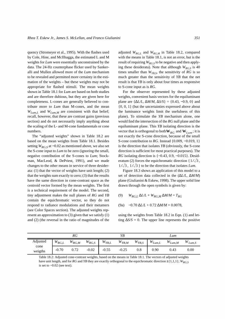
, } to be the direction that isolatesLum.Figure 18.3 shows an application of this model to a

set of detection data collected in the (∆L/L, ∆M/M)plane (Giulianini & Eskew, 1998). The upper solid linedrawn through the open symbols is given by:

(9) WRG,L ∆L/L + WRG,M ∆M/M = TRG

(9a) −0.70∆L/L + 0.72∆M/M = 0.0078,

using the weights from Table 18.2 in Eqn. (1) and let-ting ∆S/S= 0. The upper line represents the positive

RG YB Lum

Adjustedcone

weigths

WRG,L WRG,M WRG,S WYB,L WYB,M WYB,S WLum,L WLum,M WLum,S

-0.70 0.72 -0.02 -0.55 -0.25 0.8 0.90 0.43 0.00

Table 18.2: Adjusted cone-contrast weights, based on the means in Table 18.1. The vectors of adjusted weightshave unit length, and forRGandYBthey are exactly orthogonal to the equichromatic direction±{1,1,1}; WRG,Sis set to−0.02 (see text).

WRG WLum

1 3⁄1 3⁄ 1 3⁄


(“green”) response polarity ofRG; the lower solid lineis obtained by changing the sign ofTRG (for the “red”polarity). The slope of both lines is−WRG,L/WRG,M =0.70/0.72 = 0.97. The dashed lines are based on theanalogous equation forLum; their slope is−WLum,L/WLum,M = −0.90/0.43 =−2.1. The filled sym-bols in Fig. 18.3 result when red/green masking noiseis added to the stimulus, raising all of theRG thresh-olds and exposing more of theLummechanism in thefirst and third quadrants (Giulianini & Eskew, 1998).The solid contour plotted near the filled symbols,which is a slice through a rounded parellelpiped, rep-resents a fit of Eqn. (8), withβ = 4 and with noYBcon-tribution.

Chromatic adaptation: first-site effects. Thedata reported in Fig. 18.3 do not constitute a test of thecone-contrast model, nor do the data of Cole, Hine,and McIlhagga (1993; 1994) or Sankeralli and Mullen(1996); all of these data could have been equally welldescribed by a model based on the sums and differ-ences of cone excitations rather than cone contrasts.Testing the contrast feature of the model requireschanging the chromaticity of the adapting field, to seehow well the first-site, cone-specific adaptation builtinto the model can account for changes in the data. WeexamineRG first.

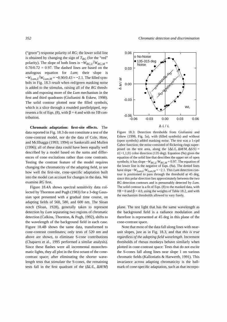
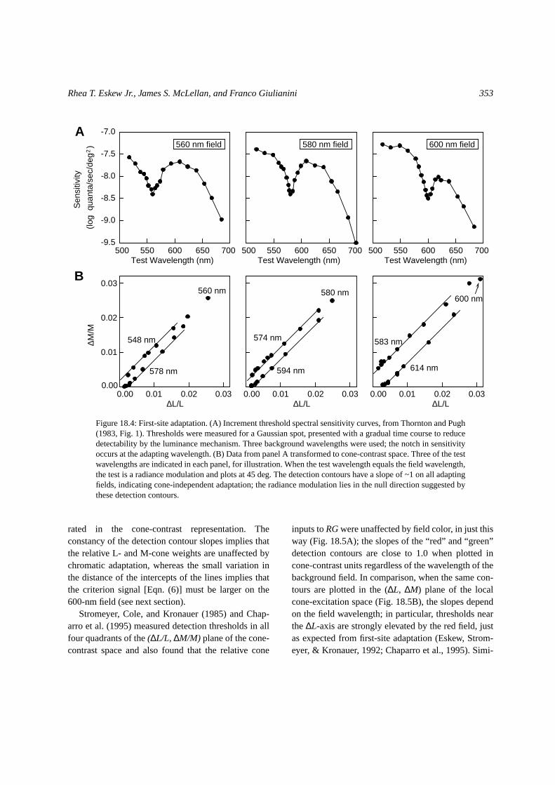
Figure 18.4A shows spectral sensitivity data col-lected by Thornton and Pugh (1983) for a 3-deg Gaus-sian spot presented with a gradual time course, onadapting fields of 560, 580, and 600 nm. The Sloannotch (Sloan, 1928), generally taken to representdetection byLumseparating two regions of chromaticdetection (Calkins, Thornton, & Pugh, 1992), shifts tothe wavelength of the background field in each case.Figure 18.4B shows the same data, transformed tocone-contrast coordinates; only tests of 520 nm andabove are shown, to eliminate S-cone contributions(Chaparro et al., 1995 performed a similar analysis).Since these flashes were all incremental monochro-matic lights, they all plot in the first octant of the cone-contrast space; after eliminating the shorter wave-length tests that stimulate the S-cones, the remainingtests fall in the first quadrant of the (∆L/L, ∆M/M)

plane. The test light that has the same wavelength asthe background field is a radiance modulation andtherefore is represented at 45 deg in this plane of thecone-contrast space.

Note that most of the data fall along lines with near-unit slopes, just as in Fig. 18.3, and thatthis is trueregardless of the adapting field wavelength. Incrementthresholds of rhesus monkeys behave similarly whenplotted in cone-contrast space: Tests that do not excitethe S-cones fall along lines near slope 1 on variouschromatic fields (Kalloniatis & Harwerth, 1991). Thisinvariance across adapting chromaticity is the hall-mark of cone-specific adaptation, such as that incorpo-

0.00

0.03

-0.03

0.06

-0.060.00 0.03-0.03 0.06-0.06

No Noise135-315 deg Noise

WL

M /

M∆

L / L∆

Figure 18.3: Detection thresholds from Giulianini andEskew (1998, Fig. 5a), with (filled symbols) and without(open symbols) added masking noise. The test was a 1-cpdGabor function; the noise consisted of flickering rings super-posed on the test area, along the {∆L/L, ∆M/M, ∆S/S} =±{ −1,1,0} color direction (135 deg). Equation (9a) gives theequation of the solid line that describes the upper set of opensymbols; it has slope−WRG,L/WRG,M = 0.97. The equation ofthe lower line is the negative of Eqn. (9a). The dotted lineshave slope−WLum,L/WLum,M = −2.1. ThisLumdetection con-tour is positioned to pass through the threshold at 45 deg,since this polar direction lies approximately between the twoRG detection contours and is presumably detected byLum.The solid contour is a fit of Eqn. (8) to the masked data, withYB= 0 andβ = 4.0, using the weights of Table 18.2, and withthe mechanism thresholds allowed to vary freely.


rated in the cone-contrast representation. Theconstancy of the detection contour slopes implies thatthe relative L- and M-cone weights are unaffected bychromatic adaptation, whereas the small variation inthe distance of the intercepts of the lines implies thatthe criterion signal [Eqn. (6)] must be larger on the600-nm field (see next section).

Stromeyer, Cole, and Kronauer (1985) and Chap-arro et al. (1995) measured detection thresholds in allfour quadrants of the(∆L/L, ∆M/M) plane of the cone-contrast space and also found that the relative cone

inputs toRGwere unaffected by field color, in just thisway (Fig. 18.5A); the slopes of the “red” and “green”detection contours are close to 1.0 when plotted incone-contrast units regardless of the wavelength of thebackground field. In comparison, when the same con-tours are plotted in the (∆L, ∆M) plane of the localcone-excitation space (Fig. 18.5B), the slopes dependon the field wavelength; in particular, thresholds nearthe∆L-axis are strongly elevated by the red field, justas expected from first-site adaptation (Eskew, Strom-eyer, & Kronauer, 1992; Chaparro et al., 1995). Simi-

0.00 0.01 0.02 0.030.00 0.01 0.02 0.030.00

0.01

0.02

0.03

0.00 0.01 0.02 0.03

∆M/M

∆L/L

560 nm

548 nm

578 nm

∆L/L

580 nm

574 nm

594 nm

600 nm

583 nm

614 nm

∆L/L

-9.5

-9.0

-8.5

-8.0

-7.5

-7.0

500 550 600 650 700Test Wavelength (nm)

560 nm field

(log

qua

nta/

sec/

deg

)2S

ensi

tivity

Test Wavelength (nm)

580 nm field

Test Wavelength (nm)

600 nm fieldA

B

500 550 600 650 700 500 550 600 650 700

Figure 18.4: First-site adaptation. (A) Increment threshold spectral sensitivity curves, from Thornton and Pugh(1983, Fig. 1). Thresholds were measured for a Gaussian spot, presented with a gradual time course to reducedetectability by the luminance mechanism. Three background wavelengths were used; the notch in sensitivityoccurs at the adapting wavelength. (B) Data from panel A transformed to cone-contrast space. Three of the testwavelengths are indicated in each panel, for illustration. When the test wavelength equals the field wavelength,the test is a radiance modulation and plots at 45 deg. The detection contours have a slope of ~1 on all adaptingfields, indicating cone-independent adaptation; the radiance modulation lies in the null direction suggested bythese detection contours.


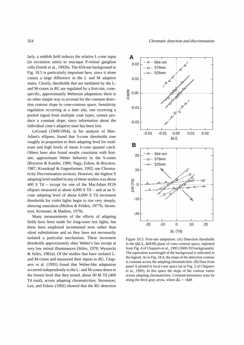
larly, a reddish field reduces the relative L-cone input(in excitation units) to macaque P-retinal ganglioncells (Smith et al., 1992b). The 654-nm background inFig. 18.5 is particularly important here, since it alonecauses a large difference in the L and M adaptivestates. Clearly, thresholds that are mediated by the L-and M-cones inRGare regulated by a first-site, cone-specific, approximately Weberian adaptation; there isno other simple way to account for the constant detec-tion contour slope in cone-contrast space. Sensitivityregulation occurring at a later site, one receiving apooled signal from multiple cone types,cannotpro-duce a constant slope, since information about theindividual cone’s adaptive state has been lost.

LeGrand (1949/1994), in his analysis of Mac-Adam's ellipses, found that S-cone thresholds roseroughly in proportion to their adapting level for mod-erate and high levels of mean S-cone quantal catch.Others have also found results consistent with first-site, approximate Weber behavior in the S-cones(Boynton & Kambe, 1980; Nagy, Eskew, & Boynton,1987; Krauskopf & Gegenfurtner, 1992; see Chroma-ticity Discrimination section). However, the highest Sadapting level studied in any of these studies was about400 S Td – except for one of the MacAdam PGNellipses measured at about 4,000 S Td – and at an S-cone adapting level of about 6,000 S Td incrementthresholds for violet lights begin to rise very steeply,showing saturation (Mollon & Polden, 1977b; Strom-eyer, Kronauer, & Madsen, 1979).

Many measurements of the effects of adaptingfields have been made for long-wave test lights, butthese have employed incremental tests rather thansilent substitutions and so they have not necessarilyisolated a particular mechanism. These incrementthresholds approximately obey Weber’s law except atvery low retinal illuminances (Stiles, 1978; Wyszecki& Stiles, 1982a). Of the studies that have isolated L-and M-cones and measured their inputs toRG, Chap-arro et al. (1995) found that Weber-like adaptationoccurred independently in the L- and M-cones down tothe lowest level that they tested, about 60 M Td (400Td total), across adapting chromaticities; Stromeyer,Lee, and Eskew (1992) showed that theRGdetection

654 nm579nm525nm

-20

-10

0

10

20

-20 -10 0 10 20

∆

∆L (Td)

-0.02

-0.01

0.00

0.01

0.02

-0.02 -0.01 0.01 0.02∆L/L

A

0.00

∆

654 nm579nm525nm

B

M/M

M (

Td)

Figure 18.5: First-site adaptation. (A) Detection thresholdsin the (∆L/L, ∆M/M) plane of cone-contrast space, replottedfrom Fig. 4 of Chaparro et al., 1995 (3000-Td backgrounds).The equivalent wavelength of the background is indicated inthe legend. As in Fig. 18.4, the slope of the detection contouris constant across the adapting chromaticities. (B) Data frompanel A plotted in local cone space (as in Fig. 2 of Chaparroet al., 1995). In this space the slope of the contour variesacross adapting chromaticities. Constant-luminance tests liealong the thick gray arrow, where∆L = −∆M.


contour had a slope near unity on a yellow field pro-ducing about 32 M Td (77 Td total); Stromeyer, Cole,and Kronauer (1985) showed that∆L/L at thresholdincreased by only about 0.1 log unit as a 638-nm fieldwas reduced from about 2970 to 39 L Td (right-mostpair of points in Figs. 18.6A & B). All of these resultsare consistent with Weber behavior in the L- and M-cones, from low photopic levels and up.

Photocurrent recordings from isolated primatecones (Schnapf et al., 1990) suggest that there is littleadaptation in cone outer segments until light levels areincreased beyond about 1,000 Td. Since psychophysi-cal cone thresholds begin to rise at 10–50 Td (Hood &Finkelstein, 1986), the photocurrent data might sug-gest that the “first site” is after the outer segment (at thecone-bipolar synapse, for example). The psychophysi-cal results discussed in this section imply only that theadaptation takes place prior to the site(s) at which sig-nals from different cone classes are combined. Psycho-physical evidence suggests that the spatial integrationarea preceding the first nonlinearity in the visual sys-tem (presumably the nonlinearity representing adapta-tion) has the width of a single foveal cone (MacLeod,Williams, & Makous, 1992; MacLeod & He, 1993).Consistent with this psychophysical result, recentphysiological recordings from both HI and HII mon-key horizontal cells show cone-specific adaptation atthis early level (Lee et al., 1997).

Chromatic adaptation: second-site desensitiza-tion. The evidence reviewed in the preceding section(and much more not discussed here) indicates that sub-stantial sensitivity regulation occurs in cone-specificpathways, prior to any opponent combination. How-ever, it is also abundantly clear that there are other sitesof sensitivity regulation occurring at or after the pointat which cone signals are combined. Cone-specific,first-site adaptation reduces the influence of the adapt-ing chromaticity; once the first-site effect has beenaccounted for (at least approximately, by taking con-trasts, for example), the remaining variation in sensi-tivity due to adapting condition is by definition a“second-site” effect. The term “adaptation” implies aloss ofabsolutesensitivity to retaindifferentialor con-

trast sensitivity (Shapley & Enroth-Cugell, 1984).Because second-site effects are losses of both absoluteand contrast sensitivity, perhaps due to a saturation ofneural mechanisms at the opponent site, the second-site effects are often called desensitization rather thanadaptation.

Chromatic fields raiseRG thresholds above andbeyond the first-site effect. This is illustrated in Fig.18.5A, which shows detection contours in the(∆L/L,∆M/M) plane of the cone-contrast space on red, yel-low, and green adapting fields (Chaparro et al., 1995).As noted in the previous section, the constant slope ofthe RG detection contours shows first-site, cone-spe-cific adaptation. However, the contours on the long-wave field are farther from the origin than on the greenor yellow fields. The long-wave field raises the “red”(L increment and M decrement) and “green” (M incre-ment and L decrement) test threshold contoursequally,so the effect is not some masking effect that is specificto the color polarity of the test. We could modify Eqn.(9) to represent this result as:

(10)

in which TRG is the mechanism threshold on a neutralfield [Eqn. (2)], and the absolute value is taken so as torepresent both response polarities. The scalarJRG is afunction of the adaptation conditions and representsthe degree to which chromatic adaptation alters thresh-olds from those found on the neutral fields. Figure18.5A requiresJRG to be about equal on the yellowishand greenish fields but higher on the long-wave field.Since the slope of the detection contour is−WRG,L/WRG,M, the data show that the relative coneweights are not altered by the second-site effect. Thuswe may use the adjusted weights from Table 18.2 and,after substituting the definition ofTRG from Eqn. (2),Eqn. (10) becomes

(11) = (1 +JRG).

The symbols in Fig. 18.6A and B show L-conethresholds from Stromeyer, Cole, and Kronauer (1985)plotted in contrast units as a function of adapting

WRG L, ∆L/L WRG M, ∆M /M+ TRG 1 JRG+( ),=

0.70 ∆L/L– 0.72∆M /M+θRG

γ RG----------


wavelength for adapting fields that produce equalquantal catch in the L-cones (so first-site adaptation –the denominator of∆L/L – is kept constant). L-conethresholds are lowest near yellow and rise to eitherside; if there were no second-site desensitization, thesethresholds should not vary with adapting conditionsince plotting cone contrast accounts for the multipli-cative first-site effect. Given the log-unit sensitivity

advantage ofRGoverYBor Lum(Table 18.1), we mayassume that these L-cone tests are detected byRG(except perhaps for the most-desensitized cases, whereanother mechanism might intrude). Setting∆M/M = 0in Eqn. (11) and rearranging,

(12) JRG = 0.70 − 1.

500 550 600 6500.001

0.01

Wavelength (nm)

∆L/L∆M/MEquiluminantHue function

AC

0.001

0.01

Low L quantaHigh L quantaHue function HC

Low L quantaHigh L quantaHue function CFS

500 550 600 650Wavelength (nm)

∆L/L∆M/MEquiluminantHue function

GC

Hue

val

ence

Red

Green Red

400 450 500 550 600 650 700

E

Wavelength (nm)

Thr

esho

ld (

L/L)

Thr

esho

ld∆

DC

BA

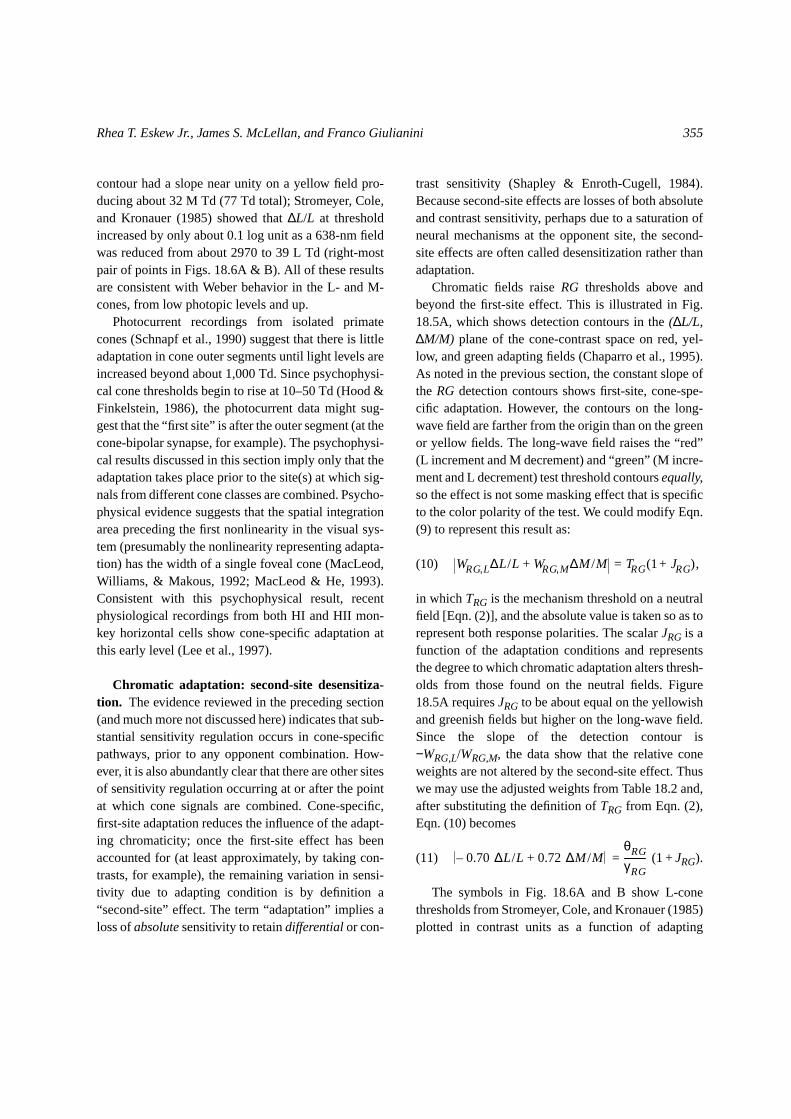
Figure 18.6: Second-site effects onRG. (A & B) ∆L/L thresholds as afunction of the equivalent back-ground wavelength, replotted fromFig. 7 of Stromeyer, Cole, and Kro-nauer (1985), for two observers. Allof the fields were equated for quantalcatch in the L-cones. Filled symbols:high intensity condition (3184 Td at638 nm). Open symbols: low inten-sity condition (42 Td at 638 nm).Solid curves are red/green huevalence functions, plotted on a equal-L quantal basis. (C & D) Data fromtwo observers, replotted from Fig. 3of Chaparro et al. (1995). L, M, andequiluminant contrast thresholds arerepresented by different symbols.The abscissa is equivalent back-ground wavelength; retinal illumi-nance was 3000 Td throughout. Thesolid curves are red/green valencefunctions, plotted on a constant-luminance basis. (E) The samered/green valence functions plottedover the whole spectrum on thefamiliar equal-energy basis. In allpanels, the hue functions were com-puted as in Eqn. (14) (using the 2 degfrom 10-deg cone fundamentals ofStockman, MacLeod, and Johnson,1993) withk0 = 0.0004,k2 = 1.244,and k3 = 0.2 (except for panel B,where k2 = 1.501 andk3 = 0.3 tomake the minimum near 580 nminstead of near 570 nm).

γ RG

θRG---------- ∆L

L-------


Thus the data in Figs. 18.6A and B provide a way toestimate the form of the second-site desensitizationeffect.JRG is roughly U- or V-shaped in this spectralregion, with a minimum in the yellow and a maximalelevating effect of about fivefold. The effect of adapt-ing chromaticity is reduced at the lower radiance.

Figures 18.6C and D show similar data from Fig. 3of Chaparro et al. (1995) but replotted in cone-contrastunits, for L, M, and equiluminant tests. Whereas theadapting fields in panels A and B were equated for L-cone quantal catch, those in panels C and D were keptat 3000 Td; this accounts for part of the difference inshape of the data between the top two panels and themiddle two panels. Again, thresholds are lowest forfields that should be near neutral for a red/green huemechanism and rise elsewhere, particularly as the fieldwavelength is lengthened. The agreement between L,M, and equiluminant tests is support for the modelsince, according to Eqn. (10), the second-site effectalters all of the RG thresholds equally.

Recently, Yeh, Lee, and Kremers (1996) foundanalogous results in macaque P-retinal ganglion cells:two adapting fields that were equated for quantal catchin one cone class (e.g., L) were alternated, so that onlythe adaptive state of the other cone type (e.g., M) var-ied over time. Responsiveness to∆L and∆M tests wasequally affected by the two fields, indicating strongsecond-site desensitization at the level of the ganglioncells.

Recall that the criterion response levelθRG is pro-portional to the standard deviation of the noise withinthe mechanism [Eqn. (6)]. Equation (11) means thatthe higher threshold on the chromatic field could be theresult of either an increase in the noise within themechanism (σRG) or a decrease in its effective gain(γRG). Noise found at the level of the retinal ganglioncells of cat (Reich et al., 1994) is independent of meanillumination, and in both the cat and monkey it isapparently additive and generated within the ganglioncells themselves (Croner, Purpura, & Kaplan, 1993); ifthis is correct, then the noise cannot vary with adaptivestate and thus could not explain second-site desensiti-zation. The gain could be reduced via a compressivenonlinearity: A strongly chromatic field would raise

the operating point on the nonlinear curve high enoughthat the tangent to the curve, which is the effective gainat the operating point, was reduced. However, if sec-ond-site desensitization is produced by means of acompressive nonlinearity, this must occur in a such away that “reddish” and “greenish” test thresholds areraised approximately equally on, for example, a red-dish field (Figs. 18.5, 18.6C & D).

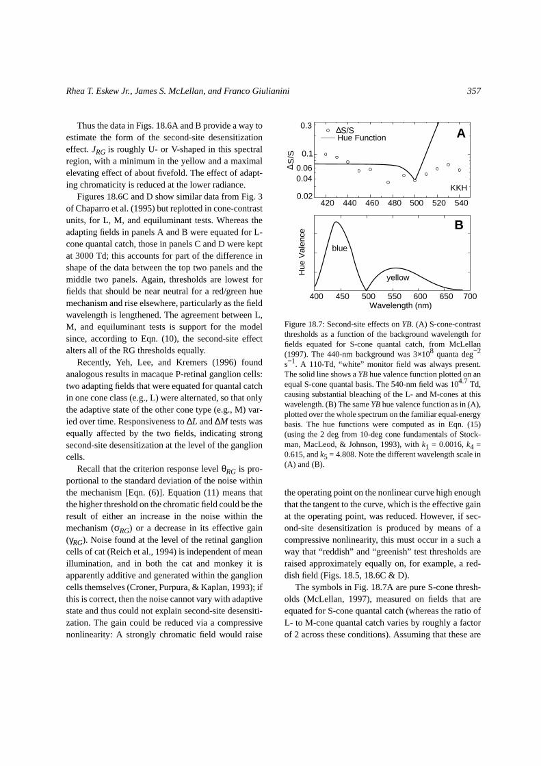
The symbols in Fig. 18.7A are pure S-cone thresh-olds (McLellan, 1997), measured on fields that areequated for S-cone quantal catch (whereas the ratio ofL- to M-cone quantal catch varies by roughly a factorof 2 across these conditions). Assuming that these are

0.02

0.040.06

0.1

0.3

420 440 460 480 500 520 540

∆S/SHue Function

∆S

/S

KKH

400 450 500 550 600 650 700Wavelength (nm)

blue

yellow

Hue

Val

ence

B

A

Figure 18.7: Second-site effects onYB. (A) S-cone-contrastthresholds as a function of the background wavelength forfields equated for S-cone quantal catch, from McLellan(1997). The 440-nm background was 3×108 quanta deg−2

s−1. A 110-Td, “white” monitor field was always present.The solid line shows aYBhue valence function plotted on anequal S-cone quantal basis. The 540-nm field was 104.7 Td,causing substantial bleaching of the L- and M-cones at thiswavelength. (B) The sameYBhue valence function as in (A),plotted over the whole spectrum on the familiar equal-energybasis. The hue functions were computed as in Eqn. (15)(using the 2 deg from 10-deg cone fundamentals of Stock-man, MacLeod, & Johnson, 1993), withk1 = 0.0016,k4 =0.615, andk5 = 4.808. Note the different wavelength scale in(A) and (B).


YB-detected, then application of the same reasoningthat was used forRG leads to:

(13) JYB = 0.80 − 1.

Thus, over this wavelength range, these S-conethresholds may be used to estimate the second-siteeffect for YB. JRG changes only very gradually withwavelength over most of this range, with most of theelevation occurring in the violet; the maximum sec-ond-site elevation here was about threefold.

WhateverJRGandJYBare, they cannot be functionsof conecontrasts– they must depend on the chroma-ticity of the adapting field. There is a long line of workon colorappearancethat posits an additive contribu-tion to the hue of a test light from the hue of the adapt-ing field (e.g., Jameson & Hurvich, 1972; Shevell,1978) above and beyond first-site adaptation; byapplying this “two-process” approach to detection onemight guess thatJRG andJYBare similar to opponent-response functions derived from the color appearanceof lights (Hurvich & Jameson, 1955). Thus, for exam-ple, we might let:

(14) JRG = k0 ,

(15) JYB = k1 ,

with positive constantsk2 throughk5 chosen so that thefunctions have zeros near the equilibrium hue wave-lengths (unique yellow, green, and blue); see Figs.18.6E and 18.7B. This choice would makeJ representan increase in mechanism thresholdT that is propor-tional to the hue valence of the adapting field. This ver-sion of JRGis similar to the “J factor” used by Boyntonto predict wavelength discrimination functions (Boyn-ton, 1979).

The smooth curves in Figs. 18.6 and 18.7 show suchhue functions plotted on the appropriate basis in eachcase. As shown in Fig. 18.6,JRG is poorly approxi-mated by a red-green valence function (one based on alinear combination of cone fundamentals, constrainedto have a zero near “yellow”). The estimates ofJYB inFig. 18.7 have almost no correspondence to a yellow-

blue valence function. Thus, this version of the two-process model cannot account for second-site desensi-tization.

Although there are many other studies of chromaticdetection under conditions of chromatic adaptationthat might in principle be used to reveal second-siteeffects, most of them suffer from one or both of the fol-lowing limitations: (1) the observer is allowed to adaptto the test as well as to the background light, makingthe actual adaptation state uncertain; (2) the postrecep-toral mechanismsRGandYBare not isolated, so thatit is not clear from the data which second-site effectcould be estimated. Thus the form taken byJRG andJYBcannot yet be fully determined, nor is it known indetail how these second-site effects vary with fieldradiance and (perhaps) test parameters.

There is, however, a puzzle that should beaddressed here: After complete first-site adaptation, allsteady-state adapting fields would produce the samesignal in each cone-specific pathway. No matter howsignals in these pathways are then combined, therecould be no second-site effects. Complete first-siteadaptation means that all adapting fields should appearthe same and produce the same detection thresholds,which is consistent with the mapping of all adaptingfields to the origin in cone-contrast space (Figs. 18.1A& C). Given the large body of evidence favoring cone-specific adaptation, how can there also be second-siteeffects? There are at least two possible answers (whichare not mutually exclusive): (1)Completefirst-siteadaptation never occurs. There is a residual, unadaptedsignal that is operated on at the second site. Record-ings from individual turtle cones (Normann & Per-lman, 1979; Burkhardt, 1993a) and extracellularrecordings in primate retina (Valeton & van Norren,1983) indicate that this is so: Although cones adapt,the response to a steady background does not stay con-stant, but instead increases with increasing quantalcatch. (2) The modulation of cones near the edge of theadapting field, produced by eye movements, maintainsthe color appearance of the field and provides the sig-nal that modulates sensitivity at the second site andraises threshold in the field center. Evidence fromcolor matching experiments (Pokorny, Smith, & Starr,

γYB

θYB---------

∆SS

-------

L k2M– k3S+

L k4M k5S–+


1976; Vienot, 1983; Elsner, Burns, & Webb, 1993;Picotte, Stromeyer, & Eskew, 1994) suggests that, atleast for relatively small fields, the edges determinefield color under normal viewing, and when fields arestabilized on the retina they generally appear colorlessregardless of their chromaticity (Sheppard, 1920;Hochberg, Triebel, & Seaman, 1951; Gur, 1986).However, there is some important evidence against this“filling-in” explanation of second-site threshold eleva-tion. Nerger, Piantanida, and Larimer (1993) foundthat when a red disk was surrounded by a yellow annu-lus, stabilizing the edge between the two fields on theretina caused the yellow to fill in, making the diskappear yellow too. This filling-in affected the colorappearanceof small tests added to the disk, but it didnot affect their increment threshold. If this result holdsgenerally, then filling-in could still explain how thecolor appearance of an adapting field is maintaineddespite first-site adaptation, but that would not sufficeto explain why chromatic adapting fields produce asecond-site elevation of test thresholds. In case 1, conecontrasts may be regarded as approximations to theactual signal in the cone-specific pathways; in case 2,effects of field configuration and eye movementswould need to be considered.

A note on equiluminance.Many studies of chro-matic detection and discrimination restrict stimuli tothe null plane of the luminance mechanism – the equi-luminant plane. There are a number of advantages todoing so: If these mechanisms are really linear, and ifequiluminance is accurately determined, then one isguaranteed to be studying chromatic mechanismswhen in the equiluminant plane. The use of only oneplane greatly reduces the need for data and simplifiesthe analysis of them. However, significant limitationsmay arise when only the equiluminant plane is studied.

First, it should be explicitly noted that, if first-siteadaptation affects the cone signals supplied toLum(Eisner & MacLeod, 1981; Stromeyer, Cole, & Kro-nauer, 1987; Pokorny, Jin, & Smith, 1993; Swanson,1993), there can be no single plane in the cone-excita-tion space that is a null plane for a luminance detectionmechanism across different adapting conditions. For

example, a plane in which the photopic luminosityfunctionV(λ) is constant (Fig. 18.1B) cannot be a nullplane for a luminance mechanism if the cones adaptindependently, because the cone-specific rescalingwould cause the mechanism’s null plane to tilt differ-ently in cone-excitation space for different adaptationstates.V(λ) is useful for specifying the photometric“effective intensity” of an adapting light, but sinceV(λ) is a fixed function of cone fundamentals, it cannotbe used to represent neural events that occur subse-quent to first-site adaptation. We use the terms “con-stant luminance” or “constant-V(λ)” to refer to thatfixed plane in cone-excitation space where∆L=−∆M(see Color Spaces section) and reserve the term “equi-luminant” for the null planein the cone-contrast spaceof a putative nonopponent, linear (luminance) detec-tion mechanism.

A drawback to using tests ofconstant luminancehas to do with detecting first-site effects onRG. Cone-specific adaptation is most readily measured by usingcone-specific tests. Presenting tests within the con-stant-V(λ) plane makes it more difficult to detect first-site changes (Eskew, Stromeyer, & Kronauer, 1992;Chaparro et al., 1995). For example, consider thedetection contours shown in Fig. 18.5B: comparedwith the 525-nm adapting field, the 654-nm field sup-presses L-cone sensitivity and relatively enhances M-cone sensitivity (in excitation units). A test presentedalong the 135-deg/315-deg,∆L = −∆M direction (grayarrows) would miss the dramatic changes in sensitivityalong the cone-specific axes, since the two first-siteeffects approximately tradeoff against one another forthat test direction. First-site adaptation in S-cones canbe easily measured in this constant-V(λ) plane, sincethe S-cone axis lies in or near it.

A drawback to usingequiluminanttests has to dowith YB. Equiluminant lights produce contrasts ofopposite signs in the L- and M-cones. Therefore theycannot produce very much differential signal in thelong-wave side ofYB, if, in fact, WYB,L and WYB,Mhave the same signs as indicated in Table 18.2. In themost extreme case, if the long-wave side ofYBhas thesame spectral sensitivity asLum (so that wouldbe a weighted difference of {0,0,1} and ), then

WYBWLum


only the S-cone signal inYBcould vary in the equilu-minant plane. Thus, restricting test modulations to theequiluminant plane might lead one to believe thatYBconsists of S-cones alone, unopposed by a long-wavesignal. Yet studies that modulate the luminance of testlights clearly show inhibitory interactions betweenlong- and short-wave increment tests at threshold (e.g.,Boynton, Ikeda, & Stiles, 1964; Thornton & Pugh,1983; Kalloniatis & Harwerth, 1991), a notch in theincrement threshold curve near unique green indicat-ing opponency in the mechanism detecting short-wavetests (e.g., King-Smith & Carden, 1976), as well asinhibition at threshold between∆S/S versus stimulithat modulate L and M equally for both increments anddecrements in cone-contrast space (Cole, Hine, &McIlhagga, 1993, 1994; Sankeralli & Mullen, 1996).

In fact, chromatic detection is (at least) a three-dimensional problem, and it is unlikely that a fullunderstanding of it can be reached by using stimulilying in only one plane. Most cone modulations (<~15Hz) are detected byRG, and it is difficult to isolateeitherYBor Lumover any substantial region of colorspace. This point is illustrated in Table 18.1 by the log-unit sensitivity advantage thatRG has overYB andLum, and by the unmasked data in Fig. 18.3 (this is forfoveal stimulation; outside of the fovea the relativesensitivity ofLumincreases: Mullen, 1991; Stromeyer,Lee, & Eskew, 1992). This sensitivity difference iswhy Sankeralli and Mullen (1996) and Cole, Hine andMcIlhagga (1994) varied spatiotemporal parameters toattempt to isolate theYBandLummechanisms. Equi-luminance is not necessary, and often not sufficient, tofully reveal the properties of chromatic detectionmechanisms.

Chromatic discrimination

Wavelength discrimination. In the typical wave-length discrimination study, subjects view a continu-ously present bipartite field, often of 2-deg diameter orso. In the two halves of the field, monochromatic lightsof wavelengthλ and (λ + ∆λ) appear; the observerturns a knob that alters∆λ until the two halves appear

discriminably different, and the threshold∆λ is plottedagainstλ. In some cases the method of adjustment isabandoned for other psychophysical procedures. Typ-ically, the experimenter attempts to keep photopicluminosity constant (usually at some rather low valuesuch as 100 Td), but this is difficult and likely it isoften not achieved. From our perspective, the classicwavelength discrimination experiment is a poor one:The adaptation state of the observer is not kept con-stant but rather varies with the wavelength under study,and it is not clear how much of the variation in∆λ isdue to changes in adaptation across wavelengths –changes in thestateof the system – and how much isdue to the direct “test” effects of wavelength differ-ence.

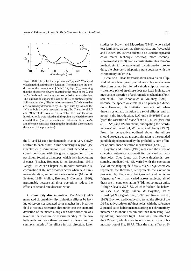
The line in Fig. 18.8 shows a “typical” wavelengthdiscrimination curve for a color-normal observerbased on several published studies (see, e.g., Wyszecki& Stiles, 1982a, Sect. 7.10.2), but individual observersmay differ substantially (e.g., Wright & Pitt, 1934),and the shape of the curve as well as its height dependson field size, luminance, and other factors (Bedford &Wyszecki, 1958; McCree, 1960). The curve often hasa fairly broad minimum near 570–600 nm, whereunder optimal conditions∆λ can be much less than 1nm (e.g., 0.2 nm at 560 nm; Hilz, Huppmann, &Cavonius, 1974).

The points in Fig. 18.8 show predicted wavelengthdiscrimination thresholds based on the cone weights inTable 18.2 and a 10:1 ratio ofRG to YB sensitivitywithout including second-site desensitization. Thepoor fit illustrates the importance of second-site effects(see Boynton, 1979). Without second-site desensitiza-tion, the model of Eqn. (8) produces the best discrim-inability in the long-wave portion of the spectrum (Fig.18.8). Incorporating second-site desensitization wouldlessen sensitivity, especially at the spectral extremes,and push the minimum∆λ to shorter wavelengths(nearer 570 nm, cf. Fig. 18.6).

The importance of second-site desensitization inwavelength discrimination has also been emphasizedby Mollon and colleagues (Mollon, Estévez, &Cavonius, 1990), who have studied the local maximumnear 460 nm (the “short-wave pessimum”). Because


the L- and M-cone fundamentals change very slowlyrelative to each other in this wavelength region (seeChapter 2), discrimination here must depend on S-cones, consistent with the great exaggeration of thepessimum found in tritanopes, which lack functioningS-cones (Fischer, Bouman, & ten Doesschate, 1951;Wright, 1952; see Chapter 2). In color normals, dis-crimination at 460 nm becomesbetterwhen field lumi-nance, duration, and saturation are reduced (Mollon &Estévez, 1988; Mollon, Estévez, & Cavonius, 1990),presumably because all three operations reduce theeffects of second-site desensitization.

Chromaticity discrimination. MacAdam (1942)generated chromaticity discrimination ellipses by hav-ing observers set repeated color matches in a bipartitefield at various reference chromaticities; the standarddeviation of the match along each color direction wastaken as the measure of discriminability of the twohalf-fields and was therefore used to determine thesemiaxis length of the ellipse in that direction. Later

studies by Brown and MacAdam (1949), who variedtest luminance as well as chromaticity, and Wyszeckiand Fielder (1971), who did not, also used the repeatedcolor match technique whereas, more recently,Romero et al. (1993) used a constant-stimulus Yes–Nomethod. As in the wavelength discrimination proce-dure, the observer’s adaptation state covaries with thechromaticity under test.

Because a linear transformation converts an ellip-soid into a sphere (an ellipse into a circle), mechanismdirections cannot be inferred a single elliptical contour– the short axis of an ellipse does not itself indicate themechanism direction of a chromatic mechanism (Poir-son et al., 1990; Knoblauch & Maloney, 1996) –because the sphere or circle has no privileged direc-tions. However, this limitation does not hold whenthere is systematic variation in asetof ellipses, and, asnoted in the Introduction, LeGrand (1949/1994) ana-lyzed the variation of MacAdam’s (1942) ellipses into(∆L − ∆M) and∆Sdirections, anticipating the “cardi-nal axes” of Krauskopf, Williams, and Heeley (1982).From the perspective outlined above, the ellipseshould be regarded as an approximation to the roundedparallelepiped generated by the probability sum of lin-ear or quasilinear detection mechanisms [Eqn. (8)].

Boynton and Kambe (1980) measured the effect ofchanging reference chromaticity on cardinal axisthresholds. They found that S-cone thresholds, pre-sumably mediated viaYB, varied with the excitationlevel of the adapting field as∆S= k(S+ S0), where∆Srepresents the threshold,S represents the excitationproduced by the steady background, andS0 is an“eigengrau” term that varied across subjects; all ofthese are in cone-excitation (STd, not contrast) units.At high S levels,∆S≈ kS, which is Weber-like behav-ior (see also Nagy, Eskew, & Boynton, 1987;Krauskopf & Gegenfurtner, 1992; and Romero et al.,1993). Boynton and Kambe also tested the effect of theL/M adaptive ratio on∆Sthresholds, with the referenceSquantal catch held constant, starting at a chromaticitymetameric to about 478 nm and then increasingL/Mby adding long-wave light. There was little effect oftheL/M ratio, which is not inconsistent with the right-most portion of Fig. 18.7A. Thus the main effect on S-

0

2

4

6

400 450 500 550 600 650Wavelength (nm)

RGYBBOTH

∆λ

Figure 18.8: The solid line represents a “typical,” W-shapedwavelength discrimination function. The points are the pre-diction of the linear model [Table 18.2, Eqn. (8)], assumingthat the observer is always adapted to the mean of theλ andλ+∆λ fields and that there is no second-site desensitization.The summation exponentβ was set to 40 to eliminate prob-ability summation; filled symbols represent∆λ’s (in nm) thatare exclusively determined byRG, open ones byYB, and the“+” symbols by both mechanisms equally. The ratio ofRGandYB thresholds was fixed as in Table 18.1, and the abso-lute thresholds were raised until the points matched the curveabout 490 nm (due to the nonlinear relationship between∆λand the cone contrasts, changing the thresholds also changesthe shape of the prediction).


cone thresholds observed by Boynton and Kambeseems to have been first-site adaptation, due (at least inpart) to their not using deep blue and violet adaptingconditions that would more strongly polarize the sec-ond site (as in the left portion of Fig. 18.7A). This isnot to say that second-site desensitization played norole in elevating thresholds on Boynton and Kambe’syellow fields; but on yellow fields, where theS Tdvalue was negligible, the only effect of second-sitedesensitization would be to raise the value ofS0 com-pared with its (unknown) value in the absence of sec-ond-site desensitization.

Boynton and Kambe also reported that constantluminance thresholds along the “red-green”∆L−∆M-axis (measured in∆L Td) were lowest for chromati-cally neutral (yellow and white) conditions and rosewith the change in referenceL/M (Td) value awayfrom neutral in either direction [at constantV(λ)].Nagy, Eskew, and Boynton (1987) and Romero et al.(1993) found a similar pattern, but both Krauskopf andGegenfurtner (1992) and Chaparro et al. (1995) foundsubstantially less elevation of these thresholds, espe-cially for long-wave adapting conditions. As was dis-cussed previously, however, testing only along the∆L = −∆M direction can obscure first-site adaptiveeffects, and when Chaparro et al.’s data are plotted incone contrast terms a clear, second-site effect of adapt-ing chromaticity is observed (Fig. 18.6).

Pedestal facilitation and masking.A “pedestal,”as the term is used here, is a reference stimulus withthe same shape and time course as the test that is to bedetected, but of possibly different spectral composi-tion (according to Tanner, 1961, the term “pedestal”was coined by psychoacoustican J. C. R. Licklider,who, incidentally, was one of the founders of the Inter-net). In a two-interval forced-choice experiment, forexample, the pedestal would be presented in both tem-poral intervals and the test would be added in oneinterval. The task of the observer is to discriminatetest+pedestal from pedestal alone. Thus, detectionreduces to the special case of discrimination with azero pedestal. A pedestal may also be used in a spatial-alternative task (e.g., Krauskopf & Gegenfurtner,

1992). Pedestal discrimination has been extensivelystudied in the spatial vision literature (e.g., Graham,1989; Foley, 1994).

Many discrimination experiments may be repre-sented as detection on a pedestal. Whereas second-sitedesensitization refers to changes in sensitivity due tochanges in the adapting state, the pedestal effectsinclude changes in sensitivity due to momentary shiftsaway from the adaptation state (shifts to which theobserver presumably does not have time to adapt).

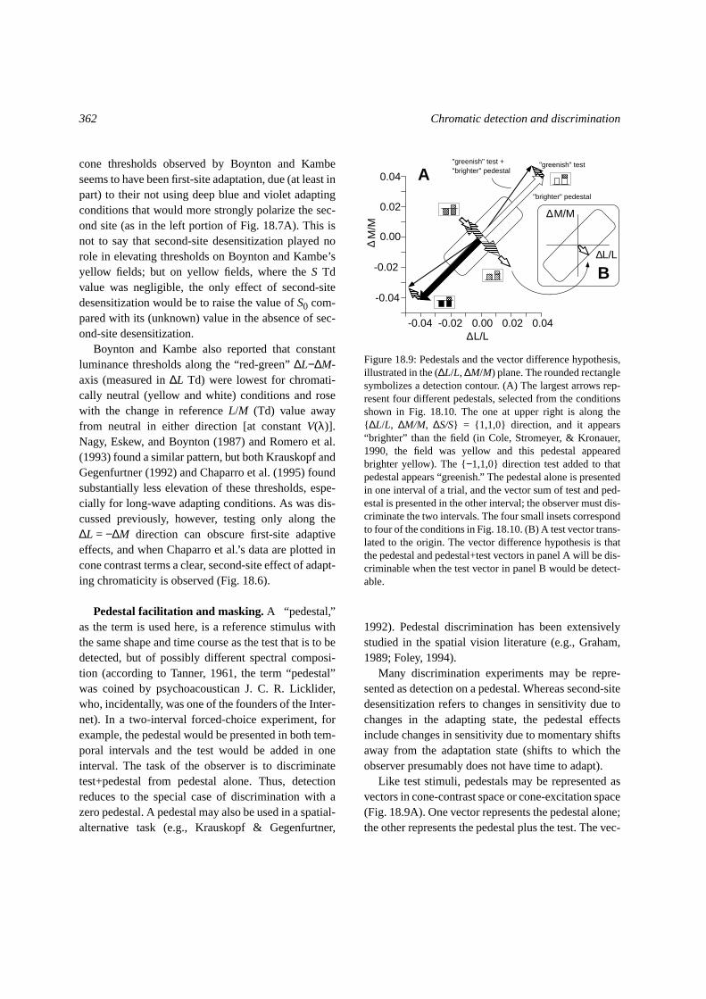
Like test stimuli, pedestals may be represented asvectors in cone-contrast space or cone-excitation space(Fig. 18.9A). One vector represents the pedestal alone;the other represents the pedestal plus the test. The vec-

0.00

0.02

-0.02

0.04

-0.04

0.02-0.02 0.04-0.04 0.00L/L

M/M

∆L/L

∆M/M

"greenish" test

"brighter" pedestal

A"greenish" test +"brighter" pedestal

∆

∆

B

Figure 18.9: Pedestals and the vector difference hypothesis,illustrated in the (∆L/L, ∆M/M) plane. The rounded rectanglesymbolizes a detection contour. (A) The largest arrows rep-resent four different pedestals, selected from the conditionsshown in Fig. 18.10. The one at upper right is along the{ ∆L/L, ∆M/M, ∆S/S} = {1,1,0} direction, and it appears“brighter” than the field (in Cole, Stromeyer, & Kronauer,1990, the field was yellow and this pedestal appearedbrighter yellow). The {−1,1,0} direction test added to thatpedestal appears “greenish.” The pedestal alone is presentedin one interval of a trial, and the vector sum of test and ped-estal is presented in the other interval; the observer must dis-criminate the two intervals. The four small insets correspondto four of the conditions in Fig. 18.10. (B) A test vector trans-lated to the origin. The vector difference hypothesis is thatthe pedestal and pedestal+test vectors in panel A will be dis-criminable when the test vector in panel B would be detect-able.


tor difference between the two is the test signal that theobserver must detect to make the discrimination. Theutility of a vector representation becomes most appar-ent when pedestals are considered: The separate pro-jections of the pedestal and test vectors onto thevarious mechanism vectors may be used to decomposethe effects of quite complex stimuli into their relevant,simpler components.

Wandell (1982, 1985) examined the “vector differ-ence hypothesis,” which supposes that two vectors arediscriminable when the vector difference betweenthem is such that the difference would be detectable byitself (Fig. 18.9B). This hypothesis is equivalent tosupposing that the only effect of a pedestal is to shiftthe origin of the representation to a new point. Thehypothesis fails, in general, since strong pedestals gen-erally raise thresholds, and weak pedestals may lowerthem. Were the vector difference hypothesis to hold,chromatic discrimination would, in essence, be identi-cal to chromatic detection and we could ignore pedes-tal effects; it is because the vector differencehypothesis fails that pedestal effects are important tounderstanding chromatic discrimination.

When the test and the pedestal are detected by thesame mechanism, weak pedestals generally facilitatedetection, so that discrimination on near-thresholdpedestals can be two- or three-times more acute thandetection, whereas intense pedestals produce masking(Nachmias & Kocher, 1970; Nachmias & Sansbury,1974; Foley & Legge, 1981; DeValois & Switkes,1983; Mullen & Losada, 1994). Cole, Stromeyer, andKronauer (1990) measured the pedestal discriminationof 1-deg spots in the(∆L/L, ∆M/M) plane of cone-con-trast space (on a yellow field); some of their data arereplotted in threshold units in Fig. 18.10. The insets ineach quadrant of the figure schematically represent thetwo intervals of a trial, with a test presented in oneinterval and the pedestal in both. The upper right-handquadrant of Fig. 18.10A shows a typical pattern ofresults when the pedestal and test stimulate the samepostreceptoral mechanism with the same polarity, inthis case the “red” side ofRG; both the pedestal andthe test were along the {∆L/L, ∆M/M, ∆S/S} ={1,−1,0} direction. When the pedestal is weak, thresh-

olds fall almost linearly with pedestal contrast,decreasing by a factor of roughly 2 and then increasingagain as pedestal contrast increases, so that pedestalsof more than three to four times their own thresholdsbegin to mask detection of the test. A line of slope−1through the weak-pedestal data gives the prediction of

2

1

0

1

2

10 5 0 5 10

RG

test

thre

shol

d el

evat

ion

RG pedestal (threshold units)"greenish" "reddish"

"gre

enis

h""r

eddi

sh"

A

1

0

1

8 4 0 4 8

RG

test

thre

shol

d el

evat

ion

Achromatic pedestal (threshold units)"darker" "brighter"

"gre

enis

h""r

eddi

sh"

B

Figure 18.10: Pedestal effects. In each panel, the inset repre-sents the presentation of two pedestals with a test added toone. (A) “Uncrossed” conditions. A greenish (solid symbols)or reddish (open symbols) test was presented with a greenish(left half of graph) or reddish (right half of graph) pedestal.Data are replotted, in units of “no pedestal” threshold, fromCole, Stromeyer, and Kronauer (1990, Fig. 4). (B) “Crossed”conditions. A greenish (solid symbols) or reddish (opensymbols) test was presented with a brighter (right half ofgraph) or darker (left half of graph) pedestal (detected byLum). Data are replotted, in units of “no pedestal” threshold,from Cole, Stromeyer, and Kronauer (1990, Fig. 5).


subthreshold summation, which approximatelyaccounts for the facilitatory effect [however, the sub-threshold summation idea is based on a repeatedly dis-credited psychophysical model, high-threshold theory(Graham, 1989); uncertainty reduction is another pos-sibility (Pelli, 1985)]. That line also predicts the rise inthreshold in the second quadrant that occurs when thepedestal polarity is opposite to the test (“green”instead of “red,” a test along the {−1,1,0} direction),and this rise has been taken as evidence against theuncertainty reduction account of the weak pedestaleffect (Bowen, 1997). The rise in the second quadrantcontinues until the point at which the pedestal againapproaches its own threshold, where the test thresholddrops abruptly. Cole, Stromeyer, and Kronauer (1990)attributed this abrupt drop in threshold to a change inthe observer’s criterion: The observer could choose the“less red” test interval (“green” pedestal + “red” test)by comparing it to the red pedestal, a strategy that canonly be used when the pedestal itself is visible. Forboth pedestal polarities, the test is masked by high-contrast pedestals (little masking is shown in this par-ticular data set, but substantial masking was reportedin the same paper for another observer, and in thepapers cited above). The curve shown in the upperright quadrant of Fig. 18.12A is sometimes called the“dipper” function.

In contrast to Fig. 18.10A, Fig. 18.10B shows thatwhen the test and pedestal are crossed – that is, theystimulate different postreceptoral mechanisms – thereis little masking by the pedestal. Here the test is greenor red and the pedestal is equichromatic. Although thisis not clear in Fig. 18.10B, in other crossed experi-ments the pedestal has little effect until it approachesor exceeds its own threshold, when the test thresholddrops abruptly to roughly one-half of its zero-pedestalvalue (Switkes, Bradley, & DeValois, 1988; Chaparroet al., 1994). Cole, Stromeyer, and Kronauer foundalmost no masking using crossed pedestals; Switkes,Bradley, and DeValois (1988) and Mullen and Losada(1994) found slightly more, but only at very high ped-estal contrasts (more than ~30× pedestal threshold).For Cole, Stromeyer, and Kronauer’s (1990) disk stim-uli, the red-green mechanism and luminance mecha-

nism are approximately interchangeable: They behavesimilarly in uncrossed conditions, and in crossed con-ditions it does not much matter which one detects thetest and which the pedestal. Whereas Switkes, Bradley,and DeValois (1988) report an asymmetry, in thatluminance test gratings were masked but never facili-tated by red-green pedestal gratings, Mullen andLosada (1994) find the two types of gratings to beinterchangeable, as Cole, Stromeyer, and Kronauer didwith spots.

Much evidence suggests that the mechanisms pro-ducing facilitation are different from those producingmasking (Pelli, 1985; Eskew et al., 1991; Foley, 1994;Mullen & Losada, 1994). The largest effect of a pedes-tal is masking in the uncrossed conditions, with facili-tation never reducing the threshold by much more thana factor of 2 or 3. The masking, which is often attrib-uted to divisive inhibition (e.g., Foley, 1994), producesthreshold elevations that approximate a power law,with reported exponents varying from about 0.5 toabout 1.0, depending in part on the spatial and tempo-ral frequencies of the stimuli. Similar or even largermasking, but not facilitation, can be obtained when theentire field is flashed instead of presenting a pedestal(e.g., Zaidi, Shapiro, & Hood, 1992) or when a noisemasking pattern is presented instead of a pedestal(Pelli, 1990).

A few studies have examined the effects of mixedpedestals, for example, a pedestal that stimulates bothRGandYB(Krauskopf & Gegenfurtner, 1992) or bothRGandLum(Wandell, 1985; Cole, Stromeyer, & Kro-nauer, 1990). Mullen and Losada (1994) measuredluminance grating thresholds in the presence of a maskgrating that had bothRG and Lum components(because the phases of mask and test were indepen-dently randomized, the mask is not a “pedestal” as wehave defined it). The chromatic contrast in the maskwas always kept fixed at a level that would by itselfslightly raise the threshold for the luminance test; theluminance contrast in the mask was varied in differentruns. The resulting function more closely resembledan uncrossed pedestal function (Fig. 18.10A) than thecrossed function (Fig. 18.10B) – there was facilitationat low mask contrasts despite the presence of the fixed


maskingRGcomponent, suggesting that in some sensethe uncrossed effect takes precedence over the crossedeffect, perhaps because the uncrossed effect takesplace at an earlier stage in the visual system.

Krauskopf and Gegenfurtner (1992) presented four36-min-diameter disks around a central fixation spot,all on a 10-deg steady adapting field. Three of the fourdisks had the same chromaticity, one of them was dif-ferent, and the observers’ task was to select that one (afour-alternative forced-choice task). In the terminol-ogy used here, three pedestal stimuli were presentedalong with a fourth stimulus that consisted of the vec-tor sum of the pedestal plus a test; the discriminationof the odd disk is equivalent to the detection of the testin the presence of a pedestal. The results were plottedin the equiluminant plane of a local cone-excitationspace. Krauskopf and Gegenfurtner varied the chroma-ticity of the pedestal, with all stimuli restricted to theconstant-V(λ) plane (~370 Td in the main experi-ments). The results are shown in Fig. 16.11 (see Chap-ter 16), with the term “test” used for what we call a“pedestal.” Red (+∆(L−M)) and green (− ∆(L−M))tests were equally masked by either red or green ped-estals with contrasts ranging from about 6× thresholdup to almost 40×, consistent with Fig. 18.10A (weakpedestals were not used, so no subthreshold facilita-tion was observed). Similarly, yellow (−∆S) and blue(+∆S) tests were approximately equally masked byyellow and blue pedestals, for pedestals up to about10× threshold – here, weak pedestals produced somefacilitation (Fig. 16.11, upper left). These data werecollected on a white adapting field. When the back-ground was made red instead of white, the minimum ofthe pedestal function shifted over to the adapting chro-maticity, suggesting that adaptation occurs prior to thesite of the pedestal effect (consistent with the first sitebeing early in the visual system). When the crossedfunctions were measured (a red or green test on a yel-low or blue pedestal, and vice versa), the pedestals pro-duced a small facilitation or no effect (upper right andlower left of Fig. 16.11), which is reasonably consis-tent with the crossed luminance and red-green func-tions shown in Fig. 18.10B. This last result isimportant because it implies thatYBandRGbehave as

LumandRGhave been shown many times to do (e.g.,Fig. 18.10B), with pedestals detected by one mecha-nism producing a small facilitation and no masking oftests detected by the other mechanism, at least up tovery high-contrast pedestals.

In another important experiment, Krauskopf andGegenfurtner (1992) used tests of various chromatici-ties on pedestals of various chromaticities. The vectordifference hypothesis requires that each set of thresh-olds be a simple translation of the roughly circular no-pedestal data. This was not the case: The pedestal doesmore than move the origin, as shown in Fig. 16.12.

The data of Fig. 16.12 were used by Krauskopf andGegenfurtner to test the following two predictions: (1)Performance is determined by mechanisms tuned tothe two chromatic dimensions of the graph, the so-called cardinal directions (Krauskopf, Williams, &Heeley, 1982). In this case, these contours should beoriented with their long axis parallel to the closest car-dinal axis, because the pedestal masking would occurprimarily in that direction, and for the pedestals thatare equidistant from the two axes (45, 135, 225, and315 deg) the contours should be roughly circular. (2)Performance is determined by many mechanismstuned to various directions in color space (“higherorder” mechanisms; Krauskopf et al., 1986; see Chap-ter 16). In this case, all of the contours should be ofsimilar shapes with their long axis pointed at the ori-gin, since each pedestal would mask maximally andequally in its own color direction. As Fig. 16.12 shows,neither hypothesis fully accounts for the data: Most ofthe sets of thresholds would be well described byhypothesis (1), but those on pedestals at 135 and 315deg are consistent with hypothesis (2).

There is, however, a third possibility that was notdiscussed by Krauskopf and Gegenfurtner, which isthat although there are only two mechanisms, they arenot tuned to the “cardinal axes” but to some other, pos-sibly nonorthogonal, directions in this plane of colorspace. For example, suppose that the red-green mech-anism receives a small S-cone input, as we have arguedabove (Table 18.2). The inclusion of a small S-coneinput toRGwill cause the contours to tilt to the left, asmany of them in Fig. 16.12 seem to do, because the


negative signal generated by an increase in S will sumwith the negative signals generated by an increase in L,and this will interact with the pedestal chromaticity.An example will illustrate this point.

Note that the 135- and 315-deg pedestal data (Fig.16.12) are narrower than the 45- and 225-deg pedestaldata along their∆(L−M), horizontal direction. Thisasymmetry could be due to the S input toRG: At 45deg, the incremental S-component produces a negativesignal thataddsto the negative produced by being onthe reddish side of∆(L−M), and this additional reddishsignal could cause theRG component of the 45-degpedestal to mask theRGmechanism. In comparison, ata pedestal angle of 135 deg the reddish S-cone signalsubtractsfrom the greenish pedestal component pro-duced by being on the other side of∆(L−M), such thatthe RG component of the 45-deg pedestal producessome facilitation ofRG. The net result would be thatthe 45-deg pedestal should produce a wider contourthan the 135-deg pedestal contour.

Summary and conclusions

To understand chromatic detection and discrimina-tion, we must understand the processes that regulatevisual sensitivity. These can be categorized into first-site, cone-specific adaptation and second-site, oppo-nent-level desensitization. The constant slope of detec-tion contours across chromatic adapting conditions(Fig. 18.5A) strongly implies cone-specific, first-siteadaptation. Representing data as cone contrasts

approximately accounts for the first-site effect, dra-matically revealing the second-site effect, but we donot currently have enough information to estimate thesecond-site effects except in limited regions of thespectrum (Figs. 18.6 and 18.7), nor do we yet under-stand the mechanisms underlying them.

In the future, the algebraic representationsexpressed here need to be generalized to time-varyingmodels, to account for the dynamic nature of thesepathways. In particular, there are phase shifts andcone-contrast weight changes as a function of tempo-ral frequency between L and M inputs toLum, but notRG, except at certain near-neutral adapting chromatic-ities (Stromeyer et al., 1997). These phase shifts makethe linear detection contours into segments of ellipses.In the long run, the strictly linear model will not do; forexample,RG andYB may each need to be half-waverectified into two opposite polarity subsystems, toaccount for phenomena such as the decrease in sensi-tivity to green (+∆M/M or −∆L/L) relative to red(−∆M/M or +∆L/L) in the periphery observed byStromeyer, Lee, and Eskew (1992).

Acknowledgments

Preparation of this chapter was supported byEY09712. We are grateful for comments on a draftmanuscript and other assistance provided by AlexChaparro, Mike D’Zmura, John Foley, Peter Gowdy,Ken Knoblauch, Barry Lee, Adam Reeves, MarcelSankeralli, Andrew Stockman, and Charles Stromeyer.

Documents

Chromatic detection and discrimination