Embed Size (px)
Citation preview
Which measure for PFE?
The Risk Appetite Measure A∗
Chris Kenyon†, Andrew Green‡ and Mourad Berrahoui§
15 December 2015
Version 1.01
Abstract
Potential Future Exposure (PFE) is a standard risk metric for man-aging business unit counterparty credit risk but there is debate on how itshould be calculated. The debate has been whether to use one of manyhistorical (“physical”) measures (one per calibration setup), or one ofmany risk-neutral measures (one per numeraire). However, we argue thatlimits should be based on the bank’s own risk appetite provided that thisis consistent with regulatory backtesting and that whichever measure isused it should behave (in a sense made precise) like a historical measure.Backtesting is only required by regulators for banks with IMM approvalbut we expect that similar methods are part of limit maintenance gener-ally. We provide three methods for computing the bank price of risk fromreadily available business unit data, i.e. business unit budgets (rate of re-turn) and limits (e.g. exposure percentiles). Hence we define and proposea Risk Appetite Measure, A, for PFE and suggest that this is uniquelyconsistent with the bank’s Risk Appetite Framework as required by soundgovernance.
1 Introduction
Potential Future Exposure (PFE) is a standard risk metric for managing busi-ness unit counterparty credit risk (Canabarro and Duffie 2003; Pykhtin andZhu 2007) however there is debate on how it should be calculated (Stein 2013),as well as regulatory constraints (BCBS-185 2010). Whilst backtesting is onlyrequired by regulators for banks with IMM approval, we expect that similarmethods are part of limit maintenance generally. The debate has been whetherto use one of many historical measures (one per calibration setup), or one ofmany risk-neutral measures (one per numeraire). However, we argue that forPFE:
∗The views expressed are those of the authors only, no other representationshould be attributed. Not guaranteed fit for any purpose. Use at your own risk.†Contact: [email protected]‡Contact: [email protected]§Contact: [email protected]
1
arX
iv:1
512.
0624
7v1
[q-
fin.
RM
] 1
9 D
ec 2
015
• whatever measure is chosen it should behave (in a sense to be made precise)like a historical measure;
• the risk appetite of the bank should be consistent with regulatory con-straints;
• open risk should be viewed according to the risk appetite of the bank, i.e.the bank’s price of risk.
Given these three constraints we identify a unique new measure, the Risk Ap-petite Measure, RAM, or A for computing PFE. We demonstrate that thismeasure can be computed simply from existing bank data and provide exam-ples.
As in (Canabarro and Duffie 2003) we define PFE as a quantile q of futureexposure, that is, as a VaR measure. Since we are considering exposure as acontrol metric this is floored at zero. It is possible that PFE as VaR may bereplaced by PFE as Expected Shortfall (ES) following (BCBS-265 2013; BCBS-325 2015). Substituting ES for VaR makes no difference to the developmenthere as both VaR and ES can be backtested (Acerbi and Szekely 2014) whichis sufficient for our purposes.
Open risk, and hence limits, is a widespread feature of banking and one mo-tivation for capital. Pricing open risk, i.e. warehoused risk, is starting to attractattention in mathematical finance (Hull, Sokol, and White 2014; Kenyon andGreen 2015) and has a long history in portfolio construction (Markowitz 1952)and investment evaluation (Sharpe 1964). Valuation adjustments on prices forcredit have a long history (Green 2015) but it is only recently that capital hasbeen incorporated (Green, Kenyon, and Dennis 2014). This paper adds to theliterature linking investment valuation and mathematical finance by proposingthat limits be computed under the bank’s risk appetite measure provided aspart of sound, and self-consistent, governance.
The contribution of this paper is to develop and propose a method of com-puting PFE that is consistent with a bank’s Risk Appetite Framework (RAF)(BCBS-328 2015; FSB 2013) using the Risk Appetite Measure A, defined here.This method avoids the issues with P-measure PFE computation (choice ofcalibration), and avoids issues with Q-measure PFE computation such as theimplicit choice of a price of risk of zero. This approach can be used wheneverthere is open risk, both for pricing as well as for limits. Arguably, comput-ing prices and limits for open positions under A is the unique method that isconsistent with the bank’s RAF.
2 Risk Appetite Measure, AHere we consider each of the constraints in the introduction and show how thisleads to a unique definition of a unique Risk Appetite Measure, A, suitable forPFE.
2.1 PFE behaviour under PConsider the flow chart in Figure 1 for computing PFE where d is an elementof the set of simulation stopping dates D and there are n paths. The output of
2

Figure 1: Flow chart for computation of PFE under one of many physical (akahistorical) measures. d is a simulation stopping date in the set of all simulationstopping dates D. Each separate physical measure corresponds to a differentchoice of calibration algorithm and selection method for calibration data. Westress that there are many physical measures in practice because of the common,and erroneous, practice of referring to “the” physical measure as though the truefuture probabilities were available for PFE computation.
the procedure is a set of PFE numbers, PFE(q,d), corresponding to the chosenexposure quantile q for each stopping date d.
The P procedure of Figure 1 can be characterized by either of the followingequivalent properties:
• Each PFE(q,d) computation is independent of all simulation paths up tod
• Only portfolio simulation values at d are required for the computation ofPFE(q,d)
We call this property of PFE behaviour under P the Independence Property.From the point of view of physical-measure simuation this also appear to becommon sense, only values at the time have any effect.
Now considering risk-neutral pricing we know from, for example FACT TWOof (Brigo and Mercurio 2006) that the price of a payoff at T seen from t
Price of Payoff(T)t = EBt
B(t)Payoff(T)
B(T)
is invariant under change of numeraire from B to any other valid numeraire.Valid numeraires are non-zero, self-financing portfolios. Hence the probabilitydistribution of the payoff at T discounted back to t is also invariant under anychange of numeraire as we now prove.
Lemma 1. The discounted cumulative distribution function (CDF) of futureportfolio value is measure invariant, as is the discounted probability distributionfunction (PDF) if it exists.
Proof. Consider dcdf(t, V ) the discounted CDF of portfolio value x(T ), (i.e.gives probability of x(T ) being less than or equal to the constant V ):
dcdf(t, V ) := EBt[B(t)
I(V, x(T ))
B(T )
]
3
Wherex(T ) is the portfolio value;I(V, x(T )) is an indicator function that is 1 when V ≥ x(T ) but zero other-
wise.Now E[I(V, x(T ))] is the CDF of x(T ), and the B(t)/B(T ) is the discount-
ing. Since dcdf(t) is invariant under change of B for any other numeraire, thediscounted CDF is measure invariant. Hence so is the discounted PDF (if itexists, as PDFs do not have to).
This suggests a numeraire-independent definition of PFE as discounted PFE.However, how can we compare P-measure PFE and discounted-PFE, i.e. howdo we discount P-measure PFE back to t? We can be almost sure that theexpected value of a P-bank account will not be worth the inverse of a zero-coupon bond from t to T . (If we could be sure then the P-measure drift wouldbe the same as the Q-measure drift which cannot be guaranteed). Thus wecan see two methods to discount P-measure PFE and it is arguable which oneto use as both investments are available at t (bank account and zero couponT-maturity bond). Should we chose the investment that generates the highestreturn? We know the calibration so this is available. This uncertainty is similarto the uncertainty over the choice of numeraire for Q-measure PFE (just apartfrom choices of calibration).
The measure-independent definition of risk-neutral PFE is discounted PFEand this cannot be compared to P-measure PFE because discounting P-measurePFE is ambiguous. That is, P-measure PFE is naturally in the future whereasQ-measure PFE is naturally in the present (and discounted).
This is where we need the Independence Property that each PFE(q,d) com-putation is independent of all simulation paths up to d. This selects a uniquemethod to inverse-discount Q-measure PFE from t (now) to T (future), thatis we must use the T-maturity zero coupon bond. This construction of futureQ-measure PFE is measure independent1. This construction is also consistentwith PFE computed using the T -Forward numeraire for each T . Thus we havea Q-measure PFE that behaves in the same way as P-measure PFE, i.e. has theIndependence Property.
2.2 Consistency of Bank Risk Appetite and RegulatoryConstraints
We develop the following points here:
• a bank has a documented risk appetite which defines prices of differentrisks;
• backtesting requirements on risk factor dynamics give limits on drifts(etc.), that is, limits on the bank prices of risks;
• we can calculate the bank price of risk from the risk appetite for each busi-ness unit using easily available information, i.e. its limits and its budget(required rate of return).
1Some readers may object that this construction uses a value not at T , i.e. the start-timevalues of T -maturity zero coupon bonds. However, these are in the same category as data usedin the P construction for calibration: observed data that is not model or simulation dependentand only refers to time T .
4

We suggest that:
• the bank price of risk should be consistent with its regulatory requirementsas expressed through backtesting limits on the price of risk;
and observe
• there is no finite risk appetite that is consistent with a zero price of risk,i.e. with a risk-neutral-based PFE.
In the following section we will develop the Risk Appetite Measure, A, for PFEthat is consistent with the bank’s risk appetite (as constrained by regulatoryrequirements).
2.2.1 Bank Risk Appetite
Banks take risks, for example lending money, for rewards, that is to make prof-its. Banks are required by regulators to document their risk appetite with aneffective Risk Appetite Framework (RAF), and the RAF is a key element ofincreased supervision endorsed by G20 leaders (FSB 2013). A Risk AppetiteStatement (RAS) is a key part of supervision (BCBS-328 2015). The BCBS andthe FSB use slightly different terminology but both see a risk appetite statementas vital. Risk appetite is defined in (BCBS-328 2015) referencing (FSB 2013)as:
The aggregate level and types of risk a bank is willing to assume, de-cided in advance and within its risk capacity, to achieve its strategicobjectives and business plan.
Risk appetite is not a single figure, rather:
Risk appetite is generally expressed through both quantitative andqualitative means and should consider extreme conditions, events,and outcomes. In addition, risk appetite should reflect potentialimpact on earnings, capital, and funding/liquidity.
Senior Supervisors Group, Observations on Developments in RiskAppetite Frameworks and IT Infrastructure, December 23, 2010
Principle three of the key elements of FSB Principles for effective RAFs is astatement of risk limits which are defined as
Quantitative measures based on forward looking assumptions thatallocate the financial institutions aggregate risk appetite statement(e.g. measure of loss or negative events) to business lines, legal en-tities as relevant, specific risk categories, concentrations, and as ap-propriate, other levels.
Furthermore:
The elements of the RAF should be applied at the business line andlegal entity levels in a manner that is proportionate to the size ofthe exposures, complexity and materiality of the risks.
5
In practice every business unit has a PFE (or VaR or other) limit and a budget.Budget is the word used for the profit over a fixed period, or rate or returnon investment (or equity, etc.) that a business unit is required to deliver. Thebusiness unit limits and the business unit budget define the risk appetite of thebank for the risk type that the business unit is engaged in. These number arereadily available within a bank and constantly monitored. Every business unithead is acutely aware of their progress towards plan on budget and their limitusage.
Now we need to link the price of risk with the risk appetite. First recall adefinition of the market price of risk following (Bjork 2004). Suppose that wehave a stock price process S(t) under a physical measure:
dS(t)/S(t) = µdt+ σdW
then the market price of risk mM is defined as:
mM :=µ− rσ
(1)
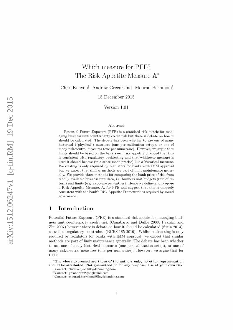
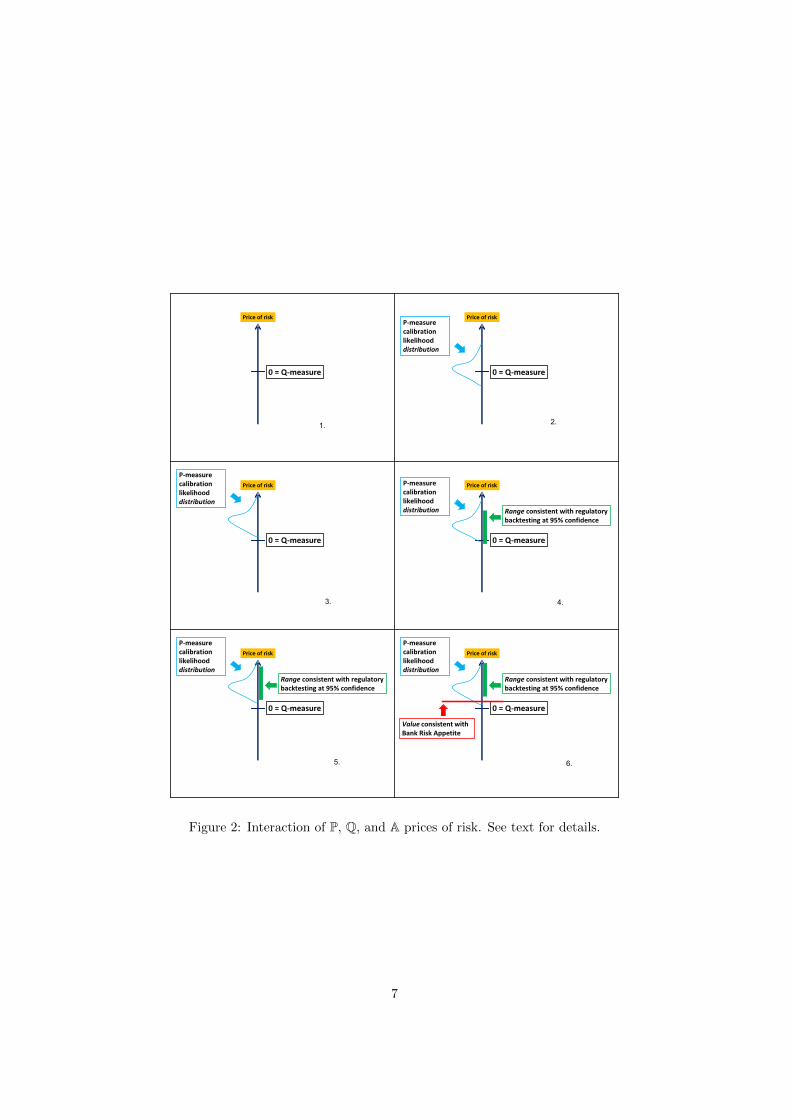
where r is the riskless rate. The price of risk gives the additional return requiredby investors per unit of return volatility σ. Of course the return can only bevolatile when it is not hedged. Were the return to be hedged, i.e. riskless, thenthe return is r, the riskless rate. Before going into details we give the intuitionbetween the interaction of the different measures and constraints in Figure 2 asfollows.
1. (Top Left) shows an axis of possible prices of risk, with zero marked andlabelled with the Q measure because a risk-neutral measure has a zeroprice of risk by definition.
2. (Top Right) adds a probability distribution of P-measure prices of risk. Amaximum-likelihood calibration will, by definition, pick the price of riskwith the highest likelihood. This particular calibration shows the supportof the P-measure prices of risk including zero.
3. (Middle Left) considers a later P-measure calibration where the probabilitydistribution of P-measure prices of risk has shifted because the input datafor the calibration has shifted. In this example the support of the P-measure prices of risk no longer includes zero.
4. (Middle Right) adds a range of possible prices of risk consistent withregulatory backtesting. There will be a most likely price of risk from theregulatory backtesting but there will also be an interval (generally, a set)of prices of risk that cannot be ruled out at any given confidence level(here given as 95%).
5. (Bottom Left) considers a later situation where the interval of prices ofrisk that cannot be ruled out with 95% confidence no longer includes zero.
6. (Bottom Right) adds the price of risk consistent with the Bank Risk Ap-petite measure A (see below for details on computation).
Figure 2 illustrates several potential issues with P, Q, and A prices of risk.Firstly, there is no guarantee that a zero price of risk will be consistent with
6
1. 2.
3. 4.
5. 6.
Figure 2: Interaction of P, Q, and A prices of risk. See text for details.
7
a P-measure price of risk, even if it was previously. Secondly, even if a zeroprice of risk is consistent with regulatory backtesting over one period there isno guarantee that a zero price of risk will remain consistent as markets move.Thirdly, if the Bank’s Risk Appetite is chosen without consideration of theregulatory backtesting there is no guarantee that the Bank’s Risk Appetite willbe consistent with regulatory backtesting. If this were to occur the Bank mightwish to reconsider its risk appetite.
2.2.2 Limits from Backtesting
Basel III (BCBS-189 2011) and its European implementation (EU 2013b; EU2013a) mandate sound backtesting for the internal model method (IMM) forcredit exposure. Principles for such backtesting are provided in (BCBS-1852010) and expanded on in (Kenyon and Stamm 2012; Anfuso, Karyampas, andNawroth 2014). If a bank is not using internal models for credit exposurefor regulatory purposes, i.e. does not have regulatory approval to do so, thenthe bank may or may not choose to follow such principles for other purposessuch as PFE. We would expect this to be part of limit maintenance generally.However, in the reverse case where regulatory approval has been obtained, thenthe Use Test element (BCBS-128 2006), paragraphs 49-54 states that the bankshould be consistent in the data used for day-to-day counterparty credit riskmanagement. Although backtesting is only required by regulators for bankswith IMM approval we expect similar methods to be part of limit maintenancegenerally.
Backtesting will select P calibrations that pass at a desired confidence level:assuming such exist, if not the bank will not be permitted to use the IMMapproach for regulatory purposes, but may still use it for other purposes. Henceit is possible to adapt the backtesting machinery to provide a set, or interval,or simulation parameters that pass at a given confidence level as in standardstatistical interval estimation, see Chapter 9 of (Casella and Berger 2002).
We suggest that whatever the bank chooses as its price of risk, this shouldbe consistent with historical backtesting. The regulatory Use Test may in factrequire this but there is no specific mention in any of the FAQs for Basel III.
2.2.3 Computing the Bank Price of Risk
Since a bank has a risk appetite it has already specified its prices of risk. Herewe demonstrate how to compute them from business unit limits and businessunit budget (i.e. rate of return on investment).
A bank can have different prices of risk for different business units and fordifferent types of risk. There is a vast literature on market prices for differenttypes of risk including early work by (Sharpe 1964; Stanton 1997; Bondarenko2014), here we deal with computing bank prices of risk for use in PFE. We usethe same form as Equation 1 to compute the Bank price of risk mB , e.g.
mB =(Business Unit Rate of Return on Investment)− r
σ⇒
where: r is riskless rate; σ⇒ is the implied volatility from the PFE (or VaR) limitand required rate of return for the business unit (i.e. budget versus investment).Economically profits can come from many sources, for example rent from a
8
monopoly position, or risk taking. Here we consider only that part of profitthat comes from risk taking.
We will start by assuming different parametric forms for the distribution ofthe rate of return of the business unit. After this will provide an extension thatrequires only an empirical (non-parametric) distribution of the rate of return ofthe business unit.
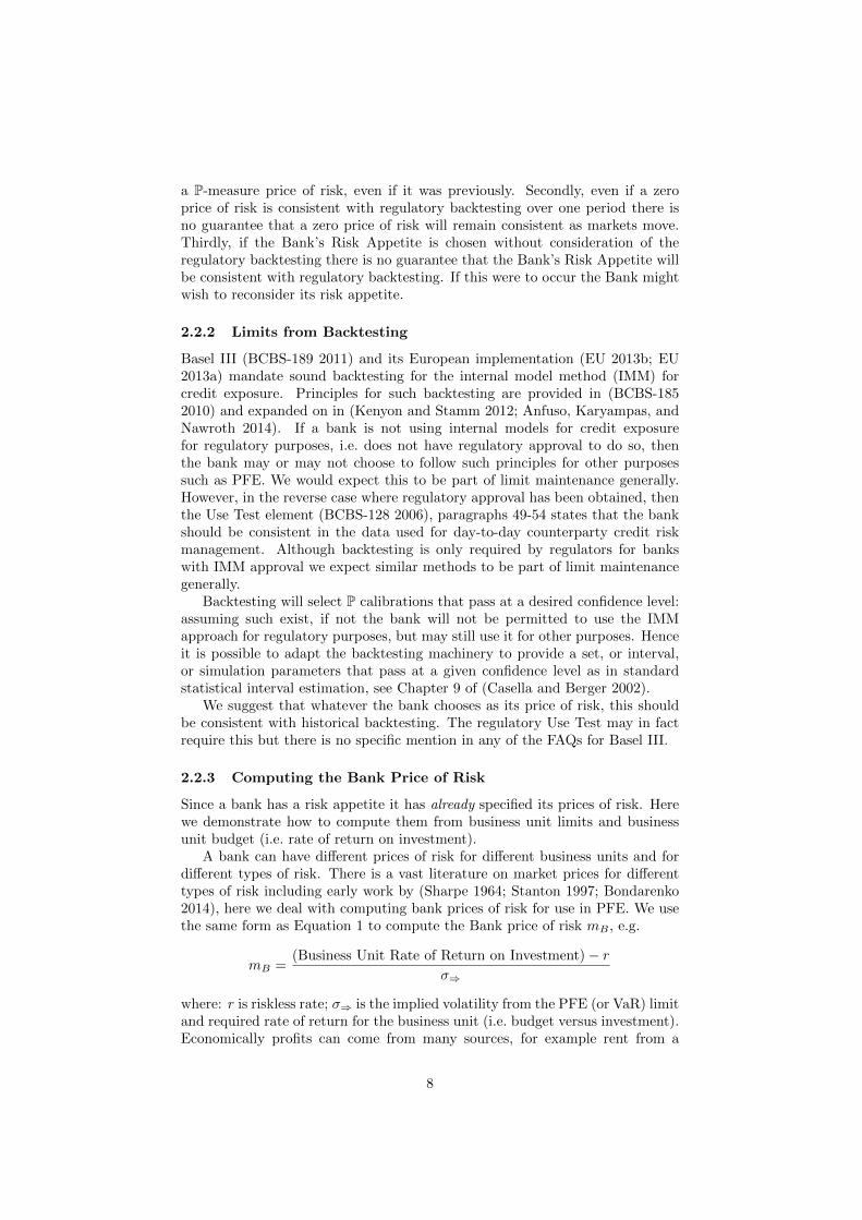
Normal relative returns Suppose the relative returns of the business unithave a Normal(µrequired, σ) distribution. µrequired is the required rate of returnof the business unit, and the business unit limit L is expressed as a PFE(q) inunits of required relative rate of return. Now we have two unknowns and twoconstraints so the unknowns are uniquely defined as:
σ⇒ =µrequired(1− L)√
2 erfc−1(2q)(2)
mB =µrequired − r
σ⇒(3)
erfc−1 is the inverse of the cumulative error function. Figure 3 shows implied
5 10 15 20
0
20
40
60
80
100
120
Quantile limit, L (multiples of budget rate of return)
ImpliedReturnVolatility
(percent)
Normal Relative Returns ModelPFE(95.) (or VaR), budget 10. percent
Figure 3: Implied volatility of required rate of return given budget (requiredrate or return) of 10% and quantile (PFE or VaR) limit using 95%. See text fordetails.
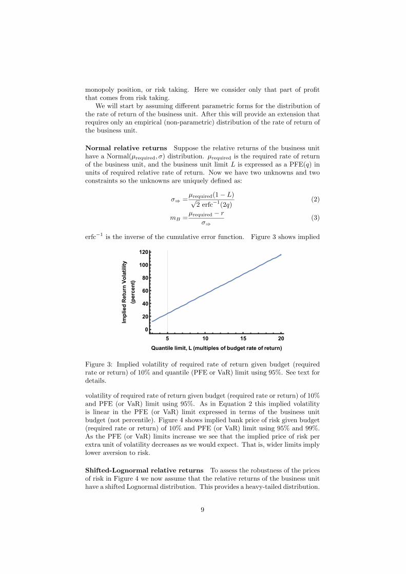
volatility of required rate of return given budget (required rate or return) of 10%and PFE (or VaR) limit using 95%. As in Equation 2 this implied volatilityis linear in the PFE (or VaR) limit expressed in terms of the business unitbudget (not percentile). Figure 4 shows implied bank price of risk given budget(required rate or return) of 10% and PFE (or VaR) limit using 95% and 99%.As the PFE (or VaR) limits increase we see that the implied price of risk perextra unit of volatility decreases as we would expect. That is, wider limits implylower aversion to risk.
Shifted-Lognormal relative returns To assess the robustness of the pricesof risk in Figure 4 we now assume that the relative returns of the business unithave a shifted Lognormal distribution. This provides a heavy-tailed distribution.
9
5 10 15 200.0
0.2
0.4
0.6
0.8
1.0
Quantile limit, L (multiples of budget rate of return)
ImpliedPriceofRisk
(excessrelativereturn
/SD)
From PFE or VaR(α), budget 10. percentNormal Relative Returns Model
0.95
0.99
Figure 4: Implied bank price of risk given budget (required rate or return) of10% and quantile (PFE or VaR) limit using 95% and 99%. See text for details.
We pick −1 as the shift as this is essentially the worst case which we assume isthe business unit losing its investment. Since a shifted Lognormal distributionhas three parameters and we have fixed one of them we can solve for the othertwo parameters. This involves a quadratic equation so there are two possiblesolutions. We chose the lower of the two as the more reasonable, i.e. given alow and a high implied price of risk it is more reasonable to conclude that thebank as the lower price of risk. Of course, depending on circumstances (e.g.observations of limits on other business units with Normal returns) it could bereasonable to make the opposite conclusion. Hence:
σSLN =−√
2erfc−1(2q)
±√
2erfc−1(2q)2 − 2(log(Lµrequired − γ)− log(µrequired − γ)) (4)
µSLN = log(µrequired − γ)− (σSLN)2
2(5)
σ⇒ =√(
eσ2SLN − 1
)e2µSLN+σ2
SLN (6)
mB =µrequired − r
σ⇒(7)
We use γ for the shift, giving the general result for a shifted Lognormal. Figure5 shows a comparison of implied bank price of risk using two different rela-tive return distributions. These have a maximum relative difference of 15%at L = 12.5, thus we conclude that the implied bank price of risk is robustagainst changes in the return specification between Normal and Unit-Shifted-Lognormal.
It is clear from Figure 5, and from simple observation, that no finite PFE(or VaR or ES) limit is compatible with a zero price of risk. By definition a zeroprice of risk indicates indifference to anything except the expected return. Thisimplies that using any risk-neutral measure alone is incompatible with a finiterisk appetite.
Empirical relative returns There are two cases here: empirical distributionfits the budget and PFE (or VaR) constraints; empirical distribution does notfit the constraints. If the empirical distribution fits the constraints all that is
10

5 10 15 200.0
0.2
0.4
0.6
0.8
Quantile limit, L (multiples of budget rate of return)
ImpliedPriceofRisk
(excessrelativereturn
/SD)
Price of Risk Implied from PFE or VaR Limit 0.95Normal vs USLN Relative Returns Models
Normal
Unit-Shifted-LogNormal
Figure 5: Comparison of implied bank price of risk using two different relativereturn distributions: Normal and Unit-Shifted-Lognormal
required is to compute the standard deviation of the relative returns which istrivial. If the empirical distribution does not fit then we shift and scale it sothat it does fit as follows.
Let the ordered, from smallest to largest, relative returns be xi, i = 1, . . . , nand
nq =dn× qe (8)
µrequired =g
n∑i=1
(xi + h) (9)
PFE(q) = Lµrequired =g(xnq+ h) (10)
So again we have two equations in two unknowns and can solve for the shift hand scale g. Hence
h =xnq− L
∑ni=1 xi
Ln− 1(11)
g =Lµ
xnq+ h
(12)
The problem is now reduced to the empirical distribution case which fits theconstraints. That is we simply calculate the empirical standard deviation forσ⇒. This can then be used to give the bank price of risk.
Whether or not it makes sense to scale and shift the empirical distributionwill depend on the individual circumstances. Here we provide the procedure incase it is reasonable.
2.3 The Risk Appetite Measure, A for PFE
Just as a P-measure is defined as a change in the drift from a risk-neutralmeasure given by the market price of risk, we define the Risk Appetite Measure,A, as a change in the drift from a risk-neutral measure given by the bank priceof risk, i.e.
µA := mBσ + r
This is used in conjunction with the T-Forward measure to provide a uniqueRisk Appetite Measure for PFE. Specifically we compute the discounted PFE (or
11

VaR, or other limit), which is measure-independent, and then apply an inversediscount given by zero coupon bond prices assuming that the rate of returnis µA. This procedure explicitly obeys the Independence Principle describedabove and implicitly makes use of the T-Forward measure. However, note thatthe procedure permits computation of the discounted PFE (or VaR) under anymeasure. Thus there is no added complexity for computation.
3 Discussion and Conclusions
Here we propose using the bank’s own risk appetite to set the measure forrisk limits, e.g. PFE, provided that the bank’s risk appetite is consistent withregulatory, or general limit maintenance, backtesting. If the bank’s risk appetiteis not consistent with regulatory backtesting this suggests that the bank’s riskappetite should be modified in order to pass the regulatory Use Test for day-to-day business decisions and satisfy the principles of a consistent Risk AppetiteFramework (BCBS-328 2015; FSB 2013). We note that a zero price of risk isinconsistent with a finite risk appetite, and this suggests that measures for PFEcannot be risk neutral.
We call this measure defined by the bank’s own risk appetite the BankRisk Appetite Measure or A. We provide a measure-independent procedure forcomputing PFE under A. A is defined by the bank price of risk and we give threemethods for computing it based on business unit budgets and limits. This datais readily available and business unit heads are acutely aware of their progressagainst plan on budget and limit usage.
This paper adds to the literature by further linking investment valuation andevaluation (Markowitz 1952; Sharpe 1964) and mathematical finance by propos-ing that limits be computed under the bank’s risk appetite measure providedas part of sound, and self-consistent, governance.
Acknowledgements
The authors would like to acknowledge useful discussions with Chris Dennisand Manlio Trovato, and feedback from participants at RiskMinds Interna-tional (Amsterdam, December 2015) where an earlier version of this work waspresented.
References
Acerbi, C. and B. Szekely (2014). Back-testing expected shortfall. Risk 28.
Anfuso, F., D. Karyampas, and A. Nawroth (2014). Credit exposure modelsbacktesting for Basel III. Risk 26, 82–87.
BCBS-128 (2006, June). International Convergence of Capital Measurementand Capital Standards. Basel Committee for Bank Supervision.
BCBS-185 (2010). Sound practices for backtesting counterparty credit riskmodels . Basel Committee for Bank Supervision.
BCBS-189 (2011). Basel III: A global regulatory framework for more resilientbanks and banking systems. Basel Committee for Bank Supervision.
12
BCBS-265 (2013). Fundamental review of the trading book - second consul-tative document. Basel Committee for Bank Supervision.
BCBS-325 (2015). Review of the Credit Valuation Adjustment Risk Frame-work. Consultative Document. Basel Committee for Bank Supervision.
BCBS-328 (2015). Guidelines. Corporate governance principles for banks.Basel Committee for Bank Supervision.
Bjork, T. (2004). Arbitrage theory in continuous time. Oxford university press.
Bondarenko, O. (2014). Variance trading and market price of variance risk.Journal of Econometrics 180 (1), 81–97.
Brigo, D. and F. Mercurio (2006). Interest Rate Models: Theory and Practice,2nd Edition. Springer.
Canabarro, E. and D. Duffie (2003). Measuring and marking counterpartyrisk. In L. Tilman (Ed.), Asset/Liability Management for Financial Insti-tutions. Institutional Investor Books.
Casella, G. and R. L. Berger (2002). Statistical inference, Volume 2. DuxburyPacific Grove, CA.
EU (2013a). Directive 2013/36/EU of the European Parliament and of theCouncil of 26 June 2013 on access to the activity of credit institutionsand the prudential supervision of credit institutions and investment firms,amending Directive 2002/87/EC and repealing Directives 2006/48/ECand 2006/49/EC Text with EEA relevance. European Commission.
EU (2013b). Regulation (EU) No 575/2013 of the European Parliament andof the Council of 26 June 2013 on prudential requirements for credit insti-tutions and investment firms and amending Regulation (EU) No 648/2012Text with EEA relevance. European Commission.
FSB (2013, November). Principles for An Effective Risk Appetite Framework.Financial Stability Board. http://www.financialstabilityboard.org/wp-content/uploads/r_131118.pdf.
Green, A. (2015). XVA: Credit, Funding and Capital Valuation Adjustments.Wiley. November.
Green, A., C. Kenyon, and C. R. Dennis (2014). KVA: Capital ValuationAdjustment by Replication. Risk 27 (12), 82–87.
Hull, J., A. Sokol, and A. White (2014, October). Short Rate Joint MeasureModels. Risk , 59–63.
Kenyon, C. and A. Green (2015). Warehousing credit risk: pricing, capital,and tax. Risk 28 (2), 70–75.
Kenyon, C. and R. Stamm (2012). Discounting, Libor, CVA and Funding:Interest Rate and Credit Pricing. Palgrave Macmillan.
Markowitz, H. (1952). Portfolio Selection. Journal of Finance 7 (1), 77–91.
Pykhtin, M. and S. Zhu (2007, July/August). A guide to modelling counter-party credit risk. Global Association of Risk Professionals (37).
Sharpe, W. F. (1964). Capital asset prices: A theory of market equilibriumunder conditions of risk*. The journal of finance 19 (3), 425–442.
13
Stanton, R. (1997). A nonparametric model of term structure dynamics andthe market price of interest rate risk. Journal of Finance, 1973–2002.
Stein, H. (2013). Fixing Underexposed Snapshots – Proper Computation ofCredit Exposures Under the Real World and Risk Neutral Measures. Tech-nical Report, Bloomberg LP December, 1–23.
14