Chp.9 Option Pricing When Underlying Stock Returns are

Discontinuous

• In this chapter, an option pricing formula is derived for the more general case where the underlying stock returns are generated by a mixture of both continuous and jump processes.

9.1 Introduction

• The critical assumptions in the Black-Scholes derivation is that trading takes place continuously in time and that the price dynamics of the stock have a continuous sample path with provability one.

• What will happened if there is a jump?

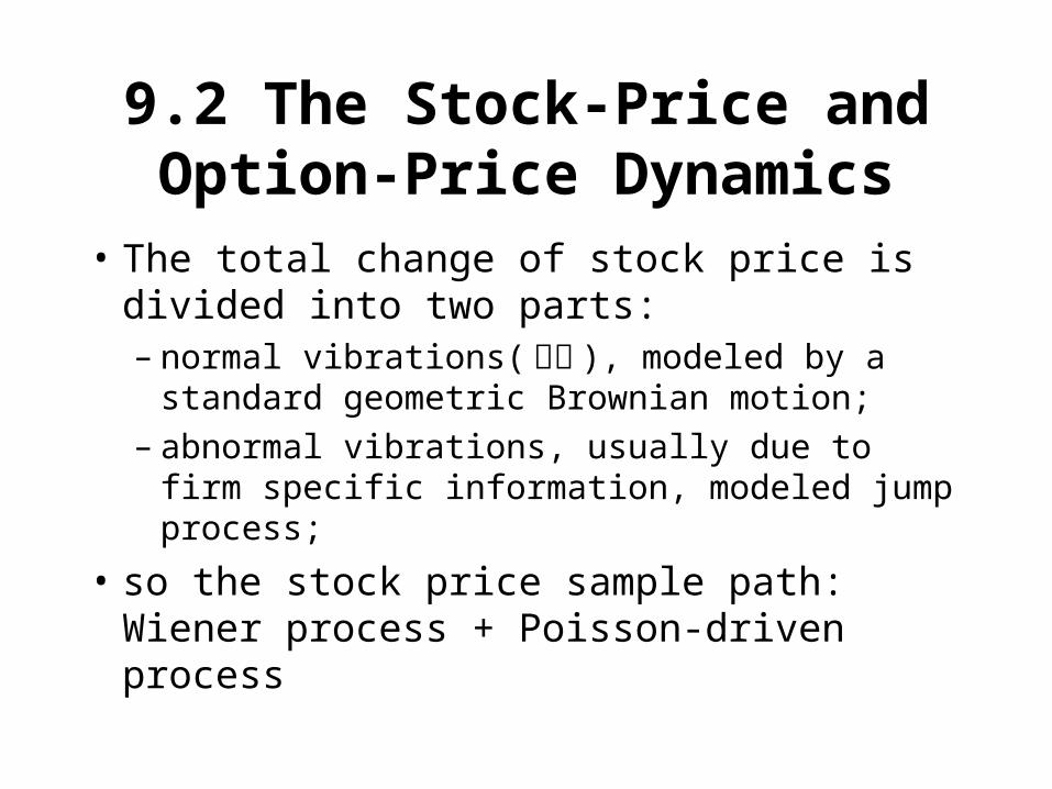
9.2 The Stock-Price and Option-Price Dynamics

• The total change of stock price is divided into two parts:– normal vibrations( 振动 ), modeled by a

standard geometric Brownian motion;– abnormal vibrations, usually due to firm

specific information, modeled jump process;

• so the stock price sample path: Wiener process + Poisson-driven process

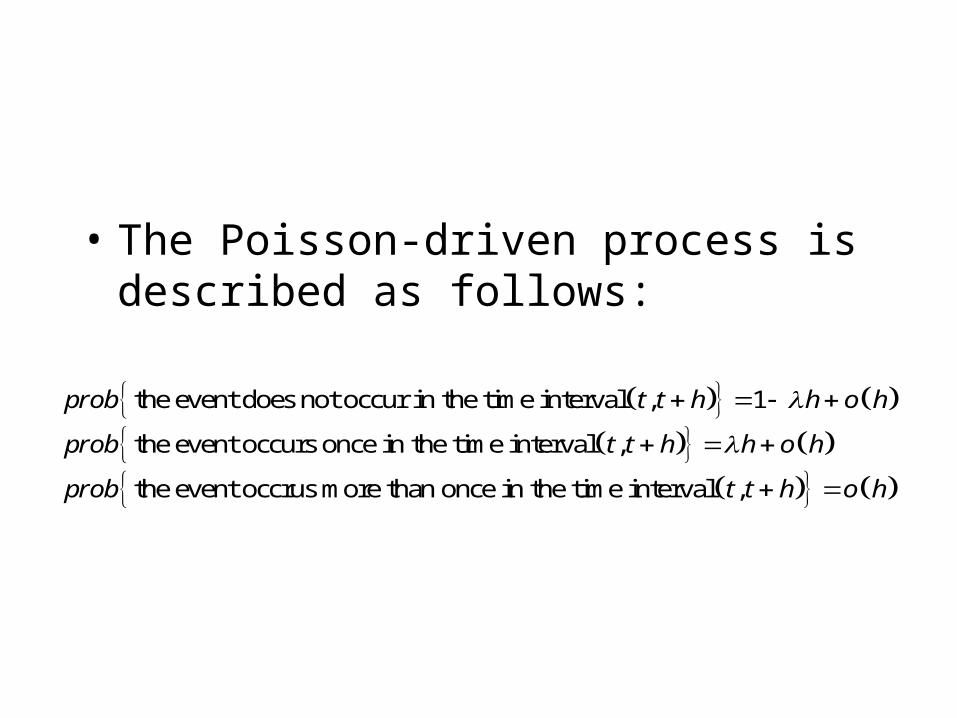
• The Poisson-driven process is described as follows:

the event does not occur in the time interval , 1

the event occurs once in the time interval ,

the event occrus more than once in the time interval ,

prob t t h h o h

prob t t h h o h

prob t t h o h

• Y: the random variable description of the drawing from a distribution to determine the impact of the information on the stock price. Then, neglecting the continuous part

•

S t h S t Y

• Then the stock-price returns can be described as

if the Poisson event does not occur

1 if the Poisson event occurs

dSk dt dZ dq

S

k dt dZ

k dt dZ Y

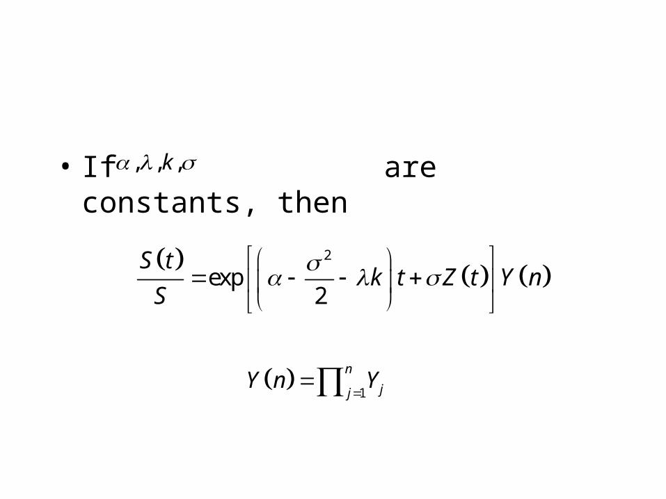
• If are constants, then , , ,k

2

exp2

S tk t Z t Y n

S

1

n

jjY n Y

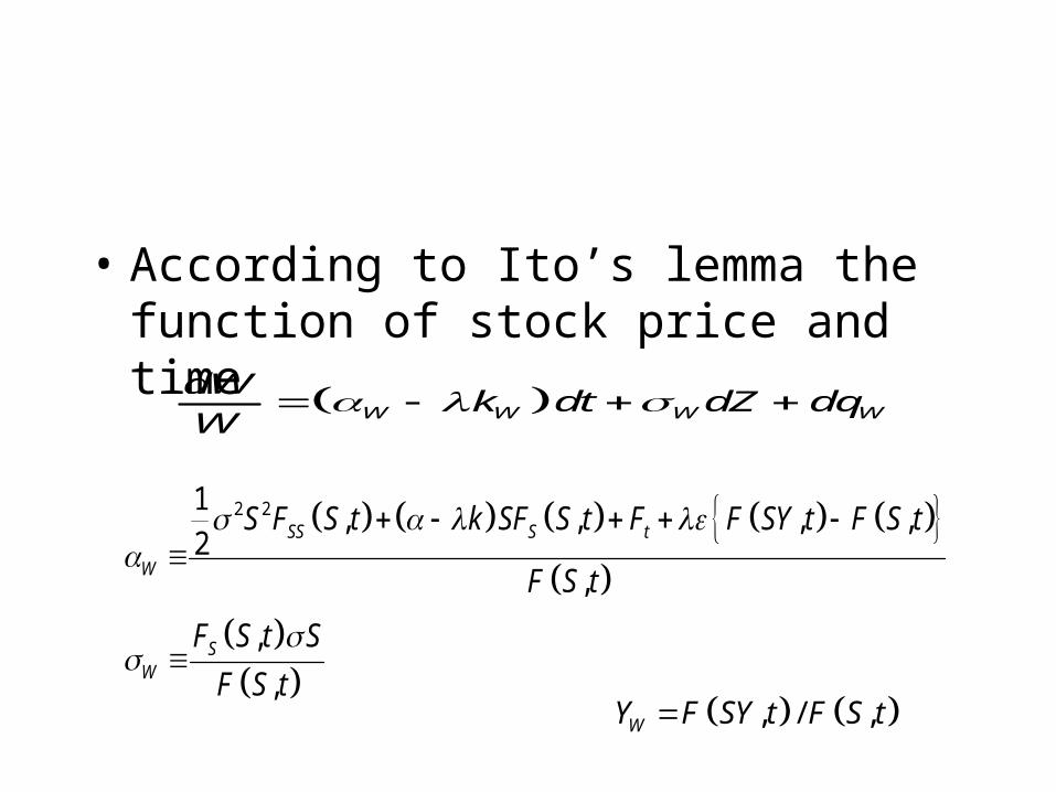
• According to Ito’s lemma the function of stock price and time

W W W W

dWk dt dZ dq

W

2 21, , , ,

2,

,

,

SS S t

W

SW

S F S t k SF S t F F SY t F S t

F S t

F S t S

F S t

, / ,WY F SY t F S t

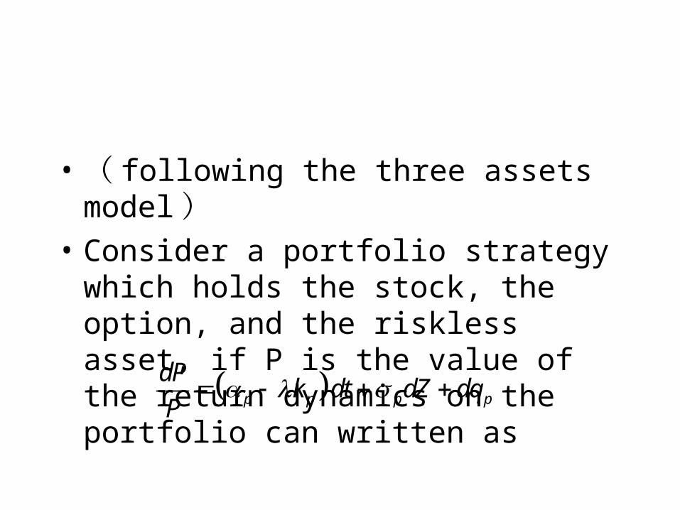
• （ following the three assets model ）• Consider a portfolio strategy which holds

the stock, the option, and the riskless asset, if P is the value of the return dynamics on the portfolio can written as

p p p p

dPk dt dZ dq

P

•

2 2 21 1 1

1 2

21

1 2

1

, ,1 1

,

,1 1

,

p w w

p w

p

w r r w w rw r w w

w w

w F SY t F S tY w Y

F S t

F SY tw Y w

F S t

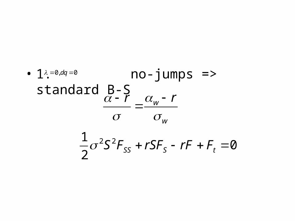
• 1. no-jumps => standard B-S

w

w

rr

2 210

2 SS S tS F rSF rF F

0, 0dq

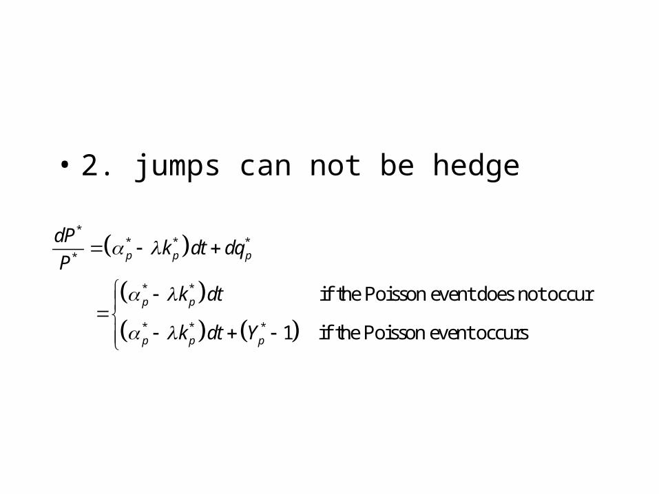
• 2. jumps can not be hedge

** * *

*

* *

* * *

if the Poisson event does not occur

1 if the Poisson event occurs

p p p

p p

p p p

dPk dt dq

P

k dt

k dt Y

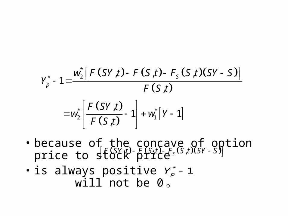
• because of the concave of option price to stock price

• is always positive will not be 0 。

*2*

* *2 1

, , ,1

,

,1 1

,

Sp

w F SY t F S t F S t SY SY

F S t

F SY tw w Y

F S t

, , ,SF SY t F S t F S t SY S

* 1pY

• Economic implications ：• （ 1 ） following B-S hedging : long stock

and short option, 平时收益高于预期，跳跃时损失很大； reverse B-S hedging: short stock and long option, 平时收益低于预期，跳跃时收益很大；

• （ 2 ）无跳跃时期权卖方获利，有跳跃时买方获利。

*2 0w

*2 0w

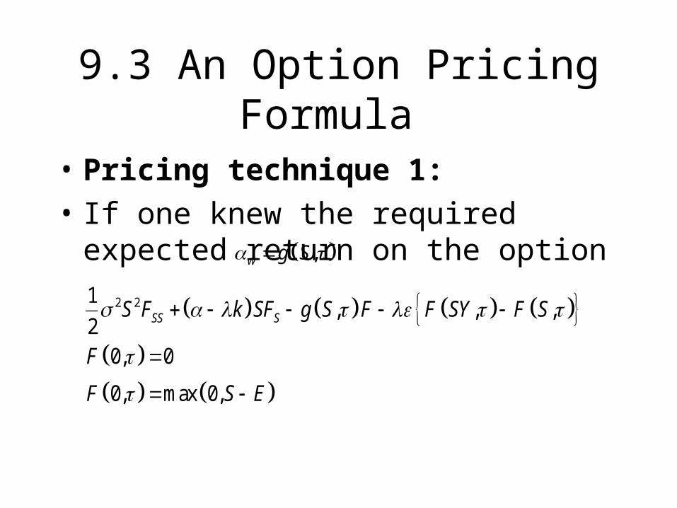
9.3 An Option Pricing Formula

• Pricing technique 1:

• If one knew the required expected return on the option

2 21, , ,

20, 0

0, max 0,

SS SS F k SF g S F F SY F S

F

F S E

,w g S

• Pricing technique 2: Assumed that the CAPM was a valid description of equilibrium security returns.

• Stock-price dynamics were described two components:– Continuous part---new information;– Jump part---important new information, usually firm

(or even industry) specific such as discovery of an important new oil or the loss of a court suit, “nonsystematic” risk.

• 跳跃部分属于非系统风险，不产生风险溢价，根据 CAPM

*p r w

w

rr

2 21, ,

2 SS SS F r k SF F rF F SY F S

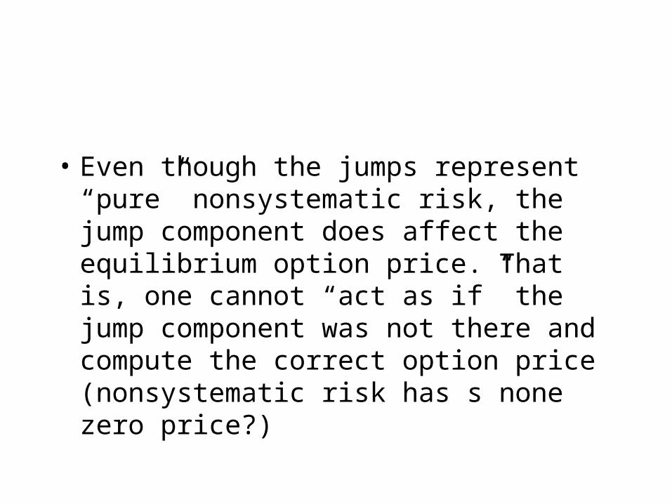
• Even though the jumps represent “pure” nonsystematic risk, the jump component does affect the equilibrium option price. That is, one cannot “act as if” the jump component was not there and compute the correct option price (nonsystematic risk has s none zero price?)

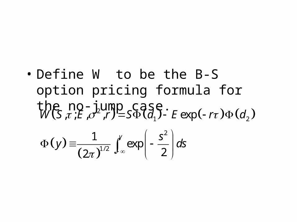
• Define W to be the B-S option pricing formula for the no-jump case.

21 2

2

1/ 2

, ; , , exp

1exp

22

y

W S E r S d E r d

sy ds

• Define Xn the random variable to have the same distribution as the product of n i.i.d. (identically distributed to Y) random variables

2

0

exp, exp , ; , ,

!

n

n nn

F S W SX k E rn

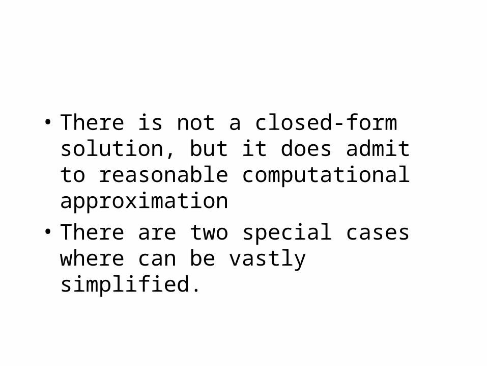
• There is not a closed-form solution, but it does admit to reasonable computational approximation

• There are two special cases where can be vastly simplified.

• Example 1: There is a positive probability of immediate ruin, i.e. if the Poisson event occurs, then the stock price goes to 0. that is Y=0 with probability one.

2 2, exp exp , ; , , , ; , ,F S W S E r W S E r

• inedntical with the standard B-S solution but with a larger “interest rate,”. As was shown in Merton (1973a, Ch.8), the option price is an increasing function of the interest rate, and therefore an option on a stock that has a positive probability of complete ruin is more valuable than an option on a stock that dose not.

• Example 2: Y has a log-normal distribution

• Define

• then

2, , ; , ,n n nf S W S E v r

0

exp, ( , )

!

n

nn

F S f Sn

• Clearly, is the value of the option, conditional on knowing that exactly n Poisson jumps will occur during the life of the option. The actual value of the option,, is just the weighted sum of each of these prices where each weighted equals the probability.

( , )nf S

• (9.16) was deduced from the twin assumptions that CAMP is valid and the jump component of a security’s return is uncorrelated with the market. One can hardly claim strong empirical evidence to support these assumptions.

• Another technique to derive (9.16): the Ross model for security pricing.

• 有 m 个跳跃过程互相独立的股票，对应有 m 个共同形式（股票＋期权）的套利组合

•

** * *

*1,2,j

j j j jj

dPk dt dq j m

P

• 用 m 个套利组合与无风险资产组成一个组合：

* * *

1 1 1

, ,

H H H H

m m m

H j j H H j j j H j jj j j

dHk dt dq

H

x r r k x k dq x dq

• 随着 m 的增加，组合接近无风险（推导），所以有

• 所以有 ，此时成立。 • 两种推导过程基于同样的原理：跳跃过

程可以分散。

*

1

10

m

j jj

u rm

*j r

• 为消除系统风险必须卖出的股票数量。

1/N W S d

*

0

2 2

1/ 22 2

exp

!

log / / 2 / 2

n

n

n

N d nn

S E r nd n

n

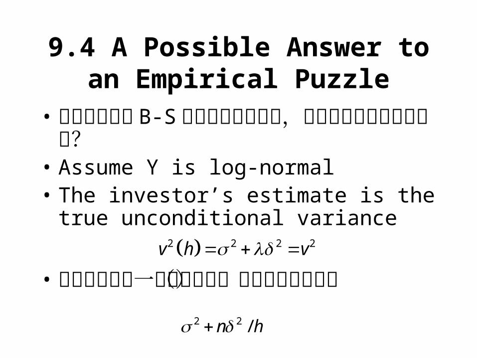
9.4 A Possible Answer to an Empirical Puzzle

• 如果投资者用 B-S 公式来为期权股价，它与理论价格的差距在哪？

• Assume Y is log-normal • The investor’s estimate is the true

unconditional variance

• 真是的应该是一个条件方差（考虑了跳跃过程）

2 2 2 2v h v

2 2 /n h

• The problem becomes, if the investor uses as his estimate of the variance rate in the standard B-S formula, then how will his appraisal of the option’s value compare with the “true”?

2 2nT n

2 2 2T T v

• Inspection of (9.18) shows that, from (9.27), fn can be rewritten as

2, ; , , exp , ;1,1,0W S E u r E r W S

, exp ,eF S E r W X T

• so the answer will depend on whether

, exp ,F S E r W X T

, exp ,F S E r W X T

, , 0W X T W X T

•

222 2

2

/ 4/0

/ 2

aW

W

2

0 exp , , arg

1 , ,

e

e

a S E r F F m inall in the money

a S EorS E F F deep in the money

deep out of the money